Geometry and the Imagination

Xiong Dan

An academic exercise presented in partial fulfillment for the degree of

Bachelor of Science with Honours in Applied Mathematics.

Supervisor: Associate Professor Helmer Aslaksen

Department of Mathematics

National University of Singapore

2003/2004

ii

Acknowledgements

I would like to thank my supervisor, A/P Aslaksen, for conducting this wonderful

project. I am grateful to him for his time and his patience with me. I benefit greatly from

discussions I have had with him on this project, and I hereby express my appreciation

for his guidance full of inspirations. This project has been a meaningful and pleasant

experience with excitements and joys of discoveries, which I will always remember.

I would like to dedicate the regular octahedron shown below to my lovely girlfriend,

Goose. To me, she is as nice and perfect as a regular octahedron.

I would like to dedicate the space hexagon highlighted in bold on the regular octahedron

to all the people who have been kind to me. I would like to share my joys with you all.

I would like to dedicate the hyperboloid of one sheet that contains all six sides of the

space hexagon to my parents. I would like to express my gratitude to them for their love

to me over the years. Something is behind the scene, silent and invisible, yet you know.

iii

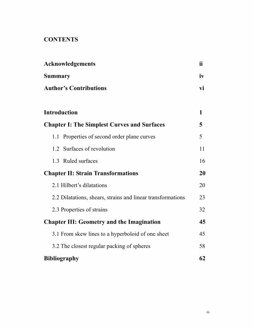
CONTENTS

Acknowledgements ii

Summary iv

Author’s Contributions vi

Introduction 1

Chapter I: The Simplest Curves and Surfaces 5

1.1 Properties of second order plane curves 5

1.2 Surfaces of revolution 11

1.3 Ruled surfaces 16

Chapter II: Strain Transformations 20

2.1 Hilbert’s dilatations 20

2.2 Dilatations, shears, strains and linear transformations 23

2.3 Properties of strains 32

Chapter III: Geometry and the Imagination 45

3.1 From skew lines to a hyperboloid of one sheet 45

3.2 The closest regular packing of spheres 58

Bibliography 62

iv

Summary

This thesis begins with discussions of properties of second order plane curves and

quadratic surfaces in Chapter I. In the study of quadratic surfaces, the concepts of

“surfaces of revolution” and “ruled surfaces” are introduced. As a particular example,

the surface of the hyperboloid of revolution of one sheet is closely examined by the

author. After showing that a hyperboloid of revolution of one sheet can be obtained by

rotating a straight line in space, the author goes on to examine the properties of the

straight lines lying in the surface. Following that the author extends these properties to

the hyperboloid of one sheet of the most general type. This process gives rise to a new

concept, called a “strain”. It is a transformation in space which can deform surfaces of

revolution to general type surfaces.

In Chapter II, the author examines the concept of “strain” and explores the properties of

this kind of transformation in space. When exploring the properties, the author notices

that strain transformations preserve collinearity, concurrency as well as tangency. From

this, the author points out the connection between the idea of perspectives in projective

geometry and the nature of strain transformations. As a demonstration, the author

concludes that if we can prove Brianchon’s theorem in the circle case, we will get the

ellipse case “for free”, by using an argument based purely on the properties of strain

transformation.

v

In Chapter III, two interesting problems are discussed. In the first problem, the author

presents a proof for the fact that given any 3 skew straight lines in space which are not

parallel to a common plane, there always exists a hyperboloid of one sheet containing

these three lines. The basic idea of the author’s proof is to find some strain

transformations that can transform the given 3 lines into positions such that a known

hyperboloid of one sheet contains all 3 of them. Due to the arbitrariness and ambiguity

of the positions of the three given straight lines, it proved difficult to determine such

strain transformations. In the author’s method of finding the desired transformations, a

very special space hexagon is constructed from the three given straight lines, and from

this, the author finishes the rest of the proof using properties of strain transformations.

In the proof of the first problem in chapter III, the author has a close look at the

structure of the regular octahedron, and discovers that the structure of the regular

octahedron can be used to visualize the connections between the face-centered cubic

lattice packing and the face-centered hexagonal lattice packing when constructing the

closest regular packing of spheres in space. This interpretation of the author’s is

explained in the second problem which concludes this thesis. □

vi

Author’s Contributions

All proofs from Chapter I onwards presented in this thesis are new proofs worked out

by the author. Among these new proofs, the author is most proud of his proof for the

fact that given any three skew straight lines which are not parallel to a common plane,

there always exists a hyperboloid of one sheet containing them. This proof is presented

in section 3.1.

The properties of strain transformations presented in section 2.3 are summarized by the

author. The proof presented in section 2.3 for the fact that strain transformations in

space preserve the type of a quadratic surface is worked out by the author.

The interpretations in section 3.2 on the closest regular packing of spheres using the

structure of the regular octahedron are due to the author.

All the figures in this thesis are drawn by the author.

1

Introduction

“In mathematics, as in any scientific research, we find two tendencies present. On the one hand the tendency toward abstraction seeks to crystallize the logical relations inherent in the maze of material that is being studied, and to correlate the material in a systematic and orderly manner. On the other hand, the tendency toward intuitive understanding fosters a more immediate grasp of the objects one studies, a live rapport with them, so to speak, which stresses the concrete meaning of their relations. “As to geometry, in particular, the abstract tendency has led to the magnificent systematic theories of Algebraic Geometry, of Riemannian Geometry, and of Topology; these theories make extensive use of abstract reasoning and symbolic calculation in the sense of algebra. Notwithstanding this, it is still as true today as it ever was that intuitive understanding plays a major role in geometry. And such concrete intuition is of great value not only for the research worker, but also for anyone who wishes to study and appreciate the results of research in geometry. “It is possible in many cases to depict the geometric outline of the methods of investigation and proof, without necessarily entering into the details connected with the strict definitions of concepts and with the actual calculations.”

----David Hilbert (1932), preface to “Geometry and the Imagination” [4]

The main scope of this project is to study the book “Geometry and the Imagination” by

David Hilbert and S. Cohn-Vossen. This book, which was written some 70 years ago, is,

according to Hilbert, intended to “give a presentation of geometry in its visual and

intuitive aspects”. In light of this statement, readers of this book indeed find that a great

number of interesting geometric problems in this book are dealt with solely by means of

visual imagination instead of abstract algebraic calculations. Take the following

2

problem from Hilbert’s book for example:

A plane not at right angles to the axis of a circular cylinder nor parallel to it

intersects the cylinder in a plane curve (Figure I-1A). Prove that the curve of

intersection is an ellipse.

Instead of building up a Cartesian coordinate system and proving this result

analytically, the proof given in Hilbert’s book is as simple as follows: Imagine we

take two spheres which just fit in the cylinder and put these two spheres inside the

cylinder so that each of the two spheres touches the cylinder in a circle. We then move

them within the cylinder until they touch the intersecting plane from opposite sides at

points f1 and f2 (Figure I-1B). Let B be any point on the curve of intersection of the

plane and the cylinder, we take the straight line trough point B lying on the cylinder

(i.e. parallel the axis). Suppose the straight line meets the circles of contact of the

spheres at two points P1 and P2.

Figure I-1B

B

f2

P1

P2

f1

Figure I-1A

3

Bf1 and BP2 are tangents to a fixed sphere through a fixed point B, and all such tangents

must be of the same length, because of the rotational symmetry of the sphere. Thus Bf1

= BP2; similarly Bf2 = BP2. It follows that

Bf1 + Bf2 = BP1 + BP2= P1P2

Again by rotational symmetry, the distance P1P2 is a constant independent of point B on

the curve. Therefore Bf1 + Bf2 is constant for all points B on the curve, so the curve of

intersection is an ellipse with foci at f1 and f2. □

The six chapters of this book covered a wide diversity of materials dealing with

interesting problems from various branches of geometry. I shall now list down the titles

of the six chapters of Hilbert’s book, they are,

Chapter 1 The simplest curves and surfaces

Chapter 2 Regular systems of points

Chapter 3 Projective configurations

Chapter 4 Differential geometry

Chapter 5 Kinematics

Chapter 6 Topology

Due to time constraint, in this project, I have only been working on the first 3 chapters

of this book, namely on simplest curves and surfaces, on regular systems of points and

on projective geometry. All problems discussed in this thesis arise from study in these

branches of geometry; there are no discussions on topology or differential geometry.

4

The content of this thesis is not a repeat of what Hilbert wrote in his book. There is no

point to discuss what have already been clearly explained in that book because the book

itself is a well-written book. My purposes of this thesis are as follows,

To apply methods used in the book to solve problems not discussed in the book;

(e.g. Section 1.1).

To give my own explanations and interpretations on the results and ideas which I

found interesting; (e.g. Section 3.2)

To provide proofs where I feel necessary but the book omitted. (e.g. Section 3.1).

Before I move on to Chapter I, I have to say here that “Geometry and the Imagination”

is a wonderful book that gives me inspirations. I admire the spirit in this book of using

imagination to sense out visual intuitive natures of geometric problems. I recommend

the book to those who have not read it, and who like to use their imagination.

5

Chapter I

The Simplest Curves and Surfaces

§1.1 Properties of second order plane curves

If we do not consider degenerate cases and imaginary curves, there are three types of

second order plane curves. They are the parabola, the hyperbola, and the ellipse (circles

are categorized as a special case of the ellipse). In this section I will discuss two

selected problems on properties of second order plane curves.

Optics properties of the Hyperbola

Second order plane curves exhibit several interesting properties, among which, they

share analogous properties in optics. Take a hyperbola (Figure1.1-1) for example,

Given the property that ||F1B| - |F2B|| is constant for any point B on a hyperbola with

Figure 1.1-1

F1 F2

B

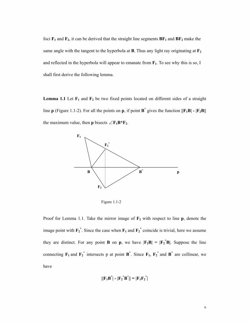
6

foci F1 and F2, it can be derived that the straight line segments BF1 and BF2 make the

same angle with the tangent to the hyperbola at B. Thus any light ray originating at F2

and reflected in the hyperbola will appear to emanate from F1. To see why this is so, I

shall first derive the following lemma.

Lemma 1.1 Let F1 and F2 be two fixed points located on different sides of a straight

line p (Figure 1.1-2). For all the points on p, if point B* gives the function ||F1B| - |F2B||

the maximum value, then p bisects ∠F1B*F2.

Proof for Lemma 1.1. Take the mirror image of F2 with respect to line p, denote the

image point with F2*. Since the case when F1 and F2

* coincide is trivial, here we assume

they are distinct. For any point B on p, we have |F2B| = |F2*B|. Suppose the line

connecting F1 and F2* intersects p at point B*. Since F1, F2

* and B* are collinear, we

have

||F1B*| - |F2*B*|| = |F1F2

*|

B

F2*

p B*

F1

F2

Figure 1.1-2

7

For any other point B distinct from B* on p, F1, F2* and B form a triangle, by the

property of a triangle we have

||F1B| - |F2*B|| ＜ |F1F2

*|

Hence for any point B on p, B = B* gives ||F1B| - |F2*B||, or ||F1B| - |F2B|| the maximum

value. Since F2* is the mirror image of F2 about p, we have ∠F2

*B*B = ∠F2B*B, or

∠F1B*B = ∠F2B*B. □

In general, for any point B1 in between the two branches of a hyperbola, B2 on the

hyperbola and B3 outside the area bounded by the two branches of hyperbola we have

||F1B1| - |F2B1|| ＜ ||F1B2| - |F2B2|| ＜ ||F1B3| - |F2B3|| …(*)

This fact can be understood by constructing a family of hyperbolas having the same pair

of foci, and the fact that none two curves of this family intersect.

Since a tangent line of a second order curve has no point in common with the curve

other than the point of contact, it follows that any tangent line to a hyperbola must lie

entirely in between the two branches of the hyperbola. Thus from (*) we see that,

among all the points on the tangent in Figure 1.1-1, point B gives ||F1B| - |F2B|| the

maximum value, by lemma 1.1, the tangent bisects ∠F1BF2 and hence the result.

8

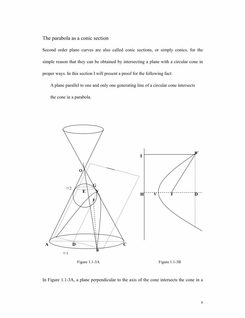
The parabola as a conic section

Second order plane curves are also called conic sections, or simply conics, for the

simple reason that they can be obtained by intersecting a plane with a circular cone in

proper ways. In this section I will present a proof for the following fact:

A plane parallel to one and only one generating line of a circular cone intersects

the cone in a parabola.

In Figure 1.1-3A, a plane perpendicular to the axis of the cone intersects the cone in a

F V

E

C

A

V

O

F

B

G

D

Figure 1.1-3A

B

D

H

I

Figure 1.1-3B

☉2

☉1

9

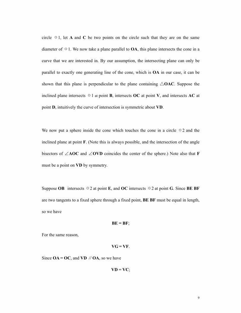
circle ☉1, let A and C be two points on the circle such that they are on the same

diameter of ☉1. We now take a plane parallel to OA, this plane intersects the cone in a

curve that we are interested in. By our assumption, the intersecting plane can only be

parallel to exactly one generating line of the cone, which is OA in our case, it can be

shown that this plane is perpendicular to the plane containing △OAC. Suppose the

inclined plane intersects ☉1 at point B, intersects OC at point V, and intersects AC at

point D, intuitively the curve of intersection is symmetric about VD.

We now put a sphere inside the cone which touches the cone in a circle ☉2 and the

inclined plane at point F. (Note this is always possible, and the intersection of the angle

bisectors of ∠AOC and ∠OVD coincides the center of the sphere.) Note also that F

must be a point on VD by symmetry.

Suppose OB intersects ☉2 at point E, and OC intersects ☉2 at point G. Since BE BF

are two tangents to a fixed sphere through a fixed point, BE BF must be equal in length,

so we have

BE = BF;

For the same reason,

VG = VF.

Since OA = OC, and VD ∥OA, so we have

VD = VC;

10

By rotational symmetry we have

BE = GC.

From the above three equalities, it follows that

BF = BE = GC = VG + VC = VF + VD …(*)

We now consider (*) on the intersecting plane, refer to Figure 1.1-3B. We have

BF = VF + VD,

if we extend DV to a point H such that VH = VF and we then draw the perpendicular

line to VD with foot at point H, we see that now, BF = HD, if BI is the distance from B

to the line we draw, then

BF = BI.

By the directrix definition of a parabola, we see that the curve of intersection is indeed a

parabola with focus at F. □

11

§1.2 Surfaces of revolution

In previous discussions, I have mentioned the circular cylinder and the circular cone.

The circular cylinder is the simplest curved surface. It can be obtained by rotating a

straight line about an axis parallel to it. Because of this, the circular cylinder is called a

surface of revolution. Surfaces of revolution are surfaces that can be generated by

rotating a plane curve about an axis lying in the plane of the curve. The generating plane

curve is called the generator of the surface. From the definition of surfaces of revolution,

we see that a circular cone is also a surface of revolution. It can be obtained by rotating

a straight line about an axis intersecting it. In Figure 1.1-3A, the straight line through

OA is a generator of the cone and it intersects the axis of the cone at point O.

In either of the cases of a circular cylinder or a circular cone, we have rotated a straight

line about another straight line that lies in a common plane with the first one. Now one

question arises, if we have two skew straight lines in space, and we rotate one about

another, what kind of surface we will get? It seems that the surface in question may not

be a surface of revolution, because it violates the condition that the generator must be a

plane curve lying in the same plane with the axis of revolution, while in our case, two

skew lines never lie in the same plane. But as it turns out, if we have two skew straight

lines in space and we rotate one about another, the surface we get is a hyperboloid of

revolution of one sheet! And this particular type of hyperboloid is a surface of

revolution because it can be obtained by rotating a hyperbola about one of its axes of

12

symmetry. In the following section, I will examine the above-mentioned beautiful result.

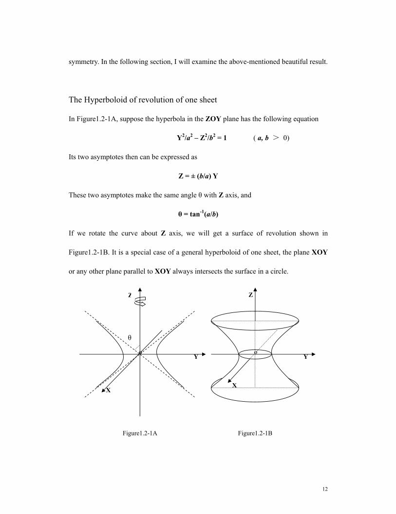
The Hyperboloid of revolution of one sheet

In Figure1.2-1A, suppose the hyperbola in the ZOY plane has the following equation

Y2/a2 – Z2/b2 = 1 ( a, b ＞ 0)

Its two asymptotes then can be expressed as

Z = ± (b/a) Y

These two asymptotes make the same angle θ with Z axis, and

θ = tan-1(a/b)

If we rotate the curve about Z axis, we will get a surface of revolution shown in

Figure1.2-1B. It is a special case of a general hyperboloid of one sheet, the plane XOY

or any other plane parallel to XOY always intersects the surface in a circle.

o

θ

X X

Y Y

Z Z

o

Figure1.2-1A Figure1.2-1B

13

We call this kind of surface the hyperboloid of revolution of one sheet. It can be

represented by the following equation:

X2/a2 + Y2/a2 – Z2/b2 = 1

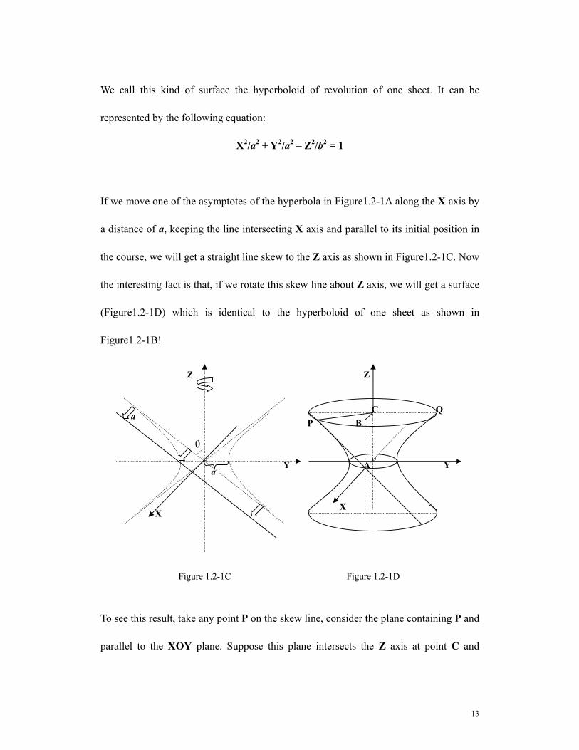
If we move one of the asymptotes of the hyperbola in Figure1.2-1A along the X axis by

a distance of a, keeping the line intersecting X axis and parallel to its initial position in

the course, we will get a straight line skew to the Z axis as shown in Figure1.2-1C. Now

the interesting fact is that, if we rotate this skew line about Z axis, we will get a surface

(Figure1.2-1D) which is identical to the hyperboloid of one sheet as shown in

Figure1.2-1B!

To see this result, take any point P on the skew line, consider the plane containing P and

parallel to the XOY plane. Suppose this plane intersects the Z axis at point C and

a o

θ

X X

Y Y

Z Z

o

Figure 1.2-1C Figure 1.2-1D

P C

A

B Q

a

14

intersects either branch of the hyperbola at point Q, I shall show that CP = CQ. In other

words, by rotating point P about the Z axis, when P hits the YOZ plane, it will hit on

the hyperbola.

In Figure 1.1-1D, suppose A is the intersection of the skew line with X axis. We take

point B in the plane which contains P and parallel to the XOY plane such that

AB∥OC.

If the distance from point P to XOY plane is Z0, then

AB = OC = Z0

By our assumption, ∠PAB = θ = Tan-1(a / b), we have

PB = AB Tan(θ) = AB (a/b) = Z0 (a/b)

It is easy to see that BCOA forms a parallelogram, therefore

BC = AO = a

It can be shown that BC is perpendicular to the plane containing A B P, and hence

BC⊥PB, it follows that

PC = √ ( PB2 + BC2 ) = √ [a2 + Z02 (a2/b2)]

Suppose by rotating P about Z axis, P will be brought to a point Q with coordinates ( 0,

Y0, Z0 ) in the ZOY plane, from above calculation, we see that

Y0 = |PC| = √ [a2 + Z02 (a2/b2)]

Or equivalently,

15

Y02/a2 – Z0

2/b2 = 1

By comparing the above equation to that of the original hyperbola, we see that point Q

must be a point on the hyperbola! Since P is arbitrarily chosen on the skew line, and for

any point Q on the hyperbola there is a one-to-one such corresponding point P, this

completes the proof. □

16

§1.3 Ruled surfaces

In the previous section, we see that if we rotate a straight line about an axis skew to it,

we will get a hyperboloid of revolution of one sheet, thus this kind of one sheeted

hyperboloid can be generated by sweeping a straight line along a circle in space in a

particular manner. In general, a surface that can be generated by moving a straight line

along a certain fixed course is called a ruled surface. By this definition, we see that

hyperboloids of revolution of one sheet are ruled surfaces, and so are circular cylinders

and circular cones. All these surfaces contain infinitely many straight lines in them.

But, as ruled surfaces, our hyperboloid of revolution of one sheet is distinguished from

circular cylinders and cones by the special property that each point of the surface is on

more than one of the straight lines lying in the surface. Because of this, the hyperboloid

of revolution of one sheet is also called a doubly ruled surface, while cylinders and

cones do not belong to this category.

To see why a hyperboloid of revolution of one sheet is a doubly ruled surface, we look

at the symmetrical properties of the two asymptotes of the hyperbola we have

considered in previous section as shown in Figure 1.2-1C. It can be shown that choosing

either one of the two asymptotes, they always generate the same surface. In fact the two

resulting hyperboloids of revolution of one sheet coincide.

17

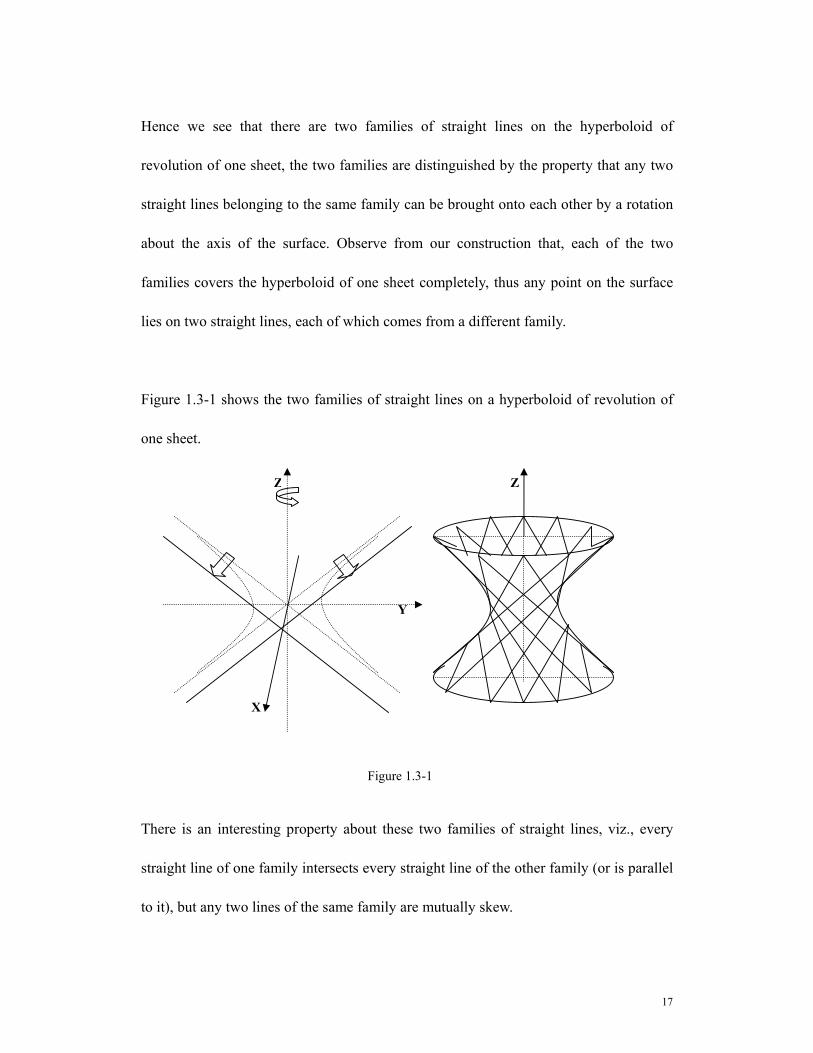
Hence we see that there are two families of straight lines on the hyperboloid of

revolution of one sheet, the two families are distinguished by the property that any two

straight lines belonging to the same family can be brought onto each other by a rotation

about the axis of the surface. Observe from our construction that, each of the two

families covers the hyperboloid of one sheet completely, thus any point on the surface

lies on two straight lines, each of which comes from a different family.

Figure 1.3-1 shows the two families of straight lines on a hyperboloid of revolution of

one sheet.

There is an interesting property about these two families of straight lines, viz., every

straight line of one family intersects every straight line of the other family (or is parallel

to it), but any two lines of the same family are mutually skew.

X

Y

Z Z

Figure 1.3-1

18

To see this result, we consider the circular cylinder generated by moving the smallest

circle on the hyperboloid along the rotation axis of the surface. It is easily seen that all

the straight lines on the surface are tangent to this cylinder, and the points of contacts

form the smallest circle on the hyperboloid, denote this circle with ⊙1. If we now

choose two straight lines p and q on the surface each from a different family

(Figure1.3-2), I shall now show that they either intersect or are parallel.

Suppose p and q touch the cylinder at points P and Q respectively. Assume P and Q are

two distinguished points on ⊙1. We now draw the two tangents to ⊙1 at points P and Q

on the plane that contains ⊙1, if they are parallel, then it is easily seen that p∥q.

Assume these two tangents meet at point R, we have RP = RQ.

S

p

q

p

q

⊙1 ⊙1

P

Q

R

Figure 1.3-2

P

Q r

19

Suppose the plane contain line p and tangent to the cylinder intersects the corresponding

plane for q intersects in a straight line r, point R must be a point on r, and further more,

r ⊥RP and r ⊥RQ.

Suppose p intersect r at S1 and q intersect r at S2, we see that

S1R = RP Tan (∠S1PR)

S2R = RQ Tan (∠S2QR)

Since we have shown that RP = RQ, and by the symmetrical properties of the two

family of straight lines we have ∠S2QR = ∠S1PR, it follows that S1R = S2R.

Thus S1 and S2 must coincide, and can be denoted by one point, say S, it follows that p q

intersect at point S. If p and q have been chosen such that they belong to the same

family, we see from Fig1.3-2 that in this case S1 and S2 never coincide, because

apparently point R must lie in between them. So any two lines from the same family

must be mutually skew.

As mentioned at the beginning of the above arguments, when the two planes containing

p and q and tangent to the cylinder are parallel, or equivalently, points P and Q are on

the same diameter of ⊙1, p and q are parallel instead of intersecting. In fact, for any

straight line p belonging to one family of the straight lines, there is one and only one

straight line q from the other family such that these two lines are parallel instead of

intersecting. This seemingly trivial case turns out to be great importance in solving the

problem to be discussed in section §3.1.□

20

Chapter II

Strain Transformations

§2.1 Hilbert’s dilatation

The hyperboloid of revolution of one sheet obtained by rotating a hyperbola or a

straight line does not give us a general type of hyperboloid of one sheet. We see the

difference by comparing the standard equations of the two in the Cartesian coordinate

system.

Hyperboloid of revolution of one sheet has the following standard equation,

X2/a2 + Y2/a2 – Z2/c2 = 1 ( a, c ＞ 0) …(1)

While the equation for the general type of hyperboloid of one sheet is

X2/a2 + Y2/b2 – Z2/c2 = 1 ( a, b, c ＞ 0) …(2)

Apparently in the equation of the surface of revolution, the two coefficients of the terms

X2 and Y2 are the same, while this condition need not be satisfied for the general type.

Despite this, we can always get the general type of the hyperboloid of one sheet from a

hyperboloid of revolution of one sheet by a deformation called “dilatation” (so called by

Hilbert). This is achieved by holding fixed all the points of some arbitrary plane

containing the axis of rotation and moving all other points in a fixed direction toward

the plane or away from it in such a way that the distances from the plane of all points in

21

space change in a fixed ratio.

I shall now demonstrate the concept of “dilatation” by deforming the surface

represented by equation (1) to the surface represented by (2) described above.

In (1) we have,

X2/a2 + Y2/a2 – Z2/c2 = 1 ( a, c ＞ 0) …(1)

If we now let

X’ = X,

Y’ = (a / b) Y, ( b ＞ 0) and

Z’ = Z

We then have

X’2/a2 + Y’2/b2 – Z’2/c2 = 1 ( a, b, c ＞ 0) …(3)

We see that we get equation (3) from (1) by introducing some special X’ Y’ and Z’

which rescales the original coordinate system. Intuitively, the meaning of introducing X’

Y’ and Z’ can be understood as follows: originally we have a surface of revolution with

equation (1), we now fix the XOZ plane, and move all the points not in the XOZ plane

along directions parallel to the Y axis in such a way that the distances from all points to

the XOZ plane change by a factor of a / b. In this process, all the points on our original

surface are moved to new positions which now form a general hyperboloid of one sheet

having equation (2).

22

In Hilbert’s book, he points out that it can be proved that such a transformation of

“dilatation” changes all circles into ellipses (or circles), straight lines into straight lines,

planes into planes, and all second-order curves and surfaces into second-order curves

and surfaces respectively.

Hilbert does not point out explicitly that, in general, “dilatations” in space always

preserve the type of second order curves or surfaces located at any position in space!

Take a hyperboloid of revolution of one sheet for example, not only can we choose the

fixed plane to be a plane containing the axis of revolution of the hyperboloid, in fact we

can choose any plane we like to be the fixed plane, and do “dilatations” as many times

as we like using different fixed planes, the resulting surface, after all these deformations,

will always remain as a hyperboloid of one sheet. It will never be deformed into any

other types of surface like a hyperboloid of two sheets or a hyperbolic paraboloid, and

of course, neither will it become a surface that has an irregular shape that we do not

know of the type. This result will be explained in the following sections when I explore

more on the properties of dilatations.

23

§2.2 Dilatations, shears, strains and linear transformations

Before I set out to explore the properties of the deformation of “dilatation” mentioned in

previous section, I think there is a need to do some clarifications about the terminology

used here.

In Hilbert’s book, he uses the term “dilatation” to mean the following deformation in

space:

Holding fixed all the points of a plane and moving all other points in a fixed

direction toward the plane or away from it in such a way that the distances

from all points in space to the fixed plane change in a fixed (nonzero) ratio.

In my first draft of this thesis, I followed Hilbert’s terminology. Whenever I came to the

above-mentioned deformation, I always referred it as the “dilatation”. But then my

supervisor, Helmer, points out that this terminology tends to be old-fashioned, modern

definition for the term “dilatation” seems to be different from what Hilbert described in

his book.

It is not surprising to see that the terminology used in Hilbert’s book tend to be

old-fashioned considering the fact that the book was written more than 70 years ago.

Later I consulted G. Martin [5] and J. Cederberg’s [2] books and learnt that, there are a

number of rather confusing concepts similar to Hilbert’s concept of “dilatation”. They

24

are “dilation”, “central dilation”, “similarity”, “central similarity”, “shear” and “strain”.

These terminologies are used in the past and nowadays to define different kinds of

transformations in the plane or in space. To avoid any confusion, I shall draw a diagram

which shows explicitly the meanings of some of the above-mentioned terms and the

time these meanings were used.

Meaning \ Time Old-fashioned terms Modern terms

Transformation Type I Dilatation Dilation

Transformation Type II Dilation Central dilation /

Central similarity

Table 2.2-1

In Table 2.2-1, Transformation of Type I represents a transformation in space such that

any straight line is transformed into a straight line parallel to it. Transformation of Type

II can be understood as the following process: holding a fixed point P in space, for any

other point Q distinct from P, we move Q along the straight line connecting P and Q in

such a way that the distance between them changes in a nonzero fixed ratio.

Nowadays, central dilation and central similarity have the same meaning. Both of them

represent Transformation of Type II. The term “similarity” alone is a transformation

such that the distances between any two points are changed by a fixed ratio. If we adapt

25

ourselves to the modern terms, there are three theorems on these concepts in the plane:

Theorem I: A dilation is either a translation or a central dilation/central similarity.

(Martin, p.139)

Theorem II: A similarity is a product of a central dilation and an isometry. (Martin,

p.139) An isometry is a transformation that preserves distances. In the plane, there are

four types of isometry: translations, rotations, reflections and glide reflections.

Theorem III: A nonidentity similarity is exactly one of the following: isometry, stretch,

stretch rotation, stretch reflection. (Martin, p.141) Here a stretch means a central

dilation of positive ratio. A stretch rotation is a composition of a stretch and a rotation

with the center of rotation coinciding the fixed point of the stretch.

We see from Table 2.2-1 that in the past people use the term “dilatation” to denote

transformations of type I. Note that even used in this way, the term “dilatation” in the

table have a different meaning from Hilbert’s concept. Hilbert’s “dilatation” clearly is

not a transformation of type I because it does not in general transform straight lines to

parallel positions, so the term “dilatation” does not seem to be a good terminology to

denote Hilbert’s concept of “dilatation”. So in the following discussions, I shall just call

it “Hilbert dilatation”. Incidentally, in Martin’s book, he uses the term “strain” to define

a very close concept to Hilbert dilatation.

A strain in the plane means that we fix a straight line in the plane, and move all points

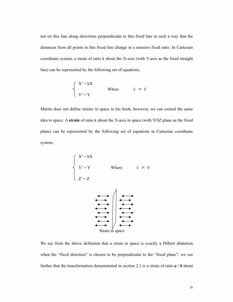
26

not on this line along directions perpendicular to this fixed line in such a way that the

distances from all points to this fixed line change in a nonzero fixed ratio. In Cartesian

coordinate system, a strain of ratio k about the X-axis (with Y-axis as the fixed straight

line) can be represented by the following set of equations,

Martin does not define strains in space in his book, however, we can extend the same

idea to space. A strain of ratio k about the X-axis in space (with YOZ plane as the fixed

plane) can be represented by the following set of equations in Cartesian coordinate

system,

We see from the above definition that a strain in space is exactly a Hilbert dilatation

when the “fixed direction” is chosen to be perpendicular to the “fixed plane”; we see

further that the transformation demonstrated in section 2.1 is a strain of ratio a / b about

Strain in space

X’ = kX Y’ = Y Z’ = Z

Where k ≠ 0

X’ = kX Y’ = Y

Where k ≠ 0

27

the Y-axis with the XOZ plane as the fixed plane.

If we assume that the “fixed direction” described in Hilbert dilatation need not be

perpendicular to the “fixed plane”, then we need to define a new transformation to fully

understand Hilbert dilatation. This new kind of transformation is called a shear. Martin

defines a shear in the plane as follows,

A shear in the plane about the X-axis is a transformation having the following

equations,

Again, shear in space is not defined by Martin, but extending the same idea, a shear in

space about the YOZ plane can be represented by

Shear in space

X’ = X Y’ = Y + k1X Z’ = Z + k2X

Where k12 + k2

2≠ 0

X’ = X + kY Y’ = Y

Where k ≠ 0

28

We see from the above definition that there is always a fixed plane in a shear in space.

In the above equations, the YOZ plane is the fixed plane of the shear.

With the definitions for strain and shear in space, I shall now give a set of equations that

can represent Hilbert dilatation. In Cartesian coordinate system, Hilbert dilatation of

ratio k with YOZ plane as the fixed plane can be represented by the following set of

equations:

We see that in the above equations, when k1 = k2 = 0, it becomes a strain.

From the equations the represent a strain, a shear and a Hilbert dilatation, I derived the

following theorem:

Theorem 2.2-1: Hilbert dilatation is a product (composition) of a strain and a shear

in space.

I omit the proof. □

X’ = kX Y’ = Y + k1X Z’ = Z + k2X

Where k＞0, and k≠1

Hilbert’s dilatation

29

There is an important theorem relating strains and general linear transformations in

space, namely,

Theorem 2.2-2: A linear transformation is a product (composition) of strains.

To see why Theorem 2.2-2 is true, here it becomes necessary to define clearly the

following terms: “transformation”, “collineation”, “linear transformation”, and “affine

transformation”.

Definition I: A transformation in space is a one-to-one correspondence from the set of

points in space onto itself.

Definition II: A collineation is a transformation that transforms straight lines to straight

lines.

Definition III: A linear transformation in the Cartesian coordinate system in space is

any mapping having the following equations:

We see from this definition that, strains, shears and Hilbert dilatations are all linear

transformations.

Note that the term “linear transformation” defined by Definition III is different from

what we usually see in linear algebra.

Definition IV: An affine transformation is a collineation that preserves parallelism

X’ = aX + bY + cZ + p, Y’ = dX + eY + fZ + q Z’ = gX + hY + mZ + r

Where a b c d e f g h m

≠0

30

among lines (Meaning that parallel straight lines are transformed to parallel straight

lines under an affine transformation).

With the above four definitions, the following three theorems are stated in Martin’s

book.

Theorem IV: A collineation is an affine transformation; an affine transformation is a

collieation. (Martin, p.167)

Theorem V: A linear transformation is an affine transformation; an affine transformation

is a linear transformation. (Martin, p. 175)

Theorem VI: An affine transformation is a product of strains. (Martin, p.179) Although

for Theorem VI Martin only gives proofs when all the transformations are plane

transformations, but using similar arguments, it can be extended to transformations in

space. Algebraically, an affine transformation in space can be represented by a 3×3

invertible matrix. This matrix can always be factorized into a product of elementary

matrices. Any one of the three types of elementary matrices is exactly a shear, a strain

and a reflection, and it can be shown that a shear and a reflection is a composition of

strains.

Theorem IV and V imply the fact that linear transformation, affine transformation and

collineation are equivalent. Theorem 2.2-2 follows immediately from theorem VI and

this fact. Despite the validity of Theorem 2.2-2, in the context of group of

31

transformations, the set of all strains does not form a group, while the set of all linear

transformations forms a group. The reason why the set of all strains does not form a

group is because this set does not satisfy the closure property of a group. The

composite of two strains in space with two intersecting fixed planes is not a strain.

However, I successfully proved the following theorem, which I shall state here without

proof:

Theorem 2.2-3: The composition of two strains with parallel (or the same) fixed

plane(s) is either a strain or a translation along the direction of the two strains.

As a summary, I end this section with the following remark on transformations in space.

Remark 2.2: Hilbert dilatation is a product of a strain and a shear in space. Affine

transformations, collineations and linear transformations are equivalent transformations.

A linear transformation is a product of strains. Since isometries, stretches, dilations,

similarities, central similarities, strains, shears and Hilbert dilatations are all linear

transformations, so each of them is a product of strains. In this regard, strains seem to be

the most fundamental transformations among all linear transformations.

Since strains seem to be the most fundamental linear transformations, in the next section,

I will explore the properties of strains.

32

§2.3 Properties of strains

In this section, I shall explore the properties of strain transformations both in the plane

and in space. Some of the properties discussed in this section will be useful in the proof

presented in section 3.1.

Strains in the plane

Property P1: Strains in the plane preserve collinearity and parallelism.

Property P1 says that, under any strains in the plane, straight lines are transformed into

straight lines and parallel straight lines remain parallel. In previous section, we have

already seen that a strain is a linear transformation, and a linear transformation is an

affine transformation. Property P1 follows immediately from the definition of affine

transformation.

Property P2: Strains in the plane preserve betweenness.

What I mean by Property P2 is that, under any strains, for all points lying on a common

straight line, the distance between any two of them changes in the same ratio. In

particular, if points P Q and R lie on the same straight line and P is the midpoint of the

other two, then P’ is always the midpoint of Q’ and R’ under any strains. To see this

33

property, we build up a Cartesian coordinate system in the plane such that X-axis is

parallel to the direction of the strain, and Y-axis coincides with the fixed straight line of

the strain. Take any straight line in the plane, suppose it has a gradient of k. then for any

two points on this straight line with X-coordinates equal to x1 and x2, the distance

between them is

D(x1, x2) = (x1 - x2) √(1+k2)

After the strain of ratio a,

D’(x1, x2) = a (x1 - x2) √(1+k2)

So after the strain, the distance between x1 and x2 changes by a ratio of

D’(x1, x2) / D (x1, x2) = [a√(1+k2)] /√(1+k2)

Since factor a is constant and k is the same for all points lying on the straight line, the

result thus follows.

Property P3: Strains in the plane preserve the type of second order plane

curves.

For this property I shall present the proof for the case that under a strain, an ellipse will

always remain as an ellipse (or a circle). Using the previous Cartesian coordinate system,

suppose an ellipse having the following general equation:

AX2 + B Y2 + CXY + DX + EY +F = 0

Let

34

For the equation to be an ellipse type, if and only if,

△≠0

J＞0 and

△/I ＜0

After a strain of ratio a along the X-axis direction, the curve can be represented by

a2AX’2 + B Y’2 + aCX’Y’ + aDX’ + EY’ +F = 0

I shall now shall that the corresponding conditions for the above equation to be an

ellipse also hold, namely

△’≠0

J’ ＞0 and

△’/ I’ ＜0

For this purpose we expand △, J, △’ and J’, we see that

△ = ABF + (1/4)CDE – (1/4) AE2 –(1/4)FC2 – (1/4)BD2

J = AB –(1/4)C2

△’ = a2ABF + (1/4) a2CDE – (1/4) a2AE2 –(1/4) a2FC2 – (1/4) a2BD2

J’ = a2AB –(1/4) a2C2

So we have △’ = a2△ and J’= a2 J

By our assumption a is nonzero, so △≠0 and J＞0 imply △’≠0 and J’＞0.

35

Note that since

J = AB –(1/4)C2 ＞0

A and B must be of the same sign, and since

I = A + B

I’ = A’ + B’ = a2A + B

So I and I’ must be of the same sign, and we know △’ = a2△, therefore △/I ＜0

implies △’/I’ ＜0. So all the three conditions still hold after a strain.□

It can be proved in a similar way that in general, under any strain in the plane,

hyperbolas will be transformed into hyperbolas, parabolas will be transformed into

hyperbolas, so strain in the plane preserves the type of second order plane curves.

Property P4: Strains in the plane preserve concurrency and tangency.

If a straight line is tangent to an ellipse in the plane, after a strain, the ellipse is

transformed into a new ellipse and the straight line a new straight line, Property P4 says

that, this new straight line must be tangent to the new ellipse. Property P4 also says that

if 3 straight lines are concurrent in the plane, they will always remain three concurrent

straight lines under any strains in the plane. These properties follow from P3 and the

fact that a strain (a linear transformation) is a mapping of points both one-to-one and

onto.

Here I present an interesting example applying the idea of Property P4. I try to derive

36

the equation of a straight line tangent at a given point on a given ellipse by transforming

the ellipse into a circle. The problem is shown below:

Suppose we have an ellipse in the plane having the following equation

X2 /a2 + Y2/b2 = 1

What is the equation of the tangent line to this ellipse through a give point P(x0,

y0) on the ellipse?

I solve this problem using strains. Suppose we keep the Y-axis fixed and do a strain to

the X-axis such that X’ = X/a. We then keep the X-axis fixed and do a strain to the

Y-axis such that Y’ = Y/b. We see that the ellipse in the original plane has become a

circle in our new plane after the two strains. The circle has an equation of X’2 + Y’2 = 1.

Suppose the in the original plane, p is the straight line tangent to the ellipse at point (x0,

X2 /a2 + Y2/b2 = 1 X’2 + Y’2 = 1

Two strains such that X’ = X/a Y’ = Y/b

Figure 1.4-1

(x0, y0) (x0’, y0’)

pP’

X

Y

X’

Y’

O O’

37

y0), then by our Property P1 and P4, p must be transformed into a new straight line

tangent to the circle at a point (x0’, y0’) where x0’ = x/a, y0’ = y/b.

Now any straight line tangent to a circle must be perpendicular to the straight line

connecting the center of the circle and the point of contact. So if the gradient of p is k, k

must satisfy k (y0’ / x0’) = -1, and hence k = -(x0’/ y0’).

Since p pass through the point (x0’ y0’), so the equation of p’ can be written as

(Y’ - y0’) / (X’- x0’) = -(x0’/ y0’)

Now if we do the reverse of the two strains in the plane, or in other words if we now

substitute back X’ = X /a and Y’= Y /b, we will get the equation of p in the original

plane, which is

y0Y / b2 + x0X / a2 = 1

This is exactly the correct equation we want! The above result, to some extend, verifies

the validity of our Property P1, P3 and P4.□

Anyone with elementary projective geometry knowledge may notice from our Property

P1 and P4 that, the idea of strains are closely related to the idea of perspectives in

Projective Geometry. Since strains always transform straight lines to straight lines and

they preserve tangency and concurrency, any projective configurations that can be

transformed into each other under strains are essentially isomorphic configurations in

38

the context of Projective Geometry.

For example, if we can proof Brianchon’s Theorem in the case that if the 6 sides of a

hexagon touch a circle, the three diagonals of the hexagon must be concurrent, we can

immediately extend this theorem to the cases for ellipses, namely if the 6 sides of a

hexagon touch an ellipse, the three diagonals of the hexagon must also be concurrent.

To see this result, we simply transform the ellipse to a circle under a number of strains,

(in fact in this case one single strain is always enough.), by Brianchon’s Theorem for the

circle case, the 3 diagonals after the strains must be concurrent. We then do the reverse

transformations to get back our original ellipse, while it can be shown that the reverse

transformation of a strain is also a strain, by P4, the result follows.

Property P5: Any two intersecting straight lines can be transformed into two

perpendicular straight lines by one strain in the plane.

Property P5 is easy to see if we choose the fixed straight line of the strain to be the

angle bisector of the two straight lines. In fact Martin states a much stronger

property similar to Property P5: given △ABC and △DEF, there is a unique affine

transformation that transforms △ABC onto △DEF. (Martin, p.176)

39

Strains in space

I shall follow the same way as in the case of strains in the plane, listing out explicitly

the properties of strains in space in this section.

Property S1: Strains in space preserve collinearity, coplanarity and

parallelism.

This property says that strains in space transform straight lines into straight lines, planes

into planes; parallel straight lines or planes remain parallel under any strains in space.

Property S2: Strains in space preserve betweenness.

Analogous to Property P2, Property S2 says that under any strain in space, for all points

lying on a common straight line, the distance between any two of them change in the

same ratio. In particular, if points P Q and R lie on the same straight line and P is the

midpoint of the other two, then P’ is always the midpoint of Q’ and R’ under any strains.

Property S2 can be shown using a similar proof presented under Property P2.

Property S3: Strains in space preserve the type of second order surfaces.

Property S3 says that, an ellipsoid in space will always remain as an ellipsoid under any

40

strains in space; a hyperboloid of one sheet will always remain as a hyperboloid of one

sheet under any strains in space, and same for other types of quadrics.

Property S4: Strains preserve concurrency and tangency in space.

Property S5: Any two intersecting planes can be transformed into two

perpendicular planes by one strain.

Property S5 is easy to see if we choose the fixed plane of the strain to be the

dihedral angle bisector of the two given intersecting planes.

All the properties of strains in space bear analogous ideas from corresponding

properties of strains in the plane, and the proofs are similar, here I shall only present

a proof for Property S3, and for the case when the quadratic surface is a

hyperboloid of one sheet.

Given a general quadratic equation in three variables,

aX2+bY2+cZ2+2fYZ+2gZX+2hXY+2pX+2qY+2rZ+d=0,

Let

For the equation to be a representation of a hyperboloid of one sheet, if and only if the

41

following 3 conditions hold,

Condition 1: Rank(e) = 3

Condition 2: Det(E) ＞0

Condition 3: The nonzero eigenvalues of e are not all of the same sign.

(Depending on whether the above conditions are satisfied or not, a general second order

equation with three variables can represent in total 17 different types of quadratic

surfaces including imaginary surfaces. For example, if in the above three conditions,

condition 3 is changed to be its negation, then the equation will represent an imaginary

ellipsoid.)

I shall show that after a strain of ratio k (k≠0) with the YOZ plane as the fixed plane, the

above three conditions still hold. After the strain, the original equation becomes

k2aX2+bY2+cZ2+2fYZ+2kgZX+2hkXY+2pkX+2qY+2rZ+d=0,

Suppose the corresponding e and E now become e’ and E’, where

It can be calculated from above that

Det(e’) = k2 Det(e) and

Det(E’) = k2 Det(E).

k2a kh kg kh b f kg f c

e’ =

k2a kh kg kp kh b f q kg f c r kp q r d

and E’ =

42

Condition 1. Since

Rank(e) =3 implies Det(e) ≠ 0

and by our assumption k ≠ 0, it follows that

Det(e’) = k2Det(e) ≠ 0

Det(e’) ≠ 0 implies Rank(e’) = 3

Condition 2:

Det(E) ＞0 and k2＞0 imply

Det(E’) = k2Det(E) ＞0

Condition 3: We need some theorems in linear algebra to see why condition 3 holds

after the strain. They are:

Theorem A: A square matrix A is invertible if and only if λ= 0 is not an eigenvalue of A.

(Anton p.343)

Theorem B: If A is a symmetric matrix, then the eigenvalues of A are all real numbers.

(Anton p.358 & p.526)

Theorem C: A symmetric matrix A is positive definite if and only if all the eigenvalues

of A are positive. (Anton p.450)

Theorem D: A symmetric matrix A is positive definite if and only if all the determinant

of every principal submatrix is positive. (Anton p.451)

From Theorem C and D, the following theorem can be deduced.

43

Theorem E: A symmetric matrix has both positive and negative eigenvalues if and only

if the determinants of its principal submatrices have both positive and negative values.

Since both matrix e and matrix e’ have a rank of 3, so both of them are invertible, we

see from Theorem A that, λ= 0 is not an eigenvalue of either e or e’. Since both matrix e

and matrix e’ are symmetric matrices, we see from Theorem B that the eigenvalues of

both e and e’ are real values. So now we know that both e and e’ has 3 nonzero real

eigenvalues.

It can be shown that the determinants of the principal submatrices of e’ are k2(＞0)

times the determinants of corresponding principal sbumatrices of e, so the strain does

not change the signs of the determinants of the principal submatrices of e. From

Theorem E, it follows that if the nonzero eigenvalues of e are not all of the same sign,

then the nonzero eighenvalues of e’ are not all of the same sign, too. Hence we see that

Condition 3 holds under the strain.

Since all the 3 conditions still hold after the strain, we have proved that under any

strains in space, a hyperboloid of one sheet will remain as a hyperboloid of one sheet.□

Intuitively, since a hyperboloid of one sheet is a doubly ruled surface which contains

two families of straight lines and infinitely many ellipses on it, and since strains in

44

space always change straight lines into straight lines, ellipses into ellipses, it can be

imagined that, any strains in space will transform a hyperboloid of one sheet into a new

quadratic surface that still contains two families of straight lines and infinitely many

ellipses on it. The only quadratic surface having these properties is the hyperboloid of

one sheet.

As have discussed in section 2.2, a linear transformation is a product of strains, so it is

concluded here that all the properties of strains listed out in this section are also true for

any other linear transformation. Since Hilbert dilatation is a linear transformation, so

Hilbert dilatation preserves the type of a quadratic surface in space, and this explains the

remarks given at the end of section 2.1.

45

Chapter III

Geometry and the Imagination

§3.1 From skew lines to a hyperboloid of one sheet

On page 14 of Hilbert’s book, he presented a method for generating a hyperboloid of

one sheet from 3 given straight lines in space which are mutually skew and are not

parallel to a common plane:

Let p q and r be the 3 given straight lines, we construct all the straight lines

which have a common point with each of the three lines. To do this, we choose

a point P on p, take the intersection of the plane containing P and q with the

plane containing P and r, hence the straight line of intersection is what we want.

By varying the position of P, we will get all the straight lines that interesting all

3 given lines. All these straight lines that we have just constructed make up a

hyperboloid of one sheet.

Hilbert argues that since a hyperboloid of one sheet consists of two families of straight

lines, and these straight lines are arranged such a way that every line of one family has a

point in common with every line of the other family and any two lines of the same

family are mutually skew, if we take the given three skew straight lines p q and r to be

three lines coming from the same family of a hyperboloid of one sheet, then any straight

46

line that intersects all the 3 given lines must be on the same surface, because no straight

line not lying in the surface can intersect a quadratic surface at more than two points.

A careful reader will soon notice that in Hilbert’s arguments, he actually made an

assumption which is not so easy to see why, that is,

For any 3 given straight lines in space which are mutually skew and are not

parallel to a common plane, there always exists a hyperboloid of one sheet such

that this hyperboloid of one sheet contains the 3 given straight lines.

Hilbert indeed made the assumption without a proof. In fact, he stated without proof on

page 15 in his book that

“Three skew straight lines always define a hyperboloid of one sheet, except in

the case where they are all parallel to one plane (but not to each other). In this

case they determine a hyperbolic paraboloid.”

In this section I will present a proof for the following theorem:

Theorem 3.1 For any three straight lines which are mutually skew and are not parallel

to a common plane, there always exist a hyperboloid of one sheet containing these three

lines.

Denote the three straight lines with p q r. I will prove the above theorem in 4 steps.

47

Step 1. Construct a space hexagon. This hexagon has the following properties.

1. p q r pass through 3 alternating sides of the hexagon. (By “3 alternating sides of

the hexagon” I mean 3 sides of the hexagon among which no two are adjacent.)

2. Any two opposite sides of this space hexagon are parallel and are of equal length.

To construct the desired hexagon, we first construct a plane S1 containing p, and a plane

S2 containing q such that S1∥S2 (Figure 3.1-1). Note that such S1,S2 always exist since

p q are two skew straight lines in space.

Claim: the third straight line r must intersect both S1 and S2. If not, then r∥ S1∥S2,

and we can always find a plane parallel to the three given lines, which contradicts our

assumption that such plane does not exist, hence the claim. Now since the claim is true,

suppose r intersect both S1 and S2 at points A, B respectively (Figure 3.1-2)

S2

S1

q

r

p

Figure 3.1-1

48

We then draw a straight line on S1 through A parallel to q, since p q are skew, the line

we draw must intersect p, for otherwise it will imply that p∥q. Denote the point of

intersection with F. Similarly we draw a straight line on S2 through B parallel to p, it

intersects q at a point, denote it with C.

Suppose we now construct a plane S3 which contains p and parallel to r, by a similar

argument as before, q must intersect with S3, denote the point of intersection with D.

Draw the straight line on S3 through D and parallel to r. This line intersects p, denote

the point of intersection E.

Now we see that ABCDEF form a space hexagon, with p q r pass through 3 alternating

sides of the hexagon. We see furthermore that each pair of opposite sides of this

hexagon are parallel.

S1

S2

B

q D

A

E pF

C

r

Figure 3.1-2

S3

49

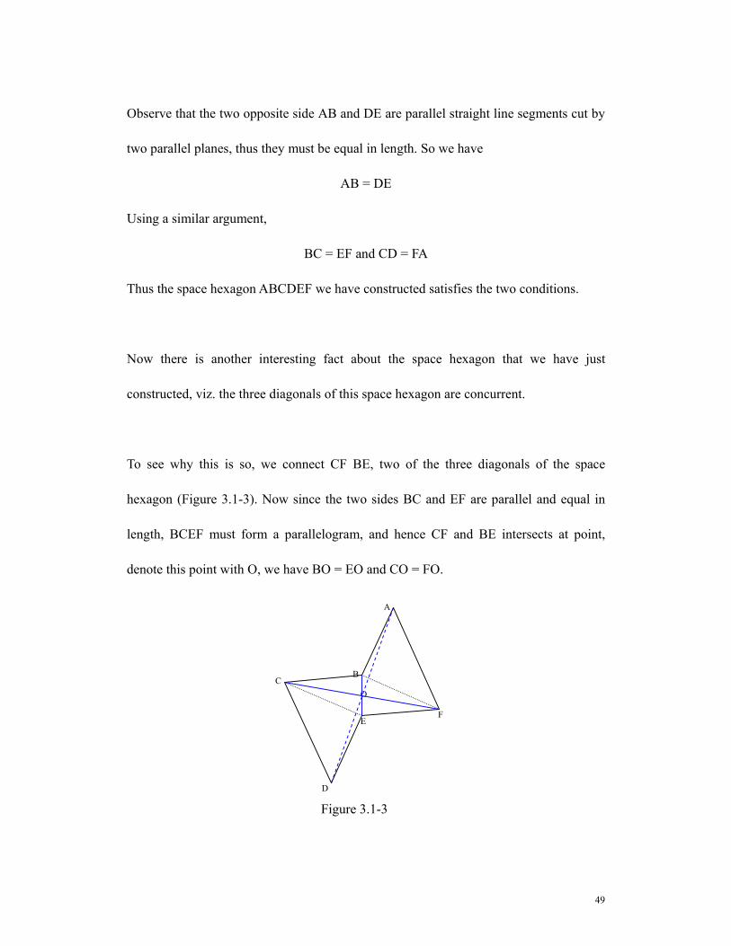
Observe that the two opposite side AB and DE are parallel straight line segments cut by

two parallel planes, thus they must be equal in length. So we have

AB = DE

Using a similar argument,

BC = EF and CD = FA

Thus the space hexagon ABCDEF we have constructed satisfies the two conditions.

Now there is another interesting fact about the space hexagon that we have just

constructed, viz. the three diagonals of this space hexagon are concurrent.

To see why this is so, we connect CF BE, two of the three diagonals of the space

hexagon (Figure 3.1-3). Now since the two sides BC and EF are parallel and equal in

length, BCEF must form a parallelogram, and hence CF and BE intersects at point,

denote this point with O, we have BO = EO and CO = FO.

O

F

D

E

B

A

C

Figure 3.1-3

50

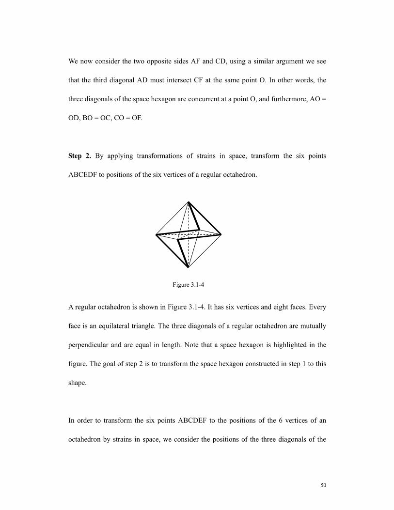
We now consider the two opposite sides AF and CD, using a similar argument we see

that the third diagonal AD must intersect CF at the same point O. In other words, the

three diagonals of the space hexagon are concurrent at a point O, and furthermore, AO =

OD, BO = OC, CO = OF.

Step 2. By applying transformations of strains in space, transform the six points

ABCEDF to positions of the six vertices of a regular octahedron.

A regular octahedron is shown in Figure 3.1-4. It has six vertices and eight faces. Every

face is an equilateral triangle. The three diagonals of a regular octahedron are mutually

perpendicular and are equal in length. Note that a space hexagon is highlighted in the

figure. The goal of step 2 is to transform the space hexagon constructed in step 1 to this

shape.

In order to transform the six points ABCDEF to the positions of the 6 vertices of an

octahedron by strains in space, we consider the positions of the three diagonals of the

Figure 3.1-4

51

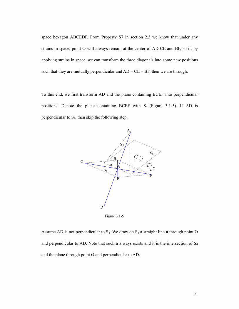
space hexagon ABCEDF. From Property S7 in section 2.3 we know that under any

strains in space, point O will always remain at the center of AD CE and BF, so if, by

applying strains in space, we can transform the three diagonals into some new positions

such that they are mutually perpendicular and AD = CE = BF, then we are through.

To this end, we first transform AD and the plane containing BCEF into perpendicular

positions. Denote the plane containing BCEF with S4 (Figure 3.1-5). If AD is

perpendicular to S4, then skip the following step.

Assume AD is not perpendicular to S4. We draw on S4 a straight line a through point O

and perpendicular to AD. Note that such a always exists and it is the intersection of S4

and the plane through point O and perpendicular to AD.

S4 O

a

F

D

E

B

A

C

Figure 3.1-5

S5

S6

52

By our construction a intersects AD at point O, thus a and AD are coplanar. Denote the

plane containing AD and a with S5. Apparently S5 and S4 intersect in a, so by Property

S6 discussed in section 2.3, S4 and S5 can be transformed into two perpendicular plane.

And the way to do this is as follows, we take a plane S6 through a such that it makes the

same dihedral angle θ with S4 and S5, θ must be greater than 0 and less than 90 degree.

We then choose S6 to be the fixed plane and apply a strain in space about this plane with

a ratio equal to Cot(θ), it can be shown that under this strain, S4 and S5 will be

transformed into two perpendicular planes.

It can further be proved that a and AD remain perpendicular in the process. Because in

the process of the strain, the projection of AD on S6 will always remains unchanged, and

it can be deduced from this that AD and a remain perpendicular under the above

transformation of strain.

We now look at the new positions of the figures after we applied the strain in space.

Since now the plane containing AD and a is perpendicular to S4, and AD is

perpendicular to a, the intersection of S4 and S5, it follows that now AD is perpendicular

to S4 (Figure 3.1-5).

In the new figure, we draw the angle bisector b of ∠BOC on S4, suppose b makes an

angle θ’ with either OC or OB. Since b has a common point O with AD, they are

53

coplanar. Denote the plane containing AD and b with S7. AD is perpendicular to S4

necessarily implies the fact that S7 is perpendicular to S4.

We then do another strain in space. This time we choose S7 as the fixed plane, and

Cot(θ’) as the strain ratio, it can be proof that after this transformation, BE and CF

become perpendicular, and in the process, AD always remain perpendicular to S4. By

now all the three diagonals AD BE and CF become mutually perpendicular, the thing

remained is to transform them into equal length. But this remaining task is easy to do.

We first choose the plane containing AD and BE to the fixed plane, and apply a strain in

space with ratio equal to the AD/CF, then CF is transformed to have the same length

with AD. We then choose the plane containing AD and CF to be the fix plane, and do a

b

S4 O

F

D

E

B

A

C

Figure 3.1-6

S7

54

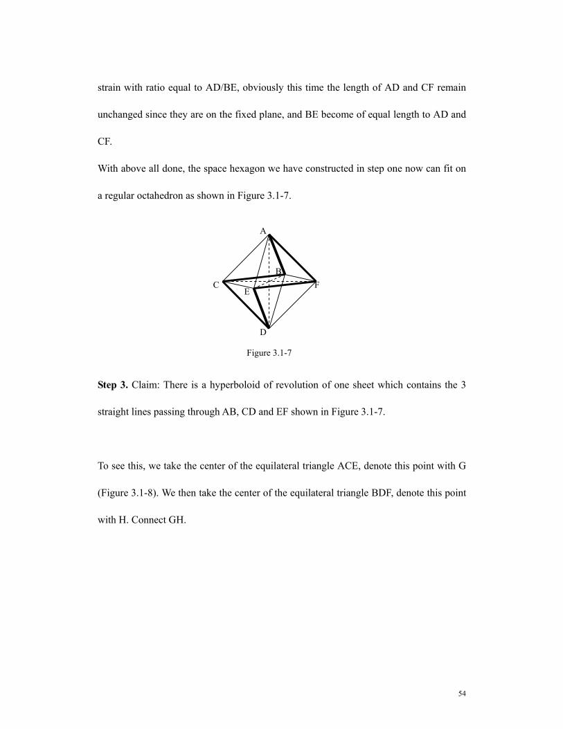
strain with ratio equal to AD/BE, obviously this time the length of AD and CF remain

unchanged since they are on the fixed plane, and BE become of equal length to AD and

CF.

With above all done, the space hexagon we have constructed in step one now can fit on

a regular octahedron as shown in Figure 3.1-7.

Step 3. Claim: There is a hyperboloid of revolution of one sheet which contains the 3

straight lines passing through AB, CD and EF shown in Figure 3.1-7.

To see this, we take the center of the equilateral triangle ACE, denote this point with G

(Figure 3.1-8). We then take the center of the equilateral triangle BDF, denote this point

with H. Connect GH.

B

D

F E

C

A

Figure 3.1-7

55

Now if we rotate the regular octahedron about the straight line passing through GH, by

the highly symmetrical nature of a regular octahedron, we see that the three sides AB,

CD and EF can be brought onto each other in the motion of rotation!

In section 1.2 we have seen that if we rotate a straight line in space about an axis skew

to it, we will get a hyperboloid of revolution of one sheet. Now if we rotate the straight

line containing the side AB about the axis GH (note that they are skew), we will get a

hyperboloid of revolution of one sheet. Furthermore, the straight line containing CD or

EF must also lie in the same hyperboloid since AB will at some moment coincide with

both two sides in the process of rotation, hence the claim.

Same result for the other three alternating sides of the space hexagon, BC, DE and FA.

It actually can be proved that the hyperboloid of revolution of one sheet generated by

rotating any sides among the six about GH are the same, in other words, AB, BC , CD,

DE, EF, FA, these six sides all lie in the surface.

B

D

F E

C

A

Figure 3.1-8

G

H

56

Step 4. Conclusion: For any three straight lines in space which are mutually skew and

are not parallel to a common plane, there always exists a hyperboloid of one sheet

containing these three lines.

Proof. For any three straight lines in space which are mutually skew and are not parallel

to a common plane, by our Step 2 and Step 3, we can always transform them into

positions such that they are contained in a hyperboloid of revolution of one sheet.

Imagine now we construct the surface with the 3 straight lines in the surface in space. If

we now do the reverse transformations of the four strains we had applied in space, by

our Property S1, S4 in section 2.3, the hyperboloid of revolution must be transformed

into a surface of a hyperboloid of one sheet which still contains the three straight lines.

Since after the reverse transformations, the three straight lines are transformed back to

their original positions, so we have seen that there always exists a hyperboloid of one

sheet containing the three lines, hence the result.□

From discussions at the end of step 3 we actually can deduce that the hyperboloid of

one sheet that contains p q and r must contain all the six sides of the space hexagon we

constructed in step 1. As what I have pointed out in section 1.3, on a hyperboloid of one

sheet, there are two families of straight lines, for any three straight lines from the same

family, there is one and exactly one straight from the other family parallel to one of

them and intersects the other two. Since in general, for any three skew straight lines in

57

space, the straight line parallel to one of them and intersecting the other two is unique,

thus this straight line must also lie in the hyperboloid of one sheet defined by the three

given skew lines. This explains why the six sides of the space hexagon are all contained

in the hyperboloid of one sheet defined by p q and r.

Of course by constructing arbitrary straight lines intersecting p q and r, we can get

infinitely many space hexagons such that the six sides of these hexagons all lie in the

hyperboloid of one sheet defined by p q and r. But these kinds of hexagons does not

help in the above proof, because it is still hard to see what kind of strain transformations

can bring the six sides of these irregular shapes to good positions, in this sense, the

space hexagon we constructed in step 1 is certainly a wise one.

For the case when the three given straight lines are parallel to a common plane, they

define a hyperbolic paraboloid. The construction of this hyperbolic paraboloid from the

given three straight lines is similar to the hyperboloid of one sheet case: we construct all

straight lines in space that intersect all three of the given straight lines. My proof for the

hyperboloid of one sheet case can not be applied directly to solve the hyperbolic

paraboloid case, because a hyperbolic paraboloid is not a surface of revolution, and

cannot be obtained from a surface of revolution by strain transformations in space.

However, algebraically, the hyperbolic paraboloid case is simpler to solve than the

hyperboloid of one sheet, I will not present the analytical proof here.

58

§3.2 The closest regular packing of spheres

In chapter 2 of Hilbert’s book, in the study of space lattices, Hilbert mentioned an

interesting problem: Suppose you have infinitely many spheres all of unit diameter, how

can you arrange them in space to form a regular sphere packing with the highest density?

The density of a packing of spheres can be understood as, within a sufficient large space,

the ratio of the volume occupied by the spheres to the volume of the space.

We can construct such a packing layer by layer. To do this we first try to arrange the

spheres on the same plane. The smartest way to do this is obviously to put 6 other

spheres tangent to one at the center shown in Figure 3.2-1A, and then extend the same

pattern in the plane, in this plane packing, every sphere is tangent to 6 others

surrounding it. Evidently you cannot put more than 6 spheres all tangent to one at the

center, so 6 is the best you can do. A not so smart way to do it is to arrange the spheres

such that the centers of the spheres form unit squares as shown in Figure 3.2-1B.

We then extend the first layers into space. To do this we construct layers immediately

above and below the first layers by adding spheres in the hollows of the first layers. We

Figure 3.2-1A Figure 3.2-1B

59

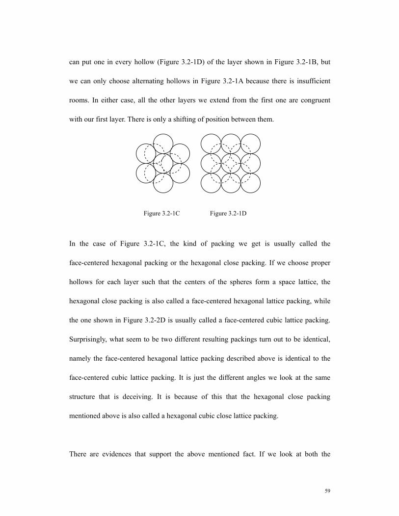
can put one in every hollow (Figure 3.2-1D) of the layer shown in Figure 3.2-1B, but

we can only choose alternating hollows in Figure 3.2-1A because there is insufficient

rooms. In either case, all the other layers we extend from the first one are congruent

with our first layer. There is only a shifting of position between them.

In the case of Figure 3.2-1C, the kind of packing we get is usually called the

face-centered hexagonal packing or the hexagonal close packing. If we choose proper

hollows for each layer such that the centers of the spheres form a space lattice, the

hexagonal close packing is also called a face-centered hexagonal lattice packing, while

the one shown in Figure 3.2-2D is usually called a face-centered cubic lattice packing.

Surprisingly, what seem to be two different resulting packings turn out to be identical,

namely the face-centered hexagonal lattice packing described above is identical to the

face-centered cubic lattice packing. It is just the different angles we look at the same

structure that is deceiving. It is because of this that the hexagonal close packing

mentioned above is also called a hexagonal cubic close lattice packing.

There are evidences that support the above mentioned fact. If we look at both the

Figure 3.2-1C Figure 3.2-1D

60

face-centered hexagonal lattice packing and face-centered cubic lattice packing, in both

packings, each sphere is tangent to 12 others surrounding it. In the hexagonal case, 6 in

the same layer, 3 below and 3 above, while in the cubic case, 4 in the same plane, 4

below and 4 above.

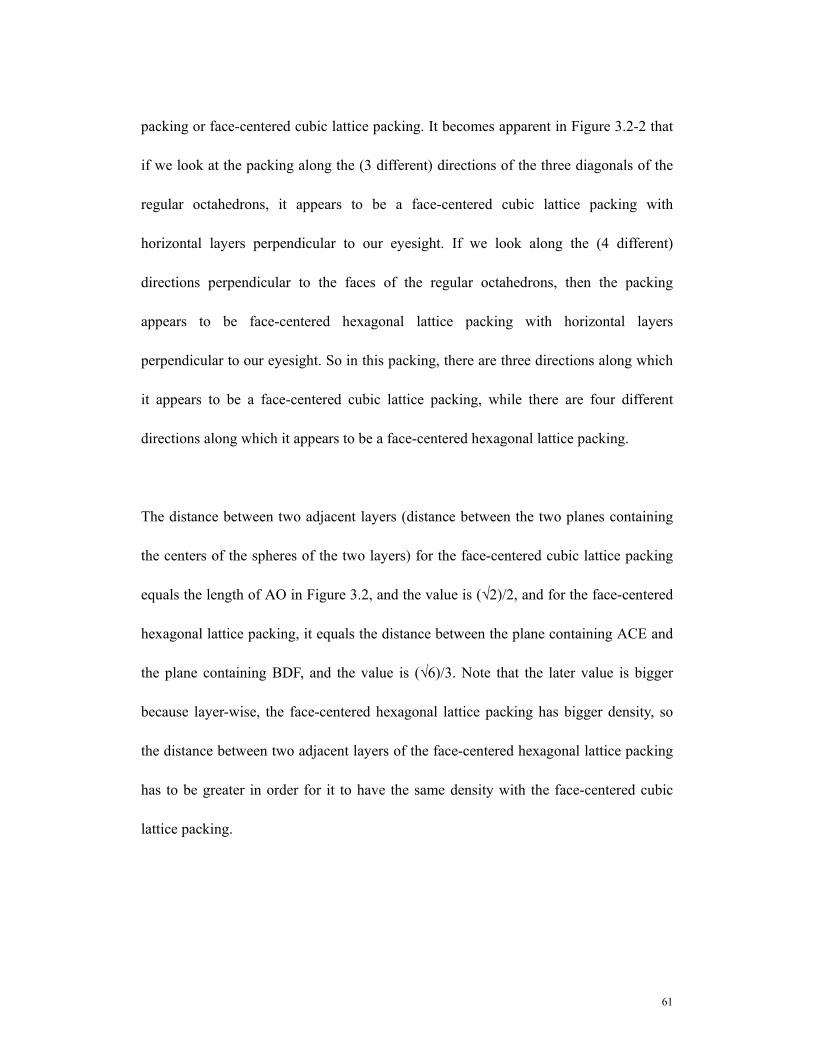
However the surprising fact can best be understood by the structure of a regular

octahedron. If we arrange unit regular octahedrons as shown in Figure 3.2-2 and extend

the same pattern in space we will get a space lattice consisting of the vertices of the

octahedrons.

If we now put spheres of unit diameter at each vertex of the lattice we get, then the

sphere packing is what we have constructed from face-centered hexagonal lattice

OB

D

FE

C

A

Figure 3.2-2

61

packing or face-centered cubic lattice packing. It becomes apparent in Figure 3.2-2 that

if we look at the packing along the (3 different) directions of the three diagonals of the

regular octahedrons, it appears to be a face-centered cubic lattice packing with

horizontal layers perpendicular to our eyesight. If we look along the (4 different)

directions perpendicular to the faces of the regular octahedrons, then the packing

appears to be face-centered hexagonal lattice packing with horizontal layers

perpendicular to our eyesight. So in this packing, there are three directions along which

it appears to be a face-centered cubic lattice packing, while there are four different

directions along which it appears to be a face-centered hexagonal lattice packing.

The distance between two adjacent layers (distance between the two planes containing

the centers of the spheres of the two layers) for the face-centered cubic lattice packing

equals the length of AO in Figure 3.2, and the value is (√2)/2, and for the face-centered

hexagonal lattice packing, it equals the distance between the plane containing ACE and

the plane containing BDF, and the value is (√6)/3. Note that the later value is bigger

because layer-wise, the face-centered hexagonal lattice packing has bigger density, so

the distance between two adjacent layers of the face-centered hexagonal lattice packing

has to be greater in order for it to have the same density with the face-centered cubic

lattice packing.

62

Bibliography

[1] Anton, Howard. Elementary Linear Algebra, Eighth Edition. John Wiley and Sons,

Inc. New York, 2000.

[2] Cederberg, Judith N. A Course in Modern Geometries. Springer-Verlag. New York

1989.

[3] Eric W. Weisstein. "Quadratic Surface." From MathWorld--A Wolfram Web

Resource. http://mathworld.wolfram.com/QuadraticSurface.html

[4] Hilbert, D. and Cohn-Vossen, S. Geometry and the Imagination, Chelsea Publishing

Company. New York, 1958.

[5] Martin, George E. Transformation Geometry: An Introduction to Symmetry.

Springer-Verlag. New York 1982.