Embed Size (px)
DESCRIPTION
This is part II of a collection of papers and book chapters on various statistical issues with a strong emphasis on the geometric perspective. Topics include linear regression (mainly), partial and canonical correlations, and Fisher's z-transformation.
Citation preview
A Geometric Approach to Compare Variables in a Regression Model
Johan BRING
Geometry is a very useful tool for illustrating regression analysis. Despite its merits the geometric approach is sel- dom used. One reason for this might be that there are very few applications at an elementary level. This article gives a brief introduction to the geometric approach in regres- sion analysis, and then geometry is used to shed some light on the problem of comparing the "importance" of the in- dependent variables in a multiple regression model. Even though no final answer of how to assess variable impor- tance is given, it is still useful to illustrate the different measures geometrically to gain a better understanding of their properties.
KEY WORDS: Coefficient of determination; Perpendicu- lar projection; Relative importance; Standardized regression coefficients; t values.
1. INTRODUCTION
Geometry is a very powerful and illustrative tool to de- scribe regression analysis. Despite its merits, geometry is seldom used in regression analysis, except for the use of scatterplots. By reviewing the history of the geometric ap- proach, Herr (1980) tries to answer the question, "Why is the geometric approach so seldom used?" His answer can be summarized in three points;
1. Tradition of an algebraic approach is so strong that it will take a lot of effort and time to make a change.
2. The use by Fisher (1915) and Durbin and Kendall (1951) of the pure geometric approach convinced two gen- erations of statisticians that geometry might be all right for the gifted few, but it would never do for the masses.
3. To fully appreciate the analytic geometric approach and to be able to use it effectively in research, teaching, and consulting requires that the statistician have an affinity for an talent in abstract thought. Dealing with abstractions is essentially a mathematical endeavor, and some statisticians eschew mathematics whenever possible (Herr 1980, p. 46).
In many regression studies one purpose is to compare the importance of different explanatory variables. Despite the fact that regression is an old and well-known technique, there is still debate about how to assess the importance of the explanatory variables. Several measures have been sug- gested and used, such as t values, standardized regression coefficient, elasticities, hierarchical partitioning, common-
ality analysis, increment in R2, semi-partial correlations, etc. Thorough discussions of some of these measures can be found in Darlington (1968, 1990), Pedhazur (1982), and Bring (1994d).
The aim of this article is twofold: first, to show the power of the geometric approach in studying regression, and sec- ond, to use this technique to shed some light on the problem of how to compare variables in a regression model.
In Section 2 a short summary of the geometric approach is given. Good introductions on how to use the geometric approach in statistics are given by Margolis (1979), Bryant (1984), Saville and Wood (1986), Saville and Wood (1991), and Draper and Smith (1981, chap. 10.5). In Sections 3-5 some measures used for comparing variables will be given a geometric interpretation, and this is followed by a summary in Section 6.
2. A GEOMETRIC PRESENTATION OF MULTIPLE REGRESSION
In most introductory texts on simple linear regression ge- ometry is used to gain a better understanding of the least squares method. The observations are plotted with the in- dependent variable (x) on one axis and the dependent vari- able (y) on the other. This presentation will be called the variable-axes presentation. In more advanced textbooks the calculations are usually solved by using matrix algebra. To geometrically illustrate the matrix calculations the variable- axes presentation is not suitable. A better way is to use what I will call the observation-axes presentation. Consider the following data matrix:
Yi Xll X12 ... Xlk
Y2 X21 X32 ... X2k
Y3 X31 X32 ... x3k
Yn Xnl Xn2 ..Xnk
It contains n observations on k + 1 variables, one depen- dent (y) and k independent (xi ... xk). One way of thinking about such a data matrix is that we have k + 1 variables spanning a k + 1-dimensional space. In this space we have n observations. In simple linear regression, where k = 1, it is easy to illustrate the data geometrically.
In matrix calculations each variable is considered as a vector in an n-dimensional space. Instead of thinking of n observations in a k + 1-dimensional space we could think
Table 1. Hypothetical Data for Adam and Eve
Height (cm) Weight (kg)
Adam 182 85 Eve 164 52
Johan Bring is a Statistician with the Regional Oncology Center, Uni- versity Hospital, S-751 85 Uppsala, Sweden. This article was written as a portion of the author's doctoral dissertation for the Department of Statis- tics at Uppsala University. The author thanks Axel Bring and the referees for their helpful comments.
? 1996 American Statistical Association The American Statistician, February 1996, Vol. 50, No. 1 57
Weight Eve
85-_ o Adam 164 Height
52-- Eve
52 Weight
164 182 Height 85 182 Adam
(a) (b)
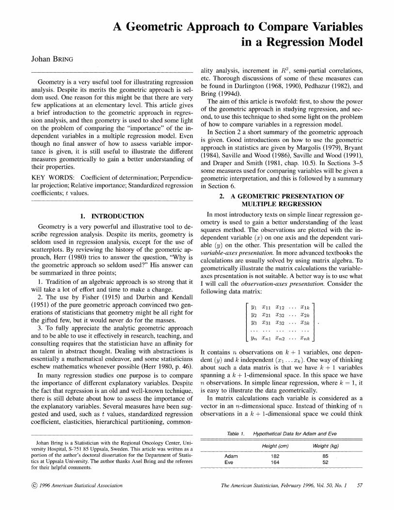
Figure 1. Two Geometrical Presentations of the Data in Table 1: (a) Variable-Axes and (b) Observation-Axes.
of k + 1 vectors in an n-dimensional space. In other words, instead of having one axis for each variable we have one axis for each observation. To clarify the difference, let us consider a simple example, Table 1 and Figure 1.
In the variable-axes presentation observations are rep- resented as points in a variable space, whereas in the observation-axes presentation variables are represented as vectors in observation space.
If we add a third person, we would, in the observation- axes presentation, get a third axis for that person, and the two vectors would now be in the three-dimensional space. Hence, independent of the number of observations, the data for height and weight will always be represented by two vectors. It is difficult to draw the vectors when there are more than three observations. However, as long as there are only two vectors, they span a two-dimensional subspace, and can therefore always be compared in a two-dimensional space.
From now on only the observation-axes presentation will be used. However, the base axes will be omitted and only the variable vectors will be displayed. To simplify the presentation we standardize the variables, xi = (x+ - ( - 1) y -
?)/sy+Y (Y+ - 1), where
x+ and y+ are the original variables. By this standardization the vectors will have length 1, and no intercept is needed in the regression model.
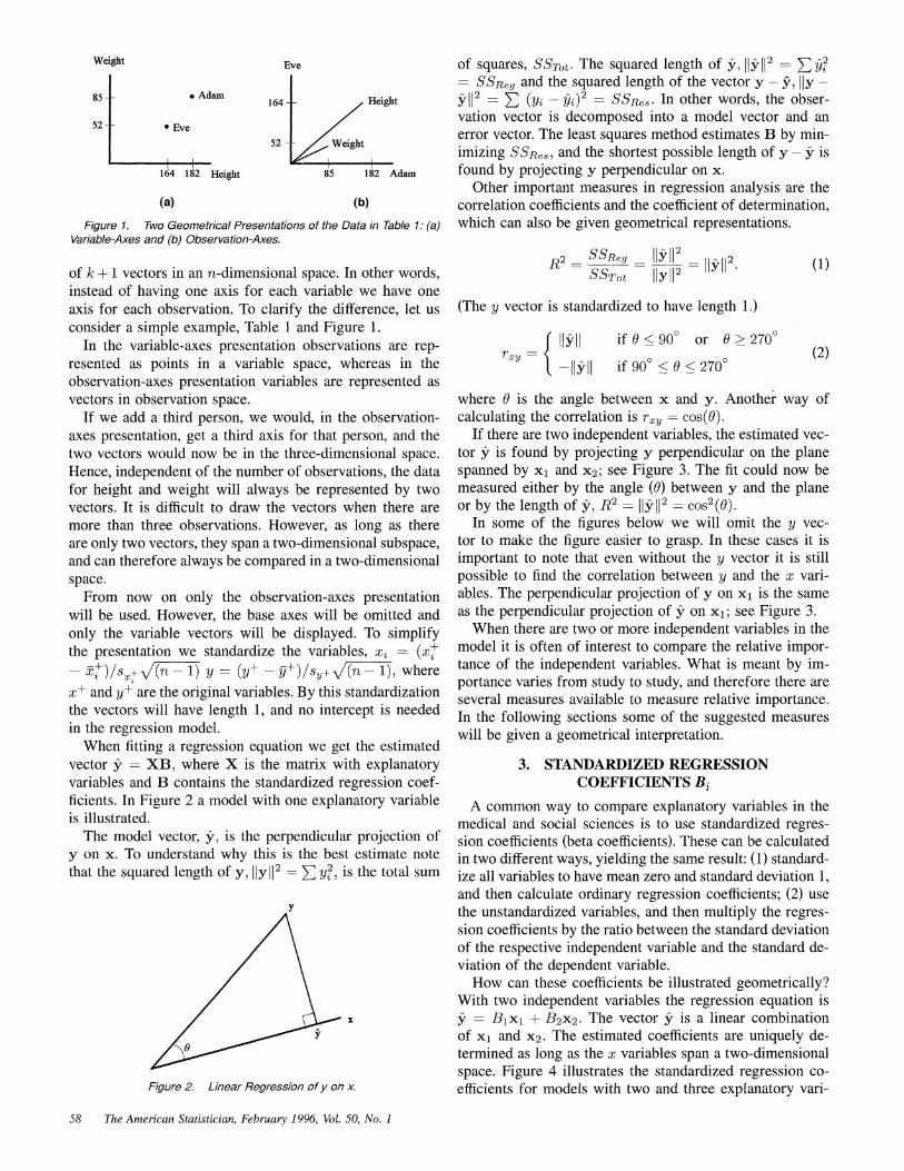
When fitting a regression equation we get the estimated vector y = XB, where X is the matrix with explanatory variables and B contains the standardized regression coef- ficients. In Figure 2 a model with one explanatory variable is illustrated.
The model vector, y, is the perpendicular projection of y on x. To understand why this is the best estimate note that the squared length of y, y2 Z 2 y?, is the total sum
y
Figure 2. Linear Regression of y on x.
of squares, SSTOt. The squared length of y 2 SSRCg and the squared length of the vector y - Y, IIy -
l2 = E (Yi _i)2 = SSRes. In other words, the obser- vation vector is decomposed into a model vector and an error vector. The least squares method estimates B by min- imizing SSRCs, and the shortest possible length of y - y is found by projecting y perpendicular on x.
Other important measures in regression analysis are the correlation coefficients and the coefficient of determination, which can also be given geometrical representations.
R2=Re = YS 2 (11 ) SST0t Iyll2
(The y vector is standardized to have length 1.)
if 0 < 900 or 0 > 2700
if 900 < 0 < 2700 (2)
where 0 is the angle between x and y. Another way of calculating the correlation is rxy = cos(0).
If there are two independent variables, the estimated vec- tor y is found by projecting y perpendicular on the plane spanned by xl and x2; see Figure 3. The fit could now be measured either by the angle (0) between y and the plane or by the length of y, R2 = I y 12 cos2 (0).
In some of the figures below we will omit the y vec- tor to make the figure easier to grasp. In these cases it is important to note that even without the y vector it is still possible to find the correlation between y and the x vari- ables. The perpendicular projection of y on xi is the same as the perpendicular projection of y on xi; see Figure 3.
When there are two or more independent variables in the model it is often of interest to compare the relative impor- tance of the independent variables. What is meant by im- portance varies from study to study, and therefore there are several measures available to measure relative importance. In the following sections some of the suggested measures will be given a geometrical interpretation.
3. STANDARDIZED REGRESSION COEFFICIENTS Bi
A common way to compare explanatory variables in the medical and social sciences is to use standardized regres- sion coefficients (beta coefficients). These can be calculated in two different ways, yielding the same result: (1) standard- ize all variables to have mean zero and standard deviation 1, and then calculate ordinary regression coefficients; (2) use the unstandardized variables, and then multiply the regres- sion coefficients by the ratio between the standard deviation of the respective independent variable and the standard de- viation of the dependent variable.
How can these coefficients be illustrated geometrically? With two independent variables the regression equation is
B = 13xi + B2x2. The vector y is a linear combination of xl and x2. The estimated coefficients are uniquely de- termined as long as the x variables span a two-dimensional space. Figure 4 illustrates the standardized regression co- efficients for models with two and three explanatory vani-
58 The American Statistician, February 1996, Vol. 50, No. 1
A2..
y
Figure 3. Regression With Two Explanatory Variables and Two Ways to Estimate the Correlation (r1) Between x1 and y
ables. The standardized coefficient Bi is the signed distance traveled parallel with xi. Note that Bi can be negative.
Whether these coefficients are good indicators of vari- able importance is still under debate; see Pedhazur (1982), Greenland, Schlesselman, and Criqui (1986), Darlington (1990), and Bring (1994a, 1994b). Afifi and Clarke (1990), positive toward the use of standardized coefficients, give the following interpretation:
The standardized coefficients of the various X variables can be directly compared in order to determine the relative contribution of each to the regression plane. The larger the magnitude of the standardized Bi the more Xi contributes to the prediction of Y (Afifi and Clarke 1990, p. 155).
When the explanatory variables are uncorrelated then the B.'s could be used as indicators of contribution to the pre- diction of y. In this case the x vectors are orthogonal, and by using the Phythagoras theorem we get the following par- titioning of the model vector:
II2 = B 2 + B 2 + ' +B 2(3)
Note that in this case the standardized coefficients coincide with the correlation coefficients between y and xi. If the explanatory variables are correlated the partitioning in (3) does not hold, as can easily be seen from Figure 4a. Then there seems to be no justification why the Bi's should rep- resent relative contribution to the regression plane. More- over, removing the variable with the smallest Bi does not necessarily cause the smallest reduction in R2; see Bring (1994a).
4. t VALUES
When estimating a regression equation, a t value is usu- ally calculated for each independent variable. These t values
B3 x2
...............................................
(a) (b)
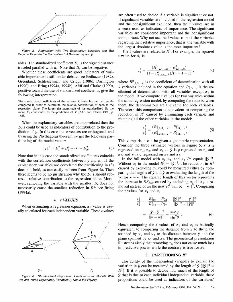
Figure 4. Standardized Regression Coefficients for Models With Two and Three Explanatory Variables (y Not in the Figure).
are often used to decide if a variable is significant or not. If significant variables are included in the regression model and the nonsignificant excluded, then the t values are in a sense used as indicators of importance. The significant variables are considered important and the nonsignificant unimportant. Why not use the t values to rank the variables regarding their relative importance, that is, the variable with the largest absolute t value is the most important?
The t values are related to R2. For example, the squared t value for i1 is
t2 1,l2,'3' ....k 2,3 .... k 1) '(4
where R1, 2,3 k is the coefficient of determination with all k variables included in the equation and R2,3 k is the co- efficient of determination with all variables except xl in the model. If we compute t values for two variables within the same regression model, by computing the ratio between them, the denominators are the same for both variables. Therefore this comparison is equivalent to comparing the reduction in R2 caused by eliminating each variable and retaining all the other variables in the model:
t _ 1 -,2,3... R2,3, .. k) (5
t2 (R1,2,3,... -kR1,3,...k)
This comparison can be given a geometric representation. Consider the three estimated vectors in Figure 5; y is y regressed on xl, x2, and X3, ... y iS y regressed on xl and x2, and y is y regressed on x2 and X3.
In the full model with x1,x2, and x3,R2 equals 1ll112. Without X3 in the model R2 = KHyl12. The reduction in R2 caused by excluding X3 could be measured either by com- paring the lengths of yi and yi or evaluating the length of the vector y - yi. The squared length of this vector represents the increase in SSRCs caused by excluding X3. If xl is re- moved instead of X3 the new R2 will be 11 y 112. Comparing the t values for xl and X3,
t2 R123-R23 _2 J-Y2 2 11 Y 112
t2 R2 - R2 JjSrJ2 _ 1Iyl2 3 123 12 K
_ _ _ _ _ _ _ _ sin 2
= KS1 1H2 sin2O (6)
Hence comparing the t values of x1 and X3 is basically equivalent to comparing the distance from y to the plane spanned by x2 and X3 to the distance between y and the plane spanned by xi and x2. The geometrical presentation illustrates nicely that removing X3 does not cause much loss in predictive power, while the contrary is true for xl.
5. PARTITIONING R2
The ability of the independent variables to explain the variation in y can be measured by the length of y (1l-M12 R2). If it is possible to decide how much of the length of y that is due to each individual independent variable, these proportions could be used as indicators of the variables'
The American Statistician, February 1996, Vol. 50, No. 1 59
X3
x2
y~~~~~ y~~~~~
xi
Figure 5. Three Regression Models (y, y, and y ) Based on Different Sets of Independent Variables (y Not in the Figure).
relative importance. In other words how much of R2 should be contributed to each of the independent variables?
Several measures of variable importance are calculated by partitioning R2 between the independent variables. If the independent variables are uncorrelated this partitioning is straightforward:
R?2 = Ir2 r22 + + rk 2(7)
However, when the variables are correlated we get different partitionings depending on the choice of method. In the next subsections three methods for partitioning R2 will be illustrated geometrically.
5.1 Stepwise
One way of selecting variables to be included in the re- gression equation is to use stepwise regression (forward); see Draper and Smith (1981). When this procedure is used most computer packages report the increment in R2 for each successive variable included. Unfortunately, these in- crements are sometimes used as indicators of the indepen- dent variables' relative importance. By using geometry it can be demonstrated that this a rather arbitrary approach for the assessment of relative importance.
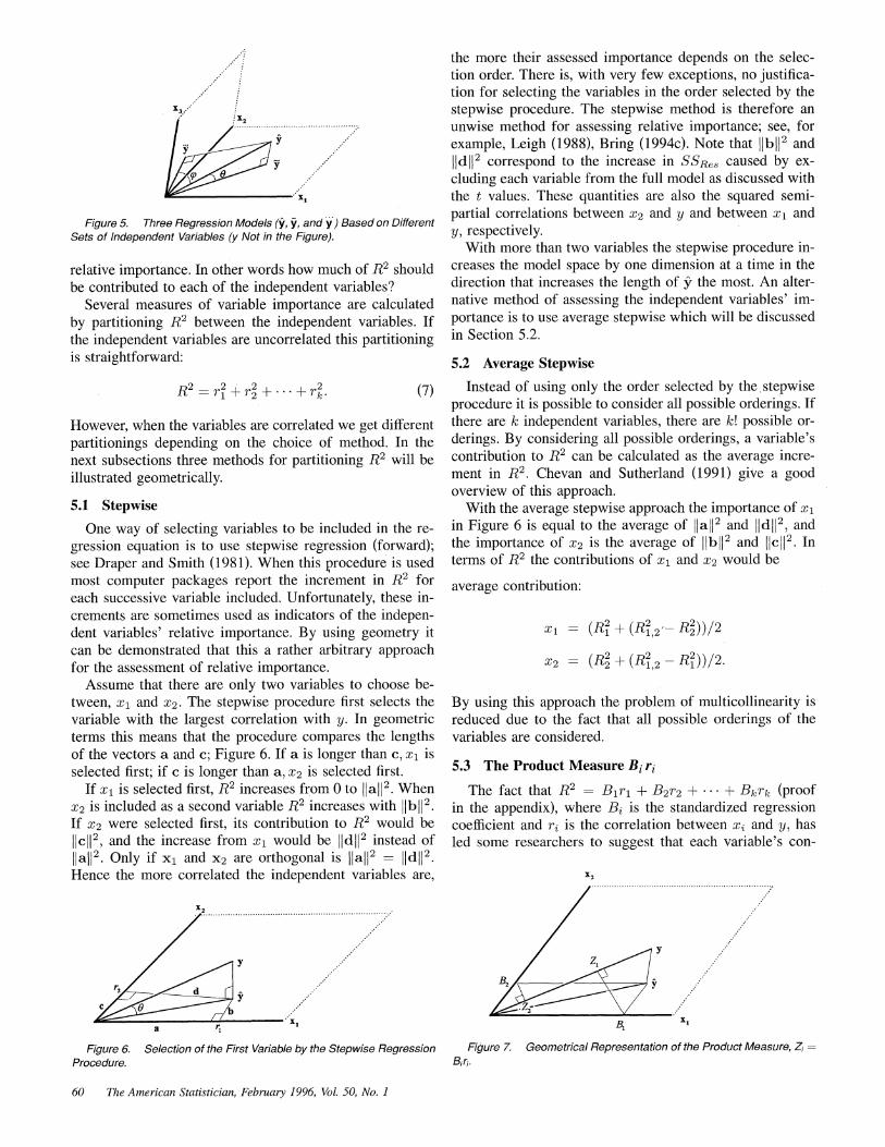
Assume that there are only two variables to choose be- tween, x1 and x2. The stepwise procedure first selects the variable with the largest correlation with y. In geometric terms this means that the procedure compares the lengths of the vectors a and c; Figure 6. If a is longer than c, x1 is selected first; if c is longer than a, x2 is selected first.
If x1 is selected first, R2 increases from 0 to flal 2. When x2 is included as a second variable R2 increases with Ilb 12.
If X2 were selected first, its contribution to R2 would be C 12, and the increase from x1 would be Ild 12 instead of
lal 2. Only if x1 and x2 are orthogonal is Ilal 2 = Ild 12. Hence the more correlated the independent variables are,
X2
y
a 1l
Figure 6. Selection of the First Variable by the Stepwise Regression Procedure.
the more their assessed importance depends on the selec- tion order. There is, with very few exceptions, no justifica- tion for selecting the variables in the order selected by the stepwise procedure. The stepwise method is therefore an unwise method for assessing relative importance; see, for example, Leigh (1988), Bring (1994c). Note that llbll2 and
Ild 12 correspond to the increase in SSRCs caused by ex- cluding each variable from the full model as discussed with the t values. These quantities are also the squared semi- partial correlations between x2 and y and between x1 and y, respectively.
With more than two variables the stepwise procedure in- creases the model space by one dimension at a time in the direction that increases the length of y the most. An alter- native method of assessing the independent variables' im- portance is to use average stepwise which will be discussed in Section 5.2.
5.2 Average Stepwise
Instead of using only the order selected by the.stepwise procedure it is possible to consider all possible orderings. If there are k independent variables, there are k! possible or- derings. By considering all possible orderings, a variable's contribution to R2 can be calculated as the average incre- ment in R2. Chevan and Sutherland (1991) give a good overview of this approach.
With the average stepwise approach the importance of xi in Figure 6 is equal to the average of Ilal 2 and Ild 12, and the importance of x2 is the average of IIb 12 and IIC 12. In terms of R2 the contributions of xl and X2 would be
average contribution:
xi = (R- 2 + (R2 -R2))/2
X2 = (R2+ (Ri,2-Rl))/2.
By using this approach the problem of multicollinearity is reduced due to the fact that all possible orderings of the variables are considered.
5.3 The Product Measure Bi ri
The fact that R2 = B1r1 + B2r2 + + Bkrk (proof in the appendix), where Bi is the standardized regression coefficient and ri is the correlation between xi and y, has led some researchers to suggest that each variable's con-
x2 ,2........................................................................
y
B2
B1 x
Figure 7. Geometrical Representation of the Product Measure, Z, B1r1.
60 The American Statistician, February 1996, Vol. 50, No. 1

y
X2
xi
Figure 8. Regression Model With Two Independent Variables.
tribution to R2 is equal to Biri. Pratt (1987) gives a solid justification for the use of this measure.
This measure is not as easy to understand as the two previous measures. The main reason for the difficulty is that the importance of each variable is calculated as a product of two factors. However, by using inner products it is easy to find a geometrical representation of this measure.
Biri ? lBixil cosO =?lBixil cosO llyI
? ?(Bi xi,y) = Zi (8)
where 0 is the angle between xi and y and K ) represents an inner product. Zi is the component of Bixi in the direction of y; see Figure 7.
Despite the ease in finding a geoiVetrical interpretation, it is still difficult to comprehend the meaning of this mea- sure. However, in Figure 8 an example is given where this measure gives a counterintuitive result.
The angle between x2 and y is 900, which means that the correlation between these variables is zero. Hence the importance of x2 in explaining R2 is zero according to the product measure. Therefore x1 is responsible for all the length of y. However, if we exclude x2, x1 would not ex- plain much at all of the variation in y, only I I y2. Hence with the product measure, x2's contribution to R2 is zero and x1's contribution to R2 equals R2. However, the inclu- sion of x2 greatly increases R2. Therefore it is not satisfac- tory that x2's contribution should be zero.
Figure 8 also illustrates the interesting situation where R2 > r2 + r2. For a discussion of when this occurs, see Bertrand and Holder (1988), Hamilton (1987), and Schey (1993). (Schey uses geometry to illustrate when this occurs.)
X2
B2~~~~~~~~~~~~~~~5
B1 'i X1
Figure A. 1. Relationship Between R2 and B1 r1?+ B2r2
6. SUMMARY
Geometry is a very powerful tool for illustrating many statistical techniques. However, it requires an ability for abstract thought. To attain this ability requires training, and it is therefore important that there are illustrations available at a rather elementary level.
This article has given a brief introduction to the geomet- ric approach to regression analysis, and I hope the presenta- tion has been at a suitable level even for the reader unfamil- iar with geometrical thinking. The geometric approach was also used to illustrate some measures that could be used for comparing the "importance" of the explanatory variables in multiple regression models. There is no unique definition of the concept importance, and no clear-cut answer can be given as to which measure to use. However, displaying these measures geometrically can increase the understanding of what they are measuring, and especially indicate situations when the measures are not suitable.
APPENDIX
Proof that R2 = B1rj + B2r2
R2= 11112 = 11y1 (a+b)
where a is the part of B1xl parallel to y and b is the part of B2x2 parallel to y (see Fig. A.1).
1IYI1(a+b) = III(B1cos0+B2 COS W)
- 11ycos O(Bi) + ||y||cos W(B2)
- rBj +r2B2.
The proof could easily be extended to more than two vari- ables.
[Received June 1993. Revised September 1994.]
REFERENCES
Afifi, A. A., and Clarke, V. (1990), Computer Aided Multivariate Analysis (2nd ed.), New York: Van Nostrand Reinhold.
Bertrand, B., and Holder, R. (1988), "A Quirk in Multiple Regression: The Whole Can Be Greater Than Its Parts," The Statistician, 37, 371-374.
Bring, J. (1994a), "How to Standardize Regression Coefficients," The American Statistician, 48(3), 209-213.
(1994b), "Standardized Regression Coefficients and Relative Im- portance of Pain and Functional Disability to Patients with Rheumatoid Arthritis," (Letter to the Editor with Reply), Journal of Rheumatology, 21(9), 1774-1775.
(1994c), "Relative Importance of Factors Affecting Blood Pres- sure," (Letter to the Editor), Journal of Human Hypertension, 8, 297.
(1994d), "Variable Importance and Regression Modelling," Doc- toral thesis, Department of Statistics, Uppsala University, Sweden.
Bryant, P. (1984), "Geometry, Statistics, Probability: Variation on a Com- mon Theme," The American Statistician, 38, 38-48.
Chevan, A., and Sutherland, M. (1991), "Hierarchical Partitioning," The American Statistician, 45, 90-96.
Darlington, R. B. (1968), "Multiple Regression in Psychological Research and Practice," Psychological Bulletin, 69, 161-182.
(1990), Regression and Linear Models, New York: McGraw-Hill. Draper, N., and Smith, H. (1981), Applied Regression Analysis (2nd ed.),
New York: John Wiley. Durbin, J., and Kendall, M. G. (1951), "The Geometry of Estimation,"
Biornetrika, 38, 150-158.
The American Statistician, February 1996, Vol. 50, No. 1 61

Fisher, R. A. (1915), "Frequency Distribution of the Values of the Cor- relation Coefficient in Samples from an Indefinitely Large Population," Biometrika, 10, 507-521.
Greenland, S., Schlesselman, J. J., and Criqui, M. H. (1986), "The Fallacy of Employing Standardized Regression Coefficients and Correlations as Measure of Effect," American Journal of Epidemiology, 123(2), 203- 208.
Hamilton, D. (1987), "Sometimes R2 > r'X1? 2 Correlated Variables Are Not Always Redundant," The American Statistician, 41, 129-132.
Herr, D. G. (1980), "On the History of the Use of Geometry in the General Linear Model," The American Statistician, 34, 131-135.
Leigh, J. P. (1988), "Assessing the Importance of an Independent Vari- able in Multiple Regression: Is Stepwise Unwise?," Journal of Clinical Epidemiology, 41(7), 669-677.
Margolis, M. S. (1979), "Perpendicular Projections and Elementary Statis-
tics," The American Statistician, 33, 131-135. Pedhazur, E. J. (1982), Multiple Regression in Behavioral Research (2nd
ed.), New York: Holt, Rinehart & Winston. Pratt, J. W. (1987), "Dividing the Indivisible: Using Simple Symmetry to
Partition Variance Explained," in Proceeding of the 2nd International Tampere Conference, eds. T. Pukkila and S. Puntanen, University of Tampere, 245-260.
Saville, D. J., and Wood, G. R. (1986), "A Method for Teaching Statistics Using N-Dimensional Geometry," The American Statistician, 40, 205- 214.
(1991), Statistical Methods: The Geometric Approach, New York: Springer-Verlag.
Schey, H. M. (1993), "The Relationship Between the Magnitudes of SSR(x2) and SSR(x21xl): A Geometric Description," The American Statistician, 47, 26-30.
62 The American Statistician, February 1996, Vol. 50, No. 1
e H A P TER 20
The Geometry of Least Squares
Comment: Philosophies on teaching the geometry of least squares vary. An early introduction is certainly possible, as demonstrated by the successful presentation by Box, Hunter, and Hunter (1978, e.g., pp. 179, 197-201) for specific types of designs. For general regression situations, more general explanations are required. Our view is that, while regression can be taught perfectly well without the geometry, understanding of the geometry provides much better understanding of, for example, the difficulties associated with singular or nearly singular regressions, and of the difficulties associated with interpretations of the R 2 statistic. For an advanced understanding of least squares, knowledge of the geometry is essential.
20.1. THE BASIC GEOMETRV
We want to fit, by least squares, the model
y = XfJ + E, (20.1.1 )
where Y and E are both n X 1, X is n X p, and fJ is p X 1. Consider a Euclidean (i.e., "ordinary") space of n dimensions, call it S. The n numbers YI , Y2 , ••• , Yn within Y define a point Y in this space. They al so define a vector (a line with length and direction) usualIy represented by the line joining the origin O, (O, O, O, ... , O), to the point Y. (In fact, any parallel line of the same length can also be regarded as the vector Y, but most of the time we think about the vector from O.) The columns of X also define vectors in the n-dimensional space. Let us assume for the present that all p of the X columns are linearly independent, that is, none of them can be represented as a linear combination of any of the others. This implies that X'X is nonsingular. Then the p columns of X define a subspace (we call it the estimation space) of S of p «n) dimensions. Consider
X/3 = [xQ, XI' X2' X), ... , xp-d [ ~ 1 = /3~ + /3I XI + ... + /3p-IXp-l,
{3p-1
(20.1.2)
where each X¡ is an n X 1 vector and the {3¡ are scalars. (Usually X() = 1.) This defines a vector formed as a linear combination of the X¡, and so XfJ is a vector in the estimation space. Precisely where it is depends on the values chosen for the {3¡. We can now draw
427
Draper NR, Smith H. 2003. Applied Regression Analysis. 3rd ed. New York: John Wiley & Sons.
428 THE GEOMETRY OF LEAST SQUARES
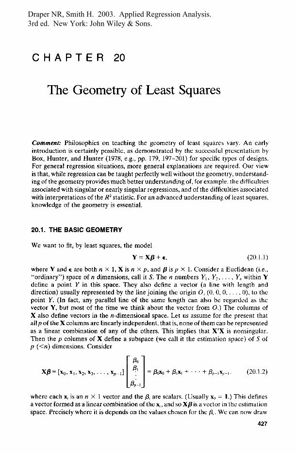
F I g u r e 20.1. A general point Xp in the estimation space.
Figure 20.1. We see that the points marked O, Y, Xp form a triangle in n-space. In general, the angles will be determined by the values of the (3¡, given Y and X. The three sides of the triangle are the vectors Y, Xp, and E = Y - xp. So the model (20.1.1) simply says that Y can be split up into two vectors, one of which, Xp, is completely in the estimation space and one of which, (Y - XP), is partially not, in general. When we estimate p by least squares, the solution b = (X'xtIX'Y is the one that minimizes the sum of squares function
S(P) = (Y - XP)'(Y - XP)· (20.1.3)
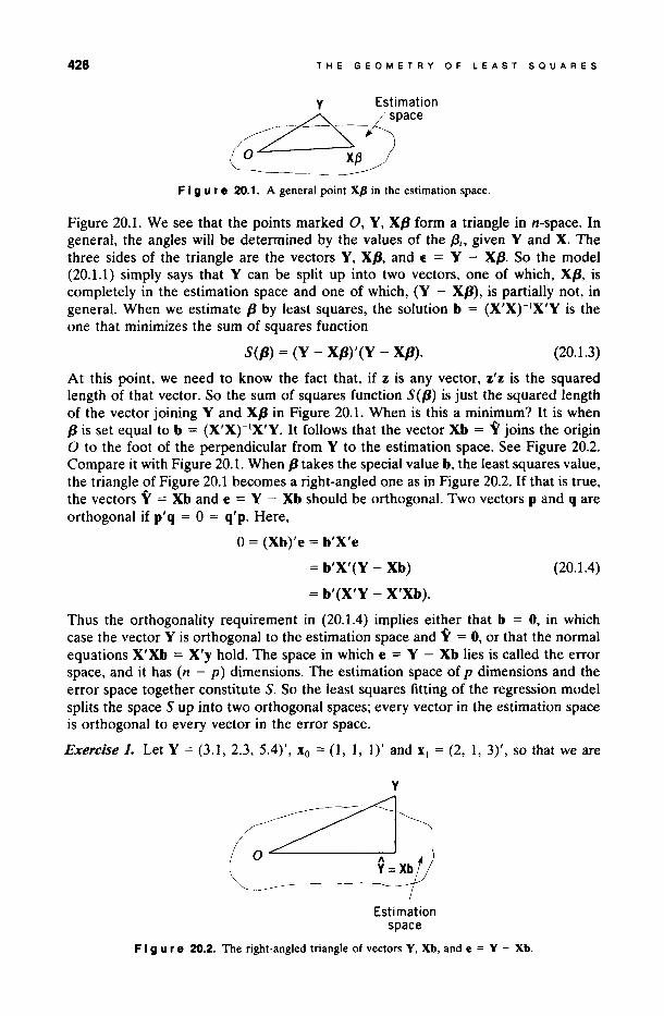
At this point, we need to know the fact that, if z is any vector, z'z is the squared length of that vector. So the sum of squares function S(P) is just the squared length of the vector joining Y and Xp in Figure 20.1. When is this a minimum? It is when p is set equal to b = (X'X)-IX'Y. It follows that the vector Xb = Y joins the origin O to the foot of the perpendicular from Y to the estimation space. See Figure 20.2. Compare it with Figure 20.1. When p takes the special value b, the least squares value, the triangle of Figure 20.1 becomes a right-angled one as in Figure 20.2. If that is true, the vectors Y = Xb and e = Y - Xb should be orthogonal. Two vectors p and q are orthogonal if p'q = O = q'p. Here,
0= (Xb)'e = b'X'e
= b'X'(Y - Xb) (20.1.4)
= b'(X'Y - X'Xb).
Thus the orthogonality requirement in (20.1.4) implies either that b = 0, in which case the vector Y is orthogonal to the estimation space and Y = 0, or that the normal equations X'Xb = X'y hold. The space in which e = Y - Xb Hes is called the error space, and it has (n - p) dimensions. The estimation space of p dimensions and the error space together constitute S. So the least squares fitting of the regression model splits the space S up into two orthogonal spaces; every vector in the estimation space is orthogonal to every vector in the error space.
Exercise 1. Let Y = (3.1, 2.3, 5.4)', Xo = (1, 1, 1)' and XI = (2, 1, 3)', so that we are
y
:2=:1 O 1\
Y = Xb
Estimation space
F I g u re 20.2. The right-angled triangle of vectors Y, Xb, and e = Y - Xb.
20.2. PYTHAGORAS ANO ANALYSIS OF VARIANCE 429
going to fit the straight line Y = /30 + /3¡X¡ + E via least squares. First, do the regression fit without worrying about the geometry. Show that Y = 0.50xo + 1.55x¡. Then show that Y = Xb = (3.60, 2.05, 5.15)' and e = (-0.50, 0.25, 0.25)'; confirm that these two vectors are orthogonal and furthermore that e is orthogonal to any vector of the form Xp = /3oXo + {3¡x¡, for aH p, because e is orthogonal to both (in general, aH) the individual columns of X. Write the coordinates of the various points on a diagram like Figure 20.2.
20.2. PYTHAGORAS ANO ANALYSIS OF VARIANCE
Every analysis of variance table arising from a regression is an application of Pythagoras's Theorem about the "square of the hypotenuse of a right-angled triangle equals the sum of squares of the other two sides." UsuaHy, repeated applications of Pythagoras's result are needed. Look again at Figure 20.2. It implies that
Y'Y = Y'Y + (Y - Xb)'(Y - Xb) (20.2.1)
or
Total sum of squares = Sum of squares due to regression + Residual sum of squares.
The corresponding degrees of freedom equation
n = p + (n - p) (20.2.2)
corresponds to the dimensional split of S into two orthogonal spaces of dimensions p and (n - p), respectively. The orthogonality of Y and e is essential for a clear splitup of the total sum of squares. Where a split-up is required of a particular sum of squares that does not have a natural orthogonal split-up, orthogonality must be introduced to achieve it.
Exercise 2. Show that for the data in Exercise 1, the two equations (20.2.1) and (20.2.2) correspond to
44.06 = 43.685 + 0.375, 3=2+1.
Further Split-up of a Regression Sum of Squares
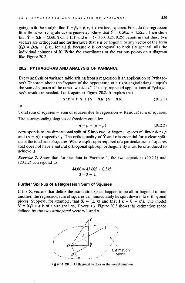
If the Xi vectors that define the estimation space happen to be aH orthogonal to one another, the regression sum of squares can immediately be split down into orthogonal pieces. Suppose, for example, that X = (1, x) and that l'x = O = x'l. The model Y = Xp + E is of a straight line, Y versus x. Figure 20.3 shows the estimation space defined by the two orthogonal vectors 1 and x.
y
Estimation space
F I 9 u r e 20.3. Orthogonal vectors in the model function.

430 THE GEOMETRY OF LEAST SQUARES
Because these vectors are orthogonal, perpendiculars from Y to these lines form a (right-angled) rectangle, so that
Oy2 = OA2 + OB2 (20.2.3)
(or OA2 + AY2, etc.). The division is unique because of the orthogonality of the base vectors 1, x; this result extends in the obvious way to any number of orthogonal base vectors, in which case the rectangle of Figure 20.3 becomes a rectangular block in the p-dimensional estimation space.
Exerc;se 3. For the least squares regression problem where
Y'=(6,9,17,18,26) and X'=[!2 !1 ~ ~ n show that the normal equations X'Xb = X'Y split up into two separa te pieces and that A and B in Figure 20.3 are the two "individual Y's" that come from looking at each piece separately. Hence evaluate Eqs. (20.2.1) and (20.2.2) for these data (1406 = 1395.3 + 10.7, and 4 = 2 + 2).
An Orthogonal Breakup of the Normal Equatlons
Let us redraw Figure 20.3 with sorne additional detail; see Figure 20.4, in which lines OYand OY are omitted but YA and YB have been drawn. In other respects the diagrams are intended to be identical. The points marked O, A, Y, and B form a rectangle, and thus Oy2 = OA2 + OB2, as mentioned. AIso, YA is perpendicular to OA, and YB is perpendicular to OB. Thus OA is "the Y for the regression of Y on 1 alone" and O B is "the Y for the regression of Y on x alone." This happens only beca use (here) 1 and x are orthogonal. The result also extends to any number of X vectors provided they are mutually orthogonal.
Exercise 4. For the data of Exercise 3, show that OA2 = 1155.2, OB2 = 240.1, and their sum is OY2 = 1395.3. AIso show that OA is the vector (15.2, 15.2, 15.2, 15.2, 15.2)', OB is (-9.8, -4.9, O, 4.9, 9.8)', and OY is the sum of these orthogonal vectors.
Orthogonallzing the Vectors of X In General
It is frequently desired to break down a regression sum of squares into components even when the vectors of X are not mutually orthogonal. Such a breakdown can
y
Estimation space
F I 9 u r e 20.4. Orthogonal breakup of the normal equations when model vectors are orthogonal.
20.2. PYTHAGORAS ANO ANALYSIS OF VARIANCE 431
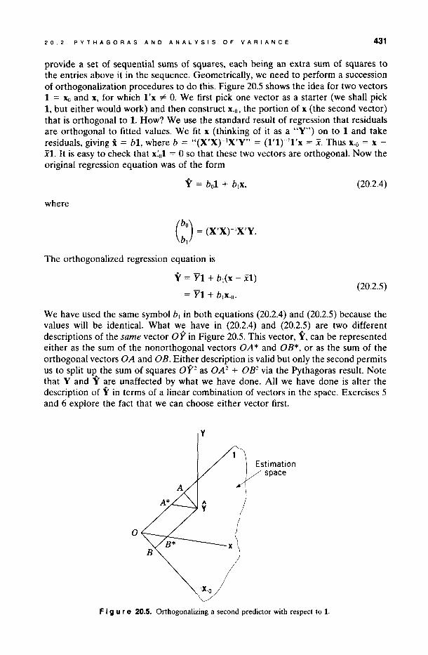
provide a set of sequential sums of squares, each being an extra sum of squares to the entries aboye it in the sequence. Geometrically, we need to perform a succession of orthogonalization procedures to do this. Figure 20.5 shows the idea for two vectors 1 = Xo and x, for which l'x ~ O. We first pick one vector as a starter (we shall pick 1, but either would work) and then construct x.o, the portion of x (the second vector) that is orthogonal to 1. How? We use the standard result of regression that residuals are orthogonal to fitted values. We fit x (thinking of it as a By") on to 1 and take residuals, giving i = bl, where b = "(X'xtIX'Y" = (l'lt'l'x = x. Thus x.o = x -xl. It is easy to check that x~ol = O so that these two vectors are orthogonal. Now the original regression equation was of the form
y = bol + b¡x,
where
(::) = (X'X¡-'X'Y.
The orthogonalized regression equation is
y = VI + b¡ (x - xl)
= VI + b,x.o.
(20.2.4)
(20.2.5)
We have used the same symbol b¡ in both equations (20.2.4) and (20.2.5) beca use the values will be identical. What we have in (20.2.4) and (20.2.5) are two different descriptions of the same vector OY in Figure 20.5. This vector, Y, can be represented either as the sum of the nonorthogonal vectors O A * and O B*, or as the sum of the orthogonal vectors OA and OB. Either description is valid but only the second permits us to split up the sum of squares Oy2 as OA 2 + OB2 via the Pythagoras result. Note that Y and Y are unaffected by what we have done. All we have done is alter the description of Y in terms of a linear combination of vectors in the space. Exercises 5 and 6 explore the fact that we can choose either vector first.
y
o
Estimation space
F I g u r e 20.5. Orthogonalizing a second predictor with respect lO 1.
432 THE GEOMETRY OF LEAST SQUARES
Exercise 5. For the data of Exercise 1, namely, Y = (3.1, 2.3, 5.4)', Xo = (1, 1, 1)', x = (2, 1, 3)', and Y = 0.501 + 1.55x, show that X.o = (O, -1, 1)', and that Y = 3.51 + 1.55x.o produces the same fitted values and residuals. Draw a (fairly) accurate diagram of the form of Figure 20.5, working out the lengths of OA*, OA, OB, OB*, OY, and YY beforehand to get it (more or less) right. Note that YA is the orthogonal projection of Y onto 1 and YB is the orthogonal projection of Y on to X.o. Show that
OY2 = OA2 + OB2 ~ OA *2 + OB*2 (20.2.6)
or
43.685 = 38.88 + 4.805 ~ 0.125 + 33.635.
The quantity OA2 = SS(bo) = ny2 = 38.88, while OB2 = SS(bdbo) = 4.805. Note that, aboye, we picked Xo = 1 first and found X.o.
Exercise 6. Pick, for the data of Exercise 5, x first and determine X¡ such that xix = o. Let A and B be replaced by perpendicuIars from Y to XI and x at e and D, sayo Show that 43.685 = Oy2 = oe2 + OD2 = OA2 + OB2 but that the split-up is different in the two cases, that is, oe ~ OA and OD ~ OB. Specifica11y, 0.107 = oe2 ~ OA2 = 38.88 and 43.578 = OD2 ~ OB2 = 4.805.
In what we have done aboye, we see, geometrically, a fact we already know algebraically. Unless all the vectors in X are mutually orthogonal, the sequential sums of squares will depend on the sequence selected for the entry of the predictor variables. After the entry of the variable selected first, the others are (essentially) successively orthogonalized to a11 the ones entered before them. We reemphasize a point of great importance in this. Y is unique and fixed no matter what the entry sequence may be. We merely give Y different descriptions according to the vectors we select in the orthogonalized sequence. That is all.
20.3. ANALYSIS OF VARIANCE ANO F-TEST FOR OVERALL REGRESSION
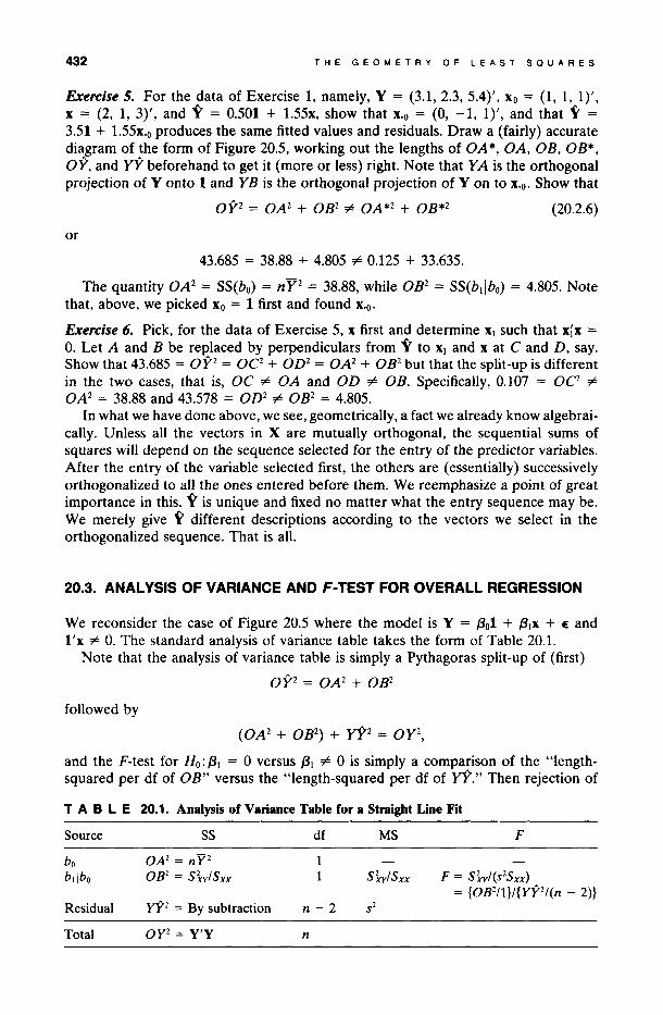
We reconsider the case of Figure 20.5 where the model is Y = /301 + /3¡x + E and l'x ~ O. The standard analysis of variance tabIe takes the form of Table 20.1.
Note that the analysis of variance tabIe is simply a Pythagoras split-up of (first)
Oy2 = OA2 + OB2
followed by
(OA2 + OB2) + yy2 = OY2,
and the F-test for Ho: /3¡ = O versus /3¡ ~ O is simply a comparison of the "lengthsquared per df of OB" versus the "length-squared per df of YY." Then rejection of
TABLE 20.1. Analysis of Variance Table for a Straigbt Line Fit
Source SS df MS F
bo OA2 = ny2
bdbo OB2 = Sh/Sxx 1 Sh/Sxx F = Sh/(S2Sxx) = {OB2/1}/{yy2/(n - 2)}
Residual yy2 = By subtraction n-2 S2
Total Oy2 = Y'Y n
20.4. THE SINGULAR X'X CASE: AN EXAMPLE 433
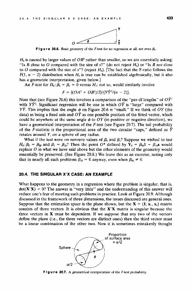
o~: F I 9 u re 20.6. Basic geometry of the F-test for no regression at aH, not even f3o.
Ho is caused by larger values oí OB2 rather than smaller, so we are essentially asking: "Is B close to O compared with the size oí s?" (do not reject Ho) or "Is B not close to O compared with the size oí s"? (reject Ho). [The fact that the F-ratio follows the F(1, n - 2) distribution when Ho is true can be established algebraically, but it also has a geometric interpretation, given below.]
An F-test íor Ho: f30 = f3¡ = O versus H¡: not so, would similarly involve
F = {(OA2 + OB2)/2}/{yy2/(n - 2)}.
Note that (see Figure 20.6) this involves a comparison oí the "per-dí lengths" oí Oy2 with yy2. Significant regression will be one in which OY is "large" compared with YY. This implies that the angle 4> on Figure 20.6 is "small." If we think oí OY (the data) as being a fixed axis and OY as one possible position of the fitted vector, which could lie anywhere at the same angle 4> to OY (in positive or negative direction), we have a geometrical interpretation oí the F-test (see Figure 20.7). The tail probability oí the F-statistic is the proportional area oí the two circular "caps," defined as Y rotates around Y, on a sphere of any radius.
What ií the test were on nonzero values oí f30 and f3¡? Suppose we wished to test Ho : f30 = f300 and f3¡ = f31O? Then the point 0* defined by Yo = f3oo1 + f3¡~ would replace O in what we have said aboye but the other elements oí the geometry would essentialIy be preserved. (See Figure 20.8.) We leave this as an exercise, noting only that in nearly all such problems f310 = O anyway, even when f300 -=1= O.
20.4. THE SINGULAR X'X CASE: AN EXAMPLE
What happens to the geometry in a regression where the problem is singular, that is, det(X'X) = O? The answer is "very liule" and the understanding oí this answer will reduce one's íear oí meeting such problems in practice. Look at Figure 20.9. Although discussed in the framework of three dimensions, the issues discussed are general ones. Suppose that the estimation space is the plane shown, but the X = (1, XI, X2) matrix consists oí three vectors. It is obvious that the X'X matrix is singular because the three vectors in X must be dependent. If we suppose that any two oí the vectors define the plane (Le., the three vectors are distinct ones) then the third vector must be a linear combination of the other two. Now it is sometimes mistakenly thought
Sphere
Proportion of surface area
=a/2
F I 9 u re 20.7. A geometrical interpretation of the F-test probability.
434 THE GEOMETRY OF LEAST SQUARES
x F I 9 u re 20.8. Testing that ({3o, (31) = ({3(Y.), (31U).
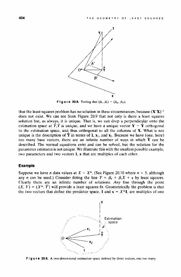
that the least squares problem has no solution in these circumstances, because (X'xt¡ does not exist. We can see from Figure 20.9 that not only is there a least squares solution but, as always!- it is unique. That is, we can drop a perpendicl!lar onto the estimation space at Y, Y is unique, and we have a unique vector Y - Y orthogonal to the estimation space, and thus orthogonal to all the columns of X. What is not unique is the description of Y in terms of 1, X¡, and X2. Because we have (one, here) too many base vectors, there are an infinite number of ways in which Y can be described. The normal equations exist and can be solved, but the solution for the parameter estimates is not unique. We illustrate this with the smallest possible example, two parameters and two vectors 1, x that are multiples of each other.
Example
Suppose we have n data values at X = X*. (See Figure 20.10 where n = 5, although any n can be used.) Consider fitting the line Y = f30 + f3¡X + E by least squares. Clearly there are an infinite number of solutions. Any line through the point (X, Y) = (X*, y) will provide a least squares fit. Geometrically the problem is that the two vectors that define the predictor space, 1 and x = X*l, are multiples of one
y
Estimation space
F I 9 u re 20.9. A two-dimensional estimation space defined by three vectors, one too many.
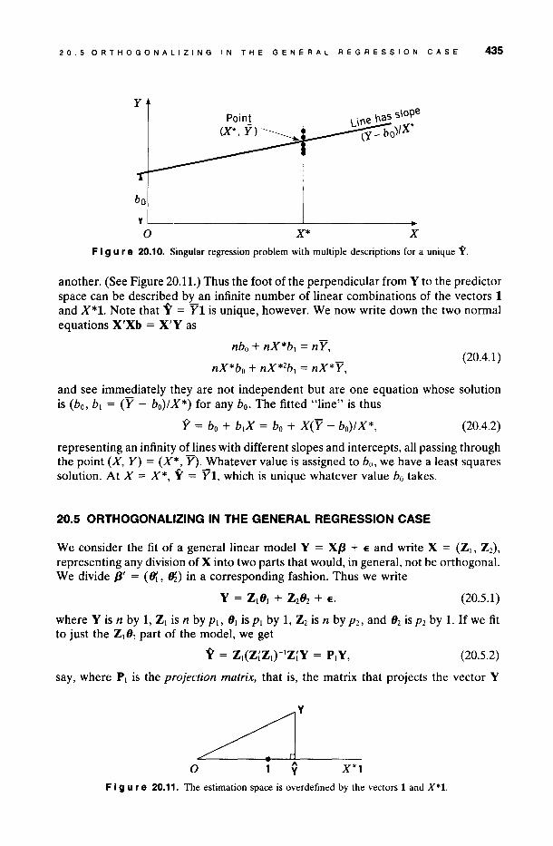
20.5 ORTHOGONALIZING IN THE GENERAL REGRESSION CASE 435
y
bo
~ '------------'-----o X* x
F I 9 u re 20.10. Singular regression problem with multiple descriptions for a unique Y.
another. (See Figure 20.11.) Thus the foot of the perpendicular from Y to the predictor space can be described by an intinite number of linear combinations of the vectors 1 and X*I. Note that Y = YI is unique, however. We now write down the two normal equations X'Xb = X'Y as
nbo + nX*b¡ = nY,
nX*bo + nX*2b¡ = nX*Y, (20.4.1)
and see immediately they are not independent but are one equation whose solution is (bo, b¡ = (Y - bo)/X*) for any bo. The titted "line" is thus
y = bo + b¡X = bo + X(Y - bo)/ X*, (20.4.2)
representing an intinity of lines with different slopes and intercepts, all passing through the point (X, Y) = (X*, Y). Whatever value is assigned to bo, we have a least squares solution. At X = X*, Y = YI, which is unique whatever value bo takes.
20.5 ORTHOGONALlZING IN THE GENERAL REGRESSION CASE
We consider the tit of a general linear model Y = Xp + E and write X = (Z¡, Z2), representing any division of X into two parts that would, in general, not be ortbogonal. We divide p' = (8í, 8í) in a corresponding fashion. Thus we write
(20.5.1)
where Y is n by 1, Z¡ is n by p¡, 8¡ is p¡ by 1, Z2 is n by P2, and 82 is P2 by 1. If we tit to just the Z¡8¡ part of the model, we get
y = Z¡(ZíZ¡)-¡ZíY = P¡Y, (20.5.2)
say, where p¡ is the projection matrix, tbat is, the matrix that projects the vector Y
o 1 Y X*l
F I 9 u re 20.11. The estimation space is overdefined by the vectors 1 and X*l.
436 THE GEOMETRY OF lEAST SQUARES
down into the estimation space defined by the columns of Z¡. The residual vector is e = Y - Y = (1 - p¡)Y. Note that in previous discussions we called p¡ the hat matrix because it converts the Y's into the Y's. We now rename it to emphasize its geometrical properties.
It is obvious that the fitted Y and the residual Y - Y are orthogonal because
Y'e = y'paI - p\)Y
= Y'(Pí - PíP¡)Y (20.5.3)
= O,
because p¡ is symmetric (so Pí = PI) and idempotent (so Pi = PI)' This calculation is a repeat of (20.1.4) with different notation. The matrix Z2, when orthogonalized to Z¡, becomes, by analogy to Y - Y,
Z2'¡ = Z2 - Z2
= (1 - P¡)Z2
= Z2 - Z¡(ZíZ\t¡Z;Z2
= Z2 - Z¡A.
A is usually called the alias or bias matrix.
Exercise 7. Prove that Z2.¡ and Z¡ are orthogonal matrices.
(20.5.4)
We can now write the full model in the orthogonalized form
y = ZlJ\ + Z282 + E
= Z¡( 8\ + A82) + (Z2 - Z¡A)82 + E (20.5.5)
= Z\8 + Z2.\82 + E.
We see immediately that 8 = (Z;Z¡t\ZíY estimates not just 8¡ but 8\ + A82. Thus A82 provides the biases in the estima tes of 8¡ if only the model Y = 8¡Z¡ + E is fitted.
Exercise 8. Show this by evaluating E(Y) = E(Z¡ 8) with E(Y) = 8¡Z\ + 82Z 2 • For the full regression we have the analysis of variance table of Table 20.2, where TI =
Z¡8\ + Z282. Note the following points:
1. The 80btained from fitting Y = Z¡8¡ + Z2.\82 + E is identical to the 8\ obtained by fitting Y = Z\8\ + E.
2. The 82 obtained from fitting Y = Z\8¡ + Z282 + E is identical to the 82 obtained by fitting just Y = Z2.\82 + E.
3. The values 6¡ and 62 in the analysis of variance table can be thought of as "test
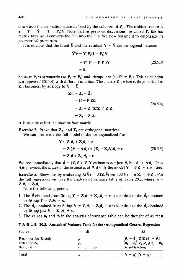
T A B L E 20.2. Analysis of Variance Table for the Orthogonalized General Regression
Source
Response for ZI only Extra for Z2 Residual
Total
PI P2
df
n-PI - P2
n
ss
(81 - 61)'Z;ZI( 81 - 61)
(82 - 62)'ZZIZ21( 82 - 62)
By subtraction
(Y - lJ)'(Y - lJ)
20.6. RANGE SPACE ANO NUll SPACE OF A MATRIX M 437
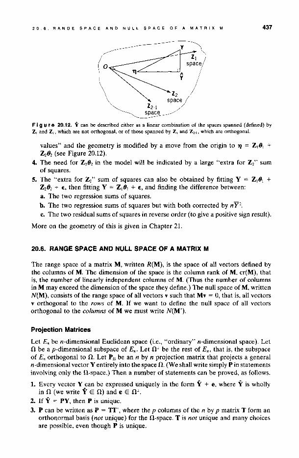
F I 9 u re 20.12. Y can be described either as a linear combination of the spaces spanned (defined) by Zl and Z2, which are not orthogonal, or of those spanned by Zl and ~l, which are orthogonal.
values" and the geometry is modified by a move from the origin to 71 = Z)8) + Z282 (see Figure 20.12).
4. The need for Z282 in the model will be indicated by a large "extra for Zz" sum of squares.
5. The "extra for Zz" sum of squares can al so be obtained by fitting Y = Z)81 + Z282 + E, then fitting Y = Z)8) + E, and finding the difference between: a. The two regression sums of squares. b. The two regression sums of squares but with both corrected by n y2. c. The two residual sums of squares in reverse order (to give a positive sign result).
More on the geometry of this is given in Chapter 21.
20.6. RANGE SPACE ANO NULL SPACE OF A MATRIX M
The range space of a matrix M, written R(M), is the space of all vectors defined by the columns of M. The dimension of the space is the column rank of M, cr(M), that is, the number of linearIy independent columns of M. (Thus the number of columns in M may exceed the dimension of the space they define.) The null space of M, written N(M), consists of the range space of a11 vectors v such that Mv = O, that is, all vectors v orthogonal to the rows of M. If we want to define the null space of a11 vectors orthogonal to the columns of M we must write N(M').
Projection Matrices
Let En be n-dimensional Euclidean space (i.e., "ordinary" n-dimensional space). Let n be a p-dimensional subspace of En. Let n.l be the rest of En, that is, the subspace of En orthogonal to n. Let Po be an n by n projection matrix that projects a general n-dimensional vector Y entirely into the space n. (We shall write simply P in statements involving only the !l-space.) Then a number of statements can be proved, as follows.
1. Every vector Y can be expressed uniquely in the form Y + e, where Y is wholly in n (we write Y E n) and e E n.l.
2. If Y = PY, then P is unique. 3. P can be written as P = TI', where the p columns of the n by p matrix T form an
orthonormal basis (not unique) for the n-space. T is not unique and many choices are possible, even though P is unique.
438 THE GEOMETRY OF LEAST SQUARES
[Note: A basis of O is a set of vectors that span the space of O, that is, permit every vector of O to be expressed as a linear combination of the base vectors. An orthogonal basis is one in which all basis vectors are orthogonal to one another. An orthonormal basis is an orthogonal basis for which the basis vectors have length (and so squared length) one, that is, v'v = 1 for aH basis vectors v.]
4. P is symmetric (P' = P) and idempotent (P2 = P).
5. The vectors of P span the space O, that is, R(P) = O.
6. 1 - P is the projection matrix for 0\ the orthogonal part of En not in O. Thus R(I - P) = 0 1
.
7. Any symmetric idempotent n by n matrix P represents an orthogonal projection matrix onto the space spanned by the columns of P, that is, onto R(P).
Statements 1-7 are generally true for any O even though we have given them in a notation that fits into the concept of regression. Statements 8 and 9 now make the connection with regression. We think of fitting the model Y = Xp + E by least squares, and O = R(X) will now be defined by the p columns of X and so will constitute the estimation space for our regression problem.
8. Suppose O is a space spanned by the columns of the n by p matrix X. Suppose (X'xt is any generalized inverse ofX'X (see Appendix 20A). Then P = X(X'xtx' is the unique projection matrix for O. Note carefully that X is not unique, nor is (X'xt, but P = X(X'xtx' is unique and so is Y = PY.
9. If cr(X) = p so that the columns of X are linearIy independent, and (X'xt l exists, then P = X(X'xt1x' and R(X) = R(P) = O. This is the situation that will typicalIy hold.
For proofs of these statements, see Seber (1977, pp. 394-395). The practical consequences of these statements are as foHows. Given an estimation space n (and so, necessarily, an error space 0 1
), any vector y can uniquely be regressed into O, via a unique projection matrix P = X(X'xtx'. The facts that, even when X and (X'xt are not unique, P is unique and so is Y =
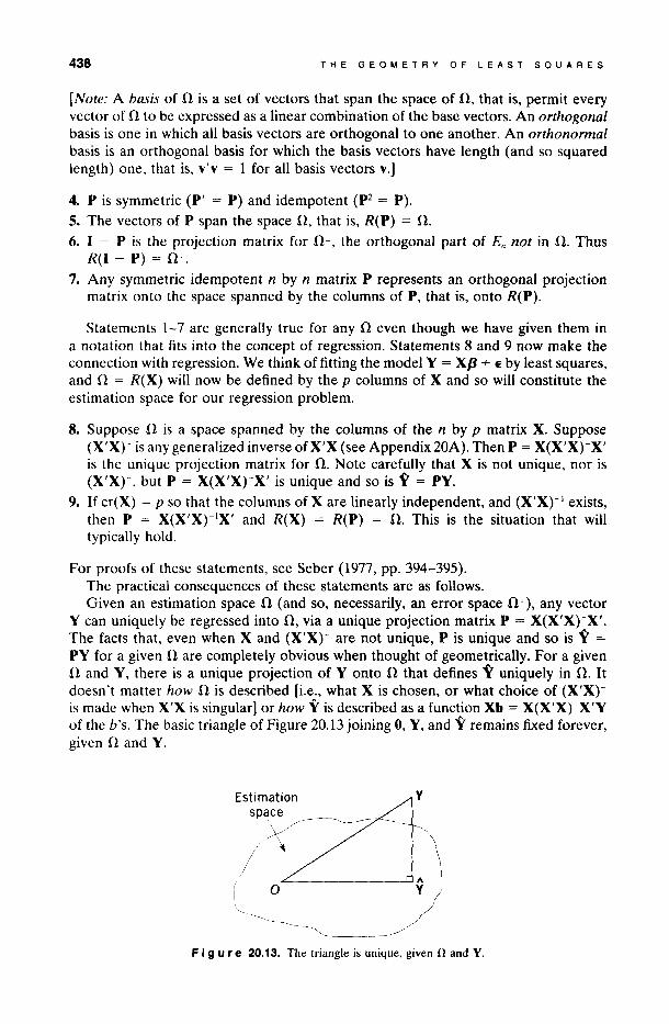
PY for a given n are completely obvious when thought of geometrically. For a given O and Y, there is a unique projection of Y onto O that defines Y uniquely in O. It doesn 't matter how O is described [i.e., what X is chosen, or what choice of (X'xt is made when X'X is singular] or how Y is described as a function Xb = X(X'xtx'y of the b's. The basic triangle of Figure 20.13 joining O, Y, and Y remains fixed forever, given O and Y.
Estimation y
space \ /---
X / ~
F i 9 u re 20.13. The triangle is unique, given n and Y.
20.7. THE ALGEBRA ANO GEOMETRY OF PURE ERROR 439
20.7. THE ALGEBRA ANO GEOMETRV OF PURE ERROR
We consider a general linear regression situation with
y = f30 + {3IX I + {32X 2 + ... + {3p- IX p- 1 + E, (20.7.1)
or y = Xp+ E.
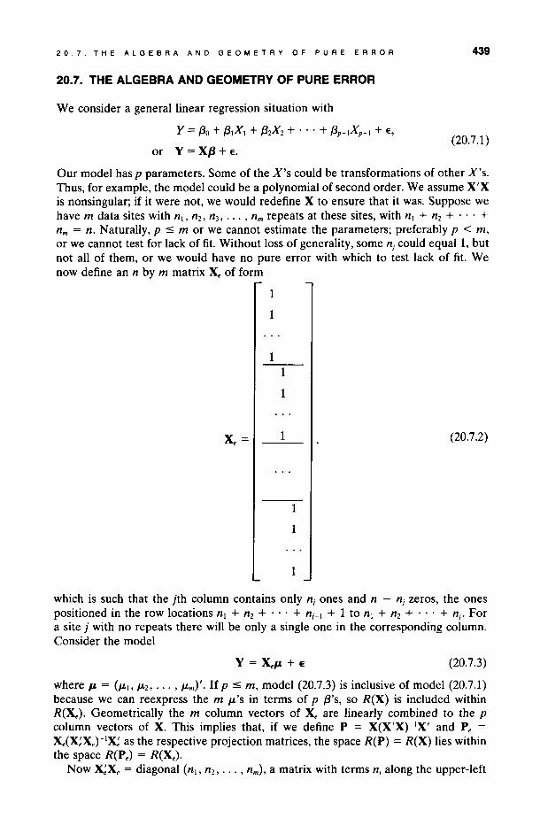
Our model has p parameters. Sorne of the X's could be transformations of other X's. Thus, for example, the model could be a polynomial of second order. We assume X'X is nonsingular; if it were not, we would redefine X to ensure that it was. Suppose we have m data sites with ni, n2, n3, ... , n m repeats at these sites, with ni + n2 + ... + nm = n. Naturally, p ~ m or we cannot estimate the parameters; preferably p < m, or we cannot test for lack of fit. Without loss of generality, sorne ni could equal 1, but not all of them, or we would have no pure error with which to test lack of fit. We now define an n by m matrix Xe of form
Xe=
1
1
1 1
1
1
1
1
1
(20.7.2)
which is such that the jth column contains only ni ones and n-ni zeros, the ones positioned in the row locations ni + n2 + ... + ni-I + 1 to ni + n2 + ... + ni' For a site j with no repeats there will be only a single one in the corresponding column. Consider the model
y = XeP, + E (20.7.3)
where P, = (11-1,11-2, ... , I1-m)'. If P ~ m, model (20.7.3) is inclusive of model (20.7.1) because we can reexpress the m I1-'S in terms of p {3's, so R(X) is included within R(Xe). Geometrically the m column vectors of Xe are linearly combined to the p column vectors of X. This implies that, if we define P = X(X'xttx' and Pe = Xe(X;xetlx; as the respective projection matrices, the space R(P) = R(X) lies within the space R(Pe) = R(Xe).
Now X;Xe = diagonal (ni, n2, ... , nm), a matrix with terms ni along the upper-left
440 THE GEOMETRY OF LEAST SQUARES
to lower-right main diagonal and zeros elsewhere, so that (X;xet l = diagonal (nl l
, ni l, ••. , n~I). It follows (an exercise for the reader here!) that Pe consists of a
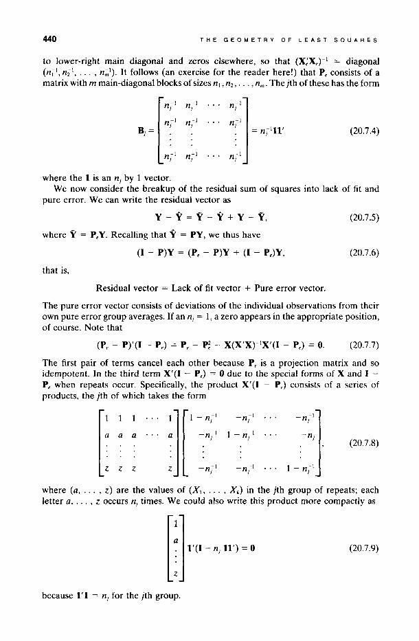
matrix with m main-diagonal blocks of sizes nI , n2, ... , nm • The jth of these has the form
n¡-I n¡-I nt
B¡= nT I nT I nT I
= nT l ll' (20.7.4)
nT I nT I nt
where the 1 is an n¡ by 1 vector. We now consider the breakup of the residual sum of squares into lack of tit and
pure error. We can write the residual vector as
y - y = y - y + y - Y,
where Y = PeY. Recalling that Y = PY, we thus have
(1 - P)Y = (Pe - P)Y + (1 - Pe)Y,
that is,
Residual vector = Lack of tit vector + Pure error vector.
(20.7.5)
(20.7.6)
The pure error vector consists of deviations of the individual observations from their own pure error group averages. If an n¡ = 1, a zero appears in the appropriate position, of course. Note that
(20.7.7)
The tirst pair of terms cancel each other because Pe is a projection matrix and so idempotent. In the third term X'(I - Pe) = O due to the special forms of X and 1 -Pe when repeats occur. Specitically, the product X'(I - Pe) consists of a series of products, the jth of which takes the form
1 1 1 1 1- nt -n¡-I -n¡-I
a -nT I 1 - nT I -ni (20.7.8)
a a a
z z z z -nTI -nTI 1 - nT I
where (a, ... , z) are the values of (XI, ... , X k) in the jth group of repeats; each letter a, ... , z occurs n¡ times. We could also write this product more compactly as
1
a (20.7.9)
z
because 1'1 = n¡ for the jth group.
APPENDIX 20A. GENERALIZED INVERSES M-
o PY
Residual (I-P)Y
Pure error y (I-Pe)Y
Lack of fit (Pe-P)Y
441
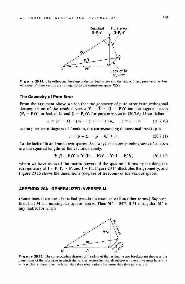
F I 9 u re 20.14. TIte orthogonal breakup of the residual vector into the lack of tit and pure error vectors. AH three of these vectors are orthogonal to the estimation space R(X).
The Geometry of Pure Error
From the argument aboye we see that the geometry of pure error is an orthogonal decomposition of the residual vector Y - Y = (1 - P)Y into orthogonal pieces (Pe - P)Y for lack of fit and (1 - Pe)Y, for pure error, as in (20.7.6). If we define
ne = (ni - 1) + (n2 - 1) + ... + (nm - 1) = n-m (20.7.10)
as the pure error degrees of freedom, the corresponding dimensional breakup is
(20.7.11)
for the lack of fit and pure error spaces. As always, the corresponding sums of squares are the squared lengths of the vectors, namely,
Y'(I - P)Y = Y'(Pe - P)Y + Y'(I - Pe)Y, (20.7.12)
where we have reduced the matrix powers of the quadratic forms by invoking the idempotency of 1 - P, Pe - P, and 1 - Pe' Figure 20.14 illustrates the geometry, and Figure 20.15 shows the dimensions (degrees of freedom) of the various spaces.
APPENDIX 20A. GENERALlZED INVERSES M-
(Sometimes these are also called pseudo-inverses, as well as other terms.) Suppose, first, that M is a non singular square matrix. Then M- = M-l. If M is singular, M- is any matrix for which
F I 9 u re 20.15. The corresponding degrees of freedom of the residual vector breakup are shown as the dimensions of the subspaces in which the various vectors lie. For all subspaces to exist, we must have n > m > p, that is, there must be fewer sites than observations but more sites than parameters.
442 THE GEOMETAY OF LEAST SQUAAES
(20A.l)
This concept of a generalized inverse is an interesting extension of the idea of the inverse matrix to singular matrices. (Although it is interesting, it can usuaBy be circumvented in practical regression situations!) A generalized inverse satisfying MM-M = M always exists and is not unique.
(Note: It is also possible to define M- in the same way when M is not square. For regression purposes, we do not need this extension.)
Moore-Penrose Inverse
A unique definition (the so-caBed Moore-Penrose inverse) can be obtained by insisting on M- satisfying three more conditions, namely,
M-MM- = M-,
(MM-)' = MM-,
(M-M) I = M-M.
Sorne writers write M+ for the Moore-Penrose inverse.
Getting a Generalized Inverse
(20A.2)
We assume M is square and, for our regression applications, is of the symmetric form X'X. Let M be p by p and have rank (row or column rank) r < p. Probably the easiest method for getting an M- is the following.
A Method for Getting M-
Examine M to find an r by r submatrix that has full rank, that is, is nonsingular. If it occupies the upper-Ieft corner, then
M = [Ml1 MI2], M 21 M 22
(20A.3)
where Mil is nonsingular, so that MIlI exists. Then
(20A.4)
will be a generalized inverse for M.
Proa!" Form the product MM-M to get
(20A.5)
which has three submatrices correct. Because of the implicit assumption that the (p - r) later columns of M depend on the first r, there exists an r by (p - r) matrix Q, say, such that
(20A.6)
APPENDIX 20A. GENERALIZED INVERSES M- 443
Solving for Q in the first of these gives Q = M111M12 whence M2IM1IIM12 = M21Q = M22 • The method works in exactly the same way wherever the elements of the nonsingular (Mil) matrix are located. It is inverted where it stands and zeros occupy all other places.
Our regression application is the following. If X'X is singular and (X'xt is any generalized inverse, the normal equations X'Xb = X'Y are satisfied by b = (X'xtx'Y. See Seber (1977, pp. 76 and 391). Note that although different choice s of (X'xt produce different b estimates, Y = Xb is invariant due to the geometry.
Example
Consider the fitting of a straight line Y = /30 + /3IX + E to n data points all at the same location X = X*. The least squares solution is any line through the point (X, Y) = (X*, Y), because a unique solution is obtained only when there are two or more X-sites, and here we have only one. The general solution is thus of the form
y = bo + (Y - bo)(X/ X*) (20A.7)
for any choice of bo. [Note that when X = X*, Y = Y $0 that Y = (Y, Y, . .. , Y)' and is unique, as we know it must be from the geometry.] For this problem, the normal equations are
[n nx*] [boJ [~Y¡]
nX* nX*2 b l = X*¿Y¡ (20A.8)
and do not have a unique solution. We now look at what is achieved by specific choices of (X'X)-, when evaluating b = (X'X)-X'Y.
Choice l. Let
(X'xt = [:-. ~J. (20A.9)
Then bo = y and b l = O. We obtain a horizontal straight line through (X*, Y).
Choice 2. Let
(X'X)- = [~ (nX~2t.]. (20A.lO)
Then bo = O, b l = Y/X*. We have a straight line joining the origin to the point (X*, Y).
Choice 3. Let
[O (nx*tl]
(X'xt = . O O
(20A.ll)
Then bo = y and b l = O, which is the same solution as Choice 1.
Choice 4. Let
(X'x¡- = Ln:'¡-' ~J. (20A.l2)
Then bo = O, b) = Y/X*, the same solution as Choice 2.
444 THE GEOMETRY OF LEAST SQUARES
We note two features from this (somewhat limited) example:
1. Any specific choice of (X'xt merely leads to one of the infinity of solutions provided by (20A.7). (This point is true in the general case also.)
2. Only the two most obvious solutions arise, those assuming that bo = y or bo = O. To get other solutions [which all still satisfy (20A.7)], other choices of (X'xt are needed. It is, however, pointless to follow this up, as other choices essentially ask us to make other assumptions about the b's. Obviously we could apply any assumption we chose directly to the general solution (20A.7) and not use a generalized inverse at aH.
What Should One Do?
Our overall recommendation is that using a generalized inverse for a practical regression problem is usually a waste of time. Four alternative choices are:
1. Keep the original data but modify the model to make the new X'X nonsingular.
2. Keep the original model but get more data to make the new X'X nonsingular. 3. Keep both data and model and decide to implement sensible linear restrictions on
the parameters to make the new X'X nonsingular. [Computer programs typicalIy set equal to zero all parameters associated with the later (in sequence, as given to the computer) dependent columns of the original X matrix.]
4. Add nonlinear restrictions and solve the least squares problem subject to them. Ridge regression is an example of this.
Choice 3 will often be the most practical.
EXERCISES FOR CHAPTER 20
A. Fit the model Y = f30 + f3 IX + E by least squares to the four data points (X, Y) = (1, 1.4), (2,2.2), (3, 2.3), (4, 3.1). l. Write down the SS function S(f3o, f31)' 2. Find the least squares estimate b. 3. Find the vector Y of fitted values and e = Y-Y. 4. Find the projection matrix P = X(X'xtIX'. 5. For the sample space (E4 space), make a plot, as best you can, showing what you have
done, and identifying a11 relevant details. 6. Write down an analysis of variance table "appropriate for checking Ho: f30 = f31 = O
versus H l : "not so," for this regression situation. Specify the test statistic and get its observed value. Identify what this means in your figure also.
7. Repeat 6 for Ho: f30 = 1, f31 = 0.5. 8. The two vectors of X and the four vectors of the least squares projection matrix P span
the same space. What specific linear combinations of the two vectors of X will give P? 9. What specific linear combinations of the four vectors of P will give X?
10. The vectors of X span the estímatíon space. Write X = (Xo, Xl)' where Xo = (1,1,1,1)'. Find Xi(), a vector orthogonal to Xo, such that (Xo, Xl.o) also spans the estimation space.
11. Hence (see 10) or otherwise, find a suitable sum of squares and F-value for testing Ho: f31 = O, irrespective of the value of f3o.
EXERCISES FOR CHAPTER 20 445
B. Consider (very carefully) the least squares regression problem with model Y = XfJ + E
where
1 X¡ X 2
1 -3 1
p= [::].
4
-1 7 7 X= Y=
13 2
3 19 3
1. Write down the normal equations. 2. Find a general solution to the normal equations. 3. Determine Y. 4. Make a few appropriate comments.
C. To be estimable, a linear combination e' fJ (say) of the elements of fJ must have a e' vector that is a linear combination of the rows of X. If e' cannot be expressed that way, e' fJ is not estimable. If the regression is of fuIl rank, aIl e' fJ are estimable beca use fJ itself can be uniquely estirnated. If the regression is not fuIl rank, then sorne e' fJ are estimable and sorne are not. With this in mind, consider the foIlowing:
Four observations of Y are taken at each of X = -1,0,1 with the intention oí fitting the cubic model Y = /30 + /3¡X + /32X2 + /3v(3 + E via least squares, under the usual error assumptions. 1. What is the projection matrix P = X(X'XtX'. 2. Is P unique? Is PY unique? 3. Which of the following are estimable?
D. Consider the least squares fit Y = /3¡X¡ + /32X2 + E (no intercept) to the data (X¡, X 2 , Y) = (1,2, 19), (2, 1, 13), and (O, 0, 16). Using axes (V), V2 , V3), say, for threedimensional space, do the following: 1. Draw a diagram showing the basic least squares fit. On this diagram, name the various
spaces and explain how they are defined, and label any points with actual coordinates. 2. Show what the nurnbers in the ANO V A table mean in your figure. 3. The regression is not a significant one. What feature(s) oí the data rnake(s) it so? 4. Is there anything "special" about the estimation space? 5. Evaluate X2.¡ and draw a new diagram explaining what the ANOV A numbers mean in
this diagrarn. X 2.¡ is the part oí X 2 orthogonal to Xl' 6. Suppose that, instead ofthe number 16, we substitute 2. Geometrically, what does that do? 7. Provide a new ANOVA table and a new F-value for the situation when the number 16
is replaced by 2.
E. 1. Find the (unique) projection matrix Ponto a space n spanned by the vectors of A, where
A=
1 -3 1
1 -1 -1
1 1-1
3
2. Find a basis for the space orthogonal to n, that is, find vectors that span that orthogonal space.
3. Find the projections into n of aIl the vectors you gave in (2), and specify the space spanned by the P you gave in (1).

446 THE GEOMETRY OF LEAST SQUARES
F. Which of the matrices below are generalized inverses of the matrix 11', namely,
[0.25
3. 0.25
[
0.1 4.
0.3
0.25].
0.25
0.2]. 0.4
G. A straight line Y = /30 + /3¡X + E is to be fitted to the data below. Show a "tree diagram" of the allocation of the 10 degrees of freedom and find 10 orthogonal vectors that span the whole space, saying which correspond to your degrees of freedom split-up, and so divide the whole space up into three distinct orthogonal spaces.
y X
Y\ -2 Y2 -2 y) -1 Y4 -1
Y~ O Y6 O Y7 1 Ys 1 Y9 2 Y IO 2
H. If P is a projection matrix for a regression with a /30 in the model, its row and column sums should all be 1. Explain geometrically why this must obviously be true?
e H A P TER 21
More Geometry of Least Squares
The basic geometry of least squares appears in the foregoing chapter. Here we take things a little further by considering what happens geometrically when we test linear hypotheses of the form Ro: Ap = e in the model Y = Xp + E. (The alternative hypothesis is always that Ro is false.) We suppose that A is a q by p matrix (q < p) of full rank so that the rows of A are linearly independent; p is p by 1 and e is a q by 1 vector of constants; X is n by p, and assumed to be of full rank p.
21.1. THE GEOMETRV OF A NULL HVPOTHESIS: A SIMPLE EXAMPLE
We first consider the simple example of fitting a straight line Y = /30 + f31 X + E using a set of n data points represented by two n by 1 vectors Y and XI. In matrix terms y = Xp + E, we thus have the model function
(21.1.1)
The estimation space n is aplane spanned by 1 and Xl. Suppose A = (2, -1) and e = 4 so that Ap = e implies 2/30 - /3¡ = 4. Obviously P = 2 and q = 1. We substitute in (21.1.1) for /31 to obtain for the model under Ap = e,
(21.1.2)
The estimation space w for this model function is a straight line swept out by combining the constant vector -4X¡ with the variable length vector f3o(l + 2XI ), as shown in Figure 21.1. The three black dots show points for which /30 = 0, 1, and 1.5 on w. Clearly w is part of n. The space n - w is spanned by any set of vectors in n that are all orthogonal to w. For our example, p = 2 and q = 1, so there is only one such vector. If we write, in (21.1.2),
u = /301 + (2f3o - 4)X I
for the vector that spans w, an obviously orthogonal vector is
(u'XI)l - (u'l)XI, (21.1.3)
which spans n - w.
447
448 MORE GEOMETRY OF LEAST SaUARES
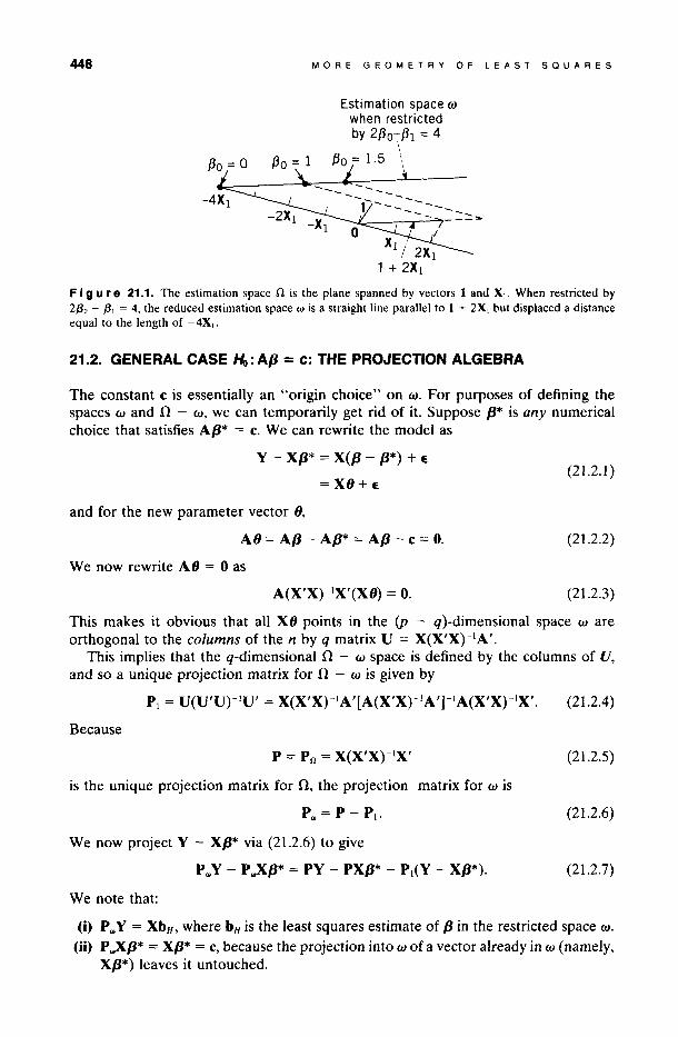
Estimation space ro when restricted by 2f30-f31 == 4
F I 9 u r e 21.1. The estimation space n is the plane spanned by vectors 1 and X¡. When restricted by 2/30 - /3¡ = 4, the reduced estimation space w is a straight line parallel to 1 + 2X¡ but displaced a distance equal to the length of -4X¡.
21.2. GENERAL CASE Ho: AfJ = e: THE PROJECTION ALGEBRA
The constant e is essentially an "origin choice" on ro. For purposes of defining the spaces ro and n-ro, we can temporarily get rid of it. Suppose fJ* is any numerical choice that satisfies AfJ* = c. We can rewrite the model as
y - XfJ* = X(fJ - fJ*) + E
= XO+E
and for the new parameter vector O,
AO = AfJ - AfJ* = AfJ - e = O.
We now rewrite AO = O as
A(X'XtIX'(XO) = O.
(21.2.1 )
(21.2.2)
(21.2.3)
This makes it obvious that all XO points in the (p - q )-dimensional space ro are orthogonal to the columns of the n by q matrix U = X(X'XtIA'.
This implies that the q-dimensional n-ro space is defined by the columns of U, and so a unique projection matrix for n-ro is given by
(21.2.4)
Because
(21.2.5)
is the unique projection matrix for n, the projection matrix for ro is
Pw = P - PI. (21.2.6)
We now project Y - XfJ* via (21.2.6) to give
p w y - P wXfJ* = PY - PXfJ* - PI(Y - XfJ*)· (21.2.7)
We note that:
(i) P w y = XbH , where bH is the least squares estimate of fJ in the restricted space ro.
(ii) P wXfJ* = XfJ* = e, beca use the projection into ro of a vector already in ro (namely, XfJ*) leaves it untouched.
21.3 GEOMETRIC ILLUSTRATIONS 449
(iii) PY = Xb, where b = (X'xtIX'Y is the usual (unrestricted) least squares estimator.
(iv) PXP* = XP* = c; the argument is similar to (ii). (v) P1(Y - XP*) = X(X'XtIA'[A(X'XtIA']-I(Ab - c). (21.2.8)
Putting the pieees baek into (21.2.7), eaneeling two c's, and multiplying through by (X'X)-IX' to "cancel" X throughout, gives the restrieted (by Ap = c) least squares estima te vector
bH = b - (X'Xt\ A'[A(X'Xt\ A']-I(Ab - c). (21.2.9)
The form of this is b adjusted by an amount that depends on X, A, and how far off Ab is from c.
Properties
AH three of the projeetion matrices are symmetrie and idempotent. Note also that
(a) PPw = Pw = PwP
(b) pp\ = p¡ = p¡p
(e) PwP1 = O = p¡pw
(21.2.10)
GeometriealIy, (a) means that a vector Y projeeted first into w and then ¡nto n stays in w, or that, if projeeted first into n and then into w, finishes up in w; (b) is a similar result. Part (c), whieh can be proved by writing p¡pw = P1(P - PI) = p¡p - Pi = PI - p¡ = O, means that the split of n into the two subspaees, w created by Ap = c, and n - w, is an orthogonal split.
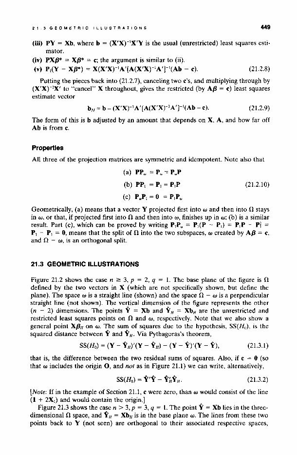
21.3 GEOMETRIC ILLUSTRATIONS
Figure 21.2 shows the case n ~ 3, p = 2, q = 1. The base plane of the figure is n defined by the two vectors in X (whieh are not speeifiealIy shown, but define the plane). The space w is a straight line (shown) and the spaee n - w is a perpendicular straight line (not shown). The vertical dimension of the figure represents the other (n - 2) dimensions. The points Y = Xb and Y H = XbH are the unrestrieted and restrieted least squares points on n and w, respeetively. Note that we also show a general point XPH on w. The sum of squares due to the hypothesis, SS(Ho), is the squared distanee between Y and Y H. Via Pythagoras's theorem,
SS(Ho) = (Y - Y H)'(Y - Y H) - (Y - Y)'(Y - Y), (21.3.1 )
that is, the differenee between the two residual sums of squares. Also, if c = O (so that w includes the origin 0, and not as in Figure 21.1) we can write, alternatively,
(21.3.2)
[Note: If in the example of Section 21.1, c were zero, than w would eonsist of the line (1 + 2X\) and would eontain the origin.]
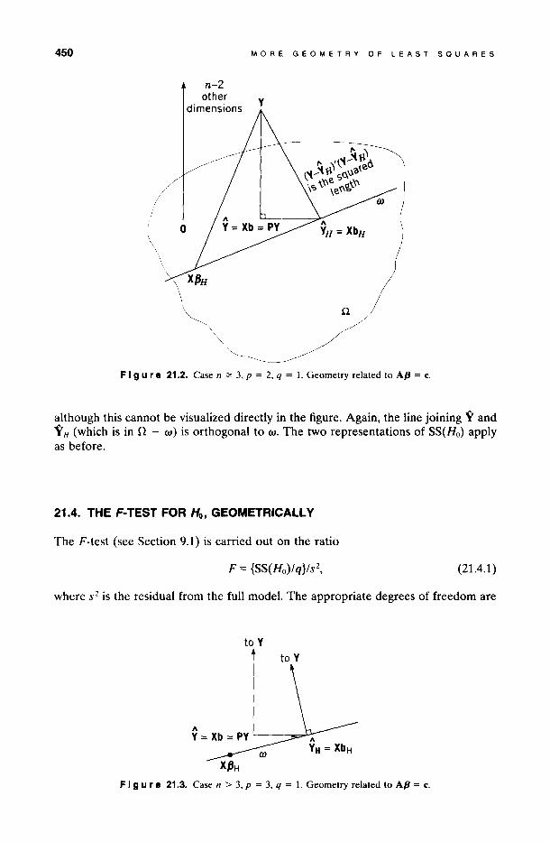
Figure 21.3 shows the case n > 3, p = 3, q = 1. The point Y = Xb lies in the threedimensional n space, and Y H = XbH is in the base plane w. The lines from these two points baek to Y (not seen) are orthogonal to their assoeiated respective spaees,
450 MORE GEOMETRY OF lEAST SQUARES
n-2 other
dimensions y
F I 9 U r e 21.2. Case n ~ 3, p = 2, q = 1. Geornetry related to AfJ = c.
although this cannot be visualized directIy in the figure. Again, the line joining Y and y H (which is in n - w) is orthogonal to w. The two representations of SS(Ho) apply as before.
21.4. THE F-TEST FOR Ho, GEOMETRICALL y
The F-test (see Section 9.1) is carried out on the ratio
F = {SS(Ho)/q}/S2, (21.4.1)
where s 2 is the residual from the full model. The appropriate degrees of freedom are
to Y
to Y
F i 9 u r e 21.3. Case n > 3, p = 3, q = 1. Geornetry related to AfJ = c.
21.4. THE F-TEST FOR Ho. GEOMETRICALLY 451
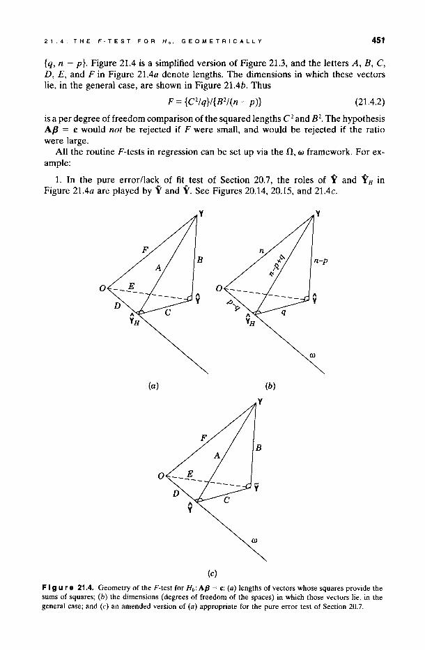
{q, n - p}. Figure 21.4 is a simplified version of Figure 21.3, and the letters A, B, C, D, E, and F in Figure 21.4a denote lengths. The dimensions in which these vectors lie, in the general case, are shown in Figure 21.4b. Thus
F = {C2Iq}/{B2/(n - p)} (21.4.2)
is a per degree offreedom comparison ofthe squared lengths C2 and B2. The hypothesis A/3 = e would not be rejected if F were small, and would be rejected if the ratio were large.
AH the routine F-tests in regression can be set up via the n, w framework. For example:
1. In the pure error/lack of fit test of Section 20.7, the roles of Y and Y H in Figure 21.4a are played by Y and Y. See Figures 20.14, 20.15, and 21.4c.
o
(a) (b)
o
(e)
F I 9 u re 21.4. Geometry of the F-test for Ho: AfJ = e: (a) lengths of vectors whose squares provide the sums of squares; (b) the dimensions (degrees of freedom of the spaces) in which those vectors lie, in the general case; and (e) an amended version of (a) appropriate for the pure error test of Section 20.7.
452 MORE GEOMETRY OF LEAST SaUARES
2. In the test for overall regression, Ho: /31 = /32 = ... = /3P-l = 0, y H is given by Yl, and q = p - 1 in Figure 21.4b. See Section 21.5 and Figure 21.5.
21.5. THE GEOMETRV OF R2
Figure 21.5 has the same general appearance as Figure 21.4. It is in fact a special case where the initial model is
(21.5.1)
and the hypothesis to be tested is that of "no regression," interpreted as Ho: /31 = /32 = ... = /3p-l = O. Thus our restriction Ap = e becomes
[O, Ip-dP = o. (21.5.2)
The reduced model is just Y = /30 + E, or Y = 1/30 + E, so that w is defined by the n by 1 vector 1. Thus Y H = YI. The R2 statistic is defined as
2 _ L(Y¡ - y)2 _ (Y - Yl)'(Y - Yl) R - L(Y¡ - y)2 - (Y - Yl)'(Y - Yl)
G2 = K2
in Figure 21.5. Special cases are R2 = 1, which results when B = ° (zero residual vector), and R2 = 0, occurring when G = 0, that is, when Y = YI and there is no regression in excess of Y¡ = Y.
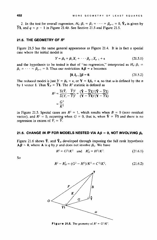
21.6. CHANGE IN R2 FOR MODELS NESTED VIA Af3 = 0, NOT INVOLVING 130
Figure 21.6 shows Y, and Y H developed through imposing the full rank hypothesis Ap = O, where A is q by p and does not involve /30. We have
(21.6.1)
So
(21.6.2)
o
F I 9 u re 21.5. The geometry of R2 = G2/K2.
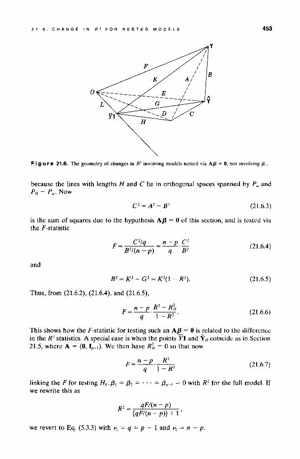
21.6. CHANGE IN R2 FOR NESTEO MOOELS 453
o
F I 9 u r e 21.6. The geometry of changes in R2 involving models nested via AfJ = 0, not involving (Jo.
beca use the lines with lengths H and C lie in orthogonal spaces spanned by Pw and Po - Pw • Now
(21.6.3)
is the sum of squares due to the hypothesis A{J = O of this section, and is tested via the F-statistic
_ C2/q _ n - p C2 F- ---.-
B2/(n - p) q B2
and
Thus, from (21.6.2), (21.6.4), and (21.6.5),
_ n - p R2 - R~ F---· 1 R?' q --
(21.6.4)
(21.6.5)
(21.6.6)
This shows how the F-statistic for testing such an A{J = O is related to the difference in the R2 statistics. A special case is when the points YI and Y H coincide as in Section 21.5, where A = (O, Ip_I)' We then have R~ = O so that now
n - p R 2
F=--·--q 1 - R2 (21.6.7)
linking the F for testing Ho: {3¡ = {32 = ... = (3p-1 = O with R2 for the full model. If we rewrite this as
R 2 = qF/(n - p) {qF/(n - p)} + 1 '
we revert to Eq. (5.3.3) with VI = q = p - 1 and Vz = n-p.
454 MORE GEOMETRY OF LEAST SaUARES
21.7. MULTIPLE REGRESSION WITH TWO PREDICTOR VARIABLES AS A SEQUENCE OF STRAIGHT LlNE REGRESSIONS
The stepwise selection procedure discussed in Chapter 15 involves the addition of one variable at a time to an existing equation. In this section we discuss, algebraically and geometrically, how a composite equation can be built up through a series of simple straight line regressions. Although this is not the best practical way of obtaining the final equation, it is instructive to consider how it is done. We illustrate using the steam data with the two variables X s and X 6 • The equation obtained from the joint regression is given in Section 6.2 as
y = 9.1266 - 0.0724Xs + 0.2029X6 •
Another way of obtaining this solution is as follows:
1. Regress Y on Xs. This straight line regression was performed in Chapter 1, and the resulting equation was
y = 13.6230 - 0.0798Xs.
This fitted equation predicts 71.44% of the variation about the mean. Adding a new variable, say, X6 (the number of operating days), to the prediction equation might improve the prediction significantly.
In order to accomplish this, we desire to relate the number of operating days to the amount of unexplained variation in the data after the atmospheric temperature effect has been removed. However, if the atmospheric temperature variations are in any way related to the variability shown in the number of operating days, we must correct for this first. Thus we need to determine the relationship between the unexplained variation in the amount of steam used after the effect of atmospheric temperature has been removed, and the remaining variation in the number of operating days after the effect of atmospheric temperature has been removed from it.
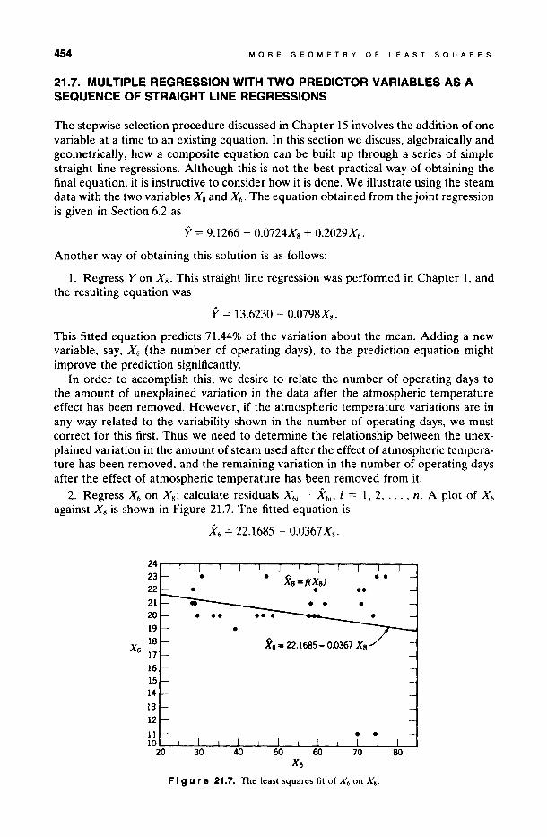
2. Regress X 6 on Xg ; calculate residuals X 6i - X6i , i = 1, 2, ... , n. A plot of X 6
against X 8 is shown in Figure 21.7. The fitted equation is
X6 = 22.1685 - 0.0367X8 •
24 23 • • ge=!(X8) • • 22 • • •• 21 20 19
X6 18
17
16 15 14 13 12
11 • • 10
20 X8
F 1 9 u re 21.7. The least squares fit of X6 on X s•
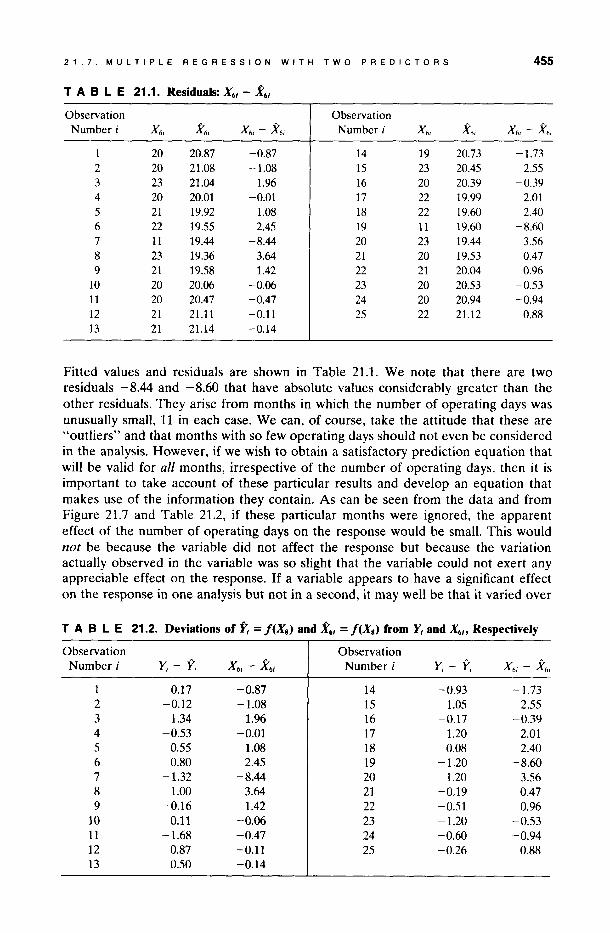
2 1 . 7 . MULTIPLE REGRESSION W I T H TWO PREDICTORS 455
TABLE 21.1. Residuals: X'I - 1"1
Observatíon Observatíon Number i X6/ XÓi X6i - X6i Number i X 6 / Xó/ X6/ - X6/
1 20 20.87 -0.87 14 19 20.73 -1.73 2 20 21.08 -1.08 15 23 20.45 2.55 3 23 21.04 1.96 16 20 20.39 -0.39 4 20 20.01 -0.01 17 22 19.99 2.01 5 21 19.92 1.08 18 22 19.60 2.40 6 22 19.55 2.45 19 11 19.60 -8.60 7 11 19.44 -8.44 20 23 19.44 3.56 8 23 19.36 3.64 21 20 19.53 0.47 9 21 19.58 1.42 22 21 20.04 0.96
10 20 20.06 -0.06 23 20 20.53 -0.53 11 20 20.47 -0.47 24 20 20.94 -0.94 12 21 21.11 -0.11 25 22 21.12 0.88 13 21 21.14 -0.14
Fitted values and residual s are shown in Table 21.1. We note that there are two residuals -8.44 and -8.60 that have absolute values considerably greater than the other residuals. They arise from months in which the number of operating days was unusually small, 11 in each case. We can, of course, take the attitude that these are "outliers" and that months with so few operating days should not even be considered in the analysis. However, if we wish to obtain a satisfactory prediction equation that will be valid for al! months, irrespective of the number of operating days, then it is important to take account of these particular results and develop an equation that makes use of the information they contain. As can be seen from the data and from Figure 21.7 and Table 21.2, if these particular months were ignored, the apparent effect of the number of operating days on the response would be small. This would no! be because the variable did not affect the response but beca use the variation actually observed in the variable was so slight that the variable could not exert any appreciable effect on the response. If a variable appears to have a significant effect on the response in one analysis but not in a second, it may well be that it varied over
TABLE 21.2. Deviations of YI = !(X8 ) and X,; = !(Xs) from Y; and X,;, Respectively
Observation Observation Number i Y i - Yi X6i - X6i Number i Y i - Yi X6/ - X6i
1 0.17 -0.87 14 -0.93 -1.73 2 -0.12 -1.08 15 1.05 2.55 3 1.34 1.96 16 -0.17 -0.39 4 -0.53 -0.01 17 1.20 2.01 5 0.55 1.08 18 0.08 2.40 6 0.80 2.45 19 -1.20 -8.60 7 -1.32 -8.44 20 1.20 3.56 8 1.00 3.64 21 -0.19 0.47 9 -0.16 1.42 22 -0.51 0.96
10 0.11 -0.06 23 -1.20 -0.53 11 -1.68 -0.47 24 -0.60 -0.94 12 0.87 -0.11 25 -0.26 0.88 13 0.50 -0.14
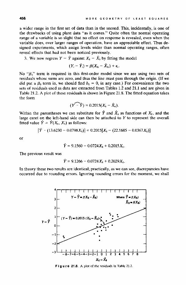
456 MORE GEOMETRY OF LEAST SaUARES
a wider range in the first set of data than in the second. This, incidentally, is one of the drawbacks of using plant data "as it comes." Quite often the normal operating range of a variable is so slight that no effect on response is revealed, even when the variable does, over larger ranges of operation, have an appreciable effect. Thus designed experiments, which assign levels wider than normal operating ranges, often reveal effects that had not been noticed previously.
3. We now regress Y - Y against X6 - X6 by fitting the model
(Yj - Yj ) = f3(X6j - X6j ) + Ej.
No H{3o" term is required in this first-order model since we are using two sets of residuals whose sums are zero, and thus the line must pass through the origino (If we did put a (3o term in, we should find bo = O, in any case.) For convenience the two sets of residuals used as data are extracted from Tables 1.2 and 21.1 and are given in Table 21.2. A plot of these residuals is shown in Figure 21.8. The fitted equation takes the form
--.." " (Y - Y) = 0.2015(X6 - X 6 ).
Within the parentheses we can substitute for Y and X6 as functions of X 8 , and the large caret on the left-hand side can then be attached to Y to represent the overall fitted value Y = Y(X6 , X 8 ) as follows:
[Y - (13.6230 - 0.0798X8 )] = 0.2015[X6 - (22.1685 - 0.0367 X 8 )]
or
Y = 9.1560 - 0.0724X8 + 0.2015X6 •
The previous result was
y = 9.1266 - 0.0724X8 + 0.2029X6 •
In theory these two results are identical; practically, as we can see, discrepancies have occurred due to rounding errors. Ignoring rounding errors for the moment, we shall
Y-9
3
2
o
-1
Where 9,. f( X8)
i e-f(X8)
F I g u re 21.8. A plot of the residuals in Table 21.2.
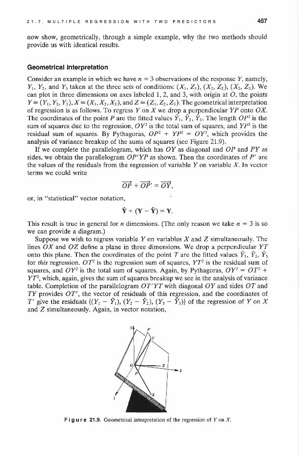
21.7. MULTIPLE REGRESSION WITH TWO PREDICTORS 457
now show, geometrically, through a simple example, why the two methods should provide us with identical results.
Geometrical Interpretation
Consider an example in which we have n = 3 observations of the response Y, namely, Yt. Y2, and Y3 taken at the three sets of conditions: (XI. Zl), (X2, Z2), (X3, Z3)' We can plot in three dimensions on axes labeled 1, 2, and 3, with origin at O, the points Y== (YI. Y2, Y3),X== (XI.X2, X3), and Z == (ZI. Z2, Z3)' The geometrical interpretation of regression is as follows. To regress Y on X we drop a perpendicular YP onto OX. The coordinates of the point Pare the fitted values YI. Y2, Y3 • The length OP2 is the sum of squares due to the regression, OY2 is the total sum of squares, and yp2 is the residual sum of squares. By Pythagoras, OP2 + yp2 = OY2, which provides the analysis of variance breakup of the sums of squares (see Figure 21.9).
If we complete the parallelogram, which has OY as diagonal and OP and PY as sides, we obtain the parailelogram OP'YP as shown. Then the coordinates of P' are the values of the residuals from the regression of variable Y on variable X. In vector terms we could write
~ ~ ~
OP + OP' = OY,
or, in "statistical" vector notation,
y + (Y - Y) = Y.
This result is true in general for n dimensions. (The only reason we take n = 3 is so we can provide a diagram.)
Suppose we wish to regress variable Y on variables X and Z simultaneously. The lines OX and OZ define a plane in three dimensions. We drop a perpendicular YT onto this planeo Then the coordinates of the point Tare the fitted values YI. Y2, Y3 for this regression. OT2 is the regression sum of squares, YT2 is the residual sum of squares, and OY2 is the total sum of squares. Again, by Pythagoras, OY2 = OT2 + YT2, which, again, gives the sum of squares breakup we see in the analysis of variance tableo Completion of the parallelogram OT'YT with diagonal OY and sides OT and TY provides OT', the vector of residual s of this regression, and the coordinates of T' give the residuals {(Y1 - Y1), (Y2 - Y2), (Y3 - Y3)} of the regression of Y on X and Z simultaneously. Again, in vector notation,
F i 9 u r e 21.9. Geometrical interpretation of the regression of Y on X.
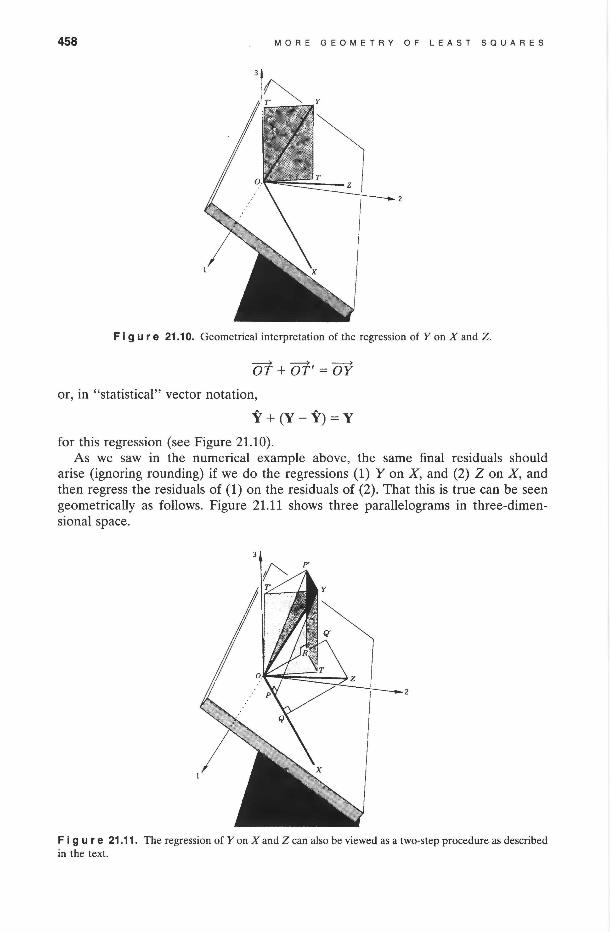
458 MORE GEOMETRY OF LEAST SQUARES
F i 9 U r e 21.10. Geometrical interpretation of the regression of Y on X and Z.
~ ~ ----+ OT+ OT' = OY
or, in "statistical" vector notation,
y + (Y - Y) = Y
for this regression (see Figure 21.10). As we saw in the numerical example above, the same final residuals should
arise (ignoring rounding) if we do the regressions (1) Y on X, and (2) Z on X, and then regress the residuals of (1) on the residuals of (2). That this is true can be seen geometrically as follows. Figure 21.11 shows three parallelograms in three-dimensional space.
F i 9 u r e 21.11. The regression of Y on X and Z can also be viewed as a two-step procedure as described in the text.
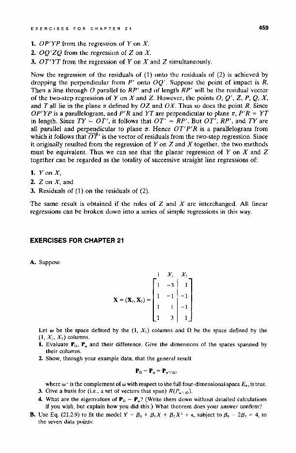
EXEACISES FOA CHAPTEA 21 459
1. OP'YP from the regression of Y on X. 2. OQ' ZQ from the regression of Z on X. 3. OT'YT from the regression of Y on X and Z simultaneously.
Now the regression of the residuals of (1) onto the residuals of (2) is achieved by dropping the perpendicular from P' onto OQ'. Suppose the point of impact is R. Then a line through O parallel to RP' and of length RP' will be the residual vector of the two-step regression of Y on X and Z. However, the points O, Q', Z, P, Q, X, and T alllie in the plane 1T defined by OZ and OX. Thus so does the point R. Since OP'YP is a parallelogram, and P' R and YT are perpendicular to plane 1T, P' R = YT in length. Since TY = OT', it follows that OT' = RP'. But OT', RP', and TY are all parallel and perpendicular to plane 1T. Hence OT' P' R is a parallelogram from which it follows that OT' is the vector of residuals from the two-step regression. Since it originally resulted from the regression of Y on Z and X together, the two methods must be equivalent. Thus we can see that the planar regression of Y on X and Z together can be regarded as the totality of successive straight line regressions of:
1. Yon X, 2. Z on X, and 3. Residuals of (1) on the residuals of (2).
The same result is obtained if the roles of Z and X are interchanged. All linear regressions can be broken down into a series of simple regressions in this way.
EXERCISES FOR CHAPTER 21
A. Suppose
Xl X 2
-3
X = (X¡, X2) = -1 -1
-1
3
Let w be the space defined by the (1, Xl) columns and n be the space defined by the (1, XI, X2) columns. 1. Evaluate Po, P w and their difference. Give the dimensions of the spaces spanned by
their columns. 2. Show, through your example data, that the general result
where w 1 is the complement of w with respect to the full four-dimensional space E4 , is true. 3. Give a basis for (Le., a set of vectors that span) R(Pw - no ).
4. What are the eigenvalues of Po - P w? (Write them down without detailed calculations if you wish, but explain how you did this.) What theorem does your answer confirm?
B. Use Eq. (21.2.9) to fit the model Y = /30 + /3IX + /32X2 + E, subject to /30 - 2/31 = 4, to the seven data points:
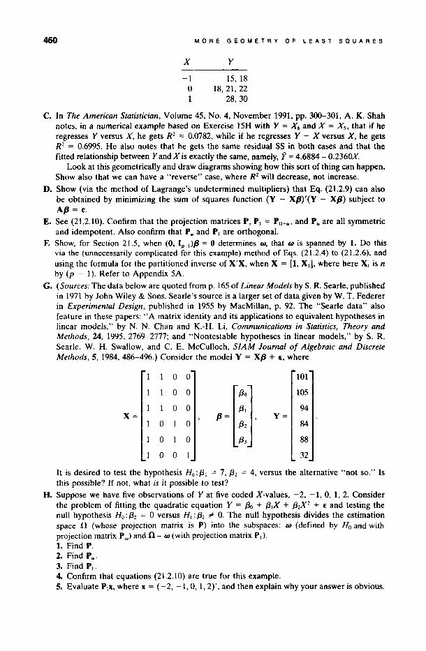
460 MORE GEOMETRV OF LEAST SaUARES
x y
-1 15, 18 O 18, 21, 22 1 28,30
c. In The American Statistician, Volume 45, No. 4, November 1991, pp. 300-301, A. K. Shah notes, in a numerical example based on Exercise 15H with Y = Xó and X = Xs, that ii he regresses y versus X, he gets R2 = 0.0782, while ii he regresses Y - X versus X, he gets R 2 = 0.6995. He also notes that he gets the same residual SS in both cases and that the fitted relationship between Yand X is exactly the same, namely, Y = 4.6884 - O.2360X.
Look at this geometricaHy and draw diagrams showing how this sort oi thing can happen. Show also that we can have a "reverse" case, where R2 will decrease, not increase.
D. Show (via the method of Lagrange's undetermined multipliers) that Eq. (21.2.9) can also be obtained by minimizing the sum of squares function (Y - XP)'(Y - XP) subject to AfJ = c.
E. See (21.2.10). Confirm that the projection matrices P, PI = Pn-... , and p ... are aH symmetric and idempotent. AIso confirm that p ... and PIare orthogonal.
F. Show, for Section 21.5, when (O, Ip- I)IJ = O determines (1), that (1) is spanned by 1. Do this via the (unnecessarily complicated for this example) method of Eqs. (21.2.4) to (21.2.6), and using the formula for the partitioned inverse of X'X, when X = [1, X.], where here XI is n by (p - 1). Refer to Appendix 5A.
G. (Sources: The data below are quoted from p. 165 of Linear Models by S. R. Searle, published in 1971 by John Wiley & Sonso Searle's so urce is a Iarger set of data given by W. T. Federer in Experimental Design, published in 1955 by MacMillan, p. 92. The "Searle data" also feature in these papers: "A matrix identity and its applications to equivalent hypotheses in linear models," by N. N. Chan and K.-H. Li, Communications in Statistics, Theory and Methods, 24, 1995, 2769-2777; and "Nontestable hypotheses in linear models," by S. R. Searle, W. H. Swallow, and C. E. McCulloch, SIAM Journal o[ Algebraic and Discrete Methods.5, 1984,486-496.) Consider the model Y = Xp + E, where
O O 101
O O /30 105
O O /31 94 X= 11= Y=
O O /32 84
O O /33 88
O O 32
It is desired to test the hypothesis Ho: /31 = 7, /32 = 4, versus the alternative "not so." Is this possible? If not, what is it possible to test?
H. Suppose we have five observations of Y at five coded X-values, -2, -1, O, 1,2. Consider the problem of fitting the quadratic equation Y = /30 + /3IX + /32X2 + E and testing the null hypothesis Ho: /32 = O versus H I : /32 #- O. The null hypothesis divides the estimation space n (whose projection matrix is P) into the subspaces: (1) (defined by Ho and with projection matrix P w) and n - (1) (with projection matrix PI)' 1. Find P. 2. Find p .... 3. Find PI' 4. Confirm that equations (21.2.10) are true for this example. 5. Evaluate PI X, where x = (-2, -1, 0,1,2)', and then explain why your answer is obvious.
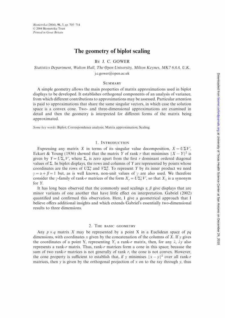
Biometrika (2004), 91, 3, pp. 705–714
© 2004 Biometrika Trust
Printed in Great Britain
The geometry of biplot scaling
B J. C. GOWER
Statistics Department, Walton Hall, T he Open University, Milton Keynes, MK7 6AA, U.K.
S
A simple geometry allows the main properties of matrix approximations used in biplotdisplays to be developed. It establishes orthogonal components of an analysis of variance,from which different contributions to approximations may be assessed. Particular attentionis paid to approximations that share the same singular vectors, in which case the solutionspace is a convex cone. Two- and three-dimensional approximations are examined indetail and then the geometry is interpreted for different forms of the matrix beingapproximated.
Some key words: Biplot; Correspondence analysis; Matrix approximation; Scaling.
1. I
Expressing any matrix X in terms of its singular value decomposition, X=USV ∞,Eckart & Young (1936) showed that the matrix Y of rank r that minimises dX−Y d2 isgiven by Y=US
rV ∞, where S
ris zero apart from the first r dominant ordered diagonal
values of S. In biplot displays, the rows and columns of Y are represented by points whosecoordinates are the rows of USa
rand VSb
r. To represent Y by its inner product we need
c=a+b=1 but, as is well known, non-unit values of c are also used. We thereforeconsider the c-family of rank-r matrices of the form X
r=USc
rV ∞, so that X1 is a synonym
for Y .It has long been observed that the commonly used scalings a, b give displays that are
minor variants of one another that have little effect on interpretation. Gabriel (2002)quantified and confirmed this observation. Here, I give a geometrical approach that Ibelieve offers additional insights and which extends Gabriel’s essentially two-dimensionalresults to three dimensions.
2. T
Any p×q matrix X may be represented by a point X in a Euclidean space of pqdimensions, with coordinates x given by the concatenation of the columns of X. If y givesthe coordinates of a point Y, representing Y , a rank-r matrix, then, for any l, ly alsorepresents a rank-r matrix. Thus, rank-r matrices form a cone in this space; because thesum of two rank-r matrices is not generally of rank r, the cone is not convex. However,the cone property is sufficient to establish that, if y minimises dx−yd2 over all rank-rmatrices, then y is given by the orthogonal projection of x on to the ray through y, thus
at University of T
exas Health S
cience Center at S
an Antonio on D
ecember 24, 2010
biomet.oxfordjournals.org
Dow
nloaded from
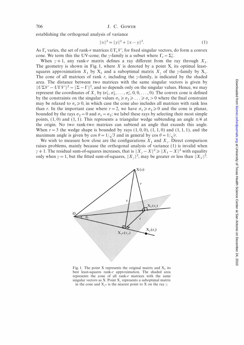
706 J. C. G
establishing the orthogonal analysis of variance
dxd2=dyd2+dx−yd2. (1)
As Crvaries, the set of rank-r matrices UC
rV ∞, for fixed singular vectors, do form a convex
cone. We term this the UV-cone; the c-family is a subset where Cr=Scr.
When cN1, any rank-r matrix defines a ray different from the ray through X1 .The geometry is shown in Fig. 1, where X is denoted by a point X, its optimal least-squares approximation X1 by X1 and a suboptimal matrix Xc of the c-family by Xc .The cone of all matrices of rank r, including the c-family, is indicated by the shadedarea. The distance between two matrices with the same singular vectors is given bydUSV ∞−UCV ∞d2=dS−Cd2, and so depends only on the singular values. Hence, we mayrepresent the coordinates of X
cby (sc
1, sc2, . . . , sc
r, 0, 0, . . . , 0). The convex cone is defined
by the constraints on the singular values s1�s2� . . .�sr>0 where the final constraintmay be relaxed to s
r�0, in which case the cone also includes all matrices with rank less
than r. In the important case where r=2, we have s1�s2�0 and the cone is planar,bounded by the rays s2=0 and s1=s2 ; we label these rays by selecting their most simplepoints, (1, 0) and (1, 1). This represents a triangular wedge subtending an angle p/4 atthe origin. No two rank-two matrices can subtend an angle that exceeds this angle.When r=3 the wedge shape is bounded by rays (1, 0, 0), (1, 1, 0) and (1, 1, 1), and themaximum angle is given by cos h=1/√3 and in general by cos h=1/√r.We wish to measure how close are the configurations X1 and Xc . Direct comparisonraises problems, mainly because the orthogonal analysis of variance (1) is invalid whencN1. The residual sum-of-squares increases, that is dX
c−Xd2�dX1−Xd2 with equality
only when c=1, but the fitted sum-of-squares, dXcd2, may be greater or less than dX1d2.
Fig. 1. The point X represents the original matrix and X1 itsbest least-squares rank-r approximation. The shaded arearepresents the cone of all rank-r matrices with the samesingular vectors as X. Point X
crepresents a suboptimal matrix
in the cone and Xc*is the nearest point to X on the ray c.
at University of T
exas Health S
cience Center at S
an Antonio on D
ecember 24, 2010
biomet.oxfordjournals.org
Dow
nloaded from
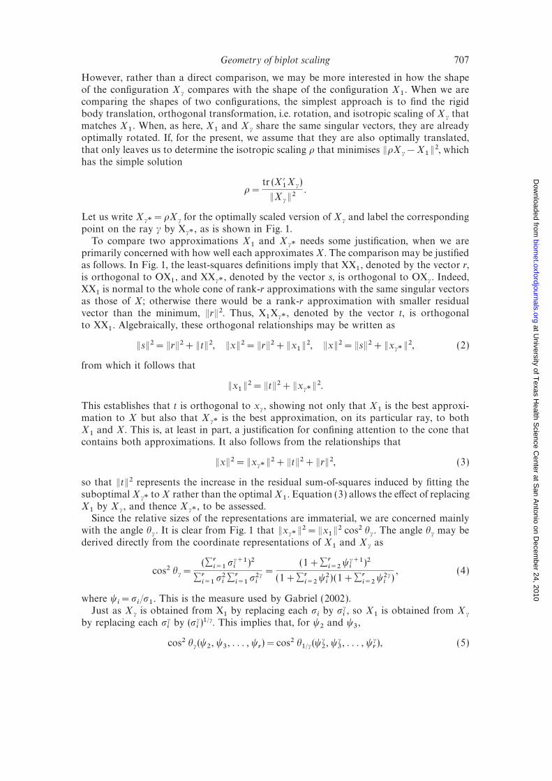
707Geometry of biplot scaling
However, rather than a direct comparison, we may be more interested in how the shapeof the configuration X
ccompares with the shape of the configuration X1 . When we are
comparing the shapes of two configurations, the simplest approach is to find the rigidbody translation, orthogonal transformation, i.e. rotation, and isotropic scaling of X
cthat
matches X1 . When, as here, X1 and Xc share the same singular vectors, they are alreadyoptimally rotated. If, for the present, we assume that they are also optimally translated,that only leaves us to determine the isotropic scaling r that minimises drX
c−X1d2, which
has the simple solution
r=tr (X∞1Xc)
dXcd2.
Let us write Xc*=rX
cfor the optimally scaled version of X
cand label the corresponding
point on the ray c by Xc*, as is shown in Fig. 1.
To compare two approximations X1 and Xc* needs some justification, when we areprimarily concerned with how well each approximatesX. The comparison may be justifiedas follows. In Fig. 1, the least-squares definitions imply that XX1 , denoted by the vector r,is orthogonal to OX1 , and XXc* , denoted by the vector s, is orthogonal to OXc . Indeed,XX1 is normal to the whole cone of rank-r approximations with the same singular vectorsas those of X; otherwise there would be a rank-r approximation with smaller residualvector than the minimum, drd2. Thus, X1Xc* , denoted by the vector t, is orthogonalto XX1 . Algebraically, these orthogonal relationships may be written as
dsd2=drd2+dtd2, dxd2=drd2+dx1d2, dxd2=dsd2+dx
c*d2, (2)
from which it follows that
dx1d2=dtd2+dx
c*d2.
This establishes that t is orthogonal to xc, showing not only that X1 is the best approxi-
mation to X but also that Xc*is the best approximation, on its particular ray, to both
X1 and X. This is, at least in part, a justification for confining attention to the cone thatcontains both approximations. It also follows from the relationships that
dxd2=dxc*d2+dtd2+drd2, (3)
so that dtd2 represents the increase in the residual sum-of-squares induced by fitting thesuboptimalX
c*toX rather than the optimalX1 . Equation (3) allows the effect of replacing
X1 by Xc , and thence Xc* , to be assessed.Since the relative sizes of the representations are immaterial, we are concerned mainly
with the angle hc. It is clear from Fig. 1 that dx
c*d2=dx
1d2 cos2 h
c. The angle h
cmay be
derived directly from the coordinate representations of X1 and Xc as
cos2 hc=(Wri=1sc+1i)2
Wri=1s2iWri=1s2ci=
(1+Wri=2yc+1i)2
(1+Wri=2y2i) (1+Wr
i=2y2ci), (4)
where yi=si/s1 . This is the measure used by Gabriel (2002).
Just as Xcis obtained from X1 by replacing each si by sci , so X1 is obtained from Xc
by replacing each sciby (sc
i)1/c. This implies that, for y2 and y3 ,
cos2 hc(y2, y3, . . . , y
r)=cos2 h
1/c(yc2, yc3, . . . , yc
r), (5)
at University of T
exas Health S
cience Center at S
an Antonio on D
ecember 24, 2010
biomet.oxfordjournals.org
Dow
nloaded from
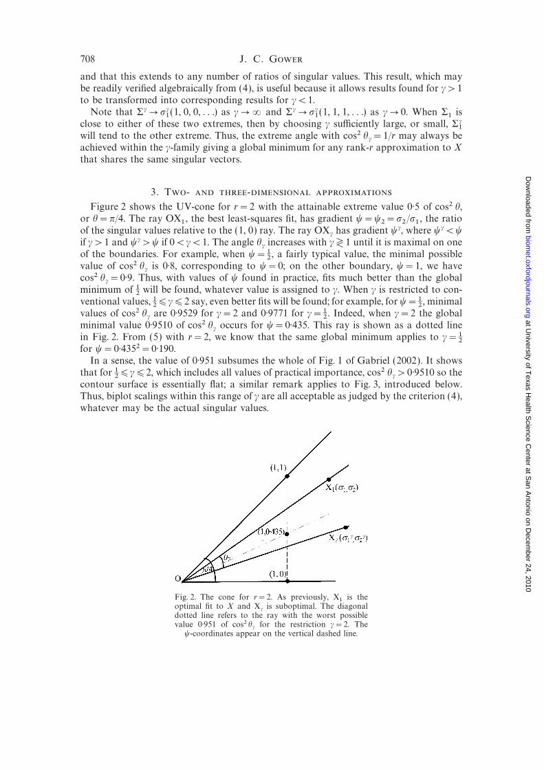
708 J. C. G
and that this extends to any number of ratios of singular values. This result, which maybe readily verified algebraically from (4), is useful because it allows results found for c>1to be transformed into corresponding results for c<1.Note that Sc� sc
1(1, 0, 0, . . .) as c�2 and Sc� sc
1(1, 1, 1, . . .) as c� 0. When S1 is
close to either of these two extremes, then by choosing c sufficiently large, or small, Sc1
will tend to the other extreme. Thus, the extreme angle with cos2 hc=1/r may always be
achieved within the c-family giving a global minimum for any rank-r approximation to Xthat shares the same singular vectors.
3. T- -
Figure 2 shows the UV-cone for r=2 with the attainable extreme value 0·5 of cos2 h,or h=p/4. The ray OX1 , the best least-squares fit, has gradient y=y2=s2/s1 , the ratioof the singular values relative to the (1, 0) ray. The ray OX
chas gradient yc, where yc<y
if c>1 and yc>y if 0<c<1. The angle hcincreases with c71 until it is maximal on one
of the boundaries. For example, when y=12, a fairly typical value, the minimal possible
value of cos2 hcis 0·8, corresponding to y=0; on the other boundary, y=1, we have
cos2 hc=0·9. Thus, with values of y found in practice, fits much better than the global
minimum of 12will be found, whatever value is assigned to c. When c is restricted to con-
ventional values, 12∏c∏2 say, even better fits will be found; for example, for y=1
2, minimal
values of cos2 hcare 0·9529 for c=2 and 0·9771 for c=1
2. Indeed, when c=2 the global
minimal value 0·9510 of cos2 hcoccurs for y=0·435. This ray is shown as a dotted line
in Fig. 2. From (5) with r=2, we know that the same global minimum applies to c=12
for y=0·4352=0·190.In a sense, the value of 0·951 subsumes the whole of Fig. 1 of Gabriel (2002). It showsthat for 1
2∏c∏2, which includes all values of practical importance, cos2 h
c>0·9510 so the
contour surface is essentially flat; a similar remark applies to Fig. 3, introduced below.Thus, biplot scalings within this range of c are all acceptable as judged by the criterion (4),whatever may be the actual singular values.
Fig. 2. The cone for r=2. As previously, X1 is theoptimal fit to X and X
cis suboptimal. The diagonal
dotted line refers to the ray with the worst possiblevalue 0·951 of cos2 h
cfor the restriction c=2. The
y-coordinates appear on the vertical dashed line.
at University of T
exas Health S
cience Center at S
an Antonio on D
ecember 24, 2010
biomet.oxfordjournals.org
Dow
nloaded from
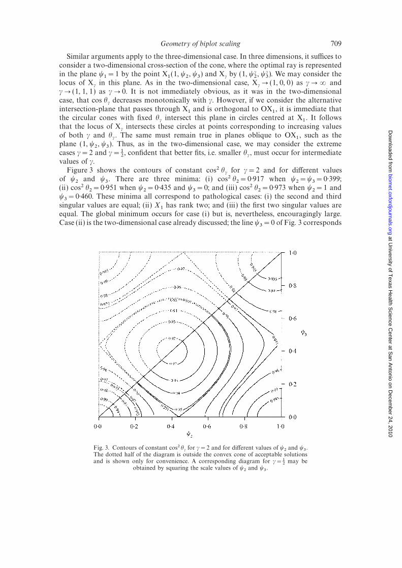
709Geometry of biplot scaling
Similar arguments apply to the three-dimensional case. In three dimensions, it suffices toconsider a two-dimensional cross-section of the cone, where the optimal ray is representedin the plane y1=1 by the point X1 (1, y2 , y3 ) and Xc by (1, yc2 , yc3 ). We may consider thelocus of X
cin this plane. As in the two-dimensional case, X
c� (1, 0, 0) as c�2 and
c� (1, 1, 1) as c� 0. It is not immediately obvious, as it was in the two-dimensionalcase, that cos h
cdecreases monotonically with c. However, if we consider the alternative
intersection-plane that passes through X1 and is orthogonal to OX1 , it is immediate thatthe circular cones with fixed h
cintersect this plane in circles centred at X1 . It follows
that the locus of Xcintersects these circles at points corresponding to increasing values
of both c and hc. The same must remain true in planes oblique to OX1 , such as the
plane (1, y2 , y3 ). Thus, as in the two-dimensional case, we may consider the extremecases c=2 and c=1
2, confident that better fits, i.e. smaller h
c, must occur for intermediate
values of c.Figure 3 shows the contours of constant cos2 h
cfor c=2 and for different values
of y2 and y3 . There are three minima: (i) cos2 h2=0·917 when y2=y3=0·399;(ii) cos2 h2=0·951 when y2=0·435 and y3=0; and (iii) cos2 h2=0·973 when y2=1 andy3=0·460. These minima all correspond to pathological cases: (i) the second and thirdsingular values are equal; (ii) X1 has rank two; and (iii) the first two singular values areequal. The global minimum occurs for case (i) but is, nevertheless, encouragingly large.Case (ii) is the two-dimensional case already discussed; the line y3=0 of Fig. 3 corresponds
Fig. 3. Contours of constant cos2 hcfor c=2 and for different values of y2 and y3 .
The dotted half of the diagram is outside the convex cone of acceptable solutionsand is shown only for convenience. A corresponding diagram for c=1
2may be
obtained by squaring the scale values of y2 and y3 .
at University of T
exas Health S
cience Center at S
an Antonio on D
ecember 24, 2010
biomet.oxfordjournals.org
Dow
nloaded from
710 J. C. G
to the vertical dashed line of Fig. 2. Despite the busy-looking contours in Fig. 3, the surfaceis essentially flat. The sharp corners in the contours at the minima on y2=1 and y3=0occur not because of any discontinuity in the gradients. If the contours are continued intothe analytically acceptable regions beyond the convex cone that correspond to inadmissiblesingular values, the sharp corners are seen as the nodes of looped contours.
4. D
4·1. Preamble
The above depends entirely on c and not on the individual values of a and b. The usualchoices are (i) a=1, b=0, (ii) a=0, b=1, (iii) a=1
2, b=1
2or (iv) a=1, b=1. Which one
to choose depends on what substantive meaning is to be assigned to X. There are threemajor considerations: is X a multivariate data-matrix with p columns referring to differentvariables or does it refer to a two-way table of a single variable classified by two factorswith p and q levels; are the entries in X quantitative measurements, counts or categorical;and are we more interested in approximating X itself or in approximating a derivedsymmetry matrix, such as X∞X or XX∞, or a distance matrix of some kind, or a similaritymatrix? These topics are covered in the literature; for a review of most of the issues, seeGower & Hand (1996). In this section, we examine the effect of the different forms of Xon our geometry.
4·2. T he case where X is a data matrix
The classical case is that of a quantitative data matrix X, centred to have zero meansand possibly normalised to have unit sums-of-squares. Then we choose a=1, b=0 toobtain the usual representation (US )V ∞ of the samples and variables in principal com-ponents analysis. We may compute the singular value decomposition via the spectraldecomposition of XX∞ or X∞X, but this is a computational convenience and does notnecessarily signify an interest in approximating these matrix products. However, thesematrices may have substantive interest and replace X itself as the primary matrix. Thus,XX∞=US2U∞, so that US also generates XX∞ and hence the distances between the rowsofX. Furthermore,X∞X=VS2V ∞, so that VS generates the correlation matrix, providedXhas been centred and normalised. The squared distance between the ith and jth columnsof X is 2(1−r
ij), where r
ijis the correlation between the ith and jth variables (Hills,
1969). This representation needs a=0, b=1, though we could also choose a=b=1, inwhich case the induced inner-product is US2V ∞ which might be regarded as our basicmatrix. The Eckart–Young approximation now has singular values S2 and hence con-tributes fourth powers to the fit, so the fits to X and to X∞X are assessed differently. Itnow becomes ambivalent as to whether we are assigning weights a=b=1 to S or weightsa=b=1
2to S2. This does not affect the geometry of §§ 2 and 3 because the only constraint
required on X is that it shares its singular vectors with those of Xc. Indeed, the analysis
of § 3 shows that X will be well approximated even when our primary objective is toapproximate X∞X and XX∞.
4·3. Approximating symmetric matrices
In the above situations, we are approximating symmetric matrices, with zero diagonalsfor distance matrices and unit diagonals for correlation and similarity matrices. Whenusing the implicit Eckart–Young approximation we note that the diagonals get half the
at University of T
exas Health S
cience Center at S
an Antonio on D
ecember 24, 2010
biomet.oxfordjournals.org
Dow
nloaded from
711Geometry of biplot scaling
weight of the symmetric off-diagonal terms; it might be more appropriate to give zeroweight to the diagonal terms. Bailey & Gower (1990) investigate some of the algebraicconsequences of using differential weightings. Diagonals are excluded when we use mostforms of metric multi-dimensional scaling, and special handling of the diagonal is one ofthe motivations for the factor analysis of a correlation matrix. By ignoring the diagonal,we can find better fits to the substantive parts of the matrix, but the approximations areno longer part of the c-family of the UV-cone, so the criterion (4) is invalid and thegeometry discussed earlier is invalid. We could continue to calculate the angle betweenX, or X∞X, and the approximation, but the geometry and the algebra both become muchmore complicated. In practice, the approximations found by different methods of multi-dimensional scaling are usually similar, so it might be expected that small angles wouldbe found as with the c-family, but this has not been formally established. The handling ofdiagonal terms for categorical variables is discussed below.
4·4. Approximating a two-way table of quantitative values
Let us now turn to the case where X is a quantitative two-way table. If we fit abi-additive model, the main effects are estimated in the usual way as the row and columnmeans of X. Then the residual matrix is Z= (I−P)X(I−Q), where I−P and I−Q arerow and column centring matrices that eliminate main effects. Thus, Z estimates multi-plicative interaction terms which can be biplotted with a=1
2, b=1
2. In this case the rows
and columns of Z have similar status and there is no case for differential weighting. Thefull geometry is discussed by Gower (1990).
4·5. Correspondence analysis
Now consider the case where the variables are categorical. First we consider a two-waycontingency table Y with p rows and q columns. This is the set-up for correspondenceanalysis. Rather than analyse Y directly, we consider X=R−DYC−D, where R and Care the row and column totals of Y expressed as diagonal matrices. The singular valuedecomposition of X has a dominant unit singular value with corresponding unnormalisedvectors RD1 and CD1. These may be removed from X to give
R−DYC−D−RD11∞CDy. .
, (6)
where y. . is the grand total of Y used as a normaliser. Apart from the removed first term,this matrix has the same singular value decomposition as X. The elements of (6) areproportional to the terms in Pearson’s chi-squared for the independence of rows andcolumns and may be exhibited in the usual way as a biplot. Rows and columns are ofsimilar status so we would use a=b=1
2. The distances between the rows and between
the columns of (6) seem to be of little interest. Correspondence analysis has a principalinterest in chi-squared distance. These are the distances between the rows of R−1YC−Dand between the columns of R−DYC−1, and could be represented by any desired methodof multi-dimensional scaling. They can also be derived as distances between points whosecoordinates are given by the rows of A=R−DUS
rand B=C−DVS
r. These are not
ordinary least-squares solutions but may be expressed in terms a weighted least-squaresanalysis. So far as our geometry is concerned, the main issue is that A and B are notmembers of the c-family and the geometry developed above does not apply. When Rand C are approximately proportional to unit matrices, we are close to the c-family and
at University of T
exas Health S
cience Center at S
an Antonio on D
ecember 24, 2010
biomet.oxfordjournals.org
Dow
nloaded from
712 J. C. G
so the inner product is close to being proportional to US2V ∞ and will give a goodapproximation to (6), now with a=b=1. However, if the row and column totals of Yare disparate the approximation could be poor.
4·6. Multiple correspondence analysis
Multiple correspondence analysis can be developed in several ways, one of which is asthe simple correspondence analysis of an indicator matrix G= (G1 , G2 , . . . , Gp ). Here Gkis an indicator matrix for the kth categorical variable, zero apart from a single unit ineach row, recording the occurrence of a category for the corresponding case. Consequentlythe row sums of G are constant, equal to p, and the correspondence analysis dependsonly on the column sums which give the frequencies of every category. We write this as1∞G=1∞L , where L=diag (L 1 , L 2 , . . . , L p ) are the category frequencies written as diagonalmatrices. Correspondence analysis requires the singular value decomposition of GL−D.This can be a large matrix and it is common to simplify the calculations by requiring thespectral decomposition of the normalised Burt matrix B=L−DG∞GL−D. The Burt matrixhas interesting structure, with unit diagonal blocks and symmetrically placed off-diagonalblocks of the contingency tables, scaled as for ordinary correspondence analysis, for allpairs of categorical variables. Thus, an analysis of B can be regarded as a generalisationof ordinary correspondence analysis that gives a simultaneous analysis of all the two-waycontingency tables. When p=2, L 1=R and L 2=C and we may ask how the analysis of Brelates to a simple correspondence analysis of L−D
1G∞1G2L−D2which corresponds precisely
with X=R−DYC−D of the previous paragraph. A crucial difference is that B contains theuninteresting unit diagonal blocks. It turns out (Gower & Hand, 1996, § 10.2) that Brecovers the singular vectors U and V but replaces the singular values S by 1
2(I+S ). This
approximation is not part of the c-family but does belong to the convex UV-cone ofrank-r matrices with singular vectors U and V . Corresponding to (4) we may evaluate
cos2 h={Wri=2si(si+1)}2
Wri=2(1+s
i)2 Wri=2(s2i). (7)
Now, cos2 h depends on the absolute values of the singular values and, unlike (4),equation (7) cannot be expressed in terms of the ratios of singular values y
i=si/s2 . For
p=2, consideration of the angle between the rays (s1 , s2 ) and 12(1+s1 , 1+s2 ) in Fig. 2
shows that, especially for the larger singular values that are of primary interest, themaximal angle that may be attained while remaining in the cone is more restricted thanpreviously. A detailed investigation of (7) gives similar results to (4) but with simplercontours, i.e. arcs of circles passing through the origin, than those of Fig. 3. When p=2,equation (7) expresses the difference between ignoring and not ignoring the uninterestinginformation on the diagonal blocks. Joint correspondence analysis (Greenacre, 1988) givesthe methodology for ignoring diagonal blocks for general values of p. In a noniterativeform of joint correspondence analysis, all blocks retain their same singular vectors andthe common singular values change. Then the two forms of each block to be comparedbelong to the same UV-cone and the geometry given above shows that they would havesimilar configurations. However, the fitted and residual parts are not now orthogonal,leading to some interpretational difficulties. An iterative form of joint correspondenceanalysis leads to a fully acceptable least-squares solution with orthogonal components
at University of T
exas Health S
cience Center at S
an Antonio on D
ecember 24, 2010
biomet.oxfordjournals.org
Dow
nloaded from
713Geometry of biplot scaling
but achieves this through allowing the singular vectors to change from block to com-parable block. Then comparable blocks do not belong to the same UV-cone and ourgeometry is not available. When p=2, both forms of joint correspondence analysis recoverordinary correspondence analysis. In general, joint correspondence analysis improves thefit to the substantive part of the Burt matrix, expressions may be found for the fitted andresidual sums-of-squares and angles may continue to be evaluated. However, at present,when p>2, there seems to be no way of investigating how these quantities vary with jointcorrespondence analysis approximations.Multiple correspondence analysis offers a good example of the ambivalence between
whether one is more interested in fitting X or X∞X, in this case between GL−D or B. Inpart, this ambivalence is fuelled by the computational convenience of working in termsof the spectral decomposition of a symmetric matrix rather than the singular valuedecomposition of a rectangular matrix. A direct approximation of GL−D or even of G itselfmay be of interest, because the distances between rows may be interpreted in terms ofdissimilarity coefficients. Alternatively, the categories may be quantified and then G isreplaced by a quantitative matrix X, subsequently represented by a variety of biplotdisplays. Indeed, L−D may be regarded as giving one set of quantifications. Confusingly,a multiple correspondence analysis of GL−D leads to a further set of quantifications; seehomogeneity analysis in Gifi (1990, Ch. 3). For computational convenience, we may pro-ceed via the Burt matrix; then the diagonal blocks appear as an essential part of thecomputation. However, as we have seen, there are substantive reasons for an interest inapproximating a correlation matrix or a Burt matrix, with its constituent contingencytables, and then improved fits can be found by excluding the uninformative diagonalblocks.
4·7. Interpreting biplots
Once we have our biplot, it has to be interpreted. Distance comparisons are easily madeby eye. Inner-products, which are a major interpretative tool, are less easy to assess byeye because they involve the product of two lengths with the cosine of an angle. It is true,as pointed out by Gabriel (2002), that projections of a set of points on to an axis givethe correct orderings of the inner products; this is because one of the two lengths isconstant, and is, of course, a basic property of Cartesian axes. However, two difficultiesremain: projections allow us to compare inner products in one column of X but not acrosstwo columns; and there are differences in the degrees of approximation of different axes,resulting in the same unit difference being represented by different lengths. That projectionson to different axes are on different scales should not be ignored. A solution is to provideeach axis with its own scale, as proposed by Gower & Hand (1996, §§ 2.3, 2.6). The axesthen behave very much like familiar coordinate axes. Gabriel (2002) may have somejustification in saying that this ‘proliferation of axes and scales then clutters up the display’.Nevertheless, it reflects reality, and what one needs is a convenient way of incorporatingscale information, not of ignoring it. One would discourage the publication of graphs andcharts that did not have appropriate scale information; the situation is no different forbiplots.
A
I thank Dr Karen Vines for preparing the contour plot.
at University of T
exas Health S
cience Center at S
an Antonio on D
ecember 24, 2010
biomet.oxfordjournals.org
Dow
nloaded from

714 J. C. G
R
B, R. A. & G, J. C. (1990). Approximating a symmetric matrix. Psychometrika 55, 665–75.E, C. & Y, G. (1936). The approximation of one matrix by another of lower rank. Psychometrika1, 211–8.G, K. R. (2002). Goodness of fit of biplots and correspondence analysis. Biometrika 89, 423–36.G, A. (1990). Nonlinear Multivariate Analysis. Chichester: John Wiley and Sons.G, J. C. (1990). Three-dimensional biplots. Biometrika 77, 773–83.G, J. C. & H, D. J. (1996). Biplots. London: Chapman and Hall.G,M. J. (1988). Correspondence analysis of multivariate categorical data by weighted least squares.Biometrika 75, 457–67.H, M. (1969). On looking at large correlation matrices. Biometrika 56, 249–53.
[Received August 2003. Revised November 2003]
at University of T
exas Health S
cience Center at S
an Antonio on D
ecember 24, 2010
biomet.oxfordjournals.org
Dow
nloaded from
Statistics, 2003, Vol. 37(2), pp. 101–117
A GEOMETRIC CHARACTERIZATION OFLINEAR REGRESSION
BRIAN J. MCCARTIN*
Applied Mathematics, Kettering University, 1700 West Third Avenue, Flint, MI 48504-4898, USA
(Received 4 December 2000; In final form 29 October 2001)
It hardly seems an exaggeration to contend that the fitting of straight lines to experimental data permeates all ofscience. Would it not seem reasonable to expect a purely geometric characterization of such a straight line? Justsuch a geometrical perspective was provided by Francis Galton in 1886 if only one of the experimental variablescontains an error. This was extended by Karl Pearson in 1901 to allow both variables to be subject tomeasurement error so long as both errors have equal variances. After an intervening century, the present paperextends the Galton=Pearson geometrical characterization of linear regression in terms of the ‘‘concentrationellipse’’ to the case of unequal variances in the experimental data.
Keywords: Orthogonal regression; Generalized least squares; Total least squares
INTRODUCTION
It hardly seems an exaggeration to contend that the fitting of straight lines to experimental
data (Fig. 1) permeates all of science. Examples that immediately leap to mind are Hooke’s
Law (elongation / applied force) and Ohm’s Law (current / applied voltage). The corre-
sponding constants of proportionality are usually determined experimentally from such linear
fits. Would it not seem reasonable to expect a purely geometric characterization of such a
straight line?
Just such a geometrical perspective was provided by Francis Galton in 1886 if only one of
the experimental variables contains error. This was extended by Karl Pearson in 1901 to
allow both variables to be subject to measurement error. However, Pearson’s geometrical
picture assumed equal error variances for both measured quantities. After an intervening cen-
tury, Section 5 of the present paper extends this Galton=Pearson geometrical characterization
of linear regression to the case of unequal error variances in the experimental data. But first
we must set the stage.
Early in the 19th Century [1, pp. 13–15, pp. 145–146], the method of least squares was
developed by Legendre (1805) and Gauss (1809) precisely in order to address such data fit-
ting problems as arose in their investigations of astronomy and geodesy. However, in fitting a
linear relationship to a set of ðx; yÞ data, they assumed that one (‘independent’) variable, say
* Tel.: (810) 762-7802; Fax: (810) 762-9796; E-mail: [email protected]
ISSN 0233-1888 print; ISSN 1029-4910 online # 2003 Taylor & Francis LtdDOI: 10.1080=0223188031000112881
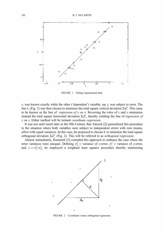
x, was known exactly while the other (‘dependent’) variable, say y, was subject to error. The
line L (Fig. 2) was then chosen to minimize the total square vertical deviation Sd2y . This came
to be known as the line of regression of y on x. Reversing the roles of x and y minimizes
instead the total square horizontal deviation Sd2x , thereby yielding the line of regression of
x on y. Either method will be termed coordinate regression.
It was not until much later in the l9th Century that Adcock [2] generalized this procedure
to the situation where both variables were subject to independent errors with zero means,
albeit with equal variances. In this case, he proposed to choose L to minimize the total square
orthogonal deviation Sd2? (Fig. 2). This will be referred to as orthogonal regression.
Almost immediately, Kummell [3] extended this approach to embrace the case where the
error variances were unequal. Defining s2u ¼ variance of x-error, s2
v ¼ variance of y-error,
and l ¼ s2v=s
2u, he employed a weighted least squares procedure thereby minimizing
FIGURE 1 Fitting experimental data.
FIGURE 2 Coordinate versus orthogonal regression.
102 B. J. MCCARTIN
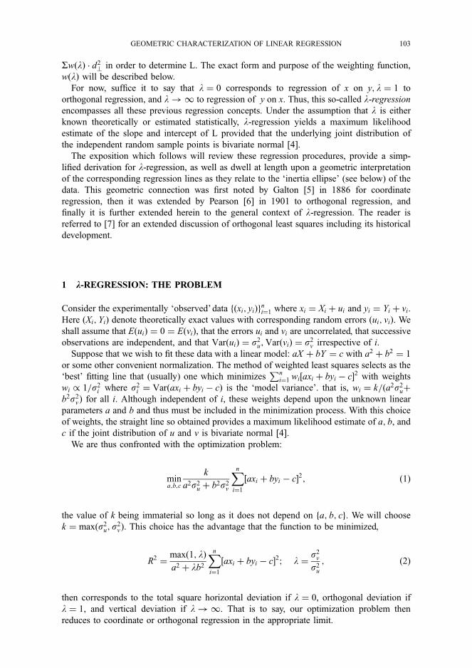
SwðlÞ � d2? in order to determine L. The exact form and purpose of the weighting function,
wðlÞ will be described below.
For now, suffice it to say that l ¼ 0 corresponds to regression of x on y; l ¼ 1 to
orthogonal regression, and l ! 1 to regression of y on x. Thus, this so-called l-regression
encompasses all these previous regression concepts. Under the assumption that l is either
known theoretically or estimated statistically, l-regression yields a maximum likelihood
estimate of the slope and intercept of L provided that the underlying joint distribution of
the independent random sample points is bivariate normal [4].
The exposition which follows will review these regression procedures, provide a simp-
lified derivation for l-regression, as well as dwell at length upon a geometric interpretation
of the corresponding regression lines as they relate to the ‘inertia ellipse’ (see below) of the
data. This geometric connection was first noted by Galton [5] in 1886 for coordinate
regression, then it was extended by Pearson [6] in 1901 to orthogonal regression, and
finally it is further extended herein to the general context of l-regression. The reader is
referred to [7] for an extended discussion of orthogonal least squares including its historical
development.
1 k-REGRESSION: THE PROBLEM
Consider the experimentally ‘observed’ data fðxi; yiÞgni¼1 where xi ¼ Xi þ ui and yi ¼ Yi þ vi.
Here ðXi; YiÞ denote theoretically exact values with corresponding random errors ðui; viÞ. We
shall assume that EðuiÞ ¼ 0 ¼ EðviÞ, that the errors ui and vi are uncorrelated, that successive
observations are independent, and that VarðuiÞ ¼ s2u;VarðviÞ ¼ s2
v irrespective of i.
Suppose that we wish to fit these data with a linear model: aX þ bY ¼ c with a2 þ b2 ¼ 1
or some other convenient normalization. The method of weighted least squares selects as the
‘best’ fitting line that (usually) one which minimizesPn
i¼1 wi½axi þ byi � c�2 with weights
wi / 1=s2i where s2
i ¼ Varðaxi þ byi � cÞ is the ‘model variance’. that is, wi ¼ k=ða2s2uþ
b2s2vÞ for all i. Although independent of i, these weights depend upon the unknown linear
parameters a and b and thus must be included in the minimization process. With this choice
of weights, the straight line so obtained provides a maximum likelihood estimate of a; b, and
c if the joint distribution of u and v is bivariate normal [4].
We are thus confronted with the optimization problem:
mina;b;c
k
a2s2u þ b2s2
v
Xni¼1
½axi þ byi � c�2; ð1Þ
the value of k being immaterial so long as it does not depend on fa; b; cg. We will choose
k ¼ maxðs2u; s
2vÞ. This choice has the advantage that the function to be minimized,
R2 ¼maxð1; lÞa2 þ lb2
Xni¼1
½axi þ byi � c�2; l ¼s2v
s2u
; ð2Þ
then corresponds to the total square horizontal deviation if l ¼ 0, orthogonal deviation if
l ¼ 1, and vertical deviation if l ! 1. That is to say, our optimization problem then
reduces to coordinate or orthogonal regression in the appropriate limit.
GEOMETRIC CHARACTERIZATION OF LINEAR REGRESSION 103
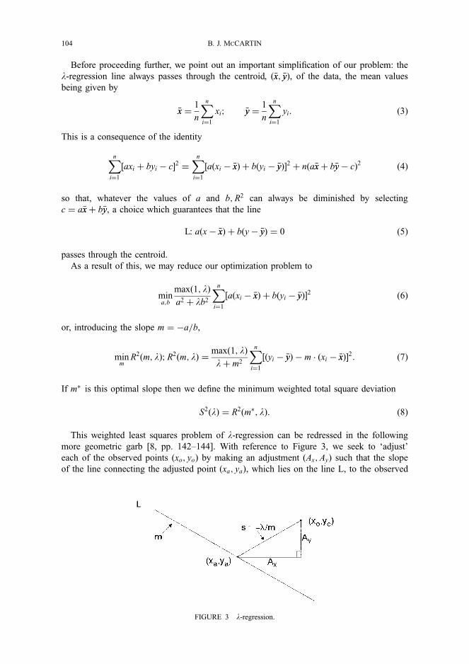
Before proceeding further, we point out an important simplification of our problem: the
l-regression line always passes through the centroid, ð�xx; �yyÞ, of the data, the mean values
being given by
�xx ¼1
n
Xni¼1
xi; �yy ¼1
n
Xni¼1
yi: ð3Þ
This is a consequence of the identity
Xni¼1
½axi þ byi � c�2 ¼Xni¼1
½aðxi � �xxÞ þ bðyi � �yyÞ�2 þ nða�xxþ b�yy� cÞ2 ð4Þ
so that, whatever the values of a and b;R2 can always be diminished by selecting
c ¼ a�xxþ b�yy, a choice which guarantees that the line
L: aðx� �xxÞ þ bðy� �yyÞ ¼ 0 ð5Þ
passes through the centroid.
As a result of this, we may reduce our optimization problem to
mina;b
maxð1; lÞa2 þ lb2
Xni¼1
½aðxi � �xxÞ þ bðyi � �yyÞ�2 ð6Þ
or, introducing the slope m ¼ �a=b,
minm
R2ðm; lÞ;R2ðm; lÞ ¼maxð1; lÞlþ m2
Xni¼1
½ðyi � �yyÞ � m � ðxi � �xxÞ�2: ð7Þ
If m� is this optimal slope then we define the minimum weighted total square deviation
S2ðlÞ ¼ R2ðm�; lÞ: ð8Þ
This weighted least squares problem of l-regression can be redressed in the following
more geometric garb [8, pp. 142–144]. With reference to Figure 3, we seek to ‘adjust’
each of the observed points ðxo; yoÞ by making an adjustment ðAx;AyÞ such that the slope
of the line connecting the adjusted point ðxa; yaÞ, which lies on the line L, to the observed
FIGURE 3 l-regression.
104 B. J. MCCARTIN
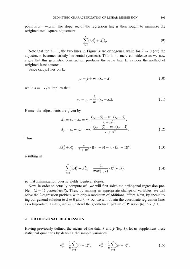
point is s ¼ �l=m. The slope, m, of the regression line is then sought to minimize the
weighted total square adjustment
Xni¼1
ðlA2x þ A2
yÞi: ð9Þ
Note that for l ¼ 1, the two lines in Figure 3 are orthogonal, while for l ! 0 ð1Þ the
adjustment becomes strictly horizontal (vertical). This is no mere coincidence as we now
argue that this geometric construction produces the same line, L, as does the method of
weighted least squares.
Since ðxa; yaÞ lies on L,
ya ¼ �yyþ m � ðxa � �xxÞ; ð10Þ
while s ¼ �l=m implies that
ya ¼ yo �lm� ðxa � xoÞ: ð11Þ
Hence, the adjustments are given by
Ax ¼ xa � xo ¼ m �ðyo � �yyÞ � m � ðxo � �xxÞ
lþ m2;
Ay ¼ ya � yo ¼ �l �ðyo � �yyÞ � m � ðxo � �xxÞ
lþ m2: ð12Þ
Thus,
lA2x þ A2
y ¼l
lþ m2� ½ðyo � �yyÞ � m � ðxo � �xxÞ�2; ð13Þ
resulting in
Xni¼1
ðlA2x þ A2
yÞi ¼l
maxð1; lÞ� R2ðm; lÞ; ð14Þ
so that minimization over m yields identical slopes.
Now, in order to actually compute m�, we will first solve the orthogonal regression pro-
blem ðl ¼ 1Þ geometrically. Then, by making an appropriate change of variables, we will
solve the l-regression problem with only a modicum of additional effort. Next, by specializ-
ing our general solution to l ¼ 0 and l ! 1, we will obtain the coordinate regression lines
as a byproduct. Finally, we will extend the geometrical picture of Pearson [6] to l 6¼ 1.
2 ORTHOGONAL REGRESSION
Having previously defined the means of the data, �xx and �yy (Eq. 3), let us supplement these
statistical quantities by defining the sample variances
s2x ¼
1
n
Xni¼1
ðxi � �xxÞ2; s2y ¼
1
n
Xni¼1
ðyi � �yyÞ2; ð15Þ
GEOMETRIC CHARACTERIZATION OF LINEAR REGRESSION 105
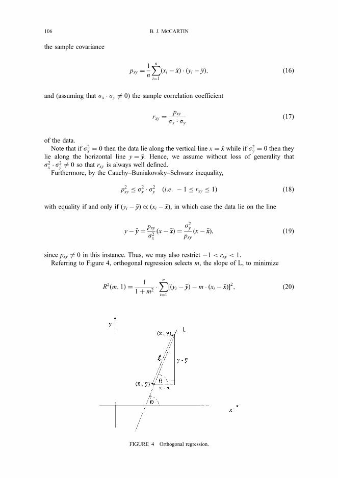
the sample covariance
pxy ¼1
n
Xni¼1
ðxi � �xxÞ � ðyi � �yyÞ; ð16Þ
and (assuming that sx � sy 6¼ 0) the sample correlation coefficient
rxy ¼pxy
sx � syð17Þ
of the data.
Note that if s2x ¼ 0 then the data lie along the vertical line x ¼ �xx while if s2
y ¼ 0 then they
lie along the horizontal line y ¼ �yy. Hence, we assume without loss of generality that
s2x � s
2y 6¼ 0 so that rxy is always well defined.
Furthermore, by the Cauchy–Buniakovsky–Schwarz inequality,
p2xy � s2
x � s2y ði:e: � 1 � rxy � 1Þ ð18Þ
with equality if and only if ðyi � �yyÞ / ðxi � �xxÞ, in which case the data lie on the line
y� �yy ¼pxy
s2x
ðx� �xxÞ ¼s2y
pxyðx� �xxÞ; ð19Þ
since pxy 6¼ 0 in this instance. Thus, we may also restrict �1 < rxy < 1.
Referring to Figure 4, orthogonal regression selects m, the slope of L, to minimize
R2ðm; 1Þ ¼1
1 þ m2�Xni¼1
½ðyi � �yyÞ � m � ðxi � �xxÞ�2; ð20Þ
FIGURE 4 Orthogonal regression.
106 B. J. MCCARTIN
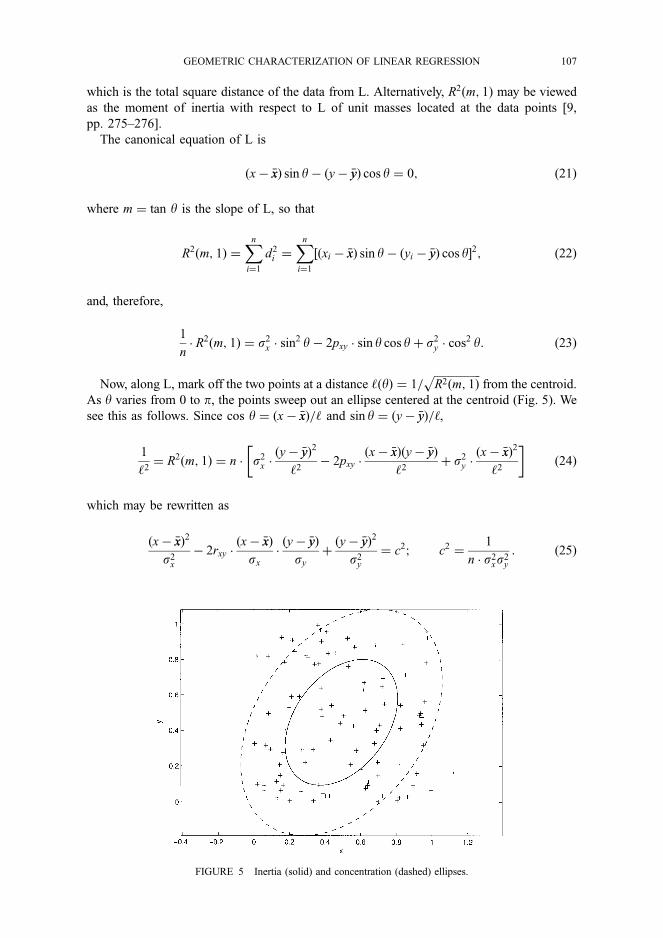
which is the total square distance of the data from L. Alternatively, R2ðm; 1Þ may be viewed
as the moment of inertia with respect to L of unit masses located at the data points [9,
pp. 275–276].
The canonical equation of L is
ðx� �xxÞ sin y� ðy� �yyÞ cos y ¼ 0; ð21Þ
where m ¼ tan y is the slope of L, so that
R2ðm; 1Þ ¼Xni¼1
d2i ¼
Xni¼1
½ðxi � �xxÞ sin y� ðyi � �yyÞ cos y�2; ð22Þ
and, therefore,
1
n� R2ðm; 1Þ ¼ s2
x � sin2 y� 2pxy � sin y cos yþ s2y � cos2 y: ð23Þ
Now, along L, mark off the two points at a distance ‘ðyÞ ¼ 1=ffiffiffiffiffiffiffiffiffiffiffiffiffiffiffiffiffiR2ðm; 1Þ
pfrom the centroid.
As y varies from 0 to p, the points sweep out an ellipse centered at the centroid (Fig. 5). We
see this as follows. Since cos y ¼ ðx� �xxÞ=‘ and sin y ¼ ðy� �yyÞ=‘,
1
‘2¼ R2ðm; 1Þ ¼ n � s2
x �ðy� �yyÞ2
‘2� 2pxy �
ðx� �xxÞðy� �yyÞ
‘2þ s2
y �ðx� �xxÞ2
‘2
� �ð24Þ
which may be rewritten as
ðx� �xxÞ2
s2x
� 2rxy �ðx� �xxÞ
sx�ðy� �yyÞ
syþðy� �yyÞ2
s2y
¼ c2; c2 ¼1
n � s2xs2
y
: ð25Þ
FIGURE 5 Inertia (solid) and concentration (dashed) ellipses.
GEOMETRIC CHARACTERIZATION OF LINEAR REGRESSION 107
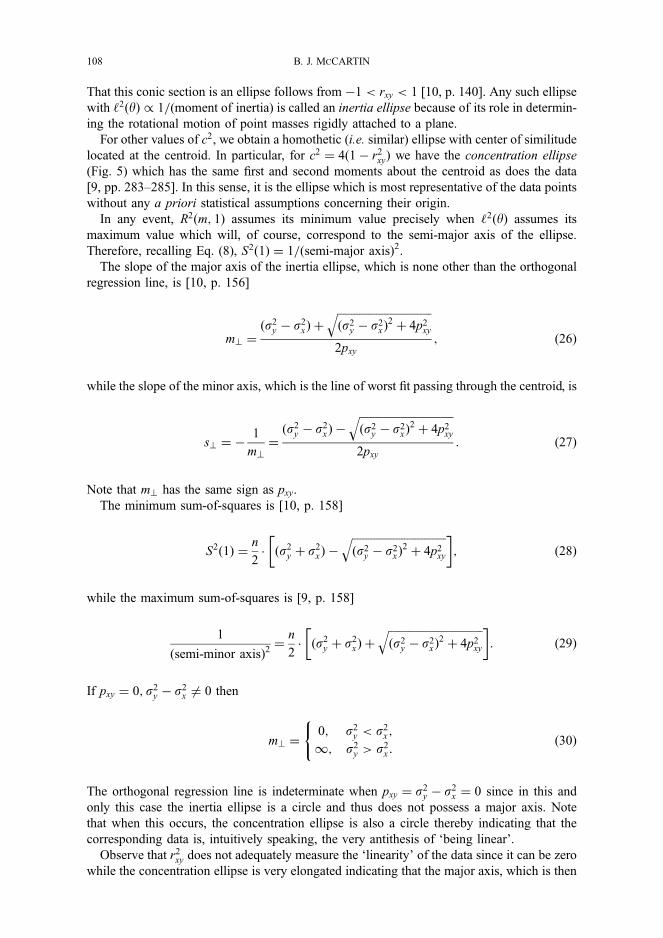
That this conic section is an ellipse follows from �1 < rxy < 1 [10, p. 140]. Any such ellipse
with ‘2ðyÞ / 1=(moment of inertia) is called an inertia ellipse because of its role in determin-
ing the rotational motion of point masses rigidly attached to a plane.
For other values of c2, we obtain a homothetic (i.e. similar) ellipse with center of similitude
located at the centroid. In particular, for c2 ¼ 4ð1 � r2xyÞ we have the concentration ellipse
(Fig. 5) which has the same first and second moments about the centroid as does the data
[9, pp. 283–285]. In this sense, it is the ellipse which is most representative of the data points
without any a priori statistical assumptions concerning their origin.
In any event, R2ðm; 1Þ assumes its minimum value precisely when ‘2ðyÞ assumes its
maximum value which will, of course, correspond to the semi-major axis of the ellipse.
Therefore, recalling Eq. (8), S2ð1Þ ¼ 1=ðsemi-major axisÞ2.
The slope of the major axis of the inertia ellipse, which is none other than the orthogonal
regression line, is [10, p. 156]
m? ¼ðs2
y � s2xÞ þ
ffiffiffiffiffiffiffiffiffiffiffiffiffiffiffiffiffiffiffiffiffiffiffiffiffiffiffiffiffiffiffiffiffiffiðs2
y � s2xÞ
2þ 4p2
xy
q2pxy
; ð26Þ
while the slope of the minor axis, which is the line of worst fit passing through the centroid, is
s? ¼ �1
m?
¼ðs2
y � s2xÞ �
ffiffiffiffiffiffiffiffiffiffiffiffiffiffiffiffiffiffiffiffiffiffiffiffiffiffiffiffiffiffiffiffiffiffiðs2
y � s2xÞ
2þ 4p2
xy
q2pxy
: ð27Þ
Note that m? has the same sign as pxy.
The minimum sum-of-squares is [10, p. 158]
S2ð1Þ ¼n
2� ðs2
y þ s2xÞ �
ffiffiffiffiffiffiffiffiffiffiffiffiffiffiffiffiffiffiffiffiffiffiffiffiffiffiffiffiffiffiffiffiffiffiðs2
y � s2xÞ
2þ 4p2
xy
q� �; ð28Þ
while the maximum sum-of-squares is [9, p. 158]
1
ðsemi-minor axisÞ2¼
n
2� ðs2
y þ s2xÞ þ
ffiffiffiffiffiffiffiffiffiffiffiffiffiffiffiffiffiffiffiffiffiffiffiffiffiffiffiffiffiffiffiffiffiffiðs2
y � s2xÞ
2þ 4p2
xy
q� �: ð29Þ
If pxy ¼ 0; s2y � s2
x 6¼ 0 then
m? ¼0; s2
y < s2x;
1; s2y > s2
x :
(ð30Þ
The orthogonal regression line is indeterminate when pxy ¼ s2y � s2
x ¼ 0 since in this and
only this case the inertia ellipse is a circle and thus does not possess a major axis. Note
that when this occurs, the concentration ellipse is also a circle thereby indicating that the
corresponding data is, intuitively speaking, the very antithesis of ‘being linear’.
Observe that r2xy does not adequately measure the ‘linearity’ of the data since it can be zero
while the concentration ellipse is very elongated indicating that the major axis, which is then
108 B. J. MCCARTIN
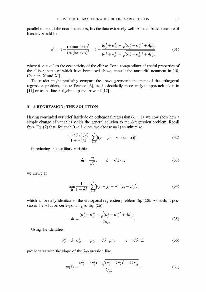
parallel to one of the coordinate axes, fits the data extremely well. A much better measure of
linearity would be
e2 ¼ 1 �ðminor axisÞ2
ðmajor axisÞ2¼ 1 �
ðs2y þ s2
xÞ �
ffiffiffiffiffiffiffiffiffiffiffiffiffiffiffiffiffiffiffiffiffiffiffiffiffiffiffiffiffiffiffiffiffiffiðs2
y � s2xÞ
2þ 4p2
xy
qðs2
y þ s2xÞ þ
ffiffiffiffiffiffiffiffiffiffiffiffiffiffiffiffiffiffiffiffiffiffiffiffiffiffiffiffiffiffiffiffiffiffiðs2
y � s2xÞ
2þ 4p2
xy
q ð31Þ
where 0 < e < 1 is the eccentricity of the ellipse. For a compendium of useful properties of
the ellipse, some of which have been used above, consult the masterful treatment in [10,
Chapters X and XI].
The reader might profitably compare the above geometric treatment of the orthogonal
regression problem, due to Pearson [6], to the decidedly more analytic approach taken in
[11] or to the linear algebraic perspective of [12].
3 k-REGRESSION: THE SOLUTION
Having concluded our brief interlude on orthogonal regression ðl ¼ 1Þ, we now show how a
simple change of variables yields the general solution to the l-regression problem. Recall
from Eq. (7) that, for each 0 < l < 1, we choose mðlÞ to minimize
maxð1; 1=lÞ1 þ m2=l
�Xni¼1
½ðyi � �yyÞ � m � ðxi � �xxÞ�2: ð32Þ
Introducing the auxiliary variables
mm ¼mffiffiffil
p ; x ¼ffiffiffil
p� x; ð33Þ
we arrive at
minmm
1
1 þ mm2�Xni¼1
½ðyi � �yyÞ � mm � ðxi � �xxÞ�2; ð34Þ
which is formally identical to the orthogonal regression problem Eq. (20). As such, it pos-
sesses the solution corresponding to Eq. (26)
mm ¼ðs2
y � s2xÞ þ
ffiffiffiffiffiffiffiffiffiffiffiffiffiffiffiffiffiffiffiffiffiffiffiffiffiffiffiffiffiffiffiffiffiffiffiðs2
y � s2xÞ
2þ 4p2
xy
q2pxy
: ð35Þ
Using the identities
s2x ¼ l � s2
x ; pxy ¼ffiffiffil
p� pxy; m ¼
ffiffiffil
p� mm ð36Þ
provides us with the slope of the l-regression line
mðlÞ ¼ðs2
y � ls2xÞ þ
ffiffiffiffiffiffiffiffiffiffiffiffiffiffiffiffiffiffiffiffiffiffiffiffiffiffiffiffiffiffiffiffiffiffiffiffiffiffiffiðs2
y � ls2xÞ
2þ 4lp2
xy
q2pxy
: ð37Þ
GEOMETRIC CHARACTERIZATION OF LINEAR REGRESSION 109
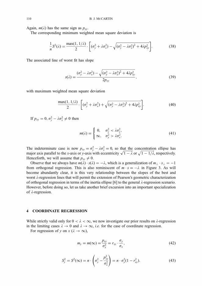
Again, mðlÞ has the same sign as pxy.
The corresponding minimum weighted mean square deviation is
1
nS2ðlÞ ¼
maxð1; 1=lÞ2
� ðs2y þ ls2
xÞ �
ffiffiffiffiffiffiffiffiffiffiffiffiffiffiffiffiffiffiffiffiffiffiffiffiffiffiffiffiffiffiffiffiffiffiffiffiffiffiffiðs2
y � ls2xÞ
2þ 4lp2
xy
q� �: ð38Þ
The associated line of worst fit has slope
sðlÞ ¼ðs2
y � ls2xÞ �
ffiffiffiffiffiffiffiffiffiffiffiffiffiffiffiffiffiffiffiffiffiffiffiffiffiffiffiffiffiffiffiffiffiffiffiffiffiffiffiðs2
y � ls2xÞ
2þ 4lp2
xy
q2pxy
; ð39Þ
with maximum weighted mean square deviation
maxð1; 1=lÞ2
� ðs2y þ ls2
xÞ þ
ffiffiffiffiffiffiffiffiffiffiffiffiffiffiffiffiffiffiffiffiffiffiffiffiffiffiffiffiffiffiffiffiffiffiffiffiffiffiffiðs2
y � ls2xÞ
2þ 4lp2
xy
q� �: ð40Þ
If pxy ¼ 0; s2y � ls2
x 6¼ 0 then
mðlÞ ¼0; s2
y < ls2x;
1; s2y > ls2
x :
(ð41Þ
The indeterminate case is now pxy ¼ s2y � ls2
x ¼ 0, so that the concentration ellipse has
major axis parallel to the x-axis or y-axis with eccentricityffiffiffiffiffiffiffiffiffiffiffi1 � l
por
ffiffiffiffiffiffiffiffiffiffiffiffiffiffiffiffi1 � 1=l
p, respectively.
Henceforth, we will assume that pxy 6¼ 0.
Observe that we always have mðlÞ � sðlÞ ¼ �l, which is a generalization of m? � s? ¼ �1
from orthogonal regression. This is also reminiscent of m � s ¼ �l in Figure 3. As will
become abundantly clear, it is this very relationship between the slopes of the best and
worst l-regression lines that will permit the extension of Pearson’s geometric characterization
of orthogonal regression in terms of the inertia ellipse [6] to the general l-regression scenario.
However, before doing so, let us take another brief excursion into an important specialization
of l-regression.
4 COORDINATE REGRESSION
While strictly valid only for 0 < l < 1, we now investigate our prior results on l-regression
in the limiting cases l ! 0 and l ! 1, i.e. for the case of coordinate regression.
For regression of y on x ðl ! 1Þ,
my ¼ mð1Þ ¼pxy
s2x
¼ rxy �sysx
; ð42Þ
S2y ¼ S2ð1Þ ¼ n � s2
y �p2xy
s2x
!¼ n � s2
yð1 � r2xyÞ: ð43Þ
110 B. J. MCCARTIN
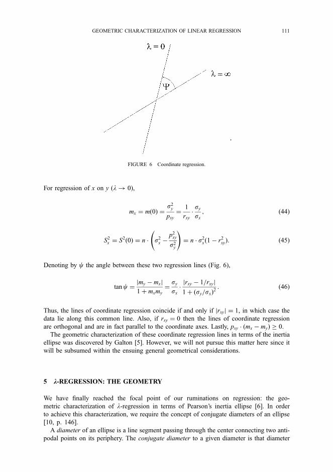
For regression of x on y ðl ! 0Þ,
mx ¼ mð0Þ ¼s2y
pxy¼
1
rxy�sysx
; ð44Þ
S2x ¼ S2ð0Þ ¼ n � s2
x �p2xy
s2y
!¼ n � s2
xð1 � r2xyÞ: ð45Þ
Denoting by c the angle between these two regression lines (Fig. 6),
tanc ¼jmy � mxj
1 þ mxmy
¼sysx
�jrxy � 1=rxyj
1 þ ðsy=sxÞ2: ð46Þ
Thus, the lines of coordinate regression coincide if and only if jrxyj ¼ 1, in which case the
data lie along this common line. Also, if rxy ¼ 0 then the lines of coordinate regression
are orthogonal and are in fact parallel to the coordinate axes. Lastly, pxy � ðmx � myÞ � 0.
The geometric characterization of these coordinate regression lines in terms of the inertia
ellipse was discovered by Galton [5]. However, we will not pursue this matter here since it
will be subsumed within the ensuing general geometrical considerations.
5 k-REGRESSION: THE GEOMETRY
We have finally reached the focal point of our ruminations on regression: the geo-
metric characterization of l-regression in terms of Pearson’s inertia ellipse [6]. In order
to achieve this characterization, we require the concept of conjugate diameters of an ellipse
[10, p. 146].
A diameter of an ellipse is a line segment passing through the center connecting two anti-
podal points on its periphery. The conjugate diameter to a given diameter is that diameter
FIGURE 6 Coordinate regression.
GEOMETRIC CHARACTERIZATION OF LINEAR REGRESSION 111
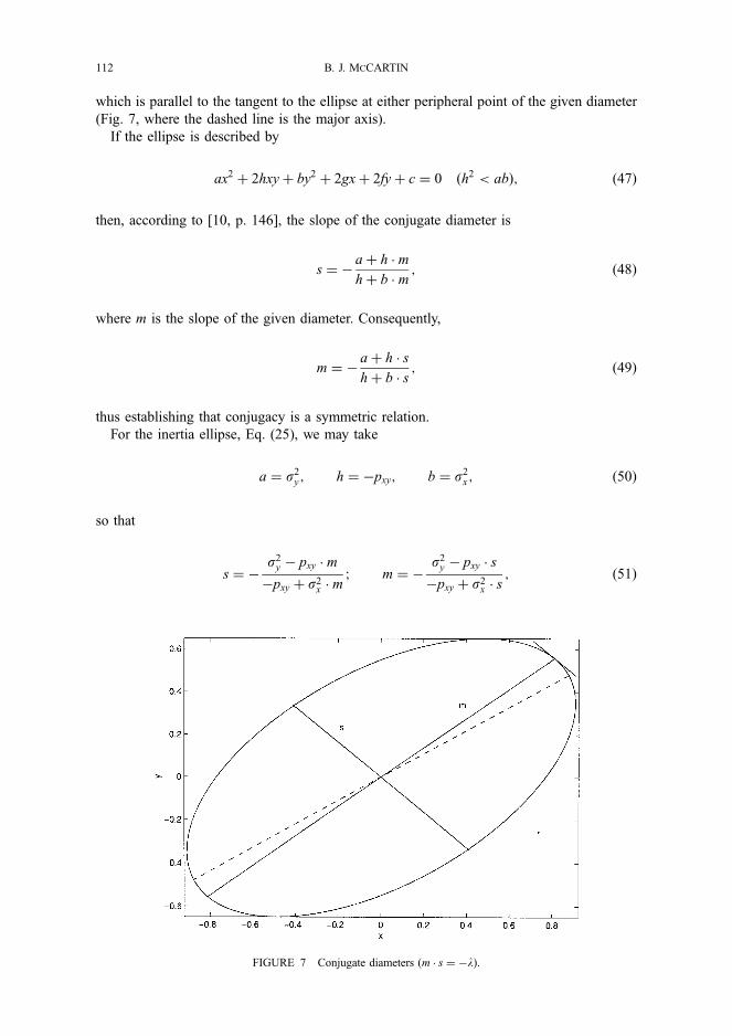
which is parallel to the tangent to the ellipse at either peripheral point of the given diameter
(Fig. 7, where the dashed line is the major axis).
If the ellipse is described by
ax2 þ 2hxyþ by2 þ 2gxþ 2fyþ c ¼ 0 ðh2 < abÞ; ð47Þ
then, according to [10, p. 146], the slope of the conjugate diameter is
s ¼ �aþ h � m
hþ b � m; ð48Þ
where m is the slope of the given diameter. Consequently,
m ¼ �aþ h � s
hþ b � s; ð49Þ
thus establishing that conjugacy is a symmetric relation.
For the inertia ellipse, Eq. (25), we may take
a ¼ s2y; h ¼ �pxy; b ¼ s2
x; ð50Þ
so that
s ¼ �s2y � pxy � m
�pxy þ s2x � m
; m ¼ �s2y � pxy � s
�pxy þ s2x � s
; ð51Þ
FIGURE 7 Conjugate diameters ðm � s ¼ �lÞ.
112 B. J. MCCARTIN
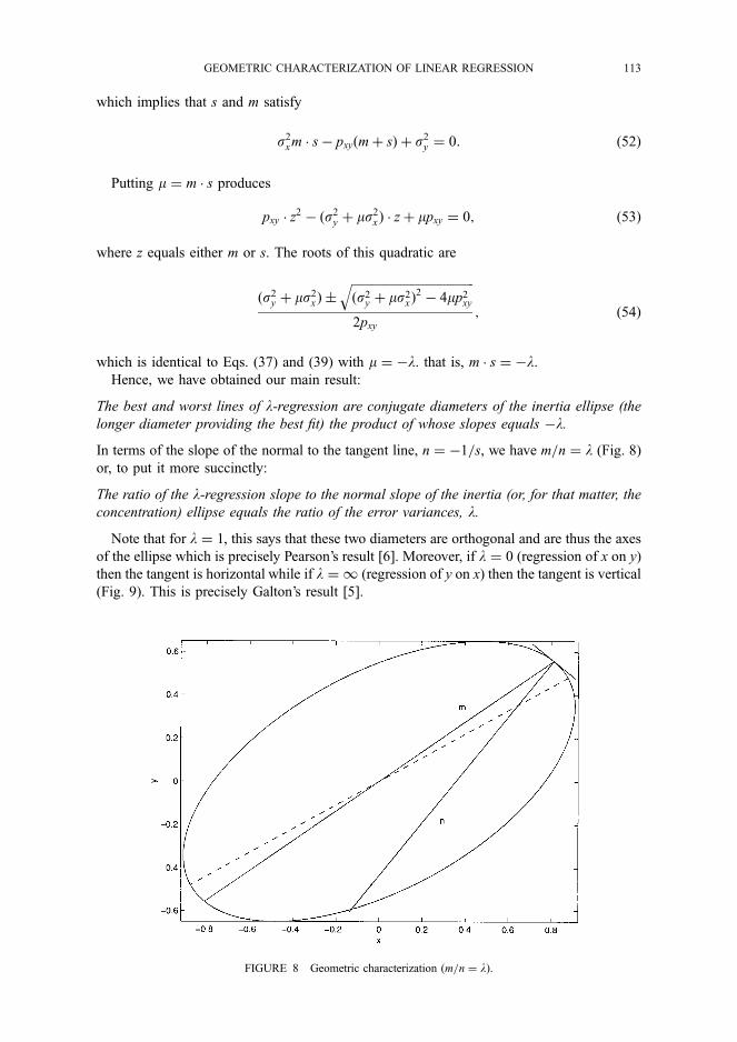
which implies that s and m satisfy
s2xm � s� pxyðmþ sÞ þ s2
y ¼ 0: ð52Þ
Putting m ¼ m � s produces
pxy � z2 � ðs2
y þ ms2xÞ � zþ mpxy ¼ 0; ð53Þ
where z equals either m or s. The roots of this quadratic are
ðs2y þ ms2
xÞ �
ffiffiffiffiffiffiffiffiffiffiffiffiffiffiffiffiffiffiffiffiffiffiffiffiffiffiffiffiffiffiffiffiffiffiffiffiffiffiffiffiðs2
y þ ms2xÞ
2� 4mp2
xy
q2pxy
; ð54Þ
which is identical to Eqs. (37) and (39) with m ¼ �l. that is, m � s ¼ �l.
Hence, we have obtained our main result:
The best and worst lines of l-regression are conjugate diameters of the inertia ellipse (the
longer diameter providing the best fit) the product of whose slopes equals �l.
In terms of the slope of the normal to the tangent line, n ¼ �1=s, we have m=n ¼ l (Fig. 8)
or, to put it more succinctly:
The ratio of the l-regression slope to the normal slope of the inertia (or, for that matter, the
concentration) ellipse equals the ratio of the error variances, l.
Note that for l ¼ 1, this says that these two diameters are orthogonal and are thus the axes
of the ellipse which is precisely Pearson’s result [6]. Moreover, if l ¼ 0 (regression of x on y)
then the tangent is horizontal while if l ¼ 1 (regression of y on x) then the tangent is vertical
(Fig. 9). This is precisely Galton’s result [5].
FIGURE 8 Geometric characterization ðm=n ¼ lÞ.
GEOMETRIC CHARACTERIZATION OF LINEAR REGRESSION 113
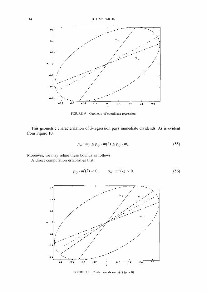
This geometric characterization of l-regression pays immediate dividends. As is evident
from Figure 10,
pxy � my � pxy � mðlÞ � pxy � mx: ð55Þ
Moreover, we may refine these bounds as follows.
A direct computation establishes that
pxy � m0ðlÞ < 0; pxy � m
00ðlÞ > 0: ð56Þ
FIGURE 9 Geometry of coordinate regression.
FIGURE 10 Crude bounds on mðlÞ ðp > 0Þ.
114 B. J. MCCARTIN
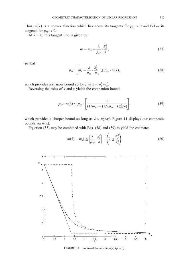
Thus, mðlÞ is a convex function which lies above its tangents for pxy > 0 and below its
tangents for pxy < 0.
At l ¼ 0, this tangent line is given by
m ¼ mx �lpxy
�S2x
n; ð57Þ
so that
pxy � mx �lpxy
�S2x
n
� �� pxy � mðlÞ; ð58Þ
which provides a sharper bound so long as l < s2y=s
2x .
Reversing the roles of x and y yields the companion bound
pxy � mðlÞ � pxy �1
ð1=myÞ � ð1=lpxyÞ � ðS2y =nÞ
" #; ð59Þ
which provides a sharper bound so long as l > s2y=s
2x . Figure 11 displays our composite
bounds on mðlÞ.Equation (55) may be combined with Eqs. (58) and (59) to yield the estimates
jmðlÞ � mxj �lpxy
�S2x
n
�������� l �
s2y
s2x
!; ð60Þ
FIGURE 11 Improved bounds on mðlÞ ðp > 0Þ.
GEOMETRIC CHARACTERIZATION OF LINEAR REGRESSION 115
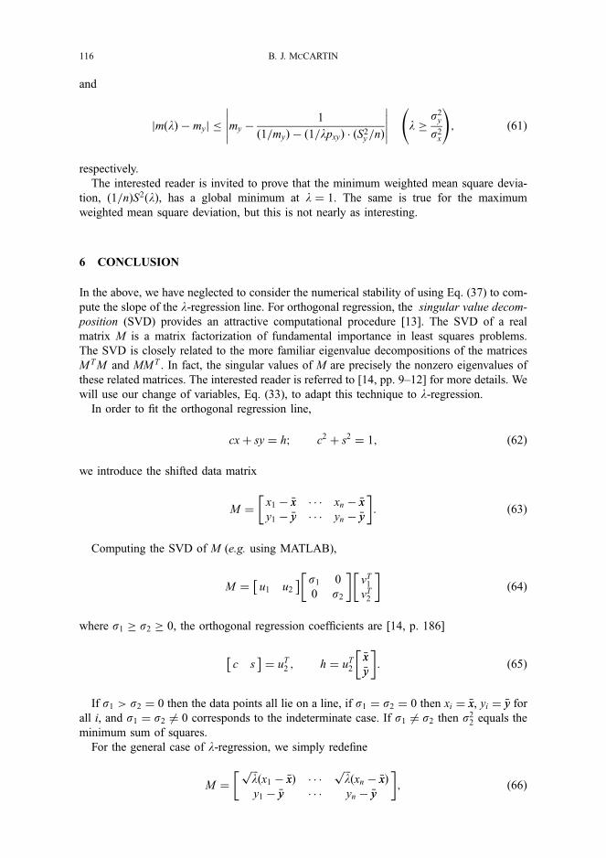
and
jmðlÞ � myj � my �1
ð1=myÞ � ð1=lpxyÞ � ðS2y =nÞ
���������� l �
s2y
s2x
!; ð61Þ
respectively.
The interested reader is invited to prove that the minimum weighted mean square devia-
tion, ð1=nÞS2ðlÞ, has a global minimum at l ¼ 1. The same is true for the maximum
weighted mean square deviation, but this is not nearly as interesting.
6 CONCLUSION
In the above, we have neglected to consider the numerical stability of using Eq. (37) to com-
pute the slope of the l-regression line. For orthogonal regression, the singular value decom-
position (SVD) provides an attractive computational procedure [13]. The SVD of a real
matrix M is a matrix factorization of fundamental importance in least squares problems.
The SVD is closely related to the more familiar eigenvalue decompositions of the matrices
MTM and MMT . In fact, the singular values of M are precisely the nonzero eigenvalues of
these related matrices. The interested reader is referred to [14, pp. 9–12] for more details. We
will use our change of variables, Eq. (33), to adapt this technique to l-regression.
In order to fit the orthogonal regression line,
cxþ sy ¼ h; c2 þ s2 ¼ 1; ð62Þ
we introduce the shifted data matrix
M ¼x1 � �xx � � � xn � �xxy1 � �yy � � � yn � �yy
� �: ð63Þ
Computing the SVD of M (e.g. using MATLAB),
M ¼ u1 u2
� � s1 0
0 s2
� �vT1vT2
� �ð64Þ
where s1 � s2 � 0, the orthogonal regression coefficients are [14, p. 186]
c s� �
¼ uT2 ; h ¼ uT2�xx�yy
� �: ð65Þ
If s1 > s2 ¼ 0 then the data points all lie on a line, if s1 ¼ s2 ¼ 0 then xi ¼ �xx, yi ¼ �yy for
all i, and s1 ¼ s2 6¼ 0 corresponds to the indeterminate case. If s1 6¼ s2 then s22 equals the
minimum sum of squares.
For the general case of l-regression, we simply redefine
M ¼
ffiffiffil
pðx1 � �xxÞ � � �
ffiffiffil
pðxn � �xxÞ
y1 � �yy � � � yn � �yy
� �; ð66Þ
116 B. J. MCCARTIN
perform the SVD, and set mðlÞ ¼ �ffiffiffil
p� c=s. If l is either very small or very large, it might
be prudent to utilize our estimates of mðlÞ, Eqs. (60) and (61), to justify a transition to the
appropriate coordinate regression formula.
Acknowledgement
The author thanks Mrs. Barbara MCCartin for her assistance in the production of this paper.
This research was supported by MCLaren Regional Medical Center and a grant from The
MCLaren Foundation, Flint, Michigan.
References
[1] Stigler, S. M. (1986). The History of Statistics. The Belknap Press of Harvard University Press, Cambridge, MA.[2] Adcock, R. J. (1878). A problem in least squares. Analyst, 5, 53–54.[3] Kummell, C. H. (1879). Reduction of observation equations which contain more than one observed quantity.
Analyst, 6, 97–105.[4] Madansky, A. (1959). The fitting of straight lines when both variables are subject to error. J. Amer. Stat. Assn., 54,
173–205.[5] Galton, F. (1886). Family likeness in stature (with Appendix by Dickson, J. D. H.). Proc. Roy. Soc. London, 40,
42–73.[6] Pearson, K. (1901). On lines and planes of closest fit to systems of points in space. Phil. Mag., 2, 559–572.[7] Farebrother, R. W. (1999). Fitting Linear Relationships: A History of the Calculus of Observations 1750–1900.
Springer-Verlag, New York, NY.[8] Deming, W. E. (1964). Statistical Adjustment of Data. Dover, New York, NY.[9] Cramer, H. (1946). Mathematical Methods of Statistics. Princeton University Press, Princeton, NJ.
[10] Salmon, G. (1954). A Treatise on Conic Sections, 6th ed. Chelsea, New York, NY.[11] Li, H. C. (1984). A generalized problem of least squares. Amer. Math. Monthly, 91, 135–137.[12] Shuchat, A. (1985). Generalized least squares and eigenvalues. Amer. Math. Monthly, 92, 656–659.[13] Nievergelt, Y. (1994). Total least squares: state-of-the-art regression in numerical analysis. SIAM Rev., 36, 258–
264.[14] Bjorck, _AA. (1996). Numerical Methods for Least Squares. SIAM, Philadelphia, PA.
GEOMETRIC CHARACTERIZATION OF LINEAR REGRESSION 117


Copyright of Statistics is the property of Taylor & Francis Ltd and its content may not be copied or emailed to
multiple sites or posted to a listserv without the copyright holder's express written permission. However, users
may print, download, or email articles for individual use.
Vol. 39, No. 1. February 2005. I-II
The geometry of linear regression with correlated errors
BRIAN J.McCARTlN*
Applied Mathematics, Ketlering University, 1700 West TTiird Avenue, Flinl, Mi 48504-4898, USA
(Received 25 February 2004: in final form 22 September 2004)
In McCartin (2003), lhe geometric characterization of linear regression in lerms of lhe 'conceniralionellipse' by Cillon (1886) and Pearson (1901) was extended to lhe case of unequal variances of lhepresumably uncorrclated errors in the cxperimenial data. In Ihis article. Ihis geometric i;haracieri?;itionis further extended to include experimental data with correlated errors.
Keywords: Orthogonal regression; Generalized least squares; Total least squares
1. Introduction
In 1886. Francis Galton 11] provided a geometric interpretation of coordinate regression lines(where mean-square distance parallel to a coordinate axis was minimised) in terms of lheconcentration ellipse which has the same first and second moments about the centroid asthe experimental data. Such coordinate regression presumes ihai only one of the variablesis subject to error. In 1901. Karl Pearson [21 extended this geometric picture to orthogonalregression where deviations are measured perpendicular to tbe regression line. This seminalwork assumed that both variables are subjected to uncorrelated errors ol" equal variances.In 2{K)3, this geometric characterization was further extended lo allow unequal variances inthese presumably uncorrelaied measurement errors 13]. The present work provides the ultimateextension of this geometric interpret at ion to correlated errors where a surprising differencefrom the case of uncorrelated errors arises. An abbreviated historical summary of this problemwas presented in ref. [31. but the reader is directed to ref. 14] for a more comprehensivetreatment.
2. (X., /^)-Rcgression: the problem
Considertheexperimentalfyobserveddata{(A/, >v)}"^,, where.v/ = X, +i(,and.Vi = K, + Vj.Here (X,, Y,) denotes theoretically exact values with corresponding random errors (H,, Vi).
'Email: [email protected]
StatisticsISSN 0233-1888 print/ISSN 1029-4910 online © 2005 Taylor & Francis Ltd
http://www.tandf.co.uk/joumalsDOI: 10.1080/02331880412331328260
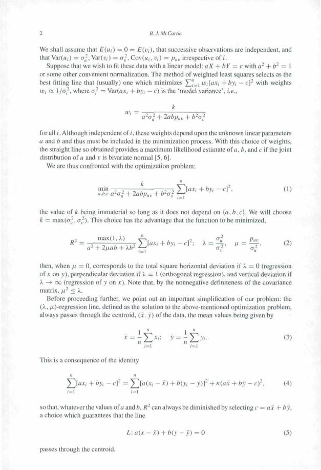
2 B. J. McCtirtin
We shall as.sume that £(»,) = 0 = Eivj). that successive observations are independent, andthat Var{Ji;) = a, . Var(i',) — a^, Cov(u,, f,) = /;„„ irrespective of/.
Suppose that we wish to fit these data with a linear model: aX + bY — c wiihu'^ + b~ = ]or some other convenient normalization. The method of weighted least squares selects as thebest fitting lino that (u.suaily) one which minimizes J2]L] u'iUiXi + hyt - c\~ with weightsUJ; OC \/a^, where a," = Var(flA-, + by-j - c) is the 'model variance', i.e..
aj + 2ahp^,, + b-a^Wi =
for all {. Although independent of /. these weights depend upon the unknown linear parametersa and b and thus must be included in the minimization process. With this choice of weights,the straight line so obtained provides a maximum likelihood estimate of «./?, and c if the jointdistribution ol' ii and v is bivariate normal [5. 6J.
We are thus confronted with Ihe optimization problem:
+ .v, - cf, (1).c a-a- + labput, + b-a; ^
the value of k being immaterial so long as it does not depend on {a, b. c). We will choo.sek = maxluj, CT,-). This choice has the advantage that the function to be minimized.
then, when fi — 0, corresponds to the total square horizontal deviation if X = 0 (regressionof J: on >•), perpendicular deviation if X = 1 (orthogonal regression), and vertical deviation ifX -»• OC (regression of v on .v). Note that, by the nonncgative dcfinitcness of the eovariancematrix, fi- < k.
Before proceeding further, we point out an important simplilication of our problem: the(A.. /^)-regression line, defined as the solution to the above-mentioned optimization problem,always passes through the centroid. (x, y) ol the data, the mean values being given by
1 " 1 "y J^
i=\ •\=\
This is a consequence ofthe identity
so ihat, whatever the values o{a and /?, f^ can always be diminished by selecting c = ax -\- by,a choice which guarantees that the line
L:a(x - X) + b(y - y) = 0 (5)
passes through the cenu-oid.
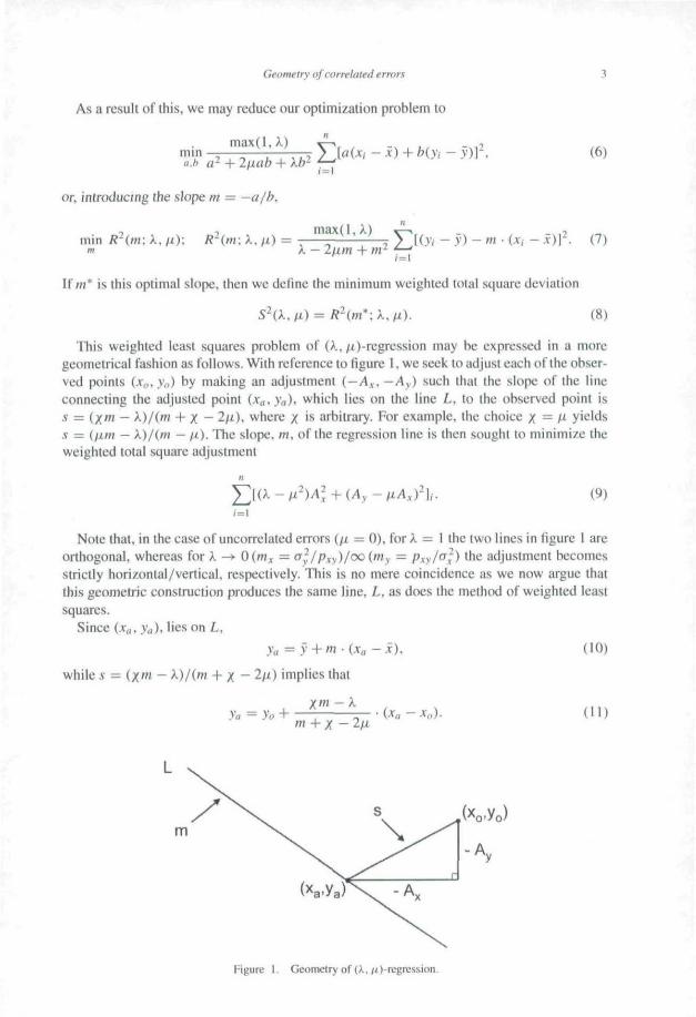
Geometry of correlated errors
As a result of this, we may reduce our optimization problem to
max(l. X) —\min ^ 'a.h a- + 2fiab +
or, introducmg the slope m — —a/b.
min R^(m: X, u): R^(nr. X. it) =
(6)
max(l, X)X - 2[im + I
If m* is this optimal slope, then we define the minimum weighted total square deviation
(7)
(8)
This weighted least squares problem of (X. ^f)-regression may be expressed in a moregeometrical fashion as follows. With reference to figure I. we seek to adjust each of the obser-ved points (x,,, y,,) by making an adjustment (—A,. -A^) such that the slope of the lineconnecting the adjusted point (x,,. »,)• vt/hich lies on the line L. to the observed point iss = (/Hi - X)/itu + X - 2/i). where x ' arbitrary. For example, the choice X — M yieldss = (fim — X)/{m — fi). The slope, m. ofthe regression line is tben sought to minimize theweighted total square adjustment
(9)
Note that, in the case of uncorrelated errors (/i = 0), for X — I the two lines in figure I areorthogonal, whereas for X -*• 0(m, — o'^.jp^y)joo{my = p.,y/n^) the adjustment becomesstrictly horizontal/vertical, respectively. This is no mere coincidence as we now argue thatthis geometric construction produces the same line, L, as does the method of weighted leastsquares.
Since (Xa, ya), lies on L,
y-a = y + m - i x a - X ) . (10)
while s = (/m - X)/{m -f- x - 2ju) implies that
>•<> +X ~
{x,, - (11)
Figure 1. Geometry of (A../i)-regressi()n.
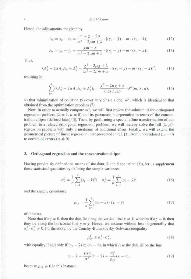
fi. / McCartin
Hence, the adjustments are given by
A,x = Xa - A-« = — — — • \(y^ - y) - m • {Xo - x)], (12)m^ 2im + X
!{>•« - j ) - m • (x,, - x)]. (13)Ay ya yo = ^ni' - 2fim + X
Thus,
] J \'l^^^] y,. - y) - m • {x,, - .x)f, (14))f^ m^ — 2/xni + k
resulting in
— • R^{ni\ k, ft), (15)( = 1
so that minimization of equation (9) over m yields a slope, m*, which is identical to thatobtained from the optimization problem (7).
Now. in order to actually compute m*. we will first review (he solution ofthe orthogonalregression problem (X — 1. /z — ()) and its geometric interpretation in terms of tbe concen-tration ellipse (defined later) 13]. Then, by performing a special affine transformation of ourproblem to a related orthogonal regression problem, we will thereby solve the full fX./O-rcgression problem with only a modicum of additional effort. Finally, we will extend thegeometrical picture of linear regression, first presented in ref. [3], from uncorrelated {fi = 0)to correlated errors (fi -^ 0).
3. Orthogonal regression and the concentration ellipse
Having previously defined the means of the data, x and y (equation (3)), lei us supplementthese statistical quantities by defining the sample variances
1 t IT—V _ 2 •) ' V—^, - . 7 , , *-,
o,T — - > {Xi — x) \ a~ = — } (y: — yr (16)n ^ ^ n ^ ' ^
\-\ 1=1
and the sample covarianee
1 APxy = ~ / Ul — x) • (yi — y) (17)
of the data.Note that if rr,-' = (). then the data lie along the vertical line.v = x. whereas if n ; = 0. then
ihey lie along the horizontal line y — y. Hence, we assume without loss of generality thatCT,- • CT^- 7 0. Furthennore, by the Cauchy-Buniakovsky-Schwarz inequality
p;, ^oj -(Jy- (18)
with equality if and only if (y — yO a (A, — x), in which case the data lie on the line
2
V - y — — j-ix - x) — —^{x - x). (19)
because j3.,v 7 0 in this instance.
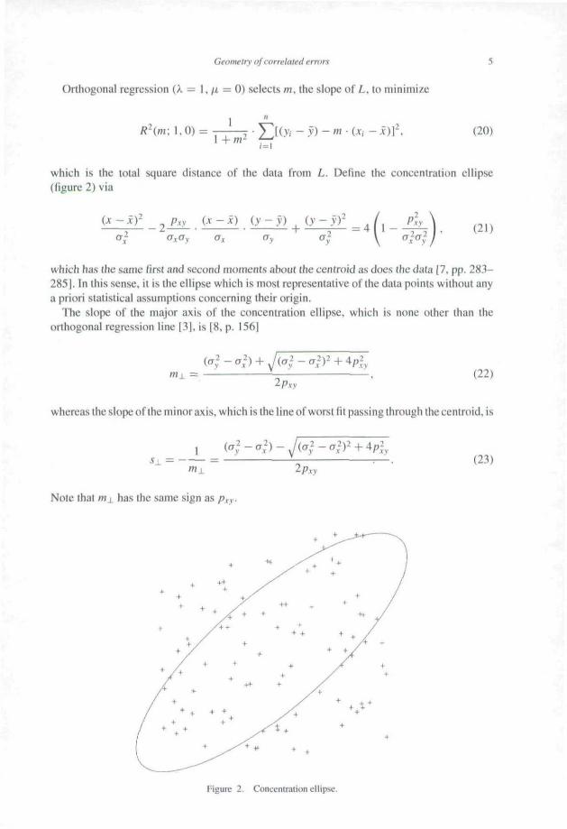
Geometry of correlated errors
Orthogonal regression (X — \, fi =0) selects m. the slope of Z.. to minimize
I +m~(y,- - y) - m • (.v, - .v)]^ (20)
which is the total square distance of tbe data from L. Define tbe concentration ellipse(figure 2) via
-X) (yy)^^—e -4 1- (21)
which has the same first and second moments about the centroid as does the data 17. pp. 283-285]. In tbis sense, it is the ellipse which is most representative ofthe data points without anya priori statistical assumptions concerning their origin.
The slope of the major axis of the concentration ellipse, which is none other than theorthogonal regression line 131, is [8. p. 1561
H l l = (22)
whereas the slope ofthe minor axis, which is the line of worst fit passing through the centroid. is
(23)
Note that mi has tbe same sign as p^y.
Figure 2. Concentration ellipse.
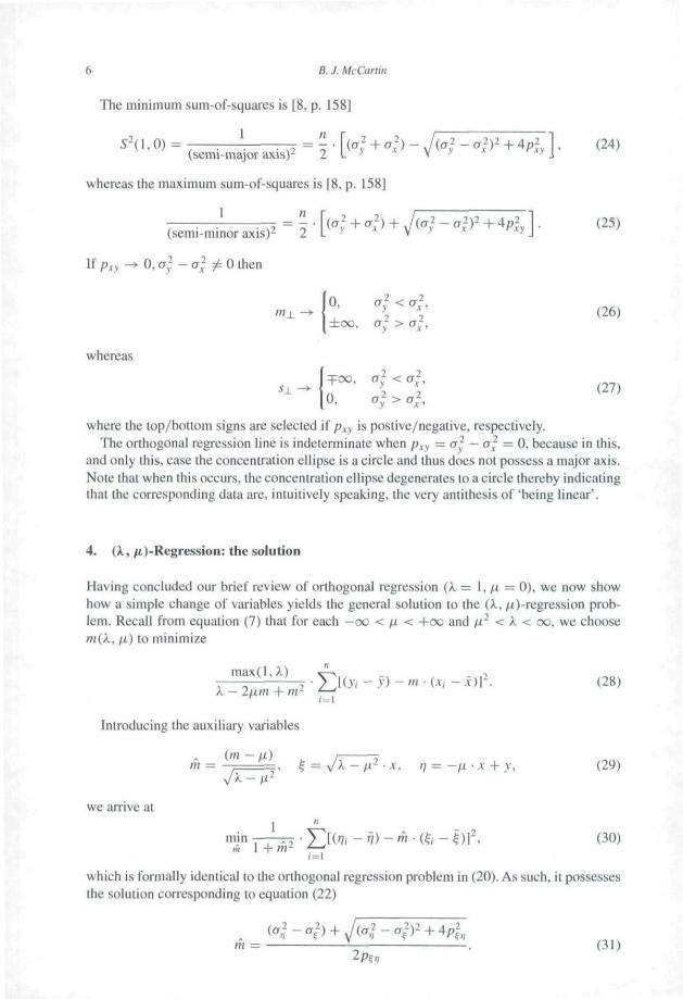
6 B. J. McCarlin
The minimum sum-of-squares is [8, p. 158]
(24)
(25)
(semi-major axis)^ 2
whereas the maximum sum-of-squares is |8. p. 158]
I _ n(semi-minor axis)^ 2
If P.V., -> 0. a^ - a^ i= 0 then
(26)i±;oo. CT; > (T;,
whereas
where the top/bottom signs are selected if /j,v is postive/negative. respectively.The orthogonal regression line is indeterminate when /;,», = o^. — a~ = 0. because in tbis.
and only this, case tbe concentration ellipse is a circle and thus does not possess a major axis.Note thai when this occurs, the concentration ellipse degenerates to a circle thereby indicatingthai the corresponding data are, intuitively speaking, the very antithesis of "being linear'.
4. (X, /i.)-Regres$ion: the solution
Having concluded our brief review of orthogonal regression (X = \, n = 0), we now showhow a simple change of variables yields the general solution to tbe (X,/i)-regression prob-lem. Recall from equation (7) that for each —oo < H < +oc and fi^ < k < oo, we chooseni(X, ll) lo minimize
max(l. X) ^ _ _ ..,Z l(>' - y ) - ' " • ( » , --v)I-. (28)X — 2fim -{- m-
Introducing the auxiliary variables
th = ^ ^ = v/X - / i - • X. n = -ft • A- + y . (29)
we arrive at
• 1 ^ - . - 2
mm ^7 • 2_[in< - ^}) ~ '" • (?/ — ? ) r . (30)
which is formally identical to the orthogonal regression problem in (20). As such, it possessesthe solution corresponding to equation (22)
2 Pi,,
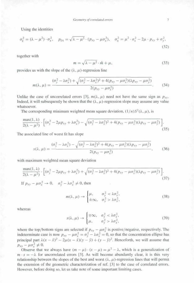
Geometry of correlated errors 7
Using the identities
aj = {X- n^) • a;, p^,, = y/X-(i- • (p.vv - M^^^). ^,f ^ M^ • (^x - 2M • Pn + ^v •
(32)
together with
m — J k ^ ix~ • m + f i . (33)
provides us with (he slope of lhe (X. /i)-regression line
(CT - ka';) + J(af- ka^)^5 ^ J - - . (34)
j)Unlike the case of uncorrelaied errors |3!. m(X.M) need not have the same sign as P(vIndeed, it will subsequently be shown ihat the (X, /i}-regression slope may assume any valuewhatsoever.
The corresponding minimum weighted mean square deviation, {\/n)S-{k, fi). is
max(l. X)2(X - fi^)
(35)The associated line of worst fit has slope
(a'; - Xa'-) -s(X. fi) = "^-^ ^ - . (36)
2( )
with maximum weighted mean square deviation
max( I, X)\ia^ - 2fip,y + Xa^) + J(a}. - Xa^)2 + 4(p,,, - /tCT ^XXp,., " /^^') ]•
(37)If Pxy — fi^l -> 0, a~ — XCT 7 0, then
±00, a^ > kaj,
whereasI nrrv-i n^ <- \n^
(39)
where the top/bottom signs are selected if Pxy — fio^ is postive/negative. respectively. Theindeterminate case is now /?vv - 1^^} — ^l — ^(^j — ^' ^" ^^^^ ^^^ concentration ellipse hasprincipal part X(^ - x)~ - 2fi(x — i ) (y — y) 4- (y — y)^- Henceforth, we will assume that
Pxy - t^^; i= (1-Observe that we always have {m - ft) • (s - [x) = fv- — X, which is a generalization of
m • s = —X for uneorrelated errors 13]. As will become abundantly clear, it is this veryrelationship between the slopes ofthe best and worst (X. /0-regression lines that will permitthe extension of the geometric characterization of ref. 131 to the case of correlated errors.However, before doing so, let us take note of some important limiting cases.
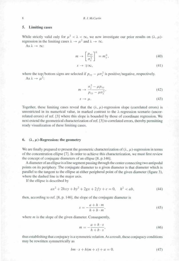
« B. J. McCartin
S. Limiting cases
While strictly valid only for /i^ < X < oo. we now investigate our prior results on (X. fi)-regression in the limiting cases k -^ fi^ and X —>• oo.
As X —*• oo;
- m ^ , (40)
5 -»• TOO, ( 4 1 )
where the top/botlom signs are selected H pxy — f-crl is positive/negative, respectively.As X -»• fr:
m ->• -^ V. (42)Pxy - P-o}
s -^ fi. (43)
Togetber, these limiting cases reveal that lhe (X, ^)-regression slope (correlated errors) isunrestricted in its numerical value, in marked contrast to the X-regression scenario (uncor-related errors) of ref. |31 where this slope is bounded by those of coordinate regression. Wenext extend the geometrical characterization of ref. 13J to correlated errors, thereby permiaingready visualization of these limiting cases.
6. (X. /t)-Regre$sion: the geometry
We are finally prepared to present the geometric characterization of (X. /i)-regression in termsof tbe concentration ellipse 17J. In order to achieve this characterization, we must lirst reviewthe concept of conjugate diameters of an ellipse [8. p.l4A|.
A diameter of an ellipse is a line segment passing through the center connecting two antipodalpoints on its periphery. The conjugate diameter to a given diameter is that diameter which isparallel to the tangent to the ellipse at either peripheral p<jint of the given diameter (figure 3),where the dashed line is the major axis.
If tbe ellipse is described by
ax^ + 2hxy + by~ -h 2^A + 2/y + c = 0. / r < ab, (44)
then, according to ref. [8. p. 146]. tlie slope ofthe conjugate diameter is
a + h • m
h + b • tn
where m is the slope ofthe given diameter. Consequently,
a -\- h • sm^——~—,
h -\-b • s
(45)
(46)
thus establishing that conjugacy is a symmetric relation. As a result, these conjugacy conditionsmay be rewritten symmetrically as
bm-s + h(m + J ) + a = 0. (47)
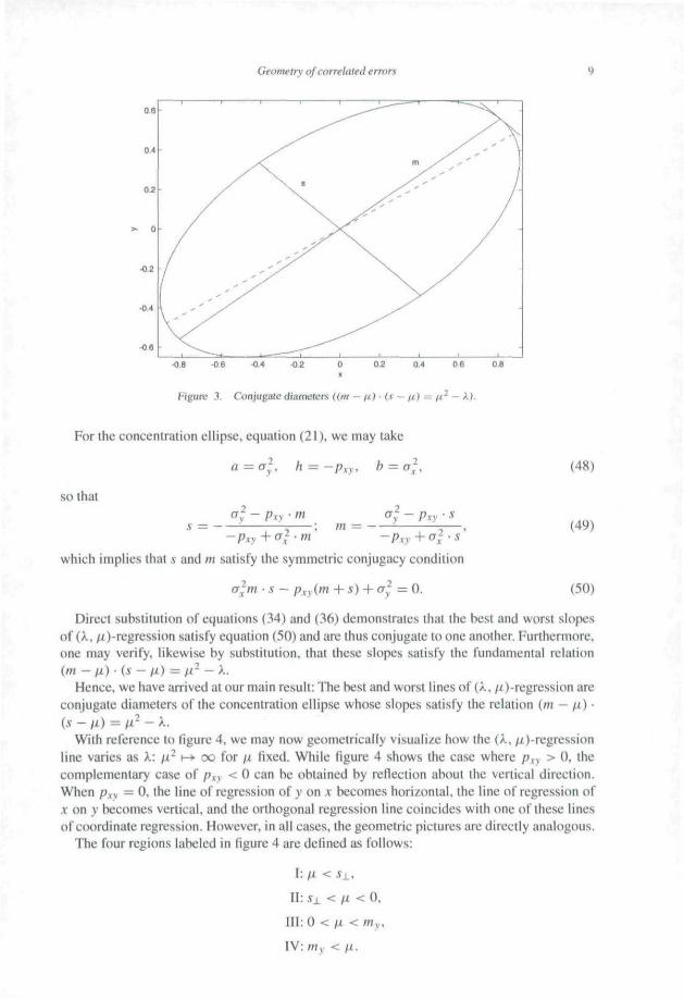
Geometry of correlated errors
•0.2
•0.8 •
-0.8 -0.6 -0.4 -0,2 0.6 0.8
Figure 3. Conjugate diameters dm •- n) • {x — /i) — n} — k).
For tbe concentration ellipse, equation (21), we may take
so that
a; -s = — m = — •
- P . xwhich implies that 5 and m satisfy the symmetric conjugacy eondition
+ s)-\-a^ — 0.s —
(48)
(49)
(50)
Direct substitution of equations (34) and (36) demonstrates that the best and worst slopesof (k, /i)-regression satisfy equation (50) and are thus conjugate to one another. Furthermore,one may verify, likewise by substitution, that these slopes satisfy the fundamental relation(m - fx) • (.y - fi) = fi' - X.
Hence, we bave arrived at our main result: The best and worst lines of (X, /i)-regression areconjugate diameters of the concentration ellipse whose slopes satisfy the relation (rti — f.i) •iS~fi)^fi^-k.
With reference to figure 4, we may now geometrically visualize how the (X. /^)-regres.sionline varies as k: p.- \-^ oo for fx fixed. While figure 4 shows the case wbere p^y > 0, thecomplementary case of pxy < 0 can be obtained by reflection about the vertical direction.When Pxy = 0, the line of regression of y on x becomes horizontal, the line of regression ofJC on y becomes vertical, and the orthogonal regression line coincides with one of these linesof coordinate regression. However, in all cases, tbe geometric pictures are directly analogous.
The four regions labeled in figure 4 are defined as follows:
l:fx< sx,
II: s± < n < 0,
III: 0 < IX < tfiy.
IV: niy < fX.
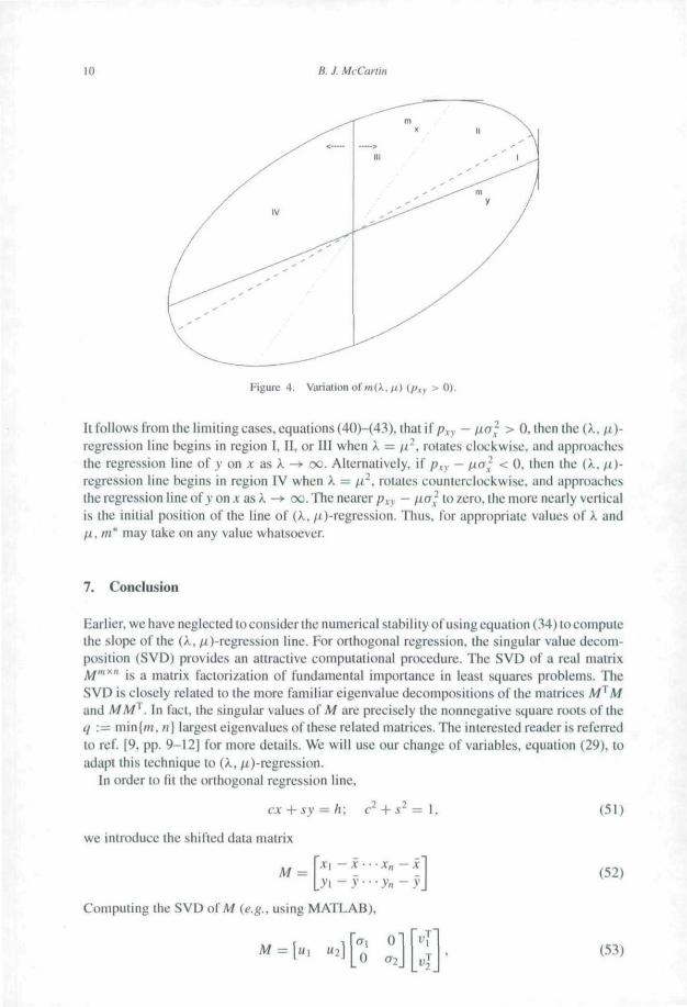
10 fi. / McCarlin
Figure 4. Variation of m(A, > 0).
It follows from the limiting cases, equations (40)-(43). that if Pvv ~ l^^^ > 0, then the (X. fx)-regrcssion line begins in region I, II, or III when X = n~, rotates clockwise, and approachesthe regression line of y on x as X -»• oc. Alternatively, if p ^ — fxcr} < 0, then the (X. fi)-regression line begins in region IV when X = fx~y rotates counterclockwise, and approachesthe regression lineofy onA asX -> oo. The nearer/J,V - fxa~ to zero, the more nearly verticalis the initial position of the line of (X, /i)-regression. Thus, for appropriate values of X andfi, m* may take on any value whatsoever.
7. Conclusion
Eariier. we have neglected to consider the numerical stability of using equation (34) to computethe slope ofthe (X, ju)-regression line. For orthogonal regression, the singular value decom-position (SVD) provides an attractive computational procedure. The SVD of a real matrixM"""' is a matrix factorization of fundamental importance in least squares problems. TheSVD is closely related to the more familiar eigenvalue decompositions of tbe matrices M^Mand MM^. In fact, lhe singular values of M are precisely the nonnegative square roots oftheq := min|/?i, n] largest eigenvalues of these related matrices. The interested reader is referredto ref. [9, pp. 9-12] for more details. We will use our change of variables, equation (29), toadapt this technique to (X, ^0-regression.
In order to lit the orthogonal regression line.
we introduce the shifted data matrix
M =r .v ,- .v- . - .«- i ib i - v " - y « - y j
Computing the SVD o{ M {e.g., using MATLAB),
(51)
(52)
(53)
Geometry of correlated errors 11
where crt > CT2 > 0. the orthogonal regression coefficients are [9. p. 186]
[c s]=ul, h=u[VX (54)
If fT| > fTT — 0. tben the data points all lie on a line, if CT] — CTT — 0. then A", = x, y,- = y for
all (. and a\ =02^ 0 corresponds to the indeterminate case. If CTJ ai, then CT^ equals the
minimum sum of squares.
For the general case of X-regression, we simply redefine
i ) ••• JT.-{x,,-x) 1x\ -x) ••• (y« - y) - (i • {x,, - .Y)J '
perform the SVD, and set m(X, fx) = ~-Jk ~ ft^ • cj^ + ft.
(yi - y) - / ix x) (y y) (i {x Y)J '
A cknowled gemen t
The author thanks Mrs. Barbara McCartin for her assistance in tbe production of tbis article.
References
[ 11 Gallon, R, 1886, Proceedings ofthe Royal Society of London. 40, 42-73-(21 Pearaon, K., \m\. Phihwpliiait Moficizine. 2. 559-572.[3i McCartin. B.J.. 2003. .Vw/w;iV-v. 37, 101-117.[41 Faa-brolhcr, R.W,. 1999. Fitting Linear Relationships: A History ofthe Calculus of Observations 1750-1900
(New York: Springer-Verlug).[5) Acltm, F.S., \9b6,Antily.\isofSlniif;ht-l.ineOata<f<ev/Yovk: Dover).[6] Spreni. H, 1969, Models in Rcf^re.s.'iion (London: Melhiien).[7] CramiJr, H., 1946. Mathematical Methods of Statistics (Frincelon: Princeton University Press).[8] Salmon, C . 19.'i4, ^ Treatise on Conic Sections, sixlh edition (New York: Chelsea).[9] BjOrck. A., 1996, Numerical Methods for Least Squares (Philadelphia: SIAM).

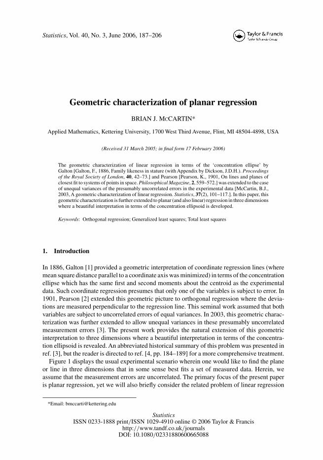
Statistics, Vol. 40, No. 3, June 2006, 187–206
Geometric characterization of planar regression
BRIAN J. MCCARTIN*
Applied Mathematics, Kettering University, 1700 West Third Avenue, Flint, MI 48504-4898, USA
(Received 31 March 2005; in final form 17 February 2006)
The geometric characterization of linear regression in terms of the ‘concentration ellipse’ byGalton [Galton, F., 1886, Family likeness in stature (with Appendix by Dickson, J.D.H.). Proceedingsof the Royal Society of London, 40, 42–73.] and Pearson [Pearson, K., 1901, On lines and planes ofclosest fit to systems of points in space. Philosophical Magazine, 2, 559–572.] was extended to the caseof unequal variances of the presumably uncorrelated errors in the experimental data [McCartin, B.J.,2003, A geometric characterization of linear regression. Statistics, 37(2), 101–117.]. In this paper, thisgeometric characterization is further extended to planar (and also linear) regression in three dimensionswhere a beautiful interpretation in terms of the concentration ellipsoid is developed.
Keywords: Orthogonal regression; Generalized least squares; Total least squares
1. Introduction
In 1886, Galton [1] provided a geometric interpretation of coordinate regression lines (wheremean square distance parallel to a coordinate axis was minimized) in terms of the concentrationellipse which has the same first and second moments about the centroid as the experimentaldata. Such coordinate regression presumes that only one of the variables is subject to error. In1901, Pearson [2] extended this geometric picture to orthogonal regression where the devia-tions are measured perpendicular to the regression line. This seminal work assumed that bothvariables are subject to uncorrelated errors of equal variances. In 2003, this geometric charac-terization was further extended to allow unequal variances in these presumably uncorrelatedmeasurement errors [3]. The present work provides the natural extension of this geometricinterpretation to three dimensions where a beautiful interpretation in terms of the concentra-tion ellipsoid is revealed. An abbreviated historical summary of this problem was presented inref. [3], but the reader is directed to ref. [4, pp. 184–189] for a more comprehensive treatment.
Figure 1 displays the usual experimental scenario wherein one would like to find the planeor line in three dimensions that in some sense best fits a set of measured data. Herein, weassume that the measurement errors are uncorrelated. The primary focus of the present paperis planar regression, yet we will also briefly consider the related problem of linear regression
*Email: [email protected]
StatisticsISSN 0233-1888 print/ISSN 1029-4910 online © 2006 Taylor & Francis
http://www.tandf.co.uk/journalsDOI: 10.1080/02331880600665088
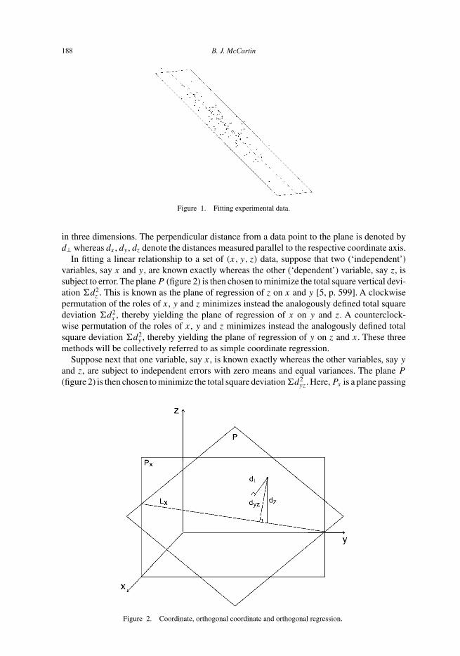
188 B. J. McCartin
Figure 1. Fitting experimental data.
in three dimensions. The perpendicular distance from a data point to the plane is denoted byd⊥ whereas dx , dy , dz denote the distances measured parallel to the respective coordinate axis.
In fitting a linear relationship to a set of (x, y, z) data, suppose that two (‘independent’)variables, say x and y, are known exactly whereas the other (‘dependent’) variable, say z, issubject to error. The plane P (figure 2) is then chosen to minimize the total square vertical devi-ation �d2
z . This is known as the plane of regression of z on x and y [5, p. 599]. A clockwisepermutation of the roles of x, y and z minimizes instead the analogously defined total squaredeviation �d2
x , thereby yielding the plane of regression of x on y and z. A counterclock-wise permutation of the roles of x, y and z minimizes instead the analogously defined totalsquare deviation �d2
y , thereby yielding the plane of regression of y on z and x. These threemethods will be collectively referred to as simple coordinate regression.
Suppose next that one variable, say x, is known exactly whereas the other variables, say y
and z, are subject to independent errors with zero means and equal variances. The plane P
(figure 2) is then chosen to minimize the total square deviation �d2yz. Here, Px is a plane passing
Figure 2. Coordinate, orthogonal coordinate and orthogonal regression.
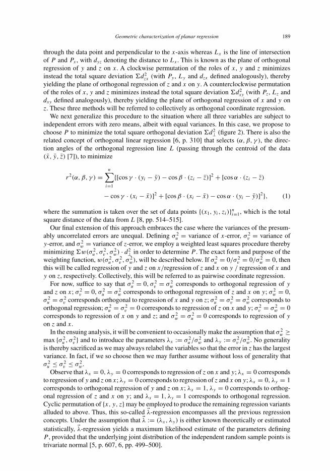
Geometric characterization of planar regression 189
through the data point and perpendicular to the x-axis whereas Lx is the line of intersectionof P and Px , with dyz denoting the distance to Lx . This is known as the plane of orthogonalregression of y and z on x. A clockwise permutation of the roles of x, y and z minimizesinstead the total square deviation �d2
zx (with Py , Ly and dzx defined analogously), therebyyielding the plane of orthogonal regression of z and x on y. A counterclockwise permutationof the roles of x, y and z minimizes instead the total square deviation �d2
xy (with Pz, Lz anddxy defined analogously), thereby yielding the plane of orthogonal regression of x and y onz. These three methods will be referred to collectively as orthogonal coordinate regression.
We next generalize this procedure to the situation where all three variables are subject toindependent errors with zero means, albeit with equal variances. In this case, we propose tochoose P to minimize the total square orthogonal deviation �d2
⊥ (figure 2). There is also therelated concept of orthogonal linear regression [6, p. 310] that selects (α, β, γ ), the direc-tion angles of the orthogonal regression line L (passing through the centroid of the data(x, y, z) [7]), to minimize
r2(α, β, γ ) =n∑
i=1
{[cos γ · (yi − y) − cos β · (zi − z)]2 + [cos α · (zi − z)
− cos γ · (xi − x)]2 + [cos β · (xi − x) − cos α · (yi − y)]2}, (1)
where the summation is taken over the set of data points {(x1, yi, zi)}ni=1, which is the totalsquare distance of the data from L [8, pp. 514–515].
Our final extension of this approach embraces the case where the variances of the presum-ably uncorrelated errors are unequal. Defining σ 2
u = variance of x-error, σ 2v = variance of
y-error, and σ 2w = variance of z-error, we employ a weighted least squares procedure thereby
minimizing �w(σ 2u , σ 2
v , σ 2w) · d2
⊥ in order to determine P . The exact form and purpose of theweighting function, w(σ 2
u , σ 2v , σ 2
w), will be described below. If σ 2u = 0/σ 2
v = 0/σ 2w = 0, then
this will be called regression of y and z on x/regression of z and x on y / regression of x andy on z, respectively. Collectively, this will be referred to as pairwise coordinate regression.
For now, suffice to say that σ 2u = 0, σ 2
v = σ 2w corresponds to orthogonal regression of y
and z on x; σ 2v = 0, σ 2
u = σ 2w corresponds to orthogonal regression of z and x on y; σ 2
w = 0,σ 2
u = σ 2v corresponds orthogonal to regression of x and y on z; σ 2
u = σ 2v = σ 2
w corresponds toorthogonal regression; σ 2
u = σ 2v = 0 corresponds to regression of z on x and y; σ 2
v = σ 2w = 0
corresponds to regression of x on y and z; and σ 2w = σ 2
u = 0 corresponds to regression of y
on z and x.In the ensuing analysis, it will be convenient to occasionally make the assumption that σ 2
w ≥max {σ 2
u , σ 2v } and to introduce the parameters λx := σ 2
u /σ 2w and λy := σ 2
v /σ 2w. No generality
is thereby sacrificed as we may always relabel the variables so that the error in z has the largestvariance. In fact, if we so choose then we may further assume without loss of generality thatσ 2
u ≤ σ 2v ≤ σ 2
w.Observe that λx = 0, λy = 0 corresponds to regression of z on x and y; λx = 0 corresponds
to regression of y and z on x; λy = 0 corresponds to regression of z and x on y; λx = 0, λy = 1corresponds to orthogonal regression of y and z on x; λx = 1, λy = 0 corresponds to orthog-onal regression of z and x on y; and λx = 1, λy = 1 corresponds to orthogonal regression.Cyclic permutation of {x, y, z} may be employed to produce the remaining regression variantsalluded to above. Thus, this so-called �λ-regression encompasses all the previous regressionconcepts. Under the assumption that �λ := (λx, λy) is either known theoretically or estimatedstatistically, �λ-regression yields a maximum likelihood estimate of the parameters definingP , provided that the underlying joint distribution of the independent random sample points istrivariate normal [5, p. 607, 6, pp. 499–500].
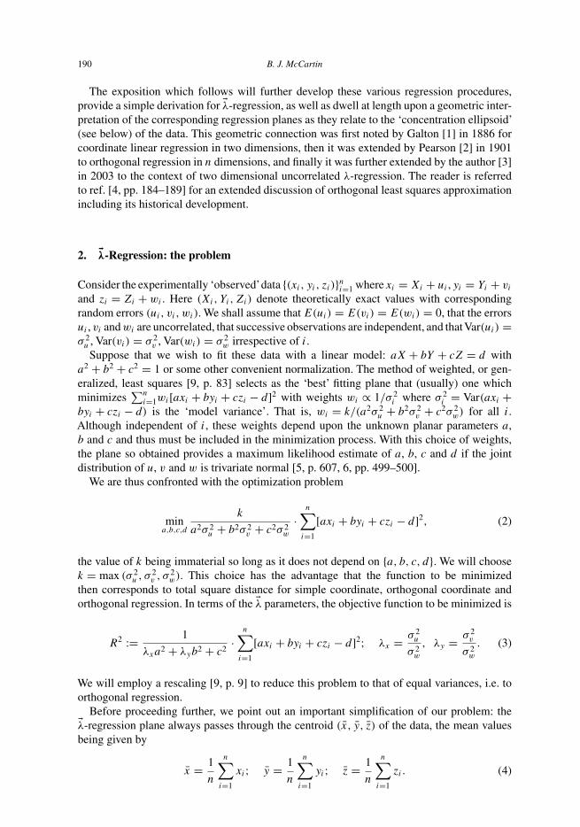
190 B. J. McCartin
The exposition which follows will further develop these various regression procedures,provide a simple derivation for �λ-regression, as well as dwell at length upon a geometric inter-pretation of the corresponding regression planes as they relate to the ‘concentration ellipsoid’(see below) of the data. This geometric connection was first noted by Galton [1] in 1886 forcoordinate linear regression in two dimensions, then it was extended by Pearson [2] in 1901to orthogonal regression in n dimensions, and finally it was further extended by the author [3]in 2003 to the context of two dimensional uncorrelated λ-regression. The reader is referredto ref. [4, pp. 184–189] for an extended discussion of orthogonal least squares approximationincluding its historical development.
2. �λ-Regression: the problem
Consider the experimentally ‘observed’data {(xi, yi, zi)}ni=1 where xi = Xi + ui , yi = Yi + vi
and zi = Zi + wi . Here (Xi, Yi, Zi) denote theoretically exact values with correspondingrandom errors (ui, vi, wi). We shall assume that E(ui) = E(vi) = E(wi) = 0, that the errorsui , vi and wi are uncorrelated, that successive observations are independent, and thatVar(ui) =σ 2
u , Var(vi) = σ 2v , Var(wi) = σ 2
w irrespective of i.Suppose that we wish to fit these data with a linear model: aX + bY + cZ = d with
a2 + b2 + c2 = 1 or some other convenient normalization. The method of weighted, or gen-eralized, least squares [9, p. 83] selects as the ‘best’ fitting plane that (usually) one whichminimizes
∑ni=1wi[axi + byi + czi − d]2 with weights wi ∝ 1/σ 2
i where σ 2i = Var(axi +
byi + czi − d) is the ‘model variance’. That is, wi = k/(a2σ 2u + b2σ 2
v + c2σ 2w) for all i.
Although independent of i, these weights depend upon the unknown planar parameters a,b and c and thus must be included in the minimization process. With this choice of weights,the plane so obtained provides a maximum likelihood estimate of a, b, c and d if the jointdistribution of u, v and w is trivariate normal [5, p. 607, 6, pp. 499–500].
We are thus confronted with the optimization problem
mina,b,c,d
k
a2σ 2u + b2σ 2
v + c2σ 2w
·n∑
i=1
[axi + byi + czi − d]2, (2)
the value of k being immaterial so long as it does not depend on {a, b, c, d}. We will choosek = max (σ 2
u , σ 2v , σ 2
w). This choice has the advantage that the function to be minimizedthen corresponds to total square distance for simple coordinate, orthogonal coordinate andorthogonal regression. In terms of the �λ parameters, the objective function to be minimized is
R2 := 1
λxa2 + λyb2 + c2·
n∑i=1
[axi + byi + czi − d]2; λx = σ 2u
σ 2w
, λy = σ 2v
σ 2w
. (3)
We will employ a rescaling [9, p. 9] to reduce this problem to that of equal variances, i.e. toorthogonal regression.
Before proceeding further, we point out an important simplification of our problem: the�λ-regression plane always passes through the centroid (x, y, z) of the data, the mean valuesbeing given by
x = 1
n
n∑i=1
xi; y = 1
n
n∑i=1
yi; z = 1
n
n∑i=1
zi . (4)
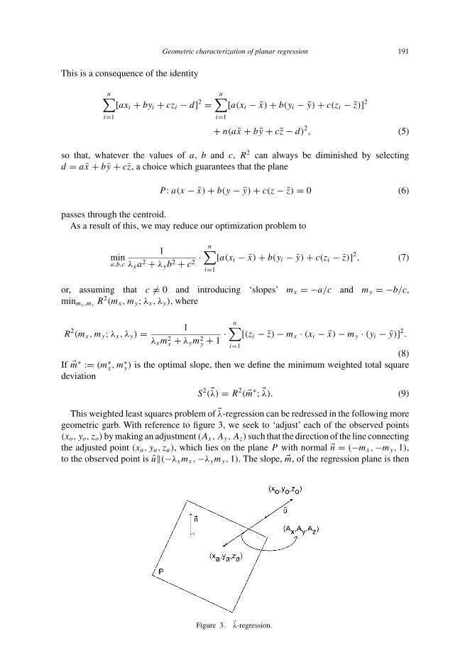
Geometric characterization of planar regression 191
This is a consequence of the identity
n∑i=1
[axi + byi + czi − d]2 =n∑
i=1
[a(xi − x) + b(yi − y) + c(zi − z)]2
+ n(ax + by + cz − d)2, (5)
so that, whatever the values of a, b and c, R2 can always be diminished by selectingd = ax + by + cz, a choice which guarantees that the plane
P : a(x − x) + b(y − y) + c(z − z) = 0 (6)
passes through the centroid.As a result of this, we may reduce our optimization problem to
mina,b,c
1
λxa2 + λyb2 + c2·
n∑i=1
[a(xi − x) + b(yi − y) + c(zi − z)]2, (7)
or, assuming that c �= 0 and introducing ‘slopes’ mx = −a/c and my = −b/c,minmx,my
R2(mx, my; λx, λy), where
R2(mx, my; λx, λy) = 1
λxm2x + λym2
y + 1·
n∑i=1
[(zi − z) − mx · (xi − x) − my · (yi − y)]2.
(8)If �m∗ := (m∗
x, m∗y) is the optimal slope, then we define the minimum weighted total square
deviation
S2(�λ) = R2( �m∗; �λ). (9)
This weighted least squares problem of �λ-regression can be redressed in the following moregeometric garb. With reference to figure 3, we seek to ‘adjust’ each of the observed points(xo, yo, zo) by making an adjustment (Ax, Ay, Az) such that the direction of the line connectingthe adjusted point (xa, ya, za), which lies on the plane P with normal �n = (−mx, −my, 1),to the observed point is u‖(−λxmx, −λymy, 1). The slope, �m, of the regression plane is then
Figure 3. �λ-regression.
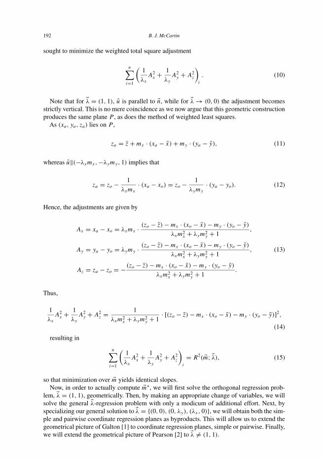
192 B. J. McCartin
sought to minimize the weighted total square adjustment
n∑i=1
(1
λx
A2x + 1
λy
A2y + A2
z
)i
. (10)
Note that for �λ = (1, 1), u is parallel to �n, while for �λ → (0, 0) the adjustment becomesstrictly vertical. This is no mere coincidence as we now argue that this geometric constructionproduces the same plane P , as does the method of weighted least squares.
As (xa, ya, za) lies on P ,
za = z + mx · (xa − x) + my · (ya − y), (11)
whereas u‖(−λxmx, −λymy, 1) implies that
za = zo − 1
λxmx
· (xa − xo) = zo − 1
λymy
· (ya − yo). (12)
Hence, the adjustments are given by
Ax = xa − xo = λxmx · (zo − z) − mx · (xo − x) − my · (yo − y)
λxm2x + λym2
y + 1,
Ay = ya − yo = λymy · (zo − z) − mx · (xo − x) − my · (yo − y)
λxm2x + λym2
y + 1, (13)
Az = za − zo = − (zo − z) − mx · (xo − x) − my · (yo − y)
λxm2x + λym2
y + 1.
Thus,
1
λx
A2x + 1
λy
A2y + A2
z = 1
λxm2x + λym2
y + 1· [(zo − z) − mx · (xo − x) − my · (yo − y)]2,
(14)
resulting in
n∑i=1
(1
λx
A2x + 1
λy
A2y + A2
z
)i
= R2( �m; �λ), (15)
so that minimization over �m yields identical slopes.Now, in order to actually compute �m∗, we will first solve the orthogonal regression prob-
lem, �λ = (1, 1), geometrically. Then, by making an appropriate change of variables, we willsolve the general �λ-regression problem with only a modicum of additional effort. Next, byspecializing our general solution to �λ = {(0, 0), (0, λy), (λx, 0)}, we will obtain both the sim-ple and pairwise coordinate regression planes as byproducts. This will allow us to extend thegeometrical picture of Galton [1] to coordinate regression planes, simple or pairwise. Finally,we will extend the geometrical picture of Pearson [2] to �λ �= (1, 1).
Geometric characterization of planar regression 193
3. Orthogonal regression
Having previously defined the means of the data, x, y and z (equation (4)), let us supplementthese statistical quantities by defining the sample variances
σ 2x = 1
n
n∑i=1
(xi − x)2, σ 2y = 1
n
n∑i=1
(yi − y)2, σ 2z = 1
n
n∑i=1
(zi − z)2, (16)
the sample covariances
pxy = 1
n
n∑i=1
(xi − x) · (yi − y), pyz = 1
n
n∑i=1
(yi − y) · (zi − z),
pzx = 1
n
n∑i=1
(zi − z) · (xi − x), (17)
and (assuming that σx · σy · σz �= 0) the sample correlation coefficients
rxy = pxy
σx · σy
, ryz = pyz
σy · σz
, rzx = pzx
σz · σx
(18)
of the data.Defining the (sample) covariance matrix as
C :=
σ 2x pxy pzx
pxy σ 2y pyz
pzx pyz σ 2z
, (19)
it is readily established that
det (C) = σ 2x σ 2
y σ 2z
∣∣∣∣∣∣∣1 rxy rzx
rxy 1 ryz
rzx ryz 1
∣∣∣∣∣∣∣. (20)
Without risk of confusion, we will henceforth abbreviate C as the covariance matrix.Furthermore, observe that �v := [a b c]T implies that
�vTC�v = E{[a(x − x) + b(y − y) + c(z − z)]2} ≥ 0, (21)
where E is the averaging operator E{u} = (1/n)∑n
i=1 ui , with equality if and only if all thedata lie on the plane
a(x − x) + b(y − y) + c(z − z) = 0. (22)
Thus, planarity of the data corresponds to a zero eigenvalue of the positive semidefinite matrixC and the corresponding eigenvector is normal to this plane. Of course, the data may furtherdegenerate to a line or a point and the reader is referred to [3] for such considerations.
Note that if σ 2x = 0 then the data lie on the plane x = x, if σ 2
y = 0 then they lie on theplane y = y and if σ 2
z = 0 then they lie on the plane z = z. Hence, we assume without lossof generality that σ 2
x · σ 2y · σ 2
z �= 0 so that rxy , ryz and rzx are always well defined.
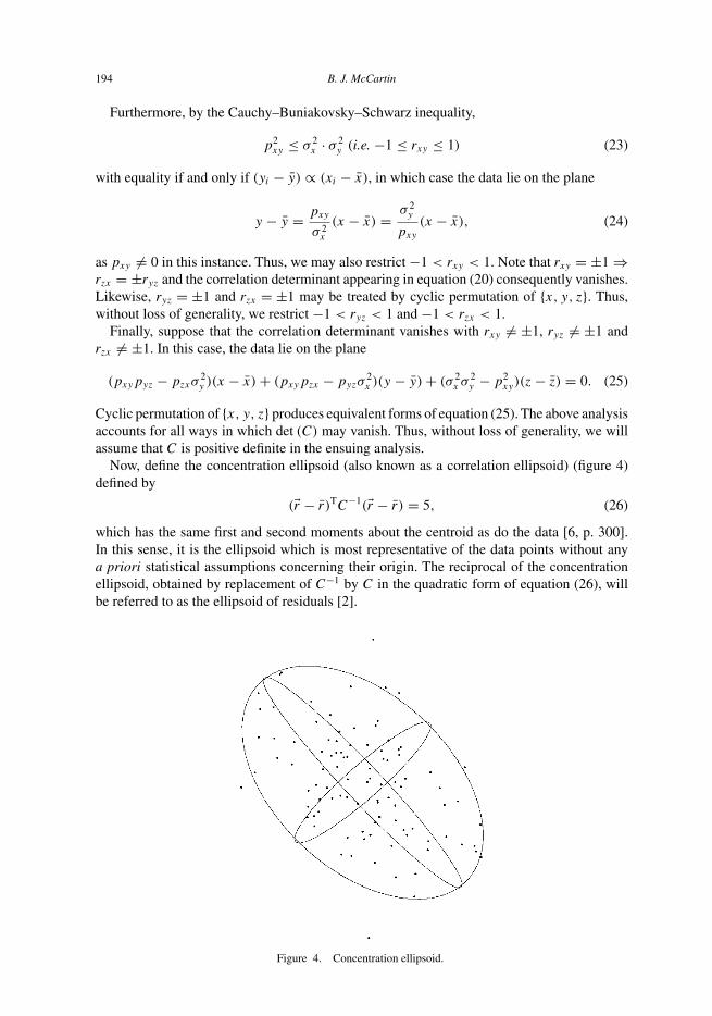
194 B. J. McCartin
Furthermore, by the Cauchy–Buniakovsky–Schwarz inequality,
p2xy ≤ σ 2
x · σ 2y (i.e. −1 ≤ rxy ≤ 1) (23)
with equality if and only if (yi − y) ∝ (xi − x), in which case the data lie on the plane
y − y = pxy
σ 2x
(x − x) = σ 2y
pxy
(x − x), (24)
as pxy �= 0 in this instance. Thus, we may also restrict −1 < rxy < 1. Note that rxy = ±1 ⇒rzx = ±ryz and the correlation determinant appearing in equation (20) consequently vanishes.Likewise, ryz = ±1 and rzx = ±1 may be treated by cyclic permutation of {x, y, z}. Thus,without loss of generality, we restrict −1 < ryz < 1 and −1 < rzx < 1.
Finally, suppose that the correlation determinant vanishes with rxy �= ±1, ryz �= ±1 andrzx �= ±1. In this case, the data lie on the plane
(pxypyz − pzxσ2y )(x − x) + (pxypzx − pyzσ
2x )(y − y) + (σ 2
x σ 2y − p2
xy)(z − z) = 0. (25)
Cyclic permutation of {x, y, z} produces equivalent forms of equation (25). The above analysisaccounts for all ways in which det (C) may vanish. Thus, without loss of generality, we willassume that C is positive definite in the ensuing analysis.
Now, define the concentration ellipsoid (also known as a correlation ellipsoid) (figure 4)defined by
(�r − r)TC−1(�r − r) = 5, (26)
which has the same first and second moments about the centroid as do the data [6, p. 300].In this sense, it is the ellipsoid which is most representative of the data points without anya priori statistical assumptions concerning their origin. The reciprocal of the concentrationellipsoid, obtained by replacement of C−1 by C in the quadratic form of equation (26), willbe referred to as the ellipsoid of residuals [2].
Figure 4. Concentration ellipsoid.
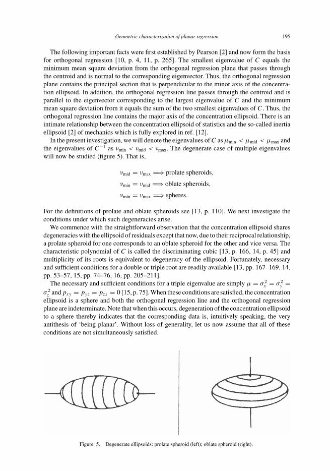
Geometric characterization of planar regression 195
The following important facts were first established by Pearson [2] and now form the basisfor orthogonal regression [10, p. 4, 11, p. 265]. The smallest eigenvalue of C equals theminimum mean square deviation from the orthogonal regression plane that passes throughthe centroid and is normal to the corresponding eigenvector. Thus, the orthogonal regressionplane contains the principal section that is perpendicular to the minor axis of the concentra-tion ellipsoid. In addition, the orthogonal regression line passes through the centroid and isparallel to the eigenvector corresponding to the largest eigenvalue of C and the minimummean square deviation from it equals the sum of the two smallest eigenvalues of C. Thus, theorthogonal regression line contains the major axis of the concentration ellipsoid. There is anintimate relationship between the concentration ellipsoid of statistics and the so-called inertiaellipsoid [2] of mechanics which is fully explored in ref. [12].
In the present investigation, we will denote the eigenvalues of C as µmin < µmid < µmax andthe eigenvalues of C−1 as νmin < νmid < νmax. The degenerate case of multiple eigenvalueswill now be studied (figure 5). That is,
νmid = νmax =⇒ prolate spheroids,
νmin = νmid =⇒ oblate spheroids,
νmin = νmax =⇒ spheres.
For the definitions of prolate and oblate spheroids see [13, p. 110]. We next investigate theconditions under which such degeneracies arise.
We commence with the straightforward observation that the concentration ellipsoid sharesdegeneracies with the ellipsoid of residuals except that now, due to their reciprocal relationship,a prolate spheroid for one corresponds to an oblate spheroid for the other and vice versa. Thecharacteristic polynomial of C is called the discriminating cubic [13, p. 166, 14, p. 45] andmultiplicity of its roots is equivalent to degeneracy of the ellipsoid. Fortunately, necessaryand sufficient conditions for a double or triple root are readily available [13, pp. 167–169, 14,pp. 53–57, 15, pp. 74–76, 16, pp. 205–211].
The necessary and sufficient conditions for a triple eigenvalue are simply µ = σ 2x = σ 2
y =σ 2
z and pxy = pyz = pzx = 0 [15, p. 75]. When these conditions are satisfied, the concentrationellipsoid is a sphere and both the orthogonal regression line and the orthogonal regressionplane are indeterminate. Note that when this occurs, degeneration of the concentration ellipsoidto a sphere thereby indicates that the corresponding data is, intuitively speaking, the veryantithesis of ‘being planar’. Without loss of generality, let us now assume that all of theseconditions are not simultaneously satisfied.
Figure 5. Degenerate ellipsoids: prolate spheroid (left); oblate spheroid (right).
196 B. J. McCartin
Then, for a double eigenvalue of C, it is necessary and sufficient that [16, pp. 210–211]
(σ 2z − µ)(σ 2
x − µ) = p2zx, (σ 2
x − µ)(σ 2y − µ) = p2
xy, (σ 2x − µ)pyz = pzxpxy. (27)
Two equivalent sets of conditions are obtainable by cyclic permutation of {x, y, z} inequation (27).
If pxypyzpzx �= 0, then we have the eigenvalues [16, p. 210]
µ1 = µ2 = σ 2x − pxypzx
pyz
; µ3 = σ 2y + σ 2
z − σ 2x + 2
pxypzx
pyz
, (28)
provided that the following conditions are satisfied.
(σ 2
z − σ 2x + pxypzx
pyz
)pxypzx
pyz
= p2zx,
(σ 2
y − σ 2x + pxypzx
pyz
)pxypzx
pyz
= p2xy. (29)
Furthermore, if 2σ 2x − σ 2
y − σ 2z > 3pxypzx/pyz then µ3 < µ1 implying that the smallest
eigenvalue of C−1 is repeated with third eigenvector [1/pyz 1/pzx 1/pxy]T so that the con-centration ellipsoid is an oblate spheroid, the orthogonal regression line is indeterminate, andthe orthogonal regression plane is given by
x − x
pyz
+ y − y
pzx
+ z − z
pxy
= 0. (30)
If this inequality is reversed then it is the largest eigenvalue of C−1 that is repeated, so that theconcentration ellipsoid is a prolate spheroid, the orthogonal regression line is parallel to thiseigenvector, and the orthogonal regression plane is indeterminate although its normal vectormust be perpendicular to this eigenvector.
If pxypyzpzx = 0 then a double eigenvalue necessitates that two of these factors vanish[16, p. 211]. Suppose that pxy = pzx = 0. Then p2
yz = (σ 2y − σ 2
x )(σ 2z − σ 2
x ) if and only ifµ1 = µ2 = σ 2
x in which case µ3 = σ 2y + σ 2
z − σ 2x . If σ 2
y = σ 2x , σ 2
z �= σ 2x then the eigenvector
corresponding to µ3 = σ 2z is parallel to the z-axis. If σ 2
z = σ 2x , σ 2
y �= σ 2x then the eigen-
vector corresponding to µ3 = σ 2y is parallel to the y-axis. If pyz �= 0, then the eigenvector
corresponding to µ3 is parallel to [0 pyz σ 2z − σ 2
x ]T or, equivalently, [0 σ 2y − σ 2
x pyz]T.As above, if µ3 < µ1 (i.e. σ 2
y + σ 2z < 2σ 2
x ), then the concentration ellipsoid is an oblatespheroid with indeterminate orthogonal regression line and determinate orthogonal regressionplane. Otherwise, the concentration ellipsoid is a prolate spheroid with determinate orthog-onal regression line and indeterminate orthogonal regression plane. The remaining cases ofpyzpxy = 0 and pzxpyz = 0 may be treated by cyclic permutation of {x, y, z}.
4. �λ-Regression: the solution
Having concluded our interlude on orthogonal regression (�λ = (1, 1)), we now show how asimple change of variables yields the general solution to the �λ-regression problem. Recallthat we may, without loss of generality, assume that σ 2
w ≥ max {σ 2u , σ 2
v }. Recall also from
Geometric characterization of planar regression 197
equation (8) that, for each �λ ∈ (0, 1)2, we choose �m(�λ) to minimize
1
λxm2x + λym2
y + 1·
n∑i=1
[(zi − z) − mx · (xi − x) − my · (yi − y)]2. (31)
Introducing the stretching transformation
x = √λx · ξ, y = √
λy · η, z = ζ =⇒ mξ = √λx · mx, mη = √
λy · my, (32)
we arrive at
minmξ ,mη
1
m2ξ + m2
η + 1·
n∑i=1
[(ζi − ζ ) − mξ · (ξi − ξ ) − mη · (ηi − η)]2, (33)
which is formally identical to the orthogonal regression problem, equation (31) with �λ =(1, 1).
The solution to this orthogonal regression problem in the transformed coordinates isdetermined by the eigenstructure of the transformed covariance matrix
C :=
σ 2ξ pξη pζξ
pξη σ 2η pηζ
pζξ pηζ σ 2ζ
=
σ 2x
λx
pxy√λxλy
pzx√λx
pxy√λxλy
σ 2y
λy
pyz√λy
pzx√λx
pyz√λy
σ 2z
, (34)
where we have invoked the identities
σ 2ξ = σ 2
x
λx
, σ 2η = σ 2
y
λy
, σ 2ζ = σ 2
z , pξη = pxy√λxλy
, pζξ = pzx√λx
, pηζ = pyz√λy
. (35)
Specifically, by our previous remarks on orthogonal regression, the smallest eigenvalue,µmin, of C equals the minimum mean square deviation from the transformed regression planewhich is normal to the corresponding eigenvector, denoted by [a b c]T. Thus, this transformedplane is given by
a(ξ − ξ ) + b(η − η) + c(ζ − ζ ) = 0. (36)
Inverse transforming this plane produces the desired �λ-regression plane
a∗(x − x) + b∗(y − y) + c∗(z − z) = 0, (37)
where
a∗ = a√λx
, b∗ = b√λy
, c∗ = c. (38)
The corresponding minimum weighted mean square deviation is
1
nS2(�λ) = µmin. (39)
Furthermore, the transformed orthogonal regression line is parallel to the eigenvector cor-responding to the largest eigenvalue, µmax, of C, denoted by [l m n]T. Inverse transforming
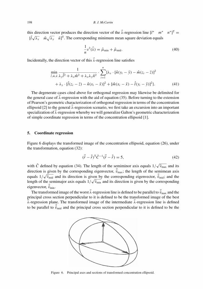
198 B. J. McCartin
this direction vector produces the direction vector of the �λ-regression line [l∗ m∗ n∗]T =[l√λx m
√λy n]T. The corresponding minimum mean square deviation equals
1
ns2(�λ) = µmin + µmid. (40)
Incidentally, the direction vector of this �λ-regression line satisfies
minl,m,n
1
λy l2 + λxm2 + λxλyn2·
n∑i=1
{λx · [n(yi − y) − m(zi − z)]2
+ λy · [l(zi − z) − n(xi − x)]2 + [m(xi − x) − l(yi − y)]2}. (41)
The degenerate cases cited above for orthogonal regression may likewise be delimited forthe general case of �λ-regression with the aid of equation (35). Before turning to the extensionof Pearson’s geometric characterization of orthogonal regression in terms of the concentrationellipsoid [2] to the general �λ-regression scenario, we first take an excursion into an importantspecialization of �λ-regression whereby we will generalize Galton’s geometric characterizationof simple coordinate regression in terms of the concentration ellipsoid [1].
5. Coordinate regression
Figure 6 displays the transformed image of the concentration ellipsoid, equation (26), underthe transformation, equation (32):
(�r − ¯r)TC−1(�r − ¯r) = 5, (42)
with C defined by equation (34). The length of the semiminor axis equals 1/√
νmax and itsdirection is given by the corresponding eigenvector, �vmax; the length of the semimean axisequals 1/
√νmid and its direction is given by the corresponding eigenvector, �vmid; and the
length of the semimajor axis equals 1/√
νmin and its direction is given by the correspondingeigenvector, �vmin.
The transformed image of the worst �λ-regression line is defined to be parallel to �vmax and theprincipal cross section perpendicular to it is defined to be the transformed image of the best�λ-regression plane. The transformed image of the intermediate �λ-regression line is definedto be parallel to �vmid and the principal cross section perpendicular to it is defined to be the
Figure 6. Principal axes and sections of transformed concentration ellipsoid.
Geometric characterization of planar regression 199
transformed image of the intermediate �λ-regression plane. The transformed image of the best�λ-regression line is defined to be parallel to �vmin and the principal cross section perpendicularto it is defined to be the transformed image of the worst �λ-regression plane.
Denoting the stretching transformation matrix by
D :=
1/√
λx 0 0
0 1/√
λy 0
0 0 1
, (43)
the normal vectors to the inverse transformed principal sections will be denoted by�nmax,mid,min := D �vmax,mid,min, which define the best, intermediate and worst �λ-regressionplanes, respectively. Likewise, the direction vectors of the inverse transformed principal semi-axes will be denoted by �dmax,mid,min := D−1 �vmax,mid,min, which define the worst, intermediateand best �λ-regression lines, respectively.
The orthogonality of the transformed vectors {�vmax, �vmid, �vmin} immediately implies the C-orthogonality of the normal vectors {�nmax, �nmid, �nmin}, as well as the C−1-orthogonality of thedirection vectors { �dmax, �dmid, �dmin}. For example,
�nTminC�nmax = �vT
minC�vmax = µmax
�vTmin
�vmax = 0, (44)
and
�dTminC
−1 �dmax = �vTminC
−1 �vmax = νmax�vT
min�vmax = 0. (45)
While strictly valid only for �λ ∈ (0, 1)2, we now investigate our prior results on �λ-regressionin the limiting cases λx → 0 and λy → 0, i.e. for the cases of simple and pairwise coordinateregression. These investigations will be facilitated by the matrix factorization
C−1 =
√λx 0 0
0√
λy 0
0 0 1
σ 2x pxy pzx
pxy σ 2y pyz
pzx pyz σ 2z
−1
√λx 0 0
0√
λy 0
0 0 1
. (46)
THEOREM 1 (Pairwise coordinate regression) Consider the pairwise coordinate regressionproblems, λx = 0, 0 < λy ≤ 1. The normals of each of the corresponding �λ-regression planesare orthogonal to the first column of the covariance matrix and thus all lie in a plane which,of course, intersects the concentration ellipsoid in an ellipse.
Proof As λx → 0 with λy �= 0, equation (46) implies that
C−1 →
0 0 0
0 λy · C2,2/ det (C)√
λy · C3,2/ det (C)
0√
λy · C2,3/ det (C) C3,3/ det (C)
, (47)
where Ci,j denotes the (i, j) cofactor of C. Thus, νmin → 0 and �vmin → [1 0 0]T. Further-more, this implies that �nmin → [1 0 0]T as λx → 0. By the previously noted C-orthogonalityof {�nmax, �nmid, �nmin}, we have �nT
maxC�nmin = 0. That is �nmax ⊥ [σ 2x pxy pzx]T. �
200 B. J. McCartin
Thus, all the normals to the planes of regression of y and z on x (λx = 0, 0 < λy ≤ 1) liein the plane
σ 2x (x − x) + pxy(y − y) + pzx(z − z) = 0. (48)
Alternatively, all of these pairwise coordinate regression planes must contain the first columnof the covariance matrix. This observation may be used to reduce this problem from three totwo dimensions.
Specifically, let �v1 and �v2 be the cross product of the first column of C with its secondand third columns, respectively. Then, the normal to the �λ-regression plane must be a linearcombination of these vectors: [mx my −1]T = α�v1 + β �v2. These three equations may besolved for α, β and mx = Amy − B (thereby implicitly defining A and B), which may thenbe substituted into equation (8) to yield the extremal problem
minmy
1
λym2y + 1
·n∑
i=1
[(Zi − Z) − my · (Yi − Y)]2, (49)
where Yi := yi + Axi, Zi := zi + Bxi .Equation (49) is formally identical to the two dimensional linear regression problem that
was exhaustively treated in [3]. Cyclic permutation of {x, y, z} provides for the remaininginstances of pairwise coordinate regression, i.e. regression of z and x on y and regression ofx and y on z.
Turning next to the case of simple coordinate regression, we have the following impor-tant result.
THEOREM 2 (Simple coordinate regression) Consider the problem of regression of z on x andy, i.e. λx = 0 = λy . The normal to the corresponding �λ-regression plane is orthogonal to thefirst two columns of the covariance matrix.
Proof By continuity of the spectrum of a matrix subject to a continuous perturbation, theconclusions of Theorem 1 remain valid as λy → 0. Thus, the normal to the (0, 0)-regressionplane is orthogonal to the first column of C. Now, perform a counterclockwise permutationof {x, y, z}, thereby implying that the normal to the (0, 0)-regression plane is also orthogonalto the second column of C. �
Thus, it is straightforward to compute the plane of regression of z on x and y. Simplyform the cross product of the first two columns of C to obtain the required normal. This isguaranteed to work as we presently assume that det (C) �= 0 after having previously disposedof all possible ways in which det (C) might vanish. This leads immediately to
(pxypyz − pzxσ2y )(x − x) + (pxypzx − pyzσ
2x )(y − y) + (σ 2
x σ 2y − p2
xy)(z − z) = 0. (50)
As is readily apparent from equation (47), νmin → 0, νmid → 0, νmax → C3,3/ det (C) asλx → 0 and λy → 0. Consequently, by equation (39), the minimum mean square deviation isgiven by
1
nS2
z := 1
nS2(0, 0) = µmin = 1
νmax= det (C)
C3,3. (51)
Cyclic permutation of {x, y, z} provides for the remaining instances of simple coordinateregression, i.e. regression of x on y and z and regression of y on z and x. Observe thatequation (50) is identical with equation (25). This is indicative of the fact that when det (C) = 0the three simple coordinate regression planes coincide.
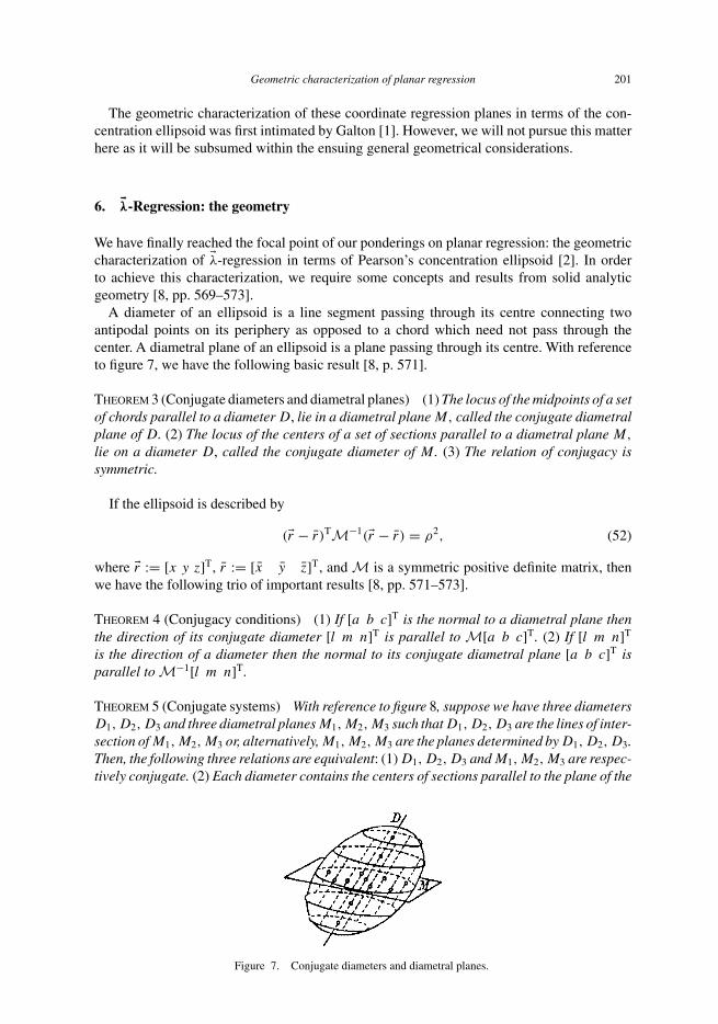
Geometric characterization of planar regression 201
The geometric characterization of these coordinate regression planes in terms of the con-centration ellipsoid was first intimated by Galton [1]. However, we will not pursue this matterhere as it will be subsumed within the ensuing general geometrical considerations.
6. �λ-Regression: the geometry
We have finally reached the focal point of our ponderings on planar regression: the geometriccharacterization of �λ-regression in terms of Pearson’s concentration ellipsoid [2]. In orderto achieve this characterization, we require some concepts and results from solid analyticgeometry [8, pp. 569–573].
A diameter of an ellipsoid is a line segment passing through its centre connecting twoantipodal points on its periphery as opposed to a chord which need not pass through thecenter. A diametral plane of an ellipsoid is a plane passing through its centre. With referenceto figure 7, we have the following basic result [8, p. 571].
THEOREM 3 (Conjugate diameters and diametral planes) (1) The locus of the midpoints of a setof chords parallel to a diameter D, lie in a diametral plane M, called the conjugate diametralplane of D. (2) The locus of the centers of a set of sections parallel to a diametral plane M,
lie on a diameter D, called the conjugate diameter of M . (3) The relation of conjugacy issymmetric.
If the ellipsoid is described by
(�r − r)TM−1(�r − r) = ρ2, (52)
where �r := [x y z]T, r := [x y z]T, and M is a symmetric positive definite matrix, thenwe have the following trio of important results [8, pp. 571–573].
THEOREM 4 (Conjugacy conditions) (1) If [a b c]T is the normal to a diametral plane thenthe direction of its conjugate diameter [l m n]T is parallel to M[a b c]T. (2) If [l m n]T
is the direction of a diameter then the normal to its conjugate diametral plane [a b c]T isparallel to M−1[l m n]T.
THEOREM 5 (Conjugate systems) With reference to figure 8, suppose we have three diametersD1, D2, D3 and three diametral planes M1, M2, M3 such that D1, D2, D3 are the lines of inter-section of M1, M2, M3 or, alternatively, M1, M2, M3 are the planes determined by D1, D2, D3.Then, the following three relations are equivalent: (1) D1, D2, D3 and M1, M2, M3 are respec-tively conjugate. (2) Each diameter contains the centers of sections parallel to the plane of the
Figure 7. Conjugate diameters and diametral planes.
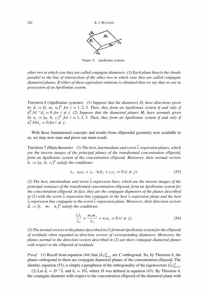
202 B. J. McCartin
Figure 8. Apollonius systems.
other two in which case they are called conjugate diameters. (3) Each plane bisects the chordsparallel to the line of intersection of the other two in which case they are called conjugatediametral planes. If either of these equivalent relations is obtained then we say that we are inpossession of an Apollonius system.
THEOREM 6 (Apollonius systems) (1) Suppose that the diameters Di have directions givenby di := [li mi ni]T for i = 1, 2, 3. Then, they form an Apollonius system if and only ifdT
i M−1dj = 0 for i �= j . (2) Suppose that the diametral planes Mi have normals givenby ni := [ai bi ci]T for i = 1, 2, 3. Then, they form an Apollonius system if and only ifnT
i Mnj = 0 for i �= j .
With these fundamental concepts and results from ellipsoidal geometry now available tous, we may now state and prove our main result.
THEOREM 7 (Main theorem) (1) The best, intermediate and worst �λ-regression planes, whichare the inverse images of the principal planes of the transformed concentration ellipsoid,form an Apollonius system of the concentration ellipsoid. Moreover, their normal vectors�ni := [ai bi ci]T satisfy the conditions:
λx · aiaj + λy · bibj + cicj = 0 (i �= j). (53)
(2) The best, intermediate and worst �λ-regression lines, which are the inverse images of theprincipal semiaxes of the transformed concentration ellipsoid, form an Apollonius system forthe concentration ellipsoid. In fact, they are the conjugate diameters of the planes describedin (1) with the worst �λ-regression line conjugate to the best �λ-regression plane and the best�λ-regression line conjugate to the worst �λ-regression plane. Moreover, their direction vectors�di := [li mi ni]T satisfy the conditions:
li lj
λx
+ mimj
λy
+ ninj = 0 (i �= j). (54)
(3) The normal vectors to the planes described in (1) form an Apollonius system for the ellipsoidof residuals when regarded as direction vectors of corresponding diameters. Moreover, theplanes normal to the direction vectors described in (2) are their conjugate diametral planeswith respect to the ellipsoid of residuals.
Proof (1) Recall from equation (44) that {�nk}3k=1 are C-orthogonal. So, by Theorem 6, the
planes orthogonal to them are conjugate diametral planes of the concentration ellipsoid. Theidentity, equation (53), is simply a paraphrase of the orthogonality of the eigenvectors {�vk}3
k=1.(2) Let �di = D−1 �vi and �ni = D �vi where D was defined in equation (43). By Theorem 4,
the conjugate diameter with respect to the concentration ellipsoid of the diametral plane with
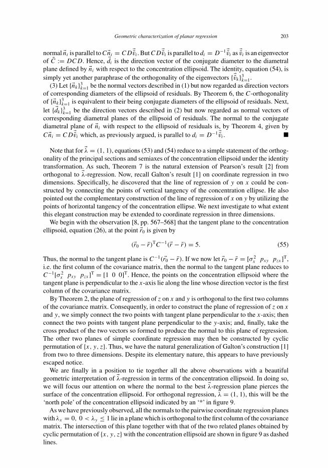
Geometric characterization of planar regression 203
normal �ni is parallel to C�ni = CD �vi . But CD �vi is parallel to di = D−1 �vi as �vi is an eigenvectorof C := DCD. Hence, �di is the direction vector of the conjugate diameter to the diametralplane defined by �ni with respect to the concentration ellipsoid. The identity, equation (54), issimply yet another paraphrase of the orthogonality of the eigenvectors {�vk}3
k=1.(3) Let {�nk}3
k=1 be the normal vectors described in (1) but now regarded as direction vectorsof corresponding diameters of the ellipsoid of residuals. By Theorem 6, the C-orthogonalityof {�nk}3
k=1 is equivalent to their being conjugate diameters of the ellipsoid of residuals. Next,let { �dk}3
k=1 be the direction vectors described in (2) but now regarded as normal vectors ofcorresponding diametral planes of the ellipsoid of residuals. The normal to the conjugatediametral plane of �ni with respect to the ellipsoid of residuals is, by Theorem 4, given byC�ni = CD �vi which, as previously argued, is parallel to di = D−1 �vi . �
Note that for �λ = (1, 1), equations (53) and (54) reduce to a simple statement of the orthog-onality of the principal sections and semiaxes of the concentration ellipsoid under the identitytransformation. As such, Theorem 7 is the natural extension of Pearson’s result [2] fromorthogonal to �λ-regression. Now, recall Galton’s result [1] on coordinate regression in twodimensions. Specifically, he discovered that the line of regression of y on x could be con-structed by connecting the points of vertical tangency of the concentration ellipse. He alsopointed out the complementary construction of the line of regression of x on y by utilizing thepoints of horizontal tangency of the concentration ellipse. We next investigate to what extentthis elegant construction may be extended to coordinate regression in three dimensions.
We begin with the observation [8, pp. 567–568] that the tangent plane to the concentrationellipsoid, equation (26), at the point �r0 is given by
(�r0 − r)TC−1(�r − r) = 5. (55)
Thus, the normal to the tangent plane is C−1( �r0 − r). If we now let �r0 − r = [σ 2x pxy pzx]T,
i.e. the first column of the covariance matrix, then the normal to the tangent plane reduces toC−1[σ 2
x pxy pzx]T = [1 0 0]T. Hence, the points on the concentration ellipsoid where thetangent plane is perpendicular to the x-axis lie along the line whose direction vector is the firstcolumn of the covariance matrix.
By Theorem 2, the plane of regression of z on x and y is orthogonal to the first two columnsof the covariance matrix. Consequently, in order to construct the plane of regression of z on x
and y, we simply connect the two points with tangent plane perpendicular to the x-axis; thenconnect the two points with tangent plane perpendicular to the y-axis; and, finally, take thecross product of the two vectors so formed to produce the normal to this plane of regression.The other two planes of simple coordinate regression may then be constructed by cyclicpermutation of {x, y, z}. Thus, we have the natural generalization of Galton’s construction [1]from two to three dimensions. Despite its elementary nature, this appears to have previouslyescaped notice.
We are finally in a position to tie together all the above observations with a beautifulgeometric interpretation of �λ-regression in terms of the concentration ellipsoid. In doing so,we will focus our attention on where the normal to the best �λ-regression plane pierces thesurface of the concentration ellipsoid. For orthogonal regression, �λ = (1, 1), this will be the‘north pole’ of the concentration ellipsoid indicated by an ‘*’ in figure 9.
As we have previously observed, all the normals to the pairwise coordinate regression planeswith λx = 0, 0 < λy ≤ 1 lie in a plane which is orthogonal to the first column of the covariancematrix. The intersection of this plane together with that of the two related planes obtained bycyclic permutation of {x, y, z} with the concentration ellipsoid are shown in figure 9 as dashedlines.
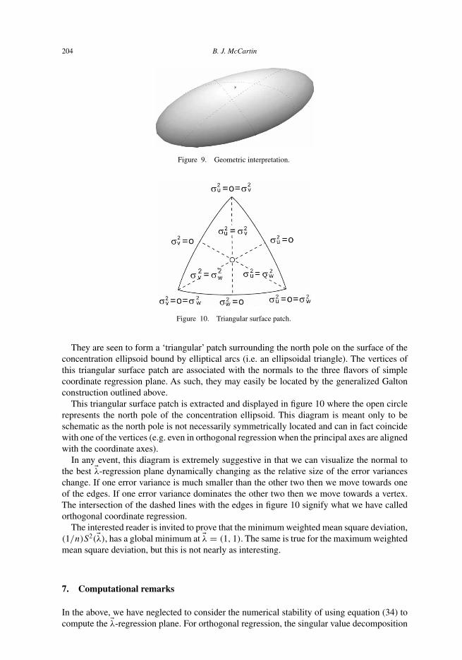
204 B. J. McCartin
Figure 9. Geometric interpretation.
Figure 10. Triangular surface patch.
They are seen to form a ‘triangular’ patch surrounding the north pole on the surface of theconcentration ellipsoid bound by elliptical arcs (i.e. an ellipsoidal triangle). The vertices ofthis triangular surface patch are associated with the normals to the three flavors of simplecoordinate regression plane. As such, they may easily be located by the generalized Galtonconstruction outlined above.
This triangular surface patch is extracted and displayed in figure 10 where the open circlerepresents the north pole of the concentration ellipsoid. This diagram is meant only to beschematic as the north pole is not necessarily symmetrically located and can in fact coincidewith one of the vertices (e.g. even in orthogonal regression when the principal axes are alignedwith the coordinate axes).
In any event, this diagram is extremely suggestive in that we can visualize the normal tothe best �λ-regression plane dynamically changing as the relative size of the error varianceschange. If one error variance is much smaller than the other two then we move towards oneof the edges. If one error variance dominates the other two then we move towards a vertex.The intersection of the dashed lines with the edges in figure 10 signify what we have calledorthogonal coordinate regression.
The interested reader is invited to prove that the minimum weighted mean square deviation,(1/n)S2(�λ), has a global minimum at �λ = (1, 1). The same is true for the maximum weightedmean square deviation, but this is not nearly as interesting.
7. Computational remarks
In the above, we have neglected to consider the numerical stability of using equation (34) tocompute the �λ-regression plane. For orthogonal regression, the singular value decomposition
Geometric characterization of planar regression 205
(SVD) provides an attractive computational procedure [17, pp. 9–10]. The SVD of a realmatrix M is a matrix factorization of fundamental importance in least squares problems. TheSVD is closely related to the more familiar eigenvalue decompositions of the matrices MTM
and MMT. In fact, the singular values of M are precisely the non-negative square roots of theq := min {m, n} largest eigenvalues of these related matrices. The interested reader is referredto [17, pp. 9–12] for more details. We will use our change of variables, equation (32), to adaptthis technique to �λ-regression.
In order to fit the orthogonal regression plane [17, pp. 184–186],
ax + by + cz = h; a2 + b2 + c2 = 1, (56)
we introduce the shifted data matrix
M =x1 − x · · · xn − x
y1 − y · · · yn − y
z1 − z · · · zn − z
. (57)
Computing the SVD of M (e.g. using MATLAB),
M = [u1 u2 u3
] σ1 0 0
0 σ2 00 0 σ3
vT1
vT2
vT3
(58)
where σ1 ≥ σ2 ≥ σ3 ≥ 0, the orthogonal regression coefficients are
[a b c
] = uT3 , h = uT
3
x
y
z
. (59)
If σ1 ≥ σ2 > σ3 = 0, then the data points all lie on a plane; if σ1 > σ2 = σ3 = 0, then thedata points all lie on a line; if σ1 = σ2 = σ3 = 0, then xi = x, yi = y , zi = z for all i; andnon-zero repetitions amongst the σ ’s correspond to the degenerate cases previously described.If σ2 �= σ3, then the orthogonal regression plane is unique and σ 2
3 equals the minimum sumof squares. The direction of the orthogonal regression line is given by uT
1 = [l m n]T andthe minimum sum of squares equals σ 2
2 + σ 23 .
For the general case of �λ-regression, we simply redefine
M =
(x1 − x)/√
λx · · · (xn − x)/√
λx
(y1 − y)/√
λy · · · (yn − y)/√
λy
z1 − z · · · zn − z
, (60)
perform the SVD, and set mx = −(1/√
λx) · a/c, my = −(1/√
λy) · b/c for the �λ-regression
plane, and l = √λx · l, m = √
λy · m, and n = n for the �λ-regression line. If either min (λx, λy)
is very small or max (λx, λy) is very large, it might be prudent to transition to the appropriatecoordinate regression formula detailed above.
Acknowledgement
The author thanks Mrs. Barbara McCartin for her dedicated assistance in the production ofthis paper.
206 B. J. McCartin
References[1] Galton, F., 1886, Family likeness in stature (with Appendix by Dickson, J.D.H.). Proceedings of the Royal
Society of London, 40, 42–73.[2] Pearson, K., 1901, On lines and planes of closest fit to systems of points in space. Philosophical Magazine, 2,
559–572.[3] McCartin, B.J., 2003, A geometric characterization of linear regression. Statistics, 37(2), 101–117.[4] Farebrother, R.W., 1999, Fitting Linear Relationships: A History of the Calculus of Observations 1750–1900
(New York, NY: Springer-Verlag).[5] von Mises, R., 1964, Mathematical Theory of Probability and Statistics (New York, NY: Academic).[6] Cramér, H., 1946, Mathematical Methods of Statistics (Princeton, NJ: Princeton University Press).[7] Jukic, D., Scitovski, R. and Ungar, S., 1998, The best total least squares line in R3. Operational Research
Proceedings KOI’98, Rovinji, Croatia, 311–316.[8] Osgood, W.F. and Graustein, W.C., 1929, Plane and Solid Analytic Geometry (New York, NY: Macmillan).[9] Cheng, C.-L. and Van Ness, J.W., 1999, Statistical Regression with Measurement Error (London: Arnold).
[10] Van Huffel, S. and Vandewalle, J., 1991, The Total Least Squares Problem: Computational Techniques andAnalysis (Philadelphia, PA: SIAM).
[11] Späth, H., 1992, Mathematical Algorithms for Linear Regression (San Diego, CA: Academic).[12] McCartin, B.J., 2006, On concentration and inertia ellipsoids. Mathematics Magazine (to appear).[13] Sommerville, D.M.Y., 1939, Analytical Geometry of Three Dimensions (London: Cambridge University Press).[14] Salmon, G., 1862, A Treatise on the Analytic Geometry of Three Dimensions (Dublin: Hodges, Smith & Co.).[15] Spain, B., 1960, Analytical Quadrics (London: Pergamon).[16] Bell, R.J.T., 1928, An Elementary Treatise on Coordinate Geometry in Three Dimensions (London: Macmillan
& Co.).[17] Björck, A., 1996, Numerical Methods for Least Squares (Philadelphia, PA: SIAM).

Computational Statistics & Data Analysis 42 (2003) 647–664www.elsevier.com/locate/csda
Transformations, regression geometry and R2
Yufen Huanga , Norman R. Draperb;∗aDepartment of Mathematics, National Chung Cheng University, Chiayi, Taiwan
bDepartment of Statistics, University of Wisconsin, 1210 West Dayton Street, Madison,WI 53706-1685, USA
Received 1 September 2001; received in revised form 1 May 2002
Abstract
In making a least-squares 2t to a set of data, it is often advantageous to transform the responsevariable. This can lead to di4culties in making comparisons between competing transformations.Several de2nitions of R2 statistics have been suggested. These calculations mostly involve theactual and 2tted values of the response, after the transformation has been inverted, or undone.Kv6alseth (Amer. Statist. 39 (1985) 279) discussed the various R2 types and Scott and Wild(Amer. Statist. 45 (1991) 127) pointed out some of the problems that arise. In this paper, weexamine such problems in a new way by considering the underlying regression geometry. Thisleads to a new suggestion for an R2 statistic based on the geometry, and to a statistic Q whichis closely connected to the quality of the estimation of the transformation parameter.c© 2002 Elsevier Science B.V. All rights reserved.
Keywords: Least-squares estimation; Regression geometry; R2; Transformations
1. Introduction
Consider a general linear model of form
y = X� + ” (1)
where y = (y1; y2; : : : ; yn)T is an n × 1 vector of responses, X is an n × p matrix ofregressors, �=(�0; �1; : : : ; �p−1)T is a p×1 vector of parameters and ” is an n×1 vectorof random errors. Fitting (1) by least-squares gives an estimator �= (XTX)−1XTy and
∗ Corresponding author. Tel.: +1-608-262-0926; fax: +1-608-262-0032.E-mail address: [email protected] (N.R. Draper).
0167-9473/03/$ - see front matter c© 2002 Elsevier Science B.V. All rights reserved.PII: S0167 -9473(02)00149 -4
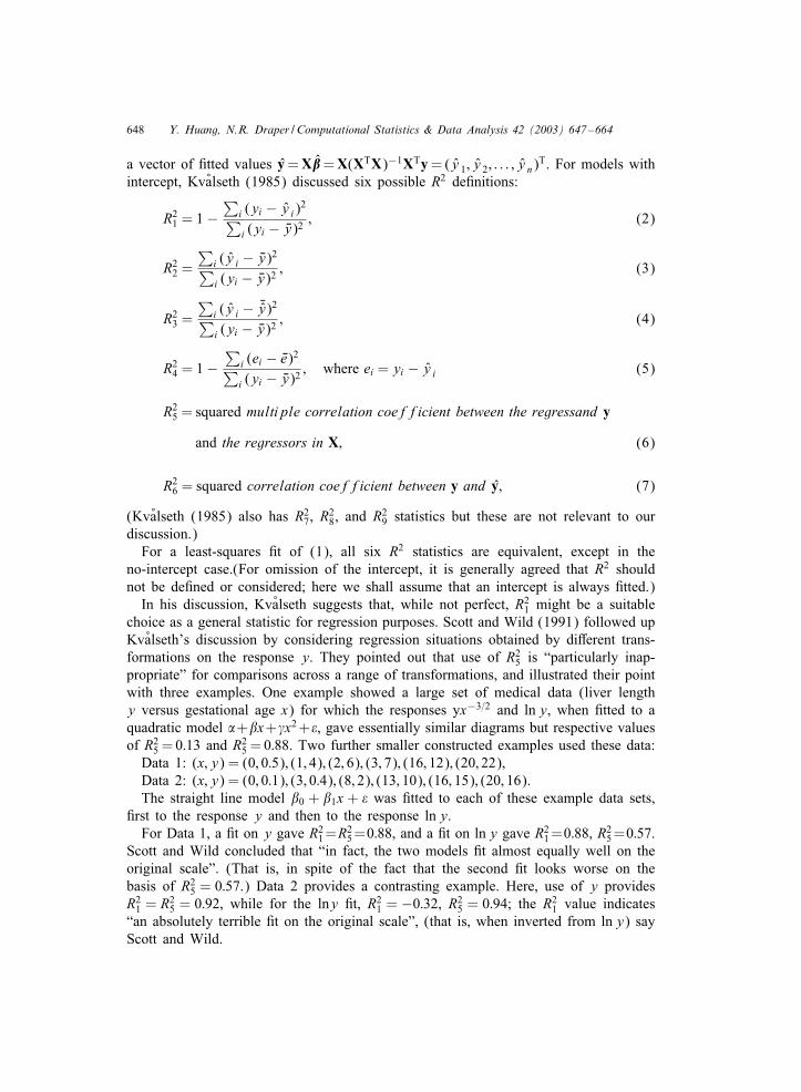
648 Y. Huang, N.R. Draper / Computational Statistics & Data Analysis 42 (2003) 647–664
a vector of 2tted values y = X�= X(XTX)−1XTy = (y 1; y 2; : : : ; y n)T. For models with
intercept, Kv6alseth (1985) discussed six possible R2 de2nitions:
R21 = 1 −
∑i (yi − y i)
2∑i (yi − Hy)2 ; (2)
R22 =
∑i (y i − Hy)2∑i (yi − Hy)2 ; (3)
R23 =
∑i (y i − Hy)2∑i (yi − Hy)2 ; (4)
R24 = 1 −
∑i (ei − He)2∑i (yi − Hy)2 ; where ei = yi − y i (5)
R25 = squared multiple correlation coefficient between the regressand y
and the regressors in X; (6)
R26 = squared correlation coefficient between y and y; (7)
(Kv6alseth (1985) also has R27, R2
8, and R29 statistics but these are not relevant to our
discussion.)For a least-squares 2t of (1), all six R2 statistics are equivalent, except in the
no-intercept case.(For omission of the intercept, it is generally agreed that R2 shouldnot be de2ned or considered; here we shall assume that an intercept is always 2tted.)
In his discussion, Kv6alseth suggests that, while not perfect, R21 might be a suitable
choice as a general statistic for regression purposes. Scott and Wild (1991) followed upKv6alseth’s discussion by considering regression situations obtained by diJerent trans-formations on the response y. They pointed out that use of R2
5 is “particularly inap-propriate” for comparisons across a range of transformations, and illustrated their pointwith three examples. One example showed a large set of medical data (liver lengthy versus gestational age x) for which the responses yx−3=2 and ln y, when 2tted to aquadratic model �+�x+�x2 +�, gave essentially similar diagrams but respective valuesof R2
5 = 0:13 and R25 = 0:88. Two further smaller constructed examples used these data:
Data 1: (x; y) = (0; 0:5); (1; 4); (2; 6); (3; 7); (16; 12); (20; 22),Data 2: (x; y) = (0; 0:1); (3; 0:4); (8; 2); (13; 10); (16; 15); (20; 16).The straight line model �0 + �1x + � was 2tted to each of these example data sets,
2rst to the response y and then to the response ln y.For Data 1, a 2t on y gave R2
1 =R25 =0:88, and a 2t on ln y gave R2
1 =0:88, R25 =0:57.
Scott and Wild concluded that “in fact, the two models 2t almost equally well on theoriginal scale”. (That is, in spite of the fact that the second 2t looks worse on thebasis of R2
5 = 0:57.) Data 2 provides a contrasting example. Here, use of y providesR2
1 = R25 = 0:92, while for the lny 2t, R2
1 = −0:32, R25 = 0:94; the R2
1 value indicates“an absolutely terrible 2t on the original scale”, (that is, when inverted from ln y) sayScott and Wild.
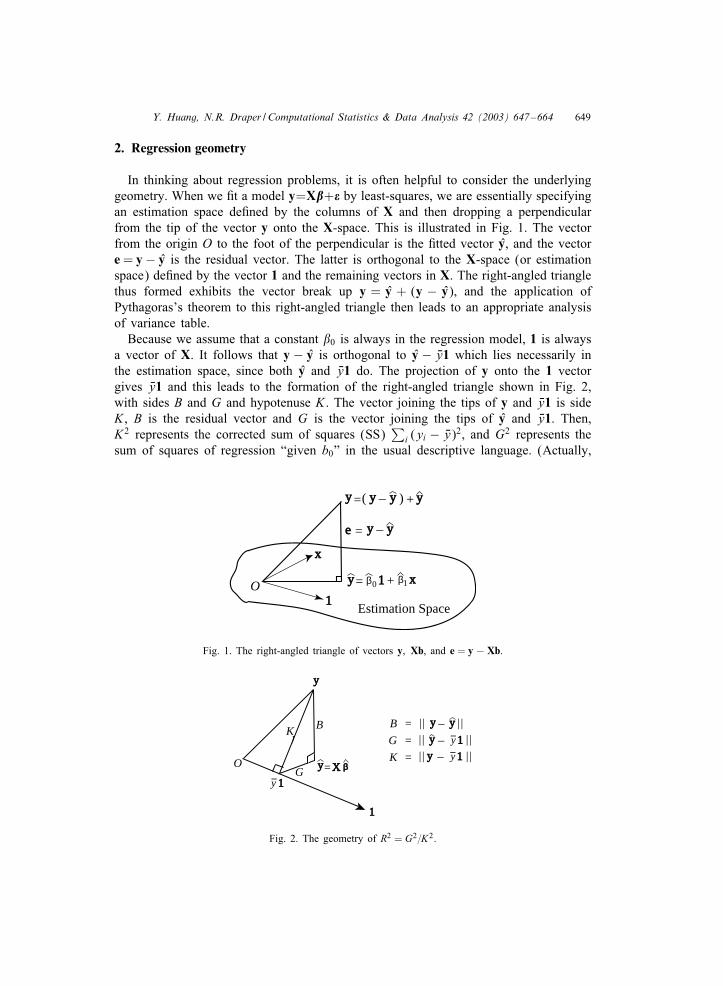
Y. Huang, N.R. Draper / Computational Statistics & Data Analysis 42 (2003) 647–664 649
2. Regression geometry
In thinking about regression problems, it is often helpful to consider the underlyinggeometry. When we 2t a model y=X�+” by least-squares, we are essentially specifyingan estimation space de2ned by the columns of X and then dropping a perpendicularfrom the tip of the vector y onto the X-space. This is illustrated in Fig. 1. The vectorfrom the origin O to the foot of the perpendicular is the 2tted vector y, and the vectore = y − y is the residual vector. The latter is orthogonal to the X-space (or estimationspace) de2ned by the vector 1 and the remaining vectors in X. The right-angled trianglethus formed exhibits the vector break up y = y + (y − y), and the application ofPythagoras’s theorem to this right-angled triangle then leads to an appropriate analysisof variance table.
Because we assume that a constant �0 is always in the regression model, 1 is alwaysa vector of X. It follows that y − y is orthogonal to y − Hy1 which lies necessarily inthe estimation space, since both y and Hy1 do. The projection of y onto the 1 vectorgives Hy1 and this leads to the formation of the right-angled triangle shown in Fig. 2,with sides B and G and hypotenuse K . The vector joining the tips of y and Hy1 is sideK , B is the residual vector and G is the vector joining the tips of y and Hy1. Then,K2 represents the corrected sum of squares (SS)
∑i (yi − Hy)2, and G2 represents the
sum of squares of regression “given b0” in the usual descriptive language. (Actually,
Estimation Space
x
1
( )y = +-y
O
e -y=
x1= +0β 1β
y y
y
y
Fig. 1. The right-angled triangle of vectors y; Xb, and e = y − Xb.
|| ||
|| ||
O
K
G
B B =
G =
K =X
1
= β
|| ||-y
y
1y--
y - 1y-
1y-
y
y
y
K
Fig. 2. The geometry of R2 = G2=K2.
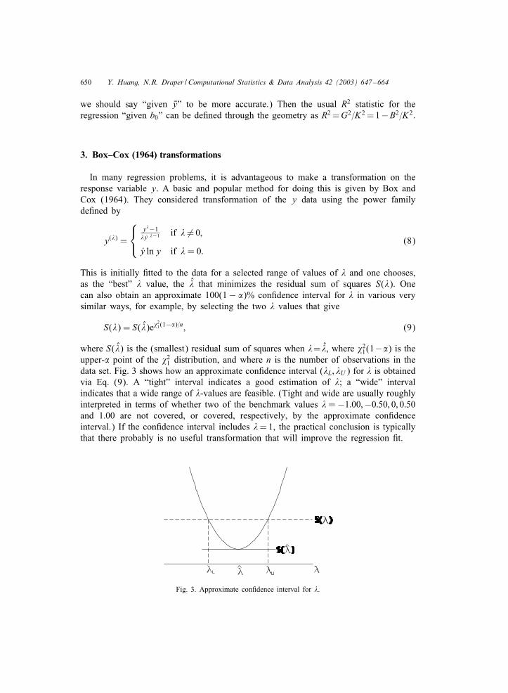
650 Y. Huang, N.R. Draper / Computational Statistics & Data Analysis 42 (2003) 647–664
we should say “given Hy” to be more accurate.) Then the usual R2 statistic for theregression “given b0” can be de2ned through the geometry as R2 =G2=K2 =1−B2=K2.
3. Box–Cox (1964) transformations
In many regression problems, it is advantageous to make a transformation on theresponse variable y. A basic and popular method for doing this is given by Box andCox (1964). They considered transformation of the y data using the power familyde2ned by
y(#) =
y#−1#y #−1 if # �= 0;
y ln y if # = 0:(8)
This is initially 2tted to the data for a selected range of values of # and one chooses,as the “best” # value, the # that minimizes the residual sum of squares S(#). Onecan also obtain an approximate 100(1 − �)% con2dence interval for # in various verysimilar ways, for example, by selecting the two # values that give
S(#) = S(#)e%21(1−�)=n; (9)
where S(#) is the (smallest) residual sum of squares when #= #, where %21(1−�) is the
upper-� point of the %21 distribution, and where n is the number of observations in the
data set. Fig. 3 shows how an approximate con2dence interval (#L; #U ) for # is obtainedvia Eq. (9). A “tight” interval indicates a good estimation of #; a “wide” intervalindicates that a wide range of #-values are feasible. (Tight and wide are usually roughlyinterpreted in terms of whether two of the benchmark values # = −1:00;−0:50; 0; 0:50and 1:00 are not covered, or covered, respectively, by the approximate con2denceinterval.) If the con2dence interval includes #= 1, the practical conclusion is typicallythat there probably is no useful transformation that will improve the regression 2t.
Fig. 3. Approximate con2dence interval for #.
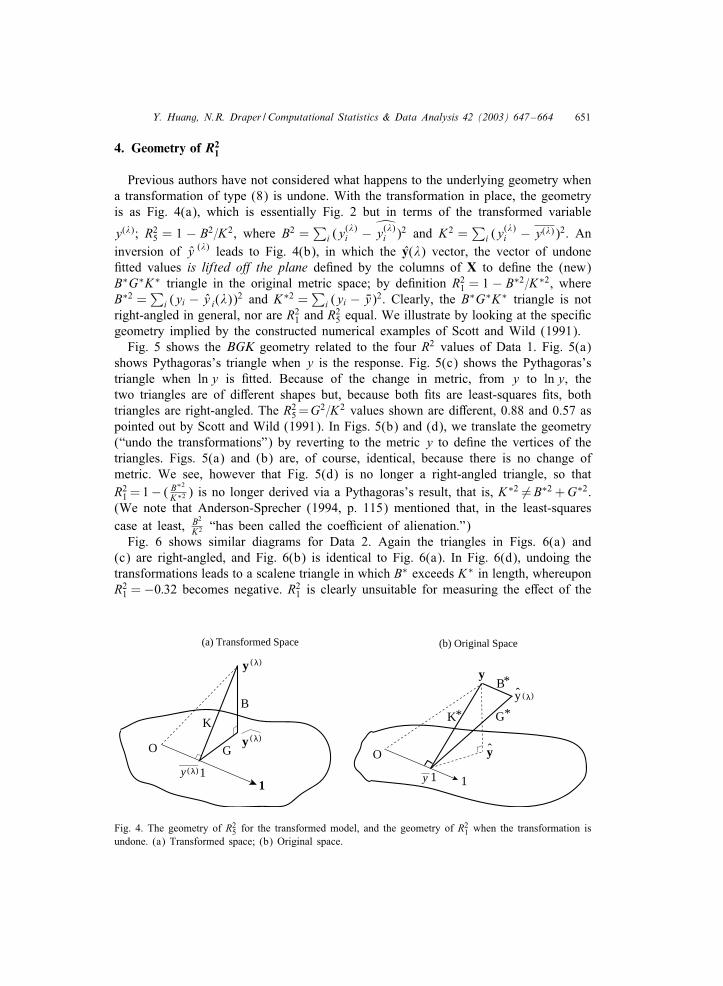
Y. Huang, N.R. Draper / Computational Statistics & Data Analysis 42 (2003) 647–664 651
4. Geometry of R21
Previous authors have not considered what happens to the underlying geometry whena transformation of type (8) is undone. With the transformation in place, the geometryis as Fig. 4(a), which is essentially Fig. 2 but in terms of the transformed variable
y(#); R25 = 1 − B2=K2, where B2 =
∑i (y
(#)i − y(#)
i )2 and K2 =∑
i (y(#)i − y(#))2. An
inversion of y (#) leads to Fig. 4(b), in which the y(#) vector, the vector of undone2tted values is lifted o6 the plane de2ned by the columns of X to de2ne the (new)B∗G∗K∗ triangle in the original metric space; by de2nition R2
1 = 1 − B∗2=K∗2, whereB∗2 =
∑i (yi − y i(#))2 and K∗2 =
∑i (yi − Hy)2. Clearly, the B∗G∗K∗ triangle is not
right-angled in general, nor are R21 and R2
5 equal. We illustrate by looking at the speci2cgeometry implied by the constructed numerical examples of Scott and Wild (1991).
Fig. 5 shows the BGK geometry related to the four R2 values of Data 1. Fig. 5(a)shows Pythagoras’s triangle when y is the response. Fig. 5(c) shows the Pythagoras’striangle when ln y is 2tted. Because of the change in metric, from y to ln y, thetwo triangles are of diJerent shapes but, because both 2ts are least-squares 2ts, bothtriangles are right-angled. The R2
5 =G2=K2 values shown are diJerent, 0.88 and 0.57 aspointed out by Scott and Wild (1991). In Figs. 5(b) and (d), we translate the geometry(“undo the transformations”) by reverting to the metric y to de2ne the vertices of thetriangles. Figs. 5(a) and (b) are, of course, identical, because there is no change ofmetric. We see, however that Fig. 5(d) is no longer a right-angled triangle, so thatR2
1 = 1− ( B∗2
K∗2 ) is no longer derived via a Pythagoras’s result, that is, K∗2 �=B∗2 +G∗2.(We note that Anderson-Sprecher (1994, p. 115) mentioned that, in the least-squarescase at least, B2
K2 “has been called the coe4cient of alienation.”)Fig. 6 shows similar diagrams for Data 2. Again the triangles in Figs. 6(a) and
(c) are right-angled, and Fig. 6(b) is identical to Fig. 6(a). In Fig. 6(d), undoing thetransformations leads to a scalene triangle in which B∗ exceeds K∗ in length, whereuponR2
1 = −0:32 becomes negative. R21 is clearly unsuitable for measuring the eJect of the
O
K
G
B
1
O
y
(a) Transformed Space (b) Original Space
)( 1y λ
y )( λ
y )( λ
y )( λ
G*
B*
K*
y
11y
ˆ
ˆ
Fig. 4. The geometry of R25 for the transformed model, and the geometry of R2
1 when the transformation isundone. (a) Transformed space; (b) Original space.
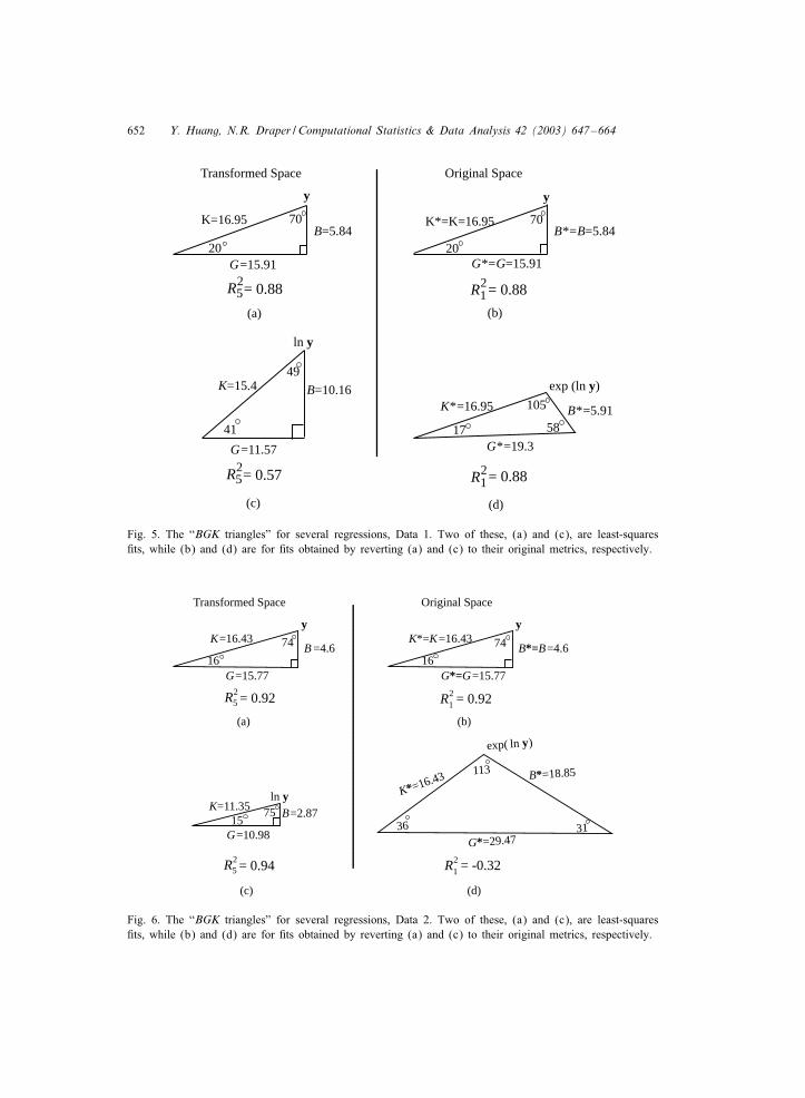
652 Y. Huang, N.R. Draper / Computational Statistics & Data Analysis 42 (2003) 647–664
K=16.95 K*=K=16.95
K*=16.95
B=5.84
B=10.16
B*=B=5.84
B*=5.91
K=15.4
G=15.91 G*=G=15.91
G=11.57 G*=19.3
20
70
49
41 17
105
58
20
70
R21= 0.885R2
= 0.88
5R2= 0.57 R2
1= 0.88
y
ln y
y
exp (ln y)
Transformed Space Original Space
(a) (b)
(c) (d)
Fig. 5. The “BGK triangles” for several regressions, Data 1. Two of these, (a) and (c), are least-squares2ts, while (b) and (d) are for 2ts obtained by reverting (a) and (c) to their original metrics, respectively.
B=2.87K=11.35
G=10.98
7515
R21 = 0.925R2
= 0.92
5R2= 0.94
ln y
K=16.43B =4.6
G=15.7716
74
yK*=K=16.43
B*=B=4.6
G*=G=15.7716
74
y
K*=16.43 B*=18.85
G*=29.4736
113
31
exp( )ln y
R21 = -0.32
Original SpaceTransformed Space
(a) (b)
(c) (d)
Fig. 6. The “BGK triangles” for several regressions, Data 2. Two of these, (a) and (c), are least-squares2ts, while (b) and (d) are for 2ts obtained by reverting (a) and (c) to their original metrics, respectively.
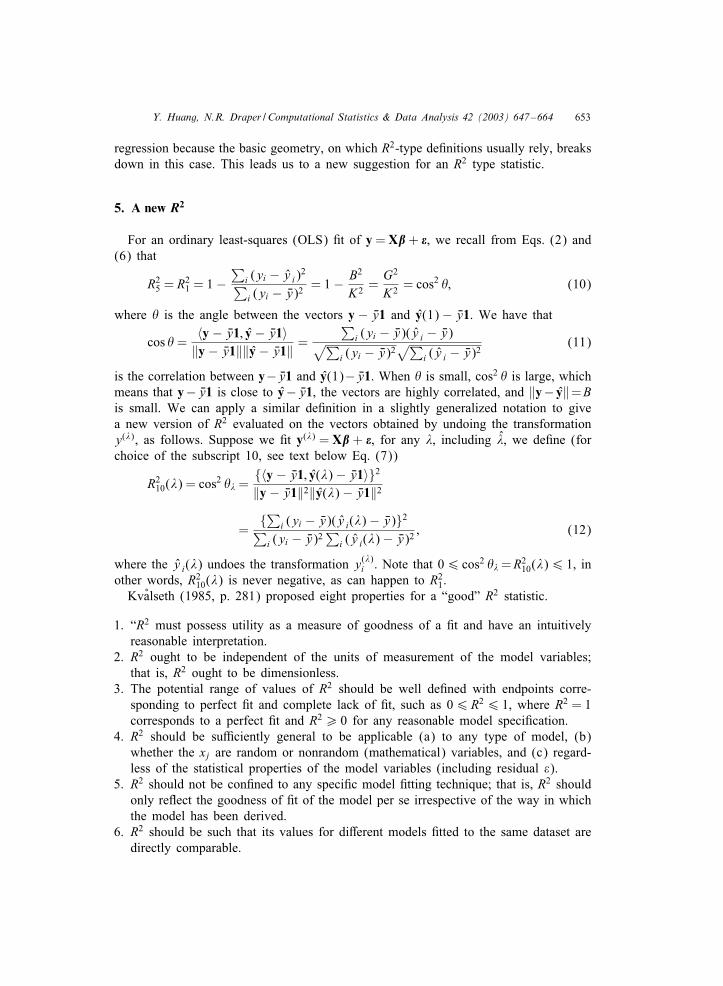
Y. Huang, N.R. Draper / Computational Statistics & Data Analysis 42 (2003) 647–664 653
regression because the basic geometry, on which R2-type de2nitions usually rely, breaksdown in this case. This leads us to a new suggestion for an R2 type statistic.
5. A new R2
For an ordinary least-squares (OLS) 2t of y = X�+ ”, we recall from Eqs. (2) and(6) that
R25 = R2
1 = 1 −∑
i (yi − y i)2∑
i (yi − Hy)2 = 1 − B2
K2 =G2
K2 = cos2 (; (10)
where ( is the angle between the vectors y − Hy1 and y(1) − Hy1. We have that
cos ( =〈y − Hy1; y − Hy1〉‖y − Hy1‖‖y − Hy1‖ =
∑i (yi − Hy)(y i − Hy)√∑
i (yi − Hy)2√∑
i (y i − Hy)2(11)
is the correlation between y− Hy1 and y(1)− Hy1. When ( is small, cos2 ( is large, whichmeans that y− Hy1 is close to y− Hy1, the vectors are highly correlated, and ‖y− y‖=Bis small. We can apply a similar de2nition in a slightly generalized notation to givea new version of R2 evaluated on the vectors obtained by undoing the transformationy(#), as follows. Suppose we 2t y(#) = X� + ”, for any #, including #, we de2ne (forchoice of the subscript 10, see text below Eq. (7))
R210(#) = cos2 (# =
{〈y − Hy1; y(#) − Hy1〉}2
‖y − Hy1‖2‖y(#) − Hy1‖2
={∑i (yi − Hy)(y i(#) − Hy)}2∑i (yi − Hy)2
∑i (y i(#) − Hy)2 ; (12)
where the y i(#) undoes the transformation y(#)i . Note that 06 cos2 (# =R2
10(#)6 1, inother words, R2
10(#) is never negative, as can happen to R21.
Kv6alseth (1985, p. 281) proposed eight properties for a “good” R2 statistic.
1. “R2 must possess utility as a measure of goodness of a 2t and have an intuitivelyreasonable interpretation.
2. R2 ought to be independent of the units of measurement of the model variables;that is, R2 ought to be dimensionless.
3. The potential range of values of R2 should be well de2ned with endpoints corre-sponding to perfect 2t and complete lack of 2t, such as 06R26 1, where R2 = 1corresponds to a perfect 2t and R2¿ 0 for any reasonable model speci2cation.
4. R2 should be su4ciently general to be applicable (a) to any type of model, (b)whether the xj are random or nonrandom (mathematical) variables, and (c) regard-less of the statistical properties of the model variables (including residual �).
5. R2 should not be con2ned to any speci2c model 2tting technique; that is, R2 shouldonly reRect the goodness of 2t of the model per se irrespective of the way in whichthe model has been derived.
6. R2 should be such that its values for diJerent models 2tted to the same dataset aredirectly comparable.
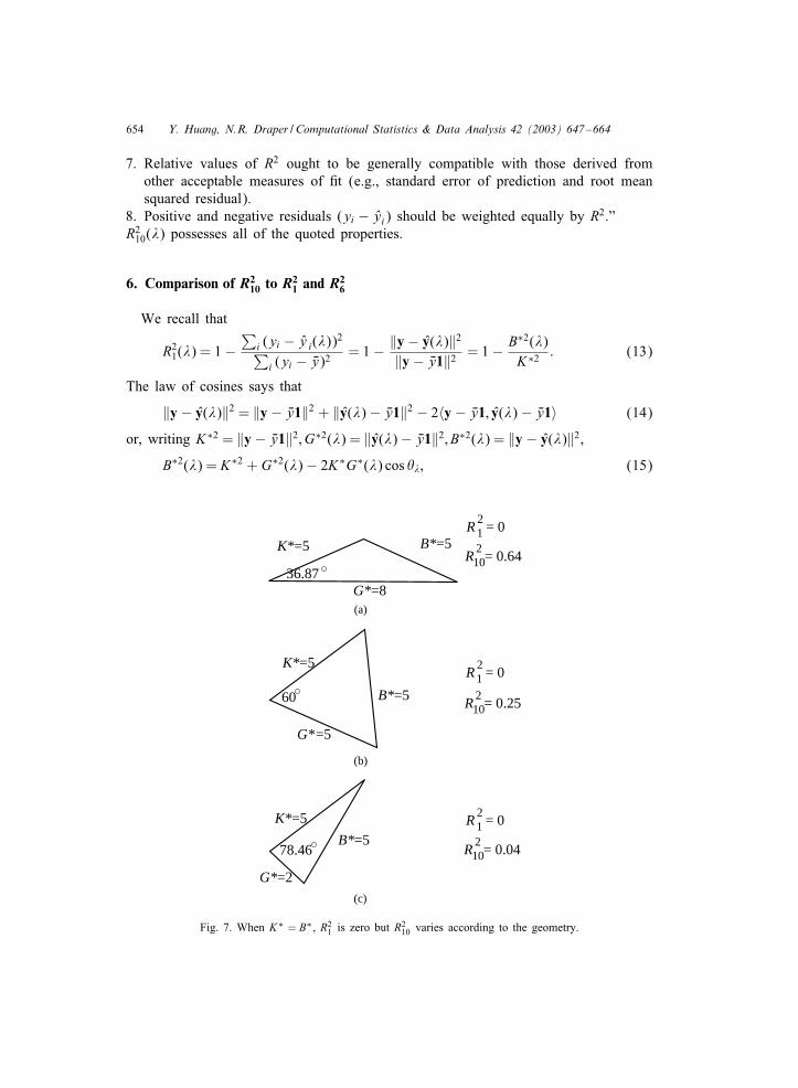
654 Y. Huang, N.R. Draper / Computational Statistics & Data Analysis 42 (2003) 647–664
7. Relative values of R2 ought to be generally compatible with those derived fromother acceptable measures of 2t (e.g., standard error of prediction and root meansquared residual).
8. Positive and negative residuals (yi − yi) should be weighted equally by R2.”R2
10(#) possesses all of the quoted properties.
6. Comparison of R210 to R2
1 and R26
We recall that
R21(#) = 1 −
∑i (yi − y i(#))2∑i (yi − Hy)2 = 1 − ‖y − y(#)‖2
‖y − Hy1‖2 = 1 − B∗2(#)K∗2 : (13)
The law of cosines says that
‖y − y(#)‖2 = ‖y − Hy1‖2 + ‖y(#) − Hy1‖2 − 2〈y − Hy1; y(#) − Hy1〉 (14)
or, writing K∗2 = ‖y − Hy1‖2; G∗2(#) = ‖y(#) − Hy1‖2; B∗2(#) = ‖y − y(#)‖2,
B∗2(#) = K∗2 + G∗2(#) − 2K∗G∗(#) cos (#; (15)
K*=5
B*=5
G*=8
B*=5
B*=5K*=5
K*=5
G*=5
G*=2
36.87
60
78.46
R21 = 0
R210= 0.64
R210= 0.25
R210= 0.04
R21 = 0
R21 = 0
(a)
(b)
(c)
Fig. 7. When K∗ = B∗, R21 is zero but R2
10 varies according to the geometry.
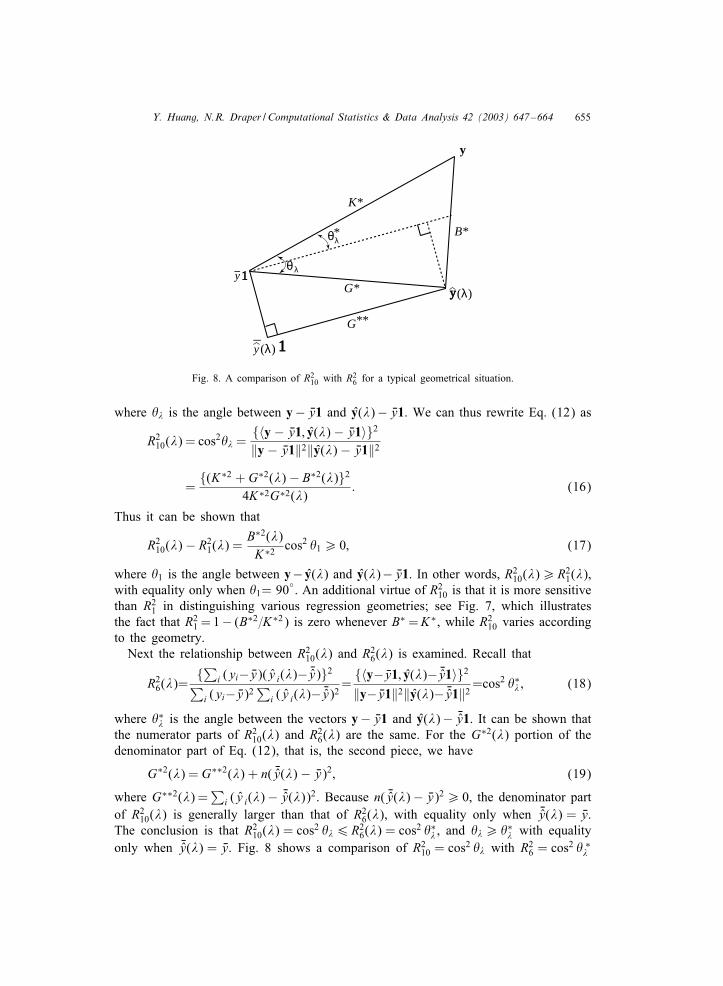
Y. Huang, N.R. Draper / Computational Statistics & Data Analysis 42 (2003) 647–664 655
K*
B*
G*
*
y
1y-
(λ)y
- (λ)
λ
λ
y 1
G**
θ
θ
Fig. 8. A comparison of R210 with R2
6 for a typical geometrical situation.
where (# is the angle between y− Hy1 and y(#)− Hy1. We can thus rewrite Eq. (12) as
R210(#) = cos2(# =
{〈y − Hy1; y(#) − Hy1〉}2
‖y − Hy1‖2‖y(#) − Hy1‖2
={(K∗2 + G∗2(#) − B∗2(#)}2
4K∗2G∗2(#): (16)
Thus it can be shown that
R210(#) − R2
1(#) =B∗2(#)K∗2 cos2 (1¿ 0; (17)
where (1 is the angle between y− y(#) and y(#)− Hy1. In other words, R210(#)¿R2
1(#),with equality only when (1= 90◦. An additional virtue of R2
10 is that it is more sensitivethan R2
1 in distinguishing various regression geometries; see Fig. 7, which illustratesthe fact that R2
1 = 1− (B∗2=K∗2) is zero whenever B∗ =K∗, while R210 varies according
to the geometry.Next the relationship between R2
10(#) and R26(#) is examined. Recall that
R26(#)=
{∑i (yi− Hy)(y i(#)− Hy)}2∑i (yi− Hy)2
∑i (y i(#)− Hy)2
={〈y− Hy1; y(#)− Hy1〉}2
‖y− Hy1‖2‖y(#)− Hy1‖2=cos2 (∗# ; (18)
where (∗# is the angle between the vectors y− Hy1 and y(#)− Hy1. It can be shown thatthe numerator parts of R2
10(#) and R26(#) are the same. For the G∗2(#) portion of the
denominator part of Eq. (12), that is, the second piece, we have
G∗2(#) = G∗∗2(#) + n( Hy(#) − Hy)2; (19)
where G∗∗2(#) =∑
i (y i(#) − Hy(#))2. Because n( Hy(#) − Hy)2¿ 0, the denominator partof R2
10(#) is generally larger than that of R26(#), with equality only when Hy(#) = Hy.
The conclusion is that R210(#) = cos2 (#6R2
6(#) = cos2 (∗# , and (#¿ (∗# with equalityonly when Hy(#) = Hy. Fig. 8 shows a comparison of R2
10 = cos2 (# with R26 = cos2 ( ∗
#
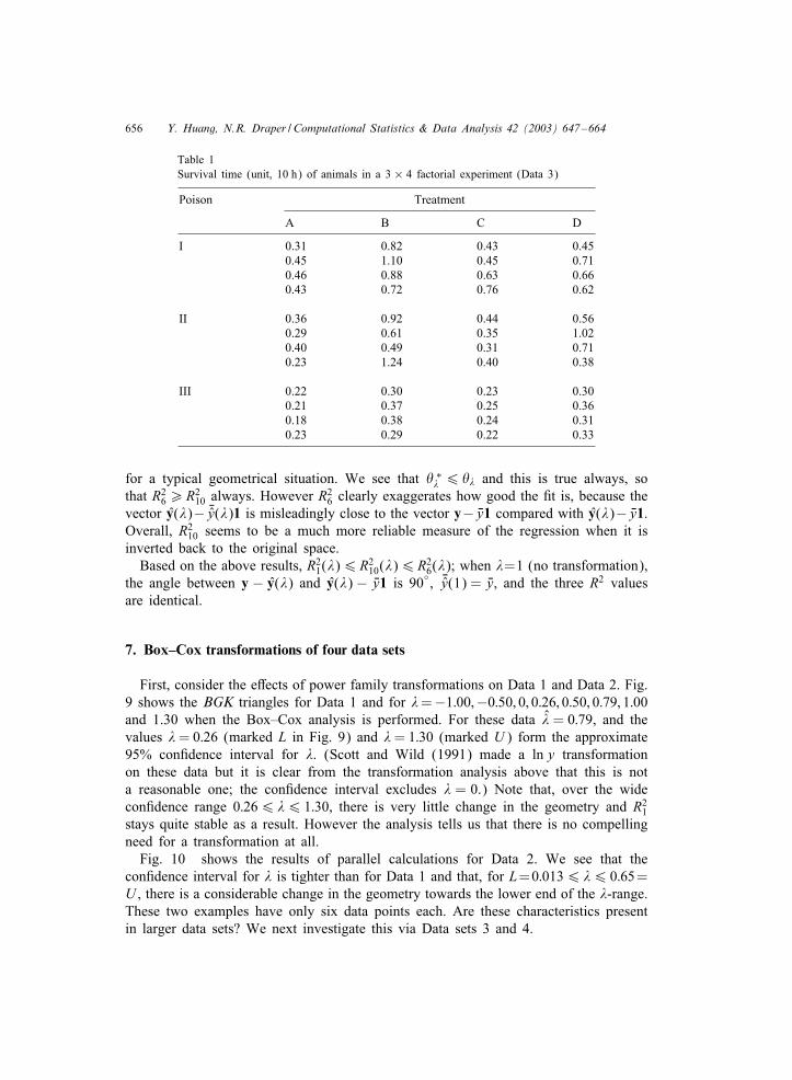
656 Y. Huang, N.R. Draper / Computational Statistics & Data Analysis 42 (2003) 647–664
Table 1Survival time (unit, 10 h) of animals in a 3 × 4 factorial experiment (Data 3)
Poison Treatment
A B C D
I 0.31 0.82 0.43 0.450.45 1.10 0.45 0.710.46 0.88 0.63 0.660.43 0.72 0.76 0.62
II 0.36 0.92 0.44 0.560.29 0.61 0.35 1.020.40 0.49 0.31 0.710.23 1.24 0.40 0.38
III 0.22 0.30 0.23 0.300.21 0.37 0.25 0.360.18 0.38 0.24 0.310.23 0.29 0.22 0.33
for a typical geometrical situation. We see that ( ∗# 6 (# and this is true always, so
that R26¿R2
10 always. However R26 clearly exaggerates how good the 2t is, because the
vector y(#)− Hy(#)1 is misleadingly close to the vector y− Hy1 compared with y(#)− Hy1.Overall, R2
10 seems to be a much more reliable measure of the regression when it isinverted back to the original space.
Based on the above results, R21(#)6R2
10(#)6R26(#); when #=1 (no transformation),
the angle between y − y(#) and y(#) − Hy1 is 90◦, Hy(1) = Hy, and the three R2 valuesare identical.
7. Box–Cox transformations of four data sets
First, consider the eJects of power family transformations on Data 1 and Data 2. Fig.9 shows the BGK triangles for Data 1 and for #=−1:00;−0:50; 0; 0:26; 0:50; 0:79; 1:00and 1.30 when the Box–Cox analysis is performed. For these data # = 0:79, and thevalues # = 0:26 (marked L in Fig. 9) and # = 1:30 (marked U ) form the approximate95% con2dence interval for #. (Scott and Wild (1991) made a ln y transformationon these data but it is clear from the transformation analysis above that this is nota reasonable one; the con2dence interval excludes # = 0.) Note that, over the widecon2dence range 0:266 #6 1:30, there is very little change in the geometry and R2
1stays quite stable as a result. However the analysis tells us that there is no compellingneed for a transformation at all.
Fig. 10 shows the results of parallel calculations for Data 2. We see that thecon2dence interval for # is tighter than for Data 1 and that, for L=0:0136 #6 0:65=U , there is a considerable change in the geometry towards the lower end of the #-range.These two examples have only six data points each. Are these characteristics presentin larger data sets? We next investigate this via Data sets 3 and 4.
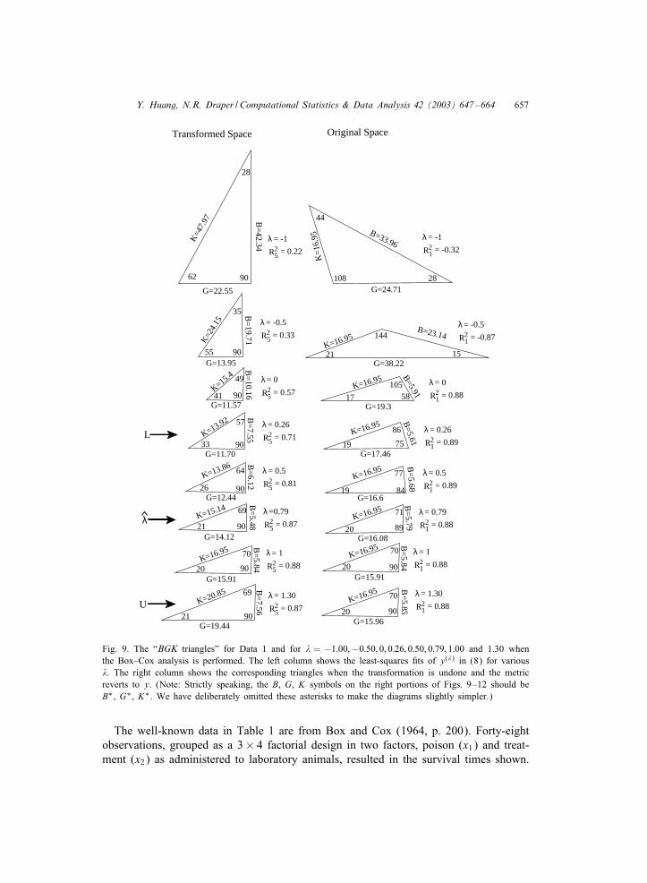
Y. Huang, N.R. Draper / Computational Statistics & Data Analysis 42 (2003) 647–664 657
G=24.71
B=33.96
K=1
6.95
108 28
44
G=38.22
B=23.14K=16.95
21
144
15
G=19.3
B=5.91
K=16.95
17 58105
G=16.6
B=
5.68
K=16.95
19 84
G=15.91
B=
5.84
K=16.95
20
70
90
77
G=17.46
B=5.61
K=16.95
K=16.95
B=
5.79
K=16.95
G=16.08
G=15.96
B=
5.85
75
89
19
86
20
71
20
70
90
9041B
=5.48
69
G=15.91
90
70
90K=16.95
20
21G=14.12
B=
5.84
K=13.92
K=15.14
90
64
G=12.4426
K=13.86 B=
6.12
57
G=11.7090
G=11.57
33
B=
7.55B
=19.71
49
90G=13.95
K=15.4
55
B=
10.16
35
90
G=22.55
K=2
4.15
62
K=4
7.97 B
=42.34
λ = -1
= 0.22R25
K=20.85
G=19.4421 90
B=
7.56
69
L
U
28
λ = -0.5
= 0.33R25
λ = 0
= 0.57R25
λ = 0.26
= 0.71R25
λ = 0.5
= 0.81R25
λ =0.79
= 0.87R25
λ = 1
= 0.88R25
λ = 1.30
= 0.87R25
λ = 1.30
= 0.88R21
λ
λ = 1
= 0.88R21
λ = 0.79
= 0.88R21
λ = 0.5
= 0.89R21
λ = 0.26
= 0.89R21
λ = 0
= 0.88R21
λ = -0.5
= -0.87R21
λ = -1
= -0.32R21
Transformed Space Original Space
Fig. 9. The “BGK triangles” for Data 1 and for # = −1:00;−0:50; 0; 0:26; 0:50; 0:79; 1:00 and 1.30 whenthe Box–Cox analysis is performed. The left column shows the least-squares 2ts of y(#) in (8) for various#. The right column shows the corresponding triangles when the transformation is undone and the metricreverts to y. (Note: Strictly speaking, the B, G, K symbols on the right portions of Figs. 9–12 should beB∗, G∗, K∗. We have deliberately omitted these asterisks to make the diagrams slightly simpler.)
The well-known data in Table 1 are from Box and Cox (1964, p. 200). Forty-eightobservations, grouped as a 3× 4 factorial design in two factors, poison (x1) and treat-ment (x2) as administered to laboratory animals, resulted in the survival times shown.
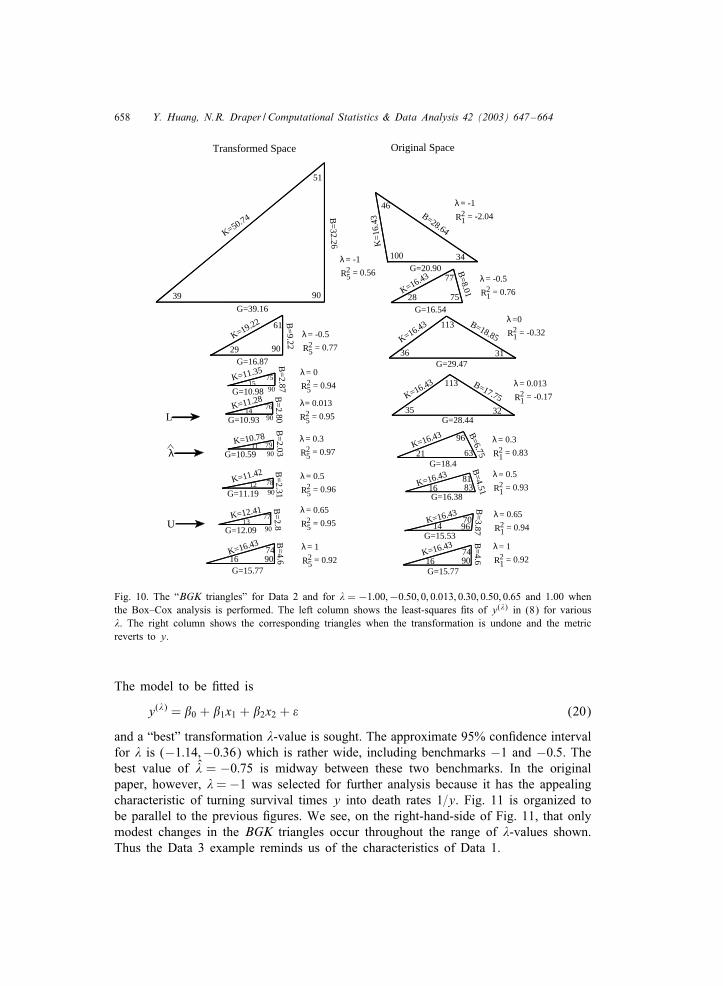
658 Y. Huang, N.R. Draper / Computational Statistics & Data Analysis 42 (2003) 647–664
K=
16.4
3
G=20.90
B=28.64
100 34
46
G=16.54
B=8.01K=16.43
28 75
G=29.47
B=18.85K=16.43
36
113
31
G=16.38
B=4.51
K=16.43
16 8381
G=15.77
B=
4.6
K=16.43
167490
77
G=10.93
76
79G=10.59
G=11.197890
77
9074
90
75
G=10.98
90
61
51
K=16.43
G=15.7716
G=12.09
K=12.4113
90
12K=11.42
1190
K=10.78
K=11.28
9014
G=16.87
K=11.3515
29
39
K=19.22
G=39.16
90
K=50.74
B=
9.22B
=4.6
B=
2.8B
=2.31
B=
2.03B
=2.80
B=
2.87
B=
32.26
L
U
λ
λ = -1
= 0.56R25
λ = -1
= -2.04R21
λ = -0.5
= 0.77R25
λ = 0
= 0.94R25
λ= 0.013
= 0.95R25
λ = 0.3
= 0.97R25
λ = 0.5
= 0.96R25
λ = 0.65
= 0.95R25
λ = 1
= 0.92R25
113
35 32
B=17.75K=16.43
G=28.44
K=16.43
K=16.43G=18.4
B=6.7521
96
63
147096
B=
3.87
G=15.53
λ = -0.5
= 0.76R21
λ =0
= -0.32R21
λ = 0.013
= -0.17R21
λ = 0.3
= 0.83R21
λ = 0.5
= 0.93R21
λ = 0.65
= 0.94R21
λ = 1
= 0.92R21
Transformed Space Original Space
Fig. 10. The “BGK triangles” for Data 2 and for # = −1:00;−0:50; 0; 0:013; 0:30; 0:50; 0:65 and 1.00 whenthe Box–Cox analysis is performed. The left column shows the least-squares 2ts of y(#) in (8) for various#. The right column shows the corresponding triangles when the transformation is undone and the metricreverts to y.
The model to be 2tted is
y(#) = �0 + �1x1 + �2x2 + � (20)
and a “best” transformation #-value is sought. The approximate 95% con2dence intervalfor # is (−1:14;−0:36) which is rather wide, including benchmarks −1 and −0:5. Thebest value of # = −0:75 is midway between these two benchmarks. In the originalpaper, however, # = −1 was selected for further analysis because it has the appealingcharacteristic of turning survival times y into death rates 1=y. Fig. 11 is organized tobe parallel to the previous 2gures. We see, on the right-hand-side of Fig. 11, that onlymodest changes in the BGK triangles occur throughout the range of #-values shown.Thus the Data 3 example reminds us of the characteristics of Data 1.
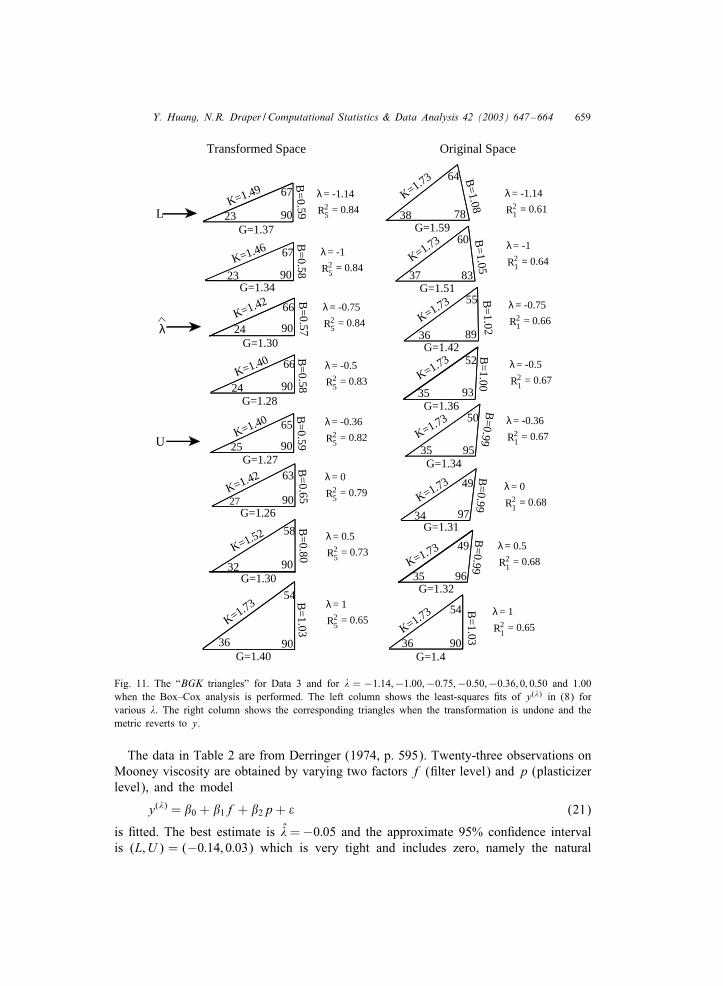
Y. Huang, N.R. Draper / Computational Statistics & Data Analysis 42 (2003) 647–664 659
B=1.05
G=1.51
K=1.73
37
60
83
B=
1.00
G=1.36
K=1.73
35
52
93
B=
0.99
G=1.31
K=1.73
34
49
97
B=
0.99
G=1.32
K=1.73
35
49
96
B=
1.03
G=1.4
K=1.73
36
54
90
38
64
78
55
36 89
35
50
95
B=1.08
K=1.73
G=1.59B
=1.02
K=1.73
G=1.42
B=0.99K=1.73
G=1.34
24 90
G=1.26
K=1.73
36G=1.40
90
B=
1.03
32G=1.30
K=1.52
90
54
B=
0.80
58
B=
0.59K=1.40
G=1.27
27K=1.42
25
63
B=
0.6590
90
K=1.40
24G=1.28
G=1.30
B=
0.5865
90
66
23
K=1.42G=1.34
K=1.46
G=1.37
90
B=
0.57
66
B=
0.58
67
23K=1.49
B=
0.5990
67
L
U
λ = -1.14
= 0.84R25
λ = -1.14
= 0.61R21
λ = -1
= 0.84R25
λ = -0.75
= 0.84R25
λ = -0.5
= 0.83R25
λ = -0.36
= 0.82R25
λ = 0
= 0.79R25
λ = 0.5
= 0.73R25
λ = 1
= 0.65R25
λ = -1
= 0.64R21
λ = -0.75
= 0.66R21
λ = -0.5
= 0.67R21
λ = -0.36
= 0.67R21
λ = 0
= 0.68R21
λ = 0.5
= 0.68R21
λ = 1
= 0.65R21
λ
Transformed Space Original Space
Fig. 11. The “BGK triangles” for Data 3 and for # = −1:14;−1:00;−0:75;−0:50;−0:36; 0; 0:50 and 1.00when the Box–Cox analysis is performed. The left column shows the least-squares 2ts of y(#) in (8) forvarious #. The right column shows the corresponding triangles when the transformation is undone and themetric reverts to y.
The data in Table 2 are from Derringer (1974, p. 595). Twenty-three observations onMooney viscosity are obtained by varying two factors f (2lter level) and p (plasticizerlevel), and the model
y(#) = �0 + �1f + �2p + � (21)
is 2tted. The best estimate is # = −0:05 and the approximate 95% con2dence intervalis (L; U ) = (−0:14; 0:03) which is very tight and includes zero, namely the natural
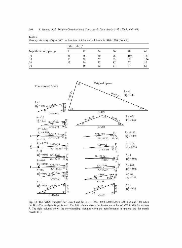
660 Y. Huang, N.R. Draper / Computational Statistics & Data Analysis 42 (2003) 647–664
Table 2Mooney viscosity MS4 at 100
◦as function of 2ller and oil levels in SBR-1500 (Data 4)
Filler, phr, f
Naphthenic oil, phr, p 0 12 24 36 48 60
0 26 38 50 76 108 15710 17 26 37 53 83 12420 13 20 27 37 57 8730 — 15 22 27 41 63
K=1
77.9
4
G=469
B=451.8
73
K=177.94 B=132.1
G=284
132
20
K=177.94
B=11.6G=175 104
4
K=177.94
B=37.5
G=158
K=177.94
B=
61.8
11
G=16720
B=
12.23G=178.59
K=177.944 91
85
72
53116
70
90
28
22
85
G=186.76
B=19.17
K=177.94
K=177.94
B=12.42G=172.74
4 63113
5 115
60
B=
9.12B
=9.45
B=
29.41B
=61.81
G=166.86
K=147.21
K=177.94
20 90
70
12G=144.24
9078
90G=135.19
K=135.554
B=
9.92
86
904
G=134.96
K=135.2986
4G=134.39
4K=134.96
G=134.658690
90
K=134.75
B=
9.92
86
K=157.41
G=149.4118
10G=136.73
K=138.69
90
B=
23.23
80
B=
49.5590
72
L
U
λ = -1
= 0.90R25
λ = -1
= 0.45R21
λ
λ = -0.5
= 0.97R25
λ = -0.135
= 0.995R25
λ = -0.05
= 0.995R25
λ = 0
= 0.995R25
λ = 0.03
= 0.995R25
λ = 0.5
= 0.96R25
λ = 1
= 0.88R25
λ= -0.5
= 0.45R21
λ = -0.135
= 0.988R21
λ = -0.05
= 0.995R21
λ = 0
= 0.996R21
λ = 0.03
= 0.995R21
λ = 0.5
= 0.96R21
λ = 1
= 0.88R21
Transformed SpaceOriginal Space
Fig. 12. The “BGK triangles” for Data 4 and for # = −1:00;−0:50; 0; 0:013; 0:30; 0:50; 0:65 and 1.00 whenthe Box–Cox analysis is performed. The left column shows the least-squares 2ts of y(#) in (8) for various#. The right column shows the corresponding triangles when the transformation is undone and the metricreverts to y.
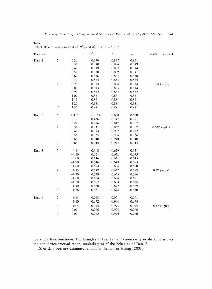
Y. Huang, N.R. Draper / Computational Statistics & Data Analysis 42 (2003) 647–664 661
Table 3Data 1–Data 4: comparisons of R2
1; R210, and R2
6, when # = L; #; U
Data set # R21 R2
10 R26 Width of interval
Data 1 L 0.26 0.890 0.897 0.9010.30 0.890 0.896 0.8990.40 0.889 0.892 0.8940.50 0.888 0.889 0.8910.60 0.886 0.887 0.8880.70 0.885 0.885 0.885
# 0.79 0.883 0.884 0.884 1.04 (wide)0.80 0.883 0.883 0.8840.90 0.882 0.882 0.8821.00 0.881 0.881 0.8811.10 0.881 0.881 0.8811.20 0.881 0.881 0.881
U 1.30 0.881 0.881 0.881
Data 2 L 0.013 −0:168 0.668 0.6780.10 0.426 0.747 0.7510.20 0.706 0.817 0.817
# 0.30 0.831 0.867 0.867 0.637 (tight)0.40 0.893 0.902 0.9020.50 0.925 0.926 0.9260.60 0.940 0.940 0.940
U 0.65 0.944 0.945 0.945
Data 3 L −1:14 0.613 0.629 0.631−1:10 0.621 0.632 0.635−1:00 0.636 0.641 0.645−0:90 0.646 0.648 0.653−0:80 0.654 0.654 0.660
# −0:75 0.657 0.657 0.663 0.78 (wide)−0:70 0.659 0.659 0.666−0:60 0.664 0.664 0.671−0:50 0.667 0.668 0.675−0:40 0.670 0.672 0.679
U −0:36 0.671 0.674 0.680
Data 4 L −0:14 0.988 0.991 0.991−0:10 0.992 0.994 0.994
# −0:05 0.995 0.995 0.995 0.17 (tight)0.00 0.996 0.996 0.996
U 0.03 0.995 0.996 0.996
logarithm transformation. The triangles in Fig. 12 vary enormously in shape even overthe con2dence interval range, reminding us of the behavior of Data 2.
Other data sets are examined in similar fashion in Huang (2001).
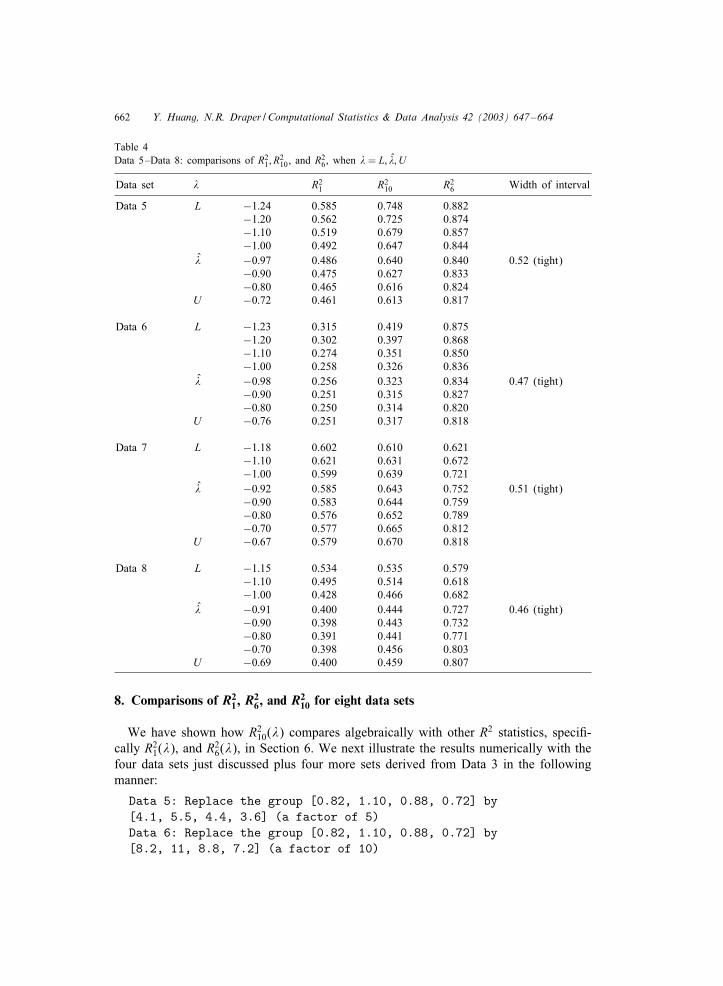
662 Y. Huang, N.R. Draper / Computational Statistics & Data Analysis 42 (2003) 647–664
Table 4Data 5–Data 8: comparisons of R2
1; R210, and R2
6, when # = L; #; U
Data set # R21 R2
10 R26 Width of interval
Data 5 L −1:24 0.585 0.748 0.882−1:20 0.562 0.725 0.874−1:10 0.519 0.679 0.857−1:00 0.492 0.647 0.844
# −0:97 0.486 0.640 0.840 0.52 (tight)−0:90 0.475 0.627 0.833−0:80 0.465 0.616 0.824
U −0:72 0.461 0.613 0.817
Data 6 L −1:23 0.315 0.419 0.875−1:20 0.302 0.397 0.868−1:10 0.274 0.351 0.850−1:00 0.258 0.326 0.836
# −0:98 0.256 0.323 0.834 0.47 (tight)−0:90 0.251 0.315 0.827−0:80 0.250 0.314 0.820
U −0:76 0.251 0.317 0.818
Data 7 L −1:18 0.602 0.610 0.621−1:10 0.621 0.631 0.672−1:00 0.599 0.639 0.721
# −0:92 0.585 0.643 0.752 0.51 (tight)−0:90 0.583 0.644 0.759−0:80 0.576 0.652 0.789−0:70 0.577 0.665 0.812
U −0:67 0.579 0.670 0.818
Data 8 L −1:15 0.534 0.535 0.579−1:10 0.495 0.514 0.618−1:00 0.428 0.466 0.682
# −0:91 0.400 0.444 0.727 0.46 (tight)−0:90 0.398 0.443 0.732−0:80 0.391 0.441 0.771−0:70 0.398 0.456 0.803
U −0:69 0.400 0.459 0.807
8. Comparisons of R21, R
26, and R2
10 for eight data sets
We have shown how R210(#) compares algebraically with other R2 statistics, speci2-
cally R21(#), and R2
6(#), in Section 6. We next illustrate the results numerically with thefour data sets just discussed plus four more sets derived from Data 3 in the followingmanner:
Data 5: Replace the group [0.82, 1.10, 0.88, 0.72] by[4.1, 5.5, 4.4, 3.6] (a factor of 5)Data 6: Replace the group [0.82, 1.10, 0.88, 0.72] by[8.2, 11, 8.8, 7.2] (a factor of 10)
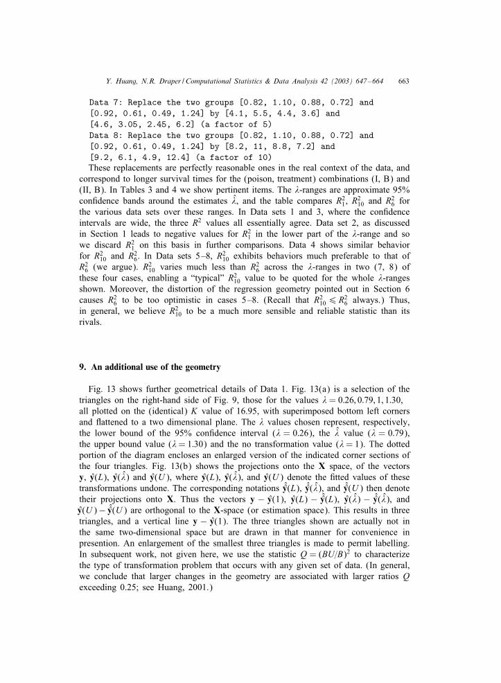
Y. Huang, N.R. Draper / Computational Statistics & Data Analysis 42 (2003) 647–664 663
Data 7: Replace the two groups [0.82, 1.10, 0.88, 0.72] and[0.92, 0.61, 0.49, 1.24] by [4.1, 5.5, 4.4, 3.6] and[4.6, 3.05, 2.45, 6.2] (a factor of 5)Data 8: Replace the two groups [0.82, 1.10, 0.88, 0.72] and[0.92, 0.61, 0.49, 1.24] by [8.2, 11, 8.8, 7.2] and[9.2, 6.1, 4.9, 12.4] (a factor of 10)These replacements are perfectly reasonable ones in the real context of the data, and
correspond to longer survival times for the (poison, treatment) combinations (I, B) and(II, B). In Tables 3 and 4 we show pertinent items. The #-ranges are approximate 95%con2dence bands around the estimates #, and the table compares R2
1, R210 and R2
6 forthe various data sets over these ranges. In Data sets 1 and 3, where the con2denceintervals are wide, the three R2 values all essentially agree. Data set 2, as discussedin Section 1 leads to negative values for R2
1 in the lower part of the #-range and sowe discard R2
1 on this basis in further comparisons. Data 4 shows similar behaviorfor R2
10 and R26. In Data sets 5–8, R2
10 exhibits behaviors much preferable to that ofR2
6 (we argue). R210 varies much less than R2
6 across the #-ranges in two (7, 8) ofthese four cases, enabling a “typical” R2
10 value to be quoted for the whole #-rangesshown. Moreover, the distortion of the regression geometry pointed out in Section 6causes R2
6 to be too optimistic in cases 5–8. (Recall that R2106R2
6 always.) Thus,in general, we believe R2
10 to be a much more sensible and reliable statistic than itsrivals.
9. An additional use of the geometry
Fig. 13 shows further geometrical details of Data 1. Fig. 13(a) is a selection of thetriangles on the right-hand side of Fig. 9, those for the values # = 0:26; 0:79; 1; 1:30,all plotted on the (identical) K value of 16.95, with superimposed bottom left cornersand Rattened to a two dimensional plane. The # values chosen represent, respectively,the lower bound of the 95% con2dence interval (# = 0:26), the # value (# = 0:79),the upper bound value (#= 1:30) and the no transformation value (#= 1). The dottedportion of the diagram encloses an enlarged version of the indicated corner sections ofthe four triangles. Fig. 13(b) shows the projections onto the X space, of the vectorsy, y(L), y(#) and y(U ), where y(L), y(#), and y(U ) denote the 2tted values of thesetransformations undone. The corresponding notations ˆy(L), ˆy(#), and ˆy(U ) then denotetheir projections onto X. Thus the vectors y − y(1), y(L) − ˆy(L), y(#) − ˆy(#), andy(U )− ˆy(U ) are orthogonal to the X-space (or estimation space). This results in threetriangles, and a vertical line y − y(1). The three triangles shown are actually not inthe same two-dimensional space but are drawn in that manner for convenience inpresention. An enlargement of the smallest three triangles is made to permit labelling.In subsequent work, not given here, we use the statistic Q = (BU=B)2 to characterizethe type of transformation problem that occurs with any given set of data. (In general,we conclude that larger changes in the geometry are associated with larger ratios Qexceeding 0.25; see Huang, 2001.)
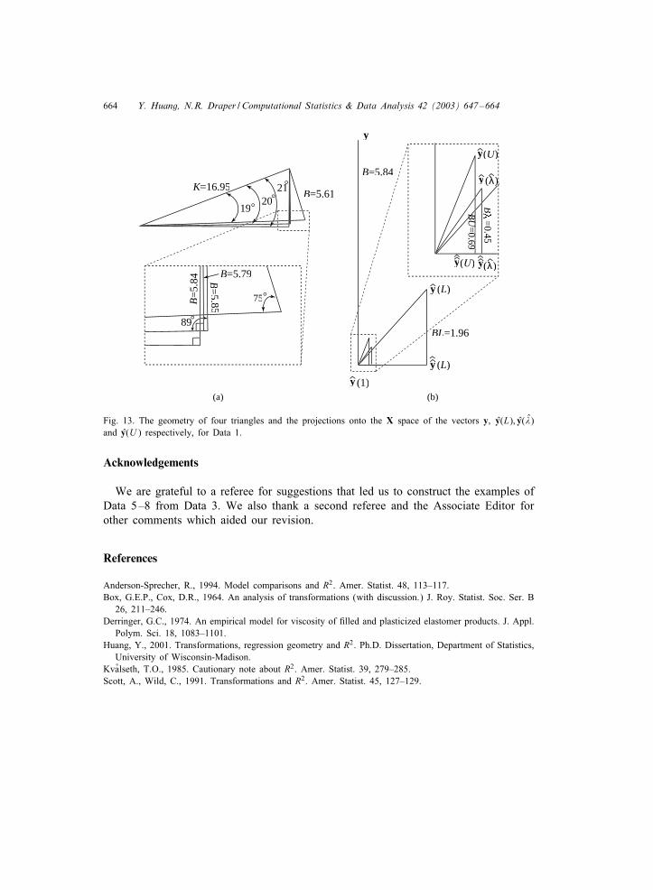
664 Y. Huang, N.R. Draper / Computational Statistics & Data Analysis 42 (2003) 647–664
K=16.95K=16.95KB=5.61
y
y
75
2120
19
89
B=
5.84
B=5.79B=
5.85
B=5.84
BL=1.96
BU
BBU
=0.690
69U
=0.69
UU
(a) (b)
(1)
y (L)
y (L)
y(U)U)U
y( ))
y (λλ))
B
=0.45
λ λ
(λλ)
Fig. 13. The geometry of four triangles and the projections onto the X space of the vectors y; y(L); y(#)and y(U ) respectively, for Data 1.
Acknowledgements
We are grateful to a referee for suggestions that led us to construct the examples ofData 5–8 from Data 3. We also thank a second referee and the Associate Editor forother comments which aided our revision.
References
Anderson-Sprecher, R., 1994. Model comparisons and R2. Amer. Statist. 48, 113–117.Box, G.E.P., Cox, D.R., 1964. An analysis of transformations (with discussion.) J. Roy. Statist. Soc. Ser. B
26, 211–246.Derringer, G.C., 1974. An empirical model for viscosity of 2lled and plasticized elastomer products. J. Appl.
Polym. Sci. 18, 1083–1101.Huang, Y., 2001. Transformations, regression geometry and R2. Ph.D. Dissertation, Department of Statistics,
University of Wisconsin-Madison.Kv6alseth, T.O., 1985. Cautionary note about R2. Amer. Statist. 39, 279–285.Scott, A., Wild, C., 1991. Transformations and R2. Amer. Statist. 45, 127–129.
The Statistician (2002) 51, Part 1, pp. 99-104
A new angle on the t-test
Graham R. Wood
Massey University, Palmerston North, New Zealand
and David J. Saville
AgResearch, Lincoln, New Zealand
[Received December 2000. Final revision December 2001]
Summary. R. A. Fisher's early work on linear models relied heavily on his knowledge of n-dimensional geometry. To illustrate this, we present an elementary, complete, modern day account of Fisher's geometric approach for the simple case of a paired samples t-test for a sample size of 3. A natural consequence of this approach is a surprisingly simple and explicit expression for the p-value.
Keywords: Linear algebra; Paired samples t-test; p-value; Vector geometry
1. Introduction
R. A. Fisher's early work on linear models relied heavily on his knowledge of n-dimensional geometry (Box (1978), pages 122-129). Unfortunately his geometric approach was not under- stood by most of his colleagues, partly because of his tendency to 'let too much be clear or obvious', to quote the words of his colleague Gosset, better known to statisticians as 'Student' (Box (1978), page 122). Because of this difficulty, Fisher derived an algebraic approach which was more universally accepted (Fisher (1925) and Box (1978), page 129). In this paper we provide an elementary, complete, modern day account of Fisher's geometric approach for the simple case of a paired samples t-test for a sample size of n = 3. Surprising insights into the theory of linear models can be gained by working through this simple example.
2. Paired samples t-test for n = 3
For a paired samples data set we use the heights of males M and females F in three mixed sex twin pairs of adult humans, from Saville and Wood (1996). In the first twin pair, John's height was 185 cm whereas Janet's height was 166 cm (the data are real, but all names are falsified). In the second twin pair, Alistair's height was 185.4 cm whereas Joanna's was 177.8 cm. In the third twin pair, Bill's height was 182.9 cm whereas Mary's was 160 cm. The three differences in height (M - F) are 19.0, 7.6 and 22.9 cm. We treat these three differences as a sample of size n = 3 drawn independently from a single normally distributed population N(A, a2), consisting of differences in height between the male and female in mixed sex twin pairs of adult humans.
Address for correspondence: David J. Saville, Statistics Group, AgResearch, PO Box 60, Lincoln, Canterbury, New Zealand. E-mail: [email protected]
? 2002 Royal Statistical Society 0039-0526/02/51099
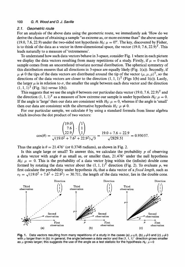
100 G. R. Wood and D. J. Saville
2.1. Geometric route For an analysis of the above data using the geometric route, we immediately ask 'How do we derive the chance of obtaining a sample "as extreme as, or more extreme than" the above sample (19.0, 7.6, 22.9) under the two-sided test hypothesis Ho: p = 0?'. The key, discovered by Fisher, is to think of the data as a vector in three-dimensional space, the vector (19.0, 7.6, 22.9)T. This leads naturally to a measure of 'extremeness'.
To understand how such data vectors behave in 3-space, consider Fig. 1 where in each picture we display the data vectors resulting from many repetitions of a study. Firstly, if p, = 0 each sample comes from an uncorrelated trivariate normal distribution. The spherical symmetry of this distribution ensures that all directions in 3-space are equally likely (Fig. 1(a)). Secondly, if pu % 0 the tips of the data vectors are distributed around the tip of the vector (/, /,, ,/)T, so the directions of the data vectors are closer to the direction (1, 1, 1)T (Figs l(b) and l(c)). Lastly, the larger p is in relation to a, the smaller the angle between each data vector and the direction (1, 1, 1)T (Fig. l(c) versus l(b)).
This suggests that we use the angle 0 between our particular data vector (19.0, 7.6, 22.9)T and the direction (1, 1, 1)T as a measure of how extreme our sample is under hypothesis Ho: /i = 0. If the angle is 'large' then our data are consistent with Ho: ,u = 0, whereas if the angle is 'small' then our data are consistent with the alternative hypothesis H1: ,L : 0.
For our particular sample, we calculate 0 by using a standard formula from linear algebra which involves the dot product of two vectors:
/19.0\ (1\ 7.61. 1
\22.9 1/ 19.0 + 7.6 + 22.9 = 0.93057 cos() = = 0.930 57. ( (19.02 + 7.62 + 22.92) 3 = 2829.51
Thus the angle is 0 = 21.476? (or 0.3748 radians), as shown in Fig. 2. Is this angle large or small? To answer this, we calculate the probability p of observing
a data vector with angle 0 as small as, or smaller than, 21.476? under the null hypothesis Ho: , = 0. This is the probability of a data vector lying within the (infinite) double cone formed by rotating the data vector about the (1, 1, 1)T direction (Fig. 2). To evaluate p, we first calculate the probability under hypothesis Ho that a data vector of a fixed length, such as ro = /(19.02 + 7.62 + 22.92) = 30.711, the length of the data vector, lies in the double cone.
Direction Direction Direction
Third Third Third o vservation observation ri
- " Second Second Second observation observation observation
^^ 1 First First First observation observation observation
(a) (b) (c)
Fig. 1. Data vectors resulting from many repetitions of a study in the cases (a) -u=O, (b) t/0 and (c) 0UO with / larger than in (b): in general, the angle between a data vector and the (1,1, 1)T direction grows smaller as [t grows larger; this suggests the use of the angle as a test statistic for the hypothesis Ho: / = 0
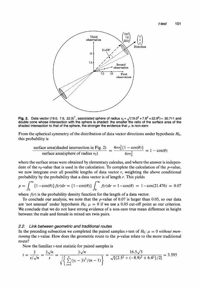
t-test 101
Fig. 2. Data vector (19.0, 7.6, 22.9)T, associated sphere of radius ro = V(19.02 + 7.62 + 22.92) = 30.711 and double cone whose intersection with the sphere is shaded: the smaller the ratio of the surface area of the shaded intersection to that of the sphere, the stronger the evidence that , is non-zero
From the spherical symmetry of the distribution of data vector directions under hypothesis Ho, this probability is
surface area(shaded intersection in Fig. 2) 47rrr2{ 1 - cos(O)} 0 1 - cos(O) surface area(sphere of radius ro) 47rr 2
where the surface areas were obtained by elementary calculus, and where the answer is indepen- dent of the ro-value that is used in the calculation. To complete the calculation of the p-value, we now integrate over all possible lengths of data vector r, weighting the above conditional probability by the probability that a data vector is of length r. This yields
p= / {l-cos(O)}f(r)dr = {1 -cos(O)} / f(r)dr = 1-cos(O) = 1-cos(21.476) = 0.07
where f(r) is the probability density function for the length of a data vector. To conclude our analysis, we note that the p-value of 0.07 is larger than 0.05, so our data
are 'not unusual' under hypothesis Ho: ,u = O if we use a 0.05 cut-off point as our criterion. We conclude that we do not have strong evidence of a non-zero true mean difference in height between the male and female in mixed sex twin pairs.
2.2. Link between geometric and traditional routes In the preceding subsection we completed the paired samples t-test of Ho: ,u = 0 without men- tioning the t-value. How does the geometric route to the p-value relate to the more traditional route?
Now the familiar t-test statistic for paired samples is
3 _ y-n _ yn 16.53 395
s/v/n s n = { (yi - )2/(n-l)} / [{2.52 + (-8.9)2 + 6.42}/2]
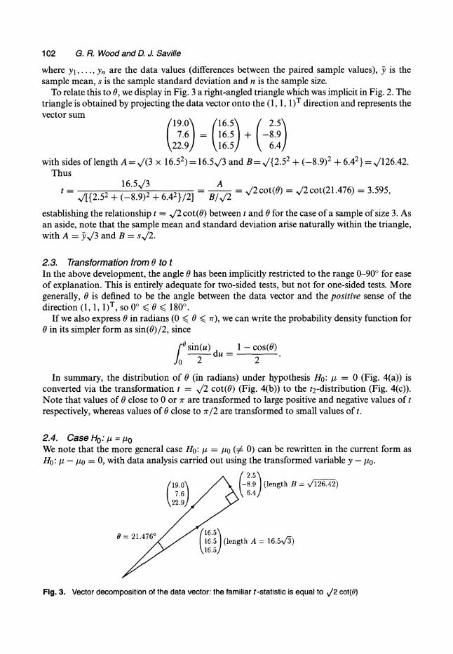
102 G. R. Wood and D. J. Saville
where y ,..., Yn are the data values (differences between the paired sample values), y is the sample mean, s is the sample standard deviation and n is the sample size.
To relate this to 0, we display in Fig. 3 a right-angled triangle which was implicit in Fig. 2. The triangle is obtained by projecting the data vector onto the (1, 1, 1)T direction and represents the vector sum
(19.0\ (16.5\ / 2.5\ 7.6 = 16.5 + -8.9
\22.91 16.51 6.4/ with sides of length A = /(3 x 16.52) = 16.5V3 and B =V /{2.52 + (-8.9)2 + 6.42}= V126.42.
Thus 16.5,/3 A =
/[{2.52 + (-8.9)2 + 6.42}/2] -
B/ = /2cot(0) = V/2cot(21.476) = 3.595,
establishing the relationship t = ,/2 cot(0) between t and 0 for the case of a sample of size 3. As an aside, note that the sample mean and standard deviation arise naturally within the triangle, with A = y5/3 and B = sV/2.
2.3. Transformation from 0 to t In the above development, the angle 0 has been implicitly restricted to the range 0-90? for ease of explanation. This is entirely adequate for two-sided tests, but not for one-sided tests. More generally, 0 is defined to be the angle between the data vector and the positive sense of the direction (1, 1, 1)T, so 0? < 0 < 180?.
If we also express 0 in radians (0 < 0 < 7r), we can write the probability density function for 0 in its simpler form as sin(0)/2, since
0 sin(u) 1 - cos(9) 2 du 2 Jo 2 2
In summary, the distribution of 0 (in radians) under hypothesis Ho: ,F = 0 (Fig. 4(a)) is converted via the transformation t = >/2 cot(0) (Fig. 4(b)) to the t2-distribution (Fig. 4(c)). Note that values of 0 close to 0 or rT are transformed to large positive and negative values of t respectively, whereas values of 0 close to 7r/2 are transformed to small values of t.
2.4. Case Ho: i = to We note that the more general case Ho: ,t = Ito (A 0) can be rewritten in the current form as Ho: p - po = 0, with data analysis carried out using the transformed variable y - to.
2.5\ (/19.0\ /) (-8.9 (length B = V126.42)
\22.9/y
0 = 21.476 /16.5 I16.5 (length A = 16.5v3)
16.5/
Fig. 3. Vector decomposition of the data vector: the familiar t-statistic is equal to V2 cot(O)
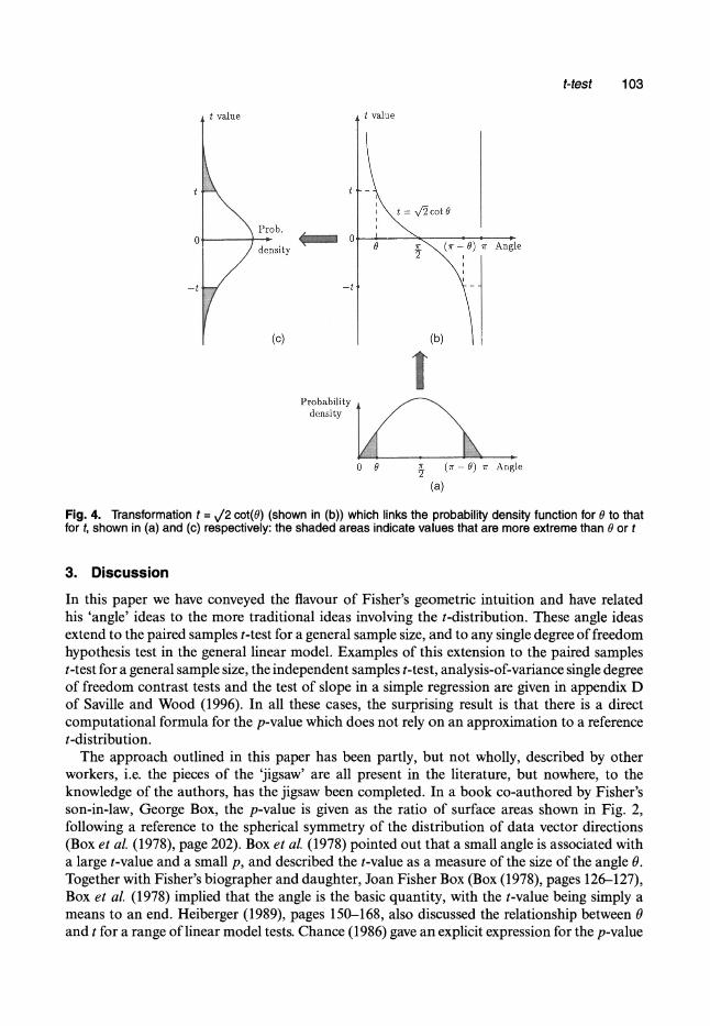
t-test 103
t value t value
Angle
-t
(c) (b)
1 Probability
density
0 0 7 (7r-0) 7r Angle
(a)
Fig. 4. Transformation t = /2 cot(O) (shown in (b)) which links the probability density function for 0 to that for t, shown in (a) and (c) respectively: the shaded areas indicate values that are more extreme than 0 or t
3. Discussion
In this paper we have conveyed the flavour of Fisher's geometric intuition and have related his 'angle' ideas to the more traditional ideas involving the t-distribution. These angle ideas extend to the paired samples t-test for a general sample size, and to any single degree of freedom hypothesis test in the general linear model. Examples of this extension to the paired samples t-test for a general sample size, the independent samples t-test, analysis-of-variance single degree of freedom contrast tests and the test of slope in a simple regression are given in appendix D of Saville and Wood (1996). In all these cases, the surprising result is that there is a direct computational formula for the p-value which does not rely on an approximation to a reference t-distribution.
The approach outlined in this paper has been partly, but not wholly, described by other workers, i.e. the pieces of the 'jigsaw' are all present in the literature, but nowhere, to the knowledge of the authors, has the jigsaw been completed. In a book co-authored by Fisher's son-in-law, George Box, the p-value is given as the ratio of surface areas shown in Fig. 2, following a reference to the spherical symmetry of the distribution of data vector directions (Box et al. (1978), page 202). Box et al. (1978) pointed out that a small angle is associated with a large t-value and a small p, and described the t-value as a measure of the size of the angle 0. Together with Fisher's biographer and daughter, Joan Fisher Box (Box (1978), pages 126-127), Box et al. (1978) implied that the angle is the basic quantity, with the t-value being simply a means to an end. Heiberger (1989), pages 150-168, also discussed the relationship between 0 and t for a range of linear model tests. Chance (1986) gave an explicit expression for the p-value
104 G. R. Wood and D. J. Saville
for the case of the correlation coefficient which involves a ratio of volumes. In Saville and Wood (1996), we elucidated the relationships between 0, t, F, the correlation coefficient r = cos(0) and the p-value for a range of linear model tests; the contribution of the current paper is to present concisely a complete analysis for a single example and to place the work in the proper historical context.
Acknowledgements
P. A. Carusi is thanked for stimulating this work by asking how our geometric approach (Saville and Wood, 1991) related to the approach taken in, for example, Chance (1986) and Box et al. (1978). Fellow statisticians Michael Ryan, Karen Baird, Lesley Hunt, Andrew Wallace and K. Govindaraju, agricultural scientists Gilbert Wells, Shona Lamoureaux and John Kean, and the journal referees are thanked for helpful suggestions. Aaron Knight is thanked for assisting with the graphic art.
References
Box, G. E. P., Hunter, W G. and Hunter, J. S. (1978) Statisticsfor Experimenters: an Introduction to Design, Data Analysis and Model Building New York: Wiley.
Box, J. E (1978) R.A. Fisher, the Life of a Scientist. New York: Wiley. Chance, W. A. (1986) A geometric derivation of the distribution of the correlation coefficient Irl when p = 0. Am.
Math. Mnthly, 93, 94-98. Fisher, R. A. (1925) Applications of "Student's" distribution. Metron, 5, 90-104. Heiberger, R. M. (1989) Computation for the Analysis of Designed Experiments. New York: Wiley. Saville, D. J. and Wood, G. R. (1991) Statistical Methods: the Geometric Approach. New York: Springer.
(1996) Statistical Methods: a Geometric Primer. New York: Springer.
J. R. Statist. Soc. A (2005) 168, Part 1, pp. 95-107
The ubiquitous angle
Graham R. Wood
Macquarie University, Sydney, Australia
and David J. Saville
AgResearch, Lincoln, New Zealand
[Received January 2003. Final revision October 2003]
Summary. Previously we used the geometry of n-dimensional space to derive the paired sam- ples t-test and its p-value. In the present paper we describe the'ubiquitous' application of these results to single degree of freedom linear model hypothesis tests. As examples, we derive the p- and t-values for the independent samples t-test, for testing a contrast in an analysis of vari- ance and for testing the slope in a simple linear regression analysis. An angle 9 in n-dimensional space is again pivotal in the development of the ideas. The relationships between p, t, 8, F and the correlation coefficient are also described by using a 'statistical triangle'.
Keywords: Analysis-of-variance contrasts; Correlation coefficient; F-test; Independent samples t-test; Linear algebra; Linear models; p-value; Regression; t-test; Vector geometry
1. Introduction
In Wood and Saville (2002) we focused on a picture which captured the essence of the paired samples t-test for a sample size of 3. This picture showed that the data supported the 'alternative'
hypothesis ('mean difference not equal to 0') when the data vector (consisting of three paired differences) tended to lie in a particular direction (the (1, 1, i)T direction). The strength of this
support was measured by using 0, the angle between these two vectors. The familiar p-value for the test of the null hypothesis 'mean difference equals 0' was then calculated as a function of 0.
The purpose of the present paper is to show that this fundamental idea is essentially all that is needed to understand most single degree of freedom (single-parameter) testing within linear models that are commonly used in applied research. We demonstrate this ubiquity by using three
examples whose geometry has already been partially introduced in Saville and Wood (1986). Additional material which follows a similar approach can be found in appendix D of Saville and Wood (1996). Some of the basic ideas are also discussed by Fisher Box (1978), Heiberger (1989) and Chance (1986).
In the context of a sample of size n for the two-sided paired samples t-test of the null hypothe- sis 'mean difference equals 0', the p-value as a function of 0 was given in Saville and Wood
(1996) to be
p = sinq-'(u) du /
sinq-l(u) du (1)
Address for correspondence: David J. Saville, Statistics Group, AgResearch, PO Box 60, Lincoln, Canterbury, New Zealand. E-mail: [email protected]
? 2005 Royal Statistical Society 0964-1998/05/168095
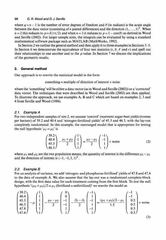
96 G. R. Wood and D. J. Saville
where q = n - 1 is the number of error degrees of freedom and 0 (in radians) is the acute angle between the data vector (consisting of n paired differences) and the direction (1,..., 1)T. When n = 2 this reduces to p = 0/(ir/2) and when n = 3 it reduces to p = 1 - cos(0) as derived in Wood and Saville (2002). For larger sample sizes, the integrals can be evaluated by using a standard mathematical software package such as MATLAB (MathWorks, 1992).
In Section 2 we outline the general method and then apply it to three examples in Sections 3-5. In Section 6 we demonstrate the equivalence of four test statistics (t, 0, F and r) and spell out their relationships to one another and to the p-value. In Section 7 we discuss the implications of the geometric results.
2. General method
Our approach is to rewrite the statistical model in the form
something = multiple of direction of interest + noise
where the 'something' will be either a data vector (as in Wood and Saville (2002)) or a 'corrected' data vector. The techniques that were described in Wood and Saville (2002) are then applied. To illustrate the approach, we use examples A, B and C which are based on examples 2, 3 and 4 from Saville and Wood (1986).
2.1. Example A For two independent samples of size 2, we assume 'control' treatment sugar-beet yields (tonnes per hectare) of 39.2 and 40.4 and 'nitrogen-fertilized yields' of 45.3 and 46.3, with the lay-out completely randomized. In this example, the rearranged model that is appropriate for testing the null hypothesis 'it1 = A2' is
(39.2 1 -1
40.4 P 1+ P2 1 2 -/ 1 -1( 45.3 2 1 2 1 noise (2 46.3 1 1
where pl and A2 are the two population means, the quantity of interest is the difference P2 - P1 and the direction of interest is (-1, -1, 1, 1)T.
2.2. Example B For an analysis of variance, we add 'nitrogen- and phosphorus-fertilized' yields of 47.8 and 47.4 to the data of example A. We also assume that the lay-out was a randomized complete-block design, with the first data value for each treatment coming from the first block. To test the null hypothesis '(P2 + /3)/2 = Pl1 (fertilized = unfertilized)' we rewrite the model as
39.2\ 1\ / 0\ -1 -1 40.4 1 0 1_ -1 45.3 1 13 - /2
-1 /2
- 1( -1 (/32 + (3)/2 - Pl 0.5 46.3 1 2 -1 2 1 1.5 0.5+noise 47.8 1 1 -1 0.5 47.4 / 1 / \ 0.5
(3)
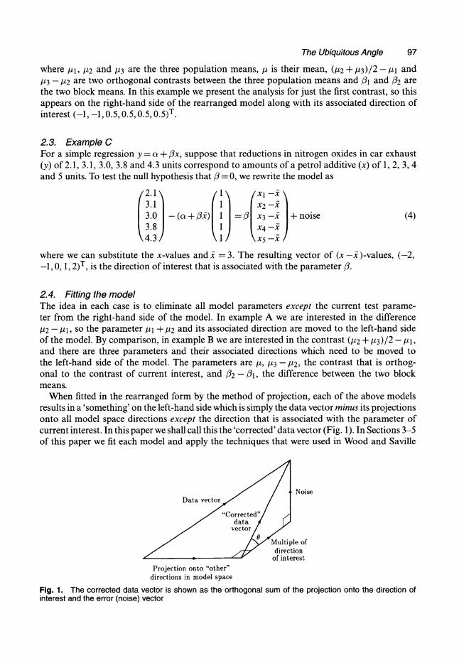
The Ubiquitous Angle 97
where p1,,
#2 and #3 are the three population means, p is their mean, (#2 + A3)/2 - 1pI and A3 - 12 are two orthogonal contrasts between the three population means and l1 and /32 are the two block means. In this example we present the analysis for just the first contrast, so this appears on the right-hand side of the rearranged model along with its associated direction of interest (-1, 1,0.5, 0.5, 0.5, 0.5)T.
2.3. Example C For a simple regression y = a + fix, suppose that reductions in nitrogen oxides in car exhaust (y) of 2.1, 3.1, 3.0, 3.8 and 4.3 units correspond to amounts of a petrol additive (x) of 1, 2, 3, 4 and 5 units. To test the null hypothesis that P = 0, we rewrite the model as
2.1\/\ /xI - 3.1 1 x2 -X
3.0 - (a + p) 1 = x3 - + noise (4) 3.8 1 x4 -x 4.3/ \ 1 X5/ \xs -/
where we can substitute the x-values and - = 3. The resulting vector of (x -i )-values, (-2,
-1,0, 1, 2)T, is the direction of interest that is associated with the parameter /.
2.4. Fitting the model The idea in each case is to eliminate all model parameters except the current test parame- ter from the right-hand side of the model. In example A we are interested in the difference
A/2 - /1, so the parameter /1 + A2 and its associated direction are moved to the left-hand side of the model. By comparison, in example B we are interested in the contrast (A/2 + /3)/2 - /11, and there are three parameters and their associated directions which need to be moved to the left-hand side of the model. The parameters are p, 3 - A2, the contrast that is orthog- onal to the contrast of current interest, and /2 - l1, the difference between the two block means.
When fitted in the rearranged form by the method of projection, each of the above models results in a 'something' on the left-hand side which is simply the data vector minus its projections onto all model space directions except the direction that is associated with the parameter of current interest. In this paper we shall call this the 'corrected' data vector (Fig. 1). In Sections 3-5 of this paper we fit each model and apply the techniques that were used in Wood and Saville
Noise Data vector
,No, "Corrected"
data vector
Multiple of direction
of interest
Projection onto "other" directions in model space
Fig. 1. The corrected data vector is shown as the orthogonal sum of the projection onto the direction of interest and the error (noise) vector
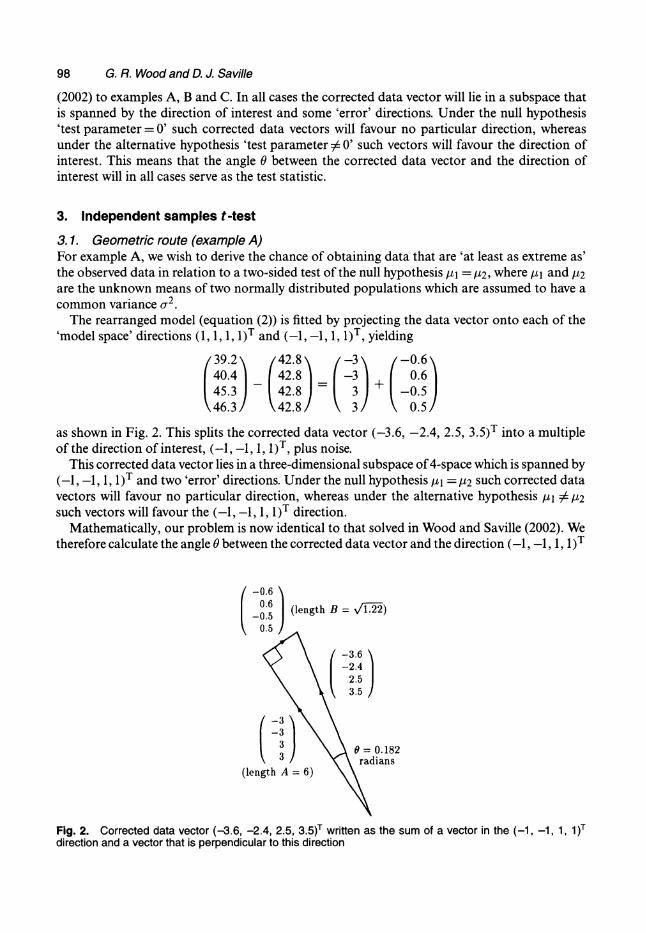
98 G. R. Wood and D. J. Saville
(2002) to examples A, B and C. In all cases the corrected data vector will lie in a subspace that is spanned by the direction of interest and some 'error' directions. Under the null hypothesis 'test parameter = O0' such corrected data vectors will favour no particular direction, whereas under the alternative hypothesis 'test parameter O0' such vectors will favour the direction of interest. This means that the angle 0 between the corrected data vector and the direction of interest will in all cases serve as the test statistic.
3. Independent samples t-test
3. 1. Geometric route (example A) For example A, we wish to derive the chance of obtaining data that are 'at least as extreme as' the observed data in relation to a two-sided test of the null hypothesis [l =
/2, where pl and /2 are the unknown means of two normally distributed populations which are assumed to have a common variance ar2
The rearranged model (equation (2)) is fitted by projecting the data vector onto each of the 'model space' directions (1, 1, 1, 1)T and (-1, -1, 1, 1)T, yielding
39.2 42.8 -3 -0.6 40.4 42.8 -3 0.6 45.3 42.8 3 -0.5 46.3 42.8 3 0.5
as shown in Fig. 2. This splits the corrected data vector (-3.6, -2.4, 2.5, 3.5)T into a multiple of the direction of interest, (-1, -1, 1, 1)T, plus noise.
This corrected data vector lies in a three-dimensional subspace of 4-space which is spanned by (-1,-11, 1, 1)T and two 'error' directions. Under the null hypothesis 1L = P2 such corrected data vectors will favour no particular direction, whereas under the alternative hypothesis L1 #
-p2 such vectors will favour the (-1, -1, 1, 1)T direction. Mathematically, our problem is now identical to that solved in Wood and Saville (2002). We
therefore calculate the angle 0 between the corrected data vector and the direction (-1, -1, 1, 1)T
-0.6
0.6 (length B - V )
-0.5
S-3.6 -2.4
2.5
3.5
-3
-3
3 0 = 0.182 3 radians (length A = 6)
Fig. 2. Corrected data vector (-3.6, -2.4, 2.5, 3.5)T written as the sum of a vector in the (-1, -1, 1, 1)T direction and a vector that is perpendicular to this direction
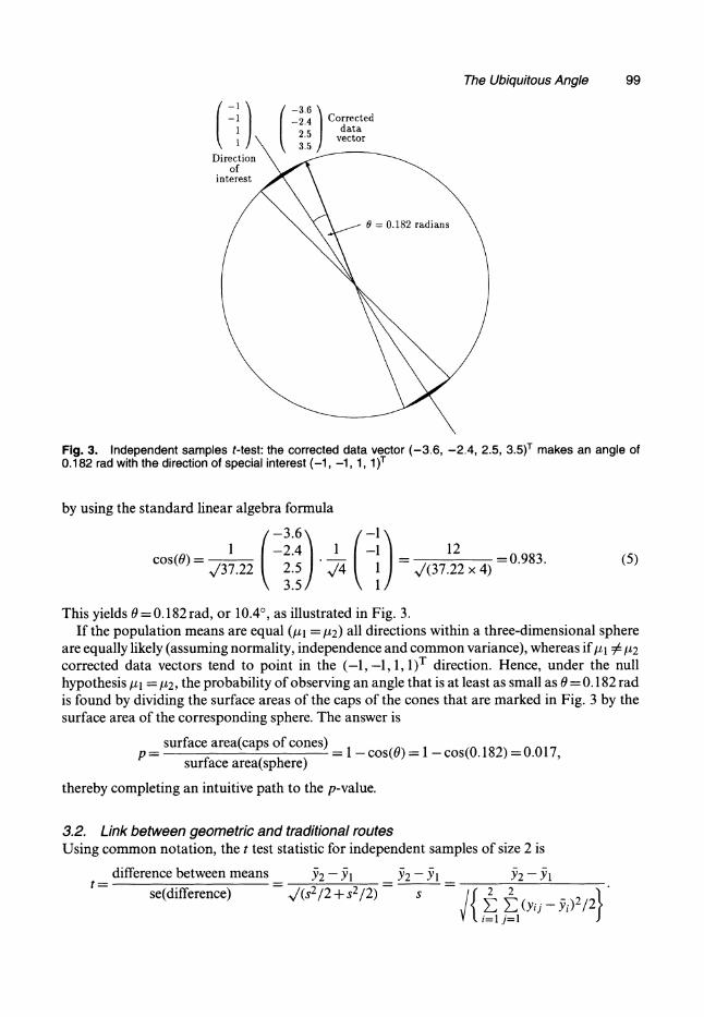
The Ubiquitous Angle 99
-1 -3.6 -1 -2.4 Corrected
1 2.5 data
.5 vector 1 ? \ \ 3.5/
Direction of
interest
0 = 0.182 radians
Fig. 3. Independent samples t-test: the corrected data vector (-3.6, -2.4, 2.5, 3.5)T makes an angle of 0.182 rad with the direction of special interest (-1, -1, 1, 1)'
by using the standard linear algebra formula
-3.6 -1
1 -2.4 1 -1 12 0.983.(5) cos(O) = V/37.22 2.5 "•V4
K1 •V(37.22
x 4) 3.5 1
This yields 0 = 0.182 rad, or 10.4', as illustrated in Fig. 3. If the population means are equal (p1l = P2) all directions within a three-dimensional sphere
are equally likely (assuming normality, independence and common variance), whereas if Al1 : /2
corrected data vectors tend to point in the (-1, -1, 1, )T direction. Hence, under the null hypothesis pl = P2, the probability of observing an angle that is at least as small as 0 = 0.182 rad is found by dividing the surface areas of the caps of the cones that are marked in Fig. 3 by the surface area of the corresponding sphere. The answer is
surface area(caps of cones) P = surface area(caps of cones)= - cos(0) = 1 - cos(0. 182) = 0.017, surface area(sphere)
thereby completing an intuitive path to the p-value.
3.2. Link between geometric and traditional routes Using common notation, the t test statistic for independent samples of size 2 is
difference between means Y2 - Y1 Y2 - Y2 -
se(difference) V(s2/2 + s2/2) s 2 2
Z= (yjl - i)2/2
i=l j=1
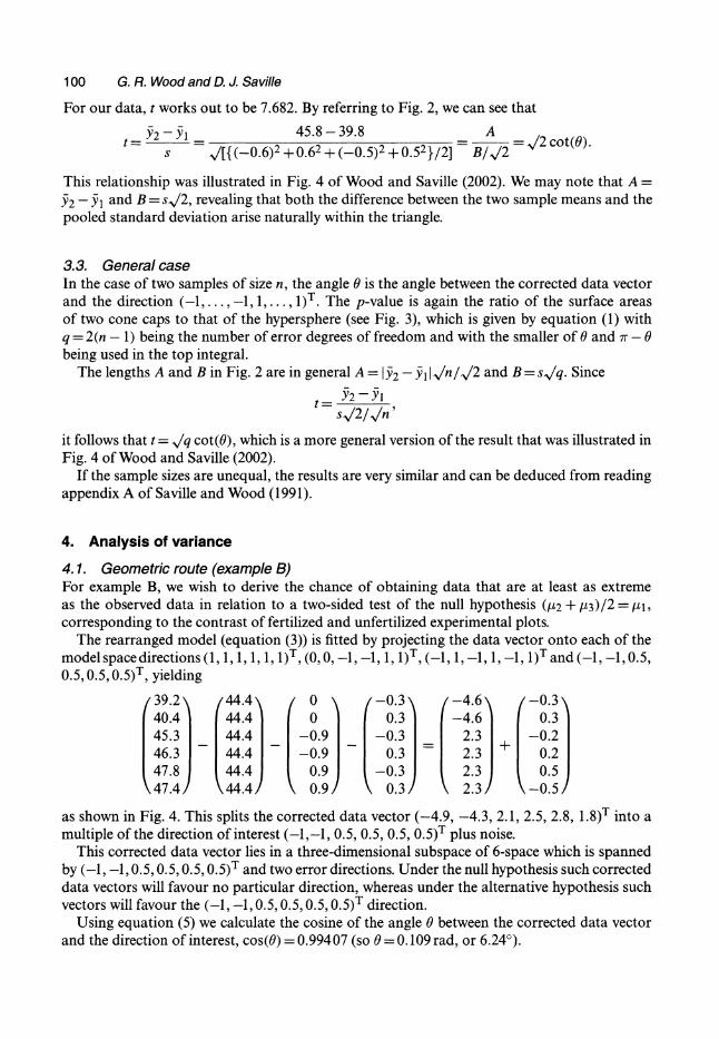
100 G. R. Wood and D. J. Saville
For our data, t works out to be 7.682. By referring to Fig. 2, we can see that
Y2 -Y1 45.8-39.8 A
s /[{ (-0.6)2 + 0.62 + (-0.5)2 + 0.52}/2] B/2 = 2 cot(
This relationship was illustrated in Fig. 4 of Wood and Saville (2002). We may note that A = Y2 - Y and B = sV/2, revealing that both the difference between the two sample means and the pooled standard deviation arise naturally within the triangle.
3.3. General case In the case of two samples of size n, the angle 0 is the angle between the corrected data vector and the direction (-l,..., -1, 1,..., 1)T. The p-value is again the ratio of the surface areas of two cone caps to that of the hypersphere (see Fig. 3), which is given by equation (1) with q = 2(n - 1) being the number of error degrees of freedom and with the smaller of 0 and r - 0 being used in the top integral.
The lengths A and B in Fig. 2 are in general A = 1Y2 - YllIn//J2 and B= s/q. Since
t Y2-Y s_/2/-n,'
it follows that t = j/q cot(0), which is a more general version of the result that was illustrated in Fig. 4 of Wood and Saville (2002).
If the sample sizes are unequal, the results are very similar and can be deduced from reading appendix A of Saville and Wood (1991).
4. Analysis of variance
4. 1. Geometric route (example B) For example B, we wish to derive the chance of obtaining data that are at least as extreme as the observed data in relation to a two-sided test of the null hypothesis (A2 + [3)/2 = ,1, corresponding to the contrast of fertilized and unfertilized experimental plots.
The rearranged model (equation (3)) is fitted by projecting the data vector onto each of the model space directions (1, 1, 1, 1, 1, 1) T, (0, 0-1, 1, 1) T, (-1, 1, -1, 1, -1, 1) T and (-1, -1,0.5, 0.5, 0.5, 0.5)T, yielding
39.2\ / 44.4 \ 0 / -0.3 \ /-4.6\ / -0.3 40.4 144.4 0 0.3 -4.6 0.3 45.3 44.4 -0.9 -0.3 2.3 -0.2 46.3 44.4 -0.9 0.3 - 2.31 0.2 47.8 44.4 0.9 -0.3 2.3 0.5 47.4 \ 44.4 / 0.9 / 0.3/ \ 2.3/ \-0.5
as shown in Fig. 4. This splits the corrected data vector (-4.9, -4.3, 2.1, 2.5, 2.8, 1.8)T into a multiple of the direction of interest (-1,-1, 0.5, 0.5, 0.5, 0.5)T plus noise.
This corrected data vector lies in a three-dimensional subspace of 6-space which is spanned by (-1, -1,0.5, 0.5, 0.5, 0.5)T and two error directions. Under the null hypothesis such corrected data vectors will favour no particular direction, whereas under the alternative hypothesis such vectors will favour the (-1,-1,0.5, 0.5, 0.5, 0.5)T direction.
Using equation (5) we calculate the cosine of the angle 9 between the corrected data vector and the direction of interest, cos(0)= 0.99407 (so 0 = 0.109 rad, or 6.240).
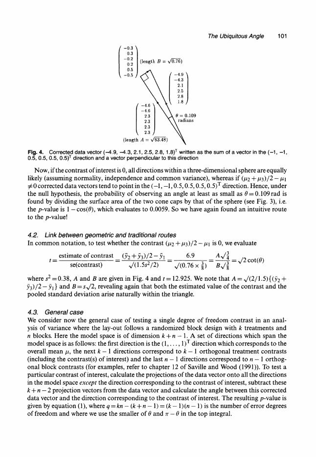
The Ubiquitous Angle 101
0.3 0.3
0.2 (length B = v4 / ) 0.2 0.5
-0.5 -4.9 -4.3
2.1 2.5 2.8
S-4.6 1.8
-4.6
2.3 0 = 0.109 2.3 radians
2.3
(e t 2.3
=
.- (length A = V6-3.8)
Fig. 4. Corrected data vector (-4.9, -4.3, 2.1, 2.5, 2.8, 1.8)T written as the sum of a vector in the (-1, -1, 0.5, 0.5, 0.5, 0.5)T direction and a vector perpendicular to this direction
Now, if the contrast of interest is 0, all directions within a three-dimensional sphere are equally likely (assuming normality, independence and common variance), whereas if (u2 + 3)/2 - Pl $0 corrected data vectors tend to point in the (-1, -1, 0.5, 0.5, 0.5, 0.5)T direction. Hence, under the null hypothesis, the probability of observing an angle at least as small as 0 = 0.109 rad is found by dividing the surface area of the two cone caps by that of the sphere (see Fig. 3), i.e. the p-value is 1 - cos(O), which evaluates to 0.0059. So we have again found an intuitive route to the p-value!
4.2. Link between geometric and traditional routes In common notation, to test whether the contrast (A2 + 3)/2 - p1 is 0, we evaluate
estimate of contrast (Y2 + Y3)/2 -Yl 6.9 A/ t - = 2 cot0 se(contrast) VJ(1.5s2/2) (0.76 x 3) B cot()
where s2 = 0.38, A and B are given in Fig. 4 and t = 12.925. We note that A = /(2/1.5){(Y2 +
3)/2 - Y } and B = s/2, revealing again that both the estimated value of the contrast and the pooled standard deviation arise naturally within the triangle.
4.3. General case We consider now the general case of testing a single degree of freedom contrast in an anal- ysis of variance where the lay-out follows a randomized block design with k treatments and n blocks. Here the model space is of dimension k + n - 1. A set of directions which span the model space is as follows: the first direction is the (1,..., 1)T direction which corresponds to the overall mean p, the next k - 1 directions correspond to k - 1 orthogonal treatment contrasts (including the contrast(s) of interest) and the last n - 1 directions correspond to n - 1 orthog- onal block contrasts (for examples, refer to chapter 12 of Saville and Wood (1991)). To test a particular contrast of interest, calculate the projections of the data vector onto all the directions in the model space except the direction corresponding to the contrast of interest, subtract these k + n - 2 projection vectors from the data vector and calculate the angle between this corrected data vector and the direction corresponding to the contrast of interest. The resulting p-value is given by equation (1), where q= kn - (k +n - 1) = (k - 1)(n - 1) is the number of error degrees of freedom and where we use the smaller of 0 and r - 0 in the top integral.
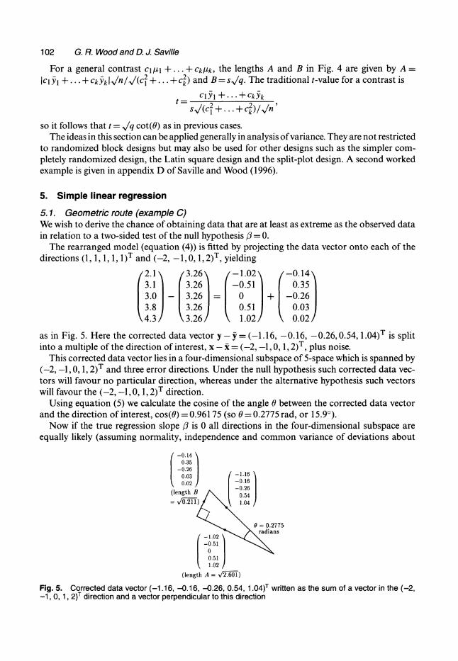
102 G. R. Wood and D. J. Saville
For a general contrast cluil + ... + ck Pk, the lengths A and B in Fig. 4 are given by A = Icll + ... +ckifk I~n/'/(c2 +... +c2) and B= s./q. The traditional t-value for a contrast is
t ClYl
+... +CkYk
s/(cf+...+c)/Vn' so it follows that t = /Iq cot(O) as in previous cases.
The ideas in this section can be applied generally in analysis of variance. They are not restricted to randomized block designs but may also be used for other designs such as the simpler com- pletely randomized design, the Latin square design and the split-plot design. A second worked example is given in appendix D of Saville and Wood (1996).
5. Simple linear regression 5. 1. Geometric route (example C) We wish to derive the chance of obtaining data that are at least as extreme as the observed data in relation to a two-sided test of the null hypothesis
- = 0.
The rearranged model (equation (4)) is fitted by projecting the data vector onto each of the directions (1, 1, 1, , 1)T and (-2, -1,0, 1,2)T, yielding
2.1 3.26 -1.02 -0.14 3.1 3.26 -0.51 0.35 3.0 - 3.261= 0 + -0.26 3.8 3.26 0.51 0.03 4.3 \3.26/ 1.02/ 0.02
as in Fig. 5. Here the corrected data vector y - y = (-1.16, -0.16, -0.26, 0.54, 1.04)T is split into a multiple of the direction of interest, x - x = (-2, -1,0, 1, 2)T, plus noise.
This corrected data vector lies in a four-dimensional subspace of 5-space which is spanned by (-2, -1,0, 1, 2)T and three error directions. Under the null hypothesis such corrected data vec- tors will favour no particular direction, whereas under the alternative hypothesis such vectors will favour the (-2, -1,0, 1, 2)T direction.
Using equation (5) we calculate the cosine of the angle 0 between the corrected data vector and the direction of interest, cos(0) = 0.96175 (so 0= 0.2775 rad, or 15.9').
Now if the true regression slope f is 0 all directions in the four-dimensional subspace are equally likely (assuming normality, independence and common variance of deviations about
-0.14 0.35
-0.26 0.03 -1.16 0.02 --0.16
(length B 0.54 = \O1) 1.04
0 = 0.2775 radians
-0.51
0.51
(length A = 2')•.)
Fig. 5. Corrected data vector (-1.16, -0.16, -0.26, 0.54, 1.04)T written as the sum of a vector in the (-2, -1, 0, 1, 2)T direction and a vector perpendicular to this direction
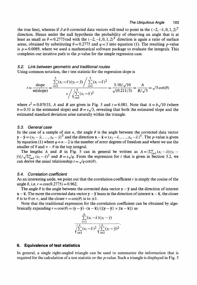
The Ubiquitous Angle 103
the true line), whereas if f0, #0 corrected data vectors will tend to point in the (-2, -1,0, 1, 2)T direction. Hence under the null hypothesis the probability of observing an angle that is at least as small as 0 = 0.2775 rad with the (-2, -1,0, 1,2)T direction is again a ratio of surface areas, obtained by substituting 0 = 0.2775 and q = 3 into equation (1). The resulting p-value is p = 0.0089, where we used a mathematical software package to evaluate the integrals. This completes our intuitive path to the p-value for the simple regression case.
5.2. Link between geometric and traditional routes Using common notation, the t test statistic for the regression slope is
5 5
so e (xi -)(yi - y) (xi --)2 slope i=1 i=_ 5.10//10 A t
. 5-2/3 cot(0) se(slope)
s ( - )2 (0.211/3) B//3
where s2 = 0.07033, A and B are given in Fig. 5 and t = 6.081. Note that A = b/10 (where b = 0.51 is the estimated slope) and B = s/3, revealing that both the estimated slope and the estimated standard deviation arise naturally within the triangle.
5.3. General case In the case of a sample of size n, the angle 0 is the angle between the corrected data vector Y - Y= (Yl - Y, .. , Yn - Y)T and the direction x - x = (x1 --,..., x, -2)T. The p-value is given by equation (1) where q = n - 2 is the number of error degrees of freedom and where we use the smaller of 0 and r - 0 in the top integral.
The lengths A and B in Fig. 5 can in general be written as A-iEn Z(xi-2)(yi-
y)•/EY=1 (xi-2)2 and B = s/q. From the expression for t that is given in Section 5.2, we
can derive the usual relationship t = %/q cot(0).
5.4. Correlation coefficient As an interesting aside, we point out that the correlation coefficient r is simply the cosine of the angle 0, i.e. r = cos(0.2775) = 0.962.
The angle 0 is the angle between the corrected data vector y - y and the direction of interest x - X. The more the corrected data vector y - y leans in the direction of interest x - x, the closer 0 is to 0 or rr, and the closer r = cos(0) is to +1.
Note that the traditional expression for the correlation coefficient can be obtained by alge- braically expanding r = cos(0) = (y - y) (x - i)/(Ily - yll x Ilx - xll) as
n
(Xi --2))(Yi--
Y-) i=1
V i= 1 i=1
6. Equivalence of test statistics
In general, a single right-angled triangle can be used to summarize the information that is required for the calculation of a test statistic or the p-value. Such a triangle is displayed in Fig. 3
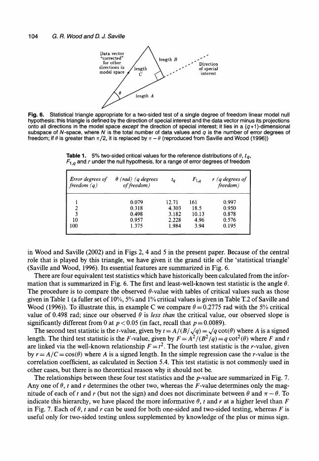
104 G. R. Wood and D. J. Saville
Data vector "corrected" length B
for other , - Direction directions in length- of special model space C -
. interest
length A
Fig. 6. Statistical triangle appropriate for a two-sided test of a single degree of freedom linear model null hypothesis: this triangle is defined by the direction of special interest and the data vector minus its projections onto all directions in the model space except the direction of special interest; it lies in a (q+l)-dimensional subspace of N-space, where N is the total number of data values and q is the number of error degrees of freedom; if 9 is greater than 7r/2, it is replaced by 7r - (reproduced from Saville and Wood (1996))
Table 1. 5% two-sided critical values for the reference distributions of 9, tq,
F1,q and r under the null hypothesis, for a range of error degrees of freedom
Error degrees of 0 (rad) (q degrees tq Fl,q r (q degrees of freedom (q) offreedom) freedom)
1 0.079 12.71 161 0.997 2 0.318 4.303 18.5 0.950 3 0.498 3.182 10.13 0.878
10 0.957 2.228 4.96 0.576 100 1.375 1.984 3.94 0.195
in Wood and Saville (2002) and in Figs 2, 4 and 5 in the present paper. Because of the central role that is played by this triangle, we have given it the grand title of the 'statistical triangle' (Saville and Wood, 1996). Its essential features are summarized in Fig. 6.
There are four equivalent test statistics which have historically been calculated from the infor- mation that is summarized in Fig. 6. The first and least-well-known test statistic is the angle 0. The procedure is to compare the observed 0-value with tables of critical values such as those given in Table 1 (a fuller set of 10%, 5% and 1% critical values is given in Table T.2 of Saville and Wood (1996)). To illustrate this, in example C we compare 0 = 0.2775 rad with the 5% critical value of 0.498 rad; since our observed 0 is less than the critical value, our observed slope is significantly different from 0 at p < 0.05 (in fact, recall that p = 0.0089).
The second test statistic is the t-value, given by t = A/(B/,/q) = /Iq cot(O) where A is a signed length. The third test statistic is the F-value, given by F = A2/(B2/q)= q cot2(0) where F and t are linked via the well-known relationship F = t2. The fourth test statistic is the r-value, given by r = A/C = cos(O) where A is a signed length. In the simple regression case the r-value is the correlation coefficient, as calculated in Section 5.4. This test statistic is not commonly used in other cases, but there is no theoretical reason why it should not be.
The relationships between these four test statistics and the p-value are summarized in Fig. 7. Any one of 0, t and r determines the other two, whereas the F-value determines only the mag- nitude of each of t and r (but not the sign) and does not discriminate between 0 and 7r - 0. To indicate this hierarchy, we have placed the more informative 0, t and r at a higher level than F in Fig. 7. Each of 0, t and r can be used for both one-sided and two-sided testing, whereas F is useful only for two-sided testing unless supplemented by knowledge of the plus or minus sign.
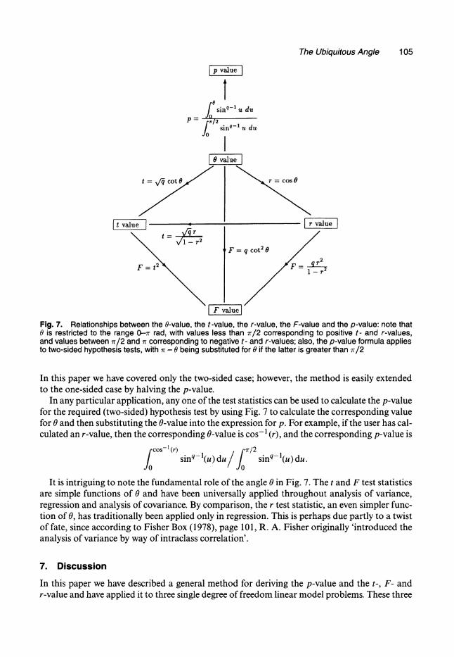
The Ubiquitous Angle 105
p value
sinq- u du
P 7/2sin q-1
u du
9 value
t = 4 cot 0 r = cos9
Itvalue - Ir value
F = q cot2 0
F t2r2
F valuel Fig. 7. Relationships between the 9-value, the t-value, the r-value, the F-value and the p-value: note that 0 is restricted to the range 0--r rad, with values less than 7r/2 corresponding to positive t- and r-values, and values between 7r/2 and ir corresponding to negative t- and r-values; also, the p-value formula applies to two-sided hypothesis tests, with 7r - 0 being substituted for 0 if the latter is greater than r/2
In this paper we have covered only the two-sided case; however, the method is easily extended to the one-sided case by halving the p-value.
In any particular application, any one of the test statistics can be used to calculate the p-value for the required (two-sided) hypothesis test by using Fig. 7 to calculate the corresponding value for 0 and then substituting the 0-value into the expression for p. For example, if the user has cal- culated an r-value, then the corresponding 0-value is cos-1 (r), and the corresponding p-value is
fcOs-' (r)
O7r/2
0cos-(r) '(u)duf sin-(u)duinq-l(u) du.
It is intriguing to note the fundamental role of the angle 0 in Fig. 7. The t and F test statistics are simple functions of 0 and have been universally applied throughout analysis of variance, regression and analysis of covariance. By comparison, the r test statistic, an even simpler func- tion of 0, has traditionally been applied only in regression. This is perhaps due partly to a twist of fate, since according to Fisher Box (1978), page 101, R. A. Fisher originally 'introduced the analysis of variance by way of intraclass correlation'.
7. Discussion
In this paper we have described a general method for deriving the p-value and the t-, F- and r-value and have applied it to three single degree of freedom linear model problems. These three
106 G. R. Wood and D. J. Saville
problems follow the general linear model
y = Xf+e
which can be written out more fully as
Y1 xll *X1P 3p 1 El1
YN XN1 o XNp p N
where for simplicity we assume that the columns of the 'design matrix' X are orthogonal. If we further assume that Op is the parameter of current interest, then we can rearrange the model in the form
(y1 ll -
XI(P-1) '1 11p
Y) - " "X(p)3p + noise
YN XN1 "" XN(p-1)
p-1 XNp
where (Xlp,... ,XNp)T is the direction that is associated with the parameter of interest. This is in the required form
something = multiple of direction of interest + noise.
This means that the hypothesis '3p = 0' (or, by reordering, /i = 0 for any i between 1 and p) in the general linear model can be tested by using the method that is described in this paper, i.e. the method is 'ubiquitous' in terms of single degree of freedom linear model testing problems. This ubiquity is demonstrated by the fact that the method can be applied to all except two of the analysis-of-variance, regression and analysis-of-covariance problems in Saville and Wood (1991). The two exceptions are the test of a composite (multidimensional) hypothesis PI = A2 =
/3 = -/4
(chapter 11) and the test for differences between the adjusted means in analysis of covariance (chapter 17).
The general method that is outlined in this paper and in Saville and Wood (1996) has not been described as comprehensively by previous researchers, though the essential ideas probably date back to R. A. Fisher in the 1920s (for references, see Wood and Saville (2002)). The method allows a unified understanding of single degree of freedom hypothesis tests in commonly used linear models. Also, the formula for the p-value may be useful for computational purposes in some applications.
Acknowledgements P. A. Carusi is thanked for stimulating this work. Michael Ryan, Karen Baird, Lesley Hunt, Gilbert Wells and the journal referees and Joint Editor are thanked for very helpful suggestions. Aaron Knight is thanked for assisting with the graphic art. Springer-Verlag New York, Inc., is thanked for permission to reproduce a modified Fig. 6 from Saville and Wood (1996).
References Chance, W. A. (1986) A geometric derivation of the distribution of the correlation coefficient Irl when p = 0.
Am. Math. Mnthly, 93, 94-98. Fisher Box, J. (1978) R. A. Fisher: the Life of a Scientist. New York: Wiley. Heiberger, R. M. (1989) Computation for the Analysis of Designed Experiments. New York: Wiley. MathWorks (1992) MATLAB Reference Guide. Natick: MathWorks.

The Ubiquitous Angle 107
Saville, D. J. and Wood, G. R. (1986) A method for teaching statistics using N-dimensional geometry. Am. Statistn, 40, 205-214.
Saville, D. J. and Wood, G. R. (1991) Statistical Methods: the Geometric Approach. New York: Springer. Saville, D. J. and Wood, G. R. (1996) Statistical Methods: a Geometric Primer. New York: Springer. Wood, G. R. and Saville, D. J. (2002) A new angle on the t-test. Statistician, 51, 99-104.
Statistics, Vol. 39, No. 4, August 2005, 287-301 ( f^ Taylor & Francis
On the geometry of F, Wald, LR, and LM tests inlinear regression models
ENIS SiNlKSARAN*
Department of Econometrics, Faculty of Economics. Istanbul University. Beyazit- Istanbul. Ttirkey
(Received M August 2()<M: ,n finat form 12 May 2005)
In ihis aniclc. we examine /•", Wald. LR. and LM tesi statistics in the linear regression model usingvector geometry. These four slalistics are expressed as a funciion of one random variable - the anglebelween Ihe vectors of unrestricted and restricted residuals. ThecxacI and nominal sampling disiribu-lions of this angle are derived lu iltuminale some facts ahoul ihe tour statistics. Aliernatively. we offerihai the angle ilself can be used as. a test statistic. A Mathematica program is also written lo carry outthe approach,
Keyword.s\ Geomelry; F-lest; Wald; Likelihood ralio; Lagrange multiplier; Projection; Angle;Malhematica
1. Introduction
As an elegant and powerful tool, geometry serves to clarify and unify the many aspects ofstatistics. Although this view was recognized by early authors like Fisher, Durbin. and Kendall,geometrical approaches have not heen commonly promoted to statistical teaching, research,and consulting in all levels. The reasons for this were stated by some authors. Herr [ 1 ] pointedout that one reason could be the tclcgraminalic style of the pure geometric approach of iheearly authors mentioned earlier. Bryani [21 indicated the lack of the relevant material in iheelementary level literature. Savillc and Wood [3| asserted that the fashion of formalism wasone of the major reasons lor the preeminence of algebraic methods in statistics. In recent years,however, statisticians and econometricians have found geometry increasingly useful. In Ihelast two decades, some hooks were written in which ihe word 'geometry' appeared in theirtitles, sec, Saville and Wood 14]. Murray and Rice |51. Wickens [61, and Marriott and Salmon17]. In some other hooks, writers devoted one or two chapters to geometrical approaches, suchas Davidson and Mackinnon [8]. Draper and Smith f9]. and Efron andTibshirani [10]. Severalpapers in which il was ail done geometrically or geometric ideas appeared as asides werewritten, including Bring [I I], Critchley et al. [12], McCartin [131. and Huang and Draper114]. Despite the recent growth, we believe that many additional attempts should he made to
*Hmail: [email protected]
StatisticsISSN 0233-1888 print/ISSN 1029-4910 online © 2005 Taylor & Francis Group Ltd
htlp://www.tandf.co.uk/jouma!sDOI: 10.1080/02331880500178521
288 E. SiniLictran
promote the geometrical approaches to statistics. This article is written to show ihe merit andthe power of geometry in the study of classical tests in the linear regression models.
As noted by Bryant (2], the statistical corresponding of two fundamental ideas in geometryshould be well understood: projection and angle. Projection gives the best fit and angle mea-sures the goodness of that fit. In this article, we show some known comparisons of F, Wald,LR, and LM tests using projections and angles in a subject-space picture. We also offer thatusing angle as a test statistic which can be very useful in exploring the relations among theclassical tests. See Buse [ 151, Ramanathan 116|, and Davidson and MacKinnon |8 | for thegeometric comparisons of W, LR, and LM tests using the shape of log-likelihood function.See also Van Garderen [17] for an alternative comparison using differential geometry.
2. Geometry of unrestricted and restricted models
Consider the linear regression model of the form
y = Xfi + e, (1)
where y is an n x 1 vector of responses, X is an /( x k non-stochastic matrix of regressorsand has a lull column rank ', ^ is a * x 1 vector of parameters, and e is an H x 1 vector ofrandom errors. We assume e - N{Q. a-l).
Now we partition X as follows
X ^ | X , | X 2 | ,
where X| has size/i x (k - r) and X2 has si/.e n x /. The model (I), then, can be rewritten as
y-X,/3,+X2^2 + e, (2)
where fii and ^2 ^re subveetors of /? with (k - r) and /• components, respectively. Assumethat we want lo test the joint significance of the regressors of submatrix X2. that is, the nullhypothesis HQ. fii = 0 against //,<: fii ? 0. The model excluding ^2 '
y -X i /3 ,+e . (3)
Let us call equation (2), the unrestricted model and equation (3), the restricted model. Let theunrestricted and restricted least squares parameter e.stimates be ^ = l^i 1 :1 and fi = 1^, |0]respectively, y , y , e,ir. and er are the vectors of unrestricted and restricted litted values andresiduals, respectively.
Figure 1 is a subject-space picture in which the variables are represented by vecttjrs inEuclidean n-dimensional space, whieh is denoted by V". The figure illustrates ihe leastsquares estimation and the orthogonal decomposition of response variable for unrestricted andrestricted models. As columns of matrix X are independent vectors, they span a it-dimensionalsubspace. This is the column space of X and generally called estimation space in statistics. Letus denote this subspace of V" by ^(X) which is illustrated by ordinary plane in figure 1. Whenwe fit the unrestricted model in equation (2) by the least .squares method, we are essentiallychoosing a linear combination y ^ ^ Xi/?, -H X2y32 in 5 (X), which is uniquely determined bythe perpendicular from y onto (S (X). The difference vector eur = y - yur ''S** •" l * orthogonalcomplement of <5 (X). This {n - A') dimensional subspace is called left-null space of X in linearalgebra or error space in statistics.
The columns of matrices Xi and X2 span {k - r) and r dimensional subspaces of 8 (X),respectively. Denote these subspaces by ^(Xi) and ^(X2). For simplicity, in figure I, these
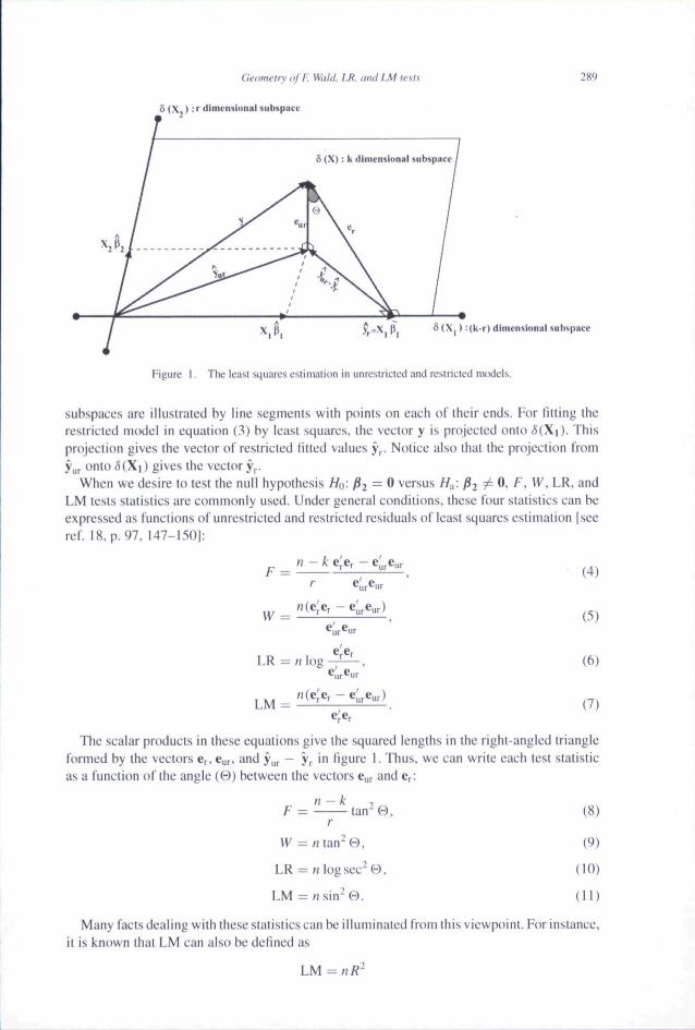
Geometry of F. Wohi. LR, and IM tests
irttlmenslunal subspace
289
•('*-'•) dimensional subspace
Figure i. The least squares estimation in unrestricted and reslricted models
subspaces are illustrated by line segments with points on each of their ends. For fitting therestricted mtxlel in equation (3) by least squares, the vector y is projected onto (5(Xi). Thisprojection gives the vector of restricted fitted values y . Notice also that the projection fromy r onto<S(X|) gives the vector y .
When we desire to test the null hypothesis Ho: 2—^ versus H^: fii i= 0. f, W. LR, andLM tests statistics are commonly used. Under general conditions, these four stalistics can beexpressed as functions of unrestricted and restricted residuals of least squares estimation [seeref. 18, p. 97, 147-150]:
F =— k
(4)
e'.
LR = n log
(5)
(6)
(7)
The scalar products in these equations give the squared lengths in the right-angled triangleInrmed by the vectors Cr, eur, and y,,,. — y in figure 1. Thus, we can wrile each test statisticas a function of the angle (BJ between the vectors e r and eri
r
H' - ntan^B.
LR — n log sec" 0 ,
LM — n sin" 0 .
(8)
(9)
(10)
(II)
Many facts dealing with these statistics can be illuminated from this viewpoint. For instance,it is known that LM can also be defined as
LM =

290 E. Siiiiksaraii
where /?^ is the squared multiple correlation coeflicient from the regression of er on X. Thisrelation can be easily seen in figure I. The projection from the response variable er onto S (X)gives the vector y ^ - yr ^ the vector of fitted values. Thus, the squared lengths of er andyur ~ ^r "" 'li^ '"tai and explained .sum of squares of this regression, respectively. The cosineof the angle between the vectors er and y ^ " yr ' 'li^ multiple correlation coefficient. Thesquared multiple conelation is then
Hence, the equation LM — iiR- is identical to the equation (II).The angular equivalents of the test statistics would also suggest that the angle itself can be
used directly as a test statistic. To do this, we need to derive angular sampling distributionsunder the null hypothesis.
3. Angular equivalent of F-test
Solving equation (H) lor © , we see that
© = arctan / - F . (12)y ft — k
When the random variable F is distributed, the non-central F distribution with r and (n - k)degrees of freedom and 6 non-centrality parameter, as a monotonic function of the randomvariable F, © has the following density
•,r,u -k.S)
— k -\- r). r / 2 , (1/2)5 sin
heta[r/2,
/r/2
, 0 < ^ <90 , (13)
where HypergeometriclFl is the Kummer eontluent hypergeometric function with threeparameters. Under the null hypothesis M,: jSj — 0, the non-centrality parameter is zero andthe non-central distribution of© becomes the following central distribution:
((» -
beta[r/2.
0 < ( 9 < 9 0 . (14)
Figure 2 shows the graphs of density functions of © with some parameter values.The critical region for F-test of HQ at significance level a is F > Fir, n — k.a), where
^ - -iTir.n-k.a) f^^' ''• " ~ ^^'^^ ^"^ ^*^' " ~ ^'' ») J (• " «) percent upper tail value of Fdensity function / ( F ; r, n - k). When we want to use 0 as a test statistic, the critical region
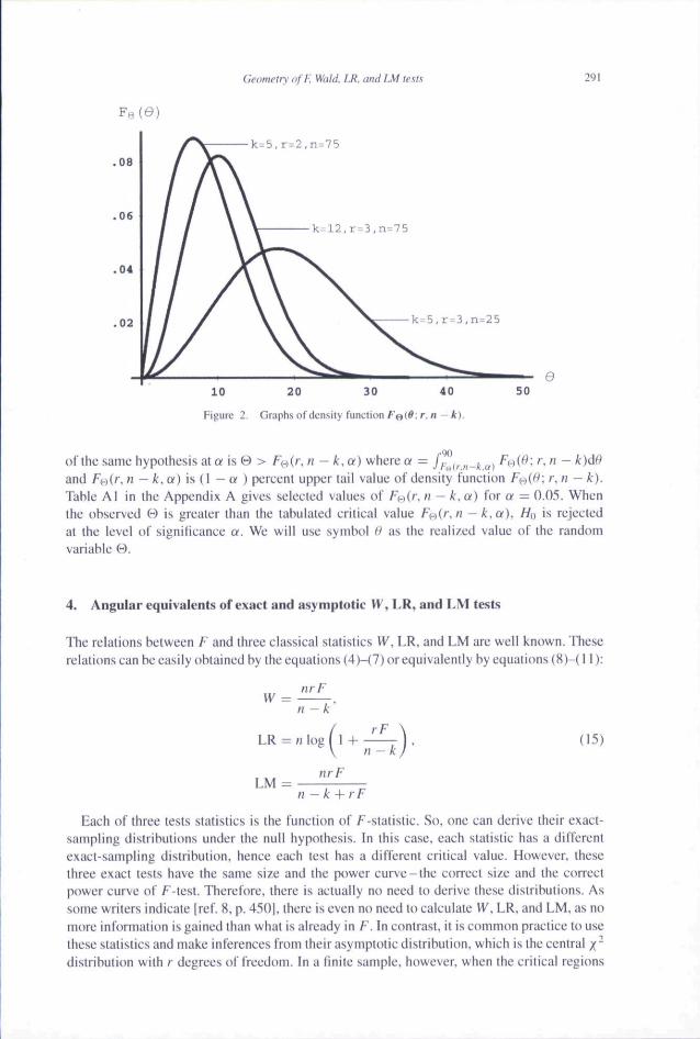
Geometry nfl] Wulti LR. antl LM 291
Fe(0}
.02
10 20 30 40
Figure 2. Graphs of density function F©t#; r.n - k).
ol lhe same hypothesis at ff is 0 > F(.-,(r.n - k.a) where « — fr,..irn-ka)and Ft-)(r. n — k.a) is. {\ - a ) percent upper tail value of density function FH( '^ : r. n - k).Tahle Al in the Appendix A gives selected values of F^Cr. n — k. a) for a = 0.05. Whenthe ohserved © is greater than the tahulated critical value F(..)ir, n — k. a ) , Ho is rejectedat the level of significance a. We will use symbol 0 as the realized value of the randomvariable B .
4. Angular equivalents of exact and asymptotic W, LR, and LM tests
The relations between F and three classical statistics IV, LR, and LM are well known. Theserelations can be easily obtained hy the equations (4)-(7) or equivalently by equations (8)-{ 11):
VV =nrF
H -k
LR - n log 1 +rF
n-k(15)
nrFn — k + rF
Each of three tests statistics is the function of F-statistic. So. one can derive their exact-sampling distributions under the null hypothesis. In this case, each statistic has a differentexact-sampling distribution, henee each test has a different critical value. However, thesethree exact tests have the same si?e and the power curve-the correct size and the correctpower curve of F test. Therefore, there is actually no need to derive these distributions. Assome writers indicate |ref. 8. p. 450|. there is even no need to calculate VV, LR. and LM. as nomore information is gained than what is already in F . In contrast, it is eomnit)n practice to usethese statistics and make inferences from their asymptotic distribution, which is the central x~distribution with /• degrees of freedom. In a finite sample, however, when the critical regions
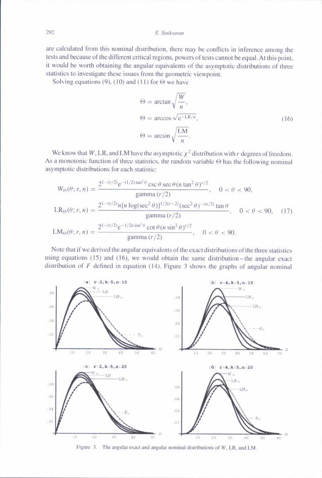
292 E. Siniksaran
are calculated from this nominal distribution, there may he conflicts in inference among thetcsls and because of ihe different critical regions, powers of tests cannot be equal. At ihis point,it would he worth obtaining the angular equivalents of the asymptotic distributions of threestatistics to investigate these issues from the geometric viewpoint.
Solving equations (9), (10) and (II) for B we have
w
t) = arctan J —,
0 — arccos ve"''*''",LM"
(16)
— arcsin
We know that VV, LR, and LM have the asymptotic x^ distribution with r degrees of freedom.As a monotonic function of three statistics, the random variable W has the following nominalasymptotic distributions for each statistic:
gamma (r/2)
gamma (r/2)
•, 0 <0 <90,
^ . 0 < f ^ < 9 0 , (17)
, 0 < ^ < 9 0 .gamma (/•/2)
Note that if we derived the angular equivalents of the exact distributions of the three statisticsusing equations (15) and (16), we would obtain the same distribution-the angular exactdistribution of F defined in equation (14). Figure 3 shows the graphs of angular nominal
;G 20 ii) jij .io
Figure ^. The angular exact and angular nominal dislributions of W, LR. and LM.
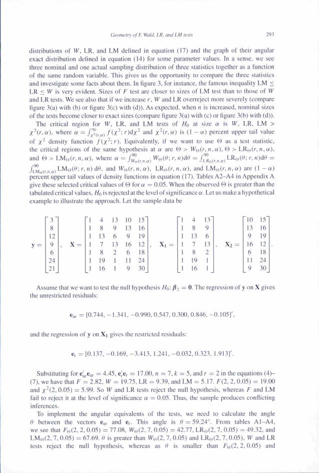
Geometry ofE. Wtilel. LR. am! LM te.m 293
distribulion.s of VV, LR, and LM delined in equation (17) and the graph of their angularexact distribution defined in equation (14) for some parameter values. In a sense, we seethree nominal and one actual sampling distribution of three statistics together a.s a functionof the same random variable. This gives us the opportunity to compare the three statisticsand investigate some facts about them. In figure 3, for instance, the famous inequality LM <LR < VV is very evident. Sizes of F test are closer to sizes of LM test than to those of VVand LR tests. We see also that if we increase r, W and LR overreject more severely (comparefigure 3(a) with (b) or figure 3(c) with (d)). As expected, when n is increased, nominal sizesof the tests become closer to exact sizes (compare figure 3(a) with (c) or figure 3(b) with (d)).
The critical region for W, LR, and LM tests of HQ at size a is W. LR, LM >X^(r.a), where a — f^.^^) /(X"- r)dx' and x"(''-«) is (I - ff) percent upper tail valueof x^ density function fix'^r-). Equivalentiy. if we want to use (-) as a test statistic.the critical regions of the same hypothesis at a are W > W(-)(r. H, or). 0 > LR{-)(r.n.a).and B > LM,,(/-. n. a), where a = /* , , , , , , , W^,{e: r, n)dO = JZ^^.^.U) LR(-)(^; r, n)dO =
fiZuirno)'^'^'--'^^-''-"'^^^- ''"^ VV,.,(/-. H.o). LRH(/-.'i.cf). and LM|..,(/-. H. a) are (1 -a)percent upper tail values of density functions in equation (17). Tables A2-A4 in Appendix Agive these selected critical values of 0 for a = 0.05. When the observed (-) is greater than thetabulated critical values. Ho is rejected at the level of significance w. Let us make a hypotheticalexample to illustrate the approach. Let the sample data be
38129 , X = I 7 13 16 12 . X, -62421
Assume that we want to test the null hypothesis H^.the unrestricted residuals:
4813781916
139613211
101391661!9
15161912182430
4813781916
13963211
10139166119
15161912182430
— 0. The regression of y on X gives
e,, = [0.744, -1.341. -0.990.0.547,0.300.0.846, -0.1051'.
and the regression of y on X| gives the restricted residuals:
, ^ [0.137,-0.169,-3.413, 1.241.-0.032.0.323, 1.913]'
Substituting fore[,jeur =4.45.erer — 17.00. n — l,k — 5. andr = 2 in the equations (4)-(7), we have that F = 2.82. W = 19.75. LR = 9.39, and LM - 5.17. F(2. 2. 0.05) - 19.00and x"(2. 0.05) - 5.99. So W and LR tests reject the null hypothe.sis, whereas F and LMfail to reject it at the level of significanee a — 0.05. Thus, the sample prcxiuces conflictinginferences.
To implement the angular equivalents of the tests, we need to calculate the angle0 between the vectors eur and er. This angle is ft* — 59.24°. From tables A1-A4,we see that F^.,{2, 2. 0.05) = 77.08, W,.,{2. 7. 0.05) = 42.77. LRH(2, 7. 0.05) - 49.32, andLM,..,(2. 7. 0.05) = 67.69. 0 is greater than ^,-,(2, 7. 0.05) and LRH(2. 7. 0.05). W and LRtests reject the null hypothesis, whereas as 0 is smaller than F(..)(2.2.0.05) and
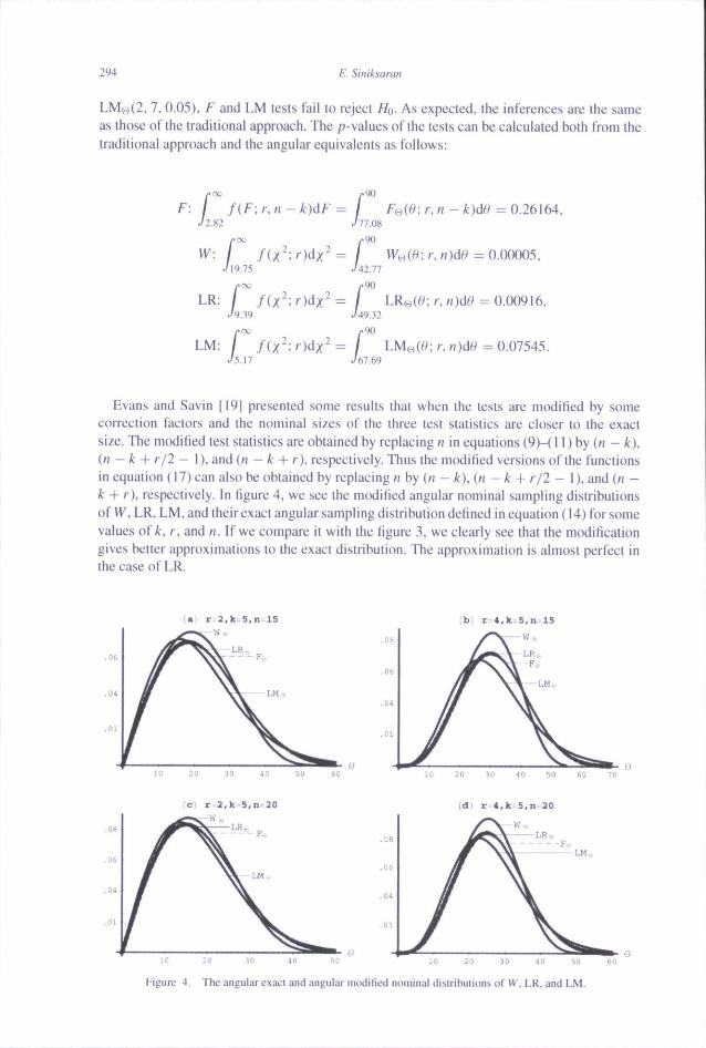
294 E. Siniksaran
LM(..)(2. 7. 0.05). F and LM lests fail to reject HQ. AS expected, the inferences are the sameas those of the traditional approach. The p-values of Ihe tests can be calculated both fromthetraditional approach and the angular equivalents as follows:
/•oo
/ ( F ; r, n - k)<iF =
H'
LR
LM
/.= / \ r, n -
77.08
90
: / / (x ' ; r)(Xx^ = /^19.75 ^4
/•CO />90
: / /(x-;r)dx-- /A.39 ^4';..12
/•OC /.W
: / f(x^\r)i\x~= /./5.I7 ^67.69
WB(6'; r, n
; r,
= 0.26164,
= 0.0(X)05,
= 0.00916.
^ 0.07545.
Evans and Savin [19] presented some results that when the tests are modified by someeorrcction factors and Ihe nominal sizes of the three test statistics are closer to the exactsize. The modified test statistics are obtained by replacing ti in equations (9)-( 11) by (« - it),(/) — k + r/2 - 1), and (n — k -\- r), respectively. Thus the modified versions of the functionsin equation (17) can also be obtained by replacing;) by [n - k). (it - k -j- r/2 - I), and (n -k + r), re.spectively. In figure 4, we see the modified angular nominal sampling distributionsof W,LR, LM, and iheir exact angular sampling distribution defined in equation (14) for somevalues o( k. r. and /(. If we compare it with ihe figure 3, we clearly see thai the modificationgives belter approximations to the exact distribution. The approximation is almost perfect inthe case of LR.
lU :U 5il -JO bii 6ii
(a ,n 20
: u i'J ao so 60
Figure 4. The angular exaci and angular modified nominal distributions of VV. LR. and LM.
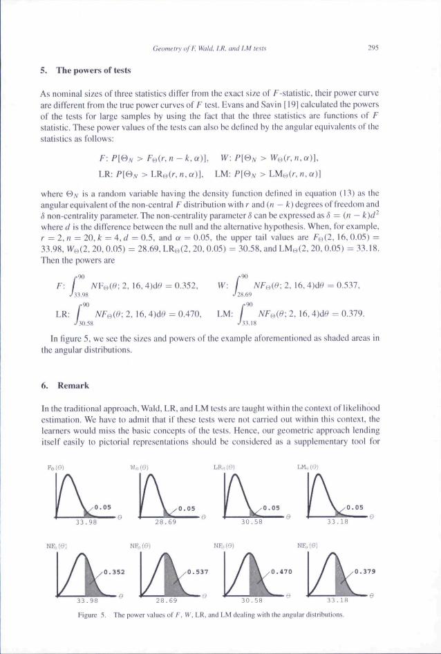
Geometry of F, Wuhl. LR. and LM tests 295
5. The powers of tests
As nominal sizes of three statistics differ from the exact size of f-statistic, their power curveare different from the true power curves of F test. Evans and Savin [ 19] calculated the powersof the tests lor large samples hy using the fact ihat the Ihree statistics are functions of Fstatistic. These power values of the tests can also he detined by the angular equivalents of thestatistics as follows:
./i - k.a)\. W\
) .a) | , LM:
F:
LR:
where (-),v is a random variable having the density function defined in equation (13) as theangular equivalent of the non-central F distribution with r and {n — k) degrees of freedom and(5 non-centrality parameter. The non-centrality parameter 5 can be expressed as 5 = {n — k)d^where (/ is the difference belween the null and the alternative hypothesis. When, for example.r = 2,n =20,k^A.iI ^ 0 . 5 , and oi - 0 . 0 5 , the upper tail values are FH(2 . 16.0.05) -3.V98. WH(2. 20. 0.05) = 28.6<J. LR,-,(2. 20. 0.05) - 30.58. and LMM(2. 20. 0.05) - 33.18.Then the powers are
F\
LR:
90
; 2. 16. - 0.352. W: : 2. 16. = 0.537.
/.90
J.10.58
' ;2 . I6.4)df^ =0.47t), LM: /^.',1,1
; 2. 16.4)d^ - 0.379.
In figure 5, we see the sizes and powers of the example aforementioned as shaded areas inthe angular distributions.
6. Remark
In the traditional approach, Wald, LR, and LM tests are taught within the context of likelihoodestimation. We have to admit that if these tests were not carried out within this context, thelearners would miss the basic concepts of the tests. Hence, our geometric approach lendingitself easily lo pictorial representations should be considered as a supplementary tool for
0.05
33.98 28.59
LK. (9)
3 0 . 5 8
0 . 0 5
33.18
0.379
33.98 ' 20.69 30.58 33.18
Figure 5. The power values of F. IV. LR, and LM dealing wiih ihe angular distribulions.
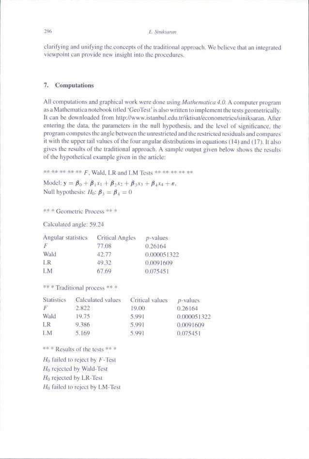
296 E. Sinikiaran
clarifying and unifying the conccpls of the traditional approach. We believe that an integratedviewpoint can provide new insight into ihe procedures.
7. Computations
All computations and graphical work were done using Mathermirica 4.0. A computer programas a Mathematica notebook titled 'GeoTest' is also written to implement the tests geometrically.It can be downloaded from http://www.istanbul.edu.tr/iktisat/econometrics/siniksaran. Afterentering the data, the parameters in the null hypothesis, and ihe level of significance, theprogram computes the angle between the unrestricted and Ihe restricted residuals and comparesit with the upper tail values of the four angular distributions in equations (14) and (17). It alsogives the results of the traditional approach. A sample output given below shows the resultsof the hypothetical example given in the article:
** ** ** ** ** F, Wald, LR and LM Tests ** ** ** ** **
Model: y - ^,, + /S|A-| + fij^i + yS.iAj + fi^x^ + e,Null hypothesis: HQ: fi^= fi^=O
** * Geometric Process ** *
Calculated angle: 59.24
Angular stattslicsFWaldLRLM
Critical Angles /j-values77.0842.7749.3267.69
** * Traditional process ** *
StatisticsFWaldLRLM
Calculated values2.82219.759.3865.169
0.261640.0000513220.00916090.075451
Critical values19.005.9915.9915.991
/J-values0.261640.0000513220.00916090.075451
*** Results of the tests** *
H{) failed to reject by F-Test
HQ rejected by Wald-Test
Ho rejected by LR-Test
Ho failed to reject by LM-Test
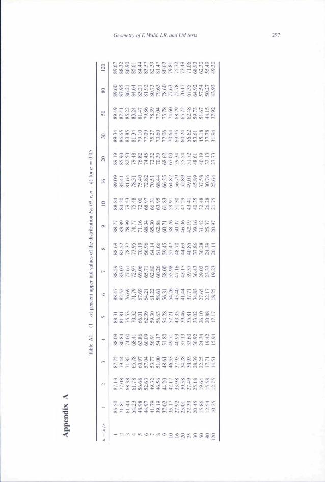
Geometry ofF. Waid. LR. anil LM te.its 297
I
CT\ oc C in " ^ f^ r i .—. ^ o^ in. f^ .—' 30 r i in O30 00 00 oc 30 30 30 3O OC r^ r—- f-^ t"— -^ *o in " ^
C in — - i - — r l rr, rr, o rr. 00 r-- m r i -T r-- r ,•C !> r i \D r i CT; r~ sC ><:> Np r-- — f , CT; m, r i CT;CT-r-id-^r^: — C!CT'30r~rior-'^i~--d'~"ioC30000Cooooooi--i---r~r--r~..CsCinin-T
CT^ rl t-— •© ^^ " 00 ^^ CT^ rl CC r , r.- in ri^ Tf r> r 1 "T 30 CF C r^ 'C r-~ I" f^ ~" CT^CT^ f in r'', .—' CT^ oo t"- in "^ 30 in ri CT^ .—' ^' t-ocooooo03or--r--t~-r--i~--o>o>0'ninTf-m
— 30 30 Tt
CTv c r* ~" CT^ r^ 'n f, rl O r**. o O '^ in r^ ^
O O O 30 r i in r i OS r l p Tt TT r i — CT^ "". f .— CT;in'T30T);(--i(-^iOOf^. inr"--.© — —if~;O> in r iCT '>d 'T r Jd3d t~^CT i>n - - odd^r | |~-o o c 0 3 0 r - - r - - t - - ^ - r ^ > . o v o u ^ l l ^ l n • * • ^ ' ^ r l
S — w — O r 4 — T f i n r i ovCT ' — CT\3C>O'^• ^ • q r ~ i ' t o o i n - : } ; i n o q r ^ a o p o o i n r ^ - q
o> in — 00 •/•) r i d od \d " ^ >b r i CT' in r- d in30 30 00 t~- r-- r~- r- -o ^ sC in, in • * • * i~". i~". r l
^ O i ^ o o o r - - — inf^. ^ -OO* ' — inooooin,
3 d r f C T > i n r i o d i D r ^ ^ — - C T ^ — - r - r H d r i ^ — •3C30r- t~- r - O i D ^ C ^ i n i n ^ TJ-TTI"". r i r i
r ^ C T ' C T ' r - 0 ^ 0 3 0 — \Cr---*OCT''C r i r-- r--r-^oOCT>r- — O r ^ 3 q r - r ~ C : O —' —^-tr^. Ov00 f i 00 rt — 00 in r i c: 00 d >d r i CT- —• m, d
a ^ r ^ r ~ - ^ n O ^ - C ' T s C l n r ~ 0 0 • ' n < D o C O " - : ^•q in I--, CT; — a- — -5 Tf • * r-- \D 30 00 r l r , —3 d H o d r ^ d > C " 7 — • C T ' t ' - o d T t d r - ^ C ' T d0000r--r~r--OsDsDu~, m, - tTt -Tf r^ . f', r i r i
CT"r--—'r-sp — O > C O C i 0 i 0 r - - r - - r r r i f , r .in ^^ ^ O ^^ t""". 00 r I c5 CT" -' ^~ ^j " ^ ' ^ rr, r i00 r* , ["... r I o m, r I D oo in. r^ f , CT^ O O^ r , CT^
c r l CT^ O CT' ~ r l ^~ ^~ 'C ^^ ^ ^~ r'l 'n, r"-- m- ^ m. ^ f^ ^ r l r l ^ f , r l ^ ^ t^ 00 ^ ^ r l
— — I--, r l — o v O r ^ o o — in>C — r^Ooo^ - -f . oom, f , p f . r ^ ' C n r t f ^ ' ^ o q p — * • "00 — in d *O r i CT- >d TI-' r i r'i CTv in r--! sd d r--'oooci^r - - i O > £ ) i n i n i n « * i ' f r ^ r ^ ' ' ' i r l r l —
in ^ r i 00 r-- ' ^ r-- p '— 1 , f . 00 r*~, CT' m . •—' —r^ • ^ 00 F CT> o r-. S ^ in CT> r i CT' i ^ ri t m,V-- o^ '—' 1/% ^^ f^ r'', 1—' oo 'C r^ "^ ^^ 00 rt f ^ '3 0 f ^ r ^ ' C ^ m j i n i n ' ^ - i " r*, rr, r'", ri r i .—i .—'
r- r-- 00 — -d r i CT- id "t r i rH d r- m O" u-: r i
C — Tf r i 00 r~- ^:^ o> r i r~- r i — 3 in lO ^ m,
tn DO - ^ r l CT^ CT^ f~ — p — CT^ p "~, • * OO in r lin — — -^ 30 - t — o~ r in, t~. mi r i d inl r i d00 r-- -c in -T "T "t f , f^ f^i r l r i r l r l — .— —
a.aO C O o— — r l n (--. in 30 r l
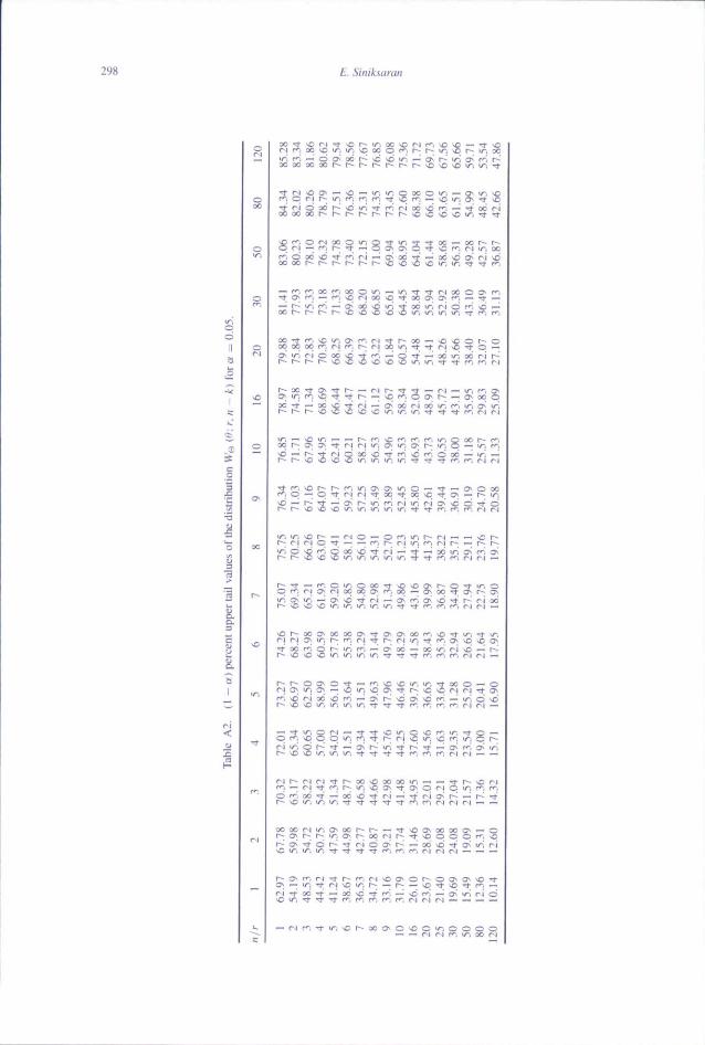
298 E. Siniksaran
00 (•~- -O f,
r r t r
— t~^ u*i r^l —
30 O O r^,
O ""i -C —•
- ^ O - ^ - - 000 O
Ttf^Ol^ t^ '^ : l /^CT><J-U". O — Tf- — O\C30' ' i p - ^ p • * r i r i •rr oc Tt 30 \o ^ o — r U-.\D •—' r~ - ^ — o^ r U-; r i r i i/S r i CT' o Tf c>
t" r^ \C ^c D " " . '/-I 'f^t ly^ 1 . " ^ ' ^ " r 'j f^ r*~, r i r j
u^u". ^Dr~- — n o — Or^ i i n t~ - r - i — — ^Ot^
t~ - ;< ' l fNp ' ^ — — f^ i t~~; r | l / " : r^ (NI^ — l ^ t ^' / " ( O ' D f ^ i o o d i O ' t r N — ^ —^oOwKo^f^icT'r~ Tt — r , O 1/-, O 00 TT ^ \C CTv r--. C • * ir. Opf~-, r-10'(~13000CT''^. oo — O>00»tO'(~-Q>f-. i^ T-, — ^ O v O ' t r i — CT'f^:O>-C'*r-^ri3dr-. 1^ ^ \C T- f-- f^i f^i V. Tj. ^ f*-j r*-j r* r j r i •—'
^ o r - - o o a ^ o c o o a ^ - i • 0 ' 0 ^ o o f . so- fu^-T-u- .r i r a> in r- 1 . r i Tt r~ r j u~. • * ( . o^ vo -c o>-a- 00 f l Q r V, r . —• a- oo — 00 !/•! r-i id —• r-t~- \O >O ^ I/". I/", u^ u". rf- Tf Tt I--, (--, r", r i r i —
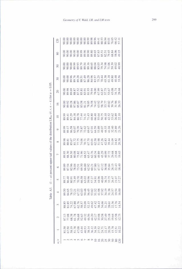
Geometry off, WuUl, LR, ami IM tests 299
— O ' O ' O
— O C f :
ao 30 00 00 00 oc r-
— OOrip > Or i oc U-, —
oo oc oe r~- r -
— r l r l p
coOCTo3CU-, V". — l~- O^ * d ^
.— r-oooc —
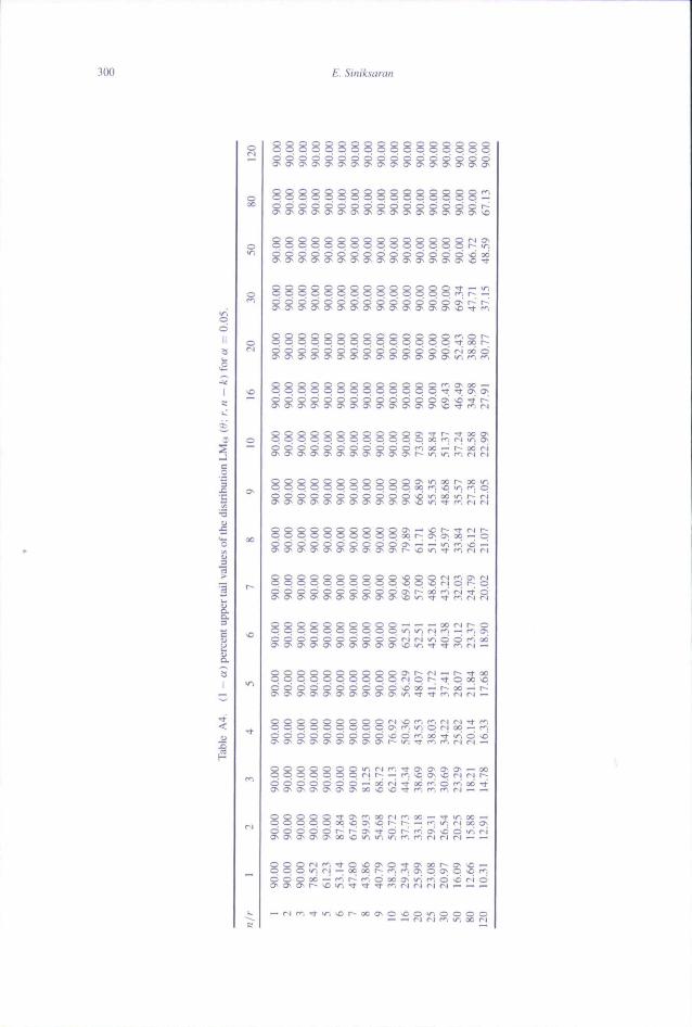
300 t. Sinikfuraii
ooooooQqqqocopoor^'O O O O O O O O O O O O O O O C - — '
d o d o d d d d d d d d d d d d r ^f^ f^ ^ Q^ CT\ CT^ O^ O ' ^ ^ O\ Q^. ^ f^ \^
c o o oo o o oo o w c o o o c o o o o f i oo O o o o o o o o o o o r "J-.O O O C O O O O O C O O v d o O^ ^ ^ ^ ^ ^ G O CT O ^ G
p p q q q q q p q q q c S q ' f o o r - ;d c d o d d o o d d d d d c r i o d d
O O O Q q r'-iO O O O O -3-
ooc!00oooddd<^lod-^r-^odr-iO\ C O- O- O> O> 3^ CT^ !?> ^ O r- U-. i/~. r'l n <~i
o o o o
O Q O C O C Q Q O Oj * ^ f^ r-l - ^ r-l . " ^ ^ r r rjno o o 00
o ;:; O o o o o
q p O O
d r i r - i i o d d r ' i o d0 ^ ^ ^
q q q q qd d d d d d d — '
. 00 — TTiotjo —-^ — r'':u-i(Nooo\~^<^io>iDdi/%ri'l f . r i n r-l — —
O O C ol f , TT C Oq q q ir, ri — oc 00o d s od —' r^, v^ r^,CT*- CT- O - r*^ ^O ^f^i ^ ^ "
GcometiynfF, WaM. LR. mdLM teats 301
ReferencesI ] 1 Hcrr. D.G.. 1980. On ihc history of ihe use of geometry in Ihe general linearmodel The Amerirmi Statistician.
34.131-135.|2| Bryanl. P.. 1984. Geiimelry, slalislics. probabiliiy; ViUiaiion on a common theme. The American Stati.sticiau,
38. 38^8 .| 3 | Sa\i!lc, 1).J and Wood. G.R.. 1986, A method for leaching stalistics using fi-dimensional geometry. r/fC/l'HpncMH
Stutisticiun. 40. 205-2]^.[4] Savillc. D.J. and Wood. G.R.. \99\.Statisticcil Melhods: the GeometricApimiarli (New York: Springcr-Vcrlag).[SI Murray. M.K. and Rice. J.W., 1993. Differential Geometry and Suiti.stitw, Monographs on Staiislics and Applied
Probaliiliiy. Vul. 48 (London: Chapman & Hall),[f)l Wickens. T.D.. 1995, The Geometry of Muhivariate Stttli.^nc.f {Hevj Jersey: Lawrence Eribaum Associates. Inc.).|71 Marrioll. P. and Salmon. M.. 2000. Appticalions of Differential Geometry to Econometrics (UK: Cambridge
University Press).|8] Davidson. R. and Mackinnon. J.G.. 1993. [estimation and Inference in FAimometries (New York: Oxford
tJniversity Press).|9 | Draper, N.R. and Smith. H.. 1998. ,4/J;J/(>(/fif,t;cc.?w»ji/\JI«/VW.? (US: Wiley Series in Prohabiiily & Slalislics).
(10] Hfron, B. and Tibshirani. R J., I998,.'lfj Introthiction to the Bootstrap. Monographs on Statistics and AppliedProbability. Vol. 57 (US: Chapman & Hall/CRC).
1111 Bring. J.. 1996. A geometric approach to compare variables in a regression model. The American Statistician.50, 57 -62.
112| Crilchlcy. K. Marriott. P. and Salmon. M., 2002, On preferred point geometry in statislics.7('i/m<j/('/.?W([.(/[C(i/I'liinnin^ ami Inference. 102. 229-245.
113| McCartin. B.J.. 2002, A geometric characterizalion of linear regression. Stati.'Hic.s, 42. 647-664.|14| Huang. Y. and Draper. N.R,. 2003. Transformations, regression geometry and R . Compuuuiimal Siatistic.\ &
Delia Aiiiilysis, 42. 647-664.[151 Bu,se. A.. 1982. The likelihmid raiio, Wald, and Lagrange mulliplier lests: an expository noie. the American
Siatistiiiiiii. 36. 153-157.|16| Ramarialhan, R.. 1993. Siatistical Methods in Hconometrici {l^ondon: Academic Press).117] Garderen. K J. Van, 2000. An allemalive comparison of classical lests: assessing ihe elTecis of curvature. In:
P. Marriott and M. Salmon (Eds) Applications of Differential Geometry in Ectmomeirics (UK: CambridgeUniversity Press).
118] Johnston, J. and DiNardo, J., 1997. Econometric Methods (US: McGraw-Hill).[19] Evans. G B.A and Savin. N.E., 1982. Conflict among the criteria revisited: the VV, LR. and LM tests.
Econometrica. 50. 737-748.

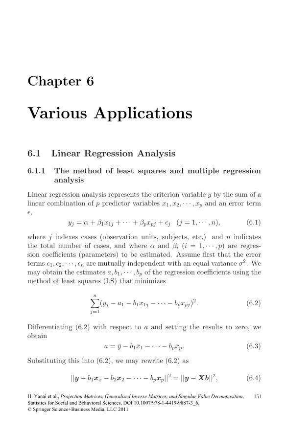
Chapter 6
Various Applications
6.1 Linear Regression Analysis
6.1.1 The method of least squares and multiple regressionanalysis
Linear regression analysis represents the criterion variable y by the sum of alinear combination of p predictor variables x1, x2, · · · , xp and an error termε,
yj = α + β1x1j + · · ·+ βpxpj + εj (j = 1, · · · , n), (6.1)
where j indexes cases (observation units, subjects, etc.) and n indicatesthe total number of cases, and where α and βi (i = 1, · · · , p) are regres-sion coefficients (parameters) to be estimated. Assume first that the errorterms ε1, ε2, · · · , εn are mutually independent with an equal variance σ2. Wemay obtain the estimates a, b1, · · · , bp of the regression coefficients using themethod of least squares (LS) that minimizes
n∑
j=1
(yj − a1 − b1x1j − · · · − bpxpj)2. (6.2)
Differentiating (6.2) with respect to a and setting the results to zero, weobtain
a = y − b1x1 − · · · − bpxp. (6.3)
Substituting this into (6.2), we may rewrite (6.2) as
||y − b1xx − b2x2 − · · · − bpxp||2 = ||y −Xb||2, (6.4)
© Springer Science+Business Media, LLC 2011 Statistics for Social and Behavioral Sciences, DOI 10.1007/978-1-4419-9887-3_6,
151H. Yanai et al., Projection Matrices, Generalized Inverse Matrices, and Singular Value Decomposition,
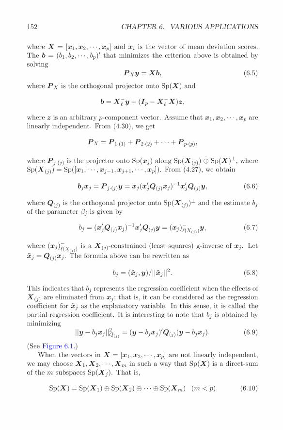
152 CHAPTER 6. VARIOUS APPLICATIONS
where X = [x1,x2, · · · , xp] and xi is the vector of mean deviation scores.The b = (b1, b2, · · · , bp)′ that minimizes the criterion above is obtained bysolving
P Xy = Xb, (6.5)
where P X is the orthogonal projector onto Sp(X) and
b = X−` y + (Ip −X−
` X)z,
where z is an arbitrary p-component vector. Assume that x1, x2, · · · , xp arelinearly independent. From (4.30), we get
P X = P 1·(1) + P 2·(2) + · · ·+ P p·(p),
where P j·(j) is the projector onto Sp(xj) along Sp(X(j))·⊕ Sp(X)⊥, where
Sp(X(j)) = Sp([x1, · · · , xj−1, xj+1, · · · ,xp]). From (4.27), we obtain
bjxj = P j·(j)y = xj(x′jQ(j)xj)−1x′jQ(j)y, (6.6)
where Q(j) is the orthogonal projector onto Sp(X(j))⊥ and the estimate bj
of the parameter βj is given by
bj = (x′jQ(j)xj)−1x′jQ(j)y = (xj)−`(X(j))y, (6.7)
where (xj)−`(X(j))is a X(j)-constrained (least squares) g-inverse of xj . Let
xj = Q(j)xj . The formula above can be rewritten as
bj = (xj , y)/||xj ||2. (6.8)
This indicates that bj represents the regression coefficient when the effects ofX(j) are eliminated from xj ; that is, it can be considered as the regressioncoefficient for xj as the explanatory variable. In this sense, it is called thepartial regression coefficient. It is interesting to note that bj is obtained byminimizing
||y − bjxj ||2Q(j)= (y − bjxj)′Q(j)(y − bjxj). (6.9)
(See Figure 6.1.)When the vectors in X = [x1,x2, · · · , xp] are not linearly independent,
we may choose X1, X2, · · · ,Xm in such a way that Sp(X) is a direct-sumof the m subspaces Sp(Xj). That is,
Sp(X) = Sp(X1)⊕ Sp(X2)⊕ · · · ⊕ Sp(Xm) (m < p). (6.10)
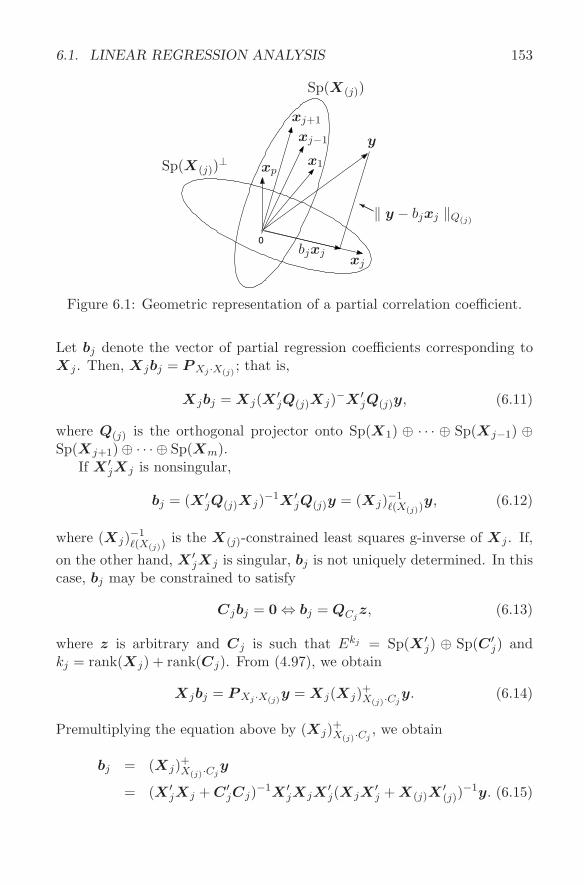
6.1. LINEAR REGRESSION ANALYSIS 153
0
Sp(X(j))
y
Sp(X(j))⊥
xj+1
xp
xj−1
x1
‖ y − bjxj ‖Q(j)
HHY
xjbjxj
Figure 6.1: Geometric representation of a partial correlation coefficient.
Let bj denote the vector of partial regression coefficients corresponding toXj . Then, Xjbj = P Xj ·X(j)
; that is,
Xjbj = Xj(X ′jQ(j)Xj)−X ′
jQ(j)y, (6.11)
where Q(j) is the orthogonal projector onto Sp(X1) ⊕ · · · ⊕ Sp(Xj−1) ⊕Sp(Xj+1)⊕ · · · ⊕ Sp(Xm).
If X ′jXj is nonsingular,
bj = (X ′jQ(j)Xj)−1X ′
jQ(j)y = (Xj)−1`(X(j))
y, (6.12)
where (Xj)−1`(X(j))
is the X(j)-constrained least squares g-inverse of Xj . If,
on the other hand, X ′jXj is singular, bj is not uniquely determined. In this
case, bj may be constrained to satisfy
Cjbj = 0 ⇔ bj = QCjz, (6.13)
where z is arbitrary and Cj is such that Ekj = Sp(X ′j) ⊕ Sp(C ′
j) andkj = rank(Xj) + rank(Cj). From (4.97), we obtain
Xjbj = P Xj ·X(j)y = Xj(Xj)+X(j)·Cj
y. (6.14)
Premultiplying the equation above by (Xj)+X(j)·Cj, we obtain
bj = (Xj)+X(j)·Cjy
= (X ′jXj + C ′
jCj)−1X ′jXjX
′j(XjX
′j + X(j)X
′(j))
−1y. (6.15)
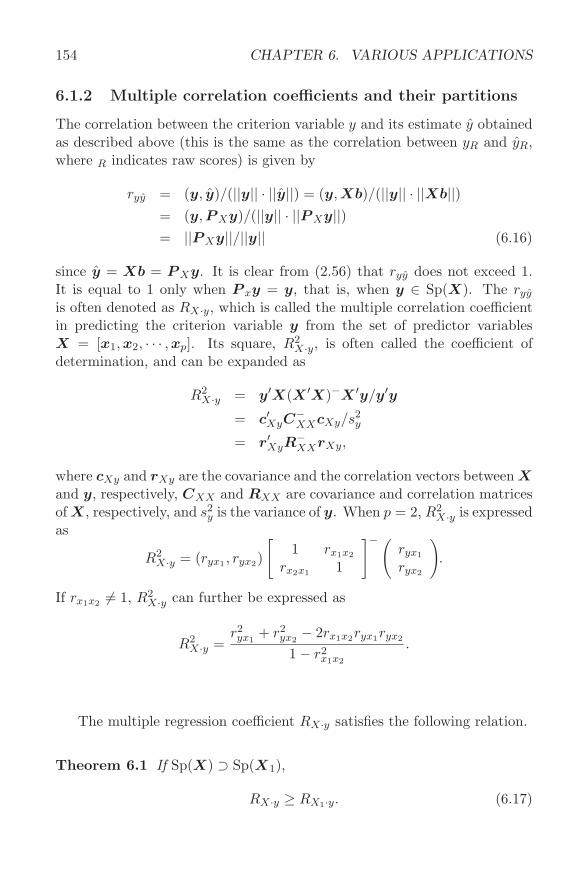
154 CHAPTER 6. VARIOUS APPLICATIONS
6.1.2 Multiple correlation coefficients and their partitions
The correlation between the criterion variable y and its estimate y obtainedas described above (this is the same as the correlation between yR and yR,where R indicates raw scores) is given by
ryy = (y, y)/(||y|| · ||y||) = (y, Xb)/(||y|| · ||Xb||)= (y, P Xy)/(||y|| · ||P Xy||)= ||P Xy||/||y|| (6.16)
since y = Xb = P Xy. It is clear from (2.56) that ryy does not exceed 1.It is equal to 1 only when P xy = y, that is, when y ∈ Sp(X). The ryy
is often denoted as RX·y, which is called the multiple correlation coefficientin predicting the criterion variable y from the set of predictor variablesX = [x1, x2, · · · ,xp]. Its square, R2
X·y, is often called the coefficient ofdetermination, and can be expanded as
R2X·y = y′X(X ′X)−X ′y/y′y
= c′XyC−XXcXy/s2
y
= r′XyR−XXrXy,
where cXy and rXy are the covariance and the correlation vectors between Xand y, respectively, CXX and RXX are covariance and correlation matricesof X, respectively, and s2
y is the variance of y. When p = 2, R2X·y is expressed
as
R2X·y = (ryx1 , ryx2)
[1 rx1x2
rx2x1 1
]−(ryx1
ryx2
).
If rx1x2 6= 1, R2X·y can further be expressed as
R2X·y =
r2yx1
+ r2yx2
− 2rx1x2ryx1ryx2
1− r2x1x2
.
The multiple regression coefficient RX·y satisfies the following relation.
Theorem 6.1 If Sp(X) ⊃ Sp(X1),
RX·y ≥ RX1·y. (6.17)
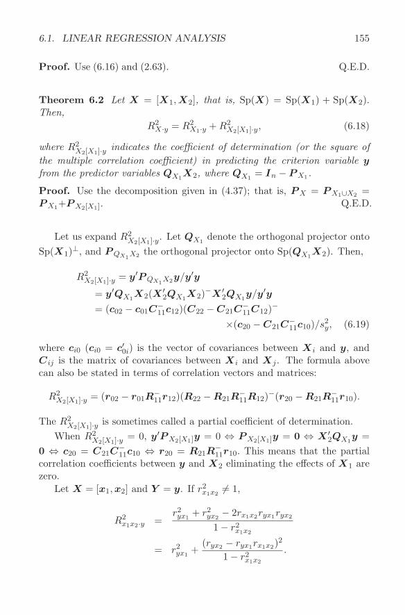
6.1. LINEAR REGRESSION ANALYSIS 155
Proof. Use (6.16) and (2.63). Q.E.D.
Theorem 6.2 Let X = [X1, X2], that is, Sp(X) = Sp(X1) + Sp(X2).Then,
R2X·y = R2
X1·y + R2X2[X1]·y, (6.18)
where R2X2[X1]·y indicates the coefficient of determination (or the square of
the multiple correlation coefficient) in predicting the criterion variable yfrom the predictor variables QX1
X2, where QX1= In − P X1.
Proof. Use the decomposition given in (4.37); that is, P X = P X1∪X2 =P X1+P X2[X1]. Q.E.D.
Let us expand R2X2[X1]·y. Let QX1
denote the orthogonal projector ontoSp(X1)⊥, and P QX1
X2 the orthogonal projector onto Sp(QX1X2). Then,
R2X2[X1]·y = y′P QX1
X2y/y′y
= y′QX1X2(X ′
2QX1X2)−X ′
2QX1y/y′y
= (c02 − c01C−11c12)(C22 −C21C
−11C12)−
×(c20 −C21C−11c10)/s2
y, (6.19)
where ci0 (ci0 = c′0i) is the vector of covariances between Xi and y, andCij is the matrix of covariances between Xi and Xj . The formula abovecan also be stated in terms of correlation vectors and matrices:
R2X2[X1]·y = (r02 − r01R
−11r12)(R22 −R21R
−11R12)−(r20 −R21R
−11r10).
The R2X2[X1]·y is sometimes called a partial coefficient of determination.
When R2X2[X1]·y = 0, y′P X2[X1]y = 0 ⇔ P X2[X1]y = 0 ⇔ X ′
2QX1y =
0 ⇔ c20 = C21C−11c10 ⇔ r20 = R21R
−11r10. This means that the partial
correlation coefficients between y and X2 eliminating the effects of X1 arezero.
Let X = [x1, x2] and Y = y. If r2x1x2
6= 1,
R2x1x2·y =
r2yx1
+ r2yx2
− 2rx1x2ryx1ryx2
1− r2x1x2
= r2yx1
+(ryx2 − ryx1rx1x2)
2
1− r2x1x2
.
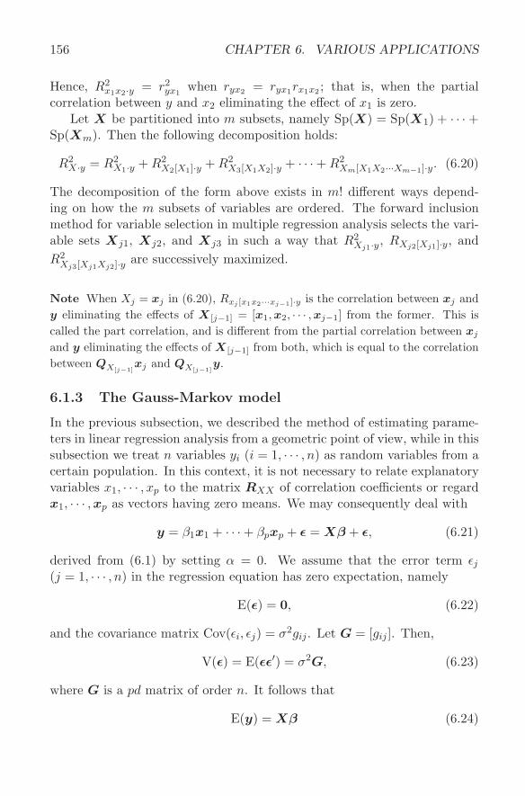
156 CHAPTER 6. VARIOUS APPLICATIONS
Hence, R2x1x2·y = r2
yx1when ryx2 = ryx1rx1x2 ; that is, when the partial
correlation between y and x2 eliminating the effect of x1 is zero.Let X be partitioned into m subsets, namely Sp(X) = Sp(X1) + · · ·+
Sp(Xm). Then the following decomposition holds:
R2X·y = R2
X1·y + R2X2[X1]·y + R2
X3[X1X2]·y + · · ·+ R2Xm[X1X2···Xm−1]·y. (6.20)
The decomposition of the form above exists in m! different ways depend-ing on how the m subsets of variables are ordered. The forward inclusionmethod for variable selection in multiple regression analysis selects the vari-able sets Xj1, Xj2, and Xj3 in such a way that R2
Xj1·y, RXj2[Xj1]·y, andR2
Xj3[Xj1Xj2]·y are successively maximized.
Note When Xj = xj in (6.20), Rxj [x1x2···xj−1]·y is the correlation between xj andy eliminating the effects of X [j−1] = [x1, x2, · · · ,xj−1] from the former. This iscalled the part correlation, and is different from the partial correlation between xj
and y eliminating the effects of X [j−1] from both, which is equal to the correlationbetween QX[j−1]
xj and QX[j−1]y.
6.1.3 The Gauss-Markov model
In the previous subsection, we described the method of estimating parame-ters in linear regression analysis from a geometric point of view, while in thissubsection we treat n variables yi (i = 1, · · · , n) as random variables from acertain population. In this context, it is not necessary to relate explanatoryvariables x1, · · · , xp to the matrix RXX of correlation coefficients or regardx1, · · · ,xp as vectors having zero means. We may consequently deal with
y = β1x1 + · · ·+ βpxp + ε = Xβ + ε, (6.21)
derived from (6.1) by setting α = 0. We assume that the error term εj
(j = 1, · · · , n) in the regression equation has zero expectation, namely
E(ε) = 0, (6.22)
and the covariance matrix Cov(εi, εj) = σ2gij . Let G = [gij ]. Then,
V(ε) = E(εε′) = σ2G, (6.23)
where G is a pd matrix of order n. It follows that
E(y) = Xβ (6.24)
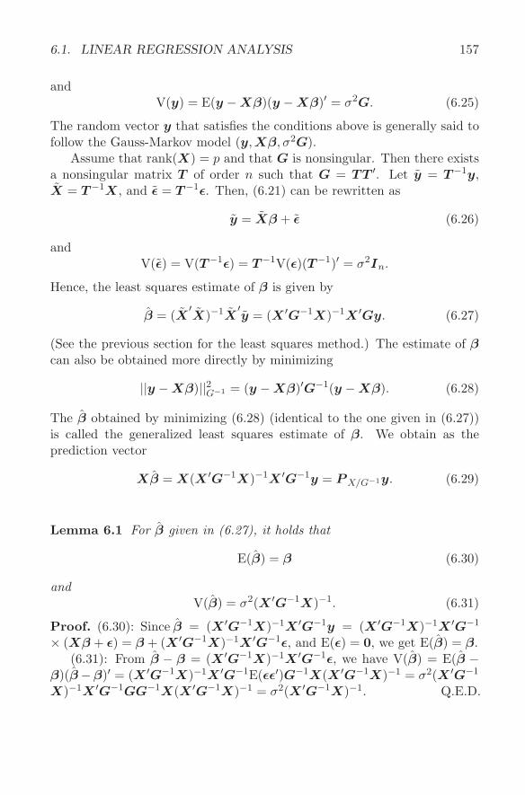
6.1. LINEAR REGRESSION ANALYSIS 157
andV(y) = E(y −Xβ)(y −Xβ)′ = σ2G. (6.25)
The random vector y that satisfies the conditions above is generally said tofollow the Gauss-Markov model (y,Xβ, σ2G).
Assume that rank(X) = p and that G is nonsingular. Then there existsa nonsingular matrix T of order n such that G = TT ′. Let y = T−1y,X = T−1X, and ε = T−1ε. Then, (6.21) can be rewritten as
y = Xβ + ε (6.26)
andV(ε) = V(T−1ε) = T−1V(ε)(T−1)′ = σ2In.
Hence, the least squares estimate of β is given by
β = (X′X)−1X
′y = (X ′G−1X)−1X ′Gy. (6.27)
(See the previous section for the least squares method.) The estimate of βcan also be obtained more directly by minimizing
||y −Xβ)||2G−1 = (y −Xβ)′G−1(y −Xβ). (6.28)
The β obtained by minimizing (6.28) (identical to the one given in (6.27))is called the generalized least squares estimate of β. We obtain as theprediction vector
Xβ = X(X ′G−1X)−1X ′G−1y = P X/G−1y. (6.29)
Lemma 6.1 For β given in (6.27), it holds that
E(β) = β (6.30)
andV(β) = σ2(X ′G−1X)−1. (6.31)
Proof. (6.30): Since β = (X ′G−1X)−1X ′G−1y = (X ′G−1X)−1X ′G−1
× (Xβ + ε) = β + (X ′G−1X)−1X ′G−1ε, and E(ε) = 0, we get E(β) = β.(6.31): From β − β = (X ′G−1X)−1X ′G−1ε, we have V(β) = E(β −
β)(β−β)′ = (X ′G−1X)−1X ′G−1E(εε′)G−1X(X ′G−1X)−1 = σ2(X ′G−1
X)−1X ′G−1GG−1X(X ′G−1X)−1 = σ2(X ′G−1X)−1. Q.E.D.
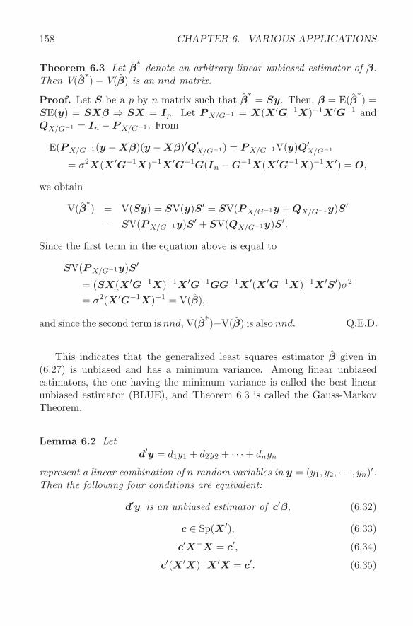
158 CHAPTER 6. VARIOUS APPLICATIONS
Theorem 6.3 Let β∗
denote an arbitrary linear unbiased estimator of β.Then V(β
∗)−V(β) is an nnd matrix.
Proof. Let S be a p by n matrix such that β∗
= Sy. Then, β = E(β∗) =
SE(y) = SXβ ⇒ SX = Ip. Let P X/G−1 = X(X ′G−1X)−1X ′G−1 andQX/G−1 = In − P X/G−1 . From
E(P X/G−1(y −Xβ)(y −Xβ)′Q′X/G−1) = P X/G−1V(y)Q′
X/G−1
= σ2X(X ′G−1X)−1X ′G−1G(In −G−1X(X ′G−1X)−1X ′) = O,
we obtain
V(β∗) = V(Sy) = SV(y)S′ = SV(P X/G−1y + QX/G−1y)S′
= SV(P X/G−1y)S′ + SV(QX/G−1y)S′.
Since the first term in the equation above is equal to
SV(P X/G−1y)S′
= (SX(X ′G−1X)−1X ′G−1GG−1X ′(X ′G−1X)−1X ′S′)σ2
= σ2(X ′G−1X)−1 = V(β),
and since the second term is nnd, V(β∗)−V(β) is also nnd. Q.E.D.
This indicates that the generalized least squares estimator β given in(6.27) is unbiased and has a minimum variance. Among linear unbiasedestimators, the one having the minimum variance is called the best linearunbiased estimator (BLUE), and Theorem 6.3 is called the Gauss-MarkovTheorem.
Lemma 6.2 Letd′y = d1y1 + d2y2 + · · ·+ dnyn
represent a linear combination of n random variables in y = (y1, y2, · · · , yn)′.Then the following four conditions are equivalent:
d′y is an unbiased estimator of c′β, (6.32)
c ∈ Sp(X ′), (6.33)
c′X−X = c′, (6.34)
c′(X ′X)−X ′X = c′. (6.35)
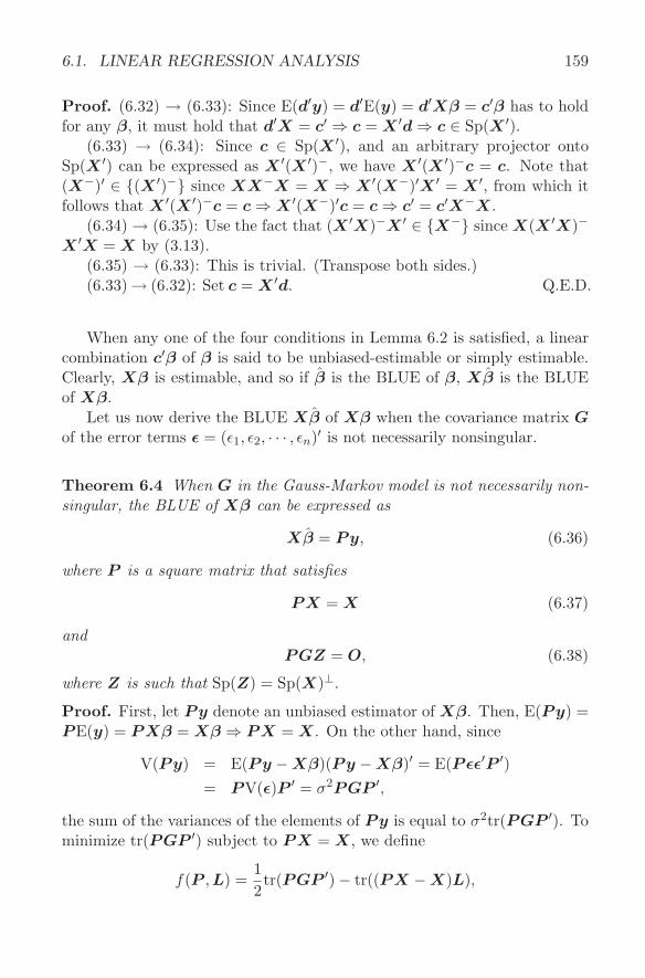
6.1. LINEAR REGRESSION ANALYSIS 159
Proof. (6.32) → (6.33): Since E(d′y) = d′E(y) = d′Xβ = c′β has to holdfor any β, it must hold that d′X = c′ ⇒ c = X ′d ⇒ c ∈ Sp(X ′).
(6.33) → (6.34): Since c ∈ Sp(X ′), and an arbitrary projector ontoSp(X ′) can be expressed as X ′(X ′)−, we have X ′(X ′)−c = c. Note that(X−)′ ∈ {(X ′)−} since XX−X = X ⇒ X ′(X−)′X ′ = X ′, from which itfollows that X ′(X ′)−c = c ⇒ X ′(X−)′c = c ⇒ c′ = c′X−X.
(6.34) → (6.35): Use the fact that (X ′X)−X ′ ∈ {X−} since X(X ′X)−
X ′X = X by (3.13).(6.35) → (6.33): This is trivial. (Transpose both sides.)(6.33)→ (6.32): Set c = X ′d. Q.E.D.
When any one of the four conditions in Lemma 6.2 is satisfied, a linearcombination c′β of β is said to be unbiased-estimable or simply estimable.Clearly, Xβ is estimable, and so if β is the BLUE of β, Xβ is the BLUEof Xβ.
Let us now derive the BLUE Xβ of Xβ when the covariance matrix Gof the error terms ε = (ε1, ε2, · · · , εn)′ is not necessarily nonsingular.
Theorem 6.4 When G in the Gauss-Markov model is not necessarily non-singular, the BLUE of Xβ can be expressed as
Xβ = Py, (6.36)
where P is a square matrix that satisfies
PX = X (6.37)
andPGZ = O, (6.38)
where Z is such that Sp(Z) = Sp(X)⊥.
Proof. First, let Py denote an unbiased estimator of Xβ. Then, E(Py) =PE(y) = PXβ = Xβ ⇒ PX = X. On the other hand, since
V(Py) = E(Py −Xβ)(Py −Xβ)′ = E(Pεε′P ′)= PV(ε)P ′ = σ2PGP ′,
the sum of the variances of the elements of Py is equal to σ2tr(PGP ′). Tominimize tr(PGP ′) subject to PX = X, we define
f(P , L) =12tr(PGP ′)− tr((PX −X)L),
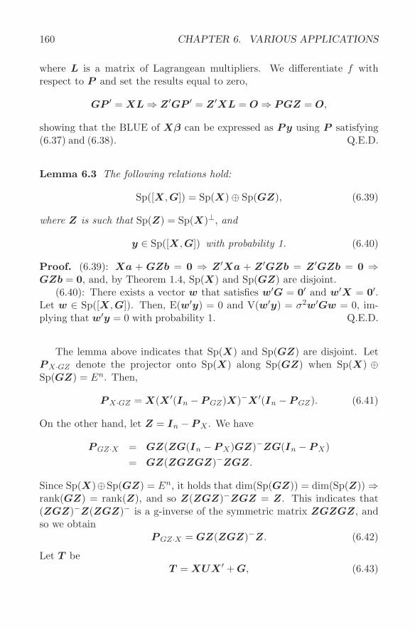
160 CHAPTER 6. VARIOUS APPLICATIONS
where L is a matrix of Lagrangean multipliers. We differentiate f withrespect to P and set the results equal to zero,
GP ′ = XL ⇒ Z ′GP ′ = Z ′XL = O ⇒ PGZ = O,
showing that the BLUE of Xβ can be expressed as Py using P satisfying(6.37) and (6.38). Q.E.D.
Lemma 6.3 The following relations hold:
Sp([X,G]) = Sp(X)⊕ Sp(GZ), (6.39)
where Z is such that Sp(Z) = Sp(X)⊥, and
y ∈ Sp([X,G]) with probability 1. (6.40)
Proof. (6.39): Xa + GZb = 0 ⇒ Z ′Xa + Z ′GZb = Z ′GZb = 0 ⇒GZb = 0, and, by Theorem 1.4, Sp(X) and Sp(GZ) are disjoint.
(6.40): There exists a vector w that satisfies w′G = 0′ and w′X = 0′.Let w ∈ Sp([X, G]). Then, E(w′y) = 0 and V(w′y) = σ2w′Gw = 0, im-plying that w′y = 0 with probability 1. Q.E.D.
The lemma above indicates that Sp(X) and Sp(GZ) are disjoint. LetP X·GZ denote the projector onto Sp(X) along Sp(GZ) when Sp(X) ⊕Sp(GZ) = En. Then,
P X·GZ = X(X ′(In − P GZ)X)−X ′(In − P GZ). (6.41)
On the other hand, let Z = In − P X . We have
P GZ·X = GZ(ZG(In − P X)GZ)−ZG(In − P X)= GZ(ZGZGZ)−ZGZ.
Since Sp(X)⊕Sp(GZ) = En, it holds that dim(Sp(GZ)) = dim(Sp(Z)) ⇒rank(GZ) = rank(Z), and so Z(ZGZ)−ZGZ = Z. This indicates that(ZGZ)−Z(ZGZ)− is a g-inverse of the symmetric matrix ZGZGZ, andso we obtain
P GZ·X = GZ(ZGZ)−Z. (6.42)
Let T beT = XUX ′ + G, (6.43)
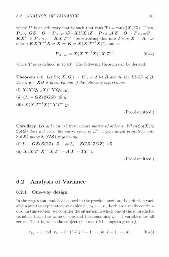
6.2. ANALYSIS OF VARIANCE 161
where U is an arbitrary matrix such that rank(T ) = rank([X, G]). Then,P X·GZGZ = O ⇒ P X·GZ(G+XUX ′)Z = P X·GZTZ = O ⇒ P X·GZT =KX ′ ⇒ P X·GZ = KX ′T−1. Substituting this into P X·GZX = X, weobtain KX ′T−1X = X ⇒ K = X(X ′T−1X)−, and so
P X·GZ = X(X ′T−1X)−X ′T−1, (6.44)
where T is as defined in (6.43). The following theorem can be derived.
Theorem 6.5 Let Sp([X, G]) = En, and let β denote the BLUE of β.Then, y = Xβ is given by one of the following expressions:
(i) X(X ′QGZX)−X ′QGZy,
(ii) (In −GZ(ZGZ)−Z)y,
(iii) X(X ′T−1X)−X ′T−1y.
(Proof omitted.)
Corollary Let A be an arbitrary square matrix of order n. When Sp(X)⊕Sp(G) does not cover the entire space of En, a generalized projection ontoSp(X) along Sp(GZ) is given by
(i) In −GZ(ZGZ)−Z + A(In −ZGZ(ZGZ)−)Z,
(ii) X(X ′T−X)−X ′T− + A(In − TT−).
(Proof omitted.)
6.2 Analysis of Variance
6.2.1 One-way design
In the regression models discussed in the previous section, the criterion vari-able y and the explanatory variables x1, x2, · · · , xm both are usually continu-ous. In this section, we consider the situation in which one of the m predictorvariables takes the value of one and the remaining m − 1 variables are allzeroes. That is, when the subject (the case) k belongs to group j,
xkj = 1 and xki = 0 (i 6= j; i = 1, · · · ,m; k = 1, · · · , n). (6.45)
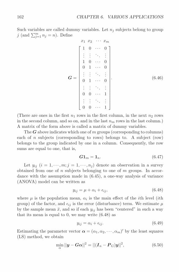
162 CHAPTER 6. VARIOUS APPLICATIONS
Such variables are called dummy variables. Let nj subjects belong to groupj (and
∑mj=1 nj = n). Define
x1 x2 · · · xm
G =
1 0 · · · 0...
.... . .
...1 0 · · · 00 1 · · · 0...
.... . .
...0 1 · · · 0...
.... . .
...0 0 · · · 1...
.... . .
...0 0 · · · 1
. (6.46)
(There are ones in the first n1 rows in the first column, in the next n2 rowsin the second column, and so on, and in the last nm rows in the last column.)A matrix of the form above is called a matrix of dummy variables.
The G above indicates which one of m groups (corresponding to columns)each of n subjects (corresponding to rows) belongs to. A subject (row)belongs to the group indicated by one in a column. Consequently, the rowsums are equal to one, that is,
G1m = 1n. (6.47)
Let yij (i = 1, · · · ,m; j = 1, · · · , nj) denote an observation in a surveyobtained from one of n subjects belonging to one of m groups. In accor-dance with the assumption made in (6.45), a one-way analysis of variance(ANOVA) model can be written as
yij = µ + αi + εij , (6.48)
where µ is the population mean, αi is the main effect of the ith level (ithgroup) of the factor, and εij is the error (disturbance) term. We estimate µby the sample mean x, and so if each yij has been “centered” in such a waythat its mean is equal to 0, we may write (6.48) as
yij = αi + εij . (6.49)
Estimating the parameter vector α = (α1, α2, · · · , αm)′ by the least squares(LS) method, we obtain
minα||y −Gα||2 = ||(In − P G)y||2, (6.50)
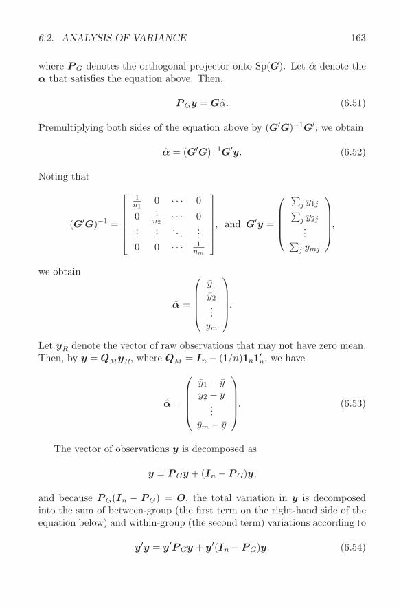
6.2. ANALYSIS OF VARIANCE 163
where P G denotes the orthogonal projector onto Sp(G). Let α denote theα that satisfies the equation above. Then,
P Gy = Gα. (6.51)
Premultiplying both sides of the equation above by (G′G)−1G′, we obtain
α = (G′G)−1G′y. (6.52)
Noting that
(G′G)−1 =
1n1
0 · · · 0
0 1n2
· · · 0...
.... . .
...0 0 · · · 1
nm
, and G′y =
∑j y1j∑j y2j...∑
j ymj
,
we obtain
α =
y1
y2...
ym
.
Let yR denote the vector of raw observations that may not have zero mean.Then, by y = QMyR, where QM = In − (1/n)1n1′n, we have
α =
y1 − yy2 − y
...ym − y
. (6.53)
The vector of observations y is decomposed as
y = P Gy + (In − P G)y,
and because P G(In − P G) = O, the total variation in y is decomposedinto the sum of between-group (the first term on the right-hand side of theequation below) and within-group (the second term) variations according to
y′y = y′P Gy + y′(In − P G)y. (6.54)
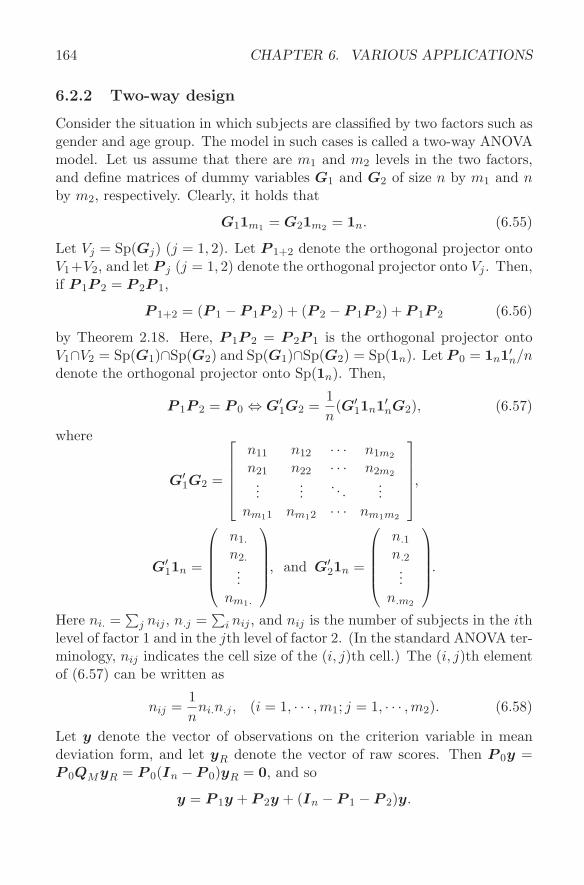
164 CHAPTER 6. VARIOUS APPLICATIONS
6.2.2 Two-way design
Consider the situation in which subjects are classified by two factors such asgender and age group. The model in such cases is called a two-way ANOVAmodel. Let us assume that there are m1 and m2 levels in the two factors,and define matrices of dummy variables G1 and G2 of size n by m1 and nby m2, respectively. Clearly, it holds that
G11m1 = G21m2 = 1n. (6.55)
Let Vj = Sp(Gj) (j = 1, 2). Let P 1+2 denote the orthogonal projector ontoV1+V2, and let P j (j = 1, 2) denote the orthogonal projector onto Vj . Then,if P 1P 2 = P 2P 1,
P 1+2 = (P 1 − P 1P 2) + (P 2 − P 1P 2) + P 1P 2 (6.56)
by Theorem 2.18. Here, P 1P 2 = P 2P 1 is the orthogonal projector ontoV1∩V2 = Sp(G1)∩Sp(G2) and Sp(G1)∩Sp(G2) = Sp(1n). Let P 0 = 1n1′n/ndenote the orthogonal projector onto Sp(1n). Then,
P 1P 2 = P 0 ⇔ G′1G2 =
1n
(G′11n1′nG2), (6.57)
where
G′1G2 =
n11 n12 · · · n1m2
n21 n22 · · · n2m2
......
. . ....
nm11 nm12 · · · nm1m2
,
G′11n =
n1.
n2....
nm1.
, and G′21n =
n.1
n.2...
n.m2
.
Here ni. =∑
j nij , n.j =∑
i nij , and nij is the number of subjects in the ithlevel of factor 1 and in the jth level of factor 2. (In the standard ANOVA ter-minology, nij indicates the cell size of the (i, j)th cell.) The (i, j)th elementof (6.57) can be written as
nij =1n
ni.n.j , (i = 1, · · · ,m1; j = 1, · · · ,m2). (6.58)
Let y denote the vector of observations on the criterion variable in meandeviation form, and let yR denote the vector of raw scores. Then P 0y =P 0QMyR = P 0(In − P 0)yR = 0, and so
y = P 1y + P 2y + (In − P 1 − P 2)y.
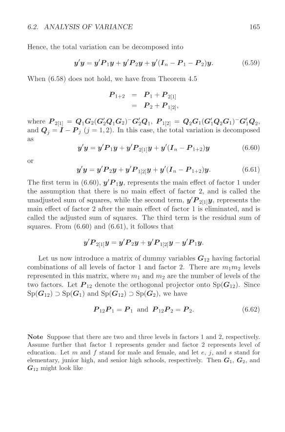
6.2. ANALYSIS OF VARIANCE 165
Hence, the total variation can be decomposed into
y′y = y′P 1y + y′P 2y + y′(In − P 1 − P 2)y. (6.59)
When (6.58) does not hold, we have from Theorem 4.5
P 1+2 = P 1 + P 2[1]
= P 2 + P 1[2],
where P 2[1] = Q1G2(G′2Q1G2)−G′
2Q1, P 1[2] = Q2G1(G′1Q2G1)−G′
1Q2,and Qj = I − P j (j = 1, 2). In this case, the total variation is decomposedas
y′y = y′P 1y + y′P 2[1]y + y′(In − P 1+2)y (6.60)
ory′y = y′P 2y + y′P 1[2]y + y′(In − P 1+2)y. (6.61)
The first term in (6.60), y′P 1y, represents the main effect of factor 1 underthe assumption that there is no main effect of factor 2, and is called theunadjusted sum of squares, while the second term, y′P 2[1]y, represents themain effect of factor 2 after the main effect of factor 1 is eliminated, and iscalled the adjusted sum of squares. The third term is the residual sum ofsquares. From (6.60) and (6.61), it follows that
y′P 2[1]y = y′P 2y + y′P 1[2]y − y′P 1y.
Let us now introduce a matrix of dummy variables G12 having factorialcombinations of all levels of factor 1 and factor 2. There are m1m2 levelsrepresented in this matrix, where m1 and m2 are the number of levels of thetwo factors. Let P 12 denote the orthogonal projector onto Sp(G12). SinceSp(G12) ⊃ Sp(G1) and Sp(G12) ⊃ Sp(G2), we have
P 12P 1 = P 1 and P 12P 2 = P 2. (6.62)
Note Suppose that there are two and three levels in factors 1 and 2, respectively.Assume further that factor 1 represents gender and factor 2 represents level ofeducation. Let m and f stand for male and female, and let e, j, and s stand forelementary, junior high, and senior high schools, respectively. Then G1, G2, andG12 might look like
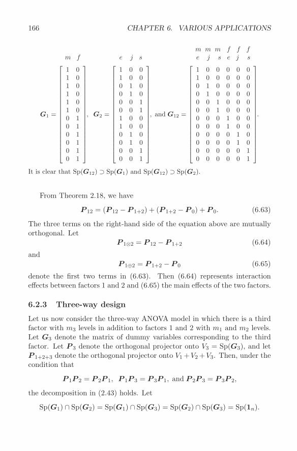
166 CHAPTER 6. VARIOUS APPLICATIONS
m m m f f fm f e j s e j s e j s
G1 =
1 01 01 01 01 01 00 10 10 10 10 10 1
, G2 =
1 0 01 0 00 1 00 1 00 0 10 0 11 0 01 0 00 1 00 1 00 0 10 0 1
, and G12 =
1 0 0 0 0 01 0 0 0 0 00 1 0 0 0 00 1 0 0 0 00 0 1 0 0 00 0 1 0 0 00 0 0 1 0 00 0 0 1 0 00 0 0 0 1 00 0 0 0 1 00 0 0 0 0 10 0 0 0 0 1
.
It is clear that Sp(G12) ⊃ Sp(G1) and Sp(G12) ⊃ Sp(G2).
From Theorem 2.18, we have
P 12 = (P 12 − P 1+2) + (P 1+2 − P 0) + P 0. (6.63)
The three terms on the right-hand side of the equation above are mutuallyorthogonal. Let
P 1⊗2 = P 12 − P 1+2 (6.64)
andP 1⊕2 = P 1+2 − P 0 (6.65)
denote the first two terms in (6.63). Then (6.64) represents interactioneffects between factors 1 and 2 and (6.65) the main effects of the two factors.
6.2.3 Three-way design
Let us now consider the three-way ANOVA model in which there is a thirdfactor with m3 levels in addition to factors 1 and 2 with m1 and m2 levels.Let G3 denote the matrix of dummy variables corresponding to the thirdfactor. Let P 3 denote the orthogonal projector onto V3 = Sp(G3), and letP 1+2+3 denote the orthogonal projector onto V1 +V2 +V3. Then, under thecondition that
P 1P 2 = P 2P 1, P 1P 3 = P 3P 1, and P 2P 3 = P 3P 2,
the decomposition in (2.43) holds. Let
Sp(G1) ∩ Sp(G2) = Sp(G1) ∩ Sp(G3) = Sp(G2) ∩ Sp(G3) = Sp(1n).
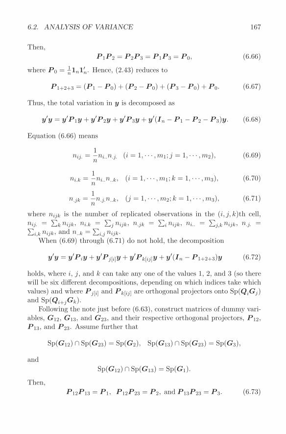
6.2. ANALYSIS OF VARIANCE 167
Then,P 1P 2 = P 2P 3 = P 1P 3 = P 0, (6.66)
where P 0 = 1n1n1′n. Hence, (2.43) reduces to
P 1+2+3 = (P 1 − P 0) + (P 2 − P 0) + (P 3 − P 0) + P 0. (6.67)
Thus, the total variation in y is decomposed as
y′y = y′P 1y + y′P 2y + y′P 3y + y′(In − P 1 − P 2 − P 3)y. (6.68)
Equation (6.66) means
nij. =1n
ni..n.j. (i = 1, · · · ,m1; j = 1, · · · ,m2), (6.69)
ni.k =1n
ni..n..k, (i = 1, · · · ,m1; k = 1, · · · , m3), (6.70)
n.jk =1n
n.j.n..k, (j = 1, · · · ,m2; k = 1, · · · ,m3), (6.71)
where nijk is the number of replicated observations in the (i, j, k)th cell,nij. =
∑k nijk, ni.k =
∑j nijk, n.jk =
∑i nijk, ni.. =
∑j,k nijk, n.j. =∑
i,k nijk, and n..k =∑
i,j nijk.When (6.69) through (6.71) do not hold, the decomposition
y′y = y′P iy + y′P j[i]y + y′P k[ij]y + y′(In − P 1+2+3)y (6.72)
holds, where i, j, and k can take any one of the values 1, 2, and 3 (so therewill be six different decompositions, depending on which indices take whichvalues) and where P j[i] and P k[ij] are orthogonal projectors onto Sp(QiGj)and Sp(Qi+jGk).
Following the note just before (6.63), construct matrices of dummy vari-ables, G12, G13, and G23, and their respective orthogonal projectors, P 12,P 13, and P 23. Assume further that
Sp(G12) ∩ Sp(G23) = Sp(G2), Sp(G13) ∩ Sp(G23) = Sp(G3),
andSp(G12) ∩ Sp(G13) = Sp(G1).
Then,P 12P 13 = P 1, P 12P 23 = P 2, and P 13P 23 = P 3. (6.73)
168 CHAPTER 6. VARIOUS APPLICATIONS
Let P [3] = P 12+13+23 denote the orthogonal projector onto Sp(G12) +Sp(G13) + Sp(G23). By Theorem 2.20 and (2.43), it holds under (6.73)that
P [3] = P 1⊗2 + P 2⊗3 + P 1⊗3 + P 1 + P 2 + P 3 + P 0, (6.74)
where P i⊗j = P ij − P i − P j + P 0 and P i = P i − P 0. Hence, the totalvariation in y is decomposed as
y′y = y′P 1⊗2y + y′P 2⊗3y
+ y′P 1⊗3y + y′P 1y + y′P 2y + y′P 3y + y′(In − P [3])y.
Equation (6.73) corresponds with
nijk =1
ni..nij.ni.k =
1n.j.
nij.n.jk =1
n..kni.kn.jk, (6.75)
but sincenijk =
1n2
ni..n.j.n..k (6.76)
follows from (6.69) through (6.71), the necessary and sufficient condition forthe decomposition in (6.74) to hold is that (6.69) through (6.71) and (6.76)hold simultaneously.
6.2.4 Cochran’s theorem
Let us assume that each element of an n-component random vector of crite-rion variables y = (y1, y2, · · · , yn)′ has zero mean and unit variance, and isdistributed independently of the others; that is, y follows the multivariatenormal distribution N (0, In) with E(y) = 0 and V(y) = In. It is wellknown that
||y||2 = y21 + y2
2 + · · ·+ y2n
follows the chi-square distribution with n degrees of freedom (df).
Lemma 6.4 Let y ∼ N (0, I) (that is, the n-component vector y = (y1, y2,· · · , yn)′ follows the multivariate normal distribution with mean 0 and vari-ance I), and let A be symmetric (i.e., A′ = A). Then, the necessary andsufficient condition for
Q =∑
i
∑
j
aijyiyj = y′Ay
6.2. ANALYSIS OF VARIANCE 169
to follow the chi-square distribution with k = rank(A) degrees of freedom is
A2 = A. (6.77)
Proof. (Necessity) The moment generating function for y′Ay is given by
φ(t) = E(etQ) =∫· · ·
∫ 1(2π)n/2
exp{
(y′Ay)t− 12y′y
}dy1 · · · dyn
= |In − 2tA|−1/2 =n∏
i=1
(1− 2tλi)−1/2,
where λi is the ith largest eigenvalue of A. From A2 = A and rank(A) = k,we have λ1 = λ2 = · · · = λk = 1 and λk+1 = · · · = λn = 0. Hence,φ(t) = (1 − 2t)−
12k, which indicates that φ(t) is the moment generating
function of the chi-square distribution with k degrees of freedom.(Sufficiency) φ(t) = (1 − 2t)−k/2 =
∏ni=1(1 − 2λit)−1/2 ⇒ λi = 1 (i =
1, · · · , k), λi = 0 (i = k+1, · · · , n), which implies A2 = A. Q.E.D.
Let us now consider the case in which y ∼ N (0, σ2G). Let rank(G) = r.Then there exists an n by r matrix T such that G = TT ′. Define z sothat y = Tz. Then, z ∼ N (0, σ2Ir). Hence, the necessary and sufficientcondition for
Q = y′Ay = z′(T ′AT )z
to follow the chi-square distribution is (T ′AT )2 = T ′AT from Lemma 6.4.Pre- and postmultiplying both sides of this equation by T and T ′, respec-tively, we obtain
GAGAG = GAG ⇒ (GA)3 = (GA)2.
We also have
rank(T ′AT ) = tr(T ′AT ) = tr(ATT ′) = tr(AG),
from which the following lemma can be derived.
Lemma 6.5 Let y ∼ N (0, σ2G). The necessary and sufficient conditionfor Q = y′Ay to follow the chi-square distribution with k = tr(AG) degreesof freedom is
GAGAG = GAG (6.78)
170 CHAPTER 6. VARIOUS APPLICATIONS
or(GA)3 = (GA)2. (6.79)
(A proof is omitted.)
Lemma 6.6 Let A and B be square matrices. The necessary and sufficientcondition for y′Ay and y′By to be mutually independent is
AB = O, if y ∼ N (0, σ2In), (6.80)
orGAGBG = O, if y ∼ N (0, σ2G). (6.81)
Proof. (6.80): Let Q1 = y′Ay and Q2 = y′By. Their joint momentgenerating function is given by φ(A,B) = |In − 2At1 − 2Bt2|−1/2, whiletheir marginal moment functions are given by φ(A) = |In − 2At1|−1/2 andφ(B) = |In − 2Bt2|−1/2, so that φ(A,B) = φ(A)φ(B), which is equivalentto AB = O.
(6.81): Let G = TT ′, and introduce z such that y = Tz and z ∼N (0, σ2In). The necessary and sufficient condition for y′Ay = z′T ′ATzand y′By = z′T ′BTz to be independent is given, from (6.80), by
T ′ATT ′BT = O ⇔ GAGBG = O.
Q.E.D.
From these lemmas and Theorem 2.13, the following theorem, calledCochran’s Theorem, can be derived.
Theorem 6.7 Let y ∼ N (0, σ2In), and let P j (j = 1, · · · , k) be a squarematrix of order n such that
P 1 + P 2 + · · ·+ P k = In.
The necessary and sufficient condition for the quadratic forms y′P 1y, y′P 2
× y, · · · , y′P ky to be independently distributed according to the chi-squaredistribution with degrees of freedom equal to n1 = tr(P 1), n2 = tr(P 2), · · · , nk
= tr(P k), respectively, is that one of the following conditions holds:
P iP j = O, (i 6= j), (6.82)
P 2j = P j , (6.83)

6.3. MULTIVARIATE ANALYSIS 171
rank(P 1) + rank(P 2) + · · ·+ rank(P k) = n. (6.84)
(Proof omitted.)
Corollary Let y ∼ N (0, σ2G), and let P j (j = 1, · · · , k) be such that
P 1 + P 2 + · · ·+ P k = In.
The necessary and sufficient condition for the quadratic form y′P jy (j =1, · · · , k) to be independently distributed according to the chi-square distribu-tion with kj = tr(GP jG) degrees of freedom is that one of the three condi-tions (6.85) through (6.87) plus the fourth condition (6.88) simultaneouslyhold:
GP iGP jG = O, (i 6= j), (6.85)
(GP j)3 = (GP j)2, (6.86)
rank(GP 1G) + · · ·+ rank(GP kG) = rank(G2), (6.87)
G3 = G2. (6.88)
Proof. Transform
y′y = y′P 1y + y′P 2y + · · ·+ y′P ky
by y = Tz, where T is such that G = TT ′ and z ∼ N (0, σ2In). Then, use
z′T ′Tz = z′T ′P 1Tz + z′T ′P 2Tz + · · ·+ z′T ′P kTz.
Q.E.D.
Note When the population mean of y is not zero, namely y ∼ N (µ, σ2In), The-orem 6.7 can be modified by replacing the “condition that y′P jy follows the in-dependent chi-square” with the “condition that y′P jy follows the independentnoncentral chi-square with the noncentrality parameter µ′P jµ,” and everythingelse holds the same. A similar modification can be made for y ∼ N (µ, σ2G) in thecorollary to Theorem 6.7.
6.3 Multivariate Analysis
Utilizing the notion of projection matrices, relationships among various tech-niques of multivariate analysis, methods for variable selection, and so on canbe systematically investigated.
172 CHAPTER 6. VARIOUS APPLICATIONS
6.3.1 Canonical correlation analysis
Let X = [x1, x2, · · · , xp] and Y = [y1, y2, · · · , yq] denote matrices of obser-vations on two sets of variables. It is not necessarily assumed that vectorsin those matrices are linearly independent, although it is assumed that theyare columnwise centered. We consider forming two sets of linear compositescores,
f = a1x1 + a2x2 + · · ·+ apxp = Xa
andg = b1y1 + b2y2 + · · ·+ bqyq = Y b,
in such a way that their correlation
rfg = (f , g)/(||f || · ||g||)= (Xa,Y b)/(||Xa|| · ||Y b||)
is maximized. This is equivalent to maximizing a′X ′Y b subject to theconstraints that
a′X ′Xa = b′Y ′Y b = 1. (6.89)
We define
f(a, b, λ1, λ2)
= a′X ′Y b− λ1
2(a′X ′Xa− 1)− λ2
2(b′Y ′Y b− 1),
differentiate it with respect to a and b, and set the result equal to zero.Then the following two equations can be derived:
X ′Y b = λ1X′Xa and Y ′Xa = λ2Y
′Y b. (6.90)
Premultiplying the equations above by a′ and b′, respectively, we obtainλ1 = λ2 by (6.89). We may let λ1 = λ2 =
√λ. Furthermore, by premulti-
plying (6.90) by X(X ′X)− and Y (Y ′Y )−, respectively, we get
P XY b =√
λXa and P Y Xa =√
λY b, (6.91)
where P X = X(X ′X)−X ′ and P Y = Y (Y ′Y )−Y ′ are the orthogonalprojectors onto Sp(X) and Sp(Y ), respectively. The linear composites thatare to be obtained should satisfy the relationships depicted in Figure 6.2.
Substituting one equation into the other in (6.91), we obtain
(P XP Y )Xa = λXa (6.92)
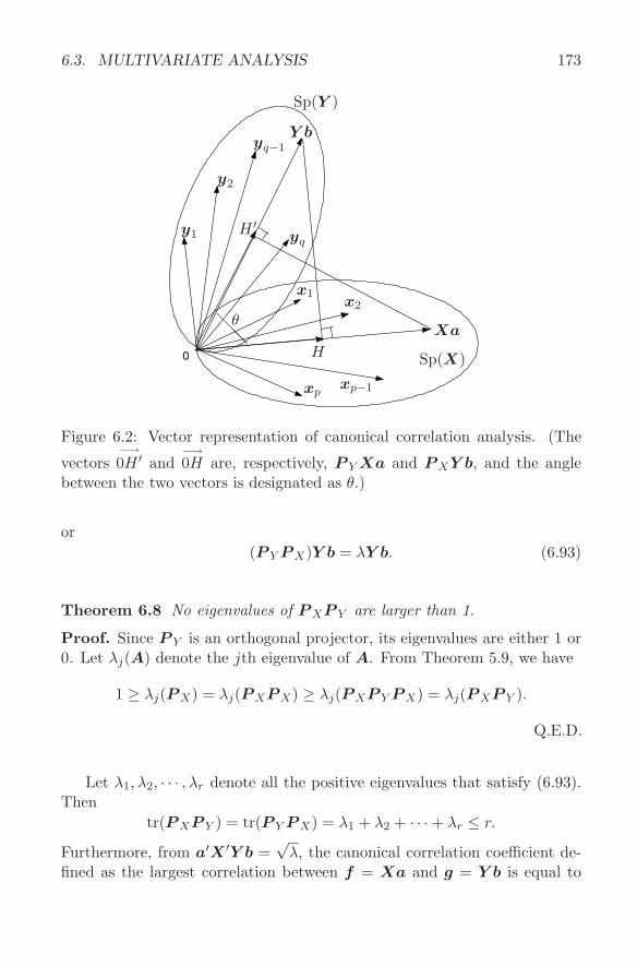
6.3. MULTIVARIATE ANALYSIS 173
0
Sp(Y )
Y byq−1
yq
y2
y1 H ′
H
x1x2
Sp(X)
Xa
xpxp−1
@@@θ
Figure 6.2: Vector representation of canonical correlation analysis. (The
vectors−→0H ′ and
−→0H are, respectively, P Y Xa and P XY b, and the angle
between the two vectors is designated as θ.)
or(P Y P X)Y b = λY b. (6.93)
Theorem 6.8 No eigenvalues of P XP Y are larger than 1.
Proof. Since P Y is an orthogonal projector, its eigenvalues are either 1 or0. Let λj(A) denote the jth eigenvalue of A. From Theorem 5.9, we have
1 ≥ λj(P X) = λj(P XP X) ≥ λj(P XP Y P X) = λj(P XP Y ).
Q.E.D.
Let λ1, λ2, · · · , λr denote all the positive eigenvalues that satisfy (6.93).Then
tr(P XP Y ) = tr(P Y P X) = λ1 + λ2 + · · ·+ λr ≤ r.
Furthermore, from a′X ′Y b =√
λ, the canonical correlation coefficient de-fined as the largest correlation between f = Xa and g = Y b is equal to
174 CHAPTER 6. VARIOUS APPLICATIONS
the square root of the largest eigenvalue of (6.92) or (6.93) (that is,√
λ),which is also the largest singular value of P XP Y . When a and b are theeigenvectors that satisfy (6.92) or (6.93), f = Xa and g = Y b are calledcanonical variates. Let ZX and ZY denote matrices of standardized scorescorresponding to X and Y . Then, Sp(X) = Sp(ZX) and Sp(Y ) = Sp(ZY ),so that tr(P XP Y ) = tr(P ZX
P ZY), and the sum of squares of canonical cor-
relations is equal to
R2X·Y = tr(P XP Y ) = tr(P ZX
P ZY) = tr(RY XR−
XXRXY R−Y Y ), (6.94)
where RXX , RXY , and RY Y are correlation matrices for X, between Xand Y , and for Y , respectively.
The following theorem is derived from Theorem 2.24.
Theorem 6.9 Let r = min(rank(X), rank(Y )). Then,
D2XY = tr(P XP Y ) ≤ r, (6.95)
where D2XY is called the generalized coefficient of determination and indi-
cates the overall strength of the relationship between X and Y .(Proof omitted.)
When Y consists of a single variable y,
D2XY = tr(P XP y) = y′P Xy/y′y = R2
X·ycoincides with the coefficient of determination, which is equal to the squaredmultiple correlation coefficient in multiple regression analysis in which Xcontains the explanatory variables and y is the criterion variable. When Xalso consists of a single variable x,
D2XY = tr(P xP y) = (x, y)2/(||x||2||y||2) = r2
xy; (6.96)
that is, D2XY is equal to the square of the correlation coefficient between x
and y.
Note The tr(P xP y) above gives the most general expression of the squared cor-relation coefficient when both x and y are mean centered. When the variance ofeither x or y is zero, or both variances are zero, we have x and/or y = 0, and ag-inverse of zero can be an arbitrary number, so
r2xy = tr(P xP y) = tr(x(x′x)−x′y(y′y)−y′)
= k(x′y)2 = 0,
where k is arbitrary. That is, rxy = 0.
6.3. MULTIVARIATE ANALYSIS 175
Assume that there are r positive eigenvalues that satisfy (6.92), and let
XA = [Xa1, Xa2, · · · ,Xar] and Y B = [Y b1, Y b2, · · · , Y br]
denote the corresponding r pairs of canonical variates. Then the followingtwo properties hold (Yanai, 1981).
Theorem 6.10P XA = (P XP Y )(P XP Y )−` (6.97)
andP Y B = (P Y P X)(P Y P X)−` . (6.98)
Proof. From (6.92), Sp(XA) ⊃ Sp(P XP Y ). On the other hand, fromrank(P XP Y ) = rank(XA) = r, we have Sp(XA) = Sp(P XP Y ). By thenote given after the corollary to Theorem 2.13, (6.97) holds; (6.98) is similar.
Q.E.D.
The theorem above leads to the following.
Theorem 6.11P XAP Y = P XP Y , (6.99)
P XP Y B = P XP Y , (6.100)
andP XAP Y B = P XP Y . (6.101)
Proof. (6.99): From Sp(XA) ⊂ Sp(X), P XAP X = P XA, from whichit follows that P XAP Y = P XAP XP Y = (P XP Y )(P XP Y )−` P XP Y =P XP Y .
(6.100): Noting that A′AA−` = A′, we obtain P XP Y B = P XP Y P Y B
= (P Y P X)′(P Y P X)(P Y P X)−` = (P Y P X)′ = P XP Y .(6.101): P XAP Y B =P XAP Y P Y B =P XP Y P Y B =P XP Y B =P XP Y .
Q.E.D.
Corollary 1
(P X − P XA)P Y = O and (P Y − P Y B)P X = O,
and(P X − P XA)(P Y − P Y B) = O.
(Proof omitted.)
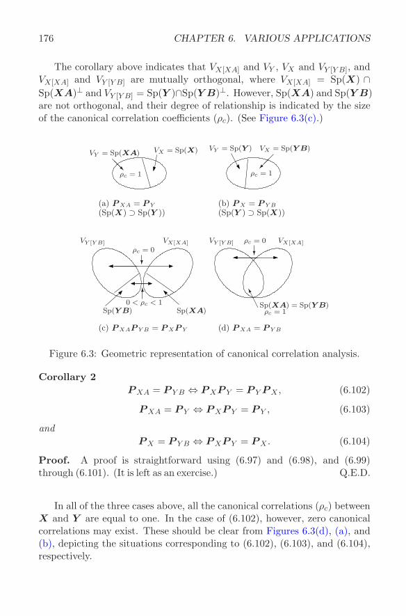
176 CHAPTER 6. VARIOUS APPLICATIONS
The corollary above indicates that VX[XA] and VY , VX and VY [Y B], andVX[XA] and VY [Y B] are mutually orthogonal, where VX[XA] = Sp(X) ∩Sp(XA)⊥ and VY [Y B] = Sp(Y )∩Sp(Y B)⊥. However, Sp(XA) and Sp(Y B)are not orthogonal, and their degree of relationship is indicated by the sizeof the canonical correlation coefficients (ρc). (See Figure 6.3(c).)
VX = Sp(X)VY = Sp(XA)
@@Rρc = 1
VY = Sp(Y ) VX = Sp(Y B)
¡¡ªρc = 1
(a) P XA = P Y
(Sp(X) ⊃ Sp(Y ))(b) P X = P Y B
(Sp(Y ) ⊃ Sp(X))
Sp(XA)Sp(Y B)0 < ρc < 1
6
VY [Y B] VX[XA]
ρc = 0
?
VY [Y B] VX[XA]ρc = 0
?
Sp(XA) = Sp(Y B)ρc = 1
AAK
(c) P XAP Y B = P XP Y (d) P XA = P Y B
Figure 6.3: Geometric representation of canonical correlation analysis.
Corollary 2P XA = P Y B ⇔ P XP Y = P Y P X , (6.102)
P XA = P Y ⇔ P XP Y = P Y , (6.103)
andP X = P Y B ⇔ P XP Y = P X . (6.104)
Proof. A proof is straightforward using (6.97) and (6.98), and (6.99)through (6.101). (It is left as an exercise.) Q.E.D.
In all of the three cases above, all the canonical correlations (ρc) betweenX and Y are equal to one. In the case of (6.102), however, zero canonicalcorrelations may exist. These should be clear from Figures 6.3(d), (a), and(b), depicting the situations corresponding to (6.102), (6.103), and (6.104),respectively.
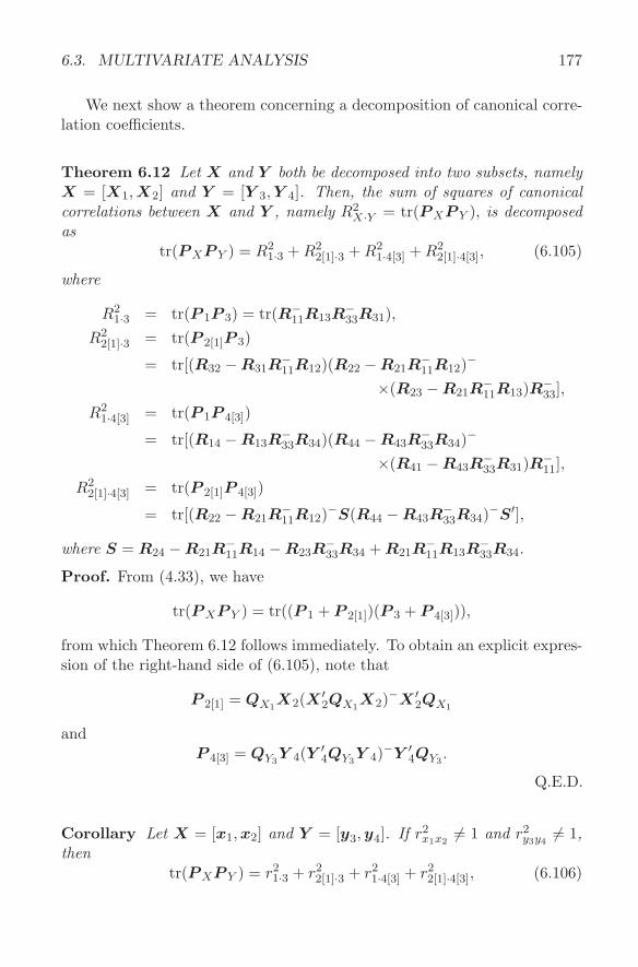
6.3. MULTIVARIATE ANALYSIS 177
We next show a theorem concerning a decomposition of canonical corre-lation coefficients.
Theorem 6.12 Let X and Y both be decomposed into two subsets, namelyX = [X1, X2] and Y = [Y 3, Y 4]. Then, the sum of squares of canonicalcorrelations between X and Y , namely R2
X·Y = tr(P XP Y ), is decomposedas
tr(P XP Y ) = R21·3 + R2
2[1]·3 + R21·4[3] + R2
2[1]·4[3], (6.105)
where
R21·3 = tr(P 1P 3) = tr(R−
11R13R−33R31),
R22[1]·3 = tr(P 2[1]P 3)
= tr[(R32 −R31R−11R12)(R22 −R21R
−11R12)−
×(R23 −R21R−11R13)R−
33],R2
1·4[3] = tr(P 1P 4[3])
= tr[(R14 −R13R−33R34)(R44 −R43R
−33R34)−
×(R41 −R43R−33R31)R−
11],R2
2[1]·4[3] = tr(P 2[1]P 4[3])
= tr[(R22 −R21R−11R12)−S(R44 −R43R
−33R34)−S′],
where S = R24 −R21R−11R14 −R23R
−33R34 + R21R
−11R13R
−33R34.
Proof. From (4.33), we have
tr(P XP Y ) = tr((P 1 + P 2[1])(P 3 + P 4[3])),
from which Theorem 6.12 follows immediately. To obtain an explicit expres-sion of the right-hand side of (6.105), note that
P 2[1] = QX1X2(X ′
2QX1X2)−X ′
2QX1
andP 4[3] = QY3
Y 4(Y ′4QY3
Y 4)−Y ′4QY3
.
Q.E.D.
Corollary Let X = [x1, x2] and Y = [y3,y4]. If r2x1x2
6= 1 and r2y3y4
6= 1,then
tr(P XP Y ) = r21·3 + r2
2[1]·3 + r21·4[3] + r2
2[1]·4[3], (6.106)
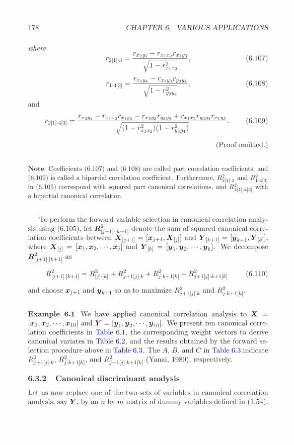
178 CHAPTER 6. VARIOUS APPLICATIONS
wherer2[1]·3 =
rx2y3 − rx1x2rx1y3√1− r2
x1x2
, (6.107)
r1·4[3] =rx1y4 − rx1y3ry3y4√
1− r2y3y4
, (6.108)
and
r2[1]·4[3] =rx2y4 − rx1x2rx1y4 − rx2y3ry3y4 + rx1x2ry3y4rx1y3√
(1− r2x1x2
)(1− r2y3y4
). (6.109)
(Proof omitted.)
Note Coefficients (6.107) and (6.108) are called part correlation coefficients, and(6.109) is called a bipartial correlation coefficient. Furthermore, R2
2[1]·3 and R21·4[3]
in (6.105) correspond with squared part canonical correlations, and R22[1]·4[3] with
a bipartial canonical correlation.
To perform the forward variable selection in canonical correlation analy-sis using (6.105), let R2
[j+1]·[k+1] denote the sum of squared canonical corre-lation coefficients between X [j+1] = [xj+1, X [j]] and Y [k+1] = [yk+1, Y [k]],where X [j] = [x1,x2, · · · , xj ] and Y [k] = [y1, y2, · · · ,yk]. We decomposeR2
[j+1]·[k+1] as
R2[j+1]·[k+1] = R2
[j]·[k] + R2j+1[j]·k + R2
j·k+1[k] + R2j+1[j]·k+1[k] (6.110)
and choose xj+1 and yk+1 so as to maximize R2j+1[j]·k and R2
j·k+1[k].
Example 6.1 We have applied canonical correlation analysis to X =[x1,x2, · · · , x10] and Y = [y1, y2, · · · , y10]. We present ten canonical corre-lation coefficients in Table 6.1, the corresponding weight vectors to derivecanonical variates in Table 6.2, and the results obtained by the forward se-lection procedure above in Table 6.3. The A, B, and C in Table 6.3 indicateR2
j+1[j]·k, R2j·k+1[k], and R2
j+1[j]·k+1[k] (Yanai, 1980), respectively.
6.3.2 Canonical discriminant analysis
Let us now replace one of the two sets of variables in canonical correlationanalysis, say Y , by an n by m matrix of dummy variables defined in (1.54).
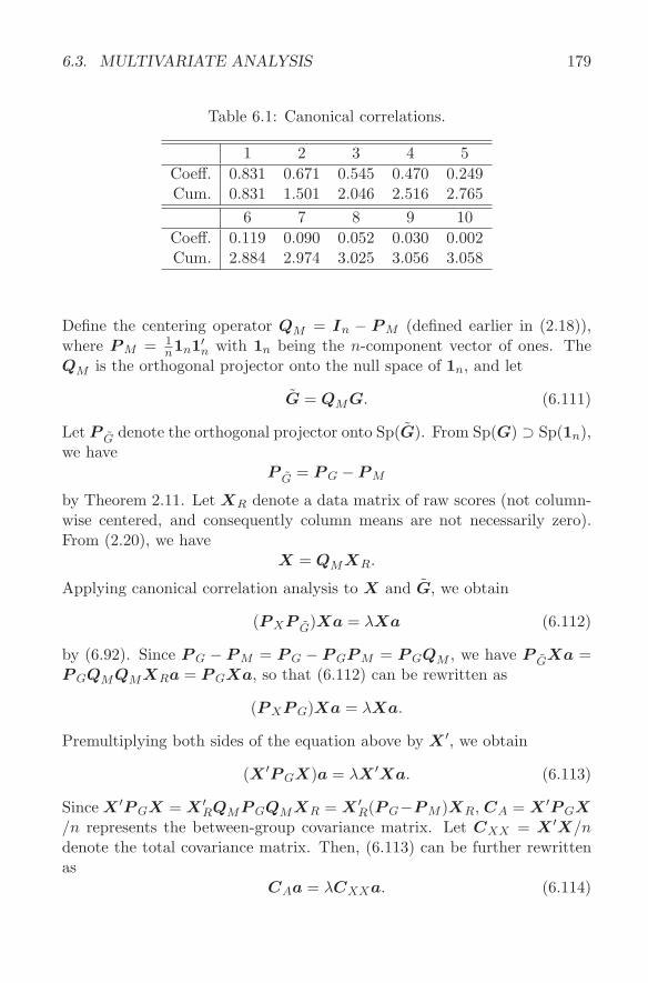
6.3. MULTIVARIATE ANALYSIS 179
Table 6.1: Canonical correlations.
1 2 3 4 5Coeff. 0.831 0.671 0.545 0.470 0.249Cum. 0.831 1.501 2.046 2.516 2.765
6 7 8 9 10Coeff. 0.119 0.090 0.052 0.030 0.002Cum. 2.884 2.974 3.025 3.056 3.058
Define the centering operator QM = In − P M (defined earlier in (2.18)),where P M = 1
n1n1′n with 1n being the n-component vector of ones. TheQM is the orthogonal projector onto the null space of 1n, and let
G = QMG. (6.111)
Let P G denote the orthogonal projector onto Sp(G). From Sp(G) ⊃ Sp(1n),we have
P G = P G − P M
by Theorem 2.11. Let XR denote a data matrix of raw scores (not column-wise centered, and consequently column means are not necessarily zero).From (2.20), we have
X = QMXR.
Applying canonical correlation analysis to X and G, we obtain
(P XP G)Xa = λXa (6.112)
by (6.92). Since P G − P M = P G − P GP M = P GQM , we have P GXa =P GQMQMXRa = P GXa, so that (6.112) can be rewritten as
(P XP G)Xa = λXa.
Premultiplying both sides of the equation above by X ′, we obtain
(X ′P GX)a = λX ′Xa. (6.113)
Since X ′P GX = X ′RQMP GQMXR = X ′
R(P G−P M )XR, CA = X ′P GX/n represents the between-group covariance matrix. Let CXX = X ′X/ndenote the total covariance matrix. Then, (6.113) can be further rewrittenas
CAa = λCXXa. (6.114)
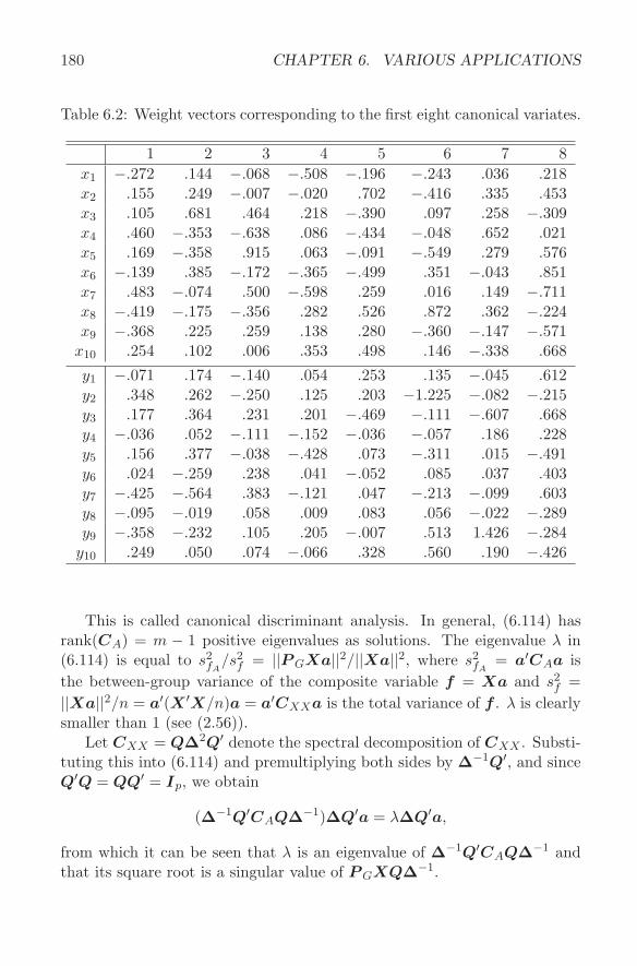
180 CHAPTER 6. VARIOUS APPLICATIONS
Table 6.2: Weight vectors corresponding to the first eight canonical variates.
1 2 3 4 5 6 7 8x1 −.272 .144 −.068 −.508 −.196 −.243 .036 .218x2 .155 .249 −.007 −.020 .702 −.416 .335 .453x3 .105 .681 .464 .218 −.390 .097 .258 −.309x4 .460 −.353 −.638 .086 −.434 −.048 .652 .021x5 .169 −.358 .915 .063 −.091 −.549 .279 .576x6 −.139 .385 −.172 −.365 −.499 .351 −.043 .851x7 .483 −.074 .500 −.598 .259 .016 .149 −.711x8 −.419 −.175 −.356 .282 .526 .872 .362 −.224x9 −.368 .225 .259 .138 .280 −.360 −.147 −.571
x10 .254 .102 .006 .353 .498 .146 −.338 .668
y1 −.071 .174 −.140 .054 .253 .135 −.045 .612y2 .348 .262 −.250 .125 .203 −1.225 −.082 −.215y3 .177 .364 .231 .201 −.469 −.111 −.607 .668y4 −.036 .052 −.111 −.152 −.036 −.057 .186 .228y5 .156 .377 −.038 −.428 .073 −.311 .015 −.491y6 .024 −.259 .238 .041 −.052 .085 .037 .403y7 −.425 −.564 .383 −.121 .047 −.213 −.099 .603y8 −.095 −.019 .058 .009 .083 .056 −.022 −.289y9 −.358 −.232 .105 .205 −.007 .513 1.426 −.284
y10 .249 .050 .074 −.066 .328 .560 .190 −.426
This is called canonical discriminant analysis. In general, (6.114) hasrank(CA) = m − 1 positive eigenvalues as solutions. The eigenvalue λ in(6.114) is equal to s2
fA/s2
f = ||P GXa||2/||Xa||2, where s2fA
= a′CAa isthe between-group variance of the composite variable f = Xa and s2
f =||Xa||2/n = a′(X ′X/n)a = a′CXXa is the total variance of f . λ is clearlysmaller than 1 (see (2.56)).
Let CXX = Q∆2Q′ denote the spectral decomposition of CXX . Substi-tuting this into (6.114) and premultiplying both sides by ∆−1Q′, and sinceQ′Q = QQ′ = Ip, we obtain
(∆−1Q′CAQ∆−1)∆Q′a = λ∆Q′a,
from which it can be seen that λ is an eigenvalue of ∆−1Q′CAQ∆−1 andthat its square root is a singular value of P GXQ∆−1.
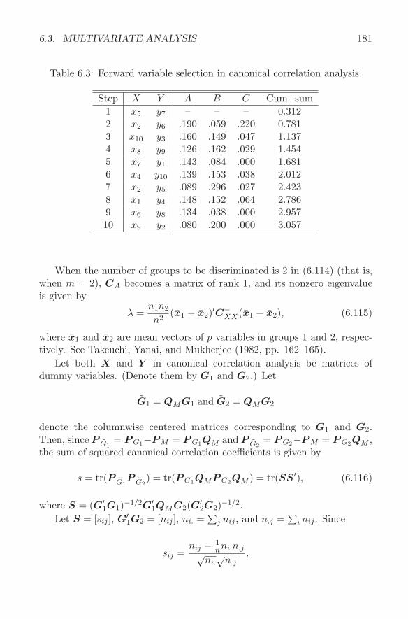
6.3. MULTIVARIATE ANALYSIS 181
Table 6.3: Forward variable selection in canonical correlation analysis.
Step X Y A B C Cum. sum1 x5 y7 – – – 0.3122 x2 y6 .190 .059 .220 0.7813 x10 y3 .160 .149 .047 1.1374 x8 y9 .126 .162 .029 1.4545 x7 y1 .143 .084 .000 1.6816 x4 y10 .139 .153 .038 2.0127 x2 y5 .089 .296 .027 2.4238 x1 y4 .148 .152 .064 2.7869 x6 y8 .134 .038 .000 2.95710 x9 y2 .080 .200 .000 3.057
When the number of groups to be discriminated is 2 in (6.114) (that is,when m = 2), CA becomes a matrix of rank 1, and its nonzero eigenvalueis given by
λ =n1n2
n2(x1 − x2)′C−
XX(x1 − x2), (6.115)
where x1 and x2 are mean vectors of p variables in groups 1 and 2, respec-tively. See Takeuchi, Yanai, and Mukherjee (1982, pp. 162–165).
Let both X and Y in canonical correlation analysis be matrices ofdummy variables. (Denote them by G1 and G2.) Let
G1 = QMG1 and G2 = QMG2
denote the columnwise centered matrices corresponding to G1 and G2.Then, since P G1
= P G1−P M = P G1QM and P G2= P G2−P M = P G2QM ,
the sum of squared canonical correlation coefficients is given by
s = tr(P G1P G2
) = tr(P G1QMP G2QM ) = tr(SS′), (6.116)
where S = (G′1G1)−1/2G′
1QMG2(G′2G2)−1/2.
Let S = [sij ], G′1G2 = [nij ], ni. =
∑j nij , and n.j =
∑i nij . Since
sij =nij − 1
nni.n.j√ni.√
n.j,
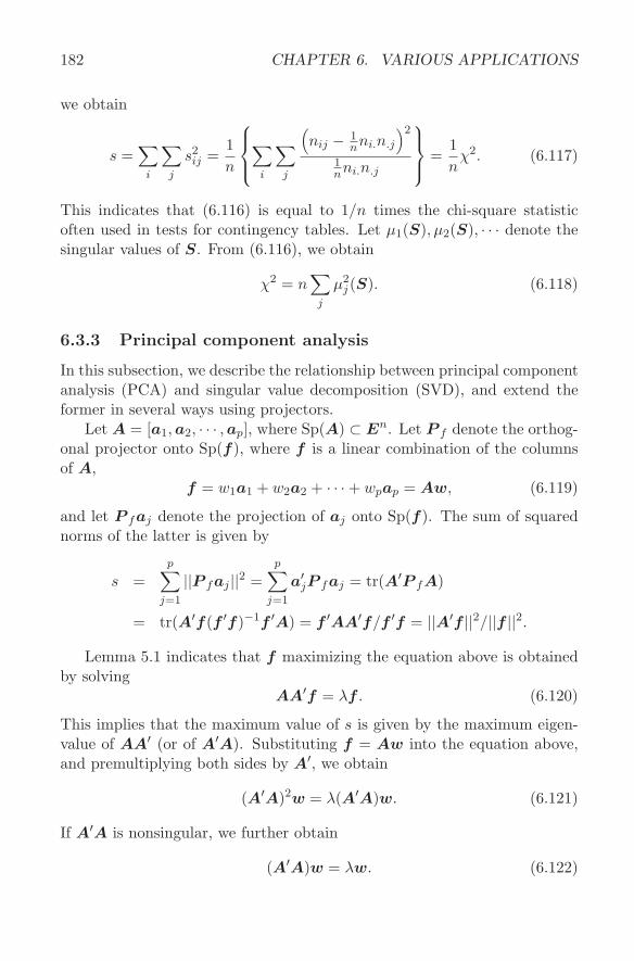
182 CHAPTER 6. VARIOUS APPLICATIONS
we obtain
s =∑
i
∑
j
s2ij =
1n
∑
i
∑
j
(nij − 1
nni.n.j
)2
1nni.n.j
=1n
χ2. (6.117)
This indicates that (6.116) is equal to 1/n times the chi-square statisticoften used in tests for contingency tables. Let µ1(S), µ2(S), · · · denote thesingular values of S. From (6.116), we obtain
χ2 = n∑
j
µ2j (S). (6.118)
6.3.3 Principal component analysis
In this subsection, we describe the relationship between principal componentanalysis (PCA) and singular value decomposition (SVD), and extend theformer in several ways using projectors.
Let A = [a1, a2, · · · , ap], where Sp(A) ⊂ En. Let P f denote the orthog-onal projector onto Sp(f), where f is a linear combination of the columnsof A,
f = w1a1 + w2a2 + · · ·+ wpap = Aw, (6.119)
and let P faj denote the projection of aj onto Sp(f). The sum of squarednorms of the latter is given by
s =p∑
j=1
||P faj ||2 =p∑
j=1
a′jP faj = tr(A′P fA)
= tr(A′f(f ′f)−1f ′A) = f ′AA′f/f ′f = ||A′f ||2/||f ||2.
Lemma 5.1 indicates that f maximizing the equation above is obtainedby solving
AA′f = λf . (6.120)
This implies that the maximum value of s is given by the maximum eigen-value of AA′ (or of A′A). Substituting f = Aw into the equation above,and premultiplying both sides by A′, we obtain
(A′A)2w = λ(A′A)w. (6.121)
If A′A is nonsingular, we further obtain
(A′A)w = λw. (6.122)
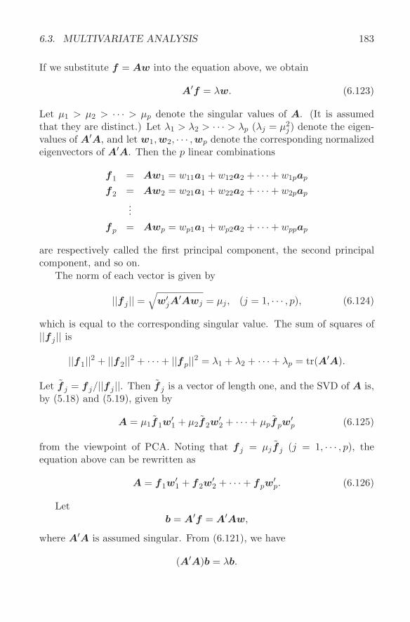
6.3. MULTIVARIATE ANALYSIS 183
If we substitute f = Aw into the equation above, we obtain
A′f = λw. (6.123)
Let µ1 > µ2 > · · · > µp denote the singular values of A. (It is assumedthat they are distinct.) Let λ1 > λ2 > · · · > λp (λj = µ2
j ) denote the eigen-values of A′A, and let w1, w2, · · · , wp denote the corresponding normalizedeigenvectors of A′A. Then the p linear combinations
f1 = Aw1 = w11a1 + w12a2 + · · ·+ w1pap
f2 = Aw2 = w21a1 + w22a2 + · · ·+ w2pap
...fp = Awp = wp1a1 + wp2a2 + · · ·+ wppap
are respectively called the first principal component, the second principalcomponent, and so on.
The norm of each vector is given by
||f j || =√
w′jA
′Awj = µj , (j = 1, · · · , p), (6.124)
which is equal to the corresponding singular value. The sum of squares of||f j || is
||f1||2 + ||f2||2 + · · ·+ ||fp||2 = λ1 + λ2 + · · ·+ λp = tr(A′A).
Let f j = f j/||f j ||. Then f j is a vector of length one, and the SVD of A is,by (5.18) and (5.19), given by
A = µ1f1w′1 + µ2f2w
′2 + · · ·+ µpfpw
′p (6.125)
from the viewpoint of PCA. Noting that f j = µj f j (j = 1, · · · , p), theequation above can be rewritten as
A = f1w′1 + f2w
′2 + · · ·+ fpw
′p. (6.126)
Letb = A′f = A′Aw,
where A′A is assumed singular. From (6.121), we have
(A′A)b = λb.
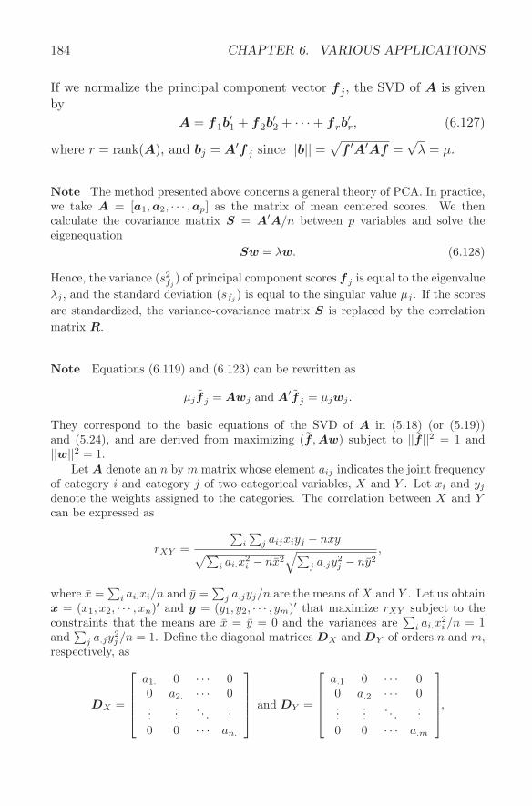
184 CHAPTER 6. VARIOUS APPLICATIONS
If we normalize the principal component vector f j , the SVD of A is givenby
A = f1b′1 + f2b
′2 + · · ·+ f rb
′r, (6.127)
where r = rank(A), and bj = A′f j since ||b|| =√
f ′A′Af =√
λ = µ.
Note The method presented above concerns a general theory of PCA. In practice,we take A = [a1, a2, · · · , ap] as the matrix of mean centered scores. We thencalculate the covariance matrix S = A′A/n between p variables and solve theeigenequation
Sw = λw. (6.128)
Hence, the variance (s2fj
) of principal component scores f j is equal to the eigenvalueλj , and the standard deviation (sfj ) is equal to the singular value µj . If the scoresare standardized, the variance-covariance matrix S is replaced by the correlationmatrix R.
Note Equations (6.119) and (6.123) can be rewritten as
µj f j = Awj and A′f j = µjwj .
They correspond to the basic equations of the SVD of A in (5.18) (or (5.19))and (5.24), and are derived from maximizing (f , Aw) subject to ||f ||2 = 1 and||w||2 = 1.
Let A denote an n by m matrix whose element aij indicates the joint frequencyof category i and category j of two categorical variables, X and Y . Let xi and yj
denote the weights assigned to the categories. The correlation between X and Ycan be expressed as
rXY =
∑i
∑j aijxiyj − nxy
√∑i ai.x2
i − nx2√∑
j a.jy2j − ny2
,
where x =∑
i ai.xi/n and y =∑
j a.jyj/n are the means of X and Y . Let us obtainx = (x1, x2, · · · , xn)′ and y = (y1, y2, · · · , ym)′ that maximize rXY subject to theconstraints that the means are x = y = 0 and the variances are
∑i ai.x
2i /n = 1
and∑
j a.jy2j /n = 1. Define the diagonal matrices DX and DY of orders n and m,
respectively, as
DX =
a1. 0 · · · 00 a2. · · · 0...
.... . .
...0 0 · · · an.
and DY =
a.1 0 · · · 00 a.2 · · · 0...
.... . .
...0 0 · · · a.m
,
6.3. MULTIVARIATE ANALYSIS 185
where ai. =∑
j aij and a.j =∑
i aij . The problem reduces to that of maximizingx′Ay subject to the constraints
x′DXx = y′DY y = 1.
Differentiating
f(x,y) = x′Ay − λ
2(x′DXx− 1)− µ
2(y′DY y − 1)
with respect to x and y and setting the results equal to zero, we obtain
Ay = λDXx and A′x = µDY y. (6.129)
(It can be easily verified that λ = µ, so µ is used for λ hereafter.) Let
D−1/2X =
1/√
a1. 0 · · · 00 1/
√a2. · · · 0
......
. . ....
0 0 · · · 1/√
an.
and
D−1/2Y =
1/√
a.1 0 · · · 00 1/
√a.2 · · · 0
......
. . ....
0 0 · · · 1/√
a.m
.
LetA = D
−1/2X AD
−1/2Y ,
and let x and y be such that x = D−1/2X x and y = D
−1/2Y y. Then, (6.129) can be
rewritten asAy = µx and A
′x = µy, (6.130)
and the SVD of A can be written as
A = µ1x1y′1 + µ2x2y
′2 + · · ·+ µrxry
′r, (6.131)
where r = min(n,m) and where µ1 = 1, x1 = 1n, and y1 = 1m.The method described above is a multivariate data analysis technique called
optimal scaling or dual scaling (Nishisato, 1980).
Let us obtain F = [f1, f2, · · · , f r], where r = rank(A), that maximizes
s =p∑
j=1
||P F aj ||2, (6.132)
186 CHAPTER 6. VARIOUS APPLICATIONS
where P F is the orthogonal projector onto Sp(F ) and aj is the jth columnvector of A = [a1, a2, · · · , ap]. The criterion above can be rewritten as
s = tr(A′P F A) = tr{(F ′F )−1F ′AA′F },
and so, for maximizing this under the restriction that F ′F = Ir, we intro-duce
f(F , L) = tr(F ′AA′F )− tr{(F ′F − Ir)L},where L is a symmetric matrix of Lagrangean multipliers. Differentiatingf(F , L) with respect to F and setting the results equal to zero, we obtain
AA′F = FL. (6.133)
Since L is symmetric, it can be decomposed as L = V ∆2rV
′, where r =rank(A′A), by spectral decomposition. Substituting this into (6.133), weobtain
AA′F = FV ∆2rV
′ ⇒ AA′(FV ) = (FV )∆2r.
Since FV is columnwise orthogonal, we let F = FV . F is the matrixof eigenvectors of AA′ corresponding to the r largest eigenvalues, so themaximum of s is given by
tr(F ′AA′F ) = tr(F ′AA′FV V ′)= tr(V ′F ′AA′FV ) = tr(V ′F ′FV ∆2
r)= tr(V ′V ∆2
r) = tr(∆2r) = λ1 + λ2 + · · ·+ λr. (6.134)
Hence, the r principal component vectors F = F V ′ are not the set ofeigenvectors corresponding to the r largest eigenvalues of the symmetricmatrix AA′ but a linear combination of those eigenvectors. That is, Sp(F )is the subspace spanned by the r principal components.
In practice, it is advisable to compute F by solving
A′A(A′F ) = (A′F )∆2r, (6.135)
obtained by pre- and postmultiplying (6.133) by A′ and V , respectively.Note that s in (6.132) is equal to the sum of squared norms of the
projection of aj onto Sp(F ), as depicted in Figure 6.4(a). The sum ofsquared lengths of the perpendicular line from the head of the vector aj toits projection onto Sp(F ),
s =p∑
j=1
||QF aj ||2,
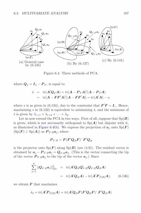
6.3. MULTIVARIATE ANALYSIS 187
Sp(F )
a1
a2
ap
QF a1
¡¡ª QF a2
¡ª
QF ap
(a) General caseby (6.135)
Sp(B)
Sp(B)⊥
a1
a2
ap
QF ·Bap@
@ISp(F )
QF ·Ba1
PPPq
QF ·Ba2
¡¡ª
(b) By (6.137)
a1
a2
ap
Sp(C)
Sp(A)
(c) By (6.141)
Figure 6.4: Three methods of PCA.
where Qf = In − P F , is equal to
s = tr(A′QF A) = tr(A− P F A)′(A− P F A)= tr(A− FF ′A)′(A− FF ′A) = tr(A′A)− s,
where s is as given in (6.134), due to the constraint that F ′F = Ir. Hence,maximizing s in (6.132) is equivalent to minimizing s, and the minimum ofs is given by λr+1 + λr+2 + · · ·+ λp.
Let us now extend the PCA in two ways. First of all, suppose that Sp(B)is given, which is not necessarily orthogonal to Sp(A) but disjoint with it,as illustrated in Figure 6.4(b). We express the projection of aj onto Sp(F )(Sp(F ) ⊂ Sp(A)) as P F ·Baj , where
P F ·B = F (F ′QBF )−F ′QB
is the projector onto Sp(F ) along Sp(B) (see (4.9)). The residual vector isobtained by aj −P F ·Baj = QF ·Baj . (This is the vector connecting the tipof the vector P F ·Baj to the tip of the vector aj .) Since
p∑
j=1
||QF ·Baj ||2QB= tr(A′QBQ′
F ·BQF ·BQBA)
= tr(A′QBA)− tr(A′P F [B]A), (6.136)
we obtain F that maximizes
s2 = tr(A′P F [B]A) = tr(A′QBF (F ′QBF )−F ′QBA)
188 CHAPTER 6. VARIOUS APPLICATIONS
under the restriction that F ′QBF = Ir. Maximizing s2 = tr(A′QBFF ′QB
A) = tr(F ′QBAA′QBF ) under the same restriction reduces to solving theeigenequation
(QBAA′QB)F = F∆2r,
where F = FV (V is an orthogonal matrix of order r), or
(A′QBA)(A′QBF ) = (A′QBF )∆2r, (6.137)
obtained by premultiplying the eigenequation above by A′QB. The derivedF represents the principal components of A eliminating the effects of B.
Let W = A′QBF . Let the normalized vectors of W and F be denotedby w1, w2, · · · , wr and f1, f2, · · · , f r, and let the diagonal elements of ∆2
r
be denoted by µ21, µ
22, · · · , µ2
r. Then,
QBA = µ1f1w′1 + µ2f2w
′2 + · · ·+ µrf rw
′r, (6.138)
where µj (j = 1, · · · , r) is the positive square root of µ2j .
The other method involves the projection of vectors C = [c1, c2, · · · , cs]in Sp(C), not necessarily contained in Sp(A), onto Sp(F )(⊂ Sp(A)) spannedby the principal components. We minimize
s2 =s∑
j=1
||QF cj ||2 = tr(C ′QF C) = tr(C ′C)− tr(C ′P F C) (6.139)
with respect to F , but minimizing the criterion above is obviously equivalentto maximizing
s2 = tr(C ′P F C) = tr(C ′F (F ′F )−1F ′C). (6.140)
Let F = AW , where W is an n by r matrix of weights. Then, (6.140) canbe rewritten as
s2 = tr(C ′AW (W ′A′AW )−1W ′A′C)= tr(W ′A′CC ′AW (W ′A′AW )−1),
which is to be maximized with respect to W subject to the restriction thatW ′A′AW = Ir. This leads to the following generalized eigenequation tobe solved.
(A′CCA)WT = A′AWT∆2r.
Premultiplying both sides of the equation above by C ′A(A′A)−, we canreduce the generalized eigenproblem to an ordinary one:
(C ′P AC)(C ′AWT ) = (C ′AWT )∆2r. (6.141)
6.3. MULTIVARIATE ANALYSIS 189
The eigenvectors C ′AWT of C ′P AC are equal to the product of C ′ andthe principal components F = AWT . The PCA by (6.137) and (6.140)is sometimes called redundancy analysis (RA; Van den Wollenberg, 1977)or PCA of instrumental variables (Rao, 1964). Takane and his collabora-tors (Takane and Shibayama, 1991; Takane and Hunter, 2001) developed acomprehensive method called CPCA (constrained PCA), which subsumesa number of representative techniques in multivariate analysis discussed inthis book, including RA as a special case.
6.3.4 Distance and projection matrices
In this subsection, we represent distances in the n-dimensional Euclideanspace from a variety of angles using projection matrices.
Lemma 6.7 Let ej denote an n-component vector in which only the jthelement is unity and all other elements are zero. Then,
12n
n∑
i=1
n∑
j=1
(ei − ej)(ei − ej)′ = QM . (6.142)
Proof.n∑
i=1
n∑
j=1
(ei − ej)(ei − ej)′
= nn∑
i=1
eie′i + n
n∑
j=1
eje′j − 2
n∑
i=1
ei
n∑
j=1
ej
′
= 2nIn − 21n1′n = 2n(
In − 1n1n1′n
)= 2nQM .
Q.E.D.
Example 6.2 That 1n
∑i<j(xi − xj)2 =
∑ni=1(xi − x)2 can be shown as
follows using the result given above.Let xR = (x1, x2, · · · , xn)′. Then, xj = (xR, ej), and so∑
i<j
(xi − xj)2 =12
∑
i
∑
j
x′R(ei − ej)(ei − ej)′xR
=12x′R
∑
i
∑
j
(ei − ej)(ei − ej)′ xR = nx′RQMxR
190 CHAPTER 6. VARIOUS APPLICATIONS
= nx′x = n||x||2 = nn∑
i=1
(xi − x)2.
We next consider the situation in which a matrix of raw scores on pvariables is given:
XR =
x11 x12 · · · x1p
x21 x22 · · · x2p...
.... . .
...xn1 xn2 · · · xnp
.
Letxj = (xj1, xj2, · · · , xjp)′
denote the p-component vector pertaining to the jth subject’s scores. Then,
xj = X ′Rej . (6.143)
Hence, the squared Euclidean distance between subjects i and j can beexpressed as
d2XR
(ei, ej) =p∑
k=1
(xik − xjk)2
= ||xi − xj ||2 = (ei − ej)′XRX ′R(ei − ej). (6.144)
Let X = QMXR represent the transformation that turns the matrix ofraw scores XR into the matrix X of mean deviation scores. We have
(ei − ej)′X = (ei − ej)′QMXR = (ei − ej)′XR,
and so
d2XR
(ei, ej) = d2X(ei, ej) = (ei − ej)′XX ′(ei − ej), (6.145)
from which the following theorem can be derived.
Theorem 6.13n∑
i=1
n∑
j=1
d2XR
(ei, ej) = ntr(X ′X). (6.146)
6.3. MULTIVARIATE ANALYSIS 191
Proof. Use the fact thatn∑
i=1
n∑
j=1
d2XR
(ei, ej)
=12tr
(XX ′)
∑
i
∑
j
(ei − ej)(ei − ej)′
= ntr(XX ′QM ) = ntr(QMXX ′) = ntr(XX ′).
Q.E.D.
Corollary Let f = x1a1 + x2a2 + · · ·+ xpap = Xa. Then,∑
i<j
d2f (ei, ej) = ntr(ff ′) = ntr(a′X ′Xa). (6.147)
(Proof omitted.)
Let D(2) = [d2ij ], where d2
ij = d2XR
(ei, ej) as defined in (6.145). Then,e′iXX ′ei represents the ith diagonal element of the matrix XX ′ and e′iXX ′
× ej represents its (i, j)th element. Hence,
D(2) = diag(XX ′)1n1′n − 2XX ′ + 1n1′ndiag(XX ′), (6.148)
where diag(A) indicates the diagonal matrix with the diagonal elements ofA as its diagonal entries. Pre- and postmultiplying the formula above byQM = In − 1
n1n1′n, we obtain
S = −12QMD(2)QM = XX ′ ≥ O (6.149)
since QM1n = 0. (6.149) indicates that S is nnd.
Note Let D(2) = [d2ij ] and S = [sij ]. Then,
sij = −12(d2
ij − d2i. − d2
.j + d2..),
where d2i. = 1
n
∑j d2
ij , d2.j = 1
n
∑i d2
ij , and d2.. = 1
n2
∑i,j d2
ij .The transformation (6.149) that turns D(2) into S is called the Young-House-
holder transformation. It indicates that the n points corresponding to the n rows
192 CHAPTER 6. VARIOUS APPLICATIONS
and columns of S can be embedded in a Euclidean space of dimensionality rank(S),which is equal to the number of positive eigenvalues of S. This method of embed-ding points in a Euclidean space is called metric multidimensional scaling (MDS)(Torgerson, 1958).
We now consider the situation in which n subjects are classified into mgroups. Each group has nj subjects with
∑j nj = n. Denote the matrix of
dummy variables defined in (6.46) by
G = [g1, g2, · · · , gm], (6.150)
where gj is an n-component vector of ones and zeroes. Assume that
||gj ||2 = nj and (gi, gj) = 0 (i 6= j).
Lethj = gj(g
′jgj)
−1.
Then the vector of group means of the jth group,
mj = (xj1, xj2, · · · , xjp)′,
on p variables can be expressed as
mj = X ′Rgj(g
′jgj)
−1 = X ′Rhj . (6.151)
Thus, the squared Euclidean distance between means of groups i and j isgiven by
d2X(gi, gj) = (hi − hj)′XX ′(hi − hj). (6.152)
Hence, the following lemma is obtained.
Lemma 6.8
12n
∑
i,j
ninj(hi − hj)(hi − hj)′ = P G − P M , (6.153)
where P G is the orthogonal projector onto Sp(G).
Proof. Use the definition of the vector hj , nj = g′jgj , and the fact thatP G = P g1 + P g2 + · · ·+ P gm . Q.E.D.
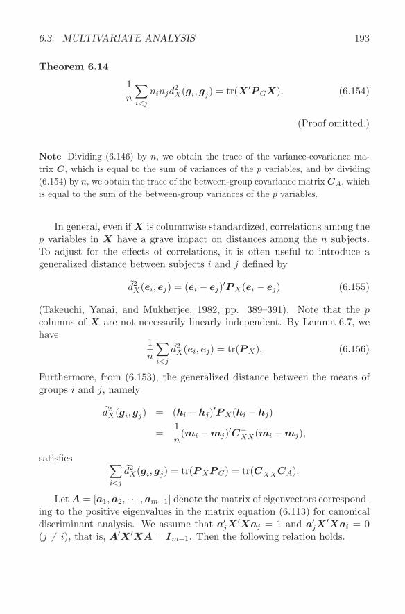
6.3. MULTIVARIATE ANALYSIS 193
Theorem 6.14
1n
∑
i<j
ninjd2X(gi, gj) = tr(X ′P GX). (6.154)
(Proof omitted.)
Note Dividing (6.146) by n, we obtain the trace of the variance-covariance ma-trix C, which is equal to the sum of variances of the p variables, and by dividing(6.154) by n, we obtain the trace of the between-group covariance matrix CA, whichis equal to the sum of the between-group variances of the p variables.
In general, even if X is columnwise standardized, correlations among thep variables in X have a grave impact on distances among the n subjects.To adjust for the effects of correlations, it is often useful to introduce ageneralized distance between subjects i and j defined by
d2X(ei, ej) = (ei − ej)′P X(ei − ej) (6.155)
(Takeuchi, Yanai, and Mukherjee, 1982, pp. 389–391). Note that the pcolumns of X are not necessarily linearly independent. By Lemma 6.7, wehave
1n
∑
i<j
d2X(ei, ej) = tr(P X). (6.156)
Furthermore, from (6.153), the generalized distance between the means ofgroups i and j, namely
d2X(gi, gj) = (hi − hj)′P X(hi − hj)
=1n
(mi −mj)′C−XX(mi −mj),
satisfies ∑
i<j
d2X(gi, gj) = tr(P XP G) = tr(C−
XXCA).
Let A = [a1, a2, · · · , am−1] denote the matrix of eigenvectors correspond-ing to the positive eigenvalues in the matrix equation (6.113) for canonicaldiscriminant analysis. We assume that a′jX
′Xaj = 1 and a′jX′Xai = 0
(j 6= i), that is, A′X ′XA = Im−1. Then the following relation holds.
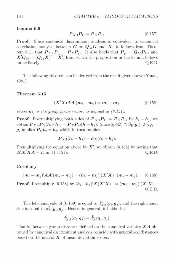
194 CHAPTER 6. VARIOUS APPLICATIONS
Lemma 6.9P XAP G = P XP G. (6.157)
Proof. Since canonical discriminant analysis is equivalent to canonicalcorrelation analysis between G = QMG and X, it follows from Theo-rem 6.11 that P XAP G = P XP G. It also holds that P G = QMP G, andX ′QM = (QMX)′ = X ′, from which the proposition in the lemma followsimmediately. Q.E.D.
The following theorem can be derived from the result given above (Yanai,1981).
Theorem 6.15
(X ′X)AA′(mi −mj) = mi −mj , (6.158)
where mj is the group mean vector, as defined in (6.151).
Proof. Postmultiplying both sides of P XAP G = P XP G by hi − hj , weobtain P XAP G(hi−hj) = P XP G(hi−hj). Since Sp(G) ⊃ Sp(gi), P Ggi =gi implies P Ghi = hi, which in turn implies
P XA(hi − hj) = P X(hi − hj).
Premultiplying the equation above by X ′, we obtain (6.158) by noting thatA′X ′XA = Ir and (6.151). Q.E.D.
Corollary
(mi −mj)′AA′(mi −mj) = (mi −mj)′(X ′X)−(mi −mj). (6.159)
Proof. Premultiply (6.158) by (hi−hj)′X(X ′X)− = (mi−mj)′(X ′X)−.Q.E.D.
The left-hand side of (6.159) is equal to d2XA(gi, gj), and the right-hand
side is equal to d2X(gi, gj). Hence, in general, it holds that
d2XA(gi, gj) = d2
X(gi, gj).
That is, between-group distances defined on the canonical variates XA ob-tained by canonical discriminant analysis coincide with generalized distancesbased on the matrix X of mean deviation scores.
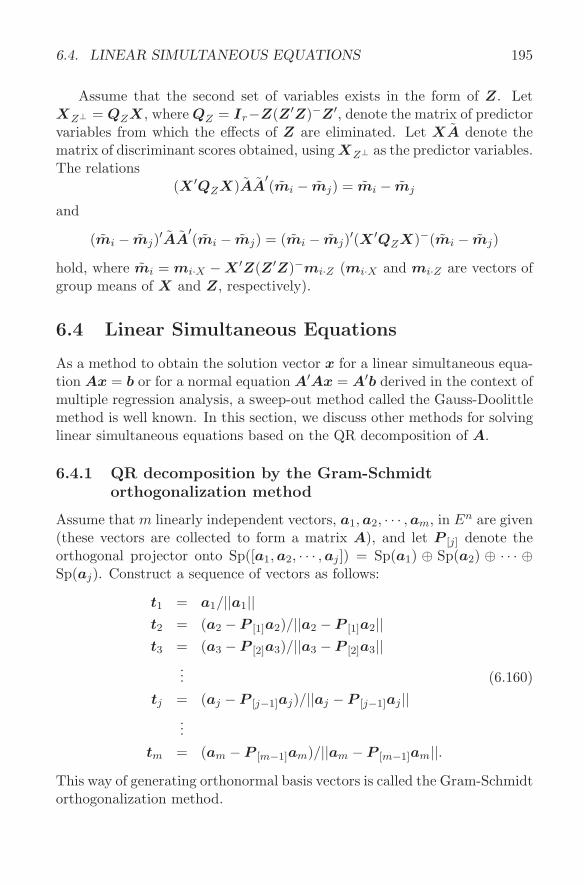
6.4. LINEAR SIMULTANEOUS EQUATIONS 195
Assume that the second set of variables exists in the form of Z. LetXZ⊥ = QZX, where QZ = Ir−Z(Z ′Z)−Z ′, denote the matrix of predictorvariables from which the effects of Z are eliminated. Let XA denote thematrix of discriminant scores obtained, using XZ⊥ as the predictor variables.The relations
(X ′QZX)AA′(mi − mj) = mi − mj
and
(mi − mj)′AA′(mi − mj) = (mi − mj)′(X ′QZX)−(mi − mj)
hold, where mi = mi·X −X ′Z(Z ′Z)−mi·Z (mi·X and mi·Z are vectors ofgroup means of X and Z, respectively).
6.4 Linear Simultaneous Equations
As a method to obtain the solution vector x for a linear simultaneous equa-tion Ax = b or for a normal equation A′Ax = A′b derived in the context ofmultiple regression analysis, a sweep-out method called the Gauss-Doolittlemethod is well known. In this section, we discuss other methods for solvinglinear simultaneous equations based on the QR decomposition of A.
6.4.1 QR decomposition by the Gram-Schmidtorthogonalization method
Assume that m linearly independent vectors, a1, a2, · · · , am, in En are given(these vectors are collected to form a matrix A), and let P [j] denote theorthogonal projector onto Sp([a1, a2, · · · , aj ]) = Sp(a1) ⊕ Sp(a2) ⊕ · · · ⊕Sp(aj). Construct a sequence of vectors as follows:
t1 = a1/||a1||t2 = (a2 − P [1]a2)/||a2 − P [1]a2||t3 = (a3 − P [2]a3)/||a3 − P [2]a3||
... (6.160)tj = (aj − P [j−1]aj)/||aj − P [j−1]aj ||
...tm = (am − P [m−1]am)/||am − P [m−1]am||.
This way of generating orthonormal basis vectors is called the Gram-Schmidtorthogonalization method.
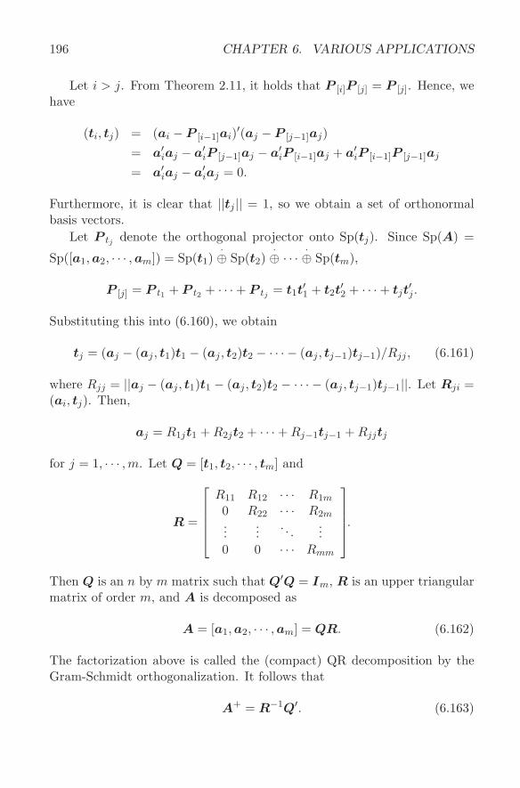
196 CHAPTER 6. VARIOUS APPLICATIONS
Let i > j. From Theorem 2.11, it holds that P [i]P [j] = P [j]. Hence, wehave
(ti, tj) = (ai − P [i−1]ai)′(aj − P [j−1]aj)= a′iaj − a′iP [j−1]aj − a′iP [i−1]aj + a′iP [i−1]P [j−1]aj
= a′iaj − a′iaj = 0.
Furthermore, it is clear that ||tj || = 1, so we obtain a set of orthonormalbasis vectors.
Let P tj denote the orthogonal projector onto Sp(tj). Since Sp(A) =
Sp([a1, a2, · · · , am]) = Sp(t1)·⊕ Sp(t2)
·⊕ · · · ·⊕ Sp(tm),
P [j] = P t1 + P t2 + · · ·+ P tj = t1t′1 + t2t
′2 + · · ·+ tjt
′j .
Substituting this into (6.160), we obtain
tj = (aj − (aj , t1)t1 − (aj , t2)t2 − · · · − (aj , tj−1)tj−1)/Rjj , (6.161)
where Rjj = ||aj − (aj , t1)t1 − (aj , t2)t2 − · · · − (aj , tj−1)tj−1||. Let Rji =(ai, tj). Then,
aj = R1jt1 + R2jt2 + · · ·+ Rj−1tj−1 + Rjjtj
for j = 1, · · · ,m. Let Q = [t1, t2, · · · , tm] and
R =
R11 R12 · · · R1m
0 R22 · · · R2m...
.... . .
...0 0 · · · Rmm
.
Then Q is an n by m matrix such that Q′Q = Im, R is an upper triangularmatrix of order m, and A is decomposed as
A = [a1, a2, · · · , am] = QR. (6.162)
The factorization above is called the (compact) QR decomposition by theGram-Schmidt orthogonalization. It follows that
A+ = R−1Q′. (6.163)
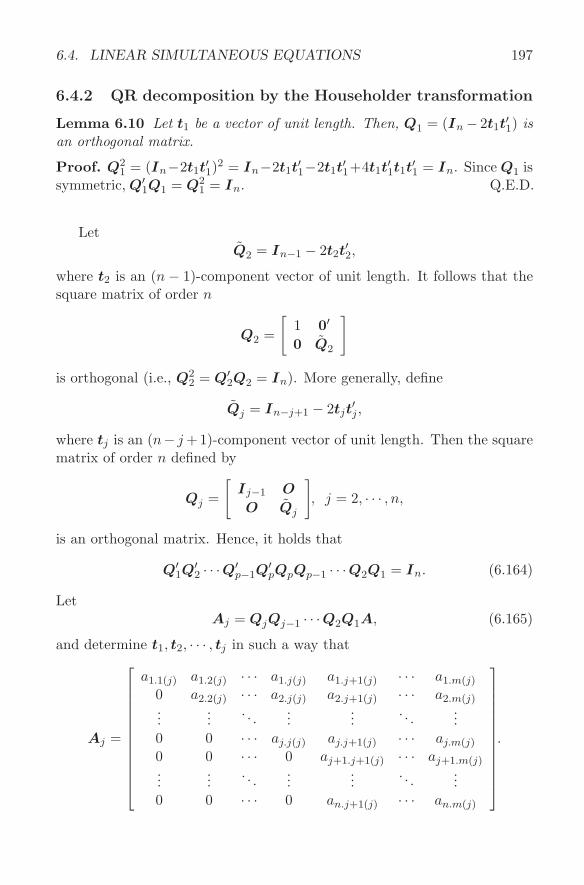
6.4. LINEAR SIMULTANEOUS EQUATIONS 197
6.4.2 QR decomposition by the Householder transformation
Lemma 6.10 Let t1 be a vector of unit length. Then, Q1 = (In− 2t1t′1) is
an orthogonal matrix.
Proof. Q21 = (In−2t1t
′1)
2 = In−2t1t′1−2t1t
′1+4t1t
′1t1t
′1 = In. Since Q1 is
symmetric, Q′1Q1 = Q2
1 = In. Q.E.D.
LetQ2 = In−1 − 2t2t
′2,
where t2 is an (n− 1)-component vector of unit length. It follows that thesquare matrix of order n
Q2 =
[1 0′
0 Q2
]
is orthogonal (i.e., Q22 = Q′
2Q2 = In). More generally, define
Qj = In−j+1 − 2tjt′j ,
where tj is an (n− j +1)-component vector of unit length. Then the squarematrix of order n defined by
Qj =
[Ij−1 O
O Qj
], j = 2, · · · , n,
is an orthogonal matrix. Hence, it holds that
Q′1Q
′2 · · ·Q′
p−1Q′pQpQp−1 · · ·Q2Q1 = In. (6.164)
LetAj = QjQj−1 · · ·Q2Q1A, (6.165)
and determine t1, t2, · · · , tj in such a way that
Aj =
a1.1(j) a1.2(j) · · · a1.j(j) a1.j+1(j) · · · a1.m(j)
0 a2.2(j) · · · a2.j(j) a2.j+1(j) · · · a2.m(j)...
.... . .
......
. . ....
0 0 · · · aj.j(j) aj.j+1(j) · · · aj.m(j)
0 0 · · · 0 aj+1.j+1(j) · · · aj+1.m(j)...
.... . .
......
. . ....
0 0 · · · 0 an.j+1(j) · · · an.m(j)
.
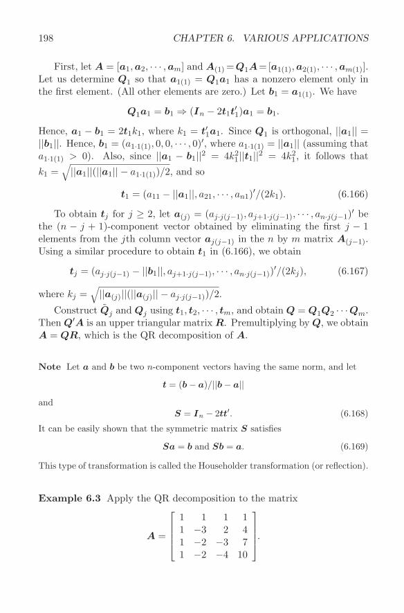
198 CHAPTER 6. VARIOUS APPLICATIONS
First, let A = [a1, a2, · · · ,am] and A(1) =Q1A=[a1(1),a2(1), · · · , am(1)].Let us determine Q1 so that a1(1) = Q1a1 has a nonzero element only inthe first element. (All other elements are zero.) Let b1 = a1(1). We have
Q1a1 = b1 ⇒ (In − 2t1t′1)a1 = b1.
Hence, a1 − b1 = 2t1k1, where k1 = t′1a1. Since Q1 is orthogonal, ||a1|| =||b1||. Hence, b1 = (a1·1(1), 0, 0, · · · , 0)′, where a1·1(1) = ||a1|| (assuming thata1·1(1) > 0). Also, since ||a1 − b1||2 = 4k2
1||t1||2 = 4k21, it follows that
k1 =√||a1||(||a1|| − a1·1(1))/2, and so
t1 = (a11 − ||a1||, a21, · · · , an1)′/(2k1). (6.166)
To obtain tj for j ≥ 2, let a(j) = (aj·j(j−1), aj+1·j(j−1), · · · , an·j(j−1)′ bethe (n − j + 1)-component vector obtained by eliminating the first j − 1elements from the jth column vector aj(j−1) in the n by m matrix A(j−1).Using a similar procedure to obtain t1 in (6.166), we obtain
tj = (aj·j(j−1) − ||b1||, aj+1·j(j−1), · · · , an·j(j−1))′/(2kj), (6.167)
where kj =√||a(j)||(||a(j)|| − aj·j(j−1))/2.
Construct Qj and Qj using t1, t2, · · · , tm, and obtain Q = Q1Q2 · · ·Qm.Then Q′A is an upper triangular matrix R. Premultiplying by Q, we obtainA = QR, which is the QR decomposition of A.
Note Let a and b be two n-component vectors having the same norm, and let
t = (b− a)/||b− a||and
S = In − 2tt′. (6.168)
It can be easily shown that the symmetric matrix S satisfies
Sa = b and Sb = a. (6.169)
This type of transformation is called the Householder transformation (or reflection).
Example 6.3 Apply the QR decomposition to the matrix
A =
1 1 1 11 −3 2 41 −2 −3 71 −2 −4 10
.
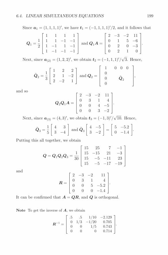
6.4. LINEAR SIMULTANEOUS EQUATIONS 199
Since a1 = (1, 1, 1, 1)′, we have t1 = (−1, 1, 1, 1)′/2, and it follows that
Q1 =12
1 1 1 11 1 −1 −11 −1 1 −11 −1 −1 −1
and Q1A =
2 −3 −2 110 1 5 −60 2 0 −30 2 1 0
.
Next, since a(2) = (1, 2, 2)′, we obtain t2 = (−1, 1, 1)′/√
3. Hence,
Q2 =13
1 2 22 1 −22 −2 1
and Q2 =
1 0 0 0000
Q2
,
and so
Q2Q1A =
2 −3 −2 110 3 1 40 0 4 −50 0 3 −2
.
Next, since a(3) = (4, 3)′, we obtain t3 = (−1, 3)′/√
10. Hence,
Q3 =15
[4 33 −4
]and Q3
[4 −53 −2
]=
[5 −5.20 −1.4
].
Putting this all together, we obtain
Q = Q1Q2Q3 =130
15 25 7 −115 −15 21 −315 −5 −11 2315 −5 −17 −19
and
R =
2 −3 −2 110 3 1 40 0 5 −5.20 0 0 −1.4
.
It can be confirmed that A = QR, and Q is orthogonal.
Note To get the inverse of A, we obtain
R−1 =
.5 .5 1/10 −2.1290 1/3 −1/20 0.7050 0 1/5 0.7430 0 0 0.714
.
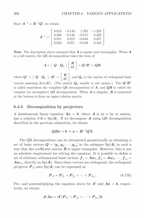
200 CHAPTER 6. VARIOUS APPLICATIONS
Since A−1 = R−1Q′, we obtain
A−1 =
0.619 −0.143 1.762 −1.2280.286 −0.143 −0.571 0.4290.071 0.214 −0.643 0.3570.024 0.071 −0.548 0.452
.
Note The description above assumed that A is square and nonsingular. When Ais a tall matrix, the QR decomposition takes the form of
A =[
Q Q0
] [RO
]= Q∗R∗ = QR,
where Q∗ =[
Q Q0
], R∗ =
[RO
], and Q0 is the matrix of orthogonal basis
vectors spanning Ker(A′). (The matrix Q0 usually is not unique.) The Q∗R∗
is called sometimes the complete QR decomposition of A, and QR is called thecompact (or incomplete) QR decomposition. When A is singular, R is truncatedat the bottom to form an upper echelon matrix.
6.4.3 Decomposition by projectors
A simultaneous linear equation Ax = b, where A is an n by m matrix,has a solution if b ∈ Sp(A). If we decompose A using QR decompositiondescribed in the previous subsection, we obtain
QRx = b ⇒ x = R−1Q′b.
The QR decomposition can be interpreted geometrically as obtaining aset of basis vectors Q = [q1, q2, · · · , qm] in the subspace Sp(A) in such away that the coefficient matrix R is upper triangular. However, this is notan absolute requirement for solving the equation. It is possible to define aset of arbitrary orthonormal basis vectors, f1 = Aw1, f2 = Aw2, · · · , fm =Awm, directly on Sp(A). Since these vectors are orthogonal, the orthogonalprojector P A onto Sp(A) can be expressed as
P A = P f1 + P f2 + · · ·+ P fm . (6.170)
Pre- and postmultiplying the equation above by A′ and Ax = b, respec-tively, we obtain
A′Ax = A′(P f1 + P f2 + · · ·+ P fm)b
6.5. EXERCISES FOR CHAPTER 6 201
since A′P A = A′. If A′A is nonsingular, the equation above can be rewrit-ten as
x = w1(f ′1f1)−1f ′1b+w2(f ′2f2)
−1f ′2b+ · · ·+wm(f ′mfm)−1f ′mb. (6.171)
The equation above can further be rewritten as
x = w1f′1b + w2f
′2b + · · ·+ wmf ′mb = WF ′b, (6.172)
where F = [f1, f2, · · · , fm], since f ′if i = 1 (i = 1, · · · ,m), assuming thatthe f j ’s constitute a set of orthonormal basis vectors.
One way of obtaining f1, f2, · · · , fm is by the Gram-Schmidt method asdescribed above. In this case, F = AW ⇒ A = FW−1, so that F = Qand W−1 = R in (6.172).
Another way of obtaining a set of orthonormal basis vectors is via sin-gular value decomposition (SVD). Let µ1, µ2, · · · , µm denote the positivesingular values of A, where the SVD of A is obtained by (5.18). Then,wj = µjvj and f j = uj , so that the solution vector in (6.171) can beexpressed as
x =1µ1
v1u′1b +
1µ2
v2u′2b + · · ·+ 1
µmvmu′mb. (6.173)
Let A = QR be the QR decomposition of A, and let B = A′A. Wehave
B = R′Q′QR = R′R.
This is called the Cholesky decomposition of B. Let B = [bij ] and R = [rij ].Since bij =
∑ik=1 rkirkj , we have
r11 =√
b11, r1j = b1j/r11, (j = 2, · · · ,m),
rjj =
bjj −
j−1∑
k=1
r2kj
1/2
, (j = 2, · · · ,m),
rij =
bij −
j−1∑
k=1
rkirkj
/rjj , (i < j).
6.5 Exercises for Chapter 6
1. Show that R2X·y = R2
X·y if Sp(X) = Sp(X).
202 CHAPTER 6. VARIOUS APPLICATIONS
2. Show that 1 − R2X·y = (1 − r2
x1y)(1 − rx2y|x1)2 · · · (1 − r2
xpy|x1x2···xp−1), where
rxjy|x1x2···xj−1 is the correlation between xj and y eliminating the effects due tox1, x2, · · · , xj−1.
3. Show that the necessary and sufficient condition for Ly to be the BLUE ofE(L′y) in the Gauss-Markov model (y, Xβ, σ2G) is
GL ∈ Sp(X).
4. Show that the BLUE of e′β in the Gauss-Markov model (y, Xβ, σ2G) is e′β,where β is an unbiased estimator of β.
5. Show that, in the Gauss-Markov model above, an estimator for fσ2, wheref = rank(X, G)− rank(X), is given by one of the following:(i) y′Z(ZGZ)−Zy.(ii) y′T−(In − P X/T−)y, where T = G + XUX ′ and rank(T ) = rank([G, X]).
6. For G = [g1, g2, · · · , gm] given in (6.46):
(i) Show that QMG(G′QMG)−G′QM = QMG(G′QMG)−1GQM , where G is a
matrix obtained by eliminating an arbitrary column from G.(ii) Show that minα ||y − G∗α||2 = y′(In − G(G
′QMG)−1G
′)y, where G∗ =
[G,1n], α is an (m + 1)-component vector of weights, and y is an n-componentvector with zero mean.
7. Define the projectors
P x[G] = QGx(x′QGx)−1x′QG
andP Dx[G] = QGDx(D′
xQGDx)−1D′xQG
using x =
x1
x2
...xm
, Dx =
x1 0 · · · 00 x2 · · · 0...
.... . .
...0 0 · · · xm
, y =
y1
y2
...ym
, and the matrix
of dummy variables G given in (6.46). Assume that xj and yj have the same sizenj . Show that the following relations hold:(i) P x[G]P Dx[G] = P x[G].(ii) P xP Dx[G] = P xP x[G].(iii) minb ||y − bx||2QG
= ||y − P x[G]y||2QG.
(iv) minb ||y −Dxb||2QG= ||y − P Dx[G]y||2QG
.(v) Show that βixi = P Dx[G]y and βxi = P x[G]y, where β = β1 = β2 = · · · = βm
in the least squares estimation in the linear model yij = αi + βixij + εij , where1 ≥ i ≥ m and 1 ≥ j ≥ ni.
6.5. EXERCISES FOR CHAPTER 6 203
8. Let X = UX∆XV ′X and Y = UY ∆Y V ′
Y represent the SVDs of X and Y .Show that the singular values of the matrix S = ∆−1
X UXCXY U ′Y ∆−1
Y are equalto the canonical correlations between X and Y .
9. Let QZXA and QZY B denote the canonical variates corresponding to QZXand QZY . Show that (Yanai, 1980):(i) P XA·Z = (P X·ZP Y ·Z)(P X·ZP Y ·Z)−`(Z).
(ii) P Y B·Z = (PY ·ZP X·Z)(P Y ·ZP X·Z)−`(Z).
(iii) P XA·ZP Y B·Z = P XA·ZP Y ·Z = P X·ZP Y B·Z = P X·ZP Y ·Z .
10. Let X and Y be n by p and n by q matrices, respectively, and let
R =[
RXX RXY
RY X RY Y
]and RR− =
[S11 S12
S21 S22
].
Show the following:(i) Sp(Ip −RR−) = Ker([X, Y ]).(ii) (Ip − S11)X ′QY = O, and (Iq − S22)Y ′QX = O.(iii) If Sp(X) and Sp(Y ) are disjoint, S11X
′ = X ′, S12Y′ = O, S21X
′ = O, andS22Y
′ = Y ′.
11. Let Z = [z1, z2, · · · , zp] denote the matrix of columnwise standardized scores,and let F = [f1, f2, · · · , fr] denote the matrix of common factors in the factoranalysis model (r < p). Show the following:(i) 1
n ||P F zj ||2 = h2j , where h2
j is called the communality of the variable j.(ii) tr(P F P Z) ≤ r.(iii) h2
j ≥ ||P Z(j)zj ||2, where Z(j) = [z1, · · · ,zj−1, zj+1, · · · ,zp].
12. Show that limk→∞(P XP Y )k = P Z if Sp(X) ∩ Sp(Y ) = Sp(Z).
13. Consider the perturbations ∆x and ∆b of X and b in the linear equationAx = b, that is, A(x + ∆x) = b + ∆b. Show that
||∆x||||x|| ≤ Cond(A)
||∆b||||b|| ,
where Cond(A) indicates the ratio of the largest singular value µmax(A) of A tothe smallest singular value µmin(A) of A and is called the condition number.
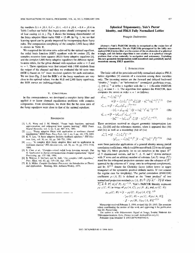
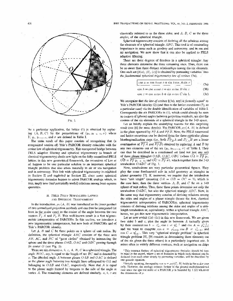
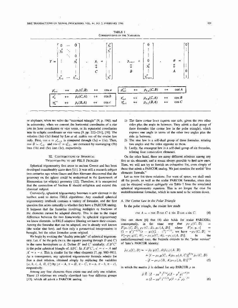
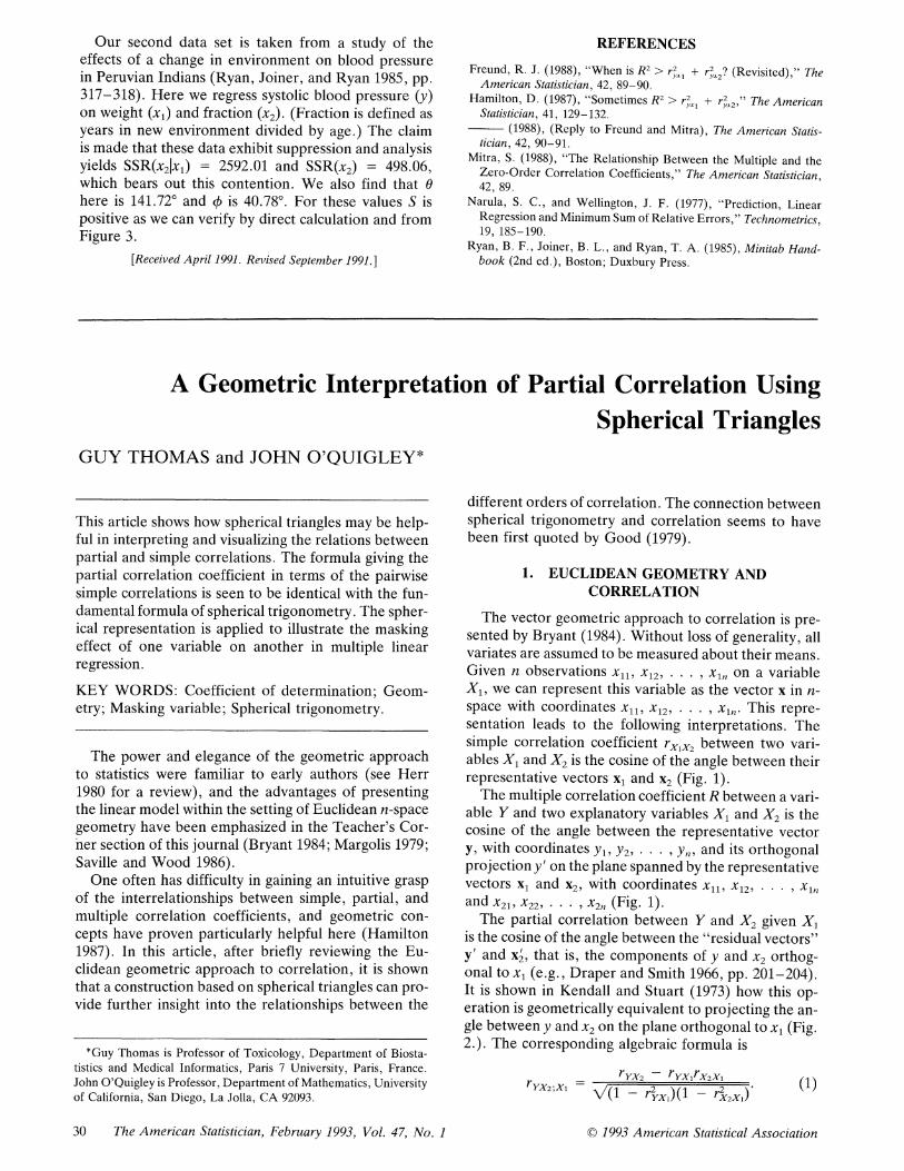
Our second data set is taken from a study of the effects of a change in environment on blood pressure in Peruvian Indians (Ryan, Joiner, and Ryan 1985, pp. 317-318). Here we regress systolic blood pressure (y) on weight (x1) and fraction (x2). (Fraction is defined as years in new environment divided by age.) The claim is made that these data exhibit suppression and analysis yields SSR(x2JxJ) = 2592.01 and SSR(x2) = 498.06, which bears out this contention. We also find that 0 here is 141.720 and 4 is 40.78?. For these values S is positive as we can verify by direct calculation and from Figure 3.
[Received April 1991. Revised September 1991.]
REFERENCES
Freund, R. J. (1988), "When is R2 > r21 + r 2? (Revisited)," The American Statistician, 42, 89-90.
Hamilton, D. (1987), "Sometimes R2 > ry2x + r -.2," The American Statistician, 41, 129-132.
- (1988), (Reply to Freund and Mitra), The American Statis- tician, 42, 90-91.
Mitra, S. (1988), "The Relationship Between the Multiple and the Zero-Order Correlation Coefficients," The American Statistician, 42, 89.
Narula, S. C., and Wellington, J. F. (1977), "Prediction, Linear Regression and Minimum Sum of Relative Errors," Technometrics, 19, 185-190.
Ryan, B. F., Joiner, B. L., and Ryan, T. A. (1985), Minitab Hand- book (2nd ed.), Boston; Duxbury Press.
A Geometric Interpretation of Partial Correlation Using Spherical Triangles
GUY THOMAS and JOHN O'QUIGLEY*
This article shows how spherical triangles may be help- ful in interpreting and visualizing the relations between partial and simple correlations. The formula giving the partial correlation coefficient in terms of the pairwise simple correlations is seen to be identical with the fun- damental formula of spherical trigonometry. The spher- ical representation is applied to illustrate the masking effect of one variable on another in multiple linear regression.
KEY WORDS: Coefficient of determination; Geom- etry; Masking variable; Spherical trigonometry.
The power and elegance of the geometric approach to statistics were familiar to early authors (see Herr 1980 for a review), and the advantages of presenting the linear model within the setting of Euclidean n-space geometry have been emphasized in the Teacher's Cor- ner section of this journal (Bryant 1984; Margolis 1979; Saville and Wood 1986).
One often has difficulty in gaining an intuitive grasp of the interrelationships between simple, partial, and multiple correlation coefficients, and geometric con- cepts have proven particularly helpful here (Hamilton 1987). In this article, after briefly reviewing the Eu- clidean geometric approach to correlation, it is shown that a construction based on spherical triangles can pro- vide further insight into the relationships between the
different orders of correlation. The connection between spherical trigonometry and correlation seems to have been first quoted by Good (1979).
1. EUCLIDEAN GEOMETRY AND CORRELATION
The vector geometric approach to correlation is pre- sented by Bryant (1984). Without loss of generality, all variates are assumed to be measured about their means. Given n observations x1l, x12, . . . , x,1, on a variable X1, we can represent this variable as the vector x in n- space with coordinates x1l, x12, . . . , x1,. This repre- sentation leads to the following interpretations. The simple correlation coefficient rxIx2 between two vari- ables X1 and X2 is the cosine of the angle between their representative vectors x1 and x2 (Fig. 1).
The multiple correlation coefficient R between a vari- able Y and two explanatory variables X1 and X2 is the cosine of the angle between the representative vector y, with coordinates Yl, Y2, . . . , y,,, and its orthogonal projection y' on the plane spanned by the representative vectors x1 and x2, with coordinates x1l, x12, . . . Xt and x21, x22, . . . , x2,n (Fig. 1).
The partial correlation between Y and X2 given X1 is the cosine of the angle between the "residual vectors" y' and x2, that is, the components of y and x2 orthog- onal to x1 (e.g., Draper and Smith 1966, pp. 201-204). It is shown in Kendall and Stuart (1973) how this op- eration is geometrically equivalent to projecting the an- gle between y and x2 on the plane orthogonal to x1 (Fig. 2.). The corresponding algebraic formula is
ryx2V - ryx rX2x1) (1) rYX2Xl v(1-
rYXI) (1 - rX2XI)'
*Guy Thomas is Professor of Toxicology, Department of Biosta- tistics and Medical Informatics, Paris 7 University, Paris, France. John O'Quigley is Professor, Department of Mathematics, University of California, San Diego, La Jolla, CA 92093.
30 The American Statistician, February 1993, Vol. 47, No. 1 ? 1993 American Statistical Association
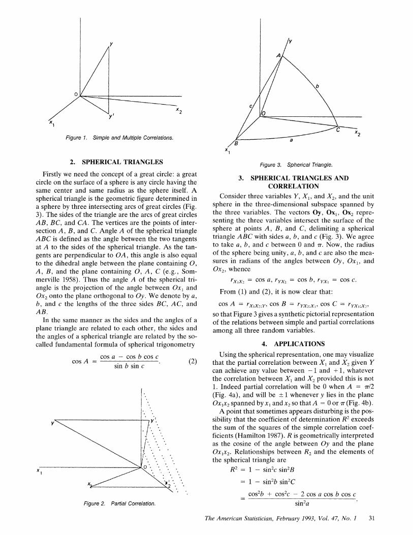
y
/m 2 ~~~~~y
Figure 1. Simple and Multiple Correlations.
2. SPHERICAL TRIANGLES
Firstly we need the concept of a great circle: a great circle on the surface of a sphere is any circle having the same center and same radius as the sphere itself. A spherical triangle is the geometric figure determined in a sphere by three intersecting arcs of great circles (Fig. 3). The sides of the triangle are the arcs of great circles AB, BC, and CA. The vertices are the points of inter- section A, B, and C. Angle A of the spherical triangle ABC is defined as the angle between the two tangents at A to the sides of the spherical triangle. As the tan- gents are perpendicular to OA, this angle is also equal to the dihedral angle between the plane containing 0, A, B, and the plane containing 0, A, C (e.g., Som- merville 1958). Thus the angle A of the spherical tri- angle is the projection of the angle between Ox1 and Ox2 onto the plane orthogonal to Oy. We denote by a, b, and c the lengths of the three sides BC, AC, and AB.
In the same manner as the sides and the angles of a plane triangle are related to each other, the sides and the angles of a spherical triangle are related by the so- called fundamental formula of spherical trigonometry
Cos A = cos a - cos b cos c (2)
sin b sin c
\ ~~~~~~~~.1.
0
X2/ 9~~~~~~~2
Figure 2. Partial Correlation.
c~~~~
x /
Figure 3. Spherical Triangle.
3. SPHERICAL TRIANGLES AND CORRELATION
Consider three variables Y, X1, and X2, and the unit sphere in the three-dimensional subspace spanned by the three variables. The vectors Oy, Ox1, Ox2 repre- senting the three variables intersect the surface of the sphere at points A, B, and C, delimiting a spherical triangle ABC with sides a, b, and c (Fig. 3). We agree to take a, b, and c between 0 and ir. Now, the radius of the sphere being unity, a, b, and c are also the mea- sures in radians of the angles between Oy, Ox1, and Ox2, whence
rX,X2 = cos a, ryx2 = cos b, ryxl = cos c.
From (1) and (2), it is now clear that:
cos A = rxXl2;y, cos B = ryx2;x, cos C = ryxl;x2, so that Figure 3 gives a synthetic pictorial representation of the relations between simple and partial correlations among all three random variables.
4. APPLICATIONS
Using the spherical representation, one may visualize that the partial correlation between X1 and X2 given Y can achieve any value between - 1 and + 1, whatever the correlation between X1 and X2 provided this is not 1. Indeed partial correlation will be 0 when A = rT!2
(Fig. 4a), and will be ? 1 whenever y lies in the plane Ox1x2 spanned by x1 and x2 so that A = 0 or X (Fig. 4b) .
A point that sometimes appears disturbing is the pos- sibility that the coefficient of determination R2 exceeds the sum of the squares of the simple correlation coef- ficients (Hamilton 1987). R is geometrically interpreted as the cosine of the angle between Oy and the plane Ox1x2. Relationships between R2 and the elements of the spherical triangle are
R2= 1 - sin2c sin2B
= 1 - sin2b sin2C
_cos2b ? cos2c - 2 cos a cos b cos c =~~~~~i2
The American Statistician, February 1993, Vol. 47, No. 1 31
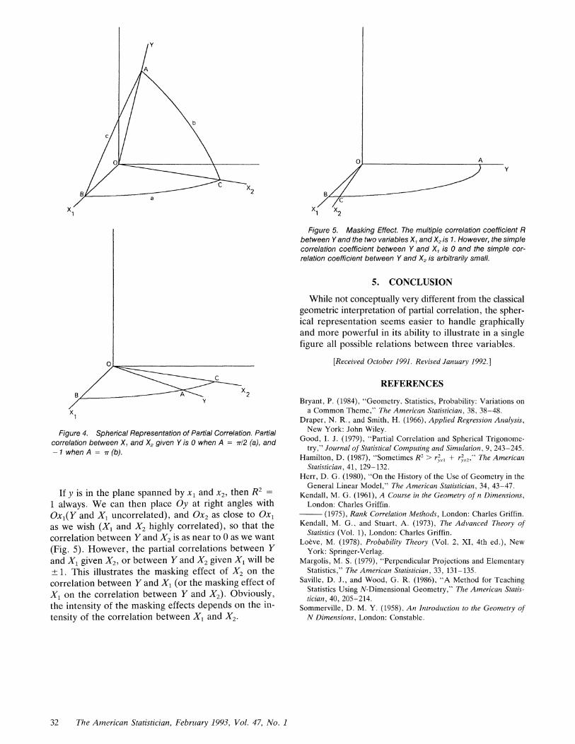
Y
8
0
B C
a
x
Figure 4. Spherical Representation of Partial Correlation. Partial
correlation between X1 and X2 given Y is O when A = 7r12 (a), and - 1whenA= r(b).
If y is in the plane spanned by x1 and x2, then R2 =
1 always. We can then place Oy at right angles with Ox1(Y and X1 uncorrelated), and Ox2 as close to Ox1 as we wish (X1 and X2 highly correlated), so that the correlation between Y and X2 is as near to 0 as we want (Fig. 5). However, the partial correlations between Y and X1 given X2, or between Y and X2 given X1 will be + 1. This illustrates the masking effect of X2 on the correlation between Y and X1 (or the masking effect of X1 on the correlation between Y and X2). Obviously, the intensity of the masking effects depends on the in- tensity of the correlation between X1 and X2.
o A Y
B
Figure 5. Masking Effect. The multiple correlation coefficient R between Y and the two variables X, and X2 is 1. However, the simple correlation coefficient between Y and X, is 0 and the simple cor- relation coefficient between Y and X2 is arbitrarily small.
5. CONCLUSION
While not conceptually very different from the classical geometric interpretation of partial correlation, the spher- ical representation seems easier to handle graphically and more powerful in its ability to illustrate in a single figure all possible relations between three variables.
[Received October 1991. Revised January 1992.]
REFERENCES
Bryant, P. (1984), "Geometry, Statistics, Probability: Variations on a Common Theme," The American Statistician, 38, 38-48.
Draper, N. R., and Smith, H. (1966), Applied Regression Analysis, New York: John Wiley.
Good, I. J. (1979), "Partial Correlation and Spherical Trigonome- try," Journal of Statistical Computing and Simulation, 9, 243-245.
Hamilton, D. (1987), "Sometimes R2 > r 2 + r2, " The American Statistician, 41, 129-132.
Herr, D. G. (1980), "On the History of the Use of Geometry in the General Linear Model," The American Statistician, 34, 43-47.
Kendall, M. G. (1961), A Course in the Geometry of n Dimensions, London: Charles Griffin.
(1975), Rank Correlation Methods, London: Charles Griffin. Kendall, M. G., and Stuart, A. (1973), The Advanced Theory of
Statistics (Vol. 1), London: Charles Griffin. Loeve, M. (1978), Probability Theory (Vol. 2, XI, 4th ed.), New
York: Springer-Verlag. Margolis, M. S. (1979), "Perpendicular Projections and Elementary
Statistics," The American Statistician, 33, 131-135. Saville, D. J., and Wood, G. R. (1986), "A Method for Teaching
Statistics Using N-Dimensional Geometry," The American Statis- tician, 40, 205-214.
Sommerville, D. M. Y. (1958), An Introductionz to the Geometry of N Dimensions, London: Constable.
32 The American Statistician, February 1993, Vol. 47, No. 1

psychometrika—vol. 69, no. 2, 291–303june 2004
SEEING THE FISHER Z-TRANSFORMATION
Charles F. Bond, Jr.
department of psychologytexas christian university
Ken Richardson
department of mathematicstexas christian university
Abstract
Since 1915, statisticians have been applying Fisher’s Z-transformationto Pearson product-moment correlation coefficients. We offer new geometricinterpretations of this transformation.
Key words: correlation coefficient, Fisher, geometry, hyperbolic, transforma-tion
1. Introduction
Noting some limitations of Pearson’s product-moment correlation coefficient (r),Fisher (1915) suggested a transformation
Zr = arctanh(r)
that has advantages over r. Relative to the correlation coefficient, Zr has a simplerdistribution; its variance is more nearly independent of the corresponding populationparameter (Zρ); and it converges more quickly to normality (Johnson, Kotz, and Bal-akhrishnan, 1995). Fisher’s Z transformation is featured in statistics texts (e.g., Casellaand Berger, 2002) and is used by meta-analysts (Lipsey and Wilson, 2001).
Much has been learned about Zr since 1915. We now know the exact distributionof Zr for data from a bivariate normal distribution (Fisher, 1921), the exact distributionof Zr for data from a bivariate Type A Edgeworth distribution (Gayen, 1951), and theasymptotic distribution of Zr for virtually any data (Hawkins, 1989). We know that Zr
can be derived as a variance-stabilizing transformation or a normalizing transformation(Winterbottom, 1979). We have Taylor series expressions for the moments of Zr andseveral related statistics (Hotelling, 1953).
Although scholars have been thorough in describing the analytic properties of Zr,they have had little to say about the geometry of this transformation. True, there is ageometric flavor to certain discussions of Zr -transformed correlation matrices (Brien,Venables, James, and Mayo, 1984). Still, the dearth of geometric knowledge about Zr isstriking, when geometric treatments of r abound (Rodgers and Nicewander, 1988).
In the current article, we offer the first geometric interpretations of Zr to date. InSection 2, we develop some Euclidean area representations. These depict r and Zr asareas — both in the two-dimensional scatterplot, and in an N -dimensional vector space.
Requests for reprints should be sent to Charles Bond, [email protected].
291
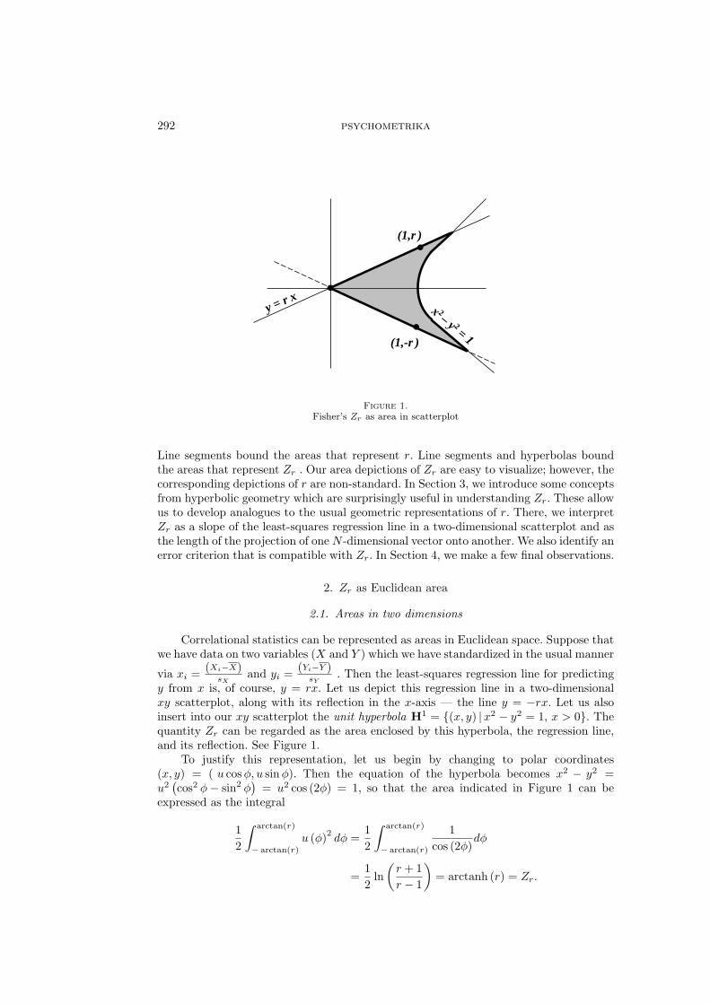
292 psychometrika
y = r xx 2 – y 2
= 1
(1,r )
(1,-r )
Figure 1.Fisher’s Zr as area in scatterplot
Line segments bound the areas that represent r. Line segments and hyperbolas boundthe areas that represent Zr . Our area depictions of Zr are easy to visualize; however, thecorresponding depictions of r are non-standard. In Section 3, we introduce some conceptsfrom hyperbolic geometry which are surprisingly useful in understanding Zr. These allowus to develop analogues to the usual geometric representations of r. There, we interpretZr as a slope of the least-squares regression line in a two-dimensional scatterplot and asthe length of the projection of one N -dimensional vector onto another. We also identify anerror criterion that is compatible with Zr. In Section 4, we make a few final observations.
2. Zr as Euclidean area
2.1. Areas in two dimensions
Correlational statistics can be represented as areas in Euclidean space. Suppose thatwe have data on two variables (X and Y ) which we have standardized in the usual manner
via xi = (Xi−X)sX
and yi = (Yi−Y )sY
. Then the least-squares regression line for predictingy from x is, of course, y = rx. Let us depict this regression line in a two-dimensionalxy scatterplot, along with its reflection in the x-axis — the line y = −rx. Let us alsoinsert into our xy scatterplot the unit hyperbola H1 = {(x, y) |x2 − y2 = 1, x > 0}. Thequantity Zr can be regarded as the area enclosed by this hyperbola, the regression line,and its reflection. See Figure 1.
To justify this representation, let us begin by changing to polar coordinates(x, y) = ( u cos φ, u sin φ). Then the equation of the hyperbola becomes x2 − y2 =u2
(cos2 φ− sin2 φ
)= u2 cos (2φ) = 1, so that the area indicated in Figure 1 can be
expressed as the integral
12
∫ arctan(r)
− arctan(r)
u (φ)2 dφ =12
∫ arctan(r)
− arctan(r)
1cos (2φ)
dφ
=12
ln(
r + 1r − 1
)= arctanh (r) = Zr.
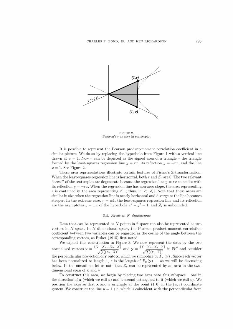
charles f. bond, jr. and ken richardson 293
y = r x
(1,r)
(1,-r)
Figure 2.Pearson’s r as area in scatterplot
It is possible to represent the Pearson product-moment correlation coefficient in asimilar picture. We do so by replacing the hyperbola from Figure 1 with a vertical linedrawn at x = 1. Now r can be depicted as the signed area of a triangle – the triangleformed by the least-squares regression line y = rx, its reflection y = −rx, and the linex = 1. See Figure 2.
These area representations illustrate certain features of Fisher’s Z transformation.When the least-squares regression line is horizontal, both r and Zr are 0. The two relevant“areas” of the scatterplot are degenerate because the regression line y = rx coincides withits reflection y = −rx. When the regression line has non-zero slope, the area representingr is contained in the area representing Zr ; thus, |r| < |Zr|. Note that these areas aresimilar in size when the regression line is nearly horizontal and diverge as the line becomessteeper. In the extreme case, r = ±1, the least-squares regression line and its reflectionare the asymptotes y = ±x of the hyperbola x2 − y2 = 1, and Zr is unbounded.
2.2. Areas in N dimensions
Data that can be represented as N points in 2-space can also be represented as twovectors in N -space. In N -dimensional space, the Pearson product-moment correlationcoefficient between two variables can be regarded as the cosine of the angle between thecorresponding vectors, as Fisher (1915) first noted.
We exploit this construction in Figure 3. We now represent the data by the two
normalized vectors x = (X1−X,...,XN−X)√∑(Xi−X)2 and y = (Y1−Y ,...,YN−Y )√∑
(Yi−Y )2 in RN and consider
the perpendicular projection of y onto x, which we symbolize by Px (y) . Since each vectorhas been normalized to length 1, r is the length of Px (y) — as we will be discussingbelow. In the meantime, let us note that Zr can be represented by an area in the two-dimensional span of x and y.
To construct this area, we begin by placing two axes onto this subspace – one inthe direction of x (which we call u) and a second orthogonal to it (which we call v). Weposition the axes so that x and y originate at the point (1, 0) in the (u, v) coordinatesystem. We construct the line u = 1+ r, which is coincident with the perpendicular from
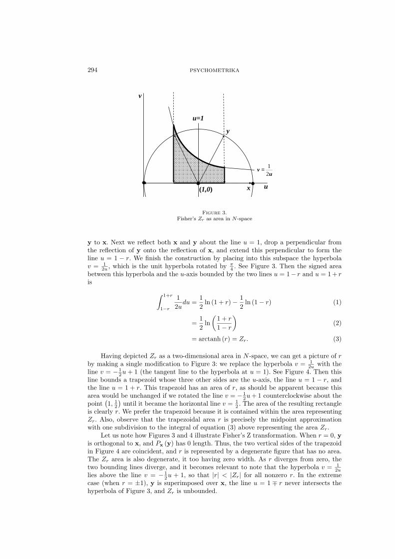
294 psychometrika
x u
y
(1,0)
u=1
v
uv
21=
Figure 3.Fisher’s Zr as area in N -space
y to x. Next we reflect both x and y about the line u = 1, drop a perpendicular fromthe reflection of y onto the reflection of x, and extend this perpendicular to form theline u = 1 − r. We finish the construction by placing into this subspace the hyperbolav = 1
2u , which is the unit hyperbola rotated by π4 . See Figure 3. Then the signed area
between this hyperbola and the u-axis bounded by the two lines u = 1− r and u = 1 + ris
∫ 1+r
1−r
12u
du =12
ln (1 + r)− 12
ln (1− r) (1)
=12
ln(
1 + r
1− r
)(2)
= arctanh (r) = Zr. (3)
Having depicted Zr as a two-dimensional area in N -space, we can get a picture of rby making a single modification to Figure 3: we replace the hyperbola v = 1
2u with theline v = − 1
2u + 1 (the tangent line to the hyperbola at u = 1). See Figure 4. Then thisline bounds a trapezoid whose three other sides are the u-axis, the line u = 1 − r, andthe line u = 1 + r. This trapezoid has an area of r, as should be apparent because thisarea would be unchanged if we rotated the line v = − 1
2u + 1 counterclockwise about thepoint
(1, 1
2
)until it became the horizontal line v = 1
2 . The area of the resulting rectangleis clearly r. We prefer the trapezoid because it is contained within the area representingZr. Also, observe that the trapezoidal area r is precisely the midpoint approximationwith one subdivision to the integral of equation (3) above representing the area Zr.
Let us note how Figures 3 and 4 illustrate Fisher’s Z transformation. When r = 0, yis orthogonal to x, and Px (y) has 0 length. Thus, the two vertical sides of the trapezoidin Figure 4 are coincident, and r is represented by a degenerate figure that has no area.The Zr area is also degenerate, it too having zero width. As r diverges from zero, thetwo bounding lines diverge, and it becomes relevant to note that the hyperbola v = 1
2ulies above the line v = − 1
2u + 1, so that |r| < |Zr| for all nonzero r. In the extremecase (when r = ±1), y is superimposed over x, the line u = 1 ∓ r never intersects thehyperbola of Figure 3, and Zr is unbounded.
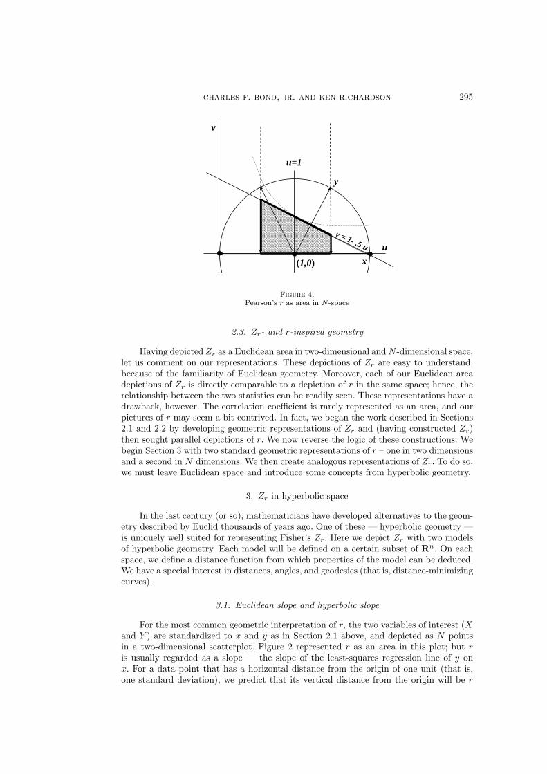
charles f. bond, jr. and ken richardson 295
v = 1- .5 u
y
x(1,0)
u=1
u
v
Figure 4.Pearson’s r as area in N-space
2.3. Zr- and r-inspired geometry
Having depicted Zr as a Euclidean area in two-dimensional and N -dimensional space,let us comment on our representations. These depictions of Zr are easy to understand,because of the familiarity of Euclidean geometry. Moreover, each of our Euclidean areadepictions of Zr is directly comparable to a depiction of r in the same space; hence, therelationship between the two statistics can be readily seen. These representations have adrawback, however. The correlation coefficient is rarely represented as an area, and ourpictures of r may seem a bit contrived. In fact, we began the work described in Sections2.1 and 2.2 by developing geometric representations of Zr and (having constructed Zr)then sought parallel depictions of r. We now reverse the logic of these constructions. Webegin Section 3 with two standard geometric representations of r – one in two dimensionsand a second in N dimensions. We then create analogous representations of Zr. To do so,we must leave Euclidean space and introduce some concepts from hyperbolic geometry.
3. Zr in hyperbolic space
In the last century (or so), mathematicians have developed alternatives to the geom-etry described by Euclid thousands of years ago. One of these — hyperbolic geometry —is uniquely well suited for representing Fisher’s Zr. Here we depict Zr with two modelsof hyperbolic geometry. Each model will be defined on a certain subset of Rn. On eachspace, we define a distance function from which properties of the model can be deduced.We have a special interest in distances, angles, and geodesics (that is, distance-minimizingcurves).
3.1. Euclidean slope and hyperbolic slope
For the most common geometric interpretation of r, the two variables of interest (Xand Y ) are standardized to x and y as in Section 2.1 above, and depicted as N pointsin a two-dimensional scatterplot. Figure 2 represented r as an area in this plot; but ris usually regarded as a slope — the slope of the least-squares regression line of y onx. For a data point that has a horizontal distance from the origin of one unit (that is,one standard deviation), we predict that its vertical distance from the origin will be r
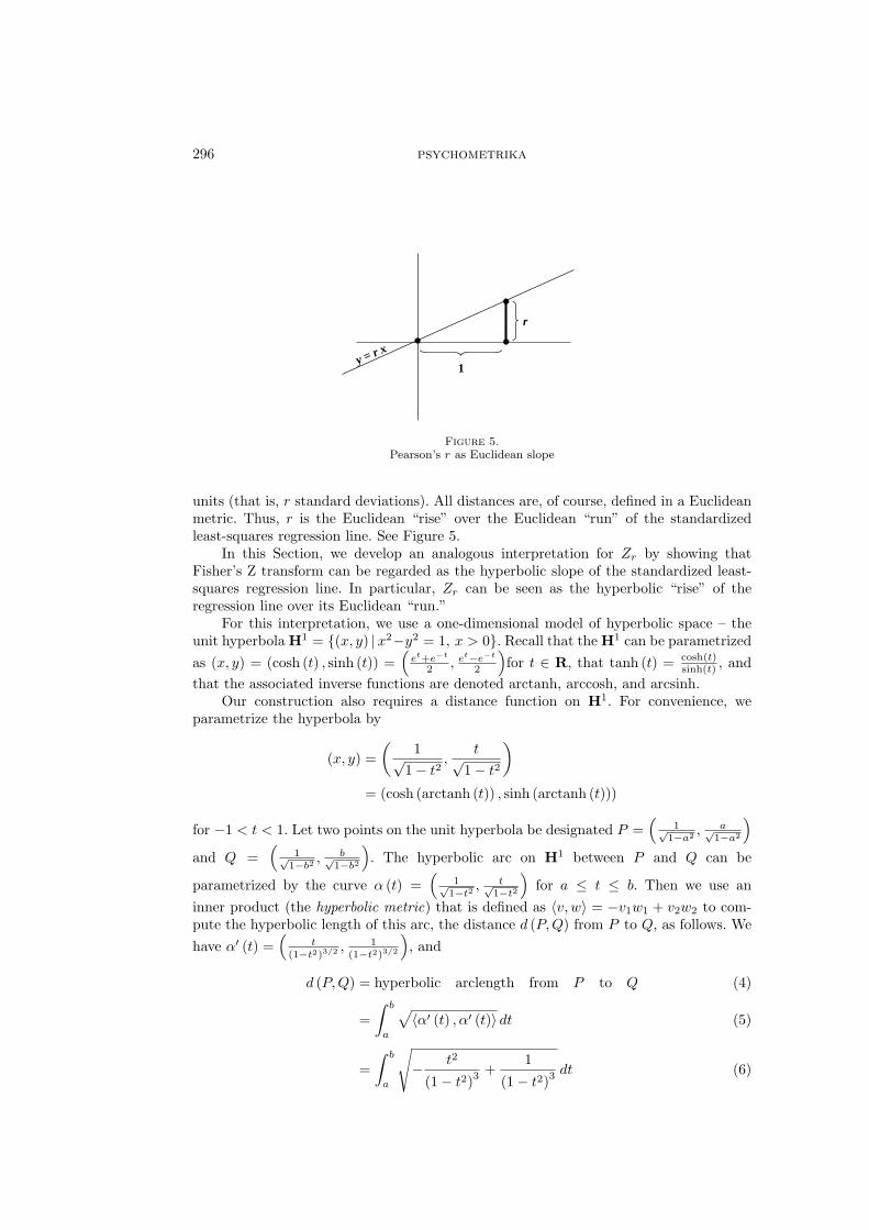
296 psychometrika
y = r x
r
1
Figure 5.Pearson’s r as Euclidean slope
units (that is, r standard deviations). All distances are, of course, defined in a Euclideanmetric. Thus, r is the Euclidean “rise” over the Euclidean “run” of the standardizedleast-squares regression line. See Figure 5.
In this Section, we develop an analogous interpretation for Zr by showing thatFisher’s Z transform can be regarded as the hyperbolic slope of the standardized least-squares regression line. In particular, Zr can be seen as the hyperbolic “rise” of theregression line over its Euclidean “run.”
For this interpretation, we use a one-dimensional model of hyperbolic space – theunit hyperbola H1 = {(x, y) |x2−y2 = 1, x > 0}. Recall that the H1 can be parametrizedas (x, y) = (cosh (t) , sinh (t)) =
(et+e−t
2 , et−e−t
2
)for t ∈ R, that tanh (t) = cosh(t)
sinh(t) , andthat the associated inverse functions are denoted arctanh, arccosh, and arcsinh.
Our construction also requires a distance function on H1. For convenience, weparametrize the hyperbola by
(x, y) =(
1√1− t2
,t√
1− t2
)
= (cosh (arctanh (t)) , sinh (arctanh (t)))
for −1 < t < 1. Let two points on the unit hyperbola be designated P =(
1√1−a2 , a√
1−a2
)
and Q =(
1√1−b2
, b√1−b2
). The hyperbolic arc on H1 between P and Q can be
parametrized by the curve α (t) =(
1√1−t2
, t√1−t2
)for a ≤ t ≤ b. Then we use an
inner product (the hyperbolic metric) that is defined as 〈v, w〉 = −v1w1 + v2w2 to com-pute the hyperbolic length of this arc, the distance d (P, Q) from P to Q, as follows. Wehave α′ (t) =
(t
(1−t2)3/2 , 1(1−t2)3/2
), and
d (P, Q) = hyperbolic arclength from P to Q (4)
=∫ b
a
√〈α′ (t) , α′ (t)〉 dt (5)
=∫ b
a
√− t2
(1− t2)3+
1(1− t2)3
dt (6)
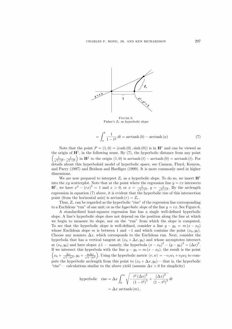
charles f. bond, jr. and ken richardson 297
y = r xx 2 – y 2
= 1
Zr
1
Figure 6.Fisher’s Zr as hyperbolic slope
=∫ b
a
11− t2
dt = arctanh (b)− arctanh (a) (7)
Note that the point P = (1, 0) = (cosh (0) , sinh (0)) is in H1 and can be viewed asthe origin of H1, in the following sense. By (7), the hyperbolic distance from any point(
1√1−t2
, t√1−t2
)in H1 to the origin (1, 0) is arctanh (t) − arctanh (0) = arctanh (t). For
details about this hyperboloid model of hyperbolic space, see Cannon, Floyd, Kenyon,and Parry (1997) and Bridson and Haefliger (1999). It is more commonly used in higherdimensions.
We are now prepared to interpret Zr as a hyperbolic slope. To do so, we insert H1
into the xy scatterplot. Note that at the point where the regression line y = rx intersectsH1, we have x2 − (rx)2 = 1 and x > 0, or x = 1√
1−r2 , y = r√1−r2 . By the arclength
expression in equation (7) above, it is evident that the hyperbolic rise of this intersectionpoint (from the horizontal axis) is arctanh (r) = Zr.
Thus, Zr can be regarded as the hyperbolic “rise” of the regression line correspondingto a Euclidean “run” of one unit; or as the hyperbolic slope of the line y = rx. See Figure 6.
A standardized least-squares regression line has a single well-defined hyperbolicslope. A line’s hyperbolic slope does not depend on the position along the line at whichwe begin to measure its slope, nor on the “run” from which the slope is computed.To see that the hyperbolic slope is well-defined, consider a line y − y0 = m (x− x0)whose Euclidean slope m is between 1 and −1 and which contains the point (x0, y0).Choose any nonzero ∆x, which corresponds to the Euclidean run. Next, consider thehyperbola that has a vertical tangent at (x0 + ∆x, y0) and whose asymptotes intersectat (x0, y0) and have slopes ±1 — namely, the hyperbola (x− x0)
2 − (y − y0)2 = (∆x)2.
If we intersect this hyperbola with the line y − y0 = m (x− x0), the result is the point(x0 + ∆x√
1−m2 , y0 + m∆x√1−m2
). Using the hyperbolic metric 〈v, w〉 = −v1w1 +v2w2 to com-
pute the hyperbolic arclength from this point to (x0 + ∆x, y0)— that is, the hyperbolic“rise”— calculations similar to the above yield (assume ∆x > 0 for simplicity)
hyperbolic rise = ∆x
∫ m
0
√− t2 (∆x)2
(1− t2)3+
(∆x)2
(1− t2)3dt
= ∆x arctanh (m) ,
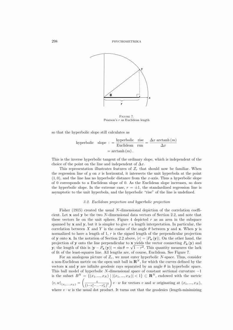
298 psychometrika
y
x
r
θθθθ
Figure 7.Pearson’s r as Euclidean length
so that the hyperbolic slope still calculates as
hyperbolic slope : =hyperbolic riseEuclidean run
=∆x arctanh (m)
∆x
= arctanh (m) .
This is the inverse hyperbolic tangent of the ordinary slope, which is independent of thechoice of the point on the line and independent of ∆x.
This representation illustrates features of Zr that should now be familiar. Whenthe regression line of y on x is horizontal, it intersects the unit hyperbola at the point(1, 0), and the line has no hyperbolic distance from the x-axis. Thus a hyperbolic slopeof 0 corresponds to a Euclidean slope of 0. As the Euclidean slope increases, so doesthe hyperbolic slope. In the extreme case, r = ±1, the standardized regression line isasymptotic to the unit hyperbola, and the hyperbolic “rise” of the line is undefined.
3.2. Euclidean projection and hyperbolic projection
Fisher (1915) created the usual N -dimensional depiction of the correlation coeffi-cient. Let x and y be the two N -dimensional data vectors of Section 2.2, and note thatthese vectors lie on the unit sphere. Figure 4 depicted r as an area in the subspacespanned by x and y, but it is simpler to give r a length interpretation. In particular, thecorrelation between X and Y is the cosine of the angle θ between y and x. When y isnormalized to have a length of 1, r is the signed length of the perpendicular projectionof y onto x. In the notation of Section 2.2 above, |r| = |Px (y)|. On the other hand, theprojection of y onto the line perpendicular to x yields the vector connecting Px (y) andy; the length of this is |y − Px (y)| = sin θ =
√1− r2. This quantity measures the lack
of fit of the least-squares line. All lengths are, of course, Euclidean. See Figure 7.For an analogous picture of Zr, we must enter hyperbolic N -space. Thus, consider
a non-Euclidean metric on the open unit ball in RN , for which the curves defined by thevectors x and y are infinite geodesic rays separated by an angle θ in hyperbolic space.This ball model of hyperbolic N -dimensional space of constant sectional curvature −1is the subset BN = {(x1, ..., xN ) | |(x1, ..., xN )| < 1} ⊂ RN , endowed with the metric
〈v, w〉(x1,...,xN ) =(
4
(1−x21−...−x2
N)2
)v · w for vectors v and w originating at (x1, ..., xN ),
where v · w is the usual dot product. It turns out that the geodesics (length-minimizing
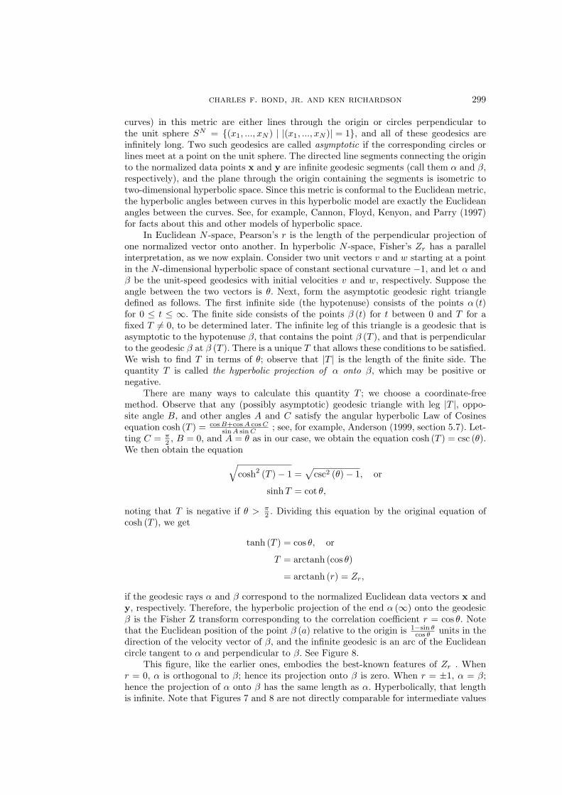
charles f. bond, jr. and ken richardson 299
curves) in this metric are either lines through the origin or circles perpendicular tothe unit sphere SN = {(x1, ..., xN ) | |(x1, ..., xN )| = 1}, and all of these geodesics areinfinitely long. Two such geodesics are called asymptotic if the corresponding circles orlines meet at a point on the unit sphere. The directed line segments connecting the originto the normalized data points x and y are infinite geodesic segments (call them α and β,respectively), and the plane through the origin containing the segments is isometric totwo-dimensional hyperbolic space. Since this metric is conformal to the Euclidean metric,the hyperbolic angles between curves in this hyperbolic model are exactly the Euclideanangles between the curves. See, for example, Cannon, Floyd, Kenyon, and Parry (1997)for facts about this and other models of hyperbolic space.
In Euclidean N -space, Pearson’s r is the length of the perpendicular projection ofone normalized vector onto another. In hyperbolic N -space, Fisher’s Zr has a parallelinterpretation, as we now explain. Consider two unit vectors v and w starting at a pointin the N -dimensional hyperbolic space of constant sectional curvature −1, and let α andβ be the unit-speed geodesics with initial velocities v and w, respectively. Suppose theangle between the two vectors is θ. Next, form the asymptotic geodesic right triangledefined as follows. The first infinite side (the hypotenuse) consists of the points α (t)for 0 ≤ t ≤ ∞. The finite side consists of the points β (t) for t between 0 and T for afixed T 6= 0, to be determined later. The infinite leg of this triangle is a geodesic that isasymptotic to the hypotenuse β, that contains the point β (T ), and that is perpendicularto the geodesic β at β (T ). There is a unique T that allows these conditions to be satisfied.We wish to find T in terms of θ; observe that |T | is the length of the finite side. Thequantity T is called the hyperbolic projection of α onto β, which may be positive ornegative.
There are many ways to calculate this quantity T ; we choose a coordinate-freemethod. Observe that any (possibly asymptotic) geodesic triangle with leg |T |, oppo-site angle B, and other angles A and C satisfy the angular hyperbolic Law of Cosinesequation cosh (T ) = cos B+cos A cos C
sin A sin C ; see, for example, Anderson (1999, section 5.7). Let-ting C = π
2 , B = 0, and A = θ as in our case, we obtain the equation cosh (T ) = csc (θ).We then obtain the equation
√cosh2 (T )− 1 =
√csc2 (θ)− 1, or
sinhT = cot θ,
noting that T is negative if θ > π2 . Dividing this equation by the original equation of
cosh (T ), we get
tanh (T ) = cos θ, or
T = arctanh (cos θ)
= arctanh (r) = Zr,
if the geodesic rays α and β correspond to the normalized Euclidean data vectors x andy, respectively. Therefore, the hyperbolic projection of the end α (∞) onto the geodesicβ is the Fisher Z transform corresponding to the correlation coefficient r = cos θ. Notethat the Euclidean position of the point β (a) relative to the origin is 1−sin θ
cos θ units in thedirection of the velocity vector of β, and the infinite geodesic is an arc of the Euclideancircle tangent to α and perpendicular to β. See Figure 8.
This figure, like the earlier ones, embodies the best-known features of Zr . Whenr = 0, α is orthogonal to β; hence its projection onto β is zero. When r = ±1, α = β;hence the projection of α onto β has the same length as α. Hyperbolically, that lengthis infinite. Note that Figures 7 and 8 are not directly comparable for intermediate values
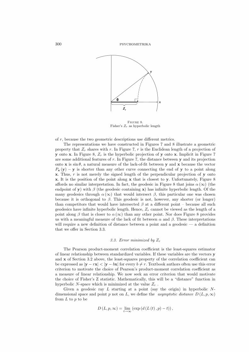
300 psychometrika
x
Zr
y
θθθθ
Figure 8.Fisher’s Zr as hyperbolic length
of r, because the two geometric descriptions use different metrics.The representations we have constructed in Figures 7 and 8 illustrate a geometric
property that Zr shares with r. In Figure 7, r is the Euclidean length of a projection ofy onto x. In Figure 8, Zr is the hyperbolic projection of y onto x. Implicit in Figure 7are some additional features of r. In Figure 7, the distance between y and its projectiononto x is sin θ, a natural measure of the lack-of-fit between y and x because the vectorPx (y) − y is shorter than any other curve connecting the end of y to a point alongx. Thus, r is not merely the signed length of the perpendicular projection of y ontox. It is the position of the point along x that is closest to y. Unfortunately, Figure 8affords no similar interpretation. In fact, the geodesic in Figure 8 that joins α (∞) (theendpoint of y) with β (the geodesic containing x) has infinite hyperbolic length. Of themany geodesics through α (∞) that would intersect β, this particular one was chosenbecause it is orthogonal to β. This geodesic is not, however, any shorter (or longer)than competitors that would have intersected β at a different point – because all suchgeodesics have infinite hyperbolic length. Hence, Zr cannot be viewed as the length of apoint along β that is closer to α (∞) than any other point. Nor does Figure 8 providesus with a meaningful measure of the lack of fit between α and β. These interpretationswill require a new definition of distance between a point and a geodesic — a definitionthat we offer in Section 3.3.
3.3. Error minimized by Zr
The Pearson product-moment correlation coefficient is the least-squares estimatorof linear relationship between standardized variables. If these variables are the vectors yand x of Section 3.2 above, the least-squares property of the correlation coefficient canbe expressed as |y − rx| < |y − bx| for every b 6= r. Textbook authors often use this errorcriterion to motivate the choice of Pearson’s product-moment correlation coefficient asa measure of linear relationship. We now seek an error criterion that would motivatethe choice of Fisher’s Z statistic. Mathematically, this will be a “distance” function inhyperbolic N -space which is minimized at the value Zr .
Given a geodesic ray L starting at a point (say the origin) in hyperbolic N -dimensional space and point p not on L, we define the asymptotic distance D (L, p,∞)from L to p to be
D (L, p,∞) = limt→∞
(exp (d (L (t) , p)− t)) ,
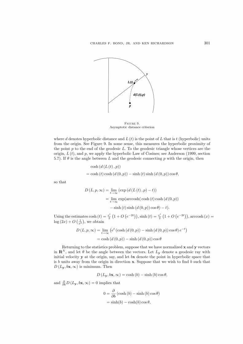
charles f. bond, jr. and ken richardson 301
p
y
L(t)
d(L(t),p)
Figure 9.Asymptotic distance criterion
where d denotes hyperbolic distance and L (t) is the point of L that is t (hyperbolic) unitsfrom the origin. See Figure 9. In some sense, this measures the hyperbolic proximity ofthe point p to the end of the geodesic L. To the geodesic triangle whose vertices are theorigin, L (t), and p, we apply the hyperbolic Law of Cosines; see Anderson (1999, section5.7). If θ is the angle between L and the geodesic connecting p with the origin, then
cosh (d (L (t) , p))
= cosh (t) cosh (d (0, p))− sinh (t) sinh (d (0, p)) cos θ,
so that
D (L, p,∞) = limt→∞
(exp (d (L (t) , p)− t))
= limt→∞
exp(arccosh( cosh (t) cosh (d (0, p))
− sinh (t) sinh (d (0, p)) cos θ)− t).
Using the estimates cosh (t) = et
2
(1 + O
(e−2t
)), sinh (t) = et
2
(1 + O
(e−2t
)), arccosh (x) =
log (2x) + O(
1x2
), we obtain
D (L, p,∞) = limt→∞
(et (cosh (d (0, p))− sinh (d (0, p)) cos θ) e−t
)
= cosh (d (0, p))− sinh (d (0, p)) cos θ
Returning to the statistics problem, suppose that we have normalized x and y vectorsin RN , and let θ be the angle between the vectors. Let Ly denote a geodesic ray withinitial velocity y at the origin, say, and let bx denote the point in hyperbolic space thatis b units away from the origin in direction x. Suppose that we wish to find b such thatD (Ly, bx,∞) is minimum. Then
D (Ly, bx,∞) = cosh (b)− sinh (b) cos θ,
and ∂∂bD (Ly, bx,∞) = 0 implies that
0 =∂
∂b(cosh (b)− sinh (b) cos θ)
= sinh(b)− cosh(b) cos θ,
302 psychometrika
or
b = arctanh (cos θ) = Zr ,
which implies that
D (Ly, Zrx,∞) = cosh (Zr)− sinh (Zr) tanh (Zr)
=cosh2 (Zr)− sinh2 (Zr)
cosh (Zr)
=1
cosh (Zr)=
1cosh (arctanh (cos θ))
=√
1− cos2 (θ) = sin θ.
We check the second derivative:
∂2
∂b2(cosh (b)− sinh (b) cos θ) = cosh (b)− sinh (b) cos θ
= D (Ly, bx,∞) > 0,
to find that the asymptotic distance D (Ly, bx,∞) in fact achieves a global minimumvalue of sin θ at b = Zr. Observe that this newly-defined asymptotic distance is the sameas the minimum Euclidean distance from y to bx, if y and x have Euclidean length 1.
4. Conclusion
Here we have developed the first geometric interpretations of Fisher’s Zr transfor-mation. As our work reveals, Zr is geometrically similar to r; indeed, the similaritiesare so strong that we regard Zr as the hyperbolic counterpart to the Euclidean r. Ourconstructions illustrate well-known features of these two statistics and allow us to see ther-to-Zr transformation for the first time.
The geometric context of this paper suggests many additional questions such asthe following, which have not yet been considered. Can the sampling properties of theZr statistic be understood in a geometric way? Does every transformation of r suggesta particular type of geometry? We offer the present work with the hope of inspiringadditional insights.
References
Anderson, J. W. (1999). Hyperbolic Geometry. London: Springer-Verlag.Bridson, M. R., and Haefliger, A. (1999). Metric spaces of nonpositive curvature. New
York: Springer-Verlag.Brien, C. J., Venables, W. N., James, A.T., and Mayo, O. (1984). An analysis of corre-
lation matrices: Equal correlations. Biometrika, 71, 545–554.Cannon, J. W., Floyd, W. J., Kenyon, R., and Parry, W. R. (1997). Hyperbolic geometry.
In Levy, S. (Ed.) Flavors of Geometry (pp. 59–116), New York: Cambridge UniversityPress.
Casella and Berger (2002). Statistical inference (Second Edition). Pacific Grove, CA:Duxbury.
Fisher, R.A. (1915). Frequency distribution of the values of the correlation coefficient insamples of an indefinitely large population. Biometrika, 10, 507–521.
Fisher, R.A. (1921). On the ‘probable error’ of a coefficient of correlation deduced froma small sample. Metron, 1, 3–32.

charles f. bond, jr. and ken richardson 303
Gayen,A.K. (1951). The frequency distribution of the product-moment correlation inrandom samples of any size drawn from non-normal universes. Biometrika, 38, 219–247.
Hawkins, D.L. (1989). Using U statistics to derive the asymptotic distribution of Fisher’sZ statistic. The American Statistician, 43, 235–237.
Hotelling, H. (1953). New light on the correlation coefficient and its transforms. Journalof the Royal Statistical Society B, 15, 193–225.
Johnson, N.L., Kotz, S., and Balakrishnan, N. (1995). Continuous univariate distributions(Second edition: Volume 2). New York: Wiley.
Lipsey, M.W., and Wilson, D.B. (2001). Practical meta-analysis. Thousand Oaks, CA:Sage.
Rodgers, J.L., and Nicewander, W.A. (1988). Thirteen ways to look at the correlationcoefficient. The American Statistician, 42, 59–66.
Winterbottom, A. (1979). A note on the derivation of Fisher’s transformation of thecorrelation coefficient. The American Statistician, 33, 142–143.
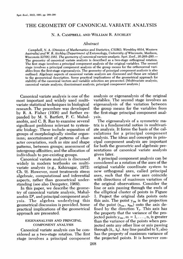
Syst. Zool., 30(3), 1981, pp. 268-280
THE GEOMETRY OF CANONICAL VARIATE ANALYSIS
N. A. CAMPBELL AND WILLIAM R. ATCHLEY
Abstract Campbell, N. A. (Division of Mathematics and Statistics, CSIRO, Wembley 6014, Western
Australia) and W. R. Atchley (Department of Entomology, University of Wisconsin, Madison, Wisconsin 53706)1981. The geometry of canonical variate analysis. Syst. Zool., 30:268-280.- The geometry of canonical variate analysis is described as a two-stage orthogonal rotation. The first stage involves a principal component analysis of the original variables. The second stage involves a principal component analysis of the group means for the orthonormal vari- ables from the first-stage eigenanalysis. The geometry of principal component analysis is also outlined. Algebraic aspects of canonical variate analysis are discussed and these are related to the geometrical description. Some practical implications of the geometrical approach for stability of the canonical vectors and variable selection are presented. [Multivariate analysis; canonical variate analysis; discriminant analysis; principal component analysis.]
Canonical variate analysis is one of the most important and widely used multi- variate statistical techniques in biological research. The procedure was developed by R. A. Fisher (1936) and further ex- panded by M. S. Bartlett, P. C. Mahal- anobis, and C. R. Rao to examine several significant problems relevant to system- atic biology. These include separation of groups of morphologically similar organ- isms; ascertainment of patterns of char- acter covariation, such as size and shape patterns, between groups; assessment of intergroup affinities; and the allocation of individuals to pre-existing groups.
Canonical variate analysis is discussed widely in modern textbooks on multi- variate analysis (e.g., Kshirsagar, 1972: Ch. 9). However, most treatments stress algebraic, computational and inferential aspects, rather than geometrical under- standing (see also Dempster, 1969).
In this paper, we describe the geome- try of canonical variate analysis, Mahal- anobis D2, and principal component anal- ysis. The algebra underlying this geometrical discussion is provided. Some practical implications of the geometrical approach are presented.
EIGENANALYSIS AND PRINCIPAL COMPONENT ANALYSIS
Canonical variate analysis can be con- sidered as a two-stage rotation. The first stage involves a principal component
analysis or eigenanalysis of the original variables. The second stage involves an eigenanalysis of the variation between the group means for the variables from the first-stage principal component anal- ysis.
The eigenanalysis of a symmetric ma- trix is a fundamental notion in multivari- ate analysis. It forms the basis of the cal- culations for a principal component analysis. The ideas and concepts in prin- cipal component analysis are important for both the geometric and algebraic pre- sentations of canonical variate analysis given later.
A principal component analysis can be considered as a rotation of the axes of the original variable coordinate system to new orthogonal axes, called principal axes, such that the new axes coincide with directions of maximum variation of the original observations. Consider the line or axis passing through the ends of the elliptical cluster of points in Figure 1. Project the original data points onto this axis. The point ylm is the projection of the point (xim, x2m) onto the axis de- fined by the direction Y1. This axis has the property that the variance of the pro- jected points Ylm, m = 1, . . . , n, is greater than the variance of the points when pro- jected onto any other line or axis passing through (x1, x2). Any line parallel to Y1 also has the property of maximum variance of the projected points. It is however con-
268

1981 GEOMETRY OF CANONICAL VARIATE ANALYSIS 269
X2-
x2~~~~~
0
FIG. 1.-Idealized representation of scatter diagram for two variables, showing the mean for each vari- able (xi and x2), 95% concentration ellipse, and principal axes Y1 and Y2. The points Ylm and Y2m give the principal component scores for the observation xi = (Xim, X2m)T. The cosine of the angle 0 between Y1 and X1 gives the first component ull of the eigenvector corresponding to Y1.
venient geometrically to use the first rep- resentation.
The property of maximum variation of the projected points defines the first prin- cipal axis; it is the line or direction with maximum variation of the projected val- ues of the original data points. The pro- jected values corresponding to this direc- tion of maximum variation are the principal component scores. The first
principal axis is often called the line of best fit since the sum of squares (SSQ) of the perpendicular deviations of the orig- inal data points from the line is a mini- mum. Successive principal axes are de- termined with the property that they are orthogonal to the previous principal axes and that they maximize the variation of the projected points subject to these con- straints. For two variables, only one more
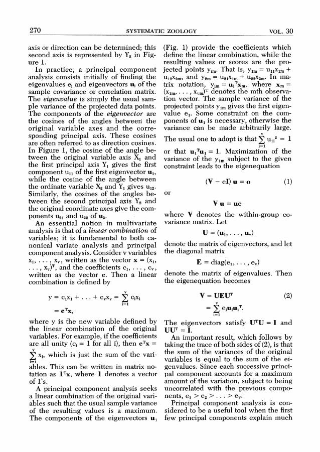
270 SYSTEMATIC ZOOLOGY VOL. 30
axis or direction can be determined; this second axis is represented by Y2 in Fig- ure 1.
In practice, a principal component analysis consists initially of finding the eigenvalues ei and eigenvectors ui of the sample covariance or correlation matrix. The eigenvalue is simply the usual sam- ple variance of the projected data points. The components of the eigenvector are the cosines of the angles betweern the original variable axes and the corre- sponding principal axis. These cosines are often referred to as direction cosines. In Figure 1, the cosine of the angle be- tween the original variable axis X1 and the first principal axis Y1 gives the first component u1l of the first eigenvector u1, while the cosine of the angle between the ordinate variable X2 and Y1 gives u12. Similarly, the cosines of the angles be- tween the second principal axis Y2 and the original coordinate axes give the com- ponents u21 and u22 of u2.
An essential notion in multivariate analysis is that of a linear combination of variables; it is fundamental to both ca- nonical variate analysis and principal component analysis. Consider v variables xl, *. , xv, written as the vector x = (x1, ... . xv)T, and the coefficients c1, ... ., cv written as the vector c. Then a linear combination is defined by
v
y = clxl + ... + cVxV = cx i=1
=TX,
where y is the new variable defined by the linear combination of the original variables. For example, if the coefficients are all unity (ci = 1 for all i), then cTx =
v
2 xi, which is just the sum of the vari- i=l ables. This can be written in matrix no- tation as lTx, where I denotes a vector of l's.
A principal component analysis seeks a linear combination of the original vari- ables such that the usual sample variance of the resulting values is a maximum. The components of the eigenvectors u1
(Fig. 1) provide the coefficients which define the linear combination, while the resulting values or scores are the pro- jected points Yim. That is, Ylm = ulixim + u12x2m, and Y2m = U21Xlm + U22X2m. In ma- trix notation, Yim = UiTXm, where xm = (XIm, .. ., Xvm)T denotes the mth observa- tion vector. The sample variance of the projected points Ylm gives the first eigen- value e1. Some constraint on the com- ponents of u1 is necessary, otherwise the variance can be made arbitrarily large. The usual one to adopt is that z u1i2 = 1
i=l or that ulTu1 = 1. Maximization of the variance of the Ylm subject to the given constraint leads to the eigenequation
(V - eI)u= (1)
or
Vu = ue
where V denotes the within-group co- variance matrix. Let
U = (ui, ***XUV)
denote the matrix of eigenvectors, and let the diagonal matrix
E = diag(e1, . . . , ev) denote the matrix of eigenvalues. Then the eigenequation becomes
V= UEUT (2) v
= 2 e1u1ui. i=l
The eigenvectors satisfy UTU = I and UUT = I.
An important result, which follows by taking the trace of both sides of (2), is that the sum of the variances of the original variables is equal to the sum of the ei- genvalues. Since each successive princi- pal component accounts for a maximum amount of the variation, subject to being uncorrelated with the previous compo- nents, e1 > e2 > ... > ev.
Principal component analysis is con- sidered to be a useful tool when the first few principal components explain much

1981 GEOMETRY OF CANONICAL VARIATE ANALYSIS 271
of the variation, so that a few bivariate scatter plots of the scores summarize the multivariate data. For morphometric data, it is often found that the elements of the first eigenvector are all positive; an increase in each variable results in a gen- eral increase in the value of the principal component score. For this reason, the first component is often termed a size component (e.g., Jolicoeur and Mosi- mann, 1960).
CANONICAL VARIATE ANALYSIS- GENERAL IDEAS
In a canonical variate analysis, linear combinations of the original variables are determnined in -such a way that the differ- ences between a number of reference groups are maximized relative to the vari- ation within groups. It is hoped that the group configuration can be adequately represented in a two or three dimen- sional subspace defined by the first two or three canonical vectors. The first ca- nonical vector is given by the coeffi- cients of the linear combination which maximizes the ratio of the between- to within-groups SSQ's for the resulting ca- nonical variate. The corresponding ratio is referred to as the canonical root. Suc- cessive linear combinations of the origi- nal variables are chosen to be uncorre- lated both within and between groups. Pythagorean distance is then appropriate for interpreting a scatter plot of the group means, with the important canonical vari- ates as the coordinates.
Figure 2 depicts a typical situation for two variables. The concentration ellipses reflect the clustering of the observations in the main body of the data. The points Xim = (xIIm, x21m)T and x2m represent typ- ical observations. The vector c represents the direction of the calculated canonical vector.
The point representing the observa- tion ylm gives the projection of the ob- servation xlm onto the canonical vector. For convenience, xkm and Ykm will be used to -denote both the observation and the point representing the observa-
tion. The observation Yim is given by the linear combination clxllm + . . . + Cvxlvm =
cTXim. The observation Ykm is the canon- ical variate score for the mth observation for the kth group. Hence the point Y2m represents the projection of the observa- tion X2m onto the canonical vector. Simi- larly the points -Yk represent the projec- tions of the group means onto the canonical vector.
When all observations Xkm are pro- jected onto the canonical vector, a distri- bution of scores for each group will re- sult. If the underlying distribution of the vectors of observations is multivariate Gaussian, then the histograms of canon- ical variate scores will follow the familiar bell-shaped appearance of a univariate Gaussian density. It is important to real- ize that the actual canonical variate scores do not follow a univariate Gauss- ian distribution, since the components of the vector of coefficients c are them- selves realizations of random variables (e.g., Kshirsagar, 1972:197).
The orientation or direction of the ca- nonical vector c is such that the ratio of the between- to within-groups SSQ from the one-way analysis of variance of the projected points Ylm, m = 1, . .. , n1; Y2m, m= 1, ..., n2; ...; Ygm, m= 1, .. ., ng, is greater than that for any other orien- tation of the canonical vector.
The ratio of the between-groups to the within-groups SSQ gives the canonical root. The cosines of the angles between the canonical vector and the original co- ordinate axes give the components of the canonical vector. The projected points or observations are the canonical variate scores.
The property of maximum ratio of be- tween- to within-groups variation defines the first canonical vector. This first axis is again a line of best fit, though the fit is now to the group means, and the shape of the concentration ellipsoids must be taken into consideration. A geometrical explanation is given in the next section.
In canonical variate analysis, the de- gree of correlation between, and the vari-
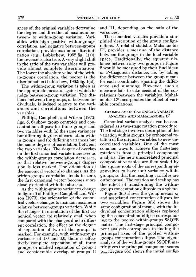
272 SYSTEMATIC ZOOLOGY VOL. 30
ances of, the original variables determine the degree and direction of maximum be- tween- to within-group variation. Vari- ables with high positive within-groups correlation, and negative between-groups correlation, provide maximum discrimi- nation (e.g., Lubischew, 1962:fig. 1(a)); the reverse is also true. A very slight shift in the ratio of the two variables will pro- vide almost complete discrimination. The lower the absolute value of the with- in-groups correlation, the poorer is the discrimination (Lubischew, 1962:fig. 1(a)).
The within-group variation is taken as the appropriate measure against which to judge between-group variation. The dis- tance between the groups, or between in- dividuals, is judged relative to the vari- ances and correlations between the variables.
Phillips, Campbell, and Wilson (1973: figs. 5, 6) show group centroids and con- centration ellipses for three groups and two variables with (a) the same variances but differing degrees of correlation with- in groups; and (b) differing variances but the same degree of correlation between the two variables. The degree of overlap on the first canonical variate increases as the within-groups correlation decreases, so that relative between-groups disper- sion is less marked. The orientation of the canonical vector also changes. As the within-groups correlation tends to zero, the first canonical vector becomes more closely oriented with the abscissa.
As the within-groups variances change in figure 6 of Phillips, Campbell and Wil- son (1973), the orientation of the canon- ical vectors changes to maintain maximum relative between-groups variation. While the changes in orientation of the first ca- nonical vector are relatively small when compared with the changes due to differ- ent correlation, the effect on the degree of separation of two of the groups is marked. For example, with within-groups variances of 1.0 and 3.0, there is effec- tively complete separation of all three groups, or marked separation of group I and considerable overlap of groups II
and III, depending on the ratio of the variances.
The canonical variates provide a sim- plified description of the group configu- rations. A related statistic, Mahalanobis D2, provides a measure of the distance between the groups in the total variable space. Traditionally, the squared dis- tance between any two groups in Figure 2 would be measured by their Euclidean or Pythagorean distance, i.e. by taking the difference between the group means for each coordinate, squaring the differ- ence and summing. However, such a measure fails to take account- of the cor- relations between the variables. Mahal- anobis D2 incorporates the effect of vari- able correlations.
GEOMETRY OF CANONICAL VARIATE ANALYSIS AND MAHALANOBIS D2
Canonical variate analysis can be con- sidered as a two-stage rotation procedure. The first stage involves description of the variation within groups, by orthogonal ro- tation of the original variables to new un- correlated variables. One of the most common ways to achieve the first-stage rotation is from a principal component analysis. The new uncorrelated principal component variables are then scaled by the square roots of the corresponding ei- genvalues to have unit variance within groups, so that the resulting variables are orthonormal. The rotation and scaling has the effect of transforming the within- groups concentration ellipsoid to a sphere.
Figure 3(a) shows the group means Xk
and associated concentration ellipses for two variables. Figure 3(b) shows the same configuration of means, with the in- dividual concentration ellipses replaced by the concentration ellipse correspond- ing to the pooled within-groups SSQPR matrix. The first-stage principal compo- nent analysis corresponds to finding the principal axes of the pooled within- groups concentration ellipse. The eigen- analysis of the within-groups SSQPR ma- trix gives the principal component scores Pikm. Figure 3(c) shows the initial config-
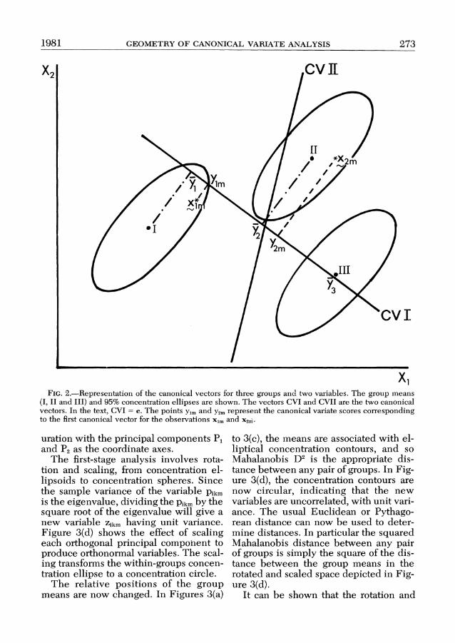
1981 GEOMETRY OF CANONICAL VARIATE ANALYSIS 273
X2~~~~~~~~~~~~*2
cvE cv / { CVJ[
XI FIG. 2.-Representation of the canonical vectors for three groups and two variables. The group means
(I, II and III) and 95% concentration ellipses are shown. The vectors CVI and CVII are the two canonical vectors. In the text, CVI = c. The points Ylm and Y2m represent the canonical variate scores corresponding to the first canonical vector for the observations xim and x2,1.
uration with the principal components P1 and P2 as the coordinate axes.
The first-stage analysis involves rota- tion and scaling, from concentration el- lipsoids to concentration spheres. Since the sample variance of the variable Pikm is the eigenvalue, dividing the Pikm by the square root of the eigenvalue will give a new variable Zikm having unit variance. Figure 3(d) shows the effect of scaling each orthogonal principal component to produce orthonormal variables. The scal- ing transforms the within-groups concen- tration ellipse to a concentration circle.
The relative positions of the group means are now changed. In Figures 3(a)
to 3(c), the means are associated with el- liptical concentration contours, and so Mahalanobis D2 is the appropriate dis- tance between any pair of groups. In Fig- ure 3(d), the concentration contours are now circular, indicating that the new variables are uncorrelated, with unit vari- ance. The usual Euclidean or Pythago- rean distance can now be used to deter- mine distances. In particular the squared Mahalanobis distance between any pair of groups is simply the square of the dis- tance between the group means in the rotated and scaled space depicted in Fig- ure 3(d).
It can be shown that the rotation and
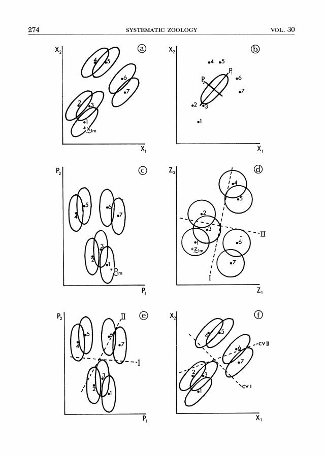
274 SYSTEMATIC ZOOLOGY VOL. 30
X2 X2 .4 .5
.2
XI XI
P2 Z2
.3
3 1 6
im~~~~~~*i
pi ZI
'VI
P1 XI
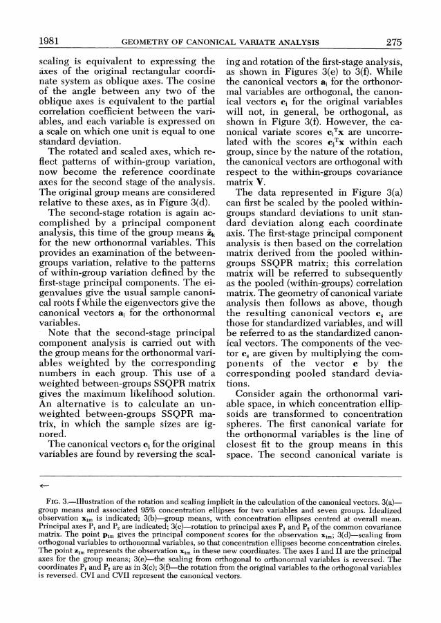
1981 GEOMETRY OF CANONICAL VARIATE ANALYSIS 275
scaling is equivalent to expressing the axes of the original rectangular coordi- nate system as oblique axes. The cosine of the angle between any two of the oblique axes is equivalent to the partial correlation coefficient between the vari- ables, and each variable is expressed on a -soale on which one unit is equal to one standard deviation.
The rotated and scaled axes, which re- flect patterns of within-group variation, now become the reference coordinate axes for the second stage of the analysis. The original group means are considered relative to these axes, as in Figure 3(d).
The second-stage rotation is again ac- complished by a principal component analysis, this time of the group means Zk
for the new orthonormal variables. This provides an examination of the between- groups variation, relative to the patterns of within-group variation defined by the first-stage principal components. The ei- genvalues give the usual sample canoni- cal roots f while the eigenvectors give the canonical vectors ai for the orthonormal variables. - Note that the second-stage principal component analysis is carried out with the group means for the orthonormal vari- ables weighted by the corresponding numbers in each group. This use of a weighted between-groups SSQPR matrix gives the maximum likelihood solution. An alternative is to calculate an un- weighted between-groups SSQPR ma- trix, in which the sample sizes are ig- nored.
The canonical vectors ci for the original variables are found by reversing the scal-
ing and rotation of the first-stage analysis, as shown in Figures 3(e) to 3(f). While the canonical vectors ai for the orthonor- mal variables are orthogonal, the canon- ical vectors ci for the original variables will not, in general, be orthogonal, as shown in Figure 3(f). However, the ca- nonical variate scores c1Tx are uncorre- lated with the scores cjTx within each group, since by the nature of the rotation, the canonical vectors are orthogonal with respect to the within-groups covariance matrix V.
The data represented in Figure 3(a) can first be scaled by the pooled within- groups standard deviations to unit stan- dard deviation along each coordinate axis. The first-stage principal component analysis is then based on the correlation matrix derived from the pooled within- groups SSQPR matrix; this correlation matrix will be referred to subsequently as the pooled (within-groups) correlation matrix. The geometry of canonical variate analysis then follows as above, though the resulting canonical vectors c, are those for standardized variables, and will be referred to as the standardized canon- ical vectors. The components of the vec- tor c, are given by multiplying the com- ponents of the vector c by the corresponding pooled standard devia- tions.
Consider again the orthonormal vari- able space, in which concentration ellip- soids are transformed to concentration spheres. The first canonical variate for the orthonormal variables is the line of closest fit to the group means in this space. The second canonical variate is
FIG. 3.-Illustration of the rotation and scaling implicit in the calculation of the canonical vectors. 3(a)- group means and associated 95% concentration ellipses for two variables and seven groups. Idealized observation xlm is indicated; 3(b)-group means, with concentration ellipses centred at overall mean. Principal axes P1 and P2 are indicated; 3(c)-rotation to principal axes P1 and P2 of the common covariance matrix. The point Plm gives the principal component scores for the observation xl.; 3(d)-scaling from orthogonal variables to orthonornal variables, so that concentration ellipses become concentration circles. The point Zlm represents the observation xim in these new coordinates. The axes I and II are the principal axes for the group means; 3(e)-the scaling from orthogonal to orthonormal variables is reversed. The coordinates P1 and P2 are as in 3(c); 3(f)-the rotation from the original variables te the orthogonal variables is reversed. CVI and CVII represent the canonical vectors.
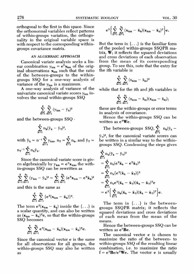
276 SYSTEMATIC ZOOLOGY VOL. 30
orthogonal to the first in this space. Since the orthonormal variables reflect patterns of within-groups variation, the orthogo- nality in the original variable space is with respect to the corresponding within- groups covariance matrix.
AN ALGEBRAIC APPROACH
Canonical variate analysis seeks a lin- ear combination Ykm = CTXkm of the orig- inal observations xkm such that the ratio of the between-groups to the within- groups SSQ for a one-way analysis of variance of the Ykm is a maximum.
A one-way analysis of variance of the univariate canonical variate scores Ykm in- volves the usual within-groups SSQ
g nk
E E (Ykm - Yk)2 k=1 m=1
and the between-groups SSQ'
E nk(Yk -T), k=1
nk g
with Yk n l Ykm, nT = E nk, and YT = m=1 k=1
g
nT 1 z nkyk. k=1
Since the canonical variate score is giv- en algebraically by Ykm = CTXkm, the with- in-groups SSQ can be rewritten as
g nk g nk
E (Ykm - Yk)2 = E E (CTXkm - CTXk)2 k=l m=l k=1 m=1
and this is the same as g nk
y a {C (Xkm - Xk)} .
k=1 m=1
The term CT(Xkm - Xk) inside the I.. .} is a scalar quantity, and can also be written as (Xkm - Xk)TC, so that the within-groups SSQ becomes
g nk
z CT(Xkm( Xk)(Xkm - Xk)TC. k=l m=l
Since the canonical vector c is the same for all observations for all groups, the within-groups SSQ may also be written as
fg nk
CT{ E (Xk- Xk)(Xkm - Xk)TC. k=1 m=1
But the term in .. . } is the familiar form of the pooled within-groups SSQPR ma- trix, W; it reflects the squared deviations and cross deviations of each observation from the mean of its corresponding group. To see this, note that the entry for the ith variable is
g nk
E E (Xkim - Xki) k=1 m=l
while that for the ith and jth variables is g nk
E Y. (Xkim - Xki)(Xkjm - xkj); k=1 m=1
these are the within-groups or error terms in analysis of covariance.
Hence the within-groups SSQ can be written as cTWc.
The between-groups SSQ, X nk(Yk -
YT)2, for the canonical variate scores can be written in a similar way to the within- groups SSQ. Condensing the steps gives
E nk(Yk - YT) k=1
-E nk(C jk - CTiT)2 k=1
= E nk{CT(i - XT)} k=1 g
- nkc (Xk - XT)(Xk - XT)C
k=1
- CT{ nk(ik - XT)(Xk - XT)T}C.
The term in ...} is the between- groups SSQPR matrix; it reflects the squared deviations and cross deviations of each mean from the mean of the means.
Hence the between-groups SSQ can be written as CTBc.
The canonical vector c is chosen to maximize the ratio of the between- to within-groups SSQ of the resulting linear combination, i.e. to maximize the ratio f = CTB/CTWC . The vector c is usually
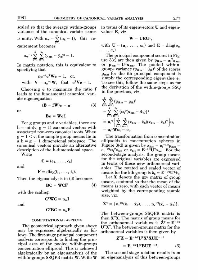
1981 GEOMETRY OF CANONICAL VARIATE ANALYSIS 277
scaled so that the average within-groups variance of the canonical variate scores
is unity. With nw = E (nk - 1), this re- k=1
quirement becomes g nk
nw-' 1 (Ykm - k)2= 1 k=1 m=1
In matrix notation, this is equivalent to specifying that
nw-'CTWc= 1, or, with V = nw-'W, that CTVc = 1.
Choosing c to maximize the ratio f leads to the fundamental canonical vari- ate eigenequation
(B - fW)c = o (3) or
Bc = Wcf.
For g groups and v variable>, there are h = min(v, g - 1) canonical vectors with associated non-zero canonical roots. When g - 1 < v, the sample group means lie in a h = g - 1 dimensional subspace. The canonical vectors provide an alternative description of the h-dimensional space.
Write
C = (Cl, * Ch) and
F = diag(f1, ..., fh).
Then the eigenanalysis in (3) becomes
BC = WCF (4)
with the scaling
CTWC = nwI and
CTBC = nwF.
COMPUTATIONAL ASPECTS The geometrical approach given above
may be expressed algebraically as fol- lows. The first-stage principal component analysis corresponds to finding the prin- cipal axes of the pooled within-groups concentration ellipsoid. This is achieved algebraically by an eigenanalysis of the within-groups SSQPR matrix W. Write W
in terms of its eigenvectors U and eigen- values E, viz.
W= UEIT,
with U = (ul, ..., uv) and E = diag(e1, ... ., ev).
The principal component scores in Fig- ure 3(c) are then given by Pikm = UiTXkm,
or Pkm = UTXkm. The pooled within- groups variance (Pikm - Pik)2 of the scores Pikm for the ith principal component is simply the corresponding eigenvalue ei. To see this, follow the same steps as for the derivation of the within-groups SSQ in the previous, viz.
g nk
_ E (Pikm - Pik) k=l m=l
g nk
E z {UiT(Xkm Xk)} k=1 m=1
g nk
= UiT{ (Xkm Xk)(Xkm Xk) Ui k=l m=l
= uiTWUi = ei.
The transformation from concentration ellipsoids to concentration spheres in Figure 3(d) is given by Zikm = ei-1'2pikm =
ei-1/2uiTxkm or Zkm = E 1/2UTXkm. For the second-stage analysis, the group means for the original variables are expressed in terms of these new orthonormal vari- ables. The rotated and scaled vector of means for the kth group is Zk = E-1/2UTik.
Let X denote the gxv matrix of group means, centered so that the mean of the means is zero, with each vector of means weighted by the corresponding sample size, viz.
XT = {nIn2(ix- XT), . . ., ng2(Xg - XT)}.
The between-groups SSQPR matrix is then XTX. The matrix of group means for the orthonormal variables is ZT= E-1/2
UTXT. The between-groups matrix for the orthonormal variables is then given by
ZTZ = E-1/2UTXTXUE-1/2
= E- 12UTBUE-12. (5) The second-stage rotation results from
an eigenanalysis of this between-groups
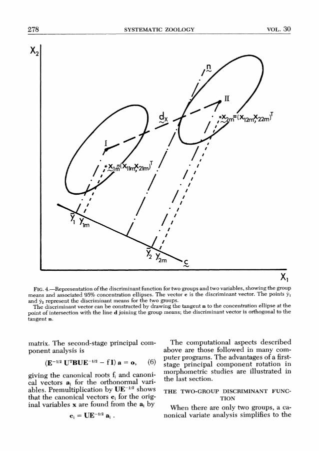
278 SYSTEMATIC ZOOLOGY VOL. 30
x2
/< n ) 2m)~~~~~~..2n-X1m,2m
( < n i~~'1 ln-?,21mj.)'
X1
FIG. 4.-Representation of the discriminant function for two groups and two variables, showing the group means and associated 95% concentration ellipses. The vector c is the discriminant vector. The points 5- and Y2 represent the discriminant means for the two groups.
The discriminant vector can be constructed by drawing the tangent n to the concentration ellipse at the point of intersection with the line d joining the group means; the discriminant vector is orthogonal to the tangent n.
matrix. The second-stage principal com- ponent analysis is
(E-1/2 UTBUE-1/2 -f I) a = o, (6)
giving the canonical roots fi and canoni- cal vectors ai for the orthonormal vari- ables. Premultiplication by UE-112 shows that the canonical vectors ci for the orig- inal variables x are found from the ai by
Ci = UE-1'2 ai .
The computational aspects described above are those followed in many com- puter programs. The advantages of a first- stage principal component rotation in morphometric studies are illustrated in the last section.
THE TWO-GROUP DISCRIMINANT FUNC- TION
When there are only two groups, a ca- nonical variate analysis simplifies to the
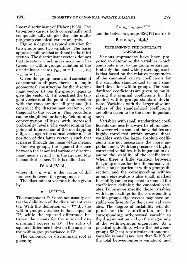
1981 GEOMETRY OF CANONICAL VARIATE ANALYSIS 279
linear discriminant of Fisher (1936). The two-group case is both conceptually and computationally simpler than the multi- ple-group canonical variate analysis.
Figure 4 depicts a typical situation for two groups and two variables. The basic approach follows that outlined in the third section. The discriminant vector c defines that direction which gives maximum be- tween- to within-groups variation of the discriminant scores Yim, m 1, ...,n; Y2m, m = 1, . . , n2.
Given the group means and associated concentration ellipses, there is a simple geometrical construction for the discrim- inant vector: (i) join the group means to give the vector dx; (ii) construct the tan- gent vector n at the point of intersection with the concentration ellipse; and (iii) construct the discriminant vector c, or- thogonal to the vector n. This procedure can be simplified further, by determining concentration ellipses with increased probability levels. The vector joining the points of intersection of the overlapping ellipses is again the normal vector n. The position of this latter vector is such that it passes through the mean of the means.
For two groups, the squared distance between the canonical variate or discrim- inant means -, and Y2 is the squared Ma- halanobis distance. This is defined as
D2 = dXTV-Wdx,
where dx - l - x2 is the vector of dif- ferences between the group means.
The discriminant vector c is then given by
c = D-tV-ldx. The component D-1 does not usually en- ter the definition of the discriminant vec- tor. With the definition cu = V-1dx, the within-groups variance is then equal to D2, while the squared difference be- tween the means for the unscaled dis- criminant scores is D4. The ratio of squared difference between the means to the within-groups variance is D2.
The canonical or discriminant root is given by
f = nw-1nln2nT-lD2
and the between-groups SSQPR matrix is
B = nln2nT-'dxdx.
DETERMINING THE IMPORTANT VARIABLES
Various approaches have been pro- posed to determine the variables which contribute most to the group separation. Probably the most widely used approach is that based on the relative magnitudes of the canonical variate coefficients for the variables standardized to unit stan- dard deviation within groups. The stan- dardized coefficients are given by multi- plying the original coefficients by the pooled within-groups standard devia- tions. Variables with the larger absolute values of the standardized coefficients are often taken to be the more important ones.
Variables with small standardized coef- ficients can nearly always be eliminated. However when some of the variables are highly correlated within groups, those variables with the larger absolute coeffi- cients are not necessarily the more im- portant ones. With the presence of highly correlated variables, it is important to ex- amine the stability of the coefficients. When there is little variation between the group means for the orthonormal vari- ables along a particular within-groups di- rection, and the corresponding within- groups eigenvalue is also small, marked instability can be expected in some of the coefficients defining the canonical vari- ates. To be more specific, those variables with large loadings for the corresponding within-groups eigenvector may have un- stable coefficients for the canonical vari- ates. The degree of instability will de- pend on the contribution of the corresponding orthonormal variable to the discrimination and on the magnitude of the within-groups eigenvalue. As a practical guideline, when the between- groups SSQ for a particular orthonormal variable is small (say, less than 5-10% of the total between-groups variation), and

280 SYSTEMATIC ZOOLOGY VOL. 30
the corresponding eigenvalue is also small (say, less than 1-2% of the sum of the eigenvalues), then some instability can be expected.
One approach to the potential problem of unstable coefficients is to introduce shrunken estimators (Campbell and Rey- ment, 1978). In practice, this involves adding shrinkage constants to some or all of the within-groups eigenvalues. This modification is done before these eigen- values are used to scale the uncorrelated first-stage principal component variables to produce the first-stage orthonormal variables.
It is often observed that while some of the coefficients of the canonical variates of interest change in magnitude and often in sign when these shrunken estimator procedures are introduced, shrinking the contribution of a within-groups eigenvec- tor/value combination has littlb effect on the corresponding canonical roots. This indicates that little or no discriminatory information has been lost. When this oc- curs, the obvious conclusion is that one or some of the variables contributing most to the orthonormal variable whose effect has been shrunk have little influ- ence on the discrimination. The variables involved are those that make the greatest contribution to the corresponding eigen- vector. In general, one or some of these variables can then be eliminated.
A further advantage of this type of pro- cedure is that the computational routine
involved can be used to assess the con- tribution of each of the first-stage princi- pal components to the discrimination. This is useful in morphometric studies, since the various eigenvectors can often be associated with patterns of growth.
ACKNOWLEDGMENTS
Thanks are due to Richard Litchfield for drafting the figures. Atchley was supported by the College of Agriculture and Life Sciences, University of Wis- consin, Madison and by NSF, DEB 7923012 and DEB 7906058.
REFERENCES
CAMPBELL, N. A., AND REYMENT, R. A. 1978. Dis- criminant analysis of a Cretaceous foraminifer using shrunken estimators. Math. Geol., 10:347- 359.
DEMPSTER, A. P. 1969. Elements of continuous multivatiate analysis. Addison-Wesley, Reading, Mass. 338 pp.
FISHER, R. A. 1936. The use of multiple measure- ments in taxonomic problems. Ann. Eugen., 7:179-188.
JOLICOEUR, P., AND MOSIMANN, J. E. 1960. Size and shape variation in the painted turtle, a prin- cipal component analysis. Growth, 24:339-354.
KSHIRSAGAR, A. M. 1972. Multivariate analysis. Marcell Dekker, New York, 534 pp.
LUBISCHEW, A. A. 1962. On the use of discriminant functions in taxonomy. Biometrics, 18:455-477.
PHILLIPS, B. F., CAMPBELL, N. A., AND WILSON, B. R. 1973. A multivariate study of geographic vari- ation in the whelk Dicathais. J. Exp. Mar. Biol. Ecol., 11:29-63.
Manuscript received May 1980 Revised February 1981
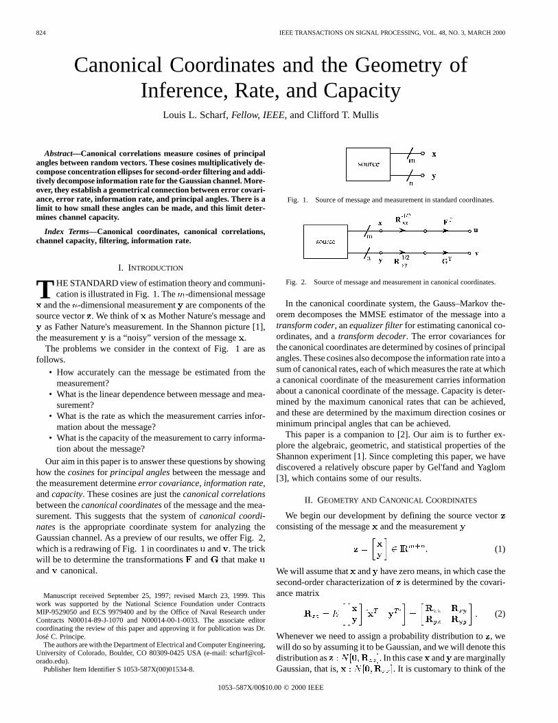
824 IEEE TRANSACTIONS ON SIGNAL PROCESSING, VOL. 48, NO. 3, MARCH 2000
Canonical Coordinates and the Geometry ofInference, Rate, and Capacity
Louis L. Scharf, Fellow, IEEE,and Clifford T. Mullis
Abstract—Canonical correlations measure cosines of principalangles between random vectors. These cosines multiplicatively de-compose concentration ellipses for second-order filtering and addi-tively decompose information rate for the Gaussian channel. More-over, they establish a geometrical connection between error covari-ance, error rate, information rate, and principal angles. There is alimit to how small these angles can be made, and this limit deter-mines channel capacity.
Index Terms—Canonical coordinates, canonical correlations,channel capacity, filtering, information rate.
I. INTRODUCTION
T HE STANDARD view of estimation theory and communi-cation is illustrated in Fig. 1. The -dimensional message
and the -dimensional measurementare components of thesource vector . We think of as Mother Nature's message and
as Father Nature's measurement. In the Shannon picture [1],the measurement is a “noisy” version of the message.
The problems we consider in the context of Fig. 1 are asfollows.
• How accurately can the message be estimated from themeasurement?
• What is the linear dependence between message and mea-surement?
• What is the rate as which the measurement carries infor-mation about the message?
• What is the capacity of the measurement to carry informa-tion about the message?
Our aim in this paper is to answer these questions by showinghow thecosinesfor principal anglesbetween the message andthe measurement determineerror covariance, information rate,andcapacity. These cosines are just thecanonical correlationsbetween thecanonical coordinatesof the message and the mea-surement. This suggests that the system ofcanonical coordi-nates is the appropriate coordinate system for analyzing theGaussian channel. As a preview of our results, we offer Fig. 2,which is a redrawing of Fig. 1 in coordinatesand . The trickwill be to determine the transformationsand that makeand canonical.
Manuscript received September 25, 1997; revised March 23, 1999. Thiswork was supported by the National Science Foundation under ContractsMIP-9529050 and ECS 9979400 and by the Office of Naval Research underContracts N00014-89-J-1070 and N00014-00-1-0033. The associate editorcoordinating the review of this paper and approving it for publication was Dr.José C. Principe.
The authors are with the Department of Electrical and Computer Engineering,University of Colorado, Boulder, CO 80309-0425 USA (e-mail: [email protected]).
Publisher Item Identifier S 1053-587X(00)01534-8.
Fig. 1. Source of message and measurement in standard coordinates.
Fig. 2. Source of message and measurement in canonical coordinates.
In the canonical coordinate system, the Gauss–Markov the-orem decomposes the MMSE estimator of the message into atransform coder, anequalizer filterfor estimating canonical co-ordinates, and atransform decoder. The error covariances forthe canonical coordinates are determined by cosines of principalangles. These cosines also decompose the information rate into asum of canonical rates, each of which measures the rate at whicha canonical coordinate of the measurement carries informationabout a canonical coordinate of the message. Capacity is deter-mined by the maximum canonical rates that can be achieved,and these are determined by the maximum direction cosines orminimum principal angles that can be achieved.
This paper is a companion to [2]. Our aim is to further ex-plore the algebraic, geometric, and statistical properties of theShannon experiment [1]. Since completing this paper, we havediscovered a relatively obscure paper by Gel'fand and Yaglom[3], which contains some of our results.
II. GEOMETRY AND CANONICAL COORDINATES
We begin our development by defining the source vectorconsisting of the messageand the measurement
(1)
We will assume that and have zero means, in which case thesecond-order characterization ofis determined by the covari-ance matrix
(2)
Whenever we need to assign a probability distribution to, wewill do so by assuming it to be Gaussian, and we will denote thisdistribution as . In this case and are marginallyGaussian, that is, . It is customary to think of the
1053–587X/00$10.00 © 2000 IEEE
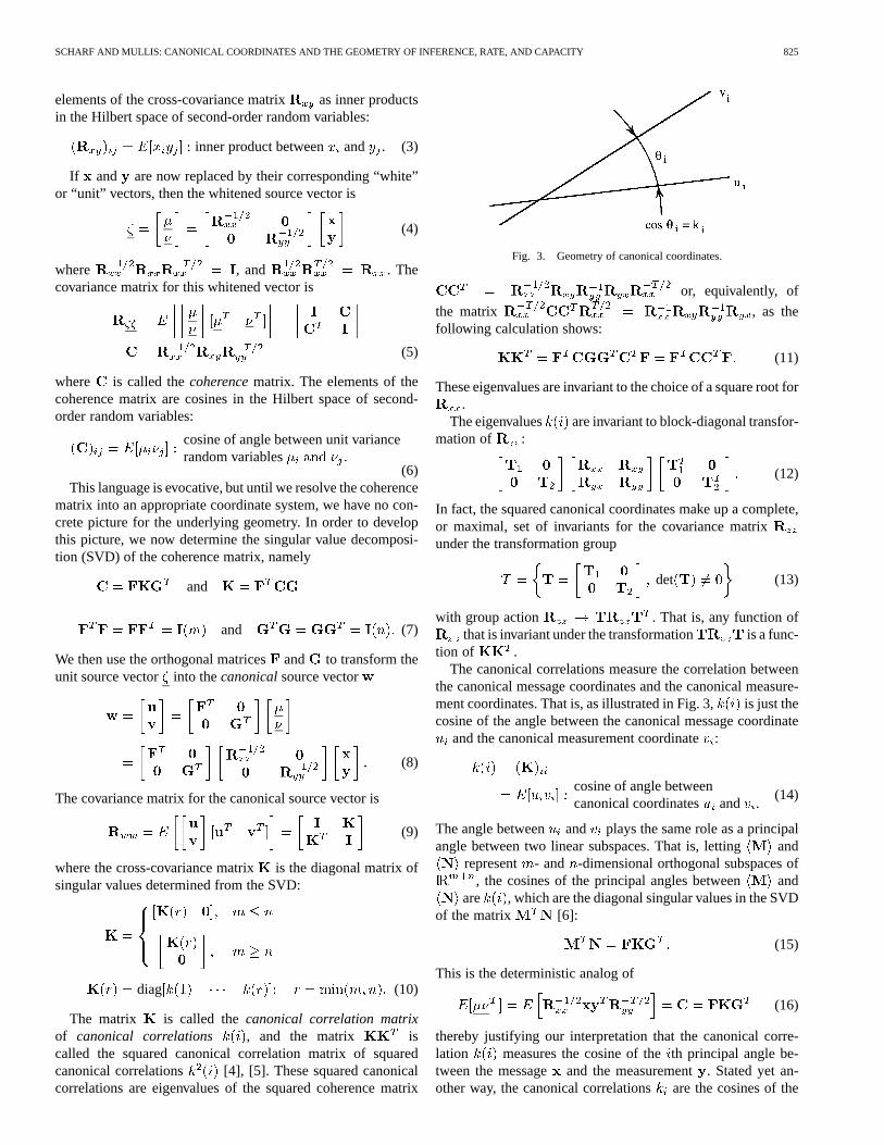
SCHARF AND MULLIS: CANONICAL COORDINATES AND THE GEOMETRY OF INFERENCE, RATE, AND CAPACITY 825
elements of the cross-covariance matrix as inner productsin the Hilbert space of second-order random variables:
inner product between and (3)
If and are now replaced by their corresponding “white”or “unit” vectors, then the whitened source vector is
(4)
where , and . Thecovariance matrix for this whitened vector is
(5)
where is called thecoherencematrix. The elements of thecoherence matrix are cosines in the Hilbert space of second-order random variables:
cosine of angle between unit variancerandom variables
(6)This language is evocative, but until we resolve the coherence
matrix into an appropriate coordinate system, we have no con-crete picture for the underlying geometry. In order to developthis picture, we now determine the singular value decomposi-tion (SVD) of the coherence matrix, namely
and
and (7)
We then use the orthogonal matricesand to transform theunit source vector into thecanonicalsource vector
(8)
The covariance matrix for the canonical source vector is
(9)
where the cross-covariance matrixis the diagonal matrix ofsingular values determined from the SVD:
diag (10)
The matrix is called thecanonical correlation matrixof canonical correlations , and the matrix iscalled the squared canonical correlation matrix of squaredcanonical correlations [4], [5]. These squared canonicalcorrelations are eigenvalues of the squared coherence matrix
Fig. 3. Geometry of canonical coordinates.
or, equivalently, of
the matrix , as thefollowing calculation shows:
(11)
These eigenvalues are invariant to the choice of a square root for.
The eigenvalues are invariant to block-diagonal transfor-mation of :
(12)
In fact, the squared canonical coordinates make up a complete,or maximal, set of invariants for the covariance matrixunder the transformation group
det (13)
with group action . That is, any function ofthat is invariant under the transformation is a func-
tion of .The canonical correlations measure the correlation between
the canonical message coordinates and the canonical measure-ment coordinates. That is, as illustrated in Fig. 3, is just thecosine of the angle between the canonical message coordinate
and the canonical measurement coordinate:
cosine of angle betweencanonical coordinates and
(14)
The angle between and plays the same role as a principalangle between two linear subspaces. That is, letting and
represent - and -dimensional orthogonal subspaces of, the cosines of the principal angles between and
are , which are the diagonal singular values in the SVDof the matrix [6]:
(15)
This is the deterministic analog of
(16)
thereby justifying our interpretation that the canonical corre-lation measures the cosine of theth principal angle be-tween the message and the measurement. Stated yet an-other way, the canonical correlationsare the cosines of the
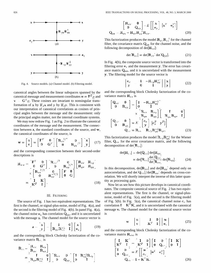
826 IEEE TRANSACTIONS ON SIGNAL PROCESSING, VOL. 48, NO. 3, MARCH 2000
Fig. 4. Source models. (a) Channel model. (b) Filtering model.
canonical angles between the linear subspaces spanned by thecanonical message and measurement coordinates and
. These cosines are invariant to nonsingular trans-formation of by and by . This is consistent withour interpretation of canonical correlations as cosines of prin-cipal angles between the message and the measurement: onlythe principal angles matter, not the internal coordinate systems.
We may now redraw Fig. 1 as Fig. 2 to illustrate the canonicalcoordinates of the message and the measurement. The connec-tion between , the standard coordinates of the source, and,the canonical coordinates of the source, is
(17)
and the corresponding connection between their second-orderdescriptions is
(18)
III. FILTERING
The source of Fig. 1 has two equivalent representations. Thefirst is the channel, or signal-plus-noise, model of Fig. 4(a), andthe second is the filtering model of Fig. 4(b). In panel Fig. 4(a),the channel noise has correlation , and it is uncorrelatedwith the message. The channel model for the source vector is
(19)
and the corresponding block Cholesky factorization of the co-variance matrix is
(20)
This factorization produces the model for the channelfilter, the covariance matrix for the channel noise, and thefollowing decomposition of det :
det det det (21)
In Fig. 4(b), the composite source vector is transformed into thefiltering error and the measurement. The error has covari-ance matrix , and it is uncorrelated with the measurement
. The filtering model for the source vector is
(22)
and the corresponding block Cholesky factorization of the co-variance matrix is
(23)
This factorization produces the model for the Wienerfilter, for the error covariance matrix, and the followingdecomposition of det :
det det det
detdetdet
det (24)
In this decomposition, det and det depend only onautocorrelation, and det det depends on cross-cor-relation. We will shortly interpret the inverse of this latter quan-tity as processing gain.
Now let us see how this picture develops in canonical coordi-nates. The composite canonical source of Fig. 2 has two equiv-alent representations. The first is the channel, or signal-plus-noise, model of Fig. 5(a), and the second is the filtering modelof Fig. 5(b). In Fig. 5(a), the canonical channel noisehascorrelation , and it is uncorrelated with the canonicalmessage . The channel model for the canonical source vectoris
(25)
and the corresponding block Cholesky factorization of the co-variance matrix is
(26)
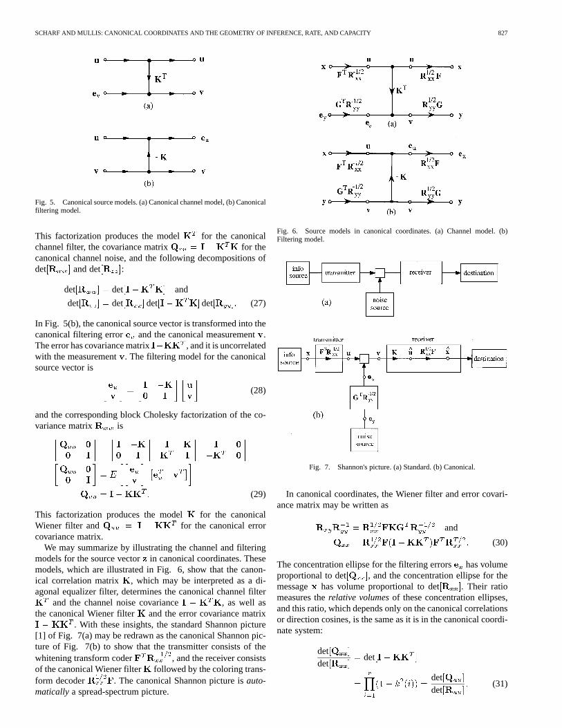
SCHARF AND MULLIS: CANONICAL COORDINATES AND THE GEOMETRY OF INFERENCE, RATE, AND CAPACITY 827
Fig. 5. Canonical source models. (a) Canonical channel model, (b) Canonicalfiltering model.
This factorization produces the model for the canonicalchannel filter, the covariance matrix for thecanonical channel noise, and the following decompositions ofdet and det :
det det and
det det det det (27)
In Fig. 5(b), the canonical source vector is transformed into thecanonical filtering error and the canonical measurement.The error has covariance matrix , and it is uncorrelatedwith the measurement. The filtering model for the canonicalsource vector is
(28)
and the corresponding block Cholesky factorization of the co-variance matrix is
(29)
This factorization produces the model for the canonicalWiener filter and for the canonical errorcovariance matrix.
We may summarize by illustrating the channel and filteringmodels for the source vectorin canonical coordinates. Thesemodels, which are illustrated in Fig. 6, show that the canon-ical correlation matrix , which may be interpreted as a di-agonal equalizer filter, determines the canonical channel filter
and the channel noise covariance , as well asthe canonical Wiener filter and the error covariance matrix
. With these insights, the standard Shannon picture[1] of Fig. 7(a) may be redrawn as the canonical Shannon pic-ture of Fig. 7(b) to show that the transmitter consists of thewhitening transform coder , and the receiver consistsof the canonical Wiener filter followed by the coloring trans-form decoder . The canonical Shannon picture isauto-maticallya spread-spectrum picture.
Fig. 6. Source models in canonical coordinates. (a) Channel model. (b)Filtering model.
Fig. 7. Shannon's picture. (a) Standard. (b) Canonical.
In canonical coordinates, the Wiener filter and error covari-ance matrix may be written as
and
(30)
The concentration ellipse for the filtering errors has volumeproportional to det , and the concentration ellipse for themessage has volume proportional to det . Their ratiomeasures therelative volumesof these concentration ellipses,and this ratio, which depends only on the canonical correlationsor direction cosines, is the same as it is in the canonical coordi-nate system:
detdet
det
detdet
(31)
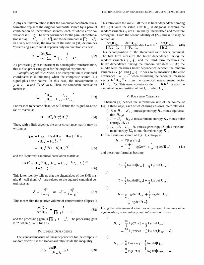
828 IEEE TRANSACTIONS ON SIGNAL PROCESSING, VOL. 48, NO. 3, MARCH 2000
A physical interpretation is that the canonical coordinate trans-formation replaces the original composite source by a parallelcombination of uncorrelated sources, each of whose error co-variance is . The error covariance for the parallel combina-tion is diag , and the determinant is .In a very real sense, the inverse of the ratio in (31) determines“processing gain,” and it depends only on direction cosines:
PGdetdet
(32)
As processing gain is invariant to nonsingular transformation,this is also processing gain for the original experiment.
Example: Signal Plus Noise. The interpretation of canonicalcoordinates is illuminating when the composite source is asignal-plus-noise source. In this case, the measurement is
and . Then, the composite correlationmatrix is
(33)
For reasons to become clear, we will define the “signal-to-noiseratio” matrix as
(34)
Then, with a little algebra, the error covariance matrix may bewritten as
(35)
and the “squared” canonical correlation matrix as
(36)
This latter identity tells us that the eigenvalues of the SNR ma-trix —call them —are related to the squared canonical co-ordinates as
or (37)
This means that the relative volume of concentration ellipses is
detdet
(38)
and the processing gain is . The processing gainis when for all .
IV. L INEAR DEPENDENCE
The standard measure of linear dependence for the compositerandom vector is the Hadamard ratio inside the inequality
det(39)
This ratio takes the value 0 iff there is linear dependence amongthe ; it takes the value 1 iff is diagonal, meaning therandom variables are all mutually uncorrelated and thereforeorthogonal. From the second identity of (27), this ratio may bewritten as
det detdet
det(40)
This decomposition of the Hadamard ratio bears comment.The first term measures the linear dependenceamong therandom variables , and the third term measures thelinear dependenceamong the random variables ; themiddle term measures linear dependencebetweenthe randomvariables and . It does so by measuring the errorcovariance when estimating the canonical messagevector from the canonical measurement vector
. This error covariance det is also thecanonical decomposition of det det .
V. RATE AND CAPACITY
Shannon [1] defines the information rate of the source ofFig. 1 three ways, each of which brings its own interpretations.
i) : message entropy minus equivoca-tion ;
ii) : measurement entropy minus noiseentropy ;
iii) : message entropy plus measure-ment entropy minus shared entropy .
For the Gaussian source of Fig. 1, entropy is
det (41)
and these rate formulas become
i)
det det
ii)
det det
iii)
det det
det
Using the determinantal identities of Section III, we may writeequivocation, noise entropy, andinformation rateas
i)
det
det
ii)
det
det
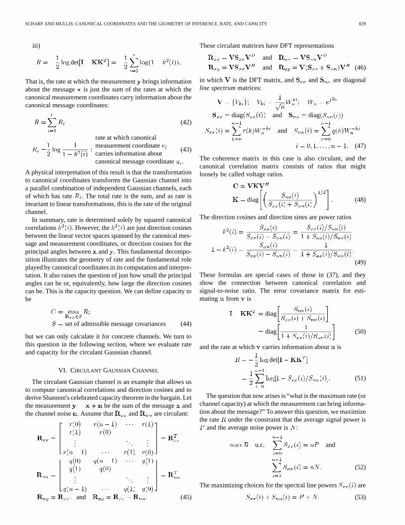
SCHARF AND MULLIS: CANONICAL COORDINATES AND THE GEOMETRY OF INFERENCE, RATE, AND CAPACITY 829
iii)
det
That is, the rate at which the measurementbrings informationabout the message is just the sum of the rates at which thecanonical measurement coordinates carry information about thecanonical message coordinates:
(42)
rate at which canonicalmeasurement coordinatecarries information aboutcanonical message coordinate
(43)
A physical interpretation of this result is that the transformationto canonical coordinates transforms the Gaussian channel intoa parallel combination of independent Gaussian channels, eachof which has rate . The total rate is the sum, and as rate isinvariant to linear transformations, this is the rate of the originalchannel.
In summary, rate is determined solely by squared canonicalcorrelations . However, the are just direction cosinesbetween the linear vector spaces spanned by the canonical mes-sage and measurement coordinates, or direction cosines for theprincipal angles betweenand . This fundamental decompo-sition illustrates the geometry of rate and the fundamental roleplayed by canonical coordinates in its computation and interpre-tation. It also raises the question of just how small the principalangles can be or, equivalently, how large the direction cosinescan be. This is the capacity question. We can define capacity tobe
set of admissible message covariances (44)
but we can only calculate it for concrete channels. We turn tothis question in the following section, where we evaluate rateand capacity for the circulant Gaussian channel.
VI. CIRCULANT GAUSSIAN CHANNEL
The circulant Gaussian channel is an example that allows usto compute canonical correlations and direction cosines and toderive Shannon's celebrated capacity theorem in the bargain. Letthe measurement be the sum of the messageandthe channel noise. Assume that and are circulant:
......
...
.... . .
...
and (45)
These circulant matrices have DFT representations
and
and (46)
in which is the DFT matrix, and and are diagonalline spectrummatrices:
diag and diag
and
(47)
The coherence matrix in this case is also circulant, and thecanonical correlation matrix consists of ratios that mightloosely be called voltage ratios.
diag (48)
The direction cosines and direction sines are power ratios
(49)
These formulas are special cases of those in (37), and theyshow the connection between canonical correlation andsignal-to-noise ratio. The error covariance matrix for esti-mating from is
diag
diag (50)
and the rate at which carries information about is
det
(51)
The question that now arises is “what is the maximum rate (orchannel capacity) at which the measurement can bring informa-tion about the message?” To answer this question, we maximizethe rate under the constraint that the average signal power is
and the average noise power is:
u.c. and
(52)
The maximizing choices for the spectral line powers are
(53)
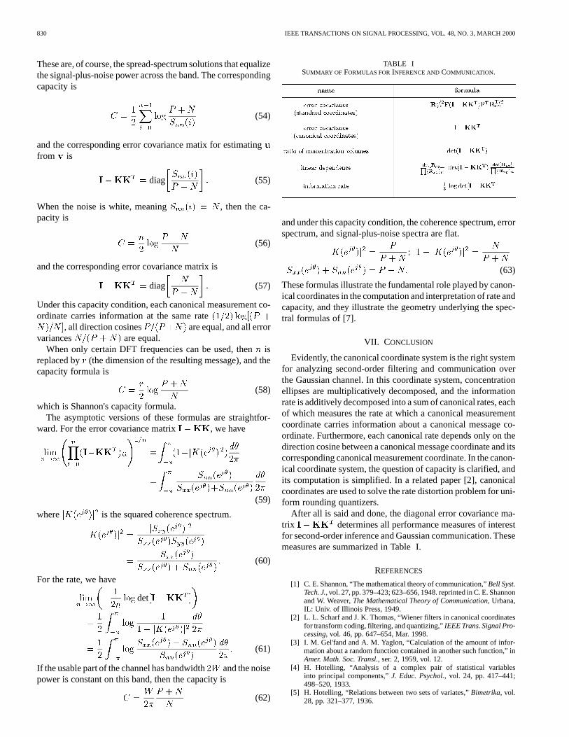
830 IEEE TRANSACTIONS ON SIGNAL PROCESSING, VOL. 48, NO. 3, MARCH 2000
These are, of course, the spread-spectrum solutions that equalizethe signal-plus-noise power across the band. The correspondingcapacity is
(54)
and the corresponding error covariance matix for estimatingfrom is
diag (55)
When the noise is white, meaning , then the ca-pacity is
(56)
and the corresponding error covariance matrix is
diag (57)
Under this capacity condition, each canonical measurement co-ordinate carries information at the same rate
, all direction cosines are equal, and all errorvariances are equal.
When only certain DFT frequencies can be used, thenisreplaced by (the dimension of the resulting message), and thecapacity formula is
(58)
which is Shannon's capacity formula.The asymptotic versions of these formulas are straightfor-
ward. For the error covariance matrix , we have
(59)
where is the squared coherence spectrum.
(60)
For the rate, we have
det
(61)
If the usable part of the channel has bandwidth and the noisepower is constant on this band, then the capacity is
(62)
TABLE ISUMMARY OF FORMULAS FORINFERENCE ANDCOMMUNICATION.
and under this capacity condition, the coherence spectrum, errorspectrum, and signal-plus-noise spectra are flat.
(63)
These formulas illustrate the fundamental role played by canon-ical coordinates in the computation and interpretation of rate andcapacity, and they illustrate the geometry underlying the spec-tral formulas of [7].
VII. CONCLUSION
Evidently, the canonical coordinate system is the right systemfor analyzing second-order filtering and communication overthe Gaussian channel. In this coordinate system, concentrationellipses are multiplicatively decomposed, and the informationrate is additively decomposed into a sum of canonical rates, eachof which measures the rate at which a canonical measurementcoordinate carries information about a canonical message co-ordinate. Furthermore, each canonical rate depends only on thedirection cosine between a canonical message coordinate and itscorresponding canonical measurement coordinate. In the canon-ical coordinate system, the question of capacity is clarified, andits computation is simplified. In a related paper [2], canonicalcoordinates are used to solve the rate distortion problem for uni-form rounding quantizers.
After all is said and done, the diagonal error covariance ma-trix determines all performance measures of interestfor second-order inference and Gaussian communication. Thesemeasures are summarized in Table I.
REFERENCES
[1] C. E. Shannon, “The mathematical theory of communication,”Bell Syst.Tech. J., vol. 27, pp. 379–423; 623–656, 1948. reprinted in C. E. Shannonand W. Weaver,The Mathematical Theory of Communication, Urbana,IL: Univ. of Illinois Press, 1949.
[2] L. L. Scharf and J. K. Thomas, “Wiener filters in canonical coordinatesfor transform coding, filtering, and quantizing,”IEEE Trans. Signal Pro-cessing, vol. 46, pp. 647–654, Mar. 1998.
[3] I. M. Gel'fand and A. M. Yaglon, “Calculation of the amount of infor-mation about a random function contained in another such function,” inAmer. Math. Soc. Transl., ser. 2, 1959, vol. 12.
[4] H. Hotelling, “Analysis of a complex pair of statistical variablesinto principal components,”J. Educ. Psychol., vol. 24, pp. 417–441;498–520, 1933.
[5] H. Hotelling, “Relations between two sets of variates,”Bimetrika, vol.28, pp. 321–377, 1936.
SCHARF AND MULLIS: CANONICAL COORDINATES AND THE GEOMETRY OF INFERENCE, RATE, AND CAPACITY 831
[6] G. H. Golub and C. F. Van Loan,Matrix Computations, 2nded. Baltimore, MD: Johns Hopkins Univ. Press, 1989.
[7] R. A. McDonald and P. M. Schultheiss, “Information rates of Gaussiansignals under criteria constraining the error spectrum,”Proc. IEEE, vol.52, pp. 415–416, Apr. 1964.
[8] M. L. Eaton,Multivariate Statistics: A Vector Space Approach. NewYork: Wiley, 1983, ch. 10.
Louis L. Scharf (F'86) received the Ph.D. degree inelectrical engineering in 1969 from the University ofWashington, Seattle.
From 1969 to 1971, he was a Member of the Tech-nical Staff at Honeywell's Marine Systems Center,Seattle. He served as Professor of Electrical Engi-neering and Statistics at Colorado State University,Fort Collins, from 1971 to 1981. From 1982 to 1985,he was Professor and Chair of Electrical and Com-puter Engineering at the University of Rhode Island,Kingston. He is currently Professor of Electrical and
Computer Engineering at the University of Colorado, Boulder, where he teachesand conducts research in signal processing. In 1974, he was Visiting Asso-ciate Professor at Duke University, Durham, NC. In 1977, he was a Memberof the Technical Staff with the CNRS Laboratoire des Signaux et Systemes,Gif-sur-Yvette, France, and Professeur Associe with the University of SouthParis, Orsay, France. In 1981, he was a Visiting Professor at Ecole NationaleSuperiere des Telecommunications, Paris, France, and at the University of LaPlata, Buenos Aires, Argentina. He was a Visiting Professor at Institut Eurecom,Sophia-Antipolis, France, in 1992.
Prof. Scharf is a Past Member of the ASSP AdCom. He has served on theEditorial Board ofSignal Processingand is a Past Associate Editor of the IEEETRANSACTIONS ONSIGNAL PROCESSING. He was Technical Program Chairmanfor the IEEE International Conference on Acoustics, Speech, and Signal Pro-cessing in 1980. In 1994, he served as a Distinguished Lecturer for the IEEESignal Processing Society, and in 1995, he received the Society's TechnicalAchievement Award.
Clifford T. Mullis received the B.S., M.S., and Ph.D.degrees in electrical engineering from the Universityof Colorado, Boulder, in 1966, 1968, and 1971, re-spectively.
He was an Assistant Professor of electrical engi-neering at Princeton University, Princeton, NJ, from1971 to 1973. He is now a Professor of electrical en-gineering at the University of Colorado.
Max–Planck–Institut für biologische KybernetikMax Planck Institute for Biological Cybernetics
Technical Report No. 108
The Geometry Of KernelCanonical Correlation Analysis
Malte Kuss1 and Thore Graepel2
May 2003
1 Max Planck Institute for Biological Cybernetics, Dept. Schölkopf,Spemannstrasse 38, 72076 Tübingen, Germany, email: [email protected] Microsoft Research Ltd, Roger Needham Building,7 J J Thomson Avenue, Cambridge CB3 0FB, U.K, email: [email protected]
This report is available in PDF–format via anonymous ftp at ftp://ftp.kyb.tuebingen.mpg.de/pub/mpi-memos/pdf/TR-108.pdf. Thecomplete series of Technical Reports is documented at: http://www.kyb.tuebingen.mpg.de/techreports.html
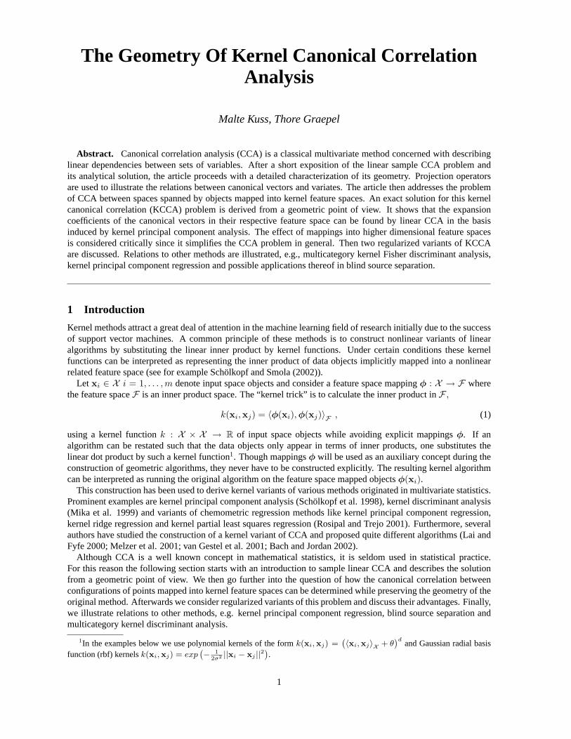
The Geometry Of Kernel Canonical CorrelationAnalysis
Malte Kuss, Thore Graepel
Abstract. Canonical correlation analysis (CCA) is a classical multivariate method concerned with describinglinear dependencies between sets of variables. After a short exposition of the linear sample CCA problem andits analytical solution, the article proceeds with a detailed characterization of its geometry. Projection operatorsare used to illustrate the relations between canonical vectors and variates. The article then addresses the problemof CCA between spaces spanned by objects mapped into kernel feature spaces. An exact solution for this kernelcanonical correlation (KCCA) problem is derived from a geometric point of view. It shows that the expansioncoefficients of the canonical vectors in their respective feature space can be found by linear CCA in the basisinduced by kernel principal component analysis. The effect of mappings into higher dimensional feature spacesis considered critically since it simplifies the CCA problem in general. Then two regularized variants of KCCAare discussed. Relations to other methods are illustrated, e.g., multicategory kernel Fisher discriminant analysis,kernel principal component regression and possible applications thereof in blind source separation.
1 Introduction
Kernel methods attract a great deal of attention in the machine learning field of research initially due to the successof support vector machines. A common principle of these methods is to construct nonlinear variants of linearalgorithms by substituting the linear inner product by kernel functions. Under certain conditions these kernelfunctions can be interpreted as representing the inner product of data objects implicitly mapped into a nonlinearrelated feature space (see for example Schölkopf and Smola (2002)).
Let xi ∈ X i = 1, . . . ,m denote input space objects and consider a feature space mappingφ : X → F wherethe feature spaceF is an inner product space. The “kernel trick” is to calculate the inner product inF ,
k(xi,xj) = 〈φ(xi),φ(xj)〉F , (1)
using a kernel functionk : X × X → R of input space objects while avoiding explicit mappingsφ. If analgorithm can be restated such that the data objects only appear in terms of inner products, one substitutes thelinear dot product by such a kernel function1. Though mappingsφ will be used as an auxiliary concept during theconstruction of geometric algorithms, they never have to be constructed explicitly. The resulting kernel algorithmcan be interpreted as running the original algorithm on the feature space mapped objectsφ(xi).
This construction has been used to derive kernel variants of various methods originated in multivariate statistics.Prominent examples are kernel principal component analysis (Schölkopf et al. 1998), kernel discriminant analysis(Mika et al. 1999) and variants of chemometric regression methods like kernel principal component regression,kernel ridge regression and kernel partial least squares regression (Rosipal and Trejo 2001). Furthermore, severalauthors have studied the construction of a kernel variant of CCA and proposed quite different algorithms (Lai andFyfe 2000; Melzer et al. 2001; van Gestel et al. 2001; Bach and Jordan 2002).
Although CCA is a well known concept in mathematical statistics, it is seldom used in statistical practice.For this reason the following section starts with an introduction to sample linear CCA and describes the solutionfrom a geometric point of view. We then go further into the question of how the canonical correlation betweenconfigurations of points mapped into kernel feature spaces can be determined while preserving the geometry of theoriginal method. Afterwards we consider regularized variants of this problem and discuss their advantages. Finally,we illustrate relations to other methods, e.g. kernel principal component regression, blind source separation andmulticategory kernel discriminant analysis.
1In the examples below we use polynomial kernels of the formk(xi,xj) =(〈xi,xj〉X + θ
)dand Gaussian radial basis
function (rbf) kernelsk(xi,xj) = exp(− 1
2σ2 ||xi − xj ||2).
1
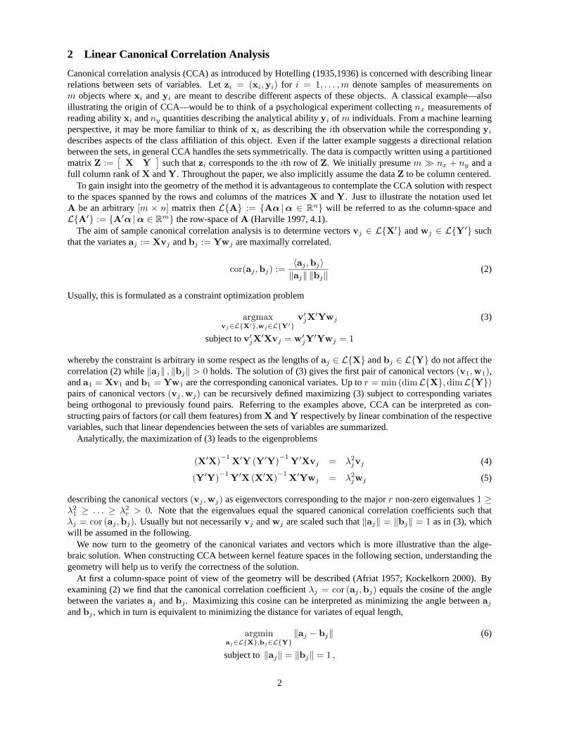
2 Linear Canonical Correlation Analysis
Canonical correlation analysis (CCA) as introduced by Hotelling (1935,1936) is concerned with describing linearrelations between sets of variables. Letzi = (xi,yi) for i = 1, . . . ,m denote samples of measurements onm objects wherexi andyi are meant to describe different aspects of these objects. A classical example—alsoillustrating the origin of CCA—would be to think of a psychological experiment collectingnx measurements ofreading abilityxi andny quantities describing the analytical abilityyi of m individuals. From a machine learningperspective, it may be more familiar to think ofxi as describing theith observation while the correspondingyi
describes aspects of the class affiliation of this object. Even if the latter example suggests a directional relationbetween the sets, in general CCA handles the sets symmetrically. The data is compactly written using a partitionedmatrixZ :=
[X Y
]such thatzi corresponds to theith row ofZ. We initially presumem � nx + ny and a
full column rank ofX andY. Throughout the paper, we also implicitly assume the dataZ to be column centered.To gain insight into the geometry of the method it is advantageous to contemplate the CCA solution with respect
to the spaces spanned by the rows and columns of the matricesX andY. Just to illustrate the notation used letA be an arbitrary[m × n] matrix thenL{A} := {Aα |α ∈ Rn} will be referred to as the column-space andL{A′} := {A′α |α ∈ Rm} the row-space ofA (Harville 1997, 4.1).
The aim of sample canonical correlation analysis is to determine vectorsvj ∈ L{X′} andwj ∈ L{Y′} suchthat the variatesaj := Xvj andbj := Ywj are maximally correlated.
cor(aj ,bj) :=〈aj ,bj〉‖aj‖ ‖bj‖
(2)
Usually, this is formulated as a constraint optimization problem
argmaxvj∈L{X′},wj∈L{Y′}
v′jX′Ywj (3)
subject tov′jX′Xvj = w′
jY′Ywj = 1
whereby the constraint is arbitrary in some respect as the lengths ofaj ∈ L{X} andbj ∈ L{Y} do not affect thecorrelation (2) while‖aj‖ , ‖bj‖ > 0 holds. The solution of (3) gives the first pair of canonical vectors(v1,w1),anda1 = Xv1 andb1 = Yw1 are the corresponding canonical variates. Up tor = min (dimL{X},dimL{Y})pairs of canonical vectors(vj ,wj) can be recursively defined maximizing (3) subject to corresponding variatesbeing orthogonal to previously found pairs. Referring to the examples above, CCA can be interpreted as con-structing pairs of factors (or call them features) fromX andY respectively by linear combination of the respectivevariables, such that linear dependencies between the sets of variables are summarized.
Analytically, the maximization of (3) leads to the eigenproblems
(X′X)−1 X′Y (Y′Y)−1 Y′Xvj = λ2jvj (4)
(Y′Y)−1 Y′X (X′X)−1 X′Ywj = λ2jwj (5)
describing the canonical vectors(vj ,wj) as eigenvectors corresponding to the majorr non-zero eigenvalues1 ≥λ2
1 ≥ . . . ≥ λ2r > 0. Note that the eigenvalues equal the squared canonical correlation coefficients such that
λj = cor (aj ,bj). Usually but not necessarilyvj andwj are scaled such that‖aj‖ = ‖bj‖ = 1 as in (3), whichwill be assumed in the following.
We now turn to the geometry of the canonical variates and vectors which is more illustrative than the alge-braic solution. When constructing CCA between kernel feature spaces in the following section, understanding thegeometry will help us to verify the correctness of the solution.
At first a column-space point of view of the geometry will be described (Afriat 1957; Kockelkorn 2000). Byexamining (2) we find that the canonical correlation coefficientλj = cor (aj ,bj) equals the cosine of the anglebetween the variatesaj andbj . Maximizing this cosine can be interpreted as minimizing the angle betweenaj
andbj , which in turn is equivalent to minimizing the distance for variates of equal length,
argminaj∈L{X},bj∈L{Y}
‖aj − bj‖ (6)
subject to‖aj‖ = ‖bj‖ = 1 ,
2
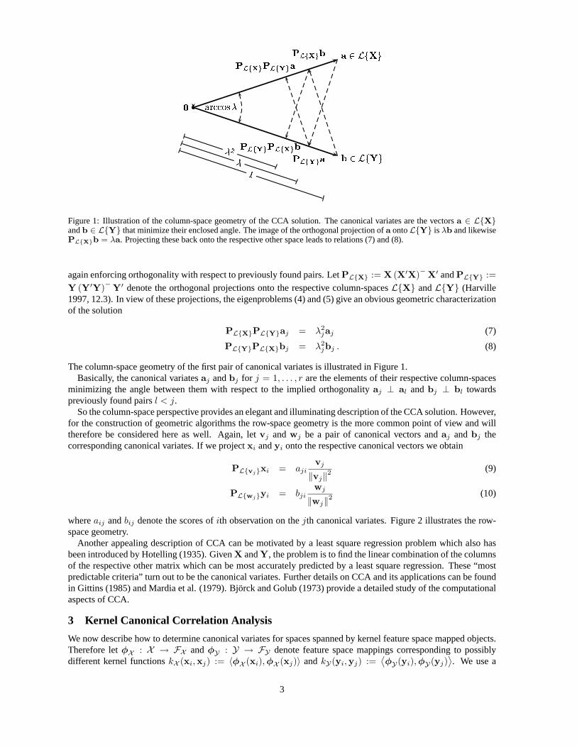
�� �����������
����������
� ���������� �"!$#&%
� �"!(')% �� �"!(')%�� �"!$#�%
� �"!$#�%�� �*!$'+% �,.- /0
1Figure 1: Illustration of the column-space geometry of the CCA solution. The canonical variates are the vectorsa ∈ L{X}andb ∈ L{Y} that minimize their enclosed angle. The image of the orthogonal projection ofa ontoL{Y} is λb and likewisePL{X}b = λa. Projecting these back onto the respective other space leads to relations (7) and (8).
again enforcing orthogonality with respect to previously found pairs. LetPL{X} := X (X′X)−X′ andPL{Y} :=Y (Y′Y)−Y′ denote the orthogonal projections onto the respective column-spacesL{X} andL{Y} (Harville1997, 12.3). In view of these projections, the eigenproblems (4) and (5) give an obvious geometric characterizationof the solution
PL{X}PL{Y}aj = λ2jaj (7)
PL{Y}PL{X}bj = λ2jbj . (8)
The column-space geometry of the first pair of canonical variates is illustrated in Figure 1.Basically, the canonical variatesaj andbj for j = 1, . . . , r are the elements of their respective column-spaces
minimizing the angle between them with respect to the implied orthogonalityaj ⊥ al andbj ⊥ bl towardspreviously found pairsl < j.
So the column-space perspective provides an elegant and illuminating description of the CCA solution. However,for the construction of geometric algorithms the row-space geometry is the more common point of view and willtherefore be considered here as well. Again, letvj andwj be a pair of canonical vectors andaj andbj thecorresponding canonical variates. If we projectxi andyi onto the respective canonical vectors we obtain
PL{vj}xi = ajivj
‖vj‖2(9)
PL{wj}yi = bjiwj
‖wj‖2(10)
whereaij andbij denote the scores ofith observation on thejth canonical variates. Figure 2 illustrates the row-space geometry.
Another appealing description of CCA can be motivated by a least square regression problem which also hasbeen introduced by Hotelling (1935). GivenX andY, the problem is to find the linear combination of the columnsof the respective other matrix which can be most accurately predicted by a least square regression. These “mostpredictable criteria” turn out to be the canonical variates. Further details on CCA and its applications can be foundin Gittins (1985) and Mardia et al. (1979). Björck and Golub (1973) provide a detailed study of the computationalaspects of CCA.
3 Kernel Canonical Correlation Analysis
We now describe how to determine canonical variates for spaces spanned by kernel feature space mapped objects.Therefore letφX : X → FX andφY : Y → FY denote feature space mappings corresponding to possiblydifferent kernel functionskX (xi,xj) := 〈φX (xi),φX (xj)〉 andkY(yi,yj) :=
⟨φY(yi),φY(yj)
⟩. We use a
3
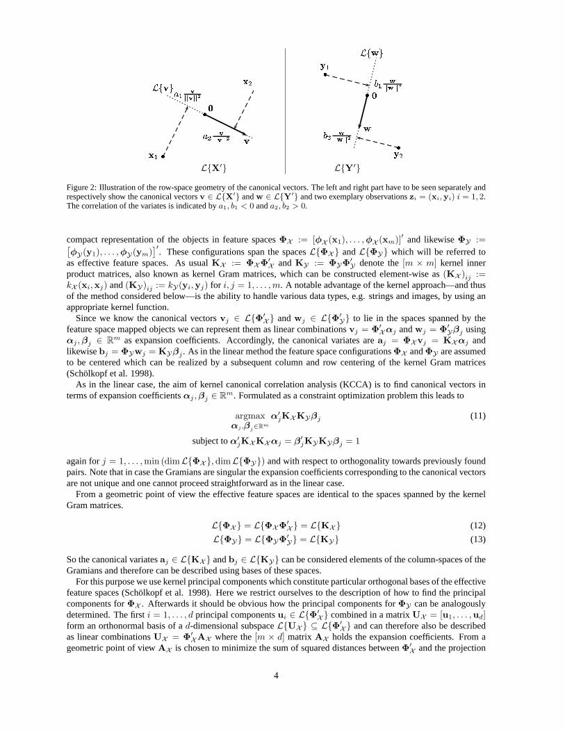
�������
��
� �
���
�
�������� � ��� �
��� ���� � ��� �
�������
��
� �
����
�
� ������ � ��� �
� � ���� � ��� �
L{X′} L{Y′}
Figure 2: Illustration of the row-space geometry of the canonical vectors. The left and right part have to be seen separately andrespectively show the canonical vectorsv ∈ L{X′} andw ∈ L{Y′} and two exemplary observationszi = (xi,yi) i = 1, 2.The correlation of the variates is indicated bya1, b1 < 0 anda2, b2 > 0.
compact representation of the objects in feature spacesΦX := [φX (x1), . . . ,φX (xm)]′ and likewiseΦY :=[φY(y1), . . . ,φY(ym)
]′. These configurations span the spacesL{ΦX } andL{ΦY} which will be referred to
as effective feature spaces. As usualKX := ΦXΦ′X andKY := ΦYΦ′
Y denote the[m × m] kernel innerproduct matrices, also known as kernel Gram matrices, which can be constructed element-wise as(KX )ij :=kX (xi,xj) and(KY)ij := kY(yi,yj) for i, j = 1, . . . ,m. A notable advantage of the kernel approach—and thusof the method considered below—is the ability to handle various data types, e.g. strings and images, by using anappropriate kernel function.
Since we know the canonical vectorsvj ∈ L{Φ′X } andwj ∈ L{Φ′
Y} to lie in the spaces spanned by thefeature space mapped objects we can represent them as linear combinationsvj = Φ′
Xαj andwj = Φ′Yβj using
αj ,βj ∈ Rm as expansion coefficients. Accordingly, the canonical variates areaj = ΦXvj = KXαj andlikewisebj = ΦYwj = KYβj . As in the linear method the feature space configurationsΦX andΦY are assumedto be centered which can be realized by a subsequent column and row centering of the kernel Gram matrices(Schölkopf et al. 1998).
As in the linear case, the aim of kernel canonical correlation analysis (KCCA) is to find canonical vectors interms of expansion coefficientsαj ,βj ∈ Rm. Formulated as a constraint optimization problem this leads to
argmaxαj ,βj∈Rm
α′jKXKYβj (11)
subject toα′jKXKXαj = β′jKYKYβj = 1
again forj = 1, . . . ,min (dimL{ΦX },dimL{ΦY}) and with respect to orthogonality towards previously foundpairs. Note that in case the Gramians are singular the expansion coefficients corresponding to the canonical vectorsare not unique and one cannot proceed straightforward as in the linear case.
From a geometric point of view the effective feature spaces are identical to the spaces spanned by the kernelGram matrices.
L{ΦX } = L{ΦXΦ′X } = L{KX } (12)
L{ΦY} = L{ΦYΦ′Y} = L{KY} (13)
So the canonical variatesaj ∈ L{KX } andbj ∈ L{KY} can be considered elements of the column-spaces of theGramians and therefore can be described using bases of these spaces.
For this purpose we use kernel principal components which constitute particular orthogonal bases of the effectivefeature spaces (Schölkopf et al. 1998). Here we restrict ourselves to the description of how to find the principalcomponents forΦX . Afterwards it should be obvious how the principal components forΦY can be analogouslydetermined. The firsti = 1, . . . , d principal componentsui ∈ L{Φ′
X } combined in a matrixUX = [u1, . . . ,ud]form an orthonormal basis of ad-dimensional subspaceL{UX } ⊆ L{Φ′
X } and can therefore also be describedas linear combinationsUX = Φ′
XAX where the[m × d] matrix AX holds the expansion coefficients. From ageometric point of viewAX is chosen to minimize the sum of squared distances betweenΦ′
X and the projection
4
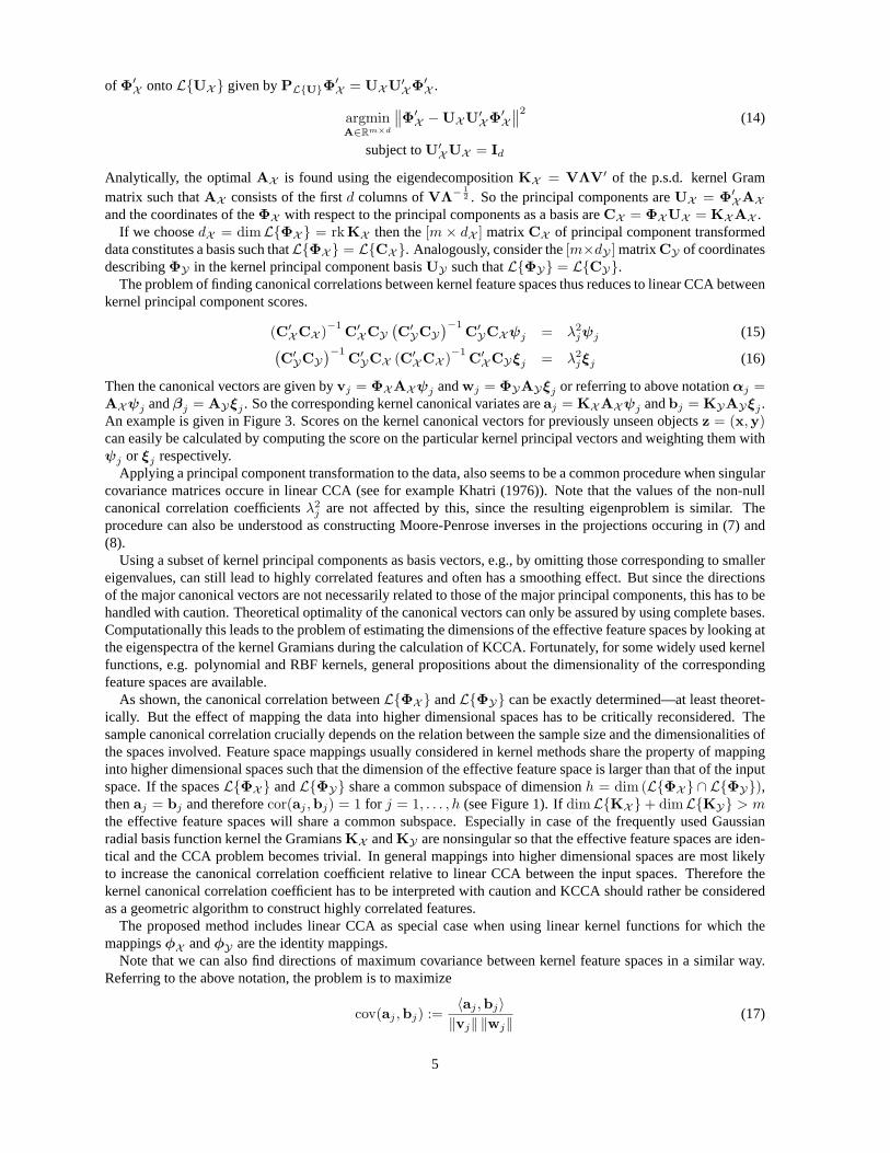
of Φ′X ontoL{UX } given byPL{U}Φ
′X = UXU′
XΦ′X .
argminA∈Rm×d
∥∥Φ′X −UXU′
XΦ′X
∥∥2(14)
subject toU′XUX = Id
Analytically, the optimalAX is found using the eigendecompositionKX = VΛV′ of the p.s.d. kernel Grammatrix such thatAX consists of the firstd columns ofVΛ− 1
2 . So the principal components areUX = Φ′XAX
and the coordinates of theΦX with respect to the principal components as a basis areCX = ΦXUX = KXAX .If we choosedX = dimL{ΦX } = rkKX then the[m × dX ] matrixCX of principal component transformed
data constitutes a basis such thatL{ΦX } = L{CX }. Analogously, consider the[m×dY ] matrixCY of coordinatesdescribingΦY in the kernel principal component basisUY such thatL{ΦY} = L{CY}.
The problem of finding canonical correlations between kernel feature spaces thus reduces to linear CCA betweenkernel principal component scores.
(C′XCX )−1 C′
XCY(C′YCY
)−1C′YCXψj = λ2
jψj (15)(C′YCY
)−1C′YCX (C′
XCX )−1 C′XCYξj = λ2
jξj (16)
Then the canonical vectors are given byvj = ΦXAXψj andwj = ΦYAYξj or referring to above notationαj =AXψj andβj = AYξj . So the corresponding kernel canonical variates areaj = KXAXψj andbj = KYAYξj .An example is given in Figure 3. Scores on the kernel canonical vectors for previously unseen objectsz = (x,y)can easily be calculated by computing the score on the particular kernel principal vectors and weighting them withψj or ξj respectively.
Applying a principal component transformation to the data, also seems to be a common procedure when singularcovariance matrices occure in linear CCA (see for example Khatri (1976)). Note that the values of the non-nullcanonical correlation coefficientsλ2
j are not affected by this, since the resulting eigenproblem is similar. Theprocedure can also be understood as constructing Moore-Penrose inverses in the projections occuring in (7) and(8).
Using a subset of kernel principal components as basis vectors, e.g., by omitting those corresponding to smallereigenvalues, can still lead to highly correlated features and often has a smoothing effect. But since the directionsof the major canonical vectors are not necessarily related to those of the major principal components, this has to behandled with caution. Theoretical optimality of the canonical vectors can only be assured by using complete bases.Computationally this leads to the problem of estimating the dimensions of the effective feature spaces by looking atthe eigenspectra of the kernel Gramians during the calculation of KCCA. Fortunately, for some widely used kernelfunctions, e.g. polynomial and RBF kernels, general propositions about the dimensionality of the correspondingfeature spaces are available.
As shown, the canonical correlation betweenL{ΦX } andL{ΦY} can be exactly determined—at least theoret-ically. But the effect of mapping the data into higher dimensional spaces has to be critically reconsidered. Thesample canonical correlation crucially depends on the relation between the sample size and the dimensionalities ofthe spaces involved. Feature space mappings usually considered in kernel methods share the property of mappinginto higher dimensional spaces such that the dimension of the effective feature space is larger than that of the inputspace. If the spacesL{ΦX } andL{ΦY} share a common subspace of dimensionh = dim (L{ΦX } ∩ L{ΦY}),thenaj = bj and thereforecor(aj ,bj) = 1 for j = 1, . . . , h (see Figure 1). IfdimL{KX }+ dimL{KY} > mthe effective feature spaces will share a common subspace. Especially in case of the frequently used Gaussianradial basis function kernel the GramiansKX andKY are nonsingular so that the effective feature spaces are iden-tical and the CCA problem becomes trivial. In general mappings into higher dimensional spaces are most likelyto increase the canonical correlation coefficient relative to linear CCA between the input spaces. Therefore thekernel canonical correlation coefficient has to be interpreted with caution and KCCA should rather be consideredas a geometric algorithm to construct highly correlated features.
The proposed method includes linear CCA as special case when using linear kernel functions for which themappingsφX andφY are the identity mappings.
Note that we can also find directions of maximum covariance between kernel feature spaces in a similar way.Referring to the above notation, the problem is to maximize
cov(aj ,bj) :=〈aj ,bj〉‖vj‖ ‖wj‖
(17)
5
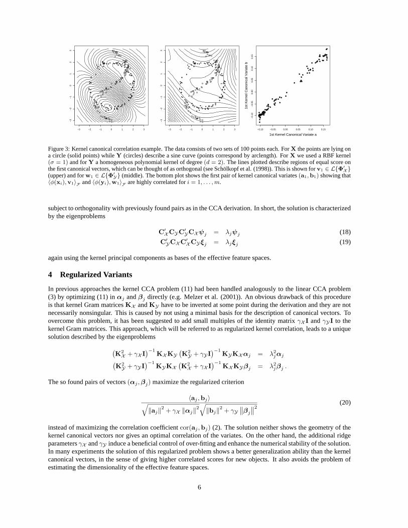
−3 −2 −1 0 1 2 3
−3
−2
−1
01
23
−3 −2 −1 0 1 2 3
−3
−2
−1
01
23
−0.10 −0.05 0.00 0.05 0.10 0.15
−0.
10−
0.05
0.00
0.05
0.10
0.15
1st Kernel Canonical Variate a
1st K
erne
l Can
onic
al V
aria
te b
Figure 3: Kernel canonical correlation example. The data consists of two sets of 100 points each. ForX the points are lying ona circle (solid points) whileY (circles) describe a sine curve (points correspond by arclength). ForX we used a RBF kernel(σ = 1) and forY a homogeneous polynomial kernel of degree(d = 2). The lines plotted describe regions of equal score onthe first canonical vectors, which can be thought of as orthogonal (see Schölkopf et al. (1998)). This is shown forv1 ∈ L{Φ′
X}(upper) and forw1 ∈ L{Φ′
Y} (middle). The bottom plot shows the first pair of kernel canonical variates(a1,b1) showing that〈φ(xi),v1〉F and〈φ(yi),w1〉F are highly correlated fori = 1, . . . , m.
subject to orthogonality with previously found pairs as in the CCA derivation. In short, the solution is characterizedby the eigenproblems
C′XCYC′
YCXψj = λjψj (18)
C′YCXC′
XCYξj = λjξj (19)
again using the kernel principal components as bases of the effective feature spaces.
4 Regularized Variants
In previous approaches the kernel CCA problem (11) had been handled analogously to the linear CCA problem(3) by optimizing (11) inαj andβj directly (e.g. Melzer et al. (2001)). An obvious drawback of this procedureis that kernel Gram matricesKX andKY have to be inverted at some point during the derivation and they are notnecessarily nonsingular. This is caused by not using a minimal basis for the description of canonical vectors. Toovercome this problem, it has been suggested to add small multiples of the identity matrixγX I andγYI to thekernel Gram matrices. This approach, which will be referred to as regularized kernel correlation, leads to a uniquesolution described by the eigenproblems(
K2X + γX I
)−1KXKY
(K2Y + γYI
)−1KYKXαj = λ2
jαj(K2Y + γYI
)−1KYKX
(K2X + γX I
)−1KXKYβj = λ2
jβj .
The so found pairs of vectors(αj ,βj) maximize the regularized criterion
〈aj ,bj〉√‖aj‖2 + γX ‖αj‖2
√‖bj‖2 + γY
∥∥βj
∥∥2(20)
instead of maximizing the correlation coefficientcor(aj ,bj) (2). The solution neither shows the geometry of thekernel canonical vectors nor gives an optimal correlation of the variates. On the other hand, the additional ridgeparametersγX andγY induce a beneficial control of over-fitting and enhance the numerical stability of the solution.In many experiments the solution of this regularized problem shows a better generalization ability than the kernelcanonical vectors, in the sense of giving higher correlated scores for new objects. It also avoids the problem ofestimating the dimensionality of the effective feature spaces.
6
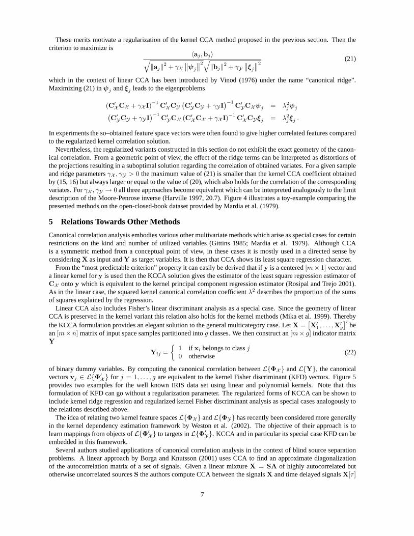
These merits motivate a regularization of the kernel CCA method proposed in the previous section. Then thecriterion to maximize is
〈aj ,bj〉√‖aj‖2 + γX
∥∥ψj
∥∥2√‖bj‖2 + γY
∥∥ξj
∥∥2(21)
which in the context of linear CCA has been introduced by Vinod (1976) under the name “canonical ridge”.Maximizing (21) inψj andξj leads to the eigenproblems
(C′XCX + γX I)−1 C′
XCY(C′YCY + γYI
)−1C′YCXψj = λ2
jψj(C′YCY + γYI
)−1C′YCX (C′
XCX + γX I)−1 C′XCYξj = λ2
jξj .
In experiments the so–obtained feature space vectors were often found to give higher correlated features comparedto the regularized kernel correlation solution.
Nevertheless, the regularized variants constructed in this section do not exhibit the exact geometry of the canon-ical correlation. From a geometric point of view, the effect of the ridge terms can be interpreted as distortions ofthe projections resulting in a suboptimal solution regarding the correlation of obtained variates. For a given sampleand ridge parametersγX , γY > 0 the maximum value of (21) is smaller than the kernel CCA coefficient obtainedby (15, 16) but always larger or equal to the value of (20), which also holds for the correlation of the correspondingvariates. ForγX , γY → 0 all three approaches become equivalent which can be interpreted analogously to the limitdescription of the Moore-Penrose inverse (Harville 1997, 20.7). Figure 4 illustrates a toy-example comparing thepresented methods on the open-closed-book dataset provided by Mardia et al. (1979).
5 Relations Towards Other Methods
Canonical correlation analysis embodies various other multivariate methods which arise as special cases for certainrestrictions on the kind and number of utilized variables (Gittins 1985; Mardia et al. 1979). Although CCAis a symmetric method from a conceptual point of view, in these cases it is mostly used in a directed sense byconsideringX as input andY as target variables. It is then that CCA shows its least square regression character.
From the “most predictable criterion” property it can easily be derived that ify is a centered[m× 1] vector anda linear kernel fory is used then the KCCA solution gives the estimator of the least square regression estimator ofCX ontoy which is equivalent to the kernel principal component regression estimator (Rosipal and Trejo 2001).As in the linear case, the squared kernel canonical correlation coefficientλ2 describes the proportion of the sumsof squares explained by the regression.
Linear CCA also includes Fisher’s linear discriminant analysis as a special case. Since the geometry of linearCCA is preserved in the kernel variant this relation also holds for the kernel methods (Mika et al. 1999). Therebythe KCCA formulation provides an elegant solution to the general multicategory case. LetX =
[X′
1, . . . ,X′g
]′be
an[m× n] matrix of input space samples partitioned intog classes. We then construct an[m× g] indicator matrixY
Yij ={
1 if xi belongs to classj0 otherwise
(22)
of binary dummy variables. By computing the canonical correlation betweenL{ΦX } andL{Y}, the canonicalvectorsvj ∈ L{Φ′
X } for j = 1, . . . , g are equivalent to the kernel Fisher discriminant (KFD) vectors. Figure 5provides two examples for the well known IRIS data set using linear and polynomial kernels. Note that thisformulation of KFD can go without a regularization parameter. The regularized forms of KCCA can be shown toinclude kernel ridge regression and regularized kernel Fisher discriminant analysis as special cases analogously tothe relations described above.
The idea of relating two kernel feature spacesL{ΦX } andL{ΦY} has recently been considered more generallyin the kernel dependency estimation framework by Weston et al. (2002). The objective of their approach is tolearn mappings from objects ofL{Φ′
X } to targets inL{Φ′Y}. KCCA and in particular its special case KFD can be
embedded in this framework.Several authors studied applications of canonical correlation analysis in the context of blind source separation
problems. A linear approach by Borga and Knutsson (2001) uses CCA to find an approximate diagonalizationof the autocorrelation matrix of a set of signals. Given a linear mixtureX = SA of highly autocorrelated butotherwise uncorrelated sourcesS the authors compute CCA between the signalsX and time delayed signalsX[τ ]
7
0 20 40 60 80 100
0.0
0.2
0.4
0.6
0.8
1.0
γ
Cor
rela
tion
of 1
st P
air
of V
aria
tes
Linear CCAKernel CCARegularized KCCARegularized Kernel Correlation
Figure 4: Example comparison of CCA variants. The dataset consists of 88 observations on 5 variables of which the first twoconstituteX and the remaining threeY. ForX a RBF kernel(σ = 1) and forY a polynomial kernel(d = 4) was used. Theplot shows correlation coefficients of the obtained variates with respect to a ridge parameterγ = γX = γY . A cross validationprocedure was used and the correlation coefficients were averaged. The respective upper line shows the averaged correlationof the first pair of variates constructed from the training sets while the lower lines give the correlation of features constructedfrom the test sets.
1st Linear Canonical Variate for X
2nd
Line
ar C
anon
ical
Var
iate
for
X
1st Kernel Canonical Variate for X
2nd
Ker
nel C
anon
ical
Var
iate
for
X
Figure 5: Kernel Fisher discriminant analysis as special case of KCCA: For illustration purposes we used Fisher’s famousIRIS data set consisting of 4 measurements on 150 flowers taken from three different iris populations (“Iris setosa” (squares),“Iris versicolor” (dots), “Iris virginica” (circles)). The plots show the first two canonical variatesa1 anda2 found by kernelcanonical correlation betweenΦX and an indicator matrixY (22). First we used a linear kernel and obtained the well knownlinear discriminant solution. For the second plot we used a homogeneous polynomial kernel(d = 4).
8
for several lagsτ . Afterwards the matrix of canonical vectors forX is used as an estimator forS−1 showingnotable performance. Using KCCA, a nonlinear transformation of the data can be incorporated into this method.However, in numerous experiments for nonlinear mixtures, it proved to be difficult to find a kernel which onlyapproximately unmixed the signals.
Regularized kernel correlation has recently been used as criterion of independence in kernel approaches to inde-pendent component analysis methods (Bach and Jordan 2002). The basic idea is that independence is equivalent touncorrelatedness under all continuous transformations of the random variables. Instead of considering all contin-uous transformations the criterion is approximated by regularized kernel canonical correlation on transformationsof the random variables restricted to the function space induced by the kernel. An early reference in this context isHannan (1961).
6 Discussion
As shown, canonical correlations between kernel feature spaces can be exactly analyzed. Geometric concepts canbe used to interpret the canonical solution. In general, relations likeL{ΦX } = L{KX } illustrate that solutions ofkernel variants of linear algorithms can be geometrically identical to solutions of the corresponding original linearalgorithm by simply using kernel principal component transformed data. Previous approaches did not considerthe geometry of CCA, e.g. Lai and Fyfe (2000), and the proposed methods were similar to regularized kernelcorrelation (van Gestel et al. 2001; Melzer et al. 2001; Bach and Jordan 2002).
The tendency of KCCA to overfit the data and numerical difficulties suggest the use of a regularized approxi-mative variant. We described regularized kernel correlation and a regularized form of KCCA, which gave highercorrelated features on training and often on test data.
Kernel principal component regression and an elegant formulation of multicategory kernel discriminant analysiscan be shown to be special cases of the proposed methods. Note that while this article only considered CCAbetween two sets of variables, a generalization towards more than two sets can be constructed as described byKettenring (1971) using kernel principal component scores instead of the raw input space data.
References
Afriat, S. N. (1957). Orthogonal and oblique projectors and the characteristics of pairs of vector spaces.Pro-ceedings of the Cambridge Philosophical Society 53(4), 800–816.
Bach, F. R. and M. I. Jordan (2002). Kernel independent component analysis.Journal of Machine LearningResearch 3, 1–48.
Björck, A. and G. H. Golub (1973). Numerical methods for computing angles between linear subspaces.Math-ematics of Computation 27(123), 579–594.
Borga, M. and H. Knutsson (2001). A canonical correlation approach to blind source separation. TechnicalReport LiU-IMT-EX-0062, Department of Biomedical Engineering, Linköping University, Sweden.
Gittins, R. (1985).Canonical Analysis - A review with applications in ecology. Berlin: Springer.
Hannan, E. J. (1961). The general theory of canonical correlation and its relation to functional analysis.TheJournal of the Australian Mathematical Society 2, 229–242.
Harville, D. A. (1997).Matrix Algebra From a Statistican’s Perspective. New York: Springer.
Hotelling, H. (1935). The most predictable criterion.The Journal of Educational Psychology 26(2), 139–143.
Hotelling, H. (1936). Relations between two sets of variates.Biometrika 28, 321–377.
Kettenring, J. R. (1971). Canonical analysis of several sets of variables.Biometrika 58(3), 433–451.
Khatri, C. G. (1976). A note on multiple and canonical correlation for a singular covariance matrix.Psychome-trika 41(4), 465–470.
Kockelkorn, U. (2000).Lineare Statistische Methoden. München: Oldenbourg.
Lai, P. L. and C. Fyfe (2000). Kernel and nonlinear canonical correlation analysis.International Journal ofNeural Systems 10(5), 365–377.
Mardia, K. V., J. Kent, and J. M. Bibby (1979).Multivariate Analysis. London: Academic Press.
9

Melzer, T., M. Reiter, and H. Bischof (2001). Nonlinear feature extraction using generalized canonical correla-tion analysis. In G. Dorffner, H. Bischof, and K. Hornik (Eds.),Proceedings of the International Conferenceon Artificial Neural Networks, Berlin, pp. 353–360. Springer.
Mika, S., G. Rätsch, J. Weston, B. Schölkopf, and K.-R. Müller (1999). Fisher discriminant analysis withkernels. In Y.-H. Hu, J. Larsen, E. Wilson, and S. Douglas (Eds.),Neural Networks for Signal ProcessingIX, pp. 41–48. IEEE.
Rosipal, R. and L. J. Trejo (2001). Kernel partial least squares regression in reproducing kernel Hilbert space.Journal of Machine Learning Research 2, 97–123.
Schölkopf, B., A. Smola, and K.-R. Müller (1998). Nonlinear component analysis as a kernel eigenvalue prob-lem.Neural Computation 10, 1299–1319.
Schölkopf, B. and A. J. Smola (2002).Learning with Kernels. Cambridge, Massachusetts: The MIT press.
van Gestel, T., J. A. K. Suykens, J. D. Brabanter, B. D. Moor, and J. Vandewalle (2001). Kernel canonicalcorrelation analysis and least squares support vector machines. In G. Dorffner, H. Bischof, and K. Hornik(Eds.),Proceedings of the International Conference on Artificial Neural Networks, Berlin, pp. 381–386.Springer.
Vinod, H. D. (1976). Canonical ridge and econometrics of joint production.Journal of Econometrics 4(2),147–166.
Weston, J., O. Chapelle, A. Elisseeff, B. Schölkopf, and V. Vapnik (2002). Kernel dependency estimation.Technical Report 098, Max Planck Institute for Biological Cybernetics, Tübingen, Germany.
10