Embed Size (px)
Citation preview
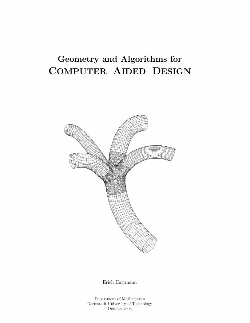
Geometry and Algorithms for
COMPUTER AIDED DESIGN
Erich Hartmann
Department of MathematicsDarmstadt University of Technology
October 2003

2
Contents
1 INTRODUCTION 71.1 Methods for DISPLAYING objects . . . . . . . . . . . . . . . . . . . . . . . . . . . 71.2 On the contents . . . . . . . . . . . . . . . . . . . . . . . . . . . . . . . . . . . . . . . 81.3 Software for displaying curves and surfaces . . . . . . . . . . . . . . . . . . . . . . . 91.4 On literature . . . . . . . . . . . . . . . . . . . . . . . . . . . . . . . . . . . . . . . . 10
2 TOOLS 112.1 Structure of a CAD-program . . . . . . . . . . . . . . . . . . . . . . . . . . . . . . . 11
2.1.1 Global constants: The file ”geoconst.pas” . . . . . . . . . . . . . . . . . . . . 112.1.2 Globale types: The file ”geotype.pas” . . . . . . . . . . . . . . . . . . . . . . 112.1.3 Globale variables: The file ”geovar.pas” . . . . . . . . . . . . . . . . . . . . . 112.1.4 Capability of the graphics software . . . . . . . . . . . . . . . . . . . . . . . . 12
2.2 Functions on IR, operations with vectors . . . . . . . . . . . . . . . . . . . . . . . . . 142.2.1 Functions on IR . . . . . . . . . . . . . . . . . . . . . . . . . . . . . . . . . . . 142.2.2 Operations with vectors . . . . . . . . . . . . . . . . . . . . . . . . . . . . . . 14
2.3 Routines to Analytic Geometry . . . . . . . . . . . . . . . . . . . . . . . . . . . . . . 172.3.1 Polarangle and quadratic equation . . . . . . . . . . . . . . . . . . . . . . . . 172.3.2 Intersection line–line, circle–line, circle–circle . . . . . . . . . . . . . . . . . . 172.3.3 Equation of a plane . . . . . . . . . . . . . . . . . . . . . . . . . . . . . . . . 182.3.4 Intersection line–plane . . . . . . . . . . . . . . . . . . . . . . . . . . . . . . . 182.3.5 Intersection of three planes . . . . . . . . . . . . . . . . . . . . . . . . . . . . 182.3.6 Intersection of two planes . . . . . . . . . . . . . . . . . . . . . . . . . . . . . 192.3.7 ξ-η–coordinates of a point in a plane . . . . . . . . . . . . . . . . . . . . . . . 192.3.8 Coordinates with respect of a new 3D-coordinate system . . . . . . . . . . . . 19
2.4 Numeric: GAUSS-elimination, NEWTON-iteration . . . . . . . . . . . . . . . . . . 19
3 PARALLEL/CENTRAL–PROJECTION 213.1 Orthographic Projection . . . . . . . . . . . . . . . . . . . . . . . . . . . . . . . . . . 21
3.1.1 The projection formulae . . . . . . . . . . . . . . . . . . . . . . . . . . . . . . 213.1.2 Procedures for orthographic projection . . . . . . . . . . . . . . . . . . . . . . 22
3.2 Central projection . . . . . . . . . . . . . . . . . . . . . . . . . . . . . . . . . . . . . 233.2.1 The projection formulae . . . . . . . . . . . . . . . . . . . . . . . . . . . . . 233.2.2 Procedures for central projection . . . . . . . . . . . . . . . . . . . . . . . . . 24
4 CURVES 274.1 Planar Curves . . . . . . . . . . . . . . . . . . . . . . . . . . . . . . . . . . . . . . . . 27
4.1.1 Definition and Representations of Planar Curves . . . . . . . . . . . . . . . . 274.1.2 Arc length and curvature of a planar curve . . . . . . . . . . . . . . . . . . . 284.1.3 Offset Curves . . . . . . . . . . . . . . . . . . . . . . . . . . . . . . . . . . . . 304.1.4 The normalform of a planar curve . . . . . . . . . . . . . . . . . . . . . . . . 30
3
4.2 Displaying Parametric Curves in IR2 . . . . . . . . . . . . . . . . . . . . . . . . . . . 324.3 Displaying implicit curves . . . . . . . . . . . . . . . . . . . . . . . . . . . . . . . . . 33
4.3.1 Marching algorithm . . . . . . . . . . . . . . . . . . . . . . . . . . . . . . . . 334.3.2 Raster algorithm . . . . . . . . . . . . . . . . . . . . . . . . . . . . . . . . . . 35
4.4 Intersection of two planar curves . . . . . . . . . . . . . . . . . . . . . . . . . . . . . 374.4.1 Intersection of a parametric curve and an implicit curve . . . . . . . . . . . . 384.4.2 Intersection of two implicit curves . . . . . . . . . . . . . . . . . . . . . . . . 384.4.3 Intersection of two parametric curves . . . . . . . . . . . . . . . . . . . . . . . 39
4.5 Foot points on planar curves . . . . . . . . . . . . . . . . . . . . . . . . . . . . . . . 394.5.1 Foot point on a parametric curve, curve inversion . . . . . . . . . . . . . . . . 394.5.2 Foot point on an implicit curve . . . . . . . . . . . . . . . . . . . . . . . . . . 404.5.3 Stable first order foot point algorithms . . . . . . . . . . . . . . . . . . . . . . 41
4.6 Bezier–curves . . . . . . . . . . . . . . . . . . . . . . . . . . . . . . . . . . . . . . . . 424.7 Applications of the normalform . . . . . . . . . . . . . . . . . . . . . . . . . . . . . . 43
4.7.1 Offset curves of implicit curves . . . . . . . . . . . . . . . . . . . . . . . . . . 444.7.2 Bisector curves . . . . . . . . . . . . . . . . . . . . . . . . . . . . . . . . . . . 454.7.3 Numerical Parameterization of Curves . . . . . . . . . . . . . . . . . . . . . 46
4.8 Space Curves . . . . . . . . . . . . . . . . . . . . . . . . . . . . . . . . . . . . . . . . 46
5 SURFACES 495.1 Definition and Representations of Surfaces . . . . . . . . . . . . . . . . . . . . . . . 495.2 The First and Second Fundamental Forms of a Surface . . . . . . . . . . . . . . . . 50
5.2.1 The first fundamental form, arc length . . . . . . . . . . . . . . . . . . . . . . 505.2.2 The second fundamental form, curvature . . . . . . . . . . . . . . . . . . . . 50
5.3 Offset surfaces . . . . . . . . . . . . . . . . . . . . . . . . . . . . . . . . . . . . . . . 525.4 Normalform of a surface . . . . . . . . . . . . . . . . . . . . . . . . . . . . . . . . . . 52
5.4.1 Definition of the normalform . . . . . . . . . . . . . . . . . . . . . . . . . . . 525.4.2 On the first and second derivatives of the normalform of a surface . . . . . . 535.4.3 Cn–contact, Gn–contact . . . . . . . . . . . . . . . . . . . . . . . . . . . . . 555.4.4 G2–continuity theorems . . . . . . . . . . . . . . . . . . . . . . . . . . . . . . 565.4.5 The curvature of an intersection curve . . . . . . . . . . . . . . . . . . . . . . 57
5.5 Normalform of an implicit surface . . . . . . . . . . . . . . . . . . . . . . . . . . . . . 585.6 Normalform of a parametric surface . . . . . . . . . . . . . . . . . . . . . . . . . . . 595.7 Foot point on a parametric surface, surface inversion . . . . . . . . . . . . . . . . . 605.8 Stable first order foot point algorithms for surfaces . . . . . . . . . . . . . . . . . . 61
5.8.1 Foot point algorithm for parametric surfaces . . . . . . . . . . . . . . . . . . 615.8.2 Foot point algorithm for implicit surfaces . . . . . . . . . . . . . . . . . . . . 61
5.9 The normalform of a space curve . . . . . . . . . . . . . . . . . . . . . . . . . . . . . 625.9.1 Definition of the normalform . . . . . . . . . . . . . . . . . . . . . . . . . . . 625.9.2 Foot point algorithm and evaluation of the normalform of a space curve . . . 635.9.3 Determining foot points on an intersection curve . . . . . . . . . . . . . . . . 64
5.10 Applications of normalforms . . . . . . . . . . . . . . . . . . . . . . . . . . . . . . . . 645.10.1 Approximation of a set of intersecting surfaces . . . . . . . . . . . . . . . . . 645.10.2 Approximation of intersecting pipe surfaces . . . . . . . . . . . . . . . . . . . 655.10.3 Numerical parametrization of implicit surfaces . . . . . . . . . . . . . . . . . 65
6 HIDDENLINE–ALGORITHM FOR NON CONVEX POLYHEDRONS 676.1 The Hiddenline-Algorithm . . . . . . . . . . . . . . . . . . . . . . . . . . . . . . . . . 676.2 Auxiliary procedures for the hiddenline algorithm . . . . . . . . . . . . . . . . . . . 71
6.2.1 The procedure aux polyhedron . . . . . . . . . . . . . . . . . . . . . . . . . . 716.2.2 The procedures aux quadrangle, aux cylinder, aux torus and displaying
a parametrized surface . . . . . . . . . . . . . . . . . . . . . . . . . . . . . . . 71
4
6.3 Intersection of faces, intersection of two polyhedrons . . . . . . . . . . . . . . . . . . 746.3.1 Intersection of faces bounded by planar polygons in IR3 . . . . . . . . . . . . 746.3.2 Intersection of two polyhedrons . . . . . . . . . . . . . . . . . . . . . . . . . 76
6.4 IS line–polygonal patch, IS polygon–polyhedron . . . . . . . . . . . . . . . . . . . . 786.4.1 Intersection of a line segment and a planar polygonal patch . . . . . . . . . . 786.4.2 Intersection points of a polygon and a polyhedron . . . . . . . . . . . . . . . 79
7 TRIANGULATION OF IMPLICIT SURFACES 817.1 The triangulation algorithm (marching method) . . . . . . . . . . . . . . . . . . . . . 81
7.1.1 The idea of the algorithm . . . . . . . . . . . . . . . . . . . . . . . . . . . . . 817.1.2 The procedure surfacepoint . . . . . . . . . . . . . . . . . . . . . . . . . . . 837.1.3 The data structure . . . . . . . . . . . . . . . . . . . . . . . . . . . . . . . . . 837.1.4 Step S0 . . . . . . . . . . . . . . . . . . . . . . . . . . . . . . . . . . . . . . . 847.1.5 Step S1 . . . . . . . . . . . . . . . . . . . . . . . . . . . . . . . . . . . . . . . 847.1.6 Step S2 . . . . . . . . . . . . . . . . . . . . . . . . . . . . . . . . . . . . . . . 847.1.7 Step S3 . . . . . . . . . . . . . . . . . . . . . . . . . . . . . . . . . . . . . . . 85
7.2 Examples . . . . . . . . . . . . . . . . . . . . . . . . . . . . . . . . . . . . . . . . . . 877.2.1 Sphere . . . . . . . . . . . . . . . . . . . . . . . . . . . . . . . . . . . . . . . . 877.2.2 Cylinder . . . . . . . . . . . . . . . . . . . . . . . . . . . . . . . . . . . . . . . 887.2.3 Torus . . . . . . . . . . . . . . . . . . . . . . . . . . . . . . . . . . . . . . . . 887.2.4 Set of two intersecting surfaces . . . . . . . . . . . . . . . . . . . . . . . . . . 887.2.5 G2-continuous blending of three cylinders . . . . . . . . . . . . . . . . . . . . 89
7.3 Sample program: trisample.p . . . . . . . . . . . . . . . . . . . . . . . . . . . . . . 917.4 Ray tracing of triangulated surfaces with POVRAY . . . . . . . . . . . . . . . . . . 92
8 INTERSECTIONS: CURVE – SURFACE, SURFACE – SURFACE 938.1 Intersection Curve – Surface . . . . . . . . . . . . . . . . . . . . . . . . . . . . . . . . 93
8.1.1 IS parametric curve – implicit surface . . . . . . . . . . . . . . . . . . . . . . 938.1.2 IS implicit curve – implicit surface . . . . . . . . . . . . . . . . . . . . . . . . 938.1.3 IS implicit curve – parametric surface . . . . . . . . . . . . . . . . . . . . . . 948.1.4 IS parametric curve – parametric surface . . . . . . . . . . . . . . . . . . . . 94
8.2 Intersection surface – surface . . . . . . . . . . . . . . . . . . . . . . . . . . . . . . . 948.2.1 IS of two implicit surfaces . . . . . . . . . . . . . . . . . . . . . . . . . . . . 948.2.2 IS of an implicit and a parametric surface . . . . . . . . . . . . . . . . . . . . 968.2.3 IS of two parametric surfaces . . . . . . . . . . . . . . . . . . . . . . . . . . . 96
8.3 Contour lines of surfaces . . . . . . . . . . . . . . . . . . . . . . . . . . . . . . . . . . 988.3.1 Contour line of an implicit surface . . . . . . . . . . . . . . . . . . . . . . . . 988.3.2 Contour line of a parametric surface . . . . . . . . . . . . . . . . . . . . . . . 998.3.3 Contour line of a quadric surface . . . . . . . . . . . . . . . . . . . . . . . . . 99
8.4 Hiddenline–algorithm for simple cases . . . . . . . . . . . . . . . . . . . . . . . . . . 1018.4.1 Fast normal–test . . . . . . . . . . . . . . . . . . . . . . . . . . . . . . . . . . 1018.4.2 Ray–test for implicit surfaces . . . . . . . . . . . . . . . . . . . . . . . . . . . 101
9 CONICS AND QUADRICS 1059.1 Conics . . . . . . . . . . . . . . . . . . . . . . . . . . . . . . . . . . . . . . . . . . . 105
9.1.1 Ellipse . . . . . . . . . . . . . . . . . . . . . . . . . . . . . . . . . . . . . . . 1059.1.2 Hyperbola . . . . . . . . . . . . . . . . . . . . . . . . . . . . . . . . . . . . . 1069.1.3 Parabola . . . . . . . . . . . . . . . . . . . . . . . . . . . . . . . . . . . . . . 1079.1.4 Equation of a conic . . . . . . . . . . . . . . . . . . . . . . . . . . . . . . . . . 1089.1.5 Conics in space . . . . . . . . . . . . . . . . . . . . . . . . . . . . . . . . . . . 108
9.2 Quadrics: ellipsoid, cylinder . . . . . . . . . . . . . . . . . . . . . . . . . . . . . . . . 1089.2.1 Ellipsoid . . . . . . . . . . . . . . . . . . . . . . . . . . . . . . . . . . . . . . . 108
5
6
9.2.2 Cylinder . . . . . . . . . . . . . . . . . . . . . . . . . . . . . . . . . . . . . . . 109
10 SURFACES OF REVOLUTION, RULED SURFACES, ... 11110.1 Surfaces of revolution . . . . . . . . . . . . . . . . . . . . . . . . . . . . . . . . . . . 11110.2 Ruled surfaces . . . . . . . . . . . . . . . . . . . . . . . . . . . . . . . . . . . . . . . 11210.3 Developable connections between curves . . . . . . . . . . . . . . . . . . . . . . . . . 11310.4 Coons patches . . . . . . . . . . . . . . . . . . . . . . . . . . . . . . . . . . . . . . . 11510.5 Canal surface, embankment surface . . . . . . . . . . . . . . . . . . . . . . . . . . . . 115
10.5.1 Canal surfaces . . . . . . . . . . . . . . . . . . . . . . . . . . . . . . . . . . . 11710.5.2 Embankment surfaces . . . . . . . . . . . . . . . . . . . . . . . . . . . . . . . 118
11 BLENDING CURVES AND SURFACES 11911.1 Gn–blending . . . . . . . . . . . . . . . . . . . . . . . . . . . . . . . . . . . . . . . . 11911.2 Implicit Gn–blending curves and surfaces . . . . . . . . . . . . . . . . . . . . . . . . 119
11.2.1 Parabolic functional splines . . . . . . . . . . . . . . . . . . . . . . . . . . . . 12011.2.2 Elliptic functional splines . . . . . . . . . . . . . . . . . . . . . . . . . . . . . 124
11.3 Parametric Gn–blending curves and surfaces . . . . . . . . . . . . . . . . . . . . . . 12711.3.1 Gn–blending of parametric curves . . . . . . . . . . . . . . . . . . . . . . . . 12711.3.2 Gn–blending of parametric surfaces . . . . . . . . . . . . . . . . . . . . . . . 129
11.4 Blending with rolling ball contact curves . . . . . . . . . . . . . . . . . . . . . . . . . 133
12 PROPERTIES OF BEZIER CURVES 13712.1 Properties of the Bernstein polynomes . . . . . . . . . . . . . . . . . . . . . . . . . . 13712.2 The Casteljau–algorithm . . . . . . . . . . . . . . . . . . . . . . . . . . . . . . . . . . 13712.3 Derivative of a Bezier curve . . . . . . . . . . . . . . . . . . . . . . . . . . . . . . . . 13912.4 Degree elevation of a Bezier curve . . . . . . . . . . . . . . . . . . . . . . . . . . . . 13912.5 Bezier spline curves . . . . . . . . . . . . . . . . . . . . . . . . . . . . . . . . . . . . . 140
12.5.1 Division of a Bezier curve . . . . . . . . . . . . . . . . . . . . . . . . . . . . . 14012.5.2 Smoothness conditions . . . . . . . . . . . . . . . . . . . . . . . . . . . . . . . 141
12.6 Rational Bezier curves . . . . . . . . . . . . . . . . . . . . . . . . . . . . . . . . . . . 14412.6.1 Rational curves and projective curves . . . . . . . . . . . . . . . . . . . . . . 144
12.7 Rational Bezier curves . . . . . . . . . . . . . . . . . . . . . . . . . . . . . . . . . . . 14412.8 Conics as rational Bezier curves . . . . . . . . . . . . . . . . . . . . . . . . . . . . . . 145
13 BEZIER–SURFACES 14713.1 Tensor product Bezier surfaces . . . . . . . . . . . . . . . . . . . . . . . . . . . . . . 14713.2 The Casteljau algorithm . . . . . . . . . . . . . . . . . . . . . . . . . . . . . . . . . . 14813.3 Degree elevation . . . . . . . . . . . . . . . . . . . . . . . . . . . . . . . . . . . . . . 14813.4 Derivatives of a Bezier surface . . . . . . . . . . . . . . . . . . . . . . . . . . . . . . . 14813.5 Bezier triangular surfaces . . . . . . . . . . . . . . . . . . . . . . . . . . . . . . . . . 149
14 B–SPLINE CURVES 15114.1 The B–Spline base functions . . . . . . . . . . . . . . . . . . . . . . . . . . . . . . . 15114.2 The de–Boor algorithm . . . . . . . . . . . . . . . . . . . . . . . . . . . . . . . . . . 153
A THE REAL PROJECTIVE PLANE 155A.1 The real affine plane . . . . . . . . . . . . . . . . . . . . . . . . . . . . . . . . . . . . 155A.2 The real projective plane . . . . . . . . . . . . . . . . . . . . . . . . . . . . . . . . . 155A.3 Isomorphism between the two models . . . . . . . . . . . . . . . . . . . . . . . . . . 156A.4 Collineations of the real projective plane . . . . . . . . . . . . . . . . . . . . . . . . . 157A.5 Projective equivalency of the conics . . . . . . . . . . . . . . . . . . . . . . . . . . . 158
Chapter 1
INTRODUCTION
Essential tasks of Computer Aided Design are:1) designing objects like parts of machines, car bodies, ... and2) displaying designed or basic objects like spheres, cylinders, tori, ...
1.1 Methods for DISPLAYING objects
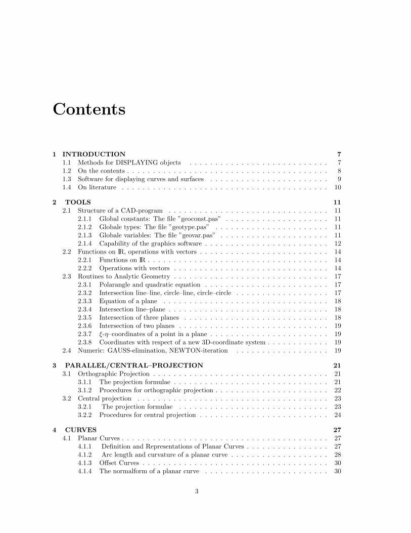
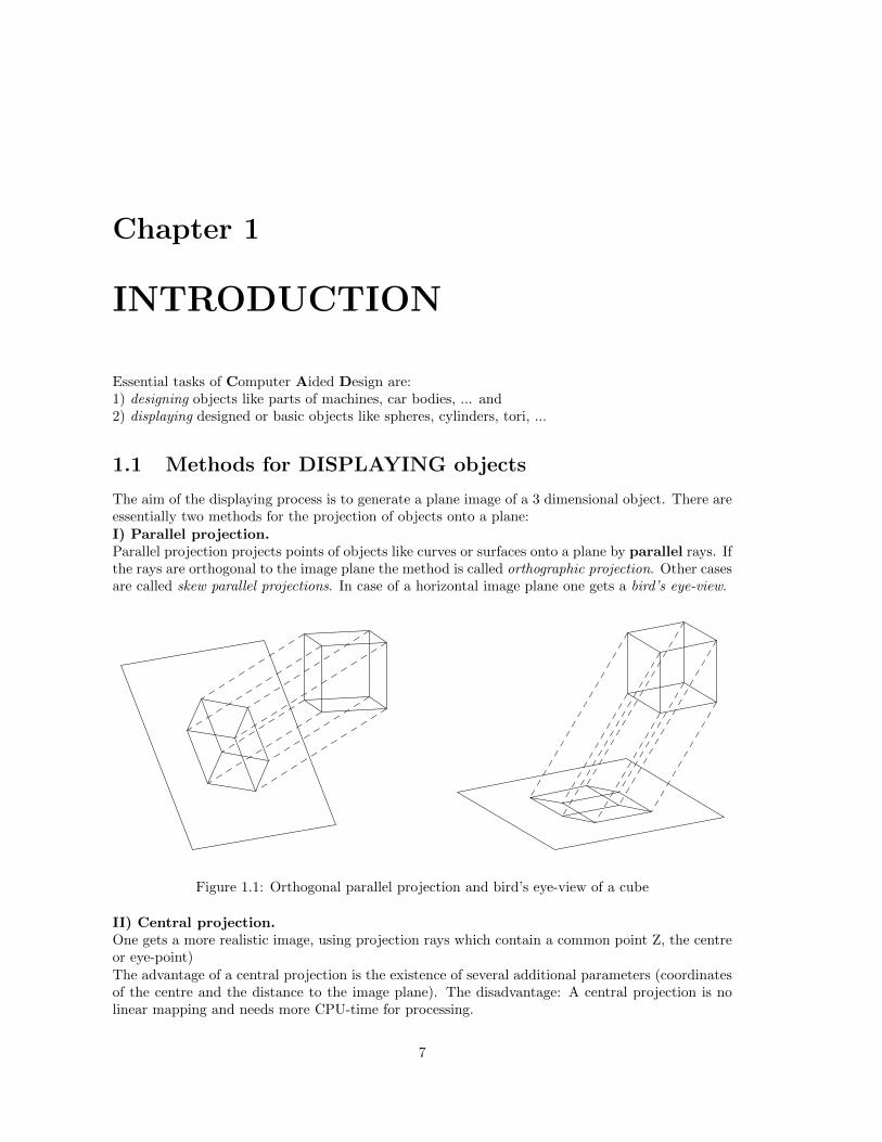
The aim of the displaying process is to generate a plane image of a 3 dimensional object. There areessentially two methods for the projection of objects onto a plane:I) Parallel projection.Parallel projection projects points of objects like curves or surfaces onto a plane by parallel rays. Ifthe rays are orthogonal to the image plane the method is called orthographic projection. Other casesare called skew parallel projections. In case of a horizontal image plane one gets a bird’s eye-view.
Figure 1.1: Orthogonal parallel projection and bird’s eye-view of a cube
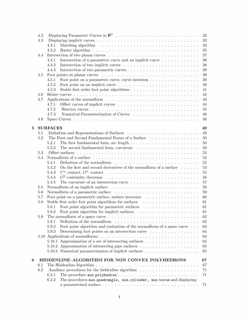
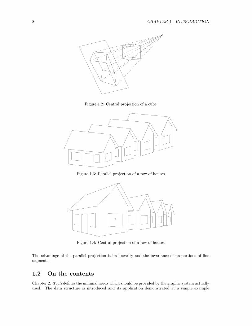
II) Central projection.One gets a more realistic image, using projection rays which contain a common point Z, the centreor eye-point)The advantage of a central projection is the existence of several additional parameters (coordinatesof the centre and the distance to the image plane). The disadvantage: A central projection is nolinear mapping and needs more CPU-time for processing.
7
8 CHAPTER 1. INTRODUCTION
Figure 1.2: Central projection of a cube
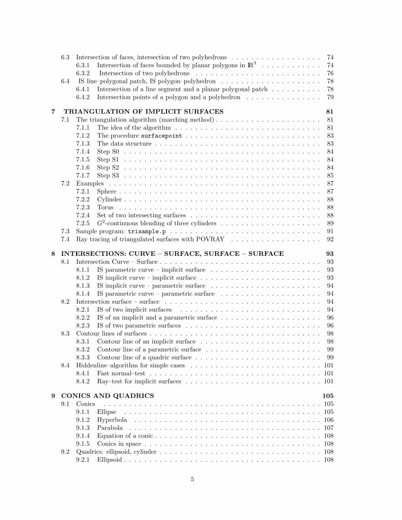
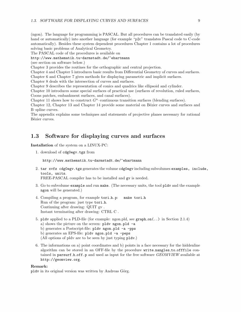
Figure 1.3: Parallel projection of a row of houses
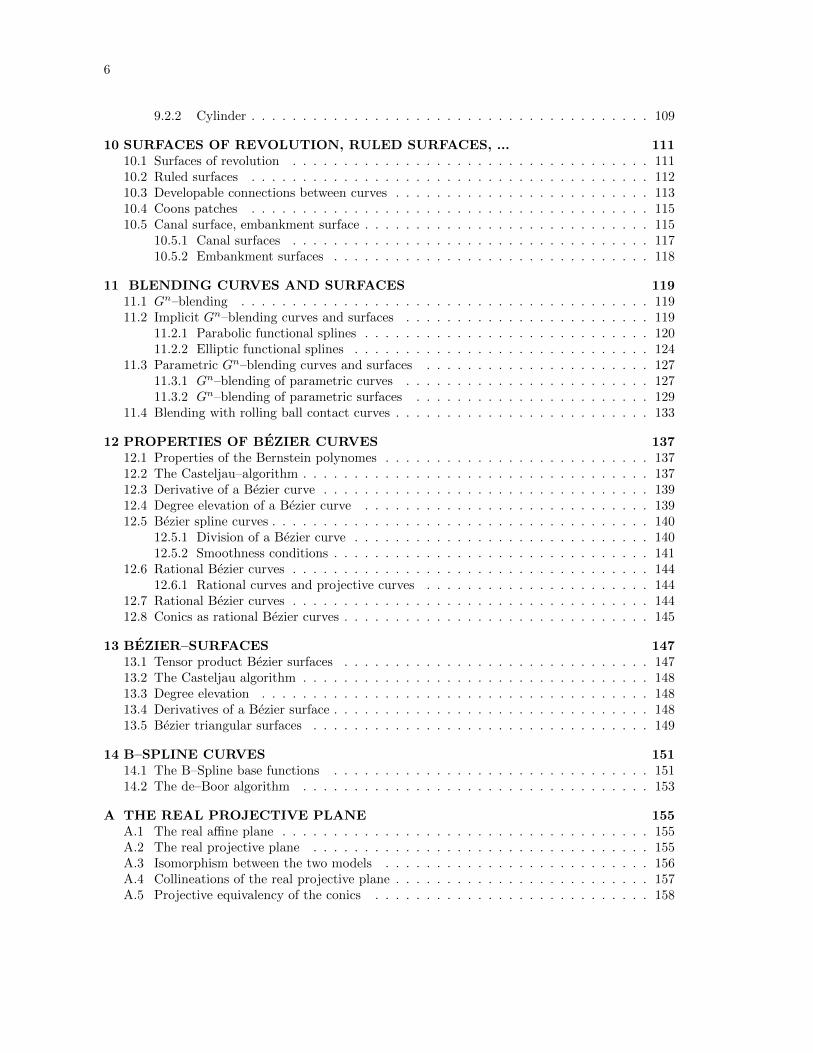
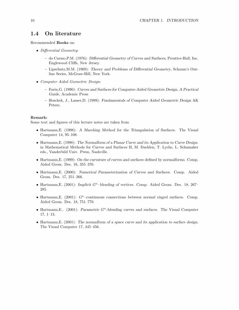
Figure 1.4: Central projection of a row of houses
The advantage of the parallel projection is its linearity and the invariance of proportions of linesegments..
1.2 On the contents
Chapter 2: Tools defines the minimal needs which should be provided by the graphic system actuallyused. The data structure is introduced and its application demonstrated at a simple example
1.3. SOFTWARE FOR DISPLAYING CURVES AND SURFACES 9
(ngon). The language for programming is PASCAL. But all procedures can be translated easily (byhand or automatically) into another language (for example “p2c” translates Pascal code to C-codeautomatically). Besides these system dependent procedures Chapter 1 contains a lot of proceduressolving basic problems of Analytical Geometry.The PASCAL code of the procedures is available onhttp://www.mathematik.tu-darmstadt.de/~ehartmann
(see section on software below.)Chapter 3 provides the routines for the orthographic and central projection.Chapter 4 and Chapter 5 introduces basic results from Differential Geometry of curves and surfaces.Chapter 6 and Chapter 7 gives methods for displaying parametric and implicit surfaces.Chapter 8 deals with the intersection of curves and surfaces.Chapter 9 describes the representation of conics and quadrics like ellipsoid and cylinder.Chapter 10 introduces some special surfaces of practical use (surfaces of revolution, ruled surfaces,Coons patches, embankment surfaces, and canal surfaces).Chapter 11 shows how to construct Gn–continuous transition surfaces (blending surfaces).Chapter 12, Chapter 13 and Chapter 14 provide some material on Bezier curves and surfaces andB–spline curves.The appendix explains some techniques and statements of projective planes necessary for rationalBezier curves.
1.3 Software for displaying curves and surfaces
Installation of the system on a LINUX-PC:
1. download of cdg0egv.tgz from
http://www.mathematik.tu-darmstadt.de/~ehartmann
2. tar xvfz cdg0egv.tgz generates the volume cdg0egv including subvolumes examples, include,
tools, units.FREE-PASCAL compiler has to be installed and gv is needed.
3. Go to subvolume example and run make. (The necessary units, the tool pldv and the examplengon will be generated.)
4. Compiling a program, for example tori h.p: make tori h
Run of the program: just type tori h.Continuing after drawing: QUIT gv .Instant terminating after drawing: CTRL C .
5. pldv applied to a PLD-file (for example: ngon.pld, see graph on(..) in Section 2.1.4)a) shows the picture on the screen: pldv ngon.pld -a
b) generates a Postscript-file: pldv ngon.pld -a -pps
b) generates an EPS-file: pldv ngon.pld -a -peps
(All options of pldv are to be seen by just typing pldv.)
6. The informations on a) point coordinates and b) points in a face necessary for the hiddenlinealgorithm can be stored in an OFF-file by the procedure write nangles to offfile con-tained in parsurf h off.p and used as input for the free software GEOMVIEW available athttp://geomview.org.
Remark:pldv in its original version was written by Andreas Gorg.
10 CHAPTER 1. INTRODUCTION
1.4 On literature
Recommended Books on:
• Differential Geometry:
– do Carmo,P.M. (1976): Differential Geometry of Curves and Surfaces, Prentice-Hall, Inc.Englewood Cliffs, New Jersey.
– Lipschutz,M.M. (1969): Theory and Problems of Differential Geometry, Schaum’s Out-line Series, McGraw-Hill, New York.
• Computer Aided Geometric Design:
– Farin,G. (1990): Curves and Surfaces for Computer-Aided Geometric Design, A PracticalGuide, Academic Press
– Hoschek, J., Lasser,D. (1989): Fundamentals of Computer Aided Geometric Design AKPeters.
Remark:Some text and figures of this lecture notes are taken from
• Hartmann,E. (1998): A Marching Method for the Triangulation of Surfaces. The VisualComputer 14, 95–108.
• Hartmann,E. (1998): The Normalform of a Planar Curve and its Application to Curve Design.in Mathematical Methods for Curves and Surfaces II, M. Daehlen, T. Lyche, L. Schumakereds., Vanderbild Univ. Press, Nashville.
• Hartmann,E. (1999): On the curvature of curves and surfaces defined by normalforms. Comp.Aided Geom. Des. 16, 355–376.
• Hartmann,E. (2000): Numerical Parameterization of Curves and Surfaces. Comp. AidedGeom. Des. 17, 251–266.
• Hartmann,E. (2001): Implicit Gn–blending of vertices. Comp. Aided Geom. Des. 18, 267–285.
• Hartmann,E. (2001): Gn–continuous connections between normal ringed surfaces. Comp.Aided Geom. Des. 18, 751–770.
• Hartmann,E.. (2001): Parametric Gn-blending curves and surfaces. The Visual Computer17, 1–13.
• Hartmann,E. (2001): The normalform of a space curve and its application to surface design.The Visual Computer 17, 445–456.
Chapter 2
TOOLS
Essential tools for solving CAD problems are basic operations for vectors (sum, scalar product, ...)and routines for simple tasks like the intersection of a line and a circle. Before introducing suchbasic procedures we discuss the minimal demand on the graphics system.
2.1 Structure of a CAD-program
First of all we define the global constants, types and variables used in any program. Essential arethe types vt2d,vt3d,vts2d,vts3d which define vectors and arrays of vectors.
2.1.1 Global constants: The file ”geoconst.pas”
The file ”geoconst.pas” contains the constant array size which will be used in 2.1.2, the realsπ, 2π, π2 and eps1, ... , eps8 used for error bounds . The constants black,... described colors.
array_size= 1000; {...20000 for hiddenline-alg.}
pi= 3.14159265358; pi2= 6.2831853; pih= 1.5707963;
eps1=0.1; eps2=0.01; eps3=0.001; eps4=0.0001;
eps5=0.00001; eps6=0.000001; eps7=0.0000001; eps8=0.00000001;
default=-1; black=0; blue=1; green=2; cyan=3; red=4; magenta=5; brown=6;
lightgray=7; darkgray=8; lightblue=9; lightgreen=10; lightcyan=11;
lightred=12; lightmagenta=13; yellow=14; white=15;
2.1.2 Globale types: The file ”geotype.pas”
r_array = array[0..array_size] of real;
i_array = array[0..array_size] of integer;
b_array = array[0..array_size] of boolean;
vt2d = record x,y: real; end;
vt3d = record x,y,z: real; end;
vts2d = array[0..array_size] of vt2d;
vts3d = array[0..array_size] of vt3d;
matrix3d= array[1..3,1..3] of real;
2.1.3 Globale variables: The file ”geovar.pas”
null2d:vt2d; null3d:vt3d; {Nullvectors}
{**for area_2d and curve2d:}
origin2d:vt2d;
11
12 CHAPTER 2. TOOLS
{**for parallel and central projection:}
u_angle,v_angle, {projection angles}
rad_u,rad_v, {rad(u), rad(v)}
sin_u,cos_u,sin_v,cos_v:real; {sin(u),cos(u), ...}
e1vt,e2vt,n0vt:vt3d; {base vectors and}
{normal vector of the image plane}
{**for Central-Projection:}
mainpt, {mainpoint}
centre:vt3d; {centre}
distance:real; {distance mainpoint - centre}
2.1.4 Capability of the graphics software
In order to ease the transportation of the system to another one all procedures for drawing relyon the following 9 machine dependent procedures. For a LINUX-PC the realization is contained inpackage cdg0egv (see Introduction).
1. graph on(ipl), ipl:integer, starts the grafics-software and sets the vectors null2d, null3d
to default;ipl = 0 : Display on screen, only,ipl 6= 0 : any application of draw area(...) (see below) generates a file name.pld thatcontains all drawing devices of the actual drawing, including color and line width.pldv name.pld shows the drawing stored in name.pld on the screen. pldv name.pld -pps
generates a POSTSCRIPT–file which can be printed.pldv name.pld -peps generates an ENCAPSULATED POSTSCRIPT–file which can be in-cluded into a TEX–file.
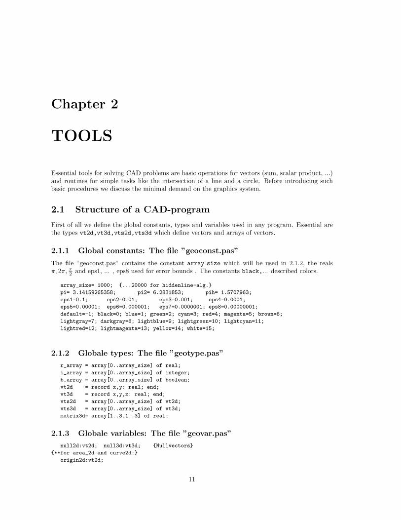
2. draw area(width,height,x0,y0,scalefactor) clears the screen and defines a drawing areaprovided with an orthogonal coordinate system.origin2d = (x0,y0) is a global variable.All length are assumed to be in mm (reals !)1 mm should be 1 mm on the screen and on the paper, if scalefactor=1.scalefactor= s scales the drawing by factor s.
x0
y0
width
height
Figure 2.1: Origin of the coordinate system for the drawing area
2.1. STRUCTURE OF A CAD-PROGRAM 13
3. draw end closes a drawing. If there is need for an additional drawing draw area has to beapplied again
4. graph off closes the graphic software definitely.
DRAWING DEVICES:
5. pointc2d(x,y,style), x,y:real; style:integer,marks the point(x,y) by o if style = 0, + if style = 1 , ... .For style = 10 oder 50 oder 100 the marks are smaller circles (scaled)point2d(p,style), p:vt2d; style:integer,like pointc2d using the type vt2d for the point.
6. linec2d(x1,y1,x2,y2,style), x1,y1,x2,y2:real; style:integer,draws the line segment (x1, y1)(x2, y2) as:———— , if style = 0, −−−−−, if style = 1, − · − · −, if style = 2, ..........The following devices are defined by linec2d.
(a) line2d(p1,p2,style), p1,p2:vt2d; style:integer,as linec2d using type vt2d for the bounding points.
(b) arrowc2d(x1,y1,x2,y2,style), x1,y1,x2,y2:real; style:integer
draws an arrow from (x1, y1) to (y2, y2).
(c) arrow2d(p1,p2,style), p1,p2:vt2d; style:integer
draws an arrow from p1 to p2.
(d) curve2d(p,n1,n2,style), p:vts2d; style:integer,draws a polyline with vertices pn1, ...,pn2.
All length and coordinates must be given in mm !
7. new color(color), color: integer,sets a new color. For example: color = red. color = default is equivalent to black.
8. new linewidth(factor), factor: real,changes the line width. factor=1 means normal line width.
STRUCTURE of a program:
After putting all global constants, types, variables and procedures into a unit geograph a programis of the following simple form:
program name;
uses geograph;
const ...
type ...
var ...:vts2d;
...:integer;
...:real;
...
{$i procs.pas} {additional procedures}
{*******************}
begin {main program}
graph_on(...);
...
{drawing:}
14 CHAPTER 2. TOOLS
draw_area(...);
...
...
draw_end;
....
graph_off;
end.
2.2 Functions on IR, operations with vectors
Now we provide PASCAL-functions and procedures for some often used real functions and opera-tions. Because of the simplicity of these functions and procedures we give only heads. The completesource is contained in the file proc ag.pas (see volume include).
2.2.1 Functions on IR
1. r → sign(a) (−1, if a < 0, else +1)function sign(a:real):integer;
2. a, b→ max{a, b} (maximum of a,b)a, b→ min{a, b} (minimum of a,b)function max(a,b:real):real; function min(a,b:real):real;
2.2.2 Operations with vectors
1. x, y → v = (x, y),x, y, z → v = (x, y, z)procedure put2d(x,y:real; var v:vt2d);
procedure put3d(x,y,z:real; var v:vt3d);
v = (x, y, z)→ x, y, zprocedure get3d(v:vt3d; var x,y,z:real);
2. r,v→ rv (scaling)procedure scale2d(r:real; v:vt2d; var vs:vt2d);
procedure scale3d(r:real; v:vt3d; var vs:vt3d);
r1, r2, (x, y)→ (r1x, r2y) bzw.r1, r2, r3, (x, y, z)→ (r1x, r2y, r3z) (scaling single coordinates)procedure scaleco2d(r1,r2:real; v:vt2d; var vs:vt2d);
procedure scaleco3d(r1,r2,r3:real; v:vt3d; var vs:vt3d);
3. v1,v2 → v = v1 + v2 (sum of two vectors)procedure sum2d(v1,v2:vt2d; var vs:vt2d);
procedure sum3d(v1,v2:vt3d; var vs:vt3d);
v1,v2 → v = v2 − v2 (difference of two vectors)procedure diff2d(v1,v2:vt2d; var vd:vt2d);
procedure diff3d(v1,v2:vt3d; var vd:vt3d);
4. r1,v1, r2,v2 → v = r1v1 + r2v2 (linear combination of vectors)procedure lcomb2vt2d(r1:real; v1:vt2d; r2:real; v2:vt2d; var vlc:vt2d);
procedure lcomb2vt3d(r1:real; v1:vt3d; r2:real; v2:vt3d; var vlc:vt3d);
and analogously linear combinations of 3 and 4 vectors:lcomb3vt2d(r1,v1, r2,v2, r3,v3, vlc);
lcomb3vt3d(r1,v1, r2,v2, r3,v3, vlc);
2.2. FUNCTIONS ON IR, OPERATIONS WITH VECTORS 15
lcomb4vt2d(r1,v1, r2,v2, r3,v3, r4,v4, vlc);
lcomb4vt3d(r1,v1, r2,v2, r3,v3, r4,v4, vlc);
5. v = (x, y)→ |x|+ |y| bzw. v = (x, y, z)→ |x|+ |y|+ |z|function abs2d(v:vt2d):real; function abs3d(v:vt3d):real;
6. v = (x, y)→ ‖v‖ =√x2 + y2 bzw.
v = (x, y, z)→ ‖v‖ =√x2 + y2 + z2
function length2d(v:vt2d):real; function length3d(v:vt3d):real;
7. v→ v/‖v‖procedure normalize2d(var v:vt2d); procedure normalize3d(var v:vt3d);
8. p,q→ ‖p− q‖ p,q→ ‖p− q‖2function distance2d(p,q:vt2d):real;
function distance3d(p,q:vt3d):real;
function distance2d square(p,q:vt2d):real;
function distance3d square(p,q:vt3d):real;
9. v1,v2 → v1 · v2 (scalar product)function scalarp2d(v1,v2:vt2d):real;
function scalarp3d(v1,v2:vt3d):real;
10. v1,v2 → v1 × v2 (vector product)procedure vectorp(v1,v2:vt3d; var vp:vt3d);
11. v1,v2,v3 → |v1v2v3|(v1 · (v2 × v3), 3x3-determinant)function determ3d(v1,v2,v3:vt3d):real;
12. cosϕ, sinϕ,p = (x, y)→ pr = (x cosϕ− y sinϕ, x sinϕ+ y cosϕ)(rotation around the origin, angle:ϕ)procedure rotor2d(cos rota,sin rota:real; p:vt2d; var pr:vt2d);
13. cosϕ, sinϕ,p0,p→ pr(rotation around point p0, angle:ϕ)rotp02d(cos rota,sin rota,p0,p, pr);
14. cosϕ, sinϕ,p→ pr(rotation around x-axis, y-axis, z-axis respect. )procedure rotorx(cos rota,sin rota,p, pr);
procedure rotory(cos rota,sin rota,p, pr);
procedure rotorz(cos rota,sin rota,p, pr);
15. cosϕ, sinϕ,p0,p→ pr(rotation around an axis through p0 parallel to a coordinate axis in IR3)procedure rotp0x(cos rota,sin rota,p0,p, pr);
procedure rotp0y(cos rota,sin rota,p0,p, pr);
procedure rotp0z(cos rota,sin rota,p0,p, pr);
16. Change of numbers and vectors resp.:a↔ b bzw. v1 ↔ v2
procedure change1d(var a,b:real);
procedure change2d(var v1,v2:vt2d);
procedure change3d(var v1,v2:vt3d);
16 CHAPTER 2. TOOLS
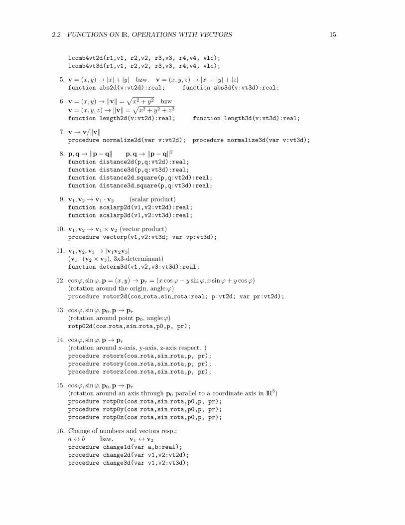
Example 2.1 The following program draws a regular n-gon and (on demand) all possible edges.The points of the ngon are on a circle with midpoint (0, 0) and radius r. The coordinates of the pointsare xi = r cos(i∆ϕ), yi = r sin(i∆ϕ) mit ∆ϕ = 2π/n, i = 0, ..n− 1.(For the program: Point Pi+1 is generated by rotating Pi).
Figure 2.2: n-gon with all possible edges (Example 2.1)
{***********************}
{*** regular n-gon ***}
{***********************}
program ngon;
uses geograph;
var p : vts2d;
n,icon,i,j,iand: integer;
r,dw,cdw,sdw: real;
{*******************}
begin {main program}
graph_on(0);
repeat
writeln(’*** n-gon ***’);
writeln(’n ? radius r of the corresponding circle ?’); readln(n,r);
writeln(’Connect any pair of points ? (yes=1)’); readln(icon);
{coordinates of the points:}
put2d(r,0, p[0]); dw:= pi2/n; cdw:= cos(dw); sdw:= sin(dw);
for i:= 0 to n-1 do rotor2d(cdw,sdw,p[i], p[i+1]);
draw_area(2*r+20,2*r+20,r+10,r+10,1);
{drawing:} new_color(yellow);
if icon=1 then
for i:= 0 to n-1 do
for j:= i+1 to n do
line2d(p[i],p[j],0)
else
curve2d(p,0,n,0);
draw_end;
writeln(’Additional drawing? (yes:1, no:0)’); readln(iand);
until iand=0;
graph_off;
end.
2.3. ROUTINES TO ANALYTIC GEOMETRY 17
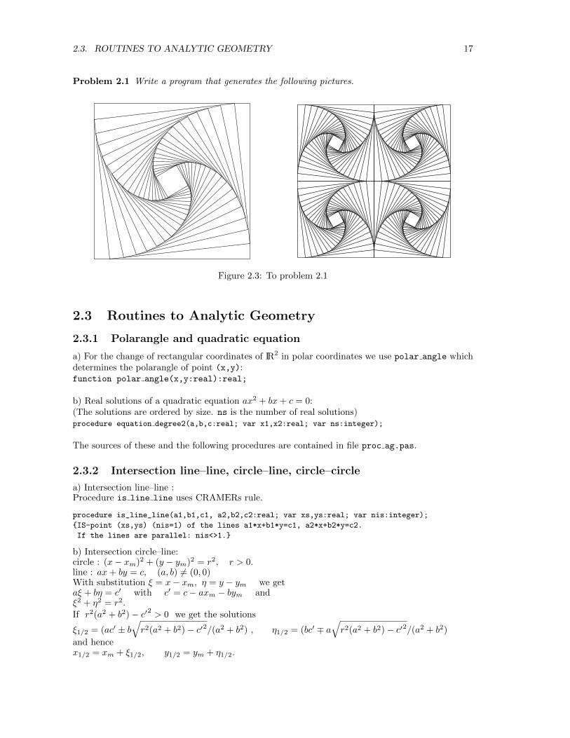
Problem 2.1 Write a program that generates the following pictures.
Figure 2.3: To problem 2.1
2.3 Routines to Analytic Geometry
2.3.1 Polarangle and quadratic equation
a) For the change of rectangular coordinates of IR2 in polar coordinates we use polar angle whichdetermines the polarangle of point (x,y):function polar angle(x,y:real):real;
b) Real solutions of a quadratic equation ax2 + bx+ c = 0:(The solutions are ordered by size. ns is the number of real solutions)procedure equation degree2(a,b,c:real; var x1,x2:real; var ns:integer);
The sources of these and the following procedures are contained in file proc ag.pas.
2.3.2 Intersection line–line, circle–line, circle–circle
a) Intersection line–line :Procedure is line line uses CRAMERs rule.
procedure is_line_line(a1,b1,c1, a2,b2,c2:real; var xs,ys:real; var nis:integer);
{IS-point (xs,ys) (nis=1) of the lines a1*x+b1*y=c1, a2*x+b2*y=c2.
If the lines are parallel: nis<>1.}
b) Intersection circle–line:circle : (x− xm)2 + (y − ym)2 = r2, r > 0.line : ax+ by = c, (a, b) 6= (0, 0)With substitution ξ = x− xm, η = y − ym we getaξ + bη = c′ with c′ = c− axm − bym andξ2 + η2 = r2.
If r2(a2 + b2)− c′2 > 0 we get the solutions
ξ1/2 = (ac′ ± b√r2(a2 + b2)− c′2/(a2 + b2) , η1/2 = (bc′ ∓ a
√r2(a2 + b2)− c′2/(a2 + b2)
and hencex1/2 = xm + ξ1/2, y1/2 = ym + η1/2.
18 CHAPTER 2. TOOLS
procedure is_circle_line(xm,ym,r, a,b,c:real; var x1,y1,x2,y2:real; var nis:integer);
{Intersection circle-line: sqr(x-xm)+sqr(y-ym)=r*r, a*x+b*y=c,
IS-points: (x1,y1),(x2,y2). x1<=x2, nis: number of intersection points.}
Intersection of the unitcircle (x2 + y2 = 1) with a line:
procedure is_unitcircle_line(a,b,c:real; var x1,y1,x2,y2:real; var nis:integer);
In both procedures we have x1 ≤ x2.
c) Intersection circle–circle :1. circle : (x− x1)2 + (y − y1)2 = r2
1, r1 > 0,2. circle : (x− x2)2 + (y − y2)2 = r2
2, r2 > 0, (x1, y1) 6= (x2, y2).This system is equivalent to:(x− x1)2 + (y − y1)2 = r2
1, ax+ by = c witha = 2(x2 − x1), b = 2(y2 − y1) and c = r2
2 − x21 − y2
1 − r22 + x2
2 + y22 .
That means: The intersection points of the circles and the intersection points of the first circle andthe line ax+ by = c are the same.
procedure is_circle_circle(xm1,ym1,r1,xm2,ym2,r2:real; var x1,y1,x2,y2:real; var nis:integer);
{Intersection circle--circle. x1<=x2. nis: number of intersection points.}
2.3.3 Equation of a plane
Given: 3 points Pi : pi, i = 1, 2, 3.Sought: equation n · x = d, that means the normal vector n and d.Solution: n = (p2 − p1)× (p3 − p1) and d = n · p1.plane equ determines n and d. The boolean variable error is set true, in case of n ≈ 0.
procedure plane_equ(p1,p2,p3:vt3d; var nv:vt3d; var d:real; var error:boolean);
{Determines the equation nv*x=d of the plane containing p1,p2,p3.
error=true: no plane.}
2.3.4 Intersection line–plane
Given: line x(t) = p + tr, plane n · x = d.Sought: Intersection point pis.Solution: pis = p− ((n · p− d)/n · r)r.is line plane determines the intersection point, if it exists.
procedure is_line_plane(p,rv,nv:vt3d; d:real; var pis:vt3d; var nis:integer);
{Intersection line-plane. Line: point p, direction r. plane: nv*x = d .
nis=0: no IS-point ,nis=1: IS--point exists, nis=2: line in plane.}
2.3.5 Intersection of three planes
Given: Three planes εi : ni · x = di, i = 1, 2, 3, n1,n2,n3 linear independent.Sought: Intersection point pis : ε1 ∩ ε2 ∩ ε3.From pis = ξ(n2 × n3) + η(n3 × n1) + ζ(n1 × n2)we getpis = (d1(n2 × n3) + d2(n3 × n1) + d3(n1 × n2))/n1 · (n2 × n3).(If the normals are not linearly independent, there exists an intersection line or two planes areparallel.)is 3 planes determines the intersection. error= true, if the intersection consists not of exactlyone point.
procedure is_3_planes(nv1:vt3d; d1:real; nv2:vt3d; d2:real; nv3:vt3d; d3:real;
var pis:vt3d; var error:boolean);
{Intersection of the planes nv1*x=d1, nv2*x=d2, nv3*x=d3.
error= true if not exactly ONE intersection point.}
2.4. NUMERIC: GAUSS-ELIMINATION, NEWTON-ITERATION 19
2.3.6 Intersection of two planes
Given: two planes εi : ni · x = di, i = 1, 2, n1,n2 linear independent.Sought: ε1 ∩ ε2 : x = p + tr.The direction of the intersection line is r = n1 × n2. We get a point P : p of the intersection lineby intersecting ε1, ε2 with the plane ε3 : x = s1n1 + s2n2.
P : p =d1n2
2 − d2(n1 · n2)
n12n2
2 − (n1 · n2)2n1 +
d2n12 − d1(n1 · n2)
n12n2
2 − (n1 · n2)2n2
is plane plane determines the direction r and a point of the intersection line. error=true, if theplanes are parallel.
procedure is_plane_plane(nv1:vt3d; d1:real; nv2:vt3d; d2:real;
var p,rv:vt3d; var error:boolean);
{Intersection of the planes nv1*x=d1, nv2*x=d2. IS--line: x = p + t*rv .
error= true: Intersection is no line.}
2.3.7 ξ-η–coordinates of a point in a plane
Given: plane ε : x = p0 + ξv1 + ηv2 and point P: p in ε .Sought: ξ, η such that p = p0 + ξv1 + ηv2.By scalar multiplication of p by v1,v2 we get the linear system:(p− p0) · v1 = ξv1
2 + ηv1 · v2, (p− p0) · v2 = ξv1 · v2 + ηv22,
ptco plane3d determines ξ, η using CRAMERs rule. error=true, if the determinant of the linearsystem is ≈ 0. (If P is not in ε and ξ, η is the solution of the linear system above, point P’:p′ = p0 + ξv1 + ηv2 is the footpoint of the perpendicular line from P to plane ε.)
procedure ptco_plane3d(p0,v1,v2,p:vt3d; var xi,eta:real; var error:boolean);
{v1,v2 linear independent, p-p0,v1,v2 are linear dependent.
We get xi,eta such that p = p0 + xi*v1 + eta*v2.}
2.3.8 Coordinates with respect of a new 3D-coordinate system
Given: new origin B0 : b0, new basis b1,b2,b3 and point P: p .Sought: ξ, η, ζ such that p = b0 + ξb1 + ηb2 + ζb3.From CRAMERs rule we get:
ξ = det(p− b0,b2,b3)/det(b1,b2,b3)
η = det(b1,p− b0,b3)/det(b1,b2,b3)
ζ = det(b1,b2,p− b0)/det(b1,b2,b3)
procedure newcoordinates3d(p,b0,b1,b2,b3: vt3d; var pnew: vt3d);
{Determines the coordinates of p with respect of basis b1,b2,b3 and origin b0.}
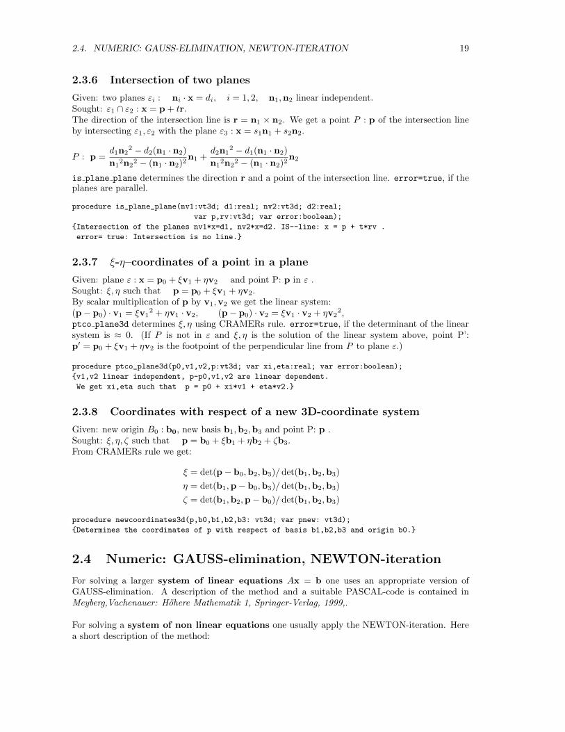
2.4 Numeric: GAUSS-elimination, NEWTON-iteration
For solving a larger system of linear equations Ax = b one uses an appropriate version ofGAUSS-elimination. A description of the method and a suitable PASCAL-code is contained inMeyberg,Vachenauer: Hohere Mathematik 1, Springer-Verlag, 1999,.
For solving a system of non linear equations one usually apply the NEWTON-iteration. Herea short description of the method:
20 CHAPTER 2. TOOLS
Given: Function F : D → IRn, D ⊆ IRn, and a starting point x0 for the iteration.Wanted: A point x∗ in the vicinity of x0 with F(x∗) = 0.
The algorithm:For ν = 0, 1, 2, . . .
(1) solve the linear systemF′(xν)dν = −F(xν) , where F′ := ( ∂Fi
∂xk) and F = (F1, F2, . . . , Fn), x = (x1, x2, . . . , xn).
(2) xν+1 = xν + dν
(3) If ‖xν+1 − xν‖ is small enough (or another termination) we set x∗ = xν+1.
Chapter 3
PARALLEL/CENTRAL–PROJECTION
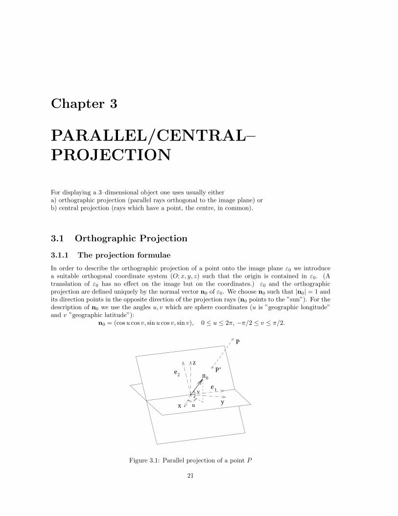
For displaying a 3–dimensional object one uses usually eithera) orthographic projection (parallel rays orthogonal to the image plane) orb) central projection (rays which have a point, the centre, in common).
3.1 Orthographic Projection
3.1.1 The projection formulae
In order to describe the orthographic projection of a point onto the image plane ε0 we introducea suitable orthogonal coordinate system (O;x, y, z) such that the origin is contained in ε0. (Atranslation of ε0 has no effect on the image but on the coordinates.) ε0 and the orthographicprojection are defined uniquely by the normal vector n0 of ε0. We choose n0 such that |n0| = 1 andits direction points in the opposite direction of the projection rays (n0 points to the ”sun”). For thedescription of n0 we use the angles u, v which are sphere coordinates (u is ”geographic longitude”and v ”geographic latitude”):
n0 = (cosu cos v, sinu cos v, sin v), 0 ≤ u ≤ 2π, −π/2 ≤ v ≤ π/2.
0
v
ux y
e
nP’
P
ze2
1
Figure 3.1: Parallel projection of a point P
21
22 CHAPTER 3. PARALLEL/CENTRAL–PROJECTION
An image of a point will be described by coordinates corresponding to a rectangular coordinatesystem (O;xe, ye) of the plane ε0 The origins of the image plane and the object space coincide andin case of |v| < π/2 the ye–axis is the image of the z-axis. Hence the xe–axis is contained in theintersection line of ε0 and the x-y-plane. The vectors
e1 = (− sinu, cosu, 0), e2 = (− cosu sin v,− sinu sin v, cos v)are an orthonormal basis in ε0 and {e1, e2,n0} is an orthonormal basis of object space IR3.
The coordinates x′, y′ of the image of a point P : p = (x, y, z) are
x′ = e1 · p = −x sinu+ y cosu
y′ = e2 · p = −(x cosu+ y sinu) sin v + z cos v.
Hence an orthographic projection is a linear mapping.
3.1.2 Procedures for orthographic projection
The reals sinu, cosu, sin v, cos v and the normal vector n0 of the image plane will be determined byprocedure init parallel projection right after the input of the angles u, v and stored in globalvariables. The following procedures are necessary for an orthographic projection and are containedin file proc pp.pas (see volume include).
procedure init_parallel_projection;
begin
writeln(’*** PARALLEL-PROJECTION ***’);
writeln;
writeln(’Projection angles u, v ? (in degree)’);
readln(u_angle,v_angle);
rad_u:= u_angle*pi/180; rad_v:= v_angle*pi/180;
sin_u:= sin(rad_u) ; cos_u:= cos(rad_u) ;
sin_v:= sin(rad_v) ; cos_v:= cos(rad_v) ;
{normal vector of the image plane:}
n0vt.x:= cos_u*cos_v; n0vt.y:= sin_u*cos_v; n0vt.z:= sin_v;
end; { init_parallel_projection }
{**************}
procedure pp_vt3d_vt2d(p:vt3d; var pp:vt2d);
{Determines the image of a point}
{*************}
procedure pp_point(p:vt3d; style:integer);
{Projects a point and marks the image with respect to style}
{*************}
procedure pp_line(p1,p2:vt3d ; style:integer);
{Projects the line segment p1,p2 with respect to style}
{*************}
procedure pp_arrow(p1,p2:vt3d; style:integer);
{Projects an arrow}
{*************}
procedure pp_axes(al:real);
{Projects the coordinate axes, al: length of an axis}
{*************}
procedure pp_vts3d_vts2d(var p:vts3d; n1,n2:integer; var pp:vts2d);
{Determines the array pp of projections of an array p of points.}
{*************}
procedure pp_curve(var p:vts3d; n1,n2,style:integer);
{Projects the 3d-ngon p[n1]...p[n2]}
{*************}
3.2. CENTRAL PROJECTION 23
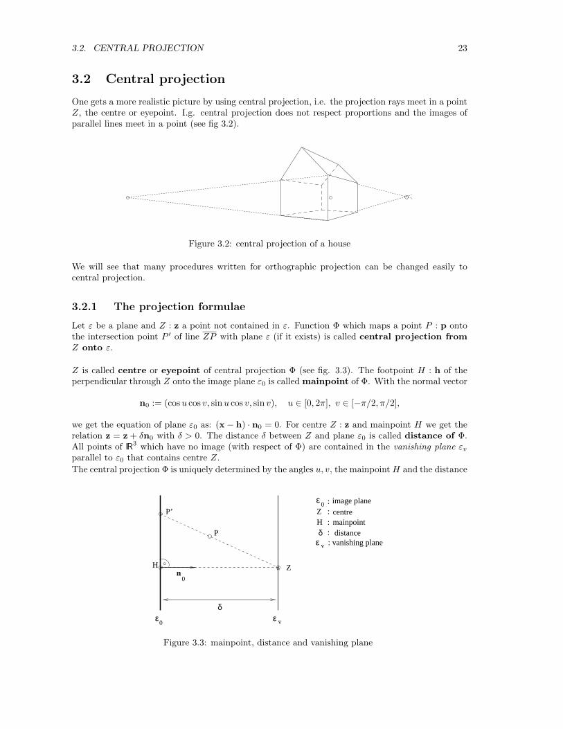
3.2 Central projection
One gets a more realistic picture by using central projection, i.e. the projection rays meet in a pointZ, the centre or eyepoint. I.g. central projection does not respect proportions and the images ofparallel lines meet in a point (see fig 3.2).
Figure 3.2: central projection of a house
We will see that many procedures written for orthographic projection can be changed easily tocentral projection.
3.2.1 The projection formulae
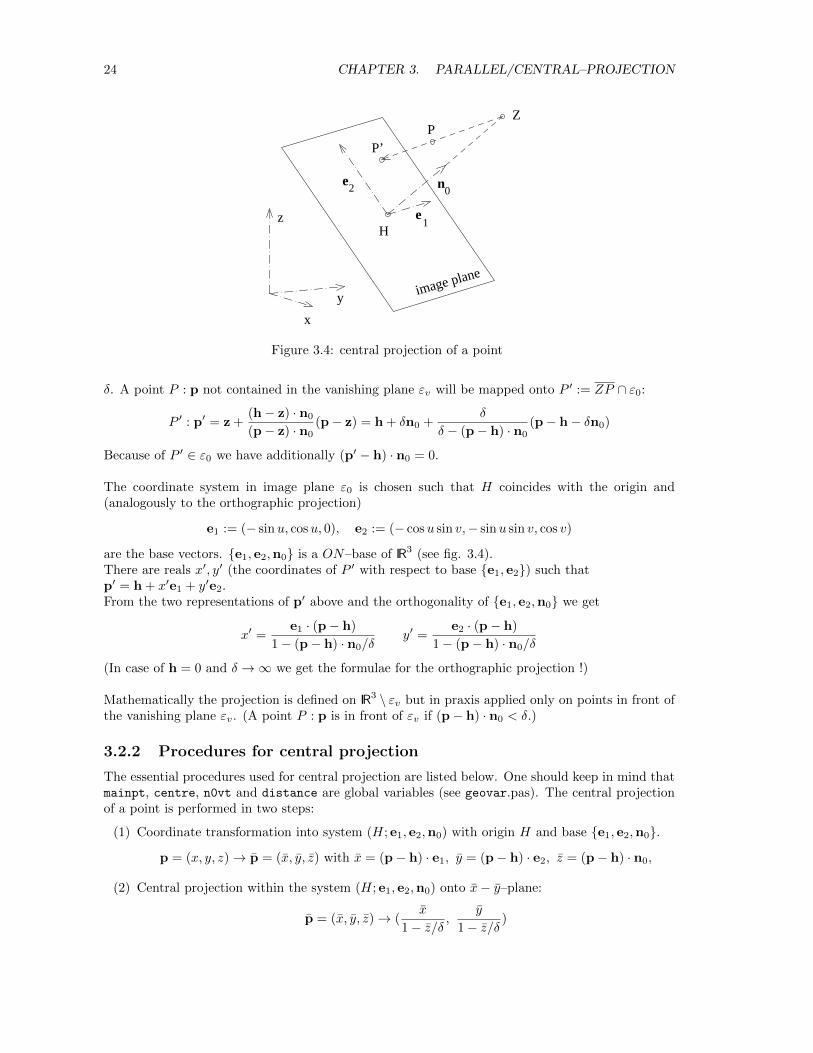
Let ε be a plane and Z : z a point not contained in ε. Function Φ which maps a point P : p ontothe intersection point P ′ of line ZP with plane ε (if it exists) is called central projection fromZ onto ε.
Z is called centre or eyepoint of central projection Φ (see fig. 3.3). The footpoint H : h of theperpendicular through Z onto the image plane ε0 is called mainpoint of Φ. With the normal vector
n0 := (cosu cos v, sinu cos v, sin v), u ∈ [0, 2π], v ∈ [−π/2, π/2],
we get the equation of plane ε0 as: (x− h) · n0 = 0. For centre Z : z and mainpoint H we get therelation z = z + δn0 with δ > 0. The distance δ between Z and plane ε0 is called distance of Φ.All points of IR3 which have no image (with respect of Φ) are contained in the vanishing plane εvparallel to ε0 that contains centre Z.
The central projection Φ is uniquely determined by the angles u, v, the mainpointH and the distance
0
0
: vanishing plane
ε v
vε
H Zn
δ
0
HZ
:::
δ
image plane
centremainpointdistance
ε
ε
P
P’
:
Figure 3.3: mainpoint, distance and vanishing plane
24 CHAPTER 3. PARALLEL/CENTRAL–PROJECTION
Z
H
x
y
z
n
e
e
1
02
PP’
image plane
Figure 3.4: central projection of a point
δ. A point P : p not contained in the vanishing plane εv will be mapped onto P ′ := ZP ∩ ε0:
P ′ : p′ = z +(h− z) · n0
(p− z) · n0(p− z) = h + δn0 +
δ
δ − (p− h) · n0(p− h− δn0)
Because of P ′ ∈ ε0 we have additionally (p′ − h) · n0 = 0.
The coordinate system in image plane ε0 is chosen such that H coincides with the origin and(analogously to the orthographic projection)
e1 := (− sinu, cosu, 0), e2 := (− cosu sin v,− sinu sin v, cos v)
are the base vectors. {e1, e2,n0} is a ON–base of IR3 (see fig. 3.4).There are reals x′, y′ (the coordinates of P ′ with respect to base {e1, e2}) such thatp′ = h + x′e1 + y′e2.From the two representations of p′ above and the orthogonality of {e1, e2,n0} we get
x′ =e1 · (p− h)
1− (p− h) · n0/δy′ =
e2 · (p− h)
1− (p− h) · n0/δ
(In case of h = 0 and δ →∞ we get the formulae for the orthographic projection !)
Mathematically the projection is defined on IR3 \ εv but in praxis applied only on points in front ofthe vanishing plane εv. (A point P : p is in front of εv if (p− h) · n0 < δ.)
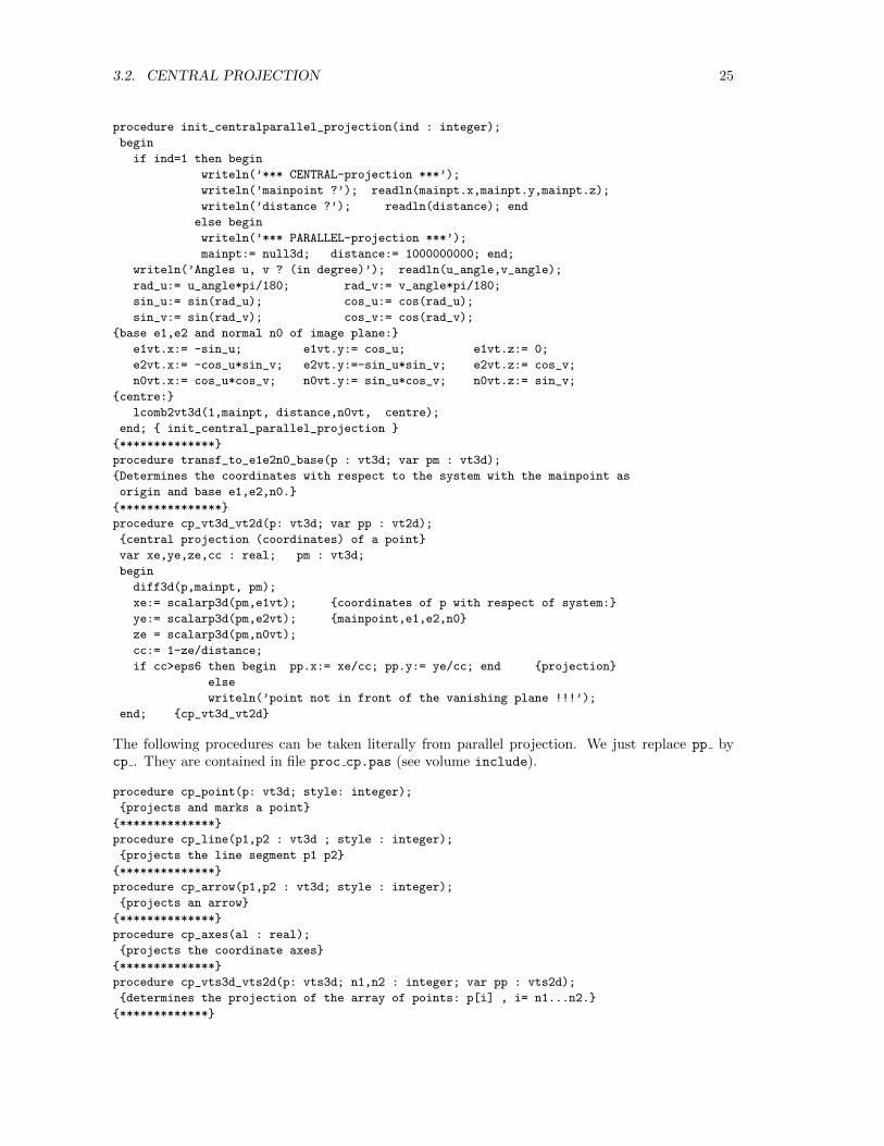
3.2.2 Procedures for central projection
The essential procedures used for central projection are listed below. One should keep in mind thatmainpt, centre, n0vt and distance are global variables (see geovar.pas). The central projectionof a point is performed in two steps:
(1) Coordinate transformation into system (H; e1, e2,n0) with origin H and base {e1, e2,n0}.
p = (x, y, z)→ p = (x, y, z) with x = (p− h) · e1, y = (p− h) · e2, z = (p− h) · n0,
(2) Central projection within the system (H; e1, e2,n0) onto x− y–plane:
p = (x, y, z)→ (x
1− z/δ,
y
1− z/δ)
3.2. CENTRAL PROJECTION 25
procedure init_centralparallel_projection(ind : integer);
begin
if ind=1 then begin
writeln(’*** CENTRAL-projection ***’);
writeln(’mainpoint ?’); readln(mainpt.x,mainpt.y,mainpt.z);
writeln(’distance ?’); readln(distance); end
else begin
writeln(’*** PARALLEL-projection ***’);
mainpt:= null3d; distance:= 1000000000; end;
writeln(’Angles u, v ? (in degree)’); readln(u_angle,v_angle);
rad_u:= u_angle*pi/180; rad_v:= v_angle*pi/180;
sin_u:= sin(rad_u); cos_u:= cos(rad_u);
sin_v:= sin(rad_v); cos_v:= cos(rad_v);
{base e1,e2 and normal n0 of image plane:}
e1vt.x:= -sin_u; e1vt.y:= cos_u; e1vt.z:= 0;
e2vt.x:= -cos_u*sin_v; e2vt.y:=-sin_u*sin_v; e2vt.z:= cos_v;
n0vt.x:= cos_u*cos_v; n0vt.y:= sin_u*cos_v; n0vt.z:= sin_v;
{centre:}
lcomb2vt3d(1,mainpt, distance,n0vt, centre);
end; { init_central_parallel_projection }
{**************}
procedure transf_to_e1e2n0_base(p : vt3d; var pm : vt3d);
{Determines the coordinates with respect to the system with the mainpoint as
origin and base e1,e2,n0.}
{***************}
procedure cp_vt3d_vt2d(p: vt3d; var pp : vt2d);
{central projection (coordinates) of a point}
var xe,ye,ze,cc : real; pm : vt3d;
begin
diff3d(p,mainpt, pm);
xe:= scalarp3d(pm,e1vt); {coordinates of p with respect of system:}
ye:= scalarp3d(pm,e2vt); {mainpoint,e1,e2,n0}
ze = scalarp3d(pm,n0vt);
cc:= 1-ze/distance;
if cc>eps6 then begin pp.x:= xe/cc; pp.y:= ye/cc; end {projection}
else
writeln(’point not in front of the vanishing plane !!!’);
end; {cp_vt3d_vt2d}
The following procedures can be taken literally from parallel projection. We just replace pp bycp . They are contained in file proc cp.pas (see volume include).
procedure cp_point(p: vt3d; style: integer);
{projects and marks a point}
{**************}
procedure cp_line(p1,p2 : vt3d ; style : integer);
{projects the line segment p1 p2}
{**************}
procedure cp_arrow(p1,p2 : vt3d; style : integer);
{projects an arrow}
{**************}
procedure cp_axes(al : real);
{projects the coordinate axes}
{**************}
procedure cp_vts3d_vts2d(p: vts3d; n1,n2 : integer; var pp : vts2d);
{determines the projection of the array of points: p[i] , i= n1...n2.}
{*************}
26 CHAPTER 3. PARALLEL/CENTRAL–PROJECTION
procedure cp_curve(p: vts3d; n1,n2,style : integer);
{projects a 3D-ngon}
{*************}
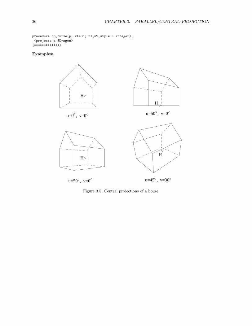
Examples:
u=0 , v=0 u=50 , v=0
u=50 , v=0 u=45 , v=30
H
H
HH
Figure 3.5: Central projections of a house
Chapter 4
CURVES
4.1 Planar Curves
4.1.1 Definition and Representations of Planar Curves
Definition 4.1 A planar curve Γ is the image of a real interval I by a locally injective C0 functionx into IR2:
Γ := {x(t)| t ∈ I}.
Definition 4.2 A regular planar curve Γ is the image of a real interval I by a C1 function x intoIR2:
Γ := {x(t)| t ∈ I} and x(t) 6= 0 for t ∈ I.x(t) is a tangent vector at curve point x(t).x is a regular parametric representation of Γ. The representation is of class Cn if x(t) is Cn.
Example 4.1 x(t) = (t, t2)>, t ∈ [0, 1] (arc of the unit parabola y = x2). The parametric repre-sentation is regular.
The parametric representation of a regular curve is not unique ! The parabola arc above for instancecan be represented byb) x(t) = (t2, t4)>, t ∈ [0, 1], c) x(t) = ( 2t
1+t , (· · · )2)>, t ∈ [0, 1], too.
Representation b) is not regular (because of x(0) = (0, 0)>), c) is regular.
Definition 4.3 A regular implicit plane curve is a non empty subset Γ ⊂ IR2 of the form
f : IR2 ⊃ D → IR, Γ : {x ∈ D|f(x) = 0}, ∇f(x) 6= 0 for x ∈ Γ,
where f is a C1–function. For a curve point x vector ∇f(x) is a normal vector.f(x) = 0 is a regular implicit representation of Γ. The representation is of class Cn if f is Cn.
Example 4.2 Γ : {x ∈ IR2|f(x) := x2 + y2 − 1 = 0} (unit circle).
Obviously, the implicit representation of a curve is not unique, too. For instanceb) f(x) :=
√x2 + y2 − 1 = 0, c) f(x) := (x2 + y2 − 1)2 =0
represent the unit circle implicitly, too. Representation b) is regular, c) is not regular.
27
28 CHAPTER 4. CURVES
Definition 4.4 The representation of a curve is called explicit if one of the coordinates x, y is afunction of the remaining coordinate.
Example 4.3 y = x2, x ∈ [0, 1] is an explicit representation of an arc of the unit parabola.
The following (theoretical) results show that the representations can be changed locally. The proofsrely on the implicit function theorem.
Lemma 4.1 Let Γ be a curve with a regular Cn-continuous implicit (parametric) representationand x0 a point of Γ. Then there exists locally a Cn-continuous explicit representation of Γ at x0.Hence there exists locally a regular parametric (implicit) representation, which is Cn–continuous,too.
Proof: a) Let be f(x, y) = 0 with ∇f(x0) 6= 0 a regular implicit representation of curve Γ.Without loss of generality we assume fy(x0) 6= 0. The implicit function theorem guarantees ina vicinity of x0 the existence of a Cn–continuous function y(x) such that f(x, y(x)) = 0 andy′(x) = −fx(x, y)/fy(x, y), .... Hence y = y(x) is locally an explicit Cn–representation.b) Let be x(t) = (x(t), y(t))> a regular parameterization of Γ with x(t0) = x0. With out loss ofgenerality we assume x(t0) 6= 0. Hence equation x− x(t) = 0 can be solved in a vicinity of t0 for t.With solution t(x) we get the explicit representation y = y(t(x)), which is Cn–continuous, too.From an explicit representation one derives easily both a parametric and an implicit representation.For example: From y = y(x) we get the parametric representation (x, y(x))> and the implicit rep-resentation y − y(x) = 0. 2
4.1.2 Arc length and curvature of a planar curve
Definition 4.5 Let Γ : x = x(t), t ∈ [a, b], be a regular curve. s(t) :=∫ ta
√x2 + y2dt is the arc
length of the arc between the points x(a) and x(t). Because of s(t) =√x2 + y2 > 0 function s(t)
is strictly monotone increasing and the equation s− s(t) = 0 can be solved for t (theoretically) ands used for a standard representation, the arc length representation: x = x(s) := x(t(s)) with itscharacteristic property ‖dxds ‖ = 1.In order to indicate the usage of the arc length as parameter one denotes the derivatives by a prime:x′ = dx
ds .
Definition 4.6 Let x(s) be the arc length parameterization of a regular C2-continuous curve. Anessential property is x′ · x′′ = 0, which is a direct consequence of x′ · x′ = 1.The curvature vector x′′ describes the change of the unit tangent vector t := x′ with respect to thearc length and is perpendicular to the tangent vector. If n(t) is any unit normal vector, one getsthe oriented curvature k = x′′ · n.(For example n(t) := (−y(t), x(t))>/‖ · · · ‖. The usage of x′′/‖x′′‖ as unit normal is possible if thecurvature is not 0.)A point with k = 0 is called inflection point.
Lemma 4.2 For the change of the unit normal we get: n′ = −kx′.
Proof: Let be n := (−y′, x′)> the unit normal (parameterized by the arc length). Hence n′ =(−y′′, x′′)> is a tangent vector and n′ · x′ = −x′y′′ + y′x′′ = −x′′ · n = −k.The choice n := (y′,−x′)> yields the same result. 2
4.1. PLANAR CURVES 29
Remark:When dealing with normalforms (see Section 4.1.4.2) one should remember the statement of thelast lemma.
Lemma 4.3 a) Let Γ : x = x(t) = (x(t), y(t))>, t ∈ [a, b], be a regular (parametric) C2–continuouscurve with unit normal n(t). The curvature vector x′′ and the curvature k at point x(t) are:
x′′ =xx2 − (x · x)x
‖x‖4=
x · n‖x‖2
n, k =x · n‖x‖2
=det(x, x)
‖x‖3, for n =
(−y, x)>
‖x‖.
b) Let Γ : y = f(x), x ∈ [a, b], be a regular (explicit) C2–continuous curve. The curvature vectorx′′and the curvature k at point (x, f(x)) are:
x′′ =f ′′(x)
(1 + f ′(x)2)3/2
(−f ′(x), 1)>√1 + f ′(x)2
, k(x) =f ′′(x)
(1 + f ′(x)2)3/2.
c) Let Γ : f(x, y) = 0, (x, y) ∈ D ⊂ IR2 be a regular (implicit) C2–continuous curve. The curvaturevector x′′ and the curvature k at point (x, y) are:
x′′ =−fxxf2
y + 2fxfyfxy − fyyf2x
(f2x + f2
y )3/2
∇f‖∇f‖
, k =−fxxf2
y + 2fxfyfxy − fyyf2x
(f2x + f2
y )3/2.
Proof: a) Differentiating x′ = x‖x‖ for the arc length s we get
dx′
ds=dx′
dt
1
ds/dt=
x
‖x‖2− (x · x)x
‖x‖4=
x · n‖x‖2
n,
which is result a).b) Applying a) to the parametric curve x(t) := (t, f(t))> we get result b).c) Because the representation of the implicit curve is regular f(x, y) = 0 can be solved locally forx or y. Without loss of generality we assume: fy(x0, y0) 6= 0, (x0, y0) ∈ Γ. The implicit func-tion theorem guarantees the existence of a function y(x) such that in a vicinity of x0 the equationf(x, y(x)) = 0 holds. Differentiating implicitly yields: y′(x) = −fx(x, y(x))/fy(x, y(x)). Analo-gously we get y′′ = −(fxxf
2y − 2fxyfxfy + fyyf
2x)/f3
y . Using result b) yields result c). 2
Example 4.4 a) For the unit parabola y = f(x) = x2 we get:
x′′ =(−2x, 1)√
1 + 4x2
2
(1 + 4x2)3/2, k(x) =
2
(1 + 4x2)3/2.
b) For an arbitrary circle f(x) = (x− xm)2 − r2 = 0 we get:∇f(x) = 2(x− xm), ‖∇f(x)‖ = 2r, fxx = fyy = 2, fxy = 0, and x′′ = xm − x, k = 1/r.
Definition 4.7 Let Γ be a regular C2–curve and x0 ∈ Γ not an inflection point.
a)The circle cx0: (x − x0 −
x′′(x0)
(x′′(x0))2)2 − 1
(x′′(x0))2= 0 is called osculating circle, its midpoint
centre of curvature at x0.b)The parabola px0
: x = x0 + sx′(x0) + s2
2 x′′(x0) is called the osculating parabola at point x0.
cx0and px0
are tangent to Γ in x0 (i.e. Γ, cx0and px0
have point x0 and the tangent at this pointin common) and have at x0 the same curvature vector as Γ.
30 CHAPTER 4. CURVES
4.1.3 Offset Curves
Definition 4.8 Let Γ : x = x(t) = (x(t), y(t))>, t ∈ [a, b], be a regular (parametric) C2–continuous
curve, n(t) =(y(t),−x(t))>√x(t)2 + y(t)2
(unit normal) and fixed d ∈ IR.
Then Γd : x = x(t) + dn(t) is called offset curve of Γ with distance d.
The offset curve Γd depends only on curve Γ as a point set in IR2 and distance d.
Lemma 4.4 Let Γ : x = x0(t) = (x(t), y(t))>, t ∈ [a, b], be a regular Cn–continuous curve, n ≥ 3,with unit normal n0(t), the oriented curvature k0(t) = x′′ · n at point x(t) (x′: unit tangent vector,x′′: curvature vector) and d ∈ IR such that 1−dk0(t) > 0 then the offset curve Γd : x = x0(t)+dn0(t)
(s. definition above) is regular of class Cn−1, and the curvature is kd(t) =k0(t)
1− dk0(t).
Proof: Without loss of generality we assume Γ0 is parameterized by arc length. From Lemma 4.2we get n′0(s) = −k0(s)x′0(s). Differentiating the parametric representation Γd : x = x0(s) + dn0(s)of the offset curve yieldsx = x′0(s) + dn′0(s) = (1− dk0(s))x′0(s) and x = −dk′0(s)x′0(s) + (1− dk0(s))x′′0(s).The unit normal vector of the offset curve agrees with n0. Hence the curvature of offset curve Γd isx · n0
‖x‖2=
(1− dk0)x′0 · n0
(1− dk0)2=
k0
1− dk0which proves the statement of the lemma. 2
4.1.4 The normalform of a planar curve
4.1.4.1 Definition of the normalform
In order to get a normalized implicit representation (comparable with the normalized arc lengthparametric representation) we extend the idea of the HESSE–normalform for lines to curves.
Definition 4.9 The implicit representation h(x) = n · x − d = 0, ‖n‖ = 1 of a line g in IR2 iscalled HESSE normalform of line g.(h(x) describes the oriented distance of point x to the line g.)
Definition 4.10 An implicit representation h(x) = 0 of a curve Γ in IR2 with ‖∇h‖ = 1 in avicinity of Γ is called normalform of curve Γ. (We regard h = 0 and −h = 0 as the same normal-forms.)h is called normalform function or, because of its geometric meaning, oriented distance function.
Example 4.5 h(x, y) :=√x2 + y2 − r = 0 is the normalform of the circle x2 + y2 = r2.
If the given curve is smooth enough, then its normalform always exists (theoretically).
Theorem 4.1 For any Cn-continuous, n ≥ 2, planar curve Γ there exists in a vicinity V of Γthe oriented distance function h and h is of class Cn, too. Hence Γ has an implicit representationh(x) = 0 such that ‖∇h‖ = 1 on V .On V function h has the properties: 1) h(x + δ∇h(x)) = h(x) + δ, 2) ∇h(x + δ∇h(x)) = ∇h(x).
4.1. PLANAR CURVES 31
Proof: Let the Cn–curve Γ, n ≥ 2, be parameterized by the arc length s:x = x0(s) = (x(s), y(s))>, s ∈ [a, b] , with unit normal n0(s) := (−y′(s), x′(s))>, curvature k0(s)andΓd : x = x0(s) + dn0(s) its offset curve with (oriented) distance d.The vector equation F (s, d, x, y) := x0(s)+dn0(s)−x=0 can be solved for s and d if det(Fs, Fd) 6= 0.With n′0(s) = −k0(s)x′0(s) (see Lemma 4.2) we getdet(Fs, Fd) = det(x′0 + dn′0,n0) = det((1− dk0)x′0,n0) = (1− dk0) 6= 0in a vicinity V : −v ≤ d ≤ v, v > 0 of curve Γ.Due to the implicit function theorem there exist functions s(x, y) and d(x, y) such that the followingequation is fulfilled in the vicinity V of curve Γ:x0(s(x, y)) + d(x, y)n0(s(x, y)) = x. Differentiating this equation for x, y yields
∇s x′>0 +∇d n>0 + d ∇s n′
>0 =
(1 00 1
)(recognize:
(a1a2
)(b1b2
)>=(a1b1 a2b1a1b2 a2b2
)).
Multiplying this matrix equation by n0 and respecting x′>0 n0 = n′
>0 n0 = 0, n>0 n0 = 1 we get
∇d = n0. Hence function d(x, y) is of class Cn, too.In order to distinguish function d(x, y) and distance parameter d we set h(x, y) := d(x, y).For points x with the same foot point x0 have the same gradient ∇h(x). Hence we get the essentialproperties of the distnace function h:1) h(x + δ∇h(x)) = h(x) + δ, 2) ∇h(x + δ∇h(x)) = ∇h(x). 2
The proof of the uniqueness of the normalform function h is omitted.
Properties 1),2) of the last theorem show that h and ∇h can be evaluated numerically at point xby determining the foot point x0 and its unit normal n0 of point x on curve Γ:h(x) = (x− x0) · n0, ∇h(x) = n0.
4.1.4.2 On the first and second derivatives of the distance function
Let be Γ a C2–continuous planar curve with normalform h = 0 and x = c(s) its arc lengthparameterization with unit normal n(s) = ∇h(c(s)). Hence h(c(s)) = 0. Differentiating thisequation yields
(1) ∇h · c′ = 0, (2) c′>Hhc
′ +∇h · c′′ = 0.
From the second equation we get the following result:The curvature of curve Γ is:
k = ∇h · c′′ = −c′>Hhc
′.
• Differentiating (∇h)2 = 1 yields Hh∇h = 0.Hence one eigenvalue of the Hessian matrix Hh is λ1 = 0 with eigenvector ∇h. There existsa second eigenvalue λ2 = κ with the tangent vector t := (−hy, hx)> as eigenvector andt>Hht = κ. Hence κ is the negative curvature of curve Γ:
−k = κ = t>Hht = h2yhxx − 2hxhyhxy + h2
xhyy.
• The characteristic polynomial of Hh is λ2 − (hxx + hyy)λ and
det(Hh) = 0, κ = hxx + hyy and H2h = κHh.
• The Hessian matrix Hh of the normalform function h at a curve point can be expressed by thegradient ∇h (unit normal) and the curvature k (The three coefficients of Hh are the solutionof the linear system Hh∇h = 0, t>Hht = −k):
Hh = −k(
h2y −hxhy
−hxhy h2x
)= −k(I −∇h∇h>),
with 2× 2 unit matrix I. ∇h> is the transpose of the column vector ∇h.
32 CHAPTER 4. CURVES
4.1.4.3 Normalform of an implicit curve
Let Γ : f(x, y) = 0 be a regular implicit curve with continuous second derivatives of function f andh its normalform function.For a curve point we get
1. h = 0,
2. ∇h =∇f‖∇f‖
,
3. −k =f2y fxx − 2fxfyfxy + f2
xfyy
(f2x + f2
y )3/2, (see Lemma 4.3),
Hh = −k(
h2y −hxhy
−hxhy h2x
)=
f2yfxx−2fxfyfxy+f2
xfyy
‖∇f‖5
(f2y −fxfy
−fxfy f2x
).
For a point x in the vicinity of the curve with foot point x0 ∈ Γ we get:
1. ∇h(x) = ∇h(x0),
2. h(x) = (x− x0) · ∇h(x0)
3. Hh(x) =−k(x0)
1− h(x)k(x0)
(h2y(x0) −hx(x0)hy(x0)
−hx(x0)hy(x0) h2x(x0)
)=
Hh(x0)
1− h(x)k(x0).
4.1.4.4 Normalform of a parametric curve
Let Γ : x = x(t) = (x(t), y(t))> be a regular parametric curve with continuous second derivativesand h its normalform function.For a curve point x(t) = (x(t), y(t))> we get
h(x) = 0, ∇h(x) =(−y, x)>
‖x‖and from k = (x · ∇h)/‖x‖2 = −xy+yx
‖|x‖3 we get
Hh(x) =xy − yx‖x‖5
(x2 xyxy y2
).
For a point in the vicinity of curve Γ: apply the analogous part of an implicit curve (see above).
4.2 Displaying Parametric Curves in IR2
For displaying a parametric curve we move through the parameter interval by not necessary equidis-tant steps, calculate a sequence of points and draw the polygon by procedure curve2d.
Example 4.6 a) ellipse: (a cos t, b sin t)>, 0 ≤ t ≤ 2πb) cycloids: c(t) = (x(t), y(t))>, 0 ≤ t ≤ 2π with
x(t) = (a+ b) cos t− λa cos((a+ b)t/a)
y(t) = (a+ b) sin t− λa sin((a+ b)t/a) b > 0, a+ b > 0, λ > 0.
(see Fig. 4.1.)In general parameter t is not the arc length and the distances of neighboured points may vary ina wide range. This behaviour can be omitted if function c(t) is differentiable and one chooses thestep length dependent of the “velocity” c(t). In order to get distances ≈ s we consider the Taylorexpansion for c(t)
c(ti+1) ≈ c(ti) + c(ti)∆ti, ∆ti+1 = ti+1 − ti.
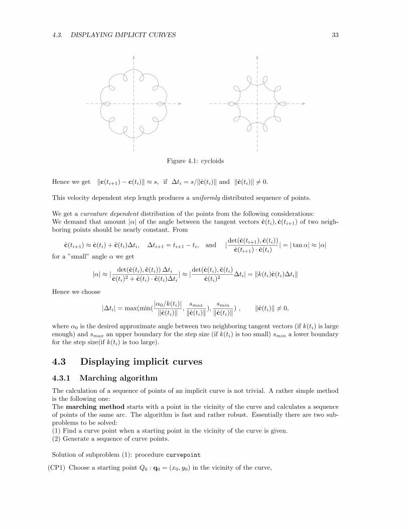
4.3. DISPLAYING IMPLICIT CURVES 33
Figure 4.1: cycloids
Hence we get ‖c(ti+1)− c(ti)‖ ≈ s, if ∆ti = s/‖c(ti)‖ and ‖c(ti)‖ 6= 0.
This velocity dependent step length produces a uniformly distributed sequence of points.
We get a curvature dependent distribution of the points from the following considerations:We demand that amount |α| of the angle between the tangent vectors c(ti), c(ti+1) of two neigh-boring points should be nearly constant. From
c(ti+1) ≈ c(ti) + c(ti)∆ti, ∆ti+1 = ti+1 − ti, and |det(c(ti+1), c(ti))
c(ti+1) · c(ti)| = | tanα| ≈ |α|
for a ”small” angle α we get
|α| ≈ | det(c(ti), c(ti)) ∆tic(ti)2 + c(ti) · c(ti)∆ti
| ≈ |det(c(ti), c(ti)
c(ti)2∆ti| = ‖k(ti)c(ti)∆ti‖
Hence we choose
|∆ti| = max(min(|α0/k(ti)|‖c(ti)‖
,smax‖c(ti)‖
),smin‖c(ti)‖
) , ‖c(ti)‖ 6= 0,
where α0 is the desired approximate angle between two neighboring tangent vectors (if k(ti) is largeenough) and smax an upper boundary for the step size (if k(ti) is too small) smin a lower boundaryfor the step size(if k(ti) is too large).
4.3 Displaying implicit curves
4.3.1 Marching algorithm
The calculation of a sequence of points of an implicit curve is not trivial. A rather simple methodis the following one:The marching method starts with a point in the vicinity of the curve and calculates a sequenceof points of the same arc. The algorithm is fast and rather robust. Essentially there are two sub-problems to be solved:(1) Find a curve point when a starting point in the vicinity of the curve is given.(2) Generate a sequence of curve points.
Solution of subproblem (1): procedure curvepoint
(CP1) Choose a starting point Q0 : q0 = (x0, y0) in the vicinity of the curve,
34 CHAPTER 4. CURVES
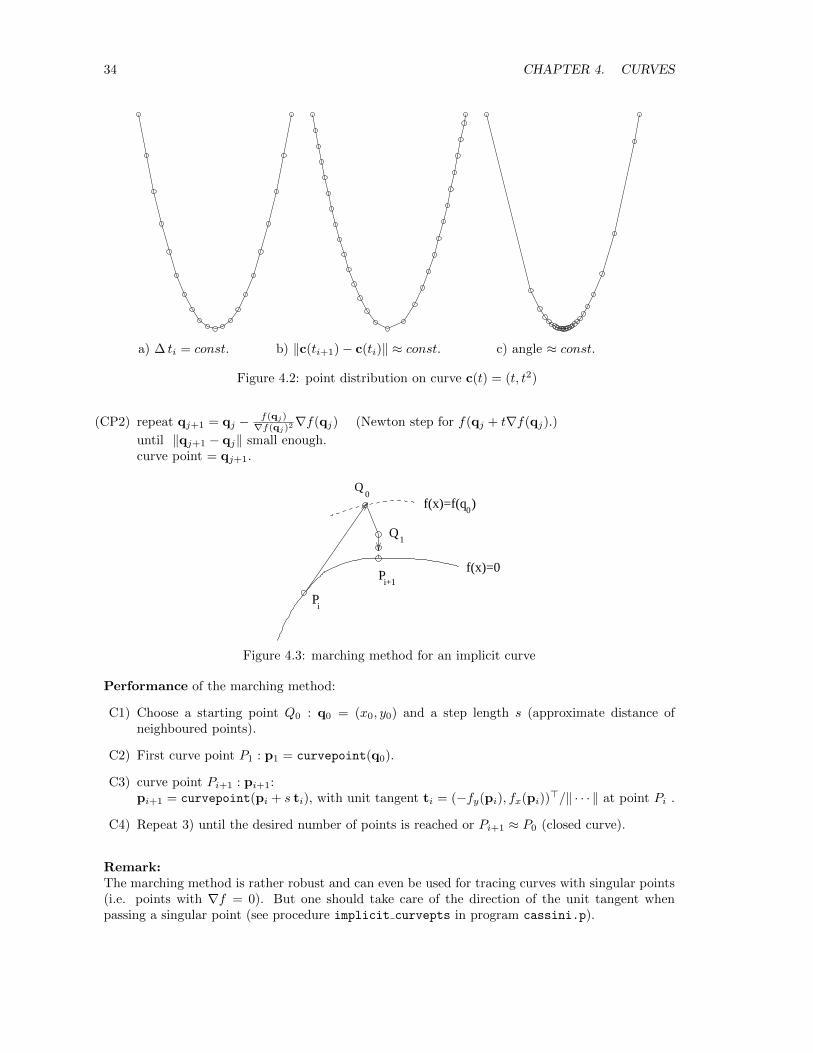
a) ∆ ti = const. b) ‖c(ti+1)− c(ti)‖ ≈ const. c) angle ≈ const.
Figure 4.2: point distribution on curve c(t) = (t, t2)
(CP2) repeat qj+1 = qj − f(qj)∇f(qj)2∇f(qj) (Newton step for f(qj + t∇f(qj).)
until ‖qj+1 − qj‖ small enough.curve point = qj+1.
Q0
Pi
P
Q
f(x)=0
f(x)=f(q )0
1
i+1
Figure 4.3: marching method for an implicit curve
Performance of the marching method:
C1) Choose a starting point Q0 : q0 = (x0, y0) and a step length s (approximate distance ofneighboured points).
C2) First curve point P1 : p1 = curvepoint(q0).
C3) curve point Pi+1 : pi+1:pi+1 = curvepoint(pi + s ti), with unit tangent ti = (−fy(pi), fx(pi))
>/‖ · · · ‖ at point Pi .
C4) Repeat 3) until the desired number of points is reached or Pi+1 ≈ P0 (closed curve).
Remark:The marching method is rather robust and can even be used for tracing curves with singular points(i.e. points with ∇f = 0). But one should take care of the direction of the unit tangent whenpassing a singular point (see procedure implicit curvepts in program cassini.p).
4.3. DISPLAYING IMPLICIT CURVES 35
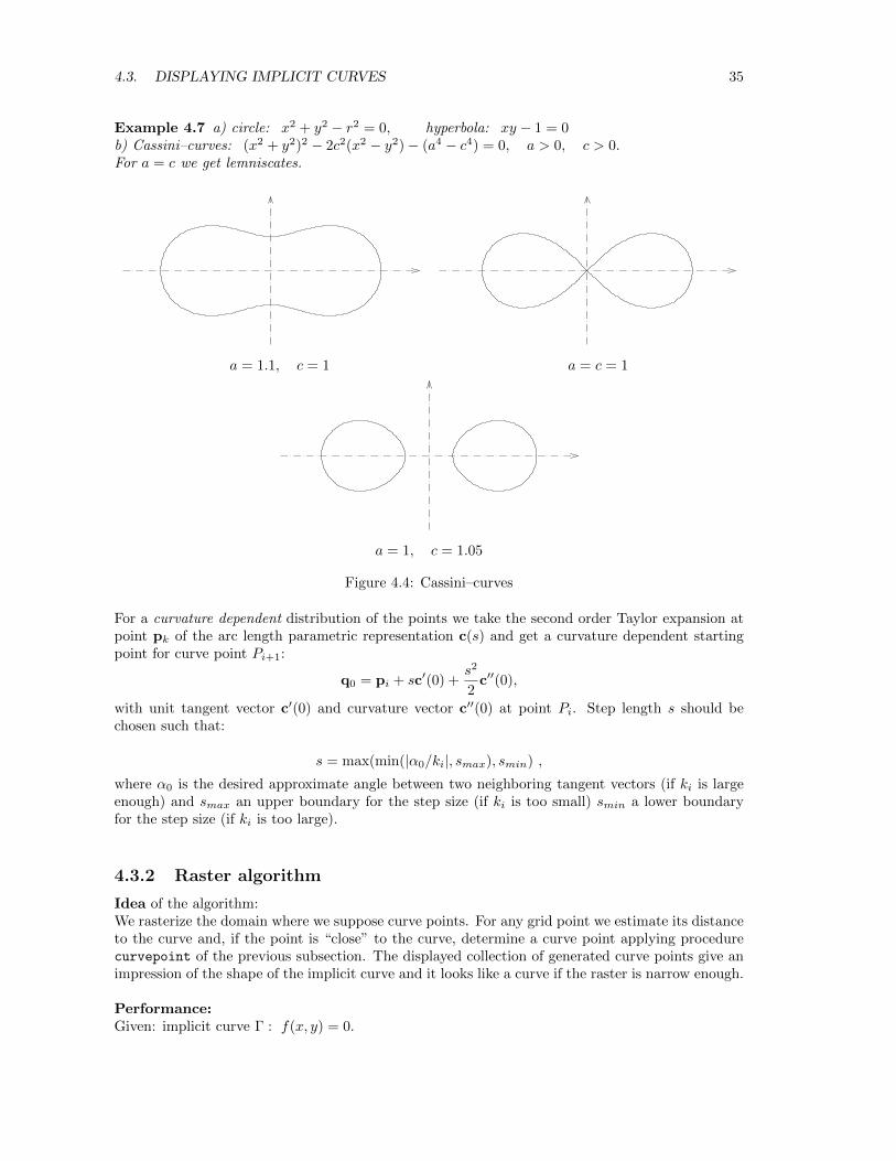
Example 4.7 a) circle: x2 + y2 − r2 = 0, hyperbola: xy − 1 = 0b) Cassini–curves: (x2 + y2)2 − 2c2(x2 − y2)− (a4 − c4) = 0, a > 0, c > 0.For a = c we get lemniscates.
a = 1.1, c = 1 a = c = 1
a = 1, c = 1.05
Figure 4.4: Cassini–curves
For a curvature dependent distribution of the points we take the second order Taylor expansion atpoint pk of the arc length parametric representation c(s) and get a curvature dependent startingpoint for curve point Pi+1:
q0 = pi + sc′(0) +s2
2c′′(0),
with unit tangent vector c′(0) and curvature vector c′′(0) at point Pi. Step length s should bechosen such that:
s = max(min(|α0/ki|, smax), smin) ,
where α0 is the desired approximate angle between two neighboring tangent vectors (if ki is largeenough) and smax an upper boundary for the step size (if ki is too small) smin a lower boundaryfor the step size (if ki is too large).
4.3.2 Raster algorithm
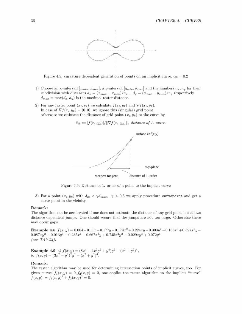
Idea of the algorithm:We rasterize the domain where we suppose curve points. For any grid point we estimate its distanceto the curve and, if the point is “close” to the curve, determine a curve point applying procedurecurvepoint of the previous subsection. The displayed collection of generated curve points give animpression of the shape of the implicit curve and it looks like a curve if the raster is narrow enough.
Performance:Given: implicit curve Γ : f(x, y) = 0.
36 CHAPTER 4. CURVES
Figure 4.5: curvature dependent generation of points on an implicit curve, α0 = 0.2
1) Choose an x–intervall [xmin, xmax], a y-intervall [ymin, ymax] and the numbers nx, ny for theirsubdivision with distances dx = (xmax − xmin)/nx , dy = (ymax − ymin)/ny respectively.dmax = max(dx, dy) is the maximal raster distance.
2) For any raster point (xi, yk) we calculate f(xi, yk) and ∇f(xi, yk).In case of ∇f(xi, yk) = (0, 0), we ignore this (singular) grid point.otherwise we estimate the distance of grid point (xi, yk) to the curve by
δik := |f(xi, yk)|/‖∇f(xi, yk)‖, distance of 1. order.
surface z=f(x,y)
x-y-plane
distance of 1. ordersteepest tangent
Figure 4.6: Distance of 1. order of a point to the implicit curve
3) For a point (xi, yk) with δik < γdmax, γ > 0.5 we apply procedure curvepoint and get acurve point in the vicinity.
Remark:The algorithm can be accelerated if one does not estimate the distance of any grid point but allowsdistance dependent jumps. One should secure that the jumps are not too large. Otherwise theremay occur gaps.
Example 4.8 f(x, y) = 0.004+0.11x−0.177y−0.174x2 +0.224xy−0.303y2−0.168x3 +0.327x2y−0.087xy2 − 0.013y3 + 0.235x4 − 0.667x3y + 0.745x2y2 − 0.029xy3 + 0.072y4
(aus TAU’94).
Example 4.9 a) f(x, y) = (8x4 − 4x2y2 + y4)y2 − (x2 + y2)4,b) f(x, y) = (3x2 − y2)2y2 − (x2 + y2)4.
Remark:The raster algorithm may be used for determining intersection points of implicit curves, too. Forgiven curves f1(x, y) = 0, f2(x, y) = 0, one applies the raster algorithm to the implicit “curve”f(x, y) := f1(x, y)2 + f2(x, y)2 = 0.
4.4. INTERSECTION OF TWO PLANAR CURVES 37
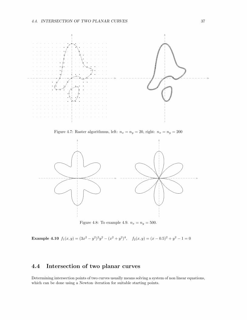
Figure 4.7: Raster algorithmus, left: nx = ny = 20, right: nx = ny = 200
Figure 4.8: To example 4.9. nx = ny = 500.
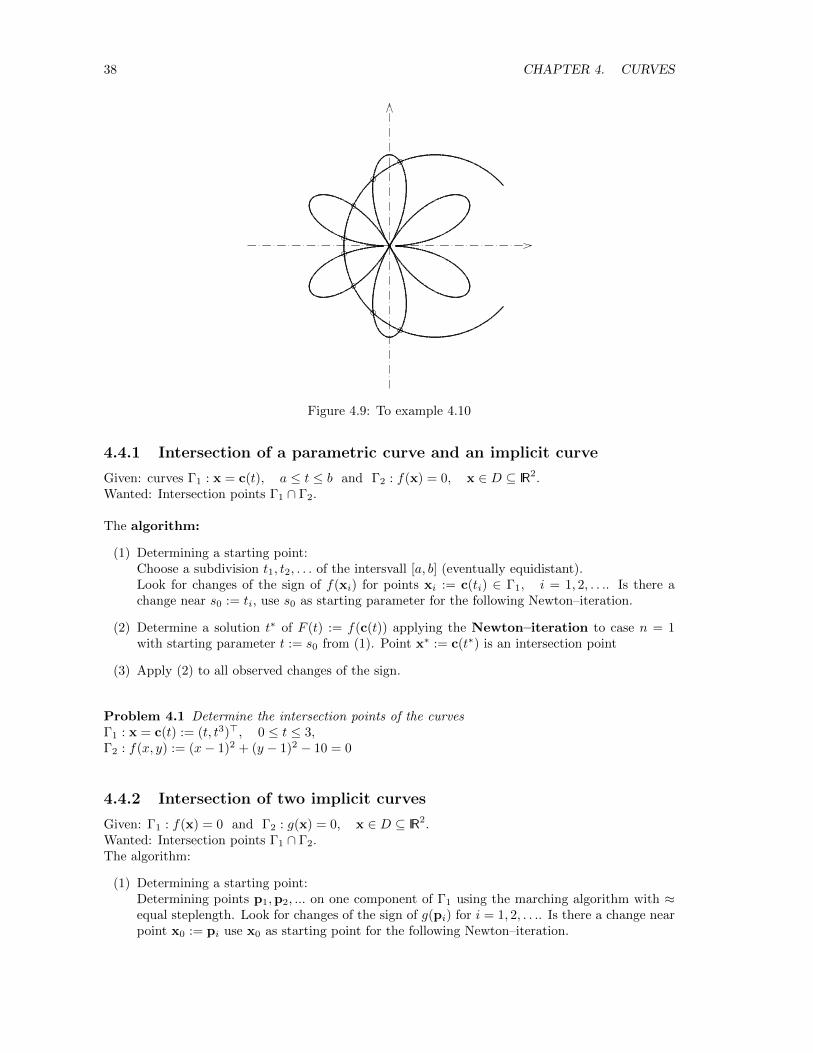
Example 4.10 f1(x, y) = (3x2 − y2)2y2 − (x2 + y2)4, f2(x, y) = (x− 0.5)2 + y2 − 1 = 0
4.4 Intersection of two planar curves
Determining intersection points of two curves usually means solving a system of non linear equations,which can be done using a Newton–iteration for suitable starting points.
38 CHAPTER 4. CURVES
Figure 4.9: To example 4.10
4.4.1 Intersection of a parametric curve and an implicit curve
Given: curves Γ1 : x = c(t), a ≤ t ≤ b and Γ2 : f(x) = 0, x ∈ D ⊆ IR2.Wanted: Intersection points Γ1 ∩ Γ2.
The algorithm:
(1) Determining a starting point:Choose a subdivision t1, t2, . . . of the intersvall [a, b] (eventually equidistant).Look for changes of the sign of f(xi) for points xi := c(ti) ∈ Γ1, i = 1, 2, . . .. Is there achange near s0 := ti, use s0 as starting parameter for the following Newton–iteration.
(2) Determine a solution t∗ of F (t) := f(c(t)) applying the Newton–iteration to case n = 1with starting parameter t := s0 from (1). Point x∗ := c(t∗) is an intersection point
(3) Apply (2) to all observed changes of the sign.
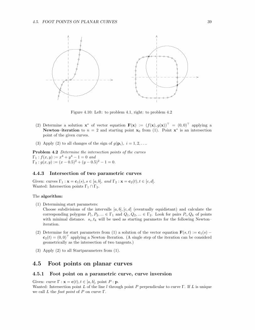
Problem 4.1 Determine the intersection points of the curvesΓ1 : x = c(t) := (t, t3)>, 0 ≤ t ≤ 3,Γ2 : f(x, y) := (x− 1)2 + (y − 1)2 − 10 = 0
4.4.2 Intersection of two implicit curves
Given: Γ1 : f(x) = 0 and Γ2 : g(x) = 0, x ∈ D ⊆ IR2.Wanted: Intersection points Γ1 ∩ Γ2.The algorithm:
(1) Determining a starting point:Determining points p1,p2, ... on one component of Γ1 using the marching algorithm with ≈equal steplength. Look for changes of the sign of g(pi) for i = 1, 2, . . .. Is there a change nearpoint x0 := pi use x0 as starting point for the following Newton–iteration.
4.5. FOOT POINTS ON PLANAR CURVES 39
Figure 4.10: Left: to problem 4.1, right: to problem 4.2
(2) Determine a solution x∗ of vector equation F(x) := (f(x), g(x))> = (0, 0)> applying aNewton–iteration to n = 2 and starting point x0 from (1). Point x∗ is an intersectionpoint of the given curves.
(3) Apply (2) to all changes of the sign of g(pi), i = 1, 2, . . ..
Problem 4.2 Determine the intersection points of the curvesΓ1 : f(x, y) := x4 + y4 − 1 = 0 andΓ2 : g(x, y) := (x− 0.5)2 + (y − 0.5)2 − 1 = 0.
4.4.3 Intersection of two parametric curves
Given: curves Γ1 : x = c1(s), s ∈ [a, b], and Γ2 : x = c2(t), t ∈ [c, d].Wanted: Intersection points Γ1 ∩ Γ2.
The algorithm:
(1) Determining start parameters:Choose subdivisions of the intervalls [a, b], [c, d] (eventually equidistant) and calculate thecorresponding polygons P1, P2, ... ∈ Γ1 and Q1, Q2, ... ∈ Γ2. Look for pairs Pi, Qk of pointswith minimal distance. si, tk will be used as starting parametrs for the following Newton–iteration.
(2) Determine for start parameters from (1) a solution of the vector equation F(s, t) := c1(s) −c2(t) = (0, 0)> applying a Newton–Iteration. (A single step of the iteration can be considerdgeometrically as the intersection of two tangents.)
(3) Apply (2) to all Startparameters from (1).
4.5 Foot points on planar curves
4.5.1 Foot point on a parametric curve, curve inversion
Given: curve Γ : x = c(t), t ∈ [a, b], point P : p.Wanted: Intersection point L of the line l through point P perpendicular to curve Γ. If L is uniquewe call L the foot point of P on curve Γ.
40 CHAPTER 4. CURVES
We assume that c(t) is C2 and foot point L is unique.
If Γ is a line x = q + tr: L : l = q + (p−q)·rr2 r.
In general we seek a point c(t) on Γ with: f(t) := (c(t)− p) · c(t) = 0.
The algorithm:
(1) Determining a starting parameter:Generate a nearly equidistant polygon Q1, Q2, ... and look for a point L0 := Qi with minimaldistance to P . Let t0 be its parameter, i.e. L0 : c(t0).
(2) Apply a Newton–iteration to equation f(t) := (c(t) − p) · c(t) = 0 with starting parameterfrom (1).f ′(t) = (c(t))2 + (c(t)− p) · c(t).(Second derivatives are used !) Or: Determine foot points on tangents succesively (only 1.derivatives are necessary.)
(2’) Let be Li the i-th approximation of the foot point and ti its corresponding parameter. x =c(ti) + ∆tc(ti) is the tangent line at point Li (linear approximation of c(t) !). Determinethe foot point of P on the tangent line. For the foot point on the tangent line we get∆t = (p−c(ti))c(ti)/c(ti)
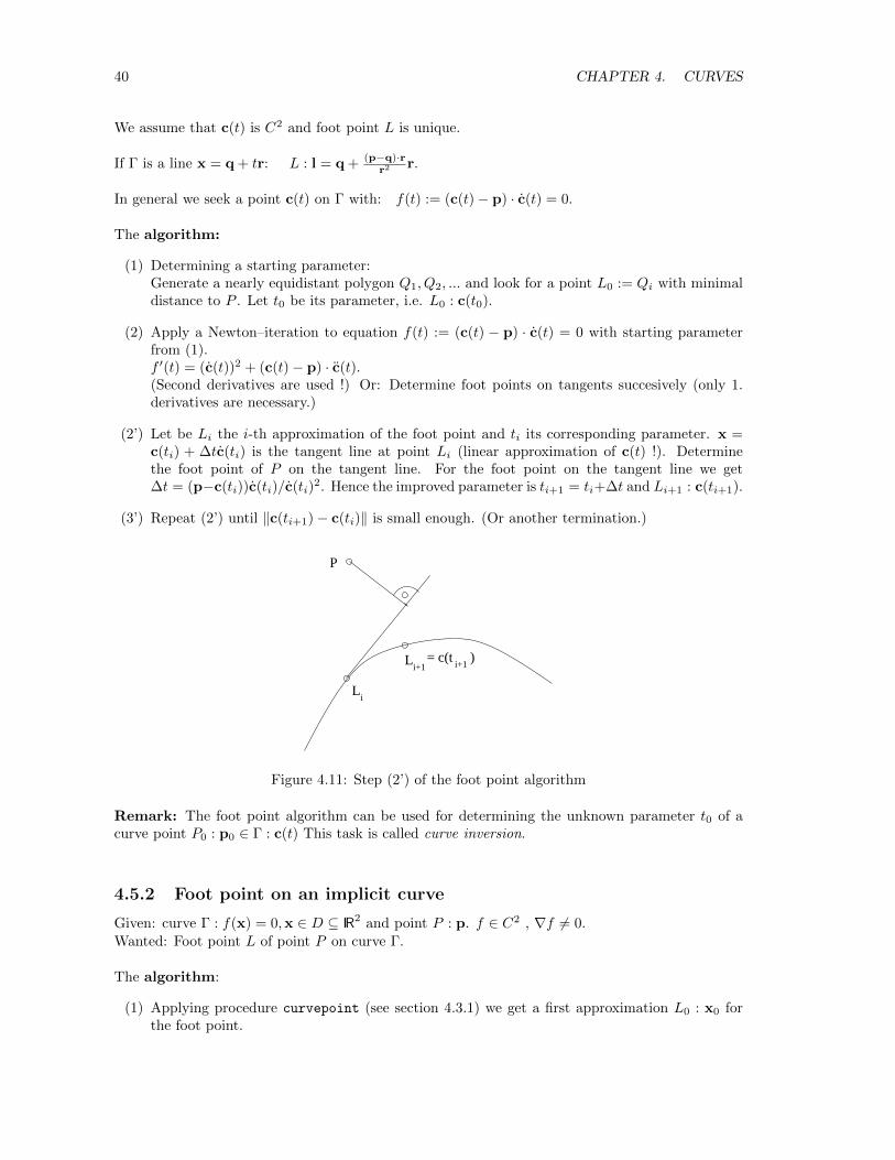
2. Hence the improved parameter is ti+1 = ti+∆t and Li+1 : c(ti+1).
(3’) Repeat (2’) until ‖c(ti+1)− c(ti)‖ is small enough. (Or another termination.)
= c(t )i+1
L
P
L
i
i+1
Figure 4.11: Step (2’) of the foot point algorithm
Remark: The foot point algorithm can be used for determining the unknown parameter t0 of acurve point P0 : p0 ∈ Γ : c(t) This task is called curve inversion.
4.5.2 Foot point on an implicit curve
Given: curve Γ : f(x) = 0,x ∈ D ⊆ IR2 and point P : p. f ∈ C2 , ∇f 6= 0.Wanted: Foot point L of point P on curve Γ.
The algorithm:
(1) Applying procedure curvepoint (see section 4.3.1) we get a first approximation L0 : x0 forthe foot point.
4.5. FOOT POINTS ON PLANAR CURVES 41
(2) The foot point is the solution of the system
(x− p) · (fy(x),−fx(x)) = 0, f(x) = 0.
(Where (fy(x), −fx(x)) is a tangent vector at curve point x.) This system will be solved bya Newton–iteration with starting point x0 from (1).(Second derivatives are needed !)Or: Determine foot points on tangents successively (first derivatives are used only).
(2’) Repeat ti+1 = p− (p− xi) · ∇f(xi)
∇f(xi)2∇f(xi)
> (foot point on tangent line),
xi+1 = curvepoint(ti+1).until ‖xi+1 − xi‖ is ”small” enough.L = xi+1.
Remark:While using the simple first order foot point algorithms there may occur problems consideringconvergence. Improved and rather stable first order algorithms are contained in the next subsection.
4.5.3 Stable first order foot point algorithms
For applying the normalform and its first two derivatives it is essential to have stable algorithmsfor determining foot points on curves. Here we give algorithms for parametric and implicit curveswhich use first order derivatives only. The heart of the algorithms is the combination of calculatingfoot points on tangents and approximate foot points on tangent parabolas. The curvature of thecurves is respected indirectly by the tangent parabolas.
4.5.3.1 Foot point algorithm for parametric curves
Let Γ : x(t) = c(t) be a smooth planar curve, p a point in the vicinity of Γ and t0 the parameter ofa starting point for the foot point algorithm:
repeatpi = c(ti)
∆t = (p−pi)·c(ti)c(ti)2
qi = pi + ∆tc(ti) (foot point on tangent)
pi+1 = c(ti + ∆t), f1 := qi − pi, f2 := pi+1 − qi,if ‖qi−pi‖ > ε then (one Newton step for the foot point on the tangent parabola x = pi+αf1+α2f2)a0 := (p− pi) · f1, a1 := 2f2 · (p− pi)− f2
1 , a2 := −3f1 · f2, a3 := −2f22
α := 1− a0 + a1 + a2 + a3
a1 + 2a2 + 3a3if 0 < α < αmax then (prevent extreme cases)ti+1 = ti + α∆t, pi+1 = c(ti+1)until ‖pi − pi+1‖ < ε.foot point f = pi+1.
Suitable values for the boundaries are ε = 10−6 and αmax = 20.
4.5.3.2 Foot point algorithm for implicit curves
Let Γ : f(x) = 0 be a smooth planar implicit curve. We use procedure curvepoint of subsection4.3.1Let p be a point in the vicinity of curve Γ. The following algorithm determines the foot point of pon Γ:
42 CHAPTER 4. CURVES
(FP0) p0 = curvepoint(p)
(FP1) repeat
qi = p− (p−pi)·∇f(pi)∇f(pi)2
∇f(pi) (foot point on tangent line),
pi+1 = curvepoint(qi), f1 := qi − pi, f2 := pi+1 − qi,if ‖qi − pi‖ > ε then (one Newton step for the foot point on the tangent parabola x =pi + αf1 + α2f2)a0 := (p− pi) · f1, a1 := 2f2 · (p− pi)− f2
1 , a2 := −3f1 · f2, a3 := −2f22
α := 1− a0 + a1 + a2 + a3
a1 + 2a2 + 3a3if 0 < α < αmax then (prevent extreme cases)qi = pi + αf1 + α2f2, pi+1 = curvepoint(qi)until ‖pi − pi+1‖ < ε.foot point f = pi+1.
4.6 Bezier–curves
Bezier–curves play an important role in CAD. This section provides just an introduction. Morematerial can be found in Chapter 12 and 13 and in books like FARIN: Curves and Surfaces forCAGD and HOSCHEK & LASSER: Fundamentals of computer aided geometric design.
Numerical simple planar curves are the following ones: x(t) = (x(t), y(t))>, t1 ≤ t ≤ t2, where x(t)and y(t) are polynomes. For x(t) := a0 +a1t+a2t
2 + · · ·+antn and y(t) := b0 +b1t+b2t+ · · ·+bnt
n,we get
x(t) = (a0, b0)> + (a1, b1)>t+ · · ·+ (an, bn)>tn.
= a0 + a1t+ · · ·+ antn
with vectors ai := (ai, bi)>.
I.g. there is no simple correlation between the points Ai : ai and the shape of the curve.This disadvantage can be omitted by representing the polynomes x(t), y(t) in Bernstein–base{Bn0 (t), Bn1 (t), · · · , Bnn(t)}:
Bni (t) :=
(n
i
)ti(1− t)n−i, 0 ≤ i ≤ n
(instead of the monom base {1, t, t2, · · · , tn}).Now n > 0 is fixed and the vectors b0,b1, · · · ,bn are the vertices of a polygon.x(t) := b0B
n0 (t) + b1B
n1 (t) + · · · + bnB
nn(t), 0 ≤ t ≤ 1, is a Bezier–curve of (maximal) degree
n. The polygon b0, · · · ,bn is the control polygon of the Bezier–curve.
Properties of the Bernstein–polynomes:
(1) Bn0 (t) +Bn1 (t) + · · ·+Bnn(t) = 1,
(2) Bn0 (0) = 1, Bni (0) = 0 for i > 0, Bnn(1) = 1, Bni (1) = 0 for i < n.
(3) Any Bernstein–polynom Bni has exactly one maximum: at t = i/n. This is the reason for theessential property:A slight change of point bi effects the shape of the curve in the vicinity of x(i/n) only.
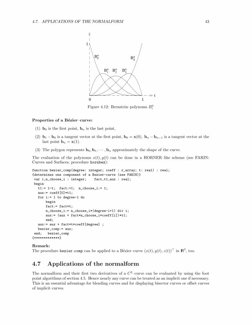
4.7. APPLICATIONS OF THE NORMALFORM 43
B40
B41 B4
2 B43
B44
0 1
1
t
Figure 4.12: Bernstein–polynoms B4i
Properties of a Bezier–curve:
(1) b0 is the first point, bn is the last point,
(2) b1−b0 is a tangent vector at the first point, b0 = x(0), bn−bn−1 is a tangent vector at thelast point bn = x(1).
(3) The polygon represents b0,b1, · · · ,bn approximately the shape of the curve.
The evaluation of the polynoms x(t), y(t) can be done in a HORNER–like scheme (see FARIN:Curves and Surfaces, procedure hornbez):
function bezier_comp(degree: integer; coeff : r_array; t: real) : real;
{determines one component of a Bezier-curve (see FARIN)}
var i,n_choose_i : integer; fact,t1,aux : real;
begin
t1:= 1-t; fact:=1; n_choose_i:= 1;
aux:= coeff[0]*t1;
for i:= 1 to degree-1 do
begin
fact:= fact*t;
n_choose_i:= n_choose_i*(degree-i+1) div i;
aux:= (aux + fact*n_choose_i*coeff[i])*t1;
end;
aux:= aux + fact*t*coeff[degree] ;
bezier_comp:= aux;
end; bezier_comp
{*************}
Remark:The procedure bezier comp can be applied to a Bezier–curve (x(t), y(t), z(t))> in IR3, too.
4.7 Applications of the normalform
The normalform and their first two derivatives of a C2–curve can be evaluated by using the footpoint algorithms of section 4.5. Hence nearly any curve can be treated as an implicit one if necessary.This is an essential advantage for blending curves and for displaying bisector curves or offset curvesof implicit curves.
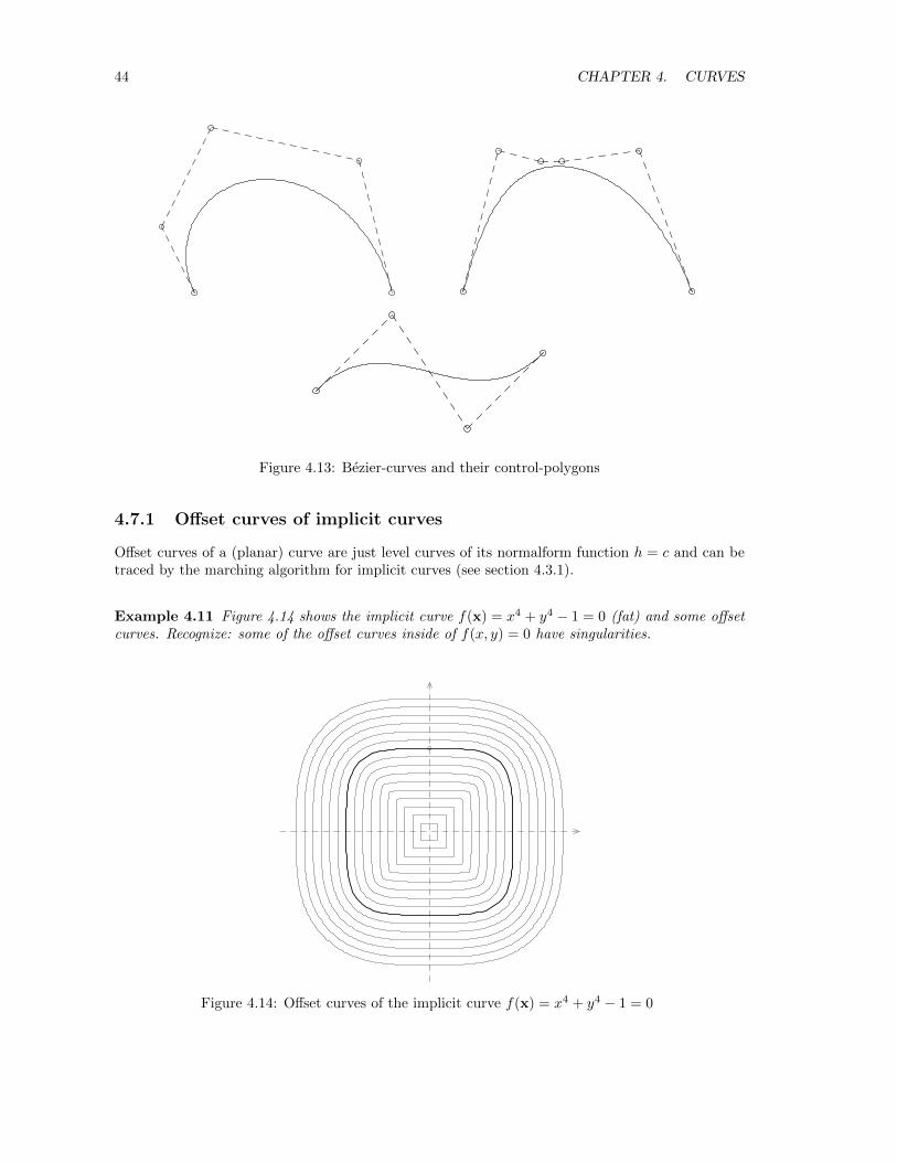
44 CHAPTER 4. CURVES
Figure 4.13: Bezier-curves and their control-polygons
4.7.1 Offset curves of implicit curves
Offset curves of a (planar) curve are just level curves of its normalform function h = c and can betraced by the marching algorithm for implicit curves (see section 4.3.1).
Example 4.11 Figure 4.14 shows the implicit curve f(x) = x4 + y4 − 1 = 0 (fat) and some offsetcurves. Recognize: some of the offset curves inside of f(x, y) = 0 have singularities.
Figure 4.14: Offset curves of the implicit curve f(x) = x4 + y4 − 1 = 0
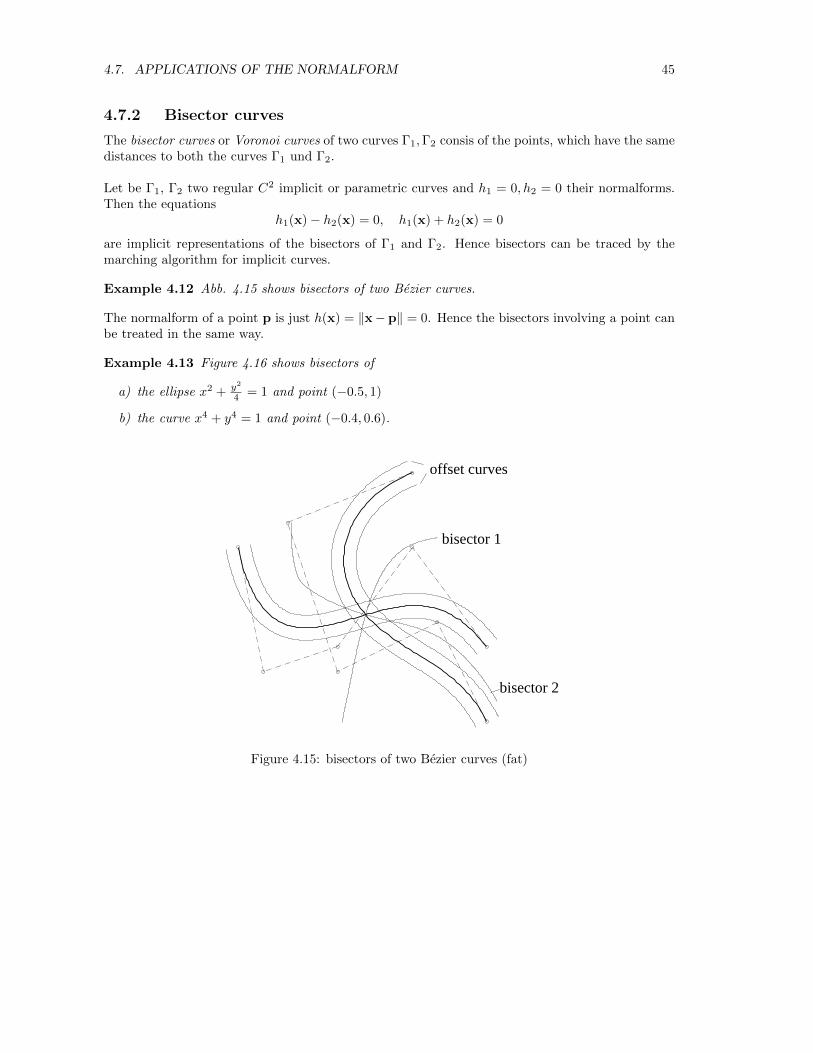
4.7. APPLICATIONS OF THE NORMALFORM 45
4.7.2 Bisector curves
The bisector curves or Voronoi curves of two curves Γ1,Γ2 consis of the points, which have the samedistances to both the curves Γ1 und Γ2.
Let be Γ1, Γ2 two regular C2 implicit or parametric curves and h1 = 0, h2 = 0 their normalforms.Then the equations
h1(x)− h2(x) = 0, h1(x) + h2(x) = 0
are implicit representations of the bisectors of Γ1 and Γ2. Hence bisectors can be traced by themarching algorithm for implicit curves.
Example 4.12 Abb. 4.15 shows bisectors of two Bezier curves.
The normalform of a point p is just h(x) = ‖x− p‖ = 0. Hence the bisectors involving a point canbe treated in the same way.
Example 4.13 Figure 4.16 shows bisectors of
a) the ellipse x2 + y2
4 = 1 and point (−0.5, 1)
b) the curve x4 + y4 = 1 and point (−0.4, 0.6).
offset curves
bisector 1
bisector 2
Figure 4.15: bisectors of two Bezier curves (fat)
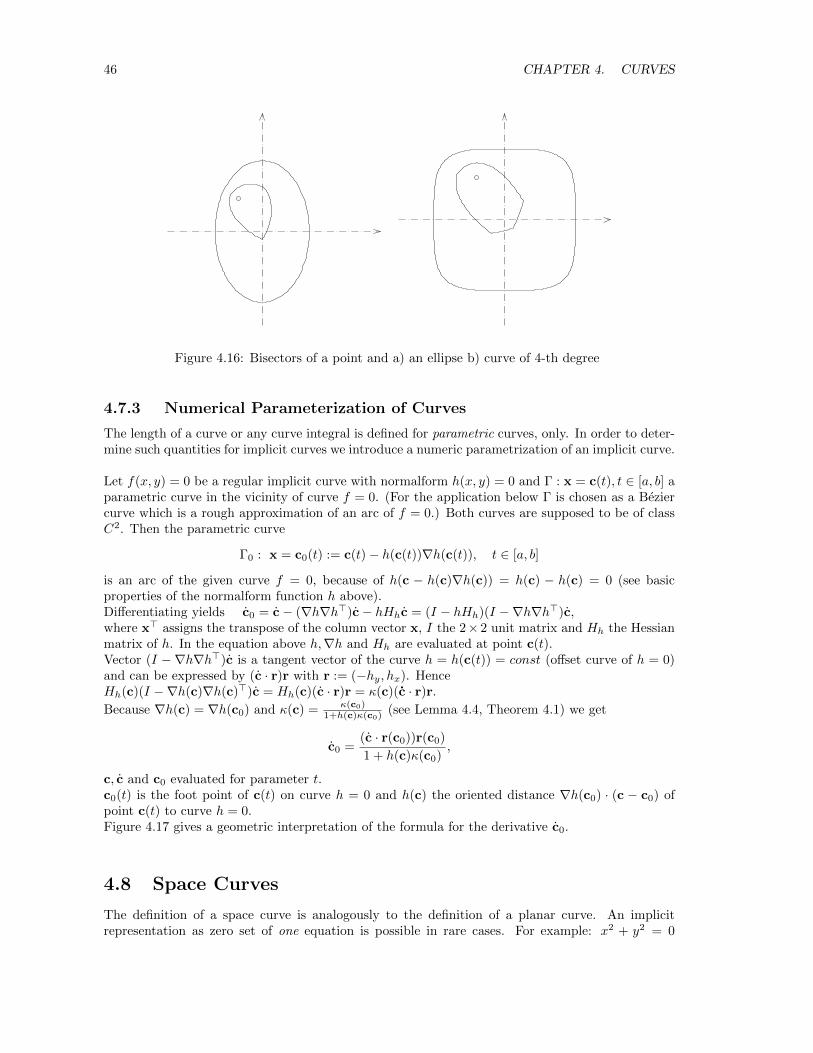
46 CHAPTER 4. CURVES
Figure 4.16: Bisectors of a point and a) an ellipse b) curve of 4-th degree
4.7.3 Numerical Parameterization of Curves
The length of a curve or any curve integral is defined for parametric curves, only. In order to deter-mine such quantities for implicit curves we introduce a numeric parametrization of an implicit curve.
Let f(x, y) = 0 be a regular implicit curve with normalform h(x, y) = 0 and Γ : x = c(t), t ∈ [a, b] aparametric curve in the vicinity of curve f = 0. (For the application below Γ is chosen as a Beziercurve which is a rough approximation of an arc of f = 0.) Both curves are supposed to be of classC2. Then the parametric curve
Γ0 : x = c0(t) := c(t)− h(c(t))∇h(c(t)), t ∈ [a, b]
is an arc of the given curve f = 0, because of h(c − h(c)∇h(c)) = h(c) − h(c) = 0 (see basicproperties of the normalform function h above).Differentiating yields c0 = c− (∇h∇h>)c− hHhc = (I − hHh)(I −∇h∇h>)c,where x> assigns the transpose of the column vector x, I the 2× 2 unit matrix and Hh the Hessianmatrix of h. In the equation above h,∇h and Hh are evaluated at point c(t).Vector (I −∇h∇h>)c is a tangent vector of the curve h = h(c(t)) = const (offset curve of h = 0)and can be expressed by (c · r)r with r := (−hy, hx). HenceHh(c)(I −∇h(c)∇h(c)>)c = Hh(c)(c · r)r = κ(c)(c · r)r.
Because ∇h(c) = ∇h(c0) and κ(c) = κ(c0)1+h(c)κ(c0) (see Lemma 4.4, Theorem 4.1) we get
c0 =(c · r(c0))r(c0)
1 + h(c)κ(c0),
c, c and c0 evaluated for parameter t.c0(t) is the foot point of c(t) on curve h = 0 and h(c) the oriented distance ∇h(c0) · (c − c0) ofpoint c(t) to curve h = 0.Figure 4.17 gives a geometric interpretation of the formula for the derivative c0.
4.8 Space Curves
The definition of a space curve is analogously to the definition of a planar curve. An implicitrepresentation as zero set of one equation is possible in rare cases. For example: x2 + y2 = 0
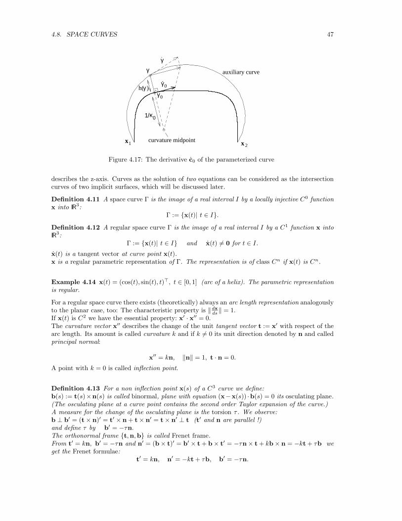
4.8. SPACE CURVES 47
h( )
.γ
γ 0.
x1 x 2
γ 0
κ01/
.
curvature midpoint
γ
γ
auxiliary curve
Figure 4.17: The derivative c0 of the parameterized curve
describes the z-axis. Curves as the solution of two equations can be considered as the intersectioncurves of two implicit surfaces, which will be discussed later.
Definition 4.11 A space curve Γ is the image of a real interval I by a locally injective C0 functionx into IR3:
Γ := {x(t)| t ∈ I}.
Definition 4.12 A regular space curve Γ is the image of a real interval I by a C1 function x intoIR3:
Γ := {x(t)| t ∈ I} and x(t) 6= 0 for t ∈ I.x(t) is a tangent vector at curve point x(t).x is a regular parametric representation of Γ. The representation is of class Cn if x(t) is Cn.
Example 4.14 x(t) = (cos(t), sin(t), t)>, t ∈ [0, 1] (arc of a helix). The parametric representationis regular.
For a regular space curve there exists (theoretically) always an arc length representation analogouslyto the planar case, too: The characteristic property is ‖dxds ‖ = 1.If x(t) is C2 we have the essential property: x′ · x′′ = 0.The curvature vector x′′ describes the change of the unit tangent vector t := x′ with respect of thearc length. Its amount is called curvature k and if k 6= 0 its unit direction denoted by n and calledprincipal normal:
x′′ = kn, ‖n‖ = 1, t · n = 0.
A point with k = 0 is called inflection point.
Definition 4.13 For a non inflection point x(s) of a C3 curve we define:b(s) := t(s)×n(s) is called binormal, plane with equation (x−x(s)) ·b(s) = 0 its osculating plane.(The osculating plane at a curve point contains the second order Taylor expansion of the curve.)A measure for the change of the osculating plane is the torsion τ . We observe:b ⊥ b′ = (t× n)′ = t′ × n + t× n′ = t× n′ ⊥ t (t′ and n are parallel !)and define τ by b′ = −τn.The orthonormal frame {t,n,b} is called Frenet frame.From t′ = kn, b′ = −τn and n′ = (b× t)′ = b′ × t + b× t′ = −τn× t + kb× n = −kt + τb weget the Frenet formulae:
t′ = kn, n′ = −kt + τb, b′ = −τn.
48 CHAPTER 4. CURVES
Hence in case of τ = 0 for all curve points the curve is planar.
In practice curves are not given by their arc length parameterization. How to compute curvature,torsion,... in general is the content of the following lemma.
Lemma 4.5 Let Γ : x = x(t) t ∈ [a, b] be a C3–continuous regular space curve. For points wherex(t), x(t) are linearly independent the following formulae are valid:
t =x(t)
‖x(t)‖, b =
x(t)× x(t)
‖x(t)× x(t)‖, n = b× t, k =
‖x(t)× x(t)‖‖x(t)‖3
, τ =(x(t)× x(t)) · ˙x(t)
‖x(t)× x(t)‖2.
Proof: Analogously to the plane case we get for the curvature vector x′′ = xx2−(x·x)x‖x‖4 . Applying
formula: a× (b× c) = b(a · c)− c(a · b) yields
x′′ = x×(x×x)‖x‖4 and k = ‖x′′‖ = ‖x‖‖x×x‖
‖x‖4 = ‖x×x‖‖x‖3 ( x ⊥ (x× x) !).
Hence n = x′′
k = x‖x‖ ×
x×x‖x×x‖ and b = x×x
‖x×x‖ .
From b′ = b/‖x‖ we get b′ = (x× ˙x)(x×x)2−(x×x)((x×x)·(x× ˙x))‖x‖‖x×x‖3 and
−τ = b′ · n = b′ · ( x‖x‖ ×
x×x‖x×x‖ ) = x× ˙x
‖x‖‖x×x‖ · (x‖x‖ ×
x×x‖x×x‖ ) = (x× ˙x)·(x×(x×x))
‖x×x‖2‖x‖2 .
Applying the identity: (a× b) · (c× d) = (a · c)(b · d)− (b · c)(a · d) yields: −τ = − (x×x)· ˙x‖x×x‖2 . 2
For displaying a space curve we use the methods and formulae for equally and curvature dependentdistribution of points developed for planar curves.
The normalform of a space curve will be introduced later (see Section 5.9).
Chapter 5
SURFACES
5.1 Definition and Representations of Surfaces
Definition 5.1 A surface Φ is the image of a rectangle D := [a, b, ] × [c, d] ⊂ IR2 by a locallyinjective C0 function x into IR3:
Φ := {x(u, v)| (u, v) ∈ D}.
For (u0, v0) ∈ D curves x = x(u0, v) and x = x(u, v0) are the parameter curves at point x(u0, v0).
Definition 5.2 A regular surface Φ is the image of a rectangle D := [a, b, ]× [c, d] ⊂ IR2 by a locallyinjective C1 function x into IR3:
Φ := {x(u, v)| (u, v) ∈ D}, xu × xv 6= 0.
xu, xv are the tangent vectors of the parameter curves and xu× xv is a normal vector (orthogonalto the tangent plane).
Example 5.1 x(u, v) = (u, v, u2 + v2)>, (u, v) ∈ D := [0, 1] × [0, 1] (patch of the paraboloidz = x2 + y2). The parametric representation is regular.
Definition 5.3 A regular implicit surface is a non empty subset Φ ⊂ IR3 of the form
f : IR2 ⊃ D → IR, Φ : {x ∈ D|f(x) = 0}, ∇f(x) 6= 0 for x ∈ Φ,
where f is a C1–function. For a surface point x vector ∇f(x) is a normal vector.f(x) = 0 is a regular implicit representation of Φ. The representation is of class Cn if f is Cn.
Example 5.2 Φ : {x ∈ IR3|f(x) := x2 + y2 + z2 − 1 = 0} (unit sphere).
Obviously, the parametric/implicit representation of a surface is not unique.
Definition 5.4 The representation of a surface is called explicit if one of the coordinates x, y, z isa function of the remaining coordinates.
The following (theoretical) results show that the representations can be changed locally. The proofsrely on the implicit function theorem.
Lemma 5.1 a) Let Φ be a regular Cn-continuous parametric (implicit) surface and x0 a point ofΦ. Then there exists a local Cn-continuous implicit (parametric) representation of Φ at point x0
which is regular, too.b) For any surface with a regular parametric or regular implicit representation there exists for anypoint x0 locally an explicit representation which is Cn if the given representation is Cn.From an explicit representation one derives easily both a parametric and an implicit representation.(For example: From z = Z(x, y) we get the parametric representation (x, y, Z(x, y)) and the implicitrepresentation Z(x, y)− z = 0.)
49
50 CHAPTER 5. SURFACES
5.2 The First and Second Fundamental Forms of a Surface
5.2.1 The first fundamental form, arc length
Definition 5.5 Let Φ : x = x(u, v), u, v ∈ D ⊂ IR2 be a regular surface and u = u(t), v = v(t), t ∈[t1, t2] a regular curve in D. Hence Γ : x = c(t) := x(u(t), v(t)), t ∈ [t1, t2] is a regular curve onthe surface. For the arc length of curve Γ we get:
s(t) :=
∫ t
t1
√c2dt =
∫ t
t1
√Eu2 + 2Fuv +Gv2dt,
where
E(u, v) := x2u, F (u, v) := xu · xv, G(u, v) := x2
v
are the coefficients of the first fundamental form and dsdt =
√Eu2 + 2Fuv +Gv2 6= 0. Hence E,F,G
are the coefficients of a strongly positive definite quadratic form: I(ξ, η) := Eξ2 + 2Fξη +Gη2.
Remark:The answer of any question about distances on a surface needs the 1.fundamental form.
5.2.2 The second fundamental form, curvature
Let Φ : x = x(u, v), u, v ∈ D ⊂ IR2 be a regular surface and Γ : x = c(s) := x(u(s), v(s)), s ∈ [s1, s2]a regular curve on surface Φ parameterized by its arc length s. Hencec′ = xuu
′ + xvv′ is the unit tangent vector and
c′′ = xuu′′ + xvv
′′ + xuuu′2 + 2xuvu
′v′ + xvvv′2 its curvature vector.
c′′ is orthogonal to the tangent vector c′ and can be split into its normal and tangential component(with respect of surface Φ):c′′ = knn + kgm where n = xu×xv
‖xu×xv‖ is the surface unit normal and m := c′ × n (tangential to
the surface). kn is called normal curvature and kg geodesic curvature of the surface curve Γ.
For measuring the curvature of the surface at a surface point x(u, v) one considers the intersectioncurves of the surface with the planes orthogonal to the surface at point x(u, v). For such normalsections curvature vector c′′ is parallel to the surface normal, i.e. kg = 0. For its curvature we get
k = kn = c′′ · n = Lu′2
+ 2Mu′v′ +Nv′2
where
L(u, v) := n · xuu, M(u, v) := n · xuv, N(u, v) := n · xvv.
L,M,N are called the coefficients of the second fundamental form.L,M,N can be considered as the coefficients of a quadratic form: II(ξ, η) := Lξ2 + 2Mξη +Nη2.
For an arbitrary parameterization we get from u′ = dudt
dtds , v
′ = dvdtdtds ,
dsdt =
√Eu2 + 2Fuv +Gv2
the formula for the normal curvature of the surface in tangential direction c′ = xudu+ xvdv:
kn =Ldu2 + 2Mdudv +Ndv2
Edu2 + 2Fdudv +Gdv2=II(du, dv)
I(du, dv).
A point with constant normal curvature is called an umbilic point or a flat point if kn = 0.If the normal curvature is not constant (at a point) there exist a maximum and a minimum.For determining these extrem curvatures and the tangential direction of the corresponding normalsection we differentiate function (subscript “n” is omitted) k(ξ, η) := II(ξ, η)/I(ξ, η) and we getfromkξ = 2 (Lξ+Mη)I−(Eξ+Fη)II
I2 = 2 (Lξ+Mη)−(Eξ+Fη)kI = 0,
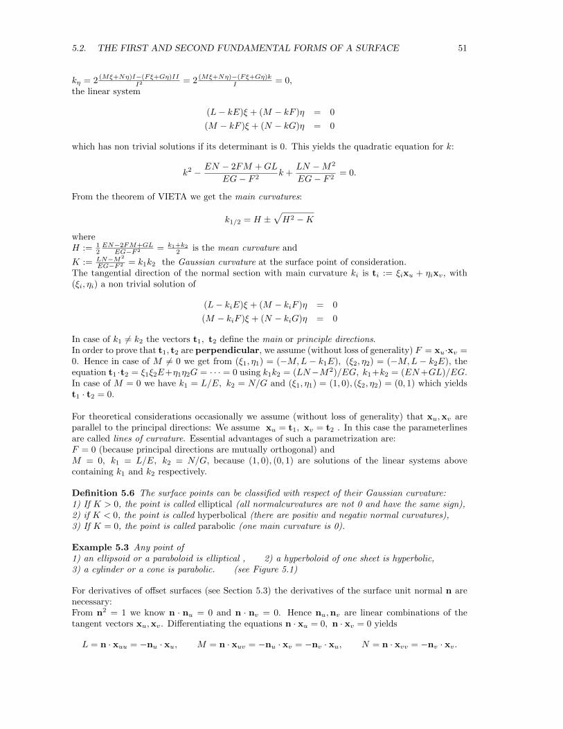
5.2. THE FIRST AND SECOND FUNDAMENTAL FORMS OF A SURFACE 51
kη = 2 (Mξ+Nη)I−(Fξ+Gη)III2 = 2 (Mξ+Nη)−(Fξ+Gη)k
I = 0,the linear system
(L− kE)ξ + (M − kF )η = 0
(M − kF )ξ + (N − kG)η = 0
which has non trivial solutions if its determinant is 0. This yields the quadratic equation for k:
k2 − EN − 2FM +GL
EG− F 2k +
LN −M2
EG− F 2= 0.
From the theorem of VIETA we get the main curvatures:
k1/2 = H ±√H2 −K
whereH := 1
2EN−2FM+GL
EG−F 2 = k1+k22 is the mean curvature and
K := LN−M2
EG−F 2 = k1k2 the Gaussian curvature at the surface point of consideration.The tangential direction of the normal section with main curvature ki is ti := ξixu + ηixv, with(ξi, ηi) a non trivial solution of
(L− kiE)ξ + (M − kiF )η = 0
(M − kiF )ξ + (N − kiG)η = 0
In case of k1 6= k2 the vectors t1, t2 define the main or principle directions.In order to prove that t1, t2 are perpendicular, we assume (without loss of generality) F = xu·xv =0. Hence in case of M 6= 0 we get from (ξ1, η1) = (−M,L − k1E), (ξ2, η2) = (−M,L − k2E), theequation t1 ·t2 = ξ1ξ2E+η1η2G = · · · = 0 using k1k2 = (LN−M2)/EG, k1+k2 = (EN+GL)/EG.In case of M = 0 we have k1 = L/E, k2 = N/G and (ξ1, η1) = (1, 0), (ξ2, η2) = (0, 1) which yieldst1 · t2 = 0.
For theoretical considerations occasionally we assume (without loss of generality) that xu,xv areparallel to the principal directions: We assume xu = t1, xv = t2 . In this case the parameterlinesare called lines of curvature. Essential advantages of such a parametrization are:F = 0 (because principal directions are mutually orthogonal) andM = 0, k1 = L/E, k2 = N/G, because (1, 0), (0, 1) are solutions of the linear systems abovecontaining k1 and k2 respectively.
Definition 5.6 The surface points can be classified with respect of their Gaussian curvature:1) If K > 0, the point is called elliptical (all normalcurvatures are not 0 and have the same sign),2) if K < 0, the point is called hyperbolical (there are positiv and negativ normal curvatures),3) If K = 0, the point is called parabolic (one main curvature is 0).
Example 5.3 Any point of1) an ellipsoid or a paraboloid is elliptical , 2) a hyperboloid of one sheet is hyperbolic,3) a cylinder or a cone is parabolic. (see Figure 5.1)
For derivatives of offset surfaces (see Section 5.3) the derivatives of the surface unit normal n arenecessary:From n2 = 1 we know n · nu = 0 and n · nv = 0. Hence nu,nv are linear combinations of thetangent vectors xu,xv. Differentiating the equations n · xu = 0, n · xv = 0 yields
L = n · xuu = −nu · xu, M = n · xuv = −nu · xv = −nv · xu, N = n · xvv = −nv · xv.
52 CHAPTER 5. SURFACES
a) b) c)
Figure 5.1: a) ellipsoid, b) hyperboloid of one sheet, c) cylinder, cone
These equations allow to determine the components of nu,nv with respect of the vectors xu,xv:
nu =MF − LGEG− F 2
xu +LF −ME
EG− F 2xv, nv =
NF −MG
EG− F 2xu +
MF −NEEG− F 2
xv.
(Weingarten equations).In case of a curvature line parametrization we have: nu = −L
Exu = −k1xu, nv = −NGxv =−k2xv.
5.3 Offset surfaces
Definition 5.7 Let Φ0 : x = x0(u, v) be a regular C2–surface and n0(u, v) the unit normal andd ∈ IR fixed. Then surface Φd : x = x0(u, v) + dn0(u, v) is called offset surface with distance d.The offset surface Φd depends only on the surface Φ0 as a point set in IR3 and distance d.
Analogously to the curve case we get
Lemma 5.2 Let Φ0 : x = x0(u, v) be a regular Cn–surface, n ≥ 2, k0,1(u, v), k0,2(u, v) the maincurvatures and d ∈ IR such that (1−dk0,1(u, v))(1−dk0,2(u, v)) > 0 then the offset surface Φd : x =xd := x0(u, v) + dn0(u, v) is a regular Cn−1 surface, nd(u, v) = n0(u, v) and the main curvaturesare
kd,1 =k0,1
1− dk0,1, kd,2 =
k0,2
1− dk0,2.
Proof: Let be x0(u, v) a curvature line parameterization. Hence: n0,u = −k1x0,u, n0,v = −k2x0,v
and xdu × xdv = (x0,u + dn0,u)× (x0,v + dn0,v) = (1− dk0,1)(1− dk0,2)x0u × x0v.For (1− dk0,1(u, v))(1− dk0,2(u, v)) > 0 the offset surface Φd is regular and of class Cn−1.Obviously, a normal plane εn of Φ0 at point x0(u, v) is a normal plane of Φd and the intersectionΦd ∩ εn is an offset curve of Φ0 ∩ εn. Hence for corresponding normal curvatures we get kdn =k0n
1−dk0n (see Lemma 4.4). Because the stationary points of kdn(ξ, η) and k0n(ξ, η) agree, we get
kd,1 =k0,1
1−dk0,1 , kd,2 =k0,2
1−dk0,2 and td,1 = t0,1, td,2 = t0,2 (directions of main curvatures). 2
5.4 Normalform of a surface
5.4.1 Definition of the normalform
Definition 5.8 The implicit representation h(x) = n · x − d = 0, ‖n‖ = 1 of a plane ε in IR3 iscalled HESSE normalform of plane ε.(h(x) describes the oriented distance of point x to the plane ε.)
5.4. NORMALFORM OF A SURFACE 53
Definition 5.9 An implicit representation h(x) = 0 of a surface Φ with ‖∇h‖ = 1 in a vicinity ofΦ is called normalform of surface Φ. (We regard h = 0 and −h = 0 as the same normalforms.)h is called normalform function or, because of its geometric meaning, oriented distance function.
Example 5.4 h(x, y, z) :=√x2 + y2 + z2−r = 0 is the normalform of the sphere x2+y2+z2 = r2.
If the given surface is smooth enough, then its normalform always exists (theoretically).
Theorem 5.1 For any Cn-continuous, n ≥ 2, surface Φ there exists in a vicinity V of Φ theoriented distance function h and h is of class Cn, too. Hence Φ has an implicit representationh(x) = 0 such that ‖∇h‖ = 1 on V .On V function h has the properties: 1) h(x + δ∇h(x)) = h(x) + δ, 2) ∇h(x + δ∇h(x)) = ∇h(x).
Proof: Let Φ : x = x(u, v) be a curvature line parametrization such that: xu = t1, xv = t2. Henceat any surface point we have nu = −k1xu, nv = −k2xv.The equation F (x, u, v, d) := x(u, v) + dn(u, v)− x = 0 is solvable for u, v, d if det(Fu, Fv, Fd) 6= 0.From
Fu = xu + dnu = (1− dk1)xu, Fv = xv + dnv = (1− dk2)xv, Fd = n
we get det(Fu, Fv, Fd) = (1− dk1)(1− dk2) det(xu,xv,n) 6= 0 in a vicinity V : −v ≤ d ≤ v, v > 0 ofsurface Φ.Due to the implicit function theorem there exist functions u(x, y, z), v(x, y, z) and d(x, y, z) suchthat the following equation is fulfilled in the vicinity V of surface Φ:x(u(x, y, z), v(x, y, z)) + d(x, y, z)n(u(x, y, z), v(x, y, z)) = x. Differentiating this equation for x, y, zyields ∇ux>u +∇vx>v +∇dn>+d∇un>u +d∇vn>v = 3×3 unit matrix (see curve case!) Multiplyingthis matrix equation by n and respecting x>u n = x>v n = n>u n = n>v n = 0, n>n = 1 we get ∇d = n.Hence function d(x, y, z) is of class Cn, too.In order to distinguish function d(x, y, z) and distance parameter d we set h(x, y, z) := d(x, y, z).Points x with the same foot point x0 have the same gradient ∇h(x). Hence we get the essentialproperties of the distance function h:1) h(x + δ∇h(x)) = h(x) + δ, 2) ∇h(x + δ∇h(x)) = ∇h(x). 2
The proof of the uniqueness of the normalform function h is omitted.
Properties 1),2) of the last theorem show that h and ∇h can be evaluated numerically at point xby determining the foot point x0 and its unit normal n0 of point x on surface Φ:h(x) = (x− x0) · n0, ∇h(x) = n0.
5.4.2 On the first and second derivatives of the normalform of a surface
Let be Φ a C2–continuous surface with normalform h = 0 and Γ : x = c(s) a C2–continuous curveon Φ with arc length parameter s. Hence h(c(s)) = 0. Differentiating this equation yields
(1) ∇h · c′ = 0, (2) c′>Hhc
′ +∇h · c′′ = 0.
From the second equation we get the following results:
• The normal curvature of surface curve Γ is: kn = ∇h · c′′ = −c′>Hhc
′.kn depends only on the surface and the tangential direction of Γ at the point of consideration.
• In case of a normal section we get k = kn = ∇h ·c′′ = −c′>Hhc
′. Hence the normal curvatureof surface Φ for tangential direction v, ‖v‖ = 1, is kn = −v>Hhv.In following considerations for simplicity we deal with the negative normal curvature κ :=−kn = v>Hhv.
54 CHAPTER 5. SURFACES
• Differentiating (∇h)2 = 1 yields Hh∇h = 0.The eigenvalues of the Hessian matrix Hh areλ1 = 0 with eigenvector ∇h,λ2 = κ1, λ3 = κ2 with eigenvectors v1 ⊥ v2, ‖vi‖ = 1.From v>i Hhvi = κi we get: ki := −κi is the normal curvature in direction vi. The normalcurvature in an arbitrary direction v(ϕ) = cos(ϕ)v1 + sin(ϕ)v2, 0 ≤ ϕ < π, iskn(ϕ) = −v(ϕ)>Hhv(ϕ) = k1 cos(ϕ)2 + k2 sin(ϕ)2 = k1 + (k2 − k1) sin(ϕ)2.In case of k1 = k2 the normal curvature is constant (umbilic case).In case of k1 6= k2 the extreme values of kn(ϕ), hence k1 = −κ1 and k2 = −κ2 are the maincurvatures. The corresponding main directions are the eigen directions v1,v2 respectively.The formula kn(ϕ) = k1 cos(ϕ)2 + k2 sin(ϕ)2 is called Euler formula.
• The characteristic polynomial of Hh is −λ3 + (κ1 + κ2)λ2 − κ1κ2λ withmean curvatureH = k1+k2
2 = − 12 (κ1 + κ2) = − 1
2 (hxx + hyy + hzz) andGaussian curvature
K = k1k2 = κ1κ2 =
∣∣∣∣ hxx hxyhyx hyy
∣∣∣∣+
∣∣∣∣ hxx hxzhzx hzz
∣∣∣∣+
∣∣∣∣ hyy hyzhzy hzz
∣∣∣∣ .The minimal polynomial isthe characteristic polynomial if κ1 6= κ2 (non umbilic case) and λ2 − κλ if κ := κ1 = κ2
(umbilic case).(Prove it after diagonalizing Hh !)
• Let Φ0 be a C2–continuous surface with main curvatures k1, k2 at x ∈ Φ0. The distanceparameter d ∈ IR is chosen in an intervall [−d0, d0], d0 > 0, such that for any d we have1− dk1(x) > 0, 1− dk2(x) > 0. Hence h is C2-continuous at point xd := x + d∇h(x). Fromequation h(xd) = h(x)+d (see Theorem 5.1) we recognize that the level surface h = d is justthe offset surface Φd of Φ0 for distance d. Equation ∇h(xd) = ∇h(x) shows that the tangentplane at point xd and at its foot point x agree. Differentiating equation ∇h(xd) = ∇h(x)yields
Hh(xd)(I + dHh(x)) = Hh(x).
Multiplying this matrix equation by vector vi (unit vector in a main direction) we get
Hh(xd)vi = − ki(x)
1− dki(x)vi.
Hence the main directions at point xd of the offset surface agree with the main directions atthe corresponding foot point on Φ0 and the main curvatures are
ki(xd) =ki(x)
1− dki(x), i = 1, 2.
• In case of a local coordinate system such that point p is the origin 0 and ∇h(0) = (0, 0, 1)>.Hence the x-y-plane is the tangent plane at pointp = 0 and for the Hessian we get thesimplification (because of Hh∇h = 0)
Hh(0) =
hxx hxy 0hyx hyy 00 0 0
.
For this specialization we get the following results
– hxx, hyy are the normal curvatures in direction (1, 0, 0)>, (0, 1, 0)> respectively.From −2H = hxx + hyy we get the general statement: The mean curvature H is thearithmetic mean of the normal curvatures of any two orthogonal (tangent) directions.The Gaussian curvature is K = hxxhyy − h2
xy.
5.4. NORMALFORM OF A SURFACE 55
– Hh is determined uniquely by the normal curvatures of any three (tangential) directions(see 3–Tangent–Theorem below).
– From the Taylor expansion of h at point 0:
h(x, y, z) = z +1
2(hxxx
2 + hyyy2 + 2hxyxy) + · · ·
we get the osculating paraboloid
z = −1
2(hxxx
2 + 2hxyxy + hyyy2)
and the Dupin indicatrix of the surface at point 0:
hxxx2 + 2hxyxy + hyyy
2 = ±1.
5.4.3 Cn–contact, Gn–contact
A Cn–continuous curve/surface considered as a set of points can be described by several para-metric representations. Essentials of a representation are its derivatives which allow to determinegeometrical attributes of the curve/surface like tangent line/plane, curvature,... Such geometricalattributes are independent of the representation accidentally chosen. So it is necessary to distin-guish between the continuity of representations (Cn–continuity) and the continuity of geometricalattributes (Gn–continuity):
Definition 5.10 1. Two regular Cn–continuous parametric curves Γ1 : x = X1(t),Γ2 : x =X2(t) (surfaces Φ1 : x = X1(s, t),Φ2 : x = X2(s, t)) have Cn–contact at a common point x0
if the (partial) derivatives of X1 and X2 at point x0 up to the n-th order are the same.
2. Two regular Cn–continuous implicit curves Γ1 : f1(x) = 0,Γ2 : f2(x) = 0 (surfaces Φ1 :f1(x) = 0,Φ2 : f2(x) = 0) have Cn–contact at a common point x0 if the partial derivatives off1 and f2 at point x0 up to the n-th order are the same.
3. Two with respect to the same coordinate explicitly represented plane curves (surfaces) haveCn–contact at a common point if the corresponding functions are Cn–continuous at this point.
Definition 5.11 Two regular parametric or implicit plane curves Γ1,Γ2 (surfaces Φ1,Φ2) with acommon point x0 have Gn–contact at x0 if they have local explicit representations for one coordinate∈ {x, y} (∈ {x, y, z}) with Cn–contact at point x0.
Remark:In former literature Gn–contact is called contact of order n.
From Lemma 4.1 and Lemma 5.1 we get the following, more useful, characterisation of the Gn–continuity.
Theorem 5.2 1. Two regular Cn–continuous parametric plane curves Γ1,Γ2 (surfaces Φ1,Φ2)have Gn–contact at a common point x0 if and only if they have Cn–contact at point x0 withrespect to some local parametric representations of the two curves (surfaces).
2. Two regular Cn–continuous implicit plane curves Γ1,Γ2 (surfaces Φ1,Φ2) have Gn–contact ata common point x0 if and only if they have Cn–contact at point x0 with respect to some localimplicit representations of the two curves (surfaces).
56 CHAPTER 5. SURFACES
5.4.4 G2–continuity theorems
There are several theorems on the G2-continuity (i.e. continuity of the normal curvatures) of twosurface patches. We will give simple proofs of such theorems using the idea of the normal form.
Theorem 5.3 3–Tangent–TheoremTwo G2–continuous surfaces Φ1,Φ2 with a common point p and a common tangent plane at p areG2–continuous at point p if they have equal normal curvatures along three directions.
Proof: We assume, without loss of generality, that p = 0 and furthermore the three directions arev1 = (1, 0, 0),v2 = (cosϕ2, sinϕ2, 0),v3 = (cosϕ3, sinϕ3, 0) with corresponding common normalcurvatures κ1, κ2, κ3. From κi = viHhv
>i we get
hxx = κ1,hxx cos2 ϕ2 + hyy sin2 ϕ2 + 2hxy cosϕ2 sinϕ2 = κ2,hxx cos2 ϕ3 + hyy sin2 ϕ3 + 2hxy cosϕ3 sinϕ3 = κ3.The determinant of this linear system for hxx, hyy, hxy is not 0 if 0 < ϕ2 < ϕ3 < π. Hence theHessian for both the surfaces is uniquely determined and the surfaces join G2-continuously at thecommon point p. 2
The essential part of the proof of the Linkage Curve Theorem is the following Lemma.
Lemma 5.3 Let Φ1,Φ2 be two G2-continuous surfaces with common point 0, common tangent planez = 0 and common tangent planes along the common smooth curve Γ : x(t) = (t, b(t), c(t))>, t ∈[0, t0] with x(0) = 0 and x(0) = (1, 0, 0)>. Then we get for the Hessian matrices Hh1
, Hh2of the
normalform functions h1, h2 of the surfaces Φ1,Φ2
h1,xx(0) = h2,xx(0), h1,xy(0) = h2,xy(0).
Proof: For a point (t, b(t), c(t)) on curve Γ we have
∇h1(t, b(t), c(t)) = ∇h2(t, b(t), c(t)).
Differentiating this equation yields
Hh1(t, b(t), c(t)) (1, b(t), c(t))> = Hh2
(t, b(t), c(t)) (1, b(t), c(t))>.
For t = 0 we get h1,xx(0) = h2,xx(0), h1,xy(0) = h2,xy(0) (Remember the simple Form of the
Hessian matrix and b(0) = 0 at point 0 !). 2
Remark:Because hxx is the normal curvature in x–direction we get from h1,xx(0) = h2,xx(0) that the normalcurvatures of the surfaces at point 0 in direction of Γ are the same and hence their Dupin indica-trices intersect at a point of the tangent of curve Γ.
Obviously we get for the Hessian matrices of the surfaces Φ1,Φ2 in the Lemma above the strongerresult Hh1
(0) = Hh2(0) if we choose additionally a suitable geometric restriction which yields
h1,yy(0) = h2,yy(0). For example one of the following conditions
• The equality of the mean curvatures:−2H(0) = h1,xx(0) + h1,yy(0) = h2,xx(0) + h2,yy(0).
• The equality of the Gaussian curvatures:K(0) = h1,xx(0)h1,yy(0)− h1,xy(0)2 = h2,xx(0)h2,yy(0)− h2,xy(0)2
if the normal curvature h1,xx(0) in direction (1, 0, 0) does not vanish.
5.4. NORMALFORM OF A SURFACE 57
• The equality of the normal curvature in a direction v = (a, 1, 0)>, a ∈ IR, transversal to curveΓ at point 0:
κa =a2h1,xx + h1,yy + 2ah1,xy
1 + a2=a2h2,xx + h2,yy + 2ah2,xy
1 + a2.
These considerations prove the following theorem
Theorem 5.4 Linkage Curve Theorem:Let Φ1 and Φ2 be two G2-continuous surfaces which are tangent plane continuous along a smoothlinkage curve Γ.Φ1 and Φ2 are G2–continuous along their linkage curve Γ if one of the following conditions isfulfilled:
• Φ1 and Φ2 have the same mean curvature along Γ(Mean Curvature Criterion)
• Φ1 and Φ2 have the same Gaussian curvature and non vanishing normal curvature in Γ–direction along Γ(Gaussian Curvature Criterion)
• There exists a transversal vector field (not necessarily continuous) along Γ, such that thenormal curvatures of Φ1 and Φ2 in directions of the vector field are the same.(Vector Field Criterion)
5.4.5 The curvature of an intersection curve
Let be ΦA,ΦB two intersecting C2–continuous surfaces and hA = 0, hB = 0 their normalforms. Theintersection curve Γ is represented by the arc length parameterization x = c(s). Hence ‖∇hA‖ =1, ‖∇hB‖ = 1 and ‖c′‖ = 1, c′ · c′′ = 0. Differentiating the following equations
hA(c(s)) = 0, hB(c(s)) = 0
yields∇hA · c′ = 0, ∇hB · c′ = 0
and∇hA · c′′ + c′
>HhA
c′ = 0, ∇hB · c′′ + c′>HhB
c′ = 0.
Because c′ is orthogonal to ∇hA and ∇hB and ‖c′‖ = 1 we can choose the parameterization of Γsuch that
c′ =∇hA ×∇hB‖∇hA ×∇hB‖
.
c′′ is a linear combination of ∇hA and ∇hB . Because the calculation becomes simpler we use adifferent base of the normal plane:
c′′ = α(∇hA × c′) + β(∇hB × c′) = (α∇hA + β∇hB)× c′.
Using kA := −c′>HhA
c′, kB := −c′>HhB
c′ (normal curvature on surface ΦA and ΦB , respectively,in direction c′) we get from the equations ∇hA · c′′ = kA, ∇hB · c′′ = kB the result:
c′′ =kA∇hB − kB∇hA‖∇hA ×∇hB‖
× c′.
This formula can be written independently of the representations of the intersecting surfaces:Let be ΦA,ΦB two intersecting C2–continuous surfaces with unit normals nA,nB ,‖nA × nB‖ 6= 0, and normal curvatures kA, kB in direction nA × nB at a point of the intersectioncurve Γ than
58 CHAPTER 5. SURFACES
• c′ :=nA × nB‖nA × nB‖
is the tangent unit vector and
• c′′ :=(kAnB − kBnA)× (nA × nB)
(nA × nB)2
is the curvature vector and from the orthogonality of kAnB − kBnA and nA × nB we get
k = ‖c′′‖ =
√k2A + k2
B − 2kAkB cosϕ
sinϕ
the curvature, where ϕ is the angle between the surface normals and kA and kB the normalcurvatures of surfaces ΦA and ΦB in direction c′.
5.5 Normalform of an implicit surface
Let f(x) = 0 be a regular implicit C2–surface and h = 0 its normalform.For a surface point x we get:
1. h = 0 ,
2. unit normal: ∇h =∇f‖∇f‖
,
3. Hessian matrix: Hh = (I −∇h∇h>)Hf
‖∇f‖,
with 3× 3 unit matrix I and matrix ∇h∇h> = (hx, hy, hz)>(hx, hy, hz).
(For proof: differentiate ∇f‖∇f‖ .)
4. Normal curvature for unit tangent direction v is kn = −v>Hfv
‖∇f‖.
5. Main curvatures, main directions, mean and Gaussian curvature:Let be e1, e2 two orthonormal vectors which are perpendicular to ∇f . A main direction canbe written as ξe1 + ηe2 and must be an eigenvector of Hh. Hence an eigenvalue κ of Hh andits eigendirection have to fulfil the following linear system:
(e>1 Hfe1
‖∇f‖− κ) ξ +
e>1 Hfe2
‖∇f‖η = 0
e>1 Hfe2
‖∇f‖ξ + (
e>2 Hfe2
‖∇f‖− κ) η = 0.
Hence, from matrix e>1 Hfe1
‖∇f‖e>1 Hfe2
‖∇f‖e>1 Hfe2
‖∇f‖e>2 Hfe2
‖∇f‖
we get a) the main curvatures (negative eigenvalues) b) the main directions (eigendirections)c) the mean curvature (half of negative trace) and d) the Gaussian curvature (determinant).
For a point x in the vicinity of the surface with foot point x0 ∈ Γ we get:
1. ∇h(x) = ∇h(x0),
2. h(x) = (x− x0) · ∇h(x0)
5.6. NORMALFORM OF A PARAMETRIC SURFACE 59
3. Hessian matrix Hh:The 6 coefficients of the matrix Hh are solutions of the 6 linear equations:
1)–3) Hh∇h = 0 and 4)–6) v>i Hhvi = −ki/(1− hki), i = 1, 2, 3,,
where v1,v2,v3 are 3 linear independent unit tangent vectors at the foot point x0 and k1, k2, k3
the corresponding normal curvatures (see above).
5.6 Normalform of a parametric surface
Let x = x(u, v) be a regular parametric C2–surface and h = 0 its normalform.
For a surface point x(u, v) we get:
1. h = 0 ,
2. ∇h =xu × xv‖xu × xv‖
,
3. Hessian matrix Hh:The 6 coefficients of the (symmetric) matrix Hh are solutions of the 6 linear equations:
1)–3) Hh∇h = 0 and 4) x>uHhxu = −L, 5) x>uHhxv = −M , 6) x>v Hhxv = −N .
Equations 4)–6) result from the normal curvatures for directions xu, xu + xv and xv.
4. Main curvatures, main directions, mean and Gaussian curvature:A main direction can be written as ξxu + ηxv and must be an eigenvector of Hh. Hence aneigenvalue κ of Hh and its eigendirection have to fulfill the equation
Hh(ξxu + ηxv) = κ(ξxu + ηxv)
Multiplying by xu and xv yields the linear system:
ξ(x>uHhxu − κ xu2) + η(x>uHhxv − κ xu · xv) = 0
ξ(x>uHhxv − κ xu · xv) + η(x>v Hhxv − κ xv2) = 0.
With x>uHhxu = −L, x>uHhxv = −M , x>v Hhxv = −N and E = x2u, F = xu ·xv, G = x2
v
we get
ξ(L+ κE) + η(M + κF ) = 0
ξ(M + κF ) + η(N + κG) = 0.
(See Section 5.2.2.)
For a point x in the vicinity of the surface with foot point x(u, v) on the surface we get:
1. ∇h =xu × xv‖xu × xv‖
,
2. h = (x− x(u, v)) · ∇h ,
3. Hessian matrix Hh:The 6 coefficients of the matrix Hh are solutions of the 6 linear equations:
1)–3) Hh∇h = 0 and 4)–6) v>i Hhvi = −ki/(1− hki), i = 1, 2, 3,,
with normal curvaturesk1 := L/M, k2 := (L+ 2M +N)/(E + 2F +G), k3 := N/Gand unit tangent vectors:v1 := xu/‖ · · · ‖, v2 := (xu + xv)/‖ · · · ‖, v3 := xv/‖ · · · ‖, respectively.
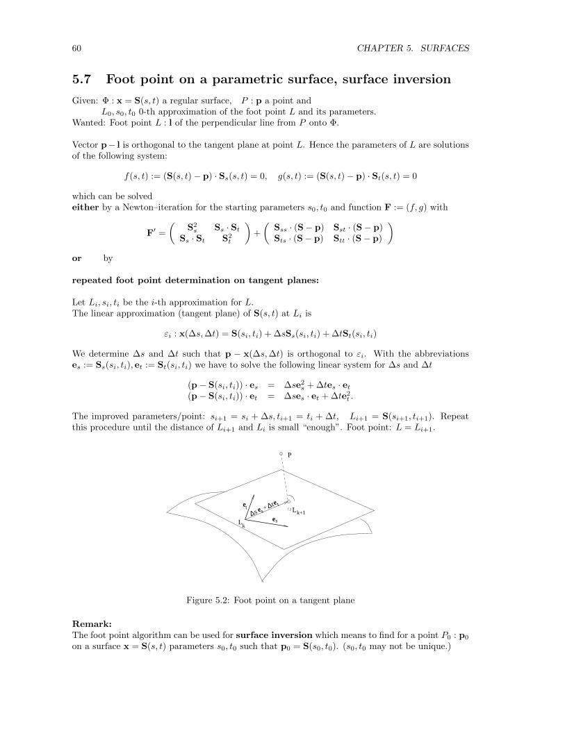
60 CHAPTER 5. SURFACES
5.7 Foot point on a parametric surface, surface inversion
Given: Φ : x = S(s, t) a regular surface, P : p a point andL0, s0, t0 0-th approximation of the foot point L and its parameters.
Wanted: Foot point L : l of the perpendicular line from P onto Φ.
Vector p− l is orthogonal to the tangent plane at point L. Hence the parameters of L are solutionsof the following system:
f(s, t) := (S(s, t)− p) · Ss(s, t) = 0, g(s, t) := (S(s, t)− p) · St(s, t) = 0
which can be solvedeither by a Newton–iteration for the starting parameters s0, t0 and function F := (f, g) with
F′ =
(S2s Ss · St
Ss · St S2t
)+
(Sss · (S− p) Sst · (S− p)Sts · (S− p) Stt · (S− p)
)or by
repeated foot point determination on tangent planes:
Let Li, si, ti be the i-th approximation for L.The linear approximation (tangent plane) of S(s, t) at Li is
εi : x(∆s,∆t) = S(si, ti) + ∆sSs(si, ti) + ∆tSt(si, ti)
We determine ∆s and ∆t such that p − x(∆s,∆t) is orthogonal to εi. With the abbreviationses := Ss(si, ti), et := St(si, ti) we have to solve the following linear system for ∆s and ∆t
(p− S(si, ti)) · es = ∆se2s + ∆tes · et
(p− S(si, ti)) · et = ∆ses · et + ∆te2t .
The improved parameters/point: si+1 = si + ∆s, ti+1 = ti + ∆t, Li+1 = S(si+1, ti+1). Repeatthis procedure until the distance of Li+1 and Li is small “enough”. Foot point: L = Li+1.
∆s se ∆te t
es
te
Lk
k+1L+
P
Figure 5.2: Foot point on a tangent plane
Remark:The foot point algorithm can be used for surface inversion which means to find for a point P0 : p0
on a surface x = S(s, t) parameters s0, t0 such that p0 = S(s0, t0). (s0, t0 may not be unique.)
5.8. STABLE FIRST ORDER FOOT POINT ALGORITHMS FOR SURFACES 61
5.8 Stable first order foot point algorithms for surfaces
5.8.1 Foot point algorithm for parametric surfaces
Analogously to the stable foot point algorithm for parametric planar curves (see Section 4.5.3.1)that respects the curvature without using second derivatives we give the surface version:
Let Φ : x = S(s, t) a regular surface, p a point in the vicinity of Φ and s0, t0 the parameter of astarting point for the foot point algorithm:
repeatpi = S(si, ti), es := Ss(si, ti), et := St(si, ti)
Solve the linear system for ∆s and ∆t:(p− S(si, ti)) · es = ∆s e2
s + ∆t es · et(p− S(si, ti)) · et = ∆s es · et + ∆t e2
t .qi = pi + ∆s Ss(si, ti) + ∆t St(si, ti) (foot point on tangent plane)pi+1 = S(si + ∆s, ti + ∆t), f1 := qi − pi, f2 := pi+1 − qi,if ‖qi−pi‖ > ε then (one Newton step for the foot point on the tangent parabola x = pi+αf1+α2f2)a0 := (p− pi) · f1, a1 := 2f2 · (p− pi)− f2
1 , a2 := −3f1 · f2, a3 := −2f22
α := 1− a0 + a1 + a2 + a3
a1 + 2a2 + 3a3if 0 < α < αmax then (prevent extreme cases)si+1 = ti + α∆s, ti+1 = ti + α∆t, pi+1 = S(si+1, ti+1)until ‖pi − pi+1‖ < ε.foot point f = pi+1.(Suitable choices for the boundaries: ε = 10−6 and αmax = 20.
5.8.2 Foot point algorithm for implicit surfaces
The foot point algorithm for implicit surfaces agrees literally with the version for planar implicitcurves (see Section 4.5.2). One has just to replace the words curve and tangent line by surface andtangent plane:
Procedure surfacepoint:
(SP1) Choose a starting point Q0 : q0 = (x0, y0) in the vicinity of the surface,
(SP2) repeat qi+1 = qi − f(qi)∇f(qi)2
∇f(qi) (Newton step for f(qi + t∇f(qi).)
until ‖qi+1 − qi‖ small enough.surfacepoint= qi+1.
Let p be a point in the vicinity of an implicit surface Φ : f(x) = 0. The following algorithmdetermines the foot point of p on Φ:
(FP0) p0 = surfacepoint(p)
(FP1) repeat
qi = p− (p−pi)·∇f(pi)∇f(pi)2
∇f(pi) (foot point on tangent plane),
pi+1 = surfacepoint(qi), f1 := qi − pi, f2 := pi+1 − qi,if ‖qi − pi‖ > ε then (one Newton step for the foot point on the tangent parabolax = pi + αf1 + α2f2)a0 := (p− pi) · f1, a1 := 2f2 · (p− pi)− f2
1 , a2 := −3f1 · f2, a3 := −2f22
α := 1− a0 + a1 + a2 + a3
a1 + 2a2 + 3a3
62 CHAPTER 5. SURFACES
if 0 < α < αmax then (prevent extreme cases)qi = pi + αf1 + α2f2, pi+1 = surfacepoint(qi)until ‖pi − pi+1‖ < ε.foot point f = pi+1.
5.9 The normalform of a space curve
5.9.1 Definition of the normalform
Definition 5.12 Let g : x = p0 + sr, ‖r‖ = 1, be a line in IR3 and P : p = (x, y, z)> a point. Thedistance of point P to line g is
h(p) =√
(p− p0)2 − ((p− p0) · r)2.
We call equation h(p) = 0 the normal form of the space line g.
Example 5.5 h(x, y, z) =√x2 + y2 = 0 is the normalform of the z-axis. The level surfaces
h = const are cylinders.
Let Γ : x = c(s), s ∈ [s1, s2] be a Cn–continuous, n ≥ 2, space curve parameterized by the arclength s (i.e. ‖c′‖ = 1) and e1(s), e2(s) two orthogonal unit vectors in the normal plane at pointc(s) such that the determinant |c′, e1, e2| = 1, i.e. e1 is a solution of the equation c′ · x = 0 ande2 = c′ × e1. With unit vector e(s, t) := e1(s) cos t+ e(s) sin t we define the family of pipe surfaceswith directrix curve Γ:
x = S(s, t, d) := c(s) + de(s, t), d > 0, t ∈ [0, 2π)
From the definition of vector e(s, t) we get the following properties:
es · e = et · e = 0, et × e = c′.
For d = const function S describes the pipe surface with directrix curve Γ and radius d.The vector equation (x, y, z)> = c(s)+de(s, t) can be solved for s, t, d if the determinant |Ss,St,Sd|is not 0. Evaluation of the determinant yields:
|Ss,St,Sd| = |c′ + des, det, e| = d|c′, et, e|+ d2|es, et, e| = dc′ · (et × e) + d2es · (et × e)
= d(1 + dc′ · es).
Hence in a vicinity of curve Γ there exists a d0 > 0 such that equation (x, y, z)> = c(s) + de(s, t)can be solved for s, t, d with 0 < d ≤ d0. The solutions are functions of x, y, z: s = s(x, y, z), t =t(x, y, z), d = h(x, y, z). Equation h(x, y, z) = 0 is an implicit representation of space curve Γ.Differentiating equation
c(s(x)) + h(x)e(s(x), t(x)) = x
yields:
∇s c′>
+∇h e> + h∇s e>s + h∇t e>t = 3× 3 unit matrix
Multiplying these equations by vector e we get from e>s e = e>t e = c′>
e = 0 the result
∇h = e =S− c
‖S− c‖.
Hence equation h = 0 is an implicit representation of curve Γ with ‖∇h‖ = 1 and in a vicinity of Γbut not on Γ the positive function h is of class Cn, n ≥ 2, too. (h is not differentiable on Γ!)The equation h = 0 is called the normalform of Γ and h the normalform function or (as of itsgeometrical meaning) the distance function of Γ.The considerations above prove of the following Theorem:
5.9. THE NORMALFORM OF A SPACE CURVE 63
Theorem 5.5 For any Cn-continuous, n ≥ 2, space curve Γ there exists in a vicinity V of Γ anormalform of class Cn, i.e. an implicit representation h(x, y, z) = 0 such that ‖∇h‖ = 1 on V \Γ.(h is not differentiable on Γ.)
Example 5.6 The normalform of the circle x2 + y2 = r2, z = 0 (as space curve !) is
h(x, y, z) =
√z2 + (
√x2 + y2 − r)2 = 0.
The level surface h = c, 0 < c < r is the torus with equation
(x2 + y2 + z2 + r2 − c2)2 − 4r2(x2 + y2) = 0.
A consequence of the Theorem 5.5 is
Theorem 5.6 A pipe surface with Cn-continuous directrix, n ≥ 2, is of class Cn, too.
Remark:A differentiable implicit representation can be achieved by using h2 instead of h:
h2 = (S− c)2, ∇h2 = 2(S− c).
The disadvantage ∇h2 = 0 on curve Γ remains.
5.9.2 Foot point algorithm and evaluation of the normalform of a spacecurve
Usually the normalform function is not known explicitly. So the evaluation of h(p) and ∇h(p) isdone numerically by determining the foot point c(tp) of point p on curve Γ.
The foot point algorithm:
Let Γ : x(t) = c(t) be a smooth curve, p a point in the vicinity of Γ and t0 the parameter of astarting point for the foot point algorithm:repeatpi = c(ti)
∆s = (p−pi)·c(ti)c(ti)2
qi = pi + ∆tc(ti) (foot point on tangent)
pi+1 = c(ti + ∆t), f1 := qi − pi, f2 := pi+1 − qi,if ‖qi − pi‖ > ε then
(one Newton step for the foot point on the tangent parabola x = pi + αf1 + α2f2)a0 := (p− pi) · f1, a1 := 2f2 · (p− pi)− f2
1 , a2 := −3f1 · f2, a3 := −2f22
α := 1− a0 + a1 + a2 + a3
a1 + 2a2 + 3a3if 0 < α < αmax then (prevent extreme cases) ti+1 = ti + α∆t, pi+1 = c(ti+1)until ‖pi − pi+1‖ < ε.foot point c(tP) := pi+1, tP := ti+1.(Suitable choices: ε = 10−6 and αmax = 20.)
The evaluation of h and ∇h:
h(p) = ‖p− c(tp)‖, (c(tp)is the foot point of p on the curve)
∇h(p) =p− c(tp)
‖ · · · ‖, if p is not on curve Γ.
64 CHAPTER 5. SURFACES
5.9.3 Determining foot points on an intersection curve
Because for any C2–continuous surface there exists a normal form it suffice to give a foot pointalgorithm for implicitly defined surfaces.
We start with two implicit surfaces Φ1 : f1(x) = 0, Φ2 : f2(x) = 0 and assume that they areregular and sufficiently differentiable for the operations described below. An essential step of thefoot point algorithm is the following procedure curvepoint which determines for a point p in the”neighborhood” of the curve a point p0 on the intersection curve.
Procedure curvepoint:
(C0) Let be f1(x) = 0, f2(x) = 0 two intersecting implicit surfaces and p a point.
(C1) q0 := p,repeat qk+1 = qk + ∆k, where∆k = αk∇f1(qk) + βk∇f2(qk) and ∆k · ∇fj(qk) = −fj(qk), j = 1, 2.(Newton step for gj(α, β) := fj(qk + α∇f1(qk) + β∇f2(qk)), j = 1, 2.)until ‖qk+1 − qk‖ is ”sufficiently” small.Curve point: p0 = qk+1.
Procedure footpoint:
(F0) Let be f1(x) = 0, f2(x) = 0 two intersecting implicit surfaces and p a point.
(F1) c0 = curvepoint(p)
(F2) repeat ri := ∇f1(ci)×∇f2(ci) (tangent direction),
ti+1 = ci +(p− ci) · ri
r2i
ri (foot point on tangent),
ci+1 = curvepoint(ti+1).until ‖ci+1 − ci‖ is ”sufficiently” small.Foot point: p0 = ci+1.
Remark: In case of problems considering convergence of the foot point algorithm one should im-prove it by a ”parabola step” (see Section 5.9.2).
5.10 Applications of normalforms
5.10.1 Approximation of a set of intersecting surfaces
Given
1. the implicit surface (x− 2)4 + y4 − r41 = 0, r1 = 2,
2. the parametric surface patchx = (10v − 5, 10u− 5, 6(u− u2 + v − v2)), 0 ≤ u ≤ 1, 0 ≤ v ≤ 0.8,
3. the parametric surface patchx = (6(u− u2 + v − v2)− 5, 10u− 5, 10v − 5), 0 ≤ u ≤ 1, 0.5 ≤ v ≤ 1.
Let be h1(x) = 0, h2(x) = 0, h3(x) = 0 the normalforms of the surfaces. The implicit surfacef(x) := h1(x)h2(x)h3(x) = c > 0 is a smooth approximation of the set of the three given surfaces.Figure 5.3b) shows the triangulation of f(x) = c for c = 0.2.
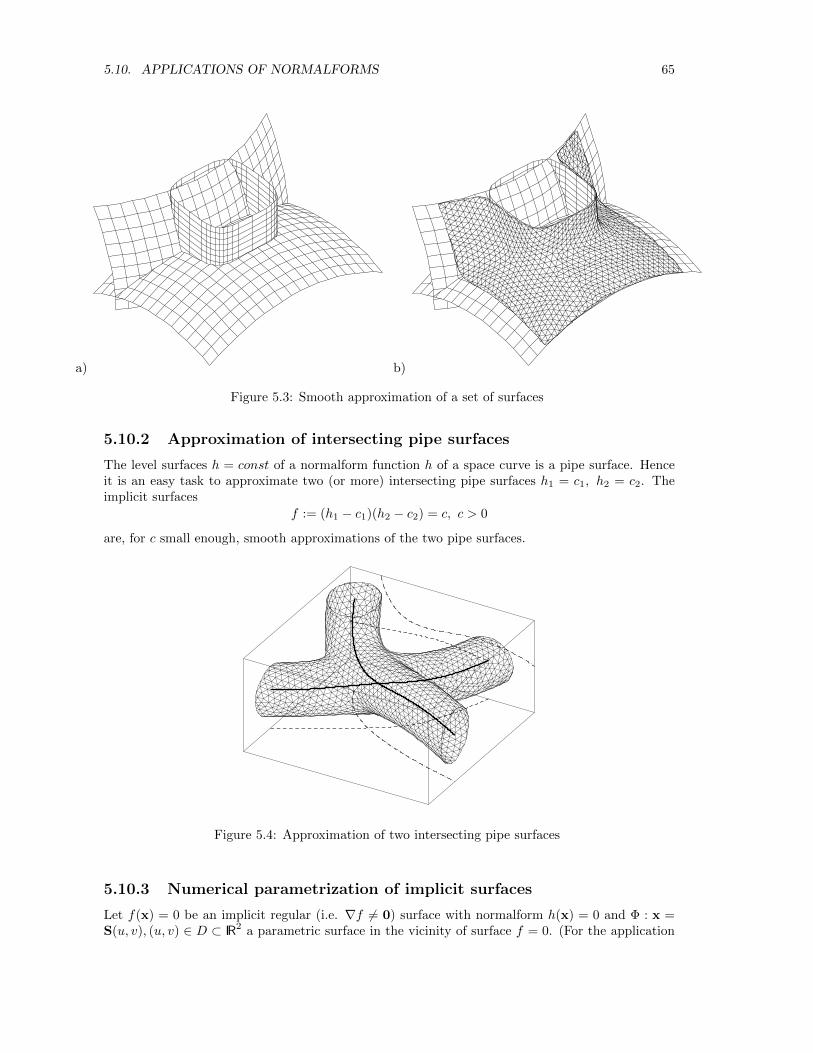
5.10. APPLICATIONS OF NORMALFORMS 65
a) b)
Figure 5.3: Smooth approximation of a set of surfaces
5.10.2 Approximation of intersecting pipe surfaces
The level surfaces h = const of a normalform function h of a space curve is a pipe surface. Henceit is an easy task to approximate two (or more) intersecting pipe surfaces h1 = c1, h2 = c2. Theimplicit surfaces
f := (h1 − c1)(h2 − c2) = c, c > 0
are, for c small enough, smooth approximations of the two pipe surfaces.
Figure 5.4: Approximation of two intersecting pipe surfaces
5.10.3 Numerical parametrization of implicit surfaces
Let f(x) = 0 be an implicit regular (i.e. ∇f 6= 0) surface with normalform h(x) = 0 and Φ : x =S(u, v), (u, v) ∈ D ⊂ IR2 a parametric surface in the vicinity of surface f = 0. (For the application
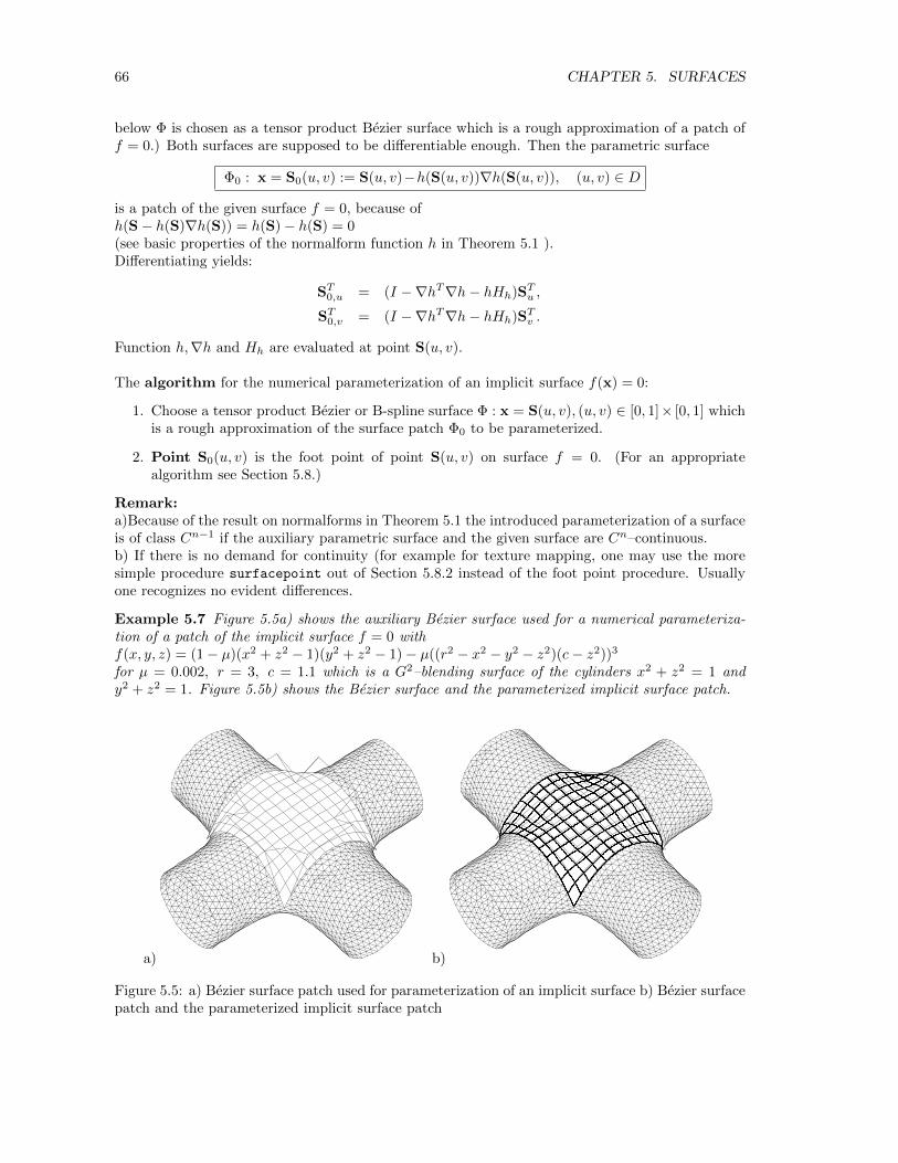
66 CHAPTER 5. SURFACES
below Φ is chosen as a tensor product Bezier surface which is a rough approximation of a patch off = 0.) Both surfaces are supposed to be differentiable enough. Then the parametric surface
Φ0 : x = S0(u, v) := S(u, v)−h(S(u, v))∇h(S(u, v)), (u, v) ∈ D
is a patch of the given surface f = 0, because ofh(S− h(S)∇h(S)) = h(S)− h(S) = 0(see basic properties of the normalform function h in Theorem 5.1 ).Differentiating yields:
ST0,u = (I −∇hT∇h− hHh)STu ,
ST0,v = (I −∇hT∇h− hHh)STv .
Function h,∇h and Hh are evaluated at point S(u, v).
The algorithm for the numerical parameterization of an implicit surface f(x) = 0:
1. Choose a tensor product Bezier or B-spline surface Φ : x = S(u, v), (u, v) ∈ [0, 1]× [0, 1] whichis a rough approximation of the surface patch Φ0 to be parameterized.
2. Point S0(u, v) is the foot point of point S(u, v) on surface f = 0. (For an appropriatealgorithm see Section 5.8.)
Remark:a)Because of the result on normalforms in Theorem 5.1 the introduced parameterization of a surfaceis of class Cn−1 if the auxiliary parametric surface and the given surface are Cn–continuous.b) If there is no demand for continuity (for example for texture mapping, one may use the moresimple procedure surfacepoint out of Section 5.8.2 instead of the foot point procedure. Usuallyone recognizes no evident differences.
Example 5.7 Figure 5.5a) shows the auxiliary Bezier surface used for a numerical parameteriza-tion of a patch of the implicit surface f = 0 withf(x, y, z) = (1− µ)(x2 + z2 − 1)(y2 + z2 − 1)− µ((r2 − x2 − y2 − z2)(c− z2))3
for µ = 0.002, r = 3, c = 1.1 which is a G2–blending surface of the cylinders x2 + z2 = 1 andy2 + z2 = 1. Figure 5.5b) shows the Bezier surface and the parameterized implicit surface patch.
a) b)
Figure 5.5: a) Bezier surface patch used for parameterization of an implicit surface b) Bezier surfacepatch and the parameterized implicit surface patch
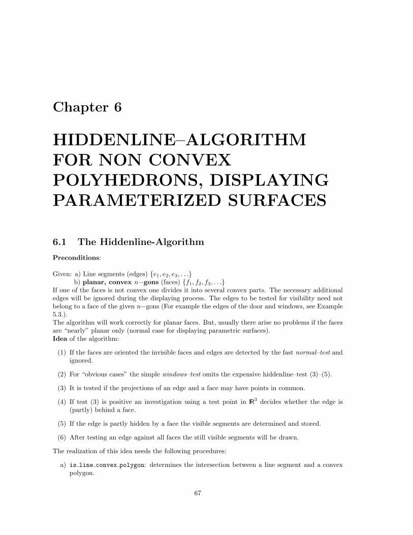
Chapter 6
HIDDENLINE–ALGORITHMFOR NON CONVEXPOLYHEDRONS, DISPLAYINGPARAMETERIZED SURFACES
6.1 The Hiddenline-Algorithm
Preconditions:
Given: a) Line segments (edges) {e1, e2, e3, . . .}b) planar, convex n−gons (faces) {f1, f2, f3, . . .}
If one of the faces is not convex one divides it into several convex parts. The necessary additionaledges will be ignored during the displaying process. The edges to be tested for visibility need notbelong to a face of the given n−gons (For example the edges of the door and windows, see Example5.3.).The algorithm will work correctly for planar faces. But, usually there arise no problems if the facesare “nearly” planar only (normal case for displaying parametric surfaces).Idea of the algorithm:
(1) If the faces are oriented the invisible faces and edges are detected by the fast normal–test andignored.
(2) For “obvious cases” the simple windows–test omits the expensive hiddenline–test (3)–(5).
(3) It is tested if the projections of an edge and a face may have points in common.
(4) If test (3) is positive an investigation using a test point in IR3 decides whether the edge is(partly) behind a face.
(5) If the edge is partly hidden by a face the visible segments are determined and stored.
(6) After testing an edge against all faces the still visible segments will be drawn.
The realization of this idea needs the following procedures:
a) is line convex polygon: determines the intersection between a line segment and a convexpolygon.
67
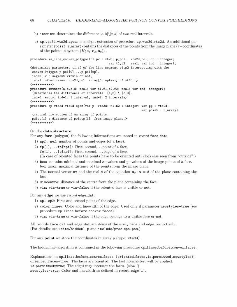
68 CHAPTER 6. HIDDENLINE–ALGORITHM FOR NON CONVEX POLYHEDRONS
b) intmint: determines the difference [a, b]\[c, d] of two real intervals.
c) cp vts3d vts2d spez: is a slight extension of procedure cp vts3d vts2d. An additional pa-rameter (pdist: r array) contains the distances of the points from the image plane (z−coordinatesof the points in system (H; e1, e2,n0)) .
procedure is_line_convex_polygon(p1,p2 : vt2d; p_pol : vts2d_pol; np : integer;
var t1,t2 : real; var ind : integer);
{determines parameters t1,t2 of the line segment p1,p2 intersecting with the
convex Polygon p_pol[0],...p_pol[np].
ind=0, 2 : segment within or not,
ind=1: other cases. vts2d_pol: array[0..npfmax] of vt2d. }
{***********}
procedure intmint(a,b,c,d: real; var e1,f1,e2,f2: real; var ind: integer);
{Determines the difference of intervals [a,b] \ [c,d].
ind=0: empty, ind=1: 1 interval, ind=2: 2 intervals}
{***********}
procedure cp_vts3d_vts2d_spez(var p: vts3d; n1,n2 : integer; var pp : vts2d;
var pdist : r_array);
{central projection of an array of points.
pdist[i] : distance of pointp[i] from image plane.}
{***********}
On the data structure:For any face (polygon) the following informations are stored in record face dat:
1) npf, nef: number of points and edges (of a face).
2) fp[1], . . . fp[npf]: First, second,. . . point of a face,fe[1], . . . fe[nef]: First, second, . . . edge of a face.(In case of oriented faces the points have to be oriented anti clockwise seen from “outside”.)
3) box: contains minimal and maximal x−values and y−values of the image points of a face.box.zmax: maximal distance of the points from the image plane.
4) The normal vector nv and the real d of the equation nv · x = d of the plane containing theface.
5) discentre: distance of the centre from the plane containing the face.
6) vis: vis=true or vis=false if the oriented face is visible or not.
For any edge we use record edge dat:
1) ep1,ep2: First and second point of the edge.
2) color,linew: Color and linewidth of the edge. Used only if parameter newstyles=true (seeprocedure cp lines before convex faces).
3) vis: vis=true or vis=false if the edge belongs to a visible face or not.
All records face dat and edge dat are items of the array face and edge respectively.(For details: see units/hiddenl.p and include/proc zpo.pas.)
For any point we store the coordinates in array p (type: vts3d).
The hiddenline–algorithm is contained in the following procedure cp lines before convex faces.
Explanations on cp lines before convex faces (oriented faces,is permitted,newstyles):oriented faces=true: The faces are oriented. The fast normal-test will be applied.is permitted=true: The edges may intersect the faces. (slow !)newstyles=true: Color and linewidth as defined in record edge[i].
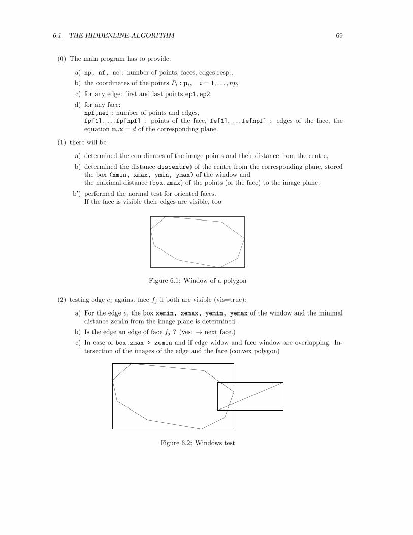
6.1. THE HIDDENLINE-ALGORITHM 69
(0) The main program has to provide:
a) np, nf, ne : number of points, faces, edges resp.,
b) the coordinates of the points Pi : pi, i = 1, . . . , np,
c) for any edge: first and last points ep1,ep2,
d) for any face:npf,nef : number of points and edges,fp[1], . . . fp[npf] : points of the face, fe[1], . . . fe[npf] : edges of the face, theequation nvx = d of the corresponding plane.
(1) there will be
a) determined the coordinates of the image points and their distance from the centre,
b) determined the distance discentre) of the centre from the corresponding plane, storedthe box (xmin, xmax, ymin, ymax) of the window andthe maximal distance (box.zmax) of the points (of the face) to the image plane.
b’) performed the normal test for oriented faces.If the face is visible their edges are visible, too
Figure 6.1: Window of a polygon
(2) testing edge ei against face fj if both are visible (vis=true):
a) For the edge ei the box xemin, xemax, yemin, yemax of the window and the minimaldistance zemin from the image plane is determined.
b) Is the edge an edge of face fj ? (yes: → next face.)
c) In case of box.zmax > zemin and if edge widow and face window are overlapping: In-tersection of the images of the edge and the face (convex polygon)
Figure 6.2: Windows test
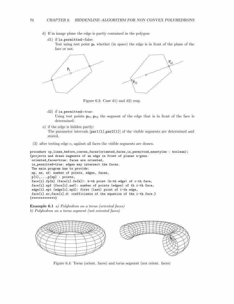
70 CHAPTER 6. HIDDENLINE–ALGORITHM FOR NON CONVEX POLYHEDRONS
d) If in image plane the edge is partly contained in the polygon:
d1) if is permitted=false:Test using test point pt whether (in space) the edge is in front of the plane of theface or not.
Pt1
Pt2
Pt
Figure 6.3: Case d1) and d2) resp.
d2) if is permitted=true:Using test points pt1,pt2 the segment of the edge that is in front of the face isdetermined.
e) if the edge is hidden partly:The parameter intervals [par1(l),par2(l)] of the visible segments are determined andstored.
(3) after testing edge ei against all faces the visible segments are drawn.
procedure cp_lines_before_convex_faces(oriented_faces,is_permitted,newstyles : boolean);
{projects and draws segments of an edge in front of planar n-gons.
oriented_faces=true: faces are oriented,
is_permitted=true: edges may intersect the faces.
The main program has to provide:
np, ne, nf: number of points, edges, faces,
p[1],...,p[np] : points,
face[i].fp[k] (face[i].fe[k]): k-th point (k-th edge) of i-th face,
face[i].npf (face[i].nef): number of points (edges) of th i-th face,
edge[i].ep1 (edge[i].ep2): first (last) point of i-th edge,
face[i].nv,face[i].d: coefficients of the equation of the i-th face.}
{*************}
Example 6.1 a) Polyhedron on a torus (oriented faces)b) Polyhedron on a torus segment (not oriented faces)
Figure 6.4: Torus (orient. faces) and torus segment (not orient. faces)
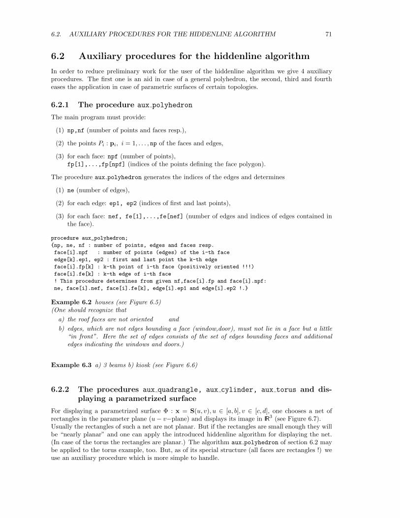
6.2. AUXILIARY PROCEDURES FOR THE HIDDENLINE ALGORITHM 71
6.2 Auxiliary procedures for the hiddenline algorithm
In order to reduce preliminary work for the user of the hiddenline algorithm we give 4 auxiliaryprocedures. The first one is an aid in case of a general polyhedron, the second, third and fourtheases the application in case of parametric surfaces of certain topologies.
6.2.1 The procedure aux polyhedron
The main program must provide:
(1) np,nf (number of points and faces resp.),
(2) the points Pi : pi, i = 1, . . . , np of the faces and edges,
(3) for each face: npf (number of points),fp[1],...,fp[npf] (indices of the points defining the face polygon).
The procedure aux polyhedron generates the indices of the edges and determines
(1) ne (number of edges),
(2) for each edge: ep1, ep2 (indices of first and last points),
(3) for each face: nef, fe[1],...,fe[nef] (number of edges and indices of edges contained inthe face).
procedure aux_polyhedron;
{np, ne, nf : number of points, edges and faces resp.
face[i].npf : number of points (edges) of the i-th face
edge[k].ep1, ep2 : first and last point the k-th edge
face[i].fp[k] : k-th point of i-th face (positively oriented !!!)
face[i].fe[k] : k-th edge of i-th face
! This procedure determines from given nf,face[i].fp and face[i].npf:
ne, face[i].nef, face[i].fe[k], edge[i].ep1 and edge[i].ep2 !.}
Example 6.2 houses (see Figure 6.5)(One should recognize that
a) the roof faces are not oriented and
b) edges, which are not edges bounding a face (window,door), must not lie in a face but a little“in front”. Here the set of edges consists of the set of edges bounding faces and additionaledges indicating the windows and doors.)
Example 6.3 a) 3 beams b) kiosk (see Figure 6.6)
6.2.2 The procedures aux quadrangle, aux cylinder, aux torus and dis-playing a parametrized surface
For displaying a parametrized surface Φ : x = S(u, v), u ∈ [a, b], v ∈ [c, d], one chooses a net ofrectangles in the parameter plane (u− v−plane) and displays its image in IR3 (see Figure 6.7).Usually the rectangles of such a net are not planar. But if the rectangles are small enough they willbe “nearly planar” and one can apply the introduced hiddenline algorithm for displaying the net.(In case of the torus the rectangles are planar.) The algorithm aux polyhedron of section 6.2 maybe applied to the torus example, too. But, as of its special structure (all faces are rectangles !) weuse an auxiliary procedure which is more simple to handle.
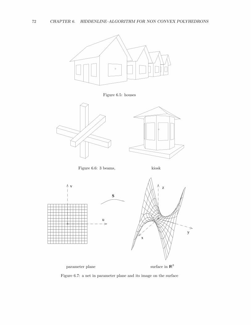
72 CHAPTER 6. HIDDENLINE–ALGORITHM FOR NON CONVEX POLYHEDRONS
Figure 6.5: houses
Figure 6.6: 3 beams, kiosk
xy
z
u
v
S
parameter plane surface in IR3
Figure 6.7: a net in parameter plane and its image on the surface
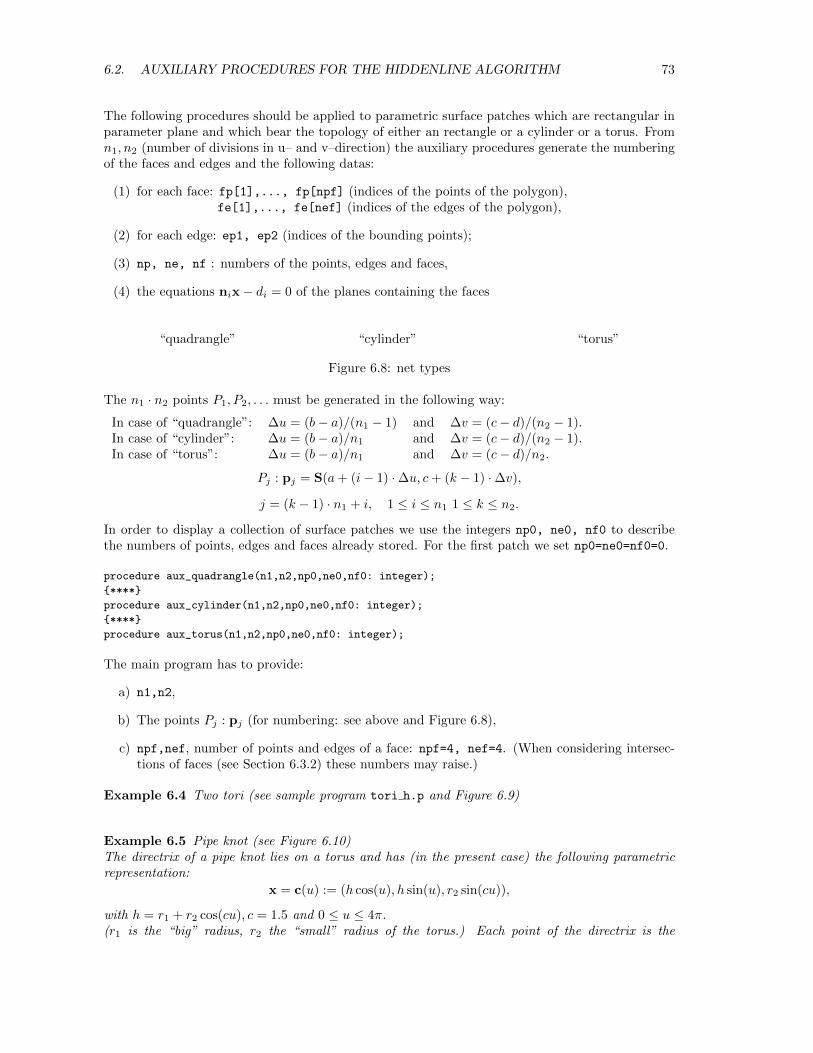
6.2. AUXILIARY PROCEDURES FOR THE HIDDENLINE ALGORITHM 73
The following procedures should be applied to parametric surface patches which are rectangular inparameter plane and which bear the topology of either an rectangle or a cylinder or a torus. Fromn1, n2 (number of divisions in u– and v–direction) the auxiliary procedures generate the numberingof the faces and edges and the following datas:
(1) for each face: fp[1],..., fp[npf] (indices of the points of the polygon),fe[1],..., fe[nef] (indices of the edges of the polygon),
(2) for each edge: ep1, ep2 (indices of the bounding points);
(3) np, ne, nf : numbers of the points, edges and faces,
(4) the equations nix− di = 0 of the planes containing the faces
“quadrangle” “cylinder” “torus”
Figure 6.8: net types
The n1 · n2 points P1, P2, . . . must be generated in the following way:
In case of “quadrangle”: ∆u = (b− a)/(n1 − 1) and ∆v = (c− d)/(n2 − 1).In case of “cylinder”: ∆u = (b− a)/n1 and ∆v = (c− d)/(n2 − 1).In case of “torus”: ∆u = (b− a)/n1 and ∆v = (c− d)/n2.
Pj : pj = S(a+ (i− 1) ·∆u, c+ (k − 1) ·∆v),
j = (k − 1) · n1 + i, 1 ≤ i ≤ n1 1 ≤ k ≤ n2.
In order to display a collection of surface patches we use the integers np0, ne0, nf0 to describethe numbers of points, edges and faces already stored. For the first patch we set np0=ne0=nf0=0.
procedure aux_quadrangle(n1,n2,np0,ne0,nf0: integer);
{****}
procedure aux_cylinder(n1,n2,np0,ne0,nf0: integer);
{****}
procedure aux_torus(n1,n2,np0,ne0,nf0: integer);
The main program has to provide:
a) n1,n2,
b) The points Pj : pj (for numbering: see above and Figure 6.8),
c) npf,nef, number of points and edges of a face: npf=4, nef=4. (When considering intersec-tions of faces (see Section 6.3.2) these numbers may raise.)
Example 6.4 Two tori (see sample program tori h.p and Figure 6.9)
Example 6.5 Pipe knot (see Figure 6.10)The directrix of a pipe knot lies on a torus and has (in the present case) the following parametricrepresentation:
x = c(u) := (h cos(u), h sin(u), r2 sin(cu)),
with h = r1 + r2 cos(cu), c = 1.5 and 0 ≤ u ≤ 4π.(r1 is the “big” radius, r2 the “small” radius of the torus.) Each point of the directrix is the
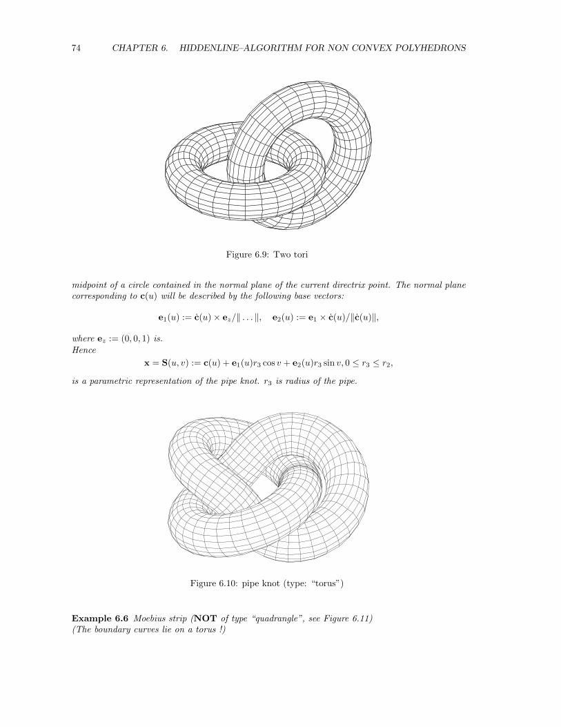
74 CHAPTER 6. HIDDENLINE–ALGORITHM FOR NON CONVEX POLYHEDRONS
Figure 6.9: Two tori
midpoint of a circle contained in the normal plane of the current directrix point. The normal planecorresponding to c(u) will be described by the following base vectors:
e1(u) := c(u)× ez/‖ . . . ‖, e2(u) := e1 × c(u)/‖c(u)‖,
where ez := (0, 0, 1) is.
Hence
x = S(u, v) := c(u) + e1(u)r3 cos v + e2(u)r3 sin v, 0 ≤ r3 ≤ r2,
is a parametric representation of the pipe knot. r3 is radius of the pipe.
Figure 6.10: pipe knot (type: “torus”)
Example 6.6 Moebius strip (NOT of type “quadrangle”, see Figure 6.11)(The boundary curves lie on a torus !)
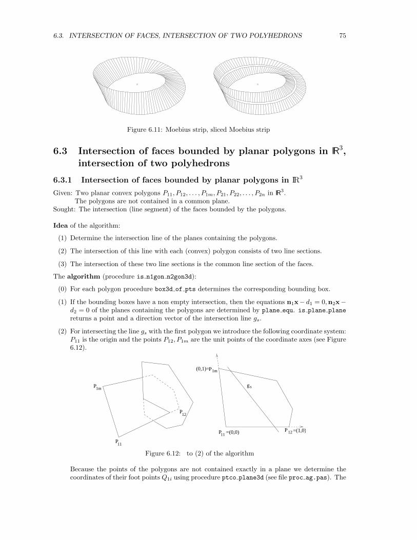
6.3. INTERSECTION OF FACES, INTERSECTION OF TWO POLYHEDRONS 75
Figure 6.11: Moebius strip, sliced Moebius strip
6.3 Intersection of faces bounded by planar polygons in IR3,intersection of two polyhedrons
6.3.1 Intersection of faces bounded by planar polygons in IR3
Given: Two planar convex polygons P11, P12, . . . , P1m, P21, P22, . . . , P2n in IR3.The polygons are not contained in a common plane.
Sought: The intersection (line segment) of the faces bounded by the polygons.
Idea of the algorithm:
(1) Determine the intersection line of the planes containing the polygons.
(2) The intersection of this line with each (convex) polygon consists of two line sections.
(3) The intersection of these two line sections is the common line section of the faces.
The algorithm (procedure is n1gon n2gon3d):
(0) For each polygon procedure box3d of pts determines the corresponding bounding box.
(1) If the bounding boxes have a non empty intersection, then the equations n1x− d1 = 0,n2x−d2 = 0 of the planes containing the polygons are determined by plane equ. is plane plane
returns a point and a direction vector of the intersection line gs.
(2) For intersecting the line gs with the first polygon we introduce the following coordinate system:P11 is the origin and the points P12, P1m are the unit points of the coordinate axes (see Figure6.12).
P11P12
P1m
P11
P12
P1mg s
=(0,0) =(1,0)
(0,1)=
Figure 6.12: to (2) of the algorithm
Because the points of the polygons are not contained exactly in a plane we determine thecoordinates of their foot points Q1i using procedure ptco plane3d (see file proc ag.pas). The
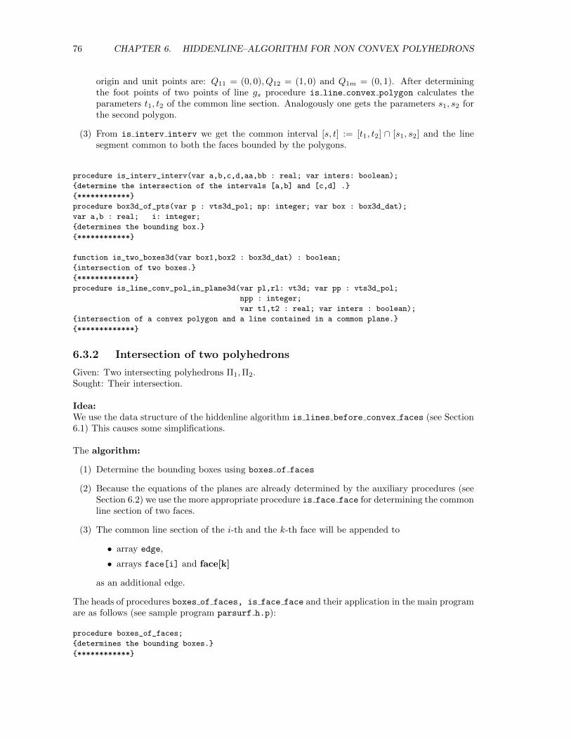
76 CHAPTER 6. HIDDENLINE–ALGORITHM FOR NON CONVEX POLYHEDRONS
origin and unit points are: Q11 = (0, 0), Q12 = (1, 0) and Q1m = (0, 1). After determiningthe foot points of two points of line gs procedure is line convex polygon calculates theparameters t1, t2 of the common line section. Analogously one gets the parameters s1, s2 forthe second polygon.
(3) From is interv interv we get the common interval [s, t] := [t1, t2] ∩ [s1, s2] and the linesegment common to both the faces bounded by the polygons.
procedure is_interv_interv(var a,b,c,d,aa,bb : real; var inters: boolean);
{determine the intersection of the intervals [a,b] and [c,d] .}
{************}
procedure box3d_of_pts(var p : vts3d_pol; np: integer; var box : box3d_dat);
var a,b : real; i: integer;
{determines the bounding box.}
{************}
function is_two_boxes3d(var box1,box2 : box3d_dat) : boolean;
{intersection of two boxes.}
{*************}
procedure is_line_conv_pol_in_plane3d(var pl,rl: vt3d; var pp : vts3d_pol;
npp : integer;
var t1,t2 : real; var inters : boolean);
{intersection of a convex polygon and a line contained in a common plane.}
{*************}
6.3.2 Intersection of two polyhedrons
Given: Two intersecting polyhedrons Π1,Π2.Sought: Their intersection.
Idea:We use the data structure of the hiddenline algorithm is lines before convex faces (see Section6.1) This causes some simplifications.
The algorithm:
(1) Determine the bounding boxes using boxes of faces
(2) Because the equations of the planes are already determined by the auxiliary procedures (seeSection 6.2) we use the more appropriate procedure is face face for determining the commonline section of two faces.
(3) The common line section of the i-th and the k-th face will be appended to
• array edge,
• arrays face[i] and face[k]
as an additional edge.
The heads of procedures boxes of faces, is face face and their application in the main programare as follows (see sample program parsurf h.p):
procedure boxes_of_faces;
{determines the bounding boxes.}
{************}
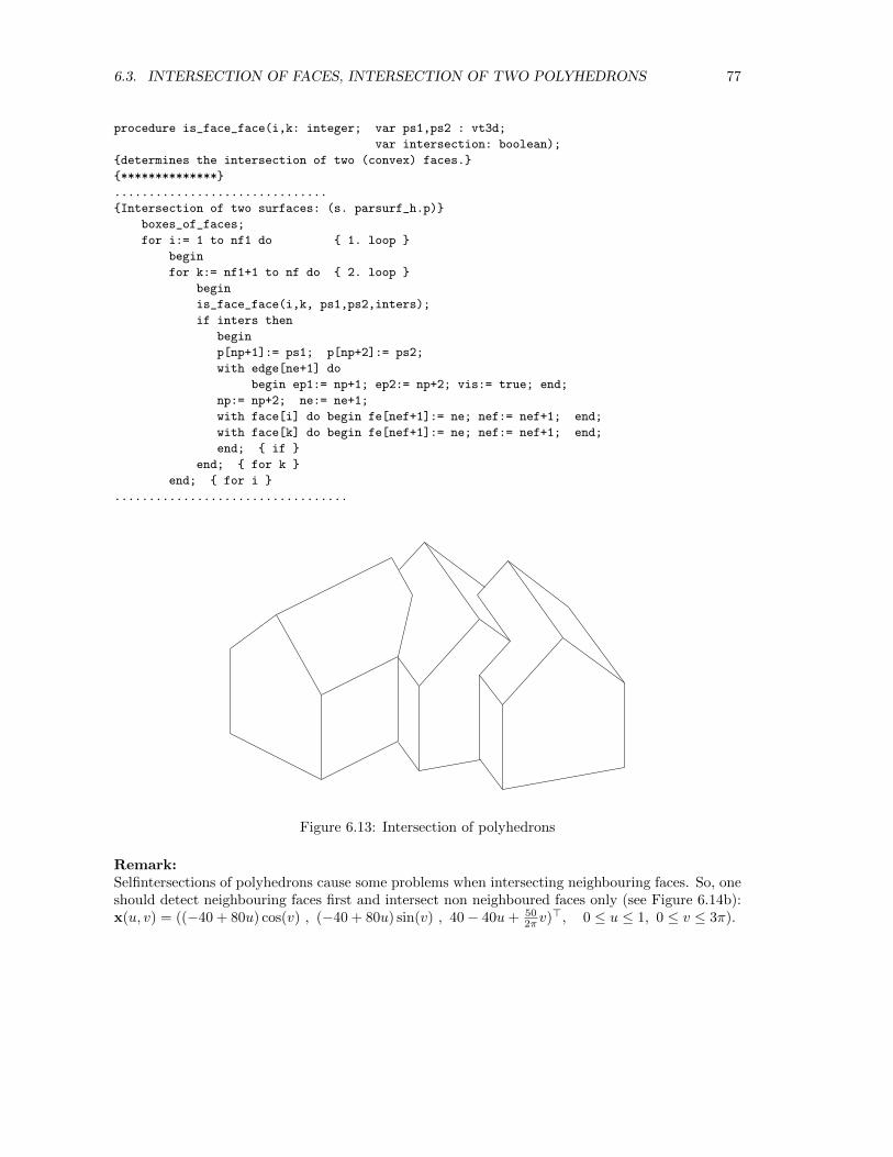
6.3. INTERSECTION OF FACES, INTERSECTION OF TWO POLYHEDRONS 77
procedure is_face_face(i,k: integer; var ps1,ps2 : vt3d;
var intersection: boolean);
{determines the intersection of two (convex) faces.}
{**************}
...............................
{Intersection of two surfaces: (s. parsurf_h.p)}
boxes_of_faces;
for i:= 1 to nf1 do { 1. loop }
begin
for k:= nf1+1 to nf do { 2. loop }
begin
is_face_face(i,k, ps1,ps2,inters);
if inters then
begin
p[np+1]:= ps1; p[np+2]:= ps2;
with edge[ne+1] do
begin ep1:= np+1; ep2:= np+2; vis:= true; end;
np:= np+2; ne:= ne+1;
with face[i] do begin fe[nef+1]:= ne; nef:= nef+1; end;
with face[k] do begin fe[nef+1]:= ne; nef:= nef+1; end;
end; { if }
end; { for k }
end; { for i }
..................................
Figure 6.13: Intersection of polyhedrons
Remark:Selfintersections of polyhedrons cause some problems when intersecting neighbouring faces. So, oneshould detect neighbouring faces first and intersect non neighboured faces only (see Figure 6.14b):x(u, v) = ((−40 + 80u) cos(v) , (−40 + 80u) sin(v) , 40− 40u+ 50
2πv)>, 0 ≤ u ≤ 1, 0 ≤ v ≤ 3π).
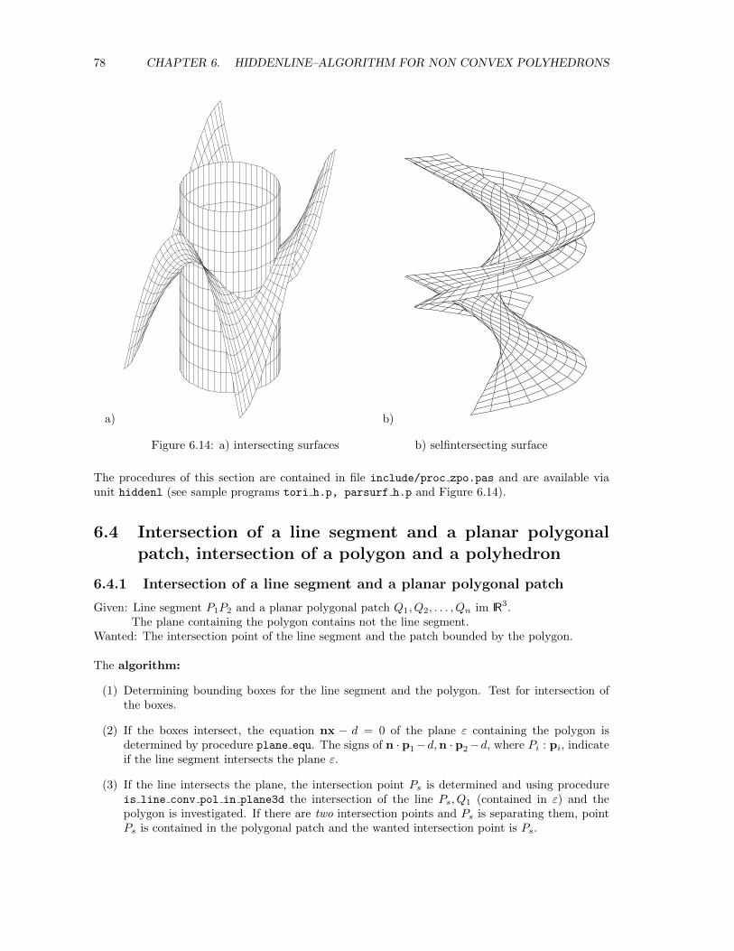
78 CHAPTER 6. HIDDENLINE–ALGORITHM FOR NON CONVEX POLYHEDRONS
a) b)
Figure 6.14: a) intersecting surfaces b) selfintersecting surface
The procedures of this section are contained in file include/proc zpo.pas and are available viaunit hiddenl (see sample programs tori h.p, parsurf h.p and Figure 6.14).
6.4 Intersection of a line segment and a planar polygonalpatch, intersection of a polygon and a polyhedron
6.4.1 Intersection of a line segment and a planar polygonal patch
Given: Line segment P1P2 and a planar polygonal patch Q1, Q2, . . . , Qn im IR3.The plane containing the polygon contains not the line segment.
Wanted: The intersection point of the line segment and the patch bounded by the polygon.
The algorithm:
(1) Determining bounding boxes for the line segment and the polygon. Test for intersection ofthe boxes.
(2) If the boxes intersect, the equation nx − d = 0 of the plane ε containing the polygon isdetermined by procedure plane equ. The signs of n · p1−d,n · p2−d, where Pi : pi, indicateif the line segment intersects the plane ε.
(3) If the line intersects the plane, the intersection point Ps is determined and using procedureis line conv pol in plane3d the intersection of the line Ps, Q1 (contained in ε) and thepolygon is investigated. If there are two intersection points and Ps is separating them, pointPs is contained in the polygonal patch and the wanted intersection point is Ps.
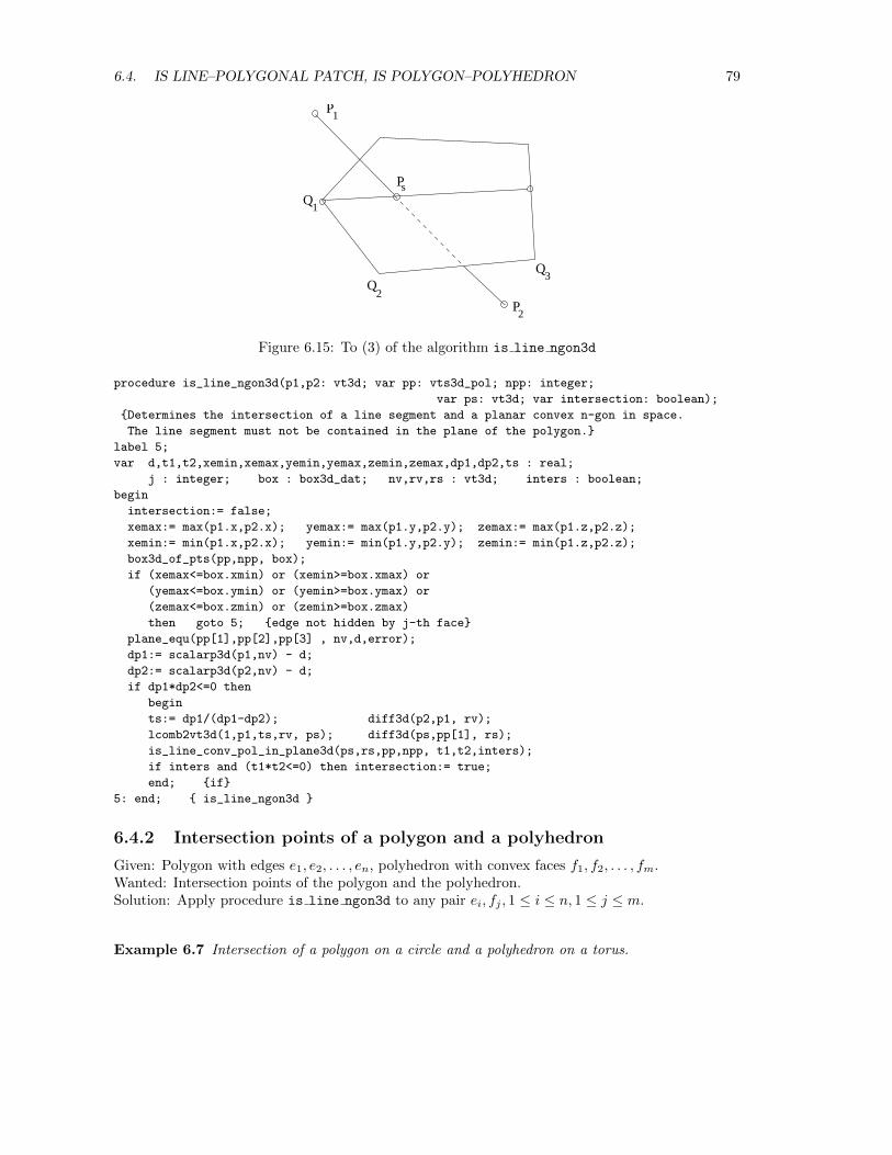
6.4. IS LINE–POLYGONAL PATCH, IS POLYGON–POLYHEDRON 79
Q1
Q2
Q3
P1
P2
Ps
Figure 6.15: To (3) of the algorithm is line ngon3d
procedure is_line_ngon3d(p1,p2: vt3d; var pp: vts3d_pol; npp: integer;
var ps: vt3d; var intersection: boolean);
{Determines the intersection of a line segment and a planar convex n-gon in space.
The line segment must not be contained in the plane of the polygon.}
label 5;
var d,t1,t2,xemin,xemax,yemin,yemax,zemin,zemax,dp1,dp2,ts : real;
j : integer; box : box3d_dat; nv,rv,rs : vt3d; inters : boolean;
begin
intersection:= false;
xemax:= max(p1.x,p2.x); yemax:= max(p1.y,p2.y); zemax:= max(p1.z,p2.z);
xemin:= min(p1.x,p2.x); yemin:= min(p1.y,p2.y); zemin:= min(p1.z,p2.z);
box3d_of_pts(pp,npp, box);
if (xemax<=box.xmin) or (xemin>=box.xmax) or
(yemax<=box.ymin) or (yemin>=box.ymax) or
(zemax<=box.zmin) or (zemin>=box.zmax)
then goto 5; {edge not hidden by j-th face}
plane_equ(pp[1],pp[2],pp[3] , nv,d,error);
dp1:= scalarp3d(p1,nv) - d;
dp2:= scalarp3d(p2,nv) - d;
if dp1*dp2<=0 then
begin
ts:= dp1/(dp1-dp2); diff3d(p2,p1, rv);
lcomb2vt3d(1,p1,ts,rv, ps); diff3d(ps,pp[1], rs);
is_line_conv_pol_in_plane3d(ps,rs,pp,npp, t1,t2,inters);
if inters and (t1*t2<=0) then intersection:= true;
end; {if}
5: end; { is_line_ngon3d }
6.4.2 Intersection points of a polygon and a polyhedron
Given: Polygon with edges e1, e2, . . . , en, polyhedron with convex faces f1, f2, . . . , fm.Wanted: Intersection points of the polygon and the polyhedron.Solution: Apply procedure is line ngon3d to any pair ei, fj , 1 ≤ i ≤ n, 1 ≤ j ≤ m.
Example 6.7 Intersection of a polygon on a circle and a polyhedron on a torus.
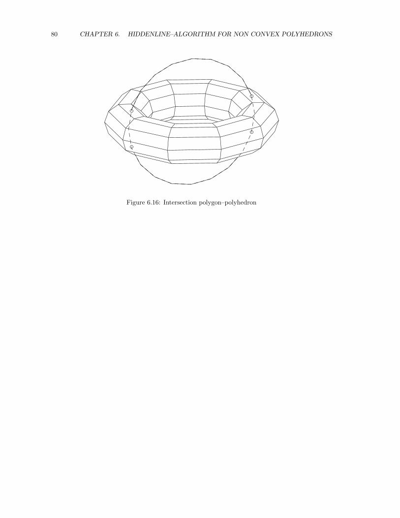
80 CHAPTER 6. HIDDENLINE–ALGORITHM FOR NON CONVEX POLYHEDRONS
Figure 6.16: Intersection polygon–polyhedron
Chapter 7
TRIANGULATION OFIMPLICIT SURFACES
Determining single points of an implicit surface is not trivial. The generation of a net of polygonson an implicit surface (for displaying, finite element methods) is a challenge. Polygonization algo-rithms for implicit surfaces are available in literature. For example: Algower & Gnutzmann (1991,Computer Aided Geom. Des. 8), Schmidt (1993, The Visual Comp. 10) and Hartmann (1998,The Visual Comp. 14). All these methods except the latter one divide the space into suitablepolyhedrons (cubes, tetrahedrons) and determine the section of the given implicit surface with theedges of these polyhedrons.The method introduced by the author is a marching method which means to build successively amesh of triangles by starting with a point or a prescribed polygon. The triangulation is terminatedby several bounding polygons (on the given surface) or a global bounding box. The method wasestablished for implicit surfaces. But using the idea of the normalform of a surface the triangulationis applicable to any surface for which foot points (i.e. points of minimal distance to the surface) canbe determined.
Remark:The following triangulation algorithm appeared in The Visual Computer 14 (1998), pp 95–108,copyright by Springer-Verlag. The original publication is available onhttp://link.springer.de/link/service/journals/00371/tocs/8014003.htm
7.1 The triangulation algorithm (marching method)
The formulation of the triangulation algorithm uses no special representation of the surface to betriangulated. The operations depending on the representation are hidden in the used proceduresurfacepoint which is defined below.
The next subsection gives first a survey and basic ideas of the algorithm. Afterwards the proceduresurfacepoint and the data structure used is introduced, and the steps of the algorithm explainedin detail.
7.1.1 The idea of the algorithm
S0 Choose a point s in the neighborhood of the the surface. Determine the corresponding surfacepoint p1. Surround p1 with a regular hexagon q2, ...,q7 in the tangent plane. With proceduresurfacepoint determine the points p2, ...,p7 corresponding to the starting points q2, ...,q7.
81
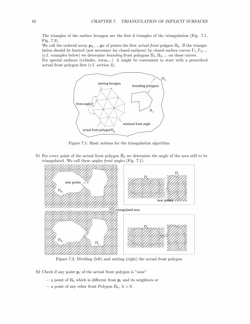
82 CHAPTER 7. TRIANGULATION OF IMPLICIT SURFACES
The triangles of the surface hexagon are the first 6 triangles of the triangulation (Fig. 7.1,Fig. 7.3).We call the ordered array p2, ...,p7 of points the first actual front polygon Π0. If the triangu-lation should be limited (not necessary for closed surfaces) by closed surface curves Γ1,Γ2, ...(c.f. examples below) we determine bounding front polygons Π1,Π2, ... on these curves.For special surfaces (cylinder, torus,...) it might be convenient to start with a prescribedactual front polygon first (c.f. section 3).
Π0
Π1
Π2starting hexagon
minimal front angle
bounding polygons
actual front polygon
front angles
Figure 7.1: Basic notions for the triangulation algorithm
S1 For every point of the actual front polygon Π0 we determine the angle of the area still to betriangulated. We call these angles front angles (Fig. 7.1).
�������������������������������������������������������������������������������������������������������������������������������������������������������������������������������������������������������������������������������������������������������������������������������������������������������������������������������������������������������������������������������������������������������������������������������������������������������������������������������������������������������������������������������������������������������������������������������
�������������������������������������������������������������������������������������������������������������������������������������������������������������������������������������������������������������������������������������������������������������������������������������������������������������������������������������������������������������������������������������������������������������������������������������������������������������������������������������������������������������������������������������������������������������������������������
��������������������������������������������������������������������������������������������������������������������������������������������������������������������������������������������������������������������������������������������������������������������������������������������������������������������������������������������������������������������������������������������������������������������������������������������������������������������������������������������������������������������������������������������������������������������������������������������������������������������������
��������������������������������������������������������������������������������������������������������������������������������������������������������������������������������������������������������������������������������������������������������������������������������������������������������������������������������������������������������������������������������������������������������������������������������������������������������������������������������������������������������������������������������������������������������������������������������������������������������������������������
Π0
near points
Π iΠ0
������������
triangulated area
Π i
������������������������������������������������������������������������������������������������������������������������������������������
������������������������������������������������������������������������������������������������������������������������������
����������������������������������������
����������������������������������������
Π0
������������������������������������������������������������������������������������������������������������������������������������������
������������������������������������������������������������������������������������������������������������������������������
� � � � � � � � � � � � � � � � � � � � � � � � � � � � � � � � � � � � � � � �
����������������������������������������������������������������������������������������
Π0
near points
Figure 7.2: Dividing (left) and uniting (right) the actual front polygon
S2 Check if any point pi of the actual front polygon is ”near”
– a point of Π0 which is different from pi and its neighbors or
– a point of any other front Polygon Πk, k > 0.
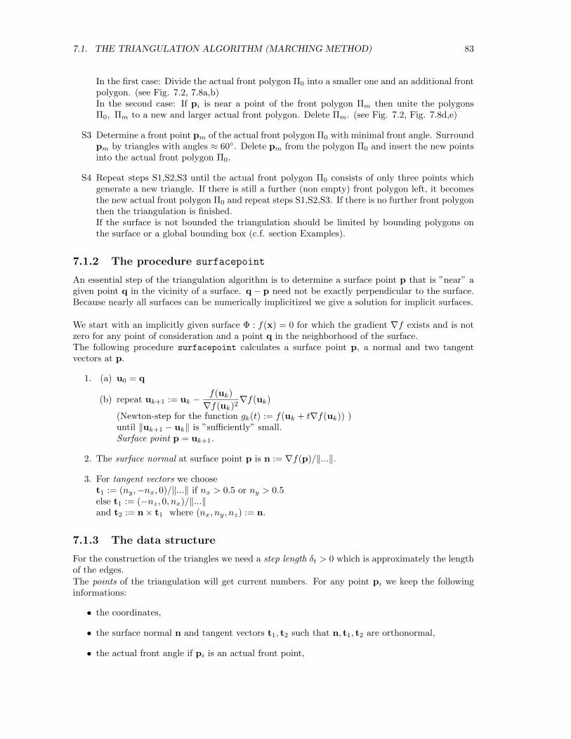
7.1. THE TRIANGULATION ALGORITHM (MARCHING METHOD) 83
In the first case: Divide the actual front polygon Π0 into a smaller one and an additional frontpolygon. (see Fig. 7.2, 7.8a,b)In the second case: If pi is near a point of the front polygon Πm then unite the polygonsΠ0, Πm to a new and larger actual front polygon. Delete Πm. (see Fig. 7.2, Fig. 7.8d,e)
S3 Determine a front point pm of the actual front polygon Π0 with minimal front angle. Surroundpm by triangles with angles ≈ 60◦. Delete pm from the polygon Π0 and insert the new pointsinto the actual front polygon Π0.
S4 Repeat steps S1,S2,S3 until the actual front polygon Π0 consists of only three points whichgenerate a new triangle. If there is still a further (non empty) front polygon left, it becomesthe new actual front polygon Π0 and repeat steps S1,S2,S3. If there is no further front polygonthen the triangulation is finished.If the surface is not bounded the triangulation should be limited by bounding polygons onthe surface or a global bounding box (c.f. section Examples).
7.1.2 The procedure surfacepoint
An essential step of the triangulation algorithm is to determine a surface point p that is ”near” agiven point q in the vicinity of a surface. q − p need not be exactly perpendicular to the surface.Because nearly all surfaces can be numerically implicitized we give a solution for implicit surfaces.
We start with an implicitly given surface Φ : f(x) = 0 for which the gradient ∇f exists and is notzero for any point of consideration and a point q in the neighborhood of the surface.The following procedure surfacepoint calculates a surface point p, a normal and two tangentvectors at p.
1. (a) u0 = q
(b) repeat uk+1 := uk −f(uk)
∇f(uk)2∇f(uk)
(Newton-step for the function gk(t) := f(uk + t∇f(uk)) )until ‖uk+1 − uk‖ is ”sufficiently” small.Surface point p = uk+1.
2. The surface normal at surface point p is n := ∇f(p)/‖...‖.
3. For tangent vectors we chooset1 := (ny,−nx, 0)/‖...‖ if nx > 0.5 or ny > 0.5else t1 := (−nz, 0, nx)/‖...‖and t2 := n× t1 where (nx, ny, nz) := n.
7.1.3 The data structure
For the construction of the triangles we need a step length δt > 0 which is approximately the lengthof the edges.The points of the triangulation will get current numbers. For any point pi we keep the followinginformations:
• the coordinates,
• the surface normal n and tangent vectors t1, t2 such that n, t1, t2 are orthonormal,
• the actual front angle if pi is an actual front point,
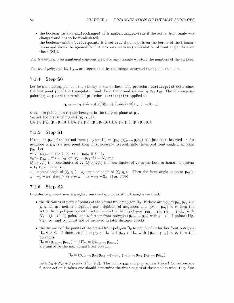
84 CHAPTER 7. TRIANGULATION OF IMPLICIT SURFACES
• the boolean variable angle changed with angle changed=true if the actual front angle waschanged and has to be recalculated,the boolean variable border point. It is set true if point pi is on the border of the triangu-lation and should be ignored for further considerations (recalculation of front angle, distancecheck (S2)).
The triangles will be numbered consecutively. For any triangle we store the numbers of the vertices.
The front polygons Π0,Π1, ... are represented by the integer arrays of their point numbers.
7.1.4 Step S0
Let be s a starting point in the vicinity of the surface. The procedure surfacepoint determinesthe first point p1 of the triangulation and the orthonormal system n1, t11, t12. The following sixpoints p2, ...,p7 are the results of procedure surfacepoint applied to
qi+2 := p1 + δt cos(iπ/3)t11 + δt sin(iπ/3)t12, i := 0, ..., 5,
which are points of a regular hexagon in the tangent plane at p1.We get the first 6 triangles (Fig. 7.3a):(p1,p2,p3), (p1,p3,p4), (p1,p4,p5), (p1,p5,p6), (p1,p6,p7), (p1,p7,p2).
7.1.5 Step S1
If a point p0i of the actual front polygon Π0 = (p01,p02, ...,p0N0) has just been inserted or if a
neighbor of p0i is a new point then it is necessary to recalculate the actual front angle ω at pointp0i. Letv1 := p0,i−1 if i > 1 or v1 := p0N0 if i = 1,v2 := p0,i+1 if i < N0 or v2 := p01 if i = N0 and(ξ1, η1, ζ1) the coordinates of v1, (ξ2, η2, ζ2) the coordinates of v2 in the local orthonormal systemn, t1, t2 at point p0i,ω1 :=polar angle of (ξ1, η1), ω2 :=polar angle of (ξ2, η2). Then the front angle at point p0i isω = ω2 − ω1 if ω2 ≥ ω1 else ω = ω2 − ω1 + 2π. (Fig. 7.3b)
7.1.6 Step S2
In order to prevent new triangles from overlapping existing triangles we check
• the distances of pairs of points of the actual front polygon Π0. If there are points p0i,p0j , i <j, which are neither neighbors nor neighbors of neighbors and ‖p0i − p0j‖ < δt then theactual front polygon is split into the new actual front polygon (p01, ...,p0i,p0j , ...,p0N0
) withN0 − (j − i − 1) points and a further front polygon (p0i, ....,p0j) with j − i + 1 points (Fig.7.2). p0i and p0j must not be involved in later distance checks.
• the distance of the points of the actual front polygon Π0 to points of all further front polygonsΠk, k > 0. If there are points p0i ∈ Π0 and pmj ∈ Πm with ‖p0i − pmj‖ < δt then thepolygonsΠ0 = (p01, ...,p0N0) and Πm = (pm1, ...,pmNm)are united to the new actual front polygon
Π0 = (p01, ...,p0i,pmj , ...pmNm,pm1, ...,pmj ,p0i, ...,p0N0
)
with N0 + Nm + 2 points (Fig. 7.2). The points p0i and pmj appear twice ! So before anyfurther action is taken one should determine the front angles of these points when they first
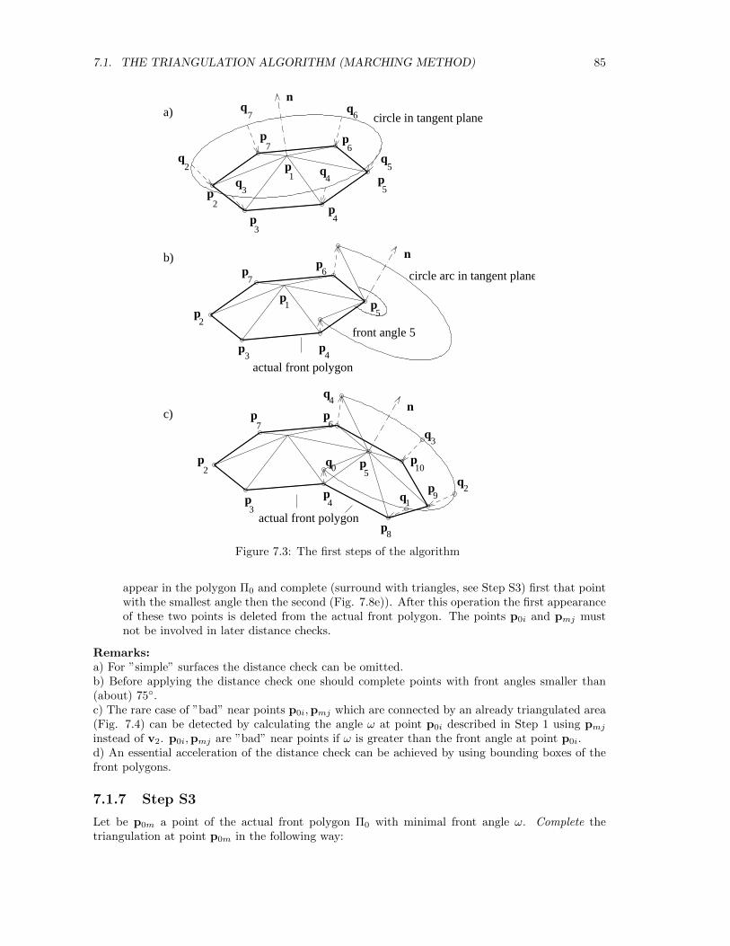
7.1. THE TRIANGULATION ALGORITHM (MARCHING METHOD) 85
p6
p3
q0
p7
q6
q7
q3p
2
p1 q
4 p5
p3
q5
p4
q2
p6
n
p3
p4
p7
p5
p1
p6
p2
q1
8p
q3
q2
p10
p9
p5
p4
p7
p2
q4
circle arc in tangent plane
a)
b)
c)
actual front polygon
circle in tangent plane
front angle 5
actual front polygon
n
n
Figure 7.3: The first steps of the algorithm
appear in the polygon Π0 and complete (surround with triangles, see Step S3) first that pointwith the smallest angle then the second (Fig. 7.8e)). After this operation the first appearanceof these two points is deleted from the actual front polygon. The points p0i and pmj mustnot be involved in later distance checks.
Remarks:a) For ”simple” surfaces the distance check can be omitted.b) Before applying the distance check one should complete points with front angles smaller than(about) 75◦.c) The rare case of ”bad” near points p0i,pmj which are connected by an already triangulated area(Fig. 7.4) can be detected by calculating the angle ω at point p0i described in Step 1 using pmjinstead of v2. p0i,pmj are ”bad” near points if ω is greater than the front angle at point p0i.d) An essential acceleration of the distance check can be achieved by using bounding boxes of thefront polygons.
7.1.7 Step S3
Let be p0m a point of the actual front polygon Π0 with minimal front angle ω. Complete thetriangulation at point p0m in the following way:
86 CHAPTER 7. TRIANGULATION OF IMPLICIT SURFACES
���������������������������������������������������������������������������������������������������������������������������������������������������������������������������������������������������������������������������������������������������������������������������������������
���������������������������������������������������������������������������������������������������������������������������������������������������������������������������������������������������������������������������������������������������������������������������������������
bad near pointsω
���������
��������� front angle Π0
Πm
triangulated area
Figure 7.4: Bad near points and their detection
1. Determine the neighbors v1,v2 of p0m (c.f. Step S1).
2. Determine the number nt of triangles to be generated:Let nt := trunc(3ω/π) + 1, ∆ω := ω/ntCorrection of ∆ω for extreme cases:if ∆ω < 0.8 and nt > 1 then nt → nt − 1 and ∆ω = ω/nt (Fig. 7.5a),if nt = 1 and ∆ω > 0.8 and ‖v1 − v2‖ > 1.25δt then nt = 2 and ∆ω → ∆ω/2 (Fig. 7.5b),if ω < 3 and (‖v1 − p0m‖ ≤ 0.5δt or ‖v2 − p0m‖ ≤ 0.5δt) then nt = 1 (Fig. 7.5c).
v2v1
p 0m
v2v1
p 0m
v1
v2
p 0m
v1
v2
p 0m
p 0m
v1v2
p 0m
v1v2
a b c
Figure 7.5: Corrections for extreme cases
3. Generate the triangles:If nt = 1 then we get one new triangle: (v1,v2,p0m)else let be q0,qnt
the orthogonal projection of v1,v2 into the tangentplane at point p0m
and let qi be the result from a rotation of p0m + δt(q0 − p0m)/‖q0 − p0m‖ by the angle i∆ωaround the normal at surface point p0m for i = 1, ..., nt − 1. (If a global bounding box isvalid the chord p0mqi is truncated and the variable border point of the corresponding newsurface point set true. Boarder points will not be considered any more.) Applying proceduresurfacepoint on qi we get the new points pN+i, i = 1, .., nt−1, where N is the total numberof already existing points, and nt new triangles (see Fig. 7.3b,c):(v1,pN+1,p0m), (pN+1,pN+2,p0m), ..., (pN+nt−1,v2,p0m).
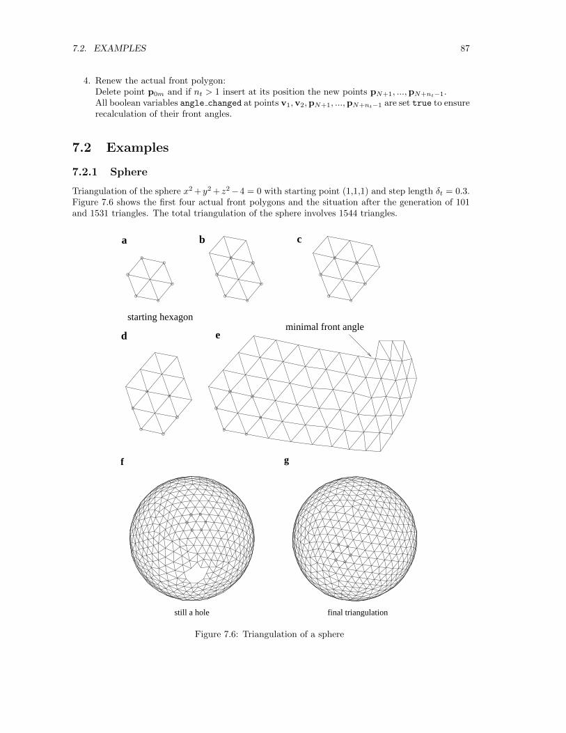
7.2. EXAMPLES 87
4. Renew the actual front polygon:Delete point p0m and if nt > 1 insert at its position the new points pN+1, ...,pN+nt−1.All boolean variables angle changed at points v1,v2,pN+1, ...,pN+nt−1 are set true to ensurerecalculation of their front angles.
7.2 Examples
7.2.1 Sphere
Triangulation of the sphere x2 +y2 +z2−4 = 0 with starting point (1,1,1) and step length δt = 0.3.Figure 7.6 shows the first four actual front polygons and the situation after the generation of 101and 1531 triangles. The total triangulation of the sphere involves 1544 triangles.
starting hexagon
a b c
d eminimal front angle
f g
still a hole final triangulation
Figure 7.6: Triangulation of a sphere
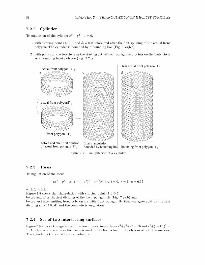
88 CHAPTER 7. TRIANGULATION OF IMPLICIT SURFACES
7.2.2 Cylinder
Triangulation of the cylinder x2 + y2 − 1 = 0,
1. with starting point (1, 0, 0) and δt = 0.2 before and after the first splitting of the actual frontpolygon. The cylinder is bounded by a bounding box (Fig. 7.7a,b,c).
2. with points on the top circle as the starting actual front polygon and points on the basic circleas a bounding front polygon (Fig. 7.7d).
actual front polygon
actual front polygon
front polygon
first actual front polygon
of actual front polygonbefore and after first division
bounded by bounding boxfinal triangulation
bounding front polygon
a
b
c dΠ
Π
Π
Π Π
Π0
0
1
1
0
0
Figure 7.7: Triangulation of a cylinder
7.2.3 Torus
Triangulation of the torus
(x2 + y2 + z2 + r2 − a2)2 − 4r2(x2 + y2) = 0, r = 1, a = 0.35
with δt = 0.1.Figure 7.8 shows the triangulation with starting point (1, 0, 0.5)before and after the first dividing of the front polygon Π0 (Fig. 7.8a,b) andbefore and after uniting front polygon Π0 with front polygon Π1 that was generated by the firstdividing (Fig. 7.8c,d) and the complete triangulation.
7.2.4 Set of two intersecting surfaces
Figure 7.9 shows a triangulation of the two intersecting surfaces x4+y4+z4 = 16 and x2+(z−1.1)2 =1. A polygon on the intersection curve is used for the first actual front polygons of both the surfaces.The cylinder is truncated by a bounding box.
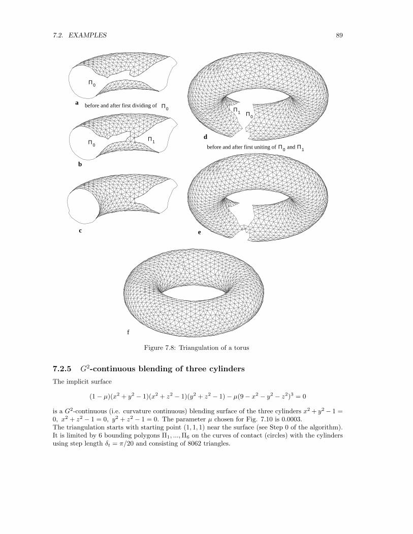
7.2. EXAMPLES 89
Π1
Π1 Π0
Π1Π0before and after first uniting of and
Π0
Π0
Π0a
b
d
e
before and after first dividing of
c
f
Figure 7.8: Triangulation of a torus
7.2.5 G2-continuous blending of three cylinders
The implicit surface
(1− µ)(x2 + y2 − 1)(x2 + z2 − 1)(y2 + z2 − 1)− µ(9− x2 − y2 − z2)3 = 0
is a G2-continuous (i.e. curvature continuous) blending surface of the three cylinders x2 + y2 − 1 =0, x2 + z2 − 1 = 0, y2 + z2 − 1 = 0. The parameter µ chosen for Fig. 7.10 is 0.0003.The triangulation starts with starting point (1, 1, 1) near the surface (see Step 0 of the algorithm).It is limited by 6 bounding polygons Π1, ...,Π6 on the curves of contact (circles) with the cylindersusing step length δt = π/20 and consisting of 8062 triangles.
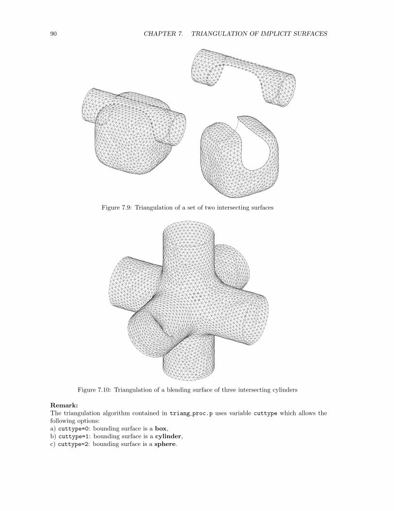
90 CHAPTER 7. TRIANGULATION OF IMPLICIT SURFACES
Figure 7.9: Triangulation of a set of two intersecting surfaces
Figure 7.10: Triangulation of a blending surface of three intersecting cylinders
Remark:The triangulation algorithm contained in triang proc.p uses variable cuttype which allows thefollowing options:a) cuttype=0: bounding surface is a box,b) cuttype=1: bounding surface is a cylinder,c) cuttype=2: bounding surface is a sphere.
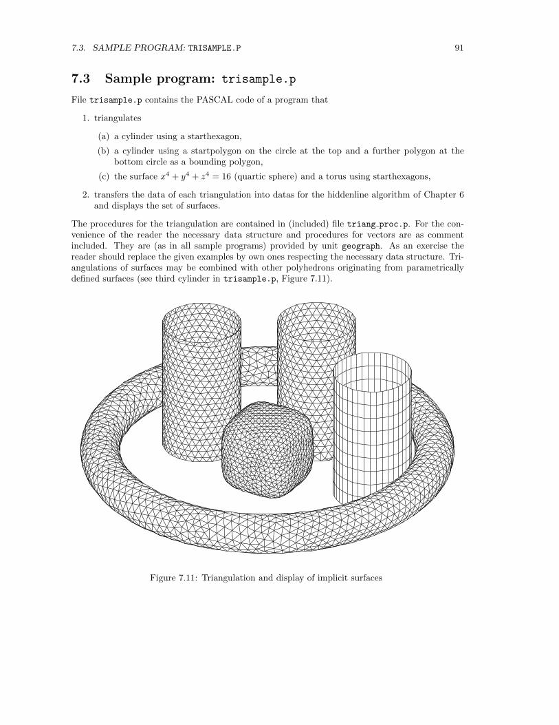
7.3. SAMPLE PROGRAM: TRISAMPLE.P 91
7.3 Sample program: trisample.p
File trisample.p contains the PASCAL code of a program that
1. triangulates
(a) a cylinder using a starthexagon,
(b) a cylinder using a startpolygon on the circle at the top and a further polygon at thebottom circle as a bounding polygon,
(c) the surface x4 + y4 + z4 = 16 (quartic sphere) and a torus using starthexagons,
2. transfers the data of each triangulation into datas for the hiddenline algorithm of Chapter 6and displays the set of surfaces.
The procedures for the triangulation are contained in (included) file triang proc.p. For the con-venience of the reader the necessary data structure and procedures for vectors are as commentincluded. They are (as in all sample programs) provided by unit geograph. As an exercise thereader should replace the given examples by own ones respecting the necessary data structure. Tri-angulations of surfaces may be combined with other polyhedrons originating from parametricallydefined surfaces (see third cylinder in trisample.p, Figure 7.11).
Figure 7.11: Triangulation and display of implicit surfaces
92 CHAPTER 7. TRIANGULATION OF IMPLICIT SURFACES
7.4 Ray tracing of triangulated surfaces with POVRAY
It is an easy task to generate a ray trancing picture of a triangulated surface. Example triblend pov.p
contains a tool for writing the necessary informations of the triangles (point coordinates and normalvectors) into a pp-file (triblend.pp) which will be included while processing file triblend.pov bythe POVRAY-device
povray +L/usr/lib/povray31/include +Itriblend.pov +Otriblend.tga +W600 +H400 +FT
Output is file triblend.tga which may be displayed by program xv (available for LINUX).
Chapter 8
INTERSECTIONS:CURVE – SURFACE,SURFACE – SURFACE
8.1 Intersection Curve – Surface
8.1.1 IS parametric curve – implicit surface
Given: regular curve Γ : x = c(t), t ∈ [a, b], regular surface Φ : f(x) = 0, x ∈ D ⊂ IR3.Wanted: Intersection points Γ ∩ Φ.
The algorithm:
(1) Determining start parameters:Calculate a (nearly) equidistant polygon on Γ (see Section 4.2). For these points determinef(x) and locate neighbored pairs of points where the sign of f changes. The correspondingparameters will be used as starting parameters for the following Newton–iteration.
(2) For any start parameter t0 (from (1)): Solve equation F (t) := f(c(t)) = 0 by a Newton–iteration. Any solution t∗ gives an intersection point x∗ := c(t∗) ∈ Γ ∩ Φ.
(3) Apply (2) on all start parameters from (1).
8.1.2 IS implicit curve – implicit surface
In this case the curve is defined as the intersection curve of two implicit surfaces.
Given: regular curve Γ : f1(x) = 0, f2(x) = 0, x ∈ D12 ⊂ IR3,regular surface Φ : f(x) = 0, x ∈ D ⊂ IR3.
Wanted: intersection points Γ ∩ Φ.
The algorithm:
(1) Determining start points:Calculate a (nearly) equidistant polygon on Γ (see Section 8.2.1). For these points determinef(x) and locate neighbored pairs of points where the sign of f changes. One of each pair ofpoints will be used as starting points for the following Newton–iteration.
93
94 CHAPTER 8. INTERSECTIONS: CURVE – SURFACE, SURFACE – SURFACE
(2) For any starting pointx0 (from (1)): Solve the non linear system F(x) := (f1(x), f2(x), f(x)) =0. F′ is the matrix F′ = (∇f1,∇f2,∇f) by a Newton–iteration. Any solution x∗ is anintersection point ∈ Γ ∩ Φ.
(3) Apply (2) on all starting points from (1).
8.1.3 IS implicit curve – parametric surface
Given: regular curve Γ : f1(x) = 0, f2(x) = 0, x ∈ D12 ⊂ IR3,regular surface Φ : x = S(u, v), (u, v) ∈ D ⊂ IR2.
Wanted: intersection points Γ ∩ Φ.
The algorithm:
(1) Intersection of surfaces f1(x) = 0 and x = S(u, v). The intersection curve is implicitly givenin parameter plane: F1(u, v) := f1(S(u, v)) = 0.
(2) Intersection of surfaces f2(x) = 0 and x = S(u, v). The intersection curve is implicitly givenin parameter plane: F2(u, v) := f2(S(u, v)) = 0.
(3) The coordinates of the intersection points of the implicit curves F1(u, v) = 0 and F2(u, v) = 0(see 4.4.2) are the parameters of intersection points ∈ Γ ∩ Φ.
8.1.4 IS parametric curve – parametric surface
Given: regular curve Γ : x = c(t), t ∈ [a, b], regular surface Φ : x = S(u, v), (u, v) ∈ D ⊂IR2.Wanted: intersection points Γ ∩ Φ.
The Algorithm:
(1) Determining starting points:
(1.1) calculate a (nearly) equidistant polygon on Γ (see 4.2).
(1.2) Triangulate the surface.
(1.3) Use the algorithm from 6.4.2 to determine pairs σi,∆j consisting of a line segment σi ofthe polygon and a triangle ∆j of the surface polyhedron
(2) For any pair σi,∆j from (1) choose the parameter of one of the end points of σi as startingparameter t0, the parameter of one of the points of the triangle ∆j as starting parametersu0, v0 and solve the non linear system F(t, u, v) := c(t)−S(u, v), F(t, u, v) = 0 by a Newton–iteration. (see 2.4). A solution (t∗, u∗, v∗) consists of the parameters of an intersection pointbetween curve Γ and surface Φ.The necessary matrix is F′ = (c,Su,Sv).
(3) Apply (2) on all pairs determined in (1).
8.2 Intersection surface – surface
8.2.1 IS of two implicit surfaces
The following marching algorithm is based on BA,HO,LY,HO’88.
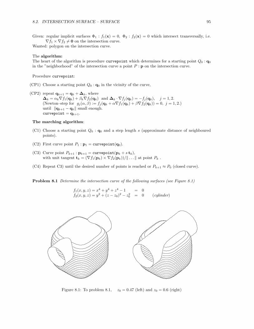
8.2. INTERSECTION SURFACE – SURFACE 95
Given: regular implicit surfaces Φ1 : f1(x) = 0, Φ2 : f2(x) = 0 which intersect transversally, i.e.∇f1 ×∇f2 6= 0 on the intersection curve.
Wanted: polygon on the intersection curve.
The algorithm:The heart of the algorithm is procedure curvepoint which determines for a starting point Q0 : q0
in the ”neighborhood” of the intersection curve a point P : p on the intersection curve.
Procedure curvepoint:
(CP1) Choose a starting point Q0 : q0 in the vicinity of the curve,
(CP2) repeat qk+1 = qk + ∆k, where∆k = αk∇f1(qk) + βk∇f2(qk) and ∆k · ∇fj(qk) = −fj(qk), j = 1, 2.(Newton–step for gj(α, β) := fj(qk + α∇f1(qk) + β∇f2(qk)) = 0, j = 1, 2.)until ‖qk+1 − qk‖ small enough.curvepoint = qk+1.
The marching algorithm:
(C1) Choose a starting point Q0 : q0 and a step length s (approximate distance of neighbouredpoints).
(C2) First curve point P1 : p1 = curvepoint(q0).
(C3) Curve point Pk+1 : pk+1 = curvepoint(pk + s tk),with unit tangent tk = (∇f1(pk)×∇f2(pk))/‖ . . . ‖ at point Pk .
(C4) Repeat C3) until the desired number of points is reached or Pk+1 ≈ P0 (closed curve).
Problem 8.1 Determine the intersection curve of the following surfaces (see Figure 8.1)
f1(x, y, z) = x4 + y4 + z4 − 1 = 0f2(x, y, z) = y2 + (z − z0)2 − z2
0 = 0 (cylinder)
Figure 8.1: To problem 8.1, z0 = 0.47 (left) and z0 = 0.6 (right)
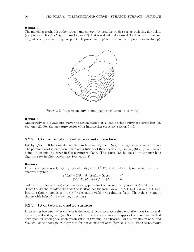
96 CHAPTER 8. INTERSECTIONS: CURVE – SURFACE, SURFACE – SURFACE
Remark:The marching method is rather robust and can even be used for tracing curves with singular points(i.e. points with ∇f1×∇f2 = 0, see Figure 8.2). But one should take care of the direction of the unittangent when passing a singular point (cf. procedure implicit curvepts in program cassini.p).
Figure 8.2: Intersection curve containing a singular point, z0 = 0.5
Remark:Analogously to a parametric curve the determination of q0 can be done curvature dependent (cf.Section 4.2). For the curvature vector of an intersection curve see Section 5.4.5.
8.2.2 IS of an implicit and a parametric surface
Let Φ1 : f(x) = 0 be a regular implicit surface and Φ2 : x = S(u, v) a regular parametric surfaceThe parameters of intersection points are solutions of the equation F (u, v) := f(S(u, v)) = 0, hencepoints of an implicit curve in the parameter plane. This curve can be traced by the marchingalgorithm for implicit curves (see Section 4.3.1).
Remark:In order to get a nearly equally spaced polygon in IR3 (!) with distance δ, one should solve thequadratic system
S2u∆u2 + 2(Su · Sv)∆u∆v + S2
v∆v2 = δ2
(∇f · Su)∆u+ (∇f · Sv)∆v = 0
and use (ui + ∆u, vi + ∆v) as a new starting point for the curvepoint procedure (see 4.3.1).(From the second equation we find: the solution has the form ∆u = −α(∇f ·Sv), ∆v = α(∇f ·Su).Inserting these expressions into the first equation yields two solutions for α. The right one can bechosen with help of the marching direction.)
8.2.3 IS of two parametric surfaces
Intersecting two parametric surfaces is the most difficult case. One simple solution uses the normal-forms h1 = 0 and h2 = 0 (see Section 5.4) of the given surfaces and applies the marching methoddeveloped for tracing the intersection curve of two implicit surfaces. For the evaluation of hi and∇hi we use the foot point algorithm for parametric surfaces (Section 5.8.1). For the necessary
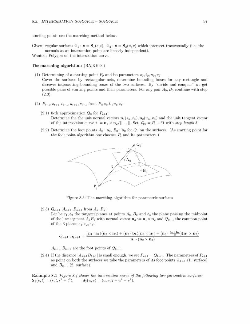
8.2. INTERSECTION SURFACE – SURFACE 97
starting point: see the marching method below.
Given: regular surfaces Φ1 : x = S1(s, t), Φ2 : x = S2(u, v) which intersect transversally (i.e. thenormals at an intersection point are linearly independent).
Wanted: Polygon on the intersection curve.
The marching algorithm: (BA,KE’90)
(1) Determining of a starting point P0 and its parameters s0, t0, u0, v0:Cover the surfaces by rectangular nets, determine bounding boxes for any rectangle anddiscover intersecting bounding boxes of the two surfaces. By “divide and conquer” we getpossible pairs of starting points and their parameters. For any pair A0, B0 continue with step(2.3).
(2) Pi+1, si+1, ti+1, ui+1, vi+1 from Pi, si, ti, ui, vi:
(2.1) 0-th approximation Q0 for Pi+1:Determine the the unit normal vectors n1(sn, tn),n2(un, vn) and the unit tangent vectorof the intersection curve t := n1 × n2/‖ . . . ‖. Set Q0 = Pi + δt with step length δ.
(2.2) Determine the foot points A0 : a0, B0 : b0 for Q0 on the surfaces. (As starting point forthe foot point algorithm one chooses Pi and its parameters.)
A0
B0
Q0
P
t
i
Figure 8.3: The marching algorithm for parametric surfaces
(2.3) Qk+1, Ak+1, Bk+1 from Ak, Bk:Let be ε1, ε2 the tangent planes at points Ak, Bk and ε3 the plane passing the midpointof the line segment AkBk with normal vector n3 := n1×n2 and Qk+1 the common pointof the 3 planes ε1, ε2, ε3:
Qk+1 : qk+1 =(n1 · ak)(n2 × n3) + (n2 · bk)(n3 × n1) + (n3 · ak+bk
2 )(n1 × n2)
n1 · (n2 × n3)
Ak+1, Bk+1 are the foot points of Qk+1.
(2.4) If the distance |Ak+1Bk+1| is small enough, we set Pi+1 = Qk+1. The parameters of Pi+1
as point on both the surfaces we take the parameters of its foot points Ak+1 (1. surface)and Bk+1 (2. surface).
Example 8.1 Figure 8.4 shows the intersection curve of the following two parametric surfaces:S1(s, t) = (s, t, s2 + t2), S2(u, v) = (u, v, 2− u4 − v4).
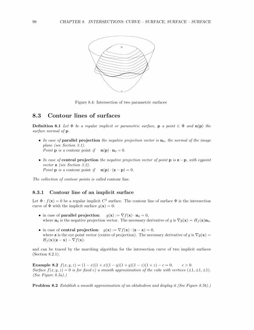
98 CHAPTER 8. INTERSECTIONS: CURVE – SURFACE, SURFACE – SURFACE
Figure 8.4: Intersection of two parametric surfaces
8.3 Contour lines of surfaces
Definition 8.1 Let Φ be a regular implicit or parametric surface, p a point ∈ Φ and n(p) thesurface normal of p.
• In case of parallel projection the negative projection vector is n0, the normal of the imageplane (see Section 3.1).Point p is a contour point if n(p) · n0 = 0.
• In case of central projection the negative projection vector of point p is z−p, with eypointvector z (see Section 3.2).Point p is a contour point if n(p) · (z− p) = 0.
The collection of contour points is called contour line.
8.3.1 Contour line of an implicit surface
Let Φ : f(x) = 0 be a regular implicit C2 surface. The contour line of surface Φ is the intersectioncurve of Φ with the implicit surface g(x) = 0:
• in case of parallel projection: g(x) := ∇f(x) · n0 = 0,where n0 is the negative projection vector. The necessary derivative of g is ∇g(x) = Hf (x)n0.
• in case of central projection: g(x) := ∇f(x) · (z− x) = 0,where z is the eye point vector (centre of projection). The necessary derivative of g is ∇g(x) =Hf (x)(z− x)−∇f(x).
and can be traced by the marching algorithm for the intersection curve of two implicit surfaces(Section 8.2.1).
Example 8.2 f(x, y, z) = (1− x)(1 + x)(1− y)(1 + y)(1− z)(1 + z)− c = 0, c > 0.Surface f(x, y, z) = 0 is for fixed c) a smooth approximation of the cube with vertices (±1,±1,±1).(See Figure 8.5a).)
Problem 8.2 Establish a smooth approximation of an oktahedron and display it (See Figure 8.5b).)
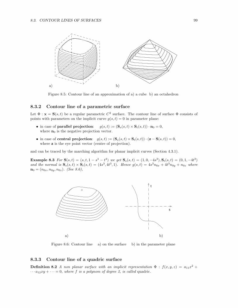
8.3. CONTOUR LINES OF SURFACES 99
a) b)
Figure 8.5: Contour line of an approximation of a) a cube b) an octahedron
8.3.2 Contour line of a parametric surface
Let Φ : x = S(s, t) be a regular parametric C2 surface. The contour line of surface Φ consists ofpoints with parameters on the implicit curve g(s, t) = 0 in parameter plane:
• in case of parallel projection: g(s, t) := (Ss(s, t)× St(s, t)) · n0 = 0,where n0 is the negative projection vector.
• in case of central projection: g(s, t) := (Ss(s, t)× St(s, t)) · (z− S(s, t)) = 0,where z is the eye point vector (centre of projection).
and can be traced by the marching algorithm for planar implicit curves (Section 4.3.1).
Example 8.3 For S(s, t) = (s, t, 1 − s4 − t4) we get Ss(s, t) = (1, 0,−4s3),St(s, t) = (0, 1,−4t3)and the normal is Ss(s, t) × St(s, t) = (4s3, 4t3, 1). Hence g(s, t) = 4s3n0x + 4t3n0y + n0z wheren0 = (n0x, n0y, n0z). (See 8.6),
s
t
a) b)
Figure 8.6: Contour line a) on the surface b) in the parameter plane
8.3.3 Contour line of a quadric surface
Definition 8.2 A non planar surface with an implicit representation Φ : f(x, y, z) = a11x2 +
· · · a12xy + · · · = 0, where f is a polynom of degree 2, is called quadric.
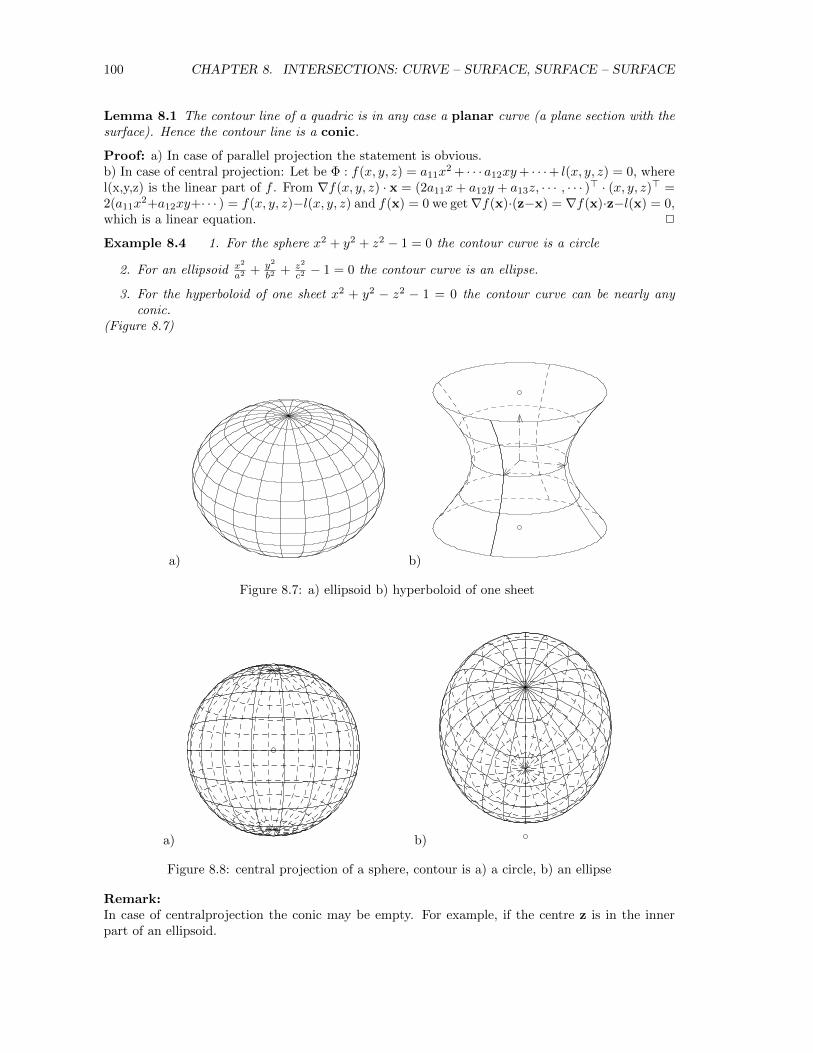
100 CHAPTER 8. INTERSECTIONS: CURVE – SURFACE, SURFACE – SURFACE
Lemma 8.1 The contour line of a quadric is in any case a planar curve (a plane section with thesurface). Hence the contour line is a conic.
Proof: a) In case of parallel projection the statement is obvious.b) In case of central projection: Let be Φ : f(x, y, z) = a11x
2 + · · · a12xy+ · · ·+ l(x, y, z) = 0, wherel(x,y,z) is the linear part of f . From ∇f(x, y, z) · x = (2a11x+ a12y + a13z, · · · , · · · )> · (x, y, z)> =2(a11x
2+a12xy+· · · ) = f(x, y, z)−l(x, y, z) and f(x) = 0 we get∇f(x)·(z−x) = ∇f(x)·z−l(x) = 0,which is a linear equation. 2
Example 8.4 1. For the sphere x2 + y2 + z2 − 1 = 0 the contour curve is a circle
2. For an ellipsoid x2
a2 + y2
b2 + z2
c2 − 1 = 0 the contour curve is an ellipse.
3. For the hyperboloid of one sheet x2 + y2 − z2 − 1 = 0 the contour curve can be nearly anyconic.
(Figure 8.7)
a) b)
Figure 8.7: a) ellipsoid b) hyperboloid of one sheet
a) b)
Figure 8.8: central projection of a sphere, contour is a) a circle, b) an ellipse
Remark:In case of centralprojection the conic may be empty. For example, if the centre z is in the innerpart of an ellipsoid.
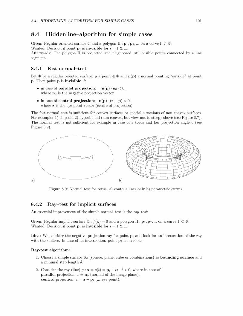
8.4. HIDDENLINE–ALGORITHM FOR SIMPLE CASES 101
8.4 Hiddenline–algorithm for simple cases
Given: Regular oriented surface Φ and a polygon Π : p1,p2, ... on a curve Γ ⊂ Φ.Wanted: Decision if point pi is invisible for i = 1, 2, ....Afterwards: The polygon Π is projected and neighbored, still visible points connected by a linesegment.
8.4.1 Fast normal–test
Let Φ be a regular oriented surface, p a point ∈ Φ and n(p) a normal pointing “outside” at pointp. Then point p is invisible if:
• in case of parallel projection: n(p) · n0 < 0,where n0 is the negative projection vector.
• in case of central projection: n(p) · (z− p) < 0,where z is the eye point vector (centre of projection).
The fast normal–test is sufficient for convex surfaces or special situations of non convex surfaces.For example: 1) ellipsoid 2) hyperboloid (non convex, but view not to steep) above (see Figure 8.7).The normal test is not sufficient for example in case of a torus and low projection angle v (seeFigure 8.9).
a) b)
Figure 8.9: Normal test for torus: a) contour lines only b) parametric curves
8.4.2 Ray–test for implicit surfaces
An essential improvement of the simple normal–test is the ray–test:
Given: Regular implicit surface Φ : f(x) = 0 and a polygon Π : p1,p2, ... on a curve Γ ⊂ Φ.Wanted: Decision if point pi is invisible for i = 1, 2, ....
Idea: We consider the negative projection ray for point pi and look for an intersection of the raywith the surface. In case of an intersection: point pi is invisible.
Ray-test algorithm:
1. Choose a simple surface Ψ0 (sphere, plane, cube or combinations) as bounding surface anda minimal step length δ.
2. Consider the ray (line) g : x = c(t) = pi + tr, t > 0, where in case ofparallel projection: r = n0 (normal of the image plane),central projection: r = z− pi (z: eye point).
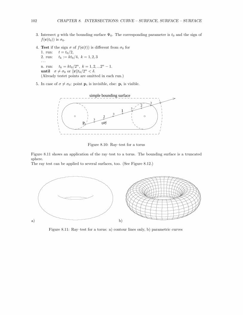
102 CHAPTER 8. INTERSECTIONS: CURVE – SURFACE, SURFACE – SURFACE
3. Intersect g with the bounding surface Ψ0. The corresponding parameter is t0 and the sign off(c(t0)) is σ0.
4. Test if the sign σ of f(c(t)) is different from σ0 for1. run: t = t0/2,2. run: tk := kt0/4, k = 1, 2, 3· · ·n. run: tk = kt0/2
n, k = 1, 2, ...2n − 1.until σ 6= σ0 or ‖r‖t0/2n < δ.(Already testet points are omitted in each run.)
5. In case of σ 6= σ0: point pi is invisible, else: pi is visible.
12
2
3
3
3
3
P
simple bounding surface
ray
Figure 8.10: Ray–test for a torus
Figure 8.11 shows an application of the ray–test to a torus. The bounding surface is a truncatedsphere.The ray test can be applied to several surfaces, too. (See Figure 8.12.)
a) b)
Figure 8.11: Ray–test for a torus: a) contour lines only, b) parametric curves
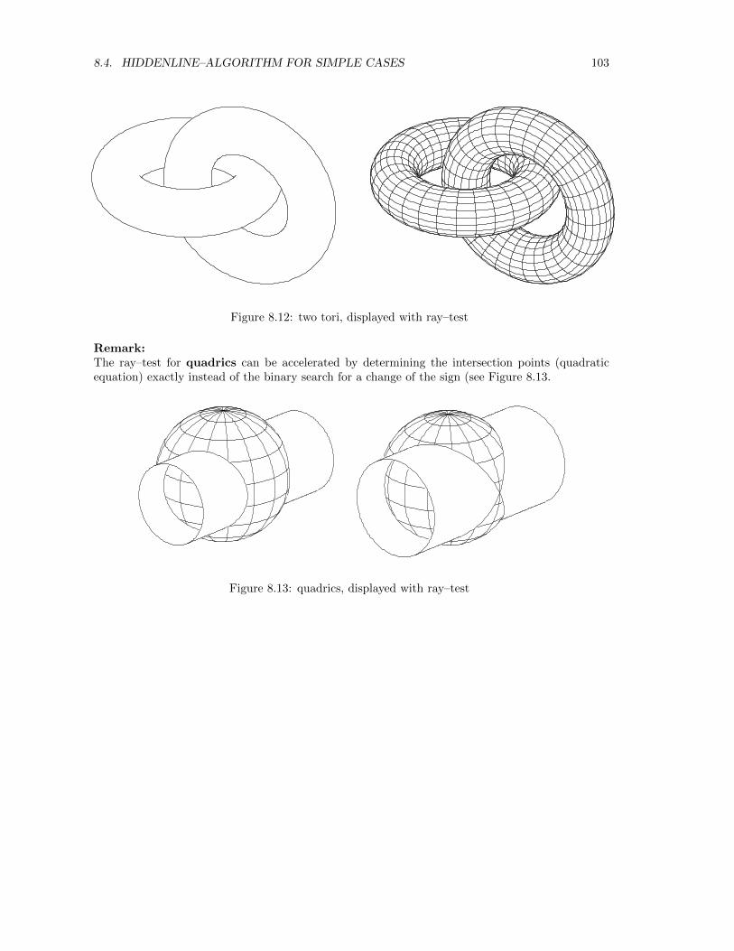
8.4. HIDDENLINE–ALGORITHM FOR SIMPLE CASES 103
Figure 8.12: two tori, displayed with ray–test
Remark:The ray–test for quadrics can be accelerated by determining the intersection points (quadraticequation) exactly instead of the binary search for a change of the sign (see Figure 8.13.
Figure 8.13: quadrics, displayed with ray–test

104 CHAPTER 8. INTERSECTIONS: CURVE – SURFACE, SURFACE – SURFACE
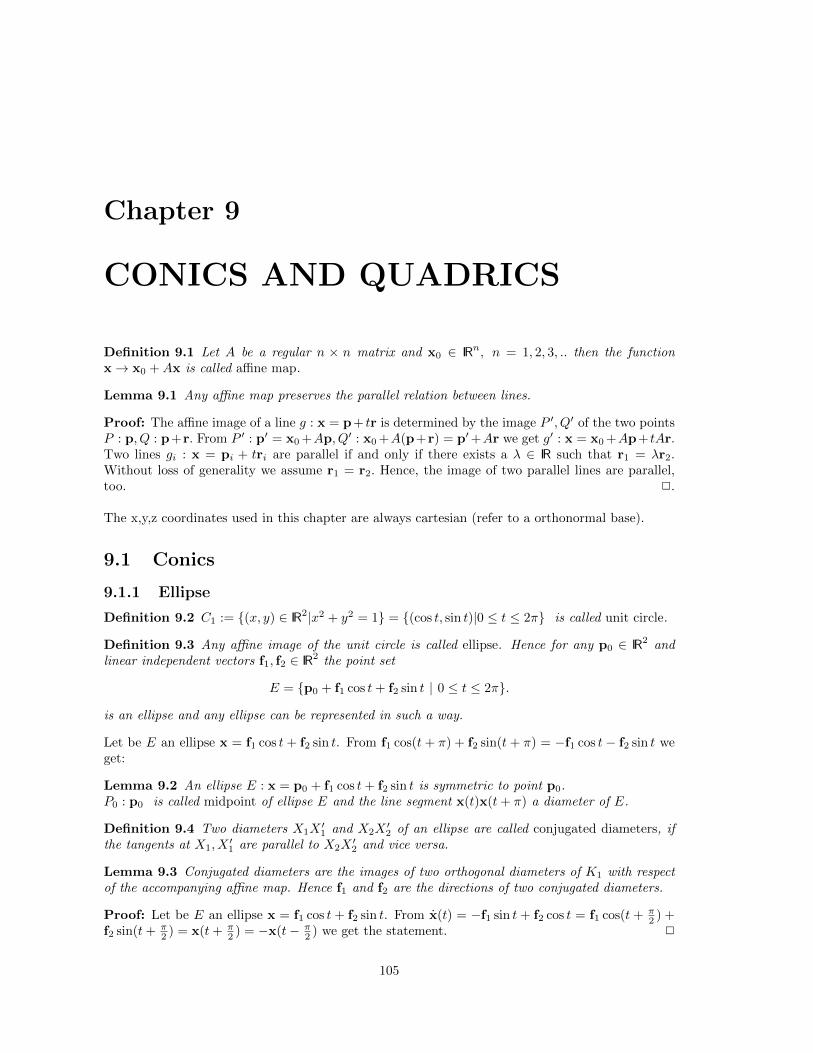
Chapter 9
CONICS AND QUADRICS
Definition 9.1 Let A be a regular n × n matrix and x0 ∈ IRn, n = 1, 2, 3, .. then the functionx→ x0 +Ax is called affine map.
Lemma 9.1 Any affine map preserves the parallel relation between lines.
Proof: The affine image of a line g : x = p+ tr is determined by the image P ′, Q′ of the two pointsP : p, Q : p+r. From P ′ : p′ = x0 +Ap, Q′ : x0 +A(p+r) = p′+Ar we get g′ : x = x0 +Ap+ tAr.Two lines gi : x = pi + tri are parallel if and only if there exists a λ ∈ IR such that r1 = λr2.Without loss of generality we assume r1 = r2. Hence, the image of two parallel lines are parallel,too. 2.
The x,y,z coordinates used in this chapter are always cartesian (refer to a orthonormal base).
9.1 Conics
9.1.1 Ellipse
Definition 9.2 C1 := {(x, y) ∈ IR2|x2 + y2 = 1} = {(cos t, sin t)|0 ≤ t ≤ 2π} is called unit circle.
Definition 9.3 Any affine image of the unit circle is called ellipse. Hence for any p0 ∈ IR2 andlinear independent vectors f1, f2 ∈ IR2 the point set
E = {p0 + f1 cos t+ f2 sin t | 0 ≤ t ≤ 2π}.
is an ellipse and any ellipse can be represented in such a way.
Let be E an ellipse x = f1 cos t+ f2 sin t. From f1 cos(t+ π) + f2 sin(t+ π) = −f1 cos t− f2 sin t weget:
Lemma 9.2 An ellipse E : x = p0 + f1 cos t+ f2 sin t is symmetric to point p0.P0 : p0 is called midpoint of ellipse E and the line segment x(t)x(t+ π) a diameter of E.
Definition 9.4 Two diameters X1X′1 and X2X
′2 of an ellipse are called conjugated diameters, if
the tangents at X1, X′1 are parallel to X2X
′2 and vice versa.
Lemma 9.3 Conjugated diameters are the images of two orthogonal diameters of K1 with respectof the accompanying affine map. Hence f1 and f2 are the directions of two conjugated diameters.
Proof: Let be E an ellipse x = f1 cos t + f2 sin t. From x(t) = −f1 sin t + f2 cos t = f1 cos(t + π2 ) +
f2 sin(t+ π2 ) = x(t+ π
2 ) = −x(t− π2 ) we get the statement. 2
105
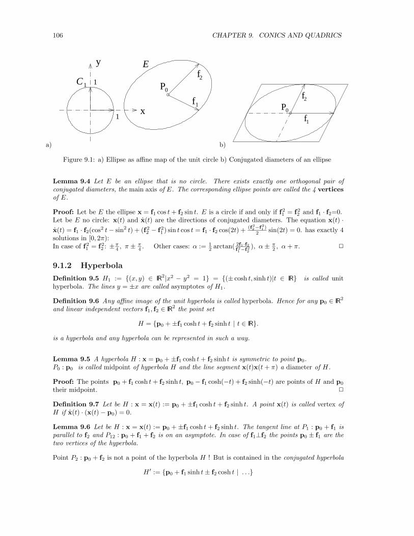
106 CHAPTER 9. CONICS AND QUADRICS
a)
f1
f2
P01
y
1x
E
1C
b)
f
f
2
1
0P
Figure 9.1: a) Ellipse as affine map of the unit circle b) Conjugated diameters of an ellipse
Lemma 9.4 Let E be an ellipse that is no circle. There exists exactly one orthogonal pair ofconjugated diameters, the main axis of E. The corresponding ellipse points are called the 4 verticesof E.
Proof: Let be E the ellipse x = f1 cos t+ f2 sin t. E is a circle if and only if f21 = f2
2 and f1 · f2=0.Let be E no circle: x(t) and x(t) are the directions of conjugated diameters. The equation x(t) ·x(t) = f1 · f2(cos2 t− sin2 t) + (f2
2 − f21 ) sin t cos t = f1 · f2 cos(2t) +
(f22−f21 )
2 sin(2t) = 0. has exactly 4solutions in [0, 2π):In case of f2
1 = f22 : ±π4 , π ±
π4 . Other cases: α := 1
2 arctan( 2f1·f2f21−f22
), α± π2 , α+ π. 2
9.1.2 Hyperbola
Definition 9.5 H1 := {(x, y) ∈ IR2|x2 − y2 = 1} = {(± cosh t, sinh t)|t ∈ IR} is called unithyperbola. The lines y = ±x are called asymptotes of H1.
Definition 9.6 Any affine image of the unit hyperbola is called hyperbola. Hence for any p0 ∈ IR2
and linear independent vectors f1, f2 ∈ IR2 the point set
H = {p0 +±f1 cosh t+ f2 sinh t | t ∈ IR}.
is a hyperbola and any hyperbola can be represented in such a way.
Lemma 9.5 A hyperbola H : x = p0 +±f1 cosh t+ f2 sinh t is symmetric to point p0.P0 : p0 is called midpoint of hyperbola H and the line segment x(t)x(t+ π) a diameter of H.
Proof: The points p0 + f1 cosh t+ f2 sinh t, p0 − f1 cosh(−t) + f2 sinh(−t) are points of H and p0
their midpoint. 2
Definition 9.7 Let be H : x = x(t) := p0 + ±f1 cosh t + f2 sinh t. A point x(t) is called vertex ofH if x(t) · (x(t)− p0) = 0.
Lemma 9.6 Let be H : x = x(t) := p0 +±f1 cosh t + f2 sinh t. The tangent line at P1 : p0 + f1 isparallel to f2 and P12 : p0 + f1 + f2 is on an asymptote. In case of f1⊥f2 the points p0 ± f1 are thetwo vertices of the hyperbola.
Point P2 : p0 + f2 is not a point of the hyperbola H ! But is contained in the conjugated hyperbola
H ′ := {p0 + f1 sinh t± f2 cosh t | . . .}
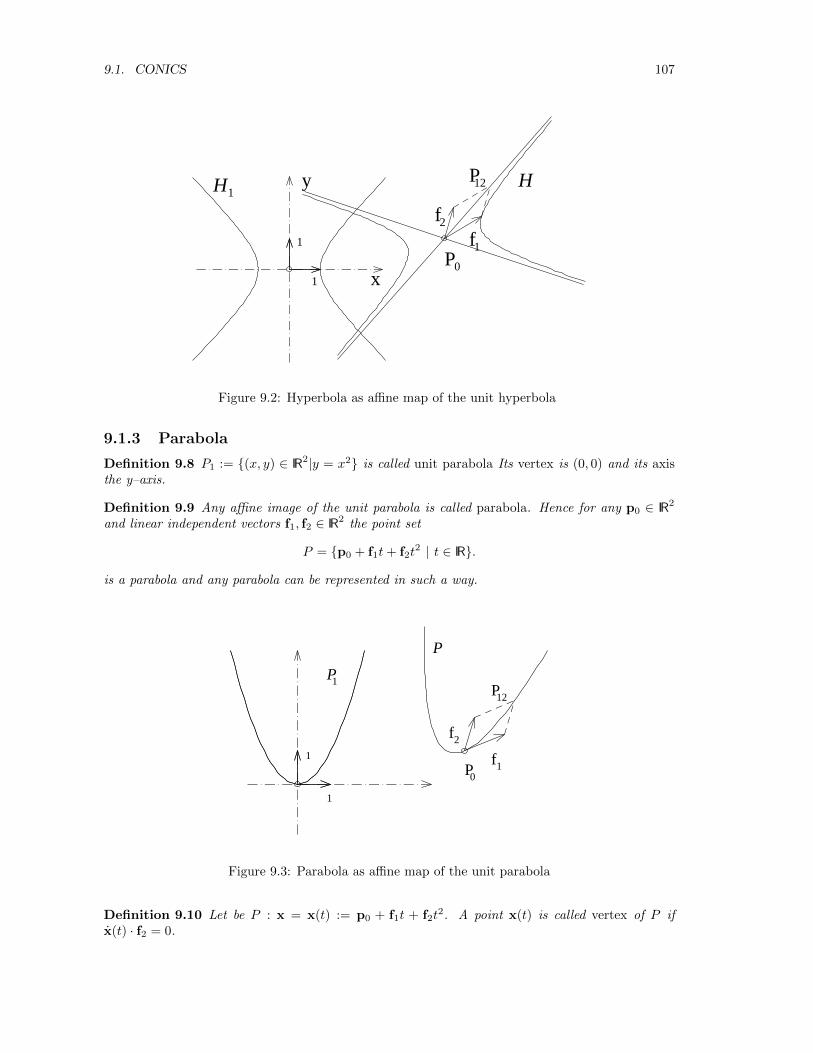
9.1. CONICS 107
ff
P
Px
y
1
2
1
0
1
12
1
HH
Figure 9.2: Hyperbola as affine map of the unit hyperbola
9.1.3 Parabola
Definition 9.8 P1 := {(x, y) ∈ IR2|y = x2} is called unit parabola Its vertex is (0, 0) and its axisthe y–axis.
Definition 9.9 Any affine image of the unit parabola is called parabola. Hence for any p0 ∈ IR2
and linear independent vectors f1, f2 ∈ IR2 the point set
P = {p0 + f1t+ f2t2 | t ∈ IR}.
is a parabola and any parabola can be represented in such a way.
P
1
1
Pf
f
1
2
12
P
1P
0
Figure 9.3: Parabola as affine map of the unit parabola
Definition 9.10 Let be P : x = x(t) := p0 + f1t + f2t2. A point x(t) is called vertex of P if
x(t) · f2 = 0.
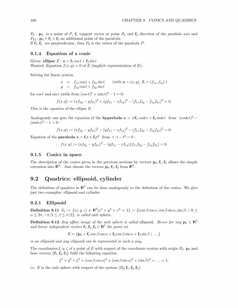
108 CHAPTER 9. CONICS AND QUADRICS
P0 : p0 is a point of P , f1 tangent vector at point P0 and f2 direction of the parabola axis andP12 : p0 + f1 + f2 an additional point of the parabola.If f1, f2 are perpendicular, then P0 is the vertex of the parabola P .
9.1.4 Equation of a conic
Given: ellipse E : x = f1 cos t+ f2 sin tWanted: Equation f(x, y) = 0 of E (implicit representation of E).
Solving the linear system
x = f1x cos t+ f2x sin t (with x = (x, y), fi = (fix, fiy).)y = f1y cos t+ f2y sin t
for cos t and sin t yields from (cos t)2 + (sin t)2 − 1 = 0:
f(x, y) := (xf2y − yf2x)2 + (yf1x − xf1y)2 − (f1xf2y − f1yf2x)2 = 0.
This is the equation of the ellipse E.
Analogously one gets the equation of the hyperbola x = ±f1 cosh t + f2 sinh t from (cosh t)2 −(sinh t)2 − 1 = 0 :
f(x, y) := (xf2y − yf2x)2 − (yf1x − xf1y)2 − (f1xf2y − f1yf2x)2 = 0,
Equation of the parabola x = f1t+ f2t2 from t · t− t2 = 0 :
f(x, y) := (xf2y − yf2x)2 − (yf1x − xf1y)(f1xf2y − f1yf2x) = 0.
9.1.5 Conics in space
The description of the conics given in the previous sections by vectors p0, f1, f2 allows the simpleextension into IR3: Just choose the vectors p0, f1, f2 from IR3.
9.2 Quadrics: ellipsoid, cylinder
The definition of quadrics in IR3 can be done analogously to the definition of the conics. We givejust two examples: ellipsoid and cylinder.
9.2.1 Ellipsoid
Definition 9.11 S1 := {(x, y, z) ∈ IR3|x2 + y2 + z2 = 1} = {(cosβ cosα, cosβ sinα, sinβ) | 0 ≤α ≤ 2π,−π/2 ≤ β ≤ π/2}, is called unit sphere.
Definition 9.12 Any affine image of the unit sphere is called ellipsoid. Hence for any p0 ∈ IR3
and linear independent vectors f1, f2, f3 ∈ IR3 the point set
E = {p0 + f1 cosβ cosα+ f2 cosβ sinα+ f3 sinβ | . . .}
is an ellipsoid and any ellipsoid can be represented in such a way.
The coordinates ξ, η, ζ of a point of E with respect of the coordinate system with origin P0: p0 andbase vectors {f1, f2, f3} fulfil the following equation
ξ2 + η2 + ζ2 = (cosβ cosα)2 + (cosβ sinα)2 + (sinβ)2 = . . . = 1,
i.e. E is the unit sphere with respect of the system (P0; f1, f2, f3).
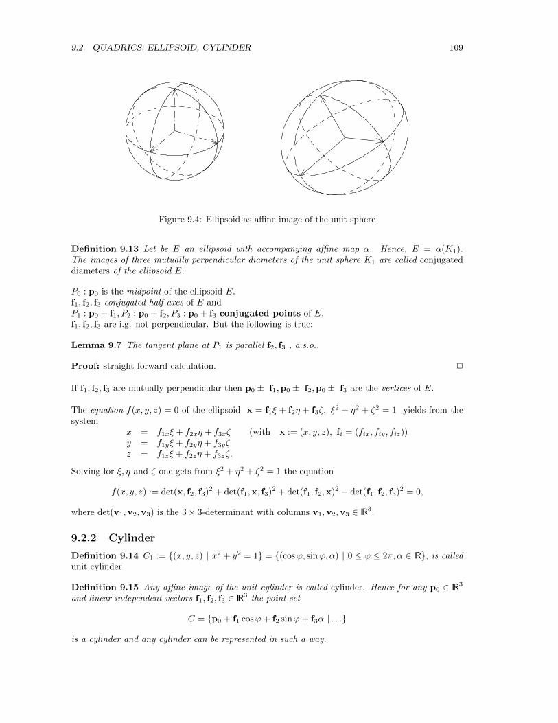
9.2. QUADRICS: ELLIPSOID, CYLINDER 109
Figure 9.4: Ellipsoid as affine image of the unit sphere
Definition 9.13 Let be E an ellipsoid with accompanying affine map α. Hence, E = α(K1).The images of three mutually perpendicular diameters of the unit sphere K1 are called conjugateddiameters of the ellipsoid E.
P0 : p0 is the midpoint of the ellipsoid E.f1, f2, f3 conjugated half axes of E andP1 : p0 + f1, P2 : p0 + f2, P3 : p0 + f3 conjugated points of E.f1, f2, f3 are i.g. not perpendicular. But the following is true:
Lemma 9.7 The tangent plane at P1 is parallel f2, f3 , a.s.o..
Proof: straight forward calculation. 2
If f1, f2, f3 are mutually perpendicular then p0 ± f1,p0 ± f2,p0 ± f3 are the vertices of E.
The equation f(x, y, z) = 0 of the ellipsoid x = f1ξ + f2η + f3ζ, ξ2 + η2 + ζ2 = 1 yields from the
systemx = f1xξ + f2xη + f3xζ (with x := (x, y, z), fi = (fix, fiy, fiz))y = f1yξ + f2yη + f3yζz = f1zξ + f2zη + f3zζ.
Solving for ξ, η and ζ one gets from ξ2 + η2 + ζ2 = 1 the equation
f(x, y, z) := det(x, f2, f3)2 + det(f1,x, f3)2 + det(f1, f2,x)2 − det(f1, f2, f3)2 = 0,
where det(v1,v2,v3) is the 3× 3-determinant with columns v1,v2,v3 ∈ IR3.
9.2.2 Cylinder
Definition 9.14 C1 := {(x, y, z) | x2 + y2 = 1} = {(cosϕ, sinϕ, α) | 0 ≤ ϕ ≤ 2π, α ∈ IR}, is calledunit cylinder
Definition 9.15 Any affine image of the unit cylinder is called cylinder. Hence for any p0 ∈ IR3
and linear independent vectors f1, f2, f3 ∈ IR3 the point set
C = {p0 + f1 cosϕ+ f2 sinϕ+ f3α | . . .}
is a cylinder and any cylinder can be represented in such a way.
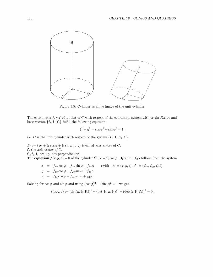
110 CHAPTER 9. CONICS AND QUADRICS
Figure 9.5: Cylinder as affine image of the unit cylinder
The coordinates ξ, η, ζ of a point of C with respect of the coordinate system with origin P0: p0 andbase vectors {f1, f2, f3} fulfill the following equation
ξ2 + η2 = cosϕ2 + sinϕ2 = 1,
i.e. C is the unit cylinder with respect of the system (P0; f1, f2, f3).
E0 := {p0 + f1 cosϕ+ f2 sinϕ | . . .} is called base ellipse of C.f3 the axis vector of C.f1, f2, f3 are i.g. not perpendicular.The equation f(x, y, z) = 0 of the cylinder C : x = f1 cosϕ+ f2 sinϕ+ f3α follows from the system
x = f1x cosϕ+ f2x sinϕ+ f3xα (with x := (x, y, z), fi := (fix, fiy, fiz))
y = f1y cosϕ+ f2y sinϕ+ f3yα
z = f1z cosϕ+ f2z sinϕ+ f3zα.
Solving for cosϕ and sinϕ and using (cosϕ)2 + (sinϕ)2 = 1 we get
f(x, y, z) := (det(x, f2, f3))2 + (det(f1,x, f3))2 − (det(f1, f2, f3))2 = 0.
Chapter 10
SURFACES OF REVOLUTION,RULED SURFACES, COONSPATCHES, CANAL SURFACES
This chapter deals with surfaces which are generated by moving a curve/surface in space. A surfaceof revolution is generated by rotating a planar curve. Moving a line generates a ruled surface.Moving spheres and cones yield canal surfaces and embankment surfaces, respectively. A Coonspatch is an interpolation of a curved quadrangle. For its generation ruled surfaces are used.
10.1 Surfaces of revolution
Definition 10.1 Let be
• Γ : (r(t), z(t))>, t ∈ [a, b] a parametric curve in r-z-plane with r > 0.Surface Φ : x = (r(t) cosϕ, r(t) sinϕ, z(t))>, t ∈ [a, b], ϕ ∈ [0, 2π] is called parametric surfaceof revolution,
• Γ : f(r, z) = 0 an implicit curve in r-z-plane with r > 0.
Surface Φ : f(√x2 + y2, z) = 0 is called implicit surface of revolution,
Γ its profile curve, the z-axis its axis and a section with a plane containing the axis a meridiancurve.
Lemma 10.1 If the profile curve of a surface of revolution (parametric or implicit) is a regularCn–curve then the surface is regular of class Cn, too.
Proof: Parametric case: From xt = (r′(t) cosϕ, r′(t) sinϕ, z′(t))>, xϕ = (−r(t) sinϕ, r(t) cosϕ, 0)>
we get ‖xt × xϕ‖ = ‖(−rz′ cosϕ,−rz′ sinϕ, rr′)>‖ = r√
(r′)2 + (z′)2 6= 0.
Implicit case: From F (x, y, z) := f(√x2 + y2, z) = 0 we get
‖∇F‖ = ‖(frx/√x2 + y2, fry/
√x2 + y2, fz)
>‖ =√f2r + f2
z 6= 0. 2
Example 10.1 Figure 10.1 shows surfaces of revolution with a) a Bezier curve b) the implicit curve(r − 2.5)4 + z4 − 1 = 0 as profile curves.
Lemma 10.2 Let be Φ a regular C2 continuous surface of revolution (parametric or implicit). Themeridians and the circles which are sections of Φ with planes perpendicular to its axis are the linesof curvature.
111
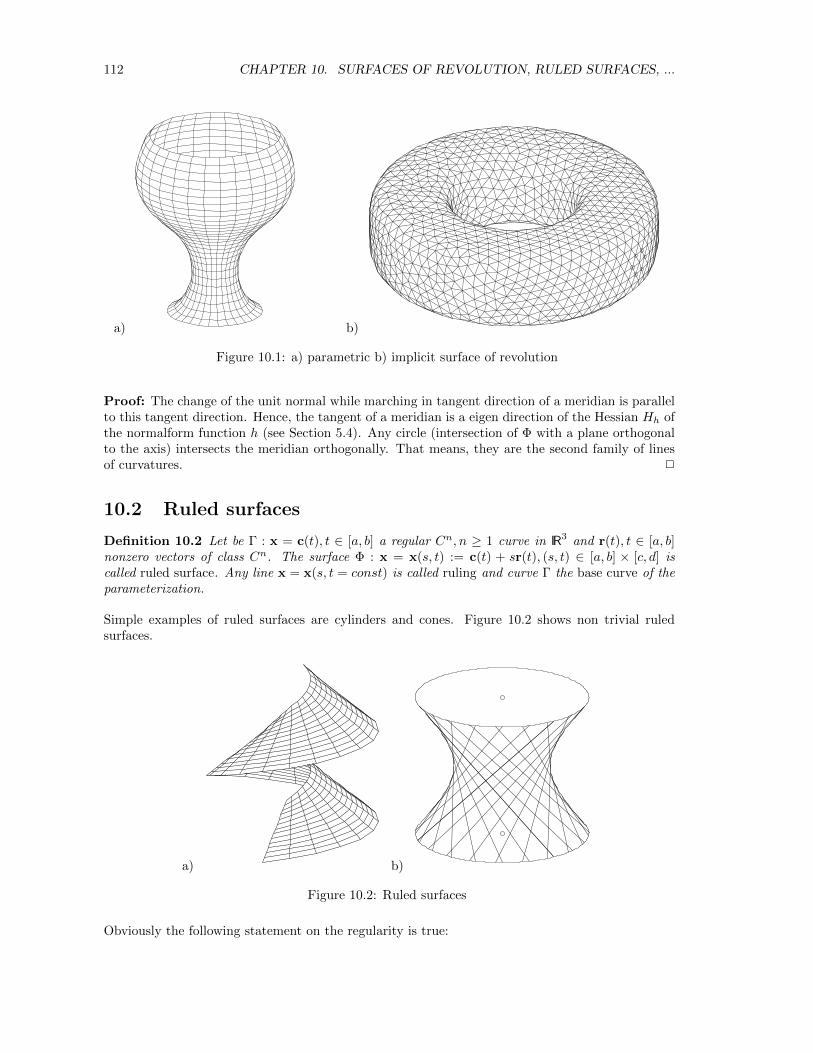
112 CHAPTER 10. SURFACES OF REVOLUTION, RULED SURFACES, ...
a) b)
Figure 10.1: a) parametric b) implicit surface of revolution
Proof: The change of the unit normal while marching in tangent direction of a meridian is parallelto this tangent direction. Hence, the tangent of a meridian is a eigen direction of the Hessian Hh ofthe normalform function h (see Section 5.4). Any circle (intersection of Φ with a plane orthogonalto the axis) intersects the meridian orthogonally. That means, they are the second family of linesof curvatures. 2
10.2 Ruled surfaces
Definition 10.2 Let be Γ : x = c(t), t ∈ [a, b] a regular Cn, n ≥ 1 curve in IR3 and r(t), t ∈ [a, b]nonzero vectors of class Cn. The surface Φ : x = x(s, t) := c(t) + sr(t), (s, t) ∈ [a, b] × [c, d] iscalled ruled surface. Any line x = x(s, t = const) is called ruling and curve Γ the base curve of theparameterization.
Simple examples of ruled surfaces are cylinders and cones. Figure 10.2 shows non trivial ruledsurfaces.
a) b)
Figure 10.2: Ruled surfaces
Obviously the following statement on the regularity is true:
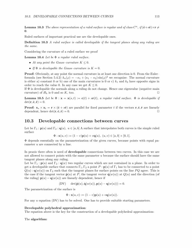
10.3. DEVELOPABLE CONNECTIONS BETWEEN CURVES 113
Lemma 10.3 The above representation of a ruled surface is regular and of class Cn, if (c+sr)×r 6=0.
Ruled surfaces of important practical use are the developable ones.
Definition 10.3 A ruled surface is called developable if the tangent planes along any ruling arethe same.
Considering the curvature of a ruled surface we proof
Lemma 10.4 Let be Φ a regular ruled surface.
• At any point the Gauss–curvature K ≤ 0.
• If Φ is developable the Gauss–curvature is K = 0.
Proof: Obviously, at any point the normal curvature in at least one direction is 0. From the Euler–formula (see Section 5.4.2) kn(ϕ) = −κ1 + (κ1 − κ2) sin(ϕ)2 we recognize: The normal curvatureis either a) constant 0 or b) one of the main curvatures is 0 or c) k1 and k2 have opposite signs inorder to reach the value 0. In any case we get K ≤ 0.If Φ is developable the normals along a ruling do not change. Hence one eigenvalue (negative maincurvature) of Hh is 0 and so K, too. 2
Lemma 10.5 Let be Φ : x = x(s, t) := c(t) + sr(t), a regular ruled surface. Φ is developable ifdet(r, c, r) = 0.
Proof: xs × xt = r × (c + sr) are parallel for fixed parameter t if the vectors r, c, r are linearlydependent, hence det(r, c, r) = 0. 2
10.3 Developable connections between curves
Let be Γ1 : p(u) and Γ2 : q(u), u ∈ [a, b] A surface that interpolates both curves is the simple ruledsurface
Φ : x(u, v) := (1− v)p(u) + vq(u), (u, v) ∈ [a, b]× [0, 1].
Φ depends essentially on the parameterization of the given curves, because points with equal pa-rameter u are connected by a line.
In praxis there often is need of developable connections between two curves. In this case we arenot allowed to connect points with the same parameter u because the surface should have the sametangent planes along any ruling.Let be Γ1 : p(u) and Γ2 : q(w) two regular curves which are not contained in a plane. In order toget a developable surface that connects Γ1,Γ2 a point P : p(u) of Γ1 has to be connected to a pointQ(u) : q(w(u)) on Γ2 such that the tangent planes for surface points on the line PQ agree. This isthe case if the tangent vector p(u) at P , the tangent vector q(w(u)) at Q(u) and the direction (ofthe ruling) p(u)− q(w(u)) are linearly dependent, hence if
(DV) det(p(u), q(w(u)),p(u)− q(w(u))) = 0.
The parametrization of the surface is
Φ : x(u, v) := (1− v)p(u) + vq(w(u)).
For any u equation (DV) has to be solved. One has to provide suitable starting parameters.
Developable polyhedral approximation:The equation above is the key for the construction of a developable polyhedral approximation:
The algorithm:
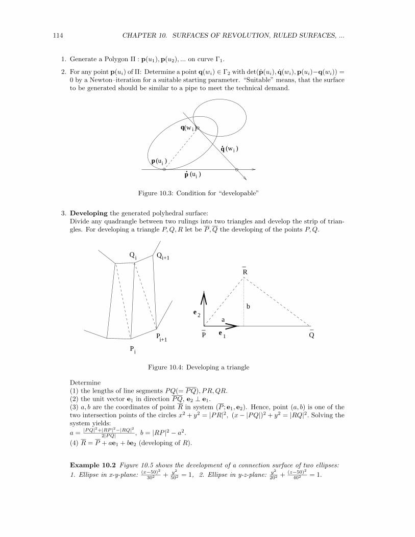
114 CHAPTER 10. SURFACES OF REVOLUTION, RULED SURFACES, ...
1. Generate a Polygon Π : p(u1),p(u2), ... on curve Γ1.
2. For any point p(ui) of Π: Determine a point q(wi) ∈ Γ2 with det(p(ui), q(wi),p(ui)−q(wi)) =0 by a Newton–iteration for a suitable starting parameter. “Suitable” means, that the surfaceto be generated should be similar to a pipe to meet the technical demand.
.
. (w )
p i
q
(u )
i
i
i(w )
(u )p
q
Figure 10.3: Condition for “developable”
3. Developing the generated polyhedral surface:Divide any quadrangle between two rulings into two triangles and develop the strip of trian-gles. For developing a triangle P,Q,R let be P ,Q the developing of the points P,Q.
Pi
Pi+1
Qi+1Q i
P_
Q_
R_
e1
e 2a
b
Figure 10.4: Developing a triangle
Determine(1) the lengths of line segments PQ(= PQ), PR,QR.(2) the unit vector e1 in direction PQ, e2 ⊥ e1.(3) a, b are the coordinates of point R in system (P ; e1, e2). Hence, point (a, b) is one of thetwo intersection points of the circles x2 + y2 = |PR|2, (x− |PQ|)2 + y2 = |RQ|2. Solving thesystem yields:
a = |PQ|2+|RP |2−|RQ|22|PQ| , b = |RP |2 − a2.
(4) R = P + ae1 + be2 (developing of R).
Example 10.2 Figure 10.5 shows the development of a connection surface of two ellipses:
1. Ellipse in x-y-plane: (x−50)2
302 + y2
502 = 1, 2. Ellipse in y-z-plane: y2
202 + (z−50)2
402 = 1.
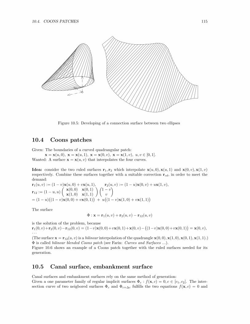
10.4. COONS PATCHES 115
Figure 10.5: Developing of a connection surface between two ellipses
10.4 Coons patches
Given: The boundaries of a curved quadrangular patch:x = x(u, 0), x = x(u, 1), x = x(0, v), x = x(1, v), u, v ∈ [0, 1].
Wanted: A surface x = x(u, v) that interpolates the four curves.
Idea: consider the two ruled surfaces r1, r2 which interpolate x(u, 0),x(u, 1) and x(0, v),x(1, v)respectively. Combine these surfaces together with a suitable correction rcd, in order to meet thedemand:
r1(u, v) := (1− v)x(u, 0) + vx(u, 1), r2(u, v) := (1− u)x(0, v) + ux(1, v),
r12 := (1− u, u)
(x(0, 0) x(0, 1)x(1, 0) x(1, 1)
)(1− vv
)= (1− u)
((1− v)x(0, 0) + vx(0, 1)
)+ u
((1− v)x(1, 0) + vx(1, 1)
)The surface
Φ : x = r1(u, v) + r2(u, v)− r12(u, v)
is the solution of the problem, becauser1(0, v)+r2(0, v)−r12(0, v) = (1−v)x(0, 0)+vx(0, 1)+x(0, v)−
((1−v)x(0, 0)+vx(0, 1)
)= x(0, v),
· · ·(The surface x = r12(u, v) is a bilinear interpolation of the quadrangle x(0, 0),x(1, 0),x(0, 1),x(1, 1).)Φ is called bilinear blended Coons patch (see Farin: Curves and Surfaces ...).Figure 10.6 shows an example of a Coons patch together with the ruled surfaces needed for itsgeneration.
10.5 Canal surface, embankment surface
Canal surfaces and embankment surfaces rely on the same method of generation:Given a one parameter family of regular implicit surfaces Φc : f(x, c) = 0, c ∈ [c1, c2]. The inter-section curve of two neigbored surfaces Φc and Φc+∆c fulfills the two equations f(x, c) = 0 and
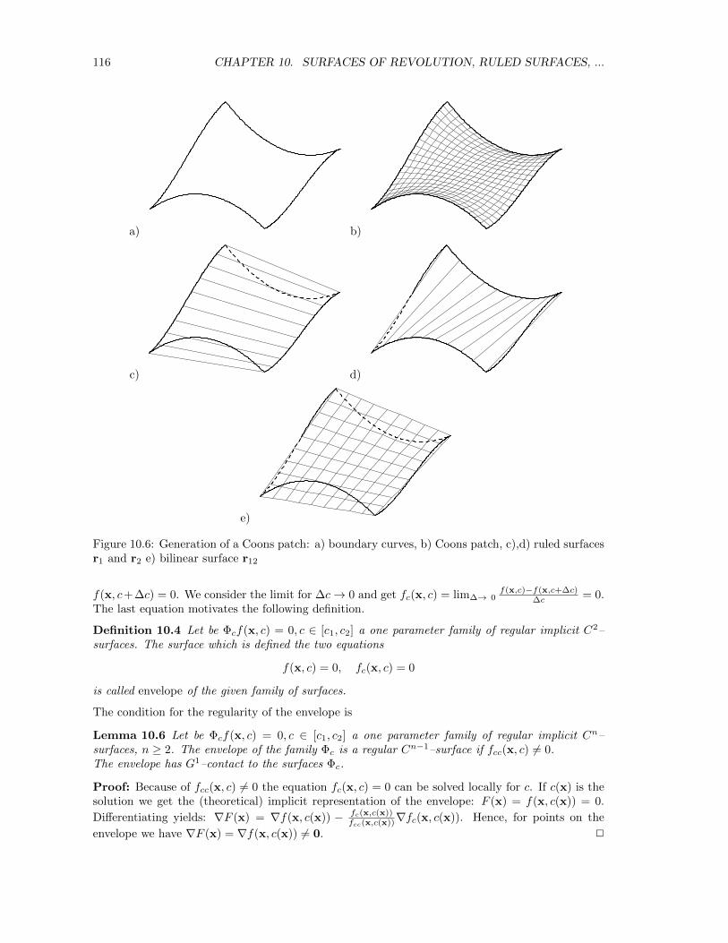
116 CHAPTER 10. SURFACES OF REVOLUTION, RULED SURFACES, ...
a) b)
c) d)
e)
Figure 10.6: Generation of a Coons patch: a) boundary curves, b) Coons patch, c),d) ruled surfacesr1 and r2 e) bilinear surface r12
f(x, c+∆c) = 0. We consider the limit for ∆c→ 0 and get fc(x, c) = lim∆→ 0f(x,c)−f(x,c+∆c)
∆c = 0.The last equation motivates the following definition.
Definition 10.4 Let be Φcf(x, c) = 0, c ∈ [c1, c2] a one parameter family of regular implicit C2–surfaces. The surface which is defined the two equations
f(x, c) = 0, fc(x, c) = 0
is called envelope of the given family of surfaces.
The condition for the regularity of the envelope is
Lemma 10.6 Let be Φcf(x, c) = 0, c ∈ [c1, c2] a one parameter family of regular implicit Cn–surfaces, n ≥ 2. The envelope of the family Φc is a regular Cn−1–surface if fcc(x, c) 6= 0.The envelope has G1–contact to the surfaces Φc.
Proof: Because of fcc(x, c) 6= 0 the equation fc(x, c) = 0 can be solved locally for c. If c(x) is thesolution we get the (theoretical) implicit representation of the envelope: F (x) = f(x, c(x)) = 0.
Differentiating yields: ∇F (x) = ∇f(x, c(x)) − fc(x,c(x))fcc(x,c(x))∇fc(x, c(x)). Hence, for points on the
envelope we have ∇F (x) = ∇f(x, c(x)) 6= 0. 2
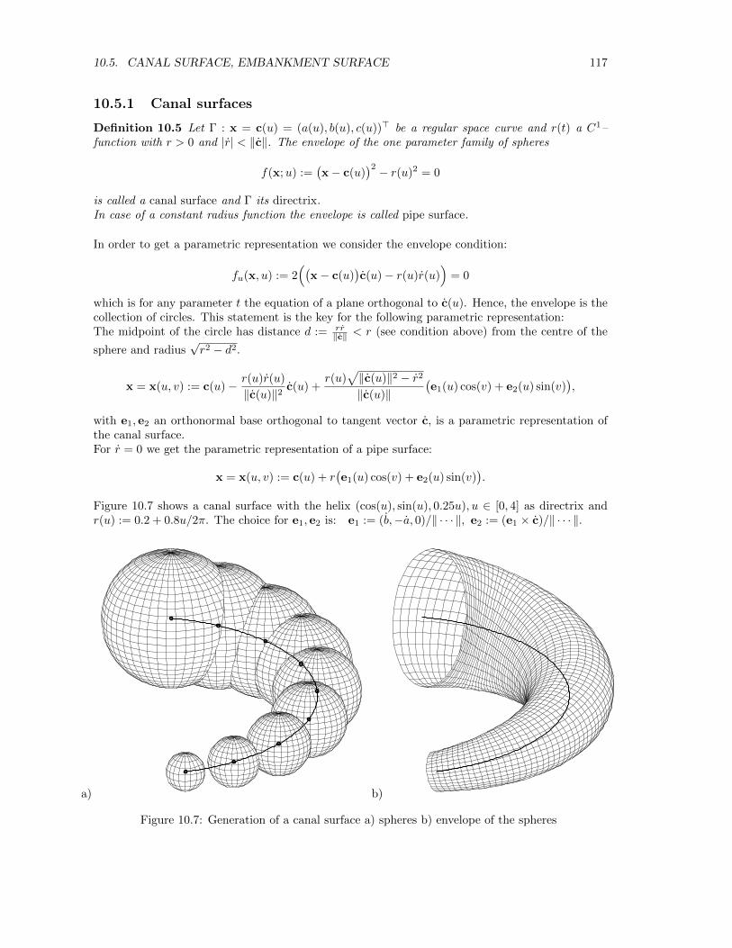
10.5. CANAL SURFACE, EMBANKMENT SURFACE 117
10.5.1 Canal surfaces
Definition 10.5 Let Γ : x = c(u) = (a(u), b(u), c(u))> be a regular space curve and r(t) a C1–function with r > 0 and |r| < ‖c‖. The envelope of the one parameter family of spheres
f(x;u) :=(x− c(u)
)2 − r(u)2 = 0
is called a canal surface and Γ its directrix.In case of a constant radius function the envelope is called pipe surface.
In order to get a parametric representation we consider the envelope condition:
fu(x, u) := 2((
x− c(u))c(u)− r(u)r(u)
)= 0
which is for any parameter t the equation of a plane orthogonal to c(u). Hence, the envelope is thecollection of circles. This statement is the key for the following parametric representation:The midpoint of the circle has distance d := rr
‖c‖ < r (see condition above) from the centre of the
sphere and radius√r2 − d2.
x = x(u, v) := c(u)− r(u)r(u)
‖c(u)‖2c(u) +
r(u)√‖c(u)‖2 − r2
‖c(u)‖(e1(u) cos(v) + e2(u) sin(v)
),
with e1, e2 an orthonormal base orthogonal to tangent vector c, is a parametric representation ofthe canal surface.For r = 0 we get the parametric representation of a pipe surface:
x = x(u, v) := c(u) + r(e1(u) cos(v) + e2(u) sin(v)
).
Figure 10.7 shows a canal surface with the helix (cos(u), sin(u), 0.25u), u ∈ [0, 4] as directrix andr(u) := 0.2 + 0.8u/2π. The choice for e1, e2 is: e1 := (b,−a, 0)/‖ · · · ‖, e2 := (e1 × c)/‖ · · · ‖.
a) b)
Figure 10.7: Generation of a canal surface a) spheres b) envelope of the spheres
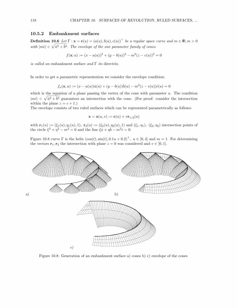
118 CHAPTER 10. SURFACES OF REVOLUTION, RULED SURFACES, ...
10.5.2 Embankment surfaces
Definition 10.6 Let Γ : x = c(u) = (a(u), b(u), c(u))> be a regular space curve and m ∈ IR,m > 0
with |mc| <√a2 + b2. The envelope of the one parameter family of cones
f(x;u) := (x− a(u))2 + (y − b(u))2 −m2(z − c(u))2 = 0
is called an embankment surface and Γ its directrix.
In order to get a parametric representation we consider the envelope condition:
fu(x, u) := (x− a(u))a(u) + (y − b(u))b(u)−m2(z − c(u))c(u) = 0
which is the equation of a plane passing the vertex of the cone with parameter u. The condition
|mc| <√a2 + b2 guarantees an intersection with the cone. (For proof: consider the intersection
within the plane z = c+ 1.)The envelope consists of two ruled surfaces which can be represented parametrically as follows:
x = x(u, v) := c(u) + vr1/2(u)
with r1(u) := (ξ1(u), η1(u), 1), r2(u) := (ξ2(u), η2(u), 1) and (ξ1, η1), (ξ2, η2) intersection points ofthe circle ξ2 + η2 −m2 = 0 and the line ξa+ ηb−m2c = 0.
Figure 10.8 curve Γ is the helix (cos(t), sin(t), 0.1u+ 0.2)>, u ∈ [0, 4] and m = 1. For determiningthe vectors r1, r2 the intersection with plane z = 0 was considered and v ∈ [0, 1].
a) b)
c)
Figure 10.8: Generation of an embankment surface a) cones b) c) envelope of the cones
Chapter 11
BLENDING CURVES ANDSURFACES
Smoothing edges and corners of objects defined by intersecting surfaces is a basic task in CAD. Theoperation is called blending. A measure of the smoothness of the blending surface is the degree nof the so called geometric continuity, Gn-continuity. G1-continuity means the tangent planes at thecurves of contact are the same. G2-continuity guarantees the continuity of the normal curvatures.There are several methods for blending two surfaces. They depend essentially on the representationsof the surfaces to be blended.
11.1 Gn–blending
Definition 11.1 a) A regular Cn–continuous curve Γ which has Gn–contact (see Section 5.4.3)to regular Cn–continuous curves Γ1,Γ2, ... at points p1 ∈ Γ1,p2 ∈ Γ2, ... respectively, is called aGn–blending curve of Γ1,Γ2, ... with contact points p1,p2, ....b) A regular Cn–continuous surface Φ which has Gn–contact to regular Cn–continuous surfacesΦ1,Φ2, ... at curves Γ1 ⊂ Φ1,Γ2 ⊂ Φ2, ... respectively, is called a Gn–blending surface of Φ1,Φ2, ...with contact curves Γ1,Γ2, ....
11.2 Implicit Gn–blending curves and surfaces
For functional splines we need the following statement.
Lemma 11.1 Let α : IR→ IR be a Cn-function with α(i)(0) = 0 for i = 0, 1, ...n and f, g, v : IRk → IRbe Cn-functions.Then Function F : IRk → IR with
F (x) := f(x)− α(g(x)
)v(x)
and function f have at points x ∈ IRk with f(x) = g(x) = 0 the same partial derivatives up to then− th order.Hence: If f = 0 and g = 0 are implicit plane curves (surfaces) then the curve (surface) F = 0 hasCn-contact to f = 0 at intersection points f = 0, g = 0.
Proof: straight forward calculation.
The known implicit blending methods can be considered as generalizations of simple plane cases:
119
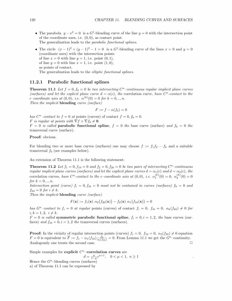
120 CHAPTER 11. BLENDING CURVES AND SURFACES
• The parabola y− x2 = 0 is a G1-blending curve of the line y = 0 with the intersection pointof the coordinate axes, i.e. (0, 0), as contact point.The generalization leads to the parabolic functional splines.
• The circle (x − 1)2 + (y − 1)2 − 1 = 0 is a G1-blending curve of the lines x = 0 and y = 0(coordinate axes) with the intersection pointsof line x = 0 with line y = 1, i.e. point (0, 1),of line y = 0 with line x = 1, i.e. point (1, 0),as points of contact.The generalization leads to the elliptic functional splines.
11.2.1 Parabolic functional splines
Theorem 11.1 Let f = 0, f0 = 0 be two intersecting Cn–continuous regular implicit plane curves(surfaces) and let the explicit plane curve d = α(c), the correlation curve, have Cn-contact to thec–coordinate axis at (0, 0), i.e. α(k)(0) = 0 for k = 0, .., n.Then the implicit blending curve (surface)
F := f − α(f0) = 0
has Cn–contact to f = 0 at points (curves) of contact f = 0, f0 = 0.F is regular at points with ∇f ×∇f0 6= 0.F = 0 is called parabolic functional spline, f = 0 the base curve (surface) and f0 = 0 thetransversal curve (surface).
Proof: obvious.
For blending two or more base curves (surfaces) one may choose f := f1f2 · · · fk and a suitabletransversal f0 (see examples below).
An extension of Theorem 11.1 is the following statement:
Theorem 11.2 Let f1 = 0, f10 = 0 and f2 = 0, f20 = 0 be two pairs of intersecting Cn–continuousregular implicit plane curves (surfaces) and let the explicit plane curves d = α1(c) and d = α2(c), the
correlation curves, have Cn-contact to the c–coordinate axis at (0, 0), i.e. α(k)1 (0) = 0, α
(k)2 (0) = 0
for k = 0, .., n.Intersection point (curve) fi = 0, fi0 = 0 must not be contained in curves (surfaces) fk = 0 andfk0 = 0 for i 6= k.Then the implicit blending curve (surface)
F (x) := f1(x) α2
(f20(x)
)− f2(x) α1
(f10(x)
)= 0
has Gn–contact to fi = 0 at regular points (curves) of contact fi = 0, fi0 = 0, αk(fk0) 6= 0 fori, k = 1, 2, i 6= k.F = 0 is called symmetric parabolic functional spline, fi = 0, i = 1, 2, the base curves (sur-faces) and fi0 = 0, i = 1, 2 the transversal curves (surfaces).
Proof: In the vicinity of regular intersection points (curves) f1 = 0, f10 = 0, α2(f20) 6= 0 equationF = 0 is equivalent to F := f1 − α1(f10) f2
α2(f20) = 0. From Lemma 11.1 we get the Gn–continuity.
Analogously one treats the second case. 2
Simple examples for explicit Cn–correlation curves ared = µ
1−µcn+1, 0 < µ < 1, n ≥ 1 .
Hence the Gn–blending curves (surfaces)a) of Theorem 11.1 can be expressed by
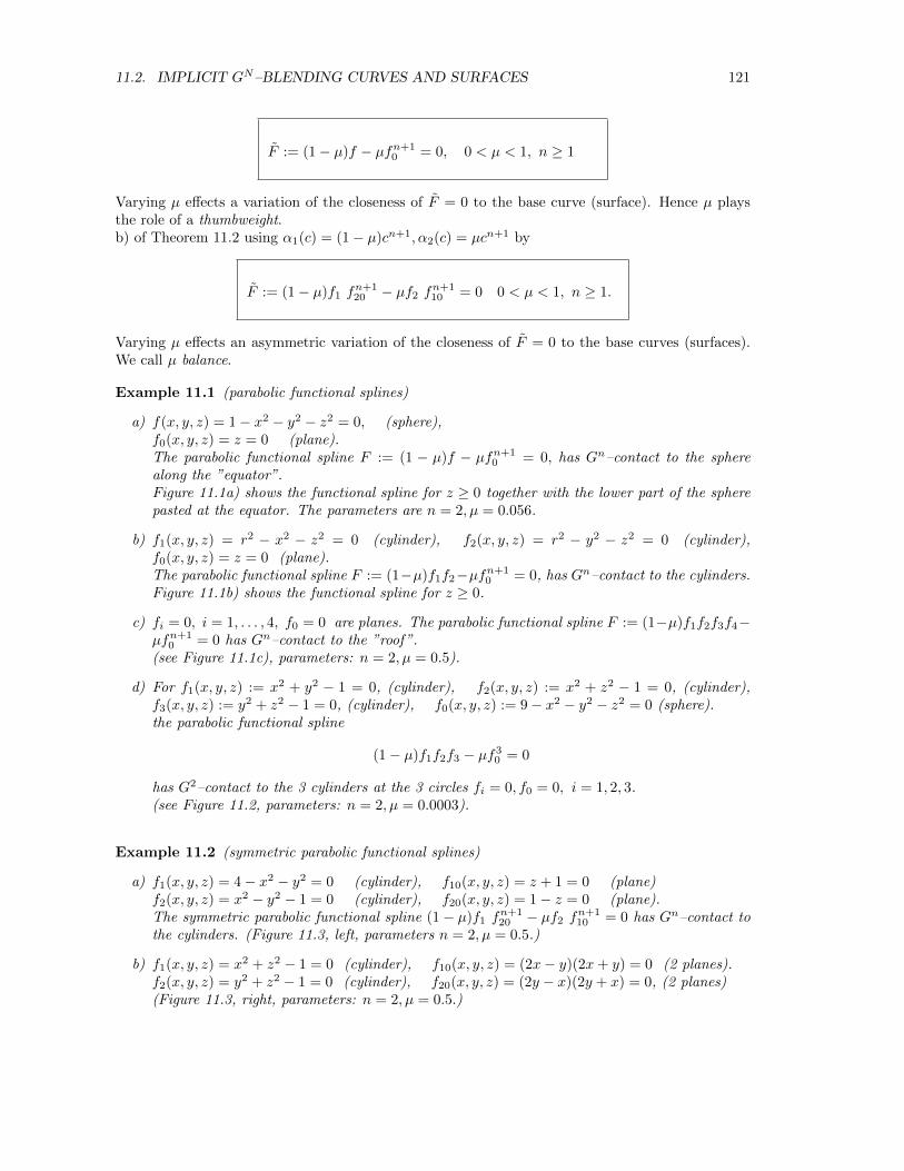
11.2. IMPLICIT GN–BLENDING CURVES AND SURFACES 121
F := (1− µ)f − µfn+10 = 0, 0 < µ < 1, n ≥ 1
Varying µ effects a variation of the closeness of F = 0 to the base curve (surface). Hence µ playsthe role of a thumbweight.b) of Theorem 11.2 using α1(c) = (1− µ)cn+1, α2(c) = µcn+1 by
F := (1− µ)f1 fn+120 − µf2 f
n+110 = 0 0 < µ < 1, n ≥ 1.
Varying µ effects an asymmetric variation of the closeness of F = 0 to the base curves (surfaces).We call µ balance.
Example 11.1 (parabolic functional splines)
a) f(x, y, z) = 1− x2 − y2 − z2 = 0, (sphere),f0(x, y, z) = z = 0 (plane).The parabolic functional spline F := (1 − µ)f − µfn+1
0 = 0, has Gn–contact to the spherealong the ”equator”.Figure 11.1a) shows the functional spline for z ≥ 0 together with the lower part of the spherepasted at the equator. The parameters are n = 2, µ = 0.056.
b) f1(x, y, z) = r2 − x2 − z2 = 0 (cylinder), f2(x, y, z) = r2 − y2 − z2 = 0 (cylinder),f0(x, y, z) = z = 0 (plane).The parabolic functional spline F := (1−µ)f1f2−µfn+1
0 = 0, has Gn–contact to the cylinders.Figure 11.1b) shows the functional spline for z ≥ 0.
c) fi = 0, i = 1, . . . , 4, f0 = 0 are planes. The parabolic functional spline F := (1−µ)f1f2f3f4−µfn+1
0 = 0 has Gn–contact to the ”roof”.(see Figure 11.1c), parameters: n = 2, µ = 0.5).
d) For f1(x, y, z) := x2 + y2 − 1 = 0, (cylinder), f2(x, y, z) := x2 + z2 − 1 = 0, (cylinder),f3(x, y, z) := y2 + z2 − 1 = 0, (cylinder), f0(x, y, z) := 9− x2 − y2 − z2 = 0 (sphere).the parabolic functional spline
(1− µ)f1f2f3 − µf30 = 0
has G2–contact to the 3 cylinders at the 3 circles fi = 0, f0 = 0, i = 1, 2, 3.(see Figure 11.2, parameters: n = 2, µ = 0.0003).
Example 11.2 (symmetric parabolic functional splines)
a) f1(x, y, z) = 4− x2 − y2 = 0 (cylinder), f10(x, y, z) = z + 1 = 0 (plane)f2(x, y, z) = x2 − y2 − 1 = 0 (cylinder), f20(x, y, z) = 1− z = 0 (plane).The symmetric parabolic functional spline (1− µ)f1 f
n+120 − µf2 f
n+110 = 0 has Gn–contact to
the cylinders. (Figure 11.3, left, parameters n = 2, µ = 0.5.)
b) f1(x, y, z) = x2 + z2 − 1 = 0 (cylinder), f10(x, y, z) = (2x− y)(2x+ y) = 0 (2 planes).f2(x, y, z) = y2 + z2 − 1 = 0 (cylinder), f20(x, y, z) = (2y − x)(2y + x) = 0, (2 planes)(Figure 11.3, right, parameters: n = 2, µ = 0.5.)
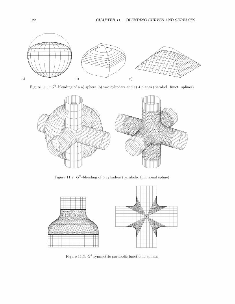
122 CHAPTER 11. BLENDING CURVES AND SURFACES
a) b) c)
Figure 11.1: G2–blending of a a) sphere, b) two cylinders and c) 4 planes (parabol. funct. splines)
Figure 11.2: G2–blending of 3 cylinders (parabolic functional spline)
Figure 11.3: G2 symmetric parabolic functional splines
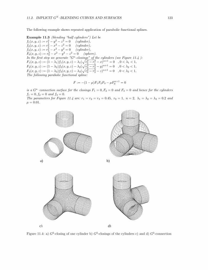
11.2. IMPLICIT GN–BLENDING CURVES AND SURFACES 123
The following example shows repeated application of parabolic functional splines.
Example 11.3 (blending “half cylinders”) Let bef1(x, y, z) := r2
1 − y2 − z2 = 0 (cylinder),f2(x, y, z) := r2
2 − x2 − z2 = 0 (cylinder),f3(x, y, z) := r2
3 − x2 − y2 = 0 (cylinder),F0(x, y, z) := r2
0 − x2 − y2 − z2 = 0 (sphere).In the first step we generate ”Gn-closings” of the cylinders (see Figure 11.4 ):F1(x, y, z) := (1− λ1)f1(x, y, z)− λ1(
√r20 − r2
1 − x)n+1 = 0 , 0 < λ1 < 1,
F2(x, y, z) := (1− λ2)f2(x, y, z)− λ2(√r20 − r2
2 − y)n+1 = 0 , 0 < λ2 < 1,
F3(x, y, z) := (1− λ3)f3(x, y, z)− λ3(√r20 − r2
3 − z)n+1 = 0 , 0 < λ3 < 1,The following parabolic functional spline:
F := −(1− µ)F1F2F3 − µFn+10 = 0
is a Gn–connection surface for the closings F1 = 0, F2 = 0 and F3 = 0 and hence for the cylindersf1 = 0, f2 = 0 and f3 = 0.The parameters for Figure 11.4 are: r1 = r2 = r3 = 0.45, r0 = 1, n = 2, λ1 = λ2 = λ3 = 0.2 andµ = 0.01.
d)c)
a) b)
Figure 11.4: a) G2-closing of one cylinder b) G2-closings of the cylinders c) and d) G2-connection
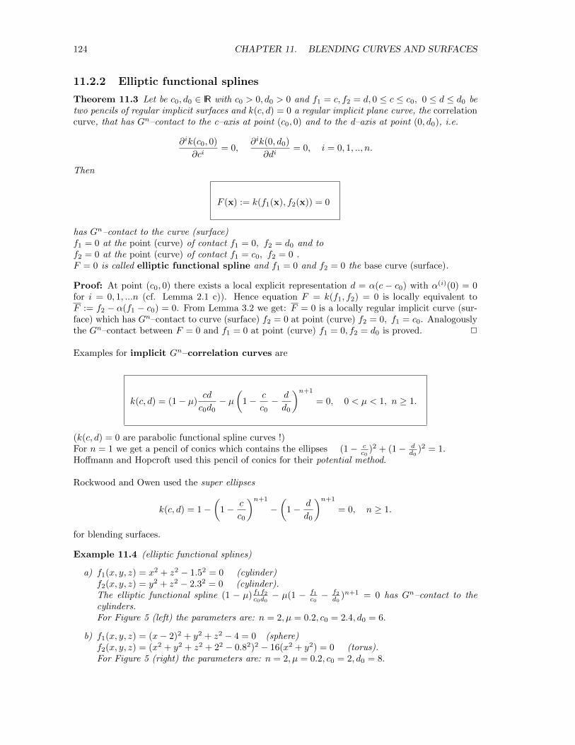
124 CHAPTER 11. BLENDING CURVES AND SURFACES
11.2.2 Elliptic functional splines
Theorem 11.3 Let be c0, d0 ∈ IR with c0 > 0, d0 > 0 and f1 = c, f2 = d, 0 ≤ c ≤ c0, 0 ≤ d ≤ d0 betwo pencils of regular implicit surfaces and k(c, d) = 0 a regular implicit plane curve, the correlationcurve, that has Gn–contact to the c–axis at point (c0, 0) and to the d–axis at point (0, d0), i.e.
∂ik(c0, 0)
∂ci= 0,
∂ik(0, d0)
∂di= 0, i = 0, 1, .., n.
Then
F (x) := k(f1(x), f2(x)) = 0
has Gn–contact to the curve (surface)f1 = 0 at the point (curve) of contact f1 = 0, f2 = d0 and tof2 = 0 at the point (curve) of contact f1 = c0, f2 = 0 .F = 0 is called elliptic functional spline and f1 = 0 and f2 = 0 the base curve (surface).
Proof: At point (c0, 0) there exists a local explicit representation d = α(c − c0) with α(i)(0) = 0for i = 0, 1, ...n (cf. Lemma 2.1 c)). Hence equation F = k(f1, f2) = 0 is locally equivalent toF := f2 − α(f1 − c0) = 0. From Lemma 3.2 we get: F = 0 is a locally regular implicit curve (sur-face) which has Gn–contact to curve (surface) f2 = 0 at point (curve) f2 = 0, f1 = c0. Analogouslythe Gn–contact between F = 0 and f1 = 0 at point (curve) f1 = 0, f2 = d0 is proved. 2
Examples for implicit Gn–correlation curves are
k(c, d) = (1− µ)cd
c0d0− µ
(1− c
c0− d
d0
)n+1
= 0, 0 < µ < 1, n ≥ 1.
(k(c, d) = 0 are parabolic functional spline curves !)For n = 1 we get a pencil of conics which contains the ellipses (1− c
c0)2 + (1− d
d0)2 = 1.
Hoffmann and Hopcroft used this pencil of conics for their potential method.
Rockwood and Owen used the super ellipses
k(c, d) = 1−(
1− c
c0
)n+1
−(
1− d
d0
)n+1
= 0, n ≥ 1.
for blending surfaces.
Example 11.4 (elliptic functional splines)
a) f1(x, y, z) = x2 + z2 − 1.52 = 0 (cylinder)f2(x, y, z) = y2 + z2 − 2.32 = 0 (cylinder).The elliptic functional spline (1 − µ) f1f2c0d0
− µ(1 − f1c0− f2
d0)n+1 = 0 has Gn–contact to the
cylinders.For Figure 5 (left) the parameters are: n = 2, µ = 0.2, c0 = 2.4, d0 = 6.
b) f1(x, y, z) = (x− 2)2 + y2 + z2 − 4 = 0 (sphere)f2(x, y, z) = (x2 + y2 + z2 + 22 − 0.82)2 − 16(x2 + y2) = 0 (torus).For Figure 5 (right) the parameters are: n = 2, µ = 0.2, c0 = 2, d0 = 8.
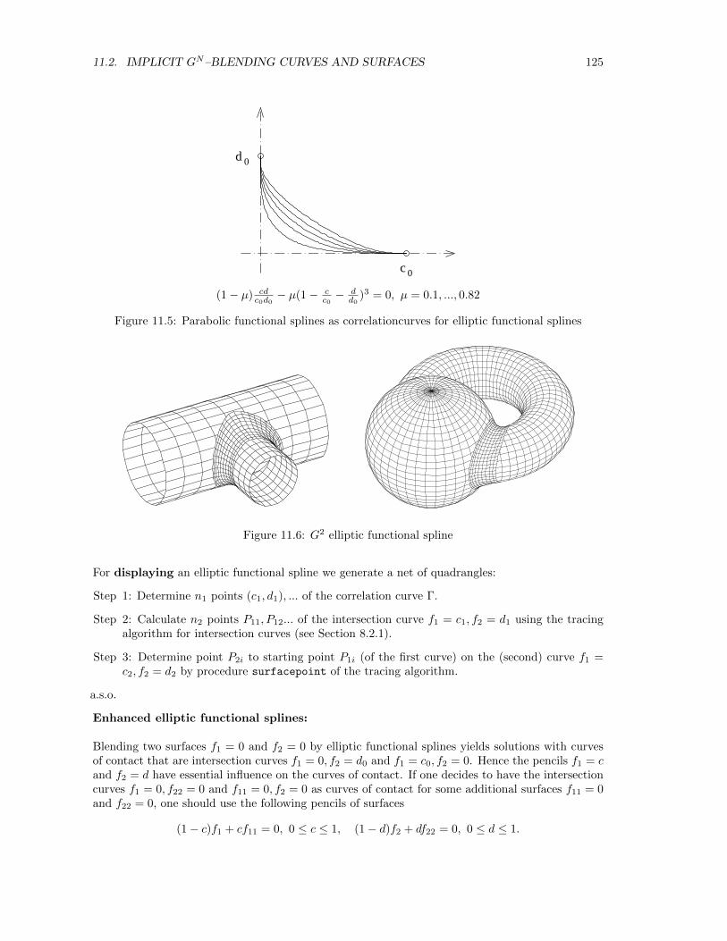
11.2. IMPLICIT GN–BLENDING CURVES AND SURFACES 125
0d
c 0
(1− µ) cdc0d0− µ(1− c
c0− d
d0)3 = 0, µ = 0.1, ..., 0.82
Figure 11.5: Parabolic functional splines as correlationcurves for elliptic functional splines
Figure 11.6: G2 elliptic functional spline
For displaying an elliptic functional spline we generate a net of quadrangles:
Step 1: Determine n1 points (c1, d1), ... of the correlation curve Γ.
Step 2: Calculate n2 points P11, P12... of the intersection curve f1 = c1, f2 = d1 using the tracingalgorithm for intersection curves (see Section 8.2.1).
Step 3: Determine point P2i to starting point P1i (of the first curve) on the (second) curve f1 =c2, f2 = d2 by procedure surfacepoint of the tracing algorithm.
a.s.o.
Enhanced elliptic functional splines:
Blending two surfaces f1 = 0 and f2 = 0 by elliptic functional splines yields solutions with curvesof contact that are intersection curves f1 = 0, f2 = d0 and f1 = c0, f2 = 0. Hence the pencils f1 = cand f2 = d have essential influence on the curves of contact. If one decides to have the intersectioncurves f1 = 0, f22 = 0 and f11 = 0, f2 = 0 as curves of contact for some additional surfaces f11 = 0and f22 = 0, one should use the following pencils of surfaces
(1− c)f1 + cf11 = 0, 0 ≤ c ≤ 1, (1− d)f2 + df22 = 0, 0 ≤ d ≤ 1.
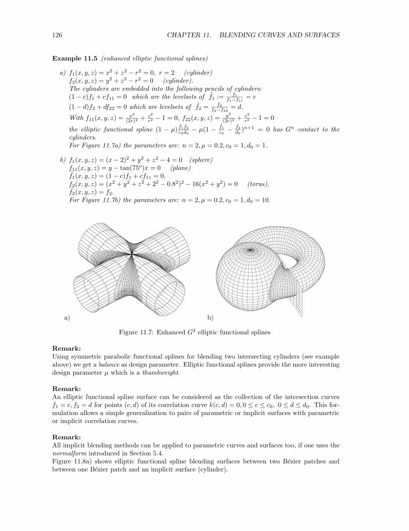
126 CHAPTER 11. BLENDING CURVES AND SURFACES
Example 11.5 (enhanced elliptic functional splines)
a) f1(x, y, z) = x2 + z2 − r2 = 0, r = 2 (cylinder)f2(x, y, z) = y2 + z2 − r2 = 0 (cylinder).The cylinders are embedded into the following pencils of cylinders:(1− c)f1 + cf11 = 0 which are the levelsets of f1 := f1
f1−f11 = c
(1− d)f2 + df22 = 0 which are levelsets of f2 = f2f2−f22 = d.
With f11(x, y, z) = x2
(2r)2 + z2
r2 − 1 = 0, f22(x, y, z) = y2
(2r)2 + z2
r2 − 1 = 0
the elliptic functional spline (1 − µ) f1f2c0d0− µ(1 − f1
c0− f2
d0)n+1 = 0 has Gn–contact to the
cylinders.For Figure 11.7a) the parameters are: n = 2, µ = 0.2, c0 = 1, d0 = 1.
b) f1(x, y, z) = (x− 2)2 + y2 + z2 − 4 = 0 (sphere)f11(x, y, z) = y − tan(75o)x = 0 (plane)f1(x, y, z) = (1− c)f1 + cf11 = 0,f2(x, y, z) = (x2 + y2 + z2 + 22 − 0.82)2 − 16(x2 + y2) = 0 (torus),f2(x, y, z) = f2.For Figure 11.7b) the parameters are: n = 2, µ = 0.2, c0 = 1, d0 = 10.
a) b)
Figure 11.7: Enhanced G2 elliptic functional splines
Remark:Using symmetric parabolic functional splines for blending two intersecting cylinders (see exampleabove) we get a balance as design parameter. Elliptic functional splines provide the more interestingdesign parameter µ which is a thumbweight.
Remark:An elliptic functional spline surface can be considered as the collection of the intersection curvesf1 = c, f2 = d for points (c, d) of its correlation curve k(c, d) = 0, 0 ≤ c ≤ c0, 0 ≤ d ≤ d0. This for-mulation allows a simple generalization to pairs of parametric or implicit surfaces with parametricor implicit correlation curves.
Remark:All implicit blending methods can be applied to parametric curves and surfaces too, if one uses thenormalform introduced in Section 5.4.Figure 11.8a) shows elliptic functional spline blending surfaces between two Bezier patches andbetween one Bezier patch and an implicit surface (cylinder).
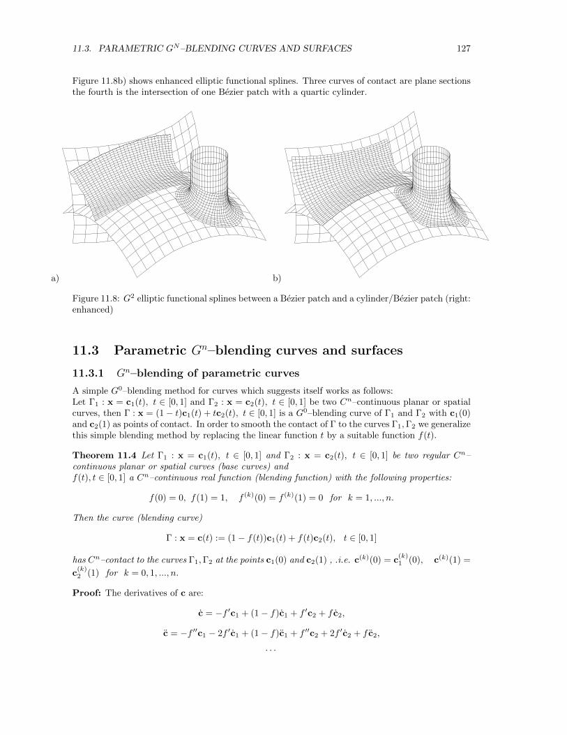
11.3. PARAMETRIC GN–BLENDING CURVES AND SURFACES 127
Figure 11.8b) shows enhanced elliptic functional splines. Three curves of contact are plane sectionsthe fourth is the intersection of one Bezier patch with a quartic cylinder.
a) b)
Figure 11.8: G2 elliptic functional splines between a Bezier patch and a cylinder/Bezier patch (right:enhanced)
11.3 Parametric Gn–blending curves and surfaces
11.3.1 Gn–blending of parametric curves
A simple G0–blending method for curves which suggests itself works as follows:Let Γ1 : x = c1(t), t ∈ [0, 1] and Γ2 : x = c2(t), t ∈ [0, 1] be two Cn–continuous planar or spatialcurves, then Γ : x = (1− t)c1(t) + tc2(t), t ∈ [0, 1] is a G0–blending curve of Γ1 and Γ2 with c1(0)and c2(1) as points of contact. In order to smooth the contact of Γ to the curves Γ1,Γ2 we generalizethis simple blending method by replacing the linear function t by a suitable function f(t).
Theorem 11.4 Let Γ1 : x = c1(t), t ∈ [0, 1] and Γ2 : x = c2(t), t ∈ [0, 1] be two regular Cn–continuous planar or spatial curves (base curves) andf(t), t ∈ [0, 1] a Cn–continuous real function (blending function) with the following properties:
f(0) = 0, f(1) = 1, f (k)(0) = f (k)(1) = 0 for k = 1, ..., n.
Then the curve (blending curve)
Γ : x = c(t) := (1− f(t))c1(t) + f(t)c2(t), t ∈ [0, 1]
has Cn–contact to the curves Γ1,Γ2 at the points c1(0) and c2(1) , .i.e. c(k)(0) = c(k)1 (0), c(k)(1) =
c(k)2 (1) for k = 0, 1, ..., n.
Proof: The derivatives of c are:
c = −f ′c1 + (1− f)c1 + f ′c2 + f c2,
c = −f ′′c1 − 2f ′c1 + (1− f)c1 + f ′′c2 + 2f ′c2 + f c2,
· · ·
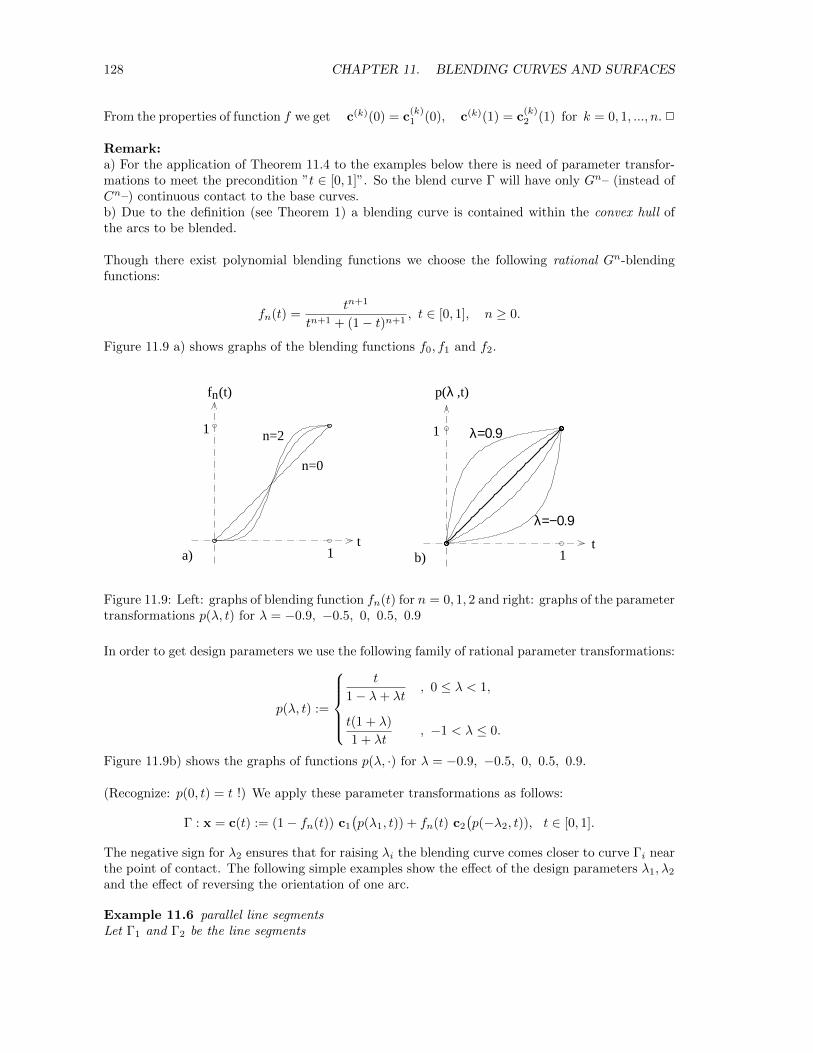
128 CHAPTER 11. BLENDING CURVES AND SURFACES
From the properties of function f we get c(k)(0) = c(k)1 (0), c(k)(1) = c
(k)2 (1) for k = 0, 1, ..., n. 2
Remark:a) For the application of Theorem 11.4 to the examples below there is need of parameter transfor-mations to meet the precondition ”t ∈ [0, 1]”. So the blend curve Γ will have only Gn– (instead ofCn–) continuous contact to the base curves.b) Due to the definition (see Theorem 1) a blending curve is contained within the convex hull ofthe arcs to be blended.
Though there exist polynomial blending functions we choose the following rational Gn-blendingfunctions:
fn(t) =tn+1
tn+1 + (1− t)n+1, t ∈ [0, 1], n ≥ 0.
Figure 11.9 a) shows graphs of the blending functions f0, f1 and f2.
f (t)n p( ,t)λ
λ=0.9
λ=−0.9
1 1
11
tta) b)
n=0
n=2
Figure 11.9: Left: graphs of blending function fn(t) for n = 0, 1, 2 and right: graphs of the parametertransformations p(λ, t) for λ = −0.9, −0.5, 0, 0.5, 0.9
In order to get design parameters we use the following family of rational parameter transformations:
p(λ, t) :=
t
1− λ+ λt, 0 ≤ λ < 1,
t(1 + λ)
1 + λt, −1 < λ ≤ 0.
Figure 11.9b) shows the graphs of functions p(λ, ·) for λ = −0.9, −0.5, 0, 0.5, 0.9.
(Recognize: p(0, t) = t !) We apply these parameter transformations as follows:
Γ : x = c(t) := (1− fn(t)) c1
(p(λ1, t)) + fn(t) c2
(p(−λ2, t)), t ∈ [0, 1].
The negative sign for λ2 ensures that for raising λi the blending curve comes closer to curve Γi nearthe point of contact. The following simple examples show the effect of the design parameters λ1, λ2
and the effect of reversing the orientation of one arc.
Example 11.6 parallel line segmentsLet Γ1 and Γ2 be the line segments
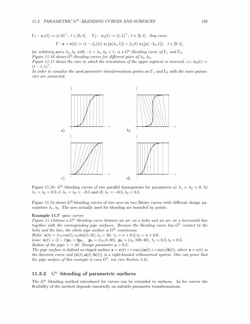
11.3. PARAMETRIC GN–BLENDING CURVES AND SURFACES 129
Γ1 : c1(t) := (t, 0)>, t ∈ [0, 1], Γ2 : c2(t) := (t, 1)>, t ∈ [0, 1]. Any curve
Γ : x = c(t) := (1− fn(t)) c1
(p(λ1, t)
)+ fn(t) c2
(p(−λ2, t)
), t ∈ [0, 1],
for arbitrary pairs λ1, λ2 with −1 < λ1, λ2 < 1, is a Gn-blending curve of Γ1 and Γ2.Figure 11.10 shows G2-blending curves for different pairs of λ1, λ2.Figure 11.11 shows the case in which the orientation of the upper segment is reversed, i.e. c2(t) :=(1− t, 1)>.In order to visualize the used parameter transformations points on Γ1 and Γ2 with the same param-eter are connected.
a) b)
c) d)
Figure 11.10: G2–blending curves of two parallel linesegments for parameters a) λ1 = λ2 = 0, b)λ1 = λ2 = 0.5 c) λ1 = λ2 = −0.5 and d) λ1 = −0.5, λ2 = 0.5
Figure 11.12 shows G2-blending curves of two arcs on two Bezier curves with different design pa-rameters λ1, λ2. The arcs actually used for blending are bounded by points.
Example 11.7 space curvesFigure 11.13shows a G3–blending curve between an arc on a helix and an arc on a horizontal linetogether with the corresponding pipe surfaces. Because the blending curve has G3–contact to thehelix and the line, the whole pipe surface is G2–continuous.Helix: x(t) = (r0 cos(t), r0 sin(t), 5t), r0 = 50, t1 = π + 0.2, t2 = π + 0.6.Line: x(t) = (1− t)p1 + tp2, p1 = (r0, 0, 40), p2 = (r0, 100, 40), t1 = 0.2, t2 = 0.5.Radius of the pipe: r = 10. Design parameter µ = 0.5.The pipe surface is defined as ringed surface x = c(t) + r cos(s)a(t) + r sin(s)b(t), where x = c(t) isthe directrix curve and {c(t),a(t),b(t)} is a right-handed orthonormal system. One can prove thatthe pipe surface of this example is even G3, too (see Section 5.6).
11.3.2 Gn–blending of parametric surfaces
The Gn–blending method introduced for curves can be extended to surfaces. As for curves theflexibility of the method depends essentially on suitable parameter transformations.
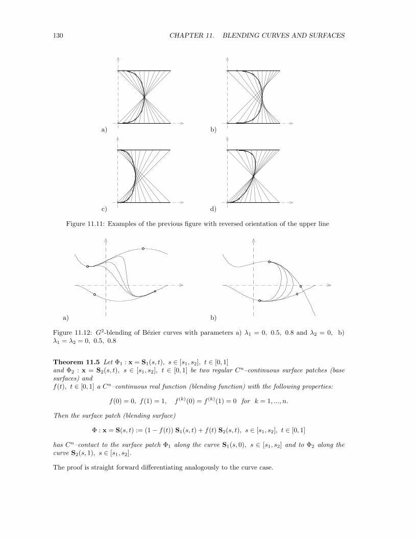
130 CHAPTER 11. BLENDING CURVES AND SURFACES
a) b)
c) d)
Figure 11.11: Examples of the previous figure with reversed orientation of the upper line
a) b)
Figure 11.12: G2-blending of Bezier curves with parameters a) λ1 = 0, 0.5, 0.8 and λ2 = 0, b)λ1 = λ2 = 0, 0.5, 0.8
Theorem 11.5 Let Φ1 : x = S1(s, t), s ∈ [s1, s2], t ∈ [0, 1]and Φ2 : x = S2(s, t), s ∈ [s1, s2], t ∈ [0, 1] be two regular Cn–continuous surface patches (basesurfaces) andf(t), t ∈ [0, 1] a Cn–continuous real function (blending function) with the following properties:
f(0) = 0, f(1) = 1, f (k)(0) = f (k)(1) = 0 for k = 1, ..., n.
Then the surface patch (blending surface)
Φ : x = S(s, t) := (1− f(t)) S1(s, t) + f(t) S2(s, t), s ∈ [s1, s2], t ∈ [0, 1]
has Cn–contact to the surface patch Φ1 along the curve S1(s, 0), s ∈ [s1, s2] and to Φ2 along thecurve S2(s, 1), s ∈ [s1, s2].
The proof is straight forward differentiating analogously to the curve case.
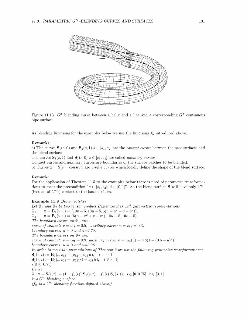
11.3. PARAMETRIC GN–BLENDING CURVES AND SURFACES 131
Figure 11.13: G3–blending curve between a helix and a line and a corresponding G2–continuouspipe surface
As blending functions for the examples below we use the functions fn introduced above.
Remarks:a) The curves S1(s, 0) and S2(s, 1) s ∈ [s1, s2] are the contact curves between the base surfaces andthe blend surface.The curves S1(s, 1) and S2(s, 0) s ∈ [s1, s2] are called auxiliary curves.Contact curves and auxiliary curves are boundaries of the surface patches to be blended.b) Curves x = S(s = const, t) are profile curves which locally define the shape of the blend surface.
Remark:For the application of Theorem 11.5 to the examples below there is need of parameter transforma-tions to meet the precondition ”s ∈ [s1, s2], t ∈ [0, 1]”. So the blend surface S will have only Gn–(instead of Cn–) contact to the base surfaces.
Example 11.8 Bezier patchesLet Φ1 and Φ2 be two tensor product Bezier patches with parametric representationsΦ1 : x = B1(u, v) = (10v − 5, 10u− 5, 6(u− u2 + v − v2)),Φ2 : x = B2(u, v) = (6(u− u2 + v − v2), 10u− 5, 10v − 5).The boundary curves on Φ1 are:curve of contact: v = v11 = 0.5, auxiliary curve: v = v12 = 0.3,boundary curves: u = 0 and u=0.75,The boundary curves on Φ2 are:curve of contact: v = v21 = 0.9, auxiliary curve: v = v22(u) = 0.8(1− (0.5− u)2),boundary curves: u = 0 and u=0.75.In order to meet the preconditions of Theorem 2 we use the following parameter transformations:S1(s, t) := B1(s, v11 + (v12 − v11)t), t ∈ [0, 1]S2(s, t) := B2(s, v21 + (v22(s)− v21)t), t ∈ [0, 1]s ∈ [0, 0.75].HenceΦ : x = S(s, t) := (1− fn(t)) S1(s, t) + fn(t) S2(s, t), s ∈ [0, 0.75], t ∈ [0, 1]is a Gn–blending surface.(fn is a Gn–blending function defined above.)
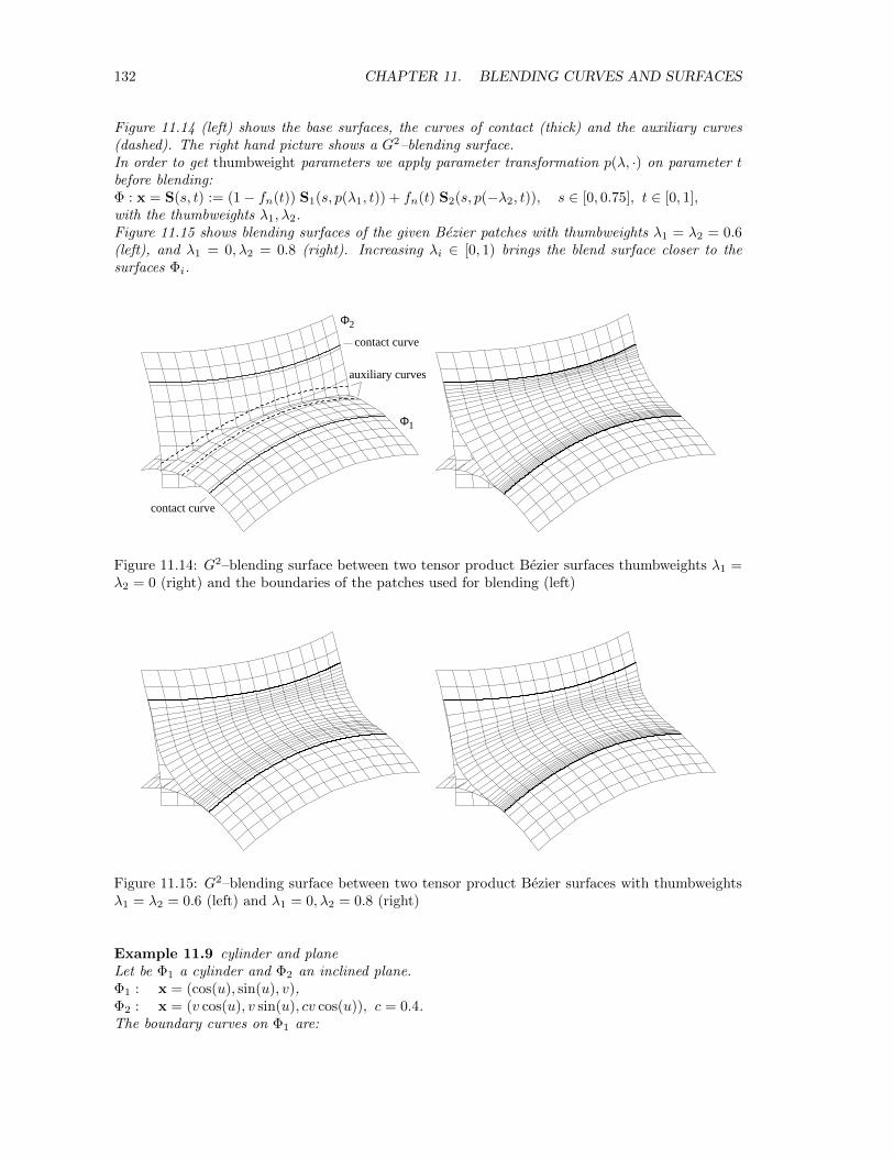
132 CHAPTER 11. BLENDING CURVES AND SURFACES
Figure 11.14 (left) shows the base surfaces, the curves of contact (thick) and the auxiliary curves(dashed). The right hand picture shows a G2–blending surface.In order to get thumbweight parameters we apply parameter transformation p(λ, ·) on parameter tbefore blending:Φ : x = S(s, t) := (1− fn(t)) S1(s, p(λ1, t)) + fn(t) S2(s, p(−λ2, t)), s ∈ [0, 0.75], t ∈ [0, 1],with the thumbweights λ1, λ2.Figure 11.15 shows blending surfaces of the given Bezier patches with thumbweights λ1 = λ2 = 0.6(left), and λ1 = 0, λ2 = 0.8 (right). Increasing λi ∈ [0, 1) brings the blend surface closer to thesurfaces Φi.
contact curve
contact curve
auxiliary curves
Φ1
Φ2
Figure 11.14: G2–blending surface between two tensor product Bezier surfaces thumbweights λ1 =λ2 = 0 (right) and the boundaries of the patches used for blending (left)
Figure 11.15: G2–blending surface between two tensor product Bezier surfaces with thumbweightsλ1 = λ2 = 0.6 (left) and λ1 = 0, λ2 = 0.8 (right)
Example 11.9 cylinder and planeLet be Φ1 a cylinder and Φ2 an inclined plane.Φ1 : x = (cos(u), sin(u), v),Φ2 : x = (v cos(u), v sin(u), cv cos(u)), c = 0.4.The boundary curves on Φ1 are:
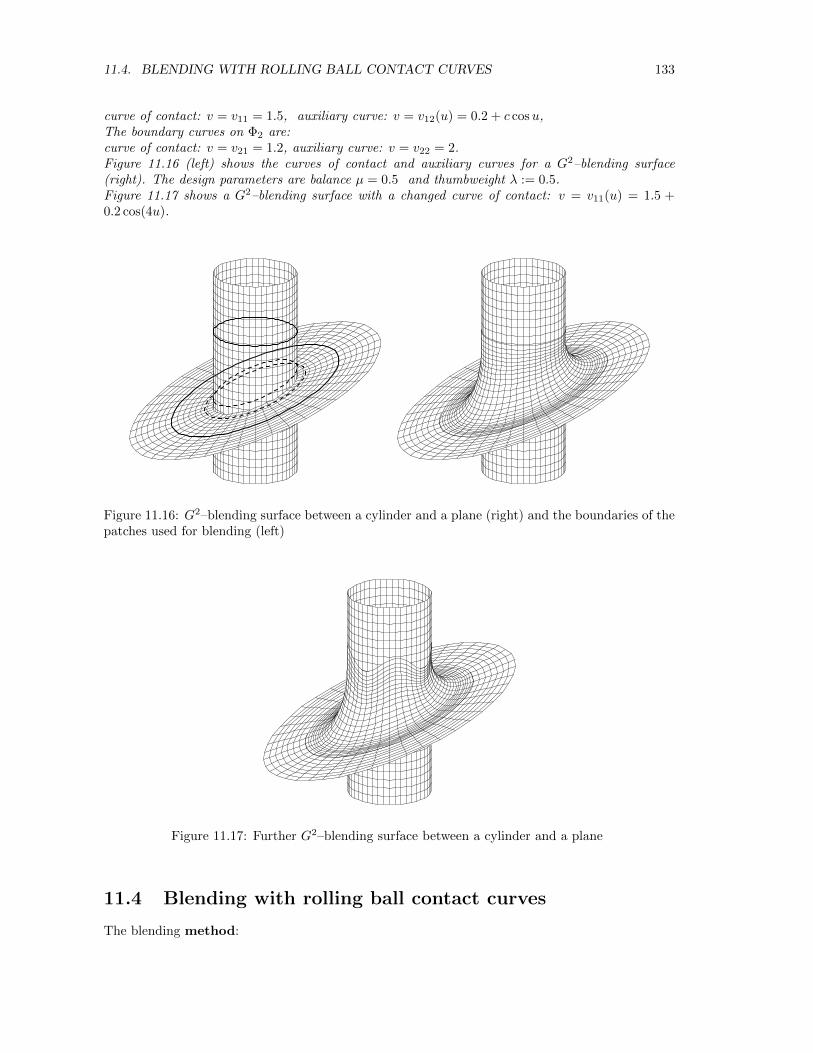
11.4. BLENDING WITH ROLLING BALL CONTACT CURVES 133
curve of contact: v = v11 = 1.5, auxiliary curve: v = v12(u) = 0.2 + c cosu,The boundary curves on Φ2 are:curve of contact: v = v21 = 1.2, auxiliary curve: v = v22 = 2.Figure 11.16 (left) shows the curves of contact and auxiliary curves for a G2–blending surface(right). The design parameters are balance µ = 0.5 and thumbweight λ := 0.5.Figure 11.17 shows a G2–blending surface with a changed curve of contact: v = v11(u) = 1.5 +0.2 cos(4u).
Figure 11.16: G2–blending surface between a cylinder and a plane (right) and the boundaries of thepatches used for blending (left)
Figure 11.17: Further G2–blending surface between a cylinder and a plane
11.4 Blending with rolling ball contact curves
The blending method:
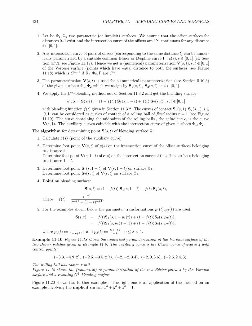
134 CHAPTER 11. BLENDING CURVES AND SURFACES
1. Let be Φ1,Φ2 two parametric (or implicit) surfaces. We assume that the offset surfaces fordistances 0..1 exist and the intersection curve of the offsets are C2–continuous for any distancet ∈ [0, 1].
2. Any intersection curve of pairs of offsets (corresponding to the same distance t) can be numer-ically parametrized by a suitable common Bezier or B-spline curve Γ : c(s), s ∈ [0, 1] (cf. Sec-tion 4.7.3, see Figure 11.18). Hence we get a (numerical) parameterization V(s, t), s, t ∈ [0, 1]of the Voronoi surface (points which have equal distance to both the surfaces, see Figure11.18) which is Cn−1 if Φ1,Φ2,Γ are Cn.
3. The parameterization V(s, t) is used for a (numerical) parameterization (see Section 5.10.3)of the given surfaces Φ1,Φ2 which we assign by S1(s, t), S2(s, t), s, t ∈ [0, 1].
4. We apply the Cn–blending method out of Section 11.3.2 and get the blending surface
Ψ : x = S(s, t) := (1− f(t)) S1(s, 1− t) + f(t) S2(s, t), s, t ∈ [0, 1]
with blending function f(t) given in Section 11.3.2. The curves of contact S1(s, 1),S2(s, 1), s ∈[0, 1] can be considered as curves of contact of a rolling ball of fixed radius r = 1 (see Figure11.19). The curve containing the midpoints of the rolling balls , the spine curve, is the curveV(s, 1). The auxiliary curves coincide with the intersection curve of given surfaces Φ1,Φ2.
The algorithm for determining point S(s, t) of blending surface Ψ:
1. Calculate c(s) (point of the auxiliary curve)
2. Determine foot point V(s, t) of c(s) on the intersection curve of the offset surfaces belongingto distance t.Determine foot point V(s, 1−t) of c(s) on the intersection curve of the offset surfaces belongingto distance 1− t.
3. Determine foot point S1(s, 1− t) of V(s, 1− t) on surface Φ1.Determine foot point S2(s, t) of V(s, t) on surface Φ2.
4. Point on blending surface:
S(s, t) = (1− f(t)) S1(s, 1− t) + f(t) S2(s, t),
where f(t) =tn+1
tn+1 + (1− t)n+1.
5. For the examples shown below the parameter transformations p1(t), p2(t) are used:
S(s, t) = f(t)S1(s, 1− p1(t)) + (1− f(t))S2(s, p2(t)),
= f(t)S1(s, p2(1− t)) + (1− f(t))S2(s, p2(t)),
where p1(t) := t1−λ+λt , and p2(t) := t(1−λ)
1−λt 0 ≤ λ < 1.
Example 11.10 Figure 11.18 shows the numerical parameterization of the Voronoi surface of thetwo Bezier patches given in Example 11.8. The auxiliary curve is the Bezier curve of degree 4 withcontrol points:
(−3.3,−4.9, 2), (−2.5,−3.5, 2.7), (−2,−2, 3.4), (−2, 0, 3.6), (−2.5, 2.4, 3).
The rolling ball has radius r = 2.Figure 11.19 shows the (numerical) re-parameterization of the two Bezier patches by the Voronoisurface and a resulting G2–blending surface.
Figure 11.20 shows two further examples. The right one is an application of the method on anexample involving the implicit surface x4 + y4 + z4 = 1.
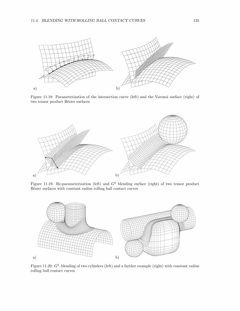
11.4. BLENDING WITH ROLLING BALL CONTACT CURVES 135
a) b)
Figure 11.18: Parameterization of the intersection curve (left) and the Voronoi surface (right) oftwo tensor product Bezier surfaces
a) b)
Figure 11.19: Re-parameterization (left) and G2–blending surface (right) of two tensor productBezier surfaces with constant radius rolling ball contact curves
a) b)
Figure 11.20: G2–blending of two cylinders (left) and a further example (right) with constant radiusrolling ball contact curves

136 CHAPTER 11. BLENDING CURVES AND SURFACES
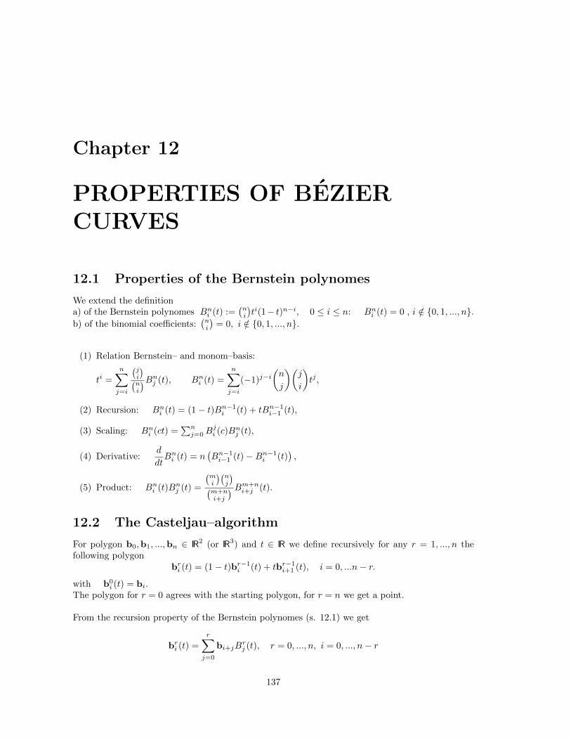
Chapter 12
PROPERTIES OF BEZIERCURVES
12.1 Properties of the Bernstein polynomes
We extend the definitiona) of the Bernstein polynomes Bni (t) :=
(ni
)ti(1− t)n−i, 0 ≤ i ≤ n: Bni (t) = 0 , i /∈ {0, 1, ..., n}.
b) of the binomial coefficients:(ni
)= 0, i /∈ {0, 1, ..., n}.
(1) Relation Bernstein– and monom–basis:
ti =
n∑j=i
(ji
)(ni
)Bnj (t), Bni (t) =
n∑j=i
(−1)j−i(n
j
)(j
i
)tj ,
(2) Recursion: Bni (t) = (1− t)Bn−1i (t) + tBn−1
i−1 (t),
(3) Scaling: Bni (ct) =∑nj=0B
ji (c)B
nj (t),
(4) Derivative:d
dtBni (t) = n
(Bn−1i−1 (t)−Bn−1
i (t)),
(5) Product: Bni (t)Bnj (t) =
(mi
)(nj
)(m+ni+j
) Bm+ni+j (t).
12.2 The Casteljau–algorithm
For polygon b0,b1, ...,bn ∈ IR2 (or IR3) and t ∈ IR we define recursively for any r = 1, ..., n thefollowing polygon
bri (t) = (1− t)br−1i (t) + tbr−1
i+1 (t), i = 0, ...n− r.
with b0i (t) = bi.
The polygon for r = 0 agrees with the starting polygon, for r = n we get a point.
From the recursion property of the Bernstein polynomes (s. 12.1) we get
bri (t) =
r∑j=0
bi+jBrj (t), r = 0, ..., n, i = 0, ..., n− r
137
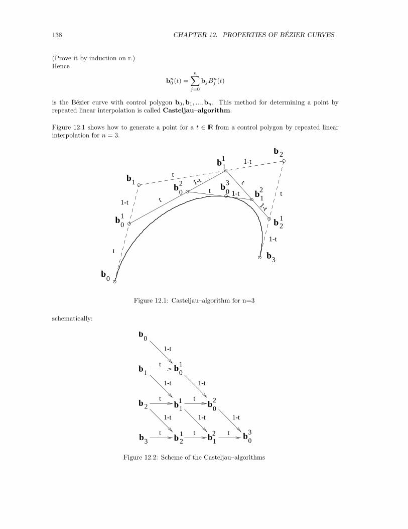
138 CHAPTER 12. PROPERTIES OF BEZIER CURVES
(Prove it by induction on r.)Hence
bn0 (t) =
n∑j=0
bjBnj (t)
is the Bezier curve with control polygon b0,b1, ...,bn. This method for determining a point byrepeated linear interpolation is called Casteljau–algorithm.
Figure 12.1 shows how to generate a point for a t ∈ IR from a control polygon by repeated linearinterpolation for n = 3.
b1
b2
b3
b0
b01
b11
b21
b12b
02 b
03
t
t
1-t
tt1-t
t1-t
t
1-t
1-t
1-t
Figure 12.1: Casteljau–algorithm for n=3
schematically:
b0
b1
b2
b3 b21
b11
b01
b12 b
03
b02
t
t
t t t
t
1-t
1-t
1-t
1-t
1-t 1-t
Figure 12.2: Scheme of the Casteljau–algorithms
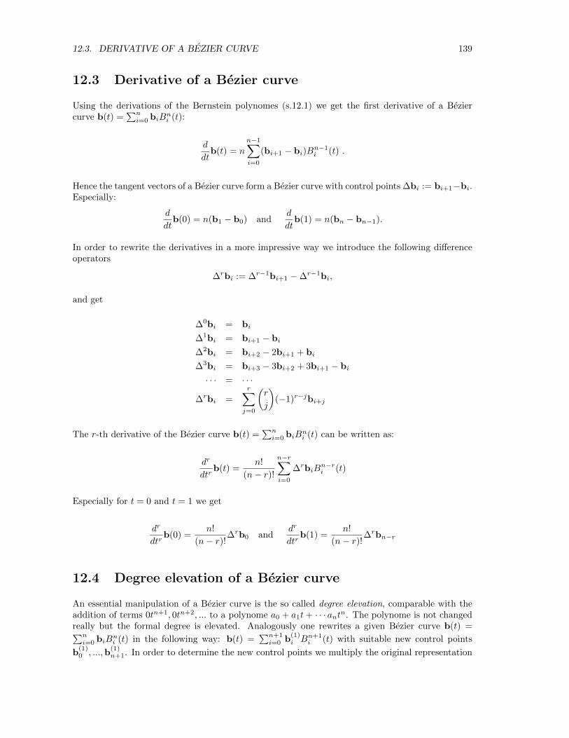
12.3. DERIVATIVE OF A BEZIER CURVE 139
12.3 Derivative of a Bezier curve
Using the derivations of the Bernstein polynomes (s.12.1) we get the first derivative of a Beziercurve b(t) =
∑ni=0 biB
ni (t):
d
dtb(t) = n
n−1∑i=0
(bi+1 − bi)Bn−1i (t) .
Hence the tangent vectors of a Bezier curve form a Bezier curve with control points ∆bi := bi+1−bi.Especially:
d
dtb(0) = n(b1 − b0) and
d
dtb(1) = n(bn − bn−1).
In order to rewrite the derivatives in a more impressive way we introduce the following differenceoperators
∆rbi := ∆r−1bi+1 −∆r−1bi,
and get
∆0bi = bi
∆1bi = bi+1 − bi
∆2bi = bi+2 − 2bi+1 + bi
∆3bi = bi+3 − 3bi+2 + 3bi+1 − bi
· · · = · · ·
∆rbi =
r∑j=0
(r
j
)(−1)r−jbi+j
The r-th derivative of the Bezier curve b(t) =∑ni=0 biB
ni (t) can be written as:
dr
dtrb(t) =
n!
(n− r)!
n−r∑i=0
∆rbiBn−ri (t)
Especially for t = 0 and t = 1 we get
dr
dtrb(0) =
n!
(n− r)!∆rb0 and
dr
dtrb(1) =
n!
(n− r)!∆rbn−r
12.4 Degree elevation of a Bezier curve
An essential manipulation of a Bezier curve is the so called degree elevation, comparable with theaddition of terms 0tn+1, 0tn+2, ... to a polynome a0 + a1t+ · · · antn. The polynome is not changedreally but the formal degree is elevated. Analogously one rewrites a given Bezier curve b(t) =∑ni=0 biB
ni (t) in the following way: b(t) =
∑n+1i=0 b
(1)i Bn+1
i (t) with suitable new control points
b(1)0 , ...,b
(1)n+1. In order to determine the new control points we multiply the original representation
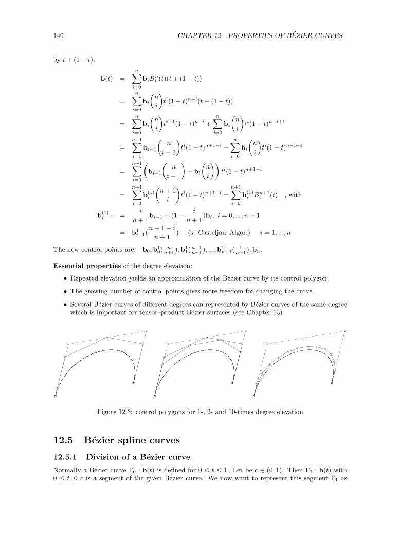
140 CHAPTER 12. PROPERTIES OF BEZIER CURVES
by t+ (1− t):
b(t) =
n∑i=0
biBni (t)(t+ (1− t))
=
n∑i=0
bi
(n
i
)ti(1− t)n−i(t+ (1− t))
=
n∑i=0
bi
(n
i
)ti+1(1− t)n−i +
n∑i=0
bi
(n
i
)ti(1− t)n−i+1
=
n+1∑i=1
bi−1
(n
i− 1
)ti(1− t)n+1−i +
n∑i=0
bi
(n
i
)ti(1− t)n−i+1
=
n+1∑i=0
(bi−1
(n
i− 1
)+ bi
(n
i
))ti(1− t)n+1−i
=n+1∑i=0
b(1)i
(n+ 1
i
)ti(1− t)n+1−i =
n+1∑i=0
b(1)i Bn+1
i (t) , with
b(1)i : =
i
n+ 1bi−1 + (1− i
n+ 1)bi, i = 0, ..., n+ 1
= b1i−1(
n+ 1− in+ 1
) (s. Casteljau–Algor.) i = 1, ..., n
The new control points are: b0,b10( nn+1 ),b1
1(n−1n+1 ), ...,b1
n−1( 1n+1 ),bn.
Essential properties of the degree elevation:
• Repeated elevation yields an approximation of the Bezier curve by its control polygon.
• The growing number of control points gives more freedom for changing the curve.
• Several Bezier curves of different degrees can represented by Bezier curves of the same degreewhich is important for tensor–product Bezier surfaces (see Chapter 13).
Figure 12.3: control polygons for 1-, 2- and 10-times degree elevation
12.5 Bezier spline curves
12.5.1 Division of a Bezier curve
Normally a Bezier curve Γ0 : b(t) is defined for 0 ≤ t ≤ 1. Let be c ∈ (0, 1). Then Γ1 : b(t) with0 ≤ t ≤ c is a segment of the given Bezier curve. We now want to represent this segment Γ1 as
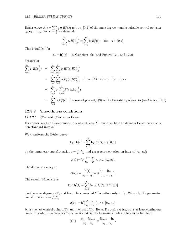
12.5. BEZIER SPLINE CURVES 141
Bezier curve c(t) =∑ni=0 ciB
ni (s) mit s ∈ [0, 1] of the same degree n and a suitable control polygon
c0, c1, ..., cn. For s := tc we demand:
n∑r=0
crBnr (t
c) =
n∑i=0
biBni (t), for t ∈ [0, c]
This is fulfilled for
cr = br0(c) (s. Casteljau–alg. and Figures 12.1 and 12.2)
because ofn∑r=0
crBnr (t
c) =
n∑r=0
r∑i=0
biBri (c)Bnr (
t
c)
=
n∑r=0
n∑i=0
biBri (c)Bnr (
t
c) from Bri (· · · ) = 0 for i > r
=
n∑i=0
bi
n∑r=0
Bri (c)Bnr (t
c)
=
n∑i=0
biBni (t) because of property (3) of the Bernstein polynomes (see Section 12.1)
12.5.2 Smoothness conditions
12.5.2.1 C1– and C2–connections
For connecting two Bezier curves to a new at least C1 curve we have to define a Bezier curve on anon standard interval.
We transform the Bezier curve
Γ1 : b(t) =
n∑i=0
biBni (t), t ∈ [0, 1]
by the parameter transformation t = s−u0
u1−u0and get a representation on interval [u0, u1]:
c(s) := b(s− u0
u1 − u0), s ∈ [u0, u1].
The derivation at u1 is:
c(u1) =b(1)
u1 − u0= n
bn − bn−1
u1 − u0.
The second Bezier curve
Γ2 : b′(t) =
n∑i=0
bn+iBni (t), t ∈ [0, 1]
has the same degree as Γ1 and has to be connected C1–continuously to Γ1. We apply the parametertransformation t = s−u1
u2−u1:
c(s) := b′(s− u1
u2 − u1), s ∈ [u1, u2].
bn is the last control point of Γ1 and the first of Γ2. Hence Γ : c(s), s ∈ [u0, u2] is at least continuouscurve. In order to achieve a C1–connection at u1 the following condition has to be fulfilled:
(C1)bn − bn−1
u1 − u0=
bn+1 − bnu2 − u1
,
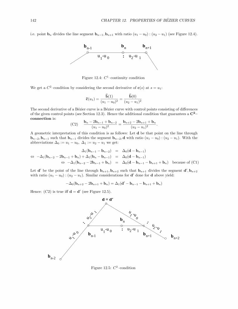
142 CHAPTER 12. PROPERTIES OF BEZIER CURVES
i.e. point bn divides the line segment bn−1,bn+1 with ratio (u1 − u0) : (u2 − u1) (see Figure 12.4).
bn-1 bn bn+1
u -u1 0 u -u2 1:
Figure 12.4: C1–continuity condition
We get a C2–condition by considering the second derivative of c(s) at s = u1:
c(u1) =b(1)
(u1 − u0)2=
b(0)
(u2 − u1)2
The second derivative of a Bezier curve is a Bezier curve with control points consisting of differencesof the given control points (see Section 12.3). Hence the additional condition that guarantees a C2–connection is:
(C2)bn − 2bn−1 + bn−2
(u1 − u0)2=
bn+2 − 2bn+1 + bn(u2 − u1)2
.
A geometric interpretation of this condition is as follows: Let d be that point on the line throughbn−2,bn−1 such that bn−1 divides the segment bn−2,d with ratio (u1 − u0) : (u2 − u1). With theabbreviations ∆0 := u1 − u0, ∆1 := u2 − u1 we get:
∆1(bn−1 − bn−2) = ∆0(d− bn−1)
⇔ −∆1(bn−2 − 2bn−1 + bn) + ∆1(bn − bn−1) = ∆0(d− bn−1)
⇔ −∆1(bn−2 − 2bn−1 + bn) = ∆0(d− bn−1 − bn+1 + bn) because of (C1)
Let d′ be the point of the line through bn+1,bn+2 such that bn+1 divides the segment d′,bn+2
with ratio (u1 − u0) : (u2 − u1). Similar considerations for d′ done for d above yield:
−∆0(bn+2 − 2bn+1 + bn) = ∆1(d′ − bn−1 − bn+1 + bn)
Hence: (C2) is true iff d = d′ (see Figure 12.5).
bn
bn-2
bn+2
u -u2 1u -u1 0 :
u -u
21
u -u
10
: u -u21
u -u10
:
bn+1bn-1
d = d’
Figure 12.5: C2–condition
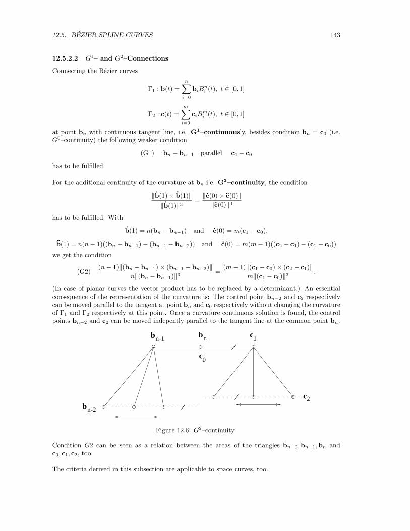
12.5. BEZIER SPLINE CURVES 143
12.5.2.2 G1– and G2–Connections
Connecting the Bezier curves
Γ1 : b(t) =
n∑i=0
biBni (t), t ∈ [0, 1]
Γ2 : c(t) =
m∑i=0
ciBmi (t), t ∈ [0, 1]
at point bn with continuous tangent line, i.e. G1–continuously, besides condition bn = c0 (i.e.G0–continuity) the following weaker condition
(G1) bn − bn−1 parallel c1 − c0
has to be fulfilled.
For the additional continuity of the curvature at bn i.e. G2–continuity, the condition
‖b(1)× b(1)‖‖b(1)‖3
=‖c(0)× c(0)‖‖c(0)‖3
has to be fulfilled. With
b(1) = n(bn − bn−1) and c(0) = m(c1 − c0),
b(1) = n(n− 1)((bn − bn−1)− (bn−1 − bn−2)) and c(0) = m(m− 1)((c2 − c1)− (c1 − c0))
we get the condition
(G2)(n− 1)‖(bn − bn−1)× (bn−1 − bn−2)‖
n‖(bn − bn−1)‖3=
(m− 1)‖(c1 − c0)× (c2 − c1)‖m‖(c1 − c0)‖3
.
(In case of planar curves the vector product has to be replaced by a determinant.) An essentialconsequence of the representation of the curvature is: The control point bn−2 and c2 respectivelycan be moved parallel to the tangent at point bn and c0 respectively without changing the curvatureof Γ1 and Γ2 respectively at this point. Once a curvature continuous solution is found, the controlpoints bn−2 and c2 can be moved indepently parallel to the tangent line at the common point bn.
bn-1 c1
c2bn-2
bn
c0
Figure 12.6: G2–continuity
Condition G2 can be seen as a relation between the areas of the triangles bn−2,bn−1,bn andc0, c1, c2, too.
The criteria derived in this subsection are applicable to space curves, too.
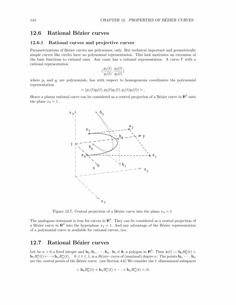
144 CHAPTER 12. PROPERTIES OF BEZIER CURVES
12.6 Rational Bezier curves
12.6.1 Rational curves and projective curves
Parametrizations of Bezier curves use polynomes, only. But technical important and geometricallysimple curves like circles have no polynomial representation. This lack motivates an extension ofthe base functions to rational ones. Any conic has a rational representation. A curve Γ with arational representation
(p1(t)
q1(t),p2(t)
q2(t))
where pi and qi are polynomials, has with respect to homogeneous coordinates the polynomialrepresentation
< (p1(t)q2(t), p2(t)q1(t), q1(t)q2(t)) > .
Hence a planar rational curve can be considered as a central projection of a Bezier curve in IR3 ontothe plane x3 = 1 .
a 0 a1
a 3
a 2
b0
b1
b2
b3
x
x
x
x
y
1
3
1
2
Figure 12.7: Central projection of a Bezier curve into the plane x3 = 1
The analogous statement is true for curves in IR3. They can be considered as a central projection ofa Bezier curve in IR4 into the hyperplane x4 = 1. And any advantage of the Bezier–representationof a polynomial curve is available for rational curves, too.
12.7 Rational Bezier curves
Let be n > 0 a fixed integer and b0,b1, · · · ,bn, bi 6= 0, a polygon in IR3. Then x(t) := b0Bn0 (t) +
b1Bn1 (t)+· · ·+bnB
nn(t), 0 ≤ t ≤ 1, is a Bezier–curve of (maximal) degree n. The points b0, · · · ,bn
are the control points of the Bezier curve. (see Section 4.6) We consider the 1–dimensional subspaces
< b0Bn0 (t) + b1B
n1 (t) + · · ·+ bnB
nn(t) >, 0,
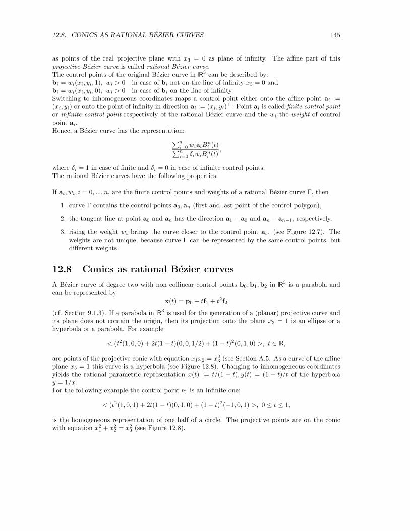
12.8. CONICS AS RATIONAL BEZIER CURVES 145
as points of the real projective plane with x3 = 0 as plane of infinity. The affine part of thisprojective Bezier curve is called rational Bezier curve.The control points of the original Bezier curve in IR3 can be described by:bi = wi(xi, yi, 1), wi > 0 in case of bi not on the line of infinity x3 = 0 andbi = wi(xi, yi, 0), wi > 0 in case of bi on the line of infinity.Switching to inhomogeneous coordinates maps a control point either onto the affine point ai :=(xi, yi) or onto the point of infinity in direction ai := (xi, yi)
>. Point ai is called finite control pointor infinite control point respectively of the rational Bezier curve and the wi the weight of controlpoint ai.Hence, a Bezier curve has the representation:∑n
i=0 wiaiBni (t)∑n
i=0 δiwiBni (t)
,
where δi = 1 in case of finite and δi = 0 in case of infinite control points.The rational Bezier curves have the following properties:
If ai, wi, i = 0, ..., n, are the finite control points and weights of a rational Bezier curve Γ, then
1. curve Γ contains the control points a0,an (first and last point of the control polygon),
2. the tangent line at point a0 and an has the direction a1 − a0 and an − an−1, respectively.
3. rising the weight wi brings the curve closer to the control point ai. (see Figure 12.7). Theweights are not unique, because curve Γ can be represented by the same control points, butdifferent weights.
12.8 Conics as rational Bezier curves
A Bezier curve of degree two with non collinear control points b0,b1,b2 in IR3 is a parabola andcan be represented by
x(t) = p0 + tf1 + t2f2
(cf. Section 9.1.3). If a parabola in IR3 is used for the generation of a (planar) projective curve andits plane does not contain the origin, then its projection onto the plane x3 = 1 is an ellipse or ahyperbola or a parabola. For example
< (t2(1, 0, 0) + 2t(1− t)(0, 0, 1/2) + (1− t)2(0, 1, 0) >, t ∈ IR,
are points of the projective conic with equation x1x2 = x23 (see Section A.5. As a curve of the affine
plane x3 = 1 this curve is a hyperbola (see Figure 12.8). Changing to inhomogeneous coordinatesyields the rational parametric representation x(t) := t/(1 − t), y(t) = (1 − t)/t of the hyperbolay = 1/x.For the following example the control point b1 is an infinite one:
< (t2(1, 0, 1) + 2t(1− t)(0, 1, 0) + (1− t)2(−1, 0, 1) >, 0 ≤ t ≤ 1,
is the homogeneous representation of one half of a circle. The projective points are on the conicwith equation x2
1 + x22 = x2
3 (see Figure 12.8).
146 CHAPTER 12. PROPERTIES OF BEZIER CURVES
x1
x2
x3
x1
x3
x2
x
y
x
y
1 1
Figure 12.8: a) hyperbola as rational Bezier curve with two infinite control points, b) half of a circleas rational Bezier curve with an infinite control point
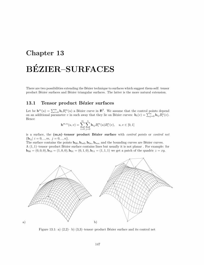
Chapter 13
BEZIER–SURFACES
There are two possibilities extending the Bezier technique to surfaces which suggest them-self: tensorproduct Bezier surfaces and Bezier triangular surfaces. The latter is the more natural extension.
13.1 Tensor product Bezier surfaces
Let be bm(u) =∑mi=0 biB
mi (u) a Bezier curve in IR3. We assume that the control points depend
on an additional parameter v in such away that they lie on Bezier curves: bi(v) =∑nj=0 bijB
ni (v).
Hence
bm,n(u, v) =
m∑i=0
n∑j=0
bijBmi (u)Bni (v), u, v ∈ [0, 1]
is a surface, the (m,n)–tensor product Bezier surface with control points or control net{bij | i = 0, ..,m, j = 0, .., n}.The surface contains the points b00,bm0,b0n,bmn and the bounding curves are Bezier curves.A (1, 1)–tensor–product Bezier surface contains lines but usually it is not planar . For example: forb00 = (0, 0, 0),b10 = (1, 0, 0),b01 = (0, 1, 0),b11 = (1, 1, 1) we get a patch of the quadric z = xy.
a) b)
Figure 13.1: a) (2,2)– b) (3,3)–tensor–product Bezier surface and its control net
147
148 CHAPTER 13. BEZIER–SURFACES
13.2 The Casteljau algorithm
Linear interpolation of pairs of points is the basic idea of the Casteljau algorithm for curves. Theanalogous technique for tensor product surfaces is the bilinear interpolation (see Section 10.4 onCoons patches) of four points which appears in the simplest example of a tensor product Beziersurface: A (1,1)-tensor–product Bezier surface for the four points b00,b10,b01,b11 is:
b1,1(u, v) = (1− u)(1− v)b00 + u(1− v)b10 + (1− u)vb01 + uvb11
Or in matrix form:
b1,1(u, v) = (1− u, u)
(b00 b01
b10 b11
)(1− vv
)We start with a (n× n)–control–net and determine for r = 1, 2, .., n and a pair of parameters (u, v)intermediate vectors by bilinear interpolation:
bri,j = (1− u, u)
(br−1i,j br−1
i,j+1
br−1i+1,j br−1
i+1,j+1
)(1− vv
),
where b0i,j := bi,j . Hence point bn0,0 is the surface point belonging to (u, v).
In case of m > n and r ≥ n the second index is constant j = 0 and the interpolation is just linear(instead of bilinear) as it is for Bezier curves. Point bm0,0 is the surface point.In case of m < n we deal analogously.
13.3 Degree elevation
It is an advantage if for a (m,n)–tensor–product Bezier surface we have m = n. If this is not thecase it can be achieved by suitable degree elevations.The degree elevation from (m,n) to (m+ 1, n) of the tensor product Bezier surface
bm,n(u, v) =
n∑j=0
[m∑i=0
bijBmi (u)
]Bni (v)
leads to the n+ 1 degree elevations for the Bezier curves [· · · ]:
m∑i=0
bijBmi (u) =
m+1∑i=0
b(1,0)ij Bm+1
i (u), j = 0, ...n
with
b(1,0)ij := (1− i
m+ 1)bi,j +
i
m+ 1bi−1,j , i = 0, ...,m+ 1.
13.4 Derivatives of a Bezier surface
The partial derivative of the tensor product Bezier surface
bm,n(u, v) =
n∑j=0
m∑i=0
bijBmi (u)Bni (v)
for u is∂
∂ubm,n(u, v) =
n∑j=0
[∂
∂u
m∑i=0
bijBmi (u)
]Bni (v).
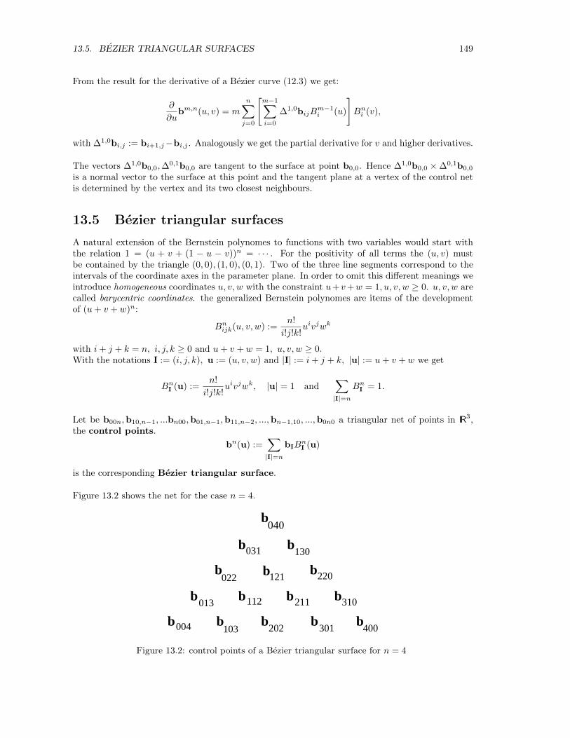
13.5. BEZIER TRIANGULAR SURFACES 149
From the result for the derivative of a Bezier curve (12.3) we get:
∂
∂ubm,n(u, v) = m
n∑j=0
[m−1∑i=0
∆1,0bijBm−1i (u)
]Bni (v),
with ∆1,0bi,j := bi+1,j−bi,j . Analogously we get the partial derivative for v and higher derivatives.
The vectors ∆1,0b0,0,∆0,1b0,0 are tangent to the surface at point b0,0. Hence ∆1,0b0,0 ×∆0,1b0,0
is a normal vector to the surface at this point and the tangent plane at a vertex of the control netis determined by the vertex and its two closest neighbours.
13.5 Bezier triangular surfaces
A natural extension of the Bernstein polynomes to functions with two variables would start withthe relation 1 = (u + v + (1 − u − v))n = · · · . For the positivity of all terms the (u, v) mustbe contained by the triangle (0, 0), (1, 0), (0, 1). Two of the three line segments correspond to theintervals of the coordinate axes in the parameter plane. In order to omit this different meanings weintroduce homogeneous coordinates u, v, w with the constraint u+v+w = 1, u, v, w ≥ 0. u, v, w arecalled barycentric coordinates. the generalized Bernstein polynomes are items of the developmentof (u+ v + w)n:
Bnijk(u, v, w) :=n!
i!j!k!uivjwk
with i+ j + k = n, i, j, k ≥ 0 and u+ v + w = 1, u, v, w ≥ 0.With the notations I := (i, j, k), u := (u, v, w) and |I| := i+ j + k, |u| := u+ v + w we get
BnI (u) :=n!
i!j!k!uivjwk, |u| = 1 and
∑|I|=n
BnI = 1.
Let be b00n,b10,n−1, ...bn00,b01,n−1,b11,n−2, ...,bn−1,10, ...,b0n0 a triangular net of points in IR3,the control points.
bn(u) :=∑|I|=n
bIBnI (u)
is the corresponding Bezier triangular surface.
Figure 13.2 shows the net for the case n = 4.
b040
b022
b121b220
b013
b112 b310
b103
b400
b004 b202
b301
b211
b130
b031
Figure 13.2: control points of a Bezier triangular surface for n = 4
150 CHAPTER 13. BEZIER–SURFACES
In order to describe the Casteljau algorithm for Bezier triangular surfaces we introduce thefollowing notations: e1 := (1, 0, 0), e2 := (0, 1, 0), e3 := (0, 0, 1) and o := (0, 0, 0).Let be {bI|I = (i, j, k), i+ j + k = n} a triangular net of points in IR3 and u a parameter vector inbarycentric coordinates. We define for r = 1, ..., n and I := (i, j, k) with i+ j + k = n− r
brI := ubr−1I+e1
(u) + vbr−1I+e2
(u) + wbr−1I+e3
(u)
with b0I(u) := bI. Point bno(u) is a point of the Bezier triangular surface. The proof of this statement
uses (analogously to the curve case) the following formulae of recursions for the Bernstein polynomes:
BnI (u) = uBn−1I−e1
(u) + vBn−1I−e2
(u) + wBn−1I−e3
(u), I = (i, j, k) with i+ j + k = n.
For more details see Farin Curves and Surfaces for Computer Aided Geometric Design orHoschek & Lasser Fundamentals of Computer Aided Geometric Design.
Chapter 14
B–SPLINE CURVES
There are two essential disadvantages using Bezier curves:
• A Bezier curve determined by many control points is of high degree.
• Changing one of the control points affects the whole curve.
This disadvantages can be omitted by using base functions with local effect.
14.1 The B–Spline base functions
The B–spline base functions are piecewise polynomial and non vanishing within a prescribed intervalonly (local support). They are defined recursively:
A vector (t0, t1, ..., tm) ∈ IRm+1 with t0 < t1 · · · < tm is called knot vector.Given n, k ∈ IN, n, k ≥ 1 and the knot vector T := (t0, t1, ..., tn+k). With functions
Ni1 :=
{1 , ti ≤ t ≤ ti+1
0 , sonst
for i = 1, 2, ..., n+ k we define recursively for k > 1:
Nik :=t− ti
ti+k−1 − tiNi,k−1(t) +
ti+k − tti+k − ti+1
Ni+1,k−1(t).
The functions Nik are called B–Spline–base functions of order k. They are piecewise polynomialof degree (k-1) and have the following properties
(B1) Nik(t) > 0 for ti < t < ti+k, the interval [ti, ti+k] is called support of Nik,
(B2) Nik(t) = 0 for t0 ≤ t ≤ ti, ti+k ≤ t ≤ tn+k,
(B3)∑ni=0Nik(t) = 1 for t ∈ [tk−1, tn+1],
(B4) at knots tl with ti ≤ tl ≤ ti+k functions Nik are Ck−2–continuous.
In case of special knot vectors (0, 1, 2, ..., n+ k) the base functions are called uniform.
Figures 14.1 show graphs of some B–spline base functions of order 1,2 and 3, respectively. They arepiecewise ploynomial of degree 0,1 bzw. 2.
151
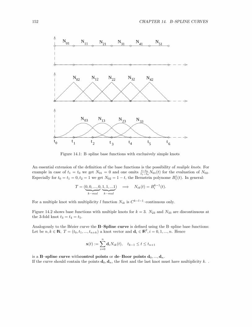
152 CHAPTER 14. B–SPLINE CURVES
N12 N22 N32N02
N03 N13 N23 N33
t0 t1 t
2 t 3t4 t
5t6
N11
N01 21
N31
N41
N51
N42
N
Figure 14.1: B–spline base functions with exclusively simple knots
An essential extension of the definition of the base functions is the possibility of muliple knots. Forexample in case of t1 = t0 we get N01 = 0 and one omits t−t0
t1−t0N01(t) for the evaluation of N02.
Especially for t0 = t1 = 0, t2 = 1 we get N02 = 1− t, the Bernstein polynome B11(t). In general:
T = (0, 0, ..., 0︸ ︷︷ ︸k−mal
, 1, 1, ...1︸ ︷︷ ︸k−mal
) =⇒ Nik(t) = Bk−1i (t).
For a multiple knot with multiplicity l function Nik is Ck−l−1–continuous only.
Figure 14.2 shows base functions with multiple knots for k = 3. N23 and N33 are discontinuous atthe 3-fold knot t3 = t4 = t5.
Analogously to the Bezier curve the B–Spline curve is defined using the B–spline base functions:Let be n, k ∈ IN, T = (t0, t1, ..., tn+k) a knot vector and di ∈ IR2, i = 0, 1, ..., n. Hence
x(t) :=
n∑i=0
diNik(t), tk−1 ≤ t ≤ tn+1
is a B–spline curve withcontrol points or de–Boor points d0, ...,dn.If the curve should contain the points d0,dn, the first and the last knot must have multiplicity k. .
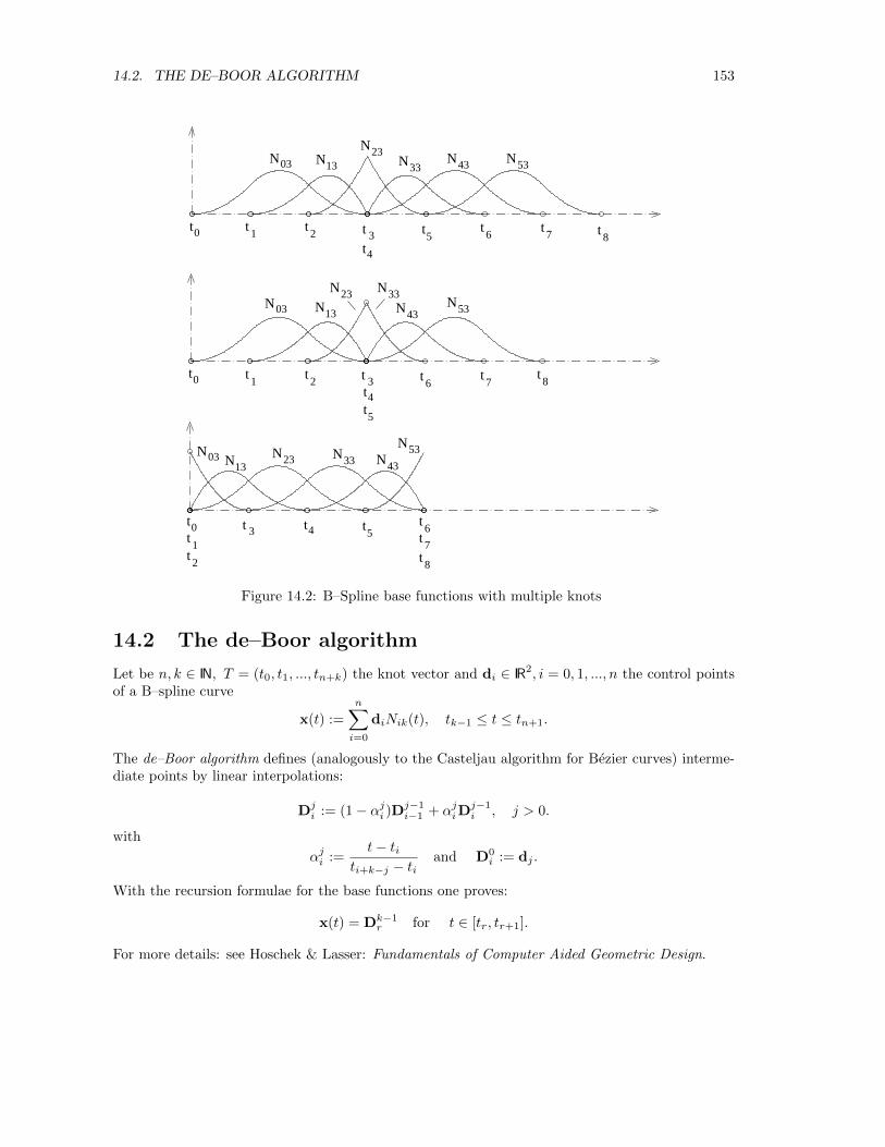
14.2. THE DE–BOOR ALGORITHM 153
t0 t1
t2 t 3 t
5t6 t
8t7
t4
N03 N13
N23N33
N03
N23N13
N33N43
t6
t7
t8
t4t5
t0 t 3
t0 t1
t2 t 3
t6
t1
t4
N03 N13N23 N33 N43
53N
t5
t8
t7
t2
N43 53N
53N
Figure 14.2: B–Spline base functions with multiple knots
14.2 The de–Boor algorithm
Let be n, k ∈ IN, T = (t0, t1, ..., tn+k) the knot vector and di ∈ IR2, i = 0, 1, ..., n the control pointsof a B–spline curve
x(t) :=
n∑i=0
diNik(t), tk−1 ≤ t ≤ tn+1.
The de–Boor algorithm defines (analogously to the Casteljau algorithm for Bezier curves) interme-diate points by linear interpolations:
Dji := (1− αji )D
j−1i−1 + αjiD
j−1i , j > 0.
with
αji :=t− ti
ti+k−j − tiand D0
i := dj .
With the recursion formulae for the base functions one proves:
x(t) = Dk−1r for t ∈ [tr, tr+1].
For more details: see Hoschek & Lasser: Fundamentals of Computer Aided Geometric Design.

154 CHAPTER 14. B–SPLINE CURVES
Appendix A
THE REAL PROJECTIVEPLANE
A.1 The real affine plane
Definition A.1 Let be
P := IR2, the points
G := {{(x, y) ∈ IR2| ax+ by + c = 0}| (0, 0) 6= (a, b) ∈ IR2}= {{(x, y) ∈ IR2| y = mx+ d}| m, d ∈ IR} ∪ {{(x, y) ∈ IR2 | x = c}|c ∈ IR}
the lines.
A(IR) := (P,G,∈) is called real affine plane.
A permutation of P which maps lines onto lines is called collineation of A(IR)).
Theorem A.1 Any collineation κ of A(IR) can be represented byκ : (x, y)→ (ax+ by + s, cx+ dy + t), ad− bc 6= 0,with suitable a, b, c, d, s, t ∈ IR. κ is called affinity.
proof: omitted.
Example A.1
a) (x, y) → (x+ s, y + t), s, t ∈ IR translation.b) (x, y) → (x, dy), 0 6= d ∈ IR axial affinity with axis y = 0 and direction (0, 1)>.c) (x, y) → (ax, y), 0 6= a ∈ IR axial affinity with axis x = 0 and direction (1, 0)>.d) (x, y) → (ax, ay), 0 6= a ∈ IR dilatation at point (0, 0).e) (x, y) → (x+ by, y), b ∈ IR shearing with axis y = 0.f) (x, y) → (x, y + cx), c ∈ IR shearing with axis x = 0.
A.2 The real projective plane
Definition A.2 Let be
P1 = IR2 ∪ IR ∪ {∞}, ∞ 6∈ IRG1 = {{(x, y) ∈ IR2| y = mx+ d} ∪ {(m)}| m, d ∈ IR}
∪{{(x, y) ∈ IR2| x = c} ∪ {(∞)}| c ∈ IR}∪ {{(m)| m ∈ IR} ∪ {(∞)}}︸ ︷︷ ︸
g∞
155
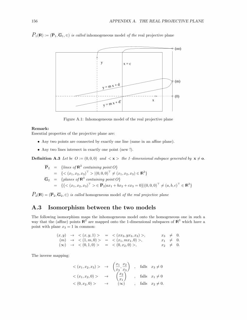
156 APPENDIX A. THE REAL PROJECTIVE PLANE
P1(IR) := (P1,G1,∈) is called inhomogeneous model of the real projective plane
y x = c
(m)
(0)
y = m x + d
y = m x + d’ x
(oo)
Figure A.1: Inhomogeneous model of the real projective plane
Remark:Essential properties of the projective plane are:
• Any two points are connected by exactly one line (same in an affine plane).
• Any two lines intersect in exactly one point (new !).
Definition A.3 Let be O := (0, 0, 0) and < x > the 1–dimensional subspace generated by x 6= o.
P2 = {lines of IR3 containing point O}= {< (x1, x2, x3)> > |(0, 0, 0)> 6= (x1, x2, x3) ∈ IR3}
G2 = {planes of IR3 containing point O}= {{< (x1, x2, x3)> > ∈ P2|ax1 + bx2 + cx3 = 0}|(0, 0, 0)> 6= (a, b, c)> ∈ IR3}
P2(IR) = (P2,G2,∈) is called homogeneous model of the real projective plane
A.3 Isomorphism between the two models
The following isomorphism maps the inhomogeneous model onto the homogeneous one in such away that the (affine) points IR2 are mapped onto the 1-dimensional subspaces of IR3 which have apoint with plane x3 = 1 in common:
(x, y) → < (x, y, 1) > = < (xx3, yx3, x3) >, x3 6= 0.(m) → < (1,m, 0) > = < (x1,mx1, 0) >, x1 6= 0.(∞) → < (0, 1, 0) > = < (0, x2, 0) >, x2 6= 0.
The inverse mapping:
< (x1, x2, x3) > →(x1
x3,x2
x3
), falls x3 6= 0
< (x1, x2, 0) > →(x2
x1
), falls x1 6= 0
< (0, x2, 0) > → (∞) , falls x2 6= 0.
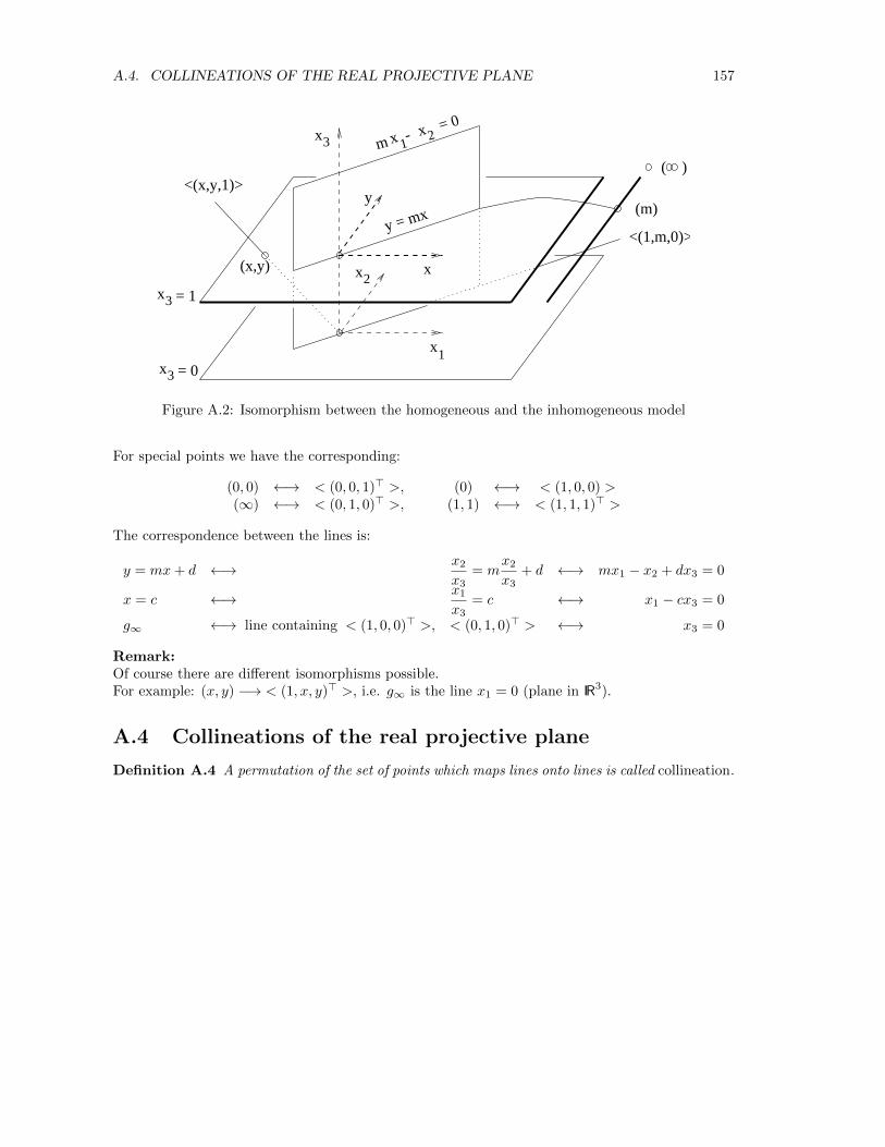
A.4. COLLINEATIONS OF THE REAL PROJECTIVE PLANE 157
x1
x2
x3
x3 = 1
x3 = 0
x 1x 2
m= 0
-
x
y
(x,y)
y = mx
<(x,y,1)>
(m)
<(1,m,0)>
( )
Figure A.2: Isomorphism between the homogeneous and the inhomogeneous model
For special points we have the corresponding:
(0, 0) ←→ < (0, 0, 1)> >, (0) ←→ < (1, 0, 0) >(∞) ←→ < (0, 1, 0)> >, (1, 1) ←→ < (1, 1, 1)> >
The correspondence between the lines is:
y = mx+ d ←→ x2
x3= m
x2
x3+ d ←→ mx1 − x2 + dx3 = 0
x = c ←→ x1
x3= c ←→ x1 − cx3 = 0
g∞ ←→ line containing < (1, 0, 0)> >, < (0, 1, 0)> > ←→ x3 = 0
Remark:Of course there are different isomorphisms possible.For example: (x, y) −→ < (1, x, y)> >, i.e. g∞ is the line x1 = 0 (plane in IR3).
A.4 Collineations of the real projective plane
Definition A.4 A permutation of the set of points which maps lines onto lines is called collineation.
158 APPENDIX A. THE REAL PROJECTIVE PLANE
Installment of the affinities:
in P1(IR) in P2(IR)
a) (x, y) → (x+ s, y + t) < (x1, x2, x3) >→ < (x1 + sx3, x2 + tx3, x3) >
(m) → (m) (in IR3 : shearing with axis) x3 = 0
(∞) → (∞)
1 0 s0 1 t0 0 1
b) (x, y) → (x, dy) < (x1, x2, x3) >→< (x1, dx2, x3) >
(m) → (md) (in IR3 : axial affinity with axis x2 = 0 and direction(0, 1, 0)>.)
(∞) → (∞)
1 0 00 d 00 0 1
c) (x, y) → (ax, ay) < (x1, x2, x3) >→< (ax1, ax2, x3) >
(m) → (m) (in IR3 : dilatation at line x1 = 0, x2 = 0)
(∞) → (∞)
a 0 00 a 00 0 1
d) (x, y) → (x, y + cx) < (x1, x2, x3) >→< (x1, x2 + cx1, x3) >
(m) → (m+ d) (in IR3 : shearing with axis x1 = 0)
(∞) → (∞)
1 0 0c 1 00 0 1
e) general case:
(x, y) → (ax+ by + s, cx+ dy + t)(m) → ( c+dma+bm )
(“Calculate” with ∞ in “usual” manner:
m→ {c+dma+bm , falls a+ bm 6= 0
∞, falls a+ bm = 0, ∞→ {
db , falls b 6= 0∞, falls b = 0 .)
< (x1, x2, x3) > → < (ax1 + bx2 + sx3, cx1 + dx2 + tx3, x3) >
Hence, the installment of an affinity can be represented in the homogeneous model by a linear mapwith matrix a b s
c d t0 0 1
A.5 Projective equivalency of the conics
In this section we shall show that all non degenerated conics (ellipse, hyperbola, parabola) areprojectively equivalent, i.e. any pair of non degenerate conics are related by a projective collineation.
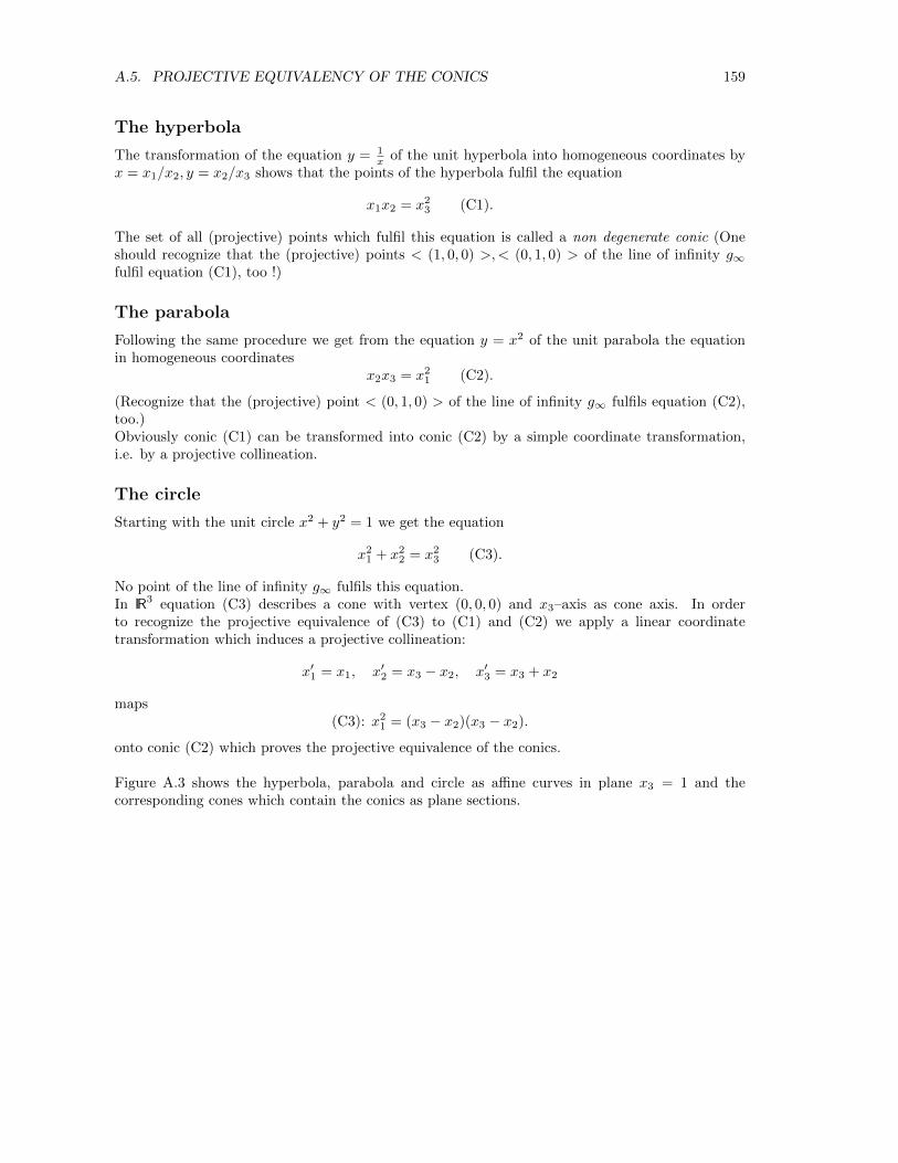
A.5. PROJECTIVE EQUIVALENCY OF THE CONICS 159
The hyperbola
The transformation of the equation y = 1x of the unit hyperbola into homogeneous coordinates by
x = x1/x2, y = x2/x3 shows that the points of the hyperbola fulfil the equation
x1x2 = x23 (C1).
The set of all (projective) points which fulfil this equation is called a non degenerate conic (Oneshould recognize that the (projective) points < (1, 0, 0) >,< (0, 1, 0) > of the line of infinity g∞fulfil equation (C1), too !)
The parabola
Following the same procedure we get from the equation y = x2 of the unit parabola the equationin homogeneous coordinates
x2x3 = x21 (C2).
(Recognize that the (projective) point < (0, 1, 0) > of the line of infinity g∞ fulfils equation (C2),too.)Obviously conic (C1) can be transformed into conic (C2) by a simple coordinate transformation,i.e. by a projective collineation.
The circle
Starting with the unit circle x2 + y2 = 1 we get the equation
x21 + x2
2 = x23 (C3).
No point of the line of infinity g∞ fulfils this equation.In IR3 equation (C3) describes a cone with vertex (0, 0, 0) and x3–axis as cone axis. In orderto recognize the projective equivalence of (C3) to (C1) and (C2) we apply a linear coordinatetransformation which induces a projective collineation:
x′1 = x1, x′2 = x3 − x2, x′3 = x3 + x2
maps(C3): x2
1 = (x3 − x2)(x3 − x2).
onto conic (C2) which proves the projective equivalence of the conics.
Figure A.3 shows the hyperbola, parabola and circle as affine curves in plane x3 = 1 and thecorresponding cones which contain the conics as plane sections.
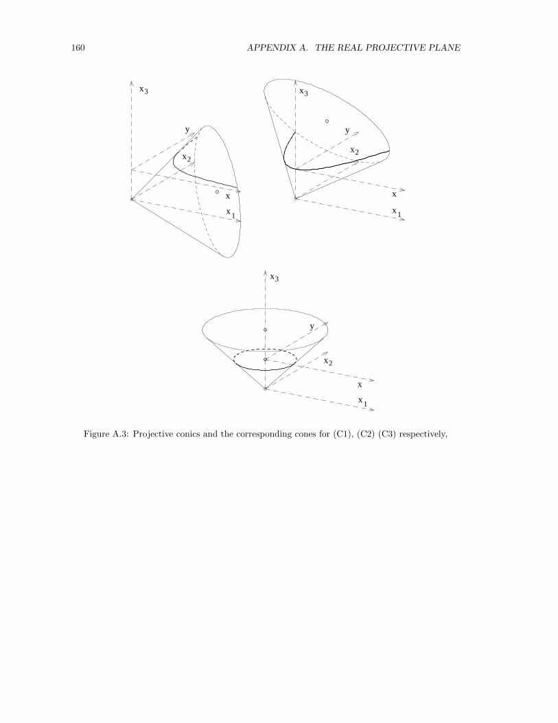
160 APPENDIX A. THE REAL PROJECTIVE PLANE
x2
x3
x2
x3
x2
x1
x3
x1
x1
y
x
y
y
x
x
Figure A.3: Projective conics and the corresponding cones for (C1), (C2) (C3) respectively,