Embed Size (px)
Citation preview

OdIO S I N E UNIVERSITY
GEOMETRICAL OPTICS DESIGN OF A COMPACT RANGE GREGORIAN
SUBREFLECTOR SYSTEM BY THE PRINCIPLE OFTHECENTRALRAY
Giancarlo Clerici Walter D. Burnside
The Ohio State University
ElectroScience Laboratory Deportment of Electrical Engineering
Columbus, Ohio 43212
Technical Report 719493-4 Grant No. NSG 1613
January 1989
National Aeronautics and Space A&linist,rat,ion Langley Research Center
Hampton, VA 22217 (bAS1-Cb-1848 1 C ) C-EC C E I E l C A L CISICE D E S I G B N0E-2C7SS
E € A CCEFAC? € A b G L GbkGCfjIAE $ C € € E E L B C I C L 5SPSTEt EY 4kI E f l K I I L I C € I f 1 CEbl6AL & B Y (Cbio S t a t e C L i v . ) 245 F CSCL SOP Unclas
63/34 C 1 9 5 5 5 4
https://ntrs.nasa.gov/search.jsp?R=19890011424 2018-07-13T10:28:39+00:00Z

NOT I C E S
When Government drawings, spec i f icat ions, o r other data are used f o r any purpose other than i n connection w i th a d e f i n i t e l y re la ted Government procurement operation , the United States Government thereby incurs no r e s p o n s i b i l i t y nor any ob l i ga t i on whatsoever, and the f a c t t h a t the Government may have formulated, furnished, o r i n any way supplied the said drawings, spec i f icat ions, o r other data, i s not t o be regarded by impl icat ion o r otherwise as i n any manner l i cens ing the holder o r any other person o r corporation, o r conveying any r i g h t s o r permission t o manufacture, use, o r s e l l any patented invent ion t h a t may i n any way be re la ted thereto.
TABLE OF CONTENTS
LIST OF FIGURES iv
LIST OF TABLES V
I. INTRODUCTION. 1
11. AN ERROR STUDY OF AN OFFSET SINGLE REFLECTOR
COMPACT RANGE 16
2.1 INTRODUCTION . . . . . . . . . . . . . . . . . . . . . . . . . 16
2.2 GEOMETRY OF THE SA REFLECTOR . . . . . . . . . . . . 17
2.3 REFLECTED FIELD TAPER ERROR ASSOCIATED WITH
THESAREFLECTOR . . . . . . . . . . . . . . . . . . . . . . . 18
CROSS-POLARIZATION ERROR ASSOCIATED WITH THE
SA REFLECTOR . . . . . . . . . . . . . . . . . . . . . . . . . . 26
2.5 APERTURE BLOCKAGE ERROR OF THE SA REFLECTOR 31
2.4
111. DESIGN CONSIDERATIONS 41
3.1 INTRODUCTION . . . . . . . . . . . . . . . . . . . . . . . . . 41
3.2 GEOMETRY OF THE SUBREFLECTOR SYSTEM. . . . . . 41
3.3 THE CENTRAL RAY . . . . . . . . . . . . . . . . . . . . . . . 48
3.4 TAPER OF THE REFLECTED FIELD . . . . . . . . . . . . . 53
PRECED\rJG PAGE BLANK NOT FlLMEDiii

IV .
V .
3.5 REDUCTION OF THE GEOMETRIC TAPER BY AN IN-
CREASE OF THE FOCAL DISTANCE . . . . . . . . . . . . . . 59
3.6 REFLECTED FIELD CROSS-POLARIZATION . . . . . . . . 64
3.7 FACTORS AFFECTING THE GO DESIGN OF A COMPACT
RANGE . . . . . . . . . . . . . . . . . . . . . . . . . . . . . . . . 68
3.7.1 SOURCE REQUIREMENTS FOR A COMPACT RANGE 68
3.7.2 EQUIVALENT FOCAL LENGTH FOR A SUBREFLEC-
TOR SYSTEM . . . . . . . . . . . . . . . . . . . . . . . 72
APERTURE BLOCKAGE AND UNWANTED INTER-
ACTIONS . . . . . . . . . . . . . . . . . . . . . . . . . . 74
3.7.4 FIELD IN THE FOCAL REGION . . . . . . . . . . . . 76
3.7.5 TIME GATING OF RAYS DIFFRACTED FROM THE
COUPLING APERTURE . . . . . . . . . . . . . . . . . 78
82
3.7.3
3.8 SHAPE OF THE CROSS SECTION OF THE TARGET ZONE
ITERATIVE SUBREFLECTOR SYSTEM DESIGN 87
4.1 EQUATIONS FOR GO FIELD COMPUTATIONS FOR A FO-
CUSSED SUBREFLECTOR SYSTEM . . . . . . . . . . . . . . 87
4.2 ITERATIVE DESIGN INITIAL VALUES . . . . . . . . . . . . 97
4.3 ITERATIVE DESIGN VIA GO COMPUTATIONS . . . . . . . 101
4.4 ITERATIVE DESIGN SUMMARY . . . . . . . . . . . . . . . . 103
4.5 ITERATIVE DESIGN EXAMPLE . . . . . . . . . . . . . . . . 105
DIRECT DESIGN THEORY 113 . 5.1 INTRODUCTION 113 . . . . . . . . . . . . . . . . . . . . . . . . . 5.1.1 .GEOMETRICAL CONSTR.AINTS . . . . . . . . . . . . 113
5.1.2 ELECTRICAL CONSTRAINTS . . . . . . . . . . . . . 116
I iv

5.1.3 FIRST DESIGN PROCEDURE (METHOD 1) . . . . . 124
5.1.4 SECOND DESIGN PROCEDURE (METHOD 2) . . . 124
5.1.5 THIRD DESIGN PROCEDURE (METHOD 3) . . . . . 125
5.1.6 FOURTH DESIGN PROCEDURE (METHOD 4) . . . 125
AN EQUATION USED IN THE FIRST, SECOND AND THIRD
DESIGN PROCEDURES . . . . . . . . . . . . . . . . . . . . . . 125
5.3 DIRECT DESIGN METHOD 1 . . . . . . . . . . . . . . . . . . 127
5.4 DIRECT DESIGN METHOD 2 . . . . . . . . . . . . . . . . . . 130
5.5 DIRECT DESIGN METHOD 3 . . . . . . . . . . . . . . . . . . 133
5.6 DIRECT DESIGN METHOD 4 . . . . . . . . . . . . . . . . . . 139
5.7 EVALUATION OF VARIOUS DESIGN PARAMETERS . . . 140
5.7.1 METHODS 1, 2AND 3 . . . . . . . . . . . . . . . . . . 141
5.7.2 METHOD 4 . . . . . . . . . . . . . . . . . . . . . . . . . 141
5.7.3 REMAINING QUANTITIES . . . . . . . . . . . . . . . 142
5.8 CONCLUSIONS . . . . . . . . . . . . . . . . . . . . . . . . . . 143
5.2
VI . COUPLING APERTURE DESIGN 144
6.1 BEHAVIOUR OF WEDGE SHAPED ABSORBER . . . . . . . 144
6.2 GO DESIGN OF THE OVERSIZED SUBREFLECTOR AND
THE COUPLING APERTURE . . . . . . . . . . . . . . . . . . . 145
VI1 . DIRECT DESIGN EXAMPLES 160
7.1 INTRODUCTION . . . . . . . . . . . . . . . . . . . . . . . . . 160
7.2 DIRECT DESIGN . AN EXAMPLE FOR COMPARISON . . . 160
7.3 DIRECT DESIGN . REQUIREMENTS FOR THE GO DESIGN
OF A NEW COMPACT RANGE . . . . . . . . . . . . . . . . . 166
DIRECT DESIGN . GO DESIGN OF A NEW COMPACT RANGE167 7.4
V

7.5 DIRECT DESIGN. COMPARISON OF THE ID AND FD DE-
SIGNS . . . . . . . . . . . . . . . . . . . . . . . . . . . . . . . . . 173
DIRECT DESIGN. EXAMPLES OF APPLICATION OF THE
DESIGN PROCEDURES . . . . . . . . . . . . . . . . . . . . . .175
7.6.1 DIRECT DESIGN. EXAMPLES DD2 AND DD3. . . . 175
7.6.2 DIRECT DESIGN. EXAMPLES DD4 AND DD5. . . . 176
7.6.3 DIRECT DESIGN. EXAMPLES DD6 AND DD7. . . . 180
7.6.4 DIRECT DESIGN. EXAMPLES DD8 AND DD9. . . . 185
7.7 CONCLUSION . . . . . . . . . . . . . . . . . . . . . . . . . . . 193
7.6
VIII. CONCLUSIONS 195
A.
B.
C.
D.
E.
F.
G .
THE VECTOR PATTERN FUNCTION 199
INTERSECTION OF A STRAIGHT LINE WITH A CONIC
OF REVOLUTION 201
COMPUTATION OF THE NORMAL FOR A CONIC OF
REVOLUTION 206
LAW OF REFLECTION 208
POLARIZATION 211
ANGULAR EXPRESSIONS 217
EXPRESSIONS FOR THE GEOMETRIC TAPER OF THE
REFLECTED FIELD 220
REFERENCES
vi
230

LIST OF FIGURES
1
2
4
5 .
6
7
8
9
10
11
12
13
14
15
Rolled edge terminations for the parabolic reflector . . . . . . . . . Parabolic reflector with rolled edge terminations . . . . . . . . . . . Plot of amplitude and phase of total field for elliptical rolled edge . Focal distance = 12'. frequency = 1 GHz . . . . . . . . . . . . . . .
edge . Focal distance = 7.25', frequency = 3 GHz . . . . . . . . . . . Aperture blockage effect . . . . . . . . . . . . . . . . . . . . . . . . . Single reflector offset design . . . . . . . . . . . . . . . . . . . . . . .
Plot of amplitude and phase of total field for cosine squared blended
Degradation of the total field with increasing target zone distance
(&) . . . . . . . . . . . . . . . . . . . . . . . . . . . . . . . . . . . Triple reflected field for a Cassegrain subreflector system . . . . . . Gregorian subreflector system with a dual chamber arrangement . .
Cross sectional and front view of the SA offset parabolic reflector . Front view of the target zone (uniform source) . . . . . . . . . . . . Front view of the target zone (Huygens source) . . . . . . . . . . . . Conservative estimate of the target zone . . . . . . . . . . . . . . . . The axis reference system and the tilt angle of t. he feed . . . . . . . Reflected field taper in dB . Omnidirectional source . Linear dinien-
sions are in feet . . . . . . . . . . . . . . . . . . . . . . . . . . . . .
7
8
9
10
11
12
13
14
15
19
20
21
22
23
27
vii

16 Overall taper in dB . Center fed Huygens source . Linear dimensions
areinfeet . . . . . . . . . . . . . . . . . . . . . . . . . . . . . . . . Overall taper in dB with a Huygens source which is tilted 20'. Lin-
ear dimensions are in feet . . . . . . . . . . . . . . . . . . . . . . . . Optimized overall taper in dB with a Huygens source which is tilted
39.75'. Linear dimensions are in feet . . . . . . . . . . . . . . . . . Cross-polarized field in dB with a Huygens source which is tilted
20° . Linear dimensions are in feet . . . . . . . . . . . . . . . . . . . Cross-polarized field in dB with a Huygens Source which is tilted
39.75'. Linear dimensions are in feet . . . . . . . . . . . . . . . . . 21 Incident shadow boundary for aperture blockage . . . . . . . . . . . 22 Aperture blockage versus vertical displacement . Frequency = 500
MHz . Distance from the reflector = 50'. . . . . . . . . . . . . . . . 23 Aperture blockage versus vertical displacement . Frequency = 10
GHz . Distance from the reflector = 50'. . . . . . . . . . . . . . . . Reflected and diffracted rays incident on a diffraction center . . . . True and spurious echoes for a scattering center . . . . . . . . . . .
17
18
19
20
24
25
29
30
32
33
37
38
39
40
40
26 Subreflector system reference axes . . . . . . . . . . . . . . . . . . . 42
27 Subreflector system geometry . . . . . . . . . . . . . . . . . . . . . . 43
28 Geometry of the target zone . . . . . . . . . . . . . . . . . . . . . . 44
29 Sequence of N confocal reflectors with N = 3 . . . . . . . . . . . . . 53
30 Determination of the equivalent axis for a single reflector . The re-
flector and the focus. Fo. a.re known. while. the focus. 8'1. is unknown . 54
Ray paths for a generic ray (a) and for the central ray (b) for N
confocal reflectors with N = 3 . . . . . . . . . . . . . . . . . . . . . 31
55
... Vll l

32
33
34
35
36
37
38
39
40
41
42
43
44
45
46
47
48
49
50
51
Limit argument to show that the direction. i". is independent from
the direction. 8. for a parabolic reflector . . . . . . . . . . . . . . . Determination of the equivalent axis and central rays for a Gregorian
subreflector system through a geometrical construction . . . . . . . Polar coordinate system for the parabolic reflector . . . . . . . . . . Typical geometric taper of the reflected field . . . . . . . . . . . . . On-axis and off-axis arrangements of the target zone . . . . . . . . . Effect of the focal distance on dpz . . . . . . . . . . . . . . . . . . Huygens source parameters . . . . . . . . . . . . . . . . . . . . . . . Feed beamwidths . . . . . . . . . . . . . . . . . . . . . . . . . . . . . Hour-glass shape of illuminating beam and its sections with planes .
More realistic illuminating beam . . . . . . . . . . . . . . . . . . . . Geometrical quantities related to the time delays of different rays . Timing diagram relating time delays and swithching times . . . . .
Convex subreflector . . . . . . . . . . . . . . . . . . . . . . . . . . . Concave subreflector . . . . . . . . . . . . . . . . . . . . . . . . . . . Geometry of the incident and reflected ray . . . . . . . . . . . . . . Geometrical quantities defining the subreflector system design . . . Values of the GO reflected field for the equivalent reflector with
uniform source . Linear dimensions are in feet . . . . . . . . . . . . . Values of the GO reflected field for the subreflector system with a
Huygens source . Linear dimensions are in feet. . . . . . . . . . . . .
Geometry for Equations (5.1), (.5.3), (5.4) and ( 5 . 5 ) ( zpc # 0) . .
Geometry for Equations (5.1), (5.3), (5.4), and (5.5) ( z p c = 0) . .
56
57
60
61
62
65
69
73
76
77
83
84
88
88
96
100
110
111
117
118
ix
52 Vertical dimensions of compact range upper room for the “iterative
design” arrangement . . . . . . . . . . . . . . . . . . . . . . . . . . . 119
53 Vertical dimensions of compact range upper room for the new design
FD . . . . . . . . . . . . . . . . . . . . . . . . . . . . . . . . . . . . 120
Condition on aC and Pc to avoid diffraction from coupling aperture . 121 54
55 Geometry of Direct Design. Method 2 . . . . . . . . . . . . . . . . . 131
56 Geometry of Direct Design. Method 3 . . . . . . . . . . . . . . . . . 134
57 Wedge absorber illuminated by a plane wave . . . . . . . . . . . . . 146
58 Extended subreflector . Linear dimensions are in feet . . . . . . . . . 154
59 Extended subreflector with coupling aperture . Linear dimensions
are in feet . . . . . . . . . . . . . . . . . . . . . . . . . . . . . . . . 155
60 Overextended subreflector . Linear dimensions are in feet . . . . . . 156
61 Overextended subreflector with coupling aperture . Linear dimen-
sions are in feet . . . . . . . . . . . . . . . . . . . . . . . . . . . . . 157
62 Detail of the coupling aperture . . . . . . . . . . . . . . . . . . . . . 158
63 Overextended subreflector with strongly diffracting coupling aper-
ture . Linear dimensions are in feet . . . . . . . . . . . . . . . . . . . 159
64 Layout of the ID design in the zm zm plane. showing the main
reflector. the subreflector. the upper and lower illuminating rays
and the central ray . Linear dimensions are in feet . . . . . . . . . . Layout of the DD1 design in the zm zm plane. showing the main
reflector. the subreflector. the upper and lower illuminating rays and
164
65
the central ray . Linear dimensions are in feet . . . . . . . . . . . . . 165
X
66
67
68
69
70
71
72
73
74
Layout of the final FD design in the 2, zm plane, showing the main
reflector, the subreflector, the upper and lower illuminating rays and
the central ray. Linear dimensions are in feet. . . . . . . . . . . . . 171
Layout of the final FD design in the z, zm plane, with first-cut
design of the coupling aperture. Linear dimensions are in feet. . . 172
Layout of the DD2 design in the zm zm plane, showing the main
reflector, the subreflector, the upper and lower illuminating rays and
the central ray. Linear dimensions are in feet. . . . . . . . . . . . . Layout of the DD3 design in the zm z, plane, showing the main
reflector, the subreflector, the upper and lower illuminating rays and
178
the central ray. Linear dimensions are in feet. . . . . . . . . . . . . 179
Layout of the DD4 design in the x m z, plane, showing the main
reflector, the subreflector, the upper and lower illuminating rays and
the central ray. Linear dimensions are in feet. . . . . . . . . . . . . Layout of the DD5 design in the zm z, plane, showing the main
reflector, the subreflector, the upper and lower illuminating rays and
the central ray. Linear dimensions are in feet. . . . . . . . . . . . . Layout of the DD6 design in the zln zm p lane, showing the main
reflector, the subreflector, the upper and lower illuminating rays and
182
183
the central ray. Linear dimensions are in feet. . . . . . . . . . . . . 187
Layout of the DD7 design in the z, z, plane, showing the main
reflector, the subreflector, the upper and lower illuminat,ing rays and
the central ray. Linear dimensions are in feet. . . . . . . . . . . . . 188
Layout of the DD8 design in the xtn z , plane, showing the main
reflector, the subreflector, the upper and lower illuminating rays and
the central ray. Linear dimensions are in feet. . . . . . . . . . . . . 191
xi

75 Layout of the DD9 design in the zm tm plane. showing the main
reflector. the subreflector. the upper and lower illuminating rays and
the central ray . Linear dimensions are in feet . . . . . . . . . . . . . 192
76
77
Geometry in polar coordinates of a conic in the plane . . . . . . . . 202
202 Geometry of the line l intersecting the conic of revolution . . . . . .
78 Incident and reflected triads . . . . . . . . . . . . . . . . . . . . . . 209
79 Huygenssource . . . . . . . . . . . . . . . . . . . . . . . . . . . . . 212
80 Truncated waveguide . . . . . . . . . . . . . . . . . . . . . . . . . . 216
81 Geometry related to the angles a. ,O and x . . . . . . . . . . . . . . 219
82 Geometry for the derivation of the gro . . . . . . . . . . . . . . . . . 221
83 Plot of IUT( versus 8, . . . . . . . . . . . . . . . . . . . . . . . . . . 222
84 Plot of lUTl versus p . . . . . . . . . . . . . . . . . . . . . . . . . . . 223
85 Geometry of a rectangular target zone . . . . . . . . . . . . . . . . . 229
xii

LIST OF TABLES
1
2
3
4
5
6
7
8
9
10
11
12
13
Allowable feed aperture versus frequency . . . . . . . . . . . . . . .
Design parameters for design ID . . . . . . . . . . . . . . . . . . .
Parameters for design DD1 . . . . . . . . . . . . . . . . . . . . . . Comparison between the ID design obtained via an iterative proce-
dure and the DD1 design obtained via the direct method . . . . . Parameters for the FD design . . . . . . . . . . . . . . . . . . . . . Comparison between the ID design (previous compact range) and
the FD design (new generation compact range) . . . . . . . . . . . Comparison between the final FD design and the DD2. DD3 designs
obtained by varying the quantity .. . . . . . . . . . . . . . . . . . Effect of increasing .. (designs DD2 and DD3) . . . . . . . . . . . Comparison between the final FD design and the .... DD5 designs
obtained by varying the quantity zpc . . . . . . . . . . . . . . . . . Effect of increasing .zF (designs DD4 and DD5) . . . . . . . . . . . Comparison between the final FD design and the .... DD7 designs
obtained by varying the quantit, ies h.... and hi, . . . . . . . . . . Effect of increasing hum and hinr (designs DD6 and DD’i) . . . . .
Comparison between the final FD design and the DD8. DD9 designs
obtained by varying the quantit, y xC . . . . . . . . . . . . . . . . .
35
112
162
163
170
174
177
180
181
184
1 SG
189
190
... XI11

CHAPTER I
INTRODUCTION.
The compact range has always been an attractive alternative to conventional
spherical ranges in that it can potentially be used to measure the pattern perfor-
mance of large antennas or scattering targets in an anechoic chamber. Within the
enclosed environment, the measurements are obviously not limited by the prevail-
ing weather conditions, and the security requirements are much easier to satisfy.
In addition, the measurement errors are definable and in many cases can be min-
imized. For example, background subtraction can be used to remove non-target
related terms in a scattering measurement, because the room and target mount
terms, which dominate the background, remain very stable in such an environment.
The first commercially available compact ranges were introduced by Scientific
Atlanta (SA) in the mid 1970’s. The SA systems consist of an offset parabolic
reflector illuminated by a low gain horn antenna. The purpose of the parabolic
reflector is to obtain a uniform plane wave (or an approximation of it) in the
quiet zone (or target zone, or sweet spot). The target is located in the quiet zone
for scattering measurements, and the antenna under test is positioned there for
radiation pattern measurements. It must be noted that the target or antenna
is in the near field of the parabolic reflector. This is an important difference as
compared to a spherical range, where the target or antenna is in the far field of
the transmit ting/receiving antenna, which obviously requires much larger ranges.
1
The SA compact range offers many advantages with respect to the spherical
range; however, it presents several problems. The most important of the short-
conlings was the serrated edge reflector which caused stray signals that illuminated
the target. Next that system used an offset design to reduce aperture blockage er-
rors caused by the feed antenna scattering which in turn illuminated the target or
antenna. However, an offset focus fed system causes taper and cross-polarization
errors associated with the field reflected by the parabolic reflector. These errors
are inherent to the offset focus fed design. In addition, the feed was not offset
enough to minimize the aperture blockage errors.
The problem of diffraction was the first one to be addressed at the Elec-
troscience Laboratory (ESL). An elliptical rolled edge design was introduced to
reduce the aniount of diffraction. This design was successfully performed using
GTD concepts [l] and is shown in Figure 1, while a parabolic reflector with the
rolled edges terminations is shown in Figure 2. Figure 3 shows a plot of the total
field at 1 GHz for a compact range with elliptical rolled edges. The parabolic
reflector under consideration has a focal length of 12', and the ellipse semiaxes are
a = 4' and b = 1'. The field is computed on a vertical cut in the principal plane at
24' from the vertex of the parabolic reflector. The feed used is an omnidirectional
source (;.e., a source having a uniform pattern). Note that the ripple of the am-
plitude is about 1 dB, and the phase variation is about 7 degrees across the target
zone. This performance was thought to be satisfactory at the time.
The blended rolled edge was introduced later as an improvement over the
elliptical rolled edge, in order to further decrease the diffraction from the junction
between the parabola and the rolled edge [2]. A blended rolled edge termination
for the parabolic reflector is shown in Figure 1. A plot of the total field at 3
GHz for a compact range with blended rolled edges is shown in Figure 4. The
2
parabolic reflector under consideration has a focal length of 7.25', and the ellipse
semiaxes are a = 3.4' and b = 0.75' with cosine squared type blending. An
omnidirectional source is used as a feed. Again, the field is computed on a vertical
cut in the principal plane at 20' from the vertex of the parabolic reflector. The
ripple variation is about 0.2 dB in amplitude and 1/2 a degree in phase across
the target zone. This design meets the desired diffraction performance but the
aperture blockage, taper and cross polarization errors remain. The purpose of this
work is to determine a design which overcomes these three errors.
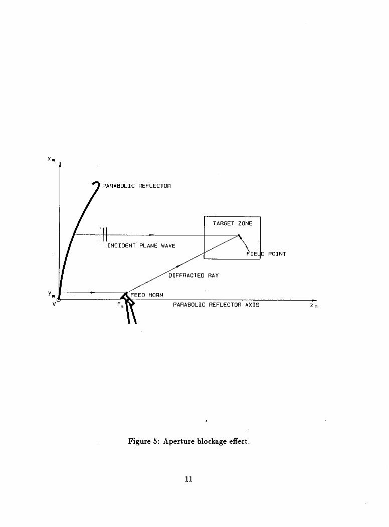
As it is well known, aperture blockage happens when an obstacle blocks the
plane wave reflected from a parabolic reflector. Typical examples of aperture
blockage structures are the feed antenna, waveguide and mounting structure. The
plane wave coming from the parabolic reflector is incident on these structures,
and a scattered field will then interact with the plane wave in the quiet zone
behind these structures, as shown in Figure 5. Consequently, if this error is not
eliminated, strong stray signals are present even if care has been taken to minimize
the field diffracted by the edges of the parabolic reflector. This stray signal error
not only causes ripple in the field illuminating the target, but also undesirable
cross-polarized components.
Aperture blockage is typically reduced through an offset design, in that the
feed is positioned outside the plane wave reflected from the parabolic reflector
(see Figure 6). The aperture blockage effects have been reduced in the SA system
through an offset design, but has not been completely eliminated, since the feed
antenna is still very close to the beam of the reflected field, as schematically shown
in Figure 5 . In the ESL compact range, the original SA antenna support has
been substituted with one of much smaller blockage dimensions; nevertheless, the
aperture blockage stray signal is the largest of all the errors present. Since this
3
stray signal cannot be time-gated, it remains a serious concern for future designs.
In order to perform effective RCS measurements, it is highly desirable to min-
iinize the amount of cross-polarization present in the target zone. In fact, the
importance of the polarization response in RCS measurenients and target identi-
fication has long been recognized [3]. It is important then to reduce the cross
polarization of the plane wave incident on the target so that it is at least 40 dB
below the co-polarized level. In this way then the cross-polarized component of the
field is below the sensitivity threshold of the system. While diffraction introduces a
cross-polarized component, which can be mimimized by reducing diffraction itself,
the offset design has an inherent cross-polarization error. Even through the cross-
polarization and the taper errors can be reduced by increasing the focal length of
the parabolic reflector, this approach in turn dictates a larger room, with a sub-
stantial increase in the cost of the facility. Besides, the plane wave obtained in the
target zone is a near field effect, which implies that the plane wave deteriorates if
the target zone is moved farther away from the main reflector. This can be seen,
for instance, from the examples illustrated in Figure 7. In these plots, the total
field has been evaluated for a parabolic reflector on a vertical cut at three different
distances tcm from the vertex of the parabolic reflector; viz., 12’, 24‘ and 36’. The
parabolic reflector has a focal distance of 12’ and elliptical rolled edges with major
and minor ax is lengths of 4‘ and l‘, respectively on the upper edge and a “skirt”
(i.e., a parabolic cylinder termination) on the lower edge. The computations have
been performed using a numerical procedure and GTD techniques. In these plots,
it can be seen that the diffraction effects or ripple levels become more significant
as the distance from the vertex of the parabolic reflector is increased.
The taper associated with the reflected field is another error present in the
compact range. A taper naturally occurs in a focus fed system in that the distance
4

from the feed to the reflector is not a constant. This fact results in a reduction of
the field strength illuminating the reflector at wide angles. Thus, the amplitude of
the plane wave illuminating the target is not constant, such that scattering centers
near the edge of the target zone are illuminated by a plane wave of lower intensity
than that in the middle. Thus, the scattering center is illuminated in the proper
direction but with a different field strength. Since the scattering center is being
measured in the proper direction, its scattering level is simply changed by the
illumination level. Thus, a taper error is still in the direction of the plane wave so
its effect on the overall measurement errors is not nearly as significant as a stray
signal which illuminates the target at a different angle. This implies that one can
tolerate larger taper than ripple errors, as shown by Burnside and Peters [4].
A subreflector system can be used to eliminate the cross-polarized component
introduced by the single reflector offset arrangement. At the same time, it can be
used to minimize the taper of the reflected field because the equivalent focal length
of the subreflector system can be easily made large. In addition, since the main
reflector focal length can be designed to be relatively short, the quiet zone can be
placed closer to the main reflector, which reduces the diffraction errors as well as
the size of the anechoic chamber.
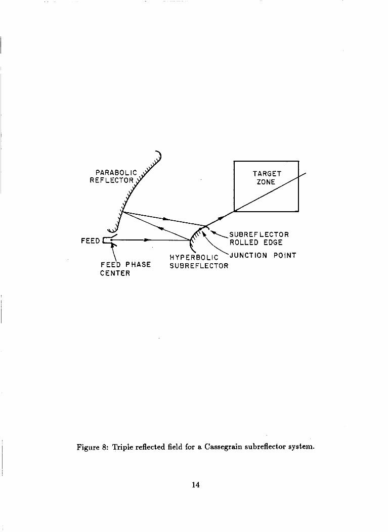
A Cassegrain subreflector system has been considered and discarded [5] in
that several undesired effects can seriously degrade its performance. Specifically,
there is a triple reflected field; i.e., a field reflected from the subreflector, main
reflector, subreflector and finally into the target zone, as shown in Figure 8. This
path length is very close to that of the rays of the plane wave illuminating the
target, such that this unwanted contribution cannot be time gated out using a
pulsed radar system. As a result, this clutter term causes a ripple error associated
with the probed field as this mechanism conies in and out of phase with the plane
5
wave. This error term is normally too large as shown by Rader [5 ] , which makes
the Cassegrain subreflector system unacceptable.
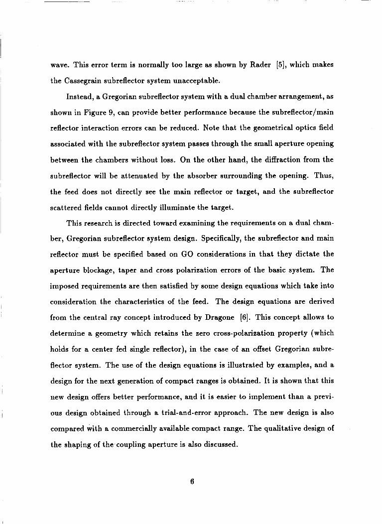
Instead, a Gregorian subreflector system with a dual chamber arrangement, as
shown in Figure 9, can provide better performance because the subreflector/main
reflector interaction errors can be reduced. Note that the geometrical optics field
associated with the subreflector system passes through the small aperture opening
between the chambers without loss. On the other hand, the diffraction from the
subreflector will be attenuated by the absorber surrounding the opening. Thus,
the feed does not directly see the main reflector or target, and the subreflector
scattered fields cannot directly illuminate the target.
This research is directed toward examining the requirements on a dual cham-
ber, Gregorian subreflector system design. Specifically, the subreflector and main
reflector must be specified based on GO considerations in that they dictate the
aperture blockage, taper and cross polarization errors of the basic system. The
imposed requirements are then satisfied by some design equations which take into
consideration the characteristics of the feed. The design equations are derived
from the central ray concept introduced by Dragone [6]. This concept allows to
determine a geometry which retains the zero cross-polarization property (which
holds for a center fed single reflector), in the case of an offset Gregorian subre-
flector system. The use of the design equations is illustrated by examples, and a
design for the next generation of compact ranges is obtained. It is shown that this
new design offers better performance, and it is easier to implement than a previ-
ous design obtained through a trial-and-error approach. The new design is also
compared with a commercially available compact range. The qualitative design of
the shaping of the coupling aperture is also discussed.
6

ENDED ABOLA
BLENDED SURFACE
A
n J U n C f l O N / -PAR ABO LA
Figure 1: Rolled edge terminations for the parabolic reflector.
7

15
111
13
12
11
10
9
+ 8
Lw7 w
6
5
4
3
2
1
0
- 1 .......................
Y
a r c , a et
L ( P U R E . E L L I P S E 1 ...................................... *-,(COS I N E B L E N D ) .. ...............-.-...,...-.,
........................................ - 2 - 1 0 1 2 3 4
FEET
Figure 2: Parabolic reflector with rolled edge terminations.
8
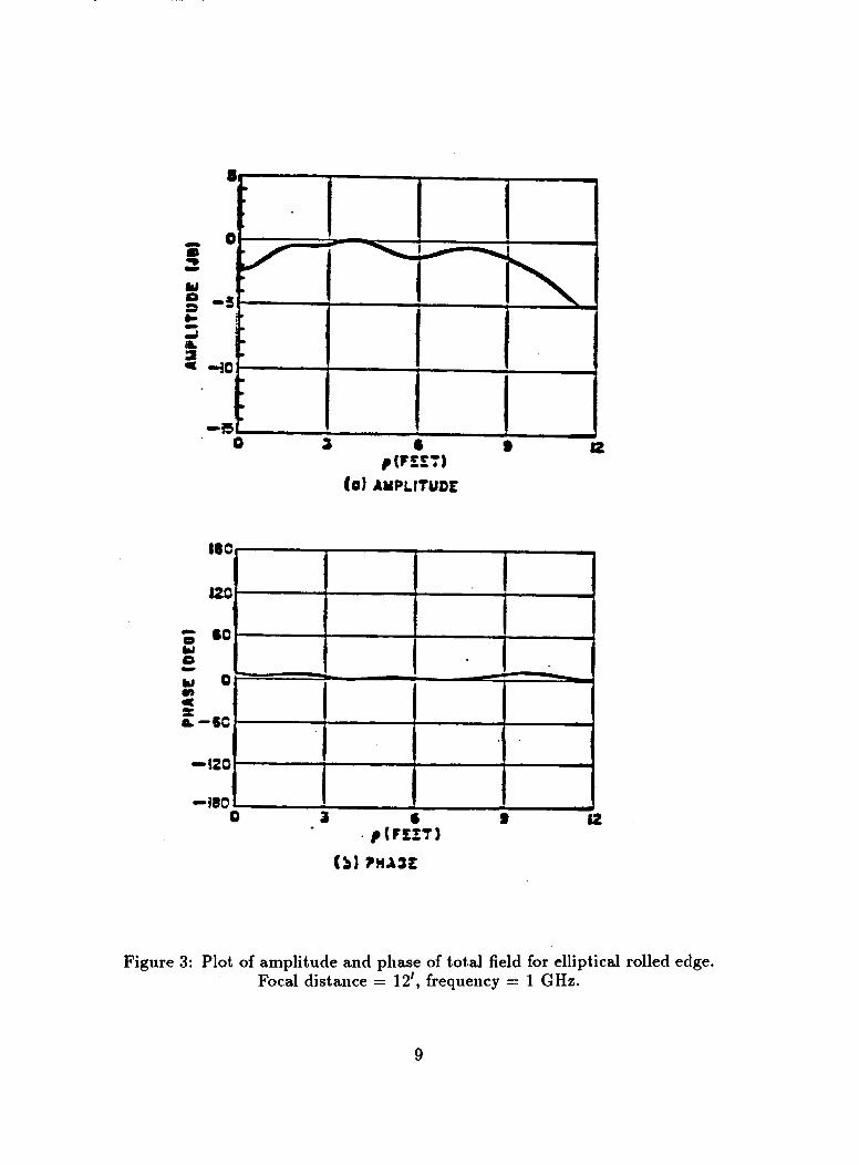
Figure 3: Plot of amplitude and phase of total field for elliptical rolled edge. Focal distance = 12', frequency = 1 GHz.
9

........................................................................... 0
* .................... i .................... i .................... ; .................... ; .................... ; .................... ; m y 0 A -1 -o .................... i ............................................................. J ' W
.- .................. .....................
- .................... i .................... i .................... i .................... ; .................... i .................... 1 -ii 01
15.5 6 .5 7 .5 8 .5 9.5 10.5 11.5 ( u 1
HEIGHT Y ( F E E T I
I I I I 1 1
I I I I I I 1
6.5 7.5 8 .5 9 .5 10.5 11.5 m, 9 . 5 I HEIGHT Y ( F E E T I
Figure 4: Plot of amplitude and phase of total field for cosine squared blended edge. Focal distance = 7.25', frequency = 3 GHz.
10
TARGET ZONE
I I INCIDENT PLANE WAVE
9 PARABOLIC REFLECTOR
D POINT
-
zm PARABOLIC REFLECTOR AXIS
Figure 5: Aperture blockage effect.
11

PLANE -* \ \ \
\ \ \ FEED HORN \
> PARABOLIC REFLECTOR A X I S Zm
Figure 6: Single reflector offset design.
12

TARGET ZONE -- 1 r - -
I 0 b l I
I
-5 I
-10
,P,m = 12 '
I -
I I I I I I I
I 3 -5t J? c m = 2 4 ' , I- -
t 2 -10 2 a
I I \ ,
Y I I I I I I I I I , I I I I
I 1
-15' 1 0-
-5 I
-10 I I
- lcm 7 36'
-
-15 I I I I I I I I I 1 I I I I 0 I 2 3 4 5 6 7 8 9 10 II 1 2 1 3 1 4 1 5
D ISPLACEMENT (FEET)
Figure 7: Degradation of the total field with increasing target zone distance (&n>.
13
TARGET
ROLLED EDGE
FEED PHASE SUBREFLECTOR CENTER
Figure 8: Triple reflected field for a Cassegrain subreflector system.
14

ROLLED BLENDED 7 13 EDGE ---MAIN REFLECTOR
‘ABSORBER
Figure 9: Gregorian subreflector system with a dual chamber arrangement.
15

CHAPTER I1
AN ERROR STUDY OF AN OFFSET SINGLE REFLECTOR
COMPACT RANGE
2.1 INTRODUCTION
In Chapter I, it has been mentioned how a single reflector offset design is
affected by three problems: aperture blockage, taper of the reflected field and cross-
polarization errors. In this chapter a specific single reflector offset design example
is considered; viz., the latest (1986) SA compact range, and it is shown how its
performance is affected by these errors. The “ -40 dB” criterion is used to establish
if an error is significant. In other words, an error is considered “acceptable” if it
is 40 dB below the intensity of the reflected field. The reflected field is the plane
wave illuminating the antenna/target under measurement; consequently, it is the
natural reference, and it is approximately constant since its taper is only a fraction
of a dB. The value of -40 dB is obtained because it represents an achievable level
without unduly restricting the design. Therefore, it is required that the errors
present in the design of the compact range be of the same order of magnitude so
that one error term is not emphasized over another.
The “-40 dB” criterion gives also a value for the acceptable ripple. This can
be seen as follows. By definition, the ripple is given by
(2.1) u e Ripple = 1 + - UP
16
where Ue is the intensity of the error field, and Up is the intensity of the plane
wave field. Both U, and Up are real scalars. By letting
one obtains
Consequently
2010g (2) = -40 ,
ue - = 0.01 . UP
and the acceptable ripple, for the “-40 dB” criterion, is approximately -0.1 dB.
For the study of the SA compact range this criterion is relaxed somewhat,
and a -0.2 dB value for the ripple was used.
2.2 GEOMETRY OF THE SA REFLECTOR
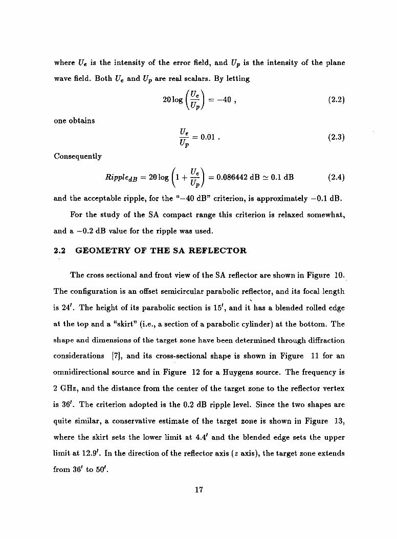
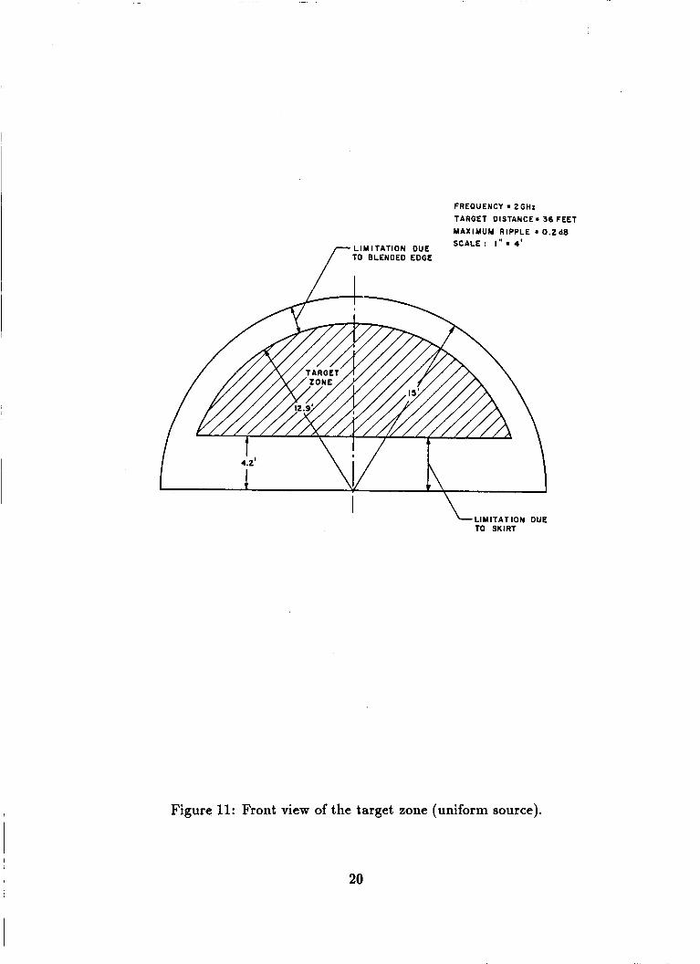
The cross sectional and front view of the SA reflector are shown in Figure 10.
The configuration is an offset semicircular parabolic reflector, and its focal length
is 24’. The height of its parabolic section is 15‘, and it has a blended rolled edge ,
at the top and a “skirt” (;.e., a section of a parabolic cylinder) at the bottom. The
shape and dimensions of the target zone have been determined through diffraction
considerations [7], and its cross-sectional shape is shown in Figure 11 for an
omnidirectional source and in Figure 12 for a Huygens source. The frequency is
2 GHz, and the distance from the center of the target zone to the reflector vertex
is 36’. The criterion adopted is the 0.2 dB ripple level. Since the two shapes are
quite similar, a conservative estimate of the target zone is shown in Figure 13,
where the skirt sets the lower limit at 4.4’ and the blended edge sets the upper
limit at 12.9‘. In the direction of the reflector axis ( z a x i s ) , the target zone extends
from 36’ to 50’.
17

The reference system adopted is as follows: the origin V is at the parabolic
reflector vertex, the 2 axis is vertical, the y axis is horizontal and the z axis
coincides with the reflector axis. The focus is located at Fm, which coincides with
the phase center of the feed. The tilt angle of the feed is the angle between the
negative z axis and the ax is of the feed (see Figure 14).
2.3 REFLECTED FIELD TAPER ERROR ASSOCIATED WITH THE SA REFLECTOR
The taper error of the SA reflector is computed with respect to a omnidi-
rectional source through a numerical implementation of the equations shown in
Chapter IV, simplified for the case of a single reflector. I
I
I An omnidirectional, or isotropic, source is an idealized, non physical source,
since no antenna has a pattern that is independent of angle. This source is intro- I
I duced in order to separate the effects of the geometry from those of the pattern of I
the feed.
The amplitude of the GO reflected field in dB with respect to a omnidirectional
source is shown in Figure 15. The computations are performed on a grid on a
plane perpendicular to the parabolic reflector axis. The data are symmetric with I
I respect to the 2 axis; therefore, the computations are performed only for y 2 0.
The grid is also shown in Figure 15. It is not necessary to specify the distance of
the plane cut on which the field is computed from the vertex of the reflector, since
the GO field is independent of this distance. In the 2 direction the computation
begins at z = 4' and ends at z = 13'; while, in the y direction, it begins at y = 0'
and ends at y = 14'. The computation is performed over a rectangle, 9' x 14' in the
z and y directions, respectively. This rectangle encoinpasses all of the target zone.
The values of the reflected field are normalized to the maximum of the computed I 18

W
PARABOLIC SECTION x
=.
. "0.
\ FOCAL POINT :JJ,UN,CT:o,N , , ,
I " " 1 " " I Y. e. 1 2 . 16. 20. 2y .
2 (FEET1 -SKIRT
x
,DGE PARA
/ I S K I R T
,BLENDED ROLLED E
Figure 10: Cross sectional and front view of the SA offset parabolic reflector.
19
FREOUENCY = 2GHx TARGET DISTANCE= 36 FEET MAXIMUM RIPPLE = 0.248 SCALE : I " = 4 ' LIMITATION DUE
TO BLENDED EDGE
LIMITATION DUE TO SKIRT
I
Figure 11: Front view of the target zone (uniform source).
20

FREQUENCY = 2GHx TARGET DISTANCE= 36FEET MAXIMUM RIPPLE = 0.2dB SCALE ' I" a 4' LIMITATION DUE
TO BLENOEO EDGE /-
Figure 12: Front view of the target zone (Huygens source).
21

FREQUENCY = 2GHt TARGET DISTANCE. 36 FEET MAXIMUM RIPPLE = 0.248 SCALE : I " = 4 '
LIMITATION DUE TO BLENDED EDGE
LIMITATION DUE TO SKIRT
Figure 13: Conservative estimate of the target zone.
22

I I\ FEED A X I S
FEED HORN ym
V REFLECTOR AXIS z:
Figure 14: The axis reference system and the tilt angle of the feed.
23

values, which corresponds to the point at y = 0', z = 4'. The overall maximum
instead corresponds to the reflector vertex, i.e., to the point z = 0', y = 0'. From
the values shown in Figure 15, it can be seen that, on the z a x i s , the normalized
reflected field at z = 13' is -0.55 dB. On the y axis instead, the value of the
normalized reflected field at y = 12' is -0.52 dB. The value of the reflected field
taper error is then -0.55 dB.
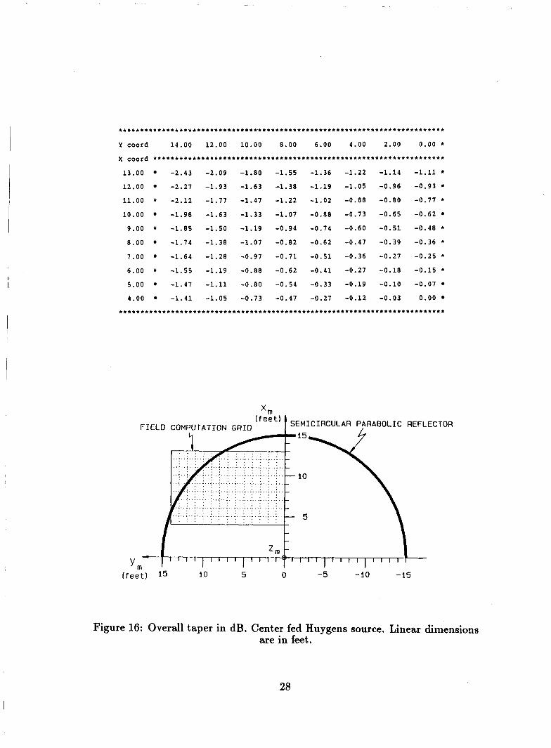
The computation of the taper is then repeated with a Huygens source. The
Huygens source is defined in Section E, and its pattern is non-uniform. A Huygens
source is used to study the polarization properties of reflector antennas and has a
pattern which is close to the patterns of an actual feed antenna (for instance, an
open ended waveguide). In this case, the total taper of the reflected field is due
to the effect of the geometry of the parabolic reflector as well as the feed pattern.
By tilting the axis of the source with respect to the axis of the reflector (offset
arrangement) it is possible to obtain a partial compensation between these two
effects. This is intuitive and is now shown through three examples. The overall
taper for a case in which the Huygens source is coincident with the main reflector
axis (tilt angle of 0') is shown in Figure 16. The values of the reflected field are
normalized to the maximum of the computed values, which corresponds to the
point at y = 0', 2 = 4' (the overall maximum instead corresponds to the reflector
vertex, i.e., to the point z = 0', y = 0'). From this data it can be seen that, on the
2 axis, the overall reflected field at z = 13' is -1.11 dB, while on the y axis , the
overall reflected field at y = 12' is -1.05 dB. The value of the overall taper error
then is -1.11 dB. The taper now is larger than the taper with the omnidirectional
source discussed earlier due to the sum of effects associated with the geometry
and the Huygens source. Next, Figure 17 shows a case in which the axis of the
Huygens source is tilted by 20' with respect to the axis of the parabolic reflector,
24

which corresponds, approximately, to directing the axis of the feed towards the
point on the reflector corresponding to the axis of the target zone. The values of
the reflected field are normalized to the overall maximum, which now corresponds,
approximately, to the point at y = 0', x = 4.5'. On the x axis, the overall reflected
field at x = 4' is 0.0 dB, while at x = 13' it is -0.55 dB, on the y axis instead,
the overall reflected field is -1.03 dB at y = 12'. Thus, the overall taper error is
-1.03 dB, which could be reduced if a smaller target zone in the y direction were
considered. For instance, for a target zone extending from -6' to 6', the overall
taper error would be -0.55 dB. In any case, the overall taper error is reduced with
respect to the center fed case. These field values show that the offset configuration
offers a way to reduce the overall taper by tilting the axis of the feed. For a given
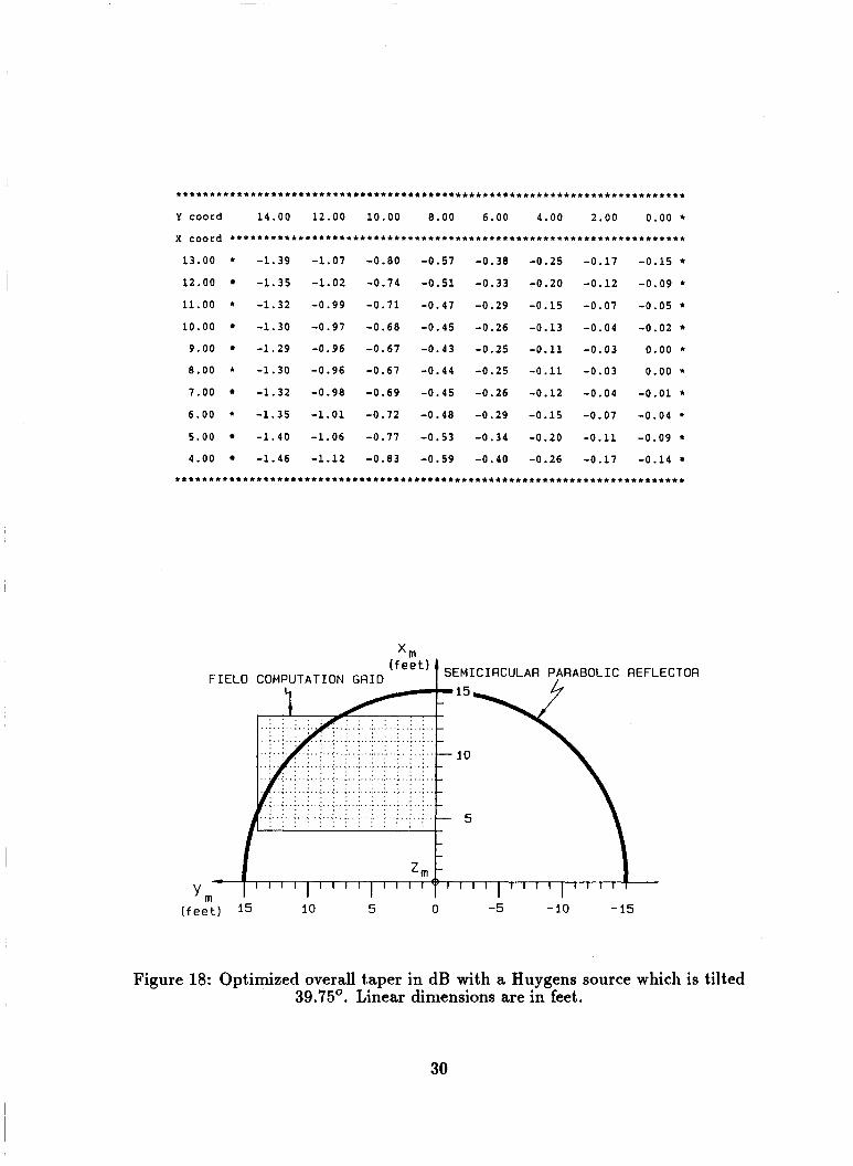
target zone it is then of interest to determine the best tilt angle of the feed. In the
present case, it has been found that a value of about 39.75' optimizes the overall
taper. The corresponding values of the reflected field are shown in Figure 18. For
this tilt angle, the overall normalized reflected field is maximum at about y = 0',
2 = 8.4'; while, on the x = 8' line, at x = 12' it is -0.96 dB, and the overall
taper error is -0.96 dB. This tilt angle is the best possible for the offset design
in order to minimize the overall taper error. For a different feed, the optimal tilt
angle will change, in that it is directly dependent on the feed pattern. It will also
depend on the frequency, since the pattern itself is frequency dependent. For this
reason a Huygens source (which is frequency independent) has been chosen as a
standard reference source. For the optimum tilt angle, the axis of the feed does not
correspond to the axis of the target zone, in order to get a better compensation
between the feed pattern and the effect of the reflected field taper error. In fact, in
the example considered, the axis of the feed corresponds to the axis of the target
zone for a tilt angle of 20', while a better compensation is obtained for a tilt angle
25

of 39.75O.
In conclusion, the performance of the SA compact range does not satisfy the
0.2 dB requirement with respect to the reflected field taper error, despite its large
focal length. On the other hand, this taper error could be reduced if the focal
length were further increased. However, this would make the chamber much larger
than desirable.
2.4 CROSS-POLARIZATION ERROR ASSOCIATED WITH THE SA REFLECTOR
The cross-polarization properties of a reflector or a combination of reflectors
are studied with respect to a focussed Huygens source. The definition of cross-
polarization is the third definition given by Ludwig [8]. As it is known, the cross-
polarization of the reflected field is zero if the a x i s of the Huygens source coincides
with the ax is of the parabolic reflector or with the central ray for a combination
of reflectors. In a real case, the feed antenna characteristics are not those of a
Huygens source, and the cross-polarization is different from zero; nevertheless, the
cross-polarization is considered as introduced by the feed alone and not by the
geometry of the reflector-feed arrangement (;.e., by the tilt angle of the feed) if the
axes are aligned as stated before.
In the offset design, the a x i s of the feed does not coincide with the a x i s of
the reflector; consequently, a component of cross-polarization is introduced by the
geometry of the reflector-feed arrangement. In the real case, the cross-polarization
of an offset design is due to both the geometry as well as the cross-polarization of
the feed antenna.
The cross-polarization levels are shown in Figure 19 for a 20' tilt angle.
As expected, on the principal plane (plane y = 0) the cross polarization is zero
26

. . . . . . . . . . . . . . . . . . . . . . . . . . . . . . . . . . . . . . . . . . . . . . . . . . . . . . . . . . . . . . . . . . . . . . . . . . .
Y coord 14.00 12.00 10.00 8.00 6.00 4.00 2.00 0.00
x coord . . . . . . . . . . . . . . . . . . . . . . . . . . . . . . . . . . . . . . . . . . . . . . . . . . . . . . . . . . . . . . . . . . .
13.00 -1.22 -1.05 -0.90 -0.78 -0.68 -0.61 -0.57 -0.55 * 12.00 -1.14 -0.96 -0.81 -0.69 -0.59 -0.52 -0.48 -0.47 * 11.00 * -1.06 -0.89 -0.74 -0.61 -0.51 -0.44 -0.40 -0.38 * 10.00 * -0.99 -0.81 -0.66 -0.54 -0.44 -0.37 -0.32 -0.31 * 9.00 * -0.93 -0.75 -0.60 -0.47 -0.37 -0.30 -0.25 -0.24
8.00 * -0.87 -0.69 -0.54 -0.41 -0.31 -0.24 -0.19 -0.18 * 7.00 * -0 .82 -0.64 -0.48 -0.36 -0.25 -0.18 -0.14 -0.12
6.00 * -0.77 -0.59 -0.44 -0.31 -0.21 -0.13 -0.09 -0.07
5-00 * -0.74 -0.55 -0.40 -0.27 -0.17 -0.09 -0.05 -0.03
4.00 * -0.70 -0.52 -0.37 -0.24 -0.13 -0.06 -0.01 0.00 * . . . . . . . . . . . . . . . . . . . . . . . . . . . . . . . . . . . . . . . . . . . . . . . . . . . . . . . . . . . . . . . . . . . . . . . . . . .
xm ( f e e t ) ' SEMICIRCULAR PARABOLIC REFLEC FIELD COMPUTATION GRID
. . . . . . .
. . . . . . . . . . . . . 5 .......................................... - . . . . . . . . . . . . . . . . . . . . . . . . . . -
( f e e t , 15 10 5 0 -5 -10 -15
TOR
Figure 15: Reflected field taper in dB. Oinnidirectional source. Linear dinlensions are in feet.
27
. . . . . . . . . . . . . . . . . . . . . . . . . . . . . . . . . . . . . . . . . . . . . . . . . . . . . . . . . . . . . . . . . . . . . . . . . . .
Y coord 1 4 . 0 0 12.00 1 0 . 0 0 8.00 6.00 4.00 2.00 0.00 * x c-ord ...................................................................
13.00 -2.43 -2.09 -1.80 -1.55 -1.36 -1.22 -1.14 -1.11 * 12.00 -2.27 -1.93 -1.63 -1.38 -1.19 -1.05 -0.96 -0.93 * 11.00 * -2.12 -1.77 -1.47 -1.22 -1.02 -0.88 -0.80 -0.77 * 10.00 -1.98 -1.63 -1.33 -1.07 -0.88 -0.73 -0.65 -0.62
9.00 * -1.85 -1.50 -1.19 -0.94 -0.74 -0.60 -0.51 -0.48 * 8 . 0 0 -1.74 -1.38 -1.07 - 0 . 8 2 -0.62 -0.47 -0.39 -0.36 * 7.00 -1.64 -1.28 -0.97 -0.71 -0.51 -0.36 -0.27 -0.25 * 6.00 * -1.55 -1.19 -0.88 -0.62 -0.41 -0.27 -0.18 -0.15 * 5.00 -1.47 -1.11 - 0 . 8 0 -0.54 -0.33 -0.19 -0.10 -0.07
4.00 -1.41 -1.05 -0.73 -0.47 -0.27 -0.12 -0.03 0.00
. . . . . . . . . . . . . . . . . . . . . . . . . . . . . . . . . . . . . . . . . . . . . . . . . . . . . . . . . . . . . . . . . . . . . . . . . . .
X m _*,.. (' ee t, 1 SEMICIRCULAR PARABOLIC REFLECTOR FIELD COMPUTATION Gniu
. . . .
: : : : : : : 10 IF . . . . . . . . . . . . I .... . . I . . I :/i j . . . . . . .
. . I . . I . . , .. . ... ..... .. . ... . ... . .,. . .. . , . . .. , , . . , . . . . . . . . . . ! . . ....... . . I , ~ ~ ; ~ ~ ~ ; ; ; ; ; ~ ~ .~ ........ . .
~
~ ............._. ............... .. . . . . . . . . . . . . . . . . . . . . . . . . . . . . 5 ,......... ~ . . . . . . . . . . . . . . . . , ,
t
( f e e t ) 15 10 5 0 -5 - 10 -15
Figure 16: Overall taper in dB. Center fed Huygens source. Linear dimensions are in feet.
28

. . . . . . . . . . . . . . . . . . . . . . . . . . . . . . . . . . . . . . . . . . . . . . . . . . . . . . . . . . . . . . . . . . . . . . . . . . .
Y coord 14.00 12.00 10.00 8.00 6.00 4.00 2.00 0.00 * x cooed . . . . . . . . . . . . . . . . . . . . . . . . . . . . . . . . . . . . . . . . . . . . . . . . . . . . . . . . . . . . . . . . . . .
13.00 * -1.86 -1.52 -1.23 -0.99 -0.80 -0.66 -0.58 -0.55 * 12.00 -1.75 -1.41 -1.12 -0.88 -0.69 -0.55 -0.46 -0.44
11.00 * -1.66 -1.32 -1.03 -0.78 -0.59 -0.45 -0.36 -0.33 * 10.00 * -1.58 -1.24 -0.94 -0.69 -0.50 -0.36 -0.27 -0.24
9.00 -1.52 -1.17 -0.87 -0.62 -0.42 -0.28 -0.20 -0.17
8.00 * -1.47 -1.12 -0.81 -0.56 -0.36 -0.22 -0.13 -0.11 * 7.00 * -1.43 -1.07 -0.77 -0.52 -0.32 -0.17 -0.09 -0.06 * 6.00 -1.40 -1.05 -0.74 -0.49 -0.28 -0.14 -0.05 -0.02 * 5.00 -1.39 -1.03 -0.72 -0.47 -0.27 -0.12 -0.03 0.00 * 4.00 * -1.39 -1.03 -0.72 -0.47 -0.26 -0.12 -0.03 0.00
. . . . . . . . . . . . . . . . . . . . . . . . . . . . . . . . . . . . . . . . . . . . . . . . . . . . . . . . . . . . . . . . . . . . . . . . . . .
Xm (' ee t ) ' SEMICIRCULAR PARABOLIC REFLECTOR FIELD COMPUTATION G R I D
15
10
. . . . . . . . . . . . . . . . . . . . . . . . . . 5 ............................................. - . . . . . . . . . . . . . . . . . . . . . . . . . .
- -
4 Zm,, I l l 1 1 1 1 1 I 1 1 1 " 1 1 1 1 I I I I I I I I I
10 5 0 -5 - 10 - 15 Y m
( f e e t ) 15
Figure 17: Overall taper in dB with a Huygens source which is tilted 20'. Linear dimensions are in feet.
29
. . . . . . . . . . . . . . . . . . . . . . . . . . . . . . . . . . . . . . . . . . . . . . . . . . . . . . . . . . . . . . . . . . . . . . . . . . . Y coord 14.00 12.00 10.00 8.00 6.00 4.00 2.00 0.00 * x coord . . . . . . . . . . . . . . . . . . . . . . . . . . . . . . . . . . . . . . . . . . . . . . . . . . . . . . . . . . . . . . . . . . .
13.00 * -1.39 -1.07 -0.80 -0.57 -0.38 -0.25 -0.17 -0.15 * 12.00 -1.35 -1.02 -0.74 -0.51 -0.33 -0.20 -0.12 -0.09 * 11-00 * -1.32 -0.99 -0.71 -0.47 -0.29 -0.15 -0.07 -0.05 * 10.00 -1.30 -0.97 -0 .68 - 0 . 4 5 -0.26 -0.13 -0.04 -0.02 * 9.00 -1.29 -0.96 -0.67 -0 .43 -0.25 -0.11 -0.03 0.00 * 8.00 * -1.30 -0.96 -0.67 -0.44 -0.25 -0.11 - 0 . 0 3 0.00 * 7.00 -1.32 -0.98 -0.69 -0.45 -0.26 -0.12 -0.04 -0.01 * 6.00 * -1.35 -1.01 -0.72 -0 .48 -0.29 -0.15 -0.07 -0.04 * 5.00 -1.40 -1.06 -0.77 -0.53 -0.34 -0.20 -0.11 -0.09 * 4 .00 - 1 . 4 6 -1.12 - 0 . 8 3 -0.59 -0.40 -0.26 -0.17 -0.14 *
. . . . . . . . . . . . . . . . . . . . . . . . . . . . . . . . . . . . . . . . . . . . . . . . . . . . . . . . . . . . . . . . . . . . . . . . . . .
1 1
(:e’t) f S E M I C I R C U L A R P /ARABOLIC REFLECTOR F I E L D COMPUTATION GRID
I 1 1 1 I l l 1 I I I I 1 1 1 1 I l l 1 1
I J I riy::::::: .............. . . . . . . . ._ ....... k . . . . . . . . . . . .
. . . . . I . . . . ..,..,.._... , ................... . . . . . . . . . . . ........................................... . . . . . . . t I 0 , . . . . . . . . .
2 . . ........................... . ~ . . . . . . . . . . . . . . . . . . . . . . . I/:..:..;..; . . . . . . . . . ............................
. . . . . . . . . . . . . . . . . . . . . .
. . . . . . . . . . . . ~ .............................. ._ ........ . . . . . . . . . . . . . ............................................ . . . . . . . . . . . . . . . . . . . . . . . . . . .................... ~ ....................... . . . . . . . . . . . . . . . . . . . . . . . . . .
y 5
I I-
Figure 18: Optimized overall taper in dB with a Huygens source which is tilted 39.75’. Linear dimensions are in feet.
30

(-100 dB represents zero); whereas, the maximum cross-polarization inside the
target zone is -21.2 dB at 2 = 4', y = 12'. As shown in Figure 20, the maximum
inside the target zone is -15.05 dB at 2 = 4', y = 12' for a 39.75' tilt angle of
the feed. By comparing the results from these two tilt angles, it is clear that,
the greater the tilt angle of the feed, the worse the cross polarization becomes.
Therefore, even if some tilt angle (39.75' in this case) minimizes the overall taper
error, it might not necessarily be the best choice because the corresponding cross-
polarization characteristics are not satisfactory.
The performance of the SA compact range with respect to the cross-polarization
for both of these angles is poor. It seems necessary then to accept a tilt angle close
to 20' in order to find a compromise between the taper and the cross-polarization
errors.
2.5 APERTURE BLOCKAGE ERROR OF THE SA REFLECTOR
The aperture blockage error associated with the SA reflector has been studied
in terms of the blockage of the feed [7], which is basically a diffraction problem.
The feed itself is simulated as a vertical plate centered at the focal point and
illuminated by the plane wave coming from the parabolic reflector (Figure 21).
The resulting scattered field is then computed at the end of the target zone because
it will be stronger there as can be seen from Figure 21. It is clear from the figure
that the points at the end of the target zone are characterized by a smaller 4 angle (for points with the same 2 height); consequently, the diffraction coefficient
evaluated for P , is larger thap that of Pb, which implies a stronger diffraction.
Also, in this case the magnitude of the diffraction coefficient is more significant
than the magnitude of the spreading factor (the points at the end have a larger
spreading factor than those at the beginning). The distance of the end of the
31

. . . . . . . . . . . . . . . . . . . . . . . . . . . . . . . . . . . . . . . . . . . . . . . . . . . . . . . . . . . . . . . . . . . . . . . . . . .
Y coocd 14.00 12.00 10.00 8.00 6.00 4.00 2.00 0.00 * x coord . . . . . . . . . . . . . . . . . . . . . . . . . . . . . . . . . . . . . . . . . . . . . . . . . . . . . . . . . . . . . . . . . . . . .
13.00 -20.14 -21.48 -23.07 -25.01 -27.52 -31.04 -37.06 -100.00
12.00 * -20.11 -21.45 -23.04 -24.98 -27.49 -31.01 -37.03 -100.00
11.00 -20.08 -21.42 -23.01 -24.95 -27.46 -30.98 -37.00 -100.00 * 10.00 * -20.05 -21.39 -22.98 -24.92 -27.42 -30.95 -36.97 -100.00 * 9.00 * -20.02 -21.36 -22.95 -24.89 -27.39 -30.92 -36.94 -100.00
8.00 -19.99 -21.33 -22.92 -24.86 -27.36 -30.89 -36.91 -100.00
7.00 -19.95 -21.30 -22.89 -24.83 -27.33 -30.86 -36.88 -100.00
6.00 -19.92 -21.27 -22.86 -24.80 -27.30 -30.82 -36.85 -100.00
5.00 -19.89 -21.24 -22.82 -24.77 -27.27 -30.79 -36.81 -100.00
4.00 -19.86 -21.20 -22.79 -24.74 -27.24 -30.76 -36.78 -100.00 * . . . . . . . . . . . . . . . . . . . . . . . . . . . . . . . . . . . . . . . . . . . . . . . . . . . . . . . . . . . . . . . . . . . . . . . . . . .
...
(' eet ) ' SEMICIRCULAR PARABOLIC REFLEC FIELD COMPUTATION GRID
.. ~ .................. ~ ._ ........ - . . . . . . . . . . . . . . . . . . . . . . . . . . - -
- Y".
111 10 5 0 -5 -10 -15 ( f e e t ) 15
TOR
Figure 19: Cross-polarized field in dB with a Huygens source which is tilted 20'. Linear dimensions are in feet.
32

. . . . . . . . . . . . . . . . . . . . . . . . . . . . . . . . . . . . . . . . . . . . . . . . . . . . . . . . . . . . . . . . . . . . . . . . . . .
Y coord 14.00 12.00 10.00 8.00 6.00 4.00 2.00 0.00 * x coord . . . . . . . . . . . . . . . . . . . . . . . . . . . . . . . . . . . . . . . . . . . . . . . . . . . . . . . . . . . . . . . . . . .
13.00 -14.25 -15.61 -17.21 -19.17 -21.68 -25.21 -31.23 -100.00 * 12.00 * -14.19 -15.55 -17.15 -19.11 -21.62 -25.15 -31.17 -100.00
11.00 * -14.13 -15.49 -17.09 -19.04 -21.56 -25.09 -31.11 -100.00
10.00 * -14.07 -15.43 -17.03 -18.98 -21.49 -25.02 -31.05 -100.00 * 9.00 * -14.00 -15.37 -16.97 -18.92 -21.43 -24.96 -30.99 -100.00 * 8.00 * -13.94 -15.30 -16.91 -18.86 -21.37 -24.90 -30.93 -100.00
7.00 * -13.88 -15.24 -16.84 -18.80 -21.31 -24.84 -30.87 -100.00 * 6 . 0 0 * -13.81 -15.18 -16.78 -18.74 -21.25 -24.78 -30.80 -100.00 * 5.00 * -13.75 -15.11 -16.72 -18.67 -21.18 -24.71 -30.74 -100.00 * 4.00 * -13.69 -15.05 -16.65 -18.61 -21.12 -24.65 -30.68 -100.00 *
. . . . . . . . . . . . . . . . . . . . . . . . . . . . . . . . . . . . . . . . . . . . . . . . . . . . . . . . . . . . . . . . . . . . . . . . . . .
xm (‘ e e t ) ’ SEMICIRCULAR PARABOLIC REFLECTOR FIELD COMPUTATION GGID
. . . . . . . . . . . . . . . . . . . . . . . . . .
. . . . . . . . . . . . . . . . . . . . . . . . . . 5 .................... ~ . . . . . . . . . . ~ ........... - - -
- - I I I I I I I 1 1 1 ’ ~ I I I I 1 1 1 1 I I I I I
10 5 0 -5 - 10 -15 y m
( f e e t ) 15
Figure 20: Cross-polarized field in dB with a Huygens Source which is tilted 39.75O. Linear dimensions are in feet.
33

target zone from the reflector vertex is 50'; while, the distance of the beginning is
36'. The source considered is the omnidirectional source.
The aperture blockage scattered field illuminates the target in directions dif-
ferent than the plane wave so the superposition of these terms results in ripple
associated with the total field in the target zone. This error term has both co- and
cross-polarized components. Since this is a diffraction effect, it is frequency de-
pendent. The aperture blockage error at 500 MHs is shown in Figure 22 together
with the GO reflected field (solid line), where the aperture dimensions 15" x 15"
(long dash plot), 12.5" x 12.5" (short dash plot) and 10" x 10" (dotted plot) are
considered. The aperture blockage scattered field levels are obtained by subtract-
ing the plotted values of the aperture blockage error from the corresponding value
of the GO plot. They are the following:
0 for the 20" x 20" aperture, the scattered field is about 25.5 dB below the
level of the GO reflected field at E = 4', and about 29 dB below at x = 13'
0 for the 15" x 15" aperture, the scattered field is about 30.5 dB below the
level of the reflected field at z = 4', and about 33.5 dB below at 2 = 13' and
0 for the 10" x 10" aperture, the field is about 37 dB below the level of the
reflected field at E = 4', and about 40.5 dB below at x = 13'.
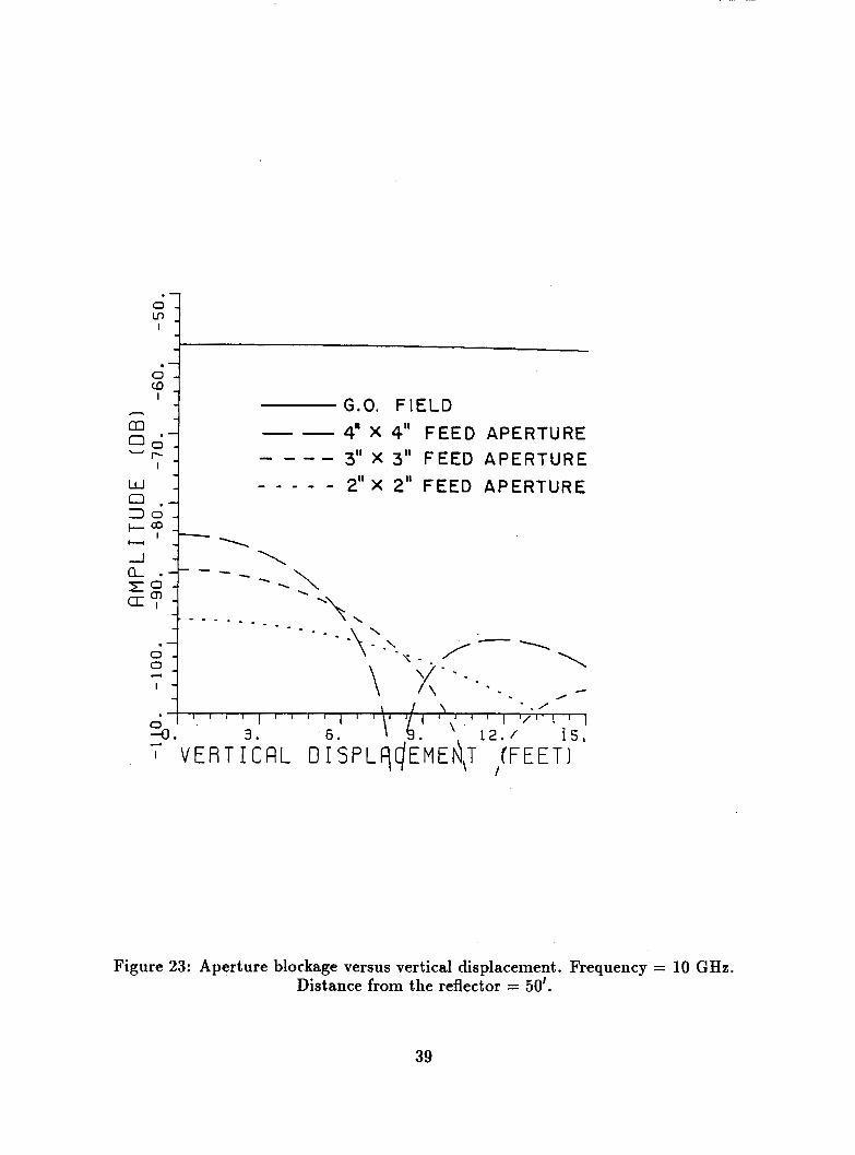
The plot for 10 GHz is shown in Figure 23 where the aperture dimensions
4" x 4", 3" x 3" and 2" x 2" are considered. The scattered field levels are:
0 for the 4" x 4" aperture, the field is about 30.5 dB below the level of the
reflected field at 5 = 4', and about 42.5 dB below at x = 13',
0 for the 3'' x 3" aperture, the field is about 34.5 dB below the level of the
reflected field at E = 4', and about 56.5 dB below at z = 13',
34
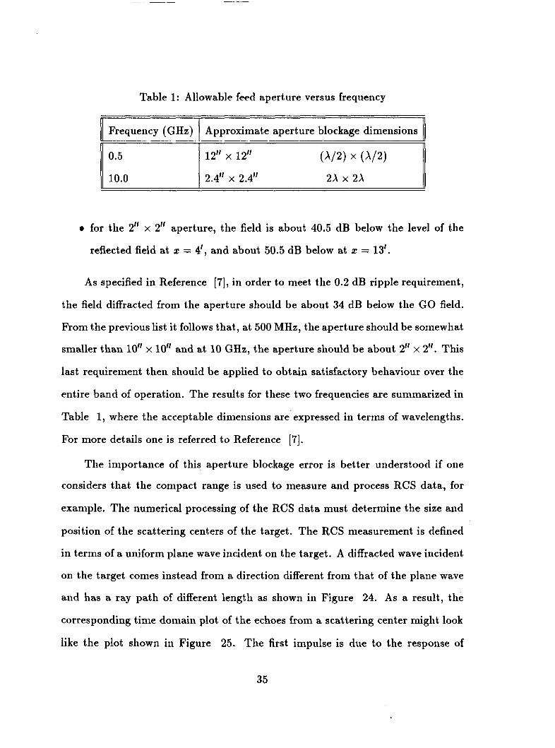
Table 1: Allowable feed aperture versus frequency
Frequency (GHz)
0.5
10.0
Approximate aperture blockage dimensions
12" x 12"
2.4" x 2.4"
(W) x ( V 2 )
2x x 2x
0 for the 2'' x 2" aperture, the field is about 40.5 dB below the level of the
reflected field at z = 4', and about 50.5 dB below at E = 13'.
As specified in Reference [7], in order to meet the 0.2 dB ripple requirement,
the field diffracted from the aperture should be about 34 dB below the GO field.
From the previous list it follows that, at 500 MHe, the aperture should be somewhat
smaller than 10" x 10" and at 10 GHe, the aperture should be about 2" x 2". This
last requirement then should be applied to obtain satisfactory behaviour over the
entire band of operation. The results for these two frequencies are summarized in
Table 1, where the acceptable dimensions are expressed in terms of wavelengths.
For more details one is referred to Reference [7].
The importance of this aperture blockage error is better understood if one
considers that the compact range is used to measure and process RCS data, for
example. The numerical processing of the RCS data must determine the size and
position of the scattering centers of the target. The RCS measurement is defined
in terms of a uniform plane wave incident on the target. A diffracted wave incident
on the target comes instead from a direction different from that of the plane wave
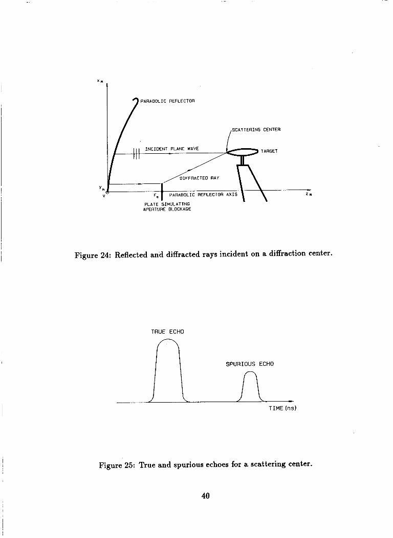
and has a ray path of different length as shown in Figure 24. As a result, the
corresponding time domain plot of the echoes from a scattering center might look
like the plot shown in Figure 25. The first impulse is due to the response of
35

the scattering center to the incident plane wave, and represents the true response.
The second echo instead is an error and is due to the response of the scattering
center to the diffracted ray. This error response is delayed in time because its
ray path is longer. The data processing algorithms then determine two scattering
centers instead of one. It is clear then how important it is to reduce the amount
of diffraction to a minimum. Consequently it would be very useful to completely
eliminate the aperture blockage, if possible.
It is worth noticing that, while a diffraction error introduces spurious scat-
tering centers, a taper instead introduces errors in the relative sizes of the various
scattering centers. While this is an error to be avoided; nevertheless, its conse-
quences are less serious than those associated with the diffraction errors in that a
diffraction error introduces false echoes which can be associated with the target.
As a consequence, one might attempt to modify the target to remove this echo,
which instead cannot be eliminated, since it is not associated with the target.
36

END OF PARABOLIC REFLECTOR BEGINNING 9 TARGET ZONE TARGET ZONE
I /
INCIDENT SHADOW BOUNDARY A
V FnlI PARABOLIC REFLECTOR AXIS zm
PLATE SIMULATING APERTURE BLOCKAGE
Figure 21: Incident shadow boundary for aperture blockage.
37

'pj G.O. FIELD - -20" X 20" FEED APERTURE - - - - 15" 15" FEED APERTURE * - - - - I O " X IO" FEED APERTURE
-- 3 0 --- - -- -- - - - - - - - - - - - - - - - - - .
- - - - - - - - - - - - - - - - - - E l ::f = g - - - - - - . - - . - _
I
0 ' -0. 3 . 6. 9. 12. 1 5 .
1 1 1 1 1 / 1 1 I I I I I I I I I 1 1 1 1
7 VERT ICRL D I SPLRCEMENT ( F E E T I
Figure 22: Aperture blockage versus vertical displacement. Frequency = 500 MHz. Distance from the reflector = 50'.
38
I
Figure 23: Aperture blockage versus vertical displacement. Frequency = 10 GHz. Distance froin the reflector = 50'.
39
PARABOLIC REFLECTOR
/ SCATTERING CENTER
I / I I I - . ----
/ PI' IAnbt' 1 = F, l/FFRACTEO RAY \ \, z. Y m
V PARABOLIC REFLECTOR AXIS
PLATE SIMULATING APERTURE BLOCKAGE
Figure 24: Reflected and diffracted rays incident on a diffraction center.
TRUE ECHO
I\ SPURIOUS ECHO
TIME (ns)
Figure 25: True and spurious echoes for a scattering center.
40

CHAPTER I11
DESIGN CONSIDERATIONS
3.1 INTRODUCTION
In this chapter the physical and geometrical foundations of the design of a
compact range subreflector system are presented in a simple way. For clarity and
convenience, the single reflector case is discussed first because the subreflector
system can be reduced to the single parabolic reflector case through the equivalent
reflector principle developed by Dragone [6].
A description of the geometry of the subreflector system and of the associated
reference systems is presented in Section 3.2. The principle of the central ray
is illustrated in Section 3.3. The problems of the taper of the reflected field
and of the cross-polarization error, mentioned in Chapter I, are treated from a
quantitative viewpoint in Sections 3.4 and 3.5. A discussion of cross-polarization
with respect to the characteristics of the feed antenna, as well as the properties
of the Huygens source is presented in Section 3.6. The factors affecting the GO
design of a compact range are examined in Section 3.7. Finally, the ambiguities
often present in the definition of the target zone are shown in Section 3.8.
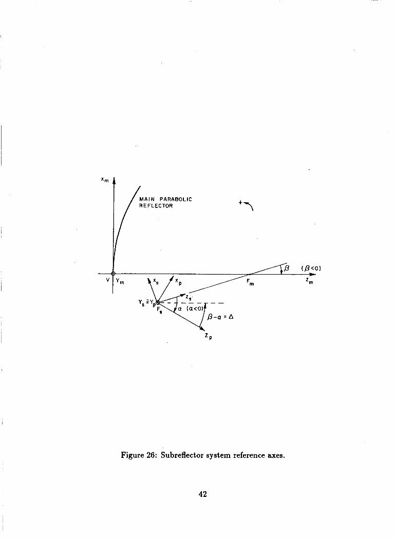
3.2 GEOMETRY OF THE SUBREFLECTOR SYSTEM
The subreflector system involves many parameters, which are shown in Figures
26 and 27, where all angles are positive if counterclockwise (ccw). As a result,
41
'1
Figure 26: Subreflector system reference axes.
42
MAIN PARABOLIC REFLECTOR
- URFACE TARGET
\ - . \, 2, AXIS _--___--. OF THE TARGET ZONE
\,-PRIMARY ILLUMINATING BEAM - -- \+ - - - - - - - -
SURFACE
SECONDARY ILLUMINATING
Figure 27: Subreflector system geometry.
43
Figure 28: Geometry of the target zone.
44

several reference systems are used (see Figure 26):
1) The parabolic reflector reference system (also called main for short) V(zm,
ym, zm) has its origin at the vertex, V, of the paraboloidal reflector. The
zm a x i s is coincident with the reflector axis, the zm ax is is vertical, and the
ym ax is is horizontal. The polar reference system, Fm(rm, e,, d m ) has its
origin at the focus, Fm, of the paraboloidal reflector, and the corresponding
Cartesian axes are parallel to the V ( z m , ym, zm) reference system. The polar
quantities are defined in the usual fashion. The focus, F', of the parabolic
reflector coincides with one of the two focii of the subreflector.
2) The subreflector reference system F,(z,, y,, z , ) has its origin at the focus,
F,, of the subreflector which is the location of the feed antenna, while the
second focus coincides with the focus, F', of the parabolic reflector. The z ,
ax is is coincident with the subreflector a x i s , the ys a x i s is horizontal, the 2 6
axis lies in the plane perpendicular to ym, and /3 is the tilt angle from z3 to
zm. The corresponding polar reference system is F, (P,, e,, #$).
3) The source reference system F, ( z p , yp, zp ) refers to a source having a
circularly symmetric pattern, for instance, a Huygens source (Section E).
It has the origin at the focus, F,, of the subreflector, where the zp a x i s
is coincident with the principal ray (direction of maximum of the pattern
of the source), the yp ax is is horizontal and the z p ax is lies in the plane
perpendicular to ym, also a is the tilt angle from z8 to zp , and A = /3 - a! is
the tilt angle from zp to zm.
Both the parabolic reflector and the subreflector are parts of a conical surface
of revolution (also called conic of revolution, i.e., paraboloid, hyperboloid, ellipsoid
of revolution).
45

The parabolic reflector is a part of a paraboloid with its vertex at V, and f
is its focal length. The subreflector is a part of an ellipsoid (Gregorian system) or
hyperboloid (Cassegrain system). A conic of revolution has two focii (note that
for the parabolic reflector, a paraboloid, the second focus is at infinity and Fm is
the unique focus). The distance between the two focii of the subreflector is d a , and
fa denotes the distance between a vertex of the subreflector and the closest focus.
The subreflector is also characterized by the parameters €8 and pa.
The geometry shown in Figure 27 is considered next. The angle p is the tilt
angle from the subreflector ax is to the paraboloid a x i s (i.e., between the oriented
axes zu and zm, from zu to zm). The feed is located at the second focus of the
subreflector, F,, and CY is the tilt angle of the subreflector ax is relative to the zp
ax is (feed axis, also called secondary principal ray). The feed boresight direction
is then tilted by the angle A = p - a, which is the angle between the principal ray
and the parabolic reflector axis, i.e., from zp to zm.
In Figure 27, it is shown that the phase center of the feed is located at the
focus Fa of the subreflector, which has coordinates Fa 3 ( -hpc, 0, zP) in the
parabolic reflector reference system, where hpc is the vertical (in the zm direction)
distance from the phase center of the feed to the ceiling of the lower chamber;
while, ZP is the horiEontal (in the zm direction) distance of the phase center of the
feed from the focus Fm of the parabolic reflector.
The target zone (also called quiet zone or sweet spot) is the zone where the
targets are located and where a uniform plane wave is required. Geometrically, a
target zone is defined as a finite volume delimited by a cylinder having generatrices
parallel to the parabolic reflector a x i s and by two planes, both perpendicular to the
parabolic reflector axis ( zm axis). The surface intersection of a plane perpendicular
to the parabolic reflector ax is with the target zone (Figure 28) is characterized by
46
its distance tl from the paraboloid vertex V, while all such sections are identical.
In the present case these sections have a rectangular shape: the sides of the target
zone are straight lines parallel to the coordinate axes, (z,, y,, 2,). A further
discussion of the shape of the target zone is presented in Section 3.8. The distance
of the center point of the target zone from the reflector vertex, V, in the t, ax is
direction is ti,, and ht, is the vertical height (;.e., in the zm direction) of its
center point from the parabolic reflector axis; while, the distance of the beginning
of the target zone from V is denoted by ztb.
The target zone is projected onto the parabolic reflector by lines parallel to the
z , axis. The part of the paraboloidal surface so determined is called the primary
illuminating surface. The axis of the target zone parallel to the tm axis intersects
the primary illuminating surface at the point It,, as shown in Figure 27. This
axis is called the z, axis of the target zone. The primary illuminating surface is
projected by a beam from the subreflector converging onto the focal point, F,, and
finally intersecting the parabolic reflector. This ideal beam is called the primary
illuminating beam. This beam illuminates the target zone after reflection from the
parabolic reflector. The ray through Fm and It , is called the primary illuminating
ray and intersects the subreflector at the point, Pi,. This ray is oriented from Fm
to It,. The angle between the tln axis and the primary illuminating ray is called
xi. If hi, is the x m coordinate of the point, Itrn, the following relationship holds
ht, = 2 f cot ($) . The intersection of the primary illuminating beam with the subreflector defines a
surface called the secondary illuminating surface. The ray through the points, Fs
and Pts, is called the secondary illuminating ray, and is oriented from Fs to Pis.
47

Then the illuminating ray is defined as the ray through Fa, Itd, Fm, Itm and from
Itm into the target zone, where (by definition) it coincides with the zm axis of the
target zone. The illunlinating ray is related primarily to tlie position of the target
zone with respect to the parabolic reflector.
3.3 THE CENTRAL RAY
The principles of the equivalent reflector and of the central ray are very impor-
tant in tlie present GO design. For completeness of presentations, the arguments
introduced by Dragone [6] are now summarized.
It is known [lo] that, in the case of a single conical (elliptical, paraboli-
cal, or hyperbolical) reflector, zero cross-polarization is achieved if the following
conditions are satisfied:
0 A focussed Huygens source feed is used.
0 The axis of tlie feed (called tlie principal ray) coincides with the axis of the
conical reflector (center fed case), in other words, the feed is pointing towards
tlie vertex of the conical reflector.
0 The ratio of the intensities of the electric and magnetic currents in the Huy-
gens source is equal to the eccentricity of the conical reflector (Section E).
For the case of a paraboloidal reflector, the eccentricity is one, and the two
currents are equal.
This zero cross-polarization property refers to the GO field only, not to higher
order effects, like edge diffraction.
The issue presently addressed is to determine how this zero cross-polarization
property can be achieved for the case of a sequence of confocal reflectors. In Figure
48

29 a sequence of N confocal conical reflectors is shown, the reflectors are called X i ,
C2, ... EN. They are called confocal because the second focus of E1 and the first
focus of C2 coincide at the point, F1, the second focus of C2 and the first focus of
C3 coincide at the point, F2, and so forth. The source is located at the first focus
Fo of C1; while, the second focus of C N is located at FN and does not coincide
with any other focus. As shown in [6] , it is possible to establish an equivalence
principle for such a sequence of confocal subreflectors. In fact, it is possible to
show that any sequence of confocal conical reflectors is equivalent, for the purpose
of GO computations, to one focussed conical reflector. The theorem proved is just
an existence theorem, in other words, it is proved that such an equivalent reflector
exists, but it is not shown how to compute its parameters. Nevertheless, this
existence theorem is the first step to actually determine the equivalent reflector. It
is also possible to show that, if the last reflector, EN, is parabolic, the equivalent
reflector is parabolic.
In order to determine the equivalent reflector, it is necessary to determine
its equivalent axis. This is important because it is possible to obtain zero cross-
polarization by satisfying the three conditions listed above, if the principal ray
coincides with the equivalent axis. The equivalent a x i s is a concept related to the
feed, and it coincides with the first segment of the central ray.
The argument to determine the equivalent axis is done in two steps. In the
first step a single reflector case is considered, and then the result is extended to a
sequence of confocal reflectors.
A single reflector case is considered. If the conical reflector together with only
one of the focii are given, while the second focus is unknown, it is still possible
to deternine the equivalent axis ( a x i s of symmetry of the conic) with a trial-and-
error procedure. This is shown as follows (see Figure 30). A test direction, i, is
49

considered, and the corresponding ray through the focus Fo is reflected twice by
the reflector, obtaining the direction 6'' after the second reflection. In the general
case i # 6'' (as in case (a) of Figure 30), unless i coincides with the direction of
the geometric ax is of the conic (which is supposed to be unknown). Then i = i'',
and S determines the direction of the equivalent axis, which is a line through the
focus, Fo, and in the i direction (cases (b) and (c) of Figure 30). Therefore, the
equivalent axis can be determined, at least in principle, through a trial-and-error
procedure for a single reflector case. The ray corresponding to the direction of
the equivalent axis retraces itself after the first two reflections, and it is the only
ray which has this property. The central path is defined as the path back and
forth from any of the two focii and corresponding to the equivalent axis . The
central path corresponds to either of the two central rays. The central rays have a
direction of travel associated with them, which are opposite. In other words, any
of the two central rays corresponds to the central path with associated a direction
of travel.
I
I
This result can be extended to a combination of N confocal reflectors. In this
case 2N reflections must be considered, 2 from each reflector. By the equivalent
reflector principle, the combination of the N reflectors is equivalent, for all the GO
purposes, to just one reflector, for which the previous argument can be applied. It
follows that the equivalent a x i s exists and can be determined through the retracing
property of the central path. The central path is unique (except for a few degen-
erate cases which are presently of no concern), and therefore there are only two
central rays, corresponding to the two possible opposite orientations of the central
path. As an example, Figure 31 shows a sequence of N confocal reflectors, with
N = 3. Part (a) of the figure shows a ray (not coincident with the central ray).
This ray starts at the focus, Fo, with direction i, is reflected by El, goes through
50
I
I

F1, which is the second focus of C1 and the first focus of C2, is then reflected by
C2 and goes through F2, which coincides with the second focus of C2 and the first
focus of C3, is then reflected by C3, goes through F3, is reflected for the second
time by C3, goes through the focus F2, and all the way back, being reflected for
the second time by each conical reflector in reverse order. After the last reflection
from C1, the direction of the ray is i", which is different from i,and it does not
retrace itself. In Figure 31 (b) instead is shown the case in which i is directed as
the equivalent axis, the ending direction, if', coincides with the starting direction,
i, and the ray can retraces itself indefinitely. Therefore, the ray traced is the cen-
tral ray. Again, at least in principle, the central ray can be determined through a
trial- and-error procedure.
This trial-and-error procedure is very important from a theoretical viewpoint,
but in practice it is not very satisfactory. Nevertheless, it is not difficult to find
geometrical or analytical criteria to determine the equivalent axis for many cases
of interest.
In the case of a Gregorian subreflector system, there are two conic reflectors
(N = 2) i.e., a parabola and an ellipse. It is now shown how the equivalent axis
and the central ray can be determined through a simple geometrical construction,
once the geometry (Le., the two reflectors and their mutual positions) is given.
In the case of a parabolic reflector, it can be shown that the direction, i", of
the ray after the second reflection, at the point at infinity of the parabolic reflector,
is independent from the direction, i. The direction 2" is parallel to the axis of the
parabola, and the corresponding ray goes through the focus F N - ~ of the parabola.
The proof of this can be seen through Figure 32 and a limiting argument, where
the parabola is obtained by moving the second focus, FN, of an ellipse to infinity.
The angle, $, then goes to 0 accordingly, for any direction of i. Then the reflected
51

ray is directed as the ax is of the limiting parabola, and must go through the focus,
F N - ~ , and therefore it must coincide with the ax is itself and is directed from the
focus at infinity, FN, towards FN-~.
By using this property, it is easy to determine the equivalent axis of the
Gregorian subreflector system by considering Figure 33. The central ray starts
at F3 (the focus of the subreflector where the feed is located) with direction 6, is
reflected by the subreflector at I d , goes through the focus, Fm, which is common to
both the main reflector and the subreflector, is reflected by the parabolic reflector
at Im, goes through the focus at infinity of the parabola Fm oo (as limiting case of
an ellipse with the second focus at infinity), is then reflected at the point at infinity
of the parabola, I d W , is reflected for the second time by the subreflector at I:, as
in Figure 33, and the path is closed back at F3. Since the axis of the parabola is
known, the point I: is known, and the central ray is known. The equivalent a x i s
corresponds to the segment F3 I:. The equivalent axis can also be found through
an equation relating the angles a, and ,8, [6], as follows
tan (;) = m tan (e) where the axial magnification factor m is given by
cs is the eccentricity of the subreflector, and the angles a, and ,8, are defined in
Figure 33.
It has been mentioned that, if the last reflector is parabolic, the equivalent
reflector is parabolic. The equivalent ax is has been found, then this equivalent
reflector is determined if the corresponding focal distance, called the equivalent
focal distance, fe, is determined. It can be shown [12], [13] that, for the Gregorian
52

= 31
Figure 29: Sequence of N confocal reflectors with N = 3.
subreflector system, the following equation holds:
where f is the focal length of the parabolic reflector and M is the magnification
factor, given by 2 1 - E ,
1 + €i - 2€* cos& *
' M = - (3.5)
At this point all the quantities of interest (i.e., the direction of the equivalent axis,
the central ray and the equivalent focal length) can be determined in terms of the
geometry of the Gregorian subreflector system.
3.4 TAPER OF THE REFLECTED FIELD
A parabolic reflector illuminated by a focussed omnidirectional source is con-
sidered here in order to simply evaluate the geometry effects associated with the
geometric taper errors. The polar reference system F'(T', e,, q5m) introduced
53
Figure 30: Determination of the equivalent axis for a single reflector. The reflector and the focus, Fo, are known, while, the focus, Fj, is unknown.
in Section 3.2 is considered. An intersection of the target zone with a plane per-
pendicular to the parabolic reflector axis (as defined in Section 3.2) is considered.
This section is rectangular in the present case, but its actual shape is unimportant
in the following considerations.
The field reflected from the parabolic reflector is a nonuniform plane wave
(see Section G), and in a plane perpendicular to the parabolic reflector axis, its
amplitude varies as
where R is the field point, and (r,, e,, 4,) are the polar coordinates of the
reflection point, I,, image of R in the Fm(rm, e,, 4m) reference system (see
Figure 34). The amplitude of the reflected field is maximum for 0, = 180' and
decreases as 8, decreases toward Oo or increases toward 360'. Since a uniform
54

( a 1 - I -EQUIVALENT AXIS
(N = 3)
Figure 31: Ray paths for a generic ray (a) and for the central ray (b) for N confocal reflectors with N = 3.
55
Figure 32: Limit argument to show that the direction, &'I, is independent from the direction, i, for a parabolic reflector.
56

SUBREFLECTOR AXIS REFLECTOR
----
PARABOLIC REFLECTOR AXIS
ELLIPTICAL SUBREFLECTOR
SUBREFLECTOR EXTENSION EQUIVALENT AXIS
I Fm 1, m
Figure 33: Determination of the equivalent axis and central rays for a Gregorian subreflector system through a geometrical construction.
57
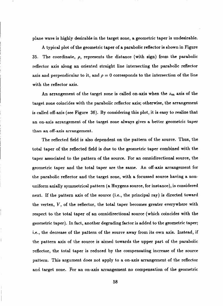
plane wave is highly desirable in the target zone, a geometric taper is undesirable.
A typical plot of the geometric taper of a parabolic reflector is shown in Figure
35. The coordinate, p, represents the distance (with sign) from the parabolic
reflector axis along an oriented straight line intersecting the parabolic reflector
axis and perpendicular to it, and p = 0 corresponds to the intersection of the line
with the reflector axis.
An arrangement of the target zone is called on-axis when the zm axis of the
target zone coincides with the parabolic reflector axis; otherwise, the arrangement
is called off-axis (see Figure 36). By considering this plot, it is easy to realize that
an on-axis arrangement of the target zone always gives a better geometric taper
than an off-axis arrangement.
The reflected field is also dependent on the pattern of the source. Thus, the
total taper of the reflected field is due to the geometric taper combined with the
taper associated to the pattern of the source. For an omnidirectional source, the
geometric taper and the total taper are the same. An off-axis arrangement for
the parabolic reflector and the target zone, with a focussed source having a non-
uniform axially symmetrical pattern (a Huygens source, for instance), is considered
next. If the pattern axis of the source (i.e., the principal ray) is directed toward
the vertex, V, of the reflector, the total taper becomes greater everywhere with
respect to the total taper of an omnidirectional source (which coincides with the
geometric taper). In fact, another degrading factor is added to the geometric taper;
i.e., the decrease of the pattern of the source away from its own axis. Instead, if
the pattern axis of the source is aimed towards the upper part of the parabolic
reflector, the total taper is reduced by the compensating increase of the source
pattern. This argument does not apply to a on-axis arrangement of the reflector
and target zone. For an on-axis arrangement no compensation of the geometric
58

taper can be made by tilting the principal ray, because what is gained on one side,
is lost on the other side.
For a subreflector system and for a single reflector offset configuration, the
geometric taper can be compensated by a tilt of the feed axis (principal ray) with
respect to the subreflector a x i s .
As shown by Dragone [6], the subreflector system is equivalent to a single
parabolic reflector having the central ray as an axis. Consequently, the best ge-
ometric taper of the reflected field is obtained for an on-axis arrangement of the
target zone with respect to the equivalent reflector; i.e., when the zm axis of the
target zone and the central ray coincide. Zero cross-polarization is obtained if the
principal ray of the feed coincides with the central ray (Section 3.6). Therefore,
the following condition
X p = X i = Xc (3.7)
which expresses that the a x i s of the target zone, the equivalent a x i s and the prin-
cipal ray all coincide, guarantees at the same time zero cross-polarization and the
minimum for the geometric taper for a subreflector system and a target zone.
How the tilt of the pattern axis (the principal ray) affects the cross polarization
is examined in Section 3.6, for the single reflector and for the subreflector system
in the case of a Huygens source feed.
3.5 REDUCTION OF THE GEOMETRIC TAPER BY AN INCREASE OF THE FOCAL DISTANCE
It was shown in Section 3.4 how the position of the zm axis of the target
zone with respect to the parabolic reflector axis affects the geometric taper of
the reflected field, and how it can be minimized if the axis coincides with the
central ray. Another factor affecting the geometric taper is the focal distance of
59
I
I
Figure 34: Polar coordinate system for the parabolic reflector.
60

DISPLACEMENT (FEET)
5
c3 w a - w o
I - 1
-2
-3
-4
cn 4
L
i
4 -
3 -
2 -
I -
- - - -
Figure 35: Typical geometric taper of the reflected field.
61

I
O F F - A X I S TARGET ZONE I t I
I - O N - A X I S TARGET ZONE-
I
I I
I - ~ ~ F F - A X I S TARGET ZONE+ -5
15
5
0
-5
-1 0
-1 5
Figure 36: On-axis and off-axis arrangements of the target zone.
62

the parabolic reflector for a single reflector system, or the equivalent focal distance
for a subreflector system. The following considerations make reference to a single
parabolic reflector, but they are immediately extended to a subreflector system via
the concept of the equivalent reflector.
For a single parabolic reflector, a way to reduce the geometric taper is sug-
gested by Equation (3.6), such that (see Figure 37)
lUrl oc sin 2 (-) 6, . 2
The reference systems considered are the polar coordinate systems F m i ( ~ m i , emi,
already defined, with i = 1,2. The maximum value of the geometric taper is
related to 6zax, polar coordinate of the upper point of the primary illuminating
surface. If 6:" is increased towards 180', the geometric taper decreases. Note
that 6):amaz increases toward 180' with increasing focal length; therefore, the taper
of the reflected field decreases with increasing focal length. In Figure 37, fi < f2, 6:;' < 6,, max , and reflector 2 has a smaller geometric taper than reflector 1. In
the limiting case where the focal length becomes infinite, the parabolic reflector
becomes a flat plate, a plane wave is incident on the reflector and a plane wave
is reflected; thus, the geometric taper is zero, and the total taper is zero if the
incident plane wave is uniform.
An increase of f seems an attractive way to reduce the geometric taper, but
there is a drawback for a single reflector system. The distance zim of the center of
the target zone in the zm direction from the vertex of the reflector must increase
with increasing focal distance, as a rule of thumb: qm E 2f. This relationship
must be satisfied in order to decouple the target from the feed and to allow the
use of time-gating techniques. Due to diffraction from the reflector, ztnr must be
kept to a minimum; in fact, with increasing qm, the near-field behaviour of the
63

total field disappears and approaches the far-field pattern. This results in larger
ripple levels in the target zone due to the increased effect of diffraction. This is
shown in Figure 7, where the total field for a “typical” compact range is shown
at three different values of the distance qm, i.e., at 12‘, 24’ and 36‘ feet away from
the reflector vertex. It is easy to see how the ripple due to diffraction progressively
increases. Consequently, in the design of a single reflector compact range, there
must be a trade-off between ztm and f .
The same considerations hold for the subreflector system. Again, rtm must
satisfy ztm N 2f in order to decouple the target from the coupling aperture, and
ztm must be kept small to avoid deterioration of the wavefront from the parabolic
reflector. But, for a subreflector system, the focal distance f is substituted by
the equivalent focal length fe (as explained in Section 3.7.2), therefore, in the
subreflector system case, the principle of the equivalent reflector shows that it
is possible to have a system with a large equivalent focal length without having
large focal length and target distance. It is possible then to reduce the geometric
taper without introducing in the total field a large ripple due to diffraction (see
Section 3.7.2).
3.8 REFLECTED FIELD CROSS-POLARIZATION
The definition of cross-polarization depends on the application considered
(81. A plane wave is desired in the target zone for compact range applications;
consequently, the cross-polarization ratio (cross-polarization for short) is defined
as
. where U_L and UII are, respectively, the field components perpendicular and par-
allel to the desired polarization direction, which is perpendicular to the parabolic
64

PARABOLIC REFLECTOR 2
PARABOLIC REFLECTOR I
TARGET jONLI Z m > 8::
Figure 37: Effect of the focal distance on O r z .
reflector axis.
It is very desirable to have a plane wave with zero (or at least very small) cross-
polarization in the target zone. In fact, some of the applications of a compact range
require excellent polarization purity, such as:
0 RCS measurements and target identification, where the received signal is
highly influenced by the interaction of the polarization direction of the inci-
dent wave with the target geometry [3].
0 Measurements of radiation patterns of communication antennas with polar-
ization diversity.
In order to control the cross-polarization of the wavefront in the target zone,
one must understand the different factors that affect it:
1) Aperture blockage.
65
2) Diffraction from edges.
3) Choice of the tilt angles of subreflector and feed.
4) Cross-polarization characteristics of the feed.
5) Mechanical misalignments.
The GO design is concerned with factor number 3). Factor 4) also can be
considered with a numerical procedure where the real feed is modeled by data
interpolation. The first two factors involve diffraction effects which are not con-
sidered here.
It is customary to refer to a Huygens source as a feed to discuss the cross-
[lo], for the following polarization of a single reflector or subreflector system
reasons:
0 It is necessary to make reference to a common, standard source in order to
compare the performance of different reflector systems.
0 The Huygens source fairly realistically models the behaviour of several simple
feeds.
0 With a Huygens source it is possible to achieve zero cross-polarization of the
reflected field with a center fed arrangement.
With a Huygens source it is possible then to conceptually separate the effects
due to the reflector (or reflectors) from the effects due to the source on the total
cross-polarization. For a single reflector, zero cross-polarization is achieved if the
principal ray of the Huygens source coincides with the negative zm axis (the ax is
of the reflector); i.e., with a center fed arrangement, where the Huygens source is
66

pointing towards the vertex of the paraboloid. For a subreflector system, zero cross-
polarization is achieved if the principal ray of the Huygens source coincides with
the central ray of the subreflector system (see Section E). Under this hypothesis,
the tilt angles a and p, denoted by ac and pC, satisfy the following relationship
(zero cross-polarization equation) [6]:
(3.10)
where for a concave elliptical subreflector, the axial magnification factor m is given
by 1 + E$
1 - €$ m = - . (3.11)
The angle, ac, is the tilt angle from the subreflector axis to the central ray, and
pc is the tilt angle from the subreflector axis to the parabolic reflector axis. These
angles are defined in the zm, ym plane having ym as normal. The parameter is
the eccentricity of the subreflector.
In the previous section, it has been shown that, for an off-axis target zone,
it is advisable to tilt the axis of the feed to compensate for the geometric taper.
Referring to a Huygens source it follows that:
0 For a single reflector, as the tilt angle x p is reduced from 180°, the cross-
polarization error increases.
0 For a subreflector system, zero cross-polarization can be achieved by satis-
fying Equation (3.10). Therefore, it is possible to tilt the feed axis without
compromising the cross-polarization.
One of the goals of the GO design is to determine the two angles a and p which
satisfy Equation (3.10) together with the other design constraints.
67

3.7 FACTORS AFFECTING THE GO DESIGN OF A COMPACT RANGE
In this section several factors affecting the design of reflector antennas and
compact ranges are analyzed.
3.7.1 SOURCE REQUIREMENTS FOR A COMPACT RANGE
A feed located at the point, F,, for a subreflector system is shown in Figure
38. The direction corresponding to the maximum of the source pattern is called
the principal ray. This ray is oriented from the source towards the reflectors. For
the subreflector system, the intersection of the principal ray (in this context also
called the secondary principal ray) with the subreflector is the point Ips. The line
through the points Ips and Fm is called the primary principal ray. It is oriented
from Ipd to Fm. It intersects the parabolic reflector at the point IP. The em
coordinate of IF is called h,. The angle in the em, zm plane from the zm axis
to the primary principal ray is called xp. The angle from the subreflector ax is to
the secondary principal ray is called p.
The part of the central ray between the source and the subreflector is called the
secondary central ray, instead the part between the subreflector and the parabolic
reflector is called the primary central ray. The central ray is oriented from the
source towards the reflectors. The angle in the em, .zm plane from the zm ax is to
the central ray is called xc. The angle on the same plane from the subreflector
axis to the secondary central ray is called ac. The intersection of the central ray
with the parabolic reflector is the point Icnr; its intersection with the subreflector
is the point ICs, and hcm is the em coordinate of the point Icm.
One of the objectives of the GO design is to determine the angles a and /3 so
as to achieve zero cross-polarization, i.e., to make the principal ray coincide with
68
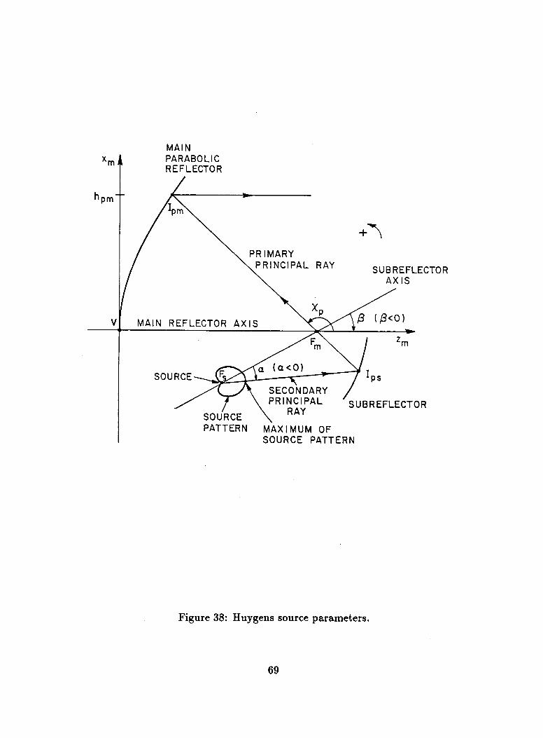
M A I N PARABO L I C REFLECTOR
+l P R I M A R Y
SUB REFLECTOR P R I N C I P A L RAY / \ AX I S I
M A I N REFLECTOR A X I S
PATTERN M A X I M U M OF SOURCE PATTERN
Figure 38: Huygens source parameters.
69

the central ray. Consequently, to achieve zero cross-polarization, the ideal source
for a compact range should have the field distribution of a Huygens source and
its principal ray should coincide with the central ray of the subreflector system.
It is also important to establish which pattern this ideal source should have. In
the ideal case, and neglecting the diffraction that such a beam would introduce
through its own shadow boundaries, the source set at the focal point, Fa, should
have a pattern different from zero in directions corresponding to the secondary
illuminating surface and zero in any other direction. Naturally this is impossible
to achieve. Instead, a real feed antenna has a pattern function having a (more or
less) symmetric main lobe and several side lobes. The pattern itself is a function of
frequency and polarization, and generally is more narrow at the higher frequencies
and broadens at the lower frequencies. Since it is desirable to use the same feed over
a wide frequency range (2-18 GHz), it is necessary to dimension the subreflector
and the feed so that the pattern considered for the GO design corresponds to the
narrowest of all the patterns of the feed, i.e., to the pattern at the highest frequency
of operation (18 GHz in the present case). It follows that it is unavoidable to
have spillover from the feed itself; therefore, the subreflector is overextended (to
reduce the amount of diffractioii by reducing the field incident on the edges, which
are made to correspond in the pattern to directions of lower radiation), and the
absorber on the walls of the lower chamber must be properly designed.
As it is shown in Section E, a truncated rectangular waveguide has radiation
characteristics very close to those of a Huygens source, and its phase center is
stable with direction (;.e., with dP, +P); therefore, these source requirements are
not unrealistic. On the other side, the use of a feed with a Cassegrain or Gregorian
configuration without the dual chamber arrangement would lead to a large amount
of spill-over and strong illumination of diffracting edges, with serious performance
70
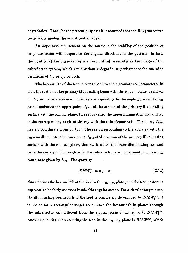
degradation. Thus, for the present purposes it is assumed that the Huygens source
realistically models the actual feed antenna.
An important requirement on the source is the stability of the position of
its phase center with respect to the angular directions in the pattern. In fact,
the position of the phase center is a very critical parameter in the design of the
subreflector system, which could seriously degrade its performance for too wide
variations of h, or z, or both.
The beamwidth of the feed is now related to some geometrical parameters. In
fact, the section of the primary illuminating beam with the z,, zm plane, as shown
in Figure 39, is considered. The ray corresponding to the angle xu with the zm
axis illuminates the upper point, I,,, of the section of the primary illuminating
surface with the z,, zm plane, this ray is called the upper illuminating ray, and a,
is the corresponding angle of the ray with the subreflector axis. The point, I,,,
has z, coordinate given by hum. The ray corresponding to the angle X I with the
zm axis illuminates the lower point, Il,, of the section of the primary illuminating
surface with the zm, z, plane, this ray is called the lower illuminating ray, and
a1 is the corresponding angle with the subreflector axis. The point, Il,, has zm
coordinate given by hi,. The quantity
characterizes the beamwidth of the feed in the z,, zm plane, and the feed pattern is
expected to be fairly constant inside this angular sector. For a circular target zone,
the illuminating beamwidth of the feed is completely determined by BMW:'; it
is not so for a rectangular target zone, since the beamwidth in planes through
the subreflector axis different from the zm, zm plane is not equal to BMW,"*.
Another quantity characterizing the feed in the zm, 2, plane is BMW"", which
71

is the beamwidth inside which the radiation pattern intensity is greater than some
specified dB level, called X. The feed pattern is lower than X dB outside this
angular sector. Since the feed used has a circular symmetry, the beamwidths
BMWf* and BMW"" characterize the feed, for the purposes considered here.
For the single reflector case, the previous definitions hold with the changes
due to the lack of the subreflector and with the source located at Fm.
3.7.2 EQUIVALENT FOCAL LENGTH FOR A SUBREFLECTOR SYSTEM
As shown by Dragone [6], a sequence of confocal reflectors is equivalent to a
single reflector, which has the same GO reflected field as the given sequence of
reflectors . The a x i s of the equivalent reflector is called the equivalent a x i s , and
coincides with the central ray after the reflection from the last reflector in the given
reflector sequence. In the present case, the equivalent reflector is a paraboloid, and
the equivalent a x i s is parallel to the parabolic reflector axis zm and goes through
the point Icm. The equivalent paraboloid is centered on the equivalent axis, and
its equivalent focal length, fe , is given by
f e = M f (3.13)
where f is the focal length of the parabolic reflector, and M is the magnification
of the subreflector system. For a concave elliptical subreflector, the magnification
is given by [12] 2 1 - €s
1 + €$ - 2 E s cospc M = (3.14)
where
0 is the eccentricity of the elliptical subreflector, and
72

xm t
Figure 39: Feed beaniwidths.
73

0 Pc is the angle from the subreflector axis to the parabolic reflector axis (121,
1131.
In the case Pc = O,SM is equal to the axial magnification, rn, given by
which is the maximum value obtained for M . Also,
where - p = arccoscs , O < P < A
and that, in this range of values of j3, one finds that
o o > M > l
(3.15)
(3.16)
(3.17)
(3.18)
according to the choice of cs.
These considerations show how a subreflector system can achieve a large equiv-
alent focal length without having a parabolic reflector with a large focal length.
3.7.3 APERTURE BLOCKAGE AND UNWANTED INTERACTIONS
Aperture blockage is a well known problem in the design of reflectors. As the
name suggests, it happens when an object (typically the feed, the subreflector,
or the supporting struts) blocks the path of the rays reflected from the parabolic
reflector. Thus, aperture blockage structures create a shadow and strong diffrac-
tions which degrade the amplitude, phase and cross-polarization characteristics of
the reflector antenna; also, this field again illuminates the reflector and is reflected
back into the feed with degradation of its SWR. Sometimes aperture blockage is
74
accepted in return for mechanical simplicity. In other cases, where good perfor-
mance is important, an offset arrangement of the reflector or subreflector system
is necessary. This arrangement, in turn, dictates a tilt of the pattern axis of the
feed with respect to the a x i s of the reflector. If a Huygens source is assumed
as a feed, for a single reflector case, the tilt of the feed axis can compensate (at
least partially) for the geometric taper in the case of an off-axis target zone, but
degrades the cross-polarization performance. For a subreflector system, an offset
arrangement with a proper choice of the tilt angles improves the geometric taper
without compromising the cross-polarization, if the axis of the feed coincides with
the central ray of the subreflector system.
There might be objects which are not on the path of the incident rays, but are
close to the reflector system and interact with it through diffraction and multiple
reflection rather than through direct shadowing, as an example, the walls of the
anechoic chamber of a compact range. These interactions can degrade the perfor-
mance of a reflector antenna. The strict requirements on a compact range dictate
not only an offset arrangement for the reflector (and for the subreflector system
combination), but also the use of time domain techniques in order to minimize un-
wanted interactions [14]. Not all unwanted interactions can be eliminated in this
way, for instance, for a Cassegrain configuration, the diffraction from the edges
of the subreflector into the reflector and from here into the target zone cannot be
time-gated. These interactions can be minimized by a Gregorian configuration and
by a dual chamber approach, as shown in Figure 9. The lower chamber contains
the feed and the subreflector; whereas, the upper chamber contains the parabolic
reflector, the pedestal and the target zone. The two chambers are coupled through
an opening centered around the focal point of the parabolic reflector, to allow
the illumination of the main reflector by the rays coming from the subreflector
75

SMALL CROSS SECTION
PRINCIPAL ' \ \ I X P ' / \
SMALL CROSS SECTION
SUBREFLECTOR AXIS
LARGE CROSS
Figure 40: Hour-glass shape of illuiilinating beam and its sections with planes.
and feed. This aperture is called the coupling aperture and must be as small as
possible to eliminate unwanted interactions, but also must be large enough not to
perturb the beam illuminating the parabolic reflector at the minimum operating
frequency. A careful design of the offset subreflector system with the dual chamber
and the coupling aperture eliminates aperture blockage and reduces interactions
and the amount of unwanted diffractions in the target zone to a minimum.
3.7.4 FIELD IN THE FOCAL REGION
The choice of the angle xp (or x,., in the case that the principal ray coin-
cides with the central ray, as it is done to obtain zero cross-polarization) between
the parabolic reflector axis and the source principal ray is presently addressed.
A choice of xp (see Figure 40) close to 90' minimizes the size of the coupling
aperture. In fact, ideally the parabolic reflector is fed by a beam (called the pri-
mary illuminating beam) coming from the subreflector and converging into the
76
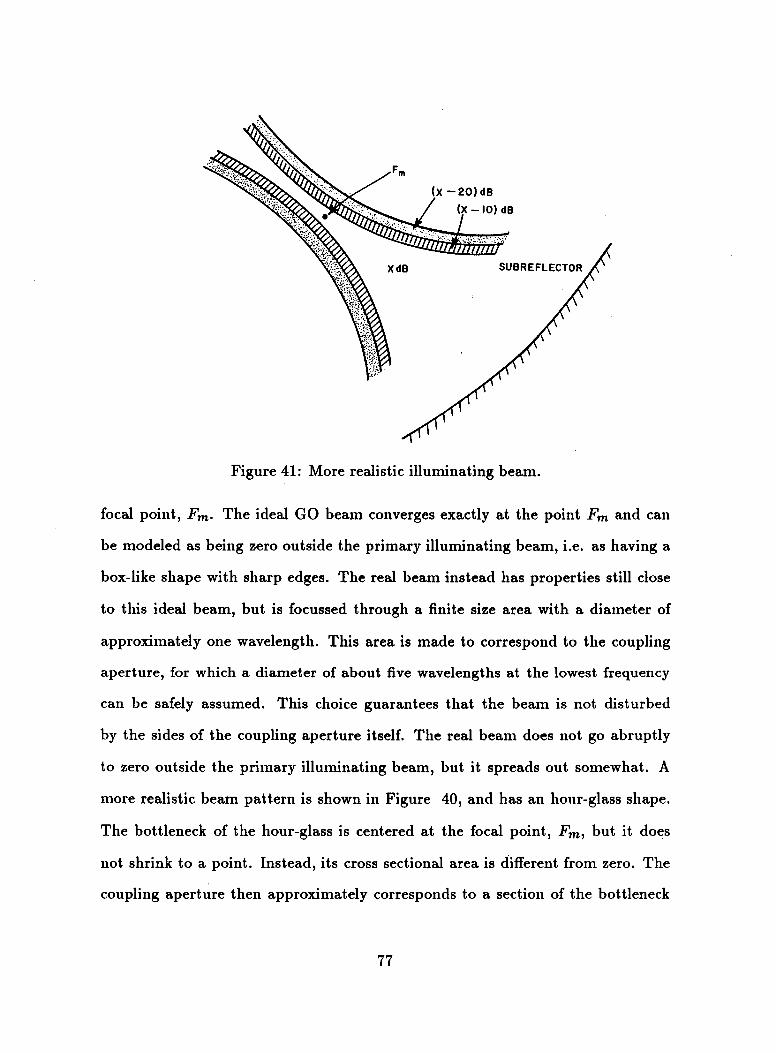
SUER EFLECTOR
Figure 41: More realistic illuminating beam.
focal point, Fm. The ideal GO beam converges exactly at the point Fm and can
be modeled as being zero outside the primary illuminating beam, i.e. as having a
box-like shape with sharp edges. The real beam instead has properties still close
to this ideal beam, but is focussed through a finite size area with a diameter of
approximately one wavelength. This area is made to correspond to the coupling
aperture, for which a diameter of about five wavelengths at the lowest frequency
can be safely assumed. This choice guarantees that the beam is not disturbed
by the sides of the coupling aperture itself. The real beam does not go abruptly
to zero outside the primary illuminating beam, but it spreads out somewhat. A
more realistic beam pattern is shown in Figure 40, and has an hour-glass shape.
The bottleneck of the hour-glass is centered at the focal point, F', but it does
not shrink to a point. Instead, its cross sectional area is different from zero. The
coupling aperture then approximately corresponds to a section of the bottleneck
77

with the yn, zm plane. The section becomes larger when the angle xp increases
from 90' to 180°, or decreases to Oo (see Figure 40). Figure 41 instead gives the
qualitative behaviour of the field contour in the focal region, where X is the field
strength in the central zone. As it can see, the gradient of the field is very high
in the focal region. It is important than that the contour of the coupling aperture
are removed from the region of fast variation of the field, to avoid slope diffraction
effects.
3.7.5 TIME GATING OF RAYS DIFFRACTED FROM THE COU- PLING APERTURE
The pulsed operation of a Compact Range allows one to time-gate out many
error terms. In this section some considerations on the time gating are presented
which refer to the GO design of the subreflector system and of the coupling aper-
ture.
In the subreflector system it is desired to time-gate the rays diffracted from
the edges of the coupling aperture into the target zone, like the ray D* shown
in Figure 42. This ray illuminates the edge, SU, from the feed, Fa, is diffracted
to the absorber wedge tip, Cf', and it is rediffracted to the point, TU. The point,
TU, belongs to the plane, n, which is perpendicular to the parabolic reflector axis
and set at the beginning of the target zone. The distance ITu - Cf'I is close to the
distance ITU - Fm), while the distance ICf' - SUI is close to the distance IFm - SUI;
consequently, for the purposes of time delay computations, this diffracted ray can
be substituted, with good approximation, with the pseudo-ray, D>m. This pseudo-
ray does not correspond to any real ray, but instead it is introduced for convenience
and ease of computation. Its path is from Fa to Su to Fm and finally to Tu. The
reason for using the ray, DT;.,, in the time delay considerations is that the time
Cl
78
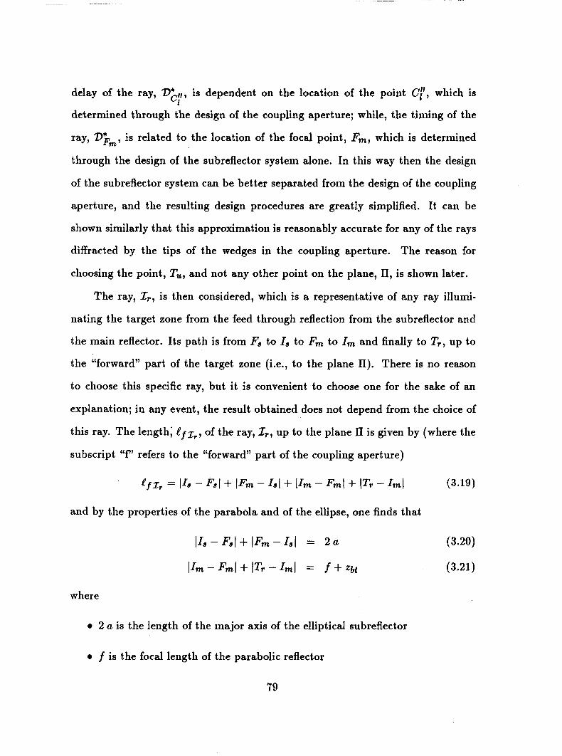
delay of the ray, D:;, is dependent on the location of the point C;, which is
determined through the design of the coupling aperture; while, the timing of the
ray, DFm, is related to the location of the focal point, Fm, which is determined
through the design of the subreflector system alone. In this way then the design
of the subreflector system can be better separated from the design of the coupling
aperture, and the resulting design procedures are greatly simplified. It can be
shown similarly that this approximation is reasonably accurate for any of the rays
diffracted by the tips of the wedges in the coupling aperture. The reason for
choosing the point, Tu, and not any other point on the plane, II, is shown later.
The ray, IT, is then considered, which is a representative of any ray illumi-
nating the target zone from the feed through reflection from the subreflector and
the main reflector. Its path is from Fa to Is to Fm to Im and finally to T,, up to
the “forward” part of the target zone (;.e., to the plane II). There is no reason
to choose this specific ray, but it is convenient to choose one for the sake of an
explanation; in any event, the result obtained does not depend from the choice of
this ray. The length; l f z , , of the ray, IT, up to the plane II is given by (where the
subscript “f’ refers to the “forward” part of the coupling aperture)
efz, = ( 1 s - &( + (Fm - Is( + IIm - %I + ( T v - Iml (3.19)
and by the properties of the parabola and of the ellipse, one finds that
= 2 u
= f + zbt
where
0 2 a is the length of the major axis of the elliptical subreflector
0 f is the focal length of the parabolic reflector
79
(3.20)
(3.21)
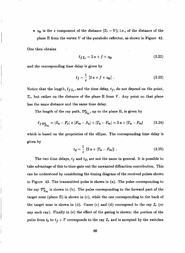
0 %(,t is the z component of the distance IT' - VI; Le., of the distance of the
plane 11 from the vertex V of the parabolic reflector, as shown in Figure 42.
One then obtains
Cfz, = 2 a + f + Z b t
and the corresponding time delay is given by
1 t f = - [2 a + f + Zbt] .
C
(3.22)
(3.23)
Notice that the length, Cfz,., and the time delay, t f , do not depend on the point,
T,., but rather on the distance of the plane II from V. Any point on that plane
has the same distance and the same time delay.
The length of the ray path, D>m, up to the plane n, is given by
which is based on the proprieties of the ellipse. The corresponding time delay is
given by
(3.25) 1 t d = - [2a+ ITu - Fm)] .
C
The two time delays, t f and id, are not the same in general. It is possible to
take advantage of this to time-gate out the unwanted diffraction contribution. This
can be understood by considering the timing diagram of the received pulses shown
in Figure 43. The transmitted pulse is shown in (a). The pulse corresponding to
the ray D[f;;, is shown in (b). The pulse corresponding to the forward part of the
target zone (plane 11) is shown in (c), while the one corresponding to the back of
the target zone is shown in (d). Cases (c) and (d) correspond to the ray 1, (or
any such ray). Finally in (e) the effect of the gating is shown: the portion of the
pulse froin t b to t f + T corresponds to the ray 1, and is accepted by the switches
80

into the receiver; while, everything else is gated out, in particular the diffracted
ray Dgm. From the Figure 43 one obtains
0 T is the length of the transmitted pulse
0 At = t f - t d is the time delay differential between the rays 1,. and D$m
0 AT = tb - t f corresponds to twice the length et, of the target zone: AT =
2 et*/2
0 Tg = t f + T - t b is the duration of the gating; also, Tg = T - AT .
Recall that
1 1 1 C C Fm t f = 2 - e f , td = 2 - ef =, t b = 2 ; (ef ZT -k et,) (3.26)
and the iime delay differential, At , is given by
(3.27)
(3.28)
In order to perform the time gating, it is required that
this inequality must be satisfied with some margin, to take into account the finite
switching time of the switches, therefore one can set
where Taw is related to the switching speed and deternines the ninimum sep-
aration between the end of the diffracted pulse and the beginning of the gate.
Therefore, one obtains
T - Taw 5 t b - t d (3.31)
81

but
t b - t d = At + AT
and one then obtains
(3.32)
(3.33)
(3.34)
In the present system one has
T = 20 ns Taw e 6 ns AT 21 16 11s (3.35)
and one then obtains
Tg = 4 ns At N 10 ns (3.36)
and the value actually obtained in the design is At N 9.5 ns, which can be consid-
ered satisfactory.
From Inequality (3.34) it is clear why the point, Tu, must be considered to
properly determine the time delays. In fact, for any other point, T', one considers
the ray, oFm. The ray path is from FB to Su to Fm to T'. By comparing the
length of this ray with the length of the ray, D$m, one obtains
and a shorter time delay is associated with the ray, @Fm. The Inequality (3.34)
must be satisfied for any point on the plane II; therefore, the minimum of the right
hand side must be considered. This minimum corresponds to the ray, D$m.
3.8 SHAPE OF THE CROSS SECTION OF THE TARGET ZONE
The target zone is defined in Section 3.2 as a portion of a solid cylinder
having generatrices parallel to the parabolic reflector axis and delimited by two
a2
UPPER CHAMBER
OVEREXTENDEO SUBREFLECTOR
LOWER CHAMBER
Figure 42: Geometrical quantities related to the time delays of different rays.
83

I TRANSMITTED PULSE
1 t i m e (ns) DIFFRACTED PULSE
.____ (b) t,; t ,+T t i m e (ns) .c; A t
I PULSE FROM FORWARO~PART OF TARGET ZONE
. . c A T - j I PULSE FROM BACK PART OF TARGET ZONE j !
GATED PULSE
(e 1 td+T t t b t f + T t i m e (ns)
. . L T , &
Figure 43: Timing diagram relating time delays and swithching times.
04

planes perpendicular to the parabolic reflector axis. A target zone is called circular,
rectangular, elliptical, etc., according to the shape of its cross section in a plane
perpendicular to the parabolic reflector axis. In the present section, it is discussed
which shape is the most appropriate to define the cross section of the target zone
with a plane perpendicular to the main reflector axis. In Section 3.2, a rectangular
cross section has been considered, but this is not the only possible shape.
Most targets have an elongated shape, like the model of an airplane; therefore,
it might seem that an elliptical cross section is a more natural one.
The feed considered (typically, a conical corrugated horn) has a radiation
pattern circularly symmetrical with respect to the axis of the horn. If this axis
coincides with the principal ray, as it is assumed in the present design, the circular
symmetry of the beam is preserved after the reflection from the subreflector and
the parabolic reflector. Consequently, from a GO viewpoint, a circular shape of
the target zone is the most appropriate, since it allows the maximum utilization
of the feed.
The shape of the upper room, where the measurements are performed, is
rectangular. The room itself is a major element in the design of the compact range
(it is by far its most expensive component), this fact then suggests a rectangular
cross-section.
Finally, the limiting factor in the compact range design is the diffraction from
the edges of the parabolic reflector. This is the factor degrading the otherwise
(almost perfect) plane wave reflected from the parabolic reflector. From the purity
of the field then, the most natural shape would be the same shape as that of the
edges of the parabolic reflector.
It is necessary, on the other side, to specify some shape for the target zone
while drafting the specification for the compact range. For instance, it is necessary
85
to specify the admissible geometric taper of the reflected field and also the taper of
the feed, which in turn becomes a specification on the beamwidth of the feed an-
tenna itself. Suppose, for instance, that the target zone is specified as rectangular,
and that the maximum admissible taper for the feed is, for the sake of an example,
0.2 dB. In a sense, this represents an excessive requirement on the feed: in order
to satisfy this requirement at the corner points, an excessively heavy requirement
is imposed on the design of the feed itself and on the GO dedgn. Very likely, this
specification is not really necessary, since the corner points are seldom if ever used.
The same argument can also be applied to the geometric taper in the case of a
rectangular cross section of the target zone. In practice instead, the requirements
on the geometeric taper are easy to satisfy; consequently, it seems acceptable to
satisfy the requirement at the four vertexes of the target zone, even if this is not
a requisite strictly necessary.
86 <-', <- - 9

CHAPTER IV
ITERATIVE SUBREFLECTOR SYSTEM DESIGN
The purpose of the geometrical optics (GO) design of a compact range sub-
reflector system is to establish the basic dimensions of the main reflector and
subreflector, the size of the primary and secondary illuminating surfaces, the tilt
angles of the subreflector and feed, an estimate for the feed beamwidth and an
evaluation of the polarization characteristics. All of these issues are addressed in
this chapter for a given reflector system.
4.1 EQUATIONS FOR GO FIELD COMPUTATIONS FOR A FO- CUSSED SUBREFLECTOR SYSTEM
The GO field equations for a compact range subreflector system are presented
in this section and they are related to the appropriate geometrical parameters.
These equations allow one to model either an elliptic (Gregorian) or an hyperbolic
(Cassegrain) subreflector system and evaluate the following:
0 Field intensity, in amplitude and phase, for both vertical and horizontal
polarization. Since the distance from the source to the field point is constant
based on the focal properties of conics, the phase is known to be constant.
0 Polarization ratio, for horizontal/vertical and vertical/horizontal components.
The definition of cross-polarization is the third of Ludwig [8].
87

MAIN R E FLECTO R
SUBREFLECTOR
\ / REFLECTOR
CONVEX SUBR EFLECTOR
Figure 44: Convex subreflector.
M A I N REFLECTOR 'mk- R
SUBR EFLECTOR A X I S /
CONCAVE SUBREFLECTOR
Figure 45: Concave subreflector.
88

In both subreflector cases, the field values or the polarization ratios are best com-
puted on a rectangular grid in a plane perpendicular to the main reflector.
Three different sources are useful while modeling a subreflector system:
1) Uniform source having field horizontally or vertically polarized.
2) Huygens source, horizontally or vertically polarized (Section E).
3) Interpolated source, to model a real source through the interpolation of
pattern values between an appropriate number of data points [15].
In most cases the uniform source is used to perform field computations, and
the Huygens source to perform polarization computations, but it is convenient to
be able to perform any computation with any source.
A simple ray-tracing technique can be used to perform the computations.
Starting from the field point, R, a ray, C, is traced all the way back to the source lo-
cated at the focus of the subreflector, Fs (see Figures 44 and 45). Two coordinate
systems are used. One is the main reflector coordinate system, Fm(xm,ym,zm),
and the other is the subreflector coordinate system, Fs(xs,ys, zs). These coordi-
nate systems are shown in Figure 26. The field point is R E (XR, YR, ZR) and the
corresponding reflection point on the main reflector is Im, which has coordinates
(xm, ym, zm) such that tm = XR, ym = YR and zm satisfies the equation of the re-
flecting surface. In other words, all the rays reflected from the parabola propagate
in the z direction; consequently, one obtains that
where f is the focal length of the parabolic reflector.
89

The ray e goes through the point Im and the focal point, F'. This part
of the ray is called e,; while, the part between Fd and Id is called e,. The
reflection point on the subreflector Is can be determined by intersecting em with
the subreflector itself. This is done as follows. The coordinates (xm,yTn,xm) of
the point In are transformed from the main reflector coordinate system to the
subreflector coordinate system, obtaining (x&, y A , zA) . This can be accomplished
through matrix multiplication, as follows [15]:
where the matrix R' represents a rotation around the ym ax is by the angle /3
and the vector position of the point V, vertex of the parabolic reflector, in the
subreflector coordinate system is given by
By knowing the points Fm and Im, the equation of the ray em can be determined
(see Section B).
The radial distance from the focal point F . to the reflection point Is is defined
by the polar equation of the subreflector such that
P, r s = 1 - e. cos e, (4.7)
90
where F,(T,, e,, 4,) is the spherical coordinate system corresponding to the carte-
sian subreflector coordinate system, F,( t , , y,, 2,). This description of a conical
surface allows one to model an elliptical (Gregorian configuration) or a hyperboli-
cal (Cassegrain configuration) subreflector with the same equation (see Section B).
The coordinates of I, z (z:, y:, 2:) can then be determined through the equa-
tions of the ray and the equation of the subreflector. The straight line through
the points F, and I, can be expressed in parametric form in terms of the distance
parameter t of the current point on the line from any of the two points, F, or I,. A
second order equation in t can be obtained from the equations of the coordinates
of the line and the equation of the conic. This second order equation has two,
one or no solutions, according to the number of intersection points. In the present
case the point F' is internal to the conic, hence the equation should always have
two solutions. It is then necessary to discard the spurious solution and to retain
the solution which corresponds to the physical subreflector. This can be done,
for instance, by verifying if the angles e,, 4, are inside a prescribed range. The
solution is derived in detail in Section B.
Knowing the points Im and I,, the GO reflected field at R, U'(R), can then
be computed, where the notation U represents either the electric (E) or magnetic
(H) field.
The following notation is introduced. Given two points, P and Q, the symbol
P - Q indicates the displacement vector starting at Q and ending at P, similarly
IP - &I indicates the magnitude of the vector P - &.
A source having unitary strength and a vector pattern function PF (function
of the direction of radiation gi) is considered here. The pattern function is discussed
91
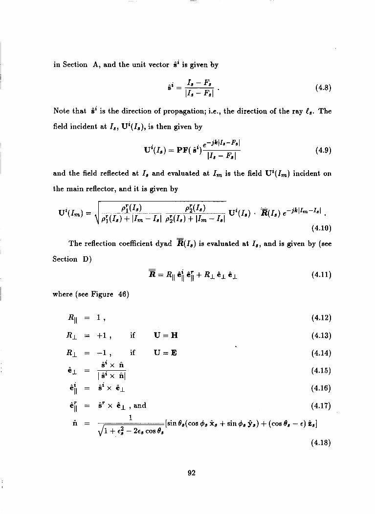
in Section A, and the unit vector ii is given by
Note that ii is the direction of propagation; i.e., the direction of the ray e,. The
field incident at I , , Ui(18), is then given by
and the field reflected at I , and evaluated at Im is the field Ui(Im) incident on
the main reflector, and it is given by
(4.10)
The reflection coefficient dyad E(&) is evaluated at I , , and is given by (see
Section D)
where (see Figure 46)
&II = i ' x 6 1
U = H
U = E
(4.11)
(4.12)
(4.13)
(4.14)
(4.15)
(4.16)
92
where 88 and $8 are the polar coordinates of Id in the FS(r8,6)8)$8) coordinate
system. The expression for n is derived in Section C. The direction of the incident
ray, Pi, is known, the direction of the reflected ray ir could be determined through
the law of reflection such that
but in the present case it is already known. The point of reflection and the vectors
6' and n define the plane of incidence.
The terms with the square root represent the spreading factors. The caustic
distance p; is the radius of curvature of the reflected wavefront in the plane of
incidence. This plane contains the radius of curvature Rcl of the surface. The
caustic distance pa is the radius of curvature of the reflected wavefront in the plane
normal to the plane of incidence. This plane contains the radius of curvature Rc2
of the surface.
In the present case, an incident spherical wave is considered because the feed
is modeled as a point source, and the plane of incidence coincides with one of
the principal planes of the conical surface. The caustic distances are given by the
equations
1 2 p; = - +
si R,1 cos di
1 2cosdi p i = 7+-
8' Rc2
(4.20)
(4.21)
where si is the distance from the source (real or virtual) to the reflection point,
and cos@ is given by
cosd' = -i' * n . (4.22)
where n is the normal to the surface.
93

The spreading factors, the caustic distances ( p i and p;) and the radii of cur-
vature (R, 1 and Rc2) are evaluated at the reflection point, I.,, on the subreflector
with the source at F.,.
The field U r ( R ) reflected at I , and evaluated at the field point R is given by
(4.23)
The dyad, R(I,), and the caustic distances are all evaluated at I, with the - -
(virtual) source at F,. In fact, the two caustic points are coincident at Fm by
the properties of the conics. Consequently, the field incident on I, is a spherical
wave, and it is still legitimate to use the Equations (4.20), (4.21) to compute the
caustic distances.
In the present case, it is not necessary to compute the caustic distances of the
reflected field in order to evaluate Ui(Im) and U'(R). For &(Im) , all the rays
reflected from the subreflector converge to the focal point, F,. By definition, then
Fn, is the caustic point for the field reflected from the subreflector (both caustics
are at the same point); consequently, one finds that
p i ( I . , ) = &I.,) = *p., - FntI (4.24)
where the plus sign holds if the subreflector is convex, and the minus sign if it is
concave (Figures 44 and 45).
Let i = {1,2), then
e if the subreflector is convex (Figure 44), one obtains that
e if the subreflector is concave (Figure 45), one obtains instead
94
In both cases, one finds that
Therefore, the expression for the spreading factor of the field reflected from the
subreflector is given by
where the plus sign holds if the subreflector is convex, and the minus sign if it is
concave.
Again it is not necessary to compute the caustic distances in order to evalu-
ate the field U'(R) reflected from the parabola. In fact, it is known that, for a
parabola, the focal points coincide at infinity, such that
then
(4.30)
In other words, the field, once reflected from the parabolic reflector, has no spread-
ing attenuation; i.e., it is a plane wave.
Therefore, the following equation is obtained for the GO reflected field at the
field point:
where the plus sign holds if the subreflector is convex, and the minus sign if it is
concave.
The equations derived in this section allow one to write a numerical solution
to perform computations of field strength and polarization ratios.
95
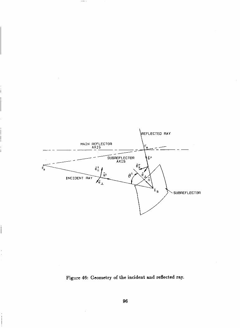
REFLECTED RAY \
Figure 46: Geometry of the incident and reflected ray.
96

4.2 ITERATIVE DESIGN INITIAL VALUES
The geometrical parameters of this section are shown in Figure 47. The size
of the target zone is determined by the size of the targets to be measured in the
compact range, which must be defined in terms of the performance specifications
required for the measurements. The first design step is to give an estimate of
the focal length, f , of the main reflector. A value for the angle, xu, close to 90'
minimizes diffraction from the edges of the coupling aperture, and also makes its
actual implementation easier. The beamwidth of the primary illuminating beam
is estimated to be approximately 30'; consequently, a value of xp close to 105'
is a good start. Let h,, be the height (the 2m coordinate) of the intersection
of the primary principal ray with the parabolic reflector. The gro (taper of the
reflected field) and the cross-polarization are minimized if the principal ray of the
feed, the equivalent axis (central ray) and the illuminating ray (ray corresponding
to the a x i s of the target zone) all coincide, that is, if xp = xi = xc. Under this
hypothesis, one finds that ht, = h p . Then, as shown by Dragone [9], it follows
that
(4.32)
where hi, is the zm coordinate of the intersection of the zm axis of the target
zone with the main reflector. There is some flexibility in choosing the height, ht,,
because the focal point, F', must be at the floor level of the anechoic chamber,
but the ax is of the target zone can be moved up or down one foot or so. A first
estimate of htm can be made by common sense, then Equation (4.32) and the
previous considerations suggest a first choice of f and xp. The eccentricity of the subreflector can be estimated as follows. The specifica-
tions on the compact range performance dictate the amount of admissible gro. By
97
using a numerical solution in the single reflector configuration and with a uniform
source it is possible to determine by a trial and error procedure an equivalent focal
length fe of an equivalent parabolic reflector with the desired gro. Notice that a
choice of fe determines the beamwidth of the feed. Once fe has been estimated,
the corresponding eccentricity of the elliptical subreflector, e,, can be computed
I by solving the following equation:
and obtaining f e - f f e + f e
E, = (4.34)
In fact, it is not possible to use the expression for the magnification factor M given
2 1 - €, 1 + €! - 2€, cos&
M = (4.35)
since the tilt angle, &, still needs to be determined. Initially, the angle Pc can be
set to zero in that Pc will be small which makes this a good approximation.
A second parameter is necessary to determine the subreflector, for instance,
the interfocii distance, d,. Its choice is suggested by the following considerations:
0 There must be a minimum separation between the focii of the subreflector,
F, and Fm. If they are too close, some of the energy is reflected back from
the subreflector into the feed, the minor lobes of the feed antenna might
radiate through the coupling aperture into the upper chamber or cause strong
diffraction by illuminating the edges of the coupling aperture with a strong
signal without much space attenuation.
0 The size of the secondary illuminating surface cannot be made too small for
mechanical reasons: the system acts as a lens; consequently, the mechanical
98

tolerances on the subreflector are even more strict than those on the main
reflector.
0 The subreflector must be in the far field of the feed, giving a ininiinum
distance between the feed and subreflector.
0 It is shown (see Section 3.2, Figure 47) that the following relationships must
be satisfied:
(4.36)
(4.37)
where h, is the vertical (i.e., in the zm direction) distance from the phase
center of the feed (i.e., the focus F, of the subreflector) to the ceiling of the
lower chamber, and IF is the horizontal (;.e., in the zm direction) distance
of the phase center of the feed from the focus, Fm, of the main reflector.
Equation (4.36) gives a minimum value for the product d , sin p, and p should
be small, in order to make the magnification factor M close to its maximum,
minimizing in turn the gro; consequently, d, should be made large, in order
to keep the product equal to or larger than its minimum value. On the other
hand, it is desirable that the upper and lower room have a common wall. For
this purpose the choice of
lpc = f (4.38)
appears very reasonable, then Equation (4.37) shows that d, cannot be made
too large. In any case, one finds that
(4.39)
These considerations suggest an estimate for the distance between focii, d,,
thus, completing the estimate for the parameters of the subreflector.
99

Figure 47: Geometrical quantities defining the subreflector system design
100

4.3 ITERATIVE DESIGN VIA GO COMPUTATIONS
The previous estimate of the geometric parameters of the subreflector system
must be refined to give an initial GO design. A sequence of operations to achieve a
GO design for a Huygens source by the use of a numerical solution can be devised
as follows.
0 Input the geometry of the reflector and subreflector, enter the estimates of
the Huygens source tilt angle, a, and the subreflector a x i s tilt angle, 0, as
previously computed from the angle, xp, of the primary principal ray.
0 Check if the overall taper error of the reflected field is satisfactory. Eventually
the height, hirn, of the zrn axis of the target zone can be adjusted somewhat
. corresponding to the center of the surface having a satisfactory taper error.
If the taper error is not satisfactory, find a new value of the tilt angle of the
feed axis a to satisfy the requirement on the overdl taper error.
0 Check if the cross-polarization, although no longer zero, is still satisfactorily
small.
0 If not, try a value of the tilt angle of the feed axis a intermediate between
the previous two cases.
0 Check if the overall taper error and cross-polarization performance are sat-
isfac t ory.
0 If any or both of the two is not satisfactory, change the subreflector axis tilt
angle, 0.
0 Compute the corresponding angle a to achieve zero cross-polarization.
101
I -
0 Check if the angle xp is close to 105'. This angle can be computed through
the equation:
[ (1 + e:) cosa - 2€, x = A - p + arctan (1 - E$) sin a
(4.40)
which holds for any angle x in terms of the corresponding angles a and
p. It might be very difficult to make this angle equal to 105' through this
iterative approach; consequently, this condition is relaxed by assuming xp to
be between 110' and 120'.
0 Start again if xp is not between 110' and 120'.
Since this is a trial-and-error approach, the values of xp, a and p are close
but not exactly equal to xc, ac and &, the tilt angles corresponding to the central
ray. The changes of values in reiterating the previous sequence should be small,
so that the broad requirements of Section 4.2 are still met. If the requirements
cannot be met satisfactorily with the chosen geometry, it is necessary to change
the parameter, d,, and begin the design sequence again. This last parameter in
fact allows some flexibility in the design.
It is necessary, once a design has been achieved, to verify that the cross-
polarization values are not too sensitive to small changes of the angles a and p, as
it has been found in some cases. If this happens for several combinations of a and
p satisfying Equation (3.10), it might be necessary to change the distance between
the focii, d,, and to go through all the previous steps.
If possible, it is advisable to model the actual source's polarization and ampli-
tude to see if the performance with the actual source is satisfactory at this point
in the design.
The design obtained in this way is still a first-cut configuration. A more com-
plete and accurate model of the system is necessary to evaluate how other factors
102 I

(like diffraction) affect the total field in the target zone. It might be necessary
then to modify the values of the GO design according to the indications of the
more complete model, but all the previous requirements still have to be satisfied.
Once all the parameters of the reflector and subreflector are determined, the
projection of the target zone on the main reflector determines the primary illumi-
nating surface. This projection is made with rays parallel to the main reflector
axis. The secondary illuminating surface in turn is defined by projecting the pri-
mary illuminating surface from the main reflector on the subreflector with rays
through the focus Fm which is in common to the reflector and subreflector. The
primary and secondary illuminating surfaces give a first indication on the physical
sizes of main reflector and subreflector.
4.4 ITERATIVE DESIGN SUMMARY
In summary, it has been shown that several of the design requirements for a
compact range, although not related to the GO field, must be taken into account
to obtain a good GO design. It is impossible to make a clear cut separation and
relate each design parameter to one and only one requirement, but the following
guidelines can be established for a Gregorian system with a parabolic reflector and
concave elliptical subreflector:
0 The choice of the focal length, f , of the main reflector is dictated both by
a choice of the height, htm, to the center of the target zone and by a choice
of xu, the angle of the upper illuminating ray with the main reflector axis,
which should be close to 90'. This in turn defines xp to be close to 105O,
since the beamwidth of the primary illuminating beam is assumed to be close
to 30'.
103

0 The geometric taper requirement is satisfied through the choice of the axial
magnification factor m, and the choice of m, in turn, determines the eccen-
tricity, e,, of the subreflector.
0 The second parameter of the subreflector (the interfocii distance d,) is deter-
mined by the necessity of keeping a minimum distance between the feed and
the coupling aperture, of having the subreflector in the far field of the feed,
of having a minimum size of the subreflector, and of making the null of the
cross-polarized field as insensitive as possible to small changes of the angles a
and p. Recall that a is the angle from the subreflector axis to the secondary
principal ray of the source, and p is the angle from the subreflector axis to
the main reflector axis. Then, the following relationships are obtained:
h, = - d a s h @
1, = d,cosp
(4.41)
(4.42)
(4.43)
These equations suggest a value of d, close but smaller than f .
0 The choice of xp determines either a or p.
0 The cross-polarization requirement determines the second one ( p or a).
0 The beamwidth of the feed BMW?’ is determined through the angles cyzl
and al.
Consequently, reflector and subreflector, tilt angles of feed and subreflector,
beamwidth and cross-polarization characteristics of the feed, and priiiiary and
secondary illuminating surfaces are determined.
104

4.6 ITERATIVE DESIGN EXAMPLE
In this section, a design example is given to show how to use the principles
just discussed to effectively satisfy the design specifications of a compact range
such as shown in Figure 9.
The desired target zone has a rectangular cross section having a vertical height
of 6' and a horizontal length of 8'. By setting the lower line delimiting the primary
illuminating surface at 5.5', allowance is made for the lower rolled edge. This in
turn sets the height, him, of the center of the rectangular target plane-sections at
8.5', and the upper line delimiting the primary illuminating surface at 11.5'.
The following relationship relates the angle from the main reflector ax is to the
primary principal ray, xp, to the focal distance, f:
h,, = 2f cot (F) . The value xp = 120' is chosen, then a value for f is obtained
= 7.36' 1 8.5' f = - 2 cot ( 60')
(4.44)
(4.45)
and f = 7.25' is chosen.
Through the use of a numerical solution in the single reflector mode with a
uniform source, it was found that a value of fe of 26.5' gives an acceptable value
(< .1 dB) for the geometric taper. The values of the field strength are shown in
Figure 48. The field is computed on a target plane-section. The field strength is
normalized to its maximum, and the values are given in dB. For convenience, the
values are given on one side only of the target plane-section, because symmetry
holds.
105

From the value of the focal length the eccentricity of the subreflector is deter-
mined. In fact, the axid magnification, m, is given initially by
m Z fe/f = 26.5'/7.25' = 3.662 (4.46)
because, for small /3, one obtains
m Z M . (4.47)
Then, € 8 can be determined from the following equation:
which can be solved for e8 m - 1
€s = - m + l
then 3.66 - 1
€8 = = 0.5708 . 3.66 + 1
(4.48)
(4.49)
(4.50)
The distance between the focii is then chosen such that dd = 6', which is close, but
smaller than f = 7.25'.
The semiaxes, a and b, of the elliptical subreflector are determined as follows.
Since 2c = d , then c = 3'. Also, one finds that
consequently
(4.51)
(4.52)
This gives
- 5.25' . (4.53) 3' .571
a=--
Since c 2 = a2 - b2, then b2 = u2 - c2 and b can be computed such that
b = 4(5.25')2 - (3')2 = 4.308' . (4.54)
106
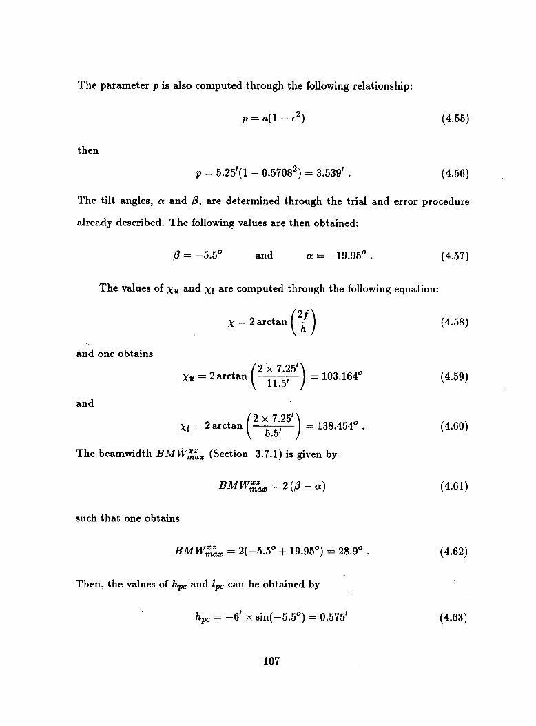
The parameter p is also computed through the following relationship:
p = a(1 - 2) (4.55)
then
p = 5.25'(1 - 0.57082) = 3.539' . (4.56)
The tilt angles, (Y and p, are determined through the trial and error procedure
already described. The following values are then obtained:
p = -5.5O and CY = -19.95O . (4.57)
The values of xu and x1 are computed through the following equation:
x = 2arctan ( y ) and one obtains
and
x1 = 2arctan ( = 138.454' .
(4.58)
(4.59)
(4.60)
The beamwidth BMWZa, (Section 3.7.1) is given by
BMWEa, = 2(p - a) (4.61)
such that one obtains
BMWZa, = 2(-5.5' + 19.95O) = 28.9' .
Then, the values of h, and Z, can be obtained by
h, = -6' x sin(-5.5') = 0.575'
(4.62)
(4.63)
107

and
lw = 6' x COS(-^.^') = 5.972' (4.64)
which are satisfactory, while the coordinate zpc of the phase center in the zm, ym,
zm coordinate system is
zw = f - IF = 7.25' - 5.972' = 1.278' . (4.65)
The actual magnification factor can now be computed through the following
expression: 2 1 - € S
1 + €? - 2 E s cosp M =
which gives -
= 3.5583 1 - 0.5712
1 + 0.5712 - 2 x 0.571 cos( -5.5O) M =
(4.66)
(4.67)
which is close to the value of the axial magnification factor, m = 3.662.
Through the use of a numerical solution in the subreflector system mode with
a Huygens source it can be checked if the total reflected field taper is acceptable.
The field is computed on a target plane-section (defined in Appendix G). The
computed values are given in Figure 49. As before, the field strength is normalized
to its maximum, the values are given in dB and on one side only of the section of
the target zone, because symmetry holds. The total taper error is still acceptable,
since it is less then 0.2 dB.
The angles au and a[ (defined in Section 3.7.4) are obtained through the
following equation (see Section F):
1 [ 2ES - (1 + €3 cos(x + p) (1 - e$)sin(x + p ) a = -arctan
which gives
(4.68)
(1 - 0.57082) ~in(103.164~ - 5.5O) 2 x 0.5708 - (1 + 0.57082) cos( 103.164O + -5.5O)
cyu = -arctan
108
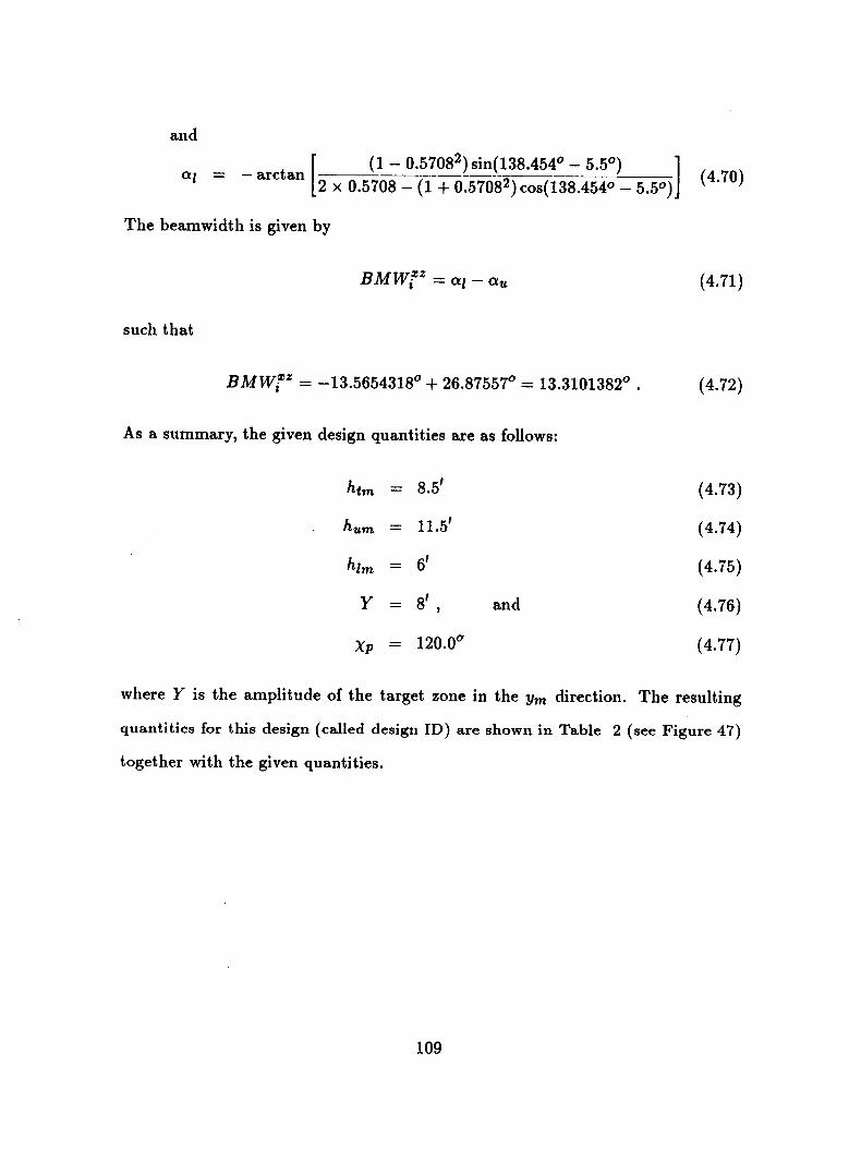
and
(1 - 0.570s2) sin( 138.454' - 5.5O) ai = -arctan
The beamwidth is given by
BMW?" (4.71)
such that
BMW?' = -13.5654318O + 26.87557O = 13.3101382O . (4.72)
As a summary, the given design quantities are as follows:
htm = 8.5'
hum = 11.5'
him = 6'
Y = 8 ' , and
x p = 120.0°
(4.73)
(4.74)
(4.75)
(4.76)
(4.77)
where Y is the amplitude of the target zone in the Ym direction. The resulting
quantities for this design (called design ID) are shown in Table 2 (see Figure 47)
together with the given quantities.
109
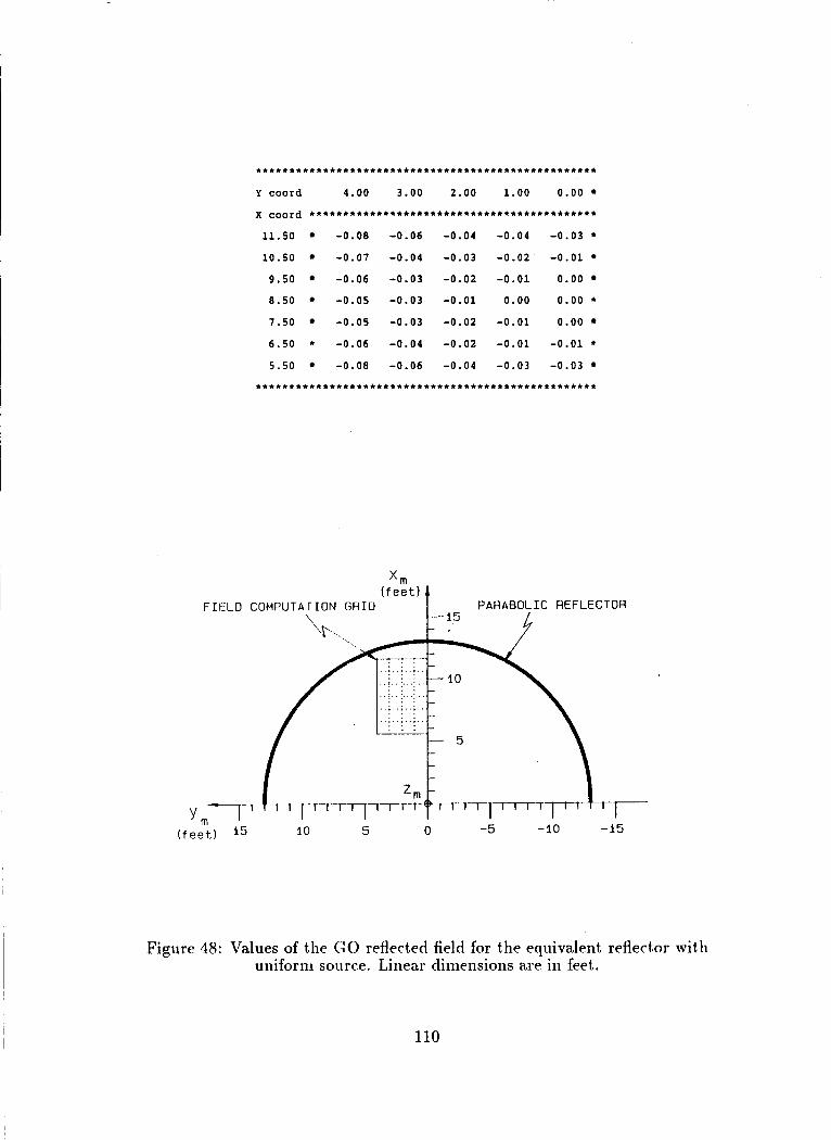
FIELD
. . . . . . . . . . . . . . . . . . . . . . . . . . . . . . . . . . . . . . . . . . . . . . . . . . . Y coord 4.00 3 .00 2 . 0 0 1 . 0 0 0 .00
X coord . . . . . . . . . . . . . . . . . . . . . . . . . . . . . . . . . . . . . . . . . . . 1 1 . 5 0 - 0 . 0 8 -0.06 -0.04 -0.04 -0 .03 * 1 0 . 5 0 - 0 . 0 7 -0 .04 -0.03 - 0 . 0 2 ' - 0 . 0 1
9 . 5 0 -0 .06 -0 .03 -0.02 - 0 . 0 1 0 .00
8 . 5 0 - 0 . 0 5 -0 .03 - 0 . 0 1 0 .00 0 . 0 0 * 7 . 5 0 - 0 . 0 5 - 0 . 0 3 -0 .02 - 0 . 0 1 0 .00
6 . 5 0 * - 0 . 0 6 -0 .04 - 0 . 0 2 - 0 . 0 1 - 0 . 0 1 * 5 . 5 0 - 0 . 0 8 - 0 . 0 6 - 0 . 0 4 -0 .03 - 0 . 0 3
. . . . . . . . . . . . . . . . . . . . . . . . . . . . . . . . . . . . . . . . . . . . . . . . . . .
P A R A B O L I C REFLECTOR FIELD COMPUTATION G R I D
10 5 0 -5 -10 -15 ( fee t ) 15
COMPUTATION G R I D P A R A B O L I C REFLECTOR
10 5 0 -5 -10 -15
Figure 48: Values of the GO reflect*ed field for t,he equivalent- refledor wit,h uniform source. Linea,r dimensions are in feet,.
110

. . . . . . . . . . . . . . . . . . . . . . . . . . . . . . . . . . . . . . . . . . . . . . . . . . . Y coord 4.00 3 . 0 0 2.00 1 . 0 0 0.00 * x coord . . . . . . . . . . . . . . . . . . . . . . . . . . . . . . . . . . . . . . . . . . .
11 .50 -0 .17 -0 .12 -0 .09 -0 .07 - 0 . 0 6 * 1 0 . 5 0 -0 .13 -0 .09 -0 .06 - 0 . 0 4 - 0 . 0 3
9 . 5 0 - 0 . 1 1 -0 .07 -0 .03 - 0 . 0 1 - 0 . 0 1
8 . 5 0 -0 .10 -0 .06 - 0 . 0 3 - 0 . 0 1 0 .00
7 . 5 0 - 0 . 1 1 -0 .06 -0 .03 - 0 . 0 1 0 .00 * 6 .50 -0 .13 -0 .08 - 0 . 0 5 -0 .03 -0 .02
5 . 5 0 -0 .16 - 0 . 1 1 -0.08 -0.06 - 0 . 0 5
. . . . . . . . . . . . . . . . . . . . . . . . . . . . . . . . . . . . . . . . . . . . . . . . . . .
( f
F I EL0
Y J- e c t ) 15
( f e e t ) P A R A B O L I C R E F L E C T O R
k C O M P U T A T I O N G R I D
\
........... . . . . . . -
10 5 0 -5 - 10 -15
_-
Figure 49: Values of the GO reflected field for the subreflector system with a Huygens source. Linear dimensions are in feet,.
111

Table 2: Design parameters for design ID
-~ hpc = 0.575' zPc = 1.2781 h,, = 11.5'
hi, = 5.5' x p = 119.24" Y = 8.0'
a = -19.95" p = -5.50 A = 14.45O
a, = -26.8750 ai = -13.565O xu = 103.164O
X I = 138.4540 A t = 10.248 ns
BMW,"' = 13.31" f = 7.25' C, = 0.5708
BMW;,, = 28.90
d, = 6.0' p , = 3.639' m = 3.662
M = 3.5583 grodB = -0.0819 dB
112

CHAPTER V
DIRECT DESIGN THEORY
5.1 INTRODUCTION
Four design procedures are derived in this chapter to perform the GO design
of the dual chamber compact range. These procedures use the geometrical and
electrical requirements to obtain an uniquely defined compact range reflector sys-
tem. Three of the design procedures assume that the quantity zpc (see Figure 50)
is set to zero (see Figure 51) in order to obtain more simple equations. In the
fourth design procedure instead zpc can assume any value. Any of the first three
design procedures then can be used to obtain an initial estimate of the design,
which is then refined through the fourth procedure.
5.1.1 GEOMETRICAL CONSTRAINTS
In this section some relations between the geometrical quantities of the coin-
pact range are established.
Since the zero cross-polarization condition is enforced, the angles a, /3 and x are denoted as a,, pc and x,. The angle a is the tilt angle of the feed axis with
respect to the subreflector axis, /3 is the tilt angle of the subreflector axis with
respect to the main reflector axis, and x is the angle of the corresponding primary
ray with the main reflector axis.
113

It has been established (see Section 4.2) that
The height ht, is the vertical coordinate (z, coordinate) of the intersection of
a line parallel to the main reflector axis and through the center of the target
zone with the parabolic reflector. This line presently coincides with the central
ray. The angle xc is the corresponding angle of the primary central ray with the
main reflector axis. Two different arrangements for the upper chamber have been
adopted.
The first arrangement has been adopted for the “iterative” design. In this
design the absorber layer has been equally divided between the two rooms, the
mid plane of the absorber corresponds to the plane 2, = 0. The equations for
this arrangement are the same as the equations for the second arrangement with
ha = 0. This arrangement is shown in Figure 52.
The second arrangement is adopted instead for the new design, and is shown
in Figure 53. The absorber layer which separates the upper and lower chamber
is set all in the upper chamber, in other words, the lower 2, coordinate of the
absorber layer is zero. The absorber thickness is denoted by h,. Then the total
height of the upper chamber is given by h, + h, where h represents the height of
the upper chamber from the “floor” of the absorber layer. The actual floor of the
upper chamber is a plane coincident with the ceiling of the lower chamber and
is set to 2, = 0. The height h of the upper chamber is, in first approximation,
divided as follows:
e h / 3 = height of the target zone = height of the primary illuminating surface
on the main reflector,
0 h./6 = height of each of the two rolled edges,
114

0 h/6 = vertical distance between the top of the upper rolled edge and the
ceiling of the upper chamber, and
0 h/6 = vertical distance between the bottom of the lower rolled edge and the
“floor” of the absorber layer.
In this fashion, the central ray after reflection from the main reflector, the zm axis
of the target zone and the zm axis of the upper chamber all coincide such that
This way to dimension the target zone and the room is common to all procedures,
and Equation (5.1) holds for any value zpm.
The following geometrical relationships have been established (Figure 50)
h, = -d,sinp,
1, = d, cosp, , and
f = d,cosp, + zpc = 1, + zpc .
The phase center of the feed antenna has tm, ym, zm coordinates given by (hW, 0,
z,). The quantity h, is the vertical (in the x m direction) distance from the phase
center of the feed to the ceiling of the lower chamber, it must be greater than a
minimum value to take into account the physical size of the feed, its mechanical
support and the electrical connections. The quantity Z, is the horizontal (in the
zm direction) distance of the phase center of the feed from the focus Fm of the
main reflector. The quantity d, is the distance between the focii of the subreflector.
It should be as large as possible to achieve the maximum decoupling between the
feed and the edges of the subreflector as well as the coupling aperture, and to
avoid spill-over of the feed into the target zone through the coupling aperture.
115

On the other hand, it is desirable that both chambers have a wall in common in
order to achieve an optimal layout of the upper and lower rooms. In order to
satisfy these two contrasting requirements the choice lF = f appears to be very
appealing, but it has been found that this choice does not optimize the remaining
parameters of the compact range. On the other side, the choice ZF = f simplifies
the mathematics necessary to derive some design procedures. Then, at present, it
is assumed that IF = f (which corresponds to zF = 0), as shown in Figure 51, for
three design procedures, while the more general case is treated later for the fourth
procedure. The following relationship is obtained by taking the ratio of Equations
(5.3) and (5.4) such that
- h~ = - t anPC. f
By taking the ratio of Equations (5.6) and (5.1) the focal distance f can be
eliminated, and one obtains
2h, - -- = - tanPC tan (F) , htm (5.7)
This equation expresses the geometrical constraints on the design, holds only for
zptn = 0 and is used in the first, second and third design procedures.
5.1.2 ELECTRICAL CONSTRAINTS
In this section the electrical constraints for the GO design are expressed
through some equations, which hold for any value of zpm and are common to
all four design procedures.
The minimum admissible geometric taper error, gromin, is a part of the spec-
ifications of the compact range. From Equation (G.41) of Section G, the corre-
sponding minimum focal length for the main reflector is
fmin fi\i QrOmin 2M 1 - gromin
116
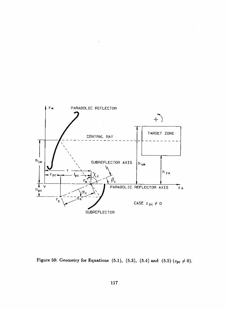
PARABOLIC REFLECTOR c x m
h
TARGET ZONE
- - - - _ _ _ _ _
- REFLECTOR A X I S
c
zm
\
SUBREFLECTOR
Figure 50: Geometry for Equations (5.1), (5.3), (5.4) and (5.5) ( zw # 0).
117

i PAR A BO L I C R EF LECTO R
CENT - - - R A L R - - - AY - - TARGET ZONE - 7 - I
\ SUBREFLECTOR A X I S I
A X I S
hlm
c REFLECTOR A X I S Z,
Jpc = f
Figure 51: Geometry for Equations (5.1), (5.3), (5.4), and (5.5) (zpc = 0).
118

e
t
v
UPPER CHAMBER
ABSORBER LAYER
;&iFi5L
Fs
LOWER CHAMBER SUBREFLECTOR
TARGET ZONE
ING LAYER
h
SUBREFLECTOR AXIS --
PARABOLIC REFLECTOR A X I S
Figure 52: Vertical dimensions of compact range upper room for the “iterative design” arrangement.
119

t
TARGET ZONE
V
7 I
Figure 53: Vertical dimensions of compact range upper room for the new design FD.
120
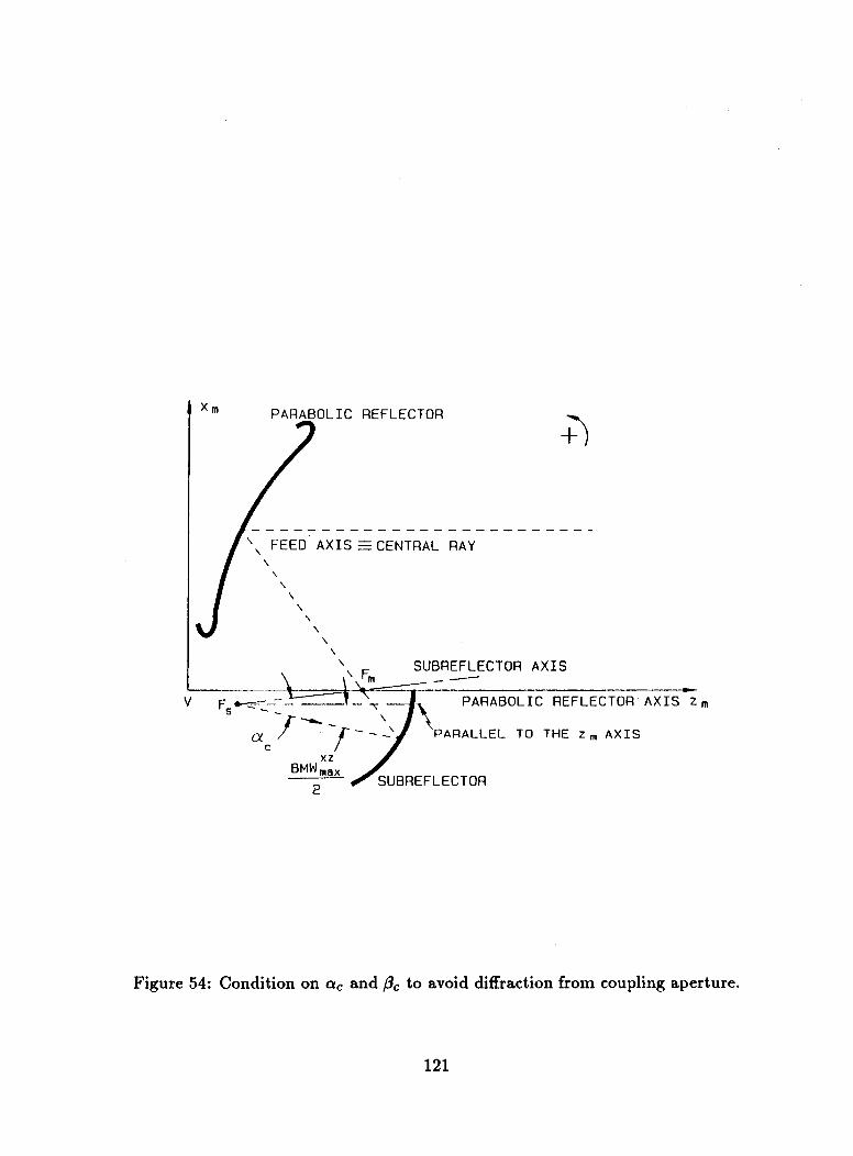
X m P A R A B O L I C R E F L E C T O R
- - - - - - - - - - - - - - \ F E E D A X I S G C E N T R A L
\ \ \
\ S U B R E F L E C T O R A X I S -- c
P A R A B O L I C R E F L E C T O R A X I S Z m
P A R A L L E L TO THE Z m A X I S
S U B R E F L E C T O R
Figure 54: Condition on aC and Pc to avoid diffraction from coupling aperture.
121
where Pd is the length of the semidiagonal of the rectangular target zone cross-
section. On the other hand, M is a function of e a , still to be determined, then
fmin is also a function of ea. Then, any f 2 fmin satisfies the taper requirements
for the reflected field. Then, in the first design procedure it has been set such
that f = fmin and therefore gro = gromin is obtained. In the remaining design
procedures instead it is necessary to verify if the gro obtained from the design
satisfies the gro,j, requirement.
The pattern behaviour of the feed is characterized through two beamwidths,
BMW"" and BMW?', which correspond to two different requirements that the
feed must satisfy.
The beamwidth, BMW"", is defined (Section 3.2) with reference to the an-
gles at which the pattern intensity of the feed becomes smaller than a given value
X in dB, where X is an appropriate small value obtained from diffraction con-
siderations in that the feed illuminates the coupling aperture. This illumination
of the coupling aperture by the feed is a very undesirable effect for two reasons.
For certain angles, there could be a direct illumination of the target zone by the
feed. This is undesirable, but can be time-gated. The second and more important
reason is that, through the lower portion of its main lobe or its side lobes, the
feed illuminates the edges of the coupling aperture, with subsequent diffraction
by the edges themselves. Some of the diffracted rays are reflected by the main
reflector into the target zone, and cannot be time-gated. Consequently, in order
to reduce this diffraction to a minimum, the field incident on the target zone must
be minimized. The appropriate value for the quantity X is determined through
diffraction considerations and is not discussed here. Since in actuality the coupling
aperture is an extended surface and not a point, it is not easy to define exactly
the beamwidth, BMWga,, as the maximum acceptable value of BMW"". Two
122
possible definitions are considered here, although, these are not the only ones pos-
sible. In actuality, one should consider in detail the field incident on the edge of the
coupling aperture and perform a diffraction computation in order to verify if the
level of the sidelobes of the feed considered is acceptable. The quantity BMWZA,
is only a first cut parameter to help in the design of the feed.
One could define BMW;;, with reference to the central point of the coupling
aperture; i.e., with respect to Fm. In this case, one would set BMWFa, = 21acl.
It seems instead a more conservative approach to define B M W Z , with re-
spect to the parallel to the main reflector a x i s through the phase center of the feed
(;.e., the focus of the subreflector, Fd). In this case, the following inequality must
be satisfied to avoid a strong illumination of the edges of the coupling aperture
(see Figure 54): B M W Z , BMWxZ
2 = a c - Pc 2 2 (5.9)
This is the definition used in the design procedures presently discussed. The second
design procedure is then obtained by letting
BMWxZ B M W Z , - - a, - pc = 2 2
(5.10)
and by computing accordingly the design parameters.
A second requisite on the feed is that it must illuminate uniformly (or with
some suitable roll-off correction) the target zone, and BMWfZ is the secondary
illuminating beamwidth defined in Section 3.2. This beamwidth is equal to the
angle subtended at the focal point Fd by the secondary illuminating surface in the
z, z plane (see Figure 55) . The third design procedure is then obtained by enforc-
ing the requirement that this beamwidth corresponds to the target zone through
the reflections from the subreflector and the main reflector, and by Computing the
design parameters accor ding1 y.
123

From the previous constraints then, together with the zero cross-polarization
condition, it is possible to obtain four design procedures, which are summarized
here.
6.1.3 FIRST DESIGN PROCEDURE (METHOD 1)
The quantities h,, hum, hl,, f d , and gromin are specified in this design pro-
cedure, and zpc is set to zero. The following parameters are computed: BMWEa,,
a c , P C , xc, f, E,, d,, M, m, and BMW:'. In this procedure, gromin (the inin-
imum admissible taper of the reflected field) is an input, and a value of the
feed beamwidth, BMW:&,, is obtained, such that the actual feed beamwidth,
BMW"', must satisfy the following inequality:
BMWxZ 5 B M W Z , . (5.11)
This procedure allows one to obtain the parameters B M W Z , and BMW:' nec-
essary for the design of the feed.
6.1.4 SECOND DESIGN PROCEDURE (METHOD 2)
The quantities h,, hum, hl,, f d , and BMWZZ are assumed, and zpc is set
to zero. The following quantities are computed: gro, cyc, Pc, xc, f, E,, d,, M, m,
and BMW:'.
In this procedure the feed beamwidth, BMWxr , is an input, and the corre-
sponding value of the gro is obtained. This procedure allows one to verify how a
given feed (for instance, a horn with given characteristics) performs if used as a
compact range feed. This second procedure can be alternated with the first and
third to obtain a satisfactory design for a given application.
124

6.1.6 THIRD DESIGN PROCEDURE (METHOD 3)
The quantities h,, htm, hum, pd, and BMW?" are assumed, and z, is set
to zero. The following quantities are computed: gro, ac, p,., xc, f, E , , d , , M, m,
and B M W Z z .
In this procedure the feed beamwidth BMW?' is an input. The corresponding
value of the gro is obtained. Again this procedure allows one to verify how a given
feed performs if used as a compact range feed.
5.1.0 FOURTH DESIGN PROCEDURE (METHOD 4)
The quantities zP, h,, hum, hl,, pd and xc are specified in this design proce-
dure, and zpc can be different from zero. The following parameters are computed:
BMWga,, ac, Pc, f, eS, d ~ , pd, M , m, and BMW?". In this procedure, the tilt
angle, xc , and the height of the axis of the target zone, htm, are assumed. This de-
termines the focal length f. The quantities t~ and m are then computed, together
with all the remaining quantities.
These design procedures are examined in detail in the following sections.
5.2 AN EQUATION USED IN THE FIRST, SECOND AND THIRD DESIGN PROCEDURES
The following basic equation has been derived in Section 5.1.1 under the
condition zpc = 0:
2h, = - tanPCtan ($1 . htm
(5.12)
From this equation, one can obtain an equation used in the first, second and third
design procedures.
Equation (5.12) is written as
1 (5.13)
125
then
where
t k - 1 tx , = H -
t Pc
H = - h, 7 tx , = tan (5) , and toc = tan (e) . htm
By making use of the cross-polarization equation, one obtains inmiediately
(5.14)
(5.15)
(5.16)
Since m2 > 0, the range of validity of the solutions must be established such that
the following inequality: - (1 + H ) - > o --
(1 + H ) t & - H - is satisfied. This inequality in turn is satisfied if
Ht$c - (1 + H ) 2 0 , and
(1 + H ) t $ C - H > 0
{ (1 + H ) t ; - H < 0 . Ht;c - (1 + H ) 5 0 , and
I or if
The first set of inequalities gives
tgC 2 (1 + H ) / H = 1 + 1 / H , and
t$c > H / ( 1 + H ) = 1 - 1/(1 + H )
which is satisfied if 1
t& 2 1 + and the second set of inequalities gives
t& 5 (1 + H ) / H = 1 + 1/H , and
1 8 < H / ( 1 + H ) = 1 - 1/ (1+ H )
(5.17)
(5.18)
(5.19)
(5.20)
(5.21)
(5.22)
126

which is satisfied if
(5.23)
Therefore, any solution of Equation (5.16) is acceptable if tZc belongs to the fol-
1 t;c < 1 - -
1 + H *
lowing union of intervals:
1 (0 I t;c < 1 (5.24)
These inequalities are important. In fact, the design equations are higher
order equations (second and fourth order) which have more than one solution. It
is necessary then to be able to discard the spurious solutions by verifying which of
the solutions satisfies both the Inequalities (5.21) and (5.23).
5.3 DIRECT DESIGN METHOD 1
The first design equation is derived in this section. The following quantities
are initially specified by the designers:
h, httn
gro, and H = - . (5.25)
An expression (called the design equation) for tan(&/2) in terms of the given
quantities Pd, gro and H is derived and then the other parameters are expressed
in terms of tan(P,/2) and the specified quantities.
By expressing the magnification factor [12] in terms of tan(Pc/2), one finds
From Equation (G.41), the focal distance f is given by
f = gd1 !?ire (5.27)
127

at the same time, f is given by
Then, by equating the two expressions, one obtains that
The quantity, Q , is presently defined by the following equation:
(5.28)
(5.29)
then one finds that
This equation is presently used to obtain tpc such that
(5.31)
&M(t& - 1) - tpc = 0 (5.32)
& m ( t h - 1 ) - tpc(m2t& + 1) = 0 . (5.33)
Note that the term m2 has been already obtained in terms of H and tpc , so that
Ht& - (1 + H ) ,2 =
(1 + H)t& - H *
Consequently, Equation (5.33) can be rearranged so that
(5.34)
One obtains from Equation (5.34)
2 2 - ( 1 + H ) (1 + H ) t z c - H
m tPc + 1 = tpc + 1 , and (5.37)
1 2 2 X nt tpc + 1 =
(1 + H)t$ C - H
{ [ H t & - ( 1 4- H)]t$c + ( 1 + H)t;c - H } (5.38)
128

where the term inside the braces gives
Therefore, one obtains
2 2 H(tZC - 1 ) rn tPc + 1 =
( 1 + H)t& - H (5.40)
and Equation (5.36) becomes
Ht$c - ( 1 + H ) ~ Q(t$c - . (5.41)
H(t$c - 1 ) (1 + H)t$c - H (1 + H)t$ - H
Both sides of the previous expression can be divided by (tZc - 1)2 and multiplied
by [(l + H)t$c - HI2 such that one obtains
Q[Ht$ C - ( 1 + H ) ] [ ( l + - H ] = H2t$c (5.42)
or
Q H ( l + H ) t $ - [H2(1 + Q ) + Q(l + H)2]t$c + Q H ( 1 + H ) = 0 - (5.43) C
If one sets t = tgC, Equation (5.43) can be written as a second order equation in
t, as follows:
I Bot2 + Blt + B2 = 0 I (5.44)
where the coefficients Bi are given by
Bo = Q H ( 1 + H ) (5.45)
B1 = -H2(1 + Q ) - Q(l + H ) 2 = -H2(1 + 2Q) - Q(l + 2 H ) (5.46)
B2 = Q H ( l + H ) , a n d (5.47)
tpc = 4i (5.48)
129

and t > 0. This second order expression is the design equation. The coefficients of
this equation are expressed in terms of the input quantities, and hence are known.
The equation can then be solved. If there is more than one solution, the actual
value of tPc can be found by substituting the roots back into the original equations
and by checking if the Inequalities (5.21) and (5.23) are satisfied. '
5.4 DIRECT DESIGN METHOD 2
The second design equation is derived in this section using the following spec-
ified quantities:
BMW"", and H = - h, . htnt
(5.49)
As seen before, the beamwidth, BMW"", describes how fast the radiation pattern
of the feed is reduced (i.e., becomes lower than a certain chosen amount of dB)
outside its main beam. An expression for tan(Pc/2) in terms of the given quantities
is derived (the design equation). All the other quantities can then be derived in
terms of tan(Pc/2), the specified quantities and the length of the semidiagonal of
the target zone, Pd.
The geometry for this design procedure is shown in Figure 55, and the fol-
lowing relationship has been derived in Section 5.1.2:
BMW"" 2 Pc - a c =
By dividing both sides by two and taking the tangent, one obtains
(5.50)
and then G is a known quantity, since BMW"" is known. One then obtains
(5.51)
(5.52)
130

Figure 55: Geoiiiet,ry of Ditpct Design. Met,liod 2.
131

From Equation (5.16), one recalls that
(5.53)
as it has been determined in Section 5.2, with the condition that t$, belongs to
the unions of intervals
1 1 -) u (1 + g < t;,) . (0 L toc < 1 - 2 1 + H
Equating Equation (5.53) with Equation (5.52) squared, one obtains that
By multiplying both sides by
(5.54)
(5.55)
one obtains
[H$, - ( 1 + H)](G$, + tpc)2 - [(l + H)t& - HI($, - G)2 = 0 (5.57)
or
HG2t$c + 2HGt$, - [l + ( 1 + H)G2]t$, -
11 + (1 + H)G2]t;, - 2HGtpc + H G ~ = 0 . (5.58)
This last expression can be factored as follows:
($, + 1)(HG2$, + 2HG$, - (1 + ( 1 + 2 H ) G r 2 Itpc 2
-2HGtpc + H G 2 ) = 0 . (5.59)
Then, dividing by the factor t& + 1 (which has only imaginary solutions), one
finally obt ains that
132

This results in the following fourth order equation in the unknown term tPc
(5.61)
where the coefficients are given by
A0 = HG2
Ai = 2HG
A2 = - [ 1 + ( 1 + 2 H ) G 2 ]
A3 = -A1 ) and
A4 = A o .
(5.62)
(5.63)
(5.64)
(5.65)
(5.66)
These coefficients are known in terms of the specified design parameters, so that the
design equation can be solved. A solution for tPc can be found using known search
procedures (Raphson-Newton, for instance) or by using the known expressions for
solving a fourth order equation, or a combination of both to improve the numerical
precision. The solution must belong to the following union of intervals:
2 1 0 I tpc < 1 - -
1 + H (5.67)
which completes the design.
6.5 DIRECT DESIGN METHOD 3
The third design equation is derived in this section. The following quantities:
(5.68)
are assumed to be specified by the designer. The quantity, BMW?', is the illu-
minating beamwidth which characterizes the main beam of the feed. Again, an
expression for tan(P,/2) in terms of the given quantities is derived (the design
133

MAIN REFLECTOR
Figure 56: Geometry of Direct Design, Method 3.
134

equation). All other quantities can then be computed in terms of t P c , the specified
quantities and pd.
Let hum be the height (the 2m coordinate) of the upper edge of the primary
illuminating area, xu be the angle of the corresponding upper illuminating ray
with the axis of the main reflector, and cyu be the polar angle of the corresponding
secondary illuminating ray with respect to the subreflector polar coordinate system
as shown in Figure 56. Then, the following relationships hold:
___ hum - - cot (F) 2f
where the geometry is shown in Figure 56. One then obtains
where
, t x , = tan (F) , and tpc = tan
From Equation (3.1) and Equation (5.14) one obtains
R = - . htm where hU,, txu = Rtxc
Then, Equation (5.71) becomes
By letting a c - a u BMWrz
t a n ( ) = t a n ( ) = ~i
where Gi is a known quantity, since BMWilEZ is known~, one obtains
m2tp,[(1 + RH)t$c - R H ] - tp , [RHt$c - (1 + R H ) ] + - m G i R H ( t i C - 1) = 0 .
(5.69)
(5.70)
(5.71)
(5.72)
(5.73)
(5.74)
(5.75)
(5.76)
135 '

This expression can be solved for m as follows:
m = G;RH(t$ - I ) {m2[(1 + R"t& - R H ] - [RHt;c - (1 + R H ) ] } (5.77) C
which can be written as
m = X { m 2 Y - Z } . (5.78)
By squaring, one obtains
m2 = x2 {m4y2 - 2 m 2 y z + z2} (5.79)
then
(5.80) (m 2 2 x 2 Y 2 - m2(1 + ~ X ~ Y Z ) + x2z2 = o
and, by Equation (5.16) 2 - (1 + H )
m = (1 + H ) t $ - H
C
Then, using these results, one obtains
(5.81)
- qc - (1 + H ) X
(1 + H)tZc - H
t$C { 1 + 2 ( G i R H ) 2 4 ( tP C - 1 ) 2
[RHtJc - (1 + R H ) ] 2 = 0 . "C
(GiRH)2(t$c - 1)2 +
(5.82)
By multiplying by
2 4 I [(I + H)t$c - HI2(GiRH) (tpc - (5.83)
136
one obtains
or
This can be written as follows:
where
Tl = HtgC - ( 1 + H ) (5.87)
T2 = ( 1 + RH)tZc - RH (5.88)
T3 = ( 1 + - H , and (5.89)
T4 = RHtgC - (1 + R H ) . (5.90)
Then, it follows that
(5.91) t&(T1T2 - T3T4)2 - (GiRH)2T1T3(t$c - 1) 2 = O
137
with
T1T2 = [Hi& - ( 1 + H ) ] [ ( l + RH)tZC - R H ]
TiT2 = H ( l + RH)t$c - RH2t$c
-(1 + H ) ( 1 + R H ) t z c + ( 1 + H ) R H
TiT2 = H ( 1 + RH)t$c - [ R H 2 + ( 1 + H ) ( 1 + RH)]tZc
+(1+ H ) R H
T3T4 = [(I + H)t$c - H ] [ R H t & - ( 1 + R H ) ]
T3T4 = ( 1 + H ) R H t j C - ( 1 + H ) ( 1 + RH)tZc
-RH2tgC + H ( l + R H )
T3T4 = (1 + H ) R H I J c - [(l + H)(1 + R H ) + RH2]t&
+ H ( 1 + R H )
TiT3 = [Ht& - ( 1 + H ) ] [ ( l + H)t$c - HI
TiT3 = H ( 1 + H)t$c - H2t& - ( 1 + H)2t$c + H ( l + H )
TlT3 = H ( 1 + H)t$c - [ H 2 + ( 1 + H)2]t$c + H ( l + H )
and
(5.92)
(5.93)
(5.94)
(5.95)
(5.96)
(5.97)
(5.98)
(5.99)
(5.100)
T1T2 - T3T4 = H ( 1 + RH)t$c - [ R H 2 + ( 1 + H ) ( 1 + RH)] tgC + ( 1 + H ) R H
-(1 + H)RHt$c + [(l + H ) ( 1 + R H ) + RH2] t zc
- H ( 1 + R H ) (5.101)
2 4 T1T2 - T3T4 = ( H + R H 2 - R H - R H ) I p
2 2 RH^ + I + RH + H + RH^ - 1 - RH - H - RH^ - RH )tpc
+RH + RH^ - H - RH^ (5.102)
(5.103) T1T2 - T3T4 = H ( l - R)t$c - H ( l - R )
138

T1T2 - T3T4 = H(l - - 1) . (5.104)
Therefore, one obtains the following equation by performing the substitutions and
by dividing Equation (5.86) by H 2 4 (tpc - 1)2, such that
t;c(l - R)2 +
(GiR)2H(1 + H)t$c + -{(GiR)2[H2 + (1 + H ) 2 ] + (1 - R) 2 2 )tpc +
+(GiR)2H(1+H) = 0 . (5.106)
By letting t = t$c one obtains the following design equation:
I Cot2 + Clt + c2 = 0 1 (5.107)
where the coefficients Ci are given by
Co = (GiR)2H(1 + H ) (5.108)
(5.109) C1 = -(Gill) [ H + (1 + H ) 2 ] - (1 - R)2 , and
Cz = (GiR)2H(1 + H ) = Co . (5.110)
2 2
5.0 DIRECT DESIGN METHOD 4
The fourth design equation is derived in this section, using the following spec-
ified quantities:
h, 9 Z p c , hum 7 hl, , and x c * (5.111)
The general case for which the phase center of the feed antenna is not vertically
aligned with the vertex of the parabolic reflector is considered in this design pro-
cedure. The geometry is shown in Figure 50.
139
The focal length f is determined in terms of the tilt angle xc and the height of
the axis of the target zone, him. All the other quantities can be derived in terms of
tan(pc/2), the specified quantities and the length of the semidiagonal of the target
zone, pd. The phase center has Xm, Ym, zm coordinates given by (h,, 0, 2,).
This equation has been previously derived
and one obtains for f 1 2 f = -htmtXc .
The following equations are derived from Figure 50
1 htm = him + Z ( L m - hi,)
f = dscospc + .+
(5.112)
(5.113)
(5.114)
(5.115)
(5.116) hpc = -ddsinPc . Equation (5.115) can be solved for d, cospc
and, by taking the ratio of (5.116) and (5.117) one obtains
(5.118)
which expresses the unknown tilt angle Pc in terms of h,, z, and f . The quantities
h, and z, are assumed to be known, while f is computed in terms of the angle xc through Equation (5.113). The quantity tPc is then known, since tpc = tan(pc/2).
6.7 EVALUATION OF VARIOUS DESIGN PARAMETERS
Having evaluated tPc with any of the design equations, the remaining quan-
tities can be computed accordingly. Some of the quantities (viz. x,., f , m) are
140

evaluated differently for methods 1, 2, 3 from method 4, while the remaining are
evaluated in the same way for all methods.
5.7.1 METHODS 1, 2 AND 3
Having evaluated tPc with any of the design equations (method 1, 2 or 3), the
remaining quantities can be computed accordingly. It has been found that
2 - (1 + H) (1 + H)t$c - H
m =
where tgC belongs to the union of intervals
( 1+z5t$c l ) . Since m > 0 (convex ellipsoidal subreflector), one writes the following:
m = @
where the square root is understood in the arithmetic sense.
Also, one finds that t$= - 1
t,, = H - t P C
xc = 2arctan(txc)
(5.119)
(5.120)
(5.121)
(5.122)
(5.123)
(5.124)
5.7.2 METHOD 4
The angle xc is an input. The focal length f is immediately derived from
Equation (5.113), and does not depend on tPc, such that
1 2 f = - htmtxc (5.125)
the axial magnification m is obtained from this equation
where only the positive sign has been considered.
141

5.7.3 REMAINING QUANTITIES
All the remaining quantities are computed in the same way for all design
procedures. One finds that
tac = mtp, (5.127)
cyc = 2arctan(tac) (5.128)
P c = 2arctan(tpc) (5.129) m - 1 m + l
€3 = (5.130)
(5.131)
(5.132)
(5.133)
BMWG, = 2(Pc - ac) using method 1, 3 or 4 (5.134)
grodB = 20 log10 { (2M f / P d 2 /[I + (2M f/PdI2]}
using method 2, 3 or 4. (5.135)
The secondary illuninating beamwidth in the zmzm plane, BMW?’, can be com-
puted through the following equations, such that
BMW:’ = aU - q (5.136)
where
xu = 2arctan ( -E)
X I = 2arctan (E) hU, (5.137)
(5.138)
(5.140)
142
Recall the following parameters:
0 au is the angle from the subreflector a x i s to the secondary illuminating ray
corresponding to the upper point of the primary illuminating surface in the
z,, plane
0 xu is the angle from the main reflector ax is to the primary illuminating ray
corresponding to the upper point of the primary illuminating surface in the
zm, z , plane, and
0 h,, is the z, coordinate of the upper point of the primary illuminating
surface in the z,, znr plane.
Sinlilar definitions correspond to a2, xi, hl, for the lower point of the primary
illuminating surface (see Figure 47). In this way all quantities are determined, and
the GO design is complete.
5.8 CONCLUSIONS
Several simple design equations have been derived in this chapter, which allow
one to compute in an exact way all the geometrical parameters of a compact
range subreflector system in terms of suitable input variables, which represent
the specifications for the design. These equations have been easily converted into
a computer program, called WAYLAND, which allow one to perform the design
simply, quickly and efficiently, without the iterations and uncertainties which are
unavoidable with an iteration procedure like the one described in Chapter IV.
143

CHAPTER VI
COUPLING APERTURE DESIGN
6.1 BEHAVIOUR OF WEDGE SHAPED ABSORBER
The qualitative behaviour of wedge shaped absorber is briefly described to
better understand the design of the coupling aperture. A more complete discussion
is available in [16]. The wedge absorber is modeled as a dielectric wedge such
as shown in Figure 57. It is assumed that a uniform plane wave is incident
on the wedge. As for a conducting wedge, an incident shadow boundary and a
reflection shadow boundary are present, and the diffracted field has to compensate
for the discontinuities of the GO field. The reflected field is equal to the incident
field multiplied by the reflection coefficient, which is considerably less than one
for a good absorber. Consequently, the reflected field for an absorber wedge is
considerably less than for a conducting wedge, and the corresponding diffracted
field is proportionally weaker. A transmitted field is also present, and its intensity
is given by the incident field multiplied by the transmission coefficient and an
exponentially decaying term depending on the actual thickness of absorber crossed
by the ray. Also, the transmitted ray changes direction. Again the diffracted
field has to Compensate for the discontinuity between the incident field and the
transmitted field. If the transmitted field is weak, the diffracted field at the shadow
boundary is strong. In other words, the more effective the wedge absorber is in
blocking the incident field, the stronger is the diffraction at the incident shadow
144

boundary. Thus to mininliae diffraction it is necessary to use low loss absorbing
materials or, alternatively, to use a wedge with a small wedge angle. On the other
side, it is also desired that the absorber attenuates the transmitted signal.
These considerations also suggest a design criterion for absorbing materials,
for which the absorbing properties should gradually increase from zero (free space)
to high absorption.
6.2 GO DESIGN OF THE OVERSIZED SUBREFLECTOR AND THE COUPLING APERTURE
In this section the GO design of the coupling aperture is illustrated through
a specific design example. The example considered is design FD, shown in Figure
66 and in Table 5.
The main parabolic reflector has rolled edges to minimize the diffraction from
its terminations. This diffraction, in fact, would corrupt the plane wave reflected
field. For the subreflector, it is necessary to avoid the diffractions from its ter-
minations which can illuminate either the main reflector or the target zone and
cause undesirable errors. This is achieved by overextending the subreflector and
by designing the coupling aperture so that the diffracted rays are absorbed in a
proper way. This is a better approach than using rolled edges on the subreflector
itself, which are difficult to design for a very concave surface. In fact, a subre-
flector with rolled edges would be as large as an overextended subreflector, while
being more complex to design and manufacture. The motivations and design of
the overextension of the subreflector can be better seen in two steps. The design
is performed in the zm, zm plane. Let t , be the length, in the zm, z, plane, of
the part of the subreflector illuminated by the secondary illuminating beam (;.e.,
by the beam from the feed antenna corresponding to the target zone) from the
145

/
1’ REFLECTION SHADOW
BOUNDARY /
/ /
/ /
/
\ \ \ \ \ \ \
\, INCIDENT TRANSMITTED SHADOW
BOUNDARY ABSORBER RAY \
WEDGE
Figure 57: Wedge absorber illuminated by a plane wave.
146
feed antenna, and delimited by the points, I,, and Id,, as shown in Figure 58.
Then, on all sides, the subreflector is extended by an amount of about C,, obtain-
ing a subreflector having, in the z,, z, plane, a total length of about 3 C,, as
shown in Figure 58. This subreflector is called the extended subreflector. From
the same figure it can be seen that the reflection shadow boundary at the edge
Si is given by the ray, R I ; while, the reflection shadow boundary at the edge S l
is given by the ray, Rsk. These rays are separated anglewise from the rays, Ri
(from Id, to Id,) and 72, (from Ius to I,,), which coincide with the lower and
upper illuminating rays and correspond to that part of the subreflector which is
actually illuminating the target zone. Still, in order to increase this separation,
and consequently to reduce the amount of diffraction from the lower into the upper
chamber, it is desirable to further extend the subreflector by, for instance, about
e,, on all sides, obtaining new edges (called S, and SI in the z,, z , plane) and
new corresponding shadow boundaries (called Rs, and Rsl) as shown in Figure
60. This is called an overextended subreflector. In performing this extension, it
is important that the rays reflected from the subreflector avoid going directly into
the target zone through the coupling aperture; in other words, it is important not
to extend the subreflector too much on the side of the edge, S,. Instead, on the
side of Si, the extension of the subreflector is limited by the fact that the sub-
reflector must be all inside the lower chamber. These new shadow boundaries,
Rs, and Rs, are farther removed from the rays, Rd and R,. The reason to intro-
duce this overextension of the subreflector becomes apparent from the design of
the coupling aperture, which is described later. In fact, it is advantageous to let
the rays, Rs:, and R I , pass through the coupling aperture without experiencing
any absorbtion. These reflected rays, coming from the points, SL and Sf, are di-
rected towards areas of the ceiling/walls which are covered by absorber material,
SI
SI
147

away from the target zone. Therefore, they can be absorbed without perturbing
the plane wave in the target zone. If instead they were absorbed in the coupling
aperture, a shadow boundary would be introduced close anglewise to the parabolic
reflector, with subsequent reflection and diffraction in the target zone. The time
delays of these reflected and diffracted rays would be very close to that of the
plane wave illuminating the target zone, and no time gating would be possible.
Instead, the reflection shadow boundaries, Rs, and as,, are further separated an-
glewise from the parabolic reflector; therefore, the related diffracted rays, reflected
or rediffracted by the parabolic reflector, are much weaker. It is possible then to
intercept these rays with the absorber at the coupling aperture, since the incident
shadow boundaries introduced by the absorber are sufficiently removed anglewise
from the parabolic reflector.
The GO design of the coupling aperture is now described. The minimum
diameter of the coupling aperture is determined by the minimum frequency of
operation of the range. This diameter, d,, is safely assumed to be about 5 wave-
lengths at the lowest frequency of operation, and it is centered around the focal
point, Fnz. In the design presently considered, this corresponds to a diameter of
approximately 75 cm, or about 2.5', because the lower frequency of operation is 2
GHz. At the focal point, Fm, the actual field does not shrink to a point, as GO
would predict, but instead occupies a finite region of space, as shown in Figures
40 and 41. Since the diameter of the coupling aperture is specified, the points
Cl and C , are located. The thickness of the coupling aperture is determined by
evaluating the performance of the absorber material used. In the present design,
the absorber thickness, h,, is 2'. The absorber layer is all above the main reflector
axis, so that the ceiling of the lower chamber is set at 2 = 0. Once the thickness,
h,, of the absorber is determined, it is necessary to determine the shape of the
148

coupling aperture. It is clear that its shape must be such that the reflected beam
from the subreflector can flare out towards the main reflector without attenuation;
while, the diffracted rays are attenuated. The absorber around the coupling aper-
ture is shaped as a series of wedges, stacked one above the other, typically two or
three wedges, having height approximately of h,/3 each.
The design of the shape of the coupling aperture of the subreflector can be
better understood through several steps. It is desired to let the rays, R r and
R s ~ , go through the coupling aperture unimpeded. Otherwise, diffraction shadow
boundaries would be introduced, which would be close anglewise to the edges, Ilrn
and I,, (lower and upper, respectively), of the parabolic reflector. In fact, the
rays, R,r and Rsh, are not directed towards the target zone, but rather towards
the wall on the back of the main reflector or towards the ceiling. Both areas are
covered with absorber, and these rays are safely absorbed (perhaps, after reflection
from the rolled edges). If the subreflector were terminated at the points, Sf and
Sh, the wedges of the coupling aperture would be shaped with sides parallel to the
rays, R,r and Rsh, and the design shown in Figure 59 would be obtained. But
this design is not satisfactory. In fact, it is important that the coupling aperture
eliminates the diffracted rays directed from the edges of the subreflector towards
the edges of the main reflector. These rays are indicated as Dsh and 2, r in Figure
59. The diffracted ray, Dsk, goes from the point, SL, to the edge point, I,,;
while, the ray, 2) r , goes from the point, Sf, to the edge point, Il,. These rays
would cause diffraction in the target zone, in that they would be rediffracted in
the target zone by the edges of the main reflector, while the diffracted rays which
are close anglewise to 2) r and ZJ r and are directed towards the portion of the
main reflector between I, and I,,, would be reflected in the target zone. In
both cases the plane wave in the target zone would be deteriorated. It can be
Sl
1
1
Sl
% s1
149
seen from Figure 59 that the absorber wedge angles are large (especially at Cl),
introducing diffraction, but at the same time the rays, and I) I , go through a
thin portion of the wedges (if they go through any at all), with little attenuation,
and the coupling aperture would fail to accomplish its main purpose. For this
reason then it is desirable to extend further the subreflector to the points, Sl and
S,, by an amount of e, on each side, obtaining the design of Figure 60, where the
subreflector has an overall length of about 5l , . In fact, after the corresponding
coupling aperture has been designed, it has been found that a length of 4Qd was
SI
not sufficient to insure a good attenuation of the rays I)s, and Ds1. The design of
the overextended subreflector is then completed.
To complete the design of the coupling aperture, it is necessary to determine
the shapes of the “Cl” and “C,” sides of the coupling aperture.
On the “C,” side, the purpose of the coupling aperture is to block the diffracted
ray, Ds,, which goes from the point, S,, to the point, Ium. The coupling aperture
at C, is slanted with a slope equal to that of the reflected ray, Ri, obtaining a
wedge-like structure, as shown in Figure 61. The angle of this wedge is suffi-
ciently small to reduce its diffraction to an acceptable value. This wedge intro-
duces a shadow boundary, with subsequent diffraction. It is important then that
this diffraction be low in the direction towards the point, Iz,, and for this reason
the subreflector is overextended on the Si side. If only one wedge were used on
the “C,” side , the coupling aperture would be too large. A second wedge then is
introduced on top of the first. In order to make the transition of the field gradual,
this second wedge is inverted. The reason for this choice can be seen through a
counterexample; in other words, it is now shown how a bad choice for the shape
of the second wedge would introduce a strong diffraction. One should consider in
fact Figure 63, where a second wedge has been added, having the same slope as
150
the first. The two rays, 'Ri and R;', which are very close anglewise, are considered.
The ray Ry goes through a thick piece of absorber, experiencing a strong atten-
uation (if the absorbing material has high absorbption properties). Instead, the
ray 72; does not experience any attenuation. This arrangement then introduces a
discontinuity in the field directed from the subreflector towards the main reflector,
with a resulting strong diffraction with' 7Z; as a shadow boundary. Instead, it is
not necessary to strongly attenuate the rays like Ry, which can be absorbed by
the absorber on the walls of the upper chamber (perhaps, after reflection from the
rolled edge). Thus, this diffraction can be reduced by the inverted wedge arrange-
ment, which does not introduce such a discontinuity. In this way the amount of
diffraction reflected by the main reflector into the target Gone is reduced. There-
fore, the inverted wedge arrangement is better suited for the present purposes, and
the design of Figure 61 is obtained, where the details of the coupling aperture are
shown in Figure 62. The position of the tip, Ch, of the second wedge is determined
as follows. A line parallel to the ray, 'Ri , is drawn, at a distance of dc /2 , obtaining
the line b,, then the tips of the wedges on the "C," side of the coupling aperture
must not cross bu. The tip of the second wedge is actually set on the 6, line. In
this way, the illuminating beam towards the parabolic reflector is not perturbed
by the absorber, which is sufficiently distant from it. This design insures a smooth
transition through the use of the inverted wedge and a third wedge on top. The
purpose of the third wedge is to make a more smooth transition from unabsorbed
to fully aborbed rays. In fact, this third wedge does not have its tip on the 6 ,
line, as the first and second wedge do, instead, it is not intercepted by the ray
R;. Therefore, since the transition of the field from the coupling aperture from
unabsorbed to very absorbed is gradual, the field diffracted is a higher order effect
with respect to the diffraction from the edges of the subreflector. Consequently,
151

through the adoption of the coupling aperture, the strong diffraction froin the
subreflector edges (S, and Si) is greatly attenuated at the expenses of introducing
a much weaker diffraction from the tips of the wedge absorbers of the coupling
aperture. The vertical heights of these three wedges is about the same, and it is
h,/3, where h, is the thickness of the absorber layer.
For the design of the “Cl” side of the coupling aperture, one should consider
that its purpose is to block the diffracted ray, Dsl, which goes froin the point, Si,
to the point, Iim. Three absorber wedges are stacked as shown in Figure 61 in
order to accomplish this objective. The length of the path of this ray inside the
absorber should be enough to insure a proper attenuation. Instead, the length of
the path corresponding to the shadow boundary, ‘Rs,,, should be such that this
reflected ray and the corresponding adjacent diffracted rays are time gated (see
Section 3.7.5). If these rays are time gated, it is not important if they are not
completely attenuated by the coupling aperture. If instead, the time gating offers a
marginal or no attenuation for these rays (as it happens when the angle xc is close
to goo), it becomes necessary to attenuate these rays by shaping accordingly the
coupling aperture; i.e., by extending the stacked wedges so that they are crossed
by these rays. The slope of these wedges is the same as that of the “C,” side. The
position of the tip, Cf, of the second wedge is determined as follows. A line parallel
to the ray, R,, is drawn at a distance of dc /2 , obtaining the line bi, then the tips
of the wedges on the “Ci” side of the coupling aperture must not cross bi. In this
way, the illuminating beam towards the parabolic reflector is not perturbed by the
absorber, which is sufficiently distant form it. The position of the tip, Cf’, of the
third wedge is determined so as to be as close to the line bl as possible without
perturbing the ray Rsl. The height of the wedges is the same, h,/3.
With this procedure, the shape of the coupling aperture “follows” the shape
152
of the illuminating beam, reducing to a minimum the size of the coupling aperture
itself, with consequent maximum decoupling between the two chambers. At the
same time, the illuminating beam is not perturbed by interactions with the sides
of the coupling aperture.
The design of the coupling aperture is then completed. However, it is im-
portant to realize that the qualitative explanations presented in this section are
just a guideline, and they do not constitute a rigid prescription. Using a similar
approach, a different discussion of the design of the coupling aperture is presented
in [2].
From these design guidelines it is clear why a rolled edge on the lower part
of the parabolic reflector offers a better performance than a continuation of the
reflector in its lower part until its edge reaches the absorber on the floor of the
upper chamber. In fact, such a parabolic continuation would reflect towards the
target zone some of the rays diffracted by the tips of the wedge absorbers in the
coupling aperture. Such rays instead are reflected by the rolled edge towards
the absorber on the walls. A similar argument applies to the upper edge of the
parabolic reflect or.
153

Figure 58: Extended subreflector. Linear dimensions are in feet.
154
0
1 1 1 I
I I I I
I I I I I I I I I I I I I 1 1 I 1 " " 1 " " " ' " '
I I
I I
I
I I I
I I I I
- - - - - - I - - - - - -
1 I
I
I I I
+-- -
-I----
I_---
0 -1 - - - - - - - -,r - - - - - -1- - - - - -
IEXTENOEO SUBR&LECTOR
-- - - - - -
- -;- - - - - -
I

Figure 59: Extended subreflector with coupling aperture. Linear dimensions are in feet.
155

G ~ , . . , ; . . . . ; . . . . ; , . . . 1 . . . . 1 I 1 I I
I -5. 0. 5. 10. 15. 20.
Figure 60: Overextended subreflector. Linear dimensions are in feet.
156

e
m'
G
I I 1 I I I I I I 1 I I I I I I I I I I I 1 I
Figure 61 : Overextended suhreflect,or wit,h coupling aperture. Linear dimensions are in feet.
157

\ \
2
\ \
”;\ \ \ \bl \
Figure 62: Detail of the coupling aperture.
158

Figure 63: Overextended subreflector with strongly diffracting coupling aperture. Linear dimensions are in feet.
159

CHAPTER VI1
DIRECT DESIGN EXAMPLES
Figure 64. From this layout it is possible to obtain an idea of the appearance of
the design itself as well as of the size of the extended subreflector. Also, the design
of the coupling aperture is performed by using this layout.
7.2 DIRECT DESIGN. AN EXAMPLE FOR COMPARISON
7.1 INTRODUCTION
The GO design of a new compact range is presented in this chapter, and sev-
eral other examples are discussed. This design is compared with the one obtained
iteratively through a numerical procedure in Chapter IV, to show that the pro-
cedure called “direct design” gives better results; while, the design is performed
in a straightforward way. Several design examples are also presented to show the
system dependence associated with the various design parameters as shown in Fig-
ure 47. For each design, it is given a table with all the design parameters and an
outline of the layout of the parabolic reflector and overextended subreflector. The
outline shows a section in the zm, ynr plane of the subreflector system, the upper
and lower illuminating rays and the central ray are also shown, as, for instance, in
In this section a design is performed with the same specifications as the itera-
tive design (ID) of Chapter IV, which was obtained by a trial-and-error procedure.
The two different designs are then compared in order to realize how much is gained
160
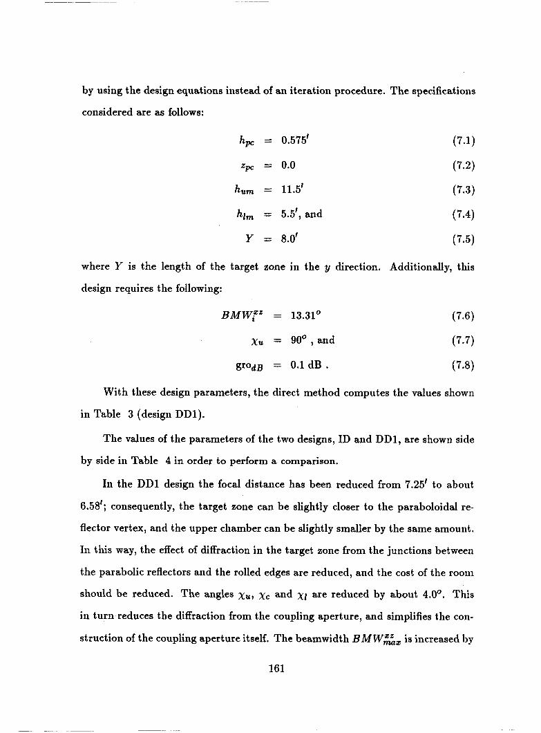
by using the design equations instead of an iteration procedure. The specifications
considered are as follows:
hF = 0.575'
zpc = 0.0
hum = 11.5'
hl, = 5.5', and
Y = 8.0' (7.5)
where Y is the length of the target zone in the y direction. Additionally, this
design requires the following:
BMWrZ = 13.31'
xu = go', and
grodB = 0.1 dB . With these design parameters, the direct method computes the values shown
in Table 3 (design DD1).
The values of the parameters of the two designs, ID and DD1, are shown side
by side in Table 4 in order to perform a comparison.
In the DD1 design the focal distance has been reduced from 7.25' to about
6.58'; consequently, the target zone can be slightly closer to the paraboloidal re-
flector vertex, and the upper chamber can be slightly smaller by the same amount.
In this way, the effect of diffraction in the target zone from the junctions between
the parabolic reflectors and the rolled edges are reduced, and the cost of the room
should be reduced. The angles xu, xc and xl are reduced by about 4.0'. This
in turn reduces the diffraction from the coupling aperture, and simplifies the con-
struction of the coupling aperture itself. The beamwidth B M W Z , is increased by
161

Table 3: Parameters for design DD1
~ h, = 0.575' ZF = 0.0' hum = 11.5'
hi, = 5.5' BMW;"' = 13.31" Y = 8.0'
a, = -19.94765" pc = -4.99295" Ac = 14.9547"
a, = -26.60265' al = -13.29265O xu = 97.71603'
= 134.6466" A t = 9.058338 ns BMWZa, = 29.90941"
xC = 114.2962" f = 6.581607' en = 0.6026589
d, = 6.606677' pa = 3.490487' m = 4.033459
hf = 3.919901 gro,jB = -0.08118021 dB
about l.Oo, reducing, albeit slightly, the direct illumination of the coupling aper-
ture by the feed, with consequent reduction of the related diffraction. The sizes
of the subreflectors are very similar. On the other hand, the DD1 design has at
least one shortcoming: a decrease in the time delay differential A t of about 1 ns.
An adequate duration of this differential is very important in order to insure the
correct time-gating of the rays diffracted by the edges of the coupling aperture into
the target zone, consequently, this time delay differential must be greater than a
minimum value, which, in the present case, is of about 9 ns. One major advantage
of the D D l design is that the design is accomplished easily and in a very short
time, while the trial-and-error approach requires a major effort, and is prone to
errors, in other words, the designer could easily m i s s the optimal design. Notice
that it could be possible to further improve the DD1 design by choosing for the
quantity zpc a value different from zero, as it is done in the examples of the next
sections.
162

Table 4: Comparison between the ID design obtained via an iterative procedure and the DD1 design obtained via the direct method
ID
hpc = 0.575'
zP, = 1.278'
hum = 11.5'
him = 5.5'
BMW?' = 13.31"
Y = 8.0'
a = -19.95"
p = -5.5"
A, = 14.45"
xp = 119.24'
CY, = -26.875"
a1 = -13.565"
xu = 103.164"
xi = 138.454"
A t = 10.248 ns
BMWZ,, = 28.9"
f = 7.25'
€8 = 0.5708
d, = 6.0'
ps = 3.639'
m = 3.662
M = 3.5583
grOdB = -0.0819 dB __
DD1
hF = 0.575'
zp, = 0.0'
hum = 11.5'
him = 5.5'
BMW?" = 13.31"
Y = 8.0'
a, = -19.94765"
= -4.99295"
A, = 14.9547
xC = 114.2962"
a, = -26.60265"
a1 = -13.29265"
xu = 97.71603"
xi = 134.6466'
A t = 9.058338 ns
BMWZa, = 29.90941"
f = 6.581607'
€8 = 0.6026589
d, = 6.606677'
ps = 3.490487'
m = 4.033459
M = 3.919901
grOdB = -0.08118021 dB
163

4
5 -- I 1 I I
I I I I I I I I I Upper ti 1 lurn inat img r a y
1 - - I - - - . 7- I
I I - 1 - - - - - - -
- - I I I I I Lower 5 1 lu rn inat in: r a y
I 1. \ I I---
I I I I I I I I
I I I
\ I \
I - - - - - - -
I \- I I I I I - - - - _ - I - - - - 0 -- - - - - -
Figure 64: Layout of the ID design in the x m zm plane, showing the main reflector, the subreflector, the upper and lower illuniinating rays and the central
ray. Linear dimensions are in feet.
164
I I I
I I I
I I I I I
~ j _ _ _ _ _ _ _ - _ _ _ _ _ - - - - - - _ _ - - - - - - - - - - - - - - I I I I Shbref l e c t o r 1 I
I I I I I I I I I I I I 1 I I I I I I I e I 1 " " 1 ' " ' 1 " " 1 ' " ' I I I
I

P a r a b d l i c r e f l e c t ' o r I I i l lumina t ipg ray I I I
I I
I I 1 I I I I
I I
I I I I I I I 1 I I
I
I------ I
_ _ - - - - - - - - - - - - - - - - - b e n t r a l Ray'
- L--
\-
- - - I
.- - ~- - -
\ I Lower li 1 lurninat inb r a y -------
I 1 I I I
-1 - - - - - - - -1 - - - - - - - - -
I I I I I I I I I
I I I I I I I 1 I I I I I I I I I I I I I I I I I I
0. 5. 10. 15. 20. e I i.,.: , . I . f . I . . : I . . . ; 1 . 1 1
-5.
Figure 65: Layout of the DD1 design in the zm znt plane, showing the main reflector, the subreflector, the upper and lower illuminating rays and the central
ray. Linear dimensions are in feet.
165
7.3 DIRECT DESIGN. REQUIREMENTS FOR THE GO DESIGN OF A NEW COMPACT RANGE
The requirements on the GO compact range are reviewed in this section in
order to improve these designs.
A broadband ridged horn has been designed and built to be used as a feed over
the full frequency range of operation (2-18 GHz). Its beamwidth at the highest fre-
quency of operation is about 12”. It is then desirable that the parameter BMW?’
be reduced from 13.31’ to a value closer to 12’ in order to match the design to
the actual performance of the feed. At the lower frequencies, the beamwidth of
the feed is greater and the consequent spillover and higher incident field on the
edges of the extended subreflector must be accepted in order to provide the desired
bandwidth from just one feed antenna.
In the ID design, the absorber layer between the upper and lower chamber is
arranged in a symmetric fashion, so that the plane which represents the boundary
between the two chambers (the “ceiling” of the lower chamber and the “floor” of
the upper chamber) is half way in the middle of the absorber layer. In the new
design instead the absorber layer is moved entirely inside the upper chamber, as
shown in Figure 53. This provides two advantages:
0 the upper chamber is made higher (which leads naturally to better values for
several design parameters) without any waste of room,
0 the layout of the lower chamber is much easier, since the feed antenna can
be inoved farther from the absorber layer.
It is desirable to increase the distance of the phase center of the feed antenna
from the “ceiling” of the lower chamber, h,, in order to make the mechanical
arrangement of the feed easier.
166

It is desirable to increase the angle A,, where A, = CY, - Pc. In this way the
field incident on the absorber on the walls of the lower chamber from the feed is
reduced, which also reduces the field incident from the feed on the edges of the
coupling aperture.
It is desirable to decrease the angle x,, which represents the tilt angle of
the a x i s of the coupling aperture, in order to make the design of the coupling
aperture itself easier and to reduce the interactions of the illuminating beam with
the absorber on the sides of the coupling aperture. On this regard, the ideal value
of the angle would be 90°, although this value cannot be adopted because in turn
it would reduce the value of the time delay differential A t to an unacceptable low
value by reducing the value of the focal distance f . Recall that A t is the time
differential between rays from the coupling aperture directly to the target zone
versus the desired path through the main reflector and then the target zone.
The size of the extended subreflector for the ID design is fairly large, but still
acceptable. It would be desirable to reduce the size of the extended subreflector,
or, at least, not to increase it.
The taper of the reflected field and the time delay differential A t of the ID
design are very good, and it is desirable to maintain this level of performance in
the new design.
7.4 DIRECT DESIGN. GO DESIGN OF A NEW COMPACT RANGE
The design of a new generation compact range, called the FD design, is pre-
sented. It is shown how its characteristics satisfy the requirements on the design
and represent a reasonable compromise between the conflicting requirements for
the compact range itself. In the Section 7.6 instead, several designs are presented,
obtained by changing the values of some design parameters around the values of
167
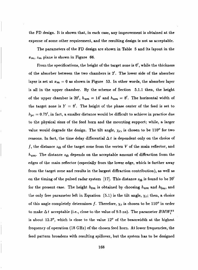
the FD design. It is shown that, in each case, any improvement is obtained at the
expense of some other requirement, and the resulting design is not as acceptable.
The parameters of the FD design are shown in Table 5 and its layout in the
Xm 7 zm plane is shown in Figure 66.
From the specifications, the height of the target zone is 6', while the thickness
of the absorber between the two chambers is 2'. The lower side of the absorber
layer is set at z m = 0 as shown in Figure 53. In other words, the absorber layer
is all in the upper chamber. By the scheme of Section 5.1.1 then, the height
of the upper chamber is 20', hum = 14' and hum = 8'. The horizontal width of
the target zone is Y = 8'. The height of the phase center of the feed is set to
h,, = 0.75', in fact, a smaller distance would be difficult to achieve in practice due
to the physical sizes of the feed horn and the mounting support; while, a larger
value would degrade the design. The tilt angle, xc, is chosen to be 110' for two
reasons. In fact, the time delay differential A t is dependent only on the choice of
f, the distance ztb of the target zone from the vertex V of the main reflector, and
hum. The distance %tb depends on the acceptable amount of diffraction from the
edges of the main reflector (especially from the lower edge, which is further away
from the target zone and results in the largest diffraction contribution), as well as
on the tinling of the pulsed radar system [17]. This distance ztb is found to be 20'
for the present case. The height htm is obtained by choosing hum and him, and
the only free parameter left in Equation (5.1) is the tilt angle, xc; then, a choice
of this angle completely determines f. Therefore, xc is chosen to be 110' in order
to make A t acceptable (;.e., close to the value of 9.5 ns). The parameter BMWrZ
is about 12.3O, which is close to the value 12' of the beamwidth at the highest
frequency of operation (18 GHe) of the chosen feed horn. At lower frequencies, the
feed pattern broadens with resulting spillover, but the system has to be designed
168
for the smallest value of the beamwidth, in order to insure adequate illumination
of the target zone at all frequencies. Since at the lower frequencies the actual
feed beamwidth are larger than the design parameter BMW?*, the subreflector is
overextended to reduce the intensity of the field illuminating its edges, which, in
turn, reduces diffraction. The size of the extended subreflector for this design is
acceptable, although it is fairly large. The “rule of thumb” adopted is to obtain
a subreflector which can be approximately inscribed in a square with 5’ sides.
The tilt angle of the axis of the feed with respect to a horizontal line, A, (where
A, = Pc - a,), is about 17.5O. It would be desirable to increase the value of this
parameter, in order to minimize the direct illumination of the coupling aperture
from the feed, with consequent diffraction into the target zone and towards the
main reflector, but an increase of A, can only be achieved at the expense of other,
equally important parameters in the design (for instance, the height hp., which
cannot be reduced below a minimum amount). At the same time, the distance zpc
cannot be increased beyond a certain amount, in that the feed might illuminate
directly the upper chamber through the coupling aperture. In this design zpc is
about 1.4’, and any spillover is avoided. The taper of the reflected field, grodB,
is about -0.07 dB, better than the required value of -0.1 dB. The design of
the coupling aperture is described in Section 6.2, where this case is used as an
example. The layout of the FD design is shown In Figure 67 together with the
coupling aperture. It can be seen that the ray Ds,, which is the diffracted ray
illuminating the upper edge Ium of the main reflector, passes through an adequate
thickness of absorber to insure adequate attenuation. The attenuation could be
increased by further overextending the subreflector. Any other ray diffracted by the
edge S,, which illuminates the main reflector and is reflected into the target zone,
passes through an even greater thickness of absorber, and is adequately attenuated.
169

Table 5: Parameters for the FD design
a, = -24.14653"
a, = -30.31467"
= 126.0258'
BMWrZ = 12.33628"
d, = 6.498242'
M = 3.544329
zpc = 1.4'
x , = 110.0"
pc = -6.627610"
a1 = -17.97840"
A t = 9.47662 ns f = 7.854814'
p , = 3.796371'
hum = 14.0'
Y = 8.0'
A, = 17.51892"
xu = 96.58686"
BMWZ., = 35.03785"
e, = 0.5739332
m = 3.694099
grads = -0.06976044 dB
The reflection shadow boundary ray Rs, is sufficiently removed from the target
zone, and any diffracted ray from the edge S , directed towards the target zone is
attenuated by the absorber wedges in the coupling aperture. These rays are also
time-gated effectively, since the time difference between the diffracted rays and
any ray of the plane wave illuminating the coupling aperture is greater than A t , which, for this design, is about 9.5 ns (nanoseconds). With respect to the edge
SI of the subreflector, the diffracted ray, ' D q , which is directed towards the lower
edge Ilnt of the main reflector, passes a sufficiently thick portion of absorber to be
properly attenuated, while all the other diffracted rays, which are reflected by the
parabolic reflector into the target zone, passes through an even thicker portion of
absorber. There are no problems related to the reflection shadow boundary of the
edge 5'1, since it. is directed towards the wall behind the main reflector or towards
the lower rolled edge.
170

s , I f I I
I I I I
4 --
0 --
uj -_ I
I I I \ 'urn/ - __ I- - +- -_
Parabolic lref 1 - '
I -1 - - - --- -1 I
- - - - - I 1 I1.l
I I I I I I I I I I I I I I I I
' -5. 0. 5. 10. 15. 20.
Figure 66: Layout of the final FD design in the x m zm plane, showing the main reflector, the subreflector, the upper and lower illuminating rays and the central
ray. Linear dimensions are in feet.
171

' -5. 0. 5. 10. 15. 20.
Figure 67: Layout of the final FD design in the zm zm plane, with first-cut design of the coupling aperture. Linear dimensions are in feet.
172

7.5 DIRECT DESIGN. COMPARISON OF THE ID AND FD DE- SIGNS
In this section a comparison is made between the ID (previous compact range)
and FD (new generation compact range) designs. The parameters of two designs
are shown, side by side, on Table 6.
From this table it can be seen that the FD design represents an overall ini-
provement over the ID one, and that the requirements of Section 7.3 are satisfied.
The new design represents a major improvement from a constructive view-
point: the lower chamber is easier to build, having made a sensible choice for the
location of the absorber layer, and having chosen a larger value for the distance
h,, so is the coupling aperture, since the central ray coming from the main reflec-
tor (which coincides with the axis of the coupling aperture) is closer to vertical by
about 9 . 2 O , and this in turn allows one to use a narrower coupling aperture. The
angle Ac is increased by about 3O, while the beamwidth BMWrz is decreased by
about lo, in this way the parameter BMWrZ is closer to the performance of the
actual feed; while, the field incident from the feed on the absorber on the walls of
the lower chamber and on the coupling aperture is weaker. The distance of the
target zone from the absorbers in the upper chamber is 6'; while, it is only 4.5' for
the ID design. Therefore, the clutter from the absorbing material is lower for the
new design, and the distance of the rolled edges from the absorber is greater, re-
ducing their illumination. The size of the subreflector for the FD design is larger,
but the overextended subreflector itself is more centrally illuminated. In other
words, the overextensions on both sides of the subreflector are approximately the
lame size. On the other hand, the overextension for the ID design is linlited on
one side by lack of suitable room. The gro (taper of the reflected field) is smaller
173

Table 6: Comparison between the ID design (previous compact range) and the FD design (new generation compact range)
hpc = 0.575'
zpc = i.27a'
h,, = 11.5'
hi, = 5.5'
Y = 8.0'
hpc = 0.75'
+ = 1.4'
h,, = 14.0'
hi, = 8.0'
Y = 8.0' ~~~~ ~
a = -19.95"
p = -5.5"
a, = -24.14653'
pc = -6.627610" I+=- A~ = i7.sia92 Ac = 14.45"
11 xp = 119.24' I xc = 110.0'
11 a, = -26.875' I a, = -30.31467'
11 ai = -13.565' I ai = -17.97840'
11 xu = 103.164' I xu = 96.58686'
11 xi = 138.454' I xi = 126.0258'
A t = 10.248 ns A t = 9.47662 ns
11 f = 7.25' I f = 7.854814'
11 e, = 0.5708 I e, = 0.5739332
11 d, = 6.0' I d, = 6.498242'
11 p, = 3.639' I pa = 3.796371'
11 m = 3.662 I m = 3.694099
M = 3.5583 M = 3.644329
grOdB = -0.0819 dB grOdB = -0.06976044 dB
174

for the FD design, but it is satisfactory in both cases. The ID design presents the
only advantage of having a larger A t , but this quantity is still satisfactory for the
FD design.
In conclusion, the FD design represents a better compromise, especially from
the point of view of ease of construction.
7.6 DIRECT DESIGN. EXAMPLES OF APPLICATION OF THE DESIGN PROCEDURES
Several compact range design examplee are evaluated in terms of changing the
the input design parameters, one at a time, around the values of the FD design. It
is shown that, in each case, any improvement is obtained at the expense of some
other requirement, and the design obtained is not as acceptable.
7.6.1 DIRECT DESIGN. EXAMPLES DD3 AND DD3
In the design examples, DD2 and DD3, the quantity h, is varied by 0.5', about
the value of the FD design; while, the other input quantities are kept constant.
The design values are shown in Table 7, with the layouts illustrated in Figures
68 and 69. The trends of the parameters are shown in Table 8. The advantages
and disadvantages offered by each design are briefly summarized.
In design DD2, the height h, is set to 0.25'. This in itself represents an
unreasonable assumption, since then it would be impossible to place the feed and
the supporting structure within this small dimension, but it is useful as an example.
The size of the subreflector is reduced, the illuminating beamwidth BMW?' is
reduced to about 7.22O, and the IgrodBI is reduced to about 0.02 dB, which are
improvements. Instead, the magnification M hae incressed to about 6, making the
tolerances in the subreflector more critical, and the tilt angle Ac has decreased to
175

about 11.3', a value completely unacceptable. The other quantities have remained
const ant.
In design DD3, the height hP is set to 1.25'. The size of the subreflector
is increased to an unacceptable value, the illuminating beamwidth BMWf' is
increased to about 15.7', a fairly large value, and the IgrodBI is increased to about
0.113 dB, which is slightly greater than the specified value of 0.1 dB. Instead,
the magnification M has decreased to about 2.7, making the tolerances in the
subreflector less critical, and the tilt angle Ac has increased to about 21.0°, a very
good value. The other quantities have remained constant.
7.0.2 DIRECT DESIGN. EXAMPLES DD4 AND DDS
In the design examples, DD4 and DD5, the quantity zpc is varied by 1.4'
about the value for the FD design; while, the other input quantities have been kept
constant. The design values are shown in Table 9, with the layouts illustrated in
Figures 70 and 71. The trends of the parameters are shown in Table 10. The
advantages and disadvantages offered by each design are shown here. In the DD4
design, the distance zpc is set to 0'. This is a reasonable assumption, and would
optimize the layout of the lower chamber. The illuminating beamwidth BMWrZ
is reduced to about 11.2', and the IgrodBl is reduced to about 0.058 dB, which
are slight improvements. Instead, the size of the subreflector is increased, the
magnification M has increased to about 3.9, and the tilt angle Ac has decreased
to about 16.3', a small value. The other quantities have remained constant. This
design is slightly inferior to the FD design, especially for the larger size of the
subreflector. In the DD5 design, the distance zpc is set to 2.8'. This is still
a reasonable value. The size of the subreflector is decreased, the magnification
M has decreased to about 3.15, and the tilt angle Ac has increased to about
176

.)
h,
ZPC
hum
hlm
x c
Y
II P c I -2.217950" I -6.627610" I -10.95989"
DD2 FD DD3
0.25' 0.75' 1.25'
1.4' 1.4' 1.4'
14.0' 14.0' 14.0'
8.0' 8.0' 8.0'
110.0" 110.0" 110.0" 8.0' 8.0' 8.0'
-31.93641" - 13.55333" - 24.14653"
II Ac 1 11.33538' 1 17.51892O I 20.97651"
f Ea
4 P.
II a, I -17.16593" I -30.31467' I -39.78915"
7.854814' 7.854814' 7.854814'
0.7198344 0.5739332 0.4978243 6.459805' 6.498242' 6.574732'
2.162013' 3.796371' 4.966936'
-9.940739' - 17.97840'
96.58686O 96.58686"
126.0258" 126.0258"
grodB
I I
~ ~~~ ~~
-0.02396253 dB -0.06976044 dB -0.1129238 dB
~~~ I 9.47662ns I 9.47662ns ~~ ~~
B M WEa, 22.67076' 35.03785'
1-=?&G187" I 12.33628'
-24.08365'
96.58686'
9.47662 ns
41.95302O
I 15.70551"
______ ~~~
2.98267 1 ; 1 6.138635 13.694099 1 --
6.055425 3.544329 2.782308
177
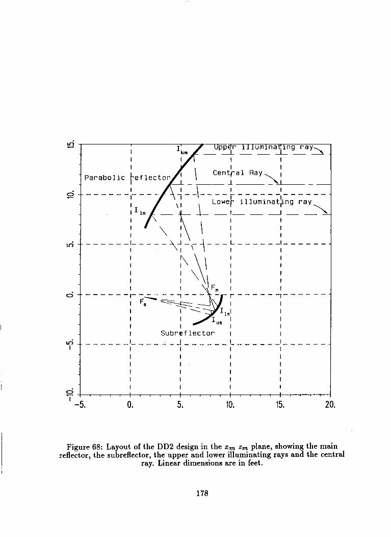
I I I 1 GI I , , I : 1 I I f . . ' ' I " ~ ' I
-5. 0. 5. 10. 15. 20.
Figure 68: Layout of the DD2 design in the zm zm plane, showing the main reflector, the subreflector, the upper and lower illuminating rays and the central
ray. Linear dimensions are in feet.
178

G
Figure 69: Layout of the DD3 design in the zm zm plane, showing the main reflector, the subreflector, the upper and lower illuminating rays and the central
ray. Linear dinlensions are in feet.
I I I I I I I I I I I I I I I I I I I I
l ~ . ~ . f ~ ~ ~ .
179

Table 8: Effect of increasing hpc (designs DD2 and DD3)
BMWEa, BMW?’
II xu 1 constant )I M I decreasing 11
increasing A, increasing
increasing
II XI I constant 11 lgrodBl [ increasing 11
19.l0, a good value, which represent slight improvements. Instead, the illuminating
beamwidth BMW;” is increased to about 13.8O, and the lgrodsl is increased to
about 0.088 dB. The other quantities have remained constant. This design offers
some advantages over the FD design, but FD is, on the overall, preferable because
its value of BMWT’ is close to the value of 1 2 O , which is the actual beamwidth of
the feed.
7.6.3 DIRECT DESIGN. EXAMPLES DD6 AND DD7
In the DD6 and DD7 design examples the quantities hum and hi, are varied
by 1.0’ from the values of the FD design; while, the other input quantities are kept
constant. The design values are shown in Table 11, with the layouts illustrated
in Figures 72 and 73. The trends of the parameters are shown in Table 12. The
advantages and disadvantages offered by each design are briefly shown.
In the DD6 design, the heights, hum and hi,, are set to 15.0‘ and 9.0’, re-
spectively. In other words, the height of the target zone is increased by 1’. This
is a reasonable assumption. The illuminating beamwidth, BMW;’, is reduced to
180

ZPC
hPC
DD4 FD DD5
0.0' 1.4' 2.8'
0.75' 0.75' 0.75'
hum
hlm
14.0' 14.0' 14.0'
8.0' 8.0' 8.0'
x c
Y
110.0" 110.0" 110.0"
8.0' 8.0' 8.0'
181
BMWZa, BMW?'
f €0
4 Pa
32.55822" 35.03785' 38.2 7 12 3"
11.22553" 1 2.336280 13.85916"
7.854814' 7.854814' 7.854814'
0.6023936 0.5739332 0.5376679
7.890527' 6.498242' 5.110146'
4.1 72 7 1 0' 3.796371' 3.378359'
4.030100 ----I M 3.895684 H 3.694099 3.325896
3.544329 3.154068
grodB -0.05778445 dB -0.06976044 dB -0.08799943 d

I I I
- -1- -
I I I I I I
l eckor
_ _ _ - I I I I I I I I 1 I I I I I I I
-5. 0. 5. 10. 15. 20. I
Figure 70: Layout of the DD4 design in the zm .zm plane, showing the main reflector, the subreflector, the upper and lower illunlinating rays and the central
ray. Linear dimensions are in feet.
182

1 C e n t i
1 , , , , : I ~ , , , , ~ , , , , ~ , , , , ~ I I 1
I I - t o . . 1-
-5. 0. 5. 10. 15. 20.
Figure 71: Layout of the DD5 design in the zm ztn plane, showing the main reflector, the subreflector, the upper and lower illuminating rays and the central
ray. Linear dimensions are in feet.
183
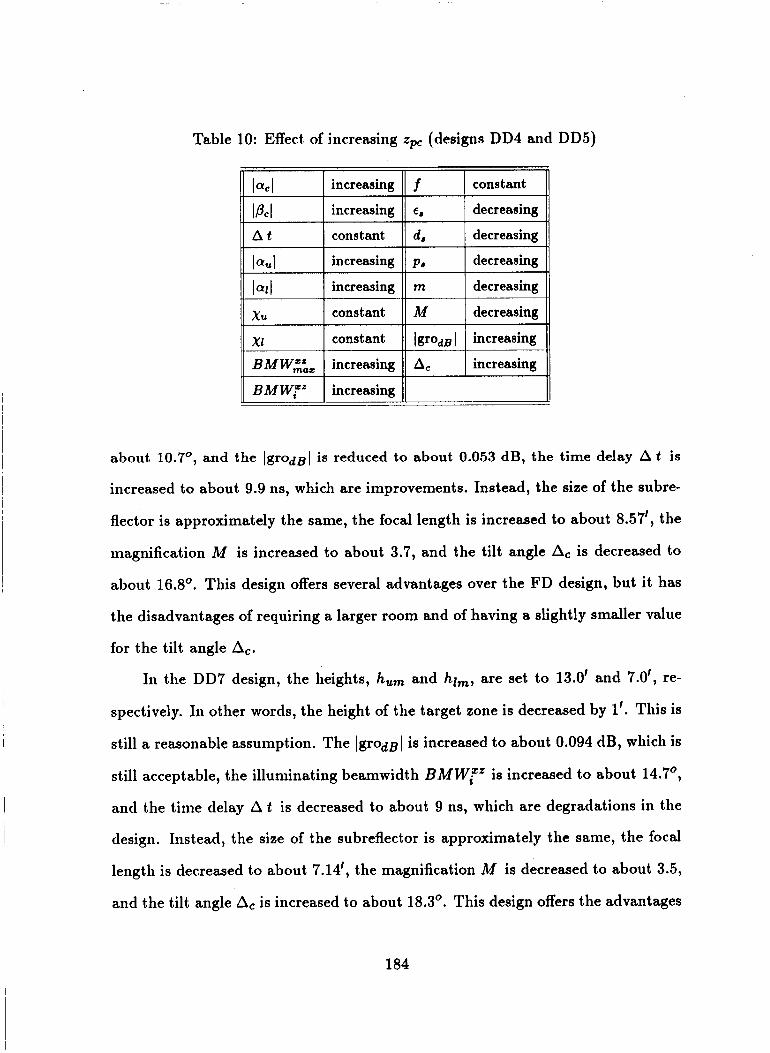
Table 10: Effect, of increasing zpc (designs DD4 and DDS)
x u
XI
II lac1 I increasing 11 f I constant
constant M decreasing
constant lgrodB 1 increasing
II lPc l I increasing 11 ea I decreasing
II A t I constant 11 d, I decreasing
II laul I increasing 11 p a I decreasing
II la11 I increasing 11 rn I decreasing . . I I 1 I
BMWEa, I increasing 11 Ac I increasing
about 10.7O, and the [grodsl is reduced to about 0.053 dB, the time delay A t is
increased to about 9.9 ns, which are improvements. Instead, the size of the subre-
flector is approximately the same, the focal length is increased to about 8.57', the
magnification M is increased to about 3.7, and the tilt angle A, is decreased to
about 16.8'. This design offers several advantages over the FD design, but it has
the disadvantages of requiring a larger room and of having a slightly smaller value
for the tilt angle A,.
In the DD7 design, the heights, h,, and hl,, are set to 13.0' and 7.0', re-
spectively. In other words, the height of the target zone is decreased by 1'. This is
still a reasonable assumption. The IgrodB( is increased to about 0.094 dB, which is
still acceptable, the illuminating beamwidth BMWrZ is increased to about 14.7',
and the time delay A t is decreased to about 9 ns, which are degradations in the
design. Instead, the size of the subreflector is approximately the same, the focal
length is decreased to about 7.14', the magnification M is decreased to about 3.5,
and the tilt angle A, is increased to about 18.3'. This design offers the advantages
184

of a reduced size room and a larger tilt angle A,, at the expense of a deterioration
of the remaining parameters, especially of BMW?'.
7.6.4 DIRECT DESIGN. EXAMPLES DD8 AND DDO
In the DD8 and DD9 design examples the quantity xc is varied by loo, about
the value of the FD design; while, the other input quantities are kept constant.
The design values are shown in Table 13, with the layouts illustrated in Figures
74 and 75. The trends of the parameters are shown in Table 14. The advantages
and disadvantages offered by each design are briefly summarized.
In the DD8 design, the tilt angle xc is set to 95.0'. In other words, the
beam illuminating the main reflector is becoming more vertical than in the FD
design. The illuminating beamwidth BMW?' is increased to about 16.9O, and the
JgrodBI is increased to about 0.131 dB, which is slightly greater than the specified
value of 0.1 dB, the time delay A t is strongly decreased to about 6.3 ns, which
are degradations in the design. Instead, the size of the subreflector is slightly
smaller, the focal length is greatly decreased to about 6.0', the magnification M is
decreased to about 3.38, and the tilt angle A, is greatly increased to about 23.6O.
This design offers several advantages over the FD design, especially for the tilt
angle of the feed A,, but it also has strong disadvantages, especially for the time
delay differential A t , which is much too low. Also, the feed beamwidth, BMW?',
is very large, besides, there are problems related to diffraction from the edges of the
main reflector. In fact, this type of design shows a greatly different behaviour of
the upper and lower edges of the main reflector with respect to diffraction. While
the diffraction from the upper edge is reduced with respect to the FD design,
the diffraction from the lower edge is increased. This is due to the fact that the
difference of the distances of the upper and lower edges is greater for this design
185
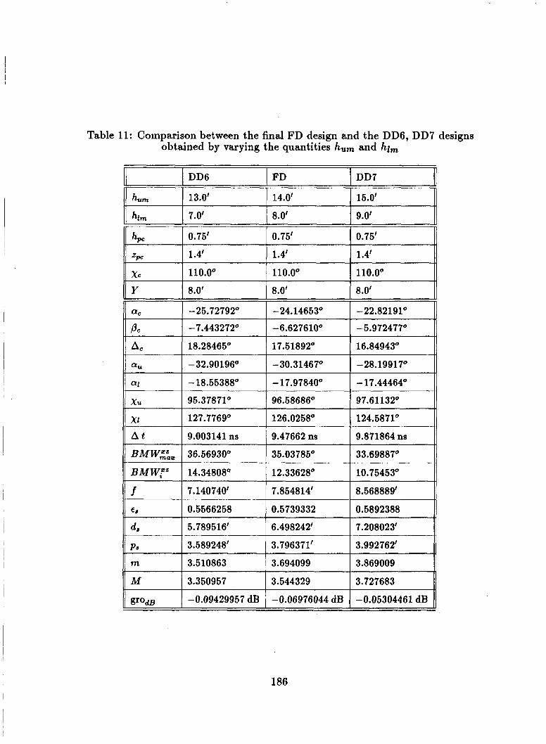
Table 11: Comparison between the final FD design and the DD6, DD7 designs obtained by varying the quantities hum and hlm
5.789516'
3.589248'
3.510863
3.350957
-0.09429957 dB
I1 f
~ -~ ~ ~
6.498242' - 7.208023'
3.796371' 3.992762'
3.694099 3.869009
3.544329 3.727683
-0.06976044 dB -0.05304461 dB
E m
DD6 FD DD7
13.0' 14.0' 15.0'
7.0' 8.0' 9.0'
0.75' 0.75' 0.75'
1.4' 1.4' 1.4'
110.0' 110.0' 110.0'
8.0' 8.0' 8.0'
-25.72792" -24.14653' -22.82191'
18.28465" 16.84943"
95.37871' 96.58686' 97.61132'
127.7769' 126.0258' 124.58'71'
9.003141 ns 9.47662 ns 9.871864 ns
36.56930' 35.03785' 33.6988'7'
14.3480a4 1 12.33628' I 10.75453' I/ 7.140740' I 7.854814' 1 8.568889' ll 0.5566258 I 0.5739332 I 0.5892388 I1
186

I
1 -
Upper' i 1 luminat i;ng r a y - I - - - A -
- - - - -
i 1 luminat ilng r a y
- 1 - - - .-- - - - 1 - - - - - - - - - - -
I I I I I I I I I I I I I I I 1 I I I I I I I I I I I I
I ' ' . ' I ' " '
' -5. 0. 5. 10. 15. 20.
Figure 72: Layout of the DD6 design in the zm zm plane, showing the main reflector, the subreflector, the upper and lower illuninating rays and the central
ray. Linear dimensions are in feet.
187
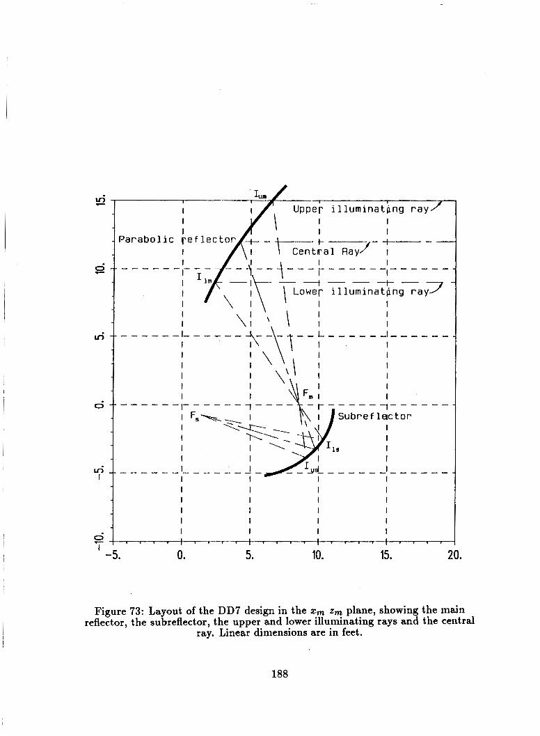
, , , , i , j , , , , ; , , , , , , , , 1 I I I e --
-5. 0. 5. 10. 15. 20. I
Figure 73: Layout of the DD7 design in the zm xm plane, showing the main reflector, the subreflector, the upper and lower illuminating rays and the central
ray. Linear dimensions are in feet.
188

Table 12: Effect of increasing h,,, and hi, (designs DD6 and DD7)
decreasing
decreasing
decreasing
decreasing
II XI
E, increasing
d, increasing
p , increasing
m increasing
decreasing 11 f I increasing 11
increasing
decreasing
M increasing
IgrodB I decreasing decreasing 11 A, I decreasing 1 1 decreasing U
than for the FD design, and also to the fact that the radii of curvature at the lower
edge are smaller for this case than for the FD design. This increases diffraction,
since the rolled edge must perform a transition from a concave surface (parabolic
section) to a convex one (elliptical section).
In the DD9 design, the tilt angle, xc, is set to 125.0'. In other words, the
beam illuminating the main reflector is coming more horizontal than in the FD
design. The illuminating beamwidth, BMW,"", is decreased to about 8.9', and
the JgrodB( is decreased to about 0.036 dB, the time delay differential, A t , is
strongly increased to about 13.9 ns, which are improvements. Instead, the size
of the subreflector is larger, the focal length is greatly increased to about 10.56',
the magnification M is increased to about 3.66, and the tilt angle A, is greatly
decreased to about 12.72'. This design offers several advantages over the FD
design, especially for the feed beamwidth BMWrZ and the time delay differential
A t , but it also has disadvantages, especially for the tilt angle A,, which is much
too low, and for the size of the subreflector.
189
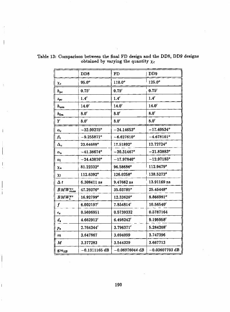
Table 13: Comparison between the final FD design and the DD8, DD9 designs obtained by varying the quantity xc
DD8 FD
X C 95.0" 110.0"
DD9
125.0"
190

I I I ,,,&$$et- illumiqating ray I urn ---- TI 5
I I I I I I 4 1 I
I I I I / Lower illuminatbng ray, I I\
0
ui I
; , , , , )
I I I I I I I I
I I I ----+---T-
I , , , , ! , 9 I -5. 0. 5. 10. 20.
Figure 74: Layout of the DD8 design in the tm zm plane, showing the main reflector, the subreflector, the upper and lower illuminating rays and the central
ray. Linear dimensions are in feet.
191
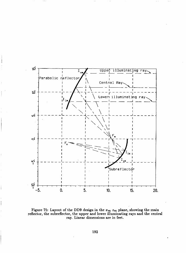
0
uj I
Figure 75: Layout of the DD9 design in the zCm zm plane, showing the main reflector, the subreflector, the upper and lower illuminating rays and the central
ray. Linear dimensions are in feet.
192

Table 14: Effect of increasing xc (designs DD8 and DD9)
decreasing f decreasing e,
decreasing d,
decreasing p s
decreasing m
II increasing increasing
increasing
increasing
increasing
lPc l
laul
. I 4
A t
II increasing
increasing
decreasing
decreasing
II XI
M increasing
JgrodB 1 decreasing Ac decreasing
7.7 CONCLUSION
The FD design for the next generation compact range has been achieved
through the design procedures introduced in Chapter V. This design, by using
Dragone's principle of the central ray, eliminates or miniinizes the three prob-
lems related to the single reflector offset design, v h . cross-polarization, aperture
blockage and taper of the reflected field. At the same time, the design satisfies
several geometrical constraints and represents a compromise between different re-
quirements which must be satisfied to minimize diffraction arising from different
causes, for instance, the coupling aperture and the edges of the main reflector
and subreflector. It has been shown that the new design represents an overall
improvement over the previous design. Through several examples it is shown how
an improvement for some of the parameters of the FD design is achieved only at
the expense of one or more other factors, therefore, the design obtained is a rea-
sonable compromise. While a detailed analysis of diffraction is not the purpose
of this study, it has been shown that nevertheless the requirements dictated by
193

diffraction considerations must be carefully taken into account to obtain a useful
GO design.
194
CHAPTER VI11
CONCLUSIONS
The geometrical optics design of a compact range has been addressed in this
report. Through this study it has been shown how an offset single reflector design
fails to solve three problems:
0 aperture blockage error
0 cross polarization error
0 geometric taper error of the reflected field.
These three errors are intrinsic to the offset single reflector design. For exam-
ple, if the axis of the feed coincides with the ax is of the parabolic reflector (center
fed arrangement), the feed and its supporting structures are illuminated by the
reflected plane wave, with a subsequent strong interaction. Then, the total signal
in the quiet zone is the sum of the reflected plane wave and the diffracted fields,
which result from the feed (and supporting structures) scatter (or aperture block-
age). This dictates an offset arrangement, in which the axis of the feed is tilted
with respect to the parabolic reflector axis. This reduces (but, does not, eliminate)
the aperture blockage, but it also introduces a st'rong cross-polarized component..
Presently cross-polarization is defined as the ratio of the cross-polarized terni over
the co-polarized component of the reflected field in the target zone. While an ten-
ter fed arrangement has no cross-polarization, an offset arrangement has a strong
195

cross-polarization. In fact, the parabolic surface is a doubly curved surface, which
introduces a “twisting” in the polarization of the reflected field with respect to the
incident field. A geometric taper error is also present for both the center fed and
offset configuration. In fact, since the distance from the focal point to the reflection
point is not constant (because the reflector is not spherical), the resulting plane
wave from an omnidirectional feed has a non-uniform field distribution. The offset
arrangement can be used to partially compensate for the geometric taper, but at
the expense of increasing the cross-polarization error.
These errors can be eliminated or reduced with a dual chambers offset Gre-
gorian subreflector system, which has the following advantages:
0 greatly reduces the aperture blockage error
0 elihinates the cross polarization error
0 minimizes the taper of the reflected field through a large equivalent focal
length and an optimal choice of the position of the target zone.
By tilting the axis of the feed, and locating the subreflector accordingly, and
with a dual chambers arrangement, the aperture blockage can be greatly reduced.
The geometric optics cross polarization can be eliminated despite the fact that the
feed ax is is tilted, since now two surfaces are reflecting, such that the “twisting” of
the one can be made to cancel the other. The geometric taper can be made small
by having a large equivalent focal length, while reducing the actual focal length of
the main reflector.
A comparison between a commercially available offset single reflector and a
Gregorian subreflector system shows the following:
196

For the offset single reflector:
1) Target zone of almost semicircular shape, with lower limit at 4.4' and
upper limit at 12.9', and extending in depth from 36' to 50'.
2) Focal distance of 24'.
3) Field taper
0 taper of the geometric reflected field of 0.55 dB
0 taper with Huygens source of 1.03 dB for a tilt angle of 20'
0 taper with Huygens source of 0.96 dB for a tilt angle of 39.75'.
4) Cross polarization error
0 -21.2 dB for a tilt angle of 20'
0 -15.05 dB for a tilt angle of 39.75'.
For the Gregorian subreflector system:
1) Target zone of rectangular shape, with lower limit at 8' and upper limit
at 14', and extending in depth from 20' to 28'.
2) Focal distance of 7.85', equivalent focal distance of 27.84'.
3) Field taper
0 taper of the geometric reflected field of 0.0698 dB
0 taper with Huygens source of 0.14 dB.
4) Cross polarization error is zero (-00 dB).
197

The GO design of a Gregorian subreflector system can be performed with an
iteration procedure, using a numerical solution which evaluates the reflected field
and the cross-polarization in the target zone, but this approach is very cumbersome
and, even with a great effort, easily misses the optimal design. Instead, some
simple algebraic design equations to solve quickly and exactly the design problem
have been developed in this report. Besides minimizing the three errors already
mentioned, these equations allow one to satisfy several geometrical conditions as
well as other conditions which minimize the amount of diffraction in the target
zone.
l
The design of a new generation subreflector system compact range has been
determined through these equations. This new design offers better electrical char-
acteristics than the offset single reflector system.
198
APPENDIX A
THE VECTOR PATTERN FUNCTION
A radiator and its electric or magnetic far field, Eff or Hff, are considered
in an homogeneous lossless medium having propagation constant IC and intrinsic
impedance 2. It is assumed that the radiator has a well defined phase center at the
point 0,constant with respect to the direction of radiation. This phase center is
assumed as origin of a polar coordinate system O(T 8 4). Under these assumptions
the wave propagating from 0 is a spherical wave, and i represents its direction
of propagation. Its phase factor is e - j k r , where r is the distance from the phase
center 0 to the field point R. The electric and magnetic fields are perpendicular
to each other and to the direction of propagation under the far field assumption
(TEM wave), as follows
Two vector functions can then be defined at each point P E { T 8 4 } in the far field
of the radiator
199

These are called vector pattern function for the E and for the H fields, respectively.
One can be derived from the other by the use of the previous equations.
The vector pattern function is a function of the direction of propagation E:
only, it does not depend on the distance P. It contains information on the radiation
intensity (as the more usual pattern function) as well as on the polarization of the
radiator in the direction i.
200

APPENDIX B
INTERSECTION OF A STRAIGHT LINE WITH A CONIC OF
REVOLUTION
A conic is defined as a plane curve characterized through the equation in polar
coordinates P
1 - € C O S 8 r =
where the quantities are shown in Figure 76, and e is the eccentricity of the conic.
In a three dimensional space, a conic of revolution is defined as a surface, as
follows.
The axis of the conic connectiong the two focai is considered. One of the focai
is at infinity for a parabola, for a circle any axis can be considered. The conic
is rotated of 180' in space around this a x i s . The surface obtained is a conic of
revolution.
A conic of revolution is still described by Equation (B.l)
P r = 1 - ecose
where now T and 6 are polar coordinates in the three dimensional space, and the
origin coincides with the appropriate focus of the conic.
Two points in space, PI = ( q , y l , q ) , P 2 f (22,y2,z2), with PI # P2, and
a conic of revolution, are considered. It is desired to determine the intersection
201
Figure 76: Geometry in polar coordinates of a conic in the plane.
Figure 77: Geometry of the line 4! intersecting the conic of revolution.
202
points of the oriented line L through P I , P2 with the conic of revolution. The line
t is oriented from PI to P2 (see Figure 77).
The equation of the straight line L through the points, PI and P2, is determined
first. The direction cosines k, 1, m of L are given by
2 2 - 2 1 d
k = Y2 - Y1
d 22 - 21
d
I =
m =
where k 2 + 1 2 + m 2 = 1
and d is the distance between PI and P2
d = J(r2 - ~ 1 ) ~ + ( ~ 2 - ~ 1 ) ~ + ( 2 2 - 2 1 ) ~
The parametric equation of t is
P . 9 )
(B.lO)
where t is the signed distance along the line t of a point P
point PI .
(2, y, z ) of L from the
The coordinates of a point on L can be expressed in polar form, and Equations
(B.8), (B.9), and (B.lO) can be used to obtain
y = I t + y 1 =rsinOsinq$
z = m t + z l =rcosO.
(B.ll)
(B.12)
(B.13)
203

From Equation (B.2)
T =p+T€COS8
hence, using Equation (B.13)
T = p + + zl)
by squaring Equations (B.ll), (B.12) and (B.13) this relation follows
T2 = (kt + + ( l t + y1)2 + (mt + z1) 2
(B.14)
(B.15)
(B.16)
by performing the squares and ordering with respect to powers of t one obtains
T2 = ( r ~ 2 + z2 + m 2 2 )t + 2(kz1+ ~ y l + mzi)t + (zf + y! + z ! )
which can be written as
T~ = t2 + 2At + B
consequently, using Equation (B.15)
t2 + 2At + B = lp + e(mt + z1)I2
expanding the square
t2 + 2At + B - p2 - 2pe(mt + z1) - e2(mt + ~ 1 ) ~ = 0
t2 + 2At + B - p2 - 2pe(mt + z1) - e2(m2t2 + 2mzlt + z f ) = 0
(1 - e 2 2 2 m >t + 2(A - pem - e2mq)t + (B - p2 - 2peq - e 2 2 z l ) = 0
a second degree equation of the form:
at2 + 2bt + c = 0
(B.17)
(B.18)
(B.19)
(B.20)
(B.21)
(B.22)
(B.23)
204

where
a = 1 - e m 2 2 (B.24)
b = L q + Zyl + m q - e m ( p + c q ) (B.25)
c = z~+y~+r;-(p+etl) 2 - (B.26)
Equation (B.23) gives two (one or none) solutions for t , t' and tl', which are
the coordinates along l of the intersection points, P' and P", with the conic of
revolution. By inserting these values of t in the equations of the straight line l ,
the zyz coordinates of the intersection points can easily be found
(B.27)
(B.28)
(B.29)
ztt = kt" + e1 (B.30)
y" = It" + y1 (B.31)
2' = mt" + zl . (B.32)
Some of the solutions might be spurious, and the coordinates of the points, PI and
Prr , must be substituted into Equation (B.2) to check if they actually are points
of the conic of revolution, i.e., actual intersection points.
205

APPENDIX C
COMPUTATION OF THE NORMAL FOR A CONIC OF
REVOLUTION
Let f ( p , v, () = 0 be the equation of a surface expressed in the p, u, ( coordi-
nate system. Its normal vector is given by
where V is the gradient in the p, v, coordinate system.
In a polar coordinate system, the gradient is given by
i a +-- a e a v = e - + - - & r 88 rsinOdt$
and the equation of a conic of revolution is
= o . P f(r,O) = r - 1 - ecose
Thus, one finds that 6
pe sin 8 and
a asf( ' ,q = (1 - cos e)2 '
consequently
e 1 pcsin8 r ( I - e COS e)2
206
n = i + -

9 E sin 8 = i + l - E c o s e
1 ,
By normalizing n, one obtains the unit vector n such that
(C.10)
This is the expression for the unit normal of a conic of revolution in a polar
coordinate sys tem.
To determine its expression in a Cartesian coordinate system, one can write
1 = s i n 8 c o s q 5 k + s i n 8 s i n ~ ~ + c o s 8 2 ((2.11)
and
(C.12)
then, the unit normal is given by
A 1 [sinB(cosq5f + sinq5y) + (cos8 - c) i] . (C.13) n = Ji + €2 - 2ECOSe
A conic of revolution divides all space into two complementary sets, called the
inside and the outside of the conic of revolution. The inside of the conic of revo-
lution is defined as the set containing the focus closest to the surface. Then the
normal n is pointing towards the outside of the conic of revolution. This is the
convention used for a convex subreflector. It might be necessary to change the sign
in Equation (C.13) if a concave subreflector is considered.
207
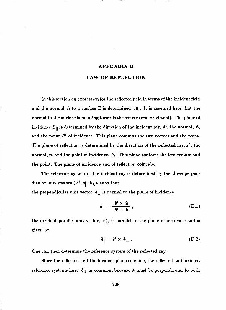
APPENDIX D
LAW OF REFLECTION
In this section an expression for the reflected field in terms of the incident field
and the normal n to a surface C is determined [18]. It is assumed here that the
normal to the surface is pointing towards the source (real or virtual). The plane of
incidence IIll is determined by the direction of the incident ray, 6’, the normal, n,
and the point Pi of incidence. This plane contains the two vectors and the point.
The plane of reflection is determined by the direction of the reflected ray, s’, the
normal, n, and the point of incidence, Pi. This plane contains the two vectors and
the point. The plane of incidence and of reflection coincide.
The reference system of the incident ray is determined by the three perpen-
dicular unit vectors ( ii, 6’ 6 ~ ) , such that
the perpendicular unit vector 61 is normal to the plane of incidence II ’
the incident parallel unit vector, “1, is parallel to the plane of incidence and is
given by
= it x d l . (D.2)
One can then determine the reference system of the reflected ray.
Since the reflected and the incident plane coincide, the reflected and incident
reference systems have 6 1 in common, because it must be perpendicular to both
208

INCIDENT R AY
Figure 78: Incident and reflected triads.
planes.
The direction of the reflected ray is given by
This equation expresses that the tangential component (with respect to the re-
flecting surface) of i' is the same as the tangential component of i', while their
normal components are opposite in sign.
The reflected parallel unit vector, 6!, is parallel to the plane of incidence
(coincident with the plane of reflection) and is given by
6; = i' x ii*
in order to have a right handed reference system (Figure 78).
The law of reflection can be expressed as
U" = RII(U' - 4ii) 6 i + R1(Ui * 61) 81
209
where U represents the field (;.e., the electric field, E, or the magnetic field, H),
Ui is the incident field, U' is the reflected field, RII and R l are the reflection
coefficients
RIl = 1,
R l = + l , i f U = H ,
R l = -1 , if U = E.
This reflection law can be expressed in a compact way by the use of a 2x2 dyad R -
and the reflected field is expressed in a compact form as
which expresses the reflected field at the reflection point in term of the incident
field at the reflection point.
210
APPENDIX E
POLARIZATION
A (generalized) Huygens source is used to study the cross-polarization prop-
erties of a conical (not necessarily parabolic) focussed reflector or of a combination
of conical focussed reflectors [ 101.
A (generalized) Huygens source consists of an electric and magnetic dipole
set at the same point in space and having perpendicular axes. In Figure 79,
the electric dipole is directed in the -x direction, the magnetic dipole in the -9
direction. In a polar reference system the resulting far field is given by
Be = cos$(AcosO+ B) = Bcos+(XcosO+ 1) ( E 4
E4 = - sin 4( A + B cos 0 ) = - B sin 4 ( X + cos 0 ) (E-2)
(E.3)
(E.4)
1 B - sin 4(A + B cos O ) = -- sin c$(X + cos e) 77 77 1 B
77 77
He =
H4 = --sinq5(Acos@+B)= --cosq5(Xcos8+1)
where
and A, B are given by
B x = - A
21 1
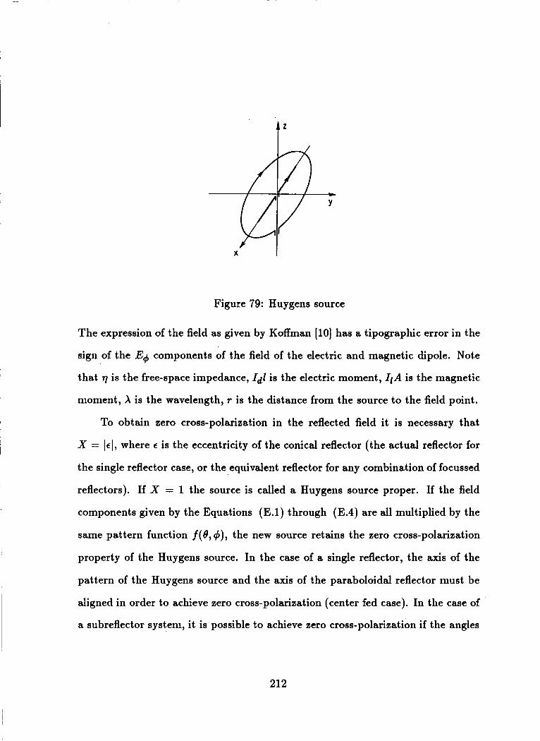
Figure 79: Huygens source
The expression of the field as given by Koffman [lo] has a tipographic error in the
sign of the E+ components of the field of the electric and magnetic dipole. Note
that 77 is the free-space impedance, Id2 is the electric moment, IlA is the magnetic
moment, A is the wavelength, r is the distance from the source to the field point.
To obtain zero cross-polarization in the reflected field it is necessary that
X = [e l , where e is the eccentricity of the conical reflector (the actual reflector for
the single reflector case, or the equivalent reflector for any combination of focussed
reflectors). If X = 1 the source is called a Huygens source proper. If the field
components given by the Equations (E.l) through (E.4) are all multiplied by the
same pattern function f(0, $), the new source retains the zero cross-polarization
property of the Huygens source. In the case of a single reflector, the a x i s of the
pattern of the Huygens source and the ax is of the paraboloidal reflector must be
aligned in order to achieve zero cross-polarization (center fed case). In the case of
a subreflector system, it is possible to achieve zero cross-polarization if the angles
212

a and P satisfy the relationship [6]
tan = mtan (:) where
1 - €1
where
0 e is the eccentricity of the subreflector
0 a is the angle from the subreflector a x i s to the feed axis,
0 P is the angle from the subreflector to the main reflector axis.
Equation (E.8) is satisfied by a = 0, P = 0, but there exists a simple infinity of
solutions different from zero; i.e., for every a it is possible to determine a P which
satisfies Equation (E.8), and vice versa. Therefore, with a subreflector system, it
is possible to achieve zero cross-polarization when the subreflector and feed axes
are tilted, and to have an extra degree of freedom in choosing one of the tilt angles
a or P. It is legitimate to ask if the Huygens source is a mathematical abstraction
or if it can be approximated with an actual feed. As an example it is shown
that a truncated waveguide feed approximates a Huygens source. Consequently a
Huygens source represents also an physical feed.
A n analysis of the truncated rectangular waveguide is available in Silver [19],
and, if the waveguide is excited in the TElo mode, the expression for the electric
far field radiated by the waveguide is given by
213
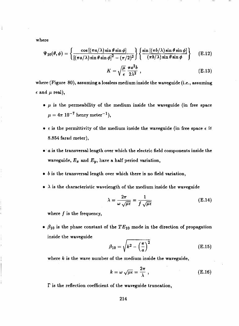
where
K = P & e 2X2 ' (E.13)
where (Figure 80), assuming a lossless medium inside the waveguide (;.e., assuming
e and p real),
0 p is the permeability of the medium inside the waveguide (in free space
p = 47r henry meter-'),
0 e is the permittivity of the medium inside the waveguide (in free space e Z
8.854 farad meter),
0 a is the transversal length over which the electric field components inside the
waveguide, E, and E,, have a half period variation,
0 b is the transversal length over which there is no field variation,
0 X is the characteristic wavelength of the medium inside the waveguide
(E.14)
where f is the frequency,
0 Plo is the phase constant of the TElo mode in the direction of propagation
inside the waveguide
PlO = Jk2 - ( :)2
where IC is the wave number of the medium inside the waveguide,
(E.15)
(E.16)
r is the reflection coefficient of the waveguide truncation,
214

r is the distance from the field point to the center of the waveguide truncation
(;.e., to the origin of the coordinate system).
The previous equations have been modified from Silver to take into account the
different coordinate system as well as to correct a printing error in the expression of
the E4 component. It is clear that, if = 0, the field components are those of the
Huygens source multiplied by a pattern factor, and they are real. The argument
of the phase factor is just r , consequently, since the amplitude is entirely real, the
phase center is fixed with respect to direction, i.e., with respect to 8,+ . Hence, two
conditions must be satisfied for the truncated waveguide to behave as a Huygens
source
r = o , (E.17)
(E.18)
Clearly this last equality can never be satisfied, and the first too can be Satisfied
only approximately, hence one obtains the more realistic conditions
r = o , (E.19)
(E.20) 7r
1 > > - a k
or
(E.21) a > $ .
The two requirements (E.19) and (E.21) are not contrasting, i.e., having large
dimensions for the waveguide satisfies the condition on small I?, and, viceversa, in
order to obtain a small I? it is necessary to have large dimensions for the waveguide.
x
The truncated waveguide example shows that there exist feeds which reason-
ably approximate the properties of a Huygens source.
215
Y
Figure 80: Truncated waveguide
216
APPENDIX F
ANGULAR EXPRESSIONS
Some expressions between the angles a, P and x, as shown in Figure 81, are
presently derived.
By considering the triangle F', Fm and Is one obtains an expression for a in
terms of e.,, ,8 and x, where cs is the eccentricity of the subreflector referred to its
left focus, as follows,
where
P8
1 + e# cosy
d, = __I 2p' , and 1 - €'
y = - r + x + P .
T r =
By substitution one obtains
and since
sin7 = --sin(x + P )
cosy = - COS(X + p )
217

one finally obtains
(1 - ez)sin(X +@) a = - arctan [2€, - (1 + €$)COS(X +@)
By considering the same triangle one obtains an expression for x (or @) in
terms of € 8 7 a and p (or x), as follows,
r1 cos a - d, rl sin a
tany =
where P8 rl =
1 - E8COsa
one then obtains (1 + €;) cos a - 2€8 tany =
(1 - e:) sin a
therefore x + /3 = A + arctan [ ( l+€:)cosa-2r.
(1 - e$) sin a
which can be solved for x or for @, as desired,
[ (1 + €Z) cos a - 2€# x = A -@+arc tan (1 - E ! ) sin a
€ 8 ) cos a - 2€# [(l e?)sina
p = A - x.+ arctan
(F.lO)
(F . l l )
(F.12)
(F.13)
(F.14)
218

SUBREFLECTOR
Figure 81: Geometry related to the angles a, /3 and x.
219

APPENDIX G
EXPRESSIONS FOR THE GEOMETRIC TAPER OF THE
REFLECTED FIELD
In this section some simple expressions for the taper of the reflected field (gro)
of a single reflector and of a subreflector system are derived. The single reflector
case is considered first for semplicity, and then the results are extended to the
subreflector system through the principle of the equivalent reflector.
A parabolic reflector illuminated by a focussed uniform source is considered.
The reference system is the polar reference system Fm(rm, e,, Qlm) introduced
in Section 3.2. A line t intersects the reflector ax is zm at a straight angle, and
its distance from the paraboloid vertex V is dl , R is a point o f t , and Im is its
z-projection (;.e., a projection parallel to the zm a x i s ) on the paraboloid, Im has
polar coordinates (rm, Om, +m), p is the distance of R from the paraboloid axis zm,
p is also the distance of Im from zm (Figure 82).
Given two points P and Q, the symbol P - Q indicates the vector starting at
Q and ending at P, and JP - Q I indicates its length.
The source considered has a vector pattern function PF
Im - Fm IIm - FmI
PF = PF ( -.) = PF( em)
where the unit vector ,. Im - Fm
IIm - FmI rm = --
220
(G.2)
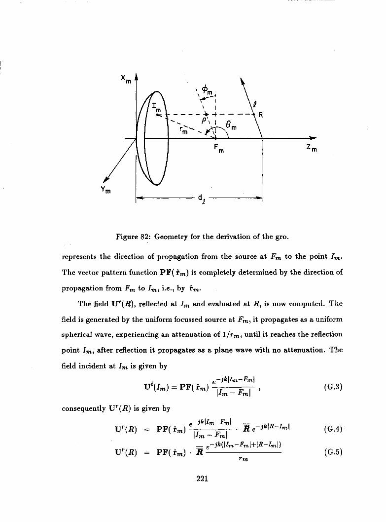
Figure 82: Geometry for the derivation of the gro.
represents the direction of propagation from the source at Fm to the point 1'.
The vector pattern function PF( tm) is completely determined by the direction of
propagation from F' to Im, i.e., by 3'.
The field Ur(R) , reflected at Im and evaluated at R, is now computed. The
field is generated by the uniform focussed source at Fna, it propagates as a uniform
spherical wave, experiencing an attenuation of 1 / r m , until it reaches the reflection
point Im, after reflection it propagates as a plane wave with no attenuation. The
field incident at Im is given by
consequently U r ( R ) is given by
221
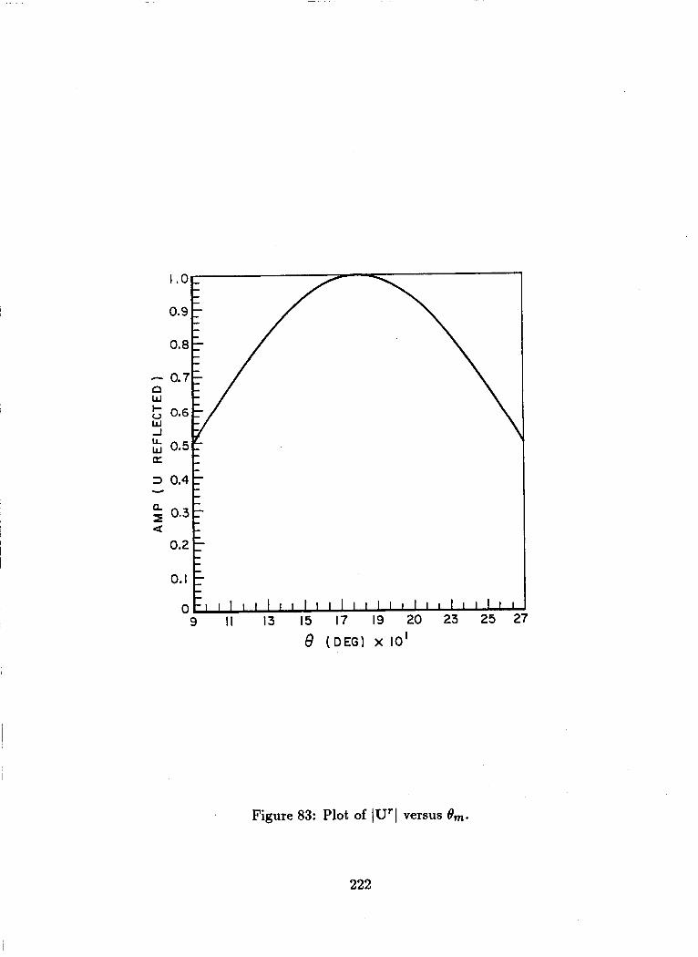
0.1 L
0 L 9 I I 13 15 17 19 20 23 25 2
8 (DEG) X IO'
Figure 83: Plot of IUrI versus 0,.
222

Os9 E / \
\ L
c
0.1
Figure 84: Plot of IU'I versus p.
223
- since T, = 11, - F,(. The is the dyadic reflection coefficient.
By the properties of the parabola, the distance 11, - Fm( + lR-Intl is constant
if R varies on the line k' previously defined, and, since the system is rotationally
symmetric, this distance is also constant if t is rotated around the axis zm in a
perpendicular fashion, generating a plane perpendicular to the parabolic axis , con-
sequently the phase of the reflected field is constant on any plane perpendicular to
the paraboloid axis , the reflected field is a (nonuniform) plane wave, the difference
in phase of the fields on two such planes depends on the distance between the
planes.
For a paraboloid
consequently
- - For a uniform source the term IPF( F,) - RI is a constant
and a typical plot of IU'(R)I versus Om is shown in Figure 83, the maximum is
for 8, = 180° and the reflected field decreases monotonically for e,, decreasing
towards 0' or increasing towards 360°, in other words, IU'(R)I is maximum when
the reflection point coincides with the vertex of the paraboloid V and the distance
p is zero, and monotonically decreases for increasing p. The same p represents
both the distances of Im and of R from the paraboloid axis. A typical plot of
IU'(R)I versus p is shown in Figure 84.
224

As the previous considerations suggest, the reflected field U' can be expressed
in terms of p instead of @my where p is a function of the field point R,
P = P(R)
and this equation can be solved for 8, in terms of p(R), as follows
1 - - sin 8, - P(R) - 2f 1 - tan(@,/2)
consequently
~ @ln = arctan (2-) 2 P(R)
aiid
sin2 (e:) = sin2 [arctan (x)] P(R)
but 2 tan2 x sin x =
tan2 x + 1 consequently
and the equations
U'(R) =
U'(R) =
I U W I =
IU'(R)I =
give the required expressions.
= 1 ( 2 f y PF( f m ) . R - 4f (2f l2 + P2(R)
(G.lO)
(G.ll)
(G.12)
(G.13)
(G.14)
(G.15)
(G.16)
(G.17)
(G.18)
(G.19)
(G.20)
225

A target zone is defined, in a general sense, as a finite part of a solid cylinder
having generatrixes parallel to the paraboloid axis and delimited by planes per-
pendicular to the cylinder a x i s . A target plane-section, (TPS for short), is defined
as the intersection of a plane perpendicular to the paraboloid axis with the target
zone (Figure 28). A target plane-section is characterized by its distance y from
the paraboloid vertex, on any other respect all target plane-sections are identical.
By the previous considerations, the phase of the reflected field is constant on a
target plane-section, while its amplitude varies (nonuniform plane wave).
The taper of the reflected field (gro) is defined as
(G.21)
where
(G.23)
(G .24)
(G .25)
(G .26)
(G.27)
and R is the field point, and T P S (target plane-section) represents the set of the
points obtained by intersecting the target zone with a plane perpendicular to the
a x i s of the parabolic reflector. It is not been necessary to specify on which target
plane-section the maximum and minimum are considered, in fact IUr(R)I depends
on p ( R ) only and not on the coordinate zl of the target plane-section, and then it
does not depend on any specific target plane-section.
226

Also
grodB = 20 log(gro)
since the gro i s defined as a ratio of field values.
Equation (G.24) can be solved for f in terms of the gro
(G.28)
( G .29)
(G .30)
(G.31)
For a subreflector system, f must be replaced by fe, the equivalent focal distance
of the subreflector system, and
consequently
gro =
f =
f =
( G .33)
( G .34)
(G.35)
( G .36)
where Pmaz and Pmin are the max and min of the distances of the points of a
target plane-section from the central ray (the ax is of the equivalent reflector).
A simple case important in practice is a target zone having rectangular zy
cross section and centered on the reflector ax is (or on the central ray, for the
subreflector system case) (Figure 85) . Let Pd is the length of the semidiagonal of
the rectangle, for this case
Pmin = 0 (G.37)
227

and the previous equations become, for a single reflector
gro = (2.f / P d l 2 (2f / P d ) 2 -k 1
and for a subreflector system
(G .38)
(G.39)
(G .40)
(G .41)
For a target zone centered on the reflector axis (or on the central ray, for the
subreflector system case), having a circular cross-section, the previous equation
holds if pd is the radius of the circle.
For a target zone centered on the reflector a x i s (or on the central ray), having
an elliptical cross-section with semiaxes a,b, the previous equation holds if Pd =
max(a, b ) .
228
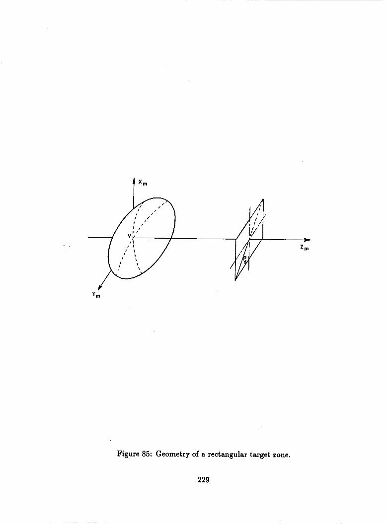
t x m
Figure 85: Geometry of a rectangular target zone.
229

REFERENCES
[l] W. D. Burnside, M. C. Gilreath, B. M. Kent, G. C. Clerici “Curved Edge Modification of Compact Range Reflector,” IEEE Transactions on Antennas and Propagation, Vol. AP-35, No 2, February 1987.
[2] C. W. I. Pistorius, W. D. Burnside, “New Main Reflector, Subreflector, and Dual Chamber Concepts for Compact Range Applications,” Tech. Report 716148-22, The Ohio State University ElectroScience Laboratory, August 1987.
[3] N. F. Chamberlain, “Radar Object Classification Using Full Polarization Scat- tering Matrix Data,” The Ohio State University ElectroScience Laboratory, Department of Electrical Engineering, Columbus, Ohio, February 1988.
[4] W. D. Burnside, L. Peters, Jr., “Target Illumination Requirements for Low RCS Target Measurements,” 1985 AMTA Symposium, Melbourne, Florida, 1985.
[5] M. D. Rader, W.D. Burnside, “A Cassegrain Reflector System for Compact Range Applications,” Tech. Report 716148-14, The Ohio State University ElectroScience Laboratory, July 1986.
[6] C. Dragone, “Offset Multireflector Antennas with Perfect Pattern Symmetry and Polarization Discrinination,” B.S.T.J., 57, No.9, pp. 2663-2685, Septeni- ber 1978.
[7] I. J. Gupta, W. D. Burnside, “Electromagnetic Performance Study of a New Compact Range Reflector,” Report 718331-1, The Ohio State Univer- sity ElectroScience Laboratory, prepared under Contract No. GR9300, Boeing Aerospace Co., June 1986.
[8] A. C. Ludwig, “The Definition of Cross Polarization,” IEEE Transactions on Antennas and Propagation, Vol. AP-21, No 1, January 1973.
[9] C. Dragone, “Conformal Mapping and Complex Coordinates in Cassegrainian and Gregorian Reflector Antennas,” B.S.T.J., 60, No. 10, pp. 2397-2420, De- cember 1981.
[lo] I. Koffman, “Feed Polarization for Parallel Currents in Reflectors Generated by Conic Sections,” IEEE Trans. on Antennas and Propagation, Vol. AP-14, pp. 37-40, January 1966.
[ll] M. R. Spiegel, “Mathematical Handbook,” McGraw-Hill Book Co., Inc., New York, N.Y., 1968.
230

[12] W. V. T. Rusch, Y. Rahmat-Samii and R. A. Shore, “The Equivalent Paraboloid of an Optimized Off-Set Cassegrain Antenna,” Digest IEEE Intl. Symp. Antennas and Prop., 1986.
[13] R. A. Shore, C. J. Sletten, “Dual Offset Reflector Antenna Systems With Ro- tationally Symnietric Aperture Distributions,” Rome Air Force Development Center, RADC-TR-84-140, In-House Report, June 1984.
[14] E. K. Walton and J. D. Young, “The Ohio State University Compact Radar Cross-Section Measurement Range,” IEEE Trans. on Antennas and Propaga- tion, Vol. AP-32, No.11, pp. 1218-1223, November 1984.
[15] G. Clerici, J. D. Young, “Pattern Processing and Feed Simulation by In- terpolation over Measured Data,” Report 719267-7, The Ohio State Univer- sity ElectroScience Laboratory, prepared under Contract No. GU0160, Boeing Aerospace Co., November 1987.
[16] P. Joseph “A UTD Pyramidal Absorber Scattering Analysis for Design of Compact Ranges,” Ph. D. Dissertation, Department of Electrical Engineering, The Ohio State University, September 1988.
[17] W. D. Burnside, G. C. Clerici, J. D. Young, “First Status Report on Con- tract OR-549651-B28 to Elizabeth Stark,” The Ohio State University Elec- troScience Lab, June 1985.
[18] “The Modern GTD Short Course, September 1980,” The Ohio University ElectroScience Laboratory, Department of Electrical Engineering, Columbus, Ohio.
[19] S. Silver, “Microwave Antenna Theory and Design,” Peter Peregrinus Ltd., London, U.K., pp. 342-343; 1984 Reprint.
231
2.
1. fltle and Subtirlc
18. Avallablllty 8taNmont 19. Suurity CIerr (This Repoft)
Unclassified
Unclassified 20. Socurlty Cbsr (This Pa#.)
GEOMETRICAL OPTICS DESIGN OF A COMPACT RANGE GREGORIAN SUBREFLECTOR SYSTEM BY THE PRINCIPLE OF THE CENTRAL RAY
22. No of Pager
231 22. Prlcc
1. AuthoNs) Giancarlo Clerici, Walter D. Burnside
D. Porformln# Omanitation Name and Address
The Ohio State University ElectroScience Laboratory 1320 Kinnear Road Columbus, Ohio 43212
12. Sponsorin# O ~ a n i r a t l o n Name and Address
National Aeronautics and Space Administration Langley Research Center Hampton, VA 22217
3. Rocipicnt's Accession No.
5. Report Date January 1989
6.
1. Por(ormi_nl Organization Rept. No.
71 9493-4 m. hioct / fash/Worh Unlt No.
11. ContractlC) or GrJnt(G) No
(C)
NSG 1613 ~ ~~
13. Type of Report 6 Period Covered
Technical Report 14.
15. Supplamentay Notes
16. Ab8tr.d (Limit 200 words)
In recent years, the compact range has become very popular for measuring Radar Cross Section (RCS) and antenna patterns. The compact ran e, in fact, offers several advantages due to reduced size, a controlled environment, and rivacy. On the other hanf, it has some problems of its own, which must be solved pro erly in order to achieve
wave in the target zone and creates spurious scattering centers in RCS measurements. While diffraction can be minimized by using rolled edges, the field of an offset single reflector compact range is corrupted by three other errors: the taper of the reflected field, the cross polarization introduced by the tilt of the feed and the aperture blocka e introduced by the feed itself. These three errors can be eliminated by the use of a subreflector system. A
minimization of the taper of the reflected field. A Gregorian odigiiratitn3as been adopted in order to enclose the
where the main parabolic reflector and the target zone are enclosed. The coupling between the two rooms is performed through a coupling aperture. The first cut design for such a subreflector system is performed through Geometrical Optics ray tracing techniques (GO), and is greatly simplified by the use of the concept of the central ray introduced by Dragone. The purpose of the GO design is to establish the basic dimensions of the main reflector and subreflector, the size of the rimary and secondary illuminating surfaces, the tilt angles of the subreflector
determined. Breflector system is performed through some design equations which ations and from the zero crow polariaation equation. Thce 22esfgn tpnatisR system for the next generation compact range with improved reflected fie1
ure blockage performance. The design of the coupling aperture is performed 11
kgh quality measurement results. For example, diffraction from the edges of the main re 8 ector corrupts the plane
proper P y designed subreflector system offers very little aperture blockage, no cross-polarization introduced and a
feed and the ellipsoidal subreflector in a lower chamber, whic %l X-GoKted by absorbers from the upper chamber,
and feed, and estimate the feed \ eamwidth. At the same time, the shape of the coupling aperture is initially
Gnsidering the reflection shadow boundaries of the overextended subreflector.
17. Docummt Anmlysls D..cri@ors