Ann. Inst. Statist. Math. Vol. 44, No. 1, 63-83 (1992)

GEOMETRICAL EXPANSIONS FOR THE DISTRIBUTIONS OF THE SCORE VECTOR AND THE MAXIMUM

LIKELIHOOD ESTIMATOR*

MARIANNE MORA

U.F.R. Sciences Economiques, Universitd de Paris X Nanterre, 200 Avenue de la Rdpublique, 92001 Nanterre Cedex, France

(Received April 13, 1989; revised June 2, 1990)

Abstract . In the present note, asymptotic expansions for conditional and un- conditional distributions of the score vector are derived. Our aim is to consider these expansions in the light of differential geometry, particularly the theory of derivative strings. Expansions for the distributions of the maximum likelihood estimator are obtained from those for the score vector via transformation, with a view to interpreting from the standpoint of differential geometry the various terms entering the expansions.

Key words and phrases: Geometrical expansions, score vector, maximum like- lihood estimator, observed and expected geometries.

i . Introduction

Asymptotic expansions for the distributions of the maximum likelihood esti- mator and the likelihood ratio statistic, with a view to the interpretability from the standpoint of differential geometry of the various terms entering the expansions, have been discussed inter alia by Amari and Kumon (1983), Barndorff-Nielsen (1986b, 1988) and McCullagh and Cox (1986). On applied as well as theoreti- cal grounds, the terms of main interest are those of order O(1), O(n -1/2) and O(n -1) under ordinary repeated sampling with sample size n. However, not all of these terms have been given a differential geometric interpretation nor have all the relevant types of expansion--conditional and unconditional--been considered. The aim of this paper is to complete the picture by considering the expansions in the light of the recently developed theory of derivative strings (Barndorff-Nielsen (1986a), Barndorff-Nielsen and Blmsild (1987a, 1987b)), and by addressing also the closely related question of asymptotic expansions for the distribution of the score vector.

* The present work was carried out at the Department of Theoretical Statistics, University of Aarhus~ Denmark, with support from the Danish-French Cultural Exchange Programme.

63

64 MARIANNE MORA

In fact, the score vector is a natural s tar t ing point for a discussion of problems of the present type because of its intrinsic geometric nature, when considered as a differential or as a covariant vector. It turns out tha t in the expansions for the score vector to be derived below the "variant" aspect of its dis tr ibut ion is wholly subsumed in the leading normal term, more precisely in the determinant of the variance matrix, while all o ther terms are invariant and involve certain tensors, the nature of which will be discussed in Section 5.

Expansions for the distr ibution of the maximum likelihood est imator may be obta ined from those for the score vector via t ransformation, and this procedure provides an automat ic separat ion of the terms into variant terms and invariant terms. We shall also comment on the nature of the variant terms, as seen from the theory of derivative strings.

The conditional distr ibutions to be discussed are relative to an exact or ap- proximate ancillary. We use the terms expected and observed geometries in the sense of Barndorff-Nielsen (1986b).

Section 2 contains some background material . Sections 3 and 4 present the various expansions for the score vector and the maximum likelihood est imator , respectively, and in Section 5 we discuss the na ture of the various variant and invariant terms. Some concluding remarks are collected in Section 6.

2. Some background material

2.1 Likelihood quantities Let A/I = {X ,p(~; x), ~} be a statistical model, where X is the sample space,

the parameter space and p(w; x) is the probabil i ty density function for the da t a x, with respect to some dominat ing measure # on X and parametr ized by a d- dimensional parameter w. Let & be the maximum likelihood es t imator of w. Let w = ( w i , . . . , 02 d) and 5~ = ( & ] , . . . , &d) be the coordinates of w and &, respectively, for which arb i t rary components are denoted by the letters r, s, t, . . . .

For a given observed value x, we denote by l:

(2.1) ~v E ~ --* l(~z; x) = logp(w; x)

the log-likelihood function of the model. It is assumed to be a smooth function in

Par t ia l derivatives of I with respect to the coordinates a~ ~ of w are wri t ten as:

(2.2) l~l...~p(~;x)---O~,-1...O~rpl(w;x ), r l , . . . , r p = l , . . . , d , p > _ l ,

and briefly as l~l...~pw, or l~ 1 .... . The score vector for the model is then given by

(2.3) l , (w;x) = (l~(w;x))~=l ..... d,

wri t ten briefly as l, (w) or l,. The joint cumulants of the log-likelihood derivatives are denoted as

K~ = E( l~) (= 0),

(2.4) Kr,s = Cure(l,., Is), K~s = Cum(l~s),

K,-,s,t -- Cum(l~, l~, lt), Kr,st = Cum(l~, lst) . . . .

GEOMETRICAL EXPANSIONS 65

The following is discussed in detail in Barndorff-Nielsen (1986b): From the viewpoint of conditional inference we shall assume that a k-dimensional sufficient statistic t and a ( k - d)-auxiliary statistic a are given such that the correspondence between (&, a) and t is a smooth bijection. Note, however, that we do not assume that t necessarily constitutes a dimensional reduction of the original data x. In fact, it is sometimes natural to let t = x, for instance in the case of the typical location-scale model. In applications, the statistic a is supposed to be ancillary, i.e. exactly or approximately distribution constant, and then inference on 5~ may be carried out in the conditional model for & given a. In this framework, without loss of generality, the log-likelihood function may be rewritten as l(w; &, a), and we may then differentiate I partially with respect to the coordinates ha* of & as well as with respect to the coordinates w ~ of w. We define the so-called mixed derivatives o f / b y setting for any rl , . . . ,rp; Sl , . . . ,sq in {1 , . . . ,d} :

(2.5) l r l . . . rp;Sl . . . sq (~O; ~), a ) = ~ o ~ " " " O~a'pO&*1" " " OCo*~ l ( w ; &, a ) .

In particular, the observed information matrix j is given by

(2.6) jrs(w;&,a) = -/rs(W;&,a), r , s e {1 , . . . , d} .

Furthermore, for any symbol indicating a function of w and of (&, a) we write a bar / through the symbol to indicate that we make the substitution & --+ w. For example, we define Yrl...rp;*l...*q (W; a), or Y~l..-rp;~l...,q for short, by

(2.7) Y r l . . . r p ; S l . . . S q ( ~ ; a ) = [ r l . . . r p ; S , . . . s q ( ~ ; ~ , a ) ,

and the matrix ~ by

(2.8) a) = a).

Notice that, by the definition of &, we have

(2.9) J/r = 0

which yields, by differentiation

(2.10) J/r, + J/r;, = 0

and thus,

(2.11) I t , = Yr;,"

By differentiating (2.10), one gets

(2.12) )'rst + J/rs;t + J/rt;~ + Yr;~t ---- O.

66 M A R I A N N E M O R A

2.2 Geometrical structures Under a differential geometric viewpoint, the statistical model M may be set

up as a differentiable manifold and, for this purpose, two parallel constructions have been made. The first approach consists in equipping Ad with an "expected" geometrical structure and is particularly useful in connection with Edgeworth ex- pansions for the maximum likelihood estimator under curved exponential models (see Amari and Kumon (1983), Amari (1985)). The second approach, based on the conditional inference standpoint, has been developed by Barndorff-Nielsen (1986b, 1988). In this framework the model is rigged with an "observed" geometrical struc- ture and this construction requires mixed derivatives of the log-model function, as defined by (2.5) and (2.7). We now recall briefly these two structures.

The expected geometrical structure Here, the metric tensor is the expected information matrix i, defined by

c~

i~ = E(l~l~), r,s = 1 . . . . ,d, and a family of a-connections F, the expected ~-

connections, is determined by the Christoffel symbols Ft~ given by Ft~ = it~F~su and

1 - - o ~ (2.13) F~st = E(l~slt) + - - ~ T r ~ t , c~ real,

where [i ~s] denotes the inverse matrix of i and

(2.14) Trot = E(lrlflt),

the so-called expected skewness tensor, is a covariant tensor of rank 3. Here and in the following, we adopt the Einstein summation convention.

The observed geometrical structure First the model is equipped with a metric tensor given by the matrix ~. Then

a collection of connections, the observed m-connections on A4, is defined by

(2.15) ~rs .tu = ~ ~rs~, ~ real,

with

(2.16) 1 - - ( ~ _ ,

where

(2.17) = - ( L s , +

is a covariant tensor of rank 3, analogous to the skewness tensor T~t and referred to as the observed skewness tensor. The symbol [ ] indicates a sum of similar terms (here 3) corresponding to appropriate permutation of the indices.

We are mostly interested in the particular cases:

1 - 1

(2.18) F~st = Y~s;t, ~ ~ t = J(t;~,

GEOMETRICAL EXPANSIONS 67

which constitute the first terms of the following geometrical objects which appear in the various expansions we are concerned with.

Let

(2.19)

(2.20)

[ ; ~ . . . 8 ~ = ~ r r ' ~ ~ 1 [ . l ~ ~ ; r , t ~ 1 ,

It is shown in Barndorff-Nielsen (1986a) that the sets of arrays ~1 ;r = { L l . . . s , , t >

1} and ]~-1 = { Y~l...s~, t _> 1} are special instances of geometrical objects referred

to as connection strings. Notice that {y;~ ;~ ~ , ~/~ls~ } and { ~/~1, ~/~2 } characterize respectively the (1)- and (-1)-observed connections (see also Barndorff-Nielsen and Blmsild (1987a, 1987b, 1988) for general settings).

Now let w0 be an arbitrary point of A/[ and let (C a) be the coordinate system around w0 given by

(2.21) !

ca((..d) = ~aa (020) ya,((.DO;O.))"

Then, in this particular coordinate system, the observed connection string ]~-1 reduces to

F~ (p) = 6~ and F a bl...b~(P)=0 t > 1

(cf. Murray and Rice (1987), Blmsild (1990)). Using such a parametrization for the statistical model will lead to some sim-

plifications in the expansion for the maximum likelihood estimator, as will appear from the following.

Finally, given any connection F, by repeated covariant differentiation of F r 8182 relative to F, a special connection string referred to as the "canonical connection string generated by F" may be defined (cf. Barndorff-Nielsen and Bl~esild (1987a)).

The (1)- and ( - 1)-connection strings ]~1 and ]~-1 and the canonical connection strings generated by the connections ~1 and ~-1, respectively, will be considered in Section 5.

2.3 Exponential models We shall be concerned with a core, i.e. full and steep, exponential model S of

order k, in the sense of Barndorff-Nielsen (1988), with model function p(O; x) = exp(0, x - K(0)), where K(O) denotes the cumulant function of a given dominating measure p and where the parameter 0 and the statistic x are k-dimensional vectors, 0 = (0i)i=l ..... k and x = (xi)i=l ..... k. Let m = K~(O) = Ee(x). The domain of values of m is denoted by T = KI(O), where O is the domain of the parameter 0.

The mean value m provides an alternative parametrization of S. We shall denote by H the inverse of K r, i.e 0 -- H(m) .'. ~. m ---- K'(O).

By restricting 0 to be a smooth function of a d-dimensional parameter w (d < k), that is 0 = ~(w), such that the domain 12 of values of w is open and ~'(w) is of rank d for any w in ~, we obtain a curved subfamily Az[ of S whose model function is p(w; x) = exp(~(w) • x - K(~(w))). We denote by 7/(w) the mean

68 M A R I A N N E M O R A

value m expressed as a function of a;, i.e. m = ~(o~) = K'(~(w)) . Geometrically speaking, the model S may be viewed as a k-dimensional manifold and the model 3~t as a d-dimensional submanifold of S. We shall assume that Ad is a regular submanifold in ,3.

The model S is equipped with a Riemannian metric tensor gij given by

9~j(o) = Oo, Oo, K(O) = K~j(O),

or equivalently, in the m-representation of 8, by a metric tensor 9ij (rn) where gij denotes the matrix H t.

c~

Then, a family of a-connections Fija is defined by

Fijk(O)a _ ~-1 - aOo~OoJOo~K(O ) _ 1 -_2 aKi jk(O) .

In the submodel 3,1 the log-likelihood function is denoted by

(2.22) l(w; x) = ~(~) . z - K(~(aJ)),

and the score vector I. = (lr)~=a ..... d is

(2.2a) t,.(~; x) = ~}~(~){x~ - K i ( ~ ( ~ ) ) ) ,

where r/i(w). Moreover, the ~}r(w) = O ~ i ( w ) and Ki( ; (w) ) = Oo, K(¢(w)) = second order partial derivatives of I with respect to 0~ are

(2.24) l~,(w;x) i = ¢ / ~ ( ~ ) { x ~ - ~ :~ ( ; (~ ) ) } - 4 } ~ ( ~ ) ~ ( ~ ) K ~ ( 4 ( ~ ) ) .

The model A/I may he equipped with a metric tensor g~ given by

(2.25) 9 ~ ( ~ ) = ~ } r ( ~ ) ; ~ ( ~ ) g i J ( ; ( ~ ) )

and with a family of a-connections F~ t given by

c~ i 02 J c~ r ~ ( ~ ) = ~}~(~)¢~(~)9~j (~(~)) + ~/~( )~/~(~)~(~)r~sk (¢(~)).

This geometrical structure is that naturally induced on 34 when ,~ is equipped c~

with the metric gij and the family Fijk.

GEOMETRICAL EXPANSIONS 69

2.4 Ancillary statistics for core exponential families Prom the viewpoint of conditionality, the basis for inference on w is the condi-

t ional distr ibution of the maximum likelihood estimator & of w given an ancillary statistic a.

We shall recall briefly how an ancillary statistic a may be introduced (see Amari (1985) and Barndorff-Nielsen (1983, 1987, 1988) for further specifications) for the model M .

First, notice tha t for the core exponential model 8 and for an observed value x, the maximum likelihood estimator 0 of 0 is given by 0 = Kt(x) and the maximum likelihood est imator rh of m is given by rh = x. For the model .£4, the maximum likelihood est imator & of w must satisfy the likelihood equations

(2.26) l, 0 i.e. K~(4(w))} 0, r 1, , d. ; . . . . . .

For any given w in ~t, the d vectors ¢/l(w),.. . ,;/d(W), where i / r ( ) = i 02 (C/ r ( ) ) i=x ..... k, r ---- 1 , . . . , d span the tangent space T ~ 4 of A/[ at w.

We may define a (k - d)-dimensional submanifold A(w) by sett ing

(2.27) = e - e

Let us consider the family A -- {A(w), w Ef t} . Then, a coordinate system v = (vl)l=l ..... k-d is introduced in each A(w) such

tha t the origin v = 0 locates the point ~(w) in M and such tha t (w, v) may be regarded as a local coordinate system of S around AJ. Let the smooth transfor- mat ion from (w, v) to m be denoted by m = A(w, v) which reduces to m = r/(w) at any point (w, 0).

Let us consider for a while the function A : (w, v) ~ m -- A(w, v), with m E A(w).

We denote by B , 1 , . . . , B,k-d the k - d vectors spanning (T~M±). Then

( 2 . 2 8 ) v) = ov,Ai( , v) --

Furthermore,

(2.29) ¢}r(w)B~l(w)=0, r = l , . . . , d ; l = l , . . . , k - d .

In terms of maximum likelihood estimators, first notice tha t from (2.26) and (2.27) we have x = rh C A(&) and then we may represent the point x in terms of the new coordinate system as x = rh = A(&, a) where the auxiliary statistic a is depending on the family A.

The statistic (&,a) forms a sufficient statistic and the first log-likelihood derivatives may be writ ten as

I~(w; &, a) = ¢~(w){Ai(&, a) - 7/i(w)},

= (/~,(w){A~(w, a) - qi(w)} - (/~(w)Ai/, (w).

70 MARIANNE MORA

If we take partial derivatives of l, with respect to & we get

(2.30) = ~lr(w)Ail,(W, a).

When S is locally parametrized by (w,v), the corresponding metric tensor 9a~ evaluated at (co, 0) is given by

(2.31)

where the indices a, ~ relate to the coordinates of (w, v). Formula (2.31) reduces to

(2.32) =

for the M-part , to

(2.33) grl(~) = 0

for the mixed part, by the use of (2.29), and to

(2.34) glk (W) = Ai/l (w)Aj/k (w)g ij (w)

for the A-part. The matrix 9~k(co) is the metric of A(co) at v = 0 and it may be assumed that the coordinate system v in any A(co) is such that

(2.35) 9Zk (w) = constant

is valid for all co, at v = O.

3. Expansions for the score vector

In this section we derive asymptotic expansions for the distribution of the score vector in the following frameworks:

1) Approximation to the marginal distribution of the score vector. 2) Approximation to the conditional distribution of the score vector for a

given ancillary statistic a, under curved exponential models. 3) Approximation to the conditional distribution of the score vector for a

given ancillary statistic a, by the use of the p*-formula. In the two first cases the model ~4 is equipped with the expected geometrical structure while the use of the p*-formula corresponds naturally to the model ~4 being equipped with the observed geometrical structure.

The three resulting expansions appear as formulas (3.4), (3.15) and (3.22) below.

GEOMETRICAL EXPANSIONS 71

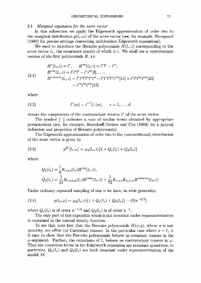
3.1 Marginal expansion for the score vector In this subsection we apply the Edgeworth approximation of order two to

the marginal distribution p(1,; w) of the score vector (see, for example, Skovgaard (1986) for precise settings concerning multivariate Edgeworth expansions).

We need to introduce the Hermite polynomials H(/ , ; i) corresponding to the score vector l,, the covariance matrix of which is i. We shall use a contravariant version of the first polynomials H, i.e.

(3.1)

H r ( l , ; i ) = l r, H ' S ( l , ; i ) = l ~ l ~ - i rs,

HrSt(l , ; i) = lrl~l t - l~ iSt[3], . . . ,

Hr~tu'~(1,; i) -- l~l~Itl~'lVW - l~l~ltlUi~[15] + l~lSitui~w[45]

-i~situivw[15]

where

(3.2) !

l ' (w) = i "~ l , , (w) , r = 1 , . . . , d

denote the components of the contravariant version l* of the score vector. The symbol [ ] indicates a sum of similar terms obtained by appropriate

permutations (see, for example, Barndorff-Nielsen and Cox (1989) for a general definition and properties of Hermite polynomials).

The Edgeworth approximation of order two to the (unconditional) distribution of the score vector is given by

(3.3) p[2][l,;w] = ~d( l , ; i ) {1 + QI(I,) + Q2(I,)}

where

Ql(1,) = ~K~,s,t(1,)H~*t(l ,; i),

Q2(1,) = 1K~,~, t ,u( l , )H~StU(l , 1 rstuvw ;i) + ~-~Kr,s, tKu,v, , ,H (l,; i).

Under ordinary repeated sampling of size n we have, in wide generality,

(3.4) p( l , ;w) = ~d( l , ; i ) {1 + QI(/ ,) + Q2(1,)} + O(n -3/2)

where Ql(1.) is of order n -U2 and Q2(I,) is of order n -1. The only part of this expansion which is not invariant under reparametrization

is contained in the normal density function. To see this, note first that the Hermite polynomials H(x; g), where x is any

quantity, are affine (or Cartesian) tensors. In the particular case where x = I. it is easy to show that the Hermite polynomials behave as covariant tensors in the w-argument. Further, the cumulants of l. behave as contravariant tensors in w. Thus the correction terms in the Edgeworth expansion are invariant quantities; in particular, Ql( l . ) and Q2(l . ) are both invariant under reparametrization of the model M .

72 MARIANNE MORA

3.2 Conditional expansion for the score vector under curved exponential families, using expected geometry

Let w be the true parameter value and let us consider inference on w under ordinary repeated sampling with sample size n. In the case when repeated ob- servations are allowed, the geometrical structure of the parametric space is quite similar to the geometrical s tructure we defined above in Subsections 2.3 and 2.4 and then we shall use the same notations.

By using Taylor expansions, Amari (1985) showed tha t the statistic T = (& - c o , a), where the statistic a is defined as an affine ancillary statistic, is asymp- totically normally distributed with covariance matr ix g~Z.

Our aim is to follow the same procedure as Amari, tha t is first to obtain expansions for the distributions of the statistics X = (l,, a), and a and finally to derive from these expansions an expansion for the conditional distribution of l, given a.

Let us first examine the local t ransformation

(3.5) (©, a) ~ X = O(&, a) = (l., a)

where l. = l. (w; &, a). We denote by X~ the generic component of X which is rewrit ten as

(3.6) Xr = Ir or Xl = a z.

Notice tha t (co, a) ~ (0, a) since/.(co; w, a) = O. The Jaeobian matrix of the t ransformation between X and (&, a) is given by

(3.7) &9 = ~ / /~

with

(3.8)

Jr,(&, a) = ir;,(co; &, a), grk(&, a) Oa~lr(co;(o,a) i ^ = = ~/r (co)&/k(co, a),

& ( C ~ , a ) = Oa,a k = ~5~.

The function A has been defined in Subsection 2.4. At the point (w, 0) these matrices reduce to

(3.9)

I t , = Jr,(w,O) = g,.s(w),

Irk = Jrk(w, O) = ¢)r(co)Ai/k(co, O) = O,

Ikz = & ( c o , 0) = ~ .

Thus YaZ is invertible and hence the t ransformation • is one-to-one around (w, 0). In order to obtain an Edgeworth expansion for the joint distr ibution of (/,, a)

we expand X = ~(&, a) around (w, 0).

GEOMETRICAL EXPANSIONS 73

Then

(~.10)

i.e.

x . -- ¢~ (~ ,0 ) + ¢~/,(~,O)T' + - ~ / ~ 7 ( w , O ) T ~ T ~ + ~ / ~ 7 e T ~ T ~ T ~ + . . .

From (3.10) it is easily seen that the asymptotic covariance matrix t of X given by

(3.11) ~a~ --- I ~ , [ ~ , g ~'~'

which may be decomposed into

(3.12) ~ = g~, ~k = 0, tkt = gk l .

Then, under mild regularity conditions, we may write the Edgeworth expansion of the distribution p(x; w) of X as

(3.13)

where

p(3/; w) = ~k(X; ~){1 + QI(X) + Q2(X)} + O(n -3/2)

Ql(x) = ~K~,f3,-~H~Z'~(X),

and where the K-quantities denote the joint cumulants of ~: and the H-quantities denote the contravariant version of the Hermite polynomials in X with respect to the matrix ~. The terms Q1 and Q2 are respectively of order n -1/2 and n -1.

By integrating (3.13) with respect to I. one obtains

p(a; w) = ~k-d(a; gkl){1 + ~51(a) + ~2(a)} + O(~ -3/2) (3.14)

where

(ol(a) = 114 Hklmla ~ -6 k , l ,m I )I

1 T 7 T . ~ t , , rTklmk' l~m~l ", ~2(a) = 1Kk,l,m,nHk~m"(a) + ~ k , l , m ~ k ,l ,m ~ (a).

p(L ;~ l a) - p (x ;~) p(a; w) - ~d(l.; gT~) ×

Now, since

1 + Q I ( ~ ) +Q2(x) 1+ ~l(a) +~2(a)

7 4 M A R I A N N E M O R A

one obtains the following expansion for the conditional distribution of the score vector, using the expected geometry,

(3.15) p ( 1 , ; w [ a ) = ~ d ( l . ; g ~ ) { l + C l ( X ) + C 2 ( x ) } + O ( n -3/2)

where

and

1 3K H ~k~ "~ CI(X) = {Kr, s,tHrSt(l*) + 3Kr,k,lHr~(X) + r,s,k [X)~

6

C2()~) l {K~,/3,.r,eH~Z're(X ) ktran = - Kk,t,m,nH (a)}

_ / ( ~ ,

1 K H k l m l a ~ f K , , , H k ' t 'm '~ ~ + -~ ~,t,m ~ )l k ,t ,m (a) - K~,~,.~H~f~'~(X)}.

It may be noticed that alternatively, at least in principle, we could apply the Edgeworth approximation of order two directly to the conditional distribution p(l*;w I a) of the score vector I. given the ancillary statistic a. Thus, if we let

K~;.(I. ]a), K~,~,t(1. l a), K.,~,,,~(l. ]a)

denote the first conditional cumulants of the score vector, we obtain the following expression

(3.16) p(l . ;w l a)

= ~d( l . ;K, . . ( l . l a))

× { l + l K r s t ( 1 . o , , l a)Hr~t(1.;K~s(1., l a))

1 + -~K~,.,t,u(l. [a)HrSt~(1.;Kr,~(l. [a))

+ 1Kr,~,t(1, l a)K~,v,~(l, l a)HrSt~w(1.;K~,~(l, l a))}

+ O(n-a/2).

Usually the cumulants and conditional cumulants entering (3.15) and (3.16) are not known explicitly and therefore they can only be found by approximation. See for example McCullagh (1987), for more precise settings.

3.3 Conditional expansion for the score vector, using observed geometry In this subsection we shall derive an asymptotic expansion for the conditional

distribution of l. given an ancillary statistic a. The starting point is an asymptotic expansion for the conditional distribution

p(&; w I a) of the maximum likelihood estimator &, for fixed value of the ancillary a, which was obtained in Barndorff-Nielsen (1986b).

GEOMETRICAL EXPANSIONS 75

This expansion may be wri t ten as

(3.17) P(&;w l a) = p * ( ~ ; ~ la){1 +

= ~d(& -- w; j ' - l ){1 + A1 + Ae + 0(n-3/2)}.

The terms A1 and A2 are given by

1 6rst 2

1 [_3(6t ~ A2 = 24 - [ tu ) {2 fS (grs tu + [rst;u q- [rsu;t + [rs;tu)

+ (6 - 1 I [3]){ + sly,,, +

2

where [31, [~a] indicate appropria te permutat ions of the indices, 6 t = (d~ - a~) t, 6 ~'~ = 6 r6~ , . . . , A1 being of order O(n -1/2) and A2 being of order O(n -1) under ordinary repeated sampling.

We shall derive from (3.17) a similar expansion for the score vector. In fact, given the ancillary statistic a, the maximum likelihood est imator & is in one-to- one correspondence with l. , at least locally around w, and the Jacobian of the t ransformat ion from & to l. is ll.=.l where l . ; . (w;&,a) = [/~;~(w;&,a)]~,.~=l ..... d. When c? is close enough to the true parameter w, it is quite reasonable to consider /.;. as invertible because for & ~ a~ we have / . ; . -~ j' which is invertible in great generality.

Hence we obtain from (3.17):

(3.18) p(1.;w l a) = - w ; I -1 ) (1 + A 1 + A 2 + O ( n - a / 2 ) ) } .

The next step consists in finding an asymptot ic expansion for 6 = & - aJ in terms of l* = ~(-1/..

By Taylor expanding l~(w, &) in its second argument & around w, we obtain

I V 6 stu 1 ~;~t(w)6s t + + " " (3.19) /~(w;&) = y~(w) + yr;~(w)6 ~ + ~ ~ r~;~t~

which may be rewrit ten as

1 1 ~ 6uvw .

On solving for 6 ~ one gets:

(3.21) 6~ = l~ 1 1/r l~ ~ _ l{y~ _ 3V~ vt ~1~.~ - -2 ~ ' 6 u v w r u t t v w J ~ - 4 - " • •

76 M A R I A N N E M O R A

with 1 u~' = l'Ul v, l m'w = UlVl w . . . By inserting (3.21) in each term of (3.18) and Taylor expanding, we obtain,

after some algebra, an expansion ofp(l.; co I a) in terms of l*. The last step consists in collecting terms into invariant terms. Details of all these calculations are given in the Appendix. The result is the following:

Under ordinary repeated sampling and with relative error of order O(n -3/2)

(3.22) p( l , ;w I a) = ~Od(l,; ~0{1 + BI + B2 + 0(n-3/2)}

with B1 = (1/6)grst~rst and

1

1 rs tu 1 r s t u v w

B1 and B2 being of order O(n -1/2) and O(n -1) respectively. Here the g-quant i t ies denote the contravariant version of the Hermite polynomials defined in terms of l, and ~(. The other quantities are covariant tensors given by

(3.23) T,-,t = -(X,-st + Y,-s;t[3]),

(3.24) ~i,~;t~, = ~/,,;t, - Y,,;. f ~ ; t J vw,

( 1 ) (3.25) Trst~ = - )/~st~ + Yrst;~[ 4] + ~(Yr~;t~ + Yr~;w~Ft~jw[6]) •

We shall discuss these various quantities in Section 5.

4. Expansions for the maximum likelihood estimator

4.1 Expansions for the maximum likelihood estimator under curved exponential families

For completeness, we mention here that a detailed s tudy of the unconditional and conditional expansions for the maximum likelihood estimator, under curved exponential families and using the expected geometrical s tructure, has been made in Amari (1985) and Amari and Kumon (1983).

4.2 Conditional expansion for the maximum likelihood estimator, using the expected geometrical structure

From the viewpoint of invariance and geometrical interpretation, it is relevant to derive the conditional expansion for the maximum likelihood est imator & via the conditional expansion for the score vector. As mentioned in Subsection 2.5, using the (locally) one-to-one transformation 1. --~ & yields an asymptot ic expansion for the distr ibution of the maximmn likelihood estimator, which is divided in two parts, a variant and an invariant.

In Barndorff-Nielsen (1986b), 5 = & - ~ is modified into the bias corrected form as 8 ~ = © - w - Pl, where the bias term #1 is given by

1 c~r st 1 1 _I/~c~ I s t

GEOMETRICAL EXPANSIONS 77

and is of order n -1. Now, making the one-to-one transformation I. -~ &, one obtains from (3.22)

(4.2) l a)

= II,;,l~a(z,; D{1 + B1 + B2 + 0(n-3 /2)}

= ~ d ( 6 ' ; j-~)(~d(l,; j')/9~d(¢5'; J'-~))l/*;* 1{1 + B~ + B2 + " "}

where

~Oa(1,; ])/qOd(6'; ] - l ) = []l-a exp { ~(t5 ''~ - l"*)],~ } .

Next, we derive expansions for exp{ (1/2)(6 'r~ - 1 ~ ) l r s } and 11.;. l I / - 1[ by inserting (3.22) in these two expressions. The explicit forms of these expansions are given in the Appendix. The last step consists again in Taylor expanding and then collecting terms of the same order.

Finally one obtains the following expansion for the bias-corrected maximum likelihood estimator:

(4.3) p ( S t ; w l a ) = ~ a d ( 8 ' ; ~ - I ) { I + B I + B 2 + . . . } { I + C I + C 2 + . . . }

where C1 = - ( 1 / 2 ) ~ t ; ~ 4 TM is of order n -1/2, and

1 V Cl r~t~ - - [ 3 ] ~ r s l TM) C2 = -- ~ t r ;s tu~

iv v + ~ , t ;~ , ~ ; ~ , ° + + 4 l ~ ] ~ u t / I t ~

_ 41tvfw~Ir~ _ it,~ffwt/I"~ + l ~ W ] TM

_ 2l,,Wff~] TM + 41s"]t~f ~ _ 4l 'wl t~f f ")

/.I r l

is of order n -1. The symbol [ ] indicates here a sum of 3 similar terms obtained by permuting

the indices r, s, t. It may be noted that I rstu - [3]ff~/TM is a contravariant tensor of rank 4 in

w. Also, the factor in C2 multiplied by the quantity Ytxs Yu;vw is a contravariant tensor of rank 6.

The expansion we have obtained involves the product of two expansions, the first of which (with terms B1, B2, . . . ) is invariant. The second is related to the observed ( - 1)-connection.

Thus, if we use the special coordinate system given in (2.21) as a parametriza- --1 --1

tion for the model, the quantities ]7 / i ~st, ]7 r~tu,"" can be made to vanish. With this choice of parametrization, the expansion for & reduces to

(4.4) p(5';w I a) = ~d(5 ' ;1-1){1+/31 + B2 + ' - . } ,

since in such a coordinate system one has

and

78 M A R I A N N E M O R A

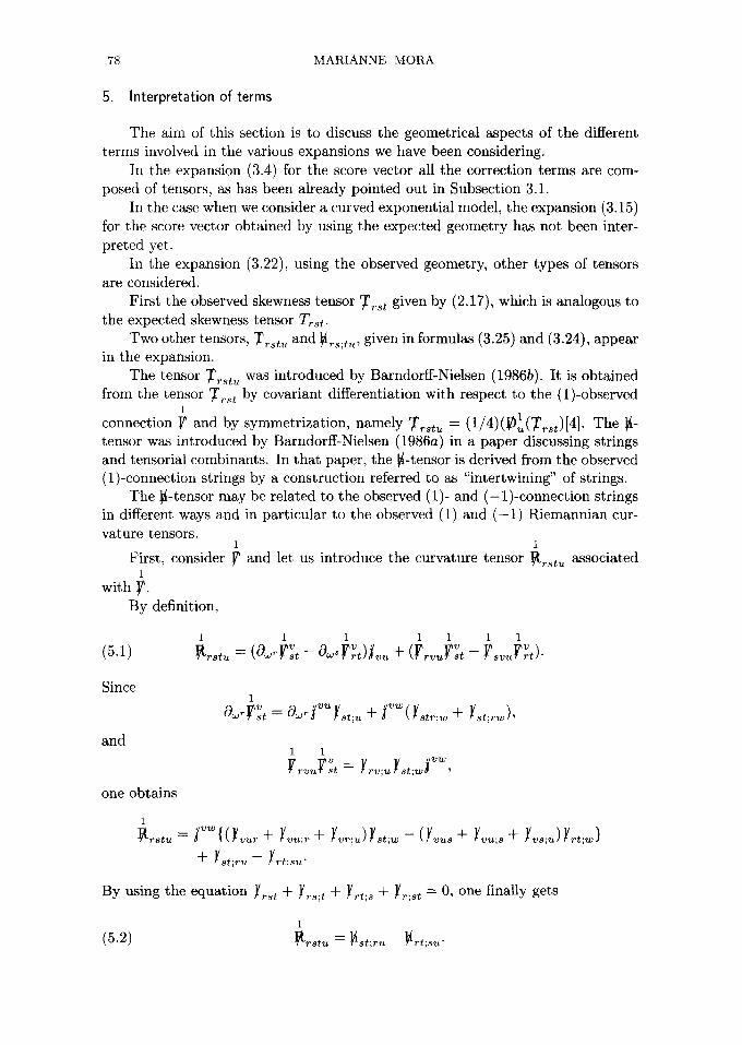
5. Interpretation of terms

The aim of this section is to discuss the geometrical aspects of the different terms involved in the various expansions we have been considering.

In the expansion (3.4) for the score vector all the correction terms are com- posed of tensors, as has been already pointed out in Subsection 3.1.

In the case when we consider a curved exponential model, the expansion (3.15) for the score vector obtained by using the expected geometry has not been inter- preted yet.

In the expansion (3.22), using the observed geometry, other types of tensors are considered.

First the observed skewness tensor ~rst given by (2.17), which is analogous to the expected skewness tensor T~.st.

Two other tensors, Tr.stu and ~s;tu, given in formulas (3.25) and (3.24), appear in the expansion.

The tensor ~rstu was introduced by Barndorff-Nielsen (1986b). It is obtained from the tensor T~st by covariant differentiation with respect to the (1)-observed

1

connection y' and by symmetrization, namely ~stu = (1/4)(]~lu(~'~.st)[4] • The }i- tensor was introduced by Barndorff-Nielsen (1986a) in a paper discussing strings and tensorial combinants. In that paper, the ~I-tensor is derived from the observed (1)-connection strings by a construction referred to as "intertwining" of strings.

The }i-tensor may be related to the observed (1)- and (-1)-connection strings in different ways and in particular to the observed (1) and ( -1) Riemannian cur- vature tensors.

1 1

First, consider ~ and let us introduce the curvature tensor ~t~.st,~ associated 1

with F- By definition,

(5.1) 1 1 1 1 1 1 1

v • v

Since

and

one obtains

1

1 1

y y r v U .st --~ r v ; u 8 t ; w '

1

+ Y.st; -

By using the equation ~/~.st + Yr.s;t + ~/~t;.s + ~/~:.st = 0, one finally gets

( 5 . 2 ) trstu = st;ru - rt; u-

G E O M E T R I C A L EXPANSIONS 79

- 1 - 1

In the same way, considering F and ]~ ~t~, one finds

- 1

( 5 . 3 ) = -

There is a similar relationship for corresponding expected quantities from curved exponential families 1 R~stu = Hst;ru - H~t;su where Hst;~u is the inner product of

lk - l t the (1) and ( -1) imbedding curvature tensors, i.e. H~t;~ = H~t H ~ qkl where H~t k and H~-~' are the components of the imbedding curvature for the (1)- and (-1)-connection, respectively (see Amari (1985)). This interpretation can be ex- tended beyond curved exponential family models by using Amari's idea of local exponential family, see Amari et al. (1987); see also Vos (1989). Because of the structure of the ~i-tensor, it is not obvious that a similar interpretation of the ~i-tensor may be derived for the observed curved exponential approximation. A clearly geometric meaning of the ~i-tensor is still missing.

However, it is possible to relate the ~i-tensor to the observed (1)- and ( -1)- connection strings also in the following way.

Since

~lrs;tu -~ Yrst;u

1 1 1 V " = +

1 1 1 W V "

we have, denoting covariant differentiation relative to ~ and with respect to w t by

(5.4) 1 1

~rs ; tu -~ ~ t ( ~ V s ) ~ v u -- Yrst;u

1 1 ; - .

= - L 3Jw

We get a similar expression for the observed (-1)-connection, namely

Therefore formula (5.4) expresses the ~-tensor as the difference between ]~ (y;~:) 1

which belongs to the canonical string generated by ~ and the corresponding term 1

in the connection string ]~. Except for this, we could not find any satisfying geometrical interpretation of this ~i-tensor.

One has an analogous result for the ~-tensor expressed in terms of the observed ( - 1)-connection.

We may notice that for (k ,k ) exponential models one has •rst -- Kr,s,t, T~stu = Kr,s,t,~ and ~i~s;t u = 0. The conditional expansions for the score vec- tor, given in (3.16) and (3.22), are quite similar. We may relate the observed

80 M A R I A N N E M O R A

tensors T~st and T,-~tu - (1/2)~i~;t~[6] to the cumulants of order 3 and 4 in (3.16), respectively (for (k, k) exponential families these observed tensors reduce to the observed cumulants of order 3 and 4). The extra term in (3.22) which is now found in (3.16) should be ascribed to the different geometrical structure involved.

Finally we shall comment on the variant part of the expansion (4.3) obtained for the conditional distribution of the maximum likelihood estimator.

The correction term of order n-1/2 contains the Hermite polynomial Ill TM (l,; ~) - 1

and the term Yt;~8 = ~' ~st" In the correction term of order n -1 we collected terms in order to emphasize the various terms Y~;st, ~/~;~t~ entering it and which belong to the (-1)-connection string. The remaining terms are not explained yet. In Amari and Kumon (1983), they give an expansion for the conditional distribution of the maximum likelihood estimator with correction terms of order n -1/2 and n -1. It may be noted that only the correction term of order n-U2 is given a geometrical interpretation.

6. Concluding remarks

The score vector appears to be a main tool in constructions of expansions that can be expressed in terms of invariant and geometrical quantities. Nevertheless the last expansion obtained in (4.3) is not quite satisfactory, since all the terms contained have not yet been given a clear geometrical interpretation. The question is how to build a procedure, based on the intrinsic geometrical properties of the score vector and the theory of strings, giving a geometrical interpretation.

Another point concerns the link between the order of the correction terms ap- pearing in the expansions obtained above and the corresponding tensors contained in these correction terms. It appears that for approximations with error of order n -1 the tensors required are the metric tensor and the skewness tensor, in both the expected case and the observed case. If we consider correction terms of order n -1 other tensors appear, namely the ~i and ~ s t u tensors, which are again related to the observed geometrical structure defined on the model. Thus, these tensors seem to be fundamental geometrical objects but in a sense which has not been fully elucidated yet.

Acknowledgements

I am indebted to the referees for their thorough readings of the paper and very constructive comments.

Appendix

PROOF OF FORMULA (3.22). From (3.18) and (3.21) we obtain the following expansions:

1) ((Iz.; .I)/(lll) = 1 - L . j

"s "~'w 1,' 1,1tu + I I + .

GEOMETRICAL EXPANSIONS 81

Here we use the differentiation formulas: 0~loglA I = aJiOraij and O,.a ij = - a i k a l J O r a k l where A ~- [aij] is any positive definite mat r ix and A -1 = [aiJ].

2) exp{ 1 ~.~. "1 exp{ l l "* ~

1 g U st 1 1/ 1 Ir 1 rstu x 1 + ~t~;~t - g t , ; r s t t ~ ~

1 V V I rstuvw } q- -g it;st ,u;vw 4- O(rz-3/2) "

3) A1 = 2 1 ~s ~/"st (}/,',;t + ~ Yrst) - ~ J (L,;~ + L,0z* +

1 rs tu "{- 4 { 1 l (Yrs;r q- Yrsr)Yt2

g r lrstu - (2L~, + / , ; , t a D , , ~ + o(n-3/~)}.

4) The t e rm A2, of order n -1, in (3.17) is rewri t ten in terms of l " . . . , just by making the subst i tut ions 8 r -+ F, 5r, ~ Us . . . . Finally we obtain

p( l , ;~ l a) = ~d(l,; ~){1 + B1 + th + . . . }

where

1 Us t / 2 B1 = - ~trSlt(~rs;t + ~rst)-k-~ L ~rs;t-b ~ ~rst)

is of order rt -1/2 under ordinary repeated sampling of size n, and

B2 ~ (ltu . tu . rs = - - ~ ){2t (L~.~ + L.,;~ + Y.~;~ + Y~,~,,)

+ ( z f ~ F TM - f~fl~)(L~;~ + L~3(Lw;. + L,~,,)}

+ ~t"~(L~;~ - + L~-)Y~. + f~z~"L;~-5.

1 rs tu vw

1 (Ust ~ { + ~ - f~F ' [3] ) (3L~,~ + s l y , ; . + 6L~;..)

82 MARIANNE MORA

2

1 rstu .vw l l r s t u .vw

1 irst u

+ + 2 + 2 l/ t ) ~( lrstuvw- f's[tu]vw[I5]) (~vw;~ ~v~o~) (Y~s;t /

l=v

is of order n-1. The last step consists in collecting terms such that geometrical quantities

appear. For B1 it is easily seen that

B1 ~- ~ g r s t ( z*; ~)Trs t"

For the terms of order n -1 the calculations are longer but the expression of B2 finally reduces to

1

1 rstuvw + ~ %~,T~v~.

PROOF OF FORMULA (4.3).

(~d(1,;~)/(~d(5';~-l)))= Ij',-i exp {~(5 ' ' ~ - I'~)~,~}.

Introducing the expansion (3.21) for ti in this expression and developing leads to

(~d(l.;l)/(Sa(5';]-l))) = IJ'l-l{1 + A i + A; + . . . }

where All - _ 1 V l TM 1 ¥ frs f l

is of order n -1/: and

A ~ = - 111 1 ~stu -6 tr;stu ~

+ ~ w ~ ( 4 L ; ~ v y w ; j vw + L: ,~G;~d w - L ~ L ; v d w)

+ l l~u1"~Y(-2L; , s G;,~ + L; ,~L;w)

1 V lrstuv w 1 V V ~rs]tu]vw

GEOMETRICAL EXPANSIONS 83

is of order n -1. Using the same method for I/,;,ll~(1-1 we get I/,;,11[I - ] = 1 + A~' + A~ ' + . . -

where A~' .,.s t n - l~2 = [ l Yt;r8 is of order and

l ltu rs ,w

is of order n-~. Inserting these two expressions in formula (4.2), developing and collecting

terms yields the final result (4.3).

REFERENCES

Amari, S. I. (1985). Differential-geometrical methods in statistics, Lecture Notes in Statistics, 28, Springer, Heidelberg.

Amari, S. I. and Kumon, M. (1983). Differential geometry of Edgeworth expansion in curved exponential family, Ann. Inst. Statist. Math., 35, 1-24.

Amari, S. I., Barndorff-Nielsen, O. E., Kass, R. E., Lauritzen, S. L. and Rao, C. R. (1987). Differential geometry in statistical inference, Institute of Mathematical Statistics~ Monograph Series, 10, Hayward, California.

Barndorff-Nielsen, O. E. (1980). Conditionality resolution, Biometrika, 6T, 293-310. Barndorff-Nielsen, O. E. (1983). On a formula for the distribution of the maximum likelihood

estimator, Biometrika, 70, 856-873. Barndorff-Nielsen, O. E. (1986a). Strings, tensorial combinants and Bartlett adjustments, Proc.

Roy. Soe. London Set. A, 406, 127-137. Barndorff-Nielsen, O. E. (1986b). Likelihood and observed geometries, Ann. Statist., 14, 856-

873. Barndorff-Nielsen, O. E. (1987). Likelihood, ancillary and strings, Proceedings of the First World

Congress of the Bernoulli Society, 2, 205-213. Barndorff-Nielsen, O. E. (1988). Parametric statistical models and likelihood, Lecture Notes in

Statistics, 50, Springer, Heidelberg. Barndorff-Nielsen, O. E. and Bl~esild, P. (1987a). Strings: Mathematical theory and statistical

examples, Proc. Roy. Soc. London Set. A, 411, 155-176. Barndorff-Nielsen, O. E. and Blmsild, P. (1987b). Strings: contravariant aspect, Proc. Roy. Soc.

London Set. A, 411,421-444. Barndorff-Nielsen, O. E. and Bhesild, P. (1988). Coordinate-free definition of structually sym-

metric derivative strings, Adv. in Appl. Math., 9, 1-6. Barndorff-Nielsen, O. E. and Cox, D. R. (1989). Asymptotic Techniques for Use in Statistics,

Chapman and Hall, London. Blmsild, P. (1990). Yokes: orthogonal and observed normal coordinates, Research Report, 205,

Department of Theoretical Statistics, Aarhus University. McCullagh, P. (1987). Tensor Methods in Statistics. Monographs on Statistics and Applied

Probability, Chapman and Hall, London. McCullagh, P. and Cox, D. R. (1986). Invariants and likelihood ratio statistics, Ann. Statist.,

14, 1419-1430. Murray, M. K. and Rice, J. W. (1987). On differential geometry in statistics, Research Report,

School of Mathematical Sciences, The Flinders University of South Australia. Skovgaard, I. M. (1986). On multivariate Edgeworth expansions, Internat. Statist. Rev., 54,

169 186. Vos, P. W. (1989). Fundamental equations for statistical submanifolds with applications to the

Bartlett correction, Ann. Inst. Statist. Math., 41, 429 450.