Embed Size (px)
Citation preview
Geometric Mechanics and Symmetry
OXFORD TEXTS IN APPLIED AND ENGINEERING MATHEMATICS
Books in the series
∗ G. D. Smith: Numerical Solution of Partial Differential Equations, third edition
∗ R. Hill: A First Course in Coding Theory
∗ I. Anderson: A First Course in Combinatorial Mathematics, second edition
∗ D. J. Ancheson: Elementary Fluid Dynamics
∗ S. Barnett:Matrices: Methods and applications
∗ L. M. Hocking: Optimal Control: An introduction to the theory with applications
∗ D. E. Ince: An Introduction to Discrete Mathematics, Formal System Specification,and Z, second edition
∗ O. Pretzel: Error-Correcting Codes and Finite Fields
∗ P. Grindrod: The Theory and Applications of Reaction-Diffusion Equations:Patterns and waves, second edition
1. Alwyn Scott:Nonlinear Science: Emergence and dynamics of coherent structures2. D.W. Jordan and P. Smith: Nonlinear Ordinary Differential Equations: An
introduction to dynamical systems, third edition3. I.J. Sobey: Introduction to Interactive Boundary Layer Theory4. A.B. Tayler:Mathematical Models in Applied Mechanics, reissue5. L. Ramdas Ram-Mohan: Finite element and Boundary Element Applications in
Quantum Mechanics6. Bernard Lapeyre, Étienne Pardoux, and Rémi Sentis: Introduction to Monte-
Carlo Methods for Transport and Diffusion Equations7. Isaac Elishakoff and Yongjian Ren: Finite Element Methods for Structures with
Large Stochastic Variations8. Alwyn Scott: Nonlinear Science: Emergence and dynamics of coherent structures,
second edition9. W.P. Petersen and P. Arbenz: Introduction to Parallel Computing: A practical
guide with examples in C10. D.W. Jordan and P. Smith: Nonlinear Ordinary Differential Equations,
fourth edition11. D.W. Jordan and P. Smith: Nonlinear Ordinary Differential Equations:
Problems and Solutions12. Darryl D. Holm, Tanya Schmah, and Cristina Stoica: Geometric Mechanics and
Symmetry: From Finite to Infinite Dimensions
Titles marked with (*) appeared in the ‘Oxford Applied Mathematics and ComputingScience Series’, which has been folded into, and is continued by, the current series.
Geometric Mechanicsand SymmetryFrom Finite to Infinite Dimensions
Darryl D. HolmImperial College London
Tanya SchmahMacquarie University and The University of Toronto
Cristina StoicaWilfrid Laurier University
With solutions to selected exercises by
David C. P. EllisImperial College London
1
3Great Clarendon Street, Oxford OX2 6DPOxford University Press is a department of the University of Oxford.It furthers the University’s objective of excellence in research, scholarship,and education by publishing worldwide in
Oxford New YorkAuckland Cape Town Dar es Salaam Hong Kong KarachiKuala Lumpur Madrid Melbourne Mexico City NairobiNew Delhi Shanghai Taipei TorontoWith offices inArgentina Austria Brazil Chile Czech Republic France GreeceGuatemala Hungary Italy Japan Poland Portugal SingaporeSouth Korea Switzerland Thailand Turkey Ukraine Vietnam
Oxford is a registered trade mark of Oxford University Pressin the UK and in certain other countries
Published in the United Statesby Oxford University Press Inc., New York
© Darryl D Holm, Tanya Schmah, and Cristina Stoica 2009
The moral rights of the authors have been assertedDatabase right Oxford University Press (maker)
First published 2009
All rights reserved. No part of this publication may be reproduced,stored in a retrieval system, or transmitted, in any form or by any means,without the prior permission in writing of Oxford University Press,or as expressly permitted by law, or under terms agreed with the appropriatereprographics rights organization. Enquiries concerning reproductionoutside the scope of the above should be sent to the Rights Department,Oxford University Press, at the address above
You must not circulate this book in any other binding or coverand you must impose the same condition on any acquirer
British Library Cataloguing in Publication DataData available
Library of Congress Cataloging in Publication DataData available
Typeset by Newgen Imaging Systems (P) Ltd., Chennai, IndiaPrinted in Great Britainon acid-free paper byCPI Antony Rowe, Chippenham, Wiltshire
ISBN 978–0–19–921290–3 (Hbk)ISBN 978–0–19–921291–0 (Pbk)
10 9 8 7 6 5 4 3 2 1
Preface
This is a textbook for graduate students that introduces geometric mechan-ics in finite and infinite dimensions, using a series of archetypal examples.
Classical mechanics, one of the oldest branches of science, has undergonea long evolution, developing hand in hand with many areas of mathematics,including calculus, differential geometry and the theory of Lie groups andLie algebras. The modern formulations of Lagrangian and Hamiltonianmechanics, in the coordinate-free language of differential geometry, areelegant and general. They provide a unifying framework for many seeminglydisparate physical systems, such as N -particle systems, rigid bodies, fluidsand other continua, and electromagnetic and quantum systems.
The first part of this book concerns finite-dimensional conservativemechanical systems. The modern formulations of Lagrangian and Hamilto-nian mechanics use the language of differential geometry. Some advantagesof this approach are: (i) it applies to systems on general manifolds, includ-ing configuration spaces defined by constraints; (ii) it is coordinate-free,or at least independent of a particular choice of coordinates; (iii) the geo-metrical structures have analogues in infinite-dimensional systems. Just asimportantly, the geometric approach provides an elegant and suggestiveviewpoint. For example, rigid body motion can be seen as geodesic motionon the rotation group. Symmetries of mechanical systems are representedmathematically by Lie group actions. The presence of symmetry allows areduction in the number of dimensions of a mechanical system, in two basicways: by grouping together equivalent states; and by exploiting conservedquantities (momentum maps) associated with the symmetry. The book dis-cusses Lie group symmetries, Poisson reduction and momentum maps ina general context before specializing to systems where the configurationspace is itself a Lie group, or possibly the product of a Lie group and avector space. For systems, such as the free rigid body, whose symmetrygroup is also its configuration space, an especially powerful reduction the-orem exists, called Euler–Poincaré reduction. An extension of this theoremcovers systems where the Lie group configuration space is augmented bya vector space describing certain ‘advected quantities’, such as the gravitycovector in the heavy top example.
vi Preface
The second part of the book treats what might be considered the infinite-dimensional versions of the rigid body and the heavy top by replacing theaction of the rotation group by the action of a group of diffeomorphisms.Roughly speaking, passing from finite to infinite dimensions in geometricmechanics means replacing matrix multiplication by composition of smoothinvertible functions. The book develops these ideas in the setting of Euler–Poincaré theory, based on reduction by symmetry of Hamilton’s variationalprinciple. The infinite-dimensional results corresponding to rigid-body andheavy-top dynamics are exemplified, respectively, in geodesic motion onthe diffeomorphisms governed by the EPDiff equation and in the action ofthe diffeomorphisms on vector spaces of ‘advected quantities’ governed bythe equations of continuum dynamics.
EPDiff arises in one spatial dimension as the zero-dispersion limit of theCamassa–Holm (CH) equation for shallow water waves. The CH equationis an approximate model of shallow water waves obtained at one orderin the asymptotic expansion beyond the famous Korteweg–de Vries (KdV)equation. KdV and CH are both nonlinear partial differential equations.They each support remarkable solutions called ‘solitons’ that interact infully nonlinear wave collisions and whose exact solution may be obtained bythe linear method of the inverse scattering transform. In the zero-dispersionlimit of shallow water wave theory in which the EPDiff equation arises,these solitons become singular particle-like solutions carrying momentumsupported on Dirac delta measures. The EPDiff equation for the Euler–Poincaré dynamics of geodesic motion on the diffeomorphisms also appliesin image analysis. In particular, EPDiff applies in the comparison of shapesin morphology and computational anatomy.
The Euler–Poincaré approach that generalizes the heavy-top problemfrom the action of the rotations on vectors in R3 to the action of the diffeo-morphisms on vector spaces produces yet another rich array of results. Inparticular, it produces the extensive family of equations for ideal continuumdynamics, whose applications range from nanofluids to galaxy dynamics.Among the many available variants of ideal continuum dynamics, we selecta single class for a unified treament. Namely, we treat a class of approxi-mate models of global ocean circulation that are used in climate prediction.Thus, the theoretical development of these parallel ideas in finite and infi-nite dimensions is capped by the explicit application in the last chapter toderive a unified formulation of the family of approximate equations forocean dynamics and climate modelling familiar to modern geoscientists.
One may think of moving from the first part of the book to the secondpart as moving from finite-dimensional to infinite-dimensional geometricmechanics. The analogies between the two types of problems are veryclose. The first part of the book deals with systems of nonlinear ordinary
Preface vii
differential equations (ODE), whose questions of existence, uniqueness andregularity of solutions may generally be answered by using standard meth-ods. The second part of the book deals with nonlinear partial differentialequations (PDE) where the answers to such questions are often quite chal-lenging and even surprising. For example, these particular PDE possesscoherent excitations and even singular solutions that emerge from smoothinitial data and whose nonlinear interactions exhibit particle-like scatteringbehaviour reminiscent of solitons. Unlike many other PDE investigations,geometric mechanics treats the emergence of these measure-valued, particle-like solutions in the initial-value problem for some of the models as achallenge to be celebrated, rather than a cause for regret.
Prerequisites and intended audience
The reader should be familiar with linear algebra, multivariable calculus,and the standard methods for solving ordinary and partial differential equa-tions. Some familiarity with variational principles and canonical Poissonbrackets in classical mechanics is desirable but not necessary. Readers withan undergraduate background in physics or engineering will have the advan-tage that many of the examples treated here, such as the motion of rigidbodies and the dynamics of fluids, will be familiar. In summary, the pre-requisites are standard for an advanced undergraduate student or first-yearpostgraduate student in mathematics or physics.
How to read this book and what is not in it
Part I is meant to be used as a textbook in an upper-level course on geo-metric mechanics. It contains many detailed explanations and exercises.Although a wide range of topics is treated, the introduction to each ofthem is meant to be gentle. Part II addresses a more advanced reader andfocuses on recent applications of geometric mechanics in soliton theory,image analysis and fluid mechanics. However, the mathematical prerequi-sites for rigorous treatments of these applications are not provided here.Readers interested in a more technical mathematical approach are invitedto consult some of the many citations in the bibliography that treat thesubject in that style.
The book focuses on Euler–Poincaré reduction by symmetry, which is abroadly applicable theory, but it excludes many other important topics,such as Lagrangian reduction of general tangent bundles and symplec-tic reduction. Likewise, it omits many other standard mechanics topics,including integrability, Hamilton–Jacobi theory, and more generally, anyquestions in the modern theory of dynamics, bifurcation and control.
viii Preface
Most of the notation is consistent with that of the Marsden–Ratiu school.This was a deliberate choice, since one of the intentions in writing thefirst part was to bridge the gap between the standard classical mechanicsbooks such as Classical Mechanics by Goldstein [Gol59] andMechanics byLandau and Lifshitz [LL76] and the more advanced books such as Foun-dations of Mechanics by Abraham and Marsden [AM78] and Introductionto Mechanics and Symmetry by Marsden and Ratiu [MR02].
Description of contents
Part I
The opening chapter briefly presents Newtonian, Lagrangian and Hamil-tonian mechanics in the familiar setting of N -particle systems in Euclideanspace. A short classical description of rigid body motion is also given. Chap-ters 2 and 3 build up the prerequisites for the extension of Lagrangianand Hamiltonian mechanics to systems on manifolds. Chapter 2 intro-duces manifolds, with emphasis on submanifolds of Euclidean space, whichappear in mechanics as configuration spaces defined by constraints. Thischapter also introduces matrix Lie groups (covered in more detail in Chap-ter 5). Chapter 3 gives a minimal introduction to differential geometry,including a taste of Riemannian and symplectic geometry. Chapter 4presents Lagrangian and Hamiltonian mechanics on manifolds, and endswith a brief look at symmetry, reduction and conserved quantities.
In order to study symmetry in more depth, one needs Lie groups and theiractions, which are the subject of Chapters 5 and 6. Lie groups and algebrasare introduced in both matrix and abstract frameworks. Lie group actionson manifolds, and the resulting quotient spaces, provide sufficient tools tointroduce Poisson reduction.
The remaining chapters focus on mechanical systems on Lie groups, thatis, mechanical systems where the configuration space is a Lie group. Chap-ter 7 covers Euler–Poincaré reduction, emphasizing the examples of thefree rigid body and the heavy top. Chapter 8 introduces momentum maps.Chapter 9 covers Lie–Poisson reduction, which is the Hamiltonian coun-terpart of Euler–Poincaré reduction. Chapter 10 applies the results of thepreceding three chapters to the example of a pseudo-rigid body. Pseudo-rigid motions provide a link between the rigid motions studied in Part I andthe fluid motions that are the subject of Part II.
Part II
In a famous paper, Arnold [Arn66] observed that Euler ideal fluidmotion may be identified with geodesic flow on the volume-preserving
Preface ix
diffeomorphisms, with a metric determined by the fluid’s kinetic energy.This observation was further developed in a rigorous analytical settingby Ebin and Marsden [EM70]. The methods of geometric mechanics sys-tematically develop this result from the Euler–Poincaré (EP) variationalprinciple for the Euler fluid equations. These methods also generate theirLie–Poisson Hamiltonian structure, Noether theorem, momentum maps,etc. As Arnold observed, the configuration space for the incompressiblemotion of an ideal fluid is the group G = DiffVol(D) of volume-preservingdiffeomorphisms (smooth invertible maps with smooth inverses) of theregion D occupied by the fluid. The tangent vectors in TG for the mapsin G = DiffV ol(D) represent the space of fluid velocities, which must satisfyappropriate physical conditions at the boundary of the region D. Groupmultiplication in G = DiffV ol(D) is composition of the smooth invertiblevolume-preserving maps. One of the purposes of this text is to explain howthe Euler equations of fluid motion may be recognized as the Euler–Poincaréequations EPDiffV ol defined on the dual of the tangent space at the identityTeG = Te DiffV ol(D) of the right-invariant vector fields over the domain D.
Applications of EPDiff in Part II
• In the motivating example, Euler’s fluid equations emerge as EPDiffV ol
when the diffeomorphisms are constrained to preserve volume so thatG = DiffV ol(D), and the kinetic energy norm is taken to be the L2 norm‖u‖2
L2 of the spatial fluid velocity. From the viewpoint of constraineddynamics, the fluid pressure p may be regarded as the Lagrange multiplierthat imposes preservation of volume.
• Other choices of the kinetic energy norm besides the L2 norm of veloc-ity also produce interesting continuum equations as geodesic flowson DiffV ol(D). For example, the choice of the H 1 norm (L2 normof the gradient) of the spatial fluid velocity yields the Lagrangian-averaged Euler-alpha (LAE-alpha) equations when incompressibility isimposed. For more discussion of the LAE-alpha equations, see, e.g.,[HMR98a, Shk00].
• The H 1 norm also yields one of a family of interesting EPDiff equationswhen incompressibility is not imposed, so that the motion takes placeon the full diffeomorphism group. In one spatial dimension on the realline (and also in a periodic domain), the EPDiff equation for the H 1
norm of the spatial fluid velocity is completely integrable in the Hamil-tonian sense and possesses soliton solutions. This equation is the limitof the Camassa–Holm (CH) equation for shallow-water wave motionwhen its linear dispersion coefficients tend to zero [CH93]. The CHequation and its peaked-soliton solutions – called peakons – that exist
x Preface
in its zero-dispersion limit are discussed in Chapter 11. EPDiff solu-tion behaviour in one dimension and its wave-train solutions for variousother norms are discussed in Chapter 12. The CH equation and its zero-dispersion limit are integrable Hamiltonian systems that possess solitonsolutions. The geometric ingredients underlying integrability and solitonsolutions are reviewed in Chapter 13.
• Another application of the family of EPDiff equations that involvesvarious choices for the kinetic energy norm in two and three spatialdimensions arises in the field of morphology, in the modern endeavourof computational anatomy (CA) [MTY02, HRTY04]. After generalizingthe peakon solutions of EPDiff for the H 1 norm to higher dimensions inChapter 14, methods for applying higher-dimensional singular EPDiffsolutions for matching image contours in computational anatomy aresketched in Chapter 15.
• After the discussion in Chapter 15 about matching image contours,Chapter 16 discusses matching also what is inside the contours. Theconceptual parallel between the two chapters reflects the step from pureEP (rigid body, incompressible fluids) to EP with advected quantities(heavy top, compressible fluids). In explaining the geometrical theoryof image matching using the metamorphosis approach, Chapter 16 setsup the remaining chapters about the EP formulation of fluid dynamics.Chapter 16 also reinforces the theme of soliton equations in the 1D reduc-tions of this approach in image matching. Finally, Chapter 16 discussesthe geometric-mechanical analogy of image matching with the problemof how a falling cat reorients its body in mid-air so that it lands onits paws.
• Chapter 17 discusses the EP theorem for ideal continuum flows carry-ing advected quantities. The application of the more general EP theoremin the derivation and analysis of models of geophysical fluid dynam-ics (GFD) is discussed in Chapter 18. These GFD models are crucial innumerical computations for global climate modelling.
This family of GFD equations is derived by applying the method ofasymptotic expansions to Hamilton’s principle for a rapidly rotating, sta-bly stratified incompressible flow in the Eulerian description. Such flowsare seen in the ocean, whose slow time scales dictate the dynamics ofthe global climate. The rapid rate of rotation and thin domain of flow inglobal ocean circulation are characterized by two small non-dimensionalparameters: the Rossby number (ratio of nonlinearity to Coriolis force)and the aspect ratio of the domain. Expansion of Hamilton’s principle
Preface xi
in these two small parameters provides a unified approach in the deriva-tion of the rich and multifaceted family of approximate equations forgeophysical fluid dynamics (GFD). Each of the equations in this familyof GFD approximations is both nonlinear and non-local in character.The Euler–Poincaré approach explains their shared properties of energyconservation and circulation dynamics.
Acknowledgements
We are enormously grateful to our friends, students and teachers, withoutwhom this endeavour would never have been completed. We thank ourfriends and collaborators, Tony Bloch, Dorje Brody, Roberto Camassa,Colin Cotter, John Gibbon, John Gibbons, Daniel Hook, Boris Kupersh-midt, Jeroen Lamb, Peter Lynch, Jerry Marsden, Peter Olver, VakhtangPutkaradze, George Patrick, Tudor Ratiu, Mark Roberts, Martin Staley,Alain Trouvé, Laurent Younes, Alan Weinstein and Beth Wingate for theirhelp and camaraderie in our research together in geometric mechanics. Weespecially thank our students Cesare Tronci and David Ellis at Imperial Col-lege London for making the teaching of these topics so rewarding. Thanksto Robert Jones for comments and careful proof-reading.
DDH: To Justine, for all our expeditions of discovery and fun.TS: To Hillary Sanctuary, whose questions, enthusiasm and friendship firstencouraged me to write a book on this subject.TS and CS: Thanks to Macquarie University and Wilfrid Laurier University,respectively, for supporting the writing of this book with teaching releases.Many thanks to Ica for the Turkish coffees she made for us during all thesummer days we spent writing.
Contents
Part I 1
1 Lagrangian and Hamiltonian mechanics 3
1.1 Newtonian mechanics 31.2 Lagrangian mechanics 131.3 Constraints 181.4 The Legendre transform and Hamiltonian mechanics 241.5 Rigid bodies 30
2 Manifolds 43
2.1 Submanifolds of Rn 432.2 Tangent vectors and derivatives 572.3 Differentials and cotangent vectors 692.4 Matrix groups as submanifolds 782.5 Abstract manifolds 83
3 Geometry on manifolds 99
3.1 Vector fields 993.2 Differential 1-forms 1123.3 Tensors 1173.4 Riemannian geometry 1283.5 Symplectic geometry 139
4 Mechanics on manifolds 155
4.1 Lagrangian mechanics on manifolds 1554.2 The Legendre transform and Hamilton’s equations 1604.3 Hamiltonian mechanics on Poisson manifolds 1664.4 A brief look at symmetry, reduction and conserved quantities 175
xiv Contents
5 Lie groups and Lie algebras 187
5.1 Matrix Lie groups and Lie algebras 1875.2 Abstract Lie groups and Lie algebras 1935.3 Isomorphisms of Lie groups and Lie algebras 1995.4 The exponential map 203
6 Group actions, symmetries and reduction 209
6.1 Lie group actions 2096.2 Actions of a Lie group on itself 2206.3 Quotient spaces 2306.4 Poisson reduction 233
7 Euler–Poincaré reduction: Rigid body and heavy top 241
7.1 Rigid body dynamics 2417.2 Euler–Poincaré reduction: the rigid body 2487.3 Euler–Poincaré reduction theorem 2557.4 Modelling heavy-top dynamics 2617.5 Euler–Poincaré systems with advected parameters 270
8 Momentum maps 281
8.1 Definition and examples 2818.2 Properties of momentum maps 291
9 Lie–Poisson reduction 295
9.1 The reduced Legendre transform 2969.2 Lie–Poisson reduction: geometry 3019.3 Lie–Poisson reduction: dynamics 3079.4 Momentum maps revisited 3109.5 Co-Adjoint orbits 3159.6 Lie–Poisson brackets on semidirect products 318
10 Pseudo-rigid bodies 325
10.1 Modelling 32510.2 Euler–Poincaré reduction 330
Contents xv
10.3 Lie–Poisson reduction 33510.4 Momentum maps: angular momentum and circulation 337
Part II 351
11 EPDiff 353
11.1 Brief history of geometric ideal continuum motion 35311.2 Geometric setting of ideal continuum motion 35511.3 Euler–Poincaré reduction for continua 35911.4 EPDiff: Euler–Poincaré equation on the diffeomorphisms 360
12 EPDiff solution behaviour 367
12.1 Introduction 36712.2 Shallow-water background for peakons 37112.3 Peakons and pulsons 378
13 Integrability of EPDiff in 1D 385
13.1 The CH equation is bi-Hamiltonian 38613.2 The CH equation is isospectral 389
14 EPDiff in n dimensions 395
14.1 Singular momentum solutions of the EPDiff equation forgeodesic motion in higher dimensions 395
14.2 Singular solution momentum map JSing 39914.3 The geometry of the momentum map 40614.4 Numerical simulations of EPDiff in two dimensions 410
15 Computational anatomy: contour matching using EPDiff 419
15.1 Introduction to computational anatomy (CA) 41915.2 Mathematical formulation of template matching for CA 42315.3 Outline matching and momentum measures 42515.4 Numerical examples of outline matching 427
xvi Contents
16 Computational anatomy: Euler–Poincaré image matching 433
16.1 Overview 43316.2 Notation and Lagrangian formulation 43416.3 Symmetry-reduced Euler equations 43616.4 Euler–Poincaré reduction 43816.5 Semidirect-product examples 442
17 Continuum equations with advection 453
17.1 Kelvin–Stokes theorem for ideal fluids 45317.2 Introduction to advected quantities 45617.3 Euler–Poincaré theorem 461
18 Euler–Poincaré theorem for geophysical fluid dynamics 469
18.1 Kelvin circulation theorem for GFD 46918.2 Approximate model fluid equations that preserve the
Euler–Poincaré structure 47618.3 Equations of 2D geophysical fluid motion 47618.4 Equations of 3D geophysical fluid motion 48118.5 Variational principle for fluids in three dimensions 48618.6 Euler’s equations for a rotating stratified ideal
incompressible fluid 48918.7 Well-posedness, ill-posedness, discretization and regularization 500
Bibliography 503
Index 509
Part
IThe theoretical development of the laws of motion of bodies is a problem ofsuch interest and importance, that it has engaged the attention of all the mosteminent mathematicians, since the invention of dynamics as a mathematicalscience by Galileo, and especially since the wonderful extension which wasgiven to that science by Newton. Among the successors of those illustriousmen, Lagrange has perhaps done more than any other analyst, to give extentand harmony to such deductive researches, by showing that the most variedconsequences respecting the motions of systems of bodies may be derivedfrom one radical formula; the beauty of the method so suiting the dignityof the results, as to make of his great work a kind of scientific poem.
– W. R. Hamilton‘On a General Method in Dynamics’, Philosophical Transactions of the
Royal Society of London, Vol. 124 (1834)

This page intentionally left blank
1 Lagrangian andHamiltonian mechanics
This chapter introduces some of the main themes of geometric mechanicsin the setting of systems of N point masses. In addition, the final sectionintroduces rigid body dynamics as motion on the group of 3×3 orthogonalmatrices. For more details, see [Arn78] or [Gol59].
1.1 Newtonian mechanics
Once a frame of reference is fixed, space is represented as Rd where d is thespatial dimension (d = 1, 2 or 3).
Definition 1.1 A point mass is an idealized zero-dimensional object thatis completely described by its mass and spatial position. Its mass is assumedto be constant and its position varies as a function of time.
At any given time, the position of a point mass, also called its config-uration, is denoted q ∈ Rd . For systems formed by N point masses, theconfiguration is a multi–vector q = (q1, q2, . . . , qN) ∈ RdN given by theposition vectors of each of the point masses. The set of all possible config-urations of a system of N point masses is called its configuration space. Inthe absence of constraints (which will be studied in Section 1.3), the con-figuration space is either RdN or some open subset of RdN (if collisions ofpoint masses are excluded).
Consider a system of N point masses, each with mass mi . The positionof each point mass is described by a time-varying vector qi (t). The velocitydqi/dt and acceleration d2qi/dt2 of a point mass are denoted qi (t) andqi (t), respectively.
Definition 1.2 Newton’s second law for the motion of a system ofN pointmasses is
Fi = mi qi for i = 1, 2, . . . ,N , (1.1)
where Fi is the total force on the ith point mass.
4 1 : Lagrangian and Hamiltonian mechanics
Definition 1.3 A frame of reference in which Newton’s second law appliesis called an inertial frame.
In this section, we assume an inertial frame of reference.The following dynamical quantities play central roles in the mechan-
ics of systems of N point masses. In many situations, these quantities areconserved, meaning that they are constant along any trajectory
q(t) = (q1(t), q2(t), . . .qN(t))
of the system N point masses that satisfies eqn (1.1).
Definition 1.4 (Dynamical quantities) The linear momentum (or impulse)of a point mass with position qi is
pi := mi qi . (1.2)
The (total) linear momentum of a system of N point masses is the sum ofthe linear momenta of all of the point masses, that is
p :=∑
mi qi . (1.3)
The angular momentum, about the origin of coordinates q = 0, of a pointmass with position qi ∈ R3 is
π i := qi ×mi qi = qi × pi , (1.4)
where × denotes the three-dimensional vector cross-product. The (total)angular momentum of an spatial system (d = 3) of N point masses, takenabout the origin of coordinates q = 0, is the sum of the angular momentaof all of the point masses, that is
π :=∑
qi ×mi qi =∑
qi × pi . (1.5)
Geometrically, the angular momentum is the sum of the N oriented areasgiven by the cross-products of pairs vectors qi and pi . For a planar sys-tem (with d = 2), the total angular momentum is the (pseudo)scalardefined by
π :=∑
mi
(q1i q
2i − q2
i q1i
)=∑
q1i p
2i − q2
i p1i , (1.6)
where qi = (q1i , q2
i ), etc. Note that if the vectors qi are embedded in R3 as(q1i , q2
i , 0), then π as defined above is the third component of the vector π
1.1 Newtonian mechanics 5
as defined in eqn (1.5). Angular momentum is undefined for systems definedon a line (d = 1).The (total) kinetic energy of the system of N point masses is
K := 12
∑mi
∥∥qi
∥∥2 . (1.7)
Here∥∥qi
∥∥2 = qi · qi =∑j
(qji
)2 denotes the squared Euclidean norm of qi .
Remark 1.5 For a planar system, the position in polar coordinates of theith point mass is given by
qi = (ri cos θi , ri sin θi) for i = 1, 2, . . . ,N .
Hence, in polar coordinates, the total angular momentum and kineticenergy are given by
π =∑
mi (ri cos θi , ri sin θi)×(ri cos θi − ri θi sin θi , ri sin θi + ri θi cos θi
)=∑
mir2i θi ,
K = 12
∑mi
∥∥(ri cos θi − ri θi sin θi , ri sin θi + ri θi cos θi)∥∥2
= 12
∑mi
(r2i + r2
i θ2i
).
Theorem 1.6 (Conservation of linear momentum) If the total force on asystem vanishes, that is, if
∑Fi = 0, then the total linear momentum is
conserved.
Proof The proof of total linear momentum conservation is verified by astraightforward computation,
dpdt=∑
mi qi =∑
Fi = 0 .
�A corresponding conservation law exists for total angular momentum,
involving torque:
Definition 1.7 The torque on a point mass with position q ∈ R3 and forceF is q× F. The total torque of a system of N point mass is
∑qi × Fi .
6 1 : Lagrangian and Hamiltonian mechanics
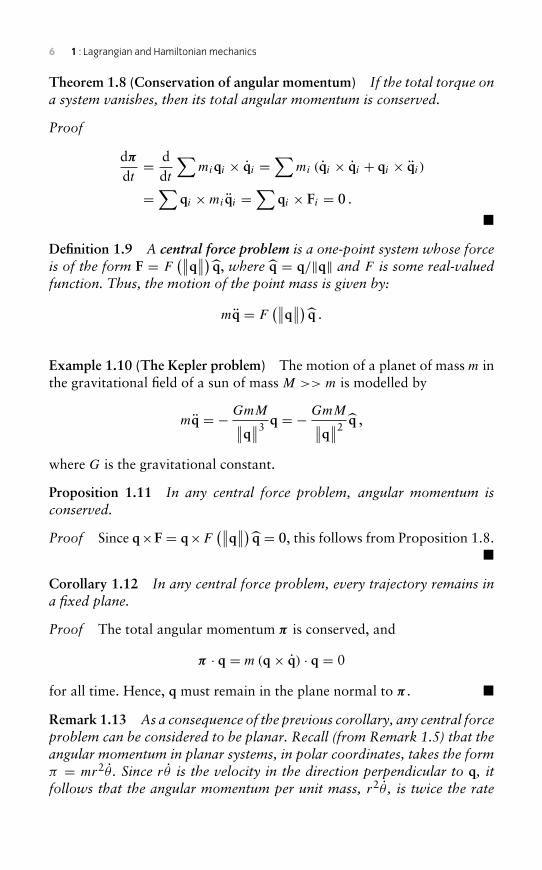
Theorem 1.8 (Conservation of angular momentum) If the total torque ona system vanishes, then its total angular momentum is conserved.
Proof
dπdt= d
dt
∑miqi × qi =
∑mi (qi × qi + qi × qi )
=∑
qi ×mi qi =∑
qi × Fi = 0 .
�
Definition 1.9 A central force problem is a one-point system whose forceis of the form F = F
(∥∥q∥∥) q, where q = q/‖q‖ and F is some real-valuedfunction. Thus, the motion of the point mass is given by:
mq = F(∥∥q∥∥) q .
Example 1.10 (The Kepler problem) The motion of a planet of mass m inthe gravitational field of a sun of mass M >> m is modelled by
mq = − GmM∥∥q∥∥3 q = − GmM∥∥q∥∥2 q ,
where G is the gravitational constant.
Proposition 1.11 In any central force problem, angular momentum isconserved.
Proof Since q×F = q×F(∥∥q∥∥) q = 0, this follows from Proposition 1.8.
�
Corollary 1.12 In any central force problem, every trajectory remains ina fixed plane.
Proof The total angular momentum π is conserved, and
π · q = m(q× q) · q = 0
for all time. Hence, q must remain in the plane normal to π . �
Remark 1.13 As a consequence of the previous corollary, any central forceproblem can be considered to be planar. Recall (from Remark 1.5) that theangular momentum in planar systems, in polar coordinates, takes the formπ = mr2θ . Since rθ is the velocity in the direction perpendicular to q, itfollows that the angular momentum per unit mass, r2θ , is twice the rate
1.1 Newtonian mechanics 7
at which area is swept out by the vector q. Expressed in these terms, theconservation of r2θ is known as Kepler’s Second Law, which, as we haveseen, applies not just to planetary motion but to all central force problems.(See [Gol59] for details.)
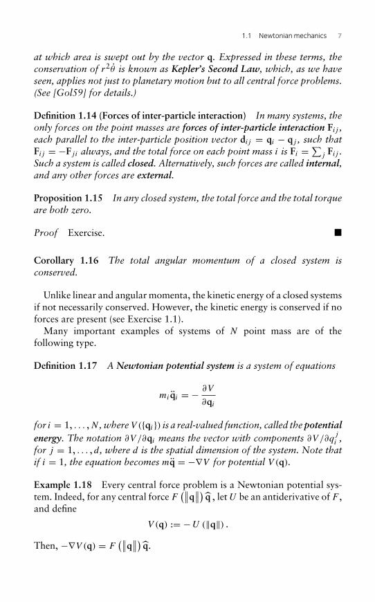
Definition 1.14 (Forces of inter-particle interaction) In many systems, theonly forces on the point masses are forces of inter-particle interaction Fij ,each parallel to the inter-particle position vector dij = qi − qj , such thatFij = −Fji always, and the total force on each point mass i is Fi =∑j Fij .Such a system is called closed. Alternatively, such forces are called internal,and any other forces are external.
Proposition 1.15 In any closed system, the total force and the total torqueare both zero.
Proof Exercise. �
Corollary 1.16 The total angular momentum of a closed system isconserved.
Unlike linear and angular momenta, the kinetic energy of a closed systemsif not necessarily conserved. However, the kinetic energy is conserved if noforces are present (see Exercise 1.1).
Many important examples of systems of N point mass are of thefollowing type.
Definition 1.17 A Newtonian potential system is a system of equations
mi qi = − ∂V
∂qi
for i = 1, . . . ,N , whereV ({qi}) is a real-valued function, called the potentialenergy. The notation ∂V /∂qi means the vector with components ∂V /∂q
ji ,
for j = 1, . . . , d, where d is the spatial dimension of the system. Note thatif i = 1, the equation becomes mq = −∇V for potential V (q).
Example 1.18 Every central force problem is a Newtonian potential sys-tem. Indeed, for any central force F
(∥∥q∥∥) q , let U be an antiderivative of F ,and define
V (q) := −U (‖q‖) .
Then, −∇V (q) = F(∥∥q∥∥) q.
8 1 : Lagrangian and Hamiltonian mechanics
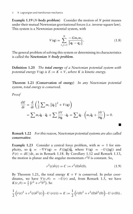
Example 1.19 (N -body problem) Consider the motion of N point massesunder their mutual Newtonian gravitational forces (i.e. inverse-square law).This system is a Newtonian potential system, with
V (q) =N∑
i,j=1
−Gmimj∥∥qi − qj
∥∥ . (1.8)
The general problem of solving this system or determining its characteristicsis called the Newtonian N-body problem.
Definition 1.20 The total energy of a Newtonian potential system withpotential energy V (q) is E := K + V , where K is kinetic energy.
Theorem 1.21 (Conservation of energy) In any Newtonian potentialsystem, total energy is conserved.
Proof
dEdt= d
dt
(12
∑mi
∥∥qi
∥∥2 + V (q))
=∑
mi qi · qi +∑ ∂V
∂qi
· qi =∑
qi ·(mi qi + ∂V
∂qi
)= 0.
�
Remark 1.22 For this reason, Newtonian potential systems are also calledconservative.
Example 1.23 Consider a central force problem, with m = 1 for sim-plicity, so q = −∇V (q) = F(‖q‖)q, where V (q) = −U(‖q‖) andF(t) = dU/dt , as in Remark 1.18. By Corollary 1.12 and Remark 1.13,the motion is planar and the angular momentum r2θ is constant. So,
r2(t)θ (t) = C := r2(0)θ(0). (1.9)
By Theorem 1.21, the total energy K + V is conserved. In polar coor-dinates, we have V (r, θ) = −U(r) and, from Remark 1.5, we haveK(r, θ) = 1
2
(r2 + r2θ2). So
12
(r(t)2 + r2(t)θ2(t)
)−U (r(t)) = E := 1
2
(r(0)2 + r2(0)θ2(0)
)−U (r(0)) .
1.1 Newtonian mechanics 9
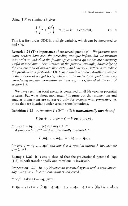
Using (1.9) to eliminate θ gives
12
(r2 + C2
r2
)− U(r) = E (a constant). (1.10)
This is a first-order ODE in a single variable, which can be integrated tofind r(t).
Remark 1.24 (The importance of conserved quantities) We presume thatmany readers have seen the preceding example before, but we mentionit in order to underline the following: conserved quantities are extremelyuseful in mechanics. For instance, in the previous example, knowledge ofthe conservation of angular momentum and energy is sufficient to reducethe problem to a first-order ODE in a single variable. Another exampleis the motion of a rigid body, which can be understood qualitatively byconsidering angular momentum and energy, as explained at the end ofSection 1.5.
We have seen that total energy is conserved in all Newtonian potentialsystems. But what about momentum? It turns out that momentum andangular momentum are conserved only for systems with symmetry, i.e.those that are invariant under certain transformations.
Definition 1.25 A function V : RdN → R is translationally invariant if
V (q1 + t, . . . , qN + t) = V (q1, . . . , qN) ,
for any q = (q1, . . . , qN) and any t ∈ Rd .A function V : RdN → R is rotationally invariant if
V (Rq1, . . . ,RqN) = V (q1, . . . , qN) ,
for any q = (q1, . . . , qN) and any d × d rotation matrix R (we assumed = 2 or 3).
Example 1.26 It is easily checked that the gravitational potential (eqn(1.8)) is both translationally and rotationally invariant.
Proposition 1.27 In any Newtonian potential system with a translation-ally invariant V , linear momentum is conserved.
Proof Taking t = −q1 gives
V (q1, . . . , qN) = V (0, q2 − q1, q3 − q1, . . . , qN − q1) = V(d2, d3, . . . , dN
),
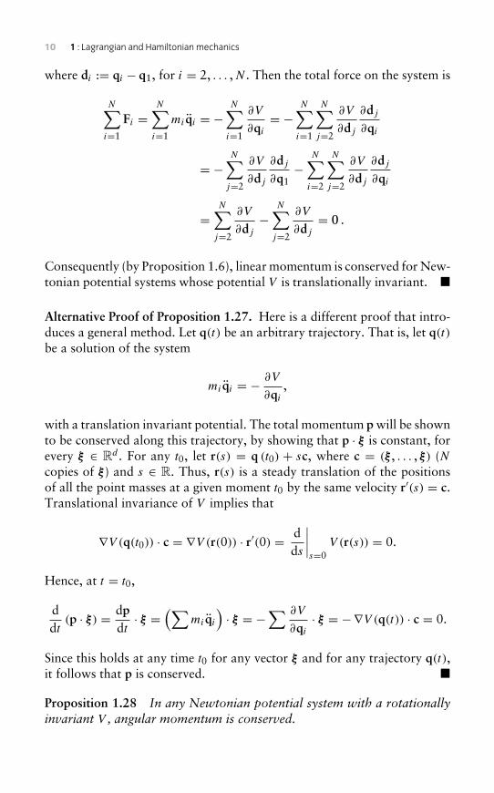
10 1 : Lagrangian and Hamiltonian mechanics
where di := qi − q1, for i = 2, . . . ,N . Then the total force on the system is
N∑i=1
Fi =N∑i=1
mi qi = −N∑i=1
∂V
∂qi
= −N∑i=1
N∑j=2
∂V
∂dj
∂dj
∂qi
= −N∑
j=2
∂V
∂dj
∂dj
∂q1−
N∑i=2
N∑j=2
∂V
∂dj
∂dj
∂qi
=N∑
j=2
∂V
∂dj
−N∑
j=2
∂V
∂dj
= 0 .
Consequently (by Proposition 1.6), linear momentum is conserved for New-tonian potential systems whose potential V is translationally invariant. �
Alternative Proof of Proposition 1.27. Here is a different proof that intro-duces a general method. Let q(t) be an arbitrary trajectory. That is, let q(t)be a solution of the system
mi qi = − ∂V
∂qi
,
with a translation invariant potential. The total momentum p will be shownto be conserved along this trajectory, by showing that p · ξ is constant, forevery ξ ∈ Rd . For any t0, let r(s) = q (t0) + sc, where c = (ξ , . . . , ξ) (Ncopies of ξ ) and s ∈ R. Thus, r(s) is a steady translation of the positionsof all the point masses at a given moment t0 by the same velocity r′(s) = c.Translational invariance of V implies that
∇V (q(t0)) · c = ∇V (r(0)) · r′(0) = dds
∣∣∣∣s=0
V (r(s)) = 0.
Hence, at t = t0,
ddt
(p · ξ) = dpdt· ξ =
(∑mi qi
)· ξ = −
∑ ∂V
∂qi
· ξ = −∇V (q(t)) · c = 0.
Since this holds at any time t0 for any vector ξ and for any trajectory q(t),it follows that p is conserved. �
Proposition 1.28 In any Newtonian potential system with a rotationallyinvariant V , angular momentum is conserved.
1.1 Newtonian mechanics 11
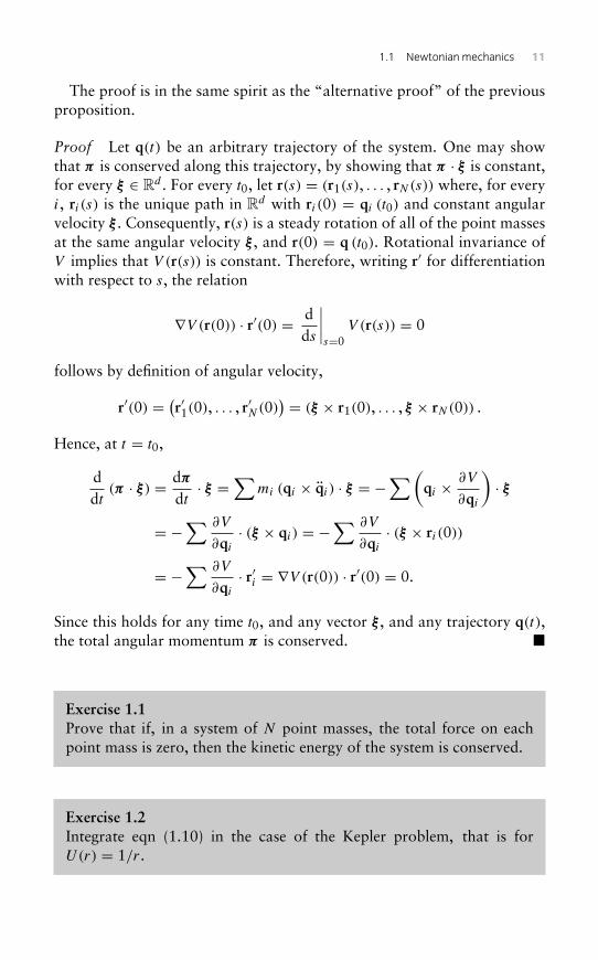
The proof is in the same spirit as the “alternative proof” of the previousproposition.
Proof Let q(t) be an arbitrary trajectory of the system. One may showthat π is conserved along this trajectory, by showing that π · ξ is constant,for every ξ ∈ Rd . For every t0, let r(s) = (r1(s), . . . , rN(s)) where, for everyi, ri (s) is the unique path in Rd with ri (0) = qi (t0) and constant angularvelocity ξ . Consequently, r(s) is a steady rotation of all of the point massesat the same angular velocity ξ , and r(0) = q (t0). Rotational invariance ofV implies that V (r(s)) is constant. Therefore, writing r′ for differentiationwith respect to s, the relation
∇V (r(0)) · r′(0) = dds
∣∣∣∣s=0
V (r(s)) = 0
follows by definition of angular velocity,
r′(0) = (r′1(0), . . . , r′N(0)) = (ξ × r1(0), . . . , ξ × rN(0)) .
Hence, at t = t0,
ddt
(π · ξ) = dπdt· ξ =
∑mi (qi × qi ) · ξ = −
∑(qi × ∂V
∂qi
)· ξ
= −∑ ∂V
∂qi
· (ξ × qi ) = −∑ ∂V
∂qi
· (ξ × ri (0))
= −∑ ∂V
∂qi
· r′i = ∇V (r(0)) · r′(0) = 0.
Since this holds for any time t0, and any vector ξ , and any trajectory q(t),the total angular momentum π is conserved. �
Exercise 1.1Prove that if, in a system of N point masses, the total force on eachpoint mass is zero, then the kinetic energy of the system is conserved.
Exercise 1.2Integrate eqn (1.10) in the case of the Kepler problem, that is forU(r) = 1/r.
12 1 : Lagrangian and Hamiltonian mechanics
Exercise 1.3In Example 1.10, on the motion of a single planet around the Sun,assume for simplicity that G = M = m = 1, so that q = − q/‖q‖2.
a) Write the equations of motion in polar coordinates, and deducedirectly that r2(t)θ (t) is constant. This constant will be denoted byC in the next parts.
b) Change independent variables, so that d/dt = θ (d/dθ). (This islegitimate, since θ(t) is monotone – why?) Set u = 1/r, and obtain
u′′ + u = 1C2 .
c) Integrate the above to obtain
u(θ) = b cos(θ − θ0)+ 1C2 ,
where b and θ0 are constants of integration. Deduce that
r(θ) = C2
1+ e cos(θ − θ0),
where e := (bC2). For 0 < e < 1 this is the polar equation for anellipse (for more on the shape of the trajectories as function of e, seefor instance [JS98]). This proves Kepler’s First Law.
Exercise 1.4Prove the following:
a) For 1-point systems, the only translationally invariant potentialsare the constant functions, corresponding to everywhere zeroacceleration.
b) For 1-point systems, V is rotationally invariant, if and only if V
depends on q only through∥∥q∥∥.
c) For 2-point systems, V is both translationally and rotationallyinvariant, if and only if V depends on q only through
∥∥q1 − q2∥∥.
1.2 Lagrangian mechanics 13
Exercise 1.5A point mass in a magnetic field experiences a force
F = eq× B,
where e is its charge (a constant) and B is the magnetic field. This equa-tion is called the Lorentz force law. Since the force depends on thevelocity, it is clear that the force is not the gradient of any functionV (q), so this is not a Newtonian potential system. Since the force isperpendicular to the velocity, kinetic energy is conserved:
dKdt= mq · q = q · (eq× B) = 0 .
Show that point masses in a constant magnetic field move in helices.
1.2 Lagrangian mechanics
The equations of motion of a Newtonian potential system, when expressedin different (non-inertial) coordinates, need not have the form given ineqn (1.17). This section and, later, Section 1.4 introduce two coordinate-independent formulations of conservative mechanics: Lagrangian andHamiltonian.
From now on, we will describe the positions of all of the point masseswith one concatenated position vector q = (q1, . . . , qN) ∈ RdN .
Theorem 1.29 Every Newtonian potential system,
mi qi = −∂V
∂qi
, i = 1, . . . ,N , (1.11)
is equivalent to the Euler–Lagrange equations,
ddt
(∂L
∂q
)− ∂L
∂q= 0, (1.12)
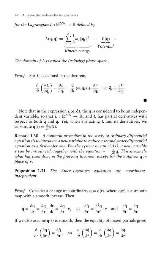
14 1 : Lagrangian and Hamiltonian mechanics
for the Lagrangian L : R2dN → R defined by
L(q, q) :=N∑i=1
12mi‖qi‖2︸ ︷︷ ︸
Kinetic energy
− V (q)︸ ︷︷ ︸Potential
.
The domain of L is called the (velocity) phase space.
Proof For L as defined in the theorem,
ddt
(∂L
∂qi
)− ∂L
∂qi
= ddt
(mi qi )+ ∂V
∂qi
= mi qi + ∂V
∂qi
.
�
Note that in the expression L(q, q), the q is considered to be an indepen-dent variable, so that L : R2dN → R, and L has partial derivatives withrespect to both q and q. Yet, when evaluating L and its derivatives, wesubstitute q(t) = d
dt q(t).
Remark 1.30 A common procedure in the study of ordinary differentialequations is to introduce a new variable to reduce a second-order differentialequation to a first-order one. For the system in eqn (1.11), a new variablev can be introduced, together with the equation v = d
dt q. This is exactlywhat has been done in the previous theorem, except for the notation q inplace of v.
Proposition 1.31 The Euler–Lagrange equations are coordinate–independent.
Proof Consider a change of coordinates q = q(r), where q(r) is a smoothmap with a smooth inverse. Then
q = dqdt= ∂q
∂r· drdt= ∂q
∂r· r, so
∂q∂r= ∂2q
∂r2· r and
∂q∂ r= ∂q
∂r.
If we also assume q(t) is smooth, then the equality of mixed partials gives
ddt
(∂q∂r
)= ∂q
∂r, so
ddt
(∂q∂ r
)= d
dt
(∂q∂r
)= ∂q
∂r.
1.2 Lagrangian mechanics 15
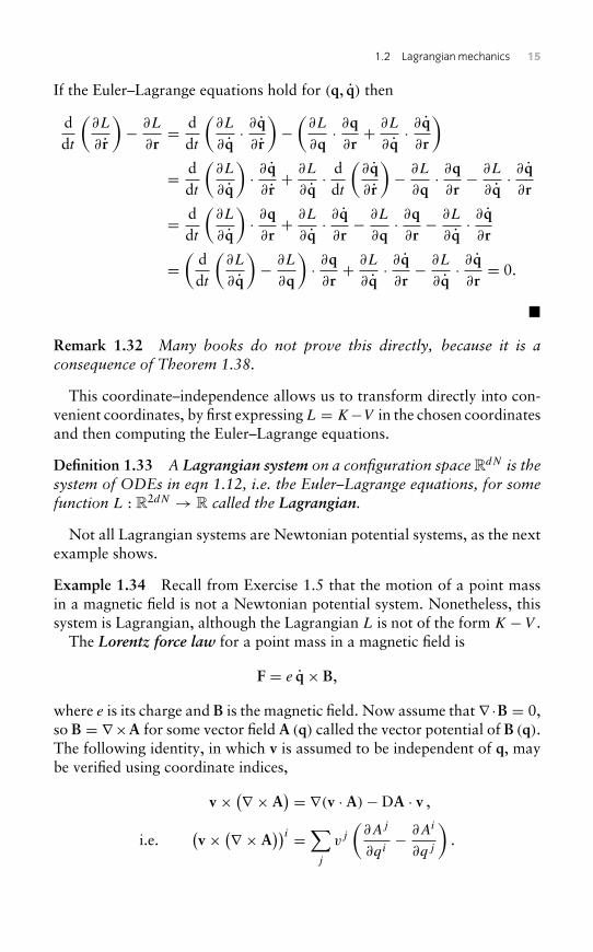
If the Euler–Lagrange equations hold for (q, q) then
ddt
(∂L
∂ r
)− ∂L
∂r= d
dt
(∂L
∂q· ∂q∂ r
)−(∂L
∂q· ∂q∂r+ ∂L
∂q· ∂q∂r
)= d
dt
(∂L
∂q
)· ∂q∂ r+ ∂L
∂q· ddt
(∂q∂ r
)− ∂L
∂q· ∂q∂r− ∂L
∂q· ∂q∂r
= ddt
(∂L
∂q
)· ∂q∂r+ ∂L
∂q· ∂q∂r− ∂L
∂q· ∂q∂r− ∂L
∂q· ∂q∂r
=(
ddt
(∂L
∂q
)− ∂L
∂q
)· ∂q∂r+ ∂L
∂q· ∂q∂r− ∂L
∂q· ∂q∂r= 0.
�
Remark 1.32 Many books do not prove this directly, because it is aconsequence of Theorem 1.38.
This coordinate–independence allows us to transform directly into con-venient coordinates, by first expressingL = K−V in the chosen coordinatesand then computing the Euler–Lagrange equations.
Definition 1.33 A Lagrangian system on a configuration space RdN is thesystem of ODEs in eqn 1.12, i.e. the Euler–Lagrange equations, for somefunction L : R2dN → R called the Lagrangian.
Not all Lagrangian systems are Newtonian potential systems, as the nextexample shows.
Example 1.34 Recall from Exercise 1.5 that the motion of a point massin a magnetic field is not a Newtonian potential system. Nonetheless, thissystem is Lagrangian, although the Lagrangian L is not of the form K −V .
The Lorentz force law for a point mass in a magnetic field is
F = e q× B,
where e is its charge and B is the magnetic field. Now assume that ∇ ·B = 0,so B = ∇×A for some vector field A (q) called the vector potential of B (q).The following identity, in which v is assumed to be independent of q, maybe verified using coordinate indices,
v × (∇ × A) = ∇(v · A)−DA · v ,
i.e.(v × (∇ × A
))i =∑j
vj
(∂Aj
∂qi− ∂Ai
∂qj
).
16 1 : Lagrangian and Hamiltonian mechanics
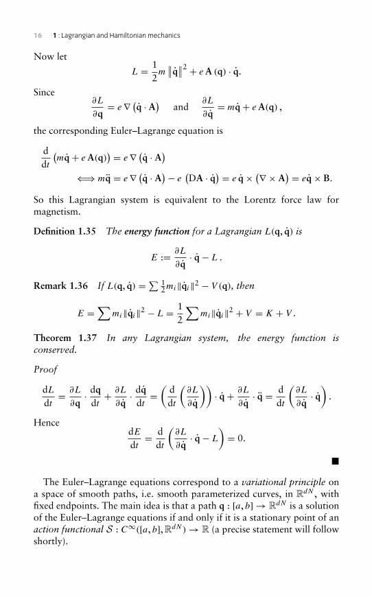
Now let
L = 12m∥∥q∥∥2 + eA (q) · q.
Since∂L
∂q= e∇ (q · A) and
∂L
∂q= mq+ eA(q) ,
the corresponding Euler–Lagrange equation is
ddt
(mq+ eA(q)
) = e∇ (q · A)⇐⇒ mq = e∇ (q · A)− e
(DA · q) = e q× (∇ × A
) = eq× B.
So this Lagrangian system is equivalent to the Lorentz force law formagnetism.
Definition 1.35 The energy function for a Lagrangian L(q, q) is
E := ∂L
∂q· q− L .
Remark 1.36 If L(q, q) =∑ 12mi‖qi‖2 − V (q), then
E =∑
mi‖qi‖2 − L = 12
∑mi‖qi‖2 + V = K + V .
Theorem 1.37 In any Lagrangian system, the energy function isconserved.
Proof
dLdt= ∂L
∂q· dq
dt+ ∂L
∂q· dq
dt=(
ddt
(∂L
∂q
))· q+ ∂L
∂q· q = d
dt
(∂L
∂q· q)
.
HencedEdt= d
dt
(∂L
∂q· q− L
)= 0.
�
The Euler–Lagrange equations correspond to a variational principle ona space of smooth paths, i.e. smooth parameterized curves, in RdN , withfixed endpoints. The main idea is that a path q : [a, b] → RdN is a solutionof the Euler–Lagrange equations if and only if it is a stationary point of anaction functional S : C∞([a, b], RdN)→ R (a precise statement will followshortly).
1.2 Lagrangian mechanics 17
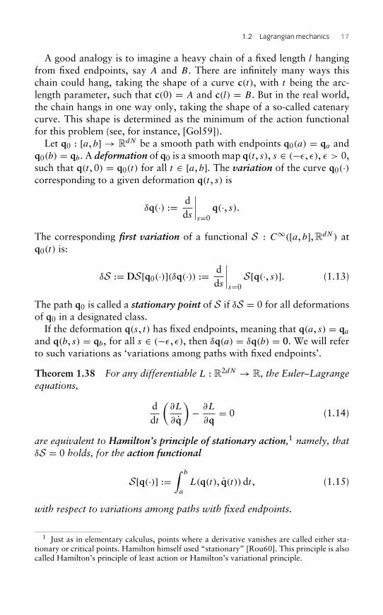
A good analogy is to imagine a heavy chain of a fixed length l hangingfrom fixed endpoints, say A and B. There are infinitely many ways thischain could hang, taking the shape of a curve c(t), with t being the arc-length parameter, such that c(0) = A and c(l) = B. But in the real world,the chain hangs in one way only, taking the shape of a so-called catenarycurve. This shape is determined as the minimum of the action functionalfor this problem (see, for instance, [Gol59]).
Let q0 : [a, b] → RdN be a smooth path with endpoints q0(a) = qa andq0(b) = qb. A deformation of q0 is a smooth map q(t , s), s ∈ (−ε, ε), ε > 0,such that q(t , 0) = q0(t) for all t ∈ [a, b]. The variation of the curve q0(·)corresponding to a given deformation q(t , s) is
δq(·) := dds
∣∣∣∣s=0
q(·, s).
The corresponding first variation of a functional S : C∞([a, b], RdN) atq0(t) is:
δS := DS[q0(·)](δq(·)) := dds
∣∣∣∣s=0
S[q(·, s)]. (1.13)
The path q0 is called a stationary point of S if δS = 0 for all deformationsof q0 in a designated class.
If the deformation q(s, t) has fixed endpoints, meaning that q(a, s) = qa
and q(b, s) = qb, for all s ∈ (−ε, ε), then δq(a) = δq(b) = 0. We will referto such variations as ‘variations among paths with fixed endpoints’.
Theorem 1.38 For any differentiable L : R2dN → R, the Euler–Lagrangeequations,
ddt
(∂L
∂q
)− ∂L
∂q= 0 (1.14)
are equivalent to Hamilton’s principle of stationary action,1 namely, thatδS = 0 holds, for the action functional
S[q(·)] :=∫ b
a
L(q(t), q(t)) dt , (1.15)
with respect to variations among paths with fixed endpoints.
1 Just as in elementary calculus, points where a derivative vanishes are called either sta-tionary or critical points. Hamilton himself used “stationary” [Rou60]. This principle is alsocalled Hamilton’s principle of least action or Hamilton’s variational principle.
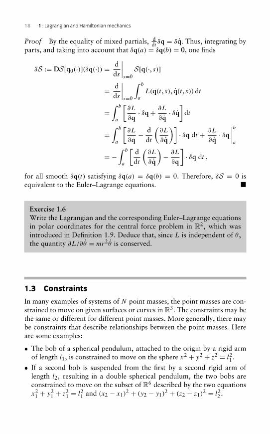
18 1 : Lagrangian and Hamiltonian mechanics
Proof By the equality of mixed partials, ddt δq = δq. Thus, integrating by
parts, and taking into account that δq(a) = δq(b) = 0, one finds
δS := DS[q0(·)](δq(·)) = dds
∣∣∣∣s=0
S[q(·, s)]
= dds
∣∣∣∣s=0
∫ b
a
L(q(t , s), q(t , s)) dt
=∫ b
a
[∂L
∂q· δq+ ∂L
∂q· δq
]dt
=∫ b
a
[∂L
∂q− d
dt
(∂L
∂q
)]· δq dt + ∂L
∂q· δq
∣∣∣∣ba
= −∫ b
a
[ddt
(∂L
∂q
)− ∂L
∂q
]· δq dt ,
for all smooth δq(t) satisfying δq(a) = δq(b) = 0. Therefore, δS = 0 isequivalent to the Euler–Lagrange equations. �
Exercise 1.6Write the Lagrangian and the corresponding Euler–Lagrange equationsin polar coordinates for the central force problem in R2, which wasintroduced in Definition 1.9. Deduce that, since L is independent of θ ,the quantity ∂L/∂θ = mr2θ is conserved.
1.3 Constraints
In many examples of systems of N point masses, the point masses are con-strained to move on given surfaces or curves in R3. The constraints may bethe same or different for different point masses. More generally, there maybe constraints that describe relationships between the point masses. Hereare some examples:
• The bob of a spherical pendulum, attached to the origin by a rigid armof length l1, is constrained to move on the sphere x2 + y2 + z2 = l21.
• If a second bob is suspended from the first by a second rigid arm oflength l2, resulting in a double spherical pendulum, the two bobs areconstrained to move on the subset of R6 described by the two equationsx21 + y2
1 + z21 = l21 and (x2 − x1)
2 + (y2 − y1)2 + (z2 − z1)
2 = l22.
1.3 Constraints 19
• If all of the mutual distances between N point masses are constrained tofixed values, then the point masses move together as a rigid body thatcan only rotate and translate, keeping a fixed shape.
Of course, any planar system is a spatial system with the added constraintthat the point masses move in a given plane. So without loss of generality,we consider spatial systems. We will assume that the constraints can bedescribed by k scalar equations, fj (q) = cj , for j = 1, . . . , k. The subsetof R3N determined by these constraints is called the configuration space,usually denoted by Q. The number of degrees of freedom of the systemis the dimension of Q. We will assume that the gradient vectors ∇fj (q)are all non-zero and linearly independent, for all q in the configurationspace.2 Constraints of this form, i.e. functions of position only, are calledholonomic. These are the only kinds of constraints that we will deal withhere. In contrast, non-holonomic constraints involve velocities q, a classicexample being the no-slip condition of an object rolling on a surface.
We begin by analysing holonomic constraints in the context of Newto-nian mechanics. In a constrained system there exist additional forces thatkeep q in the configuration space. Let Ci be the constraint force on the ithpoint mass, and let Fi be the total of all other forces on it. Then, Newton’ssecond law says that (in an inertial coordinate system)
mi qi = Fi + Ci .
We cannot find the magnitude of the constraint forces Ci directly, butwe can make a physically–reasonable assumption about the directions inwhich they act. Indeed, consider first a single point mass moving on a fixedsurface. If we assume that the surface is frictionless, then it seems intuitivelyreasonable that the force exerted by the surface on the point mass must benormal to the surface (i.e. orthogonal to it). Similar considerations applyto multiple point masses, each with its own independent constraint. Thesituation is less clear when the constraints describe relationships betweenpoint masses. However, there is a good physical reason to assume thatthe vector of constraint forces (C1, . . . ,CN) is normal to the configurationspace. Indeed, since the velocity q(t) = (q1(t), . . . , qN(t)
)is tangent to the
configuration space at the point q(t), the assumption implies that
N∑i=1
Ci · qi = 0 (1.16)
2 This ensures that the configuration space is a smooth manifold, as shown in Chapter 2.
20 1 : Lagrangian and Hamiltonian mechanics
for all t . But Ci · qi is the rate of work done by the force Ci on a pointmass with velocity qi . Thus, the assumption that (C1, . . . ,CN) is alwaysnormal to the configuration space ensures that the total rate of work doneby the constraint forces, summed over all the point masses, must be zero.Therefore, the constraints don’t affect conservation of energy. The best jus-tification of this assumption is that, in practice, it leads to accurate modelsof physical systems. For further discussion of this widely–accepted modelof constraint forces, see [Blo03, BL05].
We have assumed that configuration space is defined by k scalar equa-tions, fj (q) = cj , for j = 1, . . . , k, and that the gradient vectors ∇fj (q) arelinearly independent. The gradient vectors ∇fj (q) span the normal space tothe configuration space. Thus, an equivalent assumption on the constraintforces is:
(C1, . . . ,CN) =k∑
j=1
λj∇fj , for some real numbers λj . (1.17)
We shall assume this relation in what follows. The next theorem corre-sponds to Theorem 1.29, with the addition of constraints.
Theorem 1.39 Every constrained Newtonian potential system,
mi qi = −∂V
∂qi
+ Ci , i = 1, . . . ,N , (1.18)
with constraints fj (q) = cj , for j = 1, . . . , k, and constraint forces satisfy-ing eqn (1.17), is equivalent to the following version of the Euler–Lagrangeequations,
ddt
(∂L
∂q
)− ∂L
∂q=
k∑j=1
λj∇fj , (1.19)
for the Lagrangian
L(q, q) :=N∑i=1
12mi‖qi‖2︸ ︷︷ ︸
Kinetic energy
− V (q)︸ ︷︷ ︸Potential
.
Proof For L as defined in the theorem,
ddt
(∂L
∂qi
)− ∂L
∂qi
= ddt
(mi qi )+ ∂V
∂qi
= mi qi + ∂V
∂qi
. (1.20)
1.3 Constraints 21
Assuming eqn (1.17), eqn (1.18) is equivalent to
mq+ ∂V
∂q= (C1, . . . ,CN) =
k∑j=1
λj∇fj ,
which from eqn (1.20) is equivalent to eqn (1.19). �
The numbers λj are called Lagrange multipliers. In order to find explicitequations of motion in the variables qi and qi only, the Lagrange multipliersmust be eliminated, which can be difficult (see Exercise 7.7). The problemis much easier if the constraints have simple relationships with the coordi-nates, which suggests that we consider changes of coordinates. However,the previous theorem applies only to Newtonian potential systems, andthese do not have the same form when expressed in different (non-inertial)coordinate systems. To study constrained dynamics in general coordinatesystems, we turn to Lagrangian mechanics. We will see that in fact eqn(1.19) applies in general coordinate systems.
Recall from the previous section the action functional
S[q(·)] :=∫ b
a
L(q(t), q(t)) dt , (1.21)
and Hamilton’s principle of stationary action, which is: δS = 0, withrespect to all variations among paths with fixed endpoints. As we saw inthe proof of Theorem 1.38, Hamilton’s principle is also equivalent to:∫ b
a
[ddt
(∂L
∂q
)− ∂L
∂q
]· δq dt = 0, (1.22)
for all variations δq(·) satisfying δq(a) = δq(b) = 0. Since the variations arearbitrary, this shows that Hamilton’s principle is equivalent to the Euler–Lagrange equations. Now instead of considering all deformations, supposewe consider only those that remain within the configuration space Q definedby the holonomic constraints
fj (q(t , s)) = cj , for j = 1, . . . , k, for all t , s.
The variations corresponding to these restricted deformations are alwaystangent3 to Q. Let SC be the restriction of S to paths that lie in Q. Thenq is a stationary point of SC if and only if DS[q0](δq) = 0 for all δq suchthat δq(t) is tangent to Q for all t .
3 A tangent vector to a surface or general manifold at a given point is a velocity vector atthat point of a curve in the manifold. Tangent vectors are discussed in detail in Chapter 2.
22 1 : Lagrangian and Hamiltonian mechanics
If we consider only variations δq of this form, then eqn (1.22) holds if
and only if ddt
(∂L∂q
)− ∂L
∂q is normal to the configuration space, for all t . Since
the gradient vectors ∇fj (q) span the normal space, we conclude that
ddt
(∂L
∂q
)− ∂L
∂q=
k∑j=1
λj ∂fj
∂q. (1.23)
If we define L = L+∑j λjfj , then
∂L∂q= ∂L
∂q+∑j
λj ∂fj
∂q,
so eqn (1.23) is equivalent to the Euler–Lagrange equations for L.In summary, we have shown the following.
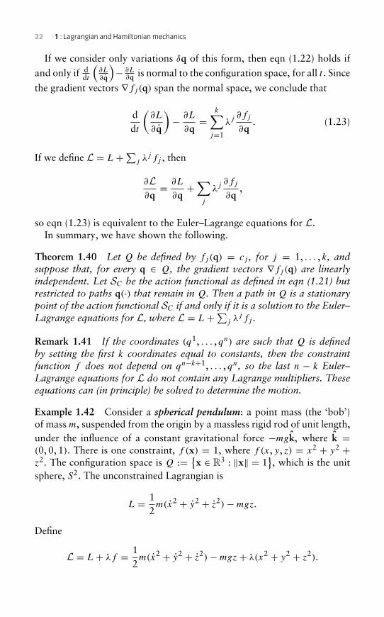
Theorem 1.40 Let Q be defined by fj (q) = cj , for j = 1, . . . , k, andsuppose that, for every q ∈ Q, the gradient vectors ∇fj (q) are linearlyindependent. Let SC be the action functional as defined in eqn (1.21) butrestricted to paths q(·) that remain in Q. Then a path in Q is a stationarypoint of the action functional SC if and only if it is a solution to the Euler–Lagrange equations for L, where L = L+∑j λjfj .
Remark 1.41 If the coordinates (q1, . . . , qn) are such that Q is definedby setting the first k coordinates equal to constants, then the constraintfunction f does not depend on qn−k+1, . . . , qn, so the last n − k Euler–Lagrange equations for L do not contain any Lagrange multipliers. Theseequations can (in principle) be solved to determine the motion.
Example 1.42 Consider a spherical pendulum: a point mass (the ‘bob’)of mass m, suspended from the origin by a massless rigid rod of unit length,under the influence of a constant gravitational force −mgk, where k =(0, 0, 1). There is one constraint, f (x) = 1, where f (x, y, z) = x2 + y2 +z2. The configuration space is Q := {x ∈ R3 : ‖x‖ = 1
}, which is the unit
sphere, S2. The unconstrained Lagrangian is
L = 12m(x2 + y2 + z2)−mgz.
Define
L = L+ λf = 12m(x2 + y2 + z2)−mgz+ λ(x2 + y2 + z2).
1.3 Constraints 23
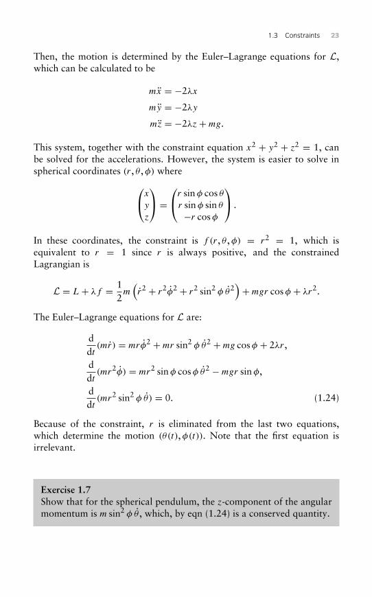
Then, the motion is determined by the Euler–Lagrange equations for L,which can be calculated to be
mx = −2λx
my = −2λy
mz = −2λz+mg.
This system, together with the constraint equation x2 + y2 + z2 = 1, canbe solved for the accelerations. However, the system is easier to solve inspherical coordinates (r, θ ,φ) wherex
y
z
=r sinφ cos θ
r sinφ sin θ
−r cosφ
.
In these coordinates, the constraint is f (r, θ ,φ) = r2 = 1, which isequivalent to r = 1 since r is always positive, and the constrainedLagrangian is
L = L+ λf = 12m(r2 + r2φ2 + r2 sin2 φ θ2
)+mgr cosφ + λr2.
The Euler–Lagrange equations for L are:
ddt
(mr) = mrφ2 +mr sin2 φ θ2 +mg cosφ + 2λr,
ddt
(mr2φ) = mr2 sinφ cosφ θ2 −mgr sinφ,
ddt
(mr2 sin2 φ θ) = 0. (1.24)
Because of the constraint, r is eliminated from the last two equations,which determine the motion (θ(t),φ(t)). Note that the first equation isirrelevant.
Exercise 1.7Show that for the spherical pendulum, the z-component of the angularmomentum is m sin2 φ θ , which, by eqn (1.24) is a conserved quantity.
24 1 : Lagrangian and Hamiltonian mechanics
1.4 The Legendre transform andHamiltonian mechanics
Theorem 1.43 Every Newtonian potential system,
mi qi = −∂V
∂qi
, i = 1, . . . ,N , (1.25)
is equivalent to Hamilton’s canonical equations,
q = ∂H
∂p, p = − ∂H
∂q, (1.26)
for the Hamiltonian
H(q, p) :=N∑i=1
12mi
‖pi‖2︸ ︷︷ ︸Kinetic energy
+ V (q)︸ ︷︷ ︸Potential
.
The precise equivalence is: (q(t), p(t)) is a solution to eqn (1.26) if and onlyif q(t) is a solution to eqn (1.25) and
p(t) = (p1(t), . . . , pN(t)) = (m1q1(t), . . . ,mN qN(t)) ,
i.e. p(t) is linear momentum. Note that for such a p(t), we have H(q, p) =∑Ni=1
12mi‖qi‖2 + V (q) = K + V .
Proof The second-order system in eqn (1.25) is equivalent to the followingfirst-order system in variables (q, q),
ddt
qi = qi , mi
ddt
qi = − ∂V
∂qi
, i = 1, . . . ,N . (1.27)
Changing variables from (q, q) to (q, p), with pi = mi qi gives the system
qi = 1mi
pi = ∂H
∂pi
, pi = − ∂V
∂qi
= −∂H
∂qi
, i = 1, . . . ,N .
�
Since we have seen that Newtonian potential systems are equivalent to theEuler–Lagrange equations with L = K − V (Theorem 1.43), we have nowshown that the Euler–Lagrange equations for such Lagrangians are equiv-alent to Hamilton’s equations with H = K + V . In fact, this equivalence
1.4 The Legendre transform and Hamiltonian mechanics 25
generalizes to a much larger class of Lagrangians. To show this, we firstgeneralize the definition of linear momentum, pi := miqi , as follows.
Definition 1.44 The Legendre transform for a Lagrangian L(q, q) is thechange of variables (q, q) → (q, p) given by
p := ∂L
∂q.
The new variables p are called the conjugate momenta (conjugate to theposition variables q).
Remark 1.45 If L(q, q) =∑i12mi‖qi‖2 − V (q), then pi = ∂L
∂qi= mi qi .
For the moment, it suffices to think of the Legendre transform simply asa change of variables on R2dN ; but see Section 4.2 for further discussion.In order to define the appropriate Hamiltonian function, this change ofvariables must be invertible.
Definition 1.46 A Lagrangian L is regular if
det∂2L
∂q2 �= 0.
L is hyperregular if the Legendre transform for L is a diffeomorphism, thatis, a differentiable map with a differentiable inverse.
Remark 1.47 The derivative of the Legendre transform has matrix I 0
∂2L
∂q∂q∂2L
∂q2
. (1.28)
This matrix is invertible if and only if ∂2L
∂q2 is invertible. It follows that if L
is hyperregular then L is regular.
Remark 1.48 If L(q, q) =∑i12mi‖qi‖2 − V (q), then the Legendre trans-
form, defined by pi := ∂L∂qi= mi qi , is hyperregular, since it is differentiable
and has a differentiable inverse given by qi = 1mi
pi . It follows that L isregular as well, but we can also check this directly:
det∂2L
∂q2 = det
m1 0. . .
0 mN
�= 0
(assuming non-zero masses).
26 1 : Lagrangian and Hamiltonian mechanics
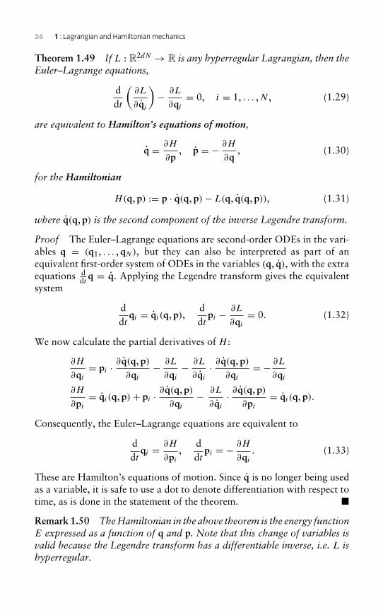
Theorem 1.49 If L : R2dN → R is any hyperregular Lagrangian, then theEuler–Lagrange equations,
ddt
(∂L
∂qi
)− ∂L
∂qi
= 0, i = 1, . . . ,N , (1.29)
are equivalent to Hamilton’s equations of motion,
q = ∂H
∂p, p = − ∂H
∂q, (1.30)
for the Hamiltonian
H(q, p) := p · q(q, p)− L(q, q(q, p)), (1.31)
where q(q, p) is the second component of the inverse Legendre transform.
Proof The Euler–Lagrange equations are second-order ODEs in the vari-ables q = (q1, . . . , qN), but they can also be interpreted as part of anequivalent first-order system of ODEs in the variables (q, q), with the extraequations d
dt q = q. Applying the Legendre transform gives the equivalentsystem
ddt
qi = qi (q, p),ddt
pi − ∂L
∂qi
= 0. (1.32)
We now calculate the partial derivatives of H :
∂H
∂qi
= pi · ∂q(q, p)∂qi
− ∂L
∂qi
− ∂L
∂qi
· ∂q(q, p)∂qi
= − ∂L
∂qi
∂H
∂pi
= qi (q, p)+ pi · ∂q(q, p)∂qi
− ∂L
∂qi
· ∂q(q, p)∂pi
= qi (q, p).
Consequently, the Euler–Lagrange equations are equivalent to
ddt
qi = ∂H
∂pi
,ddt
pi = − ∂H
∂qi
. (1.33)
These are Hamilton’s equations of motion. Since q is no longer being usedas a variable, it is safe to use a dot to denote differentiation with respect totime, as is done in the statement of the theorem. �
Remark 1.50 TheHamiltonian in the above theorem is the energy functionE expressed as a function of q and p. Note that this change of variables isvalid because the Legendre transform has a differentiable inverse, i.e. L ishyperregular.
1.4 The Legendre transform and Hamiltonian mechanics 27
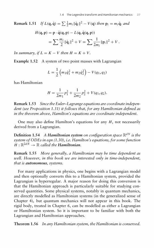
Remark 1.51 If L(q, q) =∑ 12mi‖qi‖2 − V (q) then pi = mi qi and
H(q, p) = p · q(q, p)− L(q, q(q, p))
=∑ mi
2‖qi‖2 + V =
∑ 12mi
‖pi‖2 + V .
In summary, if L = K − V then H = K + V .
Example 1.52 A system of two point masses with Lagrangian
L = 12
(m1q
21 +m2q
22
)− V (q1, q2)
has Hamiltonian
H = 12m1
p21 +
12m2
p22 + V (q1, q2).
Remark 1.53 Since the Euler–Lagrange equations are coordinate indepen-dent (see Proposition 1.31) it follows that, for any Hamiltonian defined asin the theorem above, Hamilton’s equations are coordinate independent.
One may also define Hamilton’s equations for any H , not necessarilyderived from a Lagrangian.
Definition 1.54 A Hamiltonian system on configuration space RdN is thesystem of ODEs in eqn (1.30), i.e. Hamilton’s equations, for some functionH : R2dN → R called the Hamiltonian.
Remark 1.55 More generally, a Hamiltonian may be time dependent aswell. However, in this book we are interested only in time-independent,that is autonomous, systems.
For many applications in physics, one begins with a Lagrangian modeland then optionally converts this to a Hamiltonian system, provided theLagrangian is hyperregular. A major reason for doing this conversion isthat the Hamiltonian approach is particularly suitable for studying con-served quantities. Some physical systems, notably in quantum mechanics,are directly modelled as Hamiltonian systems (in the generalized sense ofChapter 4), but quantum mechanics will not appear in this book. Therigid body, treated in Chapter 6, can be modelled as either a Lagrangianor Hamiltonian system. So it is important to be familiar with both theLagrangian and Hamiltonian approaches.
Theorem 1.56 In any Hamiltonian system, the Hamiltonian is conserved.
28 1 : Lagrangian and Hamiltonian mechanics
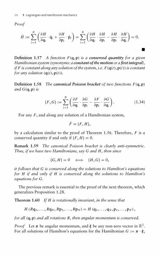
Proof
H :=N∑i=1
(∂H
∂qi
· qi + ∂H
∂pi
· pi
)=
N∑i=1
(∂H
∂qi
· ∂H∂pi
− ∂H
∂pi
· ∂H∂qi
)= 0.
�
Definition 1.57 A function F(q, p) is a conserved quantity for a givenHamiltonian system (synonyms: a constant of the motion or afirst integral),ifF is constant along any solution of the system, i.e. F(q(t), p(t)) is constantfor any solution (q(t), p(t)).
Definition 1.58 The canonical Poisson bracket of two functions F(q, p)and G(q, p) is
{F ,G} :=N∑i=1
(∂F
∂qi
· ∂G∂pi
− ∂F
∂pi
· ∂G∂qi
). (1.34)
For any F , and along any solution of a Hamiltonian system,
F = {F ,H },by a calculation similar to the proof of Theorem 1.56. Therefore, F is aconserved quantity if and only if {F ,H } = 0.
Remark 1.59 The canonical Poisson bracket is clearly anti-symmetric.Thus, if we have two Hamiltonians, say G and H , then since
{G,H } = 0 ⇐⇒ {H ,G} = 0,
it follows that G is conserved along the solutions to Hamilton’s equationsfor H if and only if H is conserved along the solutions to Hamilton’sequations for G.
The previous remark is essential to the proof of the next theorem, whichgeneralizes Proposition 1.28.
Theorem 1.60 If H is rotationally invariant, in the sense that
H (Rq1, . . . ,RqN ,Rp1, . . . ,RpN) = H (q1, . . . , qN , p1, . . . , pN) ,
for all (q, p) and all rotations R, then angular momentum is conserved.
Proof Let π be angular momentum, and ξ be any non-zero vector in R3.For all solutions of Hamilton’s equations for the Hamiltonian G := π · ξ ,
1.4 The Legendre transform and Hamiltonian mechanics 29
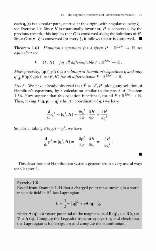
each qi (t) is a circular path, centred at the origin, with angular velocity ξ –see Exercise 1.9. Since H is rotationally invariant, H is conserved. By theprevious remark, this implies that G is conserved along the solutions of H .Since G = π · ξ is conserved for every ξ , it follows that π is conserved. �
Theorem 1.61 Hamilton’s equations for a given H : R2dN → R areequivalent to:
F = {F ,H } for all differentiable F : R2dN → R .
More precisely, (q(t), p(t)) is a solution of Hamilton’s equations if and onlyif d
dt F (q(t), p(t)) = {F ,H } for all differentiable F : R2dN → R.
Proof We have already observed that F = {F ,H } along any solution ofHamilton’s equations, by a calculation similar to the proof of Theorem1.56. Now suppose that this equation is satisfied, for all F : R2dN → R.Then, taking F(q, p) = qj
i (the j th coordinate of qi) we have
ddt
qji = {qj
i ,H } =∂qj
i
∂qi
· ∂H∂pi
= ∂H
∂pji
.
Similarly, taking F(q, p) = pji , we have
ddt
pji = {qj
i ,H } = −∂pj
i
∂pi
· ∂H∂qi
= − ∂H
∂qji
.
�
This description of Hamiltonian systems generalizes in a very useful way:see Chapter 4.
Exercise 1.8Recall from Example 1.34 that a charged point mass moving in a staticmagnetic field in R3 has Lagrangian
L = 12m∥∥q∥∥2 + eA (q) · q,
where A (q) is a vector potential of the magnetic field B (q) , i.e. B (q) =∇ × A (q). Compute the Legendre transform; invert it, and check thatthe Lagrangian is hyperregular; and compute the Hamiltonian.
30 1 : Lagrangian and Hamiltonian mechanics
Exercise 1.9Compute Hamilton’s equations in R6 determined by
H(q, p) := π · ξ = (q× p) · ξ ,for a fixed non-zero ξ ∈ R3. Verify that the solutions of these equationsare circular paths, centred at the origin, with angular velocity ξ .
Exercise 1.10Show that the canonical Poisson bracket satisfies the Jacobi identity:
{F , {G,H }} + {H , {F ,G}} + {G, {H ,F }} = 0.
Given two constants of motion, what does the Jacobi identity implyabout additional constants of motion?
1.5 Rigid bodies
A rigid body is a system of three or more point masses, not all collinear,constrained so that the distance between any two point masses remainsconstant over time. Instead of a finite number of point masses, we mayconsider an infinite collection of points with mass density instead of mass,forming a solid object. We will assume here that the body is solid, and notethat essentially the same analysis applies to assemblies of a finite number ofparticles, with integrals replaced by sums. We assume that the motion is con-tinuous, which implies that the orientation of the object is preserved. Thisassumption, together with the constraint that the inter-particle distancesremain constant, implies that the body can only move by combinations ofrotations and translations.4
It is often possible to deal separately with the rotational and transla-tional motion. For example, this is the case for the motion of a sphericallysymmetric body (with symmetric mass distribution) in a gravitational field:gravitation determines the translational motion but has no effect on therotation of the body. In this book, we will only deal with the rigid body’srotational motion. We will assume that one point of the body – the ‘pivot
4 More details can be found in [Arn78]
1.5 Rigid bodies 31
point’ – remains fixed in some inertial frame, and base our coordinate sys-tems at that point. It is common to assume that this point is the centre ofmass of the body, but this is not necessary. In Section 7.4, we will considerthe heavy top, in which the pivot point of the top is not at the centre ofmass.
We fix an inertial coordinate system, called the spatial coordinate system,with origin at the pivot point. The position and velocity of a given particlein the body at time t are denoted x(t) and x(t). Both are considered ascoordinate vectors in R3, as defined by the spatial coordinate system. Wealso fix a reference configuration of the body. The position of a givenparticle when the body is in the reference configuration is denoted X andcalled the particle’s label.
The configuration of the body at time t is determined by a rotation matrixR(t) that takes every label X to the position x(t) (in spatial coordinates) ofthe corresponding particle at time t :
x(X, t) = R(t)X .
Often, the dependence of x on X is suppressed and the above equation iswritten as
x(t) = R(t)X . (1.35)
At a particular time t , the map X → x = RX is called the body-to-spacemap; note that this map is just the rotation R.
Recall that all rotation matrices are orthogonal, so that RT = R−1.At every time t , there exists a unique angular velocity vector ω(t) such
that, for every particle in the body,
x = ω × x. (1.36)
In this equation, all vectors are expressed in spatial coordinates, so ω is alsocalled the spatial angular velocity vector. The existence of such a vector ωcan be derived directly from the constraint of constant inter-point distances(see [JS98]). Alternatively, it can be deduced from properties of rotationmatrices, as follows. From the basic relation x = RX, we deduce that
x = RX = RR−1x = RRT x . (1.37)
Since all rotation matrices are orthogonal, R(t) satisfies RRT = I for all t .Differentiating with respect to t gives
RRT + RRT = 0,
32 1 : Lagrangian and Hamiltonian mechanics
which implies that RRT is skew-symmetric, i.e. is of the form
RRT = 0 −ω3 ω2
ω3 0 −ω1−ω2 ω1 0
,
for some ω1,ω2,ω3. Defining ω := (ω1,ω2,ω3), it can be directlyverified that
RR−1x = RRT x = ω × x. (1.38)
We introduce notation for the hat map
ω := 0 −ω3 ω2
ω3 0 −ω1−ω2 ω1 0
, (1.39)
so that
RR−1 = ω. (1.40)
The correspondence between skew-symmetric matrices and vectors will bediscussed further in Chapter 5.
Recall that the total angular momentum (around the origin) of a systemof N particles is π := ∑
mi xi × xi . For a solid body, the correspondingdefinition is an integral over the body. Let ρ(X) be the density of the bodyat the point with label X. Let B be the region of space occupied by the bodyin its reference configuration, and note that the labels X range over B. The(spatial) angular momentum of the body at any given time is
π :=∫
Bρ(X) x × x d3X =
∫B
ρ(X) x × (ω × x) d3X , (1.41)
where x = RX. By standard vector identities, x × (ω × x) = (x · x)ω −(x · ω) x and (x · ω) x = (xTω
)x = x
(xTω
) = (xxT)ω. Therefore
π =∫
Bρ(X)
(‖x‖2I − xxT
)ω d3X (1.42)
=(∫
Bρ(X)
(‖x‖2I − xxT
)d3X
)ω,
where I is the 3 × 3 identity matrix. The last step is valid because angularvelocity ω is a property of the entire body, independent of X. This motivatesthe definition of the spatial moment of inertia tensor of the rigid body,
IS :=∫
Bρ(X)
(‖x‖2I − xxT
)d3X .
1.5 Rigid bodies 33
Note that IS , π and ω, are all time-dependent, since x and R are. With thisdefinition, eqn (1.42) becomes:
π = IS ω.
Note the similarity to the familiar formula p = mx defining linear momen-tum. We see that the moment of inertia is the rotational analogue of mass.However, there are important difference: mass is a scalar, and it is constantand independent of the choice of coordinate system; whereas the spatialmoment of inertia is a matrix with entries that depend on time and thechoice of coordinate system.
The moment of inertia tensor may look more familiar if we write x =(x, y, z), in which case,
ρ(X)(‖x‖2I − xxT
)= ρ(X)
y2 + z2 −xy −xz−xy x2 + z2 −yz−xz −yz x2 + y2
.
For example, the term ρ(X)(x2+y2) is analogous to the formulam(x2 + y2)
for the scalar moment of inertia of a particle of mass m moving around thez axis.
By analogy with the N -particle total torque∑
i mix× x, the total torqueon a rigid body is defined as∫
Bρ(X)x × x d3X.
As for N -particle systems (see Proposition 1.8), when the total torque on arigid body is zero, the total spatial angular momentum is conserved: π = 0.This can be easily checked from eqn (1.41).
Now suppose that there is no external torque on the rigid body, that is,the only torque (if any) arises from the forces of inter-particle interactionwithin the body. For N -particle systems, we have seen in Proposition 1.15that forces of interaction within the system always give rise to zero totaltorque, and hence the conservation of spatial angular momentum. The sameis true for solid bodies, a fact sometimes called Euler’s Law:
In the absence of external torque, spatial angular momentum is constant,i.e. π = 0.
Remark 1.62 We will show later, in Chapter 8, that the conservation ofspatial angular momentum can also be deduced from symmetry consid-erations. In particular, systems with no external forces are rotationally
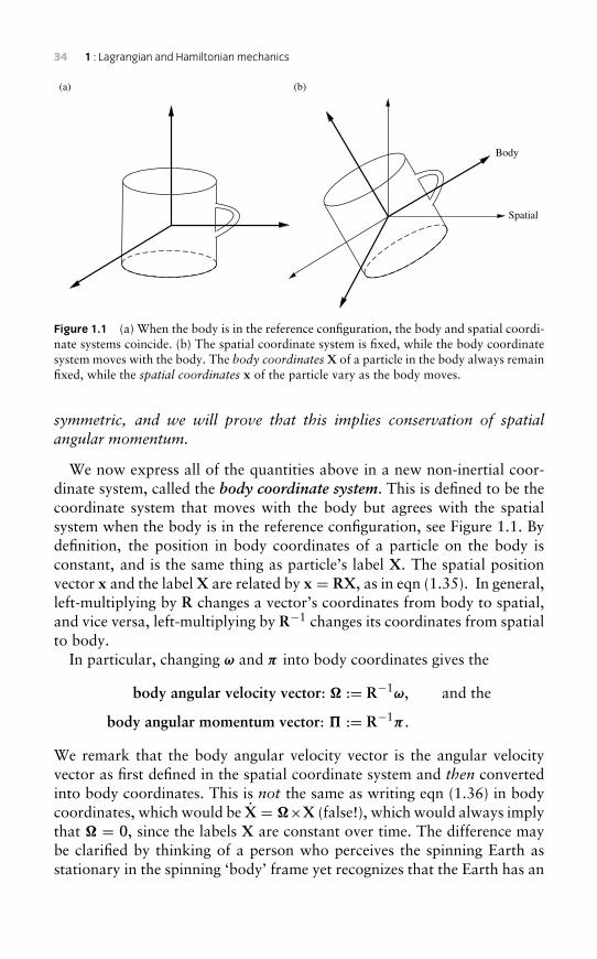
34 1 : Lagrangian and Hamiltonian mechanics
Body
(a) (b)
Spatial
Figure 1.1 (a) When the body is in the reference configuration, the body and spatial coordi-nate systems coincide. (b) The spatial coordinate system is fixed, while the body coordinatesystem moves with the body. The body coordinatesX of a particle in the body always remainfixed, while the spatial coordinates x of the particle vary as the body moves.
symmetric, and we will prove that this implies conservation of spatialangular momentum.
We now express all of the quantities above in a new non-inertial coor-dinate system, called the body coordinate system. This is defined to be thecoordinate system that moves with the body but agrees with the spatialsystem when the body is in the reference configuration, see Figure 1.1. Bydefinition, the position in body coordinates of a particle on the body isconstant, and is the same thing as particle’s label X. The spatial positionvector x and the label X are related by x = RX, as in eqn (1.35). In general,left-multiplying by R changes a vector’s coordinates from body to spatial,and vice versa, left-multiplying by R−1 changes its coordinates from spatialto body.
In particular, changing ω and π into body coordinates gives the
body angular velocity vector: � := R−1ω, and the
body angular momentum vector: � := R−1π .
We remark that the body angular velocity vector is the angular velocityvector as first defined in the spatial coordinate system and then convertedinto body coordinates. This is not the same as writing eqn (1.36) in bodycoordinates, which would be X = �×X (false!), which would always implythat � = 0, since the labels X are constant over time. The difference maybe clarified by thinking of a person who perceives the spinning Earth asstationary in the spinning ‘body’ frame yet recognizes that the Earth has an
1.5 Rigid bodies 35
angular velocity vector parallel to its North/South axis. Note that
�×X = R−1ω × R−1x = R−1(ω × x) = R−1RR−1x = R−1RX. (1.43)
Thus, using the notation of eqn (1.39),
� = R−1R. (1.44)
It is important to remember that the body coordinate system is not (in gen-eral) inertial. Nonetheless, we can translate the formulae we have derivedin spatial coordinates into body coordinates. In particular, the conservationof angular momentum π = 0 becomes:
ddt
(R�) = 0,
which, using the product rule, is equivalent to R�+ R� = 0 or,
� = −R−1
R� = −�×� = �×�. (1.45)
The relation π = IS ω becomes R = IS R�, or equivalently
� =(R−1ISR
)�. (1.46)
We define the body moment of inertia to be I := R−1ISR, so that eqn (1.46)becomes
� = I�. (1.47)
Further, if I is invertible, then eqn (1.45) can be written as
� = �×(I−1�
), (1.48)
in which form it is called Euler’s equation for a rigid body. Note that
I = R−1(∫
Bρ(X)
(‖x‖2I − xxT
)d3X
)R (1.49)
=∫
Bρ(X)
(‖x‖2I − R−1xxT R
)d3X (1.50)
=∫
Bρ(X)
(‖X‖2 I −XXT
)d3X. (1.51)
Thus, the body moment of inertia I is independent of time, which is thegreat advantage of working in body coordinates. We will call I simply the
36 1 : Lagrangian and Hamiltonian mechanics
moment of inertia tensor from now on. Since I is constant, � = I�, soEuler’s equation has the following equivalent form,
I� = I��. (1.52)
Since I is symmetric, it is diagonalizable by a rotation matrix. Its eigenvaluesare called the principal moments of inertia and its eigenvectors are calledthe principal axes. If coordinates are chosen so that I is diagonal, withdiagonal entries I1, I2, I3, then it is easily checked that Euler’s equation isequivalent to the following set of three scalar equations,
I1�1 = (I2 − I3)�2�3,
I2�2 = (I3 − I1)�3�1,
I3�3 = (I1 − I2)�1�2.
We emphasize that these equations are just the conservation of spatial angu-lar momentum, π = 0, written in body coordinates. They hold wheneverthere is no external torque on the body.
Since the moment of inertia is constant (in body coordinates), the scalarsI1, I2, I3 are constant. Thus Euler’s equations form a system of first-order,linear ordinary differential equations in �1,�2,�3, which can in fact beintegrated in closed form for all time, though doing so requires ellipticintegrals (see [LL76]). Once a solution �(t) is found, it can in principlebe used to obtain the body’s configuration R(t) by solving the so-calledreconstruction equation
R = R�,
which is simply a rearrangement of eqn (1.44). However, the interpretationof this last differential equation is a bit tricky, because the dependent vari-able R is a rotation matrix, and the set of rotation matrices, denoted SO(3),is not a Euclidean space. In fact, SO(3) is a 3-dimensional manifold, as wewill see in the next chapter. We will return to the study of rigid bodies,including the Lagrangian and Hamiltonian formulations of their equationsof motion, in Chapters 7 and 9.
Though finding explicit solutions for �(t) and R(t) is difficult, we canlearn a lot just by considering angular momentum and energy. As we haveseen, the spatial angular momentum is conserved, which implies that ‖π‖ isconserved. Since the body angular momentum vector� satisfies� = R−1π ,it follows that ‖�‖ is conserved as well. Thus, �(t) moves on a sphere ofconstant radius, say
‖�‖ = c.
1.5 Rigid bodies 37
The kinetic energy of the rigid body is
K := 12�T I� = 1
2�T I−1�.
We will show in Chapter 7 that this formula is the natural generalization ofthe kinetic energy of a system of point masses. However, it suffices at thispoint to take it as a definition. Assuming that there are no external forces,the kinetic energy is in fact the total energy of the rigid body, which wedenote by H . It follows from Euler’s equation that H is conserved:
dHdt= 1
2�
TI−1�+ 1
2�T I−1�
= 12
(�× I−1�
)·(I−1�
)+ 1
2
(I−1�
)·(�× I−1�
)= 0.
Thus �(t) moves on a level set of H , say
12�T I−1� = h,
which is an ellipsoid. In summary, �(t) must move on the intersectionof an angular momentum sphere and an energy ellipsoid. As long as theprincipal moments of inertia (i.e. the eigenvalues of I) are not all equal,the ellipsoid is not spherical, so the intersection of the ellipsoid and thesphere is a union of a finite number of curves and points. This is sufficientto determine the solution curve given any initial condition, though not thetime-parameterization of that curve or even its orientation. Figure 1.2 showsseveral solution curves on a sphere of constant angular momentum, for thecase when the principal moments of inertia are all distinct.
Exercise 1.11Show that
(Rω)× (Rx) = R (ω × x)
for any rotation matrix R.
Exercise 1.12Suppose there are two orthogonal spatial coordinate systems, with thesame origin, with a fixed change-of-coordinates matrix P from the firstto the second system. If ω and ω′ are the angular velocity vectors definedwith respect to the two coordinate systems, show that ω′ = Pω.
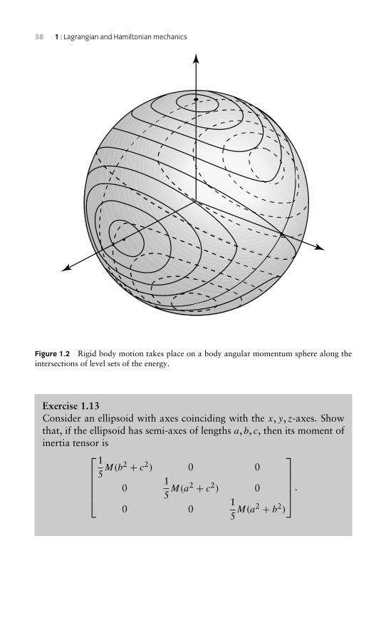
38 1 : Lagrangian and Hamiltonian mechanics
Figure 1.2 Rigid body motion takes place on a body angular momentum sphere along theintersections of level sets of the energy.
Exercise 1.13Consider an ellipsoid with axes coinciding with the x, y, z-axes. Showthat, if the ellipsoid has semi-axes of lengths a, b, c, then its moment ofinertia tensor is
15M(b2 + c2) 0 0
015M(a2 + c2) 0
0 015M(a2 + b2)
.
Solutions to selected exercises 39
Exercise 1.14Show that if a body is two- or three-dimensional, meaning that thereis no line that contains all of the mass of the body, then its moment ofinertia matrix is always invertible.
Exercise 1.15Check the equivalence of the vector and scalar forms of Euler’s equation.
Solutions to selected exercises
Solution to Exercise 1.2 Let U(r) = 1/r. Then, the equation of motionreads
12
(r2 + C2
r2
)− 1
r= E. (1.53)
Integrating with respect to t gives a complicated quadrature. Therefore, weintegrate with respect to θ(t) by making the following transformation:
ddt= θ
ddθ
.
Since we are studying a central force problem, angular momentum is con-served, in fact r2θ = C. It is also convenient to introduce the coordinatechange 1/r = u. The transformation of the derivative r to u′, where ′ denotesdifferentiation with respect to θ , is given by:
r = θ r ′ = Cr ′
r2 = −Cu′.
Equation (1.53) transforms into an equation involving θ as follows:
r2 + C2
r2 −2r= C2(u′)2 + u2C2 − 2u = 2E.
40 1 : Lagrangian and Hamiltonian mechanics
Therefore,
(u′)2 = 2EC2 +
2uC2 − u2
= 2EC2 + 1C4 −
(1C4 −
2uC2 + u2
)= 2EC2 + 1
C4 −(u− 1
C2
)2
.
This leads us to introduce v = (u− 1/C2), noting that v′ = u′. In terms ofv, eqn (1.53) becomes
(v′)2 =( e
C2
)2 − v2,
where
e2 = 2EC2 + 1 > 0.
The solution to this differential equation is easily seen to be
v = e
C2 cos(θ − θ0).
Finally, r in terms of θ is:
r = 1u= C2
C2v + 1= C2
e cos(θ − θ0)+ 1.
This is the equation for a conic section.
Solution to Exercise 1.4a) Since our system is a 1-particle system, V = V (q). Translationalinvariance then gives V (q) = V (q − q) = V (0) = const.b) For each q, let Rq be a rotation such that Rq q = e for some constantunit vector, e. Now consider a 1-particle system with potential V = V (q).Rotational invariance gives us V (q) = V (Rqq) = V (‖q‖e). Therefore, wecan always express the potential as V = V (‖q‖). The converse is trivial.c) For a 2-particle system, V = V (q1, q2). Translational invariance gives usV (q1, q2) = V (0, q2− q1). Therefore, V = V (q2− q1). Now applying partb) yields V = V (‖q2 − q1‖). Again, the converse is trivial.
Solution to Exercise 1.5 The problem is best set up in Cartesian coor-dinates q = (x, y, z) such that B = (0, 0,B). Let the initial position andvelocity of the point mass be (x0, y0, z0) and (vx , vy , vz), respectively. To
Solutions to selected exercises 41
calculate z(t) we observe that
dzdt= d
dt(q · (0, 0, 1)) = q · (0, 0, 1)
= 1m
(eq × (0, 0,B)) · (0, 0, 1) = 0.
Therefore z = vz is constant, and z(t) = vzt + z0. Calculating the equationsof motion for x and y yields
mq = m(x, y, 0) = e (q × B)
= eB (x, y, vz)× (0, 0, 1) = eB (y,−x, 0) .
Integrating these equations gives,[x
y
]=[
cos (Ct) sin (Ct)
− sin (Ct) cos (Ct)
] [vxvy
],
where
C = eB
m.
Integrating a second time gives[x
y
]=[x0 + vy/C
y0 − vx/C
]+ 1
C
[cos
(Ct − π
2
)sin(Ct − π
2
)− sin
(Ct − π
2
)cos
(Ct − π
2
)] [vxvy
].
Putting all the solutions together yields the equation
q − q0 =1C
vy−vx0
= 1C
cos(Ct − π
2
)sin(Ct − π
2
)0
− sin(Ct − π
2
)cos
(Ct − π
2
)0
0 0 Ct
vxvyvz
,
which is a helix along the z-axis of square radius (v2x + v2
y )/C2.
Solution to Exercise 1.6 For a central force problem, V = V (‖q‖). Thekinetic energy in polar coordinates (r, θ) ∈ R2 is
K = m
2‖q‖ = m
2
(r2 + r2θ2
).
Therefore, the Lagrangian is
L = K − V = m
2
(r2 + r2θ2
)− V (r).
42 1 : Lagrangian and Hamiltonian mechanics
Clearly the Lagrangian does not depend on θ . The Euler–Lagrange equationfor θ gives
ddt
∂L
∂θ− ∂L
∂θ= d
dt∂L
∂θ= d
dt
(mr2θ
)= 0.
Thus mr2θ is a conserved quantity.
Solution to Exercise 1.12 Let x′ = Px for some orthogonal 3× 3 matrixP . The defining relationship for the angular velocity, ω, is x = ω × x.Initiating the change of coordinates using the formula derived in Exercise1.11 gives
x′ = P x = P (ω × x)
= Pω × Px = Pω × x′ = ω′ × x′.
Therefore, ω′ = Pω.
2Manifolds
A manifold is basically a smooth curve or surface or higher-dimensionalanalogue. The key property of a manifold is the existence of consistent localcoordinate charts, for example spherical coordinates on a sphere, whichallow us to do calculus on manifolds just as in Euclidean spaces Rn. Man-ifolds appear in many contexts in mechanics, including as configurationspaces. For example, the unit sphere S2 = {(x, y, z) : x2 + y2 + z2 = 1} isthe configuration space of a spherical pendulum. The sphere is a submani-fold of R3. Abstract manifolds can also be defined that are not submanifoldsof Rn. Abstract manifolds are important in mechanics as reduced spaces,obtained from phase spaces by identifying points via a symmetry.
In Part I, we consider only finite-dimensional manifolds. Throughout thisbook, ‘smooth’ will mean C∞.
2.1 Submanifolds of Rn
Recall that the graph of y = f (x), for some function f : R→ R, is the setof points {(x, f (x)) : x ∈ R}. The graph of x = f (y) is {(f (y), y) : y ∈ R}.Similarly, the graph of y = f (x, z), for some function f : A→ R, with A asubset of R2, is
{(x, f (x, z), z) : (x, z) ∈ A}.A general definition of ‘graph’ is awkward for notational reasons, but theidea should be clear from the preceding examples.
A submanifold is the union of one or more graphs of functions. Thefollowing definition ensures that these graphs fit together smoothly. Recallthat a neighbourhood of a point a ∈ Rn is an open set U containing a.
Definition 2.1 Anm-dimensional (embedded) submanifold ofRn is a sub-setM ofRn such that, for every a ∈ M, there is a neighbourhoodU of a suchthat M ∩ U is the graph of some smooth function (with an open domain)1
1 We will assume that, for a function to be smooth, or even just differentiable, its domainmust be an open set. This is usually part of the definition of differentiability.
44 2 : Manifolds
expressing (n − m) of the standard coordinates in terms of the other m.The codimension of M is n − m. Special cases: by definition, any non-empty open subset of Rn is an n-dimensional submanifold of Rn; and anynon-empty subset of Rn containing only isolated points is a 0-dimensionalsubmanifold of Rn.
Example 2.2 S1 is a submanifold of R2, because the top and bottom semi-circles are graphs of the functions y = ±
√1− x2, with domain (−1, 1), and
the left and right semicircles are the graphs of x = ±√1− y2, with domain(−1, 1).
Example 2.3 Any line segment in any Rn, without its endpoints, is a one-dimensional submanifold of Rn; but the same segment with its endpoints isnot (it is a ‘manifold with boundary’, which we will not define).
Definition 2.4 For any subset M of Rn, subsets of M of the form M ∩ U ,with U open, are called open relative to M, or just relatively open (if M isunderstood).
Remark 2.5 If M is a submanifold of Rn, and N is open relative to M,then it follows easily from the definitions that N is a submanifold of Rn, ofthe same dimension as M.
Remark 2.6 The significance of the name ‘embedded submanifold’ willbecome apparent later – see Theorem 2.32 and the remarks that precedeit. There are also immersed submanifolds (see Remark 2.27). In this book‘submanifold’, without qualification, means embedded submanifold.
Manifolds are often described as level sets, for example S1 = {(x, y) ∈R2 : x2 + y2 = 1}, which is f−1(1), where f (x, y) = x2 + y2. Config-uration spaces in mechanical problems are typically defined in this way,by one or more constraints: f1 = c1, . . . , fk = ck, for some smooth func-tions fi : Rn → R. We now discuss conditions under which level sets aresubmanifolds of Rn.
Definition 2.7 Given f : A→ B, The image of D ⊆ A is f (D) := {f (x) ∈B : x ∈ D}. The image of f , or range of f , is Im f := f (A). The preimageof C ⊆ B is f−1(C) := {x ∈ A : f (x) ∈ C}. (This notation does notimply that f is an invertible function). For sets containing only one point,f−1(c) := f−1({c}) = {x ∈ A : f (x) = c}. A level set of f is f−1(c) forsome c ∈ B. This set is also sometimes called the locus of the equationf (x) = c.
2.1 Submanifolds of Rn 45
Example 2.8 Let f (x, y) = xy. The level sets f (x, y) = c, for c �= 0, arethe hyperbolae y = c/x, which are submanifolds. At each point (x, y), thegradient vectors∇f (x, y) = (y, x) is perpendicular to the hyperbola passingthrough (x, y). The level set f (x, y) = 0 is the union of the x- and y-axes.and this set is not a submanifold, because no function has a graph thatcrosses itself. The ‘trouble point’ is the origin, because if it were removed,then each of the remaining four rays would be submanifolds. Note that thisis the only point where the gradient vector, ∇f (x, y) = (y, x), equals zero.
In general, a level set f (x) = c, for a real-valued function f , is a subman-ifold whenever the gradient vectors ∇f (x) are non-zero at all points x inthe level set. This is a consequence of the Implicit Function Theorem. Butbefore we state that theorem, we consider the general situation in whichthere may be more than one constraint, f1 = c1, . . . , fk = ck.
Definition 2.9 Let f1, . . . , fk be differentiable functions from A ⊆ Rn toR. If, for all x ∈ A, the gradient vectors ∇f1(x), . . . ,∇fk(x) are linearlyindependent, then f1, . . . , fk are said to be functionally independent.
Any set of k functions f1, . . . , fk : A → R, taken together, define afunction f = (f1, . . . , fk) : A → Rk. Since the rows of the matrix Df (x)(the derivative, i.e. Jacobian) are ∇f1(x), . . . ,∇fk(x), it follows that the fisare functionally independent if and only if Df (x) has rank k, for every x,which is equivalent to the linear transformation Df (x) being a surjective(i.e. onto). Such functions f are called submersions:
Definition 2.10 A differentiable function f : (A ⊆ Rn)→ Rk is a submer-sion at x ∈ A if the derivative Df (x) is surjective. A function that satisfiesthis condition at all points x ∈ A is a submersion.
Remark 2.11 A function f : (A ⊆ Rn) → Rk can only be a submersionif n ≥ k.
Remark 2.12 The condition that Df (x) is surjective is equivalent to eachof the following conditions (with n and k as above): (i) Im Df (x) = Rk;(ii) rank Df (x) = k; and (iii) dim ker Df (x) = n− k.
Remark 2.13 A real-valued function f is a submersion if and only if∇f (x) �= 0 for every x.
Definition 2.14 A diffeomorphism is a differentiable map with a differen-tiable inverse.
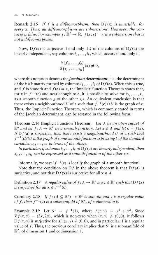
46 2 : Manifolds
Remark 2.15 If f is a diffeomorphism, then Df (x) is invertible, forevery x. Thus, all diffeomorphisms are submersions. However, the con-verse is false. For example f : R2 → R, f (x, y) = x is a submersion that isnot a diffeomorphism.
Now, Df (a) is surjective if and only if k of the columns of Df (a) arelinearly independent, say columns i1, . . . , ik, which occurs if and only if
∂ (f1, . . . , fk)
∂(xi1 , . . . , xik
) (a) �= 0,
where this notation denotes the Jacobian determinant, i.e. the determinantof the k×k matrix formed by columns i1, . . . , ik of Df (a). When this is true,and f is smooth and f (a) = c, the Implicit Function Theorem states that,for x in f−1(c) and near enough to a, it is possible to solve for xi1 , . . . , xikas a smooth function g of the other xis. An equivalent conclusion is thatthere exists a neighbourhood U of a such that f−1(c)∩U is the graph of g.Thus, the Implicit Function Theorem, which is commonly stated in termsof the Jacobian determinant, can be restated in the following form:
Theorem 2.16 (Implicit Function Theorem) Let A be an open subset ofRn and let f : A → Rk be a smooth function. Let a ∈ A and let c = f (a).If Df (a) is surjective, then there exists a neighbourhood U of a such thatf−1(c)∩U is the graph of some smooth function expressing k of the standardvariables x1, . . . , xn in terms of the others.In particular, if columns i1, . . . , ik ofDf (a) are linearly independent, then
xi1 , . . . , xik can be expressed as a smooth function of the other xis.
Informally, we say: ‘f−1(c) is locally the graph of a smooth function’.Note that the condition on Df in the above theorem is that Df (a) is
surjective, and not that Df (x) is surjective for all x ∈ A.
Definition 2.17 A regular value of f : A→ Rk is a c ∈ Rk such thatDf (x)is surjective for all x ∈ f−1(c).
Corollary 2.18 If f : (A ⊆ Rn) → Rk is smooth and c is a regular valueof f , then f−1(c) is a submanifold of Rn, of codimension k.
Example 2.19 Let S1 = f−1(1), where f (x, y) = x2 + y2. Since∇f (x, y) = (2x, 2y), which is non-zero when (x, y) �= (0, 0), it followsDf (x, y) is surjective for all (x, y) �= (0, 0), and in particular, 1 is a regularvalue of f . Thus, the previous corollary implies that S1 is a submanifold ofR2, of dimension 1 and codimension 1.
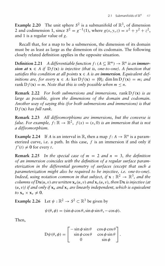
2.1 Submanifolds of Rn 47
Example 2.20 The unit sphere S2 is a submanifold of R3, of dimension2 and codimension 1, since S2 = g−1(1), where g(x, y, z) = x2 + y2 + z2,and 1 is a regular value of g.
Recall that, for a map to be a submersion, the dimension of its domainmust be as least as large as the dimension of its codomain. The followingclosely related definition applies in the opposite situation.
Definition 2.21 A differentiable function f : (A ⊆ Rm)→ Rn is an immer-sion at x ∈ A if Df (x) is injective (that is, one-to-one). A function thatsatisfies this condition at all points x ∈ A is an immersion. Equivalent def-initions are, for every x ∈ A: ker Df (x) = {0}; dim Im Df (x) = m; andrank Df (x) = m. Note that this is only possible when m ≤ n.
Remark 2.22 For both submersions and immersions, rank Df (x) is aslarge as possible, given the dimensions of the domain and codomain.Another way of saying this (for both submersions and immersions) is thatDf (x) has full rank.
Remark 2.23 All diffeomorphisms are immersions, but the converse isfalse. For example, f : R→ R2, f (x) = (x, 0) is an immersion that is nota diffeomorphism.
Example 2.24 If A is an interval in R, then a map f : A→ Rn is a param-eterized curve, i.e. a path. In this case, f is an immersion if and only iff ′(t) �= 0 for every t .
Remark 2.25 In the special case of m = 2 and n = 3, the definitionof an immersion coincides with the definition of a regular surface param-eterization in the differential geometry of surfaces (except that such aparameterization might also be required to be injective, i.e. one-to-one).Indeed, using notation common in that subject, if x : R2 → R3, and thecolumns ofDx(u, v) are written xu(u, v) and xv(u, v), thenDx is injective (at(u, v)) if and only if xu and xv are linearly independent, which is equivalentto xu × xv �= 0.
Example 2.26 Let ψ : R2 → S2 ⊂ R3 be given by
ψ(θ ,φ) = (sinφ cos θ , sinφ sin θ ,− cosφ).
Then,
Dψ(θ ,φ) =− sinφ sin θ cosφ cos θ
sinφ cos θ cosφ sin θ
0 sinφ
.
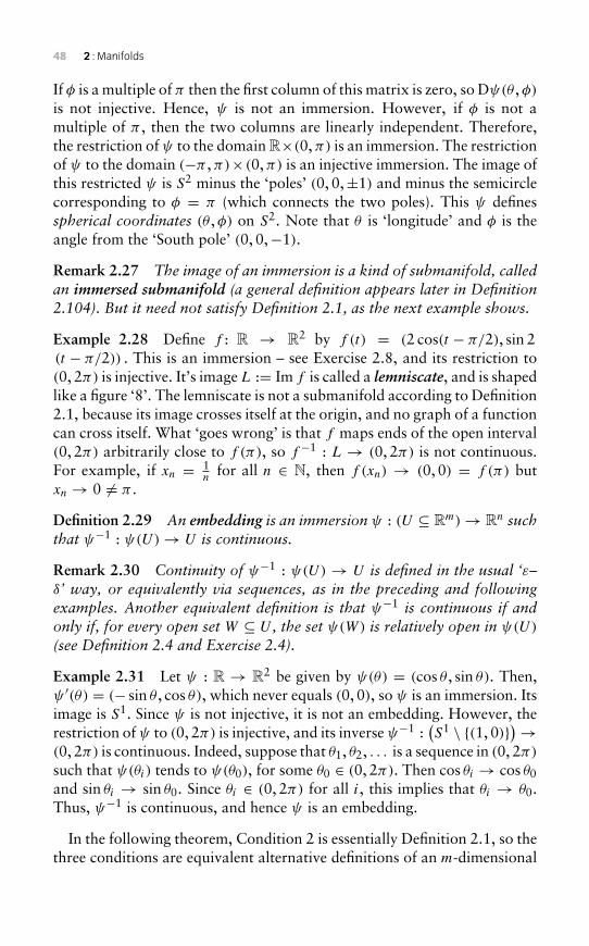
48 2 : Manifolds
If φ is a multiple of π then the first column of this matrix is zero, so Dψ(θ ,φ)is not injective. Hence, ψ is not an immersion. However, if φ is not amultiple of π , then the two columns are linearly independent. Therefore,the restriction of ψ to the domain R×(0,π) is an immersion. The restrictionof ψ to the domain (−π ,π)× (0,π) is an injective immersion. The image ofthis restricted ψ is S2 minus the ‘poles’ (0, 0,±1) and minus the semicirclecorresponding to φ = π (which connects the two poles). This ψ definesspherical coordinates (θ ,φ) on S2. Note that θ is ‘longitude’ and φ is theangle from the ‘South pole’ (0, 0,−1).
Remark 2.27 The image of an immersion is a kind of submanifold, calledan immersed submanifold (a general definition appears later in Definition2.104). But it need not satisfy Definition 2.1, as the next example shows.
Example 2.28 Define f : R → R2 by f (t) = (2 cos(t − π/2), sin 2(t − π/2)) . This is an immersion – see Exercise 2.8, and its restriction to(0, 2π) is injective. It’s image L := Im f is called a lemniscate, and is shapedlike a figure ‘8’. The lemniscate is not a submanifold according to Definition2.1, because its image crosses itself at the origin, and no graph of a functioncan cross itself. What ‘goes wrong’ is that f maps ends of the open interval(0, 2π) arbitrarily close to f (π), so f−1 : L → (0, 2π) is not continuous.For example, if xn = 1
nfor all n ∈ N, then f (xn) → (0, 0) = f (π) but
xn→ 0 �= π .
Definition 2.29 An embedding is an immersion ψ : (U ⊆ Rm)→ Rn suchthat ψ−1 : ψ(U)→ U is continuous.
Remark 2.30 Continuity of ψ−1 : ψ(U) → U is defined in the usual ‘ε–δ’ way, or equivalently via sequences, as in the preceding and followingexamples. Another equivalent definition is that ψ−1 is continuous if andonly if, for every open set W ⊆ U , the set ψ(W) is relatively open in ψ(U)
(see Definition 2.4 and Exercise 2.4).
Example 2.31 Let ψ : R → R2 be given by ψ(θ) = (cos θ , sin θ). Then,ψ ′(θ) = (− sin θ , cos θ), which never equals (0, 0), so ψ is an immersion. Itsimage is S1. Since ψ is not injective, it is not an embedding. However, therestriction of ψ to (0, 2π) is injective, and its inverse ψ−1 :
(S1 \ {(1, 0)})→
(0, 2π) is continuous. Indeed, suppose that θ1, θ2, . . . is a sequence in (0, 2π)
such that ψ(θi) tends to ψ(θ0), for some θ0 ∈ (0, 2π). Then cos θi → cos θ0and sin θi → sin θ0. Since θi ∈ (0, 2π) for all i, this implies that θi → θ0.Thus, ψ−1 is continuous, and hence ψ is an embedding.
In the following theorem, Condition 2 is essentially Definition 2.1, so thethree conditions are equivalent alternative definitions of an m-dimensional
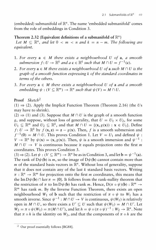
2.1 Submanifolds of Rn 49
(embedded) submanifold of Rn. The name ‘embedded submanifold’ comesfrom the role of embeddings in Condition 3.
Theorem 2.32 (Equivalent definitions of a submanifold of Rn)Let M ⊆ Rn, and let 0 < m < n and k = n − m. The following areequivalent.
1. For every a ∈ M there exists a neighbourhood U of a, a smoothsubmersion f : U → Rk and a c ∈ Rk such that M ∩ U = f−1(c).
2. For every a ∈ M there exists a neighbourhood U of a suchM ∩U is thegraph of a smooth function expressing k of the standard coordinates interms of the others.
3. For every a ∈ M there exists a neighbourhood U of a and a smoothembedding ψ : (V ⊆ Rm)→ Rn such that ψ(V ) = M ∩ U .
Proof Sketch2
(1) ⇒ (2). Apply the Implicit Function Theorem (Theorem 2.16) (the Usmay have to shrink).(2) ⇒ (1) and (3). Suppose that M ∩ U is the graph of a smooth functiong, and suppose, without loss of generality, that U = U1 × U2, for someU1 ⊆ Rm and U2 ⊆ Rk, and that M ∩ U = {(x, g(x)) : x ∈ U1}. Definef : U → Rk by f (x, z) = z − g(x). Then, f is a smooth submersion andf−1(0) = M ∩ U . This proves Condition 1. Let V = U1 and defined ψ :V → Rn by ψ(x) = (x, g(x)). Then, ψ is a smooth immersion and ψ−1 :M ∩ U → V is continuous because it equals projection onto the first m
coordinates. This proves Condition 3.(3)⇒ (2). Letψ : (V ⊆ Rm)→ Rn be as in Condition 3, and let b = ψ−1(a).The rank of Dψ(b) is m, so the image of Dψ(b) cannot contain more thanm of the standard basis vectors in Rn. Without loss of generality, supposethat it does not contain any of the last k standard basis vectors. Writingπ : Rn → Rm for projection onto the first m coordinates, this means thatthe Im Dψ(b) ∩ kerπ = {0}. It follows from the rank-nullity theorem thatthe restriction of π to Im Dψ(b) has rank m. Hence, D(π ◦ ψ)(b) : Rm →Rm has rank m. By the Inverse Function Theorem, there exists an openneighbourhood W1 of b such that the restriction of π ◦ ψ to W1 has asmooth inverse. Since ψ−1 : M ∩U → V is continuous, ψ(W1) is relativelyopen in M ∩ U , so there exists a U ′ ⊆ U such that ψ(W1) = M ∩ U ′. LetW2 = π ◦ψ(W1) = π(M ∩U ′), and let h = ψ ◦ (π ◦ψ)−1 : W2 → Rn. Notethat π ◦ h is the identity on W2, and that the components of π ◦ h are the
2 Our proof essentially follows [BG88].
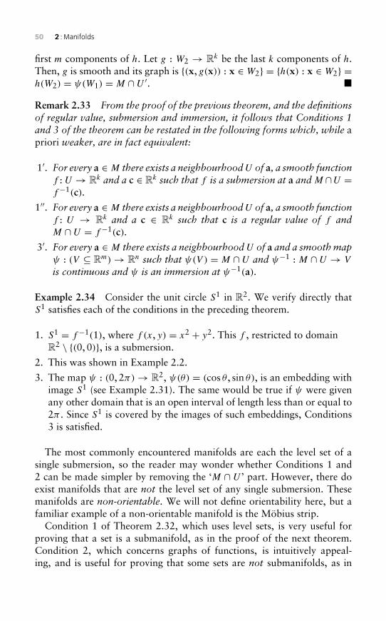
50 2 : Manifolds
first m components of h. Let g : W2 → Rk be the last k components of h.Then, g is smooth and its graph is {(x, g(x)) : x ∈ W2} = {h(x) : x ∈ W2} =h(W2) = ψ(W1) = M ∩ U ′. �
Remark 2.33 From the proof of the previous theorem, and the definitionsof regular value, submersion and immersion, it follows that Conditions 1and 3 of the theorem can be restated in the following forms which, while apriori weaker, are in fact equivalent:
1′. For every a ∈ M there exists a neighbourhoodU of a, a smooth functionf : U → Rk and a c ∈ Rk such that f is a submersion at a andM ∩U =f−1(c).
1′′. For every a ∈ M there exists a neighbourhoodU of a, a smooth functionf : U → Rk and a c ∈ Rk such that c is a regular value of f andM ∩ U = f−1(c).
3′. For every a ∈ M there exists a neighbourhoodU of a and a smooth mapψ : (V ⊆ Rm)→ Rn such that ψ(V ) = M ∩ U and ψ−1 : M ∩ U → V
is continuous and ψ is an immersion at ψ−1(a).
Example 2.34 Consider the unit circle S1 in R2. We verify directly thatS1 satisfies each of the conditions in the preceding theorem.
1. S1 = f−1(1), where f (x, y) = x2 + y2. This f , restricted to domainR2 \ {(0, 0)}, is a submersion.
2. This was shown in Example 2.2.
3. The map ψ : (0, 2π)→ R2, ψ(θ) = (cos θ , sin θ), is an embedding withimage S1 (see Example 2.31). The same would be true if ψ were givenany other domain that is an open interval of length less than or equal to2π . Since S1 is covered by the images of such embeddings, Conditions3 is satisfied.
The most commonly encountered manifolds are each the level set of asingle submersion, so the reader may wonder whether Conditions 1 and2 can be made simpler by removing the ‘M ∩ U ’ part. However, there doexist manifolds that are not the level set of any single submersion. Thesemanifolds are non-orientable. We will not define orientability here, but afamiliar example of a non-orientable manifold is the Möbius strip.
Condition 1 of Theorem 2.32, which uses level sets, is very useful forproving that a set is a submanifold, as in the proof of the next theorem.Condition 2, which concerns graphs of functions, is intuitively appeal-ing, and is useful for proving that some sets are not submanifolds, as in
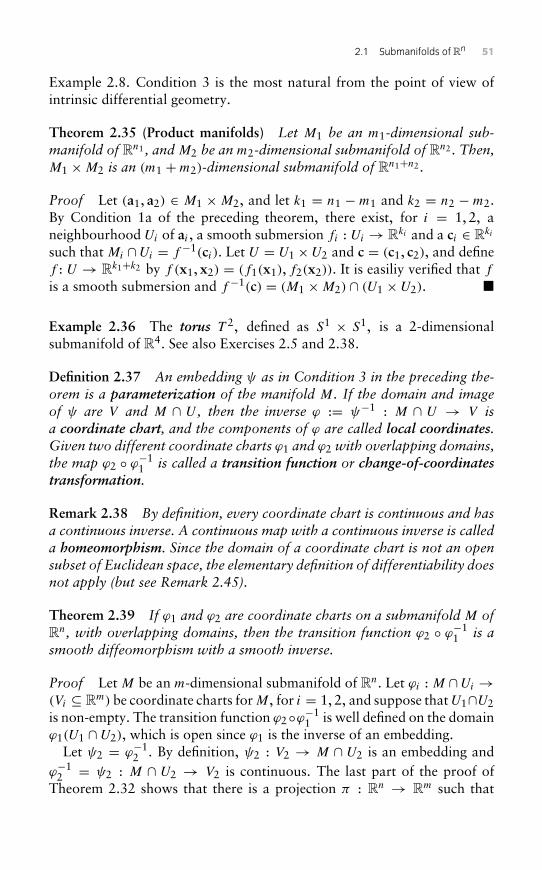
2.1 Submanifolds of Rn 51
Example 2.8. Condition 3 is the most natural from the point of view ofintrinsic differential geometry.
Theorem 2.35 (Product manifolds) Let M1 be an m1-dimensional sub-manifold of Rn1 , andM2 be an m2-dimensional submanifold of Rn2 . Then,M1 ×M2 is an (m1 +m2)-dimensional submanifold of Rn1+n2 .
Proof Let (a1, a2) ∈ M1 ×M2, and let k1 = n1 − m1 and k2 = n2 − m2.By Condition 1a of the preceding theorem, there exist, for i = 1, 2, aneighbourhood Ui of ai , a smooth submersion fi : Ui → Rki and a ci ∈ Rki
such that Mi ∩Ui = f−1(ci ). Let U = U1 ×U2 and c = (c1, c2), and definef : U → Rk1+k2 by f (x1, x2) = (f1(x1), f2(x2)). It is easiliy verified that f
is a smooth submersion and f−1(c) = (M1 ×M2) ∩ (U1 × U2). �
Example 2.36 The torus T 2, defined as S1 × S1, is a 2-dimensionalsubmanifold of R4. See also Exercises 2.5 and 2.38.
Definition 2.37 An embedding ψ as in Condition 3 in the preceding the-orem is a parameterization of the manifold M. If the domain and imageof ψ are V and M ∩ U , then the inverse ϕ := ψ−1 : M ∩ U → V isa coordinate chart, and the components of ϕ are called local coordinates.Given two different coordinate charts ϕ1 and ϕ2 with overlapping domains,the map ϕ2 ◦ ϕ−1
1 is called a transition function or change-of-coordinatestransformation.
Remark 2.38 By definition, every coordinate chart is continuous and hasa continuous inverse. A continuous map with a continuous inverse is calleda homeomorphism. Since the domain of a coordinate chart is not an opensubset of Euclidean space, the elementary definition of differentiability doesnot apply (but see Remark 2.45).
Theorem 2.39 If ϕ1 and ϕ2 are coordinate charts on a submanifoldM ofRn, with overlapping domains, then the transition function ϕ2 ◦ ϕ−1
1 is asmooth diffeomorphism with a smooth inverse.
Proof Let M be an m-dimensional submanifold of Rn. Let ϕi : M ∩Ui →(Vi ⊆ Rm) be coordinate charts forM, for i = 1, 2, and suppose thatU1∩U2is non-empty. The transition function ϕ2◦ϕ−1
1 is well defined on the domainϕ1(U1 ∩ U2), which is open since ϕ1 is the inverse of an embedding.
Let ψ2 = ϕ−12 . By definition, ψ2 : V2 → M ∩ U2 is an embedding and
ϕ−12 = ψ2 : M ∩ U2 → V2 is continuous. The last part of the proof of
Theorem 2.32 shows that there is a projection π : Rn → Rm such that
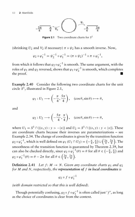
52 2 : Manifolds
Figure 2.1 Two coordinate charts for S1
(shrinking U2 and V2 if necessary) π ◦ ψ2 has a smooth inverse. Now,
ϕ2 ◦ ϕ−11 = ψ−1
2 ◦ ϕ−11 = (π ◦ ψ2)
−1 ◦ π ◦ ϕ−11 ,
from which it follows that ϕ2 ◦ϕ−11 is smooth. The same argument, with the
roles of ϕ1 and ϕ2 reversed, shows that ϕ1 ◦ϕ−12 is smooth, which completes
the proof. �
Example 2.40 Consider the following two coordinate charts for the unitcircle S1, illustrated in Figure 2.1,
ϕ1 : U1 −→(−π
4,5π4
), (cos θ , sin θ) −→ θ ,
and
ϕ2 : U2 −→(−5π
4,π
4
), (cos θ , sin θ) −→ θ ,
where U1 = S1 ∩ {(x, y) : y > −|x|} and U2 = S1 ∩ {(x, y) : y < |x|}. Theseare coordinate charts because their inverses are parameterizations – seeExample 2.34. The change of coordinates is given by the transition function
ϕ2 ◦ϕ−11 , which is well defined on ϕ1 (U1 ∩ U2) =
(−π4 , π
4
)∪ (3π4 , 5π
4
). The
smoothness of the transition function is guaranteed by Theorem 2.39, butcan also be checked directly, since ϕ2 ◦ ϕ−1
1 (θ) = θ for all θ ∈ (−π4 , π
4
)and
ϕ2 ◦ ϕ−11 (θ) = θ − 2π for all θ ∈
(3π4 , 5π
4
).
Definition 2.41 Let f : M → N . Given any coordinate charts ϕ1 and ϕ2for M and N , respectively, the representation of f in local coordinates is
ϕ2 ◦ f ◦ ϕ−11
(with domain restricted so that this is well defined).
Though potentially confusing, ϕ2 ◦f ◦ϕ−11 is often called just ‘f ’, as long
as the choice of coordinates is clear from the context.
2.1 Submanifolds of Rn 53
The usual definitions of ‘differentiable’ and ‘smooth’ do not apply togeneral maps f between manifolds, since the domain of f need not be anopen subset of Euclidean space. One way to remedy this is to use localrepresentations ϕ2 ◦ f ◦ ϕ−1
1 , because their domains and codomains arealways open subsets of Euclidean spaces, so the usual definitions do apply.
Definition 2.42 Let M be a submanifold of Rp and N a submanifold ofRs . The map f is differentiable at a ∈ M if for every coordinate chartϕ1 of M with domain containing a, and every coordinate chart ϕ2 of Nwith domain containing f (a), the composition ϕ2 ◦f ◦ϕ−1
1 is differentiableat ϕ1(a). A map f : M → N is differentiable if it is differentiable at allpoints in its domain, i.e. if every representation of f in local coordinatesis differentiable. The definition of smooth is analagous. The map f is adiffeomorphism if f is differentiable and has a differentiable inverse.
Remark 2.43 In fact, though the preceding definition says ‘for everycoordinate chart’, it suffices to check just enough charts to cover the twomanifolds M and N , because of Theorem 2.39 – see Exercise 2.10.
Remark 2.44 It is easily checked that the composition of two differentiable(resp. smooth) maps is differentiable (resp. smooth). Also, since every coor-dinate chart is continuous and has a continuous inverse, every differentiablemap is continuous.
Remark 2.45 Every coordinate chart is smooth in the sense of the preced-ing definition. Indeed, let ϕ : M ∩ U → (V ⊆ Rm) be a coordinate chartfor M. The identity map idV : V → V is a coordinate chart for V , and therepresentation of ϕ in coordinate charts ϕ and idV is idV ◦ ϕ ◦ ϕ−1 = idV ,which is clearly smooth.In conclusion, if ψ : V → Rp is a parameterization of M with image
M ∩U , then both ψ and ψ−1 : M ∩U → V are smooth. In this sense, ψ is a(smooth) diffeomorphism; but since ψ is not surjective, we say instead thatψ is a ‘diffeomorphism onto its image’. Since the image of every embeddingψ is a submanifold with parameterization ψ , we have shown that everyembedding is a diffeomorphism onto its image. Indeed, an equivalent defi-nition of an embedding is: an immersion that is a diffeomorphism onto itsimage.
Theorem 2.46 Let M be a submanifold of Rp and N a submanifold ofRs . If f : M → N is the restriction of a differentiable (resp. smooth) mapf : U → Rs , where U is an open neighbourhood of M in Rp, then f isdifferentiable (resp. smooth).
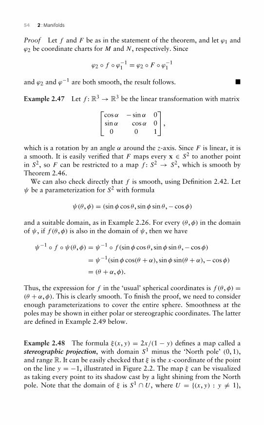
54 2 : Manifolds
Proof Let f and F be as in the statement of the theorem, and let ϕ1 andϕ2 be coordinate charts for M and N , respectively. Since
ϕ2 ◦ f ◦ ϕ−11 = ϕ2 ◦ F ◦ ϕ−1
1
and ϕ2 and ϕ−1 are both smooth, the result follows. �
Example 2.47 Let f : R3 → R3 be the linear transformation with matrixcosα − sinα 0sinα cosα 0
0 0 1
,
which is a rotation by an angle α around the z-axis. Since F is linear, it isa smooth. It is easily verified that F maps every x ∈ S2 to another pointin S2, so F can be restricted to a map f : S2 → S2, which is smooth byTheorem 2.46.
We can also check directly that f is smooth, using Definition 2.42. Letψ be a parameterization for S2 with formula
ψ(θ ,φ) = (sinφ cos θ , sinφ sin θ ,− cosφ)
and a suitable domain, as in Example 2.26. For every (θ ,φ) in the domainof ψ , if f (θ ,φ) is also in the domain of ψ , then we have
ψ−1 ◦ f ◦ ψ(θ ,φ) = ψ−1 ◦ f (sinφ cos θ , sinφ sin θ ,− cosφ)
= ψ−1(sinφ cos(θ + α), sinφ sin(θ + α),− cosφ)
= (θ + α,φ).
Thus, the expression for f in the ‘usual’ spherical coordinates is f (θ ,φ) =(θ + α,φ). This is clearly smooth. To finish the proof, we need to considerenough parameterizations to cover the entire sphere. Smoothness at thepoles may be shown in either polar or stereographic coordinates. The latterare defined in Example 2.49 below.
Example 2.48 The formula ξ(x, y) = 2x/(1 − y) defines a map called astereographic projection, with domain S1 minus the ‘North pole’ (0, 1),and range R. It can be easily checked that ξ is the x-coordinate of the pointon the line y = −1, illustrated in Figure 2.2. The map ξ can be visualizedas taking every point to its shadow cast by a light shining from the Northpole. Note that the domain of ξ is S1 ∩ U , where U = {(x, y) : y �= 1},
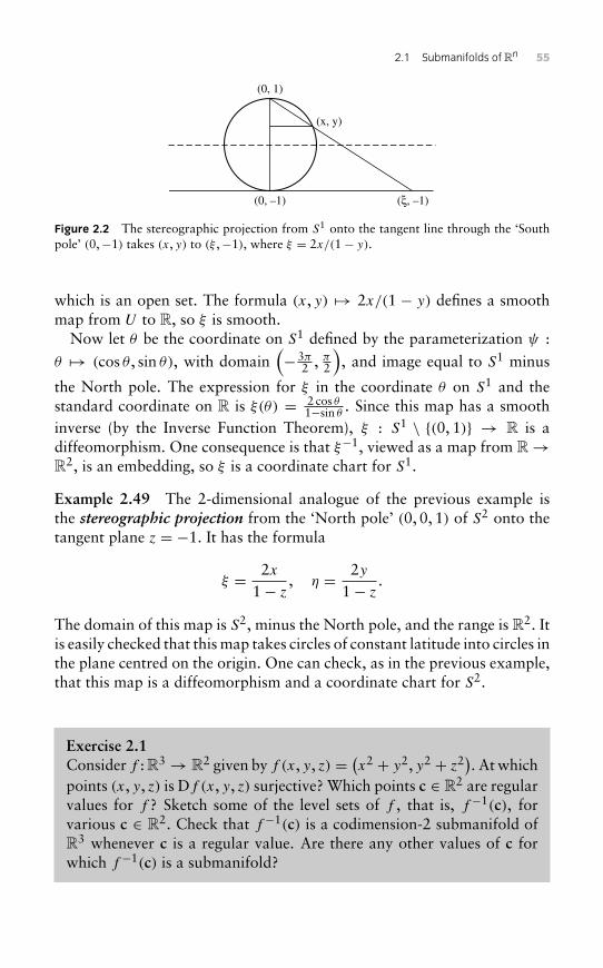
2.1 Submanifolds of Rn 55
(0, 1)
(0, –1) (ξ, –1)
(x, y)
Figure 2.2 The stereographic projection from S1 onto the tangent line through the ‘Southpole’ (0,−1) takes (x, y) to (ξ ,−1), where ξ = 2x/(1− y).
which is an open set. The formula (x, y) → 2x/(1 − y) defines a smoothmap from U to R, so ξ is smooth.
Now let θ be the coordinate on S1 defined by the parameterization ψ :
θ → (cos θ , sin θ), with domain(−3π
2 , π2
), and image equal to S1 minus
the North pole. The expression for ξ in the coordinate θ on S1 and thestandard coordinate on R is ξ(θ) = 2 cos θ
1−sin θ. Since this map has a smooth
inverse (by the Inverse Function Theorem), ξ : S1 \ {(0, 1)} → R is adiffeomorphism. One consequence is that ξ−1, viewed as a map from R→R2, is an embedding, so ξ is a coordinate chart for S1.
Example 2.49 The 2-dimensional analogue of the previous example isthe stereographic projection from the ‘North pole’ (0, 0, 1) of S2 onto thetangent plane z = −1. It has the formula
ξ = 2x1− z
, η = 2y1− z
.
The domain of this map is S2, minus the North pole, and the range is R2. Itis easily checked that this map takes circles of constant latitude into circles inthe plane centred on the origin. One can check, as in the previous example,that this map is a diffeomorphism and a coordinate chart for S2.
Exercise 2.1Consider f : R3 → R2 given by f (x, y, z) = (x2 + y2, y2 + z2). At whichpoints (x, y, z) is Df (x, y, z) surjective? Which points c ∈ R2 are regularvalues for f ? Sketch some of the level sets of f , that is, f−1(c), forvarious c ∈ R2. Check that f−1(c) is a codimension-2 submanifold ofR3 whenever c is a regular value. Are there any other values of c forwhich f−1(c) is a submanifold?
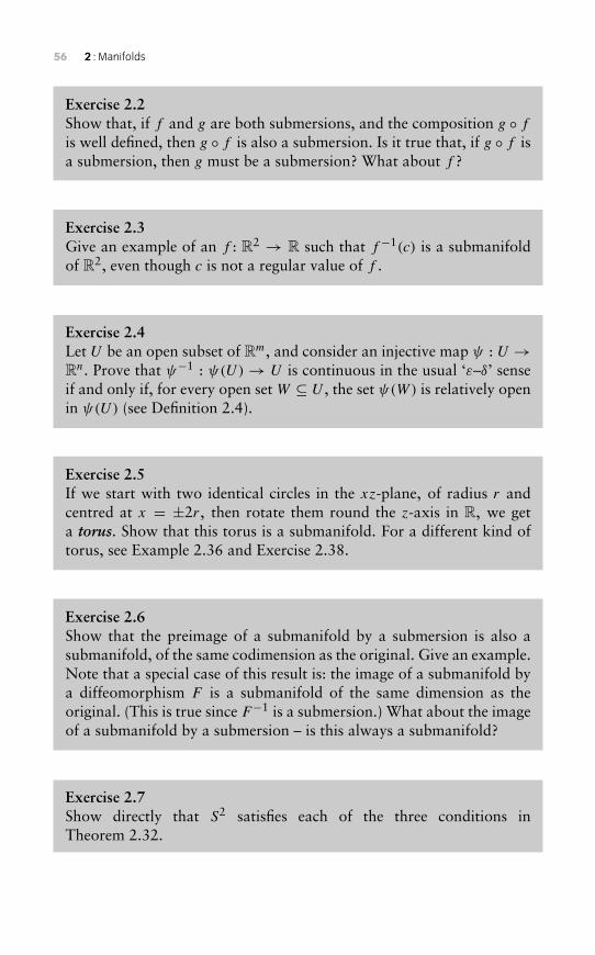
56 2 : Manifolds
Exercise 2.2Show that, if f and g are both submersions, and the composition g ◦ fis well defined, then g ◦ f is also a submersion. Is it true that, if g ◦ f isa submersion, then g must be a submersion? What about f ?
Exercise 2.3Give an example of an f : R2 → R such that f−1(c) is a submanifoldof R2, even though c is not a regular value of f .
Exercise 2.4Let U be an open subset of Rm, and consider an injective map ψ : U →Rn. Prove that ψ−1 : ψ(U)→ U is continuous in the usual ‘ε–δ’ senseif and only if, for every open set W ⊆ U , the set ψ(W) is relatively openin ψ(U) (see Definition 2.4).
Exercise 2.5If we start with two identical circles in the xz-plane, of radius r andcentred at x = ±2r, then rotate them round the z-axis in R, we geta torus. Show that this torus is a submanifold. For a different kind oftorus, see Example 2.36 and Exercise 2.38.
Exercise 2.6Show that the preimage of a submanifold by a submersion is also asubmanifold, of the same codimension as the original. Give an example.Note that a special case of this result is: the image of a submanifold bya diffeomorphism F is a submanifold of the same dimension as theoriginal. (This is true since F−1 is a submersion.) What about the imageof a submanifold by a submersion – is this always a submanifold?
Exercise 2.7Show directly that S2 satisfies each of the three conditions inTheorem 2.32.
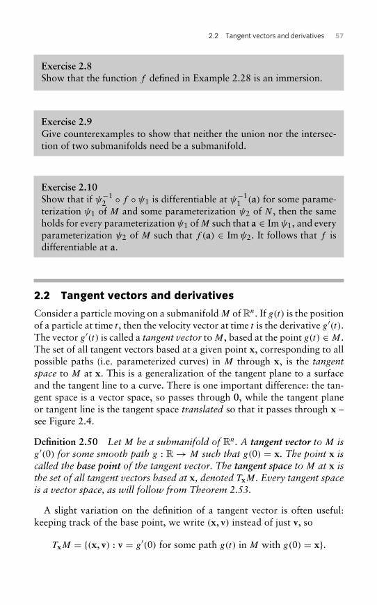
2.2 Tangent vectors and derivatives 57
Exercise 2.8Show that the function f defined in Example 2.28 is an immersion.
Exercise 2.9Give counterexamples to show that neither the union nor the intersec-tion of two submanifolds need be a submanifold.
Exercise 2.10Show that if ψ−1
2 ◦ f ◦ ψ1 is differentiable at ψ−11 (a) for some parame-
terization ψ1 of M and some parameterization ψ2 of N , then the sameholds for every parameterization ψ1 of M such that a ∈ Imψ1, and everyparameterization ψ2 of M such that f (a) ∈ Imψ2. It follows that f isdifferentiable at a.
2.2 Tangent vectors and derivatives
Consider a particle moving on a submanifold M of Rn. If g(t) is the positionof a particle at time t , then the velocity vector at time t is the derivative g′(t).The vector g′(t) is called a tangent vector to M, based at the point g(t) ∈ M.The set of all tangent vectors based at a given point x, corresponding to allpossible paths (i.e. parameterized curves) in M through x, is the tangentspace to M at x. This is a generalization of the tangent plane to a surfaceand the tangent line to a curve. There is one important difference: the tan-gent space is a vector space, so passes through 0, while the tangent planeor tangent line is the tangent space translated so that it passes through x –see Figure 2.4.
Definition 2.50 Let M be a submanifold of Rn. A tangent vector to M isg′(0) for some smooth path g : R→ M such that g(0) = x. The point x iscalled the base point of the tangent vector. The tangent space to M at x isthe set of all tangent vectors based at x, denoted TxM. Every tangent spaceis a vector space, as will follow from Theorem 2.53.
A slight variation on the definition of a tangent vector is often useful:keeping track of the base point, we write (x, v) instead of just v, so
TxM = {(x, v) : v = g′(0) for some path g(t) in M with g(0) = x}.
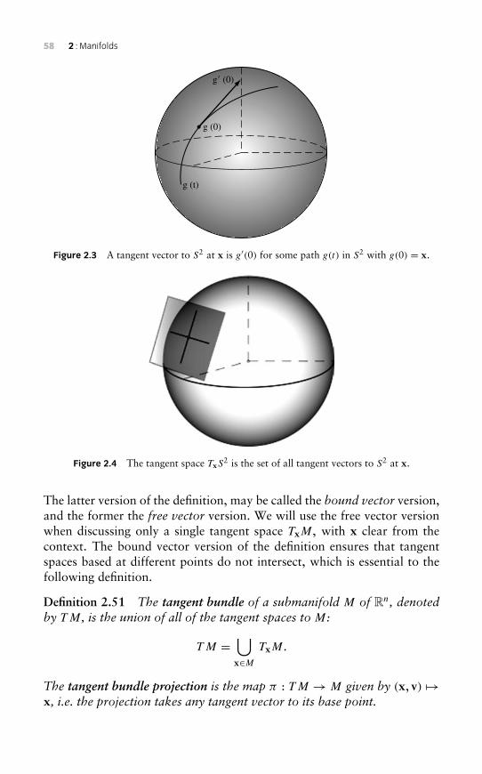
58 2 : Manifolds
g (t)
g (0)
g� (0)
Figure 2.3 A tangent vector to S2 at x is g′(0) for some path g(t) in S2 with g(0) = x.
Figure 2.4 The tangent space TxS2 is the set of all tangent vectors to S2 at x.
The latter version of the definition, may be called the bound vector version,and the former the free vector version. We will use the free vector versionwhen discussing only a single tangent space TxM, with x clear from thecontext. The bound vector version of the definition ensures that tangentspaces based at different points do not intersect, which is essential to thefollowing definition.
Definition 2.51 The tangent bundle of a submanifold M of Rn, denotedby TM, is the union of all of the tangent spaces to M:
TM =⋃x∈M
TxM.
The tangent bundle projection is the map π : TM → M given by (x, v) →x, i.e. the projection takes any tangent vector to its base point.
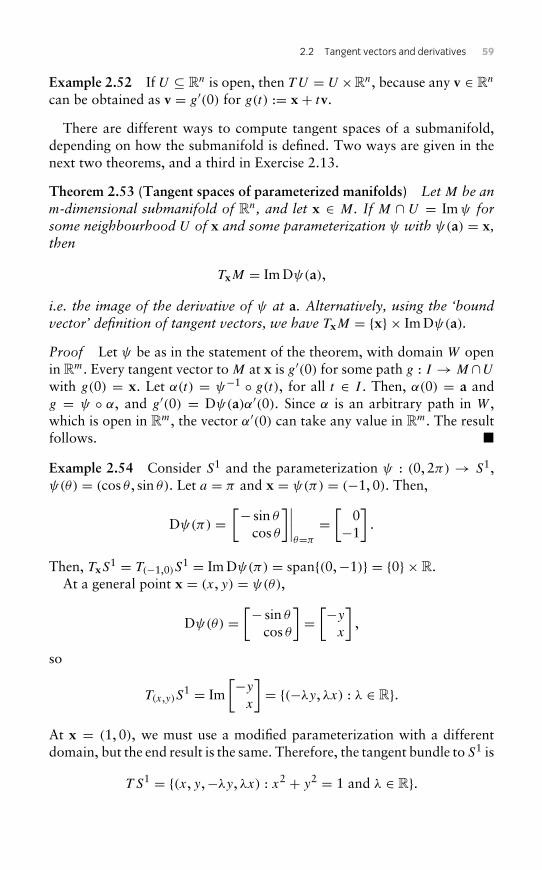
2.2 Tangent vectors and derivatives 59
Example 2.52 If U ⊆ Rn is open, then T U = U ×Rn, because any v ∈ Rn
can be obtained as v = g′(0) for g(t) := x + tv.
There are different ways to compute tangent spaces of a submanifold,depending on how the submanifold is defined. Two ways are given in thenext two theorems, and a third in Exercise 2.13.
Theorem 2.53 (Tangent spaces of parameterized manifolds) LetM be anm-dimensional submanifold of Rn, and let x ∈ M. If M ∩ U = Imψ forsome neighbourhood U of x and some parameterization ψ with ψ(a) = x,then
TxM = Im Dψ(a),
i.e. the image of the derivative of ψ at a. Alternatively, using the ‘boundvector’ definition of tangent vectors, we have TxM = {x} × Im Dψ(a).
Proof Let ψ be as in the statement of the theorem, with domain W openin Rm. Every tangent vector to M at x is g′(0) for some path g : I → M ∩U
with g(0) = x. Let α(t) = ψ−1 ◦ g(t), for all t ∈ I . Then, α(0) = a andg = ψ ◦ α, and g′(0) = Dψ(a)α′(0). Since α is an arbitrary path in W ,which is open in Rm, the vector α′(0) can take any value in Rm. The resultfollows. �
Example 2.54 Consider S1 and the parameterization ψ : (0, 2π) → S1,ψ(θ) = (cos θ , sin θ). Let a = π and x = ψ(π) = (−1, 0). Then,
Dψ(π) =[− sin θ
cos θ
]∣∣∣∣θ=π=[
0−1
].
Then, TxS1 = T(−1,0)S
1 = Im Dψ(π) = span{(0,−1)} = {0} ×R.At a general point x = (x, y) = ψ(θ),
Dψ(θ) =[− sin θ
cos θ
]=[−y
x
],
so
T(x,y)S1 = Im
[−yx
]= {(−λy, λx) : λ ∈ R}.
At x = (1, 0), we must use a modified parameterization with a differentdomain, but the end result is the same. Therefore, the tangent bundle to S1 is
T S1 = {(x, y,−λy, λx) : x2 + y2 = 1 and λ ∈ R}.
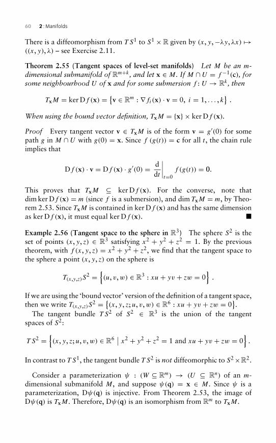
60 2 : Manifolds
There is a diffeomorphism from T S1 to S1 ×R given by (x, y,−λy, λx) →((x, y), λ) – see Exercise 2.11.
Theorem 2.55 (Tangent spaces of level-set manifolds) Let M be an m-dimensional submanifold of Rm+k, and let x ∈ M. If M ∩ U = f−1(c), forsome neighbourhood U of x and for some submersion f : U → Rk, then
TxM = ker Df (x) = {v ∈ Rm : ∇fi(x) · v = 0, i = 1, . . . , k}
.
When using the bound vector definition, TxM = {x} × ker Df (x).
Proof Every tangent vector v ∈ TxM is of the form v = g′(0) for somepath g in M ∩ U with g(0) = x. Since f (g(t)) = c for all t , the chain ruleimplies that
Df (x) · v = Df (x) · g′(0) = ddt
∣∣∣∣t=0
f (g(t)) = 0.
This proves that TxM ⊆ ker Df (x). For the converse, note thatdim ker Df (x) = m (since f is a submersion), and dim TxM = m, by Theo-rem 2.53. Since TxM is contained in ker Df (x) and has the same dimensionas ker Df (x), it must equal ker Df (x). �
Example 2.56 (Tangent space to the sphere in R3) The sphere S2 is theset of points (x, y, z) ∈ R3 satisfying x2 + y2 + z2 = 1. By the previoustheorem, with f (x, y, z) = x2 + y2 + z2, we find that the tangent space tothe sphere a point (x, y, z) on the sphere is
T(x,y,z)S2 =
{(u, v,w) ∈ R3 : xu+ yv + zw = 0
}.
If we are using the ‘bound vector’ version of the definition of a tangent space,then we write T(x,y,z)S
2 = {(x, y, z; u, v,w) ∈ R6 : xu+ yv + zw = 0}.
The tangent bundle T S2 of S2 ∈ R3 is the union of the tangentspaces of S2:
T S2 ={(x, y, z; u, v,w) ∈ R6 ∣∣ x2 + y2 + z2 = 1 and xu+ yv + zw = 0
}.
In contrast to T S1, the tangent bundle T S2 is not diffeomorphic to S2×R2.
Consider a parameterization ψ : (W ⊆ Rm) → (U ⊆ Rn) of an m-dimensional submanifold M, and suppose ψ(q) = x ∈ M. Since ψ is aparameterization, Dψ(q) is injective. From Theorem 2.53, the image ofDψ(q) is TxM. Therefore, Dψ(q) is an isomorphism from Rm to TxM.
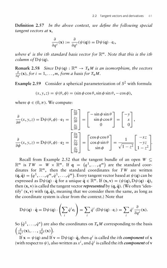
2.2 Tangent vectors and derivatives 61
Definition 2.57 In the above context, we define the following specialtangent vectors at x,
∂
∂qi(x) := ∂
∂qi(ψ(q)) = Dψ(q) · ei ,
where ei is the ith standard basis vector for Rm. Note that this is the ithcolumn of Dψ(q).
Remark 2.58 Since Dψ(q) : Rm → TxM is an isomorphism, the vectors∂
∂qi (x), for i = 1, . . . ,m, form a basis for TxM.
Example 2.59 Consider a spherical parameterization of S2 with formula
(x, y, z) = ψ(θ ,φ) = (sinφ cos θ , sinφ sin θ ,− cosφ),
where φ ∈ (0,π). We compute:
∂
∂θ(x, y, z) = Dψ(θ ,φ) · e1 =
∂x∂θ
∂y∂θ
∂z∂θ
=− sinφ sin θ
sinφ cos θ0
=−yx
0
,
∂
∂φ(x, y, z) = Dψ(θ ,φ) · e2 =
∂x∂φ
∂y∂φ
∂z∂φ
=cosφ cos θ
cosφ sin θ
sinφ
= 1√1− z2
−xz−yz1− z2
.Recall from Example 2.52 that the tangent bundle of an open W ⊆
Rm is TW = W × Rm. If q = (q1, . . . , qm
)are the standard coor-
dinates for Rm, then the standard coordinates for TW are written(q, q) = (q1, . . . , qm, q1, . . . , qm
). Every tangent vector based at ψ(q) can be
expressed as Dψ(q) · q for a unique q ∈ Rm. If (x, v) = (ψ(q), Dψ(q) · q),then (x, v) is called the tangent vector represented by (q, q). (We often ‘iden-tify’ (x, v) with (q, q), meaning that we consider them the same, as long asthe coordinate system is clear from the context.) Note that
Dψ(q) · q = Dψ(q) ·(∑
i
qiei
)=∑i
qi (Dψ(q) · ei ) =∑i
qi ∂
∂qi(x).
So(q1, . . . , qn
)are also the coordinates on TxM corresponding to the basis(
∂
∂q1 (x), . . . ,∂
∂qn (x)).
If x = ψ(q) and If v = Dψ(q) · q, then qi is called the ith component of x(with respect toψ), also written as xi , and qi is called the ith component of v
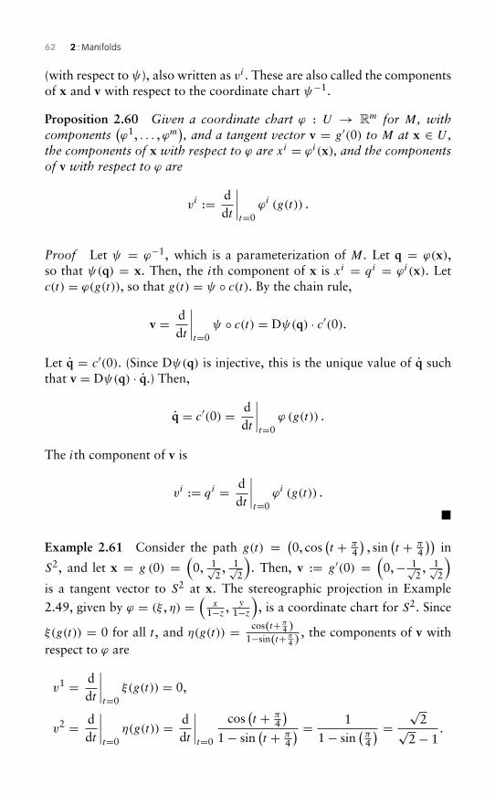
62 2 : Manifolds
(with respect to ψ), also written as vi . These are also called the componentsof x and v with respect to the coordinate chart ψ−1.
Proposition 2.60 Given a coordinate chart ϕ : U → Rm for M, withcomponents
(ϕ1, . . . ,ϕm
), and a tangent vector v = g′(0) to M at x ∈ U ,
the components of x with respect to ϕ are xi = ϕi(x), and the componentsof v with respect to ϕ are
vi := ddt
∣∣∣∣t=0
ϕi (g(t)) .
Proof Let ψ = ϕ−1, which is a parameterization of M. Let q = ϕ(x),so that ψ(q) = x. Then, the ith component of x is xi = qi = ϕi(x). Letc(t) = ϕ(g(t)), so that g(t) = ψ ◦ c(t). By the chain rule,
v = ddt
∣∣∣∣t=0
ψ ◦ c(t) = Dψ(q) · c′(0).
Let q = c′(0). (Since Dψ(q) is injective, this is the unique value of q suchthat v = Dψ(q) · q.) Then,
q = c′(0) = ddt
∣∣∣∣t=0
ϕ (g(t)) .
The ith component of v is
vi := qi = ddt
∣∣∣∣t=0
ϕi (g(t)) .
�
Example 2.61 Consider the path g(t) = (0, cos
(t + π
4
), sin
(t + π
4
))in
S2, and let x = g (0) =(0, 1√
2, 1√
2
). Then, v := g′(0) =
(0,− 1√
2, 1√
2
)is a tangent vector to S2 at x. The stereographic projection in Example
2.49, given by ϕ = (ξ , η) =(
x1−z ,
y1−z
), is a coordinate chart for S2. Since
ξ(g(t)) = 0 for all t , and η(g(t)) = cos(t+ π4 )
1−sin(t+ π4 )
, the components of v withrespect to ϕ are
v1 = ddt
∣∣∣∣t=0
ξ(g(t)) = 0,
v2 = ddt
∣∣∣∣t=0
η(g(t)) = ddt
∣∣∣∣t=0
cos(t + π
4
)1− sin
(t + π
4
) = 11− sin
(π4
) = √2√
2− 1.
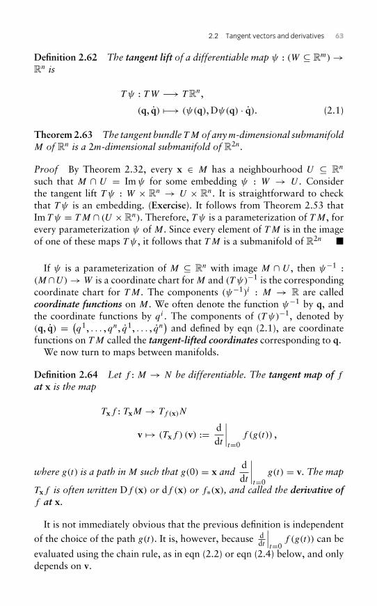
2.2 Tangent vectors and derivatives 63
Definition 2.62 The tangent lift of a differentiable map ψ : (W ⊆ Rm)→Rn is
T ψ : TW −→ T Rn,
(q, q) −→ (ψ(q), Dψ(q) · q). (2.1)
Theorem2.63 The tangent bundle TM of anym-dimensional submanifoldM of Rn is a 2m-dimensional submanifold of R2n.
Proof By Theorem 2.32, every x ∈ M has a neighbourhood U ⊆ Rn
such that M ∩ U = Imψ for some embedding ψ : W → U . Considerthe tangent lift T ψ : W × Rn → U × Rn. It is straightforward to checkthat T ψ is an embedding. (Exercise). It follows from Theorem 2.53 thatIm T ψ = TM ∩ (U ×Rn). Therefore, T ψ is a parameterization of TM, forevery parameterization ψ of M. Since every element of TM is in the imageof one of these maps T ψ , it follows that TM is a submanifold of R2n �
If ψ is a parameterization of M ⊆ Rn with image M ∩ U , then ψ−1 :(M ∩U)→ W is a coordinate chart for M and (T ψ)−1 is the correspondingcoordinate chart for TM. The components (ψ−1)i : M → R are calledcoordinate functions on M. We often denote the function ψ−1 by q, andthe coordinate functions by qi . The components of (T ψ)−1, denoted by(q, q) = (
q1, . . . , qn, q1, . . . , qn)
and defined by eqn (2.1), are coordinatefunctions on TM called the tangent-lifted coordinates corresponding to q.
We now turn to maps between manifolds.
Definition 2.64 Let f : M → N be differentiable. The tangent map of f
at x is the map
Txf : TxM → Tf (x)N
v → (Txf ) (v) := ddt
∣∣∣∣t=0
f (g(t)) ,
where g(t) is a path inM such that g(0) = x andddt
∣∣∣∣t=0
g(t) = v. The map
Txf is often written Df (x) or df (x) or f∗(x), and called the derivative off at x.
It is not immediately obvious that the previous definition is independent
of the choice of the path g(t). It is, however, because ddt
∣∣∣t=0
f (g(t)) can be
evaluated using the chain rule, as in eqn (2.2) or eqn (2.4) below, and onlydepends on v.
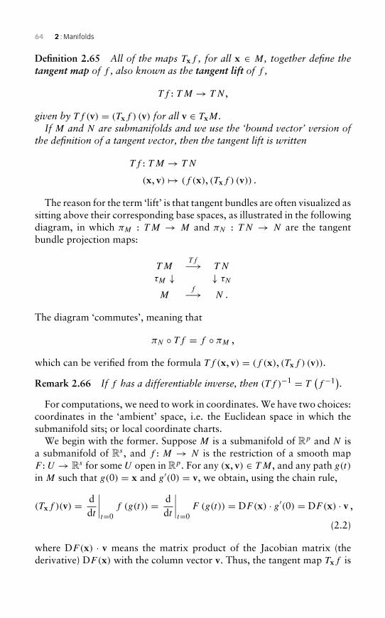
64 2 : Manifolds
Definition 2.65 All of the maps Txf , for all x ∈ M, together define thetangent map of f , also known as the tangent lift of f ,
Tf : TM → TN ,
given by Tf (v) = (Txf ) (v) for all v ∈ TxM.If M and N are submanifolds and we use the ‘bound vector’ version of
the definition of a tangent vector, then the tangent lift is written
Tf : TM → TN
(x, v) → (f (x), (Txf ) (v)) .
The reason for the term ‘lift’ is that tangent bundles are often visualized assitting above their corresponding base spaces, as illustrated in the followingdiagram, in which πM : TM → M and πN : TN → N are the tangentbundle projection maps:
TMTf−→ TN
τM ↓ ↓ τN
Mf−→ N .
The diagram ‘commutes’, meaning that
πN ◦ Tf = f ◦ πM ,
which can be verified from the formula Tf (x, v) = (f (x), (Txf ) (v)).
Remark 2.66 If f has a differentiable inverse, then (Tf )−1 = T(f−1).
For computations, we need to work in coordinates. We have two choices:coordinates in the ‘ambient’ space, i.e. the Euclidean space in which thesubmanifold sits; or local coordinate charts.
We begin with the former. Suppose M is a submanifold of Rp and N isa submanifold of Rs , and f : M → N is the restriction of a smooth mapF : U → Rs for some U open in Rp. For any (x, v) ∈ TM, and any path g(t)
in M such that g(0) = x and g′(0) = v, we obtain, using the chain rule,
(Txf )(v) = ddt
∣∣∣∣t=0
f (g(t)) = ddt
∣∣∣∣t=0
F (g(t)) = DF(x) · g′(0) = DF(x) · v ,
(2.2)
where DF(x) · v means the matrix product of the Jacobian matrix (thederivative) DF(x) with the column vector v. Thus, the tangent map Txf is
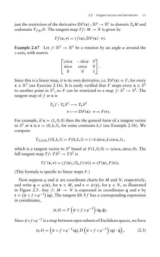
2.2 Tangent vectors and derivatives 65
just the restriction of the derivative DF(x) : Rp → Rs to domain TxM andcodomain Tf (x)N . The tangent map Tf : M → N is given by
Tf (x, v) = (f (x), DF(x) · v).Example 2.67 Let f : R3 → R3 be a rotation by an angle α around thez-axis, with matrix cosα − sinα 0
sinα cosα 00 0 1
.
Since this is a linear map, it is its own derivative, i.e. DF(x) = F , for everyx ∈ R3 (see Exercise 2.16). It is easily verified that F maps every x ∈ S2
to another point in S2, so F can be restricted to a map f : S2 → S2. Thetangent map of f at x is
Txf : TxS2 −→ TxS
2
v −→ DF(x) · v = F(v).
For example, if x = (1, 0, 0) then the the general form of a tangent vectorto S2 at x is v = (0, k, l), for some constants k, l (see Example 2.56). Wecompute:
T(1,0,0)f (0, k, l) = F(0, k, l) = (−k sinα, k cosα, l) ,
which is a tangent vector to S2 based at F(1, 0, 0) = (cosα, sinα, 0). Thefull tangent map Tf : T S2 → T S2 is
Tf (x, v) = (f (x), (Txf ) (v)) = (F (x),F(v)).
(This formula is specific to linear maps F .)
Now suppose ϕ and ψ are coordinate charts for M and N , respectively,and write q = ϕ(x), for x ∈ M, and r = ψ(y), for y ∈ N , as illustratedin Figure 2.5. Any f : M → N is expressed in coordinates q and r byr = (ψ ◦ f ◦ ϕ−1) (q). The tangent lift Tf has a corresponding expressionin coordinates,
(r, r) = T(ψ ◦ f ◦ ϕ−1
)(q, q).
Sinceψ◦f ◦ϕ−1 is a map between open subsets of Euclidean spaces, we have
(r, r) =(ψ ◦ f ◦ ϕ−1(q), D
(ψ ◦ f ◦ ϕ−1
)(q) · q
), (2.3)
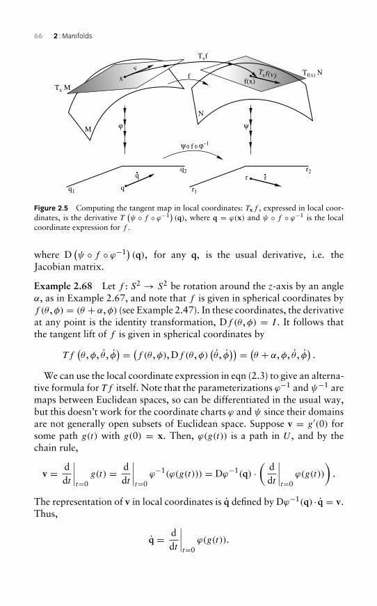
66 2 : Manifolds
x f(x)
M
v
Txf
Txf(v)
N
q
r
f
q1
q2
r1
r2
ψϕ
q r
Tf(x) N
Tx M
ψ f ϕ–1
Figure 2.5 Computing the tangent map in local coordinates: Txf , expressed in local coor-dinates, is the derivative T
(ψ ◦ f ◦ ϕ−1) (q), where q = ϕ(x) and ψ ◦ f ◦ ϕ−1 is the local
coordinate expression for f .
where D(ψ ◦ f ◦ ϕ−1) (q), for any q, is the usual derivative, i.e. the
Jacobian matrix.
Example 2.68 Let f : S2 → S2 be rotation around the z-axis by an angleα, as in Example 2.67, and note that f is given in spherical coordinates byf (θ ,φ) = (θ + α,φ) (see Example 2.47). In these coordinates, the derivativeat any point is the identity transformation, Df (θ ,φ) = I . It follows thatthe tangent lift of f is given in spherical coordinates by
Tf(θ ,φ, θ , φ
) = (f (θ ,φ), Df (θ ,φ)(θ , φ
)) = (θ + α,φ, θ , φ).
We can use the local coordinate expression in eqn (2.3) to give an alterna-tive formula for Tf itself. Note that the parameterizations ϕ−1 and ψ−1 aremaps between Euclidean spaces, so can be differentiated in the usual way,but this doesn’t work for the coordinate charts ϕ and ψ since their domainsare not generally open subsets of Euclidean space. Suppose v = g′(0) forsome path g(t) with g(0) = x. Then, ϕ(g(t)) is a path in U , and by thechain rule,
v = ddt
∣∣∣∣t=0
g(t) = ddt
∣∣∣∣t=0
ϕ−1(ϕ(g(t))) = Dϕ−1(q) ·(
ddt
∣∣∣∣t=0
ϕ(g(t))
).
The representation of v in local coordinates is q defined by Dϕ−1(q) · q = v.Thus,
q = ddt
∣∣∣∣t=0
ϕ(g(t)).
2.2 Tangent vectors and derivatives 67
Note that
f = ψ−1 ◦(ψ ◦ f ◦ ϕ−1
)◦ ϕ.
Applying the chain rule again gives,
(Txf ) (v) = ddt
∣∣∣∣t=0
f (g(t))
= ddt
∣∣∣∣t=0
ψ−1 ◦(ψ ◦ f ◦ ϕ−1
)◦ ϕ ◦ g(t)
= Dψ−1(r) ◦D(ψ ◦ f ◦ ϕ−1
)(q) ·
(ddt
∣∣∣∣t=0
ϕ(g(t))
)= Dψ−1(r) ◦D
(ψ ◦ f ◦ ϕ−1
)(q) · q. (2.4)
This formula is more complicated than our original definition of the tangentmap, but it does not depend on a choice of path g(t) such that g′(0) = v.This shows that the original definition of the tangent map is well defined.
The formula r = D(ψ ◦ f ◦ ϕ−1) (q) · q in eqn (2.3) can also be written
r i =∑j
∂ri
∂qjqj , (2.5)
(with the base point q omitted). Sometimes, if the choice of coordinates isclear from the context, the map ψ ◦ f ◦ ϕ−1 (which we have called r) willalso be called f , in which case we write r = Df (q) · q, or equivalently,
r i =∑j
∂f i
∂qjqj . (2.6)
An important special case occurs when f is the identity map from M toitself, and ϕ and ψ are two overlapping coordinate charts on M, definingtwo systems of coordinates, q and r. In this case, eqn (2.5) applies with r =ψ ◦ ϕ−1(q), and gives the change of coordinates from q to r correspondingto the change of coordinates from q to r.
Exercise 2.11Show that the map T S1 → S1 ×R, (x, y,−λy, λx) → ((x, y), λ), whichappeared in Example 2.54, is a diffeomorphism.
68 2 : Manifolds
Exercise 2.12Compute the tangent bundle of the cylinder C given by
C = S1 ×R ={(x, y, z) ∈ R3 : x2 + y2 = 1
}.
Exercise 2.13 (Tangent spaces of manifolds defined as graphs) Let M
be an n-dimensional submanifold of Rn+k, let x ∈ M and let U be aneighbourhood of x. Show that, if M ∩ U is the graph of a smoothfunction g of the first n standard coordinates of Rn+k, then
TxM = {x} × {(v, Dg (x1, . . . , xn) (v)) : v ∈ Rn} .
Exercise 2.14Consider spherical coordinates on S2 defined by
(x, y, z) = (sinφ cos θ , sinφ sin θ ,− cosφ).
Let (x, v) be the tangent vector to S2 given in the spherical coordinates by(θ ,φ, θ , φ
) = (0, π4 , 2,−1
). Compute (x, v) in the standard coordinates
(x, y, z) for R3.
Exercise 2.15Let ϕ : S2 → R2 be the stereographic projection (x, y, z) → (ξ , η) givenin Example 2.49. Compute ∂
∂θ(x, y, z) in (ξ , η) coordinates, where θ is
the usual spherical coordinate, as in Exercise 2.14.
Exercise 2.16Check that if F : Rp → Rs is a linear map, then DF(x) = F for all x.
2.3 Differentials and cotangent vectors 69
Exercise 2.17Compute the change of coordinates from (r, θ ) to (x, y) correspondingto the change from polar to Cartesian coordinates in R2.
Exercise 2.18Consider the cylinder C = S1 ×R = {(x, y, z) ∈ R3 : x2 + y2 = 1
}. Let
f : S2 → C be given by f (θ ,φ) = (θ ,− cosφ), in spherical coordinateson S2 as in Exercise 2.14, and cylindrical coordinates (θ , z) on C definedby (x, y, z) = (cos θ , sin θ , z). Compute Tf in these coordinates.
Exercise 2.19Compute the tangent map of the stereographic projection S2 → R2
given in Example 2.49, in two ways: first, using Cartesian coordi-nates (x, y, z) on S2 ⊆ R3, and second, using spherical coordinates(θ ,φ) on S2.
Exercise 2.20The tangent bundle projection map, τ : TM → M, given by (x, v) → x,is written in any tangent-lifted coordinate chart (q, q) as τ(q, q) = q.Write down the matrix Dτ(q, q) in these coordinates, and check that τis a submersion.
Exercise 2.21Give an alternative proof that TM is a submanifold, by describing M asa union of level sets.
2.3 Differentials and cotangent vectors
Let f be a smooth real-valued function on a manifold M. Note thatTf (x)R = R, for any x ∈ M, so the tangent map of f at x can be writ-ten Txf : TxM → R. In this case, Txf is also called the differential of f at
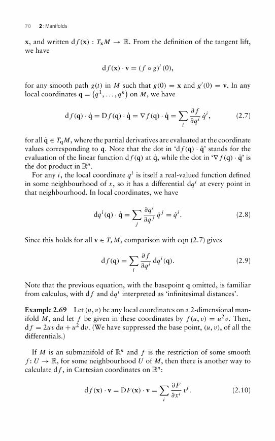
70 2 : Manifolds
x, and written df (x) : TxM → R. From the definition of the tangent lift,we have
df (x) · v = (f ◦ g)′ (0),
for any smooth path g(t) in M such that g(0) = x and g′(0) = v. In anylocal coordinates q = (q1, . . . , qn
)on M, we have
df (q) · q = Df (q) · q = ∇f (q) · q =∑i
∂f
∂qiqi , (2.7)
for all q ∈ TqM, where the partial derivatives are evaluated at the coordinatevalues corresponding to q. Note that the dot in ‘df (q) · q’ stands for theevaluation of the linear function df (q) at q, while the dot in ‘∇f (q) · q’ isthe dot product in Rn.
For any i, the local coordinate qi is itself a real-valued function definedin some neighbourhood of x, so it has a differential dqi at every point inthat neighbourhood. In local coordinates, we have
dqi(q) · q =∑j
∂qi
∂qjqj = qi . (2.8)
Since this holds for all v ∈ TxM, comparison with eqn (2.7) gives
df (q) =∑i
∂f
∂qidqi(q). (2.9)
Note that the previous equation, with the basepoint q omitted, is familiarfrom calculus, with df and dqi interpreted as ‘infinitesimal distances’.
Example 2.69 Let (u, v) be any local coordinates on a 2-dimensional man-ifold M, and let f be given in these coordinates by f (u, v) = u2v. Then,df = 2uv du+ u2 dv. (We have suppressed the base point, (u, v), of all thedifferentials.)
If M is an submanifold of Rn and f is the restriction of some smoothf : U → R, for some neighbourhood U of M, then there is another way tocalculate df , in Cartesian coordinates on Rn:
df (x) · v = DF(x) · v =∑i
∂F
∂xivi . (2.10)
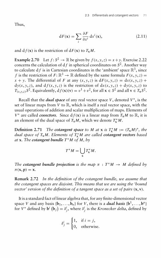
2.3 Differentials and cotangent vectors 71
Thus,
dF(x) =∑i
∂F
∂xidxi(x), (2.11)
and df (x) is the restriction of dF(x) to TxM.
Example 2.70 Let f : S2 → R be given by f (x, y, z) = x+y. Exercise 2.22concerns the calculation of df in spherical coordinates on S2. Another wayto calculate df is in Cartesian coordinates in the ‘ambient’ space R3, sincef is the restriction of F : R3 → R defined by the same formula F(x, y, z) =x + y. The differential of F at any (x, y, z) is dF(x, y, z) = dx(x, y, z) +dy(x, y, z), and df (x, y, z) is the restriction of dx(x, y, z) + dy(x, y, z) toT(x,y,z)S
2. Equivalently, df (x)(v) = v1+v2, for all x ∈ S2 and all v ∈ TxS2.
Recall that the dual space of any real vector space V , denoted V ∗, is theset of linear maps from V to R, which is itself a real vector space, with theusual operations of addition and scalar mulfiplication of maps. Elements ofV ∗ are called covectors. Since df (x) is a linear map from TxM to R, it isan element of the dual space of TxM, which we denote T ∗x M.
Definition 2.71 The cotangent space to M at x is T ∗x M := (TxM)∗, thedual space of TxM. Elements of T ∗x M are called cotangent vectors basedat x. The cotangent bundle T ∗M of M, by
T ∗M =⋃x
T ∗x M.
The cotangent bundle projection is the map π : T ∗M → M defined byπ(x, p) = x.
Remark 2.72 In the definition of the cotangent bundle, we assume thatthe cotangent spaces are disjoint. This means that we are using the ‘boundvector’ version of the definition of a tangent space as a set of pairs (x, v).
It is a standard fact of linear algebra that, for any finite-dimensional vectorspace V and any basis {b1, . . . , bn} for V , there is a dual basis {b1, . . . , bn}for V ∗ defined by bi
(bj
) = δij , where δij is the Kronecker delta, defined by
δij ={
1, if i = j ,
0, otherwise.
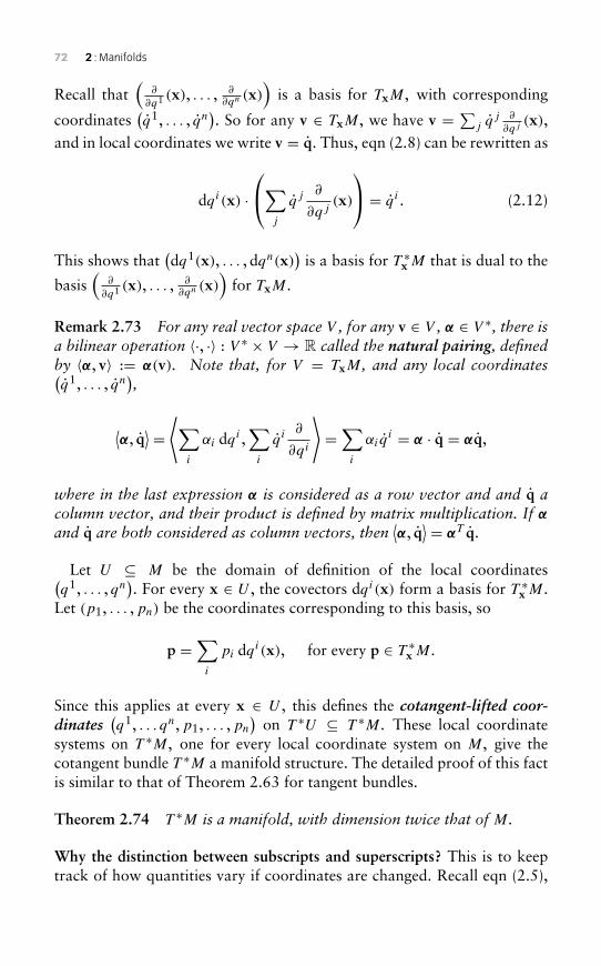
72 2 : Manifolds
Recall that(
∂
∂q1 (x), . . . ,∂
∂qn (x))
is a basis for TxM, with corresponding
coordinates(q1, . . . , qn
). So for any v ∈ TxM, we have v = ∑j qj ∂
∂qj (x),and in local coordinates we write v = q. Thus, eqn (2.8) can be rewritten as
dqi(x) ·∑
j
qj ∂
∂qj(x)
= qi . (2.12)
This shows that(dq1(x), . . . , dqn(x)
)is a basis for T ∗x M that is dual to the
basis(
∂
∂q1 (x), . . . ,∂
∂qn (x))
for TxM.
Remark 2.73 For any real vector space V , for any v ∈ V , α ∈ V ∗, there isa bilinear operation 〈·, ·〉 : V ∗ × V → R called the natural pairing, definedby 〈α, v〉 := α(v). Note that, for V = TxM, and any local coordinates(q1, . . . , qn
),
⟨α, q
⟩ = ⟨∑i
αi dqi ,∑i
qi ∂
∂qi
⟩=∑i
αi qi = α · q = αq,
where in the last expression α is considered as a row vector and and q acolumn vector, and their product is defined by matrix multiplication. If αand q are both considered as column vectors, then
⟨α, q
⟩ = αT q.
Let U ⊆ M be the domain of definition of the local coordinates(q1, . . . , qn
). For every x ∈ U , the covectors dqi(x) form a basis for T ∗x M.
Let (p1, . . . ,pn) be the coordinates corresponding to this basis, so
p =∑i
pi dqi(x), for every p ∈ T ∗x M.
Since this applies at every x ∈ U , this defines the cotangent-lifted coor-dinates
(q1, . . . qn,p1, . . . ,pn
)on T ∗U ⊆ T ∗M. These local coordinate
systems on T ∗M, one for every local coordinate system on M, give thecotangent bundle T ∗M a manifold structure. The detailed proof of this factis similar to that of Theorem 2.63 for tangent bundles.
Theorem 2.74 T ∗M is a manifold, with dimension twice that of M.
Why the distinction between subscripts and superscripts? This is to keeptrack of how quantities vary if coordinates are changed. Recall eqn (2.5),
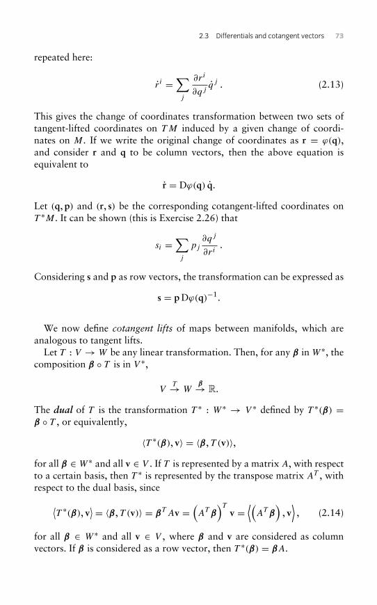
2.3 Differentials and cotangent vectors 73
repeated here:
r i =∑j
∂ri
∂qjqj . (2.13)
This gives the change of coordinates transformation between two sets oftangent-lifted coordinates on TM induced by a given change of coordi-nates on M. If we write the original change of coordinates as r = ϕ(q),and consider r and q to be column vectors, then the above equation isequivalent to
r = Dϕ(q) q.
Let (q, p) and (r, s) be the corresponding cotangent-lifted coordinates onT ∗M. It can be shown (this is Exercise 2.26) that
si =∑j
pj
∂qj
∂ri.
Considering s and p as row vectors, the transformation can be expressed as
s = pDϕ(q)−1.
We now define cotangent lifts of maps between manifolds, which areanalogous to tangent lifts.
Let T : V → W be any linear transformation. Then, for any β in W ∗, thecomposition β ◦ T is in V ∗,
VT→ W
β→ R.
The dual of T is the transformation T ∗ : W ∗ → V ∗ defined by T ∗(β) =β ◦ T , or equivalently,
〈T ∗(β), v〉 = 〈β, T (v)〉,for all β ∈ W ∗ and all v ∈ V . If T is represented by a matrix A, with respectto a certain basis, then T ∗ is represented by the transpose matrix AT , withrespect to the dual basis, since⟨
T ∗(β), v⟩ = 〈β, T (v)〉 = βT Av =
(AT β
)Tv =
⟨(AT β
), v⟩, (2.14)
for all β ∈ W ∗ and all v ∈ V , where β and v are considered as columnvectors. If β is considered as a row vector, then T ∗(β) = βA.
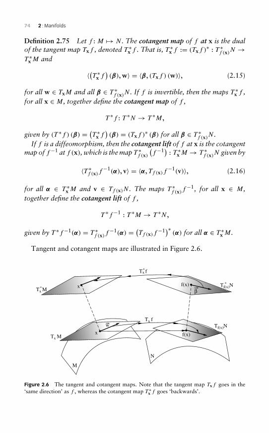
74 2 : Manifolds
Definition 2.75 Let f : M → N . The cotangent map of f at x is the dualof the tangent map Txf , denoted T ∗x f . That is, T ∗x f := (Txf )∗ : T ∗f (x)N →T ∗x M and
〈(T ∗x f)(β),w〉 = 〈β, (Txf ) (w)〉, (2.15)
for all w ∈ TxM and all β ∈ T ∗f (x)N . If f is invertible, then the maps T∗x f ,
for all x ∈ M, together define the cotangent map of f ,
T ∗f : T ∗N → T ∗M,
given by (T ∗f ) (β) = (T ∗x f)(β) = (Txf )∗ (β) for all β ∈ T ∗f (x)N .
If f is a diffeomorphism, then the cotangent lift of f at x is the cotangentmap of f−1 at f (x), which is themap T ∗f (x)
(f−1) : T ∗x M → T ∗f (x)N given by
〈T ∗f (x)f−1(α), v〉 = 〈α, Tf (x)f
−1(v)〉, (2.16)
for all α ∈ T ∗x M and v ∈ Tf (x)N . The maps T ∗f (x)f−1, for all x ∈ M,
together define the cotangent lift of f ,
T ∗f−1 : T ∗M → T ∗N ,
given by T ∗f−1(α) = T ∗f (x)f−1(α) = (Tf (x)f
−1)∗ (α) for all α ∈ T ∗x M.
Tangent and cotangent maps are illustrated in Figure 2.6.
x f(x)
M
w
N
Tx *M
Tx*f
Tx f
Tx M
*Tf(x)N
Tf(x)N
βx f(x)
Figure 2.6 The tangent and cotangent maps. Note that the tangent map Txf goes in the‘same direction’ as f , whereas the cotangent map T ∗x f goes ‘backwards’.
2.3 Differentials and cotangent vectors 75
Remark 2.76 (T ∗f )−1 = T ∗(f−1), so the notation T ∗f−1 is unam-
biguous. The base points are tricky, as(T ∗x f
)−1 = T ∗f (x)
(f−1). Since the
definition is complicated, the cotangent lift is best remembered as the most‘natural’ way of getting a cotangent vector based at f (x) from a cotangentvector based at x.
Remark 2.77 Note that if f maps from M to N , then its cotangent mapT ∗f maps from T ∗N to T ∗M, i.e. it ‘goes backwards’, as illustrated inFigure 2.6. For this reason, when f is a diffeomorphism, we more often usethe cotangent lift T ∗f−1, which goes ‘in the same direction’ as f . We saythat the cotangent lift of f ‘covers’ f .
The cotangent lift is often represented in the following diagram, in whichπM : T ∗M → M and πN : T ∗N → N are the cotangent bundle projectionmaps:
T ∗M (T ∗f )−1
−→ T ∗NτM ↓ ↓ τN
Mf−→ N .
The diagram commutes, which means that τN ◦ (T ∗f )−1 = f ◦ τM . Indeed,if α ∈ TxM, then (T ∗f )−1 (α) ∈ Tf (x)N , so
τN ◦(T ∗f
)−1(α) = f (x) = f ◦ τM(α).
We now consider representations of cotangent lifts in local coordinates.Let (q, q) and (r, r) be tangent-lifted local coordinates, and let (q, p) and(r, s) be the corresponding cotangent-lifted coordinates. Recall from eqn(2.6) that the tangent lift Tf can be written in coordinates as (r, r) =Tf (q, q), where
r i =∑j
∂f i
∂qjqj , or r = Df (q) q (tangent lift in coordinates).
From this it follows that, if (r, s) = (T ∗f )−1 (q, p), then
pj =∑i
si∂f i
∂qj, or s = p (Df (q))−1 (cotangent lift in coordinates),
where p and s are considered as row vectors. If p and s are considered as
column vectors, then s =((Df (q))−1
)Tp.
76 2 : Manifolds
Example 2.78 Consider the cylinder S1 × R = {(x, y, z) ∈ R3 : x2+
y2 = 1}, with cylindrical coordinates (θ , z) defined by (x, y, z) =
(cos θ , sin θ , z). Let f : S2 → S1 × R be given, in spherical coordinateson S2 and cylindrical coordinates on S1 × R, by f (θ ,φ) = (θ ,− cosφ). Inthese coordinates,
Df (θ ,φ) =[1 00 sinφ
],
so the tangent lift of f is
Tf (θ ,φ, θ , φ) =(f (θ ,φ), Df (θ ,φ)[θ , φ]T
)= (θ ,− cosφ, θ , sinφ φ
),
and the cotangent lift of f is
T ∗f−1(θ ,φ,pθ ,pφ) =(f (θ ,φ), [pθ ,pφ]Df (θ ,φ)−1
)=(θ ,− cosφ,pθ ,
pφ
sinφ
).
Example 2.79 Consider f : Rn → Rn defined (with respect to the stan-dard coordinates) by f (x) = Ax, for some n × n matrix A. Since f islinear, Df (x) = f for all x (see Exercise 2.16), so Df (x) has matrix A.The tangent lift of f is given in tangent-lifted coordinates by Tf (q, q) =(Aq,Aq). The cotangent lift of f is given in cotangent-lifted coordinatesby (T ∗f )−1 (q, p) = (Aq, pA−1) (if we think of p as a row vector), or(T ∗f )−1 (q, p) = (Aq,
(A−1)T p) (if we think of p as a column vector).
Exercise 2.22Let f : S2 → R be given by f (x, y, z) = x + y. Express f in sphericalcoordinates (θ ,φ) and then compute df in these coordinates.
Exercise 2.23For every v ∈ Rn, let αv ∈ (Rn)∗ be given by by 〈αv,w〉 := v · w. Showthat the map Rn → (Rn)∗, given by v → αv, is an isomorphism. Notethat an analogous isomorphism exists for any finite-dimensional innerproduct space.
2.3 Differentials and cotangent vectors 77
Exercise 2.24Let V be a finite-dimensional vector space. The double dual of V isthe dual of V ∗, i.e. V ∗∗ := (V ∗)∗. Show that the map � : V → V ∗∗defined by
〈�(v),α〉 = 〈α, v〉is an isomorphism.
Exercise 2.25If V is an inner product space, and T : V → V , what is the relationshipbetween the dual of T and the adjoint of T ?
Exercise 2.26Show that the change of coordinates transformation between cotangent-lifted coordinates (q, p) and (r, s) on T ∗M is
si =∑j
pj
∂qj
∂ri.
Show that, considering s and p as row vectors, the transformation canbe expressed as
s = pDϕ(q)−1,
where r = ϕ(q). Note the equivalent formulae,
pj =∑i
si∂ri
∂qj, p = sDϕ(q).
Exercise 2.27Consider f : R2 → R2 given by f (x, y) = (2x+1, sin xy). Calculate the
tangent and cotangent lifts of f , and calculate(T ∗(x,y)f
)−1 (dy (x, y)
)in
terms of dx (x, y) and dy (x, y) .
78 2 : Manifolds
Exercise 2.28If f : M → N and g : N → R are both differentiable, show thatT ∗x f
(dg(f (x))
) = d(g ◦ f )(x) for all x ∈ M.
2.4 Matrix groups as submanifolds
The set of all n × n matrices with real entries, M(n, R), is isomorphic toRn2
. If we ‘identify’ M(n, R) with Rn2, i.e. consider them as the same, then
the definition of a submanifold carries over to sets of matrices. Similarly,the set of all n×n matrices with complex entries, M(n, C), is isomorphic toCn2
, which is isomorphic to R2n2, so we may identify M(n, C) with R2n2
,and consider submanifolds of this space.
It turns out that all of the classical groups of matrices, for example SO(n)
and U(n), are submanifolds of M(n, R) or M(n, C). They are examples ofLie groups, which will be studied in more depth in Chapter 5.
We will now review the definitions of some of these groups, and reviewwhy they are really groups, and then show that they are submanifolds. Tostart with, recall the abstract definition of a group:
Definition 2.80 A group is a set of elements G with a binary operationG × G → G, which we will write as (g,h) → gh, with the followingproperties:
1. it is associative, that is (gh)k = g(hk) for all g,h, k ∈ G;
2. it has an identity element e ∈ G, satisfying g = eg = ge for allg ∈ G; and
3. each g ∈ G has an inverse element g−1 ∈ G satisfying gg−1 = g−1g = e.
If in addition, gh = hg, for all g,h ∈ G, then the group is calledcommutative or Abelian.
Definition 2.81 A subgroup of a group G is a subset H of G such that thegroup operation on G, restricted to H , makes H a group.
Remark 2.82 It is easily checked thatH is of a subgroupG if and only if:
1. H is closed under the group operation, i.e. h1h2 ∈ H whenever h1,h2 ∈ H ; and
2. H is closed under inversion. That is, h−1 ∈ H whenever h ∈ H .
2.4 Matrix groups as submanifolds 79
Note that these two conditions imply that the group identity of G is thegroup identity of H . Also note that the intersection of any two subgroupsof G is also a subgroup of G.
Note that we have used multiplicative notation for the group operationand group inverse in the previous definitions. This is because we wish toconsider sets of matrices as groups with respect to the matrix multiplicationoperation:
Definition 2.83 Amatrix group is a subset ofM(n, R) orM(n, C) that isa group, with the group operation being matrix multiplication.
Example 2.84 The general linear group GL(n, R) is the set of all linearisomorphisms from Rn to itself. Every such isomorphism corresponds to amatrix in M(n, R), so we can consider GL(n, R) to be a subset of M(n, R),which we do from now on: GL(n, R) is the set of all invertible n×n matriceswith real entries. Since the product of two invertible matrices is invertible,GL(n, R) is closed under matrix multiplication. It is easily checked thatGL(n, R) satisfies the definition of a group, with the group operation beingmatrix multiplication, with the identity matrix I as identity element; i.e.GL(n, R) is a matrix group. The complex general linear group GL(n, C) isdefined similarly.
Remark 2.85 All other matrix groups are subgroups of GL(n, R) andGL(n, C), since the elements of a matrix group must be invertible. ByRemark 2.82, a subset of GL(n, R) or GL(n, C) is a subgroup if and onlyif it is closed under matrix multiplication and inversion.
Definition 2.86 A symmetric matrix is one satisfying AT = A. We denotethe set of real symmetric n× n matrices by Sym(n, R).A skew-symmetric or anti-symmetric matrix is one satisfying AT = −A.
We denote the set of real skew-symmetric n× n matrices by Skew(n, R).An orthogonal matrix is one satisfying AT A = I , where I is the n × n
identity matrix (for some n). The group of real orthogonal n × n matricesis denoted O(n, R) or simply O(n).A unitary matrix is a complex matrix U such that U∗U = I , where U∗
is the conjugate transpose of U . The group of n × n unitary matrices isdenoted U(n).
A symplectic matrix is one satisfying AT JA = J , where J =[
0 I
−I 0
].
The group of real symplectic 2n×2nmatrices is denoted Sp(2n, R). (Thereare no odd-dimensional symplectic matrices!)
80 2 : Manifolds
All of the matrix groups defined above are important in mechanics. O(n)
is especially important as a symmetry group, while Sp(2n, R) appears in thegeneral setting of Hamiltonian systems on symplectic manifolds.
Definition 2.87 A matrix Lie group is a matrix group that is also asubmanifold ofM(n, R) (orM(n, C)).
Remark 2.88 All of the examples we will consider are embedded subman-ifolds. Some matrix Lie groups may only be immersed submanifolds (seeRemark 2.27).
Example 2.89 GL(n, R) is an n2-dimensional submanifold of M(n, R),since it is an open subset of M(n, R). Similarly, GL(n, C) is an open subset,and hence a submanifold, of M(n, C).
In fact, all of the matrix groups defined above are matrix Lie groups, asshown in the following proposition and Exercises 2.31 and 2.32.
Proposition 2.90 O(n) is a matrix Lie group of dimension n(n−1)/2, andTIO(n) = Skew(n, R).
Proof It is easily checked that O(n) is a matrix group (see Exercise 2.29).Since AT A is always symmetric, the following map is well defined,
F : GL(n, R) −→ Sym(n, R),
A −→ AT A− I .
Note that GL(n, R) is an open subset of M(n, R) and O(n) = F−1(0),where 0 is the zero matrix. We now compute DF(A), for an arbitraryA ∈ GL(n, R):
DF(A)(B) = ddt
∣∣∣∣t=0
F(A+ tB)
= ddt
∣∣∣∣t=0
(A+ tB)T (A+ tB)− I = BT A+ AT B ,
for any B ∈ M(n, R). To prove that DF(A) is surjective, we must showthat, for any n × n symmetric matrix S, there exists a matrix B such thatBT A+ AT B = S. But this is proven by setting
B = 12A−T S ,
where A−T := (A−1)T . Hence, DF(A) is surjective, for any A. We concludethat F is a submersion. It follows that O(n) is a submanifold of M(n, R).
2.4 Matrix groups as submanifolds 81
Since Sym(n, R) has dimension n(n+ 1)/2, the group O(n) has dimensionn2 − n(n+ 1)/2 = n(n− 1)/2.
Substituting A = I in the above calculations gives
DF(I)(B) = BT + B .
Thus, using Theorem 2.55,
TIO(n) = ker DF(I) = {B ∈M(n, R) : BT + B = 0} = Skew(n, R).
�
Definition 2.91 The special linear group SL(n, R) is the subgroup ofGL(n, R) consisting of all matrices of determinant 1. The complex speciallinear group SL(n, C) is defined similarly.The special orthogonal group is SO(n) := O(n) ∩ SL(n, R).The special unitary group is SU(n) := U(n) ∩ SL(n, C).
It is easily checked that these are all matrix groups.
Proposition 2.92 SL(n, R) is a matrix Lie group of dimension n2 − 1, i.e.codimension 1.
Proof SL(n, R) = f−1(1), where f : GL(n, R) → R is the determinantmap f (A) := detA. We will show that f is a submersion. For any A ∈GL(n, R), define the path γ in GL(n, R) by γ (t) = (1+ t)A. Then, γ ′(0) ∈TAGL(n, R) and
Df (A)(γ ′(0)
) = (f ◦ γ )′ (0) = ddt
∣∣∣∣t=0
det ((1+ t)A)
= ddt
∣∣∣∣t=0
(1+ t)n detA = n detA .
Since detA �= 0, this shows that Df (A) is a non-zero linear transformation.Since the codomain of f is R, it follows that Df (A) is surjective. Hence,f is a submersion, and therefore SL(n, R) is a submanifold of M(n, R). Itscodimension is the dimension of the range of f , which is 1. Since SL(n, R)
is also a matrix group, it is a matrix Lie group. �
The situation for SO(n) is rather different, since all orthogonal matricesautomatically have determinant ±1, see Exercise 2.30.
Remark 2.93 SO(3) is the group of rotations in R3. O(3) is the group ofall ‘rigid linear transformations’, namely rotations, reflections, and com-positions of these. Rotations have determinant +1, while other elements
82 2 : Manifolds
of O(3) have determinant −1. Both groups often appear in mechanics assymmetry groups. SO(3) is the configuration space of a rigid body with onepoint fixed, as discussed in Section 1.5.
Proposition 2.94 SO(n) is a matrix Lie group of dimension n(n− 1)/2.
Proof SO(n) = O(n) ∩ U , where U = det−1(0,∞), where det :
M(n, R) → R is the determinant map. Since det is continuous (in fact,it is a polynomial), U is open. Thus, SO(n) is a non-empty relatively opensubset of O(n). Since O(n) is a submanifold of M(n, R), by Proposition2.90, it follows that SO(n) is also a submanifold of M(n, R), of the samedimension as O(n). Since SO(n) is a matrix group, the result follows. �
Remark 2.95 In fact, all of the matrix groups we have seen so far areconnected, except for O(n) and U(n). For proofs, see [MR02].
Proposition 2.96 O(n) has two connected components: SO(n) (whichcontains the identity matrix) and another component diffeomorphic toSO(n).
Proof We saw in Proposition 2.94 that SO(n) is open relative to O(n).Recall that all elements of O(n) have determinant ±1. If A is any elementof O(n) with detA = −1, then the map B → BA is a diffeomorphismthat maps SO(n) onto O(n) \ SO(n). It follows that O(n) \ SO(n) is alsoopen relative to O(n), and therefore O(n) is not connected. Since SO(n)
is connected (see Exercise 2.34 and [MR02]), and hence O(n) \ SO(n)
is connected, it follows that SO(n) and O(n) \ SO(n) are the connectedcomponents of O(n). �
Exercise 2.29Prove that all of the groups defined in Definition 2.86 really are matrixgroups. Prove that Sym(n, R) and Skew(n, R) are vector spaces and arenot matrix groups.
Exercise 2.30Show that all orthogonal matrices and all symplectic matrices havedeterminant ±1. (In fact, all symplectic matrices have determinant 1,but this is harder to prove – see [MS95].)
2.5 Abstract manifolds 83
Exercise 2.31Show that Sp(2n, R) is a matrix Lie group, of dimension 2n2 + n, and
TISp(2n, R) = {B ∈M(n, R) : BT J + JB = 0}.Hint: Modify the definition of F in the proof of Proposition 2.90, andreplace Sym(n, R) with Skew(n, R).
Exercise 2.32Modify the proof of Proposition 2.90 to prove that U(n) is a submani-fold of M(n, C). What is its (real) dimension? Calculate TIU(n).
Exercise 2.33Prove that SL(n, C) is a matrix Lie group of (real) dimension 2(n2−1).
Exercise 2.34Convince yourself that SO(3) is path-connected, and hence connected.Hint: a rotation is completely determined by how it transforms thestandard orthonormal frame. Starting with the standard frame, howcan you continuously move it so as to coincide with an arbitrary givenright-handed orthonormal frame? This defines a path in SO(3).
Exercise 2.35Prove that SU(n) is a matrix Lie group, with (real) dimension n2 − 1.This is considerably more difficult than for SO(n), since SU(n) is ofcodimension 1 in U(n).
2.5 Abstract manifolds
A manifold is a set covered by consistent local coordinate charts; the precisedefinition appears below. All submanifolds of Euclidean spaces are mani-folds, but there are other kinds of manifold that satisfy the general ‘abstract’
84 2 : Manifolds
definition, notably quotient spaces (see Definition 2.101). These appear inmechanics in many ways. However, abstract manifolds do not play a centralrole in this book, so this section could be skipped on first reading.
To motivate the definition, recall that whenever ϕ1 and ϕ2 are coordinatecharts for a submanifold of Rn, with overlapping domains, the transitionfunction ϕ2 ◦ ϕ−1
1 (also called the change-of-coordinates transformation) issmooth (see Theorem 2.39). For the abstract definition of a manifold, wekeep only this requirement that transition functions ϕ2 ◦ ϕ−1
1 be smooth,without requiring anything of the maps ϕ1 and ϕ2 individually.
Definition 2.97 A coordinate chart (or local coordinate system) for aset M is a 1-to-1 mapping ϕ : U → Rn, for some subset U of M andsome n, such that ϕ(U) is an open subset of Rn. The set U is called acoordinate patch. The components of ϕ are called local coordinates. Theinverse mapping ϕ−1 (with domain ϕ(U)) is called a parameterization.Two coordinate charts ϕ1 : U1 → Rn and ϕ2 : U2 → Rn for M are
compatible if the map ϕ2 ◦ ϕ−11 , with domain ϕ1 (U1 ∩ U2), is a smooth
diffeomorphism with a smooth inverse. (Implicit in this definition is theassumption that ϕ1 (U1 ∩ U2) and ϕ2 (U1 ∩ U2) are open subsets of Rn.)The map ϕ2 ◦ ϕ−1
1 is called a transition function or change-of-coordinatestransformation.An n-dimensional atlas for a set M is a family of mutually compatible
n-dimensional charts coveringM, i.e. a family {ϕi : Ui → Rn}i∈J , for someindex set J , such that
⋃i∈J Ui = M.
Two atlases for M are equivalent if all of their charts are mutuallycompatible. A smooth structure (or differential structure) onM is an equiv-alence class of atlases for M; each of the atlases in the class is said todetermine the smooth structure. A smooth manifold is a set M with asmooth structure. (Informally, we usually say ‘M is a manifold’, if thesmooth structure is clear from the context.)
Example 2.98 The two charts for S1 in Example 2.40 form an atlas for S1.But we could equally well have chosen two different compatible charts thatcovered S1, with the same formula but different domains and codomains.These two charts would define a second atlas for S1, equivalent to the first.Both atlases determine the same smooth structure for S1.
Theorem 2.99 Every submanifold of RN is a manifold, with a smoothstructure determined by the coordinate charts given in Definition 2.37.
Proof The smoothness of transition functions is guaranteed byTheorem 2.39. �
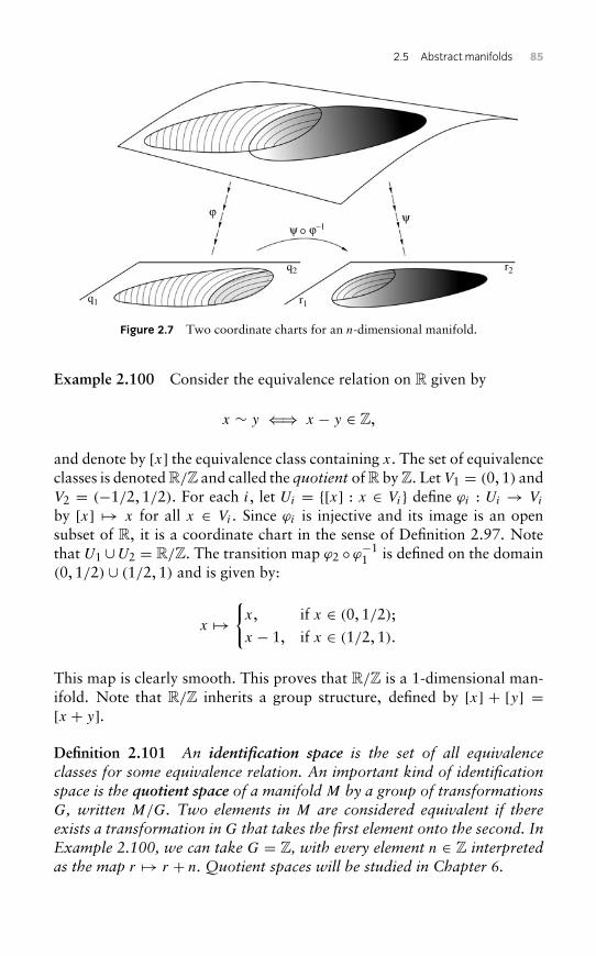
2.5 Abstract manifolds 85
ϕ ψψ ϕ–1
q1
q2
r1
r2
Figure 2.7 Two coordinate charts for an n-dimensional manifold.
Example 2.100 Consider the equivalence relation on R given by
x ∼ y ⇐⇒ x − y ∈ Z,
and denote by [x] the equivalence class containing x. The set of equivalenceclasses is denoted R/Z and called the quotient of R by Z. Let V1 = (0, 1) andV2 = (−1/2, 1/2). For each i, let Ui = {[x] : x ∈ Vi} define ϕi : Ui → Vi
by [x] → x for all x ∈ Vi . Since ϕi is injective and its image is an opensubset of R, it is a coordinate chart in the sense of Definition 2.97. Notethat U1 ∪U2 = R/Z. The transition map ϕ2 ◦ ϕ−1
1 is defined on the domain(0, 1/2) ∪ (1/2, 1) and is given by:
x →{x, if x ∈ (0, 1/2);
x − 1, if x ∈ (1/2, 1).
This map is clearly smooth. This proves that R/Z is a 1-dimensional man-ifold. Note that R/Z inherits a group structure, defined by [x] + [y] =[x + y].
Definition 2.101 An identification space is the set of all equivalenceclasses for some equivalence relation. An important kind of identificationspace is the quotient space of a manifoldM by a group of transformationsG, written M/G. Two elements in M are considered equivalent if thereexists a transformation in G that takes the first element onto the second. InExample 2.100, we can take G = Z, with every element n ∈ Z interpretedas the map r → r + n. Quotient spaces will be studied in Chapter 6.
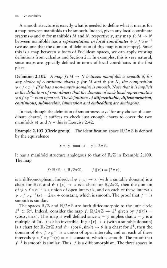
86 2 : Manifolds
A smooth structure is exactly what is needed to define what it means fora map between manifolds to be smooth. Indeed, given any local coordinatesystems ϕ and ψ for manifolds M and N , respectively, any map f : M → N
between manifolds has a representation in local coordinates ψ ◦ f ◦ ϕ−1
(we assume that the domain of definition of this map is non-empty). Sincethis is a map between subsets of Euclidean spaces, we can apply existingdefinitions from calculus and Section 2.1. In examples, this is very natural,since maps are typically defined in terms of local coordinates in the firstplace.
Definition 2.102 A map f : M → N between manifolds is smooth if, forany choice of coordinate charts ϕ for M and ψ for N , the compositionψ ◦f ◦ϕ−1 (if it has a non-empty domain) is smooth. Note that it is implicitin the definition of smoothness that the domain of each local representativeψ ◦f ◦ϕ−1 is an open set. The definitions of differentiable, diffeomorphism,continuous, submersion, immersion and embedding are analogous.
In fact, though the definition of smoothness says ‘for any choice of coor-dinate charts’, it suffices to check just enough charts to cover the twomanifolds M and N – this is Exercise 2.42.
Example 2.103 (Circle group) The identification space R/2πZ is definedby the equivalence
x ∼ y ⇐⇒ x − y ∈ 2πZ.
It has a manifold structure analogous to that of R/Z in Example 2.100.The map
f : R/Z→ R/2πZ, f ([x]) = [2πx],is a diffeomorphism, Indeed, if ϕ : [x] → x (with a suitable domain) is achart for R/Z and ψ : [x] → x is a chart for R/2πZ, then the domainof ψ ◦ f ◦ ϕ−1 is a union of open intervals, and on each of these intervalsψ ◦ f ◦ ϕ−1(x) = 2πx + constant, which is smooth. The proof that f−1 issmooth is similar.
The spaces R/Z and R/2πZ are both diffeomorphic to the unit circleS1 ⊂ R2. Indeed, consider the map f : R/2πZ → S1 given by f ([x]) =(cos x, sin x). This map is well defined since x ∼ y implies that x − y is amultiple of 2π . It is also invertible. If ϕ : [x] → x (with a suitable domain)is a chart for R/2πZ and ψ : (cos θ , sin θ) → θ is a chart for S1, then thedomain of ψ ◦ f ◦ ϕ−1 is a union of open intervals, and on each of theseintervals ψ ◦ f ◦ ϕ−1(x) = x + constant, which is smooth. The proof thatf−1 is smooth is similar. Thus, f is a diffeomorphism. The three spaces in
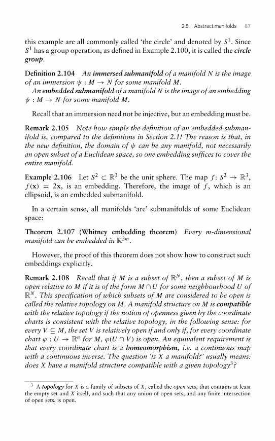
2.5 Abstract manifolds 87
this example are all commonly called ‘the circle’ and denoted by S1. SinceS1 has a group operation, as defined in Example 2.100, it is called the circlegroup.
Definition 2.104 An immersed submanifold of a manifold N is the imageof an immersion ψ : M → N for some manifold M.An embedded submanifold of a manifoldN is the image of an embedding
ψ : M → N for some manifold M.
Recall that an immersion need not be injective, but an embedding must be.
Remark 2.105 Note how simple the definition of an embedded subman-ifold is, compared to the definitions in Section 2.1! The reason is that, inthe new definition, the domain of ψ can be any manifold, not necessarilyan open subset of a Euclidean space, so one embedding suffices to cover theentire manifold.
Example 2.106 Let S2 ⊂ R3 be the unit sphere. The map f : S2 → R3,f (x) = 2x, is an embedding. Therefore, the image of f , which is anellipsoid, is an embedded submanifold.
In a certain sense, all manifolds ‘are’ submanifolds of some Euclideanspace:
Theorem 2.107 (Whitney embedding theorem) Every m-dimensionalmanifold can be embedded in R2m.
However, the proof of this theorem does not show how to construct suchembeddings explicitly.
Remark 2.108 Recall that if M is a subset of RN , then a subset of M isopen relative toM if it is of the formM ∩U for some neighbourhood U ofRN . This specification of which subsets of M are considered to be open iscalled the relative topology onM. A manifold structure onM is compatiblewith the relative topology if the notion of openness given by the coordinatecharts is consistent with the relative topology, in the following sense: forevery V ⊆ M, the set V is relatively open if and only if, for every coordinatechart ϕ : U → Rn for M, ϕ(U ∩ V ) is open. An equivalent requirement isthat every coordinate chart is a homeomorphism, i.e. a continuous mapwith a continuous inverse. The question ‘is X a manifold?’ usually means:does X have a manifold structure compatible with a given topology3?
3 A topology for X is a family of subsets of X, called the open sets, that contains at leastthe empty set and X itself, and such that any union of open sets, and any finite intersectionof open sets, is open.
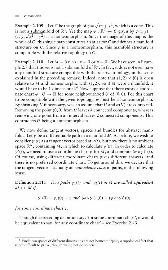
88 2 : Manifolds
Example 2.109 Let C be the graph of z = √x2 + y2, which is a cone. Thisis not a submanifold of R3. Yet the map ϕ : R2 → C given by ϕ(x, y) =(x, y,
√x2 + y2) is a homeomorphism. Since the image of this map is the
whole of C, this single map constitutes an atlas for C and defines a manifoldstructure on C. Since ϕ is a homeomorphism, this manifold structure iscompatible with the relative topology on C.
Example 2.110 Let M = {(x, y) : x = 0 or y = 0}. We have seen in Exam-ple 2.8 that this set is not a submanifold of R2. In fact, it does not even haveany manifold structure compatible with the relative topology, in the senseexplained in the preceding remark. Indeed, note that (1, 2) × {0} is openrelative to M and homeomorphic with (1, 2). So if M were a manifold, itwould have to be 1-dimensional.4 Now suppose that there exists a coordi-nate chart ϕ : U → R for some neighbourhood U of (0, 0). For this chartto be compatible with the given topology, ϕ must be a homeomorphism.By shrinking U if necessary, we can assume that U and ϕ(U) are connected.Removing the point (0, 0) from U leaves 4 connected components, whereasremoving one point from an interval leaves 2 connected components. Thiscontradicts U being a homeomorphism.
We now define tangent vectors, spaces and bundles for abstract mani-folds. Let γ be a differentiable path in a manifold M. As before, we wish toconsider γ ′(t) as a tangent vector based at γ (t), but now there is no ambientspace RN , containing M, in which to calculate γ ′(t). In order to calculateγ ′(t), we need to use a coordinate chart ϕ for M, and compute (ϕ ◦ γ )′ (t).Of course, using different coordinate charts gives different answers, andthere is no preferred coordinate chart. To get around this, we declare thatthe tangent vector is actually an equivalence class of paths, in the followingsense.
Definition 2.111 Two paths γ1(t) and γ2(t) in M are called equivalentat x ∈ M if
γ1(0) = γ2(0) = x and (ϕ ◦ γ1)′ (0) = (ϕ ◦ γ2)
′ (0)
for some coordinate chart ϕ.
Though the preceding definition says ‘for some coordinate chart’, it wouldbe equivalent to say ‘for any coordinate chart’ – see Exercise 2.43.
4 Euclidean spaces of different dimensions are not homeomorphic, a topological fact thatis not difficult to prove, though we do not do so here.
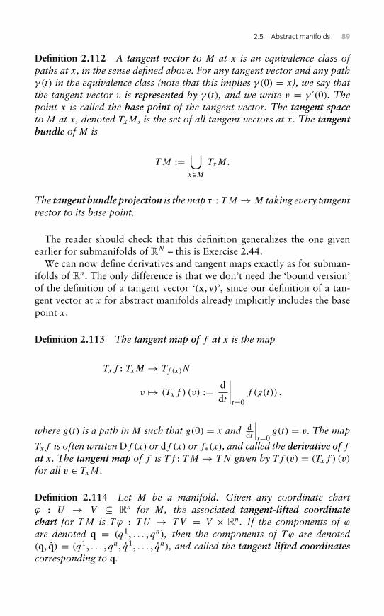
2.5 Abstract manifolds 89
Definition 2.112 A tangent vector to M at x is an equivalence class ofpaths at x, in the sense defined above. For any tangent vector and any pathγ (t) in the equivalence class (note that this implies γ (0) = x), we say thatthe tangent vector v is represented by γ (t), and we write v = γ ′(0). Thepoint x is called the base point of the tangent vector. The tangent spaceto M at x, denoted TxM, is the set of all tangent vectors at x. The tangentbundle of M is
TM :=⋃x∈M
TxM.
The tangent bundle projection is themap τ : TM → M taking every tangentvector to its base point.
The reader should check that this definition generalizes the one givenearlier for submanifolds of RN – this is Exercise 2.44.
We can now define derivatives and tangent maps exactly as for subman-ifolds of Rn. The only difference is that we don’t need the ‘bound version’of the definition of a tangent vector ‘(x, v)’, since our definition of a tan-gent vector at x for abstract manifolds already implicitly includes the basepoint x.
Definition 2.113 The tangent map of f at x is the map
Txf : TxM → Tf (x)N
v → (Txf ) (v) := ddt
∣∣∣∣t=0
f (g(t)) ,
where g(t) is a path inM such that g(0) = x and ddt
∣∣∣t=0
g(t) = v. The map
Txf is often writtenDf (x) or df (x) or f∗(x), and called the derivative of fat x. The tangent map of f is Tf : TM → TN given by Tf (v) = (Txf ) (v)
for all v ∈ TxM.
Definition 2.114 Let M be a manifold. Given any coordinate chartϕ : U → V ⊆ Rn for M, the associated tangent-lifted coordinatechart for TM is T ϕ : T U → T V = V × Rn. If the components of ϕare denoted q = (q1, . . . , qn), then the components of T ϕ are denoted(q, q) = (q1, . . . , qn, q1, . . . , qn), and called the tangent-lifted coordinatescorresponding to q.
90 2 : Manifolds
If f : M → N is expressed in local coordinates q on M and r on N , thenTf is expressed in the corresponding tangent-lifted coordinates as
(r, r) = (f (q), Df (q) · q) .
Theorem 2.115 The tangent bundle TM of any manifoldM is a manifoldof twice the dimension ofM, with coordinate charts T ϕ for any coordinatechart ϕ of M, If N is another manifold and f : M → N is smooth, thenTf : TM → TN is also smooth.
Proof Exercise. �
Remark 2.116 The tangent bundle is more than just a manifold: it is anexample of a vector bundle, which we will now describe by highlightingand generalizing certain properties of TM. For any coordinate chart ϕ :U → V ⊆ Rn, the tangent map T ϕ : T U → V × Rn is a diffeomorphism.Also, T U = π−1(U), where where π : TM → M is the tangent bundleprojection. Hence, we have the diffeomorphisms,
π−1(U) = T U ∼= V ×Rn ∼= U ×Rn.
SinceM is covered by an atlas of coordinate charts, every point inM has aneighbourhood U such that
π−1(U) ∼= U ×Rn.
This property is informally described as ‘TM locally looks like M × Rn’.In general, an n-dimensional vector bundle is a base manifold M, a totalmanifold P (generalizing TM), and a submersion π : P → M, such that‘P locally looks like M × Rn’, meaning that, for every open subset U ofM, there is a diffeomorphism from π−1(U) to U ×Rn. For any x ∈ M, thepreimage π−1(x) ∈ P is called the fibre over x (it is diffeomorphic to Rn).For the tangent bundle, the fibre over x is the tangent space TxM.
Exercise 2.36Consider the stereographic projection of S1 given by ξN(x, y) = 2x
1−y .
This is a diffeomorphism from S1, excluding the ‘North pole’ (0, 1), toR, as shown in Example 2.48. The map ξS(x, y) = 2x
1+y has a similareffect, using lines through the South pole instead of the North. Checkthat the two maps ξN and ξS form an atlas for S1, making S1 a manifold.Prove that this manifold structure is compatible with the structure on
2.5 Abstract manifolds 91
S1 defined by the parameterizations ϕ1 and ϕ2 given at the beginning ofthis section.
Exercise 2.37Let (ξN , ηN) and (ξS , ηS) be the stereographic projections of S2 definedin Example 2.49. Show that the transition from coordinates (ξN , ηN) to(ξS , ηS) is a diffeomorphism, thus showing that these two projectionsare coordinate charts defining a manifold structure on S2. (Hint: (1+z)(1 − z) = 1 − z2 = x2 + y2 on S2.) This exercise generalizes in theobvious way to Sn ⊆ Rn for any n.
Exercise 2.38The symbol ‘T 2’, which denotes a 2-dimensional torus, has two stan-dard interpretations: (i) S1 × S1 ⊆ R4, see Example 2.36; and (ii) asubmanifold of R3 shaped like the surface of an idealized doughnut(with a hole), see Exercise 2.5. Show that these are diffeomorphic.
Exercise 2.39Show that the ray [0,∞) is not a manifold, in the sense explained inRemark 2.108. The ray is an example of what is called a ‘manifold withboundary’.
Exercise 2.40IfM is a set andN is a manifold, and ϕ : M → N is a bijection, show thatthe manifold structure onN can be used to define a manifold structure onM such that ϕ is a diffeomorphism, and that this is the unique manifoldstructure on M with this property. This manifold structure on M iscalled the structure induced by ϕ, or the pull-back by ϕ of the manifoldstructure on N .
Exercise 2.41If we begin with a figure eight in the xz-plane, along the x-axis andcentred at the origin, and spin it round the z-axis in R3, we get a ‘pinched
92 2 : Manifolds
surface’ that looks like a sphere that has been ‘pinched’ so that the Northand South poles touch. Prove that this is not a manifold.
Exercise 2.42Let F : M → N . Let ϕ1 and ϕ2 be two coordinate charts for M with thesame domain, and let ψ1 and ψ2 two coordinate charts for N with thesame domain. Show that if ψ1 ◦ F ◦ ϕ−1
1 is smooth then ψ2 ◦ F ◦ ϕ−12 is
as well. Conclude that, to check smoothness, it suffices to consider onlyone atlas of charts for M and one atlas of charts for N .
Exercise 2.43Check that the definition if a tangent vector in Definition 2.111 is inde-pendent of the choice of chart ϕ. More precisely, check that if ϕ andψ are two charts (with x in the domain of both), then (ϕ ◦ γ1)
′ (0) =(ϕ ◦ γ2)
′ (0) if and only if (ψ ◦ γ1)′ (0) = (ψ ◦ γ2)
′ (0).
Exercise 2.44Explain why Definition 2.112 generalizes the definitions of tangentvectors, spaces and bundles given earlier for submanifolds of RN .
Solutions to selected exercises
Solution to Exercise 2.1 Let f (x, y, z) = (x2 + y2, y2 + z2) then,
Df (x, y, z) = 2[x y 00 y z
].
This map is onto R2 when its rank is 2. Therefore, Df (x, y, z) is surjectivefor all (x, y, z) except on the axes. A point (a, b) ∈ R2 is a regular value off if and only if the level set f−1{(a, b)} does not intersect the axes. Thus,(a, b) is a regular value of f if and only if a and b are unequal and non-zero.
The level sets satisfy x2 + y2 = a and y2 + z2 = b. Therefore, if a, b > 0,the levels sets are intersections of cylinders about the z-axis and cylindersabout the x-axis. If a �= b, then the level set is the union of two disjointclosed curves, which is a 1-dimensional submanifold. This verifies that the
Solutions to selected exercises 93
preimage of any regular value is a codimension-2 submanifold of R3. Ifa = b, then the cylinders are of equal radius and their intersection is theunion of two circles that intersect on the y-axis; this is not a submanifold. Ifone or both of a and b is zero, then f−1{(a, b)} consists of either one or twopoints, and is thus a 0-dimensional manifold. These are all submanifoldsthat are preimages of non-regular values.
Solution to Exercise 2.2 Suppose g ◦ f is well defined. By the chain rule,D(g ◦ f )(z) = Dg(f (z))Df (z) for every z in the domain of f . If f and g
are both submersions, then Df (z) and Dg(f (z)) are both surjective, whichimplies that Dg(f (z))Df (z) is surjective, for all z in the domain of f , whichis also the domain of g ◦ f . Hence, g ◦ f is a submersion.
If g ◦ f is a submersion, then Dg(f (z))Df (z) is surjective, for every z inthe domain of f . This does not imply that Df (z) is surjective, so f neednot be a submersion. It does imply that Dg(f (z)) is surjective for everyy = f (z) in the image of f , but not necessarily for every y in the domain ofg, so g need not be a submersion (even though it is a submersion at f (z),for every z). For example, if f : (0,∞)→ R2 and g : R2 → R are given by
g(x, y) = x3, f (z) = (z, 0),
then
T(x,y)g =[3x2 0
], Tzf =
[10
], Tz(g ◦ f ) = [3z2
].
Since Tzf is never surjective, f is not a submersion. Since T(x,y)g is notsurjective at points with x = 0, the map g is not a submersion either. Thedomain of g◦f is (0,∞) and Tz(g◦f ) is surjective at all z ∈ (0,∞), thereforeg ◦ f is a submersion.
Solution to Exercise 2.3 Let f : R2 → R1 be given by f (x, y) = 1. Then,Df = 0 so Df is not surjective, but f−1(1) = R2, which is a submanifoldof R2.
Solution to Exercise 2.5 The relation(2r −
√x2 + y2
)2
+ z2 = r2,
relates the Cartesian coordinates, (x, y, z) ∈ R3, to the radius, r ∈ R,of a torus. We want to solve this relation for r to obtain a submersion.Expanding the relation gives:
3r2 − 4r√x2 + y2 + z2 = 0,
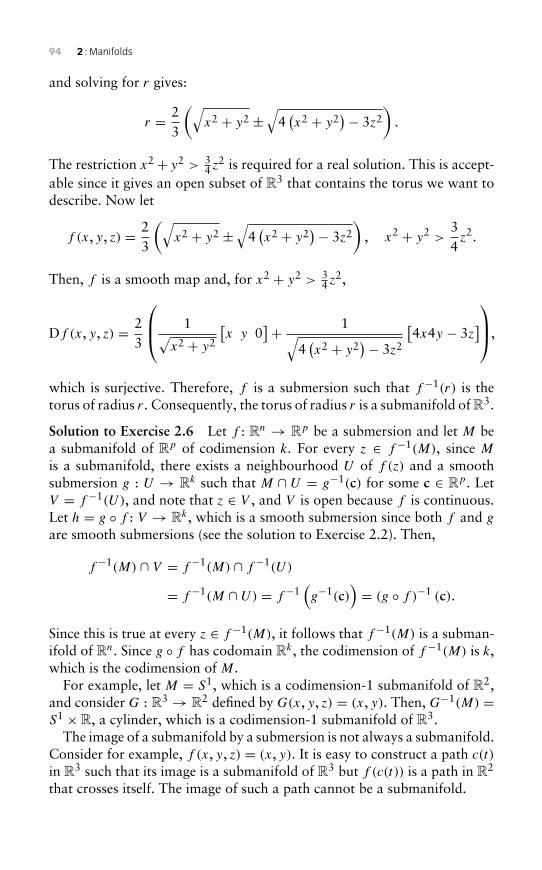
94 2 : Manifolds
and solving for r gives:
r = 23
(√x2 + y2 ±
√4(x2 + y2
)− 3z2
).
The restriction x2+ y2 > 34z
2 is required for a real solution. This is accept-able since it gives an open subset of R3 that contains the torus we want todescribe. Now let
f (x, y, z) = 23
(√x2 + y2 ±
√4(x2 + y2
)− 3z2
), x2 + y2 >
34z2.
Then, f is a smooth map and, for x2 + y2 > 34z
2,
Df (x, y, z) = 23
1√x2 + y2
[x y 0
]+ 1√4(x2 + y2
)− 3z2
[4x4y − 3z
],
which is surjective. Therefore, f is a submersion such that f−1(r) is thetorus of radius r. Consequently, the torus of radius r is a submanifold of R3.
Solution to Exercise 2.6 Let f : Rn → Rp be a submersion and let M bea submanifold of Rp of codimension k. For every z ∈ f−1(M), since M
is a submanifold, there exists a neighbourhood U of f (z) and a smoothsubmersion g : U → Rk such that M ∩ U = g−1(c) for some c ∈ Rp. LetV = f−1(U), and note that z ∈ V , and V is open because f is continuous.Let h = g ◦ f : V → Rk, which is a smooth submersion since both f and g
are smooth submersions (see the solution to Exercise 2.2). Then,
f−1(M) ∩ V = f−1(M) ∩ f−1(U)
= f−1(M ∩ U) = f−1(g−1(c)
)= (g ◦ f )−1 (c).
Since this is true at every z ∈ f−1(M), it follows that f−1(M) is a subman-ifold of Rn. Since g ◦ f has codomain Rk, the codimension of f−1(M) is k,which is the codimension of M.
For example, let M = S1, which is a codimension-1 submanifold of R2,and consider G : R3 → R2 defined by G(x, y, z) = (x, y). Then, G−1(M) =S1 ×R, a cylinder, which is a codimension-1 submanifold of R3.
The image of a submanifold by a submersion is not always a submanifold.Consider for example, f (x, y, z) = (x, y). It is easy to construct a path c(t)
in R3 such that its image is a submanifold of R3 but f (c(t)) is a path in R2
that crosses itself. The image of such a path cannot be a submanifold.
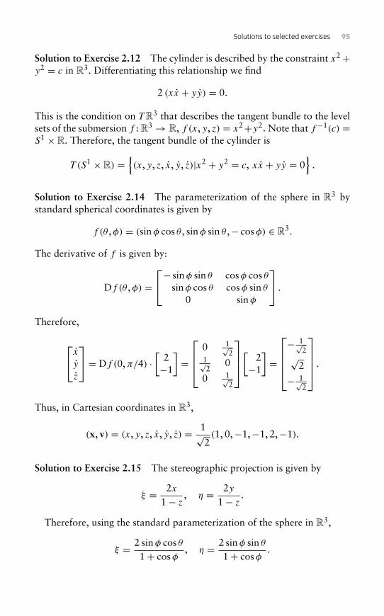
Solutions to selected exercises 95
Solution to Exercise 2.12 The cylinder is described by the constraint x2+y2 = c in R3. Differentiating this relationship we find
2 (xx + yy) = 0.
This is the condition on T R3 that describes the tangent bundle to the levelsets of the submersion f : R3 → R, f (x, y, z) = x2+y2. Note that f−1(c) =S1 ×R. Therefore, the tangent bundle of the cylinder is
T (S1 ×R) ={(x, y, z, x, y, z)|x2 + y2 = c, xx + yy = 0
}.
Solution to Exercise 2.14 The parameterization of the sphere in R3 bystandard spherical coordinates is given by
f (θ ,φ) = (sinφ cos θ , sinφ sin θ ,− cosφ) ∈ R3.
The derivative of f is given by:
Df (θ ,φ) =− sinφ sin θ cosφ cos θ
sinφ cos θ cosφ sin θ
0 sinφ
.
Therefore,
x
y
z
= Df (0,π/4) ·[
2−1
]=
0 1√
21√2
0
0 1√2
[ 2−1
]=
− 1√
2√2
− 1√2
.
Thus, in Cartesian coordinates in R3,
(x, v) = (x, y, z, x, y, z) = 1√2(1, 0,−1,−1, 2,−1).
Solution to Exercise 2.15 The stereographic projection is given by
ξ = 2x1− z
, η = 2y1− z
.
Therefore, using the standard parameterization of the sphere in R3,
ξ = 2 sinφ cos θ1+ cosφ
, η = 2 sinφ sin θ
1+ cosφ.
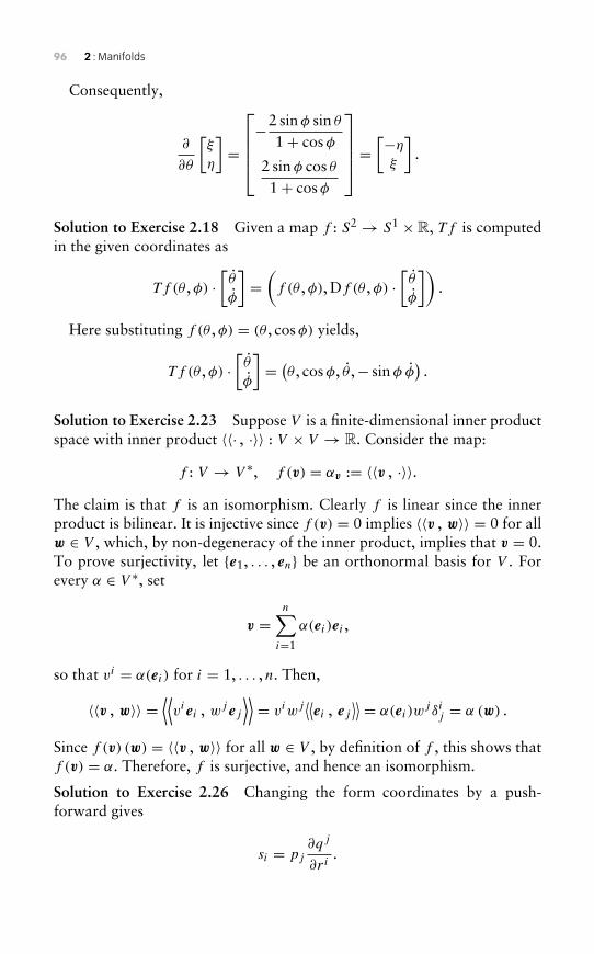
96 2 : Manifolds
Consequently,
∂
∂θ
[ξ
η
]=
−2 sinφ sin θ
1+ cosφ
2 sinφ cos θ1+ cosφ
=[−η
ξ
].
Solution to Exercise 2.18 Given a map f : S2 → S1 ×R, Tf is computedin the given coordinates as
Tf (θ ,φ) ·[θ
φ
]=(f (θ ,φ), Df (θ ,φ) ·
[θ
φ
]).
Here substituting f (θ ,φ) = (θ , cosφ) yields,
Tf (θ ,φ) ·[θ
φ
]= (θ , cosφ, θ ,− sinφ φ
).
Solution to Exercise 2.23 Suppose V is a finite-dimensional inner productspace with inner product 〈〈· , ·〉〉 : V × V → R. Consider the map:
f : V → V ∗, f (v) = αv := 〈〈v , ·〉〉.The claim is that f is an isomorphism. Clearly f is linear since the innerproduct is bilinear. It is injective since f (v) = 0 implies 〈〈v , w〉〉 = 0 for allw ∈ V , which, by non-degeneracy of the inner product, implies that v = 0.To prove surjectivity, let {e1, . . . , en} be an orthonormal basis for V . Forevery α ∈ V ∗, set
v =n∑
i=1
α(ei )ei ,
so that vi = α(ei ) for i = 1, . . . , n. Then,
〈〈v , w〉〉 =⟨⟨viei , wjej
⟩⟩= viwj
⟨⟨ei , ej
⟩⟩ = α(ei )wj δij = α (w) .
Since f (v) (w) = 〈〈v , w〉〉 for all w ∈ V , by definition of f , this shows thatf (v) = α. Therefore, f is surjective, and hence an isomorphism.
Solution to Exercise 2.26 Changing the form coordinates by a push-forward gives
si = pj
∂qj
∂ri.
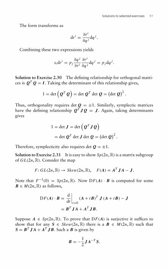
Solutions to selected exercises 97
The form transforms as
dri = ∂ri
∂qjdqj .
Combining these two expressions yields
sidri = pj
∂qj
∂ri
∂ri
∂qjdqj = pjdqj .
Solution to Exercise 2.30 The defining relationship for orthogonal matri-ces is QTQ = I . Taking the determinant of this relationship gives,
1 = det(QTQ
)= detQT detQ = (detQ
)2 .
Thus, orthogonality requires detQ = ±1. Similarly, symplectic matriceshave the defining relationship QT JQ = J . Again, taking determinantsgives
1 = det J = det(QT JQ
)= detQT det J detQ = (detQ
)2 .
Therefore, symplecticity also requires detQ = ±1.
Solution to Exercise 2.31 It is easy to show Sp(2n, R) is a matrix subgroupof GL(2n, R). Consider the map
F : GL(2n, R)→ Skew(2n, R), F(A) = AT JA− J .
Note that F−1(0) = Sp(2n, R). Now DF(A) · B is computed for someB ∈ M(2n, R) as follows,
DF(A) · B = ddt
∣∣∣∣t=0
(A+ tB)T J (A+ tB)− J
= BT JA+AT JB.
Suppose A ∈ Sp(2n, R). To prove that DF(A) is surjective it suffices toshow that for any S ∈ Skew(2n, R) there is a B ∈ M(2n, R) such thatS = BT JA+AT JB. Such a B is given by
B = −12JA−T S.
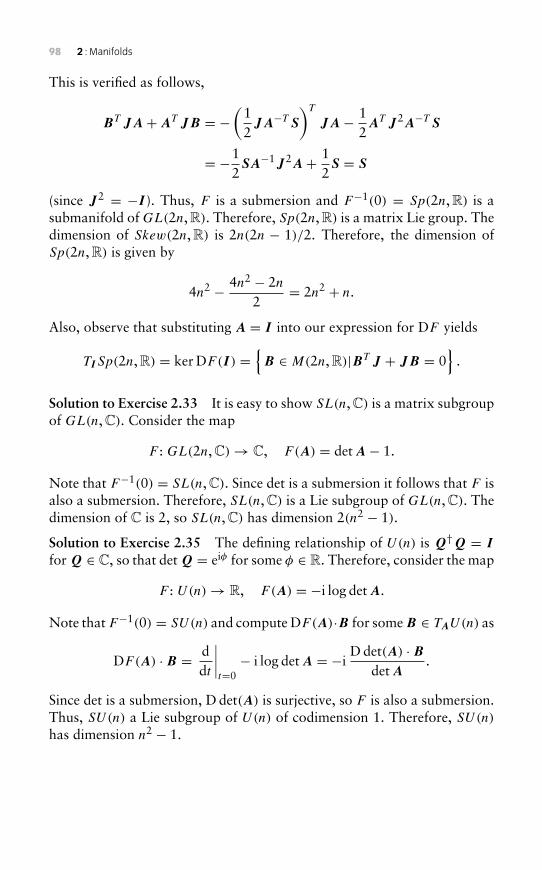
98 2 : Manifolds
This is verified as follows,
BT JA+AT JB = −(
12JA−T S
)T
JA− 12AT J 2A−T S
= −12SA−1J 2A+ 1
2S = S
(since J 2 = −I ). Thus, F is a submersion and F−1(0) = Sp(2n, R) is asubmanifold of GL(2n, R). Therefore, Sp(2n, R) is a matrix Lie group. Thedimension of Skew(2n, R) is 2n(2n − 1)/2. Therefore, the dimension ofSp(2n, R) is given by
4n2 − 4n2 − 2n2
= 2n2 + n.
Also, observe that substituting A = I into our expression for DF yields
TISp(2n, R) = ker DF(I ) ={B ∈ M(2n, R)|BT J + JB = 0
}.
Solution to Exercise 2.33 It is easy to show SL(n, C) is a matrix subgroupof GL(n, C). Consider the map
F : GL(2n, C)→ C, F(A) = detA− 1.
Note that F−1(0) = SL(n, C). Since det is a submersion it follows that F isalso a submersion. Therefore, SL(n, C) is a Lie subgroup of GL(n, C). Thedimension of C is 2, so SL(n, C) has dimension 2(n2 − 1).
Solution to Exercise 2.35 The defining relationship of U(n) is Q†Q = I
forQ ∈ C, so that detQ = eiφ for some φ ∈ R. Therefore, consider the map
F : U(n)→ R, F(A) = −i log detA.
Note thatF−1(0) = SU(n) and compute DF(A)·B for someB ∈ TAU(n) as
DF(A) · B = ddt
∣∣∣∣t=0− i log detA = −i
D det(A) · BdetA
.
Since det is a submersion, D det(A) is surjective, so F is also a submersion.Thus, SU(n) a Lie subgroup of U(n) of codimension 1. Therefore, SU(n)
has dimension n2 − 1.
3Geometry on manifolds
Differential geometry is geometry studied via advanced calculus. It appliesnot just in Euclidean space but on general smooth manifolds.
Riemannian geometry is the oldest branch of differential geometry, andthe branch that most directly generalizes Euclidean geometry: it is concernedwith lengths and angles. In mechanics, Riemannian geometry is used todescribe kinetic energy; and also the paths followed by particles in theabsence of external forces, which are geodesics.
Symplectic geometry is very different: it is not concerned with lengthsor angles, but it does generalize area. It is used in mechanics to generalizeHamilton’s equations of motion. These can be further generalized usingPoisson brackets.
Vector fields are essentially ordinary differential equations. Vector fields,general tensors and differential forms are used in all branches of differentialgeometry.
We begin with vector fields and differential 1-forms, then introducegeneral tensor fields. The chapter concludes with brief introductions toRiemannian and symplectic geometry.
3.1 Vector fields
A vector field is a collection of tangent vectors, one at every point in themanifold:
Definition 3.1 A vector field on a manifoldM is a mapX : M → TM suchthat X(z) ∈ TzM for all z ∈ M. Vector fields can be added to each other,and multiplied by functions k : M → R (called scalar fields), as follows:
(X1 +X2) (z) := X1(z)+X2(z), (kX) (z) := k(z)X(z).
A smooth (resp. differentiable) vector field is one that is a smooth (resp.differentiable) map from M to TM. The set of all smooth vector fields onM is written X(M). The set of all smooth scalar fields is denoted F(M).
Given any tangent-lifted local coordinates(q1, . . . , qn, q1, . . . , qn
)defined
on T U ⊆ TM, the ith component of a vector field X is the scalar field
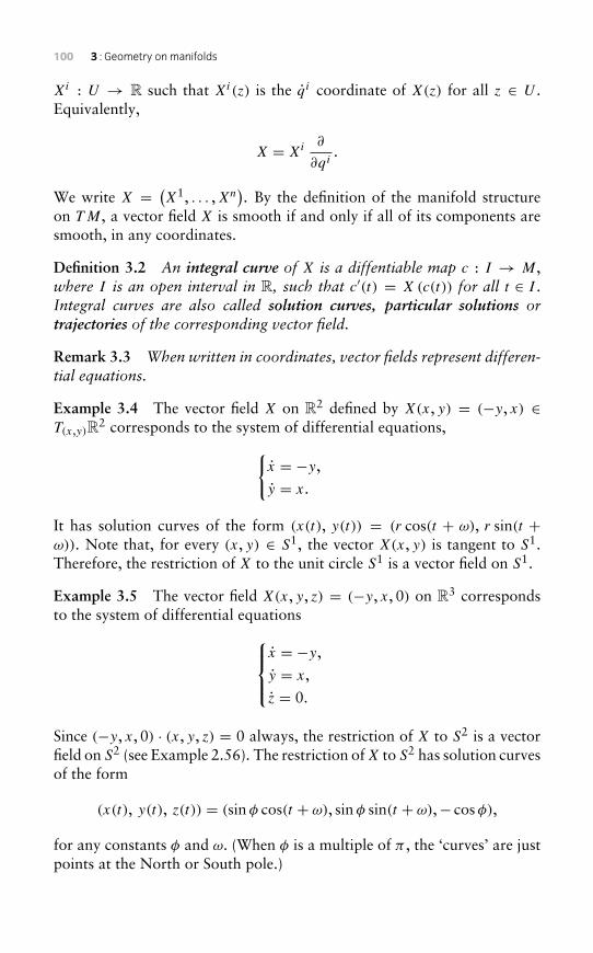
100 3 : Geometry on manifolds
Xi : U → R such that Xi(z) is the qi coordinate of X(z) for all z ∈ U .Equivalently,
X = Xi ∂
∂qi.
We write X = (X1, . . . ,Xn
). By the definition of the manifold structure
on TM, a vector field X is smooth if and only if all of its components aresmooth, in any coordinates.
Definition 3.2 An integral curve of X is a diffentiable map c : I → M,where I is an open interval in R, such that c′(t) = X (c(t)) for all t ∈ I .Integral curves are also called solution curves, particular solutions ortrajectories of the corresponding vector field.
Remark 3.3 When written in coordinates, vector fields represent differen-tial equations.
Example 3.4 The vector field X on R2 defined by X(x, y) = (−y, x) ∈T(x,y)R
2 corresponds to the system of differential equations,{x = −y,
y = x.
It has solution curves of the form (x(t), y(t)) = (r cos(t + ω), r sin(t +ω)). Note that, for every (x, y) ∈ S1, the vector X(x, y) is tangent to S1.Therefore, the restriction of X to the unit circle S1 is a vector field on S1.
Example 3.5 The vector field X(x, y, z) = (−y, x, 0) on R3 correspondsto the system of differential equations
x = −y,
y = x,
z = 0.
Since (−y, x, 0) · (x, y, z) = 0 always, the restriction of X to S2 is a vectorfield on S2 (see Example 2.56). The restriction ofX to S2 has solution curvesof the form
(x(t), y(t), z(t)) = (sinφ cos(t + ω), sinφ sin(t + ω),− cosφ),
for any constants φ and ω. (When φ is a multiple of π , the ‘curves’ are justpoints at the North or South pole.)
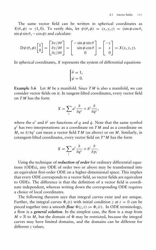
3.1 Vector fields 101
The same vector field can be written in spherical coordinates asX(θ ,φ) = (1, 0). To verify this, let ψ(θ ,φ) = (x, y, z) = (sinφ cos θ ,sinφ sin θ ,− cosφ) and calculate:
Dψ(θ ,φ)[10
]=∂x/∂θ
∂y/∂θ
∂z/∂θ
=− sinφ sin θ
sinφ cos θ0
=−yx
0
= X(x, y, z).
In spherical coordinates, X represents the system of differential equations{θ = 1,
ϕ = 0.
Example 3.6 Let M be a manifold. Since TM is also a manifold, we canconsider vector fields on it. In tangent-lifted coordinates, every vector fieldon TM has the form
X =∑i
ai ∂
∂qi+ bi ∂
∂qi,
where the ai and bi are functions of q and q. Note that the same symbolqi has two interpretations: as a coordinate on TM and as a coordinate onM, so ∂/∂qi can mean a vector field TM (as above) or on M. Similarly, incotangent-lifted coordinates, every vector field on T ∗M has the form
X =∑i
ai ∂
∂qi+ bi ∂
∂pi
.
Using the technique of reduction of order for ordinary differential equa-tions (ODEs), any ODE of order two or above may be transformed intoan equivalent first-order ODE on a higher-dimensional space. This impliesthat every ODE corresponds to a vector field, so vector fields are equivalentto ODEs. The difference is that the definition of a vector field is coordi-nate independent, whereas writing down the corresponding ODE requiresa choice of local coordinates.
The following theorem says that integral curves exist and are unique.Further, the integral curves �z(t) with initial condition z at t = 0 can bepieced together into a smooth flow �(z, t) := �z(t). In ODE terminology,a flow is a general solution. In the simplest case, the flow is a map fromM × R to M, but the domain of � may be restricted, because the integralcurves may have limited domains, and the domains can be different fordifferent z values.
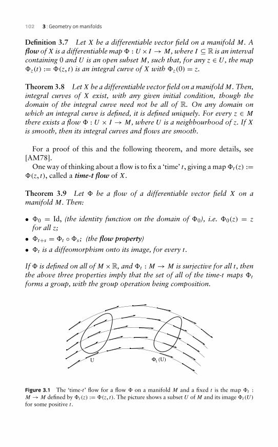
102 3 : Geometry on manifolds
Definition 3.7 Let X be a differentiable vector field on a manifold M. Aflow ofX is a differentiable map� : U×I → M, where I ⊆ R is an intervalcontaining 0 and U is an open subsetM, such that, for any z ∈ U , the map�z(t) := �(z, t) is an integral curve of X with �z(0) = z.
Theorem 3.8 LetX be a differentiable vector field on amanifoldM. Then,integral curves of X exist, with any given initial condition, though thedomain of the integral curve need not be all of R. On any domain onwhich an integral curve is defined, it is defined uniquely. For every z ∈ M
there exists a flow � : U × I → M, where U is a neighbourhood of z. If Xis smooth, then its integral curves and flows are smooth.
For a proof of this and the following theorem, and more details, see[AM78].
One way of thinking about a flow is to fix a ‘time’ t , giving a map�t(z) :=�(z, t), called a time-t flow of X.
Theorem 3.9 Let � be a flow of a differentiable vector field X on amanifold M. Then:
• �0 = Id, (the identity function on the domain of �0), i.e. �0(z) = z
for all z;
• �t+s = �t ◦�s ; (the flow property)
• �t is a diffeomorphism onto its image, for every t .
If � is defined on all ofM ×R, and �t : M → M is surjective for all t , thenthe above three properties imply that the set of all of the time-t maps �t
forms a group, with the group operation being composition.
Φt (U)U
Figure 3.1 The ‘time-t ’ flow for a flow � on a manifold M and a fixed t is the map �t :M → M defined by �t(z) := �(z, t). The picture shows a subset U of M and its image �t(U)
for some positive t .
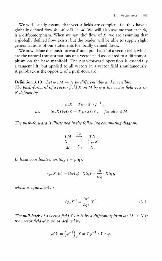
3.1 Vector fields 103
We will usually assume that vector fields are complete, i.e. they have aglobally defined flow � : M × R → M. We will also assume that each �t
is a diffeomorphism. When we say ‘the’ flow of X, we are assuming thata globally defined flow exists, but the reader will be able to supply slightgeneralizations of our statements for locally defined flows.
We now define the ‘push-forward’ and ‘pull-back’ of a vector field, whichare the natural transformations of a vector field associated to a diffeomor-phism on the base manifold. The push-forward operation is essentiallya tangent lift, but applied to all vectors in a vector field simultaneously.A pull-back is the opposite of a push-forward.
Definition 3.10 Let ϕ : M → N be differentiable and invertible.The push-forward of a vector field X on M by ϕ is the vector field ϕ∗X onN defined by
ϕ∗X = T ϕ ◦X ◦ ϕ−1 ;
i.e. (ϕ∗X) (ϕ(z)) = Tzϕ (X(z)) , for all z ∈ M.
The push-forward is illustrated in the following commuting diagram:
TMTϕ−→ TN
X ↑ ↑ ϕ∗XM
ϕ−→ N .
In local coordinates, writing r = ϕ(q),
(ϕ∗X)(r) = Dϕ(q) ·X(q) = drdq·X(q),
which is equivalent to
(ϕ∗X)i = ∂ri
∂qjXj . (3.1)
The pull-back of a vector field Y on N by a diffeomorphism ϕ : M → N isthe vector field ϕ∗Y on M defined by
ϕ∗Y =(ϕ−1
)∗ Y = T ϕ−1 ◦ Y ◦ ϕ.
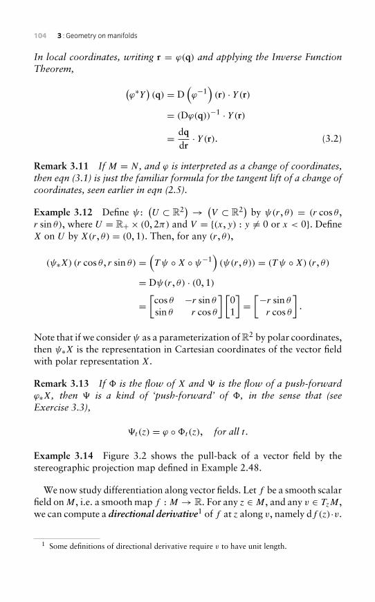
104 3 : Geometry on manifolds
In local coordinates, writing r = ϕ(q) and applying the Inverse FunctionTheorem, (
ϕ∗Y)(q) = D
(ϕ−1
)(r) · Y (r)
= (Dϕ(q))−1 · Y (r)
= dqdr· Y (r). (3.2)
Remark 3.11 If M = N , and ϕ is interpreted as a change of coordinates,then eqn (3.1) is just the familiar formula for the tangent lift of a change ofcoordinates, seen earlier in eqn (2.5).
Example 3.12 Define ψ :(U ⊂ R2) → (
V ⊂ R2) by ψ(r, θ) = (r cos θ ,r sin θ), where U = R+ × (0, 2π) and V = {(x, y) : y �= 0 or x < 0}. DefineX on U by X(r, θ) = (0, 1). Then, for any (r, θ),
(ψ∗X) (r cos θ , r sin θ) =(T ψ ◦X ◦ ψ−1
)(ψ(r, θ)) = (T ψ ◦X) (r, θ)
= Dψ(r, θ) · (0, 1)
=[cos θ −r sin θ
sin θ r cos θ
] [01
]=[−r sin θ
r cos θ
].
Note that if we considerψ as a parameterization of R2 by polar coordinates,then ψ∗X is the representation in Cartesian coordinates of the vector fieldwith polar representation X.
Remark 3.13 If � is the flow of X and � is the flow of a push-forwardϕ∗X, then � is a kind of ‘push-forward’ of �, in the sense that (seeExercise 3.3),
�t(z) = ϕ ◦�t(z), for all t .
Example 3.14 Figure 3.2 shows the pull-back of a vector field by thestereographic projection map defined in Example 2.48.
We now study differentiation along vector fields. Let f be a smooth scalarfield on M, i.e. a smooth map f : M → R. For any z ∈ M, and any v ∈ TzM,we can compute a directional derivative1 of f at z along v, namely df (z)·v.
1 Some definitions of directional derivative require v to have unit length.
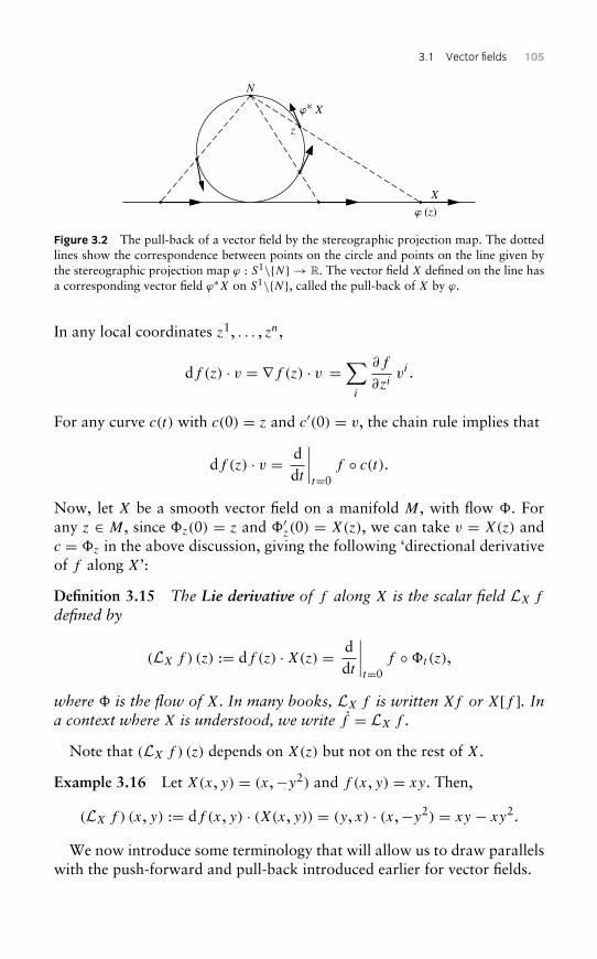
3.1 Vector fields 105
N
z
X
w∗ X
w (z)
Figure 3.2 The pull-back of a vector field by the stereographic projection map. The dottedlines show the correspondence between points on the circle and points on the line given bythe stereographic projection map ϕ : S1\{N} → R. The vector field X defined on the line hasa corresponding vector field ϕ∗X on S1\{N}, called the pull-back of X by ϕ.
In any local coordinates z1, . . . , zn,
df (z) · v = ∇f (z) · v =∑i
∂f
∂zivi .
For any curve c(t) with c(0) = z and c′(0) = v, the chain rule implies that
df (z) · v = ddt
∣∣∣∣t=0
f ◦ c(t).
Now, let X be a smooth vector field on a manifold M, with flow �. Forany z ∈ M, since �z(0) = z and �′z(0) = X(z), we can take v = X(z) andc = �z in the above discussion, giving the following ‘directional derivativeof f along X’:
Definition 3.15 The Lie derivative of f along X is the scalar field LX f
defined by
(LX f ) (z) := df (z) ·X(z) = ddt
∣∣∣∣t=0
f ◦�t(z),
where � is the flow of X. In many books, LX f is written Xf or X[f ]. Ina context where X is understood, we write f = LX f .
Note that (LX f ) (z) depends on X(z) but not on the rest of X.
Example 3.16 Let X(x, y) = (x,−y2) and f (x, y) = xy. Then,
(LX f ) (x, y) := df (x, y) · (X(x, y)) = (y, x) · (x,−y2) = xy − xy2.
We now introduce some terminology that will allow us to draw parallelswith the push-forward and pull-back introduced earlier for vector fields.
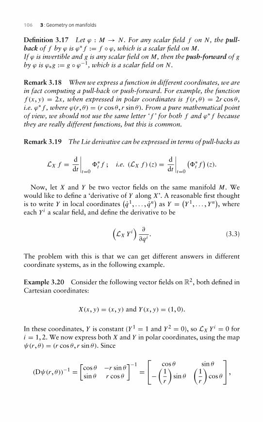
106 3 : Geometry on manifolds
Definition 3.17 Let ϕ : M → N . For any scalar field f on N , the pull-back of f by ϕ is ϕ∗f := f ◦ ϕ, which is a scalar field on M.If ϕ is invertible and g is any scalar field onM, then the push-forward of gby ϕ is ϕ∗g := g ◦ ϕ−1, which is a scalar field on N .
Remark 3.18 When we express a function in different coordinates, we arein fact computing a pull-back or push-forward. For example, the functionf (x, y) = 2x, when expressed in polar coordinates is f (r, θ) = 2r cos θ ,i.e. ϕ∗f , where ϕ(r, θ) = (r cos θ , r sin θ). From a pure mathematical pointof view, we should not use the same letter ‘f ’ for both f and ϕ∗f becausethey are really different functions, but this is common.
Remark 3.19 The Lie derivative can be expressed in terms of pull-backs as
LX f = ddt
∣∣∣∣t=0
�∗t f ; i.e. (LX f ) (z) = ddt
∣∣∣∣t=0
(�∗t f
)(z).
Now, let X and Y be two vector fields on the same manifold M. Wewould like to define a ‘derivative of Y along X’. A reasonable first thoughtis to write Y in local coordinates
(q1, . . . , qn
)as Y = (Y 1, . . . ,Yn
), where
each Y i a scalar field, and define the derivative to be
(LX Y i
) ∂
∂qi. (3.3)
The problem with this is that we can get different answers in differentcoordinate systems, as in the following example.
Example 3.20 Consider the following vector fields on R2, both defined inCartesian coordinates:
X(x, y) = (x, y) and Y (x, y) = (1, 0).
In these coordinates, Y is constant (Y 1 = 1 and Y 2 = 0), so LX Y i = 0 fori = 1, 2. We now express both X and Y in polar coordinates, using the mapψ(r, θ) = (r cos θ , r sin θ). Since
(Dψ(r, θ))−1 =[cos θ −r sin θ
sin θ r cos θ
]−1
= cos θ sin θ
−(
1r
)sin θ
(1r
)cos θ
,
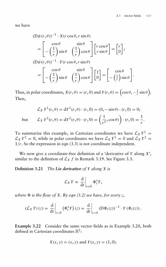
3.1 Vector fields 107
we have
(Dψ(r, θ))−1 ·X(r cos θ , r sin θ)
= cos θ sin θ
−(
1r
)sin θ
(1r
)cos θ
[r cos θr sin θ
]=[r
0
];
(Dψ(r, θ))−1 · Y (r cos θ , r sin θ)
= cos θ sin θ
−(
1r
)sin θ
(1r
)cos θ
[10
]=[
cos θ
−(
1r
)sin θ
].
Thus, in polar coordinates, X(r, θ) = (r, 0) and Y (r, θ) =(cos θ ,−1
rsin θ
).
Then,
LX Y 1(r, θ) = dY 1(r, θ) · (r, 0) = (0,− sin θ) · (r, 0) = 0;
but LX Y 2(r, θ) = dY 2(r, θ) · (r, 0) =(
1r2 , cos θ)
)· (r, 0) = 1
r.
To summarize this example, in Cartesian coordinates we have LX Y 1 =LX Y 2 = 0, while in polar coordinates we have LX Y 1 = 0 and LX Y 2 =1/r. So the expression in eqn (3.3) is not coordinate independent.
We now give a coordinate-free definition of a ‘derivative of Y along X’,similar to the definition of LX f in Remark 3.19. See Figure 3.3.
Definition 3.21 The Lie derivative of Y along X is
LX Y ≡ ddt
∣∣∣∣t=0
�∗t Y ,
where � is the flow of X. By eqn (3.2) we have, for every z,
(LX Y) (z) = ddt
∣∣∣∣t=0
(�∗t Y
)(z) = d
dt
∣∣∣∣t=0
(D�t(z))−1 · Y (�t(z)) .
Example 3.22 Consider the same vector fields as in Example 3.20, bothdefined in Cartesian coordinates R2:
X(x, y) = (x, y) and Y (x, y) = (1, 0).
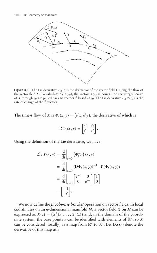
108 3 : Geometry on manifolds
Y2~
Y1~ Y0
Y1Y2
X0 X1
z1z0 z2
X2
XY(z0)
Figure 3.3 The Lie derivative LX Y is the derivative of the vector field Y along the flow ofthe vector field X. To calculate LX Y(z0), the vectors Y (z) at points z on the integral curveof X through z0 are pulled back to vectors Y based at z0. The Lie derivative LX Y(z0) is therate of change of the Y vectors.
The time-t flow of X is �t(x, y) = (et x, et y), the derivative of which is
D�t(x, y) =[et 00 et
].
Using the definition of the Lie derivative, we have
LX Y(x, y) = ddt
∣∣∣∣t=0
(�∗t Y
)(x, y)
= ddt
∣∣∣∣t=0
(D�t(x, y))−1 · Y (�t(x, y))
= ddt
∣∣∣∣t=0
[e−t 00 e−t
] [10
]=[−1
0
].
We now define the Jacobi–Lie bracket operation on vector fields. In localcoordinates on an n-dimensional manifold M, a vector field X on M can beexpressed as X(z) = (X1(z), . . . ,Xn(z)
)and, in the domain of the coordi-
nate system, the base points z can be identified with elements of Rn, so X
can be considered (locally) as a map from Rn to Rn. Let DX(z) denote thederivative of this map at z.
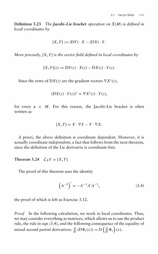
3.1 Vector fields 109
Definition 3.23 The Jacobi–Lie bracket operation on X(M) is defined inlocal coordinates by
[X,Y ] := (DY ) ·X − (DX) · Y .
More precisely, [X,Y ] is the vector field defined in local coordinates by
[X,Y ](z) := DY (z) ·X(z)−DX(z) · Y (z).
Since the rows of DX(z) are the gradient vectors ∇Xi(z),
(DX(z) · Y (z))i = ∇Xi(z) · Y (z),
for every z ∈ M. For this reason, the Jacobi–Lie bracket is oftenwritten as
[X,Y ] = X · ∇Y − Y · ∇X.
A priori, the above definition is coordinate dependent. However, it isactually coordinate independent, a fact that follows from the next theorem,since the definition of the Lie derivative is coordinate-free.
Theorem 3.24 LXY = [X,Y ]
The proof of this theorem uses the identity
(A−1
)′ = −A−1A′A−1, (3.4)
the proof of which is left as Exercise 3.12.
Proof In the following calculation, we work in local coordinates. Thus,we may consider everything as matrices, which allows us to use the productrule, the rule in eqn (3.4), and the following consequence of the equality of
mixed second partial derivatives: ddt (D�t(x)) = D
(ddt �t
)(x).
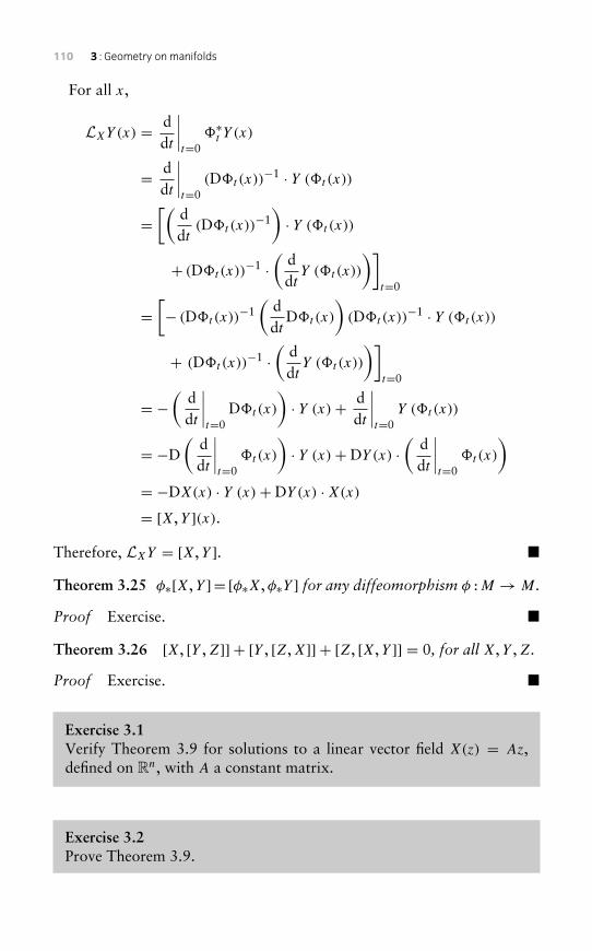
110 3 : Geometry on manifolds
For all x,
LXY(x) = ddt
∣∣∣∣t=0
�∗t Y (x)
= ddt
∣∣∣∣t=0
(D�t(x))−1 · Y (�t(x))
=[(
ddt
(D�t(x))−1)· Y (�t(x))
+ (D�t(x))−1 ·
(ddt
Y (�t(x))
)]t=0
=[− (D�t(x))
−1(
ddt
D�t(x)
)(D�t(x))
−1 · Y (�t(x))
+ (D�t(x))−1 ·
(ddt
Y (�t(x))
)]t=0
= −(
ddt
∣∣∣∣t=0
D�t(x)
)· Y (x)+ d
dt
∣∣∣∣t=0
Y (�t(x))
= −D(
ddt
∣∣∣∣t=0
�t(x)
)· Y (x)+DY (x) ·
(ddt
∣∣∣∣t=0
�t(x)
)= −DX(x) · Y (x)+DY (x) ·X(x)
= [X,Y ](x).Therefore, LXY = [X,Y ]. �
Theorem 3.25 φ∗[X,Y ]= [φ∗X,φ∗Y ] for any diffeomorphism φ :M → M.
Proof Exercise. �
Theorem 3.26 [X, [Y ,Z]] + [Y , [Z,X]] + [Z, [X,Y ]] = 0, for all X,Y ,Z.
Proof Exercise. �
Exercise 3.1Verify Theorem 3.9 for solutions to a linear vector field X(z) = Az,defined on Rn, with A a constant matrix.
Exercise 3.2Prove Theorem 3.9.
3.1 Vector fields 111
Exercise 3.3Prove the formula in Remark 3.13 regarding the flow of the push-forward of a vector field.
Exercise 3.4Let (θ ,φ) be the spherical coordinates on S2 defined by
(x, y, z) = (sinφ cos θ , sinφ sin θ ,− cosφ),
for θ ∈ (−π ,π),φ ∈ (0,π). With f as in Exercise 2.18, and X on S2
defined in spherical coordinates by (θ , φ) = X(θ ,φ) = (1, 1), calculatef∗X. Sketch X and f∗X.
Exercise 3.5Sketch the vector field X defined in spherical coordinates by X(θ ,φ) =(1, sinφ). Express X in the stereographic coordinates (ξ , η) defined inExample 2.49.
Exercise 3.6If X(x, y) = (−y, x) and H(x, y) = 1
2
(x2 + y2), compute LX H .
Exercise 3.7Prove the Leibniz rule (a.k.a. product rule): LX(fg) = (LX f ) g +f (LX g).
Exercise 3.8Calculate [X,Y ] for X and Y as in Example 3.22, and check that youranswer equals LX Y as calculated directly in that example.
Exercise 3.9Let X(x, y, z) = (−y, x, 1) and Y (x, y, z) = (x, y, z). Calculate LX Y intwo ways: directly from Definition 3.21, and as [X,Y ].
112 3 : Geometry on manifolds
Exercise 3.10Show that, if X = Xi ∂
∂qi , then LX qi = Xi .
Exercise 3.11Let � be the flow of X. Show that LX Y = − d
dt
∣∣∣t=0
(�t )∗ Y .
Exercise 3.12Let A(t) be a path in M(n, R), the set of n × n matrices. By dif-ferentiating the equation A−1A = I with respect to t , show that(A−1)′ = −A−1A′A−1.
3.2 Differential 1-forms
Just as a vector field is a ‘field’ of tangent vectors, a differential 1-form is a‘field’ of cotangent vectors, one for every base point. Recall that a cotangentvector based at z ∈ M is a linear map from TzM to R, and the set of allsuch maps is the cotangent space T ∗z M, which is the dual to the tangentspace TzM. Differential 1-forms are often called just 1-forms.
Definition 3.27 A (differential) 1-form on a manifoldM is a map θ : M →T ∗M such that θ(z) ∈ T ∗z M for every z ∈ M. Differential 1-forms can beadded together, and multiplied by scalar fields k : M → R, as follows:
(α + β) (z) := α(z)+ β(z), (kθ) (z) := k(z)θ(z).
A smooth (resp. differentiable) 1-form is one that is a smooth (resp.differentiable) map from M → T ∗M.
The most important example of a 1-form is the differential of a scalarfield, the definition of which appeared in Chapter 2 and is repeated here.
Definition 3.28 The differential of a scalar field f : M → R is the 1-formdf such that, for any z ∈ M, df (z) : TzM → R is the derivative, i.e. thetangent map, of f at z.
Not all 1-forms are differentials, as the next example shows.
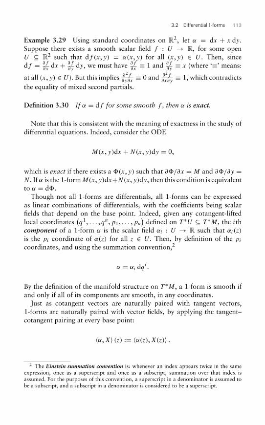
3.2 Differential 1-forms 113
Example 3.29 Using standard coordinates on R2, let α = dx + x dy.Suppose there exists a smooth scalar field f : U → R, for some openU ⊆ R2 such that df (x, y) = α(x, y) for all (x, y) ∈ U . Then, sincedf = ∂f
∂xdx + ∂f
∂ydy, we must have ∂f
∂x≡ 1 and ∂f
∂y≡ x (where ‘≡’ means:
at all (x, y) ∈ U ). But this implies ∂2f∂y∂x≡ 0 and ∂2f
∂x∂y≡ 1, which contradicts
the equality of mixed second partials.
Definition 3.30 If α = df for some smooth f , then α is exact.
Note that this is consistent with the meaning of exactness in the study ofdifferential equations. Indeed, consider the ODE
M(x, y)dx +N(x, y)dy = 0,
which is exact if there exists a �(x, y) such that ∂�/∂x = M and ∂�/∂y =N . If α is the 1-formM(x, y)dx+N(x, y)dy, then this condition is equivalentto α = d�.
Though not all 1-forms are differentials, all 1-forms can be expressedas linear combinations of differentials, with the coefficients being scalarfields that depend on the base point. Indeed, given any cotangent-liftedlocal coordinates
(q1, . . . , qn,p1, . . . ,pn
)defined on T ∗U ⊆ T ∗M, the ith
component of a 1-form α is the scalar field αi : U → R such that αi(z)
is the pi coordinate of α(z) for all z ∈ U . Then, by definition of the pi
coordinates, and using the summation convention,2
α = αi dqi .
By the definition of the manifold structure on T ∗M, a 1-form is smooth ifand only if all of its components are smooth, in any coordinates.
Just as cotangent vectors are naturally paired with tangent vectors,1-forms are naturally paired with vector fields, by applying the tangent–cotangent pairing at every base point:
〈α,X〉 (z) := 〈α(z),X(z)〉 .
2 The Einstein summation convention is: whenever an index appears twice in the sameexpression, once as a superscript and once as a subscript, summation over that index isassumed. For the purposes of this convention, a superscript in a denominator is assumed tobe a subscript, and a subscript in a denominator is considered to be a superscript.
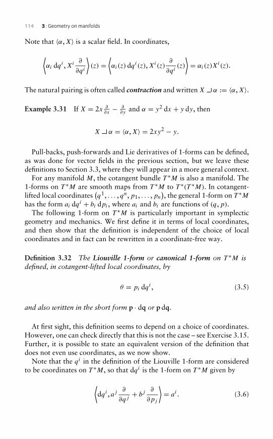
114 3 : Geometry on manifolds
Note that 〈α,X〉 is a scalar field. In coordinates,
⟨αi dqi ,Xi ∂
∂qi
⟩(z) =
⟨αi(z) dqi(z),Xi(z)
∂
∂qi(z)
⟩= αi(z)X
i(z).
The natural pairing is often called contraction and written X α := 〈α,X〉.
Example 3.31 If X = 2x ∂∂x− ∂
∂yand α = y2 dx + y dy, then
X α = 〈α,X〉 = 2xy2 − y.
Pull-backs, push-forwards and Lie derivatives of 1-forms can be defined,as was done for vector fields in the previous section, but we leave thesedefinitions to Section 3.3, where they will appear in a more general context.
For any manifold M, the cotangent bundle T ∗M is also a manifold. The1-forms on T ∗M are smooth maps from T ∗M to T ∗(T ∗M). In cotangent-lifted local coordinates
(q1, . . . , qn,p1, . . . ,pn
), the general 1-form on T ∗M
has the form ai dqi + bi dpi , where ai and bi are functions of (q,p).The following 1-form on T ∗M is particularly important in symplectic
geometry and mechanics. We first define it in terms of local coordinates,and then show that the definition is independent of the choice of localcoordinates and in fact can be rewritten in a coordinate-free way.
Definition 3.32 The Liouville 1-form or canonical 1-form on T ∗M isdefined, in cotangent-lifted local coordinates, by
θ = pi dqi , (3.5)
and also written in the short form p · dq or p dq.
At first sight, this definition seems to depend on a choice of coordinates.However, one can check directly that this is not the case – see Exercise 3.15.Further, it is possible to state an equivalent version of the definition thatdoes not even use coordinates, as we now show.
Note that the qi in the definition of the Liouville 1-form are consideredto be coordinates on T ∗M, so that dqi is the 1-form on T ∗M given by
⟨dqi , aj ∂
∂qj+ bj ∂
∂pj
⟩= ai . (3.6)
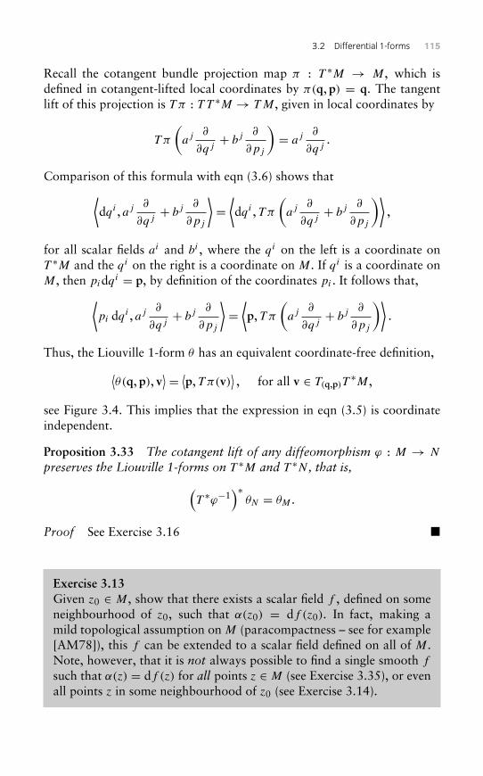
3.2 Differential 1-forms 115
Recall the cotangent bundle projection map π : T ∗M → M, which isdefined in cotangent-lifted local coordinates by π(q, p) = q. The tangentlift of this projection is T π : T T ∗M → TM, given in local coordinates by
T π
(aj ∂
∂qj+ bj ∂
∂pj
)= aj ∂
∂qj.
Comparison of this formula with eqn (3.6) shows that⟨dqi , aj ∂
∂qj+ bj ∂
∂pj
⟩=⟨dqi , T π
(aj ∂
∂qj+ bj ∂
∂pj
)⟩,
for all scalar fields ai and bi , where the qi on the left is a coordinate onT ∗M and the qi on the right is a coordinate on M. If qi is a coordinate onM, then pidqi = p, by definition of the coordinates pi . It follows that,⟨
pi dqi , aj ∂
∂qj+ bj ∂
∂pj
⟩=⟨p, T π
(aj ∂
∂qj+ bj ∂
∂pj
)⟩.
Thus, the Liouville 1-form θ has an equivalent coordinate-free definition,⟨θ(q, p), v
⟩ = ⟨p, T π(v)⟩, for all v ∈ T(q,p)T
∗M,
see Figure 3.4. This implies that the expression in eqn (3.5) is coordinateindependent.
Proposition 3.33 The cotangent lift of any diffeomorphism ϕ : M → N
preserves the Liouville 1-forms on T ∗M and T ∗N , that is,(T ∗ϕ−1
)∗θN = θM .
Proof See Exercise 3.16 �
Exercise 3.13Given z0 ∈ M, show that there exists a scalar field f , defined on someneighbourhood of z0, such that α(z0) = df (z0). In fact, making amild topological assumption on M (paracompactness – see for example[AM78]), this f can be extended to a scalar field defined on all of M.Note, however, that it is not always possible to find a single smooth f
such that α(z) = df (z) for all points z ∈ M (see Exercise 3.35), or evenall points z in some neighbourhood of z0 (see Exercise 3.14).
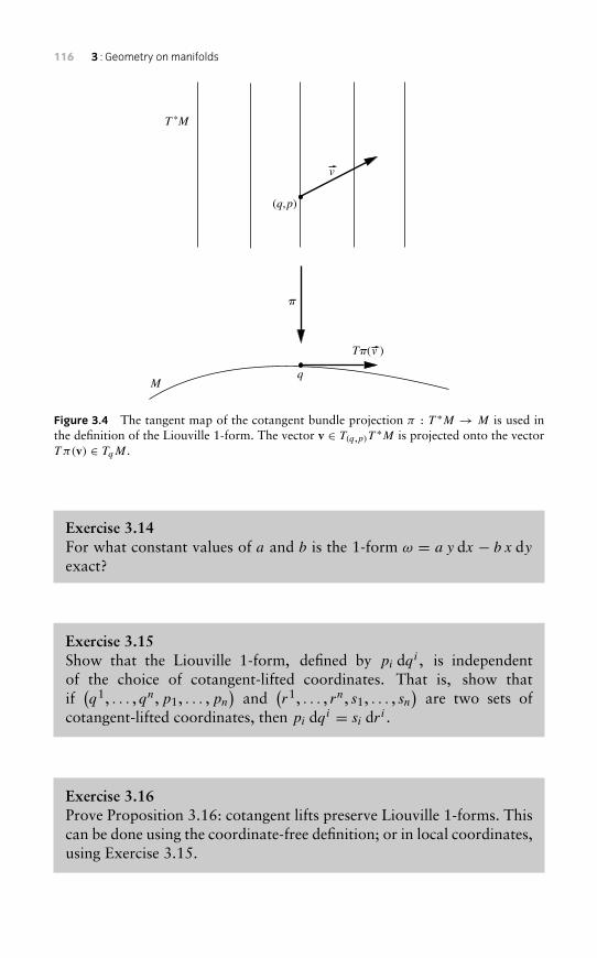
116 3 : Geometry on manifolds
T *M
q
p
(q,p)
v
M
Tp(v )
Figure 3.4 The tangent map of the cotangent bundle projection π : T ∗M → M is used inthe definition of the Liouville 1-form. The vector v ∈ T(q,p)T
∗M is projected onto the vectorT π(v) ∈ TqM.
Exercise 3.14For what constant values of a and b is the 1-form ω = a y dx − b x dyexact?
Exercise 3.15Show that the Liouville 1-form, defined by pi dqi , is independentof the choice of cotangent-lifted coordinates. That is, show thatif(q1, . . . , qn,p1, . . . ,pn
)and
(r1, . . . , rn, s1, . . . , sn
)are two sets of
cotangent-lifted coordinates, then pi dqi = si dri .
Exercise 3.16Prove Proposition 3.16: cotangent lifts preserve Liouville 1-forms. Thiscan be done using the coordinate-free definition; or in local coordinates,using Exercise 3.15.
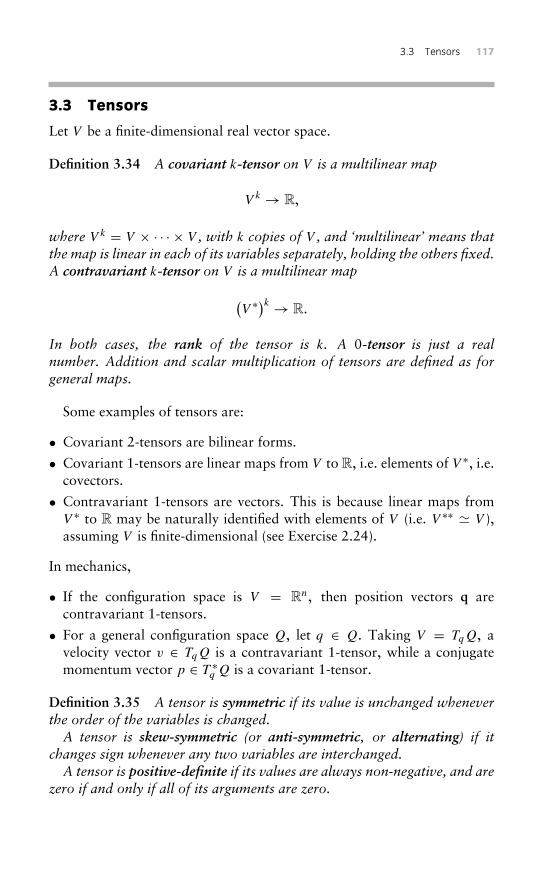
3.3 Tensors 117
3.3 Tensors
Let V be a finite-dimensional real vector space.
Definition 3.34 A covariant k-tensor on V is a multilinear map
V k → R,
where V k = V × · · · × V , with k copies of V , and ‘multilinear’ means thatthe map is linear in each of its variables separately, holding the others fixed.A contravariant k-tensor on V is a multilinear map
(V ∗)k → R.
In both cases, the rank of the tensor is k. A 0-tensor is just a realnumber. Addition and scalar multiplication of tensors are defined as forgeneral maps.
Some examples of tensors are:
• Covariant 2-tensors are bilinear forms.
• Covariant 1-tensors are linear maps from V to R, i.e. elements of V ∗, i.e.covectors.
• Contravariant 1-tensors are vectors. This is because linear maps fromV ∗ to R may be naturally identified with elements of V (i.e. V ∗∗ � V ),assuming V is finite-dimensional (see Exercise 2.24).
In mechanics,
• If the configuration space is V = Rn, then position vectors q arecontravariant 1-tensors.
• For a general configuration space Q, let q ∈ Q. Taking V = TqQ, avelocity vector v ∈ TqQ is a contravariant 1-tensor, while a conjugatemomentum vector p ∈ T ∗q Q is a covariant 1-tensor.
Definition 3.35 A tensor is symmetric if its value is unchanged wheneverthe order of the variables is changed.A tensor is skew-symmetric (or anti-symmetric, or alternating) if it
changes sign whenever any two variables are interchanged.A tensor is positive-definite if its values are always non-negative, and are
zero if and only if all of its arguments are zero.
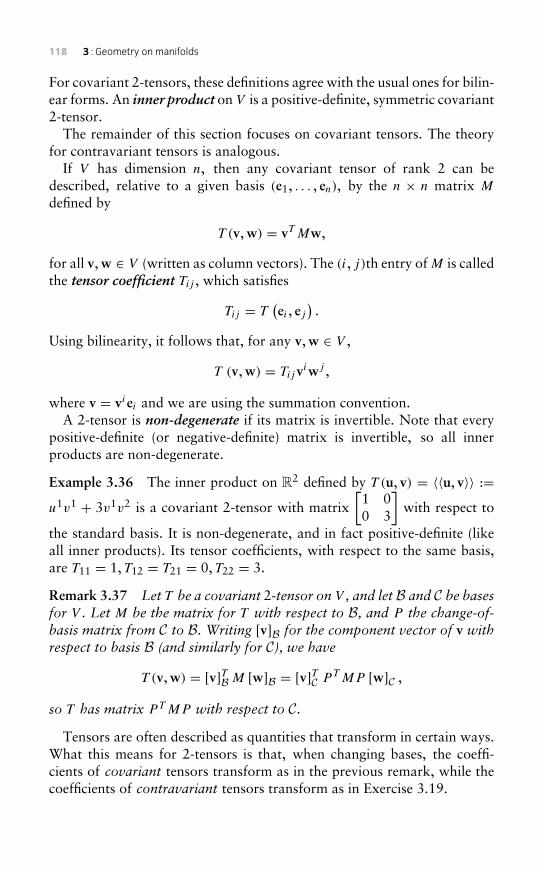
118 3 : Geometry on manifolds
For covariant 2-tensors, these definitions agree with the usual ones for bilin-ear forms. An inner product on V is a positive-definite, symmetric covariant2-tensor.
The remainder of this section focuses on covariant tensors. The theoryfor contravariant tensors is analogous.
If V has dimension n, then any covariant tensor of rank 2 can bedescribed, relative to a given basis (e1, . . . , en), by the n × n matrix M
defined by
T (v,w) = vT Mw,
for all v,w ∈ V (written as column vectors). The (i, j)th entry of M is calledthe tensor coefficient Tij , which satisfies
Tij = T(ei , ej
).
Using bilinearity, it follows that, for any v,w ∈ V ,
T (v,w) = Tijviwj ,
where v = viei and we are using the summation convention.A 2-tensor is non-degenerate if its matrix is invertible. Note that every
positive-definite (or negative-definite) matrix is invertible, so all innerproducts are non-degenerate.
Example 3.36 The inner product on R2 defined by T (u, v) = 〈〈u, v〉〉 :=u1v1 + 3v1v2 is a covariant 2-tensor with matrix
[1 00 3
]with respect to
the standard basis. It is non-degenerate, and in fact positive-definite (likeall inner products). Its tensor coefficients, with respect to the same basis,are T11 = 1, T12 = T21 = 0, T22 = 3.
Remark 3.37 Let T be a covariant 2-tensor on V , and let B and C be basesfor V . Let M be the matrix for T with respect to B, and P the change-of-basis matrix from C to B. Writing [v]B for the component vector of v withrespect to basis B (and similarly for C), we have
T (v,w) = [v]TB M [w]B = [v]TC PT MP [w]C ,
so T has matrix PT MP with respect to C.Tensors are often described as quantities that transform in certain ways.
What this means for 2-tensors is that, when changing bases, the coeffi-cients of covariant tensors transform as in the previous remark, while thecoefficients of contravariant tensors transform as in Exercise 3.19.
3.3 Tensors 119
For general k, covariant tensors of rank k can be described, with respectto a given basis (e1, . . . , en) for V , by the nk coefficients,
Tj1 ···jk := T(ej1 , . . . , ejk
).
Thus, tensors can be thought of as ‘k-dimensional matrices’. For any vectorsv1, . . . , vk ∈ V ,
T (v1, . . . , vk) = Tj1 ···jkvj11 · · · vjk
k ,
where va = vjaej .
Given a choice of basis for V , the tensor is determined by its tensor coef-ficients. A logical notation would be T = (Tj1 ···jk
), but the more common
notation is just T = Tj1 ···jk .
Definition 3.38 The tensor product of a covariant k-tensor S and acovariant l-tensor T is the covariant (k + l)-tensor S ⊗ T defined by
(S ⊗ T ) (v1, . . . , vk+l) = S (v1, . . . , vk) T (vk+1, . . . , vk+l) ,
i.e. the first k vectors get ‘plugged into’ S, and the rest get ‘plugged into’ T .
It is easily checked that tensor product is an associative bilinear operation.
Example 3.39 Let(e1, e2, e3) be the dual basis to the standard basis on
R3; so for example, e1(u) = u1 for all u = (u1, u2, u3) ∈ R3. Note thateach ei is a map from R3 to R, so it is a covariant 1-tensor on R3. Then,(e1 ⊗ e2) (u, v) = u1v2. The bilinear form T defined by T (u, v) = 2u1v3 −
3u2v1 can be written as T = 2e1 ⊗ e3 − 3e2 ⊗ e1.
The next proposition, which generalizes the previous example, is aconsequence of the multilinearity of tensors and the definition of tensorcoefficients.
Proposition 3.40 Given a basis(e1, . . . , en
)for V ∗, any covariant k-tensor
T on V satisfies T = Ti1...ikei1 ⊗ · · · ⊗ eik , where the sum is over all possible
choices of the k indices i1, . . . , ik. This expression uniquely defines the tensorcoefficients, so the set {ei1 ⊗ · · · ⊗ eik }, of all possible kth-order tensorproducts of the basis elements, forms a basis for T 0
k V .
Definition 3.41 A tensor field on a manifold M is a smoothly varyingfamily of tensors {T (z)}, all of the same rank, such that T (z) is a tensor onTzM, for each z ∈ M. The tensor coefficients now depend on z, so they are
120 3 : Geometry on manifolds
scalar fields. They also depend on a choice of local coordinate system, andare defined by
Tj1...jk (z) := T
(∂
∂qj1(z), . . . ,
∂
∂qjk(z)
).
The tensor field is smooth if all of the tensor coefficients are smooth (in anycoordinate system).
The set of all tensor fields on M of a given rank is called a tensor bundleover M, generalizing the tangent and cotangent bundles. It is a manifold.
A tensor field T is symmetric (resp. skew-symmetric, non-degenerate,positive-definite) if T (z) is symmetric (resp. skew-symmetric, non-degenerate, positive-definite), for every z ∈ M.Some examples of tensor fields are:
• a 0-tensor field is a scalar field;
• a covariant 1-tensor field is a differential 1-form;
• a contravariant 1-tensor field is a vector field;
• a Riemannian metric on M is a positive-definite, symmetric covariant2-tensor field on M, i.e. a tensor g such that g(z) is an inner product onTzM, for every z ∈ M. See Section 3.4.
Covariant tensor fields of rank 2 are represented by matrices with entriesthat depend on the base point, z, as in the following example.
Example 3.42 Let (θ ,φ) be spherical coordinates on the unit sphereS2, and suppose that T is a covariant 2-tensor field on S2 with matrixrepresentation
T =[
0 sinφ
− sinφ 0
].
If v and w are tangent vectors to S2 based at the same point (θ ,φ), then
T (v,w) = [vθ vφ] [ 0 sinφ
− sinφ 0
] [wθ
wφ
]= sinφ
(vθwφ − vφwθ
).
Note that T is skew-symmetric. In fact, T is the ‘area form’ for S2, asexplained later in Examples 3.52 and 3.53.
Remark 3.43 (Change of coordinates) If ψ is a coordinate transformationfrom ‘new’ to ‘old’ coordinates on M, then Dψ(z) is the correspondinglinear change-of-basis transformation on TzM (for every z). If M is thematrix representation of a covariant 2-tensor T (z) with respect to the old
3.3 Tensors 121
coordinates, then, by Remark 3.37, the matrix representation of T (z) inthe new coordinates is (Dψ(z))T MDψ(z).
Definition 3.44 The tensor product of two tensor fields is defined ‘point-wise’:
(α ⊗ β) (z) = α(z)⊗ β(z), for every z.
Example 3.45 For any smooth f , g : M → R, the covariant 2-tensor fielddf ⊗ dg is defined by(
df ⊗ dg)(z) (v,w) = (df (z) · v) (df (z) · w)
for any z ∈ M and any v,w ∈ TzM.
Proposition 3.46 Given any local coordinates q1, . . . , qn on M, anycovariant k-tensor field T on M can be locally expressed as
T = Ti1...ikdqi1 ⊗ · · · ⊗ dqik .
Proof This follows from Proposition 3.40 and the fact that, for every z,the covectors
(dqi1(z), . . . , dqik (z)
)form a basis for TzM. �
Definition 3.47 The symmetric product of two covectors (i.e. covariant1-tensors) α and β is the symmetric covariant 2-tensor αβ defined by
αβ = 12(α ⊗ β + β ⊗ α) , i.e. (3.7)
(αβ) (v,w) = 12(α(v)β(w)+ β(v)α(w)) .
The definition applies ‘pointwise’ to tensor fields.
Example 3.48 If g is a symmetric covariant 2-tensor field then gij = gji
for all i, j , so (using the summation convention)
g = gij dxi ⊗ dxj = 12
(gij + gji
)dxi ⊗ dxj
= 12gij
(dxi ⊗ dxj + dxj ⊗ dxi
)= gijdxidxj .
Remark 3.49 The following notation is widely used, despite beingpotentially ambiguous: dx2 := (dx)2 := dx dx.
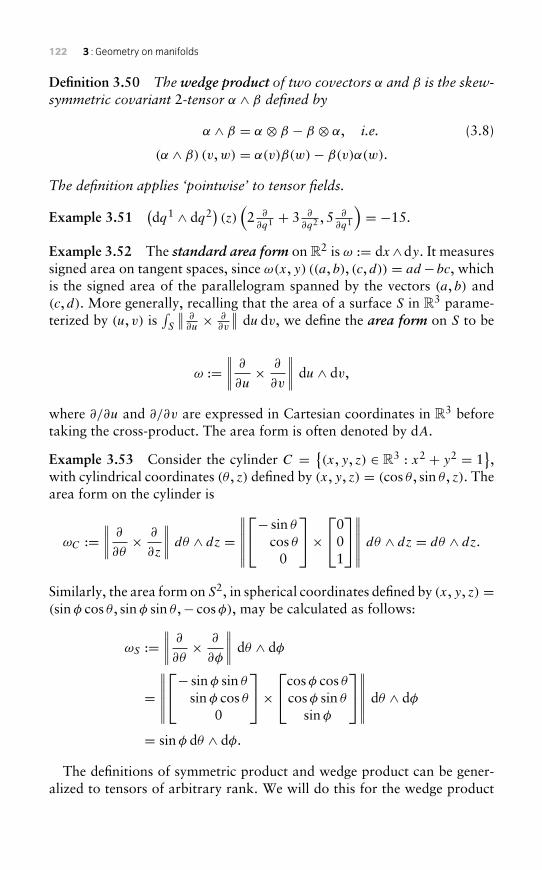
122 3 : Geometry on manifolds
Definition 3.50 The wedge product of two covectors α and β is the skew-symmetric covariant 2-tensor α ∧ β defined by
α ∧ β = α ⊗ β − β ⊗ α, i.e. (3.8)
(α ∧ β) (v,w) = α(v)β(w)− β(v)α(w).
The definition applies ‘pointwise’ to tensor fields.
Example 3.51(dq1 ∧ dq2) (z) (2 ∂
∂q1 + 3 ∂
∂q2 , 5 ∂
∂q1
)= −15.
Example 3.52 The standard area form on R2 is ω := dx∧dy. It measuressigned area on tangent spaces, since ω(x, y) ((a, b), (c, d)) = ad−bc, whichis the signed area of the parallelogram spanned by the vectors (a, b) and(c, d). More generally, recalling that the area of a surface S in R3 parame-terized by (u, v) is
∫S
∥∥ ∂∂u× ∂
∂v
∥∥ du dv, we define the area form on S to be
ω :=∥∥∥∥ ∂
∂u× ∂
∂v
∥∥∥∥ du ∧ dv,
where ∂/∂u and ∂/∂v are expressed in Cartesian coordinates in R3 beforetaking the cross-product. The area form is often denoted by dA.
Example 3.53 Consider the cylinder C = {(x, y, z) ∈ R3 : x2 + y2 = 1
},
with cylindrical coordinates (θ , z) defined by (x, y, z) = (cos θ , sin θ , z). Thearea form on the cylinder is
ωC :=∥∥∥∥ ∂
∂θ× ∂
∂z
∥∥∥∥ dθ ∧ dz =∥∥∥∥∥∥− sin θ
cos θ0
×0
01
∥∥∥∥∥∥ dθ ∧ dz = dθ ∧ dz.
Similarly, the area form on S2, in spherical coordinates defined by (x, y, z) =(sinφ cos θ , sinφ sin θ ,− cosφ), may be calculated as follows:
ωS :=∥∥∥∥ ∂
∂θ× ∂
∂φ
∥∥∥∥ dθ ∧ dφ
=∥∥∥∥∥∥− sinφ sin θ
sinφ cos θ0
×cosφ cos θ
cosφ sin θ
sinφ
∥∥∥∥∥∥ dθ ∧ dφ
= sinφ dθ ∧ dφ.
The definitions of symmetric product and wedge product can be gener-alized to tensors of arbitrary rank. We will do this for the wedge product
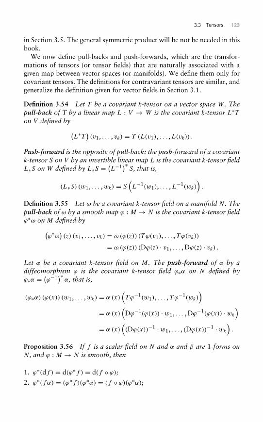
3.3 Tensors 123
in Section 3.5. The general symmetric product will be not be needed in thisbook.
We now define pull-backs and push-forwards, which are the transfor-mations of tensors (or tensor fields) that are naturally associated with agiven map between vector spaces (or manifolds). We define them only forcovariant tensors. The definitions for contravariant tensors are similar, andgeneralize the definition given for vector fields in Section 3.1.
Definition 3.54 Let T be a covariant k-tensor on a vector space W . Thepull-back of T by a linear map L : V → W is the covariant k-tensor L∗Ton V defined by(
L∗T)(v1, . . . , vk) = T (L(v1), . . . ,L(vk)) .
Push-forward is the opposite of pull-back: the push-forward of a covariantk-tensor S on V by an invertible linear map L is the covariant k-tensor fieldL∗S on W defined by L∗S =
(L−1)∗ S, that is,
(L∗S) (w1, . . . ,wk) = S(L−1(w1), . . . ,L−1(wk)
).
Definition 3.55 Let ω be a covariant k-tensor field on a manifold N . Thepull-back of ω by a smooth map ϕ : M → N is the covariant k-tensor fieldϕ∗ω on M defined by(
ϕ∗ω)(z) (v1, . . . , vk) = ω (ϕ(z)) (T ϕ(v1), . . . , T ϕ(vk))
= ω (ϕ(z)) (Dϕ(z) · v1, . . . , Dϕ(z) · vk) .
Let α be a covariant k-tensor field on M. The push-forward of α by adiffeomorphism ϕ is the covariant k-tensor field ϕ∗α on N defined byϕ∗α =
(ϕ−1)∗ α, that is,
(ϕ∗α) (ϕ(x)) (w1, . . . ,wk) = α (x)(T ϕ−1(w1), . . . , T ϕ−1(wk)
)= α (x)
(Dϕ−1(ϕ(x)) · w1, . . . , Dϕ−1(ϕ(x)) · wk
)= α (x)
((Dϕ(x))−1 · w1, . . . , (Dϕ(x))−1 · wk
).
Proposition 3.56 If f is a scalar field on N and α and β are 1-forms onN , and ϕ : M → N is smooth, then
1. ϕ∗(df ) = d(ϕ∗f ) = d(f ◦ ϕ);2. ϕ∗(f α) = (ϕ∗f )(ϕ∗α) = (f ◦ ϕ)(ϕ∗α);
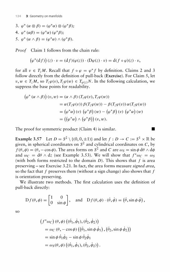
124 3 : Geometry on manifolds
3. ϕ∗ (α ⊗ β) = (ϕ∗α)⊗ (ϕ∗β);4. ϕ∗ (αβ) = (ϕ∗α) (ϕ∗β);5. ϕ∗ (α ∧ β) = (ϕ∗α) ∧ (ϕ∗β).
Proof Claim 1 follows from the chain rule:(ϕ∗(df )
)(z) · v = (df )(ϕ(z)) · (Dϕ(z) · v) = d(f ◦ ϕ)(z) · v,
for all v ∈ TzM. Recall that f ◦ ϕ = ϕ∗f by definition. Claims 2 and 3follow directly from the definition of pull-back (Exercise). For Claim 5, letv,w ∈ TzM, so Tzϕ(v), Tzϕ(w) ∈ Tϕ(z)N . In the following calculation, wesuppress the base points for readability.(
ϕ∗ (α ∧ β))(v,w) = (α ∧ β) (Tzϕ(v), Tzϕ(w))
= α(Tzϕ(v)) β(Tzϕ(w))− β(Tzϕ(v)) α(Tzϕ(w))
= (ϕ∗α) (v) (ϕ∗β) (w)− (ϕ∗β) (v) (ϕ∗α) (w)
= ((ϕ∗α) ∧ (ϕ∗β)) (v,w).
The proof for symmetric product (Claim 4) is similar. �
Example 3.57 Let D = S2 \ {(0, 0,±1)} and let f : D→ C := S1 ×R begiven, in spherical coordinates on S2 and cylindrical coordinates on C, byf (θ ,φ) = (θ ,− cosφ). The area forms on S2 and C are ωS = sinφ dθ ∧ dφand ωC = dθ ∧ dz (see Example 3.53). We will show that f ∗ωC = ωS
(with both forms restricted to the domain D). This shows that f is areapreserving – see Exercise 3.21. In fact, the area forms measure signed area,so the fact that f preserves them (without a sign change) also shows that fis orientation preserving.
We illustrate two methods. The first calculation uses the definition ofpull-back directly:
Df (θ ,φ) =[1 00 sinφ
], and Df (θ ,φ) · (θ , φ) = (θ , sinφ φ
),
so (f ∗ωC
)(θ ,φ)
((θ1, φ1), (θ2, φ2)
)= ωC (θ ,− cosφ)
((θ1, sinφ φ1
),(θ2, sinφ φ2
))= sinφ θ1φ2 − sinφ θ2φ1
= ωS(θ ,φ)((θ1, φ1), (θ2, φ2)
).
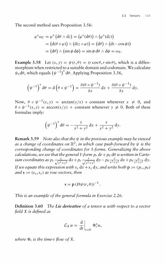
3.3 Tensors 125
The second method uses Proposition 3.56:
ϕ∗ωC = ϕ∗(dθ ∧ dz
) = (ϕ∗(dθ)) ∧ (ϕ∗(dz))= (d(θ ◦ ϕ)) ∧ (d(z ◦ ϕ)) = (dθ) ∧ (d(− cosφ)
)= (dθ) ∧ (sinφ dφ
) = sinφ dθ ∧ dφ = ωS .
Example 3.58 Let (x, y) = ψ(r, θ) = (r cos θ , r sin θ), which is a diffeo-morphism when restricted to a suitable domain and codomain. We calculateψ∗dθ , which equals
(ψ−1)∗ dθ . Applying Proposition 3.56,
(ψ−1
)∗dθ = d
(θ ◦ ψ−1
)= ∂(θ ◦ ψ−1)
∂xdx + ∂(θ ◦ ψ−1)
∂ydy.
Now, θ ◦ ψ−1(x, y) = arctan(y/x) + constant whenever x �= 0, andθ ◦ ψ−1(x, y) = arccot(x/y) + constant whenever y �= 0. Both of theseformulae imply:
(ψ−1
)∗dθ = − y
x2 + y2 dx + x
x2 + y2 dy.
Remark 3.59 Note also that the ψ in the previous example may be viewedas a change of coordinates on R2, in which case push-forward by ψ is thecorresponding change of coordinates for 1-forms. Generalizing the abovecalculations, we see that the general 1-form pr dr+pθ dθ is written in Carte-sian coordinates as pr
x√x2+y2
dx+pry√
x2+y2dy−pθ
y
x2+y2 dx+pθx
x2+y2 dy.
If we equate this expression with sx dx+ sy dy, and write both p := (pr ,pθ)
and s := (sx , sy) as row vectors, then
s = p (Dψ(r, θ))−1 .
This is an example of the general formula in Exercise 2.26.
Definition 3.60 The Lie derivative of a tensor α with respect to a vectorfield X is defined as
LX α = ddt
∣∣∣∣t=0
�∗t α,
where �t is the time-t flow of X.
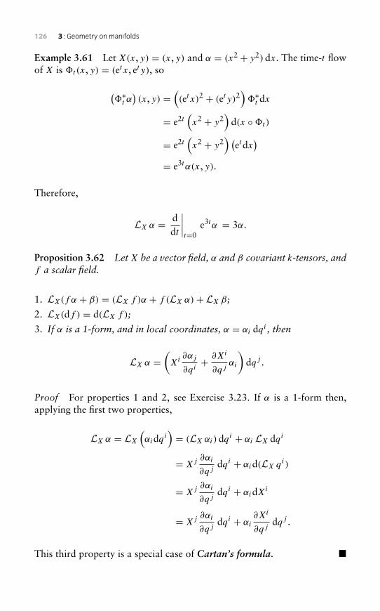
126 3 : Geometry on manifolds
Example 3.61 Let X(x, y) = (x, y) and α = (x2 + y2) dx. The time-t flowof X is �t(x, y) = (et x, et y), so
(�∗t α
)(x, y) =
((et x)2 + (et y)2
)�∗t dx
= e2t(x2 + y2
)d(x ◦�t)
= e2t(x2 + y2
) (etdx
)= e3tα(x, y).
Therefore,
LX α = ddt
∣∣∣∣t=0
e3tα = 3α.
Proposition 3.62 Let X be a vector field, α and β covariant k-tensors, andf a scalar field.
1. LX(f α + β) = (LX f )α + f (LX α)+ LX β;
2. LX(df ) = d(LX f );
3. If α is a 1-form, and in local coordinates, α = αi dqi , then
LX α =(Xi ∂αj
∂qi+ ∂Xi
∂qjαi
)dqj .
Proof For properties 1 and 2, see Exercise 3.23. If α is a 1-form then,applying the first two properties,
LX α = LX
(αidqi
)= (LX αi) dqi + αi LX dqi
= Xj ∂αi
∂qjdqi + αid(LX qi)
= Xj ∂αi
∂qjdqi + αidXi
= Xj ∂αi
∂qjdqi + αi
∂Xi
∂qjdqj .
This third property is a special case of Cartan’s formula. �
3.3 Tensors 127
Exercise 3.17For each of the following tensors: write down its tensor coefficients,with respect to the standard basis; and, if it’s a rank 2 tensor, writedown its matrix.a) the skew-symmetric bilinear form on R3 defined by
T (u, v) = 3u1v2 − 3u2v1 − 4u1v3 + 4u3v1;
b) the dot product in Rn;c) the scalar triple product in R3.
Exercise 3.18Express each of the tensors in Exercise 3.17 as linear combinations oftensor products of standard basis vectors.
Exercise 3.19(See Remark 3.37). Let B and C be bases for V , and let P be the change-of-basis matrix from C to B. Let B∗ and C∗ be the dual bases of B andC, respectively. Show that the change-of-basis matrix from C∗ to B∗ isP−T (inverse transpose). Defining the matrix of a contravariant 2-tensorby analogy with the covariant case, show that, if T has matrix M withrespect to B∗ then it has matrix P−1MP−T with respect to C∗. Comparethis with Exercise 2.26.
Exercise 3.20Determine how tensor coefficients transform when changing bases, bygeneralizing Example 3.37 and Exercise 3.19.
Exercise 3.21Let f be as in the Example 3.57. Using the standard change-of-variablesrule from multivariable calculus, check that f is area-preserving,meaning that, for any region B ⊆ S2,∫
B
sinφ dθ dφ =∫f (B)
dθ dz.
128 3 : Geometry on manifolds
Compare your calculations with those in Example 3.57.
Exercise 3.22If X(x, y) = (−y, x) and ω = dx ∧ dy, show that LX ω = 0.
Exercise 3.23Prove Proposition 3.62. Hint: The first property follows from linearityof derivatives and the product rule. For the second, use the chain ruleand equality of mixed partials.
3.4 Riemannian geometry
A Riemannian metric on a manifold Q is a smoothly varying family of innerproducts on each of the tangent spaces TqQ. A formal definition appearsbelow. Recall that an inner product on a vector space is a positive-definite,symmetric bilinear form. It is represented, with respect to any basis, by apositive-definite symmetric matrix. Two vectors v and w are orthogonalwith respect to a given inner product if and only if 〈〈v,w〉〉 = 0. Given aninner product 〈〈·, ·〉〉, the associated norm is given by ‖v‖ := 〈〈v, v〉〉1/2, and‖v‖ is called the norm of v or the length of v.
Example 3.63 The Euclidean inner product on Rn is the bilinear formthat, when written in standard Cartesian coordinates, equals the dotproduct:
〈〈v,w〉〉 := v ·w =∑i
viwi .
It is represented, with respect to the standard basis, by the identity matrixI , because 〈〈v,w〉〉 = vT w = vT Iw. The associated norm is called theEuclidean norm. The speed of a particle with velocity q ∈ Rn is
∥∥q∥∥.Example 3.64 Recall that the kinetic energy of an N -particle Newtoniansystem in R3 is K = 1
2∑
i mi
∥∥qi∥∥2, with ‖·‖ being the Euclidean norm.
3.4 Riemannian geometry 129
Writing q = (q1, . . . , qN)
and defining
M := diag (m1,m1,m1,m2,m2,m2, . . . ,mN ,mN ,mN) (3.9)
(the diagonal matrix with these entries along the diagonal), we have
K = 12qT Mq.
Let 〈〈·, ·〉〉M be the inner product on on R3N with matrix M with respect tothe standard basis, and let ‖ · ‖M be the associated norm. Then,
K = 12
∥∥q∥∥2M= 1
2
⟨⟨q, q
⟩⟩M
.
Now, consider a particle moving on a general manifold Q, with trajectoryq(t). Its velocity, q(t), is a tangent vector based at q(t). So, for a generaldefinition of speed or kinetic energy of such particles, we need a normon TqQ, for every q. For a system of particles, the same remarks apply,except that each point in the configuration space Q represents the positionsof all particles, and q(t) describes the velocity of all particles. These aremotivations for the following definition.
Definition 3.65 A Riemannian metric on a manifold Q is a smooth sym-metric positive-definite covariant 2-tensor field g onQ. Thismeans that g(q)is an inner product on TqQ, for every q ∈ Q, and that the tensor coefficientsgij , in any choice of local coordinates, are smooth functions of q.Notation: g(q) is also written as gq or 〈〈·, ·〉〉q , and g is written as〈〈·, ·〉〉. Using the notation for symmetric products introduced in the pre-vious section, g = gijdqidqj ; recall that dqidqi is also written as
(dqi)2,
with the parentheses often omitted, for example dx2 := dx dx. The pair(Q, g) is called a Riemannian manifold.Given g, the associated norm (really a family of norms, one at each q ∈ Q)
is defined as follows: the norm of a tangent vector v ∈ TqQ is ‖v‖q definedby ‖v‖2q := 〈〈v, v〉〉q = g(q) (v, v) = gij (q) v
ivj (the latter expression isin local coordinates). Two tangent vectors v,w ∈ TqQ, based at the samepoint q ∈ Q, are orthogonal if 〈〈v,w〉〉q = 0, i.e. gij (q) v
iwj = 0.
The simplest manifolds are vector spaces. Any inner product on a vectorspace V defines a constant Riemannian metric g on V such that g(q) equalsthe given inner product, for every q ∈ V . The following example is of thistype. There also exist non-constant Riemannian metrics on vector spaces.
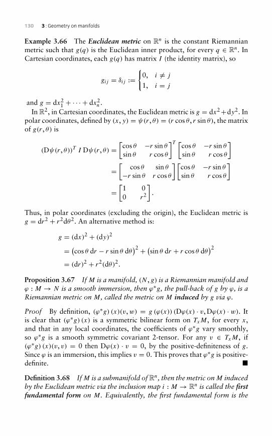
130 3 : Geometry on manifolds
Example 3.66 The Euclidean metric on Rn is the constant Riemannianmetric such that g(q) is the Euclidean inner product, for every q ∈ Rn. InCartesian coordinates, each g(q) has matrix I (the identity matrix), so
gij = δij :={
0, i �= j
1, i = j
and g = dx21 + · · · + dx2
n .In R2, in Cartesian coordinates, the Euclidean metric is g = dx2+dy2. In
polar coordinates, defined by (x, y) = ψ(r, θ) = (r cos θ , r sin θ), the matrixof g(r, θ) is
(Dψ(r, θ))T I Dψ(r, θ) =[cos θ −r sin θ
sin θ r cos θ
]T [cos θ −r sin θ
sin θ r cos θ
]=[
cos θ sin θ
−r sin θ r cos θ
] [cos θ −r sin θ
sin θ r cos θ
]=[1 00 r2
].
Thus, in polar coordinates (excluding the origin), the Euclidean metric isg = dr2 + r2dθ2. An alternative method is:
g = (dx)2 + (dy)2
= (cos θ dr − r sin θ dθ)2 + (sin θ dr + r cos θ dθ
)2= (dr)2 + r2(dθ)2.
Proposition 3.67 IfM is a manifold, (N , g) is a Riemannian manifold andϕ : M → N is a smooth immersion, then ϕ∗g, the pull-back of g by ϕ, is aRiemannian metric on M, called the metric on M induced by g via ϕ.
Proof By definition, (ϕ∗g) (x)(v,w) = g (ϕ(x)) (Dϕ(x) · v, Dϕ(x) · w). Itis clear that (ϕ∗g) (x) is a symmetric bilinear form on TxM, for every x,and that in any local coordinates, the coefficients of ϕ∗g vary smoothly,so ϕ∗g is a smooth symmetric covariant 2-tensor. For any v ∈ TxM, if(ϕ∗g) (x)(v, v) = 0 then Dϕ(x) · v = 0, by the positive-definiteness of g.Since ϕ is an immersion, this implies v = 0. This proves that ϕ∗g is positive-definite. �
Definition 3.68 IfM is a submanifold ofRn, then the metric onM inducedby the Euclidean metric via the inclusion map i : M → Rn is called the firstfundamental form on M. Equivalently, the first fundamental form is the
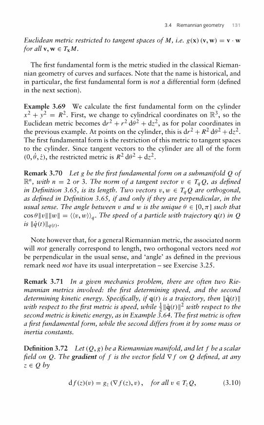
3.4 Riemannian geometry 131
Euclidean metric restricted to tangent spaces of M, i.e. g(x) (v,w) = v · wfor all v,w ∈ TxM.
The first fundamental form is the metric studied in the classical Rieman-nian geometry of curves and surfaces. Note that the name is historical, andin particular, the first fundamental form is not a differential form (definedin the next section).
Example 3.69 We calculate the first fundamental form on the cylinderx2 + y2 = R2. First, we change to cylindrical coordinates on R3, so theEuclidean metric becomes dr2 + r2 dθ2 + dz2, as for polar coordinates inthe previous example. At points on the cylinder, this is dr2+R2 dθ2+ dz2.The first fundamental form is the restriction of this metric to tangent spacesto the cylinder. Since tangent vectors to the cylinder are all of the form(0, θ , z), the restricted metric is R2 dθ2 + dz2.
Remark 3.70 Let g be the first fundamental form on a submanifold Q ofRn, with n = 2 or 3. The norm of a tangent vector v ∈ TqQ, as definedin Definition 3.65, is its length. Two vectors v,w ∈ TqQ are orthogonal,as defined in Definition 3.65, if and only if they are perpendicular, in theusual sense. The angle between v and w is the unique θ ∈ [0,π ] such thatcos θ‖v‖‖w‖ = 〈〈v,w〉〉q . The speed of a particle with trajectory q(t) in Q
is ‖q(t)‖q(t).
Note however that, for a general Riemannian metric, the associated normwill not generally correspond to length, two orthogonal vectors need notbe perpendicular in the usual sense, and ‘angle’ as defined in the previousremark need not have its usual interpretation – see Exercise 3.25.
Remark 3.71 In a given mechanics problem, there are often two Rie-mannian metrics involved: the first determining speed, and the seconddetermining kinetic energy. Specifically, if q(t) is a trajectory, then ‖q(t)‖with respect to the first metric is speed, while 1
2‖q(t)‖2 with respect to thesecond metric is kinetic energy, as in Example 3.64. The first metric is oftena first fundamental form, while the second differs from it by some mass orinertia constants.
Definition 3.72 Let (Q, g) be a Riemannianmanifold, and let f be a scalarfield on Q. The gradient of f is the vector field ∇f on Q defined, at anyz ∈ Q by
df (z)(v) = gz (∇f (z), v) , for all v ∈ TzQ, (3.10)
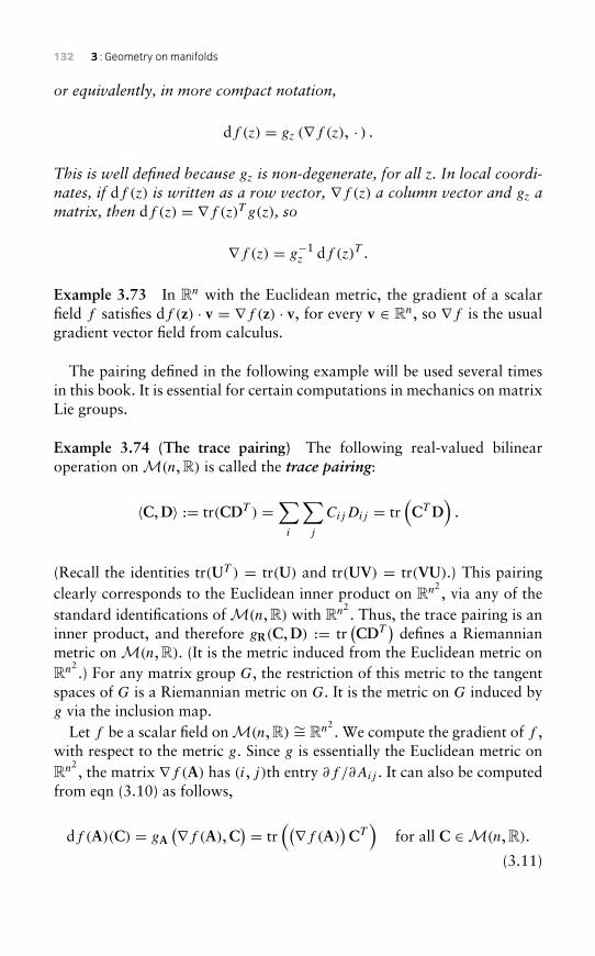
132 3 : Geometry on manifolds
or equivalently, in more compact notation,
df (z) = gz (∇f (z), · ) .
This is well defined because gz is non-degenerate, for all z. In local coordi-nates, if df (z) is written as a row vector, ∇f (z) a column vector and gz amatrix, then df (z) = ∇f (z)T g(z), so
∇f (z) = g−1z df (z)T .
Example 3.73 In Rn with the Euclidean metric, the gradient of a scalarfield f satisfies df (z) · v = ∇f (z) · v, for every v ∈ Rn, so ∇f is the usualgradient vector field from calculus.
The pairing defined in the following example will be used several timesin this book. It is essential for certain computations in mechanics on matrixLie groups.
Example 3.74 (The trace pairing) The following real-valued bilinearoperation on M(n, R) is called the trace pairing:
〈C,D〉 := tr(CDT ) =∑i
∑j
CijDij = tr(CT D
).
(Recall the identities tr(UT ) = tr(U) and tr(UV) = tr(VU).) This pairingclearly corresponds to the Euclidean inner product on Rn2
, via any of thestandard identifications of M(n, R) with Rn2
. Thus, the trace pairing is aninner product, and therefore gR(C,D) := tr
(CDT
)defines a Riemannian
metric on M(n, R). (It is the metric induced from the Euclidean metric onRn2
.) For any matrix group G, the restriction of this metric to the tangentspaces of G is a Riemannian metric on G. It is the metric on G induced byg via the inclusion map.
Let f be a scalar field on M(n, R) ∼= Rn2. We compute the gradient of f ,
with respect to the metric g. Since g is essentially the Euclidean metric onRn2
, the matrix ∇f (A) has (i, j)th entry ∂f /∂Aij . It can also be computedfrom eqn (3.10) as follows,
df (A)(C) = gA(∇f (A),C
) = tr((∇f (A)
)CT)
for all C ∈M(n, R).
(3.11)
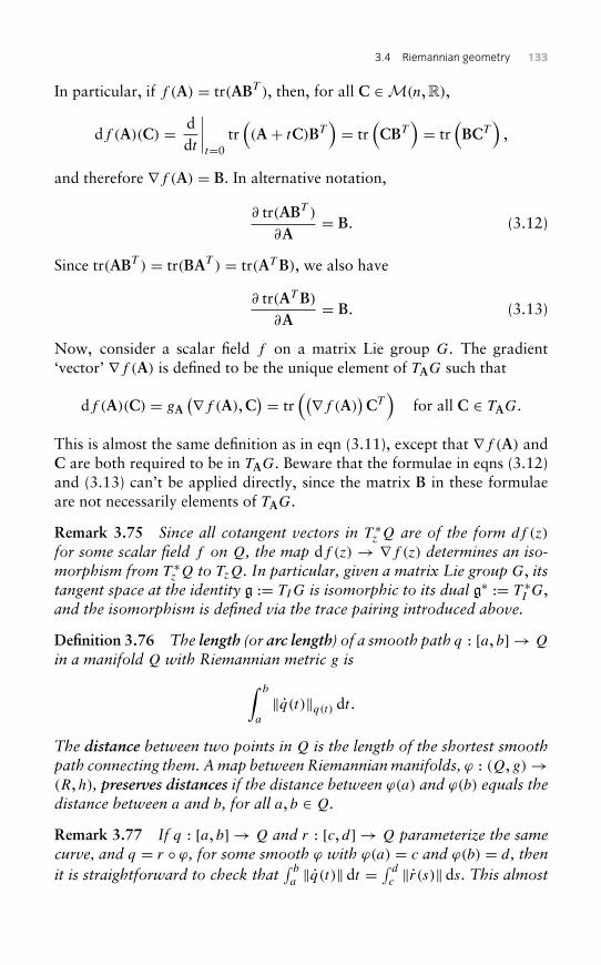
3.4 Riemannian geometry 133
In particular, if f (A) = tr(ABT ), then, for all C ∈M(n, R),
df (A)(C) = ddt
∣∣∣∣t=0
tr((A + tC)BT
)= tr
(CBT
)= tr
(BCT
),
and therefore ∇f (A) = B. In alternative notation,
∂ tr(ABT )
∂A= B. (3.12)
Since tr(ABT ) = tr(BAT ) = tr(AT B), we also have
∂ tr(AT B)
∂A= B. (3.13)
Now, consider a scalar field f on a matrix Lie group G. The gradient‘vector’ ∇f (A) is defined to be the unique element of TAG such that
df (A)(C) = gA(∇f (A),C
) = tr((∇f (A)
)CT)
for all C ∈ TAG.
This is almost the same definition as in eqn (3.11), except that ∇f (A) andC are both required to be in TAG. Beware that the formulae in eqns (3.12)and (3.13) can’t be applied directly, since the matrix B in these formulaeare not necessarily elements of TAG.
Remark 3.75 Since all cotangent vectors in T ∗z Q are of the form df (z)
for some scalar field f on Q, the map df (z) → ∇f (z) determines an iso-morphism from T ∗z Q to TzQ. In particular, given a matrix Lie group G, itstangent space at the identity g := TIG is isomorphic to its dual g∗ := T ∗I G,and the isomorphism is defined via the trace pairing introduced above.
Definition 3.76 The length (or arc length) of a smooth path q : [a, b] → Q
in a manifold Q with Riemannian metric g is∫ b
a
‖q(t)‖q(t) dt .
The distance between two points in Q is the length of the shortest smoothpath connecting them. Amap between Riemannianmanifolds, ϕ : (Q, g)→(R,h), preserves distances if the distance between ϕ(a) and ϕ(b) equals thedistance between a and b, for all a, b ∈ Q.
Remark 3.77 If q : [a, b] → Q and r : [c, d] → Q parameterize the samecurve, and q = r ◦ ϕ, for some smooth ϕ with ϕ(a) = c and ϕ(b) = d, thenit is straightforward to check that
∫ b
a‖q(t)‖ dt = ∫ d
c‖r(s)‖ ds. This almost
134 3 : Geometry on manifolds
proves that the formula above defines the length of a curve, independent ofthe choice of parameterization. What remains to be shown is that, given anytwo smooth parameterizations q and r with the same image, there existsa ϕ as above. This is true if r is an immersion and r−1 : Im r → [c, d] iscontinuous, by Theorem 2.39.
Remark 3.78 Distance as defined above satisfies the axioms of a metric,namely: d(x, y) ≥ 0; d(x, y) = 0⇔ x = y; d(x, y) = d(y, x); and d(x, z) ≤d(x, y)+ d(y, z).
In Rn, the shortest curve joining two points is a line segment. On asphere, the shortest curve joining two points is an arc of a great circle.These curves are examples of geodesics. In general, a curve is a geodesic ifit ‘locally minimizes length’, meaning that no ‘small’ change in the curvecould produce a shorter curve connecting the same two points q(a) and q(b).The following formal definition uses the calculus of variations (introducedin Section 1.2).
Definition 3.79 A smooth path q : [a, b] → Q in a Riemannianmanifold isa geodesic if it has constant non-zero speed
∥∥q(t)∥∥ = c and it is a stationarypoint of the length functional
Sl[q(·)] :=∫ b
a
∥∥q(t)∥∥q(t) dt , (3.14)
with respect to variations among paths with fixed endpoints. A path definedon an unbounded interval is a geodesic if every finite piece of it is a geodesic.
When we introduced the calculus of variations, it was for curves in Rn,not general manifolds. But this is no obstacle because a curve is a stationarypoint of the length functional if and only if each piece of the curve has thesame property (see Section 4.1). It follows that, to check whether a curve isa geodesic, we can cover the manifold in coordinate charts, and use localcoordinates to check pieces of the curve. Note that the definition specifies astationary point rather than a local minimum. However, it can be proventhat, for this functional, the stationary points are always local minima.
Remark 3.80 A geodesic need not globally minimize length. For example,a trajectory that follows three quarters of a great circle on a sphere is ageodesic, because any small change to it would produce a longer curve. Yetthere does exist a shorter curve connecting the two endpoints, namely thearc that ‘goes the other way’ around the great circle.
3.4 Riemannian geometry 135
In general, to find geodesics, we have to find stationary points of thelength functional. But we already have a great tool for doing this: the Euler–Lagrange equations. Indeed, the length functional is the action functionalfor the Lagrangian l(q, q) := ∥∥q∥∥q, so by Theorem 1.38, the stationarypoints of the length functional are the solutions of the Euler–Lagrangeequations,
ddt
(∂l
∂qi
)− ∂l
∂qi= 0, for i = 1, . . . , n. (3.15)
In local coordinates, l(q, q) = ∥∥q∥∥q = √gij (q) qi qj , and eqn (3.15)
becomes, for m = 1, . . . , n (changing i to m),
ddt
[(1
2∥∥q∥∥q
)∂
∂qm
(gij (q) qi qj
)]=(
12∥∥q∥∥q
)∂
∂qm
(gij (q) qi qj
).
If q(t) is a constant-speed parameterization then 12‖q‖q is constant and so
the Euler–Lagrange equations simplify to
ddt
[∂
∂qm
(gij (q) qi qj
)]= ∂
∂qm
(gij (q) qi qj
), for m = 1, . . . , n, (3.16)
or equivalently,
ddt
[gmj q
j + gimqi]= ∂gij
∂qmqi qj , for m = 1, . . . , n. (3.17)
Further calculations lead to the form given in Exercise 3.31, involving theChristoffel symbols.
Example 3.81 For the Euclidean metric, gij = δij , so the geodesic equa-tions (in eqn (3.17)) reduce to: q = 0. This proves that the geodesics forthis metric are straight lines, or segments of them.
Theorem 3.82 Given a Riemannian manifold, let L be the Lagrangian
L(q, q) = 12‖q‖2q =
12gij (q) qi qj .
Then, q(t) is a geodesic if and only if it is a solution of the Euler–Lagrangeequations for L, with non-zero speed.
136 3 : Geometry on manifolds
Proof We have seen that a geodesic is a path that satisfies eqn (3.16)and has constant non-zero speed. It is easily checked that eqn (3.16) arethe Euler–Lagrange equations for L. Recall that solutions of the Euler–Lagrange equations always conserve the energy function: this was shownfor Rn in Theorem 1.37, and the proof applies on general manifolds. Forthe present Lagrangian L, the corresponding energy function is L itself.Hence, L is conserved, which implies that speed ‖q‖ is also automaticallyconserved by all solutions. Therefore, all solutions of the Euler–Lagrangeequations for L with non-zero speed are geodesics. �
Remark 3.83 In many examples, the Lagrangian L = 12‖q‖2 can be inter-
preted as kinetic energy. Thus, the previous theorem generalizes the factthat, in Newtonian mechanics, in the absence of forces, particles move instraight lines.
Definition 3.84 An isometry is a diffeomorphism ϕ from one Riemannianmanifold (Q, g) to another (R,h), such that ϕ∗h = g. If such a ϕ exists, wesay that (Q, g) and (R,h) are isometric.
Theorem 3.85 Let ϕ : (Q, g) → (R,h) be a diffeomorphism betweenRiemannian manifolds. Then, the folllowing are equivalent:
1. ϕ is an isometry;
2. ϕ preserves lengths of tangent vectors, i.e. ‖T ϕ(v)‖h = ‖v‖g for allv ∈ TQ.
3. ϕ preserves arc length;
4. ϕ preserves distances;
5. ϕ preserves geodesics.
Proof See Exercise 3.27. �
Example 3.86 Let D = S2\{(0, 0,±1)} and C = S1×R. Let f : D→ C begiven, in spherical coordinates (θ ,φ) on S2 and cylindrical coordinates (θ , z)on C, by f (θ ,φ) = (θ ,− cosφ). From Example 3.69 we know that the firstfundamental form on the cylinder is gC = dθ2+dz2. The first fundamentalform on the unit sphere is gS = sin2 φ dθ2+dφ2 (this is Exercise 3.24). Thederivative of f is
Df (θ ,φ) · (θ , φ) = (θ , sinφ φ).
3.4 Riemannian geometry 137
By the Inverse Function Theorem, f : D→ f (D) is a diffeomorphism. Thepull-back of gC by f is,
(f ∗gC
)(θ ,φ)
((θ1, φ1), (θ2, φ2)
) = gC(θ ,−cosφ)((θ1, sinφ φ1
),(θ2, sinφ φ2
))= θ1θ2 + sin2 φ φ1φ2.
Therefore, f ∗gC = dθ2 + sin2 φ dφ2. Note that this does not equal gS .Therefore, f is not an isometry, i.e. f is not distance preserving. Recall,however, from Example 3.57, that f is area preserving. In cartography,this f is known as the Lambert cylindrical equal-area projection.
Example 3.87 The unit sphere S2 minus any one point is diffeomorphic toR2 (for example via stereographic projection, see Example 2.49). However,there is no isometry between these two spaces. One way to see this is that thedistance between two points in S2 is at most π , whereas distances betweenpoints in R2 are unbounded; and isometries must preserve distances.
Further, there is no open subset of S2 that is isometric to any open subsetof R2. To see this, consider circles in both spaces. In any 2-dimensionalRiemannian manifold, a circle is the set of points at distance r from c,for a given radius r and centre c. Since this definition depends only onthe Riemannian metric, it is easily checked that circles are preserved byisometries, i.e. the image of a circle by an isometry is another circle. InR2, the perimeter of a circle with radius r is 2πr. Since isometries preservedistances, this must be true of circles in any space that is isometric to anopen subset of R2. But a circle of radius r on the unit sphere (with radiusmeasured as an arc length in S2) always has perimeter less than r. Indeed,if x is a point on a circle with centre c and radius r (measured in S2), thenthe angle (in R3) between the vectors x and c is r (in radians), so the radiusof the circle with respect to the Euclidean metric on R3 is 2 sin(r/2) and theperimeter of the circle has length 4π sin(r/2).
The following theorem, not proven here, is an extension of the Whitneyembedding theorem (Theorem 2.107) for general smooth manifolds.
Theorem 3.88 (Nash embedding theorem) For every Riemannian mani-fold (M, g) there exists an embedding ϕ : M → Rn, for some n, such that thepull-back of the Euclidean metric by ϕ equals g. Thus, every Riemannianmetric arises as a first fundamental form.
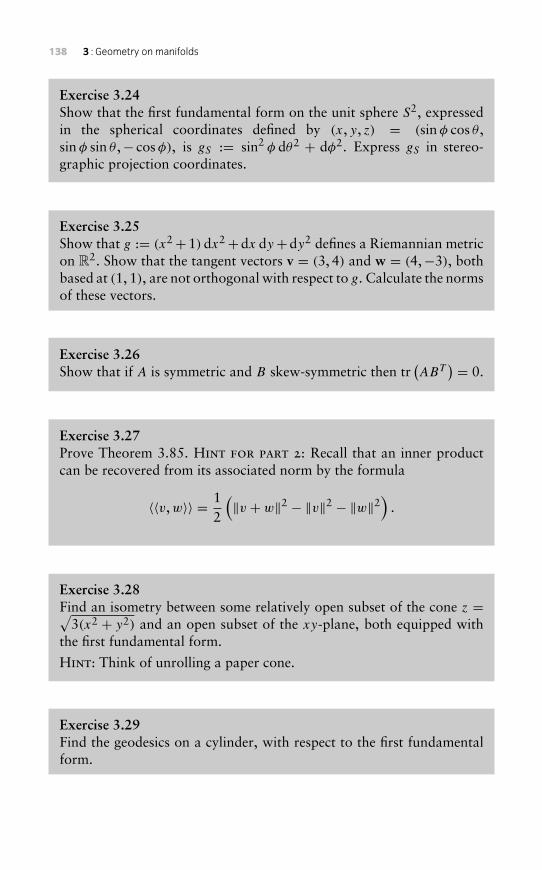
138 3 : Geometry on manifolds
Exercise 3.24Show that the first fundamental form on the unit sphere S2, expressedin the spherical coordinates defined by (x, y, z) = (sinφ cos θ ,sinφ sin θ ,− cosφ), is gS := sin2 φ dθ2 + dφ2. Express gS in stereo-graphic projection coordinates.
Exercise 3.25Show that g := (x2+1) dx2+dx dy+dy2 defines a Riemannian metricon R2. Show that the tangent vectors v = (3, 4) and w = (4,−3), bothbased at (1, 1), are not orthogonal with respect to g. Calculate the normsof these vectors.
Exercise 3.26Show that if A is symmetric and B skew-symmetric then tr
(ABT
) = 0.
Exercise 3.27Prove Theorem 3.85. Hint for part 2: Recall that an inner productcan be recovered from its associated norm by the formula
〈〈v,w〉〉 = 12
(‖v + w‖2 − ‖v‖2 − ‖w‖2
).
Exercise 3.28Find an isometry between some relatively open subset of the cone z =√
3(x2 + y2) and an open subset of the xy-plane, both equipped withthe first fundamental form.
Hint: Think of unrolling a paper cone.
Exercise 3.29Find the geodesics on a cylinder, with respect to the first fundamentalform.
3.5 Symplectic geometry 139
Exercise 3.30Find the geodesics on a cone, with respect to the first fundamental form.Hint: use Exercise 3.28 and the fact that the geodesics for the Euclideanmetric in Rn are straight lines (see Example 3.81).
Exercise 3.31Show that the Euler–Lagrange equations for geodesics, eqn (3.17), areequivalent to the geodesic equations,
qm + �mij q
i qj = 0, (3.18)
where
�mij := 1
2gkm
(∂gik
∂qj+ ∂gjk
∂qi− ∂gij
∂qk
).
By gkm(q) we mean the (k,m)th entry of the inverse of the matrix[gij (q)
]. An equivalent definition is: gikg
km = δmi , for all i,m. The �mij
are called the Christoffel symbols, of the second kind, of the Levi–Civitaconnection on (Q, g).
Exercise 3.32Check that great circles on S2 satisfy the geodesic equations for the firstfundamental form.
Hint: without loss of generality, it suffices to consider ‘the Equator’.
3.5 Symplectic geometry
Symplectic geometry has played a central role in the mathematical devel-opment of Hamiltonian mechanics. For simplicity, we have chosen notto emphasize it in this book. Instead, we present Hamiltonian mechan-ics via Poisson brackets, which generalize symplectic forms and aresomewhat easier to define. This section is included mostly for generalknowledge.
Recall that a bilinear form is non-degenerate if its matrix is non-singular.
140 3 : Geometry on manifolds
Definition 3.89 A symplectic bilinear form is one that is skew-symmetricand non-degenerate. A vector space with an associated symplectic bilinearform is called a symplectic vector space.
Example 3.90 The canonical symplectic bilinear form on R2n is
ω ((x1, y1), (x2, y2)) := x1 · y2 − x2 · y1.
Its matrix, with respect to the standard basis, is
J :=[
0 I
−I 0
], (3.19)
where I is the n× n identity matrix. Note that, in R2, the bilinear form ω
is the standard area form (see Example 3.52).
Remark 3.91 If R2n is identified with Cn via(x1, . . . , xn, y1, . . . , yn
)↔(x1 + iy1, . . . , xn + iyn
),
then the matrix of the canonical symplectic form can be written as −iI (ann×n complex diagonal matrix). Etymological note: ‘symplectic’ is the greektranslation of the latin ‘complex’.
In order to define symplectic forms on manifolds, we first need tointroduce some of the theory of differential forms.
Definition 3.92 A differential form (or simply form) is a skew-symmetriccovariant tensor field.3 An n-form is a form of rank n.
Some examples are:
• a scalar field is a 0-form;
• differential 1-forms satisfy the general definition because all 1-tensors areautomatically skew-symmetric;
• the area form on any surface in R3, defined in Example 3.52, is adifferential 2-form.
• the volume form µ in R3, defined by µ(z)(u, v,w) := (u × v) · w, is adifferential 3-form.
3 Confusingly, bilinear forms can be skew-symmetric, symmetric or neither, whiledifferential forms are assumed to be skew-symmetric.
3.5 Symplectic geometry 141
One of the main uses of differential forms is to define integration on man-ifolds. We will not develop the theory of differential forms here. Instead,we will give the bare minimum to allow us to define symplectic forms, inparticular what it means for a form to be closed. We need to define theexterior derivative operation, which in turn can be described in terms ofthe wedge product.
Recall from Section 3.3 the wedge product of two 1-forms,
α ∧ β = α ⊗ β − β ⊗ α, i.e.
(α ∧ β) (z)(v,w) = α(z)(v) β(z)(w)− α(z)(w)β(z)(v).
Example 3.93 If x1, x2 are coordinates, then(dx1 ∧ dx2
)(x)(u, v) = u1v2 − v1u2.
The next two definitions generalize the wedge product.
Definition 3.94 The wedge product of 1-forms α1, . . . ,αr on a givenmanifold is
α1 ∧ · · · ∧ αr :=∑σ∈Sr
sign(σ ) ασ(1) ⊗ · · · ⊗ ασ(r),
where the sum runs over all permutations σ of the indices {1, . . . , r}, andsign(σ ) is +1 if σ is an even permutation and −1 if it is odd.
Example 3.95 Let x, y, z be the standard coordinates on R3.(dx ∧ dy ∧ dz
)(x)(u, v,w)
= (dx ⊗ dy ⊗ dz+ dy ⊗ dz⊗ dx + dz⊗ dx ⊗ dy − dy ⊗ dx ⊗ dz
− dx ⊗ dz⊗ dy − dz⊗ dy ⊗ dx) (x)(u, v,w)
= u1v2w3 + u2v3w1 + u3v1w2 − u2v1w3 − u1v3w2 − u3v2w1
= (u× v) ·w.
Thus, dx ∧ dy ∧ dz = µ, the volume form on R3.
Remark 3.96 It follows easily from the previous definition that inter-changing the order of any two of the arguments in the wedge product of1-forms multiplies the result by −1. Thus, if any two arguments are iden-tical, the wedge product must be zero, for example dx ∧ dy ∧ dx = 0. Afurther implication is that α1 ∧ · · · ∧ αr is a differential r-form.
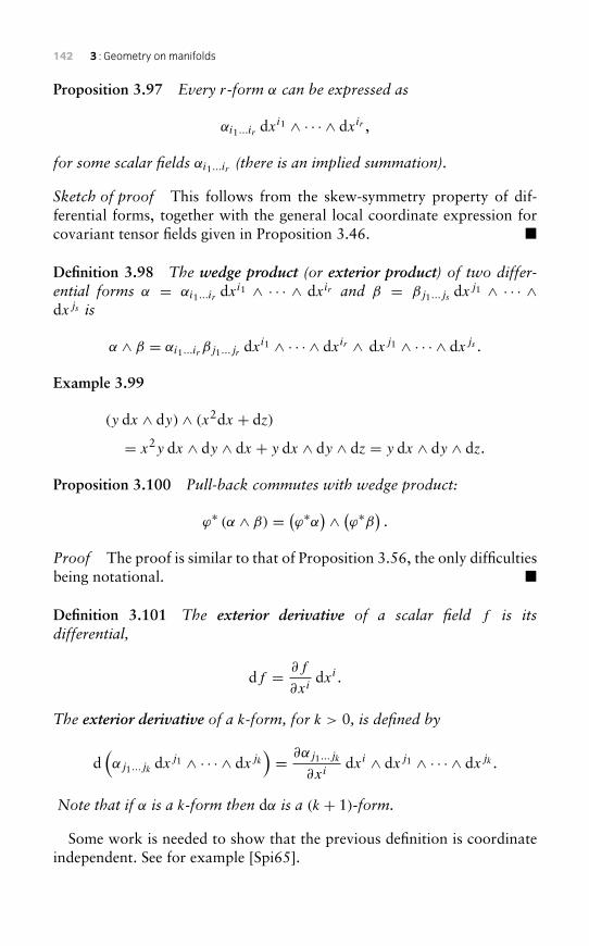
142 3 : Geometry on manifolds
Proposition 3.97 Every r-form α can be expressed as
αi1...ir dxi1 ∧ · · · ∧ dxir ,
for some scalar fields αi1...ir (there is an implied summation).
Sketch of proof This follows from the skew-symmetry property of dif-ferential forms, together with the general local coordinate expression forcovariant tensor fields given in Proposition 3.46. �
Definition 3.98 The wedge product (or exterior product) of two differ-ential forms α = αi1...ir dxi1 ∧ · · · ∧ dxir and β = βj1...js dxj1 ∧ · · · ∧dxjs is
α ∧ β = αi1...ir βj1...jr dxi1 ∧ · · · ∧ dxir ∧ dxj1 ∧ · · · ∧ dxjs .
Example 3.99
(y dx ∧ dy) ∧ (x2dx + dz)
= x2y dx ∧ dy ∧ dx + y dx ∧ dy ∧ dz = y dx ∧ dy ∧ dz.
Proposition 3.100 Pull-back commutes with wedge product:
ϕ∗ (α ∧ β) = (ϕ∗α) ∧ (ϕ∗β) .Proof The proof is similar to that of Proposition 3.56, the only difficultiesbeing notational. �
Definition 3.101 The exterior derivative of a scalar field f is itsdifferential,
df = ∂f
∂xidxi .
The exterior derivative of a k-form, for k > 0, is defined by
d(αj1...jk dxj1 ∧ · · · ∧ dxjk
)= ∂αj1...jk
∂xidxi ∧ dxj1 ∧ · · · ∧ dxjk .
Note that if α is a k-form then dα is a (k + 1)-form.
Some work is needed to show that the previous definition is coordinateindependent. See for example [Spi65].
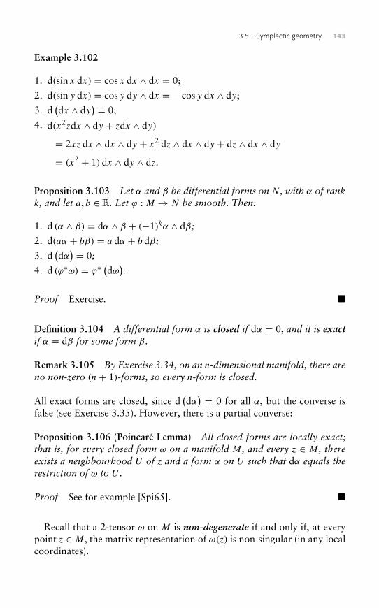
3.5 Symplectic geometry 143
Example 3.102
1. d(sin x dx) = cos x dx ∧ dx = 0;
2. d(sin y dx) = cos y dy ∧ dx = − cos y dx ∧ dy;
3. d(dx ∧ dy
) = 0;
4. d(x2zdx ∧ dy + zdx ∧ dy)
= 2xz dx ∧ dx ∧ dy + x2 dz ∧ dx ∧ dy + dz ∧ dx ∧ dy
= (x2 + 1) dx ∧ dy ∧ dz.
Proposition 3.103 Let α and β be differential forms on N , with α of rankk, and let a, b ∈ R. Let ϕ : M → N be smooth. Then:
1. d (α ∧ β) = dα ∧ β + (−1)kα ∧ dβ;
2. d(aα + bβ) = a dα + b dβ;
3. d(dα) = 0;
4. d (ϕ∗ω) = ϕ∗(dω).
Proof Exercise. �
Definition 3.104 A differential form α is closed if dα = 0, and it is exactif α = dβ for some form β.
Remark 3.105 By Exercise 3.34, on an n-dimensional manifold, there areno non-zero (n+ 1)-forms, so every n-form is closed.
All exact forms are closed, since d(dα) = 0 for all α, but the converse is
false (see Exercise 3.35). However, there is a partial converse:
Proposition 3.106 (Poincaré Lemma) All closed forms are locally exact;that is, for every closed form ω on a manifold M, and every z ∈ M, thereexists a neighbourhood U of z and a form α on U such that dα equals therestriction of ω to U .
Proof See for example [Spi65]. �
Recall that a 2-tensor ω on M is non-degenerate if and only if, at everypoint z ∈ M, the matrix representation of ω(z) is non-singular (in any localcoordinates).
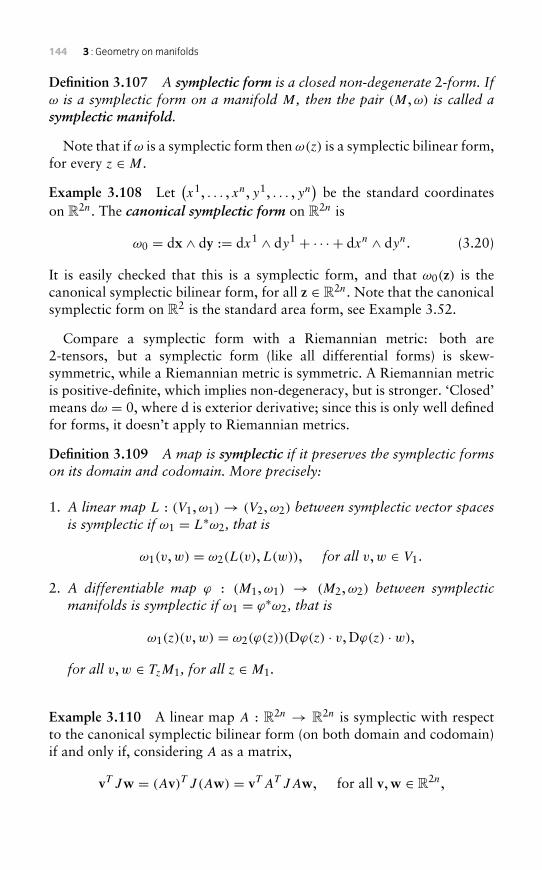
144 3 : Geometry on manifolds
Definition 3.107 A symplectic form is a closed non-degenerate 2-form. Ifω is a symplectic form on a manifold M, then the pair (M,ω) is called asymplectic manifold.
Note that if ω is a symplectic form then ω(z) is a symplectic bilinear form,for every z ∈ M.
Example 3.108 Let(x1, . . . , xn, y1, . . . , yn
)be the standard coordinates
on R2n. The canonical symplectic form on R2n is
ω0 = dx ∧ dy := dx1 ∧ dy1 + · · · + dxn ∧ dyn. (3.20)
It is easily checked that this is a symplectic form, and that ω0(z) is thecanonical symplectic bilinear form, for all z ∈ R2n. Note that the canonicalsymplectic form on R2 is the standard area form, see Example 3.52.
Compare a symplectic form with a Riemannian metric: both are2-tensors, but a symplectic form (like all differential forms) is skew-symmetric, while a Riemannian metric is symmetric. A Riemannian metricis positive-definite, which implies non-degeneracy, but is stronger. ‘Closed’means dω = 0, where d is exterior derivative; since this is only well definedfor forms, it doesn’t apply to Riemannian metrics.
Definition 3.109 A map is symplectic if it preserves the symplectic formson its domain and codomain. More precisely:
1. A linear map L : (V1,ω1)→ (V2,ω2) between symplectic vector spacesis symplectic if ω1 = L∗ω2, that is
ω1(v,w) = ω2(L(v),L(w)), for all v,w ∈ V1.
2. A differentiable map ϕ : (M1,ω1) → (M2,ω2) between symplecticmanifolds is symplectic if ω1 = ϕ∗ω2, that is
ω1(z)(v,w) = ω2(ϕ(z))(Dϕ(z) · v, Dϕ(z) · w),
for all v,w ∈ TzM1, for all z ∈ M1.
Example 3.110 A linear map A : R2n → R2n is symplectic with respectto the canonical symplectic bilinear form (on both domain and codomain)if and only if, considering A as a matrix,
vT Jw = (Av)T J (Aw) = vT AT JAw, for all v,w ∈ R2n,
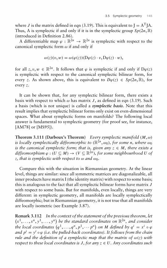
3.5 Symplectic geometry 145
where J is the matrix defined in eqn (3.19). This is equivalent to J = ATJA.Thus, A is symplectic if and only if it is in the symplectic group Sp(2n, R)
(introduced in Definition 2.86).A differentiable map ϕ : R2n → R2n is symplectic with respect to the
canonical symplectic form ω if and only if
ω(z)(v,w) = ω(ϕ(z))(Dϕ(z) · v, Dϕ(z) · w),
for all z, v,w ∈ R2n. It follows that ϕ is symplectic if and only if Dϕ(z)
is symplectic with respect to the canonical symplectic bilinear form, forevery z. As shown above, this is equivalent to Dϕ(z) ∈ Sp(2n, R), forevery z.
It can be shown that, for any symplectic bilinear form, there exists abasis with respect to which ω has matrix J , as defined in eqn (3.19). Sucha basis (which is not unique) is called a symplectic basis. Note that thisresult implies that symplectic bilinear forms only exist on even-dimensionalspaces. What about symplectic forms on manifolds? The following localanswer is fundamental to symplectic geometry (for proof see, for instance,[AM78] or [MS95]).
Theorem 3.111 (Darboux’s Theorem) Every symplectic manifold (M,ω)
is locally symplectically diffeomorphic to (R2n,ω0), for some n, where ω0is the canonical symplectic form; that is, given any z ∈ M, there exists adiffeomorphism ϕ : (U ⊆ M)→ (V ⊆ R2n), for some neighbourhood U ofz, that is symplectic with respect to ω and ω0.
Compare this with the situation in Riemannian geometry. At the linearlevel, things are similar: since all symmetric matrices are diagonalizable, allinner products have matrix I (the identity matrix) with respect to some basis;this is analogous to the fact that all symplectic bilinear forms have matrix J
with respect to some basis. But for manifolds, even locally, things are verydifferent: in symplectic geometry, all manifolds are locally symplecticallydiffeomorphic; but in Riemannian geometry, it is not true that all manifoldsare locally isometric (see Example 3.87).
Remark 3.112 In the context of the statement of the previous theorem, let(x1, . . . , xn, y1, . . . , yn
)be the standard coordinates on R2n, and consider
the local coordinates(q1, . . . , qn,p1, · · ·pn
)on M defined by qi = xi ◦ ϕ
and pi = yi ◦ϕ (i.e. the pulled-back coordinates). It follows from the chainrule and the definition of a symplectic map that the matrix of ω(z) withrespect to these local coordinates is J , for any z ∈ U . Any coordinates such
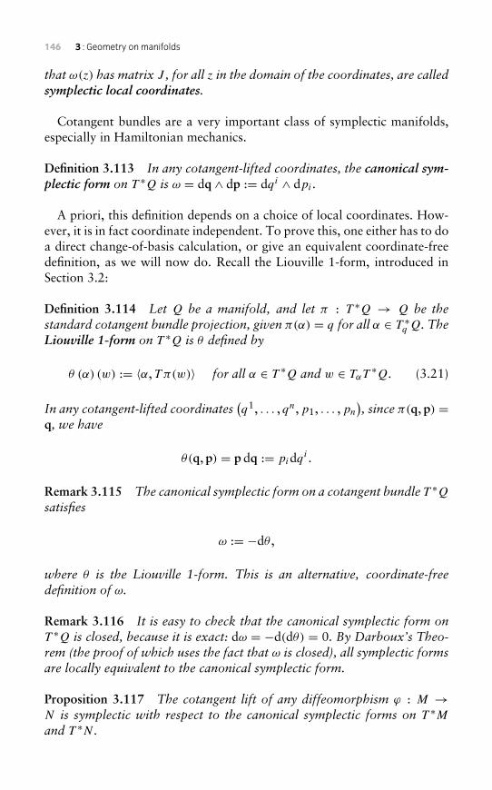
146 3 : Geometry on manifolds
that ω(z) has matrix J , for all z in the domain of the coordinates, are calledsymplectic local coordinates.
Cotangent bundles are a very important class of symplectic manifolds,especially in Hamiltonian mechanics.
Definition 3.113 In any cotangent-lifted coordinates, the canonical sym-plectic form on T ∗Q is ω = dq ∧ dp := dqi ∧ dpi .
A priori, this definition depends on a choice of local coordinates. How-ever, it is in fact coordinate independent. To prove this, one either has to doa direct change-of-basis calculation, or give an equivalent coordinate-freedefinition, as we will now do. Recall the Liouville 1-form, introduced inSection 3.2:
Definition 3.114 Let Q be a manifold, and let π : T ∗Q → Q be thestandard cotangent bundle projection, given π(α) = q for all α ∈ T ∗q Q. TheLiouville 1-form on T ∗Q is θ defined by
θ (α) (w) := 〈α, T π(w)〉 for all α ∈ T ∗Q and w ∈ TαT∗Q. (3.21)
In any cotangent-lifted coordinates(q1, . . . , qn,p1, . . . ,pn
), since π(q, p) =
q, we have
θ(q, p) = p dq := pidqi .
Remark 3.115 The canonical symplectic form on a cotangent bundle T ∗Qsatisfies
ω := −dθ ,
where θ is the Liouville 1-form. This is an alternative, coordinate-freedefinition of ω.
Remark 3.116 It is easy to check that the canonical symplectic form onT ∗Q is closed, because it is exact: dω = −d(dθ) = 0. By Darboux’s Theo-rem (the proof of which uses the fact that ω is closed), all symplectic formsare locally equivalent to the canonical symplectic form.
Proposition 3.117 The cotangent lift of any diffeomorphism ϕ : M →N is symplectic with respect to the canonical symplectic forms on T ∗Mand T ∗N .
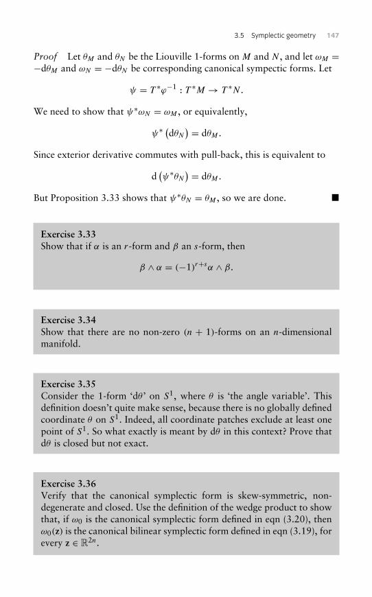
3.5 Symplectic geometry 147
Proof Let θM and θN be the Liouville 1-forms on M and N , and let ωM =−dθM and ωN = −dθN be corresponding canonical sympectic forms. Let
ψ = T ∗ϕ−1 : T ∗M → T ∗N .
We need to show that ψ∗ωN = ωM , or equivalently,
ψ∗(dθN
) = dθM .
Since exterior derivative commutes with pull-back, this is equivalent to
d(ψ∗θN
) = dθM .
But Proposition 3.33 shows that ψ∗θN = θM , so we are done. �
Exercise 3.33Show that if α is an r-form and β an s-form, then
β ∧ α = (−1)r+sα ∧ β.
Exercise 3.34Show that there are no non-zero (n + 1)-forms on an n-dimensionalmanifold.
Exercise 3.35Consider the 1-form ‘dθ ’ on S1, where θ is ‘the angle variable’. Thisdefinition doesn’t quite make sense, because there is no globally definedcoordinate θ on S1. Indeed, all coordinate patches exclude at least onepoint of S1. So what exactly is meant by dθ in this context? Prove thatdθ is closed but not exact.
Exercise 3.36Verify that the canonical symplectic form is skew-symmetric, non-degenerate and closed. Use the definition of the wedge product to showthat, if ω0 is the canonical symplectic form defined in eqn (3.20), thenω0(z) is the canonical bilinear symplectic form defined in eqn (3.19), forevery z ∈ R2n.
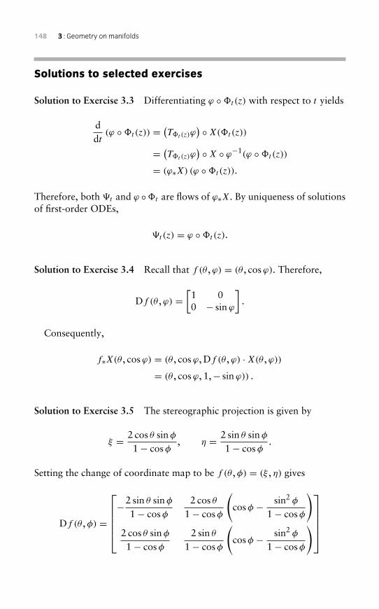
148 3 : Geometry on manifolds
Solutions to selected exercises
Solution to Exercise 3.3 Differentiating ϕ ◦�t(z) with respect to t yields
ddt
(ϕ ◦�t(z)) =(T�t (z)ϕ
) ◦X(�t(z))
= (T�t (z)ϕ) ◦X ◦ ϕ−1(ϕ ◦�t(z))
= (ϕ∗X) (ϕ ◦�t(z)).
Therefore, both �t and ϕ ◦�t are flows of ϕ∗X. By uniqueness of solutionsof first-order ODEs,
�t(z) = ϕ ◦�t(z).
Solution to Exercise 3.4 Recall that f (θ ,ϕ) = (θ , cosϕ). Therefore,
Df (θ ,ϕ) =[1 00 − sin ϕ
].
Consequently,
f∗X(θ , cosϕ) = (θ , cosϕ, Df (θ ,ϕ) ·X(θ ,ϕ))
= (θ , cosϕ, 1,− sin ϕ)) .
Solution to Exercise 3.5 The stereographic projection is given by
ξ = 2 cos θ sinφ
1− cosφ, η = 2 sin θ sinφ
1− cosφ.
Setting the change of coordinate map to be f (θ ,φ) = (ξ , η) gives
Df (θ ,φ) =
−2 sin θ sinφ
1− cosφ2 cos θ
1− cosφ
(cosφ − sin2 φ
1− cosφ
)2 cos θ sinφ
1− cosφ2 sin θ
1− cosφ
(cosφ − sin2 φ
1− cosφ
)
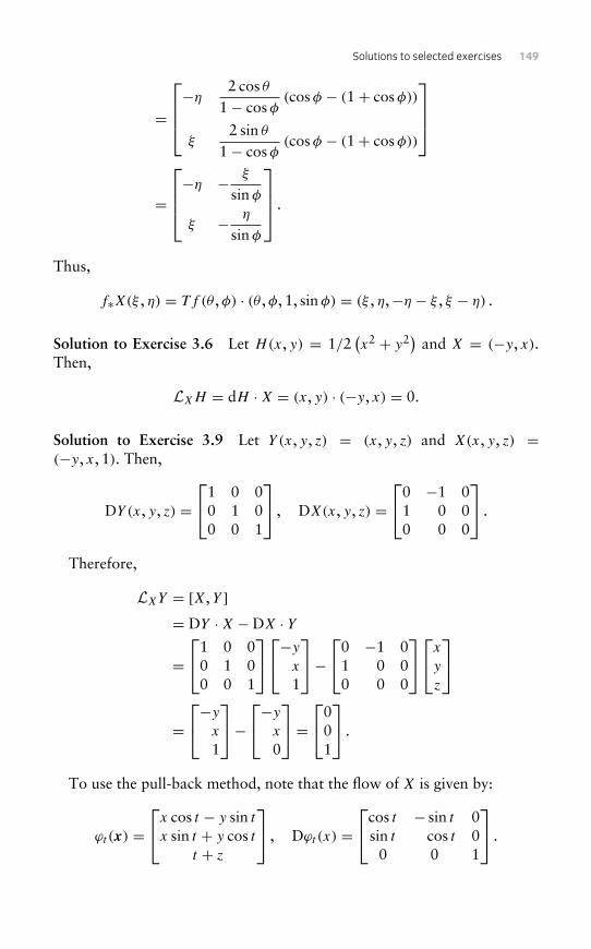
Solutions to selected exercises 149
=
−η2 cos θ
1− cosφ(cosφ − (1+ cosφ))
ξ2 sin θ
1− cosφ(cosφ − (1+ cosφ))
=
−η − ξ
sinφ
ξ − η
sinφ
.
Thus,
f∗X(ξ , η) = Tf (θ ,φ) · (θ ,φ, 1, sinφ) = (ξ , η,−η − ξ , ξ − η) .
Solution to Exercise 3.6 Let H(x, y) = 1/2(x2 + y2) and X = (−y, x).
Then,
LXH = dH ·X = (x, y) · (−y, x) = 0.
Solution to Exercise 3.9 Let Y (x, y, z) = (x, y, z) and X(x, y, z) =(−y, x, 1). Then,
DY (x, y, z) =1 0 0
0 1 00 0 1
, DX(x, y, z) =0 −1 0
1 0 00 0 0
.
Therefore,
LXY = [X,Y ]= DY ·X −DX · Y
=1 0 0
0 1 00 0 1
−yx1
−0 −1 0
1 0 00 0 0
x
y
z
=−yx
1
−−yx
0
=0
01
.
To use the pull-back method, note that the flow of X is given by:
ϕt (x) =x cos t − y sin t
x sin t + y cos tt + z
, Dϕt (x) =cos t − sin t 0
sin t cos t 00 0 1
.
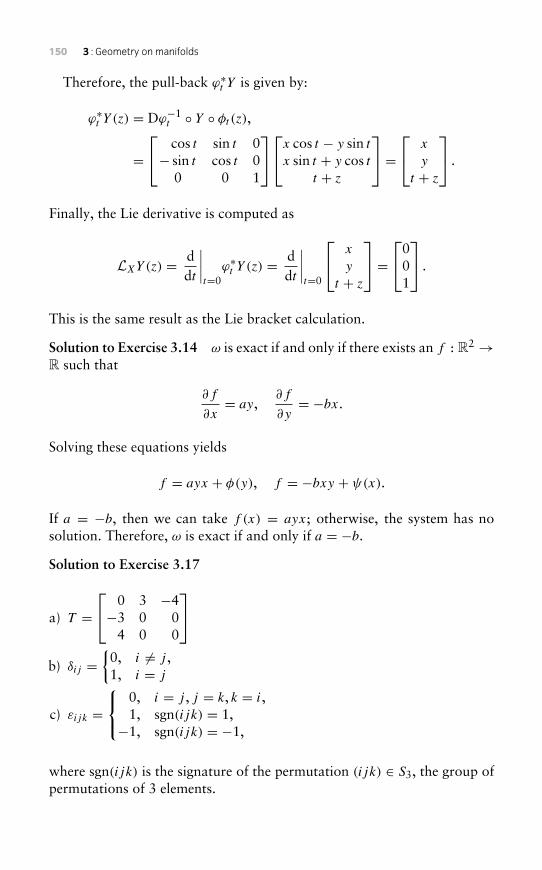
150 3 : Geometry on manifolds
Therefore, the pull-back ϕ∗t Y is given by:
ϕ∗t Y (z) = Dϕ−1t ◦ Y ◦ φt (z),
= cos t sin t 0− sin t cos t 0
0 0 1
x cos t − y sin t
x sin t + y cos tt + z
= x
y
t + z
.
Finally, the Lie derivative is computed as
LXY(z) = ddt
∣∣∣∣t=0
ϕ∗t Y (z) = ddt
∣∣∣∣t=0
x
y
t + z
=0
01
.
This is the same result as the Lie bracket calculation.
Solution to Exercise 3.14 ω is exact if and only if there exists an f : R2 →R such that
∂f
∂x= ay,
∂f
∂y= −bx.
Solving these equations yields
f = ayx + φ(y), f = −bxy + ψ(x).
If a = −b, then we can take f (x) = ayx; otherwise, the system has nosolution. Therefore, ω is exact if and only if a = −b.Solution to Exercise 3.17
a) T = 0 3 −4−3 0 0
4 0 0
b) δij =
{0, i �= j ,1, i = j
c) εijk =
0, i = j , j = k, k = i,1, sgn(ijk) = 1,−1, sgn(ijk) = −1,
where sgn(ijk) is the signature of the permutation (ijk) ∈ S3, the group ofpermutations of 3 elements.
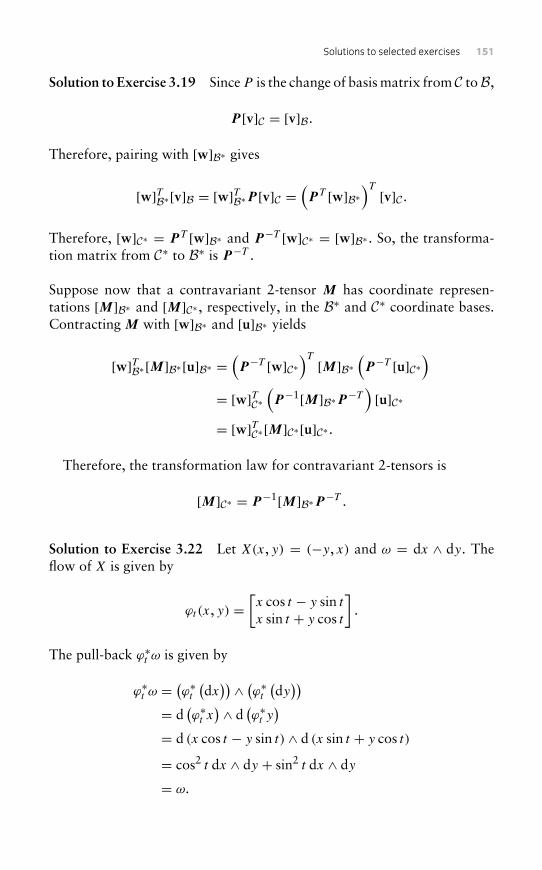
Solutions to selected exercises 151
Solution to Exercise 3.19 SinceP is the change of basis matrix from C to B,
P [v]C = [v]B.
Therefore, pairing with [w]B∗ gives
[w]TB∗[v]B = [w]TB∗P [v]C =(P T [w]B∗
)T [v]C .
Therefore, [w]C∗ = P T [w]B∗ and P−T [w]C∗ = [w]B∗ . So, the transforma-tion matrix from C∗ to B∗ is P−T .
Suppose now that a contravariant 2-tensor M has coordinate represen-tations [M]B∗ and [M]C∗ , respectively, in the B∗ and C∗ coordinate bases.Contracting M with [w]B∗ and [u]B∗ yields
[w]TB∗[M]B∗[u]B∗ =(P−T [w]C∗
)T [M]B∗ (P−T [u]C∗)= [w]TC∗
(P−1[M]B∗P−T
)[u]C∗
= [w]TC∗[M]C∗[u]C∗ .
Therefore, the transformation law for contravariant 2-tensors is
[M]C∗ = P−1[M]B∗P−T .
Solution to Exercise 3.22 Let X(x, y) = (−y, x) and ω = dx ∧ dy. Theflow of X is given by
ϕt (x, y) =[x cos t − y sin t
x sin t + y cos t
].
The pull-back ϕ∗t ω is given by
ϕ∗t ω =(ϕ∗t(dx)) ∧ (ϕ∗t (dy))
= d(ϕ∗t x
) ∧ d(ϕ∗t y
)= d (x cos t − y sin t) ∧ d (x sin t + y cos t)
= cos2 t dx ∧ dy + sin2 t dx ∧ dy
= ω.
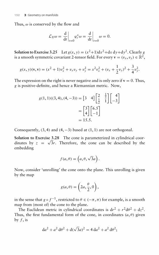
152 3 : Geometry on manifolds
Thus, ω is conserved by the flow and
LXω = ddt
∣∣∣∣t=0
ϕ∗t ω =ddt
∣∣∣∣t=0
ω = 0.
Solution to Exercise 3.25 Let g(x, y) = (x2+1)dx2+dx dy+dy2. Clearly g
is a smooth symmetric covariant 2-tensor field. For every v = (vx , vy) ∈ R2,
g(x, y)(v, v) = (x2 + 1)v2x + vxvy + v2
y = x2v2x + (vx + 1
2vy)
2 + 34v2y .
The expression on the right is never negative and is only zero if v = 0. Thus,g is positive-definite, and hence a Riemannian metric. Now,
g(1, 1)((3, 4), (4,−3)) = [3 4] [2 1
212 1
] [4−3
]=[34
] [6.5−1
]= 15.5.
Consequently, (3, 4) and (4,−3) based at (1, 1) are not orthogonal.
Solution to Exercise 3.28 The cone is parameterized in cylindrical coor-dinates by z = √
3r. Therefore, the cone can be described by theembedding
f (a, θ) =(a, θ ,√
3a)
.
Now, consider ‘unrolling’ the cone onto the plane. This unrolling is givenby the map
g(a, θ) =(
2a,θ
2, 0)
,
in the sense that g ◦f−1, restricted to θ ∈ (−π ,π) for example, is a smoothmap from (most of) the cone to the plane.
The Euclidean metric in cylindrical coordinates is dr2 + r2dθ2 + dz2.Thus, the first fundamental form of the cone, in coordinates (a, θ) givenby f , is
da2 + a2 dθ2 + d(√
3a)2 = 4 da2 + a2 dθ2;
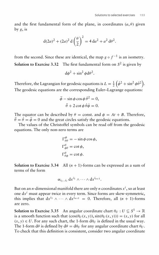
Solutions to selected exercises 153
and the first fundamental form of the plane, in coordinates (a, θ) givenby g, is
d(2a)2 + (2a)2 d(θ
2
)2
= 4 da2 + a2 dθ2.
from the second. Since these are identical, the map g ◦ f−1 is an isometry.
Solution to Exercise 3.32 The first fundamental form on S2 is given by
dφ2 + sin2 φdθ2.
Therefore, the Lagrangian for geodesic equations is L = 12
(φ2 + sin2 φθ2
).
The geodesic equations are the corresponding Euler–Lagrange equations:
φ − sinφ cosφ θ2 = 0,
θ + 2 cot φ θφ = 0.
The equator can be described by θ = const. and φ = At + B. Therefore,θ = θ = φ = 0 and the great circles satisfy the geodesic equations.
The values of the Christoffel symbols can be read off from the geodesicequations. The only non-zero terms are
�φθθ = − sinφ cosφ,
�θφθ = cot φ,
�θθφ = cot φ.
Solution to Exercise 3.34 All (n+ 1)-forms can be expressed as a sum ofterms of the form
αi1...ir dxi1 ∧ · · · ∧ dxin+1 .
But on an n-dimensional manifold there are only n coordinates xi , so at leastone dxi must appear twice in every term. Since forms are skew-symmetric,this implies that dxi1 ∧ · · · ∧ dxin+1 = 0. Therefore, all (n + 1)-formsare zero.
Solution to Exercise 3.35 An angular coordinate chart θU : U ⊆ S1 → R
is a smooth function such that (cos(θU (x, y)), sin(θU (x, y))) = (x, y) for all(x, y) ∈ U . For any such chart, the 1-form dθU is defined in the usual way.The 1-form dθ is defined by dθ = dθU for any angular coordinate chart θU .To check that this definition is consistent, consider two angular coordinate
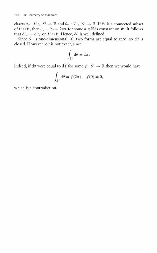
154 3 : Geometry on manifolds
charts θU : U ⊆ S1 → R and θV : V ⊆ S1 → R. If W is a connected subsetof U ∩ V , then θV − θU = 2nπ for some n ∈ N is constant on W . It followsthat dθU = dθV on U ∩ V . Hence, dθ is well defined.
Since S1 is one-dimensional, all two forms are equal to zero, so dθ isclosed. However, dθ is not exact, since∫
S1dθ = 2π .
Indeed, if dθ were equal to df for some f : S1 → R then we would have∫S1
dθ = f (2π)− f (0) = 0,
which is a contradiction.
4Mechanics on manifolds
Manifolds are locally equivalent to Euclidean spaces. The Lagrangian andHamiltonian formulations of mechanics on Euclidean spaces introducedin Chapter 1 provide the local mathematical formulations of mechanicson manifolds. However, global issues may still arise from the need to usemultiple coordinate charts.
This chapter reformulates some key definitions from Chapter 1 in acoordinate-free manner. This reformulation emphasizes the fundamen-tal concepts while suppressing inessential details. However, a return tocoordinate expressions is still necessary for doing calculations in examples.
We assume that all manifolds are finite-dimensional and all Lagrangiansare smooth.
4.1 Lagrangian mechanics on manifolds
In Chapter 1, working in Euclidean space, we saw that the Euler–Lagrangeequations:
ddt
(∂L
∂q
)= ∂L
∂q, (4.1)
are equivalent to Hamilton’s principle of stationary action: δS = 0, forthe action functional
S[q(·)] :=∫ b
a
L(q(t), q(t)) dt , (4.2)
with respect to variations among paths with fixed endpoints. Recall that anequivalent statement of Hamilton’s principle is:
∂
∂s
∫ b
a
L(q(t , s), q(t , s)) dt∣∣∣∣s=0= 0, (4.3)
for all deformations q(t , s) of q(t) leaving the endpoints fixed.In general, the configuration space is a manifoldQ . Recall from Chapter 2
that every local coordinate system(q1, . . . , qn
)onQ induces a tangent-lifted
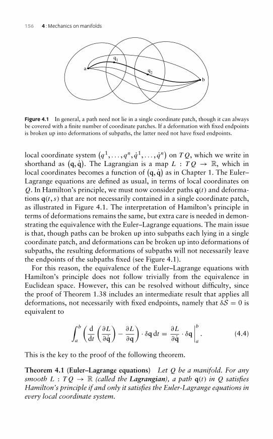
156 4 : Mechanics on manifolds
a
b
q1
q2
Figure 4.1 In general, a path need not lie in a single coordinate patch, though it can alwaysbe covered with a finite number of coordinate patches. If a deformation with fixed endpointsis broken up into deformations of subpaths, the latter need not have fixed endpoints.
local coordinate system(q1, . . . , qn, q1, . . . , qn
)on TQ, which we write in
shorthand as(q, q
). The Lagrangian is a map L : TQ → R, which in
local coordinates becomes a function of(q, q
)as in Chapter 1. The Euler–
Lagrange equations are defined as usual, in terms of local coordinates onQ. In Hamilton’s principle, we must now consider paths q(t) and deforma-tions q(t , s) that are not necessarily contained in a single coordinate patch,as illustrated in Figure 4.1. The interpretation of Hamilton’s principle interms of deformations remains the same, but extra care is needed in demon-strating the equivalence with the Euler–Lagrange equations. The main issueis that, though paths can be broken up into subpaths each lying in a singlecoordinate patch, and deformations can be broken up into deformations ofsubpaths, the resulting deformations of subpaths will not necessarily leavethe endpoints of the subpaths fixed (see Figure 4.1).
For this reason, the equivalence of the Euler–Lagrange equations withHamilton’s principle does not follow trivially from the equivalence inEuclidean space. However, this can be resolved without difficulty, sincethe proof of Theorem 1.38 includes an intermediate result that applies alldeformations, not necessarily with fixed endpoints, namely that δS = 0 isequivalent to ∫ b
a
(ddt
(∂L
∂q
)− ∂L
∂q
)· δq dt = ∂L
∂q· δq
∣∣∣∣ba
. (4.4)
This is the key to the proof of the following theorem.
Theorem 4.1 (Euler–Lagrange equations) Let Q be a manifold. For anysmooth L : TQ → R (called the Lagrangian), a path q(t) in Q satisfiesHamilton’s principle if and only it satisfies the Euler-Lagrange equations inevery local coordinate system.
4.1 Lagrangian mechanics on manifolds 157
Proof Let {t0 = a, t1, . . . , tr = b} be a partition of [a, b] such thatevery subpath from ti−1 to ti is contained in a single coordinate patch,as illustrated in Figure 4.1.
First suppose that q(t) satisfies the Euler–Lagrange equations every-where. Then Theorem 1.38 applies to every subpath of q(t), as does theintermediate result in eqn (4.4), giving∫ ti
ti−1
(ddt
(∂L
∂q
)− ∂L
∂q
)· δq dt = ∂L
∂q· δq
∣∣∣∣titi−1
, (4.5)
for any variation δq of the subpath. Now, let δq be a variation of the entirepath, such that δq(a) = δq(b) = 0. Then, the restriction of δq to anysubinterval [ti−1, ti] is a variation of the ith subpath, so the equation aboveholds for every subpath. When copies of this equation, for i = 1, . . . , r,
are added together, the terms ∂L∂q · δq
∣∣∣titi−1
cancel, leaving ∂L∂q · δq
∣∣∣ba, which
equals zero because of the assumption that δq(a) = δq(b) = 0.Conversely, suppose that q(t) satisfies Hamilton’s principle. Then eqn
(4.3) holds for any variation δq(t) that vanishes at the endpoints. For anyi, any variation of the ith subpath such that δq(ti−1) = δq(ti) = 0 canbe extended to a variation of the entire path that is trivial for t outside of[ti−1, ti], i.e. such that δq(t) = 0 for t outside of [ti−1, ti]. Unfortunately,this extension is not necessarily smooth, but we can approximate it arbi-trarily closely by smooth variations δq(t) that are trivial for t outside of[ti−1, ti]. Thus,∫ ti
ti−1
(ddt
(∂L
∂q
)− ∂L
∂q
)· δq dt �
∫ b
a
(d
dt
(∂L
∂q
)− ∂L
∂q
)· δq dt = 0,
(4.6)
where the δq on the left is the original variation on the subpath, and the δqon the right is a smooth approximation to the extension defined above. Itfollows, with a little analytical work, that in fact the left-hand side equalszero. Thus Hamilton’s principle holds for the subpath from ti−1 to ti , andthus by Theorem 1.38, the Euler–Lagrange equations are satisfied by thissubpath. Since this is true for all subpaths, the result follows. �
We now examine the Euler–Lagrange equations more closely. Expandingthe time derivative gives equivalent equations,
∂2L
∂q2 q+ ∂2L
∂q ∂qq = ∂L
∂q. (4.7)
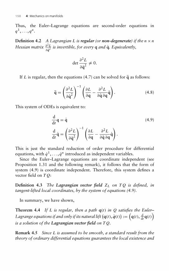
158 4 : Mechanics on manifolds
Thus, the Euler–Lagrange equations are second-order equations inq1, . . . , qn.
Definition 4.2 A Lagrangian L is regular (or non-degenerate) if the n× n
Hessian matrix ∂2L
∂q2 is invertible, for every q and q. Equivalently,
det∂2L
∂q2 �= 0.
If L is regular, then the equations (4.7) can be solved for q as follows:
q =(∂2L
∂q2
)−1 (∂L
∂q− ∂2L
∂q ∂qq
). (4.8)
This system of ODEs is equivalent to:
ddt
q = q (4.9)
ddt
q =(∂2L
∂q2
)−1 (∂L
∂q− ∂2L
∂q ∂qq
).
This is just the standard reduction of order procedure for differentialequations, with q1, . . . , qn introduced as independent variables.
Since the Euler–Lagrange equations are coordinate independent (seeProposition 1.31 and the following remark), it follows that the form ofsystem (4.9) is coordinate independent. Therefore, this system defines avector field on TQ:
Definition 4.3 The Lagrangian vector field ZL on TQ is defined, intangent-lifted local coordinates, by the system of equations (4.9).
In summary, we have shown,
Theorem 4.4 If L is regular, then a path q(t) in Q satisfies the Euler–
Lagrange equations if and only if its natural lift(q(t), q(t)
):=(q(t), d
dt q(t))
is a solution of the Lagrangian vector field on TQ.
Remark 4.5 Since L is assumed to be smooth, a standard result from thetheory of ordinary differential equations guarantees the local existence and
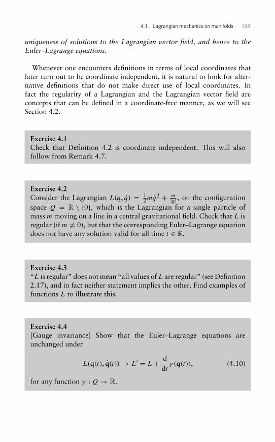
4.1 Lagrangian mechanics on manifolds 159
uniqueness of solutions to the Lagrangian vector field, and hence to theEuler–Lagrange equations.
Whenever one encounters definitions in terms of local coordinates thatlater turn out to be coordinate independent, it is natural to look for alter-native definitions that do not make direct use of local coordinates. Infact the regularity of a Lagrangian and the Lagrangian vector field areconcepts that can be defined in a coordinate-free manner, as we will seeSection 4.2.
Exercise 4.1Check that Definition 4.2 is coordinate independent. This will alsofollow from Remark 4.7.
Exercise 4.2Consider the Lagrangian L(q, q) = 1
2mq2 + m|q| , on the configuration
space Q = R \ {0}, which is the Lagrangian for a single particle ofmass m moving on a line in a central gravitational field. Check that L isregular (if m �= 0), but that the corresponding Euler–Lagrange equationdoes not have any solution valid for all time t ∈ R.
Exercise 4.3“L is regular” does not mean “all values ofL are regular” (see Definition2.17), and in fact neither statement implies the other. Find examples offunctions L to illustrate this.
Exercise 4.4[Gauge invariance] Show that the Euler–Lagrange equations areunchanged under
L(q(t), q(t))→ L′ = L+ ddt
γ (q(t)), (4.10)
for any function γ : Q→ R.
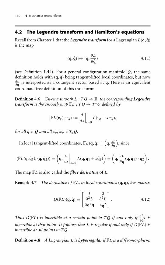
160 4 : Mechanics on manifolds
4.2 The Legendre transform and Hamilton’s equations
Recall from Chapter 1 that the Legendre transform for a Lagrangian L(q, q)is the map
(q, q) → (q,∂L
∂q) (4.11)
(see Definition 1.44). For a general configuration manifold Q, the samedefinition holds with (q, q) being tangent-lifted local coordinates, but now∂L
∂qis interpreted as a cotangent vector based at q. Here is an equivalent
coordinate-free definition of this transform:
Definition 4.6 Given a smooth L : TQ→ R, the corresponding Legendretransform is the smooth map FL : TQ→ T ∗Q defined by
〈FL(vq),wq〉 := d
ds
∣∣∣∣s=0
L(vq + swq),
for all q ∈ Q and all vq ,wq ∈ TqQ.
In local tangent-lifted coordinates, FL(q, q) =(q, ∂L
∂q
), since
〈FL(q, q1), (q, q2)〉 =(q,
dds
∣∣∣∣s=0
L(q, q1 + sq2)
)=(q,
∂L
∂q(q, q1) · q2
).
The map FL is also called the fibre derivative of L.
Remark 4.7 The derivative of FL, in local coordinates (q, q), has matrix
D(FL)(q, q) = I 0
∂2L
∂q∂q∂2L
∂q2
. (4.12)
Thus D(FL) is invertible at a certain point in TQ if and only if ∂2L
∂q2 is
invertible at that point. It follows that L is regular if and only if D(FL) isinvertible at all points in TQ.
Definition 4.8 A Lagrangian L is hyperregular if FL is a diffeomorphism.
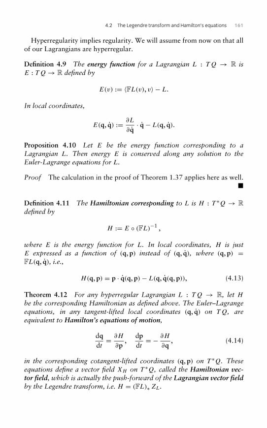
4.2 The Legendre transform and Hamilton’s equations 161
Hyperregularity implies regularity. We will assume from now on that allof our Lagrangians are hyperregular.
Definition 4.9 The energy function for a Lagrangian L : TQ → R isE : TQ→ R defined by
E(v) := 〈FL(v), v〉 − L.
In local coordinates,
E(q, q) := ∂L
∂q· q− L(q, q).
Proposition 4.10 Let E be the energy function corresponding to aLagrangian L. Then energy E is conserved along any solution to theEuler-Lagrange equations for L.
Proof The calculation in the proof of Theorem 1.37 applies here as well.�
Definition 4.11 The Hamiltonian corresponding to L is H : T ∗Q → R
defined by
H := E ◦ (FL)−1 ,
where E is the energy function for L. In local coordinates, H is justE expressed as a function of (q, p) instead of (q, q), where (q, p) =FL(q, q), i.e.,
H(q, p) = p · q(q, p)− L(q, q(q, p)), (4.13)
Theorem 4.12 For any hyperregular Lagrangian L : TQ → R, let Hbe the corresponding Hamiltonian as defined above. The Euler–Lagrangeequations, in any tangent-lifted local coordinates (q, q) on TQ, areequivalent to Hamilton’s equations of motion,
dqdt= ∂H
∂p,
dpdt= − ∂H
∂q, (4.14)
in the corresponding cotangent-lifted coordinates (q, p) on T ∗Q. Theseequations define a vector field XH on T ∗Q, called the Hamiltonian vec-tor field, which is actually the push-forward of the Lagrangian vector fieldby the Legendre transform, i.e. H = (FL)∗ ZL.
162 4 : Mechanics on manifolds
Proof The Euler–Lagrange equations, together with the equations dqdt= q,
form a system of implicit first order differential equations in the variables(q, q). Applying the Legendre transform gives the equivalent system
dpdt− ∂L
∂q= 0,
dqdt= q(q, p). (4.15)
In fact the vector field defined by these equations is the push-forward of theLagrangian vector field for L, as can be verified from eqns (4.8) and (4.12)(see Exercise 4.5). The resulting vector field is called XH . We now calculatethe partial derivatives of H :
∂H
∂q= p · ∂q(q, p)
∂q− ∂L
∂q− ∂L
∂q· ∂q(q, p)
∂q= −∂L
∂q
∂H
∂p= q(q, p)+ p · ∂q(q, p)
∂q− ∂L
∂q· ∂q(q, p)
∂p= q(q, p).
Substituting these into eqn (4.15) gives Hamilton’s equations. These are theequations for the vector field XH in local coordinates. �
Solutions to a Lagrangian system correspond to solutions to the asso-ciated Hamiltonian system. Specifically, if c(t) is a path in TQ that is asolution to a Lagrangian vector field, then FL ◦ c(t) is a path in T ∗Q that isa solution to the the associated Hamiltonian vector field. Both paths projectdown to the same path in Q, that is, they describe the same physical motion.In local coordinates, if c(t) = (q(t), q(t)) then FL ◦ c = (q(t), p(t)), withp(t) = ∂L
∂q (q(t), q(t)).
Hamilton’s equations can be studied for any H : T ∗Q → R, not justthose corresponding to Lagrangians:
Definition 4.13 Let H : T ∗Q → R be smooth. The Hamiltonian vectorfield corresponding to H is the vector field XH on T ∗Q that is given, in anycotangent-lifted coordinates, by Hamilton’s equations.
For this definition to make sense, it is necessary to verify that it iscoordinate independent. This is a direct consequence of the definitionof cotangent-lifted coordinates, and is left to Exercise 4.6. The resultshould be very plausible, since we have already seen that it is true forHamiltonians that correspond to Lagrangians. Indeed, in this case, Hamil-ton’s equations are equivalent to the Euler–Lagrange equations, which arecoordinate-independent.
Remark 4.14 Consider a Hamiltonian function H . If H is hyperregular(the definition is analagous to the definition for Lagrangians), then it is
4.2 The Legendre transform and Hamilton’s equations 163
possible to define a Lagrangian L in terms of H such that solutions to theLagrangian vector field ZL correspond to solutions to the Hamiltonian vec-tor field XH . Further, the two constructions: H from L, and L from H , areinverse to each other. Thus, there is a one-to-one correspondence betweenhyperregular Lagrangians and hyperregular Hamiltonians. For details, see[MR02].
Theorem 4.15 The Hamiltonian is a conserved quantity of the motiondefined by Hamilton’s equations.
Proof This can be verified directly by a simple calculation, which hasalready appeared in the proof of Theorem 1.56. �
Another important property of Hamiltonian systems is conservation ofphase space volume. For systems with one degree of freedom, i.e. a two-dimensional phase space, ‘phase-space volume’ is just area. In general, thephase-space volume of a region D ⊆ T ∗Q is the integral
vol(D) :=∫D
dq1dp1 · · ·dqndpn.
This definition is independent of the choice of cotangent-lifted coordinates(see Exercise 4.8), and it can be extended to domains D that do not lie in asingle coordinate patch. The flow � of a vector field is volume preservingif every time-t map �t preserves phase space volume, that is, vol(D) =vol (�t (D)), for every subset D of the phase space.
Theorem 4.16 The flow of a Hamiltonian vector field is volume-preserving.
Sketch of proof The divergence of a Hamiltonian vector field is zero:
∇ ·XH =(
∂
∂qi
∂H
∂pi
)+ ∂
∂qi
(−∂H
∂pi
)= 0.
In two (or three) dimensions, it is intuitively clear that the flow of adivergence-free vector field preserves area (or volume). This is proven invector calculus texts, e.g., [Spi65], and the proof generalizes to arbitrarymanifolds [Spi79]. �
For Hamiltonian systems with one degree of freedom, the previous theo-rem states that the flow of the system is area preserving. This is illustratedfor a simple example in Figure 4.2.
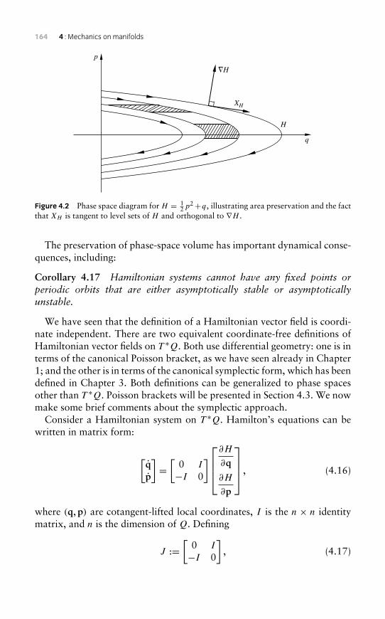
164 4 : Mechanics on manifolds
XH
q
p
H
�H
Figure 4.2 Phase space diagram for H = 12p
2+q, illustrating area preservation and the factthat XH is tangent to level sets of H and orthogonal to ∇H .
The preservation of phase-space volume has important dynamical conse-quences, including:
Corollary 4.17 Hamiltonian systems cannot have any fixed points orperiodic orbits that are either asymptotically stable or asymptoticallyunstable.
We have seen that the definition of a Hamiltonian vector field is coordi-nate independent. There are two equivalent coordinate-free definitions ofHamiltonian vector fields on T ∗Q. Both use differential geometry: one is interms of the canonical Poisson bracket, as we have seen already in Chapter1; and the other is in terms of the canonical symplectic form, which has beendefined in Chapter 3. Both definitions can be generalized to phase spacesother than T ∗Q. Poisson brackets will be presented in Section 4.3. We nowmake some brief comments about the symplectic approach.
Consider a Hamiltonian system on T ∗Q. Hamilton’s equations can bewritten in matrix form:
[qp
]=[
0 I
−I 0
]∂H
∂q∂H
∂p
, (4.16)
where (q, p) are cotangent-lifted local coordinates, I is the n × n identitymatrix, and n is the dimension of Q. Defining
J :=[
0 I
−I 0
], (4.17)
4.2 The Legendre transform and Hamilton’s equations 165
the matrix form of Hamilton’s equations can be re-expressed as
XH = J∇H . (4.18)
Recall from Chapter 3 the canonical symplectic form ω := −dθ , where θ isthe canonical 1-form. In cotangent lifted coordinates,
ω = dqi ∧ dpi .
The matrix of ω in these coordinates is constant and equals J as definedabove. It follows that, for any v,w ∈ R2n,
ω(q, p)(v,w) = vT Jw.
In particular, since J−1 = −J ,
ω(XH(q, p),w) = XTH (q, p) J w = (∇H(q, p))T w = dH(q, p)(w),
for all w. Thus,
ω(XH , ·) = dH . (4.19)
This is the coordinate-independent definition of XH . More common waysof writing the left-hand side in differential geometry are XH ω or iXH
ω.The coordinate-free definition of XH in eqn (4.19) is valid on any man-
ifold with a symplectic form. Thus, Hamiltonian systems can be definedand studied on phase spaces that are not cotangent bundles. An example isgiven in Exercise 4.9.
Exercise 4.5Given the formula for the Lagrangian vector fieldZL in local coordinatesin eqn (4.8), and the formula for the matrix of D(FL)(q, q) in eqn (4.12),calculate the push-forward of ZL by FL, and show that the result is thesystem in Equation 4.15.
Exercise 4.6Show that Hamilton’s equations are coordinate independent, so theyuniquely define a Hamiltonian vector field. In other words, show thatif (q, p) and (r, s) are two systems of cotangent-lifted local coordinatesfor the same domain, then a trajectory satisfies Hamilton’s equationsfor (q, p) if and only if it satisfies Hamilton’s equations for (r, s).
166 4 : Mechanics on manifolds
Exercise 4.7[Spherical pendulum] The spherical pendulum, defined in Exercise 1.42,has configuration space S2. Write down its Lagrangian and the equa-tions of motion, in spherical coordinates. Show explicitly that theLagrangian is hyperregular. Use the Legendre transformation to con-vert the equations to Hamiltonian form. Find the conservation lawcorresponding to angular momentum about the axis of gravity by “barehands” methods.
Exercise 4.8Show that if (q, p) and (r, s) are two sets of cotangent-lifted coordi-nates with the same domain, and D is a subset of this domain, then thephase-space volume of D is the same in both coordinate systems, i.e.if D1 is the domain expressed in (q, p) coordinates and D2 is the samedomain expressed in (r, s) coordinates, then
∫D1
dq1dp1 · · ·dqndpn =∫D2
dr1ds1 · · ·drndsn.
Exercise 4.9Let ω be the area form on S2, which is a symplectic form. LetH(x, y, z) = z. Calculate XH .
4.3 Hamiltonian mechanics on Poisson manifolds
Recall the definition of the canonical Poisson bracket from Chapter 1,which we can rewrite, using coordinates
(q1, . . . , qn,p1, . . . ,pn
), as
{F ,G} := ∂F
∂qi
∂G
∂pi
− ∂F
∂pi
∂G
∂qi. (4.20)
The same definition applies to cotangent bundles T ∗Q, for arbitrarymanifoldsQ, using cotangent-lifted local coordinates. The definition is inde-pendent of the choice of cotangent-lifted coordinates (this is Exercise 4.12),so it can be extended to an operation on scalar fields F ,G : T ∗Q → R,even when T ∗Q cannot be covered by a single coordinate patch. Notice
4.3 Hamiltonian mechanics on Poisson manifolds 167
that eqn (4.20) can be written in matrix form as
{F ,G}(z) := dF(z)
[0 I
−I 0
] (dG(z)
)T , (4.21)
where I is the n× n identity matrix, and dF(z) and dG(z) are representedby row vectors, e.g. dF(z) = ∇F(z)T . The reason we write the equationin terms of dF and dG instead of ∇F and ∇G is that differentials areintrinsically defined quantities, unlike gradient vectors, which depend ona choice of coordinates or Riemannian metric. The matrix in the equationabove is the matrix of the Poisson tensor for the canonical Poisson bracket,which is a contravariant 2-tensor.
The Poisson bracket is preserved by cotangent-lifted transformations, asthe next theorem shows:
Theorem 4.18 Let � : T ∗Q → T ∗Q be the cotangent lift of some dif-feomorphism � : Q → Q, that is � = T ∗�. For any smooth F ,G:T ∗Q→ R,
{� ◦ F ,� ◦G} = � ◦ {F ,G},where {·, ·} is the canonical Poisson bracket on T ∗Q.
The properties in the following theorem can all be verified by directcalculation. The Jacobi identity was the subject of Exercise 1.10.
Theorem 4.19 The canonical Poisson bracket has the followingproperties:
• {F + G,H } = {F ,H } + {G,H } and {F ,G + H } = {F ,H } + {F ,G}(bilinearity);
• {F ,G} = −{G,F } (skew-symmetry);
• {F , {G,H }} + {H , {F ,G}} + {G, {H ,F }} = 0 (Jacobi identity);
• {FG,H } = F {G,H } + {F ,H }G (Leibniz identity).
The relation of the canonical Poisson bracket to Hamilton’s equationswas given in Theorem 1.61. The result generalizes to arbitrary configurationmanifolds Q, as stated in the next theorem. The proof is the same as forTheorem 1.61, except that local coordinates are used.
Theorem 4.20 Let {·, ·} be the canonical Poisson bracket on T ∗Q.Hamilton’s equations for a given H : T ∗Q→ R are equivalent to:
F = {F ,H } for all differentiable F : T ∗Q→ R, (4.22)
168 4 : Mechanics on manifolds
along all integral curves. More precisely, (q(t), p(t)) is a solution of Hamil-ton’s equations if and only if d
dt F (q(t), p(t)) = {F ,H }(q(t), p(t)) for alldifferentiable F : T ∗Q→ R.
Note that, if (q(t), p(t)) is a solution of a vector field X, then
F (q(t), p(t)) =⟨dF(q(t), p(t)),
ddt
(q(t), p(t))⟩= LX F(q(t), p(t)).
So the condition F = {F ,H }, for all integral curves of X, is equivalentto LX F = {F ,H }. Thus, the previous theorem can be restated as: theHamiltonian vector field XH , defined by Hamilton’s equations, is uniquelydetermined by
LXHF = {F ,H } for all differentiable F : T ∗Q→ R. (4.23)
Since LXHF = 〈dF ,XH 〉, the Hamiltonian vector field XH is uniquely
determined by the previous equation for arbitrary F .
Due to the skew-symmetry property of the bracket, an immediatecorollary of the previous theorem is that H = 0 along solutions, that is:
Corollary 4.21 The Hamiltonian H is a conserved quantity of the flow ofthe corresponding Hamiltonian vector field XH .
The following definition abstracts the four properties of the canonicalPoisson bracket given in Theorem 4.19.
Definition 4.22 A Poisson bracket on a manifold P is a bilinear, skew-symmetric operator {·, ·} on C∞(P , R) satisfying the Jacobi identity and theLeibniz identity, as defined above. The pair (P , {·, ·}) is called a Poissonmanifold. Given any smooth H : P → R, the corresponding Hamiltonianvector field, denoted XH , is uniquely determined by the relation
LXHF = {F ,H }, for all smooth F : P → R, (4.24)
i.e.,
F = {F ,H }, along all solutions to XH . (4.25)
4.3 Hamiltonian mechanics on Poisson manifolds 169
Remark 4.23 The preceding definition extends Hamiltonian dynamics tophase spaces that are not cotangent bundles.
Example 4.24 (Rigid body bracket) The formula
{F ,G} (�) := −� · (∇F (�)×∇G(�))
defines a Poisson bracket on R3 (see Exercise 4.13.) Let
H(�) = 12
(2
1
I1+ 2
2
I2+ 2
3
I3
),
where Ii > 0, i = 1, 2, 3, and denote I = diag(I1, I2, I3), so that
H(�) = 12
⟨�, I−1�
⟩.
Note that∇H(�) = I−1�. Using eqn (4.25), and setting F = i , we obtainthree scalar equations of motion, which together have the vector form,
� = �× I−1�. (4.26)
This is Euler’s equation, which was first derived in Section 1.5.
Definition 4.25 Let (P ,ω) be a symplectic manifold. The Poisson bracketassociated with ω is defined by
{F ,G}(z) := ω(z)(XF (z),XG(z)),
for any smooth F ,G ∈ F(P ), whereXF andXG are the Hamiltonian vectorfields corresponding to F and G, respectively, as defined in eqn (4.19).Alternative equivalent notation is: {F ,G} = XG (XF ω).
Definition 4.26 For any Poisson bracket on a manifold P , the associatedPoisson tensor is the contravariant 2-tensor B defined by
{F ,H }(z) = B(z)(dF(z), dH(z)),
for every F ,H ∈ F(P ), for every z ∈ P . (Showing that the Poisson tensoris well-defined is non-trivial – see [MR02][GS84].) In any local coordinatesx1, . . . , xn on P , the tensor B(z) is the matrix with entries
Bij (z) = {xi , xj }(z).
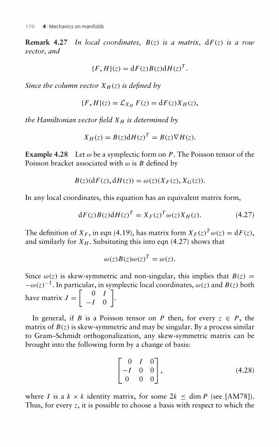
170 4 : Mechanics on manifolds
Remark 4.27 In local coordinates, B(z) is a matrix, dF(z) is a rowvector, and
{F ,H }(z) = dF(z)B(z)dH(z)T .
Since the column vector XH(z) is defined by
{F ,H }(z) = LXHF(z) = dF(z)XH (z),
the Hamiltonian vector field XH is determined by
XH(z) = B(z)dH(z)T = B(z)∇H(z).
Example 4.28 Let ω be a symplectic form on P . The Poisson tensor of thePoisson bracket associated with ω is B defined by
B(z)(dF(z), dH(z)) = ω(z)(XF (z),XG(z)).
In any local coordinates, this equation has an equivalent matrix form,
dF(z)B(z)dH(z)T = XF (z)T ω(z)XH (z). (4.27)
The definition of XF , in eqn (4.19), has matrix form XF (z)T ω(z) = dF(z),and similarly for XH . Subsituting this into eqn (4.27) shows that
ω(z)B(z)ω(z)T = ω(z).
Since ω(z) is skew-symmetric and non-singular, this implies that B(z) =−ω(z)−1. In particular, in symplectic local coordinates, ω(z) and B(z) both
have matrix J =[
0 I
−I 0
].
In general, if B is a Poisson tensor on P then, for every z ∈ P , thematrix of B(z) is skew-symmetric and may be singular. By a process similarto Gram–Schmidt orthogonalization, any skew-symmetric matrix can bebrought into the following form by a change of basis: 0 I 0
−I 0 00 0 0
, (4.28)
where I is a k × k identity matrix, for some 2k ≤ dimP (see [AM78]).Thus, for every z, it is possible to choose a basis with respect to which the
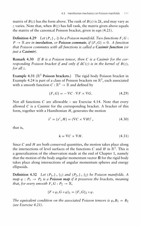
4.3 Hamiltonian mechanics on Poisson manifolds 171
matrix of B(z) has the form above. The rank of B(z) is 2k, and may vary asz varies. Note that, when B(z) has full rank, the matrix given above equalsthe matrix of the canonical Poisson bracket, given in eqn (4.21).
Definition 4.29 Let (P , {·, ·}) be a Poisson manifold. Two functions F ,G :P → R are in involution, or Poisson commute, if {F ,G} = 0. A functionthat Poisson commutes with all functions is called a Casimir function (orjust a Casimir).
Remark 4.30 If B is a Poisson tensor, then C is a Casimir for the cor-responding Poisson bracket if and only if dC(z) is in the kernel of B(z),for all z.
Example 4.31 (R3 Poisson brackets.) The rigid body Poisson bracket inExample 4.24 is part of a class of Poisson brackets on R3, each associatedwith a smooth function C : R3 → R and defined by
{F ,G} = −∇C · ∇F ×∇G. (4.29)
Not all functions C are allowable – see Exercise 4.14. Note that everyallowed C is a Casimir for the corresponding bracket. A bracket of thisform, together with a Hamiltonian H , generates the motion
xi = {xi ,H } = (∇C ×∇H)i , (4.30)
that is,
x = ∇C ×∇H . (4.31)
Since C and H are both conserved quantities, the motion takes place alongthe intersections of level surfaces of the functions C and H in R3. This isa generalization of the observation made at the end of Chapter 1, namelythat the motion of the body angular momentum vector � for the rigid bodytakes place along intersections of angular momentum spheres and energyellipsoids.
Definition 4.32 Let (P1, {·, ·}1) and (P2, {·, ·}2) be Poisson manifolds. Amap ϕ : P1 → P2 is a Poisson map if it preserves the brackets, meaningthat, for every smooth F ,G : P2 → R,
{F ◦ ϕ,G ◦ ϕ}1 = {F ,G}2 ◦ ϕ.
The equivalent condition on the associated Poisson tensors is ϕ∗B1 = B2(see Exercise 4.21).
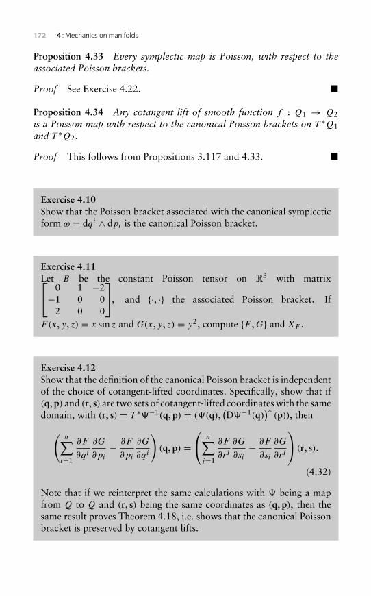
172 4 : Mechanics on manifolds
Proposition 4.33 Every symplectic map is Poisson, with respect to theassociated Poisson brackets.
Proof See Exercise 4.22. �
Proposition 4.34 Any cotangent lift of smooth function f : Q1 → Q2is a Poisson map with respect to the canonical Poisson brackets on T ∗Q1and T ∗Q2.
Proof This follows from Propositions 3.117 and 4.33. �
Exercise 4.10Show that the Poisson bracket associated with the canonical symplecticform ω = dqi ∧ dpi is the canonical Poisson bracket.
Exercise 4.11Let B be the constant Poisson tensor on R3 with matrix 0 1 −2−1 0 0
2 0 0
, and {·, ·} the associated Poisson bracket. If
F(x, y, z) = x sin z and G(x, y, z) = y2, compute {F ,G} and XF .
Exercise 4.12Show that the definition of the canonical Poisson bracket is independentof the choice of cotangent-lifted coordinates. Specifically, show that if(q, p) and (r, s) are two sets of cotangent-lifted coordinates with the samedomain, with (r, s) = T ∗�−1(q, p) = (�(q),
(D�−1(q)
)∗(p)), then(
n∑i=1
∂F
∂qi
∂G
∂pi
− ∂F
∂pi
∂G
∂qi
)(q, p) =
n∑j=1
∂F
∂ri
∂G
∂si− ∂F
∂si
∂G
∂ri
(r, s).
(4.32)
Note that if we reinterpret the same calculations with � being a mapfrom Q to Q and (r, s) being the same coordinates as (q, p), then thesame result proves Theorem 4.18, i.e. shows that the canonical Poissonbracket is preserved by cotangent lifts.
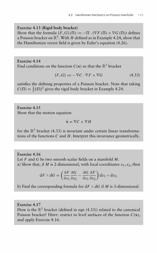
4.3 Hamiltonian mechanics on Poisson manifolds 173
Exercise 4.13 (Rigid body bracket)Show that the formula {F ,G} () := − · (∇F ()×∇G()) definesa Poisson bracket on R3. With H defined as in Example 4.24, show thatthe Hamiltonian vector field is given by Euler’s equation (4.26).
Exercise 4.14Find conditions on the function C(x) so that the R3 bracket
{F ,G} := −∇C · ∇F ×∇G (4.33)
satisfies the defining properties of a Poisson bracket. Note that takingC() = 1
2‖‖2 gives the rigid body bracket in Example 4.24.
Exercise 4.15Show that the motion equation
x = ∇C ×∇Hfor the R3 bracket (4.33) is invariant under certain linear transforma-tions of the functions C and H . Interpret this invariance geometrically.
Exercise 4.16Let F and G be two smooth scalar fields on a manifold M.a) Show that, if M is 2-dimensional, with local coordinates x1, x2, then
dF ∧ dG =(
∂F
∂x1
∂G
∂x2− ∂G
∂x1
∂F
∂x2
)dx1 ∧ dx2.
b) Find the corresponding formula for dF ∧ dG if M is 3-dimensional.
Exercise 4.17How is the R3 bracket (defined in eqn (4.33)) related to the canonicalPoisson bracket? Hint: restrict to level surfaces of the function C(x),and apply Exercise 4.16.
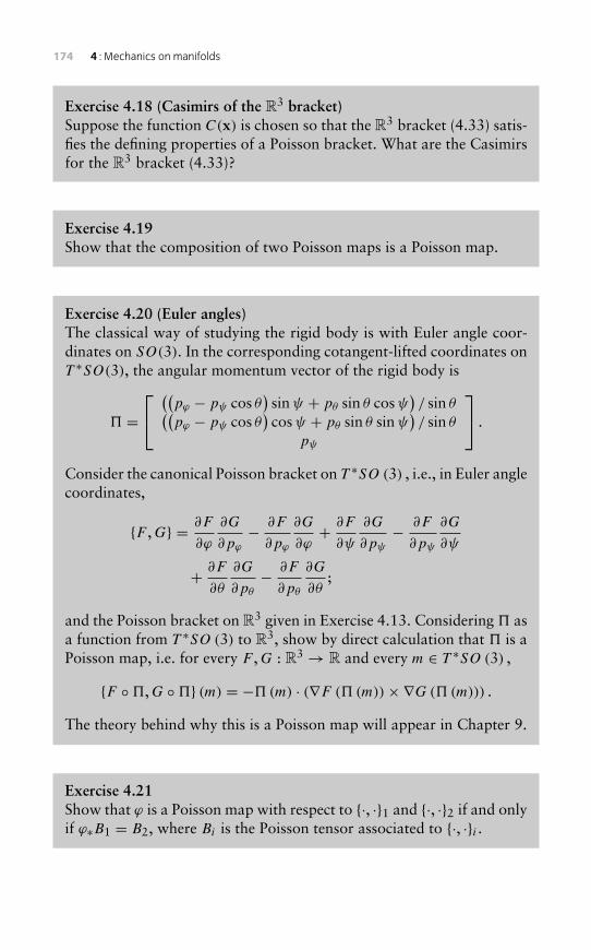
174 4 : Mechanics on manifolds
Exercise 4.18 (Casimirs of the R3 bracket)Suppose the function C(x) is chosen so that the R3 bracket (4.33) satis-fies the defining properties of a Poisson bracket. What are the Casimirsfor the R3 bracket (4.33)?
Exercise 4.19Show that the composition of two Poisson maps is a Poisson map.
Exercise 4.20 (Euler angles)The classical way of studying the rigid body is with Euler angle coor-dinates on SO(3). In the corresponding cotangent-lifted coordinates onT ∗SO(3), the angular momentum vector of the rigid body is
= ((
pϕ − pψ cos θ)sinψ + pθ sin θ cosψ
)/ sin θ((
pϕ − pψ cos θ)cosψ + pθ sin θ sinψ
)/ sin θ
pψ
.
Consider the canonical Poisson bracket on T ∗SO (3) , i.e., in Euler anglecoordinates,
{F ,G} = ∂F
∂ϕ
∂G
∂pϕ
− ∂F
∂pϕ
∂G
∂ϕ+ ∂F
∂ψ
∂G
∂pψ
− ∂F
∂pψ
∂G
∂ψ
+ ∂F
∂θ
∂G
∂pθ
− ∂F
∂pθ
∂G
∂θ;
and the Poisson bracket on R3 given in Exercise 4.13. Considering asa function from T ∗SO (3) to R3, show by direct calculation that is aPoisson map, i.e. for every F ,G : R3 → R and every m ∈ T ∗SO (3) ,
{F ◦,G ◦} (m) = −(m) · (∇F ( (m))×∇G( (m))) .
The theory behind why this is a Poisson map will appear in Chapter 9.
Exercise 4.21Show that ϕ is a Poisson map with respect to {·, ·}1 and {·, ·}2 if and onlyif ϕ∗B1 = B2, where Bi is the Poisson tensor associated to {·, ·}i .
4.4 A brief look at symmetry, reduction and conserved quantities 175
Exercise 4.22Prove Proposition 4.33: every symplectic map is Poisson, with respectto the associated Poisson brackets. Hint: one way to do this is usingPoisson tensors and Example 4.28.
4.4 A brief look at symmetry, reduction andconserved quantities
Consider the Euler–Lagrange equations,
ddt
(∂L
∂qi
)= ∂L
∂qi, i = 1, . . . , n.
Definition 4.35 A coordinate qi is cyclic if L is independent of it.
If L is independent of qi , then ∂L∂qi = 0, so clearly ∂L
∂qi , for the same i, isconstant. Therefore:
Proposition 4.36 If qi is a cyclic coordinate for a Lagrangian L, then ∂L∂qi
is a first integral, i.e. a conserved quantity.
Example 4.37 Consider a Lagrangian on configuration space R3,expressed in standard Cartesian coordinates. The Lagrangian L is transla-tionally invariant it is independent of x, y, z, i.e. if it depends only on x, y, z.In this case, x, y, z are all cyclic variables, and by the previous proposition,
all of the conjugate momenta∂L
∂x,∂L
∂y,∂L
∂zare conserved. For example, if
L = 12m
(x2 + y2 + z2) , then the conjugate momenta are
∂L
∂x= mx,
∂L
∂y= my,
∂L
∂z= mz,
i.e. the components of linear momentum.
Example 4.38 Consider a Lagrangian on configuration space R2,expressed in polar coordinates. L is rotationally invariant if it is inde-pendent of θ . By the previous proposition, the conjugate momentum ∂L
∂θis
conserved. For example, if L = 12m
(r2 + r2θ2) − V (r) for some V , then
∂L/∂θ = mr2θ , which is the formula for angular momentum.
176 4 : Mechanics on manifolds
Definition 4.39 For a Hamiltonian system, a coordinate is called cyclic ifthe Hamiltonian is independent of it.
Remark 4.40 If H is the Hamiltonian corresponding to a Lagrangian L,as in eqn (4.13), then every coordinate that is cyclic for L is cyclic for H .
Recall Hamilton’s equations,
ddt
qi = ∂H
∂pi
,ddt
pi = − ∂H
∂qii = 1, . . . , n.
The second of these equations directly implies the following:
Remark 4.41 If qi is a cyclic coordinate for a Hamiltonian H , then theconjugate momentum pi is a first integral, i.e. a conserved quantity.
Suppose for simplicity that q1 is cyclic. Along any particular solution,p1 = c, for some constant c determined by the initial conditions. Hamilton’sequations become
dq1
dt= ∂H
∂p1, p1 = c,
dqi
dt= ∂H
∂pi,
dpi
dt= −∂H
∂qii = 2, . . . , n.
Since H is independent of q1, and p1 is constant, the last 2n − 2 equa-tions decouple from the first two. The last 2n − 2 equations comprise thereduced Hamiltonian system. Note that they are Hamilton’s equations forthe reduced Hamiltonian,
Hred(q2, . . . , qn,p2, . . . ,pn) := H(q1, . . . , qn, c,p2, . . . ,pn), (4.34)
where the value of q1 is immaterial.In summary, we have:
Proposition 4.42 (Naive reduction) If q1 is a cyclic coordinate for aHamiltonian H , then the solutions of Hamilton’s equations are completelydetermined by the solutions toHamilton’s equations for the reducedHamil-tonian Hred defined in eqn (4.34). Specifically, p1 has a constant value c
given by the initial conditions; qi(t) and pi(t), for i = 2, . . . , n, j �= i areobtained by solving Hamilton’s equations for Hred; and then q1(t) is given
4.4 A brief look at symmetry, reduction and conserved quantities 177
by integrating
dq1
dt= ∂
∂p1H(q1, q2(t), . . . , qn(t), c,p2(t), . . . ,pn(t)).
(This last equation is called the reconstruction equation.)
When naive reduction is possible, it reduces the number of degrees offreedom in the system, i.e. reduces the size of the system of ODEs to besolved. This is of great practical importance.1 In addition, naive reductionserves as an introduction to more general reduction theorems, which arecentral to geometric mechanics. Reduction theorems are ways of takingadvantages of symmetry transformations, which are transformations thatleave L or H invariant. Reduction in general has two facets: ‘ignoring’ somevariables of which L or H are independent (e.g. qi in naive reduction); andnoting that some quantities are conserved (e.g. pi in naive reduction). Inthis section we concentrate on conserved quantities.
The concept of a cyclic variable is limited by its dependence on the choiceof a particular coordinate system. To start with, that coordinate systemmay not cover the entire configuration manifold, and the conservation ofthe corresponding conjugate momentum would only apply to trajectoriesas long as they stay within that coordinate patch. Another issue is thatinvariance properties of L or H are not always naturally expressed in termsof some variables being cyclic.
These considerations point to the need for a coordinate-free concept ofan invariance property, and a general way of finding conserved quantitiesassociated with them. Recall that a flow of a vector field X on a manifoldM is its general solution � : M×R→ M. The concept of a flow generalizesas follows:
Definition 4.43 A flow on a manifoldM is a smooth map� : M×R→ M
such that, the ‘time-t ’ maps �t : M → M defined, for every t ∈ R, by�t(·) = �(·, t), satisfy the three properties in Theorem 3.9.The infinitesimal flow corresponding to � is the vector field X defined by
X(z) = dds
∣∣∣∣s=0
�(z, s).
There is a one-to-one correspondence between flows and complete vectorfields.2
1 In fact V.I. Arnold [Arn78] wrote, ‘Almost all the solved problems in mechanics havebeen solved by [this method].’
2 Assuming that all of them are sufficiently smooth. See Theorem 3.9.
178 4 : Mechanics on manifolds
Definition 4.44 A symmetry transformation (or just a symmetry) of afunction F : M → R is a map ϕ : M → M such that F ◦ ϕ = F .The function F is invariant (or symmetric) with respect to the flow � ifeach time-t map �t is a symmetry of F , that is, F ◦�t = F for all t .
The next examples show that translational and rotational invariance canbe expressed in terms of flows. Note that we are identifying T RdN withRdN ×RdN .
Example 4.45 For a given v ∈ R3, Define �v : R6N ×R→ R6N by
�v ((q1, . . . , qN , q1, . . . , qN) , t) = (q1 + tv, . . . , qN + tv, q1, . . . , qN) .
Thus, for every t , the map �vt translates every particle by tv, leaving the
velocities unchanged. It follows directly from the definitions thatL : R6N →R is translationally invariant if and only if it is symmetric with respect toall of the flows �v, for all v ∈ R3.
Example 4.46 Consider N -particle systems in the plane. Let � be the flowon T R2N given in polar coordinates by
�((r1, θ1, . . . , rN , θN , r1, θ1, . . . , rN , θN ), t
)= (r1, θ1 + t , . . . , rN , θN + t , r1, θ1, . . . , rN , θN ).
Thus, for every t , the map �t rotates all particles by an angle t , leaving theirangular and radial velocities unchanged. Then L is rotationally invariant ifand only if it is symmetric with respect to the flow �.
A diffeomorphism from a configuration space Q to itself is called a pointtransformation. If � is a flow on configuration space, then each of thetime-t maps �t is a point transformation. The tangent lifts of these pointtransformations, taken together, define a flow on the phase space TQ:
Definition 4.47 The tangent lift of a flow � on Q is the flow � on TQ
defined by �t = T�t , for all t ∈ R.
Example 4.48 In the Example 4.45, the point transformations are
�vt (q1, . . . , qN) := (q1 + v, . . . , qN + v).
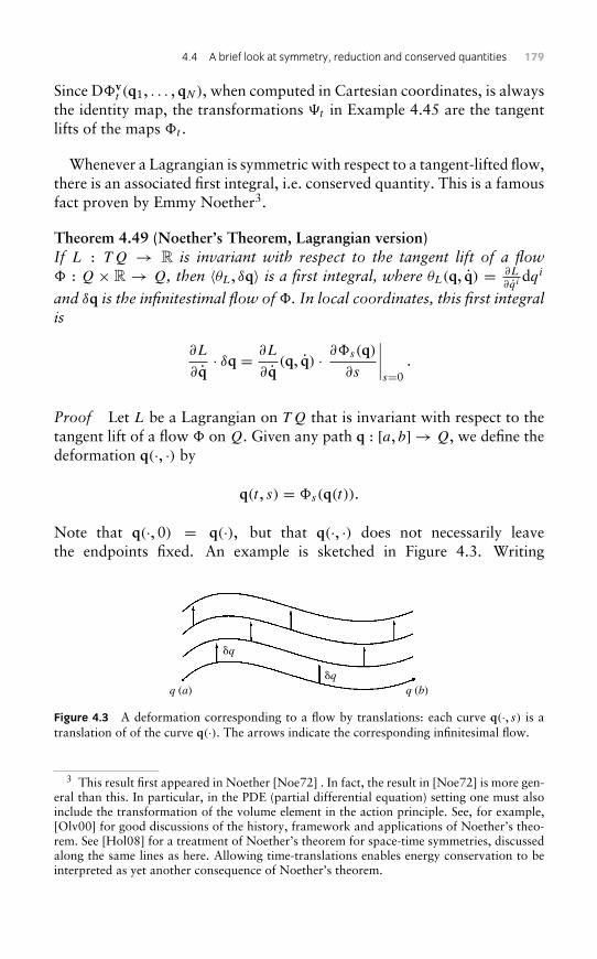
4.4 A brief look at symmetry, reduction and conserved quantities 179
Since D�vt (q1, . . . , qN), when computed in Cartesian coordinates, is always
the identity map, the transformations �t in Example 4.45 are the tangentlifts of the maps �t .
Whenever a Lagrangian is symmetric with respect to a tangent-lifted flow,there is an associated first integral, i.e. conserved quantity. This is a famousfact proven by Emmy Noether3.
Theorem 4.49 (Noether’s Theorem, Lagrangian version)If L : TQ → R is invariant with respect to the tangent lift of a flow� : Q × R → Q, then 〈θL, δq〉 is a first integral, where θL(q, q) = ∂L
∂qi dqi
and δq is the infinitestimal flow of�. In local coordinates, this first integralis
∂L
∂q· δq = ∂L
∂q(q, q) · ∂�s(q)
∂s
∣∣∣∣s=0
.
Proof Let L be a Lagrangian on TQ that is invariant with respect to thetangent lift of a flow � on Q. Given any path q : [a, b] → Q, we define thedeformation q(·, ·) by
q(t , s) = �s(q(t)).
Note that q(·, 0) = q(·), but that q(·, ·) does not necessarily leavethe endpoints fixed. An example is sketched in Figure 4.3. Writing
q (a)
�q
�qq (b)
Figure 4.3 A deformation corresponding to a flow by translations: each curve q(·, s) is atranslation of of the curve q(·). The arrows indicate the corresponding infinitesimal flow.
3 This result first appeared in Noether [Noe72] . In fact, the result in [Noe72] is more gen-eral than this. In particular, in the PDE (partial differential equation) setting one must alsoinclude the transformation of the volume element in the action principle. See, for example,[Olv00] for good discussions of the history, framework and applications of Noether’s theo-rem. See [Hol08] for a treatment of Noether’s theorem for space-time symmetries, discussedalong the same lines as here. Allowing time-translations enables energy conservation to beinterpreted as yet another consequence of Noether’s theorem.
180 4 : Mechanics on manifolds
q(t , s) = ∂∂t
q(t , s), we have, for every t , s,
L(q(t , s), q(t , s)) = L(�s(q(t)),∂
∂t�s(q(t)))
= L(�s(q(t)), D�s(q(t)) · q(t))= L(T�s(q(t), q(t))
= L(q(t), q(t)),
where in the last line we have used the assumption that L is invariant withrespect to the tangent lift of �. It follows that
∂
∂s
∣∣∣∣s=0
∫ b
a
L(q(t , s), q(t , s))dt = 0.
(In fact, the equation holds for all s, but we will only need the case s = 0.)As we have seen earlier in eqn (4.4), the previous equation is equivalent to∫ b
a
(ddt
(∂L
∂q
)− ∂L
∂q
)· δq dt = ∂L
∂q· δq
∣∣∣∣ba
,
where δq(t , s) := ∂∂s
∣∣s=0 q(t , s). Note that δq(t , s) is the infinitesimal flow
of � at (t , s). Now if q(·) is a trajectory satisfying the Euler–Lagrangeequations for L, then the expression in parentheses in the previous equationvanishes, leaving
∂L
∂q· δq
∣∣∣∣ba
= 0,
i.e. the value of ∂L∂q ·δq is the same at (q(a), q(a)) as (q(b), q(b)). Since this is
true for all solutions to the Euler–Lagrange equations, ∂L∂q · δq is a first inte-
gral, i.e. a conserved quantity. This quantity can also be expressed in termsthe Lagrangian 1-form on TQ, which is defined in local coordinates as
θL (q, q) := ∂L
∂qidqi .
A straightforward calculation shows that this definition is coordinate inde-pendent. This fact also follows from the relationship between θL and thecanonical 1-form θ = pidqi on T ∗Q, which was introduced in Chapter 3,namely,
θL = (FL)∗ θ .
4.4 A brief look at symmetry, reduction and conserved quantities 181
If we view the vector field δq as a vector field on TQ with zero qcomponent, then
∂L
∂q· δq = 〈θL, δq
⟩.
The notation on the right-hand side means that the 1-form θL has beenpaired with the vector field δq to give a scalar field on TQ; and the valueof this scalar field, at any (q, q), is 〈θL(q, q), δq(q)
⟩. �
Noether’s Theorem has an analogue in Hamiltonian mechanics. To stateit, we need the following analogue of the tangent lift of a flow.
Definition 4.50 The cotangent lift of a flow � on Q is the flow � on TQ
defined by �t = T ∗�−1t , for all t ∈ R.
Theorem 4.51 (Noether’s Theorem, first Hamiltonian version)If H : T ∗Q → R is invariant with respect to the cotangent lift of a flow� : Q×R→ Q then 〈θ , δq〉 is a conserved quantity, where θ is the canon-ical 1-form and δq is the infinitestimal flow of �. In local cotangent-liftedcoordinates, this first integral is
p · δq = p · ∂�s(q)∂s
∣∣∣∣s=0
.
For Hamiltonians that correspond to hyperregular Lagrangrians (in thesense of Definition 4.9), the previous theorem is a direct consequence of theLagrangian version of Noether’s Theorem and the following proposition.
Proposition 4.52 Let � : Q × R → Q be a flow. Let L : TQ → R be ahyperregular Lagrangian, with corresponding Hamiltonian H : T ∗Q→ R.Then L is invariant with respect to the tangent lift of the flow � if and onlyif H is invariant with respect to the cotangent lift of �.
Proof Suppose that L is invariant with respect to the tangent lift of �. Adirect calculation shows that
(T ∗�−1
s
) ◦ FL = FL ◦ T�s , for every s, (seeExercise 4.24). This implies that the energy function E is invariant withrespect to the tangent lift of � (see Exercise 4.25). Since H = E ◦ (FL)−1
by definition, it follows that,
H ◦(T ∗�−1
s
)◦ FL = E ◦ (FL)−1 ◦ FL ◦ T�s = E ◦ T�s = E,
and hence that H ◦(T ∗�−1) = H . Hence H is invariant under the cotangentlift of �. The converse is similar. �
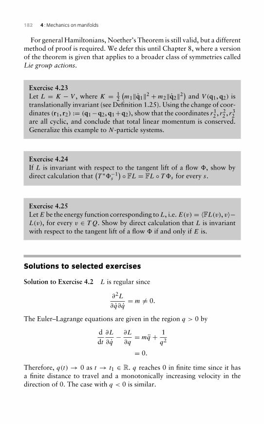
182 4 : Mechanics on manifolds
For general Hamiltonians, Noether’s Theorem is still valid, but a differentmethod of proof is required. We defer this until Chapter 8, where a versionof the theorem is given that applies to a broader class of symmetries calledLie group actions.
Exercise 4.23Let L = K − V , where K = 1
2
(m1‖q1‖2 +m2‖q2‖2
)and V (q1, q2) is
translationally invariant (see Definition 1.25). Using the change of coor-dinates (r1, r2) := (q1−q2, q1+q2), show that the coordinates r1
2 , r22 , r3
2are all cyclic, and conclude that total linear momentum is conserved.Generalize this example to N -particle systems.
Exercise 4.24If L is invariant with respect to the tangent lift of a flow �, show bydirect calculation that
(T ∗�−1
s
) ◦ FL = FL ◦ T�s for every s.
Exercise 4.25LetE be the energy function corresponding toL, i.e. E(v) = 〈FL(v), v〉−L(v), for every v ∈ TQ. Show by direct calculation that L is invariantwith respect to the tangent lift of a flow � if and only if E is.
Solutions to selected exercises
Solution to Exercise 4.2 L is regular since
∂2L
∂q∂q= m �= 0.
The Euler–Lagrange equations are given in the region q > 0 by
ddt
∂L
∂q− ∂L
∂q= mq + 1
q2
= 0.
Therefore, q(t) → 0 as t → t1 ∈ R. q reaches 0 in finite time since it hasa finite distance to travel and a monotonically increasing velocity in thedirection of 0. The case with q < 0 is similar.
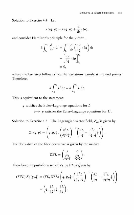
Solutions to selected exercises 183
Solution to Exercise 4.4 Let
L′(q, q) = L(q, q)+ ddt
γ (q).
and consider Hamilton’s principle for the γ term.
δ
∫ t1
t0
ddt
γdt =∫ t1
t0
ddt
(∂γ
∂q· δq
)dt
=[∂γ
∂q· δq
]t1t0
= 0,
where the last step follows since the variations vanish at the end points.Therefore,
δ
∫ t1
t0
L′ dt = δ
∫ t1
t0
L dt .
This is equivalent to the statement:
q satisfies the Euler–Lagrange equations for L
⇐⇒ q satisfies the Euler–Lagrange equations for L′.
Solution to Exercise 4.5 The Lagrangian vector field, ZL, is given by
ZL(q, q) =q, q, q,
(∂2L
∂ q∂ q
)−1 (∂L
∂q− ∂2L
∂q∂ qq
) .
The derivative of the fiber derivative is given by the matrix
DFL =(
I 0∂2L∂q∂ q
∂2L∂ q∂ q
).
Therefore, the push-forward of ZL by FL is given by
(T FL)ZL(q, q) = (FL, DFL)
q, q, q,
(∂2L
∂ q∂ q
)−1 (∂L
∂q− ∂2L
∂q∂ qq
)=(q,
∂L
∂ q, q,
∂L
∂q
).
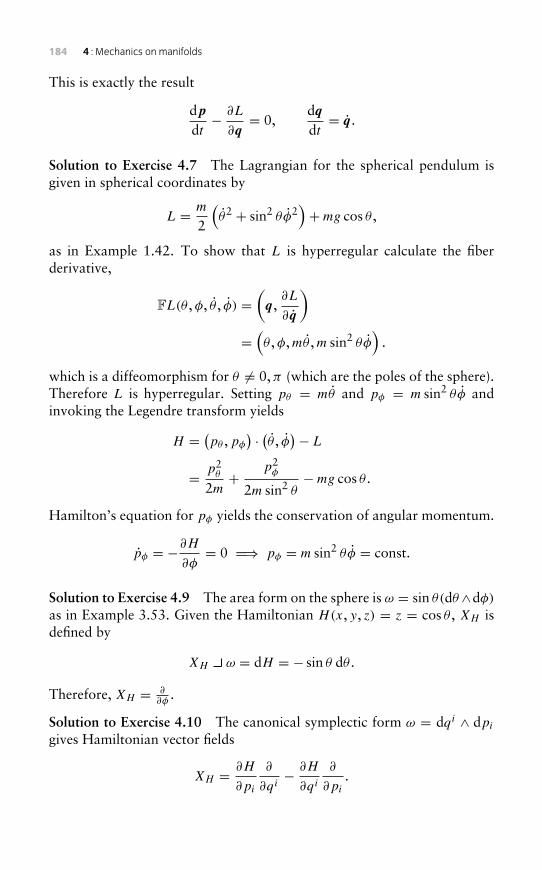
184 4 : Mechanics on manifolds
This is exactly the result
dpdt− ∂L
∂q= 0,
dqdt= q.
Solution to Exercise 4.7 The Lagrangian for the spherical pendulum isgiven in spherical coordinates by
L = m
2
(θ2 + sin2 θφ2
)+mg cos θ ,
as in Example 1.42. To show that L is hyperregular calculate the fiberderivative,
FL(θ ,φ, θ , φ) =(q,
∂L
∂ q
)=(θ ,φ,mθ ,m sin2 θφ
).
which is a diffeomorphism for θ �= 0,π (which are the poles of the sphere).Therefore L is hyperregular. Setting pθ = mθ and pφ = m sin2 θφ andinvoking the Legendre transform yields
H = (pθ ,pφ
) · (θ , φ)− L
= p2θ
2m+ p2
φ
2m sin2 θ−mg cos θ .
Hamilton’s equation for pφ yields the conservation of angular momentum.
pφ = −∂H
∂φ= 0 =⇒ pφ = m sin2 θφ = const.
Solution to Exercise 4.9 The area form on the sphere is ω = sin θ(dθ∧dφ)as in Example 3.53. Given the Hamiltonian H(x, y, z) = z = cos θ , XH isdefined by
XH ω = dH = − sin θ dθ .
Therefore, XH = ∂∂φ
.
Solution to Exercise 4.10 The canonical symplectic form ω = dqi ∧ dpi
gives Hamiltonian vector fields
XH = ∂H
∂pi
∂
∂qi− ∂H
∂qi
∂
∂pi
.
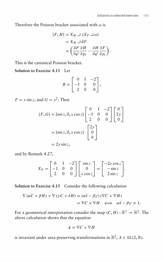
Solutions to selected exercises 185
Therefore the Poisson bracket associated with ω is
{F ,H } = XH (XF ω)
= XH dF
=(∂F
∂qi
∂H
∂pi
− ∂H
∂qi
∂F
∂pi
).
This is the canonical Poisson bracket.
Solution to Exercise 4.11 Let
B = 0 1 −2−1 0 02 0 0
,
F = x sin z, and G = y2. Then
{F ,G} = [sin z, 0, x cos z] 0 1 −2−1 0 02 0 0
02y0
= [sin z, 0, x cos z] ·
2y00
= 2y sin z,
and by Remark 4.27,
XF = 0 1 −2−1 0 02 0 0
sin z
0x cos z
=−2x cos z− sin z
2 sin z
.
Solution to Exercise 4.15 Consider the following calculation
∇ (αC + βH)×∇ (γC + δH) = (αδ − βγ ) (∇C ×∇H)
= ∇C ×∇H ⇐⇒ αδ − βγ = 1.
For a geometrical interpretation consider the map (C,H) : R3 → R2. Theabove calculation shows that the equation
x = ∇C ×∇H
is invariant under area-preserving transformations in R2, A ∈ SL(2, R).
186 4 : Mechanics on manifolds
Solution to Exercise 4.17 Let (x1, x2) be coordinates of the level surfaceof C. The Poisson bracket is given by
{F ,G}dX1 ∧ dX2 ∧ dX3 = dC ∧ dF ∧ dG.
Using coordinates that align with a level set of C gives
{F ,G}dX1 ∧ dX2 ∧ dX3 = dC ∧ dF ∧ dG,
= dC ∧ {F ,G}|C dx1 ∧ dx2.
Therefore,
{F ,G}|C =(
∂F
∂x1
∂G
∂x2 −∂G
∂x1
∂F
∂x2
),
which is the canonical Poisson bracket in x coordinates.
Solution to Exercise 4.18 Any function, �(C), is a Casimir function for{F ,H } = ∇C · (∇F ×∇H), since
{�(C),H } = �′(C)∇C · (∇C ×∇H) = 0.
These are the only Casimirs since ∇F must be parallel to ∇C everywherefor F to be a Casimir.
Solution to Exercise 4.25 Suppose that L ◦ T�s = L. Then
E ◦ T�s(v) = 〈FL ◦ T�s(v) , T�s(v)〉 − L ◦ T�s(v)
=⟨T ∗�−1
s ◦ FL(v) , T�s(v)⟩− L(v)
= 〈FL(v) , v〉 − L(v)
= E(v).
Therefore, E is invariant under T�s . The converse is similar.
5Lie groups andLie algebras
In general, a system is symmetric when its state does not change under acertain transformation. For mechanical systems, a symmetry is a transfor-mation of phase space, and possibly time, that leaves the Hamiltonian orLagrangian invariant. Symmetries form groups, with the group operationbeing composition. For instance, a group consisting of a reflection and theidentity transformation is isomorphic to Z2; while the group of rotationsof R3 is the matrix Lie group SO(3).
Lie groups are the mathematical concept appropriate for describingcontinuously varying groups of transformations. The present chapter intro-duces general Lie groups, Lie algebras and the exponential map, beginningwith the special cases of matrix Lie groups (first introduced in Chapter 2)and matrix Lie algebras. Group actions, which associate group elementswith transformations, will be defined in the next chapter.
5.1 Matrix Lie groups and Lie algebras
The following definition is repeated from Section 2.4.
Definition 5.1 Amatrix group is a subset ofM(n, R), orM(n, C), that is agroup, with the group operation being matrix multiplication. A matrix Liegroup is a matrix group that is also a submanifold ofM(n, R) orM(n, C).
Recall that M(n, R) is the space of n × n real matrices, which is a realvector space that can be identified with Rn×n = Rn2
. Similarly M(n, C) is acomplex vector space that can be identified with Cn2
or R(2n)2 . Note that,to satisfy the group axioms, the identity matrix I must be contained in thegroup. Also, all matrices in the group must be invertible, so the group mustbe a subgroup of GL(n, R) or GL(n, C).
Definition 5.2 The matrix commutator of any pair of n × n matrices Aand B is defined as [A,B] := AB − BA.
188 5 : Lie groups and Lie algebras
Proposition 5.3 (Properties of the matrix commutator)Thematrix commutator operation has the following properties for any n×n
matrices A, B and C:
(i) [B,A] = −[A,B] (skew-symmetry); and
(ii) [[A,B],C] + [[B,C],A] + [[C,A],B] = 0 (the Jacobi identity).
Proof These straightforward calculations are left as Exercise 5.1. �
Example 5.4 (The orthogonal group, O(n)) Recall from Proposition 2.90that the set O(n) of real orthogonal n× n matrices is a matrix Lie group ofdimension n(n − 1)/2. The tangent space to O(n) at the identity, TIO(n),is the vector subspace of skew-symmetric matrices, i.e. those matrices A
satisfying
AT + A = 0.
For any pair of matrices A,B ∈ TIO(n), the matrix commutator [A,B] isalso in TIO(n). Indeed,
[A,B]T + [A,B] = (AB − BA)T + (AB − BA)
= BT AT − AT BT + AB − BA = 0,
since AT = −A and BT = −B.
The previous example shows that TIO(n) is closed under the matrix com-mutator operation. In fact, this is true for the tangent space at the identityTIG of any matrix Lie group G, as we will now show. The proof relies onthe following lemma, which states that TIG is closed under conjugation1
by any element of G.
Lemma 5.5 Let R be an arbitrary element of a matrix Lie group G, andlet B ∈ TIG. Then RBR−1 ∈ TIG.
Proof Let CB(t) be a curve in G such that CB(0) = I and C′B(0) = B.Define V (t) = RCB(t)R
−1 ∈ G for all t . Then V (0) = I and V ′(0) =RBR−1. Hence, RBR−1 = V ′(0) ∈ TIG, which proves the lemma. �
Proposition 5.6 Let G be a matrix Lie group, and let A,B ∈ TIG. Then[A,B] ∈ TIG.
1 Conjugation by a group element g is the map h → ghg−1.
5.1 Matrix Lie groups and Lie algebras 189
Proof Let RA(s) be a curve in G such that RA(0) = I and R′A(0) = A.Define C(s) = RA(s)B(RA(s))
−1. Then the previous lemma implies thatC(s) ∈ TIG for every s. Hence, C′(s) ∈ TIG, for every s, in particular fors = 0. Since C′(0) = AB −BA = [A,B] (using a formula in Exercise 3.12),this shows that [A,B] ∈ TIG . �
Definition 5.7 A matrix Lie algebra is a vector subspace of M(n, R) orM(n, C) for some n, with the usual operations of matrix addition and scalarmultiplication, that is also closed under the matrix commutator [·, ·].Proposition 5.8 For any matrix Lie group G, the tangent space at theidentity TIG is a matrix Lie algebra, called the Lie algebra of G. Conversely,any matrix Lie algebra is the Lie algebra of some matrix Lie group.
Sketch of proof The first statement follows from Proposition 5.6 and thefact that TIG is a vector subspace of M(n, R) or M(n, C). For the converse,recall the matrix exponential operation exp, defined by
exp(A) := I + A+ 12!A
2 + 13!A
3 + . . .
Suppose we are given a matrix Lie algebra V . Let
G := exp(V ) := {exp(A) : A ∈ V }.It can be shown that G is a matrix Lie group, and that TIG = V . See[Bak02]. �
Note that there may be more than one matrix Lie group with the same Liealgebra. For example, O(n) and SO(n) have the same Lie algebra: the set ofskew-symmetric matrices, as shown in Proposition 2.90 and Example 5.12.
The remainder of this section consists of examples of matrix Lie groupsand their Lie algebras. Parts of some examples have already appeared earlierin Section 2.4. All of the examples given here are groups of matrices withreal entries; for example ‘GL(n)’ denotes GL(n, R) (some complex matrixgroups appear in the exercises). We use the notational convention that theLie algebra of a Lie group is denoted by the lower-case Gothic version ofthe letter(s) denoting the Lie group.
Example 5.9 (General linear group GL(n) and Lie algebra gl(n)) Thematrix Lie group GL(n) is formed by all n × n matrices with non-zerodeterminant. It is an open subset of M(n, R), and hence an n2-dimensionalsubmanifold of M(n, R). Its Lie algebra is M(n, R), with the commutatoroperation, and is denoted in this context by gl(n).
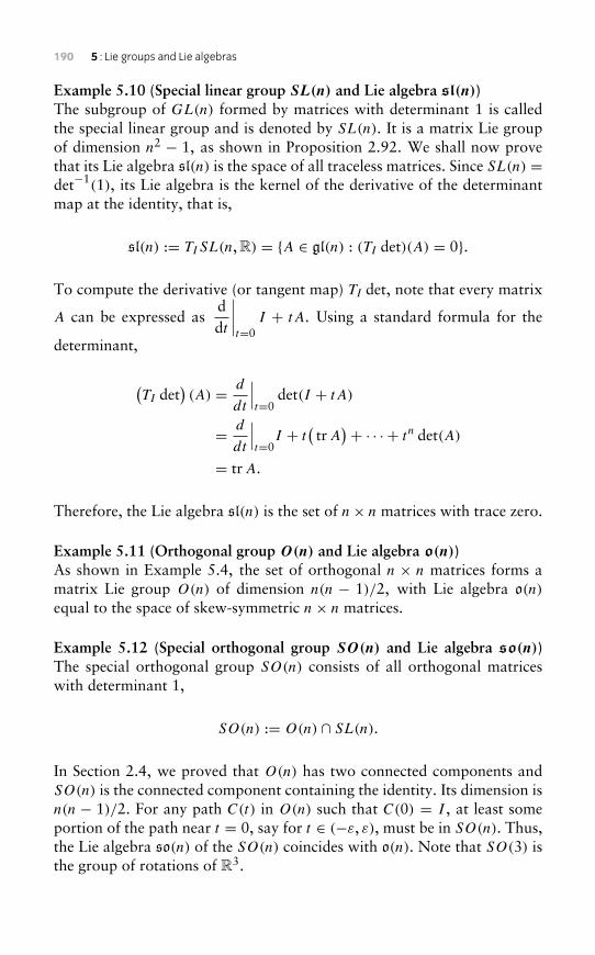
190 5 : Lie groups and Lie algebras
Example 5.10 (Special linear group SL(n) and Lie algebra sl(n))The subgroup of GL(n) formed by matrices with determinant 1 is calledthe special linear group and is denoted by SL(n). It is a matrix Lie groupof dimension n2 − 1, as shown in Proposition 2.92. We shall now provethat its Lie algebra sl(n) is the space of all traceless matrices. Since SL(n) =det−1
(1), its Lie algebra is the kernel of the derivative of the determinantmap at the identity, that is,
sl(n) := TISL(n, R) = {A ∈ gl(n) : (TI det)(A) = 0}.
To compute the derivative (or tangent map) TI det, note that every matrix
A can be expressed asddt
∣∣∣∣t=0
I + tA. Using a standard formula for the
determinant,
(TI det
)(A) = d
dt
∣∣∣t=0
det(I + tA)
= d
dt
∣∣∣t=0
I + t(trA
)+ · · · + tn det(A)
= trA.
Therefore, the Lie algebra sl(n) is the set of n× n matrices with trace zero.
Example 5.11 (Orthogonal group O(n) and Lie algebra o(n))As shown in Example 5.4, the set of orthogonal n × n matrices forms amatrix Lie group O(n) of dimension n(n − 1)/2, with Lie algebra o(n)equal to the space of skew-symmetric n× n matrices.
Example 5.12 (Special orthogonal group SO(n) and Lie algebra so(n))The special orthogonal group SO(n) consists of all orthogonal matriceswith determinant 1,
SO(n) := O(n) ∩ SL(n).
In Section 2.4, we proved that O(n) has two connected components andSO(n) is the connected component containing the identity. Its dimension isn(n − 1)/2. For any path C(t) in O(n) such that C(0) = I , at least someportion of the path near t = 0, say for t ∈ (−ε, ε), must be in SO(n). Thus,the Lie algebra so(n) of the SO(n) coincides with o(n). Note that SO(3) isthe group of rotations of R3.
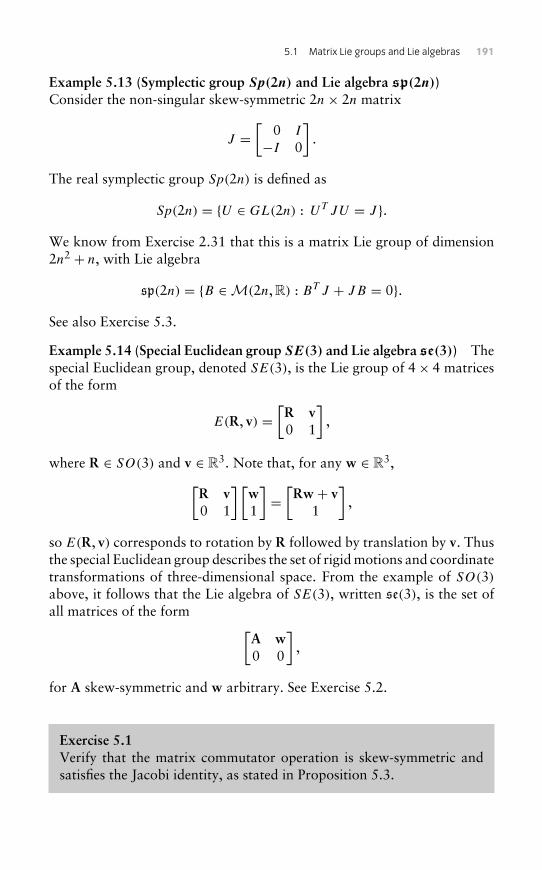
5.1 Matrix Lie groups and Lie algebras 191
Example 5.13 (Symplectic group Sp(2n) and Lie algebra sp(2n))Consider the non-singular skew-symmetric 2n× 2n matrix
J =[
0 I
−I 0
].
The real symplectic group Sp(2n) is defined as
Sp(2n) = {U ∈ GL(2n) : UT JU = J }.We know from Exercise 2.31 that this is a matrix Lie group of dimension2n2 + n, with Lie algebra
sp(2n) = {B ∈M(2n, R) : BT J + JB = 0}.See also Exercise 5.3.
Example 5.14 (Special Euclidean group SE(3) and Lie algebra se(3)) Thespecial Euclidean group, denoted SE(3), is the Lie group of 4× 4 matricesof the form
E(R, v) =[R v0 1
],
where R ∈ SO(3) and v ∈ R3. Note that, for any w ∈ R3,[R v0 1
] [w1
]=[Rw + v
1
],
so E(R, v) corresponds to rotation by R followed by translation by v. Thusthe special Euclidean group describes the set of rigid motions and coordinatetransformations of three-dimensional space. From the example of SO(3)above, it follows that the Lie algebra of SE(3), written se(3), is the set ofall matrices of the form [
A w0 0
],
for A skew-symmetric and w arbitrary. See Exercise 5.2.
Exercise 5.1Verify that the matrix commutator operation is skew-symmetric andsatisfies the Jacobi identity, as stated in Proposition 5.3.
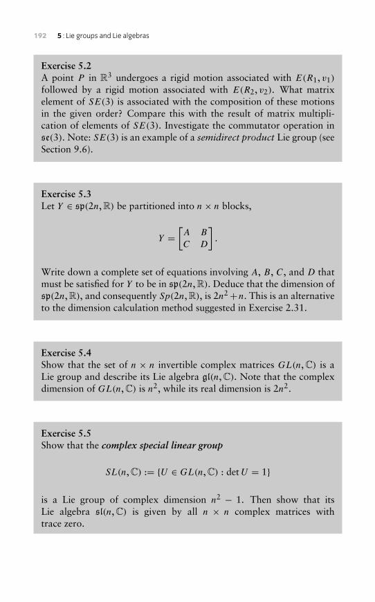
192 5 : Lie groups and Lie algebras
Exercise 5.2A point P in R3 undergoes a rigid motion associated with E(R1, v1)
followed by a rigid motion associated with E(R2, v2). What matrixelement of SE(3) is associated with the composition of these motionsin the given order? Compare this with the result of matrix multipli-cation of elements of SE(3). Investigate the commutator operation inse(3). Note: SE(3) is an example of a semidirect product Lie group (seeSection 9.6).
Exercise 5.3Let Y ∈ sp(2n, R) be partitioned into n× n blocks,
Y =[A B
C D
].
Write down a complete set of equations involving A, B, C, and D thatmust be satisfied for Y to be in sp(2n, R). Deduce that the dimension ofsp(2n, R), and consequently Sp(2n, R), is 2n2+n. This is an alternativeto the dimension calculation method suggested in Exercise 2.31.
Exercise 5.4Show that the set of n × n invertible complex matrices GL(n, C) is aLie group and describe its Lie algebra gl(n, C). Note that the complexdimension of GL(n, C) is n2, while its real dimension is 2n2.
Exercise 5.5Show that the complex special linear group
SL(n, C) := {U ∈ GL(n, C) : detU = 1}
is a Lie group of complex dimension n2 − 1. Then show that itsLie algebra sl(n, C) is given by all n × n complex matrices withtrace zero.
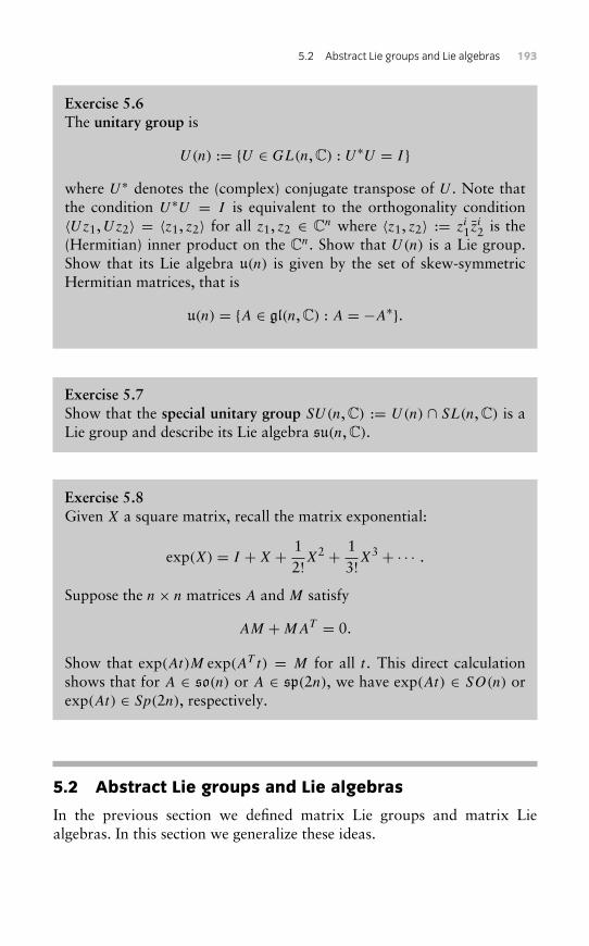
5.2 Abstract Lie groups and Lie algebras 193
Exercise 5.6The unitary group is
U(n) := {U ∈ GL(n, C) : U∗U = I }where U∗ denotes the (complex) conjugate transpose of U . Note thatthe condition U∗U = I is equivalent to the orthogonality condition〈Uz1,Uz2〉 = 〈z1, z2〉 for all z1, z2 ∈ Cn where 〈z1, z2〉 := zi1z
i2 is the
(Hermitian) inner product on the Cn. Show that U(n) is a Lie group.Show that its Lie algebra u(n) is given by the set of skew-symmetricHermitian matrices, that is
u(n) = {A ∈ gl(n, C) : A = −A∗}.
Exercise 5.7Show that the special unitary group SU(n, C) := U(n) ∩ SL(n, C) is aLie group and describe its Lie algebra su(n, C).
Exercise 5.8Given X a square matrix, recall the matrix exponential:
exp(X) = I +X + 12!X
2 + 13!X
3 + · · · .
Suppose the n× n matrices A and M satisfy
AM +MAT = 0.
Show that exp(At)M exp(AT t) = M for all t . This direct calculationshows that for A ∈ so(n) or A ∈ sp(2n), we have exp(At) ∈ SO(n) orexp(At) ∈ Sp(2n), respectively.
5.2 Abstract Lie groups and Lie algebras
In the previous section we defined matrix Lie groups and matrix Liealgebras. In this section we generalize these ideas.
194 5 : Lie groups and Lie algebras
Definition 5.15 A Lie group is a smooth manifold that is also a group,with the property that the operations of group multiplication, (g,h) → gh
and inversion, g → g−1, are smooth.
Every matrix Lie group is a Lie group. Indeed, it is a manifold by defini-tion, and the operations of matrix multiplication and matrix inversion aresmooth because they are rational operations on the matrix entries.
Here is an example of a Lie group that is not a matrix group:
Example 5.16 In Rn consider the equivalence relation x ∼ y iff x −y ∈ 2πZn. The set of equivalence classes [x] = {y ∈ Rn | y − x =2πk for some k = (k1, k2, . . . , kn) ∈ Zn}, is denoted Rn/2πZn or Tn, and iscalled the n-torus. The n-torus is a smooth manifold, as can be shown by adirect generalization of Example 2.100. It is clearly an Abelian group withrespect to the sum operation ([x], [y])→ [x] + [y] := [x + y], with inverse−[x] = [−x]. By using local coordinate charts, one can check that theaddition and inverse operations are smooth. The 1-torus, with this groupoperation, is called the circle group because it is diffeomorphic to the unitcircle S1.
One of the fundamental properties of a Lie group is that given a localchart, one may construct an entire atlas. This is achieved by using the groupmultiplication. For any given g ∈ G, the left translation by g is the map
Lg : G→ G, h→ Lg(h) := gh.
The definition of a Lie group ensures that this map and its inverse aresmooth. Left translation by g shifts any given chart U that covers the iden-tity to a chart Lg(U) that covers g. The union of such charts, for all g,covers G, i.e.,
⋃g∈G Lg(U) = G and in fact they are compatible and hence
form an atlas – see Exercise 5.11. Alternatively, one may use the righttranslation maps
Rg : G→ G, h→ Rg(h) := hg.
We will now give an abstract definition of a Lie algebra and then showthat the tangent space at the identity TeG of any Lie group G, with aparticular bracket, is a Lie algebra.
Definition 5.17 A (real) Lie algebra is a (real) vector space A togetherwith a bilinear operation (v,w) ∈ A×A→ [v,w] ∈ A, called the bracket,such that
5.2 Abstract Lie groups and Lie algebras 195
1. [v,w] = −[w, v] for all v,w ∈ V (skew-symmetry),
2. [[v,w], u]+[[u, v],w]+[[w, u], v] = 0 for all v,w, u ∈ V (Jacobi identity).
Example 5.18 The vector space R3 is a Lie algebra when endowed with abracket given by the usual vector cross-product [x, y] := x × y.
Example 5.19 Every matrix Lie algebra, with bracket given by commuta-tor [A,B] := AB − BA, is a Lie algebra, by Proposition 5.3.
Example 5.20 The space of linear maps on a vector space V is a Liealgebra, with bracket [f , g] = f ◦ g − g ◦ f .
Example 5.21 The vector space X(M) of all smooth vector fields on asmooth manifold M is a Lie algebra, with the Jacobi-Lie bracket [X,Y ] :=LX Y . Recall from Chapter 3 that in local coordinates we have
[X,Y ] = (DY ) ·X − (DX) · Y= X · ∇Y − Y · ∇X.
Definition 5.22 A Lie subalgebra of a Lie algebra A is a subspace of Aclosed under the bracket. Clearly, any such subalgebra is itself a Lie algebra,with the same bracket as A.
Consider a Lie group G and its tangent space at the identity TeG. We arelooking for a meaningful bracket [·, ·]TeG on TeG. We have just learned fromExample 5.21 that the vector space X(G) of smooth vector fields on G is aLie algebra. Should we have an isomorphism between TeG and a subalgebraof X(G), we could then define the bracket on TeG via this isomorphism.More precisely, given an isomorphism λ : TeG→ C ⊆ X(G), where C is asubalgebra of X(G), the bracket on TeG may be defined via:
[ξ , η]TeG := [λ(ξ), λ(η)]X(G).
The map λ will be defined using the left translation maps Lg introducedearlier. Recall that the tangent map TeLg shifts vectors based at e to vectorsbased at g ∈ G. By doing this operation for every g ∈ G, we define a vectorfield:
Definition 5.23 The left extension of any ξ ∈ TeG is the vector field XLξ
given by
XLξ (g) := TeLg(ξ).
196 5 : Lie groups and Lie algebras
Definition 5.24 A vector field X : G → TG, h → X(h), is called leftinvariant if
(Lg)∗(X) = X for all g ∈ G.
The set of left invariant vector fields on G is denoted XL(G). By defini-tion of the push-forward (Lg)∗, an equivalent definition of X being leftinvariant is
ThLg(X(h)) = X(Lg(h)) = X(gh), for all g,h ∈ G.
Because of this second way of writing the definition, left invariant vectorfields are also sometimes called left equivariant (see Definition 6.36).
Lemma 5.25 A vector field on G is left invariant if and only if it equalsXL
ξ for some ξ ∈ TeG, i.e.
XL(G) ={XL
ξ : ξ ∈ TeG}
.
The set XL(G) is a vector subspace of X(G), and the following map is avector space isomorphism,
λ : TeG −→ XL(G)
ξ −→ XLξ .
Proof We begin by showing that XLξ is left invariant, for every ξ :
ThLg(XLξ (h)) = ThLg ◦ TeLh(ξ) = Te(Lg ◦ Lh)(ξ) = TeLgh(ξ) = XL
ξ (gh).
Next, for any left invariant vector field X on G, if we define ξ := X(e), thenby left invariance
X(g) = TeLg(X(e)) = TeLg(ξ) = XLξ (g), for any g ∈ G,
so X = XLξ . Thus, we have proven the first claim. The second claim is left
as an exercise. �
Lemma 5.26 The subspace XL(G) is a Lie subalgebra of X(G).
Proof Applying the left invariance property and Theorem 3.25, we seethat, for any ξ , η ∈ TeG,
[XLξ ,XL
η ] = [L∗gXLξ ,L∗gXL
η ] = L∗g[XLξ ,XL
η ],
5.2 Abstract Lie groups and Lie algebras 197
which shows that [XLξ ,XL
η ] is left invariant. This shows that XL(G) is a Liesubalgebra of X(G). �
Definition 5.27 For any Lie groupG, the Lie bracket on TeG is defined viathe isomorphism λ : TeG→ XL(G), ξ → XL
ξ , as follows: for all ξ , η ∈ TeG,
[ξ , η] := [XLξ ,XL
η ](e).The Lie bracket is called the pull-back by λ of the Jacobi–Lie bracket.
Since XL(G), with the Jacobi-Lie bracket, is a Lie algebra, it followsdirectly that the space TeG, together with the Lie bracket defined above, isa Lie algebra.
Definition 5.28 The tangent space at the identity TeG of a Lie group G,together with the Lie bracket defined above, is called the Lie algebra of G.
It remains to show that this abstract definition is consistent with thecorresponding definition for matrix Lie groups:
Proposition 5.29 The Lie algebra of a matrix Lie group is the space TIG,together with the commutator operation.
Proof This is left as Exercise 5.13. �
The Lie algebra of a group is conventionally denoted by the same letter(s)as the group itself, but in lower-case gothic. For example, the Lie algebraof G is denoted by g.
Exercise 5.9 Show that R, with addition, is a Lie group. Show thatR\{0}, with multiplication, is also a Lie group. Describe the Lie algebraand Lie bracket for both Lie groups (see Example 5.38).
Exercise 5.10 (Abelian Lie groups and Lie algebras)Let G be an Abelian group and g its Lie algebra. Show that [ξ , η] = 0for all ξ , η ∈ g.
The converse is not true! For instance, take G = R × S3 whereS3 is the permutation group of three elements. Show that G is a non-Abelian Lie group when the multiplication operation is defined as((x1, σ1), (x2, σ2))→ (x1+ x2, σ1 ◦ σ2). Then describe g, the Lie algebraof G, and show that [ξ , η] = 0 for all ξ , η ∈ g.
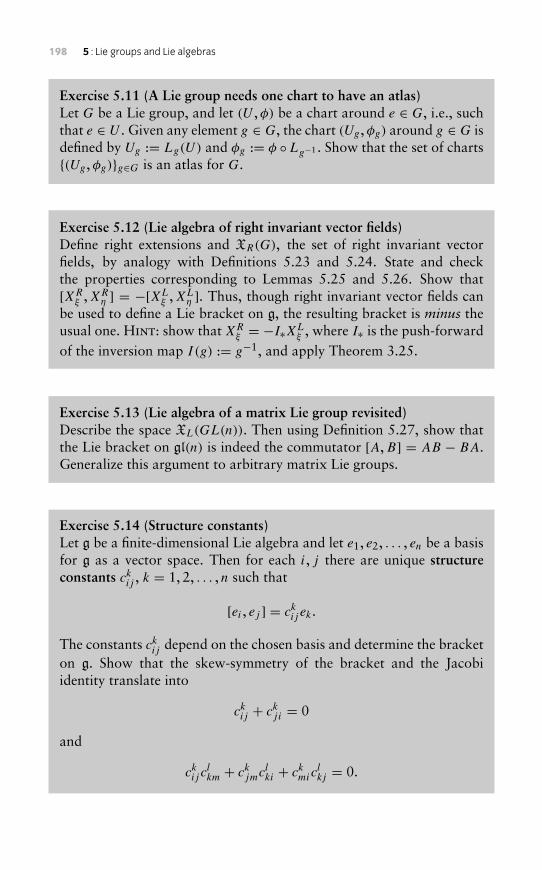
198 5 : Lie groups and Lie algebras
Exercise 5.11 (A Lie group needs one chart to have an atlas)Let G be a Lie group, and let (U ,φ) be a chart around e ∈ G, i.e., suchthat e ∈ U . Given any element g ∈ G, the chart (Ug,φg) around g ∈ G isdefined by Ug := Lg(U) and φg := φ ◦Lg−1 . Show that the set of charts{(Ug,φg)}g∈G is an atlas for G.
Exercise 5.12 (Lie algebra of right invariant vector fields)Define right extensions and XR(G), the set of right invariant vectorfields, by analogy with Definitions 5.23 and 5.24. State and checkthe properties corresponding to Lemmas 5.25 and 5.26. Show that[XR
ξ ,XRη ] = −[XL
ξ ,XLη ]. Thus, though right invariant vector fields can
be used to define a Lie bracket on g, the resulting bracket is minus theusual one. Hint: show that XR
ξ = −I∗XLξ , where I∗ is the push-forward
of the inversion map I (g) := g−1, and apply Theorem 3.25.
Exercise 5.13 (Lie algebra of a matrix Lie group revisited)Describe the space XL(GL(n)). Then using Definition 5.27, show thatthe Lie bracket on gl(n) is indeed the commutator [A,B] = AB − BA.Generalize this argument to arbitrary matrix Lie groups.
Exercise 5.14 (Structure constants)Let g be a finite-dimensional Lie algebra and let e1, e2, . . . , en be a basisfor g as a vector space. Then for each i, j there are unique structureconstants ckij , k = 1, 2, . . . , n such that
[ei , ej ] = ckij ek.
The constants ckij depend on the chosen basis and determine the bracketon g. Show that the skew-symmetry of the bracket and the Jacobiidentity translate into
ckij + ckji = 0
and
ckij clkm + ckjmclki + ckmic
lkj = 0.
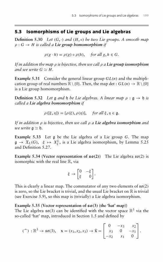
5.3 Isomorphisms of Lie groups and Lie algebras 199
5.3 Isomorphisms of Lie groups and Lie algebras
Definition 5.30 Let (G, ·) and (H , ◦) be two Lie groups. A smooth mapρ : G→ H is called a Lie group homomorphism if
ρ(g · h) = ρ(g) ◦ ρ(h), for all g,h ∈ G.
If in addition the map ρ is bijective, then we call ρ a Lie group isomorphismand we write G � H .
Example 5.31 Consider the general linear group GL(n) and the multipli-cation group of real numbers R \ {0}. Then, the map det : GL(n)→ R \ {0}is a Lie group homomorphism.
Definition 5.32 Let g and h be Lie algebras. A linear map ρ : g → h iscalled a Lie algebra homomorphism if
ρ([ξ , η]) = [ρ(ξ), ρ(η)], for all ξ , η ∈ g.
If in addition ρ is bijective, then we call ρ a Lie algebra isomorphism andwe write g � h.
Example 5.33 Let g be the Lie algebra of a Lie group G. The mapg → XL(G), ξ → XL
ξ , is a Lie algebra isomorphism, by Lemma 5.25and Definition 5.27.
Example 5.34 (Vector representation of so(2)) The Lie algebra so(2) isisomorphic with the real line R, via
ξ →[0 −ξξ 0
].
This is clearly a linear map. The commutator of any two elements of so(2)is zero, so the Lie bracket is trivial, and the usual Lie bracket on R is trivial(see Exercise 5.9), so this map is (trivially) a Lie algebra isomorphism.
Example 5.35 (Vector representation of so(3) (the ‘hat’ map))The Lie algebra so(3) can be identified with the vector space R3 via theso-called ‘hat’ map, introduced in Section 1.5 and defined by
() : R3 → so(3), x = (x1, x2, x3)→ x = 0 −x3 x2
x3 0 −x1−x2 x1 0
.
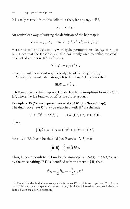
200 5 : Lie groups and Lie algebras
It is easily verified from this definition that, for any x, y ∈ R3,
xy = x × y.
An equivalent way of writing the definition of the hat map is
xij = −εijk xk, where (x1, x2, x3) = (x, y, z).
Here, ε123 = 1 and ε321 = −1, with cyclic permutations, i.e. εijk = εjki =εkij . Note that the tensor εijk is also commonly used to define the cross-product of vectors in R3, as follows:
(x × y)i = εijk xj yk,
which provides a second way to verify the identity xy = x × y.A straightforward calculation, left to Exercise 5.19, shows that
[x, y] = x × y.
It follows that the hat map is a Lie algebra homomorphism from so(3) toR3, where the Lie bracket on R3 is the cross-product.
Example 5.36 (Vector representation of so(3)∗ (the ‘breve’ map))The dual space2 so(3)∗ may be identified with R3 via the map
( ˘ ) : R3 → so(3)∗, � = (1,2,3) → �,
where ⟨�, x
⟩:= � · x = 1x1 +2x2 +3x3,
for all x ∈ R3. It can be checked (see Exercise 5.15) that⟨�, x
⟩= 1
2tr(� xT ).
Thus, � corresponds to 12� under the isomorphism so(3)→ so(3)∗ given
by the trace pairing. If � is identified with the matrix 12�, then
�ij = 12�ij = −1
2εijk
k
2 Recall that the dual of a vector space V is the set V ∗ of all linear maps from V to R, andthat V ∗ is itself a vector space. As vector spaces, Lie algebras have duals. As usual, these aredenoted with the asterisk notation.
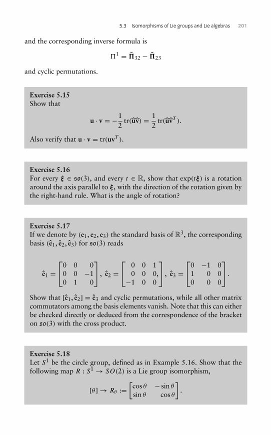
5.3 Isomorphisms of Lie groups and Lie algebras 201
and the corresponding inverse formula is
1 = �32 − �23
and cyclic permutations.
Exercise 5.15Show that
u · v = −12
tr(uv) = 12
tr(uvT ).
Also verify that u · v = tr(uvT ).
Exercise 5.16For every ξ ∈ so(3), and every t ∈ R, show that exp(tξ) is a rotationaround the axis parallel to ξ , with the direction of the rotation given bythe right-hand rule. What is the angle of rotation?
Exercise 5.17If we denote by (e1, e2, e3) the standard basis of R3, the correspondingbasis (e1, e2, e3) for so(3) reads
e1 =0 0 0
0 0 −10 1 0
, e2 = 0 0 1
0 0 0−1 0 0
,
, e3 =0 −1 0
1 0 00 0 0
.
Show that [e1, e2] = e3 and cyclic permutations, while all other matrixcommutators among the basis elements vanish. Note that this can eitherbe checked directly or deduced from the correspondence of the bracketon so(3) with the cross product.
Exercise 5.18Let S1 be the circle group, defined as in Example 5.16. Show that thefollowing map R : S1 → SO(2) is a Lie group isomorphism,
[θ ] → Rθ :=[cos θ − sin θ
sin θ cos θ
].
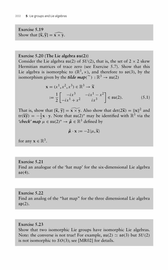
202 5 : Lie groups and Lie algebras
Exercise 5.19Show that [x, y] = x × y.
Exercise 5.20 (The Lie algebra su(2))Consider the Lie algebra su(2) of SU(2), that is, the set of 2 × 2 skewHermitian matrices of trace zero (see Exercise 5.7). Show that thisLie algebra is isomorphic to (R3,×), and therefore to so(3), by theisomorphism given by the tilde map(˜) : R3 → su(2)
x = (x1, x2, x3) ∈ R3 → x
:= 12
[ −ix3 −ix1 − x2
−ix1 + x2 ix3
]∈ su(2). (5.1)
That is, show that [x, y] = x × y. Also show that det(2x) = ‖x‖2 andtr(xy) = −1
2x · y. Note that su(2)∗ may be identified with R3 via the‘check’ map µ ∈ su(2)∗ → µ ∈ R3 defined by
µ · x := −2〈µ, x〉for any x ∈ R3.
Exercise 5.21Find an analogue of the ‘hat map’ for the six-dimensional Lie algebraso(4).
Exercise 5.22Find an analog of the “hat map” for the three dimensional Lie algebrasp(2).
Exercise 5.23Show that two isomorphic Lie groups have isomorphic Lie algebras.Note: the converse is not true! For example, su(2) � so(3) but SU(2)is not isomorphic to SO(3); see [MR02] for details.
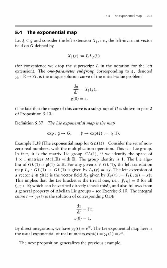
5.4 The exponential map 203
5.4 The exponential map
Let ξ ∈ g and consider the left extension Xξ , i.e., the left-invariant vectorfield on G defined by
Xξ(g) := TeLg(ξ)
(for convenience we drop the superscript L in the notation for the leftextension). The one-parameter subgroup corresponding to ξ , denotedγξ : R→ G, is the unique solution curve of the initial-value problem
dgdt= Xξ(g),
g(0) = e.
(The fact that the image of this curve is a subgroup of G is shown in part 2of Proposition 5.40.)
Definition 5.37 The Lie exponential map is the map
exp : g→ G, ξ → exp(ξ) := γξ (1).
Example 5.38 (The exponential map for GL(1)) Consider the set of non-zero real numbers, with the multiplication operation. This is a Lie group.In fact, it is the matrix Lie group GL(1), if we identify the space of1 × 1 matrices M(1, R) with R. The group identity is 1. The Lie alge-bra of GL(1) is gl(1) � R. For any given x ∈ GL(1), the left translationmap Lx : GL(1) → GL(1) is given by Lx(y) = xy. The left extension ofa vector ξ ∈ gl(1) is the vector field Xξ given by Xξ(x) := T1Lx(ξ) = xξ .This implies that the Lie bracket is the trivial one, i.e., [ξ , η] = 0 for allξ , η ∈ R; which can be verified directly (check this!), and also follows froma general property of Abelian Lie groups – see Exercise 5.10. The integralcurve t → γξ (t) is the solution of corresponding ODE
dxdt= ξx,
x(0) = 1.
By direct integration, we have γξ (t) = etξ . The Lie exponential map here isthe usual exponential of real numbers exp(ξ) = γξ (1) = eξ .
The next proposition generalizes the previous example.
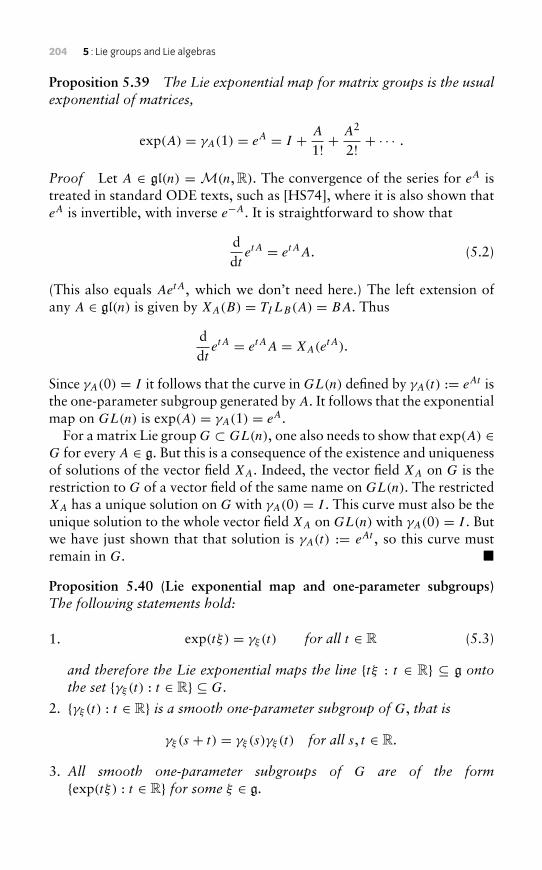
204 5 : Lie groups and Lie algebras
Proposition 5.39 The Lie exponential map for matrix groups is the usualexponential of matrices,
exp(A) = γA(1) = eA = I + A
1! +A2
2! + · · · .
Proof Let A ∈ gl(n) = M(n, R). The convergence of the series for eA istreated in standard ODE texts, such as [HS74], where it is also shown thateA is invertible, with inverse e−A. It is straightforward to show that
ddt
etA = etAA. (5.2)
(This also equals AetA, which we don’t need here.) The left extension ofany A ∈ gl(n) is given by XA(B) = TILB(A) = BA. Thus
ddt
etA = etAA = XA(etA).
Since γA(0) = I it follows that the curve in GL(n) defined by γA(t) := eAt isthe one-parameter subgroup generated by A. It follows that the exponentialmap on GL(n) is exp(A) = γA(1) = eA.
For a matrix Lie group G ⊂ GL(n), one also needs to show that exp(A) ∈G for every A ∈ g. But this is a consequence of the existence and uniquenessof solutions of the vector field XA. Indeed, the vector field XA on G is therestriction to G of a vector field of the same name on GL(n). The restrictedXA has a unique solution on G with γA(0) = I . This curve must also be theunique solution to the whole vector field XA on GL(n) with γA(0) = I . Butwe have just shown that that solution is γA(t) := eAt , so this curve mustremain in G. �
Proposition 5.40 (Lie exponential map and one-parameter subgroups)The following statements hold:
1. exp(tξ) = γξ (t) for all t ∈ R (5.3)
and therefore the Lie exponential maps the line {tξ : t ∈ R} ⊆ g ontothe set {γξ (t) : t ∈ R} ⊆ G.
2. {γξ (t) : t ∈ R} is a smooth one-parameter subgroup of G, that is
γξ (s + t) = γξ (s)γξ (t) for all s, t ∈ R.
3. All smooth one-parameter subgroups of G are of the form{exp(tξ) : t ∈ R} for some ξ ∈ g.
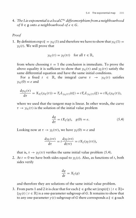
5.4 The exponential map 205
4. TheLie exponential is a local C∞ diffeomorphism from a neighbourhoodof 0 ∈ g onto a neighbourhood of e ∈ G.
Proof
1. By definition exp tξ = γtξ (1) and therefore we have to show that γtξ (1) =γξ (t). We will prove that
γtξ (τ ) = γξ (τ t) for all τ ∈ R,
from where choosing τ = 1 the conclusion is immediate. To prove theabove equality it is sufficient to show that γtξ (τ ) and γξ (tτ ) satisfy thesame differential equation and have the same initial conditions.
For a fixed t ∈ R, the integral curve τ → γtξ (τ ) satisfiesγtξ (0) = e and
dγtξ (τ )dτ
= Xtξ (γtξ (τ )) = TeLγtξ (τ )(tξ) = tTeLγtξ (τ )(ξ) = tXξ (γtξ (τ )),
where we used that the tangent map is linear. In other words, the curveτ → γtξ (τ ) is the solution of the initial value problem
dgdτ= tXξ (g), g(0) = e. (5.4)
Looking now at τ → γξ (τ t), we have γξ (0) = e and
dγξ (τ t)dτ
= tdγξ (τ t)d(τ t)
= tXξ (γξ (τ t)),
that is, τ → γξ (τ t) verifies the same initial value problem (5.4).
2. At t = 0 we have both sides equal to γξ (s). Also, as functions of t , bothsides verify
dgdt= Xξ(g)
and therefore they are solutions of the same initial value problem.
3. From parts 1 and 2 it is clear that for each ξ ∈ g the set {exp(tξ) | t ∈ R}={γξ (t) | t ∈ R} is a one-parameter subgroup of G. It remains to show thatto any one-parameter γ (t) subgroup of G there corresponds a ξ ∈ g such
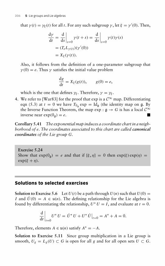
206 5 : Lie groups and Lie algebras
that γ (t) = γξ (t) for all t . For any such subgroup γ , let ξ = γ ′(0). Then,
dγdt= d
ds
∣∣∣∣s=0
γ (t + s) = dds
∣∣∣∣s=0
γ (t)γ (s)
= (TeLγ (t))(γ′(0))
= Xξ(γ (t)).
Also, it follows from the definition of a one-parameter subgroup thatγ (0) = e. Thus γ satisfies the initial value problem
dgdt= Xξ(g(t)), g(0) = e,
which is the one that defines γξ . Therefore, γ = γξ .
4. We refer to [War83] for the proof that exp is a C∞ map. Differentiatingeqn (5.3) at t = 0 we have T0g
exp = Idg (the identity map on g. Bythe Inverse Function Theorem, the map exp : g→ G is has a local C∞inverse near exp(0g) = e. �
Corollary 5.41 The exponentialmap induces a coordinate chart in a neigh-borhood of e. The coordinates associated to this chart are called canonicalcoordinates of the Lie group G.
Exercise 5.24Show that exp(0g) = e and that if [ξ , η] = 0 then exp(ξ) exp(η) =exp(ξ + η).
Solutions to selected exercises
Solution to Exercise 5.6 Let U(t) be a path through U(n) such that U(0) =I and U (0) = A ∈ u(n). The defining relationship for the Lie algebra isfound by differentiating the relationship, U∗ U = I , and evaluate at t = 0.
ddt
∣∣∣∣t=0
U∗ U = U∗ U + U∗ U∣∣t=0 = A∗ + A = 0.
Therefore, elements A ∈ u(n) satisfy A∗ = −A.
Solution to Exercise 5.11 Since group multiplication in a Lie group issmooth, Ug = Lg(U) ⊂ G is open for all g and for all open sets U ⊂ G.
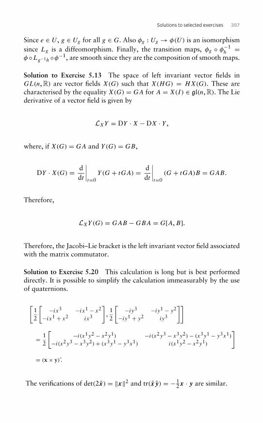
Solutions to selected exercises 207
Since e ∈ U , g ∈ Ug for all g ∈ G. Also φg : Ug → φ(U) is an isomorphismsince Lg is a diffeomorphism. Finally, the transition maps, φg ◦ φ−1
h =φ ◦Lg−1h ◦φ−1, are smooth since they are the composition of smooth maps.
Solution to Exercise 5.13 The space of left invariant vector fields inGL(n, R) are vector fields X(G) such that X(HG) = HX(G). These arecharacterised by the equality X(G) = GA for A = X(I) ∈ gl(n, R). The Liederivative of a vector field is given by
LXY = DY ·X −DX · Y ,
where, if X(G) = GA and Y (G) = GB,
DY ·X(G) = ddt
∣∣∣∣t=0
Y (G+ tGA) = ddt
∣∣∣∣t=0
(G+ tGA)B = GAB.
Therefore,
LXY(G) = GAB −GBA = G[A,B].
Therefore, the Jacobi–Lie bracket is the left invariant vector field associatedwith the matrix commutator.
Solution to Exercise 5.20 This calculation is long but is best performeddirectly. It is possible to simplify the calculation immeasurably by the useof quaternions.
[12
[−ix3 −ix1 − x2
−ix1 + x2 ix3
],12
[−iy3 −iy1 − y2
−iy1 + y2 iy3
]]
= 12
[−i(x1y2 − x2y1) −i(x2y3 − x3y2)− (x3y1 − y3x1)
−i(x2y3 − x3y2)+ (x3y1 − y3x1) i(x1y2 − x2y1)
]
= (x × y) .
The verifications of det(2x) = ‖x‖2 and tr(xy) = −12x · y are similar.
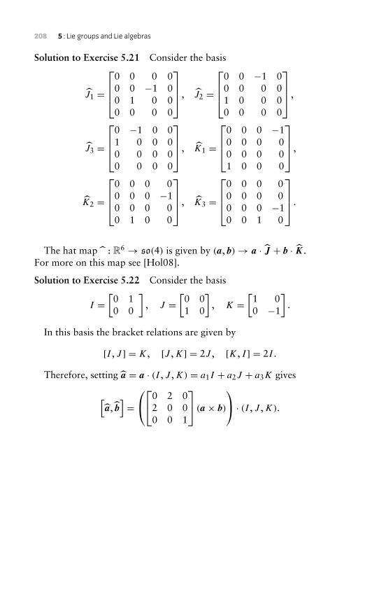
208 5 : Lie groups and Lie algebras
Solution to Exercise 5.21 Consider the basis
J1 =
0 0 0 00 0 −1 00 1 0 00 0 0 0
, J2 =
0 0 −1 00 0 0 01 0 0 00 0 0 0
,
J3 =
0 −1 0 01 0 0 00 0 0 00 0 0 0
, K1 =
0 0 0 −10 0 0 00 0 0 01 0 0 0
,
K2 =
0 0 0 00 0 0 −10 0 0 00 1 0 0
, K3 =
0 0 0 00 0 0 00 0 0 −10 0 1 0
.
The hat map : R6 → so(4) is given by (a, b)→ a · J + b · K.For more on this map see [Hol08].
Solution to Exercise 5.22 Consider the basis
I =[0 10 0
], J =
[0 01 0
], K =
[1 00 −1
].
In this basis the bracket relations are given by
[I , J ] = K, [J ,K] = 2J , [K, I ] = 2I .
Therefore, setting a = a · (I , J ,K) = a1I + a2J + a3K gives
[a, b
]=0 2 0
2 0 00 0 1
(a × b)
· (I , J ,K).
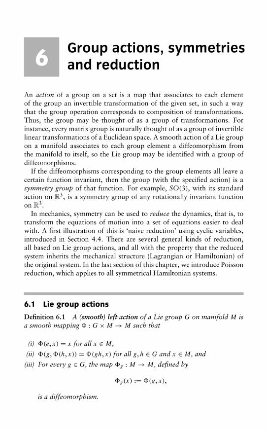
6 Group actions, symmetriesand reduction
An action of a group on a set is a map that associates to each elementof the group an invertible transformation of the given set, in such a waythat the group operation corresponds to composition of transformations.Thus, the group may be thought of as a group of transformations. Forinstance, every matrix group is naturally thought of as a group of invertiblelinear transformations of a Euclidean space. A smooth action of a Lie groupon a manifold associates to each group element a diffeomorphism fromthe manifold to itself, so the Lie group may be identified with a group ofdiffeomorphisms.
If the diffeomorphisms corresponding to the group elements all leave acertain function invariant, then the group (with the specified action) is asymmetry group of that function. For example, SO(3), with its standardaction on R3, is a symmetry group of any rotationally invariant functionon R3.
In mechanics, symmetry can be used to reduce the dynamics, that is, totransform the equations of motion into a set of equations easier to dealwith. A first illustration of this is ‘naive reduction’ using cyclic variables,introduced in Section 4.4. There are several general kinds of reduction,all based on Lie group actions, and all with the property that the reducedsystem inherits the mechanical structure (Lagrangian or Hamiltonian) ofthe original system. In the last section of this chapter, we introduce Poissonreduction, which applies to all symmetrical Hamiltonian systems.
6.1 Lie group actions
Definition 6.1 A (smooth) left action of a Lie group G on manifold M isa smooth mapping � : G×M → M such that
(i) �(e, x) = x for all x ∈ M,
(ii) �(g,�(h, x)) = �(gh, x) for all g,h ∈ G and x ∈ M, and
(iii) For every g ∈ G, the map �g : M → M, defined by
�g(x) := �(g, x),
is a diffeomorphism.
210 6 : Group actions, symmetries and reduction
Note that, the condition (ii) may also be written as �g ◦�h = �gh. Weoften use the notation
gx := �g(x) = �(g, x)
and say that g acts on x. With this notation, condition (ii) above then simplyreads
g(hx) = (gh)x.
All actions of Lie groups will be assumed to be smooth.
Example 6.2 The standard action of a matrix Lie group G ⊆ GL(n, R) onRn is given by �(A, v) = Av (matrix multiplication). It is easily verified thatthis is a left action. In particular, note that condition (ii) in the definitionfollows from associativity of matrix multiplication:
�(A,�(B, v)) = A(Bv) = (AB)v = �(AB, v).
Definition 6.3 A right action of a Lie groupG on manifoldM is a smoothmapping� : G×M → M satisfying the same conditions as for a left actiongiven in Definition 6.1, except that condition (ii) is replaced by:
(ii)′ �(g,�(h, x)) = �(hg, x) for all g,h ∈ G and x ∈ M.
The convenient notation for a right action is xg := �g(x) = �(g, x),because with this notation, condition (ii)′ above then simply reads
(xh)g = x(hg).
A left (or right) action by a group G is called a left (or right) G action.Note that if G is abelian, then every left G action is a right G action andvice versa.
Example 6.4 (Group actions generalise flows) The flow of any completevector field is both a left and a right R action, as can be seen by comparingthe previous definitions with Theorem 3.9. (Recall that R is an abelian Liegroup, with the group operation being addition.) The “flow property” ofthe flow of a vector field is a special case of both conditions (ii) and (ii)′above.
Remark 6.5 Any left action (g, x) → gx gives rise to a right action by(g, x)→ g−1x. See Exercise 6.1.
6.1 Lie group actions 211
The next definitions will use the notation of left actions, but they applyequally well to right actions.
Definition 6.6 (Isotropy) Let G be a group acting on M. The isotropysubgroup of any x ∈ M is
Gx := {g ∈ G : gx = x}.
If Gx is nontrivial, i.e., contains elements other than the group identity,then x is called an isotropic (or symmetric) point.
Example 6.7 For the standard action of any nontrivial matrix Lie group,the origin is always an isotropic point.
Definition 6.8 (Orbits) Let G act on M. For a given point x ∈ M, thesubset
Orb (x) := {gx : g ∈ G} ⊆ M,
is called the group orbit through x.
Example 6.9 For the flow of a complete field, considered as an R action,this definition of an orbit agrees with the familiar notion of orbit in dynam-ical systems. Also, a point is isotropic if and only if it is either fixed orperiodic.
Definition 6.10 (Properties of group actions) The action � : G×M → M
of a group G on a manifold M is said to be:
1. transitive if for every x, y ∈ M, there exists a g ∈ G such that gx = y;
2. free if it has no isotropic points, i.e. for all x, if gx = x then g = e;
3. faithful (or effective) if for all g ∈ G such that g �= e, there exists x ∈ M
such that gx �= x; and
4. proper if, whenever the sequences {xn} and {gnxn} converge in M, thesequence {gn} has a convergent subsequence in G.
Remark 6.11 A transitive action has only one group orbit.
Remark 6.12 An equivalent definition of a faithful action is: if �g is theidentity transformation on M, then g = e.
Proposition 6.13 Every action of a compact group is proper.
212 6 : Group actions, symmetries and reduction
Proof In a compact group, every sequence {gn} has a convergentsubsequence. �
Example 6.14 (SO(2) action on R2) Consider the standard action ofSO(2) on R2,([
cos θ − sin θ
sin θ cos θ
],[x
y
])→[cos θ − sin θ
sin θ cos θ
]·[x
y
]=[x cos θ − y sin θ
x sin θ + y cos θ
].
The group orbits are circles around the origin, except for the one-pointorbit {(0, 0)}. The isotropy group of the origin is SO(2), and the isotropygroup of every other point (x, y) ∈ R2 is trivial, i.e, G(x,y) = {I}, the setcontaining only the group identity. This action is non-transitive, non-free(since (0, 0) is isotropic), faithful and proper (since SO(2) is compact).
The following property of proper actions is proven in [AM78].
Proposition 6.15 Orbits of proper group actions are embeddedsubmanifolds.
Example 6.16 (A non-proper group action) Consider the left action of R
on T2 given by (θ , (φ1,φ2)
)→ (φ1 + θ ,φ2 +√
2 θ).
The orbit of any point is dense in T2 (see Exercise 6.4). This action is non-transitive, free, faithful and non-proper. If the irrational
√2 is replaced by
a rational number, then the action becomes proper and the orbit of anypoint is closed.
Definition 6.17 A G action on a vector space V is called linear if �g is alinear map, for every g ∈ G.
Clearly, the standard action of any matrix Lie group is linear.
Remark 6.18 A linear action of a groupG onRn is called a representationof G. Note that if � is such an action, then each �g corresponds to anelement of GL(n).
Definition 6.19 Let G act on Q, and let ω be a symplectic form on Q.The action is symplectic with respect to ω if, for every g ∈ G, the map�g is symplectic, that is (see Definition 3.109), �∗gω = ω. Similarly, if Qhas a Poisson bracket {·, ·}, then the G action is Poisson with respect to
6.1 Lie group actions 213
that bracket if, for every g ∈ G, the map �g is a Poisson map, that is (seeDefinition 4.32), for all scalar fields F ,G on Q,
{F ◦�g,G ◦�g} = {F ,G} ◦�g.
Both symplectic and Poisson actions are also called canonical actions.
Example 6.20 The standard action of SO(2) on R2 (see Example 6.14) issymplectic with respect to the canonical symplectic form on R2, which isω = dx ∧ dy. Indeed, for any R ∈ SO(2), the map �R is symplectic if andonly if �∗Rω = ω, that is,
ω(�R(x)) (D�R(x)v, D�R(x)w) = ω(v,w),
for all x, v,w ∈ R2. The map �R is R itself, viewed as a linear transfor-mation. Since it is linear its derivative, at any point, is itself: D�R(x)v =�R(v) = Rv, for all x, v. Also, recall from Example 3.108 that the matrixof ω(x), for any x ∈ R2, is
J =[
0 1−1 0
].
Thus, �R is symplectic if and only if
(Rv)T J (Rw) = vT Jw,
for all v,w ∈ R2, which is equivalent to
RT J R = J.
This can be verified by direct computation, for any R ∈ SO(2), whichshows that the action is symplectic. Note that the previous equation is thecondition for R to be an element of the symplectic group Sp(2, R), as definedin Example 5.13. So we have also shown that SO(2) ⊂ Sp(2, R).
The next proposition generalizes the previous example.
Proposition 6.21 The standard action of a matrix Lie group G on R2n issymplectic with respect to the canonical symplectic form on Rn if and onlyif G ⊆ Sp(2n, R).
Proof Example 3.110 showed that an action � of G on R2n is symplecticif and only if D�A(z) ∈ Sp(2n) for all A ∈ G. For the standard action ofG ⊆ GL(n), the map �A is the linear transformation A, and the derivativeof A, at any point, is A itself. Thus, the standard action of G is symplecticif and only if A ∈ Sp(2n, R), for all A ∈ G. �
214 6 : Group actions, symmetries and reduction
Definition 6.22 (Infinitesimal generator) Consider the left action of a Liegroup G on the manifold M, (g, x)→ gx. Let ξ ∈ g be a vector in the Liealgebra of G and consider the one-parameter subgroup {exp(tξ) : t ∈ R} ⊆G. The orbit of an element x with respect to this subgroup is a smooth patht → (exp(tξ)) x in M. The infinitesimal generator associated to ξ at x ∈ M,denoted ξM(x), is the tangent (or velocity) vector to this curve at x, that is:
ξM(x) := ddt
∣∣∣t=0
(exp(tξ) x) ∈ TxM. (6.1)
The smooth vector field ξM : M → TM, x → ξM(x), is called theinfinitesimal generator vector field associated to ξ .
Remark 6.23 The infinitesimal generator map g × M → TM, (ξ , x) →ξM(x) can be thought of as the ‘infinitesimal action’ of g on M. It is theexpression at the tangent level of the action of G on M.
Remark 6.24 For the standard action of a matrix Lie group on Rn, theexpression exp(tξ)x is the matrix product of exp(tξ) and x. Hence,
ξM (x) = ddt
∣∣∣t=0
(exp(tξ)x) =(
ddt
∣∣∣t=0
exp(tξ))
x = ξx (matrix product).
Example 6.25 (The infinitesimal generator for the SO(2) action on R2)Let
ξ :=[0 −ξξ 0
]∈ so(2) and x :=
[x1x2
]∈ R2.
Then
ξR2(x) = ξ
[x1x2
]=[0 −ξξ 0
] [x1x2
]=[−ξx2
ξx1
].
Proposition 6.26 The map g→ X(M), ξ → ξM , is linear and satisfies
[ξ , η] = −[ξM , ηM ],for all ξ , η ∈ g (such a map is called a Lie algebra anti-homomorphism).
Proof See for example [MR02]. �
Corollary 6.27 Given a G action on M, the set of infinitesimal generatorvector fields forms a subalgebra of X(M).
Infinitesimal generator vector fields are not necessarily left invariant, asshown by Exercise 6.6.
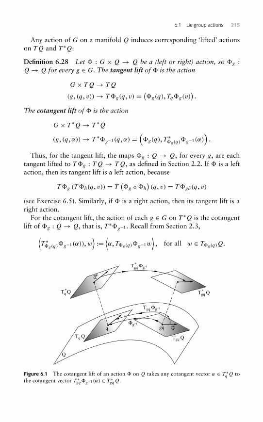
6.1 Lie group actions 215
Any action of G on a manifold Q induces corresponding ‘lifted’ actionson TQ and T ∗Q:
Definition 6.28 Let � : G × Q → Q be a (left or right) action, so �g :Q→ Q for every g ∈ G. The tangent lift of � is the action
G× TQ→ TQ
(g, (q, v))→ T�g(q, v) = (�g(q), Tq�g(v)).
The cotangent lift of � is the action
G× T ∗Q→ T ∗Q
(g, (q,α))→ T ∗�g−1(q,α) =(�g(q), T ∗�g(q)
�g−1(α))
.
Thus, for the tangent lift, the maps �g : Q → Q, for every g, are eachtangent lifted to T�g : TQ→ TQ, as defined in Section 2.2. If � is a leftaction, then its tangent lift is a left action, because
T�g (T�h(q, v)) = T(�g ◦�h
)(q, v) = T�gh(q, v)
(see Exercise 6.5). Similarly, if � is a right action, then its tangent lift is aright action.
For the cotangent lift, the action of each g ∈ G on T ∗Q is the cotangentlift of �g : Q→ Q, that is, T ∗�g−1 . Recall from Section 2.3,⟨
T ∗�g(q)�g−1(α)),w
⟩:=⟨α, T�g(q)�g−1w
⟩, for all w ∈ T�g(q)Q.
gqq
α
Q
Tq Q*
Tgq Φg–1*
Tgq Φg–1
Tgq QTq Q
Φg–1
Tgq Q*
w
Figure 6.1 The cotangent lift of an action � on Q takes any cotangent vector α ∈ T ∗q Q tothe cotangent vector T ∗gq�g−1 (α) ∈ T ∗gqQ.
216 6 : Group actions, symmetries and reduction
It is straightforward to verify that
T ∗�g−1(T ∗�h−1(q,α)
) = T ∗(�h−1 ◦�g−1
)(q, v) = T ∗�(gh)−1(q, v).
This implies that the cotangent lift of a left (resp. right) action is a left (resp.right) action – see Exercise 6.5. This is the reason for the inverse in thedefinition.
Example 6.29 It follows from Example 2.79 that the tangent lift of thestandard action of a matrix group is given, in tangent-lifted coordinates, by
T�A(q, q) = (Aq,Aq).
The cotangent lifted action is given, in cotangent-lifted coordinates, by
T ∗�A−1(q, p) = (Aq, pA−1)
(if we represent p as a row vector), or
T ∗�A−1(q, p) = (Aq,A−T p) = (Aq,(A−1
)Tp)
(if we represent p as a column vector).
Remark 6.30 It is straightforward to verify that⟨T ∗�g−1(q,α), T�g(q, v)
⟩= 〈(q,α), (q, v)〉 .
Equivalently, using concatenation notation,
〈g(q,α), g(q, v)〉 = 〈(q,α), (q, v)〉 . (6.2)
Proposition 6.31 (Infinitesimal lifted actions) Let G act on Q, and bytangent and cotangent lifts on TQ and T ∗Q. Let ξ ∈ g. Note that, in localcoordinates, the infinitesimal generator vector field on Q reads,
ξQ : Rn→ Rn, q→ ξQ(q).
The infinitesimal generator vector fields on TQ and T ∗Q are given by
ξTQ(q, q) = (ξQ(q),DξQ(q) · q) ,ξT ∗Q(q, p) =
(ξQ(q),− (DξQ(q)
)T · p) .
Proof Let � be the action of G on Q, so that
ξQ(q) = ddt
∣∣∣∣t=0
�exp tξ (q).
6.1 Lie group actions 217
By the equality of mixed partials,
ddt
∣∣∣∣t=0
D�exp tξ (q) · q = D(
ddt
∣∣∣∣t=0
�exp tξ (q))· q = DξQ(q) · q.
Thus,
ξTQ(q, q) = d
dt
∣∣∣∣t=0
(exp tξ )(q, q)
= d
dt
∣∣∣∣t=0
(�exp tξ (q), D�exp tξ (q) · q
)= (ξQ(q), DξQ(q) · q) .
This proves the first claim. Recall from Section 2.3 that if cotangent vectorsare are considered as columns, then
(T ∗f
)−1(q, p) =
(f (q), (Df (q))−T · p
).
It follows that
ξT ∗Q(q, p) = ddt
∣∣∣∣t=0
(T ∗�exp−tξ
)(q, p)
= ddt
∣∣∣∣t=0
(�exp tξ (q),
(D�exp−tξ (q)
)−T · p)=(ξQ(q),
ddt
∣∣∣∣t=0
(D�exp−tξ (q)
)−T · p) .
Since ⟨(D�exp−tξ (q)
)−T · p, D�exp−tξ (q) · q⟩= ⟨q, p
⟩,
for all t , differentiation with respect to t (in local coordinates) gives,⟨ddt
∣∣∣∣t=0
(D�exp−tξ (q)
)−T · p, q⟩= −
⟨p,
ddt
∣∣∣∣t=0
D�exp−tξ (q) · q⟩
= − ⟨p, DξQ(q) · q⟩= −
⟨(DξQ(q)
)T · p, q⟩.
This completes the proof, since q is arbitrary. �
218 6 : Group actions, symmetries and reduction
Proposition 6.32 The tangent and cotangent lifts of any proper action areproper.
Proof Let G act properly on Q, and consider the tangent-lifted action onTQ. Suppose that {(qi , vi)} and {gi(qi , vi)} are convergent sequences in TQ.Considering the base points of each vector in each of these sequences, itfollows that {qi} and {giqi} are convergent too. Since the action on Q isassumed to be proper, it follows that {gi} has a convergent subsequence.The argument for cotangent lifts is analogous. �
Proposition 6.33 Every cotangent-lifted action is symplectic and Poisson,with respect to the canonical symplectic form and the canonical Poissonbracket.
Proof This follows directly from Propositions 3.117 and 4.34. �
The following definition generalizes Definition 4.44.
Definition 6.34 A function F is invariant (or symmetric) with respect toan action � of a Lie group G if, for every g ∈ G, the map �g is a symmetryof F , that is, F ◦�g = F . The group G is called a Lie group symmetry orsymmetry group of F .
The following proposition generalizes Proposition 4.52. Its proof is leftas Exercise 6.10.
Proposition 6.35 Let � : G×Q→ Q be an action. Let L : TQ→ R be ahyperregular Lagrangian, with corresponding Hamiltonian H : T ∗Q→ R.Then L is invariant with respect to the tangent lift of � if and only if H isinvariant with respect to the cotangent lift of �.
Definition 6.36 LetG act on two manifoldsM and N . A map f : M → N
is equivariant if
f (gz) = gf (z),
for all g ∈ G, z ∈ M.
Exercise 6.1If (g, x)→ gx is a left action, verify that (g, x)→ g−1x is a right action.Similary, if (g, x)→ xg is a right action, verify that (g, x)→ xg−1 is aleft action.
6.1 Lie group actions 219
Exercise 6.2Show that an action is faithful if and only if the map g→ �g is injective.
Exercise 6.3 (SO(3) action on R3)Show that the standard action of SO(3) is faithful, non-transitive, non-free and proper. Find all of the orbits.
Exercise 6.4Show that, for the action in Example 6.16, the orbit of any point isdense in T2, but does not equal T2. Conclude that the orbit is not anembedded submanifold of T2.
Exercise 6.5Show that the tangent and cotangent lifts of a left (resp., right) actionare left (resp., right) actions.
Exercise 6.6Compute the infinitesimal generator for the SO(3) action on R3. Usethe hat map to show that for ξ ∈ so(3), ξSO(3)(x) = ξ × x. Show
that, for all non-zero ξ ∈ so(3), the infinitesimal generator vector fieldcorresponding to ξ is not left invariant.
Exercise 6.7Given ξ ∈ g, consider ξM , the corresponding (left) invariant vector field.Show that the integral curve of ξM through a point x0 ∈ M is t →exp(tξ)x0.
Exercise 6.8Consider the left action of a Lie group G on the manifold M. Assumex ∈ M a point with a non-trivial isotropy subgroup Gx . Show that forany ξ in the Lie subalgebra gx we have ξM(x) = 0.
220 6 : Group actions, symmetries and reduction
Exercise 6.9 (preview of Adjoint and adjoint actions on so(3))The Adjoint action of SO(3) and so(3) is (R, w) → RwR−1. Show thatthe infinitesimal generator of v ∈ so(3), which is denoted by adv, isgiven by
advw := vso(3)(w) = [v, w] = v ×w.
Exercise 6.10Check that Proposition 6.35 is a generalization of Proposition 4.52, andprove the former by generalizing the proof of the latter.
6.2 Actions of a Lie group on itself
Let G be a Lie group. There are four different translation actions of G onitself, defined as follows:
Left action Right actionLeft multiplication (g,h)→ Lg(h) := gh (g,h)→ Lg−1(h) := g−1h
Right multiplication (g,h)→ Rg−1h := hg−1 (g,h)→ Rg(h) := hg
From now on, unless otherwise specified, we use the followingterminology:
Definition 6.37 The action of G on itself by left translation (or leftmultiplication) is the left action defined by
(g,h)→ Lg(h) := gh.
Analogously, the right translation (or right multiplication) action is theright action defined by
(g,h)→ Rg(h) := hg.
All actions above can be lifted to actions on the tangent bundle TG andthe cotangent bundle T ∗G. For instance, for the left multiplicative action
6.2 Actions of a Lie group on itself 221
we have:
G× TG→ TG (tangent-lifted left translation)
(g, (h, v))→ (gh, gv) := (gh, ThLg(v)) =(gh,
ddt
(gc(t))∣∣t=0
),
where c(t) is any path in G with c(0) = h and c′(0) = v; and
G× T ∗G→ T ∗G (cotangent-lifted left translation)
(g, (h,α))→ (gh, gα) := (gh, T ∗ghLg−1(α)),
where ⟨T ∗ghLg−1(α),w
⟩=⟨α, TghLg−1(w)
⟩for all w ∈ TghG.
Example 6.38 (Left translation action of a matrix Lie group on itself) LetG be a matrix Lie group and consider the left translation action of G onitself. For any R ∈ G and any (A, A) ∈ TG, if C(t) is a path in G withC(0) = A and C′(0) = A, then
TALR(A) = ddt
(R C(t))∣∣t=0 = R
ddt
C(t)∣∣t=0 = RA.
Thus the tangent lifted left translation action is
(R, (A, A))→ (RA, TALR(A)) = (RA,RA).
The cotangent-lifted left translation action is:
(R, (A,P))→ (RA, T ∗RALR−1(P )),
for every P ∈ T ∗AG, where⟨T ∗RALR−1(P ), R
⟩ = ⟨P , TRALR−1(R)⟩ = ⟨P ,R−1R
⟩for all R ∈ TRAG.
Identifying T ∗AG with TAG via the trace pairing (see Example 3.74),⟨P ,R−1R
⟩= tr
(P(R−1R)T
)= tr
(R−T P RT
)=⟨R−T P , R
⟩,
so
T ∗RALR−1(P ) = R−T P .
222 6 : Group actions, symmetries and reduction
Thus, using the identification above, the cotangent-lifted left translationaction is
(R, (A,P))→ (RA, T ∗RALR−1P) = (RA,R−T P ).
Definition 6.39 The action of G on itself by conjugation, or innerautomorphism, is
G×G→ G, (g,h)→ Ig(h) := (Lg ◦ Rg−1)(h) = ghg−1.
Orbits of this action are called conjugacy classes.
Definition 6.40 The Adjoint action of G on g is
G× g→ g, (g, ξ)→ Adgξ := TeIg(ξ) = Te(Lg ◦ Rg−1)ξ .
Example 6.41 (Adjoint action for matrix Lie groups) For any matrix Liegroup G, the inner automorphisms are IR(B) = RBR−1, R ∈ G. Taking apath B(t) with B(0) = I and B ′(0) = ξ ∈ g, we have
AdRξ = TI IRξ = ddt
∣∣∣t=0
IR(B(t)) = ddt
∣∣∣t=0
RB(t) R−1 = R ξ R−1.
Note that we have already seen an example of the Adjoint action formatrix Lie groups acting on matrix Lie algebras, when we defined
C(s) = RA(s) B RA(s)−1,
in the proof of Proposition 5.6.
Definition 6.42 The Co-Adjoint action of G on g∗ is the inverse dual ofthe Adjoint action:
G× g∗ → g∗, (g,µ)→ Ad∗g−1µ,
where
〈Ad∗g−1µ, ξ〉 = 〈µ, Adg−1ξ〉
for all µ ∈ g∗, ξ ∈ g and 〈·, ·〉 : g∗ × g→ R is the natural pairing.
6.2 Actions of a Lie group on itself 223
Note that for a fixed g ∈ G, the maps Adg and Ad∗g−1 are the tangent and
cotangent lifts, respectively, at the identity, of the inner automorphism Ig.When there is no confusion, it is common to use either concatenation
notation or ‘dot’ notation for both Adjoint and Co-Adjoint action. Thus:
gξ = g · ξ := Adgξ and gµ = g · µ := Ad∗g−1µ. (6.3)
For the inverse Adjoint and Co-Adjoint actions, it is also common to denote
ξg = ξ · g := Adg−1ξ and µg = µ · g := Ad∗gµ. (6.4)
Example 6.43 (Co-Adjoint action for matrix Lie groups) For any matrixLie group G, we have seen in Example 6.41 that AdRξ = R ξ R−1. It followsthat, for any µ ∈ g∗, ξ ∈ g,⟨
Ad∗R−1 µ, ξ
⟩ = ⟨µ, AdR−1 ξ⟩ = ⟨µ,R−1ξR
⟩.
Now, if we identify µ ∈ g∗ with a matrix µ ∈ g via the trace pairing, asexplained in Remark 3.75, then⟨
µ,R−1ξR⟩= tr
(µRT ξT R−T
)= tr
(R−T µRT ξT
)=⟨R−T µRT , ξ
⟩.
Therefore,
Ad∗R−1 µ = R−T µRT .
Example 6.44 (Adjoint and Co-Adjoint actions for SO(3)) We use the hatmap () : R3 → so(3) as defined in Example 5.35 and the formula for theAdjoint action of matrix groups as given in Example 6.41. Let R ∈ SO(3)and � ∈ so(3). We have
AdR� = R�R−1.
For any w ∈ R3,(AdR�
)w =
(R�R−1
)w = R
(�(R−1w)
)= R(�×R−1w) = (R�)×w = R�w,
224 6 : Group actions, symmetries and reduction
where we have used the relation R(u× v) = Ru×Rv, which holds for anyu, v ∈ R3 and R ∈ SO(3). Consequently,
AdR� = R�.
Identifying so(3) � R3 then gives
AdR� = R�.
Thus, the Adjoint action of SO(3) on so(3) may be identified with the leftmultiplicative action of SO(3) on R3.
To compute the Co-Adjoint action of SO(3) on so(3)∗, first recall thatan element of � ∈ so(3)∗ may be identified with a vector � ∈ R3 by〈�, �〉 = � ·� for all � ∈ R3 (see Example 5.36). We have⟨
Ad∗R−1�, �
⟩=⟨�, AdR−1�
⟩=⟨�, R−1�
⟩= � ·R−1� = (R�) ·� =
⟨(R�), �
⟩.
Hence, the Co-Adjoint action of SO(3) on so(3)∗ has the expression
Ad∗R−1� = (R�).
Identifying so(3)∗ � R3 then gives
Ad∗R−1 = R.
Thus, the Co-Adjoint action of SO(3) on so(3)∗ may also be identified withthe left multiplicative action of SO(3) on R3.
Definition 6.45 For any Lie group G, and any µ ∈ g∗, the Co-Adjointorbit of µ is the orbit of µ under the Co-Adjoint action of G on g∗,
Oµ := {g · µ : g ∈ G} = {Ad∗g−1µ : g ∈ G}.
Example 6.46 (Co-Adjoint orbit for SO(3)) Example 6.44 shows thatthe Co-Adjoint action of SO(3) on so(3)∗ may be identified with the leftmultiplicative action of SO(3) on R3. Thus, the Co-Adjoint orbit of � ∈so(3)∗ � R3 is
O� = {R� : R ∈ SO(3)} ⊂ R3,
which is a 2-sphere of radius ‖�‖.
6.2 Actions of a Lie group on itself 225
The infinitesimal generator (see Definition 6.22) of the Adjoint action ofG is the vector field ξg defined by
ξg(η) = ddt
∣∣∣∣t=0
Adexp tξ η = Te(Ad(·) η) ξ ,
where Ad(·)η is the map from G to g that takes g to Adgη. Since g is a vectorspace, T g � g × g, a vector field on g can be considered as a map from gto g. Considered in this way, the vector field ξg is denoted by adξ .
Definition 6.47 The infinitesimal generator map,
g× g→ g, (ξ , η) → adξ (η) = ξg(η) = ddt
∣∣∣∣t=0
Adexp tξ η,
is called the adjoint action of g on itself, even though it is not a groupaction. The adjoint operator on g, denoted by ad, is defined by
adξ η = ξg(η) for all η ∈ g.
Example 6.48 (adjoint action for matrix Lie algebras) Recall from Exam-ple 6.41 that for any matrix group,
AdR η = RηR−1.
It follows that
adξ η = ddt
∣∣∣∣t=0
Adexp tξ η
= ddt
∣∣∣∣t=0
(exp tξ ) η exp(−tξ )
= ξη − ηξ = [ξ , η].
In fact, this result holds for all Lie algebras:
Proposition 6.49
adξ η = [ξ , η], (6.5)
where [ξ , η] :=[XL
ξ ,XLη
]is the Lie bracket defined in Definition 5.27.
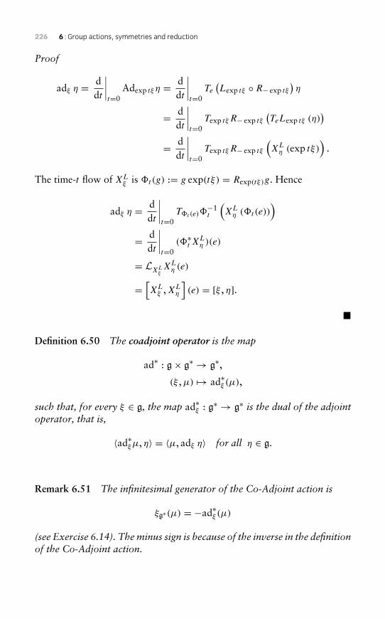
226 6 : Group actions, symmetries and reduction
Proof
adξ η = ddt
∣∣∣∣t=0
Adexp tξ η = ddt
∣∣∣∣t=0
Te
(Lexp tξ ◦ R− exp tξ
)η
= ddt
∣∣∣∣t=0
Texp tξR− exp tξ
(TeLexp tξ (η)
)= d
dt
∣∣∣∣t=0
Texp tξR− exp tξ
(XL
η (exp tξ ))
.
The time-t flow of XLξ is �t(g) := g exp(tξ) = Rexp(tξ)g. Hence
adξ η = ddt
∣∣∣∣t=0
T�t (e)�−1t
(XL
η (�t(e)))
= ddt
∣∣∣∣t=0
(�∗t XLη )(e)
= LXLξXL
η (e)
=[XL
ξ ,XLη
](e) = [ξ , η].
�
Definition 6.50 The coadjoint operator is the map
ad∗ : g× g∗ → g∗,(ξ ,µ) → ad∗ξ (µ),
such that, for every ξ ∈ g, the map ad∗ξ : g∗ → g∗ is the dual of the adjointoperator, that is,
〈ad∗ξµ, η〉 = 〈µ, adξ η〉 for all η ∈ g.
Remark 6.51 The infinitesimal generator of the Co-Adjoint action is
ξg∗(µ) = −ad∗ξ (µ)
(see Exercise 6.14). The minus sign is because of the inverse in the definitionof the Co-Adjoint action.
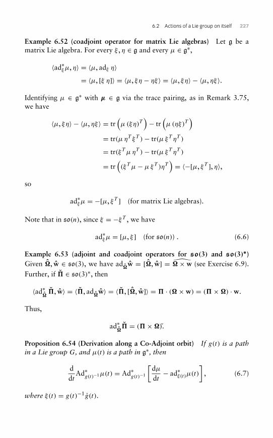
6.2 Actions of a Lie group on itself 227
Example 6.52 (coadjoint operator for matrix Lie algebras) Let g be amatrix Lie algebra. For every ξ , η ∈ g and every µ ∈ g∗,
〈ad∗ξµ, η〉 = 〈µ, adξ η〉= 〈µ, [ξ η]〉 = 〈µ, ξη − ηξ〉 = 〈µ, ξη〉 − 〈µ, ηξ〉.
Identifying µ ∈ g∗ with µ ∈ g via the trace pairing, as in Remark 3.75,we have
〈µ, ξη〉 − 〈µ, ηξ〉 = tr(µ (ξη)T
)− tr
(µ (ηξ)T
)= tr(µ ηT ξT )− tr(µ ξT ηT )
= tr(ξT µ ηT )− tr(µ ξT ηT )
= tr((ξT µ− µξT )ηT
)= 〈−[µ, ξT ], η〉,
so
ad∗ξµ = −[µ, ξT ] (for matrix Lie algebras).
Note that in so(n), since ξ = −ξT , we have
ad∗ξµ = [µ, ξ ] (for so(n)) . (6.6)
Example 6.53 (adjoint and coadjoint operators for so(3) and so(3)∗)Given �, w ∈ so(3), we have ad
�w = [�, w] = �×w (see Exercise 6.9).
Further, if � ∈ so(3)∗, then
〈ad∗��, w〉 = 〈�, ad
�w〉 = 〈�, [�, w]〉 = � · (�×w) = (�×�) ·w.
Thus,
ad∗�� = (�×�).
Proposition 6.54 (Derivation along a Co-Adjoint orbit) If g(t) is a pathin a Lie group G, and µ(t) is a path in g∗, then
ddt
Ad∗g(t)−1µ(t) = Ad∗
g(t)−1
[dµdt− ad∗ξ(t)µ(t)
], (6.7)
where ξ(t) = g(t)−1g(t).
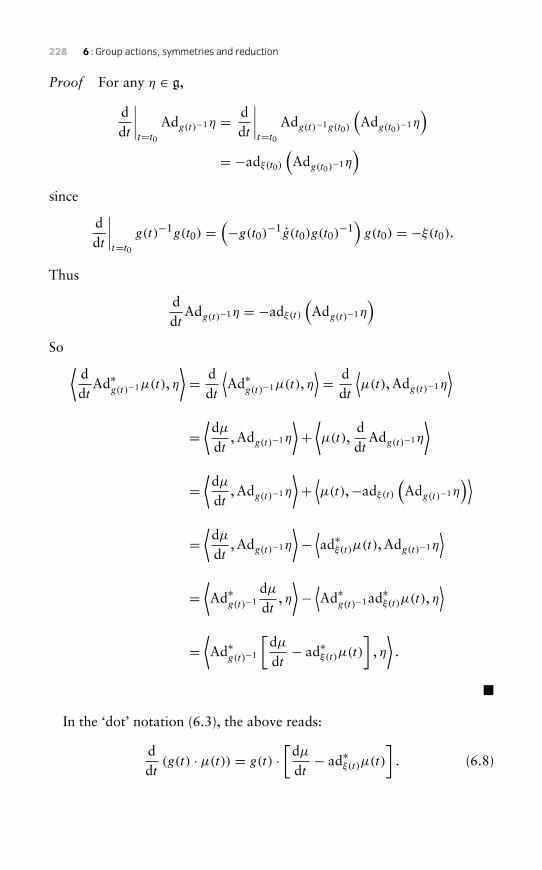
228 6 : Group actions, symmetries and reduction
Proof For any η ∈ g,
ddt
∣∣∣∣t=t0
Adg(t)−1η = ddt
∣∣∣∣t=t0
Adg(t)−1g(t0)
(Adg(t0)
−1η)
= −adξ(t0)
(Adg(t0)
−1η)
since
ddt
∣∣∣∣t=t0
g(t)−1g(t0) =(−g(t0)−1g(t0)g(t0)
−1)g(t0) = −ξ(t0).
Thus
ddt
Adg(t)−1η = −adξ(t)
(Adg(t)−1η
)So ⟨
ddt
Ad∗g(t)−1µ(t), η
⟩= d
dt
⟨Ad∗
g(t)−1µ(t), η⟩= d
dt
⟨µ(t), Adg(t)−1η
⟩
=⟨dµdt
, Adg(t)−1η
⟩+⟨µ(t),
ddt
Adg(t)−1η
⟩
=⟨dµdt
, Adg(t)−1η
⟩+⟨µ(t),−adξ(t)
(Adg(t)−1η
)⟩
=⟨dµdt
, Adg(t)−1η
⟩−⟨ad∗ξ(t)µ(t), Adg(t)−1η
⟩
=⟨Ad∗
g(t)−1dµdt
, η⟩−⟨Ad∗
g(t)−1ad∗ξ(t)µ(t), η⟩
=⟨Ad∗
g(t)−1
[dµdt− ad∗ξ(t)µ(t)
], η⟩.
�
In the ‘dot’ notation (6.3), the above reads:
ddt
(g(t) · µ(t)) = g(t) ·[dµdt− ad∗ξ(t)µ(t)
]. (6.8)
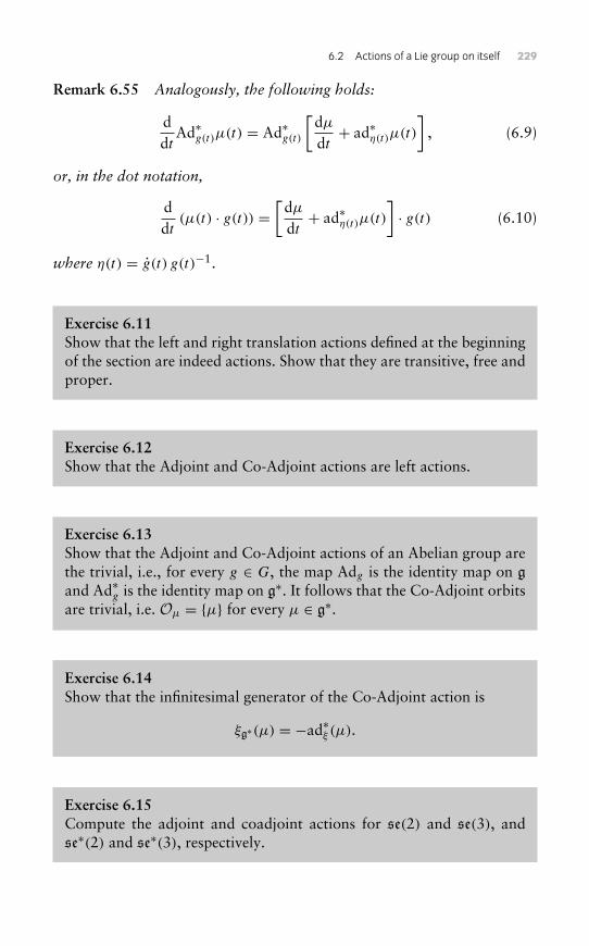
6.2 Actions of a Lie group on itself 229
Remark 6.55 Analogously, the following holds:
ddt
Ad∗g(t)µ(t) = Ad∗g(t)[dµdt+ ad∗η(t)µ(t)
], (6.9)
or, in the dot notation,
ddt
(µ(t) · g(t)) =[dµdt+ ad∗η(t)µ(t)
]· g(t) (6.10)
where η(t) = g(t) g(t)−1.
Exercise 6.11Show that the left and right translation actions defined at the beginningof the section are indeed actions. Show that they are transitive, free andproper.
Exercise 6.12Show that the Adjoint and Co-Adjoint actions are left actions.
Exercise 6.13Show that the Adjoint and Co-Adjoint actions of an Abelian group arethe trivial, i.e., for every g ∈ G, the map Adg is the identity map on gand Ad∗g is the identity map on g∗. It follows that the Co-Adjoint orbitsare trivial, i.e. Oµ = {µ} for every µ ∈ g∗.
Exercise 6.14Show that the infinitesimal generator of the Co-Adjoint action is
ξg∗(µ) = −ad∗ξ (µ).
Exercise 6.15Compute the adjoint and coadjoint actions for se(2) and se(3), andse∗(2) and se∗(3), respectively.
230 6 : Group actions, symmetries and reduction
Exercise 6.16Consider a left action of a Lie group G on a manifold M, and its tangent-lifted action on TM. Prove that for any g ∈ G, ξ ∈ g and z ∈ M,
g(ξM(g−1z)
)= (Adgξ)M(z).
6.3 Quotient spaces
Consider a smooth action of a Lie group G on a manifold M. It can be easilyverified that the relation
x ∼ y if and only if there exists g ∈ G such that gx = y
is an equivalence relation on M. The equivalence class containing x isprecisely the orbit of x,
[x] := {y : y ∼ x} = {y : y ∈ Orb(x)} = Orb(x).
The set of all orbits is called the orbit space, or quotient space, and denotedM/G. Let
π : M → M/G
be the map assigning to each x ∈ M its orbit Orb(x) ∈ M/G, that isπ(x) = [x] = Orb(x). The orbit space is endowed with a topologicalstructure, called the quotient topology, defined by
U ⊆ M/G is open if and only if π−1(U) is open in M.
It is natural to ask whether M/G has a smooth manifold structure. A widelyapplicable, though partial, answer is given in the following proposition:
Proposition 6.56 If the action of a Lie group G on a manifold M is free,proper and smooth, then the quotient space M/G is has a unique smoothmanifold structure such that π : M → M/G, defined by π(x) = Orb(x),is a submersion. This manifold structure is compatible with the quotienttopology defined above, and has the following properties:
1. A map f : M/G→ N , for any manifold N , is smooth if and only if thecomposition f ◦ π is smooth.
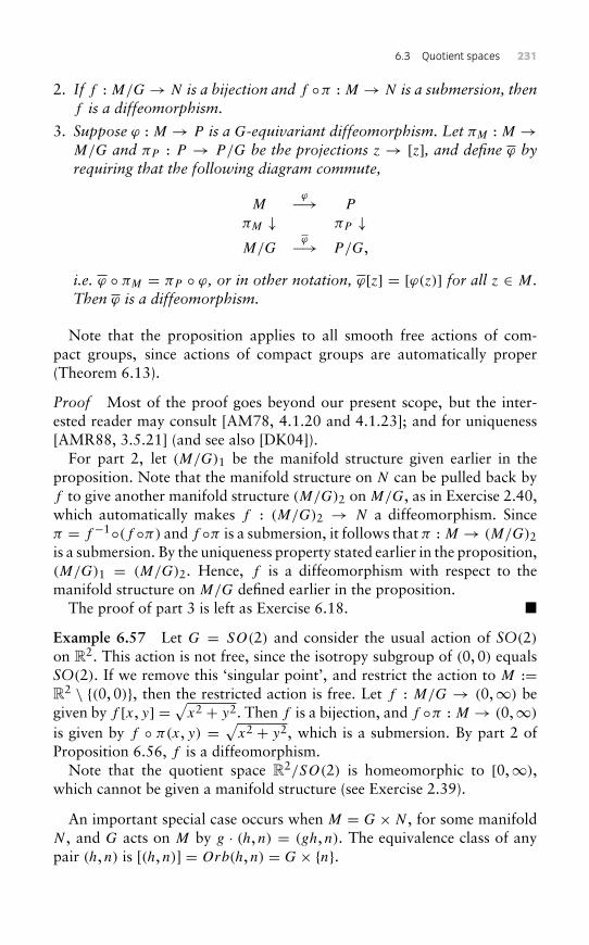
6.3 Quotient spaces 231
2. If f : M/G→ N is a bijection and f ◦π : M → N is a submersion, thenf is a diffeomorphism.
3. Suppose ϕ : M → P is a G-equivariant diffeomorphism. Let πM : M →M/G and πP : P → P/G be the projections z → [z], and define ϕ byrequiring that the following diagram commute,
Mϕ−→ P
πM ↓ πP ↓M/G
ϕ−→ P/G,
i.e. ϕ ◦ πM = πP ◦ ϕ, or in other notation, ϕ[z] = [ϕ(z)] for all z ∈ M.Then ϕ is a diffeomorphism.
Note that the proposition applies to all smooth free actions of com-pact groups, since actions of compact groups are automatically proper(Theorem 6.13).
Proof Most of the proof goes beyond our present scope, but the inter-ested reader may consult [AM78, 4.1.20 and 4.1.23]; and for uniqueness[AMR88, 3.5.21] (and see also [DK04]).
For part 2, let (M/G)1 be the manifold structure given earlier in theproposition. Note that the manifold structure on N can be pulled back byf to give another manifold structure (M/G)2 on M/G, as in Exercise 2.40,which automatically makes f : (M/G)2 → N a diffeomorphism. Sinceπ = f−1◦(f ◦π) and f ◦π is a submersion, it follows that π : M → (M/G)2is a submersion. By the uniqueness property stated earlier in the proposition,(M/G)1 = (M/G)2. Hence, f is a diffeomorphism with respect to themanifold structure on M/G defined earlier in the proposition.
The proof of part 3 is left as Exercise 6.18. �
Example 6.57 Let G = SO(2) and consider the usual action of SO(2)on R2. This action is not free, since the isotropy subgroup of (0, 0) equalsSO(2). If we remove this ‘singular point’, and restrict the action to M :=R2 \ {(0, 0)}, then the restricted action is free. Let f : M/G → (0,∞) begiven by f [x, y] = √x2 + y2. Then f is a bijection, and f ◦π : M → (0,∞)
is given by f ◦ π(x, y) = √x2 + y2, which is a submersion. By part 2 of
Proposition 6.56, f is a diffeomorphism.Note that the quotient space R2/SO(2) is homeomorphic to [0,∞),
which cannot be given a manifold structure (see Exercise 2.39).
An important special case occurs when M = G× N , for some manifoldN , and G acts on M by g · (h, n) = (gh, n). The equivalence class of anypair (h, n) is [(h, n)] = Orb(h, n) = G× {n}.
232 6 : Group actions, symmetries and reduction
Remark 6.58 We use the notation [h, n] := [(h, n)].
There is a bijection
M/G � (G×N)/Gf−→ N
[h, n] −→ n.
Clearly f ◦π : M → N , given by (h, n)→ n, is a submersion. Thus, by part2 of the previous proposition, M/G is diffeomorphic to N . In summary,
Proposition 6.59 If M = G × N and G acts on M by g(h, n) = (gh, n),then M/G is diffeomorphic to N via the map [h, n] −→ n.
Now, we consider the cases where the manifold M is either the tangent orthe cotangent bundle of a Lie group G, with G acting on M by either tangentor cotangent lifts (respectively) of the left multiplicative action ofG on itself.We begin with the case M = TG. Consider the left trivialization map
λ : TG→ G× g, (h, h)→ λ(h, h) := (h,h−1h) = (h, ThLh−1 h), (6.11)
which has inverse λ−1(h, ξ) = (h,hξ). Note that, since the left multiplicativeoperation and the projection (h, h)→ h are both smooth, it follows that λ isa diffeomorphism. The left multiplicative action of G on TG induces, via λ,a corresponding action of G on G× g that makes λ equivariant, defined byg(λ(h, h)) = λ(g(h, h)) (this is called ‘the push-forward by λ’ of the originalaction). It is straightforward to compute this action:
g(h, ξ) = g(λ(h,hξ)) = λ(g(h,hξ)) = λ(gh, ghξ) = (gh, ξ).
Note that this action on G× g is a special case of the action in Proposition6.59, with N = g. Applying that proposition, we see that (G × g)/G isdiffeomorphic to g via the map [g, ξ ] → ξ . Now, since λ is a G-equivariantdiffeomorphism, part 3 of Proposition 6.56 shows that (T G)/G is diffeo-morphic to (G × g)/G, via the diffeomorphism λ defined by λ([h, h]) =[λ(h, h)] = [h,h−1h]. We have shown the following.:
Proposition 6.60 Let G act on TG by tangent-lifted left multiplication.Then the following are diffeomorphisms,
(T G)/G � (G× g)/G � g,[h, h
] −→ [h,h−1h] −→ h−1h.
6.4 Poisson reduction 233
Analogously one can show that under the cotangent left trivialization
λ∗ : T ∗G→ G× g∗, (h,α)→ (h,h−1α) := (h, T ∗e Lhα), (6.12)
the induced left action of G on G× g∗ is given by
g(h,µ) = (gh,µ).
Again, Proposition 6.59 applies, this time with N = g∗, so (G × g∗)/G isdiffeomorphic to g∗ via the map [g,µ] → µ. Thus, we have,
Proposition 6.61 LetG act on T ∗G by cotangent-lifted left multiplication.Then the following are diffeomorphisms,
(T ∗G)/G � (G× g∗)/G � g∗,
[h,α] −→ [h,h−1α] −→ h−1α.
Remark 6.62 The identification of (G×g)/Gwith g, and (G×g∗)/Gwithg∗, may equally well be achieved using the right trivializations
µ : TG→ G× g, (h, h)→ (h, hh−1) := (h, ThRh−1 h);
µ∗ : T ∗G→ G× g∗, (h,α)→ (h,αh−1) := (h, T ∗e Rhα).
Exercise 6.17Let π : M → M/G be as defined in the text. Show that a functionf : M → P , where P is any manifold, is G-invariant if and only iff can be written as ϕ ◦ π for some ϕ : M/G → P . Note that, byProposition 6.56, ϕ is smooth if and only if f is.
Exercise 6.18Prove part 3 Proposition 6.56, using part 2 of the same proposition.
6.4 Poisson reduction
We start with a general theorem concerning reduction on a Poisson manifoldP . Recall from Definition 6.19 that an action � of some Lie group G on P
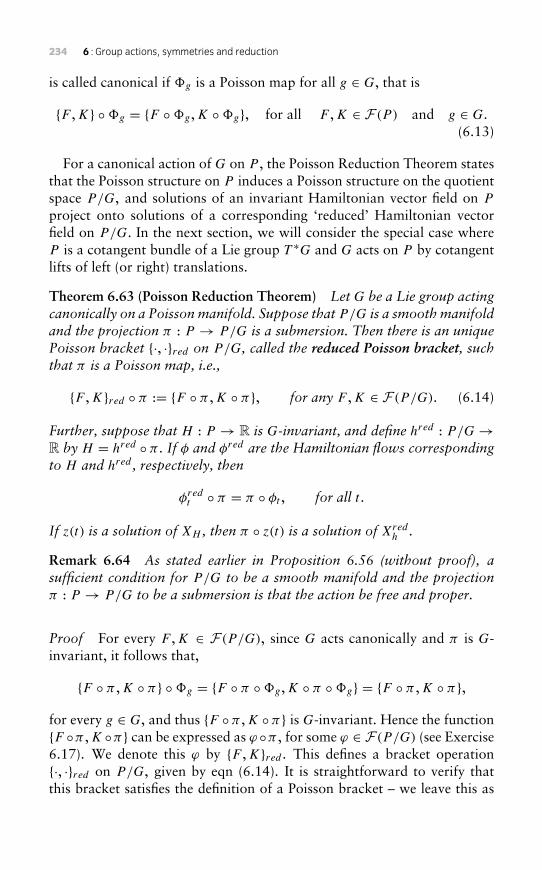
234 6 : Group actions, symmetries and reduction
is called canonical if �g is a Poisson map for all g ∈ G, that is
{F ,K} ◦�g = {F ◦�g,K ◦�g}, for all F ,K ∈ F(P ) and g ∈ G.(6.13)
For a canonical action of G on P , the Poisson Reduction Theorem statesthat the Poisson structure on P induces a Poisson structure on the quotientspace P/G, and solutions of an invariant Hamiltonian vector field on P
project onto solutions of a corresponding ‘reduced’ Hamiltonian vectorfield on P/G. In the next section, we will consider the special case whereP is a cotangent bundle of a Lie group T ∗G and G acts on P by cotangentlifts of left (or right) translations.
Theorem 6.63 (Poisson Reduction Theorem) Let G be a Lie group actingcanonically on a Poisson manifold. Suppose that P/G is a smooth manifoldand the projection π : P → P/G is a submersion. Then there is an uniquePoisson bracket {·, ·}red on P/G, called the reduced Poisson bracket, suchthat π is a Poisson map, i.e.,
{F ,K}red ◦ π := {F ◦ π ,K ◦ π}, for any F ,K ∈ F(P /G). (6.14)
Further, suppose that H : P → R is G-invariant, and define hred : P/G→R by H = hred ◦ π . If φ and φred are the Hamiltonian flows correspondingto H and hred , respectively, then
φredt ◦ π = π ◦ φt , for all t .
If z(t) is a solution of XH , then π ◦ z(t) is a solution of Xredh .
Remark 6.64 As stated earlier in Proposition 6.56 (without proof), asufficient condition for P/G to be a smooth manifold and the projectionπ : P → P/G to be a submersion is that the action be free and proper.
Proof For every F ,K ∈ F(P /G), since G acts canonically and π is G-invariant, it follows that,
{F ◦ π ,K ◦ π} ◦�g = {F ◦ π ◦�g,K ◦ π ◦�g} = {F ◦ π ,K ◦ π},for every g ∈ G, and thus {F ◦π ,K ◦π} is G-invariant. Hence the function{F ◦π ,K ◦π} can be expressed as ϕ ◦π , for some ϕ ∈ F(P /G) (see Exercise6.17). We denote this ϕ by {F ,K}red . This defines a bracket operation{·, ·}red on P/G, given by eqn (6.14). It is straightforward to verify thatthis bracket satisfies the definition of a Poisson bracket – we leave this as
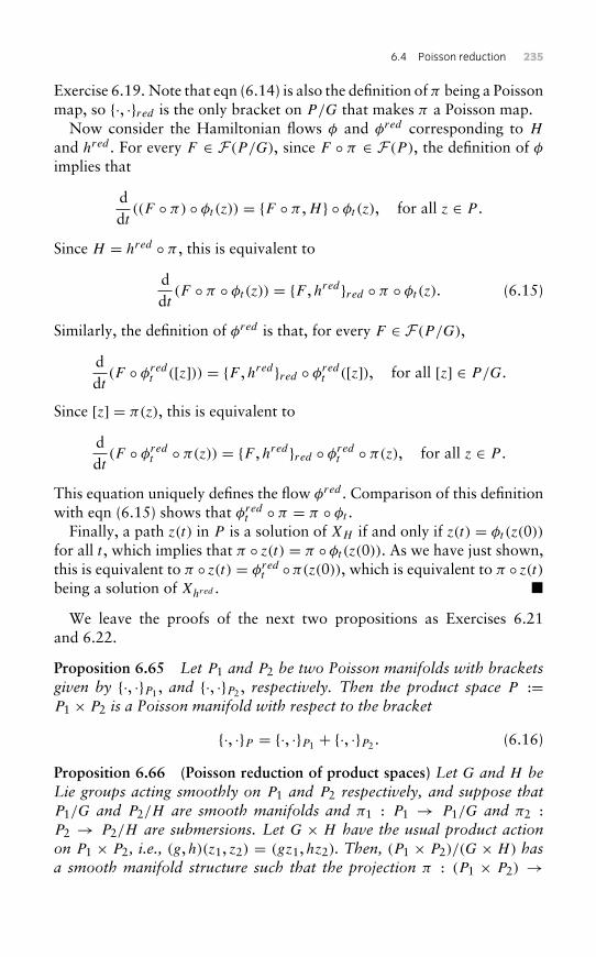
6.4 Poisson reduction 235
Exercise 6.19. Note that eqn (6.14) is also the definition of π being a Poissonmap, so {·, ·}red is the only bracket on P/G that makes π a Poisson map.
Now consider the Hamiltonian flows φ and φred corresponding to H
and hred . For every F ∈ F(P /G), since F ◦ π ∈ F(P ), the definition of φ
implies that
ddt
((F ◦ π) ◦ φt (z)) = {F ◦ π ,H } ◦ φt (z), for all z ∈ P .
Since H = hred ◦ π , this is equivalent to
ddt
(F ◦ π ◦ φt (z)) = {F ,hred}red ◦ π ◦ φt (z). (6.15)
Similarly, the definition of φred is that, for every F ∈ F(P /G),
ddt
(F ◦ φredt ([z])) = {F ,hred}red ◦ φred
t ([z]), for all [z] ∈ P/G.
Since [z] = π(z), this is equivalent to
ddt
(F ◦ φredt ◦ π(z)) = {F ,hred}red ◦ φred
t ◦ π(z), for all z ∈ P .
This equation uniquely defines the flow φred . Comparison of this definitionwith eqn (6.15) shows that φred
t ◦ π = π ◦ φt .Finally, a path z(t) in P is a solution of XH if and only if z(t) = φt (z(0))
for all t , which implies that π ◦ z(t) = π ◦ φt (z(0)). As we have just shown,this is equivalent to π ◦ z(t) = φred
t ◦π(z(0)), which is equivalent to π ◦ z(t)being a solution of Xhred . �
We leave the proofs of the next two propositions as Exercises 6.21and 6.22.
Proposition 6.65 Let P1 and P2 be two Poisson manifolds with bracketsgiven by {·, ·}P1 , and {·, ·}P2 , respectively. Then the product space P :=P1 × P2 is a Poisson manifold with respect to the bracket
{·, ·}P = {·, ·}P1 + {·, ·}P2 . (6.16)
Proposition 6.66 (Poisson reduction of product spaces) Let G and H beLie groups acting smoothly on P1 and P2 respectively, and suppose thatP1/G and P2/H are smooth manifolds and π1 : P1 → P1/G and π2 :P2 → P2/H are submersions. Let G × H have the usual product actionon P1 × P2, i.e., (g,h)(z1, z2) = (gz1,hz2). Then, (P1 × P2)/(G × H) hasa smooth manifold structure such that the projection π : (P1 × P2) →
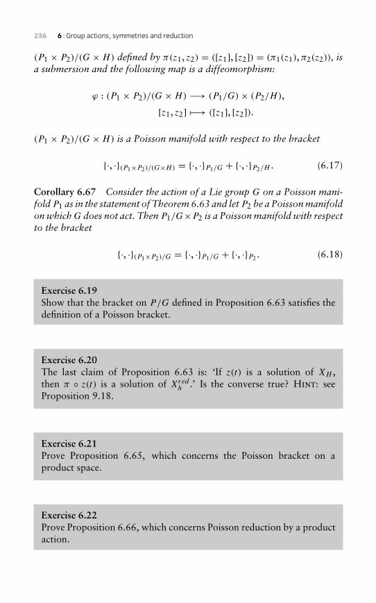
236 6 : Group actions, symmetries and reduction
(P1 × P2)/(G×H) defined by π(z1, z2) = ([z1], [z2]) = (π1(z1),π2(z2)), isa submersion and the following map is a diffeomorphism:
ϕ : (P1 × P2)/(G×H) −→ (P1/G)× (P2/H),
[z1, z2] −→ ([z1], [z2]).
(P1 × P2)/(G×H) is a Poisson manifold with respect to the bracket
{·, ·}(P1×P2)/(G×H) = {·, ·}P1/G + {·, ·}P2/H . (6.17)
Corollary 6.67 Consider the action of a Lie group G on a Poisson mani-foldP1 as in the statement of Theorem 6.63 and letP2 be a Poissonmanifoldon whichG does not act. Then P1/G×P2 is a Poissonmanifold with respectto the bracket
{·, ·}(P1×P2)/G = {·, ·}P1/G + {·, ·}P2 . (6.18)
Exercise 6.19Show that the bracket on P/G defined in Proposition 6.63 satisfies thedefinition of a Poisson bracket.
Exercise 6.20The last claim of Proposition 6.63 is: ‘If z(t) is a solution of XH ,then π ◦ z(t) is a solution of Xred
h .’ Is the converse true? Hint: seeProposition 9.18.
Exercise 6.21Prove Proposition 6.65, which concerns the Poisson bracket on aproduct space.
Exercise 6.22Prove Proposition 6.66, which concerns Poisson reduction by a productaction.
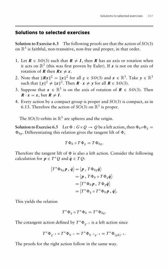
Solutions to selected exercises 237
Solutions to selected exercises
Solution to Exercise 6.3 The following proofs are that the action of SO(3)on R3 is faithful, non-transitive, non-free and proper, in that order.
1. Let R ∈ SO(3) such that R �= I , then R has an axis or rotation whenit acts on R3 (this was first proven by Euler). If x is not on the axis ofrotation of R then Rx �= x.
2. Note that ‖Rx‖2 = ‖x‖2 for all g ∈ SO(3) and x ∈ R3. Take y ∈ R3
such that ‖y‖2 �= ‖x‖2. Then R · x �= y for all R ∈ SO(3).
3. Suppose that x ∈ R3 is on the axis of rotation of R ∈ SO(3). ThenR · x = x, but R �= I .
4. Every action by a compact group is proper and SO(3) is compact, as in6.13. Therefore the action of SO(3) on R3 is proper.
The SO(3)-orbits in R3 are spheres and the origin.
Solution to Exercise 6.5 Let� : G×Q→ Q be a left action, then�h◦�g =�hg. Differentiating this relation gives the tangent lift of �,
T�h ◦ T�g = T�hg.
Therefore the tangent lift of � is also a left action. Consider the followingcalculation for p ∈ T ∗Q and q ∈ TQ:⟨
T ∗�hgp , q⟩ = ⟨p , T�hg q
⟩= ⟨p , T�h ◦ T�g q
⟩= ⟨T ∗�hp , T�g q
⟩= ⟨T ∗�g ◦ T ∗�hp , q
⟩.
This yields the relation
T ∗�g ◦ T ∗�h = T ∗�hg.
The cotangent action defined by T ∗�g−1 is a left action since
T ∗�g−1 ◦ T ∗�h−1 = T ∗�h−1g−1 = T ∗�(gh)−1 .
The proofs for the right action follow in the same way.
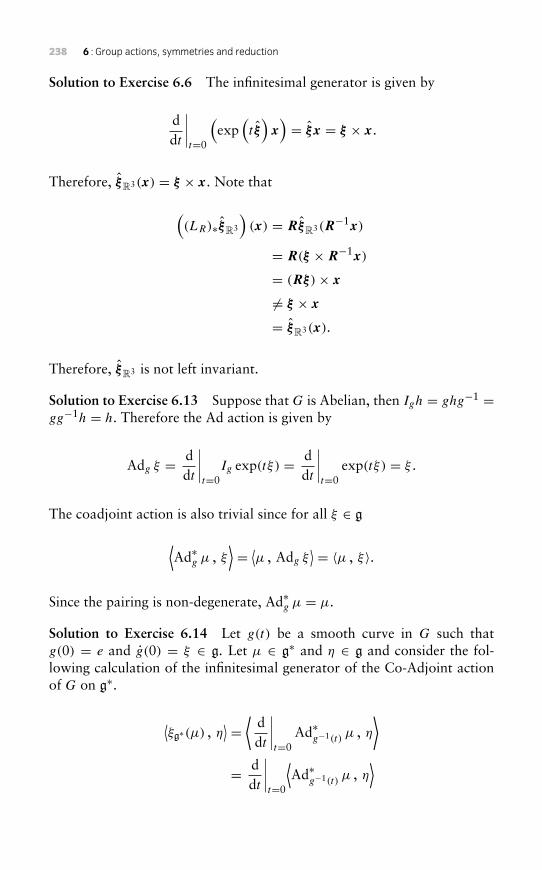
238 6 : Group actions, symmetries and reduction
Solution to Exercise 6.6 The infinitesimal generator is given by
ddt
∣∣∣∣t=0
(exp
(t ξ)x)= ξx = ξ × x.
Therefore, ξR3(x) = ξ × x. Note that
((LR)∗ξR3
)(x) = RξR3(R−1x)
= R(ξ ×R−1x)
= (Rξ)× x
�= ξ × x
= ξR3(x).
Therefore, ξR3 is not left invariant.
Solution to Exercise 6.13 Suppose that G is Abelian, then Igh = ghg−1 =gg−1h = h. Therefore the Ad action is given by
Adg ξ = ddt
∣∣∣∣t=0
Ig exp(tξ) = ddt
∣∣∣∣t=0
exp(tξ) = ξ .
The coadjoint action is also trivial since for all ξ ∈ g
⟨Ad∗g µ , ξ
⟩= ⟨µ , Adg ξ
⟩ = 〈µ , ξ〉.
Since the pairing is non-degenerate, Ad∗g µ = µ.
Solution to Exercise 6.14 Let g(t) be a smooth curve in G such thatg(0) = e and g(0) = ξ ∈ g. Let µ ∈ g∗ and η ∈ g and consider the fol-lowing calculation of the infinitesimal generator of the Co-Adjoint actionof G on g∗.
⟨ξg∗(µ) , η
⟩ = ⟨ ddt
∣∣∣∣t=0
Ad∗g−1(t) µ , η
⟩= d
dt
∣∣∣∣t=0
⟨Ad∗
g−1(t) µ , η⟩
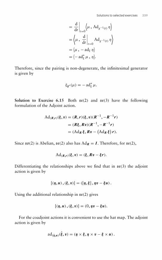
Solutions to selected exercises 239
= ddt
∣∣∣∣t=0
⟨µ , Adg−1(t) η
⟩=⟨µ ,
ddt
∣∣∣∣t=0
Adg−1(t) η
⟩= ⟨µ , − adξ η
⟩= ⟨− ad∗ξ µ , η
⟩.
Therefore, since the pairing is non-degenerate, the infinitesimal generatoris given by
ξg∗(µ) = − ad∗ξ µ.
Solution to Exercise 6.15 Both se(2) and se(3) have the followingformulation of the Adjoint action.
Ad(R,r)(ξ , v) = (R, r)(ξ , v)(R−1,−R−1r)
= (Rξ ,Rv)(R−1,−R−1r)
= (AdR ξ ,Rv − (AdR ξ)r).
Since so(2) is Abelian, se(2) also has AdR = I . Therefore, for se(2),
Ad(R,r)(ξ , v) = (ξ ,Rv − ξr).
Differentiating the relationships above we find that in se(3) the adjointaction is given by
[(η,u) , (ξ , v)] = ([η, ξ ] , ηv − ξu) .
Using the additional relationship in se(2) gives
[(η,u) , (ξ , v)] = (0, ηv − ξu).
For the coadjoint actions it is convenient to use the hat map. The adjointaction is given by
ad(η,u)(ξ , v) = (η × ξ , η × v − ξ × u) .
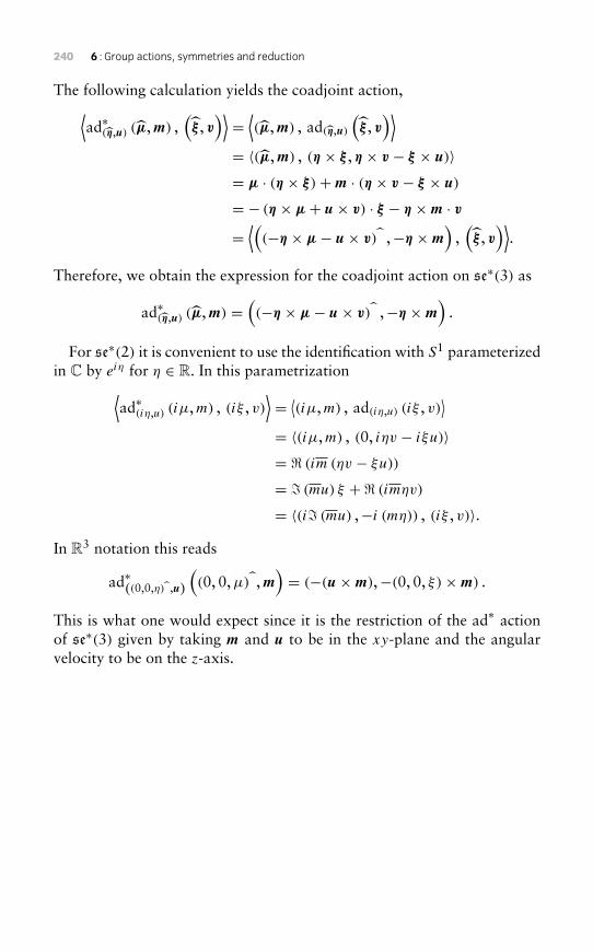
240 6 : Group actions, symmetries and reduction
The following calculation yields the coadjoint action,⟨ad∗(η,u) (µ,m) ,
(ξ , v
)⟩=⟨(µ,m) , ad(η,u)
(ξ , v
)⟩= 〈(µ,m) , (η × ξ , η × v − ξ × u)〉= µ · (η × ξ)+m · (η × v − ξ × u)
= − (η × µ+ u× v) · ξ − η ×m · v=⟨(
(−η × µ− u× v) ,−η ×m)
,(ξ , v
)⟩.
Therefore, we obtain the expression for the coadjoint action on se∗(3) as
ad∗(η,u) (µ,m) =((−η × µ− u× v) ,−η ×m
).
For se∗(2) it is convenient to use the identification with S1 parameterizedin C by eiη for η ∈ R. In this parametrization⟨
ad∗(iη,u) (iµ,m) , (iξ , v)⟩= ⟨(iµ,m) , ad(iη,u) (iξ , v)
⟩= 〈(iµ,m) , (0, iηv − iξu)〉= $ (im (ηv − ξu))
= % (mu) ξ +$ (imηv)
= 〈(i% (mu) ,−i (mη)) , (iξ , v)〉.In R3 notation this reads
ad∗((0,0,η) ,u)
((0, 0,µ) ,m
)= (−(u×m),−(0, 0, ξ)×m) .
This is what one would expect since it is the restriction of the ad∗ actionof se∗(3) given by taking m and u to be in the xy-plane and the angularvelocity to be on the z-axis.
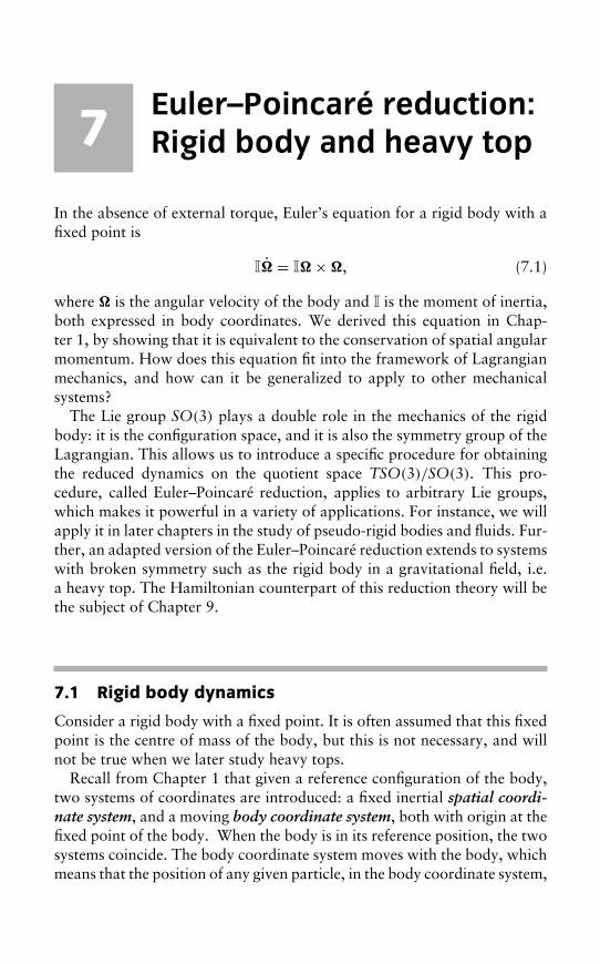
7Euler–Poincaré reduction:Rigid body and heavy top
In the absence of external torque, Euler’s equation for a rigid body with afixed point is
I� = I��, (7.1)
where � is the angular velocity of the body and I is the moment of inertia,both expressed in body coordinates. We derived this equation in Chap-ter 1, by showing that it is equivalent to the conservation of spatial angularmomentum. How does this equation fit into the framework of Lagrangianmechanics, and how can it be generalized to apply to other mechanicalsystems?
The Lie group SO(3) plays a double role in the mechanics of the rigidbody: it is the configuration space, and it is also the symmetry group of theLagrangian. This allows us to introduce a specific procedure for obtainingthe reduced dynamics on the quotient space TSO(3)/SO(3). This pro-cedure, called Euler–Poincaré reduction, applies to arbitrary Lie groups,which makes it powerful in a variety of applications. For instance, we willapply it in later chapters in the study of pseudo-rigid bodies and fluids. Fur-ther, an adapted version of the Euler–Poincaré reduction extends to systemswith broken symmetry such as the rigid body in a gravitational field, i.e.a heavy top. The Hamiltonian counterpart of this reduction theory will bethe subject of Chapter 9.
7.1 Rigid body dynamics
Consider a rigid body with a fixed point. It is often assumed that this fixedpoint is the centre of mass of the body, but this is not necessary, and willnot be true when we later study heavy tops.
Recall from Chapter 1 that given a reference configuration of the body,two systems of coordinates are introduced: a fixed inertial spatial coordi-nate system, and a moving body coordinate system, both with origin at thefixed point of the body. When the body is in its reference position, the twosystems coincide. The body coordinate system moves with the body, whichmeans that the position of any given particle, in the body coordinate system,
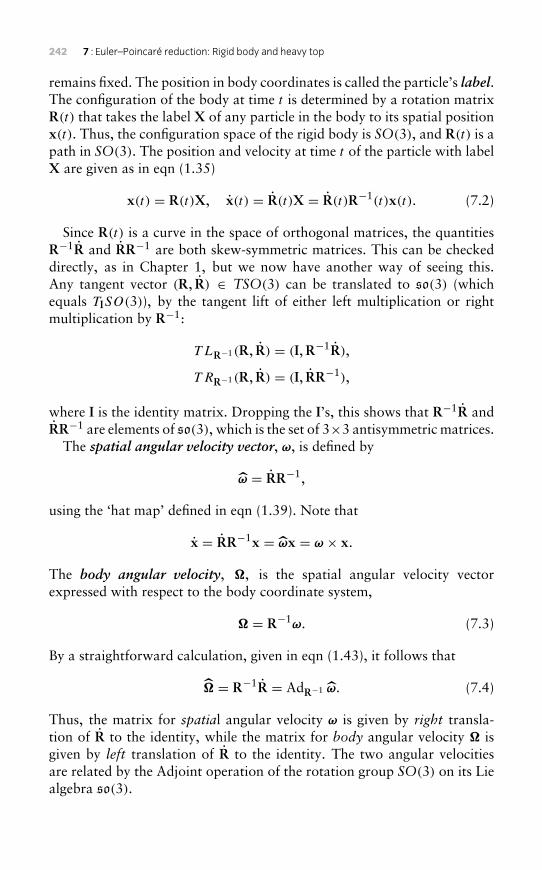
242 7 : Euler–Poincaré reduction: Rigid body and heavy top
remains fixed. The position in body coordinates is called the particle’s label.The configuration of the body at time t is determined by a rotation matrixR(t) that takes the label X of any particle in the body to its spatial positionx(t). Thus, the configuration space of the rigid body is SO(3), and R(t) is apath in SO(3). The position and velocity at time t of the particle with labelX are given as in eqn (1.35)
x(t) = R(t)X, x(t) = R(t)X = R(t)R−1(t)x(t). (7.2)
Since R(t) is a curve in the space of orthogonal matrices, the quantitiesR−1R and RR−1 are both skew-symmetric matrices. This can be checkeddirectly, as in Chapter 1, but we now have another way of seeing this.Any tangent vector (R, R) ∈ TSO(3) can be translated to so(3) (whichequals TISO(3)), by the tangent lift of either left multiplication or rightmultiplication by R−1:
T LR−1(R, R) = (I,R−1R),
T RR−1(R, R) = (I, RR−1),
where I is the identity matrix. Dropping the I’s, this shows that R−1R andRR−1 are elements of so(3), which is the set of 3×3 antisymmetric matrices.
The spatial angular velocity vector, ω, is defined by
ω = RR−1,
using the ‘hat map’ defined in eqn (1.39). Note that
x = RR−1x = ωx = ω × x.
The body angular velocity, �, is the spatial angular velocity vectorexpressed with respect to the body coordinate system,
� = R−1ω. (7.3)
By a straightforward calculation, given in eqn (1.43), it follows that
� = R−1R = AdR−1 ω. (7.4)
Thus, the matrix for spatial angular velocity ω is given by right transla-tion of R to the identity, while the matrix for body angular velocity � isgiven by left translation of R to the identity. The two angular velocitiesare related by the Adjoint operation of the rotation group SO(3) on its Liealgebra so(3).
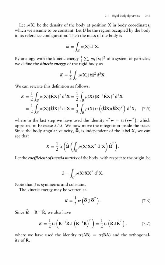
7.1 Rigid body dynamics 243
Let ρ(X) be the density of the body at position X in body coordinates,which we assume to be constant. Let B be the region occupied by the bodyin its reference configuration. Then the mass of the body is
m =∫
Bρ(X) d3X.
By analogy with the kinetic energy 12∑
i mi‖xi‖2 of a system of particles,we define the kinetic energy of the rigid body as
K = 12
∫Bρ(X)‖x‖2 d3X.
We can rewrite this definition as follows:
K = 12
∫Bρ(X)‖RX‖2 d3X = 1
2
∫Bρ(X)‖R−1RX‖2 d3X
= 12
∫Bρ(X)‖�X‖2 d3X = 1
2
∫Bρ(X) tr
((�X)(�X)T
)d3X, (7.5)
where in the last step we have used the identity vT w = tr(vwT
), which
appeared in Exercise 5.15. We now move the integration inside the trace.Since the body angular velocity, �, is independent of the label X, we cansee that
K = 12
tr(�
(∫Bρ(X)XXT d3X
)�
T)
.
Let the coefficient of inertia matrix of the body, with respect to the origin, be
J =∫
Bρ(X)XXT d3X.
Note that J is symmetric and constant.The kinetic energy may be written as
K = 12
tr(� J �
T)
. (7.6)
Since � = R−1R, we also have
K = 12
tr(R−1R J
(R−1R
)T) = 12
tr(R J R
T)
, (7.7)
where we have used the identity tr(AB) = tr(BA) and the orthogonal-ity of R.
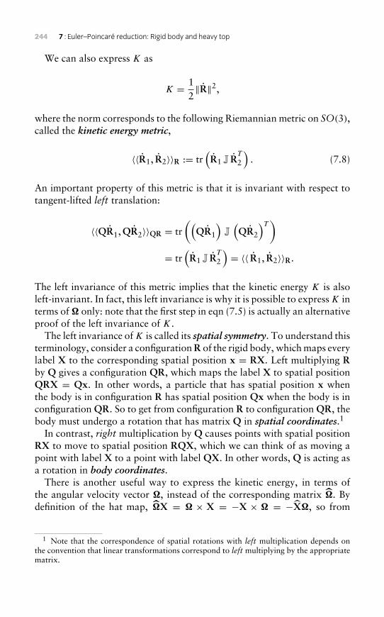
244 7 : Euler–Poincaré reduction: Rigid body and heavy top
We can also express K as
K = 12‖R‖2,
where the norm corresponds to the following Riemannian metric on SO(3),called the kinetic energy metric,
〈〈R1, R2〉〉R := tr(R1 J R
T
2
). (7.8)
An important property of this metric is that it is invariant with respect totangent-lifted left translation:
〈〈QR1,QR2〉〉QR = tr((
QR1
)J(QR2
)T)= tr
(R1 J R
T
2
)= 〈〈 R1, R2〉〉R.
The left invariance of this metric implies that the kinetic energy K is alsoleft-invariant. In fact, this left invariance is why it is possible to express K interms of � only: note that the first step in eqn (7.5) is actually an alternativeproof of the left invariance of K.
The left invariance of K is called its spatial symmetry. To understand thisterminology, consider a configurationR of the rigid body, which maps everylabel X to the corresponding spatial position x = RX. Left multiplying Rby Q gives a configuration QR, which maps the label X to spatial positionQRX = Qx. In other words, a particle that has spatial position x whenthe body is in configuration R has spatial position Qx when the body is inconfiguration QR. So to get from configuration R to configuration QR, thebody must undergo a rotation that has matrix Q in spatial coordinates.1
In contrast, right multiplication by Q causes points with spatial positionRX to move to spatial position RQX, which we can think of as moving apoint with label X to a point with label QX. In other words, Q is acting asa rotation in body coordinates.
There is another useful way to express the kinetic energy, in terms ofthe angular velocity vector �, instead of the corresponding matrix �. Bydefinition of the hat map, �X = � × X = −X × � = −X�, so from
1 Note that the correspondence of spatial rotations with left multiplication depends onthe convention that linear transformations correspond to left multiplying by the appropriatematrix.
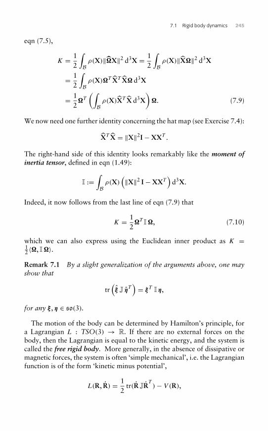
7.1 Rigid body dynamics 245
eqn (7.5),
K = 12
∫Bρ(X)‖�X‖2 d3X = 1
2
∫Bρ(X)‖X�‖2 d3X
= 12
∫Bρ(X)�T XT X� d3X
= 12�T
(∫Bρ(X)XT X d3X
)�. (7.9)
We now need one further identity concerning the hat map (see Exercise 7.4):
XT X = ‖X‖2I −XXT .
The right-hand side of this identity looks remarkably like the moment ofinertia tensor, defined in eqn (1.49):
I :=∫
Bρ(X)
(‖X‖2 I −XXT
)d3X.
Indeed, it now follows from the last line of eqn (7.9) that
K = 12�T I�, (7.10)
which we can also express using the Euclidean inner product as K =12 〈�, I�〉.Remark 7.1 By a slight generalization of the arguments above, one mayshow that
tr(ξ J ηT
)= ξT I η,
for any ξ , η ∈ so(3).
The motion of the body can be determined by Hamilton’s principle, fora Lagrangian L : TSO(3) → R. If there are no external forces on thebody, then the Lagrangian is equal to the kinetic energy, and the system iscalled the free rigid body. More generally, in the absence of dissipative ormagnetic forces, the system is often ‘simple mechanical’, i.e. the Lagrangianfunction is of the form ‘kinetic minus potential’,
L(R, R) = 12
tr(R JRT)− V (R),
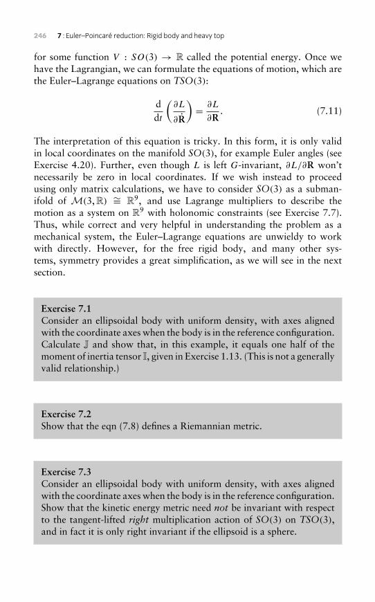
246 7 : Euler–Poincaré reduction: Rigid body and heavy top
for some function V : SO(3) → R called the potential energy. Once wehave the Lagrangian, we can formulate the equations of motion, which arethe Euler–Lagrange equations on TSO(3):
ddt
(∂L
∂R
)= ∂L
∂R. (7.11)
The interpretation of this equation is tricky. In this form, it is only validin local coordinates on the manifold SO(3), for example Euler angles (seeExercise 4.20). Further, even though L is left G-invariant, ∂L/∂R won’tnecessarily be zero in local coordinates. If we wish instead to proceedusing only matrix calculations, we have to consider SO(3) as a subman-ifold of M(3, R) ∼= R9, and use Lagrange multipliers to describe themotion as a system on R9 with holonomic constraints (see Exercise 7.7).Thus, while correct and very helpful in understanding the problem as amechanical system, the Euler–Lagrange equations are unwieldy to workwith directly. However, for the free rigid body, and many other sys-tems, symmetry provides a great simplification, as we will see in the nextsection.
Exercise 7.1Consider an ellipsoidal body with uniform density, with axes alignedwith the coordinate axes when the body is in the reference configuration.Calculate J and show that, in this example, it equals one half of themoment of inertia tensor I, given in Exercise 1.13. (This is not a generallyvalid relationship.)
Exercise 7.2Show that the eqn (7.8) defines a Riemannian metric.
Exercise 7.3Consider an ellipsoidal body with uniform density, with axes alignedwith the coordinate axes when the body is in the reference configuration.Show that the kinetic energy metric need not be invariant with respectto the tangent-lifted right multiplication action of SO(3) on TSO(3),and in fact it is only right invariant if the ellipsoid is a sphere.
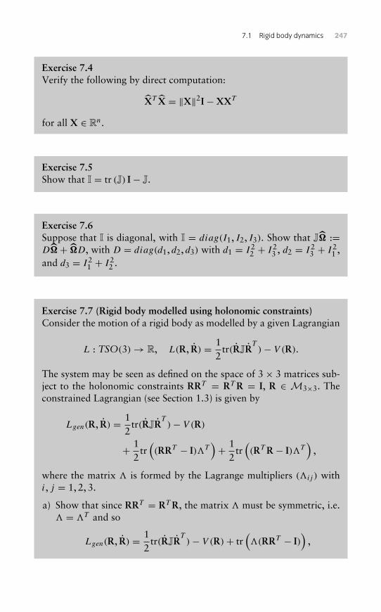
7.1 Rigid body dynamics 247
Exercise 7.4Verify the following by direct computation:
XT X = ‖X‖2I −XXT
for all X ∈ Rn.
Exercise 7.5Show that I = tr (J) I − J.
Exercise 7.6Suppose that I is diagonal, with I = diag(I1, I2, I3). Show that J� :=D�+ �D, with D = diag(d1, d2, d3) with d1 = I2
2 + I23 , d2 = I2
3 + I21 ,
and d3 = I21 + I2
2 .
Exercise 7.7 (Rigid body modelled using holonomic constraints)Consider the motion of a rigid body as modelled by a given Lagrangian
L : TSO(3)→ R, L(R, R) = 12
tr(RJRT)− V (R).
The system may be seen as defined on the space of 3 × 3 matrices sub-ject to the holonomic constraints RRT = RT R = I, R ∈ M3×3. Theconstrained Lagrangian (see Section 1.3) is given by
Lgen(R, R) = 12
tr(RJRT)− V (R)
+ 12
tr((RRT − I)�T
)+ 1
2tr((RT R − I)�T
),
where the matrix � is formed by the Lagrange multipliers (�ij ) withi, j = 1, 2, 3.
a) Show that since RRT = RT R, the matrix � must be symmetric, i.e.� = �T and so
Lgen(R, R) = 12
tr(RJRT)− V (R)+ tr
(�(RRT − I)
),
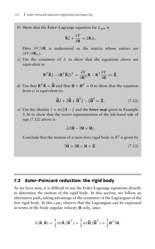
248 7 : Euler–Poincaré reduction: Rigid body and heavy top
b) Show that the Euler–Lagrange equation for Lgen is
RJ+ ∂V
∂R= 2R�.
Here ∂V /∂R is understood as the matrix whose entries are(∂V /∂Rij ).
c) Use the symmetry of � to show that the equations above areequivalent to
RT RJ− (RT RJ)T = ∂V
∂RTR − RT ∂V
∂R=: .
d) Use that RT R = � and that �+�T = 0 to show that the equationfrom c) is equivalent to:
˙�J+ J
˙�+ �
2J− J�
2 = . (7.12)
e) Use the identity I = tr(J)I − J and the breve map given in Example5.36 to show that the vector representation of the left-hand side ofeqn (7.12) above is
2(I�− I�×�).
Conclude that the motion of a (non-free) rigid body in R3 is given by
I� = I��+. (7.13)
7.2 Euler–Poincaré reduction: the rigid body
As we have seen, it is difficult to use the Euler–Lagrange equations directlyto determine the motion of the rigid body. In this section, we follow analternative path, taking advantage of the symmetry of the Lagrangian of thefree rigid body. In this case, observe that the Lagrangian can be expressedin terms of the body angular velocity � only, since
L(R, R) = 12
tr(R JRT) = 1
2tr(� J�
T) = 1
2�T I�.
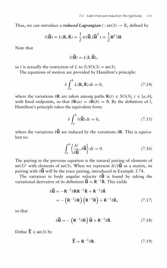
7.2 Euler–Poincaré reduction: the rigid body 249
Thus, we can introduce a reduced Lagrangian l : so(3)→ R, defined by
l(�) = L(R, R) = 12
tr(� J�T) = 1
2�T I�.
Note that
l(�) = L(I, �),
so l is actually the restriction of L to TISO(3) = so(3).The equations of motion are provided by Hamilton’s principle:
δ
∫ b
a
L(R, R) dt = 0, (7.14)
where the variations δR are taken among paths R(t) ∈ SO(3), t ∈ [a, b],with fixed endpoints, so that δR(a) = δR(b) = 0. By the definition of l,Hamilton’s principle takes the equivalent form:
δ
∫ b
a
l(�) dt = 0, (7.15)
where the variations δ� are induced by the variations δR. This is equiva-lent to: ∫ b
a
⟨δl
δ�, δ�
⟩dt = 0. (7.16)
The pairing in the previous equation is the natural pairing of elements ofso(3)∗ with elements of so(3). When we represent δl/δ� as a matrix, itspairing with δ� will be the trace pairing, introduced in Example 3.74.
The variation in body angular velocity δ� is found by taking thevariational derivative of its definition � = R−1R. This yields
δ� = −R−1δRR−1R+ R−1δR
= −(R−1δR
) (R−1R
)+ R−1δR, (7.17)
so that
δ� = −(R−1δR
)�+ R−1δR. (7.18)
Define ∈ so(3) by
= R−1δR. (7.19)
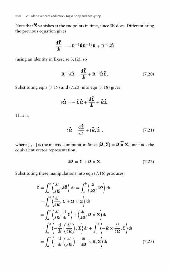
250 7 : Euler–Poincaré reduction: Rigid body and heavy top
Note that vanishes at the endpoints in time, since δR does. Differentiatingthe previous equation gives
ddt= −R−1RR−1δR + R−1δR
(using an identity in Exercise 3.12), so
R−1δR = ddt+ R−1R. (7.20)
Substituting eqns (7.19) and (7.20) into eqn (7.18) gives
δ� = − �+ ddt+ �.
That is,
δ� = ddt+ [�, ], (7.21)
where [ ·, · ] is the matrix commutator. Since [�, ] = � × , one finds theequivalent vector representation,
δ� = +�×. (7.22)
Substituting these manipulations into eqn (7.16) produces:
0 =∫ b
a
⟨δl
δ�, δ�
⟩dt =
∫ b
a
⟨δl
δ�, δ�
⟩dt
=∫ b
a
⟨δl
δ�, +�×
⟩dt
=∫ b
a
⟨δl
δ�,
ddt
⟩+⟨δl
δ�,�×
⟩dt
=∫ b
a
⟨− d
dt
(δl
δ�
),⟩dt +
∫ b
a
⟨−�× δl
δ�,⟩dt
=∫ b
a
⟨− d
dt
(δl
δ�
)+ δl
δ�×�,
⟩dt (7.23)
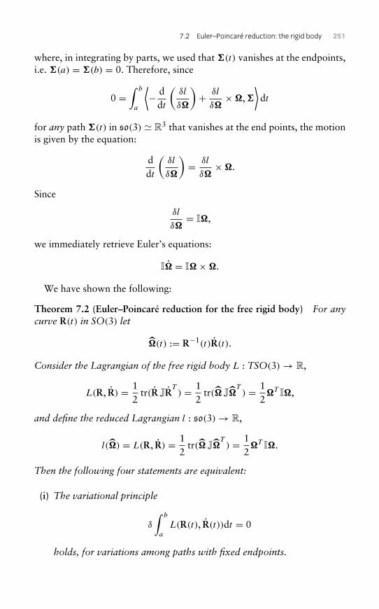
7.2 Euler–Poincaré reduction: the rigid body 251
where, in integrating by parts, we used that (t) vanishes at the endpoints,i.e. (a) = (b) = 0. Therefore, since
0 =∫ b
a
⟨− d
dt
(δl
δ�
)+ δl
δ�×�,
⟩dt
for any path (t) in so(3) � R3 that vanishes at the end points, the motionis given by the equation:
ddt
(δl
δ�
)= δl
δ�×�.
Since
δl
δ�= I�,
we immediately retrieve Euler’s equations:
I� = I��.
We have shown the following:
Theorem 7.2 (Euler–Poincaré reduction for the free rigid body) For anycurve R(t) in SO(3) let
�(t) := R−1(t)R(t).
Consider the Lagrangian of the free rigid body L : TSO(3)→ R,
L(R, R) = 12
tr(R JRT) = 1
2tr(� J�
T) = 1
2�T I�,
and define the reduced Lagrangian l : so(3)→ R,
l(�) = L(R, R) = 12
tr(� J�T) = 1
2�T I�.
Then the following four statements are equivalent:
(i) The variational principle
δ
∫ b
a
L(R(t), R(t))dt = 0
holds, for variations among paths with fixed endpoints.
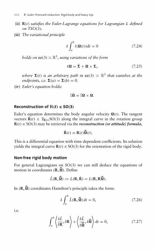
252 7 : Euler–Poincaré reduction: Rigid body and heavy top
(ii) R(t) satisfies the Euler-Lagrange equations for Lagrangian L definedon TSO(3).
(iii) The variational principle
δ
∫ b
a
l(�(t))dt = 0 (7.24)
holds on so(3) � R3, using variations of the form
δ� = +�×, (7.25)
where (t) is an arbitrary path in so(3) � R3 that vanishes at theendpoints, i.e. (a) = (b) = 0.
(iv) Euler’s equation holds:
I� = I��.
Reconstruction of R(t) ∈ SO(3)
Euler’s equation determines the body angular velocity �(t). The tangentvectors R(t) ∈ TR(t)SO(3) along the integral curve in the rotation groupR(t) ∈ SO(3) may be retrieved via the reconstruction (or attitude) formula,
R(t) = R(t)�(t).
This is a differential equation with time-dependent coefficients. Its solutionyields the integral curve R(t) ∈ SO(3) for the orientation of the rigid body.
Non-free rigid body motion
For general Lagrangians on SO(3) we can still deduce the equations ofmotion in coordinates (R, �). Define
L(R, �) := L(R, R) = L(R,R�).
In (R, �) coordinates Hamilton’s principle takes the form:
δ
∫ b
a
L(R, �) dt = 0, (7.26)
i.e. ∫ b
a
⟨δL
δR, δR
⟩+⟨δL
δ�, δ�
⟩dt = 0, (7.27)
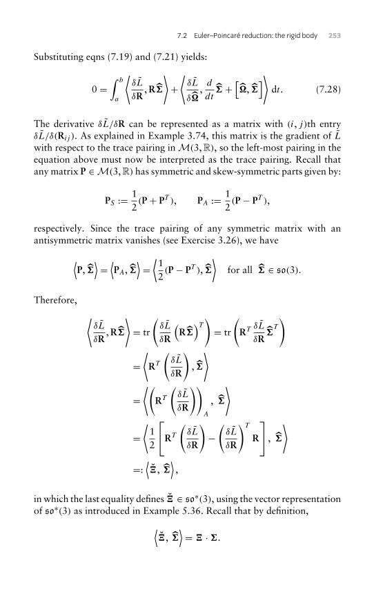
7.2 Euler–Poincaré reduction: the rigid body 253
Substituting eqns (7.19) and (7.21) yields:
0 =∫ b
a
⟨δL
δR,R
⟩+⟨δL
δ�,d
dt +
[�,
]⟩dt . (7.28)
The derivative δL/δR can be represented as a matrix with (i, j)th entryδL/δ(Rij ). As explained in Example 3.74, this matrix is the gradient of L
with respect to the trace pairing in M(3, R), so the left-most pairing in theequation above must now be interpreted as the trace pairing. Recall thatany matrix P ∈M(3, R) has symmetric and skew-symmetric parts given by:
PS := 12(P + PT ), PA := 1
2(P − PT ),
respectively. Since the trace pairing of any symmetric matrix with anantisymmetric matrix vanishes (see Exercise 3.26), we have
⟨P,
⟩=⟨PA,
⟩=⟨12(P − PT ),
⟩for all ∈ so(3).
Therefore, ⟨δL
δR,R
⟩= tr
(δL
δR
(R
)T) = tr
(RT δL
δR
T
)
=⟨RT
(δL
δR
),
⟩
=⟨(
RT
(δL
δR
))A
,
⟩
=⟨
12
RT
(δL
δR
)−(δL
δR
)T
R
,
⟩
=:⟨,
⟩,
in which the last equality defines ∈ so∗(3), using the vector representationof so∗(3) as introduced in Example 5.36. Recall that by definition,⟨
, ⟩= ·.
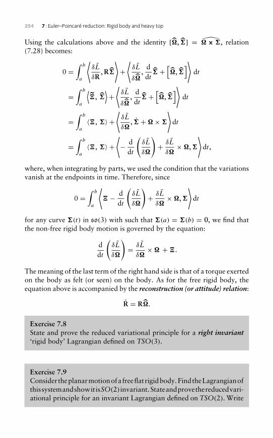
254 7 : Euler–Poincaré reduction: Rigid body and heavy top
Using the calculations above and the identity [�, ] = � × , relation(7.28) becomes:
0 =∫ b
a
⟨δL
δR,R
⟩+⟨δL
δ�,
ddt
+[�,
]⟩dt
=∫ b
a
⟨,
⟩+⟨δL
δ�,
ddt
+[�,
]⟩dt
=∫ b
a
〈, 〉 +⟨δL
δ�, +�×
⟩dt
=∫ b
a
〈, 〉 +⟨− d
dt
(δL
δ�
)+ δL
δ�×�,
⟩dt ,
where, when integrating by parts, we used the condition that the variationsvanish at the endpoints in time. Therefore, since
0 =∫ b
a
⟨− d
dt
(δL
δ�
)+ δL
δ�×�,
⟩dt
for any curve (t) in so(3) with such that (a) = (b) = 0, we find thatthe non-free rigid body motion is governed by the equation:
ddt
(δL
δ�
)= δL
δ�×� +.
The meaning of the last term of the right hand side is that of a torque exertedon the body as felt (or seen) on the body. As for the free rigid body, theequation above is accompanied by the reconstruction (or attitude) relation:
R = R�.
Exercise 7.8State and prove the reduced variational principle for a right invariant‘rigid body’ Lagrangian defined on TSO(3).
Exercise 7.9Considertheplanarmotionofafreeflatrigidbody.FindtheLagrangianofthissystemandshowitisSO(2)invariant.Stateandprovethereducedvari-ational principle for an invariant Lagrangian defined on TSO(2). Write

7.3 Euler–Poincaré reduction theorem 255
the equations of motion and solve them. Then write explicitly thereconstruction equation and deduce its general solution.
Exercise 7.10Let �(t) = �0 = const . be an equilibrium solution of Euler’sequation (7.1). Integrate the reconstruction equation. What aboutnon-equilibrium solutions?
7.3 Euler–Poincaré reduction theorem
Theorem 7.2 generalizes naturally to any left (or right) invariant Lagrangiandefined on the tangent bundle of a Lie group G.
Consider a Lie group G together with the left multiplication action onitself,
G×G→ G, (g,h)→ Lg(h) := gh.
Proposition 7.3 (Left trivialized motion on a Lie group) Let G be a Liegroup together with a Lagrangian L : TG → R. Then, in left trivial-ized coordinates (g, ξ) := (g, g−1g) := (g, TgLg−1 g) ∈ G × g of TG, theequations of motion are given by
ddt
(δL
δξ
)= ad∗ξ
δL
δξ+ T ∗e Lg
(δL
δg
), (7.29)
g = gξ . (7.30)
Proof Consider the Lagrangian L written in (g, ξ) coordinates, thatis, define L(g, ξ) := L(g, gξ), or equivalently, L(g, g) = L(g, g−1g).Hamilton’s variational principle becomes
0 = δ
b∫a
L(g(t), g(t))dt = δ
b∫a
L (g(t), ξ(t))dt
for variations δg among paths g(t) ∈ G with fixed endpoints. So we have:
0 = δ
b∫a
L (g(t), ξ(t)) dt =b∫
a
⟨δL
δg, δg
⟩+⟨δL
δξ, δξ
⟩dt , (7.31)
where the variations δξ are induced by the variations δg.
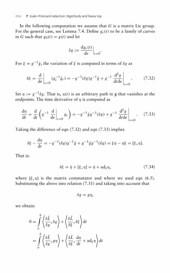
256 7 : Euler–Poincaré reduction: Rigid body and heavy top
In the following computation we assume that G is a matrix Lie group.For the general case, see Lemma 7.4. Define gε(t) to be a family of curvesin G such that g0(t) = g(t) and let
δg := dgε(t)
dε
∣∣∣ε=0
.
For ξ = g−1g, the variation of ξ is computed in terms of δg as
δξ = ddε
∣∣∣∣ε=0
(g−1ε gε) = −g−1(δg)g−1g + g−1 d2g
dtdε
∣∣∣∣∣ε=0
. (7.32)
Set η := g−1δg. That is, η(t) is an arbitrary path in g that vanishes at theendpoints. The time derivative of η is computed as
dηdt= d
dt
(g−1 d
dε
∣∣∣∣ε=0
gε
)= −g−1gg−1(δg)+ g−1 d2g
dtdε
∣∣∣∣∣ε=0
. (7.33)
Taking the difference of eqn (7.32) and eqn (7.33) implies
δξ − dηdt= −g−1(δg)g−1g + g−1gg−1(δg) = ξη − ηξ = [ξ , η].
That is:
δξ = η + [ξ , η] = η + adξ η, (7.34)
where [ξ , η] is the matrix commutator and where we used eqn (6.5).Substituting the above into relation (7.31) and taking into account that
δg = gη,
we obtain:
0 =b∫
a
⟨δL
δg, δg
⟩+⟨δL
δξ, δξ
⟩dt
=b∫
a
⟨δL
δg, gη
⟩+⟨δL
δξ,dηdt+ adξ η
⟩dt
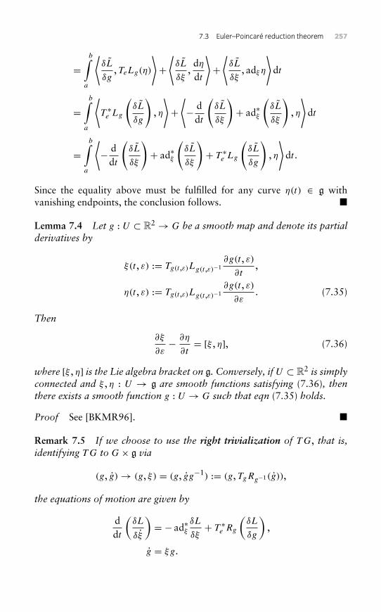
7.3 Euler–Poincaré reduction theorem 257
=b∫
a
⟨δL
δg, TeLg(η)
⟩+⟨δL
δξ,dηdt
⟩+⟨δL
δξ, adξ η
⟩dt
=b∫
a
⟨T ∗e Lg
(δL
δg
), η
⟩+⟨− d
dt
(δL
δξ
)+ ad∗ξ
(δL
δξ
), η
⟩dt
=b∫
a
⟨− d
dt
(δL
δξ
)+ ad∗ξ
(δL
δξ
)+ T ∗e Lg
(δL
δg
), η
⟩dt .
Since the equality above must be fulfilled for any curve η(t) ∈ g withvanishing endpoints, the conclusion follows. �
Lemma 7.4 Let g : U ⊂ R2 → G be a smooth map and denote its partialderivatives by
ξ(t , ε) := Tg(t ,ε)Lg(t ,ε)−1∂g(t , ε)
∂t,
η(t , ε) := Tg(t ,ε)Lg(t ,ε)−1∂g(t , ε)
∂ε. (7.35)
Then
∂ξ
∂ε− ∂η
∂t= [ξ , η], (7.36)
where [ξ , η] is the Lie algebra bracket on g. Conversely, if U ⊂ R2 is simplyconnected and ξ , η : U → g are smooth functions satisfying (7.36), thenthere exists a smooth function g : U → G such that eqn (7.35) holds.
Proof See [BKMR96]. �
Remark 7.5 If we choose to use the right trivialization of TG, that is,identifying TG to G× g via
(g, g)→ (g, ξ) = (g, gg−1) := (g, TgRg−1(g)),
the equations of motion are given by
ddt
(δL
δξ
)= − ad∗ξ
δL
δξ+ T ∗e Rg
(δL
δg
),
g = ξg.
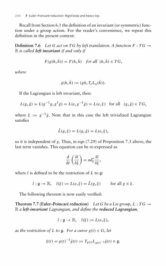
258 7 : Euler–Poincaré reduction: Rigid body and heavy top
Recall from Section 6.1 the definition of an invariant (or symmetric) func-tion under a group action. For the reader’s convenience, we repeat thisdefinition in the present context:
Definition 7.6 Let G act on TG by left translation. A function F : TG→R is called left invariant if and only if
F(g(h, h)) = F(h, h) for all (h, h) ∈ TG,
where
g(h, h) := (gh, TeLg(h)).
If the Lagrangian is left invariant, then:
L(g, g) = L(g−1g, g1g) = L(e, g−1g) = L(e, ξ) for all (g, g) ∈ TG,
where ξ := g−1g. Note that in this case the left trivialized Lagrangiansatisfies
L(g, ξ) = L(g, g) = L(e, ξ),
so it is independent of g. Thus, in eqn (7.29) of Proposition 7.3 above, thelast term vanishes. This equation can be re-expressed as
ddt
(δl
δξ
)= ad∗ξ
δl
δξ,
where l is defined to be the restriction of L to g:
l : g→ R, l(ξ) := L(e, ξ) = L(g, ξ) for all g ∈ ξ .
The following theorem is now easily verified:
Theorem 7.7 (Euler–Poincaré reduction) LetG be a Lie group, L : TG→R a left-invariant Lagrangian, and define the reduced Lagrangian,
l : g→ R, l(ξ) := L(e, ξ),
as the restriction of L to g. For a curve g(t) ∈ G, let
ξ(t) = g(t)−1g(t) := Tg(t)Lg(t)−1 g(t) ∈ g.
7.3 Euler–Poincaré reduction theorem 259
Then, the following four statements are equivalent:
(i) The variational principle
δ
∫ b
a
L(g(t), g(t))dt = 0
holds, for variations among paths with fixed endpoints.
(ii) g(t) satisfies the Euler–Lagrange equations for Lagrangian L
defined on G.
(iii) The variational principle
δ
∫ b
a
l(ξ(t))dt = 0
holds on g, using variations of the form δξ = η+[ξ , η], where η(t) is anarbitrary path in g that vanishes at the endpoints, i.e. η(a) = η(b) = 0.
(iv) The (left-invariant) Euler–Poincaré equations hold:
ddt
δl
δξ= ad∗ξ
δl
δξ.
Remark 7.8 A similar statement holds, with obvious changes for right-invariant Lagrangian systems on TG. In this case the Euler-Poincaréequations are given by:
ddt
δl
δξ= − ad∗ξ
δl
δξ. (7.37)
Reconstruction
The reconstruction of the solution g(t) of the Euler–Lagrange equations,with initial conditions g(0) = g0 and g(0) = v0, is as follows: first, solvethe initial value problem for the left-invariant Euler–Poincaré equations:
ddt
δl
δξ= ad∗ξ
δl
δξwith ξ(0) = ξ0 := g−1
0 v0.
Second, using the solution ξ(t) of the above, find the curve g(t) ∈ G bysolving the reconstruction equation
g(t) = g(t)ξ(t) with g(0) = g0,
which is a differential equation with time-dependent coefficients.
260 7 : Euler–Poincaré reduction: Rigid body and heavy top
Exercise 7.11Prove the Euler–Poincaré reduction Theorem 7.7.
Exercise 7.12Write out the proof of the Euler–Poincaré reduction theorem for right-invariant Lagrangians.
Exercise 7.13Describe the corresponding reconstruction procedure for right-invariantLagrangians.
Exercise 7.14 (Motion on SE(3))Write Euler–Poincaré equations for motion on SE(3).
Exercise 7.15 (Motion on SO(4))Write out the Euler–Poincaré equations in matrix form for a free rigidbody fixed at its centre of mass in a 4-dimensional space. Then use theanalogue of the ‘hat’ map for so(4) (see Exercise 5.21) and write the R6
vector representation of the equations.
Exercise 7.16Consider the following action of a Lie groupG on a product spaceG×Y ,where Y is some manifold:
(g, (h, y))→ (gh, y).
Let L : T (G × Y )→ R be invariant with respect to this action. Definel : g× T Y → R as the restriction of L, i.e.
l(ξ , y, y) := L(e, ξ , y, y).
7.4 Modelling heavy-top dynamics 261
Deduce the reduced Hamilton’s principle for l and show that theequations of motion are given by:
ddt
δl
δξ= ad∗ξ
δl
δξ,
ddt
δl
δy= δl
δy.
7.4 Modelling heavy-top dynamics
The heavy top is a rigid body rotating with a fixed point of support (the‘pivot’) in a constant gravitational field. Just as for the free rigid body inthe absence of gravity, the kinetic energy of the heavy top is:
K := 12
∫B
ρ(X)||RX||2d3X = 12
tr(RJRT) = 1
2tr(�J�
T) = 1
2�T I�,
where J is the coefficient of inertia matrix and I is the moment of inertiamatrix. However, for the top, the matrices J and I must be calculated withrespect to the pivot, which is not in general the centre of mass.
Let m be the mass of the body, and let k be the vertical unit vector. Letχ be the vector from the point of support to the body’s centre of mass,and note that χ is constant in body coordinates. With this notation, thepotential is given by:
Vk(R) = mg⟨k,Rχ
⟩, (7.38)
where 〈·, ·χ〉 is the standard dot product in R3. Thus, the dynamics isdetermined by the Lagrangian
Lk : TSO(3)→ R,
given explicitly by
Lk(R, R) = K − Vk = 12
tr(RJRT)−mg
⟨k,R χ
⟩, (7.39)
where k is a fixed parameter. We will identify the vector k ∈ R3 with themap
⟨k, ·⟩, which is a covector in (R3)∗.
262 7 : Euler–Poincaré reduction: Rigid body and heavy top
In the absence of gravity, i.e. for V = 0, the Lagrangian models a freerigid body; in particular, it is SO(3) left invariant. Gravity breaks thissymmetry, leaving invariance only with respect the subgroup SO(2)vert ofrotations around the vertical axis. While, in principle, one can apply reduc-tion with respect to SO(2)vert only, we can take advantage of the full brokensymmetry as follows.
First, we extend the configuration space SO(3) to SO(3)× (R3)∗ so thatthe direction of gravity k can be considered as a value of the new coordinatev ∈ (R3)∗. The purpose of this is to obtain an extended Lagrangian that isleft-invariant under an action of all of SO(3), not just SO(2)vert . Define
Lext : TSO(3)× T (R3)∗ → R,
as
Lext (R, R, v, v) = 12
tr(RJRT)−mg 〈v,Rχ〉 . (7.40)
Note that
Lext (R, R, v, v)∣∣∣∣{v=k}
= Lk(R, R). (7.41)
The motion determined by Lk (via Hamilton’s principle) corresponds to themotion determined by Lext , with the added constraint
v(t) = k = const .
Remark 7.9 By construction, the extended Lagrangian Lext is a functionof (R, R, v) ∈ TSO(3) × (R3)∗ only. However, the heavy-top variationalprinciple deduced in this section is the end result of the application ofHamil-ton’s principle with constraints. This is a variational principle defined on atangent bundle. Consequently, we choose to carry the domain of definitionofLext as T
(SO(3)× (R3)∗
)only to restrict it again later to TSO(3)×(R3)∗.
Definition 7.10 The (left) diagonal action of SO(3) on SO(3)× (R3)∗ is:
(Q, (R, v))→ (QR,Qv) , for all Q ∈ SO(3). (7.42)
Its tangent lift is given by(Q,(R, R, v, v
))→ Q
(R, R, v, v
):=(QR,QR,Qv,Qv
). (7.43)
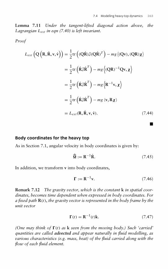
7.4 Modelling heavy-top dynamics 263
Lemma 7.11 Under the tangent-lifted diagonal action above, theLagrangian Lext in eqn (7.40) is left invariant.
Proof
Lext
(Q(R, R, v, v
))= 1
2tr((QR)J(QR)T
)−mg
⟨(Qv), (QR)χ
⟩= 1
2tr(RJR
T)−mg
⟨(QR)−1Qv,χ
⟩= 1
2tr(RJR
T)−mg
⟨R−1v,χ
⟩= 1
2tr(RJR
T)−mg 〈v,Rχ〉
= Lext (R, R, v, v). (7.44)
�
Body coordinates for the heavy top
As in Section 7.1, angular velocity in body coordinates is given by:
� := R−1R. (7.45)
In addition, we transform v into body coordinates,
� := R−1v. (7.46)
Remark 7.12 The gravity vector, which is the constant k in spatial coor-dinates, becomes time dependent when expressed in body coordinates. Fora fixed path R(t), the gravity vector is represented in the body frame by theunit vector
�(t) = R−1(t)k. (7.47)
(One may think of �(t) as k seen from the moving body.) Such ‘carried’quantities are called advected and appear naturally in fluid modelling, asvarious characteristics (e.g. mass, heat) of the fluid carried along with theflow of each fluid element.
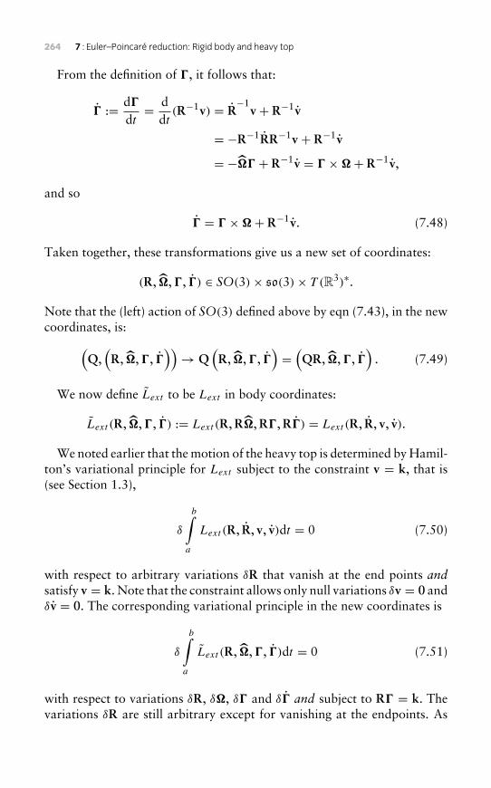
264 7 : Euler–Poincaré reduction: Rigid body and heavy top
From the definition of �, it follows that:
� := d�dt= d
dt(R−1v) = R
−1v + R−1v
= −R−1RR−1v + R−1v
= −�� + R−1v = � ×�+ R−1v,
and so
� = � ×�+ R−1v. (7.48)
Taken together, these transformations give us a new set of coordinates:
(R, �,�, �) ∈ SO(3)× so(3)× T (R3)∗.
Note that the (left) action of SO(3) defined above by eqn (7.43), in the newcoordinates, is:(
Q,(R, �,�, �
))→ Q
(R, �,�, �
)=(QR, �,�, �
). (7.49)
We now define Lext to be Lext in body coordinates:
Lext (R, �,�, �) := Lext (R,R�,R�,R�) = Lext (R, R, v, v).
We noted earlier that the motion of the heavy top is determined by Hamil-ton’s variational principle for Lext subject to the constraint v = k, that is(see Section 1.3),
δ
b∫a
Lext (R, R, v, v)dt = 0 (7.50)
with respect to arbitrary variations δR that vanish at the end points andsatisfy v = k. Note that the constraint allows only null variations δv = 0 andδv = 0. The corresponding variational principle in the new coordinates is
δ
b∫a
Lext (R, �,�, �)dt = 0 (7.51)
with respect to variations δR, δ�, δ� and δ� and subject to R� = k. Thevariations δR are still arbitrary except for vanishing at the endpoints. As
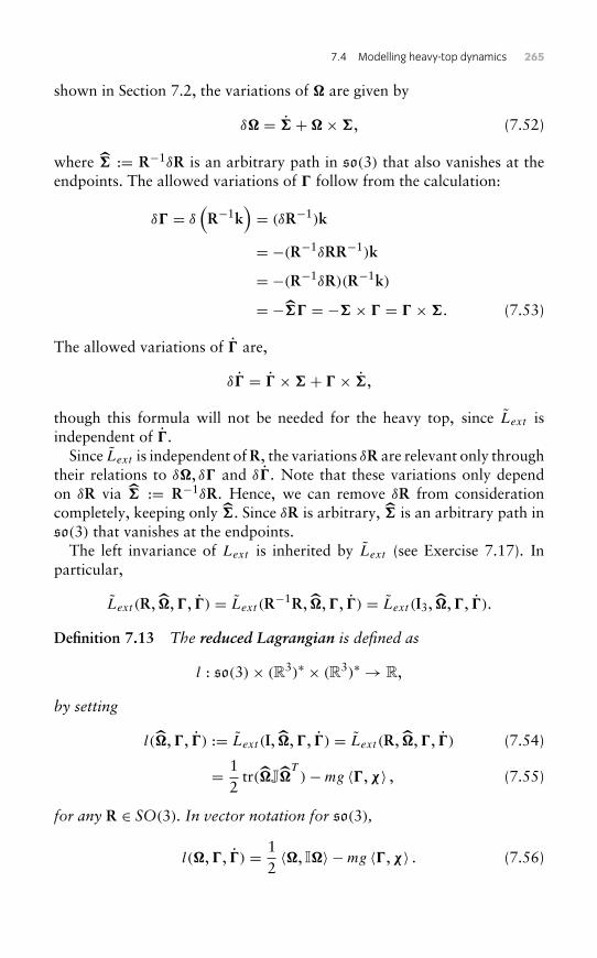
7.4 Modelling heavy-top dynamics 265
shown in Section 7.2, the variations of � are given by
δ� = +�×, (7.52)
where := R−1δR is an arbitrary path in so(3) that also vanishes at theendpoints. The allowed variations of � follow from the calculation:
δ� = δ(R−1k
)= (δR−1)k
= −(R−1δRR−1)k
= −(R−1δR)(R−1k)
= −� = − × � = � ×. (7.53)
The allowed variations of � are,
δ� = � × + � × ,
though this formula will not be needed for the heavy top, since Lext isindependent of �.
Since Lext is independent of R, the variations δR are relevant only throughtheir relations to δ�, δ� and δ�. Note that these variations only dependon δR via := R−1δR. Hence, we can remove δR from considerationcompletely, keeping only . Since δR is arbitrary, is an arbitrary path inso(3) that vanishes at the endpoints.
The left invariance of Lext is inherited by Lext (see Exercise 7.17). Inparticular,
Lext (R, �,�, �) = Lext (R−1R, �,�, �) = Lext (I3, �,�, �).
Definition 7.13 The reduced Lagrangian is defined as
l : so(3)× (R3)∗ × (R3)∗ → R,
by setting
l(�,�, �) := Lext (I, �,�, �) = Lext (R, �,�, �) (7.54)
= 12
tr(�J�T)−mg 〈�,χ〉 , (7.55)
for any R ∈ SO(3). In vector notation for so(3),
l(�,�, �) = 12〈�, I�〉 −mg 〈�,χ〉 . (7.56)
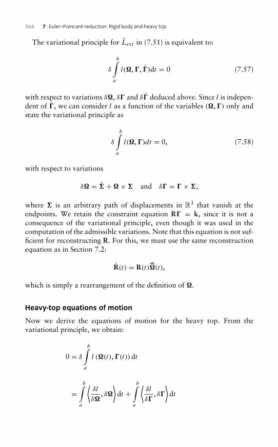
266 7 : Euler–Poincaré reduction: Rigid body and heavy top
The variational principle for Lext in (7.51) is equivalent to:
δ
b∫a
l(�,�, �)dt = 0 (7.57)
with respect to variations δ�, δ� and δ� deduced above. Since l is indepen-dent of �, we can consider l as a function of the variables (�,�) only andstate the variational principle as
δ
b∫a
l(�,�)dt = 0, (7.58)
with respect to variations
δ� = +�× and δ� = � ×,
where is an arbitrary path of displacements in R3 that vanish at theendpoints. We retain the constraint equation R� = k, since it is not aconsequence of the variational principle, even though it was used in thecomputation of the admissible variations. Note that this equation is not suf-ficient for reconstructing R. For this, we must use the same reconstructionequation as in Section 7.2:
R(t) = R(t)�(t),
which is simply a rearrangement of the definition of �.
Heavy-top equations of motion
Now we derive the equations of motion for the heavy top. From thevariational principle, we obtain:
0 = δ
b∫a
l (�(t),�(t)) dt
=b∫
a
⟨δl
δ�, δ�
⟩dt +
b∫a
⟨δl
δ�, δ�
⟩dt
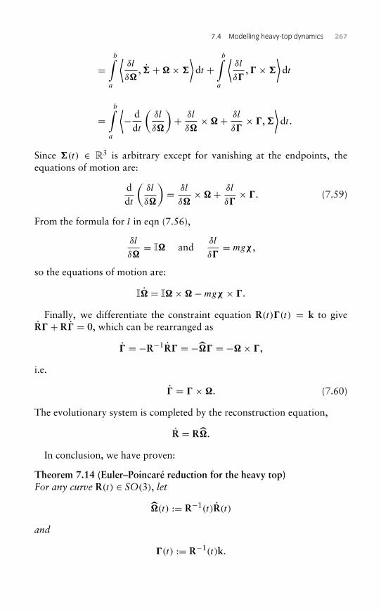
7.4 Modelling heavy-top dynamics 267
=b∫
a
⟨δl
δ�, +�×
⟩dt +
b∫a
⟨δl
δ�,� ×
⟩dt
=b∫
a
⟨− d
dt
(δl
δ�
)+ δl
δ�×�+ δl
δ�× �,
⟩dt .
Since (t) ∈ R3 is arbitrary except for vanishing at the endpoints, theequations of motion are:
ddt
(δl
δ�
)= δl
δ�×�+ δl
δ�× �. (7.59)
From the formula for l in eqn (7.56),
δl
δ�= I� and
δl
δ�= mgχ ,
so the equations of motion are:
I� = I�×�−mgχ × �.
Finally, we differentiate the constraint equation R(t)�(t) = k to giveR� + R� = 0, which can be rearranged as
� = −R−1R� = −�� = −�× �,
i.e.
� = � �. (7.60)
The evolutionary system is completed by the reconstruction equation,
R = R�.
In conclusion, we have proven:
Theorem 7.14 (Euler–Poincaré reduction for the heavy top)For any curve R(t) ∈ SO(3), let
�(t) := R−1(t)R(t)
and
�(t) := R−1(t)k.
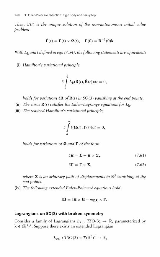
268 7 : Euler–Poincaré reduction: Rigid body and heavy top
Then, �(t) is the unique solution of the non-autonomous initial valueproblem
�(t) = �(t)×�(t), �(0) = R−1(0)k.
WithLk and l defined in eqn (7.54), the following statements are equivalent:
(i) Hamilton’s variational principle,
δ
b∫a
Lk(R(t), R(t))dt = 0,
holds for variations δR of R(t) in SO(3) vanishing at the end points.
(ii) The curve R(t) satisfies the Euler–Lagrange equations for Lk.
(iii) The reduced Hamilton’s variational principle,
δ
b∫a
l(�(t),�(t))dt = 0,
holds for variations of � and � of the form
δ� = +�×, (7.61)
δ� = � ×, (7.62)
where is an arbitrary path of displacements in R3 vanishing at theend points.
(iv) The following extended Euler–Poincaré equations hold:
I� = I�×�−mgχ × �.
Lagrangians on SO(3) with broken symmetry
Consider a family of Lagrangians Lk : TSO(3) → R, parameterized byk ∈ (R3)∗. Suppose there exists an extended Lagrangian
Lext : TSO(3)× T (R3)∗ → R,
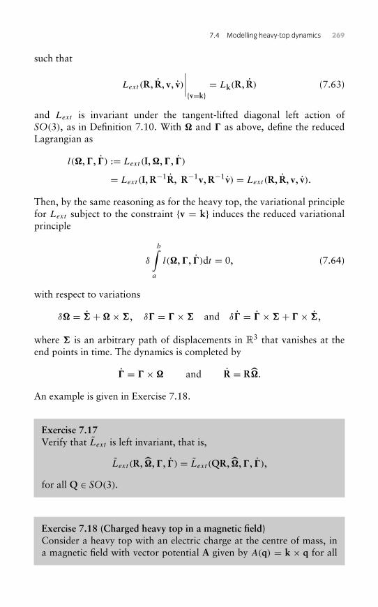
7.4 Modelling heavy-top dynamics 269
such that
Lext (R, R, v, v)∣∣∣∣{v=k}
= Lk(R, R) (7.63)
and Lext is invariant under the tangent-lifted diagonal left action ofSO(3), as in Definition 7.10. With � and � as above, define the reducedLagrangian as
l(�,�, �) := Lext (I,�,�, �)
= Lext (I,R−1R, R−1v,R−1v) = Lext (R, R, v, v).
Then, by the same reasoning as for the heavy top, the variational principlefor Lext subject to the constraint {v = k} induces the reduced variationalprinciple
δ
b∫a
l(�,�, �)dt = 0, (7.64)
with respect to variations
δ� = +�×, δ� = � × and δ� = � × + � × ,
where is an arbitrary path of displacements in R3 that vanishes at theend points in time. The dynamics is completed by
� = � � and R = R�.
An example is given in Exercise 7.18.
Exercise 7.17Verify that Lext is left invariant, that is,
Lext (R, �,�, �) = Lext (QR, �,�, �),
for all Q ∈ SO(3).
Exercise 7.18 (Charged heavy top in a magnetic field)Consider a heavy top with an electric charge at the centre of mass, ina magnetic field with vector potential A given by A(q) = k × q for all
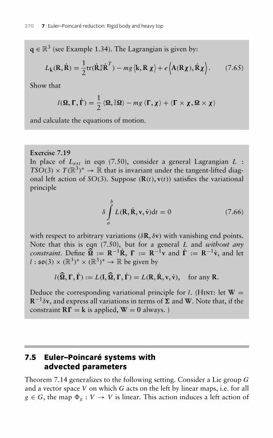
270 7 : Euler–Poincaré reduction: Rigid body and heavy top
q ∈ R3 (see Example 1.34). The Lagrangian is given by:
Lk(R, R) = 12
tr(RJRT)−mg
⟨k,R χ
⟩+ e⟨A(Rχ), Rχ
⟩. (7.65)
Show that
l(�,�, �) = 12〈�, I�〉 −mg 〈�,χ〉 + 〈� × χ ,�× χ〉
and calculate the equations of motion.
Exercise 7.19In place of Lext in eqn (7.50), consider a general Lagrangian L :TSO(3) × T (R3)∗ → R that is invariant under the tangent-lifted diag-onal left action of SO(3). Suppose (R(t), v(t)) satisfies the variationalprinciple
δ
b∫a
L(R, R, v, v)dt = 0 (7.66)
with respect to arbitrary variations (δR, δv) with vanishing end points.Note that this is eqn (7.50), but for a general L and without anyconstraint. Define � := R−1R, � := R−1v and � := R−1v, and letl : so(3)× (R3)∗ × (R3)∗ → R be given by
l(�,�, �) := L(I, �,�, �) = L(R, R, v, v), for any R.
Deduce the corresponding variational principle for l. (Hint: let W =R−1δv, and express all variations in terms of and W. Note that, if theconstraint R� = k is applied, W = 0 always. )
7.5 Euler–Poincaré systems withadvected parameters
Theorem 7.14 generalizes to the following setting. Consider a Lie group G
and a vector space V on which G acts on the left by linear maps, i.e. for allg ∈ G, the map �g : V → V is linear. This action induces a left action of
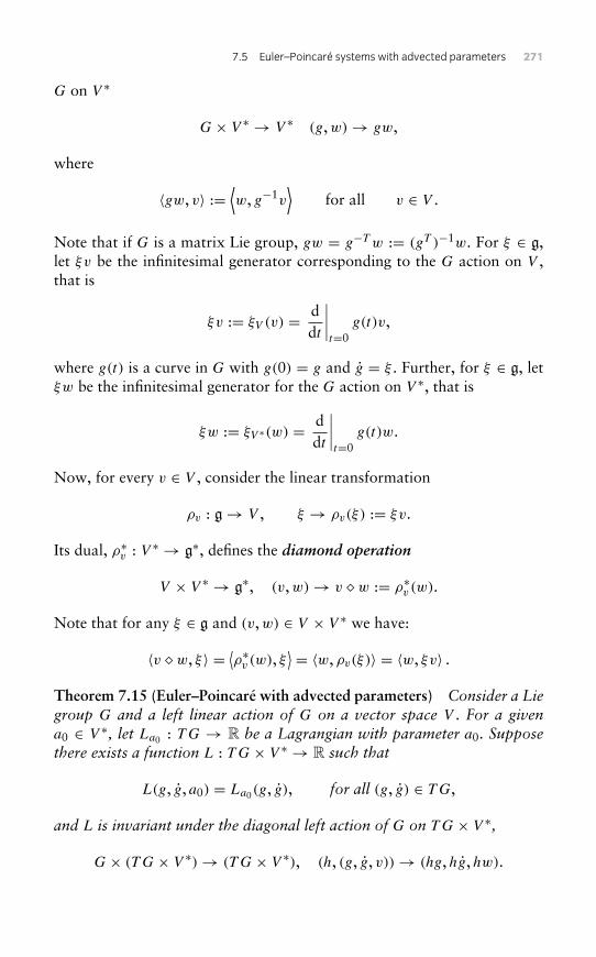
7.5 Euler–Poincaré systems with advected parameters 271
G on V ∗
G× V ∗ → V ∗ (g,w)→ gw,
where
〈gw, v〉 :=⟨w, g−1v
⟩for all v ∈ V .
Note that if G is a matrix Lie group, gw = g−T w := (gT )−1w. For ξ ∈ g,let ξv be the infinitesimal generator corresponding to the G action on V ,that is
ξv := ξV (v) = ddt
∣∣∣∣t=0
g(t)v,
where g(t) is a curve in G with g(0) = g and g = ξ . Further, for ξ ∈ g, letξw be the infinitesimal generator for the G action on V ∗, that is
ξw := ξV ∗(w) = ddt
∣∣∣∣t=0
g(t)w.
Now, for every v ∈ V , consider the linear transformation
ρv : g→ V , ξ → ρv(ξ) := ξv.
Its dual, ρ∗v : V ∗ → g∗, defines the diamond operation
V × V ∗ → g∗, (v,w)→ v & w := ρ∗v (w).
Note that for any ξ ∈ g and (v,w) ∈ V × V ∗ we have:
〈v & w, ξ〉 = ⟨ρ∗v (w), ξ⟩ = 〈w, ρv(ξ)〉 = 〈w, ξv〉 .
Theorem 7.15 (Euler–Poincaré with advected parameters) Consider a Liegroup G and a left linear action of G on a vector space V . For a givena0 ∈ V ∗, let La0 : TG → R be a Lagrangian with parameter a0. Supposethere exists a function L : TG× V ∗ → R such that
L(g, g, a0) = La0(g, g), for all (g, g) ∈ TG,
and L is invariant under the diagonal left action of G on TG× V ∗,
G× (T G× V ∗)→ (T G× V ∗), (h, (g, g, v))→ (hg,hg,hw).
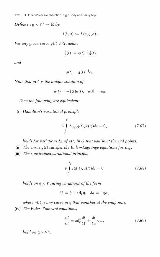
272 7 : Euler–Poincaré reduction: Rigid body and heavy top
Define l : g× V ∗ → R by
l(ξ , a) := L(e, ξ , a).
For any given curve g(t) ∈ G, define
ξ(t) := g(t)−1g(t)
and
a(t) = g(t)−1a0.
Note that a(t) is the unique solution of
a(t) = −ξ(t)a(t), a(0) = a0.
Then the following are equivalent:
(i) Hamilton’s variational principle,
δ
t2∫t1
La0(g(t), g(t))dt = 0, (7.67)
holds for variations δg of g(t) in G that vanish at the end points.
(ii) The curve g(t) satisfies the Euler–Lagrange equations for La0 .
(iii) The constrained variational principle
δ
t2∫t1
l(ξ(t), a(t))dt = 0 (7.68)
holds on g× V , using variations of the form
δξ = η + adξ η, δa = −ηa,
where η(t) is any curve in g that vanishes at the endpoints.
(iv) The Euler–Poincaré equations,
dldt= ad∗ξ
δl
δξ+ δl
δa& a, (7.69)
hold on g× V ∗.
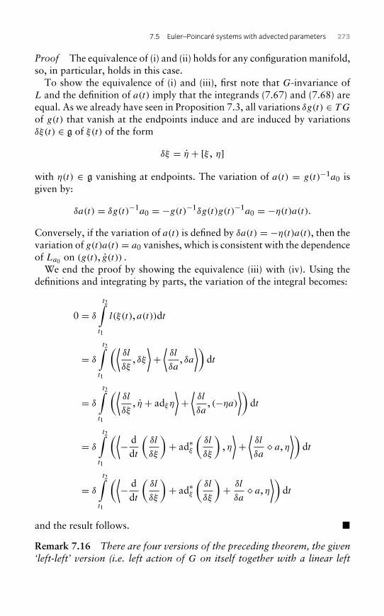
7.5 Euler–Poincaré systems with advected parameters 273
Proof The equivalence of (i) and (ii) holds for any configuration manifold,so, in particular, holds in this case.
To show the equivalence of (i) and (iii), first note that G-invariance ofL and the definition of a(t) imply that the integrands (7.67) and (7.68) areequal. As we already have seen in Proposition 7.3, all variations δg(t) ∈ TG
of g(t) that vanish at the endpoints induce and are induced by variationsδξ(t) ∈ g of ξ(t) of the form
δξ = η + [ξ , η]
with η(t) ∈ g vanishing at endpoints. The variation of a(t) = g(t)−1a0 isgiven by:
δa(t) = δg(t)−1a0 = −g(t)−1δg(t)g(t)−1a0 = −η(t)a(t).Conversely, if the variation of a(t) is defined by δa(t) = −η(t)a(t), then thevariation of g(t)a(t) = a0 vanishes, which is consistent with the dependenceof La0 on (g(t), g(t)) .
We end the proof by showing the equivalence (iii) with (iv). Using thedefinitions and integrating by parts, the variation of the integral becomes:
0 = δ
t2∫t1
l(ξ(t), a(t))dt
= δ
t2∫t1
(⟨δl
δξ, δξ⟩+⟨δl
δa, δa
⟩)dt
= δ
t2∫t1
(⟨δl
δξ, η + adξ η
⟩+⟨δl
δa, (−ηa)
⟩)dt
= δ
t2∫t1
(⟨− d
dt
(δl
δξ
)+ ad∗ξ
(δl
δξ
), η⟩+⟨δl
δa& a, η
⟩)dt
= δ
t2∫t1
(⟨− d
dt
(δl
δξ
)+ ad∗ξ
(δl
δξ
)+ δl
δa& a, η
⟩)dt
and the result follows. �
Remark 7.16 There are four versions of the preceding theorem, the given‘left-left’ version (i.e. left action of G on itself together with a linear left
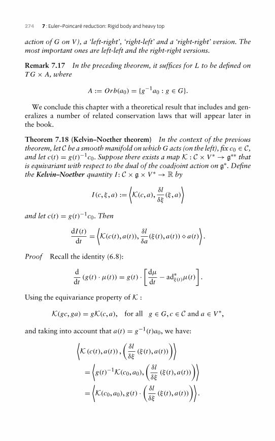
274 7 : Euler–Poincaré reduction: Rigid body and heavy top
action of G on V ), a ‘left-right’, ‘right-left’ and a ‘right-right’ version. Themost important ones are left-left and the right-right versions.
Remark 7.17 In the preceding theorem, it suffices for L to be defined onTG× A, where
A := Orb(a0) = {g−1a0 : g ∈ G}.
We conclude this chapter with a theoretical result that includes and gen-eralizes a number of related conservation laws that will appear later inthe book.
Theorem 7.18 (Kelvin–Noether theorem) In the context of the previoustheorem, let C be a smoothmanifold onwhichG acts (on the left), fix c0 ∈ C,and let c(t) = g(t)−1c0. Suppose there exists a map K : C × V ∗ → g∗∗ thatis equivariant with respect to the dual of the coadjoint action on g∗. Definethe Kelvin–Noether quantity I : C × g× V ∗ → R by
I (c, ξ , a) :=⟨K(c, a),
δl
δξ(ξ , a)
⟩and let c(t) = g(t)−1c0. Then
dI (t)dt=⟨K(c(t), a(t)),
δl
δa(ξ(t), a(t)) & a(t)
⟩.
Proof Recall the identity (6.8):
ddt
(g(t) · µ(t)) = g(t) ·[dµdt− ad∗ξ(t)µ(t)
].
Using the equivariance property of K :
K(gc, ga) = gK(c, a), for all g ∈ G, c ∈ C and a ∈ V ∗,
and taking into account that a(t) = g−1(t)a0, we have:⟨K (c(t), a(t)) ,
(δl
δξ(ξ(t), a(t))
)⟩=⟨g(t)−1K(c0, a0),
(δl
δξ(ξ(t), a(t))
)⟩=⟨K(c0, a0), g(t) ·
(δl
δξ(ξ(t), a(t))
)⟩.
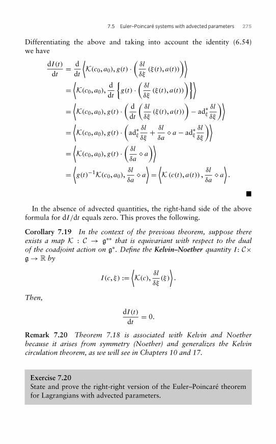
7.5 Euler–Poincaré systems with advected parameters 275
Differentiating the above and taking into account the identity (6.54)we have
dI (t)dt= d
dt
⟨K(c0, a0), g(t) ·
(δl
δξ(ξ(t), a(t))
)⟩=⟨K(c0, a0),
ddt
{g(t) ·
(δl
δξ(ξ(t), a(t))
)}⟩=⟨K(c0, a0), g(t) ·
(ddt
(δl
δξ(ξ(t), a(t))
)− ad∗ξ
δl
δξ
)⟩=⟨K(c0, a0), g(t) ·
(ad∗ξ
δl
δξ+ δl
δa& a − ad∗ξ
δl
δξ
)⟩=⟨K(c0, a0), g(t) ·
(δl
δa& a)⟩
=⟨g(t)−1K(c0, a0),
δl
δa& a⟩=⟨K (c(t), a(t)) ,
δl
δa& a⟩.
�
In the absence of advected quantities, the right-hand side of the aboveformula for dI/dt equals zero. This proves the following.
Corollary 7.19 In the context of the previous theorem, suppose thereexists a map K : C → g∗∗ that is equivariant with respect to the dualof the coadjoint action on g∗. Define the Kelvin–Noether quantity I : C×g→ R by
I (c, ξ) :=⟨K(c),
δl
δξ(ξ)
⟩.
Then,
dI (t)dt= 0.
Remark 7.20 Theorem 7.18 is associated with Kelvin and Noetherbecause it arises from symmetry (Noether) and generalizes the Kelvincirculation theorem, as we will see in Chapters 10 and 17.
Exercise 7.20State and prove the right-right version of the Euler–Poincaré theoremfor Lagrangians with advected parameters.
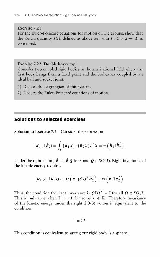
276 7 : Euler–Poincaré reduction: Rigid body and heavy top
Exercise 7.21For the Euler–Poincaré equations for motion on Lie groups, show thatthe Kelvin quantity I (t), defined as above but with I : C × g → R, isconserved.
Exercise 7.22 (Double heavy top)Consider two coupled rigid bodies in the gravitational field where thefirst body hangs from a fixed point and the bodies are coupled by anideal ball and socket joint.
1) Deduce the Lagrangian of this system.
2) Deduce the Euler–Poincaré equations of motion.
Solutions to selected exercises
Solution to Exercise 7.3 Consider the expression
⟨R1 , IR2
⟩ = ∫B
(R1X
) · (R2X)d3X = tr
(R1IR
T
2
).
Under the right action, R→ RQ for some Q ∈ SO(3). Right invariance ofthe kinetic energy requires
⟨R1Q , IR2Q
⟩ = tr(R1QIQT R
T
2
)= tr
(R1IR
T
2
).
Thus, the condition for right invariance is QIQT = I for all Q ∈ SO(3).This is only true when I = λI for some λ ∈ R. Therefore invarianceof the kinetic energy under the right SO(3) action is equivalent to thecondition
I = λI .
This condition is equivalent to saying our rigid body is a sphere.
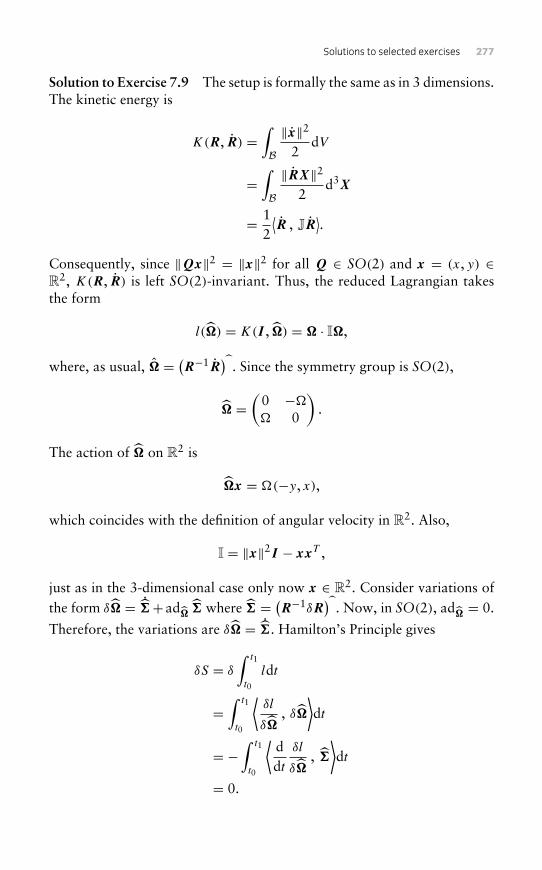
Solutions to selected exercises 277
Solution to Exercise 7.9 The setup is formally the same as in 3 dimensions.The kinetic energy is
K(R, R) =∫
B‖x‖2
2dV
=∫
B‖RX‖2
2d3X
= 12
⟨R , JR
⟩.
Consequently, since ‖Qx‖2 = ‖x‖2 for all Q ∈ SO(2) and x = (x, y) ∈R2, K(R, R) is left SO(2)-invariant. Thus, the reduced Lagrangian takesthe form
l(�) = K(I , �) = � · I�,
where, as usual, � = (R−1R)
. Since the symmetry group is SO(2),
� =(
0 −�� 0
).
The action of � on R2 is
�x = �(−y, x),
which coincides with the definition of angular velocity in R2. Also,
I = ‖x‖2I − xxT ,
just as in the 3-dimensional case only now x ∈ R2. Consider variations ofthe form δ� = ˙+ad� where = (R−1δR
). Now, in SO(2), ad� = 0.
Therefore, the variations are δ� = ˙. Hamilton’s Principle gives
δS = δ
∫ t1
t0
ldt
=∫ t1
t0
⟨δl
δ�, δ�
⟩dt
= −∫ t1
t0
⟨ddt
δl
δ�, ⟩dt
= 0.
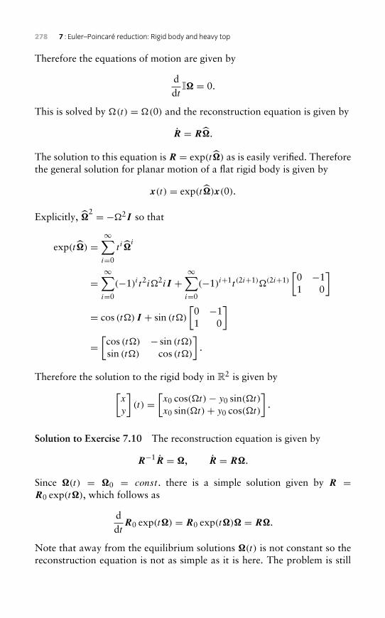
278 7 : Euler–Poincaré reduction: Rigid body and heavy top
Therefore the equations of motion are given by
ddt
I� = 0.
This is solved by �(t) = �(0) and the reconstruction equation is given by
R = R�.
The solution to this equation is R = exp(t�) as is easily verified. Thereforethe general solution for planar motion of a flat rigid body is given by
x(t) = exp(t�)x(0).
Explicitly, �2 = −�2I so that
exp(t�) =∞∑i=0
t i�i
=∞∑i=0
(−1)i t2i�2iI +∞∑i=0
(−1)i+1t (2i+1)�(2i+1)[0 −11 0
]
= cos (t�) I + sin (t�)
[0 −11 0
]=[cos (t�) − sin (t�)
sin (t�) cos (t�)
].
Therefore the solution to the rigid body in R2 is given by[x
y
](t) =
[x0 cos(�t)− y0 sin(�t)
x0 sin(�t)+ y0 cos(�t)
].
Solution to Exercise 7.10 The reconstruction equation is given by
R−1R = �, R = R�.
Since �(t) = �0 = const . there is a simple solution given by R =R0 exp(t�), which follows as
ddt
R0 exp(t�) = R0 exp(t�)� = R�.
Note that away from the equilibrium solutions �(t) is not constant so thereconstruction equation is not as simple as it is here. The problem is still
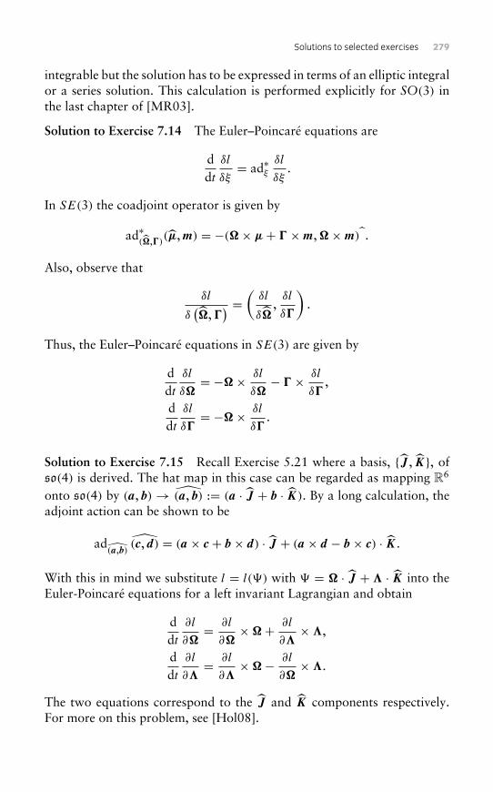
Solutions to selected exercises 279
integrable but the solution has to be expressed in terms of an elliptic integralor a series solution. This calculation is performed explicitly for SO(3) inthe last chapter of [MR03].
Solution to Exercise 7.14 The Euler–Poincaré equations are
ddt
δl
δξ= ad∗ξ
δl
δξ.
In SE(3) the coadjoint operator is given by
ad∗(�,�)
(µ,m) = −(�× µ+ � ×m,�×m) .
Also, observe that
δl
δ(�,�
) = ( δl
δ�,δl
δ�
).
Thus, the Euler–Poincaré equations in SE(3) are given by
ddt
δl
δ�= −�× δl
δ�− � × δl
δ�,
ddt
δl
δ�= −�× δl
δ�.
Solution to Exercise 7.15 Recall Exercise 5.21 where a basis, {J , K}, ofso(4) is derived. The hat map in this case can be regarded as mapping R6
onto so(4) by (a, b)→ (a, b) := (a · J + b · K). By a long calculation, theadjoint action can be shown to be
ad(a,b) (c, d) = (a × c + b × d) · J + (a × d − b × c) · K.
With this in mind we substitute l = l(�) with � = � · J + · K into theEuler-Poincaré equations for a left invariant Lagrangian and obtain
ddt
∂l
∂�= ∂l
∂�×�+ ∂l
∂ × ,
ddt
∂l
∂ = ∂l
∂ ×�− ∂l
∂�× .
The two equations correspond to the J and K components respectively.For more on this problem, see [Hol08].
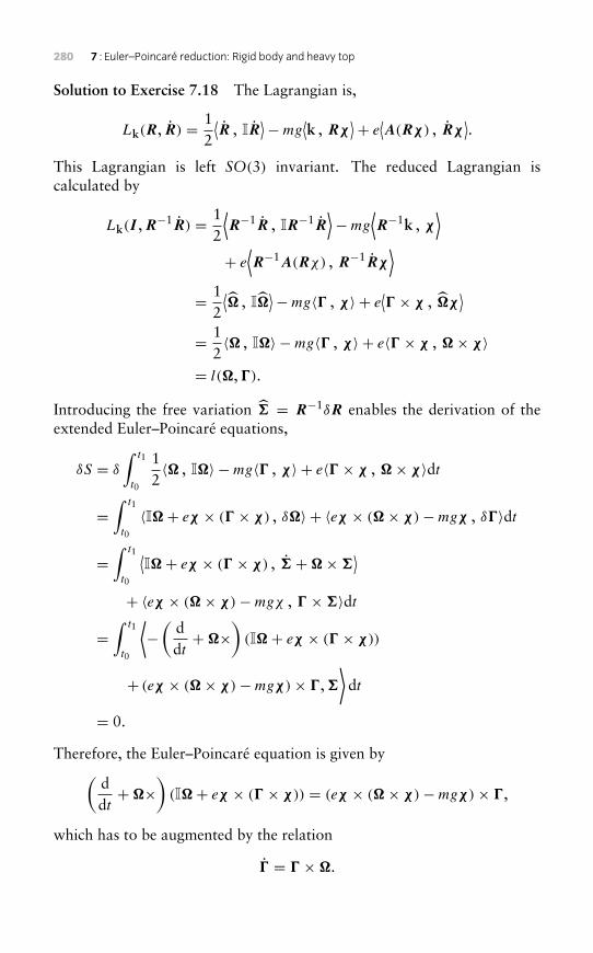
280 7 : Euler–Poincaré reduction: Rigid body and heavy top
Solution to Exercise 7.18 The Lagrangian is,
Lk(R, R) = 12
⟨R , IR
⟩−mg⟨k , Rχ
⟩+ e⟨A(Rχ) , Rχ
⟩.
This Lagrangian is left SO(3) invariant. The reduced Lagrangian iscalculated by
Lk(I ,R−1R) = 12
⟨R−1R , IR−1R
⟩−mg
⟨R−1k , χ
⟩+ e
⟨R−1A(Rχ) , R−1Rχ
⟩= 1
2
⟨� , I�
⟩−mg〈� , χ〉 + e⟨� × χ , �χ
⟩= 1
2〈� , I�〉 −mg〈� , χ〉 + e〈� × χ , �× χ〉
= l(�,�).
Introducing the free variation = R−1δR enables the derivation of theextended Euler–Poincaré equations,
δS = δ
∫ t1
t0
12〈� , I�〉 −mg〈� , χ〉 + e〈� × χ , �× χ〉dt
=∫ t1
t0
〈I�+ eχ × (� × χ) , δ�〉 + 〈eχ × (�× χ)−mgχ , δ�〉dt
=∫ t1
t0
⟨I�+ eχ × (� × χ) , +�×
⟩+ 〈eχ × (�× χ)−mgχ , � ×〉dt
=∫ t1
t0
⟨−(
ddt+�×
)(I�+ eχ × (� × χ))
+ (eχ × (�× χ)−mgχ)× �,⟩dt
= 0.
Therefore, the Euler–Poincaré equation is given by(ddt+�×
)(I�+ eχ × (� × χ)) = (eχ × (�× χ)−mgχ)× �,
which has to be augmented by the relation
� = � �.
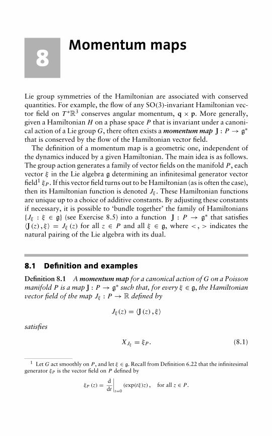
8Momentum maps
Lie group symmetries of the Hamiltonian are associated with conservedquantities. For example, the flow of any SO(3)-invariant Hamiltonian vec-tor field on T ∗R3 conserves angular momentum, q × p. More generally,given a Hamiltonian H on a phase space P that is invariant under a canoni-cal action of a Lie group G, there often exists a momentum map J : P → g∗that is conserved by the flow of the Hamiltonian vector field.
The definition of a momentum map is a geometric one, independent ofthe dynamics induced by a given Hamiltonian. The main idea is as follows.The group action generates a family of vector fields on the manifold P , eachvector ξ in the Lie algebra g determining an infinitesimal generator vectorfield1 ξP . If this vector field turns out to be Hamiltonian (as is often the case),then its Hamiltonian function is denoted Jξ . These Hamiltonian functionsare unique up to a choice of additive constants. By adjusting these constantsif necessary, it is possible to ‘bundle together’ the family of Hamiltonians{Jξ : ξ ∈ g} (see Exercise 8.5) into a function J : P → g∗ that satisfies〈J (z) , ξ〉 = Jξ (z) for all z ∈ P and all ξ ∈ g, where < , > indicates thenatural pairing of the Lie algebra with its dual.
8.1 Definition and examples
Definition 8.1 Amomentum map for a canonical action ofG on a Poissonmanifold P is a map J : P → g∗ such that, for every ξ ∈ g, the Hamiltonianvector field of the map Jξ : P → R defined by
Jξ (z) = 〈J (z) , ξ〉satisfies
XJξ = ξP . (8.1)
1 Let G act smoothly on P , and let ξ ∈ g. Recall from Definition 6.22 that the infinitesimalgenerator ξP is the vector field on P defined by
ξP (z) = ddt
∣∣∣∣t=0
(exp(tξ)z) , for all z ∈ P .
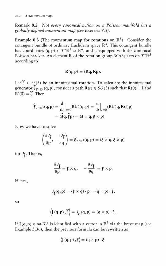
282 8 : Momentummaps
Remark 8.2 Not every canonical action on a Poisson manifold has aglobally defined momentum map (see Exercise 8.3).
Example 8.3 (The momentum map for rotations on R3) Consider thecotangent bundle of ordinary Euclidean space R3. This cotangent bundlehas coordinates (q, p) ∈ T ∗R3 � R6, and is equipped with the canonicalPoisson bracket. An element R of the rotation group SO(3) acts on T ∗R3
according to
R(q, p) = (Rq,Rp).
Let ξ ∈ so(3) be an infinitesimal rotation. To calculate the infinitesimalgenerator ξT ∗R3(q, p), consider a path R(t) ∈ SO(3) such that R(0) = I andR′(0) = ξ . Then
ξT ∗R3(q, p) = ddt
∣∣∣t=0
R(t)(q, p) = ddt
∣∣∣t=0
(R(t)q,R(t)p)
= (ξq, ξp) = (ξ × q, ξ × p).
Now we have to solve(∂J
ξ
∂p,−
∂Jξ
∂q
)= ξT ∗R3(q, p) = (ξ × q, ξ × p)
for Jξ. That is,
∂Jξ
∂p= ξ × q, −
∂Jξ
∂q= ξ × p.
Hence,
Jξ(q, p) = (ξ × q) · p = (q× p) · ξ ,
so ⟨J (q, p) , ξ
⟩= J
ξ(q, p) = (q× p) · ξ .
If J (q, p) ∈ so(3)∗ is identified with a vector in R3 via the breve map (seeExample 5.36), then the previous formula can be rewritten as⟨
J (q, p) , ξ⟩ = (q× p) · ξ .
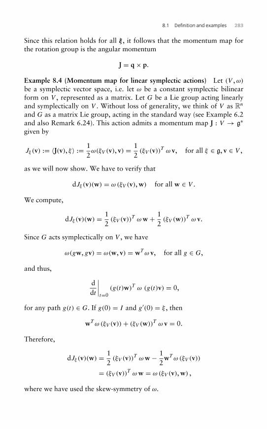
8.1 Definition and examples 283
Since this relation holds for all ξ , it follows that the momentum map forthe rotation group is the angular momentum
J = q× p.
Example 8.4 (Momentum map for linear symplectic actions) Let (V ,ω)
be a symplectic vector space, i.e. let ω be a constant symplectic bilinearform on V , represented as a matrix. Let G be a Lie group acting linearlyand symplectically on V . Without loss of generality, we think of V as Rn
and G as a matrix Lie group, acting in the standard way (see Example 6.2and also Remark 6.24). This action admits a momentum map J : V → g∗given by
Jξ (v) := 〈J(v), ξ〉 := 12ω(ξV (v), v) = 1
2(ξV (v))T ω v, for all ξ ∈ g, v ∈ V ,
as we will now show. We have to verify that
dJξ (v)(w) = ω (ξV (v),w) for all w ∈ V .
We compute,
dJξ (v)(w) = 12(ξV (v))T ωw + 1
2(ξV (w))T ω v.
Since G acts symplectically on V , we have
ω(gw, gv) = ω(w, v) = wT ω v, for all g ∈ G,
and thus,
ddt
∣∣∣∣t=0
(g(t)w)T ω (g(t)v) = 0,
for any path g(t) ∈ G. If g(0) = I and g′(0) = ξ , then
wT ω (ξV (v))+ (ξV (w))T ω v = 0.
Therefore,
dJξ (v)(w) = 12(ξV (v))T ωw − 1
2wT ω (ξV (v))
= (ξV (v))T ωw = ω (ξV (v),w) ,
where we have used the skew-symmetry of ω.
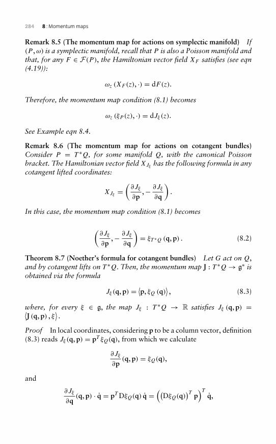
284 8 : Momentummaps
Remark 8.5 (The momentum map for actions on symplectic manifold) If(P ,ω) is a symplectic manifold, recall that P is also a Poisson manifold andthat, for any F ∈ F(P ), the Hamiltonian vector field XF satisfies (see eqn(4.19)):
ωz (XF (z), ·) = dF(z).
Therefore, the momentum map condition (8.1) becomes
ωz (ξP (z), ·) = dJξ (z).
See Example eqn 8.4.
Remark 8.6 (The momentum map for actions on cotangent bundles)Consider P = T ∗Q, for some manifold Q, with the canonical Poissonbracket. The Hamiltonian vector field XJξ has the following formula in anycotangent lifted coordinates:
XJξ =(∂Jξ
∂p,− ∂Jξ
∂q
).
In this case, the momentum map condition (8.1) becomes
(∂Jξ
∂p,− ∂Jξ
∂q
)= ξT ∗Q (q, p) . (8.2)
Theorem 8.7 (Noether’s formula for cotangent bundles) Let G act on Q,and by cotangent lifts on T ∗Q. Then, the momentum map J : T ∗Q→ g∗ isobtained via the formula
Jξ (q, p) = ⟨p, ξQ (q)⟩, (8.3)
where, for every ξ ∈ g, the map Jξ : T ∗Q → R satisfies Jξ (q, p) =⟨J (q, p) , ξ
⟩.
Proof In local coordinates, considering p to be a column vector, definition(8.3) reads Jξ (q, p) = pT ξQ(q), from which we calculate
∂Jξ
∂p(q, p) = ξQ(q),
and
∂Jξ
∂q(q, p) · q = pT DξQ(q) q =
((DξQ(q)
)T p)T
q,
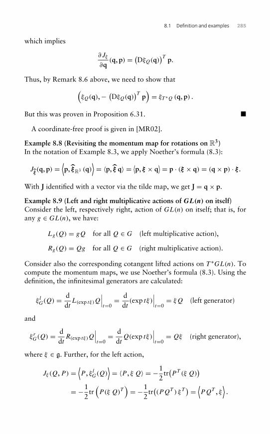
8.1 Definition and examples 285
which implies
∂Jξ
∂q(q, p) = (DξQ(q)
)T p.
Thus, by Remark 8.6 above, we need to show that(ξQ(q),− (DξQ(q)
)T p)= ξT ∗Q (q, p) .
But this was proven in Proposition 6.31. �
A coordinate-free proof is given in [MR02].
Example 8.8 (Revisiting the momentum map for rotations on R3)In the notation of Example 8.3, we apply Noether’s formula (8.3):
Jξ(q, p) =
⟨p, ξR3 (q)
⟩= 〈p, ξ q〉 = ⟨p, ξ × q
⟩ = p · (ξ × q) = (q× p) · ξ .
With J identified with a vector via the tilde map, we get J = q× p.
Example 8.9 (Left and right multiplicative actions of GL(n) on itself)Consider the left, respectively right, action of GL(n) on itself; that is, forany g ∈ GL(n), we have:
Lg(Q) = gQ for all Q ∈ G (left multiplicative action),
Rg(Q) = Qg for all Q ∈ G (right multiplicative action).
Consider also the corresponding cotangent lifted actions on T ∗GL(n). Tocompute the momentum maps, we use Noether’s formula (8.3). Using thedefinition, the infinitesimal generators are calculated:
ξ lG(Q) = d
dtL(exp tξ )Q
∣∣∣t=0= d
dt(exp tξ )
∣∣∣t=0= ξQ (left generator)
and
ξ rG(Q) = d
dtR(exp tξ )Q
∣∣∣t=0= d
dtQ(exp tξ )
∣∣∣t=0= Qξ (right generator),
where ξ ∈ g. Further, for the left action,
Jξ (Q,P) =⟨P , ξ l
G(Q)⟩= 〈P , ξ Q〉 = −1
2tr(PT (ξ Q)
)= −1
2tr(P(ξ Q)T
)= −1
2tr((PQT ) ξT
) = ⟨PQT , ξ⟩.
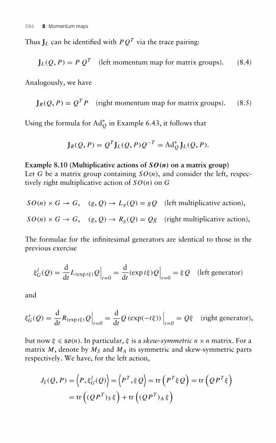
286 8 : Momentummaps
Thus JL can be identified with PQT via the trace pairing:
JL(Q,P) = P QT (left momentum map for matrix groups). (8.4)
Analogously, we have
JR(Q,P) = QT P (right momentum map for matrix groups). (8.5)
Using the formula for Ad∗Q in Example 6.43, it follows that
JR(Q,P) = QT JL(Q,P)Q−T = Ad∗Q JL(Q,P).
Example 8.10 (Multiplicative actions of SO(n) on a matrix group)Let G be a matrix group containing SO(n), and consider the left, respec-tively right multiplicative action of SO(n) on G
SO(n)×G→ G, (g,Q)→ Lg(Q) = gQ (left multiplicative action),
SO(n)×G→ G, (g,Q)→ Rg(Q) = Qg (right multiplicative action),
The formulae for the infinitesimal generators are identical to those in theprevious exercise
ξ lG(Q) = d
dtL(exp tξ )Q
∣∣∣t=0= d
dt(exp tξ )Q
∣∣∣t=0= ξQ (left generator)
and
ξ rG(Q) = d
dtR(exp tξ )Q
∣∣∣t=0= d
dtQ (exp(−tξ ))
∣∣∣t=0= Qξ (right generator),
but now ξ ∈ so(n). In particular, ξ is a skew-symmetric n×n matrix. For amatrix M, denote by MS and MA its symmetric and skew-symmetric partsrespectively. We have, for the left action,
Jξ (Q,P) =⟨P , ξ l
G(Q)⟩=⟨PT , ξQ
⟩= tr
(PT ξQ
)= tr
(QPT ξ
)= tr
((QPT )S ξ
)+ tr
((QPT )A ξ
)
8.1 Definition and examples 287
= tr((QPT )A ξ
)= tr
((PQT )TA ξ
)=⟨(PQT )A, ξ
⟩=⟨12
(PQT − (PQT )T
), ξ⟩=⟨12
(PQT −QPT
), ξ⟩.
Thus, JL can be identified with 12
(PQT −QPT
)via the trace pairing:
JL(Q,P) = 12
(P QT −QPT
), (8.6)
for the left multiplicative action of SO(n) on a matrix group. Analogously,the momentum map for the right action is:
JR(Q,P) = 12
(QT P − PT Q
). (8.7)
This example applies to the left and right multiplicative actions of SO(n)
on GL(n). It also applies to the left and right multiplicative actions ofSO(n) on itself. In the latter case, for any (Q,P) ∈ T ∗SO(n), we haveP QT = P Q−1 ∈ so(n) and, similarly, QT P = Q−1P ∈ so(n), so bothP QT and QT P are skew-symmetric. Thus, the momentum maps for theactions of SO(n) on itself are
JL(Q,P) = P QT (left multiplicative action),
JR(Q,P) = QT P (right multiplicative action). (8.8)
Note that these are the same formulae as for the multiplicative actions ofGL(n) on itself, given in the previous example. We also have:
JR(Q,P) = QT JL(Q,P)Q = Ad∗Q JL(Q,P).
Remark 8.11 (Angular momentum of a rigid body) For a rigid body, themomentum JL, as computed in the previous example, can be interpreted asspatial angularmomentum. Indeed, consider a rigid bodywith a fixed centreof mass, which has configuration space SO(3) and a simple mechanical
288 8 : Momentummaps
Lagrangian of the form
L(R, R) = 12
tr(RJRT )+ V (R),
where J is the coefficient of the inertia matrix, introduced in Section 7.1.The Legendre transform for this Lagrangian is
(R, P) =(R,
∂L
∂R
)= (R, RJ
),
where ∂L
∂Rhas been computed using the trace pairing as in Section 3.4. The
left multiplicative action of SO(3) on itself corresponds to spatial rotations,as noted earlier in Section 7.1. From Example 8.10, the momentum mapof the cotangent lift of this action is JL(R, P) = PRT . We now show that JLcorresponds to the spatial angular momentum vector π of the rigid body,which was introduced in Section 1.5, where it was shown that π = R� =RI�. Recall from Remark 7.1 that
tr(ξ J ηT
)= ξT I η,
for all ξ , η ∈ so(3), where I is the moment of inertia matrix. Thus, for allξ ∈ so(3), ⟨
JL(R, P), ξ⟩= tr
(R JRT ξ
T)
= tr(R−1R JRT ξ
TR)
= tr(� J
(RT ξ
)T)= �T IRT ξ
= πT ξ .
By definition of the isomorphism ˘ : R3 → so(3)∗ defined in Chapter 5,we have
JL = π .
In this sense, JL ‘is’ spatial angular momentum for the rigid body. Weknow from Chapter 1 that spatial angular momentum is conserved, a factthat we deduced from Newton’s laws (and the corresponding properties ofsolid bodies). For the rigid body, we now have another way of deducingthis conservation law, namely Noether’s theorem. Indeed, the Lagrangian
8.1 Definition and examples 289
above is clearly invariant under the tangent-lifted left multiplicative action,as was noted in Chapter 7, and from this it follows that the correspondingHamiltonian is invariant under the the cotangent-lifted left multiplicativeaction of SO(3) on T ∗SO(3) (see Chapter 4). Thus Noether’s theorem(Theorem 8.14) implies that JL is constant.Recall also that the body angular momentum (i.e. angular momentum in
body coordinates) is � := RT π . From Example 6.44, it follows that
� =(RT π
)˘= Ad∗R JL = RT JL(R, P)R = JR(R, P).
Example 8.12 (Momentum maps for actions of a Lie group on itself) LetG be a Lie group and consider the left and right actions of G on itself; thatis, for any h ∈ G, we have:
G×G→ G, (h, g)→ Lh(g) = hg (left multiplicative action),
G×G→ G, (h, g)→ Rh(g) = gh (right multiplicative action).
It is useful to recall that the tangent lifts are:
TgLh(v) = ddt
hg(t)
∣∣∣t=0= hv (left tangent action),
TgRh(v) = ddt
g(t)h
∣∣∣t=0= vh (right tangent action),
where g(t) is a path in G with g(0) = g and g′(0) = v. The infinitesimalactions on G are
ξ lG (g) = d
dtexp (tξ) g
∣∣t=0 = ξg = TeRgξ (left infinitesimal action),
ξ rG (g) = d
dtg exp (tξ)
∣∣t=0 = gξ = TeLgξ (right infinitesimal action).
Let α ∈ T ∗g G. For every ξ ∈ g, we have 〈JL (α) , ξ〉 = 〈α, ξG (g)〉 =⟨α, TeRg(ξ)
⟩ = ⟨T ∗e Rg(α), ξ⟩so
JL (α) = T ∗e Rg(α) (left momentum for a Lie group). (8.9)
290 8 : Momentummaps
A similar calculation shows:
JR (α) = T ∗e Lg(α) (right momentum for a Lie group). (8.10)
Alternatively, writing α = T ∗g Lg−1(ρ) for some ρ ∈ g∗ we have
JL(T ∗g Lg−1(ρ)
)= T ∗e Rg ◦ T ∗g Lg−1(ρ) = T ∗e (Lg−1 ◦ Rg)(ρ) = Ad∗
g−1(ρ) and
JR(T ∗g Lg−1(ρ)
)= T ∗e Lg ◦ T ∗g Lg−1(ρ) = T ∗e (Lg−1 ◦ Lg)(ρ) = ρ.
It follows that JR(α) = Ad∗g JL(α).
Exercise 8.1 (Momentum map for the scaling group)Consider the action of the multiplicative group of real numbers on Rn:
(R \ {0})×Rn→ Rn (8.11)
(λ, q)→ λq. (8.12)
Show that the momentum map J : T ∗Rn→ R for the correspondingcotangent-lifted action is J(q, p) = pT q.
Exercise 8.2Compute the momentum map for the cotangent lift of the standardaction of SE(3) on R3.
Exercise 8.3Show that the S1 action on the torus T2 given by θ · (α,β) = (α + θ ,β)is canonical with respect to the area form dα ∧ dβ but has no globallydefined momentum map (see, for example, [Sin01]).
Exercise 8.4Suppose that G acts on P1, with momentum map J1. Let P2 be anothermanifold, and define the G action on P1 × P2 by g(p1,p2) = (gp1,p2).Define J : P1 × P2 → g∗ by J (p1,p2) = J1(p1). Show that J is amomentum map for the G action on P1 × P2.
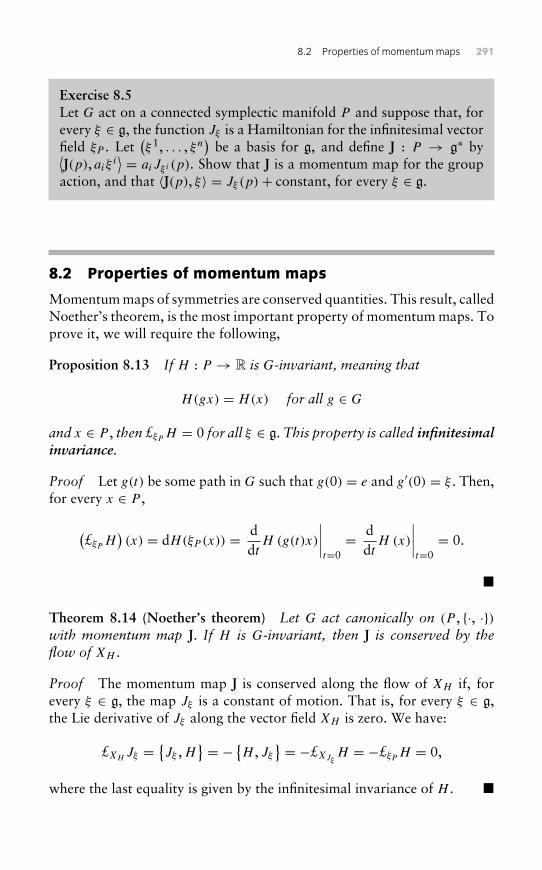
8.2 Properties of momentummaps 291
Exercise 8.5Let G act on a connected symplectic manifold P and suppose that, forevery ξ ∈ g, the function Jξ is a Hamiltonian for the infinitesimal vectorfield ξP . Let
(ξ1, . . . , ξn
)be a basis for g, and define J : P → g∗ by⟨
J(p), aiξ i⟩ = aiJξi (p). Show that J is a momentum map for the group
action, and that 〈J(p), ξ〉 = Jξ (p)+ constant, for every ξ ∈ g.
8.2 Properties of momentum maps
Momentum maps of symmetries are conserved quantities. This result, calledNoether’s theorem, is the most important property of momentum maps. Toprove it, we will require the following,
Proposition 8.13 If H : P → R is G-invariant, meaning that
H(gx) = H(x) for all g ∈ G
and x ∈ P , then £ξP H = 0 for all ξ ∈ g. This property is called infinitesimalinvariance.
Proof Let g(t) be some path in G such that g(0) = e and g′(0) = ξ . Then,for every x ∈ P ,
(£ξP H
)(x) = dH(ξP (x)) = d
dtH (g(t)x)
∣∣∣∣t=0= d
dtH (x)
∣∣∣∣t=0= 0.
�
Theorem 8.14 (Noether’s theorem) Let G act canonically on (P , {·, ·})with momentum map J. If H is G-invariant, then J is conserved by theflow of XH .
Proof The momentum map J is conserved along the flow of XH if, forevery ξ ∈ g, the map Jξ is a constant of motion. That is, for every ξ ∈ g,the Lie derivative of Jξ along the vector field XH is zero. We have:
£XHJξ =
{Jξ ,H
} = − {H , Jξ
} = −£XJξH = −£ξP H = 0,
where the last equality is given by the infinitesimal invariance of H . �
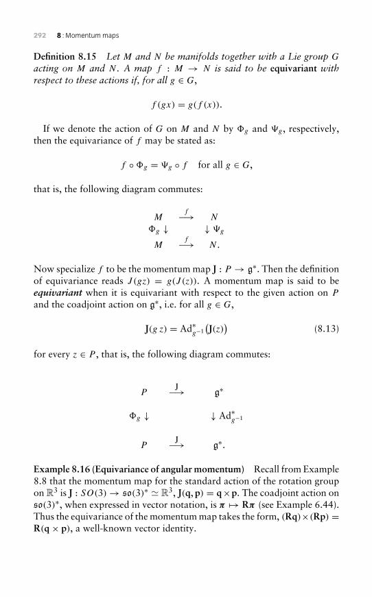
292 8 : Momentummaps
Definition 8.15 Let M and N be manifolds together with a Lie group G
acting on M and N . A map f : M → N is said to be equivariant withrespect to these actions if, for all g ∈ G,
f (gx) = g(f (x)).
If we denote the action of G on M and N by �g and �g, respectively,then the equivariance of f may be stated as:
f ◦�g = �g ◦ f for all g ∈ G,
that is, the following diagram commutes:
Mf−→ N
�g ↓ ↓ �g
Mf−→ N .
Now specialize f to be the momentum map J : P → g∗. Then the definitionof equivariance reads J (gz) = g(J (z)). A momentum map is said to beequivariant when it is equivariant with respect to the given action on P
and the coadjoint action on g∗, i.e. for all g ∈ G,
J(g z) = Ad∗g−1
(J(z)
)(8.13)
for every z ∈ P , that is, the following diagram commutes:
PJ−→ g∗
�g ↓ ↓ Ad∗g−1
PJ−→ g∗.
Example 8.16 (Equivariance of angular momentum) Recall from Example8.8 that the momentum map for the standard action of the rotation groupon R3 is J : SO(3)→ so(3)∗ � R3, J(q, p) = q×p. The coadjoint action onso(3)∗, when expressed in vector notation, is π → Rπ (see Example 6.44).Thus the equivariance of the momentum map takes the form, (Rq)×(Rp) =R(q× p), a well-known vector identity.
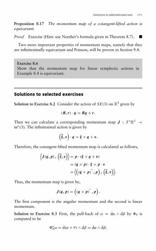
Solutions to selected exercises 293
Proposition 8.17 The momentum map of a cotangent-lifted action isequivariant.
Proof Exercise (Hint: use Noether’s formula given in Theorem 8.7). �
Two more important properties of momentum maps, namely that theyare infinitesimally equivariant and Poisson, will be proven in Section 9.4.
Exercise 8.6Show that the momentum map for linear symplectic actions inExample 8.4 is equivariant.
Solutions to selected exercises
Solution to Exercise 8.2 Consider the action of SE(3) on R3 given by
(R, r) · q = Rq + r.
Then we can calculate a corresponding momentum map J : T ∗R3 →se∗(3). The infinitesimal action is given by(
ξ , v)· q = ξ × q + v.
Therefore, the cotangent-lifted momentum map is calculated as follows,⟨J (q,p) ,
(ξ , v
)⟩= p · (ξ × q + v)
= (q × p) · ξ + p · v=⟨(
(q × p) ,p)
,(ξ , v
)⟩.
Thus, the momentum map is given by,
J (q,p) =((q × p) ,p
).
The first component is the angular momentum and the second is linearmomentum.
Solution to Exercise 8.3 First, the pull-back of ω = dα ∧ dβ by �θ iscomputed to be
�∗θω = d(α + θ) ∧ dβ = dα ∧ dβ.
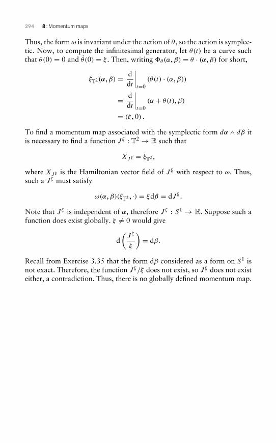
294 8 : Momentummaps
Thus, the form ω is invariant under the action of θ , so the action is symplec-tic. Now, to compute the infinitesimal generator, let θ(t) be a curve suchthat θ(0) = 0 and θ (0) = ξ . Then, writing �θ(α,β) = θ · (α,β) for short,
ξT2(α,β) = ddt
∣∣∣∣t=0
(θ(t) · (α,β))
= ddt
∣∣∣∣t=0
(α + θ(t),β)
= (ξ , 0) .
To find a momentum map associated with the symplectic form dα ∧ dβ itis necessary to find a function J ξ : T2 → R such that
XJξ = ξT2 ,
where XJξ is the Hamiltonian vector field of J ξ with respect to ω. Thus,such a J ξ must satisfy
ω(α,β)(ξT2 , ·) = ξdβ = dJ ξ .
Note that J ξ is independent of α, therefore J ξ : S1 → R. Suppose such afunction does exist globally. ξ �= 0 would give
d(J ξ
ξ
)= dβ.
Recall from Exercise 3.35 that the form dβ considered as a form on S1 isnot exact. Therefore, the function J ξ/ξ does not exist, so J ξ does not existeither, a contradiction. Thus, there is no globally defined momentum map.
9Lie–Poisson reduction
In Chapter 7, the Euler equations of motion for the rigid body,
I� = I��, (9.1)
were shown to be determined by a reduced variational principle applied tothe reduced Lagrangian l: so(3)→ R,
l(�) = 12〈�, I�〉 .
The Euler equations can be reformulated in the variable � := I� as
� = �× I−1�. (9.2)
As shown in Example 4.24, these equations actually define a Hamiltonianvector field Xh for the Hamiltonian
h(�) = 12
⟨�, I−1�
⟩and the rigid body bracket
{F ,K}(�) := −〈�,∇F ×∇K〉. (9.3)
The purpose of the present chapter is to generalize the rigid body exampleto symmetric mechanical systems on Lie groups, in two ways:
1. We introduce a reduced Legendre transformation, generalizing thechange of coordinates � → �, which allows us to write equations ong∗, called Lie-Poisson equations, that correspond to the Euler–Poincaréequations on g.
2. We show that the Lie–Poisson equations have a Hamiltonian structurewith respect to a suitable bracket.
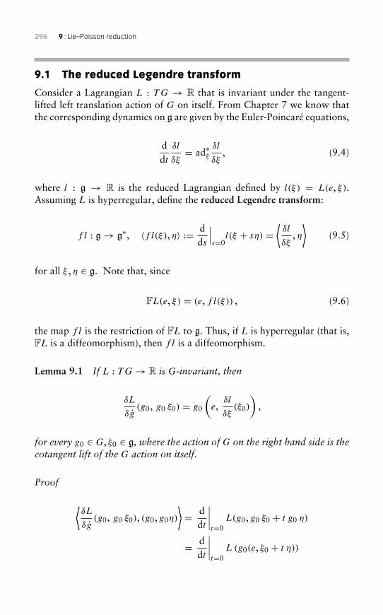
296 9 : Lie–Poisson reduction
9.1 The reduced Legendre transform
Consider a Lagrangian L : TG → R that is invariant under the tangent-lifted left translation action of G on itself. From Chapter 7 we know thatthe corresponding dynamics on g are given by the Euler-Poincaré equations,
ddt
δl
δξ= ad∗ξ
δl
δξ, (9.4)
where l : g → R is the reduced Lagrangian defined by l(ξ) = L(e, ξ).Assuming L is hyperregular, define the reduced Legendre transform:
f l : g→ g∗, 〈f l(ξ), η〉 := dds
∣∣∣s=0
l(ξ + sη) =⟨δl
δξ, η⟩
(9.5)
for all ξ , η ∈ g. Note that, since
FL(e, ξ) = (e, f l(ξ)) , (9.6)
the map f l is the restriction of FL to g. Thus, if L is hyperregular (that is,FL is a diffeomorphism), then f l is a diffeomorphism.
Lemma 9.1 If L : TG→ R is G-invariant, then
δL
δg(g0, g0 ξ0) = g0
(e,
δl
δξ(ξ0)
),
for every g0 ∈ G, ξ0 ∈ g, where the action of G on the right hand side is thecotangent lift of the G action on itself.
Proof
⟨δL
δg(g0, g0 ξ0), (g0, g0η)
⟩= d
dt
∣∣∣∣t=0
L(g0, g0 ξ0 + t g0 η)
= ddt
∣∣∣∣t=0
L (g0(e, ξ0 + t η))
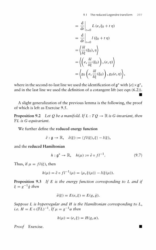
9.1 The reduced Legendre transform 297
= ddt
∣∣∣∣t=0
L (e, ξ0 + t η)
= ddt
∣∣∣∣t=0
l (ξ0 + t η)
=⟨δl
δξ(ξ0), η
⟩=⟨(
e,δl
δξ(ξ0)
), (e, η)
⟩=⟨g0
(e,
δl
δξ(ξ0)
), g0(e, η)
⟩,
where in the second-to-last line we used the identification of g∗ with {e}×g∗,and in the last line we used the definition of a cotangent lift (see eqn (6.2)).
�
A slight generalization of the previous lemma is the following, the proofof which is left as Exercise 9.5.
Proposition 9.2 LetQ be a manifold. If L : TQ→ R is G-invariant, thenFL is G-equivariant.
We further define the reduced energy function
e : g→ R, e(ξ) := 〈f l(ξ), ξ〉 − l(ξ),
and the reduced Hamiltonian
h : g∗ → R, h(µ) := e ◦ f l−1. (9.7)
Thus, if µ = f l(ξ), then
h(µ) = e ◦ f l−1(µ) = 〈µ, ξ(µ)〉 − l(ξ(µ)).
Proposition 9.3 If E is the energy function corresponding to L and ifξ = g−1g then
e(ξ) = E(e, ξ) = E(g, g).
Suppose L is hyperregular and H is the Hamiltonian corresponding to L,i.e. H = E ◦ (FL)−1. If µ = g−1α then
h(µ) = (e, ξ) = H(g,α).
Proof Exercise. �
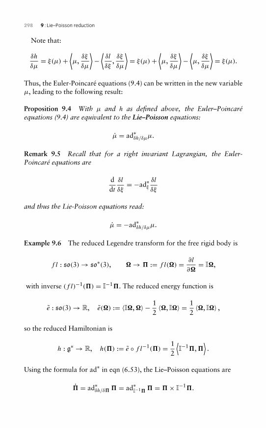
298 9 : Lie–Poisson reduction
Note that:
δh
δµ= ξ(µ)+
⟨µ,
δξ
δµ
⟩−⟨δl
δξ,δξ
δµ
⟩= ξ(µ)+
⟨µ,
δξ
δµ
⟩−⟨µ,
δξ
δµ
⟩= ξ(µ).
Thus, the Euler-Poincaré equations (9.4) can be written in the new variableµ, leading to the following result:
Proposition 9.4 With µ and h as defined above, the Euler–Poincaréequations (9.4) are equivalent to the Lie–Poisson equations:
µ = ad∗δh/δµµ.
Remark 9.5 Recall that for a right invariant Lagrangian, the Euler-Poincaré equations are
ddt
δl
δξ= −ad∗ξ
δl
δξ
and thus the Lie-Poisson equations read:
µ = −ad∗δh/δµµ.
Example 9.6 The reduced Legendre transform for the free rigid body is
f l : so(3)→ so∗(3), �→ � := f l(�) = ∂l
∂�= I�,
with inverse (f l)−1(�) = I−1�. The reduced energy function is
e : so(3)→ R, e(�) := 〈I�,�〉 − 12〈�, I�〉 = 1
2〈�, I�〉 ,
so the reduced Hamiltonian is
h : g∗ → R, h(�) := e ◦ f l−1(�) = 12
⟨I−1�,�
⟩.
Using the formula for ad∗ in eqn (6.53), the Lie–Poisson equations are
� = ad∗δh/δ�� = ad∗I−1�� = �× I−1�.
9.1 The reduced Legendre transform 299
Having obtained the Lie–Poisson equations, the next question is: are theseequations Hamiltonian? We will see in the following sections that they areHamiltonian, with respect to a bracket on g∗ called theLie–Poisson bracket.The theory relating canonical dynamics on T ∗G with reduced Hamiltoniandynamics on g∗ is called Lie–Poisson reduction. This is a Hamiltonian coun-terpart to Euler–Poincaré reduction, in which reduced Lagrangian dynamicson g are shown to be determined by a reduced variational principle.
Lie–Poisson reduction is a special case of the theory of Poisson reduction,presented in Section 6.4. Suppose L is hyperregular, and let H : T ∗G→ R
be the corresponding Hamiltonian, which is leftG-invariant, by Proposition6.35. Poisson reduction theory shows that the canonical Hamiltonian flowon T ∗G corresponds to a Hamiltonian flow on (T ∗G)/G. By Proposition6.61, the following map is a diffeomorphism,
(T ∗G)/G � (G× g∗)/G � g∗,
[g,α] −→ [g, g−1α] −→ µ := g−1α.
This map can be used to push-forward the reduced Poisson bracket andreduced Hamiltonian on (T ∗G)/G to a bracket and Hamiltonian on g∗.The push-forward of the bracket will be done in the following section. Thepush-forward of the Hamiltonian is straightforward. Indeed, the reducedHamiltonian hred on (T ∗G)/G is defined by hred([g,α]) = H(g,α). Let h−be the push-forward of hred to g∗. Then, by definition,
h−(µ) = hred([e,µ]) = H(e,µ).
Proposition 9.7 (Consistency with the reduced Legendre transform) In theabove context, the Hamiltonian h− coincides with the reducedHamiltonianh defined in eqn (9.7).
Proof Since FL(e, ξ) = (e, f l(ξ)) for every ξ ∈ g,
h−(f l(ξ)) = H(e, f l(ξ))
= E ◦ (FL)−1 (e, f l(ξ)) = E(e, ξ) = e(ξ) = h(f l(ξ)).
�
Remark 9.8 Lie–Poisson reduction is a general theory that applies to anysymmetric HamiltonianH on T ∗G. In particular,H need not to correspondto a hyperregular Lagrangian.
300 9 : Lie–Poisson reduction
Exercise 9.1Consider the left trivializations of TG and T ∗G given by the maps
λ : TG→ G× g, (h, h)→ λ(h, h) := (h,h−1h) = (h, ThLh−1 h),
λ∗ : T ∗G→ G× g∗, (h,α)→ (h,h−1α) := (h, T ∗e Lhα),
(first defined in eqn (6.11) and eqn (6.12), respectively).Let λ2 and λ∗2 be the second components of these maps. Show that
the following diagram commutes,
TG � G× gFL−→ G× g∗ � T ∗G
λ2 ↓ ↓ λ∗2
gf l−→ g∗
Exercise 9.2Show that if (g(t), g(t)) is an integral curve for a left invariantLagrangian L, then E (g(t), g(t)) = e (ξ(t)) = const ., where ξ = g−1g.
Exercise 9.3Consider a product Lie group G×K acting on itself by(
(g, k), (g, k))→ (gg, kk).
Use Proposition 9.4 and Remark 9.5 to deduce Lie–Poisson equationsfor a reduced Hamiltonian h : g∗ × k∗ → R.
Exercise 9.4Consider the following action of a Lie groupG on a product spaceG×Y ,where Y is some manifold:
(g, (h, y))→ (gh, y).
9.2 Lie–Poisson reduction: geometry 301
Let L : T (G × Y )→ R be invariant with respect to this action. Definel : g× T Y → R to be the restriction of L, i.e.
l(ξ , y, y) := L(e, ξ , y, y).
The equations of motion for this l appear in Exercise 7.16. Define areduced Legendre transformation and reduced Hamiltonian, by analogywith eqns (9.5) and (9.7), and show that the equations of motion ong∗ × T ∗Y are:
µ = ad∗δh/δµ µ,
y = ∂h
∂p,
p = −∂h
∂y,
where p is the conjugate momentum corresponding to y.
Exercise 9.5Prove Proposition 9.2.
9.2 Lie–Poisson reduction: geometry
Consider the cotangent bundle T ∗G of a Lie group G under the cotangent-lifted left multiplication action of G. We know from Section 6.3 that thequotient space P/G = T ∗G/G is diffeomorphic to g∗, the dual of the Liealgebra of G.
Recall from Section 6.3 the left trivialization map for T ∗G :
λ : T ∗G→ G× g∗, λ(g,α) = (λ1(g,α), λ2(g,α)) = (g, T ∗e Lgα), (9.8)
and the diffeomorphism
ψ : (T ∗G)/G −→ g∗, [g,α] −→ g−1α := T ∗e Lg(α).
Note that ψ ◦ π = λ2, where π : T ∗G → (T ∗G)/G is projection and λ2is the second component of λ, defined above. The map ψ , together withthe reduced Poisson bracket on (T ∗G)/G from Theorem 6.63, induces a
302 9 : Lie–Poisson reduction
Poisson bracket on g∗ that makes ψ a Poisson map. The induced Poissonbracket on g∗ will be denoted {·, ·}lef t
g∗ to indicate that it is associated withthe left translation.
By definition of this bracket, ψ is a Poisson map. By definition of thereduced Poisson bracket on (T ∗G)/G, the projection π is a Poisson map.Since λ2 = ψ ◦ π , it follows that λ2 is a Poisson map, i.e.
{F ,K}lef tg∗ ◦ λ2 := {F ◦ λ2,K ◦ λ2}T ∗G, (9.9)
where the bracket on the right is the canonical Poisson bracket.For any F ∈ F(g∗), the corresponding function F ◦ λ2 ∈ F(T ∗G) is left
G−invariant and it is called the left extension of F . We denote by FL(T∗G)
the space of smooth left invariant functions on T ∗G. The map
F(g∗)→ FL(T∗G), F → F ◦ λ2,
is in fact a bijection, with the inverse given by restriction to g∗ (this isExercise 9.6).
Theorem 9.9 Let FL and KL be G-invariant smooth functions on T ∗G,and let F andK be their restrictions (respectively) to g∗. For every (g0,α0) ∈T ∗G, let µ0 = T ∗e Lg(α0). Then
{FL,KL} (g0,α0) = −⟨µ0,
[δF
δµ,δK
δµ
]∣∣∣∣µ0
⟩, (9.10)
where the bracket on the left is the canonical Poisson bracket.
Proof Recall from Section 4.3 that, given a Poisson structure on a man-ifold P, the Poisson bracket {F1,F2} at a point p ∈ P of two functionsF1,F2 ∈ F(P ) depends only on the first derivatives of F1 and F2 at p. Thusthe value of {FL,KL} (g,α) depends only on the first derivatives of FL andKL at (g,α), and so we can assume, without loss of generality, that FL andKL are linear in the cotangent fibres, i.e., that they depend linearly on α.
Thus, in particular, δFδµ
and δKδµ
are constant elements of g. Let X =(
δFδµ
)L,
i.e. the left-invariant vector field on G corresponding to δFδµ
, defined by
X(h) = TeLh
(δFδµ
), for all h ∈ G. By left-invariance,
δFL
δα(g,α) = T Lg
(δF
δµ
)= X(g), (9.11)
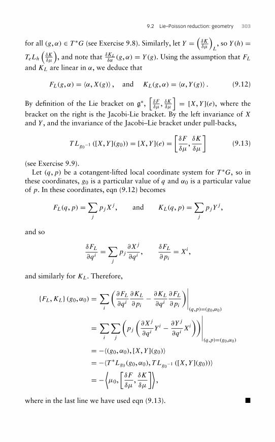
9.2 Lie–Poisson reduction: geometry 303
for all (g,α) ∈ T ∗G (see Exercise 9.8). Similarly, let Y =(
δKδµ
)L, so Y (h) =
TeLh
(δKδµ
), and note that δKL
δα(g,α) = Y (g). Using the assumption that FL
and KL are linear in α, we deduce that
FL(g,α) = 〈α,X(g)〉 , and KL(g,α) = 〈α,Y (g)〉 . (9.12)
By definition of the Lie bracket on g∗,[δFδµ
, δKδµ
]= [X,Y ](e), where the
bracket on the right is the Jacobi-Lie bracket. By the left invariance of X
and Y , and the invariance of the Jacobi–Lie bracket under pull-backs,
T Lg0−1 ([X,Y ](g0)) = [X,Y ](e) =
[δF
δµ,δK
δµ
](9.13)
(see Exercise 9.9).Let (q,p) be a cotangent-lifted local coordinate system for T ∗G, so in
these coordinates, g0 is a particular value of q and α0 is a particular valueof p. In these coordinates, eqn (9.12) becomes
FL(q,p) =∑j
pjXj , and KL(q,p) =
∑j
pjYj ,
and so
δFL
∂qi=∑j
pj
∂Xj
∂qi,
δFL
∂pi
= Xi ,
and similarly for KL. Therefore,
{FL,KL} (g0,α0) =∑i
(∂FL
∂qi
∂KL
∂pi
− ∂KL
∂qi
∂FL
∂pi
)∣∣∣∣∣(q,p)=(g0,α0)
=∑i
∑j
(pj
(∂Xj
∂qiY i − ∂Y j
∂qiXi
))∣∣∣∣∣∣(q,p)=(g0,α0)
= −〈(g0,α0), [X,Y ](g0)〉= −〈T ∗Lg0(g0,α0), T Lg0
−1 ([X,Y ](g0))〉
= −⟨µ0,
[δF
δµ,δK
δµ
]⟩,
where in the last line we have used eqn (9.13). �
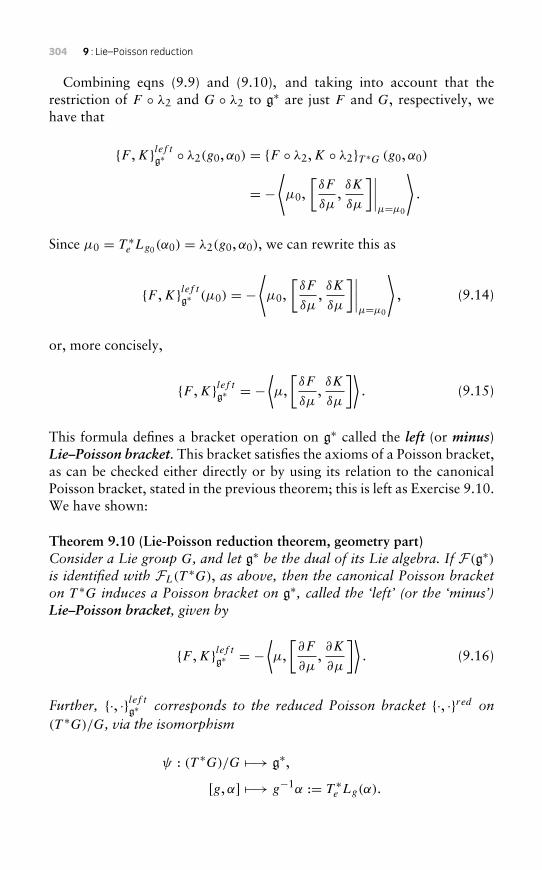
304 9 : Lie–Poisson reduction
Combining eqns (9.9) and (9.10), and taking into account that therestriction of F ◦ λ2 and G ◦ λ2 to g∗ are just F and G, respectively, wehave that
{F ,K}lef tg∗ ◦ λ2(g0,α0) = {F ◦ λ2,K ◦ λ2}T ∗G (g0,α0)
= −⟨µ0,
[δF
δµ,δK
δµ
]∣∣∣∣µ=µ0
⟩.
Since µ0 = T ∗e Lg0(α0) = λ2(g0,α0), we can rewrite this as
{F ,K}lef tg∗ (µ0) = −
⟨µ0,
[δF
δµ,δK
δµ
]∣∣∣∣µ=µ0
⟩, (9.14)
or, more concisely,
{F ,K}lef tg∗ = −
⟨µ,[δF
δµ,δK
δµ
]⟩. (9.15)
This formula defines a bracket operation on g∗ called the left (or minus)Lie–Poisson bracket. This bracket satisfies the axioms of a Poisson bracket,as can be checked either directly or by using its relation to the canonicalPoisson bracket, stated in the previous theorem; this is left as Exercise 9.10.We have shown:
Theorem 9.10 (Lie-Poisson reduction theorem, geometry part)Consider a Lie group G, and let g∗ be the dual of its Lie algebra. If F(g∗)is identified with FL(T
∗G), as above, then the canonical Poisson bracketon T ∗G induces a Poisson bracket on g∗, called the ‘left’ (or the ‘minus’)Lie–Poisson bracket, given by
{F ,K}lef tg∗ = −
⟨µ,[∂F
∂µ,∂K
∂µ
]⟩. (9.16)
Further, {·, ·}lef tg∗ corresponds to the reduced Poisson bracket {·, ·}red on
(T ∗G)/G, via the isomorphism
ψ : (T ∗G)/G −→ g∗,
[g,α] −→ g−1α := T ∗e Lg(α).
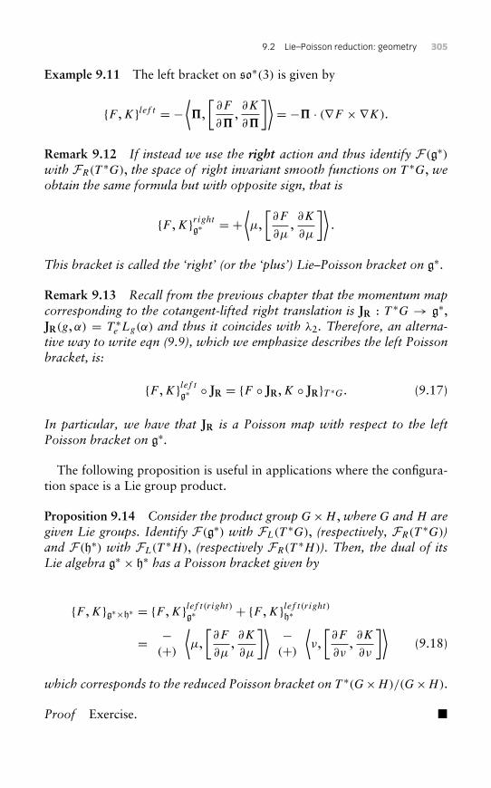
9.2 Lie–Poisson reduction: geometry 305
Example 9.11 The left bracket on so∗(3) is given by
{F ,K}lef t = −⟨�,[∂F
∂�,∂K
∂�
]⟩= −� · (∇F ×∇K).
Remark 9.12 If instead we use the right action and thus identify F(g∗)with FR(T
∗G), the space of right invariant smooth functions on T ∗G, weobtain the same formula but with opposite sign, that is
{F ,K}rightg∗ = +⟨µ,[∂F
∂µ,∂K
∂µ
]⟩.
This bracket is called the ‘right’ (or the ‘plus’) Lie–Poisson bracket on g∗.
Remark 9.13 Recall from the previous chapter that the momentum mapcorresponding to the cotangent-lifted right translation is JR : T ∗G → g∗,JR(g,α) = T ∗e Lg(α) and thus it coincides with λ2. Therefore, an alterna-tive way to write eqn (9.9), which we emphasize describes the left Poissonbracket, is:
{F ,K}lef tg∗ ◦ JR = {F ◦ JR,K ◦ JR}T ∗G. (9.17)
In particular, we have that JR is a Poisson map with respect to the leftPoisson bracket on g∗.
The following proposition is useful in applications where the configura-tion space is a Lie group product.
Proposition 9.14 Consider the product group G×H , where G and H aregiven Lie groups. Identify F(g∗) with FL(T
∗G), (respectively, FR(T∗G))
and F(h∗) with FL(T∗H), (respectively FR(T
∗H)). Then, the dual of itsLie algebra g∗ × h∗ has a Poisson bracket given by
{F ,K}g∗×h∗ = {F ,K}lef t(right)g∗ + {F ,K}lef t(right)
h∗
= −(+)
⟨µ,[∂F
∂µ,∂K
∂µ
]⟩ −(+)
⟨ν,[∂F
∂ν,∂K
∂ν
]⟩(9.18)
which corresponds to the reduced Poisson bracket on T ∗(G×H)/(G×H).
Proof Exercise. �
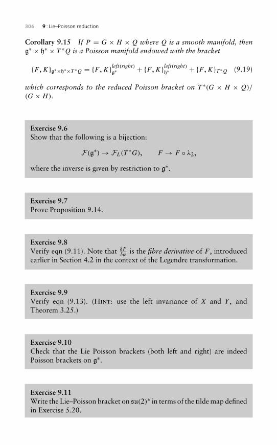
306 9 : Lie–Poisson reduction
Corollary 9.15 If P = G × H ×Q where Q is a smooth manifold, theng∗ × h∗ × T ∗Q is a Poisson manifold endowed with the bracket
{F ,K}g∗×h∗×T ∗Q = {F ,K}left(right)g∗ + {F ,K}left(right)h∗ + {F ,K}T ∗Q (9.19)
which corresponds to the reduced Poisson bracket on T ∗(G × H × Q)/
(G×H).
Exercise 9.6Show that the following is a bijection:
F(g∗)→ FL(T∗G), F → F ◦ λ2,
where the inverse is given by restriction to g∗.
Exercise 9.7Prove Proposition 9.14.
Exercise 9.8Verify eqn (9.11). Note that δF
δαis the fibre derivative of F , introduced
earlier in Section 4.2 in the context of the Legendre transformation.
Exercise 9.9Verify eqn (9.13). (Hint: use the left invariance of X and Y , andTheorem 3.25.)
Exercise 9.10Check that the Lie Poisson brackets (both left and right) are indeedPoisson brackets on g∗.
Exercise 9.11Write the Lie–Poisson bracket on su(2)∗ in terms of the tilde map definedin Exercise 5.20.
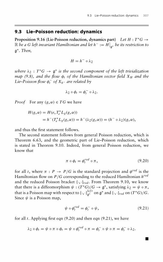
9.3 Lie–Poisson reduction: dynamics 307
9.3 Lie–Poisson reduction: dynamics
Proposition 9.16 (Lie-Poisson reduction, dynamics part) Let H : T ∗G→R be a G left invariant Hamiltonian and let h− := H
∣∣g∗ be its restriction to
g∗. Then,
H = h− ◦ λ2
where λ2 : T ∗G → g∗ is the second component of the left trivializationmap (9.8), and the flow φt of the Hamiltonian vector field XH and theLie–Poisson flow φ−t of Xh− are related by
λ2 ◦ φt = φ−t ◦ λ2.
Proof For any (g,α) ∈ TG we have
H(g,α) = H(e, T ∗e Lg(g,α))
= h−(T ∗e Lg(g,α)) = h−(λ2(g,α)) = (h− ◦ λ2)(g,α),
and thus the first statement follows.The second statement follows from general Poisson reduction, which is
Theorem 6.63, and the geometric part of Lie–Poisson reduction, whichis stated in Theorem 9.10. Indeed, from general Poisson reduction, weknow that
π ◦ φt = φredt ◦ π , (9.20)
for all t , where π : P → P/G is the standard projection and φred is theHamiltonian flow on P/G corresponding to the reduced Hamiltonian hred
and the reduced Poisson bracket {·, ·}red . From Theorem 9.10, we knowthat there is a diffeomorphism ψ : (T ∗G)/G→ g∗, satisfying λ2 = ψ ◦ π ,that is a Poisson map with respect to {·, ·}lef t
g∗ on g∗ and {·, ·}red on (T ∗G)/G.Since ψ is a Poisson map,
ψ ◦ φredt = φ−t ◦ ψ , (9.21)
for all t . Applying first eqn (9.20) and then eqn (9.21), we have
λ2 ◦ φt = ψ ◦ π ◦ φt = ψ ◦ φredt ◦ π = φ−t ◦ ψ ◦ π = φ−t ◦ λ2.
�
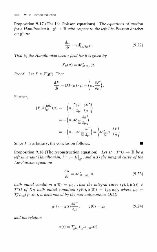
308 9 : Lie–Poisson reduction
Proposition 9.17 (The Lie–Poisson equations) The equations of motionfor a Hamiltonian h : g∗ → R with respect to the left Lie–Poisson bracketon g∗ are
dµdt= ad∗δh/δµ µ. (9.22)
That is, the Hamiltonian vector field for h is given by
Xh(µ) = ad∗δh/δµ µ.
Proof Let F ∈ F(g∗). Then
dFdt= DF(µ) · µ =
⟨µ,
δF
δµ
⟩.
Further,
{F ,h}leftg∗ (µ) = −⟨µ,[δF
δµ,δh
δµ
]⟩= −
⟨µ, ad δF
δµ
δh
δµ
⟩= −
⟨µ,−ad δh
δµ
δF
δµ
⟩=⟨ad∗δh
δµ
µ,δF
δµ
⟩.
Since F is arbitrary, the conclusion follows. �
Proposition 9.18 (The reconstruction equation) Let H : T ∗G → R be aleft invariant Hamiltonian, h− := H
∣∣g∗ , and µ(t) the integral curve of the
Lie-Poisson equations
dµdt= ad∗δh−/δµ µ (9.23)
with initial condition µ(0) = µ0. Then the integral curve (g(t),α(t)) ∈T ∗G of XH with initial condition (g(0),α(0)) = (g0,α0), where µ0 =T ∗e Lg0(g0,α0), is determined by the non-autonomous ODE
g(t) = g(t)δh−
δµ, g(0) = g0 (9.24)
and the relation
α(t) = T ∗g(t)Lg−1(t)µ(t).
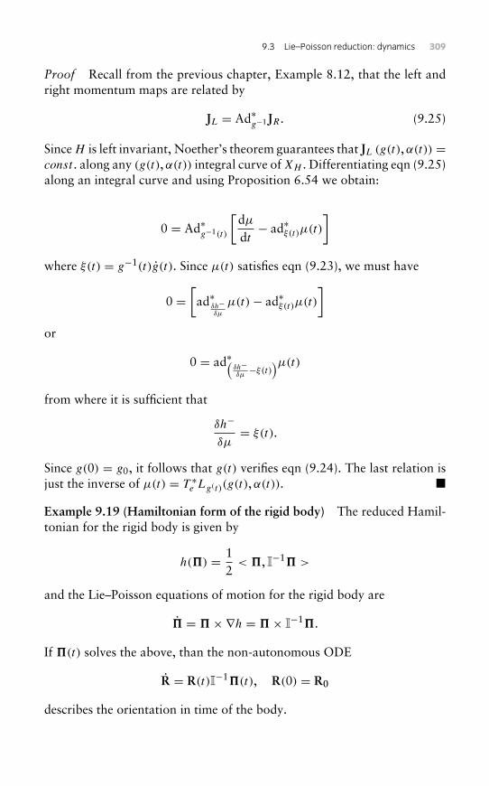
9.3 Lie–Poisson reduction: dynamics 309
Proof Recall from the previous chapter, Example 8.12, that the left andright momentum maps are related by
JL = Ad∗g−1JR. (9.25)
Since H is left invariant, Noether’s theorem guarantees that JL (g(t),α(t)) =const . along any (g(t),α(t)) integral curve of XH . Differentiating eqn (9.25)along an integral curve and using Proposition 6.54 we obtain:
0 = Ad∗g−1(t)
[dµdt− ad∗ξ(t)µ(t)
]where ξ(t) = g−1(t)g(t). Since µ(t) satisfies eqn (9.23), we must have
0 =[ad∗δh−
δµ
µ(t)− ad∗ξ(t)µ(t)
]or
0 = ad∗(δh−δµ−ξ(t)
)µ(t)
from where it is sufficient that
δh−
δµ= ξ(t).
Since g(0) = g0, it follows that g(t) verifies eqn (9.24). The last relation isjust the inverse of µ(t) = T ∗e Lg(t)(g(t),α(t)). �
Example 9.19 (Hamiltonian form of the rigid body) The reduced Hamil-tonian for the rigid body is given by
h(�) = 12
< �, I−1� >
and the Lie–Poisson equations of motion for the rigid body are
� = �×∇h = �× I−1�.
If �(t) solves the above, than the non-autonomous ODE
R = R(t)I−1�(t), R(0) = R0
describes the orientation in time of the body.
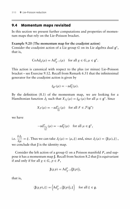
310 9 : Lie–Poisson reduction
9.4 Momentum maps revisited
In this section we present further computations and properties of momen-tum maps that rely on the Lie–Poisson bracket.
Example 9.20 (The momentum map for the coadjoint action)Consider the coadjoint action of a Lie group G on its Lie algebra dual g∗,that is,
CoAdg(µ) = Ad∗g−1(µ) for all g ∈ G,µ ∈ g∗.
This action is canonical with respect to the plus (or minus) Lie–Poissonbracket – see Exercise 9.12. Recall from Remark 6.51 that the infinitesimalgenerator for the coadjoint action is given by
ξg∗(µ) = −ad∗ξ (µ).
By the definition (8.1) of the momentum map, we are looking for aHamiltonian function Jξ such that XJξ (µ) = ξg∗(µ) for all µ ∈ g∗. Since
XF (µ) = −ad∗δFδµ
(µ) for all F ∈ F(g∗)
we have
−ad∗δJξδµ
(µ) = −ad∗ξ (µ) for all µ ∈ g∗,
i.e.δJξ
δµ= ξ . Thus we can take Jξ (µ) = 〈µ, ξ〉 and, since Jξ (µ) = 〈J(µ), ξ〉 ,
we conclude that J is the identity map.
Consider the left action of a group G on a Poisson manifold P , and sup-pose it has a momentum map J. Recall from Section 8.2 that J is equivariantif and only if for all g ∈ G, p ∈ P ,
J(gp) = Ad∗g−1
(J(p)
),
that is,
〈J(gp), ξ〉 =⟨Ad∗
g−1
(J(p)
), ξ⟩
for all ξ ∈ g.
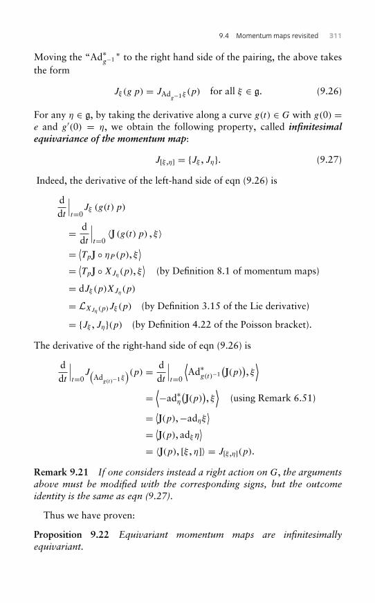
9.4 Momentummaps revisited 311
Moving the “Ad∗g−1" to the right hand side of the pairing, the above takes
the form
Jξ (g p) = JAdg−1ξ
(p) for all ξ ∈ g. (9.26)
For any η ∈ g, by taking the derivative along a curve g(t) ∈ G with g(0) =e and g′(0) = η, we obtain the following property, called infinitesimalequivariance of the momentum map:
J[ξ ,η] = {Jξ , Jη}. (9.27)
Indeed, the derivative of the left-hand side of eqn (9.26) is
ddt
∣∣∣t=0
Jξ (g(t) p)
= ddt
∣∣∣t=0〈J (g(t) p) , ξ〉
= ⟨TpJ ◦ ηP (p), ξ⟩
= ⟨TpJ ◦XJη(p), ξ⟩
(by Definition 8.1 of momentum maps)
= dJξ (p)XJη(p)
= LXJη (p)Jξ (p) (by Definition 3.15 of the Lie derivative)
= {Jξ , Jη}(p) (by Definition 4.22 of the Poisson bracket).
The derivative of the right-hand side of eqn (9.26) is
ddt
∣∣∣t=0
J(Ad
g(t)−1ξ)(p) = d
dt
∣∣∣t=0
⟨Ad∗
g(t)−1
(J(p)
), ξ⟩
=⟨−ad∗η
(J(p)
), ξ⟩
(using Remark 6.51)
= ⟨J(p),−adηξ⟩
= ⟨J(p), adξ η⟩
= 〈J(p), [ξ , η]〉 = J[ξ ,η](p).
Remark 9.21 If one considers instead a right action on G, the argumentsabove must be modified with the corresponding signs, but the outcomeidentity is the same as eqn (9.27).
Thus we have proven:
Proposition 9.22 Equivariant momentum maps are infinitesimallyequivariant.
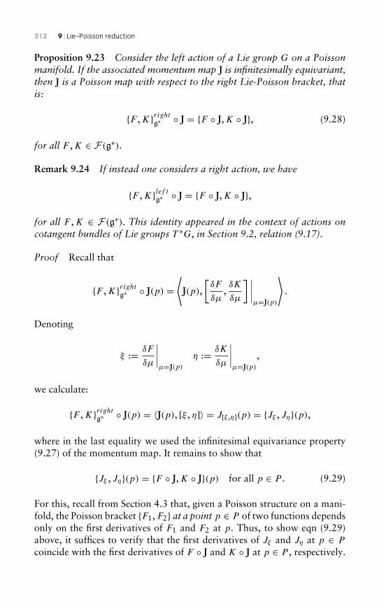
312 9 : Lie–Poisson reduction
Proposition 9.23 Consider the left action of a Lie group G on a Poissonmanifold. If the associated momentum map J is infinitesimally equivariant,then J is a Poisson map with respect to the right Lie-Poisson bracket, thatis:
{F ,K}rightg∗ ◦ J = {F ◦ J,K ◦ J}, (9.28)
for all F ,K ∈ F(g∗).
Remark 9.24 If instead one considers a right action, we have
{F ,K}lef tg∗ ◦ J = {F ◦ J,K ◦ J},
for all F ,K ∈ F(g∗). This identity appeared in the context of actions oncotangent bundles of Lie groups T ∗G, in Section 9.2, relation (9.17).
Proof Recall that
{F ,K}rightg∗ ◦ J(p) =⟨J(p),
[δF
δµ,δK
δµ
] ∣∣∣∣µ=J(p)
⟩.
Denoting
ξ := δF
δµ
∣∣∣∣µ=J(p)
η := δK
δµ
∣∣∣∣µ=J(p)
,
we calculate:
{F ,K}rightg∗ ◦ J(p) = 〈J(p), [ξ , η]〉 = J[ξ ,η](p) = {Jξ , Jη}(p),
where in the last equality we used the infinitesimal equivariance property(9.27) of the momentum map. It remains to show that
{Jξ , Jη}(p) = {F ◦ J,K ◦ J}(p) for all p ∈ P . (9.29)
For this, recall from Section 4.3 that, given a Poisson structure on a mani-fold, the Poisson bracket {F1,F2} at a point p ∈ P of two functions dependsonly on the first derivatives of F1 and F2 at p. Thus, to show eqn (9.29)above, it suffices to verify that the first derivatives of Jξ and Jη at p ∈ P
coincide with the first derivatives of F ◦ J and K ◦ J at p ∈ P , respectively.
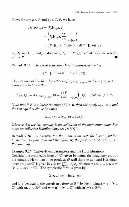
9.4 Momentummaps revisited 313
Now, for any p ∈ P and vp ∈ TpP , we have:
dJξ (p)(vp) =⟨TpJ(vp), ξ
⟩=⟨TpJ(vp),
δF
δµ
∣∣∣∣µ=J(p)
⟩= dF (J(p)) ◦ TpJ(vp) = d(F ◦ J)(p)(vp).
So, Jξ and F ◦ J and, analogously, Jη and K ◦ J, have identical derivativesat p ∈ P . �
Remark 9.25 The set of collective Hamiltonians is defined as
{F ◦ J : P → R | F ∈ F(g∗)}.
The equality of the first derivatives of J(δF/δµ)|µ=J(p)and F ◦ J at p ∈ P
allows one to prove that
XF◦J (p) = XJ(δF/δµ)|µ=J(p)(p) =
(δF
δµ
∣∣∣µ=J(p)
)P
(p) f or all p ∈ P .
Note that if F is a linear function of ξ ∈ g, then (δF/δµ)|µ=J(p) = ξ andthe last equality above becomes
XF◦J (p) = XJξ (p) = ξP (p).
Observe that the last equality is the definition of the momentum map. Formore on collective Hamiltonians, see [MR02].
Remark 9.26 By Exercise 8.6 the momentum map for linear symplec-tic actions is equivariant and therefore, by the previous proposition, is aPoisson map.
Example 9.27 (Cayley–Klein parameters and the Hopf fibration)Consider the symplectic form on C2 given by minus the imaginary part ofthe standard Hermitian inner product. (Recall that the standard Hermitianinner product Cn is given by z·w :=∑n
j=1 zjwj , where z = (z1, . . . , zn),w =(w1, . . . ,wn) ∈ Cn.) The symplectic form is given by
�(z,w) := − Im(z ·w)
and it is identical to the one given before on R2n by identifying z = u+ iv ∈Cn with (u, v) ∈ R2n and w = u′ + iv′ ∈ Cn with (u′, v′) ∈ R2n.
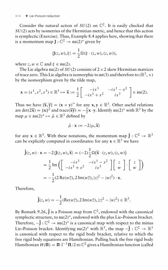
314 9 : Lie–Poisson reduction
Consider the natural action of SU(2) on C2. It is easily checked thatSU(2) acts by isometries of the Hermitian metric, and hence that this actionis symplectic (Exercise). Thus, Example 8.4 applies here, showing that thereis a momentum map J : C2 → su(2)∗ given by
〈J(z,w), ξ〉 = 12�(ξ · (z,w), (z,w)),
where z,w ∈ C and ξ ∈ su(2).The Lie algebra su(2) of SU(2) consists of 2×2 skew Hermitian matrices
of trace zero. This Lie algebra is isomorphic to so(3) and therefore to (R3,×)by the isomorphism given by the tilde map,
x = (x1, x2, x3) ∈ R3 → x := 12
[ −ix3 −ix1 − x2
−ix1 + x2 ix3
]∈ su(2).
Thus we have [x, y] = (x × y) for any x, y ∈ R3. Other useful relationsare det(2x) = ‖x‖2 and trace(xy) = −1
2x ·y. Identify su(2)∗ with R3 by themap µ ∈ su(2)∗ → µ ∈ R3 defined by
µ · x := −2〈µ, x〉
for any x ∈ R3. With these notations, the momentum map J : C2 → R3
can be explicitly computed in coordinates: for any x ∈ R3 we have
J(z,w) · x = −2〈J(z,w), x〉 = (−2)12�(x · (z,w), (z,w)
)= 1
2Im([ −ix3 −ix1 − x2
−ix1 + x2 ix3
] [z
w
]·[
z
w
])= −1
2(2 Re(wz), 2 Im(wz), |z|2 − |w|2) · x.
Therefore,
J(z,w) = −12(Re(wz), 2 Im(wz), |z|2 − |w|2) ∈ R3.
By Remark 9.26, J is a Poisson map from C2, endowed with the canonicalsymplectic structure, to su(2)∗, endowed with the plus Lie–Poisson bracket.Therefore, −J : C2 → su(2)∗ is a canonical map with respect to the minusLie–Poisson bracket. Identifying su(2)∗ with R3, the map −J : C2 → R3
is canonical with respect to the rigid body bracket, relative to which thefree rigid body equations are Hamiltonian. Pulling back the free rigid bodyHamiltonianH(�) = �·I−1�/2 to C2 gives a Hamiltonian function (called
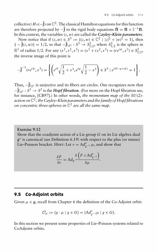
9.5 Co-Adjoint orbits 315
collective)H◦(−J) on C2. The classical Hamilton equations for this functionare therefore projected by −J to the rigid body equations � = � × I−1�.In this context, the variables (z,w) are called the Cayley–Klein parameters.
Now notice that if (z,w) ∈ S3 := {(z,w) ∈ C2 | |z|2 + |w|2 = 1}, then‖ − J(z,w)‖ = 1/2, so that −J|S3 : S3 → S2
1/2, where S21/2 is the sphere in
R3 of radius 1/2. For any (x1, x2, x3) = (x1 + ix2, x3) = (reiψ , x3) ∈ S21/2,
the inverse image of this point is
−J−1
(reiψ , x3) ={(
eiθ
√12+ x3, eiϕ
√12− x3
)∈ S3 | ei(θ−ϕ+ψ) = 1
}.
Thus, −J|S3 is surjective and its fibers are circles. One recognizes now that−J|S3 : S3 → S2 is the Hopf fibration. (For more on the Hopf fibration see,for instance, [CB97].) In other words, the momentum map of the SU(2)-action onC2, theCayley–Klein parameters and the family ofHopf fibrationson concentric three-spheres in C2 are all the same map.
Exercise 9.12Show that the coadjoint action of a Lie group G on its Lie algebra dualg∗ is canonical (see Definition 6.19) with respect to the plus (or minus)Lie–Poisson bracket. Hint: Let ν = Ad∗
g−1 µ, and show that
δF
δν= Adg
δ(F ◦ Ad∗
g−1
)δµ
.
9.5 Co-Adjoint orbits
Given µ ∈ g, recall from Chapter 6 the definition of the Co-Adjoint orbit:
Oµ := {g · µ | g ∈ G} = {Ad∗g−1µ | g ∈ G}.
In this section we present some properties of Lie–Poisson systems related toCoAdjoint orbits.
316 9 : Lie–Poisson reduction
Proposition 9.28 Let h ∈ F(g∗) and let µ(t) be the solution of the initialvalue problem
µ = ad∗δh/δµ µ,
µ(0) = µ0.
Then, µ(t) ∈ Oµ0 .
Proof Given µ(t), the solution of the above initial-value problem, wehave to show that for every t there is a g(t) ∈ G such that µ(t) ∈ Oµ0 ={Ad∗
g−1µ0 | g ∈ G} = {Ad∗g µ0 | g ∈ G}. We will show that µ(t) = Ad∗g(t)µ0,where g(t) is the solution of the initial value problem:
g = gδh
δµ,
g(0) = e.
Since g−1(t)g(t) = (δh/δµ)(t) for all t , applying Proposition 6.54, weobtain:
ddt
(Ad∗
g(t)−1µ(t))= Ad∗
g(t)−1µ(t)
[dµ(t)
dt− ad∗
g−1(t)g(t)µ(t)
]= Ad∗
g(t)−1µ(t)
[dµ(t)
dt− ad∗δh
δµ(t)
µ(t)
]= 0.
Thus, Ad∗g(t)−1µ(t) = const . = Ad∗g(0)µ(0) = Ad∗eµ0 = µ0. �
Definition 9.29 The Co-Adjoint isotropy group of µ ∈ g∗ is
Gµ := {g ∈ G | Ad∗g−1µ = µ}.
Definition 9.30 The coadjoint isotropy algebra of µ ∈ g∗ is
gµ := {ξ ∈ g | ad∗ξµ = 0}.Recall from Chapter 4 that a function C ∈ F(P ) is a Casimir of
{C,F } = 0 for all F ∈ F(P ).
We have the following
Proposition 9.31 A function C ∈ F(g∗) is a Casimir function if and onlyif δC/δµ ∈ gµ for all µ ∈ g∗.
9.5 Co-Adjoint orbits 317
Proof Since C ∈ F(g∗) is a Casimir, we have {C,F } = 0 for all F ∈ F(g∗).We have
0 = {C,F }(µ) = −⟨µ,[δC
δµ,δF
δµ
]⟩= −
⟨µ, ad δC
δµ
δF
δµ
⟩= −
⟨ad∗δC
δµ
µ,δF
δµ
⟩for F arbitrary. Thus,
ad∗δCδµ
µ = 0,
and the conclusion follows. �
Proposition 9.32 If C ∈ F(g∗) is Ad∗ invariant, then C is a Casimirfunction.
Remark 9.33 The converse of this statement can be found in [MR02].
Proof Since C is Ad∗ invariant, we have C(Ad∗g−1µ) = C(µ) for all µ ∈ g∗.
Taking the derivative with respect to g at g = e we have
dC(µ)(−ad∗ξµ
) = 0
where ξ = g(0). Thus
0 =⟨−ad∗ξµ,
δC
δµ
⟩=⟨µ,−adξ
δC
δµ
⟩=⟨µ, ad δC
δµξ⟩=⟨ad∗δC
δµ
µ, ξ⟩.
Since ξ is arbitrary, we have
ad∗δCδµ
µ = 0,
and thus δC/δµ ∈ gµ. The conclusion follows by applying the previousproposition. �
Example 9.34 (Co-Adjoint orbits on SO(3) and rigid body Casimirs) Forso(3)∗ the Co-Adjoint orbits are the sets (see Example 6.44)
O� = {R� | R ∈ SO(3)}.Given � ∈ so(3)∗, the coadjoint isotropy group is given by
(so(3))� = {� ∈ so(3) | �×� = 0}
318 9 : Lie–Poisson reduction
i.e. it contains all angular velocities parallel to �. The rigid body Casimirsare functions of the form
C(�) = �
(12||�||2
).
Indeed, since
δC
δ�=(�′(
12||�||2
))�
belongs to the coadjoint isotropy group (so(3))� , by Proposition 9.31, �is a Casimir.
Exercise 9.13Recall the left and right momentum maps from Example 8.12. Showthat JL(J
−1R (µ)) = Oµ.
9.6 Lie–Poisson brackets on semidirect products
In Chapter 5, Example 5.14 we introduced the special Euclidian groupSE(3), a Lie group that describes rigid motions and coordinate transfor-mations of the three-dimensional space. Recall that SE(3) � SO(3) × R3
and that it may be described as the set of (4 × 4)-dimensional matrices ofthe form {[
R v0 1
] ∣∣∣ R ∈ SO(3), v ∈ R3}
The group operation is the usual multiplication of matrices. Equivalently,we can write the multiplication as the operation � :
(SO(3)×R3) ×(
SO(3)×R3)→ SO(3)×R3 :
(R1, v1) � (R2, v2) = (R1R2, v1 + R1v2) .
This kind of product structure generalizes naturally as follows:
Definition 9.35 (Semidirect products) Consider a Lie group G and vectorspace V on which G acts on the left by linear maps. That is, for g ∈ G,
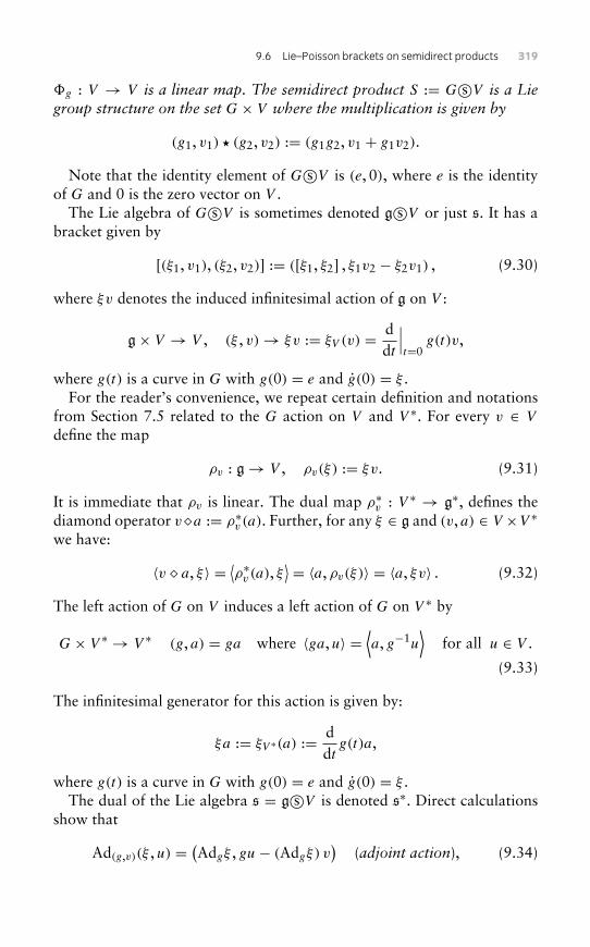
9.6 Lie–Poisson brackets on semidirect products 319
�g : V → V is a linear map. The semidirect product S := G s©V is a Liegroup structure on the set G× V where the multiplication is given by
(g1, v1) � (g2, v2) := (g1g2, v1 + g1v2).
Note that the identity element of G s©V is (e, 0), where e is the identityof G and 0 is the zero vector on V .
The Lie algebra of G s©V is sometimes denoted g s©V or just s. It has abracket given by
[(ξ1, v1), (ξ2, v2)] := ([ξ1, ξ2] , ξ1v2 − ξ2v1) , (9.30)
where ξv denotes the induced infinitesimal action of g on V :
g× V → V , (ξ , v)→ ξv := ξV (v) = ddt
∣∣∣t=0
g(t)v,
where g(t) is a curve in G with g(0) = e and g(0) = ξ .For the reader’s convenience, we repeat certain definition and notations
from Section 7.5 related to the G action on V and V ∗. For every v ∈ V
define the map
ρv : g→ V , ρv(ξ) := ξv. (9.31)
It is immediate that ρv is linear. The dual map ρ∗v : V ∗ → g∗, defines thediamond operator v&a := ρ∗v (a). Further, for any ξ ∈ g and (v, a) ∈ V ×V ∗we have:
〈v & a, ξ〉 = ⟨ρ∗v (a), ξ ⟩ = 〈a, ρv(ξ)〉 = 〈a, ξv〉 . (9.32)
The left action of G on V induces a left action of G on V ∗ by
G× V ∗ → V ∗ (g, a) = ga where 〈ga, u〉 =⟨a, g−1u
⟩for all u ∈ V .
(9.33)
The infinitesimal generator for this action is given by:
ξa := ξV ∗(a) := ddt
g(t)a,
where g(t) is a curve in G with g(0) = e and g(0) = ξ .The dual of the Lie algebra s = g s©V is denoted s∗. Direct calculations
show that
Ad(g,v)(ξ , u) = (Adgξ , gu− (Adgξ) v)
(adjoint action), (9.34)
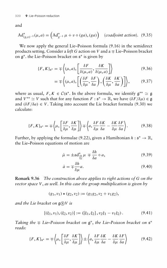
320 9 : Lie–Poisson reduction
and
Ad∗(g,v)−1(µ, a) =
(Ad∗
g−1 µ+ v & (ga), (ga))
(coadjoint action). (9.35)
We now apply the general Lie–Poisson formula (9.16) in the semidirectproducts setting. Consider a left G action on V and a∓ Lie–Poisson bracketon g∗. the Lie–Poisson bracket on s∗ is given by
{F ,K}s∗ = ∓⟨(µ, a),
[δF
δ(µ, a),
δK
δ(µ, a)
]⟩(9.36)
= ∓⟨(µ, a),
[(δF
δµ,δF
δa
),(δK
δµ,δK
δa
)]⟩, (9.37)
where as usual, F ,K ∈ C(s∗. In the above formula, we identify g∗∗ � gand V ∗∗ � V such that for any function F : s∗ → R, we have (δF/δµ) ∈ gand (δF/δa) ∈ V . Taking into account the Lie bracket formula (9.30) wecalculate:
{F ,K}s∗ = ∓⟨µ,[δF
δµ,δK
δµ
]⟩∓⟨a,
δF
δµ
δK
δa− δK
δµ
δF
δa
⟩. (9.38)
Further, by applying the formulae (9.22), given a Hamiltonian h : s∗ → R,the Lie–Poisson equations of motion are
µ = ±ad∗δhδµ
µ ∓ δh
δa& a, (9.39)
a = ∓ δh
δµa. (9.40)
Remark 9.36 The construction above applies to right actions of G on thevector space V , as well. In this case the group multiplication is given by
(g1, v1) � (g2, v2) := (g1g2, v2 + v1g2),
and the Lie bracket on g s©V is
[(ξ1, v1), (ξ2, v2)] := ([ξ1, ξ2] , v2ξ1 − v1ξ2) . (9.41)
Taking the ∓ Lie–Poisson bracket on g∗, the Lie–Poisson bracket on s∗reads:
{F ,K}s∗ = ∓⟨µ,[δF
δµ,δK
δµ
]⟩±⟨a,
δF
δµ
δK
δa− δK
δµ
δF
δa
⟩(9.42)
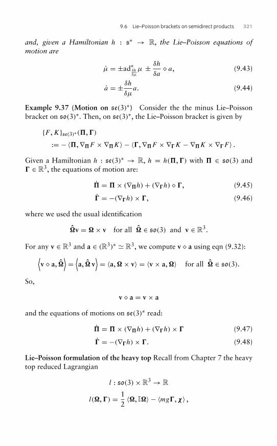
9.6 Lie–Poisson brackets on semidirect products 321
and, given a Hamiltonian h : s∗ → R, the Lie–Poisson equations ofmotion are
µ = ±ad∗δhδµ
µ ± δh
δa& a, (9.43)
a = ± δh
δµa. (9.44)
Example 9.37 (Motion on se(3)∗) Consider the the minus Lie–Poissonbracket on so(3)∗. Then, on se(3)∗, the Lie–Poisson bracket is given by
{F ,K}se(3)∗(�,�)
:= −〈�,∇�F ×∇�K〉 − 〈�,∇�F ×∇�K − ∇�K ×∇�F 〉 .Given a Hamiltonian h : se(3)∗ → R, h = h(�,�) with � ∈ so(3) and� ∈ R3, the equations of motion are:
� = �× (∇�h)+ (∇�h) & �, (9.45)
� = −(∇�h)× �, (9.46)
where we used the usual identification
�v = �× v for all � ∈ so(3) and v ∈ R3.
For any v ∈ R3 and a ∈ (R3)∗ � R3, we compute v & a using eqn (9.32):⟨v & a, �
⟩=⟨a, � v
⟩= 〈a,�× v〉 = 〈v × a,�〉 for all � ∈ so(3).
So,
v & a = v × a
and the equations of motions on se(3)∗ read:
� = �× (∇�h)+ (∇�h)× � (9.47)
� = −(∇�h)× �. (9.48)
Lie–Poisson formulation of the heavy top Recall from Chapter 7 the heavytop reduced Lagrangian
l : so(3)×R3 → R
l(�,�) = 12〈�, I�〉 − 〈mg�,χ〉 ,
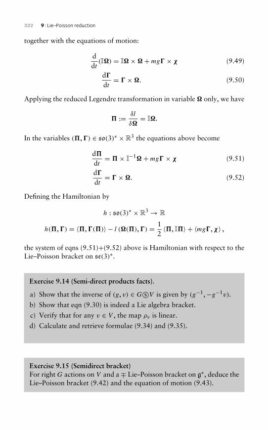
322 9 : Lie–Poisson reduction
together with the equations of motion:
ddt
(I�) = I�×�+mg� × χ (9.49)
d�dt= � �. (9.50)
Applying the reduced Legendre transformation in variable � only, we have
� := δl
δ�= I�.
In the variables (�,�) ∈ so(3)∗ ×R3 the equations above become
d�dt= �× I−1�+mg� × χ (9.51)
d�dt= � �. (9.52)
Defining the Hamiltonian by
h : so(3)∗ ×R3 → R
h(�,�) = 〈�,�(�)〉 − l (�(�),�) = 12〈�, I�〉 + 〈mg�,χ〉 ,
the system of eqns (9.51)+(9.52) above is Hamiltonian with respect to theLie–Poisson bracket on se(3)∗.
Exercise 9.14 (Semi-direct products facts).
a) Show that the inverse of (g, v) ∈ G s©V is given by (g−1,−g−1v).
b) Show that eqn (9.30) is indeed a Lie algebra bracket.
c) Verify that for any v ∈ V , the map ρv is linear.
d) Calculate and retrieve formulae (9.34) and (9.35).
Exercise 9.15 (Semidirect bracket)For right G actions on V and a∓ Lie–Poisson bracket on g∗, deduce theLie–Poisson bracket (9.42) and the equation of motion (9.43).
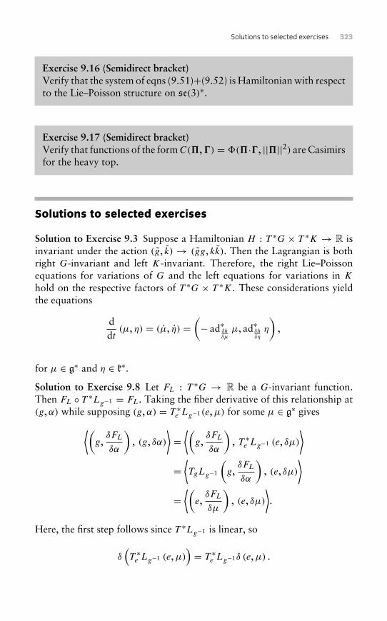
Solutions to selected exercises 323
Exercise 9.16 (Semidirect bracket)Verify that the system of eqns (9.51)+(9.52) is Hamiltonian with respectto the Lie–Poisson structure on se(3)∗.
Exercise 9.17 (Semidirect bracket)Verify that functions of the formC(�,�) = �(�·�, ||�||2) are Casimirsfor the heavy top.
Solutions to selected exercises
Solution to Exercise 9.3 Suppose a Hamiltonian H : T ∗G × T ∗K → R isinvariant under the action (g, k) → (gg, kk). Then the Lagrangian is bothright G-invariant and left K-invariant. Therefore, the right Lie–Poissonequations for variations of G and the left equations for variations in K
hold on the respective factors of T ∗G × T ∗K. These considerations yieldthe equations
ddt
(µ, η) = (µ, η) =(− ad∗δh
δµ
µ, ad∗δhδη
η
),
for µ ∈ g∗ and η ∈ k∗.
Solution to Exercise 9.8 Let FL : T ∗G → R be a G-invariant function.Then FL ◦ T ∗Lg−1 = FL. Taking the fiber derivative of this relationship at(g,α) while supposing (g,α) = T ∗e Lg−1(e,µ) for some µ ∈ g∗ gives⟨(
g,δFL
δα
), (g, δα)
⟩=⟨(
g,δFL
δα
), T ∗e Lg−1 (e, δµ)
⟩=⟨TgLg−1
(g,
δFL
δα
), (e, δµ)
⟩=⟨(
e,δFL
δµ
), (e, δµ)
⟩.
Here, the first step follows since T ∗Lg−1 is linear, so
δ(T ∗e Lg−1 (e,µ)
)= T ∗e Lg−1δ (e,µ) .
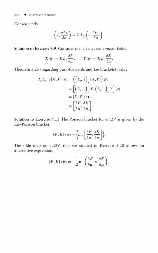
324 9 : Lie–Poisson reduction
Consequently, (g,
δFL
δα
)= TeLg
(e,
δFL
δµ
).
Solution to Exercise 9.9 Consider the left invariant vector fields
X(g) = TeLg
δF
δµ, Y (g) = TeLg
δK
δµ.
Theorem 3.25 (regarding push-forwards and Lie brackets) yields
TgLg−1 [X,Y ] (g) =((
Lg−1
)∗ [X,Y ]
)(e)
=[(
Lg−1
)∗X,
(Lg−1
)∗ Y](e)
= [X,Y ] (e)
=[δF
δµ,δK
δµ
].
Solution to Exercise 9.11 The Poisson bracket for su(2)∗ is given by theLie–Poisson bracket.
{F ,K} (µ) =⟨µ ,
[δF
δµ,δK
δµ
]⟩.
The tilde map on su(2)∗ that we studied in Exercise 5.20 allows analternative expression,
{F ,K} (µ) = −12µ ·(∂F
∂µ× ∂K
∂µ
).
10Pseudo-rigid bodies
Consider a body that can stretch and shear as well as rotate, so that itcan undergo arbitrary orientation-preserving linear transformations aroundsome fixed point. The configuration of the object at a certain time is deter-mined by an element of GL+(3) that maps a given reference configurationto the current one. This system is called the pseudo-rigid body, or affinerigid body. It is very similar to the rigid body, modelled in Sections 1.5 and7.1, except that the the configuration space is larger. Pseudo-rigid bodiesare used to model solid objects undergoing small elastic deformations, andalso some fluid motions, for example rotating gas planets and liquid drops[Cha87].
We will assume in this chapter that, in the reference configuration, thebody is spherically symmetric, meaning that the moment of inertia tensoris rotationally invariant. A sufficient condition for this symmetry is thatthe body’s density function is spherically symmetric, which implies that thebody is spherical in the reference configuration and ellipsoidal at all times.For most of the chapter, we will study free ellipsoidal motion, meaning thatthe pseudo-rigid body evolves according to a Lagrangian that equals kineticenergy only, with no potential energy.
10.1 Modelling
We fix a reference configuration of the body. We use a fixed inertial spatialcoordinate system, and a moving body coordinate system, both with originat the fixed point of the body. When the body is in its reference position, thetwo systems coincide. The body coordinate system moves with the body,which means that the position of any given particle, in the body coordinatesystem, remains fixed. The position in body coordinates is called the par-ticle’s label. The spatial position of a particle at a given time is also calledits Eulerian position, while its label is called its Lagrangian position. Wedenote by GL+(3) the set of all real-valued matrices with positive determi-nant, i.e. matrices corresponding to orientation-preserving transformations.We assume that the configuration of the body at time t is determined by amatrix Q(t) ∈ GL+(3) that takes the label X of any particle in the body toits spatial position x(t). Thus the configuration space of the pseudo-rigid
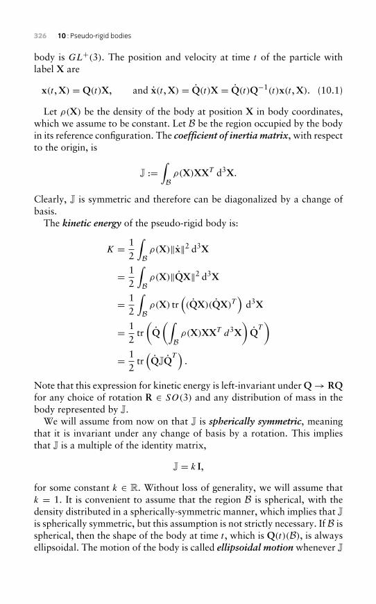
326 10 : Pseudo-rigid bodies
body is GL+(3). The position and velocity at time t of the particle withlabel X are
x(t ,X) = Q(t)X, and x(t ,X) = Q(t)X = Q(t)Q−1(t)x(t ,X). (10.1)
Let ρ(X) be the density of the body at position X in body coordinates,which we assume to be constant. Let B be the region occupied by the bodyin its reference configuration. The coefficient of inertia matrix, with respectto the origin, is
J :=∫
Bρ(X)XXT d3X.
Clearly, J is symmetric and therefore can be diagonalized by a change ofbasis.
The kinetic energy of the pseudo-rigid body is:
K = 12
∫Bρ(X)‖x‖2 d3X
= 12
∫Bρ(X)‖QX‖2 d3X
= 12
∫Bρ(X) tr
((QX)(QX)T
)d3X
= 12
tr(Q(∫
Bρ(X)XXT d3X
)Q
T)
= 12
tr(QJQ
T)
.
Note that this expression for kinetic energy is left-invariant under Q→ RQfor any choice of rotation R ∈ SO(3) and any distribution of mass in thebody represented by J.
We will assume from now on that J is spherically symmetric, meaningthat it is invariant under any change of basis by a rotation. This impliesthat J is a multiple of the identity matrix,
J = k I,
for some constant k ∈ R. Without loss of generality, we will assume thatk = 1. It is convenient to assume that the region B is spherical, with thedensity distributed in a spherically-symmetric manner, which implies that J
is spherically symmetric, but this assumption is not strictly necessary. If B isspherical, then the shape of the body at time t , which is Q(t)(B), is alwaysellipsoidal. The motion of the body is called ellipsoidal motion whenever J
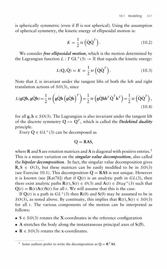
10.1 Modelling 327
is spherically symmetric (even if B is not spherical). Using the assumptionof spherical symmetry, the kinetic energy of ellipsoidal motion is:
K = 12
tr(QQ
T)
. (10.2)
We consider free ellipsoidal motion, which is the motion determined bythe Lagrangian function L : T GL+(3)→ R that equals the kinetic energy:
L(Q, Q) = K = 12
tr(QQ
T)
. (10.3)
Note that L is invariant under the tangent lifts of both the left and righttranslation actions of SO(3), since
L(gQh, gQh)= 12
tr(gQh
(gQh
)T)= 12
tr(gQhhT Q
ThT)= 1
2tr(QQ
T)
,
(10.4)
for all g, h ∈ SO(3). The Lagrangian is also invariant under the tangent liftof the discrete symmetry Q → QT , which is called the Dedekind dualityprinciple.
Every Q ∈ GL+(3) can be decomposed as
Q = RAS,
where R and S are rotation matrices and A is diagonal with positive entries.1
This is a minor variation on the singular value decomposition, also calledthe bipolar decomposition. In fact, the singular value decomposition givesR, S ∈ O(3), but these matrices can be easily modified to be in SO(3)(see Exercise 10.1). This decomposition Q = RAS is not unique. Howeverit is known (see [Kat76]) that if Q(t) is an analytic path in GL(3), thenthere exist analytic paths R(t), S(t) ∈ O(3) and A(t) ∈ Diag+(3) such thatQ(t) = R(t)A(t)S(t) for all t . We will assume that this is the case.
If Q(t) is a path in GL+(3) then R(0) and S(0) may be assumed to be inSO(3), as noted above. By continuity, this implies that R(t), S(t) ∈ SO(3)for all t . The various components of the motion can be interpreted asfollows:
• S ∈ SO(3) rotates the X-coordinates in the reference configuration
• A stretches the body along the instantaneous principal axes of S(B).
• R ∈ SO(3) rotates the x-coordinates.
1 Some authors prefer to write the decomposition as Q = RT AS.
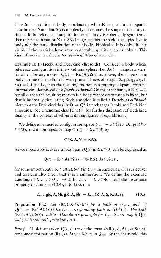
328 10 : Pseudo-rigid bodies
Thus S is a rotation in body coordinates, while R is a rotation in spatialcoordinates. Note that A(t) completely determines the shape of the body attime t . If the reference configuration of the body is spherically-symmetric,then the transformation X → SX changes neither the region occupied by thebody nor the mass distribution of the body. Physically, it is only directlyvisible if the particles have some observable quality such as colour. Thiskind of motion is called internal circulation of material.
Example 10.1 (Jacobi and Dedekind ellipsoids) Consider a body whosereference configuration is the solid unit sphere. Let A(t) = diag(a1, a2, a3)
for all t . For any motion Q(t) = R(t)A(t)S(t) as above, the shape of thebody at time t is an ellipsoid with principal axes of lengths 2a1, 2a2, 2a3. IfS(t) = I, for all t , then the resulting motion is a rotating ellipsoid with nointernal circulation, called a Jacobi ellipsoid. On the other hand, if R(t) = I,for all t , then the resulting motion is a body whose orientation is fixed, butthat is internally circulating. Such a motion is called a Dedekind ellipsoid.Note that the Dedekind duality Q → QT interchanges Jacobi and Dedekindellipsoids. (See Chandrasekhar [Cha87] for further discussion of Dedekindduality in the context of self-gravitating figures of equilibrium.)
We define an extended configuration space Qext := SO(3)×Diag(3)+×SO(3), and a non-injective map � : Q→ GL+(3) by
�(R,A, S) = RAS.
As we noted above, every smooth path Q(t) in GL+(3) can be expressed as
Q(t) = R(t)A(t)S(t) = �(R(t),A(t), S(t)),
for some smooth path (R(t),A(t), S(t)) inQext . In particular, � is surjective,and one can also check that it is a submersion. We define the extendedLagrangian Lext : TQext → R by Lext = L ◦ T�. From the invarianceproperty of L in eqn (10.4), it follows that
Lext (gR,A, Sh, gR, A, Sh) = Lext (R,A, S, R, A, S). (10.5)
Proposition 10.2 Let (R(t),A(t), S(t)) be a path in Qext , and letQ(t) := R(t)A(t)S(t) be the corresponding path in GL+(3). The path(R(t),A(t), S(t)) satisfies Hamilton’s principle for Lext if and only if Q(t)
satisfies Hamilton’s principle for L.
Proof All deformations Q(t , s) are of the form �(R(t , s),A(t , s), S(t , s))for some deformation (R(t , s),A(t , s), S(t , s) in Qext . By the chain rule, this
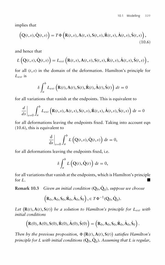
10.1 Modelling 329
implies that(Q(t , s), Q(t , s)
)= T�
(R(t , s),A(t , s), S(t , s), R(t , s), A(t , s), S(t , s)
),
(10.6)
and hence that
L(Q(t , s), Q(t , s)
)= Lext
(R(t , s),A(t , s), S(t , s), R(t , s), A(t , s), S(t , s)
),
for all (t , s) in the domain of the deformation. Hamilton’s principle forLext is
δ
∫ b
a
Lext
(R(t),A(t), S(t), R(t), A(t), S(t)
)dt = 0
for all variations that vanish at the endpoints. This is equivalent to
d
ds
∣∣∣∣s=0
∫ b
a
Lext
(R(t , s),A(t , s), S(t , s), R(t , s), A(t , s), S(t , s)
)dt = 0
for all deformations leaving the endpoints fixed. Taking into account eqn(10.6), this is equivalent to
dds
∣∣∣∣s=0
∫ b
a
L(Q(t , s), Q(t , s)
)dt = 0,
for all deformations leaving the endpoints fixed, i.e.
δ
∫ b
a
L(Q(t), Q(t)
)dt = 0,
for all variations that vanish at the endpoints, which is Hamilton’s principlefor L. �
Remark 10.3 Given an initial condition (Q0, Q0), suppose we choose(R0,A0, S0, R0, A0, S0
),∈ T�−1(Q0, Q0).
Let(R(t),A(t), S(t)
)be a solution to Hamilton’s principle for Lext with
initial conditions(R(0),A(0), S(0), R(0), A(0), S(0)
)=(R0,A0, S0, R0, A0, S0
).
Then by the previous proposition, �(R(t),A(t), S(t)
)satisfies Hamilton’s
principle for L with initial conditions (Q0, Q0). Assuming that L is regular,
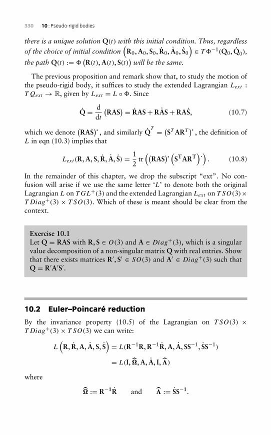
330 10 : Pseudo-rigid bodies
there is a unique solution Q(t) with this initial condition. Thus, regardless
of the choice of initial condition(R0,A0, S0, R0, A0, S0
)∈ T�−1(Q0, Q0),
the path Q(t) := �(R(t),A(t), S(t)
)will be the same.
The previous proposition and remark show that, to study the motion ofthe pseudo-rigid body, it suffices to study the extended Lagrangian Lext :TQext → R, given by Lext = L ◦�. Since
Q = ddt
(RAS
) = RAS+ RAS+ RAS, (10.7)
which we denote(RAS
)� , and similarly QT = (ST ART
)� , the definition ofL in eqn (10.3) implies that
Lext (R,A, S, R, A, S) = 12
tr((
RAS)� (START
)˙)
. (10.8)
In the remainder of this chapter, we drop the subscript “ext”. No con-fusion will arise if we use the same letter ‘L’ to denote both the originalLagrangian L on TGL+(3) and the extended Lagrangian Lext on T SO(3)×TDiag+(3) × T SO(3). Which of these is meant should be clear from thecontext.
Exercise 10.1Let Q = RAS with R, S ∈ O(3) and A ∈ Diag+(3), which is a singularvalue decomposition of a non-singular matrix Q with real entries. Showthat there exists matrices R′, S′ ∈ SO(3) and A′ ∈ Diag+(3) such thatQ = R′A′S′.
10.2 Euler–Poincaré reduction
By the invariance property (10.5) of the Lagrangian on T SO(3) ×TDiag+(3)× T SO(3) we can write:
L(R, R,A, A, S, S
)= L(R−1R,R−1R,A, A, SS−1, SS−1)
= L(I, �,A, A, I, )
where
� := R−1R and := SS−1.
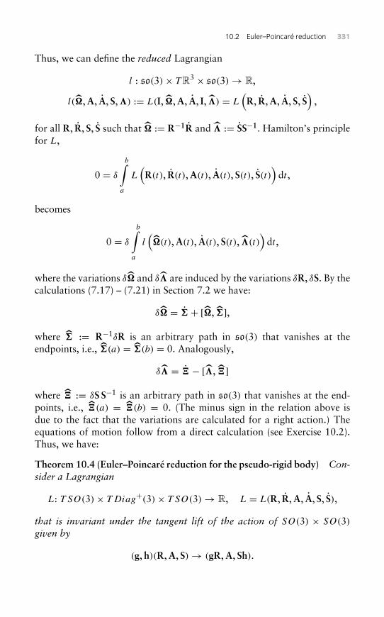
10.2 Euler–Poincaré reduction 331
Thus, we can define the reduced Lagrangian
l : so(3)× T R3 × so(3)→ R,
l(�,A, A, S, ) := L(I, �,A, A, I, ) = L(R, R,A, A, S, S
),
for all R, R, S, S such that � := R−1R and := SS−1. Hamilton’s principlefor L,
0 = δ
b∫a
L(R(t), R(t),A(t), A(t), S(t), S(t)
)dt ,
becomes
0 = δ
b∫a
l(�(t),A(t), A(t), S(t), (t)
)dt ,
where the variations δ� and δ are induced by the variations δR, δS. By thecalculations (7.17) – (7.21) in Section 7.2 we have:
δ� = + [�, ],
where := R−1δR is an arbitrary path in so(3) that vanishes at theendpoints, i.e., (a) = (b) = 0. Analogously,
δ = − [ , ]
where := δS S−1 is an arbitrary path in so(3) that vanishes at the end-points, i.e., (a) = (b) = 0. (The minus sign in the relation above isdue to the fact that the variations are calculated for a right action.) Theequations of motion follow from a direct calculation (see Exercise 10.2).Thus, we have:
Theorem 10.4 (Euler–Poincaré reduction for the pseudo-rigid body) Con-sider a Lagrangian
L: T SO(3)× TDiag+(3)× T SO(3)→ R, L = L(R, R,A, A, S, S),
that is invariant under the tangent lift of the action of SO(3) × SO(3)given by
(g, h)(R,A, S)→ (gR,A, Sh).
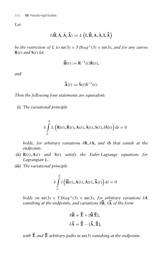
332 10 : Pseudo-rigid bodies
Let
l(�,A, A, ) := L(I, �,A, A, I,
)be the restriction of L to so(3) × TDiag+(3) × so(3), and for any curvesR(t) and S(t) let
�(t) := R−1(t)R(t),
and
(t) := S(t)S−1(t).
Then the following four statements are equivalent:
(i) The variational principle
δ
b∫a
L(R(t), R(t),A(t), A(t), S(t), δS(t)
)dt = 0
holds, for arbitrary variations δR, δA, and δS that vanish at theendpoints.
(ii) R(t),A(t) and S(t) satisfy the Euler-Lagrange equations forLagrangian L.
(iii) The variational principle
δ
b∫a
l(�(t),A(t), A(t), (t)
)dt = 0
holds on so(3) × TDiag+(3) × so(3), for arbitrary variations δAvanishing at the endpoints, and variations δ�, δ of the form
δ� = ˙ + [� ],
δ = ˙− [ , ],
with and arbitrary paths in so(3) vanishing at the endpoints.
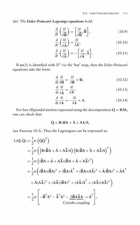
10.2 Euler–Poincaré reduction 333
(iv) The Euler–Poincaré–Lagrange equations hold:
ddt
(δl
δ�
)=[
δl
δ�, �]
, (10.9)
ddt
(δl
δA
)= δl
δA, (10.10)
ddt
(δl
δ
)= −
[δl
δ , ]
. (10.11)
If so(3) is identified with R3 via the ‘hat’ map, then the Euler–Poincaréequations take the form:
ddt
δl
δ�= δl
δ�×�, (10.12)
ddt
δl
δA= δl
δA, (10.13)
ddt
δl
δ = − δl
δ × . (10.14)
For free ellipsoidal motion expressed using the decomposition Q = RAS,one can check that
Q = R(�A + A+ A )S,
(see Exercise 10.3). Thus the Lagrangian can be expressed as:
L(Q, Q) = 12
tr(QQ
T)
= 12
tr((
R(�A + A+ A )S) (
R(�A + A+ A )S)T)
= 12
tr((�A + A+ A )(�A + A+ A )T
)= 1
2tr((�A)(�A)T + (�A)A
T + (�A)(A )T + A(�A)T + AAT
+ A(A )T + (A )(�A)T + (A )AT + (A )(A )T
)
= 12
tr
−�2A2 −
2A2 − 2�A A︸ ︷︷ ︸
Coriolis coupling
+ A2
,
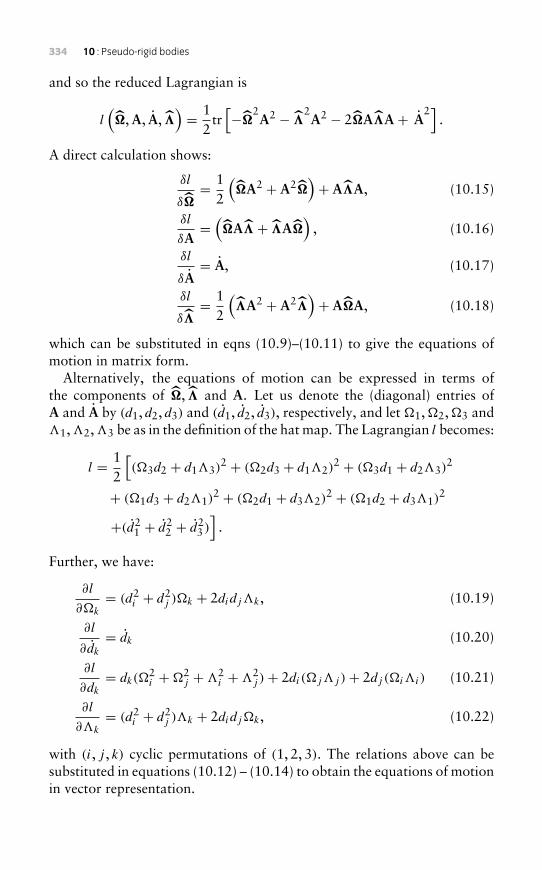
334 10 : Pseudo-rigid bodies
and so the reduced Lagrangian is
l(�,A, A,
)= 1
2tr[−�2
A2 − 2A2 − 2�A A + A
2].
A direct calculation shows:
δl
δ�= 1
2
(�A2 + A2�
)+ A A, (10.15)
δl
δA=(�A + A�
), (10.16)
δl
δA= A, (10.17)
δl
δ = 1
2
( A2 + A2
)+ A�A, (10.18)
which can be substituted in eqns (10.9)–(10.11) to give the equations ofmotion in matrix form.
Alternatively, the equations of motion can be expressed in terms ofthe components of �, and A. Let us denote the (diagonal) entries ofA and A by (d1, d2, d3) and (d1, d2, d3), respectively, and let �1,�2,�3 and�1,�2,�3 be as in the definition of the hat map. The Lagrangian l becomes:
l = 12
[(�3d2 + d1�3)
2 + (�2d3 + d1�2)2 + (�3d1 + d2�3)
2
+ (�1d3 + d2�1)2 + (�2d1 + d3�2)
2 + (�1d2 + d3�1)2
+(d21 + d2
2 + d23 )].
Further, we have:
∂l
∂�k
= (d2i + d2
j )�k + 2didj�k, (10.19)
∂l
∂dk= dk (10.20)
∂l
∂dk= dk(�
2i +�2
j +�2i +�2
j )+ 2di(�j�j )+ 2dj (�i�i) (10.21)
∂l
∂�k
= (d2i + d2
j )�k + 2didj�k, (10.22)
with (i, j , k) cyclic permutations of (1, 2, 3). The relations above can besubstituted in equations (10.12) – (10.14) to obtain the equations of motionin vector representation.
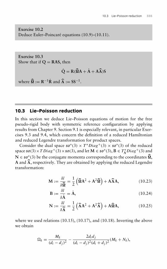
10.3 Lie–Poisson reduction 335
Exercise 10.2Deduce Euler–Poincaré equations (10.9)–(10.11).
Exercise 10.3Show that if Q = RAS, then
Q = R(�A + A+ A )S
where � := R−1R and := SS−1.
10.3 Lie–Poisson reduction
In this section we deduce Lie–Poisson equations of motion for the freepseudo-rigid body with symmetric reference configuration by applyingresults from Chapter 9. Section 9.1 is especially relevant, in particular Exer-cises 9.3 and 9.4, which concern the definition of a reduced Hamiltonianand reduced Legendre transformation for product spaces.
Consider the dual space so∗(3) × T ∗Diag+(3) × so∗(3) of the reducedspace so(3)×TDiag+(3)×so(3), and let M ∈ so∗(3), B ∈ T ∗ADiag+(3) andN ∈ so∗(3) be the conjugate momenta corresponding to the coordinates �,A and , respectively. They are obtained by applying the reduced Legendretransformation:
M := δl
δ�= 1
2
(�A2 + A2�
)+ A A, (10.23)
B := δl
δA= A, (10.24)
N := δl
δ = 1
2
( A2 + A2
)+ A�A, (10.25)
where we used relations (10.15), (10.17), and (10.18). Inverting the abovewe obtain
�k = Mk
(di − dj )2− 2didj
(di − dj )2(di + dj )2(Mk +Nk),
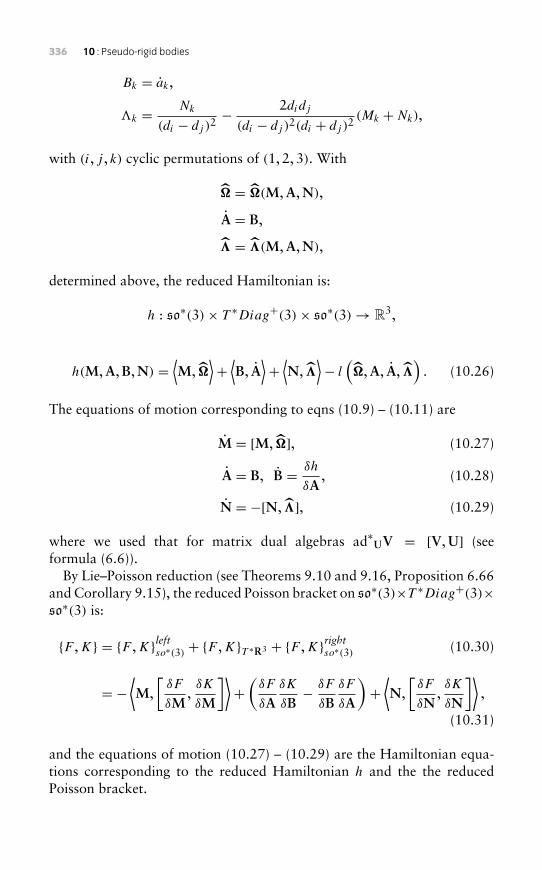
336 10 : Pseudo-rigid bodies
Bk = ak,
�k = Nk
(di − dj )2− 2didj
(di − dj )2(di + dj )2(Mk +Nk),
with (i, j , k) cyclic permutations of (1, 2, 3). With
� = �(M,A,N),
A = B,
= (M,A,N),
determined above, the reduced Hamiltonian is:
h : so∗(3)× T ∗Diag+(3)× so∗(3)→ R3,
h(M,A,B,N) =⟨M, �
⟩+⟨B, A
⟩+⟨N,
⟩− l
(�,A, A,
). (10.26)
The equations of motion corresponding to eqns (10.9) – (10.11) are
M = [M, �], (10.27)
A = B, B = δh
δA, (10.28)
N = −[N, ], (10.29)
where we used that for matrix dual algebras ad∗UV = [V,U] (seeformula (6.6)).
By Lie–Poisson reduction (see Theorems 9.10 and 9.16, Proposition 6.66and Corollary 9.15), the reduced Poisson bracket on so∗(3)×T ∗Diag+(3)×so∗(3) is:
{F ,K} = {F ,K}leftso∗(3) + {F ,K}T ∗R3 + {F ,K}right
so∗(3) (10.30)
= −⟨M,
[δF
δM,δK
δM
]⟩+(δF
δAδK
δB− δF
δBδF
δA
)+⟨N,[δF
δN,δK
δN
]⟩,
(10.31)
and the equations of motion (10.27) – (10.29) are the Hamiltonian equa-tions corresponding to the reduced Hamiltonian h and the the reducedPoisson bracket.
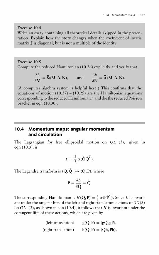
10.4 Momentummaps 337
Exercise 10.4Write an essay containing all theoretical details skipped in the presen-tation. Explain how the story changes when the coefficient of inertiamatrix J is diagonal, but is not a multiple of the identity.
Exercise 10.5Compute the reduced Hamiltonian (10.26) explicitly and verify that
δh
δM= �(M,A,N), and
δh
δN= (M,A,N).
(A computer algebra system is helpful here!) This confirms that theequations of motion (10.27) – (10.29) are the Hamiltonian equationscorresponding to the reduced Hamiltonian h and the the reduced Poissonbracket in eqn (10.30).
10.4 Momentum maps: angular momentumand circulation
The Lagrangian for free ellipsoidal motion on GL+(3), given ineqn (10.3), is
L = 12
tr(QQT).
The Legendre transform is (Q, Q) → (Q, P), where
P = δL
δQ= Q.
The corresponding Hamiltonian is H(Q, P) = 12 tr(PP
T). Since L is invari-
ant under the tangent lifts of the left and right translation actions of SO(3)on GL+(3), as shown in eqn (10.4), it follows that H is invariant under thecotangent lifts of these actions, which are given by
(left translation) g(Q, P) = (gQ, gP),
(right translation) h(Q, P) = (Qh, Ph).
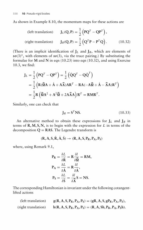
338 10 : Pseudo-rigid bodies
As shown in Example 8.10, the momentum maps for these actions are
(left translation) JL(Q, P) = 12
(PQT −QPT
),
(right translation) JR(Q, P) = 12
(QT P − PT Q
). (10.32)
(There is an implicit identification of JL and JR, which are elements ofso(3)∗, with elements of so(3), via the trace pairing.) By substituting theformulae for M and N in eqn (10.23) into eqn (10.32), and using Exercise10.3, we find:
JL = 12
(PQT −QPT
)= 1
2
(QQT −QQ
T)
= 12
(R(�A + A+ A )ART − RA(−A�+ A− A)RT
)= 1
2R(�A2 + A2�+ 2A A
)RT = RMRT .
Similarly, one can check that
JR = ST NS. (10.33)
An alternative method to obtain these expressions for JL and JR interms of R,M, S,N, is to begin with the expression for L in terms of thedecomposition Q = RAS. The Legendre transform is
(R,A, S, R, A, S)→ (R,A, S, PR, PA, PS)
where, using Remark 9.1,
PR = δL
δR= R
δl
δ�= RM,
PA = δL
δA= R
δl
δA,
PS = δL
δS= δl
δ S = NS.
The corresponding Hamiltonian is invariant under the following cotangent-lifted actions
(left translation) g(R,A, S, PR, PA, PS) = (gR,A, S, gPR, PA, PS),
(right translation) h(R,A, S, PR, PA, PS) = (R,A, Sh, PR, PA, PSh).
10.4 Momentummaps 339
As shown in Example 8.10, the momentum maps for these actions are
(left translation) JL = PRRT = RMRT ,
(right translation) JR = ST PS = ST NS.
Proposition 10.5 The momentum maps JL and JR are conservedquantities.
Proof This is immediate because the Hamiltonian H(Q, P) = 12 tr(PP
T) is
both left- and right-invariant under the cotangent lift of SO(3) action. �
Remark 10.6 The discrete symmetryQ → QT (Dedekind duality) reversesthe roles and senses of Eulerian and Lagrangian rotations, and interchangesthe angular momentum and the circulation, JL ↔ JR.
Spatial angular momentum for the pseudo-rigid body
We saw in Remark 8.11 that, for the SO(3) action on the rigid body,JL corresponds to the spatial angular momentum vector π , via the “breve”map (defined in Example 5.36). The same arguments apply in the case of thepseudo-rigid body. An alternative argument begins with original definitionof angular momentum in eqn (1.41),
π :=∫
Bρ(X) x × x d3X,
and proceeds by direct computation. Recall that π can be identified with12 π via the trace pairing. The following identity can be verified directly,
x × x = xxT − xxT .
Thus,
π ↔ 12π = 1
2
∫B(t)
ρ(x)x × x d3x
= 12
∫B(t)
ρ(x)(xxT − xxT
)d3x
= 12
∫Bρ(X)
((QX)(QX)T − (QX)(QX)T
)d3X
= 12
((JQ)QT −Q(JQ)T
)= 1
2
(PQT −QPT
)↔ JL,
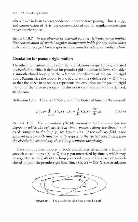
340 10 : Pseudo-rigid bodies
where “↔” indicates correspondence under the trace pairing. Thus π = JL,and conservation of JL is just conservation of spatial angular momentumin yet another guise.
Remark 10.7 In the absence of external torques, left-invariance impliesthat conservation of spatial angular momentum holds for any initial massdistribution, not just for the spherically symmetric reference configuration.
Circulation for pseudo-rigid motion
The other momentum map, JR for right translations in eqn (10.32), is relatedto circulation, which is defined for pseudo-rigid motion as follows. Considera smooth closed loop γ in the reference coordinates of the pseudo-rigidbody. Parametrize the loop γ by s ∈ R and at time t define c(t) = Q(t) ◦ γ ,so that the curve in space c(t) represents the evolution under pseudo-rigidmotion of the reference loop γ . In this notation, the circulation is defined,as follows.
Definition 10.8 The circulation around the loop c at time t is the integral:
Ic(t) :=∮c(t)
x(t , x) · dx :=∮γ
x(t , s) · dxds
ds. (10.34)
Remark 10.9 The circulation (10.34) around a path summarizes thedegree to which the velocity x(t) at time t projects along the direction ofdx/ds tangent to the loop γ ; see Figure 10.1. If the velocity field is thegradient of a smooth function with respect to the spatial coordinate, thenthe circulation around any closed loop vanishes identically.
The smooth closed loop γ in body coordinates determines a family ofsmooth closed loops c(t) := Q(t) ◦ γ parameterized by time t , which maybe regarded as the path of the loop γ carried along in the space of smoothclosed loops by the pseudo-rigid flow. Since x(t ,X) = Q(t)X, the circulation
γ
Figure 10.1 The circulation of a flow around a path.
10.4 Momentummaps 341
around such a loop c(t) is defined as
Ic(t) =∮c
x · dx =∮γ
(QX
)· (Q dX
) = ∮γ
(QT QX
)· dX. (10.35)
Following [RdSD99], we transform this integral by using an elementaryidentity, whose proof is left to Exercise 10.6.
Lemma 10.10 If LA = 12 (L− LT ), then
∮γLX · dX = ∮
γLAX · dX.
It follows that the circulation in eqn (10.35) around the loop c(t) equals
Ic(t) = 12
∮γ
((QT Q−QT Q
)X)· dX.
The skew-symmetric 3× 3 matrix in this circulation integral,
K := 12
(QT Q− Q
TQ)
, (10.36)
defines, via the hat map, a vector K called the Kelvin vector.According to Lemma 10.10, the circulation around the loop c may be
expressed in factored form as
Ic =∮γ
(KX
)· dX =
∮γ
(K×X) · dX = K ·(∮
γ
X× dX)
. (10.37)
The factor in parentheses in the last line depends only on the reference curveγ and not on the pseudo-rigid motion. Thus, by eqn (10.37), the evolutionof the circulation Ic(t) is determined by the evolution of the Kelvin vectorK defined by K in (10.36). It so happens that, for a pseudo-rigid body witha spherically symmetric reference configuration, K equals the momentummap JR (more precisely, they correspond via the trace pairing), and JR is aconserved quantity; see Proposition 10.5. Consequently, K is constant andtherefore Ic is also constant. This calculation proves the following.
Proposition 10.11 (Kelvin circulation theorem: pseudo-rigid bodies)Pseudo-rigid motion starting initially from spherical symmetry conservesthe circulation (10.34).
Remark 10.12 The Kelvin circulation theorem can be seen as a specialcase of the Kelvin–Noether theorem, in particular the simplified versionin Corollary 7.19, in which there are no advected quantities. Indeed, takeG = SO(3), acting on the right onGL(3)+. Fix a closed loop γ and let C be
342 10 : Pseudo-rigid bodies
the space of all closed loops of the form c = S◦γ for some S ∈ SO(3), withleft SO(3) action given by Sc = S ◦ c. Define K : C → so(3)∗∗ by setting
〈K(γ ),N〉 =∮γ
(NX) · dX
and requiring that K be SO(3)-equivariant:
〈K(S ◦ γ ),N〉 =⟨SK(γ ) ST ,N
⟩=⟨K(γ ), ST NS
⟩=∮γ
(ST NSX
)· dX.
The associated Kelvin-Noether quantity I : C × g→ R is given by
I (c, ) = I (S ◦ γ , )) =⟨K(S ◦ γ ),
δl
δ ( )
⟩=∮γ
(ST
δl
δ ( )SX
)· dX
=∮γ
(JR X) · dX,
using the formula for JR in eqn (10.33). Corollary 7.19 implies that I is aconserved quantity. As noted earlier, JR = K when the reference configura-tion is spherically symmetric, so comparison with eqn (10.37) shows thatIc is a conserved quantity.
Remark 10.13
• Geometrically, the quantity in parentheses in the factored form of thecirculation Ic in eqn (10.37) is given by∮
γ
X× dX = 2∫∫
S(γ )
dSγ , (10.38)
where S(γ ) is any surface in Stokes’ theoremwhose boundary is the curveγ = ∂S(γ ) in the fluid reference coordinates and
dSγi =12εijkdXj ∧ dXk
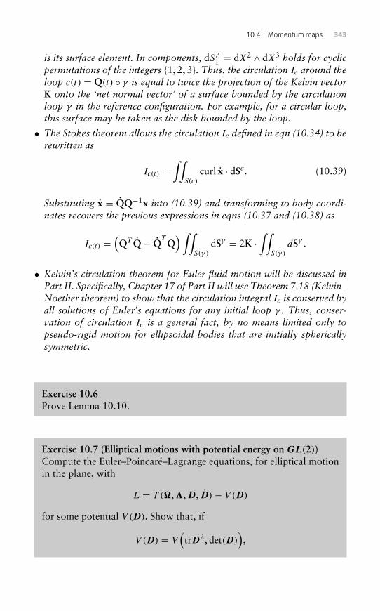
10.4 Momentummaps 343
is its surface element. In components, dSγ
1 = dX2 ∧ dX3 holds for cyclicpermutations of the integers {1, 2, 3}. Thus, the circulation Ic around theloop c(t) = Q(t) ◦ γ is equal to twice the projection of the Kelvin vectorK onto the ‘net normal vector’ of a surface bounded by the circulationloop γ in the reference configuration. For example, for a circular loop,this surface may be taken as the disk bounded by the loop.
• The Stokes theorem allows the circulation Ic defined in eqn (10.34) to berewritten as
Ic(t) =∫∫
S(c)
curl x · dSc. (10.39)
Substituting x = QQ−1x into (10.39) and transforming to body coordi-nates recovers the previous expressions in eqns (10.37 and (10.38) as
Ic(t) =(QT Q− Q
TQ) ∫∫
S(γ )
dSγ = 2K ·∫∫
S(γ )
dSγ .
• Kelvin’s circulation theorem for Euler fluid motion will be discussed inPart II. Specifically, Chapter 17 of Part II will use Theorem 7.18 (Kelvin–Noether theorem) to show that the circulation integral Ic is conserved byall solutions of Euler’s equations for any initial loop γ . Thus, conser-vation of circulation Ic is a general fact, by no means limited only topseudo-rigid motion for ellipsoidal bodies that are initially sphericallysymmetric.
Exercise 10.6Prove Lemma 10.10.
Exercise 10.7 (Elliptical motions with potential energy on GL(2))Compute the Euler–Poincaré–Lagrange equations, for elliptical motionin the plane, with
L = T (�, ,D, D)− V (D)
for some potential V (D). Show that, if
V (D) = V(trD2, det(D)
),
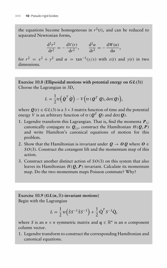
344 10 : Pseudo-rigid bodies
the equations become homogeneous in r2(t), and can be reduced toseparated Newtonian forms,
d2r2
dt2= − dV (r)
dr2 ,d2α
dt2= − dW(α)
dα,
for r2 = x2 + y2 and α = tan−1(y/x) with x(t) and y(t) in twodimensions.
Exercise 10.8 (Ellipsoidal motions with potential energy on GL(3))Choose the Lagrangian in 3D,
L = 12
tr(Q
TQ)− V
(tr (QT Q), det(Q)
),
where Q(t) ∈ GL(3) is a 3×3 matrix function of time and the potentialenergy V is an arbitrary function of tr (QT Q) and det(Q).
1. Legendre transform this Lagrangian. That is, find the momenta P ij
canonically conjugate to Qij , construct the Hamiltonian H(Q,P )
and write Hamilton’s canonical equations of motion for thisproblem.
2. Show that the Hamiltonian is invariant under Q→ OQ where O ∈SO(3). Construct the cotangent lift and the momentum map of thisaction.
3. Construct another distinct action of SO(3) on this system that alsoleaves its Hamiltonian H(Q,P ) invariant. Calculate its momentummap. Do the two momentum maps Poisson commute? Why?
Exercise 10.9 (GL(n,R)-invariant motions)Begin with the Lagrangian
L = 12
tr(SS−1SS−1
)+ 1
2Q
TS−1Q,
where S is an n × n symmetric matrix and q ∈ Rn is an n componentcolumn vector.1. Legendre transform to construct the corresponding Hamiltonian and
canonical equations.
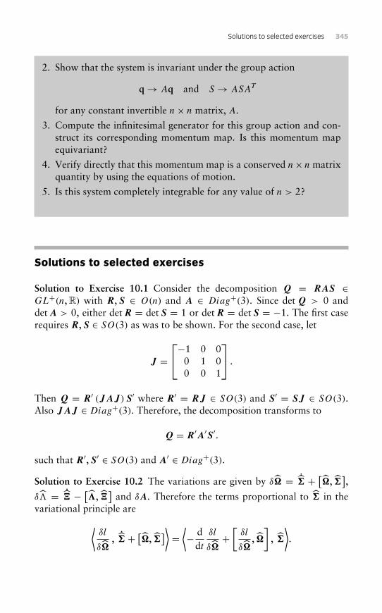
Solutions to selected exercises 345
2. Show that the system is invariant under the group action
q→ Aq and S → ASAT
for any constant invertible n× n matrix, A.
3. Compute the infinitesimal generator for this group action and con-struct its corresponding momentum map. Is this momentum mapequivariant?
4. Verify directly that this momentum map is a conserved n× n matrixquantity by using the equations of motion.
5. Is this system completely integrable for any value of n > 2?
Solutions to selected exercises
Solution to Exercise 10.1 Consider the decomposition Q = RAS ∈GL+(n, R) with R,S ∈ O(n) and A ∈ Diag+(3). Since detQ > 0 anddetA > 0, either detR = det S = 1 or detR = det S = −1. The first caserequires R,S ∈ SO(3) as was to be shown. For the second case, let
J =−1 0 0
0 1 00 0 1
.
Then Q = R′ (JAJ )S′ where R′ = RJ ∈ SO(3) and S′ = SJ ∈ SO(3).Also JAJ ∈ Diag+(3). Therefore, the decomposition transforms to
Q = R′A′S′.
such that R′,S′ ∈ SO(3) and A′ ∈ Diag+(3).
Solution to Exercise 10.2 The variations are given by δ� = ˙ + [�, ],
δ� = ˙ − [ , ]
and δA. Therefore the terms proportional to in thevariational principle are⟨
δl
δ�, ˙ + [�,
]⟩ = ⟨− ddt
δl
δ�+[
δl
δ�, �]
, ⟩.
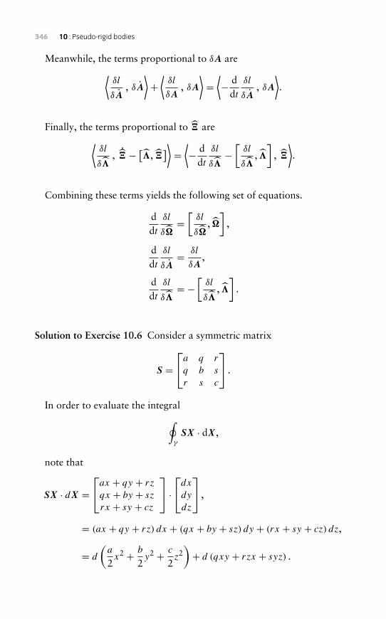
346 10 : Pseudo-rigid bodies
Meanwhile, the terms proportional to δA are⟨δl
δA, δA
⟩+⟨δl
δA, δA
⟩=⟨− d
dtδl
δA, δA
⟩.
Finally, the terms proportional to are⟨δl
δ , ˙− [ ,
]⟩ = ⟨− ddt
δl
δ −[
δl
δ , ]
, ⟩.
Combining these terms yields the following set of equations.
ddt
δl
δ�=[
δl
δ�, �]
,
ddt
δl
δA= δl
δA,
ddt
δl
δ = −
[δl
δ , ]
.
Solution to Exercise 10.6 Consider a symmetric matrix
S =a q r
q b s
r s c
.
In order to evaluate the integral∮γ
SX · dX,
note that
SX · dX =ax + qy + rz
qx + by + sz
rx + sy + cz
·dx
dy
dz
,
= (ax + qy + rz) dx + (qx + by + sz) dy + (rx + sy + cz) dz,
= d
(a
2x2 + b
2y2 + c
2z2)+ d (qxy + rzx + syz) .
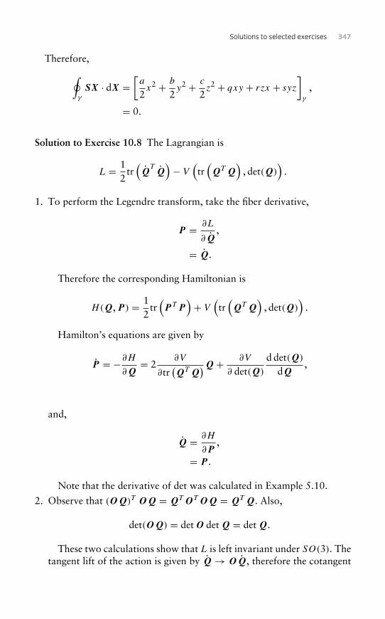
Solutions to selected exercises 347
Therefore,∮γ
SX · dX =[a
2x2 + b
2y2 + c
2z2 + qxy + rzx + syz
]γ
,
= 0.
Solution to Exercise 10.8 The Lagrangian is
L = 12
tr(Q
TQ)− V
(tr(QTQ
), det(Q)
).
1. To perform the Legendre transform, take the fiber derivative,
P = ∂L
∂Q,
= Q.
Therefore the corresponding Hamiltonian is
H(Q,P ) = 12
tr(P TP
)+ V
(tr(QTQ
), det(Q)
).
Hamilton’s equations are given by
P = −∂H
∂Q= 2
∂V
∂tr(QTQ
)Q+ ∂V
∂ det(Q)
d det(Q)
dQ,
and,
Q = ∂H
∂P,
= P .
Note that the derivative of det was calculated in Example 5.10.
2. Observe that (OQ)T OQ = QTOTOQ = QTQ. Also,
det(OQ) = detO detQ = detQ.
These two calculations show that L is left invariant under SO(3). Thetangent lift of the action is given by Q→ OQ, therefore the cotangent
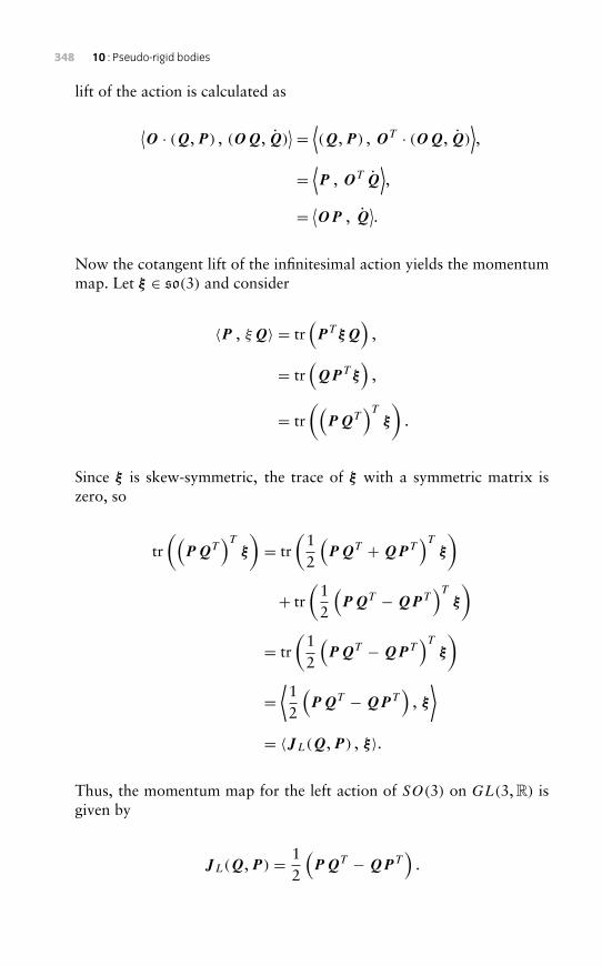
348 10 : Pseudo-rigid bodies
lift of the action is calculated as
⟨O · (Q,P ) , (OQ, Q)
⟩ = ⟨(Q,P ) , OT · (OQ, Q)⟩,
=⟨P , OT Q
⟩,
= ⟨OP , Q⟩.
Now the cotangent lift of the infinitesimal action yields the momentummap. Let ξ ∈ so(3) and consider
〈P , ξQ〉 = tr(P T ξQ
),
= tr(QP T ξ
),
= tr((
PQT)T
ξ
).
Since ξ is skew-symmetric, the trace of ξ with a symmetric matrix iszero, so
tr((
PQT)T
ξ
)= tr
(12
(PQT +QP T
)Tξ
)
+ tr(
12
(PQT −QP T
)Tξ
)
= tr(
12
(PQT −QP T
)Tξ
)
=⟨12
(PQT −QP T
), ξ⟩
= 〈JL(Q,P ) , ξ〉.
Thus, the momentum map for the left action of SO(3) on GL(3, R) isgiven by
JL(Q,P ) = 12
(PQT −QP T
).
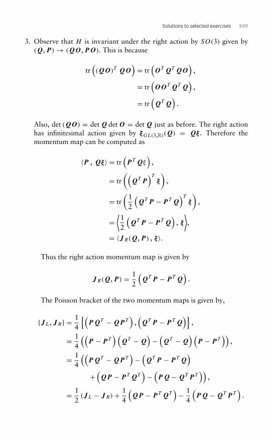
Solutions to selected exercises 349
3. Observe that H is invariant under the right action by SO(3) given by(Q,P )→ (QO,PO). This is because
tr((QO)T QO
)= tr
(OTQTQO
),
= tr(OOTQTQ
),
= tr(QTQ
).
Also, det (QO) = detQ detO = detQ just as before. The right actionhas infinitesimal action given by ξGL(3,R)(Q) = Qξ . Therefore themomentum map can be computed as
〈P , Qξ〉 = tr(P TQξ
),
= tr((
QTP)T
ξ
),
= tr(
12
(QTP − P TQ
)Tξ
),
=⟨12
(QTP − P TQ
), ξ⟩,
= 〈JR(Q,P ) , ξ〉.
Thus the right action momentum map is given by
JR(Q,P ) = 12
(QTP − P TQ
).
The Poisson bracket of the two momentum maps is given by,
{JL,JR} = 14
{(PQT −QP T
),(QTP − P TQ
)},
= 14
((P − P T
) (QT −Q
)−(QT −Q
) (P − P T
)),
= 14
((PQT −QP T
)−(QTP − P TQ
)+(QP − P TQT
)−(PQ−QTP T
)),
= 12(JL − JR)+ 1
4
(QP − P TQT
)− 1
4
(PQ−QTP T
).
350 10 : Pseudo-rigid bodies
Therefore the momentum maps do not Poisson commute. JL and JR
are not in involution. Jacobi’s identity shows that {JL,JR} is also a con-served quantity. Although the difference of the momentum maps occurs,there are also two other terms, indicating that the left and right SO(3)symmetry has not captured all of the symmetry of the Hamiltonian, i.e.there are more conserved quantities than those given to us by SO(3)invariance.
Part
III shall speak of things …so singular in their oddity as in some manner toinstruct, or at least entertain, without wearying.
– Lorenzo da Ponte (1749–1838)Memoirs of Lorenzo Da Ponte (2000). Translated by E. Abbott;
edited and annotated by A. Livingston; introduction by C. Rosen.The New York Review of Books, New York.

This page intentionally left blank
11EPDiff
11.1 Brief history of geometric idealcontinuum motion
Arnold [Arn66] showed that the Euler equations for incompressible motionof an ideal fluid may be cast into Lagrangian and Hamiltonian forms thatare similar to those for the rigid body, but are suitably generalized to allowfor continuum motions, instead of only rigid rotations. Rigid rotationspreserve the distances between any pair of particles. However, in con-tinuum motions, no metric relation is imposed on the distances betweenthe particles. In his generalization of dynamics from rigid-body rotationsto continuum motions, Arnold applied the Lagrangian and Hamiltoniantheories of geometric mechanics presented in Part I to rederive the Eulerfluid equations. In particular, Arnold began with a configuration spaceQ and formed a Lagrangian L on the velocity space TQ, then passed toa Hamiltonian description on the momentum phase space T ∗Q. In thisapproach, the methods of geometric mechanics systematically generatedthe Euler–Poincaré variational principle for the Euler fluid equations, aswell as their associated Lie–Poisson Hamiltonian structure, Noether the-orem, momentum maps, etc. For incompressible motion of an ideal fluid,the configuration space Q = G is the group G = DiffV ol(D) of volumepreserving smooth diffeomorphisms (smooth invertible maps with smoothinverses) of the region D occupied by the fluid. The tangent vectors in TG
for the maps in G = DiffV ol(D) represent the space of fluid velocities, whichmust satisfy appropriate physical conditions at the boundary of the regionD. Group multiplication in G = DiffV ol(D) is composition of the smoothinvertible volume-preserving maps.
This chapter begins by explaining how the Euler equations of idealincompressible fluid motion may be recognized as Euler–Poincaré equa-tions EPDiffV ol defined on the dual of the tangent space at the identityTeG = Te DiffV ol(D) of the right invariant vector fields over the domainD. Then it sets about developing these ideas to apply to EPDiff, theEuler–Poincaré equations on the full diffeomorphism group.
354 11 : EPDiff
Arnold’s geometric approach for incompressible ideal fluid motion hasbeen extended and applied to many other cases of ideal continuum motion.See, e.g., [HMRW85, HMR98a] for references, discussion and progress inthese more general applications. This wide range of applications of thegeometric mechanics approach in fluids, plasmas and other continua hasemerged for two reasons. First, all models of ideal continuum motion admitequivalent descriptions in either the material (or Lagrangian) picture or thespatial (or Eulerian) picture. Second, the potential energy of a continuumflow depends upon material properties that are carried along (or advected)by the flow. These material properties evolve by the action of the flow asif each fluid parcel being carried along by the flow were a closed thermo-dynamic system. However, these advected material properties need not bepassive. They may also influence the flow, because fluid dynamics allowsan exchange between potential and kinetic energy.
In Hamilton’s principle for the Eulerian description of ideal continuumdynamics, the kinetic energy may be expressed in terms of the right invari-ant spatial fluid velocity defined on smooth vector fields TeG = X(D).When only kinetic energy is present, the reduction of Hamilton’s principlein the Lagrangian picture for fluids by the symmetries of its Eulerian pic-ture produces the Euler–Poincaré (EP) theorem. When the kinetic energyLagrangian is right invariant under the diffeomorphisms, the dynamicalequation resulting from the symmetry reduction of Hamilton’s principle iscalled EPDiff.
Definition 11.1 (EPDiff)EPDiff is the family of equations governing geodesic motion on the fulldiffeomorphism group with respect to whatever right invariant metric ischosen on the tangent space of the diffeomorphisms.
Remark 11.2 Arnold’s result [Ar1966] that the Euler fluid equationsdescribe geodesic motion on the volume-preserving diffeomorphisms maythen be understood by interpreting these equations as EPDiffV ol withrespect to the right invariantL2metric of the Eulerian fluid velocity suppliedby the fluid’s kinetic energy.
If potential energy due to advected quantities is present in an ideal con-tinuum flow, then reduction by right invariance of Hamilton’s principleunder the diffeomorphisms produces the EP theorem with advected quan-tities discussed later in Theorem 17.8 in Chapter 17. The latter theoremencompasses most ideal continuum theories. This theorem was first statedand proved in [HMR98a], to which one may refer for additional details, aswell as for abstract definitions and proofs. We shall also follow [HMR98a]
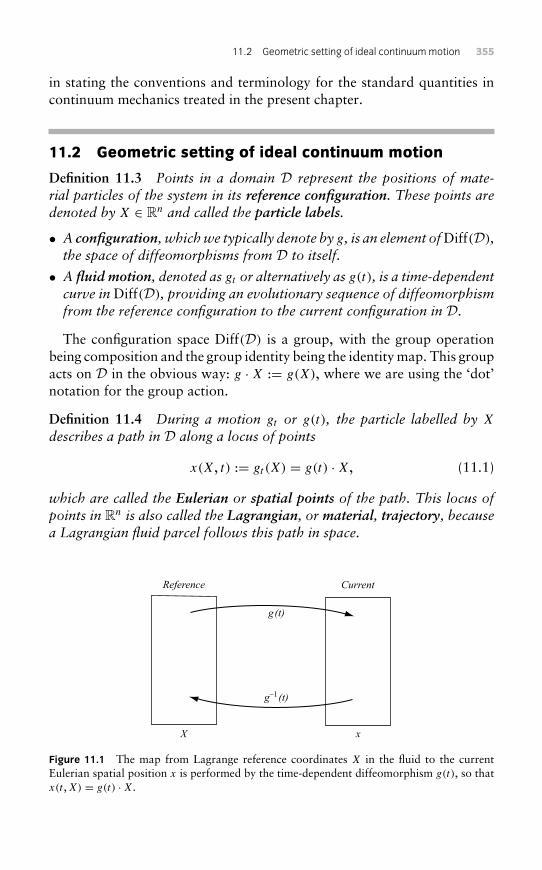
11.2 Geometric setting of ideal continuummotion 355
in stating the conventions and terminology for the standard quantities incontinuum mechanics treated in the present chapter.
11.2 Geometric setting of ideal continuum motion
Definition 11.3 Points in a domain D represent the positions of mate-rial particles of the system in its reference configuration. These points aredenoted by X ∈ Rn and called the particle labels.
• A configuration, whichwe typically denote by g, is an element ofDiff(D),the space of diffeomorphisms from D to itself.• A fluid motion, denoted as gt or alternatively as g(t), is a time-dependentcurve in Diff(D), providing an evolutionary sequence of diffeomorphismfrom the reference configuration to the current configuration in D.The configuration space Diff(D) is a group, with the group operation
being composition and the group identity being the identity map. This groupacts on D in the obvious way: g · X := g(X), where we are using the ‘dot’notation for the group action.
Definition 11.4 During a motion gt or g(t), the particle labelled by X
describes a path in D along a locus of pointsx(X, t) := gt (X) = g(t) ·X, (11.1)
which are called the Eulerian or spatial points of the path. This locus ofpoints in Rn is also called the Lagrangian, or material, trajectory, becausea Lagrangian fluid parcel follows this path in space.
g–1(t)
g(t)
x
CurrentReference
X
Figure 11.1 The map from Lagrange reference coordinates X in the fluid to the currentEulerian spatial position x is performed by the time-dependent diffeomorphism g(t), so thatx(t ,X) = g(t) ·X.
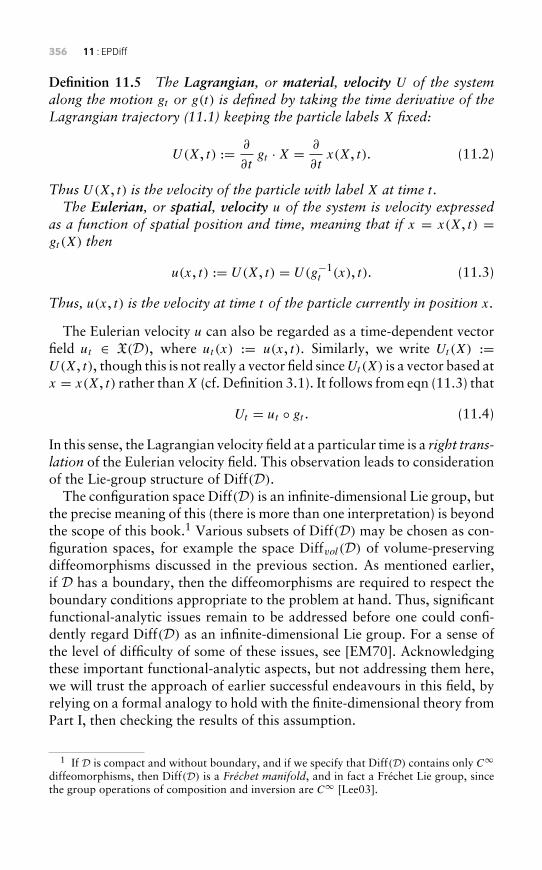
356 11 : EPDiff
Definition 11.5 The Lagrangian, or material, velocity U of the systemalong the motion gt or g(t) is defined by taking the time derivative of theLagrangian trajectory (11.1) keeping the particle labels X fixed:
U(X, t) := ∂
∂tgt ·X = ∂
∂tx(X, t). (11.2)
Thus U(X, t) is the velocity of the particle with label X at time t .The Eulerian, or spatial, velocity u of the system is velocity expressed
as a function of spatial position and time, meaning that if x = x(X, t) =gt (X) then
u(x, t) := U(X, t) = U(g−1t (x), t). (11.3)
Thus, u(x, t) is the velocity at time t of the particle currently in position x.
The Eulerian velocity u can also be regarded as a time-dependent vectorfield ut ∈ X(D), where ut (x) := u(x, t). Similarly, we write Ut(X) :=U(X, t), though this is not really a vector field sinceUt(X) is a vector based atx = x(X, t) rather thanX (cf. Definition 3.1). It follows from eqn (11.3) that
Ut = ut ◦ gt . (11.4)
In this sense, the Lagrangian velocity field at a particular time is a right trans-lation of the Eulerian velocity field. This observation leads to considerationof the Lie-group structure of Diff(D).
The configuration space Diff(D) is an infinite-dimensional Lie group, butthe precise meaning of this (there is more than one interpretation) is beyondthe scope of this book.1 Various subsets of Diff(D) may be chosen as con-figuration spaces, for example the space Diffvol(D) of volume-preservingdiffeomorphisms discussed in the previous section. As mentioned earlier,if D has a boundary, then the diffeomorphisms are required to respect theboundary conditions appropriate to the problem at hand. Thus, significantfunctional-analytic issues remain to be addressed before one could confi-dently regard Diff(D) as an infinite-dimensional Lie group. For a sense ofthe level of difficulty of some of these issues, see [EM70]. Acknowledgingthese important functional-analytic aspects, but not addressing them here,we will trust the approach of earlier successful endeavours in this field, byrelying on a formal analogy to hold with the finite-dimensional theory fromPart I, then checking the results of this assumption.
1 If D is compact and without boundary, and if we specify that Diff(D) contains only C∞diffeomorphisms, then Diff(D) is a Fréchet manifold, and in fact a Fréchet Lie group, sincethe group operations of composition and inversion are C∞ [Lee03].
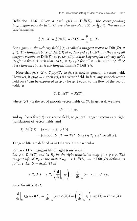
11.2 Geometric setting of ideal continuummotion 357
Definition 11.6 Given a path g(t) in Diff(D), the correspondingLagrangian velocity fields Ut are also denoted g(t) or ∂
∂tg(t). We use the
‘dot’ notation,
g(t) ·X := g(t)(X) = Ut(X) = ∂
∂tgt ·X.
For a given t , the velocity field g(t) is called a tangent vector to Diff(D) atg(t). The tangent space of Diff(D) at g, denoted Tg Diff(D), is the set of alltangent vectors to Diff(D) at g, i.e. all possible Lagrangian velocity fieldsUt (for a fixed t) such that Ut(X) ∈ Tg(X)D for all X. The union of all ofthese tangent spaces is the tangent bundle T Diff(D).
Note that g(t) · X ∈ Tg(t)·XD, so g(t) is not, in general, a vector field.However, if g(t0) = e, then g(t0) is a vector field. In fact, any smooth vectorfield on D can be expressed as g(0) for g(t) equal to the flow of the vectorfield, so
Te Diff(D) = X(D),
where X(D) is the set of smooth vector fields on D. In general, we have
Ut = ut ◦ gt ,
and ut (for a fixed t) is a vector field, so general tangent vectors are righttranslations of vector fields, and
Tg Diff(D) = {u ◦ g : u ∈ X(D)}= {smooth U : D→ TD | U(X) ∈ Tg(X)D for all X}.
Tangent lifts are defined as in Chapter 2. In particular,
Remark 11.7 (Tangent lift of right translation)Let ϕ ∈ Diff(D) and let Rϕ be the right translation map g → g ◦ ϕ. Thetangent lift of Rϕ is the map T Rϕ : T Diff(D) → T Diff(D) defined asfollows. Let U = g(t0). Then
T Rϕ(U) = T Rϕ
(ddt
∣∣∣∣t0
gt
):= d
dt
∣∣∣∣t0
(gt ◦ ϕ) = U ◦ ϕ,
since for all X ∈ D,
ddt
∣∣∣∣t0
(gt ◦ ϕ)(X) = ddt
∣∣∣∣t0
(gt ◦ ϕ(X)) =(
ddt
∣∣∣∣t0
gt
)· ϕ(X)) = U ◦ ϕ(X).
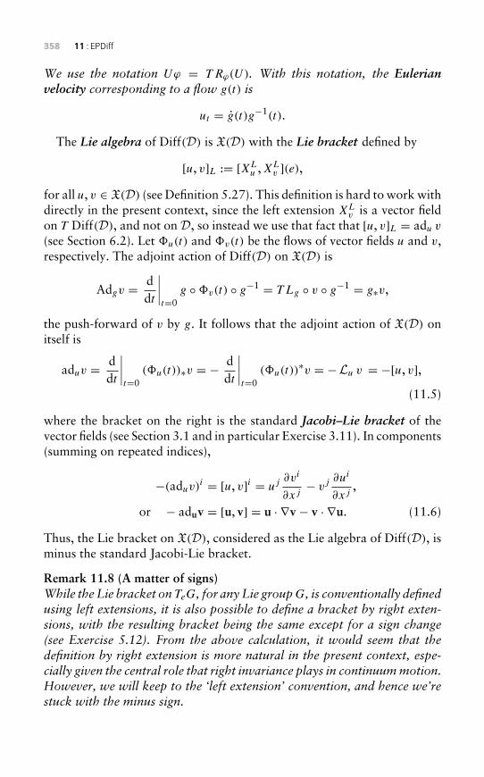
358 11 : EPDiff
We use the notation Uϕ = T Rϕ(U). With this notation, the Eulerianvelocity corresponding to a flow g(t) is
ut = g(t)g−1(t).
The Lie algebra of Diff(D) is X(D) with the Lie bracket defined by
[u, v]L := [XLu ,XL
v ](e),for all u, v ∈ X(D) (see Definition 5.27). This definition is hard to work withdirectly in the present context, since the left extension XL
v is a vector fieldon T Diff(D), and not on D, so instead we use that fact that [u, v]L = adu v
(see Section 6.2). Let �u(t) and �v(t) be the flows of vector fields u and v,respectively. The adjoint action of Diff(D) on X(D) is
Adgv = ddt
∣∣∣∣t=0
g ◦�v(t) ◦ g−1 = T Lg ◦ v ◦ g−1 = g∗v,
the push-forward of v by g. It follows that the adjoint action of X(D) onitself is
aduv = ddt
∣∣∣∣t=0
(�u(t))∗v = − ddt
∣∣∣∣t=0
(�u(t))∗v = −Lu v = −[u, v],
(11.5)
where the bracket on the right is the standard Jacobi–Lie bracket of thevector fields (see Section 3.1 and in particular Exercise 3.11). In components(summing on repeated indices),
−(aduv)i = [u, v]i = uj ∂vi
∂xj− vj ∂ui
∂xj,
or − aduv = [u, v] = u · ∇v − v · ∇u. (11.6)
Thus, the Lie bracket on X(D), considered as the Lie algebra of Diff(D), isminus the standard Jacobi-Lie bracket.
Remark 11.8 (A matter of signs)While the Lie bracket on TeG, for any Lie groupG, is conventionally definedusing left extensions, it is also possible to define a bracket by right exten-sions, with the resulting bracket being the same except for a sign change(see Exercise 5.12). From the above calculation, it would seem that thedefinition by right extension is more natural in the present context, espe-cially given the central role that right invariance plays in continuummotion.However, we will keep to the ‘left extension’ convention, and hence we’restuck with the minus sign.
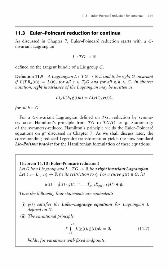
11.3 Euler–Poincaré reduction for continua 359
11.3 Euler–Poincaré reduction for continua
As discussed in Chapter 7, Euler–Poincaré reduction starts with a G-invariant Lagrangian
L : TG→ R
defined on the tangent bundle of a Lie group G.
Definition 11.9 A Lagrangian L : TG→ R is said to be rightG-invariantif L(T Rh(v)) = L(v), for all v ∈ TgG and for all g,h ∈ G. In shorternotation, right invariance of the Lagrangian may be written as
L(g(t)h, g(t)h) = L(g(t), g(t)),
for all h ∈ G.
For a G-invariant Lagrangian defined on TG, reduction by symme-try takes Hamilton’s principle from TG to TG/G � g. Stationarityof the symmetry-reduced Hamilton’s principle yields the Euler–Poincaréequations on g∗ discussed in Chapter 7. As we shall discuss later, thecorresponding reduced Legendre transformation yields the now-standardLie–Poisson bracket for the Hamiltonian formulation of these equations.
Theorem 11.10 (Euler–Poincaré reduction)LetG be a Lie group andL : TG→ R be a right invariant Lagrangian.Let � := L|g : g→ R be its restriction to g. For a curve g(t) ∈ G, let
u(t) = g(t) · g(t)−1 := Tg(t)Rg(t)−1 g(t) ∈ g.
Then the following four statements are equivalent:
(i) g(t) satisfies the Euler–Lagrange equations for Lagrangian L
defined on G.
(ii) The variational principle
δ
∫ b
a
L(g(t), g(t))dt = 0, (11.7)
holds, for variations with fixed endpoints.
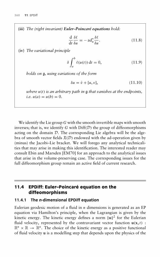
360 11 : EPDiff
(iii) The (right invariant) Euler–Poincaré equations hold:
ddt
δ�
δu= − ad∗u
δ�
δu. (11.8)
(iv) The variational principle
δ
∫ b
a
�(u(t)) dt = 0, (11.9)
holds on g, using variations of the form
δu = v + [u, v], (11.10)
where u(t) is an arbitrary path in g that vanishes at the endpoints,i.e. u(a) = u(b) = 0.
We identify the Lie groupGwith the smooth invertible maps with smoothinverses; that is, we identify G with Diff(D) the group of diffeomorphismsacting on the domain D. The corresponding Lie algebra will be the alge-bra of smooth vector fields X(D) endowed with the ad-operation given by(minus) the Jacobi–Lie bracket. We will forego any analytical technicali-ties that may arise in making this identification. The interested reader mayconsult Ebin and Marsden [EM70] for an approach to the analytical issuesthat arise in the volume-preserving case. The corresponding issues for thefull diffeomorphism group remain an active field of current research.
11.4 EPDiff: Euler–Poincaré equation on thediffeomorphisms
11.4.1 The n-dimensional EPDiff equation
Eulerian geodesic motion of a fluid in n dimensions is generated as an EPequation via Hamilton’s principle, when the Lagrangian is given by thekinetic energy. The kinetic energy defines a norm ‖u‖2 for the Eulerianfluid velocity, represented by the contravariant vector function u(x, t) :Rn × R → Rn. The choice of the kinetic energy as a positive functionalof fluid velocity u is a modelling step that depends upon the physics of the
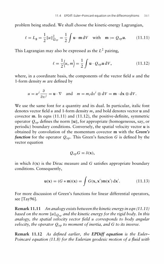
11.4 EPDiff: Euler–Poincaré equation on the diffeomorphisms 361
problem being studied. We shall choose the kinetic-energy Lagrangian,
� = Lg = 12‖u‖2Qop
= 12
∫u ·m dV with m := Qopu. (11.11)
This Lagrangian may also be expressed as the L2 pairing,
� = 12
⟨u, m
⟩= 1
2
∫u ·Qopu dV , (11.12)
where, in a coordinate basis, the components of the vector field u and the1-form density m are defined by
u = uj ∂
∂xj= u · ∇ and m = midxi ⊗ dV = m · dx⊗ dV .
We use the same font for a quantity and its dual. In particular, italic fontdenotes vector field u and 1-form density m, and bold denotes vector u andcovector m. In eqns (11.11) and (11.12), the positive-definite, symmetricoperator Qop defines the norm ‖u‖, for appropriate (homogeneous, say, orperiodic) boundary conditions. Conversely, the spatial velocity vector u isobtained by convolution of the momentum covector m with the Green’sfunction for the operator Qop. This Green’s function G is defined by thevector equation
QopG = δ(x),
in which δ(x) is the Dirac measure and G satisfies appropriate boundaryconditions. Consequently,
u(x) = (G ∗m)(x) =∫
G(x, x′)m(x′) dx′. (11.13)
For more discussion of Green’s functions for linear differential operators,see [Tay96].
Remark 11.11 An analogy exists between the kinetic energy in eqn (11.11)based on the norm ‖u‖Qop and the kinetic energy for the rigid body. In thisanalogy, the spatial velocity vector field u corresponds to body angularvelocity, the operator Qop to moment of inertia, and G to its inverse.
Remark 11.12 As defined earlier, the EPDiff equation is the Euler–Poincaré equation (11.8) for the Eulerian geodesic motion of a fluid with
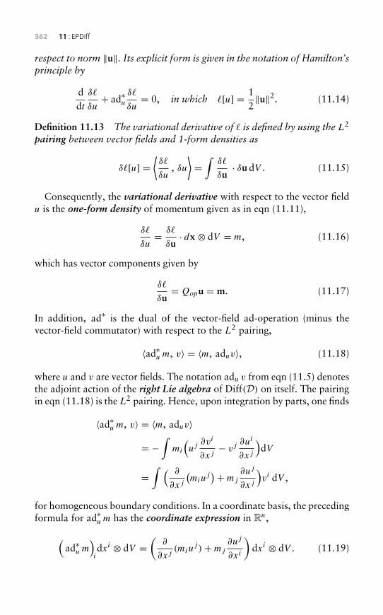
362 11 : EPDiff
respect to norm ‖u‖. Its explicit form is given in the notation of Hamilton’sprinciple by
ddt
δ�
δu+ ad∗u
δ�
δu= 0, in which �[u] = 1
2‖u‖2. (11.14)
Definition 11.13 The variational derivative of � is defined by using the L2
pairing between vector fields and 1-form densities as
δ�[u] =⟨δ�
δu, δu
⟩=∫
δ�
δu· δu dV . (11.15)
Consequently, the variational derivative with respect to the vector fieldu is the one-form density of momentum given as in eqn (11.11),
δ�
δu= δ�
δu· dx⊗ dV = m, (11.16)
which has vector components given by
δ�
δu= Qopu = m. (11.17)
In addition, ad∗ is the dual of the vector-field ad-operation (minus thevector-field commutator) with respect to the L2 pairing,
〈ad∗u m, v〉 = 〈m, aduv〉, (11.18)
where u and v are vector fields. The notation adu v from eqn (11.5) denotesthe adjoint action of the right Lie algebra of Diff(D) on itself. The pairingin eqn (11.18) is the L2 pairing. Hence, upon integration by parts, one finds
〈ad∗u m, v〉 = 〈m, aduv〉
= −∫
mi
(uj ∂vi
∂xj− vj ∂ui
∂xj
)dV
=∫ ( ∂
∂xj
(miu
j)+mj
∂uj
∂xj
)vi dV ,
for homogeneous boundary conditions. In a coordinate basis, the precedingformula for ad∗u m has the coordinate expression in Rn,
(ad∗u m
)idxi ⊗ dV =
(∂
∂xj(miu
j )+mj
∂uj
∂xi
)dxi ⊗ dV . (11.19)
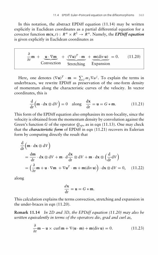
11.4 EPDiff: Euler–Poincaré equation on the diffeomorphisms 363
In this notation, the abstract EPDiff equation (11.14) may be writtenexplicitly in Euclidean coordinates as a partial differential equation for acovector function m(x, t) : Rn × R1 → Rn. Namely, the EPDiff equationis given explicitly in Euclidean coordinates as
∂
∂tm + u · ∇m︸ ︷︷ ︸
Convection
+ (∇u)T ·m︸ ︷︷ ︸Stretching
+ m(div u)︸ ︷︷ ︸Expansion
= 0. (11.20)
Here, one denotes (∇u)T · m = ∑j mj∇uj . To explain the terms in
underbraces, we rewrite EPDiff as preservation of the one-form densityof momentum along the characteristic curves of the velocity. In vectorcoordinates, this is
ddt
(m · dx⊗ dV
)= 0 along
dxdt= u = G ∗m. (11.21)
This form of the EPDiff equation also emphasizes its non-locality, since thevelocity is obtained from the momentum density by convolution against theGreen’s function G of the operator Qop, as in eqn (11.13). One may checkthat the characteristic form of EPDiff in eqn (11.21) recovers its Eulerianform by computing directly the result that
ddt
(m · dx⊗ dV
)= dm
dt· dx⊗ dV +m · ddx
dt⊗ dV +m · dx⊗
( ddt
dV)
=( ∂
∂tm+ u · ∇m + ∇uT ·m+m(div u)
)· dx⊗ dV = 0, (11.22)
along
dxdt= u = G ∗m.
This calculation explains the terms convection, stretching and expansion inthe under-braces in eqn (11.20).
Remark 11.14 In 2D and 3D, the EPDiff equation (11.20) may also bewritten equivalently in terms of the operators div, grad and curl as,
∂
∂tm− u× curlm+ ∇(u ·m)+m(div u) = 0. (11.23)
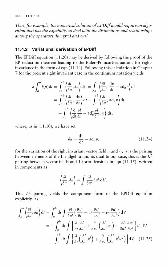
364 11 : EPDiff
Thus, for example, the numerical solution of EPDiff would require an algo-rithm that has the capability to deal with the distinctions and relationshipsamong the operators div, grad and curl.
11.4.2 Variational derivation of EPDiff
The EPDiff equation (11.20) may be derived by following the proof of theEP reduction theorem leading to the Euler–Poincaré equations for right-invariance in the form of eqn (11.14). Following this calculation in Chapter7 for the present right invariant case in the continuum notation yields
δ
∫ b
a
l(u)dt =∫ b
a
⟨δl
δu, δu
⟩dt =
∫ b
a
⟨δl
δu,
dvdt− aduv
⟩dt
=∫ b
a
⟨δl
δu,
dvdt
⟩dt −
∫ b
a
⟨δl
δu, aduv
⟩dt
= −∫ b
a
⟨ddt
δl
δu+ ad∗u
δl
δu, v⟩
dt ,
where, as in (11.10), we have set
δu = dvdt− aduv, (11.24)
for the variation of the right invariant vector field u and 〈·, ·〉 is the pairingbetween elements of the Lie algebra and its dual In our case, this is the L2
pairing between vector fields and 1-form densities in eqn (11.15), writtenin components as ⟨
δl
δu, δu
⟩=∫
δl
δuiδui dV .
This L2 pairing yields the component form of the EPDiff equationexplicitly, as∫ b
a
⟨δl
δu, δu
⟩dt =
∫ b
a
dt∫
δl
δui
(∂vi
∂t+ uj ∂vi
∂xj− vj ∂ui
∂xj
)dV
= −∫ b
a
dt∫ {
∂
∂t
δl
δui+ ∂
∂xj
( δl
δuiuj)+ δl
δuj
∂uj
∂xi
}vi dV
+∫ b
a
dt∫ {
∂
∂t
( δl
δuivi)+ ∂
∂xj
( δl
δuiviuj
)}dV . (11.25)
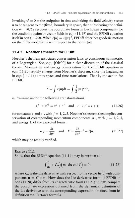
11.4 EPDiff: Euler–Poincaré equation on the diffeomorphisms 365
Invoking vi = 0 at the endpoints in time and taking the fluid velocity vectoru to be tangent to the (fixed) boundary in space, then substituting the defini-tion m = δl/δu recovers the coordinate forms in Euclidean components forthe coadjoint action of vector fields in eqn (11.19) and the EPDiff equationitself in eqn (11.20). When �[u] = 1
2‖u‖2, EPDiff describes geodesic motionon the diffeomorphisms with respect to the norm ‖u‖.
11.4.3 Noether’s theorem for EPDiff
Noether’s theorem associates conservation laws to continuous symmetriesof a Lagrangian. See, e.g., [Olv00] for a clear discussion of the classicaltheory. Momentum and energy conservation for the EPDiff equation ineqn (11.20) readily emerge from Noether’s theorem, since the Lagrangianin eqn (11.11) admits space and time translations. That is, the action forEPDiff,
S =∫
�[u]dt =∫
12‖u‖2dt ,
is invariant under the following transformations,
xj → x′j = xj + cj and t → t ′ = t + τ , (11.26)
for constants τ and cj , with j = 1, 2, 3. Noether’s theorem then implies con-servation of corresponding momentum components mj , with j = 1, 2, 3,and energy E of the expected forms,
mj = δ�
δujand E = δ�
δujuj − �[u], (11.27)
which may be readily verified.
Exercise 11.1Show that the EPDiff equation (11.14) may be written as( ∂
∂t+ Lu
)(m · dx⊗ dV
)= 0, (11.28)
where Lu is the Lie derivative with respect to the vector field with com-ponents u = G ∗ m. How does the Lie-derivative form of EPDiff ineqn (11.28) differ from its characteristic form (11.21)? Hint: comparethe coordinate expression obtained from the dynamical definition ofthe Lie derivative with the corresponding expression obtained from itsdefinition via Cartan’s formula.
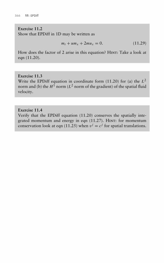
366 11 : EPDiff
Exercise 11.2Show that EPDiff in 1D may be written as
mt + umx + 2mux = 0. (11.29)
How does the factor of 2 arise in this equation? Hint: Take a look ateqn (11.20).
Exercise 11.3Write the EPDiff equation in coordinate form (11.20) for (a) the L2
norm and (b) the H 1 norm (L2 norm of the gradient) of the spatial fluidvelocity.
Exercise 11.4Verify that the EPDiff equation (11.20) conserves the spatially inte-grated momentum and energy in eqn (11.27). Hint: for momentumconservation look at eqn (11.25) when vj = cj for spatial translations.
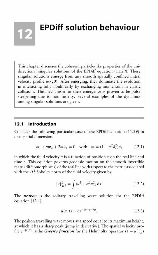
12EPDiff solution behaviour
This chapter discusses the coherent particle-like properties of the uni-directional singular solutions of the EPDiff equation (11.29). Thesesingular solutions emerge from any smooth spatially confined initialvelocity profile u(x, 0). After emerging, they dominate the evolutionin interacting fully nonlinearly by exchanging momentum in elasticcollisions. The mechanism for their emergence is proven to be pulsesteepening due to nonlinearity. Several examples of the dynamicsamong singular solutions are given.
12.1 Introduction
Consider the following particular case of the EPDiff equation (11.29) inone spatial dimension,
mt + umx + 2mux = 0 with m = (1− α2∂2x )u, (12.1)
in which the fluid velocity u is a function of position x on the real line andtime t . This equation governs geodesic motion on the smooth invertiblemaps (diffeomorphisms) of the real line with respect to the metric associatedwith the H 1 Sobolev norm of the fluid velocity given by
‖u‖2H1 =
∫(u2 + α2u2
x) dx. (12.2)
The peakon is the solitary travelling wave solution for the EPDIffequation (12.1),
u(x, t) = c e−|x−ct |/α. (12.3)
The peakon travelling wave moves at a speed equal to its maximum height,at which it has a sharp peak (jump in derivative). The spatial velocity pro-file e−|x|/α is the Green’s function for the Helmholtz operator (1 − α2∂2
x )
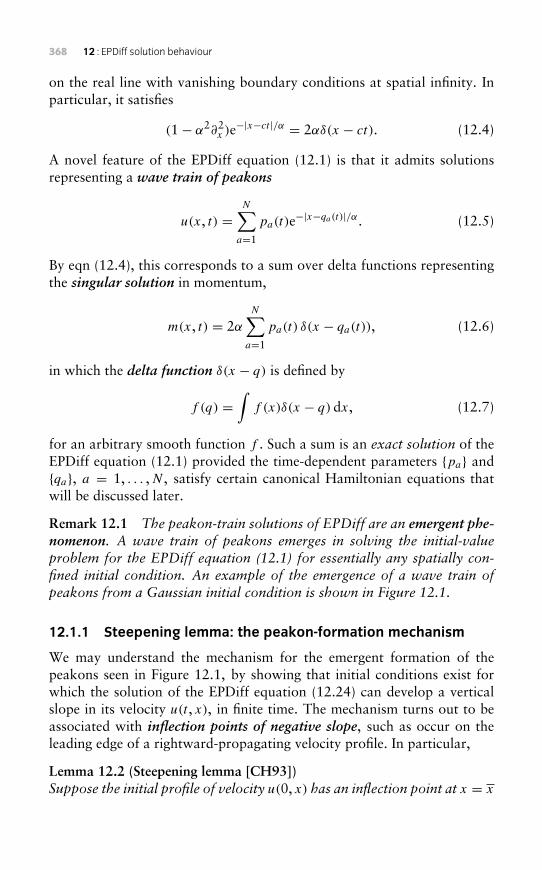
368 12 : EPDiff solution behaviour
on the real line with vanishing boundary conditions at spatial infinity. Inparticular, it satisfies
(1− α2∂2x )e−|x−ct |/α = 2αδ(x − ct). (12.4)
A novel feature of the EPDiff equation (12.1) is that it admits solutionsrepresenting a wave train of peakons
u(x, t) =N∑
a=1
pa(t)e−|x−qa(t)|/α. (12.5)
By eqn (12.4), this corresponds to a sum over delta functions representingthe singular solution in momentum,
m(x, t) = 2αN∑
a=1
pa(t) δ(x − qa(t)), (12.6)
in which the delta function δ(x − q) is defined by
f (q) =∫
f (x)δ(x − q) dx, (12.7)
for an arbitrary smooth function f . Such a sum is an exact solution of theEPDiff equation (12.1) provided the time-dependent parameters {pa} and{qa}, a = 1, . . . ,N , satisfy certain canonical Hamiltonian equations thatwill be discussed later.
Remark 12.1 The peakon-train solutions of EPDiff are an emergent phe-nomenon. A wave train of peakons emerges in solving the initial-valueproblem for the EPDiff equation (12.1) for essentially any spatially con-fined initial condition. An example of the emergence of a wave train ofpeakons from a Gaussian initial condition is shown in Figure 12.1.
12.1.1 Steepening lemma: the peakon-formation mechanism
We may understand the mechanism for the emergent formation of thepeakons seen in Figure 12.1, by showing that initial conditions exist forwhich the solution of the EPDiff equation (12.24) can develop a verticalslope in its velocity u(t , x), in finite time. The mechanism turns out to beassociated with inflection points of negative slope, such as occur on theleading edge of a rightward-propagating velocity profile. In particular,
Lemma 12.2 (Steepening lemma [CH93])Suppose the initial profile of velocity u(0, x) has an inflection point at x = x
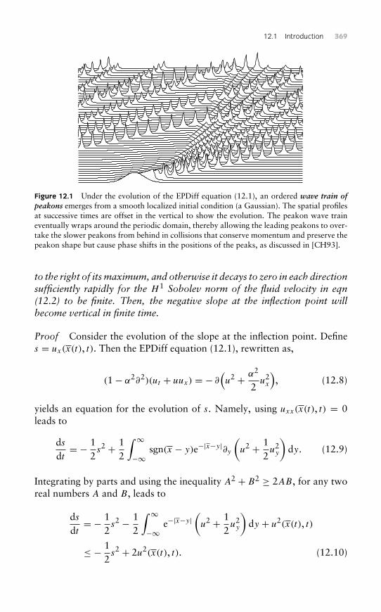
12.1 Introduction 369
Figure 12.1 Under the evolution of the EPDiff equation (12.1), an ordered wave train ofpeakons emerges from a smooth localized initial condition (a Gaussian). The spatial profilesat successive times are offset in the vertical to show the evolution. The peakon wave traineventually wraps around the periodic domain, thereby allowing the leading peakons to over-take the slower peakons from behind in collisions that conserve momentum and preserve thepeakon shape but cause phase shifts in the positions of the peaks, as discussed in [CH93].
to the right of its maximum, and otherwise it decays to zero in each directionsufficiently rapidly for the H 1 Sobolev norm of the fluid velocity in eqn(12.2) to be finite. Then, the negative slope at the inflection point willbecome vertical in finite time.
Proof Consider the evolution of the slope at the inflection point. Defines = ux(x(t), t). Then the EPDiff equation (12.1), rewritten as,
(1− α2∂2)(ut + uux) = − ∂(u2 + α2
2u2x
), (12.8)
yields an equation for the evolution of s. Namely, using uxx(x(t), t) = 0leads to
dsdt= − 1
2s2 + 1
2
∫ ∞−∞
sgn(x − y)e−|x−y|∂y(u2 + 1
2u2y
)dy. (12.9)
Integrating by parts and using the inequality A2 + B2 ≥ 2AB, for any tworeal numbers A and B, leads to
dsdt= − 1
2s2 − 1
2
∫ ∞−∞
e−|x−y|(u2 + 1
2u2y
)dy + u2(x(t), t)
≤ − 12s2 + 2u2(x(t), t). (12.10)
370 12 : EPDiff solution behaviour
Then, provided u2(x(t), t) remains finite, say less than a number M/4,we have
dsdt= − 1
2s2 + M
2, (12.11)
which implies, for negative slope initially s ≤ −√M, that
s ≤ √M coth(σ + t
2
√M
), (12.12)
where σ is a negative constant that determines the initial slope, also negative.Hence, at time t = −2σ/
√M the slope becomes negative and vertical. The
assumption that M in eqn (12.11) exists is verified in general by a Sobolevinequality. In fact, M = 8H1, since
maxx∈R u2(x, t) ≤
∫ ∞−∞
(u2 + u2
x
)dx = 2H1 = const . (12.13)
�
Remark 12.3 Suppose the initial condition is anti-symmetric, so the inflec-tion point at u = 0 is fixed and dx/dt = 0, due to the symmetry(u, x) → (−u,−x) admitted by eqn (13.1). In this case, M = 0 and nomatter how small |s(0)| (with s(0) < 0) verticality s → −∞ develops at xin finite time.
The steepening lemma indicates that travelling wave solutions of theEPDiff equation (12.1) cannot have the sech2 shape that appears for KdVsolitons, since inflection points with sufficiently negative slope can lead tounsteady changes in the shape of the profile if inflection points are present.In fact, numerical simulations show that the presence of an inflection pointof negative slope in any confined initial velocity distribution triggers thesteepening lemma as the mechanism for the formation of the peakons.Namely. the initial (positive) velocity profile “leans” to the right and steep-ens, then produces a peakon that is taller than the initial profile, so itpropagates away to the right. This process leaves a profile behind with aninflection point of negative slope; so it repeats, thereby producing a wavetrain of peakons with the tallest and fastest ones moving rightward in orderof height. Remarkably, this recurrent process produces only peakons.
The EPDiff equation (12.1) arises from a shallow water wave equationin the limit of zero linear dispersion in one dimension. As we shall see,the peakon solutions (12.6) for EPDiff generalize to higher dimensions andother kinetic energy norms.
12.2 Shallow-water background for peakons 371
Exercise 12.1Verify that the EPDIff equation (12.1) preserves the H 1 norm (12.2).
Exercise 12.2Verify that the peakon formula (12.3) provides the solitary travellingwave solution for the EPDIff equation (12.1).
Exercise 12.3Verify formula (12.4) for the Green’s function. Why is this formula use-ful in representing the travelling-wave solution of the EPDIff equation(12.1)?
12.2 Shallow-water background for peakons
The EPDiff equation (12.1) whose solutions admit peakon wave trains(12.5) may be derived by taking the zero-dispersion limit of another equa-tion obtained from Euler’s fluid equations by using asymptotic expansionsfor shallow water waves [CH93]. Euler’s equations for irrotational incom-pressible ideal fluid motion under gravity with a free surface have anasymptotic expansion for shallow water waves that involves two smallparameters, ε and δ2, with ordering ε ≥ δ2. These small parameters areε = a/h0 (the ratio of wave amplitude to mean depth) and δ2 = (h0/lx)
2
(the squared ratio of mean depth to horizontal length, or wavelength).In one spatial dimension, EPDiff is the zero-dispersion limit of the
Camassa–Holm (CH) equation for shallow water waves, which is the b = 2case of the following b-equation, that results from the asymptotic expansionfor shallow water waves,
mt + c0ux + umx + bmux − γ uxxx = 0. (12.14)
Here, m = u − α2uxx is the momentum variable, and the constants α2
and γ /c0 are squares of length scales. At linear order in the asymptoticexpansion for shallow water waves in terms of the small parameters ε andδ2, one finds α2 → 0, so that m → u in (12.14). In this case, the famousKorteweg–de Vries (KdV) soliton equation is recovered for b = 2,
ut + 3uux = −c0ux + γ uxxx . (12.15)
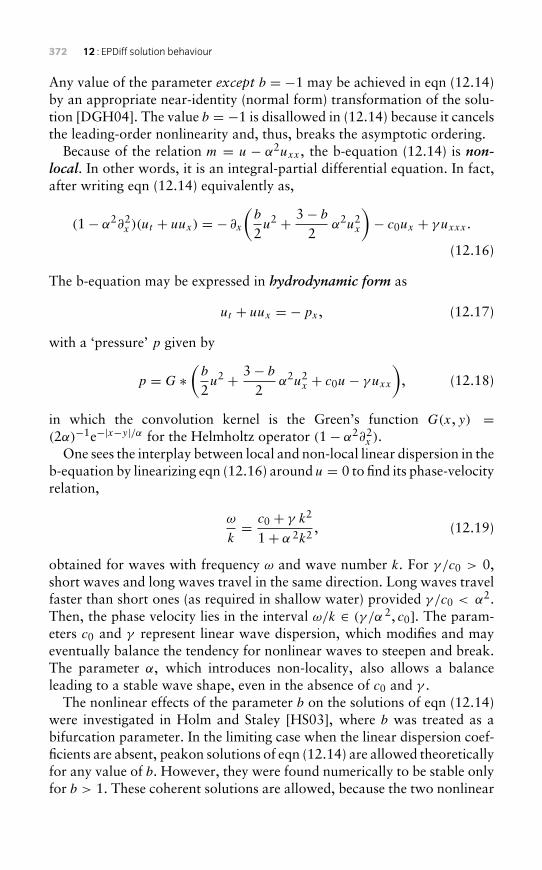
372 12 : EPDiff solution behaviour
Any value of the parameter except b = −1 may be achieved in eqn (12.14)by an appropriate near-identity (normal form) transformation of the solu-tion [DGH04]. The value b = −1 is disallowed in (12.14) because it cancelsthe leading-order nonlinearity and, thus, breaks the asymptotic ordering.
Because of the relation m = u − α2uxx , the b-equation (12.14) is non-local. In other words, it is an integral-partial differential equation. In fact,after writing eqn (12.14) equivalently as,
(1− α2∂2x )(ut + uux) = − ∂x
(b
2u2 + 3− b
2α2u2
x
)− c0ux + γ uxxx .
(12.16)
The b-equation may be expressed in hydrodynamic form as
ut + uux = −px , (12.17)
with a ‘pressure’ p given by
p = G ∗(b
2u2 + 3− b
2α2u2
x + c0u− γ uxx
), (12.18)
in which the convolution kernel is the Green’s function G(x, y) =(2α)−1e−|x−y|/α for the Helmholtz operator (1− α2∂2
x ).One sees the interplay between local and non-local linear dispersion in the
b-equation by linearizing eqn (12.16) around u = 0 to find its phase-velocityrelation,
ω
k= c0 + γ k2
1+ α 2k2 , (12.19)
obtained for waves with frequency ω and wave number k. For γ /c0 > 0,short waves and long waves travel in the same direction. Long waves travelfaster than short ones (as required in shallow water) provided γ /c0 < α2.Then, the phase velocity lies in the interval ω/k ∈ (γ /α 2, c0]. The param-eters c0 and γ represent linear wave dispersion, which modifies and mayeventually balance the tendency for nonlinear waves to steepen and break.The parameter α, which introduces non-locality, also allows a balanceleading to a stable wave shape, even in the absence of c0 and γ .
The nonlinear effects of the parameter b on the solutions of eqn (12.14)were investigated in Holm and Staley [HS03], where b was treated as abifurcation parameter. In the limiting case when the linear dispersion coef-ficients are absent, peakon solutions of eqn (12.14) are allowed theoreticallyfor any value of b. However, they were found numerically to be stable onlyfor b > 1. These coherent solutions are allowed, because the two nonlinear
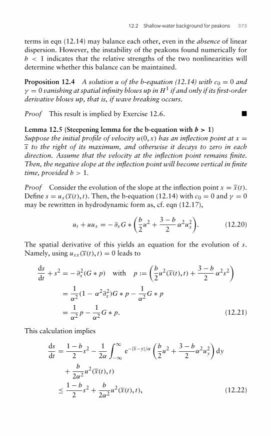
12.2 Shallow-water background for peakons 373
terms in eqn (12.14) may balance each other, even in the absence of lineardispersion. However, the instability of the peakons found numerically forb < 1 indicates that the relative strengths of the two nonlinearities willdetermine whether this balance can be maintained.
Proposition 12.4 A solution u of the b-equation (12.14) with c0 = 0 andγ = 0 vanishing at spatial infinity blows up inH 1 if and only if its first-orderderivative blows up, that is, if wave breaking occurs.
Proof This result is implied by Exercise 12.6. �
Lemma 12.5 (Steepening lemma for the b-equation with b > 1)Suppose the initial profile of velocity u(0, x) has an inflection point at x =x to the right of its maximum, and otherwise it decays to zero in eachdirection. Assume that the velocity at the inflection point remains finite.Then, the negative slope at the inflection point will become vertical in finitetime, provided b > 1.
Proof Consider the evolution of the slope at the inflection point x = x(t).Define s = ux(x(t), t). Then, the b-equation (12.14) with c0 = 0 and γ = 0may be rewritten in hydrodynamic form as, cf. eqn (12.17),
ut + uux = − ∂xG ∗(b
2u2 + 3− b
2α2u2
x
). (12.20)
The spatial derivative of this yields an equation for the evolution of s.Namely, using uxx(x(t), t) = 0 leads to
dsdt+ s2 = − ∂2
x (G ∗ p) with p :=(b
2u2(x(t), t)+ 3− b
2α2s2
)= 1
α2 (1− α2∂2x )G ∗ p −
1α2G ∗ p
= 1α2p −
1α2G ∗ p. (12.21)
This calculation implies
dsdt= 1− b
2s2 − 1
2α
∫ ∞−∞
e−|x−y|/α(b
2u2 + 3− b
2α2u2
y
)dy
+ b
2α2u2(x(t), t)
≤ 1− b
2s2 + b
2α2u2(x(t), t), (12.22)
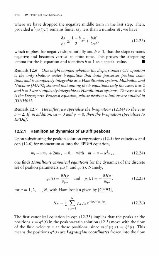
374 12 : EPDiff solution behaviour
where we have dropped the negative middle term in the last step. Then,provided u2(x(t), t) remains finite, say less than a number M, we have
dsdt≤ 1− b
2s2 + bM
2α2 , (12.23)
which implies, for negative slope initially and b > 1, that the slope remainsnegative and becomes vertical in finite time. This proves the steepeninglemma for the b-equation and identifies b = 1 as a special value. �
Remark 12.6 One might wonder whether the dispersionless CH equationis the only shallow water b-equation that both possesses peakon solu-tions and is completely integrable as a Hamiltonian system. Mikhailov andNovikov [MN02] showed that among the b-equations only the cases b = 2and b = 3 are completely integrable asHamiltonian systems. The case b = 3is the Degasperis–Processi equation, whose peakon solutions are studied in[DHH03].
Remark 12.7 Hereafter, we specialize the b-equation (12.14) to the caseb = 2. If, in addition, c0 = 0 and γ = 0, then the b-equation specializes toEPDiff.
12.2.1 Hamiltonian dynamics of EPDiff peakons
Upon substituting the peakon solution expressions (12.5) for velocity u andeqn (12.6) for momentum m into the EPDiff equation,
mt + umx + 2mux = 0, with m = u− α2uxx , (12.24)
one finds Hamilton’s canonical equations for the dynamics of the discreteset of peakon parameters pa(t) and qa(t). Namely,
qa(t) = ∂HN
∂pa
and pa(t) = − ∂HN
∂qa, (12.25)
for a = 1, 2, . . . ,N , with Hamiltonian given by [CH93],
HN = 12
N∑a,b=1
pa pb e−|qa−qb|/α. (12.26)
The first canonical equation in eqn (12.25) implies that the peaks at thepositions x = qa(t) in the peakon-train solution (12.5) move with the flowof the fluid velocity u at those positions, since u(qa(t), t) = qa(t). Thismeans the positions qa(t) are Lagrangian coordinates frozen into the flow
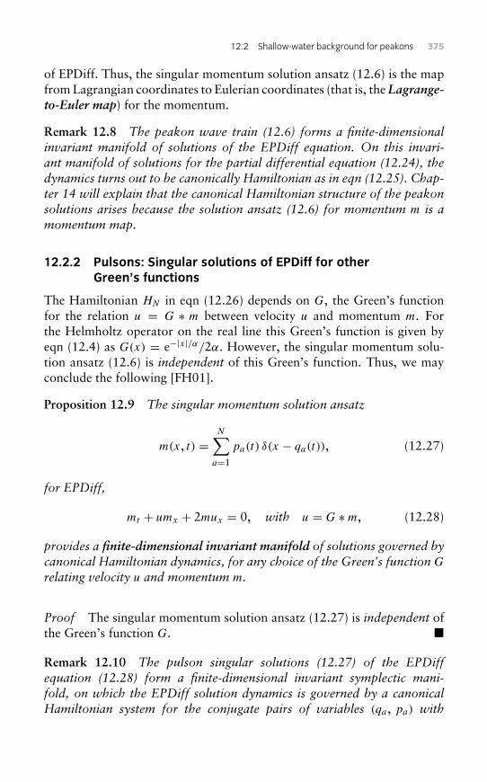
12.2 Shallow-water background for peakons 375
of EPDiff. Thus, the singular momentum solution ansatz (12.6) is the mapfrom Lagrangian coordinates to Eulerian coordinates (that is, the Lagrange-to-Euler map) for the momentum.
Remark 12.8 The peakon wave train (12.6) forms a finite-dimensionalinvariant manifold of solutions of the EPDiff equation. On this invari-ant manifold of solutions for the partial differential equation (12.24), thedynamics turns out to be canonically Hamiltonian as in eqn (12.25). Chap-ter 14 will explain that the canonical Hamiltonian structure of the peakonsolutions arises because the solution ansatz (12.6) for momentum m is amomentum map.
12.2.2 Pulsons: Singular solutions of EPDiff for otherGreen’s functions
The Hamiltonian HN in eqn (12.26) depends on G, the Green’s functionfor the relation u = G ∗ m between velocity u and momentum m. Forthe Helmholtz operator on the real line this Green’s function is given byeqn (12.4) as G(x) = e−|x|/α/2α. However, the singular momentum solu-tion ansatz (12.6) is independent of this Green’s function. Thus, we mayconclude the following [FH01].
Proposition 12.9 The singular momentum solution ansatz
m(x, t) =N∑
a=1
pa(t) δ(x − qa(t)), (12.27)
for EPDiff,
mt + umx + 2mux = 0, with u = G ∗m, (12.28)
provides a finite-dimensional invariant manifold of solutions governed bycanonical Hamiltonian dynamics, for any choice of the Green’s function G
relating velocity u and momentum m.
Proof The singular momentum solution ansatz (12.27) is independent ofthe Green’s function G. �
Remark 12.10 The pulson singular solutions (12.27) of the EPDiffequation (12.28) form a finite-dimensional invariant symplectic mani-fold, on which the EPDiff solution dynamics is governed by a canonicalHamiltonian system for the conjugate pairs of variables (qa, pa) with
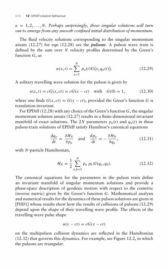
376 12 : EPDiff solution behaviour
a = 1, 2, . . . ,N . Perhaps surprisingly, these singular solutions will turnout to emerge from any smooth confined initial distribution of momentum.
The fluid velocity solutions corresponding to the singular momentumansatz (12.27) for eqn (12.28) are the pulsons. A pulson wave train isdefined by the sum over N velocity profiles determined by the Green’sfunction G, as
u(x, t) =N∑
a=1
pa(t)G(x, qa(t)
). (12.29)
A solitary travelling wave solution for the pulson is given by
u(x, t) = cG(x, ct) = cG(x − ct) with G(0) = 1, (12.30)
where one finds G(x, ct) = G(x − ct), provided the Green’s function G istranslation-invariant.
For EPDiff (12.28) with any choice of the Green’s functionG, the singularmomentum solution ansatz (12.27) results in a finite-dimensional invariantmanifold of exact solutions. The 2N parameters pa(t) and qa(t) in thesepulson-train solutions of EPDiff satisfy Hamilton’s canonical equations
dqadt= ∂HN
∂pa
anddpa
dt= − ∂HN
∂qa, (12.31)
with N -particle Hamiltonian,
HN = 12
N∑a,b=1
pa pb G(qa, qb). (12.32)
The canonical equations for the parameters in the pulson train definean invariant manifold of singular momentum solutions and provide aphase-space description of geodesic motion with respect to the cometric(inverse metric) given by the Green’s function G. Mathematical analysisand numerical results for the dynamics of these pulson solutions are given in[FH01] whose results show how the results of collisions of pulsons (12.29)depend upon the shape of their travelling wave profile. The effects of thetravelling-wave pulse shape
u(x − ct) = cG(x − ct)
on the multipulson collision dynamics are reflected in the Hamiltonian(12.32) that governs this dynamics. For example, see Figure 12.2, in whichthe pulsons are triangular.
12.2 Shallow-water background for peakons 377
0.2
0.1
00 10 20 30 40 50
x
x
t
x
t60 70 80 90 100
u (x
)
Figure 12.2 When the Green’s function G has a triangular profile, a train of triangularpulsons emerges from a Gaussian initial velocity distribution as it evolves under the EPDiffequation (12.1). The upper panels show the collisions that occur as the faster triangularpulsons overtake the slower ones as they cross and re-cross the periodic domain. The upperleft panel shows the progress of the pulsons by by showing offsets of the velocity profile atequal time intervals. The upper right panel shows the pulson paths obtained by plotting theirelevation topography.
Exercise 12.4Verify the hydrodynamic form of the b-equation in eqn (12.16).
Exercise 12.5Verify that the b-equation (12.14) with c0 = 0 and γ = 0 admitspeakon-train solutions of the form (12.5) for any value of b.
Exercise 12.6Verify that the b-equation (12.14) with c0 = 0 and γ = 0 satisfies
ddt‖u‖2
H1 = (b − 2)∫
u3x dx,
for any value of b and for solutions that vanish sufficiently rapidly atspatial infinity that no endpoint contributions arise upon integration byparts.
378 12 : EPDiff solution behaviour
Exercise 12.7Prove a steepening lemma for the b-equation (12.14) with c0 = 0 andγ = 0 that avoids the assumption that u2(x(t), t) remains finite. Thatis, establish a necessary and sufficient condition depending only on theinitial data for blow-up to occur in finite time. How does this conditiondepend on the value of b? Does this steepening lemma hold for everyvalue of b > 1?
Exercise 12.8Are the equations of peakon dynamics for the b-equation (12.14) withc0 = 0 and γ = 0 canonically Hamiltonian for every value of b? Hint:try b = 3.
12.3 Peakons and pulsons
12.3.1 Pulson–Pulson interactions
The solution of EPDiff in 1D
∂tm+ umx + 2uxm = 0, (12.33)
with u = G ∗m for the momentum m = Qopu is given for the interaction ofonly two pulsons by the sum of delta functions in eqn (12.27) with N = 2,
m(x, t) =2∑
i=1
pi(t) δ(x − qi(t)). (12.34)
The parameters satisfy the finite dimensional geodesic canonical Hamil-tonian equations (12.25), in which the Hamiltonian for N = 2 isgiven by
HN=2(q1, q2,p1,p2) = 12(p2
1 + p22)+ p1p2 G(q1 − q2). (12.35)
Conservation laws and reduction to quadrature
Provided the Green’s function G is symmetric under spatial reflections,G(−x) = G(x), the two-pulson Hamiltonian system conserves the total
12.3 Peakons and pulsons 379
momentum
P = p1 + p2. (12.36)
Conservation ofP ensures integrability, by Liouville’s theorem, and reducesthe 2-pulson system to quadratures. To see this, we introduce sum anddifference variables as
P = p1 + p2, Q = q1 + q2, p = p1 − p2, q = q1 − q2. (12.37)
In these variables, the Hamiltonian (12.35) becomes
H(q,p,P) = 14(P 2 − p2)
(1−G(q)
). (12.38)
Likewise, the 2-pulson equations of motion transform to sum and differencevariables as
dPdt= −2
∂H
∂Q= 0,
dQdt= 2
∂H
∂P= P(1+G(q)),
dpdt= −2
∂H
∂q= 1
2(p2 − P 2)G ′(q),dq
dt= 2
∂H
∂p= −p(1−G(q)).
Eliminating p2 between the formula for H and the equation of motionfor q yields (
dqdt
)2
= P 2(1−G(q))2 − 4H
(1−G(q)
)=: Z(G(q);P ,H) ≥ 0, (12.39)
which rearranges into the following quadrature,
dt = dG(q)
G ′(q)√Z(G(q);P ,H)
. (12.40)
For the peakon case, we have G(q) = eq so that G ′(q) = G(q) and thequadrature (12.40) simplifies to an elementary integral. Having obtainedq(t) from the quadrature, the momentum difference p(t) is found from eqn(12.38) via the algebraic expression
p2 = P 2 − 4H1−G(q)
, (12.41)
in terms of q and the constants of motion P and H . Finally, the sum Q(t)
is found by a further quadrature.
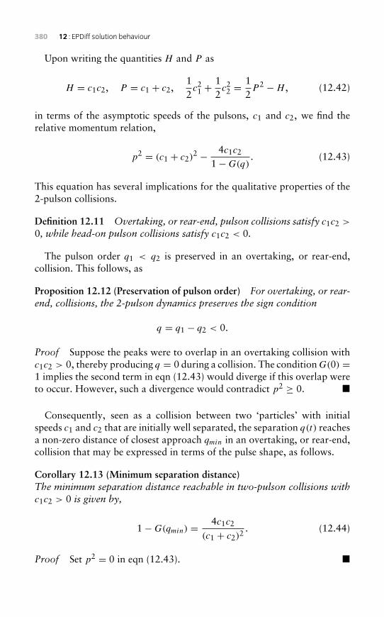
380 12 : EPDiff solution behaviour
Upon writing the quantities H and P as
H = c1c2, P = c1 + c2,12c21 +
12c22 =
12P 2 −H , (12.42)
in terms of the asymptotic speeds of the pulsons, c1 and c2, we find therelative momentum relation,
p2 = (c1 + c2)2 − 4c1c2
1−G(q). (12.43)
This equation has several implications for the qualitative properties of the2-pulson collisions.
Definition 12.11 Overtaking, or rear-end, pulson collisions satisfy c1c2 >
0, while head-on pulson collisions satisfy c1c2 < 0.
The pulson order q1 < q2 is preserved in an overtaking, or rear-end,collision. This follows, as
Proposition 12.12 (Preservation of pulson order) For overtaking, or rear-end, collisions, the 2-pulson dynamics preserves the sign condition
q = q1 − q2 < 0.
Proof Suppose the peaks were to overlap in an overtaking collision withc1c2 > 0, thereby producing q = 0 during a collision. The conditionG(0) =1 implies the second term in eqn (12.43) would diverge if this overlap wereto occur. However, such a divergence would contradict p2 ≥ 0. �
Consequently, seen as a collision between two ‘particles’ with initialspeeds c1 and c2 that are initially well separated, the separation q(t) reachesa non-zero distance of closest approach qmin in an overtaking, or rear-end,collision that may be expressed in terms of the pulse shape, as follows.
Corollary 12.13 (Minimum separation distance)The minimum separation distance reachable in two-pulson collisions withc1c2 > 0 is given by,
1−G(qmin) = 4c1c2
(c1 + c2)2 . (12.44)
Proof Set p2 = 0 in eqn (12.43). �
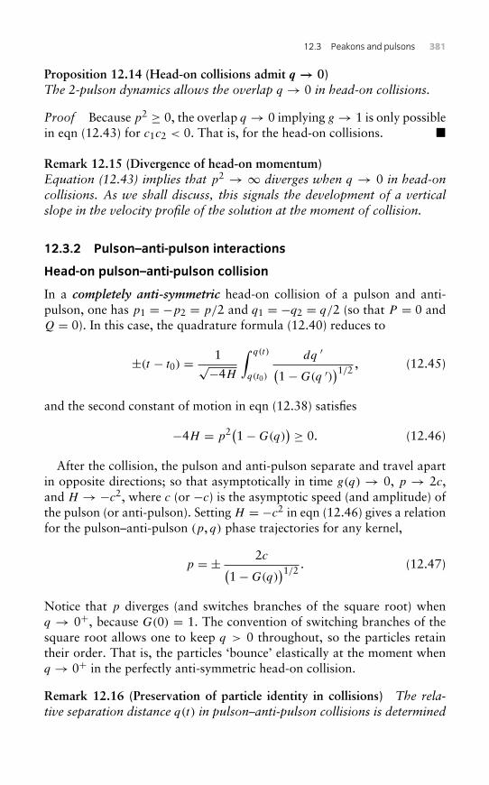
12.3 Peakons and pulsons 381
Proposition 12.14 (Head-on collisions admit q → 0)The 2-pulson dynamics allows the overlap q → 0 in head-on collisions.
Proof Because p2 ≥ 0, the overlap q → 0 implying g→ 1 is only possiblein eqn (12.43) for c1c2 < 0. That is, for the head-on collisions. �
Remark 12.15 (Divergence of head-on momentum)Equation (12.43) implies that p2 → ∞ diverges when q → 0 in head-oncollisions. As we shall discuss, this signals the development of a verticalslope in the velocity profile of the solution at the moment of collision.
12.3.2 Pulson–anti-pulson interactions
Head-on pulson–anti-pulson collision
In a completely anti-symmetric head-on collision of a pulson and anti-pulson, one has p1 = −p2 = p/2 and q1 = −q2 = q/2 (so that P = 0 andQ = 0). In this case, the quadrature formula (12.40) reduces to
±(t − t0) = 1√−4H
∫ q(t)
q(t0)
dq ′(1−G(q ′)
)1/2 , (12.45)
and the second constant of motion in eqn (12.38) satisfies
−4H = p2(1−G(q)) ≥ 0. (12.46)
After the collision, the pulson and anti-pulson separate and travel apartin opposite directions; so that asymptotically in time g(q) → 0, p → 2c,and H →−c2, where c (or −c) is the asymptotic speed (and amplitude) ofthe pulson (or anti-pulson). Setting H = −c2 in eqn (12.46) gives a relationfor the pulson–anti-pulson (p, q) phase trajectories for any kernel,
p = ± 2c(1−G(q)
)1/2 . (12.47)
Notice that p diverges (and switches branches of the square root) whenq → 0+, because G(0) = 1. The convention of switching branches of thesquare root allows one to keep q > 0 throughout, so the particles retaintheir order. That is, the particles ‘bounce’ elastically at the moment whenq → 0+ in the perfectly anti-symmetric head-on collision.
Remark 12.16 (Preservation of particle identity in collisions) The rela-tive separation distance q(t) in pulson–anti-pulson collisions is determined
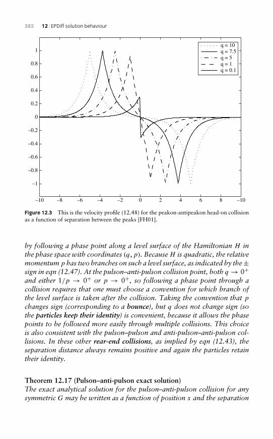
382 12 : EPDiff solution behaviour
–10
–1
–0.8
–0.6
–0.4
–0.2
0
0.2
0.4
0.6
0.8
1
–8 –6 –4 –2 0 2 4 6 8 –10
q = 10q = 7.5q = 5q = 1q = 0.1
Figure 12.3 This is the velocity profile (12.48) for the peakon-antipeakon head-on collisionas a function of separation between the peaks [FH01].
by following a phase point along a level surface of the Hamiltonian H inthe phase space with coordinates (q,p). BecauseH is quadratic, the relativemomentum p has two branches on such a level surface, as indicated by the±sign in eqn (12.47). At the pulson–anti-pulson collision point, both q → 0+and either 1/p → 0+ or p → 0+, so following a phase point through acollision requires that one must choose a convention for which branch ofthe level surface is taken after the collision. Taking the convention that pchanges sign (corresponding to a bounce), but q does not change sign (sothe particles keep their identity) is convenient, because it allows the phasepoints to be followed more easily through multiple collisions. This choiceis also consistent with the pulson–pulson and anti-pulson–anti-pulson col-lisions. In these other rear-end collisions, as implied by eqn (12.43), theseparation distance always remains positive and again the particles retaintheir identity.
Theorem 12.17 (Pulson–anti-pulson exact solution)The exact analytical solution for the pulson–anti-pulson collision for anysymmetric G may be written as a function of position x and the separation
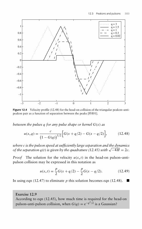
12.3 Peakons and pulsons 383
–3
–1
–0.8
–0.6
–0.4
–0.2
0
0.2
0.4
0.6
0.8
1
–2 –1 0 1 2
q = 0.02q = 0.3q = 1q = 1.5q = 3
3
Figure 12.4 Velocity profile (12.48) for the head-on collision of the triangular peakon–anti-peakon pair as a function of separation between the peaks [FH01].
between the pulses q for any pulse shape or kernel G(x) as
u(x, q) = c(1−G(q)
)1/2 [G(x + q/2)−G(x − q/2)], (12.48)
where c is the pulson speed at sufficiently large separation and the dynamicsof the separation q(t) is given by the quadrature (12.45) with
√−4H = 2c.
Proof The solution for the velocity u(x, t) in the head-on pulson–anti-pulson collision may be expressed in this notation as
u(x, t) = p
2G(x + q/2)− p
2G(x − q/2). (12.49)
In using eqn (12.47) to eliminate p this solution becomes eqn (12.48). �
Exercise 12.9According to eqn (12.45), how much time is required for the head-onpulson–anti-pulson collision, when G(q) = e−q2/2 is a Gaussian?
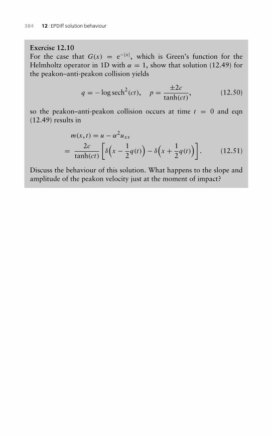
384 12 : EPDiff solution behaviour
Exercise 12.10For the case that G(x) = e−|x|, which is Green’s function for theHelmholtz operator in 1D with α = 1, show that solution (12.49) forthe peakon–anti-peakon collision yields
q = − log sech2(ct), p = ±2c
tanh(ct), (12.50)
so the peakon–anti-peakon collision occurs at time t = 0 and eqn(12.49) results in
m(x, t) = u− α2uxx
= 2ctanh(ct)
[δ(x − 1
2q(t)
)− δ
(x + 1
2q(t)
)]. (12.51)
Discuss the behaviour of this solution. What happens to the slope andamplitude of the peakon velocity just at the moment of impact?
13 Integrability ofEPDiff in 1D
In the previous chapter, we discussed the CH equation for unidirectionalshallow-water waves derived in [CH93], as a special case of the b-equation(12.14) with b = 2,
mt + umx + 2mux = −c0ux + γ uxxx , m = u− α2uxx . (13.1)
This partial differential equation (PDE) describes shallow-water dynamicsat quadratic order in the asymptotic expansion for unidirectional shallow-water waves on a free surface under gravity. The previous chapter discussedits elastic particle-collision solution properties in the dispersionless case forwhich the linear terms on the right side of eqn (13.1) are absent. Theseelastic-collision solution properties hold for any Green’s function G(x)
in the convolution relation u = G ∗ m between velocity u and momen-tum m. For the CH equation G(x) = e−|x|/α is the Green’s function forthe 1D Helmholtz operator on the real line with homogeneous boundaryconditions.
This chapter explains the noncanonical Hamiltonian properties of theCH equation (13.1) in one spatial dimension. In fact, the CH equationhas two compatible Hamiltonian structures, so it is bi-Hamiltonian. Inthis situation, Magri’s lemmas for bi-Hamiltonian PDE in 1D implysystematically that CH arises as a different compatibility conditionfor an isospectral eigenvalue problem and a linear evolution equa-tion for the corresponding eigenfunctions in the case when G(x) =e−|x|/α. The properties of being bi-Hamiltonian and possessing anassociated isospectral problem are ingredients for proving the one-dimensional CH equation (13.1) is completely integrable as a Hamil-tonian system and is solvable by the inverse scattering transform (IST)method.
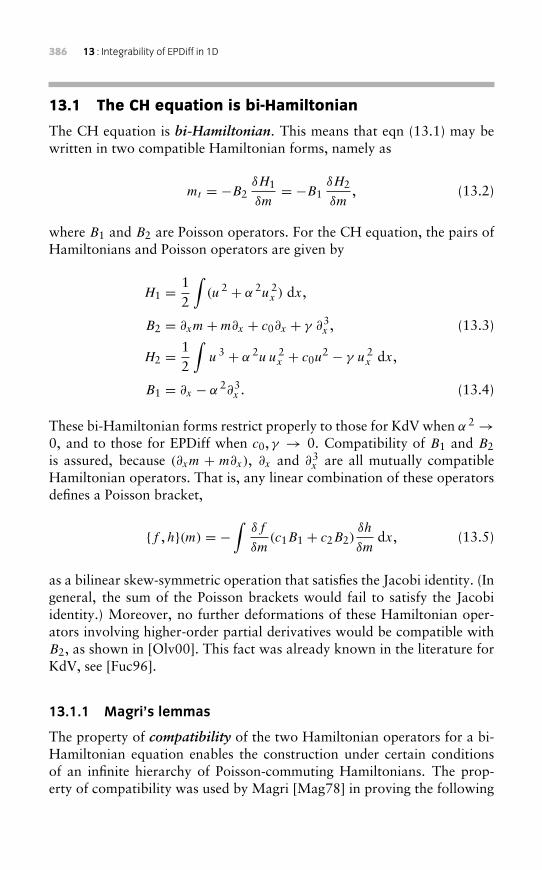
386 13 : Integrability of EPDiff in 1D
13.1 The CH equation is bi-Hamiltonian
The CH equation is bi-Hamiltonian. This means that eqn (13.1) may bewritten in two compatible Hamiltonian forms, namely as
mt = −B2δH1
δm= −B1
δH2
δm, (13.2)
where B1 and B2 are Poisson operators. For the CH equation, the pairs ofHamiltonians and Poisson operators are given by
H1 = 12
∫(u2 + α 2u2
x ) dx,
B2 = ∂xm+m∂x + c0∂x + γ ∂3x , (13.3)
H2 = 12
∫u3 + α 2u u2
x + c0u2 − γ u 2
x dx,
B1 = ∂x − α 2∂3x . (13.4)
These bi-Hamiltonian forms restrict properly to those for KdV when α 2 →0, and to those for EPDiff when c0, γ → 0. Compatibility of B1 and B2is assured, because (∂xm + m∂x), ∂x and ∂3
x are all mutually compatibleHamiltonian operators. That is, any linear combination of these operatorsdefines a Poisson bracket,
{f ,h}(m) = −∫
δf
δm(c1B1 + c2B2)
δh
δmdx, (13.5)
as a bilinear skew-symmetric operation that satisfies the Jacobi identity. (Ingeneral, the sum of the Poisson brackets would fail to satisfy the Jacobiidentity.) Moreover, no further deformations of these Hamiltonian oper-ators involving higher-order partial derivatives would be compatible withB2, as shown in [Olv00]. This fact was already known in the literature forKdV, see [Fuc96].
13.1.1 Magri’s lemmas
The property of compatibility of the two Hamiltonian operators for a bi-Hamiltonian equation enables the construction under certain conditionsof an infinite hierarchy of Poisson-commuting Hamiltonians. The prop-erty of compatibility was used by Magri [Mag78] in proving the following
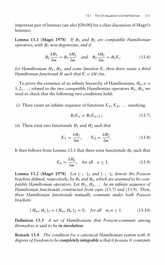
13.1 The CH equation is bi-Hamiltonian 387
important pair of lemmas (see also [Olv00] for a clear discussion of Magri’slemmas):
Lemma 13.1 (Magri 1978) If B1 and B2 are compatible Hamiltonianoperators, with B1 non-degenerate, and if
B2δH1
δm= B1
δH2
δmand B2
δH2
δm= B1K, (13.6)
for Hamiltonians H1, H2, and some function K, then there exists a thirdHamiltonian functional H such that K = δH/δm.
To prove the existence of an infinite hierarchy of Hamiltonians, Hn, n =1, 2, . . . , related to the two compatible Hamiltonian operators B1, B2, weneed to check that the following two conditions hold:
(i) There exists an infinite sequence of functions K1, K2, . . . satisfying
B2Kn = B1Kn+1 ; (13.7)
(ii) There exist two functionals H1 and H2 such that
K1 = δH1
δm, K2 = δH2
δm. (13.8)
It then follows from Lemma 13.1 that there exist functionals Hn such that
Kn = δHn
δm, for all n ≥ 1. (13.9)
Lemma 13.2 (Magri 1978) Let { · , · }1 and { · , · }2 denote the Poissonbrackets defined, respectively, by B1 and B2, which are assumed to be com-patible Hamiltonian operators. Let H1, H2, . . . be an infinite sequence ofHamiltonian functionals constructed from eqns (13.7) and (13.9). Then,these Hamiltonian functionals mutually commute under both Poissonbrackets:
{Hm, Hn }1 = {Hm, Hn }2 = 0, for all m, n ≥ 1. (13.10)
Definition 13.3 A set of Hamiltonians that Poisson-commute amongthemselves is said to be in involution.
Remark 13.4 The condition for a canonical Hamiltonian system with N
degrees of freedom to be completely integrable is that it possessN constants
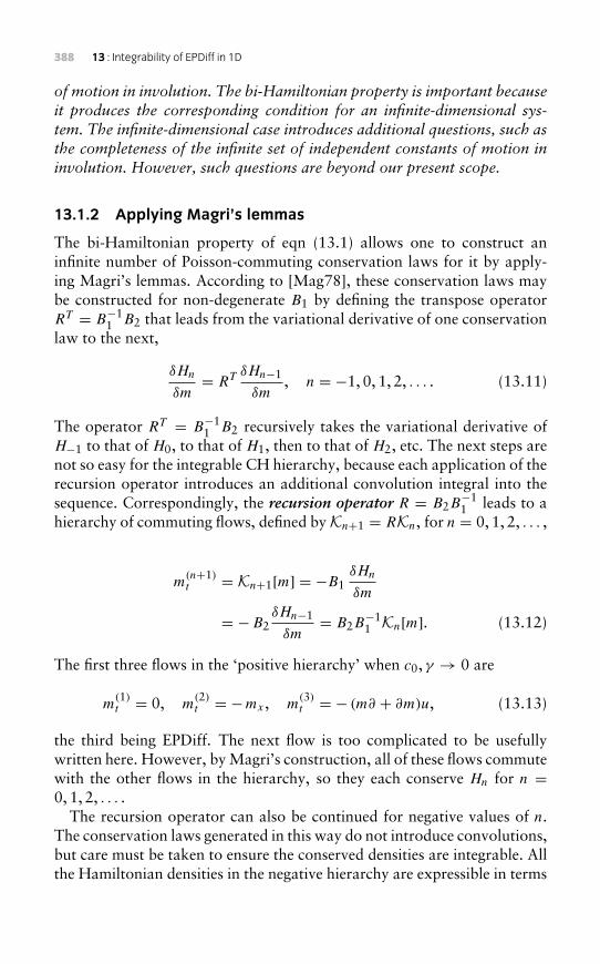
388 13 : Integrability of EPDiff in 1D
of motion in involution. The bi-Hamiltonian property is important becauseit produces the corresponding condition for an infinite-dimensional sys-tem. The infinite-dimensional case introduces additional questions, such asthe completeness of the infinite set of independent constants of motion ininvolution. However, such questions are beyond our present scope.
13.1.2 Applying Magri’s lemmas
The bi-Hamiltonian property of eqn (13.1) allows one to construct aninfinite number of Poisson-commuting conservation laws for it by apply-ing Magri’s lemmas. According to [Mag78], these conservation laws maybe constructed for non-degenerate B1 by defining the transpose operatorRT = B−1
1 B2 that leads from the variational derivative of one conservationlaw to the next,
δHn
δm= RT δHn−1
δm, n = −1, 0, 1, 2, . . . . (13.11)
The operator RT = B−11 B2 recursively takes the variational derivative of
H−1 to that of H0, to that of H1, then to that of H2, etc. The next steps arenot so easy for the integrable CH hierarchy, because each application of therecursion operator introduces an additional convolution integral into thesequence. Correspondingly, the recursion operator R = B2B
−11 leads to a
hierarchy of commuting flows, defined by Kn+1 = RKn, for n = 0, 1, 2, . . . ,
m(n+1)t = Kn+1[m] = −B1
δHn
δm
= −B2δHn−1
δm= B2B
−11 Kn[m]. (13.12)
The first three flows in the ‘positive hierarchy’ when c0, γ → 0 are
m(1)t = 0, m
(2)t = −mx , m
(3)t = − (m∂ + ∂m)u, (13.13)
the third being EPDiff. The next flow is too complicated to be usefullywritten here. However, by Magri’s construction, all of these flows commutewith the other flows in the hierarchy, so they each conserve Hn for n =0, 1, 2, . . . .
The recursion operator can also be continued for negative values of n.The conservation laws generated in this way do not introduce convolutions,but care must be taken to ensure the conserved densities are integrable. Allthe Hamiltonian densities in the negative hierarchy are expressible in terms
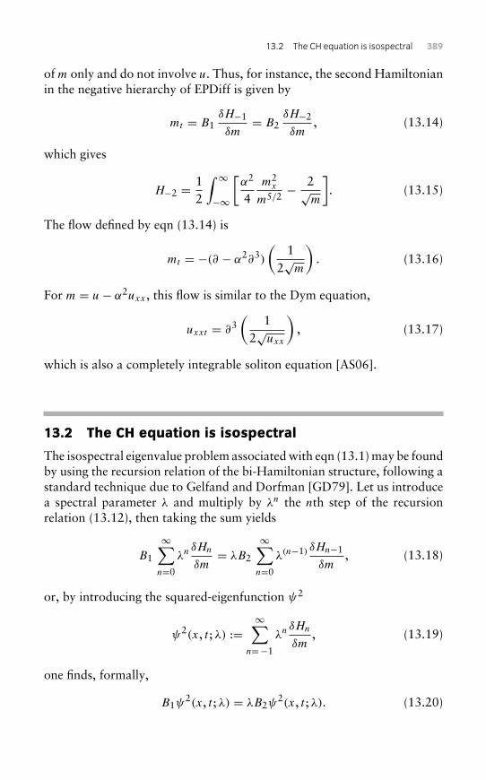
13.2 The CH equation is isospectral 389
of m only and do not involve u. Thus, for instance, the second Hamiltonianin the negative hierarchy of EPDiff is given by
mt = B1δH−1
δm= B2
δH−2
δm, (13.14)
which gives
H−2 = 12
∫ ∞−∞
[α2
4m2
x
m5/2 −2√m
]. (13.15)
The flow defined by eqn (13.14) is
mt = −(∂ − α2∂3)
(1
2√m
). (13.16)
For m = u− α2uxx , this flow is similar to the Dym equation,
uxxt = ∂3(
12√uxx
), (13.17)
which is also a completely integrable soliton equation [AS06].
13.2 The CH equation is isospectral
The isospectral eigenvalue problem associated with eqn (13.1) may be foundby using the recursion relation of the bi-Hamiltonian structure, following astandard technique due to Gelfand and Dorfman [GD79]. Let us introducea spectral parameter λ and multiply by λn the nth step of the recursionrelation (13.12), then taking the sum yields
B1
∞∑n=0
λn δHn
δm= λB2
∞∑n=0
λ(n−1) δHn−1
δm, (13.18)
or, by introducing the squared-eigenfunction ψ2
ψ2(x, t ; λ) :=∞∑
n=−1
λn δHn
δm, (13.19)
one finds, formally,
B1ψ2(x, t ; λ) = λB2ψ
2(x, t ; λ). (13.20)
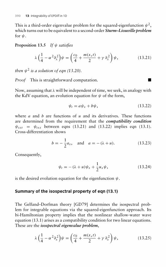
390 13 : Integrability of EPDiff in 1D
This is a third-order eigenvalue problem for the squared-eigenfunction ψ2,which turns out to be equivalent to a second-order Sturm–Liouville problemfor ψ .
Proposition 13.5 If ψ satisfies
λ(14− α 2∂ 2
x
)ψ =
(c0
4+ m(x, t)
2+ γ ∂ 2
x
)ψ , (13.21)
then ψ2 is a solution of eqn (13.20).
Proof This is straightforward computation. �
Now, assuming that λ will be independent of time, we seek, in analogy withthe KdV equation, an evolution equation for ψ of the form,
ψt = aψx + bψ , (13.22)
where a and b are functions of u and its derivatives. These functionsare determined from the requirement that the compatibility conditionψxxt = ψtxx between eqns (13.21) and (13.22) implies eqn (13.1).Cross-differentiation shows
b = − 12ax , and a = − (λ+ u). (13.23)
Consequently,
ψt = − (λ+ u)ψx + 12uxψ , (13.24)
is the desired evolution equation for the eigenfunction ψ .
Summary of the isospectral property of eqn (13.1)
The Gelfand–Dorfman theory [GD79] determines the isospectral prob-lem for integrable equations via the squared-eigenfunction approach. Itsbi-Hamiltonian property implies that the nonlinear shallow-water waveequation (13.1) arises as a compatibility condition for two linear equations.These are the isospectral eigenvalue problem,
λ(14− α 2∂ 2
x
)ψ =
(c0
4+ m(x, t)
2+ γ ∂ 2
x
)ψ , (13.25)
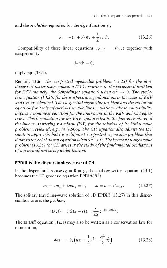
13.2 The CH equation is isospectral 391
and the evolution equation for the eigenfunction ψ ,
ψt = −(u+ λ)ψx + 12ux ψ . (13.26)
Compatibility of these linear equations (ψxxt = ψtxx) together withisospectrality
dλ/dt = 0,
imply eqn (13.1).
Remark 13.6 The isospectral eigenvalue problem (13.25) for the non-linear CH water-wave equation (13.1) restricts to the isospectral problemfor KdV (namely, the Schrödinger equation) when α 2 → 0. The evolu-tion equation (13.26) for the isospectral eigenfunctions in the cases of KdVand CH are identical. The isospectral eigenvalue problem and the evolutionequation for its eigenfunctions are two linear equations whose compatibilityimplies a nonlinear equation for the unknowns in the KdV and CH equa-tions. This formulation for the KdV equation led to the famous method ofthe inverse scattering transform (IST) for the solution of its initial-valueproblem, reviewed, e.g., in [AS06]. The CH equation also admits the ISTsolution approach, but for a different isospectral eigenvalue problem thatlimits to the Schrödinger equationwhen α 2 → 0. The isospectral eigenvalueproblem (13.25) for CH arises in the study of the fundamental oscillationsof a non-uniform string under tension.
EPDiff is the dispersionless case of CH
In the dispersionless case c0 = 0 = γ , the shallow-water equation (13.1)becomes the 1D geodesic equation EPDiff(H 1)
mt + umx + 2mux = 0, m = u− α2uxx . (13.27)
The solitary travelling-wave solution of 1D EPDiff (13.27) in this disper-sionless case is the peakon,
u(x, t) = cG(x − ct) = c
2αe−|x−ct |/α.
The EPDiff equation (12.1) may also be written as a conservation law formomentum,
∂tm = −∂x(um+ 1
2u2 − α2
2u2x
). (13.28)
392 13 : Integrability of EPDiff in 1D
Its isospectral problem forms the basis for completely integrating the EPDiffequation as a Hamiltonian system and, thus, for finding its soliton solu-tions. Remarkably, the isospectral problem (13.25) in the dispersionlesscase c0 = 0 = � has a purely discrete spectrum on the real line and theN -soliton solutions for this equation may be expressed as a peakon wavetrain,
u(x, t) =N∑i=1
pi(t)e−|x−qi(t)|/α. (13.29)
As before, pi(t) and qi(t) satisfy the finite-dimensional geodesic motionequations obtained as Hamilton’s canonical equations
qi = ∂HN
∂pi
and pi = − ∂HN
∂qi, (13.30)
where the Hamiltonian is given by,
HN = 12
N∑i,j=1
pi pj e−|qi−qj |/α. (13.31)
Thus, we have proved the following.
Theorem 13.7 CH peakons are an integrable subcase of EPDiff pulsonsin one dimension for the choice of the H 1 norm.
Remark 13.8 The discrete process of peakon creation via the steepeninglemma 12.1.1 is consistent with the discreteness of the isospectrum for theeigenvalue problem (13.25) in the dispersionless case, when c0 = 0 = γ .These discrete eigenvalues correspond in turn to the asymptotic speeds ofthe peakons. The discreteness of the isospectrum means that only peakonswill emerge in the initial-value problem for EPDiff(H 1) in 1D.
Constants of motion for integrable N-peakon dynamics
One may verify the integrability of the N -peakon dynamics by substi-tuting the N -peakon solution (13.29) (which produces the sum of deltafunctions (12.6) for the momentum m) into the isospectral problem(13.25). This substitution reduces (13.25) to an N × N matrix eigenvalueproblem.
13.2 The CH equation is isospectral 393
In fact, the canonical equations (13.30) for the peakon Hamiltonian(13.31) may be written directly in Lax matrix form,
dLdt= [L,A] ⇐⇒ L(t) = U(t)L(0)U†(t), (13.32)
with A = UU†(t) and UU† = Id. Explicitly, L and A are N × N matriceswith entries
Ljk = √pjpk φ(qi − qj ), Ajk = −2√pjpk φ
′(qi − qj ). (13.33)
Here, φ′(x) denotes derivative with respect to the argument of the func-tion φ, given by φ(x) = e−|x|/2α = 2αG(x/2). The Lax matrix L in eqn(13.32) evolves by time-dependent unitary transformations, which leaveits spectrum invariant. Isospectrality then implies that the traces trLn,n = 1, 2, . . . ,N of the powers of the matrix L (or, equivalently, its N
eigenvalues) yield N constants of the motion. These turn out to be function-ally independent, non-trivial and in involution under the canonical Poissonbracket. Hence, the canonically Hamiltonian N -peakon dynamics (13.30)is completely integrable in the finite-dimensional (Liouville) sense.
Exercise 13.1Verify that the compatibility condition (equality of cross derivativesψxxt = ψtxx) obtained from the eigenvalue equation (13.25) and theevolution equation (13.26) do indeed yield the CH shallow-water waveequation (13.1) when the eigenvalue λ is constant.
Exercise 13.2Show that the peakon Hamiltonian HN in (13.31) may be expressed asa function of the invariants of the matrix L, as
HN = −trL2 + 2(trL)2. (13.34)
Show that evenness of HN implies
1. The N coordinates qi , i = 1, 2, . . . ,N keep their initial ordering.
2. The N conjugate momenta pi , i = 1, 2, . . . ,N keep their initial signs.
This means that no difficulties arise, either due to the non-analyticity ofφ(x), or the sign in the square roots in the Lax matrices L and A.
394 13 : Integrability of EPDiff in 1D
Exercise 13.3 (Hunter–Saxton equation)Retrace the progress of this chapter for the EPDiff equation
mt + umx + 2mux = 0, with m = −uxx . (13.35)
This integrable Hamiltonian partial differential equation arises in thetheory of liquid crystals. Its peakon solutions are the compactly sup-ported triangles in Figure 12.2 and Figure 12.4. It may also be regardedas the α→∞ limit of the CH equation. For more results and discussionof this equation, see [HZ94].
14EPDiff in n dimensions
This chapter discusses the n-dimensional generalization of the one-dimensional singular solutions of the EP equation studied in theprevious chapter. Much of the one-dimensional structure persists inhigher dimensions. For example, the parameters defining the singularsolutions of EPDiff in n dimensions still obey canonical Hamilto-nian equations. This is understood by identifying the singular solutionansatz as a cotangent-lift momentum map for the left action of thediffeomorphisms on the lower-dimensional support set of the singularsolutions.
14.1 Singular momentum solutions of the EPDiffequation for geodesic motion in higher dimensions
14.1.1 n-dimensional EPDiff equation
Eulerian geodesic motion of an ideal continuous fluid in n dimensions isgenerated as an EP equation via Hamilton’s principle, when the Lagrangianis given by the kinetic energy. The kinetic energy defines a norm ‖u‖2 for theEulerian fluid velocity, u(x, t) : Rn × R1 → Rn. As mentioned earlier, thechoice of the kinetic energy as a positive functional of fluid velocity u is amodelling step that depends upon the physics of the problem being studied.Following our earlier procedure, as in eqns (11.11) and (11.14), we shallchoose the Lagrangian,
‖u‖2 =∫
u ·Qopu dnx =∫
u ·m dnx, (14.1)
so that the positive-definite, symmetric, operator Qop defines the norm ‖u‖,under integration by parts for appropriate boundary conditions and theEPDiff equation for Eulerian geodesic motion of a fluid emerges,
ddt
δ�
δu+ ad∗u
δ�
δu= 0, with �[u] = 1
2‖u‖2. (14.2)
396 14 : EPDiff in n dimensions
Legendre transforming to the Hamiltonian side
The corresponding Legendre transform yields the following invertiblerelations between momentum and velocity,
m = Qopu and u = G ∗m, (14.3)
where G is the Green’s function for the operator Qop, assuming appropriateboundary conditions (on u) that allow inversion of the operator Qop todetermine u from m.
The associated Hamiltonian is,
h[m] = 〈m, u〉 − 12‖u‖2 = 1
2
∫m ·G ∗m dnx =:
12‖m‖2, (14.4)
which also defines a norm ‖m‖ via a convolution kernel G that is symmetricand positive, when the Lagrangian �[u] is a norm. As expected, the norm‖m‖ given by the Hamiltonian h[m] specifies the velocity u in terms of itsLegendre-dual momentum m by the variational operation,
u = δh
δm= G ∗m ≡
∫G(x − y)m(y) dny. (14.5)
We shall choose the kernelG(x−y) to be translation-invariant (so Noether’stheorem implies that total momentum M = ∫ m dnx is conserved) and sym-metric under spatial reflections (so that u and m have the same parity underspatial reflections).
After the Legendre transformation (14.4), the EPDiff equation (11.14)appears in its equivalent Lie–Poisson Hamiltonian form,
∂
∂tm = {m,h} = − ad∗δh/δmm. (14.6)
Here the operation {·, · } denotes the Lie–Poisson bracket dual to the (right)action of vector fields amongst themselves by vector-field commutation.That is,
{f , h } = −⟨m,[δf
δm,
δh
δm
]⟩. (14.7)
For more details and additional background concerning the relation ofclassical EP theory to Lie–Poisson Hamiltonian equations, see [MR02,HMR98a]. In a moment we will also consider the momentum maps forEPDiff.
14.1 Singular solutions of EPDiff 397
14.1.2 Pulsons in n dimensions
The momentum for the one-dimensional pulson solutions (12.6) on the realline is supported at points via the Dirac delta measures in its solution ansatz,
m(x, t) =N∑i=1
pi(t) δ(x − qi(t)
), m ∈ R. (14.8)
We shall develop n-dimensional analogues of these one-dimensional pulsonsolutions for the Euler–Poincaré equation (11.23) by generalizing this solu-tion ansatz to allow measure-valued n-dimensional vector solutions m ∈ Rn
for which the Euler–Poincaré momentum is supported on codimension-ksubspaces Rn−k with integer k ∈ [1, n]. For example, one may con-sider the two-dimensional vector momentum m ∈ R2 in the plane thatis supported on one-dimensional curves (momentum fronts). Likewise, inthree dimensions, one could consider two-dimensional momentum surfaces(sheets), one-dimensional momentum filaments, etc. The correspondingvector momentum ansatz that we shall use is the following, cf. the pulsonsolutions (14.8),
m(x, t) =N∑i=1
∫Pi (s, t) δ
(x −Q i (s, t)
)ds, m ∈ Rn. (14.9)
Here, Pi ,Qi ∈ Rn for i = 1, 2, . . . ,N . For example, when n−k = 1, so thats ∈ R is one-dimensional, the delta function in solution (14.9) supports anevolving family of vector-valued curves, called momentum filaments. (Forsimplicity of notation, we suppress the implied subscript i in the arclengths for each Pi and Qi .) The Legendre-dual relations (14.3) imply that thevelocity corresponding to the momentum filament ansatz (14.9) is,
u(x, t) = G ∗m =N∑
j=1
∫Pj (s
′, t)G(x −Q j (s
′, t))ds′. (14.10)
Just as for the 1D case of the pulsons, we shall show that substitution ofthe n-D solution ansatz (14.9) and (14.10) into the EPDiff equation (11.20)produces canonical geodesic Hamiltonian equations for the n-dimensionalvector parameters Qi (s, t) and Pi (s, t), i = 1, 2, . . . ,N .
Canonical Hamiltonian dynamics of momentum filaments
For definiteness in what follows, we shall consider the example of momen-tum filaments m ∈ Rn supported on one-dimensional space curves in Rn,
398 14 : EPDiff in n dimensions
so s ∈ R is the arclength parameter of one of these curves. This solutionansatz is reminiscent of the Biot–Savart Law for vortex filaments, althoughthe flow is not incompressible. The dynamics of momentum surfaces, fors ∈ Rk with k < n, follow a similar analysis.
Substituting the momentum filament ansatz (14.9) for s ∈ R and itscorresponding velocity (14.10) into the Euler–Poincaré equation (11.20),then integrating against a smooth test function φ(x) implies the followingcanonical equations (denoting explicit summation on i, j ∈ 1, 2, . . . N),
∂
∂tQi (s, t) =
N∑j=1
∫P′j G(Qi −Q′j )ds′ =
δHN
δPi
, (14.11)
∂
∂tPi (s, t) = −
N∑j=1
∫ (Pi · P′j
) ∂
∂Qi
G(Qi −Q′j ) ds′
= − δHN
δQi
, (14.12)
where Pi = Pi (s, t), P′j := Pj (s′, t) and
G(Qi −Q′j ) := G(Qi (s, t)−Qj (s′, t)). (14.13)
The dot product Pi · P′j denotes the inner, or scalar, product of the twovectors Pi and P′j in T ∗Rn. Thus, the solution ansatz (14.9) yields a closedset of integro-partial-differential equations (IPDEs) given by (14.11) and(14.12) for the vector parameters Qi (s, t) and Pi (s, t) with i = 1, 2 . . . N .These equations are generated canonically by the Hamiltonian functionHN : (T ∗Rn)N → R given by
HN [P,Q] = 12
∫∫ N∑i, j=1
(Pi · P′j
)G(Qi −Q′j
)ds ds′ =:
12‖P‖2. (14.14)
This Hamiltonian arises by inserting the momentum ansatz (14.9) intothe Hamiltonian (14.4) obtained from the Legendre transformation of theLagrangian corresponding to the kinetic energy norm of the fluid veloc-ity. Thus, the evolutionary IPDE system (14.11) and (14.12) representscanonically Hamiltonian geodesic motion on the space of curves in Rn withrespect to the cometric given on these curves in eqn (14.14). The Hamil-tonian HN = 1
2‖P‖2 in eqn (14.14) defines the norm ‖P‖ in terms of thiscometric that combines convolution using the Green’s function G and sumover filaments with the scalar product of momentum vectors in Rn.
14.2 Singular solution momentummap 399
Remark 14.1 Note that the coordinate s is a Lagrangian label movingwith the fluid, since
∂
∂tQi (s, t) = u(Qi (s, t), t).
Exercise 14.1Explain the meaning of the Hamiltonian equation (14.6) with Lie–Poisson bracket (14.7). Discuss the interpretation of {m,h} when mis a vector.Hint: write m(x, t) as a spatial integral by inserting a delta function,
m(x, t) =∫
R3m(y, t) δ(x − y) d3y.
Use this representation to show that the Lie–Poisson bracket (14.7)yields dynamics in the form of eqn (14.6),
{m,h} = −⟨ad∗δh/δmm, δ(x − y)
⟩= − ad∗δh/δmm.
14.2 Singular solution momentum map JSingThe momentum filament ansatz (14.9) reduces the solution of the geodesicEP PDE (11.20) in n+1 dimensions to the system of eqns (14.11) and (14.12)of 2N canonical evolutionary IPDEs. One can summarize the mechanismby which this process occurs, by saying that the map that implements thecanonical (Q, P) variables in terms of singular solutions is a (cotangentbundle) momentum map.
Such momentum maps are Poisson maps; so the canonical Hamiltoniannature of the dynamical equations for (Q, P) fits into a general theory thatalso provides a framework for suggesting other avenues of investigation.
Theorem 14.2 Themomentum ansatz (14.9) formeasure-valued solutionsof the EPDiff equation (11.20), defines an equivariant momentum map
JSing : T ∗ Emb(S, Rn)→ X(Rn)∗,
called the singular solution momentum map in [HM04].
400 14 : EPDiff in n dimensions
We shall explain the notation used in the theorem’s statement in thecourse of its proof. By ‘defines’ one means that the momentum solutionansatz (14.9) expressing m (a vector function of spatial position x) in termsof Q, P (which are functions of s) can be regarded as a map from the spaceof (Q(s), P(s)) to the space of m’s. This will turn out to be the Lagrange-to-Euler map for the fluid description of the singular solutions.
Following [HM04], we shall give two proofs of this result from tworather different viewpoints. The first proof below uses the formula for amomentum map for a cotangent lifted action, while the second proof focuseson a Poisson bracket computation. Each proof also explains the context inwhich one has a momentum map. (See [MR02] for general discussions onmomentum maps.)
First proof. For simplicity and without loss of generality, let us take N = 1and so suppress the index a. That is, we shall take the case of an isolatedsingular solution. As the proof will show, this is not a real restriction.
Proof To set the notation, fix a k-dimensional manifold S with a givenvolume element and whose points are denoted s ∈ S. Let Emb(S, Rn) denotethe set of smooth embeddings Q : S → Rn. (If the EPDiff equations aretaken on a manifold M, replace Rn with M.) Under appropriate technicalconditions, which we shall just treat formally here, Emb(S, Rn) is a smoothmanifold. (See, for example, [EM70] and [MH94] for a discussion andreferences.)
The tangent space TQ Emb(S, Rn) to Emb(S, Rn) at a point Q ∈Emb(S, Rn) is given by the space of material velocity fields, namely thelinear space of maps V : S → Rn that are vector fields over the map Q. Thedual space to this space will be identified with the space of one-form den-sities over Q, which we shall regard as maps P : S → (Rn)∗. In summary,the cotangent bundle T ∗ Emb(S, Rn) is identified with the space of pairs ofmaps (Q, P).
These give us the domain space for the singular solution momentum map.Now we consider the action of the symmetry group. Consider the groupG =Diff of diffeomorphisms of the space Rn in which the EPDiff equations areoperating, concretely in our case this is Rn. Let it act on Rn by compositionon the left. Namely, for η ∈ Diff(Rn), we let
η ·Q = η ◦Q. (14.15)
Now lift this action to the cotangent bundle T ∗ Emb(S, Rn) in the stan-dard way. One may consult, for instance, [MR02] for this cotangent-lift
14.2 Singular solution momentummap 401
construction. However, it is also given explicitly by the variational con-struction in eqn (15.4). This lifted action is a symplectic (and hencePoisson) action and has an equivariant momentum map. This cotangent-lift momentum map for the left action (14.15) is precisely given by theansatz (14.9).
To see this, one only needs to recall and then apply the general formulafor the momentum map associated with an action of a general Lie group G
on a configuration manifold Q and cotangent lifted to T ∗Q.First let us recall the general formula. Namely, the momentum map is the
map J : T ∗Q→ g∗ (g∗ denotes the dual of the Lie algebra g of G) defined by
J(αq) · ξ =⟨αq , ξQ(q)
⟩, (14.16)
where αq ∈ T ∗q Q and ξ ∈ g, where ξQ is the infinitesimal generator ofthe action of G on Q associated to the Lie algebra element ξ , and where⟨αq , ξQ(q)
⟩is the natural pairing of an element of T ∗q Q with an element
of TqQ.Now we apply this formula to the special case in which the group G is the
diffeomorphism group Diff(Rn), the manifold Q is Emb(S, Rn) and wherethe action of the group on Emb(S, Rn) is given by eqn (14.15). The Liealgebra of G = Diff is the space g = X of vector fields. Hence, its dual isnaturally regarded as the space of one-form densities. The momentum mapis thus a map J : T ∗ Emb(S, Rn)→ X∗.
With J given by (14.16), we only need to work out this formula. First,we shall work out the infinitesimal generators. Let X ∈ X be a Lie algebraelement. By differentiating the action (14.15) with respect to η in the direc-tion of X at the identity element we find that the infinitesimal generator isgiven by
XEmb(S,Rn)(Q) = X ◦Q.
Thus, on taking αq to be the cotangent vector (Q, P), eqn (14.16) gives
⟨J(Q, P),X
⟩ = ⟨(Q, P),X ◦Q⟩=∫S
Pi(s)Xi(Q(s))dks.
On the other hand, note that the right-hand side of eqn (14.9) (again withthe index a suppressed, and with t suppressed as well), when paired with
402 14 : EPDiff in n dimensions
the Lie algebra element X is⟨∫S
P(s) δ (x −Q(s))dks,X⟩
=∫
Rn
∫S
(Pi(s) δ (x −Q(s)) dks
)Xi(x)dnx
=∫S
Pi(s)Xi(Q(s))dks.
This shows that the expression given by eqn (14.9) is equal to J and so theresult is proved. �
Second proof. Momentum maps may be characterized by means ofthe following relation [MR02], required to hold for all functions F onT ∗ Emb(S, Rn). Namely, for all functions F of Q and P one requires thePoisson-bracket relation,
{F , 〈J, ξ〉} = ξP [F ]. (14.17)
For the second proof, we shall take J to be given by the solution ansatz(14.9) and verify that it satisfies this momentum-map relation.
Proof On one hand, let ξ ∈ X so that the left side of eqn (14.17) becomes{F ,∫S
Pi(s)ξi(Q(s))dks
}=∫S
[δF
δQiξ i(Q(s))− Pi(s)
δF
δPj
δ
δQjξ i(Q(s))
]dks.
On the other hand, one can compute directly from the definitions that theinfinitesimal generator of the action on T ∗ Emb(S, Rn) corresponding tothe vector field ξ i(x) ∂
∂Qi (a Lie algebra element), is given by (see [MR02],formula (12.1.14)):
δQ = ξ ◦Q, δP = −Pi(s)∂
∂Qξ i(Q(s)),
which verifies that eqn (14.17) holds.An important element left out in this proof so far is that it does not
make clear that the momentum map is equivariant, a condition neededfor the momentum map to be Poisson. The first proof took care of thisproperty automatically since momentum maps for cotangent-lifted actionsare always equivariant and hence are Poisson.
Thus, to complete the second proof, one should check that the momentummap is equivariant and is thus Poisson. Instead, one may simply check
14.2 Singular solution momentummap 403
directly that it is a Poisson map from T ∗ Emb(S, Rn) to m ∈ X∗ (the dualspace of the Lie algebra X) with its Lie–Poisson bracket.
The following direct computation shows that the singular solutionmomentum map (14.9) is Poisson. For this, one uses the canonical Poissonbrackets for {P}, {Q} and applies the chain rule to compute
{mi(x),mj(y)
},
with notation δ ′k(y) ≡ ∂δ(y)/∂yk. The result then follows by a directsubstitution of the singular solution (14.9) into the Poisson bracket,
{mi(x),mj(y)
}={ N∑
a=1
∫ds P a
i (s, t) δ(x −Qa(s, t)),
N∑b=1
∫ds′Pb
j (s′, t) δ(y −Qb(s′, t))
}
=N∑
a,b=1
∫∫dsds′
[{Pa
i (s),Pbj (s′)} δ(x −Qa(s)) δ(y −Qb(s′))
− {Pai (s),Q
bk(s′)}Pb
j (s′) δ(x −Qa(s)) δ ′k(y −Qb(s′))
− {Qak(s),P
bj (s′)}Pa
i (s) δ′k(x −Qa(s)) δ(y −Qb(s′))
+ {Qak(s),Q
b�(s′)}Pa
i (s)Pbj (s′) δ ′k(x −Qa(s)) δ ′�(y −Qb(s′))
].
Substituting the canonical Poisson bracket relations
{Pai (s),P
bj (s′)} = 0
{Qak(s),Q
b�(s′)} = 0, and
{Qak(s),P
bj (s′)} = δabδkj δ(s − s′)
into the preceding computation yields,
{mi(x),mj(y)
} = N∑a=1
∫dsP a
j (s) δ(x −Qa(s)) δ ′i (y −Qa(s))
−N∑
a=1
∫dsP a
i (s) δ′j (x −Qa(s)) δ(y −Qa(s))
= −(mj(x)
∂
∂xi+ ∂
∂x jmi(x)
)δ(x − y).
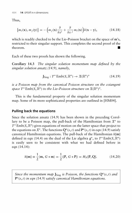
404 14 : EPDiff in n dimensions
Thus,
{mi(x), mj(y)
} = − (mj(x)∂
∂xi+ ∂
∂x jmi(x)
)δ(x − y), (14.18)
which is readily checked to be the Lie–Poisson bracket on the space of m’s,restricted to their singular support. This completes the second proof of thetheorem. �
Each of these two proofs has shown the following.
Corollary 14.3 The singular solution momentum map defined by thesingular solution ansatz (14.9), namely,
JSing : T ∗ Emb(S, Rn)→ X(Rn)∗ (14.19)
is a Poisson map from the canonical Poisson structure on the cotangentspace T ∗ Emb(S, Rn) to the Lie–Poisson structure on X(Rn)∗.
This is the fundamental property of the singular solution momentummap. Some of its more sophisticated properties are outlined in [HM04].
Pulling back the equations
Since the solution ansatz (14.9) has been shown in the preceding Corol-lary to be a Poisson map, the pull-back of the Hamiltonian from X∗ toT ∗ Emb(S, Rn) gives equations of motion on the latter space that project tothe equations on X∗. The functions Qa(s, t) and Pa(s, t) in eqn (14.9) satisfycanonical Hamiltonian equations. The pull-back of the Hamiltonian h[m]defined in eqn (14.4) on the dual of the Lie algebra g∗, to T ∗ Emb(S, Rn)
is easily seen to be consistent with what we had defined before ineqn (14.14):
h[m] ≡ 12〈m, G ∗m〉 = 1
2〈〈P, G ∗ P〉〉 = HN [P,Q]. (14.20)
Since the momentum map JSing is Poisson, the functions Qa(s, t) andPa(s, t) in eqn (14.9) satisfy canonical Hamiltonian equations.
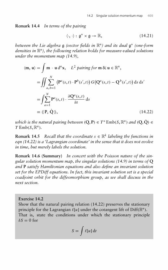
14.2 Singular solution momentummap 405
Remark 14.4 In terms of the pairing
〈·, ·〉 : g∗ × g→ R, (14.21)
between the Lie algebra g (vector fields in Rn) and its dual g∗ (one-formdensities in Rn), the following relation holds for measure-valued solutionsunder the momentum map (14.9),
〈m, u〉 =∫
m · u dnx, L2 pairing for m& u ∈ Rn,
=∫∫ N∑
a, b=1
(Pa(s, t) · Pb(s′, t)
)G(Qa(s, t)−Q b(s′, t)
)ds ds′
=∫ N∑
a=1
Pa(s, t) · ∂Qa(s, t)∂t
ds
≡ 〈〈 P, Q 〉〉, (14.22)
which is the natural pairing between (Q, P) ∈ T ∗ Emb(S, Rn) and (Q, Q) ∈T Emb(S, Rn).
Remark 14.5 Recall that the coordinate s ∈ Rk labeling the functions ineqn (14.22) is a ‘Lagrangian coordinate’ in the sense that it does not evolvein time, but merely labels the solution.
Remark 14.6 (Summary) In concert with the Poisson nature of the sin-gular solution momentum map, the singular solutions (14.9) in terms of Qand P satisfy Hamiltonian equations and also define an invariant solutionset for the EPDiff equations. In fact, this invariant solution set is a specialcoadjoint orbit for the diffeomorphism group, as we shall discuss in thenext section.
Exercise 14.2Show that the natural pairing relation (14.22) preserves the stationaryprinciple for the Lagrangian �[u] under the cotangent lift of Diff(Rn).That is, state the conditions under which the stationary principleδS = 0 for
S =∫
�[u] dt
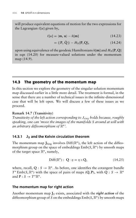
406 14 : EPDiff in n dimensions
will produce equivalent equations of motion for the two expressions forthe Lagrangian �[u] given by,
�[u] = 〈m, u〉 − h[m] (14.23)
= 〈〈 P, Q 〉〉 −HN [P,Q], (14.24)
upon using equivalence of the geodesic Hamiltonians h[m] andHN [P,Q]in eqn (14.20) for measure-valued solutions under the momentummap (14.9).
14.3 The geometry of the momentum map
In this section we explore the geometry of the singular solution momentummap discussed earlier in a little more detail. The treatment is formal, in thesense that there are a number of technical issues in the infinite-dimensionalcase that will be left open. We will discuss a few of these issues as weproceed.
Remark 14.7 (Transitivity)Transitivity of the left action corresponding to Jsing holds because, roughlyspeaking, one can ‘move the images of the manifolds S around at will withan arbitrary diffeomorphism of Rn’.
14.3.1 JS and the Kelvin circulation theorem
The momentum map JSing involves Diff(Rn), the left action of the diffeo-morphism group on the space of embeddings Emb(S, Rn) by smooth mapsof the target space Rn, namely,
Diff(Rn) : Q · η = η ◦Q, (14.25)
where, recall, Q : S → Rn. As before, one identifies the cotangent bundleT ∗ Emb(S, Rn) with the space of pairs of maps (Q, P), with Q : S → Rn
and P : S → T ∗Rn.
The momentum map for right action
Another momentum map JS exists, associated with the right action of thediffeomorphism group of S on the embeddings Emb(S, Rn) by smooth maps
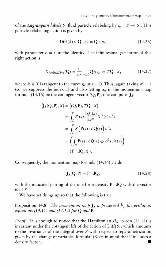
14.3 The geometry of the momentummap 407
of the Lagrangian labels S (fluid particle relabeling by ηr : S → S). Thisparticle-relabelling action is given by
Diff(S) : Q · ηr = Q ◦ ηr , (14.26)
with parameter r = 0 at the identity. The infinitesimal generator of thisright action is
XEmb(S,Rn)(Q) = ddr
∣∣∣r=0
Q ◦ ηr = TQ ·X, (14.27)
where X ∈ X is tangent to the curve ηr at r = 0. Thus, again taking N = 1(so we suppress the index a) and also letting αq in the momentum mapformula (14.16) be the cotangent vector (Q, P), one computes JS :⟨
JS(Q, P),X⟩ = ⟨(Q, P), TQ ·X⟩=∫S
Pi(s)∂Qi(s)
∂smXm(s) dks
=∫S
X(P(s) · dQ(s)
)dks
=(∫
S
P(s) · dQ(s)⊗ dks,X(s)
)= 〈P · dQ,X 〉.
Consequently, the momentum map formula (14.16) yields
JS(Q, P) = P · dQ, (14.28)
with the indicated pairing of the one-form density P · dQ with the vectorfield X.
We have set things up so that the following is true.
Proposition 14.8 The momentum map JS is preserved by the evolutionequations (14.11) and (14.12) for Q and P.
Proof It is enough to notice that the Hamiltonian HN in eqn (14.14) isinvariant under the cotangent lift of the action of Diff(S), which amountsto the invariance of the integral over S with respect to reparametrizationgiven by the change of variables formula. (Keep in mind that P includes adensity factor.) �
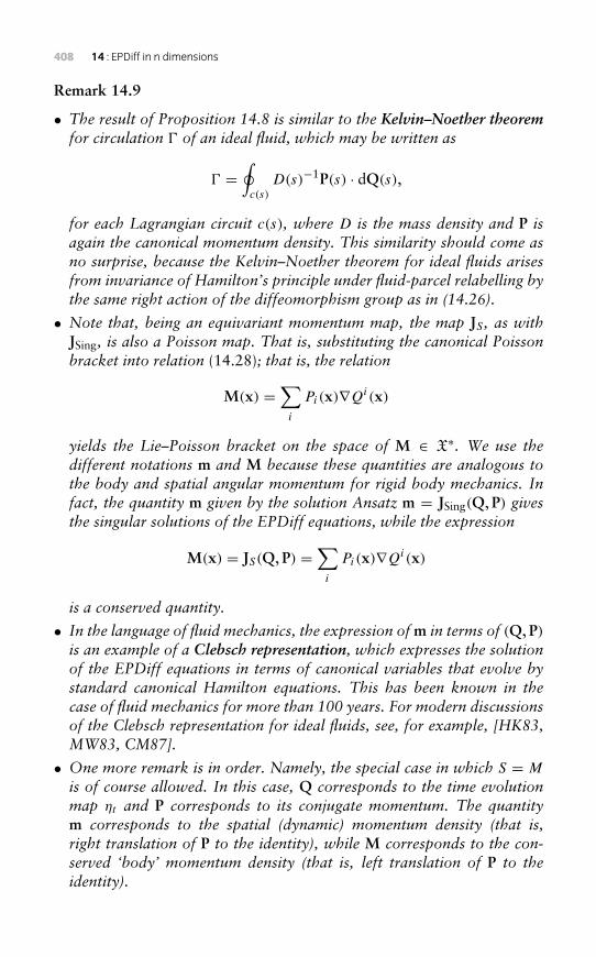
408 14 : EPDiff in n dimensions
Remark 14.9
• The result of Proposition 14.8 is similar to the Kelvin–Noether theoremfor circulation � of an ideal fluid, which may be written as
� =∮c(s)
D(s)−1P(s) · dQ(s),
for each Lagrangian circuit c(s), where D is the mass density and P isagain the canonical momentum density. This similarity should come asno surprise, because the Kelvin–Noether theorem for ideal fluids arisesfrom invariance of Hamilton’s principle under fluid-parcel relabelling bythe same right action of the diffeomorphism group as in (14.26).
• Note that, being an equivariant momentum map, the map JS , as withJSing, is also a Poisson map. That is, substituting the canonical Poissonbracket into relation (14.28); that is, the relation
M(x) =∑i
Pi(x)∇Qi(x)
yields the Lie–Poisson bracket on the space of M ∈ X∗. We use thedifferent notations m and M because these quantities are analogous tothe body and spatial angular momentum for rigid body mechanics. Infact, the quantity m given by the solution Ansatz m = JSing(Q, P) givesthe singular solutions of the EPDiff equations, while the expression
M(x) = JS(Q, P) =∑i
Pi(x)∇Qi(x)
is a conserved quantity.
• In the language of fluid mechanics, the expression ofm in terms of (Q, P)is an example of a Clebsch representation, which expresses the solutionof the EPDiff equations in terms of canonical variables that evolve bystandard canonical Hamilton equations. This has been known in thecase of fluid mechanics for more than 100 years. For modern discussionsof the Clebsch representation for ideal fluids, see, for example, [HK83,MW83, CM87].
• One more remark is in order. Namely, the special case in which S = M
is of course allowed. In this case, Q corresponds to the time evolutionmap ηt and P corresponds to its conjugate momentum. The quantitym corresponds to the spatial (dynamic) momentum density (that is,right translation of P to the identity), while M corresponds to the con-served ‘body’ momentum density (that is, left translation of P to theidentity).
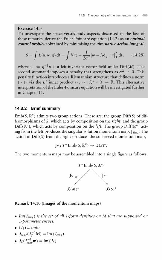
14.3 The geometry of the momentummap 409
Exercise 14.3To investigate the space-versus-body aspects discussed in the last ofthese remarks, derive the Euler-Poincaré equation (14.2) as an optimalcontrol problem obtained by minimising the alternative action integral,
S =∫
L(u,w, η) dt =∫
l(u)+ 12σ 2
∣∣w − Adη−1 u∣∣2X
dt , (14.29)
where w := η−1η is a left-invariant vector field under Diff(M). Thesecond summand imposes a penalty that strengthens as σ 2 → 0. Thispenalty function introduces a Riemannian structure that defines a norm| · |X via the L2 inner product 〈 · , · 〉 : X∗ × X → R. This alternativeinterpretation of the Euler-Poincaré equation will be investigated furtherin Chapter 15.
14.3.2 Brief summary
Emb(S, Rn) admits two group actions. These are: the group Diff(S) of dif-feomorphisms of S, which acts by composition on the right; and the groupDiff(Rn), which acts by composition on the left. The group Diff(Rn) act-ing from the left produces the singular solution momentum map, JSing. Theaction of Diff(S) from the right produces the conserved momentum map,
JS : T ∗ Emb(S, Rn)→ X(S)∗.
The two momentum maps may be assembled into a single figure as follows:
T ∗ Emb(S,M)
JSing JS
X(M)∗ X(S)∗
��
���
��
���
Remark 14.10 (Images of the momentum maps)
• Im(Jsing) is the set of all 1-form densities on M that are supported on1-parameter curves.
• (JS) is onto.
• Jsing(J−1S M) = Im (Jsing).
• JS(J−1singm) = Im (JS).
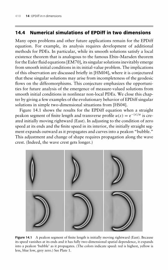
410 14 : EPDiff in n dimensions
14.4 Numerical simulations of EPDiff in two dimensions
Many open problems and other future applications remain for the EPDiffequation. For example, its analysis requires development of additionalmethods for PDEs. In particular, while its smooth solutions satisfy a localexistence theorem that is analogous to the famous Ebin–Marsden theoremfor the Euler fluid equations [EM70], its singular solutions inevitably emergefrom smooth initial conditions in its initial-value problem. The implicationsof this observation are discussed briefly in [HM04], where it is conjecturedthat these singular solutions may arise from incompleteness of the geodesicflows on the diffeomorphisms. This conjecture emphasizes the opportuni-ties for future analysis of the emergence of measure-valued solutions fromsmooth initial conditions in nonlinear non-local PDEs. We close this chap-ter by giving a few examples of the evolutionary behavior of EPDiff singularsolutions in simple two-dimensional situations from [HS04].
Figure 14.1 shows the results for the EPDiff equation when a straightpeakon segment of finite length and transverse profile u(x) = e−|x|/α is cre-ated initially moving rightward (East). In adjusting to the condition of zerospeed at its ends and the finite speed in its interior, the initially straight seg-ment expands outward as it propagates and curves into a peakon “bubble.”This adjustment and change of shape requires propagation along the wavecrest. (Indeed, the wave crest gets longer.)
Figure 14.1 A peakon segment of finite length is initially moving rightward (East). Becauseits speed vanishes at its ends and it has fully two-dimensional spatial dependence, it expandsinto a peakon ‘bubble’ as it propagates. (The colors indicate speed: red is highest, yellow isless, blue low, grey zero.) See Plate 1.
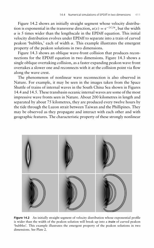
14.4 Numerical simulations of EPDiff in two dimensions 411
Figure 14.2 shows an initially straight segment whose velocity distribu-tion is exponential in the transverse direction, u(x) = e−|x|/α, but the widthα is 5 times wider than the lengthscale in the EPDiff equation. This initialvelocity distribution evolves under EPDiff to separate into a train of curvedpeakon ‘bubbles,’ each of width α. This example illustrates the emergentproperty of the peakon solutions in two dimensions.
Figure 14.3 shows an oblique wave-front collision that produces recon-nections for the EPDiff equation in two dimensions. Figure 14.3 shows asingle oblique overtaking collision, as a faster expanding peakon wave frontovertakes a slower one and reconnects with it at the collision point via flowalong the wave crest.
The phenomenon of nonlinear wave reconnection is also observed inNature. For example, it may be seen in the images taken from the SpaceShuttle of trains of internal waves in the South China Sea shown in Figures14.4 and 14.5. These transbasin oceanic internal waves are some of the mostimpressive wave fronts seen in Nature. About 200 kilometres in length andseparated by about 75 kilometres, they are produced every twelve hours bythe tide through the Luzon strait between Taiwan and the Phillipines. Theymay be observed as they propagate and interact with each other and withgeographic features. The characteristic property of these strongly nonlinear
Figure 14.2 An initially straight segment of velocity distribution whose exponential profileis wider than the width of the peakon solution will break up into a train of curved peakon‘bubbles’. This example illustrates the emergent property of the peakon solutions in twodimensions. See Plate 2.
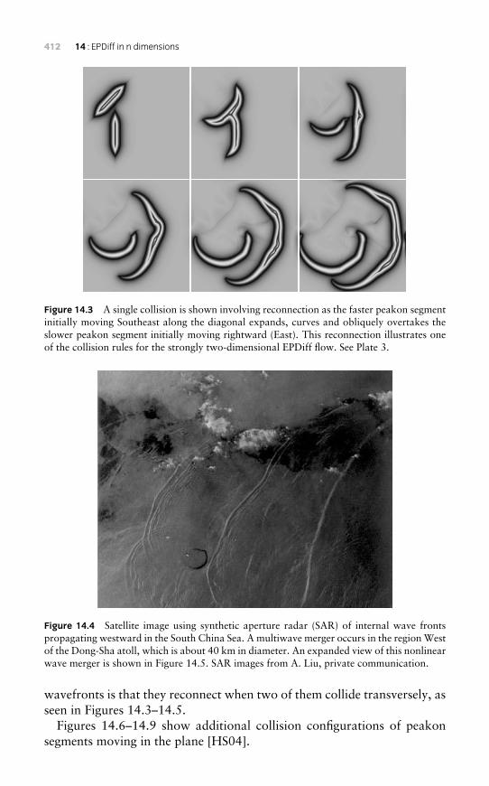
412 14 : EPDiff in n dimensions
Figure 14.3 A single collision is shown involving reconnection as the faster peakon segmentinitially moving Southeast along the diagonal expands, curves and obliquely overtakes theslower peakon segment initially moving rightward (East). This reconnection illustrates oneof the collision rules for the strongly two-dimensional EPDiff flow. See Plate 3.
Figure 14.4 Satellite image using synthetic aperture radar (SAR) of internal wave frontspropagating westward in the South China Sea. A multiwave merger occurs in the region Westof the Dong-Sha atoll, which is about 40 km in diameter. An expanded view of this nonlinearwave merger is shown in Figure 14.5. SAR images from A. Liu, private communication.
wavefronts is that they reconnect when two of them collide transversely, asseen in Figures 14.3–14.5.
Figures 14.6–14.9 show additional collision configurations of peakonsegments moving in the plane [HS04].
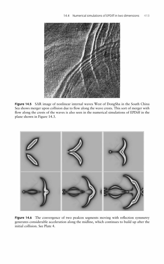
14.4 Numerical simulations of EPDiff in two dimensions 413
Figure 14.5 SAR image of nonlinear internal waves West of DongSha in the South ChinaSea shows merger upon collision due to flow along the wave crests. This sort of merger withflow along the crests of the waves is also seen in the numerical simulations of EPDiff in theplane shown in Figure 14.3.
Figure 14.6 The convergence of two peakon segments moving with reflection symmetrygenerates considerable acceleration along the midline, which continues to build up after theinitial collision. See Plate 4.
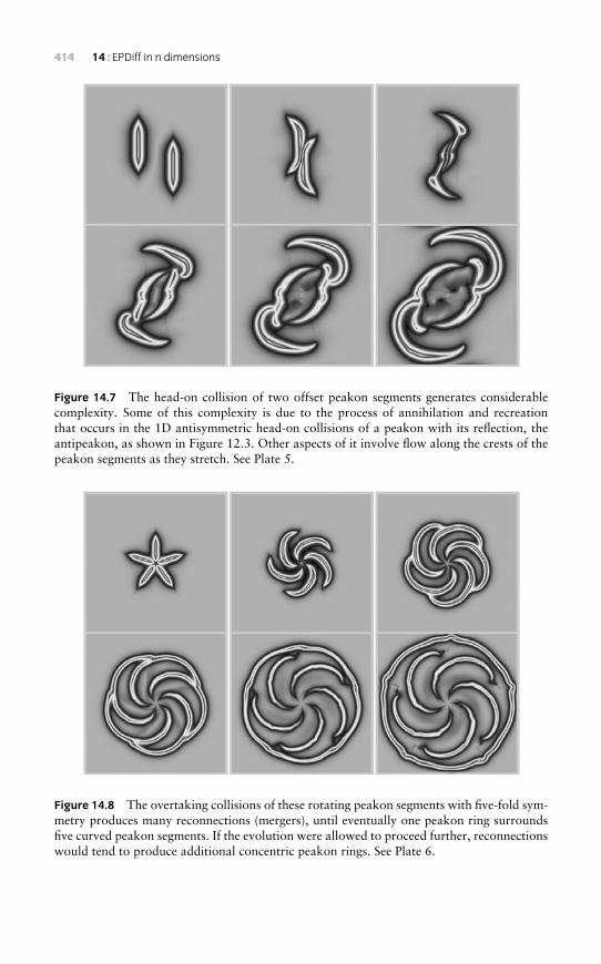
414 14 : EPDiff in n dimensions
Figure 14.7 The head-on collision of two offset peakon segments generates considerablecomplexity. Some of this complexity is due to the process of annihilation and recreationthat occurs in the 1D antisymmetric head-on collisions of a peakon with its reflection, theantipeakon, as shown in Figure 12.3. Other aspects of it involve flow along the crests of thepeakon segments as they stretch. See Plate 5.
Figure 14.8 The overtaking collisions of these rotating peakon segments with five-fold sym-metry produces many reconnections (mergers), until eventually one peakon ring surroundsfive curved peakon segments. If the evolution were allowed to proceed further, reconnectionswould tend to produce additional concentric peakon rings. See Plate 6.
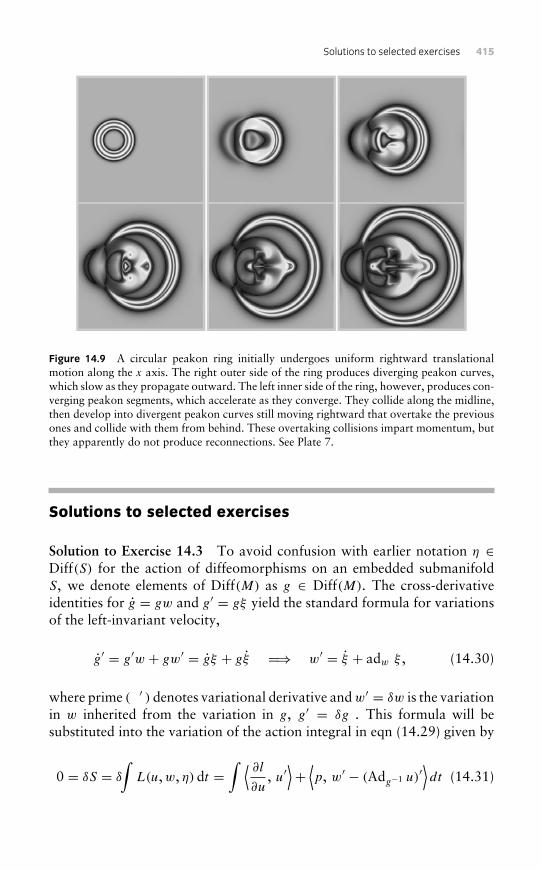
Solutions to selected exercises 415
Figure 14.9 A circular peakon ring initially undergoes uniform rightward translationalmotion along the x axis. The right outer side of the ring produces diverging peakon curves,which slow as they propagate outward. The left inner side of the ring, however, produces con-verging peakon segments, which accelerate as they converge. They collide along the midline,then develop into divergent peakon curves still moving rightward that overtake the previousones and collide with them from behind. These overtaking collisions impart momentum, butthey apparently do not produce reconnections. See Plate 7.
Solutions to selected exercises
Solution to Exercise 14.3 To avoid confusion with earlier notation η ∈Diff(S) for the action of diffeomorphisms on an embedded submanifoldS, we denote elements of Diff(M) as g ∈ Diff(M). The cross-derivativeidentities for g = gw and g′ = gξ yield the standard formula for variationsof the left-invariant velocity,
g′ = g′w + gw′ = gξ + gξ =⇒ w′ = ξ + adw ξ , (14.30)
where prime ( ′ ) denotes variational derivative andw′ = δw is the variationin w inherited from the variation in g, g′ = δg . This formula will besubstituted into the variation of the action integral in eqn (14.29) given by
0 = δS = δ
∫L(u,w, η) dt =
∫ ⟨ ∂l∂u
, u′⟩+⟨p, w′ − (Adg−1 u)′
⟩dt (14.31)
416 14 : EPDiff in n dimensions
where the momentum 1-form density, p, dual to the vector field w, isgiven by
p := δL
δw= 1
σ 2
(w − Adg−1 u
)(14.32)
and the pairing by the L2 inner product 〈 · , · 〉 : X∗ ×X→ R is induced bythe variational-derivative operation from the Riemannian structure intro-duced by the penalty term. Formula (14.30) gives the variation ω′ in eqn(14.31) in terms of the vector field ξ = g−1g′ ∈ X. One calculates the othervariation as
(Adg−1 �)′ = (g−1�g)′ = Adg−1 u′ + ad(Adg−1 u) ξ .
Hence, the variation of the action integral in (14.31) becomes
0 = δS =∫ ⟨
δl
δu, u′⟩+⟨p , ξ + adw ξ − ad(Ad
g−1 u) ξ − Adg−1 u′)⟩dt
=∫ ⟨
δl
δu− Ad∗
g−1 p , u′⟩−⟨p − ad∗ω π + ad∗(Ad
g−1 u) p , ξ⟩dt ,
where we assume endpoint terms may be ignored when integrating by parts.Requiring the coefficients of the independent variations to vanish yields theexpressions we seek,
m := δl
δu= Ad∗
g−1 p,
p − ad∗w p = − ad∗(Adg−1 u) p. (14.33)
The first of these relates the momenta p,m ∈ X∗ dual to the vector fieldsw, u ∈ X exactly as the spatial and body angular momenta are related forthe rigid body.
The variational eqns (14.33) imply, when paired with a fixed vector fieldξ ∈ X, that
d
dt〈m , ξ〉 = d
dt
⟨Ad∗
g−1 p , ξ⟩
Solutions to selected exercises 417
On taking ddt
Ad∗g−1 =
⟨Ad∗
g−1
(p − ad∗w p
), ξ⟩
On using p-eqn (14.33) = −⟨Ad∗
g−1
(ad∗(Ad
g−1 u) p), ξ⟩
On using Ad & ad definitions = −⟨p , ad(Ad
g−1 u)
(Adg−1 ξ
)⟩On rearranging = −
⟨p , Adg−1
(adu ξ
)⟩On taking duals = −
⟨ad∗u
(Ad∗
g−1 p), ξ⟩
On substituting the definition of m = − ⟨ad∗u m , ξ⟩.
This recovers EPDiff, the Euler-Poincaré equation,
d
dt
δl
δu= − ad∗u
δl
δu, or
d
dt
(Ad∗g
δl
δu
)= 0.
Thus, using a penalty term in the action integral to impose the action ofAdg−1 on vector fields as a ‘soft constraint’ when σ 2 > 0 yields EPDiffdynamics for coadjoint motion on the L2 dual, X∗, of the right-invariantLie-algebra, X.
Equation (14.33) for p may also be written as, cf. eqn (14.32),
p − σ 2 ad∗p p = 0. (14.34)
Since ad∗ and Lie derivative with respect to a vector field are the samefor 1-form densities, this relation for the evolution of the left-invariantmomentum density may be interpreted as
d
dt
(p · dx⊗ dV
)= 0 along
dxdt= −σ 2p. (14.35)
In Euclidean components, this is
∂tpi = σ 2 ∂
∂xj
(pip
j + 12δji |p|2
),
which implies conservation of the integrated left linear momentum,
d
dt
∫pi(x, t) d3x = 0,
for homogeneous boundary conditions. This is the analogue for EPDiff ofthe conservation of spatial angular momentum for the rigid body.

This page intentionally left blank
15Computational anatomy:contour matchingusing EPDiff
15.1 Introduction to computational anatomy (CA)
Morphology and computational anatomy
Computational anatomy (CA) must measure and analyse a range of varia-tions in shape, or appearance, of highly deformable biological structures.The problem statement for CA was formulated long ago in a famous bookby D’Arcy Thompson [Tho92]
In a very large part of morphology, our essential task lies in the comparisonof related forms rather than in the precise definition of each . . .. This processof comparison, of recognizing in one form a definite permutation or defor-mation of another, . . . lies within the immediate province of mathematicsand finds its solution in . . . the Theory of Transformations. . . . I learnt of itfrom Henri Poincaré.
– D’Arcy Thompson, On Growth and Form (1917)
D’Arcy Thompson’s book [Tho92] examines the idea that the growthand form of all plants and animals can be explained by mathematical prin-ciples. His book also acts as a practical guide to understanding how flowsof smooth invertible maps may be used to compare shapes. For example,his chapter on transformations contains remarkable diagrams showing howdifferences in the forms of, say, species of fish can be understood in termsof smooth invertible distortions of the reference coordinate systems ontowhich they are mapped. A fish is drawn on a square grid, which is thenstretched, sheared or shifted so that the deformed image may be identifiedas that of a related species, as in Figures 15.1 and 15.2.
This chapter explains that EPDiff is the perfect tool to realize D’ArcyThompson’s concept of comparing shapes, upon choosing a norm
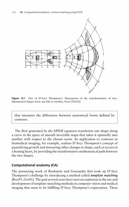
420 15 : Computational anatomy: contour matching using EPDiff
0 011
2
2
3
3
4
4
5
5
6
6
a
a
b
b
c
c
d
d
e
e
Figure 15.1 One of D’Arcy Thompson’s illustrations of the transformation of two-dimensional shapes from one fish to another, from [Tho92].
that measures the differences between anatomical forms defined bycontours.
The flow generated by the EPDiff equation transforms one shape alonga curve in the space of smooth invertible maps that takes it optimally intoanother with respect to the chosen norm. Its application to contours inbiomedical imaging, for example, realizes D’Arcy Thompson’s concept ofquantifying growth and measuring other changes in shape, such as occurs ina beating heart, by providing the transformative mathematical path betweenthe two shapes.
Computational anatomy (CA)
The pioneering work of Bookstein and Grenander first took up D’ArcyThompson’s challenge by introducing a method called template matching[Boo91, Gre81]. The past several years have seen an explosion in the use anddevelopment of template-matching methods in computer vision and medicalimaging that seem to be fulfilling D’Arcy Thompson’s expectation. These
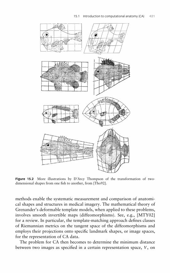
15.1 Introduction to computational anatomy (CA) 421
Figure 15.2 More illustrations by D’Arcy Thompson of the transformation of two-dimensional shapes from one fish to another, from [Tho92].
methods enable the systematic measurement and comparison of anatomi-cal shapes and structures in medical imagery. The mathematical theory ofGrenander’s deformable template models, when applied to these problems,involves smooth invertible maps (diffeomorphisms). See, e.g., [MTY02]for a review. In particular, the template-matching approach defines classesof Riemannian metrics on the tangent space of the diffeomorphisms andemploys their projections onto specific landmark shapes, or image spaces,for the representation of CA data.
The problem for CA then becomes to determine the minimum distancebetween two images as specified in a certain representation space, V , on
422 15 : Computational anatomy: contour matching using EPDiff
which the diffeomorphisms act. Metrics are written so that the optimal pathin Diff satisfies an evolution equation. This equation turns out to be EPDiff,when V is a closed contour representing the shape of the image. A discussionof EPDiff and the application of its peakons and other singular solutionsfor matching templates defined by contours of image outlines appears in[HRTY04].
Objectives
This chapter and the next discuss how the Euler–Poincaré theory may beused to develop new perspectives in CA. In particular, these chapters discusshow CA may be informed by the concept of weak solutions, solitons andmomentum maps for geodesic flows [HRTY04, CH93, HS04]. For example,among the geometric structures of interest in CA, the landmark points andimage outlines may be identified with the singular solutions of the EPDiffequation. These singular solutions are given by the momentum map JSing
for EPDiff in Chapter 14. This momentum map also yields the canonicalHamiltonian formulation of their dynamics. This evolution, in turn, pro-vides a complete parameterization of the landmarks and image outlines bythe linear vector space comprising their canonical positions and momenta.The singular momentum map JSing for EPDiff provides an isomorphismbetween the landmarks and outlines for images and the singular solitonsolutions of the EPDiff equation. This isomorphism provides a dynamicalparadigm for CA, as well as a basis for anatomical data representation in alinear vector space.
This chapter introduces the variational formulation of template match-ing problems in computational anatomy. It makes the connection tothe EPDiff evolution equation and discusses the relation of images inCA to the singular momentum map of the EPDiff equation. Then itdraws some consequences of EPDiff for the outline matching problemin CA and gives a numerical example. The numerical example is remi-niscent of the chapter in D’Arcy Thompson’s book where the shapes offish are related to each other by stretching one shape into another on asquare grid.
Outline of the chapter. Section 15.2 describes the template-matching vari-ational problems of computational anatomy and the fundamental role ofthe EPDiff evolution equation. The singular solutions for the EPDiff equa-tion (15.2) with diffeomorphism group G are discussed in Section 15.3.
15.2 Mathematical formulation of template matching for CA 423
They are, in particular, related to the contour-matching problem in CA (or,more generally, in computer vision), examples of which are given in Section15.4.
15.2 Mathematical formulation of templatematching for CA
15.2.1 Cost
Most problems in CA can be formulated as:
Find the deformation path (flow) with minimal cost, under the constraintthat it carries the template to the target.
The cost assigned in template matching for comparing images η0 and η1considered as points on a manifold N is assigned as a functional
Cost(t → gt ) =∫ 1
0�(ut ) dt ,
which is defined on curves gt in a Lie group with tangents
dgt
dt= ut ◦ gt and ηt = gt · η0. (15.1)
In what follows, the function ut → �(ut ) = ‖ut‖2 will be taken as a squaredfunctional norm on the space of velocity vectors along the flow. The Liegroup property specifies the representation space for template matching asa manifold of smooth mappings, which may be differentiated, composedand inverted. The vector space of right-invariant instantaneous velocities,ut = (dgt/dt)◦g−1
t forms the tangent space at the identity of the consideredLie group, and may be identified as the group’s Lie algebra, denoted g.
15.2.2 Mathematical analogy between template matching andfluid dynamics
(I) The frameworks of both CA and fluid dynamics each involve a station-ary principle whose action, or cost function, is right invariant. Themain difference is that template matching is formulated as an optimalcontrol problem whose cost function is designed for the application,while fluid dynamics is formulated as an initial value problem whosecost function is the fluid’s kinetic energy.
424 15 : Computational anatomy: contour matching using EPDiff
(II) The geodesic evolution for both template matching and fluid dynamicsis governed by the EPDiff equation (11.20), rewritten as( ∂
∂t+ u · ∇
)m+ (∇u)T ·m+m(div u) = 0, (15.2)
in which (∇u)T ·m =∑j mj∇uj . Here u = K ∗m, where K∗ denotesconvolution with the Green’s kernel K for the operator Qop, where
m = δ�
δu=: Qopu.
The operator Qop is symmetric and positive-definite for the costdefined by
Cost(t → gt ) =∫ 1
0�(ut ) dt = 1
2
∫ 1
0‖ut‖2 dt = 1
2
∫ 1
0〈 ut , Qoput 〉 dt ,
with L2 pairing 〈 ·, · 〉 whenever ‖ut‖2 is a norm.
(III) The flows in CA and fluid dynamics both evolve under a left groupaction on a linear representation space, ηt = gt · η0. They differ in theroles of their advected quantities, at = a0 ◦g−1
t . The main difference isthat image properties are passive and affect the template matching asa constraint in the cost function, while advected quantities may affectfluid flows directly, for example through the pressure, and therebyproduce waves.
15.2.3 How EPDiff emerges in CA
Choose the cost function for continuously morphing η0 into η1 along ηt =gt · η0 as
Cost(t → gt ) =∫ 1
0�(ut ) dt =
∫ 1
0‖ut‖2 dt ,
where ut is the velocity of the fluid deformation at time t and
‖ut‖2 = 〈ut , Qoput 〉,and Qop is our positive symmetric linear operator. Then, according to theEuler–Poincaré theory, the momentum governing the process, mt = Qoput
with Green’s kernel K : ut = K ∗mt satisfies the EPDiff equation, (15.2).The EPDiff equation arises in both template matching and fluid dynamics,and it informs both fields of endeavour.
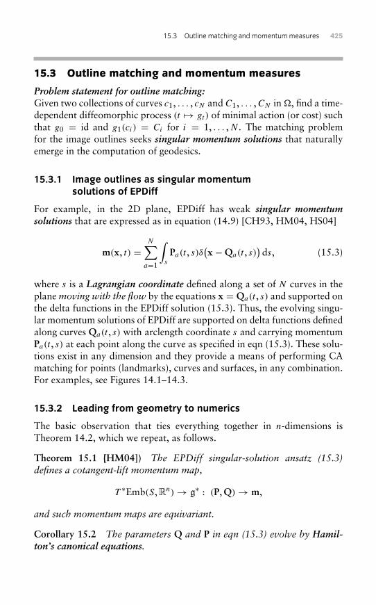
15.3 Outline matching and momentummeasures 425
15.3 Outline matching and momentum measures
Problem statement for outline matching:Given two collections of curves c1, . . . , cN and C1, . . . ,CN in �, find a time-dependent diffeomorphic process (t → gt ) of minimal action (or cost) suchthat g0 = id and g1(ci) = Ci for i = 1, . . . ,N . The matching problemfor the image outlines seeks singular momentum solutions that naturallyemerge in the computation of geodesics.
15.3.1 Image outlines as singular momentumsolutions of EPDiff
For example, in the 2D plane, EPDiff has weak singular momentumsolutions that are expressed as in equation (14.9) [CH93, HM04, HS04]
m(x, t) =N∑
a=1
∫s
Pa(t , s)δ(x −Qa(t , s)
)ds, (15.3)
where s is a Lagrangian coordinate defined along a set of N curves in theplanemoving with the flow by the equations x = Qa(t , s) and supported onthe delta functions in the EPDiff solution (15.3). Thus, the evolving singu-lar momentum solutions of EPDiff are supported on delta functions definedalong curves Qa(t , s) with arclength coordinate s and carrying momentumPa(t , s) at each point along the curve as specified in eqn (15.3). These solu-tions exist in any dimension and they provide a means of performing CAmatching for points (landmarks), curves and surfaces, in any combination.For examples, see Figures 14.1–14.3.
15.3.2 Leading from geometry to numerics
The basic observation that ties everything together in n-dimensions isTheorem 14.2, which we repeat, as follows.
Theorem 15.1 ([HM04]) The EPDiff singular-solution ansatz (15.3)defines a cotangent-lift momentum map,
T ∗Emb(S, Rn)→ g∗ : (P,Q)→ m,
and such momentum maps are equivariant.
Corollary 15.2 The parameters Q and P in eqn (15.3) evolve by Hamil-ton’s canonical equations.
426 15 : Computational anatomy: contour matching using EPDiff
Proof This is also a property of cotangent-lift momentum maps. �
Remark 15.3 The parameters Q and P in eqn (15.3) provide a completeparameterization of the landmarks and image outlines.
The proof of this theorem and the mathematics underlying such momen-tum maps for diffeomorphisms were explained in Chapter 14. Forconvenience, the main results for template matching are recapped, asfollows:
– The embedded manifold S is the support set of (P, Q).
– The momentum map is for left action of the diffeomorphisms on S.
– The whole system is right invariant.
– Consequently, the momentum map for right action is conserved.
– These constructions persist for a certain class of numerical schemes.
– They apply in template matching for every choice of norm.
15.3.3 EPDiff dynamics informs optimal control for CA
CA must compare two geometric objects, and thus it is concerned with anoptimal control problem. However, the initial-value problem for EPDiffalso has important consequences for CA applications.
• When matching two geometric structures, the momentum at time t=0contains all required information for reconstructing the target from thetemplate. This is done via Hamiltonian geodesic flow.
• Being canonically conjugate, the momentum has exactly the samedimension as the matched structures, so there is no redundancy.
• Right invariance eliminates the relabelling motions from the optimalsolution and also yields a conserved momentum map.
• Besides being one-to-one, the momentum representation is defined on alinear space, being dual to the velocity vectors.This means that one may, for example,:
• study linear instability of CA processes,
• take averages and
• apply statistics to the space of image contours.
Thus, the momentum-map representation (15.3) enables building, sam-pling and estimating statistical models on a linear space.
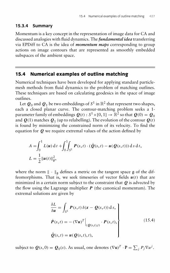
15.4 Numerical examples of outline matching 427
15.3.4 Summary
Momentum is a key concept in the representation of image data for CA anddiscussed analogies with fluid dynamics. The fundamental idea transferringvia EPDiff to CA is the idea of momentum maps corresponding to groupactions on image contours that are represented as smoothly embeddedsubspaces of the ambient space.
15.4 Numerical examples of outline matching
Numerical techniques have been developed for applying standard particle-mesh methods from fluid dynamics to the problem of matching outlines.These techniques are based on calculating geodesics in the space of imageoutlines.
Let Q0 and Q1 be two embeddings of S1 in R2 that represent two shapes,each a closed planar curve. The contour-matching problem seeks a 1-parameter family of embeddingsQ(t) : S1×[0, 1] → R2 so thatQ(0) = Q0andQ(1) matchesQ1 (up to relabelling). The evolution of the contourQ(t)
is found by minimizing the constrained norm of its velocity. To find theequation for Q we require extremal values of the action defined by
A =∫ 1
0L(u) d t +
∫ 1
0
∫S1
P (s, t) · (Q(s, t)− u(Q(s, t))) d s d t ,
L = 12‖u(t)‖2g,
where the norm ‖ · ‖g defines a metric on the tangent space g of the dif-feomorphisms. That is, we seek timeseries of vector fields u(t) that areminimized in a certain norm subject to the constraint that Q is advected bythe flow using the Lagrange multiplier P (the canonical momentum). Theextremal solutions are given by
δL
δu=∫S1
P (s, t) δ(x −Q(s, t)) d s,
P (s, t) = − (∇u)T∣∣∣(Q(s,t),t)
· P (s, t),
Q(s, t) = u(Q(s, t), t),
(15.4)
subject to Q(s, 0) = Q0(s). As usual, one denotes (∇u)T · P =∑j Pj∇uj .
428 15 : Computational anatomy: contour matching using EPDiff
The first equation in the system (15.4) is the momentum map JSing in(14.19) corresponding to the cotangent-lift of the action of vector fields uon embedded curves given by
Q → u(Q).
For a suitable test function w, the singular momentum solutions m satisfy
ddt〈w,m〉 − 〈∇w,um〉 + 〈w, (∇u)T ·m〉 = 0, m = δL
δu,
which is the weak form of the EPDiff equation (15.2).For contour matching, one must seek an initial momentum distribution
P (s, 0) that takes shape Q0(s) to shape Q1(s). For this, a functional J ofthe advected shape Q(1, s) must be chosen that is minimized when Q(1, s)matches Q1(s). Following [GTY04], we describe the contours by singulardensities:
µ =∫S1
µ(s) δ(x −Q(1, s)) d s dV (x), (15.5)
η =∫S1
η(s) δ(x −Q1(s)) d s dV (x), (15.6)
and write J = ‖µ− η‖2K , where ‖ · ‖2K is a norm for singular densities in areproducing-kernel Hilbert space with kernel K. This approach allows thecontours to be matched modulo relabelling.
The remaining matching problem may be solved, for example, by using agradient algorithm, in which the gradient of the residual error with respectto P (s, 0) is calculated using the standard method based on the adjointequation [Gun03]. Another, more general, approach will be discussed inChapter 16.
15.4.1 Numerical discretization
Various methods, including the Variational particle-mesh (VPM) method[Cot05, CH08] may be used to discretize the equations in (15.4). Thismethod may be sketched, as follows. First, discretize the velocity on anEulerian grid with ng points and approximate ‖u‖ there. Then replace theembedded contour S1 by a finite set of np Lagrangian particles {Qβ}np
β=1(labelled by Greek indices) and interpolate from the grid to the particles by
15.4 Numerical examples of outline matching 429
using basis functions
u(Qβ) =ng∑k=1
ukψk(Qβ), withng∑k=1
ψk(x) = 1, ∀ x,
for ng grid points (labelled by Latin indices). The action for the continuous-time motion on the grid then becomes
A =∫ 1
0
12‖u(t)‖2 +
∑β
P β ·(Qβ −
∑k
ukψk(Qβ)
)d t ,
and one can obtain a fully discrete method by discretizing the action in time.For example, a first-order method is obtained by extremizing
A = �t
N∑n=1
12‖un‖2 +
∑β
P nβ ·(Qn
β −Qn−1β
�t−∑k
unkψk(Q
n−1β )
) .
This time-stepping method is the (first-order) symplectic Euler-A methodfor the time-continuous Hamiltonian system for the Lagrangian particles.In general, the method will be symplectic because it arises from a discretevariational principle. See [LR04] for a broad introduction to symplecticnumerical methods and their conservation properties. The conservationproperties of VPM are discussed in [CH08].
The densities µ and η may be approximated on the grid by using thestandard particle-mesh approach (see [FGR02]). This approach producesthe representation,
µk =∑β
µβψk(QNβ ), ηk =
∑β
ηβψk(Q1,β),
where Q1,β are the positions of particles on the target shape. This repre-sentation amounts to pixellating the singular densities (15.5) and (15.6) onthe grid. For a given kernel K, one may approximate the norm J by
J =∑kl
K(xk − xl)(µk − ηk)(µl − ηl). (15.7)
The discrete adjoint equation may then be applied in computing the inver-sion for the initial conditions for P β that generate the flow. A numericalexample calculated by using this method is given in Figure 15.3.
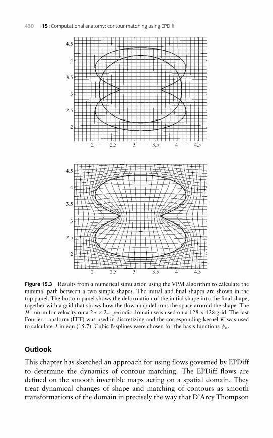
430 15 : Computational anatomy: contour matching using EPDiff
2
2
2.5
2.5
3
3
3.5
3.5
4
4
4.5
4.5
2
2
2.5
2.5
3
3
3.5
3.5
4
4
4.5
4.5
Figure 15.3 Results from a numerical simulation using the VPM algorithm to calculate theminimal path between a two simple shapes. The initial and final shapes are shown in thetop panel. The bottom panel shows the deformation of the initial shape into the final shape,together with a grid that shows how the flow map deforms the space around the shape. TheH 1 norm for velocity on a 2π × 2π periodic domain was used on a 128× 128 grid. The fastFourier transform (FFT) was used in discretizing and the corresponding kernel K was usedto calculate J in eqn (15.7). Cubic B-splines were chosen for the basis functions ψk .
Outlook
This chapter has sketched an approach for using flows governed by EPDiffto determine the dynamics of contour matching. The EPDiff flows aredefined on the smooth invertible maps acting on a spatial domain. Theytreat dynamical changes of shape and matching of contours as smoothtransformations of the domain in precisely the way that D’Arcy Thompson
15.4 Numerical examples of outline matching 431
envisioned them. The application of EPDiff to the dynamics of contourmatching involves a geodesic curve in the full group of diffeomorphismswith respect to a metric ‖u(t)‖2g defined on its tangent space g. In this sce-nario, contour matching means connecting two shapes defined by contoursin the plane so that the action of the diffeomorphisms on the domain car-ries one shape to the other smoothly along the geodesic curve. Chapter 16will discuss an approach to the dynamics of morphology that goes beyondwhat D’Arcy Thompson envisioned. In this approach, geodesic evolutionunder the action of the diffeomorphisms carries additional properties, suchas colour, intensity or orientation of pixels in the image, as well as shape.Moreover, these additional image properties may evolve under their ownoptimal dynamics.
Exercise 15.1Verify the equations in the system (15.4).
Hint: Before taking variations in velocity u, insert a delta function bywriting ∫ 1
0
∫S1
P (s, t) · u(Q(s, t), t) d s d t
=∫ 1
0
∫S1
∫R2
P (s, t) · u(x, t) δ(x −Q(s, t)
)d2x d s d t .
This yields the first equation in (15.4). The others follow by standardmanipulations.
Exercise 15.2Find the system of equations defined by minimizing the alternativeaction,
A =∫ 1
0L(u) d t + 1
2σ 2
∫ 1
0
∫S1
∣∣Q(s, t)− u(Q(s, t), t)∣∣2 d s d t ,
L = 12
∥∥u(t)∥∥2g,
where σ 2 > 0 is a constant parameter, the norm ‖ · ‖g defines a metric onthe tangent space g of the diffeomorphisms and | · |without subscript isthe Euclidean metric for vectors. Do the equations for the minimizers of
432 15 : Computational anatomy: contour matching using EPDiff
this action still admit the momentum-map relation in the first equationof system (15.4)?
Hint: in minimizing this action, the quantity Q(s, t) − u(Q(s, t)) isminimized by imposing it as a penalty, rather than constraining it tovanish exactly, as in the action for the system (15.4). Before takingvariations of this alternative action, it is helpful to rewrite the penaltyterm equivalently as∫ 1
0
∫S1
[P (s, t) · (Q(s, t)− u(Q(s, t), t)
)− σ 2
2|P |2(s, t)
]d s d t .
This form of the penalty term is seen to be equivalent to the original one,upon taking stationary variations with respect to P to find the definingrelation
σ 2P (s, t) = Q(s, t)− u(Q(s, t), t
).
16Computational anatomy:Euler–Poincaré imagematching
16.1 Overview
Pattern matching is an important component of imaging science, and isfundamental in computational anatomy (computerized anatomical analy-sis of medical images). When comparing images, the purpose is to find anoptimal deformation that aligns the images and matches their photometricproperties. Diffeomorphic pattern matching methods have been developedto achieve both this objective and the additional goal of defining a (Rieman-nian) metric structure on spaces of deformable objects [DGM98, Tro98].This approach has found many applications in medical imaging, where theobjects of interest include images, landmarks, measures (supported on pointsets) and currents (supported on curves and surfaces). These methods usu-ally address the registration problem by solving a variational problem ofthe form
Minimize(d(id, g)2 + Error term(g.ntemp, ntarg)
)(16.1)
over all diffeomorphisms g, where ntemp and ntarg are the images beingcompared (usually referred to as the template and the target), (g, n) → g.nis the action of diffeomorphisms on the objects and d is a right-invariantRiemannian distance on diffeomorphisms.
This chapter explains how the pattern-matching problem for imagesis governed by the Euler–Poincaré equations of geodesic motion fora Lagrangian given by a right-invariant norm on (TDiff × TN)/Diff,where N is the manifold of images on which Diff acts.
In problems formulated as in eqn (16.1), the error term breaks the metricaspects inherited from the distance d on the diffeomorphisms because the
434 16 : Computational anatomy: Euler–Poincaré image matching
error term has an inherent template vs. target asymmetry. With the aimof designing a fully metric approach to the template-matching problem,the metamorphosis approach was formulated in [TY05]. The metamor-phosis approach embraces what are called morphing and warping incomputer graphics while endowing the composition of the two operationswith a Riemannian variational structure. The metamorphosis approachprovides interesting alternatives to the pattern-matching approach basedon eqn (16.1), in the context of a metric framework. This chapterexplains the Lagrangian formulation for metamorphosis of images devel-oped in [HTY09] that includes the Riemannian formalism introducedin [TY05].
The discussion will be general enough to include a range of applications.Consider a manifold N that is acted upon by a Lie group G. The manifoldN contains the deformable objects and G is the Lie group of deformations,which is taken to be the group of diffeomorphisms. (A few examples ofthe space N will be discussed later. In particular, N could be another Liegroup.)
Definition 16.1 A metamorphosis [TY05] is a pair of curves (gt , ηt ) ∈G×N parameterized by time t , with g0 = id. Its image is the curve nt ∈ N
defined by the action nt = gt .ηt . The quantities gt and ηt are called the defor-mation component of the metamorphosis, and its template component,respectively. When ηt is constant, the metamorphosis reduces to standardtemplate matching, which is a pure deformation. In the general case, theimage is a composition of deformation and template variation.
This chapter places the metamorphosis approach into a Lagrangian for-mulation, and applies the Euler–Poincaré variational framework to deriveits evolution equations. Analytical questions about these equations (forexample, the existence and uniqueness of their solutions) require additionalassumptions on G and the space N of deformed objects that are beyond thescope of the present text. For analytical discussions of the equations in thischapter, see [HTY09].
The next section provides notation and definitions related to the problemof metamorphosis.
16.2 Notation and Lagrangian formulation
The letters η or n will be used to denote elements of N , the former beingassociated to the template component of a metamorphosis, and the latterto its image under the action of the group.
16.2 Notation and Lagrangian formulation 435
The variational problem we shall study optimizes over metamorphoses(gt , ηt ) by minimizing, for some Lagrangian L, the integral∫ 1
0L(gt , gt , ηt , ηt )dt , (16.2)
with fixed endpoint conditions for the initial and final images n0 and n1(with nt = gtηt ) and g0 = idG (so only the images are constrained at theendpoints, with the additional normalization g0 = id).
Let g denote the Lie algebra of G and let (g,Ug, η, ξη) ∈ TG × TN . Wewill consider Lagrangians defined on TG × TN , that satisfy the followinginvariance conditions: there exists a function � defined on g×TN such that
L(g,Ug, η, ξη) = �(Ugg−1, gη, gξη).
In other words, L is taken to be invariant under the right action of G onG×N defined by (g, η)h = (gh,h−1η).
For a metamorphosis (gt , ηt ), the following definitions
ut = gt g−1t , nt = gtηt , and νt = gt ηt (16.3)
lead by right invariance to an expression for the reduced Lagrangian
L(gt , gt , ηt , ηt ) = �(ut , nt , νt ). (16.4)
More notation
The Lie derivative with respect to a vector field X will be denoted £X. TheLie algebra of G is identified with the set of right-invariant vector fieldsUg = ug, u ∈ TeG = g, g ∈ G. If G acts on a set N , and f : N → R, onefinds £uf (n) = (d/dt)f (gt n) with g0 = id and gt (0) = u.
The Lie bracket [u, v] on g is defined by
£[u,v] = −(£u£v − £v£u) (16.5)
and the associated adjoint operator is adu v = [u, v]. Letting Ig(h) = ghg−1
and Advg = £vIg(id) yields adu v = £u(Adv)(id). When G is a group ofdiffeomorphisms, this defines
aduv = du v − dv u, (16.6)
as in eqn (11.6).The pairing between a linear form l and a vector u will be denoted
⟨l, u
⟩.
Duality with respect to this pairing will be denoted with an asterisk ( · )∗.
436 16 : Computational anatomy: Euler–Poincaré image matching
When the Lie group G acts on a manifold N , the associated diamondoperation (&) (or dual action) is defined on T N∗ × N and takes values ing∗, so that
& : T N∗ × N → g∗. (16.7)
The diamond operation is defined in terms of the pairing⟨ · , · ⟩ : g∗×g→ R
as in eqn (9.32). That is, diamond is defined in this notation by⟨γ & n, u
⟩ = −⟨γ , un⟩T N∗ , (16.8)
where (γ , n) ∈ T N∗ × N , un = £uη and the bracket⟨ · , · ⟩
T N∗ denotes thepairing between N and TN∗.
16.3 Symmetry-reduced Euler equations
We compute the symmetry-reduced Euler equations as stationarity condi-tions that extremalize the reduced action, defined in terms of the reducedLagrangian by,
Sred :=∫ 1
0�(ut , nt , νt )dt , (16.9)
with respect to variations δu and ω = δn = δ(gη) for fixed endpoint condi-tions n0 and n1. The variation δν can be obtained from n = gη and ν = gη
yielding
n = ν + un and ω = δν + uω + δun, (16.10)
in which Lie algebra action is denoted by concatenation from the left. Forexample, un = £un denotes the Lie derivative of n along the vector fieldu, etc. The computations are performed in a local chart on TN in terms ofwhich partial derivatives are taken.
Taking stationary variations of Sred yields∫ 1
0
(⟨δ�
δu, δut
⟩+⟨δ�
δn, ωt
⟩+⟨δ�
δν, ωt − utωt − δut nt
⟩)dt = 0. (16.11)
The δu-term yields the constant of motion,
δ�
δu+ δ�
δν& nt = 0. (16.12)
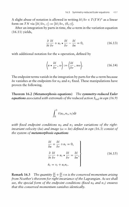
16.3 Symmetry-reduced Euler equations 437
A slight abuse of notation is allowed in writing δ�/δν ∈ T (T N)∗ as a linearform on TN via
⟨δ�/δν, z
⟩:= ⟨δ�/δν, (0, z)
⟩.
After an integration by parts in time, the ω-term in the variation equation(16.11) yields,
∂
∂t
δ�
δν+ ut �
δ�
δν− δ�
δn= 0, (16.13)
with additional notation for the � operation, defined by
⟨u �
δ�
δν, ω⟩
:=⟨δ�
δν, uω
⟩. (16.14)
The endpoint terms vanish in the integration by parts for the ω-term becauseδn vanishes at the endpoints for n0 and n1 fixed. These manipulations haveproven the following.
Theorem 16.2 (Metamorphosis equations) The symmetry-reduced Eulerequations associated with extremals of the reduced action Sred in eqn (16.9)
∫ 1
0�(ut , nt , νt )dt
with fixed endpoint conditions n0 and n1 under variations of the right-invariant velocity (δu) and image (ω = δn) defined in eqn (16.3) consist ofthe system of metamorphosis equations
δ�
δu+ δ�
δν& nt = 0,
∂
∂t
δ�
δν+ ut �
δ�
δν= δ�
δn,
nt = νt + utnt .
(16.15)
Remark 16.3 The quantity δ�δu+ δ�
δν&n is the conserved momentum arising
from Noether’s theorem for right invariance of the Lagrangian. As we shallsee, the special form of the endpoint conditions (fixed n0 and n1) ensuresthat this conserved momentum vanishes identically.
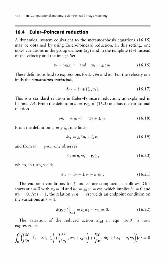
438 16 : Computational anatomy: Euler–Poincaré image matching
16.4 Euler–Poincaré reduction
A dynamical system equivalent to the metamorphosis equations (16.15)may be obtained by using Euler–Poincaré reduction. In this setting, onetakes variations in the group element (δg) and in the template (δη) insteadof the velocity and the image. Set
ξt = δgtg−1t and �t = gtδηt . (16.16)
These definitions lead to expressions for δu, δn and δν. For the velocity onefinds the constrained variation,
δut = ξt + [ξt , ut ]. (16.17)
This is a standard relation in Euler–Poincaré reduction, as explained inLemma 7.4. From the definition nt = gtηt in (16.3) one has the variationalrelation
δnt = δ(gtηt ) = �t + ξtnt . (16.18)
From the definition νt = gt ηt , one finds
δνt = gtδηt + ξtνt , (16.19)
and from �t = gtδηt one observes
�t = ut�t + gt ηt , (16.20)
which, in turn, yields
δνt = �t + ξtνt − ut�t . (16.21)
The endpoint conditions for ξ and � are computed, as follows. Onestarts at t = 0 with g0 = id and n0 = g0η0 = cst, which implies ξ0 = 0 and�0 = 0. At t = 1, the relation g1η1 = cst yields an endpoint condition onthe variations at t = 1,
δ(gtηt )
∣∣∣t=1= ξ1n1 +�1 = 0. (16.22)
The variation of the reduced action Sred in eqn (16.9) is nowexpressed as∫ 1
0
(⟨δ�
δu, ξt − adut ξt
⟩+⟨δ�
δnt
, �t + ξtnt
⟩+⟨δ�
δν, �t + ξtνt − ut�t
⟩)dt = 0.
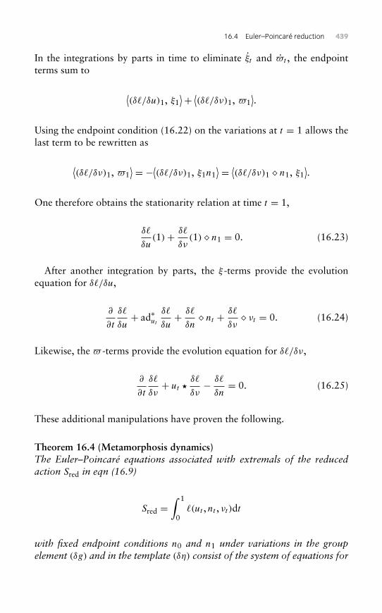
16.4 Euler–Poincaré reduction 439
In the integrations by parts in time to eliminate ξt and �t , the endpointterms sum to
⟨(δ�/δu)1, ξ1
⟩+ ⟨(δ�/δν)1, �1⟩.
Using the endpoint condition (16.22) on the variations at t = 1 allows thelast term to be rewritten as
⟨(δ�/δν)1, �1
⟩ = −⟨(δ�/δν)1, ξ1n1⟩ = ⟨(δ�/δν)1 & n1, ξ1
⟩.
One therefore obtains the stationarity relation at time t = 1,
δ�
δu(1)+ δ�
δν(1) & n1 = 0. (16.23)
After another integration by parts, the ξ -terms provide the evolutionequation for δ�/δu,
∂
∂t
δ�
δu+ ad∗ut
δ�
δu+ δ�
δn& nt + δ�
δν& νt = 0. (16.24)
Likewise, the � -terms provide the evolution equation for δ�/δν,
∂
∂t
δ�
δν+ ut �
δ�
δν− δ�
δn= 0. (16.25)
These additional manipulations have proven the following.
Theorem 16.4 (Metamorphosis dynamics)The Euler–Poincaré equations associated with extremals of the reducedaction Sred in eqn (16.9)
Sred =∫ 1
0�(ut , nt , νt )dt
with fixed endpoint conditions n0 and n1 under variations in the groupelement (δg) and in the template (δη) consist of the system of equations for
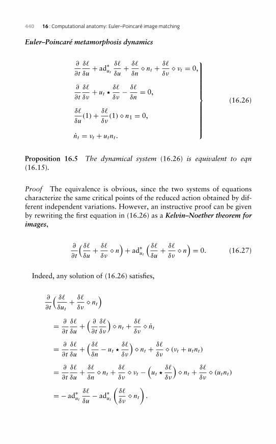
440 16 : Computational anatomy: Euler–Poincaré image matching
Euler–Poincaré metamorphosis dynamics
∂
∂t
δ�
δu+ ad∗ut
δ�
δu+ δ�
δn& nt + δ�
δν& νt = 0,
∂
∂t
δ�
δν+ ut �
δ�
δν− δ�
δn= 0,
δ�
δu(1)+ δ�
δν(1) & n1 = 0,
nt = νt + utnt .
(16.26)
Proposition 16.5 The dynamical system (16.26) is equivalent to eqn(16.15).
Proof The equivalence is obvious, since the two systems of equationscharacterize the same critical points of the reduced action obtained by dif-ferent independent variations. However, an instructive proof can be givenby rewriting the first equation in (16.26) as a Kelvin–Noether theorem forimages,
∂
∂t
( δ�δu+ δ�
δν& n)+ ad∗ut
( δ�δu+ δ�
δν& n)= 0. (16.27)
Indeed, any solution of (16.26) satisfies,
∂
∂t
( δ�
δut
+ δ�
δν& nt
)= ∂
∂t
δ�
δu+( ∂
∂t
δ�
δν
)& nt + δ�
δν& nt
= ∂
∂t
δ�
δu+( δ�δn− ut �
δ�
δν
)& nt + δ�
δν& (νt + utnt )
= ∂
∂t
δ�
δu+ δ�
δn& nt + δ�
δν& νt −
(ut �
δ�
δν
)& nt + δ�
δν& (utnt )
= − ad∗ut
δ�
δu− ad∗ut
(δ�
δν& nt
).
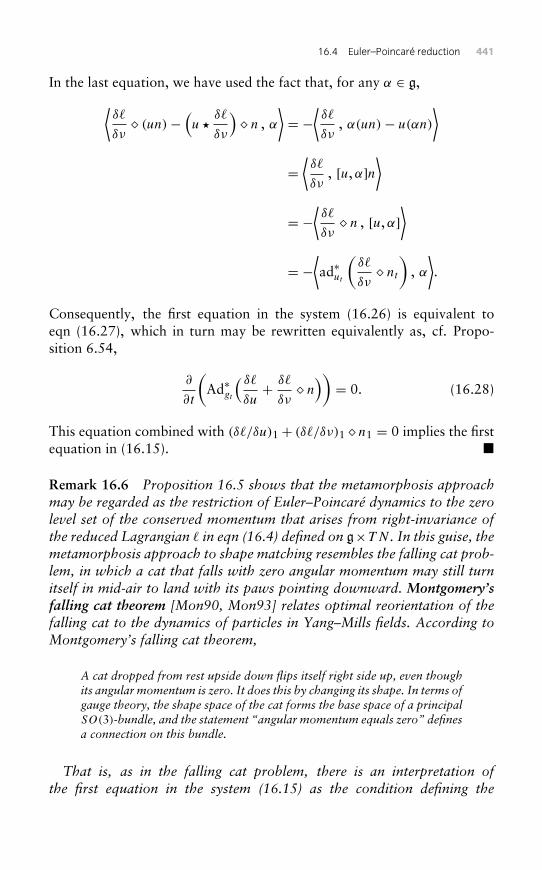
16.4 Euler–Poincaré reduction 441
In the last equation, we have used the fact that, for any α ∈ g,⟨δ�
δν& (un)−
(u �
δ�
δν
)& n , α
⟩= −
⟨δ�
δν, α(un)− u(αn)
⟩
=⟨δ�
δν, [u,α]n
⟩
= −⟨δ�
δν& n , [u,α]
⟩
= −⟨ad∗ut
(δ�
δν& nt
), α⟩.
Consequently, the first equation in the system (16.26) is equivalent toeqn (16.27), which in turn may be rewritten equivalently as, cf. Propo-sition 6.54,
∂
∂t
(Ad∗gt
( δ�δu+ δ�
δν& n))= 0. (16.28)
This equation combined with (δ�/δu)1 + (δ�/δν)1 & n1 = 0 implies the firstequation in (16.15). �
Remark 16.6 Proposition 16.5 shows that the metamorphosis approachmay be regarded as the restriction of Euler–Poincaré dynamics to the zerolevel set of the conserved momentum that arises from right-invariance ofthe reduced Lagrangian � in eqn (16.4) defined on g×TN . In this guise, themetamorphosis approach to shape matching resembles the falling cat prob-lem, in which a cat that falls with zero angular momentum may still turnitself in mid-air to land with its paws pointing downward. Montgomery’sfalling cat theorem [Mon90, Mon93] relates optimal reorientation of thefalling cat to the dynamics of particles in Yang–Mills fields. According toMontgomery’s falling cat theorem,
A cat dropped from rest upside down flips itself right side up, even thoughits angular momentum is zero. It does this by changing its shape. In terms ofgauge theory, the shape space of the cat forms the base space of a principalSO(3)-bundle, and the statement “angular momentum equals zero” definesa connection on this bundle.
That is, as in the falling cat problem, there is an interpretation ofthe first equation in the system (16.15) as the condition defining the
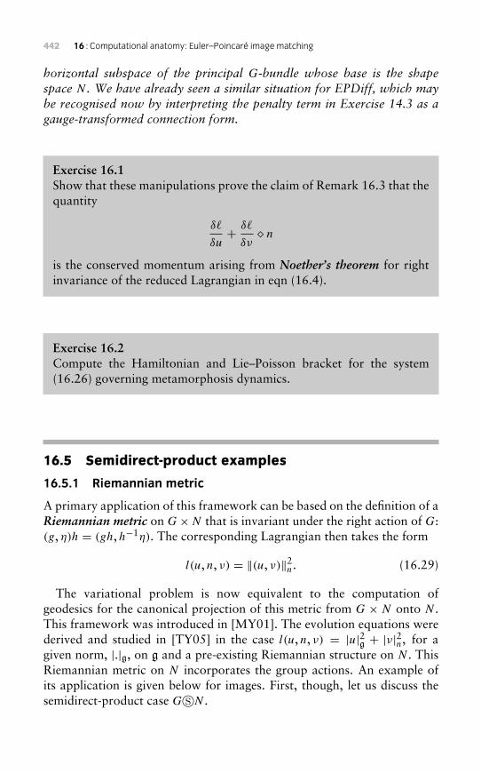
442 16 : Computational anatomy: Euler–Poincaré image matching
horizontal subspace of the principal G-bundle whose base is the shapespace N . We have already seen a similar situation for EPDiff, which maybe recognised now by interpreting the penalty term in Exercise 14.3 as agauge-transformed connection form.
Exercise 16.1Show that these manipulations prove the claim of Remark 16.3 that thequantity
δ�
δu+ δ�
δν& n
is the conserved momentum arising from Noether’s theorem for rightinvariance of the reduced Lagrangian in eqn (16.4).
Exercise 16.2Compute the Hamiltonian and Lie–Poisson bracket for the system(16.26) governing metamorphosis dynamics.
16.5 Semidirect-product examples
16.5.1 Riemannian metric
A primary application of this framework can be based on the definition of aRiemannian metric on G×N that is invariant under the right action of G:(g, η)h = (gh,h−1η). The corresponding Lagrangian then takes the form
l(u, n, ν) = ‖(u, ν)‖2n. (16.29)
The variational problem is now equivalent to the computation ofgeodesics for the canonical projection of this metric from G × N onto N .This framework was introduced in [MY01]. The evolution equations werederived and studied in [TY05] in the case l(u, n, ν) = |u|2g + |ν|2n, for agiven norm, |.|g, on g and a pre-existing Riemannian structure on N . ThisRiemannian metric on N incorporates the group actions. An example ofits application is given below for images. First, though, let us discuss thesemidirect-product case G�N .
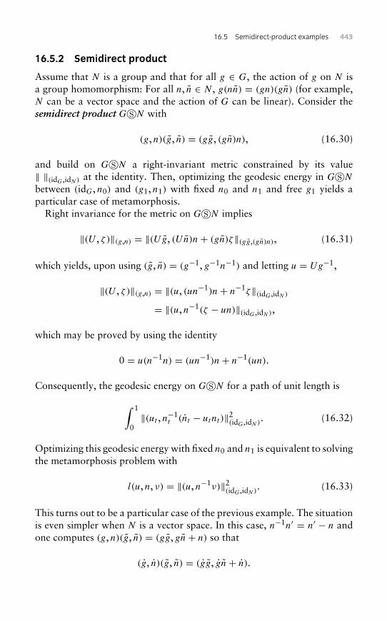
16.5 Semidirect-product examples 443
16.5.2 Semidirect product
Assume that N is a group and that for all g ∈ G, the action of g on N isa group homomorphism: For all n, n ∈ N , g(nn) = (gn)(gn) (for example,N can be a vector space and the action of G can be linear). Consider thesemidirect product G�N with
(g, n)(g, n) = (gg, (gn)n), (16.30)
and build on G�N a right-invariant metric constrained by its value‖ ‖(idG,idN) at the identity. Then, optimizing the geodesic energy in G�N
between (idG, n0) and (g1, n1) with fixed n0 and n1 and free g1 yields aparticular case of metamorphosis.
Right invariance for the metric on G�N implies
‖(U , ζ )‖(g,n) = ‖(Ug, (Un)n+ (gn)ζ‖(gg,(gn)n), (16.31)
which yields, upon using (g, n) = (g−1, g−1n−1) and letting u = Ug−1,
‖(U , ζ )‖(g,n) = ‖(u, (un−1)n+ n−1ζ‖(idG,idN)
= ‖(u, n−1(ζ − un)‖(idG,idN),
which may be proved by using the identity
0 = u(n−1n) = (un−1)n+ n−1(un).
Consequently, the geodesic energy on G�N for a path of unit length is
∫ 1
0‖(ut , n−1
t (nt − utnt )‖2(idG,idN). (16.32)
Optimizing this geodesic energy with fixed n0 and n1 is equivalent to solvingthe metamorphosis problem with
l(u, n, ν) = ‖(u, n−1ν)‖2(idG,idN)
. (16.33)
This turns out to be a particular case of the previous example. The situationis even simpler when N is a vector space. In this case, n−1n′ = n′ − n andone computes (g, n)(g, n) = (gg, gn+ n) so that
(g, n)(g, n) = (gg, gn+ n).
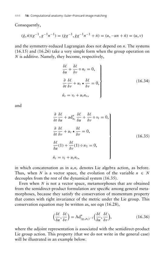
444 16 : Computational anatomy: Euler–Poincaré image matching
Consequently,
(g, n)(g−1, g−1n−1) = (gg−1, gg−1n−1 + n) = (u,−un+ n) = (u, ν)
and the symmetry-reduced Lagrangian does not depend on n. The systems(16.15) and (16.26) take a very simple form when the group operation onN is additive. Namely, they become, respectively,
δ�
δu+ δ�
δν& nt = 0,
∂
∂t
δ�
δν+ ut �
δ�
δν= 0,
nt = νt + utnt ,
(16.34)
and
∂
∂t
δ�
δu+ ad∗ut
δ�
δu+ δ�
δν& νt = 0,
∂
∂t
δ�
δν+ ut �
δ�
δν= 0,
δ�
δu(1)+ δ�
δν(1) & n1 = 0,
nt = νt + utnt ,
(16.35)
in which concatenation as in utnt denotes Lie algebra action, as before.Thus, when N is a vector space, the evolution of the variable n ∈ N
decouples from the rest of the dynamical system (16.35).Even when N is not a vector space, metamorphoses that are obtained
from the semidirect-product formulation are specific among general meta-morphoses, because they satisfy the conservation of momentum propertythat comes with right invariance of the metric under the Lie group. Thisconservation equation may be written as, see eqn (16.28),( δ�
δu,δ�
δν
)= Ad∗
(gt ,nt )−1
( δ�δu
,δ�
δν
), (16.36)
where the adjoint representation is associated with the semidirect-productLie group action. This property (that we do not write in the general case)will be illustrated in an example below.
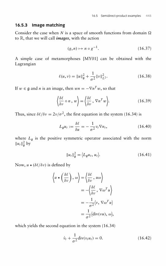
16.5 Semidirect-product examples 445
16.5.3 Image matching
Consider the case when N is a space of smooth functions from domain �
to R, that we will call images, with the action
(g, n) → n ◦ g−1. (16.37)
A simple case of metamorphoses [MY01] can be obtained with theLagrangian
�(u, ν) = ‖u‖2g +1σ 2 ‖ν‖2L2 . (16.38)
If w ∈ g and n is an image, then wn = −∇nT w, so that⟨δ�
δν& n , w
⟩=⟨δ�
δν, ∇nT w
⟩. (16.39)
Thus, since δ�/δν = 2ν/σ 2, the first equation in the system (16.34) is
Lgut := δ�
δu= − 1
σ 2 νt∇nt , (16.40)
where Lg is the positive symmetric operator associated with the norm‖ut‖2g by
‖ut‖2g =⟨Lgut , ut
⟩. (16.41)
Now, u � (δ�/δν) is defined by⟨u �
(δ�
δν
), ω⟩=⟨δ�
δν, uω
⟩= −
⟨δ�
δν, ∇ωT u
⟩= − 1
σ 2
⟨ν, ∇ωT u
⟩= 1
σ 2
⟨div(νu), ω
⟩,
which yields the second equation in the system (16.34)
νt + 1σ 2 div(νtut ) = 0. (16.42)
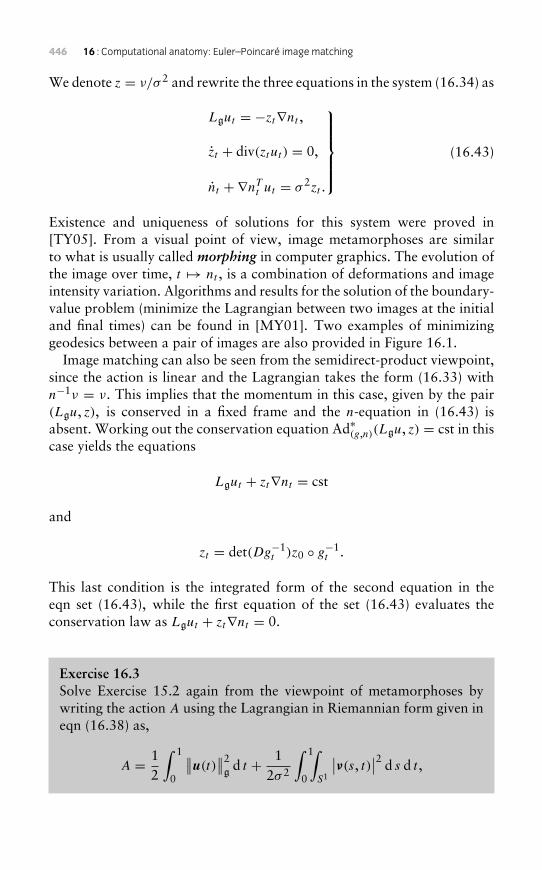
446 16 : Computational anatomy: Euler–Poincaré image matching
We denote z = ν/σ 2 and rewrite the three equations in the system (16.34) as
Lgut = −zt∇nt ,
zt + div(ztut ) = 0,
nt + ∇nTt ut = σ 2zt .
(16.43)
Existence and uniqueness of solutions for this system were proved in[TY05]. From a visual point of view, image metamorphoses are similarto what is usually called morphing in computer graphics. The evolution ofthe image over time, t → nt , is a combination of deformations and imageintensity variation. Algorithms and results for the solution of the boundary-value problem (minimize the Lagrangian between two images at the initialand final times) can be found in [MY01]. Two examples of minimizinggeodesics between a pair of images are also provided in Figure 16.1.
Image matching can also be seen from the semidirect-product viewpoint,since the action is linear and the Lagrangian takes the form (16.33) withn−1ν = ν. This implies that the momentum in this case, given by the pair(Lgu, z), is conserved in a fixed frame and the n-equation in (16.43) isabsent. Working out the conservation equation Ad∗(g,n)(Lgu, z) = cst in thiscase yields the equations
Lgut + zt∇nt = cst
and
zt = det(Dg−1t )z0 ◦ g−1
t .
This last condition is the integrated form of the second equation in theeqn set (16.43), while the first equation of the set (16.43) evaluates theconservation law as Lgut + zt∇nt = 0.
Exercise 16.3Solve Exercise 15.2 again from the viewpoint of metamorphoses bywriting the action A using the Lagrangian in Riemannian form given ineqn (16.38) as,
A = 12
∫ 1
0
∥∥u(t)∥∥2gd t + 1
2σ 2
∫ 1
0
∫S1
∣∣ν(s, t)∣∣2 d s d t ,
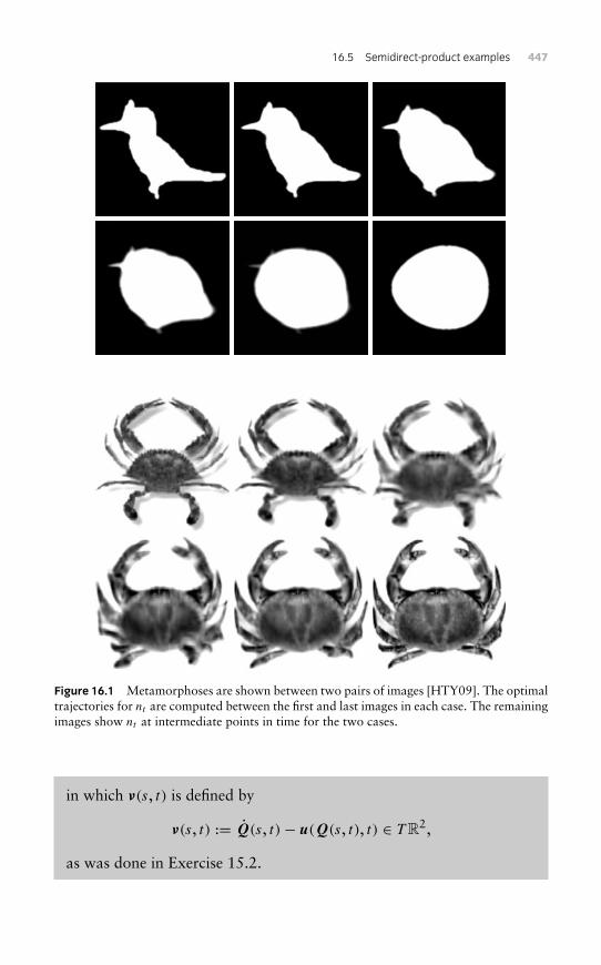
16.5 Semidirect-product examples 447
Figure 16.1 Metamorphoses are shown between two pairs of images [HTY09]. The optimaltrajectories for nt are computed between the first and last images in each case. The remainingimages show nt at intermediate points in time for the two cases.
in which ν(s, t) is defined by
ν(s, t) := Q(s, t)− u(Q(s, t), t) ∈ T R2,
as was done in Exercise 15.2.
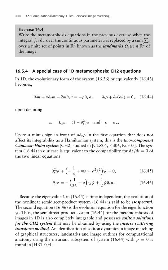
448 16 : Computational anatomy: Euler–Poincaré image matching
Exercise 16.4Write the metamorphosis equations in the previous exercise when theintegral
∫S1 d s over the continuous parameter s is replaced by a sum
∑s
over a finite set of points in R2 known as the landmarks Qs(t) ∈ R2 ofthe image.
16.5.4 A special case of 1D metamorphosis: CH2 equations
In 1D, the evolutionary form of the system (16.26) or equivalently (16.43)becomes,
∂tm+ u∂xm+ 2m∂xu = −ρ∂xρ, ∂tρ + ∂x(ρu) = 0, (16.44)
upon denoting
m = Lgu = (1− ∂2x )u and ρ = σz.
Up to a minus sign in front of ρ∂xρ in the first equation that does notaffect its integrability as a Hamiltonian system, this is the two-componentCamassa–Holm system (CH2) studied in [CLZ05, Fal06, Kuz07]. The sys-tem (16.44) in our case is equivalent to the compatibility for dλ/dt = 0 ofthe two linear equations
∂2x ψ +
(− 1
4+mλ+ ρ2λ2
)ψ = 0, (16.45)
∂tψ = −( 12λ+ u
)∂xψ + 1
2ψ∂xu. (16.46)
Because the eigenvalue λ in (16.45) is time independent, the evolution ofthe nonlinear semidirect-product system (16.44) is said to be isospectral.The second equation (16.46) is the evolution equation for the eigenfunctionψ . Thus, the semidirect-product system (16.44) for the metamorphosis ofimages in 1D is also completely integrable and possesses soliton solutionsfor the CH2 system that may be obtained by using the inverse scatteringtransform method. An identification of soliton dynamics in image matchingof graphical structures, landmarks and image outlines for computationalanatomy using the invariant subsystem of system (16.44) with ρ = 0 isfound in [HRTY04].
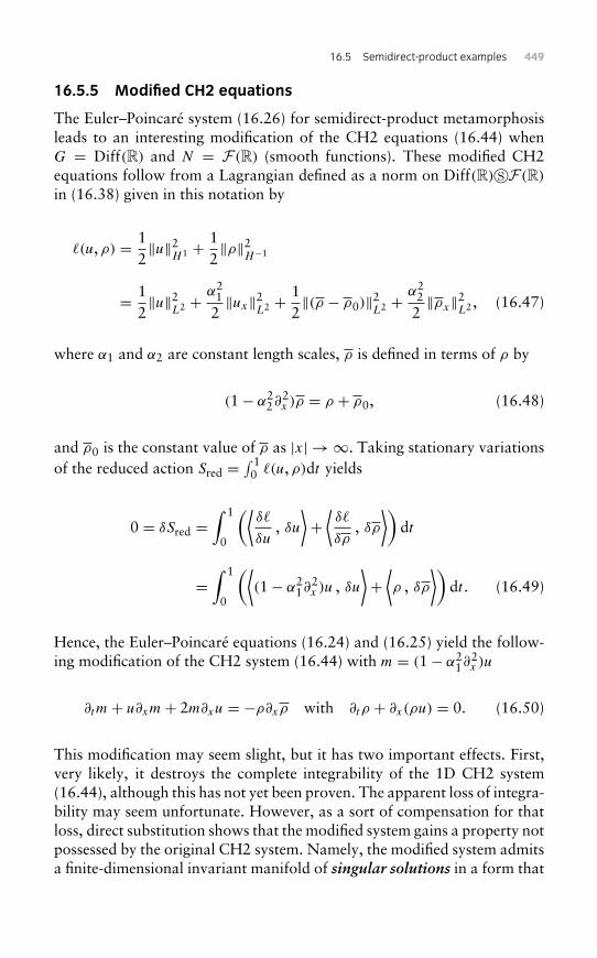
16.5 Semidirect-product examples 449
16.5.5 Modified CH2 equations
The Euler–Poincaré system (16.26) for semidirect-product metamorphosisleads to an interesting modification of the CH2 equations (16.44) whenG = Diff(R) and N = F(R) (smooth functions). These modified CH2equations follow from a Lagrangian defined as a norm on Diff(R)�F(R)
in (16.38) given in this notation by
�(u, ρ) = 12‖u‖2
H1 + 12‖ρ‖2
H−1
= 12‖u‖2
L2 +α2
1
2‖ux‖2L2 + 1
2‖(ρ − ρ0)‖2L2 +
α22
2‖ρx‖2L2 , (16.47)
where α1 and α2 are constant length scales, ρ is defined in terms of ρ by
(1− α22∂
2x )ρ = ρ + ρ0, (16.48)
and ρ0 is the constant value of ρ as |x| → ∞. Taking stationary variationsof the reduced action Sred =
∫ 10 �(u, ρ)dt yields
0 = δSred =∫ 1
0
(⟨δ�
δu, δu
⟩+⟨δ�
δρ, δρ
⟩)dt
=∫ 1
0
(⟨(1− α2
1∂2x )u , δu
⟩+⟨ρ , δρ
⟩)dt . (16.49)
Hence, the Euler–Poincaré equations (16.24) and (16.25) yield the follow-ing modification of the CH2 system (16.44) with m = (1− α2
1∂2x )u
∂tm+ u∂xm+ 2m∂xu = −ρ∂xρ with ∂tρ + ∂x(ρu) = 0. (16.50)
This modification may seem slight, but it has two important effects. First,very likely, it destroys the complete integrability of the 1D CH2 system(16.44), although this has not yet been proven. The apparent loss of integra-bility may seem unfortunate. However, as a sort of compensation for thatloss, direct substitution shows that the modified system gains a property notpossessed by the original CH2 system. Namely, the modified system admitsa finite-dimensional invariant manifold of singular solutions in a form that
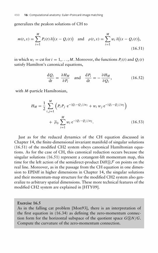
450 16 : Computational anatomy: Euler–Poincaré image matching
generalizes the peakon solutions of CH to
m(t , x) =M∑i=1
Pi(t) δ((x −Qi(t)
)and ρ(t , x) =
M∑i=1
wi δ((x −Qi(t)
),
(16.51)
in which wi = cst for i = 1, . . . ,M. Moreover, the functions Pi(t) and Qi(t)
satisfy Hamilton’s canonical equations,
dQi
dt= ∂HM
∂Pi
anddPi
dt= − ∂HM
∂Qi
, (16.52)
with M-particle Hamiltonian,
HM = 12
M∑i,j=1
(PiPj e−|Qi−Qj |/α1 + wi wj e−|Qi−Qj |/α2
)
+ ρ0
M∑i=1
wi e−|Qi−Qj |/α2 . (16.53)
Just as for the reduced dynamics of the CH equation discussed inChapter 14, the finite-dimensional invariant manifold of singular solutions(16.51) of the modified CH2 system obeys canonical Hamiltonian equa-tions. As for the case of CH, this canonical reduction occurs because thesingular solutions (16.51) represent a cotangent-lift momentum map, thistime for the left action of the semidirect-product Diff�F on points on thereal line. Moreover, as in the passage from the CH equation in one dimen-sion to EPDiff in higher dimensions in Chapter 14, the singular solutionsand their momentum-map structure for the modified CH2 system also gen-eralize to arbitrary spatial dimensions. These more technical features of themodified CH2 system are explained in [HTY09].
Exercise 16.5As in the falling cat problem [Mon93], there is an interpretation ofthe first equation in (16.34) as defining the zero-momentum connec-tion form for the horizontal subspace of the quotient space G�N/G.Compute the curvature of the zero-momentum connection.
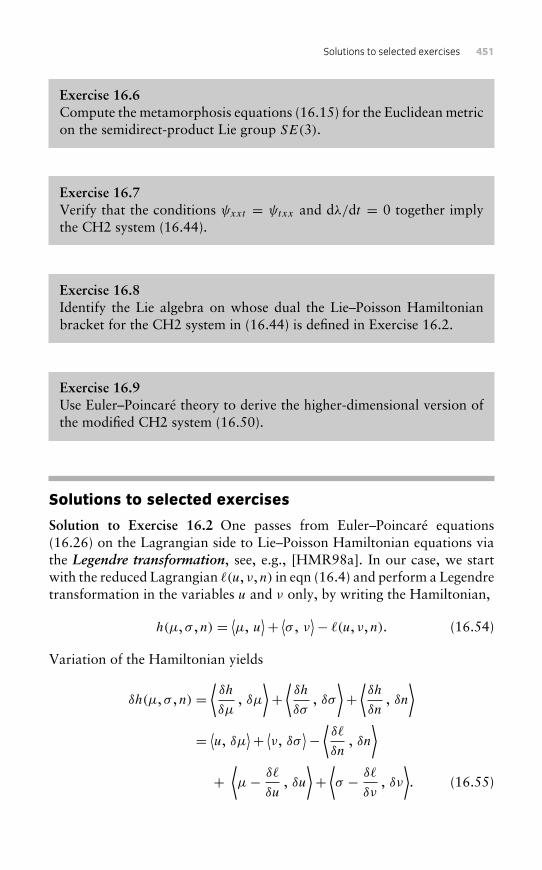
Solutions to selected exercises 451
Exercise 16.6Compute the metamorphosis equations (16.15) for the Euclidean metricon the semidirect-product Lie group SE(3).
Exercise 16.7Verify that the conditions ψxxt = ψtxx and dλ/dt = 0 together implythe CH2 system (16.44).
Exercise 16.8Identify the Lie algebra on whose dual the Lie–Poisson Hamiltonianbracket for the CH2 system in (16.44) is defined in Exercise 16.2.
Exercise 16.9Use Euler–Poincaré theory to derive the higher-dimensional version ofthe modified CH2 system (16.50).
Solutions to selected exercises
Solution to Exercise 16.2 One passes from Euler–Poincaré equations(16.26) on the Lagrangian side to Lie–Poisson Hamiltonian equations viathe Legendre transformation, see, e.g., [HMR98a]. In our case, we startwith the reduced Lagrangian �(u, ν, n) in eqn (16.4) and perform a Legendretransformation in the variables u and ν only, by writing the Hamiltonian,
h(µ, σ , n) = ⟨µ, u⟩+ ⟨σ , ν
⟩− �(u, ν, n). (16.54)
Variation of the Hamiltonian yields
δh(µ, σ , n) =⟨δh
δµ, δµ
⟩+⟨δh
δσ, δσ
⟩+⟨δh
δn, δn
⟩= ⟨u, δµ
⟩+ ⟨ν, δσ⟩− ⟨ δ�
δn, δn
⟩+⟨µ− δ�
δu, δu
⟩+⟨σ − δ�
δν, δν
⟩. (16.55)
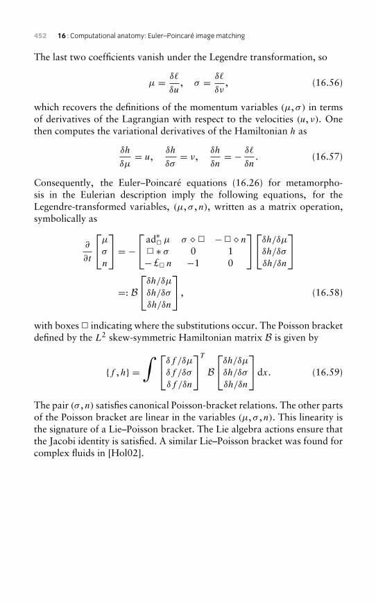
452 16 : Computational anatomy: Euler–Poincaré image matching
The last two coefficients vanish under the Legendre transformation, so
µ = δ�
δu, σ = δ�
δν, (16.56)
which recovers the definitions of the momentum variables (µ, σ) in termsof derivatives of the Lagrangian with respect to the velocities (u, ν). Onethen computes the variational derivatives of the Hamiltonian h as
δh
δµ= u,
δh
δσ= ν,
δh
δn= − δ�
δn. (16.57)
Consequently, the Euler–Poincaré equations (16.26) for metamorpho-sis in the Eulerian description imply the following equations, for theLegendre-transformed variables, (µ, σ , n), written as a matrix operation,symbolically as
∂
∂t
µ
σ
n
= − ad∗� µ σ &� −� & n
� ∗ σ 0 1− £� n −1 0
δh/δµ
δh/δσ
δh/δn
=: B
δh/δµ
δh/δσ
δh/δn
, (16.58)
with boxes � indicating where the substitutions occur. The Poisson bracketdefined by the L2 skew-symmetric Hamiltonian matrix B is given by
{f ,h} =∫ δf /δµ
δf /δσ
δf /δn
T
Bδh/δµ
δh/δσ
δh/δn
dx. (16.59)
The pair (σ , n) satisfies canonical Poisson-bracket relations. The other partsof the Poisson bracket are linear in the variables (µ, σ , n). This linearity isthe signature of a Lie–Poisson bracket. The Lie algebra actions ensure thatthe Jacobi identity is satisfied. A similar Lie–Poisson bracket was found forcomplex fluids in [Hol02].
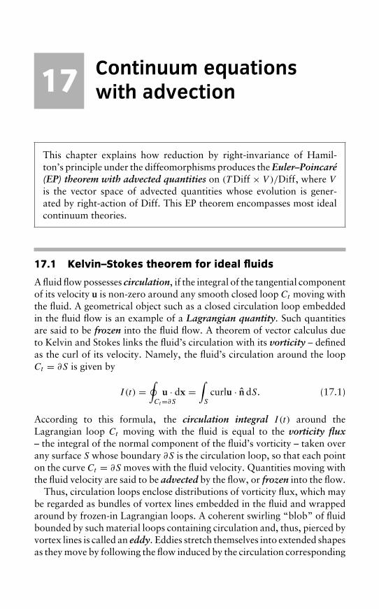
17 Continuum equationswith advection
This chapter explains how reduction by right-invariance of Hamil-ton’s principle under the diffeomorphisms produces the Euler–Poincaré(EP) theorem with advected quantities on (TDiff × V )/Diff, where V
is the vector space of advected quantities whose evolution is gener-ated by right-action of Diff. This EP theorem encompasses most idealcontinuum theories.
17.1 Kelvin–Stokes theorem for ideal fluids
A fluid flow possesses circulation, if the integral of the tangential componentof its velocity u is non-zero around any smooth closed loop Ct moving withthe fluid. A geometrical object such as a closed circulation loop embeddedin the fluid flow is an example of a Lagrangian quantity. Such quantitiesare said to be frozen into the fluid flow. A theorem of vector calculus dueto Kelvin and Stokes links the fluid’s circulation with its vorticity – definedas the curl of its velocity. Namely, the fluid’s circulation around the loopCt = ∂S is given by
I (t) =∮Ct=∂S
u · dx =∫S
curlu · n dS. (17.1)
According to this formula, the circulation integral I (t) around theLagrangian loop Ct moving with the fluid is equal to the vorticity flux– the integral of the normal component of the fluid’s vorticity – taken overany surface S whose boundary ∂S is the circulation loop, so that each pointon the curve Ct = ∂S moves with the fluid velocity. Quantities moving withthe fluid velocity are said to be advected by the flow, or frozen into the flow.
Thus, circulation loops enclose distributions of vorticity flux, which maybe regarded as bundles of vortex lines embedded in the fluid and wrappedaround by frozen-in Lagrangian loops. A coherent swirling “blob” of fluidbounded by such material loops containing circulation and, thus, pierced byvortex lines is called an eddy. Eddies stretch themselves into extended shapesas they move by following the flow induced by the circulation corresponding
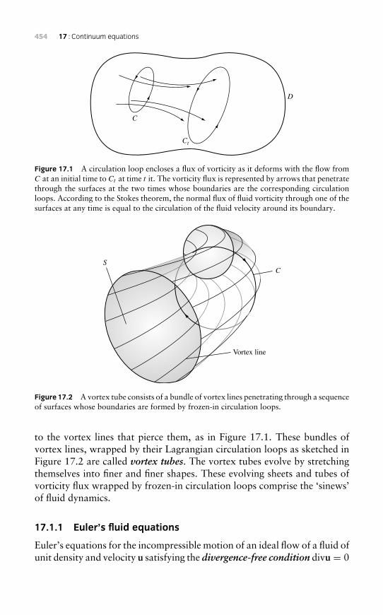
454 17 : Continuum equations
C
D
Ct
Figure 17.1 A circulation loop encloses a flux of vorticity as it deforms with the flow fromC at an initial time to Ct at time t it. The vorticity flux is represented by arrows that penetratethrough the surfaces at the two times whose boundaries are the corresponding circulationloops. According to the Stokes theorem, the normal flux of fluid vorticity through one of thesurfaces at any time is equal to the circulation of the fluid velocity around its boundary.
C
Vortex line
S
Figure 17.2 A vortex tube consists of a bundle of vortex lines penetrating through a sequenceof surfaces whose boundaries are formed by frozen-in circulation loops.
to the vortex lines that pierce them, as in Figure 17.1. These bundles ofvortex lines, wrapped by their Lagrangian circulation loops as sketched inFigure 17.2 are called vortex tubes. The vortex tubes evolve by stretchingthemselves into finer and finer shapes. These evolving sheets and tubes ofvorticity flux wrapped by frozen-in circulation loops comprise the ‘sinews’of fluid dynamics.
17.1.1 Euler’s fluid equations
Euler’s equations for the incompressible motion of an ideal flow of a fluid ofunit density and velocity u satisfying the divergence-free condition divu = 0
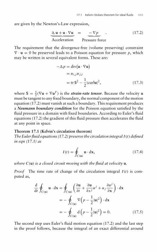
17.1 Kelvin–Stokes theorem for ideal fluids 455
are given by the Newton’s-Law expression,
∂t u+ u · ∇u︸ ︷︷ ︸Acceleration
= −∇p︸ ︷︷ ︸Pressure force
. (17.2)
The requirement that the divergence-free (volume preserving) constraint∇ · u = 0 be preserved leads to a Poisson equation for pressure p, whichmay be written in several equivalent forms. These are:
−�p = div(u · ∇u
)= ui,juj ,i
= tr S2 − 12|curlu|2, (17.3)
where S = 12 (∇u + ∇uT ) is the strain-rate tensor. Because the velocity u
must be tangent to any fixed boundary, the normal component of the motionequation (17.2) must vanish at such a boundary. This requirement producesa Neumann boundary condition for the Poisson equation satisfied by thefluid pressure in a domain with fixed boundaries. According to Euler’s fluidequations (17.2) the gradient of this fluid pressure then accelerates the fluidat any point in space.
Theorem 17.1 (Kelvin’s circulation theorem)TheEuler fluid equations (17.2) preserve the circulation integral I (t) definedin eqn (17.1) as
I (t) =∮C(u)
u · dx, (17.4)
where C(u) is a closed circuit moving with the fluid at velocity u.
Proof The time rate of change of the circulation integral I (t) is com-puted as,
ddt
∮C(u)
u · dx =∮C(u)
(∂u∂t+ ∂u
∂xjuj + uj
∂uj
∂x
)· dx
= −∮C(u)∇(p − 1
2|u|2
)· dx
= −∮C(u)
d(p − 1
2|u|2
)= 0. (17.5)
The second step uses Euler’s fluid motion equation (17.2) and the last stepin the proof follows, because the integral of an exact differential around
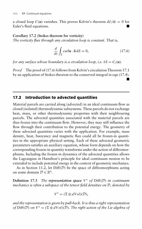
456 17 : Continuum equations
a closed loop C(u) vanishes. This proves Kelvin’s theorem dI/dt = 0 forEuler’s fluid equations. �
Corollary 17.2 (Stokes theorem for vorticity)The vorticity flux through any circulation loop is constant. That is,
d
dt
∫S
curlu · n dS = 0, (17.6)
for any surface whose boundary is a circulation loop, i.e. ∂S = Ct(u).
Proof The proof of (17.6) follows from Kelvin’s circulation Theorem 17.1by an application of Stokes theorem to the conserved integral in eqn (17.4).
�
17.2 Introduction to advected quantities
Material parcels are carried along (advected) in an ideal continuum flow asclosed (isolated) thermodynamic subsystems. These parcels do not exchangeheat, mass, or other thermodynamic properties with their neighbouringparcels. The advected quantities associated with the material parcels arethus frozen into the continuum flow. However, they may still influence theflow through their contribution to the potential energy. The geometry ofthese advected quantities varies with the application. For example, massdensity, heat, buoyancy and magnetic flux could all be frozen-in quanti-ties in the appropriate physical setting. Each of these advected geometricparameters satisfies an auxiliary equation, whose form depends on how thecorresponding frozen-in quantity transforms under the action of diffeomor-phisms. Including the frozen-in dynamics of the advected quantities allowsthe Lagrangian in Hamilton’s principle for ideal continuum motion to beextended to include potential energy in the context of geometric mechanics.
As in Section 11.2, let Diff(D) be the space of diffeomorphisms actingon some domain D ∈ Rn.
Definition 17.3 The representation space V ∗ of Diff(D) in continuummechanics is often a subspace of the tensor field densities on D, denoted by
V ∗ = (T⊗ dV ol)(D),
and the representation is given by pull-back. It is thus a right representationof Diff(D) on V ∗ = (T⊗ dV ol)(D). The right action of the Lie algebra of
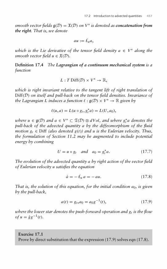
17.2 Introduction to advected quantities 457
smooth vector fields g(D) = X(D) on V ∗ is denoted as concatenation fromthe right. That is, we denote
au := £ua,
which is the Lie derivative of the tensor field density a ∈ V ∗ along thesmooth vector field u ∈ X(D).
Definition 17.4 The Lagrangian of a continuum mechanical system is afunction
L : T Diff(D)× V ∗ → R,
which is right invariant relative to the tangent lift of right translation ofDiff(D) on itself and pull-back on the tensor field densities. Invariance ofthe Lagrangian L induces a function � : g(D)× V ∗ → R given by
�(u, a) = L(u ◦ gt , g∗t a) = L(U , a0),
where u ∈ g(D) and a ∈ V ∗ ⊂ T(D) ⊗ dV ol, and where g∗t a denotes thepull-back of the advected quantity a by the diffeomorphism of the fluidmotion gt ∈ Diff (also denoted g(t)) and u is the Eulerian velocity. Thus,the formulation of Section 11.2 may be augmented to include potentialenergy by combining
U = u ◦ gt and a0 = g∗t a. (17.7)
The evolution of the advected quantity a by right action of the vector fieldof Eulerian velocity u satisfies the equation
a = −£u a = − au. (17.8)
That is, the solution of this equation, for the initial condition a0, is givenby the pull-back,
a(t) = gt∗a0 = a0g−1(t), (17.9)
where the lower star denotes the push-forward operation and gt is the flowof u = gg−1(t).
Exercise 17.1Prove by direct substitution that the expression (17.9) solves eqn (17.8).
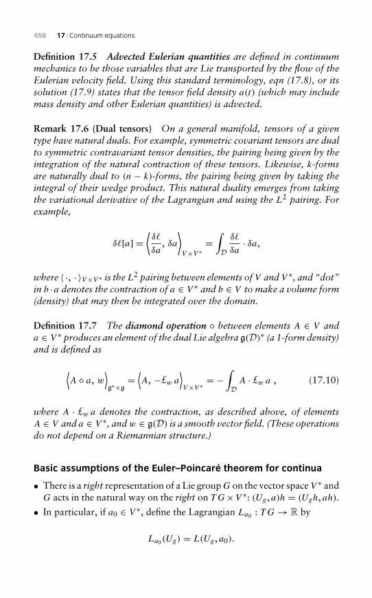
458 17 : Continuum equations
Definition 17.5 Advected Eulerian quantities are defined in continuummechanics to be those variables that are Lie transported by the flow of theEulerian velocity field. Using this standard terminology, eqn (17.8), or itssolution (17.9) states that the tensor field density a(t) (which may includemass density and other Eulerian quantities) is advected.
Remark 17.6 (Dual tensors) On a general manifold, tensors of a giventype have natural duals. For example, symmetric covariant tensors are dualto symmetric contravariant tensor densities, the pairing being given by theintegration of the natural contraction of these tensors. Likewise, k-formsare naturally dual to (n − k)-forms, the pairing being given by taking theintegral of their wedge product. This natural duality emerges from takingthe variational derivative of the Lagrangian and using the L2 pairing. Forexample,
δ�[a] =⟨δ�
δa, δa
⟩V×V ∗
=∫
Dδ�
δa· δa,
where 〈 ·, · 〉V×V ∗ is theL2 pairing between elements of V and V ∗, and “dot”in b ·a denotes the contraction of a ∈ V ∗ and b ∈ V to make a volume form(density) that may then be integrated over the domain.
Definition 17.7 The diamond operation & between elements A ∈ V anda ∈ V ∗ produces an element of the dual Lie algebra g(D)∗ (a 1-form density)and is defined as
⟨A & a, w
⟩g∗×g=⟨A, −£w a
⟩V×V ∗ = −
∫D
A · £w a , (17.10)
where A · £w a denotes the contraction, as described above, of elementsA ∈ V and a ∈ V ∗, andw ∈ g(D) is a smooth vector field. (These operationsdo not depend on a Riemannian structure.)
Basic assumptions of the Euler–Poincaré theorem for continua
• There is a right representation of a Lie groupG on the vector spaceV ∗ andG acts in the natural way on the right on TG×V ∗: (Ug, a)h = (Ugh, ah).
• In particular, if a0 ∈ V ∗, define the Lagrangian La0 : TG→ R by
La0(Ug) = L(Ug, a0).
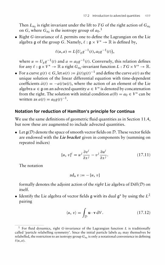
17.2 Introduction to advected quantities 459
Then La0 is right invariant under the lift to TG of the right action of Ga0
on G, where Ga0 is the isotropy group of a0.1
• Right G-invariance of L permits one to define the Lagrangian on the Liealgebra g of the group G. Namely, � : g× V ∗ → R is defined by,
�(u, a) = L(Ugg
−1(t), a0g−1(t)
),
where u = Ugg−1(t) and a = a0g
−1(t). Conversely, this relation definesfor any � : g×V ∗ → R a right Ga0-invariant function L : TG×V ∗ → R.
• For a curve g(t) ∈ G, let u(t) := g(t)g(t)−1 and define the curve a(t) as theunique solution of the linear differential equation with time-dependentcoefficients a(t) = −a(t)u(t), where the action of an element of the Liealgebra u ∈ g on an advected quantity a ∈ V ∗ is denoted by concatenationfrom the right. The solution with initial condition a(0) = a0 ∈ V ∗ can bewritten as a(t) = a0g(t)
−1.
Notation for reduction of Hamilton’s principle for continua
We use the same definitions of geometric fluid quantities as in Section 11.4,but now these are augmented to include advected quantities.
• Let g(D) denote the space of smooth vector fields on D. These vector fieldsare endowed with the Lie bracket given in components by (summing onrepeated indices)
[u, v]i = uj ∂vi
∂xj− vj ∂ui
∂xj. (17.11)
The notation
adu v := −[u, v]formally denotes the adjoint action of the right Lie algebra of Diff(D) onitself.
• Identify the Lie algebra of vector fields g with its dual g∗ by using the L2
pairing
〈u, v〉 =∫
Du · v dV . (17.12)
1 For fluid dynamics, right G-invariance of the Lagrangian function L is traditionallycalled ‘particle relabelling symmetry’. Since the initial particle labels a0 may themselves berelabelled, the restriction to an isotropy groupGa0 is only a notational convenience in defining�(u, a).
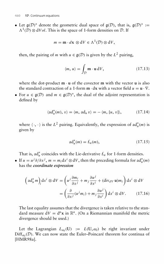
460 17 : Continuum equations
• Let g(D)∗ denote the geometric dual space of g(D), that is, g(D)∗ :=�1(D)⊗ dV ol. This is the space of 1-form densities on D. If
m = m · dx ⊗ dV ∈ �1(D)⊗ dV ,
then, the pairing of m with u ∈ g(D) is given by the L2 pairing,
〈m, u〉 =∫
Dm · u dV , (17.13)
where the dot-product m · u of the covector m with the vector u is alsothe standard contraction of a 1-form m · dx with a vector field u = u · ∇.
• For u ∈ g(D) and m ∈ g(D)∗, the dual of the adjoint representation isdefined by
〈ad∗u(m), v〉 = 〈m, adu v〉 = − 〈m, [u, v]〉, (17.14)
where 〈 ·, · 〉 is the L2 pairing. Equivalently, the expression of ad∗u(m) isgiven by
ad∗u(m) = £u(m), (17.15)
That is, ad∗u coincides with the Lie-derivative £u for 1-form densities.
• If u = uj∂/∂xj , m = midxi ⊗dV , then the preceding formula for ad∗u(m)
has the coordinate expression
(ad∗u m
)idxi ⊗ dV =
(uj ∂mi
∂xj+mj
∂uj
∂xi+ (divdV u)mi
)dxi ⊗ dV
=(
∂
∂xj(ujmi)+mj
∂uj
∂xi
)dxi ⊗ dV . (17.16)
The last equality assumes that the divergence is taken relative to the stan-dard measure dV = dnx in Rn. (On a Riemannian manifold the metricdivergence should be used.)
Let the Lagrangian La0(U) := L(U, a0) be right invariant underDiffa0(D). We can now state the Euler–Poincaré theorem for continua of[HMR98a].
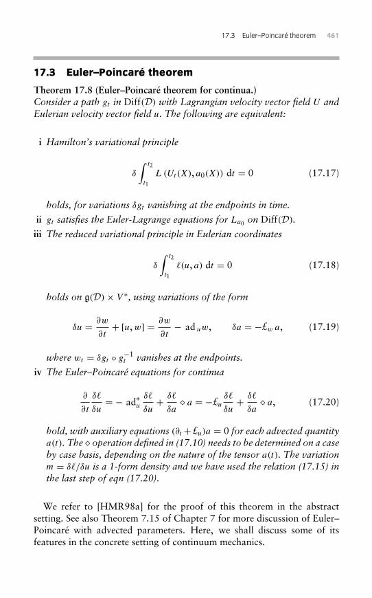
17.3 Euler–Poincaré theorem 461
17.3 Euler–Poincaré theorem
Theorem 17.8 (Euler–Poincaré theorem for continua.)Consider a path gt in Diff(D) with Lagrangian velocity vector field U andEulerian velocity vector field u. The following are equivalent:
i Hamilton’s variational principle
δ
∫ t2
t1
L (Ut(X), a0(X)) dt = 0 (17.17)
holds, for variations δgt vanishing at the endpoints in time.
ii gt satisfies the Euler-Lagrange equations for La0 on Diff(D).
iii The reduced variational principle in Eulerian coordinates
δ
∫ t2
t1
�(u, a) dt = 0 (17.18)
holds on g(D)× V ∗, using variations of the form
δu = ∂w
∂t+ [u,w] = ∂w
∂t− ad uw, δa = −£w a, (17.19)
where wt = δgt ◦ g−1t vanishes at the endpoints.
iv The Euler–Poincaré equations for continua
∂
∂t
δ�
δu= − ad∗u
δ�
δu+ δ�
δa& a = −£u
δ�
δu+ δ�
δa& a, (17.20)
hold, with auxiliary equations (∂t +£u)a = 0 for each advected quantitya(t). The & operation defined in (17.10) needs to be determined on a caseby case basis, depending on the nature of the tensor a(t). The variationm = δ�/δu is a 1-form density and we have used the relation (17.15) inthe last step of eqn (17.20).
We refer to [HMR98a] for the proof of this theorem in the abstractsetting. See also Theorem 7.15 of Chapter 7 for more discussion of Euler–Poincaré with advected parameters. Here, we shall discuss some of itsfeatures in the concrete setting of continuum mechanics.
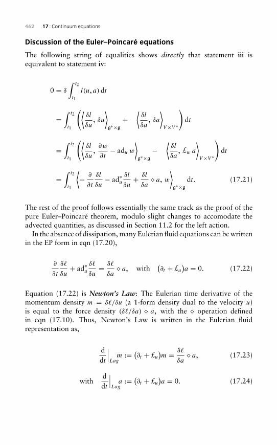
462 17 : Continuum equations
Discussion of the Euler–Poincaré equations
The following string of equalities shows directly that statement iii isequivalent to statement iv:
0 = δ
∫ t2
t1
l(u, a) dt
=∫ t2
t1
(⟨δl
δu, δu
⟩g∗×g
+⟨δl
δa, δa
⟩V×V ∗
)dt
=∫ t2
t1
(⟨δl
δu,∂w
∂t− adu w
⟩g∗×g
−⟨δl
δa, £w a
⟩V×V ∗
)dt
=∫ t2
t1
⟨− ∂
∂t
δl
δu− ad∗u
δl
δu+ δl
δa& a, w
⟩g∗×g
dt . (17.21)
The rest of the proof follows essentially the same track as the proof of thepure Euler–Poincaré theorem, modulo slight changes to accomodate theadvected quantities, as discussed in Section 11.2 for the left action.
In the absence of dissipation, many Eulerian fluid equations can be writtenin the EP form in eqn (17.20),
∂
∂t
δ�
δu+ ad∗u
δ�
δu= δ�
δa& a, with
(∂t + £u
)a = 0. (17.22)
Equation (17.22) is Newton’s Law: The Eulerian time derivative of themomentum density m = δ�/δu (a 1-form density dual to the velocity u)is equal to the force density (δ�/δa) & a, with the & operation definedin eqn (17.10). Thus, Newton’s Law is written in the Eulerian fluidrepresentation as,
ddt
∣∣∣Lag
m := (∂t + £u
)m = δ�
δa& a, (17.23)
withddt
∣∣∣Lag
a := (∂t + £u
)a = 0. (17.24)
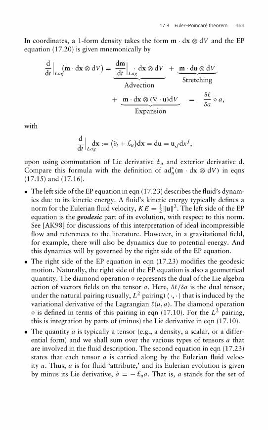
17.3 Euler–Poincaré theorem 463
In coordinates, a 1-form density takes the form m · dx ⊗ dV and the EPequation (17.20) is given mnemonically by
ddt
∣∣∣Lag
(m · dx⊗ dV
) = dmdt
∣∣∣Lag· dx⊗ dV︸ ︷︷ ︸
Advection
+ m · du⊗ dV︸ ︷︷ ︸Stretching
+ m · dx⊗ (∇ · u)dV︸ ︷︷ ︸Expansion
= δ�
δa& a,
with
ddt
∣∣∣Lag
dx := (∂t + £u
)dx = du = u,jdxj ,
upon using commutation of Lie derivative £u and exterior derivative d.Compare this formula with the definition of ad∗u(m · dx ⊗ dV ) in eqns(17.15) and (17.16).
• The left side of the EP equation in eqn (17.23) describes the fluid’s dynam-ics due to its kinetic energy. A fluid’s kinetic energy typically defines anorm for the Eulerian fluid velocity, KE = 1
2‖u‖2. The left side of the EPequation is the geodesic part of its evolution, with respect to this norm.See [AK98] for discussions of this interpretation of ideal incompressibleflow and references to the literature. However, in a gravitational field,for example, there will also be dynamics due to potential energy. Andthis dynamics will by governed by the right side of the EP equation.
• The right side of the EP equation in eqn (17.23) modifies the geodesicmotion. Naturally, the right side of the EP equation is also a geometricalquantity. The diamond operation & represents the dual of the Lie algebraaction of vectors fields on the tensor a. Here, δ�/δa is the dual tensor,under the natural pairing (usually, L2 pairing) 〈 ·, · 〉 that is induced by thevariational derivative of the Lagrangian �(u, a). The diamond operation& is defined in terms of this pairing in eqn (17.10). For the L2 pairing,this is integration by parts of (minus) the Lie derivative in eqn (17.10).
• The quantity a is typically a tensor (e.g., a density, a scalar, or a differ-ential form) and we shall sum over the various types of tensors a thatare involved in the fluid description. The second equation in eqn (17.23)states that each tensor a is carried along by the Eulerian fluid veloc-ity u. Thus, a is for fluid ‘attribute,’ and its Eulerian evolution is givenby minus its Lie derivative, a = − £ua. That is, a stands for the set of
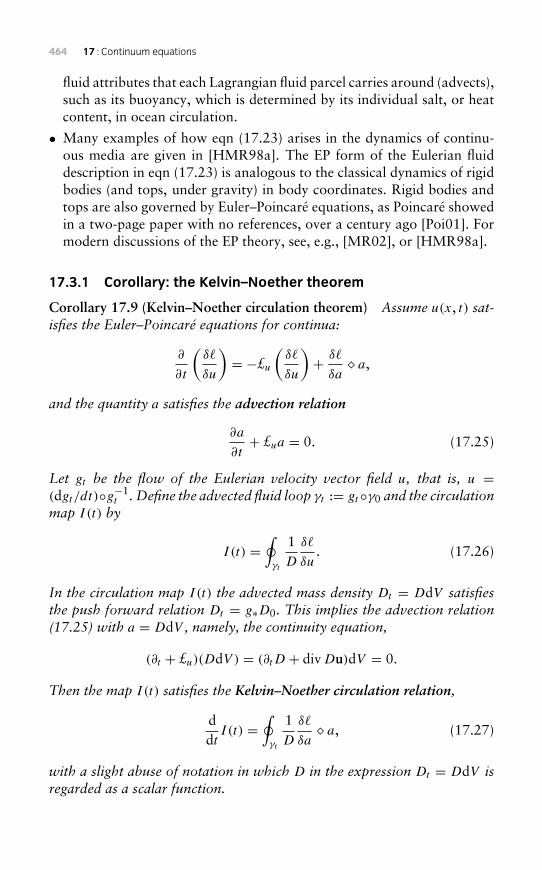
464 17 : Continuum equations
fluid attributes that each Lagrangian fluid parcel carries around (advects),such as its buoyancy, which is determined by its individual salt, or heatcontent, in ocean circulation.
• Many examples of how eqn (17.23) arises in the dynamics of continu-ous media are given in [HMR98a]. The EP form of the Eulerian fluiddescription in eqn (17.23) is analogous to the classical dynamics of rigidbodies (and tops, under gravity) in body coordinates. Rigid bodies andtops are also governed by Euler–Poincaré equations, as Poincaré showedin a two-page paper with no references, over a century ago [Poi01]. Formodern discussions of the EP theory, see, e.g., [MR02], or [HMR98a].
17.3.1 Corollary: the Kelvin–Noether theorem
Corollary 17.9 (Kelvin–Noether circulation theorem) Assume u(x, t) sat-isfies the Euler–Poincaré equations for continua:
∂
∂t
(δ�
δu
)= −£u
(δ�
δu
)+ δ�
δa& a,
and the quantity a satisfies the advection relation
∂a
∂t+ £ua = 0. (17.25)
Let gt be the flow of the Eulerian velocity vector field u, that is, u =(dgt/dt)◦g−1
t . Define the advected fluid loop γt := gt ◦γ0 and the circulationmap I (t) by
I (t) =∮γt
1D
δ�
δu. (17.26)
In the circulation map I (t) the advected mass density Dt = DdV satisfiesthe push forward relation Dt = g∗D0. This implies the advection relation(17.25) with a = DdV , namely, the continuity equation,
(∂t + £u)(DdV ) = (∂tD + divDu)dV = 0.
Then the map I (t) satisfies the Kelvin–Noether circulation relation,
ddt
I (t) =∮γt
1D
δ�
δa& a, (17.27)
with a slight abuse of notation in which D in the expression Dt = DdV isregarded as a scalar function.
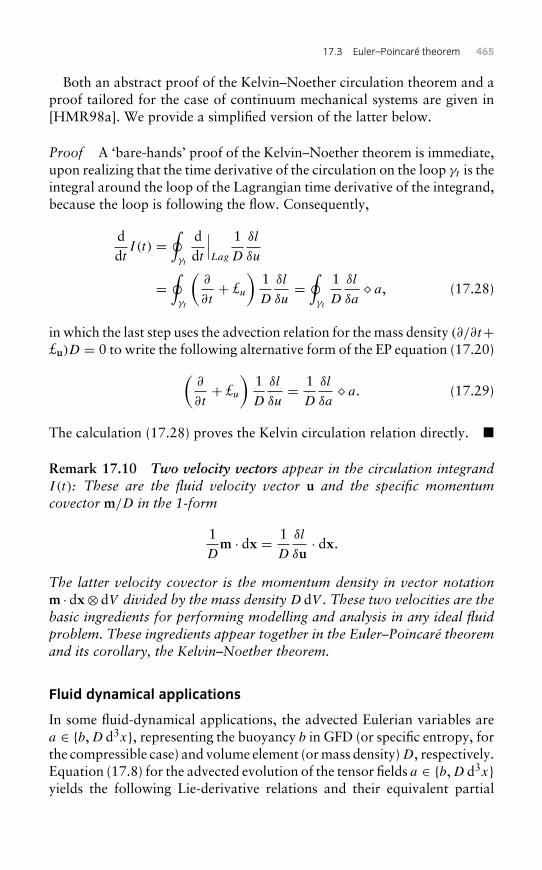
17.3 Euler–Poincaré theorem 465
Both an abstract proof of the Kelvin–Noether circulation theorem and aproof tailored for the case of continuum mechanical systems are given in[HMR98a]. We provide a simplified version of the latter below.
Proof A ‘bare-hands’ proof of the Kelvin–Noether theorem is immediate,upon realizing that the time derivative of the circulation on the loop γt is theintegral around the loop of the Lagrangian time derivative of the integrand,because the loop is following the flow. Consequently,
ddt
I (t) =∮γt
ddt
∣∣∣Lag
1D
δl
δu
=∮γt
(∂
∂t+ £u
)1D
δl
δu=∮γt
1D
δl
δa& a, (17.28)
in which the last step uses the advection relation for the mass density (∂/∂t+£u)D = 0 to write the following alternative form of the EP equation (17.20)(
∂
∂t+ £u
)1D
δl
δu= 1
D
δl
δa& a. (17.29)
The calculation (17.28) proves the Kelvin circulation relation directly. �
Remark 17.10 Two velocity vectors appear in the circulation integrandI (t): These are the fluid velocity vector u and the specific momentumcovector m/D in the 1-form
1D
m · dx = 1D
δl
δu· dx.
The latter velocity covector is the momentum density in vector notationm · dx⊗ dV divided by the mass density D dV . These two velocities are thebasic ingredients for performing modelling and analysis in any ideal fluidproblem. These ingredients appear together in the Euler–Poincaré theoremand its corollary, the Kelvin–Noether theorem.
Fluid dynamical applications
In some fluid-dynamical applications, the advected Eulerian variables area ∈ {b,D d3x}, representing the buoyancy b in GFD (or specific entropy, forthe compressible case) and volume element (or mass density)D, respectively.Equation (17.8) for the advected evolution of the tensor fields a ∈ {b,D d3x}yields the following Lie-derivative relations and their equivalent partial
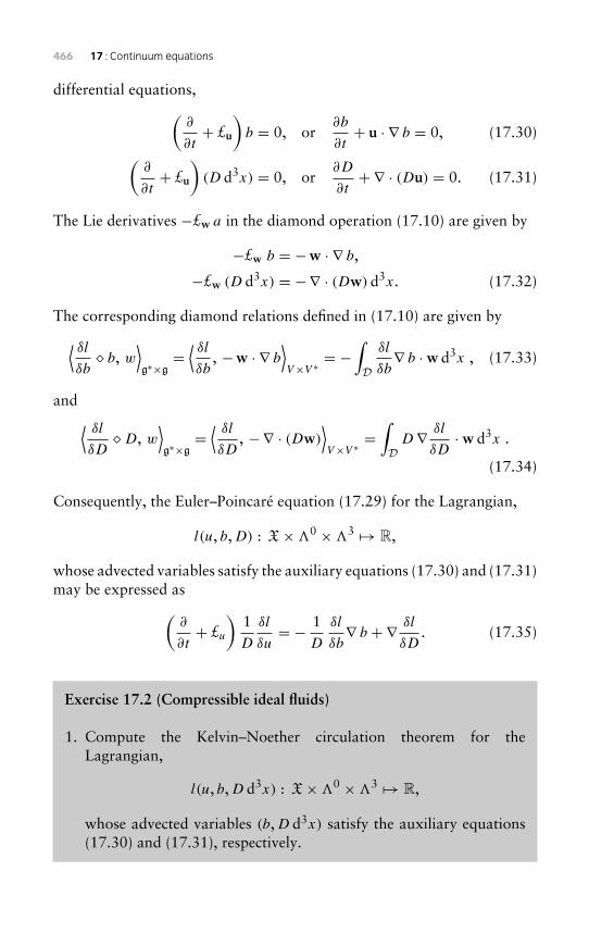
466 17 : Continuum equations
differential equations,(∂
∂t+ £u
)b = 0, or
∂b
∂t+ u · ∇ b = 0, (17.30)(
∂
∂t+ £u
)(D d3x) = 0, or
∂D
∂t+ ∇ · (Du) = 0. (17.31)
The Lie derivatives −£w a in the diamond operation (17.10) are given by
−£w b = −w · ∇ b,
−£w (D d3x) = −∇ · (Dw) d3x. (17.32)
The corresponding diamond relations defined in (17.10) are given by⟨ δlδb& b, w
⟩g∗×g=⟨ δlδb
, −w · ∇ b⟩V×V ∗ = −
∫D
δl
δb∇ b ·w d3x , (17.33)
and ⟨ δlδD&D, w
⟩g∗×g=⟨ δlδD
, −∇ · (Dw)⟩V×V ∗ =
∫D
D∇ δl
δD·w d3x .
(17.34)
Consequently, the Euler–Poincaré equation (17.29) for the Lagrangian,
l(u, b,D) : X×�0 ×�3 → R,
whose advected variables satisfy the auxiliary equations (17.30) and (17.31)may be expressed as(
∂
∂t+ £u
)1D
δl
δu= − 1
D
δl
δb∇ b + ∇ δl
δD. (17.35)
Exercise 17.2 (Compressible ideal fluids)
1. Compute the Kelvin–Noether circulation theorem for theLagrangian,
l(u, b,D d3x) : X×�0 ×�3 → R,
whose advected variables (b,D d3x) satisfy the auxiliary equations(17.30) and (17.31), respectively.
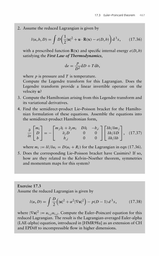
17.3 Euler–Poincaré theorem 467
2. Assume the reduced Lagrangian is given by
l(u, b,D) =∫
D
(12|u|2 + u · R(x)− e(D, b)
)d3x, (17.36)
with a prescribed function R(x) and specific internal energy e(D, b)satisfying the First Law of Thermodynamics,
de = p
D2 dD + T db,
where p is pressure and T is temperature.Compute the Legendre transform for this Lagrangian. Does theLegendre transform provide a linear invertible operator on thevelocity u?
3. Compute the Hamiltonian arising from this Legendre transform andits variational derivatives.
4. Find the semidirect-product Lie–Poisson bracket for the Hamilto-nian formulation of these equations. Assemble the equations intothe semidirect-product Hamiltonian form,
∂
∂t
mi
D
b
= −mj∂i + ∂jmi D∂i −b,i
∂jD 0 0b,j 0 0
δh/δmj
δh/δD
δh/δb
, (17.37)
where mi := δl/δui = D(ui +Ri) for the Lagrangian in eqn (17.36).
5. Does the corresponding Lie–Poisson bracket have Casimirs? If so,how are they related to the Kelvin–Noether theorem, symmetriesand momentum maps for this system?
Exercise 17.3Assume the reduced Lagrangian is given by
l(u,D) =∫
D
2
(|u|2 + α2|∇u|2
)− p(D − 1) d 3x, (17.38)
where |∇u|2 := ui,jui,j . Compute the Euler–Poincaré equation for thisreduced Lagrangian. The result is the Lagrangian-averaged Euler-alpha(LAE-alpha) equation, introduced in [HMR98a] as an extension of CHand EPDiff to incompressible flow in higher dimensions.

This page intentionally left blank
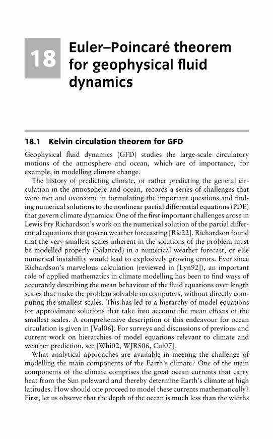
18Euler–Poincaré theoremfor geophysical fluiddynamics
18.1 Kelvin circulation theorem for GFD
Geophysical fluid dynamics (GFD) studies the large-scale circulatorymotions of the atmosphere and ocean, which are of importance, forexample, in modelling climate change.
The history of predicting climate, or rather predicting the general cir-culation in the atmosphere and ocean, records a series of challenges thatwere met and overcome in formulating the important questions and find-ing numerical solutions to the nonlinear partial differential equations (PDE)that govern climate dynamics. One of the first important challenges arose inLewis Fry Richardson’s work on the numerical solution of the partial differ-ential equations that govern weather forecasting [Ric22]. Richardson foundthat the very smallest scales inherent in the solutions of the problem mustbe modelled properly (balanced) in a numerical weather forecast, or elsenumerical instability would lead to explosively growing errors. Ever sinceRichardson’s marvelous calculation (reviewed in [Lyn92]), an importantrole of applied mathematics in climate modelling has been to find ways ofaccurately describing the mean behaviour of the fluid equations over lengthscales that make the problem solvable on computers, without directly com-puting the smallest scales. This has led to a hierarchy of model equationsfor approximate solutions that take into account the mean effects of thesmallest scales. A comprehensive description of this endeavour for oceancirculation is given in [Val06]. For surveys and discussions of previous andcurrent work on hierarchies of model equations relevant to climate andweather prediction, see [Whi02, WJRS06, Cul07].
What analytical approaches are available in meeting the challenge ofmodelling the main components of the Earth’s climate? One of the maincomponents of the climate comprises the great ocean currents that carryheat from the Sun poleward and thereby determine Earth’s climate at highlatitudes. How should one proceed to model these currents mathematically?First, let us observe that the depth of the ocean is much less than the widths
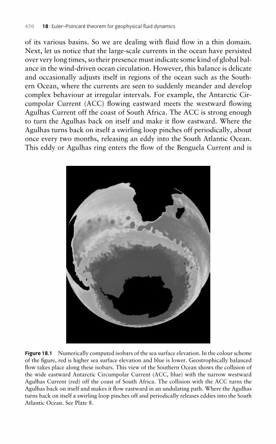
470 18 : Euler–Poincaré theorem for geophysical fluid dynamics
of its various basins. So we are dealing with fluid flow in a thin domain.Next, let us notice that the large-scale currents in the ocean have persistedover very long times, so their presence must indicate some kind of global bal-ance in the wind-driven ocean circulation. However, this balance is delicateand occasionally adjusts itself in regions of the ocean such as the South-ern Ocean, where the currents are seen to suddenly meander and developcomplex behaviour at irregular intervals. For example, the Antarctic Cir-cumpolar Current (ACC) flowing eastward meets the westward flowingAgulhas Current off the coast of South Africa. The ACC is strong enoughto turn the Agulhas back on itself and make it flow eastward. Where theAgulhas turns back on itself a swirling loop pinches off periodically, aboutonce every two months, releasing an eddy into the South Atlantic Ocean.This eddy or Agulhas ring enters the flow of the Benguela Current and is
Figure 18.1 Numerically computed isobars of the sea surface elevation. In the colour schemeof the figure, red is higher sea surface elevation and blue is lower. Geostrophically balancedflow takes place along these isobars. This view of the Southern Ocean shows the collision ofthe wide eastward Antarctic Circumpolar Current (ACC, blue) with the narrow westwardAgulhas Current (red) off the coast of South Africa. The collision with the ACC turns theAgulhas back on itself and makes it flow eastward in an undulating path. Where the Agulhasturns back on itself a swirling loop pinches off and periodically releases eddies into the SouthAtlantic Ocean. See Plate 8.
18.1 Kelvin circulation theorem 471
translated north-westward all the way across the Atlantic Ocean in aboutthree years.
Ocean currents persist because pressure gradients come into balance insome average sense with the two main forces in global ocean circulation.These are the Coriolis force due to rotation and the buoyancy force due tostratification. Thus, the persistence of patterns in the currents suggests thatpressure gradients in the ocean tend to arrange themselves in the horizon-tal and vertical directions, so as to balance these two main forces. Thesebalances are called:
• Geostrophic balance between Coriolis force and horizontal pressuregradient;
• Hydrostatic balance between buoyancy force and vertical pressuregradient.
Following Richardson [Ric22], these are also the balances that meteorolo-gists must introduce in initializing and adjusting their weather forecasts.
To cast these observations of the phenomena into a useful mathematicalframework for modelling them, let us begin by identifying the small dimen-sionless numbers that are associated with these flows. In particular, let ustake advantage of having a thin domain that rotates rapidly (f0, once perday). This daily rotation rate is much faster than the rate (U0/L, once permonth) for even relatively small mesoscale eddies of, say, L ≈ 100 km toturn around. That is, let us use the available separation of time scales tocreate the small dimensionless ratio
ε = U0/(Lf0) ≈ 1/30- 1,
called the Rossby number. As we shall see, the Rossby number ε alsomeasures the ratio of the flow’s nonlinearity to the Coriolis force.
We are interested in length scales for eddies that are hundreds of kilome-tres in diameter, but the ocean depth is only about B0 ≈ 4 km. So the aspectratio of our rapidly rotating domain is small. This aspect ratio providesanother small dimensionless number,
σ = B0/L ≈ 4/100- 1.
The Rossby number, ε, and the aspect ratio, σ , comprise two small ratiosof length scales and time scales that may be used as parameters in anasymptotic expansion of the solutions of the exact equations for a rotating,surface-driven, stratified fluid moving under gravity in a neighbourhood ofthe balanced state. Because the acceleration of gravity g is also acting onthese flows, we may introduce the dimensionless ratio, F = f 2
0 L2/(gB0),
472 18 : Euler–Poincaré theorem for geophysical fluid dynamics
called the rotational Froude number. However, oceanic observations showthat this parameter is of order unity, F = O(1), so it is not available as anexpansion parameter for ocean circulation dynamics.
At leading order in the asymptotic expansion of the solutions in ε, σ - 1,the mathematical model recovers the geostrophic and hydrostatic balances.At the next orders in the expansion, a family of approximate equationsemerges. Eventually, the asymptotic expansion and balance considerationsat each power of ε and σ determine a hierarchy of equations of motioncontaining the three non-dimensional numbers. This hierarchy of equationsis designed to approximate the solutions of the original equations more andmore accurately near the geophysically balanced state.
The utility of these equations is that they approximate the solutions of theoriginal Euler fluid equations for the global ocean circulation by replacingthe exact equations with a model that is accurate near the balanced state andmay also be simulated on a computer over the long periods of time needed tocharacterize the climate. Such computations are already enormously com-putationally intensive; but they would be impossible for today’s computersif the exact equations were used at the high resolution needed to accuratelyaccount for the smallest important scales.
What about dissipation? Motion at such scales is very non-dissipative:large gyres and their smaller eddies in the ocean basins are driven by thewinds, but the only significant dissipation mechanism for the currents andeddies in the ocean is their interaction with the bottom. The ocean gyresare thousands of kilometers in diameter. The eddies created by the cur-rents at their edges are about 200–300 km across, so they are also largeenough to be in geostrophic balance, although they are much smaller thanthe gyres. However, these mesoscale eddies still involve a great deal of massand momentum – so they certainly would not be stopped by molecular vis-cosity any time soon. In fact, the eddies may persist for years, until theyeventually run into a coastline, where they start feeling the drag due to bot-tom topography. The Reynolds number for an eddy 100 km across turningat 10 cm/s in water of viscosity 0.01 cm2/s is about 1010. Obviously, theinverse of the Reynolds number is negligible, so viscosity would not enterin these asymptotic balance equations for the large-scale motion. In fact,the only significant dissipation mechanism for this system of gyres, eddiesand currents would be their interaction with the bottom, or along the shal-lows near the lateral boundaries, where turbulent dissipation is generatedat much smaller scales. However, the complexities of drag on the oceanflow due to its interaction with the bottom will not be considered here.
A list of leading candidates in the hierarchy of GFD balance equationsderived in the literature via this asymptotic procedure was investigated byAllen, Barth and Newberger (ABN) in [ABN90a]. On consulting this ‘ABNlist’ of balance equations reproduced in Figure 18.3, one would want to
18.1 Kelvin circulation theorem 473
know the properties of each equation in the hierarchy and the behaviourof its solutions. This question has been asked perennially throughout theGFD modelling community during the past few decades, as the GFD bal-ance models have been developed in concert with the improvement of thecomputer capabilities for their simulation.
This is where geometric mechanics plays a constructive role in the devel-opment of ocean science for climate prediction. Two fundamental criteriahave emerged for selecting ‘good’ approximate sets of balance equations.Namely, in dealing with the circulation of either the ocean or atmo-sphere, whatever governing equations one would choose will need twoproperties:
1. a circulation theorem; and
2. a law of energy conservation.
These two properties are guaranteed in the Euler–Poincaré (EP) framework,both for the exact fluid equations, and for any of their asymptotic approxi-mations in this framework. Thus, the EP framework may be used to developocean models that possess these two fundamental properties.
This chapter applies the asymptotic expansion approach to Hamilton’sprinciple in the EP theorem with advected quantities proved in the pre-vious chapter. It then uses this theorem to organize and derive themain series of GFD approximations for modelling ocean circulationdynamics. The method of applying asymptotics in the Lagrangian forthe EP Hamilton’s principle is chosen for GFD, rather than the standardapproach of applying asymptotic expansions to the fluid equations.This choice is made because Hamilton’s-principle asymptotics in theEP approach will guarantee preservation of two key properties of theGFD balances that are responsible for large-scale ocean and atmospherecirculations. Namely:
(1) the Kelvin circulation theorem, leading to proper potential-vorticity(PV) dynamics; and
(2) the law of energy conservation.
These two important properties are preserved in the EP approachfor Hamilton’s-principle asymptotics at every level of approximation.However, they have often been lostwhen using the standard asymptoticexpansions of the fluid equations.
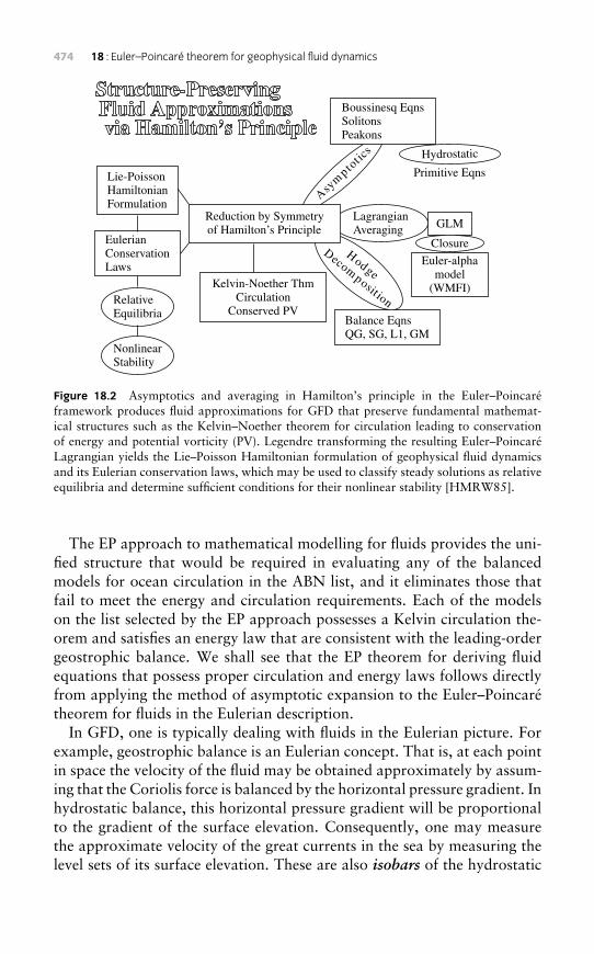
474 18 : Euler–Poincaré theorem for geophysical fluid dynamics
scitotpmysA
Primitive Eqns
Boussinesq EqnsSolitonsPeakons
Hydrostatic
egdoH
noitis
opmoceD
Lie-PoissonHamiltonianFormulation
EulerianConservationLaws
RelativeEquilibria
NonlinearStability
LagrangianAveraging
Closure
GLMReduction by Symmetryof Hamilton’s Principle
Balance EqnsQG, SG, L1, GM
Kelvin-Noether ThmCirculation
Conserved PV
Euler-alphamodel
(WMFI)
Figure 18.2 Asymptotics and averaging in Hamilton’s principle in the Euler–Poincaréframework produces fluid approximations for GFD that preserve fundamental mathemat-ical structures such as the Kelvin–Noether theorem for circulation leading to conservationof energy and potential vorticity (PV). Legendre transforming the resulting Euler–PoincaréLagrangian yields the Lie–Poisson Hamiltonian formulation of geophysical fluid dynamicsand its Eulerian conservation laws, which may be used to classify steady solutions as relativeequilibria and determine sufficient conditions for their nonlinear stability [HMRW85].
The EP approach to mathematical modelling for fluids provides the uni-fied structure that would be required in evaluating any of the balancedmodels for ocean circulation in the ABN list, and it eliminates those thatfail to meet the energy and circulation requirements. Each of the modelson the list selected by the EP approach possesses a Kelvin circulation the-orem and satisfies an energy law that are consistent with the leading-ordergeostrophic balance. We shall see that the EP theorem for deriving fluidequations that possess proper circulation and energy laws follows directlyfrom applying the method of asymptotic expansion to the Euler–Poincarétheorem for fluids in the Eulerian description.
In GFD, one is typically dealing with fluids in the Eulerian picture. Forexample, geostrophic balance is an Eulerian concept. That is, at each pointin space the velocity of the fluid may be obtained approximately by assum-ing that the Coriolis force is balanced by the horizontal pressure gradient. Inhydrostatic balance, this horizontal pressure gradient will be proportionalto the gradient of the surface elevation. Consequently, one may measurethe approximate velocity of the great currents in the sea by measuring thelevel sets of its surface elevation. These are also isobars of the hydrostatic
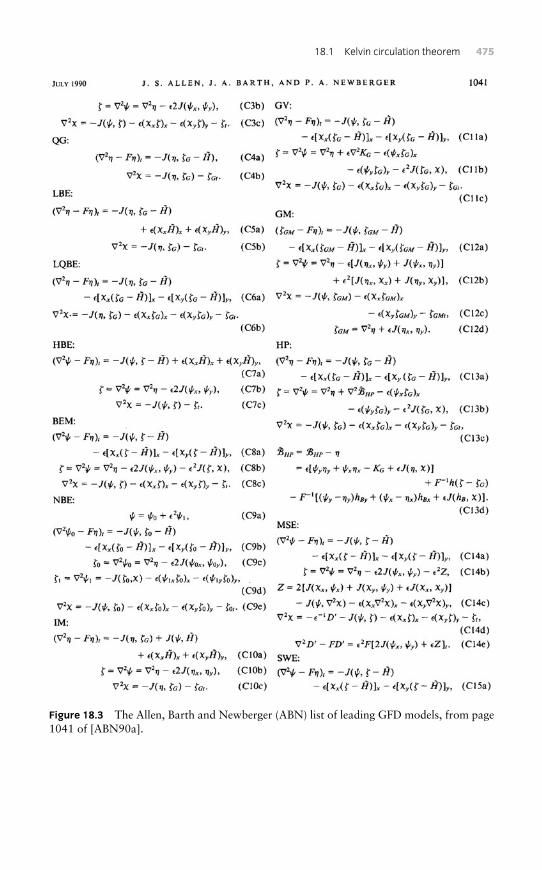
18.1 Kelvin circulation theorem 475
Figure 18.3 The Allen, Barth and Newberger (ABN) list of leading GFD models, from page1041 of [ABN90a].
476 18 : Euler–Poincaré theorem for geophysical fluid dynamics
pressure. Just as the movement of the atmosphere tends to follow the pres-sure isobars, the ocean’s flow takes place primarily along streamlines definedby the level sets, or isobars of the sea-surface elevation.
Some of the GFD models on the ABN list in Figure 18.3 survive the dualselection criteria of proper energetics and circulation by being EP equa-tions with advected parameters in their own right. These form the mainsequence of GFD model equations and they follow from the Euler–Poincaréform of Hamilton’s principle for a fluid Lagrangian that depends paramet-rically on the advected quantities such as mass, salt and heat, all carried asmaterial properties of the fluid’s motion. Thus, the Euler–Poincaré theoremwith advected quantities systematically selects and derives the useful GFDfluid models possessing the two main properties of energy balance and thecirculation theorem.
18.2 Approximate model fluid equations that preservethe Euler–Poincaré structure
The preceding section argues for the applicability of the Euler–Poincarétheorem for ideal continua in deriving approximate fluid models that pre-serve the Euler–Poincaré structure, and are obtained by making asymptoticexpansions and other approximations in Hamilton’s principle for a givenset of model equations. As examples, we first discuss the derivation ofthe quasigeostrophic approximation in geophysical fluid dynamics in twodimensions from an approximation of Hamilton’s principle for the motionof a single layer of rotating shallow water. Later, we discuss a sequence ofGFD approximations of the same type in three dimensions.
18.3 Equations of 2D geophysical fluid motion
Rotating shallow-water dynamics as Euler–Poincaré equations
We first consider dynamics of rotating shallow water (RSW) in a two-dimensional domain with horizontal coordinates x = (x1, x2). RSW motionis governed by the following non-dimensional equations for horizontal fluidvelocity u = (u1, u2) and depth D,
εddt
u+ f z× u+ ∇ψ = 0,∂D
∂t+ ∇ ·Du = 0, (18.1)
18.3 GFD motion equations in 2D 477
with notation
ddt≡(
∂
∂t+ u · ∇
)and ψ ≡
(D − B
εF)
. (18.2)
These equations include variable Coriolis parameter f = f (x) and bottomtopography B = B(x).
The dimensionless scale factors appearing in the non-dimensional RSWequations (18.1) and (18.2) are the Rossby number ε and the rotationalFroude number F , given in terms of typical dimensional scales by
ε = U0
f0L- 1 and F = f 2
0 L2
gB0= O(1). (18.3)
The dimensional scales (B0,L,U0, f0, g) denote equilibrium fluid depth,horizontal length scale, horizontal fluid velocity, reference Coriolis parame-ter, and gravitational acceleration, respectively. Dimensionless quantities ineqns (18.1) are unadorned and are related to their dimensional counterparts(primed), according to
u′ = U0u, x′ = Lx, t ′ =(
L
U0
)t , f ′ = f0f ,
B ′ = B0B, D′ = B0D, and D′ − B ′ = B0(D − B). (18.4)
Here, dimensional quantities are: u′, the horizontal fluid velocity; D′, thefluid depth; B ′, the equilibrium depth; andD′−B ′, the free surface elevation.
For barotropic (i.e. z-independent) horizontal motions at length scales L
in the ocean, say, for which the rotational Froude number F is order O(1)– as we shall assume – the Rossby number ε is typically quite small (ε - 1)as indicated in eqn (18.3). Thus, ε - 1 is a natural parameter for makingasymptotic expansions. For example, we shall assume |∇f | = O(ε) and|∇B| = O(ε), so we may write f = 1+ εf1(x) and B = 1+ εB1(x). In thisscaling, the leading-order implications of equation (18.1) are u = z × ∇ψand ∇ · u = 0. This is geostrophic balance, which is imposed in the ε → 0limit of the non-dimensional RSW equations in (18.1).
Substitution into eqn (17.35) with b absent shows that the non-dimensional RSW equations (18.1) arise as Euler–Poincaré equations fromHamilton’s principle with action SRSW,
SRSW =∫
dt∫
dx1dx2
[Du · R(x)− (D − B)2
2εF + ε
2D|u|2
], (18.5)
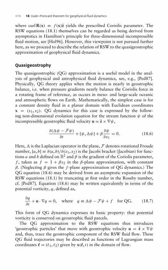
478 18 : Euler–Poincaré theorem for geophysical fluid dynamics
where curlR(x) ≡ f (x)z yields the prescribed Coriolis parameter. TheRSW equations (18.1) themselves can be regarded as being derived fromasymptotics in Hamilton’s principle for three-dimensional incompressiblefluid motion, see [Hol96]. However, this viewpoint is not pursued furtherhere, as we proceed to describe the relation of RSW to the quasigeostrophicapproximation of geophysical fluid dynamics.
Quasigeostrophy
The quasigeostrophic (QG) approximation is a useful model in the anal-ysis of geophysical and astrophysical fluid dynamics, see, e.g., [Ped87].Physically, QG theory applies when the motion is nearly in geostrophicbalance, i.e. when pressure gradients nearly balance the Coriolis force ina rotating frame of reference, as occurs in meso- and large-scale oceanicand atmospheric flows on Earth. Mathematically, the simplest case is fora constant density fluid in a planar domain with Euclidean coordinatesx = (x1, x2). QG dynamics for this case is expressed by the follow-ing non-dimensional evolution equation for the stream function ψ of theincompressible geostrophic fluid velocity u = z×∇ψ ,
∂(�ψ −Fψ)
∂t+ [ψ ,�ψ] + β
∂ψ
∂x1= 0. (18.6)
Here, � is the Laplacian operator in the plane, F denotes rotational Froudenumber, [a, b] ≡ ∂(a, b)/∂(x1, x2) is the Jacobi bracket (Jacobian) for func-tions a and b defined on R2 and β is the gradient of the Coriolis parameter,f , taken as f = 1 + βx2 in the β-plane approximation, with constantβ. (Neglecting β gives the f -plane approximation of QG dynamics.) TheQG equation (18.6) may be derived from an asymptotic expansion of theRSW equations (18.1) by truncating at first order in the Rossby number,cf. [Ped87]. Equation (18.6) may be written equivalently in terms of thepotential vorticity, q, defined as,
∂q
∂t+ u · ∇q = 0, where q ≡ �ψ −Fψ + f for QG. (18.7)
This form of QG dynamics expresses its basic property: that potentialvorticity is conserved on geostrophic fluid parcels.
The QG approximation to the RSW equations thus introduces‘geostrophic particles’ that move with geostrophic velocity u = z × ∇ψand, thus, trace the geostrophic component of the RSW fluid flow. TheseQG fluid trajectories may be described as functions of Lagrangian masscoordinates � = (�1, �2) given by x(�, t) in the domain of flow.
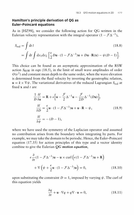
18.3 GFD motion equations in 2D 479
Hamilton’s principle derivation of QG asEuler–Poincaré equations
As in [HZ98], we consider the following action for QG written in theEulerian velocity representation with the integral operator (1−F�−1),
Sred =∫
dt l (18.8)
=∫
dt∫
dx1dx2
[ ε2Du · (1−F�−1)u+Du · R(x)− ψ(D − 1)
].
This choice can be found as an asymptotic approximation of the RSWaction SRSW in eqn (18.5), in the limit of small wave amplitudes of orderO(ε2) and constant mean depth to the same order, when the wave elevationis determined from the fluid velocity by inverting the geostrophic relation,u = z × ∇ψ . The variational derivatives of the reduced Lagrangian Sred atfixed x and t are
1D
δl
δu= R + ε
[u− F
2�−1u− F
2D�−1(Du)
],
δl
δD= ε
2u · (1−F�−1)u+ u · R − ψ , (18.9)
δl
δψ= − (D − 1),
where we have used the symmetry of the Laplacian operator and assumedno contribution arises from the boundary when integrating by parts. Forexample, we may take the domain to be periodic. Hence, the Euler–Poincaréequation (17.35) for action principles of this type and a vector identitycombine to give the Eulerian QG motion equation,
ε∂
∂t(1−F�−1)u− u× curl
(ε(1−F�−1)u+ R
)+ ∇
(ψ + ε
2u · (1−F�−1)u
)= 0, (18.10)
upon substituting the constraint D = 1, imposed by varying ψ . The curl ofthis equation yields
∂q
∂t+ u · ∇q + q∇ · u = 0, (18.11)
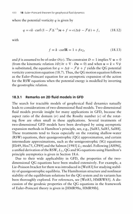
480 18 : Euler–Poincaré theorem for geophysical fluid dynamics
where the potential vorticity q is given by
q = εz · curl (1−F�−1)u+ f = ε(�ψ −Fψ)+ f , (18.12)
with
f ≡ z · curlR = 1+ βx2, (18.13)
and β is assumed to be of order O(ε). The constraint D = 1 implies∇·u = 0(from the kinematic relation ∂D/∂t + ∇ · Du = 0) and when u = z × ∇ψis substituted, the equation for q = �ψ −Fψ + f yields the QG potentialvorticity convection equation (18.7). Thus, the QG motion equation followsas the Euler–Poincaré equation for an asymptotic expansion of the actionfor the RSW equations when the potential energy is modelled by invertingthe geostrophic relation.
18.3.1 Remarks on 2D fluid models in GFD
The search for tractable models of geophysical fluid dynamics natuallyleads to considerations of two-dimensional fluid models. Two-dimensionalfluid models provide insight for many applications in GFD, because theaspect ratio of the domain (σ ) and the Rossby number (ε) of the rotat-ing flow are often small in these applications. Several treatments oftwo-dimensional GFD models have been developed by using asymptoticexpansion methods in Hamilton’s principle, see, e.g., [Sal83, Sal85, Sal88].These treatments tend to focus especially on the rotating shallow-water(RSW) equations, their quasigeostrophic (QG) approximation, and certainintermediate approximations, such as the semigeostrophic (SG) equations[Eli49, Hos75, CP89] and the Salmon [1985] L1 model. Following [AH96],a unified derivation of the RSW,L1, QG and SG equations using Hamilton’sprinciple asymptotics is given in Section 18.6.
Due to their wide applicability in GFD, the properties of the two-dimensional QG equations have been studied extensively. For example, aLie–Poisson bracket for them was introduced in [Wei83] for studying stabil-ity of quasigeostrophic equilibria. The Hamiltonian structure and nonlinearstability of the equilibrium solutions for the QG system and its variants hasbeen thoroughly explored. For references, see [Wei83, HMRW85]. A dis-cussion of the geodesic properties of the QG equations in the frameworkof Euler–Poincaré theory is given in [HMR98a, HMR98b].
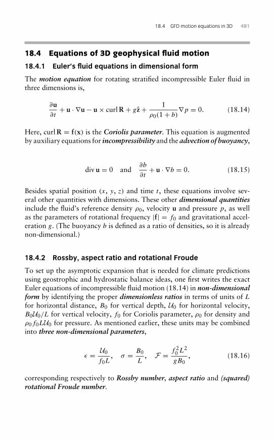
18.4 GFD motion equations in 3D 481
18.4 Equations of 3D geophysical fluid motion
18.4.1 Euler’s fluid equations in dimensional form
The motion equation for rotating stratified incompressible Euler fluid inthree dimensions is,
∂u∂t+ u · ∇u− u× curlR + gz+ 1
ρ0(1+ b)∇p = 0. (18.14)
Here, curlR = f(x) is the Coriolis parameter. This equation is augmentedby auxiliary equations for incompressibility and the advection of buoyancy,
div u = 0 and∂b
∂t+ u · ∇b = 0. (18.15)
Besides spatial position (x, y, z) and time t , these equations involve sev-eral other quantities with dimensions. These other dimensional quantitiesinclude the fluid’s reference density ρ0, velocity u and pressure p, as wellas the parameters of rotational frequency |f| = f0 and gravitational accel-eration g. (The buoyancy b is defined as a ratio of densities, so it is alreadynon-dimensional.)
18.4.2 Rossby, aspect ratio and rotational Froude
To set up the asymptotic expansion that is needed for climate predictionsusing geostrophic and hydrostatic balance ideas, one first writes the exactEuler equations of incompressible fluid motion (18.14) in non-dimensionalform by identifying the proper dimensionless ratios in terms of units of L
for horizontal distance, B0 for vertical depth, U0 for horizontal velocity,B0U0/L for vertical velocity, f0 for Coriolis parameter, ρ0 for density andρ0f0LU0 for pressure. As mentioned earlier, these units may be combinedinto three non-dimensional parameters,
ε = U0
f0L, σ = B0
L, F = f 2
0 L2
gB0, (18.16)
corresponding respectively to Rossby number, aspect ratio and (squared)rotational Froude number.
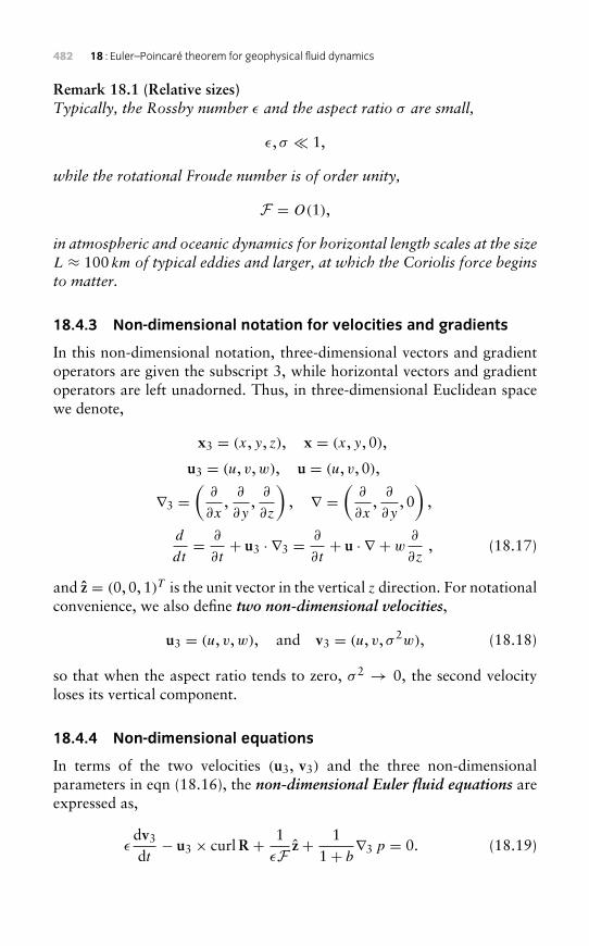
482 18 : Euler–Poincaré theorem for geophysical fluid dynamics
Remark 18.1 (Relative sizes)Typically, the Rossby number ε and the aspect ratio σ are small,
ε, σ - 1,
while the rotational Froude number is of order unity,
F = O(1),
in atmospheric and oceanic dynamics for horizontal length scales at the sizeL ≈ 100 km of typical eddies and larger, at which the Coriolis force beginsto matter.
18.4.3 Non-dimensional notation for velocities and gradients
In this non-dimensional notation, three-dimensional vectors and gradientoperators are given the subscript 3, while horizontal vectors and gradientoperators are left unadorned. Thus, in three-dimensional Euclidean spacewe denote,
x3 = (x, y, z), x = (x, y, 0),
u3 = (u, v,w), u = (u, v, 0),
∇3 =(
∂
∂x,∂
∂y,∂
∂z
), ∇ =
(∂
∂x,∂
∂y, 0)
,
d
dt= ∂
∂t+ u3 · ∇3 = ∂
∂t+ u · ∇ + w
∂
∂z, (18.17)
and z = (0, 0, 1)T is the unit vector in the vertical z direction. For notationalconvenience, we also define two non-dimensional velocities,
u3 = (u, v,w), and v3 = (u, v, σ 2w), (18.18)
so that when the aspect ratio tends to zero, σ 2 → 0, the second velocityloses its vertical component.
18.4.4 Non-dimensional equations
In terms of the two velocities (u3, v3) and the three non-dimensionalparameters in eqn (18.16), the non-dimensional Euler fluid equations areexpressed as,
εdv3
dt− u3 × curlR + 1
εF z+ 11+ b
∇3 p = 0. (18.19)
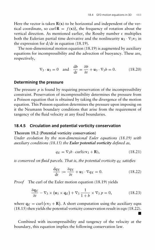
18.4 GFD motion equations in 3D 483
Here the vector is taken R(x) to be horizontal and independent of the ver-tical coordinate, so curlR = f (x)z, the frequency of rotation about thevertical direction. As mentioned earlier, the Rossby number ε multipliesboth the Eulerian partial time derivative and the nonlinearity u3 · ∇3v3 inthe expression for d/dt in equation (18.19).
The non-dimensional motion equation (18.19) is augmented by auxiliaryequations for incompressibility and the advection of buoyancy. These are,respectively,
∇3 · u3 = 0 anddbdt= ∂b
∂t+ u3 · ∇3b = 0. (18.20)
Determining the pressure
The pressure p is found by requiring preservation of the incompressibilityconstraint. Preservation of incompressibility determines the pressure froma Poisson equation that is obtained by taking the divergence of the motionequation. This Poisson equation determines the pressure upon imposing onit the Neumann boundary conditions that arise from the requirement oftangency of the fluid velocity at any fixed boundaries.
18.4.5 Circulation and potential vorticity conservation
Theorem 18.2 (Potential vorticity conservation)Under evolution by the non-dimensional Euler equations (18.19) withauxiliary conditions (18.15) the Euler potential vorticity defined as,
qE = ∇3b · curl(εv3 + R), (18.21)
is conserved on fluid parcels. That is, the potential vorticity qE satisfies
dqEdt
:= ∂qE
∂t+ u3 · ∇qE = 0. (18.22)
Proof The curl of the Euler motion equation (18.19) yields
∂qE
∂t− ∇3 ×
(u3 × qE
)+ ∇31
1+ b×∇3 p = 0, (18.23)
where qE = curl(εv3 + R
). A short computation using the auxiliary eqns
(18.15) then yields the potential vorticity conservation result in eqn (18.22).�
Combined with incompressibility and tangency of the velocity at theboundary, this equation implies the following conservation law.
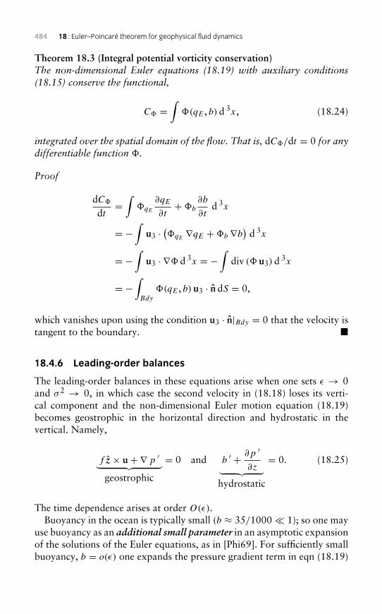
484 18 : Euler–Poincaré theorem for geophysical fluid dynamics
Theorem 18.3 (Integral potential vorticity conservation)The non-dimensional Euler equations (18.19) with auxiliary conditions(18.15) conserve the functional,
C� =∫
�(qE , b) d 3x, (18.24)
integrated over the spatial domain of the flow. That is, dC�/dt = 0 for anydifferentiable function �.
Proof
dC�
dt=∫
�qE
∂qE
∂t+�b
∂b
∂td 3x
= −∫
u3 ·(�qE ∇qE +�b ∇b
)d 3x
= −∫
u3 · ∇� d 3x = −∫
div (� u3) d 3x
= −∫Bdy
�(qE , b) u3 · n dS = 0,
which vanishes upon using the condition u3 · n|Bdy = 0 that the velocity istangent to the boundary. �
18.4.6 Leading-order balances
The leading-order balances in these equations arise when one sets ε → 0and σ 2 → 0, in which case the second velocity in (18.18) loses its verti-cal component and the non-dimensional Euler motion equation (18.19)becomes geostrophic in the horizontal direction and hydrostatic in thevertical. Namely,
f z× u+ ∇ p ′︸ ︷︷ ︸geostrophic
= 0 and b ′ + ∂p ′
∂z︸ ︷︷ ︸hydrostatic
= 0. (18.25)
The time dependence arises at order O(ε).Buoyancy in the ocean is typically small (b ≈ 35/1000- 1); so one may
use buoyancy as an additional small parameter in an asymptotic expansionof the solutions of the Euler equations, as in [Phi69]. For sufficiently smallbuoyancy, b = o(ε) one expands the pressure gradient term in eqn (18.19)
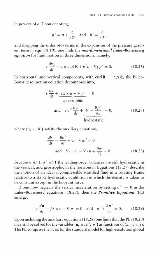
18.4 GFD motion equations in 3D 485
in powers of ε. Upon denoting,
p ′ = p + z
εF and b ′ = b
εF ,
and dropping the order o(ε) terms in the expansion of the pressure gradi-ent term in eqn (18.19), one finds the non-dimensional Euler–Boussinesqequation for fluid motion in three dimensions, namely,
εdv3
dt− u× curlR + b ′z+ ∇3 p ′ = 0. (18.26)
In horizontal and vertical components, with curlR = f (x)z, the Euler–Boussinesq motion equation decomposes into,
εdudt+ f z× u+ ∇ p ′︸ ︷︷ ︸
geostrophic
= 0
and ε σ 2 dwdt+ b ′ + ∂p ′
∂z︸ ︷︷ ︸hydrostatic
= 0, (18.27)
where {u, w, b ′} satisfy the auxiliary equations,
db ′
dt= ∂b ′
∂t+ u3 · ∇3b
′ = 0
and ∇3 · u3 = ∇ · u+ ∂w
∂z= 0. (18.28)
Because ε - 1, σ 2 - 1 the leading-order balances are still hydrostatic inthe vertical, and geostrophic in the horizontal. Equations (18.27) describethe motion of an ideal incompressible stratified fluid in a rotating framerelative to a stable hydrostatic equlibrium in which the density is taken tobe constant except in the buoyant force.
If one now neglects the vertical acceleration by setting σ 2 → 0 in theEuler–Boussinesq equations (18.27), then the Primitive Equations (PE)emerge,
εdudt+ f z× u+ ∇ p ′ = 0 and b ′ + ∂p ′
∂z= 0. (18.29)
Upon including the auxiliary equations (18.28) one finds that the PE (18.29)may still be solved for the variables {u, w, b ′, p ′} as functions of (x, y, z, t).The PE comprise the basis for the standard model for high-resolution global
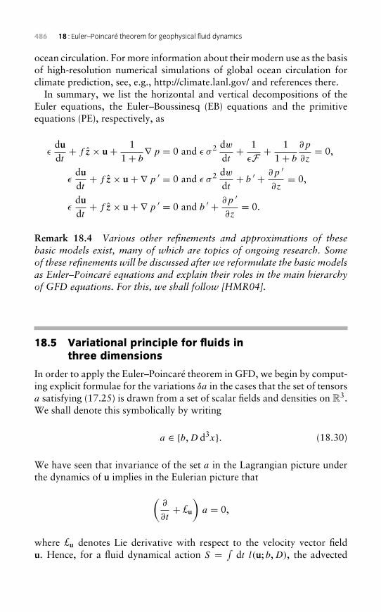
486 18 : Euler–Poincaré theorem for geophysical fluid dynamics
ocean circulation. For more information about their modern use as the basisof high-resolution numerical simulations of global ocean circulation forclimate prediction, see, e.g., http://climate.lanl.gov/ and references there.
In summary, we list the horizontal and vertical decompositions of theEuler equations, the Euler–Boussinesq (EB) equations and the primitiveequations (PE), respectively, as
εdudt+ f z× u+ 1
1+ b∇ p = 0 and ε σ 2 dw
dt+ 1
εF +1
1+ b
∂p
∂z= 0,
εdudt+ f z× u+ ∇ p ′ = 0 and ε σ 2 dw
dt+ b ′ + ∂p ′
∂z= 0,
εdudt+ f z× u+ ∇ p ′ = 0 and b ′ + ∂p ′
∂z= 0.
Remark 18.4 Various other refinements and approximations of thesebasic models exist, many of which are topics of ongoing research. Someof these refinements will be discussed after we reformulate the basic modelsas Euler–Poincaré equations and explain their roles in the main hierarchyof GFD equations. For this, we shall follow [HMR04].
18.5 Variational principle for fluids inthree dimensions
In order to apply the Euler–Poincaré theorem in GFD, we begin by comput-ing explicit formulae for the variations δa in the cases that the set of tensorsa satisfying (17.25) is drawn from a set of scalar fields and densities on R3.We shall denote this symbolically by writing
a ∈ {b,D d3x}. (18.30)
We have seen that invariance of the set a in the Lagrangian picture underthe dynamics of u implies in the Eulerian picture that
(∂
∂t+ £u
)a = 0,
where £u denotes Lie derivative with respect to the velocity vector fieldu. Hence, for a fluid dynamical action S = ∫
dt l(u; b,D), the advected
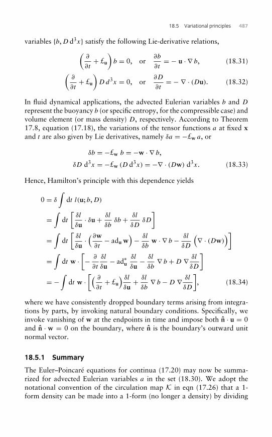
18.5 Variational principles 487
variables {b,D d3x} satisfy the following Lie-derivative relations,(∂
∂t+ £u
)b = 0, or
∂b
∂t= − u · ∇ b, (18.31)(
∂
∂t+ £u
)D d3x = 0, or
∂D
∂t= − ∇ · (Du). (18.32)
In fluid dynamical applications, the advected Eulerian variables b and D
represent the buoyancy b (or specific entropy, for the compressible case) andvolume element (or mass density) D, respectively. According to Theorem17.8, equation (17.18), the variations of the tensor functions a at fixed xand t are also given by Lie derivatives, namely δa = −£w a, or
δb = −£w b = −w · ∇ b,
δD d3x = −£w (D d3x) = −∇ · (Dw) d3x. (18.33)
Hence, Hamilton’s principle with this dependence yields
0 = δ
∫dt l(u; b,D)
=∫
dt[δl
δu· δu+ δl
δbδb + δl
δDδD
]=∫
dt[δl
δu·(∂w
∂t− adu w
)− δl
δbw · ∇ b − δl
δD
(∇ · (Dw)
)]=∫
dt w ·[− ∂
∂t
δl
δu− ad∗u
δl
δu− δl
δb∇ b +D ∇ δl
δD
]= −
∫dt w ·
[( ∂
∂t+ £u
) δl
δu+ δl
δb∇ b −D ∇ δl
δD
], (18.34)
where we have consistently dropped boundary terms arising from integra-tions by parts, by invoking natural boundary conditions. Specifically, weinvoke vanishing of w at the endpoints in time and impose both n · u = 0and n · w = 0 on the boundary, where n is the boundary’s outward unitnormal vector.
18.5.1 Summary
The Euler–Poincaré equations for continua (17.20) may now be summa-rized for advected Eulerian variables a in the set (18.30). We adopt thenotational convention of the circulation map K in eqn (17.26) that a 1-form density can be made into a 1-form (no longer a density) by dividing
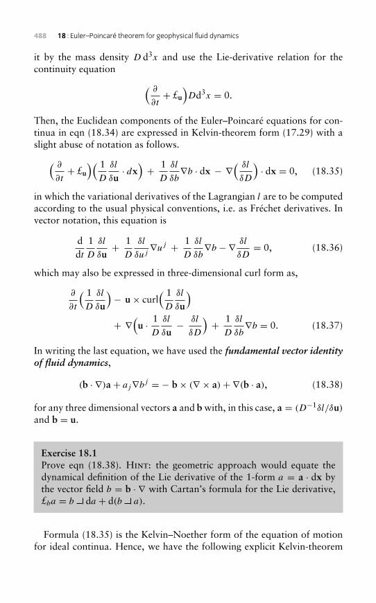
488 18 : Euler–Poincaré theorem for geophysical fluid dynamics
it by the mass density D d3x and use the Lie-derivative relation for thecontinuity equation ( ∂
∂t+ £u
)Dd3x = 0.
Then, the Euclidean components of the Euler–Poincaré equations for con-tinua in eqn (18.34) are expressed in Kelvin-theorem form (17.29) with aslight abuse of notation as follows.( ∂
∂t+ £u
)( 1D
δl
δu· dx
)+ 1
D
δl
δb∇b · dx − ∇
( δl
δD
)· dx = 0, (18.35)
in which the variational derivatives of the Lagrangian l are to be computedaccording to the usual physical conventions, i.e. as Fréchet derivatives. Invector notation, this equation is
ddt
1D
δl
δu+ 1
D
δl
δuj∇uj + 1
D
δl
δb∇b − ∇ δl
δD= 0, (18.36)
which may also be expressed in three-dimensional curl form as,
∂
∂t
( 1D
δl
δu
)− u× curl
( 1D
δl
δu
)+ ∇
(u · 1
D
δl
δu− δl
δD
)+ 1
D
δl
δb∇b = 0. (18.37)
In writing the last equation, we have used the fundamental vector identityof fluid dynamics,
(b · ∇)a + aj∇bj = − b× (∇ × a)+ ∇(b · a), (18.38)
for any three dimensional vectors a and b with, in this case, a = (D−1δl/δu)and b = u.
Exercise 18.1Prove eqn (18.38). Hint: the geometric approach would equate thedynamical definition of the Lie derivative of the 1-form a = a · dx bythe vector field b = b · ∇ with Cartan’s formula for the Lie derivative,£ba = b da + d(b a).
Formula (18.35) is the Kelvin–Noether form of the equation of motionfor ideal continua. Hence, we have the following explicit Kelvin-theorem
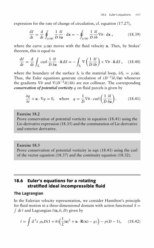
18.6 Euler’s equations 489
expression for the rate of change of circulation, cf. equation (17.27),
dIdt= d
dt
∮γt (u)
1D
δl
δu· dx = −
∮γt (u)
1D
δl
δb∇b · dx , (18.39)
where the curve γt (u) moves with the fluid velocity u. Then, by Stokes’theorem, this is equal to
dIdt= d
dt
∫St
curl1D
δl
δu· n dS = −
∫St
∇(
1D
δl
δb
)×∇b · n dS , (18.40)
where the boundary of the surface St is the material loop, ∂St = γt (u).Thus, the Euler equations generate circulation of (D−1δl/δu) wheneverthe gradients ∇b and ∇(D−1δl/δb) are not collinear. The correspondingconservation of potential vorticity q on fluid parcels is given by
∂q
∂t+ u · ∇q = 0, where q = 1
D∇b · curl
(1D
δl
δu
). (18.41)
Exercise 18.2Prove conservation of potential vorticity in equation (18.41) using theLie-derivative expression (18.35) and the commutation of Lie derivativeand exterior derivative.
Exercise 18.3Prove conservation of potential vorticity in eqn (18.41) using the curlof the vector equation (18.37) and the continuity equation (18.32).
18.6 Euler’s equations for a rotatingstratified ideal incompressible fluid
The Lagrangian
In the Eulerian velocity representation, we consider Hamilton’s principlefor fluid motion in a three-dimensional domain with action functional S =∫
dt l and Lagrangian l(u, b,D) given by
l =∫
d3x ρ0D(1+ b)(12|u|2 + u · R(x)− gz
)− p(D − 1), (18.42)
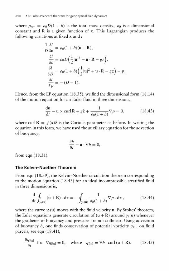
490 18 : Euler–Poincaré theorem for geophysical fluid dynamics
where ρtot = ρ0D(1 + b) is the total mass density, ρ0 is a dimensionalconstant and R is a given function of x. This Lagrangian produces thefollowing variations at fixed x and t
1D
δl
δu= ρ0(1+ b)(u+ R),
δl
δb= ρ0D
(12|u|2 + u · R − gz
),
δl
δD= ρ0(1+ b)
(12|u|2 + u · R − gz
)− p,
δl
δp= − (D − 1).
Hence, from the EP equation (18.35), we find the dimensional form (18.14)of the motion equation for an Euler fluid in three dimensions,
dudt− u× curlR + gz+ 1
ρ0(1+ b)∇p = 0, (18.43)
where curlR = f (x)z is the Coriolis parameter as before. In writing theequation in this form, we have used the auxiliary equation for the advectionof buoyancy,
∂b
∂t+ u · ∇b = 0,
from eqn (18.31).
The Kelvin–Noether Theorem
From eqn (18.39), the Kelvin–Noether circulation theorem correspondingto the motion equation (18.43) for an ideal incompressible stratified fluidin three dimensions is,
ddt
∮γt (u)
(u+ R) · dx = −∮γt (u)
1ρ0(1+ b)
∇p · dx , (18.44)
where the curve γt (u) moves with the fluid velocity u. By Stokes’ theorem,the Euler equations generate circulation of (u+ R) around γt (u) wheneverthe gradients of bouyancy and pressure are not collinear. Using advectionof buoyancy b, one finds conservation of potential vorticity qEul on fluidparcels, see eqn (18.41),
∂qEul
∂t+ u · ∇qEul = 0, where qEul = ∇b · curl (u+ R). (18.45)
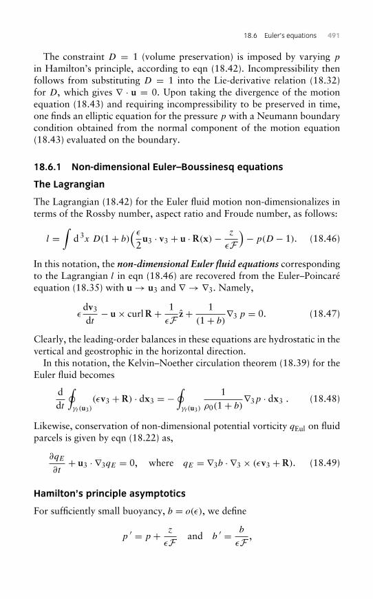
18.6 Euler’s equations 491
The constraint D = 1 (volume preservation) is imposed by varying p
in Hamilton’s principle, according to eqn (18.42). Incompressibility thenfollows from substituting D = 1 into the Lie-derivative relation (18.32)for D, which gives ∇ · u = 0. Upon taking the divergence of the motionequation (18.43) and requiring incompressibility to be preserved in time,one finds an elliptic equation for the pressure p with a Neumann boundarycondition obtained from the normal component of the motion equation(18.43) evaluated on the boundary.
18.6.1 Non-dimensional Euler–Boussinesq equations
The Lagrangian
The Lagrangian (18.42) for the Euler fluid motion non-dimensionalizes interms of the Rossby number, aspect ratio and Froude number, as follows:
l =∫
d3x D(1+ b)( ε2u3 · v3 + u · R(x)− z
εF)− p(D − 1). (18.46)
In this notation, the non-dimensional Euler fluid equations correspondingto the Lagrangian l in eqn (18.46) are recovered from the Euler–Poincaréequation (18.35) with u→ u3 and ∇ → ∇3. Namely,
εdv3
dt− u× curlR + 1
εF z+ 1(1+ b)
∇3 p = 0. (18.47)
Clearly, the leading-order balances in these equations are hydrostatic in thevertical and geostrophic in the horizontal direction.
In this notation, the Kelvin–Noether circulation theorem (18.39) for theEuler fluid becomes
ddt
∮γt (u3)
(εv3 + R) · dx3 = −∮γt (u3)
1ρ0(1+ b)
∇3p · dx3 . (18.48)
Likewise, conservation of non-dimensional potential vorticity qEul on fluidparcels is given by eqn (18.22) as,
∂qE
∂t+ u3 · ∇3qE = 0, where qE = ∇3b · ∇3 × (εv3 + R). (18.49)
Hamilton’s principle asymptotics
For sufficiently small buoyancy, b = o(ε), we define
p ′ = p + z
εF and b ′ = b
εF ,
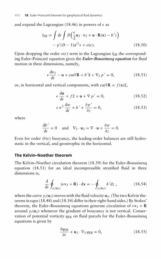
492 18 : Euler–Poincaré theorem for geophysical fluid dynamics
and expand the Lagrangian (18.46) in powers of ε as
lEB =∫
dt∫
D( ε2u3 · v3 + u · R(x)− b ′z
)− p′(D − 1)d 3x + o(ε). (18.50)
Upon dropping the order o(ε) term in the Lagrangian lEB the correspond-ing Euler–Poincaré equation gives the Euler–Boussinesq equation for fluidmotion in three dimensions, namely,
εdv3
dt− u× curlR + b ′z+ ∇3 p ′ = 0, (18.51)
or, in horizontal and vertical components, with curlR = f (x)z,
εdudt+ f z× u+ ∇ p ′ = 0, (18.52)
ε σ 2 dwdt+ b ′ + ∂p ′
∂z= 0, (18.53)
where
db ′
dt= 0 and ∇3 · u3 = ∇ · u+ ∂w
∂z= 0.
Even for order O(ε) buoyancy, the leading-order balances are still hydro-static in the vertical, and geostrophic in the horizontal.
The Kelvin–Noether theorem
The Kelvin–Noether circulation theorem (18.39) for the Euler–Boussinesqequation (18.51) for an ideal incompressible stratified fluid in threedimensions is,
ddt
∮γt (u3)
(εv3 + R) · dx = −∮γt (u3)
b ′dz , (18.54)
where the curve γt (u3)moves with the fluid velocity u3. (The two Kelvin the-orems in eqns (18.48) and (18.54) differ in their right-hand sides.) By Stokes’theorem, the Euler–Boussinesq equations generate circulation of εv3 + Raround γt (u3) whenever the gradient of bouyancy is not vertical. Conser-vation of potential vorticity qEB on fluid parcels for the Euler–Boussinesqequations is given by
∂qEB
∂t+ u3 · ∇3 qEB = 0, (18.55)
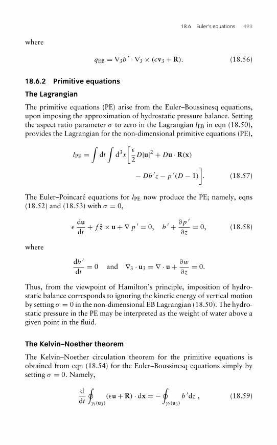
18.6 Euler’s equations 493
where
qEB = ∇3b′ · ∇3 × (εv3 + R). (18.56)
18.6.2 Primitive equations
The Lagrangian
The primitive equations (PE) arise from the Euler–Boussinesq equations,upon imposing the approximation of hydrostatic pressure balance. Settingthe aspect ratio parameter σ to zero in the Lagrangian lEB in eqn (18.50),provides the Lagrangian for the non-dimensional primitive equations (PE),
lPE =∫
dt∫
d3x
[ε
2D|u|2 +Du · R(x)
−Db ′z− p ′(D − 1)]. (18.57)
The Euler–Poincaré equations for lPE now produce the PE; namely, eqns(18.52) and (18.53) with σ = 0,
εdudt+ f z× u+ ∇ p ′ = 0, b ′ + ∂p ′
∂z= 0, (18.58)
where
db ′
dt= 0 and ∇3 · u3 = ∇ · u+ ∂w
∂z= 0.
Thus, from the viewpoint of Hamilton’s principle, imposition of hydro-static balance corresponds to ignoring the kinetic energy of vertical motionby setting σ = 0 in the non-dimensional EB Lagrangian (18.50). The hydro-static pressure in the PE may be interpreted as the weight of water above agiven point in the fluid.
The Kelvin–Noether theorem
The Kelvin–Noether circulation theorem for the primitive equations isobtained from eqn (18.54) for the Euler–Boussinesq equations simply bysetting σ = 0. Namely,
ddt
∮γt (u3)
(εu+ R) · dx = −∮γt (u3)
b ′dz , (18.59)
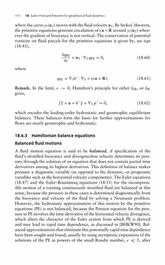
494 18 : Euler–Poincaré theorem for geophysical fluid dynamics
where the curve γt (u3) moves with the fluid velocity u3. By Stokes’ theorem,the primitive equations generate circulation of εu+R around γt (u3) when-ever the gradient of bouyancy is not vertical. The conservation of potentialvorticity on fluid parcels for the primitive equations is given by, see eqn(18.41),
∂qPE
∂t+ u3 · ∇3 qPE = 0, (18.60)
where
qPE = ∇3b′ · ∇3 × (εu+ R). (18.61)
Remark. In the limit, ε → 0, Hamilton’s principle for either lEB, or lPEgives,
f z× u+ b ′ z+ ∇3 p ′ = 0, (18.62)
which encodes the leading-order hydrostatic and geostrophic equilibriumbalances. These balances form the basis for further approximations forflows are nearly geostrophic and hydrostatic.
18.6.3 Hamiltonian balance equations
Balanced fluid motions
A fluid motion equation is said to be balanced, if specification of thefluid’s stratified buoyancy and divergenceless velocity determines its pres-sure through the solution of an equation that does not contain partial timederivatives among its highest derivatives. This definition of balance makespressure a diagnostic variable (as opposed to the dynamic, or prognosticvariables such as the horizontal velocity components). The Euler equations(18.47) and the Euler–Boussinesq equations (18.51) for the incompress-ible motion of a rotating continuously stratified fluid are balanced in thissense, because the pressure in these cases is determined diagnostically fromthe buoyancy and velocity of the fluid by solving a Neumann problem.However, the hydrostatic approximation of this motion by the primitiveequations (PE) is not balanced, because the Poisson equation for the pres-sure in PE involves the time-derivative of the horizontal velocity divergence,which alters the character of the Euler system from which PE is derivedand may lead to rapid time dependence, as discussed in [BHKW90]. Bal-anced approximations that eliminate this potentially rapid time dependencehave been sought and found, usually by using asymptotic expansions of thesolutions of the PE in powers of the small Rossby number, ε - 1, after
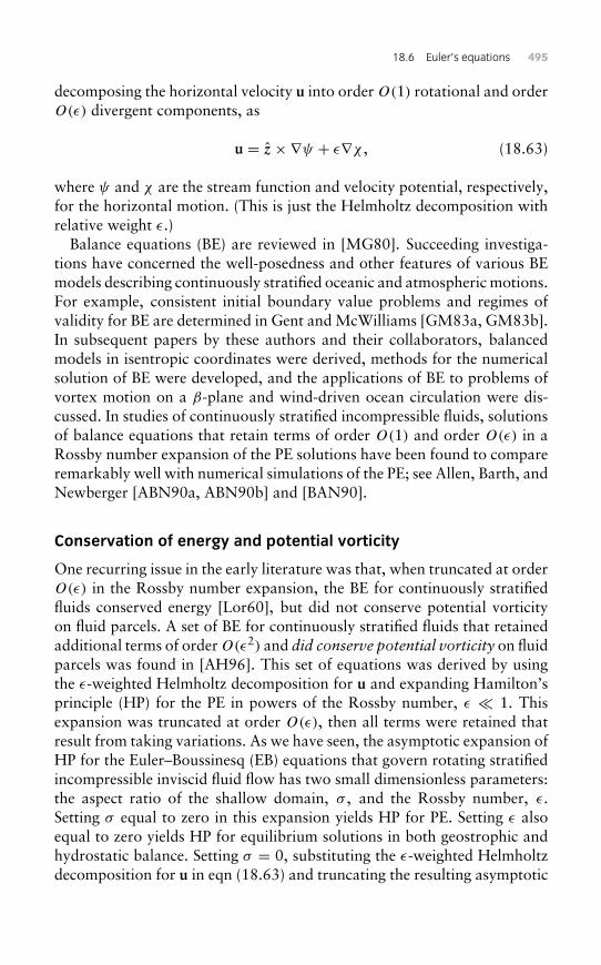
18.6 Euler’s equations 495
decomposing the horizontal velocity u into order O(1) rotational and orderO(ε) divergent components, as
u = z×∇ψ + ε∇χ , (18.63)
where ψ and χ are the stream function and velocity potential, respectively,for the horizontal motion. (This is just the Helmholtz decomposition withrelative weight ε.)
Balance equations (BE) are reviewed in [MG80]. Succeeding investiga-tions have concerned the well-posedness and other features of various BEmodels describing continuously stratified oceanic and atmospheric motions.For example, consistent initial boundary value problems and regimes ofvalidity for BE are determined in Gent and McWilliams [GM83a, GM83b].In subsequent papers by these authors and their collaborators, balancedmodels in isentropic coordinates were derived, methods for the numericalsolution of BE were developed, and the applications of BE to problems ofvortex motion on a β-plane and wind-driven ocean circulation were dis-cussed. In studies of continuously stratified incompressible fluids, solutionsof balance equations that retain terms of order O(1) and order O(ε) in aRossby number expansion of the PE solutions have been found to compareremarkably well with numerical simulations of the PE; see Allen, Barth, andNewberger [ABN90a, ABN90b] and [BAN90].
Conservation of energy and potential vorticity
One recurring issue in the early literature was that, when truncated at orderO(ε) in the Rossby number expansion, the BE for continuously stratifiedfluids conserved energy [Lor60], but did not conserve potential vorticityon fluid parcels. A set of BE for continuously stratified fluids that retainedadditional terms of order O(ε2) and did conserve potential vorticity on fluidparcels was found in [AH96]. This set of equations was derived by usingthe ε-weighted Helmholtz decomposition for u and expanding Hamilton’sprinciple (HP) for the PE in powers of the Rossby number, ε - 1. Thisexpansion was truncated at order O(ε), then all terms were retained thatresult from taking variations. As we have seen, the asymptotic expansion ofHP for the Euler–Boussinesq (EB) equations that govern rotating stratifiedincompressible inviscid fluid flow has two small dimensionless parameters:the aspect ratio of the shallow domain, σ , and the Rossby number, ε.Setting σ equal to zero in this expansion yields HP for PE. Setting ε alsoequal to zero yields HP for equilibrium solutions in both geostrophic andhydrostatic balance. Setting σ = 0, substituting the ε-weighted Helmholtzdecomposition for u in eqn (18.63) and truncating the resulting asymptotic
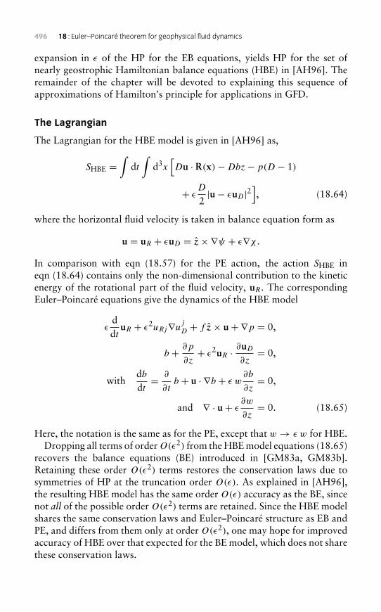
496 18 : Euler–Poincaré theorem for geophysical fluid dynamics
expansion in ε of the HP for the EB equations, yields HP for the set ofnearly geostrophic Hamiltonian balance equations (HBE) in [AH96]. Theremainder of the chapter will be devoted to explaining this sequence ofapproximations of Hamilton’s principle for applications in GFD.
The Lagrangian
The Lagrangian for the HBE model is given in [AH96] as,
SHBE =∫
dt∫
d3x[Du · R(x)−Dbz− p(D − 1)
+ εD
2|u− εuD|2
], (18.64)
where the horizontal fluid velocity is taken in balance equation form as
u = uR + εuD = z×∇ψ + ε∇χ .
In comparison with eqn (18.57) for the PE action, the action SHBE ineqn (18.64) contains only the non-dimensional contribution to the kineticenergy of the rotational part of the fluid velocity, uR. The correspondingEuler–Poincaré equations give the dynamics of the HBE model
εddt
uR + ε2uRj∇ujD + f z× u+ ∇p = 0,
b + ∂p
∂z+ ε2uR · ∂uD
∂z= 0,
withdbdt= ∂
∂tb + u · ∇b + ε w
∂b
∂z= 0,
and ∇ · u+ ε∂w
∂z= 0. (18.65)
Here, the notation is the same as for the PE, except that w→ ε w for HBE.Dropping all terms of order O(ε2) from the HBE model equations (18.65)
recovers the balance equations (BE) introduced in [GM83a, GM83b].Retaining these order O(ε2) terms restores the conservation laws due tosymmetries of HP at the truncation order O(ε). As explained in [AH96],the resulting HBE model has the same order O(ε) accuracy as the BE, sincenot all of the possible order O(ε2) terms are retained. Since the HBE modelshares the same conservation laws and Euler–Poincaré structure as EB andPE, and differs from them only at order O(ε2), one may hope for improvedaccuracy of HBE over that expected for the BE model, which does not sharethese conservation laws.
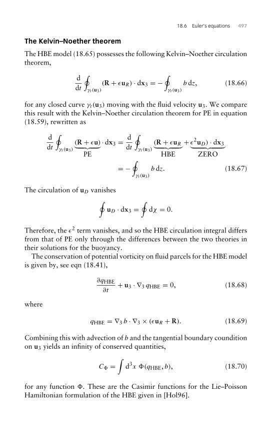
18.6 Euler’s equations 497
The Kelvin–Noether theorem
The HBE model (18.65) possesses the following Kelvin–Noether circulationtheorem,
ddt
∮γt (u3)
(R + εuR) · dx3 = −∮γt (u3)
b dz, (18.66)
for any closed curve γt (u3) moving with the fluid velocity u3. We comparethis result with the Kelvin–Noether circulation theorem for PE in equation(18.59), rewritten as
ddt
∮γt (u3)
(R + εu)︸ ︷︷ ︸PE
· dx3 = ddt
∮γt (u3)
(R + εuR︸ ︷︷ ︸HBE
+ ε2uD) · dx3︸ ︷︷ ︸ZERO
= −∮γt (u3)
b dz. (18.67)
The circulation of uD vanishes∮uD · dx3 =
∮dχ = 0.
Therefore, the ε2 term vanishes, and so the HBE circulation integral differsfrom that of PE only through the differences between the two theories intheir solutions for the buoyancy.
The conservation of potential vorticity on fluid parcels for the HBE modelis given by, see eqn (18.41),
∂qHBE
∂t+ u3 · ∇3 qHBE = 0, (18.68)
where
qHBE = ∇3 b · ∇3 × (εuR + R). (18.69)
Combining this with advection of b and the tangential boundary counditionon u3 yields an infinity of conserved quantities,
C� =∫
d3x �(qHBE, b), (18.70)
for any function �. These are the Casimir functions for the Lie–PoissonHamiltonian formulation of the HBE given in [Hol96].
498 18 : Euler–Poincaré theorem for geophysical fluid dynamics
HBE discussion
By their construction as Euler–Poincaré equations from a Lagrangian thatpossesses the classic fluid symmetries, the HBE conserve integrated energyand conserve potential vorticity on fluid parcels. Their Lie–Poisson Hamil-tonian structure endows the HBE with the same type of self-consistencythat the PE possess (for the same Hamiltonian reason). After all, the con-servation laws in both HBE and PE are not accidental. They correspond tosymmetries of the Hamiltonian or Lagrangian for the fluid motion undercontinuous group transformations, in accordance with Noether’s theorem.In particular, energy is conserved because the Hamiltonian in both theo-ries does not depend on time explicitly, and potential vorticity is conservedon fluid parcels because the corresponding Hamiltonian or Lagrangian isright invariant under the infinite set of transformations that relabel thefluid parcels without changing the Eulerian velocity and buoyancy. See,e.g., [Sal85, Sal88] for reviews of these ideas in the GFD context, as wellas [HMR98a, HMR98b] and Chapter 17 for the general context for suchresults.
The vector fields that generate these relabelling transformations turn outto be the steady flows of the HBE and PE models. By definition, these steadyflows leave invariant the Eulerian velocity and buoyancy as they move theLagrangian fluid parcels along the flow lines. Hence, as a direct consequenceof their shared Hamiltonian structure, the steady flows of both HBE and PEare relative equilibria. That is, steady HBE and PE flows are critical pointsof a sum of conserved quantities, including the (constrained) Hamiltonian.This shared critical-point property enables one, for example, to use theLyapunov method to investigate the stability of relative equilibrium solu-tions of HBE and PE. According to the Lyapunov method, convexity ofthe constrained Hamiltonian at its critical point (the relative equilibrium)is sufficient to provide a norm that limits the departure of the solution fromequilibrium under perturbations. See, e.g., [AHMR86] for applications ofthis method to the Euler equations for incompressible fluid dynamics and[HMRW85] for a range of other applications in fluid and plasma theories.
Thus, the HBE arise as Euler–Poincaré equations and possess the sameLie–Poisson Hamiltonian structure as EB and PE, and differ in their Hamil-tonian and conservation laws by small terms of order O(ε2). Moreover,the HBE conservation laws are fundamentally of the same nature as thoseof the EB equations and the PE from which they descend. These conservedquantities – particularly the quadratic conserved quantities – may eventu-ally be useful measures of the deviations of the HBE solutions from EB andPE solutions under time evolution starting from identical initial conditions.
Three-dimensional versions of the QG and SG equations also exist, andrecently a continuously stratified L1 model was reviewed in [AHN02] from
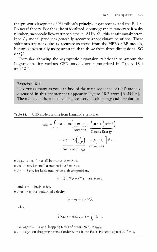
18.6 Euler’s equations 499
the present viewpoint of Hamilton’s principle asymptotics and the Euler–Poincaré theory. For the suite of idealized, oceanographic, moderate Rossbynumber, mesoscale flow test problems in [AHN02], this continuously strat-ified L1 model produces generally accurate approximate solutions. Thesesolutions are not quite as accurate as those from the HBE or BE models,but are substantially more accurate than those from three dimensional SGor QG.
Formulae showing the asymptotic expansion relationships among theLagrangians for various GFD models are summarized in Tables 18.1and 18.2.
Exercise 18.4Pick out as many as you can find of the main sequence of GFD modelsdiscussed in this chapter that appear in Figure 18.3 from [ABN90a].The models in the main sequence conserve both energy and circulation.
Table 18.1 GFD models arising from Hamilton’s principle.
lEuler =∫ [
D(1+ b)
(R(x) · u︸ ︷︷ ︸Rotation
+ ε
2|u|2 + ε
2σ 2w2︸ ︷︷ ︸
Kinetic Energy
)
− D(1+ b)
(z
εF
)︸ ︷︷ ︸Potential Energy
− p(D − 1)︸ ︷︷ ︸Constraint
]d3x
• lEuler → lEB, for small buoyancy, b = O(ε).
• lEB → lPE, for small aspect ratio, σ 2 = O(ε).
• lPE → lHBE, for horizontal velocity decomposition,
u = z×∇ψ + ε∇χ = uR + εuD ,
and |u|2 → |uR |2 in lPE.
• lHBE → l1, for horizontal velocity,
u = u1 = z×∇φ,
where
φ(x3, t) = φS(x, y, t)+∫ 0
z
dz′ b,
i.e. ∂φ/∂z = − b and dropping terms of order O(ε2) in lHBE.
• l1 → lQG, on dropping terms of order O(ε2) in the Euler–Poincaré equations for l1.
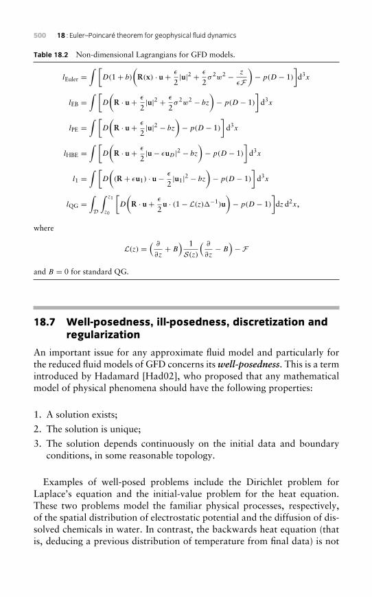
500 18 : Euler–Poincaré theorem for geophysical fluid dynamics
Table 18.2 Non-dimensional Lagrangians for GFD models.
lEuler =∫ [
D(1+ b)
(R(x) · u+ ε
2|u|2 + ε
2σ 2w2 − z
εF
)− p(D − 1)
]d3x
lEB =∫ [
D
(R · u+ ε
2|u|2 + ε
2σ 2w2 − bz
)− p(D − 1)
]d3x
lPE =∫ [
D
(R · u+ ε
2|u|2 − bz
)− p(D − 1)
]d3x
lHBE =∫ [
D
(R · u+ ε
2|u− εuD |2 − bz
)− p(D − 1)
]d3x
l1 =∫ [
D
((R + εu1) · u− ε
2|u1|2 − bz
)− p(D − 1)
]d3x
lQG =∫
D
∫ z1
z0
[D
(R · u+ ε
2u · (1− L(z)�−1)u
)− p(D − 1)
]dz d2x,
where
L(z) =( ∂
∂z+ B
) 1S(z)
( ∂
∂z− B
)− F
and B = 0 for standard QG.
18.7 Well-posedness, ill-posedness, discretization andregularization
An important issue for any approximate fluid model and particularly forthe reduced fluid models of GFD concerns its well-posedness. This is a termintroduced by Hadamard [Had02], who proposed that any mathematicalmodel of physical phenomena should have the following properties:
1. A solution exists;
2. The solution is unique;
3. The solution depends continuously on the initial data and boundaryconditions, in some reasonable topology.
Examples of well-posed problems include the Dirichlet problem forLaplace’s equation and the initial-value problem for the heat equation.These two problems model the familiar physical processes, respectively,of the spatial distribution of electrostatic potential and the diffusion of dis-solved chemicals in water. In contrast, the backwards heat equation (thatis, deducing a previous distribution of temperature from final data) is not
18.7 Well-posedness, ill-posedness, discretization and regularization 501
well-posed, because the solution is highly sensitive to changes in the finaldata. Problems that are not well-posed in the sense of Hadamard are termedill-posed. An example of an ill-posed fluids problem is an inviscid shear flowwith a discontinuous velocity distribution at the interface between two fluidlayers with different velocities. (The interface is sometimes called a vortexsheet.) This situation produces the Kelvin-Helmholtz instability in whichthe interface rolls up tightly into whorls, and whose unstable growth rateincreases with wave number according to Euler’s fluid equations; so that thesmaller the wavelength of the disturbance, the faster it grows and distortsthe interface.
Fluid-dynamics problems must often be represented at discrete pointsrather than continuously in space and time in order to obtain a numeri-cal solution. Such numerical discretizations of continuous problems maysuffer from numerical instability when solved with finite precision, or witherrors in the data. Even if a continuous problem is well-posed, it may stillbe numerically ill-conditioned for a given choice of numerical algorithm,meaning that a small error in the initial data can result in much larger errorsin the results of numerical simulations.
Although extremely important in applications, the design of optimaltechniques for stabilizing numerical algorithms for simulations of fluidequations is beyond the scope of the present text. We only mention thatthe Euler–Poincaré formulation of fluids may be quite useful in guiding thedesign of numerical methods that preserve the fundamental mathematicalstructures of fluid dynamics. This is a fruitful and active field of ongoingstudy [CH08].
If a continuous problem is well-posed, then it has a chance of being solvedon a computer using a stable algorithm for its discrete representation. If itis not well-posed, then it must be reformulated for numerical treatment.Typically this reformulation involves introducing additional assumptionsthat are designed to guarantee smoothness of the solution. This process isknown as regularization.
The famous example of regularization for fluids is Leray’s regularizationof the Navier–Stokes equations [Ler34], obtained by smoothing the trans-port velocity relative to the circulation velocity. Various choices amongthe GFD balance equations may or may not be well-posed, depending onwhich model is chosen and these, in turn, may or may not be numericallywell-conditioned, depending on which algorithm is used. The issue of reg-ularization of models to achieve well-posedness is extremely important forthe evaluation of fluid models and their application in problems such as cli-mate prediction. For example, regularization of fluid equations may also beachieved by the introduction of viscous dissipation of energy, as happensphysically for the Kelvin–Helmholtz instability. However, regularization
502 18 : Euler–Poincaré theorem for geophysical fluid dynamics
by enhanced energy dissipation may produce sluggish fluid response withunrealistically low variability that may under-predict the effects of vari-ations of the driving parameters for the flow. Again, the Euler–Poincaréformulation of fluid dynamics may be quite useful in guiding the designof regularization methods that preserve fluid structure and thus producesolutions whose variability is physically realistic, not over damped becauseof unphysical added dissipation. The approach of using the Euler–Poincaréformulation for regularization has recently made some advances, for exam-ple, in turbulence modelling [FHT01, FHT02]. However, this is anotherongoing field of study whose discussion we have decided to place outsidethe scope of the present text.
Bibliography
[ABN90a] J. S. Allen, J. A. Barth, and P. A. Newberger. On intermediate models forbarotropic continental shelf and slope flow fields. Part I: Formulation andcomparison of exact solutions. J. of Phys. Oceanog., 20:1017–1042, 1990.
[ABN90b] J. S. Allen, J. A. Barth, and P. A. Newberger. On intermediate modelsfor barotropic continental shelf and slope flow fields. Part III: Comparisonof numerical model solutions in periodic channels. J. of Phys. Oceanog.,20:1949–1973, 1990.
[AH96] J. S. Allen and D. D. Holm. Extended-geostrophic Hamiltonian models forrotating shallow water motion. Physica D, 98:229–248, 1996.
[AHMR86] H. D. I. Abarbanel, D. D. Holm, J. E. Marsden, and T. S. Ratiu. Nonlinear sta-bility analysis of stratified ideal fluid equilibria. Phil. Trans. Roy. Soc. (London)A, 318:349–409, 1986.
[AHN02] J. S. Allen, D. D. Holm, and P. A. Newberger. Toward an extended-geostrophicEuler–Poincaré model for mesoscale oceanographic flow. In J. Norbury andI. Roulstone, editors, Large-Scale Atmosphere-Ocean Dynamics 1: AnalyticalMethods and Numerical Models, pages 101–125. Cambridge University Press,Cambridge, 2002.
[AK98] V. I. Arnold and B. A. Khesin. Topological Methods in Hydrodynamics.Springer, New York, 1998.
[AM78] R. Abraham and J. E. Marsden. Foundations of Mechanics. Addison-Wesley,New York, 2nd edition, 1978.
[AMR88] R. Abraham, J. E. Marsden, and T. S. Ratiu.Manifolds, Tensor Analysis, andApplications, volume 75 of Applied Mathematical Sciences. Springer, NewYork, 2nd edition, 1988.
[Arn66] V. I. Arnold. Sur la géometrie differentialle des groupes de Lie de dimiensioninfinie et ses applications à l’hydrodynamique des fluids parfaits. Ann. Inst.Fourier, Grenoble, 16:319–361, 1966.
[Arn78] V. I. Arnold. Mathematical Methods of Classical Mechanics, volume 60 ofGraduate Texts in Mathematics. Springer, New York, 1978.
[AS06] M. J. Ablowitz and H. Segur. Solitons and the Inverse Scattering Transform.Cambridge University Press, New York, 2006.
[Bak02] A. Baker. Matrix Groups: An Introduction to Lie Group Theory. Undergrad-uate Mathematics Series. Springer, New York, 2002.
[BAN90] J. A. Barth, J. S. Allen, and P. A. Newberger. On intermediate models forbarotropic continental shelf and slope flow fields. Part II: Comparison ofnumerical model solutions in doubly periodic domains. J. of Phys. Oceanog.,20:1044–1076, 1990.
[BG88] M. Berger and B. Gostiaux. Differential Geometry: Manifolds, Curves andSurfaces. Springer, New York, 1988.
504 Bibliography
[BHKW90] G. L. Browning, W. R. Holland, H. O. Kreiss, and S. J. Worley. An accu-rate hyperbolic system for approximately hydrostatic and incompressibleoceanographic flows. Dyn. Atm. Oceans, 14:303–332, 1990.
[BKMR96] A. M. Bloch, P. S. Krishnaprasad, J. E. Marsden, and T. S. Ratiu. TheEuler-Poincaré equations and double bracket dissipation. Comm. Math. Phys.,175:1–42, 1996.
[BL05] F. Bullo and A. D. Lewis.Geometric Control of Mechanical Systems. Springer,New York, 2005.
[Blo03] A. M. Bloch. Nonholonomic Mechanics and Control, volume 24 of Interdis-ciplinary Applied Mathematics. Springer-Verlag, New York, 2003. With thecollaboration of J. Baillieul, P. Crouch and J. Marsden, With scientific inputfrom P. S. Krishnaprasad, R. M. Murray and D. Zenkov, Systems and Control.
[Boo91] F. L. Bookstein. Morphometric Tools for Landmark Data; geometry andbiology. Cambridge University Press, Cambridge, 1991.
[CB97] R. H. Cushman and L. M. Bates. Global Aspects of Integrable Systems.Birkhäuser, New York, 1997.
[CH93] R. Camassa and D. D. Holm. An integrable shallow water equation with peakedsolitons. Phys. Rev. Lett., 71:1661–64, 1993.
[CH08] C. J. Cotter and D. D. Holm. Discrete momentum maps for lattice EPDiff. InR. Temam and J. Tribbia, editors, Computational Methods for the Atmosphereand the Ocean, volume Special Volume of Handbook of Numerical Analysis,pages 247–278. North-Holland, Amsterdam, 2008.
[Cha87] S. Chandrasekhar.Ellipsoidal Figures of Equilibrium. Dover, New York, 1987.[CLZ05] M. Chen, S. Liu, and Y. Zhang. A two-component generalization of the
Camassa-Holm equation and its solutions. Lett. Math. Phys., 75:1–15, 2005.[CM87] H. Cendra and J. E. Marsden. Lin constraints, Clebsch potentials and
variational principles. Physica D, 27:63–89, 1987.[Cot05] C. J. Cotter. A general approach for producing Hamiltonian numerical schemes
for fluid equations. Arxiv preprint math.NA/0501468, 2005.[CP89] M. J. P. Cullen and R. J. Purser. Properties of the Lagrangian semigeostrophic
equations. J. Atmos. Sci., 46:1477–1497, 1989.[Cul07] M. J. P. Cullen. Modelling atmospheric flows. Acta Numerica, 16:67–154,
2007.[DGH04] H. Dullin, G. Gottwald, and D. D. Holm. On asymptotically equivalent shallow
water wave equations. Physica D, 190:1–14, 2004.[DGM98] P. Dupuis, U. Grenander, and M. Miller. Variational problems on flows of
diffeomorphisms for image matching. Quarterly of Applied Math., 56:587–600, 1998.
[DHH03] A. Degasperis, D. D. Holm, and A. N. W. Hone. Integrable and noninte-grable equations with peakons. In M. J. Ablowitz, M. Boiti, F. Pempinelli, andB. Prinari, editors,Nonlinear Physics: Theory and Experiment (Gallipoli 2002)Vol II, pages 37–43. World Scientific, Singapore, 2003.
[DK04] J. J. Duistermaat and J. A. C. Kolk. Lie Groups. Universitext, Amsterdam,2004.
[Eli49] A. Eliassen. The quasi-static equations of motion with pressure as independentvariable. Geofysiske Publikasjoner, 17:327–342, 1949.
[EM70] D. G. Ebin and J. E. Marsden. Groups of diffeomorphisms and the motion ofan incompressible fluid. Ann. of Math., 92:102–163, 1970.
[Fal06] G. Falqui. On a Camassa-Holm type equation with two dependent variables.J. Phys. A: Math. and Theor., 39:327–342, 2006.
Bibliography 505
[FGR02] J. Frank, G. Gottwald, and S. Reich. A Hamiltonian particle-mesh methodfor the rotating shallow-water equations. In M. Griebel and M. A. Schweitzer,editors, Meshfree Methods for Partial Differential Equations, volume 26 ofLecture Notes in Computational Science and Engineering, pages 131–142.Springer, 2002.
[FH01] O. B. Fringer and D. D. Holm. Integrable vs nonintegrable geodesic solitonbehavior. Physica D, 150:237–263, 2001.
[FHT01] C. Foias, D. D. Holm, and E. S. Titi. The Navier–Stokes–alpha model of fluidturbulence. Physica D, 152–153:505–519, 2001.
[FHT02] C. Foias, D. D. Holm, and E. S. Titi. The three dimensional viscous Camassa–Holm equations, and their relation to the Navier–Stokes equations andturbulence theory. J. Dyn. Diff. Eq., 14:1–35, 2002.
[Fuc96] B. Fuchssteiner. Some tricks from the symmetry-toolbox for nonlinear equa-tions: Generalizations of the Camassa-Holm equation. Physica D, 95:229–243,1996.
[GD79] I. M. Gelfand and I. Ya. R. Dorfman. Hamiltonian operators and algebraicstructures associated with them. Funct. Anal. Appl., 13:248–254, 1979.
[GM83a] P. R. Gent and J. C. McWilliams. Consistent balanced models in bounded andperiodic domains. Dyn. Atmos. Oceans, 7:67–93, 1983.
[GM83b] P. R. Gent and J. C. McWilliams. Regimes of validity for balanced models.Dyn. Atmos. Oceans, 7:167–183, 1983.
[Gol59] H. Goldstein.ClassicalMechanics. Addison-Wesley Publishing Company, NewYork, 1959.
[Gre81] U. Grenander. Lectures in Pattern Theory, volume 33 ofAppliedMathematicalSciences. Springer, New York, 1981.
[GS84] V. Guillemin and S. Sternberg. Symplectic Techniques in Physics. CambridgeUniversity Press, Cambridge, 1984.
[GTY04] J. Glaunes, A. Trouve, and L. Younes. Diffeomorphic matching of distribu-tions: A new approach for unlabelled point-sets and sub-manifolds matching.In IEEE Computer Society Conference on Computer Vision and PatternRecognition, volume 2, pages 712–718. IEEE, 2004.
[Gun03] M. D. Gunzburger. Perspectives in Flow Control and Optimization. Advancesin design and control. SIAM, Philadelphia, 2003.
[Had02] J. Hadamard. Sur les problèmes aux drives partielles et leur significationphysique. Princeton University Bulletin, pages 49–52, 1902.
[HK83] D. D. Holm and B. A. Kupershmidt. Poisson brackets and Clebsch represen-tations for magnetohydrodynamics, multifluid plasmas, and elasticity. PhysicaD, 6:347–363, 1983.
[HM04] D. D. Holm and J. E. Marsden. Momentum maps and measure valued solu-tions (peakons, filaments, and sheets) of the Euler–Poincaré equations for thediffeomorphism group. In J. E. Marsden and T. S. Ratiu, editors, The Breadthof Symplectic and Poisson Geometry, Progr. Math., 232, pages 203–235.Birkhäuser, Boston, 2004.
[HMR98a] D. D. Holm, J. E. Marsden, and T. S. Ratiu. The Euler-Poincaré equationsand semidirect products with applications to continuum theories. Adv. Math.,137:1–81, 1998.
[HMR98b] D. D. Holm, J. E. Marsden, and T. S. Ratiu. Euler-Poincaré models of idealfluids with nonlinear dispersion. Phys. Rev. Lett., 80:4173–4177, 1998.
[HMR04] D. D. Holm, J. E. Marsden, and T. S. Ratiu. The Euler–Poincaré equations ingeophysical fluid dynamics. In J. Norbury and I. Roulstone, editors, Large-Scale
506 Bibliography
Atmosphere-Ocean Dynamics 2: Geometric Methods and Models, pages 251–299. Cambridge University Press, Cambridge, 2004.
[HMRW85] D. D. Holm, J. E. Marsden, T. S. Ratiu, and A. Weinstein. Nonlinear stabilityof fluid and plasma equilibria. Phys. Rep., 123:1–116, 1985.
[Hol96] D. D. Holm. Hamiltonian balance equations. Physica D, 98:379–414, 1996.[Hol02] D. D. Holm. Euler-Poincaré dynamics of perfect complex fluids. In P. Holmes
P. Newton and A. Weinstein, editors, Geometry, Mechanics and Dynamics,pages 113–167. Springer, New York, 2002.
[Hol08] D. D. Holm. Geometric Mechanics Part 2: Rotating, Translating and Rolling.Imperial College Press, London, 2008.
[Hos75] B. J. Hoskins. The geostrophic momentum approximation and the semi-geostrophic equations. J. Atmos. Sci., 32:233–242, 1975.
[HRTY04] D. D. Holm, J. T. Ratnanather, A. Trouvé, and L. Younes. Soliton dynamicsin computational anatomy. Neuroimage, 23:S170–S178, 2004.
[HS74] M. Hirsch and S. Smale.Differential Equations, Dynamical Systems and LinearAlgebra. Academic Press, New York, 1974.
[HS03] D. D. Holm and M. F. Staley. Wave structures and nonlinear balances ina family of 1+1 evolutionary PDEs. SIAM J. Appl. Dyn. Syst., 2:323–380,2003.
[HS04] D. D. Holm and M. F. Staley. Interaction dynamics of singular wave fronts.Unpublished, 2004.
[HTY09] D. D. Holm, A. Trouvé, and Y. Younes. The Euler–Poincaré formulation ofmetamorphosis. Quart. Appl. Math. and Mech., To appear, 2009.
[HZ94] J. K. Hunter and Y. Zheng. On a completely integrable nonlinear hyperbolicvariational equation. Physica D, 79:361–386, 1994.
[HZ98] D. D. Holm and V. Zeitlin. Hamilton’s principle for quasigeostrophic motion.Phys. Fluids, 10:800–806, 1998.
[JS98] J. V. José and E. J. Saletan. Classical Dynamics: A Contemporary Approach.Cambridge University Press, Cambridge, 1998.
[Kat76] T. Kato.PerturbationTheory for LinearOperators. Springer, New York, 1976.[Kuz07] A. P. Kuz’min. Two-component generalizations of the Camassa-Holm equa-
tion.Math. Notes, 81:130–134, 2007.[Lee03] J. Lee. Introduction to Smooth Manifolds, volume 218 of Graduate Texts in
Mathematics. Springer-Verlag, New York, 2003.[Ler34] J. Leray. Sur le mouvement d’un liquide visqueux emplissant l’espace. Acta
Mathematica, 63:193–248, 1934.[LL76] L. D. Landau and E. M. Lifshitz.Mechanics. Butterworth-Heinemann, Elsevier,
Amsterdam, The Netherlands, 3rd edition, 1976.[Lor60] E. N. Lorenz. Energy and numerical weather prediction. Tellus, 12:364–373,
1960.[LR04] B. Leimkuhler and S. Reich. Simulating Hamiltonian Dynamics, volume 14
of Cambridge Monographs on Applied and Computational Mathematics.Cambridge University Press, Cambridge, 2004.
[Lyn92] P. Lynch. Richardson’s barotropic forecast: A reappraisal. Bull. Am. Met. Soc.,73:35–47, 1992.
[Mag78] F. Magri. A simple model of the integrable Hamiltonian equation. J. Math.Phys., 19:1156–1162, 1978.
[MG80] J. C. McWilliams and P. R. Gent. Intermediate models of planetary circulationsin the atmosphere and ocean. J. of the Atmos. Sci., 37:1657–1678, 1980.
Bibliography 507
[MH94] J. E. Marsden and T. J. R. Hughes. Mathematical Foundations of Elasticity,volume 174 of London Mathematical Society Lecture Notes. Prentice Hall.Reprinted by Dover Publications, New York, 1994.
[MN02] A. V. Mikhailov and V. S. Novikov. Perturbative symmetry approach. J. Phys.A, 35:4775–4790, 2002.
[Mon90] R. Montgomery. Isoholonomic problems and some applications. Comm. MathPhys., 128:565–592, 1990.
[Mon93] R. Montgomery. Gauge theory of the falling cat. Fields Inst. Commun., 1:193–218, 1993.
[MR02] J. E. Marsden and T. S. Ratiu. Introduction to Mechanics and Symme-try: A Basic Exposition of Classical Mechanical Systems. Texts in AppliedMathematics. Springer, New York, 2nd edition, 2002.
[MR03] J. E. Marsden and T. S. Ratiu. Mechanics and Symmetry: Reduction theory. Inpreparation, 2003.
[MS95] D. McDuff and D. Salamon. Introduction to Symplectic Topology. ClarendonPress, Oxford, 1995.
[MTY02] M. I. Miller, A. Trouvé, and L. Younes. On metrics and euler-lagrange equa-tions of computational anatomy. Ann. Rev. Biomed. Engng., 4:375–405,2002.
[MW83] J. E. Marsden and A. Weinstein. Coadjoint orbits, vortices and Clebschvariables for incompressible fluids. Physica D, 7:305–323, 1983.
[MY01] M. I. Miller and L. Younes. Group action, diffeomorphism and matching: ageneral framework. Int. J. Comp. Vis., 41:61–84, 2001.
[Noe72] E. Noether. Invariante variationsprobleme. Nachr. v. d. Ges. d. Wiss. zu Göt-tingen, 1918:235–257, 1918. See also C. H. Kimberling,Amer.Math.Monthly,79:136–149, 1972.
[Olv00] P. J. Olver. Applications of Lie Groups to Differential Equations. Springer,New York, 2000.
[Ped87] J. Pedlosky. Geophysical Fluid Dynamics. Springer-Verlag, New York, 1987.[Phi69] O. M. Phillips.TheDynamics of the UpperOcean. Cambridge Monographs on
Mechanics and Applied Mathematics. Cambridge University Press, Cambridge,1969.
[Poi01] H. Poincaré. Sur une forme nouvelle des équations de la méchanique. C.R.Acad. Sci., 132:369–371, 1901.
[RdSD99] R. M. Roberts and M. E. R. de Sousa-Dias. Symmetries of riemann ellipsoids.Resenhas- IME. USP, 4:183–221, 1999.
[Ric22] L. F. Richardson. Weather Prediction by Numerical Process. CambridgeMonographs on Mechanics and Applied Mathematics. Cambridge Univer-sity Press. Reprinted by Dover Publications, N.Y. (1965), Cambridge,1922.
[Rou60] E. J. Routh.Treatise of theDynamics of a System of Rigid Bodies andAdvancedRigid BodyDynamics. MacMillan and Co., London, 1884; reprinted by Dover,N.Y., 1960.
[Sal83] R. Salmon. Practical use of Hamilton’s principle. J. Fluid Mech., 132:431–444,1983.
[Sal85] R. Salmon. New equations for nearly geostrophic flow. J. Fluid Mech.,153:461–477, 1985.
[Sal88] R. Salmon. Hamiltonian fluid dynamics. Ann. Rev. Fluid Mech., 20:225–256,1988.
508 Bibliography
[Shk00] S. Shkoller. Analysis on groups of diffeomorphisms of manifolds with boundaryand the averaged motion of a fluid. J. Diff. Geom., 55:145–191, 2000.
[Sin01] S. Singer. Symmetry inMechanics: AGentle, Modern Introduction. Birkhäuser,New York, 2001.
[Spi65] M. Spivak. Calculus on manifolds : a modern approach to classical theoremsof advanced calculus. Benjamin/Cummings, New York, 1965.
[Spi79] M. Spivak. Differential Geometry. Publish or Perish, Inc., Houston, Texas,1979.
[Tay96] M. E. Taylor. Partial Differential Equations I. Springer-Verlag, New York,1996.
[Tho92] D’A. W. Thompson.On Growth and Form. Dover Reprint, New York, 1992.[Tro98] A. Trouvé. Diffeomorphism groups and pattern matching in image analysis.
Int. J. Computer Vision, 28:213–221, 1998.[TY05] A. Trouvé and L. Younes. Metamorphoses through lie group action. Found.
Comp. Math., 5:173–198, 2005.[Val06] G. K. Vallis. Atmospheric and Oceanic Fluid Dynamics: Fundamentals and
Large-scale Circulation. Cambridge University Press, Cambridge, 2006.[War83] F. W. Warner. Foundation of Differentiable Manifolds and Lie Groups, vol-
ume 94 of Graduate Texts in Mathematics. Springer-Verlag, New York,1983.
[Wei83] A. Weinstein. Hamiltonian structure for drift waves and geostrophic flow.Phys.Fluids, 26:388–390, 1983.
[Whi02] A. A. White. A view of the equations of meteorological dynamics and var-ious approximations. In J. Norbury and I. Roulstone, editors, Large ScaleAtmosphere Ocean Dynamics. Volume I: Analytical Methods and NumericalModels, pages 1–100. Cambridge University Press, Cambridge, 2002.
[WJRS06] A. A. White, Hoskins B. J., I. Roulstone, and A. Staniforth. Consistent approx-imate models of the global atmosphere: shallow, deep, hydrostatic, quasi-hydrostatic and non-hydrostatic. Quart. J. Roy. Met. Soc., 131:2081–2107,2006.
Index
ABN listof GFD models, 474
actionof a group, 209
action functional, 17, 155ad-operation, 358Adjoint action, 222
for matrix Lie groups, 222of SO(3) on so(3), 223of SE(3) on se(3), 239
adjoint action, 225for so(3), 220for matrix Lie algebras, 225Lie bracket formula for, 226
adjoint operator, 225advected quantity, 263, 453advection
buoyancy, 481affine rigid body, 325angular momentum
of a point mass, 4of a rigid body, 32
angular velocitybody, 242spatial, 242
arc length, 133area form, 122aspect ratio, 481atlas, 84
b-equation, 371balance
geostrophic, 471hydrostatic, 471
bi-Hamiltonian, 386bilinear form
symplectic, 140bipolar decomposition, 327body angular momentum, 34body angular velocity, 34, 242
variation, 249body coordinate system, 34, 241body moment of inertia, 35
body-to-space map, 31breve map, 200
Camassa–Holm equationCH, 371
Camassa–Holm system, 448complete integrability, 448two-component, 448
Camassa-Holm equationcomplete integrability, 385isospectral problem, 385, 389
canonical 1-form, 114canonical action, 213canonical bilinear form, 140canonical Poisson bracket, 28canonical symplectic form, 144, 146Casimir function, 171central force, 6
Kepler problem, 6characteristic form
of EPDiff, 363check map, 202circle group, 87circulation, 340, 453
integral, 453loop, 453
Clebsch representation, 408closed differential form, 143closed system, 7Co-Adjoint action, 222
for matrix Lie groups, 223of SO(3) on so(3)∗, 223of SE(3) on se(3)∗, 239
Co-Adjoint orbit, 224derivation along, 227
coadjoint actionfor matrix Lie algebras, 227of so(3) on so∗(3), 227
coadjoint operator, 226codimension, 44coefficient of inertia matrix, 243, 326compatibility
of two Hamiltonian operators, 387
510 Index
compatibility condition, 390compatible
coordinate charts, 84complete integrability
CH in 1D, 385for N -peakon dynamics, 392
completely integrable, 388configuration, 3
space, 3conjugacy classes, 222conjugate momenta, 25conjugation, 222conserved quantity, 28constant of the motion, 28constants of motion
for N -peakon dynamics, 392constrained velocity variation, 438constraint forces, 19constraints
holonomic, 18non-holonomic, 18
contravariant k-tensor, 117coordinate chart, 84
tangent-lifted, 89coordinate expression
for ad∗u, 362coordinate functions, 63Coriolis parameter, 481cotangent bundle, 71
projection, 71cotangent lift
of a flow, 181of a Lie group action, 215
cotangent space, 71cotangent vector, 71cotangent-lifted coordinates, 72covariant k-tensor, 117covector, 71, 117cyclic coordinate, 175
Darboux’s Theorem, 145Dedekind duality
for pseudo-rigid motion, 327Dedekind ellipsoid, 328deformable objects, 434deformation, 17deformation component, 434Degasperis-Processi equation, 374delta function, 368derivative
directional, 104Lie, 105of a function, 63
diagonal action, 262diamond operation (&), 271, 436, 458diffeomorphism, 45, 353, 355
Diff(D), 360geodesic motion, 365tangent space, 354
differentiable map, 53differential
of a function, 70differential 1-form, 112differential form, 140
closed, 143exact, 143
differential structure, 84directional derivative, 104discretization
ill-conditioned, 501nimerical, 501
distance, 133distance-preserving map, 133divergence-free condition, 455dual
basis, 72of a linear transformation, 73of a vector space, 71
Duffing’s equation
eddy, 453embedding, 48emergent phenomenon
peakon wave train, 368energy, 161
conservation, 8EPDiff equation, 354, 362, 363
complete integrability of CH in 1D, 385conservation of momentum, 391in n dimensions, 360, 395Noether’s theorem, 365peakon solution, 367pulson solutions, 375
EPDiffV ol equation, 354incompressible fluids, 353
equivariantmap, 218, 292momentum map, 292
Euclideaninner product, 128metric, 130norm, 128
Euclidean norm, 5Euler’s equation
for a rigid body, 35Euler’s fluid equations, 454
for GFD, 479non-dimensional, 480
Euler’s Law, 33Euler–Lagrange equations, 14, 155, 359
Index 511
Euler–Poincaré (EP) theorem, 354with advected quantities, 453
Euler–Poincaré equationleft-invariant, 259right-invariant, 360
Euler–Poincaré reductionfor the rigid body, 251for the heavy top, 267theorem, 258, 359with advected parameters, 271, 461
Eulerianspatial points, 355spatial velocity, 356
evolution equationfor the isospectral eigenfunction, 391
exact differential form, 143exponential map, 203exterior derivative, 142external force, 7
faithful group action, 211Falling cat theorem, 441fibre derivative, 160first fundamental form, 130, 131first integral, 28
cyclic coordinate, 176flow, 101, 102
general solution, 101on a manifold, 177time-t , 102
flow property, 102fluid dynamics
material (or Lagrangian) picture, 354spatial (or Eulerian) picture, 354
fluid motion, 355free ellipsoidal motion, 327free group action, 211free rigid body, 245Froude number
rotational, 481frozen
into the flow, 453function, 1, 5, 7, 9
image, 44immersion, 47Jacobian determinant, 46level set, 44preimage, 44range, 44regular value, 46
functionally independent, 45fundamental criteria
in ocean models, 473
G-invariant Lagrangian, 359gradient
of a function, 131Green’s function, 361group
Abelian, 78abstract definition, 78commutative, 78definition, 78matrix, 79
group action, 209group actions
properties, 211group orbit, 211
Hadamardill-posed problem, 501well-posed problem, 501
Hamilton vector field, 161, 162Hamilton’s canonical equations, 374, 376,
392, 398, 404, 450Hamilton’s equations, 24, 161Hamilton’s principle
stationary action, 17, 155Hamiltonian, 24, 161
system, 27harmonic balancehat map, 32, 199heavy top, 261
charged, in a magnetic field, 269hyperregular
Lagrangian, 160
ideal continuum motion, 354identification space, 85ill-conditioned discretization, 501ill-posed problem, 501image, 434image matching, 445immersion, 47implicit function theorem, 46incompressibility
of ocean flow, 481inertial frame
Newton’s second law, 4infinitesimal equivariance
momentum map, 311infinitesimal flow, 177infinitesimal generator
vector field, 214inner automorphism, 222inner product, 118, 128
associated norm, 128Euclidean, 128
internal circulation, 328internal force, 7
512 Index
invarianceunder a group action, 218with respect to a flow, 178
invariantfunction, 291infinitesimal, 291
inverse scattering transformfor CH equation, 391for CH2 system, 448
involution, 171, 387isobars
in sea-surface elevation, 476isometry, 136isospectral eigenvalue problem
for CH, 390for CH2 system, 448for KdV, 390
isotropy subgroup, 211
Jacobi ellipsoid, 328Jacobi–Lie bracket, 108Jacobi-Lie bracket, 195
vector fields, 358Jacobian determinant, 46
Kelvin circulation theoremfor ideal incompressible fluids, 455for pseudo-rigid bodies, 343
Kelvin vector, 343Kelvin–Noether theorem, 274
circulation, 408, 465for images, 440for pseudo-rigid bodies, 341
Kelvin–Stokes theoremfor ideal fluids, 453
Kelvin-Helmholtz instability, 501Kelvin-Stokes theorem, 342Kepler’s Second Law, 7kinetic energy, 5, 129
ellipsoidal motion, 327metric of rigid body, 244pseudo-rigid body, 326rigid body, 243
kinetic-energy Lagrangian, 361Korteweg–de Vries
KdV equation, 371
Lagrange multipliers, 21Lagrange-to-Euler map
of the EPDiff momentum, 375Lagrangian, 14, 156
fluid trajectory, 355frozen-in quantity, 453hyperregular, 25, 160material velocity, 356nondegenerate, 158
reduced, 258regular, 158system, 15vector field, 158
Lagrangian 1-form, 180Lagrangian coordinates, 375Lagrangian vector field, 161Lagrangian-averaged Euler-alpha
(LAE-alpha) equation, 467landmarks
of an image, 448left translation, 194left action
of a Lie group, 209left equivariant
vector field, 196left invariant
vector field, 196left translation, 220
action of matrix Lie group on itself, 221left trivialization
motion on a Lie group, 255of T ∗G, 233of TG, 232
Legendre transform, 25, 160reduced, 296
Leibniz rule, 111Leray’s regularization, 501Lie algebra, 189
abstract definition, 195antihomomorphism, 214of Diff(D), 358
Lie bracket, 195, 197, 358, 435, 459Lie derivative, 105, 107, 435
Cartan’s formula, 365, 488of a tensor, 125
Lie group, 194canonical coordinates, 206homomorphism, 199isomorphism, 199symmetry, 218
Lie subalgebra, 195Lie–Poisson bracket, 359Lie–Poisson reduction, 301linear momentum
of a point mass, 4Liouville 1-form, 114, 146local coordinate representation, 52Lorentz force law, 15
Magri’s lemmas, 387main series
of GFD approximations, 473manifold structure, 91
pull-back, 91material velocity fields, 400matrix
Index 513
orthogonal, 79skew-symmetric, 79symmetric, 79symplectic, 79unitary, 79
matrix commutator, 187matrix group, 79, 187matrix Lie algebra, 189
complex special linear g(n, C), 192general linear gl(n), 189orthogonal o(n), 190special linear sl(n), 190special orthogonal so(n), 190symplectic sp(2n), 191
matrix Lie group, 80, 187general linear GL(n, R), 79special linear SL(n, C), 81special linear SL(n, R), 81special orthogonal SO(n), 81special unitary SU(n), 81symplectic Sp(2n, R), 79
metamorphosisapproach in image matching, 434dynamics, 440equations, 437
moment of inertia tensor, 36, 245momentum map
infinitesimal equivariance, 311momentum filaments, 397momentum map, 281
coadjoint action, 310cotangent bundle, 399cotangent lift, 402, 450cotangent-lifted left action of Diff, 401cotangent-lifted right action of Diff, 406equivariant, 399, 402for GL(n) action on itself, 285for SO(n) action on a matrix group, 286for actions of a Lie group on itself, 289for cotangent bundles, 284for linear symplectic actions, 283for pseudo-rigid bodies, 339for symplectic manifolds, 284for the rigid body, 287Noether’s formula for cotangent
bundles, 284Poisson map, 399singular solutions of EPDiff, 399, 406
morphing, 446
Nash embedding theorem, 137natural pairing, 72Neumann boundary condition, 455Newton’s second law, 3Newtonian N -body problem, 8Newtonian potential system, 7
Noether’s Theorem, 291First Hamiltonian Version, 181Lagrangian Version, 179
Noether’s theoremEPDiff, 365for images, 442
non-degenerate2-tensor, 118
non-free rigid body, 252norm, 128
one-formcomponent, 113differentiable, 112smooth, 112
one-form densitymomentum, 362
orbit space, 230orthogonal group O(n), 190orthogonal group, O(n), 188orthogonal vectors, 128
pairing, 72L2, 362
parameterization, 84particle label, 242particle labels, 355particle-relabeling
right action, 407pattern matching, 433peakon wave train, 368, 392Poincaré Lemma, 143point transformation, 178Poisson action, 213Poisson bracket, 168
associated with symplectic form, 169canonical, 28, 166on R3, 171properties, 167rigid body, 169
Poisson commute, 171Poisson manifold, 168
Hamiltonian vector field, 168Poisson map, 171Poisson tensor, 169potential energy, 7potential vorticity conservation, 483principal axes, 36product rule, 111proper group action, 211pseudo-rigid body, 325pull-back, 105
of a tensor, 123of a tensor field, 123of a vector field, 103of the Jacobi–Lie bracket, 197
pulson solutions of EPDiff, 376
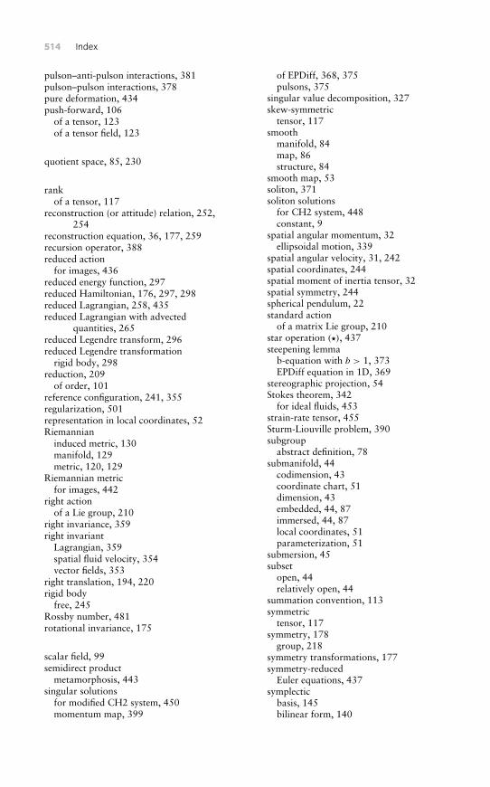
514 Index
pulson–anti-pulson interactions, 381pulson–pulson interactions, 378pure deformation, 434push-forward, 106
of a tensor, 123of a tensor field, 123
quotient space, 85, 230
rankof a tensor, 117
reconstruction (or attitude) relation, 252,254
reconstruction equation, 36, 177, 259recursion operator, 388reduced action
for images, 436reduced energy function, 297reduced Hamiltonian, 176, 297, 298reduced Lagrangian, 258, 435reduced Lagrangian with advected
quantities, 265reduced Legendre transform, 296reduced Legendre transformation
rigid body, 298reduction, 209
of order, 101reference configuration, 241, 355regularization, 501representation in local coordinates, 52Riemannian
induced metric, 130manifold, 129metric, 120, 129
Riemannian metricfor images, 442
right actionof a Lie group, 210
right invariance, 359right invariant
Lagrangian, 359spatial fluid velocity, 354vector fields, 353
right translation, 194, 220rigid body
free, 245Rossby number, 481rotational invariance, 175
scalar field, 99semidirect product
metamorphosis, 443singular solutions
for modified CH2 system, 450momentum map, 399
of EPDiff, 368, 375pulsons, 375
singular value decomposition, 327skew-symmetric
tensor, 117smooth
manifold, 84map, 86structure, 84
smooth map, 53soliton, 371soliton solutions
for CH2 system, 448constant, 9
spatial angular momentum, 32ellipsoidal motion, 339
spatial angular velocity, 31, 242spatial coordinates, 244spatial moment of inertia tensor, 32spatial symmetry, 244spherical pendulum, 22standard action
of a matrix Lie group, 210star operation (�), 437steepening lemma
b-equation with b > 1, 373EPDiff equation in 1D, 369
stereographic projection, 54Stokes theorem, 342
for ideal fluids, 453strain-rate tensor, 455Sturm-Liouville problem, 390subgroup
abstract definition, 78submanifold, 44
codimension, 43coordinate chart, 51dimension, 43embedded, 44, 87immersed, 44, 87local coordinates, 51parameterization, 51
submersion, 45subset
open, 44relatively open, 44
summation convention, 113symmetric
tensor, 117symmetry, 178
group, 218symmetry transformations, 177symmetry-reduced
Euler equations, 437symplectic
basis, 145bilinear form, 140
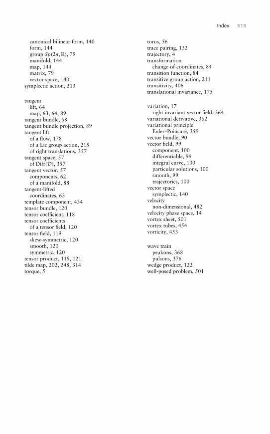
Index 515
canonical bilinear form, 140form, 144group Sp(2n, R), 79manifold, 144map, 144matrix, 79vector space, 140
symplectic action, 213
tangentlift, 64map, 63, 64, 89
tangent bundle, 58tangent bundle projection, 89tangent lift
of a flow, 178of a Lie group action, 215of right translations, 357
tangent space, 57of Diff(D), 357
tangent vector, 57components, 62of a manifold, 88
tangent-liftedcoordinates, 63
template component, 434tensor bundle, 120tensor coefficient, 118tensor coefficients
of a tensor field, 120tensor field, 119
skew-symmetric, 120smooth, 120symmetric, 120
tensor product, 119, 121tilde map, 202, 248, 314torque, 5
torus, 56trace pairing, 132trajectory, 4transformation
change-of-coordinates, 84transition function, 84transitive group action, 211transitivity, 406translational invariance, 175
variation, 17right invariant vector field, 364
variational derivative, 362variational principle
Euler–Poincaré, 359vector bundle, 90vector field, 99
component, 100differentiable, 99integral curve, 100particular solutions, 100smooth, 99trajectories, 100
vector spacesymplectic, 140
velocitynon-dimensional, 482
velocity phase space, 14vortex sheet, 501vortex tubes, 454vorticity, 453
wave trainpeakons, 368pulsons, 376
wedge product, 122well-posed problem, 501

This page intentionally left blank
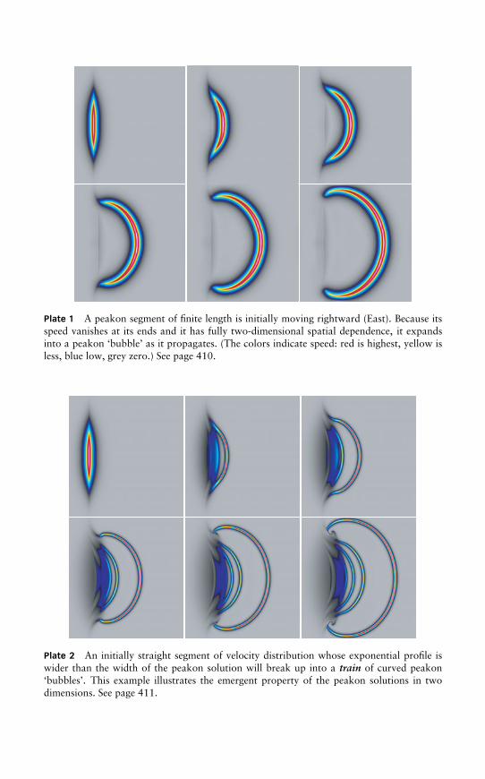
Plate 1 A peakon segment of finite length is initially moving rightward (East). Because itsspeed vanishes at its ends and it has fully two-dimensional spatial dependence, it expandsinto a peakon ‘bubble’ as it propagates. (The colors indicate speed: red is highest, yellow isless, blue low, grey zero.) See page 410.
Plate 2 An initially straight segment of velocity distribution whose exponential profile iswider than the width of the peakon solution will break up into a train of curved peakon‘bubbles’. This example illustrates the emergent property of the peakon solutions in twodimensions. See page 411.
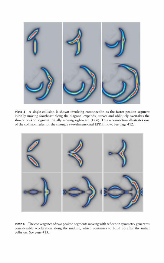
Plate 3 A single collision is shown involving reconnection as the faster peakon segmentinitially moving Southeast along the diagonal expands, curves and obliquely overtakes theslower peakon segment initially moving rightward (East). This reconnection illustrates oneof the collision rules for the strongly two-dimensional EPDiff flow. See page 412.
Plate 4 The convergence of two peakon segments moving with reflection symmetry generatesconsiderable acceleration along the midline, which continues to build up after the initialcollision. See page 413.
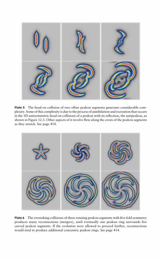
Plate 5 The head-on collision of two offset peakon segments generates considerable com-plexity. Some of this complexity is due to the process of annihilation and recreation that occursin the 1D antisymmetric head-on collisions of a peakon with its reflection, the antipeakon, asshown in Figure 12.3. Other aspects of it involve flow along the crests of the peakon segmentsas they stretch. See page 414.
Plate 6 The overtaking collisions of these rotating peakon segments with five-fold symmetryproduces many reconnections (mergers), until eventually one peakon ring surrounds fivecurved peakon segments. If the evolution were allowed to proceed further, reconnectionswould tend to produce additional concentric peakon rings. See page 414.
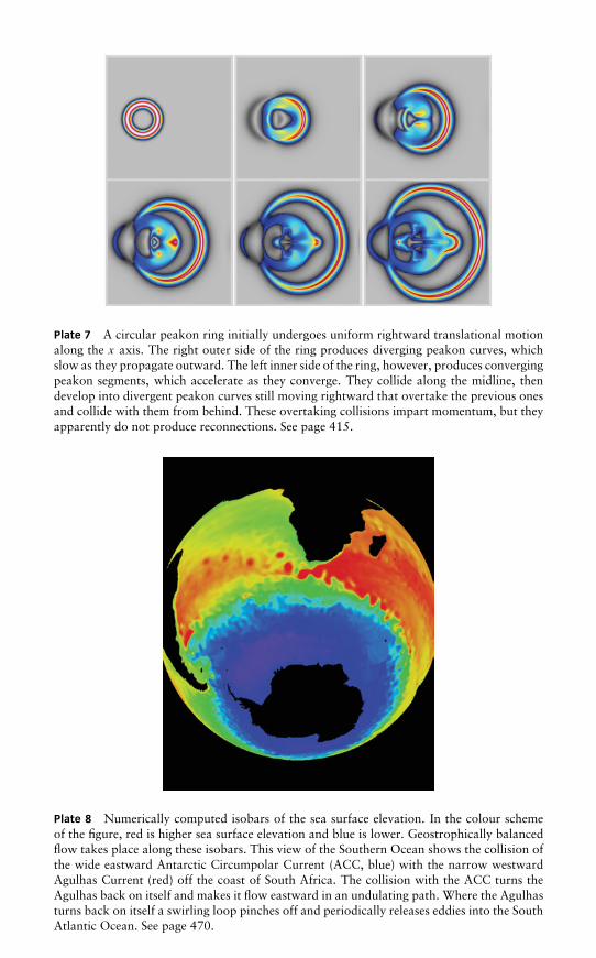
Plate 7 A circular peakon ring initially undergoes uniform rightward translational motionalong the x axis. The right outer side of the ring produces diverging peakon curves, whichslow as they propagate outward. The left inner side of the ring, however, produces convergingpeakon segments, which accelerate as they converge. They collide along the midline, thendevelop into divergent peakon curves still moving rightward that overtake the previous onesand collide with them from behind. These overtaking collisions impart momentum, but theyapparently do not produce reconnections. See page 415.
Plate 8 Numerically computed isobars of the sea surface elevation. In the colour schemeof the figure, red is higher sea surface elevation and blue is lower. Geostrophically balancedflow takes place along these isobars. This view of the Southern Ocean shows the collision ofthe wide eastward Antarctic Circumpolar Current (ACC, blue) with the narrow westwardAgulhas Current (red) off the coast of South Africa. The collision with the ACC turns theAgulhas back on itself and makes it flow eastward in an undulating path. Where the Agulhasturns back on itself a swirling loop pinches off and periodically releases eddies into the SouthAtlantic Ocean. See page 470.


![A Primer on Geometric Mechanics [5pt] Why Geometric Mechanics?isg · I Lecture 4: Symmetry and reduction. I Lecture 5: ... we shall see, comes from the world of geometric mechanics](https://img.pdfslide.us/doc/110x75/5ee02d74ad6a402d666b6978/a-primer-on-geometric-mechanics-5pt-why-geometric-mechanics-i-lecture-4-symmetry.jpg)