Embed Size (px)
Citation preview
Geometric flows and holographyHolography
Euclidean prescriptionReal-time gauge-gravity duality
ExamplesConcluding remarks
Geometric flows and holography
Kostas Skenderis
University of Amsterdam
Workshop on Field Theory and Geometric Flows28 November 2008
Kostas Skenderis Geometric flows and holography
Geometric flows and holographyHolography
Euclidean prescriptionReal-time gauge-gravity duality
ExamplesConcluding remarks
Calabi flowRicci flow
Introduction
The aim of this talk is two-fold:
1 I would like to argue for a connection between geometric flows and threedimensional quantum field theories using holography.
2 Discuss the necessary holographic tools needed to flesh out this connection.
Kostas Skenderis Geometric flows and holography
Geometric flows and holographyHolography
Euclidean prescriptionReal-time gauge-gravity duality
ExamplesConcluding remarks
Calabi flowRicci flow
References
The first part is based on on-going work with I. Bakas.The second part is based onKS, Balt van Rees, Phys.Rev.Lett. (2008), arXiv:0805.0150.KS, Balt van Rees, arXiv:0812.xxxx
Kostas Skenderis Geometric flows and holography
Geometric flows and holographyHolography
Euclidean prescriptionReal-time gauge-gravity duality
ExamplesConcluding remarks
Calabi flowRicci flow
The main idea
The main idea is the following:
Certain geometric flows can be embedded in Einstein’s equations with negativecosmological constant in four dimensions.Solutions that are asymptotically AdS4 encode quantum field theory (QFT) datafor a QFT in three dimensions.Therefore, these geometric flows should be related to QFTs in three dimensions.
Kostas Skenderis Geometric flows and holography
Geometric flows and holographyHolography
Euclidean prescriptionReal-time gauge-gravity duality
ExamplesConcluding remarks
Calabi flowRicci flow
Geometric flows and Asymptotically AdS spacetimes
There are two main examples of such connection:
1 Calabi flow and Robinson-Trautman spacetimes.2 Normalized Ricci flow and certain perturbations of AdS4 Schwarzschild black
holes.
Kostas Skenderis Geometric flows and holography
Geometric flows and holographyHolography
Euclidean prescriptionReal-time gauge-gravity duality
ExamplesConcluding remarks
Calabi flowRicci flow
Robinson-Trautman spacetimes
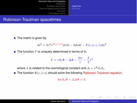
The metric is given by
ds2 = 2r2e!(z,z̄;u)dzdz̄ ! 2dudr ! F (r, u, z, z̄)du2
The function F is uniquely determined in terms of !,
F = r!u!!"!!2m
r!
#
3r2
where # is related to the cosmological constant and " = e!!z!z̄ .The function !(z, z̄; u) should solve the following Robinson-Trautman equation,
3m!u! + ""! = 0.
Kostas Skenderis Geometric flows and holography
Geometric flows and holographyHolography
Euclidean prescriptionReal-time gauge-gravity duality
ExamplesConcluding remarks
Calabi flowRicci flow
Calabi flow
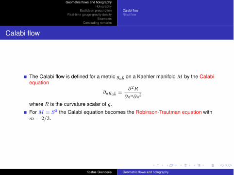
The Calabi flow is defined for a metric gab̄ on a Kaehler manifold M by the Calabiequation
!ugab̄ =!2R
!za!zb̄
where R is the curvature scalar of g.For M = S2 the Calabi equation becomes the Robinson-Trautman equation withm = 2/3.
Kostas Skenderis Geometric flows and holography
Geometric flows and holographyHolography
Euclidean prescriptionReal-time gauge-gravity duality
ExamplesConcluding remarks
Calabi flowRicci flow
Schwarzschild AdS solution from Robinson-Trautman
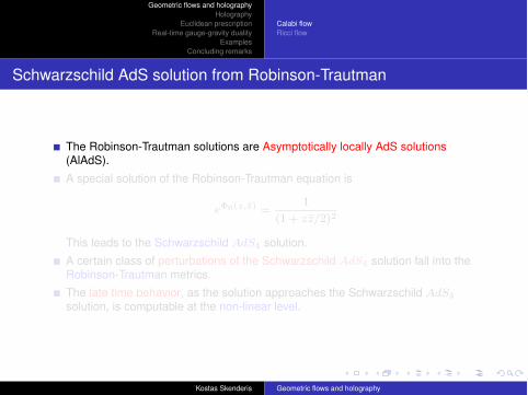
The Robinson-Trautman solutions are Asymptotically locally AdS solutions(AlAdS).A special solution of the Robinson-Trautman equation is
e!0(z,z̄) =1
(1 + zz̄/2)2
This leads to the Schwarzschild AdS4 solution.A certain class of perturbations of the Schwarzschild AdS4 solution fall into theRobinson-Trautman metrics.The late time behavior, as the solution approaches the Schwarzschild AdS4
solution, is computable at the non-linear level.
Kostas Skenderis Geometric flows and holography
Geometric flows and holographyHolography
Euclidean prescriptionReal-time gauge-gravity duality
ExamplesConcluding remarks
Calabi flowRicci flow
Schwarzschild AdS solution from Robinson-Trautman
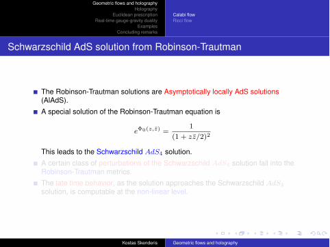
The Robinson-Trautman solutions are Asymptotically locally AdS solutions(AlAdS).A special solution of the Robinson-Trautman equation is
e!0(z,z̄) =1
(1 + zz̄/2)2
This leads to the Schwarzschild AdS4 solution.A certain class of perturbations of the Schwarzschild AdS4 solution fall into theRobinson-Trautman metrics.The late time behavior, as the solution approaches the Schwarzschild AdS4
solution, is computable at the non-linear level.
Kostas Skenderis Geometric flows and holography
Geometric flows and holographyHolography
Euclidean prescriptionReal-time gauge-gravity duality
ExamplesConcluding remarks
Calabi flowRicci flow
Schwarzschild AdS solution from Robinson-Trautman
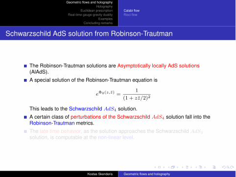
The Robinson-Trautman solutions are Asymptotically locally AdS solutions(AlAdS).A special solution of the Robinson-Trautman equation is
e!0(z,z̄) =1
(1 + zz̄/2)2
This leads to the Schwarzschild AdS4 solution.A certain class of perturbations of the Schwarzschild AdS4 solution fall into theRobinson-Trautman metrics.The late time behavior, as the solution approaches the Schwarzschild AdS4
solution, is computable at the non-linear level.
Kostas Skenderis Geometric flows and holography
Geometric flows and holographyHolography
Euclidean prescriptionReal-time gauge-gravity duality
ExamplesConcluding remarks
Calabi flowRicci flow
Schwarzschild AdS solution from Robinson-Trautman
The Robinson-Trautman solutions are Asymptotically locally AdS solutions(AlAdS).A special solution of the Robinson-Trautman equation is
e!0(z,z̄) =1
(1 + zz̄/2)2
This leads to the Schwarzschild AdS4 solution.A certain class of perturbations of the Schwarzschild AdS4 solution fall into theRobinson-Trautman metrics.The late time behavior, as the solution approaches the Schwarzschild AdS4
solution, is computable at the non-linear level.
Kostas Skenderis Geometric flows and holography
Geometric flows and holographyHolography
Euclidean prescriptionReal-time gauge-gravity duality
ExamplesConcluding remarks
Calabi flowRicci flow
Normalized Ricci flow
Recall that the Ricci flow equation is
!ugij = !Rij
This flow does not preserve the spacetime volume.One can modify the flow to become volume preserving leading to the normalizedRicci flow. For metrics ds2 = 2e!dzdz̄ on S2 this flow is governed by
!u! = "! + 1
Kostas Skenderis Geometric flows and holography
Geometric flows and holographyHolography
Euclidean prescriptionReal-time gauge-gravity duality
ExamplesConcluding remarks
Calabi flowRicci flow
Normalized Ricci flow and large AdS4 black holes
The constant curvature metric provides a fixed point for the flow.The spectrum of axial perturbations as the flow approaches this fixed point can becomputed analytically.Large AdS4 black holes exhibit certain purely dissipative axial perturbations withexactly the same (imaginary) frequencies (computed now numerically) as in thenormalized Ricci flow. [I. Bakas (2008)]
Kostas Skenderis Geometric flows and holography
Geometric flows and holographyHolography
Euclidean prescriptionReal-time gauge-gravity duality
ExamplesConcluding remarks
Calabi flowRicci flow
Geometric flows and AdS/CFT
We have seen that both geometric flows are related to perturbations around theAdS4 Schwarzschild black hole, with the Calabi flow being more generallyassociated with Asymptotically locally AdS spacetimes.In AdS/CFT the Schwarzschild black hole is associated with a thermal state in thedual 3d QFT.Perturbations around any given AlAdS solution are associated with QFTcorrelators of specific operators in the state specified by the background solution:
linearized perturbations! 2-point functions2nd order perturbations! 3-point functions...
" Geometric flows control the behavior of certain QFT correlators at strong coupling.
Kostas Skenderis Geometric flows and holography
Geometric flows and holographyHolography
Euclidean prescriptionReal-time gauge-gravity duality
ExamplesConcluding remarks
Holography
The remainder of this talk will be devoted into explaining the holographic toolsneeded to understand in detail the relation sketched in the previous slide.We will actually ask a more general question:How do we set up the gravity/gauge theory duality in real-time?
Kostas Skenderis Geometric flows and holography
Geometric flows and holographyHolography
Euclidean prescriptionReal-time gauge-gravity duality
ExamplesConcluding remarks
Holography in real-time
One would like to set up a prescription as general as the Euclidean one. In particular, itshould
apply to any n-point function, including correlators in non-trivial states.apply to all QFTs with a holographic dual.the prescription should be fully holographic, i.e. only boundary data and regularityshould suffice.Within the supergravity approximation, all information should be encoded inclassical bulk dynamics.
Kostas Skenderis Geometric flows and holography
Geometric flows and holographyHolography
Euclidean prescriptionReal-time gauge-gravity duality
ExamplesConcluding remarks
Motivation
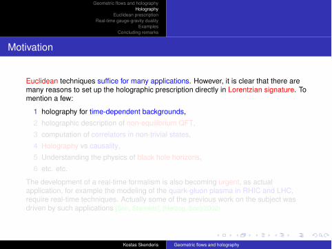
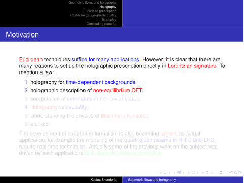
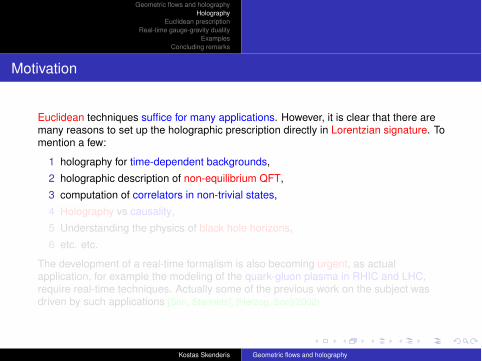
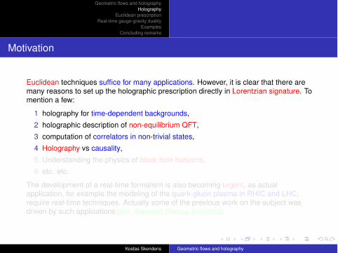
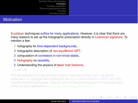
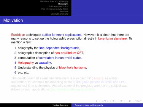
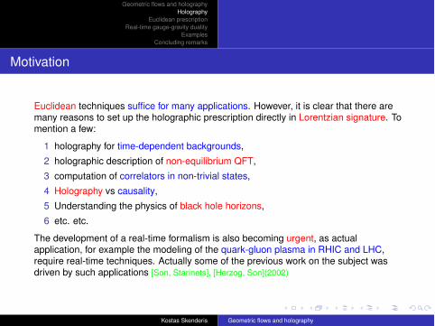
Euclidean techniques suffice for many applications. However, it is clear that there aremany reasons to set up the holographic prescription directly in Lorentzian signature. Tomention a few:
1 holography for time-dependent backgrounds,2 holographic description of non-equilibrium QFT,3 computation of correlators in non-trivial states,4 Holography vs causality,5 Understanding the physics of black hole horizons,6 etc. etc.
The development of a real-time formalism is also becoming urgent, as actualapplication, for example the modeling of the quark-gluon plasma in RHIC and LHC,require real-time techniques. Actually some of the previous work on the subject wasdriven by such applications [Son, Starinets], [Herzog, Son](2002)
Kostas Skenderis Geometric flows and holography
Geometric flows and holographyHolography
Euclidean prescriptionReal-time gauge-gravity duality
ExamplesConcluding remarks
Motivation
Euclidean techniques suffice for many applications. However, it is clear that there aremany reasons to set up the holographic prescription directly in Lorentzian signature. Tomention a few:
1 holography for time-dependent backgrounds,2 holographic description of non-equilibrium QFT,3 computation of correlators in non-trivial states,4 Holography vs causality,5 Understanding the physics of black hole horizons,6 etc. etc.
The development of a real-time formalism is also becoming urgent, as actualapplication, for example the modeling of the quark-gluon plasma in RHIC and LHC,require real-time techniques. Actually some of the previous work on the subject wasdriven by such applications [Son, Starinets], [Herzog, Son](2002)
Kostas Skenderis Geometric flows and holography
Geometric flows and holographyHolography
Euclidean prescriptionReal-time gauge-gravity duality
ExamplesConcluding remarks
Outline
1 Review of Euclidean prescription2 Lorentzian prescription3 Examples4 Conclusions
Kostas Skenderis Geometric flows and holography
Geometric flows and holographyHolography
Euclidean prescriptionReal-time gauge-gravity duality
ExamplesConcluding remarks
Outline
1 Review of Euclidean prescription2 Lorentzian prescription3 Examples4 Conclusions
Kostas Skenderis Geometric flows and holography
Geometric flows and holographyHolography
Euclidean prescriptionReal-time gauge-gravity duality
ExamplesConcluding remarks
Outline
1 Review of Euclidean prescription2 Lorentzian prescription3 Examples4 Conclusions
Kostas Skenderis Geometric flows and holography
Geometric flows and holographyHolography
Euclidean prescriptionReal-time gauge-gravity duality
ExamplesConcluding remarks
Outline
1 Review of Euclidean prescription2 Lorentzian prescription3 Examples4 Conclusions
Kostas Skenderis Geometric flows and holography
Geometric flows and holographyHolography
Euclidean prescriptionReal-time gauge-gravity duality
ExamplesConcluding remarks
Basic DictionaryHolographic renormalizationRadial Hamiltonian formalism
Basic Dictionary
Let us start by briefly reviewing the basics of holography. In the low energyapproximation, where the bulk theory is approximated by supergravity the basicholographic dictionary is [GKP,W (1998)]:
1 There is 1-1 correspondence between local gauge invariant operators O of theboundary QFT and bulk supergravity modes !.
2 The fields "(0) parametrizing the boundary conditions of the bulk fields ! areidentified with the sources of dual operators.
Kostas Skenderis Geometric flows and holography
Geometric flows and holographyHolography
Euclidean prescriptionReal-time gauge-gravity duality
ExamplesConcluding remarks
Basic DictionaryHolographic renormalizationRadial Hamiltonian formalism
Basic Dictionary
3 The fundamental relation between the bulk and boundary theories in Euclideansignature within the supegravity approximation is
ZSUGRA["(0)] =
!
!!!(0)
D! exp (!S[!]) = #exp(!!
"M"(0)O)$QFT
To leading orderSon"shell["(0), ...] = !WQFT ["(0), ...]
on-shell SUGRA action = generating functional of QFT connected graphs
Such a relation is however formal as both sides diverge. On the QFT side these are theusual UV divergences, dealt with by standard renormalization techniques. On thegravitational side, the infinities are due to the infinite volume of the spacetime. Thisissue is dealt with by the formalism of holographic renormalization, which is the precisegravitational analogue of QFT renormalization. [Henningson, KS (1998)], ...
Kostas Skenderis Geometric flows and holography
Geometric flows and holographyHolography
Euclidean prescriptionReal-time gauge-gravity duality
ExamplesConcluding remarks
Basic DictionaryHolographic renormalizationRadial Hamiltonian formalism
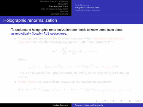
Holographic renormalization
To understand holographic renormalization one needs to know some facts aboutasymptotically (locally) AdS spacetimes.
These spacetimes solve the Einstein equations with a negative cosmologicalconstant and have the following asymptotic (Fefferman-Graham) form
ds2 =dr2
r2+
1
r2gij(x, r)dxidxj
where
gij(x, r) = g(0)ij + r2g(2)ij + ... + rd "log r2h(d)ij + g(d)ij
#+ ...
This is an expansion in r (the conformal boundary of the spacetime is located atr = 0).Matter fields, e.g. scalar fields, have a similar asymptotic expansion
!(x, r) = rd""$"(0) + r2"(2) + ... + r2""d "
log r2#(2""d) + "(2""d)
#+ ...
%
Kostas Skenderis Geometric flows and holography
Geometric flows and holographyHolography
Euclidean prescriptionReal-time gauge-gravity duality
ExamplesConcluding remarks
Basic DictionaryHolographic renormalizationRadial Hamiltonian formalism
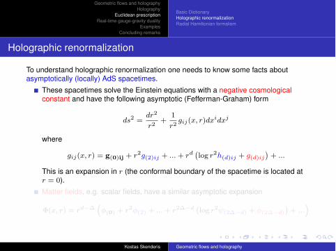
Holographic renormalization
To understand holographic renormalization one needs to know some facts aboutasymptotically (locally) AdS spacetimes.
These spacetimes solve the Einstein equations with a negative cosmologicalconstant and have the following asymptotic (Fefferman-Graham) form
ds2 =dr2
r2+
1
r2gij(x, r)dxidxj
where
gij(x, r) = g(0)ij + r2g(2)ij + ... + rd "log r2h(d)ij + g(d)ij
#+ ...
This is an expansion in r (the conformal boundary of the spacetime is located atr = 0).Matter fields, e.g. scalar fields, have a similar asymptotic expansion
!(x, r) = rd""$"(0) + r2"(2) + ... + r2""d "
log r2#(2""d) + "(2""d)
#+ ...
%
Kostas Skenderis Geometric flows and holography
Geometric flows and holographyHolography
Euclidean prescriptionReal-time gauge-gravity duality
ExamplesConcluding remarks
Basic DictionaryHolographic renormalizationRadial Hamiltonian formalism
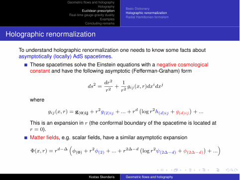
Holographic renormalization
To understand holographic renormalization one needs to know some facts aboutasymptotically (locally) AdS spacetimes.
These spacetimes solve the Einstein equations with a negative cosmologicalconstant and have the following asymptotic (Fefferman-Graham) form
ds2 =dr2
r2+
1
r2gij(x, r)dxidxj
where
gij(x, r) = g(0)ij + r2g(2)ij + ... + rd "log r2h(d)ij + g(d)ij
#+ ...
This is an expansion in r (the conformal boundary of the spacetime is located atr = 0).Matter fields, e.g. scalar fields, have a similar asymptotic expansion
!(x, r) = rd""$"(0) + r2"(2) + ... + r2""d "
log r2#(2""d) + "(2""d)
#+ ...
%
Kostas Skenderis Geometric flows and holography
Geometric flows and holographyHolography
Euclidean prescriptionReal-time gauge-gravity duality
ExamplesConcluding remarks
Basic DictionaryHolographic renormalizationRadial Hamiltonian formalism
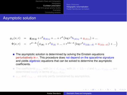
Asymptotic solution
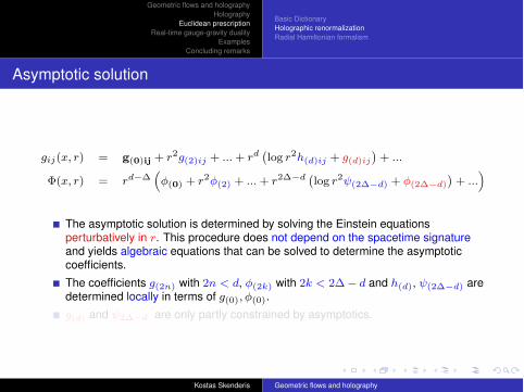
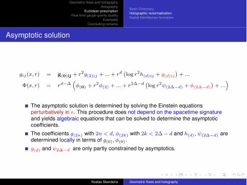
gij(x, r) = g(0)ij + r2g(2)ij + ... + rd "log r2h(d)ij + g(d)ij
#+ ...
!(x, r) = rd""$"(0) + r2"(2) + ... + r2""d "
log r2#(2""d) + "(2""d)
#+ ...
%
The asymptotic solution is determined by solving the Einstein equationsperturbatively in r. This procedure does not depend on the spacetime signatureand yields algebraic equations that can be solved to determine the asymptoticcoefficients.The coefficients g(2n) with 2n < d, "(2k) with 2k < 2"! d and h(d), #(2""d) aredetermined locally in terms of g(0), "(0).g(d) and #2""d are only partly constrained by asymptotics.
Kostas Skenderis Geometric flows and holography
Geometric flows and holographyHolography
Euclidean prescriptionReal-time gauge-gravity duality
ExamplesConcluding remarks
Basic DictionaryHolographic renormalizationRadial Hamiltonian formalism
Asymptotic solution
gij(x, r) = g(0)ij + r2g(2)ij + ... + rd "log r2h(d)ij + g(d)ij
#+ ...
!(x, r) = rd""$"(0) + r2"(2) + ... + r2""d "
log r2#(2""d) + "(2""d)
#+ ...
%
The asymptotic solution is determined by solving the Einstein equationsperturbatively in r. This procedure does not depend on the spacetime signatureand yields algebraic equations that can be solved to determine the asymptoticcoefficients.The coefficients g(2n) with 2n < d, "(2k) with 2k < 2"! d and h(d), #(2""d) aredetermined locally in terms of g(0), "(0).g(d) and #2""d are only partly constrained by asymptotics.
Kostas Skenderis Geometric flows and holography
Geometric flows and holographyHolography
Euclidean prescriptionReal-time gauge-gravity duality
ExamplesConcluding remarks
Basic DictionaryHolographic renormalizationRadial Hamiltonian formalism
Holographic Renormalization
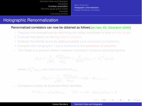
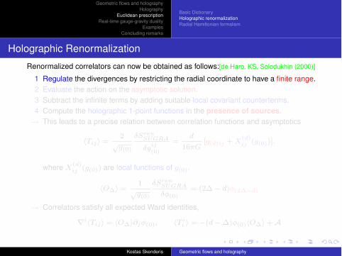
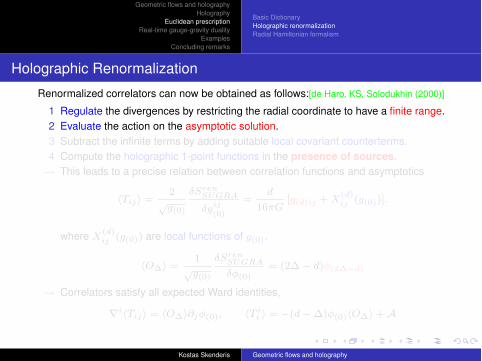
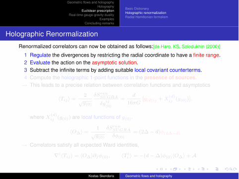
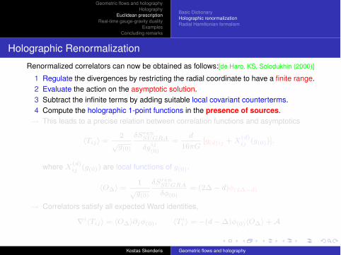
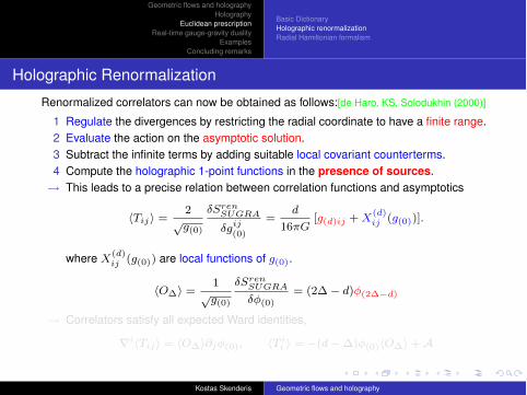
Renormalized correlators can now be obtained as follows:[de Haro, KS, Solodukhin (2000)]
1 Regulate the divergences by restricting the radial coordinate to have a finite range.2 Evaluate the action on the asymptotic solution.3 Subtract the infinite terms by adding suitable local covariant counterterms.4 Compute the holographic 1-point functions in the presence of sources.% This leads to a precise relation between correlation functions and asymptotics
#Tij$ =2
&g(0)
$SrenSUGRA
$gij(0)
=d
16%G[g(d)ij + X
(d)ij (g(0))].
where X(d)ij (g(0)) are local functions of g(0).
#O"$ =1
&g(0)
$SrenSUGRA
$"(0)= (2"! d)"(2""d)
% Correlators satisfy all expected Ward identities,
'i#Tij$ = #O"$!j"(0), #T ii $ = !(d!")"(0)#O"$+A
Kostas Skenderis Geometric flows and holography
Geometric flows and holographyHolography
Euclidean prescriptionReal-time gauge-gravity duality
ExamplesConcluding remarks
Basic DictionaryHolographic renormalizationRadial Hamiltonian formalism
Holographic Renormalization
Renormalized correlators can now be obtained as follows:[de Haro, KS, Solodukhin (2000)]
1 Regulate the divergences by restricting the radial coordinate to have a finite range.2 Evaluate the action on the asymptotic solution.3 Subtract the infinite terms by adding suitable local covariant counterterms.4 Compute the holographic 1-point functions in the presence of sources.% This leads to a precise relation between correlation functions and asymptotics
#Tij$ =2
&g(0)
$SrenSUGRA
$gij(0)
=d
16%G[g(d)ij + X
(d)ij (g(0))].
where X(d)ij (g(0)) are local functions of g(0).
#O"$ =1
&g(0)
$SrenSUGRA
$"(0)= (2"! d)"(2""d)
% Correlators satisfy all expected Ward identities,
'i#Tij$ = #O"$!j"(0), #T ii $ = !(d!")"(0)#O"$+A
Kostas Skenderis Geometric flows and holography
Geometric flows and holographyHolography
Euclidean prescriptionReal-time gauge-gravity duality
ExamplesConcluding remarks
Basic DictionaryHolographic renormalizationRadial Hamiltonian formalism
Holographic Renormalization: higher point functions
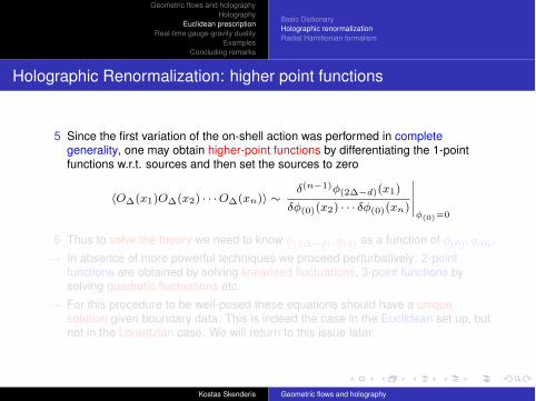
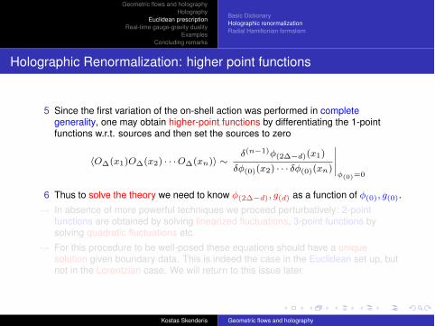
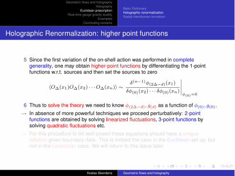
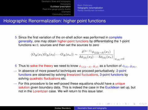
5 Since the first variation of the on-shell action was performed in completegenerality, one may obtain higher-point functions by differentiating the 1-pointfunctions w.r.t. sources and then set the sources to zero
#O"(x1)O"(x2) · · ·O"(xn)$ ($(n"1)"(2""d)(x1)
$"(0)(x2) · · · $"(0)(xn)
&&&&&!(0)=0
6 Thus to solve the theory we need to know "(2""d), g(d) as a function of "(0), g(0).% In absence of more powerful techniques we proceed perturbatively: 2-point
functions are obtained by solving linearized fluctuations, 3-point functions bysolving quadratic fluctuations etc.
% For this procedure to be well-posed these equations should have a uniquesolution given boundary data. This is indeed the case in the Euclidean set up, butnot in the Lorentzian case. We will return to this issue later.
Kostas Skenderis Geometric flows and holography
Geometric flows and holographyHolography
Euclidean prescriptionReal-time gauge-gravity duality
ExamplesConcluding remarks
Basic DictionaryHolographic renormalizationRadial Hamiltonian formalism
Holographic Renormalization: higher point functions
5 Since the first variation of the on-shell action was performed in completegenerality, one may obtain higher-point functions by differentiating the 1-pointfunctions w.r.t. sources and then set the sources to zero
#O"(x1)O"(x2) · · ·O"(xn)$ ($(n"1)"(2""d)(x1)
$"(0)(x2) · · · $"(0)(xn)
&&&&&!(0)=0
6 Thus to solve the theory we need to know "(2""d), g(d) as a function of "(0), g(0).% In absence of more powerful techniques we proceed perturbatively: 2-point
functions are obtained by solving linearized fluctuations, 3-point functions bysolving quadratic fluctuations etc.
% For this procedure to be well-posed these equations should have a uniquesolution given boundary data. This is indeed the case in the Euclidean set up, butnot in the Lorentzian case. We will return to this issue later.
Kostas Skenderis Geometric flows and holography
Geometric flows and holographyHolography
Euclidean prescriptionReal-time gauge-gravity duality
ExamplesConcluding remarks
Basic DictionaryHolographic renormalizationRadial Hamiltonian formalism
Radial Hamiltonian formalism
The method of holographic renormalization used so far is conceptually simple, butcomputationally inefficient as it does not exploit the underlying conformalstructure.For most explicit computations, it is better to use the radial Hamiltonian formalism,a Hamiltonian formulation in which the radius plays the role of time.One relates the regularized holographic 1-point of an operator O! to the radialcanonical momentum %! of the corresponding bulk field ! [de Boer,Verlinde2],[Papadimitriou, KS].
$S =
!dr
'!L
!!! !r
!L
!(!r!)
($! +
)!L
!(!r!)$!
*
r
, L )!
ddx&
GL
"$Son"shell
$!=
!L
!(!r!)) %!
% Note that in the Lorentzian context there are additional boundary terms att = ±*.
Kostas Skenderis Geometric flows and holography
Geometric flows and holographyHolography
Euclidean prescriptionReal-time gauge-gravity duality
ExamplesConcluding remarks
Basic DictionaryHolographic renormalizationRadial Hamiltonian formalism
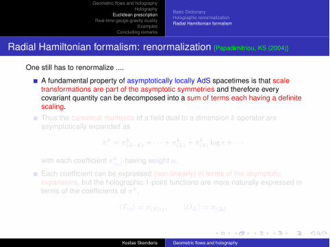
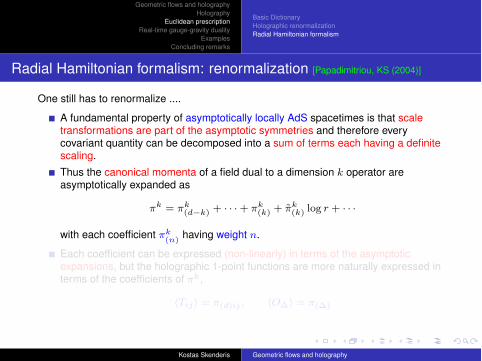
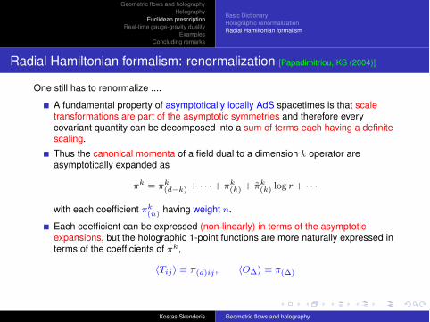
Radial Hamiltonian formalism: renormalization [Papadimitriou, KS (2004)]
One still has to renormalize ....
A fundamental property of asymptotically locally AdS spacetimes is that scaletransformations are part of the asymptotic symmetries and therefore everycovariant quantity can be decomposed into a sum of terms each having a definitescaling.Thus the canonical momenta of a field dual to a dimension k operator areasymptotically expanded as
%k = %k(d"k) + · · ·+ %k
(k) + %̃k(k) log r + · · ·
with each coefficient %k(n) having weight n.
Each coefficient can be expressed (non-linearly) in terms of the asymptoticexpansions, but the holographic 1-point functions are more naturally expressed interms of the coefficients of %k,
#Tij$ = %(d)ij , #O"$ = %(")
Kostas Skenderis Geometric flows and holography
Geometric flows and holographyHolography
Euclidean prescriptionReal-time gauge-gravity duality
ExamplesConcluding remarks
Basic DictionaryHolographic renormalizationRadial Hamiltonian formalism
Radial Hamiltonian formalism: renormalization [Papadimitriou, KS (2004)]
One still has to renormalize ....
A fundamental property of asymptotically locally AdS spacetimes is that scaletransformations are part of the asymptotic symmetries and therefore everycovariant quantity can be decomposed into a sum of terms each having a definitescaling.Thus the canonical momenta of a field dual to a dimension k operator areasymptotically expanded as
%k = %k(d"k) + · · ·+ %k
(k) + %̃k(k) log r + · · ·
with each coefficient %k(n) having weight n.
Each coefficient can be expressed (non-linearly) in terms of the asymptoticexpansions, but the holographic 1-point functions are more naturally expressed interms of the coefficients of %k,
#Tij$ = %(d)ij , #O"$ = %(")
Kostas Skenderis Geometric flows and holography
Geometric flows and holographyHolography
Euclidean prescriptionReal-time gauge-gravity duality
ExamplesConcluding remarks
IntroductionQFT interludeLorentzian prescriptionCorrelators
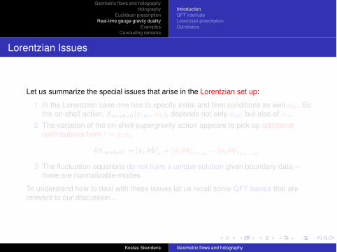
Lorentzian Issues
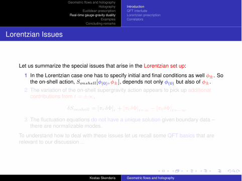
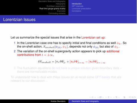
Let us summarize the special issues that arise in the Lorentzian set up:
1 In the Lorentzian case one has to specify initial and final conditions as well "±. Sothe on-shell action, Sonshell["(0), "±], depends not only "(0) but also of "±.
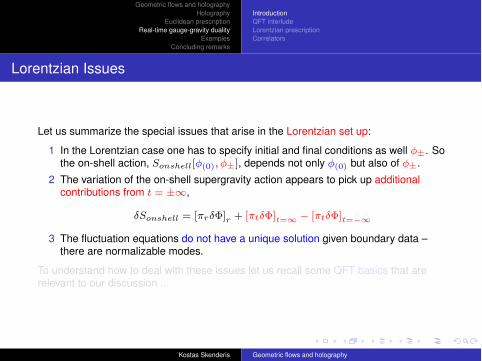
2 The variation of the on-shell supergravity action appears to pick up additionalcontributions from t = ±*,
$Sonshell = [%r$!]r + [%t$!]t=# ! [%t$!]t="#
3 The fluctuation equations do not have a unique solution given boundary data –there are normalizable modes.
To understand how to deal with these issues let us recall some QFT basics that arerelevant to our discussion ...
Kostas Skenderis Geometric flows and holography
Geometric flows and holographyHolography
Euclidean prescriptionReal-time gauge-gravity duality
ExamplesConcluding remarks
IntroductionQFT interludeLorentzian prescriptionCorrelators
Lorentzian Issues
Let us summarize the special issues that arise in the Lorentzian set up:
1 In the Lorentzian case one has to specify initial and final conditions as well "±. Sothe on-shell action, Sonshell["(0), "±], depends not only "(0) but also of "±.
2 The variation of the on-shell supergravity action appears to pick up additionalcontributions from t = ±*,
$Sonshell = [%r$!]r + [%t$!]t=# ! [%t$!]t="#
3 The fluctuation equations do not have a unique solution given boundary data –there are normalizable modes.
To understand how to deal with these issues let us recall some QFT basics that arerelevant to our discussion ...
Kostas Skenderis Geometric flows and holography
Geometric flows and holographyHolography
Euclidean prescriptionReal-time gauge-gravity duality
ExamplesConcluding remarks
IntroductionQFT interludeLorentzian prescriptionCorrelators
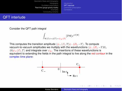
QFT interlude
Consider the QFT path integral!
#(#x,t=±T )=$±(#x)[D$]eiS[#]
This computes the transition amplitude ##+(&x), T |#"(&x),!T $. To computevacuum-to-vacuum amplitudes we multiply with the wavefunctions ##"(&x),!T |0$,#0|#+(&x), T $ and integrate over #±. The insertions of these wavefunctions isequivalent to extending the fields in the path integral to live along the red contour in thecomplex time plane:
Re t
Im tC
C
!
+
0
Kostas Skenderis Geometric flows and holography
Geometric flows and holographyHolography
Euclidean prescriptionReal-time gauge-gravity duality
ExamplesConcluding remarks
IntroductionQFT interludeLorentzian prescriptionCorrelators
Remarks
Re t
Im tC
C
!
+
0
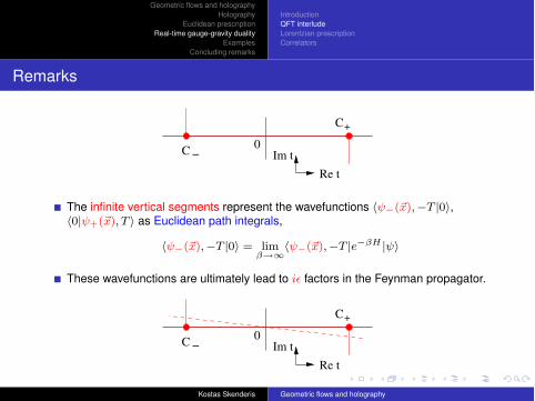
The infinite vertical segments represent the wavefunctions ##"(&x),!T |0$,#0|#+(&x), T $ as Euclidean path integrals,
##"(&x),!T |0$ = lim%$#
##"(&x),!T |e"%H |#$
These wavefunctions are ultimately lead to i' factors in the Feynman propagator.
Re t
Im tC
C
!
+
0
Kostas Skenderis Geometric flows and holography
Geometric flows and holographyHolography
Euclidean prescriptionReal-time gauge-gravity duality
ExamplesConcluding remarks
IntroductionQFT interludeLorentzian prescriptionCorrelators
Remarks
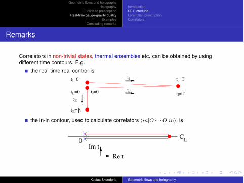
Correlators in non-trivial states, thermal ensembles etc. can be obtained by usingdifferent time contours. E.g.
the real-time real contror ist
t
t =T
t =T
t =0
t =0
1
2
1
2
1
t
t =0
t = !E
E
E 2
the in-in contour, used to calculate correlators #in|O · · ·O|in$, is
Re t
Im t0 L
C
Kostas Skenderis Geometric flows and holography
Geometric flows and holographyHolography
Euclidean prescriptionReal-time gauge-gravity duality
ExamplesConcluding remarks
IntroductionQFT interludeLorentzian prescriptionCorrelators
Lorentzian prescription
The holographic prescription is now to use "piece-wise" holography:Real segments are associated with Lorentzian solutions,Imaginary segments are associated with Euclidean solutions,Solutions are matched at the corners.
Kostas Skenderis Geometric flows and holography
Geometric flows and holographyHolography
Euclidean prescriptionReal-time gauge-gravity duality
ExamplesConcluding remarks
IntroductionQFT interludeLorentzian prescriptionCorrelators
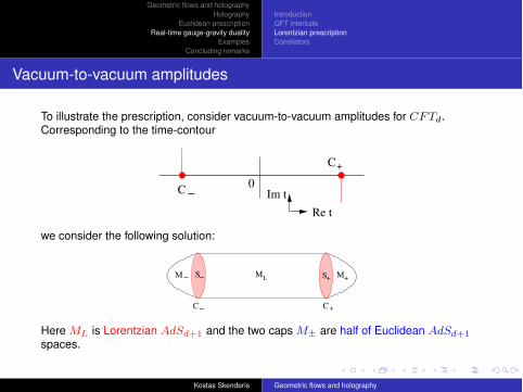
Vacuum-to-vacuum amplitudes
To illustrate the prescription, consider vacuum-to-vacuum amplitudes for CFTd.Corresponding to the time-contour
Re t
Im tC
C
!
+
0
we consider the following solution:
M
CC
L!M! MS
+
+ +
!
S
Here ML is Lorentzian AdSd+1 and the two caps M± are half of Euclidean AdSd+1
spaces.
Kostas Skenderis Geometric flows and holography
Geometric flows and holographyHolography
Euclidean prescriptionReal-time gauge-gravity duality
ExamplesConcluding remarks
IntroductionQFT interludeLorentzian prescriptionCorrelators
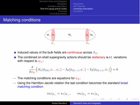
Matching conditions
M
CC
L!M! MS
+
+ +
!
S
Induced values of the bulk fields are continuous across S±.The combined on-shell supergravity actions should be stationary w.r.t. variationswith respect to "±:
$
$"±
$iIL["(0), "", "+]! IE ["(0,"), ""]! IE ["(0,+), "+]
%= 0
% The matching conditions are equations for "±.% Using the Hamilton-Jacobi relation the last condition becomes the standard Israel
matching condition
i%t|S! = %& |S! , i%t|S+ = %& |S+
Kostas Skenderis Geometric flows and holography
Geometric flows and holographyHolography
Euclidean prescriptionReal-time gauge-gravity duality
ExamplesConcluding remarks
IntroductionQFT interludeLorentzian prescriptionCorrelators
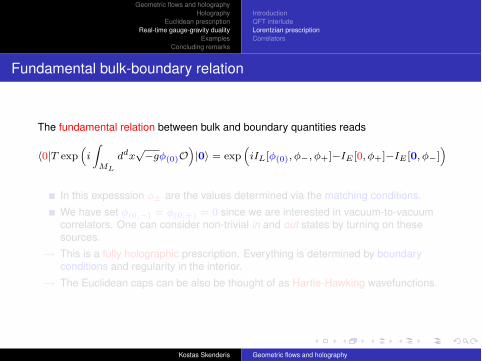
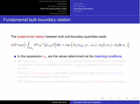
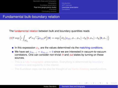
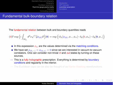
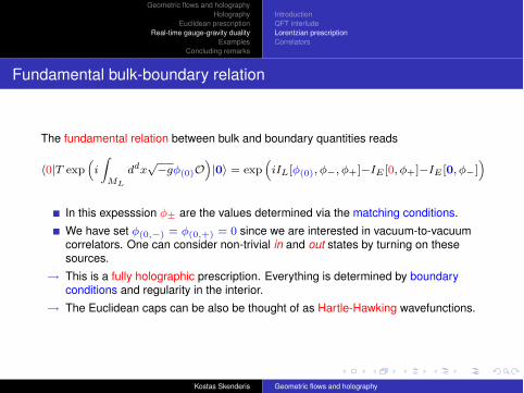
Fundamental bulk-boundary relation
The fundamental relation between bulk and boundary quantities reads
#0|T exp$i
!
ML
ddx&!g"(0)O
%|0$ = exp
$iIL["(0), "", "+]!IE [0, "+]!IE [0, ""]
%
In this expesssion "± are the values determined via the matching conditions.We have set "(0,") = "(0,+) = 0 since we are interested in vacuum-to-vacuumcorrelators. One can consider non-trivial in and out states by turning on thesesources.
% This is a fully holographic prescription. Everything is determined by boundaryconditions and regularity in the interior.
% The Euclidean caps can be also be thought of as Hartle-Hawking wavefunctions.
Kostas Skenderis Geometric flows and holography
Geometric flows and holographyHolography
Euclidean prescriptionReal-time gauge-gravity duality
ExamplesConcluding remarks
IntroductionQFT interludeLorentzian prescriptionCorrelators
Correlators
Having set up the prescription one can verify that there are no additionalambiguities.A well known problem in the computation of 2-point functions is that the linearizedfield equations do not have a unique solution with Dirichlet boundary conditions.The reason is that the field equations admit regular solutions (normalizablemodes) that vanish at the boundary, so one can freely add them to any givensolution satisfying the boundary conditions.In our case the matching conditions eliminate this ambiguity.
Kostas Skenderis Geometric flows and holography
Geometric flows and holographyHolography
Euclidean prescriptionReal-time gauge-gravity duality
ExamplesConcluding remarks
2-point function of scalar operatorsThermal 2-point functions
Massive scalar field in AdS3
As the simplest yet illustrative example we consider a free massive scalar field in AdS3,
S =1
2
!d3x
+|G|(!!µ!!µ!!m2!2).
The dimension of O is " = 1 +&
1 + m2 = 1 + l with l + {0, 1, 2, . . .}.We want to solve
(!!m2)!(t, ", r) = 0
in the AdS3 background,
ds2 = !(r2 + 1)dt2 +dr2
r2 + 1+ r2d"2 ,
Kostas Skenderis Geometric flows and holography
Geometric flows and holographyHolography
Euclidean prescriptionReal-time gauge-gravity duality
ExamplesConcluding remarks
2-point function of scalar operatorsThermal 2-point functions
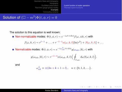
Solution of (!!m2)!(t, !, r) = 0
The solution to this equation is well known:Non-normalizable modes: !(t, ", r) ( e"i't+ik!f((,±k, r) with
f((, k, r) ( rl"1 + . . . + r"l"1)((, k, l)[ln(r2) + *((, k, l)] + . . .
Normalizable modes: !(t, ", r) ( e"i'±nkt+ik!g((nk, |k|, r) with
g((nk, |k|, r) ( r"l"1)((nk, k, l)$ ,
'nk
d(*((, k, l)%.
and(±nk ) ±(2n + k + 1 + l) , n + {0, 1, 2, . . .}.
Kostas Skenderis Geometric flows and holography
Geometric flows and holographyHolography
Euclidean prescriptionReal-time gauge-gravity duality
ExamplesConcluding remarks
2-point function of scalar operatorsThermal 2-point functions
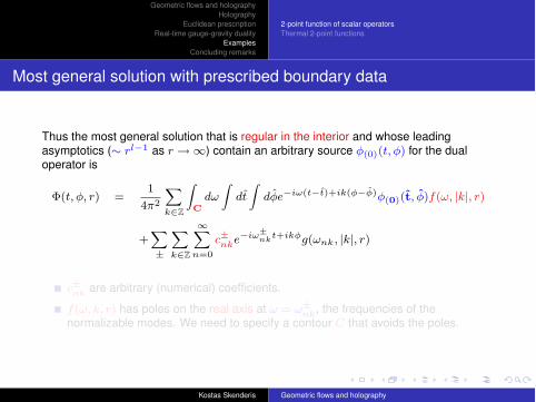
Most general solution with prescribed boundary data
Thus the most general solution that is regular in the interior and whose leadingasymptotics (( rl"1 as r %*) contain an arbitrary source "(0)(t, ") for the dualoperator is
!(t, ", r) =1
4%2
-
k%Z
!
Cd(
!dt̂
!d"̂e"i'(t"t̂)+ik(!"!̂)"(0) (̂t, "̂)f((, |k|, r)
+-
±
-
k%Z
#-
n=0
c±nke"i'±nkt+ik!g((nk, |k|, r)
c±nk are arbitrary (numerical) coefficients.
f((, k, r) has poles on the real axis at ( = (±nk, the frequencies of thenormalizable modes. We need to specify a contour C that avoids the poles.
Kostas Skenderis Geometric flows and holography
Geometric flows and holographyHolography
Euclidean prescriptionReal-time gauge-gravity duality
ExamplesConcluding remarks
2-point function of scalar operatorsThermal 2-point functions
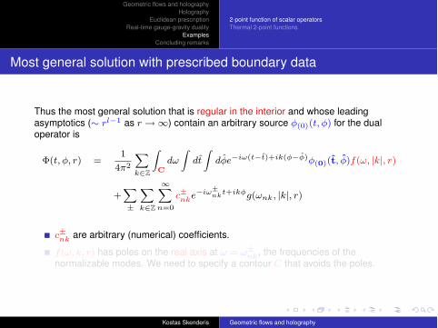
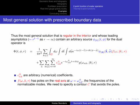
Most general solution with prescribed boundary data
Thus the most general solution that is regular in the interior and whose leadingasymptotics (( rl"1 as r %*) contain an arbitrary source "(0)(t, ") for the dualoperator is
!(t, ", r) =1
4%2
-
k%Z
!
Cd(
!dt̂
!d"̂e"i'(t"t̂)+ik(!"!̂)"(0) (̂t, "̂)f((, |k|, r)
+-
±
-
k%Z
#-
n=0
c±nke"i'±nkt+ik!g((nk, |k|, r)
c±nk are arbitrary (numerical) coefficients.
f((, k, r) has poles on the real axis at ( = (±nk, the frequencies of thenormalizable modes. We need to specify a contour C that avoids the poles.
Kostas Skenderis Geometric flows and holography
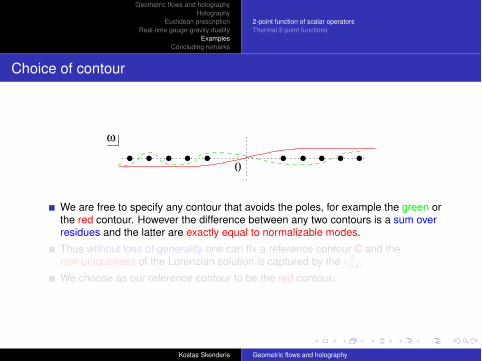
Geometric flows and holographyHolography
Euclidean prescriptionReal-time gauge-gravity duality
ExamplesConcluding remarks
2-point function of scalar operatorsThermal 2-point functions
Choice of contour
0
!
We are free to specify any contour that avoids the poles, for example the green orthe red contour. However the difference between any two contours is a sum overresidues and the latter are exactly equal to normalizable modes.Thus without loss of generality one can fix a reference contour C and thenon-uniqueness of the Lorenzian solution is captured by the c±nk.We choose as our reference contour to be the red contour.
Kostas Skenderis Geometric flows and holography
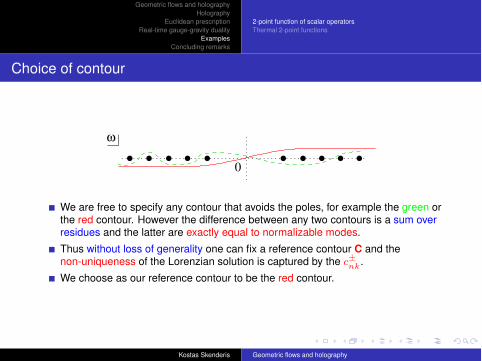
Geometric flows and holographyHolography
Euclidean prescriptionReal-time gauge-gravity duality
ExamplesConcluding remarks
2-point function of scalar operatorsThermal 2-point functions
Choice of contour
0
!
We are free to specify any contour that avoids the poles, for example the green orthe red contour. However the difference between any two contours is a sum overresidues and the latter are exactly equal to normalizable modes.Thus without loss of generality one can fix a reference contour C and thenon-uniqueness of the Lorenzian solution is captured by the c±nk.We choose as our reference contour to be the red contour.
Kostas Skenderis Geometric flows and holography

Geometric flows and holographyHolography
Euclidean prescriptionReal-time gauge-gravity duality
ExamplesConcluding remarks
2-point function of scalar operatorsThermal 2-point functions
Euclidean solutions
We will now show that the matching conditions determine c±nk.
Consider the solution on the ‘initial cap’, so on the space specified by the metric,
ds2 = (r2 + 1)d+2 +dr2
r2 + 1+ r2d"2
with !* < + , 0, so that we have half of Euclidean AdS space.Had the bulk been the entire Euclidean AdS space, the Klein-Gordon equationwould have a unique regular solution given boundary data. In particular, with zerosources the unique regular solution is identically equal to zero.In our case the sources are zero but we only consider half of the space, sosolutions that would be excluded are now allowed because they are only singularat the other half of the space,
!(+, ", r) =-
n,k
d"nke"'!nk&+ik!g((nk, |k|, r) ,
with thus far arbitrary coefficients d"nk.
Kostas Skenderis Geometric flows and holography
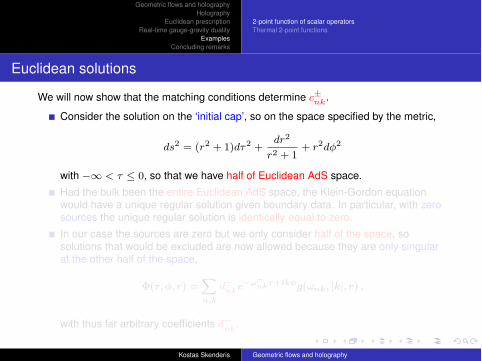
Geometric flows and holographyHolography
Euclidean prescriptionReal-time gauge-gravity duality
ExamplesConcluding remarks
2-point function of scalar operatorsThermal 2-point functions
Euclidean solutions
We will now show that the matching conditions determine c±nk.
Consider the solution on the ‘initial cap’, so on the space specified by the metric,
ds2 = (r2 + 1)d+2 +dr2
r2 + 1+ r2d"2
with !* < + , 0, so that we have half of Euclidean AdS space.Had the bulk been the entire Euclidean AdS space, the Klein-Gordon equationwould have a unique regular solution given boundary data. In particular, with zerosources the unique regular solution is identically equal to zero.In our case the sources are zero but we only consider half of the space, sosolutions that would be excluded are now allowed because they are only singularat the other half of the space,
!(+, ", r) =-
n,k
d"nke"'!nk&+ik!g((nk, |k|, r) ,
with thus far arbitrary coefficients d"nk.
Kostas Skenderis Geometric flows and holography
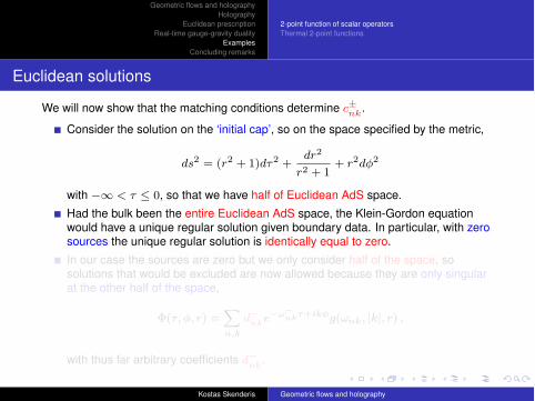
Geometric flows and holographyHolography
Euclidean prescriptionReal-time gauge-gravity duality
ExamplesConcluding remarks
2-point function of scalar operatorsThermal 2-point functions
Euclidean solutions
We will now show that the matching conditions determine c±nk.
Consider the solution on the ‘initial cap’, so on the space specified by the metric,
ds2 = (r2 + 1)d+2 +dr2
r2 + 1+ r2d"2
with !* < + , 0, so that we have half of Euclidean AdS space.Had the bulk been the entire Euclidean AdS space, the Klein-Gordon equationwould have a unique regular solution given boundary data. In particular, with zerosources the unique regular solution is identically equal to zero.In our case the sources are zero but we only consider half of the space, sosolutions that would be excluded are now allowed because they are only singularat the other half of the space,
!(+, ", r) =-
n,k
d"nke"'!nk&+ik!g((nk, |k|, r) ,
with thus far arbitrary coefficients d"nk.
Kostas Skenderis Geometric flows and holography
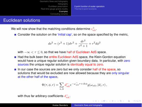
Geometric flows and holographyHolography
Euclidean prescriptionReal-time gauge-gravity duality
ExamplesConcluding remarks
2-point function of scalar operatorsThermal 2-point functions
Euclidean solutions
We will now show that the matching conditions determine c±nk.
Consider the solution on the ‘initial cap’, so on the space specified by the metric,
ds2 = (r2 + 1)d+2 +dr2
r2 + 1+ r2d"2
with !* < + , 0, so that we have half of Euclidean AdS space.Had the bulk been the entire Euclidean AdS space, the Klein-Gordon equationwould have a unique regular solution given boundary data. In particular, with zerosources the unique regular solution is identically equal to zero.In our case the sources are zero but we only consider half of the space, sosolutions that would be excluded are now allowed because they are only singularat the other half of the space,
!(+, ", r) =-
n,k
d"nke"'!nk&+ik!g((nk, |k|, r) ,
with thus far arbitrary coefficients d"nk.
Kostas Skenderis Geometric flows and holography
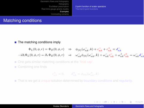
Geometric flows and holographyHolography
Euclidean prescriptionReal-time gauge-gravity duality
ExamplesConcluding remarks
2-point function of scalar operatorsThermal 2-point functions
Matching conditions
The matching conditions imply
!L(0, ", r) = !E(0, ", r) " "(0)(("nk, k) + c"nk + c+nk = d"nk
!i!t!L(0, ", r) = !&!E(0, ", r) " ("nk"(0)(("nk, k) + ("nkc"nk + (+
nkc+nk = ("nkd"nk
One gets similar matching conditions at the ’final cap’.Combining one finds
c±nk = 0, d±nk = "(0)((±nk, k)
That is we get a unique solution determined by boundary conditions and regularity.
Kostas Skenderis Geometric flows and holography
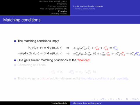
Geometric flows and holographyHolography
Euclidean prescriptionReal-time gauge-gravity duality
ExamplesConcluding remarks
2-point function of scalar operatorsThermal 2-point functions
Matching conditions
The matching conditions imply
!L(0, ", r) = !E(0, ", r) " "(0)(("nk, k) + c"nk + c+nk = d"nk
!i!t!L(0, ", r) = !&!E(0, ", r) " ("nk"(0)(("nk, k) + ("nkc"nk + (+
nkc+nk = ("nkd"nk
One gets similar matching conditions at the ’final cap’.Combining one finds
c±nk = 0, d±nk = "(0)((±nk, k)
That is we get a unique solution determined by boundary conditions and regularity.
Kostas Skenderis Geometric flows and holography
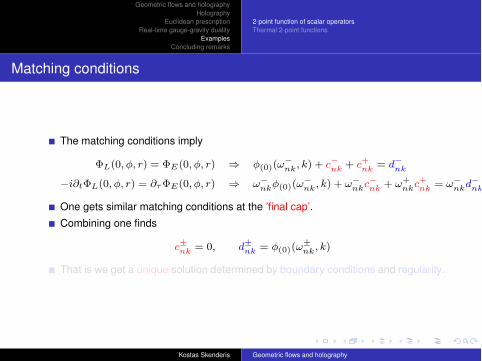
Geometric flows and holographyHolography
Euclidean prescriptionReal-time gauge-gravity duality
ExamplesConcluding remarks
2-point function of scalar operatorsThermal 2-point functions
Matching conditions
The matching conditions imply
!L(0, ", r) = !E(0, ", r) " "(0)(("nk, k) + c"nk + c+nk = d"nk
!i!t!L(0, ", r) = !&!E(0, ", r) " ("nk"(0)(("nk, k) + ("nkc"nk + (+
nkc+nk = ("nkd"nk
One gets similar matching conditions at the ’final cap’.Combining one finds
c±nk = 0, d±nk = "(0)((±nk, k)
That is we get a unique solution determined by boundary conditions and regularity.
Kostas Skenderis Geometric flows and holography
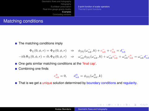
Geometric flows and holographyHolography
Euclidean prescriptionReal-time gauge-gravity duality
ExamplesConcluding remarks
2-point function of scalar operatorsThermal 2-point functions
Matching conditions
The matching conditions imply
!L(0, ", r) = !E(0, ", r) " "(0)(("nk, k) + c"nk + c+nk = d"nk
!i!t!L(0, ", r) = !&!E(0, ", r) " ("nk"(0)(("nk, k) + ("nkc"nk + (+
nkc+nk = ("nkd"nk
One gets similar matching conditions at the ’final cap’.Combining one finds
c±nk = 0, d±nk = "(0)((±nk, k)
That is we get a unique solution determined by boundary conditions and regularity.
Kostas Skenderis Geometric flows and holography
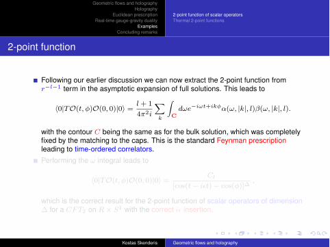
Geometric flows and holographyHolography
Euclidean prescriptionReal-time gauge-gravity duality
ExamplesConcluding remarks
2-point function of scalar operatorsThermal 2-point functions
2-point function
Following our earlier discussion we can now extract the 2-point function fromr"l"1 term in the asymptotic expansion of full solutions. This leads to
#0|TO(t, ")O(0, 0)|0$ =l + 1
4%2i
-
k
!
Cd(e"i't+ik!)((, |k|, l)*((, |k|, l).
with the contour C being the same as for the bulk solution, which was completelyfixed by the matching to the caps. This is the standard Feynman prescriptionleading to time-ordered correlators.Performing the ( integral leads to
#0|TO(t, ")O(0, 0)|0$ =Cl
[cos(t! i't)! cos(")]",
which is the correct result for the 2-point function of scalar operators of dimension" for a CFT2 on R- S1 with the correct i' insertion.
Kostas Skenderis Geometric flows and holography
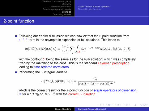
Geometric flows and holographyHolography
Euclidean prescriptionReal-time gauge-gravity duality
ExamplesConcluding remarks
2-point function of scalar operatorsThermal 2-point functions
2-point function
Following our earlier discussion we can now extract the 2-point function fromr"l"1 term in the asymptotic expansion of full solutions. This leads to
#0|TO(t, ")O(0, 0)|0$ =l + 1
4%2i
-
k
!
Cd(e"i't+ik!)((, |k|, l)*((, |k|, l).
with the contour C being the same as for the bulk solution, which was completelyfixed by the matching to the caps. This is the standard Feynman prescriptionleading to time-ordered correlators.Performing the ( integral leads to
#0|TO(t, ")O(0, 0)|0$ =Cl
[cos(t! i't)! cos(")]",
which is the correct result for the 2-point function of scalar operators of dimension" for a CFT2 on R- S1 with the correct i' insertion.
Kostas Skenderis Geometric flows and holography
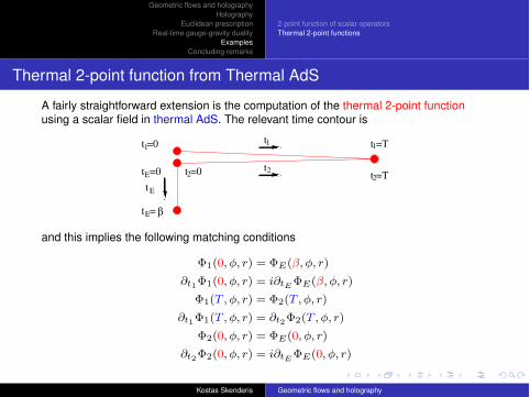
Geometric flows and holographyHolography
Euclidean prescriptionReal-time gauge-gravity duality
ExamplesConcluding remarks
2-point function of scalar operatorsThermal 2-point functions
Thermal 2-point function from Thermal AdS
A fairly straightforward extension is the computation of the thermal 2-point functionusing a scalar field in thermal AdS. The relevant time contour is
t
t
t =T
t =T
t =0
t =0
1
2
1
2
1
t
t =0
t = !E
E
E 2
and this implies the following matching conditions
!1(0, ", r) = !E(*, ", r)
!t1!1(0, ", r) = i!tE !E(*, ", r)
!1(T , ", r) = !2(T , ", r)
!t1!1(T , ", r) = !t2!2(T , ", r)
!2(0, ", r) = !E(0, ", r)
!t2!2(0, ", r) = i!tE !E(0, ", r)
Kostas Skenderis Geometric flows and holography
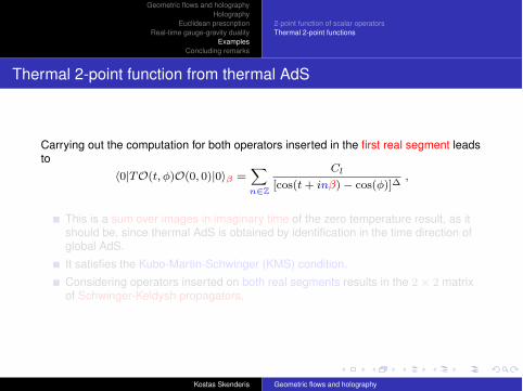
Geometric flows and holographyHolography
Euclidean prescriptionReal-time gauge-gravity duality
ExamplesConcluding remarks
2-point function of scalar operatorsThermal 2-point functions
Thermal 2-point function from thermal AdS
Carrying out the computation for both operators inserted in the first real segment leadsto
#0|TO(t, ")O(0, 0)|0$% =-
n%Z
Cl
[cos(t + in*)! cos(")]",
This is a sum over images in imaginary time of the zero temperature result, as itshould be, since thermal AdS is obtained by identification in the time direction ofglobal AdS.It satisfies the Kubo-Martin-Schwinger (KMS) condition.Considering operators inserted on both real segments results in the 2- 2 matrixof Schwinger-Keldysh propagators.
Kostas Skenderis Geometric flows and holography
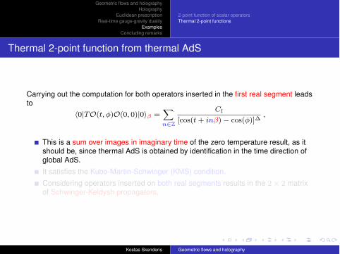
Geometric flows and holographyHolography
Euclidean prescriptionReal-time gauge-gravity duality
ExamplesConcluding remarks
2-point function of scalar operatorsThermal 2-point functions
Thermal 2-point function from thermal AdS
Carrying out the computation for both operators inserted in the first real segment leadsto
#0|TO(t, ")O(0, 0)|0$% =-
n%Z
Cl
[cos(t + in*)! cos(")]",
This is a sum over images in imaginary time of the zero temperature result, as itshould be, since thermal AdS is obtained by identification in the time direction ofglobal AdS.It satisfies the Kubo-Martin-Schwinger (KMS) condition.Considering operators inserted on both real segments results in the 2- 2 matrixof Schwinger-Keldysh propagators.
Kostas Skenderis Geometric flows and holography
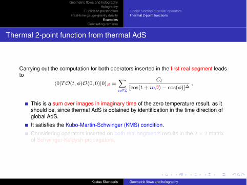
Geometric flows and holographyHolography
Euclidean prescriptionReal-time gauge-gravity duality
ExamplesConcluding remarks
2-point function of scalar operatorsThermal 2-point functions
Thermal 2-point function from thermal AdS
Carrying out the computation for both operators inserted in the first real segment leadsto
#0|TO(t, ")O(0, 0)|0$% =-
n%Z
Cl
[cos(t + in*)! cos(")]",
This is a sum over images in imaginary time of the zero temperature result, as itshould be, since thermal AdS is obtained by identification in the time direction ofglobal AdS.It satisfies the Kubo-Martin-Schwinger (KMS) condition.Considering operators inserted on both real segments results in the 2- 2 matrixof Schwinger-Keldysh propagators.
Kostas Skenderis Geometric flows and holography
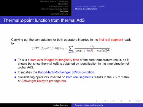
Geometric flows and holographyHolography
Euclidean prescriptionReal-time gauge-gravity duality
ExamplesConcluding remarks
2-point function of scalar operatorsThermal 2-point functions
Thermal 2-point function from thermal AdS
Carrying out the computation for both operators inserted in the first real segment leadsto
#0|TO(t, ")O(0, 0)|0$% =-
n%Z
Cl
[cos(t + in*)! cos(")]",
This is a sum over images in imaginary time of the zero temperature result, as itshould be, since thermal AdS is obtained by identification in the time direction ofglobal AdS.It satisfies the Kubo-Martin-Schwinger (KMS) condition.Considering operators inserted on both real segments results in the 2- 2 matrixof Schwinger-Keldysh propagators.
Kostas Skenderis Geometric flows and holography
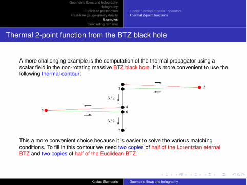
Geometric flows and holographyHolography
Euclidean prescriptionReal-time gauge-gravity duality
ExamplesConcluding remarks
2-point function of scalar operatorsThermal 2-point functions
Thermal 2-point function from the BTZ black hole
A more challenging example is the computation of the thermal propagator using ascalar field in the non-rotating massive BTZ black hole. It is more convenient to use thefollowing thermal contour:
! / 2
! / 2
3
12
7
6
45
This a more convenient choice because it is easier to solve the various matchingconditions. To fill in this contour we need two copies of half of the Lorentzian eternalBTZ and two copies of half of the Euclidean BTZ.
Kostas Skenderis Geometric flows and holography

Geometric flows and holographyHolography
Euclidean prescriptionReal-time gauge-gravity duality
ExamplesConcluding remarks
2-point function of scalar operatorsThermal 2-point functions
Bulk solution corresponding to time contour
The Penrose diagram for the eternal BTZ black is
P
L R
F
Kostas Skenderis Geometric flows and holography
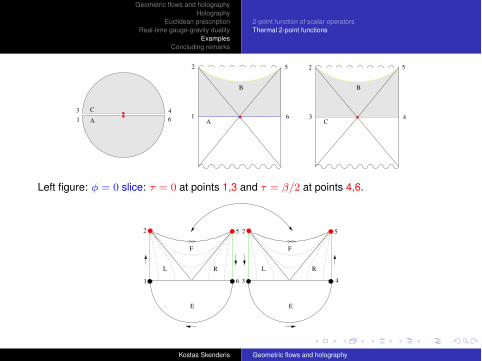
Geometric flows and holographyHolography
Euclidean prescriptionReal-time gauge-gravity duality
ExamplesConcluding remarks
2-point function of scalar operatorsThermal 2-point functions
A
C
1
3 4
6 A
B
52
1 6C
B
52
3 4
Left figure: " = 0 slice: + = 0 at points 1,3 and + = */2 at points 4,6.
P
F
RL
P
F
RL
2 5
4
2 5
E E
1 36
Kostas Skenderis Geometric flows and holography
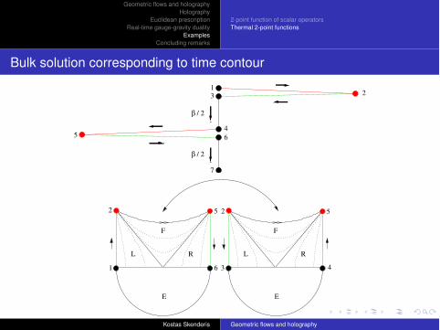
Geometric flows and holographyHolography
Euclidean prescriptionReal-time gauge-gravity duality
ExamplesConcluding remarks
2-point function of scalar operatorsThermal 2-point functions
Bulk solution corresponding to time contour
! / 2
! / 2
3
12
7
6
45
P
F
RL
P
F
RL
2 5
4
2 5
E E
1 36
Kostas Skenderis Geometric flows and holography
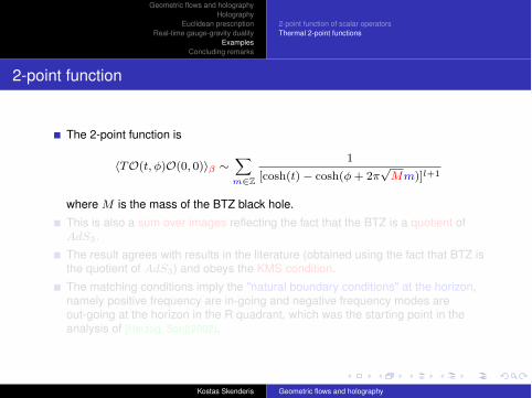
Geometric flows and holographyHolography
Euclidean prescriptionReal-time gauge-gravity duality
ExamplesConcluding remarks
2-point function of scalar operatorsThermal 2-point functions
2-point function
The 2-point function is
#TO(t, ")O(0, 0)$% (-
m%Z
1
[cosh(t)! cosh(" + 2%&
Mm)]l+1
where M is the mass of the BTZ black hole.This is also a sum over images reflecting the fact that the BTZ is a quotient ofAdS3.The result agrees with results in the literature (obtained using the fact that BTZ isthe quotient of AdS3) and obeys the KMS condition.The matching conditions imply the "natural boundary conditions" at the horizon,namely positive frequency are in-going and negative frequency modes areout-going at the horizon in the R quadrant, which was the starting point in theanalysis of [Herzog, Son](2002).
Kostas Skenderis Geometric flows and holography
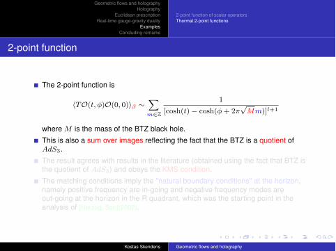
Geometric flows and holographyHolography
Euclidean prescriptionReal-time gauge-gravity duality
ExamplesConcluding remarks
2-point function of scalar operatorsThermal 2-point functions
2-point function
The 2-point function is
#TO(t, ")O(0, 0)$% (-
m%Z
1
[cosh(t)! cosh(" + 2%&
Mm)]l+1
where M is the mass of the BTZ black hole.This is also a sum over images reflecting the fact that the BTZ is a quotient ofAdS3.The result agrees with results in the literature (obtained using the fact that BTZ isthe quotient of AdS3) and obeys the KMS condition.The matching conditions imply the "natural boundary conditions" at the horizon,namely positive frequency are in-going and negative frequency modes areout-going at the horizon in the R quadrant, which was the starting point in theanalysis of [Herzog, Son](2002).
Kostas Skenderis Geometric flows and holography
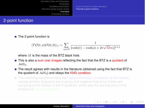
Geometric flows and holographyHolography
Euclidean prescriptionReal-time gauge-gravity duality
ExamplesConcluding remarks
2-point function of scalar operatorsThermal 2-point functions
2-point function
The 2-point function is
#TO(t, ")O(0, 0)$% (-
m%Z
1
[cosh(t)! cosh(" + 2%&
Mm)]l+1
where M is the mass of the BTZ black hole.This is also a sum over images reflecting the fact that the BTZ is a quotient ofAdS3.The result agrees with results in the literature (obtained using the fact that BTZ isthe quotient of AdS3) and obeys the KMS condition.The matching conditions imply the "natural boundary conditions" at the horizon,namely positive frequency are in-going and negative frequency modes areout-going at the horizon in the R quadrant, which was the starting point in theanalysis of [Herzog, Son](2002).
Kostas Skenderis Geometric flows and holography
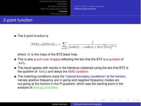
Geometric flows and holographyHolography
Euclidean prescriptionReal-time gauge-gravity duality
ExamplesConcluding remarks
2-point function of scalar operatorsThermal 2-point functions
2-point function
The 2-point function is
#TO(t, ")O(0, 0)$% (-
m%Z
1
[cosh(t)! cosh(" + 2%&
Mm)]l+1
where M is the mass of the BTZ black hole.This is also a sum over images reflecting the fact that the BTZ is a quotient ofAdS3.The result agrees with results in the literature (obtained using the fact that BTZ isthe quotient of AdS3) and obeys the KMS condition.The matching conditions imply the "natural boundary conditions" at the horizon,namely positive frequency are in-going and negative frequency modes areout-going at the horizon in the R quadrant, which was the starting point in theanalysis of [Herzog, Son](2002).
Kostas Skenderis Geometric flows and holography
Geometric flows and holographyHolography
Euclidean prescriptionReal-time gauge-gravity duality
ExamplesConcluding remarks
Concluding remarks
We have outlined a connection of geometric flows with 3d QFT using holography.We have present a general prescription for holographic computation in real time.
The prescription amounts to "filling-in" the complex time contour with bulk solution: realsegments with Lorentzian solutions and imaginary segments with Euclidean solutions.This prescription fulfils all requirements described earlier: it allows for computation ofn-point functions in any holographic QFT and in non-trivial states. It is fully holographicand all information is encoded in classical bulk dynamics.
Kostas Skenderis Geometric flows and holography
Geometric flows and holographyHolography
Euclidean prescriptionReal-time gauge-gravity duality
ExamplesConcluding remarks
On-going and future work
Using these techniques one would like to return to the AdS4 case and
compute the 2-point function of the stress energy using the linearizedperturbations around the Schwarzschild solution.understand the implications of the connection with the geometric flows.in the case of Calabi flow/Robinson-Trautman spacetimes, compute higher pointfunctions.
These and related computations are in progress ....
Kostas Skenderis Geometric flows and holography