Embed Size (px)
Citation preview

1/59
Partial functionalcorrespondence
Michael Bronstein
University of Lugano Intel Corporation
Lyon, 7 July 2016

Microsoft Kinect 2010

4/59
(Acquired by Intel in 2012)

7/59
Different form factor computers featuring Intel RealSense 3D camera

8/59
Deluge of geometric data
3D sensors Repositories 3D printers

9/59
Applications
Deformable fusion Motion transfer
Motion capture Texture mapping
Dou et al. 2015; Sumner, Popovic 2004; Faceshift; Cow image: Moore 2014

10/59
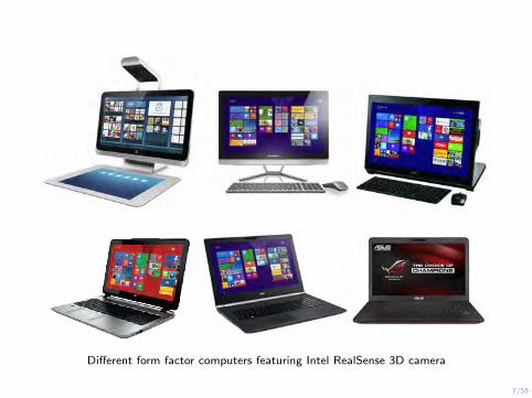
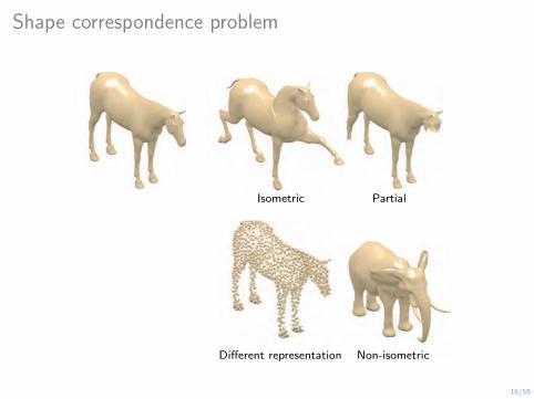
Shape correspondence problem
Isometric
10/59
Shape correspondence problem
Isometric Partial

10/59
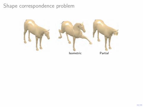
Shape correspondence problem
Isometric Partial
Different representation
10/59
Shape correspondence problem
Isometric Partial
Different representation Non-isometric

11/59
Computer Graphics ForumSGP 2016
Computer Graphics ForumSGP 2016 Best paper award
12/59
Outline
Background: Spectral analysis on manifolds
Functional correspondence
Partial functional correspondence
Non-rigid puzzles

13/59
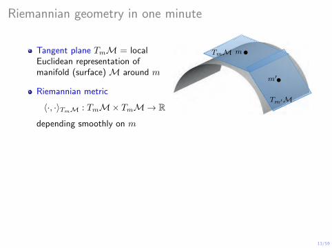
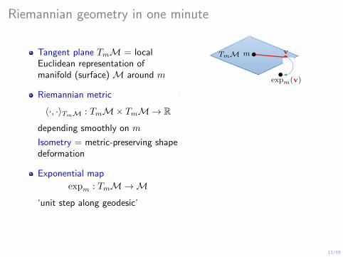
Riemannian geometry in one minute
Tangent plane TmM = localEuclidean representation ofmanifold (surface) M around m
Riemannian metric
〈·, ·〉TmM : TmM× TmM→ R
depending smoothly on m
Exponential map
expm : TmM→M
‘unit step along geodesic’
mTmM
M
13/59
Riemannian geometry in one minute
Tangent plane TmM = localEuclidean representation ofmanifold (surface) M around m
Riemannian metric
〈·, ·〉TmM : TmM× TmM→ R
depending smoothly on m
Exponential map
expm : TmM→M
‘unit step along geodesic’
mTmM
m′
Tm′M

13/59
Riemannian geometry in one minute
Tangent plane TmM = localEuclidean representation ofmanifold (surface) M around m
Riemannian metric
〈·, ·〉TmM : TmM× TmM→ R
depending smoothly on m
Isometry = metric-preserving shapedeformation
Exponential map
expm : TmM→M
‘unit step along geodesic’
mTmM
m′
Tm′M
13/59
Riemannian geometry in one minute
Tangent plane TmM = localEuclidean representation ofmanifold (surface) M around m
Riemannian metric
〈·, ·〉TmM : TmM× TmM→ R
depending smoothly on m
Isometry = metric-preserving shapedeformation
Exponential map
expm : TmM→M
‘unit step along geodesic’
m vTmM
expm(v)

14/59
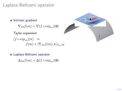
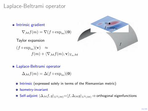
Laplace-Beltrami operator
Intrinsic gradient
∇Mf(m) = ∇(f ◦ expm)(0)
Taylor expansion
(f ◦ expm)(v) ≈f(m) + 〈∇Mf(m),v〉TmM
Laplace-Beltrami operator
∆Mf(m) = ∆(f ◦ expm)(0)
m
f
Smooth field f :M→ R
Intrinsic (expressed solely in terms of the Riemannian metric)
Isometry-invariant
Self-adjoint 〈∆Mf, g〉L2(M)=〈f,∆Mg〉L2(M)
Positive semidefinite ⇒ non-negative eigenvalues

14/59
Laplace-Beltrami operator
Intrinsic gradient
∇Mf(m) = ∇(f ◦ expm)(0)
Taylor expansion
(f ◦ expm)(v) ≈f(m) + 〈∇Mf(m),v〉TmM
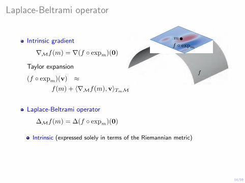
Laplace-Beltrami operator
∆Mf(m) = ∆(f ◦ expm)(0)
m
f
f ◦ expm
Smooth field f ◦ expm : TmM→ R
Intrinsic (expressed solely in terms of the Riemannian metric)
Isometry-invariant
Self-adjoint 〈∆Mf, g〉L2(M)=〈f,∆Mg〉L2(M)
Positive semidefinite ⇒ non-negative eigenvalues

14/59
Laplace-Beltrami operator
Intrinsic gradient
∇Mf(m) = ∇(f ◦ expm)(0)
Taylor expansion
(f ◦ expm)(v) ≈f(m) + 〈∇Mf(m),v〉TmM
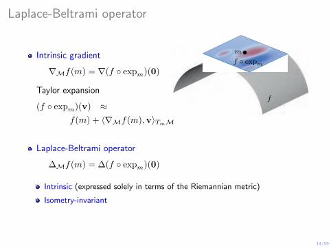
Laplace-Beltrami operator
∆Mf(m) = ∆(f ◦ expm)(0)
m
f
f ◦ expm
Intrinsic (expressed solely in terms of the Riemannian metric)
Isometry-invariant
Self-adjoint 〈∆Mf, g〉L2(M)=〈f,∆Mg〉L2(M)
Positive semidefinite ⇒ non-negative eigenvalues
14/59
Laplace-Beltrami operator
Intrinsic gradient
∇Mf(m) = ∇(f ◦ expm)(0)
Taylor expansion
(f ◦ expm)(v) ≈f(m) + 〈∇Mf(m),v〉TmM
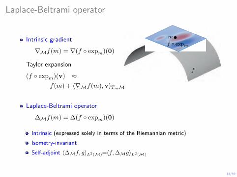
Laplace-Beltrami operator
∆Mf(m) = ∆(f ◦ expm)(0)
m
f
f ◦ expm
Intrinsic (expressed solely in terms of the Riemannian metric)
Isometry-invariant
Self-adjoint 〈∆Mf, g〉L2(M)=〈f,∆Mg〉L2(M)
Positive semidefinite ⇒ non-negative eigenvalues
14/59
Laplace-Beltrami operator
Intrinsic gradient
∇Mf(m) = ∇(f ◦ expm)(0)
Taylor expansion
(f ◦ expm)(v) ≈f(m) + 〈∇Mf(m),v〉TmM
Laplace-Beltrami operator
∆Mf(m) = ∆(f ◦ expm)(0)
m
f
f ◦ expm
Intrinsic (expressed solely in terms of the Riemannian metric)
Isometry-invariant
Self-adjoint 〈∆Mf, g〉L2(M)=〈f,∆Mg〉L2(M)⇒ orthogonal eigenfunctions
Positive semidefinite ⇒ non-negative eigenvalues
15/59
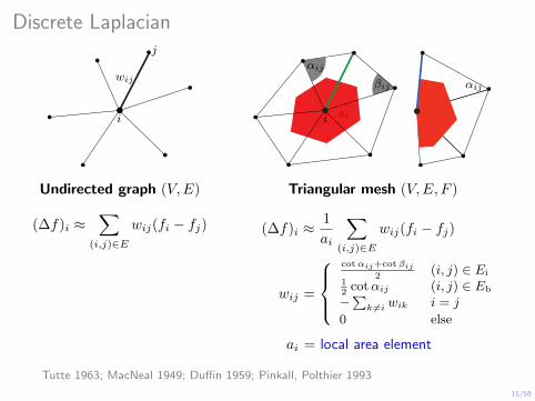
Discrete Laplacianj
i
wij
j
i
αij
βij
ai
αij
Undirected graph (V,E)
(∆f)i ≈∑
(i,j)∈E
wij(fi − fj)
Triangular mesh (V,E, F )
(∆f)i ≈1
ai
∑(i,j)∈E
wij(fi − fj)
wij =
cotαij+cot βij
2(i, j) ∈ Ei
12
cotαij (i, j) ∈ Eb
−∑k 6=i wik i = j
0 else
ai = local area element
Tutte 1963; MacNeal 1949; Duffin 1959; Pinkall, Polthier 1993
16/59
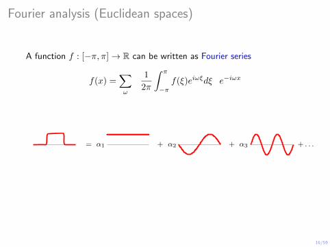
Fourier analysis (Euclidean spaces)
A function f : [−π, π]→ R can be written as Fourier series
f(x) =∑ω
1
2π
∫ π
−πf(ξ)eiωξdξ
︸ ︷︷ ︸f(ω)=〈f,e−iωx〉L2([−π,π])
e−iωx
α1 α2 α3= + + + . . .
Fourier basis = Laplacian eigenfunctions: ∆e−iωx = ω2e−iωx

16/59
Fourier analysis (Euclidean spaces)
A function f : [−π, π]→ R can be written as Fourier series
f(x) =∑ω
1
2π
∫ π
−πf(ξ)eiωξdξ︸ ︷︷ ︸
f(ω)=〈f,e−iωx〉L2([−π,π])
e−iωx
α1 α2 α3= + + + . . .
Fourier basis = Laplacian eigenfunctions: ∆e−iωx = ω2e−iωx

16/59
Fourier analysis (Euclidean spaces)
A function f : [−π, π]→ R can be written as Fourier series
f(x) =∑ω
1
2π
∫ π
−πf(ξ)eiωξdξ︸ ︷︷ ︸
f(ω)=〈f,e−iωx〉L2([−π,π])
e−iωx
α1 α2 α3= + + + . . .
Fourier basis = Laplacian eigenfunctions: ∆e−iωx = ω2e−iωx
17/59
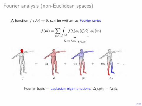
Fourier analysis (non-Euclidean spaces)
A function f :M→ R can be written as Fourier series
f(m) =∑k≥1
∫Mf(ξ)φk(ξ)dξ︸ ︷︷ ︸
fk=〈f,φk〉L2(M)
φk(m)
= α1 + α2 + α3 + . . .
f φ1 φ2 φ3
Fourier basis = Laplacian eigenfunctions: ∆Mφk = λkφk

18/59
Outline
Background: Spectral analysis on manifolds
Functional correspondence
Partial functional correspondence
Non-rigid puzzles
19/59
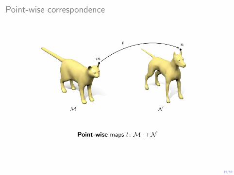
Point-wise correspondence
m
M
n
N
t
Point-wise maps t : M→N

19/59
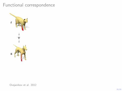
Functional correspondence
f
F(M)
g
F(N )
T
Functional maps T : F(M)→ F(N )
Ovsjanikov et al. 2012
20/59
Functional correspondence
f
g
↓T↓
where Φk = (φ1, . . . ,φk), Ψk = (ψ1, . . . ,ψk) are truncatedLaplace-Beltrami eigenbases
Ovsjanikov et al. 2012
20/59
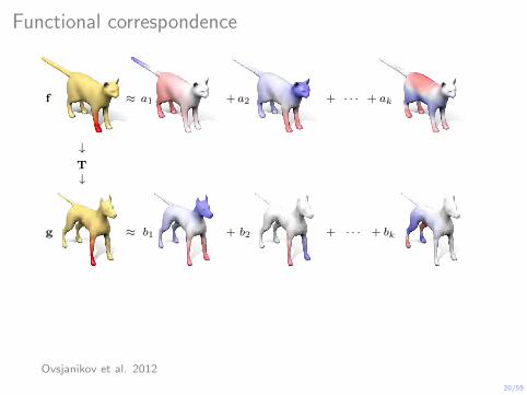
Functional correspondence
f
g
≈ a1 + a2 + · · · + ak
≈ b1 + b2 + · · · + bk
↓T↓
where Φk = (φ1, . . . ,φk), Ψk = (ψ1, . . . ,ψk) are truncatedLaplace-Beltrami eigenbases
Ovsjanikov et al. 2012

20/59
Functional correspondence
f
g
≈ a1 + a2 + · · · + ak
≈ b1 + b2 + · · · + bk
↓T↓
↓C>
↓Translates Fourier coefficients from Φ to Ψ
where Φk = (φ1, . . . ,φk), Ψk = (ψ1, . . . ,ψk) are truncatedLaplace-Beltrami eigenbases
Ovsjanikov et al. 2012

20/59
Functional correspondence
f
g
≈ a1 + a2 + · · · + ak
≈ b1 + b2 + · · · + bk
↓T↓
↓C>
↓Translates Fourier coefficients from Φ to Ψ≈ Ψk Φ>k
g>Ψk = f>ΦkC
where Φk = (φ1, . . . ,φk), Ψk = (ψ1, . . . ,ψk) are truncatedLaplace-Beltrami eigenbases
Ovsjanikov et al. 2012

21/59
Functional correspondence in Laplacian eigenbases
For isometric simple spectrum shapes C is diagonal since ψi = ±Tφi

22/59
Computing functional correspondence
Given ordered set of functions f1, . . . , fq on M and correspondingfunctions g1, . . . ,gq on N (gi ≈ Tf i)
C found by solving a system of qk equations with k2 variables
Ovsjanikov et al. 2012

22/59
Computing functional correspondence
f1 f2 · · · fq g1 g2 · · · gq
Given ordered set of functions f1, . . . , fq on M and correspondingfunctions g1, . . . ,gq on N (gi ≈ Tf i)
C found by solving a system of qk equations with k2 variables
Ovsjanikov et al. 2012

22/59
Computing functional correspondence
f1 f2 · · · fq g1 g2 · · · gq
Given ordered set of functions f1, . . . , fq on M and correspondingfunctions g1, . . . ,gq on N (gi ≈ Tf i)
C found by solving a system of qk equations with k2 variables
G>Ψk = F>ΦkC
where F = (f1, . . . , fq) and G = (g1, . . . ,gq) are n× q and m× qmatrices
Ovsjanikov et al. 2012

23/59
Key issues
How to recover point-wise correspondence with some guarantees(e.g. bijectivity)?
How to automatically find corresponding functions F, G?
Near isometric shapes: easy (a lot of structure!)
Non-isometric shapes: hard
Does not work well in case of missing parts and topological noise

24/59
Partial Laplacian eigenvectors
φ2 φ3 φ4 φ5 φ6 φ7 φ8 φ9
ψ2 ψ3 ψ4 ψ5 ψ6 ψ7 ψ8 ψ9
ζ2 ζ3 ζ4 ζ5 ζ6 ζ7 ζ8 ζ9
Laplacian eigenvectors of a shape with missing parts(Neumann boundary conditions)
Rodola, Cosmo, B, Torsello, Cremers 2016

25/59
Partial Laplacian eigenvectors
Functional correspondence matrix C
Rodola, Cosmo, B, Torsello, Cremers 2016

26/59
Perturbation analysis: intuition
∆M
∆M
∆M
φ1 φ2 φ3
φ1 φ2 φ3
φ1 φ2 φ3
M
M
Ignoring boundary interaction: disjoint parts (block-diagonal matrix)
Eigenvectors = Mixture of eigenvectors of the parts
Rodola, Cosmo, B, Torsello, Cremers 2016

27/59
Perturbation analysis: eigenvalues
10 20 30 40 500.00
2.00
4.00
6.00
8.00·10−2
eigenvalue number
r kN
M
Slope rk≈ |M||N| (depends on the area of the cut)
Consistent with Weil’s law
Rodola, Cosmo, B, Torsello, Cremers 2016

28/59
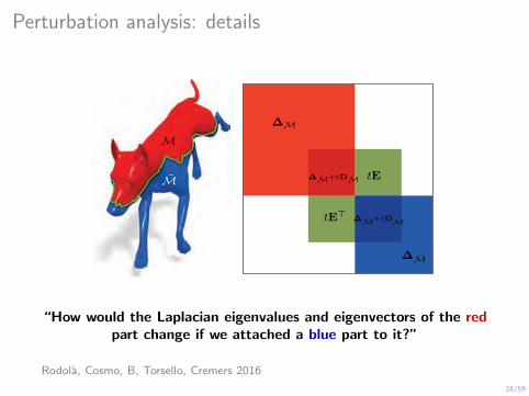
Perturbation analysis: details
∆M
∆M
∆M+tDM
∆M+tDM
tE
tE>
M
M
“How would the Laplacian eigenvalues and eigenvectors of the redpart change if we attached a blue part to it?”
Rodola, Cosmo, B, Torsello, Cremers 2016
28/59
Perturbation analysis: details
∆M
∆M
∆M+tDM
∆M+tDM
tE
tE>
M
M
“How would the Laplacian eigenvalues and eigenvectors of the redpart change if we attached a blue part to it?”
Rodola, Cosmo, B, Torsello, Cremers 2016

28/59
Perturbation analysis: details
PM P
EDM
n× n n× nM
M
“How would the Laplacian eigenvalues and eigenvectors of the redpart change if we attached a blue part to it?”
Rodola, Cosmo, B, Torsello, Cremers 2016
29/59
Perturbation analysis: details
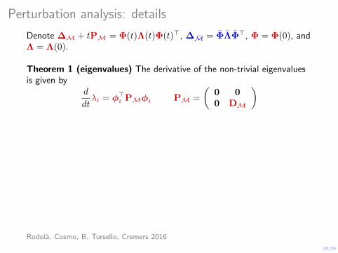
Denote ∆M + tPM = Φ(t)Λ(t)Φ(t)>, ∆M = ΦΛΦ>, Φ = Φ(0), andΛ = Λ(0).
Theorem 1 (eigenvalues) The derivative of the non-trivial eigenvaluesis given by
d
dtλi = φ>i PMφi PM =
(0 00 DM
)
Theorem 2 (eigenvectors) Assuming λi 6= λj for i 6= j and λi 6= λj forall i, j, the derivative of the non-trivial eigenvectors is given by
d
dtφi =
n∑j=1j 6=i
φ>i PMφjλi − λj
φj +n∑j=1
φ>i P φjλi − λj
φj P =
(0 0E 0
)
Rodola, Cosmo, B, Torsello, Cremers 2016

29/59
Perturbation analysis: details
Denote ∆M + tPM = Φ(t)Λ(t)Φ(t)>, ∆M = ΦΛΦ>, Φ = Φ(0), andΛ = Λ(0).
Theorem 1 (eigenvalues) The derivative of the non-trivial eigenvaluesis given by
d
dtλi = φ>i PMφi PM =
(0 00 DM
)
Theorem 2 (eigenvectors) Assuming λi 6= λj for i 6= j and λi 6= λj forall i, j, the derivative of the non-trivial eigenvectors is given by
d
dtφi =
n∑j=1j 6=i
φ>i PMφjλi − λj
φj +n∑j=1
φ>i P φjλi − λj
φj P =
(0 0E 0
)
Rodola, Cosmo, B, Torsello, Cremers 2016

30/59
Perturbation analysis: boundary interaction strength
Value of f
10
20
Eigenvector perturbation depends on length and position of the boundary
Perturbation strength ‖ ddtΦ‖F ≤ c
∫∂M f(m)dm, where
f(m) =n∑
i,j=1j 6=i
(φi(m)φj(m)
λi − λj
)2
Rodola, Cosmo, B, Torsello, Cremers 2016

31/59
Laplacian perturbation: typical picture
Plate
Punctured plate
Figure: Filoche, Mayboroda 2009

32/59
Partial functional maps
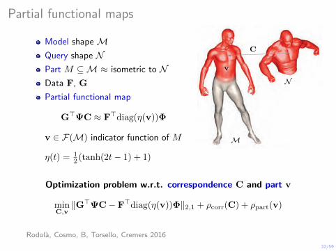
Model shape MQuery shape NPart M ⊆M ≈ isometric to NData F, G
Partial functional map
TG ≈ F(M)
v ∈ F(M) indicator function of M
η(t) = 12 (tanh(2t− 1) + 1)
M
N
M
T
Optimization problem w.r.t. correspondence C and part v
minC,v‖G>ΨC− F>diag(η(v))Φ‖2,1 + ρcorr(C) + ρpart(v)
Rodola, Cosmo, B, Torsello, Cremers 2016

32/59
Partial functional maps
Model shape MQuery shape NPart M ⊆M ≈ isometric to NData F, G
Partial functional map
G>ΨC ≈ F(M)>Φ
v ∈ F(M) indicator function of M
η(t) = 12 (tanh(2t− 1) + 1)
M
N
M
C
Optimization problem w.r.t. correspondence C and part v
minC,v‖G>ΨC− F>diag(η(v))Φ‖2,1 + ρcorr(C) + ρpart(v)
Rodola, Cosmo, B, Torsello, Cremers 2016

32/59
Partial functional maps
Model shape MQuery shape NPart M ⊆M ≈ isometric to NData F, G
Partial functional map
G>ΨC ≈ F>diag(v)Φ
v ∈ F(M) indicator function of M
η(t) = 12 (tanh(2t− 1) + 1)
M
N
v
C
Optimization problem w.r.t. correspondence C and part v
minC,v‖G>ΨC− F>diag(η(v))Φ‖2,1 + ρcorr(C) + ρpart(v)
Rodola, Cosmo, B, Torsello, Cremers 2016
32/59
Partial functional maps
Model shape MQuery shape NPart M ⊆M ≈ isometric to NData F, G
Partial functional map
G>ΨC ≈ F>diag(η(v))Φ
v ∈ F(M) indicator function of M
η(t) = 12 (tanh(2t− 1) + 1)
M
N
v
C
Optimization problem w.r.t. correspondence C and part v
minC,v‖G>ΨC− F>diag(η(v))Φ‖2,1 + ρcorr(C) + ρpart(v)
Rodola, Cosmo, B, Torsello, Cremers 2016

33/59
Partial functional maps
minC,v‖G>ΨC− F>diag(η(v))Φ‖2,1 + ρcorr(C) + ρpart(v)
Part regularization
ρpart(v) = µ1
(|N | −
∫Mη(v)dm
)2
︸ ︷︷ ︸area preservation
+ µ2
∫Mξ(v)‖∇Mv‖dm
︸ ︷︷ ︸Mumford−Shah
where ξ(t) ≈ δ(η(t)− 1
2
)Correspondence regularization
ρcorr(C) = µ3‖C ◦W‖2F
︸ ︷︷ ︸slant
+µ4
∑i6=j
(C>C)2ij
︸ ︷︷ ︸≈ orthogonality
+µ5
∑i
((C>C)ii − di)2
︸ ︷︷ ︸rank≈r
Rodola, Cosmo, B, Torsello, Cremers 2016
; BB 2008

33/59
Partial functional maps
minC,v‖G>ΨC− F>diag(η(v))Φ‖2,1 + ρcorr(C) + ρpart(v)
Part regularization
ρpart(v) = µ1
(|N | −
∫Mη(v)dm
)2
︸ ︷︷ ︸area preservation
+ µ2
∫Mξ(v)‖∇Mv‖dm
︸ ︷︷ ︸Mumford−Shah
where ξ(t) ≈ δ(η(t)− 1
2
)
Correspondence regularization
ρcorr(C) = µ3‖C ◦W‖2F
︸ ︷︷ ︸slant
+µ4
∑i6=j
(C>C)2ij
︸ ︷︷ ︸≈ orthogonality
+µ5
∑i
((C>C)ii − di)2
︸ ︷︷ ︸rank≈r
Rodola, Cosmo, B, Torsello, Cremers 2016; BB 2008

33/59
Partial functional maps
minC,v‖G>ΨC− F>diag(η(v))Φ‖2,1 + ρcorr(C) + ρpart(v)
Part regularization
ρpart(v) = µ1
(|N | −
∫Mη(v)dm
)2
︸ ︷︷ ︸area preservation
+ µ2
∫Mξ(v)‖∇Mv‖dm︸ ︷︷ ︸
Mumford−Shah
where ξ(t) ≈ δ(η(t)− 1
2
)Correspondence regularization
ρcorr(C) = µ3‖C ◦W‖2F
︸ ︷︷ ︸slant
+µ4
∑i6=j
(C>C)2ij
︸ ︷︷ ︸≈ orthogonality
+µ5
∑i
((C>C)ii − di)2
︸ ︷︷ ︸rank≈r
Rodola, Cosmo, B, Torsello, Cremers 2016; BB 2008

33/59
Partial functional maps
minC,v‖G>ΨC− F>diag(η(v))Φ‖2,1 + ρcorr(C) + ρpart(v)
Part regularization
ρpart(v) = µ1
(|N | −
∫Mη(v)dm
)2
︸ ︷︷ ︸area preservation
+ µ2
∫Mξ(v)‖∇Mv‖dm︸ ︷︷ ︸
Mumford−Shah
where ξ(t) ≈ δ(η(t)− 1
2
)Correspondence regularization
ρcorr(C) = µ3‖C ◦W‖2F︸ ︷︷ ︸slant
+µ4
∑i6=j
(C>C)2ij︸ ︷︷ ︸
≈ orthogonality
+µ5
∑i
((C>C)ii − di)2
︸ ︷︷ ︸rank≈r
Rodola, Cosmo, B, Torsello, Cremers 2016; BB 2008

34/59
Structure of partial functional correspondence
C W C>C0 20 40 60 80 100
0
2
4
singular values
Rodola, Cosmo, B, Torsello, Cremers 2016

35/59
Alternating minimization
C-step: fix v∗, solve for correspondence C
minC‖G>ΨC− F>diag(η(v∗))Φ‖2,1 + ρcorr(C)
v-step: fix C∗, solve for part v
minv‖G>ΨC∗ − F>diag(η(v))Φ‖2,1 + ρpart(v)
Iteration 1 2 3 4
Rodola, Cosmo, B, Torsello, Cremers 2016

35/59
Alternating minimization
C-step: fix v∗, solve for correspondence C
minC‖G>ΨC− F>diag(η(v∗))Φ‖2,1 + ρcorr(C)
v-step: fix C∗, solve for part v
minv‖G>ΨC∗ − F>diag(η(v))Φ‖2,1 + ρpart(v)
Iteration 1 2 3 4
Rodola, Cosmo, B, Torsello, Cremers 2016

36/59
Example of convergence
0 20 40 60 80 100104
105
106
107
108
109
1010
Iteration
En
erg
y
C-stepv-step
0 5 10 15 20 25
Time (sec.)
Rodola, Cosmo, B, Torsello, Cremers 2016

37/59
Examples of partial functional maps
Rodola, Cosmo, B, Torsello, Cremers 2016

37/59
Examples of partial functional maps
Rodola, Cosmo, B, Torsello, Cremers 2016

37/59
Examples of partial functional maps
Rodola, Cosmo, B, Torsello, Cremers 2016

37/59
Examples of partial functional maps
Rodola, Cosmo, B, Torsello, Cremers 2016

38/59
Partial functional maps vs Functional maps
0 0.05 0.1 0.15 0.2 0.250
20
40
60
80
100
50100
150
50
100150
Geodesic error
%C
orre
spo
nd
ence
s
PFMFunc. maps
Correspondence performance for different rank values k
Rodola, Cosmo, B, Torsello, Cremers 2016
39/59
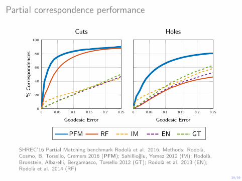
Partial correspondence performance
0 0.05 0.1 0.15 0.2 0.250
20
40
60
80
100
Geodesic Error
%C
orre
spo
nd
ence
sCuts
0 0.05 0.1 0.15 0.2 0.25
Geodesic Error
Holes
PFM RF IM EN GT
SHREC’16 Partial Matching benchmark Rodola et al. 2016; Methods: Rodola,Cosmo, B, Torsello, Cremers 2016 (PFM); Sahillioglu, Yemez 2012 (IM); Rodola,Bronstein, Albarelli, Bergamasco, Torsello 2012 (GT); Rodola et al. 2013 (EN);Rodola et al. 2014 (RF)

40/59
Partial correspondence performance
20 40 60 800
0.2
0.4
0.6
0.8
1
Partiality (%)
Mea
ng
eod
esic
erro
rCuts
20 40 60 80
Partiality (%)
Holes
PFM RF IM EN GT
SHREC’16 Partial Matching benchmark Rodola et al. 2016; Methods: Rodola,Cosmo, B, Torsello, Cremers 2016 (PFM); Sahillioglu, Yemez 2012 (IM); Rodola,Bronstein, Albarelli, Bergamasco, Torsello 2012 (GT); Rodola et al. 2013 (EN);Rodola et al. 2014 (RF)
41/59
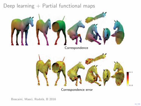
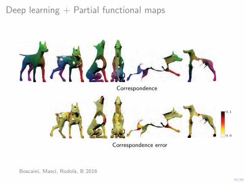
Deep learning + Partial functional maps
Correspondence
Correspondence error
0.0
0.1
Boscaini, Masci, Rodola, B 2016
42/59
Deep learning + Partial functional maps
Correspondence
Correspondence error
0.0
0.1
Boscaini, Masci, Rodola, B 2016

43/59
Outline
Background: Spectral analysis on manifolds
Functional correspondence
Partial functional correspondence
Non-rigid puzzles

Litani, BB 2012

45/59
Partial correspondence
Rodola, Cosmo, B, Torsello, Cremers 2016

45/59
Non-rigid puzzle
Litani, Rodola, BB, Cremers 2016
46/59
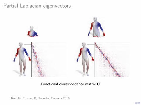
Partial Laplacian eigenvectors
Functional correspondence matrix C
Rodola, Cosmo, B, Torsello, Cremers 2016

47/59
Key observation
N
N
M
M
CNN
slant ∝ |N ||N |
CMM
slant ∝ |M ||M|
Litani, Rodola, BB, Cremers 2016

47/59
Key observation
N
N
M
M
CNM = CNNCNMCMM
slant ∝ |N ||N ||M||M |
=|N ||M|
Litani, Rodola, BB, Cremers 2016

47/59
Key observation
N
N
M
M
CNM = CNNCNMCMM
slant ∝ |N ||N ||M||M |
=|N ||M|
Litani, Rodola, BB, Cremers 2016

48/59
Non-rigid puzzles problem formulation
Input
Model MParts N1, . . . ,Np
Output
Segmentation Mi ⊆MLocated parts Ni ⊆ NiCorrespondences Ci
Clutter N ci
Missing parts M0
Model Parts
M1
M2
C1
C2
N2
N1N c2
N c1
M0
M N2
N1
Litani, Rodola, BB, Cremers 2016

48/59
Non-rigid puzzles problem formulation
Data Fi, Gi
Model basis Φ, Φ(Mi)
Part bases Ψi, Ψi(Ni)
Data term
F>i Φ(Mi) ≈ G>i Ψi(Ni)Ci
Model Parts
M1
M2
C1
C2
N2
N1N c2
N c1
M0
M N2
N1
Litani, Rodola, BB, Cremers 2016

49/59
Non-rigid puzzles problem formulation
minCi
Mi⊆M,Ni⊆Ni
p∑i=1
‖G>i ΨΨΨi(Ni)Ci − F>i ΦΦΦ(Mi)‖2,1
+ λM
p∑i=0
ρpart(Mi) + λN
p∑i=1
ρpart(Ni)
+ λcorr
p∑i=1
ρcorr(Ci)
s.t. Mi ∩Mj = ∅ ∀i 6= j
M0 ∪M1 ∪ · · · ∪Mp =M|Mi| = |Ni| ≥ α|Ni|,
Litani, Rodola, BB, Cremers 2016

49/59
Non-rigid puzzles problem formulation
minCi
ui,vi
p∑i=1
‖G>i diag(η(ui))ΨΨΨiCi − F>i diag(η(vi))ΦΦΦ‖2,1
+ λM
p∑i=0
ρpart(η(vi)) + λN
p∑i=1
ρpart(η(ui))
+ λcorr
p∑i=1
ρcorr(Ci)
s.t.
p∑i=1
η(ui) = 1
a>Mui = a>Nvi ≥ αa>Ni1
Litani, Rodola, BB, Cremers 2016

50/59
Convergence example
Outer iteration 1
Litani, Rodola, BB, Cremers 2016

50/59
Convergence example
Outer iteration 2
Litani, Rodola, BB, Cremers 2016

50/59
Convergence example
Outer iteration 3
Litani, Rodola, BB, Cremers 2016

51/59
Convergence example
80 90 100 110 120 130 140 150 160Iteration number
Time (sec)30 32 34 36 38 40 42 44 46 48
Litani, Rodola, BB, Cremers 2016

52/59
“Perfect puzzle” example
Model/Part Synthetic (TOSCA)
Transformation Isometric
Clutter No
Missing part No
Data term Dense (SHOT)
Litani, Rodola, BB, Cremers 2016

52/59
“Perfect puzzle” example
Model/Part Synthetic (TOSCA)
Transformation Isometric
Clutter No
Missing part No
Data term Dense (SHOT)
Segmentation
Litani, Rodola, BB, Cremers 2016

52/59
“Perfect puzzle” example
Model/Part Synthetic (TOSCA)
Transformation Isometric
Clutter No
Missing part No
Data term Dense (SHOT)
Correspondence
Litani, Rodola, BB, Cremers 2016

53/59
Overlapping parts example
Model/Part Synthetic (FAUST)
Transformation Near-isometric
Clutter Yes (overlap)
Missing part No
Data term Dense (SHOT)
Segmentation
Litani, Rodola, BB, Cremers 2016

53/59
Overlapping parts example
Model/Part Synthetic (FAUST)
Transformation Near-isometric
Clutter Yes (overlap)
Missing part No
Data term Dense (SHOT)
Correspondence
Litani, Rodola, BB, Cremers 2016

53/59
Overlapping parts example
Model/Part Synthetic (FAUST)
Transformation Near-isometric
Clutter Yes (overlap)
Missing part No
Data term Dense (SHOT)
0.0
0.1
Correspondence error
Litani, Rodola, BB, Cremers 2016

54/59
Missing parts example
Model/Part Synthetic (TOSCA)
Transformation Isometric
Clutter Yes (extra part)
Missing part Yes
Data term Dense (SHOT)
Litani, Rodola, BB, Cremers 2016

54/59
Missing parts example
Model/Part Synthetic (TOSCA)
Transformation Isometric
Clutter Yes (extra part)
Missing part Yes
Data term Dense (SHOT)
Segmentation
Litani, Rodola, BB, Cremers 2016

54/59
Missing parts example
Model/Part Synthetic (TOSCA)
Transformation Isometric
Clutter Yes (extra part)
Missing part Yes
Data term Dense (SHOT)
Correspondence
Litani, Rodola, BB, Cremers 2016

55/59
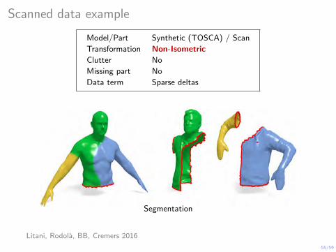
Scanned data example
Model/Part Synthetic (TOSCA) / Scan
Transformation Non-Isometric
Clutter No
Missing part No
Data term Sparse deltas
Litani, Rodola, BB, Cremers 2016
55/59
Scanned data example
Model/Part Synthetic (TOSCA) / Scan
Transformation Non-Isometric
Clutter No
Missing part No
Data term Sparse deltas
Segmentation
Litani, Rodola, BB, Cremers 2016

56/59
Non-rigid puzzle vs Partial functional map
Partial functional map (pair-wise)
Non-rigid puzzle
Rodola, Cosmo, B, Torsello, Cremers 2016; Litani, Rodola, BB, Cremers 2016
57/59
Summary
New insights about spectral properties of Laplacians
Extension of functional correspondence framework to the partialsetting
Practically working methods for challenging shape correspondencesettings
Code available (SGP Reproducibility Stamp)
Some over-engineering - can be done simpler! (stay tuned...)

58/59
D. Cremers
Supported by
E. Rodolà O. Litany L. Cosmo A. TorselloA. Bronstein

59/59
Thank you!