Geometric Correction

of SEM Images

Jay P. Kapur Masters Project Report

Dr. David Casasent Graduate Advisor

Carnegie Mellon University Department of Electrical and Computer Engineering

1

Table of Contents

Table of Contents ................................................................................ 1

Abstract.............................................................................................. 2

Introduction......................................................................................... 3

Why do we need accurate SEM images?.......................................... 3

Sources of Distortion in SEM Images ................................................ 4

Correcting Geometric Distortions ........................................................... 8

Background .................................................................................. 8

Correction Using A Piecewise Approach......................................... 10

Affine Transforms for Piecewise Correction ..................................... 12

The Correction Algorithm.................................................................... 16

Bibliography...................................................................................... 23

2

Abstract

While the resolution that can be achieved with scanning electron microscopy is unquestioned,

the accuracy of any scientific measurements derived from scanning electron microscopes

(SEM) are limited due to a variety of sources of distortion in the microscope and the

equipment setup. For this reason, SEM images are not often used for making geometric

measurements. To facilitate such measurements, a consistent and accurate means of

correcting geometric distortions using a piecewise affine transform is described and

implemented. This method works independently of specific microscope settings and

therefore generalizes well to compensate for nearly any source of geometric distortion in

images. The result is a technique that can be applied with no knowledge of the distorting

functions. The distortion correction routine is performed once on an image of a calibration

standard, and the associated lookup table is used to correct all subsequent images.

Collection of large amounts of high quality data from scanning electron microscope imagery,

even when many images are required to capture an entire sample, is now possible with

automated correction and registration of adjacent images.

3

Introduction

Why do we need accurate SEM images?

Often scanning electron microscopy is used to observe incredibly small objects not visible to

the naked eye for the purposes of qualitative (not quantitative) study. SEM has benefited

researchers from the biologist studying bacteria to the engineer designing integrated circuits.

The majority of these applications do not require accurate representation of lines, angles, and

curves in the images. Typically the only quantitative analysis in any of these observations is

the level of magnification, so that one is able to judge the relative size of the object being

studied. However, accuracy in SEM images is becoming increasingly important in research

environments, especially those relating to crystallography [1,12].

Of particular interest to researchers working on the Mesoscale Interface Mapping Project

(MIMP) in the Department of Material Science Engineering at Carnegie Mellon University

(CMU) are grain boundaries, the border between two or more crystalline structures in a

material. Features such as the curvature of a boundary, the angles made at the triple

junctions where three grains meet (Figure 1), and the orientations of grains are being studied

to better understand how intergrannular behavior relates to material stress and failure. These

researchers depend on quantitative scientific observations of the microscopic polycrystalline

structure to form or verify their hypotheses. Geometric correction is necessary to provide

better quantitative measurements; the accuracy of angle measurements at triple junctions

(dihedral angles) is of particular importance [12].

4

• Figure 1: Backscatter Electron Image of a triple junction in Aluminum

Sources of Distortion in SEM Images

The sources of distortion in SEM images are numerous and vary in their affects and severity.

Many of the distortions are not specifically geometric (i.e. added noise, blurring, low

sharpness, or low contrast); we do not address them. The single greatest source of

geometric distortion, our primary concern, is specimen tilt.

5

• Figure 2: Setup for secondary electron emission with specimen tilted [2]

Typically, measurements of specimen geometry are not performed when the microscope

stage is tilted. However, tilting the specimen and using secondary electron emission (Figure

2) can provide benefits such as improved contrast and specimen topography information

(Figure 3). Moreover, the MIMP researchers at CMU specifically require a tilted specimen

because they perform electron back-scatter probes (EBSP) in each grain around each triple

junction. A tilted sample is needed to provide high contrast EBSP images (the EBSP data

provide grain orientation information). The secondary electron image (SEI) data is used to

determine locations of triple junctions, and the EBSP data is taken in the grains around triple

junctions. The specimen must be in the same (tilted) location while collecting the SEI and

EBSP data. Thus, the sample must be tilted while taking the SEI images.

6

• Figure 3: Improvement of topographical information using secondary electron emission with specimen tilt

The distortion caused by specimen tilt, seen in Figure 4 for a specimen at 60o, is

characterized by a demagnification of 1/cosθ along the tilt axis (vertical in Figure 4) [2]. The

SEM image in Figure 4 is of a calibration standard containing squares arranged in a regular

pattern. Note that the uncorrected image in Figure 4 shows the squares with a much different

height-to-width ratio due to the demagnification caused by specimen tilt. The distortion is not

simply a demagnification, because the SEM images are perspective projections. Looking at

the image in Figure 4, we can see that vertical lines do not appear at right angles to horizontal

lines as they should; the vertical lines are slanted 3o to the right.

Modern scanning electron microscopes are often equipped with scan rotation and tilt (SRT)

correction to compensate for demagnification caused by specimen tilt (Figure 5). Such

systems are often deemed good enough for qualitative observations, but don't always provide

the level of precise correction needed for quantitative geometric measurements. The SRT

correction built into the Philips SEM used by the MIMP researchers gives the result shown in

Figure 5. As seen, it only corrects the 1/cosθ demagnification in the vertical direction. (Note

that only a portion of the original distorted image appears in the SRT corrected result in

Figure 5 due to a limitation on the image size when using the Philips SEM.) Careful

inspection of the corrected image in Figure 5 shows the image is still skewed by 3o in the

vertical direction. This is an artifact of the perspective projection, which the SRT correction

does not account for. We could use a global projective transform to correct this distortion, but

7

there are other sources of distortion present in SEM images which this approach cannot

address.

• Figure 4: SEM image with 60 degree sample tilt at 1000X

• Figure 5: Result of automatic tilt correction

The other sources of distortion include scan generator error, external magnetic fields, and

user error [1,2]. Scan generator error can have deleterious effects on SEM image geometry.

Scan generator error or distortion in the scanning frame results from non-linearities inherent

8

in the SEM hardware [3]. These distortions can be corrected with electronic hardware now

commonly found in modern SEM devices. External magnetic fields, arising from any number

of sources, can alter the electron beam and add non-linear geometric distortions to the

image. Finally, user error can result in geometric distortion, such as in the case of improperly

setting the angle of the sample with respect to the beam axis. The scan generator distortions

can be corrected with internal hardware[3], but the other sources of distortion cannot. With

the exception of sample tilt, none of these distortions can be predicted, they must be

measured. We can address distortion caused by sample tilt, scan generator error, external

magnetic fields, and user error with a single technique. This requires a flexible distortion

correction method, such as the one we discuss in the following section.

Correcting Geometric Distortions

Background

The method we employ is a software based approach which is capable of addressing all

geometric distortions as a post-imaging step on the PC. The method can complement any

correction systems present internally in the SEM. Early SEM systems with analog outputs

did not facilitate efficient correction and as a result high precision measurements were, and

still are, generally not taken from SEM images. Hardware based correction systems have

been integrated with microscopes to address specific problems, such as scan generator

function correction [3]. With digital output from the SEM and a software based approach,

more general correction is made possible.

Geometric correction can be thought of as a mapping from distorted image space to

undistorted space. This mapping is represented as a function that transforms a source

coordinate (u,v) in the distorted image to a destination coordinate (x,y) in the corrected image:

9

x = f(u,v) y=g(u,v).

The transformation can just as easily be considered in the reverse direction, from a corrected

space coordinate (x,y) to a distorted space coordinate (u,v) as:

u = p(x,y) v = q(x,y).

The forward mapping will take every pixel in the distorted image and place it in the corrected

image, but there is a possibility that the corrected image will have some "holes" because this

method does not assure that every pixel in the corrected image will be used. When the

mapping is done in the reverse direction, the corrected image is guaranteed to have every

pixel mapped to a pixel in the original distorted image. Thus, in our system, we choose to

use the reverse mapping so as to avoid holes in the corrected image.

Some research efforts have focused on designing specific correction functions for specific

imaging devices. One example is a correction algorithm for endoscope imaging based on a

specific model of the "barrel" distortion in medical endoscope images [4]. SRT correction for

sample tilt distortion in SEM uses this approach to compensate for the demagnification.

These methods attempt to predict the distorting function, this is a complex task and is not

possible for external magnetic field or user setup distortions. Our approach is to correct a

distorted image of a calibration standard, determine the distortion analytically (not

theoretically), and then apply the transformation to all subsequent images using a lookup

table which stores the pixel mappings. Another benefit is that this approach results in a

generalized method that can be applied to other imaging systems besides SEM.

Many correction methods using this approach (correcting a known calibration pattern) have

been used, which we now discuss. A common general correction method is global

polynomial warping. This method fits an N-th order polynomial to specified points in a

10

reference image in order to model the distortion. Polynomial warping has been applied to

SEM [5] as well as numerous other imaging devices [6]. The approach is appealing because

of its simplicity, but it is not guaranteed to produce the best result, since such a global

approach attempts to fit a function to the entire image. This means that some regions of the

image may not be corrected as well as others (or might even have increased distortions) and

there is always the question of determining the best N-th order polynomial to use. We found

that applying the global polynomial warp (with bilinear interpolation of pixels) to the MIMP

data gave poor accuracy and made registration of adjacent sector images difficult.

Correction Using A Piecewise Approach

Our approach is to use a general correction method based on a piecewise transform. A

piecewise approach means that a reference distorted image (an image of a calibration

standard with a regularly repeated pattern) is broken up into regions bounded by points

(sometimes called tie-points or control points [7]) at vertices of primitive geometric shapes.

The primitive shape is typically a triangle when using the affine transform or a quadrilateral

when using a projective transform. The distortion for each local region is modeled by using

the control points to determine the transform equation coefficients. The piecewise correction

method allows a different correction to be applied to each local region. The piecewise

transform is commonly used in computer graphics for image warping and has been applied to

various applications, including X-ray image correction [8,11], but bilinear interpolation was

used and methods to handle points on triangular boundaries were not addressed. The

procedure can be easily automated and the transform method (affine, projective, curvilinear)

can be chosen to suit the application.

The calibration standard is an object with a regular pattern placed on its surface for the

purpose of observing image distortions. The image taken of the calibration standard is

referred to as the reference distorted image. The reference distorted image is separated into

11

the desired regions by locating landmarks and using their coordinates as control points

(points whose distances in the calibration standard and pixel coordinates in the reference

distorted image are known). The only requirement of the calibration standard is that it contain

features spaced at known real world distances and, for completely automated systems, that

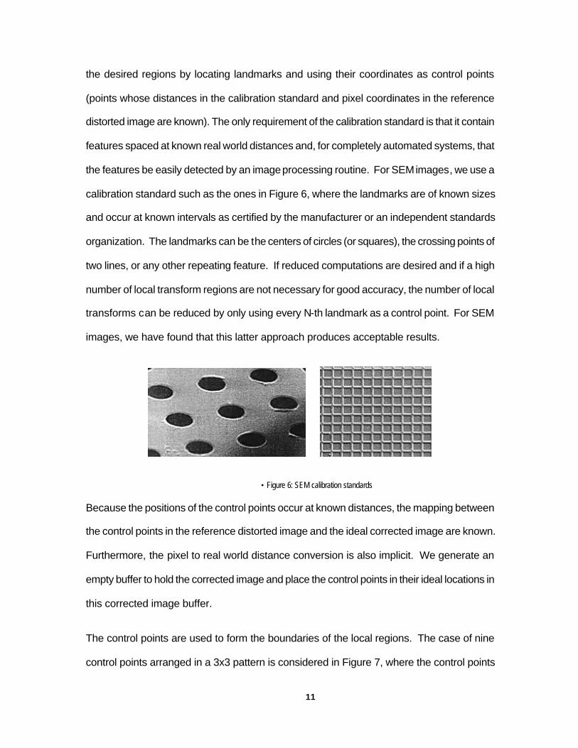
the features be easily detected by an image processing routine. For SEM images, we use a

calibration standard such as the ones in Figure 6, where the landmarks are of known sizes

and occur at known intervals as certified by the manufacturer or an independent standards

organization. The landmarks can be the centers of circles (or squares), the crossing points of

two lines, or any other repeating feature. If reduced computations are desired and if a high

number of local transform regions are not necessary for good accuracy, the number of local

transforms can be reduced by only using every N-th landmark as a control point. For SEM

images, we have found that this latter approach produces acceptable results.

• Figure 6: SEM calibration standards

Because the positions of the control points occur at known distances, the mapping between

the control points in the reference distorted image and the ideal corrected image are known.

Furthermore, the pixel to real world distance conversion is also implicit. We generate an

empty buffer to hold the corrected image and place the control points in their ideal locations in

this corrected image buffer.

The control points are used to form the boundaries of the local regions. The case of nine

control points arranged in a 3x3 pattern is considered in Figure 7, where the control points

12

are the centers of the circular landmarks. Sets of three control points form a triangle region

and create eight total local regions as in Figure 7a. Using sets of four control points form

quadrilaterals and creates four total local regions as in Figure 7b. Each set of control points

which form the vertices of a region are used to solve for the coefficients of the chosen

transform function. The transform function with the determined coefficients is then used to

map all points within each local region. By storing the mapping for each local region in a

single lookup table, future correction of images taken with the SEM can be performed quickly.

• Figure 7: Using 3x3 control points to form triangle regions (a) or square regions (b)

Affine Transforms for Piecewise Correction

We choose to model the local distortion as an affine transform. The affine transform allows a

combination of 2D scale, rotation, and translation for six degrees of freedom. Mathematically

the transform is written as:

u = a + by + cx v = d + ey + fx.

Or in matrix form as:

=

11001yx

fedcba

vu

(a) (b)

13

The affine transform coefficients (a,b,c,d,e,f) can be computed from three 2D points, thus the

local regions used in the correction are triangles whose vertices are three control points as in

Figure 7a. With an affine transform, any parallelogram can be warped to a square. Parallel

lines are preserved with an affine transform.

Higher-order transforms can also be used to warp any quadrilateral into a square while still

preserving straight lines (eight degree of freedom projective transform), or to fit curves

between control points (curvilinear transforms), but this will not preserve straight lines. The

projective transform is defined as:

u=(ax+by+c)/(gx+hy+i) v=(dx+ey+f)/(gx+hy+i).

The projective transform, requiring four control points (assuming i=1), can be implemented in

such a manner that matrix inversion is not required [9], making it a viable alternative to the

affine transform. The computational costs this method are much higher than when using

affine transforms, but not prohibitive. Higher-order transforms, such as the curvilinear

transforms are sometimes called rubber-sheeting transforms because their warps do not

preserve straight lines. Examples of curvilinear transforms are

u=ax+by+cxy+d v=ex+fy+gxy+h

or

u=ax+by+cx2+dy2+exy+f v=gx+hy+ix2+jy2+kxy+l.

The correction result with curvilinear transforms can be similar to the global polynomial warp

methods in that some points may be corrected more accurately, but others less accurately

than a if simple affine transform were used [13]. Thus, greater precision in locating the

control points is desired when using higher-order transforms. Six or more control points can

14

be required to solve for the coefficients of the curvilinear transform. Solving this system of

equations requires a general matrix inversion, which can be computationally expensive.

Curvilinear transforms do not lend themselves well to piecewise correction and are

uncommon in this regard.

Two issues of precision arise when using the piecewise affine transform: interpolation of data

resulting from mapping corrected pixels to non-integer pixel locations in the distorted

reference image and interpolation of data corresponding to points lying on the line shared by

two triangles in the corrected image. In the case where a pixel in the corrected image maps

to a non-integer pixel value in the distorted image, interpolation of data can be performed

using bilinear interpolation, zero-order interpolation, or more complex cubic convolution

interpolation[7]. Bilinear interpolation is most commonly used because it averages a

neighborhood of data, giving a smooth appearance to the final image. The problem with this

approach is that sharp transitions are blurred and high frequency content is lost. This loss of

information presents problems when the corrected images need to be registered or when the

images will undergo image further processing off-line (e.g. edge detection). Using zero-order

(nearest neighbor) interpolation gives an image that is not as smooth in appearance, but

preserves frequency content and transitions when compared to bilinear interpolation. Zero-

order interpolation also has the benefit of being computationally efficient, which cubic

convolution (sinx/x lowpass filter) is not. Thus, we use zero-order interpolation to avoid the

blurring effects and complexity of bilinear interpolation or cubic convolution interpolation. We

found better registration of adjacent MIMS sector images using zero-order interpolation. To

address the problem of a point lying along a line shared by two triangles, the mapping for

both triangles is computed for the one point. The two pixel intensities assigned by the two

mappings for this point (from the two different triangle regions) are averaged and assigned to

the pixel in the corrected image.

15

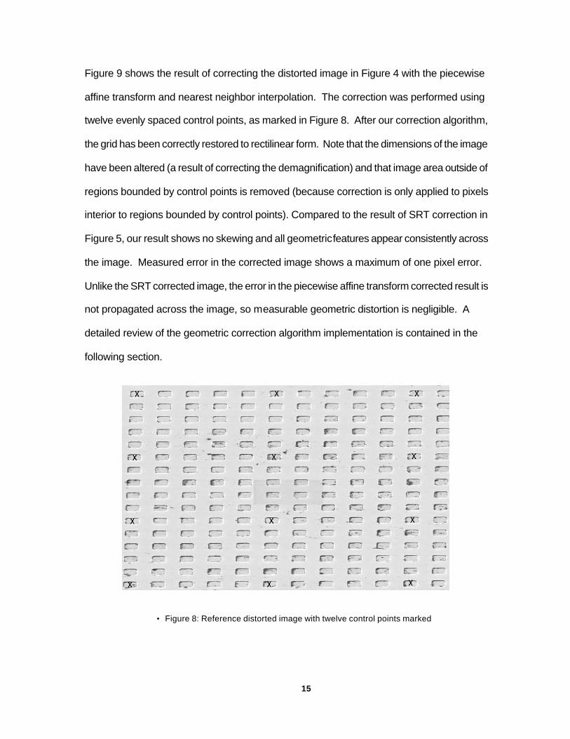
Figure 9 shows the result of correcting the distorted image in Figure 4 with the piecewise

affine transform and nearest neighbor interpolation. The correction was performed using

twelve evenly spaced control points, as marked in Figure 8. After our correction algorithm,

the grid has been correctly restored to rectilinear form. Note that the dimensions of the image

have been altered (a result of correcting the demagnification) and that image area outside of

regions bounded by control points is removed (because correction is only applied to pixels

interior to regions bounded by control points). Compared to the result of SRT correction in

Figure 5, our result shows no skewing and all geometric features appear consistently across

the image. Measured error in the corrected image shows a maximum of one pixel error.

Unlike the SRT corrected image, the error in the piecewise affine transform corrected result is

not propagated across the image, so measurable geometric distortion is negligible. A

detailed review of the geometric correction algorithm implementation is contained in the

following section.

• Figure 8: Reference distorted image with twelve control points marked

16

• Figure 9: Piecewise affine transform correction result

The Correction Algorithm

In this section we will cover the steps for correcting a single SEM image. Implementing the

geometric correction begins by taking a reference image of the calibration standard. The

image is taken with the SEM configured as it will be used for subsequent images. For this

discussion, we will use a reference image of the calibration standard in Figure 10. This

standard is made of circular holes of consistent 4 micron center-to-center spacing, but tilt

17

distortion has occurred. Notice that the circular holes now appear elliptical and the grid

arrangement of the holes is not orthogonal. We will now correct the distortion using our

algorithm. The landmarks used as control points are the centers of the nine circles (3x3

arrangement). The coordinates of these landmarks are stored in order starting with the top

leftmost control point and moving left to right, top to bottom. Note that we could determine

the locations of the circles with sub-pixel accuracy through an automated image processing

routine, but low-accuracy hand selected locations (one pixel accuracy) are tolerable for SEM

images with use of the piecewise affine transform. To demonstrate this, the following

example uses coarsely determined landmark coordinates (approximately one pixel

accuracy).

• Figure 10: Reference distorted image showing sample tilt distortions

The user enters the ideal pixel spacing between landmarks that would occur in an undistorted

image. This number is generally arbitrary (it scales the output image size) but, for

consistency and reduced interpolation in real applications, the distance should be

determined from the landmark distance occurring at the center (or least distorted region) of

the reference distorted image. We choose 60 pixels to equal the distance between the

centers of two circles. Since the landmark spacing in the real world (4 microns) distance is

known, the pixel to real world conversion is thus defined as 15 pixels equals 1 micron.

An empty buffer, which will contain the corrected image, is generated based on the number of

control points and the ideal distance between points. The number of control points V used in

18

the reference image along the vertical v-axis determines the corrected image height and the

number of control points U used along the horizontal u-axis are used to determine the

corrected image width as:

distUUwidthdistVVheight

×−+=×−+=

)1()1(

where dist is the user-specified distance in pixels between control points (60 for our

example). In this case, we set U and V to equal three because of the 3x3 arrangement of

circular holes in the image.

The number of triangle primitives T that can be formed given the number of control points is:

2)1()1( ×−×−= UVT

The eight triangles are organized as in Figure 7a so that the pattern of triangulation over four

points alternates between the two possible forms shown in Figure 11. The triangulations in

the left of Figure 11 are the triangles with vertices at {C1,C3,C4} and {C1,C2,C4}. The

triangulations in the right of Figure 11 are the triangles with vertices at {C2,C1,C3} and

{C2,C4,C3}. In general, given the k-th control point Ck, a triangulation as shown in the left of

Figure 11 is formed as the triangles with vertices {Ck,Ck+U,Ck+U+1} and {Ck,Ck+1,Ck+U+1}. The

triangulation shown in the right of Figure 11 is formed as the triangles with vertices

{Ck+1,Ck,Ck+U} and {Ck+1,Ck+1+U,Ck+U}. This simple formulation of the triangle vertices works

because of the defined ordering of the control points with C1 being the top left-most control

point and with k increasing from left to right, top to bottom.

19

C1 C2

C3 C4

C1 C2

C3 C4

• Figure 11: Two possible triangulations over four control points

Some amount of organization is required to ensure that the same triangle is formed over the

same control points in the reference distorted image and in the corrected image. This is of

course important for assuring that the correct transform is applied to the correct region of the

image. Figure 7a shows the alternating pattern of triangulations created for our example.

The nine white pixels in Figure 12 indicate where in the corrected image the control points will

be placed.

• Figure 12: Ideal locations of the landmarks in the corrected image

The ideal locations of the control points in the corrected image are generated and stored in a

list in the same ordering use to store the reference distorted image control points. Regions in

the reference distorted image outside of these control points will not be corrected and are

discarded by the correction process, thus the corrected image will typically not contain the

20

information in the borders of the reference distorted image. The top leftmost control point in

the corrected image is placed at (x,y) = (0,0).

With the local regions defined by eight triangles in both the reference distorted image and the

corrected image, the affine correction coefficients for each local region can now be

determined. For one triangle region, the reference distorted image control point pixel

locations (ui,v i) and the ideal control point pixel locations (xi,y i) are related by the affine

transform:

ui=a+by i+cxi i=1,2,3

vi=d+ey i+fx i i=1,2,3

This set of three equations and three unknowns for each triangle is written in matrix form as:

=

3

2

1

33

22

11

111

uuu

cba

xyxyxy

=

3

2

1

33

22

11

111

vvv

fed

xyxyxy

To solve for the correction coefficients {a,b,c} and {d,e,f} we only need take a 3x3 matrix

inverse, which does not require any specialized algorithm for general matrix inversion.

The next task is to determine in which of the eight triangulations a pixel in the corrected

image belongs, and hence which correction coefficients should be applied to it. A pixel in the

corrected image may lie on the line separating two adjacent triangulations. In this event, the

mapping for both triangular regions is computed and the average of both results are used for

the intensity value for that pixel.

21

In order for the correction to work efficiently, a simple algorithm for determining which pixels

belong to which local triangle regions is used [10]. A pixel can automatically be determined

as being interior to a triangle, exterior to a triangle, or lying on a vertex of a triangle (a point

shared by two triangulations). Let T(t1,t2,t3) be a triangle in two dimensions with t1,t2,and t3

being 2D row vectors containing the coordinates of the triangle vertices. Given a point p (a

2D row vector), we can represent p by the parametric equation:

p=t1+q1(t2-t1)+q2(t3-t2)

where q1 and q2 are scalars. Solving for q1 and q2 determines where the point is located

relative to the triangle T. The point p is interior to T or lies on the edge of T if q2≤q1, 0≤q1≤1,

and 0≤q2≤1. Furthermore, if q1=1 and 0≤q2<1, p is on the line segment (t2,t3). If q2=0 and

0<q1≤1, p is on the line segment (t1,t2). If 0<q1<1 and 0<q2<1 and q1=q2, p is on the line

segment (t1,t3). For all other cases, the point is outside of the triangle T.

Now that the correction coefficients for every region and the pixels contained in every region

are known, any pixel (x,y) in the corrected image can be mapped to a pixel (u,v) in the

original distorted image. A lookup table is generated giving the mapping of every pixel in the

corrected image to its corresponding pixel (or pixels in the case where the corrected point lies

on the boundary of two regions) in the distorted image. This lookup table is used for quickly

correcting all images taken with the SEM. In the event that the (u,v) coordinates are non-

integers, the nearest neighbor pixel in the distorted image is used by rounding to the nearest

integer.

22

• Figure 13: Corrected image

Figure 13 shows the corrected image resulting from the piecewise affine transform algorithm.

Angles formed by drawing lines through the centers of the holes will now be orthogonal and

the holes now appear circular. Note that the damage to the holes on the right side of the

image is physical, not a result of any distortion. Measurable error is within 1.5 pixels in the

final image (with one pixel maximum error due to selection of control points and a half pixel

due to nearest neighbor interpolation). Note that because of the nature of the piecewise

approach, the error does not accumulate across the image, so geometry is generally

unaffected. Automation of the control point selection could improve the error to subpixel

levels. Future work will include varying the accuracy of control point locations and varying the

number of control points to see how these factors can influence accuracy of the correction.

23

Bibliography

[1] S. Murray and A. Windle, "Characterisation and Correction of Distortions in SEM Micrographs," Conference on Scanning Electron Microscopy: Systems and Applications , pp. 88-93, Inst. Physics, UK July 1973.

[2] A Guide to Scanning Microscope Observation, 2nd ed., published by JEOL LTD. available at http://www.jeol.com

[3] R. Barrett and C. Quate, "Optical scan-correction system applied to atomic force microscopy," Review of Scientific Instruments, vol. 12 no. 6, pp. 1393-1399, June 1991.

[4] H. Haneishi, Y. Yagihashi, and Y. Miyake, "A new method for distortion correction of electronic endoscope images," IEEE Transactions on Medical Imaging, vol. 14 no. 3, pp. 548-555, September 1995.

[5] R. Marschallinger and D. Topa, "Assessment and correction of geometric distortions in low-magnification scanning electron microscopy images," Scanning, vol 19, pp. 36-41, 1997.

[6] Y. Christophe, J. Cornelius, and P. DeMuynck, "Subpixel geometric correction of digital images," Signal Processing IV: Theories and Applications, pp. 1605-1607, 1988.

[7] R. Gonzalez and R. Woods, Digital Image Processing, Addison-Wesley, pp. 296-302, 1993.

[8] D. Reimann and M. Flynn, "Automated distortion correction of x-ray image intensifier images," IEEE Nuclear Science Symposium and Medical Imaging Conference Record, pp. 1339-1341, Orlando, FL, October 1992.

[9] P. Heckbert, Fundamentals of Texture Mapping and Image Warping, Master's Thesis, UCB/CSD 89/516, CS Division, U.C. Berkeley, 1989.

[10] J. Otto, A. Smith, Ray-Tracing with Affine Transforms, MathVision Inc. Technical Journal available at http://www.olympus.net/biz/7seas/tjour.html, July 1995.

[11] J. Lind, L. Ostergaard, O. Larsen, H. Nielsen, N. Bartholdy, and J. Haase, System for 3D Localisation of Malformations in the Human Brain, Technical Report, No. 98-3, ISSN 1397-9507, Virtual Centre for Health Informatics, Aalborg University, September, 1998.

[12] B. L. Adams, et al., "Extraction of Grain Boundary Energies from Triple Juinction Geometry", Proc. of the Twelfth International Conference on Textures of Materials, Montréal, Canada, NRC Research Press, pp. 9-20, August 1999.

24

[13] M. Goodchild, M., Spatial Statistics and Models, G. Gaile and C. Willmott, eds., Reidel Publishing Co., Dordrecht, Holland, pp. 33-53, 1984.