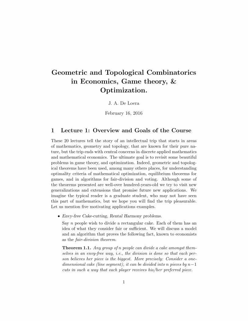
Geometric and Topological Combinatorics

in Economics, Game theory, &

Optimization.

J. A. De Loera

February 16, 2016

1 Lecture 1: Overview and Goals of the Course

These 20 lectures tell the story of an intellectual trip that starts in areasof mathematics, geometry and topology, that are known for their pure na-ture, but the trip ends with central concerns in discrete applied mathematicsand mathematical economics. The ultimate goal is to revisit some beautifulproblems in game theory, and optimization. Indeed, geometric and topolog-ical theorems have been used, among many others places, for understandingoptimality criteria of mathematical optimization, equilibrium theorems forgames, and in algorithms for fair-division and voting. Although some ofthe theorems presented are well-over hundred-years-old we try to visit newgeneralizations and extensions that promise future new applications. Weimagine the typical reader is a graduate student, who may not have seenthis part of mathematics, but we hope you will find the trip pleasurable.Let us mention five motivating applications examples.

• Envy-free Cake-cutting, Rental Harmony problems.

Say n people wish to divide a rectangular cake. Each of them has anidea of what they consider fair or sufficient. We will discuss a modeland an algorithm that proves the following fact, known to economistsas the fair-division theorem.

Theorem 1.1. Any group of n people can divide a cake amongst them-selves in an envy-free way, i.e., the division is done so that each per-son believes her piece is the biggest. More precisely: Consider a one-dimensional cake (line segment), it can be divided into n pieces by n−1cuts in such a way that each player receives his/her preferred piece.

1

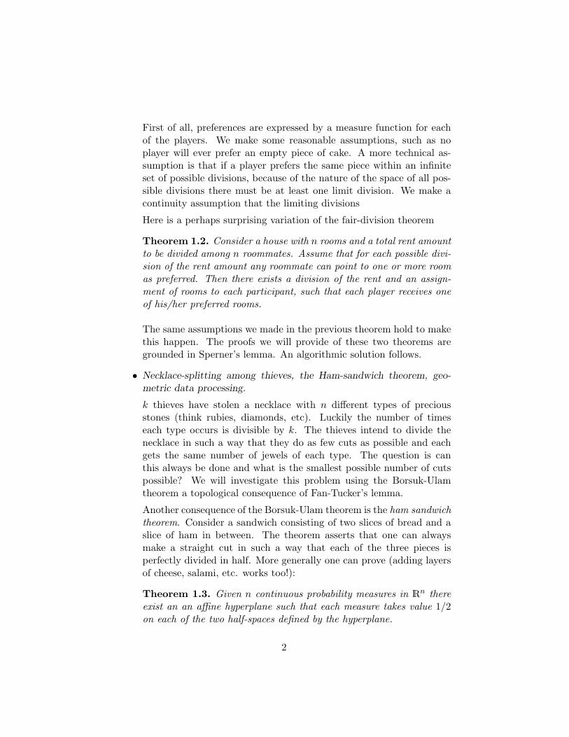
First of all, preferences are expressed by a measure function for eachof the players. We make some reasonable assumptions, such as noplayer will ever prefer an empty piece of cake. A more technical as-sumption is that if a player prefers the same piece within an infiniteset of possible divisions, because of the nature of the space of all pos-sible divisions there must be at least one limit division. We make acontinuity assumption that the limiting divisions

Here is a perhaps surprising variation of the fair-division theorem

Theorem 1.2. Consider a house with n rooms and a total rent amountto be divided among n roommates. Assume that for each possible divi-sion of the rent amount any roommate can point to one or more roomas preferred. Then there exists a division of the rent and an assign-ment of rooms to each participant, such that each player receives oneof his/her preferred rooms.

The same assumptions we made in the previous theorem hold to makethis happen. The proofs we will provide of these two theorems aregrounded in Sperner’s lemma. An algorithmic solution follows.

• Necklace-splitting among thieves, the Ham-sandwich theorem, geo-metric data processing.

k thieves have stolen a necklace with n different types of preciousstones (think rubies, diamonds, etc). Luckily the number of timeseach type occurs is divisible by k. The thieves intend to divide thenecklace in such a way that they do as few cuts as possible and eachgets the same number of jewels of each type. The question is canthis always be done and what is the smallest possible number of cutspossible? We will investigate this problem using the Borsuk-Ulamtheorem a topological consequence of Fan-Tucker’s lemma.

Another consequence of the Borsuk-Ulam theorem is the ham sandwichtheorem. Consider a sandwich consisting of two slices of bread and aslice of ham in between. The theorem asserts that one can alwaysmake a straight cut in such a way that each of the three pieces isperfectly divided in half. More generally one can prove (adding layersof cheese, salami, etc. works too!):

Theorem 1.3. Given n continuous probability measures in Rn thereexist an an affine hyperplane such that each measure takes value 1/2on each of the two half-spaces defined by the hyperplane.

2

There are recent advanced generalizations of the ham-sandwich the-orem. In [] the authors show that, for any prime power n and anycompact convex set with interior K ⊂ Rd, there exists a partition ofK into n convex sets with equal volumes and equal surface areas. Thegoal is to have an equi-partition among n players of a divisible good. Inthe plane this boils down to the following fact proven in []. Any convexbody in the plane can be partitioned into n convex regions with equalareas and equal perimeters. The theorem has received the funny namethe spicy chicken theorem because it can be applied to equi-partitionof a (perfectly convex) chicken among guests. You will cut the rawchicken fillet with a sharp knife, marinate each of the pieces in a spicysauce, and then fry the pieces. The surface of each piece will be crispyand spicy, so the challenge is to cut the chicken so that all your guestsget the same amount of crispy (surface) crust and the same volumeamount of chicken meat. The theorem shows it is possible! But it isan open question on how to carry on the partition.

Another fascinating result, which aims to find good portion divisionsrather than envy-free divisions, is the following proposition, which westate for the plane but generalizes to all dimensions.

Theorem 1.4. Given any compact set K in the plane, there exist apoint p in K such that no matter which line one traces passing throughp leaves at least 1

3 of the area of K in each side of the line.

The techniques to prove the above result, and algorithmically find thepoint too, are a consequence of Helly’s theorem. Helly’s theorem hasmany surprising applications. Let us mentioned two more.

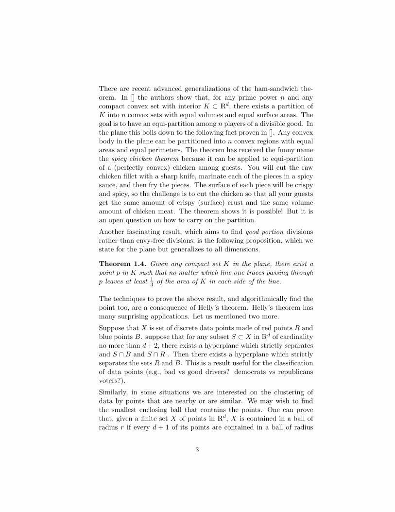
Suppose that X is set of discrete data points made of red points R andblue points B. suppose that for any subset S ⊂ X in Rd of cardinalityno more than d+ 2, there exists a hyperplane which strictly separatesand S ∩B and S ∩R . Then there exists a hyperplane which strictlyseparates the sets R and B. This is a result useful for the classificationof data points (e.g., bad vs good drivers? democrats vs republicansvoters?).

Similarly, in some situations we are interested on the clustering ofdata by points that are nearby or are similar. We may wish to findthe smallest enclosing ball that contains the points. One can provethat, given a finite set X of points in Rd, X is contained in a ball ofradius r if every d + 1 of its points are contained in a ball of radius

3

r. For example,if you are given s points in the plane such that everythree of them are contained in a disk of radius 1, then all s points arecontained in a disk of radius 1. The techniques are stronger and onecan use them to solve the following problem:

Suppose the points represent bad objects that need to be containedin a smallest-radius enclosing ball, but we have lack of exactly howmany and where the points are. There is a risk. You are given points(u1, u2, . . . , ud) ∈ Rd, belonging to an unknown measurable set. Yourgoal is to find the center x the ball of smallest radius R that containsa “large proportion” of those points. E.g., if these are cancerous cells,you do not wish to loose more than 1 percent of the bad cells. But thebad news you may not know explicitly the probability measure. Theare sampling algorithms to attempt this problem. Clearly this is anstochastic optimization problem that can be formulated as

min R

subject to Pr[

√√√√ d∑1

(xi − ui)2 −R ≤ 0] ≥ 1− ε,x ∈ Rd+1.

• The games of chicken, matching pennies & Nash Equilibria.

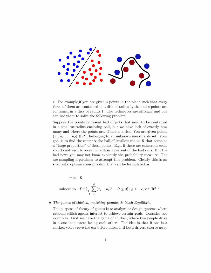
The purpose of theory of games is to analyze or design systems whererational selfish agents interact to achieve certain goals. Consider twoexamples. First we have the game of chicken, where two people drivein a one lane street facing each other. The idea is that if one is achicken you swerve the car before impact. If both drivers swerve away

4

then they are both chickens (not a very pleasant nickname). Of courseif nobody is chicken the outcome is fatal. What is the best strategyto follow? Clearly, no pure strategy will suffice to please both players.A key idea to find a compromise, some kind of stable solution, is tohave a traffic light that takes turns assigning whose turn is it to swerveaway before from crashing. This method has a superior payoff over thepure strategies (and preserves the lifes of players).

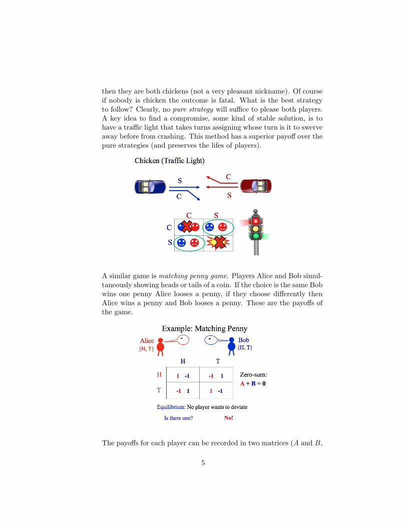
A similar game is matching penny game. Players Alice and Bob simul-taneously showing heads or tails of a coin. If the choice is the same Bobwins one penny Alice looses a penny, if they choose differently thenAlice wins a penny and Bob looses a penny. These are the payoffs ofthe game.

The payoffs for each player can be recorded in two matrices (A and B,

5

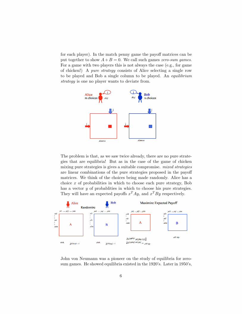
for each player). In the match penny game the payoff matrices can beput together to show A+B = 0. We call such games zero-sum games.For a game with two players this is not always the case (e.g., for gameof chicken!) A pure strategy consists of Alice selecting a single rowto be played and Bob a single column to be played. An equilibriumstrategy is one no player wants to deviate from.

The problem is that, as we saw twice already, there are no pure strate-gies that are equilibria! But as in the case of the game of chickenmixing pure strategies is gives a suitable compromise. mixed strategiesare linear combinations of the pure strategies proposed in the payoffmatrices. We think of the choices being made randomly. Alice has achoice x of probabilities in which to choose each pure strategy, Bobhas a vector y of probablities in which to choose his pure strategies.They will have an expected payoffs xTAy, and xTBy respectively.

John von Neumann was a pioneer on the study of equilibria for zero-sum games. He showed equilibria existed in the 1920’s. Later in 1950’s,

6

with the emergence of linear optimization and the simplex methodDantzig showed that zero-sum games are special in that equilibria canbe computed solving a linear optimization problem. In 1949, JohnNash showed that in any game there is always at least one mixedstrategy that is an equilibrium solution. We call them Nash equilibria.Later we will prove Nash’s theorem for which he received the Nobelprize in Economics. The existence of Nash equilibria is proven usingfixed-point theorem, such as Brouwer’s and Kakutani’s theorem. Theyin turn are consequences of Sperner’s lemma. We will look at thedetails of these theorems and try to discuss some of the computationalmethods.

• Coin-exchange and bin-packing problems.

Suppose we are given some coins of different denominations. One canask the following natural questions (try to answer them for the twocoins in the picture):

1. How many ways are there to give change for b cents?

2. What is the smallest number of coins necessary to do so?

3. What is largest quantity b that cannot be expressed using thecoins?

4. Which values of b have exactly 20 ways to be broken in change?

Another similar family of problems is that for the bin-packing problemsThe problem is we are given n items and n bins. Item j has size sjand bin i has capacity c. The goal is to assign each item to a bin (topack the bins!) so that the total weight of the items in each bin doesnot exceed c, but the number of bins used is smallest possible. This

7

is a difficult problem and for the most part one is interested on goodapproximation algorithms.

Let us consider one instance of the problem. Let (s, a) be an instancefor bin packing with item sizes s1, . . . , sd ∈ [0, 1] and a vector a ∈ Zd≥0

of item multiplicities. In other words, our instance contains ai manycopies of an item of size si. (we assume that si is given as a rationalnumber and ∆ is the largest number appearing in the denominator ofsi or the multiplicities ai.)

Consider the polytope P := x ∈ Zd≥0 | sTx ≤ 1. Now the binpacker’s objective is to select a minimum number of vectors from Pthat sum up to a,

min

1Tλ |∑x∈P

λx · x = a; λ ∈ ZP≥0

(1)

where λx is the weight that is given to x ∈ P. This special case isknown as the (1-dimensional) cutting stock problem.

Bin packing and the cutting stock problem belong to a family of prob-lems that consist of selecting integer points in a polytope with multi-plicities. In fact, several scheduling problems fall into this frameworkas well, where the polytope describes the set of jobs that are admis-sible on a machine under various constraints. Recently Goemans andRothvoss showed

Theorem 1.5. For any Bin Packing instance (s, a) with s ∈ [0, 1]d

and a ∈ Zd≥0, an optimum integral solution can be computed in time

(log ∆)2O(d)

where ∆ is the largest integer appearing in a denominatorsi or in a multiplicity ai.

Fundamentally, one is interested on finding the sparsest representationof a vector b from a list of vectors X = (x1, . . . , xt) ⊂ Rd which wethink of as the columns of the matrix A In the case of the cuttingstock problem the vectors xi are the possible packing patterns. Theydefine the following sparse representation problem.

min ‖x‖0, Ax = b, x ≥ 0, x ∈ Zt. (2)

Here, ‖ · ‖0 denotes the 0-norm, which counts the cardinality of thesupport of x, i.e. supp(x) = i : xi 6= 0. In other words, the value of

8

‖x‖0 equals the number of non-zero entries in the vector x. Problem(2) aims to find the vector of minimal support.

There is a rich literature about this problem. The sparsest solutionof a system of linear equations is quite important in applications tosignal processing [?], cryptography and coding theory [?]. Sparse in-teger solutions also appear in the context of finding guarantees forbin-packing problems via the Gilmore-Gomory formulation [?], as firstsuggested in [?]. More generally, upper bounds given for the size ofthe sparsest integer solution indicate that if there exists an optimalsolution to such an integer program, then there exists one which ispolynomial in the number of equations and the maximum binary en-coding length among integers in the objective function vector and theconstraint matrix (see Section 3 in [?]). The sparsity of the solution isalso strongly connected to the integer Caratheodory problem (see [?]and the references there).

It is known that even for real variables, the 0-norm minimization isNP-hard [?], but that the greedy algorithm provides a guaranteedapproximation in this setting. Moreover, when one looks at randommatrices, one can prove nice properties for the size of the solution [?].It is precisely such structural differences that we wish to study herefor integer solutions.

There are two important geometric objects associated with the sparserepresentation problem. First, the conic hull of X is the set

cone(X) = λ1x1 + · · ·+ λtxt : x1, . . . , xt ∈ X,λ1, . . . , λt ∈ R≥0,

and the semigroup of X or the integer conic hull of X is the set

Sg(X) = λ1x1 + · · ·+ λtxt : x1, . . . , xt ∈ X,λ1, . . . , λt ∈ Z≥0.

For each b ∈ Sg(X), we are interested in finding upper bounds and theasymptotic behavior of the function

m0(b) = min‖a‖0 : a ∈ PX(b),

where PX(b) = a ∈ Zt≥0 : a1x1 + · · ·+ atxt = b is the solution set forb. Note that the convex hull of PX(b) is a lattice polytope.

In the context of the applications, the upper bounds for m0(b) are ofspecial interest. The problem of estimatingM0(X) := maxb∈Sg(X) m0(b)

9

goes back to classical results on the integer Caratheodory problem.Cook, Fonlupt, and Schrijver [?] showed that M0(X) ≤ 2d − 1 ifC = cone(X) is pointed and X forms a Hilbert basis of C. This resultwas later improved by Sebo [?] to M0(X) ≤ 2d−2. It remains an openquestion to determine the exact value even when X is a Hilbert basis.For an arbitrary set X ⊂ Zd, Eisenbrand and Shmonin [?] obtainedthe bound

M0(X) ≤ 2d log(4d‖X‖∞), (3)

where ‖X‖∞ = maxx∈X ‖x‖∞.

There are two challenging open problems: What are the optimal boundsfor m0(b) in terms of the generating set X? What is the asymptoticbehavior of the univariate function f0(λ) := m0(λb) obtained fromsuccessive dilations of the vector b?

Let us conclude this introduction with a bird-view of the four founda-tional combinatorial theorems from geometry and topology. First, two fromcombinatorial topology, Sperner’s and Fan-Tucker’s lemmas, and then, sec-ond, two corner stones of combinatorial convex geometry, Caratheodory, andHelly theorems. We will see how these four “mathematical cornerstones” aredeeply interrelated among themselves (e.g., the topological results imply thethe geometric statements, while they imply each other in some form or an-other), and each theorem, is in fact a family of theorems of certain type,with many generalizations, corollaries and extensions. The landscape is solovely one is often tempted to stay longer at many stops, but remember ourfinal destination is the world of applications!

First, Sperner’s Lemma is a combinatorial statement about labelingsof triangulated simplices. It is quite well-known as equivalent with thetopological fixed-point theorem of Brouwer [?, ?].

Theorem (Sperner’s lemma, 1928 []). Let T be a triangulation of a (n−1)-simplex, and suppose that the vertices of T have a labeling satisfying theseconditions: each vertex of the triangulation is assigned a unique label fromthe set 1, 2, . . . , n, and each other vertex v of T is assigned a label of oneof the vertices of P in carr(v).

Any Sperner labeling of a triangulation T of the d-simplex must containan odd number of cells for which all their labels are distinct. In particular,there is at least one such cell.

Second, the Fan’s lemma is a combinatorial analogue of the famousBorsuk-Ulam theorem (see []). We need to start with a little bit of ter-minology and notation. Denote by Sd be the unit d-sphere, the set of all

10

points of unit Euclidean distance from the origin in Rd+1. Any pair of pointsin Sd of the form x,−x is a pair of antipodes in Sd. A triangulation of Sn hasan anti-symmetric labeling ` if `(−v) = −`(v) for all vertices v. A labelinghas a complementary edge if some adjacent pair of vertices has labels thatsum to zero. A simplex is alternating if its vertex’s labels are distinct inmagnitude and alternate signs, when arranged in order of increasing value.

Theorem (Fan’s lemma 1946 []). Let T be a symmetric triangulation of Sn

with an m-labeling that is anti-symmetric and has no complementary edge.Then has at least one positive alternating n-simplex.

We recall now Caratheodory’s, and Helly’s theorems. They are clearlyamong the most important theorems in convex geometry.

Theorem (C. Caratheodory 1911 [?]). Let S be any subset of Rd. Theneach point in the convex hull of S is a convex combination of at most d+ 1points of S.

Theorem (E. Helly, 1913 [?]). Let F be a finite family of convex sets ofRd. If

⋂K 6= ∅ for all K ⊂ F of cardinality at most d+ 1, then⋂F 6= ∅.

We chose these four theorems because they are centrally located andessential! One can sense this because they imply many of the later re-sults and they have many corollaries generalizations and extensions. Ourcourse presents a interconnected theory and we can see what theorems implyothers, E.g., Sperner’s lemma implies Helly theorems. Fan-Tucker impliesCaratheodory.

(see the diagram of implications below).These four fantastic theorems and their variations are key for discrete

applied mathematics today; a fact we will demonstrate with plenty of ex-amples.

2 Combinatorial Topology Tools: Midterm 1

A triangulation is a subdivision by simplices that meet either face-to-face ornot at all. Each simplex is the affine hull of its vertices; these are the verticesof the triangulation. We are interested on coloring or labeling the vertices ofa triangulated manifold, most often a triangulated ball or a sphere followingcertain rules and then make conclusions about multicolored simplices insidethe triangulation.

11

2.1 Lectures 2: Preliminaries

The line segment joining two points x, y ∈ Rd is given by the set of allpoints of the form

[x, y] := γx+ (1− γ)y : 0 ≤ γ ≤ 1.A set A ⊂ Rd is convex if it contains the line segment joining two of its

points, for every pair of points in the set. A lot of our arguments will relyon convex sets.

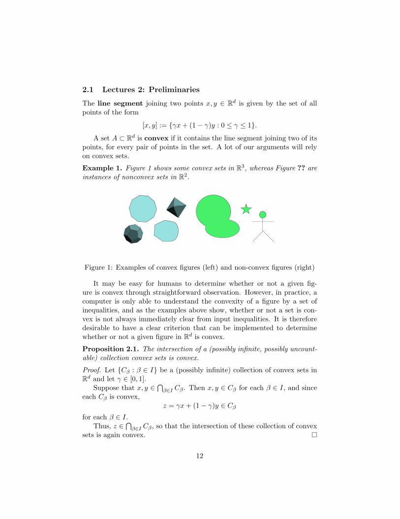
Example 1. Figure 1 shows some convex sets in R3, whereas Figure ?? areinstances of nonconvex sets in R2.

Figure 1: Examples of convex figures (left) and non-convex figures (right)

It may be easy for humans to determine whether or not a given fig-ure is convex through straightforward observation. However, in practice, acomputer is only able to understand the convexity of a figure by a set ofinequalities, and as the examples above show, whether or not a set is con-vex is not always immediately clear from input inequalities. It is thereforedesirable to have a clear criterion that can be implemented to determinewhether or not a given figure in Rd is convex.

Proposition 2.1. The intersection of a (possibly infinite, possibly uncount-able) collection convex sets is convex.

Proof. Let Cβ : β ∈ I be a (possibly infinite) collection of convex sets inRd and let γ ∈ [0, 1].

Suppose that x, y ∈ ⋂β∈I Cβ. Then x, y ∈ Cβ for each β ∈ I, and sinceeach Cβ is convex,

z = γx+ (1− γ)y ∈ Cβfor each β ∈ I.

Thus, z ∈ ⋂β∈I Cβ, so that the intersection of these collection of convexsets is again convex.

12

Hyperplanes and Half-Spaces

For every nonzero c ∈ Rd, we may associate c with a linear functionalf : Rd → R. An example of this is f : Rd → R where f(x) = c · x, with theusual dot product in Rd.

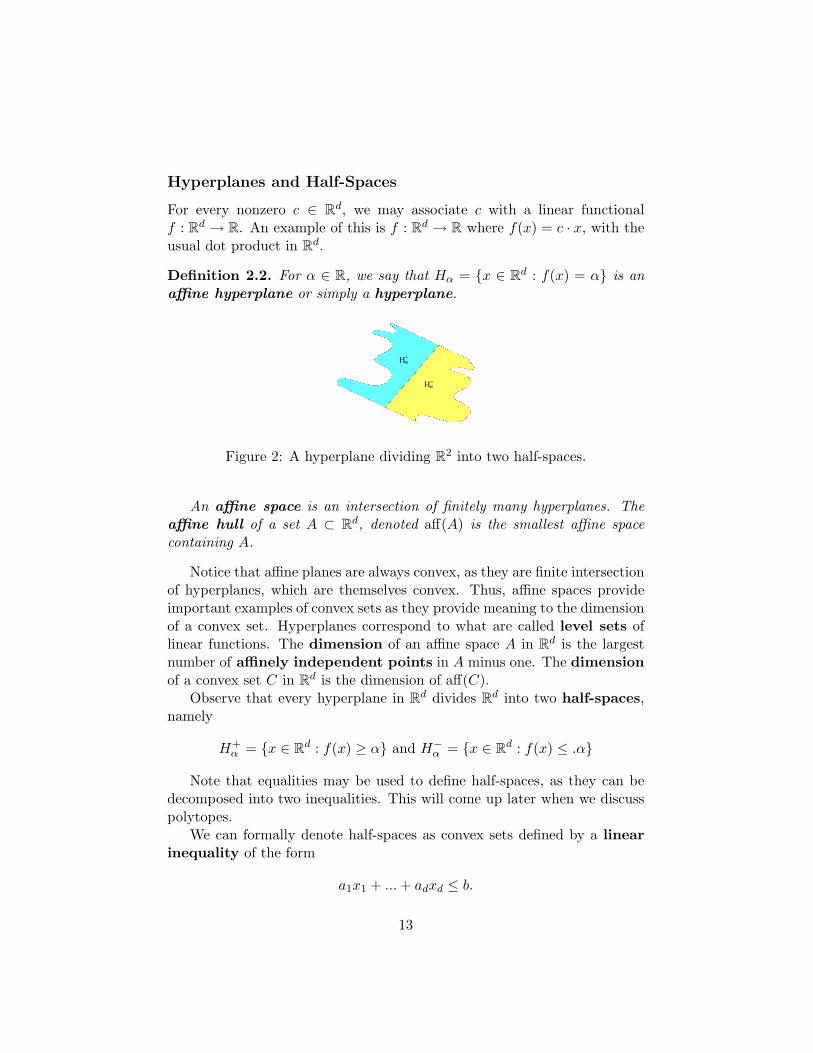
Definition 2.2. For α ∈ R, we say that Hα = x ∈ Rd : f(x) = α is anaffine hyperplane or simply a hyperplane.

H+α

Hα-

Figure 2: A hyperplane dividing R2 into two half-spaces.

An affine space is an intersection of finitely many hyperplanes. Theaffine hull of a set A ⊂ Rd, denoted aff(A) is the smallest affine spacecontaining A.

Notice that affine planes are always convex, as they are finite intersectionof hyperplanes, which are themselves convex. Thus, affine spaces provideimportant examples of convex sets as they provide meaning to the dimensionof a convex set. Hyperplanes correspond to what are called level sets oflinear functions. The dimension of an affine space A in Rd is the largestnumber of affinely independent points in A minus one. The dimensionof a convex set C in Rd is the dimension of aff(C).

Observe that every hyperplane in Rd divides Rd into two half-spaces,namely

H+α = x ∈ Rd : f(x) ≥ α and H−α = x ∈ Rd : f(x) ≤ .α

Note that equalities may be used to define half-spaces, as they can bedecomposed into two inequalities. This will come up later when we discusspolytopes.

We can formally denote half-spaces as convex sets defined by a linearinequality of the form

a1x1 + ...+ adxd ≤ b.

13

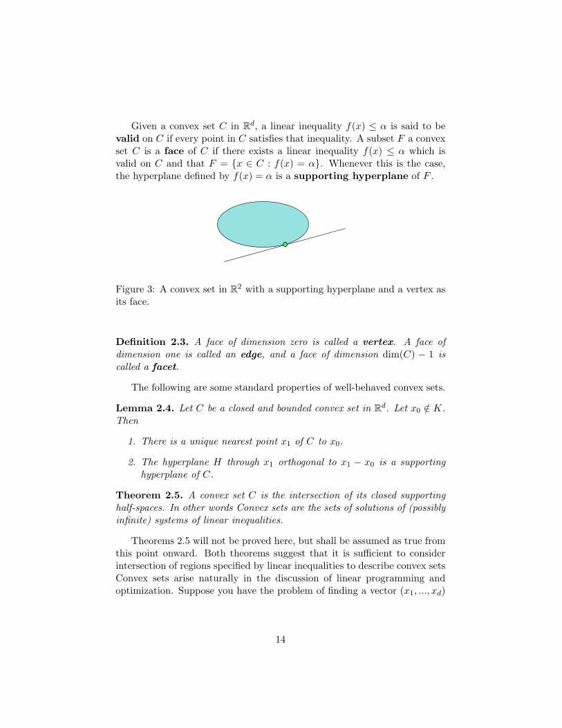
Given a convex set C in Rd, a linear inequality f(x) ≤ α is said to bevalid on C if every point in C satisfies that inequality. A subset F a convexset C is a face of C if there exists a linear inequality f(x) ≤ α which isvalid on C and that F = x ∈ C : f(x) = α. Whenever this is the case,the hyperplane defined by f(x) = α is a supporting hyperplane of F .

Figure 3: A convex set in R2 with a supporting hyperplane and a vertex asits face.

Definition 2.3. A face of dimension zero is called a vertex. A face ofdimension one is called an edge, and a face of dimension dim(C) − 1 iscalled a facet.

The following are some standard properties of well-behaved convex sets.

Lemma 2.4. Let C be a closed and bounded convex set in Rd. Let x0 /∈ K.Then

1. There is a unique nearest point x1 of C to x0.

2. The hyperplane H through x1 orthogonal to x1 − x0 is a supportinghyperplane of C.

Theorem 2.5. A convex set C is the intersection of its closed supportinghalf-spaces. In other words Convex sets are the sets of solutions of (possiblyinfinite) systems of linear inequalities.

Theorems 2.5 will not be proved here, but shall be assumed as true fromthis point onward. Both theorems suggest that it is sufficient to considerintersection of regions specified by linear inequalities to describe convex setsConvex sets arise naturally in the discussion of linear programming andoptimization. Suppose you have the problem of finding a vector (x1, ..., xd)

14

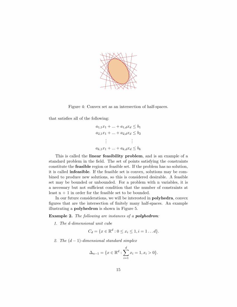
Figure 4: Convex set as an intersection of half-spaces.

that satisfies all of the following:

a1,1x1 + ...+ a1,dxd ≤ b1a2,1x1 + ...+ a2,dxd ≤ b2

......

ak,1x1 + ...+ ak,dxd ≤ bkThis is called the linear feasibility problem, and is an example of a

standard problem in the field. The set of points satisfying the constraintsconstitute the feasible region or feasible set. If the problem has no solution,it is called infeasible. If the feasible set is convex, solutions may be com-bined to produce new solutions, so this is considered desirable. A feasibleset may be bounded or unbounded. For a problem with n variables, it isa necessary but not sufficient condition that the number of constraints atleast n + 1 in order for the feasible set to be bounded.

In our future considerations, we will be interested in polyhedra, convexfigures that are the intersection of finitely many half-spaces. An exampleillustrating a polyhedron is shown in Figure 5.

Example 2. The following are instances of a polyhedron:

1. The d-dimensional unit cube

Cd = x ∈ Rd : 0 ≤ xi ≤ 1, i = 1 . . . d.

2. The (d− 1)-dimensional standard simplex

∆n−1 = x ∈ Rd :d∑i=1

xi = 1, xi > 0.

15

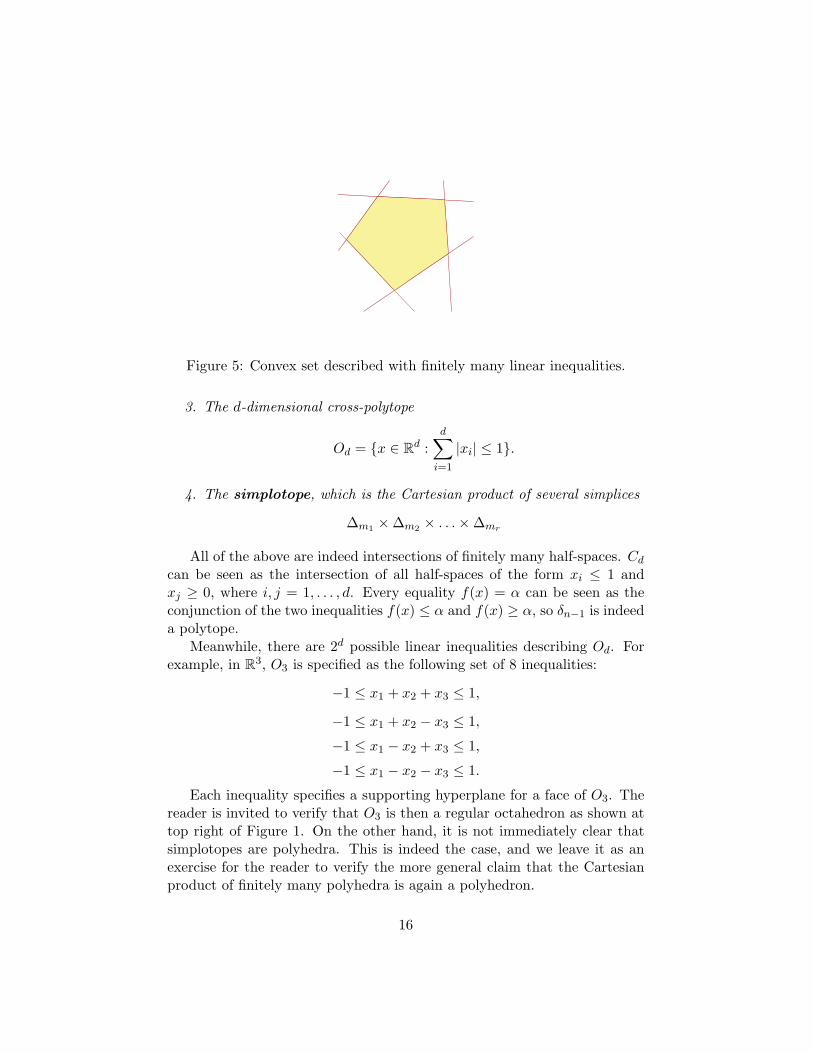
Figure 5: Convex set described with finitely many linear inequalities.

3. The d-dimensional cross-polytope

Od = x ∈ Rd :d∑i=1

|xi| ≤ 1.

4. The simplotope, which is the Cartesian product of several simplices

∆m1 ×∆m2 × . . .×∆mr

All of the above are indeed intersections of finitely many half-spaces. Cdcan be seen as the intersection of all half-spaces of the form xi ≤ 1 andxj ≥ 0, where i, j = 1, . . . , d. Every equality f(x) = α can be seen as theconjunction of the two inequalities f(x) ≤ α and f(x) ≥ α, so δn−1 is indeeda polytope.

Meanwhile, there are 2d possible linear inequalities describing Od. Forexample, in R3, O3 is specified as the following set of 8 inequalities:

−1 ≤ x1 + x2 + x3 ≤ 1,

−1 ≤ x1 + x2 − x3 ≤ 1,

−1 ≤ x1 − x2 + x3 ≤ 1,

−1 ≤ x1 − x2 − x3 ≤ 1.

Each inequality specifies a supporting hyperplane for a face of O3. Thereader is invited to verify that O3 is then a regular octahedron as shown attop right of Figure 1. On the other hand, it is not immediately clear thatsimplotopes are polyhedra. This is indeed the case, and we leave it as anexercise for the reader to verify the more general claim that the Cartesianproduct of finitely many polyhedra is again a polyhedron.

16

Convex and Affine Combinations

Even though not every shape in nature appears as a convex set, we mayalways use convex sets to approximate these shapes!

Definition 2.6. Let A ⊂ Rd. The convex hull of A, denoted by conv(A), isthe intersection of all the convex sets containing A, that is, it is the smallestconvex set that contains A.

We usually denote by conv(a1, . . . , an) for the convex hull of a1, . . . , an ⊂Rd.

Definition 2.7. A polytope is the convex hull of a finite set of points inRd. It is the smallest convex set containing the points.

Definition 2.8. Given finitely many points A = x1, x2, ..., xd, we say thelinear combination

∑di=1 γixi is

• a conic combination if all γi are nonnegative.

• an affine combination if∑d

i=1 γi = 1

• a convex combination if it is both a conic and affine combination.

Lemma 2.9. For a set of points A in Rd we have that conv(A) equals theset of all finite convex combinations of points in A.

Sketch of Proof Denote B as the set of all finite convex combinationsof points in A. In other words, x ∈ B if and only if there is a finite subsetS = x1, . . . , xn of A with x =

∑ni=1 γixi, γi ≥ 0 for all i and

∑ni=1 γi = 1.

We need to prove that B = conv(A).Let us first prove that B is a convex set containing A. Obviously, each

x ∈ A can be expressed as a finite convex combination, that is x = 1 · x,so A ⊂ B. Now, if u, v ∈ B, then we may assume that there is a commonsubset S = x1, . . . , xn of A such that u and v can be expressed as convexcombinations of points in S (Why?). Suppose that

u =n∑i=1

γixi

and

v =n∑i=1

γ′ixi,

whereγi, γ

′i ≥ 0

17

andn∑i=1

γi =n∑i=1

γ′i = 1.

Thus, if λ ∈ [0, 1], then we obtain

λu+ (1− λ) =n∑i=1

λγixi + (1− λ)γ′ixi

=n∑i=1

λγi + (1− λ)γ′i]xi.

For each i, we have

λγi + (1− λ)γ′i ≥ λ(0) + (1− λ)(0) = 0,

and moreover,

n∑i=1

λγi + (1− λ)γ′i = λ

n∑i=1

γi + (1− λ)n∑i=1

γ′i

= λ(1) + (1− λ)(1)= 1.

Thus, λu + (1 − λ)v is also a finite convex combination of points in A, soB is indeed a convex set containing A. We then have conv(A) ⊂ B by thedefinition of convex hull of A.

The interested reader is then invited to prove that B ⊂ conv(A) byshowing that if C is any convex set containing A, then B ⊂ C. It thenfollows that B ⊂ conv(A), so conv(A) is precisely the set of all finite convexcombinations of points in A.

Definition 2.10. A set of points x1, ..., xk is affinely dependent if thereis a nontrivial linear combination

∑ki=1 γixi = 0 with

∑ki=1 γi = 0. Other-

wise, it is said to be affinely independent.

Lemma 2.11. A set of d+ 2 or more points in Rd is affinely dependent.

Proof. Suppose that x1, . . . , xk are vectors in Rd, and consider the vectorsx′1, . . . , x

′k in Rd+1 where x′i is the vector whose first d components coincide

with those of xi.

18

Since k > d + 1, then this collection of vectors is linearly dependent,that is, there are γi ∈ R with

∑ki=1 γix

′i = 0 and γ1, . . . , γk are not all zero.

Thus, we have both∑k

i=1 γixi = 0 and∑k

i=1 γi = 0 by considering thelinear dependence on the first d components and on the last component ofx′i separately.

Furthermore, this linear combination is nontrivial, because, some γj isnonzero. By definition, x1, . . . , xk forms an affinely dependent set.

We have the following characterization of affinely independent sets inRd.

Lemma 2.12. A set B ⊂ Rd is affinely independent if and only if everypoint in aff(B) has a unique representation as an affine combination ofpoints in B.

Proof. Suppose that B = x1, . . . , xk and that some point x in aff(B)admits two different affine combinations

x =k∑i=1

βixi,

and

x =k∑i=1

γixi,

with βj 6= γj for some j and

k∑i=1

βi =k∑i=1

γi = 1.

Then, by taking differences,

k∑i=1

(βi − γi)xi = 0,

withk∑i=1

(βi − γi) =k∑i=1

βi −k∑i=1

γi = 1− 1 = 0.

This linear combination of 0 is nontrivial, because βj − γj 6= 0, so thatB is an affinely dependent set. Hence, if every point in aff(B) is uniquely

19

expressed as an affine combination of points in B, then B must be affinelyindependent.

On the other hand, if x ∈ aff(B), then it can be shown that x can beexpressed as an affine combination of some points in B. In other words,x =

∑mi=1 αixi and

∑mi=1 αi = 1 where x1, . . . , xm ⊂ B. If B is affinely

independent, then B cannot have more than d + 1 points by Lemma 2.11,let B = x1, . . . , xk+1 for some k ≤ d.

We claim that the set x1−xk+1, . . . , xk−xk+1 is linearly independentover R. Suppose that

∑ki=1 γi(x1−xk+1) = 0, for some γi ∈ R, i = 1, . . . , k.

Thus,∑k+1

j=1 βjxj = 0, where βj = γj for j = 1, . . . , k and βk+1 = −∑kj=1 γj ,

so that∑k+1

j=1 βj = 0. The affine independence of B forces βj = 0 for allj = 1, . . . , k + 1, so we have γi = 0 for all i = 1, . . . , k. This demonstratesthe linear independence of the set x1 − xk+1, . . . , xk − xk+1.

Now, if x ∈ B, then by the remark above, x =∑k+1

i=1 αixi and∑k+1

i=1 αi =1. We then obtain

x− xk+1 =k∑i=1

αi(xi − xk+1)

As we know that the set x1 − xk+1, . . . , xk − xk+1 is linearly indepen-dent, the coefficients αi must be unique. x =

∑k+1i=1 αixi + xk+1

The proof of Lemma 2.11 offers a test for affine dependence of pointsx1, . . . , xk, one may treat them as vectors in Rd and write them as columnsof a matrix, and append a row of 1’s to the bottom as follows:

M =

x1,1 x2,1 . . . xk,1x1,2 x2,2 . . . xk,2

......

. . ....

x1,d x2,d . . . xk,d1 1 . . . 1

If the null space of the M is trivial, the points are then affinely independent.Otherwise, they are affinely dependent.

Triangulations of Convex Polytopes and Point Configurations

A point configuration is a finite set of points A in Rd. As noted earlierin the lectures, a convex polytope is the convex hull of finitely many points.Recall that from Lemma 2.9, we may describe a convex polytope P with

20

vertices p1, . . . , pn as

P = conv(p1, ..., pn) :=

n∑i=1

γipi : γi ≥ 0, ∀i = 1, . . . , n, andn∑i=1

αi = 1

.

Recall a k-dimensional simplex is the convex hull of a set of k+1 affinelyindependent points.

Definition 2.13. A triangulation of a point configuration A is a finitecollection T of simplices σ that partitions conv(A) such that

1.⋃σ∈T

σ = conv(A).

2. Any pair of simplices intersects at a (possibly empty) common face.

3. Every vertex of T is contained in A.

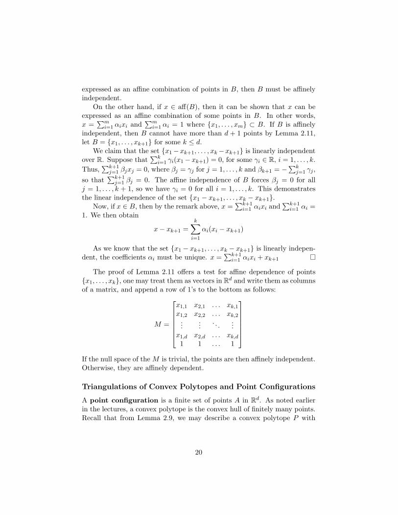
Observe that we need not use all points in the interior of conv(A). How-ever, we are not allowed to add points that were absent in A into a trian-gulation of A. Figure 6 illustrates an example of valid triangulation thatdoes not use all points of A, whereas Figure 7 displays examples that arenot triangulations.

A common face in the definition refers to the intersection between twosimplices being a face for both of the simplices. For example, on the leftpart of Figure 8, although an edge is a 1-dimensional face for any one of thethe triangles on the right, the same edge is not a face for the triangle on theleft.

On the other hand, two simplices are not allowed to intersect at theinterior for both of them, as portrayed on the right part of Figure 8.

Figure 6: A permissible triangulation.

21

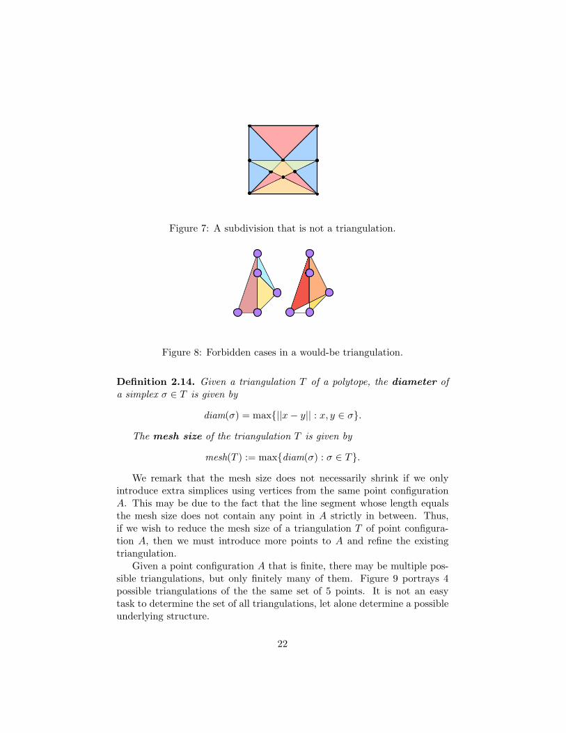
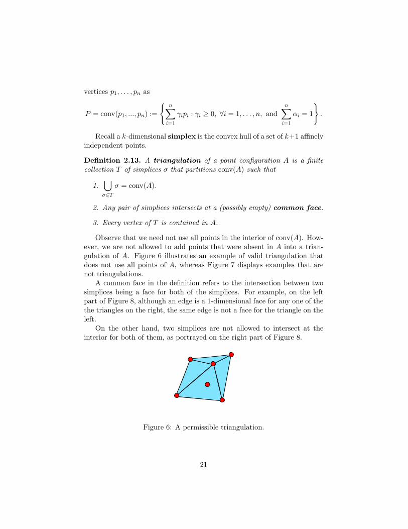
Figure 7: A subdivision that is not a triangulation.

Figure 8: Forbidden cases in a would-be triangulation.

Definition 2.14. Given a triangulation T of a polytope, the diameter ofa simplex σ ∈ T is given by

diam(σ) = max||x− y|| : x, y ∈ σ.

The mesh size of the triangulation T is given by

mesh(T ) := maxdiam(σ) : σ ∈ T.

We remark that the mesh size does not necessarily shrink if we onlyintroduce extra simplices using vertices from the same point configurationA. This may be due to the fact that the line segment whose length equalsthe mesh size does not contain any point in A strictly in between. Thus,if we wish to reduce the mesh size of a triangulation T of point configura-tion A, then we must introduce more points to A and refine the existingtriangulation.

Given a point configuration A that is finite, there may be multiple pos-sible triangulations, but only finitely many of them. Figure 9 portrays 4possible triangulations of the the same set of 5 points. It is not an easytask to determine the set of all triangulations, let alone determine a possibleunderlying structure.

22

Figure 9: Four possible triangulations for the same point configuration.

Having covered the basic terminology for triangulations, we are ready todefine barycentric triangulations.

Definition 2.15. The barycenter of a simplex σ = conv(a1, . . . , ak+1)where a1, . . . , ak+1 is affinely independent, is the point

k+1∑i=1

1k + 1

ai.

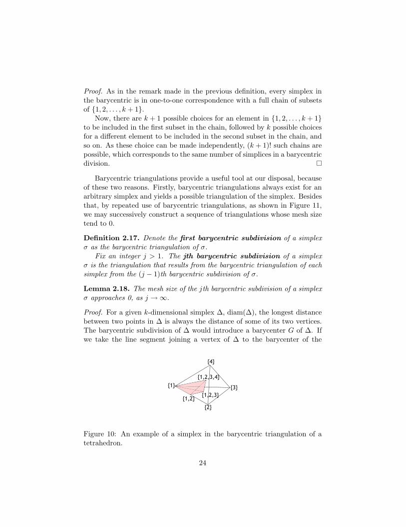
The barycentric triangulation Tb of a simplex, denoted σ = conv(a1, . . . , ak+1)has the following characterization:

1. The vertices of the triangulation Tb are the barycenters of faces of σ(including the vertices a1, . . . , ak+1 themselves).

2. If ai1 , ai2 , . . . , aid are the d vertices contained in a face F of σ, then as-sociate the barycenter of F with the subset i1, i2, . . . , id of 1, 2, . . . , k+1. Observe that this now gives a bijection between the set of faces ofσ with the subsets of 1, 2, . . . , k + 1.

3. The simplices in Tb are the convex hulls of the subsets of barycentersb1, b2, . . . , bk+1 such that corresponding subsets form a full chain ofcontainment in the indices:

i1 ⊂ i1, i2 ⊂ . . . ⊂ i1, i2, . . . , ik+1.

In other words, there cannot be further insertions of subsets withinthis chain. An example is shown for a tetrahedron, a 3-dimensionalsimplex, in Figure 10.

Observation 2.16. There are (k+ 1)! simplices in the barycentric triangu-lation of a k-dimensional simplex.

23

Proof. As in the remark made in the previous definition, every simplex inthe barycentric is in one-to-one correspondence with a full chain of subsetsof 1, 2, . . . , k + 1.

Now, there are k + 1 possible choices for an element in 1, 2, . . . , k + 1to be included in the first subset in the chain, followed by k possible choicesfor a different element to be included in the second subset in the chain, andso on. As these choice can be made independently, (k + 1)! such chains arepossible, which corresponds to the same number of simplices in a barycentricdivision.

Barycentric triangulations provide a useful tool at our disposal, becauseof these two reasons. Firstly, barycentric triangulations always exist for anarbitrary simplex and yields a possible triangulation of the simplex. Besidesthat, by repeated use of barycentric triangulations, as shown in Figure 11,we may successively construct a sequence of triangulations whose mesh sizetend to 0.

Definition 2.17. Denote the first barycentric subdivision of a simplexσ as the barycentric triangulation of σ.

Fix an integer j > 1. The jth barycentric subdivision of a simplexσ is the triangulation that results from the barycentric triangulation of eachsimplex from the (j − 1)th barycentric subdivision of σ.

Lemma 2.18. The mesh size of the jth barycentric subdivision of a simplexσ approaches 0, as j →∞.

Proof. For a given k-dimensional simplex ∆, diam(∆), the longest distancebetween two points in ∆ is always the distance of some of its two vertices.The barycentric subdivision of ∆ would introduce a barycenter G of ∆. Ifwe take the line segment joining a vertex of ∆ to the barycenter of the

1

2

31,2,3

4

1,2

1,2,3,4

Figure 10: An example of a simplex in the barycentric triangulation of atetrahedron.

24

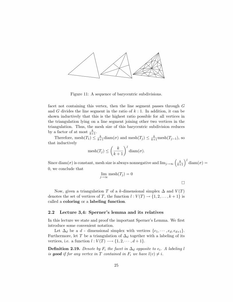
Figure 11: A sequence of barycentric subdivisions.

facet not containing this vertex, then the line segment passes through Gand G divides the line segment in the ratio of k : 1. In addition, it can beshown inductively that this is the highest ratio possible for all vertices inthe triangulation lying on a line segment joining other two vertices in thetriangulation. Thus, the mesh size of this barycentric subdivision reducesby a factor of at most k

k+1 .Therefore, mesh(T1) ≤ k

k+1diam(σ) and mesh(Tj) ≤ kk+1mesh(Tj−1), so

that inductively

mesh(Tj) ≤(

k

k + 1

)jdiam(σ).

Since diam(σ) is constant, mesh size is always nonnegative and limj→∞

(kk+1

)jdiam(σ) =

0, we conclude thatlimj→∞

mesh(Tj) = 0

Now, given a triangulation T of a k-dimensional simplex ∆ and V (T )denotes the set of vertices of T , the function l : V (T )→ 1, 2, . . . , k + 1 iscalled a coloring or a labeling function.

2.2 Lecture 3,4: Sperner’s lemma and its relatives

In this lecture we state and proof the important Sperner’s Lemma. We firstintroduce some convenient notation.

Let ∆d be a d - dimensional simplex with vertices e1, · · · , ed, ed+1.Furthermore, let T be a triangulation of ∆d together with a labeling of itsvertices, i.e. a function l : V (T ) −→ 1, 2, · · · , d+ 1.Definition 2.19. Denote by Fi the facet in ∆d opposite to ei. A labeling lis good if for any vertex in T contained in Fi we have l(v) 6= i.

25

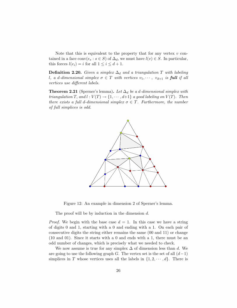
Note that this is equivalent to the property that for any vertex v con-tained in a face conv(es : s ∈ S) of ∆d, we must have l(v) ∈ S. In particular,this forces l(ei) = i for all 1 ≤ i ≤ d+ 1.

Definition 2.20. Given a simplex ∆d and a triangulation T with labelingl, a d-dimensional simplex σ ∈ T with vertices v1, · · · , vd+1 is full if allvertices use different labels.

Theorem 2.21 (Sperner’s lemma). Let ∆d be a d-dimensional simplex withtriangulation T, and l : V (T )→ 1, · · · , d+1 a good labeling on V (T ). Thenthere exists a full d-dimensional simplex σ ∈ T . Furthermore, the numberof full simplices is odd.

Figure 12: An example in dimension 2 of Sperner’s lemma.

The proof will be by induction in the dimension d.

Proof. We begin with the base case d = 1. In this case we have a stringof digits 0 and 1, starting with a 0 and ending with a 1. On each pair ofconsecutive digits the string either remains the same (00 and 11) or change(10 and 01). Since it starts with a 0 and ends with a 1, there must be anodd number of changes, which is precisely what we needed to check.

We now assume is true for any simplex ∆ of dimension less than d. Weare going to use the following graph G. The vertex set is the set of all (d−1)simplices in T whose vertices uses all the labels in 1, 2, · · · , d. There is

26

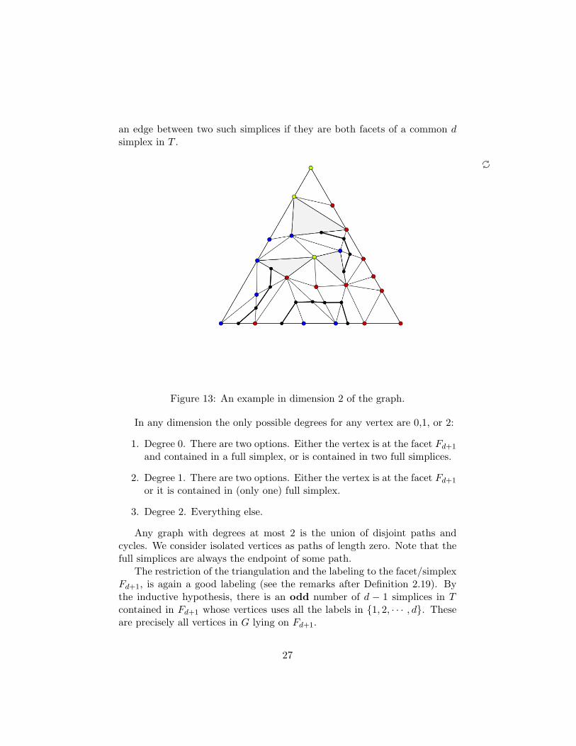
an edge between two such simplices if they are both facets of a common dsimplex in T .

Figure 13: An example in dimension 2 of the graph.

In any dimension the only possible degrees for any vertex are 0,1, or 2:

1. Degree 0. There are two options. Either the vertex is at the facet Fd+1

and contained in a full simplex, or is contained in two full simplices.

2. Degree 1. There are two options. Either the vertex is at the facet Fd+1

or it is contained in (only one) full simplex.

3. Degree 2. Everything else.

Any graph with degrees at most 2 is the union of disjoint paths andcycles. We consider isolated vertices as paths of length zero. Note that thefull simplices are always the endpoint of some path.

The restriction of the triangulation and the labeling to the facet/simplexFd+1, is again a good labeling (see the remarks after Definition 2.19). Bythe inductive hypothesis, there is an odd number of d − 1 simplices in Tcontained in Fd+1 whose vertices uses all the labels in 1, 2, · · · , d. Theseare precisely all vertices in G lying on Fd+1.

27

Furthermore, all the vertices lying in T are all endpoints of a path (pos-sibly of length zero). If we follow the path they begin, then we will eitherend up in a full simplex or back to Fd+1. The latter can happen just aneven number of times, so it must happen an odd number of times that weend up in a full simplex. Cycles do not add any full simplices. Also a pathwhose two endpoints are both full simplices adds two to the number of fullsimplices, so it does not affect parity either, hence we are done.

Sperner’s lemma’s key importance is its role on the computation of fixedpoints of continuous maps. This is a topological challenge with applicationsin game theory and economics where the notion of equilibrium is very im-portant [?]. Mathematically an equilibrium is a fixed point of a continuousmapping. Finding a fixed point is then an issue of practical importance.A wide variety of algorithms have been proposed and there is an extensiveliterature in the mathematical programming community.

One of the most famous theorems about fixed points is due to the Dutchmathematician L. E. J. Brouwer:

Theorem (Brouwer). If C is a topological d-dimensional ball and f : C 7→ Cis a continuous function, then f has a fixed point, namely, there is a pointx∗ in C with f(x∗) = x∗.

Recall that a homeomorphism is a one-to-one and onto continuous func-tion whose inverse is also continuous. A topological d-ball is the image ofthe standard unit ball Bd = x ∈ Rd :

∑i x

2i ≤ 1 under a homeomorphism.

A simplex is our favorite example of a topological ball. Brouwer’s originalproof says nothing about how to find the fixed point or a good approximationto a fixed point, not even in the case when C is a simplex. In the case of asimplex Brouwer’s theorem may be demonstrated via a combinatorial resultabout labeling triangulations due to Sperner. A non-obvious consequenceof Sperner’s Lemma is the famous Brouwer Fixed Point Theorem.

Theorem 2.22 (Brouwer’s fixed point theorem, 1912). Let C be a nonempty,compact, convex subset of Rn, and f : C → C a continuous function. Thenthere is an x ∈ C such that f(x) = x, i.e. a fixed point of f .

The next goal will be showing how the Brouwer’s theorem is a con-sequence of Sperner’s Lemma. We begin this journey with the Knaster-Kuratowski-Mazurkiewicz Lemma. This set-covering variant of Sperner’slemma is known as the KKM Lemma.

28

Theorem 2.23 (Knaster–Kuratowski–Mazurkiewicz (KKM) lemma, 1929).Let ∆ be an (n − 1)-dimensional simplex with vertices labeled 1, . . . , n. LetC1, . . . , Cn be closed sets such that for any I ⊆ 1, . . . , n,

conv(I) ⊆⋃i∈I

Ci, (4)

where conv(I) is the convex hull of the vertices in I. Thenn⋂i=1

Ci is nonempty.

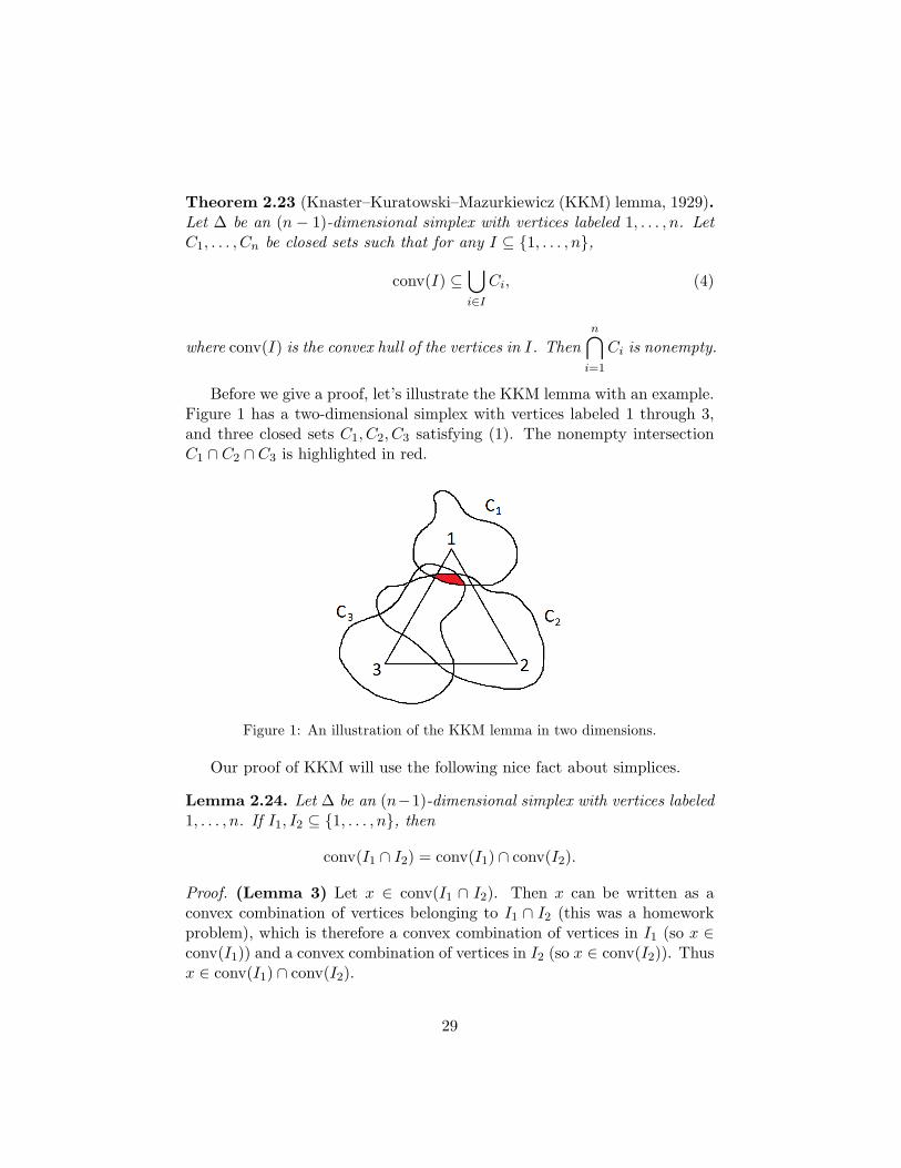
Before we give a proof, let’s illustrate the KKM lemma with an example.Figure 1 has a two-dimensional simplex with vertices labeled 1 through 3,and three closed sets C1, C2, C3 satisfying (1). The nonempty intersectionC1 ∩ C2 ∩ C3 is highlighted in red.

Figure 1: An illustration of the KKM lemma in two dimensions.

Our proof of KKM will use the following nice fact about simplices.

Lemma 2.24. Let ∆ be an (n−1)-dimensional simplex with vertices labeled1, . . . , n. If I1, I2 ⊆ 1, . . . , n, then

conv(I1 ∩ I2) = conv(I1) ∩ conv(I2).

Proof. (Lemma 3) Let x ∈ conv(I1 ∩ I2). Then x can be written as aconvex combination of vertices belonging to I1 ∩ I2 (this was a homeworkproblem), which is therefore a convex combination of vertices in I1 (so x ∈conv(I1)) and a convex combination of vertices in I2 (so x ∈ conv(I2)). Thusx ∈ conv(I1) ∩ conv(I2).

29

Now let y ∈ conv(I1) ∩ conv(I2). Then we can write y as two convexcombinations:

y =∑i∈I1

γixi, y =∑i∈I2

λixi,

where xi is the vertex of ∆ corresponding to i ∈ 1, . . . , n, all γi ≥ 0, allλi ≥ 0,

∑i∈I1 γi = 1 and

∑i∈I2 λi = 1. Then∑

i∈I1

γixi −∑i∈I2

λixi = 0.

We re-index this into three disjoint sums, setting ηi = γi − λi:∑i∈I1∩I2

ηixi +∑

i∈I1\I2

γixi −∑

i∈I2\I1

λixi = 0 (5)

There are two cases. If γi = 0 for all i ∈ I1 \ I2, then

y =∑i∈I1

γixi =∑

i∈I1∩I2

γixi +∑

i∈I1\I2

γixi =∑

i∈I1∩I2

γixi

and1 =

∑i∈I1

γi =∑

i∈I1∩I2

γi +∑

i∈I1\I2

γi =∑

i∈I1∩I2

γi,

and thus y ∈ conv(I1 ∩ I2). Consider the other case, in which γi 6= 0 forsome i ∈ I1 \ I2. Note that∑

i∈I1∩I2

ηi +∑

i∈I1\I2

γi −∑

i∈I2\I1

λi =∑i∈I1

γi −∑i∈I2

λi = 1− 1 = 0. (6)

Disaster strikes! Now (2) and (3) give an affine dependence relation amongthe vertices I1 ∪ I2—but ∆ is by definition the convex hull of the affinelyindependent vertices 1, . . . , n, so the vertices I1 ∪ I2 must be affinely in-dependent. Contradiction! This completes the proof.

Note that Lemma 3 does not hold for a general polytope! Try it for asquare. Lemma 3 is immediately extended by induction to any finite list ofsubsets I1, . . . , Ik ⊆ I.

We now return to proving KKM.

30

Proof. (Theorem 2) We will apply Sperner’s lemma. For each integerk ≥ 0, let Tk be the kth barycentric subdivision of ∆, where T0 = ∆. LetV (Tk) be the set of all vertices of all simplices in Tk, and set V =

⋃∞k=0 V (Tk).

For each v ∈ V , define

I(v) = I ⊆ 1, . . . , n : v ∈ conv(I)

andI∗(v) =

⋂I∈I(v)

I.

Define a labeling ` : V → 1, . . . , n by

`(v) = mini ∈ I∗(v) : v ∈ Ci.

We need to prove that `(v) always exists. Let v ∈ V . Note that v ∈ ∆ =conv(1, . . . , n), so I(v) is nonempty. Now we need I∗(v) to be nonempty.We have

v ∈⋂

I∈I(v)

conv(I) =∗ conv

⋂I∈I(v)

I

= conv(I∗(v)).

*By Lemma 3. Because conv(I∗(v)) is nonempty, it follows that I∗(v) isnonempty. (Note that carr(v) := conv(I∗(v)) is the unique smallest di-mensional face of ∆ containing v, called the carrier of v.) Next, by theassumption (1) of C1, . . . , Cn,

v ∈ conv(I∗(v)) ⊆⋃

i∈I∗(v)

Ci,

so there is an i ∈ I∗(v) such that v ∈ Ci. (Note that we have now used thefull power of the assumption (1).) Therefore, the set i ∈ I∗(v) : v ∈ Ci isnonempty, so applying the well-ordering principle, `(v) exists.

Now we show that for any k ≥ 0, ` restricted to V (Tk) is a Spernerlabeling of Tk. Suppose that v ∈ V (Tk) belongs to a face of ∆ containingthe vertices in I ⊆ 1, . . . , n; that is, v ∈ conv(I). Then by definition of`, we have `(v) ∈ I∗(v), and by definition of I∗(v), we have I∗(v) ⊆ I. So`(v) ∈ I, which proves that ` is a Sperner labeling.

By Sperner’s lemma, for each k ≥ 0, there is a fully colored simplexσk ∈ Tk. We can write σk as the convex hull of its vertices:

σk = conv(xk1, . . . , xkn),

31

where, without loss of generality (by re-indexing the xki ’s), `(xki ) = i for each

i = 1, . . . , n. By definition of `, we have xki ∈ Ci for every k ≥ 0. Becausethe sequence (xk1)k≥0 is contained in the compact set ∆, it has a convergentsubsequence (xkj

1 )j≥0 with limit x ∈ ∆. Because (xkj

1 )j≥0 is a sequence inC1, and C1 is closed, we have x ∈ C1.

The final step is to show that every other subsequence (xkj

i )j≥0, 2 ≤ i ≤ nof vertices also converges to the same limit x. For any k ≥ 0, recall that themesh size of Tk is defined by

mesh(Tk) = maxdiam(σ) : σ ∈ Tkwhere for any σ ∈ Tk,

diam(σ) = max‖x− y‖2 : x, y ∈ σand ‖ · ‖2 is the Euclidean norm. (Note that the maximum in the mesh sizeis attained because Tk consists of finitely many simplices, and the maximumin the diameter is attained because ‖ · ‖2 is continuous and σ is compact.)An important property of the barycentric subdivision (indeed, the reasonfor its existence) is that

mesh(Tk) ≤(

1− 1n

)kmesh(T0)

for all k ≥ 0 (see Munkres Elements of Algebraic Topology), where mesh(T0) =diam(∆). Let i ∈ 2, . . . , n. Then

‖xkj

i − x‖2 ≤ ‖xkj

i − xkj

1 ‖2 + ‖xkj

1 − x‖2≤ diam(σkj

) + ‖xkj

1 − x‖2≤ mesh(Tkj

) + ‖xkj

1 − x‖2

≤(

1− 1n

)kj

diam(∆) + ‖xkj

1 − x‖2 → 0

as j → ∞. Thus xkj

i → x as j → ∞. Because xkj

i is a sequence in Ci, andCi is closed, it follows that x ∈ Ci. Therefore, x ∈ Ci for all i = 1, . . . , n,and

⋂ni=1Ci is nonempty.

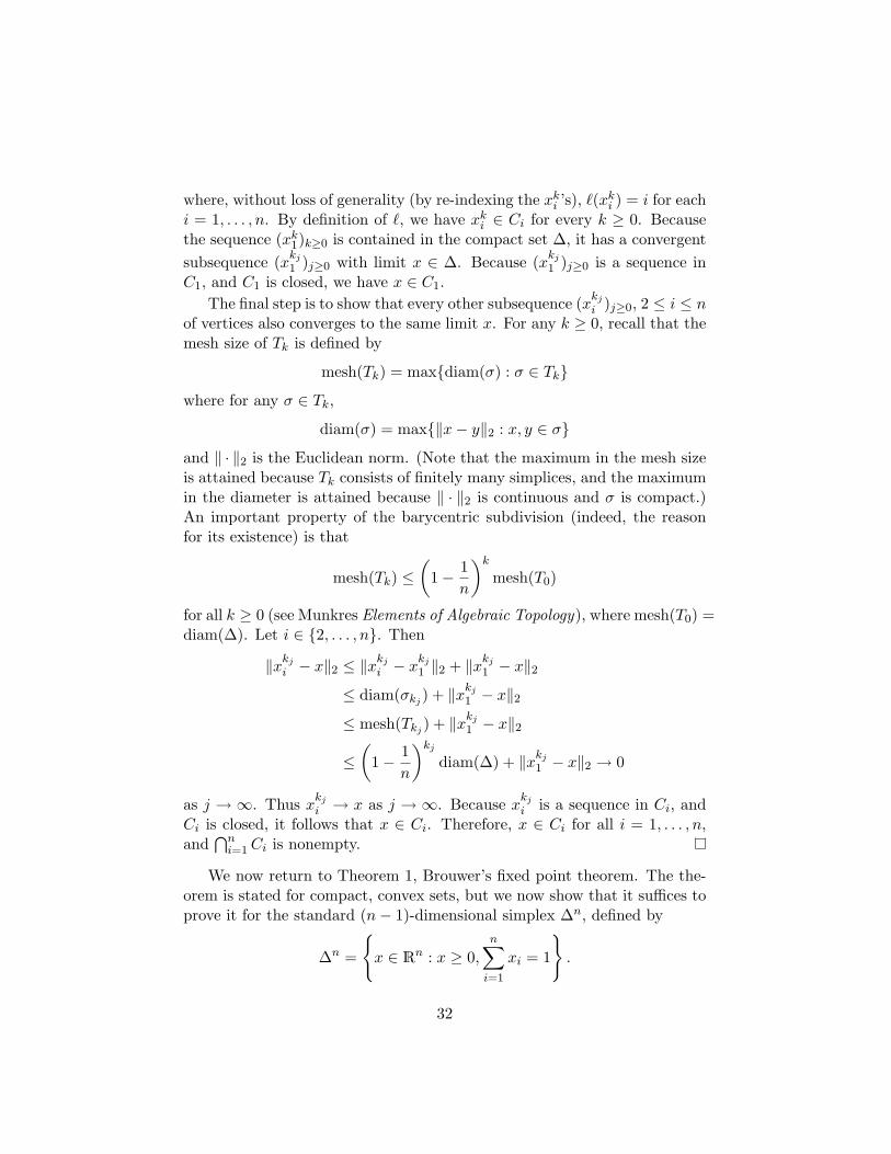
We now return to Theorem 1, Brouwer’s fixed point theorem. The the-orem is stated for compact, convex sets, but we now show that it suffices toprove it for the standard (n− 1)-dimensional simplex ∆n, defined by

∆n =

x ∈ Rn : x ≥ 0,

n∑i=1

xi = 1

.

32

Here, ∆n is (n− 1)-dimensional but “lives in” Rn.If ω is any other (n − 1)-dimensional simplex, ω is homeomorphic to

∆n. This is because every point of ω has unique barycentric coordinates. Inother words, if v1, . . . , vn are the vertices of ω, then every point p ∈ ω canbe written uniquely as a convex combination of the vertices:

p =n∑i=1

βivi, with all βi ≥ 0 andn∑i=1

βi = 1.

Then the map from ω to ∆n given by∑n

i=1 βivi 7→∑n

i=1 βiei is a homeo-morphism, where ei is the ith standard basis vector of Rn. It follows thatproving Brouwer for the standard simplex will prove it for any simplex, byconsidering the continuous function f composed with this homeomorphism.

In fact, if C is any nonempty, compact, convex subset of Rn, then C ishomeomorphic to a simplex. This is a fact that we will not prove, but whichallows us to extend the following proof to its more general statement above.

Proof. (Theorem 1) We give a proof for the case that C = ∆n. Letf : ∆n → ∆n be continuous. We want to find x ∈ ∆n so that f(x) = x. Foreach j = 1, . . . , n, let

Cj := x ∈ ∆n : f(x)j ≤ xj.

We claim that C1, . . . , Cn, satisfy the hypotheses of the KKM lemma.

1. Let j ∈ 1, . . . , n, and we show that Cj is closed. Let (x(k))k≥1 be anyconvergent sequence in Cj with limit x∗. So for every k ≥ 1, we havef(x(k))j ≤ x

(k)j . By the continuity of f , f(x(k)) → f(x∗) as k → ∞.

Then by convergence in the infinity norm on Rn, we have x(k)j → x∗j

and f(x(k))j → f(x∗)j as k →∞. Therefore,

f(x∗)j = limk→∞

f(x(k))j ≤ limk→∞

x(k)j = x∗j .

Thus x∗ ∈ Cj , so Cj is closed.

2. To show: for any I ⊆ 1, . . . , n, conv(I) ⊆ ⋃j∈I Cj .

If I = ∅, then conv(I) = ∅ and⋃j∈I Cj = ∅, and ∅ ⊆ ∅. So assume

that I 6= ∅. Let x ∈ conv(I). Assume to the contrary that f(x)j > xj

33

for all j ∈ I. Then because f(x) ∈ ∆n,

1 =n∑j=1

f(x)j ≥∑j∈I

f(x)j >∑j∈I

xj = 1,

a contradiction. So there is a j ∈ I such that f(x)j ≤ xj . Therefore,x ∈ ⋃j∈I Cj . So conv(I) ⊆ ⋃j∈I Cj .

Since the sets C1, . . . , Cn satisfy the hypotheses, KKM says that⋂nj=1Cj 6=

∅. So let x ∈ ⋂nj=1Cj , and we claim that x is a fixed point. Because x ∈ Cj

for every j, f(x)j ≤ xj for all j. So

1 =n∑j=1

f(x)j ≤n∑j=1

xj = 1.

Since equality holds throughout, f(x)j = xj for all j. Thus f(x) = x.

Brouwer’s fixed point theorem has a lot of applications. Notably, Johnvon Neumann used it to prove the Minimax Theorem in game theory, whichis equivalent to strong duality in linear programming. John Nash provedthe existence of equilibria in strategic games using Brouwer’s fixed pointtheorem.

Another interesting result is a generalization of Sperner’s lemma provedby our very own professor. Let P be a d-dimensional polytope, which isthe convex hull of its n vertices v1, . . . , vn. Let T be a triangulation of P ,possibly using additional vertices. A Sperner labeling of T is a labeling ofthe vertices of T by 1, . . . , n such that a vertex v of T can only be labeledby j if vj ∈ carr(v).

2.3 lectures 4,5

Theorem 2.25 (Polytopal Sperner’s Lemma (De Loera, Peterson, Su)). LetP be a d-dimensional polytope with n vertices, and T a triangulation of P . For anySperner labeling of T , there are at least n− d d-dimensional simplices of Teach with d+ 1 different labels on its vertices (“fully colored”).

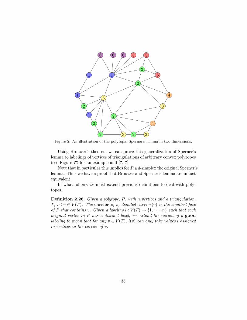
For example, in the hexagon in Figure 2, we have n = 6 and d = 2. Soby Theorem 4 there must be at least 4 fully colored simplices. In fact, thereare 10 in this example. Notice that because we are using 6 colors, “fullycolored” refers to any set of 3 distinct colors.

34

1

2 3

4

56

2

1

2

3 2

4

3

5

566

1

3

2

2

12

Figure 2: An illustration of the polytopal Sperner’s lemma in two dimensions.

Using Brouwer’s theorem we can prove this generalization of Sperner’slemma to labelings of vertices of triangulations of arbitrary convex polytopes(see Figure ?? for an example and [?, ?]

Note that in particular this implies for P a d-simplex the original Sperner’slemma. Thus we have a proof that Brouwer and Sperner’s lemma are in factequivalent.

In what follows we must extend previous definitions to deal with poly-topes.

Definition 2.26. Given a polytope, P , with n vertices and a triangulation,T , let v ∈ V (T ). The carrier of v, denoted carrier(v) is the smallest faceof P that contains v. Given a labeling l : V (T )→ 1, · · · , n such that eachoriginal vertex in P has a distinct label, we extend the notion of a goodlabeling to mean that for any v ∈ V (T ), l(v) can only take values l assignedto vertices in the carrier of v.

35

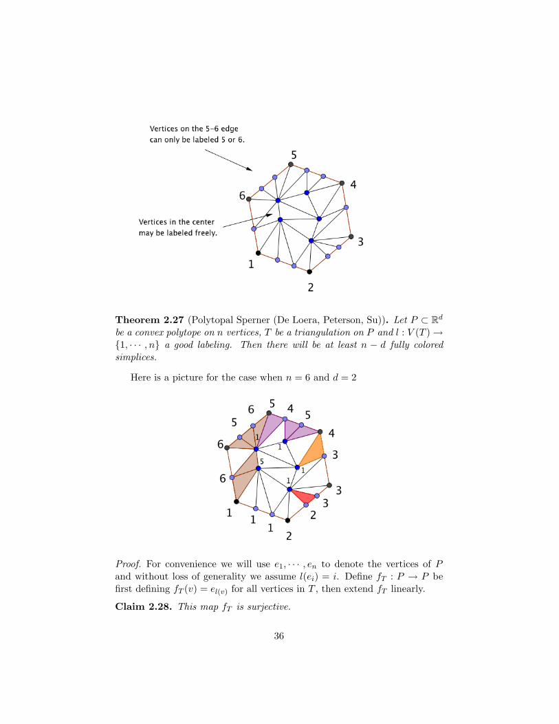
Theorem 2.27 (Polytopal Sperner (De Loera, Peterson, Su)). Let P ⊂ Rd

be a convex polytope on n vertices, T be a triangulation on P and l : V (T )→1, · · · , n a good labeling. Then there will be at least n − d fully coloredsimplices.

Here is a picture for the case when n = 6 and d = 2

Proof. For convenience we will use e1, · · · , en to denote the vertices of Pand without loss of generality we assume l(ei) = i. Define fT : P → P befirst defining fT (v) = el(v) for all vertices in T , then extend fT linearly.

Claim 2.28. This map fT is surjective.

36

Observation 2.29. 1. Since our labeling is good, if F is a face of P , weknow fT (F ) ⊆ F .

2. Since faces of a polytope are polytopes themselves, it suffices to showfT is surjective on the interior of P .

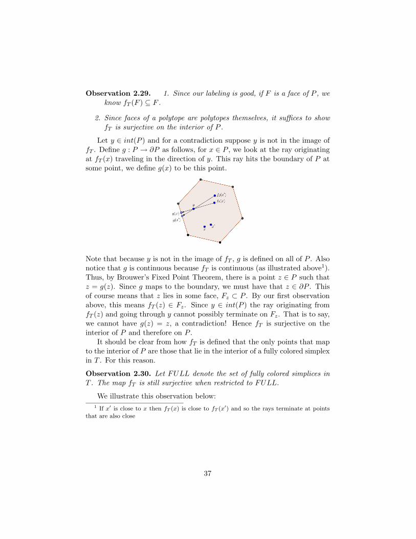
Let y ∈ int(P ) and for a contradiction suppose y is not in the image offT . Define g : P → ∂P as follows, for x ∈ P , we look at the ray originatingat fT (x) traveling in the direction of y. This ray hits the boundary of P atsome point, we define g(x) to be this point.

Note that because y is not in the image of fT , g is defined on all of P . Alsonotice that g is continuous because fT is continuous (as illustrated above1).Thus, by Brouwer’s Fixed Point Theorem, there is a point z ∈ P such thatz = g(z). Since g maps to the boundary, we must have that z ∈ ∂P . Thisof course means that z lies in some face, Fz ⊂ P . By our first observationabove, this means fT (z) ∈ Fz. Since y ∈ int(P ) the ray originating fromfT (z) and going through y cannot possibly terminate on Fz. That is to say,we cannot have g(z) = z, a contradiction! Hence fT is surjective on theinterior of P and therefore on P .

It should be clear from how fT is defined that the only points that mapto the interior of P are those that lie in the interior of a fully colored simplexin T . For this reason.

Observation 2.30. Let FULL denote the set of fully colored simplices inT . The map fT is still surjective when restricted to FULL.

We illustrate this observation below:1 If x′ is close to x then fT (x) is close to fT (x′) and so the rays terminate at points

that are also close

37

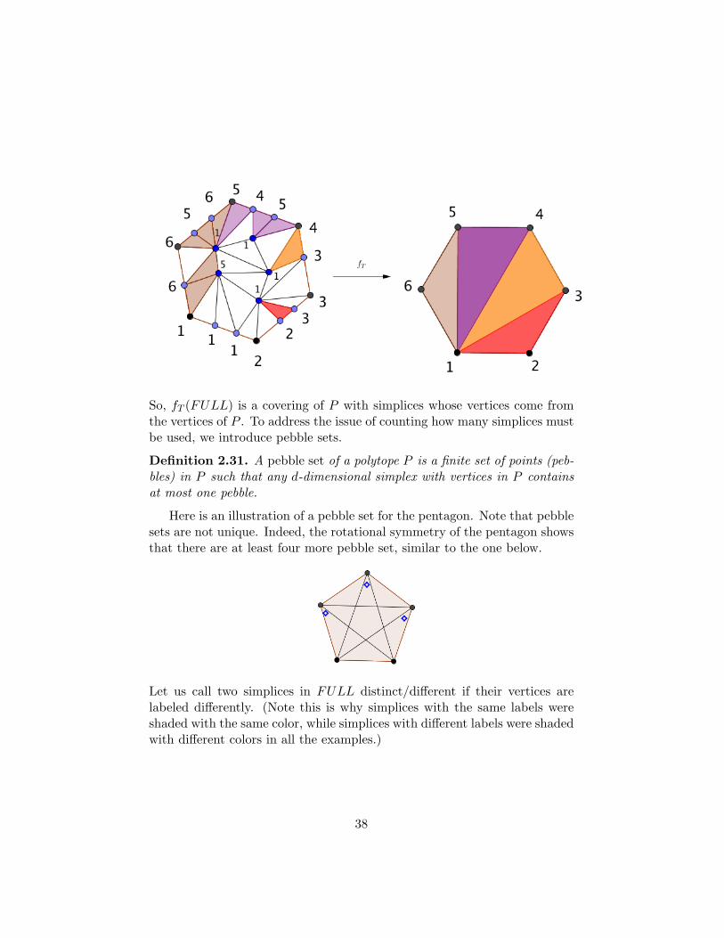
So, fT (FULL) is a covering of P with simplices whose vertices come fromthe vertices of P . To address the issue of counting how many simplices mustbe used, we introduce pebble sets.

Definition 2.31. A pebble set of a polytope P is a finite set of points (peb-bles) in P such that any d-dimensional simplex with vertices in P containsat most one pebble.

Here is an illustration of a pebble set for the pentagon. Note that pebblesets are not unique. Indeed, the rotational symmetry of the pentagon showsthat there are at least four more pebble set, similar to the one below.

Let us call two simplices in FULL distinct/different if their vertices arelabeled differently. (Note this is why simplices with the same labels wereshaded with the same color, while simplices with different labels were shadedwith different colors in all the examples.)

38

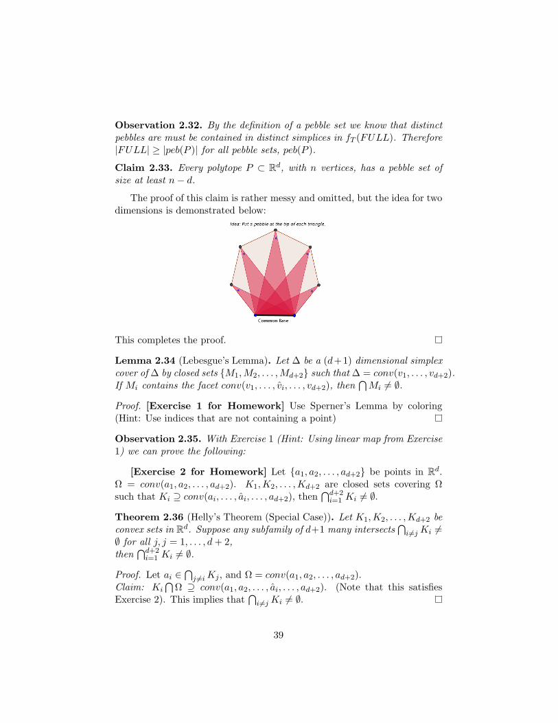
Observation 2.32. By the definition of a pebble set we know that distinctpebbles are must be contained in distinct simplices in fT (FULL). Therefore|FULL| ≥ |peb(P )| for all pebble sets, peb(P ).

Claim 2.33. Every polytope P ⊂ Rd, with n vertices, has a pebble set ofsize at least n− d.

The proof of this claim is rather messy and omitted, but the idea for twodimensions is demonstrated below:

This completes the proof.

Lemma 2.34 (Lebesgue’s Lemma). Let ∆ be a (d+1) dimensional simplexcover of ∆ by closed sets M1,M2, . . . ,Md+2 such that ∆ = conv(v1, . . . , vd+2).If Mi contains the facet conv(v1, . . . , vi, . . . , vd+2), then

⋂Mi 6= ∅.

Proof. [Exercise 1 for Homework] Use Sperner’s Lemma by coloring(Hint: Use indices that are not containing a point)

Observation 2.35. With Exercise 1 (Hint: Using linear map from Exercise1) we can prove the following:

[Exercise 2 for Homework] Let a1, a2, . . . , ad+2 be points in Rd.Ω = conv(a1, a2, . . . , ad+2). K1,K2, . . . ,Kd+2 are closed sets covering Ωsuch that Ki ⊇ conv(ai, . . . , ai, . . . , ad+2), then

⋂d+2i=1 Ki 6= ∅.

Theorem 2.36 (Helly’s Theorem (Special Case)). Let K1,K2, . . . ,Kd+2 beconvex sets in Rd. Suppose any subfamily of d+1 many intersects

⋂i 6=jKi 6=

∅ for all j, j = 1, . . . , d+ 2,then

⋂d+2i=1 Ki 6= ∅.

Proof. Let ai ∈⋂j 6=iKj , and Ω = conv(a1, a2, . . . , ad+2).

Claim: Ki⋂

Ω ⊇ conv(a1, a2, . . . , ai, . . . , ad+2). (Note that this satisfiesExercise 2). This implies that

⋂i 6=jKi 6= ∅.

39

O. Musin generalized of Sperner and Tucker lemmas to large classes ofmanifolds with or without boundary;

One more fascinating consequence is S. Kakutani’s 1941 theorem

Theorem (Kakutani’s). Let X be a compact, convex subset of Euclideand-space. Let F be a continuous set-valued function on X; i.e., a mappingfrom X to the set of all subsets of X, If T (x) is convex for all x belongingto X, then there exists a vector z such that z ∈ T (z).

To prove this theorem we will use Brouwer’s fixed point theorem incombination of the barycentric triangulation we have used before.

Anecdote: In his game theory textbook, Ken Binmore recalls that Kaku-tani once asked him at a conference why so many economists had attendedhis talk. When Binmore told him that it was probably because of the Kaku-tani fixed point theorem, Kakutani was puzzled and replied, ”What is theKakutani fixed point theorem?”

First we need to generalize the classical concept of point-valued func-tions.

Definition 2.37. A set-valued function is a function F : X −→ 2X . Inwords, it is a function that send elements of a set X to subsets of X.

We are interested in the membership problem, i.e. we want to findx ∈ X such that x ∈ F (X). This generalizes the notion of fixed point forthe classical point-valued functions.

In the same way that most of the time we restrict our attention tocontinuous functions, we need to ask for a similar condition on set-valuedfunctions.

Proposition 2.38. A function f : X −→ Y between two topological spacesis continuous if and only if its graph Γf = (x, y) ∈ X × Y : y = f(x) isclosed in X × Y .

Analogously we can define the graph for any set valued function F as

ΓF = (x, x′) ∈ X ×X : x′ ∈ F (x)

If additionally X is a topological space, it makes sense to talk about itsclosedness. More specifically we say that ΓF is closed if given a sequence(xk, x′k) with x′k ∈ F (xk) and such that x = limxk and x′ = limx′k exist,then x′ ∈ F (x).

40

Theorem 2.39. Let X ⊂ Rn be a compact convex set. If F : X −→ 2X is aset valued function with closed graph and the property that F (x) is nonemptyand convex for all x ∈ X, then there exist a x∗ ∈ X such that x∗ ∈ F (x∗).

It is enough to prove it for the standard simplices and that’s what we’lldo.

Proof. Let ∆ the d−dimensional standard simplex. Consider the Tn then−th barycentric subdivision. We construct a continuous function fn asfollows. For all vertices v ∈ Tn we define fn(v) as an arbitrary point inF (v). Having defined it on the vertices of Tn we extend linearly to allthe simplices inside the barycentric subdivision. The resulting map fn iscontinuous since it is piecewise linear.

Brouwer’s theorem guarantess that for each n there exists a fixed pointxn. If any of the xn is a vertex of its corresponding barycentric subdivision,then we are done since xn = f(xn) ∈ F (xn) by definition. From nowon we assume that xn is not a vertex of Tn, then it is in some simplexconv(xn0 , · · · , xnd), hence we have a convex expression

xn = θn0xn0 + · · ·+ θndxnd (7)

Since the function f is linear on simplices we can apply it to Equation 7to get

xn = θn0yn0 + · · ·+ θndynd (8)

where yni = f(xni). Now we have 2d+ 3 sequences

xn, θni ∀i, ynj ∀j.By repeatedly taking convergent subsequents, and relabeling, we can

assume that each sequence convergences while Equation 8 remains true forall n.

Observation 2.40. As n goes to infinity, the mesh in Tn goes to zero, sox∗ = lim

n→∞xn = lim

n→∞xni for all i.

Taking limits on Equation 8 we get

x∗ = θ∗0y∗0 + · · ·+ θ∗dy

∗d (9)

where limn→∞

θni = θ∗i . Here is where we use the closedness of the graph.

Since ynj = fn(xnj ) ∈ F (xnj ), in the limit we have

y∗j = limn→∞

ynj ∈ F(

limn→∞

xnj

)= F (x∗)

41

This means that the right hand side of Equation 9 is a convex combinationof points in F (x∗). Since F (x∗) is convex, this proves that x∗ ∈ F (x∗) aswe wanted.

The following examples shows that we cannot drop some of the conditionsin the statement.

Boundedness of XLet X = R and consider the function F : R→ 2R:

F (x) =

−1x for x < 02 for x = 0 1x for x > 0

There is no fixed point. Kakutani’s theorem doesn’t apply since R is notcompact.

Convexity of F (x)Consider X = [−1, 1] ⊂ R. Which is compact and convex. We defineF : X −→ 2X as

F (x) =

1

2 for − 1 ≤ x < 0−1

2 ,12 for x = 0

−12 for − 1 ≤ x > 0

The graph is closed, but the conclusion fails. What fails is that F (0) isnot convex.

3 Nash Equilibria

A nice application of Kakutani’s fixed point theorem appears in the proofof Nash Equilibrium (for finite games). We define games in the extensiveform. Each game G has three main components: The set of players (P ),sets of strategies for each player (Sp for p ∈ P ) and the set of payoffsfor each player given the strategies played (up). We’ll star with a simpleexample with 3 players (results can be extended to any finite number ofplayers and strategies). Let G be a game with 3 players: Abe (A), Bernie(B) and Charlie (C). The set of players is defined as P = A,B,C. In thisgame, each player has a finite set of pure-strategies defined, i.e., for Abe wedefine his strategy set as SA = 1, 2, . . . , i0, for Bernie SB = 1, 2, . . . , j0and for Charlie SC = 1, 2, . . . , k0. Elements for each strategy set will bedenoted by sp ∈ Sp with p ∈ P . A strategy profile is is a vector s ∈ Swhere S = ×p∈PSp. Therefore, for each strategy profile s ∈ S, agents have

42

payoffs given by up(s) ∈ R. Thus, the game can summarized as followsG =

(P, Sp, up(s),

)p∈P .

To simplify notation, payoffs will be written as follows: For an strategyprofile s = (i, j, k) ∈ S (Abe plays i ∈ SA, Bernie plays j ∈ SB and Charlieplays k ∈ SC), payoffs will be aijk, bijk and cijk, for Abe, Bernie and Charlie,respectively.

We allow agents to play a given pure strategy sp ∈ SP or to randomize oftheir set of strategies. For example, Abe is allowed to play i ∈ SA or to playi ∈ SA with probability pi and all others with probability 1−pi for pi ∈ [0, 1].Over the set of pure strategies, we define mixed strategies σp as a probabilitydistribution over pure strategies. The assumption behind randomizationis that mixed strategies for each player’s are statistically independent ofthose of his opponents. Let the space of player’s p mixed strategies beΣp, where σp(sp) is the probability that σp that player p assigns to sp.The space of mixed strategy profiles is denoted Σ = ×p∈PΣp, with elementσ. Hence, if Abe plays a mixed strategy σA = (p1, . . . , pi0), Bernie playsσB = (q1, . . . , qj0) and Charlie plays σC = (r1, . . . , ri0), the expected payoffto profile σ = (σA, σB, σC) is given by

UA(σ) =∑i,j,k

(piqjrk)aijk, UB(σ) =∑i,j,k

(piqjrk)bijk, UC(σ) =∑i,j,k

(piqjrk)cijk,

for Abe, Bernie and Charlie, respectively.Since each mixed strategy σp is a probability distribution over pure

strategies, we must have:

pi ≥ 0,i0∑i=1

pi = 1; qj ≥ 0,j0∑j=1

qj = 1; rk ≥ 0,k0∑k=1

rk = 1.

To simplify notation, we will write the expected payoff for a mixed strategyσ = (p, q, r) as a(p, q, r), b(p, q, r) and c(p, q, r).

In this 3-person game, we can ask the following question: Which strat-egy (pure or mixed) each agent has to take given the rules of the game?Clearly we are missing one important assumption to answer this question:selfishness. In economics, is common to assume that agents are selfish, i.e.,agents want to maximize their (expected) payoff for any given strategy oftheir opponents independent of the payoff of their opponents. For instance,when thinking about the optimal decision for Abe, for any mixed strategyq ∈ ΣB that Bernie plays and any mixed-strategy r ∈ ΣC that Charlie plays,Abe will choose a mixed strategy p ∈ ΣA such that

a(p, q, r) ≥ a(p, q, r), ∀p ∈ ΣA.

43

I.e., p is the mixed strategy that allows Abe to get the highest expectedpayoff. Clearly, for each strategy (pure or mixed) Abe can have differentstrategies that maximize his (expected) payoff.

In this scenario, we can informally define a Nash equilibrium as theprofile of strategies such that each player’s strategy is an optimal responseto the other player’s strategies. Formally:

Definition 3.1. A mixed strategy profile (p, q, r) ∈ Σ is a Nash equilibriumif, for all players (Abe, Bernie and Charlie),

a(p, q, r) ≥ a(p, q, r), ∀p ∈ ΣA;

b(p, q, r) ≥ b(p, q, r), ∀q ∈ ΣB;

c(p, q, r) ≥ c(p, q, r), ∀r ∈ ΣC .

Finally, after all of this necessary notation, we are able to state thefollowing theorem:

Theorem 3.2 (Nash (1950)). A Nash equilibrium always exists on finitegames.

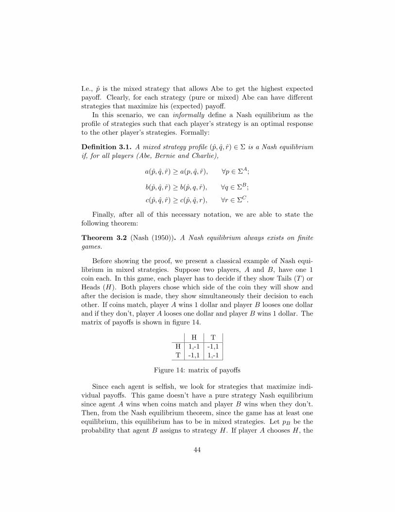
Before showing the proof, we present a classical example of Nash equi-librium in mixed strategies. Suppose two players, A and B, have one 1coin each. In this game, each player has to decide if they show Tails (T ) orHeads (H). Both players chose which side of the coin they will show andafter the decision is made, they show simultaneously their decision to eachother. If coins match, player A wins 1 dollar and player B looses one dollarand if they don’t, player A looses one dollar and player B wins 1 dollar. Thematrix of payoffs is shown in figure 14.

H TH 1,-1 -1,1T -1,1 1,-1

Figure 14: matrix of payoffs

Since each agent is selfish, we look for strategies that maximize indi-vidual payoffs. This game doesn’t have a pure strategy Nash equilibriumsince agent A wins when coins match and player B wins when they don’t.Then, from the Nash equilibrium theorem, since the game has at least oneequilibrium, this equilibrium has to be in mixed strategies. Let pB be theprobability that agent B assigns to strategy H. If player A chooses H, the

44

expected payoff is UA(H) = pB(1)+(1−pB)(−1) = 2pB−1 and if A choosesT his payoff is UA(T ) = pB(−1) + (1 − pB)(1) = 1 − 2pB. Then, if we callpA the probability that player A assigns to playing H, the optimal decisionwill be

pA(pB) =

1 if pB > 1/2[0,1] if pB = 1/20 if pB < 1/2

clearly pA is a set function and by symmetry of payoffs, optimal prob-abilities for agent B given that player A plays H with probability pA aregiven by

pB(pA) =

0 if pA > 1/2[0,1] if pA = 1/21 if pA < 1/2

Hence, Nash equilibrium in the matching pennies game is given by pA = 1/2and pB = 1/2.From last episode: We presented a game with three players A,B,C, anddenoted their payoffs by A → aijk, B → bijk and C → cijk. Therefore,expected payoffs for each agent where written as:

A : a(p, q, r) =∑i,j,k

aijkpiqjrk,

B : b(p, q, r) =∑i,j,k

bijkpiqjrk,

C : c(p, q, r) =∑i,j,k

bijkpiqjrk.

Finally, we gave the definition of Nash equilibrium for this game:

Definition 3.3. A Nash equilibrium is a triple of probability vectors (p, q, r)such that:

a(p, q, r) ≥ a(p, q, r), ∀p probability vector,

b(p, q, r) ≥ c(p, q, r), ∀q probability vector,

c(p, q, r) ≥ c(p, q, r), ∀r probability vector,

the above inequalities are called Nash inequalities.

Commercial break: Simplices are useful! Probability vectors for eachplayer are just points inside the standard simplex in the dimension defined

45

by the number of pure strategies for that player. For instance, for player Awe have

4i0−1 = (p1, p2, ..., pi0)|∑i

pi = 1, pi ≥ 0.

Note: The space 4 of mixed strategies (p, q, r) will be denoted by

4 = 4i0−1 ×4j0−1 ×4k0−1.

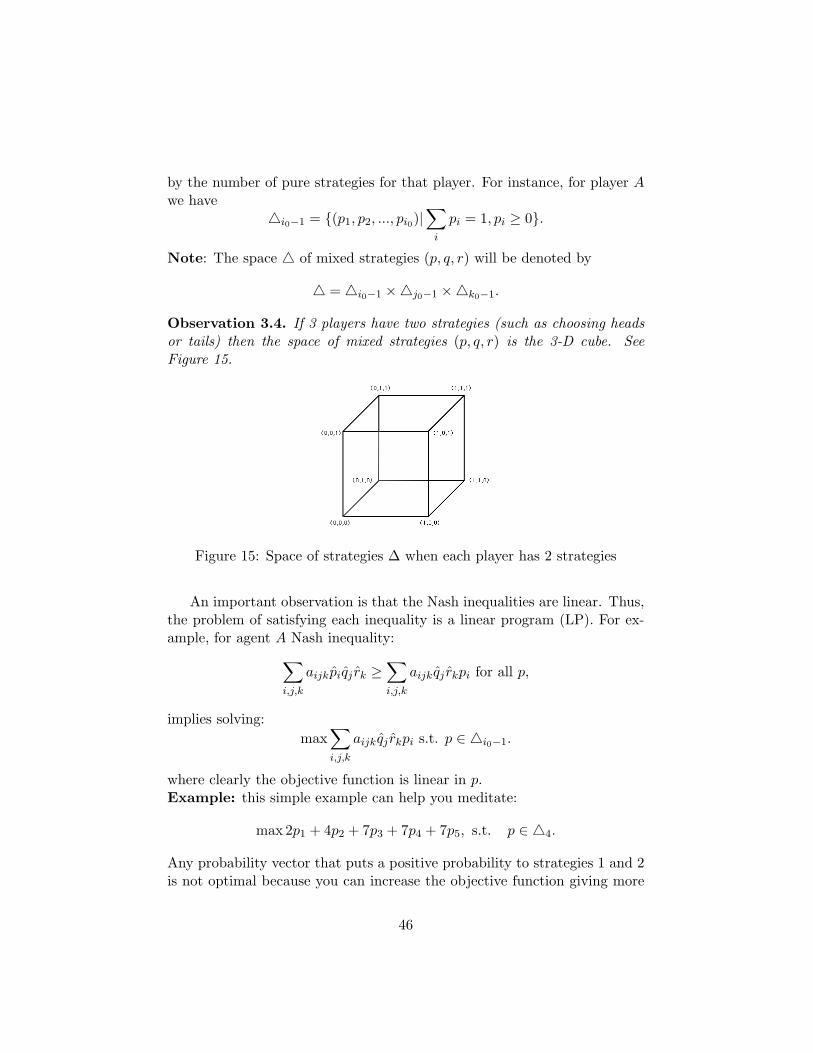
Observation 3.4. If 3 players have two strategies (such as choosing headsor tails) then the space of mixed strategies (p, q, r) is the 3-D cube. SeeFigure 15.

Figure 15: Space of strategies ∆ when each player has 2 strategies

An important observation is that the Nash inequalities are linear. Thus,the problem of satisfying each inequality is a linear program (LP). For ex-ample, for agent A Nash inequality:∑

i,j,k

aijkpiqj rk ≥∑i,j,k

aijkqj rkpi for all p,

implies solving:max

∑i,j,k

aijkqj rkpi s.t. p ∈ 4i0−1.

where clearly the objective function is linear in p.Example: this simple example can help you meditate:

max 2p1 + 4p2 + 7p3 + 7p4 + 7p5, s.t. p ∈ 44.

Any probability vector that puts a positive probability to strategies 1 and 2is not optimal because you can increase the objective function giving more

46

probability to strategies 3, 4 and 5. Hence, at the optimum we must havep1 = p2 = 0.

The maximum on the first Nash inequality occurs on the face of 4i0−1

defined by the vertices selected by the largest coefficients aijkqj rk:

P (q, r) :=

p : pi ≥ 0,

∑i

pi = 1, pi = 0 when aijkqj rk < max aijkqj rk,

which is a face of 4i0−1.Similarly, on the second Nash inequality, again the maximum exists only

within the face

Q(p, r) :=

q : qj ≥ 0,∑j

qj = 1, qj = 0 when bijkpirk < max bijkpirk

,

which is a face of 4j0−1.Finally, for the third Nash inequality, the maximum exists within the

face

R(p, q) :=

r : rk ≥ 0,

∑k

rk = 1, rk = 0 when cijkpiqj < max cijkpiqj,

which is a face of 4k0−1.Now, as Nash realized, equilibria exist if and only if there exists a triple

(p, q, r) with p ∈ P (q, r), q ∈ Q(p, r), and r ∈ R(p, q).

Theorem 3.5. (1950 Nash) A Nash equilibrium of mixed strategies (p, q, r)exists.

Proof. We will use Kakutani’s theorem to prove this. Define X := 4i0−1 ×4j0−1 ×4k0−1 to be the space of mixed strategies. Define F : X → 2X asthe set-valued function that mapspq

r

7→P (q, r)Q(p, r)R(p, q)

.

Now, clearly, since X is the product of simplices, it is a compact, convexset. Additionally, F (x) is convex since it is the product of faces of simplices.Now, we need only show that F satisfies the last hypothesis of Kakutani’s

47

theorem, that the graph of F is closed, i.e., (x, y) : y ∈ F (x) is a closedset.

Take a convergent sequence xn ⊂ X. Say that limn→∞

xn =: x0. Take

another sequence yn with yn ∈ F (xn) and say that limn→∞

yn = y0. Our goal

is to show that y0 ∈ F (x0).Now, each xn and yn is a triple of mixed strategies, call them

xn =

pnqnrn

, yn =

unvnwn

.

By definition, un ∈ P (qn, rn), vn ∈ Q(pn, rn) and wn ∈ R(pn, qn) and so thethree Nash inequalities are satisfied:

a(un, qn, rn) ≥ a(p′, qn, rn), ∀p′ ∈ ∆i0−1,

b(pn, vn, rn) ≥ b(pn, q′, rn), ∀q′ ∈ ∆j0−1,

c(pn, qn, wn) ≥ c(pn, qn, r′), ∀r′ ∈ ∆k0−1,

Note that as n goes to infinity the vector (pn, qn, rn) converges to x0

and (un, vn, wn) converges to y0. Since the inequalities are linear and thuscontinuous, they are satisfied in the limit and so they hold true at x0, y0 sowe have that y0 ∈ F (x0).

Thus, Kakutani’s theorem gives us that there exists some x∗ ∈ X withx∗ ∈ F (x∗). Thus, this point provides a Nash equilibrium

x∗ =

p∗q∗r∗

with p∗ ∈ P (q∗, r∗), q∗ ∈ Q(p∗, r∗) and r∗ ∈ R(p∗, q∗).

We move to the final application of Sperner’s lemma. We will provideproof of the 1982 theorem of Imre Barany the colorful Caratheodory’s the-orem. Recall the usual form first:

Let A ∈ Zd×n be an integer matrix.

Theorem 3.6. (Caratheodory) If Ax = b, x ≥ 0 has a solution then thereexists a solution with no more than d non-zero entries in x.

The nonnegative entries in x are called the support of x, i.e., supp(x) =i : xi 6= 0.

48

Theorem 3.7. (Colorful Caratheodory) Suppose B1, B2, ..., Bd are d pair-wise disjoint subsets of indices of columns, each with d-columns, of thematrix A. If the d systems ABix = b, x ≥ 0 all have a solution for alli = 1, . . . , d then there exists a set of indices B such that

ABx = b, x ≥ 0

has solution too and, in addition, |B ∩Bi| ≤ 1 for all i.

One can prove this theorem using Sperner’s theorem. It has some re-markable consequences, e.g., Tverberg’s theorem can be proved from it.

3.1 Lecture Borsuk-Ulam and Tucker’s Lemma

In this lecture, we introduce the Borsuk–Ulam theorem and some of its ap-plications. The Borsuk–Ulam theorem comes in many different forms, andin this lecture we will prove that its different statements are indeed equiv-alent. The proof of the theorem itself will come later using combinatorialgeometry again.

Let ‖ · ‖2 be the Euclidean norm on a Euclidean space. Let §n be then-dimensional sphere, that is,

§n =x ∈ Rn+1 : ‖x‖2 = 1

.

A function f : §n → Rn is antipodal if f(−x) = −f(x) for all x ∈ §n. Thatis, f is an odd function.

Theorem 3.8 (Borsuk–Ulam).

(1) If a function f : §n → §m is continuous and antipodal, then m ≥ n.

(2) If a function f : §n → Rn is continuous and antipodal, there is anx ∈ §n with f(x) = 0.

(3) If a function f : §n → Rn is continuous, there is an x ∈ §n withf(x) = f(−x).

(4) If §n =⋃ni=0 Si and each Si is closed, there is an x ∈ §n and an

i ∈ 0, 1, . . . , n with x,−x ⊆ Si.

Proof. We postpone the proof until later.

Claim 3.9. The statements (1)–(4) in Theorem 3.8 are equivalent.

49

Proof. We prove the implications (1)⇒ (2)⇒ (3)⇒ (4)⇒ (1).(1) ⇒ (2): For a contradiction, assume there is a function f : §n → Rn

that is continuous and antipodal, but f(x) 6= 0 for all x ∈ §n. Then we canconsider the function F : §n → §n−1 defined by

F (x) =f(x)‖f(x)‖2

.

For any x ∈ §n,

F (−x) =f(−x)‖f(−x)‖2

=−f(x)‖ − f(x)‖2

= −F (x),

so F is antipodal. Because f is continuous, F is also continuous. Thisproduces a contradiction to (1).

(2) ⇒ (3): Let f : §n → Rn be a continuous function. Consider F :§n → Rn defined by F (x) = f(x) − f(−x). Then F (−x) = −F (x), so Fis antipodal, and F is continuous. By (2), there is an x∗ ∈ §n such thatF (x∗) = 0, i.e. f(x∗) = f(−x∗).

(3) ⇒ (4): Assume that §n =⋃ni=0 Si and each Si is closed. Define

f : §n → Rn byf(x) =

(d(x, S1), . . . , d(x, Sn)

),

where d(x, Si) is the Euclidean distance of x from Si, which because Si iscompact is given by

d(x, Si) = min‖x− y‖2 : y ∈ Si.

Because f is continuous, (3) gives an x∗ ∈ §n with f(x∗) = f(−x∗).Case (a): There is some coordinate f(x∗)i = 0 = f(−x∗)i. Then x∗ ∈ Si

and −x∗ ∈ Si.Case (b): f(x∗)i > 0 for every i = 1, . . . , n. So x∗ /∈ Si for every

i = 1, . . . , d. But §n =⋃ni=0 Si, so x∗ ∈ S0, and similarly for −x∗.

(4) ⇒ (1): For a contradiction, assume that f : §n → §m is continuousand antipodal, but m < n. Let ε > 0 and build a cover §n =

⋃ni=0 Si by

definingRi = (x0, . . . , xm) ∈ §m : xi ≥ ε

for i = 0, 1, . . . ,m, and

Rm+1 =

(x0, . . . , xm) ∈ §m :

m∑i=0

xi ≤ −ε.

50

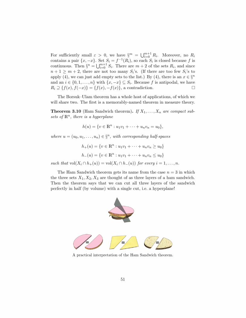
For sufficiently small ε > 0, we have §m =⋃m+1i=0 Ri. Moreover, no Ri

contains a pair x,−x. Set Si = f−1(Ri), so each Si is closed because f iscontinuous. Then §n =

⋃m+1i=0 Si. There are m+ 2 of the sets Ri, and since

n + 1 ≥ m + 2, there are not too many Si’s. (If there are too few Si’s toapply (4), we can just add empty sets to the list.) By (4), there is an x ∈ §nand an i ∈ 0, 1, . . . , n with x,−x ⊆ Si. Because f is antipodal, we haveRi ⊇ f(x), f(−x) = f(x),−f(x), a contradiction.

The Borsuk–Ulam theorem has a whole host of applications, of which wewill share two. The first is a memorably-named theorem in measure theory.

Theorem 3.10 (Ham Sandwich theorem). If X1, . . . , Xn are compact sub-sets of Rn, there is a hyperplane

h(u) = v ∈ Rn : u1v1 + · · ·+ unvn = u0,

where u = (u0, u1, . . . , un) ∈ §n, with corresponding half-spaces

h+(u) = v ∈ Rn : u1v1 + · · ·+ unvn ≥ u0

h−(u) = v ∈ Rn : u1v1 + · · ·+ unvn ≤ u0such that vol(Xi ∩ h+(u)) = vol(Xi ∩ h−(u)) for every i = 1, . . . , n.

The Ham Sandwich theorem gets its name from the case n = 3 in whichthe three sets X1, X2, X3 are thought of as three layers of a ham sandwich.Then the theorem says that we can cut all three layers of the sandwichperfectly in half (by volume) with a single cut, i.e. a hyperplane!

A practical interpretation of the Ham Sandwich theorem.

51

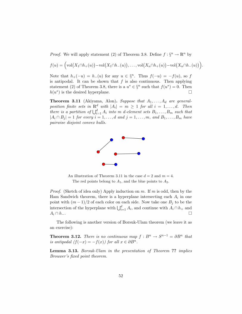
Proof. We will apply statement (2) of Theorem 3.8. Define f : §n → Rn by

f(u) =(

vol(X1∩h+(u)

)−vol

(X1∩h−(u)

), . . . , vol

(Xn∩h+(u)

)−vol

(Xn∩h−(u)

)).

Note that h+(−u) = h−(u) for any u ∈ §n. Thus f(−u) = −f(u), so fis antipodal. It can be shown that f is also continuous. Then applyingstatement (2) of Theorem 3.8, there is a u∗ ∈ §n such that f(u∗) = 0. Thenh(u∗) is the desired hyperplane.

Theorem 3.11 (Akiyama, Alon). Suppose that A1, . . . , Ad are general-position finite sets in Rd with |Ai| = m ≥ 1 for all i = 1, . . . , d. Thenthere is a partition of

⋃di=1Ai into m d-element sets B1, . . . , Bm such that

|Ai ∩Bj | = 1 for every i = 1, . . . , d and j = 1, . . . ,m, and B1, . . . , Bm havepairwise disjoint convex hulls.

An illustration of Theorem 3.11 in the case d = 2 and m = 4.The red points belong to A1, and the blue points to A2.

Proof. (Sketch of idea only) Apply induction on m. If m is odd, then by theHam Sandwich theorem, there is a hyperplane intersecting each Ai in onepoint with (m− 1)/2 of each color on each side. Now take one Bj to be theintersection of the hyperplane with

⋃di=1Ai, and continue with Ai ∩ h+ and

Ai ∩ h−.

The following is another version of Borsuk-Ulam theorem (we leave it asan exercise):

Theorem 3.12. There is no continuous map f : Bn → Sn−1 = ∂Bn thatis antipodal (f(−x) = −f(x)) for all x ∈ ∂Bn.

Lemma 3.13. Borsuk-Ulam in the presentation of Theorem ?? impliesBrouwer’s fixed point theorem.

52

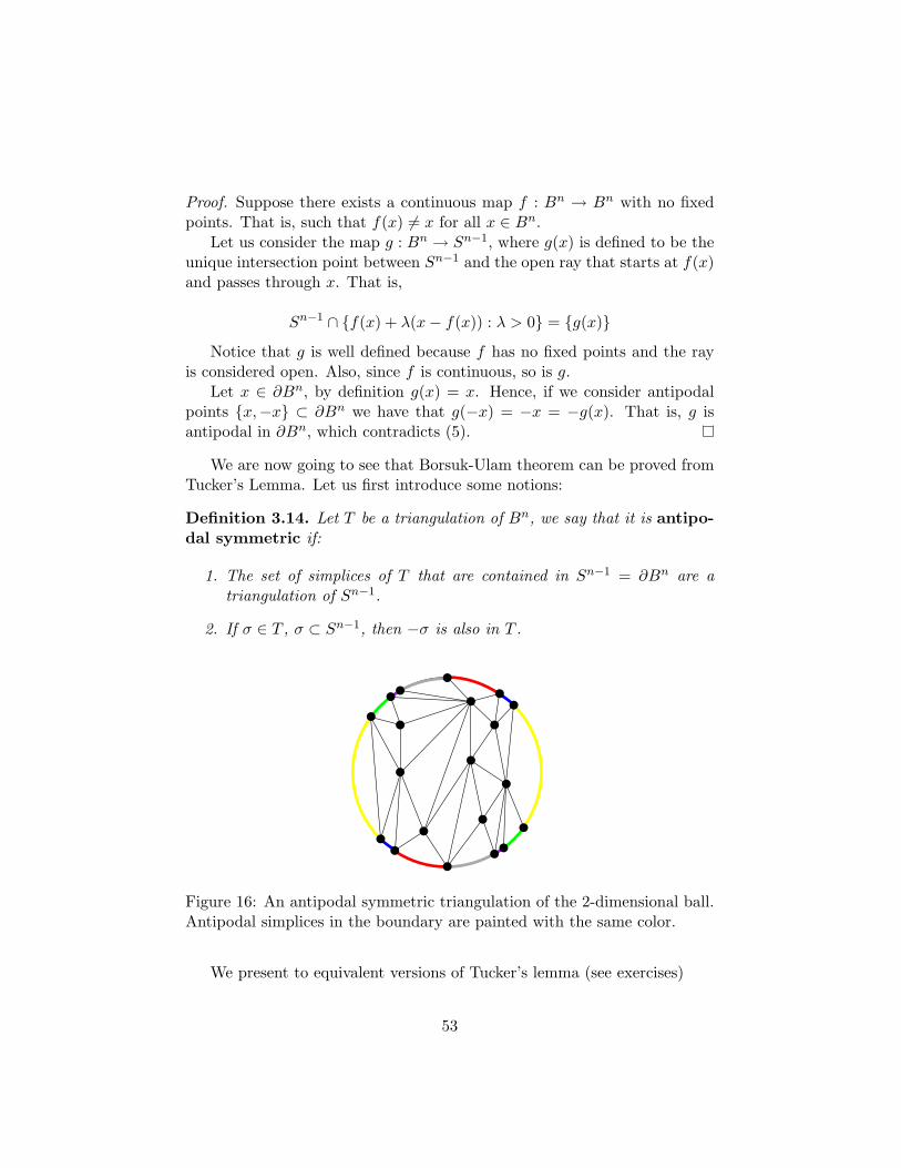
Proof. Suppose there exists a continuous map f : Bn → Bn with no fixedpoints. That is, such that f(x) 6= x for all x ∈ Bn.

Let us consider the map g : Bn → Sn−1, where g(x) is defined to be theunique intersection point between Sn−1 and the open ray that starts at f(x)and passes through x. That is,

Sn−1 ∩ f(x) + λ(x− f(x)) : λ > 0 = g(x)Notice that g is well defined because f has no fixed points and the ray

is considered open. Also, since f is continuous, so is g.Let x ∈ ∂Bn, by definition g(x) = x. Hence, if we consider antipodal

points x,−x ⊂ ∂Bn we have that g(−x) = −x = −g(x). That is, g isantipodal in ∂Bn, which contradicts (5).

We are now going to see that Borsuk-Ulam theorem can be proved fromTucker’s Lemma. Let us first introduce some notions:

Definition 3.14. Let T be a triangulation of Bn, we say that it is antipo-dal symmetric if:

1. The set of simplices of T that are contained in Sn−1 = ∂Bn are atriangulation of Sn−1.

2. If σ ∈ T , σ ⊂ Sn−1, then −σ is also in T .

Figure 16: An antipodal symmetric triangulation of the 2-dimensional ball.Antipodal simplices in the boundary are painted with the same color.

We present to equivalent versions of Tucker’s lemma (see exercises)

53

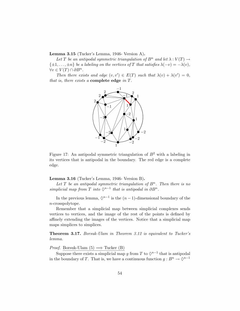
Lemma 3.15 (Tucker’s Lemma, 1946- Version A).Let T be an antipodal symmetric triangulation of Bn and let λ : V (T )→

±1, . . . ,±n be a labeling on the vertices of T that satisfies λ(−v) = −λ(v),∀v ∈ V (T ) ∩ ∂Bn.

Then there exists and edge (v, v′) ∈ E(T ) such that λ(v) + λ(v′) = 0,that is, there exists a complete edge in T .

−12

1

−2−1

1

2

−2−2

22

−2

−1

−2

−1

−1

−2

1

1

1

Figure 17: An antipodal symmetric triangulation of B2 with a labeling inits vertices that is antipodal in the boundary. The red edge is a completeedge.

Lemma 3.16 (Tucker’s Lemma, 1946- Version B).Let T be an antipodal symmetric triangulation of Bn. Then there is no

simplicial map from T into ♦n−1 that is antipodal in ∂Bn.

In the previous lemma, ♦n−1 is the (n− 1)-dimensional boundary of then-crosspolytope.

Remember that a simplicial map between simplicial complexes sendsvertices to vertices, and the image of the rest of the points is defined byaffinely extending the images of the vertices. Notice that a simplicial mapmaps simplices to simplices.

Theorem 3.17. Borsuk-Ulam in Theorem 3.12 is equivalent to Tucker’slemma.

Proof. Borsuk-Ulam (5) =⇒ Tucker (B)Suppose there exists a simplicial map g from T to ♦n−1 that is antipodal

in the boundary of T . That is, we have a continuous function g : Bn → ♦n−1

54

that is antipodal in ∂Bn. Consider now the function f : Bn → Sn−1 definedby f(x) = g(x)/||g(x)||. f is, by construction, continuous and antipodal onthe boundary, which is a contradiction with Borsuk-Ulam (5).

Tucker (A) =⇒ Borsuk-Ulam (5)Suppose f : Bn → Sn−1 is a continuous function, antipodal in ∂Bn.

Since f is continuous and Bn is compact, f is uniformly continuous. Givenε = n−1/2 there exists a universal constant δ > 0 such that, if x, y ∈ Bn aresuch that ||x− y||2 < δ (norm 2 or ∞???), then ||f(x)− f(y)||∞ < 2ε.

Let us now choose an antipodal symmetric triangulation T of diameter≤ δ. Observe that such a triangulation can be found, since any antipodalsymmetric triangulation can be made finer and finer by barycentric subdi-vision, being careful that antipodality at the boundary is preserved.

Let k : V (T )→ 1, . . . , n be a map defined as

k(v) := mini ∈ 1, . . . , n : |f(v)i| ≥ ε, v ∈ V (T ).

Let us see that k well defined. Let y = f(v) ∈ Sn−1, and suppose that |yi| <ε, for all i ∈ 1, . . . , n. Then ||y||22 := y2

1 + · · ·+ y2n < nε2 = n(n−1/2)2 = 1,

which is a contradiction with the fact that y ∈ Sn−1. Hence there exists atleast one index i such that |f(v)i| ≥ ε.

Let us now define the following labeling:

λ(v) :=

+k(v) if f(v)k(v) > 0−k(v) if f(v)k(v) < 0

Suppose now there exists a complete edge, that is there exist v, v′ ∈ V (T )such that (v, v′) ∈ E(T ), λ(v) = i and λ(v′) = −i, for some i ∈ 1, . . . , n.On one hand, since (v, v′) is an edge, we have that ||v − v′||2 ≤ diam(T ) ≤δ. On the other, we have f(v)i ≥ ε and −f(v′)i ≥ ε, which implies that||f(v)−f(v′)||∞ ≥ |f(v)i−f(v′)i| ≥ 2ε. But this is a contradiction with thechoice of δ. Hence no such complete edge exists, which contradicts Tucker(A).

3.2 Exercises:

1. Take a regular tetrahedron. Can you triangulate it, with the help ofextra interior points, in such a way that only regular tetrahedra appearinside?

2. (**) Prove that it is always possible to label the vertices of the k-thbarycentric subdivision of a (d − 1)-dimensional simplex with labels

55

1, 2, . . . , d such that each simplex present obtains all d labels in itsvertices.

3. How many vertices are there in the k-th barycenter subdivision of asimplex?

4. Provide an inductive proof of Sperner’s lemma for arbitrary dimension.This is another existence proof, but can you think of an algorithmicway to find the fully colored simplices?

5. Prove Sperner’s lemma (for simplices) using Brouwer’s theorem di-rectly (show they are equivalent!).

6. (**) Prove that it is enough to prove Brouwer’s theorem for simplicesto derive it for convex sets (or even topological balls).

7. Perron’s theorem say that n× n positive matrix must have a positiveeigenvalue with an eigenvector all of whose entries are positive. UseBrouwer’s fixed point theorem to prove this fact.

8. (**) Here is another polytopal Sperner lemma (a la Budapest): LetP be a simple d-dimensional convex polytope (i.e., every vertex is inexactly d-facets). You color the facets with d-colors (no way or rulein particular). Suppose that at the end of your coloring, one of thevertices has its touching facets of different colors. Show that theremost be at least another vertex of P with all the colors surroundingit. HINT: How can you reduce this to the usual Sperner’s lemma?

9. Let X be a compact set in Rd. Let f : X → Rd be a usual function.Prove that f is a continuous function if and only if its graph (x, y) :y = f(x) is a closed set.

10. Let X be a compact-convex set and define f : X → X, with f acontinuous function. Prove that f has a fixed point using Kakutani’sfixed point theorem, i.e., prove that Kakutani fixed point theoremimplies Brouwer fixed point theorem (under the above assumptions).

11. Prove that it is enough to prove Kakutani’s fixed point theorem forsimplexes to derive it for compact-convex sets.

12. (**) Write a careful proof of the existence of Nash equilibria for Nplayers.

56

13. Let X = [−1, 1] and F (x) = set of numbers y satisfying x2 + y2 ≥1/4. Do all of the hypotheses of Kakutani’s theorem hold for thisexample?

14. Consider the game with three players A,B,C in which each playerwrites a number from 1 to 10. If A writes i, B writes j and C writesk, then they have the playoffs

aijk = |i− j|, bijk = |j − k|, cijk = |k − i|.

Find at least one Nash equilibria. (BONUS: Can you find them all?).

15. Prove that the four statements (1), (2), (3) and (4) in Borsuk-Ulam’stheorem Theorem 3.8 are in fact equivalent to:

There is no continuous map f : Bn → Sn−1 = ∂Bn that is antipodal(f(−x) = −f(x)) for all x ∈ ∂Bn.

—————-FORTHCOMING TOPICS —————-

4 Combinatorial Geometry Tools: Midterm 2

4.1 Lectures 8,9,10 Caratheodory-type theorems

4.2 Lectures 11,12,13 Helly-type theorems

5 Applications: Midterm 3

5.1 Lecture 14,15,16 Game Theory and Fair-Division

5.2 Lecture 17,18,19,20 Data Analysis and Optimization

References

57