Geomagnetic Induced Current Effects on Power Transformers

Geomagnetic Induced Current Effects onPower Transformers

Benjamin Røen

Master of Energy and Environmental Engineering

Supervisor: Hans Kristian Høidalen, ELKRAFTCo-supervisor: Lars Lundgaard, SINTEF

Trond Magne Ohnstad, Statnett

Department of Electric Power Engineering

Submission date: June 2016

Norwegian University of Science and Technology

iii

Problem Description

Solar storms are inevitable and have a number of negative effects on technological sys-

tems, the power grid being no exception. High geoelectric field values due to severe

geomagnetic storms cause geomagnetic induced currents to flow in conducting struc-

tures of the power system. The geomagnetic induced currents will enter and leave the

power grid through the neutral grounding of power transformers. This may cause half-

cycle saturation of the transformer core, which in turn leads to high levels of harmonics

in transformer currents, increased transformer reactive power consumption and heat-

ing of transformer. Furthermore, flow of geomagnetic induced current in power trans-

formers can cause tripping of components with to sensitive safety limits and damaging

of transformer. Cascading failure may be initiated, which in turn can lead to blackouts

and loss of production.

The effects of geomagnetic induced current on power transformers should be fur-

ther investigated. In addition, a basic knowledge of solar storms, geomagnetic induced

currents and their effects on power transformers and power systems should be pro-

vided.

iv

v

Preface

The Master’s thesis is about geomagnetic induced current effects on power transform-

ers during geomagnetic storms, and is written at NTNU as part of the study program

Energy and Environmental Engineering. The work was carried out during the spring

semester of 2016. The idea to the project was brought up in the context of a coopera-

tion project involving Statnett, Sintef Energy and NTNU, among others. The mission of

the cooperation project is to understand how the geomagnetic storms affect the Nor-

wegian power grid, and how to develop best practice mitigation measures to reduce or

prevent damage from geomagnetic induced currents.

The work is aimed to help people with an electrical engineer background to better

understand the power transformers response to geomagnetic induced current, in addi-

tion to providing a greater understanding of solar storms and effects of space weather

on the Norwegian power grid.

Trondheim, 2016-06-10

Benjamin Røen

vi

vii

Acknowledgment

I would like to thank the following persons for all their help, motivation and support

during this study:

First, I would like to thank my parents, my big brother and my big sister for always

believing in me and supporting me no matter what I have tried to accomplish. With

your love and encouragement, I have been able to follow my dreams. And without your

guidance I could never have reached this far.

My beloved boyfriend, Sigurd. You are my love and inspiration. You are my rock.

Without your advice and patience during this work I would never have made it.

Finally, I would like to thank my supervisor, Prof. Hans Kristian Høidalen, for your

enlightening suggestions and encouragement. I greatly appreciate your guidance and

helpful advice in using ATPDraw, and I consider myself very fortunate for being able to

work with such a talented supervisor.

B.R.

viii

ix

Abstract

This project paper is a study on the solar storms and their effects on power systems.

The main focus will be on geomagnetic induced currents and their effects on power

transformers, i.e. half-cycle saturation, increased reactive power consumption, high

levels of harmonics and heating. The project report may be divided into two parts.

The first part presents the litterature rewiev on solar storms and geomagnetic induced

currents, and their effects on power transformers and power systems. The second part

concerns the simulation setup in ATPDraw and the corresponding results. First, the

circuit diagrams and power transformer models are explained. Then, measurement

methods are described and results are given and discussed.

Solar storms are inevitable and has a number of negative effects on technologial

systems. High geoelectric field values due to severe geomagnetic storms cause geo-

magnetic induced currents to flow in conducting structures of the power system. For

power lines, the geomagnetic induced current enters and leaves through the neutral

grounding of transformers.

The solar activity varies with a frequency of approximately 11 years. This periodicity

is known as the sunspot cycle because it is closely related to the number of dark spots

on the surface of the sun.

Geomagnetic induced current flow can cause tripping of components with to sen-

sitive safety limits and damaging of transformer. Cascading failure may be initiated,

which in turn can lead to blackouts and loss of production.

Development of mitigation strategies and risk assessment should be carried out.

Key factors are space weather prediction, modifications of the power system and emer-

gency operation plans.

Factors influencing geomagnetic induced current values have also been reviewed

providing a tool to discuss the probability of and area to be exposed to adverse effects

due to severe geomagnetic storms or not.

It turned out to be a challenge to represent the geomagnetic induced current by

using a voltage source. Thus, results are only given for the circuit diagram where the ge-

omagnetic induced current is represented by a DC current source connected to the HV

x

winding of the power transformer of interest. The results indicates that the three-phase

three-legged transformer are less susceptible to geomagnetic induced current effects

than the three-phase five-legged transformer. Furthermore, having a delta connected

tertiary winding gives higher steady-state values in terms of reactive power consump-

tion and current flowing into the high voltage side of the transformer. On the other

hand, an interesting observation is that the reactive power consumption and trans-

former current have a smaller time step. Consequently, not having a delta connected

tertiary winding results in higher reactive power consumption and transformer current

to begin with. On the basis of the results the three-phase three-legged transformer with

a delta connected tertiary winding seems to be the best choice during large geomag-

netic disturbances.

xi

Sammendrag

Masteroppgaven er et studie av solstormer og deres effekter på kraftnettet. Hoved-

fokuset vil være på geomagnetisk induserte strømmer og deres effekter på transforma-

torer. Effektene skyldes at transformatoren går i metning, som igjen fører til økt reaktivt

konsum, høye verdier av harmoniske strømmer og overoppheting av transformatoren.

Prosjektrapporten kan deles inn i to. Prosjektrapporten kan deles inn i to. Den første de-

len presenterer litteratursøket knyttet til solstormer og geomagnetisk induserte strøm-

mer, og deres effekt på transformatorer og kraftsystemer. Den andre delen omhandler

simuleringoppsettet i ATPDraw og tilsvarende resultater. Først blir koblingsskjemaer og

transformator modeller forklart. Deretter blir målemetoder beskrevet, og resultatene er

angitt og diskutert.

Solstormer er ikke til å unngå, og har en rekke negative effekter på teknologiske sys-

temer. Høye geoelektriske felt på grunn av kraftige geomagnetiske stormer fører til at

geomagnetisk induserte strømmen flyter gjennom kraftnettet. Den geomagnetisk in-

duserte strømmen kommer opp i og forlater kraftledninger gjennom nøytraljordinger

av transformatorer.

Solens aktivitet varierer med en syklus på omtrent 11 år. Denne syklusen er kjent

som solflekksyklus fordi det er nært knyttet til antallet av mørke flekker på overflaten av

solen.

Geomagnetiske induserte strømmer kan føre til utløsning av relevern med oversen-

sitive sikkerhetsmarginer, som kan være ødeleggende for transformatoren. Dominoef-

fekter kan forekomme, noe som igjen kan føre til strømbrudd og tap av produksjon.

Utvikling av reduserende strategier og risikovurdering må gjennomføres. Viktige

faktorer er prediksjon av romvær, modifikasjoner av kraftsystemet og beredskapsplaner.

Faktorer som påvirker geomagnetiske induserte strømverdier er også blitt vurdert,

og gir et verktøy for å diskutere sannsynligheten for om et område er spesielt utsatt for

kraftige geomagnetiske stormer eller ikke.

Det viste seg å være en utfordring å representere den geomagnetisk induserte strøm-

men ved hjelp av en spenningskilde. Dermed er resultater kun gitt for koblingsskje-

maet hvor den geomagnetisk induserte strømmen er representert ved en likestrøm-

xii

skilde koblet til den høyspentviklingen til den aktuelle transformatoren. Resultatene

indikerer at en trefase trebent transformator er mindre utsatt for effekter knyttet til ge-

omagnetisk induserte strømmer enn en trefase fembent transformator. Videre finner

man at å ha en delta tertiærvikling gir høyere steady-state verdier i form av reaktivt ef-

fektforbruk og strømmer inn på høyspenningssiden av transformatoren. På den an-

dre siden kan en observere at det reaktive effektforbruket og transformatorstrømmen

har et mindre tidstrinn uten deltakobling. Følgelig, å ikke å ha en deltakobling re-

sulterer i høyere reaktivt strømforbruk og transformatorstrøm til å begynne med. På

grunnlag av resultatene konkluderes det med at trefase trebent transformatorer med

en deltakobling synes å være det beste valget med tanke på sårbarheten mot geomag-

netisk induserte strømmer.

Contents

Preface . . . . . . . . . . . . . . . . . . . . . . . . . . . . . . . . . . . . . . . . . . . iii

Preface . . . . . . . . . . . . . . . . . . . . . . . . . . . . . . . . . . . . . . . . . . . v

Acknowledgment . . . . . . . . . . . . . . . . . . . . . . . . . . . . . . . . . . . . . vii

Summary and Conclusions . . . . . . . . . . . . . . . . . . . . . . . . . . . . . . . ix

Summary and Conclusions . . . . . . . . . . . . . . . . . . . . . . . . . . . . . . . xi

1 Introduction 1

1.1 Background . . . . . . . . . . . . . . . . . . . . . . . . . . . . . . . . . . . . . 1

1.2 Limitations . . . . . . . . . . . . . . . . . . . . . . . . . . . . . . . . . . . . . . 4

1.3 Approach . . . . . . . . . . . . . . . . . . . . . . . . . . . . . . . . . . . . . . . 4

1.4 Structure of the Report . . . . . . . . . . . . . . . . . . . . . . . . . . . . . . . 5

2 From Solar Storms to GIC 7

2.1 Solar Storm . . . . . . . . . . . . . . . . . . . . . . . . . . . . . . . . . . . . . . 7

2.2 Sunspots and The Sunspot Cycle . . . . . . . . . . . . . . . . . . . . . . . . . 9

2.3 Some Space Weather Phenomena . . . . . . . . . . . . . . . . . . . . . . . . 9

2.3.1 Solar Flare . . . . . . . . . . . . . . . . . . . . . . . . . . . . . . . . . . 10

2.3.2 CME . . . . . . . . . . . . . . . . . . . . . . . . . . . . . . . . . . . . . 10

2.3.3 SPE . . . . . . . . . . . . . . . . . . . . . . . . . . . . . . . . . . . . . . 10

2.4 GICs . . . . . . . . . . . . . . . . . . . . . . . . . . . . . . . . . . . . . . . . . . 11

2.4.1 The Causal Factors Associated with GICs . . . . . . . . . . . . . . . . 11

xiii

xiv CONTENTS

3 Effects of GICs on Power Transformers and Power Systems 15

3.1 Historical Events . . . . . . . . . . . . . . . . . . . . . . . . . . . . . . . . . . 16

3.1.1 The Carrington Event (1859) . . . . . . . . . . . . . . . . . . . . . . . 16

3.1.2 The Hydro-Québec Event (1989) . . . . . . . . . . . . . . . . . . . . . 17

3.1.3 The Halloween Storm (2003) . . . . . . . . . . . . . . . . . . . . . . . 18

3.1.4 Norway . . . . . . . . . . . . . . . . . . . . . . . . . . . . . . . . . . . . 18

3.2 Exposed Areas . . . . . . . . . . . . . . . . . . . . . . . . . . . . . . . . . . . . 18

3.2.1 Geomagnetic Latitude and Magnitude of GMS . . . . . . . . . . . . . 18

3.2.2 Ground Conductivity and Conductance Maps . . . . . . . . . . . . . 20

3.2.3 Coast Effect . . . . . . . . . . . . . . . . . . . . . . . . . . . . . . . . . 21

3.2.4 Length . . . . . . . . . . . . . . . . . . . . . . . . . . . . . . . . . . . . 21

3.2.5 Orientation . . . . . . . . . . . . . . . . . . . . . . . . . . . . . . . . . 22

3.3 Transformers . . . . . . . . . . . . . . . . . . . . . . . . . . . . . . . . . . . . 23

3.3.1 The Concept . . . . . . . . . . . . . . . . . . . . . . . . . . . . . . . . . 24

3.3.2 Half-Cycle Saturation . . . . . . . . . . . . . . . . . . . . . . . . . . . 24

3.3.3 Thermal Effects . . . . . . . . . . . . . . . . . . . . . . . . . . . . . . . 25

3.3.4 Dependency of Type of Transformer . . . . . . . . . . . . . . . . . . . 27

3.3.5 ∆ . . . . . . . . . . . . . . . . . . . . . . . . . . . . . . . . . . . . . . . . 30

3.4 Power Systems . . . . . . . . . . . . . . . . . . . . . . . . . . . . . . . . . . . . 30

3.4.1 Harmonic Generation . . . . . . . . . . . . . . . . . . . . . . . . . . . 30

3.4.2 Reactive Power Consumption . . . . . . . . . . . . . . . . . . . . . . . 32

4 GIC Simulations using ATPDraw 35

4.1 GIC modeling . . . . . . . . . . . . . . . . . . . . . . . . . . . . . . . . . . . . 35

4.1.1 How to Determine GIC . . . . . . . . . . . . . . . . . . . . . . . . . . . 35

4.1.2 Important Factors . . . . . . . . . . . . . . . . . . . . . . . . . . . . . 37

4.2 Circuit Diagram . . . . . . . . . . . . . . . . . . . . . . . . . . . . . . . . . . . 38

4.2.1 Model A . . . . . . . . . . . . . . . . . . . . . . . . . . . . . . . . . . . 39

4.2.2 Model B . . . . . . . . . . . . . . . . . . . . . . . . . . . . . . . . . . . 40

4.3 Transformer model . . . . . . . . . . . . . . . . . . . . . . . . . . . . . . . . . 41

4.3.1 300MVA-5 . . . . . . . . . . . . . . . . . . . . . . . . . . . . . . . . . . 41

CONTENTS xv

4.3.2 300MVA-3 . . . . . . . . . . . . . . . . . . . . . . . . . . . . . . . . . . 41

4.4 Measurement Methods . . . . . . . . . . . . . . . . . . . . . . . . . . . . . . . 43

4.4.1 Three-Legged and Five-Legged Transformers . . . . . . . . . . . . . 45

4.4.2 Delta Conntected Tertiary Winding . . . . . . . . . . . . . . . . . . . 45

4.4.3 Air Path Inductance . . . . . . . . . . . . . . . . . . . . . . . . . . . . 45

4.4.4 Magnitude of the Geomagnetically Induced Electric Field and the

size of the GIC . . . . . . . . . . . . . . . . . . . . . . . . . . . . . . . . 47

4.4.5 X/R ratio . . . . . . . . . . . . . . . . . . . . . . . . . . . . . . . . . . . 47

5 Results 51

5.1 Reactive Power Consuption and RMS current of Transformer T2 . . . . . . 51

5.2 Phase currents of Transformer T2 . . . . . . . . . . . . . . . . . . . . . . . . 54

5.3 Harmonic Currents of Phase A of transformer T2 . . . . . . . . . . . . . . . 55

5.4 Flux-Linkages . . . . . . . . . . . . . . . . . . . . . . . . . . . . . . . . . . . . 55

6 Summary 59

6.1 Summary and Conclusions . . . . . . . . . . . . . . . . . . . . . . . . . . . . 59

6.2 ATPDraw . . . . . . . . . . . . . . . . . . . . . . . . . . . . . . . . . . . . . . . 60

6.3 Discussion . . . . . . . . . . . . . . . . . . . . . . . . . . . . . . . . . . . . . . 61

6.4 Recommendations for Further Work . . . . . . . . . . . . . . . . . . . . . . . 62

A Acronyms and Notations 65

B Combination graphs, Q, T2RMS 67

B.1 Introduction . . . . . . . . . . . . . . . . . . . . . . . . . . . . . . . . . . . . . 67

C Phase Currents 77

C.1 Introduction . . . . . . . . . . . . . . . . . . . . . . . . . . . . . . . . . . . . . 77

D Current Harmonics 81

D.1 Introduction . . . . . . . . . . . . . . . . . . . . . . . . . . . . . . . . . . . . . 81

E Flux Distribution 85

E.1 Introduction . . . . . . . . . . . . . . . . . . . . . . . . . . . . . . . . . . . . . 85

xvi CONTENTS

Bibliography 90

Chapter 1

Introduction

1.1 Background

Solar storms pose a substantial risk to the power systems and thus a threat to human-

ity. Because of increasing complexity of the power system the effects of solar storms

on power systems, especially relating to GICs, pose a serious threat with major conse-

quences. If a GMS with magnitude in the range of the solar storm of 1859 would occur

today it is estimated to cause billions of dollars of damage to technological systems, e.g.

power grids and spacecraft electronics [Council, 2008].

Norway’s Contingency Regulations impose on Statnett to mitigate risks associated

with GMDs. This means primarily the mitigation of GICs induced by severe GMSs. No

specific actions or use of technology are required [Beck, 2013], and Statnett has to per-

form risk analysis on the Norwegian power grid and investigate different mitigation

strategies to find a good way to mitigate the GIC effects.

Power transformers experience numerous effects due to GIC flow through the high

voltage winding, such as half-cycle saturation, which in turn can lead to transformer

heating, harmonic generation and system voltage instability [NASA, 2013]. It may also

lead to an increase of the transformer reactive power consumption.

The main objectives of the project realated to the providing of information was

achieved reviewing articles about effects of GIC on power transformers. These arti-

1

2 CHAPTER 1. INTRODUCTION

cles were mostly selected from the database of IEEE, but also other project reports and

articles were included.

The article Girgis and Vedante together with Chiesa et al., NERC [2013] and Lahtinen

and Elovaara [2002] has been given extra attention as it discusses a wide range of GIC ef-

fects on power transformers. The article Girgis and Vedante claims that only some spe-

cific transformers could suffer some winding damage due to high winding circulating

currents if exposed to high levels of GIC. It demonstrates that most power transformers

would not experience much overheating or damage.

It is shown by Chiesa et al. that air path inductances play a signifiant role for reac-

tive power consumption due to saturation of the outer limbs of three-phase five-legged

power transformers. Chiesa et al. analyses the influence of transformer core topology

and the air path inductances. The article is of special interest because it is considering a

hybrid transformer model which is very similiar to the transformer models used in the

Master’s thesis. It is shown by Girgis and Vedante, Chiesa et al. and Lahtinen and Elo-

vaara [2002] that the differential current harmonics due to GIC may cause maloperation

of differential relays.

The document NERC [2013] addresses the transformer models that are available for

GMD planning studies. They are divided into two categories: magnetic models describ-

ing reactive power consumption and harmonic generation caused by GIC and thermal

models that account for hot spot heating due to GIC. This project will adress the reactive

power consumption and harmonic generation of three-winding transformers under the

influence of GIC.

The article Lahtinen and Elovaara [2002] provides test results for a 400 kV system

transformer due to GIC occurences, and the test arrangements presented has served as

inspiration for the circuit diagram used in this project.

In addition to the main topic of GIC effects on power transformers, the project re-

port also provides an introduction to the background of the topic, i.e. literature review

of articles related to solar storms, GICs and their effects on power systems. Articles

used in the context of GICs and their effects on power systems were mainly selected

from ”IEEE Xplore Digital Library”, and preferably journals and magazines published

1.1. BACKGROUND 3

after year 2000. Information about the Sun and solar storms was primarily obtained

from the website of NASA, being a recognized and credible independent agency of the

United States government. Additionally, other papers that could provide a better un-

derstanding of the topics were used with a critical eye.

The GIC effects on power transformers need further investigation to better under-

stand how they respond to GIC, and thus be better prepared to mitigate the GIC effects

due to big GMDs, both in terms of an economic and safety aspects. Moreover, to do so,

one should have some basic knowledge of solar storms, GIC and their effects on power

systems.

The main objectives of this Master’s project are

1. Provide basic knowledge of solar storms, geomagnetic induced currents and their

effects on power systems

2. Gather information about GIC effects on power transformers

3. Construct a simple circuit diagram of part of a power grid in ATPDraw

4. Investigate how the GIC effects are influenced by some specific conditions:

• Three-phase three-legged and three-phase five-legged transformers

• With or without a delta connected tertiary winding (∆) in the transformer

• Magnitude of air path inductances

• Magnitude of the geomagnetically induced electric field

• Magnitude of GIC

• Investigate if the X/R ratio, especially with respect to the zero sequence sys-

tem, in the adjacent high voltage lines along with the power transformer is

crucial for the time to equilibrium of the GIC in the power transformer.

5. Evaluate the constructed circuit diagrams and the different power transformer

designs, and give recommendations regarding which power transformers to pre-

fer.


1.2 Limitations

Two electrical circuit models, which are suppossed to represent a section of a power

grid, are presented, where only the results from one of the models are included in this

project report. The selected model is highly simplified, e.i. the HV windings of the

power transformers are connected at the same node and the GIC is represented by a

fixed DC current flowing into one of the HV windings.

Parameters chosen for the simulations, e.i. GIC value and air path inductance, are

selected on the basis of related articles and by intuition. For some unknown reason the

simulation model has difficulty dealing with small values of the air path inductance,

thus it is never set to a value below 250 mH. And, the size of the time step value in

ATPDraw is limited, which may cause inaccurate results.

Due to shortage of time there were only performed data simulations, while the ideal

would have been to verify the results with a real GIC setup in a power electrical labora-

tory. Thus, because of lack of data for comparison, when analyzing the results the aim

is to find patterns and trends rather than exact numerical results.

1.3 Approach

A theoretical bakcground of the topic was provided by conductiong a literature review.

Furthermore, the main objectives concerning the investigation of GIC effects on power

transformers were completet by using the ATPDraw program. Simulations are done

separately for 300 MVA three phase three-legged transformers and 300 MVA three-phase

five-legged transformer. The results are analyzed with respect to several measurements:

the reactive power consumption, magnitude and current harmonics of the transformer

where the GIC is applied, and the flux distribution in the core, limbs and yokes as well

as air paths. The tasks related to ∆, the magnitude of air path inductances and the GIC

magnitude are carried out in a similar manner.

1.4. STRUCTURE OF THE REPORT 5

1.4 Structure of the Report

The rest of the report is organized as follows. Chapter 2 gives an introduction to solar

storms and GIC. Chapter 3 gives a theoretical and historical background of the influ-

ence of GIC on power transformers and power systems. Chapter 4 mainly describes

the circuit diagrams developed in ATPDraw, as well as the transformer models used in

this project. Chapter 4 also gives a description of measurement methods. The simula-

tion results from ATPDraw is given in chapter 5 and Appendices B-E. Chapter 6 gives a

summary, a discussion of the results and recommendaions for further work.


Chapter 2

From Solar Storms to GIC

The solar activity on the Sun is the cause of most of the terrestrial space weather and,

with the possible exception of a nova shockwave, it is normally the only natural source

of GICs that is taken into consideration [Thorberg, 2012].

In this chapter the chain of events leading to GIC will be reviewed, beginning at the

Sun and ending up as a current flowing through the power system.

2.1 Solar Storm

Figure 2.1 illustrates a solar storm. Solar wind is a constant stream of charged particles

emitted by the Sun, which in case of facing Earth are deflected by the Earth’s magnetic

field, the magnetosphere. This magnetic interaction is observed at the sunward side of

the Earth as compressed field lines, leading the field lines to snap and reconnect. Now

the magnetosphere and the magnetic field of the solar wind are linked and holes are

created at the north pole and the south pole, letting the charged particles from the solar

wind enter the magnetosphere. The solar wind continues its way past the Earth and the

linked field lines of the magnetic field on the side of the magnetosphere facing away

from the Sun are stretched.

Due to Len’z law the interaction of the solar wind with the Earth’s magnetic field

causes a current to flow in the ionosphere. This current is known as an electrojet and

7

8 CHAPTER 2. FROM SOLAR STORMS TO GIC

Figure 2.1: The illustration demonstrates a coronal mass ejection traveling throughspace and its interaction with the Earth’s magnetosphere [Hill/NASA] (Courtesy ofSteele Hill/NASA).

can reach several millions of Amperes[Thorberg, 2012]. Figure 2.1 also indicates the

fact that the GIC levels are affected by the Earth’s axial tilt and the season of the year

[Thorberg, 2012].

Explained in simple terms, most of the time the solar wind is too weak to pene-

trate the magnetosphere. But in some cases, e.g. in the case of a coronal mass ejection

(CME), the magnetic field from the charged particles of the solar wind may be strong

enough for the charged particles to get inside the magnetosphere.

2.2. SUNSPOTS AND THE SUNSPOT CYCLE 9

2.2 Sunspots and The Sunspot Cycle

On the photosphere, which is the definition of the surface of the Sun, it can be observed

groups of dark spots. These dark spots are called sunspots and are temporarily, during

from a few days to a few months. Sunspots can be seen with the naked eye, and are

observed as dark compared to the surrounding areas because of the low temperature

compared to the rest of the photosphere. The reduced temperature at the sunspots is

due to high magnetic fields that counteract the convection preventing hotter material

to reach the surface.

The number of sunspots varies with a cycle of 11 years, which is approximately the

time the Sun uses to change polarity. This phenomenon is called the sunspot cycle or

the solar cycle. One 11-year cycle is defined as the time between the minimum occur-

rence of sunspots with changed magnetic polarity. The current solar cycle is the solar

cycle 24, being the 24th solar cycle since 1755. The periodicity of the sunspot cycle is

shown in Figure 2.2.

The number of sunspots is strongly related to CMEs, which is the cause of GICs. It

is also an indication of creation of other space weather phenomena such as solar flares

and solar proton events (SPE). So, counting of sunspots is still an easy and excellent way

to measure the activity of the Sun, even though today there are several modern ways to

measure the solar activity.

2.3 Some Space Weather Phenomena

Solar flares, CME and solar proton events (SPEs) are only three of the phenomena that

occurs during solar storms, but are the predominant causes to adverse effects at the

ground level and in vicinity of the Earth (see Table 2.2). GICs and GMS mainly arise

from CMEs.

The solar storm events have different arrival times, i.e. amount of time spent from

the sun to Earth, and effect duration (see Table 2.1).


2.3.1 Solar Flare

Explosions as a result of built up magnetic energy in the solar atmosphere leads to solar

flares, and heat up particles, e.g. electrons, protons and heavy nuclei which are acceler-

ated in the atmosphere of the Sun. The radiation represents the entire electromagnetic

spectrum, from radio waves to gamma rays.

Immense amounts of energy are released, and the energy released from a large solar

flare is equal to the sum of the energy released from ten million volcanic explosions at

the same time[NASA, d].

2.3.2 CME

Similar to solar flares, CMEs occur from massive explosions of energy at the Sun, where

CMEs are nearly always correlated with the strongest flares. In spite of the common

cause and the fact that both solar storm phenomena may occur at the same time, solar

flares and CME are considered as separate phenomena due to their different properties,

e.g. appearance, traveling time and effects near planets [NASA, a].

The CME can be compared to the cannonball when firing a cannon, the cannonball

being a gigantic cloud of magnetized particles ejected from the Sun moving in a certain

direction, i.e. CME, while the flare would represent the muzzle flash [NASA, a].

2.3.3 SPE

SPE occurs from either a flare or a CME. It is a result of an acceleration of particles,

primarily protons, emitted by the Sun.

Table 2.1: Arrival Time and Effect Duration for the most important Solar Storm Events[Marusek, 2007].

Event Arrival Time Effect DurationSolar Flares 8 minutes 1-2 hoursSolar Proton Event 15 minutes to a few hours DaysCoronal Mass Ejection 2-4 days Days

2.4. GICS 11

Table 2.2: Solar Storm Threats [Marusek, 2007].

Threat Solar Flare Solar Proton Event Coronal Mass EjectionInduced Currents XGeomagnetic Field Distortions X XNuclear Radiation Exposure X XIonospheric Reflectivity and Scintillation X X XOther Atmospheric Effects

- Aurora Borealis X- Atmospheric Envelope Expansion X X- Shifting Radiation Belts X- Ozone Layer Depletion X

2.4 GICs

2.4.1 The Causal Factors Associated with GICs

Sunspots can give rise to solar flares and CMEs. A CME has its own current and mag-

netic field which are strong enough to interfere with the Earth’s magnetic field. That

is, the CME leads to large fluctuations of the currents in the magnetosphere and the

ionosphere, causing electrojets. The disturbances of the earth’s geomagnetic field due

to the electrojets induce a geoelectric field at the Earth’s surface. This field will induce

a quasi-DC voltage in technological conductor networks. If these conductors are parts

of a closed loop, e.g. neutral grounding of transformers at the ends of a high-voltage

transmission line, a quasi-DC current will circulate by entering and exiting the power

system through the neutral grounding of transformers, see Figure 2.3. This current is

known as geomagnetic induced currents (GICs) and has a range of frequency between

0.1 mHz-0.1 Hz, which is equivalent to waves with periods ranging from seconds to a

few hours.

The duration of a GMS may be one to two days and the fluctuations of the geomag-

netic field will continually generate GICs with a varying intensity. Most of the time the

GIC level will be low to moderate, whereas high GIC pulses are only generated sporadi-

cally [NASA, 2013].

GIC is only one of many effects that have their roots in space weather driven by solar

activity, but may have one of the most destructive impacts on humanity as it affects

electric power transmission grids, oil and gas pipelines, telecommunication cables and


railway circuits [Myllys et al., 2014].

2.4. GICS 13

Figure 2.2: Sunspot cycles from 1750 to 2012 [Thorberg, 2012] (data courtesy SIDC-team).


Figure 2.3: Illustration of GIC generation in power network [Thorberg, 2012].

Chapter 3

Effects of GICs on Power

Transformers and Power Systems

Many technological conductor networks, e.g. telecommunication cables, railway cir-

cuits, oil and gas pipelines, suffers from GIC problems.

This chapter will, in accordance with the main objective of this project paper, give

an overview of the GIC effects on the electric power systems, with primary focus on the

effects on the transformer.

It can easily be seen from Figure 3.1 that the effects from GICs on transformers are

many and that the transformer is a crucial component with regard to understand how

the power system respond to solar storms and how to mitigate the GIC effects.

There are other components in the power grid that are affected by GICs, e.g. genera-

tors, high voltage synchronous motors and protection relays , but a detailed description

of the GIC effects of these is beyond the scope of this project. Nonetheless, because of

the interdependencies between the components in the power grid, it is important to

investigate the GIC response of all components to be able to understand and predict

the consequences of GICs.

Still, a short description of possible relay protection failure under the influence of

GICs will be given due to its importance: Poorly adjusted protection schemes may lead

15

16CHAPTER 3. EFFECTS OF GICS ON POWER TRANSFORMERS AND POWER SYSTEMS

to false trips which can cause cascading failures and black out. This is what happened

under the Hydro-Québec event.

Figure 3.1: Potential effects of GICs on power system grid [AG].

3.1 Historical Events

There have been many strong GMSs leading to critical GIC levels, and there are still

many to come. In this section three historical events which are of special importance

will be presented. The first is the largest GMS ever recorded, the second resulted in a

severe power blackout and the third gives clear indications that Norway could be vul-

nerable to GIC events.

3.1.1 The Carrington Event (1859)

The largest GMS ever recorded occurred on the morning of September 1, 1859. It is re-

ferred to as the Carrington event after the British astronomer Richard Carrington which,

for the very first time in the history, observed a solar flare. While a CME normally spends

two to four days (see Table 2.1) on its journey from the Sun to the Earth, it took 17 hours

before the Earth experienced a big GMS, probably due to a large CME. It lasted for days

3.1. HISTORICAL EVENTS 17

and the effects where many and widespread. Colorful northern lights could be observed

all over the world at latitudes as far south as Tahiti, and it is reported that light emitted

from the northern lights was bright enough to read the newspaper without any further

light sources. The GMS also caused global telegraph lines to spark, setting fire to some

telegraph offices and telegraph systems all over North America and Europe went down

[Baker et al., 2008].

The Carrington event is the largest GMS in the last 500 years. From sunspot records

and samples from ice cores scientists assume that GMSs of similar magnitudes are to

be expected once every 500 years, or even as often as once in a century. Even though it

may occur a GMS with a magnitude greater than the one experienced during the Car-

rington event, research and development related to worst case scenarios are based on

the Carrington Event.

It is important to emphasize that both the solar cycle of 11 years and the assumption

that a GMS of magnitude in the range of the one during the Carrington event will occur

once every 500 years arise only from statistics. Which means they give no more than

probabilities of a massive CME hitting Earth. However, a severe GMS scenario leading

to large GICs can occur at any time, and preparation against an estimated worst case

scenario should be carried out as soon as possible.

3.1.2 The Hydro-Québec Event (1989)

On the night of March 13, 1989 a severe GMS caused a protective relay to trip due to

GIC, which in turn made a 100 ton static VAR capacitor trip. This led to tripping of

several protective relays, cascading failure, and resulted in the entire Quebec power grid

to collapse. The whole sequence of failure events happened fast and within 75 seconds

from the first capacitor tripped [Thorberg, 2012] six million people where left without

power for up to nine hours during this wintry period.

After the Hydro-Québec the world realized the seriousness of the imposed GIC risk

and several power companies in the Western world began to investigate GIC risk and

do research on mitigation strategies.


3.1.3 The Halloween Storm (2003)

At the end of october and the beginning of november 2003 several CMEs hit earth in

a cumulative manner and caused severe GMSs. The sequence of storms due to solar

flares and CMEs during this period is known as the Halloween storm.

Once again a blackout occurred and 50 000 people connected to the power grid of

Malmö were left without power for 20-50 minutes. The blackout was caused by the

high geoelectric field values of 2 V/km saturating a transformer due to GIC, which in

turn tripped a relay that was too sensitive to the third harmonics[Thorberg, 2012].

South Africa was also affected by the Halloween storm and several large transform-

ers were damaged. But the lack of measuring equipment makes it hard to analyze the

events retrospectively.

The Halloween storm also had major consequences for different technological sys-

tems, e.g. communication and navigation systems.

3.1.4 Norway

Until today, Norway has not uncovered any serious or widespread system damage to

be caused by GMDs. But still there are some incidents worth mentioning, such as the

activation of a 90 MVAR shunt capacitor at Kristiansand in 1999, caused by GIC flows.

Another example happened at Lyse in 2004 where a Buchholz relay tripped and led to

disconnection of a transformer [Beck, 2013].

3.2 Exposed Areas

3.2.1 Geomagnetic Latitude and Magnitude of GMS

Geomagnetic Latitude

The geomagnetic field that surrounds the earth is working like a solar storm shield and

thus the GICs are dependent on the geomagnetic latitude (GML). For the same rea-

sons as the northern lights, which also originate from electrojets, are more frequent and

3.2. EXPOSED AREAS 19

much brighter in northern regions, the GICs are in general more frequent and stronger

at high latitudes.

For most strong GMSs it seems to be a threshold around 50-55 degrees of GML, with

a drop of the geoelectric field amplitude of around a factor of 10 from 60 to 40 degrees

[Thorberg, 2012]. Then it is not surprising that two of the most important GIC-events

took place in Canada and Sweden as they are situated above the threshold. Yet there are

examples of GIC-effects much farther south, e.g. vibration and noise in transformers at

the Shanghe substation and the Ling’ao nuclear power plant in China were experienced

due to GICs [Liu et al., 2009]. The Shanghe substation and the Ling’ao nuclear power

plant have a GML of approximately 30 and 20 degrees, respectively. Thus, together with

the GIC impact from the Halloween storm on South Africa, with a GML of about -40

degrees, it proves that the threshold around 50-55 degrees is only indicative.

In theory, given the same assumptions in terms of electrojet and latitude, the GIC-

level should be equal in both south and north relative to the GML. But in reality far

south in the Southern Hemisphere there is mostly sea, thus GIC problems in this region

will not be as widespread as in the Northern Hemisphere. The main areas included in

the region below GML -40 degrees are the tips of Chile, Argentina, part of South Africa

and Australia, Arctic and New Zealand.

Inside the aurora oval the geomagnetic field is directly linked to the solar wind. Dur-

ing a solar storm it will be observed strong GMDs within the aurora oval, but the influ-

ence on these GMDs will mostly be controlled by the parameters in the solar wind, i.e.

velocity, magnetic field and density. While in the aurora oval the GMDs is determined by

the dynamics of the magnetosphere, which is loaded with energy from the solar wind.

Magnitude of GMS

Under big GMDs due to big GMSs the aurora oval will be extended. The expansion of

the aurora oval consists mostly of the southern boundary to move even further south.

The northern boundary, on the other hand, will move further south somewhat, but not

as much as the southern boundary. That is, under great GMSs all of Norway will be

covered by the aurora oval, and the biggest GIC values are still most likely to be found at


high magnetic latitudes. But one must still consider other parameters such as ground

conductivity, coast lines and configuration of the power grid, which all have an impact

on the GIC susceptibility, and may make other areas more vulnerable.

It is suggested that even small magnitudes of GIC over an extended period of time

could lead to transformer failures[Gaunt, 2014]. Thus, it may be that small GMSs, which

happens with a higher frequency than the strongest GMSs, could be part of the prob-

lem for several failures in the power system without having been detected as one of the

causes. If that is the case, GICs are of greater importance than assumed and risk assess-

ment and development of mitigation methods due to GICs should also include low GIC

values.

3.2.2 Ground Conductivity and Conductance Maps

Ground Conductivity

Countries normally related to GIC events are typically countries in the north, e.g. Canada

and Sweden. Also, Norway is located far north and should therefore be particularly vul-

nerable to GIC events. An interesting fact is that because of the smaller values of ground

conductivity in the south of Norway, which leads to an increase of the electric field,

magnitudes of GICs which occurs south in Norway are comparable to the magnitudes

which are expected to occur in the north during extreme GMSs. And more important

the highest GICs will probably occur in the south of Norway because of the structure of

the power grid. While in the north significantly GIC levels will only occur in proximity

of the main transmission line [Myllys et al., 2014].

Conductance Maps

A map in cells on the electrical resistivity distribution in Europe has been developed

[Ádám et al., 2013]. The GMD may manifest itself as far as 100 km beneath the surface

of the Earth and conductance maps are developed, i.e. Figure 3.3, both for the upper

80 km and the upper 160 km of the Earth. These maps are of great importance in sim-

ulations of GIC-related risk endangering the power grids and communications systems

[Ádám et al., 2013]. But the cells are big and the accuracy of the simulations are lim-

3.2. EXPOSED AREAS 21

ited. Further development of the conductance map is desirable to get more accurate

simulations of GIC flow in Europe.

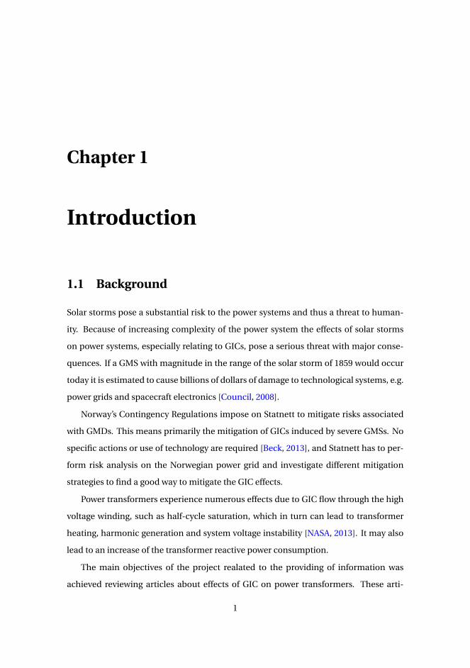
3.2.3 Coast Effect

The change in surface conductivity due to the ocean-land interface may enhance the

geomagnetically induced electric field on land close to the ocean. This phenomenon

is called the coast effect and depends on the land and sea conductivity, the depth of

the sea and the geomagnetic field characteristics [NERC, 2013]. The coast effect is un-

fortunate because electrical generating plants tend to be placed near the seashore for

cooling purposes[Gilbert].

In the transition from sea to land the horizontal conductivity structure experience

a great change as shown in Figure 3.2. Because the conductivity is higher in the sea-

water than in the soil, higher currents are induced i the sea than in the crust of the

earth. When a current is crossing the boundary between land and sea the geoelectric

field perpendicular to the boundary is higher when taking into account the coast effect

than only considering the land conductivity. This arises from the necessity of current

continuity while the charge cannot accumulate and there is a difference between the

current density arriving at the coast from the sea and the one departing from the coast

into the land [NERC, 2013].

The physics behind the coast effect is quite complex and a further description is out

of scope for this report, and the coast effect on transformers will not be looked into in

this project. Nevertheless, Norway has a long coastline and it would be natural to look

into the impact of the coast effect when simulating GIC-scenarios in the Norwegian

power grid.

3.2.4 Length

The vulnerability of power transmission lines increases with the length of the line. The

basis for calculating the voltage across a section of a conductor is given by Equation 3.1,

VAB =∫ B

AE · dl , (3.1)


Figure 3.2: Coast effect [NERC, 2013].

where VAB is the voltage between nodes A and B induced by the electric field E

over a line segment, e.g. a transmission line. If the electric field E across the power

system is assumed to be uniform the voltage across transmission lines could be found

be integrating over straight lines between substations [Bernabeu, 2013].

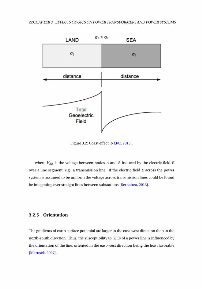
3.2.5 Orientation

The gradients of earth surface potential are larger in the east-west direction than in the

north-south direction. Thus, the susceptibility to GICs of a power line is influenced by

the orientation of the line, oriented in the east-west direction being the least favorable

[Marusek, 2007].

3.3. TRANSFORMERS 23

Figure 3.3: Conductance map of Europe, upper 80 km [Ádám et al., 2013].

3.3 Transformers

GICs may flow through any grounded component of the power grid. But of all the con-

sequences that may occur in the power grids due to solar storms, the consequences

of GIC flowing through high voltage transformers are maybe the most severe ones and

pose the greatest risk. It can cause damage to transformers and lead to blackouts, where

both consequences will result in great financial expenses and may even endanger hu-

man lives. Therefore the effects of the GIC on the transformers should be carefully ex-

amined and thoroughly understood to avoid such incidents.


Figure 3.4: Idealized single-phase transformer [BillC].

3.3.1 The Concept

GICs will flow through the high voltage transformers. In power transformers this causes

half-cycle saturation, which in turn can lead to transformer heating, harmonic genera-

tion and system voltage instability [NASA, 2013]. It can also lead to an increase of the

reactive power consumption.

3.3.2 Half-Cycle Saturation

When GICs, which are quasi-DC currents, flows in a power transformer, it causes a uni-

directional DC flux to flow in the core. As a result the total flux in the core is the sum

of the DC flux and the AC flux, as shown in Equation 3.2. Consequently, in the negative

half-cycle the DC flux will be subtracted from the AC flux and there is no saturation.

While in the positive half-cycle the core will go into saturation due to the DC flux, as

shown in Figure 3.6, hence the name half-cycle saturation.


φ=φAC +φDC (3.2)

The magnitude of the DC flux depends on three factors: the magnitude of the in-

duced quasi-DC current, number of turns in the windings where the quasi-DC current

flows, and the reluctance of the path of the DC flux [Girgis and Vedante]. This relation

is shown in Equation 3.3,

φDC = N ·GIC

ℜ , (3.3)

where N is the number of turns, GIC is the magnitude of the DC current and ℜ is

the reluctance of the magnetic circuit. The reluctance ℜ is found using Equation 3.4,

ℜ= l

µ · A, (3.4)

where l is the length of the magnetic circuit,µ is the permeability of the material and

A is the cross-sectional area of the circuit. Furthermore the reluctance ℜ is a function

of the ac excitation. So, to find the magnitude of the direct flux biasφDC one has to take

into account the direct flux bias φDC dependency of the ac excitation and the level of

saturation, and not only the GIC magnitude [Bernabeu, 2015].

The significant increase of reactive power consumption due to half-cycle saturation

can cause unusual transmission flow of active and reactive power, generator problems

due to reactive power limits, and intolerable system voltage depression [Fuchs and Ma-

soum, 2008].

3.3.3 Thermal Effects

GIC flowing in the transformer leads to a higher magnetizing current, which shape pro-

duce a higher leakage flux, that also contains a lot of harmonics. This leads to a sig-

nificant increase of eddy and circulating current losses in both windings and structural

parts of the transformer, causing heat generation and transformer losses [Girgis and

Vedante]. Because the GIC-imposed thermal duty is outside the standard service pa-

rameters the increase in temperature and load losses of windings and structural parts


Figure 3.5: Flux density shift in the core caused by DC [Girgis and Vedante].

should be assessed individually for each type of power transformer design [NASA, 2013].

Several articles from the ”IEEE Xplore Digital Library”, e.g. [Girgis and Vedante] and

[NASA, 2013], concludes that overheating due to induced DC-current should not nec-

essarily have any negative impact on the reliability of the transformer. The reason is

said to be that the duration and frequency of the occurrence of GICs is too short to pro-

duce a critical temperature rise and low enough to give the transformer time to cool off,

respectively.

The article [Girgis and Vedante] concludes that in most cases even high levels of

GIC should not lead to damaging overheating of neither windings nor structural parts

of power transformers, with core form and shell form being the exceptions. It claims

that some cases of significant overheating and winding damage believed to be caused

by GICs, were found to be caused by other effects, or by system instability experienced

during a GIC event [Girgis and Vedante]. The article [NASA, 2013] confirms the neces-

sity to determine the possibility of winding overheating due to high levels of GIC, but

depreciate the overheating of the tank wall as an issue.


Figure 3.6: Part-Cycle, Semi-Saturation of Transformer cores [Girgis and Vedante].

In the research on whether the Norwegian power grid is exposed to solar storms,

Statnett wants to measure the temperature in transformers, at points where it is most

likely to experience high temperatures due to GICs. In this way one can find the degree

of the correlation between overheating damaging and GIC flow.

3.3.4 Dependency of Type of Transformer

The magnitude of the DC flux shift in the core is dependent on the magnetic reluctance

of the DC flux path [Girgis and Vedante], hence the extension of GIC effects on power

transformers depends on the design of the core.

In Figure 3.7 the white arrows symbolize the possible return paths for induced DC

flux and the larger gray arrows symbolize the induction of magnetic flux from the wind-

ings. The core designs with return paths through the limbs are more likely to saturate

from GICs. So, although the three-legged core and the five-legged core will conduct the


same amount of GICs, the three-legged core will not saturate as easily [Thorberg, 2012].

Figure 3.7: Core DC Flux path in various core types [Girgis and Vedante].

For the three-phase three-legged core the return path of the DC flux begins at the

top yoke, continuing through the high reluctance path to the tank cover, going through

the tank wall, returning to the bottom yoke through the high reluctance path from the

tank bottom. This results in the highest reluctance path of the transformer types which

gives the smallest DC flux shift. Thus the three-phase three-legged core is the least

sensitive to GICs [Girgis and Vedante], while the single-phase transformer on the other

hand is more sensitive than three-phase transformers.

The different DC flux shift experienced from GICs in different core types leads to

varying magnitudes of magnetizing currents drawn by the transformer. In this context,

transformers may be divided into two groups: three-phase three-legged transformers


and other core types. In Figure 3.8 these groups are represented by a large three-phase

three-legged transformer and a large single-phase transformer, respectively. It can also

be seen in Figure 3.8 that the magnetizing current drawn by the single-phase trans-

former is much higher than the magnetizing current drawn by the three-phase trans-

former for the same values of DC currents flowing in each phase [Girgis and Vedante].

Also, since the return limbs is much less than the sum of the main limbs for the group

represented by the large single-phase transformer, saturation will occur at an earlier

time than for the three-legged transformer [Price, 2002].

Figure 3.8: Peak magnetizing current for 2 different core types [Girgis and Vedante].

Earlier the manufacturer has not been required to provide knowledge of transformer

functionality and sensitivity against GICs. Today the specification of GIC tolerance lev-

els for new transformers is usually included in the datasheet of the transformer. A fur-

ther development of this trend should be encouraged so that the buyer can make a

reasonable choice of transformer considering the risks associated with GICs.


3.3.5 ∆

In Figure 3.9 one can see that the dc equivalent circuit of both two-winding and three-

winding transformers are the same. This is because the ∆ does not provide a path for

GIC flow in steady-state and is therefore not included [NERC, 2013]. H1, H2, H3, L1,

L2 and L3 represents the nodes of the three phases on the HV and LV side. H0 and

L0 represent the neutral winding. Both H0 and L0 may be ungrounded, but if the GIC

effects are to be studied at least the H0 need to be grounded. RWH1 and RWL2 refer to

the DC winding resistance of the HV side and the LV side, respectively.

Figure 3.9: Single-phase dc equivalent of a two-winding or three-winding transformer[NERC, 2013].

Applying a DC step voltage to the HV winding may cause a current flow in the∆ if the

transformer is unsaturated. But when reaching the point of saturation the applied DC

voltage will cause the induced GIC in the tertiary winding to fall to zero. Additionally,

the delta connection will work as a path for the triplen harmonics [Price, 2002].

3.4 Power Systems

3.4.1 Harmonic Generation

Saturation in the power transformer caused by GICs leads to induced harmonic cur-

rents. The effects due to these harmonics are many, some of them are given in the list

3.4. POWER SYSTEMS 31

below [Fuchs and Masoum, 2008]:

• Overheating of capacitor banks

• Possible misoperation of relays

• Sustained overvoltages on long-line energization

• Higher secondary arc currents during single-pole switching

• Higher circuit breaker recovery voltage

• Overloading of harmonic filters of high voltage DC (HVDC) converter terminals

• Distortion of the AC voltage wave shape that may result in loss of power transmis-

sion

Some particularly important issues are the increase of reactive power consumption

and the probability of misoperation of protection and relay schemes when the config-

uration of these are not taking into account the harmonic currents produced by GICs.

Figure 3.10 shows the % harmonic content of two types of transformers, in accor-

dance with the group division explained in subsection 3.3.4. It can be seen in Figure 3.10

that three-phase transformer subjected to DC current give rise to a magnetizing current

pulse with an amplitude much higher for low order harmonics than for high order har-

monics. On the other hand, for the single-phase transformer, which represents other

core types, the amplitudes of the magnetizing current pulse between low and high or-

der harmonics are more much more uniform.

In Figure 5 it is also observed that the amplitude of the 2nd order harmonic for the

single-phase, transformer are, relatively to the amplitude of the 2nd order harmonic for

the three-phase transformer, very low. The same goes for other transformers as well,

except from the three-phase three-legged core. This is unfortunate because a differen-

tial relay set to actuate for low 2nd harmonic components, to distinguish inrush current

from fault condition, may lead to erroneous operation during a GIC event.


Figure 3.10: Harmonic content of magnetizing current of transformers subjected to DC[Girgis and Vedante].

3.4.2 Reactive Power Consumption

Simulation results from the system configuration in article [Chiesa et al.] confirm that

while there is only a minor effect of the GICs on active power, the reactive power con-

sumption of the transformer increases by a factor of 3 when applying 100 A GIC.

In several articles, e.g. [NASA, 2013] and [Chiesa et al.], it is assumed to be a linear

relationship between the reactive power consumption of a transformer and the mag-

nitude of GIC. Nevertheless, in the article [Bergsåker, 2014] there was concluded for

a type of hybrid transformer that the relationship is non-linear, even though there is

an approximately linear region. In the article [Chiesa et al.], on the other hand, using

the hybrid transformer model approach [Høidalen et al., 2009], the reactive power con-

sumption as a function of GIC is found to be fully linear.

3.4. POWER SYSTEMS 33

Figure 3.11: Reactive power drawn by a transformer as function of GIC [Chiesa et al.].

The results in the article [Bergsåker, 2014] indicates that an increased cross-sectional

area of the transformer leads to a smaller increase in reactive power consumption un-

der the influence of GICs. Accordingly, it is concluded that a larger transformer core will

be more resistant to GICs in terms of reactive power consumption [Bergsåker, 2014].


Chapter 4

GIC Simulations using ATPDraw

The simulation program ATP and the plotting program PlotXY can be integrated with

ATPDraw [Høidalen]. In this project ATPDraw, Windows version 5.9p3, is the solver

used to carry out the simulations.

4.1 GIC modeling

To determine GIC in power lines and earth connections a number of parameters with

respect to geomagnetic field, electric field strength and DC voltage induced across the

power grid have to be determined. However, for this project the GIC values are prede-

termined, and only a brief overview of GIC modeling is given.

4.1.1 How to Determine GIC

The occurrence of GIC is dependent on three factors: geometry of the grid, spatial varia-

tions of the geomagnetic field, and spatial variations of the ground conductivity [Myllys

et al., 2014].

In reality the GICs in the network only depend on one environmental parameter,

the geoelectric field. But because of no regular recordings of the geoelectric field close

to the power grids one must use numerical modeling to determine the GICs. To achieve

35

36 CHAPTER 4. GIC SIMULATIONS USING ATPDRAW

this values we must base the simulation on the two geophysical parameters geomag-

netic variations and the earth surface impedance [Zheng et al., 2013].

To understand and predict the effects of GICs it is essential to make accurate models

of the power grid, its components and their response to GICs. To do so FEM-based

models and magnetic circuit models can be used.

The process of modeling GICs in the power system can be divided into three steps:

”Calculation of the geoelectric field, DC mapping of the power system, and calculation

of GIC flows in the system” [Bernabeu, 2013].

Transformer Model

The transformer models used for GIC study purposes can be devided into two cate-

gories: Magnetic models that deal with reactive power consumption and harmonic

generation and thermal models that deal with hot spot heating [NERC, 2013]. In this

project there are only used magnetic models.

When modeling a transformer one must determine a multitude of parameters. There

are three ways to choose these parameters: from factory test reports, from detailed fac-

tory design information or, if the basic ratings of the transformer are the only data avail-

able, from a complete estimation [Negri and Gotti, 2007].

FEM models

The requirement of detailed design information and the computational burden of the

FEM model makes it an unsuitable choice for simulations of the power grid. Neverthe-

less it is a great option for simulations of the tank and other metallic components where

power losses and temperature rises are of concern [Chiesa et al.].

Magnetic Circuit Models

When using models based on magnetic circuit theory to analyze the GIC effects on

transformers it is important to take all the necessary parameters into account to get

an adequate representation. To do so, topological representation of the core structure

with independent core sections and air flux paths needs to be included [Chiesa et al.].

4.1. GIC MODELING 37

4.1.2 Important Factors

Interdependencies in the power system

In real life there are interdependencies to consider in the power systems, e.g. mitigation

of one transformer may lead to higher magnitudes of GIC at a connected transformer

nearby, and these should be included in the simulations of GIC effects on the power

system. Also, if not modeling the entire power grid, but only a part of it, the rest of the

grid should be represented by an equivalent.

In this project only a part of a power grid is modeled. But since it is not part of a

specific power system and the circuit diagram given is considered to be sufficient for

the purpose of this project, an equivalent replacing the rest of the power system will

not be developed.

Air-Core Inductance and Air Path Inductance

It is important to include the air-core inductance to achieve an accurate representa-

tion of highly saturated state of the core. Furthermore it is crucial to include off-core

flux paths in the model, i.e. include air path inductance, because part of the flux fol-

low paths outside the core, and air paths inductances are shown to be much larger for

DC than for 50 Hz [Chiesa et al.]. Not doing so would lead to misleading results, e.g.

false values of the harmonic content and the reactive power consumption, which in

turn could lead to false tripping of protection relays under the influence of GIC [Chiesa

et al.]. Due to the theory in subsection 3.3.4 the deviations will be greater for the three-

phase three-legged transformer than for the three-phase five-legged transformer.

In reality the flux forced outside the transformer core has a continuous distribution

across space. That is, it could be represented by an infinite number of flux paths on

the inside and outside of each winding of the transformer. The transformer models

used in this project include off-core flux paths by air path inductance and inductances

representing the space between the leg and inner winding, inner winding and middle

winding, and middle winding and outer winding.


GIC Signature

In order to conduct realistic simulation studies of the GIC thermal capability of a trans-

former it would be convenient to use a GIC signature. The GIC signature is based on

data from a large number of measured GIC profiles during GMDs and a reference geo-

electric profile, and is consisting of a large number of consecutive narrow pulses. These

pulses may be divided into two categories, one being low to medium level pulses last-

ing for a period in the range of hours and the other being high peaks with a duration of

a fraction of a minute until several minutes [IEEE, 2015, 7.2.1 Suggested standard GIC

signature, p. 25].

Establishing thermal capability of the power transformer is out of scope for this

project, and an appropriate GIC signature will not be applied. Nevertheless, it is men-

tioned because of its utility in the determination of thermal response of a power trans-

former when establishing power transformer capability.

4.2 Circuit Diagram

The electrical diagram in Figure 4.1, named Model A, was initially intended to use to

accomplish the tasks in this project, but it turned out that it was difficult to obtain re-

sults without major flaws from this model. So, for the last part of the project, another

electrical diagram was used, see Figure 4.2. This test arrangement, called Model B, is

based on the article [Lahtinen and Elovaara, 2002].

Model B showed greater accuracy in terms of less noise, less current and voltage

spikes, and the findings were more in accordance with the GIC theory. Hence, mea-

surements done in Model B will be assumed to be more relevant. Thus, even though

results from using Model A seem to confirm some tendencies seen for Model B, the

results from Model A will be left out due to their inaccuracy. Nevertheless, a descrip-

tion of Model A, some measurement methods and a few simple reflections will still be

included. The purpose is to discuss errors and deficiencies of model Model A in the

discussion part of the report, and in case someone would find interest in carrying out a

further investigating of the test arrangement.

4.2. CIRCUIT DIAGRAM 39

Omitting the resistors added to the windings of the transformers in Model A and

Model B, whether the winding is isolated from earth or grounded, normally results in

error. Therefore, the resistors are needed for the simulation to ensure that the models

work properly. This should not be the case and the need for excessive resistances may

be due to errors in the source code of ATPDraw.

4.2.1 Model A

The geomagnetic field causing GIC to flow in Model A is represented by a grounded

voltage ramp which is connected to the HV side of the 300MVA transformer. The voltage

rises from zero to a constant, E0, in one second. To be able to measure the GIC induced

by the ramp block a measuring switch is placed between the ramp block and the HV

winding.

Figure 4.1: Circuit diagram of Model A


4.2.2 Model B

As already stated, the results from Model B is more as expected than for Model A, with

respect to the GIC theory. But on the other hand, Model B is not a particularly realistic

circuit diagram as the HV side of the two transformers are connected at the same node,

i.e. no physical distance. Trying to improve Model B, e.g. adding line impedances, is a

laborious work which requires a lot of troubleshooting, and will be left out of the scope

of this project due to the time limit.

The GIC is fed into the network from a grounded DC current source which is con-

nected to the HV winding of transformer number two, T2, see Figure 4.2. The DC cur-

rent source applies a current of a given value and works instantaneously.

Figure 4.2: Circuit diagram of Model B

4.3. TRANSFORMER MODEL 41

Table 4.1: Transformer rating and design for both the 300MVA-5 and the 300MVA-3transformer model.

HV 420 kV 300 MVA Y groundedLV 132 kV 300 MVA Y groundedTV 47 kV 100 MVA ∆

4.3 Transformer model

As the transformer connected to the GIC source there are used two types. The two types

mainly have the same ratings and designs, see Table 4.1, except that they have three and

five limbs.

4.3.1 300MVA-5

Figure 4.3 shows the electrical diagram of the 300MVA-5 core transformer from ATP-

Draw which is working as a passage for GIC to enter the power grid. The transformer

is a three-phase, five-legged 300 MVA transformer. Both the high voltage winding on

the primary side and the low voltage winding on the secondary side are star connected,

and connected to ground by a low resistance path. Furthermore, it has a ∆, isolated

from ground by a high resistance path. The ∆ can be eliminated from the circuit by

opening the switch which can be seen in Figure 4.3.

The upper part of the diagram in Figure 4.3 , except the far right, represents one

phase, R, and is repeated three times downwards due to the three phases R, S and T.

The total losses in the core are assumed to be divided more or less equally between

the eddy current losses and the hysteresis losses, and are represented by RC and LC,

respectively. The far right of the circuit represents the yoke with the outer limbs. A list

of parameters description is given in Table 4.2.

4.3.2 300MVA-3

The description of the three-phase three-legged transformer, 300MVA-3, is similar to

the 300MVA-5 core transformer, see Figure 4.4. The 300MVA-3 core transformer only

have three limbs, thus no outer limbs. This taken into account, one can see that the


Figure 4.3: Topology of the 300MVA-5 transformer model

Figure 4.4: Topology of the 300MVA-3 transformer model

topology of the two transformer types are nearly identical, except from to the right in

the circuit diagrams, where the 300MVA-3 model is represented by only the yoke, as the

limbs are all main legs.

4.4. MEASUREMENT METHODS 43

Table 4.2: Parameters description for the 300MVA-5 transformer model, see Figure 4.3.To better get an idea of the parameters description look at the sketch of the "Core Form,3 phase, 5 limb" in Figure 3.7.

RC Resistance representing losses in legLC Inductance in leg, may be saturatedRWL Resistance in LV windingRWH Resistance in HV windingRWT Resistance in tertiary windingLLC Leakage inductance representing the space between the inner winding and the legLHL Leakage inductance between LV winding and HV windingLHT Leakage inductance between HV winding and tertiary windingLOC Leakage inductance representing the space outside the core, referred to as air path inductanceLOY Inductance of outer limb, may be saturatedROY Resistancerepresenting losses of outer limbLIY Inductance of the yoke, may be saturatedRIY Resistance representing losses of the yoke

4.4 Measurement Methods

In this section the measuring techniques will be described. Most of the methods applies

for both Model A and Model B, and it will be specified when this is not the case. For both

models the focus will mainly be on the transformer where the GIC enters, T2, and the

reactive power flow in the system. This is because the saturation is expected to be the

highest in T2.

The main purpose is to investigate how the GIC effects change with respect to cer-

tain conditions. Parameters of interest will be, unless otherwise stated, as given in Ta-

ble 4.3.

Table 4.3: Default values and default settings for Model A and Model B

Parameter Default Value/Setting DescriptionTmax 70 End time [s] of simulation.

U0 420 Generator voltage [kV].E0 150 The maxiumum voltage [V] induced by the ramp block in Model A.

GIC0 200 The DC current [A] induced by the DC current source in Model B.TCL closed (-1) Closing time [s] of switch in ∆,

denoting whether the switch is closed (-1) or open (1000).LOC 500 Air path inductance [mH] due to each phase.

Power Transformer 300MVA-5 Type of power transformer connected to the GIC source.

The setup of Model B will differ in terms of transformer model, presence of ∆, mag-


nitude of GIC0 and value of LOC. This gives a total of eight different setup configura-

tions, see Figure 4.5. A more detailed explanation will be given in subsections 4.4.1-

4.4.4.

Figure 4.5: The flow chart shows the different combinations that makes up the eightsetup configurations used in the project report.

It would be interesting to measure the reactive power consumption, current, voltage

and magnetic flux at a large number of nodes to understand the GIC effects on the en-

tire power system and how the different components in the electrical diagram interfers

with each other. Nevertheless, the measurements are limited to only a few components.

This is for the benefit of comparing several setups, i.e. combinations of 300MVA-3 and

300MVA-5 transformers, with or without a ∆, and for different values of air path induc-

tances and GIC magnitudes.

It is of crucial importance to set the step of simulation, delta T, to adequate values in

ATPDraw. In Model A the time step is set to 4 µs. If the time step is reduced by a factor of

ten the compilation does not terminate when having an end time of simulation, Tmax,

of several tens of seconds. In Model B the time step is set to a value of 40 µs. Increasing

the time step in both models by a factor of ten in an attempt to reduce the solving time

leads to incorrect results.

The end time of simulation, Tmax, is set to 70 s beacuse the different systems are all

found to be in an approximated steady-state at this time.

The effect of GIC on active power loss is in general relatively small, hence, the active

power measurements will be disregarded.


4.4.1 Three-Legged and Five-Legged Transformers

The differences between three-phase three-legged and three-phase five-legged trans-

formers when it comes to GIC response will be explored for each of the other tasks.

This is simply done by replacing the 300MVA three-winding transformers in a circuit

diagram with either all 300MVA-3 or all 300MVA-5 transformer models. This applies to

the transformer T2 in Model A, see Figure 4.1, and to both T1 and T2 in Model B, see

Figure 4.2.

If using Model A one would measure the current through the connection from the

ramp block to the HV winding of the adjacent power transformer. For Model B the GIC

magnitude is already given, and the currents of interest are the RMS current and the

phase currents across Switch C, see Figure 4.2. When measuring current the factors of

interest are the shape, magnitude and harmonics. In addition the reactive power flow in

the power system should be measured for both models. Furthermore the flux-linkages

in the different sections of the transformer, including off-core flux, should me graphed.

4.4.2 Delta Conntected Tertiary Winding

To find out which impact the ∆ has on the GIC effects both the three-legged and the

five-legged transformer were tested with and without the ∆.

4.4.3 Air Path Inductance

To find how the effects of GIC change with the air path inductance, i.e. different values

of LOC, it is convenient to look at the flux-linkages in different core sections. To do so

in ATPDraw one can use the relation

|ε| =∣∣∣∣dφ

d t

∣∣∣∣ (4.1)

and plot the integration of the voltage across the different core sections using the

integration function in the PlotXY program. In Equation 4.1 ε is the term for induced

voltage [V], φ is magnetic flux [Wb] and t is time [s].

The ideal would have been to set the value of LOC to 0 mH, i.e. no flux driven outside


the core, and a few higher values to look at the difference in flux-linkages, current in

the HV winding of T2 and the reactive power consumption of the system. However,

setting LOC to 0 mH or a small value, such as 0,1 mH or 50 mH, is causing trouble when

running the simulation in ATPDraw. Therefore, the LOC is set to 250 mH, 500 mH, 750

mH and 1000 mH for the different transformer configurations, assuming that LOC is 0

mH would follow the same pattern pattern. Using the 300MVA-5 without∆ even setting

LOC to 250 mH gives an error message when trying to run the simulation, and will be

omitted for this particular configuration.

The idea is to visualize the air path inductance influence on the GIC effect. To do

so one will compare the magnetic flux through certain parts of the transformer, the air

paths included. These are plotted together for different values of the air path induc-

tance, LOC. The paths chosen for the 300MVA-5 transformer, see Figure 4.3 and Fig-

ure 4.6, are

LC Leg

LOY Outer limb

LIY Yoke

LOC Air path

For the 300MVA-3 transformer there are no outer limbs and the magnetic flux is only

measured through the leg, yoke and air path, see Figure 4.4 and Figure 4.7,

Figure 4.6: The illustration shows a five-legged core transformer model and the fluxpaths measured in ATPDraw.


Figure 4.7: The illustration shows a three-legged core transformer model and the fluxpaths measured in ATPDraw.

4.4.4 Magnitude of the Geomagnetically Induced Electric Field and

the size of the GIC

It would be interesting to check how much the GIC effects depend on the magnitude

of either the geomagnetically induced electric field or the GIC for Model A and Model

B, respectively. For Model A the magnitude of the geomagnetically induced electric

field is changed simply by changing the maximum voltage induced by the ramp block.

For Model B the magnitude of GIC is changed by choosing different values for the DC

current induced by the DC current source. More specific, the value of the DC current

source in Model B will be set to 100 A, 200 A and 300 A. To compare with the system

when GIC is not induced one replaces the DC current source in an electrical diagram

configuration with a small grounded resistance.

4.4.5 X/R ratio

There may exist a relationship between the time constant which describes how fast the

GIC is rising, and the X/R ratio of the transformer and its adjacent lines. In the sequence

network a transformer is represented as its positive and negative sequence impedances

in the positive and negative sequence networks, respectively. The transformer repre-

sentation in the zero sequence network, however, may have a high complexity [Amberg

and Rangel, 2014].

Power lines, and transformers, are passive elements. Given that the three phases of


Table 4.4: Parameters description of the three-phase RLC symmetrical PI-equivalent.The negative sequence impedance components are equal to the components of thepositive sequence impedance.

R0 Resistance in the zero sequence system [Ω/m]L0 Inductance in the zero sequence system [mH/m]C0 Capacitance in the zero sequence system [µF/m]R+ Resistance in the positive sequence system [Ω/m]L+ Inductance in the positive sequence system [mH/m]C+ Capacitance in the positive sequence system [µF/m]Length Length of the line [m]

the line are symmetrical, this implies that the sequence of the applied phase voltages

does not matter in regard to the voltage drops across the line. As a result the positive

and negative sequence impedances of a symmetrical three-phase transmission line, or

a transformer, are assumed to be identical.

The two transmission lines connected to the five-legged transformer in Figure 4.1

are 3-phase RLC symmetrical PI-equivalents. The parameter description for the line is

given in Table 4.4.

The total impedance in the line is given by Equation 4.2.

Ztot al ,l i ne = Z++Z−+Z0 = 2Z++Z0 = (2R++R0)+ j (2ωL++ωL0−2· 1

ωC+− 1

ωC0) (4.2)

Using Equation 4.2 one can find an X/R ratio for the transmission lines, see Equa-

tion 4.3.

X /Rl i ne =(2ωL++ωL0 −2 · 1

ωC+ − 1ωC0

2R++R0(4.3)

Then the X/R ratio for the transformer should be derived and together with the

X /Rl i ne ratio one could have concluded whether there seems to be a relationship be-

tween the GIC time constant and the ratio between the resistance and the reactance in

the lines-transformer conjuction.

The idea was to investigate the influence of the X/R-ratio using Model A. But since


one ended up using Model B, and this model does not have a realistic line representa-

tion, the derivation of the X/R ratio for the transformer as well the simulation testing

was omitted from the project. Instead, it will be added as a suggestion for further work.


Chapter 5

Results

In this chapter the most important findings and plots from the simulation testing in

ATPDraw, using Model B, will be presented. Furthermore, graphs which are of less im-

portance, or left out for the benefit of good order in the text, will be given in appendices.

Most of the plots for the 300MVA-5 transformer model, as well as some of the plots

for the 300MVA-3 transformer model, show big transient values at the beginning of the

simulation when when a∆ is not present. Nevertheless, all graphs are adjusted with the

purpose of showing how the measured parameters change with time irrespective of the

transients.

5.1 Reactive Power Consuption and RMS current of Trans-

former T2

In Table 5.1 the reactive power consumption and the RMS current flowing into the HV

winding of T2 is given for the different configurations of Model B. These are steady-state

values, and corresponding graphs are found in Figures B.1-B.16 in Appendix B. For the

purpose of visualization the data are also given as column charts in Figures 5.1 and 5.2.

Comparing the different transformers, having the same values of GIC0 and LOC, one

see a clear trend. The three-phase five-legged transformer leads to larger steady-state

51

52 CHAPTER 5. RESULTS

Table 5.1: The table shows the steady state values for both the reactive power consump-tion, Q, and the RMS current flowing into the HV winding of T2, IT2RMS, for the differentsetups of Model B. The column "Delta" states if the transformers do have a ∆ or not.

Transformer type Delta GIC0 [A] LOC [mH] Q [MVAr] IT2RMS [A]300MVA-3 With 0 500 0,16 0,22

100 0,72 33,35200 25,95 72,86300 59,44 116,52

300MVA-5 0 0,19 0,20100 58,19 68,45200 113,11 125,63300 162,74 177,72

300MVA-3 Without 0 0,16 0,22100 0,68 33,34200 22,06 69,29300 53,58 109,14

300MVA-5 0 0,19 0,19100 53,13 52,86200 105,82 106,48300 155,23 159,50

300MVA-3 With 200 250 2,31 66,77500 25,95 72,86750 45,15 81,65

1000 58,60 89,11300MVA-5 250 107,72 122,66

500 113,11 125,63750 115,70 127,11

1000 117,26 128,02300MVA-3 Without 250 1,93 66,71

500 22,06 69,29750 39,50 73,65

1000 52,70 78,14300MVA-5 250 - -

500 105,82 106,48750 108,44 107,92

1000 110,03 108,91

values for both reactive power consumption in the system, Q, and RMS current flowing

into the HV winding of T2, IT2RMS, than for the three-phase three-legged transfomer.

Having a∆ results in higher steady-state values for Q and IT2RMS than without the∆,

with respect to either the 300MVA-3 model or the 300MVA-5 model. However, Figure 5.3

and Figure 5.4 show a much smaller time constant for a transformer without a ∆. That

5.1. REACTIVE POWER CONSUPTION AND RMS CURRENT OF TRANSFORMER T253

Figure 5.1: The column chart illustrates the reactive power consumption in the systemat steady-state for the different setups of Model B. The legends refers to which trans-formers are used: 300MVA-3 w/∆, 300MVA-5 w/∆, 300MVA-3 w/o∆ and 300MVA-5 w/o∆ indicating three-legged with ∆, five-legged with ∆, three-legged without ∆ and five-legged without ∆, respectively. The parameters are fixed, as given in Table 4.3, exceptfor either the GIC value, GIC0, or the air path inductance, LOC, which are given on thex-axis.

is, in the beginning Q and IT2RMS are larger for a given transformer without the ∆ than

for the same transformer having a ∆.

There seem to be a linear relationship between the reactive power consumption and

the GIC magnitude for all four transformer configurations used in this project, i.e. both

the 300MVA-3 and 300MVA-5 transformer models with and without ∆, see the left side

of Figure 5.1. Likewise, it also appears to be a linear relationship between IT2RMS and

the GIC magnitude. Furthermore,

Not having a ∆ may result in transients with large values for Q and IT2RMS for large

values of GIC0 or LOC for both the 300MVA-3 and the 300MVA-5 transformer models,

see plots in Appendix B. The maximum values of both Q and IT2RMS may reach values of

5 to 6 times the steady-state values. For the 300MVA-5 transformer model without the

∆ there also appears sharp spikes in both Q and IT2RMS, see Figures B.15 and B.16.


Figure 5.2: The column chart illustrates the RMS currents of transformer T2 at steady-state for the different setups of Model B. The legends refers to which transformers areused: TD, FD, TU and FU stand for three-legged with∆, five-legged with∆, three-leggedwithout ∆ and five-legged without ∆, respectively. The parameters are set as given inTable 4.3, except for either the GIC value or the air path inductance, LOC, which aregiven on the x-axis.

5.2 Phase currents of Transformer T2

The graphs in Appendix C show a close-up view of the phase currents flowing into the

HV side of the transformer T2 during the test at 200 A DC-current and a LOC value of

500 mH for the different transformer configurations. From the shape one can clearly

see that the transformers experience half-cycle saturation. That is, with the exception

from for the five-legged transformer without a ∆, see Figure C.4, where the shape of

the curves are hard to interpret. Nonetheless, looking more closely at the Figures C.1-

C.3 reveals that for the 300MVA-3 transformer model there are a smoother half-cycle

saturation shape than for the 300MVA-5 transforme model.

5.3. HARMONIC CURRENTS OF PHASE A OF TRANSFORMER T2 55

Figure 5.3: Reactive power consumption in the system when GIC0 is 200 A and LOC is500 mH. The curves represent the tests with the following transformers: 300MVA-5 w/∆(red), 300MVA-5 w/o ∆ (green), 300MVA-3 w/∆ (blue) and 300MVA-3 w/o ∆ (pink).

5.3 Harmonic Currents of Phase A of transformer T2

Some plots of the current harmonics of phase A of transformer T2 for the different

power transformer configurations are shown in Appendix D, when GIC0 is set to 200

A and LOC is 500 mH.

5.4 Flux-Linkages

When changing the values of LOC the flux in the legs, yoke and limbs did not change

significantly. The off-core flux, on the other hand, increases noticeably with the value

of LOC. The flux-linkages in different core sections of the transformer T2 for different

transformer configurations, when GIC0 is 200 A and LOC is 500 mH, is shown by figures

in Appendix E.

The air path flux for the three-phase three-legged transformer with a∆, see E.1, does

not fluctuate. Furthermore, the shape of the air path flux for the 300MVA-5 transformer

model without a ∆ develops with time, see Figure E.3, while the steady-state shape of


Figure 5.4: RMS current flowing into the HV side of transformer T2 when GIC0 is 200A and LOC is 500 mH. The curves represent the tests with the following transformers:300MVA-5 w/∆ ∆ (red), 300MVA-5 w/o ∆ (green), 300MVA-3 w/∆ (blue) and 300MVA-3w/o ∆ (pink).

the three other transformer configurations appears instantaneously, see Figures E.1,

E.7 and E.5. Comparing the air path flux for the different transformer configurations in

Appendix E shows that at steady-state there are more flux flowing outside the core for a

transformer model with three limbs than with five limbs, see Figure 5.5.

5.4. FLUX-LINKAGES 57

Figure 5.5: The figure shows the the air path flux for the different transformer config-urations when GIC0 is 200 A and LOC is 500 mH. The curves represent the 300MVA-5w/∆ (red), the 300MVA-5 w/o ∆ (green), the 300MVA-3 w/∆ (blue) and the 300MVA-3w/o ∆ (pink).


Chapter 6

Summary and Recommendations

for Further Work

Recommend further work: Thermal model.

6.1 Summary and Conclusions

The overriding purpose of this Master’s project was to better understand GIC effects on

power transformers. To accomplish that goal it became necessary to reach some pre-

requisite goals. Chapters 2 and 3 concerns solar storms, GICs and their effects on power

systems and power transformers. It is presented in the form of theoretical knowledge,

referring to related work, and an introduction to the most important historical events is

given.

In chapter 4 the circuit diagram, as well as the power transformer models, used in

this project are presented. In addition, a few comments on how to determine the GIC

magnitude are included. Simulations are performed using ATPDraw, and the results are

graphed using the plotting program PlotXY. As mentioned, initially a circuit diagram

model with a geomagnetically induced current applied was used for the simulations,

see subsection 4.2.1. But since it was difficult to obtain results without major flaws

59

60 CHAPTER 6. SUMMARY

from this circuit diagram it was replaced by another one with a DC current source rep-

resenting the GIC instead of a voltage ramp block, see subsection 4.2.2. Furthermore,

the measurement methods used in the investigation of how the GIC effects are influ-

enced by the conditions given in the main objectives are explained. Due to the change

of circuit diagram to a model which is less realistic with respect to power lines the in-

vestigation of the X/R ratio was omitted.

The simulations are done using the different transformer configurations, i.e. three-

phase three-legged transformer or three-phase five-legged transformer with or without

∆. The parameters which have been modified are the value of the air path inductance

and the magnitude of the DC-current applied to the HV winding of transformer T2. The

results of the simulations are given in chapter 5 and Appendices B-E. Current harmon-

ics plots of the phase current A of the different transformer configurations are to be

found in Appendix D. A discussion based on harmonics will not be given due to short-

age of time.

6.2 ATPDraw

Major challenges with respect to the simulations in ATPDraw were experienced during

the project work. This fact led to that a greater proportion of the time than planned was

spent developing a functional circuit diagram. Thus, when such a diagram was aquired,

there was not much time left before the deadline of the Master’s project, which imposed

limitations on the thoroughness and extention of the work. Some of the challenges were

• running the simulation several times for the exact same circuit model sometimes

gave different results,

• in some very few cases a circuit diagram in ATPDraw which worked fine stopped

working after saving the ACP file,

• normally adding big or small grounded resistances between the transformer wind-

ings and ground were necessary to be able to run the simulations, but in a few ap-

parently inexplicable cases they had to be removed for the model to work prop-

erly,

6.3. DISCUSSION 61

• small values of LOC normally resulted in error when running the simulation,

• ATPDraw frequently froze or stopped working when running simulations or plot-

ting the results, loosing all the results and having to reinitiate the program,

• and one was not able to make the circuit diagram Model A work properly.

Reasons for why Model A, see subsection 4.2.1, did not provide usable results may

be numerous. It might be due to

• errors in the source code of ATPDraw,

• issues related to the use of a voltage source to represent the GIC,

• the possibility of the GIC being harder to distinguish from other effects for Model

A than for Model B,

• or it might be that Model A is more sensitive to the value of the time step.

Decreasing the time step value from 4 µs to 0,4 µs drastically increases the quality

of the results for Model A, but the plots still includes spikes and irregularities which are

difficult to explain. A further reduction of the time step value results in error, but en-

abeling such a reduction would probably increase the quality of the results even more.

For Model B there often were difficulties with running the simulation when choosing

time step values smaller than 20 µs. Thus, in the end, a time step value of 40 µs was

chosen for Model B. Considering the high frequencies present in electrical power sys-

tems, 40 µs is a relatively large time step value and may compromise the results.

6.3 Discussion

The main focus during this project have been on the simulations in ATPDraw and the

GIC effects on power transformers. And thus, that is what will be discussed in this part.

The simulation results are only digital. In other words they are not verified by val-

ues of real life recordings. Consequently, the veracity of the results are questionable.

Nevertheless, a major part of the results are in accordance with the GIC theory, e.i. lin-

ear relationship between Q and GIC magnitude and three-legged transformers being

less suceptible to GIC than five-legged transformers. Therefore, although values may


not excact, it is likely to assume that most of the results are fairly reasonable with re-

spect to trends. An exception is the simulations done using the 300MVA-5 w/o∆, which

in general gave unexpected plots. It gave large current spikes and big transient val-

ues Figure B.16, not the typical half-cycle saturation pattern for the phase currents, see

Figure C.4, and were not able to run even for a LOC value as high as 250 mH. All the

peculiarities just mentioned give reasons to doubt all the results coming from the tests

using the 300MVA-5 w/o ∆. Nonetheless, the fact that the steady-state values follows

the increasing pattern for Q and IT2RMS when increasing GIC0 and LOC, see Figures 5.1

and 5.2 show some credibility.

As expected, five-legged transformers showed greater susceptibility to GIC than three-

legged transformers. Furthermore, having a ∆ resulted in smaller steady-state values of

Q and IT2RMS, even though the time step was smaller such that for a period of time the

values where higher than for the same transformer with

The the smoother curves of the air-path flux of three-legged transformers may be

due to the fact that there are no return flux paths through the core. In other words, the

three-legged transformer will experience half-cycle saturation a for a larger portion of

time than five-legged transformers under the same conditions. That is may also be seen

by the large flux values of the air path flux for three-legged transformers, 100 Wb, while

for the five-legged transformer it fluctuates around 0 Wb.

Finally, with respect to GIC effects, one may draw the conclusion that one should

choose three-phase three-legged transformers over three-phase five-legged transform-

ers without a ∆ due to its resistance against GIC. Also, it would be interesting to look

into the possibility of closing the ∆ at the point were the reactive power consumption

of the three-legged transformer with and without a ∆

6.4 Recommendations for Further Work

The research that has been undertaken for this project has highlighted a number of top-

ics on which further research would be beneficial. Possible extensions to this Master’s

project could be as given:

6.4. RECOMMENDATIONS FOR FURTHER WORK 63

• Develop Model A in terms of adding power lines, loads, transformers and en-

trances and exit points. Then, one could study the secondary effects, i.e. GIC

effects on the other components in the power grid. It would also be possible to

continue with the X/L ratio testing, see subsection 4.4.5. In addition one should

advance with the interpretation of current harmonics.

• Research whether there is a way to use the ∆ in a transformer to mitigate the GIC

effects. One way to do this would be to see how the measurements, e.i. reactive

power consumption, would react when the switch in the ∆ closes at the point of

where the reactive power consumption is equal for a transformer with or without

∆ during GMDs, see Figure 5.3.

• Develop a functional circuit diagram in ATPDraw which uses a current source to

induce GIC.

• Develop a circuit diagram model in ATPDraw with temperature dependent impedances

which take into account the heating of the transformer parts. The first step would

be to perform real life GIC testing to find the correlations between heating of the

different parts of the transformer and phase currents of the transformer. Then,

this information could be used to program GIC dependent impedance moduls

which acts as temperature dependent.

• The simulations done in this project are rather short compared to the duration of

potential large GMDs. Thus, it would be interesting to know how the transformer,

e.i. transformer T2 in Model A, would be affected during a more realistic GIC

scenario, see the part about GIC signatures in subsection 4.1.2.

• Adjust Model A so that the results fits real life recordings. An example of this has

already been done by the supervisor for this Master’s project. He obtained a re-

markable fit for the reactive power consumption of the five-legged transformer in

ATPDraw and recorded apparent power in [Lahtinen and Elovaara, 2002].


Appendix A

Acronyms and Notations

AC Alternating Current

∆ Delta connected tertiary winding

EMF Electromotive Force

EMTP Electromagnetic Transients Program

GIC Geomagnetic Induced Current

GIC0 Magnitude of the DC current [A], representing the GIC, flowing into the ground

connection of transformer T2

GMD Geomagnetic Disturbances

GMS Geomagnetic Storm

HV High Voltage

IEEE Institute of Electrical and Electronics Engineers

IT2RMS The current [A] flowing into the HV side of the transformer T2

LOC Value of the air path inductance [mH] input to the 300MVA transformer model

representing the off-core flux paths

65

66 APPENDIX A. ACRONYMS AND NOTATIONS

LV Low Voltage

MVA Mega-Volt Ampere

NTNU Norwegian University of Science and Technology

Q The reactive power consumption [VAr] in the system

RMS Root Means Square

300MVA-5 w/o∆ Three-phase five-legged transformer model without a delta connected

tertiary winding

300MVA-5 w/∆ Three-phase five-legged transformer model with a delta connected ter-

tiary winding

300MVA-3 w/o∆ Three-phase three-legged transformer model without a delta con-

nected tertiary winding

300MVA-3 w/∆ Three-phase three-legged transformer model with a delta connected

tertiary winding

T1 Transformer number one

T2 Transformer number two

Appendix B

Combination graphs, Q, T2RMS

B.1 Introduction

The graphs shows the reactive power consumption and the RMS currents of trans-

former T2 for the different setups of Model B shown in Figure 4.5.

67

68 APPENDIX B. COMBINATION GRAPHS, Q, T2RMS

Figure B.1: Reactive power consumption due to a 300MVA-3 w/∆ when changing theGIC value and LOC is 500 mH. The curves represent the tests of the following DC-currents: 0 A (red), 100 A (green), 200 A (blue) and 300 A (pink).

Figure B.2: RMS current flowing into the HV side of transformer T2 when using a300MVA-3 w/∆. The GIC value is changed, while the LOC is 500 mH. The curves rep-resent the tests of the following DC-currents: 0 A (red), 100 A (green), 200 A (blue) and300 A (pink).

B.1. INTRODUCTION 69

Figure B.3: Reactive power consumption due to a 300MVA-5 w/∆ when changing theGIC value and LOC is 500 mH. The curves represent the tests of the following DC-currents: 0 A (red), 100 A (green), 200 A (blue) and 300 A (pink).

Figure B.4: RMS current flowing into the HV side of transformer T2 when using a300MVA-5 w/∆. The GIC value is changed, while the LOC is 500 mH. The curves rep-resent the tests of the following DC-currents: 0 A (red), 100 A (green), 200 A (blue) and300 A (pink).


Figure B.5: Reactive power consumption due to a 300MVA-3 w/o ∆ when changingthe GIC value and LOC is 500 mH. The curves represent the tests of the following DC-currents: 0 A (red), 100 A (green), 200 A (blue) and 300 A (pink).

Figure B.6: RMS current flowing into the HV side of transformer T2 when using a300MVA-3 w/o ∆. The GIC value is changed, while the LOC is 500 mH. The curves rep-resent the tests of the following DC-currents: 0 A (red), 100 A (green), 200 A (blue) and300 A (pink).


Figure B.7: Reactive power consumption due to a 300MVA-5 w/o ∆ when changingthe GIC value and LOC is 500 mH. The curves represent the tests of the following DC-currents: 0 A (red), 100 A (green), 200 A (blue) and 300 A (pink).

Figure B.8: RMS current flowing into the HV side of transformer T2 when using a300MVA-5 w/o ∆. The GIC value is changed, while the LOC is 500 mH. The curves rep-resent the tests of the following DC-currents: 0 A (red), 100 A (green), 200 A (blue) and300 A (pink).


Figure B.9: Reactive power consumption due to a 300MVA-3 w/∆ when changing theLOC value and GIC0 is 200 A. The curves represent the tests of when LOC is set to avalue of 250 mH (red), 500 mH (green), 750 mH (blue) and 1000 mH (pink).

Figure B.10: RMS current flowing into the HV side of transformer T2 when using a300MVA-3 w/∆. The LOC value is changed, while the GIC0 is 200 A. The curves rep-resent the tests of when LOC is set to a value of 250 mH (red), 500 mH (green), 750 mH(blue) and 1000 mH (pink).


Figure B.11: Reactive power consumption due to a 300MVA-5 w/∆ when changing theLOC value and GIC0 is 200 A. The curves represent the tests of when LOC is set to avalue of 250 mH (red), 500 mH (green), 750 mH (blue) and 1000 mH (pink).

Figure B.12: RMS current flowing into the HV side of transformer T2 when using a300MVA-5 w/∆. The LOC value is changed, while the GIC0 is 200 A. The curves rep-resent the tests of when LOC is set to a value of 250 mH (red), 500 mH (green), 750 mH(blue) and 1000 mH (pink).


Figure B.13: Reactive power consumption due to a 300MVA-3 w/o∆when changing theLOC value and GIC0 is 200 A. The curves represent the tests of when LOC is set to avalue of 250 mH (red), 500 mH (green), 750 mH (blue) and 1000 mH (pink).

Figure B.14: RMS current flowing into the HV side of transformer T2 when using a300MVA-3 w/o ∆. The LOC value is changed, while the GIC0 is 200 A. The curves rep-resent the tests of when LOC is set to a value of 250 mH (red), 500 mH (green), 750 mH(blue) and 1000 mH (pink).


Figure B.15: Reactive power consumption due to a 300MVA-5 w/o∆when changing theLOC value and GIC0 is 200 A. The curves represent the tests of when LOC is set to avalue of 500 mH (green), 750 mH (blue) and 1000 mH (pink).

Figure B.16: RMS current flowing into the HV side of transformer T2 when using a300MVA-5 w/o ∆. The LOC value is changed, while the GIC0 is 200 A. The curves repre-sent the tests of when LOC is set to a value of 500 mH (green), 750 mH (blue) and 1000mH (pink).


Appendix C

Phase Currents

C.1 Introduction

The graphs shows the three phase currents flowing into the HV winding of transformer

T2 for the different transformer configurations in Model B when the GIC, GIC0, is 200 A

and the air path inductance, LOC, is 500 mH.

77

78 APPENDIX C. PHASE CURRENTS

Figure C.1: Phase currents of phases A (red), B (green) and C (blue) flowing into the HVside of transformer T2 during the test at 200 A DC-current and LOC is 500 mH whenusing a 300MVA-3 w/∆.

Figure C.2: Phase currents of phases A (red), B (green) and C (blue) flowing into the HVside of transformer T2 during the test at 200 A DC-current and LOC is 500 mH whenusing a 300MVA-5 w/∆.

C.1. INTRODUCTION 79

Figure C.3: Phase currents of phases A (red), B (green) and C (blue) flowing into the HVside of transformer T2 during the test at 200 A DC-current and LOC is 500 mH whenusing a 300MVA-3 w/o ∆.

Figure C.4: Phase currents of phases A (red), B (green) and C (blue) flowing into the HVside of transformer T2 during the test at 200 A DC-current and LOC is 500 mH whenusing a 300MVA-5 w/o ∆.

80 APPENDIX C. PHASE CURRENTS

Appendix D

Current Harmonics

D.1 Introduction

This appendix shows the current harmonics of phase A of transformer T2 for the differ-

ent power transformer configurations. GIC0 is set to 200 A and LOC is 500 mH.

Figure D.1: Current harmonics of phase A of a 300MVA-3 w∆, when GIC0 is 200A andLOC is 500 mH.

81

82 APPENDIX D. CURRENT HARMONICS

Figure D.2: Current harmonics of phase A of a 300MVA-5 w∆, when GIC0 is 200A andLOC is 500 mH.

Figure D.3: Current harmonics of phase A of a 300MVA-3 w/o∆, when GIC0 is 200A andLOC is 500 mH.

D.1. INTRODUCTION 83

Figure D.4: Current harmonics of phase A of a 300MVA-5 w/o∆, when GIC0 is 200A andLOC is 500 mH.

84 APPENDIX D. CURRENT HARMONICS

Appendix E

Flux Distribution

E.1 Introduction

The graphs shows the flux-linkages in different core sections of transformer T2 for the

different transformer configurations in Model B. The GIC, GIC0, is 200 A and the air path

inductance, LOC, is 500 mH. There are two graphs for every transformer configuration,

the first showing the results for the first 70 seconds and the second showing a section of

about two cycles at steady-state.

85

86 APPENDIX E. FLUX DISTRIBUTION

Figure E.1: Flux-linkages in different core sections, including the air path, of trans-former T2 during the test at 200 A DC-current and LOC is 500 mH when using a300MVA-3 w/∆. The curves represents leg (red), yoke (green) and air path (pink).

Figure E.2: Section of Figure E.1.

E.1. INTRODUCTION 87

Figure E.3: Flux-linkages in different core sections, including the air path, of trans-former T2 during the test at 200 A DC-current and LOC is 500 mH when using a300MVA-5 w/∆. The curves represents leg (red), yoke (green), outer limb (blue) andair path (pink).



Figure E.5: Flux-linkages in different core sections, including the air path, of trans-former T2 during the test at 200 A DC-current and LOC is 500 mH when using a300MVA-3 w/o ∆. The curves represents leg (red), yoke (green) and air path (pink).


E.1. INTRODUCTION 89

Figure E.7: Flux-linkages in different core sections, including the air path, of trans-former T2 during the test at 200 A DC-current and LOC is 500 mH when using a300MVA-5 w/o ∆. The curves represents leg (red), yoke (green), outer limb (blue) andair path (pink).



Bibliography

Siemens AG. Geomagnetic induced currents, Accessed 11 Apr 2016

. URL http://www.energy.siemens.com/us/pool/hq/services/

power-transmission-distribution/power-technologies-international/

software-solutions/pss-e/GIC%20Module_FF%20120809.pdf.

A. Amberg and A. Rangel. Tutorial on symmetrical components part 2: Answer key.

Report, Schweitzer Engineering Laboratories, Inc„ 2014.

National Earth Science Teachers Association. History of sunspot observations, Ac-

cessed 5 Apr 2016 . URL http://www.windows2universe.org/sun/activity/

sunspot_history.html.

D. Baker, R. Balstad, J. M. Bodeau, E. Cemron, J. F. Fennell, and G. M. Fisher. Severe

space weather events-understanding societal and economic impacts. Report, 2008.

C. Beck. The international e-pro report. Report, EPRO, 2013. URL

http://www.ourenergypolicy.org/wp-content/uploads/2014/01/

The-International-EPRO-Report.pdf.

C. Bergsåker. Impact of transformer core size on the reactive power requirement of

power transformers due to gic. Report, 2014. URL http://www.diva-portal.se/

smash/get/diva2:769799/FULLTEXT01.pdf.

E. E. Bernabeu. Modeling geomagnetically induced currents in dominion virginia

power using extreme 100-year geoelectric field scenarios; part 1. IEEE Transactions

91

http://www.energy.siemens.com/us/pool/hq/services/power-transmission-distribution/power-technologies-international/software-solutions/pss-e/GIC%20Module_FF%20120809.pdf



http://www.windows2universe.org/sun/activity/sunspot_history.html

http://www.windows2universe.org/sun/activity/sunspot_history.html

http://www.ourenergypolicy.org/wp-content/uploads/2014/01/The-International-EPRO-Report.pdf

http://www.ourenergypolicy.org/wp-content/uploads/2014/01/The-International-EPRO-Report.pdf

http://www.diva-portal.se/smash/get/diva2:769799/FULLTEXT01.pdf

http://www.diva-portal.se/smash/get/diva2:769799/FULLTEXT01.pdf

92 BIBLIOGRAPHY

on Power Delivery, 28(1):516–523, 2013. ISSN 0885-8977. doi: 10.1109/TPWRD.2012.

2224141.

E. E. Bernabeu. Single-phase transformer harmonics produced during geomagnetic

disturbances: Theory, modeling, and monitoring. IEEE Transactions on Power Deliv-

ery, 30(3):1323–1330, 2015. ISSN 0885-8977. doi: 10.1109/TPWRD.2014.2371927.

Wikipedia BillC, Accessed 5 Apr 2015 . URL https://upload.wikimedia.

org/wikipedia/commons/thumb/6/64/Transformer3d_col3.svg/

325px-Transformer3d_col3.svg.png.

N. Chiesa, A. Lotfi, H. K. Høidalen, B. A. Mork, Ø. Rui, and T. M. Ohnstad. Five-leg

transformer model for gic studies.

National Research Council. Severe Space Weather Events–Understanding

Societal and Economic Impacts: A Workshop Report. The National

Academies Press, Washington, DC, 2008. ISBN 978-0-309-12769-1.

doi: doi:10.17226/12507. URL http://www.nap.edu/catalog/12507/

severe-space-weather-events-understanding-societal-and-economic-impacts-a.

E. F. Fuchs and M. A. S. Masoum. Chapter 2 - Harmonic Models of Transformers A2 -

Fuchs, Ewald F, pages 55–108. Academic Press, Burlington, 2008. ISBN 978-0-12-

369536-9. doi: http://dx.doi.org/10.1016/B978-012369536-9.50003-6. URL http:

//www.sciencedirect.com/science/article/pii/B9780123695369500036.

C. T. Gaunt. Reducing uncertainty – responses for electricity utilities to severe solar

storms. J. Space Weather Space Clim., 4:A01, 2014. URL http://dx.doi.org/10.

1051/swsc/2013058.

J. L. Gilbert. Simplified techniques for treating the ocean-land interface for geomag-

netically induced electric fields. In Electromagnetic Compatibility (EMC), 2014 IEEE

International Symposium on, pages 566–569. doi: 10.1109/ISEMC.2014.6899035.

R. Girgis and K. Vedante. Effects of gic on power transformers and power

systems. In Transmission and Distribution Conference and Exposition (T&D),

https://upload.wikimedia.org/wikipedia/commons/thumb/6/64/Transformer3d_col3.svg/325px-Transformer3d_col3.svg.png



http://www.nap.edu/catalog/12507/severe-space-weather-events-understanding-societal-and-economic-impacts-a

http://www.nap.edu/catalog/12507/severe-space-weather-events-understanding-societal-and-economic-impacts-a

http://www.sciencedirect.com/science/article/pii/B9780123695369500036

http://www.sciencedirect.com/science/article/pii/B9780123695369500036

http://dx.doi.org/10.1051/swsc/2013058


BIBLIOGRAPHY 93

2012 IEEE PES, pages 1–8. ISBN 2160-8555. doi: 10.1109/TDC.2012.6281595.

URL http://ieeexplore.ieee.org/ielx5/6267012/6281396/06281595.pdf?

tp=&arnumber=6281595&isnumber=6281396.

Steele Hill/NASA, Accessed 5 Apr 2016 . URL http://www.cosmosportal.org/

files/35201_35300/35204/file_35204.gif.

H. K. Høidalen. Atpdraw, Accessed 12 apr 2016 . URL http://www.atpdraw.net/.

H. K. Høidalen, B. A. Mork, F. Gonzalez, D. Ishchenko, and N. Chiesa. Implementation

and verification of the hybrid transformer model in atpdraw. Electric Power Systems

Research, 79(3):454–459, 2009. ISSN 0378-7796.

IEEE. Ieee guide for establishing power transformer capability while under geomag-

netic disturbances. IEEE Std C57.163-2015, pages 1–50, 2015. doi: 10.1109/IEEESTD.

2015.7286929.

M. Lahtinen and J. Elovaara. Gic occurrences and gic test for 400 kv system trans-

former. IEEE Transactions on Power Delivery, 17(2):555–561, 2002. ISSN 0885-8977.

doi: 10.1109/61.997938. URL http://ieeexplore.ieee.org/ielx5/61/21528/

00997938.pdf?tp=&arnumber=997938&isnumber=21528.

Store norske leksikon. Sola, Accessed 5 Apr 2016 . URL https://snl.no/Sola.

C. M. Liu, L. G. Liu, and R. Pirjola. Geomagnetically induced currents in the high-voltage

power grid in china. IEEE Transactions on Power Delivery, 24(4):2368–2374, 2009.

ISSN 0885-8977. doi: 10.1109/TPWRD.2009.2028490.

J. A. Marusek. Solar storm threat analysis. Report, 2007. URL http://www.

breadandbutterscience.com/SSTA.pdf.

M. Myllys, A. Viljanen, Ø. A. Rui, and T. M. Ohnstad. Geomagnetically induced currents

in norway: the northernmost high-voltage power grid in the world. J. Space Weather

Space Clim., 4:A10, 2014. URL http://dx.doi.org/10.1051/swsc/2014007.

http://ieeexplore.ieee.org/ielx5/6267012/6281396/06281595.pdf?tp=&arnumber=6281595&isnumber=6281396


http://www.cosmosportal.org/files/35201_35300/35204/file_35204.gif

http://www.cosmosportal.org/files/35201_35300/35204/file_35204.gif

http://www.atpdraw.net/



https://snl.no/Sola

http://www.breadandbutterscience.com/SSTA.pdf

http://www.breadandbutterscience.com/SSTA.pdf


94 BIBLIOGRAPHY

NASA. Cme week: The difference between flares and cmes, Accessed

5 Apr 2016 a. URL https://www.nasa.gov/content/goddard/

the-difference-between-flares-and-cmes.

NASA. The sun’s layers and temperatures, Accessed 5 Apr 2016 b. URL http://nmp.

jpl.nasa.gov/st5/SCIENCE/sun.html.

NASA. The sunspot cycle, Accessed 5 Apr 2016 c. URL http://solarscience.msfc.

nasa.gov/SunspotCycle.shtml.

NASA. What is a solar flare?, Accessed 5 Apr 2016 d. URL http://hesperia.gsfc.

nasa.gov/sftheory/flare.htm.

NASA. Geomagnetic disturbances: Their impact on the power grid. IEEE Power and En-

ergy Magazine, 11(4):71–78, 2013. ISSN 1540-7977. doi: 10.1109/MPE.2013.2256651.

D. Negri and M. Gotti. Transformer model benchmarking. Report, Politecnico di Milano

and NTNU, 2007.

NERC. Application guide - computing geomagnetically-induced current in the bulk-

power system. Report, 2013.

NOAA/SWPC. Planetary k-index, Accessed 5 Apr 2016 . URL http://www.swpc.noaa.

gov/products/planetary-k-index.

P. R. Price. Geomagnetically induced current effects on transformers. Power Delivery,

IEEE Transactions on, 17(4):1002–1008, 2002. ISSN 0885-8977. doi: 10.1109/TPWRD.

2002.803710. URL http://ieeexplore.ieee.org/ielx5/61/22435/01046876.

pdf?tp=&arnumber=1046876&isnumber=22435.

R. Thorberg. Risk analysis of geomagnetically induced currents in power systems.

Report, 2012. URL http://www.iea.lth.se/publications/MS-Theses/Full%

20document/5296_full_document_GIC.pdf.

K. Zheng, L. Trichtchenko, R. Pirjola, and L. G. Liu. Effects of geophysical parameters

on gic illustrated by benchmark network modeling. IEEE Transactions on Power De-

livery, 28(2):1183–1191, 2013. ISSN 0885-8977. doi: 10.1109/TPWRD.2013.2249119.

https://www.nasa.gov/content/goddard/the-difference-between-flares-and-cmes

https://www.nasa.gov/content/goddard/the-difference-between-flares-and-cmes

http://nmp.jpl.nasa.gov/st5/SCIENCE/sun.html

http://nmp.jpl.nasa.gov/st5/SCIENCE/sun.html

http://solarscience.msfc.nasa.gov/SunspotCycle.shtml

http://solarscience.msfc.nasa.gov/SunspotCycle.shtml

http://hesperia.gsfc.nasa.gov/sftheory/flare.htm

http://hesperia.gsfc.nasa.gov/sftheory/flare.htm

http://www.swpc.noaa.gov/products/planetary-k-index

http://www.swpc.noaa.gov/products/planetary-k-index



http://www.iea.lth.se/publications/MS-Theses/Full%20document/5296_full_document_GIC.pdf

http://www.iea.lth.se/publications/MS-Theses/Full%20document/5296_full_document_GIC.pdf

BIBLIOGRAPHY 95

A. Ádám, E. Prácser, and V. Wesztergom. Estimation of the electric resistivity distribu-

tion (eurhom) in the european lithosphere in the frame of the eurisgic wp2 project.

Acta Geodaetica et Geophysica Hungarica, 47(4):377–387, 2013. ISSN 1587-1037. doi:

10.1556/AGeod.47.2012.4.1. URL http://dx.doi.org/10.1556/AGeod.47.2012.

4.1.

http://dx.doi.org/10.1556/AGeod.47.2012.4.1

http://dx.doi.org/10.1556/AGeod.47.2012.4.1

Documents

Geomagnetic Induced Current Effects on Power Transformers