GEOMAGNETIC INDUCTION

Falayi Elijah Olukayode (Ph.D)

Department of Physics, Tai Solarin University of Education, Ijagun, Ogun State

Sources of Geomagnetic Field

1) Core motion: Convectionmotion of the conducting fluidcore of the Earth constitutes aself exciting dynamo.

90% of the Earth magneticfield is from the core field. Theouter core is Fe+Ni alloy thatis conducting iron.

The presence of the conductingiron and the magnetic fieldinduce electric current and theelectric current producemagnetic field.

(2) Crustal Magnetization: Residual permanent magnetism exists in the crust of the

Earth.

(3) Solar electromagnetic radiation : Atmospheric wind (produced by solar heating)

move charge particles (produced ionizing radiation) ;this constitute an ionospheric

current which generates a field.

(4) Gravitational : The gravitational field of the Sun and moon produce a tidal motion

of air masses that generates a field in the same way a does the air motion from solar

heating.

(5) Solar corpuscular radiation and interplanetary field: A number of the field

contributions arise directly or indirectly from the interaction of the solar wind and its

imbedded magnetic field with the main field of the Earth.

There are others sources that do not contribute appreciably ; examples

Are the mantle of the Earth and energetic cosmic rays.

Units of Magnetic FieldThe geomagnetic field is a vector that has both magnetic

and direction.

(i) Oersted is a magnetic intensity of non varying field

(e.g. a permanent magnet)

(ii) Gauss is a magnetic intensity of induced field by

electric current

1 Tesla=104 gauss

Components of the Magnetic Field

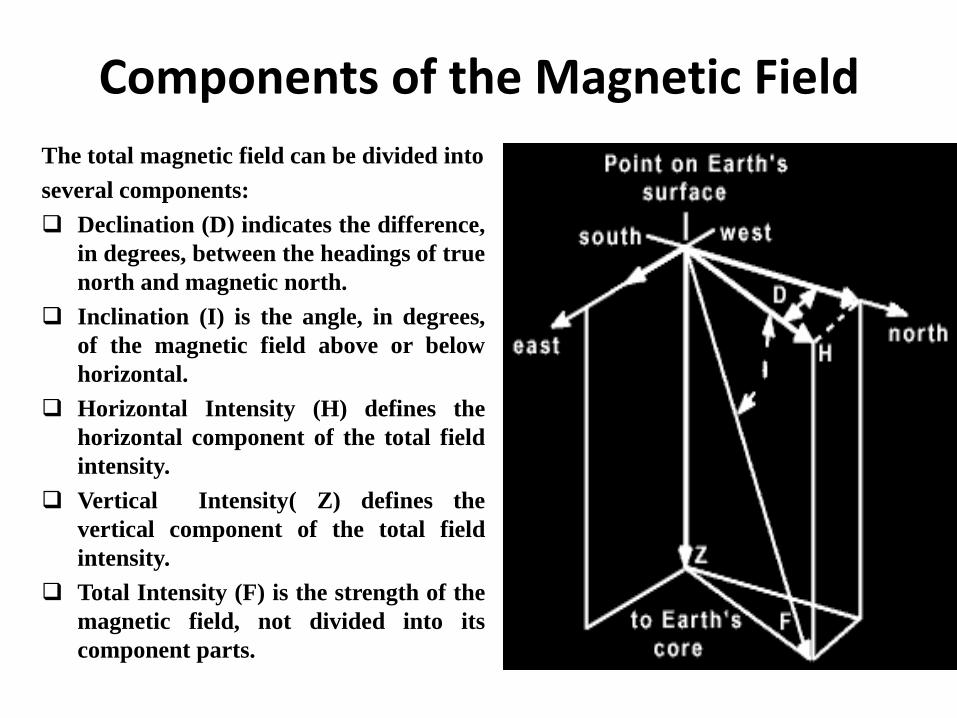
The total magnetic field can be divided into

several components:

Declination (D) indicates the difference,

in degrees, between the headings of true

north and magnetic north.

Inclination (I) is the angle, in degrees,

of the magnetic field above or below

horizontal.

Horizontal Intensity (H) defines the

horizontal component of the total field

intensity.

Vertical Intensity( Z) defines the

vertical component of the total field

intensity.

Total Intensity (F) is the strength of the

magnetic field, not divided into its

component parts.

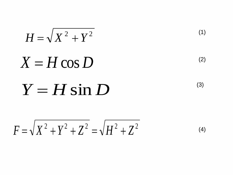
22222 ZHZYXF

DHX cos

DHY sin

22 YXH (1)

(2)

(3)

(4)

On occasion, the declination angle D in degrees (D◦) is expressed in magnetic

eastward directed field strength D (nT) and obtained from the relationship.

Sometimes the change of D (nT) about its mean is called a magnetic eastward

field strength, E. (For small, incremental changes in a value it is the custom to use

the symbol)

)tan( ODHnTD (6)

X

YD 1tan (5)

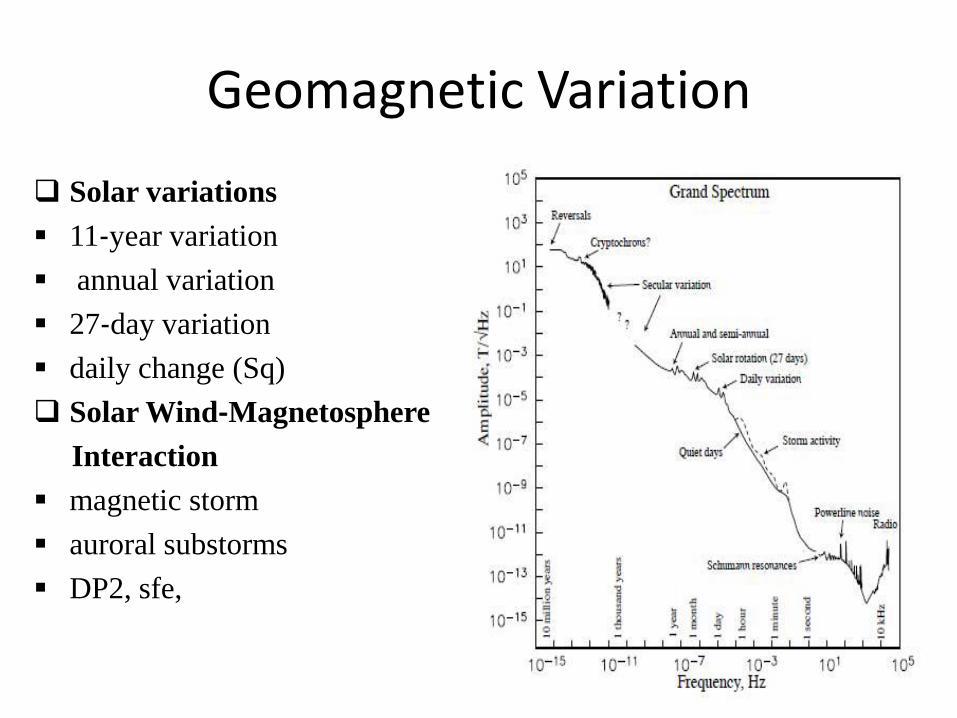
Geomagnetic Variation

Solar variations

11‐year variation

annual variation

27‐day variation

daily change (Sq)

Solar Wind‐Magnetosphere

Interaction

magnetic storm

auroral substorms

DP2, sfe,

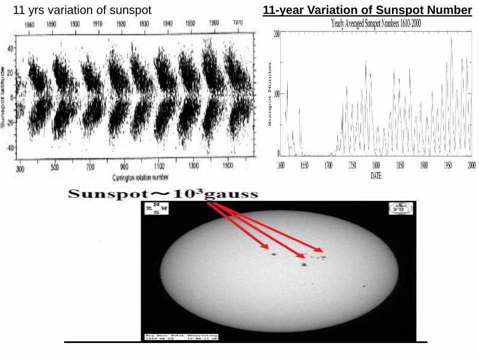
11 yrs variation of sunspot 11-year Variation of Sunspot Number

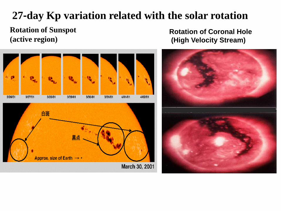
27‐day Kp variation related with the solar rotation

Rotation of Sunspot

(active region)Rotation of Coronal Hole

(High Velocity Stream)

The Sun is the source of the solar wind disturbances that drive

geomagnetic activity and thus it seems that solar activity should

predict geomagnetic activity.

Solar eruptions such as flares, filament eruptions and coronal mass

ejections are active producers of geomagnetic activity. The frequency

of these eruptions rises and falls with the solar activity cycle as

indicated by the number of sunspots.

The sunspot number could be used to estimate the state of

geomagnetic activity in the declining and maximum phase of solar

activity during intervals when geomagnetic measures were not

available (Rangarajan and Barreto ,1999)

Six steps of the space weather chain from the Sun to the ground (Adopted

from Antti Pulkkinen, 2003)

33

How are power systems affected? In power transmission systems, electrical

lines are connected to the Earth throughtransformers.

The geomagnetically induced currents flowthrough the transformer windings attransformer substations, producing extramagnetization that can saturate the core ofthe transformer.

This results in overheating of the transformerand the malfunctioning of relays and otherequipment in the system.

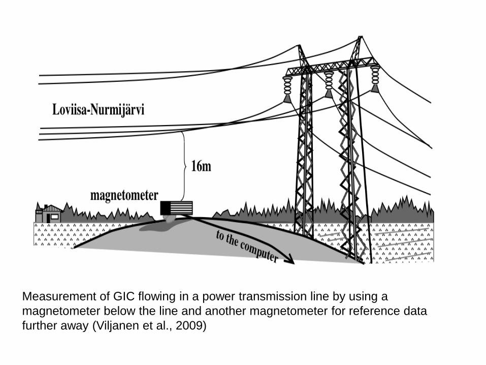
Measurement of GIC flowing in a power transmission line by using a

magnetometer below the line and another magnetometer for reference data

further away (Viljanen et al., 2009)

How are pipelines affected?

To prevent corrosion, steel pipelines are covered withan isolating coating and, using corrosion protectionrectifiers, kept within a safe range of voltages thatminimizes the corrosion process.

Geomagnetic variations create voltage swings that takethe pipeline voltage out of that safe ‘protected' range.

During geomagnetic storms, these variations can belarge enough to keep portions of a pipeline in theunprotected regime for some time. This effect iscumulative and can result in increased corrosion and asignificant reduction in the lifetime of the pipeline

Modelling of GIC

1. Determination of the horizontal geoelectric field at theEarth’s surface (“geophysical part“).

2. Computation of GIC in the network produced by thegeoelectric field (“engineering part“).

The geophysical part does not depend on the particularnetwork and is thus the same for power networks, pipelinesand other conductor systems. The input of the geophysicalpart consists of knowledge or assumptions about the Earth’sconductivity and about the magnetospheric-ionosphericcurrents or about the geomagnetic variations at the Earth’ssurface. The solution is based on Maxwell’s equations

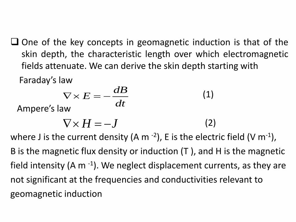
One of the key concepts in geomagnetic induction is that of theskin depth, the characteristic length over which electromagneticfields attenuate. We can derive the skin depth starting with

Faraday’s law

(1)

Ampere’s law

(2)

where J is the current density (A m -2), E is the electric field (V m-1),

B is the magnetic flux density or induction (T ), and H is the magnetic

field intensity (A m -1). We neglect displacement currents, as they are

not significant at the frequencies and conductivities relevant to

geomagnetic induction

dt

dBE

JH

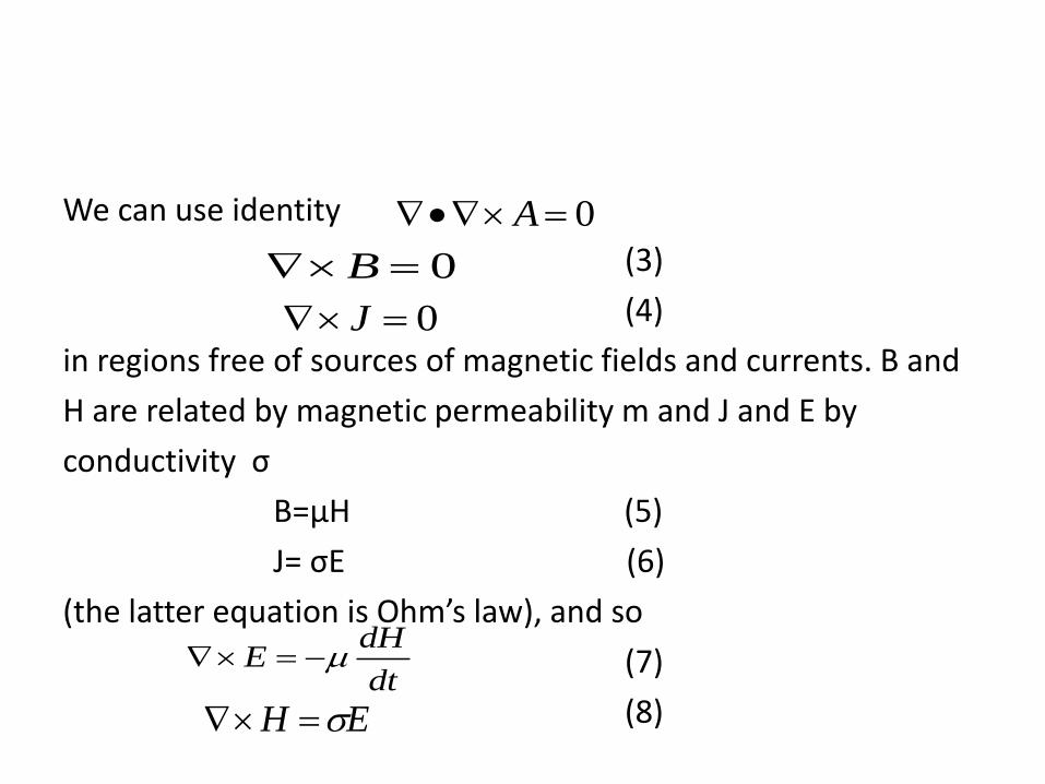
We can use identity

(3)

(4)

in regions free of sources of magnetic fields and currents. B and

H are related by magnetic permeability m and J and E by

conductivity σ

B=µH (5)

J= σE (6)

(the latter equation is Ohm’s law), and so

(7)

(8)

0 A

0 B

0 J

dt

dHE

EH

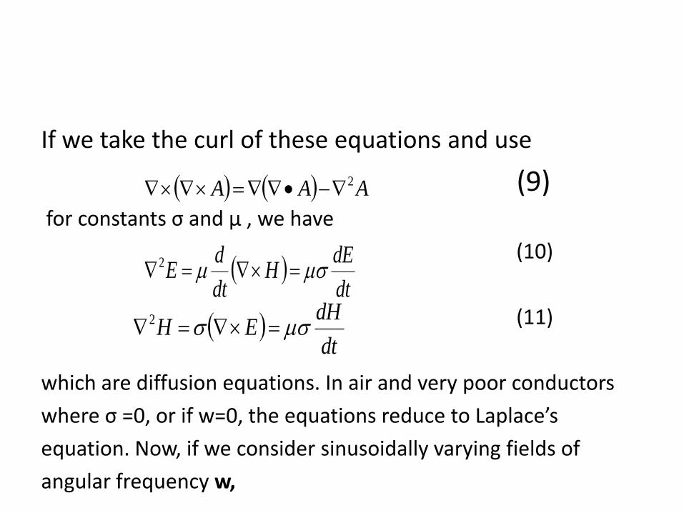
If we take the curl of these equations and use

(9)for constants σ and µ , we have

(10)

(11)

which are diffusion equations. In air and very poor conductors

where σ =0, or if w=0, the equations reduce to Laplace’s

equation. Now, if we consider sinusoidally varying fields of

angular frequency w,

AAA 2

dt

dEH

dt

dE 2

dt

dHEH 2

(12)

(13)

and so

(14)

(15)

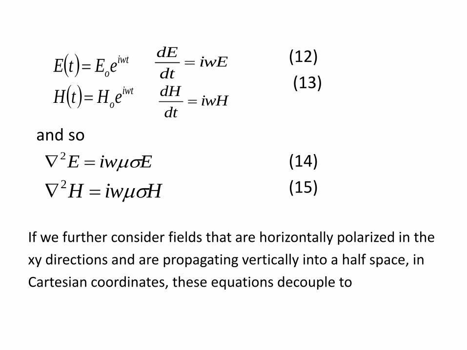
If we further consider fields that are horizontally polarized in the

xy directions and are propagating vertically into a half space, in

Cartesian coordinates, these equations decouple to

iwt

oeHtH iwHdt

dH

iwt

oeEtE iwEdt

dE

EiwE 2

HiwH 2

(16)

(17)

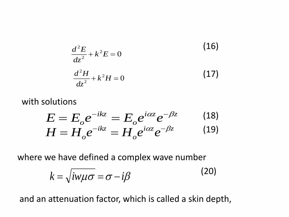
with solutions

(18)

(19)

where we have defined a complex wave number

(20)

and an attenuation factor, which is called a skin depth,

02

2

2

Ekdz

Ed

02

2

2

Hkdz

Hd

zzi

o

ikz

o eeEeEE zzi

o

ikz

o eeHeHH

iiwk

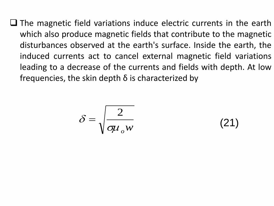
The magnetic field variations induce electric currents in the earthwhich also produce magnetic fields that contribute to the magneticdisturbances observed at the earth's surface. Inside the earth, theinduced currents act to cancel external magnetic field variationsleading to a decrease of the currents and fields with depth. At lowfrequencies, the skin depth δ is characterized by

wo

2 (21)

The geoelectric field model

The induced electric field observed at the Earth’s surfacedepends primarily on the magnetospheric-ionosphericcurrents, which in turn are dependent on space weatherconditions, while the secondary effects are determined by theconductivity structure of the Earth (Pirjola, 2000).

Pirjola (2002b) explains that the horizontal geoelectric field atthe surface of the Earth is an important quantity that must beknown in order to determine the magnitude of the GIC in thenetwork.

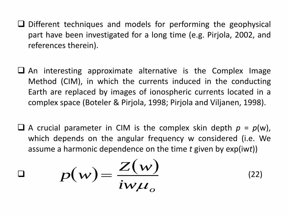
Different techniques and models for performing the geophysicalpart have been investigated for a long time (e.g. Pirjola, 2002, andreferences therein).

An interesting approximate alternative is the Complex ImageMethod (CIM), in which the currents induced in the conductingEarth are replaced by images of ionospheric currents located in acomplex space (Boteler & Pirjola, 1998; Pirjola and Viljanen, 1998).

A crucial parameter in CIM is the complex skin depth p = p(w),which depends on the angular frequency w considered (i.e. Weassume a harmonic dependence on the time t given by exp(iwt))

(22)

oiw

wZwp

where Z = Z(w) is the surface impedance at the Earth’ssurface relating a horizontal electric field component Ey =Ey(w) to the perpendicular horizontal magnetic fieldcomponent Bx = Bx(w) (see e.g. Kaufman & Keller, 1981;Pirjola et al., 2009).

(23)

It is implicitly required in equation (23) that the (flat) Earthsurface is the xy plane of a right handed Cartesian coordinatesystem in which the z axis points downwards. In practice, the

surface impedance included in equation (23) and especially inequation (22) refers to the plane wave

wBWZ

wE x

o

y

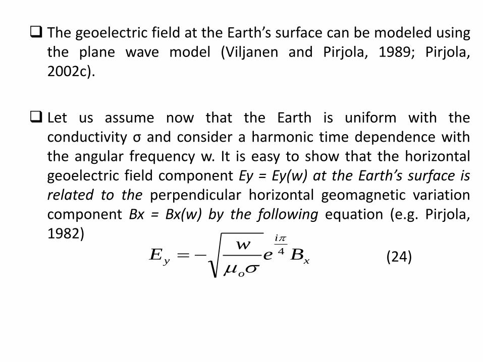
The geoelectric field at the Earth’s surface can be modeled usingthe plane wave model (Viljanen and Pirjola, 1989; Pirjola,2002c).

Let us assume now that the Earth is uniform with theconductivity σ and consider a harmonic time dependence withthe angular frequency w. It is easy to show that the horizontalgeoelectric field component Ey = Ey(w) at the Earth’s surface isrelated to the perpendicular horizontal geomagnetic variationcomponent Bx = Bx(w) by the following equation (e.g. Pirjola,1982)

(24)x

i

o

y Bew

E 4

Equation (24) shows that there is a 45-degree (π/4-radian) phaseshift between the geoelectric and geomagnetic fields. We also seethat an increase of the angular frequency and a decrease of theEarth’s conductivity enhance the geoelectric field with respect tothe geomagnetic field.

Noting that is associated with the time derivative of ,equation (24) can be inverse-Fourier transformed to give thefollowing time domain convolution integral (Cagniard, 1953; Pirjola,1982)

wiwBx tBx

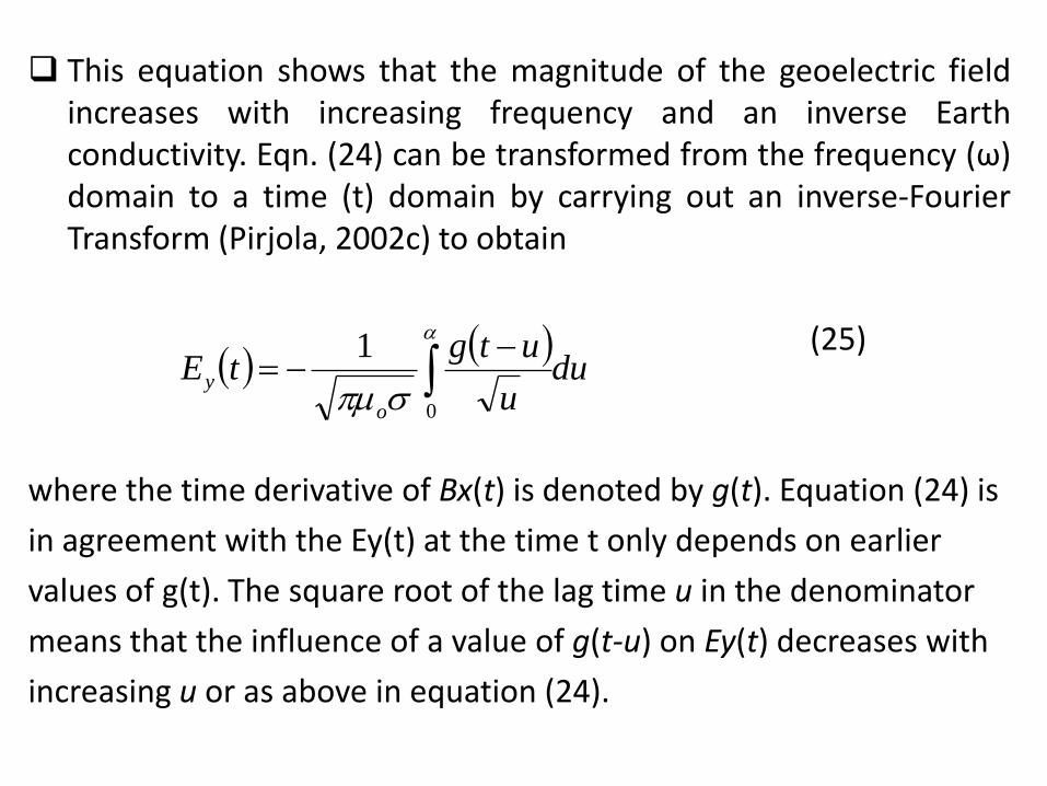
This equation shows that the magnitude of the geoelectric fieldincreases with increasing frequency and an inverse Earthconductivity. Eqn. (24) can be transformed from the frequency (ω)domain to a time (t) domain by carrying out an inverse-FourierTransform (Pirjola, 2002c) to obtain

(25)

where the time derivative of Bx(t) is denoted by g(t). Equation (24) is

in agreement with the Ey(t) at the time t only depends on earlier

values of g(t). The square root of the lag time u in the denominator

means that the influence of a value of g(t-u) on Ey(t) decreases with

increasing u or as above in equation (24).

duu

utgtE

o

y

0

1

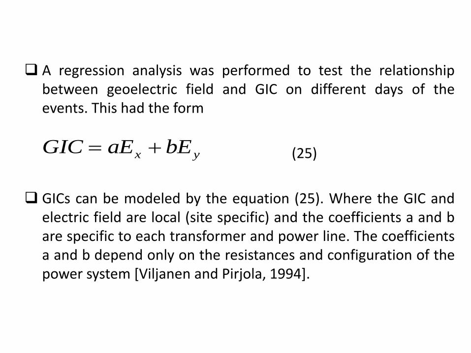
A regression analysis was performed to test the relationshipbetween geoelectric field and GIC on different days of theevents. This had the form

(25)

GICs can be modeled by the equation (25). Where the GIC andelectric field are local (site specific) and the coefficients a and bare specific to each transformer and power line. The coefficientsa and b depend only on the resistances and configuration of thepower system [Viljanen and Pirjola, 1994].

yx bEaEGIC

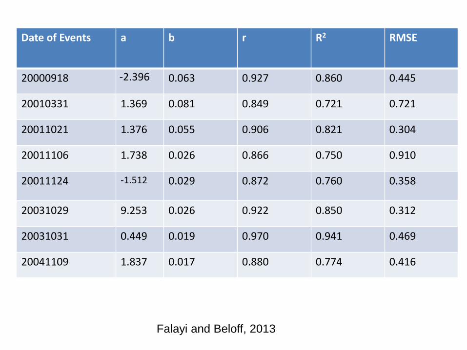
Date of Events a b r R2 RMSE

20000918 -2.396 0.063 0.927 0.860 0.445

20010331 1.369 0.081 0.849 0.721 0.721

20011021 1.376 0.055 0.906 0.821 0.304

20011106 1.738 0.026 0.866 0.750 0.910

20011124 -1.512 0.029 0.872 0.760 0.358

20031029 9.253 0.026 0.922 0.850 0.312

20031031 0.449 0.019 0.970 0.941 0.469

20041109 1.837 0.017 0.880 0.774 0.416

Falayi and Beloff, 2013

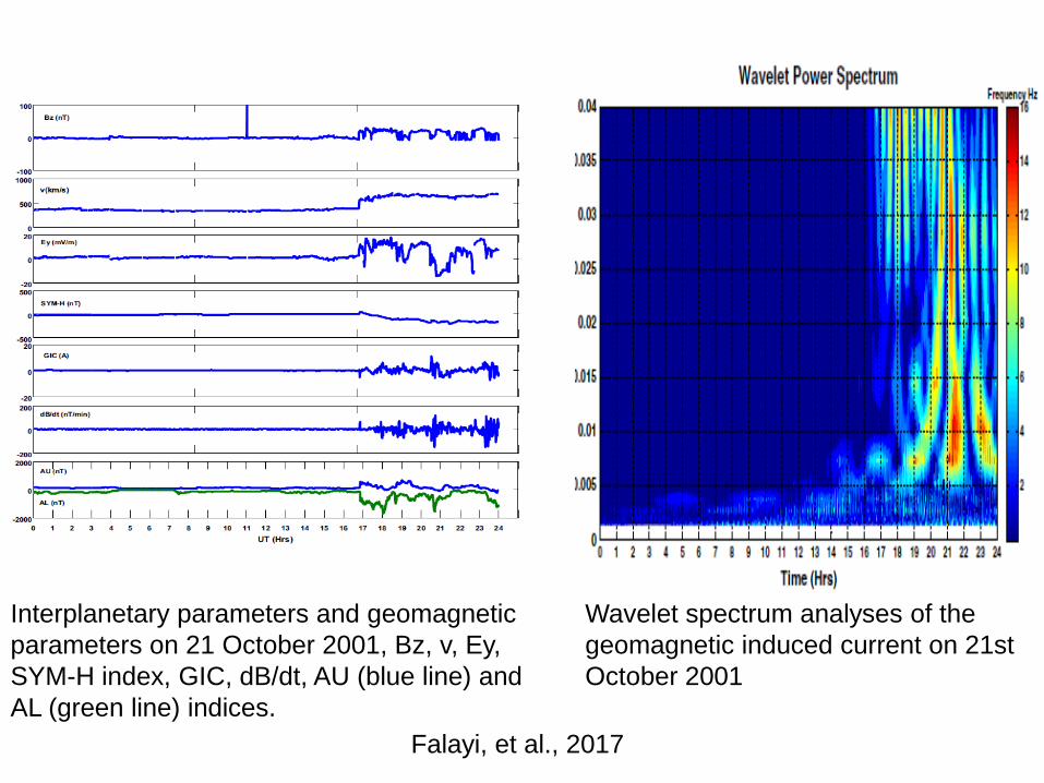
Interplanetary parameters and geomagnetic

parameters on 21 October 2001, Bz, v, Ey,

SYM-H index, GIC, dB/dt, AU (blue line) and

AL (green line) indices.

Wavelet spectrum analyses of the

geomagnetic induced current on 21st

October 2001

Falayi, et al., 2017

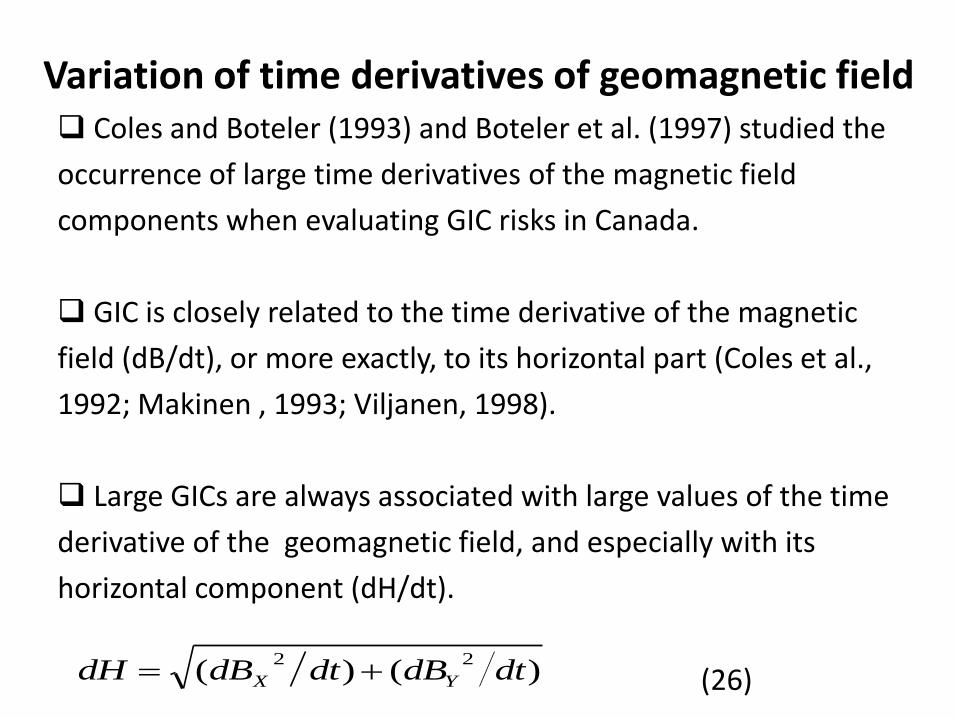
Variation of time derivatives of geomagnetic field Coles and Boteler (1993) and Boteler et al. (1997) studied the

occurrence of large time derivatives of the magnetic field

components when evaluating GIC risks in Canada.

GIC is closely related to the time derivative of the magnetic

field (dB/dt), or more exactly, to its horizontal part (Coles et al.,

1992; Makinen , 1993; Viljanen, 1998).

Large GICs are always associated with large values of the time

derivative of the geomagnetic field, and especially with its

horizontal component (dH/dt).

(26))()(22

dtdBdtdBdH YX

Average diurnal time derivative of the magnetic

field at NUR,MAS, BJN during the 157 days

samples (Viljanen, 1997)

Top panel: X (thick line) and Y (thin line) at PEL on March2 4,

1991. The sampling interval is 20 s. Middle panel: dX/dt

(thick line) and dY/dt (thin line). Zero levels are plotted

with dashed line. Bottom panel: Geomagnetically

induced current Pirttikoski 400kV transformer positive

current flows (Viljanen, 1997)

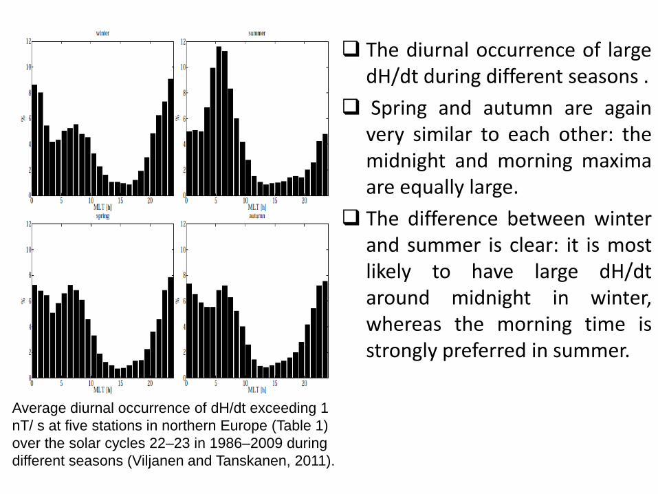
Average diurnal occurrence of dH/dt exceeding 1

nT/ s at five stations in northern Europe (Table 1)

over the solar cycles 22–23 in 1986–2009 during

different seasons (Viljanen and Tanskanen, 2011).

The diurnal occurrence of largedH/dt during different seasons .

Spring and autumn are againvery similar to each other: themidnight and morning maximaare equally large.

The difference between winterand summer is clear: it is mostlikely to have large dH/dtaround midnight in winter,whereas the morning time isstrongly preferred in summer.

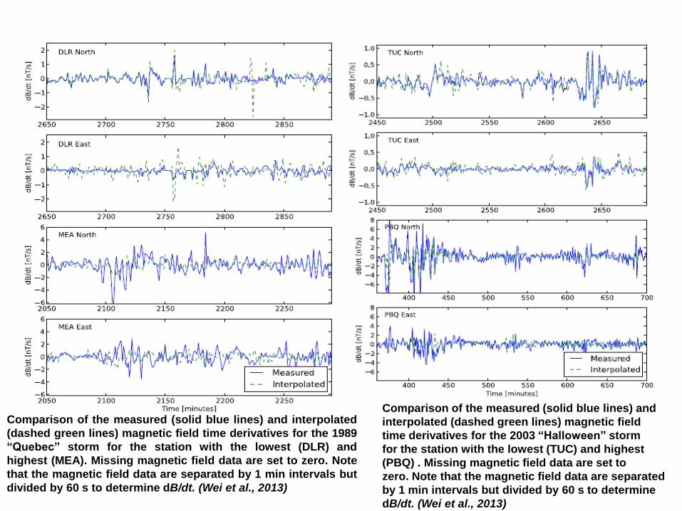
Comparison of the measured (solid blue lines) and interpolated

(dashed green lines) magnetic field time derivatives for the 1989

“Quebec” storm for the station with the lowest (DLR) and

highest (MEA). Missing magnetic field data are set to zero. Note

that the magnetic field data are separated by 1 min intervals but

divided by 60 s to determine dB/dt. (Wei et al., 2013)

Comparison of the measured (solid blue lines) and

interpolated (dashed green lines) magnetic field

time derivatives for the 2003 “Halloween” storm

for the station with the lowest (TUC) and highest

(PBQ) . Missing magnetic field data are set to

zero. Note that the magnetic field data are separated

by 1 min intervals but divided by 60 s to determine

dB/dt. (Wei et al., 2013)

Recommendation for Power Failure

Ground based technology are prone to GICwhen oriented east-west, rather than north-south. The ionospheric response is associatedwith geomagnetic disturbance which usuallyflows in an east west direction including GIC.

According to Pirjola (2002) implementation ofseries capacitors in transmission lines or in theearthling wires of transformer are readilyavailable technology that can be used to blockGIC

Interconnectedness should be discourage because itincreases vulnerability. When a geomagnetic stormdamages one piece of equipment, anotherconnected to the affected system can alsoexperience power failure.

During geomagnetic disturbance and when electricalpower grids are highly loaded, increased powerdemand from customer and industry led to thesystem operating closer to their limit or above theirlimit making susceptible to external disturbance

Measuring and monitoring of ground basedtechnology especially at site vulnerable to GIC.

Variations of electromagnetic induction (dZ/dH) duringgeomagnetic disturbance

Magnetotellurics and geomagnetic depth sounding are the twomajor way of estimating the induced response of a laterallyinhomogeneous sub surface, Tikhonov-Cagniard impedanceexpressing the relation between Electric E and magnetic H fieldscomponents forms the fundamental EM response function.

described the inductive response of the electrically conductingEarth interior to geomagnetic variation that can be inferred frommagnetic Z-H relation. Non uniformities in conductivity of theupper mantle produce local variation in Z-H relation.

The geomagnetic field components Z (vertical field variation) andH (horizontal geomagnetic field) are used to map the lateralconductivity (Schmucker, 1970).

Mayaud (1973) reported that the rate of induction due to electrojet canbe determined by using the ratio ΔZ/ΔH and asserted that such ratios arehighly sensitive to the importance of the induced fields since internaleffects are subtracted from the external effects in Z while they are addedin H

39

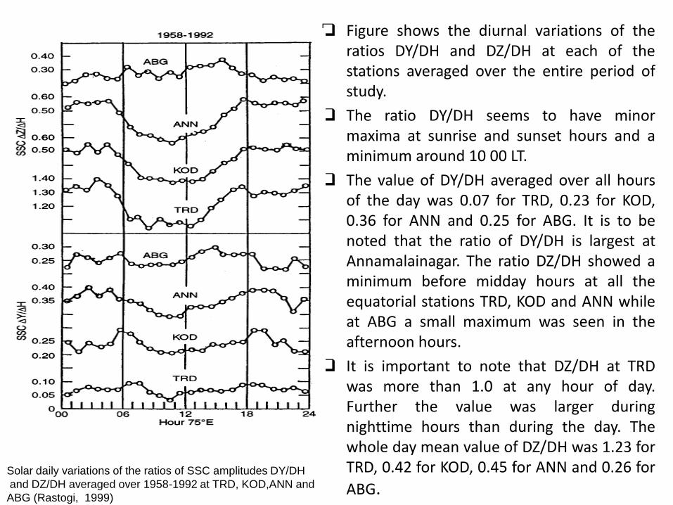
Figure shows the diurnal variations of theratios DY/DH and DZ/DH at each of thestations averaged over the entire period ofstudy.

The ratio DY/DH seems to have minormaxima at sunrise and sunset hours and aminimum around 10 00 LT.

The value of DY/DH averaged over all hoursof the day was 0.07 for TRD, 0.23 for KOD,0.36 for ANN and 0.25 for ABG. It is to benoted that the ratio of DY/DH is largest atAnnamalainagar. The ratio DZ/DH showed aminimum before midday hours at all theequatorial stations TRD, KOD and ANN whileat ABG a small maximum was seen in theafternoon hours.

It is important to note that DZ/DH at TRDwas more than 1.0 at any hour of day.Further the value was larger duringnighttime hours than during the day. Thewhole day mean value of DZ/DH was 1.23 forTRD, 0.42 for KOD, 0.45 for ANN and 0.26 for

ABG.Solar daily variations of the ratios of SSC amplitudes DY/DH

and DZ/DH averaged over 1958-1992 at TRD, KOD,ANN and

ABG (Rastogi, 1999)

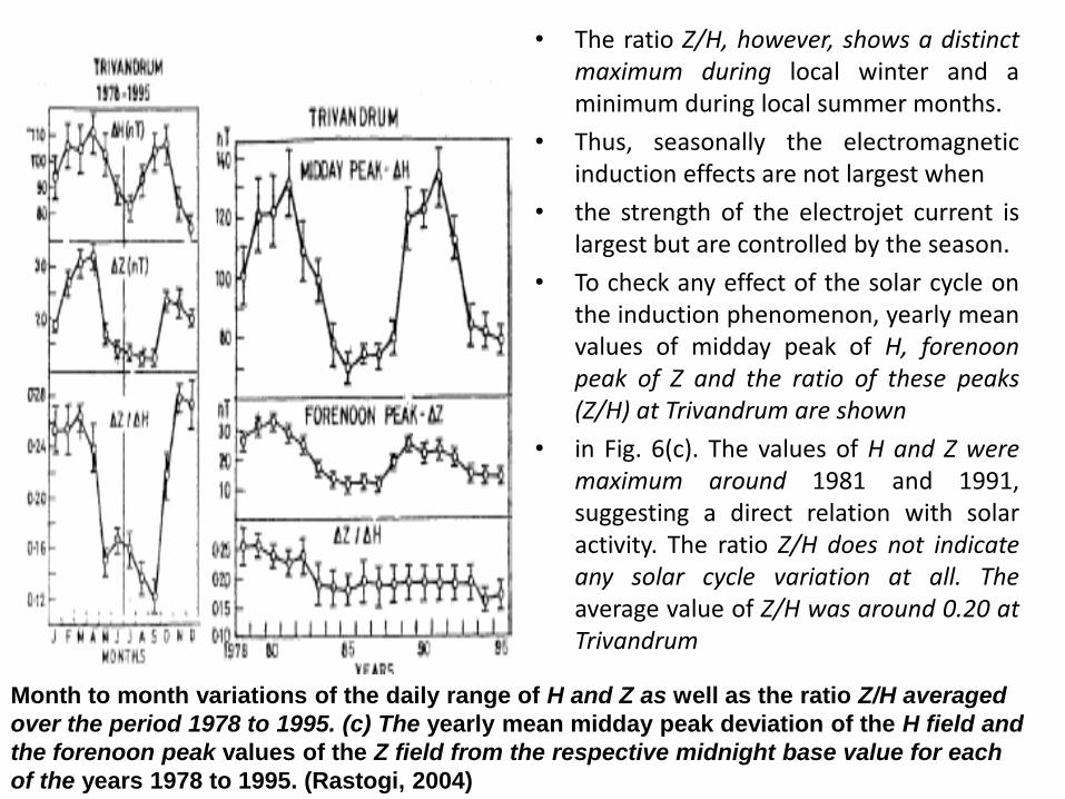
• The ratio Z/H, however, shows a distinctmaximum during local winter and aminimum during local summer months.

• Thus, seasonally the electromagneticinduction effects are not largest when

• the strength of the electrojet current islargest but are controlled by the season.

• To check any effect of the solar cycle onthe induction phenomenon, yearly meanvalues of midday peak of H, forenoonpeak of Z and the ratio of these peaks(Z/H) at Trivandrum are shown

• in Fig. 6(c). The values of H and Z weremaximum around 1981 and 1991,suggesting a direct relation with solaractivity. The ratio Z/H does not indicateany solar cycle variation at all. Theaverage value of Z/H was around 0.20 atTrivandrum

Month to month variations of the daily range of H and Z as well as the ratio Z/H averaged

over the period 1978 to 1995. (c) The yearly mean midday peak deviation of the H field and

the forenoon peak values of the Z field from the respective midnight base value for each

of the years 1978 to 1995. (Rastogi, 2004)

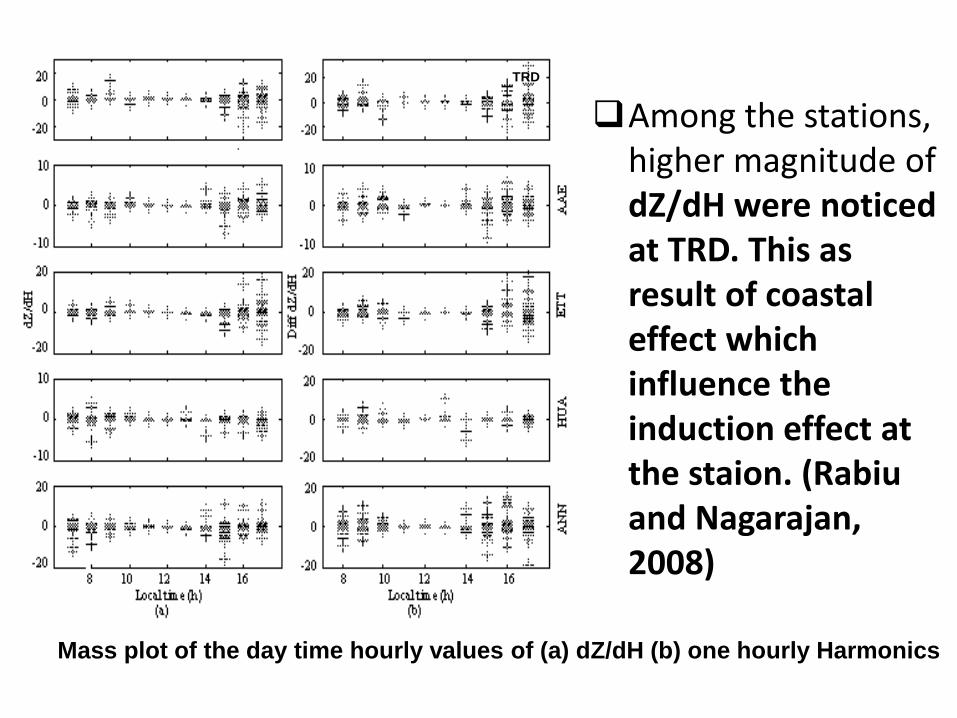
Among the stations, higher magnitude of dZ/dH were noticed at TRD. This as result of coastal effect which influence the induction effect at the staion. (Rabiu and Nagarajan, 2008)

TRD

Mass plot of the day time hourly values of (a) dZ/dH (b) one hourly Harmonics

43

聞いていただきありがとうございますWatashi ni kiite itadaki

arigatōgozaimasu

Thanks for Listening

安全な旅

Anzen'na tabi

safe journey