Geology from Geo-neutrino Flux Measurements Eugene Guillian / Queen’s University DOANOW March 24, 2007

Geology from Geo-neutrino Flux Measurements

Eugene Guillian / Queen’s University

DOANOW

March 24, 2007

Content of This Presentation• KamLAND: The Pioneering Geo-neutrino Detector

– Proved that geo-neutrinos can be detected, but under very unfavorable conditions

• How to proceed in the next generation– 10 KamLAND (size time)– Low background– Simple neighboring geology– Multiple sites

• How to extract geological information from flux measurements– 1 site– 2 sites

• Statistical sensitivity• Effect of nuclear reactor background• Possible applications

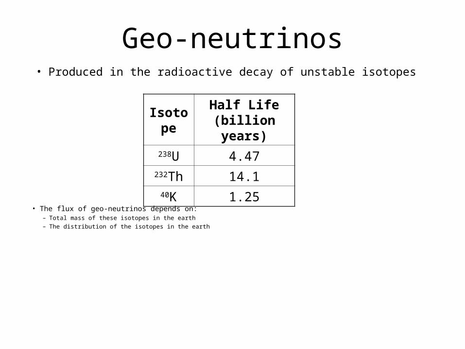
Geo-neutrinos• Produced in the radioactive decay of unstable isotopes

IsotopeHalf Life

(billion years)238U 4.47

232Th 14.140K 1.25

• The flux of geo-neutrinos depends on:– Total mass of these isotopes in the earth– The distribution of the isotopes in the earth

Total Isotopic Mass in the Earth• An educated guess:

– CI carbonaceous chondrite meteorite• Representative of the raw material from which the earth was formed

• Based on the isotopic abundances in this type of meteorite, estimate the initial elemental abundance

• Evolution of the early earth– Core separation

– Bulk Silicate Earth (BSE)

– Crust extraction from BSE

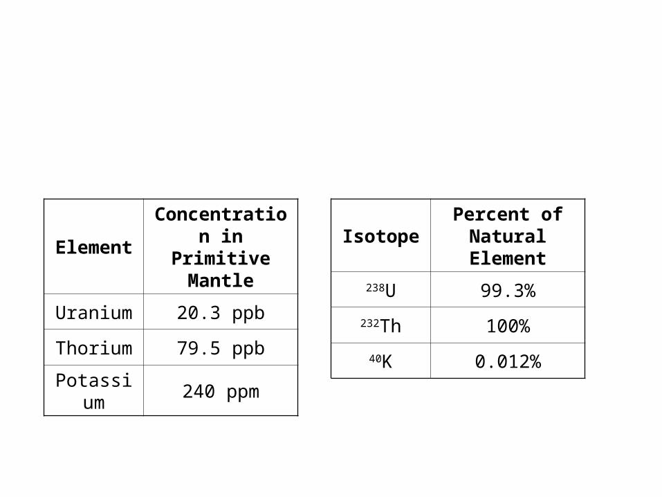
ElementConcentration in Primitive Mantle

Uranium 20.3 ppb

Thorium 79.5 ppb

Potassium 240 ppm

IsotopePercent of

Natural Element

238U 99.3%

232Th 100%

40K 0.012%

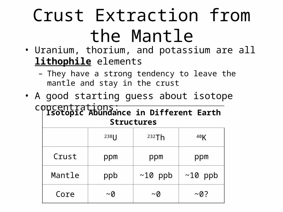
Crust Extraction from the Mantle• Uranium, thorium, and potassium are all lithophile

elements– They have a strong tendency to leave the mantle and stay in the

crust

• A good starting guess about isotope concentrations:

Isotopic Abundance in Different Earth Structures

238U 232Th 40K

Crust ppm ppm ppm

Mantle ppb ~10 ppb ~10 ppb

Core ~0 ~0 ~0?

More Detailed Earth Models

• Examples:– Mantovani et al., Phys. Rev. D 69, 013001 (2004)

– S. Enomoto, Ph. D. Thesis, Tohoku University (2005)

– Turcotte et al., J. Geophys. Res. 106, 4265-4276 (2001)

The Mantovani et al. Reference Model

LayerIsotopic Concentration (ppb)

238U 232Th 40K

Ocean 3.2 0 48

Sediments 1700 6900 2000

Oceanic Crust 100 220 150

Contiental Crust

Upper 2500 9800 3100

Middle 1600 6100 2000

Lower 620 3700 860

MantleUpper 7 17 9

Lower 13 52 19

Core 0 0 0

• Note: These are just educated guesses• There is considerable spread in what could “reasonably” be assigned to these values

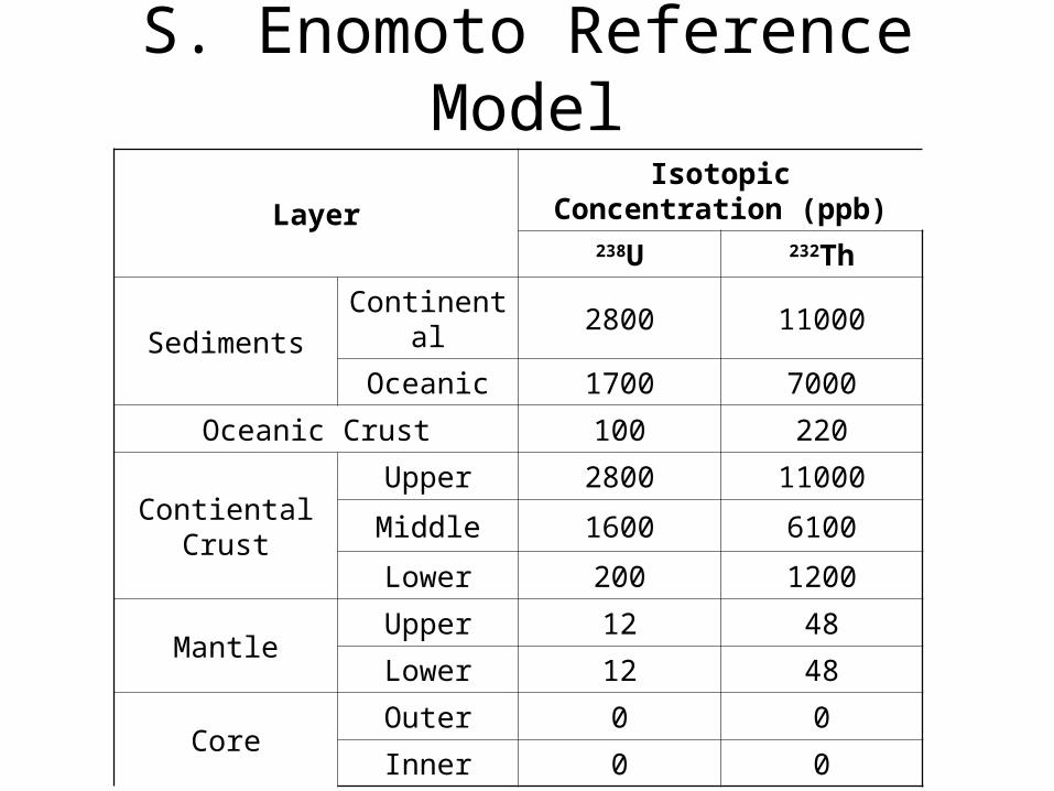
S. Enomoto Reference Model

LayerIsotopic Concentration (ppb)

238U 232Th

SedimentsContinental 2800 11000

Oceanic 1700 7000

Oceanic Crust 100 220

Contiental Crust

Upper 2800 11000

Middle 1600 6100

Lower 200 1200

MantleUpper 12 48

Lower 12 48

CoreOuter 0 0

Inner 0 0

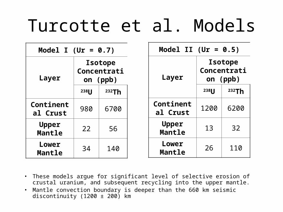
Turcotte et al. ModelsModel I (Ur = 0.7)

Layer

Isotope Concentration

(ppb)

238U 232Th

Continental Crust

980 6700

Upper Mantle

22 56

Lower Mantle

34 140

Model II (Ur = 0.5)

Layer

Isotope Concentration

(ppb)

238U 232Th

Continental Crust

1200 6200

Upper Mantle

13 32

Lower Mantle

26 110

• These models argue for significant level of selective erosion of crustal uranium, and subsequent recycling into the upper mantle.

• Mantle convection boundary is deeper than the 660 km seismic discontinuity (1200 ± 200) km

The Overall Picture of Geo-neutrinos

• The models differ in:– The number of geological subdivision

– The assignment of isotopic concentrations in each subdivision

• But, at the very basic level, similar (i.e. within a factor of several) geo-neutrino fluxes are predicted– The flux at the surface of the earth is ~106 cm-2 s-1

– The flux varies by a factor of several depending on the location

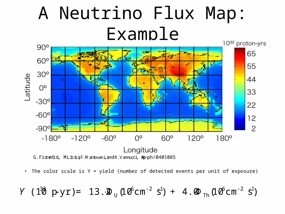
A Neutrino Flux Map: Example

G. Fiorentini, M. Lissia, F. Mantovani, and R. Vannucci, hep-ph/0401085

• The color scale is Y = yield (number of detected events per unit of exposure)

€

Y (1032 p - yr) = 13.2 ⋅ΦU(106cm-2 s-1) + 4.0 ⋅ΦTh (106cm-2 s-1)

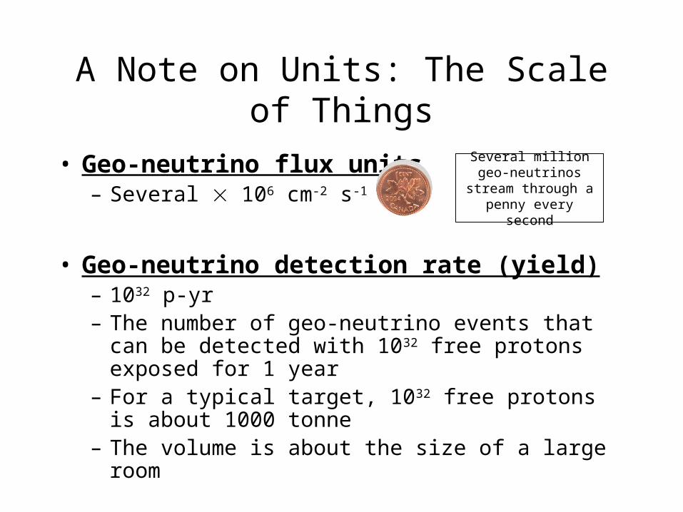
A Note on Units: The Scale of Things

• Geo-neutrino flux units– Several 106 cm-2 s-1

• Geo-neutrino detection rate (yield)– 1032 p-yr– The number of geo-neutrino events that can be detected

with 1032 free protons exposed for 1 year– For a typical target, 1032 free protons is about 1000

tonne– The volume is about the size of a large room

Several million geo-neutrinos stream through

a penny every second

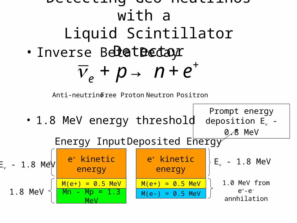
Detecting Geo-neutrinos with a Liquid Scintillator Detector

• Inverse Beta Decay

€

ν e + p → n + e+

Anti-neutrino Free Proton Neutron Positron

• 1.8 MeV energy threshold

Mn - Mp = 1.3 MeV

M(e+) = 0.5 MeV1.8 MeV

e+ kinetic energyEν - 1.8 MeV

M(e+) = 0.5 MeV

e+ kinetic energy

M(e-) = 0.5 MeV1.0 MeV from e+-e-

annhilation

Eν - 1.8 MeV

Energy Input Deposited Energy

Prompt energy deposition Eν - 0.8 MeV

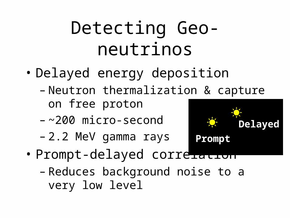
Detecting Geo-neutrinos

• Delayed energy deposition– Neutron thermalization & capture on free

proton– ~200 micro-second– 2.2 MeV gamma rays

• Prompt-delayed correlation– Reduces background noise to a very low level

Prompt

Delayed

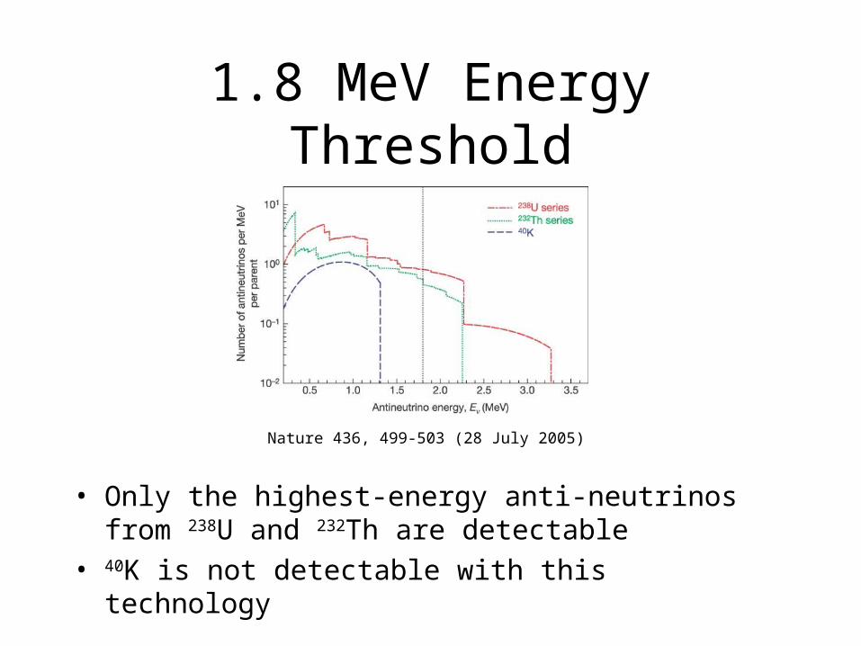
1.8 MeV Energy Threshold

Nature 436, 499-503 (28 July 2005)

• Only the highest-energy anti-neutrinos from 238U and 232Th are detectable

• 40K is not detectable with this technology

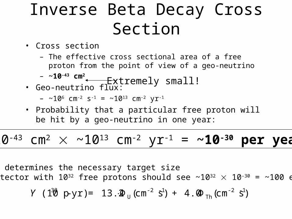
Inverse Beta Decay Cross Section

• Cross section – The effective cross sectional area of a free proton from the point of view

of a geo-neutrino

– ~10-43 cm2

• Geo-neutrino flux:– ~106 cm-2 s-1 = ~1013 cm-2 yr-1

• Probability that a particular free proton will be hit by a geo-neutrino in one year:

~10-43 cm2 ~1013 cm-2 yr-1 = ~10-30 per year

• This determines the necessary target size• A detector with 1032 free protons should see ~1032 10-30 = ~100 events

Extremely small!

€

Y (1032 p - yr) = 13.2 ⋅ΦU(cm-2 s-1) + 4.0 ⋅ΦTh (cm-2 s-1)

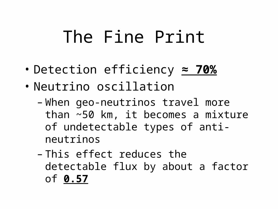
The Fine Print

• Detection efficiency ≈ 70%

• Neutrino oscillation– When geo-neutrinos travel more than ~50 km,

it becomes a mixture of undetectable types of anti-neutrinos

– This effect reduces the detectable flux by about a factor of 0.57

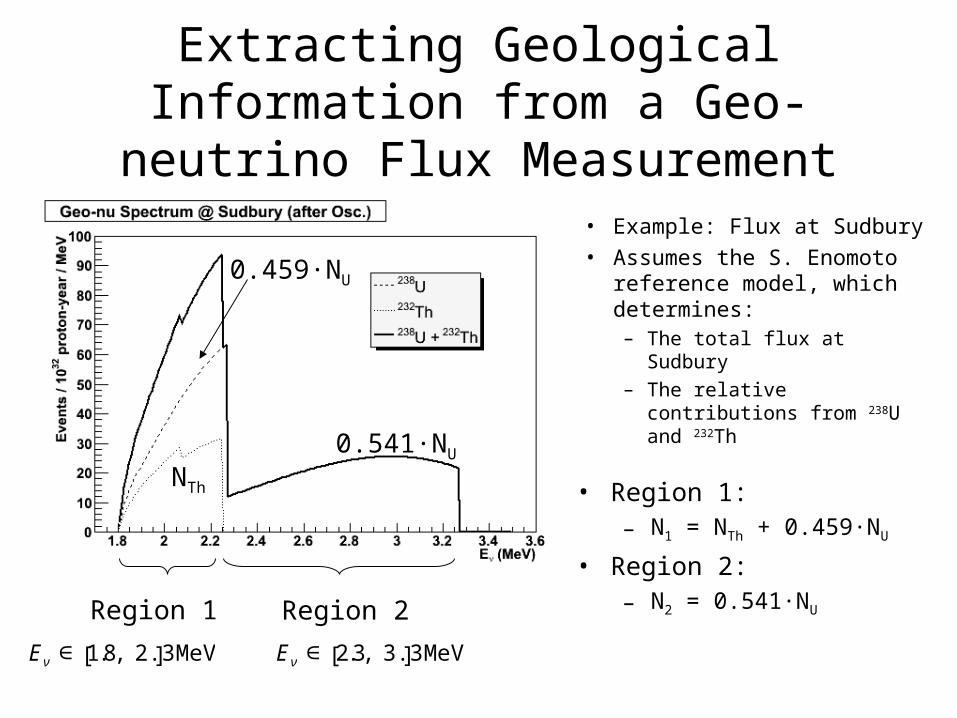
Extracting Geological Information from a Geo-neutrino Flux Measurement

• Example: Flux at Sudbury

• Assumes the S. Enomoto reference model, which determines:– The total flux at Sudbury

– The relative contributions from 238U and 232Th

Region 1

€

Eν ∈ 1.8, 2.3[ ] MeV

Region 2

€

Eν ∈ 2.3, 3.3[ ] MeV

• Region 1:– N1 = NTh + 0.459·NU

• Region 2:– N2 = 0.541·NU

0.541·NU

0.459·NU

NTh

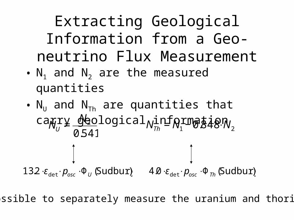
Extracting Geological Information from a Geo-neutrino Flux Measurement

• N1 and N2 are the measured quantities

• NU and NTh are quantities that carry geological information

€

NU =N2

0.541

€

NTh = N1 − 0.848 ⋅N2

€

13.2 ⋅εdet ⋅ posc ⋅ΦU (Sudbury)

€

4.0 ⋅εdet ⋅ posc ⋅ΦTh (Sudbury)

It is possible to separately measure the uranium and thorium flux

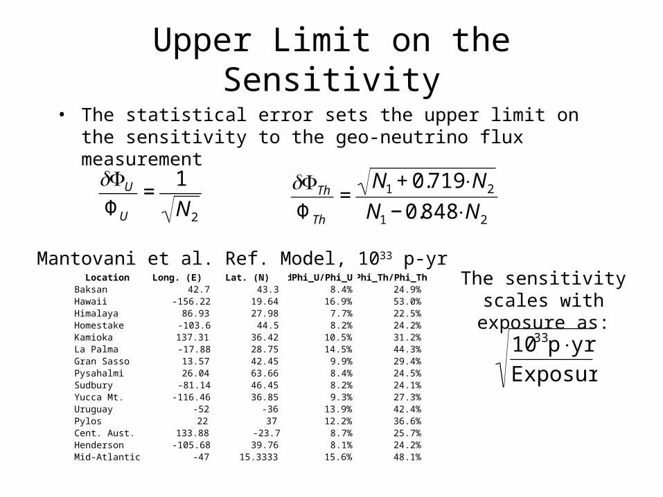
Upper Limit on the Sensitivity

• The statistical error sets the upper limit on the sensitivity to the geo-neutrino flux measurement

€

δΦU

ΦU

=1

N2

€

δΦTh

ΦTh

=N1 + 0.719 ⋅N2

N1 − 0.848 ⋅N2

Location Long. (E) Lat. (N)Baksan 42.7 43.3Hawaii -156.22 19.64Himalaya 86.93 27.98Homestake -103.6 44.5Kamioka 137.31 36.42La Palma -17.88 28.75Gran Sasso 13.57 42.45Pysahalmi 26.04 63.66Sudbury -81.14 46.45Yucca Mt. -116.46 36.85Uruguay -52 -36Pylos 22 37Cent. Aust. 133.88 -23.7Henderson -105.68 39.76Mid-Atlantic -47 15.3333

dPhi_U/Phi_UdPhi_Th/Phi_Th8.4% 24.9%

16.9% 53.0%7.7% 22.5%8.2% 24.2%

10.5% 31.2%14.5% 44.3%

9.9% 29.4%8.4% 24.5%8.2% 24.1%9.3% 27.3%

13.9% 42.4%12.2% 36.6%

8.7% 25.7%8.1% 24.2%

15.6% 48.1%

Mantovani et al. Ref. Model, 1033 p-yr

€

1033p ⋅yr

Exposure

The sensitivity scales with exposure as:

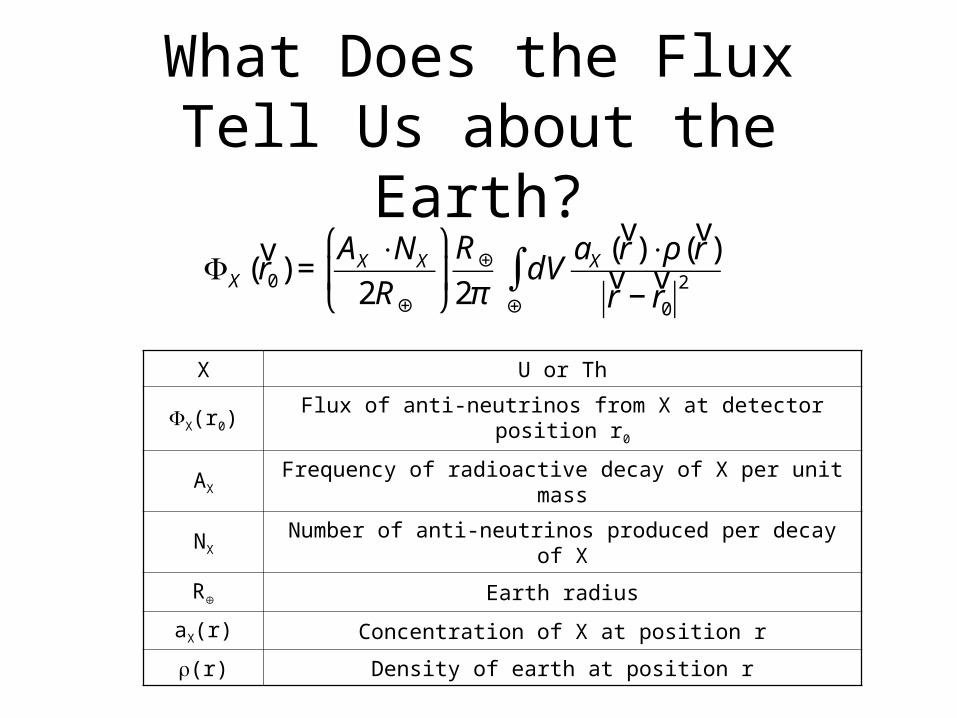
What Does the Flux Tell Us about the Earth?

€

ΦX (v r 0) =

AX ⋅NX

2R⊕

⎛

⎝ ⎜

⎞

⎠ ⎟R⊕

2πdV

aX (v r ) ⋅ρ(

v r )

v r −

v r 0

2⊕

∫

X U or Th

ΦX(r0) Flux of anti-neutrinos from X at detector position r0

AX Frequency of radioactive decay of X per unit mass

NX Number of anti-neutrinos produced per decay of X

R Earth radius

aX(r) Concentration of X at position r

(r) Density of earth at position r

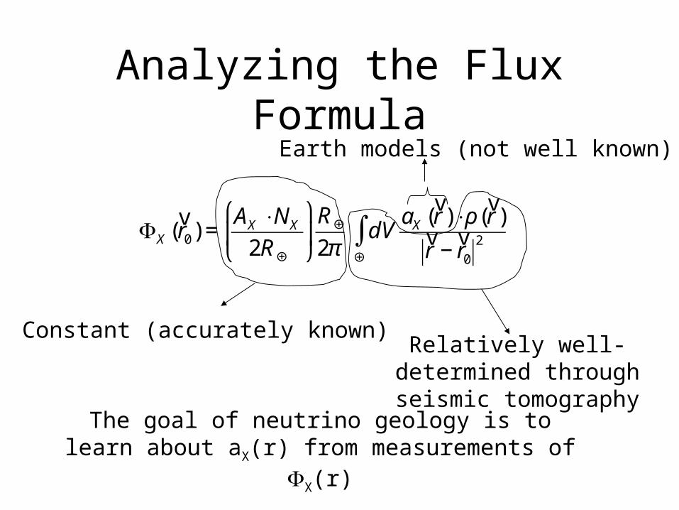
Analyzing the Flux Formula

€

ΦX (v r 0) =

AX ⋅NX

2R⊕

⎛

⎝ ⎜

⎞

⎠ ⎟R⊕

2πdV

aX (v r ) ⋅ρ(

v r )

v r −

v r 0

2⊕

∫

Constant (accurately known)Relatively well-determined

through seismic tomography

Earth models (not well known)

The goal of neutrino geology is to learn about aX(r) from measurements of ΦX(r)

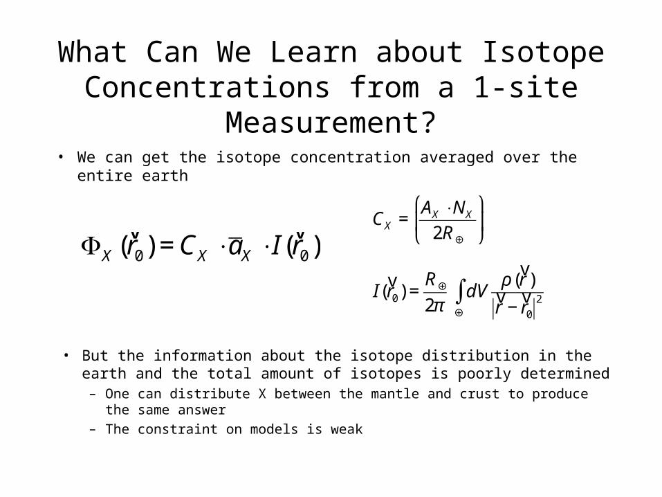
What Can We Learn about Isotope Concentrations from a 1-site Measurement?

• We can get the isotope concentration averaged over the entire earth

€

ΦX (v r 0) = CX ⋅a X ⋅ I(

v r 0)

€

CX =AX ⋅NX

2R⊕

⎛

⎝ ⎜

⎞

⎠ ⎟

€

I(v r 0) =

R⊕

2πdV

ρ (v r )

v r −

v r 0

2⊕

∫

• But the information about the isotope distribution in the earth and the total amount of isotopes is poorly determined

– One can distribute X between the mantle and crust to produce the same answer

– The constraint on models is weak

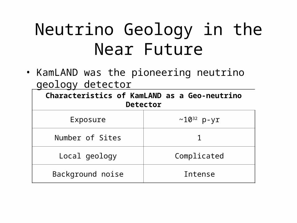
Neutrino Geology in the Near Future

• KamLAND was the pioneering neutrino geology detector

Characteristics of KamLAND as a Geo-neutrino Detector

Exposure ~1032 p-yr

Number of Sites 1

Local geology Complicated

Background noise Intense

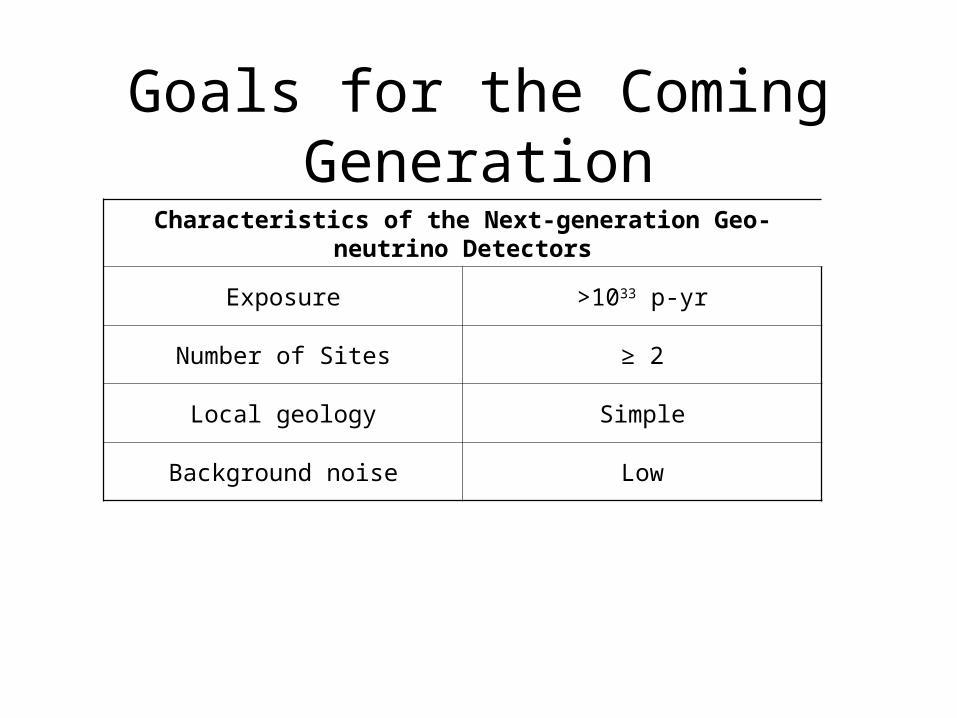
Goals for the Coming Generation

Characteristics of the Next-generation Geo-neutrino Detectors

Exposure >1033 p-yr

Number of Sites ≥ 2

Local geology Simple

Background noise Low

A 2-site Geo-neutrino Measurement: An Example

• Two measurements– Can solve for two unknowns

• The continental crust and mantle account for most of the observed geo-neutrinos, regardless of the detector location

– The two unknowns:1. Average isotope concentration in the continental crust2. Average isotope concentration in the mantle

– The small contribution from other geological subdivisions is approximated as being zero

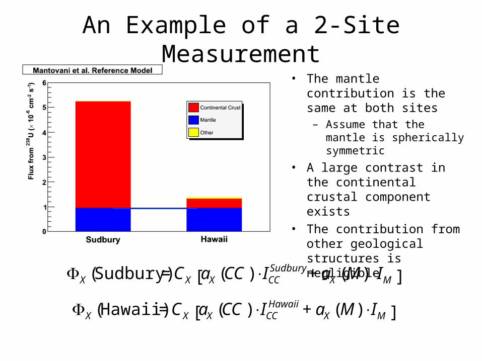
An Example of a 2-Site Measurement

• The mantle contribution is the same at both sites– Assume that the mantle is

spherically symmetric

• A large contrast in the continental crustal component exists

• The contribution from other geological structures is negligible

€

ΦX (Sudbury) = CX aX (CC) ⋅ ICCSudbury + aX (M) ⋅ IM[ ]

€

ΦX (Hawaii) = CX aX (CC) ⋅ ICCHawaii + aX (M) ⋅ IM[ ]

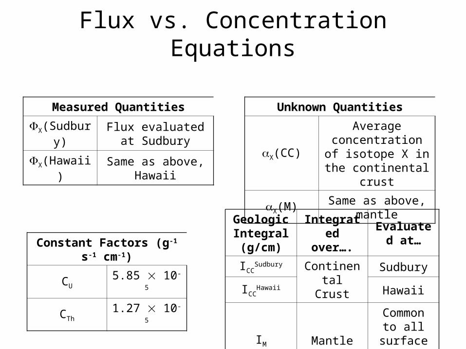
Flux vs. Concentration Equations

€

ΦX(Sudbury)=CXaX(CC)⋅ICCSudbury

+aX(M)⋅IM []

€

ΦX(Hawaii)=CXaX(CC)⋅ICCHawaii

+aX(M)⋅IM []

Constant Factors (g-1 s-1 cm-1)

CU 5.85 10-5

CTh 1.27 10-5

Geologic Integral (g/cm)

Integrated over….

Evaluated at…

ICCSudbury

Continental Crust

Sudbury

ICCHawaii Hawaii

IM MantleCommon to all surface locations

Measured Quantities

ΦX(Sudbury) Flux evaluated at Sudbury

ΦX(Hawaii) Same as above, Hawaii

Unknown Quantities

X(CC)Average concentration

of isotope X in the continental crust

X(M) Same as above, mantle

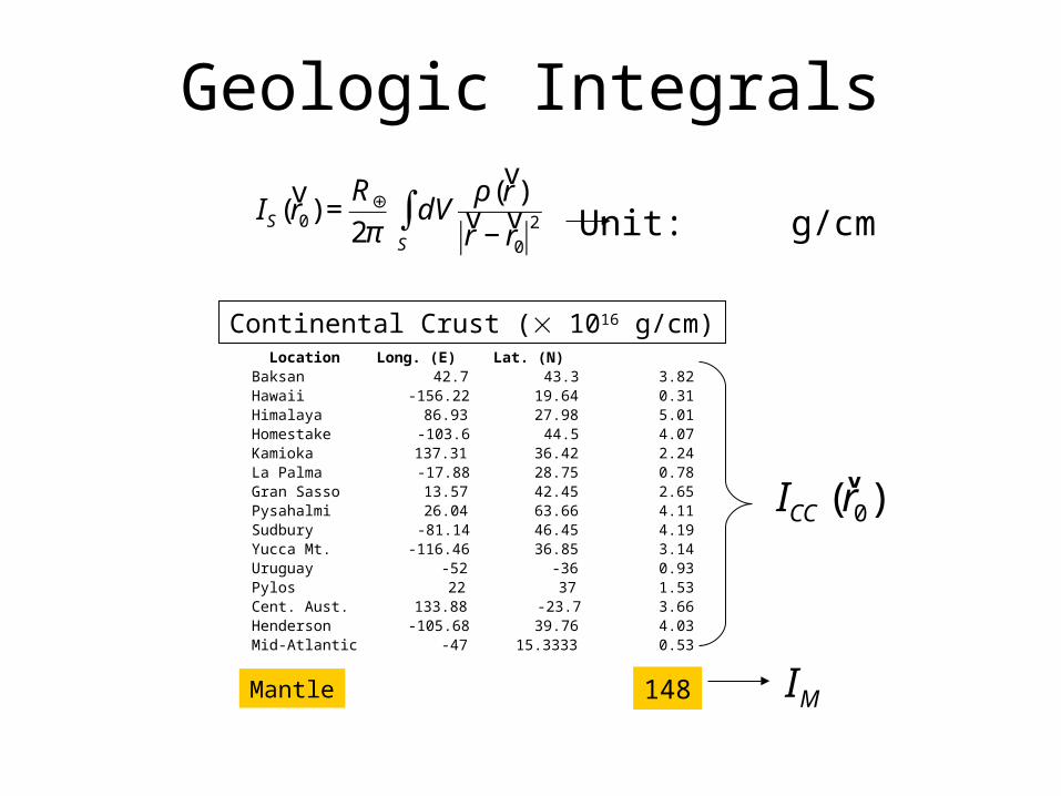
Geologic Integrals

€

IS (v r 0) =

R⊕

2πdV

ρ (v r )

v r −

v r 0

2S

∫ Unit: g/cm


Continental Crust ( 1016 g/cm)

3.820.315.014.072.240.782.654.114.193.140.931.533.664.030.53

Mantle 148

€

ICC (v r 0)

€

IM

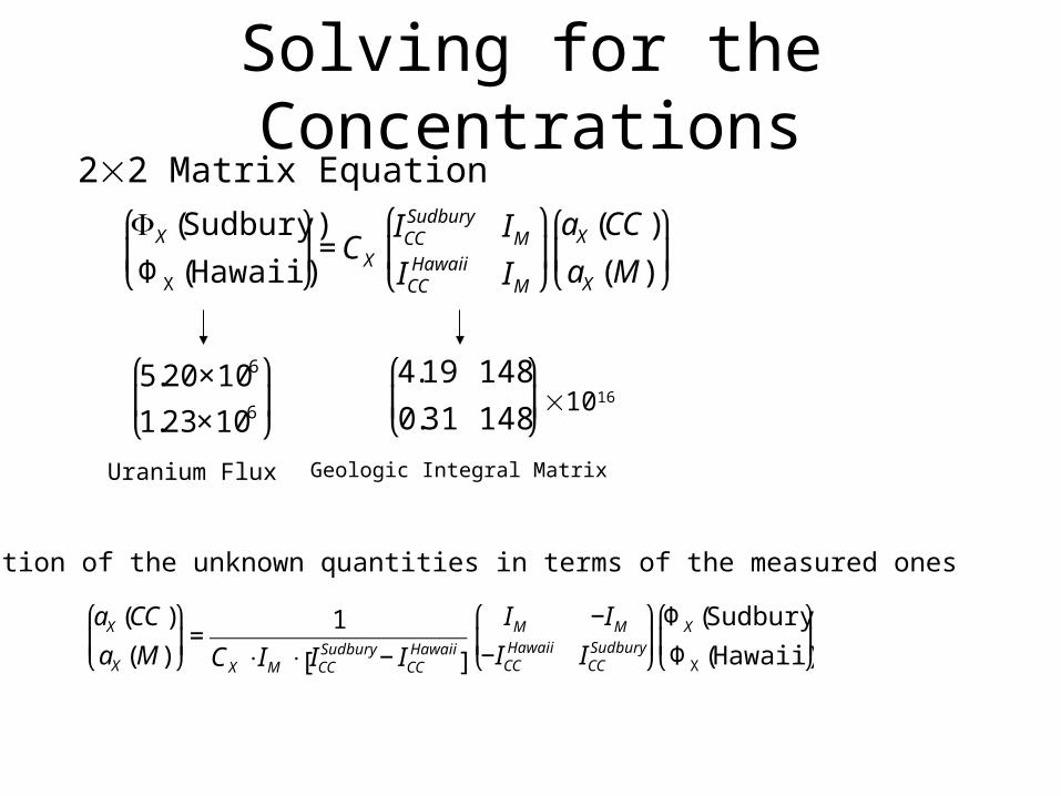
Solving for the Concentrations

€

ΦX (Sudbury)

ΦX (Hawaii)

⎛

⎝ ⎜

⎞

⎠ ⎟= CX

ICCSudbury IM

ICCHawaii IM

⎛

⎝ ⎜

⎞

⎠ ⎟aX (CC)

aX (M)

⎛

⎝ ⎜

⎞

⎠ ⎟

€

4.19 148

0.31 148

⎛

⎝ ⎜

⎞

⎠ ⎟

€

5.20 ×106

1.23×106

⎛

⎝ ⎜

⎞

⎠ ⎟

Uranium Flux

22 Matrix Equation

€

aX (CC)

aX (M)

⎛

⎝ ⎜

⎞

⎠ ⎟=

1

CX ⋅ IM ⋅ ICCSudbury − ICC

Hawaii[ ]

IM −IM

−ICCHawaii ICC

Sudbury

⎛

⎝ ⎜

⎞

⎠ ⎟ΦX (Sudbury)

ΦX (Hawaii)

⎛

⎝ ⎜

⎞

⎠ ⎟

Solution of the unknown quantities in terms of the measured ones

Geologic Integral Matrix

1016

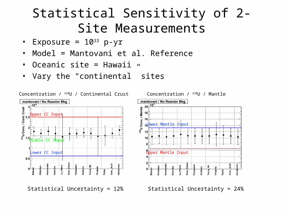
Statistical Sensitivity of 2-Site Measurements

• Exposure = 1033 p-yr

• Model = Mantovani et al. Reference

• Oceanic site = Hawaii

• Vary the “continental” sites

Upper CC Input

Middle CC Input

Lower CC Input

Statistical Uncertainty ≈ 12%

Lower Mantle Input

Upper Mantle Input

Statistical Uncertainty ≈ 24%

Concentration / 238U / Continental Crust Concentration / 238U / Mantle

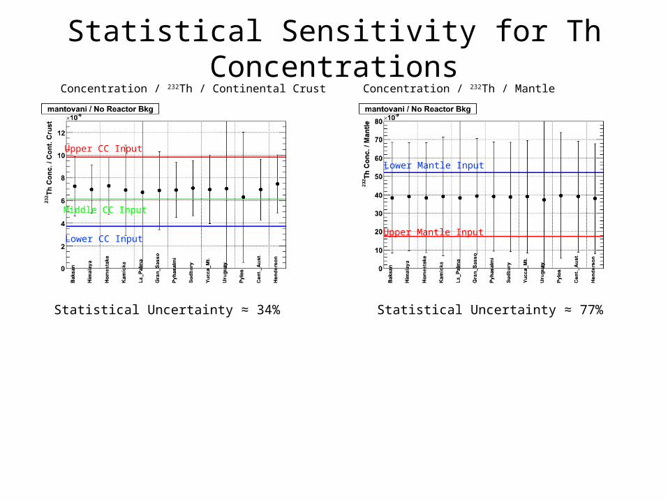
Statistical Sensitivity for Th ConcentrationsConcentration / 232Th / Continental Crust Concentration / 232Th / Mantle

Upper CC Input

Middle CC Input

Lower CC Input

Lower Mantle Input

Upper Mantle Input

Statistical Uncertainty ≈ 34% Statistical Uncertainty ≈ 77%

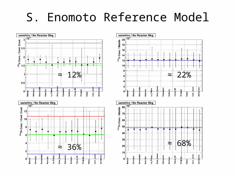
S. Enomoto Reference Model

≈ 12% ≈ 22%

≈ 36% ≈ 68%

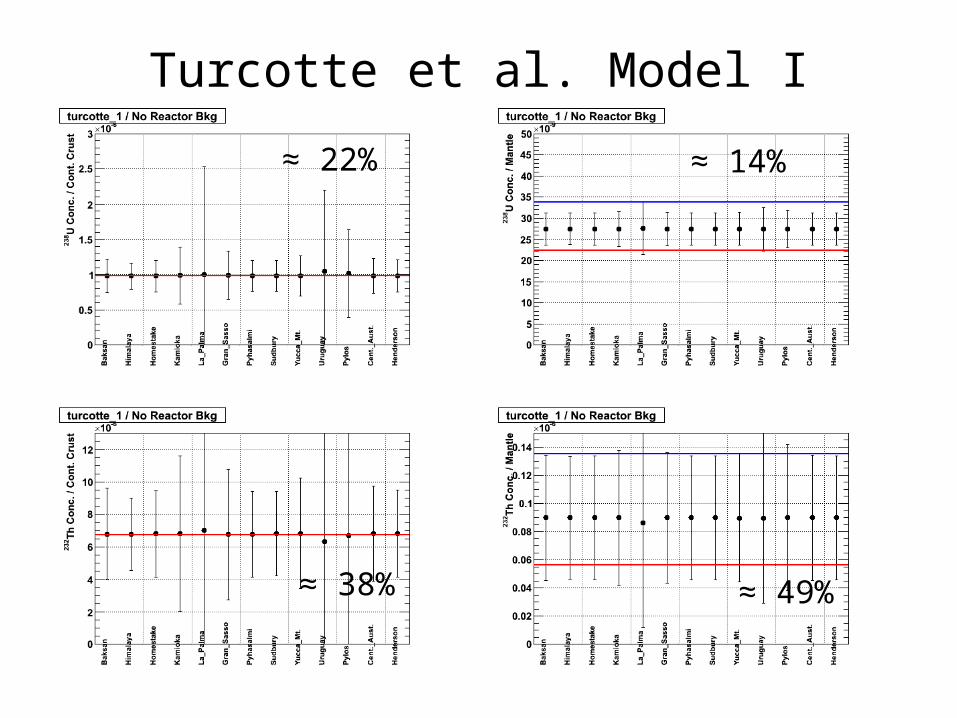
Turcotte et al. Model I

≈ 22% ≈ 14%

≈ 38% ≈ 49%

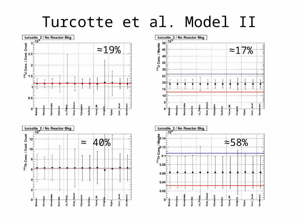
Turcotte et al. Model II

≈19% ≈17%

≈ 40% ≈58%

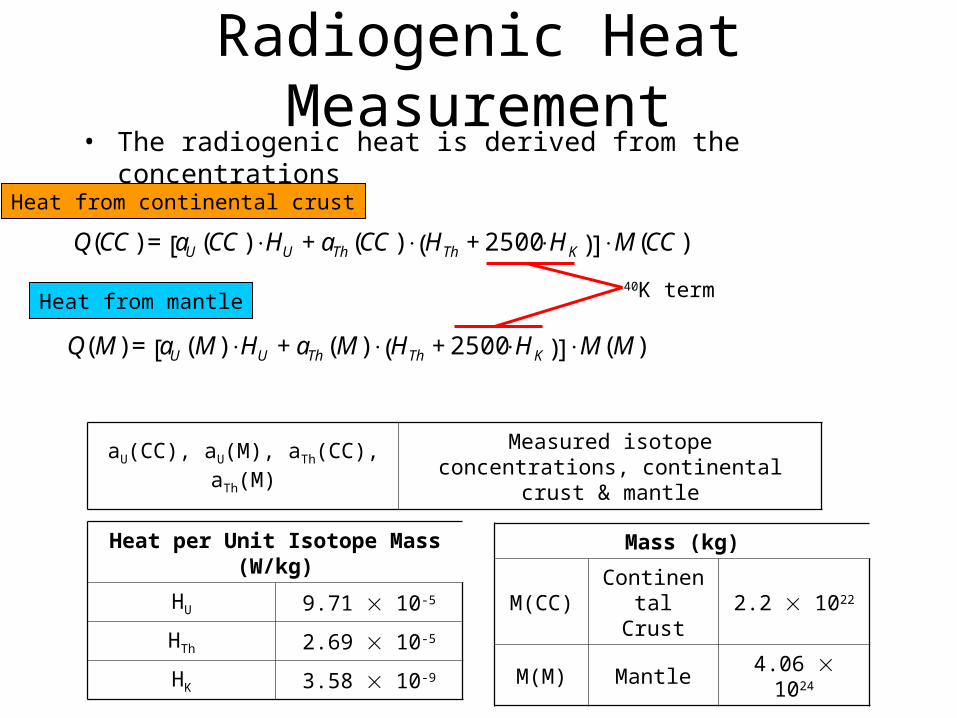
Radiogenic Heat Measurement• The radiogenic heat is derived from the concentrations

€

Q(CC) = aU (CC) ⋅HU + aTh (CC) ⋅ HTh + 2500 ⋅HK( )[ ] ⋅M(CC)

€

Q(M) = aU (M) ⋅HU + aTh (M) ⋅ HTh + 2500 ⋅HK( )[ ] ⋅M(M)

Heat from continental crust

Heat from mantle40K term

aU(CC), aU(M), aTh(CC), aTh(M) Measured isotope concentrations, continental crust & mantle

Heat per Unit Isotope Mass (W/kg)

HU 9.71 10-5

HTh 2.69 10-5

HK 3.58 10-9

Mass (kg)

M(CC)Continental

Crust2.2 1022

M(M) Mantle 4.06 1024

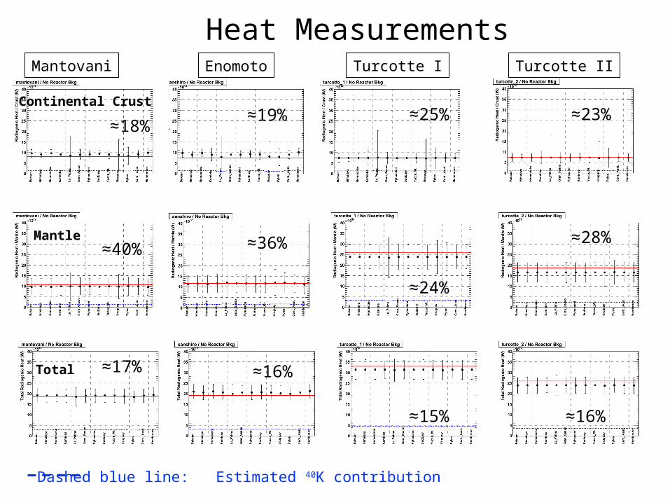
Heat Measurements

≈18%≈19%

≈36%

≈16%

≈25%

≈24%

≈15%

≈23%

≈28%

≈16%

Mantovani Enomoto Turcotte I Turcotte II

Continental Crust

Mantle

Total

≈40%

≈17%

Dashed blue line: Estimated 40K contribution

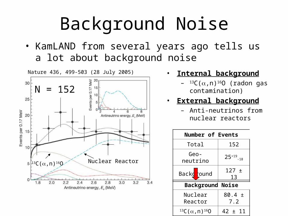
Background Noise• KamLAND from several years ago tells us a lot about

background noiseNature 436, 499-503 (28 July 2005) • Internal background

– 13C(,n)16O (radon gas contamination)

• External background– Anti-neutrinos from nuclear

reactors

Nuclear Reactor13C(,n)16O

N = 152

Number of Events

Total 152

Geo-neutrino 25+19-18

Background 127 ± 13

Background Noise

Nuclear Reactor 80.4 ± 7.2

13C(,n)16O 42 ± 11

Internal Background• A lot of R & D by the KamLAND team and others have

taken place since the first geo-neutrino measurement

• Make use of the R & D results, and learn from experience:– Make sure the liquid scintillator and other internal detector

components have minimal exposure to radon gas

– Use newly developed purification techniques to remove 210Pb (radioactive lead) from the liquid scintillator

Assume that the internal background can be reduced to a negligible level

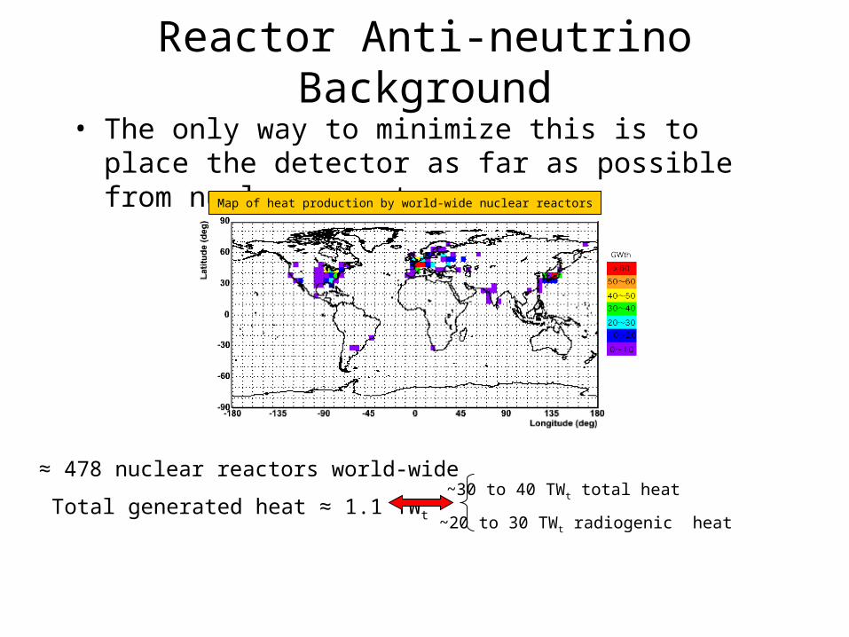
Reactor Anti-neutrino Background

• The only way to minimize this is to place the detector as far as possible from nuclear reactors

Map of heat production by world-wide nuclear reactors

≈ 478 nuclear reactors world-wide

Total generated heat ≈ 1.1 TWt

~30 to 40 TWt total heat

~20 to 30 TWt radiogenic heat

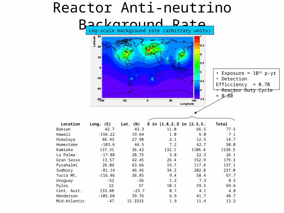
Reactor Anti-neutrino Background RateLog-scale background rate (arbitrary units)


E in [1.8,2.3] E in [2.3,3.3] Total11.0 66.5 77.5

1.0 6.0 7.12.1 12.5 14.77.2 42.7 50.0

132.1 1106.4 1238.53.8 22.3 26.1

26.4 152.9 179.319.7 117.4 137.134.2 202.8 237.0

9.4 58.4 67.71.2 7.3 8.5

10.1 59.5 69.60.7 4.1 4.86.9 41.7 48.71.9 11.4 13.3

• Exposure = 1033 p-yr• Detection Efficciency = 0.70• Reactor Duty Cycle = 0.80

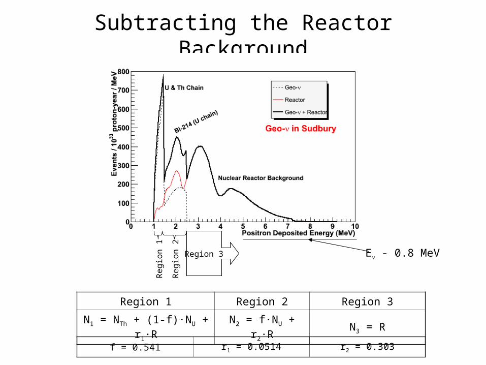
Subtracting the Reactor Background

Eν - 0.8 MeV

Reg

ion

1

Reg

ion

2

Region 3

Region 1 Region 2 Region 3

N1 = NTh + (1-f)·NU + r1·R N2 = f·NU + r2·R N3 = R

f = 0.541 r1 = 0.0514 r2 = 0.303

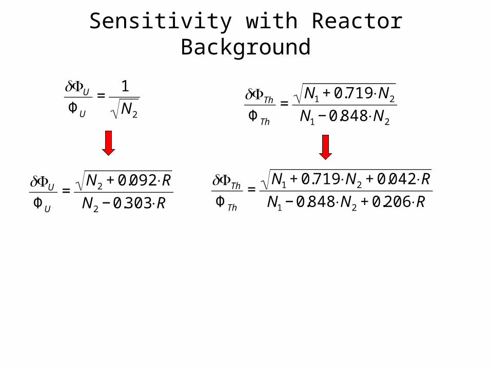
Sensitivity with Reactor Background

€

δΦU

ΦU

=1

N2

€

δΦTh

ΦTh

=N1 + 0.719 ⋅N2

N1 − 0.848 ⋅N2

€

δΦU

ΦU

=N2 + 0.092 ⋅R

N2 − 0.303⋅R

€

δΦTh

ΦTh

=N1 + 0.719 ⋅N2 + 0.042 ⋅R

N1 − 0.848 ⋅N2 + 0.206 ⋅R

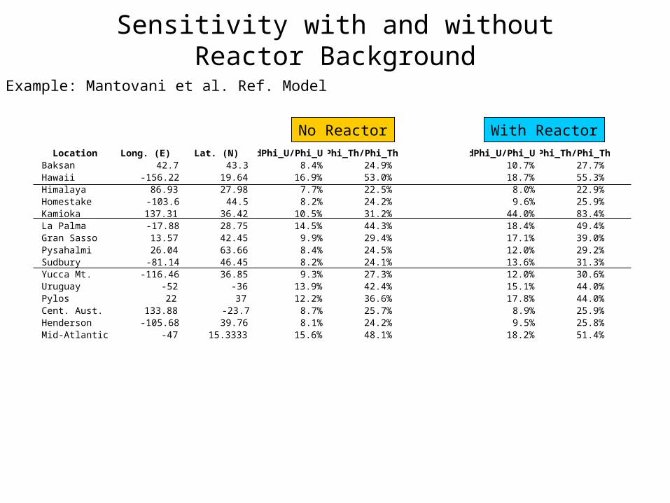
Sensitivity with and without Reactor Background


dPhi_U/Phi_UdPhi_Th/Phi_Th8.4% 24.9%

16.9% 53.0%7.7% 22.5%8.2% 24.2%

10.5% 31.2%14.5% 44.3%

9.9% 29.4%8.4% 24.5%8.2% 24.1%9.3% 27.3%

13.9% 42.4%12.2% 36.6%

8.7% 25.7%8.1% 24.2%

15.6% 48.1%

dPhi_U/Phi_UdPhi_Th/Phi_Th10.7% 27.7%18.7% 55.3%

8.0% 22.9%9.6% 25.9%

44.0% 83.4%18.4% 49.4%17.1% 39.0%12.0% 29.2%13.6% 31.3%12.0% 30.6%15.1% 44.0%17.8% 44.0%

8.9% 25.9%9.5% 25.8%

18.2% 51.4%

Example: Mantovani et al. Ref. Model

No Reactor With Reactor

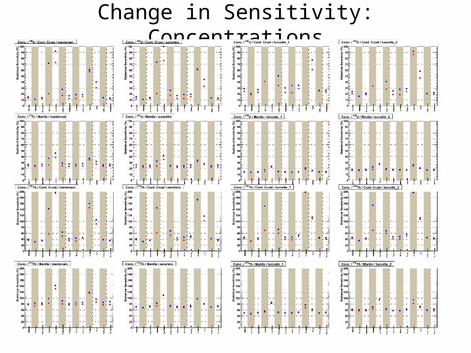
Change in Sensitivity: Concentrations

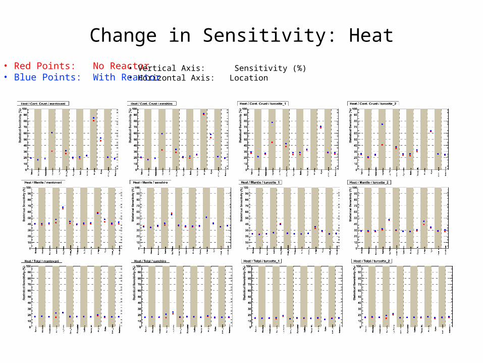
Change in Sensitivity: Heat

• Red Points: No Reactor• Blue Points: With Reactor

• Vertical Axis: Sensitivity (%)• Horizontal Axis: Location

Testing Geological Models

• Examples of what kind of sensitivity the next-generation geo-neutrino measurements might have to geological models

1. Distinguishing the Turcotte et al. models from the “Reference” models

2. What can we say about the Th/U ratio?

3. How well can we constrain radiogenic heat?

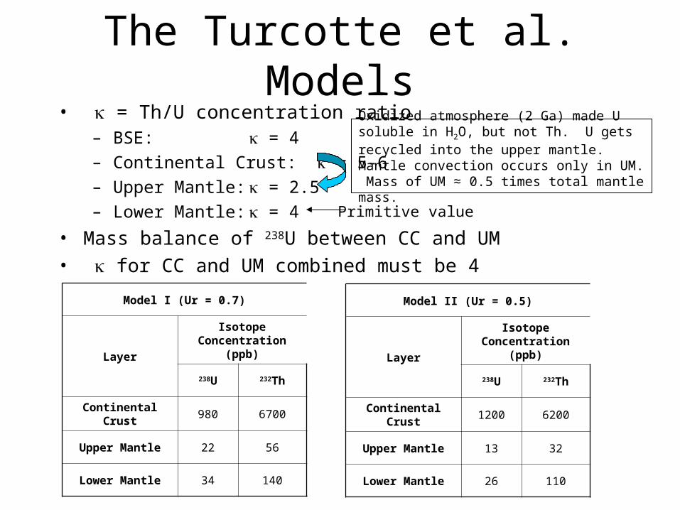
The Turcotte et al. Models• = Th/U concentration ratio

– BSE: = 4

– Continental Crust: = 5-6

– Upper Mantle: = 2.5

– Lower Mantle: = 4

• Mass balance of 238U between CC and UM

• for CC and UM combined must be 4

Oxidized atmosphere (2 Ga) made U soluble in H2O, but not Th. U gets recycled into the upper mantle. Mantle convection occurs only in UM. Mass of UM ≈ 0.5 times total mantle mass.

Primitive value

Model I (Ur = 0.7)

Layer

Isotope Concentration (ppb)

238U 232Th

Continental Crust 980 6700

Upper Mantle 22 56

Lower Mantle 34 140

Model II (Ur = 0.5)

Layer

Isotope Concentration (ppb)

238U 232Th

Continental Crust 1200 6200

Upper Mantle 13 32

Lower Mantle 26 110

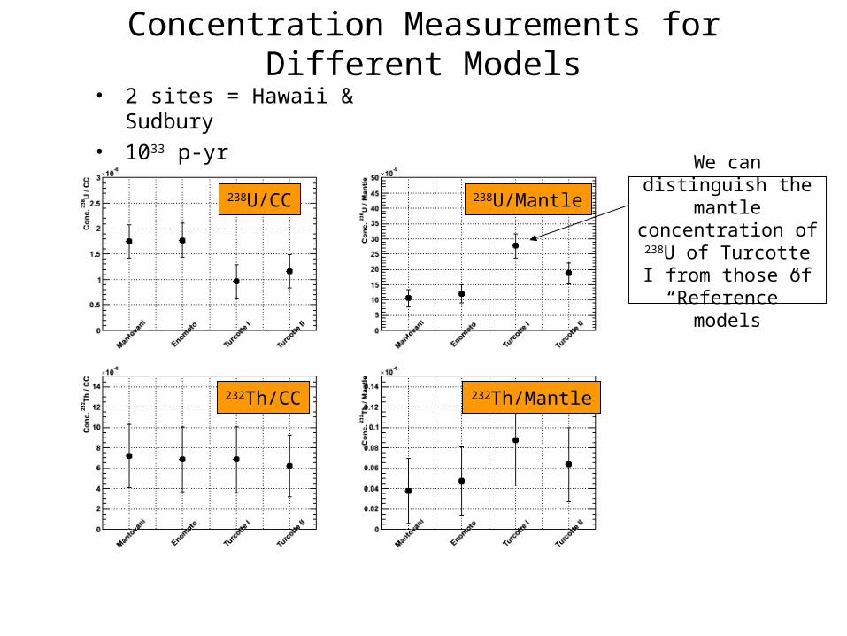
Concentration Measurements for Different Models

• 2 sites = Hawaii & Sudbury

• 1033 p-yr

238U/CC 238U/Mantle

232Th/CC 232Th/Mantle

We can distinguish the mantle concentration of 238U of Turcotte I from those of “Reference”

models

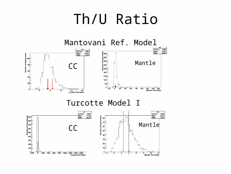
Th/U Ratio

Mantovani Ref. Model

Turcotte Model I

CC

CC

Mantle

Mantle

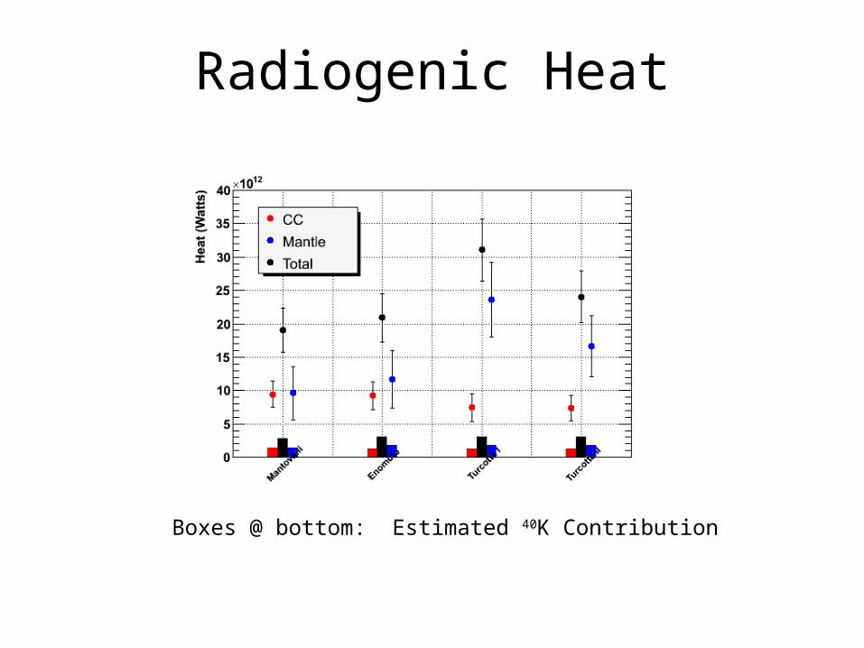
Radiogenic Heat

Boxes @ bottom: Estimated 40K Contribution

Conclusions• Next generation geo-neutrino experiments:

– Exposure > 1033 p-yr– 2 sites: continental & oceanic location– Low background

• We can begin to distinguish models– Separate information about continental crust & mantle– 238U concentration in the mantle

• Can separate reference models from Turcotte model I at 4-5 sigma level

– Radiogenic heat• 15-20% uncertainty in total radiogenic heat• But extra uncertainty due to unknown 40K heat

Documents

Geology from Geo-neutrino Flux Measurements Eugene Guillian / Queen’s University DOANOW March 24, 2007