Geologically Constrained Probabilistic Mapping of Gold Potential, Baguio District, Philippines

Natural Resources Research, Vol. 9, No. 3, 2000

Geologically Constrained Probabilistic Mapping of GoldPotential, Baguio District, Philippines

Emmanuel John M. Carranza1,3 and Martin Hale2

Received and accepted 23 June 2000

Binary predictor patterns of geological features are integrated based on a probabilisticapproach known as weights of evidence modeling to predict gold potential. In weights ofevidence modeling, the loge of the posterior odds of a mineral occurrence in a unit cell isobtained by adding a weight, W� or W� for presence of absence of a binary predictor pattern,to the loge of the prior probability. The weights are calculated as loge ratios of conditionalprobabilities. The contrast, C � W� � W�, provides a measure of the spatial associationbetween the occurrences and the binary predictor patterns. Addition of weights of the inputbinary predictor patterns results in an integrated map of posterior probabilities representinggold potential. Combining the input binary predictor patterns assumes that they are condition-ally independent from one another with respect to occurrences.

KEY WORDS: Bayesian probability; weights of evidence; spatial association; mineral potential mapping;Baguio gold district (Philippines).

INTRODUCTION

The geology of any given area probably is thesingle most important indicator of its mineral poten-tial. In well-explored areas, the qualitative knowledgeof the spatial associations of known mineral depositswith the different geological features is the basis formost exploration programs. However, as the spatialassociation of mineral occurrences with geologicalfeatures differs from place to place, a qualitativeknowledge alone is inadequate for discovering newdeposits. A quantitative knowledge of the spatial as-sociation between known occurrences and the differ-ent geological features present is equally or moreimportant in mineral exploration.

Previous work on quantitative methods for map-

1 Mines and Geosciences Bureau, Regional Office No. 5, Philip-pines.

2International Institute for Aerospace Survey and Earth Sciences(ITC), Kanaalweg 3, 2628 EB Delft, The Netherlands.

3To whom all correspondence should be mailed. Present address:ITC, Kanaalweg 3, 2628 EB Delft, The Netherlands. (e-mail:[email protected])

237

1520-7439/00/0900-0237$18.00/0 2000 International Association for Mathematical Geology

ping mineral potential, based on known occurrences,mainly used regression techniques (e.g., Chung andAgterberg, 1980; Harris, 1984). The known occur-rences are used to develop a multivariate signaturefor mineralization, expressed as a vector of coeffi-cients for the geological predictor variables. The coef-ficients are calculated using least-squares regression;the resulting equation is used to generate regressionscores whose magnitude reflect mineral potential.Regression techniques, however, are weak. They in-variably assume that the relationship of the depen-dent variables (i.e., location of mineral occurrences)to the predictor variables (i.e., geological features)is linear, which is not always the situation. In addition,there is no assumption of and, consequently, no testfor, conditional independence between the predictorvariables is required.

An alternative approach to mapping mineralpotential that avoids the limitations associated withregression techniques is to use Bayes’ rule (e.g.,Bonham-Carter, Agterberg, and Wright, 1988; Ag-terberg, Bonham-Carter, and Wright 1990). Startingwith a prior probability of mineral occurrences in aunit area, a posterior probability is calculated based

238 Carranza and Hale

on the weights of evidence for the presence or ab-sence of a binary predictor pattern. The weights ofall predictor variables are combined with the priorprobability to estimate the posterior probability of anoccurrence. Combining the binary predictor patternsassumes that they are conditionally independent.When pairs of binary predictor patterns are tested forconditional independence with respect to the knownoccurrences, it can lead to the rejection of some bi-nary predictor patterns.

In this paper, we describe an application of theBayesian approach of combining binary patterns ofgeological features for mapping gold potential in theBaguio district of the Philippines. We use two setsof mineral occurrence data: (1) locations of small-scale gold deposits worked by local people and(2) locations of gold deposits that either have beenmined on a large scale or have been explored exten-sively for development. These are used to cross vali-date the resulting predictive maps. In addition, weshow the usefulness of the small-scale occurrences inguiding exploration for potentially more economicdeposits. Because of the general lack of mineral ex-ploration data other than geological data for most ofthe Philippines, we constrain our analysis to geologi-cal features. We use a geographic information system(GIS) of geological and mineral occurrence data toexamine empirically the spatial association betweenthe geological features and the large-scale and small-scale gold occurrences. Predictive maps of gold po-tential then are developed using the spatial associa-tions between the geological features and theknown occurrences.

BAYESIAN PROBABILITY MODEL

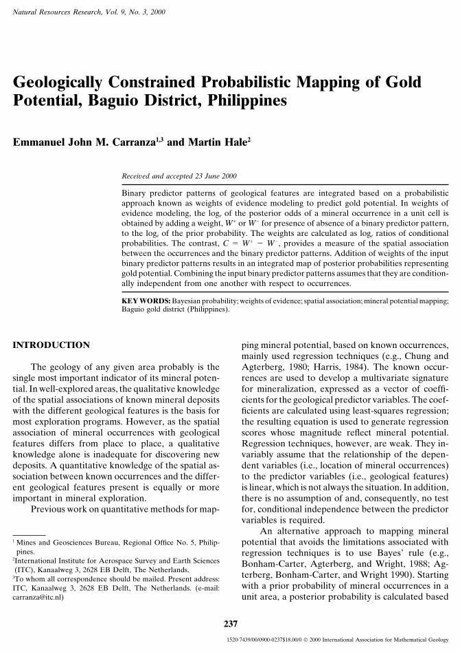
The following formulation of a Bayesian proba-bility model, known as weights of evidence model,applied to mineral potential mapping is synthesizedfrom Bonham-Carter (1994) and Bonham-Carter,Agterberg, and Wright (1989). If a study region isdivided into unit cells (or pixels) with a fixed size, s,and the total area is t, then N�T� � t/s is the totalnumber of unit cells in the study area. If there are anumber of units cells, N�D�, containing an occurrenceD (Fig. 1), equal to the number of occurrences if sis small enough (i.e., one occurrence per cell), thenthe prior probability of an occurrence is expressed by

P�D� �N�D�N�T�

(1)

Figure 1. Venn diagram to illustrate weights of evidence calcula-tions. T, area; B, binary predictor pattern present, B, binary pre-dictor pattern absent; D, mineral occurrence present; D, mineraloccurrence absent.

Now suppose that a binary predictor pattern B, occu-pying N�B� unit cells occurs in the region and thata number of known deposits occur preferentiallywithin the pattern, that is, N�D � B�. Clearly, theprobability of a deposit occurring within the predictorpattern is greater than the prior probability. Con-versely, the probability of a deposit occurring outsidethe predictor pattern is lower than the prior probabil-ity. The favorability of locating an occurrence giventhe presence of a predictor pattern can be expressedby the conditional probability

P�D�B� �P�D � B�

P�B�� P�D� P�B�D�

P�B�(2)

where P�D�B� is the posterior probability of an oc-currence given the presence of the predictor pattern,P�B�D� is the posterior probability of being in thepredictor pattern B, given the presence of an occur-rence D, and P�B� is the prior probability of thepredictor pattern. The favorability of discovering anoccurrence given the absence of a predictor patterncan be expressed by the conditional probability

P�D�B� �P�D � B�

P�B�� P�D� P�B�D�

P�B�(3)

where P�D�B� is the posterior probability of an oc-currence given the absence of a predictor pattern,P�B�D� is the posterior probability of being outsidethe predictor B, given the presence of an occurrenceD, and P�B� is the prior probability of the area out-side the predictor pattern.

Equations (2) and (3) satisfy Bayes’ rule. The

Geologically Constrained Probabilistic Mapping 239

same model can be expressed in an odds formulation,where odds, O, are defined as O � P/(1 � P). Ex-pressed as odds, Equations (2) and (3), respec-tively, become:

O�D�B� � O�D� P�B�D�P�B�D�

(4)

and

O�D�B� � O�D� P�B�D�P�B�D�

, (5)

where O�D�B� and O�D�B� are, respectively, the pos-terior odds of an occurrence given the presence andabsence of a binary predictor pattern, and O�D� isthe prior odds of an occurrence. The weights for thebinary predictor pattern are defined as

W � � logeP�B�D�P�B�D�

(6)

and

W � � logeP�B�D�P�B�D�

(7)

where W � and W � are the weights of evidence whena binary predictor pattern is present and absent, re-spectively. Hence,

loge O�D�B� � loge O�D� � W � (8)

and

loge O�D�B� � loge O�D� � W � (9)

The variances of the weights can be calculated by(Bishop, Feinberg, and Holland, 1975):

s 2(W �) �1

N�B � D��

1N�B � D�

(10)

and

s 2(W �) �1

N�B � D��

1N�B � D�

(11)

Now suppose there are two binary predictor patterns,B1 and B2 . It can be shown that the posterior probabil-ity of an occurrence given the presence of two pre-dictor patterns is

P�D�B1 � B2�

�P�B1 � B2�D� P�D�

P�B1 � B2�D� P�D� � P�B1 � B2�D� P�D�(12)

If B1 and B2 are conditionally independent of eachother with respect to a set of occurrences, it indicatesthat the following relation is satisfied:

P�B1 � B2�D� � P�B1�D� P�B2�D� (13)

This allows Equation (10) to be simplified, thus:

P�D�B1 � B2� � P�D�P�B1�D� P�B2�D�

P�B1� P�B2�(14)

Equation (14) is similar to Equation (2), except thatmultiplication factors for two maps are used to updatethe prior probability to give the posterior probability.Using the odds formulation, it can be shown that:

loge O�D�B1 � B2� � loge O�D� � W �1 � W �

2 (15)

loge O�D�B1 � B2� � loge O�D� � W�1 � W �

2 (16)


2 (17)

and


2 (18)

Similarly, if more than two binary predictor patternsare used, they can be added, provided they also areconditionally independent of one another with re-spect to the occurrences. Thus, with Bj ( j � 1,2, . . . , n) binary predictor patterns, the loge poste-rior odds are:

loge O�D�Bk1 � Bk

2 � B k3 . . . B k

n� � �n

j�1W k

j

� loge O�D� (19)

where the superscript k is positive (�) or negative(�) if the binary predictor pattern is present or ab-sent, respectively. The posterior odds are convertedto posterior probabilities, based on the relation P �O/(1 � O), to represent favorability of locating an oc-currence.

APPLICATION TO GOLD OCCURRENCES INBAGUIO DISTRICT

Geological Background

The Baguio district (Fig. 2) is underlain mainlyby five major lithologic units. The Pugo Formationof Cretaceous to Eocene age, is a sequence of meta-volcanic and metasedimentary rocks. Zigzag Forma-tion unconformably overlies the Pugo Formation. Itconsists mainly of marine sedimentary rocks of Earlyto Middle Miocene age (Balce and others, 1980).However, it is intruded by andesite prophyry dated15.0 � 1.6 Ma (Wolfe, 1981) or pre-Middle Miocene.Mitchell and Leach (1991) consider the Zigzag For-mation to be mainly Late Eocene, but it may include


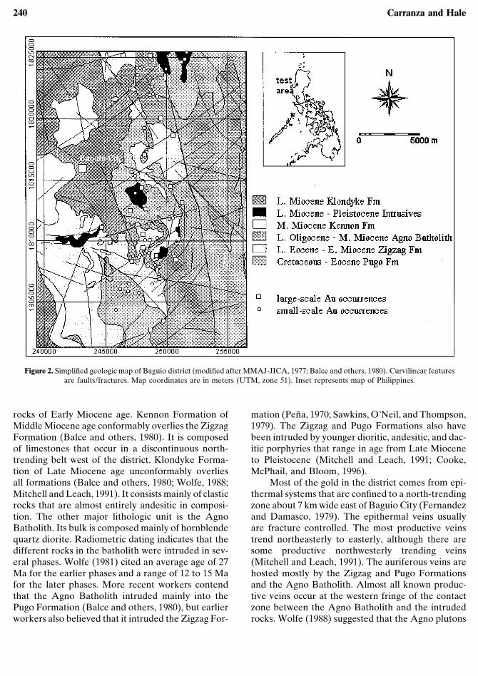
Figure 2. Simplified geologic map of Baguio district (modified after MMAJ-JICA, 1977; Balce and others, 1980). Curvilinear featuresare faults/fractures. Map coordinates are in meters (UTM, zone 51). Inset represents map of Philippines.

rocks of Early Miocene age. Kennon Formation ofMiddle Miocene age conformably overlies the ZigzagFormation (Balce and others, 1980). It is composedof limestones that occur in a discontinuous north-trending belt west of the district. Klondyke Forma-tion of Late Miocene age unconformably overliesall formations (Balce and others, 1980; Wolfe, 1988;Mitchell and Leach, 1991). It consists mainly of clasticrocks that are almost entirely andesitic in composi-tion. The other major lithologic unit is the AgnoBatholith. Its bulk is composed mainly of hornblendequartz diorite. Radiometric dating indicates that thedifferent rocks in the batholith were intruded in sev-eral phases. Wolfe (1981) cited an average age of 27Ma for the earlier phases and a range of 12 to 15 Mafor the later phases. More recent workers contendthat the Agno Batholith intruded mainly into thePugo Formation (Balce and others, 1980), but earlierworkers also believed that it intruded the Zigzag For-

mation (Pena, 1970; Sawkins, O’Neil, and Thompson,1979). The Zigzag and Pugo Formations also havebeen intruded by younger dioritic, andesitic, and dac-itic porphyries that range in age from Late Mioceneto Pleistocene (Mitchell and Leach, 1991; Cooke,McPhail, and Bloom, 1996).

Most of the gold in the district comes from epi-thermal systems that are confined to a north-trendingzone about 7 km wide east of Baguio City (Fernandezand Damasco, 1979). The epithermal veins usuallyare fracture controlled. The most productive veinstrend northeasterly to easterly, although there aresome productive northwesterly trending veins(Mitchell and Leach, 1991). The auriferous veins arehosted mostly by the Zigzag and Pugo Formationsand the Agno Batholith. Almost all known produc-tive veins occur at the western fringe of the contactzone between the Agno Batholith and the intrudedrocks. Wolfe (1988) suggested that the Agno plutons


are important source of the gold. Recent workers,however, claim that the epithermal gold mineraliza-tion is related to the younger intrusive complexes(Mitchell and Leach, 1991; Cooke, McPhail, andBloom, 1996).

Data Input and GIS Operations

The data used are a geological map, map offaults/fractures, and locations of large-scale andsmall-scale gold occurrences (Fig. 1). These data werederived from published works (e.g., Mitchell andLeach, 1991; MMAJ, 1996; MMAJ-JICA, 1977) andunpublished maps/reports in the Philippine Minesand Geosciences Bureau. The boundaries of litho-logic units, fault/fractures, and the locations of 19large-scale gold occurrences and 63 small-scale goldoccurrences were digitized from paper maps. Thedata capture and map operations and analyses werecarried out using ILWIS (Integrated Land and WaterInformation Systems), a GIS software package devel-oped by the International Institute for AerospaceSurvey and Earth Sciences (ITC) in the Netherlands.In ILWIS, spatial data are analyzed in raster mode.The procedure for generating the binary predictorpatterns used in mapping gold potential is discussednext. A pixel size (or unit cell) of 100 m by 100 mwas used in rasterizing the input vector maps to createand compute the weights of the binary predictor pat-terns. This pixel size was selected to ensure that onlyone occurrence is present in any given pixe; it alsois a realistic size for a mineralized area.

Generation of Binary Predictor Patterns

Geological knowledge of the gold occurrencesin the Baguio district suggests five binary predictorpatterns of geological features that are likely to beuseful evidences for predicting gold potential. Thesebinary predictor patterns are: (1) favorable hostrocks, that is Zigzag and Pugo Formations; (2) prox-imity to Agno Batholith contact; (3) proximity toyoung (i.e., Late Miocene to Pleistocene) intrusivescontact; (4) proximity to northeasterly trendingfaults/fractures; and (5) proximity to northwesterlytrending faults/fractures. To generate the binary pre-dictor pattern of favorable host rocks, the rasterizedlithologic map (Fig. 2) was reclassified into a binarypattern by relabeling the Zigzag and Pugo Forma-tions as ‘‘favorable’’ and the other formations as

‘‘nonfavorable.’’ To generate the binary predictorpatterns of proximity to the other geological features,we have to determine the distance for which the spa-tial association between the occurrences and geologi-cal features is optimal.

The optimum cutoff distance is determined bycalculating the weights (W �, W �) for successive cu-mulative distance intervals away from the geologicalfeatures and examining the variation of the weightsand contrast (C). The scientific basis for this is thatif more points occur within a pattern than would beexpected by chance, then W � is positive and W � isnegative. Conversely, W � is negative and W � is posi-tive for the situation where fewer points occur withina pattern than would be expected by chance. Themagnitude of the contrast, C, determined as the dif-ference W � � W �, provides a measure of spatialassociation between a set of points and a binary pat-tern (Bonham-Carter, Agterberg, and Wright 1989).For a positive spatial association, C is positive; C isnegative in the situation of negative association. Themaximum C usually gives the cutoff distance at whichthe predictive power of the resulting pattern is max-imized (Bonham-Carter, Agterberg, and Wright,1988). However, in situation of a small number ofoccurrences or small areas, such as the present exam-ple, the uncertainty of the weights could be large sothat C is meaningless. The Studentized value of C,calculated as the ratio of C to its standard deviation,C/s(C), serves as a guide to the significance of thespatial association (Bonham-Carter, 1994). The stan-dard deviation of C is calculated as

s(C) � �s 2(W �) � s 2(W�)

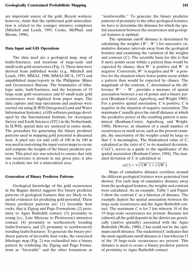
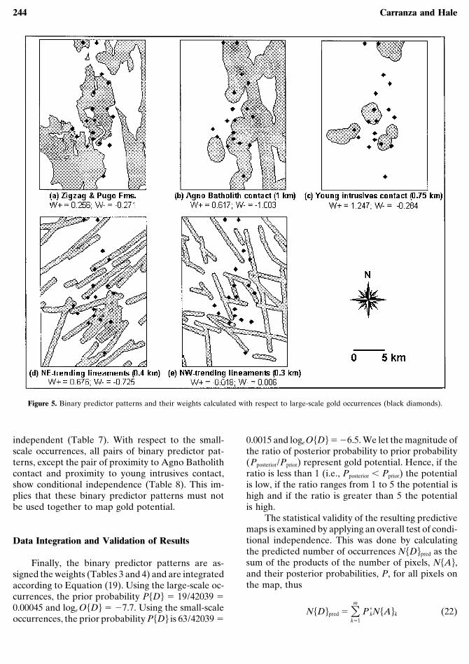
Maps of cumulative distance corridors aroundthe different geological features were generated (notshown). For each map of cumulative distance awayfrom the geological features, the weights and contrastwere calculated. As an example, Table 1 and Figure3 show the contrast C as a function of distance. Theexample depicts the spatial association between thelarge-scale occurrences and the Agno Batholith con-tact. The maximum C is for 2 km wherein 18 of the19 large-scale occurrences are present. Because not(almost) all the gold deposits in the district are geneti-cally (and/or spatially) associated with the AgnoBatholith (Wolfe, 1988), 2 km could not be the opti-mum cutoff distance. The studentized C indicates thatthe most significant cutoff distance is 1 km wherein 15of the 19 large-scale occurrences are present. Thisdistance is used to create a binary predictor patternof proximity to Agno Batholith contact.


Table 1. Weights and Contrasts for Cumulative Distances Away from Agno Batholith Contact with Respect to Large-Scale Gold Occurrencesa

Data used tocalculate weights

Distance No. ofcorridor No. of pixels gold occurrences Contrast, S.D. Studentized

(km) in pattern in pattern W � W � C � W � � W� of C C

0.25 5881 6 0.815 �0.229 1.044 0.494 2.1140.50 10725 9 0.619 �0.347 0.967 0.460 2.1030.75 14581 10 0.417 �0.321 0.739 0.460 1.6071.00 17907 15 0.617 �1.003 1.621 0.563 2.8801.25 20514 16 0.546 �1.177 1.723 0.629 2.7381.50 22898 16 0.436 �1.059 1.495 0.629 2.3761.75 24785 16 0.357 �0.956 1.312 0.629 2.0852.00 26186 18 0.420 �1.970 2.389 1.027 2.3252.25 27466 18 0.372 �1.885 2.257 1.027 2.1972.50 28441 19

a Total pixels in study area, 42,039; total number of large-scale gold occurrences, 19.

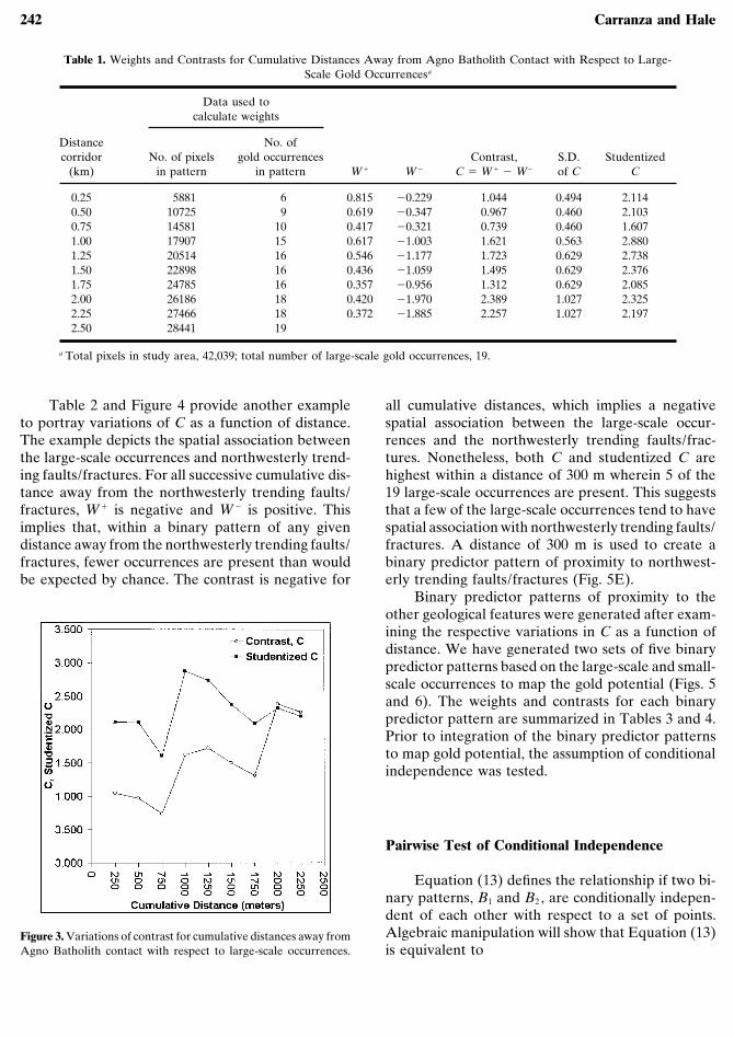
Table 2 and Figure 4 provide another exampleto portray variations of C as a function of distance.The example depicts the spatial association betweenthe large-scale occurrences and northwesterly trend-ing faults/fractures. For all successive cumulative dis-tance away from the northwesterly trending faults/fractures, W � is negative and W � is positive. Thisimplies that, within a binary pattern of any givendistance away from the northwesterly trending faults/fractures, fewer occurrences are present than wouldbe expected by chance. The contrast is negative for

Figure 3. Variations of contrast for cumulative distances away fromAgno Batholith contact with respect to large-scale occurrences.

all cumulative distances, which implies a negativespatial association between the large-scale occur-rences and the northwesterly trending faults/frac-tures. Nonetheless, both C and studentized C arehighest within a distance of 300 m wherein 5 of the19 large-scale occurrences are present. This suggeststhat a few of the large-scale occurrences tend to havespatial association with northwesterly trending faults/fractures. A distance of 300 m is used to create abinary predictor pattern of proximity to northwest-erly trending faults/fractures (Fig. 5E).

Binary predictor patterns of proximity to theother geological features were generated after exam-ining the respective variations in C as a function ofdistance. We have generated two sets of five binarypredictor patterns based on the large-scale and small-scale occurrences to map the gold potential (Figs. 5and 6). The weights and contrasts for each binarypredictor pattern are summarized in Tables 3 and 4.Prior to integration of the binary predictor patternsto map gold potential, the assumption of conditionalindependence was tested.

Pairwise Test of Conditional Independence

Equation (13) defines the relationship if two bi-nary patterns, B1 and B2 , are conditionally indepen-dent of each other with respect to a set of points.Algebraic manipulation will show that Equation (13)is equivalent to


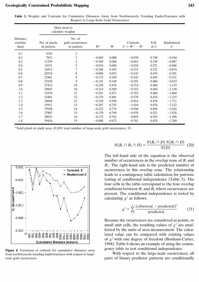
Table 2. Weights and Contrasts for Cumulative Distances Away from Northwesterly Trending Faults/Fractures withRespect to Large-Scale Gold Occurrences


Distance No. ofcorridor No. of pixels gold occurrences Contrast, S.D. Studentized

(km) in pattern in pattern W � W � C � W � � W � of C C

0.1 4743 20.2 7812 2 �0.069 0.008 �0.078 0.748 �0.1040.3 11259 5 �0.569 0.094 �0.663 0.748 �0.8870.4 14151 5 �0.018 0.006 �0.024 0.521 �0.0460.5 16913 7 �0.246 0.105 �0.351 0.521 �0.6740.6 20218 8 �0.088 0.055 �0.143 0.476 �0.3010.7 22961 9 �0.133 0.109 �0.242 0.465 �0.5210.8 25254 9 �0.142 0.148 �0.291 0.460 �0.6330.9 27413 10 �0.238 0.476 �0.514 0.460 �1.1191.0 29607 10 �0.214 0.309 �0.523 0.460 �1.1381.1 31670 12 �0.291 0.471 �0.763 0.460 �1.6601.2 33401 12 �0.176 0.401 �0.578 0.476 �1.2151.3 34666 12 �0.230 0.584 �0.814 0.476 �1.7111.4 35911 13 �0.267 0.743 �1.010 0.476 �2.1221.5 37058 14 �0.222 0.774 �0.996 0.494 �2.0161.6 37907 15 �0.179 0.799 �0.978 0.521 �1.8761.7 38651 16 �0.133 0.762 �0.895 0.563 �1.5901.8 39414 19 �0.088 0.673 �0.761 0.629 �1.209

a Total pixels in study area, 42,039; total number of large-scale gold occurrences, 19.

Figure 4. Variations of contrast for cumulative distances awayfrom northwesterly trending faults/fractures with respect to large-scale gold occurrences.

N�B1 � B2 � D� �N�B1 � D� N�B2 � D�

N�D�(20)

The left-hand side of the equation is the observednumber of occurrences in the overlap zone of B1 andB2 . The right-hand side is the predicted number ofoccurrences in this overlap zone. The relationshipleads to a contingency table calculation for pairwisetesting of conditional independence (Table 5). Thefour cells in the table correspond to the four overlapconditions between B1 and B2 where occurrences arepresent. The conditional independence is tested bycalculating � 2 as follows:

� 2 � �4

i�1

(observedi � predictedi)2

predictedi(21)

Because the occurrences are considered as points, orsmall unit cells, the resulting values of � 2 are unaf-fected by the units of area measurement. The calcu-lated value can be compared with existing valuesof � 2 with one degree of freedom (Bonham-Carter,1994). Table 6 shows an example of using the contin-gency table to test conditional independence.

With respect to the large-scale occurrences, allpairs of binary predictor patterns are conditionally


Figure 5. Binary predictor patterns and their weights calculated with respect to large-scale gold occurrences (black diamonds).

independent (Table 7). With respect to the small-scale occurrences, all pairs of binary predictor pat-terns, except the pair of proximity to Agno Batholithcontact and proximity to young intrusives contact,show conditional independence (Table 8). This im-plies that these binary predictor patterns must notbe used together to map gold potential.

Data Integration and Validation of Results

Finally, the binary predictor patterns are as-signed the weights (Tables 3 and 4) and are integratedaccording to Equation (19). Using the large-scale oc-currences, the prior probability P�D� � 19/42039 �0.00045 and loge O�D� � �7.7. Using the small-scaleoccurrences, the prior probability P�D� is 63/42039 �

0.0015 and loge O�D� � �6.5. We let the magnitude ofthe ratio of posterior probability to prior probability(Pposterior/Pprior) represent gold potential. Hence, if theratio is less than 1 (i.e., Pposterior � Pprior) the potentialis low, if the ratio ranges from 1 to 5 the potential ishigh and if the ratio is greater than 5 the potentialis high.

The statistical validity of the resulting predictivemaps is examined by applying an overall test of condi-tional independence. This was done by calculatingthe predicted number of occurrences N�D�pred as thesum of the products of the number of pixels, N�A�,and their posterior probabilities, P, for all pixels onthe map, thus

N�D�pred � �mk�1

P *kN�A�k (22)


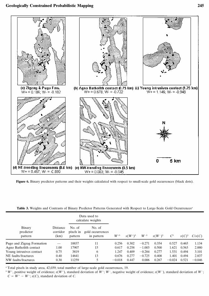
Figure 6. Binary predictor patterns and their weights calculated with respect to small-scale gold occurrences (black dots).

Table 3. Weights and Contrasts of Binary Predictor Patterns Generated with Respect to Large-Scale Gold Occurrencesa


Binary Distance No. of No. ofpredictor corridor pixels in gold occurrencespattern (km) pattern in pattern W�b s(W�)b W �b s(W �)b Cb s(C)b C/s(C)

Pugo and Zigzag Formation — 18837 11 0.256 0.302 �0.271 0.354 0.527 0.465 1.134Agno Batholith contact 1.00 17907 15 0.617 0.258 �1.003 0.500 1.621 0.563 2.880Young intrusives contact 0.75 3819 6 1.247 0.409 �0.284 0.277 1.531 0.494 3.101NE faults/fractures 0.40 14641 13 0.676 0.277 �0.725 0.408 1.401 0.494 2.837NW faults/fractures 0.30 11259 5 �0.018 0.447 0.006 0.267 �0.024 0.521 �0.046

a Total pixels in study area, 42,039; total number of large-scale gold occurrences, 19.b W �, positive weight of evidence; s(W �), standard deviation of W �; W �, negative weight of evidence; s(W �), standard deviation of W �;

C � W � � W �; s(C), standard deviation of C.


Table 4. Weights and Contrasts of Binary Predictor Patterns Generated with Respect to Small-Scale Gold Occurrencesa


Binary Distance No. of No. ofpredictor corridor pixels in gold occurrencespattern (km) pattern in pattern W �b s(W �)b W �b s(W �)b Cb s(C)b C/s(C)

Pugo and Zigzag Formations — 18837 34 0.186 0.172 �0.182 0.186 0.368 0.253 1.455Agno Batholith contact 0.75 14581 43 0.678 0.153 �0.722 0.224 1.401 0.271 5.171Young intrusives contact 1.75 9366 44 1.146 0.151 �0.948 0.229 2.093 0.275 7.619NE lineaments 0.6 20928 50 0.467 0.142 �0.890 0.277 1.358 0.311 4.358NW lineaments 0.5 16913 27 0.063 0.193 �0.045 0.167 0.108 0.255 0.425

a Total pixels in study area, 42,039; total number of small-scale gold occurrences, 63.b W �, positive weight of evidence; s(W �), standard deviation of W �; W �, negative weight of evidence; s(W �), standard deviation of W �;

C � W � � W�; s(C), standard deviation of C.

where there are k � 1, 2, . . . , m pixels on the map.If the predicted number of occurrences is larger than10 to 15% of the observed occurrences, then the as-sumption of conditional independence is seriouslyviolated (Bonham-Carter, 1994). Problematic inputbinary predictor patterns should be removed fromthe analysis.

To validate the usefulness of the predictive mapsfor identifying potential zones of gold mineralization,we determine the number of known and ‘‘undiscov-ered’’ occurrences falling within zones of high to veryhigh potential. The predictive maps must be able toidentify the known occurrences that were used todevelop them. This validation, however, is not highlyconvincing. For a more convincing validation, we as-sume that the set of occurrences not used to developa predictive map are ‘‘undiscovered’’ and determineif the predictive map is able to identify them. Hence,predictive maps based on the large-scale occurrencesare cross validated against the small-scale occur-rences and vice versa. We consider that a predictivemap is useful if it identifies at least 70% of the occur-rences that were to develop it and at least 50% of

Table 5. Contingency Table for Testing Conditional Independence,Based on Cells that Contain Occurrencea

B1 Present B1 Absent Totals

B2 Present N�B1 � B2 � D� N�B1 � B2 � D� N�B2 � D�B2 Absent N�B1 � B2 � D� N�B2 � B2 � D� N�B2 � D�

Totals N�B1 � D� N�B1 � D� N�D�

a Four values within table are either calculated using Equation(20) or observed from maps. There is one degree of freedom(adopted from Bonham-Carter, 1994).

the ‘‘undiscovered’’ occurrences. The criteria may beconservative, but because our probabilistic mappingis constrained to geological features, we considerthem adequate.

RESULTS

Initially, we ignore the results of pairwise testof conditional independence, integrate all the binarypredictor patterns for each occurrence data set, andevaluate the results.

Using Large-Scale Gold Occurrences

The predictive map of gold potential resultingfrom combining binary predictor patterns whoseweights were calculated with respect to the large-scale occurrences is shown in Figure 7A. With this

Table 6. Example of Using Contingency Table to Test ConditionalIndependence between Binary Pattern of Pugo/Zigzag Formations(B1) and Binary Pattern of Proximity Agno Batholith Contact

(B2)a

B1 Present B1 Absent Totals

B2 Present 7 (8.7) 4 (2.3) 11B2 Absent 8 (6.3) 0 (1.7) 8

Totals 15 4 19

a Values in bold are observed on map, those in brackets are calcu-lated using right-hand side of Equation (20). Calculated � 2 �

3.68 while tabled � 2.95, 1 � 3.8. Assumption of conditional indepen-

dence between binary patterns is not rejected at 95% level.


Table 7. Calculated � 2 Values for Testing Conditional Independence between All Pairs of Binary Patternswith Respect to Large-Scale Gold Occurrences

Binary predictor Agno Batholith Young intrusives NE-trending NW-trendingpattern contact contact faults/fractures faults/fractures

Pugo and Zigzag 3.68 2.33 0.28 0.01Formations

Agno Batholith 4.42 0.80 0.00contact

Young intrusives 1.38 0.22contact

NE-trending 0.22faults/fractures

a With one degree of freedom and probability level of 98%, tabled � 2 value is 5.4. Values in bold indicatepairs for which null hypothesis of conditional independence is not rejected at 98% probability level.

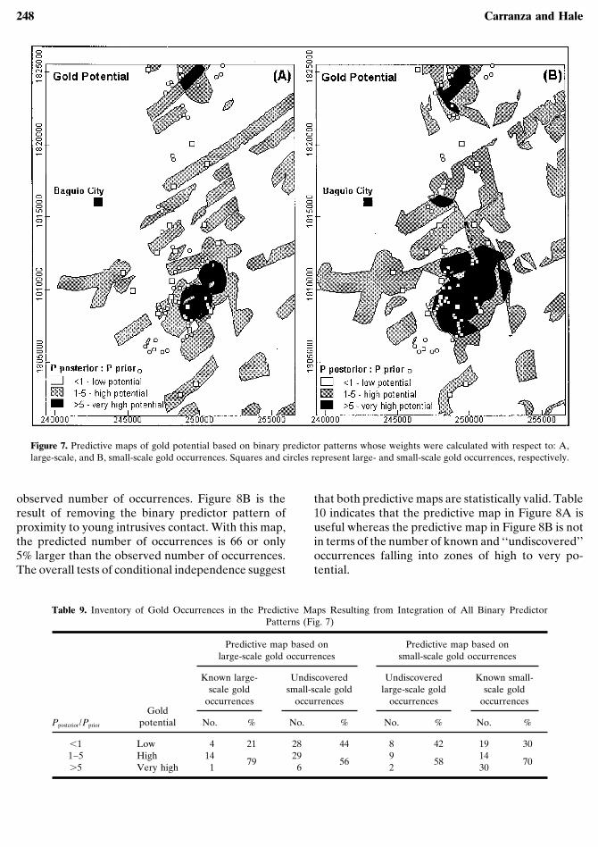
map, the predicted number of gold occurrences basedon Equation (22) is 21. This predicted number is onlyabout 11% larger than the observed number of large-scale occurrences, which implies that the assumptionof conditional independence is not seriously violated(Bonham-Carter, 1994).

In the predictive map, 15 or 79% of the 19 large-scale occurrences are in zones of high to very highpotential (Table 9). It can be gleaned from Figure7A and Table 9 that as many as 35 or 56% of the 63‘‘undiscovered’’ occurrences fall into or near zonesof high to very high gold potential. This predictivemap is useful for surface exploration of undiscoveredoccurrences in the district.

Using Small-Scale Gold Occurrences

Figure 7B shows the map of gold potential aftercombining the binary predictor patterns whose

Table 8. Calculated � 2 Values for Testing Conditional Independence between All Pairs of Binary Mapswith Respect to Small-Scale Gold Occurrencesa

Binary predictor Agno Batholith Young intrusives NE-trending NW-trendingpattern contact contact faults/fractures faults/fractures

Pugo and Zigzag 3.03 2.29 1.59 5.12Formations

Agno Batholith 8.58 0.34 0.61contact

Young intrusives 0.00 4.58contact

NE-trending 2.62faults/fractures

a With 1 degree of freedom and probability level of 98%, tabled � 2 value is 5.4. Values in bold indicatepairs for which the null hypothesis of conditional independence is not rejected at 98% probability level.

weights were calculated with respect to the small-scale occurrences. With this map, the predicted num-ber of small-scale occurrences, based on Equation(22), is 73 or about 16% larger than the observednumber of small-scale occurrences, which indicatesthat the assumption of conditional independence isseriously violated (Bonham-Carter, 1994). This is be-cause the binary predictor patterns of proximity toAgno Batholith and to young intrusives contacts,which are conditionally dependent of each other withrespect to the small-scale occurrences, were used to-gether to develop the predictive map. To determinewhich of the two binary predictor patterns is prob-lematic or less useful, they are combined separatelywith the other binary predictor patterns to developtwo predictive maps, as shown in Figure 8.

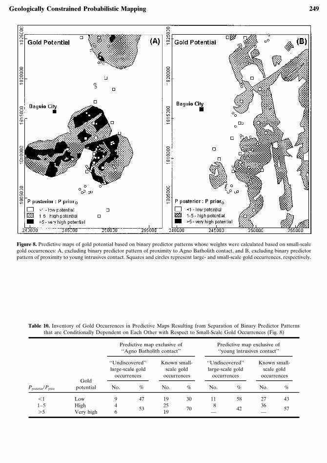
Figure 8A is the result of removing the binarypredictor pattern of proximity to Agno Batholithcontact. With this map, the predicted number of oc-currences is 68 or only about 8% larger than the


Figure 7. Predictive maps of gold potential based on binary predictor patterns whose weights were calculated with respect to: A,large-scale, and B, small-scale gold occurrences. Squares and circles represent large- and small-scale gold occurrences, respectively.

observed number of occurrences. Figure 8B is theresult of removing the binary predictor pattern ofproximity to young intrusives contact. With this map,the predicted number of occurrences is 66 or only5% larger than the observed number of occurrences.The overall tests of conditional independence suggest

Table 9. Inventory of Gold Occurrences in the Predictive Maps Resulting from Integration of All Binary PredictorPatterns (Fig. 7)

Predictive map based on Predictive map based onlarge-scale gold occurrences small-scale gold occurrences

Known large- Undiscovered Undiscovered Known small-scale gold small-scale gold large-scale gold scale gold

occurrences occurrences occurrences occurrencesGold

Pposterior/Pprior potential No. % No. % No. % No. %

�1 Low 4 21 28 44 8 42 19 301–5 High 14 29 9 14

79 56 58 70�5 Very high 1 6 2 30

that both predictive maps are statistically valid. Table10 indicates that the predictive map in Figure 8A isuseful whereas the predictive map in Figure 8B is notin terms of the number of known and ‘‘undiscovered’’occurrences falling into zones of high to very po-tential.


Figure 8. Predictive maps of gold potential based on binary predictor patterns whose weights were calculated based on small-scalegold occurrences: A, excluding binary predictor pattern of proximity to Agno Batholith contact, and B, excluding binary predictorpattern of proximity to young intrusives contact. Squares and circles represent large- and small-scale gold occurrences, respectively.

Table 10. Inventory of Gold Occurrences in Predictive Maps Resulting from Separation of Binary Predictor Patternsthat are Conditionally Dependent on Each Other with Respect to Small-Scale Gold Occurrences (Fig. 8)

Predictive map exclusive of Predictive map exclusive of‘‘Agno Batholith contact’’ ‘‘young intrusives contact’’

‘‘Undiscovered’’ Known small- ‘‘Undiscovered’’ Known small-large-scale gold scale gold large-scale gold scale gold

occurrences occurrences occurrences occurrencesGold

Pposterior/Pprior potential No. % No. % No. % No. %

�1 Low 9 47 19 30 11 58 27 431–5 High 4 25 8 36

53 70 42 57�5 Very high 6 19 — —


DISCUSSION

As shown here, the studentized C was useful indetermining the cutoff distance for which the spatialassociation between a set of points and a binary pat-tern is optimal. Bonham-Carter, Agterberg, andWright (1988) state that the maximum value of C,under normal conditions, would give the cutoff dis-tance. They did not state, however, what these ‘‘nor-mal’’ conditions are. We propose two possibilities asto why the maximum value of C alone was not usefulin determining the cutoff distances, although we didnot investigate these quantitatively. One is that thegold occurrences in our study area are geneticallyand spatially associated with at least two intrusiveregimes. The other is that the gold occurrences arespatially concentrated within a north–south trendingzone. In the study area of Bonham-Carter, Agter-berg, and Wright (1988), the gold occurrences areassociated with one intrusive regime and the goldoccurrences are more or less evenly distributed spa-tially.

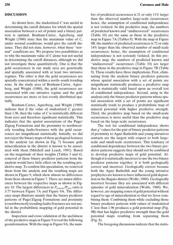
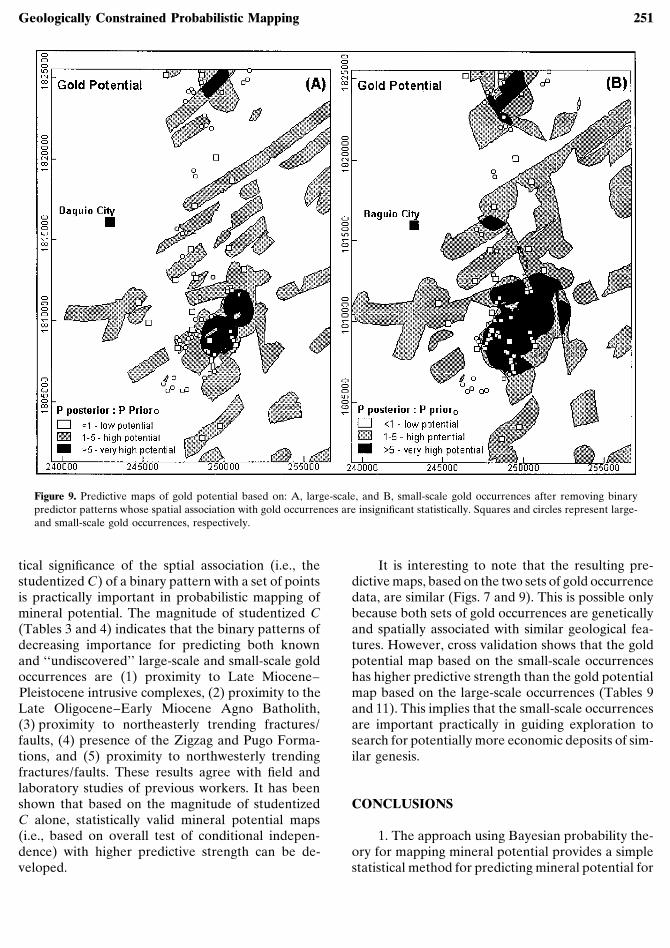
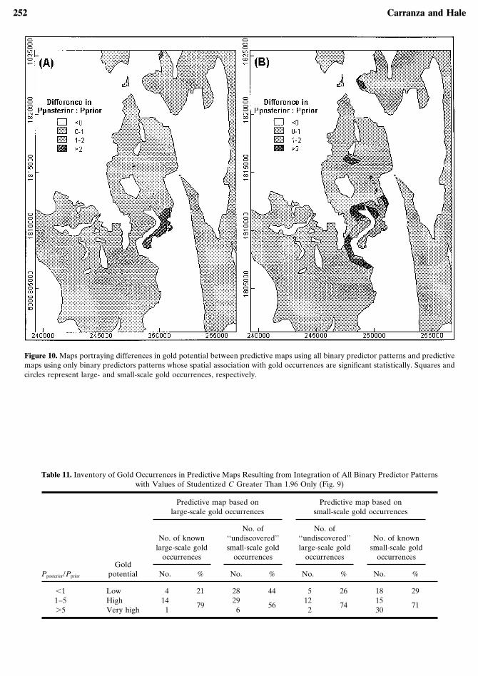
Bonham-Carter, Agterberg, and Wright (1989)indicate that if the value of studentized C greaterthan 1.96, then the value of C is statistically differentfrom zero and therefore significant statistically. Thisindicates that the spatial associations of the Pugo/Zigzag Formations and the proximity to northwest-erly trending faults/fractures with the gold occur-rences are insignificant statistically. Initially, we didnot reject the binary maps of these geological featuresin the analysis (as shown in Fig. 7) because goldmineralization in the district is known to be associ-ated with them (Mitchell and Leach, 1991). Basedon the magnitude of their weights (Tables 3 and 4),removal of these binary predictor patterns from theanalysis would have little effect on the resulting pre-dictive map. To confirm this speculation, we removedthem from the analysis and the resulting maps areshown in Figure 9, which show almost no differencesfrom those shown in Figure 7. There are minor differ-ences between the respective maps as shown in Fig-ure 10. The largest differences in Pposterior/Pprior ratio is3.77 between Figure 7A and Figure 9A. The differ-ence maps illustrate mainly that the binary predictorpatterns of Pugo/Zigzag Formations and proximityto northwesterly trending faults/fractures are not use-ful in the probabilistic mapping of gold potential inthe district.

Inspection and cross validation of the usefulnessof the predictive maps in Figure 9 reveal the followinggeoinformation. With the map in Figure 9A, the num-

ber of predicted occurrences is 21 or only 11% largerthan the observed number large-scale occurrences;hence, the assumption of conditional independenceis not violated. In this predictive map, the numbersof predicted known and ‘‘undiscovered’’ occurrences(Table 10) are the same as those in the predictivemap in Figure 7A (Tables 9). With the map in Figure9B, the number of predicted occurrences is 72 or only14% larger than the observed number of small-scaleoccurrences; hence, the assumption of conditionalindependence is not seriously violated. In this pre-dictive map, the numbers of predicted known and‘‘undiscovered’’ occurrences (Table 10) are largerthan those in the predictive map in Figure 7B (Table9). These results have three implications. First, elimi-nating from the analysis binary predictor patternswhose spatial association with a set of points areinsignificant statistically produces a predictive mapthat is statistically valid based upon an overall testof conditional independence. Second, using in theanalysis only the binary predictor patterns whose spa-tial association with a set of points are significantstatistically tends to produce a probabilistic map ofmineral potential with higher predictive strength.Third, the predictive map based on the small-scaleoccurrences is more useful than the predictive mapbased on the large-scale occurrences.

The test for conditional independence showsthat � 2 values for the pair of binary predictor patternsof proximity to Agno Batholith and young intrusivescontacts are the largest with respect to both large-scale and small-scale occurrences. This tendency ofconditional dependence between the two binary pre-dictor patterns suggests they should not be combinedto develop predictive maps of gold potential. Al-though it is statistically incorrect to use the two binarypredictor patterns together, it is both geologicallycorrect and incorrect. Geologically correct becauseboth the Agno Batholith and the young intrusiveporphyries are known to have influenced gold deposi-tion in the Baguio district (Wolfe, 1988). Geologicallyincorrect because they are associated with differentepisodes of gold mineralization (Wolfe, 1988). We,however, are mapping zones of gold potential withoutregard to age of mineralization so that we favor com-bining them. Combining them while excluding thosebinary predictor patterns with values of studentizedC less than 1.96 produces a gold potential map (Fig.9B) that has higher predictive strength than the goldpotential maps resulting from separating them(Fig. 8).

The foregoing discussions indicate that the statis-


Figure 9. Predictive maps of gold potential based on: A, large-scale, and B, small-scale gold occurrences after removing binarypredictor patterns whose spatial association with gold occurrences are insignificant statistically. Squares and circles represent large-and small-scale gold occurrences, respectively.

tical significance of the sptial association (i.e., thestudentized C) of a binary pattern with a set of pointsis practically important in probabilistic mapping ofmineral potential. The magnitude of studentized C(Tables 3 and 4) indicates that the binary patterns ofdecreasing importance for predicting both knownand ‘‘undiscovered’’ large-scale and small-scale goldoccurrences are (1) proximity to Late Miocene–Pleistocene intrusive complexes, (2) proximity to theLate Oligocene–Early Miocene Agno Batholith,(3) proximity to northeasterly trending fractures/faults, (4) presence of the Zigzag and Pugo Forma-tions, and (5) proximity to northwesterly trendingfractures/faults. These results agree with field andlaboratory studies of previous workers. It has beenshown that based on the magnitude of studentizedC alone, statistically valid mineral potential maps(i.e., based on overall test of conditional indepen-dence) with higher predictive strength can be de-veloped.

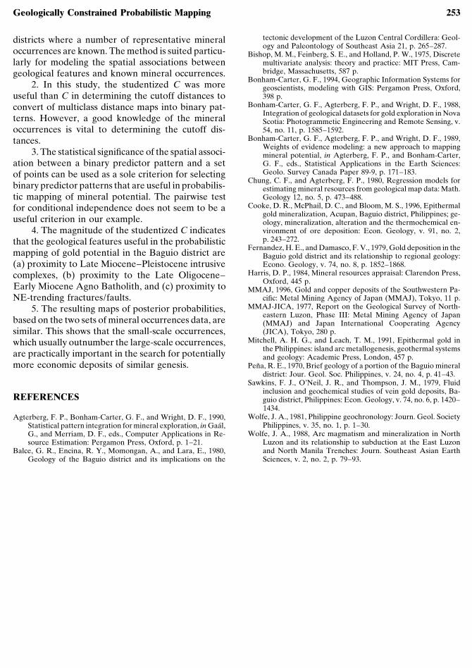
It is interesting to note that the resulting pre-dictive maps, based on the two sets of gold occurrencedata, are similar (Figs. 7 and 9). This is possible onlybecause both sets of gold occurrences are geneticallyand spatially associated with similar geological fea-tures. However, cross validation shows that the goldpotential map based on the small-scale occurrenceshas higher predictive strength than the gold potentialmap based on the large-scale occurrences (Tables 9and 11). This implies that the small-scale occurrencesare important practically in guiding exploration tosearch for potentially more economic deposits of sim-ilar genesis.

CONCLUSIONS

1. The approach using Bayesian probability the-ory for mapping mineral potential provides a simplestatistical method for predicting mineral potential for


Figure 10. Maps portraying differences in gold potential between predictive maps using all binary predictor patterns and predictivemaps using only binary predictors patterns whose spatial association with gold occurrences are significant statistically. Squares andcircles represent large- and small-scale gold occurrences, respectively.

Table 11. Inventory of Gold Occurrences in Predictive Maps Resulting from Integration of All Binary Predictor Patternswith Values of Studentized C Greater Than 1.96 Only (Fig. 9)

Predictive map based on Predictive map based onlarge-scale gold occurrences small-scale gold occurrences

No. of No. ofNo. of known ‘‘undiscovered’’ ‘‘undiscovered’’ No. of known

large-scale gold small-scale gold large-scale gold small-scale goldoccurrences occurrences occurrences occurrences

GoldPposterior/Pprior potential No. % No. % No. % No. %

�1 Low 4 21 28 44 5 26 18 291–5 High 14 29 12 15

79 56 74 71�5 Very high 1 6 2 30


districts where a number of representative mineraloccurrences are known. The method is suited particu-larly for modeling the spatial associations betweengeological features and known mineral occurrences.

2. In this study, the studentized C was moreuseful than C in determining the cutoff distances toconvert of multiclass distance maps into binary pat-terns. However, a good knowledge of the mineraloccurrences is vital to determining the cutoff dis-tances.

3. The statistical significance of the spatial associ-ation between a binary predictor pattern and a setof points can be used as a sole criterion for selectingbinary predictor patterns that are useful in probabilis-tic mapping of mineral potential. The pairwise testfor conditional independence does not seem to be auseful criterion in our example.

4. The magnitude of the studentized C indicatesthat the geological features useful in the probabilisticmapping of gold potential in the Baguio district are(a) proximity to Late Miocene–Pleistocene intrusivecomplexes, (b) proximity to the Late Oligocene–Early Miocene Agno Batholith, and (c) proximity toNE-trending fractures/faults.

5. The resulting maps of posterior probabilities,based on the two sets of mineral occurrences data, aresimilar. This shows that the small-scale occurrences,which usually outnumber the large-scale occurrences,are practically important in the search for potentiallymore economic deposits of similar genesis.

REFERENCES

Agterberg, F. P., Bonham-Carter, G. F., and Wright, D. F., 1990,Statistical pattern integration for mineral exploration, in Gaal,G., and Merriam, D. F., eds., Computer Applications in Re-source Estimation: Pergamon Press, Oxford, p. 1–21.

Balce, G. R., Encina, R. Y., Momongan, A., and Lara, E., 1980,Geology of the Baguio district and its implications on the

tectonic development of the Luzon Central Cordillera: Geol-ogy and Paleontology of Southeast Asia 21, p. 265–287.

Bishop, M. M., Feinberg, S. E., and Holland, P. W., 1975, Discretemultivariate analysis: theory and practice: MIT Press, Cam-bridge, Massachusetts, 587 p.

Bonham-Carter, G. F., 1994, Geographic Information Systems forgeoscientists, modeling with GIS: Pergamon Press, Oxford,398 p.

Bonham-Carter, G. F., Agterberg, F. P., and Wright, D. F., 1988,Integration of geological datasets for gold exploration in NovaScotia: Photogrammetic Engineering and Remote Sensing, v.54, no. 11, p. 1585–1592.

Bonham-Carter, G. F., Agterberg, F. P., and Wright, D. F., 1989,Weights of evidence modeling: a new approach to mappingmineral potential, in Agterberg, F. P., and Bonham-Carter,G. F., eds., Statistical Applications in the Earth Sciences:Geolo. Survey Canada Paper 89-9, p. 171–183.

Chung, C. F., and Agterberg, F. P., 1980, Regression models forestimating mineral resources from geological map data: Math.Geology 12, no. 5, p. 473–488.

Cooke, D. R., McPhail, D. C., and Bloom, M. S., 1996, Epithermalgold mineralization, Acupan, Baguio district, Philippines; ge-ology, mineralization, alteration and the thermochemical en-vironment of ore deposition: Econ. Geology, v. 91, no. 2,p. 243–272.

Fernandez, H. E., and Damasco, F. V., 1979, Gold deposition in theBaguio gold district and its relationship to regional geology:Econo. Geology, v. 74, no. 8, p. 1852–1868.

Harris, D. P., 1984, Mineral resources appraisal: Clarendon Press,Oxford, 445 p.

MMAJ, 1996, Gold and copper deposits of the Southwestern Pa-cific: Metal Mining Agency of Japan (MMAJ), Tokyo, 11 p.

MMAJ-JICA, 1977, Report on the Geological Survey of North-eastern Luzon, Phase III: Metal Mining Agency of Japan(MMAJ) and Japan International Cooperating Agency(JICA), Tokyo, 280 p.

Mitchell, A. H. G., and Leach, T. M., 1991, Epithermal gold inthe Philippines: island arc metallogenesis, geothermal systemsand geology: Academic Press, London, 457 p.

Pena, R. E., 1970, Brief geology of a portion of the Baguio mineraldistrict: Jour. Geol. Soc. Philippines, v. 24, no. 4, p. 41–43.

Sawkins, F. J., O’Neil, J. R., and Thompson, J. M., 1979, Fluidinclusion and geochemical studies of vein gold deposits, Ba-guio district, Philippines: Econ. Geology, v. 74, no. 6, p. 1420–1434.

Wolfe, J. A., 1981, Philippine geochronology: Journ. Geol. SocietyPhilippines, v. 35, no. 1, p. 1–30.

Wolfe, J. A., 1988, Arc magmatism and mineralization in NorthLuzon and its relationship to subduction at the East Luzonand North Manila Trenches: Journ. Southeast Asian EarthSciences, v. 2, no. 2, p. 79–93.

Documents

Geologically Constrained Probabilistic Mapping of Gold Potential, Baguio District, Philippines