Embed Size (px)
DESCRIPTION
Structural Geology
Citation preview


Geological Structures
and Maps
A PRACTICAL GUIDE

This Page Intentionally Left Blank

Geological Structures
and Maps
A PRACTICAL GUIDEThird edition
RICHARD J. LISLECardiff University
AMSTERDAM BOSTON HEIDELBERG LONDON NEW YORK OXFORD
PARIS SAN DIEGO SAN FRANCISCO SINGAPORE SYDNEY TOKYO

Elsevier Butterworth-Heinemann
Linacre House, Jordan Hill, Oxford OX2 8DP
200 Wheeler Road, Burlington MA 01803
First published by Pergamon Press 1988
Second edition 1995
Reprinted 1999
Third edition 2004
Copyright © Richard J. Lisle 1995, 2004. All rights reserved
The right of Richard J. Lisle to be identified as the author of this work
has been asserted in accordance with the Copyright, Designs and
Patents Act 1988
No part of this publication may be reproduced in any material form (includingphotocopying or storing in any medium by electronic means and whetheror not transiently or incidentally to some other use of this publication) withoutthe written permission of the copyright holder except in accordance with theprovisions of the Copyright, Designs and Patents Act 1988 or under the terms ofa licence issued by the Copyright Licensing Agency Ltd, 90 Tottenham Court Road,London, England W1T 4LP. Applications for the copyright holder’s writtenpermission to reproduce any part of this publication should be addressedto the publisher. Permissions may be sought directly from Elsevier’s Science andTechnology Rights Department in Oxford, UK: phone: (+44) (0) 1865 843830;fax: (+44) (0) 1865 853333; e-mail: [email protected]. You may alsocomplete your request on-line via the Elsevier homepage (http://www.elsevier.com),by selecting ‘Customer Support’ and then ‘Obtaining Permissions’.
British Library Cataloguing in Publication DataA catalogue record for this book is available from the British Library
ISBN 0 7506 5780 4
For information on all Butterworth-Heinemann publications
visit our website at www.bh.com
Composition by Genesis Typesetting Limited, Rochester, Kent
Printed and bound in Great Britain

Contents
Preface vii
Geological Map Symbols viii
1 Geological Maps 1
2 Uniformly Dipping Beds 2
3 Folding 29
4 Faulting 59
5 Unconformity 77
6 Igneous Rocks 85
7 Folding with Cleavage 94
Further Reading 102
Index 103

This Page Intentionally Left Blank

Preface
GEOLOGICAL maps represent the expression on the earth’s
surface of the underlying geological structure. For this
reason the ability to correctly interpret the relationships
displayed on a geological map relies heavily on a knowl-
edge of the basic principles of structural geology.
This book discusses, from first principles up to and
including first-year undergraduate level, the morphology of
the most important types of geological structures, and
relates them to their manifestation on geological maps.
Although the treatment of structures is at an elementary
level, care has been taken to define terms rigorously and in
a way that is in keeping with current professional usage. All
too often concepts such as ‘asymmetrical fold’, ‘fold axis’
and ‘cylindrical fold’ explained in first textbooks have to be
re-learned ‘correctly’ at university level.
Photographs of structures in the field are included to
emphasize the similarities between structures at outcrop
scale and on the scale of the map. Ideally, actual fieldwork
experience should be gained in parallel with this course.
The book is designed, as far as possible, to be read
without tutorial help. Worked examples are given to assist
with the solution of the exercises. Emphasis is placed
throughout on developing the skill of three-dimensional
visualization so important to the geologist.
In the choice of the maps for the exercises, an attempt
has been made to steer a middle course between the
artificial-looking idealized type of ‘problem map’ and real
survey maps. The latter can initially overwhelm the
student with the sheer amount of data presented. Many of
the exercises are based closely on selected ‘extracts’ from
actual maps.
I am grateful to the late Professor T.R. Owen who
realized the need for a book with this scope and encouraged
me to write it. Peter Henn and Catherine Shephard of
Pergamon Books are thanked for their help and patience.
Thanks are also due to Vivienne Jenkins and Wendy
Johnson for providing secretarial help, and to my wife Ann
for her support.

Geological Map Symbols
inclined strata, dip in degrees
horizontal strata
vertical strata
axial surface trace of antiform
axial surface trace of synform
fold hinge line, fold axis or other
linear structure, plunge in degrees
inclined cleavage, dip in degrees
horizontal cleavage
vertical cleavage
geological boundary
fault line, mark on downthrow side
younging direction of beds
metamorphic aureole

NN
CLAYSCLAYS
+Broadway
+Broadway
Stanton+
Stanton+
SILTS &
SANDS
SILTS &
SANDS
+Buckland
+Buckland
OOLITIC
LIMESTONE
OOLITIC
LIMESTONE
152
152
229229
0 1 2 km
+Childswickham+Childswickham
79m
79m
BroadwayHill
BroadwayHill
305
305
1
1
Geological Maps
1.1 What are geological maps?
A geological map shows the distribution of various types of
bedrock in an area. It usually consists of a topographic map
(a map giving information about the form of the earth’s
surface) which is shaded, or coloured to show where
different rock units occur at or just below the ground
surface. Figure 1.1 shows a geological map of an area in the
Cotswolds. It tells us for instance that clays form the
bedrock at Childswickham and Broadway but if we move
eastwards up the Cotswold escarpment to Broadway Hill we
can find oolitic limestones. Lines on the map are drawn to
show the boundaries between each of the rock units.
1.2 How is such a geological map made?
The geologist in the field firstly records the nature of rock
where it is visible at the surface. Rock outcrops are
examined and characteristics such as rock composition,
internal structure and fossil content are recorded. By using
these details, different units can be distinguished and shown
separately on the base map. Of course, rocks are not
everywhere exposed at the surface. In fact, over much of the
area in Fig. 1.1 rocks are covered by soil and by alluvial
deposits laid down by recent rivers. Deducing the rock unit
which underlies the areas of unexposed rock involves
making use of additional data such as the type of soil, the
land’s surface forms (geomorphology) and information
from boreholes. Geophysical methods allow certain phys-
ical properties of rocks (such as their magnetism and
density) to be measured remotely, and are therefore useful
for mapping rocks in poorly exposed regions. This addi-
tional information is taken into account when the geologist
decides on the position of the boundaries of rock units to be
drawn on the map. Nevertheless, there are always parts of
the map where more uncertainty exists about the nature of
the bedrock, and it is important for the reader of the map to
realize that a good deal of interpretation is used in the map-
making process.
1.3 What is a geological map used for?
The most obvious use of a geological map is to indicate the
nature of the near-surface bedrock. This is clearly of great
importance to civil engineers who, for example, have to
advise on the excavation of road cuttings or on the siting of
bridges; to geographers studying the use of land and to
companies exploiting minerals. The experienced geologist
can, however, extract more from the geological map. To the
trained observer the features on a geological map reveal
vital clues about the geological history of an area.
Furthermore, the bands of colour on a geological map are
the expression on the ground surface of layers or sheets of
rock which extend and slant downwards into the crust of the
earth. The often intricate pattern on a map, like the
graininess of a polished wooden table top, provides tell-tale
evidence of the structure of the layers beneath the surface.
To make these deductions first requires knowledge of the
characteristic form of common geological structures such as
faults and folds.
This book provides a course in geological map reading. It
familiarizes students with the important types of geological
structures and enables them to recognize these as they
would appear on a map or cross-section.Fig. 1.1 A geological map of the Broadway area in the Cotswolds.

2
2
Uniformly Dipping Beds
2.1 Introduction
Those who have observed the scenery in Western movies
filmed on the Colorado Plateau will have been impressed by
the layered nature of the rock displayed in the mountain-
sides. The layered structure results from the deposition of
sediments in sheets or beds which have large areal extent
compared to their thickness. When more beds of sediment
are laid down on top the structures comes to resemble a
sandwich or a pile of pages in a book (Fig. 2.1A & B). This
stratified structure is known as bedding.
In some areas the sediments exposed on the surface of the
earth still show their unmodified sedimentary structure; that
is, the bedding is still approximately horizontal. In other
parts of the world, especially those in ancient mountain
belts, the structure of the layering is dominated by the
buckling of the strata into corrugations or folds so that the
slope of the bedding varies from place to place. Folds,
which are these crumples of the crust’s layering, together
with faults where the beds are broken and shifted, are
examples of geological structures to be dealt with in later
chapters. In this chapter we consider the structure consisting
of planar beds with a uniform slope brought about by the
tilting of originally horizontal sedimentary rocks.
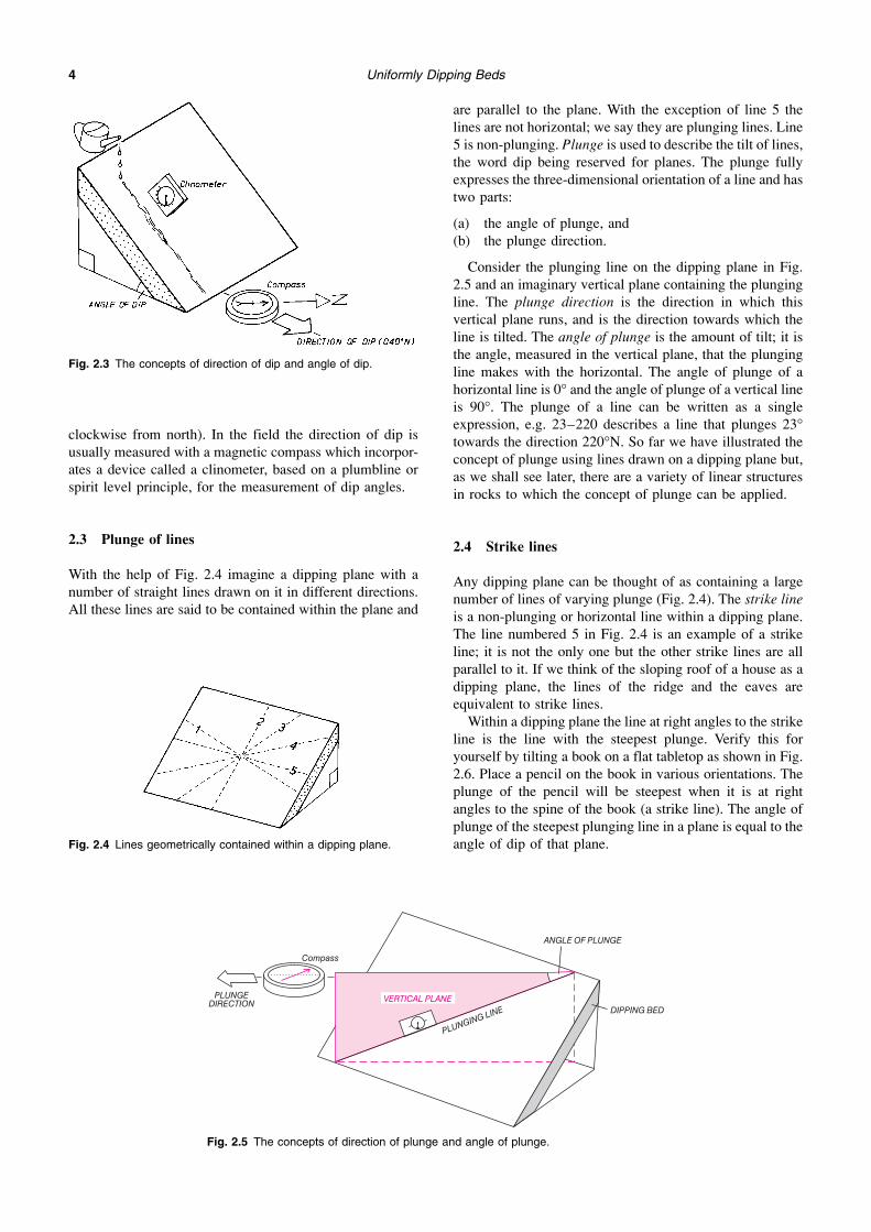
2.2 Dip
Bedding and other geological layers and planes that are not
horizontal are said to dip. Figure 2.2 shows field examples
of dipping beds. The dip is the slope of a geological surface.
There are two aspects to the dip of a plane:
(a) the direction of dip, which is the compass direction
towards which the plane slopes; and
(b) the angle of dip, which is the angle that the plane
makes with a horizontal plane (Fig. 2.3).
The direction of dip can be visualized as the direction in
which water would flow if poured onto the plane. The angle
of dip is an angle between 0° (for horizontal planes) and 90°
(for vertical planes). To record the dip of a plane all that is
needed are two numbers; the direction of dip followed by
the angle of dip, e.g. 138/74 is a plane which dips 74° in the
direction 138°N (this is a direction which is SE, 138°
Fig. 2.1A Horizontal bedding: Lower Jurassic, near Cardiff, South Wales.

Uniformly Dipping Beds 3
Fig. 2.1B Horizontal bedding: UpperCarboniferous, Cornwall, England
Fig. 2.2 Dipping beds in Teruel Province,Spain. A: Cretaceous Limestones dippingat about 80°. B: Tertiary conglomerates andsandstones dipping at about 50°.
A
B
PLUNGEDIRECTION
Compass
ANGLE OF PLUNGE
DIPPING BED
PLUNGING LINE
VERTICAL PLANE
Uniformly Dipping Beds4
clockwise from north). In the field the direction of dip is
usually measured with a magnetic compass which incorpor-
ates a device called a clinometer, based on a plumbline or
spirit level principle, for the measurement of dip angles.
2.3 Plunge of lines
With the help of Fig. 2.4 imagine a dipping plane with a
number of straight lines drawn on it in different directions.
All these lines are said to be contained within the plane and
are parallel to the plane. With the exception of line 5 the
lines are not horizontal; we say they are plunging lines. Line
5 is non-plunging. Plunge is used to describe the tilt of lines,
the word dip being reserved for planes. The plunge fully
expresses the three-dimensional orientation of a line and has
two parts:
(a) the angle of plunge, and
(b) the plunge direction.
Consider the plunging line on the dipping plane in Fig.
2.5 and an imaginary vertical plane containing the plunging
line. The plunge direction is the direction in which this
vertical plane runs, and is the direction towards which the
line is tilted. The angle of plunge is the amount of tilt; it is
the angle, measured in the vertical plane, that the plunging
line makes with the horizontal. The angle of plunge of a
horizontal line is 0° and the angle of plunge of a vertical line
is 90°. The plunge of a line can be written as a single
expression, e.g. 23–220 describes a line that plunges 23°
towards the direction 220°N. So far we have illustrated the
concept of plunge using lines drawn on a dipping plane but,
as we shall see later, there are a variety of linear structures
in rocks to which the concept of plunge can be applied.
2.4 Strike lines
Any dipping plane can be thought of as containing a large
number of lines of varying plunge (Fig. 2.4). The strike line
is a non-plunging or horizontal line within a dipping plane.
The line numbered 5 in Fig. 2.4 is an example of a strike
line; it is not the only one but the other strike lines are all
parallel to it. If we think of the sloping roof of a house as a
dipping plane, the lines of the ridge and the eaves are
equivalent to strike lines.
Within a dipping plane the line at right angles to the strike
line is the line with the steepest plunge. Verify this for
yourself by tilting a book on a flat tabletop as shown in Fig.
2.6. Place a pencil on the book in various orientations. The
plunge of the pencil will be steepest when it is at right
angles to the spine of the book (a strike line). The angle of
plunge of the steepest plunging line in a plane is equal to the
angle of dip of that plane.
Fig. 2.3 The concepts of direction of dip and angle of dip.
Fig. 2.4 Lines geometrically contained within a dipping plane.
Fig. 2.5 The concepts of direction of plunge and angle of plunge.

Uniformly Dipping Beds 5
When specifying the direction of a strike line we can
quote either of two directions which are 180° different (Fig.
2.6). For example, a strike direction of 060° is the same as
a strike direction of 240°. The direction of dip is always at
right angles to the strike and can therefore be obtained by
either adding or subtracting 90° from the strike whichever
gives the down-dip direction.
The map symbol used to represent the dip of bedding
usually consists of a stripe in the direction of the strike with
a short dash on the side towards the dip direction (see list of
symbols at the beginning of the book). Some older maps
display dip with an arrow that points in the dip direction.
2.5 Apparent dip
At many outcrops where dipping beds are exposed the
bedding planes themselves are not visible as surfaces.
Cliffs, quarries and cuttings may provide more or less
vertical outcrop surfaces which make an arbitrary angle
with the strike of the beds (Fig. 2.7A). When such vertical
sections are not perpendicular to the strike (Fig. 2.7B), the
beds will appear to dip at a gentler angle than the true dip.
This is an apparent dip.
It is a simple matter to derive an equation which
expresses how the size of the angle of apparent dip depends
on the true dip and the direction of the vertical plane on
which the apparent dip is observed (the section plane). In
Fig. 2.8 the obliquity angle is the angle between the trend of
the vertical section plane and the dip direction of the
beds.
From Fig. 2.8 we see that:
the tangent of the angle of apparent dip = p/q,
the tangent of the angle of true dip = p/rand the cosine of the obliquity angle = r/q.
Since it is true that:
p/r � r/q = p/q
it follows that:
tan (apparent dip) = tan (true dip)
� cos (obliquity angle)
It is sometimes necessary to calculate the angle of apparent
dip, for instance when we want to draw a cross-section
through beds whose dip direction is not parallel to the
section line.
Fig. 2.6 A classroom demonstration of a dipping plane.
Fig. 2.7 Relationship between apparent dip and true dip. Fig. 2.8 Relation of apparent dip to true dip.

Uniformly Dipping Beds6
2.6 Outcrop patterns of uniformly dipping beds
The geological map in Fig. 2.9A shows the areal distribu-
tion of two rock formations. The line on the map separating
the formations has an irregular shape even though the
contact between the formations is a planar surface (Fig.
2.9B).
To understand the shapes described by the boundaries of
formations on geological maps it is important to realize that
they represent a line (horizontal, plunging or curved)
produced by the intersection in three dimensions of two
surfaces (Fig. 2.9B, D). One of these surfaces is the
‘geological surface’ – in this example the surface of contact
between the two formations. The other is the ‘topographic
surface’ – the surface of the ground. The topographic
surface is not planar but has features such as hills, valleys
and ridges. As the block diagram in Fig. 2.9B shows, it is
these irregularities or topographic features which produce
the sinuous trace of geological contacts we observe on
maps. If, for example, the ground surface were planar (Fig.
2.9D), the contacts would run as straight lines on the map
(Fig. 2.9C).
The extent to which topography influences the form of
contacts depends also on the angle of dip of the beds. Where
beds dip at a gentle angle, valleys and ridges produce
pronounced ‘meanders’ (Fig. 2.10A, B). Where beds dip
steeply the course of the contact is straighter on the map
(Fig. 2.10C, D, E, F). When contacts are vertical their
course on the map will be a straight line following the
direction of the strike of the contact.
2.7 Representing surfaces on maps
In the previous section two types of surface were men-
tioned: the geological (or structural) surface and the ground
(topographic) surface. It is possible to describe the form of
either type on a map. The surface shown in Fig. 2.11B can
be represented on a map if the heights of all points on the
surface are specified on the map. This is usually done by
stating, with a number, the elevation of individual points
such as that of point X (a spot height) and by means of lines
drawn on the map which join all points which share the
same height (Fig. 2.11A). The latter are contour lines and
Fig. 2.9 The concept of outcrop of a geological contact.

Uniformly Dipping Beds 7
are drawn usually for a fixed interval of height. Topographic
maps depict the shape of the ground usually by means of
topographic contours. Structure contours record the height
of geological surfaces.
2.8 Properties of contour maps
Topographic contour patterns and structure contour patterns
are interpreted in similar ways and can be discussed
together. Contour patterns are readily understood if we
consider the changing position of the coastline, if sea level
were to rise in, say, 10-metre stages. The contour lines are
analogous to the shoreline which after the first stage of
inundation would link all points on the ground which are 10
metres above present sea level and so on. For a geological
surface the structure contours are lines which are every-
where parallel to the local strike of the dipping surface. The
local direction of slope (dip) at any point is at right angles
to the trend of the contours. Contour lines will be closer
together when the slope (dip) is steep. A uniformly sloping
(dipping) surface is represented by parallel, equally spaced
contours. Isolated hills (dome-shaped structures) will yield
closed concentric arrangements of contours and valleys and
ridges give V-shaped contour patterns (compare Figs 2.12A
and B).
Fig. 2.10 The effect of the angle of dip on the sinuosity of a contact’s outcrop.

Uniformly Dipping Beds8
2.9 Drawing vertical cross-sections throughtopographical and geological surfaces
Vertical cross-sections represent the form of the topog-
raphy and geological structure as seen on a ‘cut’ through the
earth. This vertical cut is imaginary rather than real, so the
construction of such a cross-section usually involves a
certain amount of interpretation.
The features displayed in the cross-section are the lines of
intersection of the section plane with topographical and
geological surfaces. Where contour patterns are given for
these surfaces the drawing of a cross-section is straightfor-
ward. If a vertical section is to be constructed between the
points X and Y on Fig. 2.13, a base line of length XY is set
out. Perpendiculars to the base line at X and Y are then
drawn which are graduated in terms of height (Fig. 2.13B).
Points on the map where the contour lines for the surface
intersect the line of section (line XY) are easily transferred
to the section, as shown in Fig. 2.13B.
Provided the vertical scale used is the same as the
horizontal scale, the angle of slope will be the correct slope
corresponding to the chosen line of section. For example, if
the surface being drawn is a geological one, the slope in the
section will equal the apparent dip appropriate for the line of
section. If an exaggerated vertical scale is used, the
gradients of lines will be steepened and the structures will
also appear distorted in other respects (see Chapter 3 on
Folds). The use of exaggerated vertical scales on cross-
sections should be avoided.
WORKED EXAMPLE
Vertical sections. Figure 2.14A shows a set of structure
contours for the surface defined by the base of a
sandstone bed. Find the direction of strike, the
direction of dip and the angle of dip of the base of the
sandstone bed. What is the apparent dip in the
direction XZ (Fig. 2.14B)?
The strike of the surface at any point is given by the
trend of the contours for that surface. On Fig. 2.14A the
trend of the contours (measured with a protractor) is
120°N.
The dip direction is 90° different from the strike
direction; giving 030° and 210° as the two possible
directions of dip. The heights of the structure contours
decrease towards the southwest, which tells us that
the surface slopes down in that direction. The direction
210° rather than 030° must therefore be the correct dip
direction.
Fig. 2.11 A surface and its representation by means of contours.
Fig. 2.12 Contour patterns and the form of a surface.

Uniformly Dipping Beds 9
To find the angle of dip we must calculate the
inclination of a line on the surface at right angles to the
strike. A constructed vertical cross-section along a line
XY on Fig. 2.14B (or any section line parallel to XY) will
tell us the true dip of the base of the sandstone. This
cross-section (Fig. 2.14C) reveals that the angle of dip
is related to the spacing of the contours: i.e.
Tangent (angle of dip)
=contour interval
spacing on map between contours
=10 m
10 m= 1
In the present example (Fig. 2.14C) the contour
interval is 10 m and the contour spacing is 10 m.
Tan (angle of dip) =10 m
10 m= 1
Therefore the angle of dip = Inverse Tan (1) = 45°.
The apparent dip in direction XZ is the observed
inclination of the sandstone bed in true scale (vertical
scale = horizontal scale) vertical section along the line
XZ. The same formula can be used as for the angle of
dip above except ‘spacing between contours’ is now
the apparent spacing observed along the line XZ.
2.10 Three-point problems
Above we have considered a surface described by contours.
If, instead of contours, a number of spot heights are given
for a surface, then it is possible to infer the form of the
contours. This is desirable since surfaces represented by
contours are easier to visualize. The number of spot heights
required to make a sensible estimate of the form of the
contour lines depends on the complexity of the surface. For
a surface which is planar, a minimum of three spot heights
are required.
WORKED EXAMPLE
A sandstone-shale contact encountered at three local-
ities A, B and C on Fig. 2.15A has heights of 150, 100
and 175 metres respectively. Assuming that the con-
tact is planar, draw structure contours for the sand-
stone-shale contact.
Consider an imaginary vertical section along line AB
on the map. In that section the contact will appear as a
straight line since it is the line of intersection of two
planes: the planar geological contact and the section
plane. Furthermore, in that vertical section the line
representing the contact will pass through the points A
and B at their respective heights (Fig. 2.15C). The
height of the contact decreases at a constant rate as
we move from A to B. This allows us to predict the
place along line AB where the surface will have a
specified height (Fig. 2.15B). For instance, the contact
will have a height of 125 metres at the mid-point
between A (height equals 150 metres) and B (height
equals 100 metres). In this way we also locate the
point D along AB which has the same height as the
third point C (175 metres). In a section along the line
Fig. 2.13 Construction of a cross-section showing surfacetopography.
Fig. 2.14 Drawing sections.

Uniformly Dipping Beds10
CD the contact will appear horizontal. Line CD is
therefore parallel to the horizontal or strike line in the
surface. We call CD the 175 metre structure contour for
the surface. Other structure contours for other heights
will be parallel to this, and will be equally spaced on the
map. The 100 metre contour must pass through B. If it
is required to find the dip of the contact the method of
the previous worked example can be used.
2.11 Outcrop patterns of geological surfaces exposedon the ground
We have seen how both the land surface and a geological
surface (such as a junction between two formations) can be
represented by contour maps. The line on a geological map
representing the contact of two formations marks the
intersection of these two surfaces. The form of this line on
the map can be predicted if the contour patterns defining the
topography and the geological surface are known, since
along the line of intersection both surfaces will have equal
height.
A rule to remember:
A geological surface crops out at points where it has the
same height as the ground surface.
WORKED EXAMPLE
Given topographic contours and structure contours for
a planar coal seam (Fig. 2.16A) predict the map
outcrop pattern of the coal seam.
Points are sought on the map where structure contours
intersect a topographic contour of the same elevation.
A series of points is obtained in this way through which
the line of outcrop of the coal seam must pass (Fig.
2.16B). This final stage of joining the points to form a
surface outcrop would seem in places to be somewhat
arbitrary with the lines labelled p and q in Fig. 2.16B
appearing equally possible. However p is incorrect,
since the line of outcrop cannot cross the 150 metre
structure contour unless there is a point along it at
which the ground surface has a height of 150
metres.
Another rule to remember:
The line of outcrop of a geological surface crosses a
structure contour for the surface only at points where
the ground height matches that of the structure
contour.
Fig. 2.15 Solution of a three-point problem

Uniformly Dipping Beds 11
2.12 Buried and eroded parts of a geological surface
The thin coal seam in the previous example only occurs at
the ground surface along a single line. The surface at other
points on the map (a point not on the line of outcrop) is
either buried (beneath ground level) or eroded (above
ground level). The line of outcrop in Fig. 2.16B divides the
map into two kinds of areas:
(a) areas where height (coal) > height (topography), so
that the surface can be thought to have existed above
the present topography but has since been eroded
away, and
(b) areas where height (coal) < height (topography) so that
the coal must exist below the topography, i.e. it is
buried.
The boundary line between these two types of areas is given
by the line of outcrop, i.e. where height (coal) = height
(topography).
WORKED EXAMPLE
Using the data on Fig. 2.16A shade the part of the area
underlain by coal.
The answer to this is red shaded area in Fig. 2.16C.
The outcrop line of the coal forms the boundary of the
area underlain by coal. The sought area is where the
contours for the topography show higher values than
the contours of the coal.
2.13 Contours of burial depth (isobaths)
A geological surface is buried below the topographic
surface when height (topography) > height (geological
surface). The difference (height of topography minus height
of geological surface) equals the depth of burial at any point
on the map. Depths of burial determined at a number of
points on a map provide data that can be contoured to yield
lines of equal depth of burial called isobaths.
WORKED EXAMPLE
Using again the data from Fig. 2.16A construct
isobaths for the coal seam.
In the area of buried coal, determine spot depths of
coal by subtracting the height of the coal seam from
the height of the topography at a number of points.
Fig. 2.16 Predicting outcrop and isobaths from structure contour information.Topographic contours are shown in red; structure contours for the coal seam areblack.

Uniformly Dipping Beds12
Isobaths, lines linking all points of equal depth of burial,
can then be drawn (dashed lines in Fig. 2.16D).
Devise an alternative way to draw isobaths, noting that a
100 metre isobath for a given geological surface is the line
of outcrop on an imaginary surface which is everywhere
100 metres lower than the ground surface.
2.14 V-shaped outcrop patterns
A dipping surface that crops out in a valley or on a ridge
will give rise to a V-shaped outcrop (Fig. 2.17). The way the
outcrop patterns vee depends on the dip of the geological
surface relative to the topography. In the case of valleys,
patterns vee upstream or downstream (Fig. 2.17). The rule
for determining the dip from the type of vee (the ‘V rule’)
is easily remembered if one considers the intermediate case
(Fig. 2.17D) where the outcrop vees in neither direction.
This is the situation where the dip is equal to the gradient of
the valley bottom. As soon as we tilt the beds away from
this critical position they will start to exhibit a V-shape. If
we visualize the bed to be rotated slightly upstream it will
start to vee upstream, at first veeing more sharply than the
topographic contours defining the valley (Fig. 2.17C). The
bed can be tilted still further upstream until it becomes
horizontal. Horizontal beds always yield outcrop patterns
which parallel the topographic contours and hence, the beds
Fig. 2.17 To illustrate the V-rule.

Uniformly Dipping Beds 13
still vee upstream (Fig. 2.17B). If the bed is tilted further
again upstream, the beds start to dip upstream and we retain
a V-shaped outcrop but now the vee is more ‘blunt’ than the
vee exhibited by the topographic contours (Fig. 2.17A).
Downstream-pointing vees are produced when the beds
dip downstream more steeply than the valley gradient (Fig.
2.17E). Finally, vertical beds have straight outcrop courses
and do not vee (Fig. 2.17F).
WORKED EXAMPLE
Complete the outcrop of the thin limestone bed
exposed in the northwest part of the area (Fig. 2.18A).
The dip of the bed is 10° towards 220° (220/10).
This type of problem is frequently encountered by
geological mappers. On published geological maps all
contacts are shown. However, rocks are not every-
where exposed. Whilst mapping, a few outcrops are
found at which contacts are visible and where dips can
be measured, but the rest of the map is based on
interpretation. The following technique can be used to
interpret the map. Using the known dip, construct
structure contours for the thin bed. These will run
parallel to the measured strike and, for a contour
interval of 10 metres, will have a spacing given by this
equation (see Section 2.9).
Spacing between contours = contour interval
Tangent (angle of dip)
Since the outcrop of the bed in the northwest part of
the map is at a height of 350 metres, the 350 metre
structure contour must pass through this point. Others
are drawn parallel at the calculated spacing. The
crossing points of the topographic contours with the
structure contours of the same height, yield points
which lie on the outcrop of the thin limestone bed. The
completed outcrop of the thin limestone bed is shown
in Fig. 2.18B.
2.15 Structure contours from outcrop patterns
A map showing outcrops of a surface together with
topographic contours can be used to construct structure
contours for that surface. The underlying principles are:
(a) where a surface crops out, the height of the surface
equals the height of the topography,
(b) if the height of a planar surface is known at a minimum
of three places, the structure contours for that surface
can be constructed (see ‘Three-point problems’, Sec-
tion 2.10).
WORKED EXAMPLE
Draw strike lines for the limestone bed in Fig. 2.20A.
What assumptions are involved?
Join points on the outcrop which share the same
height. These join lines are structure contours for that
particular height (Fig. 2.20B).
Draw as many structure contours as possible to test
the assumption of constant dip (planarity of surface).
The structure contours in Fig. 2.20B are parallel and
evenly spaced. This confirms that the limestone bed
has a uniform dip.
Fig. 2.18 Interpreting the shape of a geological contact in an areaof limited rock exposure.

Uniformly Dipping Beds14
2.16 Geological surfaces and layers
So far in this chapter the geological structure considered has
consisted of a single surface such as the contact surface
between two rock units. However formations of rock,
together with the individual beds of sediments from which
they are composed, are tabular in form and have a definite
thickness. Such ‘layers’ can be dealt with by considering the
two bounding surfaces which form the contacts with
adjacent units.
2.17 Stratigraphic thickness
The true or stratigraphic thickness of a unit is the distance
between its bounding surfaces measured in a direction
perpendicular to these surfaces (TT in Fig. 2.21).
The vertical thickness (VT) is more readily calculated
from structure contour maps. The vertical thickness is the
height difference between the top and base of the unit at any
point. It is the vertical ‘drilled’ thickness, and is obtained by
subtracting the height of the base from the height of the top.
Depending on the angle of dip, the vertical thickness (VT)
differs from the true thickness (TT), because from Fig.
2.20B:
cos (dip) = TT/VT
and
TT = VT cos (dip).
This equation can be used to calculate the true thickness if
the vertical thickness is known. The horizontal thickness
(HT) is a distance measured at right angles to the strike
between a point on the base of the unit and a point of the
same height on the top of the unit. It can be found by taking
the separation on the map between a contour line for the
base of the bed and one for the top of the bed of the same
altitude.
Fig. 2.19 Please supply caption.
Fig. 2.20 Drawing structure contours.

Uniformly Dipping Beds 15
From Fig. 2.21B is can be also seen that
sin (dip) = TT/HT
therefore,
TT = sin (dip) HT.
If VT and HT are both known, the dip can be calculated
from
tan (dip) =VT
HT.
It is important to note that the width of outcrop of a bed
on a map (W on Fig. 2.21) is not equal to the horizontal
thickness unless the ground surface is horizontal. In cross-
sections care must be taken when interpreting thicknesses.
Vertical thickness will be correct in any vertical section but
the true thickness will only be visible in cross-sections
parallel to the dip direction of the beds.
WORKED EXAMPLE
Find the vertical thickness, horizontal thickness, true
thickness and angle of dip of the sandstone formation
from the structure contours in Fig. 2.22.
The vertical thickness is obtained by taking any point
on the map, say A, and using the equation:
Vertical thickness = height of top – height of base
= 465 m – 425 m
= 40 m.
The horizontal thickness is given by the horizontal
separation of any pair of structure contours of the
same altitude (one for base, one for top). The
horizontal thickness in this example is 120 m.
2.18 Isochores and isopachs
Contour lines and isobaths are examples of lines drawn on
a map which join points where some physical quantity has
equal value. Isochores are lines of equal vertical thickness
and isopachs are lines of equal stratigraphic (true)
thickness.
2.19 Topographic effects and map scale
If the surface of the earth’s surface were everywhere
horizontal, geological map reading would be much easier,
since all contacts on the map would run parallel to their
strikes. For a geological surface it is the existence of slopes
in the landscape which causes the discrepancy between its
course on the map and the direction of strike. This ‘terrain
effect’ is most marked on a smaller scale because natural
ground slopes are generally steeper at this scale. On
1:10,000 scale maps for instance, the presence of valleys
and ridges exercises a strong influence on the shape of all
but the steepest dipping surfaces. On the other hand the run
of geological boundaries on, say, the 1:625,000 geological
map of the United Kingdom, is a direct portrayal of the local
strike of the rocks. Only where dips are gentle and relief is
high (e.g. the Jurassic outcrops of the Cotswolds) does the
‘terrain effect’ play any significant role. The generally
lower average slopes of the earth’s surface at this scale
makes the interpretation of the map pattern much more
straightforward.
Fig. 2.21 Bed thickness and width of outcrop.
Fig. 2.22 Calculation of thickness from structure contours.

Uniformly Dipping Beds16
PROBLEM 2.1
The photograph shows dipping beds of Carboniferous
Limestone at Brandy Cove, Gower, South Wales. The north
direction is shown by an arrow in the sand.
(a) What is the approximate direction of the strike of these
beds? (Give a three-figure compass direction.)
(b) What is the approximate angle of dip?
(c) Write down the attitude of the bedding as a single
expression of the form: Dip direction/angle of dip.

Uniformly Dipping Beds 17
PROBLEM 2.2
The map shows outcrops on a horizontal topographic
surface.
Interpret the run of the geological boundaries and
complete the map.
Draw the structure on the three vertical faces of the block
diagram (below).
Label the following on the completed block diagram:
(a) angle of dip
(b) angle of apparent dip
(c) the strike of the beds
(d) the direction of dip of the beds

Uniformly Dipping Beds18
PROBLEM 2.3
An underground passage linking two cave systems follows
the line of intersection of the base of a limestone bed and a
vertical rock fracture. The bedding in the limestone dips
060/60 and the strike of the fracture is 010°. What is the
inclination (plunge) of the underground passage?
PROBLEM 2.4
An imaginary London to Swansea railway has a number of
vertical cuttings which run in an east-west direction.
At Port Talbot, Coal Measures rock dip 010/30; near
Newport, Old Red Sandstone rocks dip 315/20; and at
Swindon, Upper Jurassic rocks have the dip 160/10.
At which cutting will railway passengers observe the
steepest dip of strata? (NB: apparent dips are observed in
the cuttings).
PROBLEM 2.5
The map shows structure contours for the basal contact of a
unit of mudstone.
What is the strike of the contact?
What is the dip direction of the contact?
What is the angle of dip of the contact?
Construct an east-west true scale cross-section (equal
vertical and horizontal scales) along the X–Y to show the
contact.
Explain why the angle of dip seen in the drawn section
differs from the dip calculated above.
Use a formula to calculate the dip observed in the section
and to check the accuracy of the cross-section.

Uniformly Dipping Beds 19
PROBLEM 2.6
For each map, determine the direction and angle of dip of
the geological contact shown.
N↑
N↑

Uniformly Dipping Beds20
PROBLEM 2.7
This is a geological map of part of the Grand Canyon,
Arizona, USA. Examine the relationship between geo-
logical boundaries and topographic contours and deduce the
dip of the rocks.
Deduce as much as possible about the thicknesses of the
formations exposed in this area.
Draw a cross-section along a line between the NW and
SE corners of the map.
Uniformly Dipping Beds 21
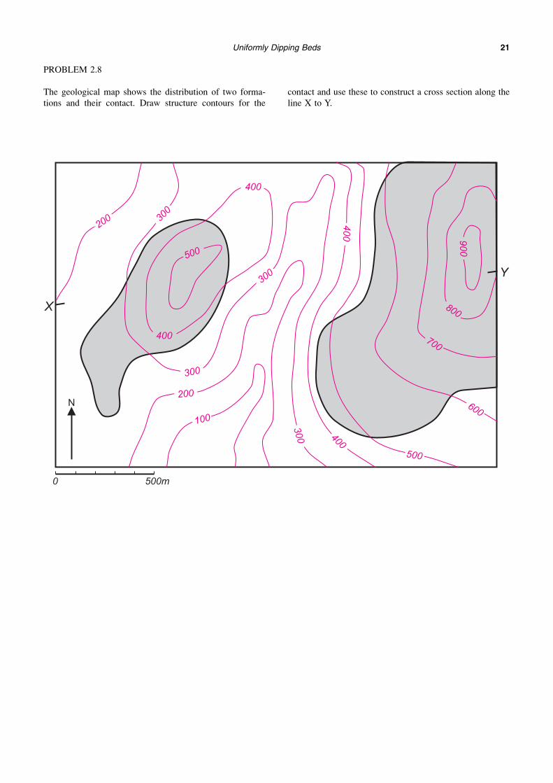
PROBLEM 2.8
The geological map shows the distribution of two forma-
tions and their contact. Draw structure contours for the
contact and use these to construct a cross section along the
line X to Y.

Uniformly Dipping Beds22
PROBLEM 2.9
The topographic map shows an area near Port Talbot in
South Wales. In three boreholes drilled in Margam Park the
‘Two-Feet-Nine’ coal seam was encountered at the follow-
ing elevations relative to sea level:
Borehole Elevation
Margam Park No. 1 –110 m
Margam Park No. 2 –150 m
Margam Park No. 3 –475 m
Draw structure contours for the Two-Feet-Nine seam,
assuming it maintains a constant dip within the area covered
by the map.
What is the direction of dip and angle of dip of the Two-
Feet-Nine seam?
Does the seam crop out within the area of the map?
A second seam (the ‘Field Vein’) occurs 625 m above the
Two-Feet-Nine seam. Construct the line of outcrop of the
Field Vein.

Uniformly Dipping Beds 23
PROBLEM 2.10
The map shows a number of outcrops where a breccia/
mudstone contact has been encountered in the field.
Interpret the run of the contact through the rest of the area
covered by the map.
Calculate:
(a) the direction of dip expressed as a compass bearing
and
(b) the angle of dip
of the contact.

Uniformly Dipping Beds24
PROBLEM 2.11
The base of the Lower Greensand is encountered in three
boreholes in Suffolk at the following attitudes relative to sea
level:
–150 m at the Culford Borehole (Map Ref. 831711)
–75 m at the Kentford Borehole (Map Ref. 702684)
–60 m at the Worlington Borehole (Map Ref. 699738)
Construct structure contours for the base of the Lower
Greensand.
Predict the height of the base of the Lower Greensand
below the Cathedral at Bury St Edmunds (856650).
Where, closest to Bury St Edmunds, would the base of
the Lower Greensand be expected to crop out if the
topography in the area of outcrop is more or less flat at a
height of 50 m above sea level?
If a new borehole at Barrow (755635) were to encounter
Lower Greensand at height –100 m, how would it affect
your earlier conclusions.
Uniformly Dipping Beds 25
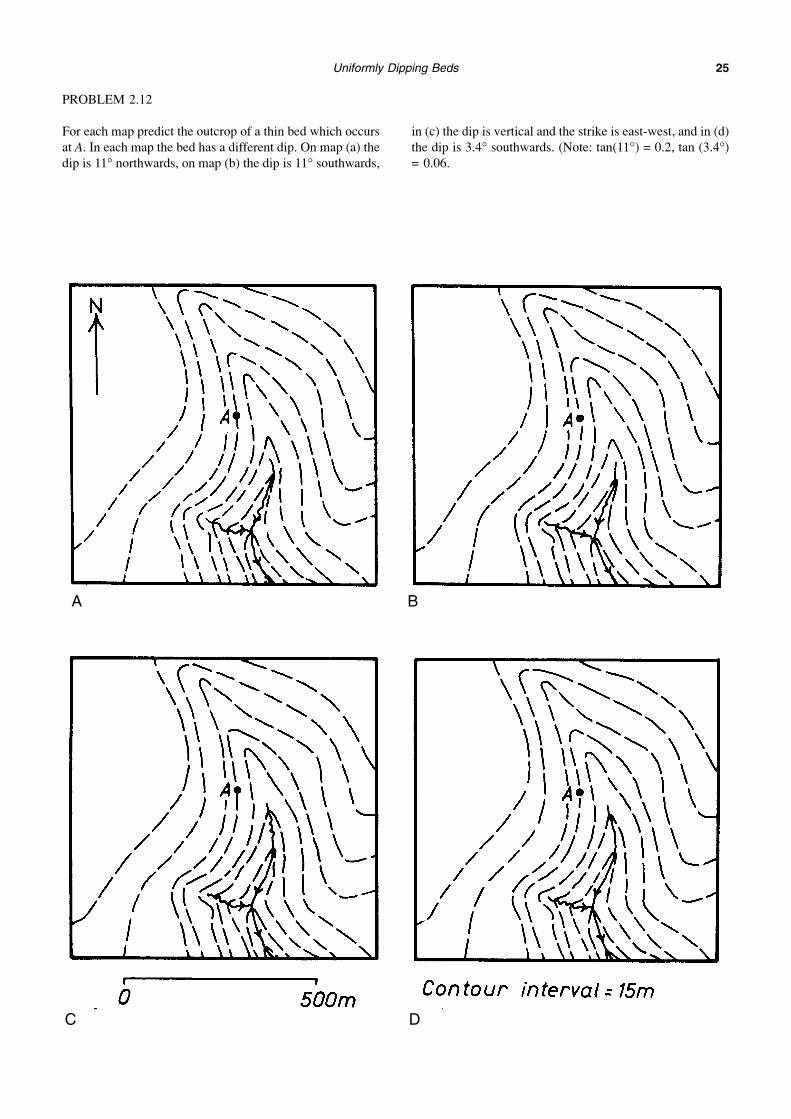
PROBLEM 2.12
For each map predict the outcrop of a thin bed which occurs
at A. In each map the bed has a different dip. On map (a) the
dip is 11° northwards, on map (b) the dip is 11° southwards,
in (c) the dip is vertical and the strike is east-west, and in (d)
the dip is 3.4° southwards. (Note: tan(11°) = 0.2, tan (3.4°)
= 0.06.
A B
C D

Uniformly Dipping Beds26
PROBLEM 2.13
Dipping Jurassic strata, southeast of Rich, Morocco
(a) Draw a geological sketch map based on the photograph
(kindly provided by Professor M. R. House). On this
map show the general form of topographic contours
together with the outcrop pattern of a number of the
exposed beds. (Note the way the dipping strata ‘vee’
over the ridge in the foreground.)
(b) Re-write the V-rule in Section 2.14 of this chapter to
express the way the outcrop pattern of beds exposed on
a ridge varies depending on the dip of the strata.
N S

Uniformly Dipping Beds 27
PROBLEM 2.14
Construct a cross-section along the line X-Y. Find the dip
and dip direction of the beds.

Uniformly Dipping Beds28
PROBLEM 2.15
Draw a cross-section of the map between points A and B.
Calculate the 30, 60, 90 and 120 m isobaths for the
‘Rhondda Rider’ coal seam.
Calculate the stratigraphic and vertical thickness of the
Llynfi Beds.

29
3
Folding
The previous chapter dealt with planar geological surfaces.
A geological surface which is curved is said to be folded.
Most folding is the result of crustal deformation whereby
rock layering such as bedding has been subjected to a
shortening in a direction within the layering. To demonstrate
this place both hands on a tablecloth and draw them
together; the shortening of the tablecloth results in a number
of folds.
The structure known as folding is not everywhere
developed equally. For example the Upper Carboniferous
rocks of southwestern England and southernmost Wales
show intense folding when compared to rocks of the same
age further north in Britain. The crustal deformation
responsible for the production of this folding was clearly
more severe in certain areas. Zones of concentrated
deformation and folding are called fold belts or mountain
belts, and these occupy long parallel-sided tracts of the
earth’s crust. For example, the present-day mountain chain
of the Andes is a fold belt produced by the shortening of the
rocks of South America since the end of the Cretaceous
times.
3.1 Cylindrical and non-cylindrical folding
A curved surface, the shape of which can be generated by
taking a straight line and moving it whilst keeping it parallel
to itself in space, is called a cylindrically folded surface
(Fig. 3.1). A corrugated iron roofing sheet or a row of
greenhouse roofs has the form of a set of cylindrical folds.
Folds which cannot be generated by translating a straight
line are called non-cylindrical. An example of this type of
shape is an egg-tray. Figures 3.2 and 3.4 show examples of
cylindrical and non-cylindrical folds. The line capable of
‘generating’ the surface of a cylindrical fold is called the
fold axis.
An important property of cylindrical folds is that the fold
shape, as viewed on serial sections (cross-section planes
which are parallel like those made by a ham slicer), remains
constant (Fig. 3.3A). This is true whatever the attitude of the
section plane. Serial sectioning of a non-cylindrical fold
produces two-dimensional fold shapes which vary from one
section to another (Fig. 3.3B).
3.2 Basic geometrical features of a fold
The single curved surface in Fig. 3.5 shows three folds. The
lines which separate adjacent folds are the inflection lines.
They mark the places where the surface changes from being
convex to concave or vice-versa. Between adjacent inflec-
tion lines the surface is not uniformly convex or concave but
there are places where the curvature is more pronounced.
Fig. 3.1 The concept of a cylindrically folded surface.
Fig. 3.2 A: Cylindrical fold. B: Non-cylindrical fold.
Fig. 3.3 Parallel sections through (A) cylindrical folds, (B)non-cylindrical folds.

Folding30
This is called the hinge zone. The hinge line is the line of
maximum curvature. Like the inflection lines, the hinge line
need not be straight except when the folding is cylindrical.
Hinge lines divide folds into separate limbs.
The terms introduced so far can be used for a single
surface such as a single folded bedding plane. Folding
usually affects a layered sequence so that a number of
surfaces are folded together. Harmonic folding is where the
number and positions of folds in successive surfaces
broadly match (Figs. 3.6A and 3.7B). Where this matching
of folds does not exist the style of folding is called
disharmonic (Fig. 3.6B).
The axial surface of a fold is the surface which contains
the hinge lines of successive harmonically folded surfaces
(Fig. 3.8). For obvious reasons this surface is sometimes
referred to as the hinge surface. The axial surface need not
be planar but is often curved.
3.3 Terms relating to the orientation of folds
As a result of folding, the overall length of a bed as
measured in a direction perpendicular to the axial surface is
shortened. When folding in a particular region is being
Fig. 3.4 A: Cylindrical folding.
Fig. 3.4 B: Non-cylindrical folding.

Folding 31
studied great attention is paid to the direction of folds, since
this is indicative of the direction in which the strata have
been most shortened.
The orientations of the fold hinge and the axial surface
are the two most important directional characteristics of a
fold. The fold hinge, which in the case of a cylindrical fold
is parallel to the fold axis, is a linear feature. As explained
in Section 2.3, such linear features have an orientation
which is described by the plunge direction and the angle of
plunge.
Non-plunging folds have horizontal hinges or plunges of
less than 10° whilst vertical folds plunge at 80–90° (Fig.
3.9). The orientation of the axial surface is described by
means of its dip direction and angle of dip. When the axial
plane dips less than 10° the adjective recumbent is
applicable. Folds are inclined when the axial plane dips and
the term upright is reserved for folds with steeply dipping
(>80°) axial surfaces (Fig. 3.9). Figure 3.7A shows a field
example of upright plunging folds.
In any fold the orientations of the hinge line and axial
surface are not independent attributes. Because the fold
hinge, by definition, is a direction which lies within the
axial surface, its maximum possible plunge is limited by the
angle of dip of the axial surface. For a given axial surface
Fig. 3.5 Some folding terms. Fig. 3.6 A: Harmonic folding. B: Disharmonic folding.
Fig. 3.7 Folds in the field. A: Upright folding with hinge lineswhich plunge towards the camera (Precambrian metasediments,Anglesey).
Fig. 3.7 B: Upright harmonic folding (Nordland, Norway).

Folding32
the steepest possible hinge-line plunge is obtained when the
fold plunges in the direction of dip of the axial surface. Such
folds are called reclined (Fig. 3.9).
Another directional feature of the fold is the direction in
which the limbs of the fold converge or close. This direction
of closure is a direction within the axial surface at right
angles to the fold hinge (Fig. 3.10).
On the basis of the direction of closure, three fold types
are distinguished:
antiforms: close upwards
synforms: close downwards
neutral folds: close in a horizontal direction.
Exercise
Which of the folds in Fig. 3.9 are neutral folds? (The answer
is given at the end of this chapter.)
Where folding affects a sequence of beds, and where their
relative ages are known, the facing of the folds can be
determined. The direction of facing is the direction in the
axial surface at right angles to the fold hinge line pointing
towards the younger beds (Fig. 3.11). Folds may face
upwards, downwards or sideways.
In anticlines the facing direction is towards the outer arcs
of the fold, i.e. away from the core of the fold (Fig. 3.12).
Fig. 3.8 The axial surface.
Fig. 3.9 Names given to folds depending on their orientation.
Fig. 3.10 Direction of closure.
Fig. 3.11 How the direction of facing is defined.
Fig. 3.12 In a syncline the beds young towards the fold’s core; inan anticline the beds young away from the core of the fold. Eithertype can be antiformal or synformal.

Folding 33
Synclines face towards their inner arcs or cores. Anticlines
can be either antiformal, synformal or neutral. The same is
true of synclines.
3.4 The tightness of folding
Folds can be classified according to their degree of
openness/tightness. The tightness of a fold is measured by
the size of the angle between the fold limbs. The interlimb
angle is defined as the angle between the planes tangential
to the folded surface at the inflection lines (Fig. 3.13).
The size of the interlimb angle allows the fold to be
classified in the following scheme:
Interlimb angle Description of fold
180°–120° Gentle
120°–70° Open
70°–30° Close
30°–0° Tight
0° Isoclinal
Negative angle Mushroom
Depending on the dip of the axial surface, tight folds may
have limbs which dip in the same general direction. Such
folds are called overturned folds.
3.5 Curvature variation around the fold
The three folds in Fig. 3.14 have the same tightness since
they possess the same interlimb angle. Nevertheless the
shapes of the fold differ significantly with respect to their
curvature. Figure 3.14A shows a fold with a fairly constant
curvature. This rounded shape contrasts with angular fold in
Fig. 3.14C. Chevron, accordion, or concertina folds are
all names used for this latter angular type of structure
(Fig. 3.16A).
3.6 Symmetrical and asymmetrical folds
When one limb of a fold is the mirror image of the other,
and the axial surface is a plane of symmetry, the fold is said
to be symmetrical (Fig. 3.15). There exists a common
misconception that the limbs of a symmetrical fold must
have equal dips in opposite directions. This need not be the
case, but the lengths of the limbs must be equal (Fig. 3.15).
Another property of a symmetrical fold is that the
enveloping surface (the surface describing the average dip
of the folded bed) is at right angles to the axial surface of
each fold.
Asymmetrical folds usually have limbs of unequal length
and an enveloping surface which is not perpendicular to the
axial surface (Fig. 3.15). Figures 3.7 and 3.19A show
asymmetrical folds.
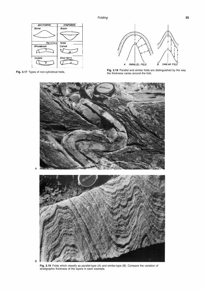
3.7 Types of non-cylindrical fold
Domes and basins (Fig. 3.17) are folds of non-cylindrical
type since their shape cannot be described by the simple
translation of a straight line. More commonly occurring
non-cylindrical folds possess a well-defined but curved
hinge line. Four types having the shapes of whalebacks,
saddles, canoes and shoe horns (Fig. 3.17) are called
periclinal folds. They are doubly-plunging with points on
their hinge line called plunge culminations and depressions
where the direction of plunge reverses. Periclinal folding
gives rise to closed elliptical patterns on the map or outcrop
surface (Fig. 3.16B).
3.8 Layer thickness variation around folds
The process leading to the formation of folds from
originally planar layers or beds involves more than a simple
Fig. 3.13 The tightness of a fold is determined from the interlimbangle.
Fig. 3.14 Folds with the same tightness but different hingecurvature.
Fig. 3.15 Symmetrical and asymmetrical folds.

Folding34
rotation of the limbs about the hinge line. The layering
around the limbs also undergoes distortions or strains which
leads to a relative thinning of the layering in some positions
in the fold relative to others. The careful measurement of
the bed thickness at a number of points between the
inflection points provides data which allow the fold to be
classified. One important class of folds in this scheme has
constant bed (stratigraphic) thickness and are called parallel
folds (Figs. 3.18A and 3.19A). In a second class of folds the
stratigraphic thickness is greater at the hinge than on the
limbs, though the bed thickness is constant if measured in a
direction parallel to the axial surface (Figs. 3.18B and
3.19B). The latter are called similar folds because the upper
and lower surfaces of the bed have identical shapes.
3.9 Structure contours and folds
In the previous chapter it was stated that uniformly dipping
surfaces are represented by structure contour patterns
Fig. 3.16 A: Recumbent chevron folds at Millook, north coast of Cornwall, England. B: Periclinalfolds exposed on a horizontal outcrop surface, Precambrian gneisses, Nordland, Norway. The closedoval arrangements of layers also characterizes the map pattern of larger-scale periclinal folds.
A
B
Folding 35
Fig. 3.17 Types of non-cylindrical folds.Fig. 3.18 Parallel and similar folds are distinguished by the waythe thickness varies around the fold.
Fig. 3.19 Folds which classify as parallel-type (A) and similar-type (B). Compare the variation ofstratigraphic thickness of the layers in each example.
A
B

Folding36
consisting of parallel, evenly spaced contour lines. Since the
strike and angle of dip of a surface usually vary around a
fold, the structure contours are generally curved and
variably spaced (Fig. 3.20).
The shape of a set of structure contour lines depicts the
shape of horizontal serial sections through the folded
surface. Since cylindrical folds give identical cross-sections
on parallel sections (see Section 3.1), these folds give
structure contour patterns consisting of contours of similar
shape and size (Fig. 3.20A). Non-cylindrical folds give rise
to more complex structure contour patterns (Fig. 3.20B).
Concentric circular contours indicate domes or basins. The
various types of periclinal folds have characteristic contour
arrangements (Fig. 3.21A). Lines can be drawn on any
contour map marking the ‘valley bottoms’ and ‘the brows of
ridges’ in the folded structure. These lines are called the
trough lines and crest lines respectively. The recognition of
these antiformal crests and synformal troughs forms a useful
preliminary step in the interpretation of a structure contour
map (Fig. 3.21B).
CLASSROOM EXERCISE
Bend a piece of card into an angular fold (Fig. 3.22A).
Tilt the card so that the fold plunges. With chalk, sketch
in the run of structure contours on the folded card and
draw, on a map, how these contours will appear as seen
from above (Fig. 3.20A). Repeat this for other angles of
plunge to investigate how the plunge affects both the
shape of the contours and their spacing. Tilt the fold
enough to make one limb overturned, i.e. to make the
fold into an overturned fold. Draw structure contours for
the fold. Note that the contour lines for the one limb
cross with those of the other limb (Fig. 3.22C). This type
of pattern signifies that overturned folds are ‘double-
valued’ surfaces; that is the surface is present at two
different heights at the same point on the map.
3.10 Determining the plunge of a fold from structurecontours
Figure 3.23 shows a plunging fold and a map of its structure
contours. If the structure contours are given, the crest (or
trough) line can be drawn in. For a cylindrical fold this line
is parallel to the hinge line, so that its plunge is measured
straight from the map. It is the trend of the crest/trough line
in the ‘downhill’ direction. The direction of plunge can be
shown on maps by an arrow (Fig. 3.23B; also see
‘Geological map symbols’). The angle of plunge is
calculated by solving the triangle in Fig. 3.23A. Note that
the contour spacing mentioned is the separation of the
contours measured in the direction of plunge.
Fig. 3.20 Structure contour patterns of cylindrical andnon-cylindrical folds.
Fig. 3.21 A folded surface.
Fig. 3.22 Visualizing the structure contour patterns of plungingfolds.

Folding 37
3.11 Lines of intersection of two surfaces
For angular folds with planar limbs the trough/crest line can
be considered to be the line of intersection of one limb with
the other. Therefore the above method to calculate the fold
plunge can be applied to calculate the plunge of the line of
intersection of any two surfaces (Fig. 3.24). If both surfaces
are planar (dip uniformly) their line of intersection will be
straight (plunge uniformly).
3.12 Determining the plunge of a fold from the dipsof fold limbs
The previous calculation of fold plunge from structure
contours also allows the position of the fold crest or trough
line to be determined. If, instead of structure contours, two
limb dips only are known, the plunge can still be
calculated.
WORKED EXAMPLE
One limb of a fold has a dip of 207/60 and the other limb
dips 100/30. Determine the plunge of the fold axis.
As the limbs are not parallel they will intersect
somewhere to give a line of intersection which is parallel
to the fold axis. Let X be a point on the line of intersection
of height h metres. The structure contours of elevation h
metres for each of the limbs must intersect at X. These
can be drawn parallel to the strike of each limb (Fig.
3.25A). Adopting a convenient scale, use the known
angles of dip and the equation in Section 2.9 to calculate
the position of structure contours for an elevation of
(h – 10) metres. These intersect at a point Y, which like X
is a point on the line of intersection. The height
difference between X and Y is 10 m and their horizontal
separation is 20 m. The triangle in Fig. 3.25B can be
solved for the angle of plunge. The fold axis thus
plunges at 26°. The direction of plunge is 138°.
It can be readily shown by means of a figure similar to Fig.
3.24 that if two portions of a folded surface have the same
angle of dip then the direction of plunge bisects the angle
between their directions of dip. Also, if the dip on any part
of a folded surface is vertical then the strike of that part is
parallel to the direction of plunge. These rules sometimes
provide a direct method of deducing the direction of plunge
of a fold from the dip symbols shown on a geological map.
The angle of plunge is obtained by looking for a dip
direction which is, as near as possible, parallel to the fold
plunge direction. The angle of dip there will be approx-
imately equal to the angle of plunge. No part of a folded
surface can dip at an angle less than the angle of plunge of
a fold. It is important to remember that these methods apply
only to cylindrical folds.
3.13 Sections through folded surfaces
We usually observe folds not as completely exposed
undulating surfaces, but in section, as they appear exposed
on the surface of a field outcrop or on the topographic
Fig. 3.23 Calculation of the fold plunge from structure contours.
Fig. 3.24 Calculation of the line of intersection of two planarsurfaces.
Fig. 3.25 Calculating the plunge of a fold axis.
Folding38
surface. In other words our usual view of folds tends to be
two-dimensional, similar to folds viewed in cross-sections.
For example, Fig. 3.30A shows the outcrop pattern yielded
by plunging folds seen on a horizontal cross-section.
CLASSROOM EXPERIMENT
Bend a piece of card into a number of folds. With
scissors, cut planes through the folded structure. On
each cut section (Fig. 3.26) note carefully (a) the
apparent tightness, (b) the apparent asymmetry, and
(c) the apparent curvature of the folds seen in oblique
section. This exercise demonstrates the importance of
the orientation of the slice through the fold for
governing the fold shape one observes.
3.14 The profile of a fold
The fold profile is the shape of a fold seen on a section plane
which is at right angles to the hinge line. The fold profile or
true fold profile is important since only this two-dimen-
sional view of the fold gives a true impression of its
tightness, curvature, asymmetry, etc. It corresponds to our
view of the fold as we look down the fold hinge line.
3.15 Horizontal sections through folds
Folds displayed on a map often present us with a more or
less horizontal section through a fold. In order to be able to
interpret the observed geometry in terms of the three-
dimensional shape of the fold, the technique of down-
plunge viewing is useful. This entails oblique viewing of the
section so that the observer’s line of sight parallels the
plunge of the structure (Fig. 3.27). The view so obtained
corresponds to a true profile of the fold structure.
WORKED EXAMPLE
The map in Fig. 3.28A shows a fold exposed in an area
of relatively flat topography. Use down-plunge viewing
to answer the following:
(1) Is the fold an antiform or a synform?
(2) How does the fold classify in the tightness
classification (Section 3.4)?
(3) Is the fold approximately similar or approximately
parallel (Section 3.8)?
View the map looking downwards towards the SW so
that your line of sight plunges at 27° towards 250°. The
view so obtained is shown in Fig. 3.28B. It reveals the
fold to be close (interlimb angle = 31°) with a shape
which is approximately parallel (constant stratigraphic
thickness).
Providing the direction of plunge is known, the apparent
direction of closure on a horizontal surface indicates
whether a fold is antiformal, synformal or neutral (Fig.
3.29). The last example serves to emphasize how oblique
sectioning produces an apparent shape which can differ
Fig. 3.26 Classroom experiment to illustrate the importance of thesection effect on a fold’s appearance.
Fig. 3.27 The ‘down-plunge’ method of viewing a geological mapallows the true shape of a fold structure to be seen.
Fig. 3.28 An example of the ‘down-plunge’ method of viewing amap.
Fig. 3.29 The outcrop pattern produced by three folds withdifferent directions of closure. The arrows show the plungedirections.
A Map
B Down-view plunge

Folding 39
Fig. 3.30 A: An upright synform (also a syncline) exposed on awave-cut platform at Welcombe, Devon, England (Upper Carboniferoussandstones and shales). The synform plunges towards the sea. Thefold is a gently plunging, upright synform.
Fig. 3.30 B: Moderately plunging upright folds, Svartisen, Norway. The hand points down the hingeline of a synformally folded quartz-rich layer in the gneisses. Note the way the fold appears to closeon the horizontal and steep parts of the outcrop surface.

Folding40
significantly from a true profile. On maps of more or less
flat terrain this effect is most marked when plunges are
low.
3.16 Construction of true fold profiles
This is a formalization of the down-plunge viewing method.
Oblique sectioning of folds on non-profile planes produces
a distortion of the shape which can be most easily visualized
by reference to a plunging circular cylinder, say a bar of
rock (of the candy variety!) The cylinder of diameter D
plunges at an angle � and will appear as an ellipse on a
horizontal section plane (Fig. 3.31A). This ellipse is a
distorted view of something which in true profile has the
shape of a circle. The shape of the ellipse shows that
distortion consists of a stretching in the direction of plunge
such that a length D appears to have length D/sin � (Figs.
3.31B and 3.31C).
The construction of the true profile involves taking off
this distortion. Place a rectangular grid on the map (Fig.
3.31B) with one axis (x) parallel to the direction of plunge
and where the scales in the x and y directions are in the ratio
1:sin �. The coordinates of points on the fold outline
referred to this grid are replotted on a square grid (Fig.
3.31D). This shortening of dimensions parallel to the plunge
compensates for the stretching brought about by oblique
sectioning.
Alternatively, place a square grid over the map with the x
axis parallel to the plunge direction, and record the
coordinates (x, y) of points on the boundary.
Transform these coordinates, i.e. calculate new ones
using xnew = x sin �, ynew = y. Replot the new coordinates on
a square grid.
3.17 Recognition of folds on maps
The interpretation of the structure of an area represented on
maps is greatly assisted if the patterns produced by fold
structures can be directly recognized. Students should use
every opportunity to practise their skills in this aspect of
geological map reading.
In Chapter 2 the sinuosities produced by the effect of
topography on uniformly dipping beds were discussed.
Many of the shapes produced look superficially like
sections through folds (see Fig. 3.32A).
These outcrop patterns due to topographic effects are
characterized by V-shapes in parts of the map where
V-shapes are shown by the topographic contours. On the
other hand outcrop patterns due to folding possess definite
curvatures which cannot be related to a corresponding
pattern in the topographic contours (Fig. 3.32B). Fold-like
sinuosities of geological contacts in a part of a map where
the terrain consists of a uniform slope must be the
expression of folding.
WORKED EXAMPLE
The map in Fig. 3.33 shows the outcrop of a thin shale
bed (white). The highly curved outcrop pattern shows
four strongly curved parts (A, B, C and D). Explain the
reason for these fold-like shapes.
The bends at A and C occur on a ridge defined by a
V-shaped arrangement of topographic contours. These
curves are therefore due to the terrain effect and are
not an expression of folding. The curvatures at B and D
are not related to a particular topographic feature, and
occur on fairly uniformly sloping valley sides. B and D
therefore represent folds.
Fig. 3.31 Construction of a true fold profile.
Fig. 3.32 A: Outcrop pattern related to topography. B: Outcroppattern related to folding.
Fig. 3.33 Structural interpretation of outcrop pattern.
Folding 41
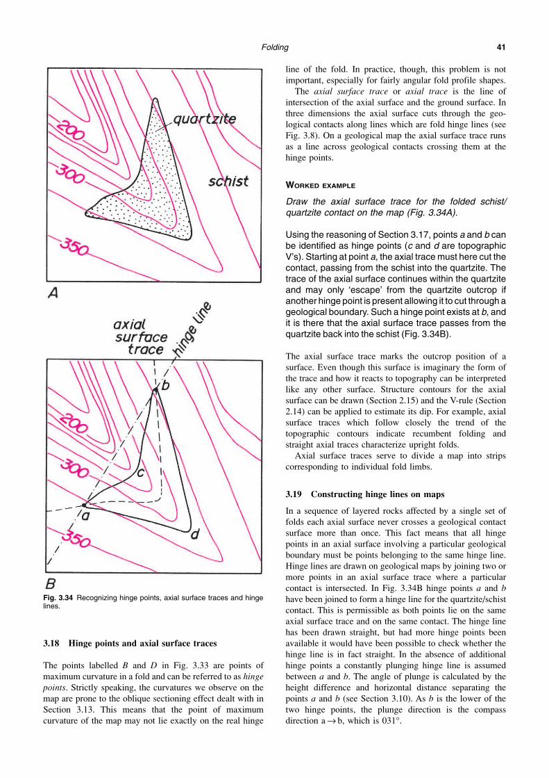
3.18 Hinge points and axial surface traces
The points labelled B and D in Fig. 3.33 are points of
maximum curvature in a fold and can be referred to as hinge
points. Strictly speaking, the curvatures we observe on the
map are prone to the oblique sectioning effect dealt with in
Section 3.13. This means that the point of maximum
curvature of the map may not lie exactly on the real hinge
line of the fold. In practice, though, this problem is not
important, especially for fairly angular fold profile shapes.
The axial surface trace or axial trace is the line of
intersection of the axial surface and the ground surface. In
three dimensions the axial surface cuts through the geo-
logical contacts along lines which are fold hinge lines (see
Fig. 3.8). On a geological map the axial surface trace runs
as a line across geological contacts crossing them at the
hinge points.
WORKED EXAMPLE
Draw the axial surface trace for the folded schist/
quartzite contact on the map (Fig. 3.34A).
Using the reasoning of Section 3.17, points a and b can
be identified as hinge points (c and d are topographic
V’s). Starting at point a, the axial trace must here cut the
contact, passing from the schist into the quartzite. The
trace of the axial surface continues within the quartzite
and may only ‘escape’ from the quartzite outcrop if
another hinge point is present allowing it to cut through a
geological boundary. Such a hinge point exists at b, and
it is there that the axial surface trace passes from the
quartzite back into the schist (Fig. 3.34B).
The axial surface trace marks the outcrop position of a
surface. Even though this surface is imaginary the form of
the trace and how it reacts to topography can be interpreted
like any other surface. Structure contours for the axial
surface can be drawn (Section 2.15) and the V-rule (Section
2.14) can be applied to estimate its dip. For example, axial
surface traces which follow closely the trend of the
topographic contours indicate recumbent folding and
straight axial traces characterize upright folds.
Axial surface traces serve to divide a map into strips
corresponding to individual fold limbs.
3.19 Constructing hinge lines on maps
In a sequence of layered rocks affected by a single set of
folds each axial surface never crosses a geological contact
surface more than once. This fact means that all hinge
points in an axial surface involving a particular geological
boundary must be points belonging to the same hinge line.
Hinge lines are drawn on geological maps by joining two or
more points in an axial surface trace where a particular
contact is intersected. In Fig. 3.34B hinge points a and b
have been joined to form a hinge line for the quartzite/schist
contact. This is permissible as both points lie on the same
axial surface trace and on the same contact. The hinge line
has been drawn straight, but had more hinge points been
available it would have been possible to check whether the
hinge line is in fact straight. In the absence of additional
hinge points a constantly plunging hinge line is assumed
between a and b. The angle of plunge is calculated by the
height difference and horizontal distance separating the
points a and b (see Section 3.10). As b is the lower of the
two hinge points, the plunge direction is the compass
direction a → b, which is 031°.
Fig. 3.34 Recognizing hinge points, axial surface traces and hingelines.

Folding42
3.20 Determining the nature of folds on maps
An essential part of geological map reading is the ability to
deduce whether a given fold closure displayed on a map is
antiformal or synformal. Use the procedures described
above to identify fold closures and assess the plunge of their
hinges. Select a part of the map where the ground slope is
opposed to the plunge of the folds. Visualize the fold shape
that could be seen on the hillside from a low vantage point
on the ground and facing up-slope. In the case of the map in
Fig. 3.35A the reader should imagine the view from a spot
in the stream looking northeast and up at the hillside which
slopes towards the observer. The quartzite/schist contact
crosses the stream to the viewer’s left and runs uphill until
a height of about 325 m is reached, and then suddenly starts
to descend, ending up in the stream to the observer’s right
(Fig. 3.35B). The structure clearly closes upwards and is
therefore an antiform.
3.21 Cross-sections through folded areas
The procedure for preparing a cross-section is best
explained by an example.
WORKED EXAMPLE
Draw a vertical section across the map in Fig. 3.36A
between points X and Y.
This is tackled in several stages:
(1) distinguish true fold hinge points from topographic
effects (Section 3.17);
(2) join these hinge points to form axial surface
traces (Section 3.18);
(3) join hinge points to form hinge lines (Section
3.19).
After drawing in the topography the shapes of the axial
surface traces are constructed in the cross-section
(Fig. 3.36C). This is most easily done by transferring
the hinge points to the section by interpolating their
heights from where hinge lines intersect the plane of
section (Fig. 3.36B). The axial surface traces are then
drawn in the section by joining the hinge points. The
final stage (Fig. 3.36D) involves drawing the folded
geological boundaries. These form the limbs of the
folds and can be considered as the portions of the fold
linking hinge points from adjacent axial surfaces. If the
more exact shape of the limbs is required additional
data can be obtained from structure contours con-
structed for the geological boundaries on the limbs.
3.22 Inliers and Outliers
Some geological boundaries on a map define a closed loop,
so that rocks belonging to one unit completely enclose those
of another. The outcrop pattern involving older rocks being
Fig. 3.35 Deducing whether a fold on a map is an antiform orsynform.
Fig. 3.36 Drawing a cross-section through a folded area.

Folding 43
surrounded by younger ones is given by the name inlier.
The reverse relationship, with younger rocks completely
encircled by older rocks, is present in an outlier.
These outcrop patterns can be produced either by erosion
(e.g. the outlier 2 km WNW of Winchcombe on the map in
Problem 2.7) or by folding (especially periclinal folding).
The pattern in Fig. 3.35 is due to a combination of folding
and erosion. If we knew that the quartzite was older than the
schist, the structure in Fig. 3.35 would be an inlier.
Answer to question set in section 3.3:
Vertical folds, reclined folds and, possibly, recumbent folds
are examples of neutral folds.

Folding44
PROBLEM 3.1
The numbers on the map give the depths in metres (below
sea level) to the top of the Wittekalk Limestone.
1. Draw structure contours for the top of the limestone.
2. Explain why the structures cannot be interpreted as
cylindrical folds.
3. Label the crest lines and trough lines on the map.
4. Give names to the various periclinal folds present.
5. Calculate the dip direction and dip at points P and Q on
the top of the limestone.

Folding 45
PROBLEM 3.2
The photograph, taken from the air in the Zagros Moun-
tains, Iran, shows folded rocks.
Draw a sketch geological map of the area to show the
geological structure. On your map use as many as possible
of the symbols given on the list at the beginning of this book
(see ‘Geological Map Symbols’).
(photo: courtesy Aerofilms)

Folding46
PROBLEM 3.3
For each map:
(a) draw the fold axial surface trace (axial trace),
(b) determine the plunge of the fold hinge and show this
on the map with the appropriate symbol (see list of
symbols at beginning of this book),
(c) determine the dip of the axial surface and show this on
the map with the appropriate symbol,
(d) classify the fold according to the scheme based on fold
orientation (Fig. 3.9).
A
B
Scale 1:2500

Folding 47
PROBLEM 3.4
Each map shows folded beds for which the younging
direction is known. Classify the folds:
(a) as antiforms, synforms or neutral folds;
(b) as anticlines or synclines;
(c) as upward-facing, downward-facing or sideways-
facing folds.
The answers to (a), (b) and (c) are not independent. By this
we mean, for instance, that a knowledge of the facing
direction (upward/downward) and the direction of closure
(antiform/synform) allows one to decide whether a fold is
an anticline or syncline. Devise a rule explaining the
interdependence of the three classifications. (A series of
sketches showing the various possible combinations will
help to clarify your thinking.)

Folding48
PROBLEM 3.5
The map shows the geology of an area in the province of
Namur in Belgium.
The distribution of the rocks and the shape of their
outcrops are structurally, rather than topographically, con-
trolled. The fold structures in the area, which are of Variscan
age, are all upward-facing.
Working on a tracing paper overlay to the map:
(a) mark the axial surface traces of anticlines and
synclines,
(b) deduce the approximate direction of plunge from the
direction of fold closure and show this with plunge
arrows on the various parts of the map (see list of
symbols), and
(c) show the location of an example of an inlier and an
example of an outlier.
Analyse the regional variation of fold plunge by locating the
position of plunge culminations and plunge depressions.
Comment on the style of the folds responsible for the
elongate oval outcrop patterns.

Folding 49
PROBLEM 3.6
(a) By consulting Fig. 3.17 draw hypothetical maps
showing the outcrop patterns of periclinally folded
beds, exposed in an area of low relief.
(b) On these sketch-maps use symbols to show the dip of
beds, as well as the course of the geological bound-
aries. Does each type of periclinal fold produce a
characteristic outcrop pattern?
The accompanying map is a geological map of part of
Derbyshire, England.
(c) Identify and mark the hinge points of folds.
(d) Establish whether these folds are antiforms or
synforms.
(e) Draw the axial traces of antiformal and synformal
folds.
(f) Deduce the approximate direction of plunge of the
various folds present.
(g) Where do the following types of periclinal folds occur
on the map: canoe-, whaleback-, shoe-horn-, and
saddle-shaped folds?
(h) Why do the sandstone beds (shown with stippled
ornament) vary so much in their width of outcrop?

Folding50
PROBLEM 3.7
The accompanying map shows Palaeozoic rocks exposed in
a part of Gloucestershire, England.
Describe the most important structure in the area and,
after calculating the fold plunge, construct a true profile of
the structure.
From the true profile, measure the interlimb angle of the
fold. What name is given to a fold with this interlimb angle
(see Section 3.4)?
Examine the thicknesses of the rock units around the fold.
Is the fold closest to a parallel or similar type? Measure the
thickness of the Carboniferous Limestone. Is it correct to
say that the Carboniferous Limestone is thicker in the region
of the fold hinge?

Folding 51
PROBLEM 3.8 (A & B)
Practise using the terms explained in this chapter to
describe, as fully as possible, the geometry of the folds in
the photographs. For example, refer to the tightness,
orientation, layer thickness variation, curvature, etc. of the
folds. In all photographs the camera is pointing in the
direction of the fold axis.
Draw sketches of the folds showing, where appropriate,
the axial traces, hinge points, inflection points, trace of the
enveloping surface, fold limbs, etc.
Photographs A and C show structures in metasedimentary
gneisses, B shows folded quartz veins (Nordland, Norway),
D shows folded turbidites, Crackington, Cornwall, England.
A
B

Folding52
PROBLEM 3.8 (C & D)
C
D

Folding 53
PROBLEM 3.9
By consulting sections 3.10 and 3.11 and Fig. 3.23, evaluate
the following statements:
(a) the plunge of a fold hinge cannot be steeper than the
dip of either of the limbs,
(b) if one limb of a fold has a vertical dip its strike is
parallel to the direction of plunge,
(c) in a plunging fold the two limbs always have different
strike directions,
(d) if a limb of a fold strikes in a direction which is
perpendicular to the plunge direction of the fold, the
angle of dip of that limb equals the angle of plunge of
the fold hinge,
(e) if the two limbs of a fold possess the same angle of dip
the direction of plunge bisects the angle defined by the
directions of the strikes of the limbs,
(f) if a fold has a vertical plunge, both limbs have vertical
dips.
PROBLEMS 3.10–3.14
(in order of increasing complexity)
On each map:
(a) mark hinge points, antiformal and synformal axial
traces and hinge lines;
(b) determine the plunge and plunge direction of the fold
hinge lines;
(c) deduce the general attitude (dip) of the fold axial
surfaces;
(d) construct a vertical cross section along the line X-Y;
(e) give a full description of the characters of the folds
(e.g. tightness, symmetry, bed thickness variations,
etc.).

Fo
ldin
g5
4PROBLEM 3.10

Fo
ldin
g5
5PROBLEM 3.11

Fo
ldin
g5
6PROBLEM 3.12

Fo
ldin
g5
7PROBLEM 3.13

Folding58
PROBLEM 3.14

59
4
Faulting
Folds and faults are both structures produced by the
deformation of rocks. Folds are structures where layering is
deformed without breaking so that the layering surfaces are
curved but continuous (Fig. 4.2A). Faults represent a
different type of response by rocks to the stresses imposed
on them. Faults are fracture surfaces along which appreci-
able displacement of the layering has taken place (Figs. 4.1
and 4.2B). Faults, unlike folds, can be thought of as
structural discontinuities.
Figure 4.2 illustrates an important difference between
faults and folds. In each sketch a stratigraphy consisting of
beds A to F is being deformed. In each cross-section a
horizontal line traverse reveals a characteristic sequence of
encountered layers. In the case of folding (Fig. 4.2A) the
sequence is
F E D E F
← →sequence sequence reversed
Fig. 4.1 A fault is a rock fracture across which displacement has occurred.Evidence of the motion on the fault comes from displaced marker layers.

Faulting60
With the fault (Fig. 4.2B) the sequence is
F E D F E D
← ←sequence sequence repeated
Folds can give rise to a duplication of a set of beds where
the order in which they appear shows reversals. It should be
noted that the axial surface marks the place where the
sequence reverses. In the example of faulting, we note that
the sequence is not reversed but repetition of the same
sequence takes place. The fault plane marks the place where
the sequence starts to repeat itself. The fault in Fig. 4.2B
places units D and F next to one another. The contact D/F
is not a normal contact because D and F do not normally
occur as adjacent units. The fault forms what is called a
tectonic contact between units D and F. Not all faults give
rise to repetition of encountered beds, but some are instead
discontinuities at which certain beds are omitted. These
differences between folds and faults allow these structures
to be distinguished in line transects (e.g. boreholes) and are
summarized below.
4.1 Fault planes
With a fault, the surface along which displacement has
taken place is the fault plane. Structure contours can be used
to describe the form of fault planes and these are interpreted
in the same way as structure contours drawn for any surface
(see Chapters 2 and 3). The inclination of a fault plane is
described by its dip. Faults with dips greater than 45° are
sometimes referred to as high-angle faults; those with dips
less than 45° are low-angle faults. The rocks which lie
above a fault plane make up the hanging wall, those below
the foot wall (Fig. 4.3).
Faults displace planar surfaces such as bedding planes.
Any geological surface (such as a bedding plane) is
truncated by a fault along a line called the cut-off line (Fig.
4.3). On a map or cross-section the point where the surface
is crossed by the fault line is a cut-off point. Lines can be
drawn on maps showing the course of the cut-off lines in the
subsurface. These lines, being the lines of intersection of
two surfaces, are calculated from the structure contours for
each surface (see Sections 3.10 and 3.11).
WORKED EXAMPLE
Determine the cut-off line for the top of the sandstone
bed in Fig. 4.4A.
From the given dips, structure contours for heights
relative to that of the ground surface are drawn for both
the fault plane and the top of the sandstone bed. The
intersection of the respective contours gives the line of
intersection (the cut-off line). This line passes through
the visible cut-off point on the map (Fig. 4.4B). The
plunge of the cut-off line can be calculated if required
(see Sections 3.10 and 3.11).
Fig. 4.2 Sequences of rocks observed on line traverses throughfolds (A) and faults (B).
Fig. 4.3 Fault terminology.
Table 4.1
Folds Faults
Linear traverses
through structure
show:
Continuous
sequences, with
reversals possible
Discontinuous sequences
with possible duplication
and omissions of units;
no reversals of sequences

Faulting 61
In the field, the trend of faults is often easier to ascertain
than the dip of a fault plane. Faults, being movement zones,
often function as lines of erosional weakness which give
rise to linear topographic features. The fault planes
themselves are rarely exposed. The dip can sometimes be
deduced from the form of its line of outcrop across irregular
topography.
Their attitude relative to the structure of the country rocks
allows faults to be classified. A strike fault has a strike
parallel to the strike of the beds it displaces. A dip fault
strikes parallel to the dip direction of the surrounding beds.
A bedding plane fault is parallel to the bedding (Fig. 4.5)
and is therefore a variety of strike fault.
4.2 Slip and separation
The slip of a fault is a measure of its actual displacement.
The slip is the distance between two points on the fault
plane, one on the foot wall and one on the hanging wall,
which were originally coincident. Slip is determined by
measuring the distance between equivalent recognizable
points across the fault plane.
Separation has to do with the offset or shift of beds or
other geological surfaces as observed on a specified outcrop
or section surface. Separation is measured from displaced
planes. In general, there is no simple agreement between the
amounts of separation and slip shown by a fault.
4.3 Separation terms
Separation is concerned with the distance between a planar
surface in the hanging wall and its counterpart in the foot
wall. This distance can be measured in various ways.
If the fault does not involve a rotation of one block
relative to the other, the two displaced half planes will be
approximately parallel. The shortest distance between two
parallel planes is the distance measured in a direction which
is perpendicular to these planes. This is the stratigraphic
separation (SS in Fig. 4.6). It is the offset of beds across the
fault expressed as a stratigraphic thickness.
If the separation is measured vertically, the distance is
called the vertical separation (VS in Figs. 4.6 and 4.7).
Vertical separation is readily calculated from structure
contour maps, being the difference in height between the
displaced geological surface in the hanging and foot walls.
The stratigraphic separation can be calculated from vertical
separation if the dip of the beds is known, using
Stratigraphic separation = vertical separation �
cosine (dip of beds)
It follows from this that the stratigraphic separation equals
the vertical separation in the case of horizontal beds.
Other measures of separation are distances measured in
special directions with respect to the fault plane. The strike
separation is measured parallel to the strike of the fault
plane (Fig. 4.7). The offset of beds across a fault visible on
a map of level terrain is equal to the strike separation. Strike
Fig. 4.4
Fig. 4.5
Fig. 4.6 Stratigraphic separation (SS) and vertical separation(VS).
Fig. 4.7 Separation terms.

Faulting62
separation can either be dextral (right lateral) or sinistral
(left lateral) (see Fig. 4.8).
‘Right lateral’ means that the beds on the opposite side of
the fault are offset to the right relative to the beds on the
observer’s side. Dip separation is the bed offset in the down
dip direction of the fault (Fig. 4.7). The vertical component
of the dip separation is called the throw and its horizontal
component is the heave; both of these quantities can be seen
in a plane perpendicular to the fault’s strike. For a given
fault, the ratio of the heave to the throw depends on the fault
plane’s dip in this manner
tan (dip of fault) = throw/heave (Fig. 4.7)
where throw = dip separation � sin (dip of fault). Vertical
faults have a throw but no heave. Based on the sense of dip
separation on a fault, the block within which the beds show
an apparent downward offset is referred to as the downthrow
side of the fault. The downthrow side of a fault can also be
easily determined from faults displayed on maps. This is
done by oblique viewing of the map so that the observer
looks down the dip of the displaced beds. By doing this, an
impression is gained of how the beds would appear in cross-
section. As an exercise, obliquely view the map in Fig. 4.9A
along a line of sight which plunges 30° southwards (i.e.
down the dip of the mudstone bed). From this it can be
readily seen that the west side of the fault is the downthrow
side. The downthrow side is denoted on many maps by a
dash on one side of the fault line (see Geological Map
Symbols).
The heave is a meaningful measure of separation in
relation to maps, as the example below shows.
WORKED EXAMPLE
For the fault on the map (Fig. 4.9A) determine (a) the
vertical separation, (b) the stratigraphic separation, (c)
the strike separation, (d) the dip separation, and (e) the
heave.
Structure contours and cut-off lines on the hanging
(hwcl) and foot walls ( fwcl) are constructed (using the
method of the worked example in Section 4.1).
The vertical separation is determined by selecting
any point on the map and calculating the height
difference of the two displaced parts of geological
surface. For example at point x (Fig. 4.9B),
height of mudstone bed in hanging wall = –10 m
height of mudstone bed in foot wall = –20 m
height difference = (–10) – (–20)
= 10 m = vertical separation
the stratigraphic separation = vertical separation
� cos (dip)
= 10 m � 0.64 = 6.4 m.
Fig. 4.8 Terms used to describe the sense of separation.
Fig. 4.9

Faulting 63
The strike separation can be measured directly from
the map in this case (Fig. 4.9B) since the map is of an
area of flat topography. Otherwise, this separation
could be measured from the map in a direction parallel
to the strike of the fault between the structure contours
of the same height for the two sides of the shifted
surface. The measured strike separation is about 20 m
and the sense of offset is dextral. The dip separation
and heave can be calculated in two ways. A vertical
cross-section perpendicular to the fault’s strike line can
be drawn and these measurements made from it (Fig.
4.9C). Alternatively, the heave can be measured
directly from the map (heave = 6 m) since it is the
distance between the hanging wall and foot wall cut-off
lines measured perpendicular to the strike of the fault.
The heave can be used to calculate the dip separation,
since
dip separation = heave / cos (dip of fault)
= 6 m / 0.64 = 9.4 m
The heave represents the gap between the cut-off
lines, and as such indicates the width of ground
(measured at right angles to the fault) not underlain by
the mudstone bed.
The sense of dip separation is either normal or reverse.
Normal separation involves a relative downward offset of
the hanging wall. Reverse separation implies a relative
upward offset of the beds in the hanging wall (Fig. 4.8). The
fault in Fig. 4.9 shows normal separation of the mudstone
bed.
4.4 Repetition and omission of strata
A straight line traverse through faulted strata will usually
reveal that certain beds occur more than once or that certain
beds do not occur at all. For any fault, beds can be either
repeated or omitted depending on the direction of the line on
which the occurrence of beds is recorded. The following
worked example will allow the reader to formulate rules for
the duplication and omission of strata resulting from
faulting.
WORKED EXAMPLE
The fault with dextral strike separation in the map in
Fig. 4.10A displaces a sequence of strata numbered 1
to 14. Record the order of occurrence of strata in
traverses A-A�, B-B�, C-C � etc., across the area.
Which traverses involve repetition and which omission
of strata? Formulate a general rule to determine which
linear traverses show repetition and which omission.
Line A-A� gives the sequence 1, 2, 3, 4, 5, 6, 10, 11, 12,
13, 14. This sequence involves omission of beds 7, 8
and 9. Lines B-B�, C-C�, D-D� also involve omissions
of strata. Traverses; E-E�, F-F�, G-G� and H-H� involve
duplication of beds. It appears, then, that the direction
of the line traverse determines whether beds are cut
out or duplicated. This exercise shows that the
directions of the line traverses of each type fall into
sectors. These two sectors (Fig. 4.10B) are bounded
by the trace of the bedding and the trace of the fault
plane. This rule can be extended to three
dimensions.
4.5 Determining the slip of a fault
The separation or the offset of individual marker beds is not
sufficient to deduce the actual movement or slip on a fault.
To calculate slip it is necessary to recognize two points; one
on the hanging wall and one on the foot wall, which were
originally coincident. Two halves of a small object, say a
pebble, fortuitously split by the fault, would provide a direct
indication of the net slip (Fig. 4.11).
Fig. 4.10 Omission and repetition of strata resulting from faulting.
Fig. 4.11 Net slip.

Faulting64
Such displaced point objects are rarely found. Slip is
more often calculated from points resulting from linear
features which intersect the fault plane. Figure 4.12 shows
an example of this where a fold hinge provides a point (a
hinge point), where the hinge line meets the fault plane.
The net slip is the displacement of the two (hinge) points.
Net slip has both direction and magnitude. The direction can
be stated as the plunge of the line joining the two displaced
points. The magnitude is the straight-line distance between
the displaced points.
The points which are vital for the determination of slip
are given whenever three planes intersect. One of these
planes is the fault plane itself, the other two are a pair of any
non-parallel planes. Such planes include fold limbs (as in
the example above and Fig. 4.14), older faults, uncon-
formities (explained in Chapter 5), sheet intrusions (Chapter
6), etc.
WORKED EXAMPLE
Determine the net slip for the fault shown on the map
in Fig. 4.13A. The fault displaces two planar calcite
veins.
For each of the three planes, one structure contour is
drawn for a convenient height, say 10 m above the
level of the ground surface. Using the usual method,
lines of intersection are drawn for each pair of planes.
These three lines of intersection cross at the point of
intersection of the three planes (Fig. 4.13B). The three
planes on the hanging wall intersect at H, on the foot
wall at F. The line FH plunges in the direction H → F
(= 070°N) because point F is lower than H. From the
difference in height and the horizontal distance F-H a
triangle can be constructed which refers to a vertical
plane through F and H (Fig. 4.13C). From this triangle
the net slip (FH) and the angle of plunge can be read
off. Therefore the plunge of the slip direction = 7–070
and the magnitude of net slip = 100 m.
4.6 Components of slip
The line representing the amount and direction of net slip of
a fault can be resolved into components in various
Fig. 4.12 Use of a displaced fold hinge line to calculate the netslip.
Fig. 4.13 Calculating the net slip of a fault.

Faulting 65
directions (Fig. 4.15). The strike-slip component is the
component of the net slip in the direction of the strike of the
fault plane. This component is either dextral or sinistral. The
dip-slip component is the component of net slip in the fault
plane’s down dip direction. This component is either normal
or reverse.
WORKED EXAMPLE
Calculate the strike slip and dip-slip components for
the fault in the map in Fig. 4.13A.
The strike-slip component is equal to length of HF
projected on to the strike line of the fault (98 m in Fig.
4.13B). The sense of movement is sinistral. If the net
slip and strike slip are known, the dip-slip component
can be calculated because these three quantities
define a right-angled triangle in the plane of the
fault.
By Pythagoras (Fig. 4.15),
(net slip)2 = (strike slip)2 + (dip slip)2
so that
dip slip = ���������������(net slip)2 – (strike slip)2 = �������1002 – 982
= 20 m.
The dip-slip sense is reverse (hanging wall is displaced
upwards relative to the foot wall).
Fig. 4.14 A fault which displaces two planes of different orientation (the limbs of a fold). Study theoffset of the limbs. Which component of slip is more important, the dip-slip or the strike-slipcomponent? (The outcrop surface is horizontal.)
Fig. 4.15 Component of net slip.
Fig. 4.16 To show that an observed separation shown by a planarmarker bed could have been brought about by slip in a largenumber of directions within the fault plane.

Faulting66
It is important to realize that there is no straightforward
correspondence between slip and separation. For example,
the dip-slip component will not usually be equal to the dip
separation. To illustrate this consider Fig. 4.16, where a
fault is observed to offset a bed. As no reference points can
be recognized to allow the slip to be determined, a large
number of possible slip directions could have given rise to
the observed separation. Some of these possible slip
directions are labelled 1 to 5 in Fig. 4.16. For instance, 5 is
a potential slip direction which would have had a dextral
strike-slip component, whereas the strike separation has a
sinistral sense.
Clearly the separation provides insufficient information
for the complete determination of slip. Nevertheless,
separation places certain limits on the possible slips. For
instance, in Fig. 4.16 the slip labelled 6 with reverse
dextral slip is clearly not a possible net slip for the fault.
It can also be seen that line 3 is the smallest of all
possible slips and therefore provides a minimum estimate
of the slip magnitude. The equation below gives that
estimate:
minimum set slip magnitude =s d
�����d2 + s2
where s is the strike separation and d the dip separation.
4.7 Classification of faults based on slip
Table 4.2 below outlines the slip classification. These are
illustrated in Fig. 4.17.
Synonyms for strike-slip are wrench, tear and trans-
current fault. Normal-slip faults are commonly high-angle
faults (Fig. 4.18A). High-angle reverse-slip faults are
generally less common than normal-slip faults. Low-angle
reverse-slip faults are called thrusts (Fig. 4.18B). Like
strike-slip faults, thrusts can have net slips with magni-
tudes of several kilometres.
There are practical difficulties associated with the
classification of faults. The slip classification is a logical
scheme based on actual fault displacement but suffers
from the disadvantage that the slip is only seldom
determinable in practice. Separation, on the other hand, is
readily measured but, as explained above, is only indi-
rectly related to fault movement.
Whether a fault is described in terms of slip or in terms
of separation it is advisable to name the fault in such a
way as to make it clear which measurement has been
made. For example terms like ‘normal-separation fault’ or
‘normal-slip fault’ should be used rather than simply
‘normal fault’.
Fig. 4.17 The slip classification of faults.
Table 4.2
Type of fault Type of slip Sub-types
Dip-slip fault slip in down-dip
direction; no strike
component
normal-slip faults,
reverse-slip faults
Strike-slip faults slip parallel to strike
of fault; no dip-slip
component
dextral-slip
sinistral-slip faults
Oblique slip faults slip with dip slip and
strike slip
components
dextral normal-slip
faults, sinistral reverse-
slip faults etc.

Faulting 67
Fig. 4.18 Faults. A: Normal fault (or, more properly, a normal-separation fault), Bude, England.B: Thrust (a low-angled reverse fault), Torquay, England.
A
B

Faulting68
PROBLEM 4.1
The figure corresponds to a vertical cross-section showing
the thicknesses and order of rock units encountered in four
boreholes drilled along the line of section.
Examine the sequences in each borehole and compare
these to the known stratigraphic sequence which is given in
the column on the right.
In each borehole sequence, mark the position of fault or
fold structures.
Interpret the structure of the cross-section by linking
structures from adjacent boreholes.

Faulting 69
PROBLEM 4.2
The aim of this exercise is to investigate the way fault
separation relates to slip.
The map shows a vertical fault which cuts off a dipping
sandstone bed.
The plane of the cross-section (lower diagram) coincides
with the plane of the fault. The cross-section shows the
trace, on the fault plane, of the sandstone bed in the block on
the north side of the fault.
In the cross-section select any point on the base of the
sandstone in the fault plane and, for an amount of slip given
below, locate the position of its equivalent point in the fault
plane on the south side of the fault. In the cross-section and
map draw the displaced sandstone for the south side of the
fault.
Measure the magnitude and sense of strike separation and
dip separation for each of the following amounts of net slip
and complete Table 4.3 on page 67:
Strike-slip component Dip-slip component
(i) 20m (sinistral) 10 m (south side down)
(ii) 0 m 20 m (south side down)
(iii) 10 m (dextral) 30 m (south side down)
(iv) 30 m (dextral) 10 m (south side down)
Investigate the possibility that a fault may show neither
strike nor dip separation.

Faulting70
PROBLEM 4.3
Using the method described in 4.3, calculate:
(a) the strike separation, and
(b) the heave of the thrust fault.
Construct a cross-section along the line X-Y and
determine:
(c) the dip separation, and
(d) the throw of the thrust fault.
Table 4.3
Strike-slip component Dip-slip component Strike separation Sense of strike separation Dip separation Sense of dip separation
20 m (sinistral) 10 m (S side down)
0 m 20 m (S side down)
10 m (dextral) 30 m (S side down)
30 m (dextral) 10 m (S side down)

Faulting 71
PROBLEM 4.4

Faulting72
PROBLEM 4.5
Determine the attitude (dip and dip direction) of the fault.
Draw a cross-section along the line X–Y.
Find the dip separation, throw, heave, vertical separation
and strike separation of the fault.
Give a name to this fault.
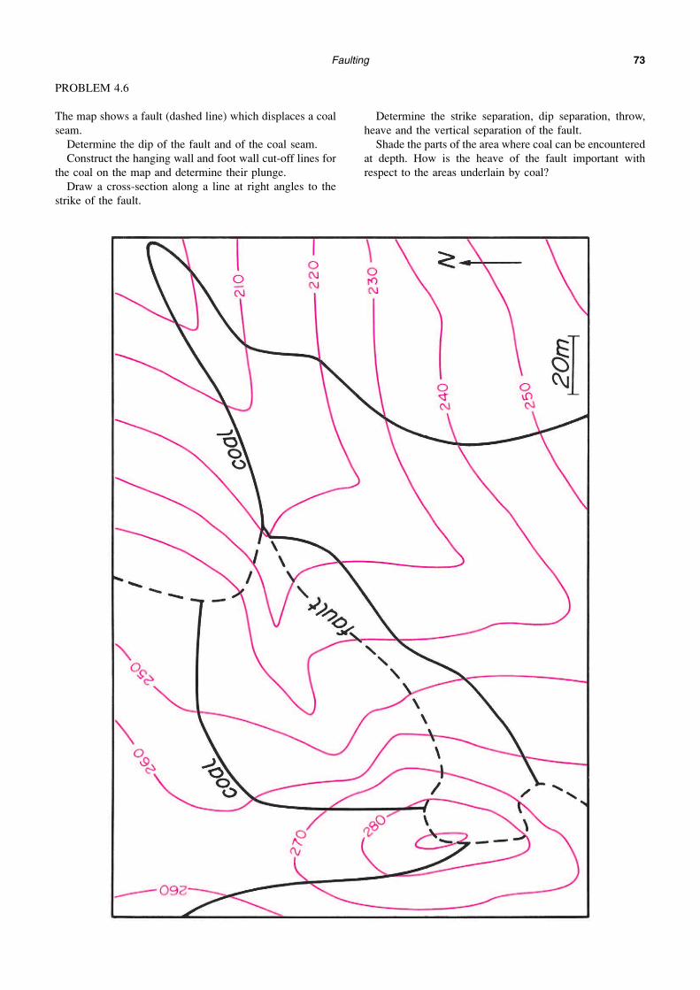
Faulting 73
PROBLEM 4.6
The map shows a fault (dashed line) which displaces a coal
seam.
Determine the dip of the fault and of the coal seam.
Construct the hanging wall and foot wall cut-off lines for
the coal on the map and determine their plunge.
Draw a cross-section along a line at right angles to the
strike of the fault.
Determine the strike separation, dip separation, throw,
heave and the vertical separation of the fault.
Shade the parts of the area where coal can be encountered
at depth. How is the heave of the fault important with
respect to the areas underlain by coal?

Faulting74
PROBLEM 4.7
Beds dipping at 60° are displaced by two faults ( f1 and f2);
f1 dips at 60° and f2 is vertical. Which fault is the
younger?
Determine the net slip of the younger fault.
Why is it not possible to find the slip on the older
fault?

Faulting 75
PROBLEM 4.8
The map shows Namurian rocks in West Lothian,
Scotland.
Study the map to identify fold hinges, fold axial traces
and faults.
Determine the approximate plunge and plunge direction
of the fold hinge lines.
Why does the strike separation vary along any one
fault?
Estimate the net slip on the most northerly of the faults.
(Assume that the faults are steep.)

Faulting76
PROBLEM 4.9
Using a sketch block diagram similar to Fig. 4.6 derive an
equation which relates the dip separation to the stratigraphic
separation. (Note: the dip separation depends on the dip of
the beds and the dip of the fault plane.)
Why is the term horizontal separation not used?
PROBLEM 4.10
Draw block diagrams like that in Fig. 4.16 to illustrate:
(a) a fault with strike separation equal to its dip
separation,
(b) a dip slip fault with zero dip separation,
(c) a strike slip fault (i.e. with zero dip slip component)
with dip separation.
PROBLEM 4.11
Referring to Fig. 4.7, given a fault with a dip separation of
35 m and that the cut-off line of bedding pitches in the plane
of the fault at 27°, calculate the strike separation.

77
5
Unconformity
THE succession of sedimentary rocks present in any
geographical area allows deductions to be made about the
geological history of that area. For example, the nature of
the sedimentary rocks indicates the physical environment in
which the sediments were laid down and how this
environment changed with time. In a particular area the
sedimentary rocks themselves contain only a partial record
of geological time since sedimentation is unlikely to have
gone on uninterrupted. Periods of sediment deposition are
likely to have alternated with intervals of non-deposition.
Although the breaks in sedimentation do not leave behind
rock products as hard evidence of their former existence,
they do give rise to characteristic structural relationships
between the rocks deposited before, and those deposited
after, the interval. The relationship which bears witness to a
period of non-deposition is called an unconformity. Because
of a discontinuity in the sedimentation, later sediments
come to rest uncomformably on older rocks. The contact
between the underlying rocks and the rocks which uncon-
formably overlie them is termed the surface of unconformity
or plane of unconformity. This surface may represent a
considerable length of time, and could therefore be of great
stratigraphic significance.
5.1 Types of unconformity
The exact nature of the relationship which defines an
unconformity depends to a large extent on the geological
events occurring during the period of non-deposition. If
erosion takes place an irregular erosion surface is formed
above the older rocks and defines the shape of the
topographic surface upon which the younger group of rocks
is deposited. This surface will become the surface of
unconformity (Fig. 5.1A). A parallel unconformity is where
the beds above and below the surface of unconformity have
the same attitude.
With an angular unconformity (Fig. 5.1B) tilting or
folding during the period of non-deposition gives rise to a
misorientation of the rocks below the surface of uncon-
formity relative to those above. When metamorphism and/
or igneous intrusion takes place in the inter-depositional
interval, the younger group of rocks rest in direct contact
with metamorphic and/or igneous rocks. This type of
unconformity is sometimes referred to as a non-conformity
(Fig. 5.1C).
Figure 5.2 shows some natural examples of
unconformities.
5.2 Overstep and overlap
The most conspicuous feature of many unconformities is the
way beds and, on a large scale, rock formations wedge out
against the surface of unconformity (Fig. 5.2). On a small
scale this same feature can be brought about by irregu-
larities in the surface of unconformity, and can therefore
occur in the case of parallel unconformities. On a regional
scale, such wedging-out exhibited on maps by a tapering out
of rock units against the surface of unconformity is likely to
signify an angular unconformity. Overstep and overlap are
terms which describe the angular relationship of strati-Fig. 5.1 Formation of unconformities.

Unconformity78
graphical boundaries to the surface of unconformity.
Overstep applies to the sub-unconformity relationship
where the surface of unconformity truncates stratigraphic
boundaries (Fig. 5.3). With distance along the unconformity
the overlying strata rest unconformably on successively
older rocks and are said to ‘overstep’ them. Overstep
usually owes its origin to tilting or folding during the pause
in sediment accumulation. Overlap (sometimes called
‘onlap’) refers to the situation above the surface of
unconformity. With overlap the sediments are deposited
oblique to the surface of unconformity (Fig. 5.3). With
distance along the unconformity, successively younger
rocks rest on the uncomformity plane. Successively younger
rocks units show greater lateral extent and thus ‘overlap’ the
previously deposited units. This type of unconformity can
result from deposition in a progressively expanding sed-
imentary basin relating to crustal subsidence. Figure 5.4
shows examples of overstep recognizable from maps.
Overlap and overstep are in no way mutually exclusive;
unconformities may show both features.
Fig. 5.2 Unconformities in the field. A: Portishead, England. Robert Lisle points to the surface ofunconformity. B: Barry Island, Wales. Triassic breccias rest unconformably on limestones of LowerCarboniferous age.
A
B
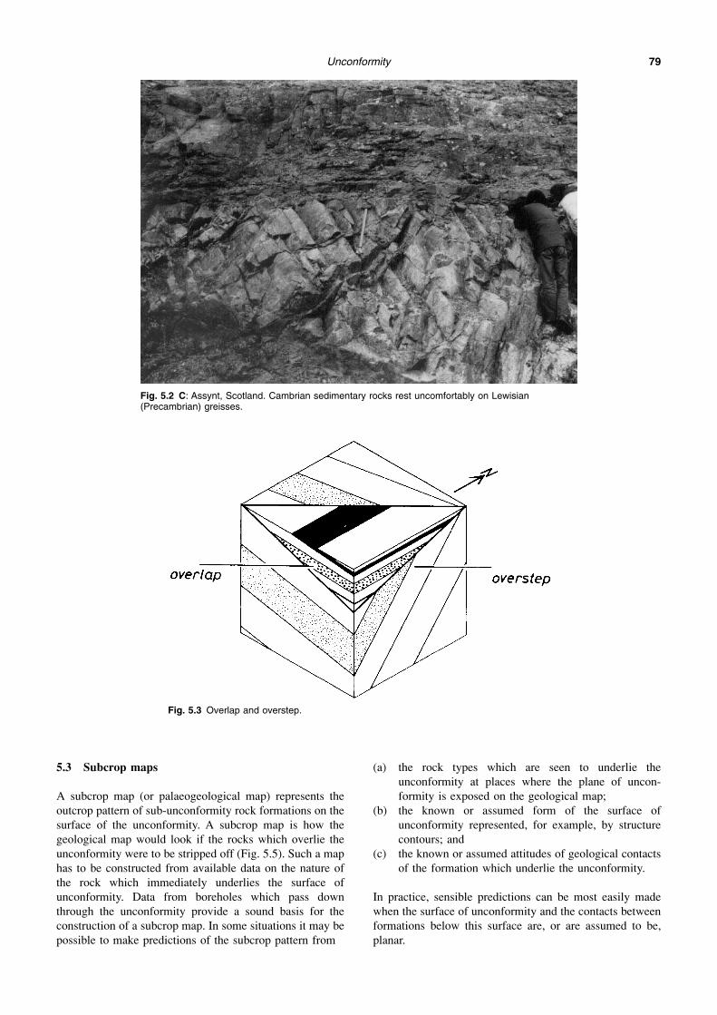
Unconformity 79
5.3 Subcrop maps
A subcrop map (or palaeogeological map) represents the
outcrop pattern of sub-unconformity rock formations on the
surface of the unconformity. A subcrop map is how the
geological map would look if the rocks which overlie the
unconformity were to be stripped off (Fig. 5.5). Such a map
has to be constructed from available data on the nature of
the rock which immediately underlies the surface of
unconformity. Data from boreholes which pass down
through the unconformity provide a sound basis for the
construction of a subcrop map. In some situations it may be
possible to make predictions of the subcrop pattern from
(a) the rock types which are seen to underlie the
unconformity at places where the plane of uncon-
formity is exposed on the geological map;
(b) the known or assumed form of the surface of
unconformity represented, for example, by structure
contours; and
(c) the known or assumed attitudes of geological contacts
of the formation which underlie the unconformity.
In practice, sensible predictions can be most easily made
when the surface of unconformity and the contacts between
formations below this surface are, or are assumed to be,
planar.
Fig. 5.2 C: Assynt, Scotland. Cambrian sedimentary rocks rest uncomfortably on Lewisian(Precambrian) greisses.
Fig. 5.3 Overlap and overstep.

Unconformity80
WORKED EXAMPLE
On the map (Fig. 5.6A) construct the subcrop of the thin
coal seam on the pre-Permian unconformity surface.
The line of subcrop corresponds to the intersection of
the coal seam with the surface of unconformity. If both
surfaces are planar, the line of subcrop will be straight.
This straight line will join all points where the coal crops
out on the surface of the unconformity. It will therefore
run as a straight line between points X and Y (Fig.
5.6B).
WORKED EXAMPLE
On the map (Fig. 5.7A) construct the subcrop of the
thin coal seam.
Fig. 5.4 Examples of unconformities displayed on maps and cross-sections.
Fig. 5.5 The concept of the subcrop map.
Fig. 5.6 Fig. 5.7 Calculating the subcrop of a coal seam.

Unconformity 81
From the given dips of the coal seam and surface of
unconformity, calculate the trend of the line of their
intersection using the method described in Section
3.11. Using the calculated trend, draw the subcrop of
the coal through the point Z on the map (Fig. 5.7B).
Vertically below all points on the map on the SE side of
this line it is possible to encounter coal at depth; to the
NW of this subcrop, the coal is absent.
5.4 The geological usefulness of unconformities
Geological map interpretation has two main facets. The first
is geometrical, and much of this book has been devoted to
the techniques for deducing the form of structures from the
patterns displayed on maps. The second aspect is historical
in nature, and is concerned with making deductions about
the relative ages of geological phenomena displayed on
maps. Unconformity is important in this second respect,
since it allows the ages of folding, faulting, metamorphism
and igneous activity relative to that of sedimentation to be
established.
As an example let us examine a map of the pre-Permian
unconformity in SW England (Fig. 5.4A). Folds are present
in the rocks below the unconformity and are absent in the
rocks above. Folding must therefore have occurred in the
time interval represented by the surface of unconformity.
The youngest rocks below the unconformity involved in the
folding are Upper Carboniferous (Westphalian) in age. The
oldest rocks above the unconformity are Permian in age.
Folding must therefore have taken place in the intervening
time interval.

Unconformity82
PROBLEM 5.1
Construct a cross-section for the line X–Y on the map.
Shade the regions on the map where the coal seam does not
exist at depth..

Unconformity 83
PROBLEM 5.2
Study the map and identify an unconformity. (The line
labelled f is a fault line.)
What type of unconformity is it?
Draw a subcrop map of the formations which underlie the
unconformity.
Discuss the age and movement on the fault.

Unconformity84
PROBLEM 5.3
Determine the net slip of the fault. What name is given to
this type of fault?
Identify an unconformity on the map and determine the
dip of the surface of unconformity.
Why does the fault appear not to displace the
unconformity?
Draw a subcrop map of the rocks below the
unconformity.

85
6
Igneous Rocks
THE maps so far discussed have involved layered piles of
rocks characteristic of successions of sedimentary rocks and
sequences of metamorphic rocks derived from such sedi-
ments. With the exception of unconformities, which repre-
sent sedimentary breaks or discontinuities, the layered
structure of such rocks arises from the deposition of beds of
sediment, one upon another.
A sequence of sediments may contain within it bodies of
rocks belonging to an important group called igneous rocks.
Igneous rocks are formed by the solidification of molten
rock or magma. They are described separately because they
may come into position in a way which is quite different
from the orderly ‘layer cake’ manner typical of sedimentary
rocks. For example they can be injected into a sequence of
rocks like jam into a doughnut.
The discussion of igneous rock varieties (in terms of
composition) is beyond the scope of this book. We will
concentrate here on the classification of igneous rock bodies
in terms of their form and structural relationship to adjacent
rocks. These aspects are the most relevant to the appearance
of igneous rocks on geological maps. This classification is
set out in Table 6.1.
6.1 Intrusive igneous rocks
These are bodies formed by the injection of magma into an
existing sequence of rocks. Many have a tabular form and
are called sheet intrusions. Sills have been intruded along
the layering or bedding of the sequence and are examples of
concordant sheet intrusions (Figs. 6.1A and 6.3). When
displayed on a map, a sill will follow the trend of other
geological units (Fig. 6.3). The Whin Sill of northern
England can be traced on the map from the Farne Islands,
off the Northumberland coast, southwards for some 170 km
to Teesdale. Its average thickness is about 30 m and it is
intruded into Carboniferous rocks but not always along
exactly the same stratigraphic horizon. The Whin Sill is
concordant over much of its trace but locally discordant. A
sill which is locally cross-cutting is called a transgressive
sill (Fig. 6.1B).
Dykes are sheet intrusions which are discordant, i.e. they
cut across the layering of the rocks they are intruded into
(Figs. 6.2 and 6.3). They usually have steeply dipping
contacts. Many dykes occur in the Inner Hebrides region of
Scotland, which was a centre of intrusive igneous activity
during the Tertiary. These dykes form swarms which are sets
of parallel or radiating dykes. As can be seen from a
geological map of the southern part of the Isle of Arran,
dolerite dykes belonging to the swarm can be very closely
spaced. On a map dykes stand out because of their discordant
nature. Their relatively straight course compared to the other
formations on a map is explained by their near-vertical
attitude. Dykes can often be followed in the field because of
their effect on the topography. In spite of their name, dykes
do not always form a positive feature (such as a ridge) on the
ground. Sometimes they weather out more than the rocks
they are intruded into, and form a linear depression.
Not all intrusive igneous bodies are sheet-like in form.
Batholiths are large bodies usually composed of acid
plutonic rock. Their contacts may be irregular in shape but
the body often has an overall dome-like form with an upper
contact (roof) which is more flat-lying than the steeper
inclined walls (Fig. 6.4). In detail the upper part of the body
may protrude into the country rocks of the roof to form a
cupola. If the roof has a depression in it, the country rock
will extend to a deeper level into the batholith. The resulting
structure is a roof pendant. By erosion removing the roof of
country rock, the igneous rocks making up the batholith
may crop out at the surface. They are typically bodies which
are roughly circular or oval in plan. Depending on the exact
level of the erosion surface relative to the height of the roof,
roof pendants and cupolas may form isolated closed
contacts between igneous rock and country rock on the map.
Stocks are smaller versions of batholiths. In SW England six
granite stocks which occur at Dartmoor, Bodmin Moor, St
Austell, Carnmenellis, Land’s End and the Scilly Isles may
represent cupolas of a single larger batholith at depth (Fig.
Table 6.1
Examples
Intrusive
igneous rocks
Concordant bodies
Discordant bodies
Sills
Dykes, volcanic necks,
batholiths
Extrusive
igneous rocks
Lava flows, volcaniclastic
deposits

Igneous Rocks86
6.5). The country rocks adjacent to batholiths (and to a
lesser extent some minor intrusions) often show marked
evidence of being affected by the heat emanating from the
intrusion. This metamorphism of rocks produced by their
proximity to an intrusion is called contact metamorphism.
The zone consisting of metamorphosed rocks is called a
metamorphic aureole, and is displayed on maps as a zone
encircling or running parallel to the contacts of the
intrusion.
Volcanic rocks or plugs represent the solidified magma
and other volcanic rocks filling the pipe (vent) of former
volcanoes of central type. Erosion produces a roughly
circular map pattern which is a cross-section of the
cylindrical pipe.
The subsurface form of discordant intrusions is fre-
quently difficult to deduce from the form displayed on a
map. For example, Fig. 6.6A shows two isolated outcrops of
igneous rock. Are they truly separate bodies or are they
really connected at depth? When the contact is cut by
topographic contours on the map, structure contours can be
constructed and the dip deduced in the usual way (Section
2.9). However, the topographic relief is often strongly
Fig. 6.1 Concordant sheet intrusions. A: Intrusion within deformed Precambrian quartz schists(Dombas, Oppdal, Norway). B: Transgressive sill (Banks Island, Northwest Territories, Canada).(Geological Society of Canada.).
A
B

Igneous Rocks 87
Fig. 6.2 Dyke of basic igneous rock (dolerite) cutting Lewisian gneiss with banding that dips gentlyto the right of the picture. Lewis, Outer Hebrides.
Fig. 6.3 Sheet intrusions.
Fig. 6.4 Features associated with batholithic intrusions.
Fig. 6.5 The SW England batholith.
Fig. 6.6 Relations between the intrusion and structures in thecountry rock.

Igneous Rocks88
influenced by the presence of a body of igneous rock which
denudes differently from the country rock. For example, a
stock could form an area of upland with topographic
contours following the contact of the intrusion (Fig. 6.6B).
In these situations the structure contour method should be
applied with caution. For example, the intrusion contact in
Fig. 6.6B could easily be misinterpreted as having a
horizontal attitude from the fact that it runs parallel to
topographic contours on the map (compare Section 2.14).
The uneven width on the map of a metamorphic aureole
may provide a hint as to the variable dip of an intrusion’s
contacts (Fig. 6.6C).
The discordant nature of a contact may not be obvious on
a map (Fig. 6.7). It should be realized that certain sections
through a discordance will show a concordant relationship.
Do not base your interpretation solely on a relationship at
one point of the map. The intrusive character of an igneous
body may be made less obvious by later deformation of the
rocks of the area. The strain (distortion) suffered by the
rocks has the effect of modifying angles between planar
structures. In this way an angle of discordance between a
dyke and the enclosing rocks could be reduced. The result
will be to make the dyke appear as sill. Intrusive igneous
bodies can also provide vital evidence for establishing a
geological history of an area. Figure 6.8 shows a dyke
which intrudes a sequence of rock labelled A. The intrusion
of the dyke clearly postdates the rocks of that sequence. The
dyke does not intrude the sequence labelled B. We can
conclude from this that sequence B was formed after dyke
intrusion. The contact between A and B must represent the
interval of time within which dyke intrusion occurred. This
contact is therefore a plane of unconformity.
6.2 Extrusive igneous rocks
These rocks are formed from the products of volcanoes.
Outpourings of lava on the earth’s surface, and accumula-
tions of fragments ejected from a volcano (volcaniclastic
rocks), form sheets of volcanic rock. These rocks, extruded
on land or under the sea, will rest on the rocks which form
the subsurface at the time of eruption. They can lie
conformably or unconformably with respect to the rocks
beneath and above. When conformable, these sheets of
volanic material could resemble sills when displayed on the
geological map. The transgressive or bifurcating (splitting)
nature of sills will sometimes allow them to be dis-
tinguished from lava flows. The presence of contact
metamorphic alteration of the overlying country rock would
indicate a sill rather than an extrusive igneous rock. If the
igneous rock includes fragments (xenoliths) of the overlying
country rock this would also rule out an extrusive origin.
Fig. 6.7 Discordant intrusion can appear concordant on somecross sections.
Fig. 6.8 A dyke intruding rock sequence A but not the overlyingrocks B indicates the presence of an unconformity between A andB.

Igneous Rocks 89
PROBLEM 6.1
Rock types 1, 2 and 3 are intrusive igneous rocks and the
rock types labelled m are contact metamorphic rocks. List
the types of intrusions present in the area. Faults are shown
by a dashed line (4 in a key). Give a name to the types of
faults present and deduce as much as you can about the slip
on these faults.
List, in order of time, the geological events which have
affected the area.

Igneous Rocks90
PROBLEM 6.2
Construct a cross-section along the line of section X-Y. List,
in chronological order, the geological events which have
affected the area.

Igneous Rocks 91
PROBLEM 6.3
Construct a cross-section along the line of section X-Y. List,
in chronological order, the geological events which have
affected the area. Comment on the type of movement on the
fault.

Igneous Rocks92
PROBLEM 6.4
The map shows the geology of part of the Assynt District in
Sutherland (NW Highlands of Scotland).
The rocks labelled G are Lewisian gneisses (coarse-
grained, banded metamorphic rocks) of Precambrian age.
The banding (layering) in the gneisses is strongly folded.
Rock types P and Q are unmetamorphosed sediments,
Cambrian in age. S are unmetamorphosed sandstones
(Torridonian). D are igneous rocks.
Estimate the dip and dip direction of the Cambrian
rocks.
Study the contact between the Lewisian gneisses and the
Torridonian sandstones. For example, does the dip of this
contact match the dips within the Torridonian Sandstone?
Explain the shape of this contact and its significance.
List, in chronological order, the geological events which
have occurred. What do the bodies of igneous rock tell us
about relative ages of the rock units in the area?
Draw a cross-section along the line A-B.

Igneous Rocks 93
PROBLEM 6.5
The geological map of New Cumnock (Dumfries) area
(scale 1. 50,000, British Geological Survey, Sheet 15W)
displays clearly the structural relationships of a variety of
igneous rock bodies.
If this map can be consulted, deduce the geological
history of that area.

94
7
Folding with Cleavage
7.1 Foliations
In earlier chapters we have considered sedimentary rocks
which possess a planar structure called bedding. The
general name given to planar structures such as bedding is
foliation. We say that bedding is a primary foliation because
it is an original structure in the sediment and produced
during sedimentation.
Other planar structures are produced in the rock at a later
stage. During periods of earth movement, crustal rocks
become subjected to stress (pressures which are not equal in
all directions, but are greatest in one direction and least in a
direction at right angles to the greatest pressure). Providing
the rocks are ductile (are able to deform without fracturing)
these stresses produce a permanent distortion or strain in the
rocks.
Fig. 7.1 A: Slaty cleavage. Electron microscope image (scale baris 20 µm long) of a Cambrian roofing slate to show the alignment offlaky minerals (mainly chlorite). This is typical of the microscopicstructure of slaty cleavage. (Photograph: Prof. W. Davies.)

Folding with Cleavage 95
The straining may be accompanied by a reorganization of
the microscopic structure of the rock. Helped by a chemical
alteration of the rocks, grains making up the rock may
change shape and rotate so that their long dimensions turn
away from the direction of greatest shortening in the rock.
The new alignment of grains gives the rock a ‘grain’ or
fabric. This structure is a type of secondary foliation.
The secondary foliation present in the finer-grained
metamorphic rocks, such as slates, is called cleavage. Slaty
cleavage usually gives a rock a well-developed ability to
split into thin plates. Roofing slates, such as those of the
Cambrian of North Wales, owe their fissility to the presence
of slaty cleavage. Slaty cleavage is expressed on a
microscopic scale by the alignment of grain shapes (Fig.
7.1A). From the shape of distorted (strained) fossils in
cleaved rocks it can be demonstrated that slaty cleavage
planes have formed perpendicular to the direction of
greatest shortening. Crenulation cleavage is a foliation
which is produced by a crinkling (small-scale folding, folds
having a wavelength of about 1–10 mm) of pre-existing
foliation. The crenulation cleavage planes are parallel to the
axial planes of these microfolds (Fig. 7.2).
7.2 Axial plane foliations
The strains needed to produce a cleavage in a rock are
similar to those suffered by the rock’s layers which have
been forced to shorten and buckle to produce folds. Not
surprisingly then, cleavage often occurs in rocks which are
strongly folded. Cleavage and other foliations often have an
attitude close to that of the axial plane (axial surface) of the
fold (Figs. 7.3, 7.4). The axial plane cleavage developed
around a fold may not be perfectly parallel to the axial
surface, but may vary in orientation across the fold (to
define a cleavage fan) or from one bed to another (a feature
called cleavage refraction (Fig. 7.4B).
7.3 The relationship of cleavage to bedding
An axial plane foliation in most instances has an attitude
which is oblique to bedding (Figs. 7.3, 7.4). An exception to
this occurs in the hinge region of the fold where foliation
and bedding are at right angles to each other. It can also be
seen from Fig. 7.3 that the sense of obliquity between
cleavage and bedding is different on each limb of the fold,
i.e. these planes intersect one another in opposite senses.
This fact is extremely important since it means that, by
comparing cleavage and bedding attitudes at an outcrop, we
are able to deduce our position with respect to large-scale
folds in an area.
WORKED EXAMPLE
Figure 7.5A shows a sketch of a rock outcrop where
bedding and cleavage are visible. It is known that the
bedding is folded in this area, and that the cleavage is
axial planar to these folds. What can be deduced about
these folds from the information at this outcrop?
We look first at the dip of the cleavage. This dips
moderately to the left (west) and from this we should
visualize folds occurring within the area with axial
planes having the same dip. Some possible folds with
westerly dipping axial planes are drawn in Fig. 7.5B. If
Fig. 7.1 B: Slaty cleavage in the field. Bedding dips gently to the left; cleavage more steeply to theleft of the photograph.

Folding with Cleavage96
Fig. 7.2 Crenulation cleavage. A: The microscopic appearance of crenulation cleavage (set ofplanes sloping at 60° towards the left of the photograph). The crenulation cleavage is parallel to theaxial planes of small folds which fold an earlier (older) foliation and bedding (appears vertical, labelledSo), Tayvallich Slates, Oban, Scotland. (Photograph: Dr. G. Borradaile.) B: Crenulation cleavage(running diagonally across the photograph, top right to bottom left). Precambrian schists, Anglesey.
A
B

Folding with Cleavage 97
Fig. 7.3 The arrangement of small-scale folding andaxial plane foliation (such as cleavage) in alarger-scale fold.
Fig. 7.4 A: Cleavage in relation to folds. The sense of obliquity between bedding and an axial planecleavage at an outcrop can be used to interpret the position of the outcrop in relation to thelarger-scale antiforms and synforms.
A

Folding with Cleavage98
Fig. 7.4 B: Close up of Fig 7.4A, showing cleavage refraction.
Fig. 7.4 C: Axial plane cleavage.
B
C

Folding with Cleavage 99
we consider one such fold of antiformal type, we find
that the bedding/cleavage relationship on its east limb
matches that observed at the outcrop. We can con-
clude from this that the outcrop is situated on the east
limb of an antiformal fold. In other words, we have
deduced that the next fold hinge to the west of the
outcrop is an antiform. We are, of course, not able to
say how far to the west the antiform is.
This method of deciding where the next antiform is located
is extremely useful in areas of tightly folded rocks, since in
these areas the attitude of the limbs of the fold is not
sufficiently different to allow each of the limbs to be
distinguished on the basis of bedding dip alone.
With overturned folds, both limbs dip in roughly the same
direction and on one of the limbs the beds are upside-down.
Providing the folds are upward-facing (i.e. the antiforms are
anticlines, the synforms are synclines), the overturned beds
can be identified from the fact that on this limb the bedding
will dip more steeply than the cleavage planes.
Fig. 7.5

Folding with Cleavage
PROBLEM 7.1
A shows a vertical outcrop face at Ilfracombe, Devon,
England, on which the traces of bedding and cleavage are
visible. The cleavage, which exhibits refraction, is parallel
to the hammer handle in that part of the outcrop (north is to
the left of the photograph).
B shows a horizontal exposure at Tayvallich, Argyllshire,
Scotland, on which a normally graded sandstone bed crops
out. The trace of cleavage is also visible and is parallel to
the pen (north is to the left of the photograph).
Describe, with the aid of a sketch-map or cross-section,
the possible larger-scale fold structures to which the
structures at each of these outcrops belong.
A
B
100

Folding with Cleavage 101
PROBLEM 7.2
Interpret the structure from the bedding/cleavage data along
the road section.
Describe the folds present. Assuming these folds to be
upward-facing, locate the outcrops with inverted bedding.

102
Further Reading
(a) Geological map interpretation: general
A. Maltman, Geological Maps: an Introduction, 1998,
Open University Press
C.A. Boulter, Four-dimensional Analysis of Geological
Maps, 1989, Wiley and Son
G.M. Bennison and K.A. Moseley, An Introduction to
Geological Structures and maps, 1997, Arnold
D.M. Ragan, Structural Geology, 1985, Wiley and Sons
(b) How geological maps are produced
J.W. Barnes, Basic Geological Mapping, 1991, Open
University Press
N. Fry, The field description of Metamorphic rocks, 1984,
Open University Press
K. McClay, The Mapping of Geological Structures, 1991,
Open University Press
(c) The geometry of structures and deformation ofrocks
J.G. Ramsay and M. Huber, The Techniques of Modern
Structural Geology, 1984, Academic Press
R.G. Park, The Foundations of Structural Geology, 1983,
Blackie
S. Marshak and G. Mitra, Basic Methods in Structural
Geology, 1988, Prentice Hall
(d) Foliations, fabrics and the study of structuresunder the microscope
G.J. Borradaile, M.B. Bayly and C. McA Powell (eds),
Atlas of Deformation and Metamorphic Rock Fabrics,
Springer-Verlag
B.E. Hobbs, W.D. Means and P.F. Williams, An Outline of
Structural Geology, 1976, Wiley and Sons

103
Index
Accordion fold, 33
Andes, 29
Angle of dip, 2, 13, 16
Anglesey, Wales, 3, 96
Angular unconformity, 77
Anticline, 32, 47, 99
Antiform, 32, 38,42, 47, 49, 97, 99
Apparent dip, 5, 9, 17
Assynt Scotland, 79, 92
Asymmetrical fold, 33
Axial plane, 95
Axial plane cleavage, 95, 98
Axial plane foliation, 97
Axial surface, 30, 31, 33, 34, 42, 53, 95
Axial surface trace, 41, 42, 46
Axial trace, 41, 49
Barry, Wales, 78
Basin, 35, 36
Batholith, 85
Bed thickness, variations in folds, 53
Bedding, 2, 3, 94
Bedding plane fault, 61
Bedding, horizontal, 2, 12
Beds, vertical, 12
Block diagram, 17
Bodmin Moor, 85
Borehole, 1, 60, 68
Borehole data, 24, 79
Boundaries, geological, 17
Boundaries, interpreting position of, 13
Bristol Coalfield, 80
Broadway, Worcestershire, 1
Bude, Cornwall, 67
Burial depth, 11
Bury St Edmunds, 24
Cambrian slate, 94
Canoe fold, 33, 35, 49
Carboniferous limestone, 50
Carnmenellis, 85
Chevron fold, 33
Cleavage, 94, 100
Cleavage fan, 95
Cleavage refraction, 95, 98
Cleavage, in relation to fold, 97
Clinometer, 4
Close fold, 33
Closure, direction of, 32
Coal, 28
Coal seam, 10, 22, 28, 73, 81
Compass-clinometer, 4
Components of slip, 64, 65
Concertina fold, 33
Concordant intrusions, 85, 86
Concordant sheet intrusions, 86
Conglomerate, 3
Contact metamorphism, 86, 88
Contact, geological, 6, 13
Contour interval, 9, 13, 37
Contour lines, 6, 8
Contour maps, 7
Contour patterns, v-shaped, 7
Contour spacing, 9, 13, 36, 37
Contours, structure, 7, 8, 10, 13, 14, 15, 34
Contours, topographic, 7, 10, 12
Core, of fold, 32
Country rock, 85, 86, 87
Crenulation cleavage, 95, 96
Crest line, 36, 44
Cross section, 8, 9, 10, 15, 29, 38, 42
Cross-sections, scales of, 8
Culmination fold, 33
Cupola, 85, 87
Cut-off line, 60, 61
Cut-off point, 60, 61
Cylindrical fold, 29, 30, 36
Dartmoor, 85
Depression, 33
Depth of burial, 11
Derbyshire, 49
Devon, 80
Dextral, 62
Dextral slip, 65, 66
Dextral slip fault, 66
Dip, 2, 9, 53
Dip angle, 13
Dip direction, 4, 5, 8, 17

Index104
Dip fault, 61
Dip of beds, 61
Dip separation, 62, 65, 66, 69, 70,73, 76
Dip slip, 65, 76
Dip slip component, 69, 70
Dip slip fault, 66
Dip, angle of, 16
Dip, apparent, 5, 9, 17
Dip, direction of, 2
Dip, true, 5
Direction of closure, 32
Direction of dip, 17
Direction of dip, 2, 4,8
Direction of plunge, 4, 37
Discordant intrusion, 85, 86, 88
Disharmonic fold, 30, 31
Dome, 7, 35, 36
Down-plunge viewing
Downthrow, 62
Downward facing, 47
Duplication of strata by faulting, 63
Dyke, 85, 87, 88
Enveloping surface, 33
Erosion, 77, 86
Extrusive igneous rocks, 85
Facing, 32, 99
Farne Islands, 85
Fault line, 60
Fault plane, 60, 64
Fault slip, 61
Fault trace, 60
Faulting, 59, 81
Fold, 2
Fold axial surface, 32, 33
Fold axis, 29, 37
Fold core, 32
Fold culmination, 33
Fold hinge, 32, 75
Fold hinge line, 75
Fold limb, 31, 36,37,64
Fold plunge, 36, 37,48
Fold, accordian, 33
Fold, accordion, 33
Fold, asymmetrical, 33
Fold, axial surface, 31
Fold, basin, 35
Fold, canoe, 33, 35
Fold, chevron, 33
Fold, close, 33
Fold, concertina, 33
Fold, cylindrical, 29, 30
Fold, disharmonic, 30, 31
Fold, dome, 35
Fold, facing of, 32
Fold, gentle, 33
Fold, harmonic, 30, 31
Fold, mushroom, 33
Fold, neutral, 32
Fold, non-cylindrical, 29, 35
Fold, non-plunging, 31
Fold, non-plunging, 32
Fold, open, 33
Fold, overturned, 33
Fold, parallel, 34, 35
Fold, periclinal, 33
Fold, plunging, 39
Fold, reclined, 32
Fold, recumbent, 31, 32
Fold, saddle, 33, 35
Fold, shoe horn, 33, 35
Fold, similar, 34
Fold, symmetrical, 33
Fold, tight, 33
Fold, upright, 31, 32
Fold, vertical, 31, 32
Fold, whaleback, 33, 35
Folding, 29, 81
Folds, recognition on maps, 40
Foliation, 94
Foot wall, 60, 65, 73
Fractures, 59
Gentle fold, 33
Geological boundaries, 17
Geological contact, 6, 13
Geological history, 1
Geological surface, 8, 11
Geomorphology, 1
Geophysics, 1
Gloucestershire, 50
Gower, 16
Grand Canyon, 20
Ground, slope of, 7
Hanging wall, 60, 65, 73
Harmonic fold, 30, 31
Heave, 61, 62, 63, 70
High-angle fault, 60
Hills, isolated, 7
Hinge, 30, 31, 32, 34
Hinge line, 30, 31, 32, 37, 41, 53
Hinge point, 41, 42, 49, 64
Hinge zone, 30
Horizontal bedding, 2
Horizontal beds, 12
Horizontal separation, 76
Horizontal thickness, 14
Horizontal thickness, 15
Igneous activity, 81
Igneous intrusion, 77
Igneous rocks, 85
Ilfracombe, Devon, 100

Index 105
Inflection line, 29, 33
Inlier, 42, 43, 48
Inner Hebrides, 85
Interlimb angle, 33, 50
Interpreting position of boundaries, 13
Isobath, 11,12, 15
Isochores, 15
Isoclinal fold, 33
Isolated hills, 7
Land use, 1
Land’s End, 85
Lava flow, 85
Left lateral, 62
Lewisian gneiss, 79, 87, 92
Limb, 53
Limb, of fold, 31, 65
Limestone, 3
Limestone, oolitic, 1
Line of intersection of two surfaces, 37
Low-angle fault, 60
Low-angle reverse fault, 67
Magma, 85
Map, contour, 7
Map, topographic, 1
Metamorphic aureole, 86, 87, 88
Metamorphic rocks, 85
Metamorphism, 77, 81
Metasediments, 31
Millook, Cornwall, 34
Morocco, 26
Mushroom fold, 33
Namur, Belgium, 48
Net slip, 63, 64, 65, 66, 74,75
Neutral fold, 32, 38
Nonconformity, 77
Non-cylindrical fold, 29, 35, 36
Non-plunging fold, 31, 32
Nordland, Norway, 34
Normal fault, 67
Normal separation, 63
Normal separation fault, 66
Normal slip, 65
Normal slip fault, 66
Oban, Scotland, 96
Oblique cross section, 38
Oblique slip fault, 66
Omission of strata caused by faulting, 63
Oolitic limestone, 1
Open fold, 33
Oppdal, Norway, 86
Outcrop, 6, 10, 11
Outcrop patterns, 10, 40
Outcrop patterns, effect of topography, 6
Outcrop, width of, 15
Outer Hebrides, 87
Outlier, 42, 43, 48
Overlap, 78, 79
Overstep, 78, 79
Overturned beds, 99
Overturned fold, 33
Palaeogeological map
Parallel fold, 34, 35, 38, 50
Parallel unconformity, 77
Periclinal fold, 33, 49
Permo-Trias, 80
Plunge, 4, 41
Plunge direction, 4
Plunge of fold, 42
Plunging fold, 36, 38, 53, 85
Plunging fold, 39
Plutonic igneous rock, 85
Portishead, 78
Primary foliation, 94
Reclined fold, 32
Recumbent fold, 31
Recumbent fold, 32
Repetition of beds by faulting, 63
Reverse separation, 63
Reverse slip, 65
Reverse slip faults, 66
Right lateral, 62
Roof pendant, 85, 87
Saddle, 33, 35, 49
Scales of cross-section, 8
Scilly Isles, 85
Secondary foliation, 95
Section, topographic, 9
Sense of dip separation, 70
Sense of strike separation, 70
Separation, 65
Sheet intrusions, 64, 85
Shoe horn, 33, 35, 49
Sill, 85, 87, 88
Similar fold, 34, 35, 38, 50
Sinistral, 62
Sinistral slip, 65
Sinistral slip fault, 66
Slaty cleavage, 95
Slip, 69
Slip classification of faults, 66
Slope of ground, 7
St Austell, 85
Stock, 85
Strain, 88, 94
Stratigraphic separation, 61, 62, 76
Stratigraphic sequence, 68

Index106
Stratigraphic thickness, 14, 34, 35
Strike, 5, 8, 16, 17
Strike fault, 61
Strike lines, 4
Strike separation, 61, 62,63, 65, 66, 69, 70, 75, 76
Strike slip, 65
Strike slip component, 69, 70
Strike slip fault, 66
Structure contours, 7, 8, 10, 13, 14, 15, 34, 36, 37, 60,
79, 86
Subcrop map, 79, 80, 83, 84
Surface of unconformity, 77, 78, 79, 84
Surface, enveloping, 33
Surface, geological, 8, 11
Surface, topographic, 8
Svartisen, Norway, 39
SW England, 81
SW England batholith, 87
Symmetrical fold, 33, 38
Syncline, 32, 33, 47, 80, 99
Synform, 32, 38, 39, 42, 47, 49, 97
Tayvallich slates, 96
Tayvallich, Scotland, 100
Tear fault, 66
Tectonic contact, 60
Tectonic deformation, 77
Teesdale, 85
Thickness, horizontal, 14, 15
Thickness, stratigraphic, 14, 34, 35
Thickness, true, 14
Thickness, vertical, 14, 15
Three-point problem, 9, 13
Throw, 61, 62, 73
Throw of fault, 70
Thrust fault, 66, 70
Tight fold, 33
Tightness, 33
Tightness, 38
Topographic contours, 7,10, 12, 86, 88
Topographic map, 1
Topographic section, 9
Topographic surface, 8
Torquay, Devon, 67
Torridonian sandstones, 92
Transcurrent fault, 66
Transgressive sill, 85
Trough line, 36, 44
True dip, 5
True fold profile, 38
True profile, 40, 50
True thickness, 14
Unconformity, 64, 77, 80, 85, 88
Unconformity surface, 80
Upright fold, 31, 32, 39
Upward facing, 47, 99
Variscan folding, 48
Veins, 64
Vertical beds, 12
Vertical fault, 69
Vertical fold, 31, 32
Vertical separation, 61
Vertical separation, 73
Vertical thickness, 14, 15
Volcanic plug, 86
Volcaniclastic rocks, 88
Volcano, 88
V-rule, 12
V-shaped contour patterns, 7
V-shaped outcrops, 40, 41
Welcombe, Devon, 39
West Lothian, Scotland, 75
Whaleback fold, 33, 35, 49
Whin Sill, 85
Width of outcrop, 15
Wrench fault, 66
Xenoliths, 88
Younging direction, 47
Zagros Mountains, 45


![An introduction to geological structures and maps, 5th ed. [george m. bennison, 1990]](https://img.pdfslide.us/doc/110x75/55a89ee31a28ab99188b4900/an-introduction-to-geological-structures-and-maps-5th-ed-george-m-bennison-1990.jpg)