GeoLearn Manual

Version 2.0 Release

2

GeoLearn was created as a joint collaboration between the Civil and Environmental Engineering (CEE) Department at the University of Illinois at Urbana-Champaign (UIUC) and the National Center for Supercomputing Applications (NCSA) at UIUC. Funding support was provided by National Aeronautics and Space Administration (NASA), National Archive and Record Administration (NARA), and National Science Foundation (NSF). The majority of the code is based on Image to Learn (Im2Learn) developed at NCSA with additional calls to (a) HDF5 library developed by NCSA, (b) ArcGIS Engine developed by ESRI to perform data integration, and (c) Data To Knowledge (D2K, Version 4.1.2) developed by NCSA to perform decision tree modeling. The NASA project was led by the principal investigators Praveen Kumar (CEE UIUC) and Peter Bajcsy (NCSA UIUC). Praveen Kumar served as the principal investigator for the NSF project. The NARA project was led by the principal investigator Peter Bajcsy (NCSA UIUC). The main programming contributions to GeoLearn came from Chulyun Kim (NCSA UIUC), Qi Li (NCSA UIUC), Vikas Mehra (CEE UIUC), Rob Kooper (NCSA UIUC), Wei-Wen Feng (NCSA UIUC), Yakov Keselman (NCSA UIUC), Pratyush Sinha (CEE UIUC), and Peter Bajcsy (NCSA UIUC). Additional help with the software requirement specifications and code release came from Amanda White (CEE UIUC), Ben Ruddel (CEE UIUC), and Tim Nee (NCSA UIUC). This document represents a preliminary user guide for an on-going research and development project and hence the code is viewed as a research effort rather than as a commercial package. Revision History Revision Date Author Notes 0.1 10/14/2005 PB, VM Initial version of the document 1.0 01/06/2006 PB, RK Initial release of the software 2.0 b 2 11/01/2006 PB, TN GeoLearn V2 Beta 2.0 2.0 b 3 11/13/2006 PB, TN GeoLearn V2 Beta 3.0 2.0 Release 11/28/2006 PB, TN GeoLearn V2 Release

3

Table of Contents Table of Contents ................................................................................................................3

Introduction .........................................................................................................................5

Chapter 1 Installation Instructions................................................................................8 1.1 Hardware requirements ...........................................................................................8 1.2 Software requirements.............................................................................................8 1.3 Installation steps ......................................................................................................8

1.3.1 Data to Knowledge (D2K).................................................................................8 1.3.2 ArcGIS Engine ..................................................................................................8 1.3.3 Modis Reprojection Tool (MRT) ......................................................................9

1.4 Notes about Execution.............................................................................................9 1.5 Notes about Data ...................................................................................................10

Chapter 2 Description of Test Data Sets ....................................................................11 2.1 Raster Files ............................................................................................................11

2.1.1 HDF EOS.........................................................................................................11 2.1.2 TIFF.................................................................................................................11 2.1.3 SRTM ..............................................................................................................11 2.1.4 Arc Grid...........................................................................................................11 2.1.5 Other supported file formats............................................................................12

2.2 Vector Files ...........................................................................................................12 2.2.1 ESRI Shapefiles...............................................................................................12 2.2.2 Other supported file formats............................................................................12

Chapter 3 Description of Processing Steps.................................................................13 3.1 Load Raster............................................................................................................13

3.1.1 Adding and Removing files.............................................................................13 3.1.2 Mosaic .............................................................................................................16 3.1.3 Functionality....................................................................................................17

3.2 Integration..............................................................................................................18 3.2.1 Parameters .......................................................................................................20

3.3 Create Mask...........................................................................................................22 3.3.1 Purpose of the Create Mask step .....................................................................22 3.3.2 How to Create masks.......................................................................................23

3.4 Attribute Selection.................................................................................................30 3.5 Data-Driven Modeling...........................................................................................30 3.6 Visualization..........................................................................................................30 3.7 File Menu...............................................................................................................31

3.7.1 Import Menu....................................................................................................31 3.7.2 Save and Save All............................................................................................32 3.7.3 Look and Feel ..................................................................................................32 3.7.4 Exit ..................................................................................................................32

3.8 Process HDF Files .................................................................................................33 3.9 Load Other Files ....................................................................................................37 3.10 Extract Hydro Features..........................................................................................38 3.11 Import SpecialBinTable and SpecialTextTable with GeoInfo ..............................39

4

3.11.1 Additional information about the Geoinfo parameter .....................................40 3.12 Open URL Browser ...............................................................................................43 3.13 MRT Reprojection.................................................................................................45

Chapter 4 GeoLearn for Out-of-Core Tables .............................................................46 4.1 Export Large Table Step........................................................................................46

Chapter 5 Additional Notes ........................................................................................46 5.1 Bug Reports and Bug Fixes ...................................................................................46 5.2 Known Problems ...................................................................................................46

5.2.1 Out of Memory Errors .....................................................................................46 5.2.2 Other Problems................................................................................................48 5.2.3 Additional Notes..............................................................................................48

5.3 Acknowledgments .................................................................................................48 5.4 License Agreement ................................................................................................48

5

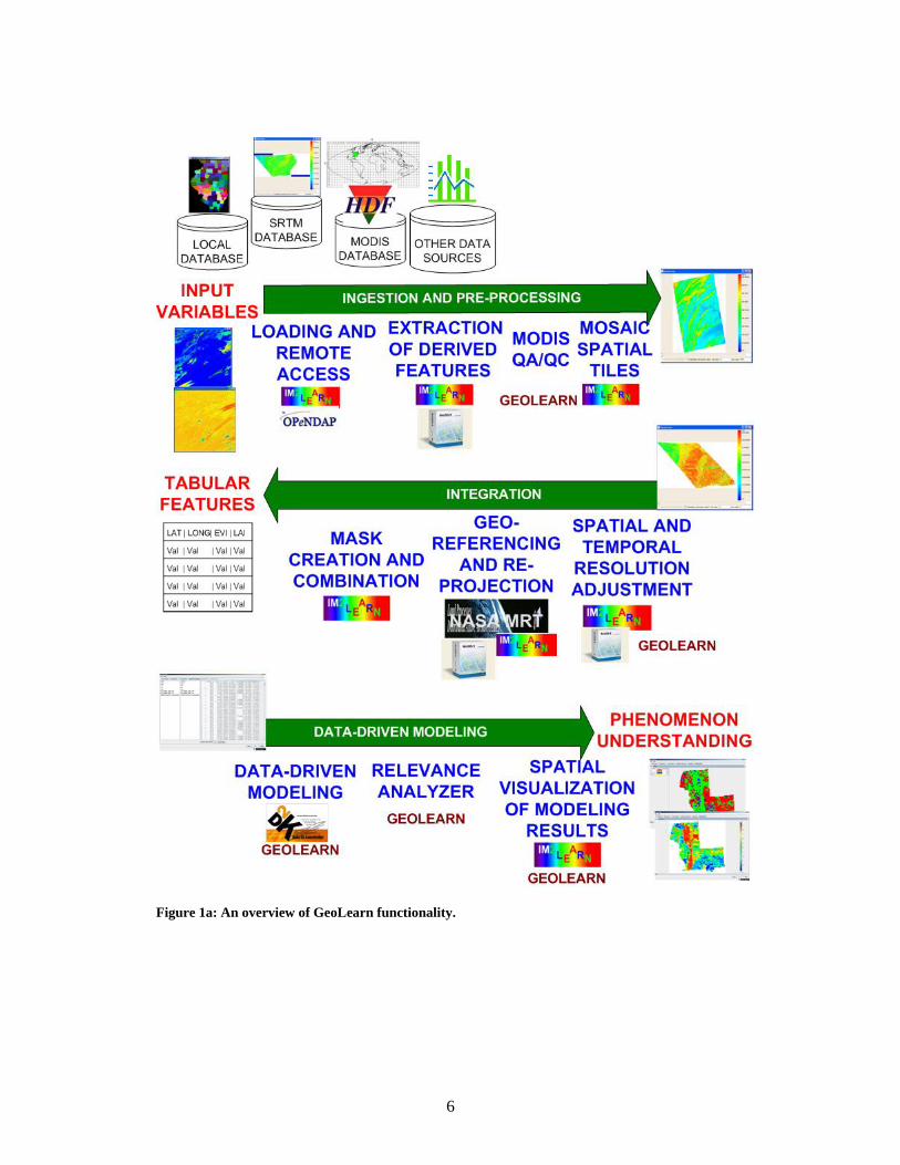
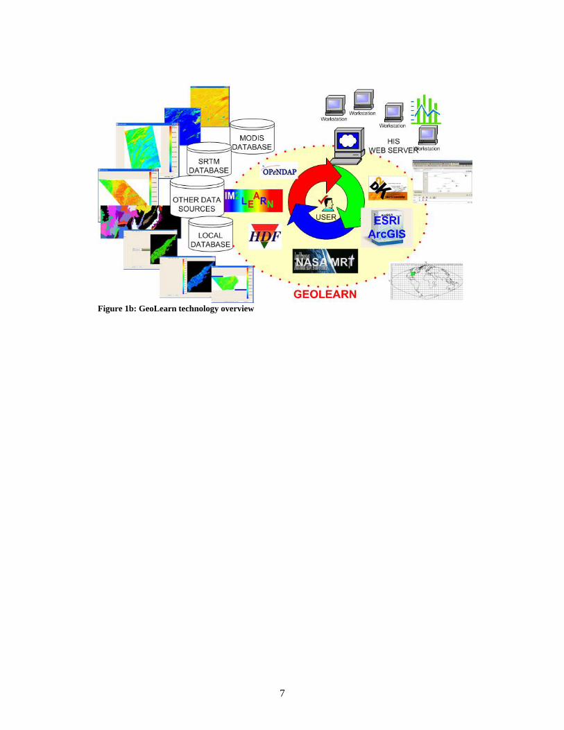
Introduction The motivation for developing GeoLearn comes from hydroclimatology and terrestrial hydrology. The research and development in this area addresses the scientific questions about causes and consequences of hydrologic variables through phenomenology, modeling, and synthesis. GeoLearn can be viewed as an encapsulated workflow for (1) loading multiple raster files (images) from local or remote locations, (2) pre-processing the files based on quality control requirements and performing feature extractions from them if necessary, (3) integrating and mosaicking all raster data sets to form a stack with consistent spatial and temporal resolution as well as geographic projection, (4) loading other files (boundaries, points or images) to create a mask for pixel selection purposes, (5) integrating the existing stack of raster images with other masking information, (6) selecting boundaries or image regions of interest and extracting variables from the stack of images, (7) performing data-driven modeling of selected input and output variables, (8) analyzing data-driven model to assign a relevance coefficient to input variables, and (9) mapping the data-driven model at a pixel level to spatial domain. All aforementioned steps are supported by visualizations (gray-scale or pseudo-color) of input, intermediate, and output data sets, as well as the data models. An overview of the functionality is provided in Figure 1a. In order to bring together so much functionality, the architecture of GeoLearn leverages several technologies as illustrated in Figure 1b. The majority of the GeoLearn code is based on Image to Learn (Im2Learn) developed at NCSA with additional calls to (a) HDF5 library developed by NCSA, (b) ArcGIS Engine developed by ESRI to perform data integration, (c) MODIS Reprojection Tool (MRT) to perform geographic re-projection, and (d) Data To Knowledge (D2K, Version 4.1.2) developed by NCSA to perform data-driven modeling with small size data sets. These software components are described in more detail in Chapter 5. The structure of this document follows the processing sequence as described above. The software installation steps are provided in Chapter 1. The software release comes with test data sets that were used in our research and are briefly described in Chapter 2. The processing steps are outlined in Chapter 3 with pictorial examples. Additional notes regarding bug reports, known problems, code maintenance, code dissemination, and licensing are presented in Chapter 5.

6

Figure 1a: An overview of GeoLearn functionality.

7

Figure 1b: GeoLearn technology overview

8

Chapter 1 Installation Instructions

1.1 Hardware requirements For processing large raster data sets, at least 512MB of RAM is recommended. Some processing steps might require significant computational resources. However, for the test data sets, a regular desktop computer should be able to handle the processing. The execution duration depends on the hardware specification and the algorithmic computational needs.

1.2 Software requirements • An Operating System capable of running Java • Java 1.5 • Optional: For data-driven modeling of small data sets, D2K must be installed -

separate license required for non-educational institutions • Optional: ArcGIS – separate license required • Optional: MODIS Reprojection Tool (MRT)

1.3 Installation steps To install the GeoLearn application, go to the Image Spatial Data Analysis (ISDA) NCSA website http://isda.ncsa.uiuc.edu/download and register to download. Your password will be e-mailed to you. After entering your password, select GeoLearn from the list of available tools.

Once you have downloaded GeoLearn, double click on the zip file and extract the files to an appropriate location. Navigate to the directory where you extracted the files, and double click on geolearn.bat.

1.3.1 Data to Knowledge (D2K) To enable the data-driven modeling functionality, you must install D2K from the ALG NCSA website http://alg.ncsa.uiuc.edu/do/downloads/d2k. Click on Download D2K to produce a login page. If you have never downloaded any code from ALG NCSA before you will need to register. Once you have registered, you can log in. A ticket will be send to your e-mail address that allows you to download the D2K software. A user has to run D2KToolkit.exe at least once before using GeoLearn. If GeoLearn produces a dialog asking for the location of D2K, navigate to its folder (e.g. C:\Program Files\D2KToolkit).

1.3.2 ArcGIS Engine For additional functionality in the file->import menu, ArcGIS Engine and/or MODIS Reprojection Tool (MRT) can be installed. ArcGIS Engine requires a separate license to be purchased. ESRI produces ArcGIS and can be found at http://www.esri.com/. MRT is free and can be downloaded from http://edcdaac.usgs.gov/landdaac/tools/modis/index.asp. To enable these functions, you must set environment variables in windows.

9

To set environment variables in windows, right click on “My Computer” and select properties from the popup menu. Select the “Advanced” tab in this dialog and click on the “Environment Variables” button. A new dialog labeled “Environment Variables” will appear. In the user variables section, click on the “New” button. A final dialog labeled “New User Variable” will appear and in this dialog you populate the “Variable name” entry with PATH and the “Variable value” entry with the location of ArcGIS’s bin folder (e.g. C:\Program Files\ArcGIS\bin). Additionally, GeoLearn will ask for the location of jintegra.jar, which will be in ArcGIS’s java folder (e.g. C:\Program Files\ArcGIS\java)

Note: The above instructions are for the ArcGIS Engine Software Developer Kit, using the complete install option to the default directory. If your install differs, you may need to set additional environment variables. If you had installed ArcGIS in a directory different from “C:\Program Files\ArcGIS” then you would need to create a variable called ARCENGINEHOME pointing to the location of the ArcGIS installation. If the ArcGIS jar files are installed at a location other than ARCENGINEHOME/java then you need to set the variable ARCGIS_JAVA to point to the location of ArcGIS jar files.

1.3.3 Modis Reprojection Tool (MRT) For MRT, you must set the PATH variable to MRT’s bin folder. Since MRT is packaged in a zip file, unzip the file to some location (e.g. C:\mrt_win). Then, set the PATH variable to the bin folder (e.g. C:\mrt_win\bin). The bin folder should contain a program called resample.exe. Note: If there are multiple locations for the PATH variable, place semicolons between locations, (e.g. C:\Program Files\ArcGIS\bin;C:\mrt_win\bin)

1.4 Notes about Execution The code is design to handle large size raster data. The word large refers to data sizes that would not fit into the allocated heap memory space during the GeoLearn execution. We use the terms ‘out-core-representation’ and ‘out-core-processing’ to indicate that the data access is enabled via partitioning data into chunks (e.g., image tiles), saving temporary data chunks on a disk and then loading a processing chunks of data sequentially. This approach is different from the ‘in-core’ representation and processing when the entire data set is loaded into RAM.

In the current implementation, the raster files that are larger than 2048x2048 (rows x cols) are represented as ‘out-of-core’. If the program fails then it might occur that the temporary chunks of data are not removed from the temporary directory. A user might check his/her default directory (e.g., C:\Documents and Settings\’user name’\Local Settings\Temp) for .img2 files and remove them manually.

The GeoLearn code is written in java which might not release memory immediately. In order to force garbage collection of unused RAM memory, one can right mouse click on the memory status bar in the lower right corner of the GeoLearn application. The memory status bar shows how much RAM is being currently occupied by GeoLearn.

10

1.5 Notes about Data The distributed zip file contains a directory called data. One can run the main step of GeoLearn with the files in the data directory. The directory contains the following files: (1) DEM_Illinois – sub-sampled USGS digital elevation map of Illinois in geographic projection (2) fpar_h10v05_2003_185.tif - fraction of Photosynthetic active radiation extracted from a MODIS HDF EOS file. The file was re-projected from sinusoidal projection to albers equal area conic projection (3) IL_County – county boundaries in the state of Illinois stored in ESRI Shapefile format (4) testGeoPoints.csv – tabular data with three columns (latitude, longitude and temperature over the state of Illinois) in a comma separated value file format. For testing purposes, one can load the data sets (1) and (2) in the first step (load raster step) and then select subsets of pixels for data-driven modeling by using data sets (3) or (4) in the third step (Create Mask step).

11

Chapter 2 Description of Test Data Sets

2.1 Raster Files

2.1.1 HDF EOS Remote sensing datasets acquired by the MODIS satellite and distributed by NASA are stored in HDF EOS format. HDF binary files can be directly loaded using Im2Learn. We are using Land Surface Temperature (LST), Emissivity, Enhanced Vegetation Index (EVI), Normalized Difference Vegetation Index (NDVI), Leaf Area Index (LAI), Fraction of Photosynthetically Active Radiation (FPAR), Snow Cover, Albedo, Land Cover variables. All above variables are processed using GeoLearn. Test datasets contain data for only two tiles (h10v05 and h11v05) and only for the year 2003 starting on the 177th Julian day. The HDF files that can be processed by GeoLearn have to contain georeferencing information.

HDF-EOS data can be downloaded from the URL: http://edcimswww.cr.usgs.gov/pub/imswelcome/

2.1.2 TIFF GeoLearn software has also the capability to load raster files stored in a tiff format. All preprocessed datasets are saved on disk in a tiff format. They can be loaded by Im2Learn loaders if the pre-processing step should be skipped and the data are ready for integration and data modeling as explained in this document. Arc Grid, SRTM, and HDF EOS data can be saved as tiff files after processing. Several processed datasets are available with the code release (HDF preprocessed data, climate data for Appalachian region, and soil data).

2.1.3 SRTM Elevation datasets from SRTM are used to extract different features such as Slope, Aspect, Flow Direction and Flow Accumulation. SRTM tiles can be mosaicked together using Im2Learn. Each of the extracted features is saved in tiff format (available with the test datasets).

SRTM data can be downloaded from the URL: http://edc.usgs.gov/products/elevation/srtmdted.html

2.1.4 Arc Grid Elevation datasets in Arc Grid format can be pre-processed by extracting features, such as slope, aspect, flow direction and flow accumulation. These data sets are provided for the Appalachian region in the USA. Data are first projected into Albers Equal Area projection and then features are extracted from the re-projected data. Feature extraction tasks can be performed at once by using “Hydro feature extraction” (see Figure 2). Any file in the proprietary Arc Grid format can be converted to open specification Tiff format and loaded into GeoLearn using “load other files” (Figure 2).

12

2.1.5 Other supported file formats In order to perform raster file integration, one needs to know the georeferencing information. In the current software, the georeferencing information can be extracted only from the file formats supported by Im2Learn, such as USGS DEM (Float), ESRI IMG format, HDF EOS, GeoTiff, and SRTM. Other image formats, such as jpg, gif, tif (Ver. 6.0 with no compression), pgm, ppm, bmp, png, pnm, img, are supported by Im2Learn but cannot be processed.

2.2 Vector Files

2.2.1 ESRI Shapefiles One of the test files is an eco-region shapefile at level III. This vector file provides a mask for processing subsets of pixels defined by a user-driven selection of eco-region of interest.

Eco-region shapefiles can be downloaded from the URL: http://www.epa.gov/wed/pages/ecoregions/level_iii.htm

From the web site one obtains a coverage file that was processed by us. The processing involves the change of geographic projection to Albers Equal Area and saving out the file in the ESRI shapefile format.

2.2.2 Other supported file formats There is a support for STATSGO and SSURGO DLG vector file format in Im2Learn software. However, these vector file formats are not currently enabled.

13

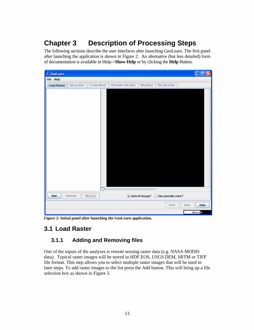
Chapter 3 Description of Processing Steps The following sections describe the user interfaces after launching GeoLearn. The first panel after launching the application is shown in Figure 2. An alternative (but less detailed) form of documentation is available in Help->Show Help or by clicking the Help Button.

Figure 2: Initial panel after launching the GeoLearn application.

3.1 Load Raster

3.1.1 Adding and Removing files

One of the inputs of the analyses is remote sensing raster data (e.g. NASA MODIS data). Typical raster images will be stored in HDF EOS, USGS DEM, SRTM or TIFF file format. This step allows you to select multiple raster images that will be used in later steps. To add raster images to the list press the Add button. This will bring up a file selection box as shown in Figure 3.

14

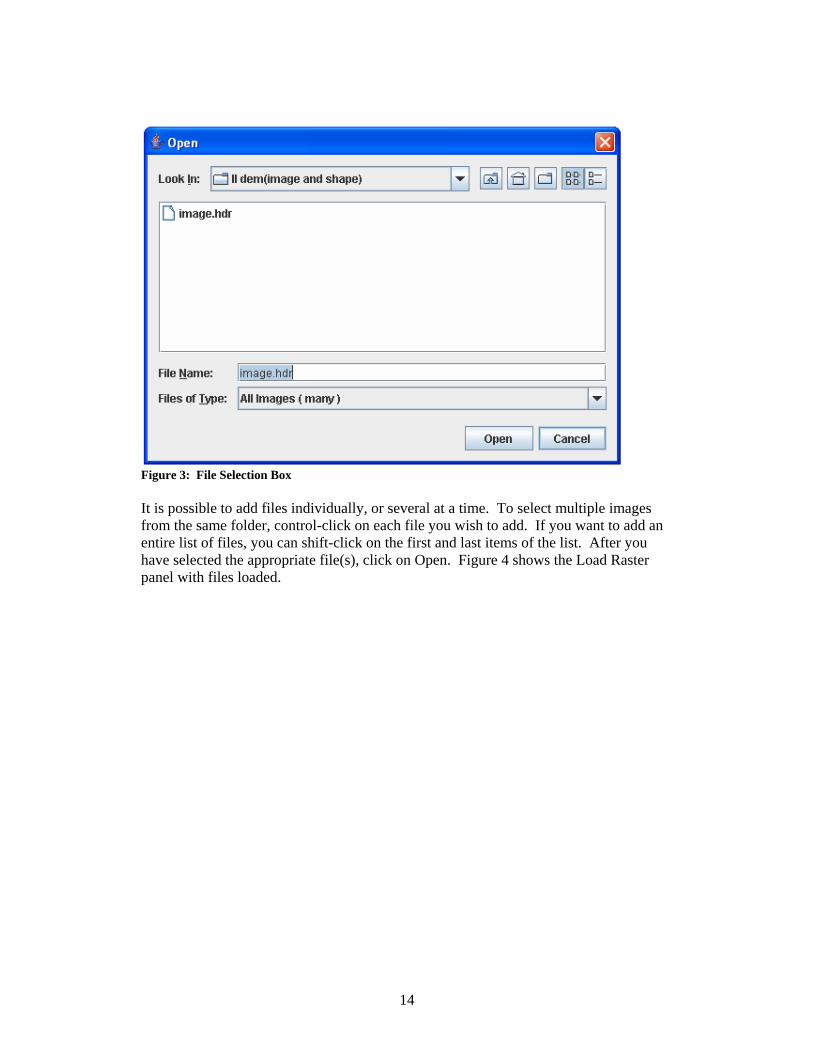
Figure 3: File Selection Box It is possible to add files individually, or several at a time. To select multiple images from the same folder, control-click on each file you wish to add. If you want to add an entire list of files, you can shift-click on the first and last items of the list. After you have selected the appropriate file(s), click on Open. Figure 4 shows the Load Raster panel with files loaded.

15

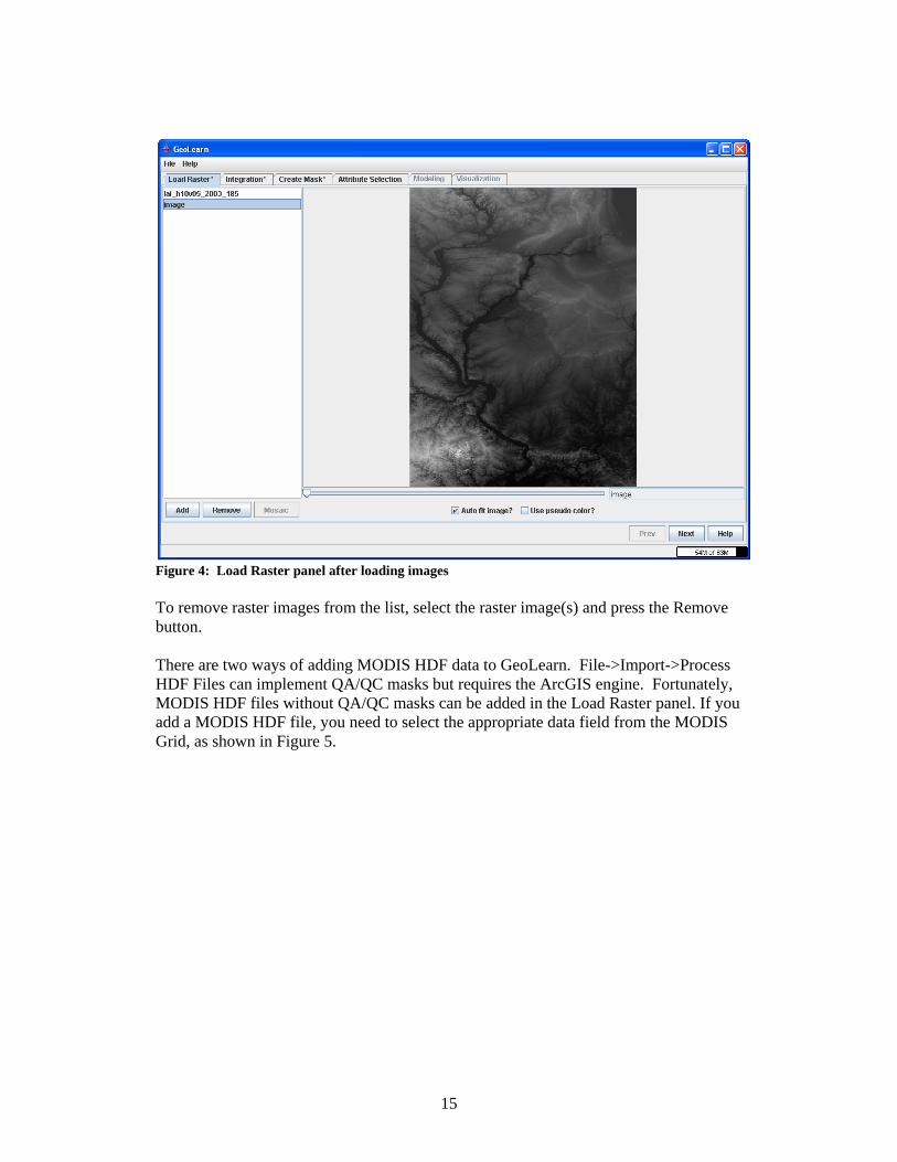
Figure 4: Load Raster panel after loading images

To remove raster images from the list, select the raster image(s) and press the Remove button.

There are two ways of adding MODIS HDF data to GeoLearn. File->Import->Process HDF Files can implement QA/QC masks but requires the ArcGIS engine. Fortunately, MODIS HDF files without QA/QC masks can be added in the Load Raster panel. If you add a MODIS HDF file, you need to select the appropriate data field from the MODIS Grid, as shown in Figure 5.

16

Figure 5: MODIS Grid data field dialog

3.1.2 Mosaic The purpose of mosaicking is to stitch together spatial tiles(e.g. SRTM tiles) to form a mosaic. To combine multiple raster images into a single raster image, select the appropriate images using control-click, then click Mosaic. This will produce a single new raster image that replaces the raster images that were used to create it. Figure 6 shows the result of mosaicking five square SRTM tiles.

Figure 6: Mosaicked Image

17

3.1.3 Functionality

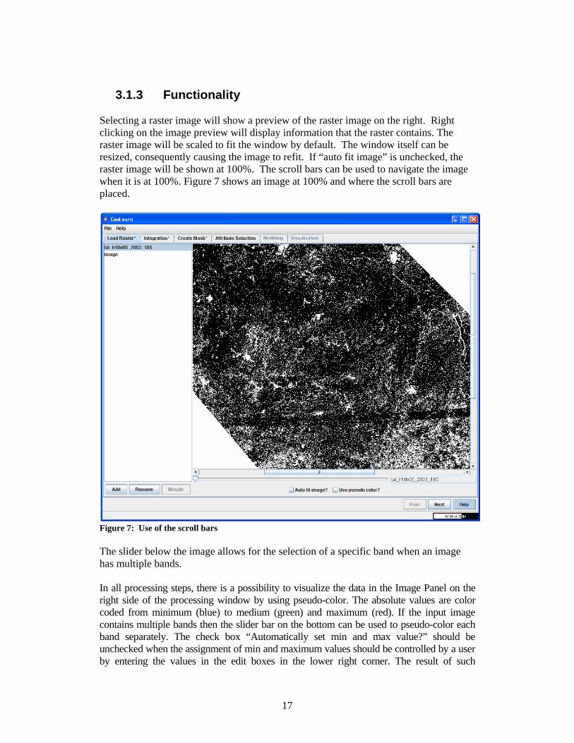
Selecting a raster image will show a preview of the raster image on the right. Right clicking on the image preview will display information that the raster contains. The raster image will be scaled to fit the window by default. The window itself can be resized, consequently causing the image to refit. If “auto fit image” is unchecked, the raster image will be shown at 100%. The scroll bars can be used to navigate the image when it is at 100%. Figure 7 shows an image at 100% and where the scroll bars are placed.

Figure 7: Use of the scroll bars The slider below the image allows for the selection of a specific band when an image has multiple bands. In all processing steps, there is a possibility to visualize the data in the Image Panel on the right side of the processing window by using pseudo-color. The absolute values are color coded from minimum (blue) to medium (green) and maximum (red). If the input image contains multiple bands then the slider bar on the bottom can be used to pseudo-color each band separately. The check box “Automatically set min and max value?” should be unchecked when the assignment of min and maximum values should be controlled by a user by entering the values in the edit boxes in the lower right corner. The result of such

18

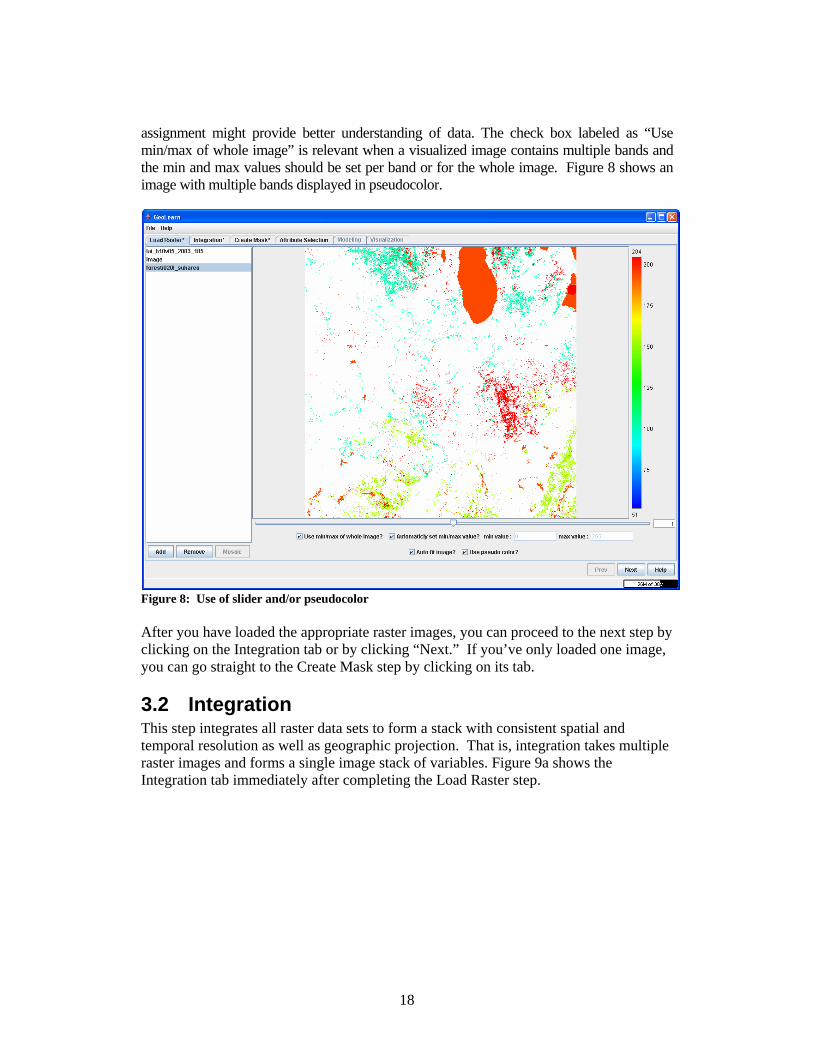
assignment might provide better understanding of data. The check box labeled as “Use min/max of whole image” is relevant when a visualized image contains multiple bands and the min and max values should be set per band or for the whole image. Figure 8 shows an image with multiple bands displayed in pseudocolor.

Figure 8: Use of slider and/or pseudocolor

After you have loaded the appropriate raster images, you can proceed to the next step by clicking on the Integration tab or by clicking “Next.” If you’ve only loaded one image, you can go straight to the Create Mask step by clicking on its tab.

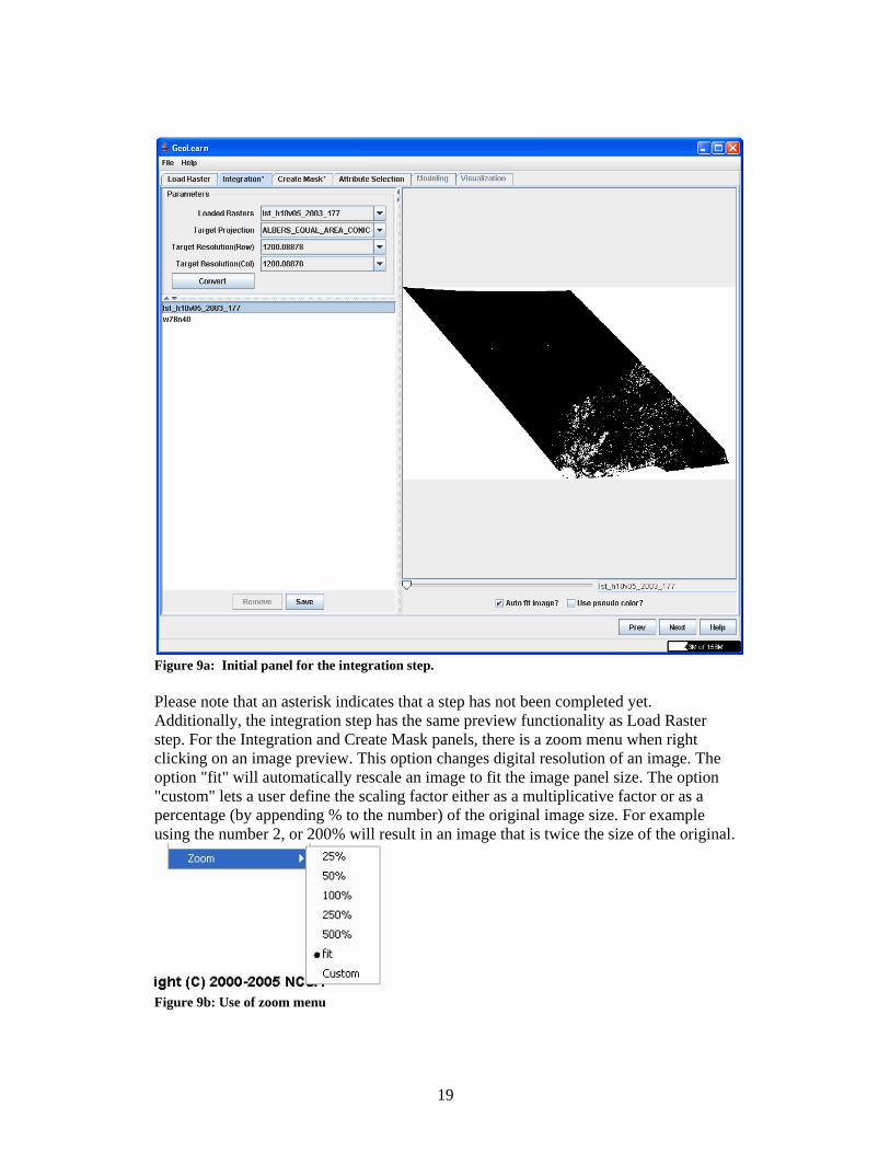
3.2 Integration This step integrates all raster data sets to form a stack with consistent spatial and temporal resolution as well as geographic projection. That is, integration takes multiple raster images and forms a single image stack of variables. Figure 9a shows the Integration tab immediately after completing the Load Raster step.

19

Figure 9a: Initial panel for the integration step. Please note that an asterisk indicates that a step has not been completed yet. Additionally, the integration step has the same preview functionality as Load Raster step. For the Integration and Create Mask panels, there is a zoom menu when right clicking on an image preview. This option changes digital resolution of an image. The option "fit" will automatically rescale an image to fit the image panel size. The option "custom" lets a user define the scaling factor either as a multiplicative factor or as a percentage (by appending % to the number) of the original image size. For example using the number 2, or 200% will result in an image that is twice the size of the original.

Figure 9b: Use of zoom menu

20

The small triangles can be clicked on to expand a specific frame in the window. The bars separating frames can be dragged to resize the frames. Figure 10 shows the GeoLearn window after clicking on the triangle pointing to the right.

Figure 10: Resizing frames

3.2.1 Parameters In order to populate correctly the re-projection parameters that lead to an integrated image stack, the current implementation allows a user to select one of the input files and make those georeferencing parameters the target projection parameters. The future releases will provide more flexibility in setting the integration parameters. Note: This means the Loaded Rasters combo box is the only field that can be modified by the user. The target resolution cannot be manually modified.

21

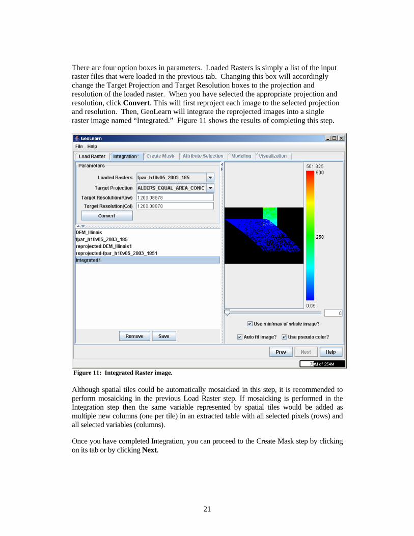
There are four option boxes in parameters. Loaded Rasters is simply a list of the input raster files that were loaded in the previous tab. Changing this box will accordingly change the Target Projection and Target Resolution boxes to the projection and resolution of the loaded raster. When you have selected the appropriate projection and resolution, click Convert. This will first reproject each image to the selected projection and resolution. Then, GeoLearn will integrate the reprojected images into a single raster image named “Integrated.” Figure 11 shows the results of completing this step.

Figure 11: Integrated Raster image. Although spatial tiles could be automatically mosaicked in this step, it is recommended to perform mosaicking in the previous Load Raster step. If mosaicking is performed in the Integration step then the same variable represented by spatial tiles would be added as multiple new columns (one per tile) in an extracted table with all selected pixels (rows) and all selected variables (columns).

Once you have completed Integration, you can proceed to the Create Mask step by clicking on its tab or by clicking Next.

22

3.3 Create Mask

3.3.1 Purpose of the Create Mask step Before proceeding with this step, please make sure that it will only receive one image (e.g. a single loaded raster or a mosaicked/integrated raster). As implied by the name, a mask hides part of an image so that only certain pixels will be used for Attribute Selection and Modeling. There are several reasons to use the Create Mask step. One is that Modeling and Visualization of large size data sets will take too long with an unmasked image on a desktop computer. Another is that you may wish to include/exclude specific data for the modeling and visualization steps, for instance, in the cases of eco-region studies, studies of water stations only, or studies constrained to limited elevation range or land use/land coverage. Creating masks in GeoLearn: The major task for creating masks in GeoLearn is to select measurements from raster files based on multiple criteria, combine generated masks by arithmetic or Boolean operation and prepare tabular file for data driven modeling. Besides data quality, up to five criteria are currently supported for mask creation in GeoLearn: 1, Geo-region locations: extracting regional boundaries information from shape file and creating masks based on user specified boundaries; 2, Geo-point locations: extracting points with geo-referencing information from either CSV or Excel files, and creating masks based on their locations and user specified radius; 3, Category of geo-locations: creating masks based on user specified categorical labels; 4, Range of measurements: creating mask by continuous value threholding with a user specified range, which is defined by one or two threshold values; 5, User defined locations: creating masks by painting rectangles or ovals to define locations. When masks are created, they are ready for combination either through arithmetic or Boolean operation: Arithmetic operations: Add: to create a new image by adding the values of corresponding pixels in all operands; Subtract: to create a new image by subtracting the values of pixels in action image from those of pixels in target image; Multiply: to create a new image by multiplying the values of corresponding pixels in all

23

operands; Divide: to create a new image by dividing the values of pixels in target image by those of pixels in action image; Average: to create a new image by adding the values of corresponding pixels in all operands and divided by number of operands; Boolean operations: AND: to create a new image by performing Boolean “AND” operation on all operands; OR: to create a new image by performing Boolean “OR” operation on all operands; XOR: to create a new image by performing Boolean “XOR” operation on target image by action image; Inverse: to create a new image by inverting values of all pixels in the operand.

3.3.2 How to Create masks This step will allow you to create masks, do operations on them, and apply one of them on the raster loaded in the previous step and at the same time get prepared to provide a table for modeling. There are three sections in this window: panel “MaskCreation” and panel “Mask Operation” on the left and main panel on the right. “Mask Creation” panel consists of four parts: 1, a combo box on the top: providing to you up to five methods to create a mask—“SHAPEFILE”, “TABLE”, “CATEGORICAL”, “THRESHOLD”, “USER DEFINED” (please see Note 1); 2, a parameter portion right below the combo box: allowing you to specify any parameters required for mask creation; 3, check box “include”: this will take effect every time you create a mask. When it is selected, pixels of the mask in the chosen area will be white; otherwise, they will be black. 4, check box “Edit Mask Name”: this will take effect every time you click “Add To List” button. When it is selected, you are allowed to set a name to the mask of interest by typing into the text field in “Mask Operation” panel. “Mask Operation” panel contains a list and functional buttons. The list, together with a text area on the top of this panel will allow you to store and display masks you are interested in. An image frame will be popped up displaying the selected mask, if you click a mask in the list (for details about functions of the other components in “Mask Operation” panel, please see Note 2). The main panel consists three parts: 1, An image panel on the top to display loaded rasters or created masks; 2, A text area to show number of valid and invalid pixels of a mask, and in the case of creating mask by “Threshold”, to show threshold values. 3, Buttons (for details about functions of each button in this part, please see Note 4). The first thing to do in this step is to select a method from the five methods available in

24

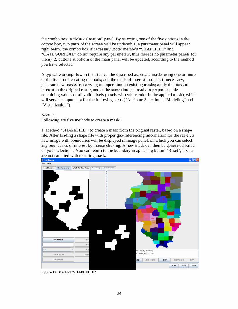
the combo box in “Mask Creation” panel. By selecting one of the five options in the combo box, two parts of the screen will be updated: 1, a parameter panel will appear right below the combo box if necessary (note: methods “SHAPEFILE” and “CATEGORICAL” do not require any parameters, thus there is no parameter panels for them); 2, buttons at bottom of the main panel will be updated, according to the method you have selected. A typical working flow in this step can be described as: create masks using one or more of the five mask creating methods; add the mask of interest into list; if necessary, generate new masks by carrying out operation on existing masks; apply the mask of interest to the original raster, and at the same time get ready to prepare a table containing values of all valid pixels (pixels with white color in the applied mask), which will serve as input data for the following steps (“Attribute Selection”, “Modeling” and “Visualization”). Note 1: Following are five methods to create a mask: 1, Method “SHAPEFILE”: to create a mask from the original raster, based on a shape file. After loading a shape file with proper geo-referencing information for the raster, a new image with boundaries will be displayed in image panel, on which you can select any boundaries of interest by mouse clicking. A new mask can then be generated based on your selections. You can return to the boundary image using button “Reset”, if you are not satisfied with resulting mask.

Figure 12: Method “SHAPEFILE”

25

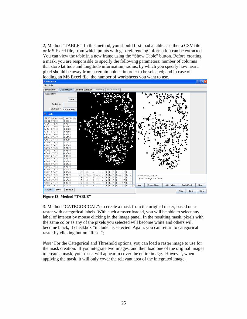
2, Method “TABLE”: In this method, you should first load a table as either a CSV file or MS Excel file, from which points with geo-referencing information can be extracted. You can view the table in a new frame using the “Show Table” button. Before creating a mask, you are responsible to specify the following parameters: number of columns that store latitude and longitude information; radius, by which you specify how near a pixel should be away from a certain points, in order to be selected; and in case of loading an MS Excel file, the number of worksheets you want to use.

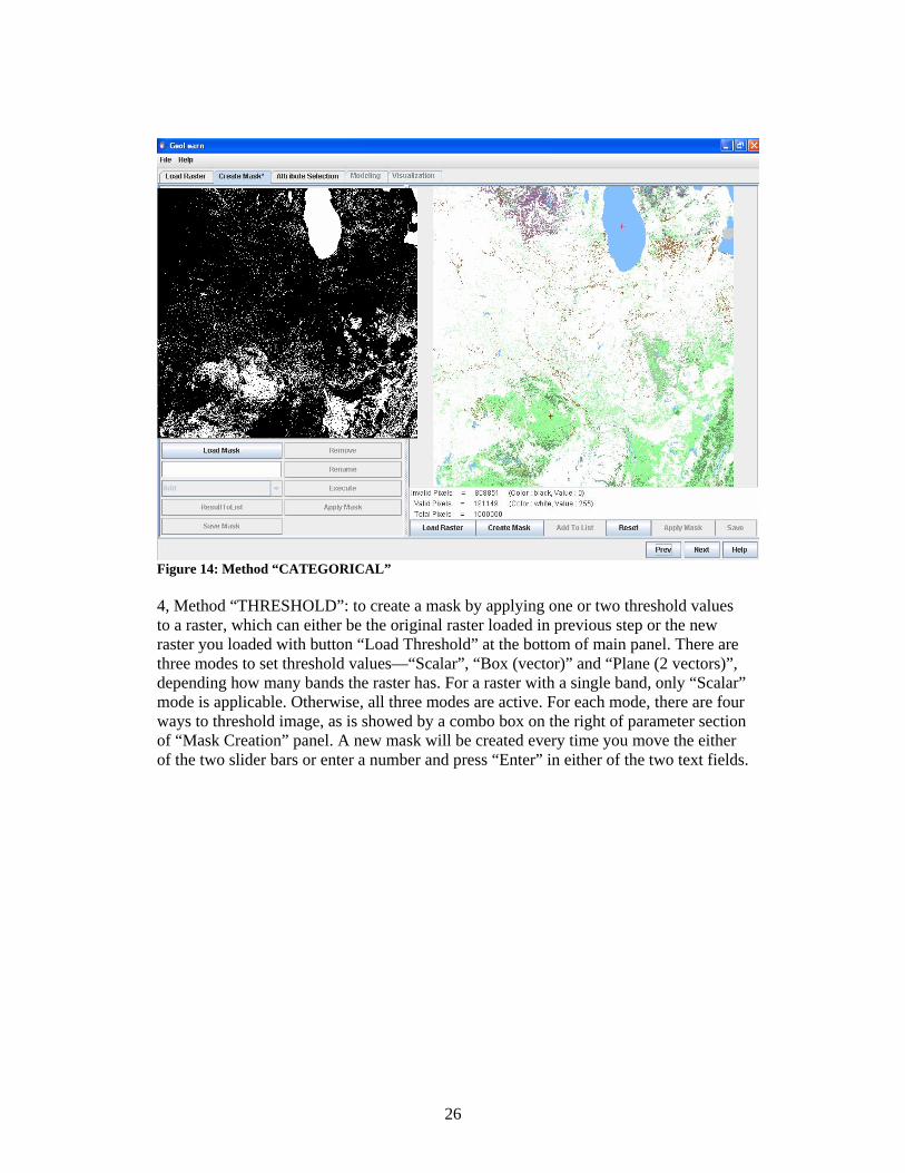
Figure 13: Method “TABLE” 3. Method “CATEGORICAL”: to create a mask from the original raster, based on a raster with categorical labels. With such a raster loaded, you will be able to select any label of interest by mouse clicking in the image panel. In the resulting mask, pixels with the same color as any of the pixels you selected will become white and others will become black, if checkbox “include” is selected. Again, you can return to categorical raster by clicking button “Reset”; Note: For the Categorical and Threshold options, you can load a raster image to use for the mask creation. If you integrate two images, and then load one of the original images to create a mask, your mask will appear to cover the entire image. However, when applying the mask, it will only cover the relevant area of the integrated image.

26

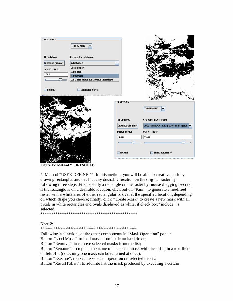
Figure 14: Method “CATEGORICAL” 4, Method “THRESHOLD”: to create a mask by applying one or two threshold values to a raster, which can either be the original raster loaded in previous step or the new raster you loaded with button “Load Threshold” at the bottom of main panel. There are three modes to set threshold values—“Scalar”, “Box (vector)” and “Plane (2 vectors)”, depending how many bands the raster has. For a raster with a single band, only “Scalar” mode is applicable. Otherwise, all three modes are active. For each mode, there are four ways to threshold image, as is showed by a combo box on the right of parameter section of “Mask Creation” panel. A new mask will be created every time you move the either of the two slider bars or enter a number and press “Enter” in either of the two text fields.

27

Figure 15: Method “THRESHOLD” 5, Method “USER DEFINED”: In this method, you will be able to create a mask by drawing rectangles and ovals at any desirable location on the original raster by following three steps. First, specify a rectangle on the raster by mouse dragging; second, if the rectangle is on a desirable location, click button “Paint” to generate a modified raster with a white area of either rectangular or oval at the specified location, depending on which shape you choose; finally, click “Create Mask” to create a new mask with all pixels in white rectangles and ovals displayed as white, if check box "include" is selected. ********************************************* Note 2: ********************************************* Following is functions of the other components in “Mask Operation” panel: Button “Load Mask”: to load masks into list from hard drive; Button “Remove”: to remove selected masks from the list; Button “Rename”: to replace the name of a selected mask with the string in a text field on left of it (note: only one mask can be renamed at once); Button “Execute”: to execute selected operation on selected masks; Button “ResultToList”: to add into list the mask produced by executing a certain

28

operation; Button “Apply Mask”: to apply the mask selected to the original raster loaded in previous step in such a way that the resulting image will display any pixels in their original color if their corresponding pixels in the mask are white, while other pixels in the raster will be displayed in black. Button “Save Mask”: to save selected masks into hard drive in “.tif” format; Text Field: place where to enter an desired name, before clicking "rename" button or “Add To List” button if check box “Edit Mask Name” is selected; Combo Box: containing nine mask operations (for details about each operation in this Combo Box, please see Note 3). ********************************************* Note 3: ********************************************* There are totally nine operations that can be executed on masks, which is divided into three categories: 1, operation that support multiple operands: Add: to create a new image by adding the values of corresponding pixels in all operands; Multiply: to create a new image by multiplying the values of corresponding pixels in all operands; Average: to create a new image by adding the values of corresponding pixels in all operands and divided by number of operands; AND: to create a new image by performing Boolean “AND” operation on all operands; OR: to create a new image by performing Boolean “OR” operation on all operands; 2, operation that need a target image and an action image: Subtract: to create a new image by subtracting the values of pixels in action image from those of pixels in target image; Divide: to create a new image by dividing the values of pixels in target image by those of pixels in action image; XOR: to create a new image by performing Boolean “XOR” operation on target image by action image; 3, operation that need only one image: Inverse: to create a new image by inverting values of all pixels in the operand *********************************************

29

Figure 16: Mask operations. Note 4: ********************************************* 1, Button “Load Table”, “Load Shape”, “Load Categorical” and “Load Threshold”: To load corresponding files from hard drive; 2, Button “Create Mask”: To create a new mask using method you select, taking into account whether checkbox “include” is selected; 3, Button “Add To List”: To add the mask being displayed in the image panel into list; 4, Button “Reset”: To go back to the initial stage of the process of mask creation, according to the mask creating method selected; 5, Button “Apply Mask”: To apply the mask selected to the original raster loaded in previous step in such a way that the resulting image will display any pixels in their original color if their corresponding pixels in the mask are white, while other pixels in the raster will be displayed in black: 6, Button “Save”: To save any image being displayed in image panel onto hard drive; Notes: A saved TIFF file obtained by selecting a sub-area or by sub-sampling the original raster file may not have the correct georeferencing information. Also, you cannot save an extracted table until after a mask has been created.

AND =

30

3.4 Attribute Selection

This step allows you to select input and output attributes to be used in the learning algorithm. At least one attribute must be selected for both input and output selections. Click on the attribute name to select it, or click on it again to deselect. Multiple inputs (by using shift-click or control-click) can be selected, but only one output can be selected. Since the data table for an image can be quite large, it is not shown unless “Show Table” is clicked on. If you wish to save the data table to your hard drive, you may select the format and click on “Save Table.”

3.5 Data-Driven Modeling

This step allows you to select the learning methods to be used in the analysis. The methods can be used include Regression Tree (RT), K-nearest Neighbors (KNN), Support Vector Machine (SVM). A fusion scheme combining the above three methods can be used. There are two fusion methods provided here: average fusion and rank fusion. A thorough explanation of these data-driven modeling techniques is available at http://isda.ncsa.uiuc.edu/peter/publications/conferences/2006/RelevanceSMC-IT2006.pdf. Select the method using the combo box in the Modeling panel.

3.6 Visualization

This step allows you to view the visualized results of analysis. Select the combo box to view different aspect of analysis. The Boundary option shows the boundary image for data covered in the analysis. The Model option shows the relevance analysis results. The color of relevance image indicates the most relevant variable at that pixel position. The table indicates the model relevance of the dataset. The Input option shows the original data for output variable chosen in the Attribute Selection step. The prediction option shows the Prediction results for output values based on the learning model we use.

31

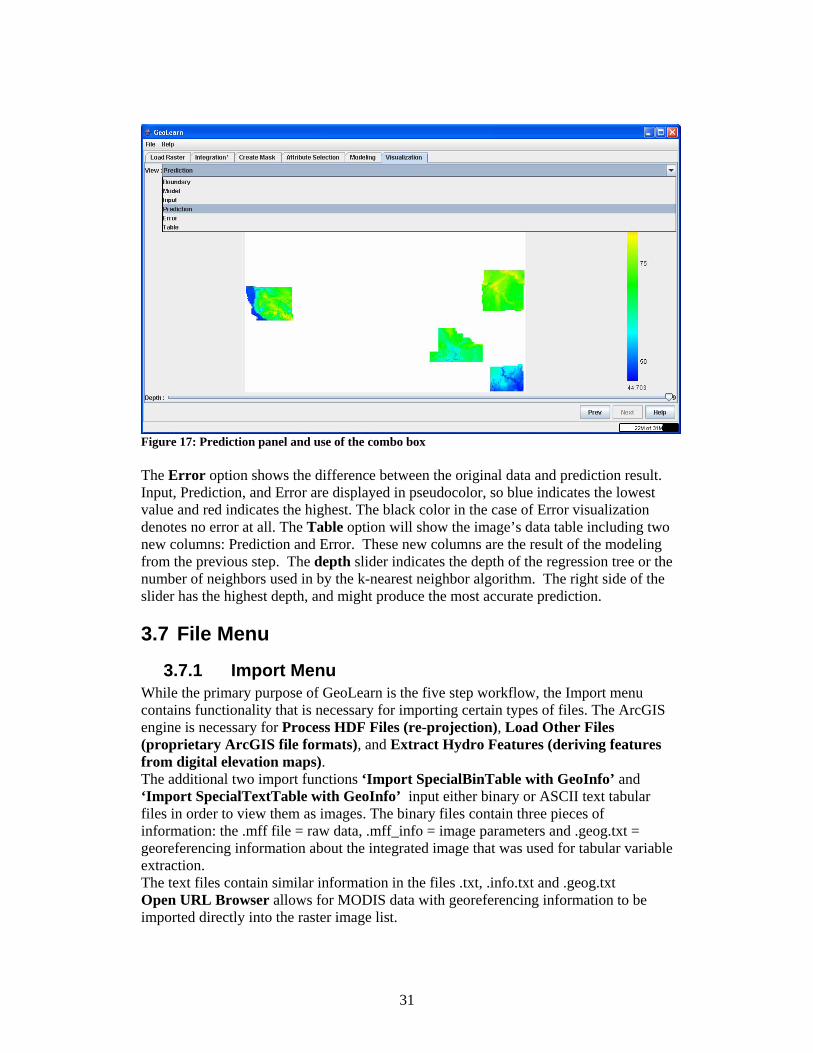
Figure 17: Prediction panel and use of the combo box

The Error option shows the difference between the original data and prediction result. Input, Prediction, and Error are displayed in pseudocolor, so blue indicates the lowest value and red indicates the highest. The black color in the case of Error visualization denotes no error at all. The Table option will show the image’s data table including two new columns: Prediction and Error. These new columns are the result of the modeling from the previous step. The depth slider indicates the depth of the regression tree or the number of neighbors used in by the k-nearest neighbor algorithm. The right side of the slider has the highest depth, and might produce the most accurate prediction.

3.7 File Menu

3.7.1 Import Menu While the primary purpose of GeoLearn is the five step workflow, the Import menu contains functionality that is necessary for importing certain types of files. The ArcGIS engine is necessary for Process HDF Files (re-projection), Load Other Files (proprietary ArcGIS file formats), and Extract Hydro Features (deriving features from digital elevation maps). The additional two import functions ‘Import SpecialBinTable with GeoInfo’ and ‘Import SpecialTextTable with GeoInfo’ input either binary or ASCII text tabular files in order to view them as images. The binary files contain three pieces of information: the .mff file = raw data, .mff_info = image parameters and .geog.txt = georeferencing information about the integrated image that was used for tabular variable extraction. The text files contain similar information in the files .txt, .info.txt and .geog.txt Open URL Browser allows for MODIS data with georeferencing information to be imported directly into the raster image list.

32

MRT Reprojection allows for MODIS images to be reprojected using the MODIS Reprojection Tool user interface developed by NASA. This interface allows a user to set all parameters for re-projecting images and then call a binary executable with the parameter file. The current re-projection implementation in GeoLearn is based on using a java native interface (JNI) to the application programming interface (API) of the MRT re-projection code.

3.7.2 Save and Save All These steps allow for images in the raster list to be saved as either a raster or in the proprietary ArcGrid format. Save will save the currently selected file, while Save All will save every image in the raster list.

3.7.3 Look and Feel There are four different options for skin of the user interface. Metal is the default skin, but others can be chosen by preference.

3.7.4 Exit Exit quits the program and returns to the desktop.

33

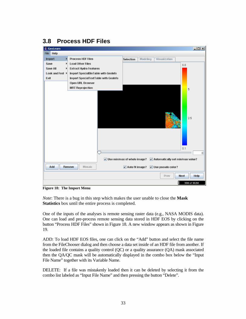
3.8 Process HDF Files

Figure 18: The Import Menu Note: There is a bug in this step which makes the user unable to close the Mask Statistics box until the entire process is completed. One of the inputs of the analyses is remote sensing raster data (e.g., NASA MODIS data). One can load and pre-process remote sensing data stored in HDF EOS by clicking on the button “Process HDF Files” shown in Figure 18. A new window appears as shown in Figure 19.

ADD: To load HDF EOS files, one can click on the “Add” button and select the file name from the FileChooser dialog and then choose a data set inside of an HDF file from another. If the loaded file contains a quality control (QC) or a quality assurance (QA) mask associated then the QA/QC mask will be automatically displayed in the combo box below the “Input File Name” together with its Variable Name.

DELETE: If a file was mistakenly loaded then it can be deleted by selecting it from the combo list labeled as “Input File Name” and then pressing the button “Delete”.

34

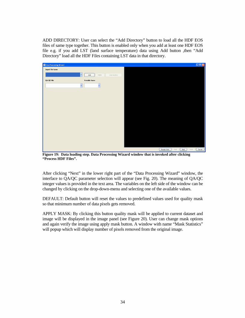
ADD DIRECTORY: User can select the “Add Directory” button to load all the HDF EOS files of same type together. This button is enabled only when you add at least one HDF EOS file e.g. if you add LST (land surface temperature) data using Add button ,then “Add Directory” load all the HDF Files containing LST data in that directory.

Figure 19: Data loading step. Data Processing Wizard window that is invoked after clicking “Process HDF Files”.

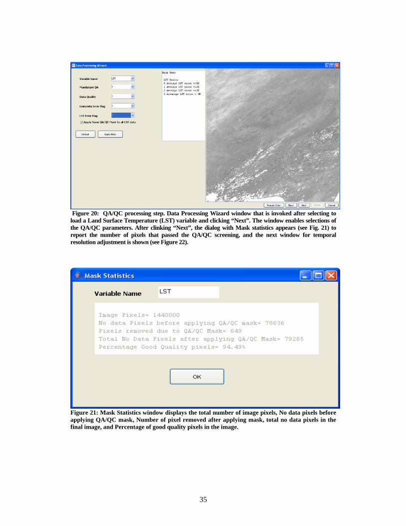
After clicking “Next” in the lower right part of the “Data Processing Wizard” window, the interface to QA/QC parameter selection will appear (see Fig. 20). The meaning of QA/QC integer values is provided in the text area. The variables on the left side of the window can be changed by clicking on the drop-down-menu and selecting one of the available values.

DEFAULT: Default button will reset the values to predefined values used for quality mask so that minimum number of data pixels gets removed.

APPLY MASK: By clicking this button quality mask will be applied to current dataset and image will be displayed in the image panel (see Figure 20). User can change mask options and again verify the image using apply mask button. A window with name “Mask Statistics” will popup which will display number of pixels removed from the original image.

35

Figure 20: QA/QC processing step. Data Processing Wizard window that is invoked after selecting to load a Land Surface Temperature (LST) variable and clicking “Next”. The window enables selections of the QA/QC parameters. After clinking “Next”, the dialog with Mask statistics appears (see Fig. 21) to report the number of pixels that passed the QA/QC screening, and the next window for temporal resolution adjustment is shown (see Figure 22).

Figure 21: Mask Statistics window displays the total number of image pixels, No data pixels before applying QA/QC mask, Number of pixel removed after applying mask, total no data pixels in the final image, and Percentage of good quality pixels in the image.

36

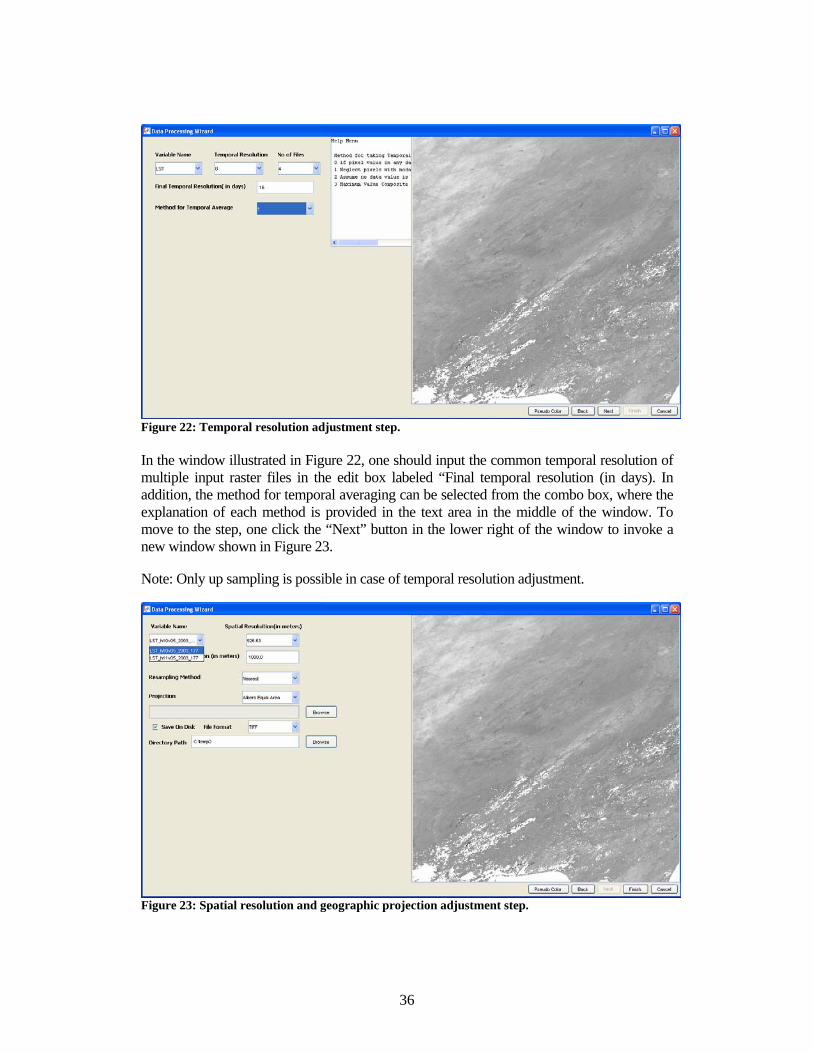
Figure 22: Temporal resolution adjustment step. In the window illustrated in Figure 22, one should input the common temporal resolution of multiple input raster files in the edit box labeled “Final temporal resolution (in days). In addition, the method for temporal averaging can be selected from the combo box, where the explanation of each method is provided in the text area in the middle of the window. To move to the step, one click the “Next” button in the lower right of the window to invoke a new window shown in Figure 23.

Note: Only up sampling is possible in case of temporal resolution adjustment.

Figure 23: Spatial resolution and geographic projection adjustment step.

37

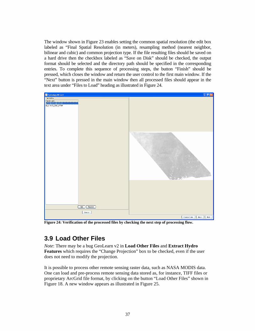
The window shown in Figure 23 enables setting the common spatial resolution (the edit box labeled as “Final Spatial Resolution (in meters), resampling method (nearest neighbor, bilinear and cubic) and common projection type. If the file resulting files should be saved on a hard drive then the checkbox labeled as “Save on Disk” should be checked, the output format should be selected and the directory path should be specified in the corresponding entries. To complete this sequence of processing steps, the button “Finish” should be pressed, which closes the window and return the user control to the first main window. If the “Next” button is pressed in the main window then all processed files should appear in the text area under “Files to Load” heading as illustrated in Figure 24.

Figure 24: Verification of the processed files by checking the next step of processing flow.

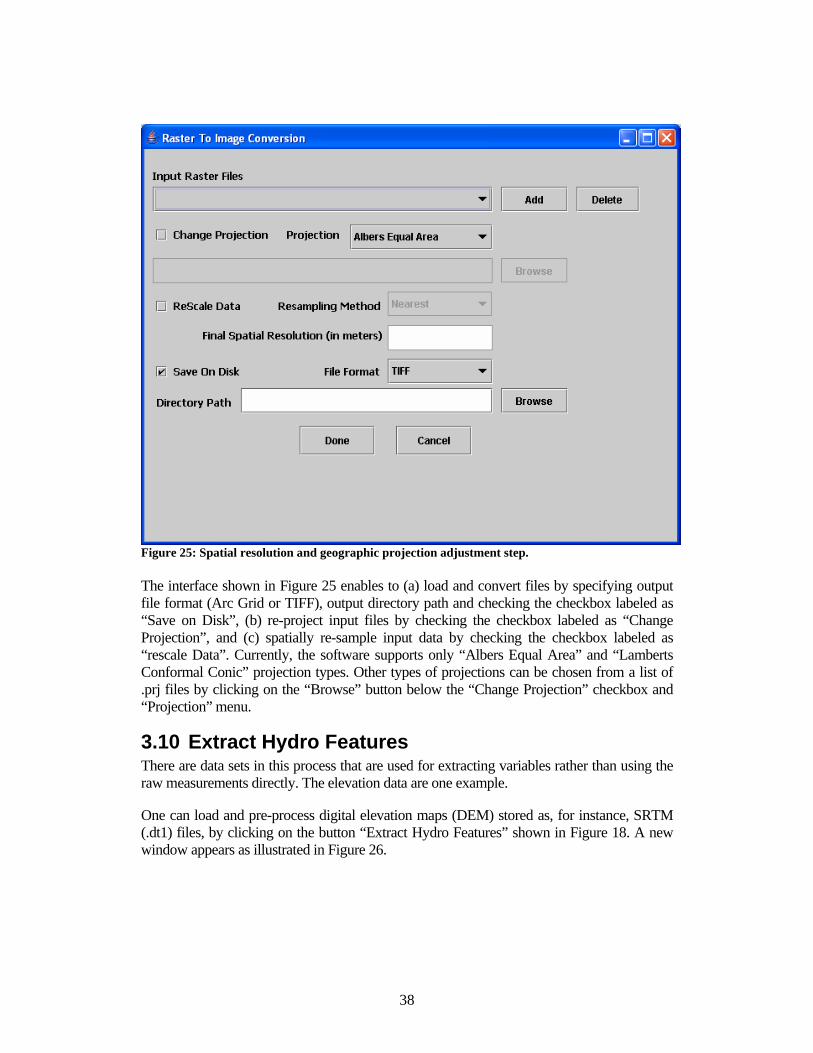
3.9 Load Other Files Note: There may be a bug GeoLearn v2 in Load Other Files and Extract Hydro Features which requires the “Change Projection” box to be checked, even if the user does not need to modify the projection. It is possible to process other remote sensing raster data, such as NASA MODIS data. One can load and pre-process remote sensing data stored as, for instance, TIFF files or proprietary ArcGrid file format, by clicking on the button “Load Other Files” shown in Figure 18. A new window appears as illustrated in Figure 25.

38

Figure 25: Spatial resolution and geographic projection adjustment step. The interface shown in Figure 25 enables to (a) load and convert files by specifying output file format (Arc Grid or TIFF), output directory path and checking the checkbox labeled as “Save on Disk”, (b) re-project input files by checking the checkbox labeled as “Change Projection”, and (c) spatially re-sample input data by checking the checkbox labeled as “rescale Data”. Currently, the software supports only “Albers Equal Area” and “Lamberts Conformal Conic” projection types. Other types of projections can be chosen from a list of .prj files by clicking on the “Browse” button below the “Change Projection” checkbox and “Projection” menu.

3.10 Extract Hydro Features There are data sets in this process that are used for extracting variables rather than using the raw measurements directly. The elevation data are one example.

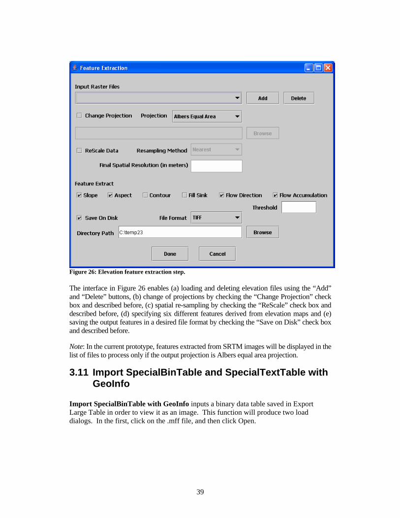
One can load and pre-process digital elevation maps (DEM) stored as, for instance, SRTM (.dt1) files, by clicking on the button “Extract Hydro Features” shown in Figure 18. A new window appears as illustrated in Figure 26.

39

Figure 26: Elevation feature extraction step. The interface in Figure 26 enables (a) loading and deleting elevation files using the “Add” and “Delete” buttons, (b) change of projections by checking the “Change Projection” check box and described before, (c) spatial re-sampling by checking the “ReScale” check box and described before, (d) specifying six different features derived from elevation maps and (e) saving the output features in a desired file format by checking the “Save on Disk” check box and described before.

Note: In the current prototype, features extracted from SRTM images will be displayed in the list of files to process only if the output projection is Albers equal area projection.

3.11 Import SpecialBinTable and SpecialTextTable with GeoInfo

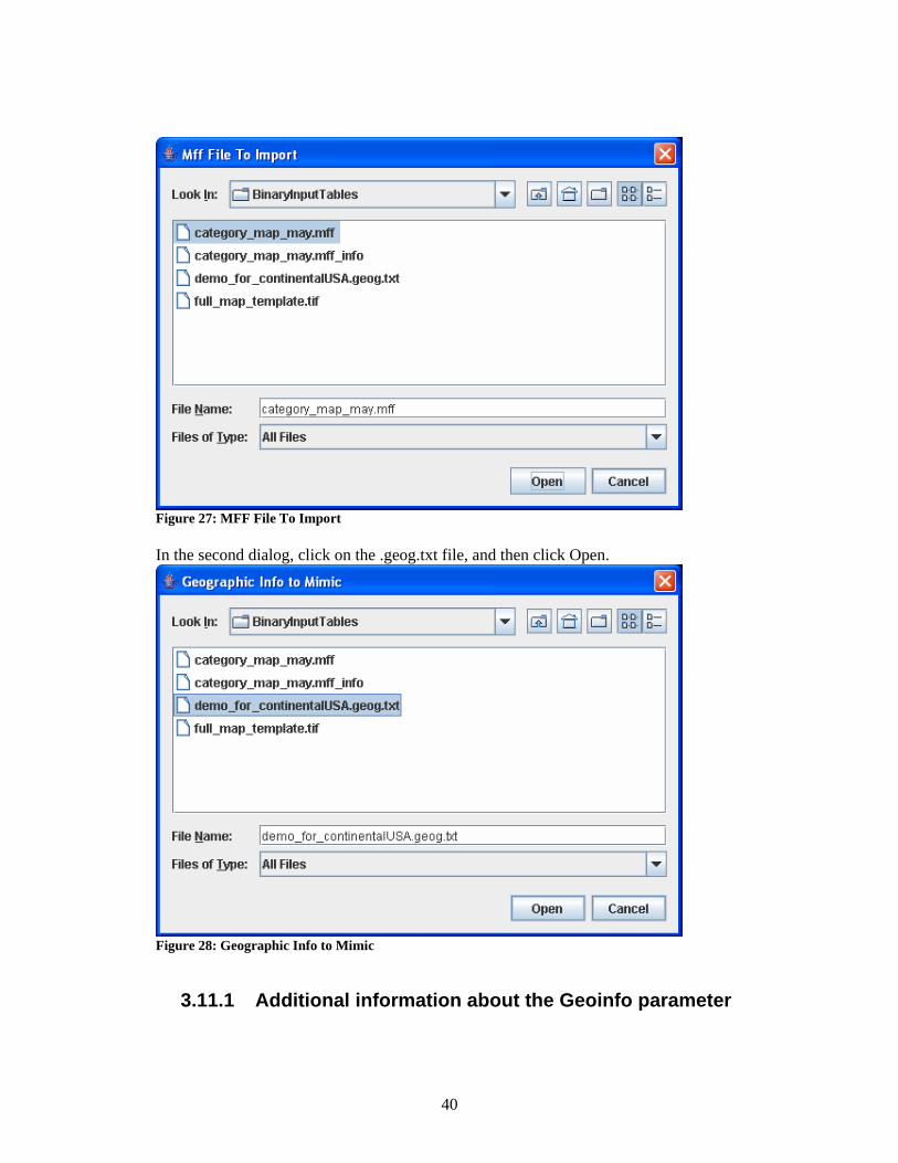
Import SpecialBinTable with GeoInfo inputs a binary data table saved in Export Large Table in order to view it as an image. This function will produce two load dialogs. In the first, click on the .mff file, and then click Open.

40

Figure 27: MFF File To Import In the second dialog, click on the .geog.txt file, and then click Open.

Figure 28: Geographic Info to Mimic

3.11.1 Additional information about the Geoinfo parameter

41

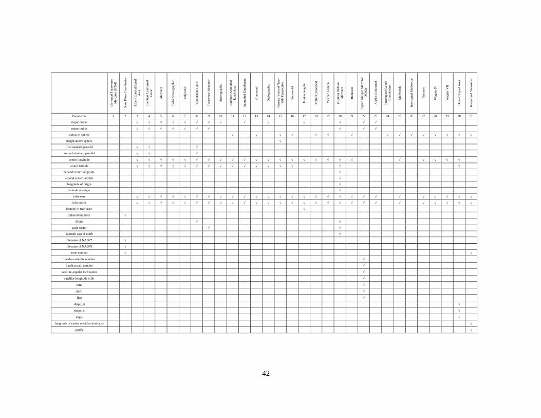
Geoinfo shows geometric information of an image. Geometric information consists of two parts; the first part is the set of general parameters which are independent on the projection type of the image and the second one is the set of specific parameters which are dependent on that.

Figure 29: Example geoinfo (to see this information The list of parameters in the general set is as following,

- ellipsoid : the type of ellipsoid - rasterSpaceI, rasterSpaceJ, rasterSpaceK: the locations of the tie point in the

context of the image - insertionX, insertionY, insertionZ: the locations of the tie point in the context of

the earth. In Geographic projection type, these are latitude/longitude coordinates, and in other projection type, these are their own model space coordinates.

- scaleX, scaleY, scaleZ: the changes in latitude/longitude per pixel - numRows, numCols: the number of rows and columns of the image - Max West Lng, Max South Lat, Max East Lng, Max North Lat: the bounding

area of the image in latitude/longitude coordinate The list of parameters in the specific set per each projection type is as the following table,

General set

Specific set

42

Uni

vers

al T

rans

vers

e M

erca

tor (

UTM

)

Stat

e Pl

ane

Coo

rdin

ates

Alb

ers C

onic

al E

qual

A

rea

Lam

bert

Conf

orm

al

Con

ic

Mer

cato

r

Pola

r Ste

reog

raph

ic

Poly

coni

c

Equi

dist

ant C

onic

Tran

sver

se M

erca

tor

Ster

eogr

aphi

c

Lam

bert

Azi

mut

hal

Equa

l Are

a

Azi

mut

hal E

quid

ista

nt

Gno

mon

ic

Orth

ogra

phic

Gen

eral

Ver

tical

Nea

r-Si

de P

ersp

ectiv

e

Sinu

siod

al

Equi

rect

angu

lar

Mill

er C

ylin

dric

al

Van

der

Grin

ten

(Hot

ine)

Obl

ique

M

erca

tor

Rob

inso

n

Spac

e O

bliq

ue M

erca

tor

(SO

M)

Ala

ska

Con

form

al

Inte

rrup

ted

Goo

de

Hom

olos

ine

Mol

lwei

de

Inte

rrup

ted

Mol

lwei

de

Ham

mer

Wag

ner I

V

Wag

ner V

II

Obl

ated

Equ

al A

rea

Inte

geriz

ed S

inus

oida

l

Parameters 1 2 3 4 5 6 7 8 9 10 11 12 13 14 15 16 17 18 19 20 21 22 23 24 25 26 27 28 29 30 31

major radius √ √ √ √ √ √ √ √ √ √ √ √ √ √

minor radius √ √ √ √ √ √ √ √ √ √

radius of sphere √ √ √ √ √ √ √ √ √ √ √ √ √ √ √

height above sphere √

first standard parallel √ √ √

second standard parallel √ √ √

center longitude √ √ √ √ √ √ √ √ √ √ √ √ √ √ √ √ √ √ √ √ √ √ √ √

center latitude √ √ √ √ √ √ √ √ √ √ √ √ √ √ √ √

second center longitude √

second center latitude √

longitude of origin √

latitude of origin √

false east √ √ √ √ √ √ √ √ √ √ √ √ √ √ √ √ √ √ √ √ √ √ √ √ √ √ √

false north √ √ √ √ √ √ √ √ √ √ √ √ √ √ √ √ √ √ √ √ √ √ √ √ √ √ √

latitude of true scale √

spheroid number √

Mode √ √

scale factor √ √

azimuth east of north √

filename of NAD27 √

filename of NAD83 √

zone number √ √

Landsat satellite number √

Landsat path number √

satellite angular inclination √

satellite longitude orbit √

time √

start1 √

flag √

shape_m √

shape_n √

angle √

longitude of center meridian (radians) √

justify √

43

3.12 Open URL Browser

Figure 30: Result of Open URL Browser By default, the browser points to http://daac.gsfc.nasa.gov/services/dods/modis_terra_dp.shtml as shown above.

44

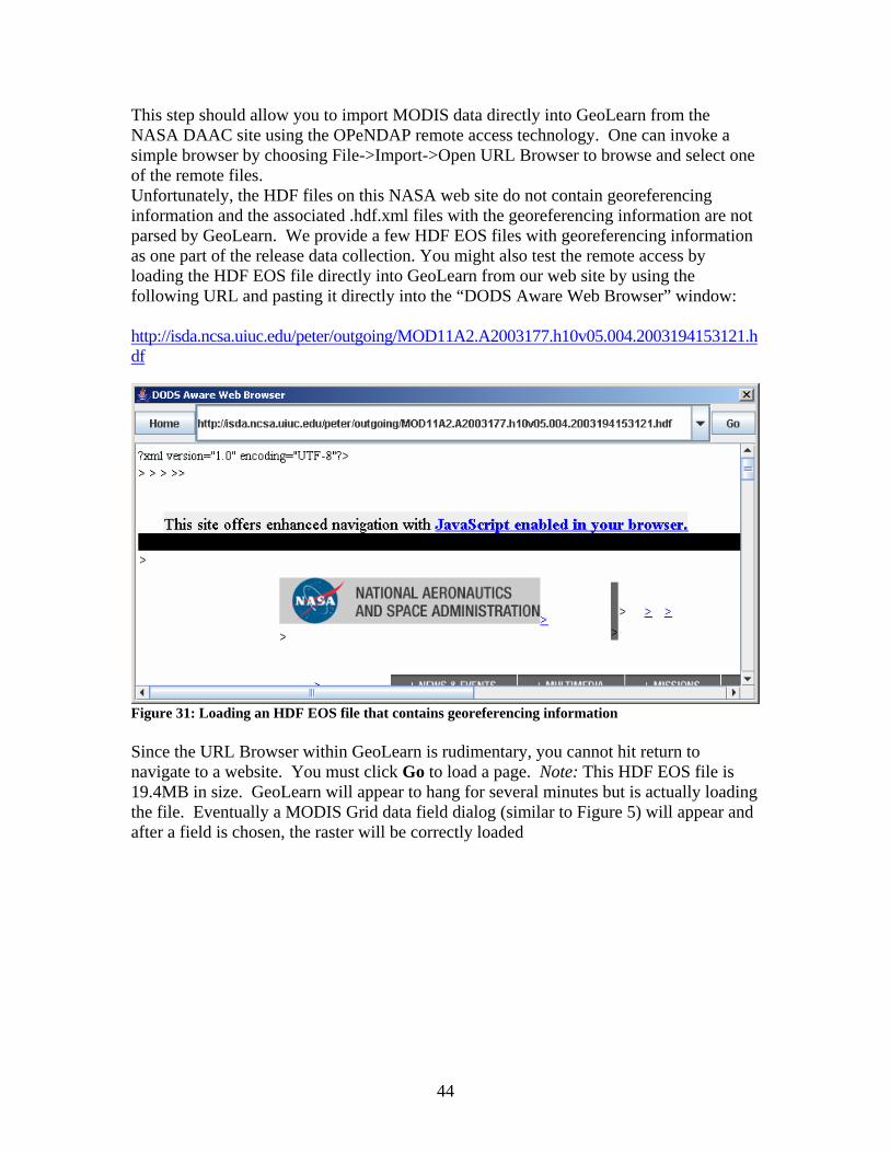
This step should allow you to import MODIS data directly into GeoLearn from the NASA DAAC site using the OPeNDAP remote access technology. One can invoke a simple browser by choosing File->Import->Open URL Browser to browse and select one of the remote files. Unfortunately, the HDF files on this NASA web site do not contain georeferencing information and the associated .hdf.xml files with the georeferencing information are not parsed by GeoLearn. We provide a few HDF EOS files with georeferencing information as one part of the release data collection. You might also test the remote access by loading the HDF EOS file directly into GeoLearn from our web site by using the following URL and pasting it directly into the “DODS Aware Web Browser” window: http://isda.ncsa.uiuc.edu/peter/outgoing/MOD11A2.A2003177.h10v05.004.2003194153121.hdf

Figure 31: Loading an HDF EOS file that contains georeferencing information Since the URL Browser within GeoLearn is rudimentary, you cannot hit return to navigate to a website. You must click Go to load a page. Note: This HDF EOS file is 19.4MB in size. GeoLearn will appear to hang for several minutes but is actually loading the file. Eventually a MODIS Grid data field dialog (similar to Figure 5) will appear and after a field is chosen, the raster will be correctly loaded

45

3.13 MRT Reprojection

Figure 32: A dialog of the MRT tool that contains entries for building a parameter file required for any geographic re-projection.

The MODIS Reprojection Tool is a program available from http://edcdaac.usgs.gov/landdaac/tools/modis/index.asp. The user interface shown above is for setting all parameters for geographic re-projections that are saved in a parameter file.

The user guide of this interface is available from http://edcdaac.usgs.gov/landdaac/tools/modis/info/MRT_Users_Manual.pdf.

46

Chapter 4 GeoLearn for Out-of-Core Tables

There are cases when the extracted pixel information (location and a list of variables for each pixel) are too large to be represented by a MS Excel spreadsheet or processed by D2K data mining algorithms. We provide a separate execution of GeoLearnOutOfCore to save out large size tabular information. This application goes through the same sequence of steps, such as LoadRaster, Integrate and MaskCreate, which are followed by ExportLargeTable step.

4.1 Export Large Table Step There are two buttons for saving out tabular information in comma separated file format as text or in binary format using the extension .mff (MultiFormatFloat). Click on Export button and name the resultant file. This step using the button ‘Export SpecialBinTable to MFF’ will produce a .mff file, a .mff_info file, and a .geog.txt file. using the button ‘Export SpecialTextTable to CSV will produce a .txt file, a . info.txt file, and a .geog.txt file. The two table formats are important because they can hold larger amounts of data than excel or D2K tables. The .mff/.txt files contain the binary/ASCII values, while the .mff_info/.info.txt and .geog.txt files contain information necessary to reconstruct the table as an image. See Section 3.11 for instructions on how to import these “SpecialTables” into Geolearn.

Chapter 5 Additional Notes 5.1 Bug Reports and Bug Fixes GeoLearn is research code. We appreciate your feedback on functionality and usability. If you find bugs, please, report them to isda@ncsa.uiuc.edu or record them at http://isda.ncsa.uiuc.edu/bugs/. However, we do not have resources to provide commercial quality software and code maintenance. Thus, the bugs will be fixed depending on our availability.

5.2 Known Problems

5.2.1 Out of Memory Errors You can tell if out of memory errors occur through three different methods. An error called “Java heap space” will pop up in GeoLearn but will not display additional information.

47

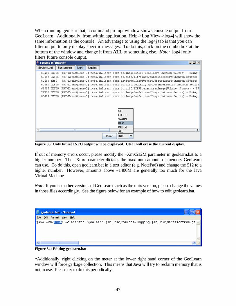
When running geolearn.bat, a command prompt window shows console output from GeoLearn. Additionally, from within application, Help->Log View->log4j will show the same information as the console. An advantage to using the log4j tab is that you can filter output to only display specific messages. To do this, click on the combo box at the bottom of the window and change it from ALL to something else. Note: log4j only filters future console output.

Figure 33: Only future INFO output will be displayed. Clear will erase the current display. If out of memory errors occur, please modify the –Xmx512M parameter in geolearn.bat to a higher number. The –Xmx parameter dictates the maximum amount of memory GeoLearn can use. To do this, open geolearn.bat in a text editor (e.g. NotePad) and change the 512 to a higher number. However, amounts above ~1400M are generally too much for the Java Virtual Machine.

Note: If you use other versions of GeoLearn such as the unix version, please change the values in those files accordingly. See the figure below for an example of how to edit geolearn.bat.

Figure 34: Editing geolearn.bat *Additionally, right clicking on the meter at the lower right hand corner of the GeoLearn window will force garbage collection. This means that Java will try to reclaim memory that is not in use. Please try to do this periodically.

48

5.2.2 Other Problems *Save dialogs will display the file name of the last loaded or saved file. However, they will append the correct file extension when saving.

*The software assumes a screen of at least 1280 pixels wide. We are aware of this issue and are currently looking at redesigning the interface to allow for smaller screen resolutions.

5.2.3 Additional Notes *If GeoLearn needs to be forced to quit, closing the command prompt window (labeled C:\WINDOWS\system32\cmd.exe) will quickly close the application.

*If you are experiencing installation problems, please check the registry values in HKEY_CURRENT_USER->Software->JavaSoft->Prefs. These values can be manually edited or deleted. To use the Registry Editor, click on the Start Menu->Run and type in “regedit”

5.3 Acknowledgments This code called GeoLearn consists of the following packages: D2K, HDF, JAI, DOM4J, Apache LOG4J, Apache Commons Logging, Dods, Jxl, LIBSVM, KD, and Grammatica. If available the GeoLearn tool will use the ArcGIS Engine. To enable the use of the ArcGIS engine a separate license needs to be purchased from ESRI (http://www.esri.com/).

5.4 License Agreement

5.4.1 Illinois Open Source License

University of Illinois/NCSA Open Source License according to http://www.otm.uiuc.edu/faculty/forms/opensource.asp

Copyright © 2006, NCSA/UIUC. All rights reserved. Developed by:

Name of Development Groups: Image Spatial Data Analysis Group (ISDAG) http://isda.ncsa.uiuc.edu/

Hydroclimatology and Terrestrial Hydrology Group (HTHG) http://cee.uiuc.edu/research/hydrology/

Name of Institutions:

49

National Center for Supercomputing Applications (NCSA) http://www.ncsa.uiuc.edu/

Civil and Environmental Engineering (CEE) http://cee.uiuc.edu/

Permission is hereby granted, free of charge, to any person obtaining a copy of this software and associated documentation files (the “Software”), to deal with the Software without restriction, including without limitation the rights to use, copy, modify, merge, publish, distribute, sublicense, and/or sell copies of the Software, and to permit persons to whom the Software is furnished to do so, subject to the following conditions:

• Redistributions of source code must retain the above copyright notice, this list of conditions and the following disclaimers.

• Redistributions in binary form must reproduce the above copyright notice, this list of conditions and the following disclaimers in the documentation and/or other materials provided with the distribution. Neither the names of University of Illinois/NCSA/CEE, nor the names of its contributors may be used to endorse or promote products derived from this Software without specific prior written permission.

THE SOFTWARE IS PROVIDED “AS IS”, WITHOUT WARRANTY OF ANY KIND, EXPRESS OR IMPLIED, INCLUDING BUT NOT LIMITED TO THE WARRANTIES OF MERCHANTABILITY, FITNESS FOR A PARTICULAR PURPOSE AND NONINFRINGEMENT. IN NO EVENT SHALL THE CONTRIBUTORS OR COPYRIGHT HOLDERS BE LIABLE FOR ANY CLAIM, DAMAGES OR OTHER LIABILITY, WHETHER IN AN ACTION OF CONTRACT, TORT OR OTHERWISE, ARISING FROM, OUT OF OR IN CONNECTION WITH THE SOFTWARE OR THE USE OR OTHER DEALINGS WITH THE SOFTWARE.