GEOHYDROLOGY, WATER QUALITY, AND ESTIMATION OF

GROUND-WATER RECHARGE IN SAN FRANCISCO,

CALIFORNIA, 1987-92

jb/Steven P. Phillips, Scott N. Hamlin and Eugene B, Yates

U.S. GEOLOGICAL SURVEY

Water-Resources Investigations Report 93-4019

Prepared in cooperation with the SAN FRANCISCO WATER DEPARTMENT

S 8

Sacramento, California 1993

U.S. DEPARTMENT OF THE INTERIOR BRUCE BABBITT, Secretary

U.S. GEOLOGICAL SURVEY Dallas L. Peck, Director

Any use of trade, product, or firm names in this publication is for descriptive purposes only and does not imply endorsement by the U.S. Government.

For sale by the Books and Open-File Reports Section U.S. Geological Survey Federal Center, Box 25425 Denver, CO 80225

For additional information write to: District Chief U.S. Geological Survey Federal Building, Room W-2233 2800 Cottage Way Sacramento, CA 95825

CONTENTS

Abstract 1 Introduction 1

Purpose and scope 2 Description of study area 2 Previous studies 4 Acknowledgments 4

Geohydrology 4 Geology 4Geometry of ground-water basins 5 Hydrologic characteristics 6

Water levels 6General trends 6 Seasonal variation 7Comparison of shallow and deep ground-water levels

Aquifer properties 9 Water quality 11

Sample collection and analysis 11 Factors affecting water quality 11 Variation of water-quality characteristics 12

General conditions 12Comparison of shallow and deep ground water 14

Characterization of nitrate sources 15 Fertilizers 15 Sewage 16Distribution of nitrate and tritium near Lake Merced 18

Seawater contamination 18 Estimation of ground-water recharge 21

Climate 22Temperature 22 Rainfall 23

Land and water use 24 Land use 24 Water use 25

Sources of recharge 26Infiltration of rainfall 26 Infiltration of irrigation water 29 Leakage from water and sewer pipes 29

Recharge interception 30 Rainfall runoff 30 Evapotranspiration 30

Calibration and sensitivity of hydrologic routing model 32 Sewer flow 33 Monthly calibration 35 Simulation of storms 36Sensitivity analysis and limitations of the model 37

Estimated ground-water recharge 39 Summary and conclusions 40 References cited 41Appendix 1. Description of variables used in hydrologic routing model 65 Appendix 2. Equations used in hydrologic routing model 67

Contents

PLATES

[Plates are in pocket at back of report]

1. Generalized geologic sections through San Francisco, California.2. Maps of San Francisco and part of San Mateo Counties, California, showing well locations, lateral extent

of ground-water basins, altitude of bedrock surface, and rainfall.3. Map showing thickness of alluvium in the vicinity of San Francisco, California.

FIGURES

1. Map showing location of study area 3 2-4. Graphs showing:

2. Variation of water levels in selected wells, 1988-92 83. Variation of water level in Lake Merced from October 1987 to February 1992 84. Variation of water levels in deep and shallow wells, 1988-92 9

5. Trilinear diagram showing quality of ground water, rain, sewage, and seawater in theSan Francisco area 13

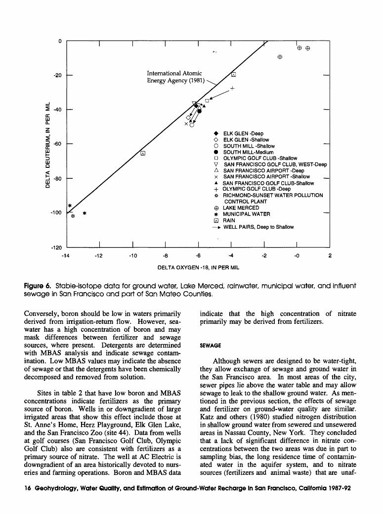
6,7. Graphs showing:6. Stable-isotope data for ground water, Lake Merced, rainwater, municipal water, and influent

sewage in San Francisco and part of San Mateo Counties 167. Average monthly temperatures at three weather stations in San Francisco and part of San Mateo

Counties, 1959-83 238. Map showing land use in San Francisco, April 1989 27

9-15. Graphs showing:9. Estimated monthly indoor and outdoor water use in San Francisco, 1987-88 28

10. Relation between actual and potential evapotranspiration based on soil type and soil moisture 32

11. Simulated sewer overflow as a function of rainfall for six storms on the west side of San Francisco in water year 1988 34

12. Sewer overflow, sewer water pumped to the ocean outfall, and measured sewer flow at the Richmond-Sunset Water Pollution Control Plant, April 1987-September 1988 34

13. Calculated and measured municipal water delivery in San Francisco, April 1987- September 1988 35

14. Calculated and measured sewer flow on the west and east sides of San Francisco, April 1987-September 1988 36

15. Calculated and measured sewer flow for six storms on the west and east sides of San Francisco, water year 1988 37

TABLES

1. Summary of results from aquifer tests in San Francisco 102. Boron, methylene blue active substance, and nitrogen species in ground water in San Francisco and part

of San Mateo Counties 143. Classification for degree of hardness 154. Stable-isotope ratios for ground water, surface water, and rain water in San Francisco and part of San

Mateo Counties 175. Tritium concentrations in ground water, surface water, and seawater in San Francisco and part of San

Mateo Counties 196. Chloride-boron and chloride-bromide ratios for ground water, surface water, sewage, and seawater in San

Francisco and part of San Mateo Counties during winter 1988 and spring 1989-90 207. Monthly average measured temperatures at San Francisco Airport, water years 1987-88 23

IV Contents

8. Average annual rainfall at the National Oceanic and Atmospheric Administration gage at the Federal Office Building in San Francisco 23

9. Population density and water use in San Francisco, 1970 2410. Estimation of monthly indoor water use as a fraction of monthly total water use in San Francisco 2811. Estimated and calculated reference evapotranspiration with pan evaporation from Lake Merced 3212. Rainfall and simulated overflow for six storms on the west side of San Francisco 3413. Rainfall for six storms in San Francisco during water year 1988 3714. Results of sensitivity analysis 3815. Areal distribution of calculated ground-water recharge in San Francisco by ground-water basin, water

years 1987-88 3916. Water-level and construction data for wells in San Francisco and part of San Mateo Counties 4517. Chemical composition of ground and surface water in San Francisco and part of San Mateo Counties 5418. Input values for variables used in the calibrated hydrologic routing model that vary by month 5619. Input values for variables used in the calibrated hydrologic routing model that vary by land-use zone 5720. Average annual output from the calibrated hydrologic routing model by land-use zone for the west side of

San Francisco, water years 1987-88 6021. Average annual output from the calibrated hydrologic routing model by land-use zone for the east side of

San Francisco, water years 1987-88 62

Conversion Factors, Vertical Datum, Water-Quality Information, and Well-Numbering System

Conversion Factors

Multiply By To obtain

acre

acre-foot (acre-ft)

acre-foot per month (acre-ft/mo)acre-foot per year (acre-ft/yr)

foot (ft)foot per day (ft/d)

foot per year (ft/yr)inch (in.)

inch per month (in/mo)inch per year (in/yr)

mile (mi)Million gallons per day (Mgal/d)

square mile (mi2)

0.40474,047

0.32591,233

0.0012331,2331,233

0.30480.30480.3048

25.425.425.4

1.6093,785

259.02.590

hectaresquare metermillion gallons (Mgal)cubic metercubic hectometercubic meter per monthcubic meter per yearmetermeter per daymeter per yearmillimetermillimeter per monthmillimeter per yearkilometercubic meter per dayhectaresquare kilometer

Temperature is given in degrees Fahrenheit (°F), which can be converted to degrees Celsius (°C) by the following equation:

°F=1.8(°C)+32.

Vertical Datum

Sea level: In this report, "sea level" refers to the National Geodetic Vertical Datum of 1929~a geodetic datum derived from a general adjustment of the first-order level nets of the United States and Canada, formerly called Sea Level Datum of 1929.

Conversion Factors, Vertical Datum, Water-Quality Information, and Well-Numbering System V

Water-Quality Information

Chemical concentration is given in milligrams per liter (mg/L) or micrograms per liter (|ig/L). Milligrams per liter is a unit expressing the solute per unit volume (liter) of water. One thousand micrograms per liter is equivalent to 1 milligram per liter. For concentrations less than 7,000 mg/L, the numerical value is the same as for concentrations in parts per million.

Well-Numbering System

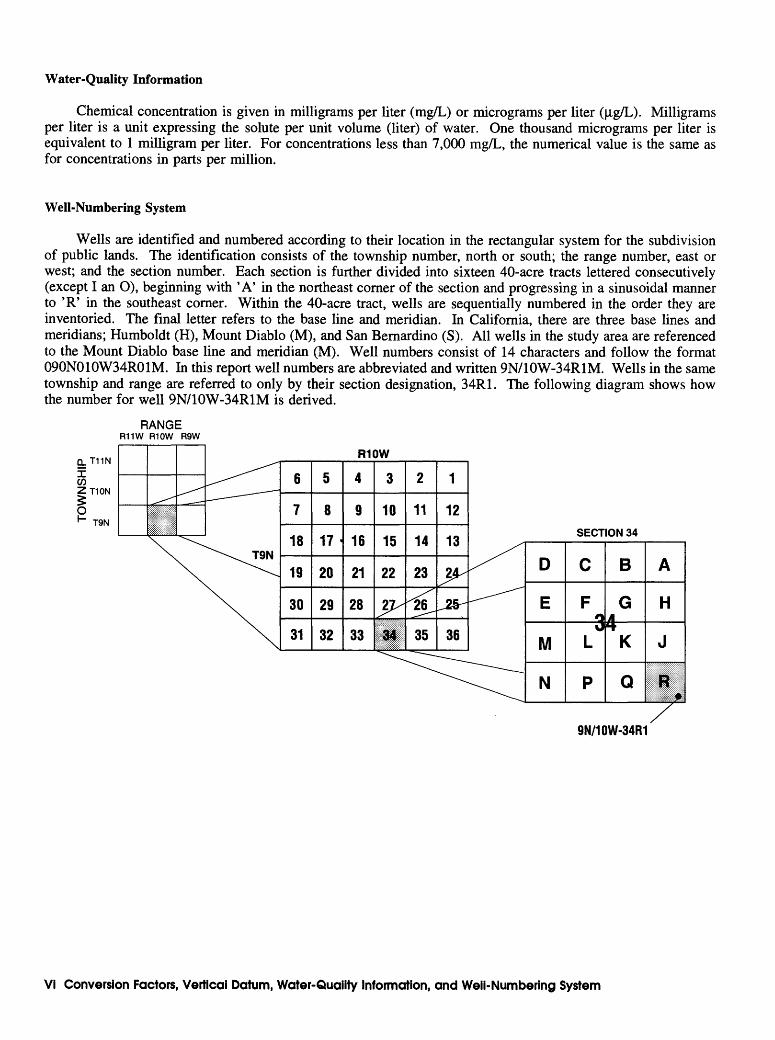
Wells are identified and numbered according to their location in the rectangular system for the subdivision of public lands. The identification consists of the township number, north or south; the range number, east or west; and the section number. Each section is further divided into sixteen 40-acre tracts lettered consecutively (except I an O), beginning with 'A' in the northeast corner of the section and progressing in a sinusoidal manner to 'R' in the southeast corner. Within the 40-acre tract, wells are sequentially numbered in the order they are inventoried. The final letter refers to the base line and meridian. In California, there are three base lines and meridians; Humboldt (H), Mount Diablo (M), and San Bernardino (S). All wells in the study area are referenced to the Mount Diablo base line and meridian (M). Well numbers consist of 14 characters and follow the format 090N010W34R01M. In this report well numbers are abbreviated and written 9N/10W-34R1M. Wells in the same township and range are referred to only by their section designation, 34R1. The following diagram shows how the number for well 9N/10W-34R1M is derived.

mowQ.T11N

COZT10N

*~ T9N

RANGER11W R10W R9W

III!! Ill

T9N

6

7

18

19

30

31

5

8

17 '

20

29

32

4

9

16

21

28

33

3

10

15

22

SSSSSSSS:

2

11

14

23

^

35

1

12

13

P-

JSr

36

SECTION 34

D

E

M

N

C

F

L

P

B

G4^

K

Q

A

H

J

111

9N/10W-34R1

VI Conversion Factors, Vertical Datum, Water-Quality Information, and Well-Numbering System

GEOHYDROLOGY, WATER QUALITY, AND ESTIMATION OF

GROUND-WATER RECHARGE IN SAN FRANCISCO,

CALIFORNIA, 1987-92

foySteven P, Phillips, Scott N, Hamlin, and Eugene B, Yates

Abstract

The city of San Francisco is considering further development of local ground-water resources as a supplemental source of water for potable or nonpotable use. By the year 2010, further water demand is projected to exceed the delivery capacity of the existing supply system, from which San Francisco draws most of its water. The existing system is fed by surface- water sources; thus, supplies are susceptible to drought conditions and damage to conveyance lines by earthquakes. The primary purpose of this study is to describe local geohydrology and water quality, and to estimate ground-water recharge in the area of the city of San Francisco.

Seven ground-water basins were identified in San Francisco on the basis of geologic and geo­ physical data. Basins on the east side of the city are relatively thin and contain a greater percent­ age of fine-grained sediments than those on the west side. The relatively small capacity of the basins and greater potential for contamination from sewer sources may limit the potential for ground-water development on the east side. Basins on the west side of the city have a rela­ tively large capacity and low density sewer net­ work. Water-level data indicate that the southern part of the largest basin on the west side of the city (Westside basin) probably cannot accommo­ date additional ground-water development with­ out adversely affecting water levels and water quality in Lake Merced; however, the remainder of the basin, which is largely undeveloped, could be developed further.

A hydrologic routing model was developed for estimating ground-water recharge throughout San Francisco. The model takes into account cli­ matic factors, land and water use, irrigation, leakage from underground pipes, rainfall runoff, evapotranspiration, and other factors associated with an urban environment. Results indicate that areal recharge rates for water years 1987-88 for the seven ground-water basins range from 0.32 to 0.78 foot per year. Recharge for the Westside basin was estimated at 0.51 foot per year. Aver­ age annual ground-water recharge represents the maximum annual long-term yield of the basin. Attainable yield may be less than the volume of ground-water recharge because interception of all discharge from the basin may not be feasible without inducing seawater intrusion or causing other undesirable effects,

INTRODUCTION

The city of San Francisco is considering further development of ground water as a local source of water for potable or nonpotable use, and as an emer­ gency supply of potable water. San Francisco cur­ rently (1993) imports most of its water, 80 to 90 percent of which comes from the Hetch Hetchy Aque­ duct pipeline system. The primary source of this water is nearly 200 mi from San Francisco, in Yo- semite National Park. Local sources of water include ground water, which is used primarily for irrigation of parks and golf courses; Lobos Creek, which is diver­ ted for potable use; and Lake Merced, from which water is used for a variety of nonpotable purposes.

The Hetch Hetchy system supplies water to about 2 million people in five counties along the pipeline

Introduction 1

route, and water demands may soon exceed the deliv­ ery capacity of the system (Cheryl K. Davis, San Francisco Water Department, written commun., 1988). Current annual average delivery capacity is equivalent to a rate of about 325 Mgal/d and water use in 1987 averaged 240 Mgal/d systemwide. Between the years 2000 and 2010, average annual demand is expected to range from 325 to 345 Mgal/d. Greater use of local ground water in San Francisco would reduce the de­ mand and dependency on the Hetch Hetchy system. Also, local ground water could be a major source of emergency drinking-water supply if the Hetch Hetchy pipeline were damaged by an earthquake and tempor­ arily put out of service.

Ground water was a significant source of water supply for San Francisco during the late 1800's and early 1900's, when water for municipal purposes was obtained from a number of wells and natural springs. Since that time, development of the Hetch Hetchy pipeline system and associated reservoirs has satisfied increasing water demands from the city and other municipalities along the pipeline. The San Francisco Water Department (SFWD) has been operating the system since 1930. Currently, the major use of spring water is withdrawal of about 2 Mgal/d from spring- fed Lobos Creek for the Presidio, which is a military reservation. The major use of ground water in the city is for irrigation at Golden Gate Park, Stern Grove, Fleishhacker Zoo, and several golf courses. A large quantity of ground water is pumped for muni­ cipal purposes and irrigation south of the city, between Daly City and San Bruno.

Basic geohydrologic data, water-quality data, and recharge estimates are all essential elements of an assessment of ground-water resources. The city of San Francisco is considering the use of its ground- water resources for supply augmentation and emer­ gency use. This report describes results of a study done by the U.S. Geological Survey in cooperation with the San Francisco Water Department and is an extension of work by Yates and others (1990), who concentrated on the Golden Gate Park and Lake Merced areas of San Francisco.

PURPOSE AND SCOPE

The primary purpose of this report is to describe local geohydrology and water quality, and to estimate ground-water recharge in the area of the city of San Francisco. Geologic and geophysical data were used

to describe the geometry and lithologic characteristics of the ground-water basins. Hydrologic data were used to describe water-level trends, general quality of ground water, and hydraulic properties of aquifer materials that make up the water-bearing part of the ground-water basins. Climate, land and water use, and other data were used to estimate ground-water recharge on an areal basis throughout San Francisco.

Previous studies that contained information pertinent to this study were reviewed. Climatic and other hydrologic data were provided by various public agencies. Additional data collected for this study include geophysical (gravity) data, water levels in Lake Merced and in 56 wells, and water quality of surface and ground water.

DESCRIPTION OF STUDY AREA

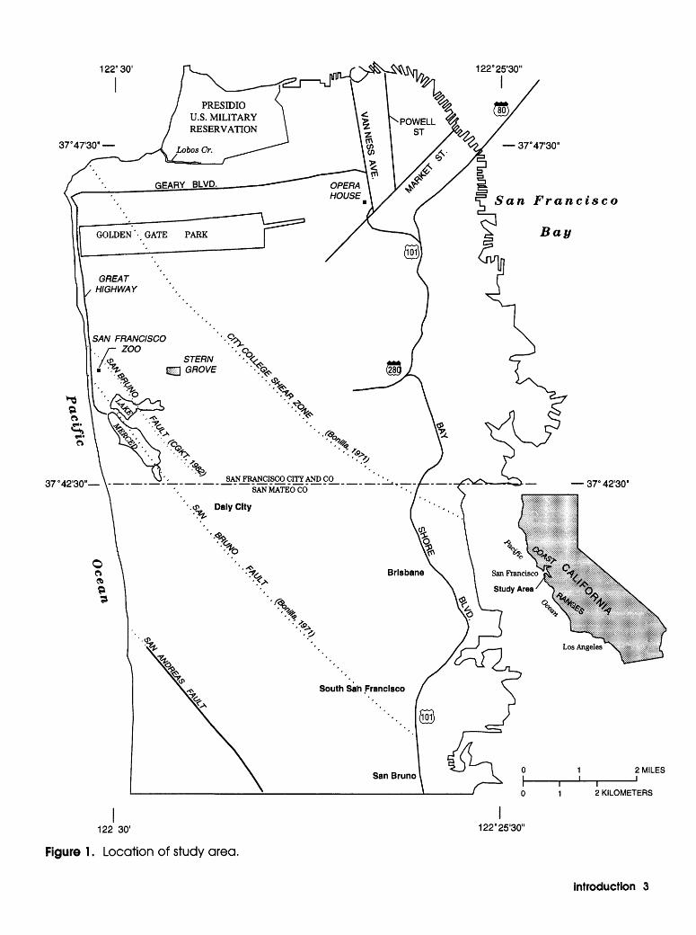
San Francisco is built on the tip of a peninsula on the central California coast. The city and county of San Francisco, which share the same boundary, are bounded on the west by the Pacific Ocean, and on the north and east by the San Francisco Bay (fig. 1). Part of San Mateo County, which is south of San Francis­ co, is included in this study; however, recharge was not estimated outside of San Francisco.

The total area of San Francisco is about 49 mi2 . The topography is hilly, with a generally north-south trending topographic divide that reaches a maximum altitude of about 925 ft above sea level. The San Francisco climate is characterized by mild, wet win­ ters and mild dry summers. Westerly winds from the Pacific Ocean and summer fog tend to moderate temperatures; the average daily temperature in Golden Gate Park ranges from 45°F in January to 69°F in September. Record high and low temperatures are 101 °F and 27°F. Annual rainfall is variable through­ out the city, but averages about 22.5 in.

The northeastern part of San Francisco is the most developed, with high-rise office and apartment buildings. This part of the city has the highest daytime population because it is the primary destin­ ation of most commuters and tourists. The south­ eastern part of the city is largely industrial and residential, with limited open space. The west side of San Francisco is primarily residential, but contains several large undeveloped areas including Golden Gate Park, the Lake Merced shoreline, and several golf courses near Lake Merced.

2 Geohydrology, Water Quality, and Estimation of Ground-Water Recharge in San Francisco, California 1987-92

122° 30

37°47'30

San Francisco

Bay

PRESIDIO U.S. MILITARY RESERVATION

37°42'30"

2 MILES I

2 KILOMETERS

122 30'

Figure 1 . Location of study area.

122°25'30"

Introduction 3

PREVIOUS STUDIES

The first comprehensive evaluation of the ground- water supply in San Francisco was completed by Bartell (1913). Bartell estimated average pumping rates for various districts in the city. At the time, virtually all ground-water development was on the east side because the west side was sparsely popu­ lated. Bartell concluded that east-side pumping generally was approaching the limits of safe yield and proposed additional withdrawal on the west side. There have been several studies of the geology of San Francisco and surrounding areas. The most definitive are the geologic maps of the San Francisco North (Schlocker, 1974) and the San Francisco South (Bonilla, 1971) U.S. Geological Survey quadrangles.

Numerous studies by engineering consultants have focused on selected aspects of local geohydrol- ogy surrounding construction sites. Many of these studies were associated with the Bayside Facilities plan. The Bayside Facilities, which now are in operation, consist of the Westside Transport System (WSTS) and the Southwest Ocean Outfall (SWOO). The WSTS is a series of high-capacity underground storage tanks along the Great Highway. These tanks are designed to store large volumes of sewer water during storms for later disposal through the SWOO or treatment at the Richmond-Sunset Water Pollution Control Plant (Richmond-Sunset WPCP). Studies for these construction projects contain borehole infor­ mation, water levels, aquifer properties, and other data.

Yates and others (1990) studied the general geohydrology and water quality of the west side of San Francisco, and studied in detail the Golden Gate Park and Lake Merced areas. Yates and others (1990) includes an extensive discussion of the geol­ ogy of western San Francisco, water levels, aquifer characteristics, water budgets, and other data and information pertinent to this study.

ACKNOWLEDGMENTS

Public agencies and corporations that have contributed information and assistance to this study, inclusive of the preliminary report by Yates and others (1990), include the San Francisco Clean Water Program, San Francisco Department of Public Works, Pacific Gas and Electric Company, San Francisco Recreation and Park Department, San Francisco Department of Public Health, San Francisco Fire Department, San Francisco Bureau of Water-Pollution

Control, and Daly City. Private businesses and individuals that contributed information and assistance to the study include Geo/Resource Consultants, Harding-Lawson Associates, Lake Merced Boating and Fishing Company, Olympic Golf Club, San Francisco Golf Club, Bendix Environmental Research, San Francisco State University, Gregory B. Yates, Eve Iverson, Carla M. Reiter, and Chris A. Phanartzis of Hydroconsult Engineers.

GEOHYDROLOGY

GEOLOGY

The geologic materials in San Francisco can be divided into two distinct categories: bedrock and unconsolidated sediments. Bedrock in San Francisco consists of consolidated rocks of the Franciscan Complex and the Great Valley Sequence of Late Jur­ assic and Cretaceous age (Schlocker, 1974). Bedrock crops out in hilly areas and accounts for about 24 percent of the land surface of San Francisco. Plate 1 shows several representative geologic sections of parts of San Francisco.

Overlying bedrock in some areas are uncon­ solidated sediments that constitute the ground-water basins. On the west side of San Francisco, unconsoli­ dated sediments consist of dune sands and the Colma and Merced Formations of Pleistocene and Pleistocene and Pliocene age, respectively (pi. IB, 1C). Gener­ ally, the Merced Formation is overlain by the Colma Formation, which in turn is overlain by the dune sands. The Merced Formation consists predominantly of shallow marine and estuarine deposits with thin interbedded muds and peats. Thicker fine-grained layers (10 to 60 ft) are known to exist (Clifton and Hunter, 1987, p. 260). The Merced Formation dips to the northeast, decreasing from 40° in the older strata exposed south of Daly City to 10 or 15° in the youngest strata exposed near Lake Merced (Bonilla, 1971). Tilted fine-grained strata might impede horizontal flow of ground water.

The Colma Formation, which overlies the Merced Formation, probably consists largely of reworked material from the Merced Formation (Schlocker, 1974). The Colma Formation consists of nearly flat- lying fine-grained sand, silty sand, and occasional beds of clay as much as 5 ft thick. Dune sands overly the Colma Formation over most of the west side of San Francisco north of Lake Merced and range in thickness from 0 to 150 ft (Schlocker, 1974). The dune sands consist of well-sorted fine- to medium-grained sand.

4 Geohydrology, Water Quality, and Estimation of Ground-Water Recharge in San Francisco, California 1987-92

On the north and east sides of San Francisco, the unconsolidated sediments consist of dune sand, the Colma Formation, bay mud and clay, artificial fill, and other relatively fine-grained surficial deposits (pi. ID-IF). The unconsolidated sediments on the east side generally are more fine grained than those on the west side. The artificial fill reaches a maximum thickness of about 60 ft, and is composed primarily of dune sand, but also contains silt, clay, and various natural and manmade debris (Schlocker, 1974). Bay mud and clay deposits, which reach a maximum thickness of about 140 ft (pi. 1D-1FJ, are described as a plastic gray silty clay (Schlocker, 1974).

Significant structural features include a series of northwest-trending faults, including the San Andreas Fault, the San Bruno Fault, and the City College Shear Zone. The San Andreas Fault is 2 to 3 mi off­ shore west of San Francisco. It is not known whether the fault has an effect on the hydraulic connection between the ground-water basin and the Pacific Ocean. The San Bruno Fault passes through the Lake Merced area, although the age, exact location, and offset are unknown. Also, it is unknown whether the fault acts as a hydraulic barrier or conduit, but water levels near Lake Merced do not indicate the presence of a barrier. The City College Shear Zone trends northwestward from Bay shore, and cuts through the western part of Golden Gate Park. Water levels in Golden Gate Park do not indicate that the fault acts as a hydraulic barrier. Yates and others (1990) provide a more extensive discussion of these faults.

The structure of the subterranean bedrock surface has been mapped in various parts of San Francisco by previous investigators (Bonilla, 1964; 1971; Carlson and McCulloch, 1970; Schlocker, 1974). A compre­ hensive map of bedrock altitude in San Francisco and northern San Mateo County was compiled using data from the aforementioned investigations, more recent borehole data, and geophysical data collected for this investigation. Borehole data were extracted from water well driller's logs provided by the California Department of Water Resources, test boring logs were provided by the California Department of Trans­ portation (CALTRANS), and from private consultants (Harding-Lawson Associates, 1976b; Dames and Moore, 1979; Caldwell-Gonzalez-Kennedy-Tudor, 1982). The overlapping existing maps and borehole data provided reasonably good coverage of the eastern and northern parts of San Francisco, but data were sparse on the west side where the bedrock surface is relatively deep. Yates and others (1990) pointed out that the depth and shape of the Westside basin is

highly speculative because of minimal borehole data and conflicting geophysical evidence.

A gravity survey was done for the purpose of estimating the shape of the bedrock surface on the west side of San Francisco and San Mateo Counties (Roberts, 1991). Relative changes in gravity meas­ ured on an areal grid indicate changes in density of subsurface materials. Consolidated materials (bed­ rock) are more dense than unconsolidated materials (alluvium); thus, relatively small gravity measure­ ments indicate relatively thick alluvium. More than 700 gravity measurements were made and the gravity data were calibrated to bedrock altitude using data from about 200 boreholes.

Plate 2B is the compiled map of bedrock altitude representing the work of previous investigators, new borehole data, and new geophysical data. The bed­ rock surface is complex, ranging in altitude from the land surface to more than 3,500 ft below sea level. The bedrock altitude is relatively high on the east side of San Francisco, with a minimum altitude of about 275 ft below sea level. On the west side, bedrock altitude generally decreases southward, and reaches a minimum altitude of about 3,500 ft below sea level along the coast about 1.5 mi south of Lake Merced in San Mateo County. The minimum bedrock altitude in San Francisco County is about 2,500 ft below sea level, shoreward of Lake Merced.

GEOMETRY OF GROUND-WATER BASINS

A ground-water basin is defined here as a contin­ uous body of unconsolidated sediments and the sur­ rounding surface drainage area. Seven major ground- water basins were identified in San Francisco (pi. 2A) on the basis of geologic and geophysical data. All basins are open to the Pacific Ocean or San Francisco Bay. The landward parts of the ground-water basins generally are bounded horizontally and vertically by bedrock, which is assumed to be relatively imperme­ able compared with unconsolidated alluvium. Ground-water flow may occur between basins where the bedrock ridge that constitutes the boundary is subterranean. The north-south topographic and bedrock high defined by the Coast Ranges generally forms an east-west hydrologic boundary through San Francisco.

The western part of San Francisco is divided into the Westside and Lobos basins on the basis of a northwest-trending bedrock ridge through the north-

Geohydrology 5

eastern part of Golden Gate Park (pi. 2A). The bedrock ridge has several small surface expressions, and bedrock altitude data indicate that the ridge is continuous, though subterranean. Some degree of hy­ draulic connection is possible between the two basins where the ridge is not exposed at the land surface, but the degree of connection probably is minimal. The Westside basin, which is the largest ground-water basin in San Francisco, is not contained fully in San Francisco, as the Merced Formation extends as far south as San Bruno. The areal extent of the Westside basin in San Francisco is about 9,451 acres. The Lobos basin to the north of the Westside basin includes about 2,379 acres.

The eastern part of San Francisco is divided into five basins on the basis of bedrock ridges that virtu­ ally are exposed entirely at the land surface. The Marina basin is the northernmost and includes about 2,224 acres. The Downtown basin, to the south of Marina basin, is the largest of the eastern basins at 7,512 acres. Continuing from north to south are the Islais Valley, South, and Visitacion Valley basins, which include about 5,000, 2,130, and 800 acres in San Francisco County, respectively. Basin names used in this report other than the formal designations Islais Valley and Visitacion Valley from the Cali­ fornia Department of Water Resources (1975a) are informal designations.

Plate 3 is a map of alluvial thickness generated from the bedrock altitude map (pi. 25) and digital topographic data. The thickness of unconsolidated alluvial deposits in a ground-water basin is a primary factor that controls the potential for ground-water development. Thin ground-water basins have a rela­ tively low storage capacity and provide a minimal buffer zone between the screens of production wells and shallow ground water that is susceptible to sur­ face contamination. Plate 3 shows that the alluvium generally is thinner on the east side of San Francisco, with a maximum thickness of less than 300 ft. Maxi­ mum alluvial thickness on the west side of San Francisco is about 2,500 ft, and thickness is as much as 3,500 ft in San Mateo County. The relatively thin ground-water basins on the east side do not preclude ground-water development in this area. In the early 1900's, about 6,900 acre-ft/yr was withdrawn from east-side ground-water basins. This level of develop­ ment was not without problems because drawdown was significant in some areas, and high chloride concentrations in at least two wells may indicate seawater intrusion (Bartell, 1913).

HYDROLOGIC CHARACTERISTICS

WATER LEVELS

The water level measured in a well indicates the hydraulic head at the depth of the well screen. Hy­ draulic head is a measure of the potential energy of ground water at a point in the ground-water basin. It is expressed as an altitude with respect to sea level in this report. Water levels were measured periodically in 56 wells for this study, 54 of which are shown on plate 2A. The two wells not shown are at the San Francisco International Airport, which is south of the study area on the shore of San Francisco Bay. Al­ though various trends in water levels were identified, a water-level contour map was not drawn because of the sparsity and uneven areal distribution of well data, and the extreme variability of the topography and the bedrock surface. Water-level data for all wells measured are given in table 16 (at back of report).

General trends. -Hydraulic gradients generally follow topographic slopes in the San Francisco area, except where affected by ground-water pumping. Water levels are lowest along the shore and in areas of pumping depressions, such as around the southern part of Lake Merced (Yates and others, 1990). Pumping from the deep part of the aquifer system also produces a downward hydraulic gradient in this area, from the shallow to the deep part of the aquifer system.

Ground-water levels on the east side of the city generally are closer to the land surface than those on the west side. Ground-water basins on the east side are thinner and smaller in volume than those on the west side. Studies of sewer flow indicate that infil­ tration of ground water predominantly occurs on the east side, where the water table commonly is above the sewer lines (San Francisco Department of Public Works, 1974a). Many underground structures in this area, such as the Powell Street Bay Area Rapid Tran­ sit (BART) station and the basement at the Opera House, require sump pumps to remove infiltrating ground water. Historically, ground-water pumping coupled with small storage resulted in water levels that declined below sea level in the downtown area (Bartell, 1913). The water table on the west side generally is below the level of sewer lines, which results in exfiltration of sewage to the ground-water system where leaks are present (San Francisco Department of Public Works, 1974b).

6 Geohydrology, Water Quality, and Estimation of Ground-Water Recharge in San Francisco, California 1987-92

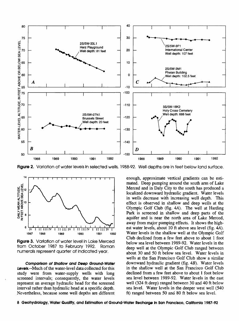
During the course of this study (1987-92), all wells showed declining water levels. This effect is primarily a result of reduced recharge during the concurrent drought. Water levels in wells near the landward edges of ground-water basins tend to have linear declines, such as at the Herz Playground (fig. 2A). Between 1989 and 1992, the water level in this well declined nearly 10 ft. Declines in this and other wells indicate that discharge from the ground-water basins exceeds recharge. A resumption of average rainfall could reverse this trend because water pre­ viously lost from storage is replenished.

Seasonal variation. -Seasonal variations in ground-water levels are affected by changes in re­ charge and pumpage. Generally, highs in the water table may occur in late winter at the end of the rainy season. Lows usually occur in the autumn at the end of the irrigation season and before winter rains.

Many wells in the San Francisco area are used for irrigation and other nonpotable purposes. The variations in the water table caused by pumping tend to mask the effects of seasonal recharge. Most wells in areas not affected by pumping showed declining water levels without significant evidence of recovery due to seasonal recharge. However, the well at Brussels Street (fig. 25) did show a small water-level rise during the winters of 1989 and 1990. Aside from the winter recovery, water levels generally declined during this period. This well is near the center of the ground-water basin in contrast to the well at the Herz Playground at the edge of the basin that showed a decline of about 10 ft during the same period.

Ground-water pumping has produced the most significant changes in water levels. Dewatering of structures below the water table in the downtown area (basements and BART tunnel) and irrigation on the west side of the city (Golden Gate Park and Lake Merced area) account for the largest withdrawals of ground water in San Francisco. Dewatering generally is continuous throughout the year and produces a fairly constant, localized drawdown in the water table. This effect may be seen in the hydrographs for wells at the International Center and the Phelan Building in the downtown area (fig. 2Q. The two wells are about 1 mi apart and 100 ft deep. The altitude of the land surface at the International Center is about 10 ft higher than at the Phelan Building. Ground-water pumping is insignificant near the International Center and water-level altitudes are about 30 ft above sea level. In contrast, the well at the Phelan Building is

near the Powell Street BART station, which pumps large quantities of ground water for dewatering purposes. Water levels at this well are about 5 ft below sea level, or 35 ft lower than those at the International Center. Ground-water levels that decline below sea level in areas near the shore may induce seawater intrusion.

In contrast to the fairly constant drawdown pro­ duced by dewatering, ground-water pumping for irri­ gation produces a seasonal variation in water levels. This phenomenon is observed in the irrigation well at Holy Cross Cemetery, where water levels are about 15 ft lower during the irrigation season (fig. 2D). Ground-water pumping has resulted in water-level altitudes greater than 100 ft below sea level in some areas. Water-level altitudes are relatively low beneath cemeteries, parks, golf courses, and other areas where ground water is pumped for irrigation. Water levels are relatively low near the southwestern part of the city as a result of pumping for irrigation in the city, and pumping for potable use in Daly City. Water levels declined more than 150 ft below sea level (Applied Consultants, 1991, fig. 11) in some areas as a result of pumping for potable use in Daly City.

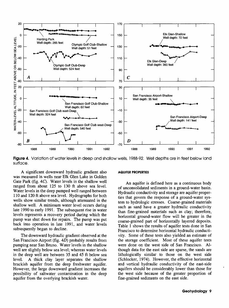
Water levels in Lake Merced show the effects of seasonal recharge and ground-water and surface-water pumping (fig. 3). The San Francisco and Olympic Golf Clubs adjacent to the south arm of Lake Merced pump ground water from the deep part of the aquifer system for irrigation as do Daly City and the Lake Merced Country Club to the south. Pumping draw­ downs in the deep aquifer have induced downward flow from the shallow aquifer in this area; conse­ quently, water levels in the shallow part of the aquifer system also declined. Lake Merced virtually is an exposed part of the water table and has been declining for more than 10 years (Yates and others, 1990). Maximum yearly water levels reflect recharge and runoff from winter rains. Subsequent natural and pumping-induced discharge cause the lake level to decline to a minimum value in the autumn before re­ charge from subsequent rainfall. Yearly declines measured among minimum values were 1.4 ft for 1987-88, 1.2 ft for 1988-89, 2.5 ft for 1989-90, and 0.3 ft for 1990-91 (fig. 3). The smaller decline for 1990-91 may reflect changes in pumping and weather. Direct pumping from the lake to irrigate the Harding Park Golf Course was discontinued in late 1990. Additionally, the San Francisco and Olympic Golf Clubs reportedly pumped less ground water as a result of an unusually cool and foggy summer.

Geohydrology 7

80

75

HI CO

O65HI CO CC2 608CO

^55HI1^75

HI§70

§65HI

HI

"£60HII

55

50

2S/5W-33L1 Herz Playground

, Well depth: 81 feet

40

30

20

10

2S/5W-27N1 Brussels Street

,Well depth: 20 feet

B

-10-100

-110

-120

-130

-140

-150

"2S/5W-9F1 International Center Well depth: 107 feet

2S/5W-3M1 Phelan Building

, Well depth: 102.5 feet

3S/5W-18K2Holy Cross CemeteryWell depth: 688 feet

D

Figure

1988 1989 1990 1991 1992 1988 1989 1990 1991 1992

2. Variation of water levels in selected wells, 1988-92. Well depths are in feet below land surface.

14

if QUJ12

10

i i i r

i i i i i i i i i iiv i ii in iv i ii in iv i ii mrv i ii in iv i

1987 1988 1989 1990 1991 1992

Figure 3. Variation of water level in Lake Merced from October 1987 to February 1992. Roman numerals represent quarter of indicated year.

Comparison of Shallow and Deep Ground-WaterLevels. Much of the water-level data collected for this study were from water-supply wells with long screened intervals; consequently, the water levels represent an average hydraulic head for the screened interval rather than hydraulic head at a specific depth. Nevertheless, because some well depths are different

enough, approximate vertical gradients can be esti­ mated. Deep pumping around the south arm of Lake Merced and in Daly City to the south has produced a localized downward hydraulic gradient. Water levels in wells decrease with increasing well depth. This effect is observed in shallow and deep wells at the Olympic Golf Club (fig. 4A). The well at Harding Park is screened in shallow and deep parts of the aquifer and is near the north area of Lake Merced, away from major pumping effects. It shows the high­ est water levels, about 10 ft above sea level (fig. 4A). Water levels in the shallow well at the Olympic Golf Club declined from a few feet above to about 1 foot below sea level between 1989-92. Water levels in the deep well at the Olympic Golf Club ranged between about 30 and 50 ft below sea level. Water levels in wells at the San Francisco Golf Club show a similar downward hydraulic gradient (fig. 4B). Water levels in the shallow well at the San Francisco Golf Club declined from a few feet above to about 1 foot below sea level between 1989-92. Water levels in the east well (324 ft deep) ranged between 30 and 40 ft below sea level. Water levels in the deeper west well (540 ft) ranged between 50 and 80 ft below sea level.

8 Geohydrology, Water Quality, and Estimation of Ground-Water Recharge in San Francisco, California 1987-92

^u

LEVEL

0

3 C

ABOVE OR BELOW SEA

5 6> J> r3 0 0 C

i \J\J

LJJ

u_ ^uzLJJ'

1 °_EVEL ALl

ro o

£-40

1-60

-fin

1 1 1 1

\ i"IAL A A

Harding Park / Well depth: 265 feet Oiympjc Q /, C|ub.sha||ow

Well depth: 51 feet

Olympic Golf Club-Deep Well depth: 524 feet

A I I I I

I I I I

\ San Francisco Golf Club-ShallowWell depth: 62 feet

~~ San Francisco Golf Club east-Deep ~ Well depth: 324 feet \

San Francisco Golf Club west-Deep

B I I I I

l/U

150

1 OU

110

90

70

ou

10

-10

-30

-50

-7fl

I I I I

Elk Glen-ShallowWell depth: 72 feet

* % *-« », -

Elk Glen-Deep / Well depth: 360 feet

C I I I I

I I I I

San Francisco Airport-ShallowWell depth: 35 feet \

San Francisco Airport-Deep_ xWell depth: 141 feet _

D I I I I

1988 1989 1990 1991 1992 1988 1989 1990 1991 1992

Figure 4. Variation of water levels in deep and shallow wells, 1988-92. Well depths are in feet below land surface.

A significant downward hydraulic gradient also was measured in wells near Elk Glen Lake in Golden Gate Park (fig. 4C). Water levels in the shallow well ranged from about 125 to 130 ft above sea level. Water levels in the deep pumped well ranged between 110 and 120 ft above sea level. Hydrographs for both wells show similar trends, although attenuated in the shallow well. A minimum water level occurs during late 1990 to early 1991. The subsequent rise in water levels represents a recovery period during which the pump was shut down for repairs. The pump was put back into operation in late 1991, and water levels subsequently began to decline.

The downward hydraulic gradient observed at the San Francisco Airport (fig. 4D) probably results from pumping near San Bruno. Water levels in the shallow well are slightly below sea level; whereas water levels in the deep well are between 35 and 45 ft below sea level. A thick clay layer separates the shallow brackish aquifer from the deep freshwater aquifer. However, the large downward gradient increases the possibility of saltwater contamination in the deep aquifer from the overlying brackish water.

AQUIFER PROPERTIES

An aquifer is defined here as a continuous body of unconsolidated sediments in a ground-water basin. Hydraulic conductivity and storage are aquifer proper­ ties that govern the response of a ground-water sys­ tem to hydrologic stresses. Coarse-grained materials such as sand have a greater hydraulic conductivity than fine-grained materials such as clay; therefore, horizontal ground-water flow will be greater in the coarse-grained part of horizontally layered deposits. Table 1 shows the results of aquifer tests done in San Francisco to determine horizontal hydraulic conducti­ vity. Some of these tests also yielded an estimate of the storage coefficient. Most of these aquifer tests were done on the west side of San Francisco. Al­ though data for the east side are sparse, the sands are lithologically similar to those on the west side (Schlocker, 1974). However, the effective horizontal and vertical hydraulic conductivity of the east-side aquifers should be considerably lower than those for the west side because of the greater proportion of fine-grained sediments on the east side.

Geohydrology 9

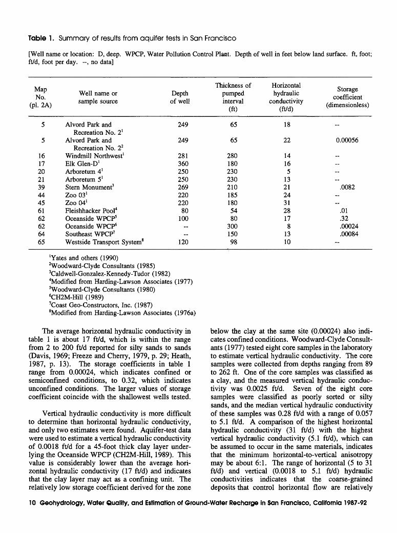
Table 1 . Summary of results from aquifer tests in San Francisco

[Well name or location: D, deep. WPCP, Water Pollution Control Plant. Depth of well in feet below land surface, ft, foot; ft/d, foot per day. , no data]

Map No.

(pi. 2A)

5

5

161720213944456162626465

Well name or sample source

Alvord Park andRecreation No. 2 1

Alvord Park andRecreation No. 22

Windmill Northwest1Elk Glen-D 1Arboretum 4lArboretum 5 lStern Monument3Zoo 03 1Zoo 04 1Fleishhacker Pool4Oceanside WPCP5Oceanside WPCP6Southeast WPCP7Westside Transport System8

Depth of well

249

249

281360250250269220220

80100

__

120

Thickness of pumped interval

(ft)

65

65

2801802302302101851805480

30015098

Horizontal hydraulic

conductivity (ft/d)

18

22

14165

132124312817

81310

Storage coefficient

(dimensionless)

_

0.00056

.0082

.01

.32

.00024

.00084-

'Yates and others (1990)2Woodward-Clyde Consultants (1985)3Caldwell-Gonzalez-Kennedy-Tudor (1982)4Modified from Harding-Lawson Associates (1977)5Woodward-Clyde Consultants (1980)6CH2M-Hill (1989)7Coast Geo-Constructors, Inc. (1987)8Modified from Harding-Lawson Associates (1976a)

The average horizontal hydraulic conductivity in table 1 is about 17 ft/d, which is within the range from 2 to 200 ft/d reported for silty sands to sands (Davis, 1969; Freeze and Cherry, 1979, p. 29; Heath, 1987, p. 13). The storage coefficients in table 1 range from 0.00024, which indicates confined or semiconfined conditions, to 0.32, which indicates unconfined conditions. The larger values of storage coefficient coincide with the shallowest wells tested.

Vertical hydraulic conductivity is more difficult to determine than horizontal hydraulic conductivity, and only two estimates were found. Aquifer-test data were used to estimate a vertical hydraulic conductivity of 0.0018 ft/d for a 45-foot thick clay layer under­ lying the Oceanside WPCP (CH2M-Hill, 1989). This value is considerably lower than the average hori­ zontal hydraulic conductivity (17 ft/d) and indicates that the clay layer may act as a confining unit. The relatively low storage coefficient derived for the zone

below the clay at the same site (0.00024) also indi­ cates confined conditions. Woodward-Clyde Consult­ ants (1977) tested eight core samples in the laboratory to estimate vertical hydraulic conductivity. The core samples were collected from depths ranging from 89 to 262 ft. One of the core samples was classified as a clay, and the measured vertical hydraulic conduc­ tivity was 0.0025 ft/d. Seven of the eight core samples were classified as poorly sorted or silty sands, and the median vertical hydraulic conductivity of these samples was 0.28 ft/d with a range of 0.057 to 5.1 ft/d. A comparison of the highest horizontal hydraulic conductivity (31 ft/d) with the highest vertical hydraulic conductivity (5.1 ft/d), which can be assumed to occur in the same materials, indicates that the minimum horizontal-to-vertical anisotropy may be about 6:1. The range of horizontal (5 to 31 ft/d) and vertical (0.0018 to 5.1 ft/d) hydraulic conductivities indicates that the coarse-grained deposits that control horizontal flow are relatively

10 Geohydrology, Water Quality, and Estimation of Ground-Water Recharge in San Francisco, California 1987-92

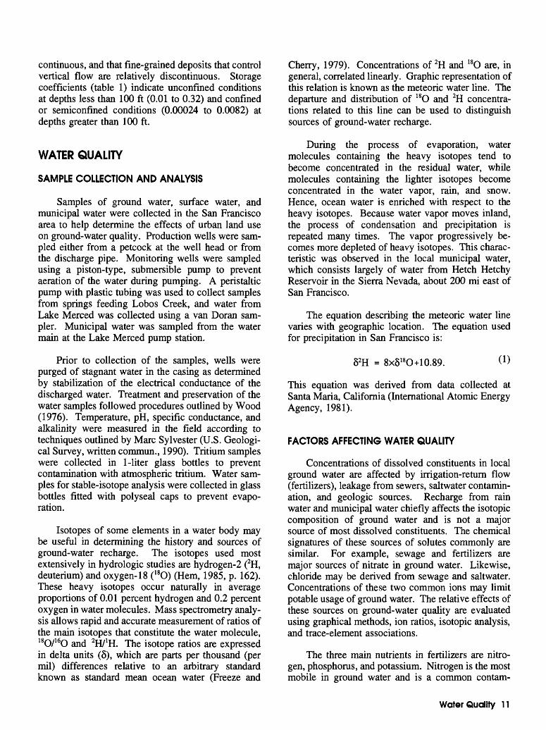
continuous, and that fine-grained deposits that control vertical flow are relatively discontinuous. Storage coefficients (table 1) indicate unconfmed conditions at depths less than 100 ft (0.01 to 0.32) and confined or semiconfmed conditions (0.00024 to 0.0082) at depths greater than 100 ft.

WATER QUALITY

SAMPLE COLLECTION AND ANALYSIS

Samples of ground water, surface water, and municipal water were collected in the San Francisco area to help determine the effects of urban land use on ground-water quality. Production wells were sam­ pled either from a petcock at the well head or from the discharge pipe. Monitoring wells were sampled using a piston-type, submersible pump to prevent aeration of the water during pumping. A peristaltic pump with plastic tubing was used to collect samples from springs feeding Lobos Creek, and water from Lake Merced was collected using a van Doran sam­ pler. Municipal water was sampled from the water main at the Lake Merced pump station.

Prior to collection of the samples, wells were purged of stagnant water in the casing as determined by stabilization of the electrical conductance of the discharged water. Treatment and preservation of the water samples followed procedures outlined by Wood (1976). Temperature, pH, specific conductance, and alkalinity were measured in the field according to techniques outlined by Marc Sylvester (U.S. Geologi­ cal Survey, written cornmun., 1990). Tritium samples were collected in 1-liter glass bottles to prevent contamination with atmospheric tritium. Water sam­ ples for stable-isotope analysis were collected in glass bottles fitted with polyseal caps to prevent evapo­ ration.

Isotopes of some elements in a water body may be useful in determining the history and sources of ground-water recharge. The isotopes used most extensively in hydrologic studies are hydrogen-2 (2H, deuterium) and oxygen-18 (18O) (Hem, 1985, p. 162). These heavy isotopes occur naturally in average proportions of 0.01 percent hydrogen and 0.2 percent oxygen in water molecules. Mass spectrometry analy­ sis allows rapid and accurate measurement of ratios of the main isotopes that constitute the water molecule, 18O/16O and 2H/1H. The isotope ratios are expressed in delta units (5), which are parts per thousand (per mil) differences relative to an arbitrary standard known as standard mean ocean water (Freeze and

Cherry, 1979). Concentrations of 2H and 18O are, in general, correlated linearly. Graphic representation of this relation is known as the meteoric water line. The departure and distribution of 18O and 2H concentra­ tions related to this line can be used to distinguish sources of ground-water recharge.

During the process of evaporation, water molecules containing the heavy isotopes tend to become concentrated in the residual water, while molecules containing the lighter isotopes become concentrated in the water vapor, rain, and snow. Hence, ocean water is enriched with respect to the heavy isotopes. Because water vapor moves inland, the process of condensation and precipitation is repeated many times. The vapor progressively be­ comes more depleted of heavy isotopes. This charac­ teristic was observed in the local municipal water, which consists largely of water from Hetch Hetchy Reservoir in the Sierra Nevada, about 200 mi east of San Francisco.

The equation describing the meteoric water line varies with geographic location. The equation used for precipitation in San Francisco is:

52H = 8x518O+10.89. (1)

This equation was derived from data collected at Santa Maria, California (International Atomic Energy Agency, 1981).

FACTORS AFFECTING WATER QUALITY

Concentrations of dissolved constituents in local ground water are affected by irrigation-return flow (fertilizers), leakage from sewers, saltwater contamin­ ation, and geologic sources. Recharge from rain water and municipal water chiefly affects the isotopic composition of ground water and is not a major source of most dissolved constituents. The chemical signatures of these sources of solutes commonly are similar. For example, sewage and fertilizers are major sources of nitrate in ground water. Likewise, chloride may be derived from sewage and saltwater. Concentrations of these two common ions may limit potable usage of ground water. The relative effects of these sources on ground-water quality are evaluated using graphical methods, ion ratios, isotopic analysis, and trace-element associations.

The three main nutrients in fertilizers are nitro­ gen, phosphorus, and potassium. Nitrogen is the most mobile in ground water and is a common contam-

Water Quality 11

inant. Fertilizers also may add sulfate to ground water. In the San Francisco area, the largest quantities of fertilizers are applied to residential landscaping and golf courses. Residential use probably accounts for the greatest contribution of fertilizer chemicals to ground water because of the larger total land area than that for golf courses. Additionally, homeowners are more likely to apply fertilizers in excess of plant needs than the gardeners at golf courses.

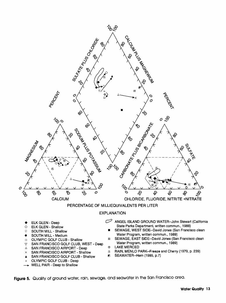
Leakage from sewers may introduce dissolved constituents to ground water that are similar to those from fertilizers (nutrients, sulfate). In addition, sewage generally contains high concentrations of chloride due to widespread use of salt in human activities and the infiltration of saltwater into sewer pipes on the east side of San Francisco. The average concentration of chloride in sewage flowing to the Richmond-Sunset WPCP on the west side of the city is 139 mg/L, compared with 793 mg/L in sewage flowing to the Southeast WPCP servicing the south­ east side of the city (Jon Loiacano, San Francisco Clean Water Program, written commun., 1991). Infil­ tration of bay water occurs at some sewer outfalls on the east side in the tidal zone. Gates and valves intended to prevent bay-water infiltration occasionally malfunction and allow saltwater to enter the sewer system. On the west side of the city, the Steinhart Aquarium in Golden Gate Park discharges wastewater from saltwater aquariums to the sewer system. The difference in average sewer-water composition be­ tween the east and west sides of the city is shown in figure 5. Water from both sewage systems shows the effects of saltwater input; however, the chemically conservative anions indicate that the composition of east-side sewage is much closer to seawater compo­ sition than west-side sewage. Additionally, salts from ocean water also may be introduced directly to ground water by seawater intrusion, or indirectly by wash- down and infiltration of salt spray.

Many dissolved constituents in natural ground water are derived, at least in part, from interaction with minerals composing the aquifer. Concentrations of ionic species, such as fluoride, may be controlled by equilibrium with a mineral, such as fluorite. Addi­ tionally, cation-exchange reactions with clay minerals often control the composition of cations in ground water. Some rocks serve as sources of the chloride and sulfate anions to ground water. However, the bicarbonate anion present in most water is derived in large part from carbon dioxide in the atmosphere (Hem, 1985).

VARIATION OF WATER-QUALITY CHARACTERISTICS

GENERAL CONDITIONS

The quality of ground water in western San Francisco was described by Yates and others (1990). The general characteristics of ground water are similar throughout the San Francisco area. Samples that rep­ resent the range of water-quality conditions in the San Francisco area are shown in a trilinear diagram (fig. 5). Trilinear diagrams are used to show the relative proportions of common cations and anions, thereby allowing comparison and classification of water sam­ ples with different concentrations (Hem, 1985). This type of diagram also is useful for showing the effects of mixing water from two different sources. If two different waters are combined, the composition of the mixture will be proportional to the relative quantities of each as long as chemical reactions do not occur. Intermediate compositions of the mixture conse­ quently will plot on a trilinear diagram along a straight line connecting the two source compositions. Most ground water in the study area is a mixed cat­ ion, bicarbonate type. Urban and natural factors may shift ion proportions to a sodium chloride type water. Ion exchange also may alter the proportions of cations in water and thereby produce ground water with a composition other than a simple mixture of water from different sources (Todd, 1980). The major anions generally are stable and conservative during mixing in local shallow ground water.

Selected water-quality data for the San Francisco area are summarized in table 17 (at back of report). Additional water-quality data for the San Francisco area are presented by Hamlin and Yates (1990) and Yates and others (1990). Concentrations of most major dissolved constituents in local ground water are within guidelines recommended by the U.S. Environ­ mental Protection Agency (1986). However, nitrate- nitrogen in ground water commonly exceeds the pri­ mary maximum contaminant level of 10 mg/L (U.S. Environmental Protection Agency, 1986).

Primary drinking-water standards are based on anticipated health effects. Nitrate-nitrogen concen­ trations greater than 10 mg/L in water may cause methemoglobinemia (blue-baby disease) when used for infant feeding. Ten of 22 sites sampled in the San Francisco area had nitrate-nitrogen concentrations of 10 mg/L or greater. The concentrations ranged from 12 to 36 mg/L, and most concentrations were between 12 and 20 mg/L (table 2).

12 Geohydrology, Water Quality, and Estimation of Ground-Water Recharge in San Francisco, California 1987-92

CALCIUM CHLORIDE, FLUORIDE, NITRITE +NITRATE

PERCENTAGE OF MILLIEQUIVALENTS PER LITER

EXPLANATION

Oo

ELK GLEN - Deep ELK GLEN - Shallow SOUTH MILL - Shallow

SOUTH MILL-Mediumn OLYMPIC GOLF CLUB - ShallowV SAN FRANCISCO GOLF CLUB, WEST - DeepA SAN FRANCISCO AIRPORT - Deepx SAN FRANCISCO AIRPORT - ShallowA SAN FRANCISCO GOLF CLUB - Shallow+ OLYMPIC GOLF CLUB - Deep > WELL PAIR - Deep to Shallow

ANGEL ISLAND GROUND WATER--John Stewart (California State Parks Department, written commun., 1988)

SEWAGE, WEST SIDE-David Jones (San Francisco clean Water Program, written commun., 1989)

SEWAGE, EAST SIDE-David Jones (San Francisco clean Water Program, written commun., 1989)

LAKE MERCEDRAIN, MENLO PARK-Freeze and Cherry (1979, p. 239)SEAWATER-Hem(1985,p.7)

Figure 5. Quality of ground water, rain, sewage, and seawater in the San Francisco area.

Water Quality 13

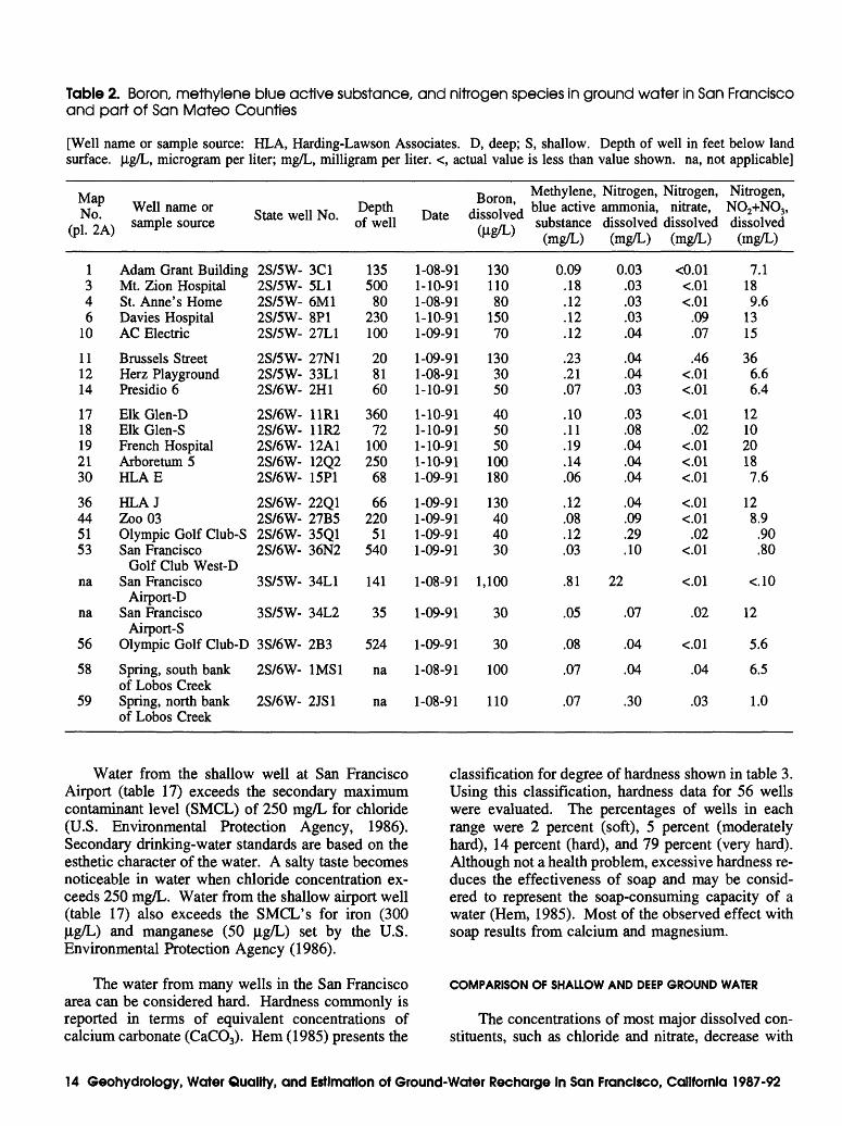
Table 2. Boron, methylene blue active substance, and nitrogen species in ground water in San Francisco and part of San Mateo Counties

[Well name or sample source: HLA, Harding-Lawson Associates. D, deep; S, shallow. Depth of well in feet below land surface. ug/L, microgram per liter; mg/L, milligram per liter. <, actual value is less than value shown, na, not applicable]

Map . vr Well name orCol 2A) samP^e source

1346

10

111214

1718192130

36445153

na

na

56

58

59

Adam Grant BuildingMt. Zion HospitalSt. Anne's HomeDavies HospitalAC Electric

Brussels StreetHerz PlaygroundPresidio 6

Elk Glen-DElk Glen-SFrench HospitalArboretum 5HLAE

HLAJZoo 03Olympic Golf Club-SSan Francisco

Golf Club West-DSan Francisco

Airport-DSan Francisco

Airport-SOlympic Golf Club-D

Spring, south bankof Lobos CreekSpring, north bankof Lobos Creek

State well No.

2S/5W-2S/5W-2S/5W-2S/5W-2S/5W-

2S/5W-2S/5W-2S/6W-

2S/6W-2S/6W-2S/6W-2S/6W-2S/6W-

2S/6W-2S/6W-2S/6W-2S/6W-

3S/5W-

3S/5W-

3S/6W-

2S/6W-

2S/6W-

3C15L16M18P127L1

27N133L12H1

11R111R212A112Q215P1

22Q127B535Q136N2

34L1

34L2

2B3

1MS1

2JS1

Depth of well

135500

80230100

208160

36072

100250

68

66220

51540

141

35

524

na

na

Date

1-08-911-10-911-08-911-10-911-09-91

1-09-911-08-911-10-91

1-10-911-10-911-10-911-10-911-09-91

1-09-911-09-911-09-911-09-91

1-08-91

1-09-91

1-09-91

1-08-91

1-08-91

g Methylene, Nitrogen, ,. * ' , blue active ammonia, /u /T \ substance dissolved ^ (mg/L) (mg/L)

13011080

15070

1303050

405050

100180

130404030

1,100

30

30

100

110

0.09.18.12.12.12

.23

.21

.07

.10

.11

.19

.14

.06

.12

.08

.12

.03

.81

.05

.08

.07

.07

0.03.03.03.03.04

.04

.04

.03

.03

.08

.04

.04

.04

.04

.09

.29

.10

22

.07

.04

.04

.30

Nitrogen, nitrate,

dissolved (mg/L)

<0.01<.01

Nitrogen, NO2+NO3 , dissolved

(mg/L)

7.118

<.01 9.6.09.07

.46<.01

1315

366.6

<.01 6.4

<.01.02

<.01<.01<.01

<.01<.01

.02<.01

<.01

.02

<.01

.04

.03

121020187.

128.

<.

12

5.

6.

1.

6

99080

10

6

5

0

Water from the shallow well at San Francisco Airport (table 17) exceeds the secondary maximum contaminant level (SMCL) of 250 mg/L for chloride (U.S. Environmental Protection Agency, 1986). Secondary drinking-water standards are based on the esthetic character of the water. A salty taste becomes noticeable in water when chloride concentration ex­ ceeds 250 mg/L. Water from the shallow airport well (table 17) also exceeds the SMCL's for iron (300 Lig/L) and manganese (50 Lig/L) set by the U.S. Environmental Protection Agency (1986).

The water from many wells in the San Francisco area can be considered hard. Hardness commonly is reported in terms of equivalent concentrations of calcium carbonate (CaCO3). Hem (1985) presents the

classification for degree of hardness shown in table 3. Using this classification, hardness data for 56 wells were evaluated. The percentages of wells in each range were 2 percent (soft), 5 percent (moderately hard), 14 percent (hard), and 79 percent (very hard). Although not a health problem, excessive hardness re­ duces the effectiveness of soap and may be consid­ ered to represent the soap-consuming capacity of a water (Hem, 1985). Most of the observed effect with soap results from calcium and magnesium.

COMPARISON OF SHALLOW AND DEEP GROUND WATER

The concentrations of most major dissolved con­ stituents, such as chloride and nitrate, decrease with

14 Geohydrology, Water Quality, and Estimation of Ground-Water Recharge in San Francisco, California 1987-92

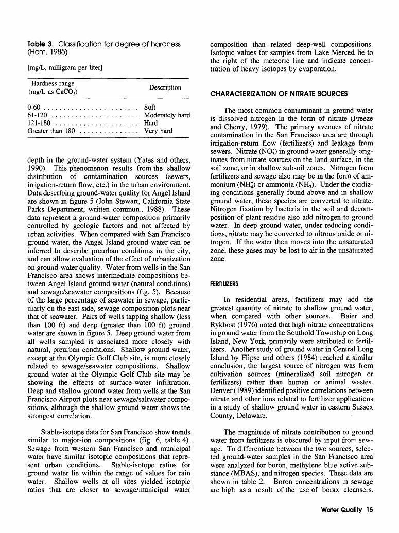
Table 3. Classification for degree of hardness (Hem, 1985)

[mg/L, milligram per liter]

Hardness range (mg/L as CaCO3) Description

0-60 ........................ Soft61-120 ...................... Moderately hard121-180 ..................... HardGreater than 180 ............... Very hard

depth in the ground-water system (Yates and others, 1990). This phenomenon results from the shallow distribution of contamination sources (sewers, irrigation-return flow, etc.) in the urban environment. Data describing ground-water quality for Angel Island are shown in figure 5 (John Stewart, California State Parks Department, written commun., 1988). These data represent a ground-water composition primarily controlled by geologic factors and not affected by urban activities. When compared with San Francisco ground water, the Angel Island ground water can be inferred to describe preurban conditions in the city, and can allow evaluation of the effect of urbanization on ground-water quality. Water from wells in the San Francisco area shows intermediate compositions be­ tween Angel Island ground water (natural conditions) and sewage/seawater compositions (fig. 5). Because of the large percentage of seawater in sewage, partic­ ularly on the east side, sewage composition plots near that of seawater. Pairs of wells tapping shallow (less than 100 ft) and deep (greater than 100 ft) ground water are shown in figure 5. Deep ground water from all wells sampled is associated more closely with natural, preurban conditions. Shallow ground water, except at the Olympic Golf Club site, is more closely related to sewage/seawater compositions. Shallow ground water at the Olympic Golf Club site may be showing the effects of surface-water infiltration. Deep and shallow ground water from wells at the San Francisco Airport plots near sewage/saltwater compo­ sitions, although the shallow ground water shows the strongest correlation.

Stable-isotope data for San Francisco show trends similar to major-ion compositions (fig. 6, table 4). Sewage from western San Francisco and municipal water have similar isotopic compositions that repre­ sent urban conditions. Stable-isotope ratios for ground water lie within the range of values for rain water. Shallow wells at all sites yielded isotopic ratios that are closer to sewage/municipal water

composition than related deep-well compositions. Isotopic values for samples from Lake Merced lie to the right of the meteoric line and indicate concen­ tration of heavy isotopes by evaporation.

CHARACTERIZATION OF NITRATE SOURCES

The most common contaminant in ground water is dissolved nitrogen in the form of nitrate (Freeze and Cherry, 1979). The primary avenues of nitrate contamination in the San Francisco area are through irrigation-return flow (fertilizers) and leakage from sewers. Nitrate (NOj) in ground water generally orig­ inates from nitrate sources on the land surface, in the soil zone, or in shallow subsoil zones. Nitrogen from fertilizers and sewage also may be in the form of am­ monium (NHJ) or ammonia (NH3). Under the oxidiz­ ing conditions generally found above and in shallow ground water, these species are converted to nitrate. Nitrogen fixation by bacteria in the soil and decom­ position of plant residue also add nitrogen to ground water. In deep ground water, under reducing condi­ tions, nitrate may be converted to nitrous oxide or ni­ trogen. If the water then moves into the unsaturated zone, these gases may be lost to air in the unsaturated zone.

FERTILIZERS

In residential areas, fertilizers may add the greatest quantity of nitrate to shallow ground water, when compared with other sources. Baier and Rykbost (1976) noted that high nitrate concentrations in ground water from the Southold Township on Long Island, New York, primarily were attributed to fertil­ izers. Another study of ground water in Central Long Island by Flipse and others (1984) reached a similar conclusion; the largest source of nitrogen was from cultivation sources (mineralized soil nitrogen or fertilizers) rather than human or animal wastes. Denver (1989) identified positive correlations between nitrate and other ions related to fertilizer applications in a study of shallow ground water in eastern Sussex County, Delaware.

The magnitude of nitrate contribution to ground water from fertilizers is obscured by input from sew­ age. To differentiate between the two sources, selec­ ted ground-water samples in the San Francisco area were analyzed for boron, methylene blue active sub­ stance (MBAS), and nitrogen species. These data are shown in table 2. Boron concentrations in sewage are high as a result of the use of borax cleansers.

Water Quality 15

-20

-40ocLLI Q.

2 -60OC LLI

-80

-100

-120

International Atomic Energy Agency (1981)

ELK GLEN -Deep ELK GLEN -ShallowSOUTH MILL -Shallow ~~ SOUTH MILL-Medium OLYMPIC GOLF CLUB -Shallow SAN FRANCISCO GOLF CLUB, WEST-Deep SAN FRANCISCO AIRPORT -Deep SAN FRANCISCO AIRPORT -Shallow _ SAN FRANCISCO GOLF CLUB-Shallow OLYMPIC GOLF CLUB -Deep RICHMOND-SUNSET WATER POLLUTION CONTROL PLANT

LAKE MERCEDMUNICIPAL WATER ~ RAIN WELL PAIRS, Deep to Shallow

-14 -12 -10 -8 -6 -4

DELTA OXYGEN -18, IN PER MIL

-2 -0

Figure 6. Stable-isotope data for ground water, Lake Merced, rainwater, municipal water, and influent sewage in San Francisco and part of San Mateo Counties.

Conversely, boron should be low in waters primarily derived from irrigation-return flow. However, sea- water has a high concentration of boron and may mask differences between fertilizer and sewage sources, where present. Detergents are determined with MBAS analysis and indicate sewage contam­ ination. Low MBAS values may indicate the absence of sewage or that the detergents have been chemically decomposed and removed from solution.

Sites in table 2 that have low boron and MBAS concentrations indicate fertilizers as the primary source of boron. Wells in or downgradient of large irrigated areas that show this effect include those at St. Anne's Home, Herz Playground, Elk Glen Lake, and the San Francisco Zoo (site 44). Data from wells at golf courses (San Francisco Golf Club, Olympic Golf Club) also are consistent with fertilizers as a primary source of nitrate. The well at AC Electric is downgradient of an area historically devoted to nurs­ eries and farming operations. Boron and MBAS data

indicate that the high concentration of nitrate primarily may be derived from fertilizers.

SEWAGE

Although sewers are designed to be water-tight, they allow exchange of sewage and ground water in the San Francisco area. In most areas of the city, sewer pipes lie above the water table and may allow sewage to leak to the shallow ground water. As men­ tioned in the previous section, the effects of sewage and fertilizer on ground-water quality are similar. Katz and others (1980) studied nitrogen distribution in shallow ground water from sewered and unsewered areas in Nassau County, New York. They concluded that a lack of significant difference in nitrate con­ centrations between the two areas was due in part to sampling bias, the long residence time of contamin­ ated water in the aquifer system, and to nitrate sources (fertilizers and animal waste) that are unaf-

16 Geohydrology, Water Quality, and Estimation of Ground-Water Recharge In San Francisco, California 1987-92

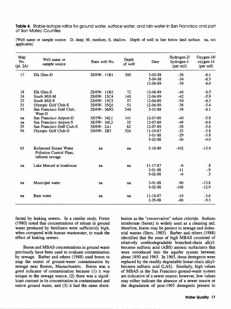
Table 4. Stable-isotope ratios for ground water, surface water, and rain water in San Francisco and part of San Mateo Counties

[Well name or sample source: D, deep; M, medium; S, shallow. Depth of well in feet below land surface, na, not applicable]

Map No.

(pi. 2A)

17

1824255153

na na5556

Well name or sample source

Elk Glen-D

Elk Glen-SSouth Mill-MSouth Mill-SOlympic Golf Club-S San Francisco Golf Club,West-D

San Francisco Airport-D San Francisco Airport-S San Francisco Golf Club-SOlympic Golf Club-D

State well No.

2S/6W- 11R1

2S/6W- 11R22S/6W- 15C42S/6W- 15C52S/6W- 35Q1 2S/6W- 36N2

3S/5W- 34L1 3S/5W- 34L2 3S/6W- 2A13S/6W- 2B3

Depth of well

360

721405751

540

141 35 62

524

Hydrogen-2/ Date hydrogen- 1

(per mil)

3-02-885-04-88

12-06-89

12-06-8912-04-8912-04-8912-06-89 5-02-88

12-07-89 12-07-89 12-07-8911-19-87 3-01-885-02-88

-36-34-39

-46-42-50-36 -38

-40 -49 -38-32 -29-30

Oxygen- 187 oxygen- 16 (per mil)

-6.1-6.3-6.0

-6.5-5.8-6.3-5.4 -6.1

-5.8 -6.6 -5.6-3.8 -3.8-4.0

63 Richmond Sunset Water Pollution Control Plant, influent sewage

na na 5-18-89 -102 -13.6

na Lake Merced at boathouse na

na Municipal water na

na Rain water na

na 11-17-873-01-885-02-88

na 3-01-885-02-88

na 11-19-872-29-88

-6-11

-6

-96-100

-19-66

.8-.9.3

-13.8-12.9

-3.6-9.3

fected by leaking sewers. In a similar study, Porter (1980) noted that concentrations of nitrate in ground water produced by fertilizers were sufficiently high, when compared with human wastewater, to mask the effect of leaking sewers.

Boron and MB AS concentrations in ground water previously have been used to evaluate contamination by sewage. Barber and others (1988) used boron to map the extent of ground-water contamination by sewage near Boston, Massachusetts. Boron was a good indicator of contamination because (1) it was unique to the sewage source, (2) there was a signif­ icant contrast in its concentration in contaminated and native ground water, and (3) it had the same distri­

bution as the "conservative" solute chloride. Sodium tetraborate (borax) is widely used as a cleaning aid; therefore, boron may be present in sewage and indus­ trial wastes (Hem, 1985). Barber and others (1988) identified that the zone of high MBAS consisted of relatively nonbiodegradable branched-chain alkyl- benzene sulfonic acid (ABS) anionic surfactants that were introduced into the aquifer system between about 1950 and 1965. In 1965, these detergents were replaced by the readily degradable linear-chain alkyl- benzene sulfonic acid (LAS). Similarly, high values of MBAS in the San Francisco ground-water system are indicative of a sewer source; however, low values may either indicate the absence of a sewer source or the degradation of post-1965 detergents present in

Water Quality 17

sewage. Le Blanc (1984) determined that boron and chloride were transported conservatively in a ground- water study at Cape Cod, Massachusetts. Boron and chloride also are present in seawater and could be indicators of seawater intrusion. The potential use of boron isotope analysis to distinguish between marine and terrestrial sources is discussed later.

In the absence of seawater contamination, sites in table 2 that show high boron and MBAS concentra­ tions indicate sewage as the primary source of nitrate. Wells that clearly show this effect are at Mt. Zion Hospital, Brussels Street, and at the San Francisco Airport. The shallow well at the San Francisco Air­ port probably is contaminated with a significant quantity of sewage and bay water. High concentra­ tions of MBAS and ammonia indicate sewage con­ tamination, whereas the excessively high boron (1,100 jig/L) and chloride (3,100 mg/L) concentrations indi­ cate the presence of bay water (saltwater). The occurrence of nitrogen in the form of ammonia may indicate close proximity to a sewer leak and (or) reducing conditions in the ground water. The leaky sewer pipe may have been a conduit for the infil­ tration of bay water, as well as a source of nitrogen.

DISTRIBUTION OF NITRATE AND TRITIUM NEAR LAKE MERCED

The concentrations of nitrate-nitrogen in shallow ground water upgradient of Lake Merced are high and average about 10 mg/L. The principal sources of ni­ trate probably are leaking sewer pipes and fertilizers applied to urban landscaping. Fertilization of adjacent golf courses probably contributes a small percentage to the total quantity of nitrate because of the small area they occupy and because only one golf course is upgradient of the lake.

Nitrate data are consistent with flow patterns in the shallow and deep parts of the aquifer system. Nitrate-nitrogen in shallow ground water upgradient of Lake Merced ranges from 5 to 17 mg/L (Yates and others, 1990). Biological processes in the lake rapidly consume nitrate-nitrogen yielding an ambient concen­ tration that is less than 0.1 mg/L. Hamlin and Yates (1990) found that shallow wells on the down gradient side of the lake also have relatively low nitrate- nitrogen concentrations (less than 1.0 mg/L), which confirms that water from the lake flows into the shallow aquifer and reaches the wells. They also found that deep wells on the downgradient side of the lake have lower nitrate-nitrogen concentrations (0.8 to 5.6 mg/L) than deep wells on the upgradient side (8.1 to 14 mg/L). This indicates that lake water is reach­ ing the deep part of the aquifer system.

The distribution of tritium in ground water around Lake Merced (table 5) is consistent with flow to the aquifer induced by nearby pumping in the deep part of the aquifer (Robert Michel, U.S. Geological Survey, written commun., 1991). Tritium is a radio­ active isotope of hydrogen that commonly is used to determine the relative age of ground water. Large quantities of tritium were introduced into the environment through atmospheric tests of nuclear weapons from 1952 to the early 1960's (Michel, 1990). The tritium concentration of water is expressed in tritium units (TU), where 1 TU is the equivalent of 1 tritium atom in 10 18 hydrogen atoms. Before 1952, the natural concentration of tritium in precipitation ranged from 1 to 10 TU (International Atomic Energy Agency, 1983). Recharge from surface-water sources that entered the ground-water system before 1952 presently would have a tritium concentration of less than 2 TU because tritium decays with time and has a half-life of 12.4 years. Recharge from surface-water sources since 1952 shows variable tritium concentrations that generally increased to a peak in 1963 and subsequently de­ creased following the end of atmospheric testing of nuclear weapons (Michel, 1990). Near Lake Merced, tritium concentrations in ground water are close to present-day concentrations (5 to 10 TU) to a depth of 50 ft below the water table (table 5). The 1963 peak was not observed in ground water near Lake Merced (Robert Michel, U.S. Geological Survey, written commun., 1991). These observations indicate that pumping of deep ground water near Lake Merced has induced flow of water from the lake to the ground- water system.

SEAWATER CONTAMINATION

Chloride is the major anion in seawater and it moves through aquifers at nearly the same rate as the intruding water. Increasing chloride concentrations in ground water may be the first indication of seawater contamination (Hem, 1985). In an area where no other source of saline contamination exists, high chloride concentrations indicate seawater contam­ ination. However, sewage also is a source of chloride in San Francisco.

Dissolved constituents other than chloride can be used to help identify seawater contamination, but dif­ ficulties are encountered while using them. Magne­ sium is present in seawater in much greater concen­ tration than calcium; therefore, a low calcium-to- magnesium ratio may indicate the presence of sea- water. The presence of sulfate in anionic proportion

18 Geohydrology, Water Quality, and Estimation of Ground-Water Recharge In San Francisco, California 1987-92

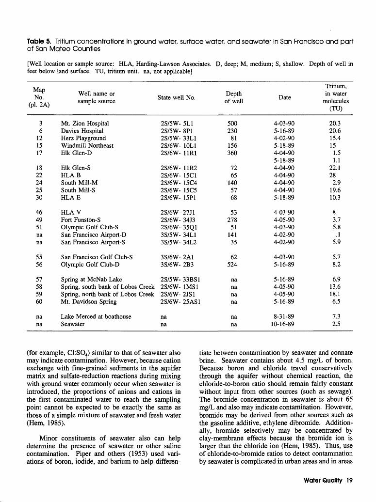
Table 5. Tritium concentrations in ground water, surface water, and seawater in San Francisco and part of San Mateo Counties

[Well location or sample source: HLA, Harding-Lawson Associates. D, deep; M, medium; S, shallow. Depth of well in feet below land surface. TU, tritium unit, na, not applicable]

MapNo.

(pi. 2A)

3 6

12 1517

1822242530

464951 na na

5556

57 58 59 60

nana

Well name or sample source

Mt. Zion Hospital Davies Hospital Herz Playground Windmill NortheastElk Glen-D

Elk Glen-SHLABSouth Mill-MSouth Mill-SHLAE

HLA VFort Funston-SOlympic Golf Club-S San Francisco Airport-D San Francisco Airport-S

San Francisco Golf Club-SOlympic Golf Club-D

Spring at McNab Lake Spring, south bank of Lobos Creek Spring, north bank of Lobos Creek Mt. Davidson Spring

Lake Merced at boathouseSeawater

State well No.

2S/5W- 5L1 2S/5W- 8P1 2S/5W- 33L1 2S/6W- 10L12S/6W- 11R1

2S/6W- 11R22S/6W- 15C12S/6W- 15C42S/6W- 15C52S/6W- 15P1

2S/6W- 27 Jl2S/6W- 34J32S/6W- 35Q1 3S/5W- 34L1 3S/5W- 34L2

3S/6W- 2A13S/6W- 2B3

2S/5W- 33BS1 2S/6W- 1MS1 2S/6W- 2JS1 2S/6W- 25AS1

nana

Depth of well

500 230

81 156360

7265

1405768

53278

51 14135

62524

na na na na

nana

Date

4-03-90 5-16-89 4-02-90 5-18-894-04-905-18-894-04-904-04-904-04-904-04-905-18-89

4-03-904-05-904-03-90 4-02-90 4-02-90

4-03-905-16-89

5-16-89 4-05-90 4-05-90 5-16-89

8-31-8910-16-89

Tritium, in water

molecules(TU)

20.3 20.6 15.4 15

1.51.1

22.128

2.919.610.3

83.75.8

.1 5.9

5.78.2

6.9 13.6 18.1 6.5

7.32.5

(for example, C1:SO4) similar to that of seawater also may indicate contamination. However, because cation exchange with fine-grained sediments in the aquifer matrix and sulfate-reduction reactions during mixing with ground water commonly occur when seawater is introduced, the proportions of anions and cations in the first contaminated water to reach the sampling point cannot be expected to be exactly the same as those of a simple mixture of seawater and fresh water (Hem, 1985).

Minor constituents of seawater also can help determine the presence of seawater or other saline contamination. Piper and others (1953) used vari­ ations of boron, iodide, and barium to help differen­

tiate between contamination by seawater and connate brine. Seawater contains about 4.5 mg/L of boron. Because boron and chloride travel conservatively through the aquifer without chemical reaction, the chloride-to-boron ratio should remain fairly constant without input from other sources (such as sewage). The bromide concentration in seawater is about 65 mg/L and also may indicate contamination. However, bromide may be derived from other sources such as the gasoline additive, ethylene dibromide. Addition­ ally, bromide selectively may be concentrated by clay-membrane effects because the bromide ion is larger than the chloride ion (Hem, 1985). Thus, use of chloride-to-bromide ratios to detect contamination by seawater is complicated in urban areas and in areas

Water Quality 19

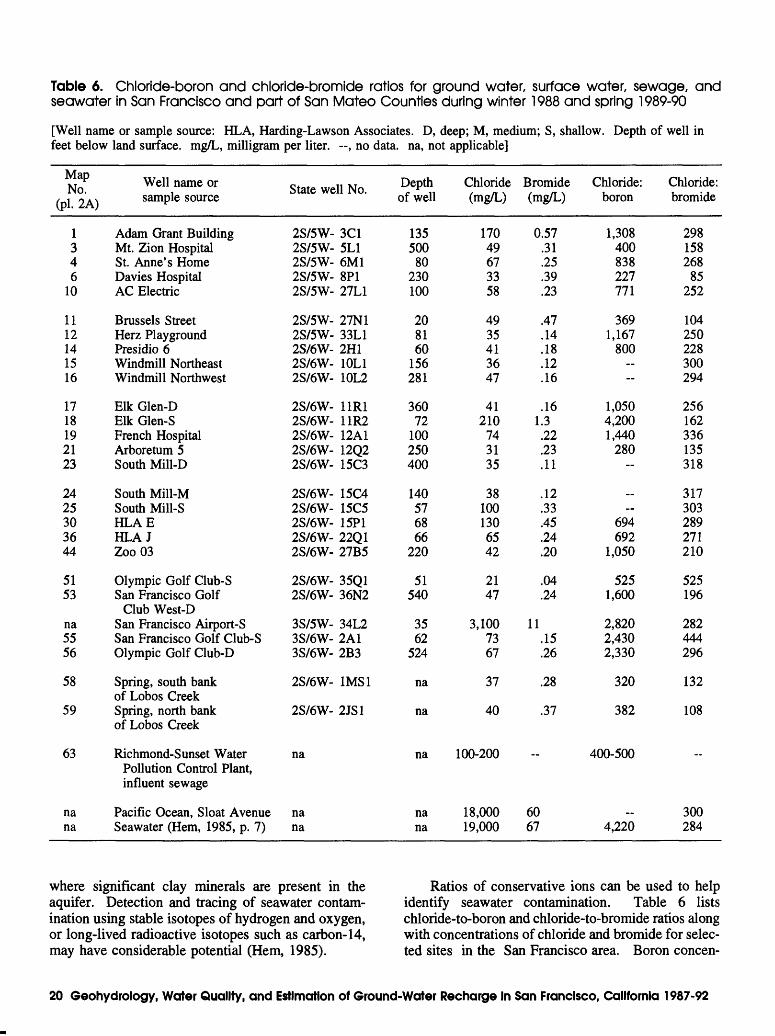
Table 6. Chloride-boron and chloride-bromide ratios for ground water, surface water, sewage, and seawater in San Francisco and part of San Mateo Counties during winter 1988 and spring 1989-90

[Well name or sample source: HLA, Harding-Lawson Associates. D, deep; M, medium; S, shallow. Depth of well in feet below land surface. mg/L, milligram per liter. --, no data, na, not applicable]

J^T Well name or Col 2A} sample source

1346

10

1112141516

1718192123

2425303644

5153

na5556

58

59

Adam Grant BuildingMt. Zion HospitalSt. Anne's HomeDavies HospitalAC Electric

Brussels StreetHerz PlaygroundPresidio 6Windmill NortheastWindmill Northwest

Elk Glen-DElk Glen-SFrench HospitalArboretum 5South Mill-D

South Mill-MSouth Mill-SHLAEHLAJZoo 03

Olympic Golf Club-SSan Francisco Golf

Club West-DSan Francisco Airport-SSan Francisco Golf Club-SOlympic Golf Club-D

Spring, south bankof Lobos CreekSpring, north bankof Lobos Creek

State well No.

2S/5W- 3C12S/5W- 5L12S/5W- 6M12S/5W- 8P12S/5W- 27L1

2S/5W- 27N12S/5W- 33L12S/6W- 2H12S/6W- 10L12S/6W- 10L2

2S/6W- 11R12S/6W- 11R22S/6W- 12A12S/6W- 12Q22S/6W- 15C3

2S/6W- 15C42S/6W- 15C52S/6W- 15P12S/6W- 22Q12S/6W- 27B5

2S/6W- 35Q12S/6W- 36N2

3S/5W- 34L23S/6W- 2A13S/6W- 2B3

2S/6W- 1MS1

2S/6W- 2JS1

Depth of well

135500

80230100

208160

156281

36072

100250400

140576866

220

51540

3562

524

na

na

Chloride (mg/L)

17049673358

4935413647

41210

743135

381001306542

2147

3,1007367

37

40

Bromide (mg/L)

0.57.31.25.39.23

.47

.14

.18

.12

.16

.161.3.22.23.11

.12

.33

.45

.24

.20

.04

.24

11.15.26

.28

.37

Chloride: boron

1,308400838227111

3691,167

800 ~

1,0504,2001,440

280~

_

694692

1,050

5251,600

2,8202,4302,330

320

382

Chloride: bromide

298158268

85252

104250228300294

256162336135318

317303289271210

525196

282444296

132

108

63 Richmond-Sunset Water na Pollution Control Plant, influent sewage

na Pacific Ocean, Sloat Avenue na na Seawater (Hem, 1985, p. 7) na

na 100-200

na na

18,00019,000

6067

400-500

4,220300284

where significant clay minerals are present in the aquifer. Detection and tracing of seawater contam­ ination using stable isotopes of hydrogen and oxygen, or long-lived radioactive isotopes such as carbon-14, may have considerable potential (Hem, 1985).

Ratios of conservative ions can be used to help identify seawater contamination. Table 6 lists chloride-to-boron and chloride-to-bromide ratios along with concentrations of chloride and bromide for selec­ ted sites in the San Francisco area. Boron concen-

20 Geohydrology, Water Quality, and Estimation of Ground-Water Recharge In San Francisco, California 1987-92

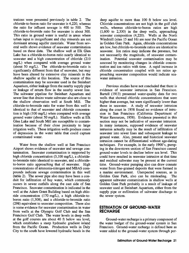
trations were presented previously in table 2. The chloride-to-boron ratio for seawater is 4,220, whereas the ratio for influent sewage is 400 to 500. The chloride-to-bromide ratio for seawater is about 300. This ratio in ground water is useful in areas where urban input is insignificant and clay minerals are not dominant among aquifer materials. Water from sev­ eral wells shows evidence of seawater contamination based on these data. The shallow well at Elk Glen Lake has a chloride-to-boron ratio nearly identical to seawater and a high concentration of chloride (210 mg/L) when compared with average ground water (about 50 mg/L). The chloride-to-bromide ratio is significantly different from that of seawater, but may have been altered by extensive clay minerals in the shallow aquifer at this location. The source of this contamination may be seawater used in the Steinhart Aquarium, either leakage from the nearby supply pipe or leakage of return flow in the nearby sewer line. The saltwater pipeline for Steinhart Aquarium and sewer line that drains waste saltwater also are close to the shallow observation well at South Mill. The chloride-to-bromide ratio for water from this well is identical to that of seawater and chloride concentra­ tion is high (100 mg/L) when compared with average ground water (about 50 mg/L). Shallow wells at Elk Glen Lake and South Mill are susceptible to contam­ ination because of their close proximity to large irrigation wells. These irrigation wells produce cones of depression in the water table that could capture contaminated water.

Water from the shallow well at San Francisco Airport shows evidence of seawater and sewage con­ tamination. Seawater contamination is supported by high chloride concentration (3,100 mg/L), a chloride- to-bromide ratio identical to seawater, and a chloride- to-boron ratio approaching that of seawater. High concentrations of ammonia-nitrogen and MB AS com­ pounds indicate sewage contamination in this well (table 2). The sewer pipe also may have been a con­ duit for infiltration of bay water, which commonly occurs in sewer outfalls along the east side of San Francisco. Seawater contamination is indicated in the well at the Adam Grant Building based on high chlo­ ride concentration (170 mg/L), a high chloride-to- boron ratio (1,308), and a chloride-to-bromide ratio (298) equivalent to seawater composition. There also is some evidence for seawater contamination in water from wells at the Olympic Golf Club and the San Francisco Golf Club. The water levels in deep wells at the golf courses are about 40 ft below sea level, which establishes a steep hydraulic gradient inland from the Pacific Ocean. Production wells in Daly City to the south have lowered hydraulic heads in the

deep aquifer to more than 100 ft below sea level. Chloride concentrations are not high in the golf club wells, whereas chloride-to-boron ratios are high (1,600 to 2,330) in the deep wells, approaching seawater composition (4,220). Wells at the North Windmill (sites 15 and 16) are near the Pacific Ocean in Golden Gate Park. Again, chloride concentrations are low, but chloride-to-bromide ratios are identical to seawater. Ion ratios may indicate the presence, but not necessarily the magnitude, of seawater contam­ ination. Potential seawater contamination may be assessed by monitoring changes in chloride concen­ tration and ion ratios with time. A rapid increase in chloride concentration coupled with ion ratios ap­ proaching seawater composition would indicate sea- water intrusion.

Previous studies have not concluded that there is evidence of seawater intrusion in San Francisco. Bartell (1913) presented water-quality data for two wells that showed chloride concentrations that were higher than average, but were significantly lower than those in seawater. A study of seawater intrusion along the coast in 1958 found no evidence of intru­ sion in San Francisco (California Department of Water Resources, 1958). Evidence presented in this section may not be indicative of seawater intrusion. In many instances, supposed evidence of seawater intrusion actually may be the result of infiltration of seawater into sewer lines and subsequent leakage to ground water. Also, present and historical seawater intrusion cannot be differentiated without age-dating techniques. For example, in the early 1900's, pump­ ing in the downtown section of San Francisco caused ground-water levels to decline below sea level. This could have resulted in seawater intrusion at that time and residual saltwater may be present at the current time. Ground-water pumping also can draw connate water from fine-grained deposits that were formed in a marine environment. Unexpected sources, as in Golden Gate Park, also can be misleading. The apparent saltwater contamination in shallow wells at Golden Gate Park probably is a result of leakage of seawater used at Steinhart Aquarium, either from the supply pipe or exfiltration of saltwater discharge to the sewer system.

ESTIMATION OF GROUND-WATER RECHARGE

Ground-water recharge is a primary component of the water budget of the ground-water system in San Francisco. Ground-water recharge is defined here as water added to the ground-water system through per-

Estimation of Ground-Water Recharge 21

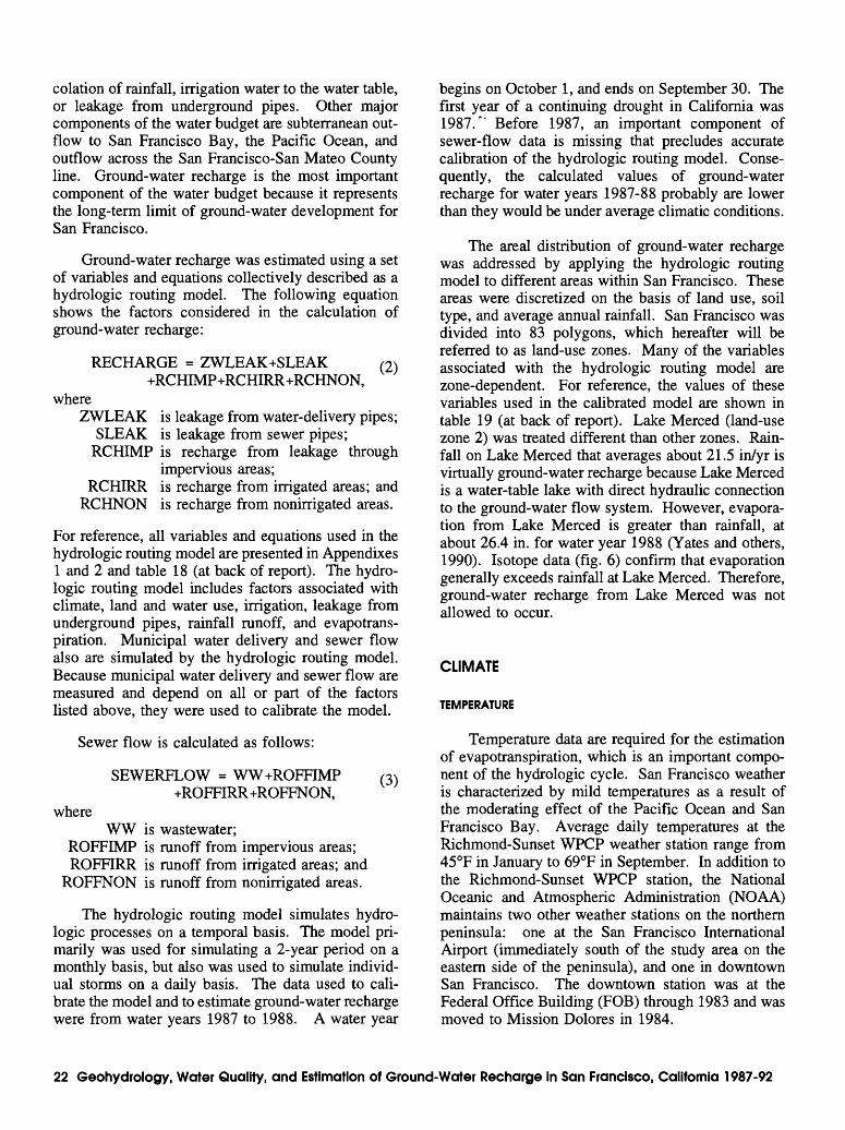
eolation of rainfall, irrigation water to the water table, or leakage from underground pipes. Other major components of the water budget are subterranean out­ flow to San Francisco Bay, the Pacific Ocean, and outflow across the San Francisco-San Mateo County line. Ground-water recharge is the most important component of the water budget because it represents the long-term limit of ground-water development for San Francisco.

Ground-water recharge was estimated using a set of variables and equations collectively described as a hydrologic routing model. The following equation shows the factors considered in the calculation of ground-water recharge:

(2)RECHARGE = ZWLEAK+SLEAK+RCHIMP+RCHIRR+RCHNON,

whereZWLEAK is leakage from water-delivery pipes;

SLEAK is leakage from sewer pipes; RCHIMP is recharge from leakage through

impervious areas;RCHIRR is recharge from irrigated areas; and

RCHNON is recharge from nonirrigated areas.

For reference, all variables and equations used in the hydrologic routing model are presented in Appendixes 1 and 2 and table 18 (at back of report). The hydro- logic routing model includes factors associated with climate, land and water use, irrigation, leakage from underground pipes, rainfall runoff, and evapotrans- piration. Municipal water delivery and sewer flow also are simulated by the hydrologic routing model. Because municipal water delivery and sewer flow are measured and depend on all or part of the factors listed above, they were used to calibrate the model.

(3)

Sewer flow is calculated as follows:

SEWERFLOW = WW+ROFFIMP +ROFFIRR +ROFFNON,

whereWW is wastewater;

ROFFIMP is runoff from impervious areas; ROFFTRR is runoff from irrigated areas; and

ROFFNON is runoff from nonirrigated areas.

The hydrologic routing model simulates hydro- logic processes on a temporal basis. The model pri­ marily was used for simulating a 2-year period on a monthly basis, but also was used to simulate individ­ ual storms on a daily basis. The data used to cali­ brate the model and to estimate ground-water recharge were from water years 1987 to 1988. A water year

begins on October 1, and ends on September 30. The first year of a continuing drought in California was 1987." Before 1987, an important component of sewer-flow data is missing that precludes accurate calibration of the hydrologic routing model. Conse­ quently, the calculated values of ground-water recharge for water years 1987-88 probably are lower than they would be under average climatic conditions.

The areal distribution of ground-water recharge was addressed by applying the hydrologic routing model to different areas within San Francisco. These areas were discretized on the basis of land use, soil type, and average annual rainfall. San Francisco was divided into 83 polygons, which hereafter will be referred to as land-use zones. Many of the variables associated with the hydrologic routing model are zone-dependent. For reference, the values of these variables used in the calibrated model are shown in table 19 (at back of report). Lake Merced (land-use zone 2) was treated different than other zones. Rain­ fall on Lake Merced that averages about 21.5 in/yr is virtually ground-water recharge because Lake Merced is a water-table lake with direct hydraulic connection to the ground-water flow system. However, evapora­ tion from Lake Merced is greater than rainfall, at about 26.4 in. for water year 1988 (Yates and others, 1990). Isotope data (fig. 6) confirm that evaporation generally exceeds rainfall at Lake Merced. Therefore, ground-water recharge from Lake Merced was not allowed to occur.

CLIMATE

TEMPERATURE

Temperature data are required for the estimation of evapotranspiration, which is an important compo­ nent of the hydrologic cycle. San Francisco weather is characterized by mild temperatures as a result of the moderating effect of the Pacific Ocean and San Francisco Bay. Average daily temperatures at the Richmond-Sunset WPCP weather station range from 45°F in January to 69°F in September. In addition to the Richmond-Sunset WPCP station, the National Oceanic and Atmospheric Administration (NOAA) maintains two other weather stations on the northern peninsula: one at the San Francisco International Airport (immediately south of the study area on the eastern side of the peninsula), and one in downtown San Francisco. The downtown station was at the Federal Office Building (FOB) through 1983 and was moved to Mission Dolores in 1984.

22 Geohydrology, Water Quality, and Estimation of Ground-Water Recharge in San Francisco, California 1987-92

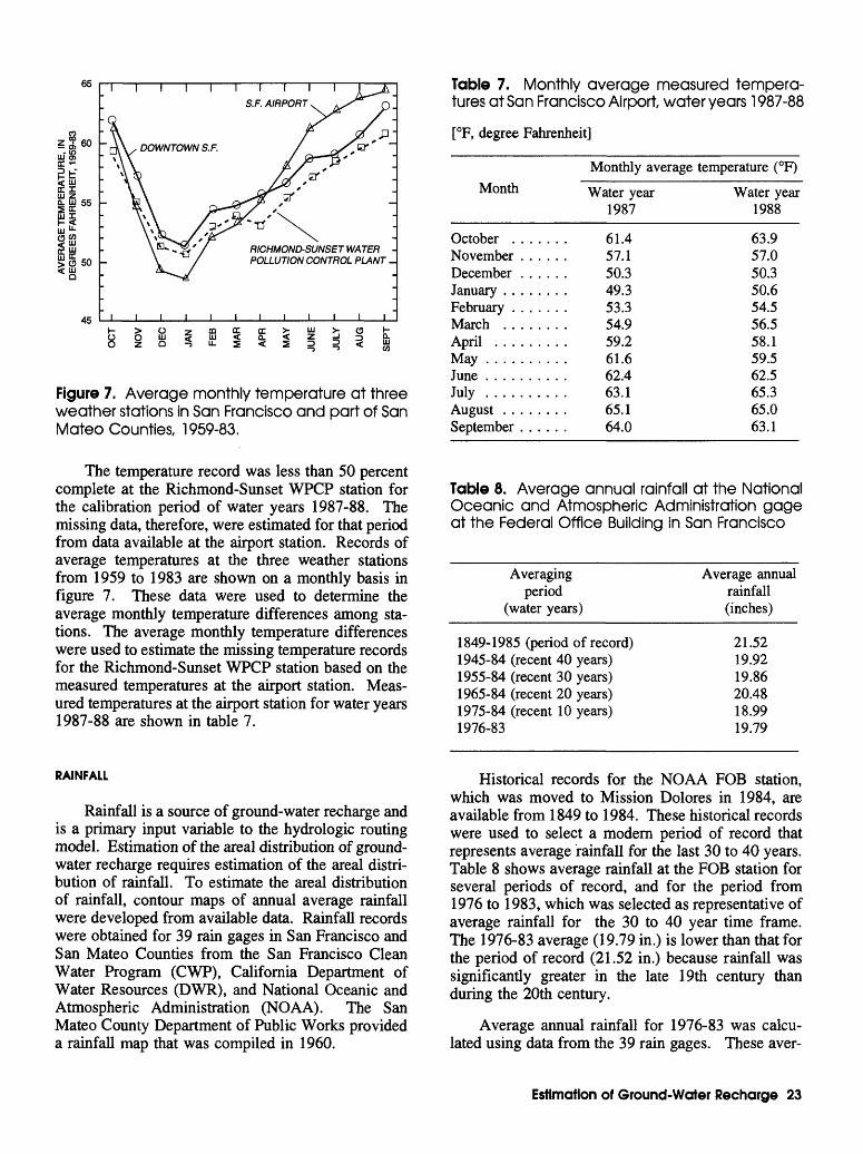
65

60

UJ "-

45

I f I T I I I I

S.F. AIRPORT.

RICHMOND-SUNSET WATER POLLUTION CONTROL PLANT.

3 aZ Q

m Q: Q: >- U >- o f111 < Q. < Z J 3 fLu-5<22 = < u

Figure 7. Average monthly temperature at three weather stations in San Francisco and part of San Mateo Counties, 1959-83.

The temperature record was less than 50 percent complete at the Richmond-Sunset WPCP station for the calibration period of water years 1987-88. The missing data, therefore, were estimated for that period from data available at the airport station. Records of average temperatures at the three weather stations from 1959 to 1983 are shown on a monthly basis in figure 7. These data were used to determine the average monthly temperature differences among sta­ tions. The average monthly temperature differences were used to estimate the missing temperature records for the Richmond-Sunset WPCP station based on the measured temperatures at the airport station. Meas­ ured temperatures at the airport station for water years 1987-88 are shown in table 7.

RAINFALL

Rainfall is a source of ground-water recharge and is a primary input variable to the hydrologic routing model. Estimation of the areal distribution of ground- water recharge requires estimation of the areal distri­ bution of rainfall. To estimate the areal distribution of rainfall, contour maps of annual average rainfall were developed from available data. Rainfall records were obtained for 39 rain gages in San Francisco and San Mateo Counties from the San Francisco Clean Water Program (CWP), California Department of Water Resources (DWR), and National Oceanic and Atmospheric Administration (NO A A). The San Mateo County Department of Public Works provided a rainfall map that was compiled in 1960.

Table 7. Monthly average measured tempera­ tures at San Francisco Airport water years 1987-88

[°F, degree Fahrenheit]

Monthly average temperature (°F)Month

October .....November ....December ....January ......February .....March ......April .......May ........June ........July ........August ......September ....

Water year 1987

61.457.150.349.353 354.959261.662.463.165.164.0

Water year 1988

63.957.050.350.654.556.558.159.562.565.365.063.1

Table 8. Average annual rainfall at the National Oceanic and Atmospheric Administration gage at the Federal Office Building in San Francisco

Averaging period

(water years)

1849-1985 (period of record) 1945-84 (recent 40 years) 1955-84 (recent 30 years) 1965-84 (recent 20 years) 1975-84 (recent 10 years) 1976-83

Average annual rainfall (inches)

21.52 19.92 19.86 20.48 18.99 19.79

Historical records for the NOAA FOB station, which was moved to Mission Dolores in 1984, are available from 1849 to 1984. These historical records were used to select a modern period of record that represents average rainfall for the last 30 to 40 years. Table 8 shows average rainfall at the FOB station for several periods of record, and for the period from 1976 to 1983, which was selected as representative of average rainfall for the 30 to 40 year time frame. The 1976-83 average (19.79 in.) is lower than that for the period of record (21.52 in.) because rainfall was significantly greater in the late 19th century than during the 20th century.

Average annual rainfall for 1976-83 was calcu­ lated using data from the 39 rain gages. These aver-

Estimation of Ground-Water Recharge 23

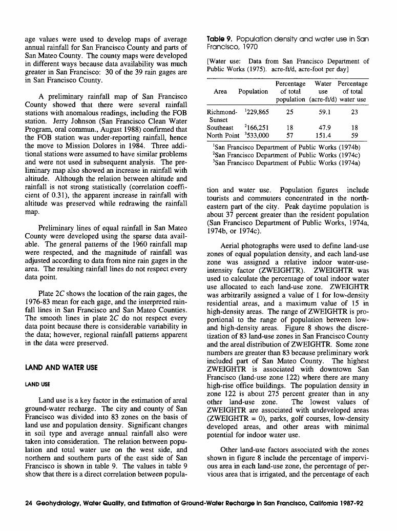
age values were used to develop maps of average annual rainfall for San Francisco County and parts of San Mateo County. The county maps were developed in different ways because data availability was much greater in San Francisco: 30 of the 39 rain gages are in San Francisco County.

A preliminary rainfall map of San Francisco County showed that there were several rainfall stations with anomalous readings, including the FOB station. Jerry Johnson (San Francisco Clean Water Program, oral commun., August 1988) confirmed that the FOB station was under-reporting rainfall, hence the move to Mission Dolores in 1984. Three addi­ tional stations were assumed to have similar problems and were not used in subsequent analysis. The pre­ liminary map also showed an increase in rainfall with altitude. Although the relation between altitude and rainfall is not strong statistically (correlation coeffi­ cient of 0.31), the apparent increase in rainfall with altitude was preserved while redrawing the rainfall map.

Preliminary lines of equal rainfall in San Mateo County were developed using the sparse data avail­ able. The general patterns of the 1960 rainfall map were respected, and the magnitude of rainfall was adjusted according to data from nine rain gages in the area. The resulting rainfall lines do not respect every data point.

Plate 1C shows the location of the rain gages, the 1976-83 mean for each gage, and the interpreted rain­ fall lines in San Francisco and San Mateo Counties. The smooth lines in plate 2C do not respect every data point because there is considerable variability in the data; however, regional rainfall patterns apparent in the data were preserved.

LAND AND WATER USE

LAND USE

Land use is a key factor in the estimation of areal ground-water recharge. The city and county of San Francisco was divided into 83 zones on the basis of land use and population density. Significant changes in soil type and average annual rainfall also were taken into consideration. The relation between popu­ lation and total water use on the west side, and northern and southern parts of the east side of San Francisco is shown in table 9. The values in table 9 show that there is a direct correlation between popula-

Table 9. Population density and water use in San Francisco, 1970

[Water use: Data from San Francisco Department of Public Works (1975). acre-ft/d, acre-foot per day]

Area PopulationPercentage Water

of total usepopulation (acre-ft/d)

Percentageof total

water use

Richmond- 1 229,865 Sunset

Southeast 2 166,251 North Point 3533,000

25

1857

59.1

47.9151.4

23

1859

'San Francisco Department of Public Works 2San Francisco Department of Public Works3

(1974b) (1974c)

San Francisco Department of Public Works (1974a)

tion and water use. Population figures include tourists and commuters concentrated in the north­ eastern part of the city. Peak daytime population is about 37 percent greater than the resident population (San Francisco Department of Public Works, 1974a, 1974b, or 1974c).

Aerial photographs were used to define land-use zones of equal population density, and each land-use zone was assigned a relative indoor water-use- intensity factor (ZWEIGHTR). ZWEIGHTR was used to calculate the percentage of total indoor water use allocated to each land-use zone. ZWEIGHTR was arbitrarily assigned a value of 1 for low-density residential areas, and a maximum value of 15 in high-density areas. The range of ZWEIGHTR is pro­ portional to the range of population between low- and high-density areas. Figure 8 shows the discre­ tization of 83 land-use zones in San Francisco County and the areal distribution of ZWEIGHTR. Some zone numbers are greater than 83 because preliminary work included part of San Mateo County. The highest ZWEIGHTR is associated with downtown San Francisco (land-use zone 122) where there are many high-rise office buildings. The population density in zone 122 is about 275 percent greater than in any other land-use zone. The lowest values of ZWEIGHTR are associated with undeveloped areas (ZWEIGHTR = 0), parks, golf courses, low-density developed areas, and other areas with minimal potential for indoor water use.

Other land-use factors associated with the zones shown in figure 8 include the percentage of impervi­ ous area in each land-use zone, the percentage of per­ vious area that is irrigated, and the percentage of each

24 Geohydrology, Water Quality, and Estimation of Ground-Water Recharge in San Francisco, California 1987-92

land-use zone covered by a body of water. These areas were determined by digitizing parts of large- scale black-and-white or infrared aerial photographs covering various land-use zones. The resulting per­ centages of area in each category for various land-use zones were extrapolated to zones with similar charac­ teristics. The ZWEIGHTR and other land-use factors associated with each of the land-use zones are presented in table 19.

WATER USE

About 99 percent of the water used in San Francisco is imported from Hetch Hetchy and other reservoirs and delivered through municipal supply lines. The remaining 1 percent is ground water pri­ marily pumped for irrigation. These figures do not include other sources of water such as Lobos Creek, which is diverted for potable use, and Lake Merced, from which water is pumped for street cleaning and irrigation. The percentage of municipal water used indoors is of primary importance to this study. In­ door water use is an important component of sewer flow; about 98 percent of water used indoors becomes sewer flow (California Department of Water Resour­ ces, 1983). This value of 98 percent is used in the hydrologic routing model as the fraction of indoor water use that becomes waste water (WWFRAC). Sewer flow and municipal flow, which are used in calibrating the hydrologic routing model, are impor­ tant for recharge calculations because leakage from pipes is a significant source of recharge in San Francisco.

Ten years of municipal delivery data from 1978 to 1987 (San Francisco Water Department, written commun., 1988) were used to calculate the average monthly total use as a fraction of annual total use (table 10). Table 10 shows that the month with the smallest fraction of annual use is February, which is partly a result of the relatively small number of days in that month. There is clearly a seasonal influence in the data, with relatively high water use in the summer and relatively low water use in the winter. Outdoor water use, which is primarily for irrigation, is highly seasonal, but some evidence indicates that indoor use also varies seasonally.

The seasonal variability of indoor water use was analyzed using municipal delivery data from the San Francisco Water Department for 17 apartment build­ ings (21 or 22 units each) with little or no outside use

of water for irrigation (Cheryl K. Davis, written commun., May 1990). These municipal delivery data were used to calculate monthly indoor water use as a fraction of annual indoor water use (table 10, column B). The values in table 10 show that indoor water use varies seasonally in the same manner as total water use, but at a lower magnitude. The indoor water use values in table 10 were reexpressed as fractions of total monthly use by assuming there is no outdoor use in February. A multiplier was used to change the February value for indoor use to the corresponding value for total use. The same multi­ plier was applied to the indoor use values for the remaining months, which resulted in monthly esti­ mates of indoor use as a fraction of annual total use (table 10, column C). Table 10 also shows the esti­ mated monthly indoor use as a fraction of monthly total use, which was used in the hydrologic routing model (FRACIND in appendixes 1 and 2).

Figure 9 shows the estimated temporal distri­ bution of indoor and outdoor water use as described above. The estimated values indicate that outdoor use, calculated by subtracting indoor water use from total municipal water use, is a relatively small component of total municipal water use about 5.8 percent. An independent estimate of outdoor use was made using irrigation consumption data provided by the San Francisco Water Department (Cheryl K. Davis, written commun., June 1988). These data from May 1987 through April 1988, reportedly are not completely reliable, but are the best available. The volume of irrigation water estimated by the San Francisco Water Department is 5.4 percent of the annual total municipal water use. This compares well with the earlier estimate of 5.8 percent of the annual total municipal water use.

Outdoor water use in San Francisco is assumed to be primarily for irrigation, whereas a small percentage probably is used for hosing driveways, washing cars, and other outdoor uses. In addition to municipal water, ground water is used in some parts of the city for irrigation. Ground-water pumpage was measured or estimated for all known active wells, which are primarily in Golden Gate Park and the golf courses. These ground-water pumpage values were used to estimate the percentage of total demand for irrigation water that was supplied by ground water. These percentages were calculated for each land-use zone and used to allocate water sources in the hydro- logic routing model (FRACGW in appendixes 1 and 2).

Estimation of Ground-Water Recharge 25

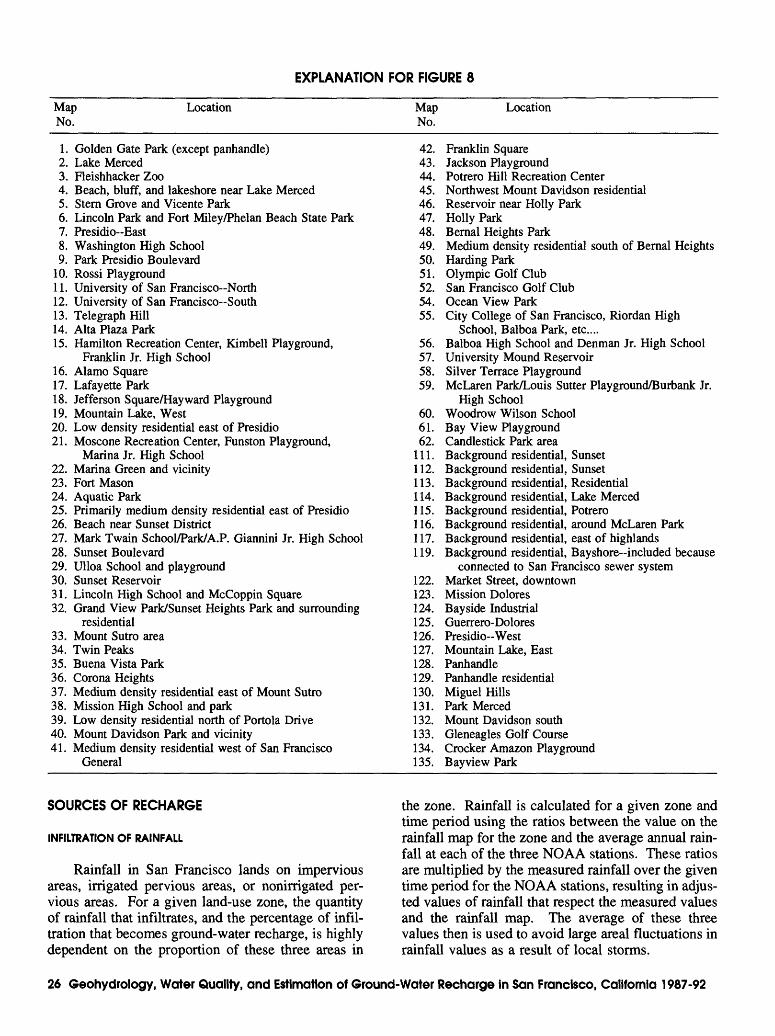
EXPLANATION FOR FIGURE 8

Map No.

Location MapNo.

Location

1. Golden Gate Park (except panhandle) 42.2. Lake Merced 43.3. Fleishhacker Zoo 44.4. Beach, bluff, and lakeshore near Lake Merced 45.5. Stern Grove and Vicente Park 46.6. Lincoln Park and Fort Miley/Phelan Beach State Park 47.7. Presidio-East 48.8. Washington High School 49.9. Park Presidio Boulevard 50.

10. Rossi Playground 51.11. University of San Francisco North 52.12. University of San Francisco-South 54.13. Telegraph Hill 55.14. Alta Plaza Park15. Hamilton Recreation Center, Kimbell Playground, 56.

Franklin Jr. High School 57.16. Alamo Square 58.17. Lafayette Park 59.18. Jefferson Square/Hay ward Playground19. Mountain Lake, West 60.20. Low density residential east of Presidio 61.21. Moscone Recreation Center, Funston Playground, 62.

Marina Jr. High School 111.22. Marina Green and vicinity 112.23. Fort Mason 113.24. Aquatic Park 114.25. Primarily medium density residential east of Presidio 115.26. Beach near Sunset District 116.27. Mark Twain School/Park/A.P. Giannini Jr. High School 117.28. Sunset Boulevard 119.29. Ulloa School and playground30. Sunset Reservoir 122.31. Lincoln High School and McCoppin Square 123.32. Grand View Park/Sunset Heights Park and surrounding 124.

residential 125.33. Mount Sutro area 126.34. Twin Peaks 127.35. Buena Vista Park 128.36. Corona Heights 129.37. Medium density residential east of Mount Sutro 130.38. Mission High School and park 131.39. Low density residential north of Portola Drive 132.40. Mount Davidson Park and vicinity 133.41. Medium density residential west of San Francisco 134.

General 135.

Franklin SquareJackson PlaygroundPotrero Hill Recreation CenterNorthwest Mount Davidson residentialReservoir near Holly ParkHolly ParkBernal Heights ParkMedium density residential south of Bernal HeightsHarding ParkOlympic Golf ClubSan Francisco Golf ClubOcean View ParkCity College of San Francisco, Riordan High

School, Balboa Park, etc.... Balboa High School and Denman Jr. High School University Mound Reservoir Silver Terrace Playground McLaren Park/Louis Sutler Playground/Burbank Jr.

High SchoolWoodrow Wilson School Bay View Playground Candlestick Park area Background residential, Sunset Background residential, Sunset Background residential, Residential Background residential, Lake Merced Background residential, Potrero Background residential, around McLaren Park Background residential, east of highlands Background residential, Bayshore-included because

connected to San Francisco sewer system Market Street, downtown Mission Dolores Bayside Industrial Guerrero-Dolores Presidio-West Mountain Lake, East PanhandlePanhandle residential Miguel Hills Park Merced Mount Davidson south Gleneagles Golf Course Crocker Amazon Playground Bayview Park

SOURCES OF RECHARGE

INFILTRATION OF RAINFALL

Rainfall in San Francisco lands on impervious areas, irrigated pervious areas, or nonirrigated per­ vious areas. For a given land-use zone, the quantity of rainfall that infiltrates, and the percentage of infil­ tration that becomes ground-water recharge, is highly dependent on the proportion of these three areas in

the zone. Rainfall is calculated for a given zone and time period using the ratios between the value on the rainfall map for the zone and the average annual rain­ fall at each of the three NOAA stations. These ratios are multiplied by the measured rainfall over the given time period for the NOAA stations, resulting in adjus­ ted values of rainfall that respect the measured values and the rainfall map. The average of these three values then is used to avoid large areal fluctuations in rainfall values as a result of local storms.

26 Geohydrology, Water Quality, and Estimation of Ground-Water Recharge in San Francisco, California 1987-92

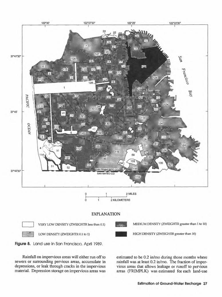
122°30' 122°27'30" 122°25' 122°22I30' I

37°47'30'

37°45'

37°42'30"

2 MILES

2 KILOMETERS

EXPLANATION

VERY LOW DENSITY (ZWEIGHTR less than 0.1)

LOW DENSITY (ZWEIGHTR 0.1 to 1)

Figure 8. Land use in San Francisco, April 1989.

MEDIUM DENSITY (ZWEIGHTR greater than 1 to 10)

HIGH DENSITY (ZWEIGHTR greater than 10)

Rainfall on impervious areas will either run off to sewers or surrounding pervious areas, accumulate in depressions, or leak through cracks in the impervious material. Depression storage on impervious areas was

estimated to be 0.2 in/mo during those months where rainfall was at least 0.2 in/mo. The fraction of imper­ vious areas that allows leakage or runoff to pervious areas (FRIMPLK) was estimated for each land-use

Estimation of Ground-Water Recharge 27

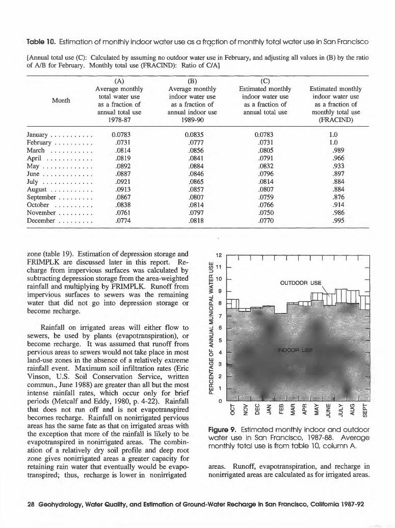
Table 10. Estimation of monthly indoor water use as a fraction of monthly total water use in San Francisco

[Annual total use (C): Calculated by assuming no outdoor water use in February, and adjusting all values in (B) by the ratio of A/B for February. Monthly total use (FRACIND): Ratio of C/A]

Month

(A)Average monthly

total water useas a fraction ofannual total use

1978-87

(B)Average monthlyindoor water useas a fraction of

annual indoor use1989-90

(QEstimated monthlyindoor water useas a fraction ofannual total use

Estimated monthlyindoor water useas a fraction of

monthly total use(FRACIND)

January .........February ........March .........April ..........May ...........June ...........July ...........August .........September .......October ........November .......December .......

0.0783.0731.0814.0819.0892.0887.0921.0913.0867.0838.0761.0774

0.0835.0777.0856.0841.0884.0846.0865.0857.0807.0814.0797.0818

0.0783.0731.0805.0791.0832.0796.0814.0807.0759.0766.0750.0770

1.01.0.989.966.933.897.884.884.876.914.986.995

zone (table 19). Estimation of depression storage and FRIMPLK are discussed later in this report. Re­ charge from impervious surfaces was calculated by subtracting depression storage from the area-weighted rainfall and multiplying by FRIMPLK. Runoff from impervious surfaces to sewers was the remaining water that did not go into depression storage or become recharge.

Rainfall on irrigated areas will either flow to sewers, be used by plants (evapotranspiration), or become recharge. It was assumed that runoff from pervious areas to sewers would not take place in most land-use zones in the absence of a relatively extreme rainfall event. Maximum soil infiltration rates (Eric Vinson, U.S. Soil Conservation Service, written commun., June 1988) are greater than all but the most intense rainfall rates, which occur only for brief periods (Metcalf and Eddy, 1980, p. 4-22). Rainfall that does not run off and is not evapotranspired becomes recharge. Rainfall on nonirrigated pervious areas has the same fate as that on irrigated areas with the exception that more of the rainfall is likely to be evapotranspired in nonirrigated areas. The combin­ ation of a relatively dry soil profile and deep root zone gives nonirrigated areas a greater capacity for retaining rain water that eventually would be evapo­ transpired; thus, recharge is lower in nonirrigated

Figure 9. Estimated monthly indoor and outdoor water use in San Francisco, 1987-88. Average monthly total use is from table 10, column A.

areas. Runoff, evapotranspiration, and recharge in nonirrigated areas are calculated as for irrigated areas.

28 Geohydrology, Water Quality, and Estimation of Ground-Water Recharge In San Francisco, California 1987-92

INFILTRATION OF IRRIGATION WATER

An efficient irrigation system would provide plants with exactly the required quantity of water at the rate at which they need it. The irrigation systems used in residential and other areas of San Francisco do not achieve 100 percent efficiency. Irrigation efficiency is defined as the percentage of irrigation water that is used by the plants; it is assumed that the remainder becomes ground-water recharge. For the purpose of this investigation, irrigation efficiency initially was assumed to be about 60 percent; how­ ever, efficiency was increased to 70 percent during calibration. Under normal circumstances, it probably is unlikely that irrigation efficiency would be as high as 70 percent, but under drought conditions (1987- 88), conservation efforts probably were sufficient to cause this increase in irrigation efficiency.

Irrigation was initiated when soil moisture was depleted to the extent that the ratio of actual to potential evapotranspiration was less than a specified threshold. It was assumed that irrigation would com­ mence when actual evapotranspiration decreased to less than 70 percent of the potential evapotrans­ piration. If rainfall for a given time period was insufficient to keep soil moisture above the threshold, irrigation was initiated. The volume of irrigation water applied was assumed to be the quantity required to increase the soil moisture to the maximum avail­ able water capacity at a 70-percent irrigation efficiency. The total volume of irrigation water unused by plants that becomes ground-water recharge is 30 percent. The hydrologic routing model indicates that about 49 percent of ground-water recharge in areas irrigated from rainfall and irrigation water (excluding leaks from water or sewer pipes and runoff from impervious surfaces) is from irrigation.

LEAKAGE FROM WATER AND SEWER PIPES

Leakage from water and sewer pipes probably is a significant source of recharge, particularly in densely populated urban areas. Leakage tests on municipal water-delivery pipes indicate a leakage rate of about 4 percent, which was assumed for this study (Pitometer Associates, 1987). The sewer system in San Francisco is a combined system that routes sew­ age and storm-drain flows through the same pipes. Sewer pipes are not tested for leakage on a regular basis in San Francisco. They are replaced when cata­ strophic breaks cause flooding or street damage. Most of the sewer pipes on the west side of San Francisco are 40 to 70 years old and are made of clay

pipe with mortared joints or reinforced concrete (San Francisco Department of Public Works, 1974b). Those on the east side are older, dating as far back as the late 1800's (San Francisco Department of Public Works, 1974a). The principal variables that control the volumes of infiltration or exfiltration are the age and condition of the sewers and the types of joints used to connect the pipes. Kimmel (1972) attributed a rapid recovery of the water table after a decrease in ground-water pumping largely to a combination of leakage from sewer and water pipes on Long Island, New York.

The San Francisco Water Department's primary concern with sewer pipe leakage is inflow and infil­ tration into the sewer system because excess flow must be treated; inflow carries soil with it, which causes clogging; and cavities that can cause collapse can develop around the sewer pipe (Dan Champeau, San Francisco Water Department, oral commun., November 1988). Infiltration of ground water into sewers below the water table may range from 0.0001 to more than 0.040 Mgal/d per mile of sewer line (Miller, 1980). This report primarily concentrates on outflow from the sewer into the ground-water re­ charge system because this outflow may constitute a significant source of ground-water recharge and potentially harmful chemical constituents.

Sewers are designed to be water tight, but leakage of sewage into the ground or exfiltration is common, especially from old sewers (Todd, 1980, p. 317). Leakage rates from water and sewer pipes to the ground-water system may vary significantly with geographic location. The sewer system on the east side of San Francisco is older than that on the west side, and therefore is more likely to develop leaks. However, the location of the water table above the sewer system in some areas on the east side will tend to decrease the overall leakage rate. The sewer sys­ tem on the west side predominantly is above the water table. Sewer pipe leakage was assumed to be the same as water pipe leakage (4 percent) for lack of better criteria. Water-quality data support the assumption that sewer water enters the ground-water system, but do not indicate the magnitude of leakage.

A water pipe leakage rate of 4 percent is lower than the national average of about 10 percent (Pitometer Associates, 1987), and some areas around the world have water and sewer pipe leakage rates in excess of 40 percent (Lerner, 1986). Nevertheless, using the above assumption, the hydrologic routing model indicates that leakage from municipal water and sewer pipes accounts for about 26 and 27 percent

Estimation of Ground-Water Recharge 29

of the total recharge in San Francisco, respectively. Sewer-pipe leakage is greater than water-pipe leakage because of the significant volume of rainfall runoff that enters the sewers in addition to the municipal wastewater. Thirty-two percent of the total water- and sewer-pipe leakage occurs in the high-density downtown area (land-use zone 122). The population density and associated usage of water and sewer pipes is more than three times greater in this land-use zone than that in any other zone. In densely populated areas, it is clear that recharge is highly sensitive to the leakage rate of water and sewer pipes.

RECHARGE INTERCEPTION

Potential recharge in the study area is intercepted by two primary processes: rainfall runoff and evapo- transpiration. Vegetation interception, which can be significant in some environments, was not accounted for in San Francisco.

RAINFALL RUNOFF

Rainfall runoff can occur on pervious or imper­ vious surfaces. It was assumed that runoff of irriga­ tion water is an insignificant component of total runoff. Runoff from pervious surfaces was assumed to be minimal because maximum soil infiltration rates (Eric Vinson, U.S. Soil Conservation Service, written commun., June 1988) are greater than all but the most intense rainfall rates, which only occur for brief periods (Metcalf and Eddy, 1980, p. 4-22). A linear relation between rainfall and runoff from pervious areas was established such that a threshold rainfall amount had to be surpassed for runoff to occur. The threshold value was assigned based on soil type, ranging from 3 in/mo for clayey soils to 9 in/mo for sandy soils, with a slope of 0.9. These threshold rainfall values effectively eliminate rainfall runoff from pervious areas except during months of intense rainfall. This method may underpredict runoff from pervious areas during months where intense rainfall occurs on consecutive days. Results from the hydro- logic routing model for water years 1987-88 indicate that rainfall runoff from pervious areas constitutes about 3 percent of total rainfall runoff.

Rainfall on impervious surfaces that does not accumulate in depressions, leak through cracks in the impervious surface, or runoff to pervious areas is assumed to enter the sewer system. Maximum de­ pression storage on impervious areas was estimated by Overton and Meadows (1976) to range from 0.06

to 0.11 in. per storm. They also identified that the volume of depression storage was a function of slope. Another estimate of depression storage was 0.0825 in. per storm (Kibler, 1962). Assuming that depression storage is about 0.06 in. per storm in San Francisco because slopes are relatively high, the annual depres­ sion storage can be estimated by multiplying by the number of storms per year. There was an average of 30 storms per year in water years 1987-88, yielding an annual depression storage of 1.8 in., or an average monthly depression storage of 0.15 in. Because there is little or no rain in the summer months, the maxi­ mum monthly depression storage for months during which there was rain was estimated to be 0.2 in.

The fraction of leakage and runoff from impervious to pervious areas was estimated for a given land-use zone and generally was based on the fraction of impervious area in that zone. There generally is an inverse relation between the size of an impervious area and the fraction of runoff that leaks or drains to pervious areas. Using these values for the variables that control rainfall runoff, the hydro- logic routing model routed about 78 percent of rain­ fall on impervious areas to the sewer, and the remain­ der was split evenly between depression storage and leakage or runoff to pervious areas, which becomes ground-water recharge.

EVAPOTRANSPIRATION

Evapotranspiration is the quantity of water used by plants for transpiration and building of plant tissue, and then evaporated from plant foliage and adjacent soil (U.S. Department of Agriculture, 1970). Poten­ tial evapotranspiration (PET) is the evapotranspiration that occurs under ideal conditions, including an unlimited supply of water. Blaney and Griddle (1950) developed a formula for calculating PET based on empirical correlations between evapotranspiration and climatic factors. The Blaney-Criddle formula has been used extensively and modified by subsequent workers (U.S. Department of Agriculture, 1970; Dunne and Leopold, 1978). The form of the Blaney-Criddle formula used in this investigation is as follows (U.S. Department of Agriculture, 1970):

PET=kkt __c ' 100

(4)

wherePET is potential evapotranspiration for a given

month, in inches; kc is a monthly crop coefficient reflecting the

30 Geohydrology, Water Quality, and Estimation of Ground-Water Recharge in San Francisco, California 1987-92

growth stage of vegetation, inches per degree Fahrenheit;

kt is a climatic coefficient related to the mean air temperature (0.0173f - 0.314) (dimensionless);

t is mean air temperature, in degrees Fahrenheit; and

P is percentage of annual daylight hours occur­ ring in the month.

Reference evapotranspiration (ET0), which is a com­ monly published form of evapotranspiration, does not take into account the growth stage of the vegetation and is defined as follows:

ET- PET(5)

The mean air temperature used was that measured at the three NOAA stations discussed earlier in this report. The percentage of daylight hours is published in table form for various latitudes (U.S. Department of Agriculture, 1970). Composite values of the coef­ ficient kc representative of the vegetation mix in each zone were estimated from reported empirical kc values for turf, trees, and nonirrigated native vegetation (U.S. Department of Agriculture, 1970; Dunne and Leopold, 1978).

The actual evapotranspiration (AET) is calculated on the basis of PET, soil properties, and soil moisture. PET was calculated as described in equation 4. Moisture-related soil properties are controlled by the lithology or type of the soil. Soil types for each land-use zone were determined using soil survey maps provided by the U.S. Soil Conservation Service (Eric Vinson, written commun., June 1988). The soils in each land-use zone were categorized into one of four groups: sand, sandy loam, silty clay loam, or clay. The available water capacity of soil (AWCAP), which is dependent on soil type, is defined as follows:

AWCAP=(FC-PWP)xRD, (6)

whereFC is volumetric moisture content at field

capacity (dimensionless); PWP is permanent wilting point (dimensionless);

and RD is root depth (L).

Field capacity is the quantity of water that soil can hold against the pull of gravity. The permanent wilting point is reached when the water content of the soil is so low that the plant cannot withdraw enough water to sustain transpiration and the plant wilts.

Estimated root depths range from 12 to 36 in. for irrigated areas, and from 24 to 120 in. for nonirri­ gated areas (table 19). The available water content (AWC) is defined here as the difference between field capacity and the permanent wilting point:

AWC = FC-PWP, (7)

Values of AWC were assigned to each land-use zone on the basis of soil type: AWC is 0.06, 0.10, 0.12, or 0.14 in/in of soil (root) depth for sand, sandy loam, silty clay loam, or clay, respectively. The resulting range of AWCAP is from 0.72 to 16.8 in., which is similar to the range 0.72 to 19.2 in. calculated from data provided by the U.S. Soil Conservation Service (Eric Vinsor, written commun., June 1988). The U.S. Soil Conservation Service did not collect data at depths greater than 60 in., so the upper bound was calculated assuming a constant AWCAP for depths greater than 60 in.

Total soil moisture for a given period of time can be broken into two components: initial soil moisture and moisture added through infiltration of rainfall or irrigation water. Initial soil moisture was estimated for the initial time step (about 85 percent of AWCAP for irrigated areas, and about 15 percent of AWCAP for nonirrigated areas). Calculated soil moisture values from the previous time steps were used for the subsequent time steps for the remainder of the simulation.

Calculation of AET is trivial if total soil moisture is greater than or equal to AWCAP; AET is then equal to PET. If the soil moisture is less than AWCAP, AET is calculated using the graphical relation shown in figure 10. The curves in figure 10 show the rela­ tion between the ratios of AET to PET and AWC to AWCAP for various soil types and are similar to curves developed by Dunne and Leopold (1978) and used by Bauer and Vaccaro (1987).

During calibration of the hydrologic routing model, calculated ET0 was decreased 30 percent to reflect the effect of coastal fog. Reference evapo­ transpiration has been estimated on a monthly basis throughout California (Pruitt and others, 1987; Snyder and others, 1987). These estimates are shown in table 11. The California Department of Water Resources (1975a) estimated that potential evapotranspiration in the San Francisco area is about 76 percent of annual pan evaporation. Yates and others (1990) compiled measured pan evaporation data from Lake Merced with modified regional pan evaporation data (Cali­ fornia Department of Water Resources, 1975b) to

Estimation of Ground-Water Recharge 31

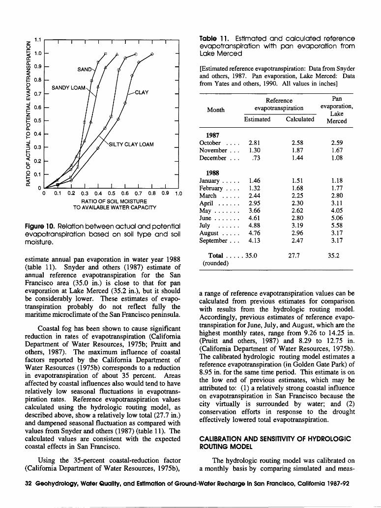
1.1

1.0

0.9

0.8

0.7

0.6

0.5

0.4

0.3

0.2

0.1

0

I f I I I I I I T

SAND

SANDY LOAMCLAY

SILTY CLAY LOAM

0.1 0.2 0.3 0.4 0.5 0.6 0.7 0.8 0.9 1.0

RATIO OF SOIL MOISTURE TO AVAILABLE WATER CAPACITY

Figure 10. Relation between actual and potential evapotranspiration based on soil type and soil moisture.

estimate annual pan evaporation in water year 1988 (table 11). Snyder and others (1987) estimate of annual reference evapotranspiration for the San Francisco area (35.0 in.) is close to that for pan evaporation at Lake Merced (35.2 in.), but it should be considerably lower. These estimates of evapo­ transpiration probably do not reflect fully the maritime microclimate of the San Francisco peninsula.

Coastal fog has been shown to cause significant reduction in rates of evapotranspiration (California Department of Water Resources, 1975b; Pruitt and others, 1987). The maximum influence of coastal factors reported by the California Department of Water Resources (1975b) corresponds to a reduction in evapotranspiration of about 35 percent. Areas affected by coastal influences also would tend to have relatively low seasonal fluctuations in evapotrans­ piration rates. Reference evapotranspiration values calculated using the hydrologic routing model, as described above, show a relatively low total (27.7 in.) and dampened seasonal fluctuation as compared with values from Snyder and others (1987) (table 11). The calculated values are consistent with the expected coastal effects in San Francisco.

Using the 35-percent coastal-reduction factor (California Department of Water Resources, 1975b),

Table 11. Estimated and calculated reference evapotranspiration with pan evaporation from Lake Merced

[Estimated reference evapotranspiration: Data from Snyder and others, 1987. Pan evaporation, Lake Merced: Data from Yates and others, 1990. All values in inches]

Reference Month evapotranspiration

Estimated

Pan evaporation,

Lake Calculated Merced

1987October ....November . . .December . . .

2.811.30

.73

2.581.871.44

2.591.671.08

1988January ..... 1.46February .... 1.32March ..... 2.44April ...... 2.95May ....... 3.66June ....... 4.61July ...... 4.88August ..... 4.76September ... 4.13

Total ..... 35.0 (rounded)

1.511.682.252.302.622.803.192.962.47

27.7

1.181.772.803.114.055.065.583.173.17

35.2

a range of reference evapotranspiration values can be calculated from previous estimates for comparison with results from the hydrologic routing model. Accordingly, previous estimates of reference evapo­ transpiration for June, July, and August, which are the highest monthly rates, range from 9.26 to 14.25 in. (Pruitt and others, 1987) and 8.29 to 12.75 in. (California Department of Water Resources, 1975b). The calibrated hydrologic routing model estimates a reference evapotranspiration (in Golden Gate Park) of 8.95 in. for the same time period. This estimate is on the low end of previous estimates, which may be attributed to: (1) a relatively strong coastal influence on evapotranspiration in San Francisco because the city virtually is surrounded by water; and (2) conservation efforts in response to the drought effectively lowered total evapotranspiration.

CALIBRATION AND SENSITIVITY OF HYDROLOGIC ROUTING MODEL

The hydrologic routing model was calibrated on a monthly basis by comparing simulated and meas-

32 Geohydrology, Water Quality, and Estimation of Ground-Water Recharge In San Francisco, California 1987-92

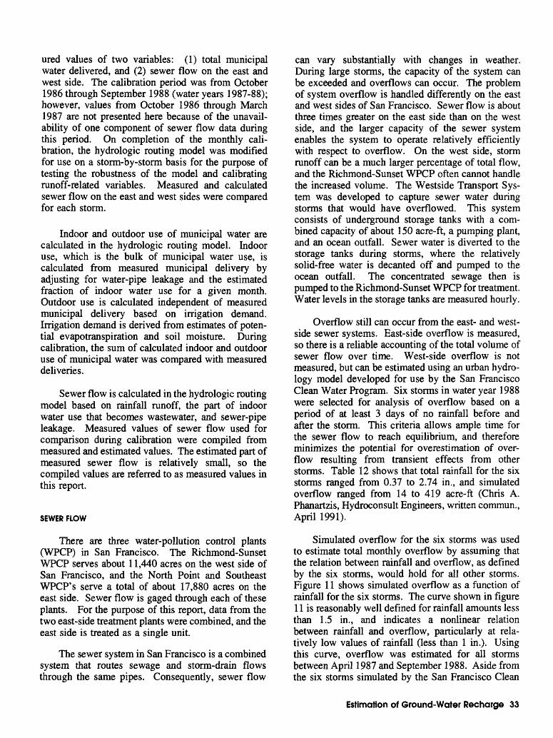
ured values of two variables: (1) total municipal water delivered, and (2) sewer flow on the east and west side. The calibration period was from October1986 through September 1988 (water years 1987-88); however, values from October 1986 through March1987 are not presented here because of the unavail­ ability of one component of sewer flow data during this period. On completion of the monthly cali­ bration, the hydrologic routing model was modified for use on a storm-by-storm basis for the purpose of testing the robustness of the model and calibrating runoff-related variables. Measured and calculated sewer flow on the east and west sides were compared for each storm.

Indoor and outdoor use of municipal water are calculated in the hydrologic routing model. Indoor use, which is the bulk of municipal water use, is calculated from measured municipal delivery by adjusting for water-pipe leakage and the estimated fraction of indoor water use for a given month. Outdoor use is calculated independent of measured municipal delivery based on irrigation demand. Irrigation demand is derived from estimates of poten­ tial evapotranspiration and soil moisture. During calibration, the sum of calculated indoor and outdoor use of municipal water was compared with measured deliveries.

Sewer flow is calculated in the hydrologic routing model based on rainfall runoff, the part of indoor water use that becomes wastewater, and sewer-pipe leakage. Measured values of sewer flow used for comparison during calibration were compiled from measured and estimated values. The estimated part of measured sewer flow is relatively small, so the compiled values are referred to as measured values in this report.

SEWER FLOW

There are three water-pollution control plants (WPCP) in San Francisco. The Richmond-Sunset WPCP serves about 11,440 acres on the west side of San Francisco, and the North Point and Southeast WPCP's serve a total of about 17,880 acres on the east side. Sewer flow is gaged through each of these plants. For the purpose of this report, data from the two east-side treatment plants were combined, and the east side is treated as a single unit.

The sewer system in San Francisco is a combined system that routes sewage and storm-drain flows through the same pipes. Consequently, sewer flow

can vary substantially with changes in weather. During large storms, the capacity of the system can be exceeded and overflows can occur. The problem of system overflow is handled differently on the east and west sides of San Francisco. Sewer flow is about three times greater on the east side than on the west side, and the larger capacity of the sewer system enables the system to operate relatively efficiently with respect to overflow. On the west side, storm runoff can be a much larger percentage of total flow, and the Richmond-Sunset WPCP often cannot handle the increased volume. The Westside Transport Sys­ tem was developed to capture sewer water during storms that would have overflowed. This system consists of underground storage tanks with a com­ bined capacity of about 150 acre-ft, a pumping plant, and an ocean outfall. Sewer water is diverted to the storage tanks during storms, where the relatively solid-free water is decanted off and pumped to the ocean outfall. The concentrated sewage then is pumped to the Richmond-Sunset WPCP for treatment. Water levels in the storage tanks are measured hourly.

Overflow still can occur from the east- and west- side sewer systems. East-side overflow is measured, so there is a reliable accounting of the total volume of sewer flow over time. West-side overflow is not measured, but can be estimated using an urban hydro­ logy model developed for use by the San Francisco Clean Water Program. Six storms in water year 1988 were selected for analysis of overflow based on a period of at least 3 days of no rainfall before and after the storm. This criteria allows ample time for the sewer flow to reach equilibrium, and therefore minimizes the potential for overestimation of over­ flow resulting from transient effects from other storms. Table 12 shows that total rainfall for the six storms ranged from 0.37 to 2.74 in., and simulated overflow ranged from 14 to 419 acre-ft (Chris A. Phanartzis, Hydroconsult Engineers, written commun., April 1991).

Simulated overflow for the six storms was used to estimate total monthly overflow by assuming that the relation between rainfall and overflow, as defined by the six storms, would hold for all other storms. Figure 11 shows simulated overflow as a function of rainfall for the six storms. The curve shown in figure 11 is reasonably well defined for rainfall amounts less than 1.5 in., and indicates a nonlinear relation between rainfall and overflow, particularly at rela­ tively low values of rainfall (less than 1 in.). Using this curve, overflow was estimated for all storms between April 1987 and September 1988. Aside from the six storms simulated by the San Francisco Clean

Estimation of Ground-Water Recharge 33

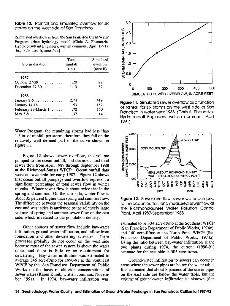
Table 12. Rainfall and simulated overflow for six storms on the west side of San Francisco

[Simulated overflow is from the San Francisco Clean Water Program urban hydrology model (Chris A. Phanartzis, Hydroconsultant Engineers, written commun., April 1991). in., inch; acre-ft, acre-foot]

Storm duration

1987October 27-29 .......December 27-30 .....

Totalrainfall

(in.)

1.201.13

Simulatedoverflow(acre-ft)

9882

1988January 2-5 ...........January 14-18 .........February 27-March 1 ....May 5-8 .............

2741.53.7237

419152150

14

Water Program, the remaining storms had less than 1.5 in. of rainfall per storm; therefore, they fell on the relatively well defined part of the curve shown in figure 11.

Figure 12 shows sewer overflow, the volume pumped to the ocean outfall, and the associated total sewer flow from April 1987 through September 1988 at the Richmond-Sunset WPCP. Ocean outfall data were not available for early 1987. Figure 12 shows that ocean outfall pumpage and overflow represent a significant percentage of total sewer flow in winter months. Winter sewer flow is about twice that in the spring and summer. On the east side, winter flow is about 35 percent higher than spring and summer flow. The difference between the seasonal variability on the east and west sides is attributed to the relatively large volume of spring and summer sewer flow on the east side, which is related to the population density.

Other sources of sewer flow include bay-water infiltration, ground-water infiltration, and inflow from foundation and other dewatering activities. These processes probably do not occur on the west side because most of the sewer system is above the water table, and there is little or no requirement for dewatering. Bay-water infiltration was estimated to average 346 acre-ft/mo for 1990-91 at the Southeast WPCP by the San Francisco Department of Public Works on the basis of chloride concentrations of sewer water (Karen Kubik, written commun., Novem­ ber 1991). In 1974, bay-water infiltration was

0 100 200 300 400 500

SIMULATED SEWER OVERFLOW, IN ACRE-FEET

Figure 11 . Simulated sewer overflow as a function of rainfall for six storms on the west side of San Francisco in water year 1988. (Chris A. Phanartzis, Hydroconsult Engineers, written commun., April 1991).

4,000

co a:z o 3,000

a ~

II2,000

CO1,000

MEASURED AT RICHMOND-SUNSET WATER POLLUTION CONTROL PLANT

co ^

1987 1988

Figure 12. Sewer overflow, sewer water pumped to the ocean outfall, and measured sewer flow at the Richmond-Sunset Water Pollution Control Plant, April 1987-September 1988.

estimated to be 304 acre-ft/mo at the Southeast WPCP (San Francisco Department of Public Works, 1974c), and 140 acre-ft/mo at the North Point WPCP (San Francisco Department of Public Works, 1974a). Using the ratio between bay-water infiltration at the two plants during 1974, the current (1990-91) estimate for the east side is 505 acre-ft/mo.

Ground-water infiltration to sewers can occur in areas where the sewer pipes are below the water table. It is estimated that about 8 percent of the sewer pipes on the east side are below the water table, but the volume of ground-water infiltration is unknown (San

34 Geohydrology, Water Quality, and Estimation of Ground-Water Recharge In San Francisco, California 1987-92

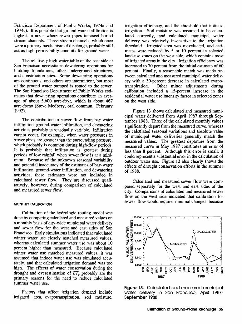
Francisco Department of Public Works, 1974a and 1974c). It is possible that ground-water infiltration is highest in areas where sewer pipes intersect buried stream channels. These stream channels, which once were a primary mechanism of discharge, probably still act as high-permeability conduits for ground water.

The relatively high water table on the east side at San Francisco necessitates dewatering operations for building foundations, other underground structures, and construction sites. Some dewatering operations are continuous, and others are intermittent, but most of the ground water pumped is routed to the sewer. The San Francisco Department of Public Works esti­ mates that dewatering operations contribute an aver­ age of about 5,600 acre-ft/yr, which is about 467 acre-ft/mo (Steve Medbery, oral commun., February 1992).

The contribution to sewer flow from bay-water infiltration, ground-water infiltration, and dewatering activities probably is seasonally variable. Infiltration cannot occur, for example, when water pressures in sewer pipes are greater than the surrounding pressure, which probably is common during high-flow periods. It is probable that infiltration is greatest during periods of low rainfall when sewer flow is at a mini­ mum. Because of the unknown seasonal variability and potential inaccuracy of the estimates of bay-water infiltration, ground-water infiltration, and dewatering activities, these estimates were not included in calculated sewer flow. They are discussed quali­ tatively, however, during comparison of calculated and measured sewer flow.

MONTHLY CALIBRATION

Calibration of the hydrologic routing model was done by comparing calculated and measured values on a monthly basis of city-wide municipal water delivery and sewer flow for the west and east sides of San Francisco. Early simulations indicated that calculated winter water use closely matched measured values, whereas calculated summer water use was about 10 percent higher than measured. Because calculated winter water use matched measured values, it was assumed that indoor water use was simulated accu­ rately, and that calculated irrigation demand was too high. The effects of water conservation during the drought and overestimation of ET0 probably are the primary reasons for the need to reduce calculated summer water use.

Factors that affect irrigation demand include irrigated area, evapotranspiration, soil moisture,

irrigation efficiency, and the threshold that initiates irrigation. Soil moisture was assumed to be calcu­ lated correctly, and calculated municipal water delivery was relatively insensitive to the irrigation threshold. Irrigated area was reevaluated, and esti­ mates were reduced by 5 or 10 percent in selected land-use zones on the west side, which contains most of irrigated areas in the city. Irrigation efficiency was increased to 70 percent from the initial estimate of 60 percent. Finally, a reasonable match was made be­ tween calculated and measured municipal water deliv­ ery with a 30-percent decrease in calculated evapo­ transpiration. Other minor adjustments during calibration included a 15-percent increase in the residential water use intensity factor in selected zones on the west side.

Figure 13 shows calculated and measured muni­ cipal water delivered from April 1987 through Sep­ tember 1988. Three of the calculated monthly values significantly depart from the measured curve, whereas the calculated seasonal variations and absolute value of municipal water deliveries generally match the measured values. The greatest departure from the measured curve in May 1987 constitutes an error of less than 8 percent. Although this error is small, it could represent a substantial error in the calculation of outdoor water use. Figure 13 also clearly shows the effects of drought conservation efforts in the summer of 1988.

Calculated and measured sewer flow were com­ pared separately for the west and east sides of the city. Comparisons of calculated and measured sewer flow on the west side indicated that calibration for sewer flow would require minimal changes because

11,000

tiUJ 10,500ccH-

% g 10,000£<<j ? 9,500

idI g 9,000

1>^ -1 8,500

8,000DC > UJ >- O b

i I i = i Si^ * T i * tog t3 W

1987 1988

Figure 13. Calculated and measured municipal water delivery in San Francisco, April 1987- September 1988.

Estimation of Ground-Water Recharge 35

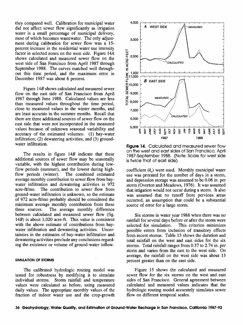
they compared well. Calibration for municipal water did not affect sewer flow significantly as irrigation water is a small percentage of municipal delivery, most of which becomes wastewater. The only adjust­ ment during calibration for sewer flow was a 15- percent increase in the residential water use intensity factor in selected zones on the west side. Figure 14A shows calculated and measured sewer flow on the west side of San Francisco from April 1987 through September 1988. The curves matched well through­ out this time period, and the maximum error in December 1987 was about 6 percent.

Figure 145 shows calculated and measured sewer flow on the east side of San Francisco from April 1987 through June 1988. Calculated values are less than measured values throughout the time period, close to measured values in the winter months, and are least accurate in the summer months. Recall that there are three additional sources of sewer flow on the east side that were not incorporated in the measured values because of unknown seasonal variability and accuracy of the estimated volumes: (1) bay-water infiltration; (2) dewatering activities; and (3) ground- water infiltration.

The results in figure 145 indicate that these additional sources of sewer flow may be seasonally variable, with the highest contribution during low- flow periods (summer), and the lowest during high- flow periods (winter). The combined estimated average monthly contribution to sewer flow from bay- water infiltration and dewatering activities is 972 acre-ft/mo. The contribution to sewer flow from ground-water infiltration is unknown, so the estimate of 972 acre-ft/mo probably should be considered the minimum average monthly contribution from these three sources. The average monthly difference between calculated and measured sewer flow (fig. 145) is about 1,020 acre-ft. This value is consistent with the above estimate of contributions from bay- water infiltration and dewatering activities. Uncer­ tainties in the estimates of bay-water infiltration and dewatering activities preclude any conclusions regard­ ing the existence or volume of ground-water inflow.

SIMULATION OF STORMS

The calibrated hydrologic routing model was tested for robustness by modifying it to simulate individual storms. Storm rainfall and temperature values were calculated as before, using measured daily values. The appropriate monthly values of the fraction of indoor water use and the crop-growth

4,000

3,000

IDUJH- 2,000UJtr

;> 1,000011,000LL

ff, 10,000

co 9,000 3*Q" 8,000I-

7,000 -

6,000

5,000

' ^CALCULATED

i i i i i i i i i i i i i i i i

\ i i i r - B EAST SIDE

/ CALCULATED

> o z CD g b g t 2 3 < £

1987 1988

Figure 14. Calculated and measured sewer flow on the west and east sides of San Francisco, April 1987-September 1988. (Note: Scale for west side is twice that of east side).

coefficient (kc) were used. Monthly municipal water use was prorated for the number of days in a storm, and depression storage was assumed to be 0.06 in. per storm (Overton and Meadows, 1976). It was assumed that irrigation would not occur during a storm. It also was assumed that no runoff from pervious areas occurred, an assumption that could be a substantial source of error for a large storm.

Six storms in water year 1988 when there was no rainfall for several days before or after the storm were selected for simulation. This criterion minimizes possible errors from inclusion of transitory effects from recent storms. Table 13 shows the duration and total rainfall on the west and east sides for the six storms. Total rainfall ranges from 0.37 to 2.74 in. per storm and varies from the east to the west side. On average, the rainfall on the west side was about 13 percent greater than on the east side.

Figure 15 shows the calculated and measured sewer flow for the six storms on the west and east sides of San Francisco. General agreement between calculated and measured values indicates that the hydrologic routing model accurately simulates sewer flow on different temporal scales.

36 Geohydrology, Water Quality, and Estimation of Ground-Water Recharge in San Francisco, California 1987-92

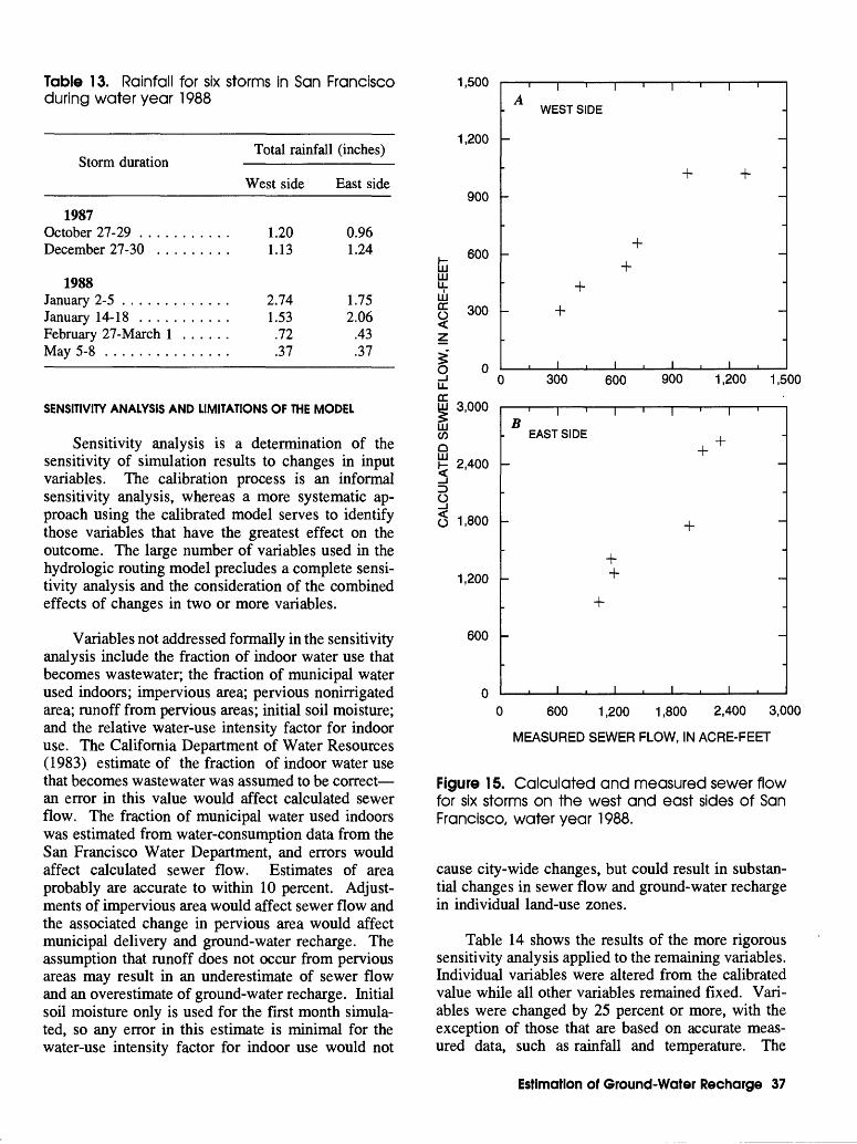
Table 13. Rainfall for six storms in San Francisco during water year 1988

Storm durationTotal rainfall (inches)

West side East side

1987October 27-29 ........December 27-30 ......

1 201.13

0.961.24

1988January 2-5 ............January 14-18 ..........February 27-March 1 .....May 5-8 ..............

2.741 53

7237

1.752.06

.4337

SENSITIVITY ANALYSIS AND LIMITATIONS OF THE MODEL

Sensitivity analysis is a determination of the sensitivity of simulation results to changes in input variables. The calibration process is an informal sensitivity analysis, whereas a more systematic ap­ proach using the calibrated model serves to identify those variables that have the greatest effect on the outcome. The large number of variables used in the hydrologic routing model precludes a complete sensi­ tivity analysis and the consideration of the combined effects of changes in two or more variables.

Variables not addressed formally in the sensitivity analysis include the fraction of indoor water use that becomes wastewater; the fraction of municipal water used indoors; impervious area; pervious nonirrigated area; runoff from pervious areas; initial soil moisture; and the relative water-use intensity factor for indoor use. The California Department of Water Resources (1983) estimate of the fraction of indoor water use that becomes wastewater was assumed to be correct an error in this value would affect calculated sewer flow. The fraction of municipal water used indoors was estimated from water-consumption data from the San Francisco Water Department, and errors would affect calculated sewer flow. Estimates of area probably are accurate to within 10 percent. Adjust­ ments of impervious area would affect sewer flow and the associated change in pervious area would affect municipal delivery and ground-water recharge. The assumption that runoff does not occur from pervious areas may result in an underestimate of sewer flow and an overestimate of ground-water recharge. Initial soil moisture only is used for the first month simula­ ted, so any error in this estimate is minimal for the water-use intensity factor for indoor use would not

LJJ in u.LJJ cc

LLCC111

HI C/DG 111

33

1,500

1,200

900

600

300

WEST SIDE

300 600 900 1,200 1,500

3,000

2,400

1,800

1,200

600

BEAST SIDE

0 600 1,200 1,800 2,400 3,000

MEASURED SEWER FLOW, IN ACRE-FEET

Figure 15. Calculated and measured sewer flow for six storms on the west and east sides of San Francisco, water year 1988.

cause city-wide changes, but could result in substan­ tial changes in sewer flow and ground-water recharge in individual land-use zones.

Table 14 shows the results of the more rigorous sensitivity analysis applied to the remaining variables. Individual variables were altered from the calibrated value while all other variables remained fixed. Vari­ ables were changed by 25 percent or more, with the exception of those that are based on accurate meas­ ured data, such as rainfall and temperature. The

Estimation of Ground-Water Recharge 37

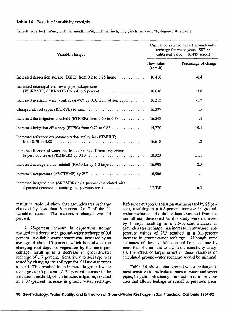
Table 14. Results of sensitivity analysis

[acre-ft, acre-foot; in/mo, inch per month; in/in, inch per inch; in/yr, inch per year; °F, degree Fahrenheit]

Variable changed

Calculated average annual ground-water recharge for water years 1987-88 calibrated value = 16,489 acre-ft

New value (acre-ft)

Percentage of change

Increased depression storage (DEPR) from 0.2 to 0.25 in/mo ........... 16,416

Increased municipal and sewer pipe leakage rates(WLKRATE, SLKRATE) from 4 to 5 percent ................... 18,636

Increased available water content (AWC) by 0.02 in/in of soil depth ...... 16,212

Changed all soil types (ICURVE) to sand ......................... 16,597

Increased the irrigation threshold (ETFIRR) from 0.70 to 0.88 .......... 16,548

Increased irrigation efficiency (EFFIC) from 0.70 to 0.88 .............. 14,770

Increased reference evapotranspiration mulitplier (ETMULT)from 0.70 to 0.88 ....................................... 16,618

Increased fraction of water that leaks or runs off from imperviousto pervious areas (FRIMPLK) by 0.10 ........................ 18,323

Increased average annual rainfall (RANNL) by 1.0 in/yr ............... 16,908

Increased temperature (AVGTEMP) by 2°F ....................... 16,506

Increased irrigated area (AREAIRR) by 4 percent (associated with4 percent decrease in nonirrigated pervious area) ................. 17,530

-0.4

13.0

-1.7

.5

.4

-10.4

11.1

2.5

.1

6.3

results in table 14 show that ground-water recharge changed by less than 3 percent for 7 of the 11 variables tested. The maximum change was 13 percent.

A 25-percent increase in depression storage resulted in a decrease in ground-water recharge of 0.4 percent. Available water content was increased by an average of about 15 percent, which is equivalent to changing root depth of vegetation by the same per­ centage, resulting in a decrease in ground-water recharge of 1.7 percent. Sensitivity to soil type was tested by changing the soil type for all land-use zones to sand. This resulted in an increase in ground-water recharge of 0.5 percent. A 25-percent increase in the irrigation threshold, which initiates irrigation, resulted in a 0.4-percent increase in ground-water recharge.

Reference evapotranspiration was increased by 25 per­ cent, resulting in a 0.8-percent increase in ground- water recharge. Rainfall values extracted from the rainfall map developed for this study were increased by 1 in/yr resulting in a 2.5-percent increase in ground-water recharge. An increase in measured tem­ perature values of 2°F resulted in a 0.1-percent increase in ground-water recharge. Although some estimates of these variables could be inaccurate by more than the amount tested in the sensitivity analy­ sis, the effect of larger errors in these variables on calculated ground-water recharge would be minimal.

Table 14 shows that ground-water recharge is most sensitive to the leakage rates of water and sewer pipes, irrigation efficiency, the fraction of impervious area that allows leakage or runoff to pervious areas,

38 Geohydrology, Water Quality, and Estimation of Ground-Water Recharge In San Francisco, California 1987-92

and irrigated area. An increase in the leakage rates of water and sewer pipes from 4 to 5 percent resulted in a 13-percent increase in ground-water recharge. The leakage rates of municipal water pipes are measured regularly, whereas sewer-pipe leakage rates are un­ known. The assumption that sewer pipes leak at the same rate as municipal water pipes could be erron­ eous. Water-quality data indicate that sewer pipes leak, but do not provide information concerning the leakage rate. Large leakage rates would result in a significantly larger estimate of ground-water recharge, particularly on the east side where the population density is greatest.

A 25-percent increase in irrigation efficiency resulted in a 10.4-percent decrease in ground-water recharge. Irrigation efficiency was increased from 60 to 70 percent during calibration, which probably is higher than under average (nondrought) conditions. The results from the sensitivity analysis indicate that if the irrigation efficiency decreases to 60 percent after the drought (a decrease of about 14 percent), ground-water recharge might increase by about 6 per­ cent. Errors in irrigation efficiency would have the greatest effect on the west side, which contains about 58 percent of the irrigated area in San Francisco.

The fraction of water that leaks or runs off from impervious to pervious areas is unknown, but was estimated on the basis of an inverse correlation between impervious areas and leakage or runoff to pervious areas. There could be significant error in these estimates. The sensitivity analysis indicates that an increase of 25 percent of the average fraction of leakage or runoff from impervious to pervious areas results in an increase in ground-water recharge of 11.1 percent. The effect of an increase in the fraction of leakage or runoff from impervious to pervious areas would affect ground-water recharge on the east side of the city more than on the west side, because the east side contains about 69 percent of the impervious area in San Francisco.

The fraction of irrigated area was determined by digitizing large-scale aerial photographs and extrap­ olating the results to similar areas. The accuracy of this method probably is within about 10 percent. For the sensitivity analysis, irrigated area was increased by 4 percent, which is about 25 percent of the area- weighted average. The 4-percent increase in irrigated area resulted in a 6.3-percent increase in ground-water recharge. Changes in irrigated area have the greatest effect on the west side, which contains about 58 per­ cent of the irrigated area in San Francisco.

Limitations of the method used to estimate ground-water recharge are embodied in the assump­ tions made in the analysis and the time period over which the analysis was done. There are two assump­ tions that could be associated with relatively large errors in the estimation of ground-water recharge: (1) there is virtually no runoff from pervious areas; (2) sewer-pipe leakage is the same as municipal water- pipe leakage. The analysis was done using data from water years 1987-88, which were the first 2 years of an ongoing drought. The lowef rainfall and decreased water use in San Francisco during the calibration period probably resulted in a low estimate of ground- water recharge relative to average conditions.

ESTIMATED GROUND-WATER RECHARGE

The calibrated hydrologic routing model was used to provide estimates of ground-water recharge for each land-use zone (tables 20 and 21, at back of report). The results for individual land-use zones were compiled and discretized for the purpose of esti­ mating average annual (water years 1987-88) ground- water recharge over larger areas. Table 15 shows that the estimated annual total ground-water recharge for San Francisco was 16,489 acre-ft, which is equivalent to a linear rate of about 0.56 ft/yr. The areal distrib­ ution of ground-water recharge is an important con­ sideration because rates of ground-water recharge vary significantly among ground-water basins (table 15) and land-use zones.

Table 15. Areal distribution of calculated ground- water recharge in San Francisco by ground-water basin, water years 1987-88

[acre-ft/yr, acre-foot per year; ft/yr, foot per year]

Average calculated ground- water recharge rate

Damn

Westside ...........Lobos .............Marina ............Downtown .........Islais Valley ........South .............Visitacion ValleyAll west side ........All east side ........All basins ..........

Value (acre-ft/yr)

4,8461,5701,3415 9^11,836

696269

6,41610,07316,489

Rate(ft/yr)

0.51.66.60.783732

.3354.57.56

Estimation of Ground-Water Recharge 39

Table 15 shows that the downtown basin has the highest calculated recharge rate of 0.78 ft/yr. This rate is as much as 140 percent greater than the calcu­ lated recharge rates for other east-side ground-water basins. The downtown basin contains land-use zones with the greatest population density, which coincides with the greatest water use and associated generation of waste water. Large volumes of municipal water delivery and sewer flow are associated with relatively large volumes of pipe leakage. Land-use zone 122, which is the highest-density downtown area, has little natural recharge because 95 percent of the zone is impervious. Calculated recharge for zone 122, how­ ever, is greater than that for any other zone (1.83 ft/yr) because of pipe leakage. Inaccurate estimation of pipe leakage would have a strong effect on calcu­ lated ground-water recharge in specific land-use zones and throughout urbanized San Francisco, particularly on the east side. Overall, pipe leakage accounts for about 34 percent of ground-water recharge on the west side, and about 64 percent of that on the eastside. This disparity is evident when comparing the average recharge rate on the west side (0.54 ft/yr) with that on the east side (0.57 ft/yr). Another factor that may bias these values is the effect of water con­ servation, which would be more pronounced on the west side, where the percentage of irrigated area is greatest.

With the exception of the Marina and Downtown basins, all other basins on the east side have ground- water recharge rates that are lower than average. Ground-water recharge rates for the Westside and Lobos basins are within about 10 percent of the city- wide average. The average calculated recharge rate for the Westside basin is 0.51 ft/yr, which is just under the average for all basins. This basin is relatively important in terms of potential future development of ground-water resources because it represents the largest ground-water basin in areal and vertical extent, and contains relatively coarse-grained alluvium. The average ground-water recharge rate for the basin represents the maximum long-term yield of the basin. To attain the maximum yield of the basin would require the interception of all ground water discharging to the ocean without inducing seawater intrusion or causing other undesirable consequences, such as the lowering of water levels in Lake Merced. This probably is an unrealistic expectation, so the attainable yield probably would be less than the average ground-water recharge rate.

The only independent estimate of rates of ground- water recharge is from analysis of tritium data col­ lected for this study (Michel and others, 1991).

Tritium is a radioactive isotope of hydrogen that is commonly used to determine the relative age of ground water. Large quantities of tritium were intro­ duced into the environment through atmospheric test­ ing of nuclear weapons from 1952 through the early 1960's (Michel, 1990). Tritium data from Golden Gate Park indicate that the average rate of ground- water recharge probably is greater than 5 in/yr. The hydrologic routing model results indicate a ground- water recharge rate of about 9.1 in/yr in Golden Gate Park.

SUMMARY AND CONCLUSIONS

The city of San Francisco is considering further development of its ground-water resources. Geologic and geophysical data were used to describe the lith- ology and extent of ground-water basins in the city. The west side of the city is separated from the east by a north-south bedrock ridge. Sediments on the west side predominantly are sands, with evidence of dis­ continuous fine-grained layers as thick as 50 ft. On the east side, coarse-grained sediments are similar to those on the west side, but fine-grained sediments are thicker and more continuous and comprise a greater percentage of these sediments. Seven ground-water basins were delineated in San Francisco separated on the basis of bedrock ridges and topographic divides. The vertical extent of ground-water basins was esti­ mated, on the basis of a compilation of previously published maps of bedrock altitude, more recent borehole data, and geophysical data collected for this investigation.

Current (1993) ground-water usage in San Fran­ cisco County primarily is for irrigation of parks and golf courses. San Mateo County withdraws ground water for potable use. Pumpage for irrigation of golf courses and other areas near Lake Merced and for po­ table use in San Mateo County has resulted in a steep downward and southward hydraulic gradient near Lake Merced. Water-level data for Lake Merced indi­ cate a long-term decline in storage beginning before 1976. The rate of decline increased with the onset of an ongoing drought in 1987. Other than the Lake Merced area, there is no evidence of long-term de­ clines in ground-water levels. During the drought, however, water levels in all measured wells have declined at varying rates.

Existing aquifer and laboratory test data were used to describe aquifer characteristics in San Francisco, whereas most of the data pertain to the west side. Horizontal hydraulic conductivities range from 5 to 31 ft/d, and vertical hydraulic conductivities

40 Geohydrology, Water Quality, and Estimation of Ground-Water Recharge in San Francisco, California 1987-92

range from 0.0018 to 5.1 ft/d. These results indicate that the coarse-grained deposits that control horizontal flow are relatively continuous and that fine-grained deposits that control vertical flow are relatively discontinuous. Tests done on wells completed in the upper 100 ft of sediments indicated storage coef­ ficients of 0.01 and 0.32, which indicates unconfined conditions. For depths greater than 100 ft (maximum 360 ft), measured storage coefficients ranged from 0.00024 to 0.0082, which represented confined or partly confined conditions.

Concentrations of dissolved constituents in local ground water may be affected by irrigation-return flow (fertilizers), leakage from sewer pipes, saltwater contamination, and geologic sources. Elevated levels of nitrates are the most pervasive water-quality prob­ lem in San Francisco. Ten of 22 sites sampled in the San Francisco area had nitrate-nitrogen concentrations greater than 10 mg/L. Inconclusive evidence indi­ cates that fertilizers probably are the primary source of nitrate, but sewer sources also are evident. High chloride concentrations were measured in water from several wells, but the source of chloride is unknown. Possible sources of chloride include sewer water, leaking seawater conveyance pipes, connate water, and historic or current seawater intrusion. Water from several wells had concentrations of iron or man­ ganese in excess of drinking-water standards, and the hardness of most samples was high. Use of local ground water for potable purposes may require mix­ ing with municipal water in some areas to meet drinking-water standards.

A hydrologic routing model was developed for estimating ground-water recharge on an areal basis throughout San Francisco. The model takes into account climatic factors, land and water use, leakage from underground pipes, rainfall runoff, evapotrans- piration, and other factors associated with an urban environment. Measured sewer flow and municipal water delivery, which also are simulated by the hy­ drologic routing model, were used to calibrate the model. The calibrated hydrologic routing model was used to estimate ground-water recharge for various land-use zones and the seven ground-water basins on a monthly basis for water years 1987-88, which are drought years. Recharge rates for the ground-water basins ranged from 0.32 to 0.78 ft/yr. The highest recharge rate is associated with the Downtown basin, which is the most densely populated basin in the city. Most recharge in this basin is associated with leakage from water and sewer pipes, though there is a high degree of uncertainty associated with estimated leakage rates of underground pipes.

The Westside basin is the most promising basin in terms of additional ground-water development. It is the largest basin in San Francisco in areal and vertical extent, and is composed primarily of coarse­ grained materials. Ground water in the southern part of the Westside basin in San Francisco County pres­ ently is being used for local irrigation and for potable use in San Mateo County. Additional development of ground water in the area near Lake Merced would accelerate present declining lake levels. North of the Lake Merced area, however, hydraulic gradients pri­ marily are westward, and discharge primarily flows to the ocean. The volume of discharge flowing to the ocean is estimated best by the volume of ground- water recharge. The volume of recharge calculated by the hydrologic routing model can be considered an estimate of the basins maximum long-term yield. Attaining the maximum yield of the Westside basin would require interception of all discharge flowing to the ocean. It may not be feasible to intercept all discharge flowing to the ocean without inducing sea- water intrusion or causing other undesirable effects, so the attainable yield probably is lower than the volume of ground-water recharge.

References Cited

Applied Consultants, 1991, Report on the Daly City ground-water investigation and model study: Prepared for the city of Daly City, California, July 1991, 153 p.

Baier, J.H., and Rykbost, K.A., 1976, The contribution of fertilizer to the ground water of Long Island: Ground Water, v. 14, no. 6, p. 439-448.

Barber, L.B., Thurman, E.M., Schroeder, M.P., and Le Blanc, D.R., 1988, Long-term fate of organic micro-pollutants in sewage-contaminated ground water: Environmental Science and Technology, v. 22, p. 205-211.

Bartell, M.J., 1913, Report on the underground water supply of San Francisco County: San Francisco Department of Public Works, 157 p.

Bauer, H.H., and Vaccaro, J.J., 1987, Documentation of a deep percolation model for estimating ground-water recharge: U.S. Geological Survey Open-File Report 86-536, 180 p.

Blaney, H.F., and Criddle, W.D., 1950, Determining water requirements in irrigated areas from climatological and irrigation data: U.S. Department of Agriculture, Soil Conservation Service, Report T., p. 96.

Bonilla, M.G., 1964, Bedrock-surface map of the San Fran­ cisco south quadrangle, California: U.S. Geological Survey Miscellaneous Field Studies Map MF-334, scale 1:31,680.

References Cited 41

Bonilla, M.G., 1971, Preliminary geologic map of the San Francisco south quadrangle and part of the Hunter's Point quadrangle, California: U.S. Geological Survey Miscellaneous Field Studies Map MF-311, 2 sheets, scale 1:24,000.

Caldwell-Gonzalez-Kennedy-Tudor, 1982, Bay side facilities plan, expanded geotechnical investigation, geotechnical reference report: San Francisco, California, Caldwell- Gonzalez-Kennedy-Tudor Consulting Engineers, 127 p.

California Department of Water Resources, 1958, Seawater intrusion in California: California Department of Water Resources Bulletin 63, 91 p.

___1975a, California's ground water: California Department of Water Resources Bulletin 118, 135 p.

___1975b, Vegetative water use in California, 1974: California Department of Water Resources Bulletin 113-3, 104 p.

___1983, Urban water use in California: CaliforniaDepartment of Water Resources Bulletin 166-3, 239 p.

Carlson, P.R., and McCulloch, D.S., 1970, Bedrock-surface map of central San Francisco Bay: U.S. Geological Survey Open-File Map, scale 1:15,840.

CH2M-Hill, 1989, Technical memorandum for Oceanside Water Pollution Control Plant groundwater develop­ ment study: Emeryville, California, CH2M-Hill, Consulting Engineers report to San Francisco Clean Water Program, 35 p.

Clifton, H.E., and Hunter, R.E., 1987, The Merced Forma­ tion and related beds: A mile-thick succession of Late Cenozoic coastal and shelf deposits in the seacliffs of San Francisco, California: Geological Society of America Centennial Field Guide Cordilleran Section, p. 257-262.

Coast Geo-Constructors, Inc., 1987, Pump test results, Southeast Water Pollution Control Plant: Coast Geo- Constructors Inc., letter report to the San Francisco Department of Public Works, July 28, 1987, 11 p.

Dames and Moore, 1979, Final report, geotechnical investi­ gation, route selection study, Richmond Transport Service, San Francisco, California: San Francisco, California, Dames and Moore, Consulting Engineers, 57 p.

Davis, S.N., 1969, Porosity and permeability of natural materials, in DeWiest, R.J.M., ed., Flow through porous media: New York, Academic Press, p. 53-89.

Denver, J.M., 1989, Effects of agricultural practices and septic-system effluent on the quality of water in the unconfmed aquifer in parts of eastern Sussex County, Delaware: Delaware Geological Survey Report of Investigations no. 45, 66 p.

Dunne, Thomas, and Leopold, L.B., 1978, Water in envi­ ronmental planning: W.H. Freeman and Company, San Francisco, California, 818 p.

Flipse, W.J., Jr., Katz, B.C., Lindner, J.B., and Markel, R., 1984, Sources of nitrate in ground water in a sewered housing development, central Long Island, New York: Ground Water, v. 22, no. 4, p. 418-426.

Freeze, R.A., and Cherry, J.A, 1979, Groundwater: Engle- wood Cliffs, New Jersey, Prentice Hall, 604 p.

Hamlin, S.N., and Yates, E.B., 1990, Relations of nitrate concentration and ground-water movement through a water-table lake in San Francisco, California: Ground Water, v. 28, no. 5, p. 794.

Harding-Lawson Associates, 1976a, Geotechnical investi­ gation, west side transport project, pump station and force mains: San Francisco, California, report prepared for Kennedy Engineers, Inc., 106 p.

___1976b, West side transport soil investigation, phase 1: San Francisco, California, prepared for San Fran­ cisco Department of Public Works, April 1976, 113 p. .1977, Westside transport, geotechnical investigation,

pump station at Fleishhacker Pool near Sloat Boulevard: San Francisco, California, report prepared for Kennedy Engineers, Inc., 66 p.

Heath, R.C., 1987, Basic ground-water hydrology: U.S. Geological Survey Water-Supply Paper 2220, 84 p.

Hem, J.D., 1985, Study and interpretation of the chemical characteristics of natural water: U.S. Geological Survey Water-Supply Paper 2254, 263 p.

International Atomic Energy Agency, 1981, Statistical treatment of environmental isotopic data in precip­ itation: International Atomic Energy Agency Technical Report Series no. 206, 255 p.

___1983, Guidebook on nuclear techniques in hydrology: International Atomic Energy Agency Technical Report Series no. 91, 439 p.

Katz, B.C., Lindner, J.B., and Ragone, S.E., 1980, A comparison of nitrogen in shallow ground water from sewered and unsewered areas, Nassau County, New York, from 1952 through 1976: Ground Water, v. 18, no. 6, p. 607-616.

Kibler, D.F., ed., 1962, Urban storm water hydrology: Water Resources Monograph 7, American Geophysical Union, Washington, D.C., p. 71-72.

Kimmel, G.E., 1972, Nitrogen content of ground water in Kings County, Long Island, New York: U.S. Geolog­ ical Survey Professional Paper 800-D, p. D199-D203.

Le Blanc, D.R., ed., 1984, Movement and fate of solutes in a plume of sewage-contaminated ground water, Cape Cod, Massachusetts: U.S. Geological Survey Open-File Report 84-475, 180 p.

Lerner, D.N., 1986, Leaking pipes recharge ground water: Journal of Ground Water, v. 24, no. 5, p. 654-662.

Metcalf and Eddy, 1980, Southwest water pollution control plant project, final project report: Palo Alto, California, Metcalf and Eddy Engineers, 73 p.

Michel, R.L., 1990, Tritium deposition in the continental United States, 1953-1983: U.S. Geological Survey Water-Resources Investigations Report 89-4072,46 p.

Michel, R.L., Hamlin, S.N., and Phillips, S.P., 1991, Tritium distributions and recharge to ground water in western San Francisco, California: Eos Transactions of the American Geophysical Union, Abstracts, v. 72, no. 44, p. 206.

42 Geohydrology, Water Quality, and Estimation of Ground-Water Recharge in San Francisco, California 1987-92

Miller, D.W., 1980, Waste disposal effects on ground water: Berkeley, California, Premier Press, 512 p.

Overton, D.E., and Meadows, M.E., 1976, Stormwater modeling: New York, Academic Press, p. 21-22.

Piper, A.M., Garrett, A.A., and others, 1953, Native and contaminated ground waters in the Long Beach-Santa Ana area, California: U.S. Geological Survey Water-Supply Paper 1136, 320 p.

Pitometer Associates, 1987, Report on pitometer water- waste survey, San Francisco, California, 1986-1987: Montclair, New Jersey, Pitometer Associates, Engineers, 30 p.

Porter, K.S., 1980, An evaluation of sources of nitrogen as causes of ground-water contamination in Nassau County, Long Island: Ground Water, v. 18, no. 6, p. 617-625.

Pruitt, W.O., Fereres, E., Kuita, K., and Snyder, R.L., 1987, Reference evapotranspiration (ET0) for California: Berkeley, California, University of California, Division of Agriculture and Natural Resources, Bulletin 1922, lip.

Roberts, C.W., 1991, Principle facts for more than 700 gravity stations in the San Francisco North and San Francisco South quadrangles, California: U.S. Geological Survey Open-File Report 91-103, 31 p.

San Francisco Department of Public Works, 1974a, Sewer system evaluation for infiltration inflow, North Point District: San Francisco Department of Public Works, 190 p.

___1974b, Sewer system evaluation for infiltration in­ flow, Phase 1, Richmond-Sunset District: San Francisco Department of Public Works, 45 p.

___1974c, Sewer system evaluation for infiltration in­ flow, Southeast District: San Francisco Department of Public Works, 51 p.

___1975, Infiltration/inflow, North Point Region Review: San Francisco Water Department, Division of Sanitary Engineering inter-office memo, January 14, 1975, 9 p.

Schlocker, Julius, 1974, Geology of the San Francisco north quadrangle, California: U.S. Geological Survey Professional Paper 782, 109 p.

Snyder, R.L., Pruitt, W.O., and Shaw, D.A., 1987, Deter­ mining daily reference evapotranspiration (ET0): Davis, University of California Cooperative Extension, Division of Agriculture and Natural Resources, Leaflet 21426, 12 p.

Todd, D.K., 1980, Groundwater hydrology: New York, John Wiley, 535 p.

U.S. Department of Agriculture, Soil Conservation Service, 1970, Irrigation water requirements: Technical Release No. 21, 88 p.

U.S. Environmental Protection Agency, 1986, Quality criteria for water, 1986, EPA 4405-85-001, 452 p.

Wood, W.W., 1976, Guidelines for collection and field analysis of ground-water samples for selected unstable constituents: U.S. Geological Survey Techniques of Water-Resources Investigations, Book 1, ch. D2, 24 p.

Woodward-Clyde Consultants, 1977, Onshore 500-ft boring (boring No. 1), sub-task 2-2, Southwest Ocean Outfall Project: San Francisco, California: Woodward-Clyde Consultants, Basic data report to PBQ&D Inc., 26 p.

___1980, Pump test and infiltration test, Southwest Water Pollution Control Plant Project: San Francisco, California: Woodward-Clyde Consultants, Geotech- nical report to PBQ&D Inc., 8 p. .1985, Report on final inspection and testing of

Alvord Lake irrigation well, Golden Gate Park, San Francisco, California: Walnut Creek, California, Woodward-Clyde Consultants letter report to San Francisco Department of Public Works, October 25, 1985, 4 p.

Yates, E.B., Hamlin, S.N., and McCann, L.H., 1990, Geo- hydrology, water quality, and water budgets of Golden Gate Park and the Lake Merced area in the western part of San Francisco, California: U.S. Geological Survey Water-Resources Investigations Report 90-4080, 45 p.

References Cited 43

AS

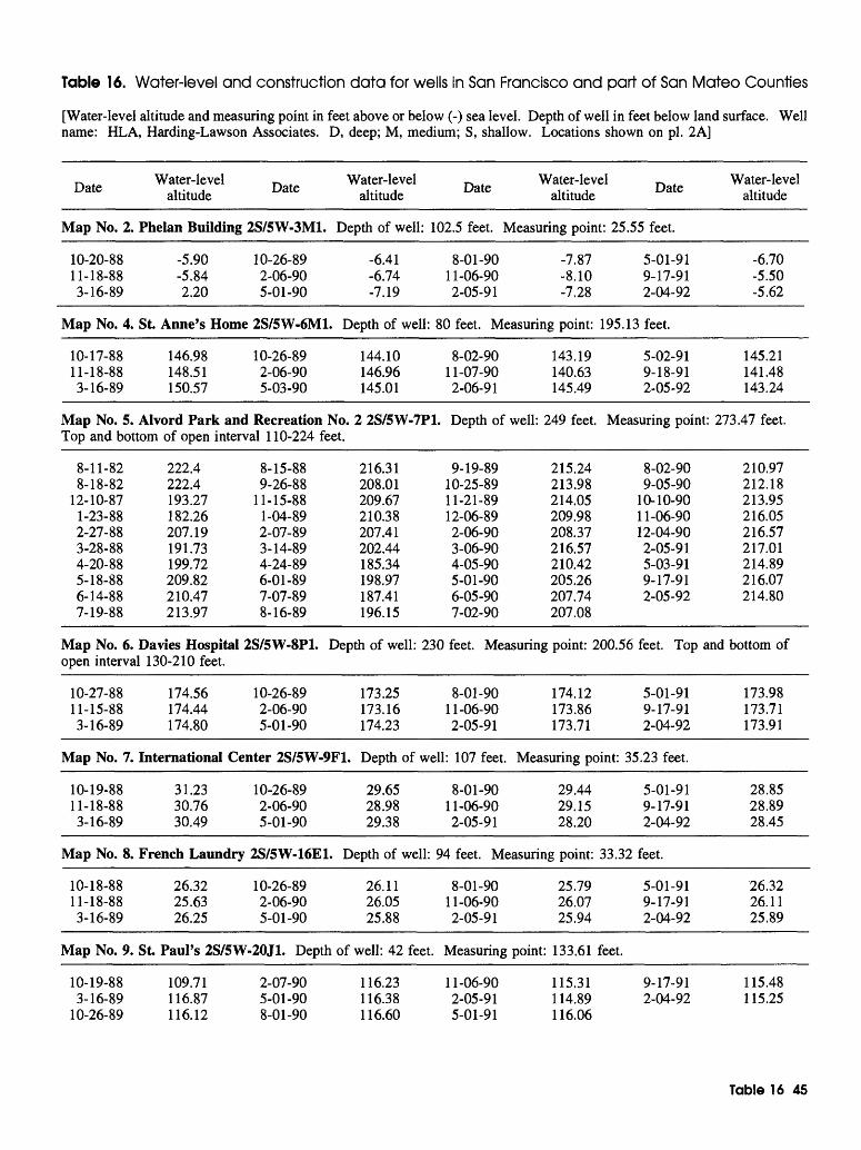
Table 16. Water-level and construction data for wells in San Francisco and part of San Mateo Counties

[Water-level altitude and measuring point in feet above or below (-) sea level. Depth of well in feet below land surface. Well name: HLA, Harding-Lawson Associates. D, deep; M, medium; S, shallow. Locations shown on pi. 2A]

Date

Map No. 2.

10-20-88 11-18-88 3-16-89

Map No. 4.

10-17-88 11-18-88 3-16-89

Water-level altitude Date

Phelan Building 2S/5W-3M1.

-5.90 -5.84 2.20

St Anne's Home

146.98 148.51 150.57

10-26-89 2-06-90 5-01-90

2S/5W-6M1.

10-26-89 2-06-90 5-03-90

Water-level altitude Date Water-level ^ , u . , Date altitude

Water-level altitude

Depth of well: 102.5 feet. Measuring point: 25.55 feet.

-6.41 -6.74 -7.19

Depth of well:

144.10 146.96 145.01

8-01-90 11-06-90 2-05-91

-7.87 -8.10 -7.28

80 feet. Measuring point:

8-02-90 11-07-90 2-06-91

143.19 140.63 145.49

Map No. 5. Alvord Park and Recreation No. 2 2S/5W-7P1. Depth of well: 249 feet. Top and bottom of open interval 110-224 feet.

8-11-82 8-18-82

12-10-87 1-23-88 2-27-88 3-28-88 4-20-88 5-18-88 6-14-88 7-19-88

222.4 222.4 193.27 182.26 207.19 191.73 199.72 209.82 210.47 213.97

8-15-88 9-26-88

11-15-88 1-04-89 2-07-89 3-14-89 4-24-89 6-01-89 7-07-89 8-16-89

216.31 208.01 209.67 210.38 207.41 202.44 185.34 198.97 187.41 196.15

9-19-89 10-25-89 11-21-89 12-06-89 2-06-90 3-06-90 4-05-90 5-01-90 6-05-90 7-02-90

215.24 213.98 214.05 209.98 208.37 216.57 210.42 205.26 207.74 207.08

5-01-91 9-17-91 2-04-92

195.13 feet.

5-02-91 9-18-91 2-05-92

Measuring point:

8-02-90 9-05-90

10-10-90 11-06-90 12-04-90 2-05-91 5-03-91 9-17-91 2-05-92

-6.70 -5.50 -5.62

145.21 141.48 143.24

273.47 feet.

210.97 212.18 213.95 216.05 216.57 217.01 214.89 216.07 214.80

Map No. 6. Davies Hospital 2S/5W-8P1. Depth of well: 230 feet. Measuring point: 200.56 feet. Top and bottom of open interval 130-210 feet.

10-27-88 11-15-88 3-16-89

Map No. 7.

10-19-88 11-18-88 3-16-89

Map No. 8.

10-18-88 11-18-88 3-16-89

Map No. 9.

10-19-88 3-16-89

10-26-89

174.56 174.44 174.80

10-26-89 2-06-90 5-01-90

173.25 173.16 174.23

8-01-90 11-06-90 2-05-91

International Center 2S/5W-9F1. Depth of well: 107 feet.

31.23 30.76 30.49

French Laundry

26.32 25.63 26.25

10-26-89 2-06-90 5-01-90

2S/5W-16E1.

10-26-89 2-06-90 5-01-90

St Paul's 2S/5W-20J1. Depth

109.71 116.87 116.12

2-07-90 5-01-90 8-01-90

29.65 28.98 29.38

Depth of well:

26.11 26.05 25.88

of well: 42 feet.

116.23 116.38 116.60

8-01-90 11-06-90 2-05-91

174.12 173.86 173.71

5-01-91 9-17-91 2-04-92

173.98 173.71 173.91

Measuring point: 35.23 feet.

29.44 29.15 28.20

94 feet. Measuring point:

8-01-90 11-06-90 2-05-91

Measuring

11-06-90 2-05-91 5-01-91

25.79 26.07 25.94

point: 133.61

115.31 114.89 1 16.06

5-01-91 9-17-91 2-04-92

33.32 feet.

5-01-91 9-17-91 2-04-92

feet.

9-17-91 2-04-92

28.85 28.89 28.45

26.32 26.11 25.89

115.48 115.25

Table 16 45

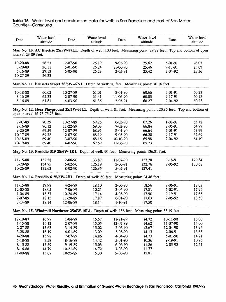
Table 16. Water-level and construction data for wells in San Francisco and part of San Mateo Counties- Continued

Date Water-level ~ . ,... , Date altitudeWater-level

altitude Date Water-level altitude Date Water-level

altitude

Map No. 10. AC Electric 2S/5W-27L1. Depth of well: 100 feet. Measuring point: 29.78 feet. Top and bottom of open interval 23-89 feet.

10-20-88 3-20-89 5-16-89

10-27-89

Map No. 11.

10-18-88 3-16-89 5-16-89

Map No. 12.open interval

7-07-89 8-16-89 9-20-89

10-17-89 10-18-89 10-19-89

Map No. 13.

11-15-88 3-20-89

10-26-89

Map No. 14.

11-15-88 12-05-88

1-04-89 2-07-89 3-14-89

Map No. 15.

12-10-87 1-15-88 2-27-88 3-28-88 4-20-88 5-18-88 8-15-88 8-16-88

11-09-88

26.23 26.11 27.13 26.23

2-07-90 5-01-90 6-05-90

Brussels Street 2S/5W-27N1.

60.62 62.33 61.81

10-27-89 2-07-90 4-03-90

Here Playground 2S/5W-33L165.75-75.75 feet.

70.39 70.12 69.59 69.28 69.40 69.40

10-27-89 11-22-89 12-07-89 2-07-90 3-07-90 4-02-90

26.19 26.24 26.23

Depth of well:

61.01 61.41 61.35

9-05-90 11-06-90 2-05-91

25.62 25.46 25.42

20 feet. Measuring point: 70.16

8-01-90 11-06-90 2-05-91

60.66 60.03 60.27

5-01-91 9-17-91 2-04-92

feet.

5-01-91 9-17-91 2-04-92

. Depth of well: 81 feet. Measuring point: 120.86 feet. Top

69.26 69.03 68.95 68.19 68.16 67.69

Presidio 319 2S/6W-1K1. Depth of well: 90

132.28 134.75 132.63

Presidio 6

17.98 18.05 18.37 18.15 18.14

Windmill

16.97 16.12 15.63 16.19 15.98 7.59

15.59 14.79 15.67

2-06-90 5-02-90 8-02-90

2S/6W-2H1. Depth

4-24-89 7-06-89

10-24-89 11-20-89 12-06-89

133.87 126.19 126.35

6-05-90 7-02-90 8-01-90 9-05-90

10-10-90 11-06-90

67.26 66.84 66.64 66.20 65.98 65.73

1-08-91 2-05-91 5-01-91 9-17-91 2-04-92

26.03 25.63 25.56

60.23 60.18 60.28

and bottom of

65.12 64.77 63.99 62.69 61.40

feet. Measuring point: 136.31 feet.

11-07-90 2-06-91 5-02-91

of well: 60 feet. Measuring

18.10 10.21 17.14 17.87 18.14

2-06-90 3-06-90 4-05-90 6-01-90 1-10-91

Northeast 2S/6W-10L1. Depth of well: 156 feet.

1-04-89 2-07-89 3-14-89 6-01-89 7-07-89 8-16-89 9-19-89

10-21-89 10-25-89

15.57 15.05 15.02 13.09 14.86 14.42 15.03 14.72 15.30

11-21-89 12-07-89 2-06-90 3-06-90 4-04-90 5-01-90 6-06-90 7-03-90 9-06-90

127.28 132.76 127.41

point: 24.46 feet.

18.56 17.81 17.90 17.63 17.50

Measuring point:

14.72 14.62 13.67 14.13 14.73 10.36 11.86 11.77 12.81

9-18-91 2-05-92

2-06-91 5-02-91 9-19-91 2-05-92

33.19 feet.

10-11-90 11-07-90 12-04-90 2-06-91 5-01-90 9-19-91 2-05-92

129.84 130.68

18.02 17.96 17.66 18.50

13.00 14.00 13.96 13.66 14.21 10.86 12.51

46 Geohydrology, Water Quality, and Estimation of Ground-Water Recharge In San Francisco, California 1987-92

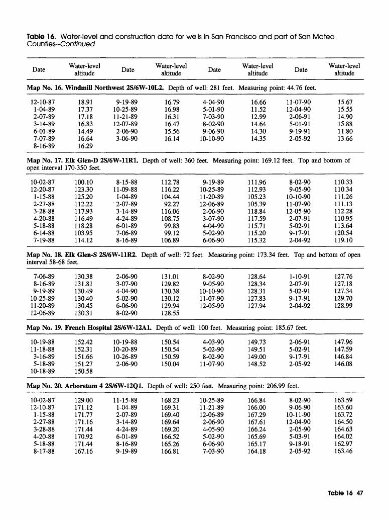
Table 16. Water-level Counties-Conf/nued

Date

Map No. 16.

12-10-87 1-04-89 2-07-89 3-14-89 6-01-89 7-07-89 8-16-89

Map No. 17.open interval

10-02-87 12-20-87

1-15-88 2-27-88 3-28-88 4-20-88 5-18-88 6-14-88 7-19-88

Map No. 18.interval 58-68

7-06-89 8-16-89 9-19-89

10-25-89 11-20-89 12-06-89

Map No. 19.

10-19-88 11-18-88 3-16-89 5-18-89

10-18-89

Map No. 20.

10-02-87 12-10-87

1-15-88 2-27-88 3-28-88 4-20-88 5-18-88 8-17-88

and construction data for wells in San Francisco and part of San Mateo

Water-level ~ . ,... , Date altitudeWater-level ~ Water-level

altitude a e altitude

Windmill Northwest 2S/6W-10L2. Depth of well: 281 feet. Measuring point:

18.91 17.37 17.18 16.83 14.49 16.64 16.29

9-19-89 10-25-89 11-21-89 12-07-89 2-06-90 3-06-90

Elk Glen-D 2S/6W-11R1.170-350 feet.

100.10 123.30 125.20 112.22 117.93 116.49 118.28 103.95 114.12

Elk Glen-Sfeet.

130.38 131.81 130.49 130.40 130.45 130.31

8-15-88 11-09-88

1-04-89 2-07-89 3-14-89 4-24-89 6-01-89 7-06-89 8-16-89

2S/6W-11R2.

2-06-90 3-07-90 4-04-90 5-02-90 6-06-90 8-02-90

16.79 16.98 16.31 16.47 15.56 16.14

Depth of well:

112.78 116.22 104.44 92.27

116.06 108.75 99.83 99.12

106.89

Depth of well:

131.01 129.82 130.38 130.12 129.94 128.55

4-04-90 5-01-90 7-03-90 8-02-90 9-06-90

10-10-90

16.66 11.52 12.9914.64 14.30 14.35

Date

44.76 feet.

11-07-90 12-04-90 2-06-91 5-01-91 9-19-91 2-05-92

Water-level altitude

15.67 15.55 14.90 15.88 11.80 13.66

360 feet. Measuring point: 169.12 feet. Top and bottom of

9-19-89 10-25-89 11-20-89 12-06-89 2-06-90 3-07-90 4-04-90 5-02-90 6-06-90

111.96 112.93 105.23 105.39 118.84 117.59 115.71 115.20 115.32

8-02-90 9-05-90

10-10-90 11-07-90 12-05-90 2-07-91 5-02-91 9-17-91 2-04-92

72 feet. Measuring point: 173.34 feet. Top and

8-02-90 9-05-90

10-10-90 11-07-90 12-05-90

128.64 128.34 128.31 127.83 127.94

French Hospital 2S/6W-12A1. Depth of well: 100 feet. Measuring point: 185

152.42 152.31 151.66 151.27 150.58

Arboretum

129.00 171.12 171.77 171.16 171.44 170.92 171.44 167.16

10-19-88 10-20-89 10-26-89 2-06-90

4 2S/6W-12Q1

11-15-88 1-04-89 2-07-89 3-14-89 4-24-89 6-01-89 8-16-89 9-19-89

150.54 150.54 150.59 150.04

4-03-90 5-02-90 8-02-90

11-07-90

. Depth of well: 250 feet. Measuring

168.23 169.31 169.40 169.64 169.20 166.52 165.26 166.81

10-25-89 11-21-89 12-06-89 2-06-90 4-05-90 5-02-90 6-06-90 7-03-90

149.73 149.51 149.00 148.52

point: 206.99

166.84 166.00 167.29 167.61 166.24 165.69 165.17 164.18

1-10-91 2-07-91 5-02-91 9-17-91 2-04-92

.67 feet.

2-06-91 5-02-91 9-17-91 2-05-92

feet.

8-02-90 9-06-90

10-11-90 12-04-90 2-05-90 5-03-91 9-18-91 2-05-92

110.33 110.34 111.26 111.13 112.28 110.95 113.64 120.54 119.10

bottom of open

127.76 127.18 127.34 129.70 128.99

147.96 147.59 146.84 146.08

163.59 163.60 163.72 164.50 164.63 164.02 162.97 163.46

Table 16 47

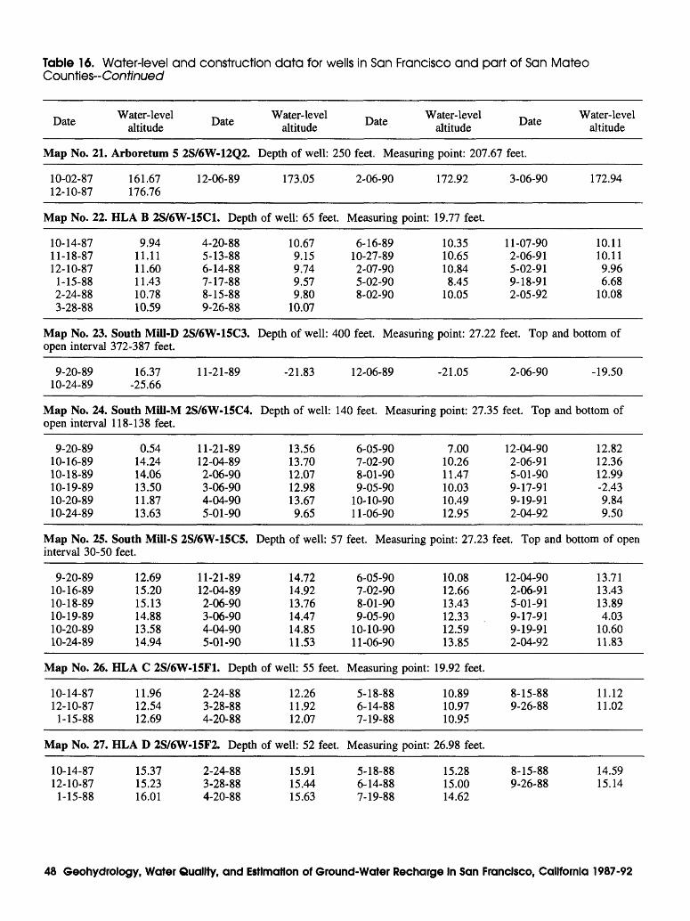
Table 16. Water-level and construction data for wells in San Francisco and part of San Mateo Counties- Continued

Date Water-level altitude Date Water-level

altitude Date Water-level altitude Date Water-level

altitude

Map No. 21. Arboretum 5 2S/6W-12Q2. Depth of well: 250 feet. Measuring point: 207.67 feet.

10-02-87 12-10-87

161.67 176.76

12-06-89 173.05 2-06-90 172.92 3-06-90 172.94

Map No. 22. HLA B 2S/6W-15C1. Depth of well: 65 feet. Measuring point: 19.77 feet.

10-14-8711-18-8712-10-87

1-15-882-24-883-28-88

9.9411.1111.6011.4310.7810.59

4-20-885-13-886-14-887-17-888-15-889-26-88

10.679.159.749.579.80

10.07

6-16-8910-27-892-07-905-02-908-02-90

10.3510.6510.848.45

10.05

11-07-902-06-915-02-919-18-912-05-92

10.1110.119.966.68

10.08

Map No. 23. South Mill-D 2S/6W-15C3. Depth of well: 400 feet. Measuring point: 27.22 feet. Top and bottom of open interval 372-387 feet.

9-20-8910-24-89

16.37 -25.66

11-21-89 -21.83 12-06-89 -21.05 2-06-90 -19.50

Map No. 24. South Mffl-M 2S/6W-15C4.open interval 118-138 feet.

Depth of well: 140 feet. Measuring point: 27.35 feet. Top and bottom of

9-20-8910-16-8910-18-8910-19-8910-20-8910-24-89

0.5414.2414.0613.5011.8713.63

11-21-8912-04-892-06-903-06-904-04-905-01-90

13.5613.7012.0712.9813.679.65

6-05-907-02-908-01-909-05-90

10-10-9011-06-90

7.0010.2611.4710.0310.4912.95

12-04-902-06-915-01-909-17-919-19-912-04-92

12.8212.3612.99-2.439.849.50

Map No. 25. South Mffl-S 2S/6W-15C5.interval 30-50 feet.

Depth of well: 57 feet. Measuring point: 27.23 feet. Top and bottom of open

9-20-8910-16-8910-18-8910-19-8910-20-8910-24-89

12.6915.2015.1314.8813.5814.94

11-21-8912-04-892-06-903-06-904-04-905-01-90

14.7214.9213.7614.4714.8511.53

6-05-907-02-908-01-909-05-90

10-10-9011-06-90

10.0812.6613.4312.3312.5913.85

12-04-902-06-915-01-919-17-919-19-912-04-92

13.7113.4313.894.03

10.6011.83

Map No. 26. HLA C 2S/6W-15F1. Depth of well: 55 feet. Measuring point: 19.92 feet.

10-14-8712-10-87

1-15-88

11.9612.5412.69

2-24-883-28-884-20-88

12.2611.9212.07

5-18-886-14-887-19-88

10.8910.9710.95

8-15-889-26-88

11.1211.02

Map No. 27. HLA D 2S/6W-15F2. Depth of well: 52 feet. Measuring point: 26.98 feet.

10-14-8712-10-87

1-15-88

15.3715.2316.01

2-24-883-28-884-20-88

15.9115.4415.63

5-18-886-14-887-19-88

15.2815.0014.62

8-15-889-26-88

14.5915.14

48 Geohydrology, Water Quality, and Estimation of Ground-Water Recharge In San Francisco, California 1987-92

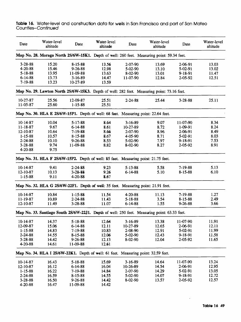
Table 16. Water-level and construction data for wells in San Francisco and part of San Mateo Counties- Continued

~ . Water-level ~ . Date .... , Date altitude

Map No. 28. Moraga North 2S/6W-15K1.

3-28-88 15.20 8-15-88 4-20-88 15.46 9-26-88 5-18-88 13.95 11-09-88 6-14-88 13.73 3-16-89 7-19-88 13.23 10-27-89

Map No. 29. Lawton North 2S/6W-15K3.

10-27-87 25.56 12-09-87 11-05-87 25.60 1-15-88

Map No. 30. HLA E 2S/6W-15P1. Depth

10-14-87 10.04 5-17-88 11-18-87 9.67 6-14-88 12-10-87 10.64 7-19-88

1-15-88 10.57 8-15-88 2-24-88 10.10 9-26-88 3-28-88 9.74 11-09-88 4-20-88 9.75

Map No. 31. HLA F 2S/6W-15P2. Depth

10-14-87 9.41 2-24-88 12-10-87 10.13 3-28-88

1-15-88 9.11 4-20-88

Map No. 32. HLA G 2S/6W-22F1. Depth

10-14-87 10.84 1-15-88 11-19-87 10.89 2-24-88 12-10-87 11.49 3-28-88

Map No. 33. Santiago South 2S/6W-22J1.

10-14-87 14.37 5-18-88 12-09-87 15.06 6-14-88

1-15-88 14.83 7-19-88 2-24-88 14.55 8-15-88 3-28-88 14.42 9-26-88 4-20-88 14.61 11-09-88

Map No. 34. HLA I 2S/6W-22K1. Depth

10-14-87 16.43 5-18-88 12-10-87 16.12 6-14-88

1-15-88 16.22 7-19-88 2-24-88 16.59 8-15-88 3-28-88 16.50 9-26-88 4-20-88 16.47 11-09-88

Water-level altitude

Depth of well:

13.56 12.98 13.63 14.47 13.59

Depth of well:

25.51 25.51

of well: 68 feet.

8.64 8.61 8.66 8.67 8.53 8.82

of well: 85 feet.

9.23 9.26 8.67

0f wei: 35 feet.

11.54 11.43 11.07

Depth of well:

12.64 12.11 10.83 12.06 12.13 12.61

of well: 61 feet.

15.69 16.04 14.84 14.55 14.42 14.42

~ . Water-level Date .... , altitude

260 feet. Measuring point: 59.34

2-07-90 13.69 5-02-90 13.10 8-02-90 13.01

11-07-90 12.84

282 feet. Measuring point: 73.16

2-24-88 25.44

Measuring point: 22.64 feet.

3-16-89 9.07 10-27-89 8.72 2-07-90 8.96 4-05-90 8.71 5-02-90 7.97 8-02-90 8.27

Measuring point: 21.75 feet.

5-13-88 5.58 6-14-88 5.10

Measuring point: 21.91 feet.

4-20-88 11.13 5-18-88 3.54 6-14-88 1.55

250 feet. Measuring point: 63.33

3-16-89 13.38 10-27-89 12.65 2-08-90 12.91 5-02-90 12.43 8-02-90 12.04

Measuring point: 32.59 feet.

3-16-89 14.64 10-26-89 14.54 2-07-90 14.29 5-02-90 14.07 8-02-90 13.57

Date

feet.

2-06-91 5-02-91 9-18-91 2-05-92

feet.

3-28-88

11-07-90 1-09-91 2-06-91 5-02-91 9-18-91 2-05-92

7-19-88 8-15-88

7-19-88 8-15-88 9-26-88

feet.

11-07-90 2-06-91 5-02-91 9-18-91 2-05-92

11-07-90 2-06-91 5-02-91 9-18-91 2-05-92

Water-level altitude

13.03 13.02 11.4712.51

25.11

8.34 8.24 8.49 8.03 7.53 8.91

5.13 6.10

1.27 2.49 3.66

11.91 12.11 11.99 U.58 11.65

13.24 12.95 13.05 12.72 12.57

Table 16 49

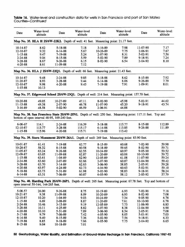
Table 16. Water-level and construction data for wells in San Francisco and part of San Mateo Counties- Continued

Date

Map No. 35.

10-14-87 12-10-87

1-15-88 2-24-88 3-28-88 4-20-88

Map No. 36.

10-14-87 11-20-87 12-10-87

1-15-88

Map No. 37.

10-20-88 11-15-88 3-16-89

Water-level altitude Date Water-level

altitude

HLA H 2S/6W-22K2. Depth of well: 41 feet.

8.62 9.32 9.47 9.04 8.67 8.61

HLA J 2S/6W

9.48 8.93 9.98

10.13

5-18-88 6-14-88 7-19-88 8-15-88 9-26-88

11-09-88

-22Q1. Depth

2-24-88 3-28-88 4-20-88

7.18 5.67 5.24 5.59 6.15 7.12

of well: 66 feet.

9.859.44 9.43

Date Water-level altitude Date Water-level

altitude

Measuring point: 21.17 feet.

3-16-89 10-26-89 2-07-90 5-02-90 8-02-90

Measuring

5-18-88 6-14-88 7-19-88

Edgewood School 2S/6W-23Q1. Depth of well: 214 feet.

49.05 49.38 48.58

10-27-89 2-07-90 5-02-90

47.11 46.78 46.59

8-02-90 11-07-90 2-06-91

7.98 7.75 8.31 7.89 6.54

point: 21.43 feet.

8.62 8.06 7.91

11-07-90 2-06-91 5-02-91 9-18-91 2-04-92

8-15-88 9-26-88 1-09-91

7,17 7.67 7.56 7.24 8.10

7.92 7.79 8.01

Measuring point: 157.70 feet.

45.98 45.20 44.88

Map No. 38. San Francisco State 2S/6W-25N1. Depth of well: 250 feet. Measuring point: bottom of open interval 48-95, 169-240 feet.

6-06-67 12-10-87

1-15-88

Map No. 39.

10-01-87 10-28-87 11-05-87 12-09-87

1-15-88 2-24-88 3-28-88 4-20-88 5-18-88 6-14-88

Map No. 40.open interval

5-08-57 10-21-87 12-10-87

1-15-88 2-24-88 3-28-88 4-20-88 5-17-88 6-14-88 7-19-88 8-15-88

114.1 113.77 115.96

2-24-88 3-28-88 4-20-88

116.39 115.17 115.71

Stern Monument 2S/6W-26A1. Depth of well

61.41 58.32 63.24 63.05 63.61 63.60 63.70 63.97 63.73 63.31

7-19-88 8-15-88 9-26-88

11-09-88 1-04-89 2-07-89 3-14-89 4-24-89 5-31-89 7-06-89

Harding Park 2S/6W-26P1.50-144, 144-265 feet.

26.00 9.38

10.20 6.69

10.46 10.11 10.10 9.79 9.40 8.85 9.04

9-26-88 11-09-88

1-04-89 2-08-89 3-15-89 4-25-89 5-31-89 7-06-89 8-15-89 9-18-89

10-18-89

62.77 60.58 62.55 62.87 62.90 62.66 62.63 62.73 61.98 60.87

5-18-88 6-14-88 7-19-88

: 269 feet.

8-15-89 9-18-89

10-24-89 11-20-89 12-05-89 2-07-90 3-06-90 4-04-90 5-02-90 6-05-90

113.77 113.85 113.42

Measuring point: 83

60.68 59.65 60.97 60.88 61.08 60.87 58.85 60.63 58.83 58.12

Depth of well: 265 feet. Measuring point: 67.78

8.75 8.09 9.03 8.87 9.19 8.82 7.89 7.42 7.36 7.66 7.01

10-19-89 10-20-89 10-24-89 11-20-89 12-05-89 2-07-90 3-06-90 4-05-90 5-02-90 6-05-90

6.93 6.937.34 7.61 7.73 8.38 8.54 8.05 7.56 7.75

5-02-91 9-18-91

117.11 feet.

8-15-88 9-26-88

.90 feet.

7-02-90 8-02-90 9-05-90

10-10-90 11-07-90 12-04-90 2-05-91 5-02-91 9-18-91 2-05-92

44.62 43.74

Top and

112.89 111.89

59.98 59.71 59.52 59.72 59.24 59.42 59.28 59.10 58.24 57.79

feet. Top and bottom of

7-02-90 8-02-90 9-05-90

10-10-90 11-06-90 12-04-90 2-05-91 5-01-91 9-18-91 2-04-92

7.18 7.08 6.78 6.78 6.85 6.90 7.08 7.03 6.33 6.65

50 Geohydrology, Water Quality, and Estimation of Ground-Water Recharge In San Francisco, California 1987-92

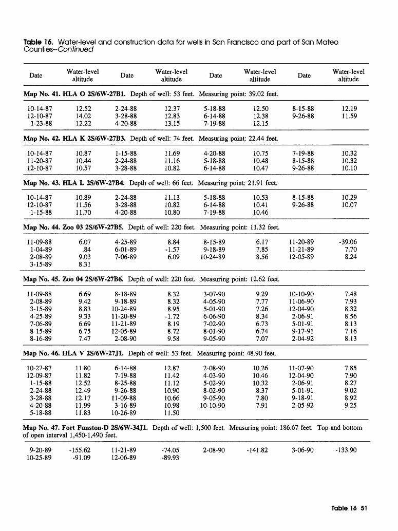
Table 16. Water-level and construction data for wells in San Francisco and part of San Mateo Counties-Conf/ni/eaf

Date

Map No. 41.

10-14-87 12-10-87

1-23-88

Map No. 42.

10-14-87 11-20-87 12-10-87

Map No. 43.

10-14-87 12-10-87

1-15-88

Map No. 44.

11-09-88 1-04-89 2-08-89 3-15-89

Map No. 45.

11-09-88 2-08-89 3-15-89 4-25-89 7-06-89 8-15-89 8-16-89

Map No. 46.

10-27-87 12-09-87

1-15-88 2-24-88 3-28-88 4-20-88 5-18-88

Water-level altitude Date

HLA O 2S/6W-27B1. Depth

12.52 14.02 12.22

2-24-88 3-28-88 4-20-88

HLA K 2S/6W-27B3. Depth

10.87 10.44 10.57

1-15-88 2-24-88 3-28-88

HLA L 2S/6W-27B4. Depth

10.89 11.56 11.70

Zoo 03 2S/6W

6.07 .84

9.03 8.31

2-24-88 3-28-88 4-20-88

-27B5. Depth

4-25-89 6-01-89 7-06-89

Zoo 04 2S/6W-27B6. Depth

6.699.42 8.83 9.33 6.69 6.75 7.47

8-18-89 9-18-89

10-24-89 11-20-89 11-21-89 12-05-89 2-08-90

HLA V 2S/6W-27J1. Depth

11.80 11.82 12.52 12.49 12.17 11.99 11.83

6-14-88 7-19-88 8-25-88 9-26-88

11-09-88 3-16-89

10-26-89

Map No. 47. Fort Funston-D 2S/6W-34J1,of open interval 1,450-1,490 feet.

9-20-89 10-25-89

-155.62 -91.09

11-21-89 12-06-89

Water-level altitude

of well: 53 feet.

12.37 12.83 13.15

of well: 74 feet.

11.69 11.16 10.82

of well: 66 feet.

11.13 10.82 10.80

of well: 220 feet.

8.84 -1.57 6.09

of well: 220 feet.

8.32 8.32 8.95

-1.72 8.19 8.72 9.58

of well: 53 feet.

12.87 11.42 11.12 10.90 10.66 10.98 11.50

, Depth of well:

-74.05 -89.93

Date

Measuring

5-18-88 6-14-88 7-19-88

Measuring

4-20-88 5-18-88 6-14-88

Measuring

5-18-88 6-14-88 7-19-88

Measuring

8-15-89 9-18-89

10-24-89

Measuring

3-07-90 4-05-90 5-01-90 6-06-90 7-02-90 8-01-90 9-05-90

Water-level altitude

point: 39.02 feet.

12.50 12.38 12.15

point: 22.44 feet.

10.75 10.48 10.47

point: 21.91 feet.

10.53 10.41 10.46

point: 11.32 feet.

6.17 7.85 8.56

point: 12.62 feet.

9.29 7.77 7.26 8.34 6.73 6.74 7.07

Date

8-15-88 9-26-88

7-19-88 8-15-88 9-26-88

8-15-88 9-26-88

11-20-89 11-21-89 12-05-89

10-10-90 11-06-90 12-04-90 2-06-91 5-01-91 9-17-91 2-04-92

Water-level altitude

12.19 11.59

10.32 10.32 10.10

10.29 10.07

-39.06 7.70 8.24

7.48 7.93 8.32 8.56 8.13 7.16 8.13

Measuring point: 48.90 feet.

2-08-90 4-03-90 5-02-90 8-02-90 9-05-90

10-10-90

1,500 feet.

2-08-90

10.26 10.46 10.32 8.37 7.80 7.91

Measuring point:

-141.82

11-07-90 12-04-90 2-06-91 5-01-91 9-18-91 2-05-92

186.67 feet.

3-06-90

7.85 7.90 8.27 9.02 8.92 9.25

Top and bottom

-133.90

Table 16 51

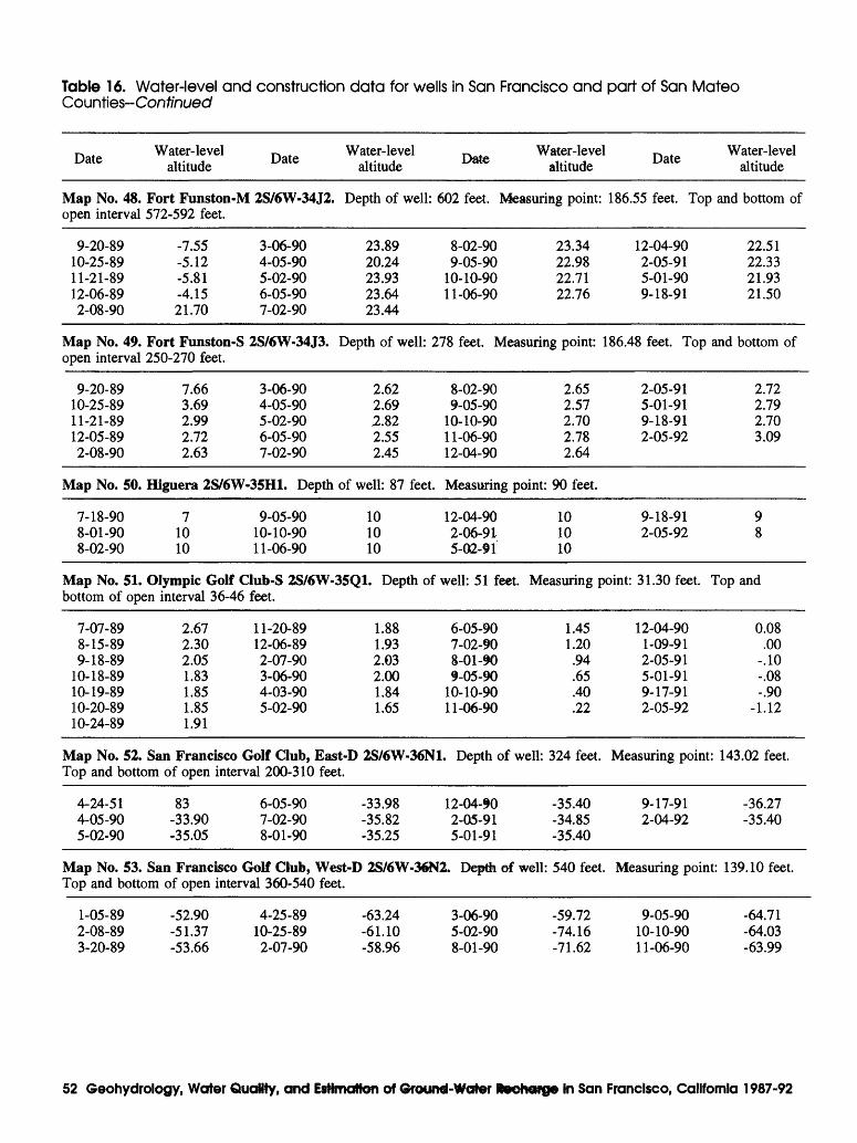
Table 16. Water-level and construction data for wells in San Francisco and part of San Mateo Counties-Con//nued

Date Water-level altitude Date Water-level

altitude Date Water-level altitude Date Water-level

altitude

Map No. 48. Fort Funston-M 2S/6W-34J2. Depth of well: 602 feet. Measuring point: 186.55 feet. Top and bottom of open interval 572-592 feet.

9-20-8910-25-8911-21-8912-06-892-08-90

-7.55-5.12-5.81-4.1521.70

3-06-904-05-905-02-906-05-907-02-90

23.8920.2423.9323.6423.44

8-02-909-05-90

10-10-9011-06-90

23.3422.9822.7122.76

12-04-902-05-915-01-909-18-91

22.5122.3321.9321.50

Map No. 49. Fort Funston-S 2S/6W-34J3.open interval 250-270 feet.

Depth of well: 278 feet. Measuring point: 186.48 feet. Top and bottom of

9-20-8910-25-8911-21-8912-05-892-08-90

7.663.692.992.722.63

3-06-904-05-905-02-906-05-907-02-90

2.622.692.822.552.45

8-02-909-05-90

10-10-9011-06-9012-04-90

2.652.572.702.782.64

2-05-915-01-919-18-912-05-92

2.722.792.703.09

Map No. 50. Higuera 2S/6W-35H1. Depth of well: 87 feet. Measuring point: 90 feet.

7-18-908-01-908-02-90

71010

9-05-9010-10-9011-06-90

101010

12-04-902-06-915-02-91

101010

9-18-912-05-92

98

Map No. 51. Olympic Golf Club-S 2S/6W-35Q1.bottom of open interval 36-46 feet.

Depth of well: 51 feet. Measuring point: 31.30 feet. Top and

7-07-898-15-899-18-89

10-18-8910-19-8910-20-8910-24-89

2.672.302.051.831.851.851.91

11-20-8912-06-892-07-903-06-904-03-905-02-90

1.881.932.032.001.841.65

6-05-907-02-908-01-909-05-90

10-10-9011-06-90

1.451.20.94.65.40.22

12-04-901-09-912-05-915-01-919-17-912-05-92

0.08.00

-.10-.08-.90

-1.12

Map No. 52. San Francisco Golf Club, East-D 2S/6W-36N1. Depth of well: 324 feet. Measuring point: 143.02 feet. Top and bottom of open interval 200-310 feet.

4-24-514-05-905-02-90

83-33.90-35.05

6-05-907-02-908-01-90

-33.98-35.82-35.25

12-04-902-05-915-01-91

-35.40-34.85-35.40

9-17-912-04-92

-36.27-35.40

Map No. 53. San Francisco Golf Club, West-D 2S/6W-36N2. Top and bottom of open interval 360-540 feet.

Depth of well: 540 feet. Measuring point: 139.10 feet.

1-05-892-08-893-20-89

-52.90-51.37-53.66

4-25-8910-25-892-07-90

-63.24-61.10-58.96

3-06-905-02-908-01-90

-59.72-74.16-71.62

9-05-9010-10-9011-06-90

-64.71-64.03-63.99

52 Geohydrology, Water Quality, and Estimation of Ground-Water Recharge In San Francisco, California 1987-92

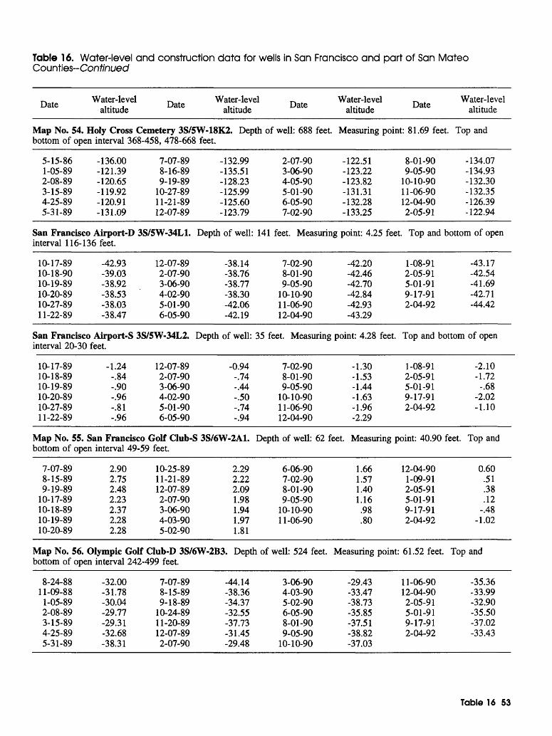
Table 16. Water-level and construction data for wells in San Francisco and part of San Mateo Counties-Conf/nuec/

~ , Water-level ~ . Date .... , Date altitude

Map No. 54. Holy Crossbottom of open

5-15-861-05-892-08-893-15-894-25-895-31-89

San Francisco

Water-level ~ . .... , Date altitudeWater-level

altitude Date Water-level altitude

Cemetery 3S/5W-18K2. Depth of well: 688 feet. Measuring point: 81.69 feet. Top andinterval 368-458, 478-668 feet.

-136.00-121.39-120.65-119.92-120.91-131.09

Airport-D

7-07-898-16-899-19-89

10-27-8911-21-8912-07-89

3S/5W-34L1.

-132.99-135.51-128.23-125.99-125.60-123.79

Depth of well:

2-07-903-06-904-05-905-01-906-05-907-02-90

-122.51-123.22-123.82-131.31-132.28-133.25

8-01-909-05-90

10-10-9011-06-9012-04-902-05-91

141 feet. Measuring point: 4.25 feet. Top and

-134.07-134.93-132.30-132.35-126.39-122.94

bottom of openinterval 116-136 feet.

10-17-8910-18-9010-19-8910-20-8910-27-8911-22-89

San Francisco

-42.93-39.03-38.92-38.53-38.03-38.47

Airport-S

12-07-892-07-903-06-904-02-905-01-906-05-90

3S/5W-34L2.

-38.14-38.76-38.77-38.30-42.06-42.19

Depth of well:

7-02-908-01-909-05-90

10-10-9011-06-9012-04-90

-42.20-42.46-42.70-42.84-42.93-43.29

35 feet. Measuring point: 4.28 feet.

1-08-912-05-915-01-919-17-912-04-92

-43.17-42.54-41.69-42.71-44.42

Top and bottom of openinterval 20-30 feet.

10-17-8910-18-8910-19-8910-20-8910-27-8911-22-89

-1.24-.84-.90-.96-.81-.96

12-07-892-07-903-06-904-02-905-01-906-05-90

-0.94-.74-.44-.50-.74-.94

Map No. 55. San Francisco Golf Club-S 3S/6W-2A1.bottom of open

7-07-898-15-899-19-89

10-17-8910-18-8910-19-8910-20-89

7-02-908-01-909-05-90

10-10-9011-06-9012-04-90

Depth of well: 62

-1.30-1.53-1.44-1.63-1.96-2.29

1-08-912-05-915-01-919-17-912-04-92

feet. Measuring point: 40.90

-2.10-1.72

-.68-2.02-1.10

feet. Top andinterval 49-59 feet.

2.902.752.482.232.372.282.28

10-25-8911-21-8912-07-892-07-903-06-904-03-905-02-90

2.292.222.091.981.941.971.81

6-06-907-02-908-01-909-05-90

10-10-9011-06-90

Map No. 56. Olympic Golf Club-D 3S/6W-2B3. Depth of well: 524 feet.bottom of open

8-24-8811-09-88

1-05-892-08-893-15-894-25-895-31-89

1.661.571.401.16.98.80

Measuring point:

12-04-901-09-912-05-915-01-919-17-912-04-92

61.52 feet.

0.60.51.38.12

-.48-1.02

Top andinterval 242-499 feet.

-32.00-31.78-30.04-29.77-29.31-32.68-38.31

7-07-898-15-899-18-89

10-24-8911-20-8912-07-892-07-90

-44.14-38.36-34.37-32.55-37.73-31.45-29.48

3-06-904-03-905-02-906-05-908-01-909-05-90

10-10-90

-29.43-33.47-38.73-35.85-37.51-38.82-37.03

11-06-9012-04-902-05-915-01-919-17-912-04-92

-35.36-33.99-32.90-35.50-37.02-33.43

Table 16 53

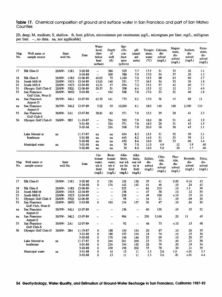
Table 17. Chemical composition of ground and surface water in San Francisco and part of San Mateo Counties

[D, deep; M, medium; S, shallow, ft, foot; ^.S/cm, microsiemen per centimeter; \ig/L, microgram per liter; mg/L, milligram per liter. --, no data, na, not applicable]

MapNo.

17

1824255153

na

na

55

56

MapNo.

17

1824255153

na

na

55

56

Well name orsample source

Elk Glen-D

Elk Glen-SSouth Mill-MSouth Mill-SOlympic Golf Club-SSan Francisco

Golf Club, West-DSan Francisco

Airport-DSan Francisco

Airport-SSan Francisco

Golf Club-SOlympic Golf Club-D

Lake Merced atboathouse

Municipal water

Well name orsample source

Elk Glen-D

Elk Glen-SSouth Mill-MSouth Mill-SOlympic Golf Club-SSan Francisco

Golf Club, West-DSan Francisco

Airport-DSan Francisco

Airport-SSan Francisco

Golf Club-SOlympic Golf Club-D

Lake Merced atboathouse

Municipal water

Statewell No.

2S/6W- 11R1

2S/6W- 11R22S/6W- 15C42S/6W- 15C52S/6W- 35Q12S/6W- 36N2

3S/5W- 34L1

3S/5W- 34L2

3S/6W- 2A1

3S/6W- 2B3

na

na

Statewell No.

2S/6W- 11R1

2S/6W- 11R22S/6W- 15C42S/6W- 15C52S/6W- 35Q12S/6W- 36N2

3S/5W- 34L1

3S/5W- 34L2

3S/6W- 2A1

3S/6W- 2B4

na

na

Date

3-02-885-04-88

12-06-8912-04-8912-04-8912-06-895-03-88

12-07-89

12-07-89

12-07-89

11-19-873-01-885-02-88

11-17-873-01-885-02-883-01-885-02-88

Date

3-02-885-04-88

12-06-8912-04-8912-04-8912-06-895-03-88

12-07-89

12-07-89

12-07-89

11-19-873-01-885-02-88

11-17-873-01-885-02-883-01-885-02-88

Water level(feet

belowland

surface)

_

43.0313.6512.3129.37-

42.39

5.22

38.81

---

nanananana

Car­bonatewater,wh itfield

(mg/L)

00 ~0

-

-

00000800

Depthof

well(ft)

36036072

1405751

540

141

35

62

524524524

nanananana

Bicar­bonatewater,wh itfield

(mg/L)

154174 - --

192

-

-

188188178244234230

1413

cificcon­duct­ance

(|iS/cm)

529586

1,160551854308588

773

10,200

571

593571568

654643650

3938

Alka­linity,

wat whtot fetfield

(mg/L)

12814222515623898

154

156

984

92

160153146201194196

1211

pH(stand­

ardunits)

7.77.97.07.77.26.47.8

8.2

8.1

7.0

7.97.87.8

8.38.28.67.88.8

Alka­linity,

wat whtot itfield

(mg/L)

126143 - «

157

-

-

154154146200192202

1111

Temper­ature,water(°C)

17.517.015.516.515.515.517.0

17.0

18.0

15.5

18.018.020.0

15.514.018.011.012.0

Sulfate,dis­

solved(mg/L)

29416447493436

60

250

46

201822232835

1.31.3

Calcium,dis­

solved(mg/L)

31346834571233

38

140

29

282826

3131304.95.0

/-ii-i _Chlo­ ride,

solved(mg/L)

4146

21038

1002147

130

3,100

73

677469757978

2.62.6

Magne­sium, dis­

solved(mg/L)

33376335421232

15

160

28

313130

323333

.12

.30

Fluo- ride,dis­

solved(mg/L)

0.20.10.10.10

<.10.10.10

.10

.20

<.10

.10

.10

.10

.40

.30

.301.0

.81

Sodium,dis­

solved(mg/L)

26286028602140

88

2,100

41

424343

595960

1.91.7

Bromide,dis­

solved(mg/L)

0.16.24

1.3.12.33.04.24

.35

11

.15

.26

.25

.26

.22

.19

.21<.01<.01

Potas­sium, dis­

solved(mg/L)

1.11.32.71.87.74.91.8

12

110

2.2

1.91.92.1

2.12.12.4

.40

.40

Silica,dis­

solved(mg/L)

43423935263030

32

45

48

353637383435

3.74.4

54 Geohydrology, Water Quality, and Estimation of Ground-Water Recharge In San Francisco, California 1987-92

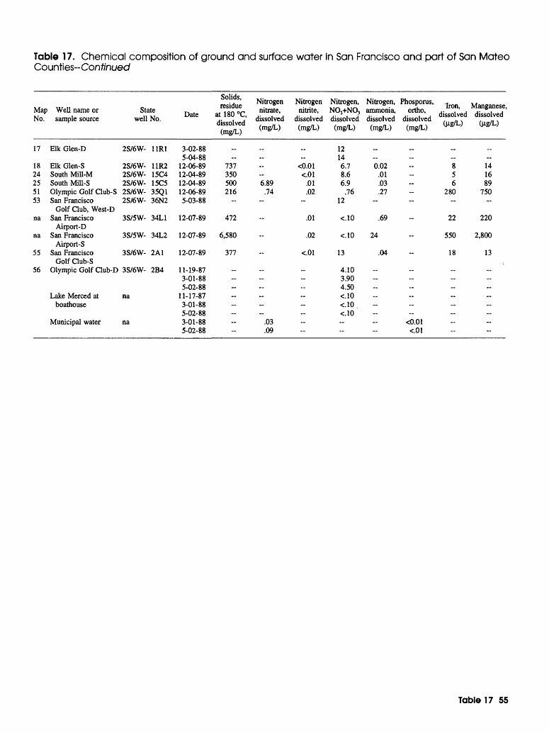
Table 17. Chemical composition of ground and surface water in San Francisco and part of San Mateo Counties-Conf/nL/ed

Map Well name or No. sample source

17

1824255153

na

na

55

56

Elk Glen-D

Elk Glen-SSouth Mill-MSouth Mill-SOlympic Golf Club-SSan Francisco

Golf Club, West-DSan Francisco

Airport-DSan Francisco

Airport-SSan Francisco

Golf Club-SOlympic Golf Club-D

Lake Merced atboathouse

Municipal water

State well No.

2S/6W-

2S/6W-2S/6W-2S/6W-2S/6W-2S/6W-

3S/5W-

3S/5W-

3S/6W-

3S/6W-

na

na

11R1

11R215C415C535Q136N2

34L1

34L2

2A1

2B4

Date

3-02-885-04-88

12-06-8912-04-8912-04-8912-06-895-03-88

12-07-89

12-07-89

12-07-89

11-19-873-01-885-02-88

11-17-873-01-885-02-883-01-885-02-88

Solids, K... residue NltrogenatlSO'C, ,mtnfe'

,. , , dissolved dissolved , ,t~ n \ (.m& L')(mg/L)

_

737350500 6.89216 .74

472

6,580

377

..

.. ....

.03

.09

Nitrogen Nitrogen, Nitrogen, Phosporus, nitrite, NO2+NO3 ammonia, ortho,

dissolved dissolved dissolved dissolved (mg/L) (mg/L) (mg/L) (mg/L)

1214

<0.01 6.7 0.02<.01 8.6 .01

.01 6.9 .03

.02 .76 .2712

.01 <.10 .69

.02 <.10 24

<.01 13 .04

4.103.904.50<.10<.10<.10

<0.01<.01

Iron, Manganese, dissolved dissolved

_ 856

280~

22

550

18

~--------

_-

141689

750-

220

2,800

13

--~~----

Table 17 55

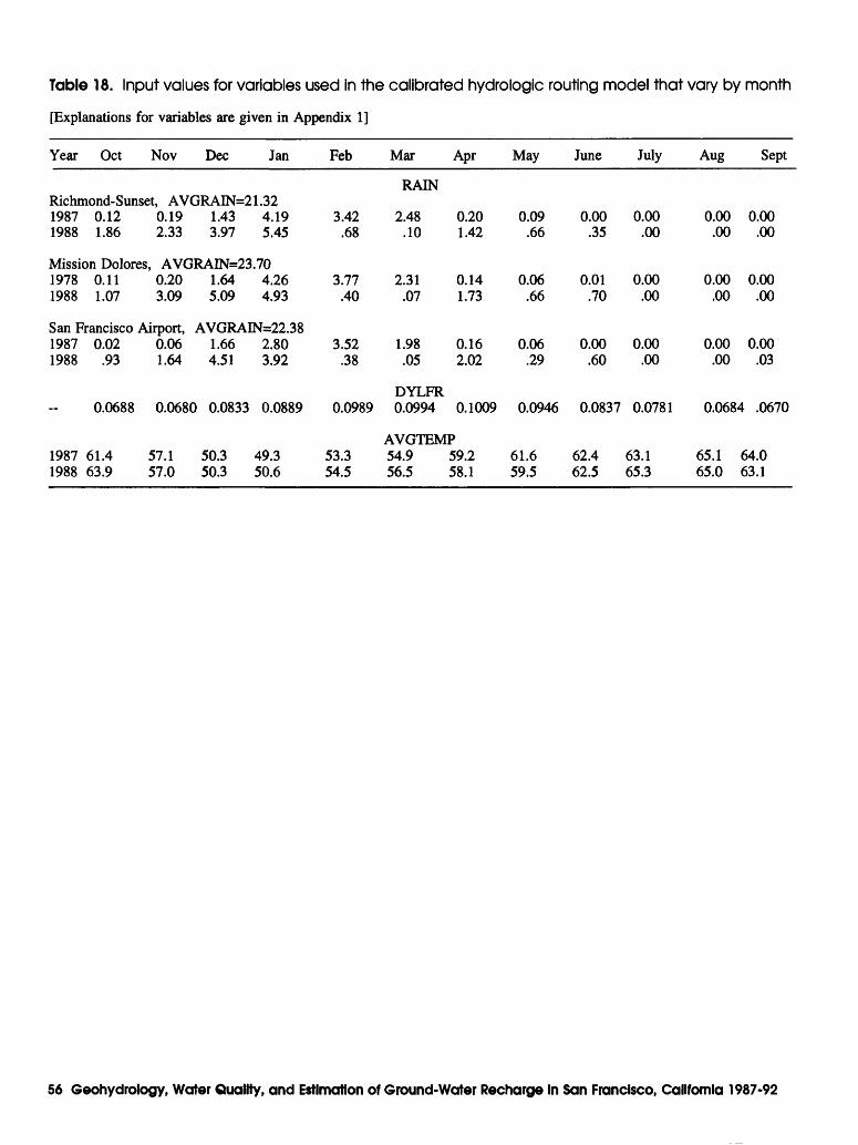
Table 18. Input values for variables used in the calibrated hydrologic routing model that vary by month

[Explanations for variables are given in Appendix 1]

Year Oct Nov Dec Jan Feb Mar

RAIN

Apr May June July Aug Sept

Richmond-Sunset, AVGRAIN=21.321987 0.121988 1.86

0.192.33

1.433.97

Mission Dolores, AVGRAIN=231978 0.111988 1.07

San Francisco1987 0.021988 .93

0.0688

0.203.09

Airport,0.061.64

1.645.09

4.195.45

.704.264.93

3.42.68

3.77.40

2.48.10

2.31.07

0.201.42

0.141.73

0.09.66

0.06.66

0.00.35

0.01.70

0.00.00

0.00.00

0.00.00

0.00.00

0.00.00

0.00.00

AVGRAIN=22.381.664.51

0.0680 0.0833

2.803.92

0.0889

3.52.38

0.0989

1.98.05

DYLFR0.0994

0.162.02

0.1009

0.06.29

0.0946

0.00.60

0.0837

0.00.00

0.0781

0.00.00

0.00.03

0.0684 .0670

AVGTEMP1987 61.41988 63.9

57.157.0

50.350.3

49.350.6

53.354.5

54.956.5

59.258.1

61.659.5

62.462.5

63.165.3

65.165.0

64.063.1

56 Geohydrology, Water Quality, and Estimation of Ground-Water Recharge in San Francisco, California 1987-92

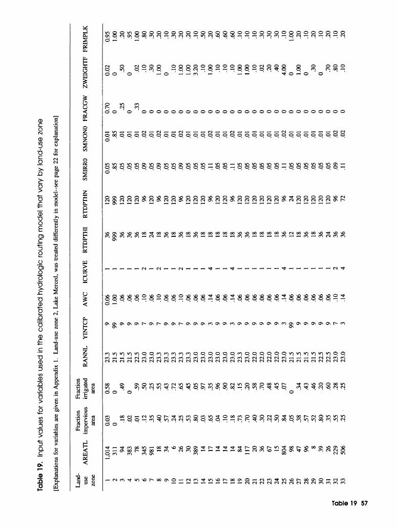
Tabl

e 19

. In

put

valu

es f

or v

aria

bles

use

d in

the

calib

rate

d h

ydro

logi

c ro

utin

g m

odel

that

vary

by

land

-use

zon

e

[Exp

lana

tions

for

var

iabl

es a

re g

iven

in

App

endi

x 1.

Land

-use

zon

e 2,

Lak

e M

erce

d, w

as t

reat

ed d

iffer

ently

in

mod

el s

ee p

age

22 f

or e

xpla

natio

n]

Q

C7

<D

Land

- us

e zo

ne 1 2 3 4 5 6 7 8 9 10 11 12 13 14 15 16 17 18 19 20 21 22 23 24 25 26 27 28 29 30 31 32 33

AR

EATL

1,01

431

1 94 383 78 345

981 18 34 6 26 30 389 14 17 14 14 14 84 117 20 36 67 15 804 98 47 96 8 39 26 229

506

Frac

tion

impe

rvio

us

area

0.03

0 .18

.02

.01

.12

.35

.40

.57

.24

.25

.53

.80

.03

.65

.04

.10

.18

.73

.70

.40

.30

.22

.50

.84

.05

.38

.57

.52

.80

.35

.55

.25

Frac

tion

irrig

ated

ar

ea

0.58

0 .49

0 .59

.50

.25

.55

.43

.72

.65

.45

.05

.97

.35

.96

.90

.82

.15

.20

.58

.70

.48

.45

.07

0 .34

.43

.46

.20

.60

.28

.25

RA

NN

L

23.3

21.5

21.5

21.5

22.5

23.0

23.0

23.3

23.3

23.3

23.3

23.3

23.0

23.0

23.0

23.0

23.0

23.0

23.3

23.0

22.0

22.0

22.0

22.0

23.0

21.5

21.5

21.5

21.5

22.5

22.5

23.0

23.0

YIN

TCP

9 99 9 9 9 7 9 7 9 9 7 9 9 9 3 9 9 3 9 9 9 9 9 9 3 99 9 9 9 9 9 7 3

AW

C

ICU

RV

E

0.06 1.00 .06

.06

.06

.10

.06

.10

.06

.06

.10

.06

.06

.06

.14

.06

.06

.14

.06

.06

.06

.06

.06

.06

.14

.06

.06

.06

.06

.06

.06

.10

.14

1 1 1 1 1 2 1 2 1 1 2 1 1 1 4 1 1 4 1 1 1 1 1 1 4 1 1 1 1 1 1 2 4

RTD

PTH

I

36 999 36 36 36 18 24 18 36 18 36 18 36 18 18 18 18 18 36 36 18 18 18 18 36 12 18 36 18 36 24 36 36

RTD

PTH

N

120

999

120

120

120 96 120 96 120

120 96 120

120

120 96 120

120 96 120

120

120

120

120

120 96 24 120

120

120

120

120 96 72

SMIR

RO

0.05 .8

5.0

5.0

5.0

5.0

9.0

5.0

9.0

5.0

5.0

9.0

5.0

5.0

5.1

1.0

5.0

5.1

1.0

5.0

5.0

5.0

5.0

5.0

5.1

1.0

5.0

5.0

5.0

5.0

5.0

5.0

9.1

1

SMN

ON

O

0.01 .8

5.0

1.0

1.0

1.0

2.0

1.0

2.0

1.0

1.0

2.0

1.0

1.0

1.0

2.0

1.0

1.0

2.0

1.0

1.0

1.0

1.0

1.0

1.0

2.0

1.0

1.0

1.0

1.0

1.0

1.0

2.0

2

FRA

CG

W

0.70

0 .25

0 .33

0 0 0 0 0 0 0 0 0 0 0 0 0 0 0 0 0 0 0 0 0 0 0 0 0 0 0 0

ZWEI

GH

TF

0.02

0 .50

0 .02

.10

.30

1.00

0 .10

1.00

1.00

3.20 .1

01.

00 .10

.10

.10

1.00

1.00 .10

.02

.20

.40

4.00

0 1.00

0 .30

0 .70

.80

.10

FRIM

PLK

0.95

1.00 .20

.95

1.00 .80

.30

.20

.10

.30

.20

.20

.10

.50

.20

.60

.60

.60

.10

.10

.10

.30

.30

.30

.10

1.00 .20

.10

.20

.10

.20

.10

.20

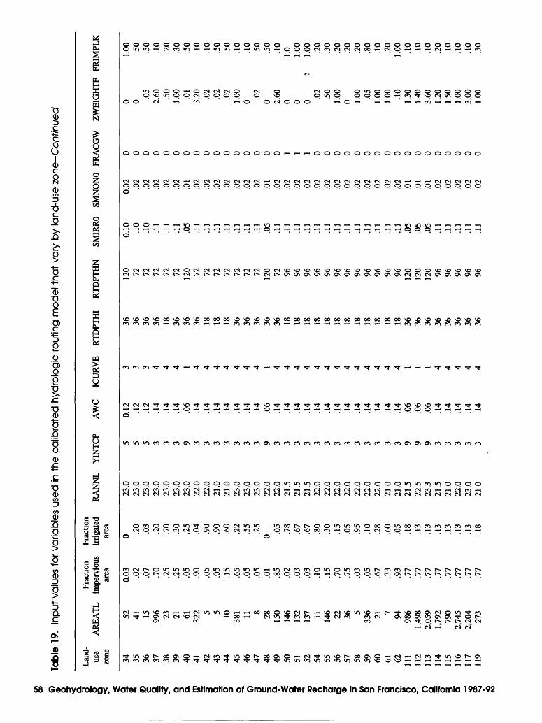
tfl

a> Geohydrology, W a <D 0 Q f? Q a I Q O o 0 5 c a 1<D TO <D

O Q (Q <D 5" j? Tl a o. o p O

a 6s 5 a <> 00

Tabl

e 19

. In

put v

alue

s fo

r

Land

- us

e zo

ne

34 35 36 37 38 39 40 41 42 43 44 45 46 47 48 49 50 51 52 54 55 56 57 58 59 60 61 62 111

112

113

114

115

116

117

119

AR

EATL

52 41 15 996 23 21 61 322 5 5 10 381 11 8 28 150

146

132

137 11 146 22 36 5

336 21 7 94 986

1,49

82,

059

1,79

279

02,

745

2,20

427

3

Frac

tion

impe

rvio

us

area

0.03 .0

2.0

7.7

0.2

5.2

5.0

5.9

0.0

5.0

5.1

5.6

5.0

5.0

5.0

1.8

5.0

2.0

3.0

3.1

0.1

5.7

0.7

5.0

3.0

5.6

7.3

3.9

3.7

7.7

7.7

7.7

7.7

7.7

7.7

7.7

7

vari

able

s

Frac

tion

irrig

ated

ar

ea

0 .20

.03

.20

.70

.30

.25

.04

.90

.90

.60

.22

.55

.25

0 .05

.78

.67

.67

.80

.30

.15

.05

.95

.10

.28

.60

.05

.18

.13

.13

.13

.13

.13

.13

.18

used

in t

he c

alib

rate

d hy

drol

ogic

rou

ting

mod

el t

hat v

ary

by l

and-

use

zone

-Con

tinu

ed

RA

NN

L Y

INTC

P

23.0

23.0

23.0

23.0

23.0

23.0

23.0

22.0

22.0

21.0

21.0

23.0

23.0

23.0

22.0

22.0

21.5

21.5

21.5

22.0

22.0

22.0

22.0

22.0

22.0

22.0

21.0

21.0

21.5

22.5

23.3

21.5

21.0

22.0

23.0

21.0

5 5 5 3 3 3 9 3 3 3 3 3 3 3 9 3 3 3 3 3 3 3 3 3 3 3 3 3 9 9 9 3 3 3 3 3

AW

C

ICU

RV

E R

TDPT

HI

0.12 .1

2.1

2.1

4.1

4.1

4.0

6.1

4.1

4.1

4.1

4.1

4.1

4.1

4.0

6.1

4.1

4.1

4.1

4.1

4.1

4.1

4.1

4.1

4.1

4.1

4.1

4.1

4.0

6.0

6.0

6.1

4.1

4.1

4.1

4.1

4

3 3 3 4 4 4 1 4 4 4 4 4 4 4 1 4 4 4 4 4 4 4 4 4 4 4 4 4 1 1 1 4 4 4 4 4

36 36 36 36 18 36 36 36 18 18 18 36 36 36 36 36 18 18 18 18 18 18 18 18 18 18 18 18 36 36 36 36 36 36 36 36

RTD

PTH

N

120 72 72 72 72 72 120 72 72 72 72 72 72 72 120 72 96 96 96 96 96 96 96 96 96 96 96 96 120

120

120 96 96 96 96 96

SMIR

RO

0.10 .1

0.1

0.1

1.1

1.1

1.0

5.1

1.1

1.1

1.1

1.1

1.1

1.1

1.0

5.1

1.1

1.1

1.1

1.1

1.1

1.1

1.1

1.1

1.1

1.1

1.1

1.1

1.0

5.0

5.0

5.1

1.1

1.1

1.1

1.1

1

SMN

ON

O

0.02 .0

2.0

2.0

2.0

2.0

2.0

1.0

2.0

2.0

2.0

2.0

2.0

2.0

2.0

1.0

2.0

2.0

2.0

2.0

2.0

2.0

2.0

2.0

2.0

2.0

2.0

2.0

2.0

1.0

1.0

1.0

2.0

2.0

2.0

2.0

2

FRA

CG

W

0 0 0 0 0 0 0 0 0 0 0 0 0 0 0 0 1 1 1 0 0 0 0 0 0 0 0 0 0 0 0 0 0 0 0 0

ZWEI

GH

TF

FRIM

PLK

0 0 .05

2.60 .5

01.

00 .01

3.20 .0

2.0

2.0

21.

000 .0

20 2.

600 0 0

?.0

2.5

01.

000 1.

00 .05

1.00

1.00 .10

1.30

1.40

3.60

1.20

1.50

1.00

3.00

1.00

1.00 .50

.50

.10

.20

.30

.50

.10

.10

.50

.50

.10

.10

.50

.50

.10

1.0

1.00

1.00 .20

.30

.20

.20

.20

.80

.10

.20

1.00 .10

.10

.10

.20

.10

.10

.10

.30

10

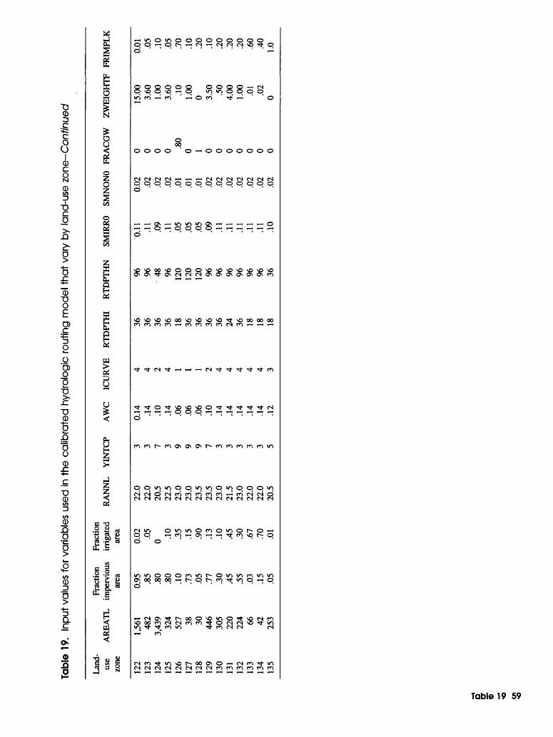
Tabl

e 19

. In

put v

alue

s fo

r va

riabl

es u

sed

in t

he c

alib

rate

d hy

drol

ogic

rou

ting

mod

el t

hat v

ary

by la

nd-u

se z

one-

Con

f/nue

d

Land

- us

e zo

ne

122

123

124

125

126

127

128

129

130

131

132

133

134

135

AR

EATL

1,56

148

23,

439

324

527 38 30 446

305

220

224 66 42 253

Frac

tion

impe

rvio

us

area

0.95 .8

5.8

0.8

0.1

0.7

3.0

5.7

7.3

0.4

5.5

5.0

3.1

5.0

5

Frac

tion

irrig

ated

ar

ea

0.02 .0

50 .1

0.3

5.1

5.9

0.1

3.1

0.4

5.3

0.6

7.7

0.0

1

RA

NN

L Y

INTC

P

22.0

22.0

20.5

22.5

23.0

23.0

23.5

23.5

23.0

21.5

23.0

22.0

22.0

20.5

3 3 7 3 9 9 9 7 3 3 3 3 3 5

AW

C

ICU

RV

E R

TDPT

HI

0.14 .1

4.1

0.1

4.0

6.0

6.0

6.1

0.1

4.1

4.1

4.1

4.1

4.1

2

4 4 2 4 1 1 1 2 4 4 4 4 4 3

36 36 36 36 18 36 36 36 36 24 36 18 18 18

RTD

PTH

N

96 96 48 96 120

120

120 96 96 96 96 96 96 36

SMIR

RO

0.11 .1

1.0

9.1

1.0

5.0

5.0

5.0

9.1

1.1

1.1

1.1

1.1

1.1

0

SMN

ON

O

0.02 .0

2.0

2.0

2.0

1.0

1.0

1.0

2.0

2.0

2.0

2.0

2.0

2.0

2

FRA

CG

W

0 0 0 0 .80

0 1 0 0 0 0 0 0 0

ZWEI

GH

TF

15.0

03.

601.

003.

60 .10

1.00

0 3.50 .5

04.

001.

00 .01

.02

0

FRIM

PLK

0.01 .0

5.1

0.0

5.7

0.1

0.2

0.1

0.2

0.2

0.2

0.6

0.4

01.

0

a

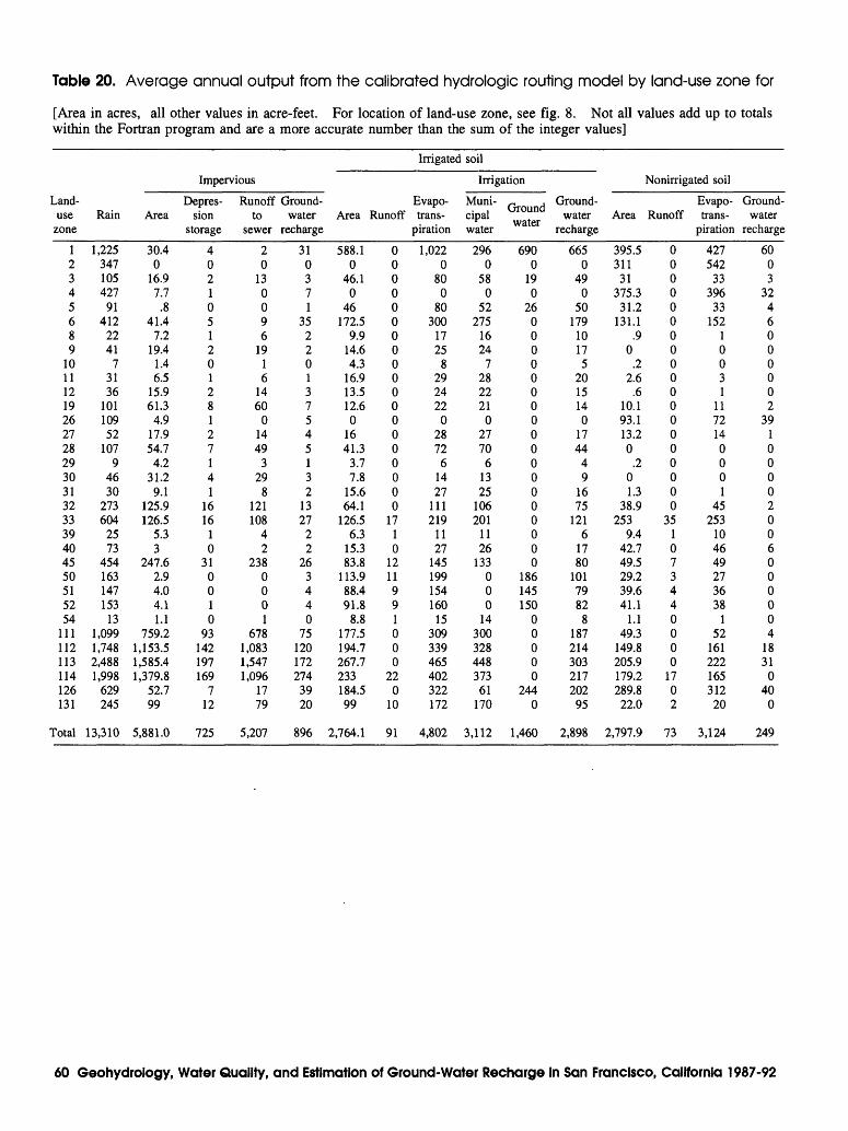
Table 20. Average annual output from the calibrated hydrologic routing model by land-use zone for

[Area in acres, all other values in acre-feet. For location of land-use zone, see fig. 8. Not all values add up to totals within the Fortran program and are a more accurate number than the sum of the integer values]

Irrigated soil

Impervious

Land- use

zone

12345689

10111219262728293031323339404550515254

111112113114126131

Total

Rain

1,225347105427

91412

2241

73136

10110952

1079

4630

273604

2573

454163147153

131,0991,7482,4881,998

629245

13,310

Area

30.40

16.97.7

.841.4

7.219.4

1.46.5

15.961.3

4.917.954.7

4.231.2

9.1125.9126.5

5.33

247.62.94.04.11.1

759.21,153.51,585.41,379.8

52.799

5,881.0

Depres­ sion

storage

402105120128127141

1616

10

310010

93142197169

712

725

Runoff to

sewer

20

130096

1916

1460

01449

329

8121108

42

2380001

6781,0831,5471,096

1779

5,207

Irrigation

Ground- water Area Runoff

recharge

310371

35220137545132

1327

22

263440

75120172274

3920

896

588.10

46.10

46172.5

9.914.64.3

16.913.512.60

1641.3

3.77.8

15.664.1

126.56.3

15.383.8

113.988.491.8

8.8177.5194.7267.7233184.599

2,764.1

0000000000000000000

1710

1211991000

220

10

91

Evapo- trans-

piration

1,0220

800

80300

1725

8292422

02872

61427

111219

1127

145199154160

15309339465402322172

4,802

Muni­ cipal water

2960

580

52275

1624

7282221

02770

61325

106201

1126

133000

14300328448373

61170

3,112

Ground water

6900

190

26000000000000000000

186145150

00000

2440

1,460

Nonirrigated soil

Ground- water Area Runoff

recharge

6650

490

50179

10175

2015140

1744

49

1675

1216

1780

1017982

8187214303217202

95

2,898

395.5311

31375.331.2

131.1.9

0.2

2.6.6

10.193.113.20

.201.3

38.9253

9.442.749.529.239.641.1

1.149.3

149.8205.9179.2289.822.0

2,797.9

0000000000000000000

351073440000

1702

73

Evapo- trans-

piration

427542

33396

33152

10031

1172140001

45253

104649273638

152

16122216531220

3,124

Ground- water

recharge

6003

3246000002

39100002006000004

1831

040

0

249

60 Geohydrology, Water Quality, and Estimation of Ground-Water Recharge In San Francisco, California 1987-92

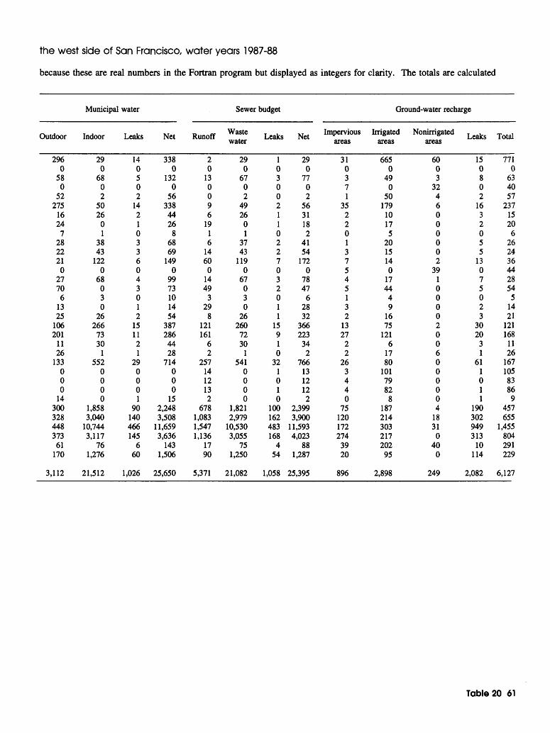
the west side of San Francisco, water years 1987-88

because these are real numbers in the Fortran program but displayed as integers for clarity. The totals are calculated

Municipal water

Outdoor

2960

580

52275

1624

72822210

27706

1325

106201

1126

133000

14300328448373

61170

3,112

Indoor

290

6802

5026

01

3843

1220

68030

26266

7330

1552

0000

1,8583,040

10,7443,117

761,276

21,512

Leaks

140502

14210336043012

151121

290001

90140466145

660

1,026

Net

3380

1320

563384426

86869

1490

9973101454

3872864428

714000

152,2483,508

11,6593,636

1431,506

25,650

Runoff

20

130096

1916

14600

1449

329

8121161

62

2571412132

6781,0831,5471,136

1790

5,371

Sewer budget

Waste water

290

6702

492601

3743

1190

67030

262607230

1541

0000

1,8212,979

10,5303,055

751,250

21,082

Leaks

103002110227032011

15910

321010

100162483168

454

1,058

Net

290

7702

5631182

4154

1720

7847

62832

36622334

2766

1312122

2,3993,900

11,5934,023

881,287

25,395

Impervious areas

310371

35220137545132

1327

22

263440

75120172274

3920

896

Ground-water recharge

Irrigated areas

6650

490

50179

10175

2015140

1744

49

1675

1216

1780

1017982

8187214303217202

95

2,898

Nonirrigated areas

6003

3246000002

39100002006000004

18310

400

249

Leaks

150802

1632055

13075023

3020

31

611011

190302949313

10114

2,082

Total

7710

634057

2371520

6262436442854

51421

121168

1126

16710583869

457655

1,455804291229

6,127

Table 20 61

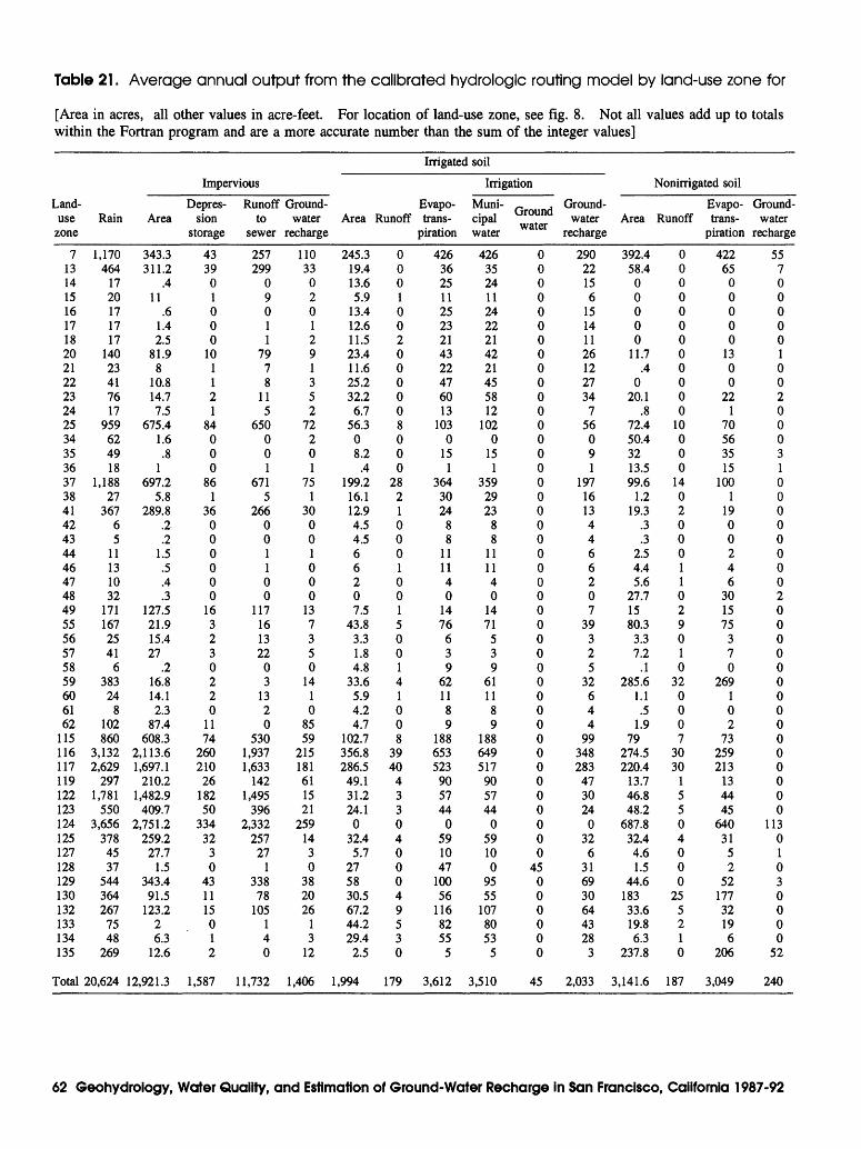
Table 21. Average annual output from the calibrated hydrologic routing model by land-use zone for

[Area in acres, all other values in acre-feet. For location of land-use zone, see fig. 8. Not all values add up to totals within the Fortran program and are a more accurate number than the sum of the integer values]

Irrigated soil

ImperviousLand- use

zone

7131415161718202122232425343536373841424344464748495556575859606162

115116117119122123124125127128129130132133134135

Total

Rain

1,170464

1720171717

14023417617

959624918

1,18827

36765

11131032

1711672541

638324

8102860

3,1322,629

2971,781

5503,656

3784537

544364267

7548

269

20,624

Area

343.3311.2

.411

.61.42.5

81.98

10.814.77.5

675.41.6.8

1697.2

5.8289.8

.2

.21.5.5.4.3

127.521.915.427

.216.814.12.3

87.4608.3

2,113.61,697.1

210.21,482.9

409.72,751.2

259.227.7

1.5343.491.5

123.226.3

12.6

12,921.3

Depres­ sion

storage

433901000

101121

84000

861

36000000

163230220

1174

26021026

18250

33432

30

431115012

1,587

Runoff to

sewer

257299

09011

7978

115

650001

6715

266001100

117161322

03

1320

5301,9371,633

1421,495

3962,332

25727

1338

78105

140

11,732

Ground- water

recharge

110330201291352

72201

751

30001000

137350

1410

8559

215181611521

2591430

382026

13

12

1,406

Irrigation

Area

245.319.413.65.9

13.412.611.523.411.625.232.2

6.756.3

08.2

.4199.2

16.112.94.54.566207.5

43.83.31.84.8

33.65.94.24.7

102.7356.8286.549.131.224.10

32.45.7

275830.567.244.229.4

2.5

1,994

Runoff

0001002000008000

28210001001500141008

3940

4330400049530

179

Evapo- trans-

piration

4263625112523214322476013

1030

151

3643024

88

111140

1476

639

6211

89

188653523905744

0591047

10056

1168255

5

3,612

Muni­ cipal water

4263524112422214221455812

1020

151

3592923

88

111140

1471

539

6111

89

188649517905744

059100

9555

1078053

5

3,510

Ground water

0000000000000000000000000000000000000000000

45000000

45

Nonirrigated soil

Ground- water

recharge

29022156

15141126122734

756091

19716134466207

39325

32644

99348283473024

032

6316930644328

3

2,033

Area

392.458.4

00000

11.7.4

020.1

.872.450.43213.599.6

1.219.3

.3

.32.54.45.6

27.71580.3

3.37.2

.1285.6

1.1.5

1.979

274.5220.4

13.746.848.2

687.832.4

4.61.5

44.618333.619.86.3

237.8

3,141.6

Runoff

000000000000

10000

140200011029010

320007

3030

15504000

255210

187

Evapo- trans-

piration

42265

00000

1300

221

70563515

1001

1900246

301575

370

269102

73259213

134445

64031

52

5211132196

206

3,049

Ground- water

recharge

55700000100200031000000002000000000000000

11301030000

52

240

62 Geohydrology, Water Quality, and Estimation of Ground-Water Recharge In San Francisco, California 1987-92

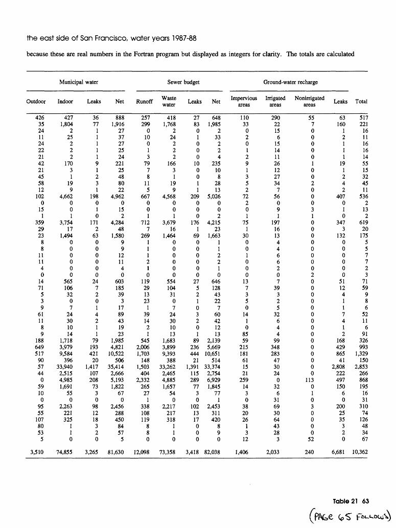
the east side of San Francisco, water years 1987-88

because these are real numbers in the Fortran program but displayed as integers for clarity. The totals are calculated

Municipal water

Outdoor

4263524112422214221455812

1020

151

3592923

88

111140

1471

539

611189

1886495179057440

59100

9555

1078053

5

3,510

Indoor

4271,804

225

222

17031

199

4,662001

3,75417

1,494000000

5651063207

24301014

1,7183,9799,584

39633,940

2,5154,9851,691

550

2,263221325

110

74,855

Leaks

3677

1111191231

198010

1712

63000000

2472014211

7919342120

1,417107208

7330

981218320

3,265

Net

8881,916

2737272524

22125488022

4,9620

152

4,28448

1,58099

121140

60318539

31789431923

1,9854,821

10,522506

35,4142,6665,1931,822

670

2,456288450

8457

5

81,630

Runoff

257299

010013

7978

115

667001

7127

269111210

119291323

1391421

5452,0061,703

1481,503

4042,332

26527

1338108119

880

12,098

Sewer budget

Waste water

4181,768

224

222

16631

199

4,568001

3,67916

1,464000000

554104

3107

24301013

1,6833,8999,393

38833,262

2,4654,8851,657

540

2,217217318

110

73,358

Leaks

278301000

100011

209000

1761

69000000

2752103201

89236444

211,391

11528977

30

1021317000

3,418

Net

6481,985

233

224

235108

2813

5,026002

4,21523

1,663112210

64612843227

60421213

2,1395,669

10,651514

33,3742,7546,9291,845

771

2,453311420

890

82,038

Impervious areas

110330201291352

72201

751

30001000

137350

1410

8559

215181611521

25914

30

382026

13

12

1,406

Ground-water recharge

Irrigated areas

29022156

15141126122734

756

091

19716134466207

39325

32644

993482834730240

326

316930644328

3

2,033

Nonirrigated areas

55700000100200031000000002000000000000000

11301030000

52

240

Leaks

63160

12111

191242

407010

3473

132000000

51124117412

168429865

412,808

222497150

60

2002535

320

6,681

Total

517221

16111616145515324511

5362

132

61920

175557723

7159

986

52116

91326993

1,329150

2,853266868195

1631

31074

126483467

10,362

Table 21 63

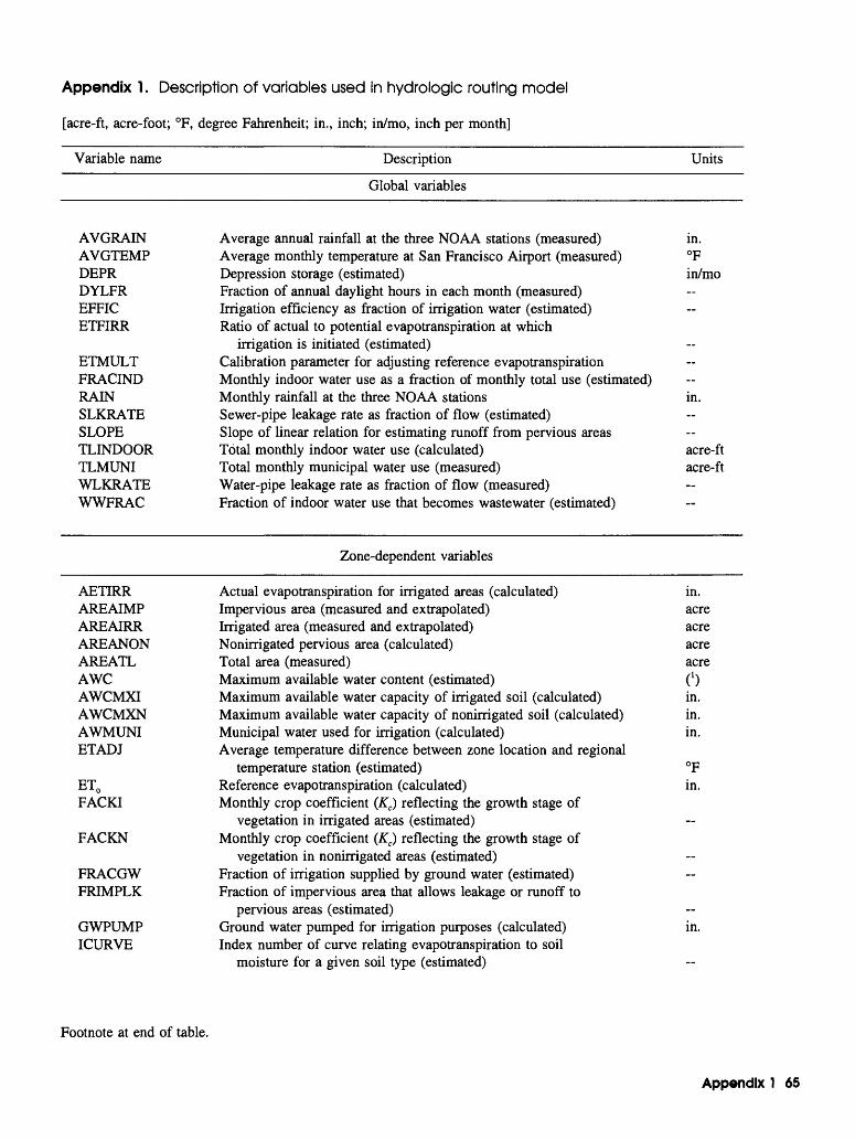
Appendix 1 . Description of variables used in hydrologic routing model

[acre-ft, acre-foot; °F, degree Fahrenheit; in., inch; in/mo, inch per month]

Variable name Description Units

Global variables

AVGRAINAVGTEMPDEPRDYLFREFFICETFIRR

ETMULTFRACINDRAINSLKRATESLOPETLINDOORTLMUNIWLKRATEWWFRAC

Average annual rainfall at the three NOAA stations (measured) in. Average monthly temperature at San Francisco Airport (measured) °F Depression storage (estimated) in/mo Fraction of annual daylight hours in each month (measured) Irrigation efficiency as fraction of irrigation water (estimated) Ratio of actual to potential evapotranspiration at which

irrigation is initiated (estimated)Calibration parameter for adjusting reference evapotranspiration Monthly indoor water use as a fraction of monthly total use (estimated) Monthly rainfall at the three NOAA stations in. Sewer-pipe leakage rate as fraction of flow (estimated) Slope of linear relation for estimating runoff from pervious areas Total monthly indoor water use (calculated) acre-ft Total monthly municipal water use (measured) acre-ft Water-pipe leakage rate as fraction of flow (measured) Fraction of indoor water use that becomes wastewater (estimated)

Zone-dependent variables

AETIRRAREAIMPAREAIRRAREANONAREATLAWCAWCMXIAWCMXNAWMUNIETADJ

ET0 FACKI

FACKN

FRACGW FRIMPLK

GWPUMP ICURVE

Actual evapotranspiration for irrigated areas (calculated) in. Impervious area (measured and extrapolated) acre Irrigated area (measured and extrapolated) acre Nonirrigated pervious area (calculated) acre Total area (measured) acre Maximum available water content (estimated) (') Maximum available water capacity of irrigated soil (calculated) in. Maximum available water capacity of nonirrigated soil (calculated) in. Municipal water used for irrigation (calculated) in. Average temperature difference between zone location and regional

temperature station (estimated) °F Reference evapotranspiration (calculated) in. Monthly crop coefficient (Kc) reflecting the growth stage of

vegetation in irrigated areas (estimated) Monthly crop coefficient (Kc) reflecting the growth stage of

vegetation in nonirrigated areas (estimated) Fraction of irrigation supplied by ground water (estimated) Fraction of impervious area that allows leakage or runoff to

pervious areas (estimated)Ground water pumped for irrigation purposes (calculated) in. Index number of curve relating evapotranspiration to soil

moisture for a given soil type (estimated)

Footnote at end of table.

Appendix 1 65

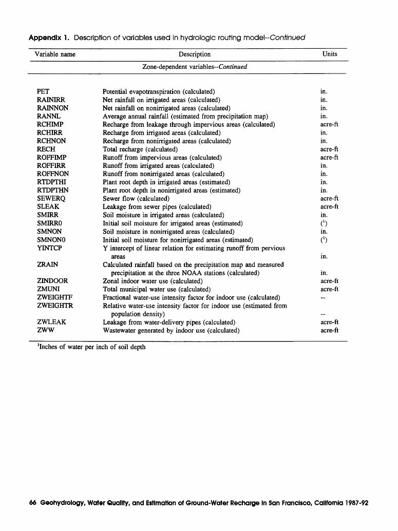
Appendix 1 . Description of variables used in hydrologic routing model-Conf/nued

Variable name Description Units

Zone-dependent variables- Continued

PETRAINIRRRAINNONRANNLRCHIMPRCHIRRRCHNONRECHROFFIMPROFFIRRROFFNONRTDPTHIRTDPTHNSEWERQSLEAKSMIRRSMIRROSMNONSMNONOYINTCP

ZRAIN

ZINDOORZMUNIZWEIGHTFZWEIGHTR

ZWLEAKZWW

Potential evapotranspiration (calculated)Net rainfall on irrigated areas (calculated)Net rainfall on nonirrigated areas (calculated)Average annual rainfall (estimated from precipitation map)Recharge from leakage through impervious areas (calculated)Recharge from irrigated areas (calculated)Recharge from nonirrigated areas (calculated)Total recharge (calculated)Runoff from impervious areas (calculated)Runoff from irrigated areas (calculated)Runoff from nonirrigated areas (calculated)Plant root depth in irrigated areas (estimated)Plant root depth in nonirrigated areas (estimated)Sewer flow (calculated)Leakage from sewer pipes (calculated)Soil moisture in irrigated areas (calculated)Initial soil moisture for irrigated areas (estimated)Soil moisture in nonirrigated areas (calculated)Initial soil moisture for nonirrigated areas (estimated)Y intercept of linear relation for estimating runoff from pervious

areasCalculated rainfall based on the precipitation map and measured

precipitation at the three NOAA stations (calculated)Zonal indoor water use (calculated)Total municipal water use (calculated)Fractional water-use intensity factor for indoor use (calculated)Relative water-use intensity factor for indoor use (estimated from

population density)Leakage from water-delivery pipes (calculated)Wastewater generated by indoor use (calculated)

in.in.in.in.acre-ftin.in.acre-ftacre-ftin.in.in.in.acre-ftacre-ftin.(')

in.(')

in.

in.acre-ftacre-ft~

~acre-ftacre-ft

Inches of water per inch of soil depth

66 Geohydrology, Water Quality, and Estimation of Ground-Water Recharge In San Francisco, California 1987-92

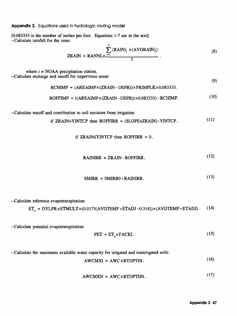
Appendix 2. Equations used in hydrologic routing model

[0.083333 is the number of inches per foot. Equations 1-7 are in the text] Calculate rainfall for the zone:

£(RAIN), x(AVGRAIN).) (8) ZRAIN = RANNLx±l______________ .

where i = NOAA precipitation station.-Calculate recharge and runoff for impervious areas:

(9)RCHIMP = (AREAIMPx(ZRAIN-DEPR))xFRIMPLKx0.083333.

ROFFIMP = ((AREAIMPx(ZRAIN-DEPR))x0.083333)-RCHIMP. ( 10)

-Calculate runoff and contribution to soil moisture from irrigation:

if ZRAIN>YINTCP then ROFFIRR = (SLOPExZRAIN)-YINTCP. (n>

if ZRAIN<YINTCP then ROFFIRR = 0.

RAINIRR = ZRAIN-ROFFIRR.

SMIRR = SMIRRO+RAINIRR.

-Calculate reference evapotranspiration:

ETo = DYLFRxETMULTx(0.0173(AVGTEMP+ETADJ-0.314))x(AVGTEMP+ETADJ). (14)

-Calculate potential evapotranspiration:

PET = ET xFACKI. (15)

-Calculate the maximum available water capacity for irrigated and nonirrigated soils:

AWCMXI = AWCxRTDPTHI.

AWCMXN = AWCxRTDPTHN.

Appendix 2 67

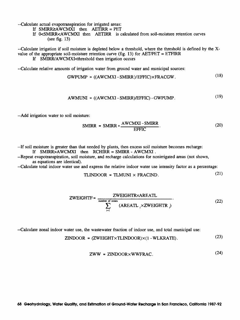
Calculate actual evapotranspiration for irrigated areas: If SMIRR>AWCMXI then AETIRR = PETIf 0<SMIRR<AWCMXI then AETIRR is calculated from soil-moisture retention curves

(see fig. 13)

Calculate irrigation if soil moisture is depleted below a threshold, where the threshold is defined by the X- value of the appropriate soil-moisture retention curve (fig. 13) for AET/PET = ETFIRR

If SMIRR/AWCMXI<threshold then irrigation occurs

Calculate relative amounts of irrigation water from ground water and municipal sources:

GWPUMP = ((AWCMXI-SMIRR)/EFFIC)xFRACGW.

AWMUNI = ((AWCMXI-SMIRR)/EFFIC)- GWPUMP. ( 19)

Add irrigation water to soil moisture:

SMIRR = ^^- (20)EFFIC

-If soil moisture is greater than that needed by plants, then excess soil moisture becomes recharge: If SMIRR>AWCMXI then RCHIRR = SMIRR - AWCMXI.

-Repeat evapotranspiration, soil moisture, and recharge calculations for nonirrigated areas (not shown, as equations are identical).

-Calculate total indoor water use and express the relative indoor water use intensity factor as a percentage:

TLINDOOR = TLMUNI x FRACESfD. (21 )

ZWEIGHTF = ZWEIGHTRxARE ATLnumber of zones (22)

£ (AREATL ^xZWEIGHTR,.)1=1

-Calculate zonal indoor water use, the waste water fraction of indoor use, and total municipal use:

ZINDOOR = (ZWEIGHTxTLINDOOR)x(l-WLKRATE). (23)

ZWW = ZINDOORxWWFRAC. (24)

68 Geohydrology, Water Quality, and Estimation of Ground-Water Recharge in San Francisco, California 1987-92

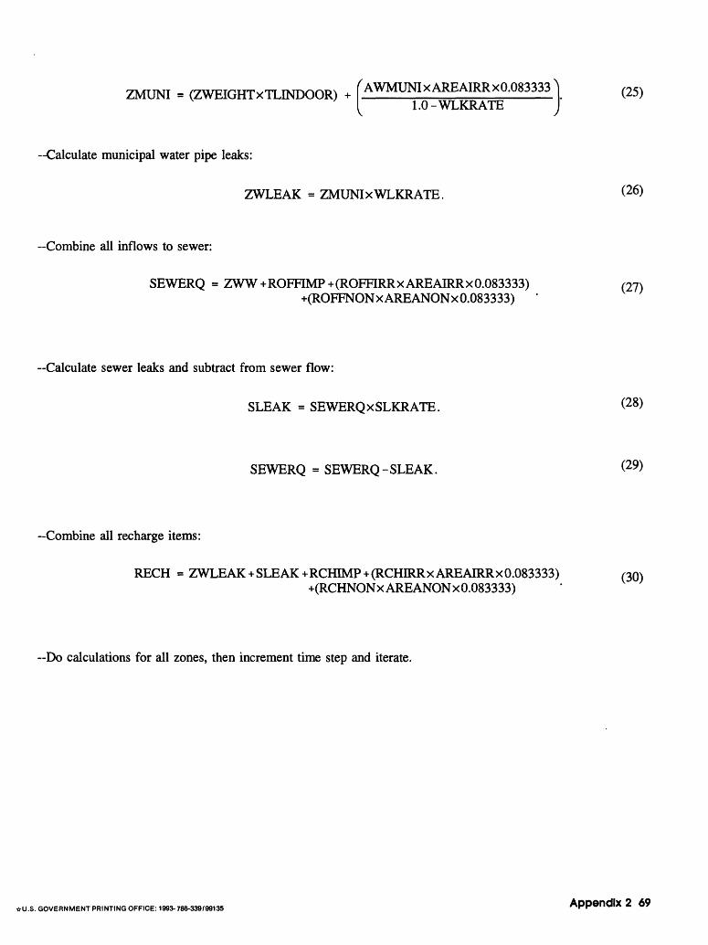
ZMUNI = (ZWEIGHTXTLINDOOR) + fAWMUNIxAREAIRRxO.083333^ (25)[ 1.0-WLKRATE J

Calculate municipal water pipe leaks:

ZWLEAK = ZMUNIxWLKRATE.

Combine all inflows to sewer:

SEWERQ = ZWW+ROFFIMP+(ROFFIRRxAREAIRRx0.083333)+(ROFFNONxAREANONx0.083333) '

Calculate sewer leaks and subtract from sewer flow:

SLEAK = SEWERQxSLKRATE.

SEWERQ = SEWERQ-SLEAK.

Combine all recharge items:

RECH = ZWLEAK+SLEAK+RCHIMP+(RCHIRRxAREAIRRx 0.083333) (30)+(RCHNONxAREANONx0.083333)

Do calculations for all zones, then increment time step and iterate.

*U.S. GOVERNMENT PRINTING OFFICE: 1993-786-339/99135 Appendix 2 69