Geohydraulic and vulnerability assessment oftropically weathered and fractured gneissic aquifersusing combined electrical resistivity andgeostatistical methodsAdedibu Sunny AKINGBOYE ( adedibu.akingboye@aaua.edu.ng )

https://orcid.org/0000-0003-2195-6098

Research Article

Keywords: ERT, Schlumberger VES, geoelectrohydraulic method, regression analysis, groundwatervulnerability, gneissic aquifer

Posted Date: December 1st, 2021

DOI: https://doi.org/10.21203/rs.3.rs-1103032/v2

License: This work is licensed under a Creative Commons Attribution 4.0 International License. Read Full License

1

Geohydraulic and vulnerability assessment of tropically weathered and fractured gneissic aquifers using

combined electrical resistivity and geostatistical methods

Adedibu Sunny Akingboye

Department of Earth Sciences, Adekunle Ajasin University, 001 Akungba-Akoko, Ondo State, Nigeria

Present Address: Geophysics Unit, School of Physics, Universiti Sains Malaysia, 11800 Pulau Pinang, Malaysia

Corresponding author: adedibu.akingboye@aaua.edu.ng // https://orcid.org/0000-0003-2195-6098

Abstract

Sustainable potable groundwater supplied by aquifers depends on the protective capacity of

the strata overlying the aquifer zones and their thicknesses, as well as the nature of the

aquifers and the conduit systems. The poor overburden development of the Araromi area of

Akungba-Akoko, in the crystalline basement of southwestern Nigeria, restricts most aquifers

to shallow depths. Hence, there is a need to investigate the groundwater quality of the

tropically weathered and fractured gneissic aquifers in the area. A combined electrical

resistivity tomography (ERT) and Schlumberger vertical electrical sounding (VES) technique

were employed to assess the groundwater-yielding potential and vulnerability of the aquifer

units. The measured geoelectric parameters (i.e., resistivity and thickness values) at the

respective VES surveyed stations were used to compute the geohydraulic parameters, such as

aquifer resistivity (𝜌𝜌𝑜𝑜), hydraulic conductivity (K), transmissivity (T), porosity (𝜑𝜑),

permeability (Ψ), hydraulic resistance (K𝑅𝑅), and longitudinal conductance (S). In addition,

regression analysis was employed to establish the correlations between the K and other

geohydraulic parameters to achieve the objectives of this study. The subsurface

lithostratigraphic units of the studied site were delineated as the motley topsoil, weathered

layers, partially weathered/fractured bedrock units, and the fresh bedrock, based on the ERT

and the A, H, AK, HA, and KQ curve models. The K model regression-assisted analysis

showed that the 𝜌𝜌𝑜𝑜, T, 𝜑𝜑, Ψ, and S contributed about 81.7%, 3.31%. 96.6%, 100%, and

11.63%, respectively, of the determined K values for the study area. The results, except T and

S, have strong high positive correlations with the K of the aquifer units; hence, accounted for

the recorded high percentages. The aquifer units in the area were classified as low to

moderate groundwater-yielding potential due to the thin overburden, with an average depth of

<4 m. However, the deep-weathered and fractured aquifer zones with depths ranging from

about 39–55 m could supply high groundwater yield for sustainable exploitation. The

estimated S values, i.e., 0.0226–0.1926 mho, for aquifer protective capacity ratings rated the

aquifer units in the area as poor/weak to moderately high with extremely high to high aquifer

vulnerability index, based on the estimated low Log K𝑅𝑅 of about 0.01–1.77 years. Hence,

intended wells/boreholes in the study area and its environs, as well as any environments with

similar geohydraulic and vulnerability characteristics, should be properly constructed to

adequately prevent surface and subsurface infiltrating contaminants.

Keywords: ERT; Schlumberger VES; geoelectrohydraulic method; regression analysis; groundwater

vulnerability; gneissic aquifer

2

1. Introduction

Globally, the percentage of people who use potable water has increased twice as fast as the

global population [1, 2, 3]. Sustainable groundwater yield in aquifer zones depends on the

detailed characterization of subsurface strata, the water-retaining capacity of the strata due to

porosity and permeability, water-rock interactions, subsurface conduits, and storage zones, as

well as the hydrodynamics of the aquifer units [3, 4–8]. The sustainability of groundwater

supplies also depends on the quality of the aquifers’ yield, which is a function of the

protective capacity of the strata overlying the aquifer zones and the depths of the aquifer

zones. The occurrences of aquifer zones at shallow depths, especially within the crystalline

basement terrain, give easy access for the percolation of surface runoffs and pollutants from

dumpsites' leachate flows, surface and buried oil tank spillages, dissolved chemicals from

mining activities, sewage from sanitation systems, etc., to degrade the stored groundwater [5,

9–12]. In addition, over-stretching of aquifers caused by over-abstraction of groundwater and

silt/clay intrusion from improperly cased boreholes degrades the quality of groundwater [3,

13–15].

Geoelectrical resistivity methods, i.e., resistivity profiling and vertical electrical sounding

(VES), and the estimation of geohydraulic parameters (e.g., hydraulic conductivity,

transmissivity, porosity, permeability, transverse resistivity, longitudinal conductance,

hydraulic conductance, etc.) from georesistivity datasets and/or pumping tests have been

employed in the determination of groundwater-yielding potential and vulnerability of aquifer

units in several geological terrains [3, 5, 13, 16, 17]. However, the pumping test method is

time-consuming and expensive; hence, it has not often been utilized recently in geohydraulic

evaluation since georesistivity methods are cost-efficient, rapid, and produce quality results

with a higher success rate, e.g., [3, 10, 11]. The advantage of the georesistivity methods is

that the measured resistivity values have strong correlations with groundwater hydraulic

characteristics; hence, the data offer the determination of geohydrodynamics of aquifer units,

protective capacity of the near-surface strata, and selection of suitable points for sustainable

potable groundwater development [5, 10, 11, 18].

The study area covered a part of the Araromi area of Akungba-Akoko, southwestern Nigeria,

which is situated between the main Akungba-Akoko town and Etioro-Akoko and is

characterized by complex subsurface geology, e.g., [3, 8, 19–21]. The study area has become

the choice location for many local settlers, staff, and students of Adekunle Ajasin University,

3

Akungba-Akoko (AAUA) due to its serenity and prospect for rapid urbanization. According

to previous workers in the study area and the surrounding towns, e.g., [3, 8, 19–21], the

overburden in the areas is poorly developed and hence causes incessant water shortages to

meet the growing population due to perennial failures of hand-dug wells and boreholes. In the

report of Mohammed et al. [19], the groundwater potential of the northern section of the

present study area was evaluated using the vertical electrical sounding (VES) technique.

Akingboye et al. [8] investigated the near-surface crustal architecture and geohydrodynamics

of the Araromi area, Akungba-Akoko (i.e., the study area) using the integrated coplanar loop

electromagnetic conductivity method, electrical resistivity tomography (ERT), and

Schlumberger VES technique, to ameliorate the difficulties of sufficient groundwater

availability and the failure of engineering structural foundations in this area. Furthermore, the

subsurface geological, hydrogeophysical, and engineering characterization, as well as the

vulnerability of the southern part, (i.e., Etioro-Akoko), some few meters away, has been

carried out and reported, e.g., [3, 8, 21]. From these studies, it was reported that most of the

aquifer zones occurred at shallow depths, except for the localized ones that are characterized

by deep-weathered troughs and fractures.

Despite the several detailed studies mentioned above, the vulnerability of the tropically

weathered and fractured aquifer zones in the Araromi area of Akungba-Akoko has not been

evaluated. Hence, it becomes necessary to determine the vulnerability of the aquifer zones to

contamination due to the occurrence of most of the aquifers in the study area at shallow

depths. The fracture densities and groundwater-yielding potential of some identified aquifers

can also offer clues on the migration rate of possible contaminants in the area. Given the

above, geoelectrohydraulic method, involving combined ERT and Schlumberger VES from

which geohydraulic characteristics were determined through various equations and

regression-assisted analysis to evaluate the vulnerability of the aquifer units in the study

area.

2. Geological setting of the study area

Araromi area of Akungba-Akoko, which is the study site, falls between latitudes 07o27’ N

and 07o27’9’’ N, and longitudes 005o43’53’’ E and 005o44’ E in the northern part of Ondo

State, southwestern Nigeria, as shown in Figs. 1 and 2. The study area is characterized by the

Nigerian rainforest belt climate, with average yearly rainfall between 1000 mm and 1500

mm, and temperature is around 33 oC. The area has a topographic relief consisting of hills,

4

low-lying outcrops, plains, and valleys, between 280 m and 400 m above the mean sea level.

The dendritic drainage system follows these topographic features, with trellis drainage

patterns in a few places, e.g., [3, 8, 21].

Geologically, the Araromi area of Akungba-Akoko is characterized by the Nigerian

Southwestern Precambrian Basement Complex, which is part of the reactivated Pan-African

mobile belt, occupying the east of the West African Craton and northwest of the Congo-

Gabon Craton [22–25], as shown in Fig. 1a. The Southwestern Basement Complex of Nigeria

is made up of three major rock suites, namely the Migmatite-Gneiss Complex, ranging in age

from Neoproterozoic to Paleoproterozoic and Archean, e.g., [22–24]; the Neoproterozoic

Schist Belts, consisting of low-grade, younger metasedimentary, and metavolcanic rocks with

ages ranging between 690 and 489 Ma, e.g., [23, 24], and the Pan-African Older Granites,

which intruded the two earlier lithologies, have ages ranging between 650 and 580 Ma, e.g.,

[26, 27]. Early magmatic phases dating from 790 to 709 Ma have also been reported in some

of the Older Granites rocks. The Younger Granites, i.e., the Mesozoic anorogenic calc-

alkaline ring complexes, as shown in Fig. 1b, intruded the Nigerian Eastern Basement

Complex terrain before the formation of any of the sedimentary basins in the eastern and

western terranes of Nigeria [26–28].

The entire Akungba-Akoko is underlain by the Migmatite-Gneiss Complex rocks of

southwestern Nigeria, which were intruded by the Pan-African Granitoids as shown in Fig.

1c. The Migmatite-Gneiss Complex rocks in the area are typically migmatite, granite gneiss,

and biotite gneiss, as well as granitoids consisting of charnockites and granites. Granite

gneisses are the most abundant rock type in the area, and this particular rock underlies the

Araromi part of the area. This particular rock type has a blastoporphyritic to porphyroblastic

fabric and is light grey, medium to coarse-grained, and moderately foliated, for example

(light and dark-colored bands). Far to the west, the rock is extensively deformed and

migmatized, forming migmatite with an ENE-WSW trend. In addition, important intrusives

in the granite gneisses in the area include quartz veins, pegmatite, aplite, basic dykes, and

sills [3, 8, 23, 29]. The tropical climatic conditions combined with the metamorphic activities

in the Akungba-Akoko Basement Complex terrain have assisted in the weathering and

fracturing of the subsurface strata.

The subsurface hydrogeological features of the Araromi area of Akungba-Akoko are similar

to those of the surrounding towns, e.g., the main Akungba-Akoko town and Etioro-Akoko

5

community, e.g., [3, 19–21], as well as some places in the crystalline basement of

southwestern Nigeria, e.g., [11, 12, 30]. The groundwater in the study area occurs in

weathered and/or fractured aquifer zones. Groundwater occurrence in these hydrogeologic

units is unevenly distributed, just like other parts of the Precambrian basement terrain.

Generally, the aquifers in the area are characterized by shallow depths with low porosity and

permeability, and hence depend on the secondary porosity resulting from deep weathering

and fracturing of the rock units to conduit and store fluids in the subsurface strata sufficiently.

It has been reported that the aquifer zones in the study area and surrounding communities

have an average depth of about 12 m, with depths exceeding 25 m for deeply weathered and

fractured aquifers, e.g., [3, 8, 21]. Some of the hand-dug wells and boreholes sited in the

study area take advantage of the former and latter aquifer depths, respectively, for the

required groundwater supplies.

3. Methods of Study

Due to the urgent need of the inhabitants of the Araromi area for steady and sufficient

drinkable groundwater supplies to suit their everyday activities, a detailed subsurface

geologic condition is highly necessary. The field data collection began with the identification

of prominent areas with records of failed hand-dug wells and low yield boreholes in the study

area. Predictions from earlier studies in the northern and southern areas of the study region,

such as [3, 8, 19, 21], enabled the selection of locations for establishing the geophysical

traverses for data collection quicker and simpler. Six traverses (TRs) were occupied in the

study area as shown in Figs. 2a and b, to investigate and characterize the subsurface

stratigraphic units, hydrodynamics, degree of weathering, and fracture densities. The

implications of these characteristic features on the groundwater potentials and vulnerability

of aquifers to contamination were also evaluated from geoelectrohydraulic and statistical

methods. TRs 1–3 and TRs 4–6 were established in the NNE-SSW and NW-SE directions,

respectively. TRs 1, 2, and 6 each have a survey profile length of 160 m, but TR3 has a

survey profile length of just 100 m due to survey spread constraints. The survey spread length

for TR4 is 150 m, although the ERT profile was terminated at a distance of 145 m from the

starting electrode. As shown in Figs. 2a and b, the TR5 survey spread length was 110 m.

Because of the population increase, structural building blockage caused a reduction in

geophysical survey spread lengths on some traverses.

6

The ABEM Resistivity Imaging System was used for the ERT field data acquisition, utilizing

the dipole-dipole electrode configuration protocol array because of its high sensitivity to

vertical and lateral subsurface structural variations and low electromagnetic coupling effects,

e.g., [8, 31, 32]. A station interval of 5 m was used for the detailed subsurface imaging of the

anomalous features of interest for this study. Although the adopted n-level of 5, i.e., (n = 5),

for dipole-dipole resistivity surveys could limit the depths of probing. However, the station

interval is considered suitable to derive more cluster near-surface information and to avoid

nuisance surface artifacts arising from the complex geological condition of the study area

terrain. The Schlumberger electrode configuration for the VES technique, on the other hand,

was carried out at the selected conductive or relatively conductive survey station points to

address depth limitations. The approach was aimed at constraining the modeled ERT results,

and to image deep-weathered bodies and the penetrative fractures. Figure 2b depicts the

spatial distribution of the investigated VES station sites, whereas Figs. 2b and 2c depict the

elevation of the surface topography. The current electrodes AB/2 varied from 60 to 160 m,

whereas the potential electrodes spread MN were varied from 0.5 to 15 m. The depth of

penetration in a homogenous subsurface geologic structure is proportional to the distance

between the current electrodes, whereas, varying the electrodes distance offers information

regarding the subsurface lithostratigraphic units, e.g., [3, 8, 12]. When a remarkable

resistivity of fresh bedrock, typically with values >1200 Ωm, was attained more than twice at

each VES station, the survey was stopped, indicating that there was no possibility of

obtaining a fracture at deeper depths even for further probing. However, because of the

barriers encountered due to primarily buildings, the surveys were sometimes halted before

reaching depth to the fresh basement.

The results from the ERT surveys were processed and inverted using RES2DINV software.

Forward modeling and data inversion, utilizing the least-squares inversion approach, which

depends on a mathematical inverse problem to derive the subsurface resistivity distribution

from apparent resistivity data sets, were used in the inversion process. Many works have

reported on the adopted inversion processes used in the RES2D data inversion, including

Akingboye et al. [8], Loke [31], DeGroot-Hedlin & Constable [33], Dahlin & Loke [34],

Akingboye & Bery [14, 35], and other. The ERT field data sets with topography were

inverted using the finite-element method of 4 nodes with L2-norm as the least-squares

constraint parameter to minimize the difference between the measured and calculated

apparent resistivities. A damping factor of 0.05 with a minimum value of 0.01 was employed

7

to increase the accuracy of the calculated apparent resistivities and the resolution of the

generated apparent resistivities. The root-mean-square (RMS) error limit for inverse model

convergence was set to less than 10% for a maximum of 7 iterations. The desired cut-off

error was set at 40% with a maximum error of 200% to achieve the desired results. Figure 3

shows the composite ERT inversion results, which include measured and calculated

pseudosections as well as inverted resistivity sections for the analyzed TR1. The VES field

results were successively inverted using the IPI2win software to curve match the field data to

generate the model resistivity curve, which included the thicknesses and depths of the

geoelectric layers, as well as the resistivity values of the delineated layers. High anomalous

peaks in a curve compared to the surrounding stations were reduced in comparison to the

surrounding data, owing to poor electrode grounding, circuit relay, or current transmission

issues due to dry ground. Following these corrections, the iteration of such VES field data

was repeated. The RMS error of the iteration convergence limit was set at less than 10%. The

results were used to compute the geohydraulic characteristics of aquifer zones in the studied

area. Other software, involving Oasis MontajTM and Geosoft SurferTM, was used to produce

two-and three-dimensional (2-D and 3-D) maps for this study.

The hydraulic conductivity (K) and transmissivity (T) of the aquifers, expressed in m/day and

m2/day, were computed using Equations 1 and 2 given by Heigold et al. [36] and Niwas &

Singhal [37], respectively. Transmissivity gives the areal extent of pore-water flow per day in

the saturated hydrogeologic units. In addition to these parameters, the porosity (𝜑𝜑) and

permeability (Ψ) of the hydrogeologic units at each VES point were also computed using

Equations 3 and 4, respectively. The longitudinal conductance (S) of the overburden at each

VES station point was also estimated using Equation 5, as suggested by [38, 39]. The

hydraulic resistance (K𝑅𝑅), expressed in years, was estimated to ascertain the AVI of the

hydrogeologic unit in the studied site using Equation 7 given by Van Stempvoort et al. [40].

The logarithm of the hydraulic resistance, i.e., 𝐿𝐿𝐿𝐿𝐿𝐿 K𝑅𝑅, was estimated to measure the AVI of

the APC of the overburden unit to the vertical flow of fluid.

𝐾𝐾 = 386.4𝜌𝜌0−0.93283 (1) 𝑇𝑇 = 𝐾𝐾𝐾𝐾𝑇𝑇𝑅𝑅 = 𝐾𝐾𝐾𝐾 𝐾𝐾⁄ = 𝐾𝐾ℎ (2) 𝜑𝜑 = 25.5 + 4.5 ln𝐾𝐾 (3) Ψ = 𝐾𝐾𝜐𝜐𝑑𝑑 𝜕𝜕𝑤𝑤𝐿𝐿⁄ (4)

8

𝐾𝐾 = ∑ ℎ𝑖𝑖 𝜌𝜌𝑖𝑖⁄𝑛𝑛𝑖𝑖=1 = ℎ1 𝜌𝜌1⁄ + ℎ2 𝜌𝜌2 +⁄ … + ℎ𝑛𝑛 𝜌𝜌𝑛𝑛⁄ (5)

K𝑅𝑅 = ∑ ℎ𝑖𝑖 𝐾𝐾𝑖𝑖⁄𝑛𝑛𝑖𝑖=1 = ℎ1 𝐾𝐾1⁄ + ℎ2 𝐾𝐾2 +⁄ … + ℎ𝑛𝑛 𝐾𝐾𝑛𝑛⁄ (6)

Where 𝜌𝜌0 is the resistivity (Ωm) of the aquifer, 𝐾𝐾, 𝐾𝐾, and h are the conductivity, longitudinal

conductance (mho), and the thickness (m) of the aquifer, respectively. 𝜐𝜐𝑑𝑑, 𝜕𝜕𝑤𝑤, and 𝐿𝐿 are the

water dynamic viscosity adopted as 0.0014 𝑘𝑘𝐿𝐿/𝑚𝑚/𝑠𝑠 according to Fetters [41], the density of

water (1000 𝑘𝑘𝐿𝐿/𝑚𝑚3), and acceleration due to gravity, respectively. 𝜌𝜌𝑖𝑖 and ℎ𝑖𝑖 are the

resistivity and thickness of the ith layer, respectively.

To further substantiate the analyses of the geohydraulic parameters for the Araromi area of

Akungba-Akoko, regression analysis was performed using geohydraulic conductivity (K), as

the independent variable, to predict the values of the dependent variables, i.e., transmissivity

(T), porosity (𝜑𝜑), permeability (Ψ), transverse resistance (𝑇𝑇𝑅𝑅), longitudinal conductance (S),

and hydraulic resistance (K𝑅𝑅), as well as aquifer resistivity (𝜌𝜌𝑜𝑜). These geostatistical analyses

illuminate the relationship between the predicted parameters (i.e., dependent variables) and

the independent variables, as well as the percentages of surface contaminants that pose a

vulnerability risk.

4. Results and discussion

4.1 Subsurface lithostratigraphic and structural characterization

The results of ERT for the surveyed traverses are presented in Figs. 4a–f, while Table 1

presents the results of the VES survey stations points, including the curve types, thicknesses,

depths, and descriptions of the delineated subsurface layers. The subsurface layers in Fig. 4a

are distinguished by four distinct subsurface layers: motley topsoil, weathered layer, partially

weathered/fractured bedrock, and fresh gneissic bedrock, with resistivities ranging from 10–

600 Ωm, 600–1000 Ωm, 1200 Ωm, and >1200 Ωm, respectively. The deep-weathered and

fractured zones are characterized by varying resistivity signatures due to water saturating fills

and aperture sizes. The given ranges of resistivity values also characterize the delineated

layers beneath TRs 2–6. Stations 30–55 m of TR1 are marked by the deep-weathered trough,

while thin-to-large apertures are delineated beneath stations 15–18 m, 65–70 m, 77 m, and

85–115 m. These apertures were enhanced by five penetrative fractures, represented as F1 to

F5, as shown in Fig. 4a. The dynamism of water-rock interactions within F4 and F5 resulted

in a huge partially weathered bedrock slab between them. The reasonably deep-weathered

9

trough stretching from 140 m to the end of the model was shown to be characterized by high

conductivity subsurface materials. The nature of the subsurface layers beneath TR1 was

affirmed by the results of VES 1 and VES 2 at survey stations 67.5 m and 95 m, which are

characterized by KQ and HA curve types, respectively, as presented in Table 1. A typical

example of each of the generated curve types is shown in Fig. 5. Beneath the VES surveyed

points 1 and 2, the motley topsoil has a thickness of about 1.51 m, and the deep-

weathered/fractured zones extend to a depth of around 55 m. The number of imaged apertures

(i.e., deep-weathered troughs and fractures) with extensive depths is clear evidence of intense

deformation, which has contributed significantly to the groundwater conduits and

distributions in the study area.

The resistivity model of TR2 on the western section with the same parallel profile length as

TR1 as shown in Fig. 4b depicts four geologic layers with similar subsurface characteristic

features to those identified in TR1. Between surveyed stations 30 m and 40 m, a fractured

zone F6 was delineated, F7 was delineated at the surveyed station 55 m within the two

segmented highly resistive bedrock, e.g., (>1200 Ωm), and F8 was delineated within the thin-

to-large-size weathered and fractured zones between surveyed stations 80 m and 130 m. The

lithostratigraphic section beneath surveyed VES 3 at station 60 m is defined by an A-

resistivity curve type as listed in Table 1. The topsoil is about 1.27 m thick, and the

weathered profile extends to a depth of about 5.67 m. The result of VES 3 coincides with the

resistivity model provided in Fig. 4b based on the thicknesses of the delineated layers and the

depth to fresh bedrock. The observed resistivity signatures beneath the geoelectric surveyed

profile of TR3 shown in Fig. 4c mirrored the high resistive zones delineated between

geoelectric surveyed stations 20 and 55 m. These zones correlate with partially weathered and

resistive bedrock segments outcropping at the near-surface from stations 45–48 m, with

resistivity values >1200 Ωm. In addition, low-resistive geoelectric subsurface materials

delineated between stations 55–75 m and 80–100 m, with a resistivity of about 200 Ωm, are

identified as water-saturated bedrock troughs that act as part of the groundwater storage

features for the study area, e.g., Akingboye et al. [8]. Apart from the delineated features, two

penetrative fractures, i.e., F9 and F10, were imaged between surveyed stations 15 and 25 m,

and 50 m and 60 m, respectively. The VES 4 and VES 5 lithostratigraphic models for

geoelectric stations at 45 m and 58 m revealed that the motley topsoil and weathered layer

beneath TR3 extended to depths of about 3.50 m and about 10.30 m at the respective VES

surveyed points as shown in Table 1. This affirms that the delineated deep-

10

weathered/fractured zones between 80 and 100 m are deeper than the imaged depths, as

shown in Fig. 4c.

Table 1: Summary of the generated curve types in relation to the interpreted VES survey

station points.

Traverse VES

point

Station

(m)

Curve

type

Resistivity

values

(Ωm)

Thickness,

h (m)

Depth,

H (m)

Geoelectric interpretation

TR1 VES1 67.5 KQ 19.4 1.16 1.16 Motley topsoil (clay rich)

7847 7.44 8.60 Fresh gneissic bedrock slab

415 43.60 52.20 Deep weathered trough/fractured

bedrock (water-saturated column) 143 ----

TR1 VES2 95 HA 110 1.51 1.51 Motley topsoil

29.2 3.13 4.64 Water-saturated weathered trough

699 50.10 54.80 Fractured bedrock slab

912 ---- Partially weathered trough.

TR2 VES3 60 A 106 1.27 1.27 Motley topsoil

415 4.40 5.67 Sandy weathered trough

2736 ---- Fresh gneissic bedrock

TR3 VES4 45 A 158 3.50 3.50 Motley topsoil

1218 12.7 16.20 Gradually increasing resistive

fresh bedrock slab 5207 ----

TR3 VES5 58 A 137 2.59 2.59 Motley topsoil

521 7.71 10.30 Sandy weathered trough

1288 ---- Fresh bedrock slab

TR4 VES6 35 A 57.5 1.68 1.68 Motley topsoil

547 4.92 6.60 Sandy weathered trough

7451 ---- Fresh bedrock slab

TR4 VES7 60 AK 53.42 1.30 1.30 Motley topsoil

267.6 4.50 5.80 Saturated sandy weathered trough

2476 33.15 38.95 Fresh bedrock slab

838.1 ---- Fractured bedrock column

TR5 VES8 55 H 567 1.35 1.35 Motley topsoil

138 5.17 6.52 Sandy clay weathered trough

3872 ---- Fresh bedrock slab

11

Figure 4d, i.e., the resistivity model of TR4, depicts the true nature of the subsurface geologic

architecture at the northern section of the studied sites along the NW-SE directions. Just like

the other traverses, the delineated low resistivity values beneath this TR4 are characterized by

deep-weathered troughs and fractures, i.e., F11–F13, from the starting station point, 40–65 m,

90–105 m, and relatively shallow depths, and could be attributed to the depths and large

apertures with water and low resistive crustal materials, e.g., clay. The probable depths of the

weathered and fractured zones beneath TR4 are supported by the results of the VES points 6

and 7 at stations 35 m and 60 m as shown in Table 1, respectively. From their results, the

topsoil (with a resistivity of about 57.5 Ωm) is delineated to be relatively thin, with a

thickness of <1.7 m at VES 6, and the saturated to dry sandy weathered materials (i.e., zones

with resistivity values between 267.6 and 547 Ωm) extend to a depth of about 6.60 m (but not

more than 5.8 m at VES 7). In addition, a depth of 39 m was mapped at VES 7, arising from

the effect of tectonic deformation that could be attributed to a penetrative fracture that was

created by either F12 or F13. In Fig. 4e (i.e., the resistivity model of TR5), the geologic

conditions towards the southern section in the same parallel direction as TR4 are clearly

depicted. Fig. 4e shows the subsurface crustal architecture similar to those identified in TR4,

especially between the surveyed stations of 20 m and 40 m and 40 m and 100 m. TR5 is

characterized by varying low resistive zones arising from the weathered materials and

fractures (i.e., F14 and F15) that demarcate the rugose fresh bedrock between stations 18 m

and 30 m, and 70 m and 95 m, respectively. According to the lithostratigraphic results of

VES 8 at a surveyed station of 55 m along TR5, the topsoil has a thickness of about 1.35 m,

and the weathered layer has an approximate depth of about 6.52 m, as shown in Table 1.

However, the depth of the weathered column, as presented in Fig. 4e, extended to a depth

above 12 m. The subsurface disparities and similarities existing between TRs 4 and 5 are

shown in the resistivity model of TR6, i.e., Fig. 4f. The model depicts a thick overburden

subsurface geoelectric profile with a high level of water saturation filling the subsurface

geologic materials. The edges of the bedrock are only seen in a few sections. The topsoil is

thicker and extends to a depth of about 3.8 m along this particular geoelectric profile.

Considering the trends and occurrences of the high resistive features shown in the model

generated, six different penetrative fractures, i.e., F16 to F21, were delineated. The model

showed that the near-surface geologic features with deep-weathering sections have a high

potential for groundwater storage and circulation, especially the central depression with two

prominent fractures, e.g., F18 and F19. Based on the surface expression and resistivity

model of TR6, the traverse is seen to occur as a depression between TRs 4 and 5; hence, the

12

topographic effect has tremendously contributed to delineated intrinsic crustal features and

the hydrodynamics of the deep-weathered and fractured zones. The perfect correlation of the

ERT model and VES results significantly proves the accuracy of the methodological (i.e.,

field and data inversion) approaches adopted for generating the resistivity models for the

studied site.

4.2 Geohydraulic characteristics of tropically weathered and fractured gneissic aquifers

and empirical relationships: insights into groundwater yielding potential

The identified weathered and fractured aquifer zones in the study area are characterized by

varied aquifer resistivity (i.e., 𝜌𝜌𝑜𝑜), and thickness values ranging from 138–838.10 Ωm, and

3.5–50.10 m, respectively, as presented in Table 2. The estimation of aquifer parameters, e.g.,

K, T, 𝜑𝜑, and Ψ, is important for evaluating the groundwater potential of tropically weathered

and fractured bedrock aquifers. The estimated K and T values for the aquifer zones in the

study area ranged from about 0.7246–3.8985 m/day and about 53079–60.8597 m2/day,

respectively, as listed in Table 2. The value of T above 20 m2/day was estimated for VES

surveyed points 1, 2, 7, and 8, while the rest of the VES points recorded values far below this

estimated value. This variation may have been due to the higher thickness and aperture of the

aquifer zones, which provided room for a higher rate of water-rock interaction from water

flows, e.g., [3, 8, 16, 17]. As presented in Table 2, the estimated values of 𝜑𝜑 and Ψ for

aquifers in the study area ranged from 24.05–31.62%, and 0.103–0.556 µm2, respectively.

The measured range of values for the recorded porosity for the aquifer depicts the dominancy

of consolidated weathered materials typical of clay, sand, and lateritic clay, e.g., [3, 7]. The

reduction in porosity at some VES surveyed stations may be due to a decrease in fluid

contents, bulk conductivities, and/or a decrease in the hydraulic conductivities, e.g., [7].

13

Table 2: Estimated values for the geohydraulic and vulnerability parameters of the aquifer

units in the study area

VES

point

𝝆𝝆𝒐𝒐

(Ωm)

h

(m)

K

(m/day)

T

(m2/day)

𝝋𝝋

(%)

Ψ

(µm2)

𝑺𝑺

(mho)

K𝑅𝑅

Log K𝑅𝑅

(year)

1 415 43.60 1.3959 60.8597 27.00 0.1990 0.1658 31.24 1.49

2 699 50.10 0.8583 42.9993 24.81 0.1220 0.1926 58.37 1.77

3 415 4.40 1.3959 6.1418 27.00 0.1990 0.0226 3.15 0.50

4 158 3.50 3.4361 12.0263 31.05 0.4900 0.0326 1.02 0.01

5 521 7.71 1.1290 8.7045 26.05 0.1610 0.0337 6.83 0.83

6 547 4.92 1.0788 5.3079 25.84 0.1540 0.0382 4.56 0.66

7 838.1 34.00 0.7246 24.6364 24.05 0.1030 0.0545 46.92 1.67

8 138 5.17 3.8985 20.1551 31.62 0.5560 0.0398 1.33 0.12

The geostatistical results derived from regression analysis as presented in Table 3, provide

additional clues on the contribution of each of the independent variables, e.g., T, 𝜑𝜑, and Ψ to

the measured K for aquifer zones in the Araromi area of Akungba-Akoko. The K model

yielded very strong positive correlation coefficient (R) values of about 0.9039, 0.9827, and 1

for 𝜌𝜌𝑜𝑜, 𝜑𝜑, and Ψ, respectively. However, T yielded a very weak positive correlation

coefficient value of about 0.182. The observed statistical results affirm that 𝜌𝜌𝑜𝑜, 𝜑𝜑, and Ψ are

significant in determining K for aquifer potential, with percentages of 81.7%, 96.6%, and

100%, respectively, based on the coefficient of determination (𝑅𝑅2) results. However, the

percentage contribution of T to the K of aquifers in the study area is about 3.31%, as listed in

Table 3. The 𝜌𝜌𝑜𝑜 and T decline with the aquifer K at a rate of 0.0046 and 0.0112, while 𝜑𝜑, and Ψ increase at a rate of 0.4342 and 7.0089, respectively. The low percentage contribution of T,

which may reduce aquifer transmissivity, could be attributed to the high resistivity values of

some aquifers and the occlusion of the deep-weathered and fractured zones by soils produced

secondary weathering. The observed 𝑅𝑅2 values suggest that the model fitted reasonably well

with the used variables for the determination of K [3, 42, 43], except for T. In addition, the

high percentage 𝑅𝑅2 contributions of both porosity and permeability to the K model suggest a

significant contribution of both parameters to water-rock interactions, and the ease of fluids

transmissibility in water-bearing aquifer units, e.g., [3, 7, 8]. The estimated standard errors

14

offered the variability determination of the coefficients and a significant non-zero slope. The

above-evaluated parameters have low coefficient standard errors; hence, suggesting very low

statistical variation. The T-stat values with corresponding p-values were used to determine

the accuracy and robustness of the analysis. The above dependent variables (i.e., 𝜌𝜌𝑜𝑜, 𝜑𝜑, and Ψ) yielded p≤0.05, except for T; hence, this significantly validates the accuracy of the

geostatistical model. The lower and upper 95% confidence limits ranging from about -0.0067

to -0.0024, -0.0714 to 0.0491, 0.3525–0.5158, and 7.0021–7.0157 for 𝜌𝜌𝑜𝑜, T, 𝜑𝜑, and Ψ,

respectively in Table 3, account for the unknown K values [3, 42–44]. The empirical

relationships between K and the parameters 𝜌𝜌𝑜𝑜, T, 𝜑𝜑, and Ψ, were derived from their listed

values in Table 3, and are given in Equations 7–10, respectively.

𝐾𝐾 = −0.0046𝜌𝜌𝑜𝑜 + 3.862 (7) 𝐾𝐾 = −0.0112𝑇𝑇 + 1.9918 (8) 𝐾𝐾 = 0.4342𝜑𝜑 − 10.060 (9) 𝐾𝐾 = 7.0089Ψ+ 0.0014 (10)

According to the reports of Krasny [45] and Akingboye et al. [3], classifications of the

magnitude of aquifer transmissivity for the evaluation of groundwater-yielding capacity

presented in Table 4, classify the aquifer potential types in the study area into the low and

moderate groundwater-yielding capacity aquifer zones. These aquifer types are efficient for

water withdrawal at smaller quantities, (i.e., local groundwater supply), the typical rate for

private/personal consumption, and also for smaller communities based on water transmissible

rates. However, delineated aquifer zones with deeper depths fractures exceeding 39 m and

higher porosity and permeability values above 30% and 0.4 µm2 respectively (see Table 2),

have higher groundwater-yielding capacity. The results further affirm that aquifer

transmissibility depends on the physical characteristics of the subsurface geologic units.

15

Table 3: Regression coefficients from the model of hydraulic conductivity against other

estimated aquifer parameters for the study area

Regression

Statistics for K

(m/day) Model

𝝆𝝆𝒐𝒐 (Ωm) T (m2/day) 𝝋𝝋 (%) Ψ (µm2) 𝑺𝑺 (mho) K𝑅𝑅

Multiple R 0.9039 0.1820 0.9827 1.000 0.3410 0.5769

R Square (𝑅𝑅2) 0.8170 0.0331 0.9658 1.000 0.1163 0.3329

Adjusted 𝑅𝑅2 0.7865 -0.1280 0.9601 1.000 -0.0310 0.2217

Standard error 0.5629 1.2941 0.2434 0.001 1.2372 1.0749

Observations 8

K Model Intercept Coefficients Standard

error

T Stat p-value 95% Confidence Limits

Lower Upper 𝜌𝜌𝑜𝑜 (Ωm) 3.8620 -0.0046 0.0009 -5.1763 0.0021 -0.0067 -0.0024

T (m2/day) 1.9918 -0.0112 0.0246 -0.4533 0.6663 -0.0714 0.0491 𝜑𝜑 (%) -10.060 0.4342 0.0334 13.0151 0.0000 0.3525 0.5158 Ψ (µm2) 0.0014 7.0089 0.0028 2523.28 0.0000 7.0021 7.0157 𝐾𝐾 (mho) 2.1900 -6.2143 6.9944 -0.8885 0.4085 -23.3290 10.9004

K𝑅𝑅 2.3242 -0.0305 0.0176 -1.7302 0.1343 -0.0736 0.0126

K implies geohydraulic conductivity, which is the dependent variable.

Table 4: Classifications of the magnitudes of aquifer transmissivity for the study area

(modified after Akingboye et al. [3] and Krasny [45])

T (m2/day) Aquifer

potential Groundwater-yielding potential

Geoelectric VES

station points of the

study area

>1000 Very high Very high withdrawal of great regional importance

100 – 1000 High Withdrawal of lesser regional importance

10 – 100 Moderate Withdrawal of local water supply (e.g., small community) 1, 2, 4, 7, & 8

1 – 10 Low Smaller withdrawal for local water supply (private

consumption) 3, 5, & 6

0.1 – 1 Very low Withdrawal of local water supply with limited

consumption

<0.1 Negligible Impermeable sources for local water supply are difficult

16

4.3 Evaluation of the vulnerability of aquifer zones in the study area

The evaluation of aquifer vulnerability in the study area depends on the estimation of the

longitudinal conductance S and hydraulic resistance K𝑅𝑅, to classify the aquifer protective

capacity (APC) and aquifer vulnerability index (AVI). The K𝑅𝑅 is an essential geological

formation factor to determine the resistance of an aquifer to vertical fluids flow through the

protective subsurface strata because it depends on K but varied inversely proportional to it.

The relationship between the AVI and the logarithm of the hydraulic resistance, i.e., Log K𝑅𝑅,

for the VES surveyed station points are as shown in Table 5. In addition to the parameters,

the thicknesses of aquifers in the study area were taken into consideration while evaluating

the aquifer vulnerability. The S of the tropically weathered and fractured gneissic aquifers

units in the study area ranged from about 0.0226–0.1926 mhos, as presented in Table 2. The

K𝑅𝑅, on the other hand, varied between 1.02 and 58.37, while the Log K𝑅𝑅 varied from about

0.01–1.77 years. The regression analysis of the K model reveals that the S of aquifer units in

the study area has weak positive correlation values of about 0.341, with a significant

percentage contribution of about 11.63% with and an adjusted coefficient of -0.031 based on

the results of the 𝑅𝑅2 and adjusted 𝑅𝑅2, respectively, as presented in Table 3. The K𝑅𝑅 yielded a

moderate positive correlation of about 0.5769 with K. This parameter contributed about

33.29% to the estimated K model. The weak positive correlation between K and S implies

that both parameters are independent of one another just as explained above, the lower and

upper 95% confidence limits derived for the S and K𝑅𝑅 account for the unknown K values that

are not presented in Table 3. The K is statistical related to S and K𝑅𝑅 through Equations 11 and

12, respectively, which were derived from model results in Table 3. It is worth noting that the

K values for the tropically weathered and fractured gneissic aquifer zones in the study area

can be determined using any of the empirical relations provided in Equations 7–12 from the

regression analysis.

𝐾𝐾 = −6.2143𝐾𝐾 + 2.19 (11) 𝐾𝐾 = −0.0305K𝑅𝑅 + 2.3242 (12)

Following the reports of Oladapo et al. [39] and Akingboye et al. [3], the identified aquifer

zones at the VES surveyed station points 3–6, and 8, and the VES points 1, 2, and 7, are

characterized by poor to weak and moderate aquifer protection capacity (i.e., APC), with the

values of S ranging from about <0.1–0.19 mho and 0.2–0.69 mho, respectively, as presented

17

in Table 5. These characterized ranges of values coincide with the range of values for Log

K𝑅𝑅, as suggested by Van Stempvoort et al. [40], which measures AVI by hydraulic resistance.

Hence, the aquifer zones were classified by the AVI into poor/weak and moderate APC, with

extremely high vulnerability and high vulnerability as presented in Table 5. These results

suggest that the Araromi area of Akungba-Akoko has poor/weak to moderate APC with

extremely high AVI and high AVI, respectively, due to the generally thin overburden soil

material cover and low hydraulic resistance, e.g., [3, 46]. Protective layers with suitable

thickness and low hydraulic conductivity provide effective groundwater protection, resulting

in a long residence time for infiltrating water. Based on the APC and AVI results, intended

wells and boreholes in the study area will require adequate protection against infiltrating

contaminants for the provision of sustainable potable groundwater supplies for the inhabitants

of the area and surrounding locations. The results derived for the present study area conform

with the reports on groundwater potential and vulnerability of the Etioro-Akoko community

in the works of Akingboye et al. [3] and Akingboye & Osazuwa [21]. This study, therefore,

affirms that both neighboring communities are characterized by the same near-surface

hydrodynamics and aquifer vulnerability conditions.

Table 5: Comparison of standard values for the longitudinal conductance, protective capacity

rating, and classification of the aquifer vulnerability index, based on the hydraulic resistance

calculated for the study area.

Longitudinal

conductance, S

(mho)

APC rating Log K𝑅𝑅

(year)

AVI AVI of VES points in

relation to APC based on

Log K𝑅𝑅

modified after Akingboye et al. [3] &

Oladapo et al. [39]

Van Stempvoort et al. [40] Present study area

>10 Excellent >4 Extremely low vulnerability

5 – 10 Very good 3-4 Low vulnerability

0.7 – 4.9 Good 2-3 Moderate vulnerability

0.2 – 0.69 Moderate 1-2 High vulnerability 1, 2, & 7

<0.1 – 0.19 Poor – weak <1 Extremely high vulnerability 3 – 6, & 8

18

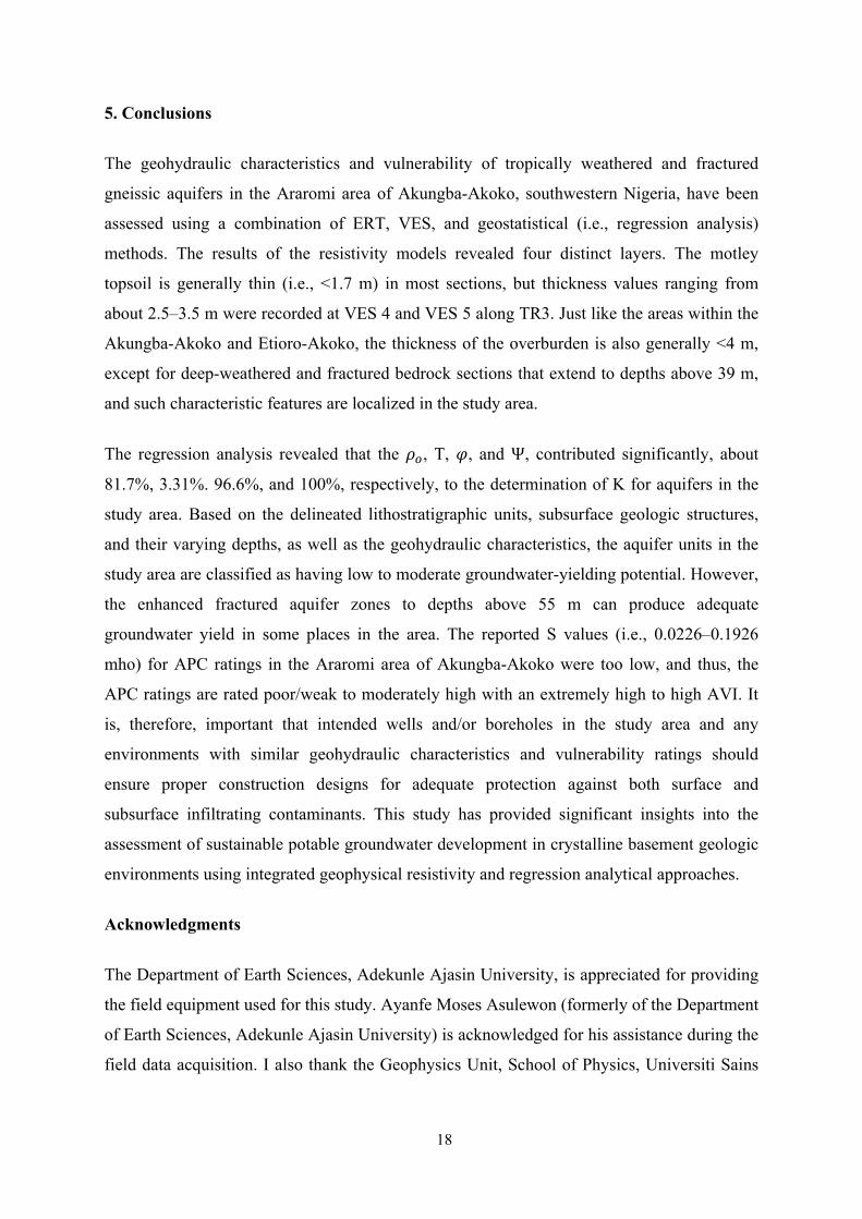
5. Conclusions

The geohydraulic characteristics and vulnerability of tropically weathered and fractured

gneissic aquifers in the Araromi area of Akungba-Akoko, southwestern Nigeria, have been

assessed using a combination of ERT, VES, and geostatistical (i.e., regression analysis)

methods. The results of the resistivity models revealed four distinct layers. The motley

topsoil is generally thin (i.e., <1.7 m) in most sections, but thickness values ranging from

about 2.5–3.5 m were recorded at VES 4 and VES 5 along TR3. Just like the areas within the

Akungba-Akoko and Etioro-Akoko, the thickness of the overburden is also generally <4 m,

except for deep-weathered and fractured bedrock sections that extend to depths above 39 m,

and such characteristic features are localized in the study area.

The regression analysis revealed that the 𝜌𝜌𝑜𝑜, T, 𝜑𝜑, and Ψ, contributed significantly, about

81.7%, 3.31%. 96.6%, and 100%, respectively, to the determination of K for aquifers in the

study area. Based on the delineated lithostratigraphic units, subsurface geologic structures,

and their varying depths, as well as the geohydraulic characteristics, the aquifer units in the

study area are classified as having low to moderate groundwater-yielding potential. However,

the enhanced fractured aquifer zones to depths above 55 m can produce adequate

groundwater yield in some places in the area. The reported S values (i.e., 0.0226–0.1926

mho) for APC ratings in the Araromi area of Akungba-Akoko were too low, and thus, the

APC ratings are rated poor/weak to moderately high with an extremely high to high AVI. It

is, therefore, important that intended wells and/or boreholes in the study area and any

environments with similar geohydraulic characteristics and vulnerability ratings should

ensure proper construction designs for adequate protection against both surface and

subsurface infiltrating contaminants. This study has provided significant insights into the

assessment of sustainable potable groundwater development in crystalline basement geologic

environments using integrated geophysical resistivity and regression analytical approaches.

Acknowledgments

The Department of Earth Sciences, Adekunle Ajasin University, is appreciated for providing

the field equipment used for this study. Ayanfe Moses Asulewon (formerly of the Department

of Earth Sciences, Adekunle Ajasin University) is acknowledged for his assistance during the

field data acquisition. I also thank the Geophysics Unit, School of Physics, Universiti Sains

19

Malaysia, for providing adequate facilities and a congenial environment to conduct this

research.

Data Availability

All data generated or analyzed during this study are included in this published article. Other

supporting analyzed data can be made available by the corresponding author upon reasonable

request.

Funding

This research did not receive any specific grants from funding agencies in the public,

commercial, or not-for-profit sectors.

Declaration of competing interest

The authors declare that they have no known competing financial interests or personal

relationships that could have appeared to influence the work reported in this paper.

References

[1] M. E. Ofodile, “Groundwater study and development in Nigeria. Mecon Geology, Jos”,

(2014).

[2] W. J. Cosgrove & D. P. Loucks, “Water management: current and future challenges

and research directions”, Water Resources Research 51 (2015) 4823.

[3] A. S. Akingboye, A. A. Bery, A. C. Ogunyele, A. O. Adeola, O. O. Omojola & A. S.

Adesida, “Groundwater-yielding capacity, water-rock interaction, and vulnerability

assessment of typical gneissic hydrogeologic units using geoelectrohydraulic method”,

(Forthcoming).

[4] S. Sajeena, V. M. Abdul Hakkim & E. K. Kurien, “Identification of groundwater

prospective zones using geoelectrical and electromagnetic surveys”, International

Journal of Engineering Inventions 3 (2014) 17.

[5] D. N. Obiora, A. E. Ajala & J. C. Ibuot, “Evaluation of aquifer protective capacity of

overburden unit and soil corrosivity in Makurdi, Benue State, Nigeria, using electrical

resistivity method”, Journal of Earth Systems Science 124 (2015) 125.

20

[6] I. Stober & K. Bucher, “Hydraulic conductivity of fractured upper crust: insights from

hydraulic tests in boreholes and fluid-rock interaction in crystalline basement rocks”,

Geofluids 15 (2015a) 161. https://doi.org/10.1111/gfl.12104

[7] N. J. George, A. E. Akpan & F. S. Akpan, “Assessment of spatial distribution of

porosity and aquifer geohydraulic parameters in parts of the Tertiary – Quaternary

hydrogeoresource of south-eastern Nigeria”, NRIAG Journal of Astronomy and

Geophysics 6 (2017) 422. https://doi.org/10.1016/j.nrjag.2017.09.001

[8] A. S. Akingboye, A. A. Bery, J. S. Kayode, A. M. Asulewon, R. Bello & O. C. Agbasi,

“Near-surface crustal architecture and geohydrodynamics of the gneissic terrain of

Araromi, Akungba-Akoko, SW Nigeria, derived from multi-geophysical methods”,

Natural Resources Research (in press).

[9] A. M. MacDonald, H. C. Bonsor, B. E. O. Dochartaigh & R. G. Taylor, “Quantitative

map of groundwater resource in Africa” Environmental Research Letters 7 (2012)

024009.

[10] M. L. Hossain, S. R. Das & M. K. Hossain, “Impact of landfill leachate on surface and

groundwater quality”, Journal of Environmental Science and Technology 7 (2014) 337.

[11] G. O. Mosuro, K. O. Omosanya, O. O. Bayewu, M. O. Oloruntola, T. A. Laniyan, O.

Atobi, M. Okubena, E. Popoola & F. Adekoya, “Assessment of groundwater

vulnerability to leachate infiltration using electrical resistivity method”, Applied Water

Science 7 (2016) 2195. https://doi.org/10.1007/s13201-016-0393-4

[12] W. O. Raji & K. A. Abdulkadri, “Evaluation of groundwater potential of bedrock

aquifers in Geological Sheet 223 Ilorin, Nigeria, using geo-electric sounding”, Applied

Water Science 10 (2020) 220. https://doi.org/10.1007/s13201-020-01303-2

[13] M. Hasan, Y. Shang, G. Akhter & M. Khan, “Geophysical investigation of fresh-saline

water interface: a case study from South Punjab, Pakistan”, Groundwater 55 (2017)

841.

[14] A. S. Akingboye & A. A. Bery, “Evaluation of lithostratigraphic units and groundwater

potential using the resolution capacities of two different electrical tomographic

electrodes at dual-spacing”, Contributions to Geophysics and Geodesy, 51 (2021a).

21

[15] A. S. Akingboye & A. A. Bery, “Borehole-constrained ERT for mapping the soil-rock

interface in a granitic environment: implications on groundwater, engineering

structures, and plant roots”, (Forthcoming) 33p.

[16] M. Hasan, Y. Shang, W. Jin & G. Akhter, “Estimation of hydraulic parameters in a

hard rock aquifer using integrated surface geoelectrical method and pumping test data

in southeast Guangdong, China”, Geosciences Journal (2020a).

https://doi.org/10.1007/s12303-020-0018-7

[17] M. Hasan, Y. Shang, G. Akhter & W. Jin, “Delineation of contaminated aquifers using

integrated geophysical methods in Northeast Punjab, Pakistan. Environmental

Monitoring and Assessment 192 (2020b) 12. https://doi.org/10.1007/s10661-019-7941-

y

[18] A. M. Ekanem, “Georesistivity modelling and appraisal of soil water retention capacity

in Akwa Ibom State University main campus and its environs, southern Nigeria”,

Modeling Earth Systems and Environment (2020). https://doi.org/10.1007/s40808-020-

00850-6

[19] M. Z. Mohammed, T. H. T. Ogunribido & A. T. Funmilayo, “Electrical resistivity

sounding for subsurface delineation and evaluation of groundwater potential of

Araromi Akungba-Akoko Ondo State southwestern Nigeria”, Journal of Environmental

Earth Sciences 2 (2012) 29.

[20] M. B. Aminu, “Electrical resistivity imaging of a thin clayey aquitard developed on

basement rocks in parts of Adekunle Ajasin University Campus, Akungba-Akoko,

south-western Nigeria”, Environmental Research, Engineering and Management 71

(2015) 47. http://doi.org/10.5755/j01.erem.71.1.9016

[21] A. S. Akingboye & I. B. Osazuwa, “Subsurface geological, hydrogeophysical, and

engineering characterisation of Etioro-Akoko, southwestern Nigeria, using electrical

resistivity tomography”, NRIAG Journal of Astronomy and Geophysics, 9 (2021) 43.

https://doi.org/10.1080/20909977.2020.1868659

[22] M. A. Rahaman, “Review of the Basement Geology of southwestern Nigeria. In: C. A.

Kogbe, (eds.) Geology of Nigeria. Elizabeth Publisher. Co., Lagos”, (1976) 41.

[23] M. A. Rahaman, “Recent advances in the study of the Basement Complex of Nigeria.

In: P. O. Oluyide, W. C. Mbonu, A. E. O. Ogezi, I. G. Egbuniwe, A. C. Ajibade & A.

22

C. Umeji, (eds.) Precambrian Geology of Nigeria. Geological Survey of Nigeria,

Kaduna”, (1988) 11.

[24] A. Krӧner, B. N. Ekwueme & R. T. Pidgeon, “The Oldest Rocks in West Africa:

SHRIMP Zircon Age for Early Archean Migmatitic Orthogneiss at Kaduna, Northern

Nigeria”, The Journal of Geology 109 (2001) 399.

[25] B. J. Fagbohun, A. A. Omitogun, O. A. Bamisaiye & F. J. Ayoola, “Remote detection

and interpretation of structural style of the Zuru Schist Belt, northwest Nigeria”,

Geocarto International (2020) 1. https://doi.org/10.1080/10106049.2020.1753822

[26] E. Ferré, G. Gleizes & R. Caby, “Obliquely convergent tectonics and granite

emplacement in the Trans-Saharan belt of Eastern Nigeria: a synthesis”, Precambrian

Research 144 (2002) 199.

[27] A. C. Ogunyele, S. O. Obaje, A. S. Akingboye, A. O. Adeola, A. O. Babalola & A. T.

Olufunmilayo, “Petrography and geochemistry of Neoproterozoic charnockite-granite

association and metasedimentary rocks around Okpella, southwestern Nigeria”,

Arabian Journal of Geosciences 13 (2020) 780. https://doi.org/10.1007/s12517-020-

05785-x

[28] M. Woakes, M. A. Rahaman & A. C. Ajibade. “Some metallogenetic features of the

Nigerian Basement”, Journal of African Earth Sciences 6 (1987) 655.

https://doi.org/10.1016/0899-5362(87)90004-2

[29] A. S. Akingboye, A. C. Ogunyele, A. T. Jimoh, O. B. Adaramoye, A. O. Adeola & T.

Ajayi, “Radioactivity, radiogenic heat production and environmental radiation risk of

the Basement Complex rocks of Akungba-Akoko, southwestern Nigeria: insights from

in situ gamma-ray spectrometry”, Environmental Earth Sciences 80 (2021b) 6.

https://doi.org/10.1007/s12665-021-09516-7

[30] P. I. Olasehinde & W. O. Raji, “Geophysical studies on fractures of basement rocks at

the University of Ilorin, southwestern Nigeria: application to groundwater exploration”,

Water Resources Research 17 (2007) 3.

[31] M. H. Loke, “Rapid 2D resistivity and IP inversion using the least-square method.

Manual for RES2DINV, version 3.54”, (2004) 53.

23

[32] A. S. Akingboye & A. C. Ogunyele, “Insight into seismic refraction and electrical

resistivity tomography techniques in subsurface investigations”, Rudarsko Geolosko

Naftni Zbornik 34 (2019) 93. https://doi.org/10.17794/rgn.2019.1.9

[33] C. DeGroot-Hedlin & S. C. Constable, “Occam’s inversion to generate smooth two-

dimensional models from magnetotelluric data”, Geophysics 55 (1990) 1613.

[34] T. Dahlin & M. H. Loke, “Underwater ERT surveying in water with resistivity layering

with example of application to site investigation for a rock tunnel in central

Stockholm”, Near Surface Geophysics 16 (2018) 230. https://doi.org/10.3997/1873-

0604.2018007

[35] A. S. Akingboye & A. A. Bery, “Performance evaluation of copper and stainless-steel

electrodes in electrical tomographic imaging”, Journal of Physical Science 32 (2021b).

[36] P. C. Heigold, R. H. Gilkeson, K. Cartwright & P. C. Reed, “Aquifer transmissivity

from surficial electrical methods”, Ground Water 17 (1979) 338.

[37] S. Niwas & D. C. Singhal, “Estimation of aquifer transmissivity from Dar-Zarrouk

parameters in porous media”, Journal of Hydrology 50 (1981) 393.

[38] A. A. R. Zohdy, G. P. Eaton & D. R. Mabey, “Application of surface geophysics to

groundwater investigations. United State Geophysical Survey, Washington”, (1974).

[39] M. I. Oladapo, M. Z. Mohammed, O. O. Adeoye & O. O. Adesola, “Geoelectric

investigation of the Ondo State Housing Corporation Estate Ijapo, Akure, southwestern

Nigeria”, Journal of Mining Geology 40 (2004) 41.

[40] D. Van Stempvoort, L. Ewert & L. Wassenaar, “Aquifer vulnerability index: a GIS-

compatible method for groundwater vulnerability mapping”, Canadian Water

Resources Journal 18 (1992) 25.

[41] Fetters, C.W. 1994. Applied hydrogeology, (3rd edn). Prentice Hall Inc., New Jersey, p

600.

[42] R. J. Freund, W. J. Wilson & D. L. Mohr, “Statistical Methods (3rd ed.)”, Elsevier Inc.,

(2010). https://doi.org/10.1016/C2009-0-20216-9

[43] G. Smith, “Essential Statistics, Regression, and Econometrics”, Elsevier Inc., (2011).

https://doi.org/10.1016/C2009-0-61163-6

24

[44] A. S. Akingboye, O. Ademila, C. C. Okpoli, A. V. Oyeshomo, et al.,

“Radiogeochemistry, uranium migration and radiogenic heat of the granite gneisses in

parts of the southwestern Basement Complex of Nigeria”, Journal of African Earth

Sciences (in press).

[45] J. Krasny, “Classification of transmissivity magnitude and variation”, Groundwater 31

(1993) 230.

[46] O. J. Akintorinwa, M. O. Atitebi & A. A. Akinlalu, “Hydrogeophysical and aquifer

vulnerability zonation of a typical basement complex terrain: A case study of Odode

Idanre southwestern Nigeria”, Heliyon 6 (2020).

https://doi.org/10.1016/j.heliyon.2020.e04549

25

Figure Captions

Figure 1. (a) Nigeria's regional geological map within the Pan-African mobile belt between

the West African and Congo Cratons. (b) A detailed regional geological map of Nigeria

showing the study area in the Nigerian Southwestern Basement Complex (modified after

[28]). (c) Geological map of Akungba-Akoko and its surroundings in Ondo State,

southwestern Nigeria (modified from [21]).

26

Figure 2. (a) Aerial map showing the data acquisition and all the geophysical traverses, (b)

elevation map showing all the VES survey station points and existing hand-dug wells in the

study area, and (c) the 3-D topographical view of the study area.

27

Figure 3. Composite results of the 2-D ERT inversion beneath TR1.

28

Figure 4. Inverted model resistivity section beneath the geoelectric surveyed traverses.

29

Figure 5. Typical iterated VES curve types generated for the study area include (a) A type,

(b) H type, (c) HA type, and (d) AK type.