Geographical segmentation of US capital markets

ARTICLE IN PRESS

Journal of Financial Economics 85 (2007) 151–178

0304-405X/$

doi:10.1016/j

$I wish t

Stromberg, J

Weisbach, M

participants

Binghamton

York Federa

E-mail ad

www.elsevier.com/locate/jfec

Geographical segmentation of US capital markets$

Bo Becker

University of Illinois at Urbana-Champaign, Champaign, IL 61820, USA

Received 30 March 2006; received in revised form 9 June 2006; accepted 13 July 2006

Available online 24 March 2007

Abstract

Demographic variation in savings behavior can be exploited to provide evidence on segmentation

in US bank loan markets. Cities with a large fraction of seniors have higher volumes of bank

deposits. Since many banks rely heavily on deposit financing, this affects local loan supply and

economic activity. I show a positive effect of local deposit supply on local outcomes, including the

number of firms, the number of manufacturing firms, and the number of new firms started. The effect

is stronger in industries that are heavily dependent on external finance. The deregulation of intrastate

branching reduced the effect of local deposit supply by approximately a third.

r 2007 Elsevier B.V. All rights reserved.

JEL classifications: G21; E22; R11

Keywords: Banks; Geographical segmentation; Seniors

1. Introduction

In most economies, banks play a large role in the intermediation of capital fromsuppliers to users. Unlike financial markets, banks are principally local intermediaries.This applies to both sides of the balance sheet. On the liability side, banks rely heavily ondeposits for funding (Kashyap and Stein, 2000) and most deposits are local. On the asset

- see front matter r 2007 Elsevier B.V. All rights reserved.

.jfineco.2006.07.001

o thank David Greenberg, Jens Josephson, Guy David, Luigi Zingales, Zahi Ben-David, Per

agadeesh Sivadasan, Ulf Axelson, Joshua Pollet, Toby Moskowitz, George Pennachi, Michael

urillo Campello, Luigi Guiso, Jeremy Stein (discussant), an anonymous referee as well as seminar

at the University of Illinois at Urbana-Champaign, Swedish Institute for Financial Research,

University, National Bureau of Economic Research, Hautes Etudes Commerciales and the New

l Reserve for helpful comments.

dress: [email protected].

www.elsevier.com/locate/jfec

dx.doi.org/10.1016/j.jfineco.2006.07.001

mailto:[email protected]

ARTICLE IN PRESSB. Becker / Journal of Financial Economics 85 (2007) 151–178152

side, much bank lending is local (Petersen and Rajan, 2002). For these reasons, localvariation in the supply of deposits could translate to local variation in the availability andcost of capital for borrowers and, hence, in the level of economic activity.Geographical segmentation is difficult to identify empirically, however. A direct

approach is to examine the correlation between local lending volumes and local economicoutcomes. In practice, this approach suffers from a severe endogeneity problem becausethe volume of local bank lending is likely to respond to both supply and demand for loans.The demand for loans is trivially correlated with economic outcomes. So, to evaluatewhether the local supply of capital affects local economic outcomes, a source of exogenousvariation in the supply of bank loans is necessary. This paper utilizes demographicvariation in the supply of deposits as such a determinant of local capital supply. Seniors(those age 65 and older) tend to hold higher levels of bank deposits than other groups bothin absolute terms and as a fraction of portfolios. However, because seniors do notparticipate much in the labor market or operate businesses, and because they consume lessthan other groups, the impact of a large fraction of seniors on the local demand forbusiness finance is likely to be small and perhaps negative (See Section 2 for a moredetailed discussion of the effect of seniors on loan demand.). Hence, a large fraction ofseniors in an area causes a higher supply of intermediated finance relative to local demandfor external financing. This makes the fraction of seniors a potentially useful instrumentfor the local supply of finance (relative to demand).Substantial demographic variation exists within the US, both across and within states. I

use data on the fraction of seniors at the level of metropolitan statistical areas (MSAs) topredict deposit volumes and loan availability. This level of geographical detail permitsincluding state fixed effects in regressions. Exploiting only within-state variation, I showthat a high fraction of seniors corresponds to a high supply of deposits. In areas with highdeposit supply, local banks use relatively more deposit financing (as opposed to equity andnondeposit debt) and have more liquid balance sheets (as measured by holdings of treasurysecurities).1

Using seniors as an instrument for deposit supply, I show that this supply is related tolocal economic outcomes. MSAs with high levels of deposits have more firms, moremanufacturing firms and establishments, relatively more small firms (up to 19 employees)and fewer large firms (more than five hundred employees), and more new firm starts. Usinga measure of dependence on external finance, based on Rajan and Zingales (1998), I showthat the effect of the local deposit supply is stronger in industries that are more externallydependent (i.e., those industries in which, on average, Compustat firms use more externalfinancing).I next examine the robustness of these results to several possible concerns. To address

the potential endogeneity of seniors, demographic predictions are used in the place ofactual data on seniors (middle-age people 20–30 years in advance), and the results remainsimilar and significant. I also consider the possibility that the seniors variable is correlatedwith wealth, perhaps driving economic outcomes through an effect on demand. I attemptto control for wealth by including average local house prices and per capita income as

1MSAs are defined by the Office of Management and Budget as a federal statistical standard. An area qualifies

for recognition as an MSA if it includes a city of at least 50 thousand inhabitants or an urbanized area of at least

50 thousand with a total metropolitan area population of at least 100,000. MSAs typically incorporate several

counties and sometimes straddle state borders.

ARTICLE IN PRESSB. Becker / Journal of Financial Economics 85 (2007) 151–178 153

control variables. This does not affect coefficient estimates much. To examine whether themarket definition used (MSAs) is too wide, results are presented for smaller areas (ZIPCodes). Smaller MSAs tend not to contain many ZIP Codes, so I focus on the three largestcities (New York, Los Angeles, Chicago). Within these cities, the ZIP Code-level depositsupply has a positive effect on the number of establishments. Finally, time-series tests,although exploiting limited variation in the data (because the fraction of seniors is stable),find a positive, borderline significant effect of deposits on outcomes.

A final set of robustness tests addresses the issue of where integration is weakest, i.e.,where local deposits have the strongest impact on local outcomes. There are multiplepotential channels for geographical reallocation of savings, in either of the steps fromdepositor to intermediary and on to borrower. Furthermore, internal and external capitalmarkets could allow funds to be transferred from bank branches in high deposit areas tobranches with lower deposit supply (or higher loan demand). Frictions involvingregulation, agency problems and information asymmetries could limit the scope forgeographic transfers, however. In Section 6, evidence is presented showing thatderegulation of intrastate branching (see Kroszner and Strahan, 1999) reduced the effectsof geographical variation by approximately one third. This suggests that one of theimportant benefits of deregulation has been better geographical integration of capitalmarkets. The increasing integration of local capital markets could be a process that is stillgoing on.

Geographic variation in the supply of capital in all likelihood implies welfare costs. Ifthe marginal productivity of capital is declining, locations with a higher local supply ofdeposits that employ more capital use capital at lower marginal productivity than locationswith less capital. Therefore, such variation reduces aggregate output compared with africtionless world.2 The magnitude of welfare costs depends primarily on the rate at whichcapital productivity declines with capital intensity and could vary by sector and over time.

A few caveats are in order. Bank lending data are not available by bank branch, so Icannot examine the effect of deposit supply on the pricing of local loans. Second, time-series variation is limited for the fraction of seniors, so time-series results must beconsidered provisional.

This paper is related to papers showing that the supply of loans affects economicoutcomes. Peek and Rosengren (1997, 2000) show that variation in Japanese banks’lending in the US, induced by Japanese economic events, has had a large effect onconstruction activity in California, Illinois, and New York. Ashcraft (2005) shows that intwo cases when the Federal Deposit Insurance Corporation closed healthy banks (to coverlosses at affiliated banks), bank loans and local incomes declined. In contrast to theseresults, Driscoll (2004) uses estimated state-specific shocks to the demand for money toinstrument for loan supply and finds a positive relation to the volume of bank lending, butno effect on output. The results in this paper complement and expand on these findings inseveral ways. The instrument is more generally available, not depending on infrequentregulatory action (such as the Texas bank closures) or specific foreign episodes (such as theJapanese boom). This offers opportunities for broader uses, e.g., comparisons over time orinternational comparisons of financial systems. Also, the instrument is available at finegeographical levels (e.g., MSAs).

2The welfare costs of varying capital supply are not as obvious for time-series variation in the supply of loans,

such as that induced by monetary policy. Cross-sectional variation, however, is almost certainly harmful.


This paper is also related to research showing that there is substantial within-countryvariation in financial systems. Jayaratne and Strahan (1996) analyze variation in bankregulation across US states and find that deregulation of entry and mergers substantiallyincreased output growth rates. Cetorelli and Strahan (2006) report that, at the state level,the number of firms is more sensitive to bank competition in industries with highdependence on external financing. With US data, Garmaise and Moskowitz (2006) usebank mergers as an instrument for local bank competition, and also find negativetemporary effects on loan supply and economic activity following a bank merger. UsingItalian data, Guiso et al. (2004) show that financial development (the probability that ahousehold is shut off from the credit market) is largely determined by regulatoryrestrictions on bank entry. They find that financial development affects rates of new firmentry, growth of existing firms (especially small firms) and product market competition.My findings match this literature in suggesting that local credit markets matter foreconomic outcomes. However, the focus here is not on variation in local competitivenessand institutional quality, which affect local financial intermediation, but on geographicalsegmentation of capital markets, which affects the transfer of capital across space. Theimplications are therefore different. In particular, much of the literature has suggested thatbank competition is beneficial and therefore implicitly or explicitly that mergers could beharmful (e.g. Sapienza, 2002; Garmaise and Moskowitz, 2006). The evidence onsegmentation in fact suggests that a cost of a dispersed banking system is that geographicalsegmentation is exacerbated. Thus, there are potential welfare benefits of mergers thatcombine banks from different areas.3

Finally, my findings on deregulation are related to the results of Jayaratne and Strahan(1996), who show large positive effects on state level growth rates after deregulation. Bankderegulation reduced the impact of local deposit supply, implying that geographicalsegmentation was reduced. This suggests a further channel through which the benefitsidentified could have come about.The rest of the paper is organized as follows. In Section 2, I show that the deposit

holdings of seniors are higher, and their labor market participation lower, than that ofother age groups. In Section 3, I discuss the conditions under which local deposits arelikely to affect bank lending and those under which bank lending in turn is likely to affecteconomic activity. Section 3 covers the data used, and Section 4 the basic empirical results.In Section 5, I introduce additional control variables and robustness tests, and in Section 6discuss what my results imply about the nature of financial frictions and presents sometests of frictions. Section 7 concludes.

2. Seniors as an instrument for local capital supply

The empirical strategy in this paper entails using seniors as an instrument for localcapital supply. This implies two main requirements on the consequences of localseniors. First, the measure of local capital supply is bank deposits (in local branches), so itis necessary that seniors have a positive effect on deposits. Second, for seniors to be avalid instrument for local capital supply it is paramount that the fraction of seniors

3The negative and positive welfare effects of mergers could coexist. Bank mergers that improve geographical

integration could be beneficial while mergers that reduce local market competitiveness are detrimental. Some

mergers could be detrimental in one respect and beneficial in the other.


not affect local capital demand. This section assesses the plausibility of these twoassumptions in turn.

2.1. Loan supply: seniors tend to hold bank deposits

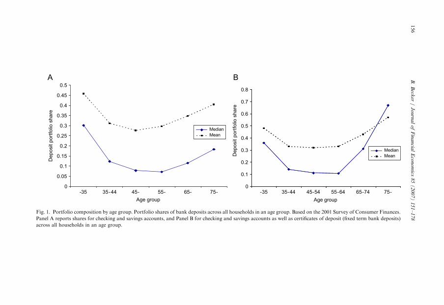
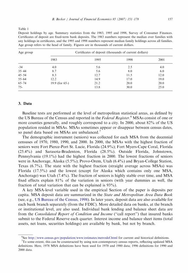
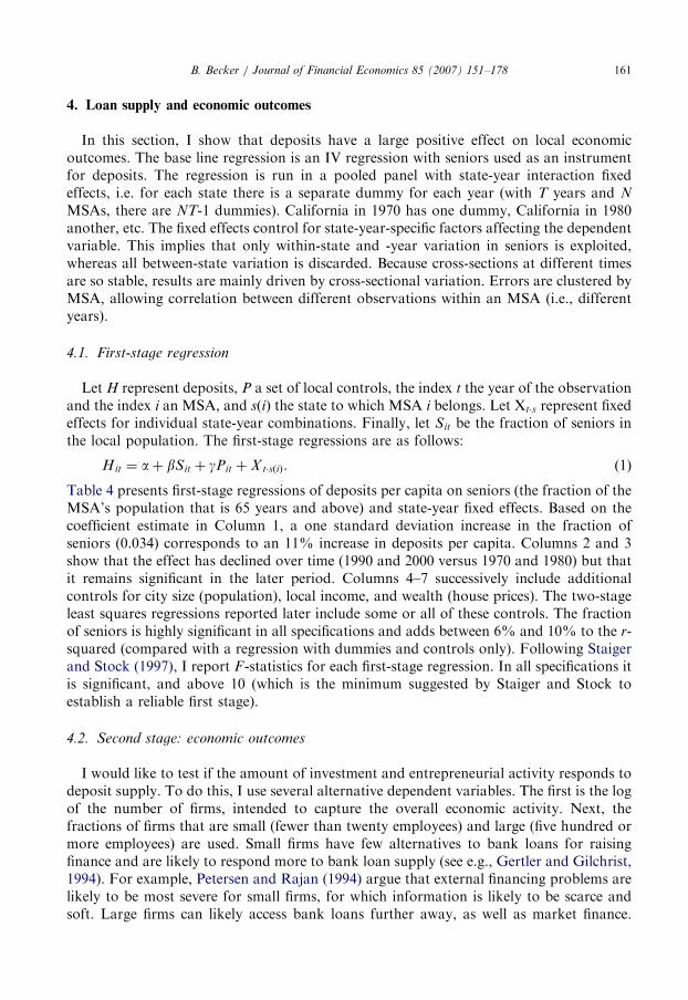
Compared with other age groups, seniors tilt their financial portfolios toward deposits.Because of this and their higher financial wealth, seniors hold more deposits than any othergroup. To show this, I calculated relative portfolio allocations for different age groupsusing the 2001 Survey of Consumer Finances (SCF). For each age group, average andmedian portfolio shares of deposits out of total financial assets are reported in Fig. 1.Seniors have higher portfolio allocations to deposits than any other group except thoseunder 35 years (who have low total holdings of financial assets). Seniors are the only agegroup in which more than 90% of individuals have transaction accounts4 and where morethan 20% hold certificates of deposits. What about absolute levels? Median holdings ofcertificates of deposits from various SCFs are reported in Table 1. Seniors have muchhigher holdings than other age groups.

2.2. Loan demand: seniors have low labor market participation and consumption

For the seniors instrument to be valid, it is important that having more seniors does notincrease local demand for loans. This probably holds because seniors produce andconsume less than other age groups.5 Seniors participate less in the labor force than othergroups. The median retirement age in the US is about 62 years (Gendell and Siegel, 1992).In 1997, the labor force participation of people age 65–69 was 24.4%; of those age 70–74 itwas 13.5%; and of those age 75 or more, 5.3% (Wiatrowski, 2001). These numbersprobably overstate the labor supply of seniors somewhat, because part-time work iscommon in older groups (51% of employed seniors according to Wiatrowski, 2001). Also,seniors tend to be less active as entrepreneurs than other age groups. Moskowitz andVissing-Jorgensen (2002) report that 10% of owners of private equity were 65 or older inthe pooled 1989, 1992, 1995, and 1998 Surveys of Consumer Finances, while constitutingabout 13% of the overall population. Again, the level of activity conditional onparticipation is probably lower than for other age groups. Heaton and Lucas (2000) reportthat seniors hold a smaller fraction of their portfolio in proprietary business than other agegroups (e.g., 2.4% of liquid assets for seniors versus 6.8% for the 50–64 age group in 1995).Finally, seniors consume less than other age groups. In 2002, median (average) moneyincome before taxes of households headed by a senior was $23,683 ($29,711) comparedwith an overall average for the population of $43,381 ($49,430) according to the 2002Consumer Expenditure Survey.

4For other forms of deposits (transaction accounts and savings accounts) the holdings are much smaller than

for certificates, but, again, the holdings of seniors are higher than those of other groups. The 75þ age group (with

the highest holdings in both 1995 and 1998) had median transaction account holdings of $5.6 thousand 1995 and

$6.1 thousand in 1998.5It is not necessary (for the validity of the instrument) that seniors do not participate at all in the labor market.

As long as seniors hold more deposits, in absolute terms, than non seniors, banks face a higher supply of deposits

(relative to demand for financing) in areas with many seniors. This holds even if seniors work and consume as

much as other age groups.

ARTIC

LEIN

PRES

S

0

0.05

0.1

0.15

0.2

0.25

0.3

0.35

0.4

0.45

0.5

-35 35-44 45- 55- 65- 75-

Median

Mean

Median

Mean

Age group

Deposit p

ort

folio

share

Deposit p

ort

folio

share

0

0.1

0.2

0.3

0.4

0.5

0.6

0.7

0.8

-35 35-44 45-54 55-64 65-74 75-

Age group

Fig. 1. Portfolio composition by age group. Portfolio shares of bank deposits across all households in an age group. Based on the 2001 Survey of Consumer Finances.

Panel A reports shares for checking and savings accounts, and Panel B for checking and savings accounts as well as certificates of deposit (fixed term bank deposits)

across all households in an age group.

B.

Beck

er/

Jo

urn

al

of

Fin

an

cial

Eco

no

mics

85

(2

00

7)

15

1–

17

8156

ARTICLE IN PRESS

Table 1

Deposit holdings by age. Summary statistics from the 1983, 1995 and 1998, Survey of Consumer Finances.

Certificates of deposit are fixed-term bank deposits. The 1983 numbers represent the median over families with

any holdings in certificates, and the 1995 and 1998 numbers represent median family holdings across all families.

Age group refers to the head of family. Figures are in thousands of current dollars.

Age group Certificates of deposit (thousands of current dollars)

1983 1995 1998 2001

-34 4.0 5.6 2.5 4.0

35–44 8.7 5.6 8.0 6.0

45–54 8.3 12.7 11.5 12.0

55–64 12.2 14.9 17.0 19.0

65–74 19.9 (for 65-) 21.2 20.0 20.0

75- 13.8 30.0 25.0

B. Becker / Journal of Financial Economics 85 (2007) 151–178 157

3. Data

Baseline tests are performed at the level of metropolitan statistical areas, as defined bythe US Bureau of the Census and reported in the Federal Register.6 MSAs consist of one ormore counties generally, and roughly correspond to a city. In 2000, about 82% of the USpopulation resided in MSAs. MSAs sometimes appear or disappear between census dates,so panel data based on MSAs are unbalanced.7

The demographic instrument (seniors) was collected for each MSA from the decennialcensuses of 1970, 1980, 1990, and 2000. In 2000, the MSAs with the highest fraction ofseniors were Fort Pierce-Port St. Lucie, Florida (24.9%); Fort Myers-Cape Coral, Florida(25.4%) and Sarasota-Bradenton, Florida (28.5%). Outside Florida, Johnstown,Pennsylvania (19.1%) had the highest fraction in 2000. The lowest fractions of seniorswere in Anchorage, Alaska (5.5%); Provo-Orem, Utah (6.4%) and Bryan-College Station,Texas (6.7%). The state with the highest fraction (straight average across MSAs) wasFlorida (17.5%) and the lowest (except for Alaska which contains only one MSA,Anchorage) was Utah (7.4%). The fraction of seniors is highly stable over time, and MSAfixed effects explain 81% of the variation in seniors (with year dummies as well, thefraction of total variation that can be explained is 93%).

A key MSA-level variable used in the empirical Section of the paper is deposits percapita. MSA deposit data are summarized in the State and Metropolitan Area Data Book

(see, e.g., US Bureau of the Census, 1998). In later years, deposit data are also available foreach bank branch separately (from the FDIC). More detailed data on banks, at the branchor institutional level, are also used. Individual bank lending and balance sheet data arefrom the Consolidated Report of Condition and Income (‘‘call report’’) that insured bankssubmit to the Federal Reserve each quarter. Interest income and balance sheet items (totalassets, net loans, securities holdings) are available by bank, but not by branch.

6See http://www.census.gov/population/www/estimates/metrodef.html for current and historical definitions.7To some extent, this can be counteracted by using non contemporary census reports, reflecting updated MSA

definitions. Here, 1978 MSA definitions have been used for 1970 and 1980 data; 1996 definitions for 1990 and

2000 data.

http://www.census.gov/population/www/estimates/metrodef.html


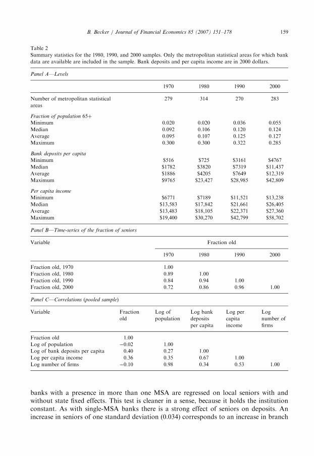
Several outcomes and control variables are taken from other sources. Data by ZIP Codeon demographics, and the number of establishments are from the 2000 census(establishment data are lagged three years). Per capita income is from the Bureau ofEconomic Analysis’ regional accounts. Other economic outcomes are collected from Stateand Metropolitan Area Data Books. House prices (in 2000) are from the census. Firmstarts are from the Small Business Administration. Industry data are from the EconomicCensus of 1997. Firm level data for 1985–1995 are collected from Compustat and used tocalculate industry-level financial dependence following Rajan and Zingales (1998).Table 2 provides summary statistics for the sample as well as the correlations of some

key variables. In single-year cross-sections, the correlation between the fraction of seniorsand the log of bank deposits per capita is 0.27 in 1970, 0.20 in 1980, 0.23 in 1990, and 0.21in 2000. The fraction of seniors is slow moving and the correlation between successivecross-sections is 0.92 on average.

3.1. Bank financing and local seniors

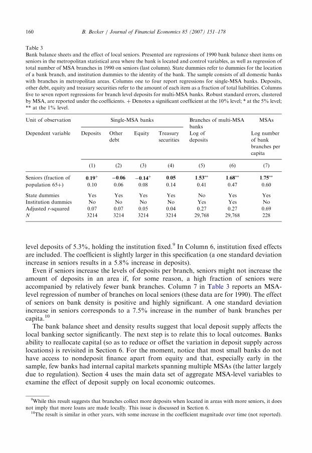
This section examines the effect of seniors on bank balance sheets. Bank level data onbalance sheets are collected for 1992 (the first year with data available) and related to 1990seniors in the MSA where the bank is headquartered. I first examine single-MSA banksand then compare branches of multi-MSA banks.The regressions presented in Columns 1–3 of Table 3 relate the financing choices of

single-MSA banks to the fraction of seniors in the local population, controlling for statefixed effects.8 Deposits constitute a larger fraction and equity a smaller fraction offinancing when local deposit supply is high (i.e., many seniors). Nondeposit debt isunaffected. This fits the findings of Kashyap and Stein (2000) and Bassett and Brady(2002), that only the largest banks use nondeposit debt financing to any significant extent.Single-MSA banks all fall in the size categories that use little or no outside debt. Thisuniversal absence of debt for smaller banks suggests that it is natural to find that thelocation of a bank does not affect debt financing. Importantly, single-MSA banks show noevidence of being able to offset demographic variation in deposit supply. Column 4 inTable 3 presents regression results for liquid securities holdings as a fraction of assets ofunit banks located in an MSA. Holdings of Treasury-issued US government securities areinsignificantly higher for unit banks located in MSAs with a high fraction of seniors. Thus,bank liquidity seems to be little affected by deposit supply (or securities holdings are toonoisy to be easily related to weaker determinants).Because multi-MSA banks face different deposit supply in different areas, there is no

direct way to test their overall financing choices against local seniors (i.e. they face differentsupply in different branch offices). In particular, running the regressions reported abovefor single-MSA banks (one bank’s capital structure regressed on the demographics of theunique MSA where it is located) is impossible for banks that have a presence in multipleMSAs. It is possible, however, to test a related idea: that deposit holdings at the branchlevel vary with local deposit supply. In Columns 5–6 of Table 3, I relate deposit volumes atthe branch level to the deposit supply of the MSA where the branch is located, controllingfor institution fixed effects (because these are branches, not banks, they have no individualcapital structure, but they do have distinct deposit volumes). Branch level deposits of

8This includes all unit banks with only one branch and banks with multiple branches located in a single MSA.

ARTICLE IN PRESS

Table 2

Summary statistics for the 1980, 1990, and 2000 samples. Only the metropolitan statistical areas for which bank

data are available are included in the sample. Bank deposits and per capita income are in 2000 dollars.

Panel A—Levels

1970 1980 1990 2000

Number of metropolitan statistical

areas

279 314 270 283

Fraction of population 65þ

Minimum 0.020 0.020 0.036 0.055

Median 0.092 0.106 0.120 0.124

Average 0.095 0.107 0.125 0.127

Maximum 0.300 0.300 0.322 0.285

Bank deposits per capita

Minimum $516 $725 $3161 $4767

Median $1782 $3820 $7319 $11,437

Average $1886 $4205 $7649 $12,319

Maximum $9765 $23,427 $28,985 $42,809

Per capita income

Minimum $6771 $7189 $11,521 $13,238

Median $13,583 $17,842 $21,661 $26,405

Average $13,483 $18,105 $22,371 $27,360

Maximum $19,400 $30,270 $42,799 $58,702

Panel B—Time-series of the fraction of seniors

Variable Fraction old

1970 1980 1990 2000

Fraction old, 1970 1.00

Fraction old, 1980 0.89 1.00

Fraction old, 1990 0.84 0.94 1.00

Fraction old, 2000 0.72 0.86 0.96 1.00

Panel C—Correlations (pooled sample)

Variable Fraction

old

Log of

population

Log bank

deposits

per capita

Log per

capita

income

Log

number of

firms

Fraction old 1.00

Log of population �0.02 1.00

Log of bank deposits per capita 0.40 0.27 1.00

Log per capita income 0.36 0.35 0.67 1.00

Log number of firms �0.10 0.98 0.34 0.53 1.00


banks with a presence in more than one MSA are regressed on local seniors with andwithout state fixed effects. This test is cleaner in a sense, because it holds the institutionconstant. As with single-MSA banks there is a strong effect of seniors on deposits. Anincrease in seniors of one standard deviation (0.034) corresponds to an increase in branch

ARTICLE IN PRESS

Table 3

Bank balance sheets and the effect of local seniors. Presented are regressions of 1990 bank balance sheet items on

seniors in the metropolitan statistical area where the bank is located and control variables, as well as regression of

total number of MSA branches in 1990 on seniors (last column). State dummies refer to dummies for the location

of a bank branch, and institution dummies to the identity of the bank. The sample consists of all domestic banks

with branches in metropolitan areas. Columns one to four report regressions for single-MSA banks. Deposits,

other debt, equity and treasury securities refer to the amount of each item as a fraction of total liabilities. Columns

five to seven report regressions for branch level deposits for multi-MSA banks. Robust standard errors, clustered

by MSA, are reported under the coefficients.þDenotes a significant coefficient at the 10% level; * at the 5% level;

** at the 1% level.

Unit of observation Single-MSA banks Branches of multi-MSA

banks

MSAs

Dependent variable Deposits Other

debt

Equity Treasury

securities

Log of

deposits

Log number

of bank

branches per

capita

(1) (2) (3) (4) (5) (6) (7)

Seniors (fraction of 0:19þ �0:06 �0:14þ 0:05 1:53�� 1:68�� 1:75��

population 65þ) 0.10 0.06 0.08 0.14 0.41 0.47 0.60

State dummies Yes Yes Yes Yes No Yes Yes

Institution dummies No No No No Yes Yes No

Adjusted r-squared 0.07 0.07 0.05 0.04 0.27 0.27 0.69

N 3214 3214 3214 3214 29,768 29,768 228

B. Becker / Journal of Financial Economics 85 (2007) 151–178160

level deposits of 5.3%, holding the institution fixed.9 In Column 6, institution fixed effectsare included. The coefficient is slightly larger in this specification (a one standard deviationincrease in seniors results in a 5.8% increase in deposits).Even if seniors increase the levels of deposits per branch, seniors might not increase the

amount of deposits in an area if, for some reason, a high fraction of seniors wereaccompanied by relatively fewer bank branches. Column 7 in Table 3 reports an MSA-level regression of number of branches on local seniors (these data are for 1990). The effectof seniors on bank density is positive and highly significant. A one standard deviationincrease in seniors corresponds to a 7.5% increase in the number of bank branches percapita.10

The bank balance sheet and density results suggest that local deposit supply affects thelocal banking sector significantly. The next step is to relate this to local outcomes. Banksability to reallocate capital (so as to reduce or offset the variation in deposit supply acrosslocations) is revisited in Section 6. For the moment, notice that most small banks do nothave access to nondeposit finance apart from equity and that, especially early in thesample, few banks had internal capital markets spanning multiple MSAs (the latter largelydue to regulation). Section 4 uses the main data set of aggregate MSA-level variables toexamine the effect of deposit supply on local economic outcomes.

9While this result suggests that branches collect more deposits when located in areas with more seniors, it does

not imply that more loans are made locally. This issue is discussed in Section 6.10The result is similar in other years, with some increase in the coefficient magnitude over time (not reported).


4. Loan supply and economic outcomes

In this section, I show that deposits have a large positive effect on local economicoutcomes. The base line regression is an IV regression with seniors used as an instrumentfor deposits. The regression is run in a pooled panel with state-year interaction fixedeffects, i.e. for each state there is a separate dummy for each year (with T years and N

MSAs, there are NT-1 dummies). California in 1970 has one dummy, California in 1980another, etc. The fixed effects control for state-year-specific factors affecting the dependentvariable. This implies that only within-state and -year variation in seniors is exploited,whereas all between-state variation is discarded. Because cross-sections at different timesare so stable, results are mainly driven by cross-sectional variation. Errors are clustered byMSA, allowing correlation between different observations within an MSA (i.e., differentyears).

4.1. First-stage regression

Let H represent deposits, P a set of local controls, the index t the year of the observationand the index i an MSA, and sðiÞ the state to which MSA i belongs. Let Xt�s represent fixedeffects for individual state-year combinations. Finally, let Sit be the fraction of seniors inthe local population. The first-stage regressions are as follows:

Hit ¼ aþ bSit þ gPit þ X t�sðiÞ. (1)

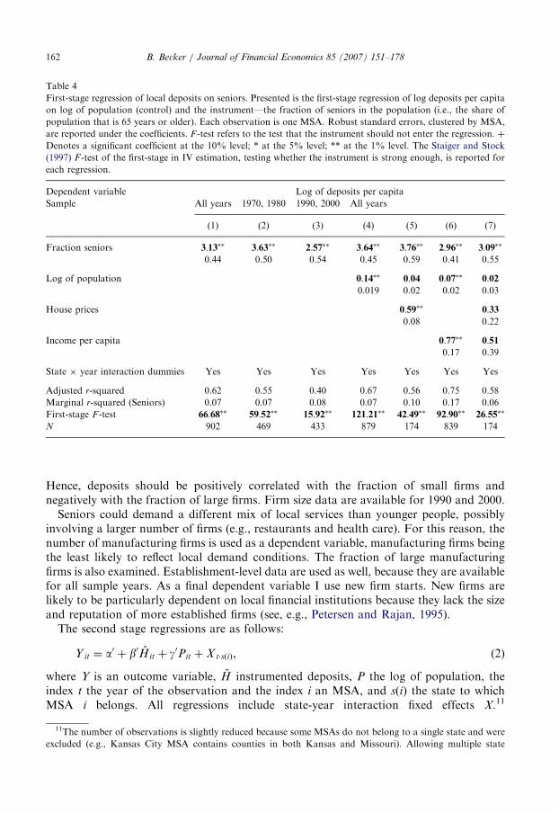
Table 4 presents first-stage regressions of deposits per capita on seniors (the fraction of theMSA’s population that is 65 years and above) and state-year fixed effects. Based on thecoefficient estimate in Column 1, a one standard deviation increase in the fraction ofseniors (0.034) corresponds to an 11% increase in deposits per capita. Columns 2 and 3show that the effect has declined over time (1990 and 2000 versus 1970 and 1980) but thatit remains significant in the later period. Columns 4–7 successively include additionalcontrols for city size (population), local income, and wealth (house prices). The two-stageleast squares regressions reported later include some or all of these controls. The fractionof seniors is highly significant in all specifications and adds between 6% and 10% to the r-squared (compared with a regression with dummies and controls only). Following Staigerand Stock (1997), I report F -statistics for each first-stage regression. In all specifications itis significant, and above 10 (which is the minimum suggested by Staiger and Stock toestablish a reliable first stage).

4.2. Second stage: economic outcomes

I would like to test if the amount of investment and entrepreneurial activity responds todeposit supply. To do this, I use several alternative dependent variables. The first is the logof the number of firms, intended to capture the overall economic activity. Next, thefractions of firms that are small (fewer than twenty employees) and large (five hundred ormore employees) are used. Small firms have few alternatives to bank loans for raisingfinance and are likely to respond more to bank loan supply (see e.g., Gertler and Gilchrist,1994). For example, Petersen and Rajan (1994) argue that external financing problems arelikely to be most severe for small firms, for which information is likely to be scarce andsoft. Large firms can likely access bank loans further away, as well as market finance.

ARTICLE IN PRESS

Table 4

First-stage regression of local deposits on seniors. Presented is the first-stage regression of log deposits per capita

on log of population (control) and the instrument—the fraction of seniors in the population (i.e., the share of

population that is 65 years or older). Each observation is one MSA. Robust standard errors, clustered by MSA,

are reported under the coefficients. F -test refers to the test that the instrument should not enter the regression. þ

Denotes a significant coefficient at the 10% level; * at the 5% level; ** at the 1% level. The Staiger and Stock

(1997) F -test of the first-stage in IV estimation, testing whether the instrument is strong enough, is reported for

each regression.

Dependent variable Log of deposits per capita

Sample All years 1970, 1980 1990, 2000 All years

(1) (2) (3) (4) (5) (6) (7)

Fraction seniors 3:13�� 3:63�� 2:57�� 3:64�� 3:76�� 2:96�� 3:09��

0.44 0.50 0.54 0.45 0.59 0.41 0.55

Log of population 0:14�� 0:04 0:07�� 0:020.019 0.02 0.02 0.03

House prices 0:59�� 0:330.08 0.22

Income per capita 0:77�� 0:510.17 0.39

State � year interaction dummies Yes Yes Yes Yes Yes Yes Yes

Adjusted r-squared 0.62 0.55 0.40 0.67 0.56 0.75 0.58

Marginal r-squared (Seniors) 0.07 0.07 0.08 0.07 0.10 0.17 0.06

First-stage F -test 66:68�� 59:52�� 15:92�� 121:21�� 42:49�� 92:90�� 26:55��

N 902 469 433 879 174 839 174


Hence, deposits should be positively correlated with the fraction of small firms andnegatively with the fraction of large firms. Firm size data are available for 1990 and 2000.Seniors could demand a different mix of local services than younger people, possibly

involving a larger number of firms (e.g., restaurants and health care). For this reason, thenumber of manufacturing firms is used as a dependent variable, manufacturing firms beingthe least likely to reflect local demand conditions. The fraction of large manufacturingfirms is also examined. Establishment-level data are used as well, because they are availablefor all sample years. As a final dependent variable I use new firm starts. New firms arelikely to be particularly dependent on local financial institutions because they lack the sizeand reputation of more established firms (see, e.g., Petersen and Rajan, 1995).The second stage regressions are as follows:

Y it ¼ a0 þ b0Hit þ g0Pit þ X t�sðiÞ, (2)

where Y is an outcome variable, H instrumented deposits, P the log of population, theindex t the year of the observation and the index i an MSA, and sðiÞ the state to whichMSA i belongs. All regressions include state-year interaction fixed effects X.11

11The number of observations is slightly reduced because some MSAs do not belong to a single state and were

excluded (e.g., Kansas City MSA contains counties in both Kansas and Missouri). Allowing multiple state

ARTICLE IN PRESS

Table 5

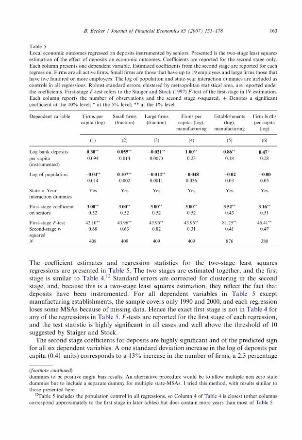
Local economic outcomes regressed on deposits instrumented by seniors. Presented is the two-stage least squares

estimation of the effect of deposits on economic outcomes. Coefficients are reported for the second stage only.

Each column presents one dependent variable. Estimated coefficients from the second stage are reported for each

regression. Firms are all active firms. Small firms are those that have up to 19 employees and large firms those that

have five hundred or more employees. The log of population and state-year interaction dummies are included as

controls in all regressions. Robust standard errors, clustered by metropolitan statistical area, are reported under

the coefficients. First-stage F -test refers to the Staiger and Stock (1997) F -test of the first-stage in IV estimation.

Each column reports the number of observations and the second stage r-squared. þ Denotes a significant

coefficient at the 10% level; * at the 5% level; ** at the 1% level.

Dependent variable Firms per

capita (log)

Small firms

(fraction)

Large firms

(fraction)

Firms per

capita. (log),

manufacturing

Establishments

(log),

manufacturing

Firm births

per capita

(log)

(1) (2) (3) (4) (5) (6)

Log bank deposits 0:30�� 0:055�� 0:021�� 1:00�� 0:86�� 0:47þ

per capita

(instrumented)

0.094 0.014 0.0073 0.23 0.18 0.28

Log of population �0:04�� 0:107�� 0:014�� 0:048 �0:02 �0:000.014 0.002 0.0011 0.036 0.03 0.05

State � Year

interaction dummies

Yes Yes Yes Yes Yes Yes

First-stage coefficient 3:00�� 3:00�� 3:00�� 3:00�� 3:52�� 3:16��

on seniors 0.52 0.52 0.52 0.52 0.43 0.51

First-stage F -test 42:10�� 43:96�� 43:96�� 43:96�� 81:25�� 46:41��

Second-stage r-

squared

0.68 0.63 0.82 0.31 0.41 0.47

N 408 409 409 409 876 380


The coefficient estimates and regression statistics for the two-stage least squaresregressions are presented in Table 5. The two stages are estimated together, and the firststage is similar to Table 4.12 Standard errors are corrected for clustering in the secondstage, and, because this is a two-stage least squares estimation, they reflect the fact thatdeposits have been instrumented. For all dependent variables in Table 5 exceptmanufacturing establishments, the sample covers only 1990 and 2000, and each regressionloses some MSAs because of missing data. Hence the exact first stage is not in Table 4 forany of the regressions in Table 5. F -tests are reported for the first stage of each regression,and the test statistic is highly significant in all cases and well above the threshold of 10suggested by Staiger and Stock.

The second stage coefficients for deposits are highly significant and of the predicted signfor all six dependent variables. A one standard deviation increase in the log of deposits percapita (0.41 units) corresponds to a 13% increase in the number of firms; a 2.3 percentage

(footnote continued)

dummies to be positive might bias results. An alternative procedure would be to allow multiple non zero state

dummies but to include a separate dummy for multiple state-MSAs. I tried this method, with results similar to

those presented here.12Table 5 includes the population control in all regressions, so Column 4 of Table 4 is closest (other columns

correspond approximately to the first stage in later tables) but does contain more years than most of Table 5.


point increase in the fraction of firms that are small (overall average 80.3%), a 0.9percentage point drop in the fraction of firms that are large (overall average 6.8%), a 50%increase in the number of manufacturing firms, and a 21% increase the number of firmsstarts.13 These fairly large magnitudes indicate that the local deposit supply is an importantdeterminant of local economic outcomes, especially affecting young and small firms.

5. Robustness and extensions

This section tackles several possible concerns with the base line results. Section 5.1examines industry-level data, offering verification that the effect of local deposit supply islargest in industries with high dependence on external finance. Section 5.2 addresseswhether seniors are exogenous in relation to economic outcomes. Seniors are replaced by alagged prediction of seniors, based on demographics. Section 5.3 verifies that variation inlocal levels of wealth is unlikely to cause a serious omitted variable bias. Controls areadded for local per capita income and house prices without affecting the results materially.Recent evidence suggests that MSAs could be too large to capture local bank markets. Thisis especially relevant for the larger MSAs that contain millions of inhabitants and tens ofthousands of firms. Section 5.4 presents results for narrower geographical areas. Finally,Section 5.5 examines the time-series evidence using changes in seniors.

5.1. Economic outcomes: industry variation

Firms in some industries are likely more dependent on external financing, such as bankloans, than others. Rajan and Zingales (1998) introduce a measure of industry externalfinance dependence based on a sample of Compustat firms. They show that countries withbetter financial development exhibit faster growth in industries with high externaldependence to a larger extent than in industries with low external dependence, and theyargue that technological factors determine external dependence. The same logic applies tolocal capital supply: if firms in some industries are exogenously more dependent onexternal financing, they respond more to local supply of bank loans. In order to assess this,I perform industry-level tests using a proxy for industry external finance dependence.Following Rajan and Zingales, I calculate the capex minus cash flow from operations,divided by capex. I use Compustat firms14 during 1985–1995, take the average across yearsfor each firm, and then determine the median across firms in an industry to get the industrymeasure of external dependence. I depart from Rajan and Zingales in defining the measurefor two-digit North American Industrial Classification System (NAICS) industries insteadof three-digit International Standard Industrial Classification (ISIC) manufacturingindustries.15 Data suppression for Census data on fine industry definitions makes itdifficult to use finer industries than the 2-digit level. Because all of manufacturing

13The ordinary least squares estimate of the coefficient (not reported) is slightly higher than the IV estimate

(0.37 versus 0.30) and has a much lower standard error (0.02 versus 0.09). This suggests an upward bias in the

ordinary least squares estimate, which could be caused by reverse causality.14As argued by Rajan and Zingales, the financing choices of Compustat firms, which are large and likely to be

the least financially constrained of all firms in the economy, are appropriate for capturing demand for financing.15NAICS 51 (Information) and NAICS 95 (Auxiliaries, exc. corp, subsidiary, and regional managing offices)

are excluded for lack of data on establishments and other outcomes (by MSA).


constitutes a single two-digit industry, I include all industries (i.e., various services as wellas manufacturing) to get useful variation.

The instrumented variable is bank deposits interacted with industry externaldependence, and the instrument is seniors interacted with external dependence:

Y ij ¼ a0 þ b0Hi � Ej þ X i þ Zj , (3)

where Y is an outcome variable, Hi � Ej deposits in MSA i times external dependence ofindustry j, and fixed effects X and Z for MSAs and industries, respectively. The instrumentfor Hi � Ej is the fraction of seniors in the local population times industry dependence:Si � Ej. By construction the interaction variable Ej does not vary by location i, only byindustry j. The interaction Si � Ej is a valid instrument for Hi � Ej (as long as seniors Si isa valid instrument for deposits HiÞ.

16

I use three alternative outcome variables available at the industry level: number ofestablishments, number of employees and sales (data on the number of firms areunavailable). All data are from the 1997 Economic Census. I use 2000 data on seniorsbecause they are closest to 1997 in time, but 1990 seniors data produce indistinguishableresults (not reported).

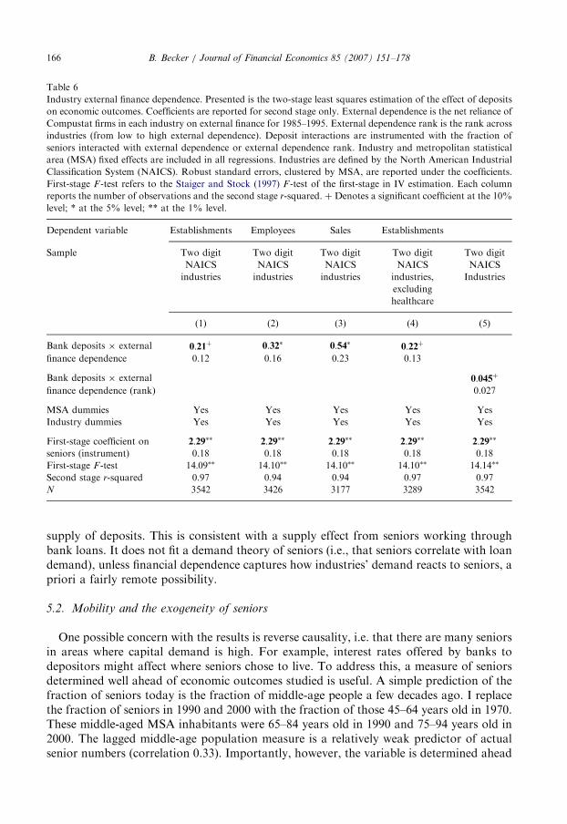
Table 6 presents second stage results from two-stage least squares regressions. First stageinformation is reported at the bottom of each column. Column 1 shows that, aftercontrolling for industry and MSA fixed effects, the interaction of bank deposits andexternal dependence has a positive and significant (10% level) effect on the number ofestablishments.17 The variable can be interpreted as follows: In an industry with externaldependence one standard deviation (0.85) above the mean, the elasticity of the number ofestablishments with respect to local bank deposit supply is 0.18 higher (than at meanexternal dependence). Columns 2 and 3 present similar regressions for the alternativedependent variables (employees and sales) where coefficient estimates are slightly morestatistically significant as well as somewhat larger.

There are more healthcare establishments where there are many seniors, presumably forreasons that have nothing to do with firm financing. This might affect the industry levelresults. Column three therefore presents results for establishments when NAICS 62 (healthcare and social assistance) is excluded. Excluding this industry has virtually no effect on theestimated coefficient.

Finally, Column 5 of Table 6 uses the rank of industry external dependence instead ofthe actual number. The rank is less sensitive to outliers and to the particular details ofestimated dependence but relies exclusively on the industry order of external dependence.The ranking is from low to high, so that a positive interaction indicates that industries withhigher external dependence are more responsive to deposit supply. The coefficient ispositive and significant (10%) and implies a magnitude similar to the one estimated in theColumn 1.

The regressions have controlled for MSA fixed effects, so omitted variables are unlikelyto be a large concern in these regressions. Therefore, it is fair to conclude that industrieswhich rely more on external financing for their investment are more sensitive to the local

16Intuitively, the test using interactions is similar to running the regression separately by industry and checking

if slopes increase with external dependence.17The fixed effects absorb almost all variation (the second-stage r-squared is above 0.9 and only slightly affected

by including the interaction).

ARTICLE IN PRESS

Table 6

Industry external finance dependence. Presented is the two-stage least squares estimation of the effect of deposits

on economic outcomes. Coefficients are reported for second stage only. External dependence is the net reliance of

Compustat firms in each industry on external finance for 1985–1995. External dependence rank is the rank across

industries (from low to high external dependence). Deposit interactions are instrumented with the fraction of

seniors interacted with external dependence or external dependence rank. Industry and metropolitan statistical

area (MSA) fixed effects are included in all regressions. Industries are defined by the North American Industrial

Classification System (NAICS). Robust standard errors, clustered by MSA, are reported under the coefficients.

First-stage F -test refers to the Staiger and Stock (1997) F -test of the first-stage in IV estimation. Each column

reports the number of observations and the second stage r-squared. þ Denotes a significant coefficient at the 10%

level; * at the 5% level; ** at the 1% level.

Dependent variable Establishments Employees Sales Establishments

Sample Two digit

NAICS

industries

Two digit

NAICS

industries

Two digit

NAICS

industries

Two digit

NAICS

industries,

excluding

healthcare

Two digit

NAICS

Industries

(1) (2) (3) (4) (5)

Bank deposits � external 0:21þ 0:32� 0:54� 0:22þ

finance dependence 0.12 0.16 0.23 0.13

Bank deposits � external 0:045þ

finance dependence (rank) 0.027

MSA dummies Yes Yes Yes Yes Yes

Industry dummies Yes Yes Yes Yes Yes

First-stage coefficient on 2:29�� 2:29�� 2:29�� 2:29�� 2:29��

seniors (instrument) 0.18 0.18 0.18 0.18 0.18

First-stage F -test 14:09�� 14:10�� 14:10�� 14:10�� 14:14��

Second stage r-squared 0.97 0.94 0.94 0.97 0.97

N 3542 3426 3177 3289 3542


supply of deposits. This is consistent with a supply effect from seniors working throughbank loans. It does not fit a demand theory of seniors (i.e., that seniors correlate with loandemand), unless financial dependence captures how industries’ demand reacts to seniors, apriori a fairly remote possibility.

5.2. Mobility and the exogeneity of seniors

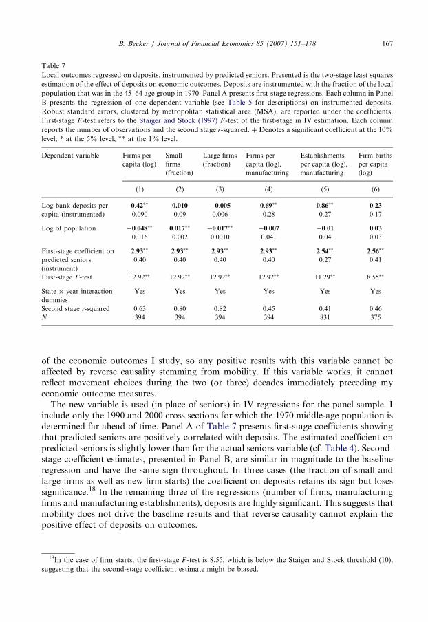
One possible concern with the results is reverse causality, i.e. that there are many seniorsin areas where capital demand is high. For example, interest rates offered by banks todepositors might affect where seniors chose to live. To address this, a measure of seniorsdetermined well ahead of economic outcomes studied is useful. A simple prediction of thefraction of seniors today is the fraction of middle-age people a few decades ago. I replacethe fraction of seniors in 1990 and 2000 with the fraction of those 45–64 years old in 1970.These middle-aged MSA inhabitants were 65–84 years old in 1990 and 75–94 years old in2000. The lagged middle-age population measure is a relatively weak predictor of actualsenior numbers (correlation 0.33). Importantly, however, the variable is determined ahead

ARTICLE IN PRESS

Table 7

Local outcomes regressed on deposits, instrumented by predicted seniors. Presented is the two-stage least squares

estimation of the effect of deposits on economic outcomes. Deposits are instrumented with the fraction of the local

population that was in the 45–64 age group in 1970. Panel A presents first-stage regressions. Each column in Panel

B presents the regression of one dependent variable (see Table 5 for descriptions) on instrumented deposits.

Robust standard errors, clustered by metropolitan statistical area (MSA), are reported under the coefficients.

First-stage F -test refers to the Staiger and Stock (1997) F -test of the first-stage in IV estimation. Each column

reports the number of observations and the second stage r-squared. þ Denotes a significant coefficient at the 10%

level; * at the 5% level; ** at the 1% level.


capita (log)

Small

firms

(fraction)

Large firms

(fraction)

Firms per

capita (log),

manufacturing

Establishments

per capita (log),

manufacturing

Firm births

per capita

(log)

(1) (2) (3) (4) (5) (6)

Log bank deposits per 0:42�� 0.010 �0:005 0:69�� 0:86�� 0:23capita (instrumented) 0.090 0.09 0.006 0.28 0.27 0.17

Log of population �0:048�� 0:017�� 0:017�� 0:007 �0:01 0:030.016 0.002 0.0010 0.041 0.04 0.03

First-stage coefficient on 2:93�� 2:93�� 2:93�� 2:93�� 2:54�� 2:56��

predicted seniors

(instrument)

0.40 0.40 0.40 0.40 0.27 0.41


State � year interaction

dummies

Yes Yes Yes Yes Yes Yes

Second stage r-squared 0.63 0.80 0.82 0.45 0.41 0.46

N 394 394 394 394 831 375


of the economic outcomes I study, so any positive results with this variable cannot beaffected by reverse causality stemming from mobility. If this variable works, it cannotreflect movement choices during the two (or three) decades immediately preceding myeconomic outcome measures.

The new variable is used (in place of seniors) in IV regressions for the panel sample. Iinclude only the 1990 and 2000 cross sections for which the 1970 middle-age population isdetermined far ahead of time. Panel A of Table 7 presents first-stage coefficients showingthat predicted seniors are positively correlated with deposits. The estimated coefficient onpredicted seniors is slightly lower than for the actual seniors variable (cf. Table 4). Second-stage coefficient estimates, presented in Panel B, are similar in magnitude to the baselineregression and have the same sign throughout. In three cases (the fraction of small andlarge firms as well as new firm starts) the coefficient on deposits retains its sign but losessignificance.18 In the remaining three of the regressions (number of firms, manufacturingfirms and manufacturing establishments), deposits are highly significant. This suggests thatmobility does not drive the baseline results and that reverse causality cannot explain thepositive effect of deposits on outcomes.

18In the case of firm starts, the first-stage F -test is 8.55, which is below the Staiger and Stock threshold (10),

suggesting that the second-stage coefficient estimate might be biased.


5.3. Additional controls

One concern with the baseline results is that there is no control for variation in wealthacross MSAs. This concern is important for policy inferences. If seniors are wealthier thanother groups, they could affect local loan demand (instead of loan supply) through theirwealth. A city with more seniors could experience more economic activity to serve thewealth driven demand for locally produced goods or services. In this case, financialfrictions do not affect the extent of geographical segmentation, so better regulation has nohope of improving the geographical allocation of capital. To rule out such a wealth-demand effect, I attempt to control for variation in local wealth levels.Measuring wealth properly is obviously difficult, but some reasonable proxies are easy

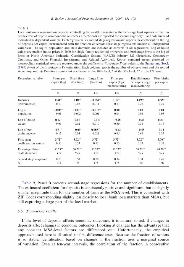
to identify. First, real estate prices are likely to reflect local wealth. I include the medianprice for residential single-family houses by MSA. This is measured as the log of medianhouse prices. A second control is the log of per capita income, also likely to be related tolocal wealth levels. House prices are only available for 2000 (income data are available forall years), so tests are cross-sectional.Results for all six dependent variables, with wealth controls, are presented in Table 8.

Population is included as a control. The estimated effects of both wealth variables aresignificantly positive for firms. High house prices predict more firm starts, and incomepredicts larger firms. Controlling for wealth tends not to affect the magnitude andsignificance of the estimated effect of deposits. The estimated deposit coefficient is positive,similar to baseline results but always somewhat larger in magnitude. This suggests that thebaseline results on deposits are not driven by omitted variable bias due to wealth. Thisconclusion is only as strong as the quality of wealth controls. To the extent that wealth isnot reflected in either house prices or incomes, I cannot rule out that senior wealth hassome effect on local demand.

5.4. What is the relevant local market?

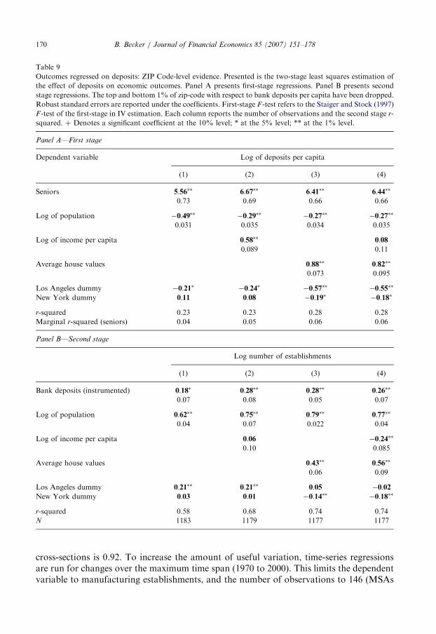
Previous research (e.g. Garmaise and Moskowitz, 2006; Petersen and Rajan, 1995) hassuggested that much bank lending is local. MSAs could be too large to capture market sizeideally. As a robustness test, it is therefore useful to look at a narrower market definitionthan the MSA, avoiding the possible pooling of distinct markets into a single observation.For this purpose, I use deposits and demographic data at the ZIP Code level. Manysmaller MSAs intersect only one or two ZIP Codes, but, for larger cities, the number ofZIP Codes could be in the hundreds. I therefore look at ZIP Code results for New York,Los Angeles, and Chicago, the MSAs cities with the largest populations. Counting all ZIPCodes that cover any part of each city’s consolidated metropolitan statistical area(CMSA), but excluding all ZIP Codes with less than one thousand residents, New Yorkhas 890, Los Angeles has 505, and Chicago has 340. At the zip-code level, little economicinformation is available. The dependent variable is number of establishments. Income andmedian house values are used to control for wealth.Results for ZIP Codes are presented in Table 9. Panel A shows that the fraction of

seniors has a large positive effect on deposits whether local house values are controlled foror not. The estimated coefficients are slightly higher than the MSA-level numbers (seeTable 4) and highly significant. This is what can be expected if ZIP Codes correspond moreclosely to the geographical market for deposits.

ARTICLE IN PRESS

Table 8

Local outcomes regressed on deposits, controlling for wealth. Presented is the two-stage least squares estimation

of the effect of deposits on economic outcomes. Coefficients are reported for second stage only. Each column head

indicates the dependent variable. Each regression is a second stage regression and reports the coefficient on the log

of deposits per capita, instrumented with the fraction of seniors (first-stage regressions include all independent

variables). The log of population and state dummies are included as controls in all regressions. Log of house

values are median house prices in 2000 for single-family residential properties and brokerage firms is the log of

firms in North American Industrial Classification System (NAICS) industry 523 (Securities, Commodity

Contracts, and Other Financial Investments and Related Activities). Robust standard errors, clustered by

metropolitan statistical area, are reported under the coefficients. First-stage F -test refers to the Staiger and Stock

(1997) F -test of the first-stage in IV estimation. Each column reports the number of observations and the second

stage r-squared. þ Denotes a significant coefficient at the 10% level; * at the 5% level; ** at the 1% level.


capita (log)

Small firms

(fraction)

Large firms

(fraction)

Firms per

capita (log),

manufacturing

Establishments

per capita (log),

manufacturing

Firm births

per capita

(1) (2) (3) (4) (5) (6)

Deposits 0:31�� 0:10�� 0:052�� 1:19�� 1:19�� 0:52þ

(instrumented) 0.10 0.02 0.011 0.27 0.28 0.29

Log of �0:05�� 0:017�� 0:018�� 0:00 0:01 0:04population 0.01 0.002 0.001 0.04 0.04 0.03

Log of house 0:12þ 0:01 �0:013 �0:25 �0:27 0:26þ

values 0.06 0.02 0.010 0.30 0.31 0.14

Log of per 0:31� �0:09� 0:055�� 0:43 �0:43 0:11capita income 0.13 0.04 0.021 0.65 0.66 0.27

First-stage 3:72�� 3:72�� 3:72�� 3:72�� 3:72�� 3:76��

coefficient on seniors 0.53 0.53 0.53 0.53 0.53 0.53


State dummies Yes Yes Yes Yes Yes Yes

Second stage r-squared 0.78 0.50 0.70 0.34 0.34 0.48

N 175 175 175 175 175 166


Table 9, Panel B presents second-stage regressions for the number of establishments.The estimated coefficient for deposits is consistently positive and significant, but of slightlysmaller magnitude than for the number of firms at the MSA level. This is consistent withZIP Codes corresponding slightly less closely to local bank loan markets than MSAs, butstill capturing a large part of the local market.

5.5. Time-series results

If the level of deposits affects economic outcomes, it is natural to ask if changes indeposits affect changes in economic outcomes. Looking at changes has the advantage thatany constant MSA-level factors are differenced out. Unfortunately, the empiricalapproach used here is ill suited to first-difference tests. Because the fraction of seniorsis so stable, identification based on changes in the fraction uses a marginal sourceof variation. Even at ten-year intervals, the correlation of the fraction in consecutive

ARTICLE IN PRESS

Table 9

Outcomes regressed on deposits: ZIP Code-level evidence. Presented is the two-stage least squares estimation of

the effect of deposits on economic outcomes. Panel A presents first-stage regressions. Panel B presents second

stage regressions. The top and bottom 1% of zip-code with respect to bank deposits per capita have been dropped.

Robust standard errors are reported under the coefficients. First-stage F -test refers to the Staiger and Stock (1997)

F -test of the first-stage in IV estimation. Each column reports the number of observations and the second stage r-

squared. þ Denotes a significant coefficient at the 10% level; * at the 5% level; ** at the 1% level.

Panel A—First stage

Dependent variable Log of deposits per capita

(1) (2) (3) (4)

Seniors 5:56�� 6:67�� 6:41�� 6:44��

0.73 0.69 0.66 0.66

Log of population �0:49�� 0:29�� 0:27�� 0:27��

0.031 0.035 0.034 0.035

Log of income per capita 0:58�� 0:080.089 0.11

Average house values 0:88�� 0:82��

0.073 0.095

Los Angeles dummy �0:21� �0:24� �0:57�� 0:55��

New York dummy 0:11 0:08 �0:19� �0:18�

r-squared 0.23 0.23 0.28 0.28

Marginal r-squared (seniors) 0.04 0.05 0.06 0.06

Panel B—Second stage

Log number of establishments

(1) (2) (3) (4)

Bank deposits (instrumented) 0:18� 0:28�� 0:28�� 0:26��

0.07 0.08 0.05 0.07

Log of population 0:62�� 0:75�� 0:79�� 0:77��

0.04 0.07 0.022 0.04

Log of income per capita 0:06 �0:24��

0.10 0.085

Average house values 0:43�� 0:56��

0.06 0.09

Los Angeles dummy 0:21�� 0:21�� 0:05 �0:02New York dummy 0:03 0:01 �0:14�� 0:18��

r-squared 0.58 0.68 0.74 0.74

N 1183 1179 1177 1177


cross-sections is 0.92. To increase the amount of useful variation, time-series regressionsare run for changes over the maximum time span (1970 to 2000). This limits the dependentvariable to manufacturing establishments, and the number of observations to 146 (MSAs

ARTICLE IN PRESS

Table 10

Time-series evidence. Reported is the two-stage least squares estimation of the effect of deposits on economic

outcomes. Deposits are instrumented with the change in seniors 1970–2000. The change in the log of population is

included as control. Robust standard errors, clustered by metropolitan statistical area, are reported under the

coefficients, and the number of observations in the row after that. First-stage F -test refers to the Staiger and Stock

(1997) F -test of the first-stage in IV estimation. Each column reports the number of observations and the second

stage r-squared. The text n/a means not available. þ Denotes a significant coefficient at the 10% level; * at the 5%

level; ** at the 1% level.

Change in number of manufacturing establishments

(log)

(1) (2) (3) (4)

Change in bank deposits (instr. with change in seniors) 1:78 1:52þ

1.07 0.82

Change in bank deposits (instr. with change in seniors 1:85þ 1:54�

and 1970 level of seniors) 1.02 0.74

Change in population �0:03 �0:00 �0:03 �0:000.39 0.21 0.40 0.21

Change in income per capita �1:17 �1:180.78 0.72

First-stage coefficient on change in seniors 2:56þ 2:96� 3:17� 3:75�

1.44 1.39 1.56 1.51

First-stage coefficient on initial level of seniors 0:96 1:230.93 0.89

First-stage F -test 2:65þ 3:54þ 2:36þ 3:26�

State dummies Yes Yes Yes Yes

Second stage r-squared n/a n/a n/a n/a

N 146 146 146 146


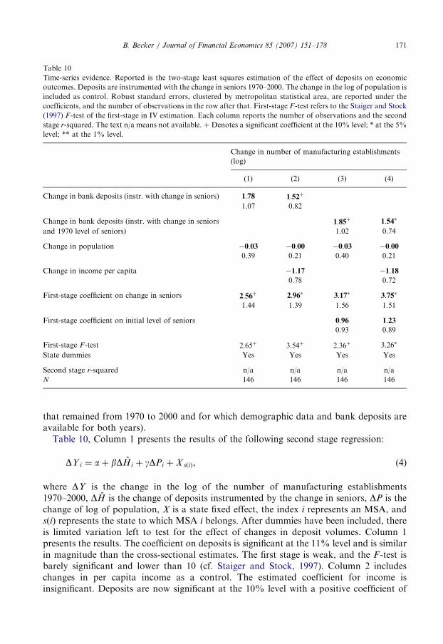
that remained from 1970 to 2000 and for which demographic data and bank deposits areavailable for both years).

Table 10, Column 1 presents the results of the following second stage regression:

DY i ¼ aþ bDHi þ gDPi þ X sðiÞ, (4)

where DY is the change in the log of the number of manufacturing establishments1970–2000, DH is the change of deposits instrumented by the change in seniors, DP is thechange of log of population, X is a state fixed effect, the index i represents an MSA, andsðiÞ represents the state to which MSA i belongs. After dummies have been included, thereis limited variation left to test for the effect of changes in deposit volumes. Column 1presents the results. The coefficient on deposits is significant at the 11% level and is similarin magnitude than the cross-sectional estimates. The first stage is weak, and the F -test isbarely significant and lower than 10 (cf. Staiger and Stock, 1997). Column 2 includeschanges in per capita income as a control. The estimated coefficient for income isinsignificant. Deposits are now significant at the 10% level with a positive coefficient of


1.52. The implied effect of a one standard deviation increase of the change in log bankdeposits per capita (0.32 for the three decades) is a 62% increase in the number ofestablishments, corresponding to a difference in annual growth rates of 1.6%. The firststage remains weak, although significance is higher.Because changes in seniors are small, this test has limited power. An additional

instrument might therefore be useful. One possibility is to use the initial level of seniors in1970, which is useful if the level of seniors has not always completely affected deposits andlending, because of some kind of lag. In Columns 3–4 of Table 10 the change in bankdeposits is instrumented with the initial level of seniors as well as the change. Now theeffect of deposits is estimated to be significant (at the 10% or 5% level depending onwhether income changes are included as a control). The first stage remains weak with thesecond instrument, and a joint significance test of the instruments gives an F -statistic ofborderline significance. Given the caveat that the first stage is weakly identified, theseresults could offer some limited support of the cross-sectional conclusion that depositshave a positive effect on the local economy. With finer geographical units, future datamight allow a better identified test.

6. Geographically segmented financial markets: what impedes reallocation?

The evidence that financial markets are geographically segmented implies that frictionsexist between MSAs. This does not pinpoint the source of geographical frictions or whatfactors determine their level. For example, are external or internal capital markets moreimportant for geographic reallocation between areas? This section goes some way towardidentifying the nature of frictions.There are several ways in which capital can be moved geographically: firms borrowing

from banks far away, banks using financing that is less local than deposits (e.g., publicequity and bonds markets), and transfers between branches of a bank present in multipleareas (internal capital markets). The following subsections discuss various modes ofreallocation, examine predictions for where local deposits are likely to be most important,and discuss the extent to which each prediction is consistent with the findings reportedabove. Finally, the substantial US bank deregulation over the last few decades is used totest whether regulation has been a source of geographical frictions.

6.1. Firm financing

The literature on what is called the credit channel of monetary policy transmission hasemphasized the different ways in which bank lending is special as a source of firm financing(i.e. does not have close substitutes). The implication is that firms cannot easily replaceabsent bank loans with alternative financing. The evidence on bank loan supply is largelybased on time-series variation in lending (see, e.g., Bernanke and Blinder, 1988; Kashyapand Stein, 1994, 2000; Bernanke and Gertler, 1995). In cross-sectional tests, Peek andRosengren (1997) as well as Ashcraft (2005) suggest that local economies can besubstantially affected by lending, indicating that alternative financing is not available foran economically important subset of firms.Even if banks constitute the sole possible source of external finance for most firms, could

they not borrow from faraway banks? The evidence presented by Petersen and Rajan(2002) suggests that perhaps not. They show that distances between US borrowers and


lenders are increasing, but that distances generally remain short even in later years. In theirsample, the median distance between borrower and bank is two miles for lendingrelationships started in 1973–1979, four miles for relationships started in 1980–1989, andfive miles for relationships started in 1990–1993. Brevoort and Hannan (2004) suggest thatdistance could be of increasing importance in US commercial lending. These resultssuggest that, for many firms, borrowing at a distance is still expensive or impossible,consistent with geographical segmentation.

6.2. Bank financing

Kashyap and Stein (2000) show that banks in general, and banks below the 75thpercentile by asset size in particular, rely very heavily on deposit financing: ‘‘The smallestbanks have a very simple capital structure—they are financed almost exclusively withdeposits and common equity.’’ Houston et al. (1997) find that the lending of bank holdingcompanies is linked to the internally generated cash and available capital, i.e., they areliquidity constrained. Driscoll (2004) also confirms banks’ dependence on deposits—hefinds that shocks to deposit volumes affect lending at both the state and regional levels.While small and medium size banks are heavily dependent on deposits, large banks havebetter access to market mediated finance. This suggests that the local supply of deposits ismost important when banks are small. Similarly, banks that are not listed on a stockexchange likely face more obstacles to equity financing.19 However, it seems reasonable topredict that areas with many listed banks are less subject to the constraints of local depositsupply.

6.3. Multi-MSA banks

One possible channel for geographic reallocation of capital is transfers between branchesof the same bank. In 1980, more than half of all US banks were unit banks (had only onebranch); in 1990, a little less than half were unit banks; and in 2000, about a third of allbanks were unit banks. These unit banks have no ability to transfer funds to otherlocations through internal capital markets. Of multi-branch banks, about 25% hadbranches in only one MSA in 2000. For bank companies with a presence in several MSAs,there are legal constraints on transfers between branches.20 Organizational reasons not totransfer funds from deposit-rich to deposit-poor areas could exist as well. For example, itcould be optimal to allow a certain local discretion in capital allocation decisions, as in themodel of Stein (2002), which is likely to limit the extent of transfers across branches.Recent empirical work has gone some way toward identifying the extent to which internalcapital markets are active in banks, at least on the year-to-year margin. Houston et al.(1997), Houston and James (1998), and Campello (2002) all find that lending by bankswith access to internal capital markets is less constrained. These findings suggest that

19Even banks listed on stock exchanges face costs of issuing equity. For the fact that firms are reluctant to issue

equity, see Welch (2004). For evidence that bank stock prices fall when they issue equity, see Slovin et al. (1991).

The cost of issuing equity could be the result of asymmetric information as in Myers and Majluf (1984).20Banks with multiple branches (or bank holding companies with multiple banks) face regulatory limits to

transfers between branches, through the Community Reinvestment Act (CRA), which was intended to encourage

depository institutions to help meet the credit needs of the communities in which they operate.


MSAs where banks are local are more exposed to local deposit supply than MSAs withmany multi-MSA banks.21

6.4. Empirical results on the regulatory nature of frictions

The overview of channels of geographical reallocation suggest that large banks generallyare likely to have better access to reallocation than small banks, both nondeposit externalfinancing and internal capital markets. Using this prediction empirically is complicated bythe potential endogeneity of bank size. The size of local banks is likely not exogenous tothe local economic environment.To test the whether access to internal and external capital markets affects segmentation,

I employ an empirical strategy using regulation. I exploit the timing of bank de-regulation, as reported in Kroszner and Strahan (1999), to identify the regulatorylimits to the creation of banks with internal capital markets spanning several cities(and states). Starting around 1970, US states deregulated their bank markets in severalstages, first allowing mergers, later intrastate branching, and finally cross-stateborder banking. Kroszner and Strahan (1999) identify the most important step asallowing within-state bank mergers, which for the first time allowed integration of branchnetworks. This deregulation happened at different rates in different states, before 1970 insome states, at some later point in some states, and not until the federal deregulation of1994 in a few.22

I test if the local capital supply had a larger effect on the local economy pre-deregulationthat post. To do this, I interact a dummy for state-years where intrastate mergers arederegulated with local bank deposits and relate the interaction to an economic outcome.23

With the interaction as well as the level of seniors both needing instruments, estimationrequires a second instrument. For this, I use the interaction of seniors and the deregulationdummy. I then run two-stage least squares with two instruments and two instrumentedvariables. The first stage regressions work as expected: The level of seniors (but not theinteraction of seniors and deregulation) predicts the level of deposits, while the interactionof seniors with deregulation (but not the level of seniors) predicts the interaction ofdeposits and deregulation. Because there are fixed MSA effects, the level of depositscontains only time-series variation, which is only weakly explained by changes in seniors(see Table 10).24

Most of the variation in regulation is early in the sample, so this estimation requires adependent variable going far back as possible. I therefore use manufacturing establish-ments, which is available starting in 1970. Table 11 presents the results of IV regressionsincluding the interaction of deregulation with deposits, controlling for MSA and year

21Furthermore, small banks lend differently from larger banks, and this could also affect how deposit supply

impacts the local economy. See, e.g., Brickley et al. (2003) and Berger et al. (2005).22Kroszner and Strahan (1999) discuss the political economy of this deregulation. As long as the decision to

deregulate was not driven by future reductions in segmentation for non regulatory reasons, it can be considered an

exogenous change.23I also tried an alternative regulation dummy defined as equal to one if all three of Kroszner and Strahan’s

deregulation steps were implemented in a state. The results (not reported) were similar.24The Staiger and Stock F -test of the instruments does not apply to the case with multiple endogenous

variables. In terms of first-stage coefficient significance and marginal r-squared, the interaction is well

instrumented.

ARTICLE IN PRESS

Table 11

Local economic effects and regulation. Presented is the two-stage least squares estimation of the effect of deposits

on economic outcomes. Deposits are instrumented with the fraction of seniors. The Intrastate mergers deregulated

dummy is equal to one if intrastate branching through mergers has been deregulated, and is based on Kroszner

and Strahan (1999). Robust standard errors, clustered by metropolitan statistical area (MSA), are reported under

the coefficients. Each column reports the number of observations and the second stage r-squared. þ Denotes a

significant coefficient at the 10% level; * at the 5% level; ** at the 1% level.

Number of manufacturing establishments per capita (log)

(1) (2)

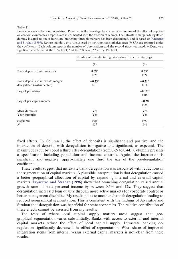
Bank deposits (instrumented) 0:69� 0:55�

0.28 0.24

Bank deposits � intrastate mergers �0:25þ �0:21þ

deregulated (instrumented) 0.13 0.11

Log of population �0:16��

0.06

Log of per capita income �0:280.28

MSA dummies Yes Yes

Year dummies Yes Yes

r-squared 0.86 0.90

N 857 841


fixed effects. In Column 1, the effect of deposits is significant and positive, and theinteraction of deposits with deregulation is negative and significant, as expected. Themagnitude is cut by about a third after deregulation (from 0.69 to 0.44). Column 2 presentsa specification including population and income controls. Again, the interaction issignificant and negative, approximately one third the size of the pre-deregulationcoefficient.

These results suggest that intrastate bank deregulation was associated with reductions inthe segmentation of capital markets. A plausible interpretation is that deregulation causeda better geographical allocation of capital by expanding internal and external capitalmarkets. Jayaratne and Strahan (1996) show that branching deregulation raised annualgrowth rates of state personal income by between 0.5% and 1%. They suggest thatderegulation increased loan quality through more active markets for corporate control orbetter management discipline. My results point to another channel: deregulation leading toreduced geographical segmentation. This is consistent with the findings of Jayaratne andStrahan that deregulation was beneficial for state economies. The relative contribution ofthese effects cannot be assessed from my results.

The tests of where local capital supply matters most suggest that geo-graphical segmentation varies substantially. Banks with access to external and internalcapital markets reduce the effect of local capital supply. Intrastate banking de-regulation significantly decreased the effect of segmentation. What share of improvedintegration stems from internal versus external capital markets is not clear from theseresults.


7. Conclusions

I use the fraction of seniors as an instrument for the local supply of deposits and, hence,of bank loans. The supply of deposits affects economic outcomes: When deposits are highas a result of demographics, there are more firms, especially small, both overall and inmanufacturing, as well as more new firms. The results are robust to several alternativespecifications: using demographic predictions of future senior numbers, including controlsfor local wealth, and reducing area size from MSA to ZIP Code. Time-series evidencebased on changes in seniors, though based on limited variation, also supports the maincross-sectional findings.If capital has a declining marginal productivity at the MSA level, the welfare

implications of variations in the supply of capital to firms are negative. Capital is usedat lower marginal productivity in locations with higher loan supply, whereas, in africtionless world, this capital could be reallocated to a different location with highermarginal productivity of capital.Bank deregulation has been shown to have positive effects on economic outcomes (see,

e.g., Jayaratne and Strahan, 1996; Morgan et al., 2004). In terms of mechanisms, the focushas been on bank competition. My results suggest that the effect of bank deregulation ongeographical allocation of capital could be important as well. I estimate that the effect oflocal deposit supply on the local economy is a third weaker after deregulation than beforeit. This suggests that US state-level deregulation reduced geographical segmentation(perhaps through increased bank size improving access to internal and external capitalmarkets). This improved geographical allocation could have important welfare benefits.This conclusion has clear regulatory implications. A banking system with small andgeographically fragmented institutions (as, e.g. Spain, the US and Italy have hadhistorically) is inefficient because it aggravates the geographical segmentation of capitalmarkets.25 This is likely to be especially severe in geographically large countries and incountries with substantial geographical variation in the supply of capital, as well as ineconomies where deposit-financed institutions play a large role in financial intermediation.Several extensions of these results would illuminate the effect of capital market

segmentation. First, along the lines of Kashyap and Stein (2000) and Campello (2002), arebanks in low deposit areas more exposed to monetary shocks? Second, after deregulation,are areas with many small, local banks more exposed to local deposit supply? Third, doesthe local deposit supply affect loan pricing and the capital structure for local firms?

References

Ashcraft, A., 2005. Are banks really special? New evidence from the FDIC-induced failure of healthy Banks.

American Economic Review 95, 1712–1730.

Bassett, B., Brady, T., 2002. What drives the persistent competitiveness of small banks? Finance and Economics

Discussion Series working paper 2002-28. Board of Governors of the Federal Reserve System.

Berger, A.N., Miller, N.H., Petersen, M.A., Rajan, R.G., Stein, J.C., 2005. Does function follow organizational

form? Evidence from the lending practices of large and small banks, vol. 76 (2), pp. 237–269.

Bernanke, B., Blinder, A., 1988. Credit, money and aggregate demand. American Economic Review 78 (3),

435–439.

25See, e.g., Cetorelli and Gambera (2001) for evidence that bank consolidation varies dramatically between

developed countries.


Bernanke, B., Gertler, M., 1995. Inside the Black Box: The Credit Channel of Monetary Policy Transmission.

Journal of Economic Perspectives 9 (4), 27–48.

Brevoort, K., Hannan, T., 2004. Commercial lending and distance: evidence from community reinvestment act

data. Finance and Economics Discussion Series working paper 2004-24. Board of Governors of the Federal

Reserve System.

Brickley, J.A., Linck, J.S., Smith, C., 2003. Boundaries of the firm: evidence from the banking industry. Journal of

Financial Economics 70 (3), 351–383.

Campello, M., 2002. Internal capital markets in financial conglomerates; evidence from small bank responses to

monetary policy. Journal of Finance 57 (6), 2773–2805.

Cetorelli, N., Gambera, M., 2001. Banking market structure, financial dependence and growth: international

evidence from industry data. Journal of Finance 61 (2), 617–648.

Cetorelli, N., Strahan, P., 2006. Finance as a barrier to entry: bank competition and industry structure in local

U.S. markets. Journal of Finance 61 (1), 437–461.

Driscoll, J., 2004. Does bank lending affect output evidence from U.S. states. Journal of Monetary Economics 51

(3), 451–471.

Garmaise, M., Moskowitz, T., 2006. Bank mergers and crime: the real and social effects of credit market

competition. Journal of Finance 61, 495–538.

Gendell, M., Siegel, J., 1992. Trends in retirement age by sex, 1950–2005. Monthly Labor Review 115 (7),

22–29.

Gertler, M., Gilchrist, S., 1994. Monetary policy, business cycles, and the behavior of small manufacturing firms.

Quarterly Journal of Economics 109 (2), 309–340.

Guiso, L., Sapienza, P., Zingales, L., 2004. Does local financial development matter? Quarterly Journal of

Economics 119 (3), 929–969.

Heaton, J., Lucas, D., 2000. Portfolio choice and asset prices: the importance of entrepreneurial risk. Journal of

Finance 55 (3), 1163–1198.

Houston, J.F., James, C., 1998. Do bank internal capital markets promote lending? Journal of Banking and

Finance 22, 899–918.

Houston, J.F., James, C., Marcus, D., 1997. Do bank internal capital markets promote lending? Journal of

Financial Economics 46 (2), 135–164.

Jayaratne, J., Strahan, P., 1996. The finance-growth nexus: evidence from bank branch deregulation. Quarterly

Journal of Economics 111 (3), 639–670.

Kashyap, A., Stein, J., 1994. Monetary policy and bank lending. In: Mankiw, G. (Ed.), Monetary Policy.

University of Chicago Press, Chicago, IL.

Kashyap, A., Stein, J., 2000. What do a million observations on banks say about the transmission of monetary

policy. American Economic Review 90 (3), 407–428.

Kroszner, R., Strahan, P., 1999. What drives deregulation? Economics and politics of the relaxation of bank

branching restrictions. Quarterly Journal of Economics 114 (4), 1437–1467.

Morgan, D.P., Rime, B., Strahan, P., 2004. Bank integration and state business cycles. Quarterly Journal of

Economics 119 (4), 1555–1585.

Moskowitz, T., Vissing-Jorgensen, A., 2002. The returns to entrepreneurial investment: a private equity premium

puzzle? American Economic Review 92 (4), 745–778.

Myers, S., Majluf, N., 1984. Corporate financing and investment decisions when firms have information that

investors do not have. Journal of Financial Economics 13, 187–221.

Peek, J., Rosengren, E., 1997. The international transmission of financial shocks: the case of Japan. American

Economic Review, September 87 (4), 495–505.

Peek, J., Rosengren, E., 2000. Collateral damage: effects of the Japanese bank crisis on real activity in the United

States. American Economic Review, March 90 (1), 30–45.

Petersen, M., Rajan, R.G., 1994. The benefits of lending relationships. Journal of Finance 49, 3–37.

Petersen, M., Rajan, R.G., 1995. The effect of credit market competition on firm-creditor relationships. Quarterly

Journal of Economics 110, 407–443.

Petersen, M., Rajan, R.G., 2002. Does distance still matter? The information revolution in small business lending.

Journal of Finance 57 (6), 2533–2570.

Rajan, R.G., Zingales, L., 1998. Financial development and growth. American Economic Review, June 88,

559–586.

Sapienza, P., 2002. The effects of banking mergers on loan contracts. Journal of Finance, February 57 (1),

329–368.


Slovin, M., Shuska, M., Polonchek, J., 1991. The informational content of multiple seasoned common stock

offerings by bank holding companies. Journal of Banking and Finance 15, 633–646.

Staiger, D., Stock, J., 1997. Instrumental variables regression with weak instruments. Econometrica 65 (3),

557–586.

Stein, J., 2002. Information production and capital allocation: decentralized versus hierarchical firms. Journal of

Finance 57 (5), 1891–1921.

US Bureau of the Census, 1998. State and Metropolitan Area Data Book 1997–98, fifth ed. Washington, DC.

Wiatrowski, W., 2001. Changing retirement age: ups and downs. Monthly Labor Review, April 124(4), 3–12.

Welch, I., 2004. Capital structure and stock returns. Journal of Political Economy 112, 106–134.

Documents

Geographical segmentation of US capital markets