Geographic Variation in the Relationship between Human

Am. J. Trop. Med. Hyg., 86(6), 2012, pp. 1062–1071doi:10.4269/ajtmh.2012.11-0630Copyright © 2012 by The American Society of Tropical Medicine and Hygiene

Geographic Variation in the Relationship between Human Lyme Disease Incidence and Density

of Infected Host-Seeking Ixodes scapularis Nymphs in the Eastern United States

Kim M. Pepin,* Rebecca J. Eisen, Paul S. Mead, Joseph Piesman, Durland Fish, Anne G. Hoen,Alan G. Barbour, Sarah Hamer, and Maria A. Diuk-Wasser

Fogarty International Center, National Institutes of Health, Bethesda, Maryland; Bacterial Diseases Branch, Division of Vector-Borne InfectiousDiseases, Centers for Disease Control and Prevention, Fort Collins, Colorado; Yale School of Public Health, New Haven, Connecticut;

Department of Community and Family Medicine, Dartmouth Medical School, Lebanon, New Hampshire; Departments of Microbiology andMolecular Genetics and Medicine, University of California, Irvine, California; Department of Fisheries and Wildlife, Michigan State University,

East Lansing, Michigan; Department of Veterinary Integrative Biosciences, Texas A&M University, College Station, Texas

Abstract. Prevention and control of Lyme disease is difficult because of the complex biology of the pathogen’s(Borrelia burgdorferi) vector (Ixodes scapularis) and multiple reservoir hosts with varying degrees of competence.Cost-effective implementation of tick- and host-targeted control methods requires an understanding of the relation-ship between pathogen prevalence in nymphs, nymph abundance, and incidence of human cases of Lyme disease. Wequantified the relationship between estimated acarological risk and human incidence using county-level human casedata and nymphal prevalence data from field-derived estimates in 36 eastern states. The estimated density of infectednymphs (mDIN) was significantly correlated with human incidence (r = 0.69). The relationship was strongest in high-prevalence areas, but it varied by region and state, partly because of the distribution of B. burgdorferi genotypes. Moreinformation is needed in several high-prevalence states before DIN can be used for cost-effectiveness analyses.

INTRODUCTION

Lyme disease is the most common vector-borne disease inthe United States, with more than 25,000 confirmed cases in2009.1 Incidence of reported cases continues to rise. Between2005 and 2009, mean incidence in the 13 states with highestincidence had increased from 29.6 ± 10.6 per 100,000 in 2005to 49.6 ± 15.5 per 100,000 in 2009, whereas in 11 states withlower incidence, mean incidence has increased from 1.3 ± 0.7to 2.3 ± 1.7 per 100,000.2 Efforts to stop this emergence havebeen hampered by the complex ecology of the disease andthe lack of effective and affordable interventions.3–7

In the Northeastern and Midwestern United States, Lymedisease is caused by the bacterium Borrelia burgdorferi sensustricto and transmitted to humans by Ixodes scapularis, pri-marily nymphs.8 Humans acquire the disease mainly duringthe months of May and July after contact with the vectorduring outdoor activities in tick habitat, which is character-ized by closed-canopy deciduous and mixed forest. Threeprevious studies have shown a positive relationship betweenhuman cases and the density of B. burgdorferi-infectedticks, but these studies were limited in geographic scopeto Connecticut and Rhode Island, which are both stateswith very high prevalence.9–11 Another two studies showed apositive correlation between tick abundance and humancases, again focusing on specific regions (Wisconsin12 andWestchester, New York13). Two more location-specific stud-ies have examined the link between numbers of ticks sam-pled by passive surveillance and cases in Rhode Island andMaine.14,15 To our knowledge, these studies are the onlystudies that have attempted to quantify and/or characterizethe relationship between acarological risk and human casesin the eastern United States. However, an understanding ofthis relationship and how it varies geographically is impor-

tant for models used in identifying optimal strategies forimplementing vector- and reservoir-targeted interventions.In 2009, 95% of Lyme disease cases in the United States

were reported from the Northeast and Midwest.2 However,there is large variation in incidence among states wheretransmission of B. burgdorferi occurs, possibly because ofdifferences in reservoir host ecology,16–18 climate,19–23 ratesof human contact,13 genetic variation among strains,23–26 ordifferences between states in reporting practices. Thus, rela-tionships between acarological risk and incidence may differamong geographic regions. Investigating the differences is animportant stepping stone to a mechanistic understanding ofthe underlying drivers linking density of infected nymphs(DIN) and human incidence. Improved knowledge of therelative importance of individual drivers in different loca-tions might aid in tailoring prevention and control recom-mendations to different geographical regions.We have previously reported on a large-scale study to

measure and develop models of the density of I. scapularisnymphs and B. burgdorferi prevalence in 36 states (2,411counties) at an 8 + 8-km spatial scale.27–29 Here, we usedthe raw data (rDIN and raw density of nymphs [rDON]) toexamine the strength of the relationship between DON,DIN, and human incidence at the county level to evaluatewhether the model-based predictions of acarological indices(mDON and mDIN) significantly correlated with reportedhuman Lyme disease incidence and identify factors that mod-ify the relationship between DIN and human cases. We thenused the estimated indices to investigate geographical differ-ences in the relationship between acarological risk andcounty-level incidence. To our knowledge, this study is thefirst study to examine the relationship over such a broadspatial extent and evaluate geographic differences in howDIN translates to human incidence.

MATERIALS AND METHODS

Human case data. Human case data were obtained fromcase reports to the Centers for Disease Control and Prevention

*Address correspondence to Kim M. Pepin, Fogarty InternationalCenter, National Institutes of Health, 31 Center Drive, MSC 2220,Bethesda, MD 20892-2220. E-mail: [email protected]

1062

(CDC) by state and territorial health departments as partof the National Notifiable Diseases Surveillance System(NNDSS); detailed information on methods and case defini-tions has been published previously.30 For each county in theUnited States, the number of cases between 2004 and 2006 wasaveraged to get the mean number of cases per county duringthe time period that tick data were collected (Figure 1C showsthese data as incidence per 100,000). Note that cases arereported based on the county of residence, and thus, it is possi-ble that transmission occurred outside the county of residenceif a person had traveled recently.Density of nymphs. Host-seeking I. scapularis nymphs were

collected by drag sampling at 301 sites in the United States eastof the 100th meridian between 2004 and 200627,28 (Figure 1A).All sites were closed-canopy deciduous forests in state parks,state forests, or other natural areas with public access. Thespatial distribution of sites included 36 states (286 counties),which we classified based on the incidence of human cases asfollows: > 10/100,000, DE, CT, ME, MD, MA, NH, NJ, NY,PA, RI, VT, WI, and MN (high); 0.5–5/100,000, VA, WV, OH,SC, NC, IL, IN, IA, MI, and ND (low); < 0.5/100,000, AL, AR,FL, GA, KS, KY, MS, MO, NE, OK, SD, TN, and TX (rare).Each site was dragged three to six times in summer between

late May and September, each time covering 1 km2 per visit.Visits were spaced as uniformly as possible throughout thistime frame in each location to prevent detection bias becauseof sampling time (Supplemental Figure 1) (note that therewere several sites where this spacing was not possible, but theywere not localized in a single area and thus, should not consis-tently bias the results). Daily nymphal density per 1,000 m2

(i.e., DON) was calculated as the area under the nymphalfrequency curve between the first and last sampling datesdivided by the total number of days during this time period.Although nymphs tend to be most active in May and June inthe northeast, we continued to sample through late summer(August and September), because (1) peak nymphal activitydates could differ across a large geographic area sampled, (2)human cases are most prevalent in late summer, and (3)humans tend to be most active in forested areas during summerholidays (May and September). In most counties, the same sitewas dragged each year except in three locations (Cumberland,ME; Suffolk, NY; and Chippewa, WI), where different siteswere visited in different years. Because each site was consid-ered to be representative of the county in which it was situated,daily nymphal densities from multiple years and/or all siteswithin the same county were averaged to get the nymphal

Figure 1. Map of study sites, estimated acarological risk, and human incidence. (A) Counties are color-coded by mDON/km2; unique study sitesare shown as dark red dots. (B) Counties are color-coded by mDIN/km2. (C) Counties are color-coded by incidence/100,000 of human Lyme disease.

RELATIONSHIP BETWEEN HUMAN LYME DISEASE AND DIN 1063

density per 1,000 m2 during the entire study period. Densityestimates were scaled to the county level by multiplying by theproportion of deciduous and mixed forest (i.e., I. scapularishabitat31) for the county where each site was located. This areawas estimated using the ArcMap Zonal Statistics tool (ESRI,Redlands, CA) based on the US Geological Survey NationalLand Cover Database (http://www.mrlc.gov/nlcd.php). Here-after, we refer to this estimate of DON as rDON. Note thataccounting for land cover in the calculation of rDON wasnecessary to compare the tick data with human case data(which were available at the county level), because there ishigh variability between counties in forest coverage (amountof I. scapularis habitat).A previous study28 developed a regression model for

predicting DON at an 8 + 8-km resolution throughout theeastern United States. This model assumed a zero-inflatednegative binomial error structure and included climate, land-scape, and spatial structure as covariates. Specifically, eleva-tion, monthly vapor pressure deficit, annual amplitude of themaximum daily temperature, and annual phase of the mini-mum daily temperature were covariates in the zero-inflatedcomponent of the model, whereas the annual amplitude ofthe normalized vegetation index and spatial autocorrelationwere covariates in the negative binomial component. For thecurrent study, we calculated the average DON by countyusing the previously developed model. We refer to model-derived estimates of DON as mDON. Nine counties wereexcluded because of missing climate or landscape data thatwere used as covariates. This lack of data was because theclimate/landscape data, obtained from National Aeronauticsand Space Administration (NASA), consisted of 8-km gridsthat were clipped to minimize the number of pixels thatcontained both land and water. Some counties that werecoastal and small did not either contain data or have asufficient number of pixels to calculate an average value.These 10 counties included Dukes, Nantucket, Suffolk, andBarnstable in Massachusetts; Bronx, Kings, New York,and Richmond in New York; and Bristol and Newport inRhode Island.Density of infected nymphs. Detection and quantification

of B. burgdorferi in nymphal tick specimens was performedby species-specific quantitative polymerase chain reaction(PCR) as previously described.23 Individual ticks werescreened for the presence of B. burgdorferi. Nymphal infec-tion prevalence (NIP) was calculated as the proportion ofnymphs that tested positive for B. burgdorferi. Using a bino-mial probability distribution, it was expected with 95% con-fidence that at least 1 of 14 ticks would be infected if the siteharbored B. burgdorferi-infected nymphs with an infectionprevalence of 0.20. Thus, the lower limit for pathogen detec-tion was 14 ticks, and sites with fewer ticks were excludedfrom analyses with rDIN. In the high and low prevalenceareas (for which we conducted the analyses using rDIN andmDIN), the average number of ticks collected per site was77.6 ± 21.6 (2 standard errors of the mean [SEMs]), meaningthat most sites had at least 55 ticks. Yearly prevalence percounty was calculated as the mean prevalence for all siteswithin the same county during the study period. The densityof infected nymphs (rDIN) was calculated as the product ofrDON and prevalence.Similar to mDON, model DIN (mDIN) was estimated at

the county level using a model that was developed previously

for predicting DIN at a finer spatial scale29 (Figure 1B). Themodel used for predicting DIN was similar to the DONmodel, except that maximum daily temperature was excludedfrom the zero-inflation component and the largest forestpatch index (which is a surrogate for fragmentation describ-ing the size of the largest forested patch in a county) wassubstituted for the normalized difference vegetation index inthe negative binomial component. Predictions were made forall counties within the study region, except for the nine men-tioned above for which there was no climate/landscape data.Additional covariates in the model of rDIN and human

incidence. We included B. burgdorferi genotype frequency,climate, and forest fragmentation variables in a model selec-tion routine that included rDIN as a fixed component of themodel (described in Statistical analyses) to examine whetherthese variables accounted for some of the variation in inci-dence left unexplained by rDIN. Our logic was that thesevariables could impact human behavior or B. burgdorferitransmission from vectors to humans. For example, the 16S-23S rRNA intergenic spacer restriction fragment length poly-morphism sequence types (RSTs) have been previouslylinked to differential capacity for hematogenous dissemina-tion in humans and severity of Lyme disease symptoms26,32 aswell as disease severity in animal models and transmissionrates in reservoir mice.25,33 Because the frequency of thesetypes varies geographically,23 we hypothesized that differ-ences in pathogenicity and transmissibility between RSTtypes may explain part of the geographic variation in Lymedisease incidence. As for the fragmentation and weathervariables, we are unaware of work that has directly testedwhether they could impact human contact with vectors ortransmission rates, but weather has been hypothesized toimpact transmission.34 Furthermore, the direction of the rela-tionship between fragmentation and DIN compared withfragmentation and human incidence is conflicting,17 suggestingthat fragmentation could act directly on incidence throughsome unexplained mechanism. Thus, we incorporated weatherand fragmentation variables from a hypothesis-generatingstandpoint. These variables included the amplitude of county-level maximum temperature (TMAXmag) derived throughtemporal Fourier transformation, the mean area of forestpatches (mean patch area [MPA]), and the mean area occu-pied by the largest forest patch (largest patch index [LPI]).The proportion of each of the three RST types was esti-

mated for 29 sites (thus, there was some missing data in thiscovariate, because the others were N = 40) as described pre-viously.35 In brief, real-time PCR with probes specific forRST 1 or RST 2 strains was carried out for all individual B.burgdorferi-positive tick extracts. A nymph was characterizedas containing an RST 3 strain if it was positive by species-specific PCR for B. burgdorferi but negative by PCR specificfor RST 1 or RST 2. These data were previously reported inthe work by Gatewood and others,23 which found that thefrequency of RST types was associated with variability in thesynchronization of I. scapularis life stages.Statistical analyses. All statistical analyses were conducted

in R and Matlab. We evaluated the relationship betweenrDON and cases (N = 286 counties in the full raw data) bynegative binomial regression on different subsets of the data(based on human incidence). County population size wasincluded as an offset, and thus, the model essentially predictsincidence (frequency of infection per county with weighted

1064 PEPIN AND OTHERS

effects from population size). Inspection of residuals showedthat a negative binomial model was better for rDON, but aPoisson model with square-root transformed case data wasequally good for rDIN (N = 40; only sites with > 14 ticks wereincluded) analyses. Thus, we used a Poisson model for all DINanalyses; the negative binomial model tended to largelyoverestimate case numbers in high prevalence areas, and thePoisson model is simpler with one less parameter.We evaluated performance of mDON and mDIN by fitting

them to incidence in counties for which there were observeddata (N = 40) using a Poisson model. We compared these fitsto those fits with rDON and rDIN by Akaike InformationCriterion (AIC). Lower scores indicate better model fits (atwo-point difference is significant). Because both mDON andmDIN fitted the incidence data better than rDON and rDIN,we used the mDIN data to investigate spatial differences inthe relationship between DIN and human cases. Thus, weassumed that mDIN in the 40 counties where rDIN was mea-sured was similarly representative of mDIN in the other 1,141counties in high- and low-prevalence regions where rDIN wasnot measured. We fitted data from all counties in high- andlow-incidence states to cases (N = 1,181) using mDIN as acontinuous covariate and state as a factor. We also fittedmDIN to cases for each state individually and compared pre-dictions from the full model to those predictions from thestate-specific models by using the likelihood function to cal-culate AIC for each set of model predictions in each state.Performance of the model predictions against observed caseswas evaluated by Spearman’s rank correlation r.We investigated geographical effects on the relationship

of mDIN and incidence by including region (east versuswest) as a factor. East included states east of and includingOhio (classification of the 23 states included is indicated inResults). To identify factors that were responsible for modi-fying the relationship between DIN and incidence region-ally, we conducted model selection with rDIN in the modelto start and six covariates: RST types 1–3, LPI, MPA, andTMAXmag (described above). Only main effects were exam-ined. Variables were selected by forward selection and 10-foldcross-validation (where coefficients are estimated from 90%of the data and used to predict the other 10%) using thec2-distributed difference in deviance for determining whethera variable is kept. This method of model selection decreasesoverfitting by requiring that candidate variables contribute tosignificantly accurate out of sample predictions for their incor-poration into a model. Competing models generated by theselection procedure were compared by AIC. Last, to under-stand the hierarchical structure of the effects of region andother factors on the relationship between rDIN and inci-dence, we conducted a recursive partitioning analysis by con-ditional inference36 implemented using the party package inR. This method is non-parametric, and it identifies covariatesthat explain the most significant amount of response variable(i.e., incidence) variation by repeatedly splitting the responsevariable into two groups. The resulting tree indicates the hier-archical nature of the covariate effects on rDIN.

RESULTS

Relationship of rDON and cases in different regions.Overall, rDON was significantly correlated to reported inci-dence (Spearman’s r = 0.66, N = 286). Next, we compared the

relationship of rDON with cases in regions where the inci-dence is rare, low, or high to investigate whether vector den-sity could explain case variability in any or all of these areas(Figure 1A versus C). We found that, within rare areas,rDON did not explain variation in human Lyme disease inci-dence across counties (P = 0.99; AIC change over the nullmodel with only an intercept was -0.7, which is less than 2)(Table 1). However, rDON explained a significant amount ofvariation in human incidence in each of the low- and high-incidence areas (P < 0.03 and P < 0.0001, respectively; DAIC =80 and 13, respectively) (Table 1).Addition of B. burgdorferi prevalence data. Next, we

examined whether the incorporation of B. burgdorferi preva-lence data explained more of the variation in incidence rela-tive to vector abundance alone (Figure 1B versus C andTable 2). For the raw data, all covariates explained a signifi-cant amount of the variation in incidence (DAIC was greaterthan two above the null model) (Table 2), but much was leftunexplained (Spearman’s r = 0.57 for rDON and 0.60 forrDIN). rDIN performed only slightly better than NIP, despitethe apparently larger variation in rDIN by location (Supple-mental Figure 2).Dissecting the roles of additional factors. Because much of

the variation in human incidence remained unexplained bythe model with rDIN (r = 0.6) (Table 2), we identified otherfactors that may be needed for interpreting human incidencein terms of rDIN. First, we examined whether accounting forgeographical region (Northeast versus Midwest) improvedthe fit of rDIN and incidence. For this examination, weincluded region as a two-level factor and examined if eitherthe intercept or slope of the relationship of rDIN and inci-dence differed by region. We found that there was no differ-ence in the slope of the relationship between regions butthat the relationship between rDIN and incidence had asignificantly higher intercept in the Northeast relative to theMidwest (P < 0.0001). Figure 2A and Table 3 show statistics

Table 1

Fit of DON in different regions

Human incidence DAIC P value n

All 45 < 0.0001 286Rare −0.7 0.99 72Low 80 0.03 125High 13 < 0.0001 89

Cases at the county scale were modeled using a negative binomial model with a log link and asquare root transformation of cases. The population size of the county was included as an offset.Fits were done on difference subsets of the data (rows 3–5) that correspond to rare- (< 0.5/104),low- (0.5–5/104), and high- (> 10/104) incidence regions. Change in AIC is the difference betweenthe model with DON and the null model (i.e., intercept only). Values above two indicate thatrDON is a significantly better explanation of incidence than the null model. Columns 3 and 4show the P value for rDON and the number of points in the dataset, respectively.

Table 2

Comparison of raw data with model data covariates

b ±SE P value r* Pseudo-R2 DAIC n

rDON 0.25 0.10 0.020 0.57 0.12 25 40mDON 0.36 0.10 0.0016 0.58 0.23 47 40rDIN 0.24 0.11 0.035 0.60 0.10 21 40mDIN 0.42 0.09 < 0.0001 0.69 0.36 74 40NIP 0.25 0.12 0.044 0.50 0.10 20 40

*Spearman’s rank correlation of predicted and observed cases (P < 0.001 for all).Cases at the county scale were modeled using a Poisson error structure with a log link

and a square root transformation of the response variable. P values were adjusted with anestimated dispersion parameter. The population size of the county was included as an off-set. Only points for which there was raw DON, prevalence, and DIN data are included.Columns 2–4 show the parameter estimates and their significance. Deviance-based pseudo-R2

is a measure of model fit relative to the mean of the data. Change in AIC is the differencebetween the model with a covariate and the null model (i.e., mean of the data).


for the reduced model that excludes the non-significantinteraction term between region and rDIN, and more of thevariation was explained (r = 0.77). Figure 2A and B high-lights that similar levels of rDIN occurred in both regions,but mean levels of incidence are lower in the Midwest rela-tive to the Northeast region (Figure 2A).When region was excluded from the model, the best model

of rDIN and incidence included the frequency of RST 3 andTMAXmag (r = 0.74) (Figure 1C and Table 3). Both variables

were negatively related to incidence (Table 3), indicating thata higher frequency of RST3 strains and a larger differencebetween summer and winter temperatures are associated withlower incidence in humans. Although RST 1, RST 2, and thefragmentations indices (MPA and LPI) were not selected asthe most significant modifiers of the rDIN–human incidencerelationship, LPI and RST1 were significant in models thatcontained only rDIN and one other variable (LPI, P < 0.031;RST 1, P < 0.0002). The regression trees in Figure 2D and E

Figure 2. Factors influencing the relationship of DIN and cases. (A) Relationship of rDIN and incidence with geographic region included inthe model (model details in the text). (A–C) Eastern counties are in black, and western counties are in grey. (B) Mean values of each candidatepredictor of incidence in eastern versus western regions. Absolute values were rescaled to be between zero and one to compare them on the sameplot. Error bars include 1 SEM. (C) Relationship of rDIN and incidence in the best model that was selected based on landscape, climate, and B.burgdorferi strain type variables. Model selection excluded the region factor and included rDIN in the model to start (Materials and Methods).Covariates in the best model included rDIN, the frequency of RST 3, and TMAXmag. (D and E) Regression trees for covariates in the models inAand B. Cases were transformed to the same scale as was used in the Poisson models in A and C [log(sqrt[x]) – offset] for comparison between thetwo analytical methods. Box plots show the median value of the transformed cases for each terminal node on the tree. The stopping criterion forsplitting was alpha = 0.05. EW = region; LPI = largest patch index; MPA = mean patch index; TMAXmag = magnitude of difference betweensummer and winter daily temperature maximums.

Table 3

Comparison of parameter estimates and model fits between a model that takes regional differences into account and the best model withoutregion effects

Model DAIC Covariate b SE P value Partial pseudo-adjR2 Model pseudo-adjR

2 P

Full model: Intercept + rDIN + regionIntercept 0 Intercept 1.72 0.11 < 0.0001 0.49 2Intercept + rDin 14.5 rDIN 0.28 0.08 0.002 0.11Intercept + rDin + Region 97.8 Region 0.59 0.11 < 0.0001 0.41

Full model: Intercept + rDIN + rst3 + TmaxIntercept + rDin + rst3 84.7 Intercept 1.74 0.14 < 0.0001 0.61 3Intercept + rDin + Tmax 78 rDIN 0.36 0.12 0.006 0.11

rst3 −0.37 0.14 0.02 0.25Tmax −0.43 0.12 0.002 0.20

DAIC for the model with rDIN relative to the null model shows that rDIN is better than the null model. Likewise, models with region, RST 3, or TMAX are better than the model withonly rDIN.


illustrate the hierarchical structure of the most significantcombination of factors explaining the variation in incidence.The major factors that separate high from low incidenceirrespective of rDIN are region (Figure 2D, top node) andRST 3 frequency (Figure 2E, top node). In the Midwest,where RST 3 frequencies are higher, incidence is lower,although rDIN occurs at similar levels as in the Northeast(Figure 2B). After variation because of region or RST 3 issegregated, in the Midwest, there is more variation in inci-dence that can be significantly classified into two groups (highversus low) according to levels of rDIN (second nodes). Thesecond node does not occur for the Northeast, because thenumber of points with low rDIN was not high enough (mini-mum number for division was 10). Although TMAXmag wasalso significant, with a lower value in the Northeast relativeto the Midwest (Figure 2B), it did not show significant par-titioning in the regression tree analysis.Evaluation of model-estimated acarological indices: mDON

and mDIN.We compared the performance of previously esti-mated acarological indices, mDON and mDIN, with rDONand rDIN by fitting all four covariates individually to the

counties for which there were empirical observations. Bothestimated indices performed significantly better than the rawdata (Table 2) (pseudo-R2 showed 11% and 26% improve-ments in fit over rDON and rDIN, respectively), and mDIN(r = 0.69) fit the incidence data better than mDON (r = 0.58).This finding shows that the estimated indices performedbetter at explaining variation in incidence, likely because theyaccount for effects of other factors (i.e., landscape fragmenta-tion, spatial autocorrelation, and weather) that are known toaffect I. scapularis and B. burgdorferi distributions16–18,28 andtheir interactions.23

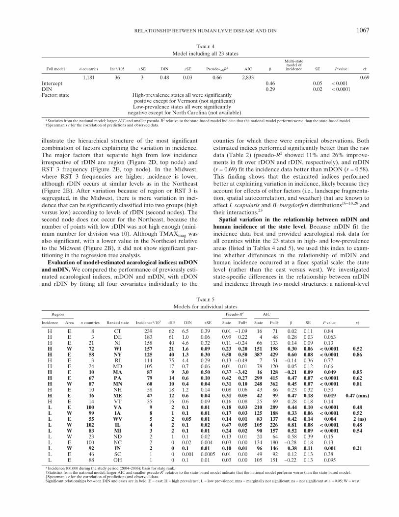
Spatial variation in the relationship between mDIN andhuman incidence at the state level. Because mDIN fit theincidence data best and provided acarological risk data forall counties within the 23 states in high- and low-prevalenceareas (listed in Tables 4 and 5), we used this index to exam-ine whether differences in the relationship of mDIN andhuman incidence occurred at a finer spatial scale: the statelevel (rather than the east versus west). We investigatedstate-specific differences in the relationship between mDINand incidence through two model structures: a national-level

Table 4

Model including all 23 states

Full model n countries Inc*/105 ±SE DIN ±SE Pseudo-adjR2 AIC b

Multi-statemodel ofincidence SE P value r†

1,181 36 3 0.48 0.03 0.66 2,833 0.69Intercept 0.46 0.05 < 0.001DIN 0.29 0.02 < 0.0001Factor: state High-prevalence states all were significantly

positive except for Vermont (not significant)Low-prevalence states all were significantly

negative except for North Carolina (not available)

*Statistics from the national model; larger AIC and smaller pseudo-R2 relative to the state-based model indicate that the national model performs worse than the state-based model.†Spearman’s r for the correlation of predictions and observed data.

Table 5

Models for individual states

Region

n countries Ranked state Incidence*/105 ±SE DIN ±SE

Pseudo-R2 AIC

b SE P value r‡Incidence Area State Full† State Full†

H E 8 CT 239 62 6.5 0.39 0.01 −1.09 16 71 0.02 0.11 0.84H E 3 DE 183 61 1.0 0.06 0.99 0.22 4 48 0.28 0.03 0.063H E 21 NJ 158 40 4.6 0.32 0.11 −0.24 66 133 0.14 0.09 0.13H W 72 WI 157 21 1.6 0.09 0.23 0.20 151 198 0.30 0.06 < 0.0001 0.52H E 58 NY 125 40 1.3 0.30 0.50 0.50 387 429 0.60 0.08 < 0.0001 0.86H E 3 RI 114 75 4.4 0.29 0.13 −0.49 7 51 −0.14 0.36 0.77H E 24 MD 105 17 0.7 0.06 0.01 0.01 78 120 0.05 0.12 0.66H E 10 MA 87 9 3.0 0.50 0.37 −3.42 16 128 −0.21 0.09 0.049 0.85H E 67 PA 79 14 0.6 0.10 0.42 0.27 299 415 0.47 0.07 < 0.0001 0.62H W 87 MN 60 10 0.4 0.04 0.31 0.10 248 362 0.45 0.07 < 0.0001 0.81H E 10 NH 58 18 1.2 0.14 0.08 0.06 43 86 0.23 0.32 0.50H E 16 ME 47 12 0.6 0.04 0.31 0.05 42 99 0.47 0.18 0.019 0.47 (mns)H E 14 VT 35 16 0.6 0.09 0.16 0.08 25 69 0.28 0.18 0.14L E 100 VA 9 2 0.1 0.01 0.18 0.03 210 289 0.44 0.10 < 0.0001 0.48L W 99 IA 8 1 0.1 0.01 0.17 0.03 125 188 0.33 0.06 < 0.0001 0.52L E 55 WV 5 2 0.05 0.01 0.14 0.01 83 137 0.42 0.14 0.004 2 (ns)L W 102 IL 4 2 0.1 0.02 0.47 0.05 105 226 0.81 0.08 < 0.0001 0.48L W 83 MI 3 2 0.1 0.01 0.24 0.02 90 157 0.52 0.09 < 0.0001 0.54L W 23 ND 2 1 0.1 0.02 0.13 0.01 20 64 0.58 0.39 0.15L E 100 NC 2 0 0.02 0.004 0.03 0.00 134 180 −0.28 0.18 0.13L W 92 IN 2 0 0.1 0.01 0.10 0.01 96 146 0.38 0.11 0.001 0.21L E 46 SC 1 0 0.001 0.0005 0.01 0.00 49 92 0.12 0.13 0.38L E 88 OH 1 0 0.1 0.01 0.03 0.00 105 151 −0.22 0.13 0.095

*Incidence/100,000 during the study period (2004–2006); basis for state rank.†Statistics from the national model; larger AIC and smaller pseudo-R2 relative to the state-based model indicate that the national model performs worse than the state-based model.‡Spearman’s r for the correlation of predictions and observed data.Significant relationships between DIN and cases are in bold; E = east; H = high prevalence; L = low prevalence; mns = marginally not significant; ns = not significant at a = 0.05; W = west.


model that included state as a factor versus separate modelsof mDIN for individual states. We found that there was asignificant effect of state in the full model (P < 0.0001) andthat the state-level models performed better than the fullmodel in all states (Tables 4 and 5, compare AIC for fullwith state). Lack of fit of the full model was not specific toany geographic location (Figure 3B–I) or levels of mDIN orincidence (Table 5, columns 6–9).Of 23 states, 12 states showed a significant relationship

between mDIN and human incidence, with an average corre-lation between model predictions and incidence of 0.55(range = 0.2–0.86) (Tables 4 and 5). The other 11 statesshowed no significant relationship. Three of these states,Delaware, Rhode Island, and Connecticut (Table 4), had avery low number of counties, and thus, their lack of fit islikely because of small sample size. For states where therelationship was significant, the fit was good (r > 0.6) in 4of 12 states (New York, Pennsylvania, Massachusetts, andMinnesota), weak (r = 0.4–0.6) in 5 more states (Wisconsin,Virginia, Iowa, Illinois, and Michigan), and poor (r < 0.40) inthe other 3 states (Maine, West Virginia, and Indiana),despite the high significance of mDIN in the models (Tables 5,bold P values and Supplemental Figure 3). Furthermore, theslopes of the relationship were significantly different amongthe states where the relationship was significant, includingan unexpected negative relationship for Massachusetts(Figure 3B–I and Table 5, bold b-values and SE), highlightingthat there are quantitative differences between states, evenwhere the relationship is highly significant.

DISCUSSION

We quantified the relationship of acarological risk andhuman Lyme disease incidence for all of the known US rangeof I. scapularis-borne B. burgdorferi. Our study is the first toexamine this association over such a large geographic range.We found that both rDON and rDIN explained a statisticallysignificant amount of variation in human incidence in low-and high-incidence areas but that neither explained variationin incidence in rare areas. Restricting the analysis to low- andhigh-incidence areas, we found that the relationship of mDINand incidence varied quantitatively by geographic location,that mDIN alone explained a statistically significant amountof variation in human incidence at the county level in only12 of 20 states (including only states with more than eightcounties), that the fit of the relationship was good in onlyfour states (New York, Pennsylvania, Massachusetts, andMinnesota), and that fit was reversed in one of these states(Massachusetts). A subanalysis of 40 high incidence countieswith NIP data identified some of the factors that contribute togeographic differences in the relationship of rDIN and inci-dence, most notably, genetic composition of B. burgdorferi.One factor that has been proposed to modify the rela-

tionship between DIN and reported cases is variation inB. burgdorferi genotype frequency.26,32 Differences in viru-lence37 and transmission efficiency25,38 may lead to differ-ences in infection risk and/or reporting rates by humansinfected with different strains. Thus, areas with low incidencebut high rDIN could be explained by an overrepresentation

Figure 3. Relationship of DIN and cases by state. The full model (A) included DIN as a continuous predictor and state as a 23-level factor.Because state was highly significant, we also modeled the relationship of DIN and human cases individually for each state (B–I) and comparedthese relationships (black circles) to predictions from the full model (grey circles). Only some of the states from each region are shown to illustratedifferences in performance between the national-level and state-based models. (B, C, F, andG) High prevalence, east. (D andH) High prevalence,west. (E and I) Low prevalence. Statistics are summarized in Table 4.


of strains with a low virulence in or transmission to humans.Although more studies are needed to confirm this hypothe-sis, our regression analyses support it for RST 3. We foundthat (1) incidence data could be partitioned similarly byregion or RST 3, (2) RST 3 was more frequent in the regionwith lower incidence but similar rDIN, and (3) there was anegative relationship between RST 3 and incidence esti-mated by the Poisson regression model. Although the othertwo RST types each showed different regional distributions,neither of these two types alone caused deviations from themean relationship of rDIN and reported incidence. Never-theless, because higher levels of RST 3 (a genetically diversegroup defined as non-RST 1 or 2) led to lower than expectedincidence based on rDIN, by extrapolation, the sum of RST 1and RST 2 frequencies was correlated with higher thanexpected incidence based on rDIN. Thus, our results suggestthat the monophyletic RST 1 and 2 groups39 cause higherthan expected reported cases based on rDIN, whereas a highprevalence of other strains results in fewer reported cases.More generally, our results highlight that genotypic differ-ences are important for predicting human incidence spatiallythrough acarological risk indices. However, more analyses ofthe genetic determinants of virulence (and transmission) inhumans and the spatial dynamics of B. burgdorferi geneticdiversity are needed to understand the effects of B. burgdorferigenotype on reported incidence.In addition to B. burgdorferi genotype, there are other

factors not measured in our study that could contribute togeographical differences and weak associations in the rela-tionship between mDIN and human incidence. One possibil-ity is human movement. Although peridomestic exposureaccounts for most cases of Lyme disease,12 some cases are aconsequence of travel to other counties for outdoor work orrecreation. This movement could explain the negativerelationship between mDIN and cases that was found forMassachusetts. For example, if Massachusetts residents tendto get infected in counties that are densely forested but live incounties (i.e., where cases would be reported) that are mainlyurban (i.e., low estimates of mDIN), then such a negativerelationship could be observed. More accurate spatial riskpredictions might be obtained if case reports included proba-ble place of exposure, although accurate estimates are verychallenging to obtain.40 Also, we found that spatial scale wascrucial for interpreting the relationship between mDIN andincidence, because we showed that there are quantitativedifferences regionally (Midwest versus Northeast) as well asbetween states within these regions. It is possible that thecounty scale is appropriate in states with larger forestedpatches, such as New York and Pennsylvania (which showedrelatively strong positive relationships between mDINand incidence), whereas a finer scale is necessary in highlyresidential states with very dispersed forest cover, such asNew Jersey and Maryland (which showed no significant rela-tionship). For example, a study that measured DIN in for-ested areas in six Rhode Island towns found that DINexplained 97% of the variation in incidence among thosetowns.9 However, most of our study sites were not located inresidential areas, and the incidence data corresponded to amuch broader range relative to the acarological data, whichincreases the variance in the relationship between mDIN andincidence. Last, geographical differences in Lyme diseasecontrol efforts at the residential or personal level could also

contribute to variation in the relationship between mDINand human incidence.There are also some experimental design caveats that

should be noted when interpreting our results. First, our esti-mates of mDIN were based on data collected exclusivelyin public forested areas. Thus, our estimates of mDIN incounties that are mainly residential could be inaccurate. Sec-ond, sampling at different sites was done at different timesbetween May and early September, and although most siteswere sampled at least five times, some sites were only sam-pled three times. Although these sampling design caveatslikely account for some of the unexplained variation in therelationship between DIN and human incidence, they werenot spatially systematic (i.e., they occurred randomly withrespect to state and region) and thus, should not introducesystematic bias in our results. Third, this analysis is basedon original field efforts that were optimized for collections ofI. scapularis nymphs based on phenology in the northeasternUnited States (emergence in late May); therefore, areas inwhich nymphs become active earlier would have inaccurateestimates of nymphal densities. For example, a previous studyfound that nymphs were observed as early as April in thesouth.41 However, even with intensive sampling, only a fewspecimens were recovered at this time; thus, this differenceshould not introduce much bias in our results. There are alsotwo other factors unaccounted for in our sampling design thatcould cause geographic variation in human incidence betweennorthern and southern areas. First, because we only sampledI. scapularis, the existence of an alternative vector mightuncouple the relationship between mDIN and incidence.However, this possibility would only occur if the alternativevector caused a significant proportion of human cases, andthere is no evidence to support this case. Second, it has beenreported that nymphs in southern areas very rarely feed onhumans,41 although it is still unclear whether this differ-ence from northern areas is because of the low densities ofI. scapularis nymphs or an actual feeding preference. Futureenvironmental surveillance should aim to quantify DIN inresidential areas as well as other habitats and potential vec-tors to better understand how DIN translates to incidenthuman cases across varying ecological conditions.

CONCLUSION

Reservoir- or vector-targeted control of human Lyme dis-ease relies on understanding how DIN corresponds to humanincidence geographically. Additionally, a mechanistic under-standing of the link between DIN and incidence should besought, because it is important for model frameworks thatanticipate changes in the geographic range of human inci-dence and evaluate the cost efficacy of all types of preventionmethods over time. Our multistate analysis showed largevariation in the relationship of DIN and incidence betweenstates, with only three states showing a reliable quantifica-tion of the relationship. To more accurately quantify howacarological risk translates to human Lyme disease riskspatially, longitudinal environmental surveillance of severalfactors at spatial scales finer than the county level wouldbe needed. Unfortunately, such studies are not likely to becost-effective if conducted using a random sampling design.Thus, future research to determine how acarological risktranslates to human incidence spatially should first aim to


identify probable sites of transmission to humans over a broadspatial scale through epidemiological studies that monitorhuman movement (preferably to and from areas whereacarological risk is quantified). Intensive environmentalsampling in some of these sites would help in quantifying therelationship betweenDIN and human incidencemore cheaply.

Received October 10, 2011. Accepted for publication February 26, 2012.

Note: Supplemental figures are available at www.ajtmh.org.

Acknowledgments: The authors thank Graham Hickling, Jean Tsao,Uriel Kitron, Edward Walker, Roberto Cortinas, Jonas Bunikis, andMichelle Rowland, who were key collaborators in the data collectionand development of the acarological risk map. The authors thankthe 80 field assistants who participated in the data collection;Tim Andreadis, Katherine Watkins, Laura Krueger, Jessica Payne,Elizabeth Racz, Kelly Liebman, Liza Lutzker, and David Boozer fortick identification and logistic support; Paul Cislo, Gwenael Vourc’h,and Robert Brinkerhoff for statistical and data analyses support;Carlos Diuk for database support; Forrest Melton, Brad Lobitz, andAndrew Michaelis for technical assistance; and Dennis Grove, LindsayRollend, and Russell Barbour for arranging collection permits. Thisproject was funded by Centers for Disease Control and Prevention–Division of Vector-Borne Infectious Diseases Cooperative Agreementno. CI00171-01. K.M.P. was supported by the Research and Policy inDisease Dynamics (RAPIDD) program of the Science and TechnologyDirectorate, the US Department of Homeland Security, and theFogarty International Center, National Institutes of Health. A.G.B.was supported by National Institute of Allergy and Infectious DiseaseGrant AI-065359.

Authors’ addresses: Kim M. Pepin, Fogarty International Center,National Institutes of Health, Bethesda, MD; and Bacterial DiseasesBranch, Division of Vector-Borne Infectious Diseases, Centers forDisease Control and Prevention, Fort Collins, CO, E-mail:[email protected] J. Eisen, Paul S. Mead, and Joseph Piesman, BacterialDiseases Branch, Division of Vector-Borne Infectious Diseases, Centersfor Disease Control and Prevention, Fort Collins, CO, E-mails:[email protected],[email protected], and [email protected]. Durland Fish andMaria A. Diuk-Wasser, Yale School of Public Health, New Haven, CT,E-mails: [email protected] and [email protected]. Anne G.Hoen, Department of Community and Family Medicine, DartmouthMedical School, Lebanon, NH, E-mail: [email protected] G. Barbour, Departments of Microbiology and MolecularGenetics and Medicine, University of California, Irvine, CA, E-mail:[email protected]. Sarah Hamer, Department of Fisheries andWildlife,Michigan State University, East Lansing, MI; and Department ofVeterinary Integrative Biosciences, Texas A&M University, CollegeStation, TX, E-mail: [email protected].

REFERENCES

1. CDC, 2011. Reported Cases of Lyme Disease by Year, UnitedStates, 1996–2010. Available at: http://www.cdc.gov/lyme/stats/chartstables/casesbyyear.html. Accessed January 2011.

2. CDC, 2011. Lyme Disease Incidence Rates by State, 2005–2010.Available at: http://www.cdc.gov/lyme/stats/chartstables/incidencebystate.html. Accessed January 2011.

3. Connally NP, Durante AJ, Yousey-Hindes KM, Meek JI,Nelson RS, Heimer R, 2009. Peridomestic lyme disease pre-vention results of a population-based case-control study. AmJ Prev Med 37: 201–206.

4. Gould LH, Nelson RS, Griffith KS, Hayes EB, Piesman J, MeadPS, Cartter ML, 2008. Knowledge, attitudes, and behaviorsregarding lyme disease prevention among Connecticut resi-dents, 1999–2004. Vector Borne Zoonotic Dis 8: 769–776.

5. Hayes EB, Piesman J, 2003. Current concepts—how can we pre-vent Lyme disease? N Engl J Med 348: 2424–2430.

6. Piesman J, Eisen L, 2008. Prevention of tick-borne diseases.Annu Rev Entomol 53: 323–343.

7. Shen AK, Mead PS, Beard CB, 2011. The lyme disease vaccine—a public health perspective. Clin Infect Dis 52: S247–S252.

8. Fish D, 1993. Population ecology of Ixodes dammini.Ginsberg H,ed. Ecology and Environmental Management of Lyme Disease.New Brunswick, NJ: Rutgers University Press, 25–42.

9. Mather TN, Nicholson MC, Donnelly EF, Matyas BT, 1996.Entomologic index for human risk of Lyme disease. Am JEpidemiol 144: 1066–1069.

10. Stafford KC, Cartter ML, Magnarelli LA, Ertel SH, Mshar PA,1998. Temporal correlations between tick abundance and prev-alence of ticks infected with Borrelia burgdorferi and increas-ing incidence of Lyme disease. J Clin Microbiol 36: 1240–1244.

11. Connally NP, Ginsberg HS, Mather TN, 2006. Assessingperidomestic entomological factors as predictors for Lymedisease. J Vector Ecol 31: 364–370.

12. Kitron U, Kazmierczak JJ, 1997. Spatial analysis of the distributionof Lyme disease in Wisconsin. Am J Epidemiol 145: 558–566.

13. Falco RC, McKenna DF, Daniels TJ, Nadelman RB,Nowakowski J, Fish D, Wormser GP, 1999. Temporal rela-tion between Ixodes scapularis abundance and risk for Lymedisease associated with erythema migrans. Am J Epidemiol149: 771–776.

14. Johnson JL, Ginsberg HS, Zhioua E, Whitworth UG, MarkowskiD, Hyland KE, Hu RJ, 2004. Passive tick surveillance, dogseropositivity, and incidence of human Lyme disease. VectorBorne Zoonotic Dis 4: 137–142.

15. Rand PW, Lacombe EH, Dearborn R, Cahill B, Elias S,Lubelczyk CB, Beckett GA, Smith RP, 2007. Passive surveil-lance in Maine, an area emergent for tick-borne diseases.J Med Entomol 44: 1118–1129.

16. Allan BF, Keesing F, Ostfeld RS, 2003. Effect of forest fragmen-tation on Lyme disease risk. Conserv Biol 17: 267–272.

17. Brownstein JS, Skelly DK, Holford TR, Fish D, 2005. Forestfragmentation predicts local scale heterogeneity of Lymedisease risk. Oecologia 146: 469–475.

18. Estrada-Pena A, 2009. Diluting the dilution effect: a spatial Lymemodel provides evidence for the importance of habitatfragmentation with regard to the risk of infection. GeospatHealth 3: 143–155.

19. Ashley ST, Meentemeyer V, 2004. Climatic analysis of Lymedisease in the United States. Clim Res 27: 177–187.

20. Brownstein JS, Holford TR, Fish D, 2003. A climate-based modelpredicts the spatial distribution of the Lyme disease vectorIxodes scapularis in the United States. Environ Health Perspect111: 1152–1157.

21. Ogden NH, Maarouf A, Barker IK, Bigras-Poulin M, LindsayLR, Morshed MG, O’Callaghan CJ, Ramay F, Waltner-ToewsD, Charron DF, 2006. Climate change and the potential forrange expansion of the Lyme disease vector Ixodes scapularisin Canada. Int J Parasitol 36: 63–70.

22. Ostfeld RS, Canham CD, Oggenfuss K, Winchcombe RJ, KeesingF, 2006. Climate, deer, rodents, and acorns as determinants ofvariation in Lyme-disease risk. PLoS Biol 4: 1058–1068.

23. Gatewood AG, Liebman KA, Vourc’h G, Bunikis J, Hamer SA,Cortinas R, Melton F, Cislo P, Kitron U, Tsao J, Barbour AG,Fish D, Diuk-Wasser MA, 2009. Climate and tick seasonalityare predictors of Borrelia burgdorferi genotype distribution.Appl Environ Microbiol 75: 2476–2483.

24. Dykhuizen DE, Brisson D, Sandigursky S, Wormser GP,Nowakowski J, Nadelman RB, Schwartz I, 2008. Short report:the propensity of different Borrelia burgdorferi sensu strictogenotypes to cause disseminated infections in humans. Am JTrop Med Hyg 78: 806–810.

25. Hanincova K, Ogden NH, Diuk-Wasser M, Pappas CJ, Iyer R,Fish D, Schwartz I, Kurtenbach K, 2008. Fitness variation ofBorrelia burgdorferi sensu stricto strains in mice. Appl EnvironMicrobiol 74: 153–157.

26. Wormser GP, Brisson D, Liveris D, Hanincova K, Sandigursky S,Nowakowski J, Nadelman RB, Ludin S, Schwartz I, 2008.Borrelia burgdorferi genotype predicts the capacity for hema-togenous dissemination during early Lyme disease. J Infect Dis198: 1358–1364.

27. Diuk-Wasser MA, Gatewood AG, Cortinas MR, Yaremych-Hamer S, Tsao J, Kitron U, Hickling G, Brownstein JS, WalkerE, Piesman J, Fish D, 2006. Spatiotemporal patterns of host-seeking Ixodes scapularis nymphs (Acari: Iodidae) in theUnited States. J Med Entomol 43: 166–176.


28. Diuk-Wasser MA, Vourc’h G, Cislo P, Hoen AG, Melton F,Hamer SA, Rowland M, Cortinas R, Hickling GJ, Tsao JI,Barbour AG, Kitron U, Piesman J, Fish D, 2010. Field andclimate-based model for predicting the density of host-seekingnymphal Ixodes scapularis, an important vector of tick-bornedisease agents in the eastern United States. Glob EcolBiogeogr 19: 504–514.

29. Diuk-Wasser M, Gatewood A, Cislo P, Brinkerhoff R, Hamer S,Rowland M, Cortinas R, Melton F, Hickling G, Tsao J, BunikisJ, Barbour A, Kitron U, Piesman J, Fish D, 2012. Human riskof infection with Borrelia burgdorferi, the Lyme disease agent,in eastern United States. Am J Trop Med Hyg, 86: 320–327.

30. Bacon RM, Kugeler KJ, Mead PS, 2008. Surveillance for Lymedisease—United States, 1992–2006. MMWR Surveill Summ57: 1–9.

31. Guerra M, Walker E, Jones C, Paskewitz S, Cortinas MR, StancilA, Beck L, Bobo M, Kitron U, 2002. Predicting the risk ofLyme disease: habitat suitability for Ixodes scapularis in thenorth central United States. Emerg Infect Dis 8: 289–297.

32. Wormser GP, Liveris D, Nowakowski J, Nadelman RB, CavaliereLF, McKenna D, Holmgren D, Schwartz I, 1999. Associationof specific subtypes of Borrelia burgdorferi with hematogenousdissemination in early Lyme disease. J Infect Dis 180: 720–725.

33. Wang G, Ojaimi C, Iyer R, Saksenberg V, McClain SA, WormserGP, Schwartz I, 2001. Impact of genotypic variation of Borreliaburgdorferi sensu stricto on kinetics of dissemination and severityof disease in C3H/HeJ mice. Infect Immun 69: 4303–4312.

34. Estrada-Pena A, 2009. Tick-borne pathogens, transmission ratesand climate change. Front Biosci 14: U2674–U2780.

35. Tsao JI, Wootton JT, Bunikis J, Luna MG, Fish D, Barbour AG,2004. An ecological approach to preventing human infection:vaccinating wild mouse reservoirs intervenes in the Lyme dis-ease cycle. Proc Natl Acad Sci USA 101: 18159–18164.

36. Hothorn T, Hornik K, Zeileis A, 2006. Unbiased recursivepartitioning: a conditioxnal inference framework. J ComputGraph Statist 15: 651–674.

37. Jones KL, Glickstein LJ, Damle N, Sikand VK, McHugh G,Steere AC, 2006. Borrelia burgdorferi genetic markers anddisseminated disease in patients with early Lyme disease.J Clin Microbiol 44: 4407–4413.

38. Derdakova M, Dudioak V, Brei B, Brownstein JS, Schwartz I,Fish D, 2004. Interaction and transmission of two Borreliaburgdorferi sensu stricto strains in a tick-rodent maintenancesystem. Appl Environ Microbiol 70: 6783–6788.

39. Bunikis J, Garpmo U, Tsao J, Berglund J, Fish D, BarbourAG, 2004. Sequence typing reveals extensive strain diversityof the Lyme borreliosis agents Borrelia burgdorferi in NorthAmerica and Borrelia afzelii in Europe. Microbiology 150:1741–1755.

40. Eisen L, Eisen RJ, 2007. Need for improved methods to collectand present spatial epidemiologic data for vectorborne dis-eases. Emerg Infect Dis 13: 1816–1820.

41. Goddard J, Piesman J, 2006. New records of immature Ixodesscapularis from Mississippi. J Vector Ecol 31: 421–422.


Supplemental Figure 1. Spatial variation in samling design. The proportion of drags that were completed in early (May and July) versus late(August and September) summer by location. Open circles are scaled relative to the proportion of drags (early/late summer); larger circles indi-cate stronger sampling intensity during early summer. Filled black circles indicate locations where no samples were collected in late summer; filledgrey circles indicate locations where no samples were collected in early summer. Size of filled circles is scaled relative to the mean proportion atall other sites.

Supplemental Figure 2. Spatial variation in prevalence (NIP) and DIN. NIP and DIN are plotted for each site sampled. Dots indicate siteswhere there were too few ticks to estimate NIP (and hence, DIN). Size of the circles is scaled to the levels of NIP or DIN.

Supplemental Figure 3. Accuracy of model predictions. Observed cases are plotted against predicted cases from the state-based model (black)and the national-level model (grey). Cases were square-root transformed. Points that fall along the dotted line indicate a perfect fit. Only states forwhich the state-based model was significant are shown.

Documents

Geographic Variation in the Relationship between Human