Embed Size (px)
Citation preview
Geographic Information Systems (GIS) for spatial
analysis of animal health data
Course handbook
16 – 19 October, 2018
Prepared by Daan Vink, Mark Stevenson, Chris Compton and Mary Van Andel
Version 1.0, October 15, 2018

i • GIS for analysis of animal health data
This manual is licensed under a Creative Commons Attribution – NonCommercial – ShareAlike license.This means that you are free to share and adapt the material in this manual as long as you give appropriatecredit, provide a link to the license, and indicate if changes were made. If you remix, transform, or buildupon the material, you must distribute your contributions under the same license as this manual. You maynot use the material for commercial purposes. You may not apply legal terms or technological measuresthat legally restrict others from doing anything the license permits.
CONTENTS GIS for analysis of animal health data • ii
Contents
1 Course introduction 11.1 Background . . . . . . . . . . . . . . . . . . . . . . . . . . . . . . . . . . . . . . 11.2 Course details . . . . . . . . . . . . . . . . . . . . . . . . . . . . . . . . . . . . . 11.3 Course programme . . . . . . . . . . . . . . . . . . . . . . . . . . . . . . . . . . 3
I Reference material 6
2 Geography and epidemiology 82.1 Definition of a GIS . . . . . . . . . . . . . . . . . . . . . . . . . . . . . . . . . . . 82.2 The elements of geographic data . . . . . . . . . . . . . . . . . . . . . . . . . . . 82.3 Spatial resolution . . . . . . . . . . . . . . . . . . . . . . . . . . . . . . . . . . . 92.4 Data formats . . . . . . . . . . . . . . . . . . . . . . . . . . . . . . . . . . . . . . 102.5 Georeferencing . . . . . . . . . . . . . . . . . . . . . . . . . . . . . . . . . . . . 122.6 Datums . . . . . . . . . . . . . . . . . . . . . . . . . . . . . . . . . . . . . . . . 142.7 Coordinate systems . . . . . . . . . . . . . . . . . . . . . . . . . . . . . . . . . . 152.8 Geography and spatial epidemiology . . . . . . . . . . . . . . . . . . . . . . . . . 19
3 Sources of spatial data 263.1 Introduction . . . . . . . . . . . . . . . . . . . . . . . . . . . . . . . . . . . . . . 263.2 Geographic data . . . . . . . . . . . . . . . . . . . . . . . . . . . . . . . . . . . . 263.3 Human geography, socio-economic and environmental data . . . . . . . . . . . . 273.4 Livestock demographic and animal health data . . . . . . . . . . . . . . . . . . . 283.5 Geocoding locations . . . . . . . . . . . . . . . . . . . . . . . . . . . . . . . . . . 30
4 Exploratory spatial data analysis (ESDA) 324.1 Introduction: exploratory data analysis (EDA) . . . . . . . . . . . . . . . . . . . . 324.2 Exploratory spatial data analysis (ESDA): EDA+ . . . . . . . . . . . . . . . . . . 334.3 A strategy for performing ESDA . . . . . . . . . . . . . . . . . . . . . . . . . . . 38
5 Spatial clustering of disease 405.1 Introduction: global versus local clustering . . . . . . . . . . . . . . . . . . . . . . 405.2 Global estimates of spatial clustering . . . . . . . . . . . . . . . . . . . . . . . . . 425.3 Local estimates of spatial clustering . . . . . . . . . . . . . . . . . . . . . . . . . 515.4 Cluster detection using SaTScan . . . . . . . . . . . . . . . . . . . . . . . . . . . 66
6 Spatial models of disease risk 836.1 Introduction . . . . . . . . . . . . . . . . . . . . . . . . . . . . . . . . . . . . . . 836.2 Data-driven and knowledge-driven models of disease risk . . . . . . . . . . . . . 836.3 Spatial risk assessment using a knowledge-driven approach . . . . . . . . . . . . 85
iii • GIS for analysis of animal health data CONTENTS
6.4 Spatial risk assessments of FMD . . . . . . . . . . . . . . . . . . . . . . . . . . . 91
II Course practicals 93
7 Getting set up 957.1 Objective . . . . . . . . . . . . . . . . . . . . . . . . . . . . . . . . . . . . . . . . 957.2 Preparing your QGIS setup . . . . . . . . . . . . . . . . . . . . . . . . . . . . . . 957.3 Preparing your project data directories . . . . . . . . . . . . . . . . . . . . . . . . 977.4 Loading your spatial data into QGIS . . . . . . . . . . . . . . . . . . . . . . . . . 987.5 Developing the ‘base map’ . . . . . . . . . . . . . . . . . . . . . . . . . . . . . . 1007.6 Cartography and map design . . . . . . . . . . . . . . . . . . . . . . . . . . . . . 106
8 Exploratory spatial data analysis (ESDA) 1128.1 Objective . . . . . . . . . . . . . . . . . . . . . . . . . . . . . . . . . . . . . . . . 1128.2 Exploratory data analysis (EDA) . . . . . . . . . . . . . . . . . . . . . . . . . . . 1128.3 Exploratory spatial data analysis (ESDA) . . . . . . . . . . . . . . . . . . . . . . 116
9 Space-time cluster scanning using SaTScan 1229.1 Objective . . . . . . . . . . . . . . . . . . . . . . . . . . . . . . . . . . . . . . . . 1229.2 Data required . . . . . . . . . . . . . . . . . . . . . . . . . . . . . . . . . . . . . 1229.3 Preparing to run SaTScan . . . . . . . . . . . . . . . . . . . . . . . . . . . . . . 1239.4 Running SaTScan . . . . . . . . . . . . . . . . . . . . . . . . . . . . . . . . . . . 1259.5 Spatio-temporal analysis . . . . . . . . . . . . . . . . . . . . . . . . . . . . . . . 130
10 Spatial risk assessment using QGIS 13410.1 Objective . . . . . . . . . . . . . . . . . . . . . . . . . . . . . . . . . . . . . . . . 13410.2 Spatial layers and data . . . . . . . . . . . . . . . . . . . . . . . . . . . . . . . . 13410.3 Standardising the layers . . . . . . . . . . . . . . . . . . . . . . . . . . . . . . . . 13910.4 Normalising and aligning the raster layers . . . . . . . . . . . . . . . . . . . . . . 14010.5 Applying the WLC using REMBRANDT weights . . . . . . . . . . . . . . . . . . . 14110.6 Further work and uses of the risk surface . . . . . . . . . . . . . . . . . . . . . . 14210.7 Discussion . . . . . . . . . . . . . . . . . . . . . . . . . . . . . . . . . . . . . . . 142
11 Spatial risk assessment using R 14411.1 Objective . . . . . . . . . . . . . . . . . . . . . . . . . . . . . . . . . . . . . . . . 14411.2 Spatial layers and data . . . . . . . . . . . . . . . . . . . . . . . . . . . . . . . . 14411.3 Normalising the layers . . . . . . . . . . . . . . . . . . . . . . . . . . . . . . . . . 15111.4 Resampling of processed rasters . . . . . . . . . . . . . . . . . . . . . . . . . . . 15211.5 Multicriteria decision analysis (MCDA) . . . . . . . . . . . . . . . . . . . . . . . . 15211.6 Applying the WLC using REMBRANDT weights . . . . . . . . . . . . . . . . . . . 15411.7 Plotting the output . . . . . . . . . . . . . . . . . . . . . . . . . . . . . . . . . . . 15511.8 Model verification . . . . . . . . . . . . . . . . . . . . . . . . . . . . . . . . . . . 157
12 Investigation of spatial clustering in R 15812.1 Preliminaries and acknowledgements . . . . . . . . . . . . . . . . . . . . . . . . 15812.2 Investigation of spatial clustering in R . . . . . . . . . . . . . . . . . . . . . . . . 160

1 • GIS for analysis of animal health data Course introduction
1 Course introduction
1.1 Background
Geographic Information Systems (GIS) are an essential tool to visualise an array of different datasets spatially through the creation of detailed maps. In recent years, applications of spatial epi-demiology using GIS software have increased in their capacity to analyse and interpret data forenhanced understanding of relationships, disease patterns and trends. Open-source GIS soft-ware, such as QGIS, is easily accessible for use by Veterinary Services (VS) for animal diseasesurveillance, research and control purposes. GIS tools can also be used in a research capac-ity to better understand animal disease in relation to risk factor determination, spatial diseasemodelling, and distribution and prevalence studies.
In addition, GIS tools can be used practically to support VS in a range of activities relevant todisease control. For example, when an outbreak of an infectious disease occurs, veterinary of-ficers can use GIS to map the locations of outbreaks and analyse this data to answer importantquestions of who, what, when and where in relation to the outbreak. Assessment of spatial trendsin disease morbidity and mortality over time can support surveillance programmes and can beapplied to detect aberrations and disease clustering. In organised disease response operations,spatial analyses can inform VS on how to prioritise the operationalisation and allocation of re-sources. In analogy with applications in surveillance and disease control, risk-based approachesusing GIS tools are increasingly being used by technical staff to manage and focus the locationof disease control and prevention efforts.
In recognizing the application of GIS software in animal disease surveillance and control, theWorld Organisation for Animal Health (OIE) Sub-Regional Representation (SRR) for South EastAsia (SEA) is organising a four-day training course. This is the second such course; the firstwas organised in October 2017. Although foundation principles of spatial analysis and GIS willbe covered, this is not designed as an introductory course, and the participants are expectedto have some proficiency in spatial analysis and skills in using GIS techniques. The course willconsolidate the material and learnings from the previous course and extend it further to increasethe capability of participants to perform such work effectively.
1.2 Course details
1.2.1 Course overview
This course is aimed at personnel who have a role in epidemiological analysis of disease data atthe national and regional level, such as WAHIS/ARAHIS and/or SEACFMD EpiNet Focal Points.
Course introduction GIS for analysis of animal health data • 2
It focuses on spatial analysis of disease incidence, clustering and density estimation, and willalso include a component on spatial risk assessment.
1.2.2 Course objectives and outcomes
The overall objective is for participants to strengthen their knowledge and skills of the analysis ofdisease data. By the end of this course, participants should:
1. Have improved their understanding of spatial epidemiology.2. Be able to detect clusters of disease in space and time, identify potential hotspots and
model the space-time cluster patterns.3. Be proficient in undertaking a spatial disease risk assessment.4. Have increased their proficiency in using tools such as QGIS and R to perform such spatial
analysis.
1.2.3 Course structure and delivery
The following topics are included in the programme:
• Topic 1: Exploratory spatial data analysis. Using a combination of disease incidencedata and census (population) data, participants will appropriately display the spatial dis-tribution of disease events and quantify measures of disease (attack rate, mortality rateand case fatality rate) at the level of the epidemiological unit (usually the village). Wherepossible, an assessment of temporal trends will be made.
• Topic 2: Analysing spatial heterogeneity of disease. Global and localised diseasecluster estimation techniques will be summarised. Relevant spatial scan statistics (purelyspatial and spatiotemporal) will be computed to test the significance of disease clusters,using SaTScan and QGIS.
• Topic 3: Assessment of spatial disease risk. Utilising the outputs of the MulticriteriaDecision Analysis (MCDA) process performed during the 2017 course, a spatial risk as-sessment for FMD will be performed.
• Topic 4: An introduction to cluster analysis and spatial modelling. This more ad-vanced topic introduces participants to more formal data-driven analysis to develop space-time statistical models and quantify differences and associations.
Delivery is by technical experts proficient in GIS, spatial analysis of animal health and veteri-nary epidemiology from Intiga Consulting, Massey University EpiCentre, Melbourne Universityand the New Zealand Ministry for Primary Industries (MPI). There is an emphasis on the prac-tical application of the material covered, including interpretation of the outputs, making use ofthe support and advice given by the course instructors. The lectures will be brief and serve tosupport the practical work. The practicals will be preceded by whole-group demonstration whererelevant.
Participants may access all course materials, data, practical exercises, software and other re-sources in an online Learning Management System (LMS). Additional and updated materialscan be added on the fly, and course participants may continue to use this after the course’s con-clusion. There will be communication with the participants prior to the course to ensure they canaccess this site. Participants may be requested to download and install the current versions ofthe software packages utilised.

3 • GIS for analysis of animal health data Course introduction
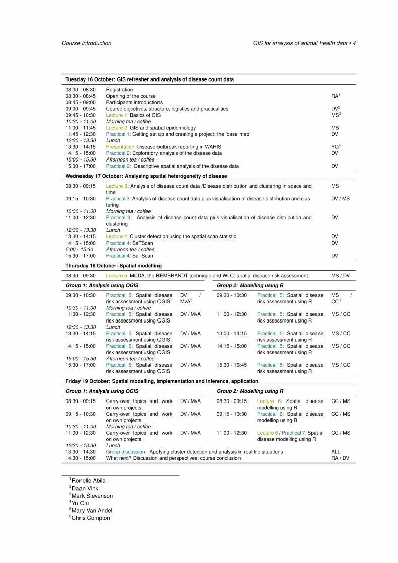
1.3 Course programme
The course programme consists of three and a half days of classroom teaching followed by asession to discuss and consolidate the course learnings.
Part of the course will be delivered in parallel to two groups, implementing comparable material.One group will utilise QGIS for this while the other group will use R. The work in R will be moreadvanced; on the final day, and introduction to spatial modelling will be included.
Course introduction GIS for analysis of animal health data • 4
Tuesday 16 October: GIS refresher and analysis of disease count data
08:00 - 08:30 Registration08:30 - 08:45 Opening of the course RA1
08:45 - 09:00 Participants introductions09:00 - 09:45 Course objectives, structure, logistics and practicalities DV2
09:45 - 10:30 Lecture 1: Basics of GIS MS3
10:30 - 11:00 Morning tea / coffee11:00 - 11:45 Lecture 2: GIS and spatial epidemiology MS11:45 - 12:30 Practical 1: Getting set up and creating a project: the ’base map’ DV12:30 - 13:30 Lunch13:30 - 14:15 Presentation: Disease outbreak reporting in WAHIS YQ4
14:15 - 15:00 Practical 2: Exploratory analysis of the disease data DV15:00 - 15:30 Afternoon tea / coffee15:30 - 17:00 Practical 2: Descriptive spatial analysis of the disease data DV
Wednesday 17 October: Analysing spatial heterogeneity of disease
08:30 - 09:15 Lecture 3: Analysis of disease count data /Disease distribution and clustering in space andtime
MS
09:15 - 10:30 Practical 3: Analysis of disease count data plus visualisation of disease distribution and clus-tering
DV / MS
10:30 - 11:00 Morning tea / coffee11:00 - 12:30 Practical 3: Analysis of disease count data plus visualisation of disease distribution and
clusteringDV
12:30 - 13:30 Lunch13:30 - 14:15 Lecture 4: Cluster detection using the spatial scan statistic DV14:15 - 15:00 Practical 4: SaTScan DV5:00 - 15:30 Afternoon tea / coffee15:30 - 17:00 Practical 4: SaTScan DV
Thursday 18 October: Spatial modelling
08:30 - 09:30 Lecture 5: MCDA, the REMBRANDT technique and WLC: spatial disease risk assessment MS / DV
Group 1: Analysis using QGIS Group 2: Modelling using R
09:30 - 10:30 Practical 5: Spatial diseaserisk assessment using QGIS
DV /MvA5
09:30 - 10:30 Practical 5: Spatial diseaserisk assessment using R
MS /CC6
10:30 - 11:00 Morning tea / coffee11:00 - 12:30 Practical 5: Spatial disease
risk assessment using QGISDV / MvA 11:00 - 12:30 Practical 5: Spatial disease
risk assessment using RMS / CC
12:30 - 13:30 Lunch13:30 - 14:15 Practical 5: Spatial disease
risk assessment using QGISDV / MvA 13:00 - 14:15 Practical 5: Spatial disease
risk assessment using RMS / CC
14:15 - 15:00 Practical 5: Spatial diseaserisk assessment using QGIS
DV / MvA 14:15 - 15:00 Practical 5: Spatial diseaserisk assessment using R
MS / CC
15:00 - 15:30 Afternoon tea / coffee15:30 - 17:00 Practical 5: Spatial disease
risk assessment using QGISDV / MvA 15:30 - 16:45 Practical 5: Spatial disease
risk assessment using RMS / CC
Friday 19 October: Spatial modelling, implementation and inference, application
Group 1: Analysis using QGIS Group 2: Modelling using R
08:30 - 09:15 Carry-over topics and workon own projects
DV / MvA 08:30 - 09:15 Lecture 6: Spatial diseasemodelling using R
CC / MS
09:15 - 10:30 Carry-over topics and workon own projects
DV / MvA 09:15 - 10:30 Practical 6: Spatial diseasemodelling using R
CC / MS
10:30 - 11:00 Morning tea / coffee11:00 - 12:30 Carry-over topics and work
on own projectsDV / MvA 11:00 - 12:30 Lecture 6 / Practical 7: Spatial
disease modelling using RCC / MS
12:30 - 13:30 Lunch13:30 - 14:30 Group discussion: Applying cluster detection and analysis in real-life situations ALL14:30 - 15:00 What next? Discussion and perspectives; course conclusion RA / DV
1Ronello Abila2Daan Vink3Mark Stevenson4Yu Qiu5Mary Van Andel6Chris Compton

5 • GIS for analysis of animal health data Course introduction

Part I
Reference material
6

Geography and epidemiology GIS for analysis of animal health data • 8
2 Geography and epidemiology
2.1 Definition of a geographic information system
A geographic information system (GIS), as defined by University of Edinburgh’s Dictionary of GISterms, is ‘a computer system for capturing, storing, checking, integrating, manipulating, analysingand displaying data related to positions on the Earth’s surface.’ Typically, a GIS is used for han-dling maps of one kind or another. These might be represented as several different layers whereeach layer holds data about a particular kind of feature (e.g. roads). Each feature is linked to aposition on the graphical image of a map. The primary value of a GIS is that it defines preciselythe location of objects and provides users with the ability to visualise the spatial arrangementof those objects. Knowledge of location allows complex calculations to be performed (such asworking out the shortest route and the shortest travel time between two locations). For epidemi-ologists, the ability to visualise spatial data is a powerful method of describing the patterns ofdisease, and is a useful technique for identifying factors that potentially influence patterns ofdisease.
2.2 The elements of geographic data
Geographic data are built up from single elements, or facts, about the real world. In its crud-est form, an element of geographic data (termed a datum) links: (1) place, (2) time, and (3) adescriptive property about place and time. For example, the statement: ‘The temperature at 12noon on 10 June 2003 at latitude 45◦ and longitude 60◦ was 25◦ Celsius’ ties place and time tothe property (or attribute) of atmospheric temperature. In many cases geographical data are slowto change and for this reason time is often omitted from geographic descriptions. On the otherhand, atmospheric temperature changes constantly, so time is an important component of thistype of representation.
The range of attribute information in geography is vast. Attribute information may be classified asfollows.
• Nominal: attributes are nominal if they are given names or titles in order to distinguishone entity from another. Place names are a good example of nominal attributes (see theGeoNames website for a complete list of place names in different languages).
• Ordinal: attributes are ordinal if their values take on a natural order. For example, agricul-tural land may be classed in terms of soil quality with class 1 representing the best, class 2second-best and so on.
• Numeric: examples include temperature, height above sea level, counts of numbers ofcases of disease. Values vary on a discrete (for example, integer) or continuous scale.

9 • GIS for analysis of animal health data Geography and epidemiology
Just as attributes can be classed into different types, so too can spatial objects. The varioustypes of spatial object include:
• Points: spatial objects that have neither length nor breadth and therefore a dimension ofzero; points may be used to indicate spatial occurrences or events; point pattern analysisis used to identify whether occurrences or events are interrelated;
• Lines: spatial objects that have length but no breadth, and hence a dimension of one;used to represent linear entities such as roads, pipelines and cables which are frequentlyassembled to form networks;
• Areas: spatial objects of two dimensions of length and breadth; may be used to representnatural objects such as countries, state boundaries or agricultural fields; areas may boundlinear features and enclose points;
• Surfaces or volumes: spatial objects of length, breadth and depth; used to represent naturalobjects such as river basins, canyons, and mountains; surfaces are frequently derivedby interpolating between lower dimension measurements such as point measurements ofheight;
• Time: often considered to be the fourth dimension of spatial objects.
2.3 Spatial resolution
The classification of geographic data into object types is dependent on scale. For example,at a low level of resolution a farm may be represented as a single point. At a higher level ofresolution the same farm may be better represented as an area, where the exact farm boundariesare explicitly defined. At an even higher level of resolution the farm may be represented asa surface where, in addition to boundary information, details of height, aspect and slope areprovided.
Figure 2.1 illustrates how, as spatial resolution increases, greater detail can be appreciated andthe shape of spatial objects will change. Objects that appear as lines at low resolution (forexample, in the left-hand and centre diagrams), are best represented by polygons when viewedat a high level of resolution (as in the right-hand diagram).
Figure 2.1: Different levels of spatial resolution.
In principle, if we collected enough items of geographic information we would be able to builda complete representation of the world. In practice any representation that is made is partial inthat it must limit the level of detail provided or ignore change that may occur through time. One
Geography and epidemiology GIS for analysis of animal health data • 10
common way of limiting detail is by ignoring information that applies to small areas — that is, toreduce the spatial resolution. A second way is to regard many attributes as remaining constantover large areas.
2.4 Data formats
Spatial data may be stored in either raster or vector formats with a GIS. Vector data are composedof points, lines, and polygons. Raster data sets are composed of rectangular arrays of regularlyspaced square grid cells. Each cell has a value, representing a property or attribute of interest.While any type of geographic data can be stored in raster format, raster data sets are especiallysuited to the representation of continuous, rather than discrete, data.
2.4.1 Vector data
Vector data are composed of points, lines, and polygons. This spatial data model is known as‘arc-node topology.’ Arcs are composed of nodes and vertices. Arcs begin and end at nodes, andmay have 0 or more vertices between nodes. The vertices define the shape of the arc along itslength. Arcs which connect to each other will share a common node.
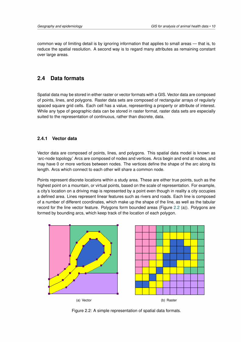
Points represent discrete locations within a study area. These are either true points, such as thehighest point on a mountain, or virtual points, based on the scale of representation. For example,a city’s location on a driving map is represented by a point even though in reality a city occupiesa defined area. Lines represent linear features such as rivers and roads. Each line is composedof a number of different coordinates, which make up the shape of the line, as well as the tabularrecord for the line vector feature. Polygons form bounded areas (Figure 2.2 (a)). Polygons areformed by bounding arcs, which keep track of the location of each polygon.
(a) Vector (b) Raster
Figure 2.2: A simple representation of spatial data formats.
11 • GIS for analysis of animal health data Geography and epidemiology
2.4.2 Raster data
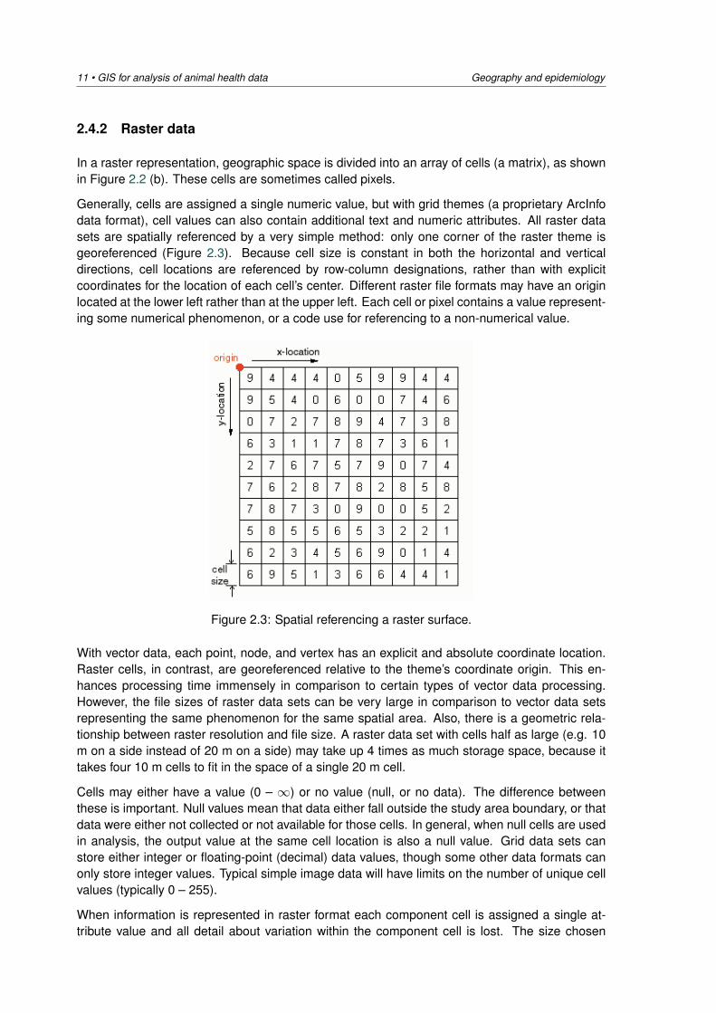
In a raster representation, geographic space is divided into an array of cells (a matrix), as shownin Figure 2.2 (b). These cells are sometimes called pixels.
Generally, cells are assigned a single numeric value, but with grid themes (a proprietary ArcInfodata format), cell values can also contain additional text and numeric attributes. All raster datasets are spatially referenced by a very simple method: only one corner of the raster theme isgeoreferenced (Figure 2.3). Because cell size is constant in both the horizontal and verticaldirections, cell locations are referenced by row-column designations, rather than with explicitcoordinates for the location of each cell’s center. Different raster file formats may have an originlocated at the lower left rather than at the upper left. Each cell or pixel contains a value represent-ing some numerical phenomenon, or a code use for referencing to a non-numerical value.
Figure 2.3: Spatial referencing a raster surface.
With vector data, each point, node, and vertex has an explicit and absolute coordinate location.Raster cells, in contrast, are georeferenced relative to the theme’s coordinate origin. This en-hances processing time immensely in comparison to certain types of vector data processing.However, the file sizes of raster data sets can be very large in comparison to vector data setsrepresenting the same phenomenon for the same spatial area. Also, there is a geometric rela-tionship between raster resolution and file size. A raster data set with cells half as large (e.g. 10m on a side instead of 20 m on a side) may take up 4 times as much storage space, because ittakes four 10 m cells to fit in the space of a single 20 m cell.
Cells may either have a value (0 – ∞) or no value (null, or no data). The difference betweenthese is important. Null values mean that data either fall outside the study area boundary, or thatdata were either not collected or not available for those cells. In general, when null cells are usedin analysis, the output value at the same cell location is also a null value. Grid data sets canstore either integer or floating-point (decimal) data values, though some other data formats canonly store integer values. Typical simple image data will have limits on the number of unique cellvalues (typically 0 – 255).
When information is represented in raster format each component cell is assigned a single at-tribute value and all detail about variation within the component cell is lost. The size chosen
Geography and epidemiology GIS for analysis of animal health data • 12
for cells within a raster surface depend on the resolution of the data used to create the surface.The cell must be small enough to capture the detail required, but large enough so the data canbe stored and analysed efficiently. As the homogeneity of the data increases so too can thedesignated cell size.
When creating raster data several rules may be applied to specify how a cell will be coded: inmost situations the attribute with the largest share of the cell’s area gets the cell attribute value.In other circumstances the rule is based on the central point of the cell and the attribute valuesat the central point are assigned to the cell. Although the largest share rule is almost alwayspreferred, the central point rule is commonly used because it is quick to calculate.
2.4.3 Raster calculations
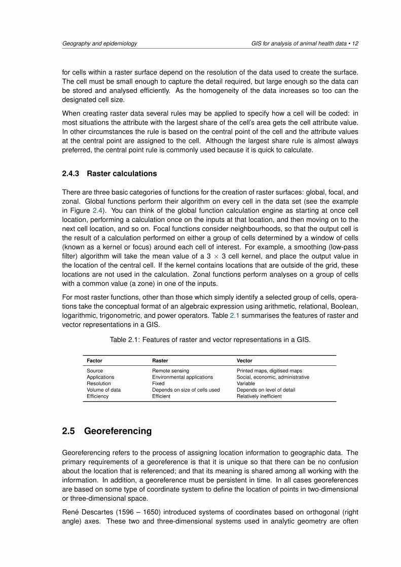
There are three basic categories of functions for the creation of raster surfaces: global, focal, andzonal. Global functions perform their algorithm on every cell in the data set (see the examplein Figure 2.4). You can think of the global function calculation engine as starting at once celllocation, performing a calculation once on the inputs at that location, and then moving on to thenext cell location, and so on. Focal functions consider neighbourhoods, so that the output cell isthe result of a calculation performed on either a group of cells determined by a window of cells(known as a kernel or focus) around each cell of interest. For example, a smoothing (low-passfilter) algorithm will take the mean value of a 3 × 3 cell kernel, and place the output value inthe location of the central cell. If the kernel contains locations that are outside of the grid, theselocations are not used in the calculation. Zonal functions perform analyses on a group of cellswith a common value (a zone) in one of the inputs.
For most raster functions, other than those which simply identify a selected group of cells, opera-tions take the conceptual format of an algebraic expression using arithmetic, relational, Boolean,logarithmic, trigonometric, and power operators. Table 2.1 summarises the features of raster andvector representations in a GIS.
Table 2.1: Features of raster and vector representations in a GIS.
Factor Raster Vector
Source Remote sensing Printed maps, digitised mapsApplications Environmental applications Social, economic, administrativeResolution Fixed VariableVolume of data Depends on size of cells used Depends on level of detailEfficiency Efficient Relatively inefficient
2.5 Georeferencing
Georeferencing refers to the process of assigning location information to geographic data. Theprimary requirements of a georeference is that it is unique so that there can be no confusionabout the location that is referenced; and that its meaning is shared among all working with theinformation. In addition, a georeference must be persistent in time. In all cases georeferencesare based on some type of coordinate system to define the location of points in two-dimensionalor three-dimensional space.
Rene Descartes (1596 – 1650) introduced systems of coordinates based on orthogonal (rightangle) axes. These two and three-dimensional systems used in analytic geometry are often
13 • GIS for analysis of animal health data Geography and epidemiology
Figure 2.4: Simple addition of four raster surfaces (an example of a global raster calculation).
referred to as Cartesian systems. Similar systems based on angles from baselines are oftenreferred to as polar systems. Before discussing the various types of coordinate systems used ingeography, some background information on ellipsoids and map projections is provided.
The best model of the earth would be a 3-dimensional sphere in the same shape as the earth.Spherical globes are often used for this purpose. However, globes have several drawbacks: (1)they are large and cumbersome, (2) they are generally of a scale unsuitable to the purposes forwhich most maps are used, and (3) we usually want to see more detail than is possible to beshown on a globe. In addition standard measurement equipment cannot be used to measuredistance on a sphere, as these tools have been constructed for use on flat surfaces.
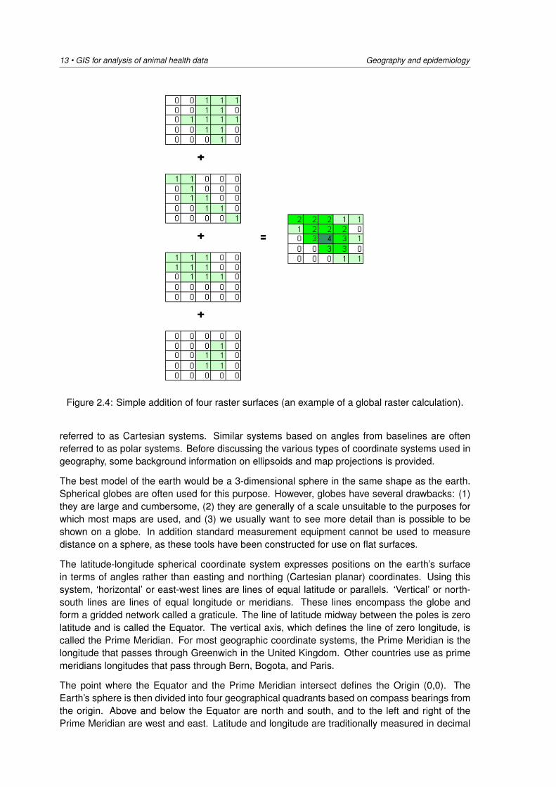
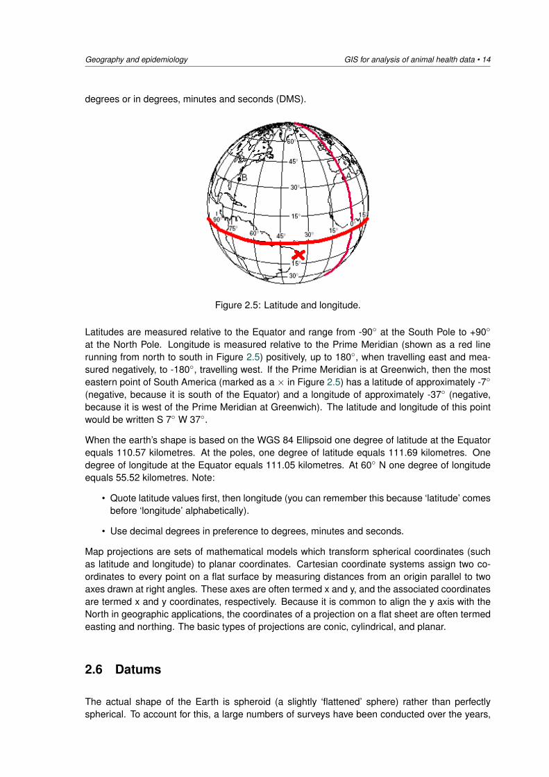
The latitude-longitude spherical coordinate system expresses positions on the earth’s surfacein terms of angles rather than easting and northing (Cartesian planar) coordinates. Using thissystem, ‘horizontal’ or east-west lines are lines of equal latitude or parallels. ‘Vertical’ or north-south lines are lines of equal longitude or meridians. These lines encompass the globe andform a gridded network called a graticule. The line of latitude midway between the poles is zerolatitude and is called the Equator. The vertical axis, which defines the line of zero longitude, iscalled the Prime Meridian. For most geographic coordinate systems, the Prime Meridian is thelongitude that passes through Greenwich in the United Kingdom. Other countries use as primemeridians longitudes that pass through Bern, Bogota, and Paris.
The point where the Equator and the Prime Meridian intersect defines the Origin (0,0). TheEarth’s sphere is then divided into four geographical quadrants based on compass bearings fromthe origin. Above and below the Equator are north and south, and to the left and right of thePrime Meridian are west and east. Latitude and longitude are traditionally measured in decimal
Geography and epidemiology GIS for analysis of animal health data • 14
degrees or in degrees, minutes and seconds (DMS).
Figure 2.5: Latitude and longitude.
Latitudes are measured relative to the Equator and range from -90◦ at the South Pole to +90◦
at the North Pole. Longitude is measured relative to the Prime Meridian (shown as a red linerunning from north to south in Figure 2.5) positively, up to 180◦, when travelling east and mea-sured negatively, to -180◦, travelling west. If the Prime Meridian is at Greenwich, then the mosteastern point of South America (marked as a × in Figure 2.5) has a latitude of approximately -7◦
(negative, because it is south of the Equator) and a longitude of approximately -37◦ (negative,because it is west of the Prime Meridian at Greenwich). The latitude and longitude of this pointwould be written S 7◦ W 37◦.
When the earth’s shape is based on the WGS 84 Ellipsoid one degree of latitude at the Equatorequals 110.57 kilometres. At the poles, one degree of latitude equals 111.69 kilometres. Onedegree of longitude at the Equator equals 111.05 kilometres. At 60◦ N one degree of longitudeequals 55.52 kilometres. Note:
• Quote latitude values first, then longitude (you can remember this because ‘latitude’ comesbefore ‘longitude’ alphabetically).
• Use decimal degrees in preference to degrees, minutes and seconds.
Map projections are sets of mathematical models which transform spherical coordinates (suchas latitude and longitude) to planar coordinates. Cartesian coordinate systems assign two co-ordinates to every point on a flat surface by measuring distances from an origin parallel to twoaxes drawn at right angles. These axes are often termed x and y, and the associated coordinatesare termed x and y coordinates, respectively. Because it is common to align the y axis with theNorth in geographic applications, the coordinates of a projection on a flat sheet are often termedeasting and northing. The basic types of projections are conic, cylindrical, and planar.
2.6 Datums
The actual shape of the Earth is spheroid (a slightly ‘flattened’ sphere) rather than perfectlyspherical. To account for this, a large numbers of surveys have been conducted over the years,

15 • GIS for analysis of animal health data Geography and epidemiology
resulting in a large number of ellipsoid definitions (examples are given in Table 2.2). The gener-alised earth-centered coordinate system (WGS84) provides a good overall mean solution for allplaces on the earth. However, for specific local measurements, WGS84 does not account wellfor local conditions. In this situation, local datums are useful. The local North American Datumof 1927 (NAD27) more closely fits the earth’s surface in the upper-left quadrant of the earth’scross-section. NAD27 only fits this quadrant, so to use it in another part of the earth will result inserious measurement errors. For mapping North America, in order to obtain the most accuratelocations and measurements, NAD27 or NAD83/91 are used.
Table 2.2: Common ellipsoid definitions used in geography.
Title Length of major axis (metres) Flattening
Airy 1830 6377563 299.325Australian National 6378160 298.250Bessel 1841 6377483 299.153Clarke 1866 6378206 294.979Clarke 1880 6378249 293.465Helmert 1906 6378200 298.300GRS 80 6378137 298.257South American 1969 6378160 298.250WGS 72 6378135 298.260WGS 84 6378137 298.257
Datum is a term you might also come across when dealing with map projections. A datum definesthe position of the spheroid relative to the centre of the Earth. Local datums are often used toalign a given spheroid to more closely to the Earth’s surface in a particular area. A local datum isnot suited for use outside the area for which it was designed.
2.7 Coordinate systems
Once geographic data are projected onto a planar surface, features must be referenced by aplanar coordinate system. The geographic system (latitude-longitude) which is based on anglesmeasured on a sphere, is not valid for measurements on a plane. Therefore, a Cartesian coor-dinate system is used, where the origin (0, 0) is toward the lower left of the planar section. Thetrue origin point (0, 0) may or may not be in the proximity of the map data you are using. Co-ordinates are then measured from the origin point. However, false eastings and false northingsare frequently used, which effectively offset the origin to a different place on the plane. This isdone in order to minimise the possibility of using negative coordinate values (to make calculationsof distance and area easier) and to lowwer the absolute value of the coordinates (to make thevalues easier to read, transcribe, and calculate). Systems for georeferencing can be divided intotwo groups:
1. Global systems, which are used to define position at all locations across the Earth’s surface.
2. Regional systems, which are defined for specific areas, often covering countries, states, orprovinces.
Whatever coordinate system is used, it must have the following features:
• It must be unique, so that there can be no confusion about the location that is referenced;
• Its meaning must be shared among all working with the information; and
• It must be persistent in time.
Geography and epidemiology GIS for analysis of animal health data • 16
Table 2.3 lists and describes some of the commonly used systems of georeferencing.
Table 2.3: Commonly used systems of georeferencing.
System Domain Resolution Example
Place name Will vary Varies by feature type Sydney, Canada; Sydney, AustraliaPostal address Global Size of location that has one
postal address - typically ahouse or building, but maymean a large farm or station
105 Woodham Lane Addlestone, Sur-rey
Post code Country Area occupied by a definednumber of mailboxes
The post code of Addlestone, Surrey,UK, is KT15 3NB
Telephone calling area Country Varies from country to coun-try
If you are phoning a residence inNew Zealand with a phone numberthat starts with 06, you know that theplace you are calling is located some-where in the south of the North Is-land.
Cadastral system Local land au-thority
Area occupied by a singleparcel of land
A map of land ownership maintainedfor the purpose of taxing land or cre-ating a public record of land owner-ship.
Latitude and longitude Global Infinite E113◦59’53.0”, N22◦22’36.6”State plane coordinates Unique to coun-
try or stateInfinite UK national grid
2.7.1 The Transverse Mercator projection
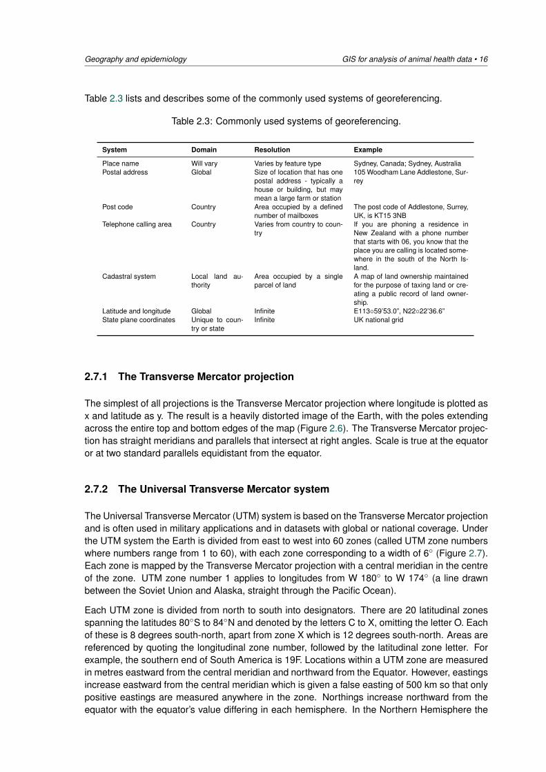
The simplest of all projections is the Transverse Mercator projection where longitude is plotted asx and latitude as y. The result is a heavily distorted image of the Earth, with the poles extendingacross the entire top and bottom edges of the map (Figure 2.6). The Transverse Mercator projec-tion has straight meridians and parallels that intersect at right angles. Scale is true at the equatoror at two standard parallels equidistant from the equator.
2.7.2 The Universal Transverse Mercator system
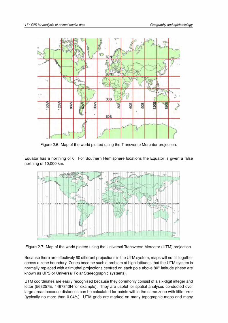
The Universal Transverse Mercator (UTM) system is based on the Transverse Mercator projectionand is often used in military applications and in datasets with global or national coverage. Underthe UTM system the Earth is divided from east to west into 60 zones (called UTM zone numberswhere numbers range from 1 to 60), with each zone corresponding to a width of 6◦ (Figure 2.7).Each zone is mapped by the Transverse Mercator projection with a central meridian in the centreof the zone. UTM zone number 1 applies to longitudes from W 180◦ to W 174◦ (a line drawnbetween the Soviet Union and Alaska, straight through the Pacific Ocean).
Each UTM zone is divided from north to south into designators. There are 20 latitudinal zonesspanning the latitudes 80◦S to 84◦N and denoted by the letters C to X, omitting the letter O. Eachof these is 8 degrees south-north, apart from zone X which is 12 degrees south-north. Areas arereferenced by quoting the longitudinal zone number, followed by the latitudinal zone letter. Forexample, the southern end of South America is 19F. Locations within a UTM zone are measuredin metres eastward from the central meridian and northward from the Equator. However, eastingsincrease eastward from the central meridian which is given a false easting of 500 km so that onlypositive eastings are measured anywhere in the zone. Northings increase northward from theequator with the equator’s value differing in each hemisphere. In the Northern Hemisphere the
17 • GIS for analysis of animal health data Geography and epidemiology
Figure 2.6: Map of the world plotted using the Transverse Mercator projection.
Equator has a northing of 0. For Southern Hemisphere locations the Equator is given a falsenorthing of 10,000 km.
Figure 2.7: Map of the world plotted using the Universal Transverse Mercator (UTM) projection.
Because there are effectively 60 different projections in the UTM system, maps will not fit togetheracross a zone boundary. Zones become such a problem at high latitudes that the UTM system isnormally replaced with azimuthal projections centred on each pole above 80◦ latitude (these areknown as UPS or Universal Polar Stereographic systems).
UTM coordinates are easily recognised because they commonly consist of a six-digit integer andletter (563257E, 4467843N for example). They are useful for spatial analyses conducted overlarge areas because distances can be calculated for points within the same zone with little error(typically no more than 0.04%). UTM grids are marked on many topographic maps and many
Geography and epidemiology GIS for analysis of animal health data • 18
countries project their topographic maps using UTM, so it is easy to obtain UTM coordinatesfrom maps for input into digital datasets.
2.7.3 Transverse Mercator Grid Systems
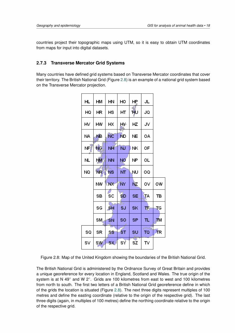
Many countries have defined grid systems based on Transverse Mercator coordinates that covertheir territory. The British National Grid (Figure 2.8) is an example of a national grid system basedon the Transverse Mercator projection.
Figure 2.8: Map of the United Kingdom showing the boundaries of the British National Grid.
The British National Grid is administered by the Ordnance Survey of Great Britain and providesa unique georeference for every location in England, Scotland and Wales. The true origin of thesystem is at N 49◦ and W 2◦. Grids are 100 kilometres from east to west and 100 kilometresfrom north to south. The first two letters of a British National Grid georeference define in whichof the grids the location is situated (Figure 2.8). The next three digits represent multiples of 100metres and define the easting coordinate (relative to the origin of the respective grid). The lastthree digits (again, in multiples of 100 metres) define the northing coordinate relative to the originof the respective grid.
19 • GIS for analysis of animal health data Geography and epidemiology
Take for example the British National Grid georeference SP254186. The origin of the SP grid (thatis, its south-western corner) is 400 kilometres east and 200 kilometres north of the map origin (N49◦ and W 2◦, the most south-west corner of the grid labelled SV in Figure 2.8). The location is(254 × 100) / 1000 = 25.4 kilometres east and (186 × 100) / 1000 = 18.6 kilometres north of theorigin of the SP grid. The grid coordinates for this location would be 4254000, 218600.
2.7.4 State plane coordinates
In the United States each state has its own State plane coordinate system. State plane sys-tems were developed in order to provide local reference systems that were tied to a nationaldatum. In the United States, the State Plane System 1927 was developed in the 1930s and wasbased on the North American Datum 1927 (NAD-27). NAD-27 coordinates are in Imperial units(feet).
2.8 Geography and spatial epidemiology
This section describes the characteristics that make spatial information different from other datatypes you may have dealt with, and explains why, when we analyse spatial data, these charac-teristics need to be accounted for.
2.8.1 Spatial autocorrelation
As a general rule spatial data tend to exhibit an increasing range of values (that is, they demon-strate increasing heterogeneity) with increasing distance. This may be stated in another way, inthe form of Tobler’s First Law of Geography (Tobler 1970): ‘Everything is related to everythingelse, but near things are more related than distant things.’
Formally, this property is known as spatial autocorrelation and statistical tests are available toquantify the degree to which near and more distant things are interrelated. A similar concept,that of temporal autocorrelation, concerns the relationship between consecutive events in time.Spatial autocorrelation measures attempt to deal simultaneously with similarities in the locationof spatial objects and their attributes. If features that are similar in location are also similar inattributes, the pattern as a whole is said to exhibit positive spatial autocorrelation. On the otherhand, negative spatial autocorrelation exists when features which are close together in spacetend to be more dissimilar in their attribute values than features that are further apart.
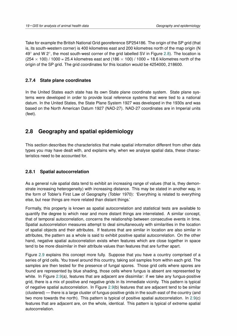
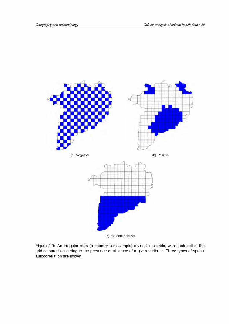
Figure 2.9 explains this concept more fully. Suppose that you have a country comprised of aseries of grid cells. You travel around this country, taking soil samples from within each grid. Thesamples are then tested for the presence of fungal spores. Those grid cells where spores arefound are represented by blue shading, those cells where fungus is absent are represented bywhite. In Figure 2.9(a), features that are adjacent are dissimilar: if we take any fungus-positivegrid, there is a mix of positive and negative grids in its immediate vicinity. This pattern is typicalof negative spatial autocorrelation. In Figure 2.9(b) features that are adjacent tend to be similar(clustered) — there is a large cluster of fungus-positive grids in the south east of the country (andtwo more towards the north). This pattern is typical of positive spatial autocorrelation. In 2.9(c)features that are adjacent are, on the whole, identical. This pattern is typical of extreme spatialautocorrelation.
Geography and epidemiology GIS for analysis of animal health data • 20
(a) Negative (b) Positive
(c) Extreme positive
Figure 2.9: An irregular area (a country, for example) divided into grids, with each cell of thegrid coloured according to the presence or absence of a given attribute. Three types of spatialautocorrelation are shown.
21 • GIS for analysis of animal health data Geography and epidemiology
In spatial data analysis an understanding of spatial autocorrelation has an important influence onthe way in which we abstract and collect data, and how we draw inferences between events andoccurrences. Spatial autocorrelation is important in the field of epidemiology for two reasons.Firstly, it helps us to generalise from a sample of observations in order to build a spatial data set.Secondly, the presence of spatial autocorrelation violates some of the key assumptions of manyof the conventional statistical techniques used to quantify the relationship between two or morevariables. Acknowledging the importance of geographic scale or level of detail is fundamental tounderstanding the likely strength and nature of spatial autocorrelation.
2.8.2 Spatial sampling
In aiming to represent the complexity of the real world, researchers have to employ abstractionand sampling of events and occurrences from a sample frame, defined as the group of eligibleelements of interest. In reality, geographic representation is based on sampling in that elementsof reality that are used are abstracted from the real world. In remote sensing each pixel isa spatially averaged reflectance value calculated at the spatial resolution characteristic of thesensor. In many situations we need to consciously select some observations and not others inorder to create an abstraction of the area we wish to represent. This is because the resourcesavailable for any given project will never allow us to measure every single aspect of the elementsthat make up the region of interest.
In any application, where the events of interest are spatially heterogeneous we will require alarge sample to capture the full variability of attribute values at all (or most) locations. Otherparts of our study may be more homogeneous and a sparser sampling interval may be moreappropriate. Both simple random and systematic random sampling designs may be adaptedin order to allow a differential sampling interval over a given area — thus it may be possibleto partition the sampling frame into sub-areas based on a knowledge of spatial structure, andspecifically of the variability of the attributes that are being measured. Other, application-specificcircumstances include the resources available for the project and accessibility of all parts of thestudy area for observation.
ExampleYou know that the concentration of a trace element in soil is closely related to soil type, and thatthere are two soil types within your area of study. Because of this you can restrict the number ofsamples that are taken within each soil type area, knowing that your samples taken at differentlocations throughout each area will yield a similar trace element concentration. In this caseknowledge about the presence of spatial autocorrelation in soil trace element concentrationhas an important influence on your sampling strategy.
2.8.3 Spatial interpolation
In sampling part of reality it follows that you will need to exercise some level of judgement to‘fill in the gaps’ — that is, to interpolate the sampled data so that your spatial representationwill be in some way complete. To do this properly, you need to have a good understandingof issues related to autocorrelation. A literal interpretation of Tobler’s First Law of Geographyimplies a continuous, smoothly declining effect of distance upon the attribute values of adjacentspatial objects as you travel throughout a study region (that is, a decay function). The precise
Geography and epidemiology GIS for analysis of animal health data • 22
nature of the decay function used to represent the effect of distance is likely to vary depending onspecific applications including linear distance, negative power distance and negative exponentialdistance.
In addition to appreciating the type of decay function, it is also important to be aware that theeffects of distance may vary depending on direction. If the decay function is uniform in everydirection it is said to be isotropic. If the decay function varies with direction it is said to beanisotropic.
ExampleTo continue our earlier example, having estimated trace element concentration at various sitesyou might then proceed to construct a contour surface to represent trace element concentra-tion throughout the entire study area. The ability to interpolate the sampled data will dependon making assumptions about autocorrelation and a knowledge of how this autocorrelationmay vary with direction. The notion of smooth, continuous variation underpins many of thetechniques used to describe spatial data.
2.8.4 Aggregation
When reporting the spatial distribution of disease within a country it is common to aggregateinformation at an area level. This is done because the units of interest (for example, householdsor farms) occupy geographically unique locations and confidentiality restrictions usually dictatethat uniquely attributable information is anonymised in some way.
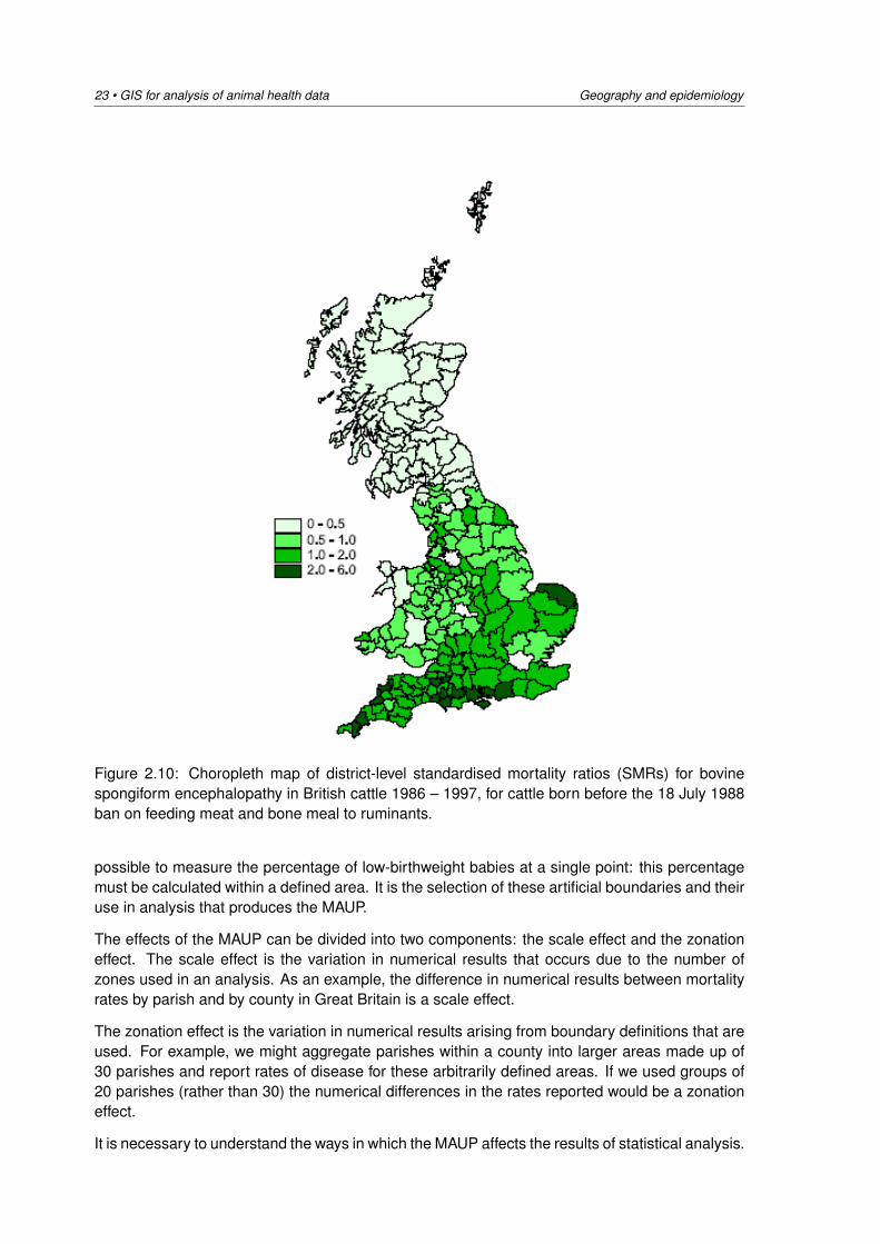
Figure 2.10 provides an example where the standardised mortality ratio (SMR) of bovine spongi-form encephalopathy (BSE) is plotted for arbitrarily defined areas of Great Britain. On the basisof Figure 2.10 we might legitimately conclude that there was a higher risk of BSE in the south ofthe country, compared with the north. While this might be the case at the area level we cannotnecessarily draw the same conclusion at the individual farm holding level. In other words, if wepicked a random holding from an area with a high SMR in the south of the country, we couldnot always guarantee that the selected holding would have experienced large numbers of BSEcases. Thus, while mapping disease at the area level is useful for identifying broad-scale spatialtrends, it hides within-area heterogeneity of disease. This phenomenon (ecological fallacy) issomething to beware of when drawing conclusions from disease data summarised at the arealevel.
2.8.5 The modifiable areal unit problem
When dealing with area data we need to consider how the zones of analysis affect results. Ifrelationships between variables change with the selection of different areal units, the reliabilityof results is called into question. The effect of the selection of areal units on analysis, termedthe modifiable areal unit problem (MAUP), is defined as: a problem arising from the impositionof artificial units of spatial reporting on continuous geographical phenomenon resulting in thegeneration of artificial spatial patterns (Openshaw 1984).
The MAUP has been most prominent in the analysis of socioeconomic and epidemiological data(see, for example Wong et al. 1999 and Nakaya 2000). Such areal data cannot be measured ata single point, but must be contained within a boundary to be meaningful. For example, it is not
23 • GIS for analysis of animal health data Geography and epidemiology
Figure 2.10: Choropleth map of district-level standardised mortality ratios (SMRs) for bovinespongiform encephalopathy in British cattle 1986 – 1997, for cattle born before the 18 July 1988ban on feeding meat and bone meal to ruminants.
possible to measure the percentage of low-birthweight babies at a single point: this percentagemust be calculated within a defined area. It is the selection of these artificial boundaries and theiruse in analysis that produces the MAUP.
The effects of the MAUP can be divided into two components: the scale effect and the zonationeffect. The scale effect is the variation in numerical results that occurs due to the number ofzones used in an analysis. As an example, the difference in numerical results between mortalityrates by parish and by county in Great Britain is a scale effect.
The zonation effect is the variation in numerical results arising from boundary definitions that areused. For example, we might aggregate parishes within a county into larger areas made up of30 parishes and report rates of disease for these arbitrarily defined areas. If we used groups of20 parishes (rather than 30) the numerical differences in the rates reported would be a zonationeffect.
It is necessary to understand the ways in which the MAUP affects the results of statistical analysis.
Geography and epidemiology GIS for analysis of animal health data • 24
(a) No boundaries within the study area (b) Four regions
(c) 18 regions
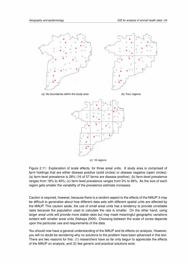
Figure 2.11: Explanation of scale effects, for three areal units. A study area is comprised offarm holdings that are either disease positive (solid circles) or disease negative (open circles):(a) farm-level prevalence is 28% (16 of 57 farms are disease positive); (b) farm-level prevalenceranges from 18% to 40%; (c) farm-level prevalence ranges from 0% to 66%. As the size of eachregion gets smaller the variability of the prevalence estimate increases.
Caution is required, however, because there is a random aspect to the effects of the MAUP. It maybe difficult to generalise about how different data sets with different spatial units are affected bythe MAUP. This caution aside, the use of small areal units has a tendency to provide unreliablerates because the population used to calculate the rate is smaller. On the other hand, usinglarger areal units will provide more stable rates but may mask meaningful geographic variationsevident with smaller areal units (Nakaya 2000). Choosing between the scale of zones dependsupon the particular use and requirements of the data.
You should now have a general understanding of the MAUP and its effects on analysis. However,you will no doubt be wondering why no solutions to the problem have been advanced in this text.There are two reasons for this: (1) researchers have so far only begun to appreciate the effectsof the MAUP on analysis; and (2) few generic and practical solutions exist.
25 • GIS for analysis of animal health data Geography and epidemiology
(a) (b)
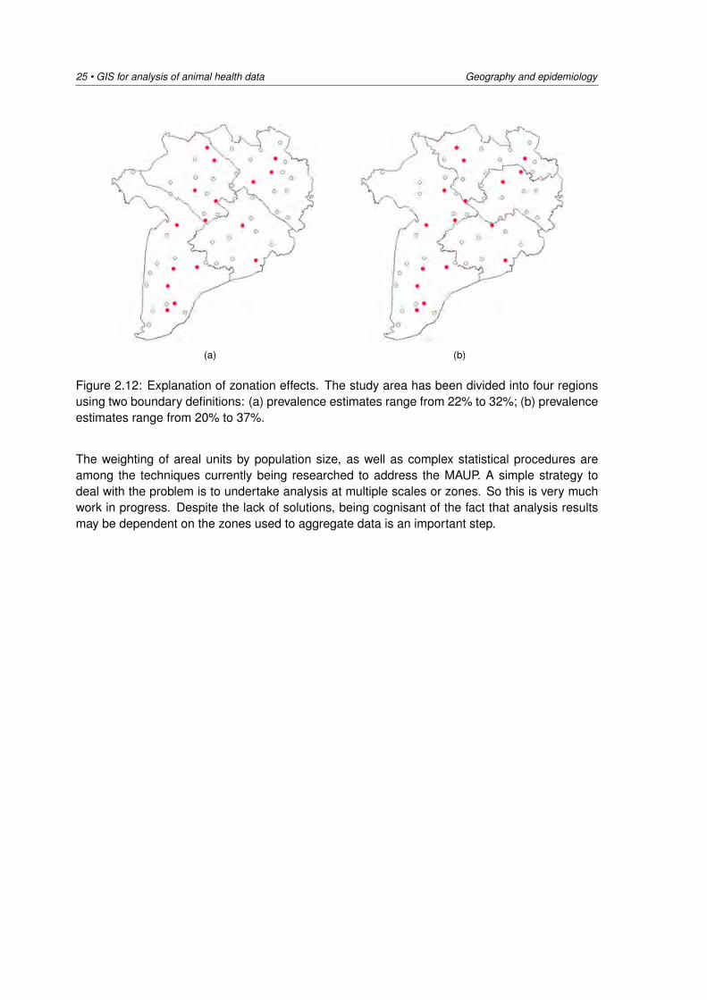
Figure 2.12: Explanation of zonation effects. The study area has been divided into four regionsusing two boundary definitions: (a) prevalence estimates range from 22% to 32%; (b) prevalenceestimates range from 20% to 37%.
The weighting of areal units by population size, as well as complex statistical procedures areamong the techniques currently being researched to address the MAUP. A simple strategy todeal with the problem is to undertake analysis at multiple scales or zones. So this is very muchwork in progress. Despite the lack of solutions, being cognisant of the fact that analysis resultsmay be dependent on the zones used to aggregate data is an important step.
Sources of spatial data GIS for analysis of animal health data • 26
3 Sources of spatial data
3.1 Introduction
There are many sources of open-source and publicly-available spatial data repositories, and itcan be time-consuming to identify specific data required for a project. It can also be frustrating,as often the descriptions (metadata) of downloadable spatial datasets is misleading, and theactual data cannot be accessed. Instead, only PDF maps can be downloaded, which are of littleanalytic value.
In addition, spatial datasets tend to be large. This results in long download times. Subsequently,some editing is usually required in the GIS software; the processing times for this, too, can beextensive. Don’t underestimate the time required to prepare the spatial data for analysis.
In this chapter, we provide brief descriptions of some data sources that are likely to be useful forspatial analysis of livestock diseases. There are a number of supplementary data sources whichprovide statistical information which may be of use but are not explicitly spatial. These can haveutility in spatial analyses. For instance, national livestock census data can be rendered useful byjoining the lowest level of aggregation (e.g. commune, subdistrict or District) with administrativearea shapefiles. The same can be done with socio-economic indicator data.
3.2 Geographic data
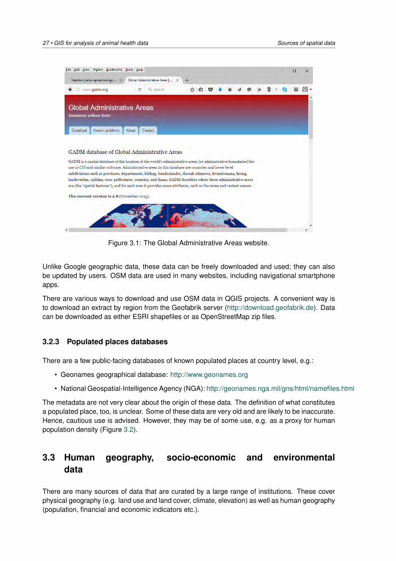
3.2.1 GADM database of Global Administrative Areas
The GADM database of Global Administrative Areas (http://www.gadm.org) is a database of dig-ital maps of the world’s adminstrative boundaries. Administrative boundaries in this databaseare countries and lower level subdivisions such as provinces, departments and communes. TheGADM database is a resource of digital maps providing details of the boundaries of administra-tive areas (the ‘spatial features’) and, for each area, attribute information including area nameand variant names. The current (September 2017) version of the GADM delimits a total of ap-proximately 294,430 administrative areas. The data are available in ESRI shapefile, .RData, andGoogle Earth .kmz formats.
3.2.2 The OpenStreetMap project and data extracts
OpenStreetMapv (OSM) is ‘a map of the world, created by people like you and free to use underan open license’. OSM is run by a non-profit foundation whose aim is to support and enable thedevelopment of freely-reusable geospatial data. It has a large and enthusiastic community base.
27 • GIS for analysis of animal health data Sources of spatial data
Figure 3.1: The Global Administrative Areas website.
Unlike Google geographic data, these data can be freely downloaded and used; they can alsobe updated by users. OSM data are used in many websites, including navigational smartphoneapps.
There are various ways to download and use OSM data in QGIS projects. A convenient way isto download an extract by region from the Geofabrik server (http://download.geofabrik.de). Datacan be downloaded as either ESRI shapefiles or as OpenStreetMap zip files.
3.2.3 Populated places databases
There are a few public-facing databases of known populated places at country level, e.g.:
• Geonames geographical database: http://www.geonames.org
• National Geospatial-Intelligence Agency (NGA): http://geonames.nga.mil/gns/html/namefiles.html
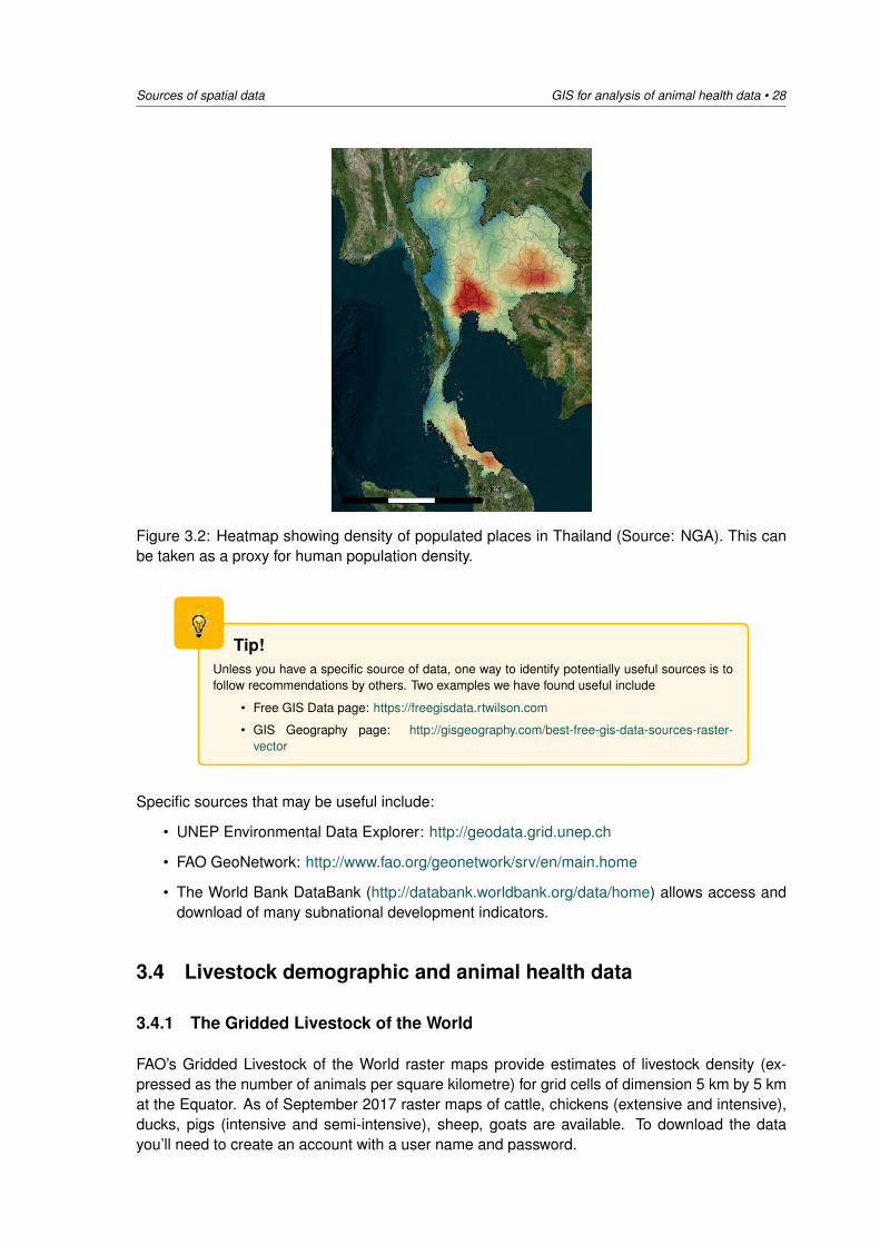
The metadata are not very clear about the origin of these data. The definition of what constitutesa populated place, too, is unclear. Some of these data are very old and are likely to be inaccurate.Hence, cautious use is advised. However, they may be of some use, e.g. as a proxy for humanpopulation density (Figure 3.2).
3.3 Human geography, socio-economic and environmentaldata
There are many sources of data that are curated by a large range of institutions. These coverphysical geography (e.g. land use and land cover, climate, elevation) as well as human geography(population, financial and economic indicators etc.).
Sources of spatial data GIS for analysis of animal health data • 28
Figure 3.2: Heatmap showing density of populated places in Thailand (Source: NGA). This canbe taken as a proxy for human population density.
Tip!Unless you have a specific source of data, one way to identify potentially useful sources is tofollow recommendations by others. Two examples we have found useful include
• Free GIS Data page: https://freegisdata.rtwilson.com
• GIS Geography page: http://gisgeography.com/best-free-gis-data-sources-raster-vector
Specific sources that may be useful include:
• UNEP Environmental Data Explorer: http://geodata.grid.unep.ch
• FAO GeoNetwork: http://www.fao.org/geonetwork/srv/en/main.home
• The World Bank DataBank (http://databank.worldbank.org/data/home) allows access anddownload of many subnational development indicators.
3.4 Livestock demographic and animal health data
3.4.1 The Gridded Livestock of the World
FAO’s Gridded Livestock of the World raster maps provide estimates of livestock density (ex-pressed as the number of animals per square kilometre) for grid cells of dimension 5 km by 5 kmat the Equator. As of September 2017 raster maps of cattle, chickens (extensive and intensive),ducks, pigs (intensive and semi-intensive), sheep, goats are available. To download the datayou’ll need to create an account with a user name and password.
29 • GIS for analysis of animal health data Sources of spatial data
3.4.2 The World Animal Health Information System
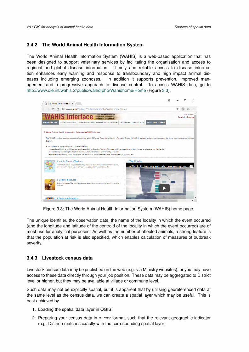
The World Animal Health Information System (WAHIS) is a web-based application that hasbeen designed to support veterinary services by facilitating the organisation and access toregional and global disease information. Timely and reliable access to disease informa-tion enhances early warning and response to transboundary and high impact animal dis-eases including emerging zoonoses. In addition it supports prevention, improved man-agement and a progressive approach to disease control. To access WAHIS data, go tohttp://www.oie.int/wahis 2/public/wahid.php/Wahidhome/Home (Figure 3.3).
Figure 3.3: The World Animal Health Information System (WAHIS) home page.
The unique identifier, the observation date, the name of the locality in which the event occurred(and the longitude and latitude of the centroid of the locality in which the event occurred) are ofmost use for analytical purposes. As well as the number of affected animals, a strong feature isthat the population at risk is also specified, which enables calculation of measures of outbreakseverity.
3.4.3 Livestock census data
Livestock census data may be published on the web (e.g. via Ministry websites), or you may haveaccess to these data directly through your job position. These data may be aggregated to Districtlevel or higher, but they may be available at village or commune level.
Such data may not be explicitly spatial, but it is apparent that by utilising georeferenced data atthe same level as the census data, we can create a spatial layer which may be useful. This isbest achieved by
1. Loading the spatial data layer in QGIS;
2. Preparing your census data in *.csv format, such that the relevant geographic indicator(e.g. District) matches exactly with the corresponding spatial layer;
Sources of spatial data GIS for analysis of animal health data • 30
3. Importing this *.csv file into QGIS as an attribute-only table (i.e. one that has no geome-try);
4. Creating a table join between the spatial layer and the data table.
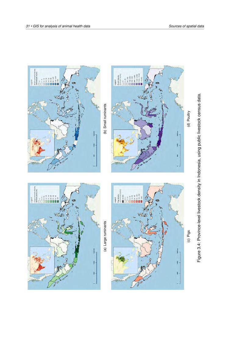
Subsequently, choropleth or raster heatmaps can be made to visualise the livestock density. Asan example, Figure 3.4 shows Province-level livestock density, comparing the outputs with thecorresponding FAO GLiPHA map.
3.5 Geocoding locations
On occasions you will be provided with only the name of an outbreak location (without theircorresponding longitude and latitude coordinates). In this situation, in order to define outbreaklocations as a single point in space, it is necessary to geocode the outbreak location names. Theresources page on the Veterinary Epidemiology at Melbourne University web site has tools forgeocoding either a single or multiple addresses.
If you are using the multiple address facility your data will need to be saved as a Microsoft Excel(*.xlsx) file with two columns. The first column should be a numeric, unique identifier. Thesecond column should list the address details as text. Because the geocoding engine usesGoogle Maps (with a limit on the number of addresses that can be geocoded on any given daywithout payment of a license) your spreadsheet should contain no more than 100 records.
31 • GIS for analysis of animal health data Sources of spatial data
(a)
Larg
eru
min
ants
(b)
Sm
allr
umin
ants
(c)
Pig
s(d
)Po
ultr
y
Figu
re3.
4:P
rovi
nce-
leve
lliv
esto
ckde
nsity
inIn
done
sia,
usin
gpu
blic
lives
tock
cens
usda
ta.
Exploratory spatial data analysis (ESDA) GIS for analysis of animal health data • 32
4 Exploratory spatial data analysis (ESDA)
4.1 Introduction: exploratory data analysis (EDA)
If a dataset can be defined as “an organised collection of pieces of information about individuals”,then exploratory data analysis (henceforth abbreviated as EDA) can be considered as the initialinteraction with a dataset which may identify important characteristics or trends that apply to thecollection of individuals (generally referred to as the study population) as a whole.
The term EDA was coined by John Tukey, who published a book on it in 1977. He considered thatEDA should be used by data analysts to examine their data sets. Rather than directly performingstatistical hypothesis testing (confirmatory data analysis), the investigator should use EDA toformulate hypotheses and identify appropriate methods to subsequently test these.
EDA is not a specific technique so much as an approach that informs subsequent analysis. Itincorporates different ways of summarising the data. A large number of terms may be used forthis; these can be used interchangeably and it is not always clear how these terms relate to EDA.Such terms may include descriptive analysis or statistics; summary analysis or statistics; datavisualisation or display; statistical graphics; etc. In recent years, the emergence of ‘big data’ anddata mining have highlighted the application of EDA.
4.1.1 The importance of EDA
EDA is an important step in the analytic process, and it has several functions. It helps to enableus to understand the data.
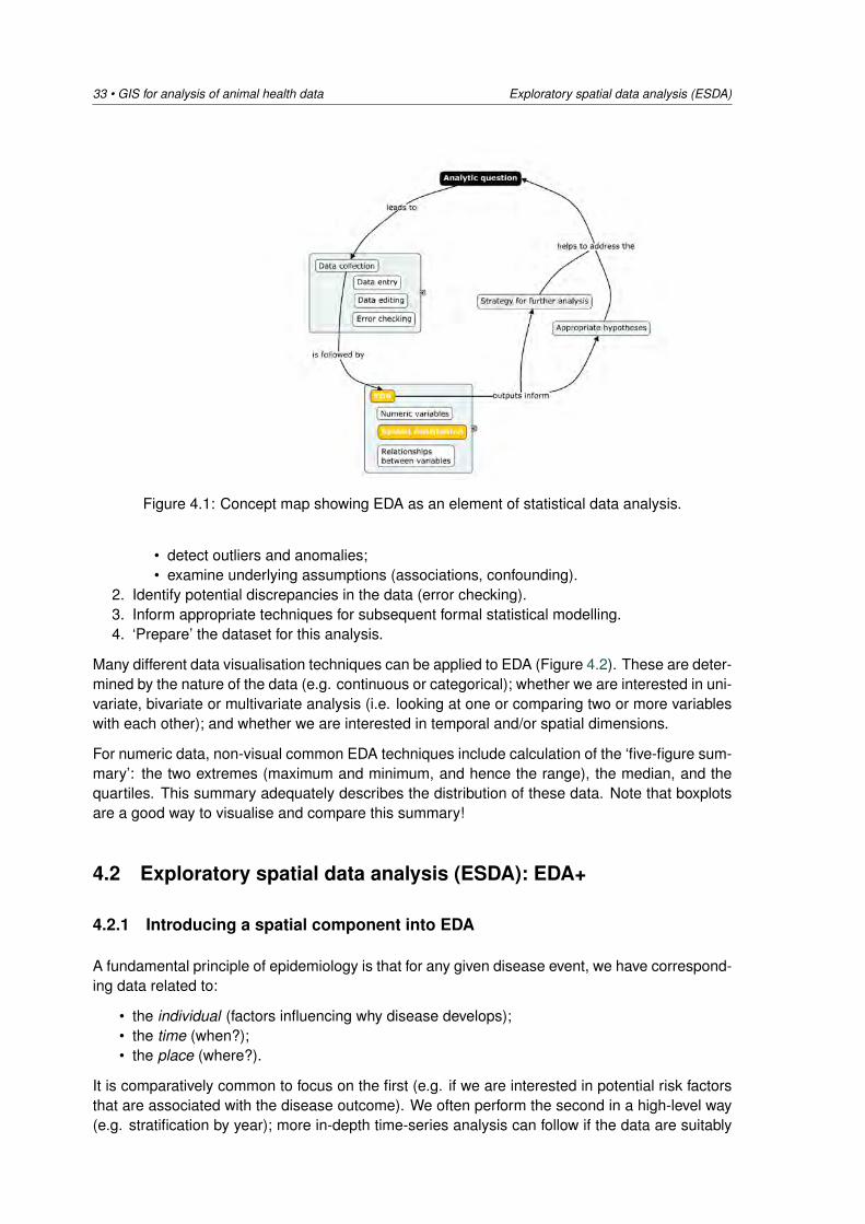
EDA can be considered as an intermediary step between the collection of data and a formalanalysis of these data (Figure 4.1). The optimal strategy for such formal analysis may not be clearfrom the outset; the specific structure and features of the dataset have a bearing on which analyticapproach will be most effective. The outputs generated by EDA should be applied to assist withhypothesis generation and determining an appropriate strategy for this analysis. Indeed, in manycases this quantitative analysis will simply provide statistically robust evidence to support thetrends detected by the EDA.
4.1.2 Aims and objectives of EDA
EDA is not a technique, but rather a variety of techniques that are employed as appropriateto
1. Generate insight into a data set (get a ‘feel’ for the data):• uncover underlying structure and identify important variables;
33 • GIS for analysis of animal health data Exploratory spatial data analysis (ESDA)
Figure 4.1: Concept map showing EDA as an element of statistical data analysis.
• detect outliers and anomalies;• examine underlying assumptions (associations, confounding).
2. Identify potential discrepancies in the data (error checking).3. Inform appropriate techniques for subsequent formal statistical modelling.4. ‘Prepare’ the dataset for this analysis.
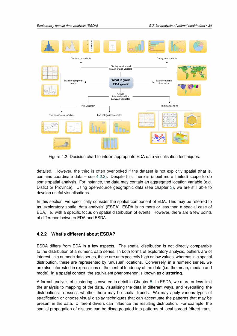
Many different data visualisation techniques can be applied to EDA (Figure 4.2). These are deter-mined by the nature of the data (e.g. continuous or categorical); whether we are interested in uni-variate, bivariate or multivariate analysis (i.e. looking at one or comparing two or more variableswith each other); and whether we are interested in temporal and/or spatial dimensions.
For numeric data, non-visual common EDA techniques include calculation of the ‘five-figure sum-mary’: the two extremes (maximum and minimum, and hence the range), the median, and thequartiles. This summary adequately describes the distribution of these data. Note that boxplotsare a good way to visualise and compare this summary!
4.2 Exploratory spatial data analysis (ESDA): EDA+
4.2.1 Introducing a spatial component into EDA
A fundamental principle of epidemiology is that for any given disease event, we have correspond-ing data related to:
• the individual (factors influencing why disease develops);• the time (when?);• the place (where?).
It is comparatively common to focus on the first (e.g. if we are interested in potential risk factorsthat are associated with the disease outcome). We often perform the second in a high-level way(e.g. stratification by year); more in-depth time-series analysis can follow if the data are suitably
Exploratory spatial data analysis (ESDA) GIS for analysis of animal health data • 34
Figure 4.2: Decision chart to inform appropriate EDA data visualisation techniques.
detailed. However, the third is often overlooked if the dataset is not explicitly spatial (that is,contains coordinate data – see 4.2.3). Despite this, there is (albeit more limited) scope to dosome spatial analysis. For instance, the data may contain an aggregated location variable (e.g.Distict or Province). Using open-source geographic data (see chapter 3), we are still able todevelop useful visualisations.
In this section, we specifically consider the spatial component of EDA. This may be referred toas ‘exploratory spatial data analysis’ (ESDA). ESDA is no more or less than a special case ofEDA, i.e. with a specific focus on spatial distribution of events. However, there are a few pointsof difference between EDA and ESDA.
4.2.2 What’s different about ESDA?
ESDA differs from EDA in a few aspects. The spatial distribution is not directly comparableto the distribution of a numeric data series. In both forms of exploratory analysis, outliers are ofinterest; in a numeric data series, these are unexpectedly high or low values, whereas in a spatialdistribution, these are represented by ‘unusual’ locations. Conversely, in a numeric series, weare also interested in expressions of the central tendency of the data (i.e. the mean, median andmode). In a spatial context, the equivalent phenomenon is known as clustering.
A formal analysis of clustering is covered in detail in Chapter 5. In ESDA, we more or less limitthe analysis to mapping of the data, visualising the data in different ways, and ‘eyeballing’ thedistributions to assess whether there may be spatial trends. We may apply various types ofstratification or choose visual display techniques that can accentuate the patterns that may bepresent in the data. Different drivers can influence the resulting distribution. For example, thespatial propagation of disease can be disaggregated into patterns of local spread (direct trans-
35 • GIS for analysis of animal health data Exploratory spatial data analysis (ESDA)
mission), as opposed to spread due to trade and animal movement. These different dynamicsare referred to as spatial regimes; although our data show a ‘mix’ of these dynamics, effectiveESDA can uncover evidence of their existence, which can subsequently be investigated in moredepth.
4.2.3 Types of spatial data and associated techniques for performing ESDA
Event data
In a spatial context, cases of disease are often referred to as events. These data refer to aspecific location: they are point data. Therefore, each record includes coordinates.
In the most atomic case, a record of event data will refer to an individual in a specified pointlocation. In practice, one event record may contain information on multiple individuals (e.g. aherd of animals); the location may aggregated to a specified area, too. For instance, the level ofobservation may be at the farm or village level. In this case, the point location is expected to berepresentative of this area. Generally, the centroid is used.
The events may be of variable levels of accuracy, e.g. observed, confirmed (by laboratory di-agnosis) or recorded / reported. As with other types of disease datasets, information on othervariables may also be associated with the location of each record.
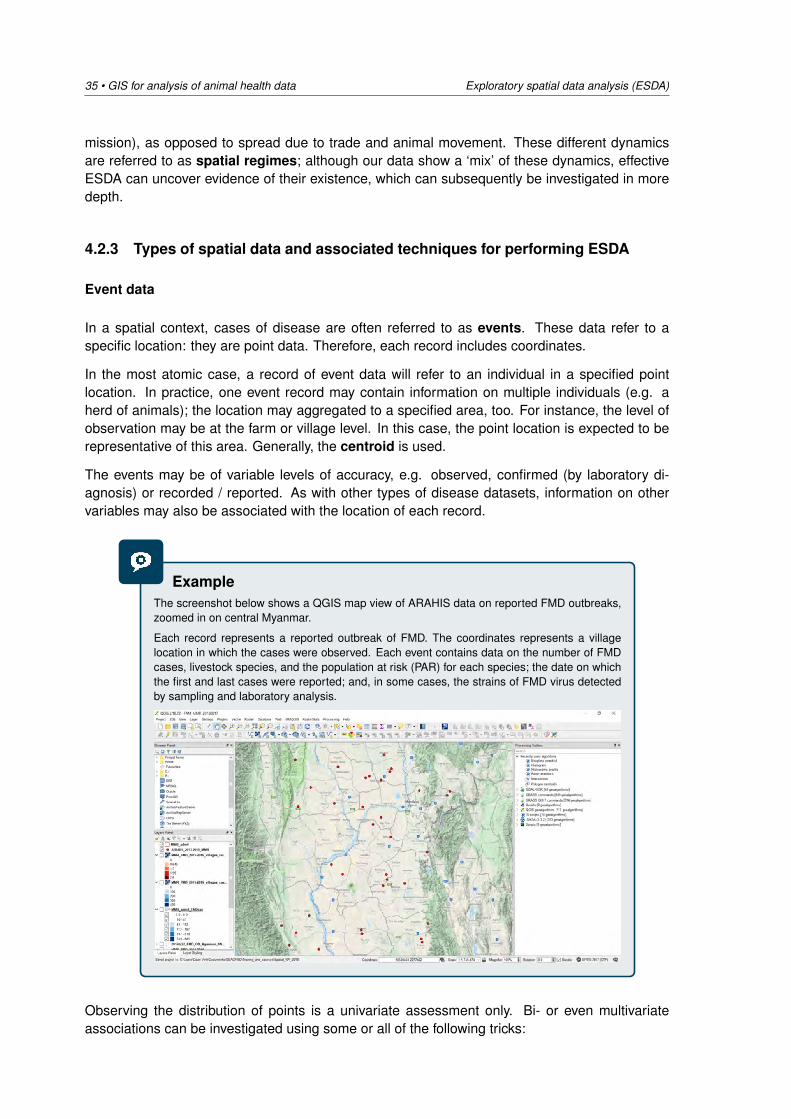
ExampleThe screenshot below shows a QGIS map view of ARAHIS data on reported FMD outbreaks,zoomed in on central Myanmar.
Each record represents a reported outbreak of FMD. The coordinates represents a villagelocation in which the cases were observed. Each event contains data on the number of FMDcases, livestock species, and the population at risk (PAR) for each species; the date on whichthe first and last cases were reported; and, in some cases, the strains of FMD virus detectedby sampling and laboratory analysis.
Observing the distribution of points is a univariate assessment only. Bi- or even multivariateassociations can be investigated using some or all of the following tricks:
Exploratory spatial data analysis (ESDA) GIS for analysis of animal health data • 36
• Stratification by a second variable. This can be a categorical variable (e.g. year of obser-vation) or a continuous variable (e.g. attack rate of the outbreak). The latter is comparableto a histogram of continuous numeric data; the criteria for determining the break pointsbecomes important.
• Applying a colouring schema according to another variable. This provides a visual cue ifthis second variable may also be clustered.
• Sizing the points according to another variable. This can be a highly effective method tovisualise the variability in this variable.
• Incorporating numeric techniques. If the number of points is small, graphs such ashistograms or pie charts can be included for each point.
Continuous data
Continuous spatial data are usually smoothed or constructed from event data. This representsa spatial distribution or ‘surface’ across the entire area under investigation. This surface is con-structed by a computational process called interpolation (see section 2.8.3).
It follows that these are usually raster layers (see 2.4.2).
The resolution and accuracy of the interpolation depend on the number of observed or recordedevents from which the surface is constructed. The degree of smoothing that is applied (referredto as the radius) depends on relevant characteristics of the event in question (e.g. dynamics oflocal spread) as well as the geographical scale on which the events are recorded.
Object data
Spatial object data contain information on specific entities which in themselves have no explicitlyspatial meaning. They are discrete spatial features which may contain information associatedwith event data. They may be exhaustive (i.e. cover the entire geographical space) or can beassociated with geographic coordinates.
This form of data can be highly relevant because they are often associated with aggregatedspatial data. The most common method of visualising an attribute in connection with such spatialobject data is choropleth maps. In these maps, object features (which usually represent admin-istrative areas) are shaded or patterned in proportion to the associated event data (for example,an attack rate or incidence rate of disease).
Another technique involves adjusting the area of each of each administrative division propor-tional to another variable; this is called a cartogram. While the resulting map may be distorted(sometimes grossly so), this provides another indication of variability across these objects.
Note that aggregation of point event data to spatial object (polygon) data inevitably results ina loss of information. Once aggregation has been performed, the scope for disaggregation islimited. One method by which this can be done is by calculating a centroid of the polygons.While this is an approximation, it may sometimes be necessary to do so. This can be done ongeographic grounds, but this can also be weighted by other criteria such as population density. Ifthe polygon is not a convex shape, it is possible that the geographic centroid falls outside of thepolygon; there are specific techniques which ensure that this is not the case.
37 • GIS for analysis of animal health data Exploratory spatial data analysis (ESDA)
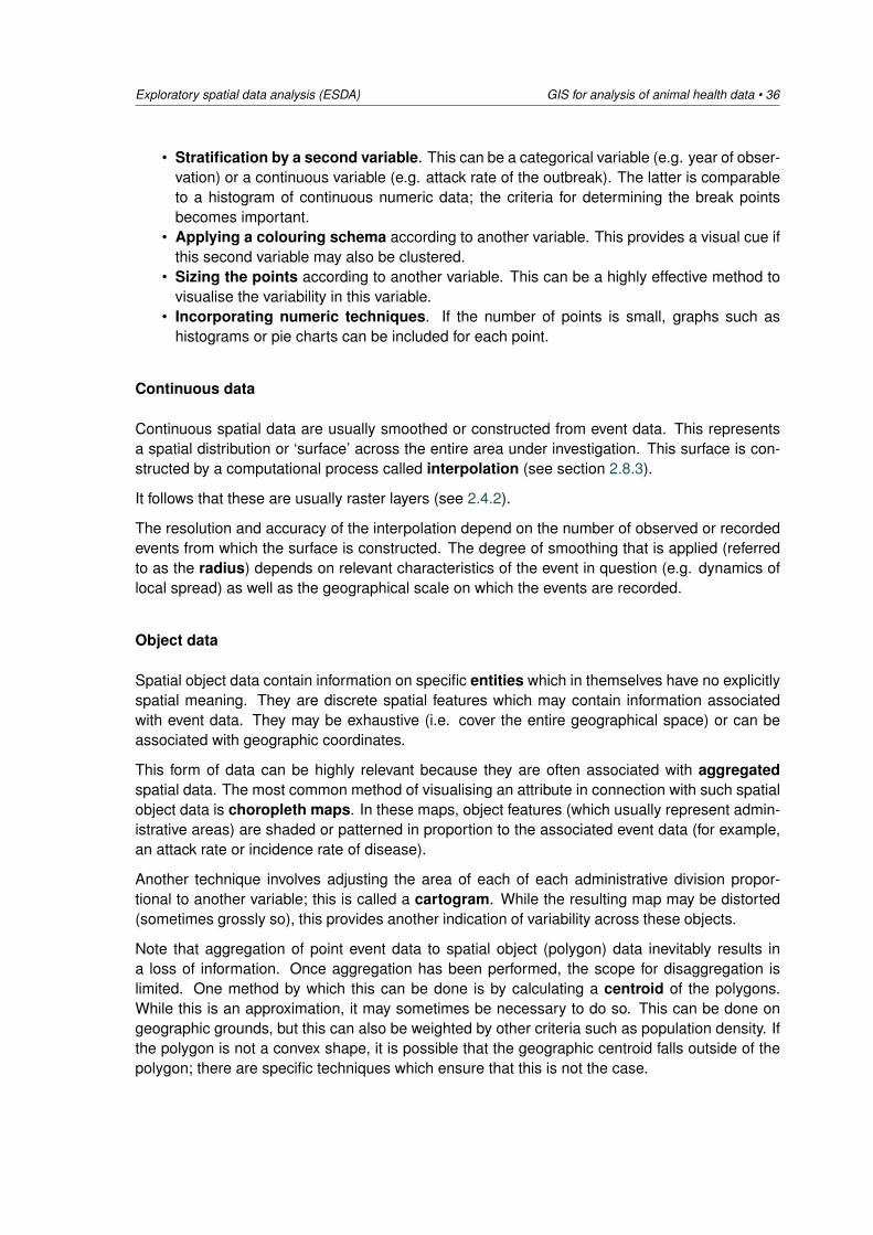
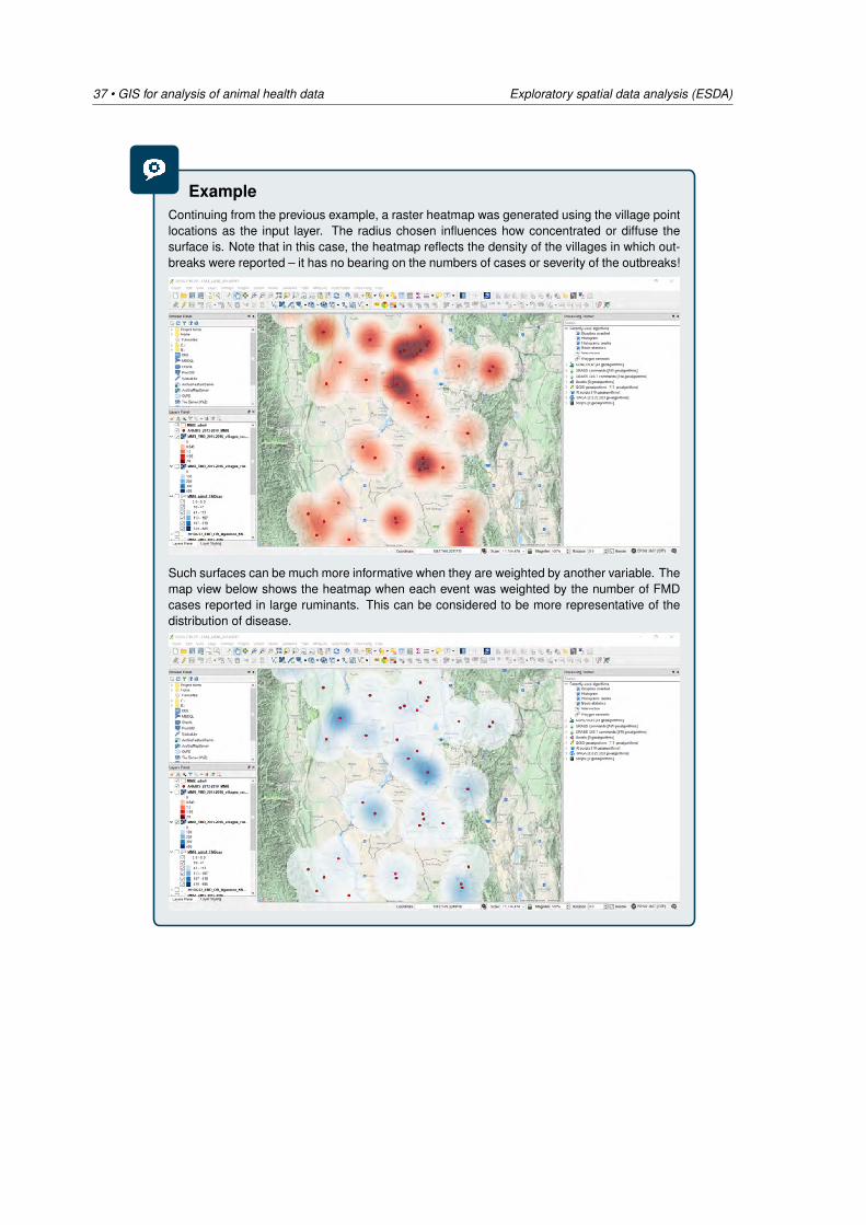
ExampleContinuing from the previous example, a raster heatmap was generated using the village pointlocations as the input layer. The radius chosen influences how concentrated or diffuse thesurface is. Note that in this case, the heatmap reflects the density of the villages in which out-breaks were reported – it has no bearing on the numbers of cases or severity of the outbreaks!
Such surfaces can be much more informative when they are weighted by another variable. Themap view below shows the heatmap when each event was weighted by the number of FMDcases reported in large ruminants. This can be considered to be more representative of thedistribution of disease.
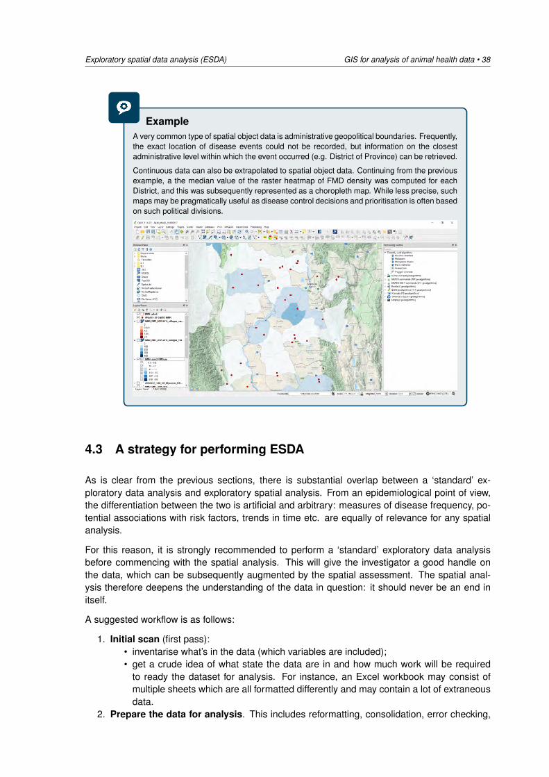
Exploratory spatial data analysis (ESDA) GIS for analysis of animal health data • 38
ExampleA very common type of spatial object data is administrative geopolitical boundaries. Frequently,the exact location of disease events could not be recorded, but information on the closestadministrative level within which the event occurred (e.g. District of Province) can be retrieved.
Continuous data can also be extrapolated to spatial object data. Continuing from the previousexample, a the median value of the raster heatmap of FMD density was computed for eachDistrict, and this was subsequently represented as a choropleth map. While less precise, suchmaps may be pragmatically useful as disease control decisions and prioritisation is often basedon such political divisions.
4.3 A strategy for performing ESDA
As is clear from the previous sections, there is substantial overlap between a ‘standard’ ex-ploratory data analysis and exploratory spatial analysis. From an epidemiological point of view,the differentiation between the two is artificial and arbitrary: measures of disease frequency, po-tential associations with risk factors, trends in time etc. are equally of relevance for any spatialanalysis.
For this reason, it is strongly recommended to perform a ‘standard’ exploratory data analysisbefore commencing with the spatial analysis. This will give the investigator a good handle onthe data, which can be subsequently augmented by the spatial assessment. The spatial anal-ysis therefore deepens the understanding of the data in question: it should never be an end initself.
A suggested workflow is as follows:
1. Initial scan (first pass):• inventarise what’s in the data (which variables are included);• get a crude idea of what state the data are in and how much work will be required
to ready the dataset for analysis. For instance, an Excel workbook may consist ofmultiple sheets which are all formatted differently and may contain a lot of extraneousdata.
2. Prepare the data for analysis. This includes reformatting, consolidation, error checking,
39 • GIS for analysis of animal health data Exploratory spatial data analysis (ESDA)
manipulation, creating new variables etc. It is easy to underestimate the time required toperform this! After completion, the data should be saved in a format that can be directlyimported into GIS or statistical software. To avoid errors, only include the variables that willbe analysed, and ensure they are complete.
3. Performing these steps may already have led to questioning: an elicitation of which vari-ables could be analysed and what such information would help to clarify.
4. Subsequently, develop a strategy to answer these questions. Perform the EDA, initially instatistical software or Excel; then perform an ESDA using GIS software such as QGIS orArcGIS.
5. Be systematic; record your findings and outputs; and reflect on their meaning. Don’t bedogmatic – frequently, unexpected new questions will emerge as the EDA is being per-formed; these should be pursued. EDA provides a large scope to be innovative and cre-ative, and a highly effective EDA will almost always result in a stronger subsequent analysis!
ExampleRevisit the steps of investigating the reported cases of FMD outbreaks in Myanmar. At eachstep, consider whether the information was useful, and synthesize this to provide some infor-mation on FMD disease trends in the area.
Plotting the locations of FMD outbreaks, were there evident signs of spatial clustering?
Judging by the distribution of affected villages, on the basis of this very limited evidence, theredoes not appear to be much evidence of clustering. Two things are relevant here: firstly, wedo not have information on the distribution of all villages – we really need to account for thatbefore drawing this conclusion. Secondly, inclusion of the Google Physical map layer showsthat outbreaks were limited to the plains. This is not surprising; again, we need to correct forthe livestock density over the whole area before we can state this as a fact.
Did the surfaces provide more compelling information?
While there may be indications of a few potential clusters, the bandwidth (radius) and colourgraduation used could influence this. The main conclusion here may be that outbreaks werereported throughout the whole area.
Was the choropleth map useful?
Not particularly; at best it may indicate that there was perhaps more FMD in the districts in thenorthern part. However, this is not convincing.
What else can we conclude?
The fact that FMD occurred throughout the area indicates that the disease is likely to be en-demic here. However, additional data on the livestock populations, human demographics andpotentially other risk factors is required to enable conclusions to be drawn with any degree ofconfidence.
Spatial clustering of disease GIS for analysis of animal health data • 40
5 Spatial clustering of disease
This text was summarised and modified from
• Chapters 4 and 5, Spatial Analysis in Epidemiology by Pfeiffer, Robinson, Stevenson,Stevens, Rogers and Clements, Oxford University Press, 2008.
• The SaTScanTM User Guide for version 9.6 by Martin Kulldorf, March 2018.
5.1 Introduction: global versus local clustering
In general, spatial patterns of health data can be classified as regular, random, or clustered.The term ‘clustering’ is used to describe the spatial aggregation of disease events. However, toaccount for the distribution of the underlying population at risk or of various risk factors, a betterdefinition is as follows:
DefinitionsSpatial disease clustering is the spatial aggregation of health events after known influenceshave been accounted for.
More specifically, a disease cluster can be defined as ‘a geographically and/or temporallybounded group of occurrences of cases, of sufficient size and concentration to be unlikely tohave occurred by chance’ (Knox, 1989).
The investigation of possible disease clustering is fundamental to epidemiology, with one of theaims being to determine whether the clustering is ‘real’ (statistically significant) and requiring fur-ther investigation or an intervention, or whether it is likely to be a chance occurrence, or whetherit is just a reflection of the distribution of the population at risk. This is essential to ensure nodisease clusters are missed, and conversely, to prevent wasting resources on spurious (false)clusters.
Investigating possible disease clusters requires a systematic approach and various cluster in-vestigation protocols are available. Such protocols may include the collection of data on thedisease frequency and potential risk factors; exploratory epidemiological analysis to scope dis-ease trends in time and space; and structured application of global and local cluster detectiontechniques. Such techniques (and the output generated by them) can be complex. It can bechallenging to ensure that the interpretation of the results (and the subsequent recommendationsprovided to the relevant decision-makers) are thoroughly considered, well-justified and clear, andunderpinned by sound scientific evidence.
41 • GIS for analysis of animal health data Spatial clustering of disease
Epidemiologists differentiate between ‘local’ and ‘global’ clustering:
• Global (non-specific) clustering methods are used to assess whether clustering is ap-parent throughout the region under investigation but do not identify the location of clusters.They provide a single statistic that measures the degree of spatial clustering, the statisti-cal significance of which can then be assessed. The null hypothesis for global clusteringmethods is simply that ‘no clustering exists’ (i.e. completer spatial randomness).
• Local (specific) methods of cluster detection define the locations and extent of clusters,and can be further divided into focused and non-focused tests:
– non-focused tests identify the location of all likely clusters in the study region, while
– focused tests investigate whether there is an increased risk of disease around a pre-determined point, such as a livestock market.
As epidemiologists, of course we are also required to develop reasonable explanations and in-terpretations that explain why an identified disease clustering has developed. Clustering of adisease can occur for a variety of reasons including the infectious spread of disease, the occur-rence of disease vectors in specific locations, the clustering of a risk factor or combination of riskfactors, or the existence of potential health hazards such as localized pollution sources scatteredthroughout a region, each creating an increased risk of disease in its immediate vicinity.
Global measures of spatial clustering assume that the disease process is the same (stationary)for the whole area under investigation. Of course, this assumption is rarely met. Although wecan investigate whether or not there is evidence for disease clustering across the area of interestas a whole, we are not able to understand local variability in disease patterns. Consequently, wemay miss significant local clustering. Conversely, we are unable to exclude the parts of the areaunder investigation in which no significant clustering exists.
It is logical that the larger the region we’re investigating, the higher the probability that thereare regions with inherently different local relationships. Many factors contribute to this: livestockpopulations and densities, disease risk factors, trade and animal movements, geographic and cli-matological factors, disease control measures which may influence the propagation of infectiousdiseases, political factors et cetera. With very large spatial datasets (for instance, encompassingthe entire south East Asia region), and particularly with large raster datasets such as remotelysensed images, global statistics such as Moran’s I (5.2.2) run the risk of losing information onspatial autocorrelation since they summarize an enormous number of possibly dissimilar spatialrelationships.
Local statistics overcome this problem by scanning the entire dataset, but only measuring de-pendence in limited portions of the study area, the bounds of which have to be specified. Thus,for clustering to be detected, it need not occur over the entire dataset, nor need it have thesame characteristics throughout the study area. Covariate data can be included to increase theaccuracy of the cluster estimation.
The aim is for such local statistics to estimate the characteristics of clusters, such as their lo-cation, size, and intensity. This can be difficult. Complications arise when dealing with variablepopulation distributions across a study area, or lack of knowledge of the disease dynamics, oran incomplete understanding of relevant risk factors. This can affect the results, leading to afailure to detect clusters (accepting the null hypothesis of spatial randomness when it is false –a Type 2 error) or conversely, detection of clusters where in reality there are none (rejecting thenull hypothesis of spatial randomness when it is true – a Type 1 error).
In this chapter, we first consider techniques to determine global spatial clustering, followed by

Spatial clustering of disease GIS for analysis of animal health data • 42
local methods of cluster detection. We subsequently cover the most-commonly utilised tool toimplement local clustering: SaTScan.
5.2 Global estimates of spatial clustering
5.2.1 Statistical concepts relevant to cluster analysis
Stationarity, isotropy, and first- and second-order effects
The concepts of stationarity, isotropy, and first-order (trend) and second-order (local) spatial ef-fects are fundamental to cluster analysis. To summarise:
• A spatial process is termed stationary if the dependence between measurements of thesame variable across space is the same for all locations in an area.
• If the dependence in a stationary process is affected by distance, but this is the same in alldirections, the process is considered to be isotropic.
• First-order effects describe large-scale variations in the mean of the outcome of interestdue to location or other explanatory variables.
• Second-order effects describe small-scale variation due to interactions between neigh-bours.
Monte Carlo simulation
Many tests for clustering use Monte Carlo simulation in order to determine the statistical sig-nificance of the cluster (i.e. does the observed spatial pattern differ significantly from the nullhypothesis of complete spatial randomness?).
This involves:
• calculating the test statistic using the observed data, and then• re-calculating it using a specified number (e.g. 99, 499, 999) of simulated data sets (or
permutations);• this simulated test statistic is subsequently used to generate the expected distribution of
the test statistic under the null hypothesis;• finally, the likelihood of obtaining the value for the test statistic derived from the observed
data is then calculated, and expressed as the p-value.
As with other statistical tests, a Monte Carlo estimate of the p-value for a one-sided test is givenby the proportion of test statistic values, obtained from the simulated datasets, that are greaterthan the value of the test statistic obtained when using the observed data.
As Monte Carlo methods rely on permutations of simulated datasets, slightly different p-valuesare obtained each time the test is run. However, using more simulations to estimate the distribu-tion of the null hypothesis (e.g. 999 versus 99), means that smaller and more stable p-values canbe calculated (e.g. p = 0.001 as opposed to p = 0.01). However, a problem with multiple testingis that the likelihood of wrongly rejecting the null hypothesis increases.
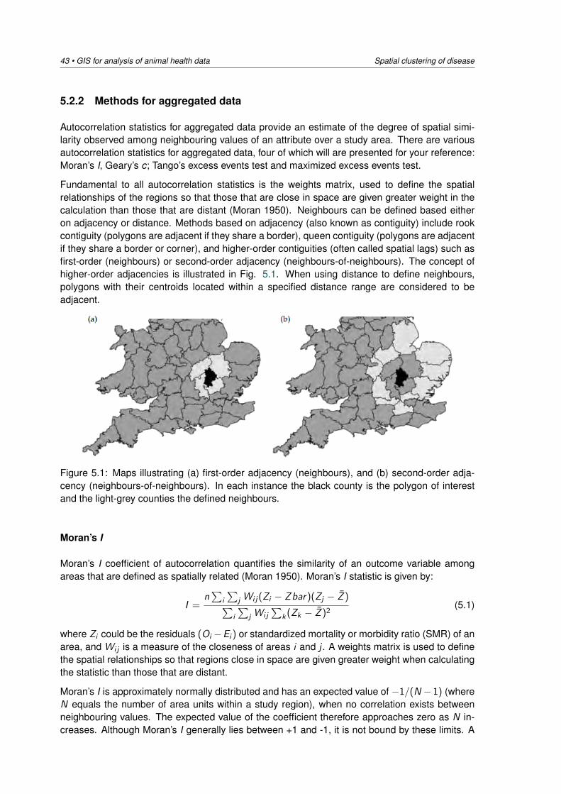
43 • GIS for analysis of animal health data Spatial clustering of disease
5.2.2 Methods for aggregated data
Autocorrelation statistics for aggregated data provide an estimate of the degree of spatial simi-larity observed among neighbouring values of an attribute over a study area. There are variousautocorrelation statistics for aggregated data, four of which will are presented for your reference:Moran’s I, Geary’s c; Tango’s excess events test and maximized excess events test.
Fundamental to all autocorrelation statistics is the weights matrix, used to define the spatialrelationships of the regions so that those that are close in space are given greater weight in thecalculation than those that are distant (Moran 1950). Neighbours can be defined based eitheron adjacency or distance. Methods based on adjacency (also known as contiguity) include rookcontiguity (polygons are adjacent if they share a border), queen contiguity (polygons are adjacentif they share a border or corner), and higher-order contiguities (often called spatial lags) such asfirst-order (neighbours) or second-order adjacency (neighbours-of-neighbours). The concept ofhigher-order adjacencies is illustrated in Fig. 5.1. When using distance to define neighbours,polygons with their centroids located within a specified distance range are considered to beadjacent.
Figure 5.1: Maps illustrating (a) first-order adjacency (neighbours), and (b) second-order adja-cency (neighbours-of-neighbours). In each instance the black county is the polygon of interestand the light-grey counties the defined neighbours.
Moran’s I
Moran’s I coefficient of autocorrelation quantifies the similarity of an outcome variable amongareas that are defined as spatially related (Moran 1950). Moran’s I statistic is given by:
I =n∑
i
∑j Wi j(Zi − Z bar)(Zj − Z )∑
i
∑j Wi j
∑k(Zk − Z )2
(5.1)
where Zi could be the residuals (Oi −Ei ) or standardized mortality or morbidity ratio (SMR) of anarea, and Wi j is a measure of the closeness of areas i and j . A weights matrix is used to definethe spatial relationships so that regions close in space are given greater weight when calculatingthe statistic than those that are distant.
Moran’s I is approximately normally distributed and has an expected value of −1/(N − 1) (whereN equals the number of area units within a study region), when no correlation exists betweenneighbouring values. The expected value of the coefficient therefore approaches zero as N in-creases. Although Moran’s I generally lies between +1 and -1, it is not bound by these limits. A

Spatial clustering of disease GIS for analysis of animal health data • 44
Moran’s I of zero indicates the null hypothesis of no clustering, a positive Moran’s I indicates pos-itive spatial autocorrelation (i.e. clustering of areas of similar attribute values), while a negativecoefficient indicates negative spatial autocorrelation (i.e. that neighbouring areas tend to havedissimilar attribute values). The significance of Moran’s I can be assessed using Monte Carlorandomization.
Disadvantages of the autocorrelation test are the assumptions that the population at risk is evenlydistributed within the study area, and that the correlation or covariance is the same in all directions(i.e. it is isotropic).
Although Moran’s I is intended for use with continuous data it can also be used to analyse countdata, even though, in such instances, any observed autocorrelation may simply be the result ofvariation in regional population sizes rather than any genuine spatial pattern in the disease counts(e.g. if regions with large populations are grouped together). Accounting for the population at riskby using regional incidence rates, instead of regional disease counts, increases the likelihoodthat any observed autocorrelation reflects a genuine spatial pattern rather than a heterogeneouspopulation distribution.
A spatial correlogram is a series of estimates of Moran’s I evaluated at increasing distances.Moran’s I is plotted on the vertical axis and distance (spatial lag) is plotted on the horizontal axis.The correlogram can therefore be used to determine where, on average, spatial autocorrelationis maximized. Correlograms can be calculated based on distance or adjacency. There are var-ious tests to determine whether a spatial autocorrelation value in a correlogram is statisticallysignificant.
As Moran’s I cannot adjust for a heterogeneous population density, Oden (1995) proposed theuse of Oden’s Ipop, a test statistic similar to Moran’s I but in which rates are adjusted for popula-tion size.
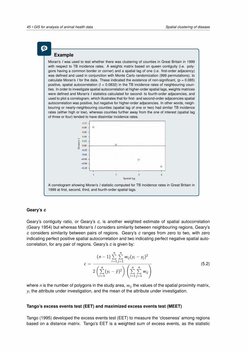
45 • GIS for analysis of animal health data Spatial clustering of disease
ExampleMoran’s I was used to test whether there was clustering of counties in Great Britain in 1999with respect to TB incidence rates. A weights matrix based on queen contiguity (i.e. poly-gons having a common border or corner) and a spatial lag of one (i.e. first-order adjacency)was defined and used in conjunction with Monte Carlo randomization (999 permutations), tocalculate Moran’s I for the data. These indicated the existence of non-significant, (p = 0.085)positive, spatial autocorrelation (I = 0.0832) in the TB incidence rates of neighbouring coun-ties. In order to investigate spatial autocorrelation at higher-order spatial lags, weights matriceswere defined and Moran’s I statistics calculated for second- to fourth-order adjacencies, andused to plot a correlogram, which illustrates that for first- and second-order adjacencies spatialautocorrelation was positive, but negative for higher-order adjacencies. In other words, neigh-bouring or nearly-neighbouring counties (spatial lag of one or two) had similar TB incidencerates (either high or low), whereas counties further away from the one of interest (spatial lagof three or four) tended to have dissimilar incidence rates.
A correlogram showing Moran’s I statistic computed for TB incidence rates in Great Britain in1999 at first, second, third, and fourth-order spatial lags.
Geary’s c
Geary’s contiguity ratio, or Geary’s c, is another weighted estimate of spatial autocorrelation(Geary 1954) but whereas Moran’s I considers similarity between neighbouring regions, Geary’sc considers similarity between pairs of regions. Geary’s c ranges from zero to two, with zeroindicating perfect positive spatial autocorrelation and two indicating perfect negative spatial auto-correlation, for any pair of regions. Geary’s c is given by:
c =
(n − 1)n∑
i=1
n∑j=1
wi j(yi − yj)2
2
(n∑
i=1(yi − y)2
)(n∑
i=1
n∑j=1
wi j
) (5.2)
where n is the number of polygons in the study area, wi j the values of the spatial proximity matrix,yi the attribute under investigation, and the mean of the attribute under investigation.
Tango’s excess events test (EET) and maximized excess events test (MEET)
Tango (1995) developed the excess events test (EET) to measure the ‘closeness’ among regionsbased on a distance matrix. Tango’s EET is a weighted sum of excess events, as the statistic
Spatial clustering of disease GIS for analysis of animal health data • 46
considers the difference between the observed rate of cases in each region and the expectedrate, and then weights these differences by a measure of the distance between the regions, witha higher weighting given when the two locations are close.
Unfortunately Tango’s EET requires the parameter λ (a measure of the spatial scale of clustering)to be specified, resulting in two problems. Firstly, λ is not generally known a priori and thereforeseveral values of λ are tested creating issues of multiple testing. Secondly, choosing a large λmakes the test sensitive to geographically large-scale clustering while a small λ makes it moresensitive to small-scale clustering. To overcome these problems, Tango (2000) proposed themaximized excess events test (MEET). This test statistic searches for the value of λ which givesthe smallest p-value of the observed value of the test statistic.
5.2.3 Methods for point data
Cuzick and Edwards’ k -nearest neighbour test
Cuzick and Edwards (1990) developed a test for spatial clustering that takes into account the po-tentially heterogeneous distribution of the population at risk. It is based on the locations of casesand randomly selected controls from a specified region and includes a spatial scale parameter k ,determined by the user. Scale in this instance refers to the number of nearest neighbours, andnot geographic distance. For each case, the test counts how many of the k -nearest neighboursare also cases, such that if there are n1 cases, and mi (k) represents the number of cases amongthe k nearest neighbours of case i so that 0 ≤ mi (k) ≤ k , for i = 1, . . . , n1, a test statistic Tk
can be calculated as follows:
Tk =
n1∑i=1
mi (k) (5.3)
Thus, when cases are clustered, the nearest neighbour to a case tends to be another case andTk will be large. However, when all cases have controls as their nearest neighbours Tk will bezero. The observed value of Tk can be compared with the distribution of values computed usingMonte Carlo randomization of the dataset.
When data are available for the population at risk a modification of Tk is:
Uk =
n1∑j=1
(Yj − Ej) (5.4)
where circular regions are centred on each case and the radius of each circular region is chosenso that the expected number cases, Ej , is as close to the pre-defined value of k as possible, andYj is the number of cases within each region. Under the null hypothesis the expected value ofUk is equal to zero and the variance may be calculated.
Information on the exact locations of cases and controls is not always available, with locationsinstead being frequently assigned to the centre of administrative areas such as counties orparishes. As a result of assigning cases and controls to the same area ‘ties’ arise, preclud-ing the calculation of Cuzick and Edwards’ test statistic. Jacquez (1994) proposed an extensionto Cuzick and Edwards’ method that allows the test to be used in such situations.
A distinct advantage of Cuzick and Edwards’ method is that it takes account of the heteroge-neous distribution of the population at risk, as cases and controls are selected from the samepopulation. In this way, the existence of any clustering of the population at risk, such as in built-up areas is accounted for. Furthermore, through the careful selection of controls, this method
47 • GIS for analysis of animal health data Spatial clustering of disease
allows confounders to be accounted for. Disadvantages of the test include the fact that the useris required to select a value for the parameter k , and that interval data must be categorized as‘case’ and ‘control’ locations resulting in a possible loss of information, although at the sametime, this aspect of the test allows for flexibility in defining case and control locations. For in-stance, cases may be locations where disease has been detected or alternately, locations atwhich disease is above a specified threshold, such as the mean disease prevalence. AlthoughCuzick and Edwards’ test was originally developed for use with point data it can easily be adaptedfor aggregated data.
Ripley’s K -function
Second-order analysis describes the spatial dependence between events of the same type. TheK -function is the most commonly-used method and identifies the distance at which clusteringoccurs. For an isotropic process with an intensity of λ points per unit area, the K -function atdistance s may be defined as K (s) such that λK (s) gives the expected number of events withina distance s of an arbitrarily-chosen event. Formally, K (s) is defined as:
K (s) =1
λ2R
∑i+j
∑Is(di j) (5.5)
where R equals the area of a region of interest, di j is the distance between the i th and j th eventsin R , and Is(di j) is an indicator function which equals 1 if di j − s and 0 otherwise. Where spatialautocorrelation is present, each event is likely to be in close proximity to other members of thesame event type and, for small values of s, K (s) will be large.
An important assumption of the K -function is that there are no first-order effects in the spatialpattern, as any evidence of spatial trend may influence the computed K -function. In addition, thevariance of K (s) increases with increasing distance, and therefore the K -function is suitable forestimating general tendencies toward clustering over distances that are small compared with thesize of the region. As a rule of thumb it is recommended to restrict the range of s to no greaterthan 0.5 times the length of the shorter side of a rectangular study area.
Due to variations in the spatial distribution of the population at risk, a K -function computed only forcases may not be very informative. Instead, the K -function calculated for cases (Kcase(s)) canbe compared with one calculated for non-cases (or controls) (Kcontrol(s)), with the differencebetween the two functions,
D(s) = Kcase(s)− Kcontrol(s) (5.6)
representing a measure of the extra aggregation of cases over and above that observed for thenon-cases. Monte Carlo randomization can then be used to randomly permute the locations ofcases and non-cases/controls, and values of the difference function D(s) computed for each per-mutation. The upper and lower bounds of these permutations are then plotted together with theobserved difference function D(s). Any deviation of D(s) above the envelope formed by the upperand lower bounds indicates significant clustering of cases, relative to non-cases/controls.
Advantages of using the K -function to investigate clustering include the fact that it does notdepend on the shape of the study region, and precise spatial locations of events are used inits estimation. It also takes into account the density of events in the region of interest, enablingspatial dependence to be compared among groups regardless of event prevalence. Furthermore,the test can accommodate an edge-correction weighting factor.
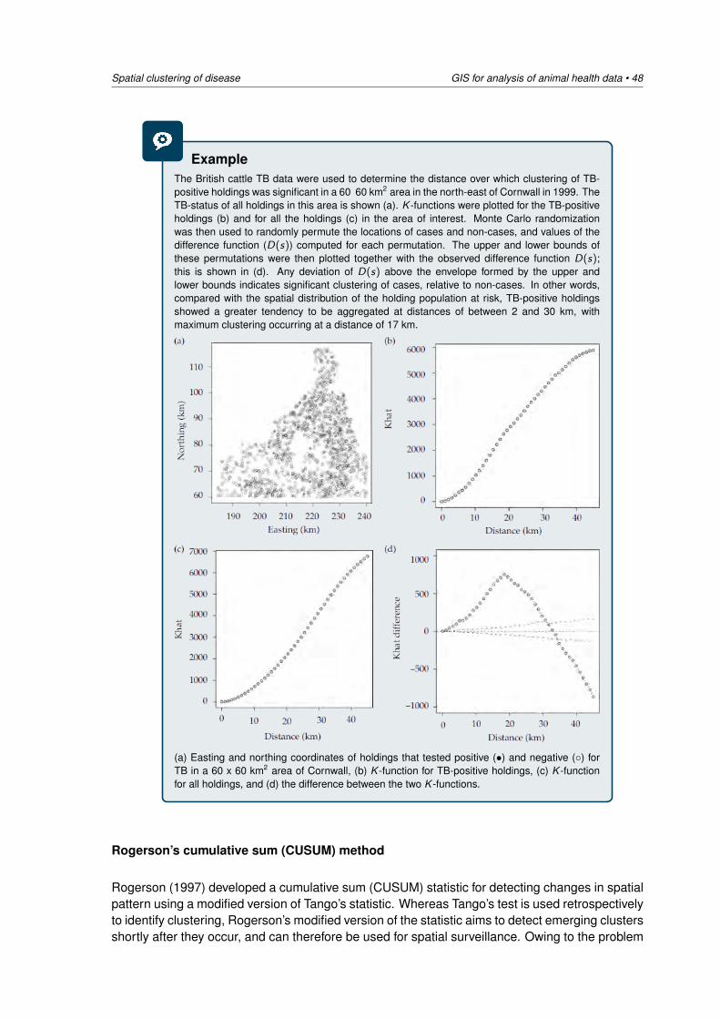
Spatial clustering of disease GIS for analysis of animal health data • 48
ExampleThe British cattle TB data were used to determine the distance over which clustering of TB-positive holdings was significant in a 60 60 km2 area in the north-east of Cornwall in 1999. TheTB-status of all holdings in this area is shown (a). K -functions were plotted for the TB-positiveholdings (b) and for all the holdings (c) in the area of interest. Monte Carlo randomizationwas then used to randomly permute the locations of cases and non-cases, and values of thedifference function (D(s)) computed for each permutation. The upper and lower bounds ofthese permutations were then plotted together with the observed difference function D(s);this is shown in (d). Any deviation of D(s) above the envelope formed by the upper andlower bounds indicates significant clustering of cases, relative to non-cases. In other words,compared with the spatial distribution of the holding population at risk, TB-positive holdingsshowed a greater tendency to be aggregated at distances of between 2 and 30 km, withmaximum clustering occurring at a distance of 17 km.
(a) Easting and northing coordinates of holdings that tested positive (•) and negative (◦) forTB in a 60 x 60 km2 area of Cornwall, (b) K -function for TB-positive holdings, (c) K -functionfor all holdings, and (d) the difference between the two K -functions.
Rogerson’s cumulative sum (CUSUM) method
Rogerson (1997) developed a cumulative sum (CUSUM) statistic for detecting changes in spatialpattern using a modified version of Tango’s statistic. Whereas Tango’s test is used retrospectivelyto identify clustering, Rogerson’s modified version of the statistic aims to detect emerging clustersshortly after they occur, and can therefore be used for spatial surveillance. Owing to the problem
49 • GIS for analysis of animal health data Spatial clustering of disease
of multiple testing, it would be inappropriate simply to re-calculate Tango’s statistic after eachnew observation. Instead, once the test statistic has been determined for a particular set ofobservations, the expected value and variance of Tango’s statistic after the next observation isestimated, based on the current value of the statistic. The expected value and variance is thenused to convert the Tango’s statistic that is observed after the next observation into a z-score,with all z-scores being incorporated into a CUSUM framework.
As Rogerson’s CUSUM method is based on Tango’s statistic, the test includes a measure of thespatial scale of clustering (λ) and thus, choosing a small value of λ makes the test more sensitiveto small clusters and vice versa.
5.2.4 Investigating space-time clustering
While spatial patterns of disease are of great interest, space-time interactions are also important,particularly so when trying to determine whether a disease is infectious. In such instances itis necessary to evaluate whether cases that are close in space are also close in time and viceversa, adjusting for any purely spatial or temporal clustering. Various tests have been developedfor this purpose; the tests for global space-time clustering are briefly reviewed here, while thelocal space-time cluster detection tests are dealt with in section 5.3.5.
It is worth noting that some tests look for clusters that relate to a fixed point in space, whilst othersallow the spatial focus to move with time. In the first instance, the idea of a two-dimensionalcircular scan window is extended to that of a cylinder passing through time. In the second case,the geographical focus of a cluster may migrate with time, as long as it relates back to previousevents.
There is also an important distinction between tests that require knowledge of the population atrisk, and those that do not. Not requiring population or control data has obvious advantagesin terms of ease of implementation, but the drawback is that it assumes that any change in thepopulation at risk occurs evenly across the distribution under study. This would obviously haveserious analytical implications, where interventions such as culling or vaccination may causehighly inhomogeneous changes in the population at risk.
The Knox test
Knox and Bartlett (1964) developed the first technique to identify spatio-temporal clustering ofdisease events and, although it has been the subject of much criticism, Knox’s test has formedthe platform from which subsequent tests have been developed. In this method, pairs of casesseparated by less than a user-defined critical space-distance are considered to be near in space,and pairs of cases separated by less than a user-defined critical time-distance are said to benear in time. This classification allows pairs of points to be assigned to one of four cells in a 22 contingency table (near space — near time, near space — far time, far space — near time,far space — far time), and a test statistic, TK is calculated as the number of pairs of cases thatare near to one another in both space and time. The test statistic is compared against simulatedresults under a Poisson model, which Knox argues is the sampling distribution of the statistic inthe absence of space-time clustering.
There are two principal limitations with Knox’s test. Firstly, the choice of critical distances issubjective and secondly, that the critical distance in space does not vary with changing populationdensity. This is unrealistic since the distance from case to case would decrease with increasing
Spatial clustering of disease GIS for analysis of animal health data • 50
population density. Baker (1996) discusses the problems associated with specifying thresholdsof proximity in space and time in the Knox test, and develops an adaptation that does not requireunknown critical parameters to be specified, but instead allows for a range to be given for each.In its most flexible form the range can be specified from zero to the maximum space and timedifferences between any two pairs of cases. The test becomes more powerful as the ranges forthresholds can be specified with increasing accuracy, and reduces to the Knox test itself whenthe range for each parameter is reduced to zero.
Kulldorff and Hjalmars (1999) proposed a modification of the Knox test that overcomes theseproblems. Using the standard Knox test, significant space-time clustering is indicated at a rangeof critical distances whilst with their adaptation it is not. They show that changes in the distributionof the population at risk over time can have a strong influence on the standard test. These effectsare particularly interesting with animal diseases where populations may be culled.
The space-time K -function
Diggle et al. (1995) extend existing second-order analysis methods for spatial data in order toinvestigate space-time interactions in point process data. They find second-order properties tobe closely related to Knox’s statistic. If KS(s) defines the K -function in space and KT (t) definesthe K -function in time, the K -function difference D(s, t) is:
D(s, t) = K (s, t)− KS(s)KT (t) (5.7)
D(s, t) estimates the cumulative number of cases expected within distance s and time-interval tof an arbitrarily-selected case attributable to the interaction between space and time. An alterna-tive expression is:
D0(s, t) =D(s, t)
KS(s)− KT (t)(5.8)
which estimates, for given distance and time separations, the proportional increase in casesattributable to space-time interaction.
The Ederer-Myers-Mantel (EMM) test
Ederer et al. (1964) developed a cell occupancy approach for exploring space-time clusteringwhereby the study region is divided into a series of space-time sub-regions within which unusualdistributions of cases are sought.
Mantel’s test
Mantel (1967) reviews the methods of Knox and Bartlett (1964) and Ederer et al. (1964), andproposes a new test that compares inter-event distances in space and time against a null hypoth-esis that time and space distances are independent. The test statistic TM is the sum, acrossall pairs of cases, of the spatial distances multiplied by the time distances. A transformation isused to reduce the effects of large space and time distances, which would not be expected to becorrelated for contagious diseases. Significance levels are then tested using a standard MonteCarlo randomization process.
The EMM test and Mantel’s test both have low statistical power for small numbers of study cases.True clinical disease excesses, as might result from proximity to a single pollution source, are
51 • GIS for analysis of animal health data Spatial clustering of disease
more likely to be detected by the EMM method whilst the Mantel method is more likely to detecthotspots such as those due to a more general exposure to a putative source.
Barton’s test
Barton et al. (1965) designed a test to detect changes in spatial patterns associated with thepassage of time, based on analysis of variance and which tests the null hypothesis that thesepatterns do not change with time.
Jacquez’s k nearest neighbours test
Jacquez (1996) developed a k nearest neighbours test for space-time interaction. The null hy-pothesis is of no association between time and space adjacencies (i.e. that the probability of twoevents being nearest neighbours in space is independent of the probability of their being nearestneighbours in time). This approach is based on the argument that geographic distance is not agood measure of spatial proximity in an epidemiological context.
5.3 Local estimates of spatial clustering
5.3.1 Introduction
Some of the more commonly-used methods for local cluster detection are reviewed below. Theyare divided into those primarily designed for aggregated data, and those for point data. Of course,point data can easily be aggregated and area data can be represented as points, for example byusing the centroids of the areas.
The methods listed for point data are ‘scanning statistics’ : they are based on variously definedcircles that ‘scan’ the data for areas of elevated (or reduced) disease frequency. Such statisticsare better suited to point, than to area data, since points fall clearly inside or outside a scancircle. Scan circles can be defined in terms of geographic distance (e.g. Openshaw’s method),number of cases (e.g. Besag and Newell’s method) or population size (e.g. Turnbull’s methodand Kulldorff’s scan statistic).
Methods for investigating clusters around point sources are then reviewed, and finally methodsthat look for clusters in both space and time.
5.3.2 Methods for aggregated data
Getis and Ord’s local Gi(d) statistic
Unlike Moran’s I statistic (see Section 5.2.2), which measures the correlation between attributevalues in adjacent areas, the Gi(d) local statistic (Getis and Ord 1992; 1996) is an indicator oflocal clustering that measures the ‘concentration’ of a spatially distributed attribute variable. Thetest statistic is calculated as:
Gi(d) =
n∑j
wi j(d)(xj − xi )
Si
√wi (n−1−wi )
n−2
, j 6= i (5.9)
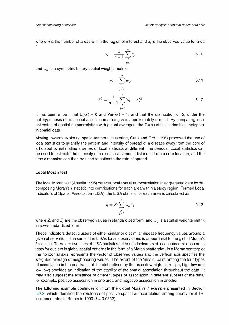
Spatial clustering of disease GIS for analysis of animal health data • 52
where n is the number of areas within the region of interest and xi is the observed value for areai
xi =1
n − 1
n∑j
j 6=i
xj (5.10)
and wi j is a symmetric binary spatial weights matrix:
wi =n∑j
j 6=i
wi j (5.11)
S2i =
1
n − 1
n∑j
j 6=i
(xj − xi )2 (5.12)
It has been shown that E(Gi ) = 0 and Var(Gi ) = 1, and that the distribution of Gi under thenull hypothesis of no spatial association among xi is approximately normal. By comparing localestimates of spatial autocorrelation with global averages, the Gi(d) statistic identifies ‘hotspots’in spatial data.
Moving towards exploring spatio-temporal clustering, Getis and Ord (1996) proposed the use oflocal statistics to quantify the pattern and intensity of spread of a disease away from the core ofa hotspot by estimating a series of local statistics at different time periods. Local statistics canbe used to estimate the intensity of a disease at various distances from a core location, and thetime dimension can then be used to estimate the rate of spread.
Local Moran test
The local Moran test (Anselin 1995) detects local spatial autocorrelation in aggregated data by de-composing Moran’s I statistic into contributions for each area within a study region. Termed LocalIndicators of Spatial Association (LISA), the LISA statistic for each area is calculated as:
Ii = Zi
n∑j
j 6=i
wi jZj (5.13)
where Zi and Zj are the observed values in standardized form, and wi j is a spatial weights matrixin row-standardized form.
These indicators detect clusters of either similar or dissimilar disease frequency values around agiven observation. The sum of the LISAs for all observations is proportional to the global Moran’sI statistic. There are two uses of LISA statistics: either as indicators of local autocorrelation or astests for outliers in global spatial patterns in the form of a Moran scatterplot. In a Moran scatterplotthe horizontal axis represents the vector of observed values and the vertical axis specifies theweighted average of neighbouring values. The extent of the ‘mix’ of pairs among the four typesof association in the quadrants of the plot defined by the axes (low-high, high-high, high-low andlow-low) provides an indication of the stability of the spatial association throughout the data. Itmay also suggest the existence of different types of association in different subsets of the data;for example, positive association in one area and negative association in another.
The following example continues on from the global Moran’s I example presented in Section5.2.2, which identified the existence of positive spatial autocorrelation among county-level TB-incidence rates in Britain in 1999 (I = 0.0832).
53 • GIS for analysis of animal health data Spatial clustering of disease
ExampleApplying the local Moran test to the data allowed a visual representation of spatial autocor-relation to be obtained. The resulting Moran scatterplot showed that most of the points werein the lower left (low-low) and upper left (low-high) quadrants indicating the existence of bothpositive and negative spatial autocorrelation among county-level TB incidence rates in Britainin 1999. The negative spatial autocorrelation arose as a result of outlier counties with a low TBincidence rate being surrounded by neighbours with high TB incidence rates, while the positivespatial autocorrelation resulted from counties with a low TB incidence rate having neighbourswith similar low incidence rates. This demonstrates that the LISA cluster map and LISA signif-icance map are additional, useful methods of visualising the spatial autocorrelation.
Moran scatterplot of county-level TB incidence rates in Britain in 1999.
5.3.3 Methods for point data
Openshaw’s Geographical Analysis Machine (GAM)
Openshaw’s Geographical Analysis Machine (GAM, not to be confused with the GeneralisedAdditive model statistical technique) was the first in a series of methods developed to exploredisease data for evidence of spatial pattern (Openshaw et al. 1987). The GAM involves apply-ing a fine grid across a study area and generating a series of circles of varying radii with theircentres based at each intersection of the grid. The observed number of cases of disease withineach circle is then compared with the expected number of cases, assuming the process underinvestigation follows a Poisson distribution. Circles that have a higher than expected occurrenceof disease are retained, resulting in a large number of overlapping circles concentrated around‘disease centres’. Visual inspection is then relied upon to decide where clusters occur.
There are some severe computational limitations of the GAM methodology, as a consequenceof which it is no longer the best option. The technique does not account for multiple testing,and therefore the change in radius and shifts in location of candidate clusters are not taken intoaccount in the calculation of significance levels. Also, since distance is the method used to definethe scan circles, circles of the same size can refer to different-sized populations and are thereforenot directly comparable.
The primary purpose of mentioning the test here is that it was the predecessor of a series oftests for cluster detection based on scan circles, which addressed and overcame many of its
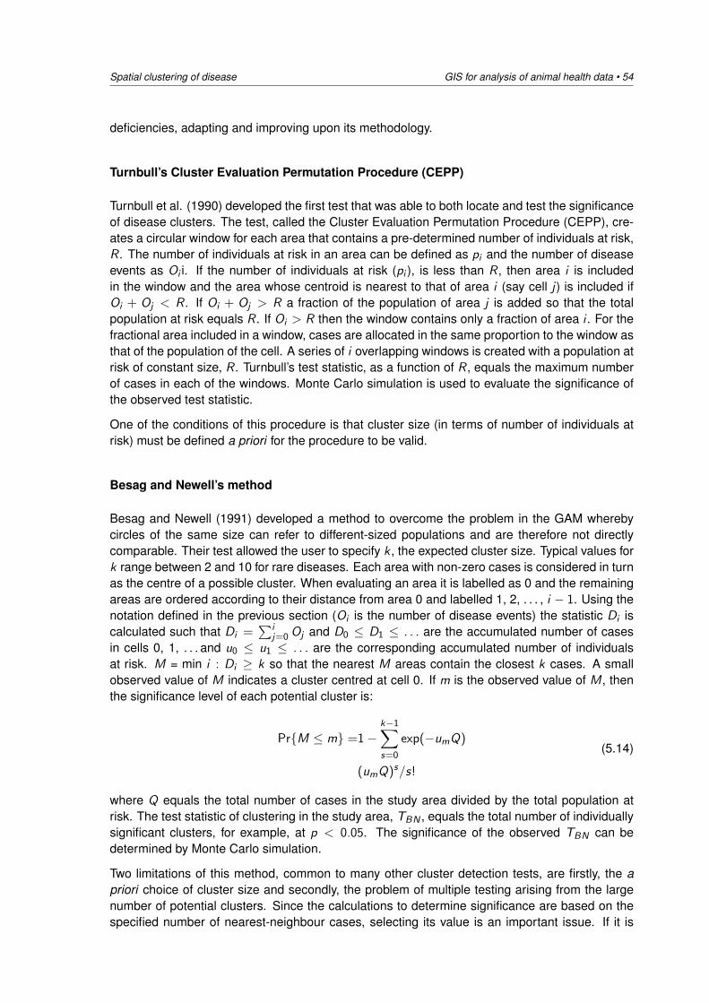
Spatial clustering of disease GIS for analysis of animal health data • 54
deficiencies, adapting and improving upon its methodology.
Turnbull’s Cluster Evaluation Permutation Procedure (CEPP)
Turnbull et al. (1990) developed the first test that was able to both locate and test the significanceof disease clusters. The test, called the Cluster Evaluation Permutation Procedure (CEPP), cre-ates a circular window for each area that contains a pre-determined number of individuals at risk,R . The number of individuals at risk in an area can be defined as pi and the number of diseaseevents as Oi i. If the number of individuals at risk (pi ), is less than R , then area i is includedin the window and the area whose centroid is nearest to that of area i (say cell j) is included ifOi + Oj < R . If Oi + Oj > R a fraction of the population of area j is added so that the totalpopulation at risk equals R . If Oi > R then the window contains only a fraction of area i . For thefractional area included in a window, cases are allocated in the same proportion to the window asthat of the population of the cell. A series of i overlapping windows is created with a population atrisk of constant size, R . Turnbull’s test statistic, as a function of R , equals the maximum numberof cases in each of the windows. Monte Carlo simulation is used to evaluate the significance ofthe observed test statistic.
One of the conditions of this procedure is that cluster size (in terms of number of individuals atrisk) must be defined a priori for the procedure to be valid.
Besag and Newell’s method
Besag and Newell (1991) developed a method to overcome the problem in the GAM wherebycircles of the same size can refer to different-sized populations and are therefore not directlycomparable. Their test allowed the user to specify k , the expected cluster size. Typical values fork range between 2 and 10 for rare diseases. Each area with non-zero cases is considered in turnas the centre of a possible cluster. When evaluating an area it is labelled as 0 and the remainingareas are ordered according to their distance from area 0 and labelled 1, 2, . . . , i − 1. Using thenotation defined in the previous section (Oi is the number of disease events) the statistic Di iscalculated such that Di =
∑ij=0 Oj and D0 ≤ D1 ≤ . . . are the accumulated number of cases
in cells 0, 1, . . . and u0 ≤ u1 ≤ . . . are the corresponding accumulated number of individualsat risk. M = min i : Di ≥ k so that the nearest M areas contain the closest k cases. A smallobserved value of M indicates a cluster centred at cell 0. If m is the observed value of M , thenthe significance level of each potential cluster is:
Pr{M ≤ m} =1−k−1∑s=0
exp(−umQ)
(umQ)s/s!
(5.14)
where Q equals the total number of cases in the study area divided by the total population atrisk. The test statistic of clustering in the study area, TBN , equals the total number of individuallysignificant clusters, for example, at p < 0.05. The significance of the observed TBN can bedetermined by Monte Carlo simulation.
Two limitations of this method, common to many other cluster detection tests, are firstly, the apriori choice of cluster size and secondly, the problem of multiple testing arising from the largenumber of potential clusters. Since the calculations to determine significance are based on thespecified number of nearest-neighbour cases, selecting its value is an important issue. If it is
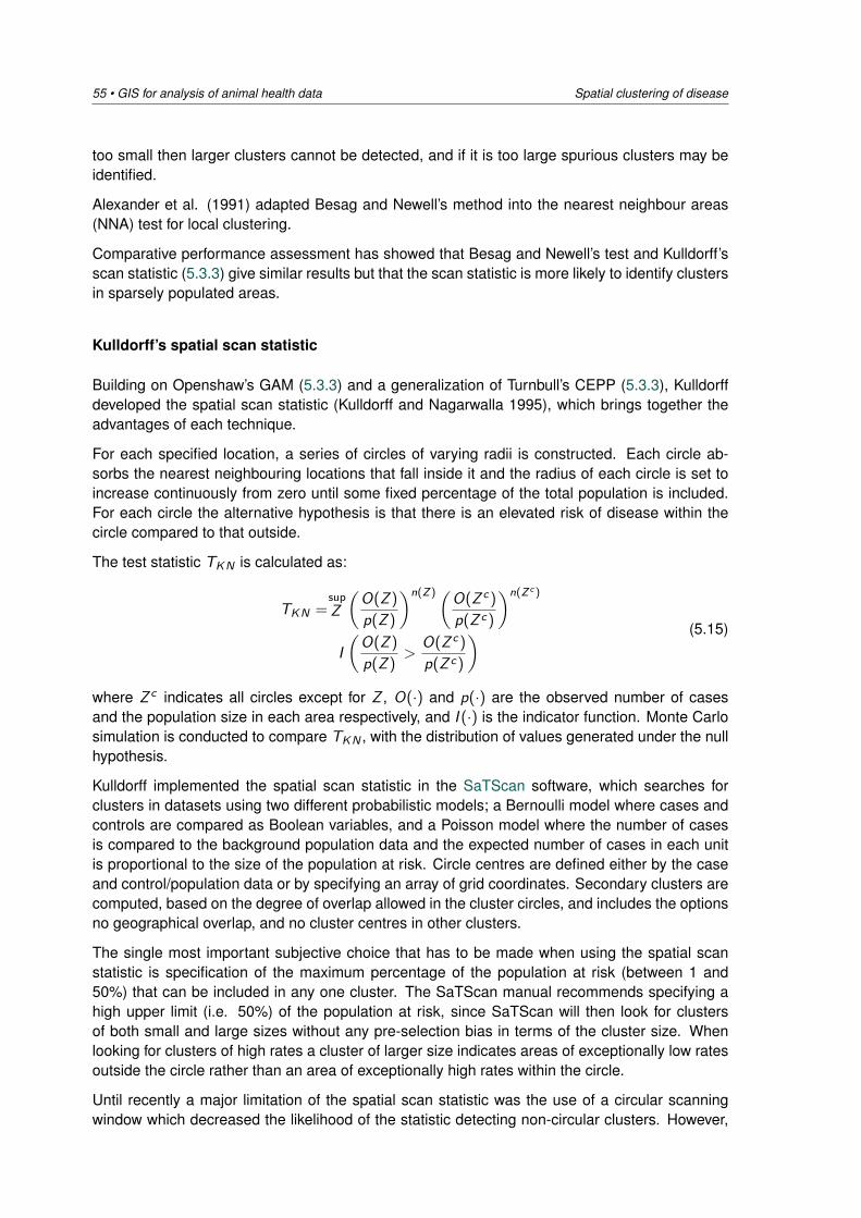
55 • GIS for analysis of animal health data Spatial clustering of disease
too small then larger clusters cannot be detected, and if it is too large spurious clusters may beidentified.
Alexander et al. (1991) adapted Besag and Newell’s method into the nearest neighbour areas(NNA) test for local clustering.
Comparative performance assessment has showed that Besag and Newell’s test and Kulldorff’sscan statistic (5.3.3) give similar results but that the scan statistic is more likely to identify clustersin sparsely populated areas.
Kulldorff’s spatial scan statistic
Building on Openshaw’s GAM (5.3.3) and a generalization of Turnbull’s CEPP (5.3.3), Kulldorffdeveloped the spatial scan statistic (Kulldorff and Nagarwalla 1995), which brings together theadvantages of each technique.
For each specified location, a series of circles of varying radii is constructed. Each circle ab-sorbs the nearest neighbouring locations that fall inside it and the radius of each circle is set toincrease continuously from zero until some fixed percentage of the total population is included.For each circle the alternative hypothesis is that there is an elevated risk of disease within thecircle compared to that outside.
The test statistic TKN is calculated as:
TKN =sup
Z
(O(Z )
p(Z )
)n(Z)(O(Z c)
p(Z c)
)n(Z c )
I
(O(Z )
p(Z )>
O(Z c)
p(Z c)
) (5.15)
where Z c indicates all circles except for Z , O(·) and p(·) are the observed number of casesand the population size in each area respectively, and I (·) is the indicator function. Monte Carlosimulation is conducted to compare TKN , with the distribution of values generated under the nullhypothesis.
Kulldorff implemented the spatial scan statistic in the SaTScan software, which searches forclusters in datasets using two different probabilistic models; a Bernoulli model where cases andcontrols are compared as Boolean variables, and a Poisson model where the number of casesis compared to the background population data and the expected number of cases in each unitis proportional to the size of the population at risk. Circle centres are defined either by the caseand control/population data or by specifying an array of grid coordinates. Secondary clusters arecomputed, based on the degree of overlap allowed in the cluster circles, and includes the optionsno geographical overlap, and no cluster centres in other clusters.
The single most important subjective choice that has to be made when using the spatial scanstatistic is specification of the maximum percentage of the population at risk (between 1 and50%) that can be included in any one cluster. The SaTScan manual recommends specifying ahigh upper limit (i.e. 50%) of the population at risk, since SaTScan will then look for clustersof both small and large sizes without any pre-selection bias in terms of the cluster size. Whenlooking for clusters of high rates a cluster of larger size indicates areas of exceptionally low ratesoutside the circle rather than an area of exceptionally high rates within the circle.
Until recently a major limitation of the spatial scan statistic was the use of a circular scanningwindow which decreased the likelihood of the statistic detecting non-circular clusters. However,
Spatial clustering of disease GIS for analysis of animal health data • 56
the most recent version of SaTScan can implement an elliptic version of the spatial scan statis-tic, which uses a scanning window of variable location, shape, angle and size, thereby greatlyincreasing the ability of the statistic to detect non-circular clusters. Choosing the shape of theellipsoid will depend on the nature of the data and the questions being asked, and the authorsstress that the type of ellipsoid to be used must be chosen before running the model in order toprevent any pre-selection bias. For example, a long, narrow ellipsoid might be used to investigatepotential clusters along a riverbank. The circular and elliptic scan statistics have similar power,with the circular scan statistic able to detect elliptic clusters and vice versa, although the ellipticscan statistic may provide a better estimate of the true area of the cluster. Although the ellipticscan statistic is more flexible than the circular scan statistic it still imposes a shape on poten-tial clusters and therefore, for irregularly-shaped clusters (e.g. along a winding river) it may bemore appropriate to use one of the non-parametric spatial scan statistics described in Section5.3.3.
The spatial scan statistic has now been applied to an very wide range of health-related problems.This is due in part to its addressing many of the problems of earlier scan statistics but also be-cause SaTScan, the freely available primary software for implementing the spatial scan statistic,makes it accessible to a wide, non-specialized audience.
Non-parametric spatial scan statistics
A significant restriction imposed by all of the methods reviewed here is that they assume diseaseclusters are circular. Such scan statistics have a low power for detecting irregularly-shaped clus-ters, and may in fact identify an irregularly-shaped cluster as a series of small circular clusters.As these conditions seldom occur in reality, a number of investigators have tried to overcomethis problem by developing a variety of tests that can locate irregularly-shaped disease clusters.Mention is only made here of the work of Tango and Takahashi (2005), who developed a flexiblyshaped spatial scan statistic for detecting irregular-shaped clusters within small areas of a region,which can be implemented using the FlexScan software.
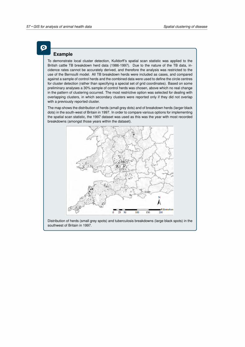
57 • GIS for analysis of animal health data Spatial clustering of disease
ExampleTo demonstrate local cluster detection, Kulldorff’s spatial scan statistic was applied to theBritish cattle TB breakdown herd data (1986-1997). Due to the nature of the TB data, in-cidence rates cannot be accurately derived, and therefore the analysis was restricted to theuse of the Bernoulli model. All TB breakdown herds were included as cases, and comparedagainst a sample of control herds and the combined data were used to define the circle centresfor cluster detection (rather than specifying a special set of grid coordinates). Based on somepreliminary analyses a 30% sample of control herds was chosen, above which no real changein the pattern of clustering occurred. The most restrictive option was selected for dealing withoverlapping clusters, in which secondary clusters were reported only if they did not overlapwith a previously reported cluster.
The map shows the distribution of herds (small grey dots) and of breakdown herds (larger blackdots) in the south-west of Britain in 1997. In order to compare various options for implementingthe spatial scan statistic, the 1997 dataset was used as this was the year with most recordedbreakdowns (amongst those years within the dataset).
Distribution of herds (small grey spots) and tuberculosis breakdowns (large black spots) in thesouthwest of Britain in 1997.
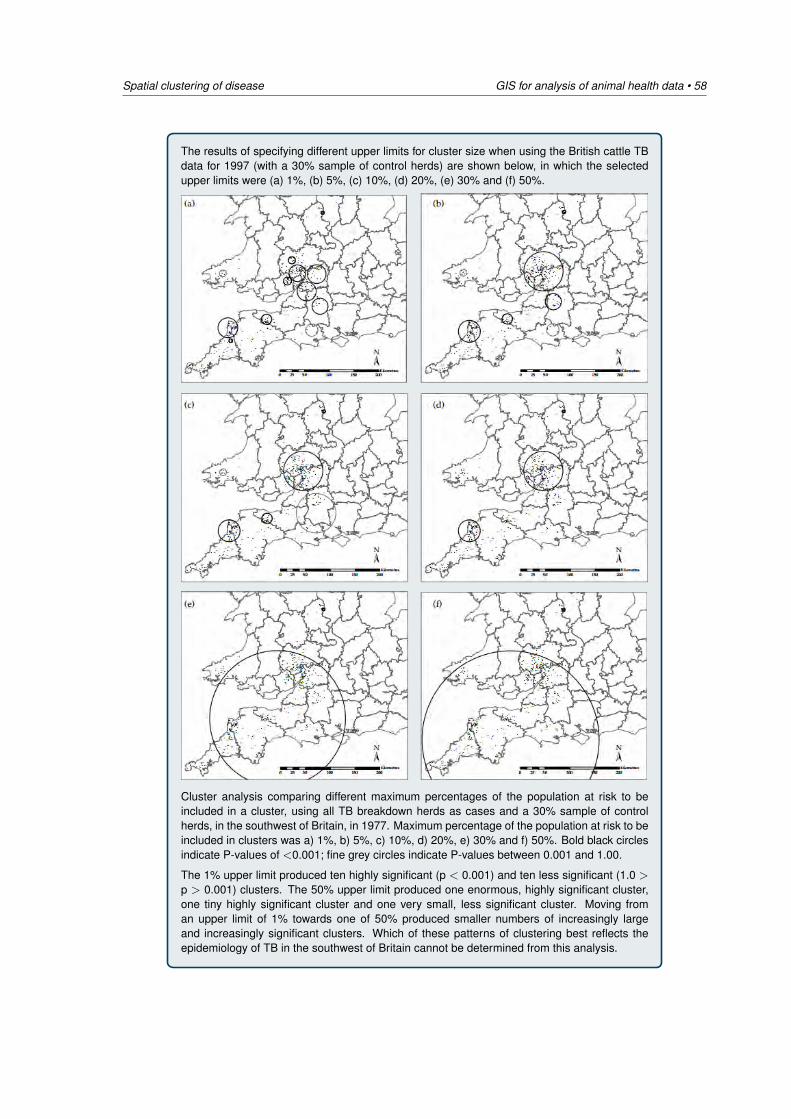
Spatial clustering of disease GIS for analysis of animal health data • 58
The results of specifying different upper limits for cluster size when using the British cattle TBdata for 1997 (with a 30% sample of control herds) are shown below, in which the selectedupper limits were (a) 1%, (b) 5%, (c) 10%, (d) 20%, (e) 30% and (f) 50%.
Cluster analysis comparing different maximum percentages of the population at risk to beincluded in a cluster, using all TB breakdown herds as cases and a 30% sample of controlherds, in the southwest of Britain, in 1977. Maximum percentage of the population at risk to beincluded in clusters was a) 1%, b) 5%, c) 10%, d) 20%, e) 30% and f) 50%. Bold black circlesindicate P-values of <0.001; fine grey circles indicate P-values between 0.001 and 1.00.
The 1% upper limit produced ten highly significant (p < 0.001) and ten less significant (1.0 >p > 0.001) clusters. The 50% upper limit produced one enormous, highly significant cluster,one tiny highly significant cluster and one very small, less significant cluster. Moving froman upper limit of 1% towards one of 50% produced smaller numbers of increasingly largeand increasingly significant clusters. Which of these patterns of clustering best reflects theepidemiology of TB in the southwest of Britain cannot be determined from this analysis.
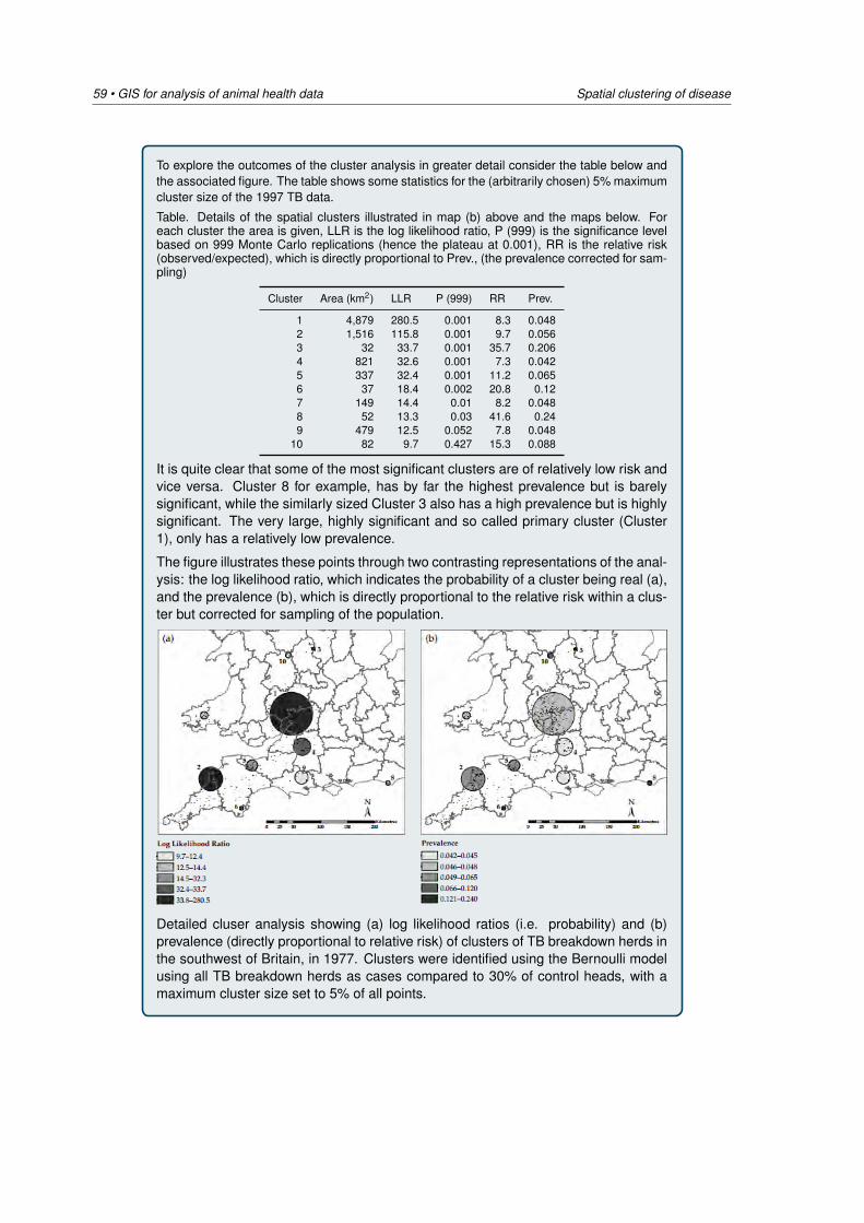
59 • GIS for analysis of animal health data Spatial clustering of disease
To explore the outcomes of the cluster analysis in greater detail consider the table below andthe associated figure. The table shows some statistics for the (arbitrarily chosen) 5% maximumcluster size of the 1997 TB data.
Table. Details of the spatial clusters illustrated in map (b) above and the maps below. Foreach cluster the area is given, LLR is the log likelihood ratio, P (999) is the significance levelbased on 999 Monte Carlo replications (hence the plateau at 0.001), RR is the relative risk(observed/expected), which is directly proportional to Prev., (the prevalence corrected for sam-pling)
Cluster Area (km2) LLR P (999) RR Prev.
1 4,879 280.5 0.001 8.3 0.0482 1,516 115.8 0.001 9.7 0.0563 32 33.7 0.001 35.7 0.2064 821 32.6 0.001 7.3 0.0425 337 32.4 0.001 11.2 0.0656 37 18.4 0.002 20.8 0.127 149 14.4 0.01 8.2 0.0488 52 13.3 0.03 41.6 0.249 479 12.5 0.052 7.8 0.048
10 82 9.7 0.427 15.3 0.088
It is quite clear that some of the most significant clusters are of relatively low risk andvice versa. Cluster 8 for example, has by far the highest prevalence but is barelysignificant, while the similarly sized Cluster 3 also has a high prevalence but is highlysignificant. The very large, highly significant and so called primary cluster (Cluster1), only has a relatively low prevalence.
The figure illustrates these points through two contrasting representations of the anal-ysis: the log likelihood ratio, which indicates the probability of a cluster being real (a),and the prevalence (b), which is directly proportional to the relative risk within a clus-ter but corrected for sampling of the population.
Detailed cluser analysis showing (a) log likelihood ratios (i.e. probability) and (b)prevalence (directly proportional to relative risk) of clusters of TB breakdown herds inthe southwest of Britain, in 1977. Clusters were identified using the Bernoulli modelusing all TB breakdown herds as cases compared to 30% of control heads, with amaximum cluster size set to 5% of all points.
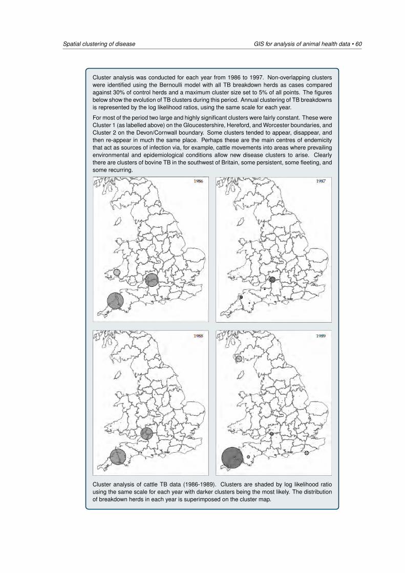
Spatial clustering of disease GIS for analysis of animal health data • 60
Cluster analysis was conducted for each year from 1986 to 1997. Non-overlapping clusterswere identified using the Bernoulli model with all TB breakdown herds as cases comparedagainst 30% of control herds and a maximum cluster size set to 5% of all points. The figuresbelow show the evolution of TB clusters during this period. Annual clustering of TB breakdownsis represented by the log likelihood ratios, using the same scale for each year.
For most of the period two large and highly significant clusters were fairly constant. These wereCluster 1 (as labelled above) on the Gloucestershire, Hereford, and Worcester boundaries, andCluster 2 on the Devon/Cornwall boundary. Some clusters tended to appear, disappear, andthen re-appear in much the same place. Perhaps these are the main centres of endemicitythat act as sources of infection via, for example, cattle movements into areas where prevailingenvironmental and epidemiological conditions allow new disease clusters to arise. Clearlythere are clusters of bovine TB in the southwest of Britain, some persistent, some fleeting, andsome recurring.
Cluster analysis of cattle TB data (1986-1989). Clusters are shaded by log likelihood ratiousing the same scale for each year with darker clusters being the most likely. The distributionof breakdown herds in each year is superimposed on the cluster map.
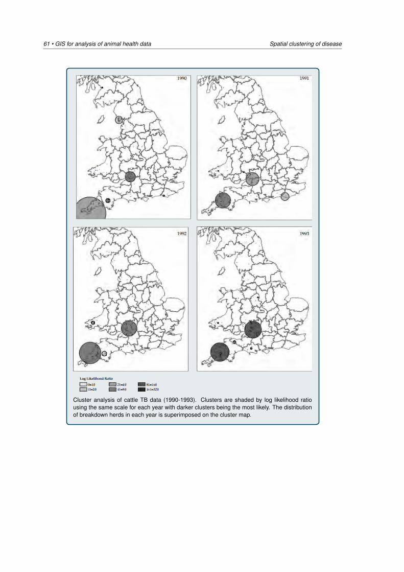
61 • GIS for analysis of animal health data Spatial clustering of disease
Cluster analysis of cattle TB data (1990-1993). Clusters are shaded by log likelihood ratiousing the same scale for each year with darker clusters being the most likely. The distributionof breakdown herds in each year is superimposed on the cluster map.
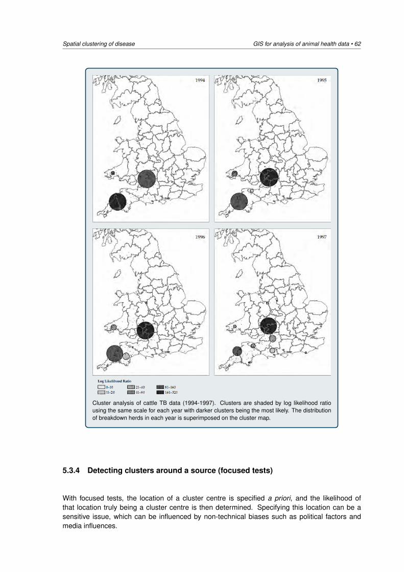
Spatial clustering of disease GIS for analysis of animal health data • 62
Cluster analysis of cattle TB data (1994-1997). Clusters are shaded by log likelihood ratiousing the same scale for each year with darker clusters being the most likely. The distributionof breakdown herds in each year is superimposed on the cluster map.
5.3.4 Detecting clusters around a source (focused tests)
With focused tests, the location of a cluster centre is specified a priori, and the likelihood ofthat location truly being a cluster centre is then determined. Specifying this location can be asensitive issue, which can be influenced by non-technical biases such as political factors andmedia influences.
63 • GIS for analysis of animal health data Spatial clustering of disease
Stone’s test
Stone (1988) developed a class of tests for trend, the maximum likelihood ratio (MLR) and Pois-son maximum (Pmax) tests, both of which use the first isotonic regression estimator, working onthe assumption that there will be a monotonic decay of risk with increasing distance from anypoint source of a disease.
A number of adaptations of the original method have been developed. For example, Morton-Jones et al. (1999) propose an extension that allows for covariate adjustments via a log-linearmodel, which they illustrate using data on the incidence of stomach cancers near municipal in-cinerators. Diggle et al. (1999) adapted Stone’s isotonic regression method to incorporate case-control data in addition to covariate information.
The Lawson-Waller score test
Lawson (1993) and Waller et al. (1992) developed the Lawson-Waller score test, sometimesreferred to as the uniformly most powerful (UMP) test. The score test detects a decreasing trendin disease frequency associated with declining exposure to a point-focus. The test statistic TLW
is given by:
TLW =I∑
i=1
gi (Oi − Ei ) (5.16)
V ar(TLW ) =I∑
i=1
g2i Ei − Oi
(I∑
i=1
pigip+
)2
(5.17)
where gi denotes the exposure to the focus for an individual residing in area i , Oi is the observednumber of disease cases in area i , Ei is the expected number of disease cases in area i , pi is thesize of the population at risk in area i , and p+ is the total population size. Monte Carlo simulationis used to evaluate the significance of the test statistic TLW .
Bithell’s linear risk score tests
Bithell et al. (1994) and Bithell (1995) developed a set of tests known as ‘linear risk score tests’,where disease incidence is weighted by some distance function from a point source (e.g. 1/di ,1/d2
i , or 1/ranki ). Using the reciprocal of distance is appropriate for detecting an environmentalhazard that declines with distance from a source and is relatively insensitive to the precise loca-tion of the assumed source. Using the reciprocal of rank is more appropriate when the relativeproximity of residence is important, rather than actual distance, but it is more sensitive to theprecise location of the putative source.
Diggle’s test
Diggle (1990) developed a test that uses nonparametric kernel smoothing to describe naturalvariation in a disease (assuming a Poisson point process), and then a maximum likelihood testto evaluate the possibility of raised incidence around a pre-specified point source. Diggle andRowlingson (1994) developed a conditional approach, which converts the original point processmodel into a non-linear binary regression model for the spatial variation in risk.
Spatial clustering of disease GIS for analysis of animal health data • 64
5.3.5 Space-time cluster detection
Kulldorff’s space-time scan statistic
Kulldorff’s spatial scan statistic can be ‘focused’ and used to search for clusters around a pointsource by making the point source the only coordinate pair in the special grid file.
The spatial scan statistic has also been adapted to look for clusters in space and time by ex-tending the idea of a two-dimensional circular window to that of a cylinder passing through time.Prospective use of the space-time scan statistic, with repeated time periodic analysis, can beapplied as part of a surveillance system to track active clusters of disease, for detecting the ge-ographic location of emerging clusters and evaluating their significance. A later development ofthis prospective space-time scan statistic led to the development of the ‘space-time permutationscan statistic’, which does not require data on the background population at risk, but estimatesexpected disease occurrence based only on case data. This technique has been applied in alarge number of scientific studies and publications.
5.3.6 Conclusion
The concepts and analytical methods discussed in this chapter extend beyond the mere visual-ization of spatial patterns. The use of statistical methods to assess whether observed patternsdiffer significantly from spatial randomness moves into the next stage of spatial analysis: that ofexploration and from there, quantitative analysis.
A variety of methods have been presented by which spatial and spatio-temporal disease clusterscan be identified statistically. New methods for detecting local clustering are continuously beingdeveloped. For example, methods using Bayesian (probabilistic) approaches or based on otherstatistical modelling techniques are increasingly applied.
A frequently quoted limitation common to many cluster detection tests is the a priori choice ofcluster size, as testing for a variety of cluster sizes results in problems of multiple inference. Anal-ysis of the British cattle TB data, presented in this chapter as the motivating example, suggeststhis to be a central problem which can have profound effects on the results. There do not seemto be clear guidelines on how to deal with it. The attendant danger is that by exploring a range ofmaximum cluster sizes, an upper cluster size threshold can be chosen that presents a pattern ofclustering best suited to support a particular argument, rather than that which best reflects reality.This may cast doubt on the validity of the numerous studies that have been reported using scancircles, and in particular those based on the spatial scan statistic.
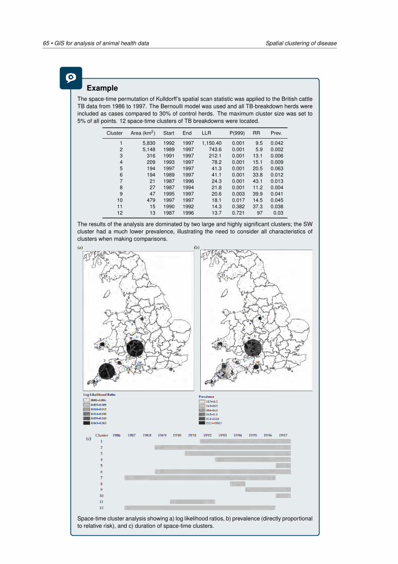
65 • GIS for analysis of animal health data Spatial clustering of disease
ExampleThe space-time permutation of Kulldorff’s spatial scan statistic was applied to the British cattleTB data from 1986 to 1997. The Bernoulli model was used and all TB-breakdown herds wereincluded as cases compared to 30% of control herds. The maximum cluster size was set to5% of all points. 12 space-time clusters of TB breakdowns were located.
Cluster Area (km2) Start End LLR P(999) RR Prev.
1 5,830 1992 1997 1,150.40 0.001 9.5 0.0422 5,148 1989 1997 743.6 0.001 5.9 0.0023 316 1991 1997 212.1 0.001 13.1 0.0064 209 1993 1997 78.2 0.001 15.1 0.0095 194 1997 1997 41.3 0.001 20.5 0.0636 194 1989 1997 41.1 0.001 33.8 0.0127 21 1987 1996 24.3 0.001 43.1 0.0138 27 1987 1994 21.8 0.001 11.2 0.0049 47 1995 1997 20.6 0.003 39.9 0.041
10 479 1997 1997 18.1 0.017 14.5 0.04511 15 1990 1992 14.3 0.382 37.3 0.03812 13 1987 1996 13.7 0.721 97 0.03
The results of the analysis are dominated by two large and highly significant clusters; the SWcluster had a much lower prevalence, illustrating the need to consider all characteristics ofclusters when making comparisons.
Space-time cluster analysis showing a) log likelihood ratios, b) prevalence (directly proportionalto relative risk), and c) duration of space-time clusters.
Spatial clustering of disease GIS for analysis of animal health data • 66
5.4 Cluster detection using SaTScan
SaTScan is a free software programme that analyses spatial, temporal and space-time datausing the spatial, temporal, or space-time scan statistics. It is designed for any of the followinginterrelated purposes:
1. Perform geographical surveillance of disease, to detect spatial or space-time disease clus-ters, and to see if they are statistically significant.
2. Test whether a disease is randomly distributed over space, over time or over space andtime.
3. Evaluate the statistical significance of disease cluster alarms.4. Perform prospective real-time or time-periodic disease surveillance for the early detection
of disease outbreaks.
5.4.1 Statistical methodology, data types and methods
Scan statistics are used to detect and evaluate clusters of cases in either a purely temporal,purely spatial or space-time setting. This is done by gradually scanning a window across timeand/or space, noting the number of observed and expected observations inside the window ateach location. In the SaTScan software, the scanning window is an interval (in time), a circle oran ellipse (in space) or a cylinder with a circular or elliptic base (in space-time). Multiple differentwindow sizes are used. The window with the maximum likelihood is the most likely cluster, thatis, the cluster least likely to be due to chance. A p-value is assigned to this cluster.
Discrete and continuous probability models
Scan statistics use a range of different probability models, depending on the nature of the dataand the purpose of the analysis. SaTScan can be used for discrete as well as continuous scanstatistics.
• For discrete scan statistics the geographical locations where data are observed are non-random and fixed by the user. These locations may be
– the actual locations of the observations, such as houses, schools or ant nests, or– a central location representing a larger area, such as the geographical or population
weighted centroids of postal areas, counties or provinces.• For continuous scan statistics, the locations of the observations are random and can
occur anywhere within a predefined study area defined by the user. This could be anadministrative area, or a bounded geographic area such as a rectangle.
For all discrete probability models, the scan statistic adjusts for the uneven geographical densityof a background population. The following probability models are available:
• a Poisson model, where the number of events in a geographical location is Poisson-distributed (i.e. counts of disease events), according to a known underlying populationat risk;
• a Bernoulli model, where individuals in the population are either cases or non-cases (i.e.0/1 event data);
• a space-time permutation model, using only case data;• a multinomial model for categorical data;• an ordinal model, for ordered categorical data;
67 • GIS for analysis of animal health data Spatial clustering of disease
• an exponential model for survival time data with or without censored variables;• a normal model for other types of continuous data; or• a spatial variation in temporal trends model, looking for geographical areas with unusually
high or low temporal trends.
A common feature of all these discrete scan statistics is that the geographical locations wheredata can be observed are non-random and fixed by the user. The data may be either aggre-gated at the census tract, zip code, county or other geographical level, or there may be uniquecoordinates for each observation. SaTScan adjusts for the underlying spatial inhomogeneity ofa background population. It can also adjust for any number of categorical covariates providedby the user, as well as for temporal trends, known space-time clusters and missing data. It ispossible to scan multiple data sets simultaneously to look for clusters that occur in one or moreof them.
For continuous scan statistics, SaTScan uses a continuous Poisson model.
All analyses are conditioned on the total number of cases observed. For all discrete spatial andspace-time analyses, the user must provide various identifiers in the data, the first two of whichare required as a minimum, and the others dependent on the analysis to be performed:
• the spatial coordinates of a set of locations (coordinates file);• for each location, information about the number of cases at that location (case file);• for temporal and space-time analyses, the number of cases must be stratified by time, e.g.
the time of diagnosis;• depending on the type of analysis, covariate data about cases such as species, breed, age,
gender, weight, length of survival etc. may also be provided;• for the Bernoulli model, it is also necessary to specify the number of non-cases at each
location;• for the discrete Poisson model, the user must specify a population size for each location
(population file). The population may vary over time.
Spatial, temporal and space-time scan statistics
Spatial scan statistic The standard purely spatial scan statistic imposes a circular window onthe map. The window is in turn centred on each of several possible gridpoints positioned throughout the study region. For each grid point, the ra-dius of the window varies continuously in size from zero to some upperlimit specified by the user. In this way, the circular window is flexible bothin location and size. In total, the method creates an infinite number of dis-tinct geographical circles with different sets of neighbouring data locationswithin them. Each circle is a possible candidate cluster.
The user defines the set of grid points used through a grid file. If no grid fileis specified, the grid points are set to be identical to the coordinates of thelocation IDs defined in the coordinates file. The latter option ensures thateach data location is a potential cluster in itself, and it is the recommendedoption for most types of analyses.
As an alternative to the circle, it is also possible to use an elliptic windowshape, in which case a set of ellipses with different shapes and anglesare used as the scanning window together with the circle. This providesslightly higher power for true clusters that are long and narrow in shape,and slightly lower power for circular and other very compact clusters.
Spatial clustering of disease GIS for analysis of animal health data • 68
It is also possible to define your own non-Euclidian distance metric usinga special neighbours file.
Space-time scan statis-tic
This is defined by a cylindrical window with a circular (or elliptic) geo-graphic base and with height corresponding to time. The base is definedexactly as for the purely spatial scan statistic, while the height reflects thetime period of potential clusters. The cylindrical window is then moved inspace and time, so that for each possible geographical location and size,it also visits each possible time period. In effect, we obtain an infinite num-ber of overlapping cylinders of different size and shape, jointly covering theentire study region, where each cylinder reflects a possible cluster.
This may be used for either a single retrospective analysis, using historicdata, or for time-periodic prospective surveillance, where the analysis isrepeated for example every day, week, month or year.
Purely temporal scanstatistic
The temporal scan statistic uses a window that moves in one dimension,time, defined in the same way as the height of the cylinder used by thespace-time scan statistic. This means that it is flexible in both start andend date.
Seasonal scan statistic The seasonal scan statistic is a purely temporal scan statistic where allthe data is on a connecting loop, such as the year, where December 31is followed by January 1. The key feature that distinguishes the seasonalscan statistic from the purely temporal scan statistic is that it ignores whichyear the observation was made and only cares about the day and month.
Spatial variation in tem-poral trends scan statis-tic
When the scan statistic is used to evaluate the spatial variation in temporaltrends, the scanning window is purely spatial in nature. The temporal trendis then calculated inside as well as outside the scanning window, for eachlocation and size of that window. The null hypothesis is that the trends arethe same, while the alternative is that they are different. Based on thesehypotheses, a likelihood is calculated, which is higher the more unlikely itis that the difference in trends is due to chance. The most likely clusteris the cluster for which the temporal trend inside the window is least likelyto be the same as the temporal trend outside the cluster. This could bebecause of various reasons. For example, if the temporal trend inside thecluster is higher, it could be because all areas has the same incidence rateof a disease at the beginning of the time period, but the cluster area hasa higher rate at the end of the time period. It could also be because thecluster area has a lower incidence rate at the beginning of the time period,after which it ‘catches up’ with the rest so that the rate is about the sameat the end of the time period. Hence, a statistically significant cluster in thespatial variation in temporal trend analysis does not necessarily mean thatthe overall rate of disease is higher or lower in the cluster.
The spatial variation in temporal trends scan statistic can only be run withthe discrete Poisson probability model. For it to work, it is important thatthe total study period length is evenly divisible by the length of the timeinterval aggregation, so that all time intervals have the same number ofyears, if it is specified in years, the same number of months if it is specifiedin months or the same number of days if it is specified in days.
69 • GIS for analysis of animal health data Spatial clustering of disease
5.4.2 A summary of the model types implemented in SaTScan
Bernoulli model
With the Bernoulli model there are cases and non-cases represented by a 0/1 variable. Thesevariables may represent animals with or without a disease, or animals showing different degreesof clinical disease severity. They may reflect cases and controls from a larger population, orthey may together constitute the population as a whole. Whatever the situation may be, thesevariables ar denoted as cases and controls, and their total will be denoted as the population.Bernoulli data can be analysed with the purely temporal, the purely spatial or the space-timescan statistics.
ExampleFor the Bernoulli model, cases may be newborns with a certain birth defect while controls areall newborns without that birth defect.
The Bernoulli model requires information about the location of a set of cases and controls, pro-vided to SaTScan using the case, control and coordinates files. Separate locations may bespecified for each case and each control, or the data may be aggregated for states, provinces,counties, parishes, census tracts, postal code areas, school districts, households, etc., with mul-tiple cases and controls at each data location. To do a temporal or space-time analysis, it isnecessary to have a time for each case and each control as well.
Discrete Poisson model
With the discrete Poisson model the number of cases in each location is Poisson-distributed.Under the null hypothesis, and when there are no covariates, the expected number of casesin each area is proportional to its population size, or to the person-years in that area. Poissondata can be analysed with the purely temporal, the purely spatial, the space-time and the spatialvariation in temporal trends scan statistics.
ExampleFor the discrete Poisson model, cases may be stroke occurrences while the population is thecombined number of person-years lived, calculated as 1 for someone living in the area for thewhole time period and ½for someone dying or moving away in the middle of the time period.
The discrete Poisson model requires case and population counts for a set of data locations suchas counties, parishes, census tracts or zip code areas, as well as the geographical coordinatesfor each of those locations. These need to be provided to SaTScan using the case, populationand coordinates files.
The population data need not be specified continuously over time, but only at one or more specific‘census times’. For times in between, SaTScan does a linear interpolation based on the popula-tion at the census times immediately preceding and immediately following. For times before thefirst census time, the population size is set equal to the population size at that first census time,and for times after the last census time, the population is set equal to the population size at that
Spatial clustering of disease GIS for analysis of animal health data • 70
last census time. To get the population size for a given location and time period, the populationsize, as defined above, is integrated over the time period in question.
Space-time permutation model
The space-time permutation model requires only case data, with information about the spatiallocation and time for each case, with no information needed about controls or a backgroundpopulation at risk. The number of observed cases in a cluster is compared to what would havebeen expected if the spatial and temporal locations of all cases were independent of each otherso that there is no space-time interaction. That is, there is a cluster in a geographical area if,during a specific time period, that area has a higher proportion of its cases in that time periodcompared to the remaining geographical areas. This means that if, during a specific week, allgeographical areas have twice the number of cases than normal, none of these areas constitutea cluster. On the other hand, if during that week, one geographical area has twice the numberof cases compared to normal while other areas have a normal amount of cases, then there willbe a cluster in that first area. The space-time permutation model automatically adjusts for bothpurely spatial and purely temporal clusters. Hence there are no purely temporal or purely spatialversions of this model.
CautionSpace-time permutation clusters may be due either to an increased risk of disease, or to differ-ent geographical population distribution at different times, where for example the population insome areas grows faster than in others. This is typically not a problem if the total study periodis less than a year. However, the user is advised to be very careful when using this methodfor data spanning several years. If the background population increases or decreases fasterin some areas than in others, there is risk for population shift bias, which may produce biasedp-values when the study period is longer than a few years.
For example, if a new large neighbourhood is developed, there will be an increase in casesthere simply because the population increases, and using only case data, the space-timepermutation model cannot distinguish an increase due to a local population increase versusan increase in the disease risk. As with all space-time interaction methods, this is mainly aconcern when the study period is longer than a few years.
Multinomial model
With the multinomial model, each observation is a case, and each case belongs to one of severalcategories. The multinomial scan statistic evaluates whether there are any clusters where thedistribution of cases is different from the rest of the study region. For example, there may bea higher proportion of cases of types 1 and 2 and a lower proportion of cases of type 3 whilethe proportion of cases of type 4 is about the same as outside the cluster. If there are only twocategories, the ordinal model is identical to the Bernoulli model, where one category representsthe cases and the other category represents the controls. The cases in the multinomial modelmay be a sample from a larger population or they may constitute a complete set of observations.Multinomial data can be analysed with the purely temporal, the purely spatial or the space-timescan statistics.
71 • GIS for analysis of animal health data Spatial clustering of disease
ExampleFor the multinomial model, the data may consist of everyone diagnosed with meningitis, withfive different categories representing five different clonal complexes of the disease. The multi-nomial scan statistic will simultaneously look for high or low clusters of any of the clonal com-plexes, or a group of them, adjusting for the overall geographical distribution of the disease.The multiple comparisons inherent in the many categories used are accounted for when cal-culating the p-values.
The multinomial model requires information about the location of each case in each category.A unique location may be specified for each case, or the data may be aggregated for states,provinces, counties, parishes, census tracts, postal code areas, school districts, households,etc., with multiple cases in the same location. To do a temporal or space-time analysis, it isnecessary to have a time for each case as well.
With the multinomial model it is not necessary to specify a search for high or low clusters, sincethere is no hierarchy among the categories, but in the output it is shown what categories aremore prominent inside the cluster. The order or indexing of the categories does not affect theanalysis in terms of the clusters found, but it may influence the randomization used to calculatethe p-values.
Ordinal model
With the ordinal model, each observation is a case, and each case belongs to one of severalordinal categories. If there are only two categories, the ordinal model is identical to the Bernoullimodel, where one category represents the cases and the other category represent the controlsin the Bernoulli model. The cases in the ordinal model may be a sample from a larger populationor they may constitute a complete set of observations. Ordinal data can be analysed with thepurely temporal, the purely spatial or the space-time scan statistics.
ExampleFor the ordinal model, the data may consist of everyone diagnosed with breast cancer duringa ten-year period, with three different categories representing early, medium and late stagecancer at the time of diagnosis.
The ordinal model requires information about the location of each case in each category. Sep-arate locations may be specified for each case, or the data may be aggregated for states,provinces, counties, parishes, census tracts, postal code areas, school districts, households,etc., with multiple cases in the same or different categories at each data location. To do a tem-poral or space-time analysis, it is necessary to have a time for each case as well.
With the ordinal model it is possible to search for high clusters, with an excess of cases in thehigh-valued categories, for low clusters with an excess of cases in the low-valued categories, orsimultaneously for both types of clusters. Reversing the order of the categories has the sameeffect as changing the analysis from high to low and vice versa.
Spatial clustering of disease GIS for analysis of animal health data • 72
Exponential model
The exponential model is designed for survival time data, although it could be used for othercontinuous type data as well. Each observation is a case, and each case has one continuousvariable attribute as well as a 0/1 censoring designation. For survival data, the continuous vari-able is the time between diagnosis and death or depending on the application, between two othertypes of events. If some of the data is censored, due to loss of follow-up, the continuous variableis then instead the time between diagnosis and time of censoring. The 0/1 censoring variable isused to distinguish between censored and non-censored observations.
ExampleFor the exponential model, the data may consist of everyone diagnosed with prostate cancerduring a ten-year period, with information about either the length of time from diagnosis untildeath or from diagnosis until a time of censoring after which survival is unknown.
When using the temporal or space-time exponential model for survival times, two very differenttime variables are involved. The first is the time the case was diagnosed, and that is the time thatthe temporal and space-time scanning window is scanning over. The second is the survival time,that is, time between diagnosis and death or for censored data the time between diagnosis andcensoring. This is an attribute of each case, and there is no scanning done over this variable.Rather, we are interested in whether the scanning window includes exceptionally many caseswith a small or large value of this attribute.
While the exponential model uses a likelihood function based on the exponential distribution, thetrue survival time distribution must not be exponential and the statistical inference (p-value) isvalid for other survival time distributions as well. The reason for this is that the randomization isnot done by generating observations from the exponential distribution, but rather, by permutingthe space-time locations and the survival time/censoring attributes of the observations.
Normal model
The normal model is designed for continuous data. For each individual or for each observation,called a case, there is a single continuous attribute that may be either negative or positive. Themodel can also be used for ordinal data when there are many categories. That is, different casesare allowed to have the same attribute value.
ExampleFor the normal model, the data may consist of the birth weight and residential census tract forall newborns, with an interest in finding clusters with lower birth weight. One individual is thena ‘case’. Alternatively, the data may consist of the average birth weight in each census tract. Itis then the census tract that is the ‘case’, and it is important to use the weighted normal model,since each average will have a different variance due to a different number of births in eachtract.
While the normal model uses a likelihood function based on the normal distribution, the truedistribution of the continuous attribute must not be normal. The statistical inference (p-value) isvalid for any continuous distribution. The reason for this is that the randomization is not done by
73 • GIS for analysis of animal health data Spatial clustering of disease
generating simulated data from the normal distribution, but rather, by permuting the space-timelocations and the continuous attribute (e.g. birth weight) of the observations. While still beingformally valid, the results can be greatly influenced by extreme outliers, so it may be wise totruncate such observations before doing the analysis.
In the standard normal model, it is assumed that each observation is measured with the samevariance. That may not always be the case. For example, if an observation is based on a largersample in one location and a smaller sample in another, then the variance of the uncertainty in theestimates will be larger for the smaller sample. If the reliability of the estimates differs, one shouldinstead use the weighted normal scan statistic that takes these unequal variances into account.The weighted version is obtained in SaTScan by simply specifying a weight for each observationas an extra column in the input file. This weight may for example be proportional to the samplesize used for each estimate or it may be the inverse of the variance of the observation.
If all values are multiplied with or added to the same constant, the statistical inference will notchange, meaning that the same clusters with the same log likelihoods and p-values will be found.Only the estimated means and variances will differ. If the weight is the same for all observations,then the weighted normal scan statistic will produce the same results as the standard normalversion. If all the weights are multiplied by the same constant, the results will not change.
Continuous Poisson model
All the models described above are based on data observed at discrete locations that are consid-ered to be non-random, as defined by a regular or irregular lattice of location points. That is, thelocations of the observations are considered to be fixed, and we evaluate the spatial randomnessof the observation conditioning on the lattice. Hence, those are all versions of what are calleddiscrete scan statistics. In a continuous scan statistics, observations may be located anywherewithin a study area, such as a square or rectangle. The stochastic aspect of the data consistsof these random spatial locations, and we are interested to see if there are any clusters that areunlikely to occur if the observations where independently and randomly distributed across thestudy area. Under the null hypothesis, the observations follow a homogeneous spatial Poissonprocess with constant intensity throughout the study area, with no observations falling outsidethe study area.
ExampleThe data may consist of the location of bird nests in a square kilometer area of a forest. Theinterest may be to see whether the bird nests are randomly distributed spatially, or in otherwords, whether there are clusters of bird nests or whether they are located independently ofeach other.
In SaTScan, the study area can be any collection of convex polygons, which are convex regionsbounded by any number straight lines. Triangles, squares, rectangles, rhombuses, pentagonsand hexagons are all examples of convex polygons. In the simplest case, there is only onepolygon, but the study area can also be the union of multiple convex polygons. If the study areais not convex, divide it into multiple convex polygons and define each one separately. The studyarea does not need to be contiguous, and may for example consist of five different islands.
The analysis is conditioned on the total number of observations in the data set. Hence, thescan statistic simply evaluates the spatial distribution of the observation, but not the number of
Spatial clustering of disease GIS for analysis of animal health data • 74
observations.
The likelihood function used as the test statistic is the same as for the Poisson model for the dis-crete scan statistic, where the expected number of cases is equal to the total number of observedobservations, times the size of the scanning window, divided by the size of the total study area.When the scanning window extends outside the study area, the expected count is still based onthe full size of the circle, ignoring the fact that some parts of the circle have zero expected counts.This is to avoid strange non-circular clusters at the border of the study area. Since the analysis isbased on Monte Carlo randomizations, the p-values are automatically adjusted for these bound-ary effects. The reported expected counts are based on the full circle though, so the Obs/Expratios provided should be viewed as a lower bound on the true value whenever the circle extendsoutside the spatial study region.
The continuous Poisson model can only be used for purely spatial data. It uses a circular scan-ning window of continuously varying radius up to a maximum specified by the user. Only circlescentred on one of the observations are considered, as specified in the coordinates file. If theoptional grid file is provided, the circles are instead centred on the coordinates specified in thatfile.
5.4.3 Probability model choice and comparison
• All discrete probability models can be used for either individual locations or aggregateddata.
• The discrete Poisson model is usually the fastest to run. The ordinal model is typically theslowest.
• With the discrete Poisson and space-time permutations models, an unlimited number ofcovariates can be adjusted for, by including them in the case and population files. Withthe normal model, it is also possible to adjust for covariates by including them in the casefile, but only for purely spatial analyses. With the Bernoulli, ordinal, exponential and normalmodels, covariates can be adjusted for by using multiple data sets, which limits the numberof covariate categories that can be defined, or through a pre-processing regression analysisdone before running SaTScan.
• With the discrete Poisson model, population data is only needed at selected time pointsand the numbers are interpolated in between. A population time must be specified even forpurely spatial analyses. Regardless of model used, the time of a case or control need onlybe specified for purely temporal and space-time analyses.
• The space-time permutation model automatically adjusts for purely spatial and purely tem-poral clusters. For the discrete Poisson model, purely temporal and purely spatial clusterscan be adjusted for in a number of different ways. For the Bernoulli, ordinal, exponentialand normal models, spatial and temporal adjustments can be done using multiple datasets, but it is limited by the number of different data sets allowed, and it is also much morecomputer intensive.
• Purely temporal and space-time analyses cannot be performed using the homogeneousPoisson model.
• Spatial variation in temporal trend analyses can only be performed using the discrete Pois-son model.
Some additional considerations regarding model choice are as follows:
• Few cases compared to controls. In a purely spatial analysis where there are few casescompared to controls, say less than 10 percent, the discrete Poisson model is a very good
75 • GIS for analysis of animal health data Spatial clustering of disease
approximation to the Bernoulli model. The former can then be used also for 0/1 Bernoullitype data, and may be preferable as it has more options for various types of adjustments,including the ability to adjust for covariates specified in the case and population files. Asan approximation for Bernoulli type data, the discrete Poisson model produces slightly con-servative p-values.
• Bernoulli versus ordinal model. The Bernoulli model is mathematically a special caseof the ordinal model, when there are only two categories. The Bernoulli model runs faster,making it the preferred model to use when there are only two categories.
• Normal versus exponential model. Both the normal and exponential models are meantfor continuous data. The exponential model is primarily designed for survival time data butcan be used for any data where all observations are positive. It is especially suitable fordata with a heavy right tail. The normal model can be used for continuous data that takesboth positive and negative values. While still formally valid, results from the normal modelare sensitive to extreme outliers.
• Normal versus ordinal model. The normal model can be used for categorical data whenthere are very many categories. As such, it is sometimes a computationally faster alterna-tive to the ordinal model. There is an important difference though. With the ordinal model,only the order of the observed values matters. For example, the results are the same forordered values ‘1 – 2 – 3 – 4’ and ‘1 – 10 – 100 – 1000’. With the normal model, the resultswill be different, as they depend on the relative distance between the values used to definethe categories.
• Discrete versus homogeneous Poisson model. Instead of using the homogeneous Pois-son model, the data can be approximated by the discrete Poisson model by dividing thestudy area into many small pieces. For each piece, a single coordinates point is specified,the size of the piece is used to define the population at that location and the number ofobservations within that small piece of area is the number of cases in that location. As thenumber of pieces increases towards infinity, and hence, as their size decreases towardszero, the discrete Poisson model will be asymptotically equivalent to the homogeneousPoisson model.
• Temporal data. For temporal and space-time data, there is an additional difference amongthe probability models, in the way that the temporal data is handled. With the Poissonmodel, population data may be specified at one or several time points, such as censusyears. The population is then assumed to exist between such time points as well, esti-mated through linear interpolation between census years. With the Bernoulli, space-timepermutation, ordinal, exponential and normal models, a time needs to be specified for eachcase and for the Bernoulli model, for each control as well.
5.4.4 Likelihood Ratio Test
For each location and size of the scanning window, the alternative hypothesis is that there isan elevated risk within the window as compared to outside. Under the Poisson assumption, thelikelihood function for a specific window is proportional to:(
c
E [c]
)c ( C − c
C − E [c]
)C−cI () (5.18)
where C is the total number of cases, c is the observed number of cases within the windowand E [c] is the covariate adjusted expected number of cases within the window under the null-hypothesis. Note that since the analysis is conditioned on the total number of cases observed,C −E [c] is the expected number of cases outside the window. I () is an indicator function. When
Spatial clustering of disease GIS for analysis of animal health data • 76
SaTScan is set to scan only for clusters with high rates, I () is equal to 1 when the window hasmore cases than expected under the null-hypothesis, and 0 otherwise. The opposite is true whenSaTScan is set to scan only for clusters with low rates. When the program scans for clusters witheither high or low rates, then I () = 1 for all windows.
The space-time permutation model uses the same function as the Poisson model. Due to theconditioning on the marginals, the observed number of cases is only approximately Poissondistributed. Hence, it is no longer a formal likelihood ratio test, but it serves the same purpose asthe test statistic.
For the Bernoulli model the likelihood function is:(c
n
)c (n − c
n
)n−c (C − c
N − n
)C−c ((N − n) (C − c)
N − n
)(N−n)(C−c)I () (5.19)
where c and C are defined as above, n is the total number of cases and controls within thewindow, while N is the combined total number of cases and controls in the data set.
The likelihood function for the multinomial, ordinal, exponential, and normal models are morecomplex, due to the more complex nature of the data. The likelihood function for the spatialvariation in temporal trends scan statistic is also more complex, as it involves the maximumlikelihood estimation of several different trend functions.
The likelihood function is maximized over all window locations and sizes, and the one with themaximum likelihood constitutes the most likely cluster. This is the cluster that is least likely tohave occurred by chance. The likelihood ratio for this window constitutes the maximum likelihoodratio test statistic. Its distribution under the null-hypothesis is obtained by repeating the sameanalytic exercise on a large number of random replications of the data set generated under thenull hypothesis.
The p-value is obtained through Monte Carlo hypothesis testing, by comparing the rank of themaximum likelihood from the real data set with the maximum likelihoods from the random datasets. If this rank is R , then p = R/(1+#simulation). In order for p to be a ‘nice looking’ number,the number of simulations is restricted to 999 or some other number ending in 999 such as 1999,9999 or 99999. That way it is always clear whether to reject or not reject the null hypothesis fortypical cut-off values such as 0.05, 0.01 and 0.001.
The SaTScan program scans for areas with high rates (clusters), for areas with low rates, orsimultaneously for areas with either high or low rates. The most common analysis is to scan forareas with high rates, that is, for clusters.
5.4.5 Secondary clusters
For purely spatial and space-time analyses, SaTScan also identifies secondary clusters in thedata set in addition to the most likely cluster, and orders them according to their likelihood ratiotest statistic. There will almost always be a secondary cluster that is almost identical with themost likely cluster and that have almost as high likelihood value, since expanding or reducingthe cluster size only marginally will not change the likelihood very much. The user can decide towhat extent overlapping clusters are reported in the results files. The default is that geographicallyoverlapping clusters are not reported.
There may also be secondary clusters that do not overlap spatially with the most likely cluster,and they may be of great interest. These are always reported. When there are multiple clusters

77 • GIS for analysis of animal health data Spatial clustering of disease
in the data set, the secondary clusters are evaluated as if there were no other clusters in the dataset. That is, they are statistically significant if and only if they are able to cause a rejection of thenull hypothesis on their own strength, whether or not the other clusters are true clusters or not.That is often the desired type of inference. Sometime though, it is also of interest to evaluatesecondary clusters after adjusting for other clusters in the data.
Note that the circle of a secondary cluster may overlap with the circle of a previously detectedmore likely cluster, and it may even completely encircle it so that the latter is a subset of theformer. This does not mean that the more likely cluster is detected twice. Rather, the more likelycluster is treated as a ‘lake’ with no population and no cases, and the new secondary clusterconsist of the areas around that ‘lake’. This may for example happen if a city has a very highelevated risk, while the surrounding suburbs have a modest elevated risk. The same phenomenamay occur when doing purely temporal or space-time analyses.
For purely temporal analyses, only the most likely cluster is reported.
5.4.6 Statistical adjustments
Covariate adjustments
A covariate should be adjusted for when all three of the following are true:
1. The covariate is related to the disease in question.2. The covariate is not randomly distributed geographically.3. You want to find clusters that cannot be explained by that covariate.
ExampleHere are three examples:
• If you are studying cancer mortality, you should adjust for age since (i) older peopleare more likely to die from cancer (ii) some areas may have a higher density of olderpeople, and (iii) you are presumably interested in finding areas where the risk of canceris high as opposed to areas with an older population.
• If you are interested in the geographical distribution of birth defects, you do not needto adjust for gender. While birth defects are not equally likely in boys and girls, thegeographical distribution of the two genders is geographically random at time of birth.
• If you are studying the geography of lung cancer incidence, you should adjust for smok-ing if you are interested in finding clusters due to non-smoking related risk factors, butyou should not adjust for smoking if you are interested in finding clusters reflectingareas with especially urgent needs to launch an anti-smoking campaign.
When the disease rate varies, for example, with age, and the age distribution varies in differentareas, then there is geographical clustering of the disease simply due to the age covariate. Whenadjusting for categorical covariates, the SaTScan program will search for clusters above and be-yond that which is expected due to these covariates. When more than one covariate is specified,each one is adjusted for as well as all the interaction terms between them.
Covariate adjustment using the input files. With the Poisson and space-time permutationmodels, it is possible to adjust for multiple categorical covariates by specifying the covariatesin the input files. To do so, simply enter the covariates as extra columns in the case file (both
Spatial clustering of disease GIS for analysis of animal health data • 78
models) and the population file (Poisson model). There is no need to enter any information onany of the window tabs.
For the Poisson model, the expected number of cases in each area under the null-hypothesis iscalculated using indirect standardization. Without covariate adjustment the expected number ofcases in a location is (spatial analysis):
E [c] = p ∗ C/P (5.20)
where c is the observed number of cases and p the population in the location of interest, while Cand P are the total number of cases and population respectively. Let ci , pi , Ci and Pi be definedin the same way, but for covariate category i . The indirectly standardized covariate adjustedexpected number of cases (spatial analysis) is:
E [c] =∑
iE [ci ] =
∑ipi ∗ Ci/Pi (5.21)
The same principle is used when calculating the covariate adjusted number of cases for thespace-time scan statistic, although the formula is more complex due to the added time dimen-sion.
Since the space-time permutation model automatically adjusts for purely spatial and purely tem-poral variation, there is no need to adjust for covariates in order to account for different spatial ortemporal densities of these covariates. Rather, covariate adjustment is used if there is space-timeinteraction due to this covariate rather than to the underlying disease process.
ExampleIf children get sick mostly in the summer and adults mostly in the winter, then there will be agegenerated space-time interaction clusters in areas with many children in the summer and viceversa. When including child/adult as a covariate, these clusters are adjusted away.
Covariate adjustment using statistical regression software. SaTScan cannot in itself do anadjustment for continuous covariates. Such adjustments can still be done for the Poisson modelbut it is a little more complex. The first step is to calculate the covariate adjusted expected numberof cases for each location ID and time using a standard statistical regression software package.These expected numbers should then replace the raw population numbers in the population file,while not including the covariates themselves.
The use of external regression software is also an excellent way to adjust for covariates in theexponential model. The first step is to fit an exponential regression model without any spatialinformation, in order to obtain risk estimates for each of the covariates. The second step is toadjust the survival and censoring time up or down for each individual based on the risk estimateshis or her covariates.
For the normal model, covariates can be adjusted for by first doing linear regression using stan-dard statistical software, and then replacing the observed value with their residuals.
Covariate adjustment using multiple data sets. It is also possible to adjust for categoricalcovariates using multiple data sets. The cases and controls/population are then divided intocategories, and a separate data set is used for each category. This type of covariate adjustment

79 • GIS for analysis of animal health data Spatial clustering of disease
is computationally much slower than the one using the input files, and is not recommended forlarge data sets. One advantage is that it can be used to adjust for covariates when runningthe multinomial or ordinal models, for which other adjustment procedures are unavailable. Adisadvantage is that since the maximum number of data sets allowed by SaTScan is twelve, themaximum number of covariate categories is also twelve.
The adjustment approach to multiple data sets is as follows (when searching for clusters withhigh rates):
1. For each window location and size, the log likelihood ratio is calculated for each data set.2. The log likelihood ratio for all data sets with less than expected number of cases in the
window is multiplied with negative one.3. The log likelihood ratios are then summed up, and this sum is the combined log likelihood
for that particular window.4. The maximum of all the combined log likelihood ratios, taken over all the window locations
and sizes, constitutes the most likely cluster, and this is evaluated in the same way as for asingle data set.
When searching for clusters with low rates, the same procedure is performed, except that it isthen the data sets with more than expected cases that we multiply by one. When searching forboth high and low clusters, both sums are calculated, and the maximum of the two is used torepresent the log likelihood ratio for that window.
Spatial and temporal adjustments
Adjusting for temporal trends. If there is an increasing temporal trend in the data, then thetemporal and space-time scan statistics will pick up that trend by assigning a cluster during theend of the study period. If there is a decreasing trend, it will instead pick up a cluster at thebeginning of the time period. Sometimes it is of interest to test whether there are temporal and/orspace-time clusters after adjusting for a temporal trend.
For the space-time permutation model, the analysis is automatically adjusted for both temporaltrends and temporal clusters, and no further adjustments are needed. For the discrete Poissonmodel, the user can specify whether a temporal adjustment should be made, and if so, whetherto adjust with a percent change or non-parametrically.
Sometimes, the best way to adjust for a temporal trend is by specifying the percent yearly in-crease or decrease in the rate that is to be adjusted for. This is a log linear adjustment. Depend-ing on the application, one may adjust either for a trend that SaTScan estimates from the databeing analysed, or from the trend as estimated from national or other similar data. In the lattercase, the percent increase or decrease must be calculated using standard statistical regressionsoftware such as R, and then inserted on the Risk Adjustments Tab.
For space-time analyses, it is also possible to adjust for a temporal trend non-parametrically.This adjusts the expected count separately for each aggregated time interval, removing all purelytemporal clusters. The randomization is then stratified by time interval to ensure that each timeinterval has the same number of events in the real and random data sets.
The ability to adjust for temporal trends is much more limited for the Bernoulli, multinomial, or-dinal, normal and exponential models, as none of the above features can be used. Instead, thetime must be divided into discrete time periods, with the cases and controls in each period corre-sponding to a separate data set with separate case and control files. The analysis is then doneusing multiple data sets.
Spatial clustering of disease GIS for analysis of animal health data • 80
Adjusting for day-of-week effects. Some data sets have a weekly pattern. If not adjusted for,that could create clusters, for example on a Monday, or from one Monday to the next Monday,simply because Mondays in general have more events than other days of the week. One wayto adjust for this is to aggregate daily data into weeks, but that will reduce the temporal resolu-tion. Another option is to select the day-of-week adjustment feature on the Spatial and TemporalAdjustment Tab, which will non-parametrically adjust for any weekly adjustment in the data. Thisfeature is only available with the discrete Poisson probability model.
The space-time permutation model automatically adjusts for any purely temporal variation in thedata, including day-of-week effects. Hence, with this probability model, there is never a need todo any special day-of-week adjustment. If different spatial locations have different day-of-weekeffects, that may lead to spurious space-time interaction clusters.
ExampleYour disease data come from different medical clinics, but only some of the clinics are open onthe weekends. That may result in weekend clusters at those clinics that are simply an artefactof their opening hours. To adjust for this, it is possible to adjust for the space-by-day-of-weekinteraction by selecting that option on the Spatial and Temporal Adjustment Tab. Doing thishas exactly the same effect as including a day-of-week variable in the input case file. Thisfeature is only valid for the space-time permutation model.
Adjusting for purely spatial clusters. In a space-time analysis with the Poisson model, it isalso possible to adjust for purely spatial clusters, in a non-parametric fashion. This adjusts theexpected count separately for each location, removing all purely spatial clusters. The randomiza-tion is then stratified by location ID to ensure that each location has the same number of eventsin the real and random data sets.
This option is not available for the Bernoulli, multinomial, ordinal, exponential, normal or space-time permutation models, in the latter case because the method automatically adjusts for anypurely spatial clusters.
Adjusting for known relative risks. Sometimes it is known a priori that a particular locationand/or time has a higher or lower risk of known magnitude, and we want to detect clusters aboveand beyond this, or in other words, we want to adjust for this known excess/lower risk. One wayto do this is to simply change the population at risk numbers in the population file. A simplerway is to use the adjustments file. In this file, a relative risk is specified for any location and timeperiod combination. The expected counts are then multiplied by this relative risk for that locationand time.
ExampleIf it is known from historical data that a particular location typically have 50 percent more casesduring the summer months June to August, then for each year one would specify a relative riskof 1.5 for this location and these months. A summer cluster will then only appear in this locationif the excess risk is more than 50 percent.
This feature is only available for the discrete Poisson model.
81 • GIS for analysis of animal health data Spatial clustering of disease
5.4.7 Missing data
If there are missing data for some locations and times, it is important to adjust for that in theanalysis. If not, you may find statistically significant low rate clusters where there is missingdata, or statistically significant high rate clusters in other locations, even though these are simplyartefacts of the missing data.
Some guidance is given below on how to adjust the different probability model types for missingdata.
Bernoulli model If cases are missing for a particular location and time period, remove thecontrols for that same location and time. Likewise, if controls are missingfor a particular location and time, remove the cases for that same locationand time. This needs to be done before providing the data to SaTScan. Ifboth cases and controls are missing for a location and time, you are fine,and there is no need for any modification of the input data.
Multinomial and ordinalmodels
If one or more categories are missing for a particular location and time pe-riod, remove all cases in the remaining categories from that same locationand time. This needs to be done before providing the data to SaTScan. Ifall cases in all categories are missing for a location and time, you are fine,and there is no need for any modification of the input data.
Discrete Poisson model Use the adjustments file to define the location and time combinations forwhich the data is missing, and assign a relative risk of zero to those loca-tion/time combinations.
Continuous Poissonmodel
Redefine the study area buy using a different set of polygons, so that areaswith missing data are excluded from the study area.
Space-time permutationmodel
It is a little more complex to adjust for missing data in the space-time per-mutation model, but still possible. First add day-of-week as a covariate inthe analysis file. When a particular location / time period is missing, thenfor that location, remove all data for the days of the week for which anydata is missing. Note that, in addition to adjusting for the missing data, thisapproach will also adjust for any day-of-week by spatial interaction effects.
The same approach can be used with other categorisation of the data, aslong as the categorisations is in some time-periodic unit that occur severaltimes and is evenly spread out over the study period.
Two more crude approaches to deal with missing data in the space-timepermutation model is to remove all data for a particular location if somedata are missing for that location or to remove all data for a particular timeperiod for dates on which there is missing data in any location. The latteris especially useful in prospective surveillance for missing data during thebeginning of the study period, to avoid removing recent data that are themost important for the early detection of disease outbreak.
5.4.8 Multivariate scan with multiple data sets
Sometimes it is interesting to simultaneously search for and evaluate clusters in more than onedata set.

Spatial clustering of disease GIS for analysis of animal health data • 82
ExampleOne may be interested in spatial clusters with excess incidence of leukaemia only, of lym-phoma only or of both simultaneously.
As another example, one may be interested in detecting a gastrointestinal disease outbreakthat affects children only, adults only or both simultaneously.
If SaTScan is used to analyse one single combined data set, one may miss a cluster that is onlypresent in one of the subgroups. On the other hand, if two SaTScan analyses are performed,one for each data set, there is a loss of power if the true cluster is about equally strong in bothdata sets. A SaTScan analysis with multiple data sets and the multivariate scan option solvesthis problem.
The multivariate scan statistic with multiple data sets works as follows (when searching for clus-ters with high rates):
1. For each window location and size, the log likelihood ratio is calculated for each data set.2. The log likelihood ratios for the data sets with more than expected number of cases is
summed up, and this sum is the likelihood for that particular window.3. The maximum of all the summed log likelihood ratios, taken over all the window locations
and sizes, constitutes the most likely cluster, and this is evaluated in the same way as for asingle data set.
When searching for clusters with low rates, the same procedure is performed, except that weinstead sum up the log likelihood ratios of the data sets with fewer than expected number ofcases within the window in question. When searching for both high and low clusters, both sumsare calculated, and the maximum of the two is used to represent the log likelihood ratio for thatwindow.
83 • GIS for analysis of animal health data Spatial models of disease risk
6 Spatial models of disease risk
6.1 Introduction
Spatial risk assessment facilitates an informed appraisal of disease risk and prioritisation of areaswithin which to concentrate control activities, and enable decision makers to develop risk man-agement strategies. A number of conditions must be met to perform such assessments. Firstly,they require a level of understanding of the underlying causal processes; it is assumed that thereis spatial heterogeneity of disease risk across the area considered (or such a risk assessmentis pointless!), and that risk groups or risky behaviours contribute to disease spread. This shouldlead to a set of criteria defining what is meant by ‘high risk’. Secondly, relevant data (usuallyfrom a range of sources) must be available, plus a methodology of combining data from differ-ent sources to inform the net risk status. The most basic data needed would be georeferenced,quantitative information about disease occurrence and the population at risk. These data canoften be complemented by various types of risk factor data such as attributes of potentially at-riskindividuals or groups, their contact networks, or environmental information.
Disease status information can be collected using targeted or scanning surveillance activities.Once a disease event has been identified a record of the event is made by the herd / flock owneror, in the case of notifiable diseases, members of the state veterinary service. For diseases thatare of transboundary significance, international animal health authorities such as the OIE arenotified. In this situation a record of the disease event is recorded in the World Animal HealthInformation System (WAHIS).
WAHIS data, when combined with details of the spatial distribution of the animal population atrisk, allows one to visualise the spatial pattern of disease risk. The higher the spatial resolutionof the data for a given area, the higher the statistical power for detecting events that occur insmall regions. Analyses aimed at explaining the variation in risk require access to risk factorinformation, which may be collected as part of targeted surveillance activities or may be accessedby linking surveillance data to census information or other risk factors such as environmentalinformation.
6.2 Data-driven and knowledge-driven models of disease risk
The spatial analysis tools suitable for risk assessment include the whole range of methods fromvisualisation of disease events through to modelling techniques. Modelling techniques can becategorised into data-driven and knowledge-driven methods.
The former is characterised by the use of statistical methods for defining relationships betweenrisk factors and disease risk as the outcome variable (usually using a regression-based approach)
Spatial models of disease risk GIS for analysis of animal health data • 84
– it follows that they tend to be used when details are available documenting disease events andthe size (and location) of the population at risk.
Knowledge-driven modelling approaches are based on existing knowledge about the causal re-lationships associated with the disease risk of interest, and tend to be used when no diseaseevent records are available or the quality of the details of disease events or the population at riskis questionable.
6.2.1 Data-driven models
Data-driven models rely on statistical analysis using data collected through surveillance and othermeans. They generate quantitative estimates of risk and the relative weights of risk factors,including the corresponding levels of statistical confidence and uncertainty. In common withother quantitative models, there is a perception of higher validity than knowledge-based onesdue to the apparently more objective method of defining the relationships. However, it needs tobe emphasized that they are strongly dependent on the quality of the data and the validity of themodel in the context of a particular decision problem.
The statistical uncertainty associated with the outputs from such models should be presentedtogether with the predicted risk estimates. For example, this can be done by presenting maps ofthe risk estimates together with maps of some specified upper and lower confidence limits. Theextent of bias associated with these outputs should be presented in a qualitative commentary.Decision makers need to be informed of these constraints, so that these are incorporated into thedecision-making process.
These models incorporate both spatial and temporal elements, and they tend to be mathemati-cally complex. Further treatment of them is out of scope for this course.
6.2.2 Knowledge-driven models
A strength of the knowledge-driven approach is that they can incorporate information on trans-mission dynamics and disease spread without requiring quantitative data. A typical use ofknowledge-driven approaches would be when a country that has not experienced an outbreak ofhighly pathogenic avian influenza wants to identify areas of the country where an incursion of thedisease is more likely to occur.
Qualitative or quantitative risk estimates can be produced based on existing or hypothesised un-derstanding of the causal relationships leading to disease occurrence. This means that eitherexpert opinion or the application of participatory techniques can be used to elicit information thatis not available in any other format. Disadvantages can be that the models become rather the-oretical; as qualitative models, they may have a strong subjective element, and are only looselyconnected to real data. Validation of the resulting maps is not always possible due to this lack ofdata, and is frequently limited to visual comparisons with existing data sources.
Models generated using this approach may be static or dynamic. Static models are defined assets of linked rules of attribute information combined to produce risk estimates. Dynamic modelsare similar, but reproduce patterns of change in space and time with respect to disease status ina population as a result of specified spatial and attribute factors.

85 • GIS for analysis of animal health data Spatial models of disease risk
6.3 Spatial risk assessment using a knowledge-driven ap-proach
6.3.1 Multicriteria Decision Analysis (MCDA)
One methodology for implementing knowledge-driven models is by using multicriteria decisionanalysis (MCDA). MCDA establishes preferences between options by reference to an explicit setof objectives that the decision maker has identified. It offers a number of ways of aggregatingdata on individual criteria to provide indicators of the overall performance of options.
MCDA methods come from the field of operations research and are commonly used in environ-mental, industrial and business management. Various analogous terms exist, e.g. multicriteriadecision-making (MCDM). A number of different MCDA algorithms have been developed to anal-yse different types of decision problems. Because MCDA is widely applied in spatial analysesof non-disease applications, the use of the word ‘criteria’ is somewhat at odds with our standardepidemiological terminology; we are more familiar with words such as ‘factors’, ‘determinants’ or‘indicators’.
In our context, MCDA is an analytical technique used to estimate the relative importance of riskfactors hypothesised to contribute to a given disease outcome. It is simply a logical frameworkthat facilitates structuring and definition of the problem, followed by a decision analysis to identifywhich criteria are relevant. These criteria can be evaluated using either quantitative and / orqualitative indicators. MCDA is performed by ranking and comparing alternatives based on thesecriteria. Relative importance ‘weights’ are applied to each of these, allowing one to provide anoverall summary estimate of spatial risk.
MCDA involves a sequence of analytical steps:
1. Defining the objective(s) of the analysis.2. Defining the factors and constraints relevant to the problem.3. Defining the relationship between each factor and their association with the objective.4. Standardising risk factor layers so they can be compared.5. Defining the relative importance of each factor in relation to the objective.6. Combining all factors and constraints to produce a final weighted estimate of suitability for
each location in the study area.7. Sensitivity analysis and validation.
This logic can be illustrated in a process diagram. Figure 6.1 shows an MCDA chart developedfor a spatial assessment of FMD risk in Laos.
A key feature of MCDA is its emphasis on the judgement of the decision making team in es-tablishing objectives and criteria and estimating relative importance weights. The advantages ofMCDA over informal judgement procedures are as follows:
• The choice of objectives and criteria that any decision making group may make are opento interpretation and to change if they are felt to be inappropriate.
• Scores and weights, when used, are also explicit and are developed according to estab-lished techniques. They can also be cross-referenced to other sources of information onrelative values, and amended if necessary.
• Scoring of comparisons can be sub-contracted to experts, so MCDA need not necessarilybe left in the hands of the decision making body itself.
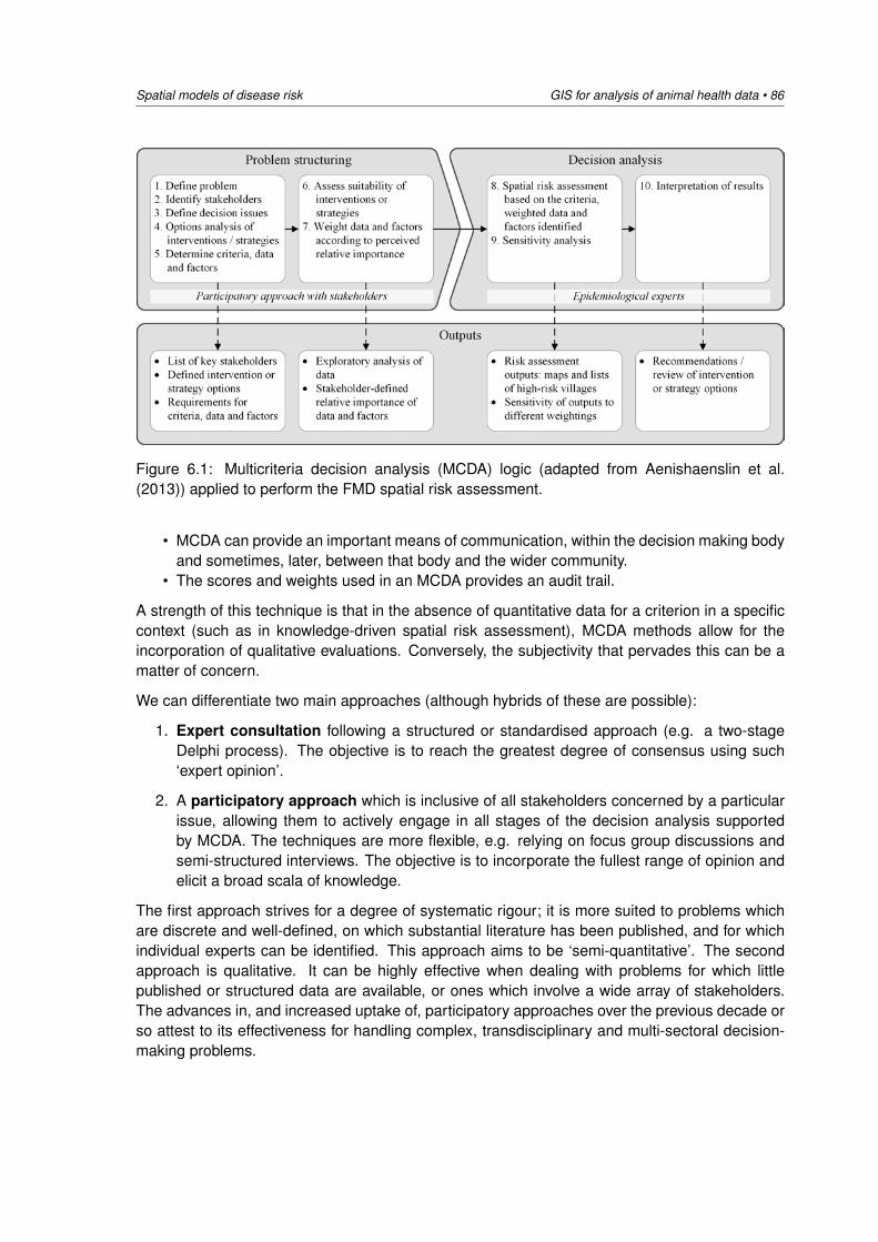
Spatial models of disease risk GIS for analysis of animal health data • 86
Figure 6.1: Multicriteria decision analysis (MCDA) logic (adapted from Aenishaenslin et al.(2013)) applied to perform the FMD spatial risk assessment.
• MCDA can provide an important means of communication, within the decision making bodyand sometimes, later, between that body and the wider community.
• The scores and weights used in an MCDA provides an audit trail.
A strength of this technique is that in the absence of quantitative data for a criterion in a specificcontext (such as in knowledge-driven spatial risk assessment), MCDA methods allow for theincorporation of qualitative evaluations. Conversely, the subjectivity that pervades this can be amatter of concern.
We can differentiate two main approaches (although hybrids of these are possible):
1. Expert consultation following a structured or standardised approach (e.g. a two-stageDelphi process). The objective is to reach the greatest degree of consensus using such‘expert opinion’.
2. A participatory approach which is inclusive of all stakeholders concerned by a particularissue, allowing them to actively engage in all stages of the decision analysis supportedby MCDA. The techniques are more flexible, e.g. relying on focus group discussions andsemi-structured interviews. The objective is to incorporate the fullest range of opinion andelicit a broad scala of knowledge.
The first approach strives for a degree of systematic rigour; it is more suited to problems whichare discrete and well-defined, on which substantial literature has been published, and for whichindividual experts can be identified. This approach aims to be ‘semi-quantitative’. The secondapproach is qualitative. It can be highly effective when dealing with problems for which littlepublished or structured data are available, or ones which involve a wide array of stakeholders.The advances in, and increased uptake of, participatory approaches over the previous decade orso attest to its effectiveness for handling complex, transdisciplinary and multi-sectoral decision-making problems.
87 • GIS for analysis of animal health data Spatial models of disease risk
6.3.2 Combining risk factor layers to derive an overall estimate of risk: theWeighted Linear Combination (WLC)
The basic principle of knowledge-driven models is to define a set of weighted rules for the factorsor criteria which may influence disease risk at any given location. If multiple such criteria affectthe disease outcome, a method needs to be adopted to combine them. One such method isthe weighted linear combination (WLC) in which criteria are standardized for comparison on acommon scale and then weights applied to each criterion so that more important criteria exerta greater influence on the outcome. There are a number of sources of information that may beutilized to determine the weights for WLC. Ideally, they would be derived from statistical dataand published literature. However, in many cases such information does not exist; in this case,expert opinion or participatory elicitation of knowledge can be used, in extension to (or part of) theMCDA process described above. Finally, a weighted average across criteria is calculated.
There are a number of common pitfalls in the application of WLC are discussed. These are wellreviewed by Malczewski (2000), and include the following.
1. Data biases and incompleteness: the attributes (i.e. factors and constraints) shouldbe measurable and complete (i.e. cover all relevant aspects of the decision problem).Factor selection should not be based on data availability alone. However, for our purposes,comprehensive data on relevant disease factors are not always available and it is oftennecessary to select attributes from limited available data resources.
2. Correlation between attributes: this is referred to as a redundancy problem that givesrise to double-counting. In other words, if two factors are similar – that is, have the samedirection or type of influence on the disease – and we include both, we are artificiallyamplifying their effect.
3. Spatial scale and levels of aggregation (MAUP): this is addressed in 2.8.4 above.
4. Attribute linearity: this occurs when transformation of the attribute for subsequent com-parison does not take into account possible non-linear associations with the outcome.
5. Incorrect weighting: this may result from failing to consider the unit of measurement andrange of the attribute.
There are different ways of calculating the weighted average across the criteria. The two mostcommon methods are discussed below.
Linear additive approaches
If it can either be proved, or reasonably assumed, that the risk factors for disease independentof each other and if uncertainty is not formally built into the MCDA model, then a simple linearadditive evaluation model is appropriate. The linear model allows one to combine each diseaserisk factor into a single combined overall value. This is done by multiplying the value assigned foreach risk factor by the weight assigned to that factor and then adding all of the weighted scorestogether.
This simple arithmetic approach is only appropriate if the criteria are mutually preference in-dependent. Most MCDA applications use this additive approach. Models of this type have awell-established record of providing robust and effective support to decision-makers working ona range of problems and in various circumstances.
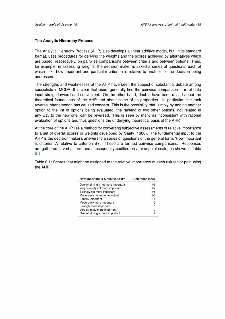
Spatial models of disease risk GIS for analysis of animal health data • 88
The Analytic Hierarchy Process
The Analytic Hierarchy Process (AHP) also develops a linear additive model, but, in its standardformat, uses procedures for deriving the weights and the scores achieved by alternatives whichare based, respectively, on pairwise comparisons between criteria and between options. Thus,for example, in assessing weights, the decision maker is asked a series of questions, each ofwhich asks how important one particular criterion is relative to another for the decision beingaddressed.
The strengths and weaknesses of the AHP have been the subject of substantial debate amongspecialists in MCDA. It is clear that users generally find the pairwise comparison form of datainput straightforward and convenient. On the other hand, doubts have been raised about thetheoretical foundations of the AHP and about some of its properties. In particular, the rankreversal phenomenon has caused concern. This is the possibility that, simply by adding anotheroption to the list of options being evaluated, the ranking of two other options, not related inany way to the new one, can be reversed. This is seen by many as inconsistent with rationalevaluation of options and thus questions the underlying theoretical basis of the AHP.
At the core of the AHP lies a method for converting subjective assessments of relative importanceto a set of overall scores or weights developed by Saaty (1980). The fundamental input to theAHP is the decision maker’s answers to a series of questions of the general form, ‘How importantis criterion A relative to criterion B?’. These are termed pairwise comparisons. Responsesare gathered in verbal form and subsequently codified on a nine-point scale, as shown in Table6.1.
Table 6.1: Scores that might be assigned to the relative importance of each risk factor pair usingthe AHP.
How important is A relative to B? Preference index
Overwhelmingly not more important 1/9Very strongly not more important 1/7Strongly not more important 1/5Moderately not more important 1/3Equally important 1Moderately more important 3Strongly more important 5Very strongly more important 7Overwhelmingly more important 9
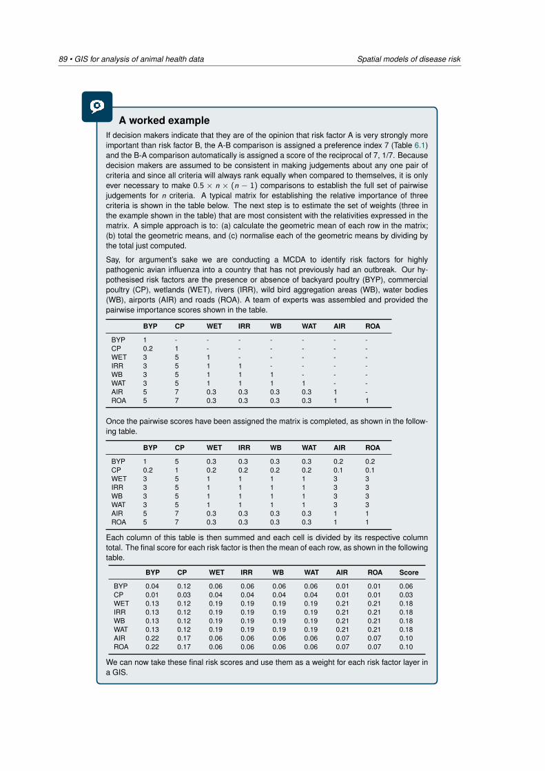
89 • GIS for analysis of animal health data Spatial models of disease risk
A worked exampleIf decision makers indicate that they are of the opinion that risk factor A is very strongly moreimportant than risk factor B, the A-B comparison is assigned a preference index 7 (Table 6.1)and the B-A comparison automatically is assigned a score of the reciprocal of 7, 1/7. Becausedecision makers are assumed to be consistent in making judgements about any one pair ofcriteria and since all criteria will always rank equally when compared to themselves, it is onlyever necessary to make 0.5 × n × (n − 1) comparisons to establish the full set of pairwisejudgements for n criteria. A typical matrix for establishing the relative importance of threecriteria is shown in the table below. The next step is to estimate the set of weights (three inthe example shown in the table) that are most consistent with the relativities expressed in thematrix. A simple approach is to: (a) calculate the geometric mean of each row in the matrix;(b) total the geometric means, and (c) normalise each of the geometric means by dividing bythe total just computed.
Say, for argument’s sake we are conducting a MCDA to identify risk factors for highlypathogenic avian influenza into a country that has not previously had an outbreak. Our hy-pothesised risk factors are the presence or absence of backyard poultry (BYP), commercialpoultry (CP), wetlands (WET), rivers (IRR), wild bird aggregation areas (WB), water bodies(WB), airports (AIR) and roads (ROA). A team of experts was assembled and provided thepairwise importance scores shown in the table.
BYP CP WET IRR WB WAT AIR ROA
BYP 1 - - - - - - -CP 0.2 1 - - - - - -WET 3 5 1 - - - - -IRR 3 5 1 1 - - - -WB 3 5 1 1 1 - - -WAT 3 5 1 1 1 1 - -AIR 5 7 0.3 0.3 0.3 0.3 1 -ROA 5 7 0.3 0.3 0.3 0.3 1 1
Once the pairwise scores have been assigned the matrix is completed, as shown in the follow-ing table.
BYP CP WET IRR WB WAT AIR ROA
BYP 1 5 0.3 0.3 0.3 0.3 0.2 0.2CP 0.2 1 0.2 0.2 0.2 0.2 0.1 0.1WET 3 5 1 1 1 1 3 3IRR 3 5 1 1 1 1 3 3WB 3 5 1 1 1 1 3 3WAT 3 5 1 1 1 1 3 3AIR 5 7 0.3 0.3 0.3 0.3 1 1ROA 5 7 0.3 0.3 0.3 0.3 1 1
Each column of this table is then summed and each cell is divided by its respective columntotal. The final score for each risk factor is then the mean of each row, as shown in the followingtable.
BYP CP WET IRR WB WAT AIR ROA Score
BYP 0.04 0.12 0.06 0.06 0.06 0.06 0.01 0.01 0.06CP 0.01 0.03 0.04 0.04 0.04 0.04 0.01 0.01 0.03WET 0.13 0.12 0.19 0.19 0.19 0.19 0.21 0.21 0.18IRR 0.13 0.12 0.19 0.19 0.19 0.19 0.21 0.21 0.18WB 0.13 0.12 0.19 0.19 0.19 0.19 0.21 0.21 0.18WAT 0.13 0.12 0.19 0.19 0.19 0.19 0.21 0.21 0.18AIR 0.22 0.17 0.06 0.06 0.06 0.06 0.07 0.07 0.10ROA 0.22 0.17 0.06 0.06 0.06 0.06 0.07 0.07 0.10
We can now take these final risk scores and use them as a weight for each risk factor layer ina GIS.
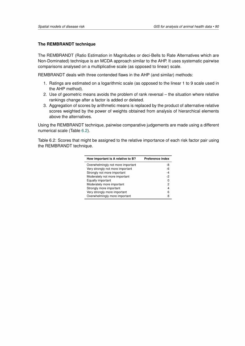
Spatial models of disease risk GIS for analysis of animal health data • 90
The REMBRANDT technique
The REMBRANDT (Ratio Estimation in Magnitudes or deci-Bells to Rate Alternatives which areNon-Dominated) technique is an MCDA approach similar to the AHP. It uses systematic pairwisecomparisons analysed on a multiplicative scale (as opposed to linear) scale.
REMBRANDT deals with three contended flaws in the AHP (and similar) methods:
1. Ratings are estimated on a logarithmic scale (as opposed to the linear 1 to 9 scale used inthe AHP method).
2. Use of geometric means avoids the problem of rank reversal – the situation where relativerankings change after a factor is added or deleted.
3. Aggregation of scores by arithmetic means is replaced by the product of alternative relativescores weighted by the power of weights obtained from analysis of hierarchical elementsabove the alternatives.
Using the REMBRANDT technique, pairwise comparative judgements are made using a differentnumerical scale (Table 6.2).
Table 6.2: Scores that might be assigned to the relative importance of each risk factor pair usingthe REMBRANDT technique.
How important is A relative to B? Preference index
Overwhelmingly not more important -8Very strongly not more important -6Strongly not more important -4Moderately not more important -2Equally important 0Moderately more important 2Strongly more important 4Very strongly more important 6Overwhelmingly more important 8
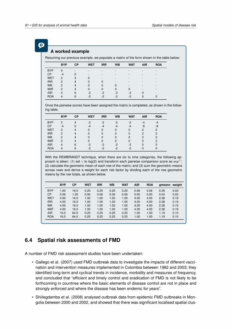
91 • GIS for analysis of animal health data Spatial models of disease risk
A worked exampleResuming our previous example, we populate a matrix of the form shown in the table below:
BYP CP WET IRR WB WAT AIR ROA
BYP 0 - - - - - - -CP -4 0 - - - - - -WET 2 4 0 - - - - -IRR 2 4 0 0 - - - -WB 2 4 0 0 0 - - -WAT 2 4 0 0 0 0 - -AIR 4 6 -2 -2 -2 -2 0 -ROA 4 6 -2 -2 -2 -2 0 0
Once the pairwise scores have been assigned the matrix is completed, as shown in the follow-ing table.
BYP CP WET IRR WB WAT AIR ROA
BYP 0 4 -2 -2 -2 -2 -4 -4CP -4 0 -4 -4 -4 -4 -8 -8WET 2 4 0 0 0 0 2 2IRR 2 4 0 0 0 0 2 2WB 2 4 0 0 0 0 2 2WAT 2 4 0 0 0 0 2 2AIR 4 6 -2 -2 -2 -2 0 0ROA 4 6 -2 -2 -2 -2 0 0
With the REMBRANDT technique, when there are six to nine categories, the following ap-proach is taken: (1) set γ to log(2) and transform each pairwise comparison score as expγi ;(2) calculate the geometric mean of each row of the matrix; and (3) sum the geometric meansacross rows and derive a weight for each risk factor by dividing each of the row geometricmeans by the row totals, as shown below.
BYP CP WET IRR WB WAT AIR ROA gmeann weight
BYP 1.00 16.0 0.25 0.25 0.25 0.25 0.06 0.06 0.35 0.03CP 0.06 1.00 0.06 0.06 0.06 0.06 0.00 0.00 0.04 0.03WET 4.00 16.0 1.00 1.00 1.00 1.00 4.00 4.00 2.38 0.19IRR 4.00 16.0 1.00 1.00 1.00 1.00 4.00 4.00 2.38 0.19WB 4.00 16.0 1.00 1.00 1.00 1.00 4.00 4.00 2.38 0.19WAT 4.00 16.0 1.00 1.00 1.00 1.00 4.00 4.00 2.38 0.19AIR 16.0 64.0 0.25 0.25 0.25 0.25 1.00 1.00 1.19 0.10ROA 16.0 64.0 0.25 0.25 0.25 0.25 1.00 1.00 1.19 0.10
6.4 Spatial risk assessments of FMD
A number of FMD risk assessment studies have been undertaken:
• Gallego et al. (2007) used FMD outbreak data to investigate the impacts of different vacci-nation and intervention measures implemented in Colombia between 1982 and 2003; theyidentified long-term and cyclical trends in incidence, morbidity and measures of frequency,and concluded that “efficient and timely control and eradication of FMD is not likely to beforthcoming in countries where the basic elements of disease control are not in place andstrongly enforced and where the disease has been endemic for years”.
• Shiilegdamba et al. (2008) analysed outbreak data from epidemic FMD outbreaks in Mon-golia between 2000 and 2002, and showed that there was significant localised spatial clus-
Spatial models of disease risk GIS for analysis of animal health data • 92
tering of FMD. They reported that while no causes for the outbreaks could be identified,illegal animal movements were likely to be implicated. They concluded that identification ofspatial clusters are helpful to identify risk factors for FMD transmission, and can be appliedto direct control and prevention measures in high-risk areas.
• A recent study by Amaral et al. (2016) applied a knowledge-based MCDA methodology,utilising the opinions of eight experts to determine a WLC of risk factors to develop riskmaps for the introduction of FMD along the border between Brazil and Paraguay. Thefactors under consideration were very similar to our investigation, but their study did notincorporate any FMD-specific data.
• In contrast, a number of studies in Southern and East Africa applied more data-driventechniques to model spatial distribution and risk factors, using outbreak data in combinationwith other geographic data.
– Hamoonga et al. (2014) determined associations between FMD outbreak intensity inZambia and distance to the nearest major international border crossing, distance tothe nearest major road, wetness index and elevation.
– Sinkala et al. (2014) applied the spatial scan statistic to outbreak data, also fromZambia, to identify FMD clusters between 2004 and 2012.
– Using Tanzanian data, Allepuz et al. (2015) found substantial spatial heterogeneity inhigh-risk areas from 2001 to 2006, and differentiated between endemic and epidemicphases. They determined that proximity to main roads was a consistent risk factor forFMD occurrence; other spatial factors (including cattle density) played a variable rolein the risk of FMD.
Comparable spatial risk assessments have not yet been published in the South East Asia re-gion. This is of high relevance, specifically considering the increasing emphasis on the ap-plication of risk-based approaches for the control and eradication of FMD, e.g. as applied bySEACFMD.

Part II
Course practicals
93

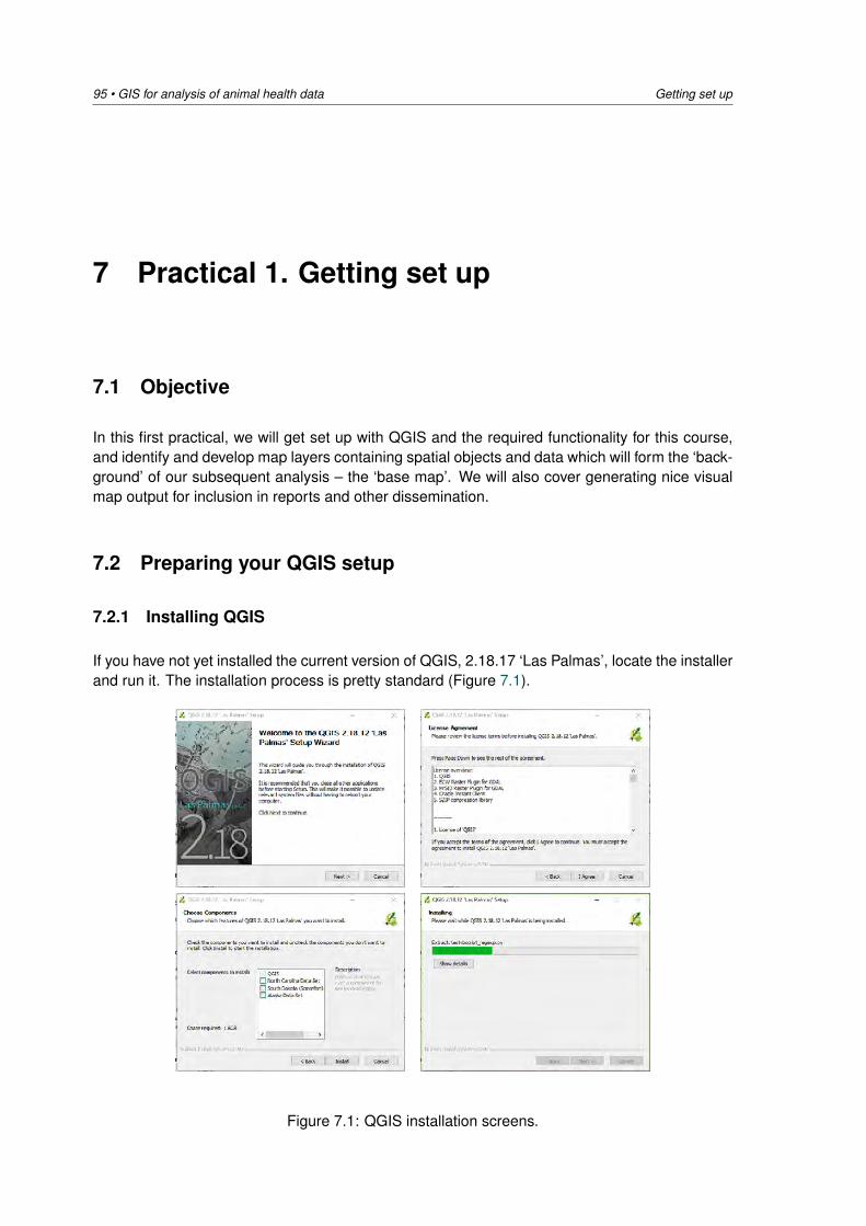
95 • GIS for analysis of animal health data Getting set up
7 Practical 1. Getting set up
7.1 Objective
In this first practical, we will get set up with QGIS and the required functionality for this course,and identify and develop map layers containing spatial objects and data which will form the ‘back-ground’ of our subsequent analysis – the ‘base map’. We will also cover generating nice visualmap output for inclusion in reports and other dissemination.
7.2 Preparing your QGIS setup
7.2.1 Installing QGIS
If you have not yet installed the current version of QGIS, 2.18.17 ‘Las Palmas’, locate the installerand run it. The installation process is pretty standard (Figure 7.1).
Figure 7.1: QGIS installation screens.
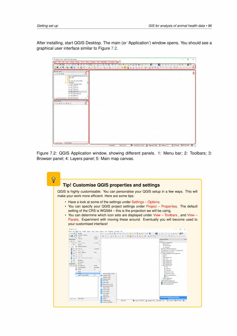
Getting set up GIS for analysis of animal health data • 96
After installing, start QGIS Desktop. The main (or ‘Application’) window opens. You should see agraphical user interface similar to Figure 7.2.
Figure 7.2: QGIS Application window, showing different panels. 1: Menu bar; 2: Toolbars; 3:Browser panel; 4: Layers panel; 5: Main map canvas.
Tip! Customise QGIS properties and settingsQGIS is highly customisable. You can personalise your QGIS setup in a few ways. This willmake your work more efficient. Here are some tips:
• Have a look at some of the settings under Settings – Options.• You can specify your QGIS project settings under Project – Properties. The default
setting of the CRS is WGS84 – this is the projection we will be using.• You can determine which icon sets are displayed under View – Toolbars , and View –
Panels. Experiment with moving these around. Eventually you will become used toyour customised interface!

97 • GIS for analysis of animal health data Getting set up
7.2.2 Downloading plugins
During this course, we will be using some functionality that is not included in the basic installationversion; this functionality is provided by plugins. To install these, click on Plugins – Manage andInstall Plugins. . . (Figure 7.3), and select and install the following plugins:
• OpenLayers Plugin• Zonal Statistics plugin• Spatial Query Plugin• Cartogram
Figure 7.3: Installing plugins in QGIS.
7.3 Preparing your project data directories
Of course, how you manage your data files and directories is entirely up to your own discretion.However, you will find out that when performing spatial analysis, more than other areas of anal-ysis, the number and size of data files increases at a rapid rate! Good data management reallyhelps to stay on top of all this information. Here we provide some generic tips for effective datamanagement:
• Work using a ‘project’ approach. Take a few minutes to set up the directory structureyou will be using in advance, for a specific piece of work. Don’t mix work done in differentprojects. It can be surprising how hard it is to locate a file when you need it!
• Use a consistent directory structure. Replicate this across different projects you maywork on. This way, you will always know where to find, for example, your map image files.
• Create sub-folders where required. If you are generating outputs for different purposes,or if you are using spatial data from different sources, it’s a good idea to utilise differentsub-folders for these.
• Different folders for different formats. For example, report documents, data, spatial files,graphical output, literature and information resources etc. It’s not a good idea to mix thesedifferent types of files and documents.
• Use a naming convention. This can be useful, if you’re really organised! For example, theprefix IDN_Java_HPAI for all files related to spatial analysis of HPAI on Java. Inserting a
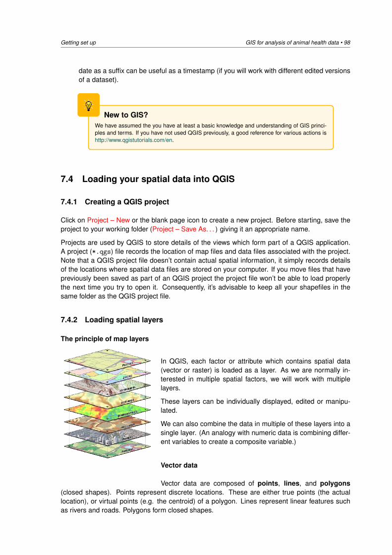
Getting set up GIS for analysis of animal health data • 98
date as a suffix can be useful as a timestamp (if you will work with different edited versionsof a dataset).
New to GIS?We have assumed the you have at least a basic knowledge and understanding of GIS princi-ples and terms. If you have not used QGIS previously, a good reference for various actions ishttp://www.qgistutorials.com/en.
7.4 Loading your spatial data into QGIS
7.4.1 Creating a QGIS project
Click on Project – New or the blank page icon to create a new project. Before starting, save theproject to your working folder (Project – Save As. . . ) giving it an appropriate name.
Projects are used by QGIS to store details of the views which form part of a QGIS application.A project (*.qgs) file records the location of map files and data files associated with the project.Note that a QGIS project file doesn’t contain actual spatial information, it simply records detailsof the locations where spatial data files are stored on your computer. If you move files that havepreviously been saved as part of an QGIS project the project file won’t be able to load properlythe next time you try to open it. Consequently, it’s advisable to keep all your shapefiles in thesame folder as the QGIS project file.
7.4.2 Loading spatial layers
The principle of map layers
In QGIS, each factor or attribute which contains spatial data(vector or raster) is loaded as a layer. As we are normally in-terested in multiple spatial factors, we will work with multiplelayers.
These layers can be individually displayed, edited or manipu-lated.
We can also combine the data in multiple of these layers into asingle layer. (An analogy with numeric data is combining differ-ent variables to create a composite variable.)
Vector data
Vector data are composed of points, lines, and polygons(closed shapes). Points represent discrete locations. These are either true points (the actuallocation), or virtual points (e.g. the centroid) of a polygon. Lines represent linear features suchas rivers and roads. Polygons form closed shapes.
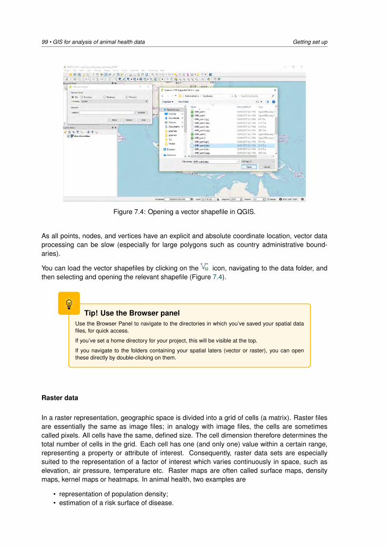
99 • GIS for analysis of animal health data Getting set up
Figure 7.4: Opening a vector shapefile in QGIS.
As all points, nodes, and vertices have an explicit and absolute coordinate location, vector dataprocessing can be slow (especially for large polygons such as country administrative bound-aries).
You can load the vector shapefiles by clicking on the icon, navigating to the data folder, andthen selecting and opening the relevant shapefile (Figure 7.4).
Tip! Use the Browser panelUse the Browser Panel to navigate to the directories in which you’ve saved your spatial datafiles, for quick access.
If you’ve set a home directory for your project, this will be visible at the top.
If you navigate to the folders containing your spatial laters (vector or raster), you can openthese directly by double-clicking on them.
Raster data
In a raster representation, geographic space is divided into a grid of cells (a matrix). Raster filesare essentially the same as image files; in analogy with image files, the cells are sometimescalled pixels. All cells have the same, defined size. The cell dimension therefore determines thetotal number of cells in the grid. Each cell has one (and only one) value within a certain range,representing a property or attribute of interest. Consequently, raster data sets are especiallysuited to the representation of a factor of interest which varies continuously in space, such aselevation, air pressure, temperature etc. Raster maps are often called surface maps, densitymaps, kernel maps or heatmaps. In animal health, two examples are
• representation of population density;• estimation of a risk surface of disease.
Getting set up GIS for analysis of animal health data • 100
If the cells are large, there will be fewer cells; as each cell has only one value, this results in lessdata being contained in the raster, and the raster file will be smaller. However, gradations andtrends cannot be as well visualised: the resolution is less.
Because cell size is constant in both the horizontal and vertical directions, if we know the size ofthe matrix, one coordinate is sufficient to spatially reference the whole raster. By convention, thisis called the ‘origin’ and it’s normally the upper left corner. This makes raster data processingmuch faster. However, as each cell has a unique value, the file sizes of raster data sets can bevery large in comparison to vector data sets.
You can load raster files by clicking on the icon, navigating to the data folder, and thenselecting and opening the relevant raster file (this is usually a .TIF format).
7.5 Developing the ‘base map’
7.5.1 What is a base map and why is it useful?
A base map is defined as “a background georeferenced image that gives a point of referenceon a map. Basemaps are non-editable and provides aesthetic appeal such as aerial imagery,topography, terrain and street layers”.
We will make a base map by loading administrative boundary data of the six countries in SouthEast Asia reporting FMD. We will build on this basemap in a subsequent practical to investigatetrends of disease incidence and reporting. In addition, we will load and prepare a number ofother layers which will be used later during this course, so that they are available when we needthem.
7.5.2 Creating a view
A View is a visual representation of spatial data and the attribute data associated with it. Thisis where the content and visual presentation of a map is defined. Within a View there can bemultiple layers of spatial data.
Referring back to Figure 7.2, the View window consists of two sections:
• The section on the left is the Layers Panel. It lists the layers which are part of the mapdisplay by name and shows the symbols used to represent each layer. The check box nextto each layer indicates if it is included in the map display. If multiple layers are selected,they will be rendered in order from top to bottom. You can reorder the layers by clicking anddragging.
• The second on the right is the main map canvas; this shows a preview of the map output.
7.5.3 Country boundary data
You can access the country administrative boundaries data shapefiles from the course website.Download these and save them to an appropriate directory on your hard drive. For this basemap,load the country boundaries (adm0) and second-level administrative data (adm2) for Cambodia,Laos, peninsular Malaysia, Myanmar, Thailand and Vietnam.
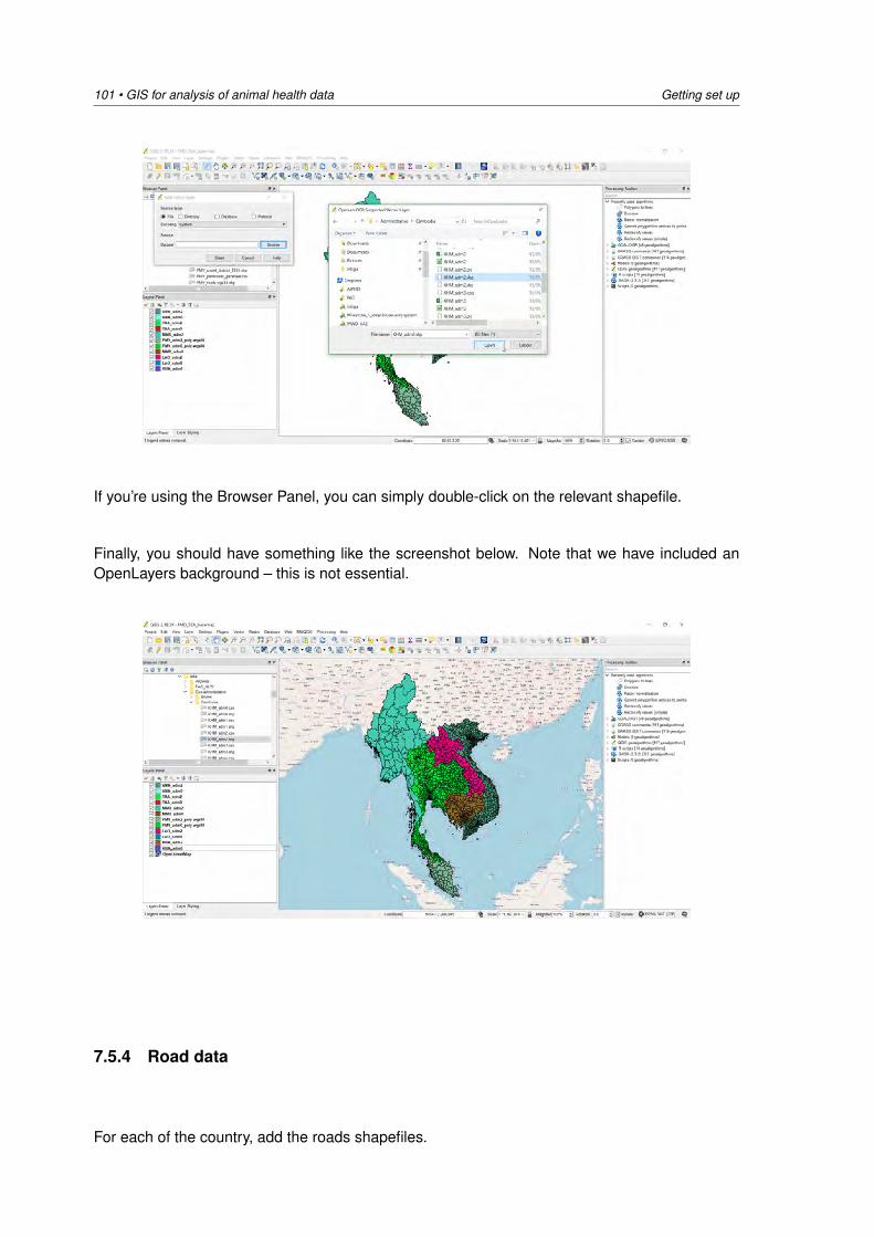
101 • GIS for analysis of animal health data Getting set up
If you’re using the Browser Panel, you can simply double-click on the relevant shapefile.
Finally, you should have something like the screenshot below. Note that we have included anOpenLayers background – this is not essential.
7.5.4 Road data
For each of the country, add the roads shapefiles.
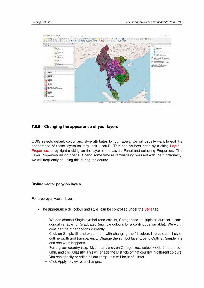
Getting set up GIS for analysis of animal health data • 102
7.5.5 Changing the appearance of your layers
QGIS selects default colour and style attributes for our layers; we will usually want to edit theappearance of these layers so they look ‘useful’. This can be best done by clicking Layer –Properties, or by right-clicking on the layer in the Layers Panel and selecting Properties. TheLayer Properties dialog opens. Spend some time re-familiarising yourself with the functionality;we will frequently be using this during the course.
Styling vector polygon layers
For a polygon vector layer:
• The appearance (fill colour and style) can be controlled under the Style tab:
– We can choose Single symbol (one colour), Categorized (multiple colours for a cate-gorical variable) or Graduated (multiple colours for a continuous variable). We won’tconsider the other options currently.
– Click on Simple fill and experiment with changing the fill colour, line colour, fill style,outline width and transparency. Change the symbol layer type to Outline: Simple lineand see what happens.
– For a given country (e.g. Myanmar), click on Categorized, select NAME_2 as the col-umn, and click Classify. This will shade the Districts of that country in different colours.You can specify or edit a colour ramp: this will be useful later.
– Click Apply to view your changes.
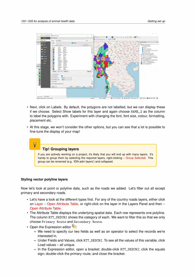
103 • GIS for analysis of animal health data Getting set up
• Next, click on Labels. By default, the polygons are not labelled, but we can display theseif we choose. Select Show labels for this layer and again choose NAME_2 as the columnto label the polygons with. Experiment with changing the font, font size, colour, formatting,placement etc.
• At this stage, we won’t consider the other options, but you can see that a lot is possible tofine-tune the display of your map!
Tip! Grouping layersIf you are actively working on a project, it’s likely that you will end up with many layers. It’shandy to group them by selecting the required layers, right-clicking – Group Selected. Thisgroup can be renamed (e.g. ‘IDN adm layers’) and collapsed.
Styling vector polyline layers
Now let’s look at point or polyline data, such as the roads we added. Let’s filter out all exceptprimary and secondary roads.
• Let’s have a look at the different types first. For any of the country roads layers, either clickon Layer – Open Attribute Table, or right-click on the layer in the Layers Panel and then –Open Attribute Table.
• The Attribute Table displays the underlying spatial data. Each row represents one polyline.The column RTT_DESCRI shows the category of each. We want to filter this so that we onlychoose Primary Route and Secondary Route.
• Open the Expression editor :– We need to specify our two fields as well as an operator to select the records we’re
interested in.– Under Fields and Values, click RTT_DESCRI. To see all the values of this variable, click
Load values – all unique.– In the Expression editor, open a bracket; double-click RTT_DESCRI; click the equals
sign; double-click the primary route; and close the bracket.
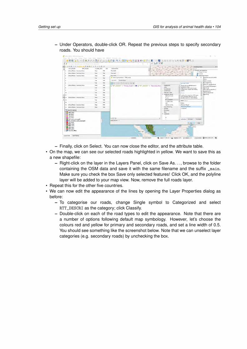
Getting set up GIS for analysis of animal health data • 104
– Under Operators, double-click OR. Repeat the previous steps to specify secondaryroads. You should have
– Finally, click on Select. You can now close the editor, and the attribute table.• On the map, we can see our selected roads highlighted in yellow. We want to save this as
a new shapefile:– Right-click on the layer in the Layers Panel, click on Save As. . . , browse to the folder
containing the OSM data and save it with the same filename and the suffix _main.Make sure you check the box Save only selected features! Click OK, and the polylinelayer will be added to your map view. Now, remove the full roads layer.
• Repeat this for the other five countries.• We can now edit the appearance of the lines by opening the Layer Properties dialog as
before:– To categorise our roads, change Single symbol to Categorized and selectRTT_DESCRI as the category; click Classify.
– Double-click on each of the road types to edit the appearance. Note that there area number of options following default map symbology. However, let’s choose thecolours red and yellow for primary and secondary roads, and set a line width of 0.5.You should see something like the screenshot below. Note that we can unselect layercategories (e.g. secondary roads) by unchecking the box.
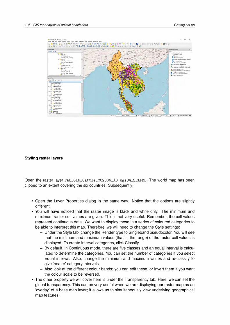
105 • GIS for analysis of animal health data Getting set up
Styling raster layers
Open the raster layer FAO_Glb_Cattle_CC2006_AD-wgs84_SEAFMD. The world map has beenclipped to an extent covering the six countries. Subsequently:
• Open the Layer Properties dialog in the same way. Notice that the options are slightlydifferent.
• You will have noticed that the raster image is black and white only. The minimum andmaximum raster cell values are given. This is not very useful. Remember, the cell valuesrepresent continuous data. We want to display these in a series of coloured categories tobe able to interpret this map. Therefore, we will need to change the Style settings:
– Under the Style tab, change the Render type to Singleband pseudocolor. You will seethat the minimum and maximum values (that is, the range) of the raster cell values isdisplayed. To create interval categories, click Classify.
– By default, in Continuous mode, there are five classes and an equal interval is calcu-lated to determine the categories. You can set the number of categories if you selectEqual interval. Also, change the minimum and maximum values and re-classify togive ‘neater’ category intervals.
– Also look at the different colour bands; you can edit these, or invert them if you wantthe colour scale to be reversed.
• The other property we will cover here is under the Transparency tab. Here, we can set theglobal transparency. This can be very useful when we are displaying our raster map as an‘overlay’ of a base map layer; it allows us to simultaneously view underlying geographicalmap features.
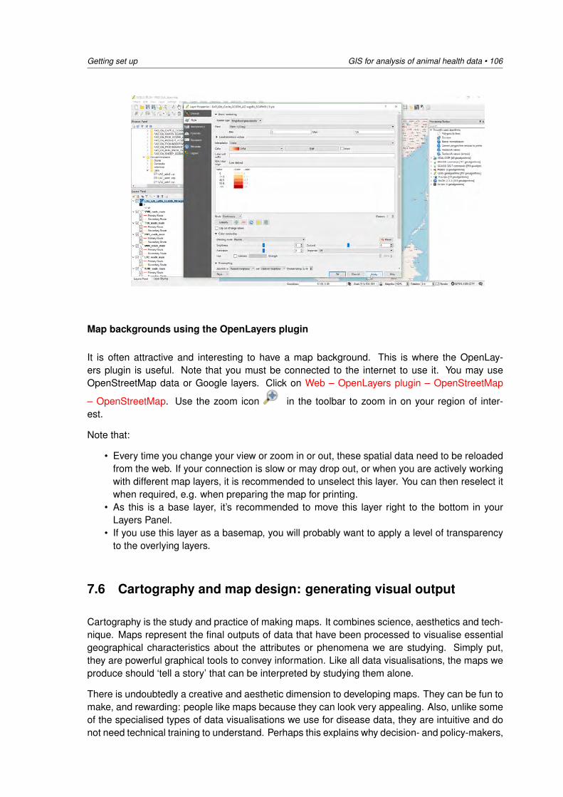
Getting set up GIS for analysis of animal health data • 106
Map backgrounds using the OpenLayers plugin
It is often attractive and interesting to have a map background. This is where the OpenLay-ers plugin is useful. Note that you must be connected to the internet to use it. You may useOpenStreetMap data or Google layers. Click on Web – OpenLayers plugin – OpenStreetMap
– OpenStreetMap. Use the zoom icon in the toolbar to zoom in on your region of inter-est.
Note that:
• Every time you change your view or zoom in or out, these spatial data need to be reloadedfrom the web. If your connection is slow or may drop out, or when you are actively workingwith different map layers, it is recommended to unselect this layer. You can then reselect itwhen required, e.g. when preparing the map for printing.
• As this is a base layer, it’s recommended to move this layer right to the bottom in yourLayers Panel.
• If you use this layer as a basemap, you will probably want to apply a level of transparencyto the overlying layers.
7.6 Cartography and map design: generating visual output
Cartography is the study and practice of making maps. It combines science, aesthetics and tech-nique. Maps represent the final outputs of data that have been processed to visualise essentialgeographical characteristics about the attributes or phenomena we are studying. Simply put,they are powerful graphical tools to convey information. Like all data visualisations, the maps weproduce should ‘tell a story’ that can be interpreted by studying them alone.
There is undoubtedly a creative and aesthetic dimension to developing maps. They can be fun tomake, and rewarding: people like maps because they can look very appealing. Also, unlike someof the specialised types of data visualisations we use for disease data, they are intuitive and donot need technical training to understand. Perhaps this explains why decision- and policy-makers,
107 • GIS for analysis of animal health data Getting set up
who may not have a technical background, tend to really appreciate maps. Consequently, it’sworth investing time in ensuring your maps are as attractive as possible.
However, it’s easy to forget that maps are one of our most sophisticated conceptual creations.Care needs to be taken to make sure our maps are clear and interpretable. Map design is anelement of cartography which focuses on ensuring that the meaning is effectively conveyed. Amap must be designed foremost with consideration to the audience and its needs. Maps areinformation rich, but displaying too much (or the wrong kind) information makes the messageharder to see.
If you regularly produce maps, some of the practices and tips below should become the norm;you will increasingly develop and use templates and develop a personal ‘style’.
7.6.1 Visual display of map layers
Our maps will show what we display in the main map canvas. Therefore, we edit and adjust theappearance of our map using the same techniques we implemented in 7.5.5 above; when we aresatisfied we have finalised this, we can start designing our map, and supplementing it with thesymbology discussed below.
Here are some tips and principles for you to consider to result in effective and beautifulmaps:
• Colour scheme. The choice of colour scheme should relate to the logic in the data youare representing:
– Sequential: used for quantitative ordinal data, i.e. higher values represent ‘more’ (e.g.poultry density). The convention is that the darker end represents the upper rangeand the lighter end represents the lower range.
– Diverging: these emphasize the low and high ends of the data range. We use thesewhen we’re especially interested in the ‘hot’ and ‘cold’ areas, such as in disease (ordisease risk) hotspots. A variant of this is the spectral theme used for thermal maps.
– Qualitative: used when there is no specific order in the data (e.g. Provinces of acountry).
– Colours and contrast. Choose the number of colour categories wisely: generally,map readers can’t tell the difference between more than six or seven levels. Ensurethat the colour range (from lightest to darkest) is sufficient to be able to distinguishbetween the categories.
– Opacity and layer order. When you wish to show the information from two or morelayers at the same time, you will need to carefully consider that the overall combinationof these layers adequately shows all of the required information in a way that can bedifferentiated and interpreted. The layer order becomes important. For example, ifwe want to relate livestock density to populated areas, our raster density map (theupper layer) needs to have a level of transparency so that we can simultaneously seethe underlying physical layer. However, if it’s too transparent, we are unable to see itproperly.
– Clipping. A final consideration relates to clipping (we will cover this in more detaillater). Specifically, density maps should be clipped to the borders of the areas fromwhich the data are derived; failure to do this is an artefact.
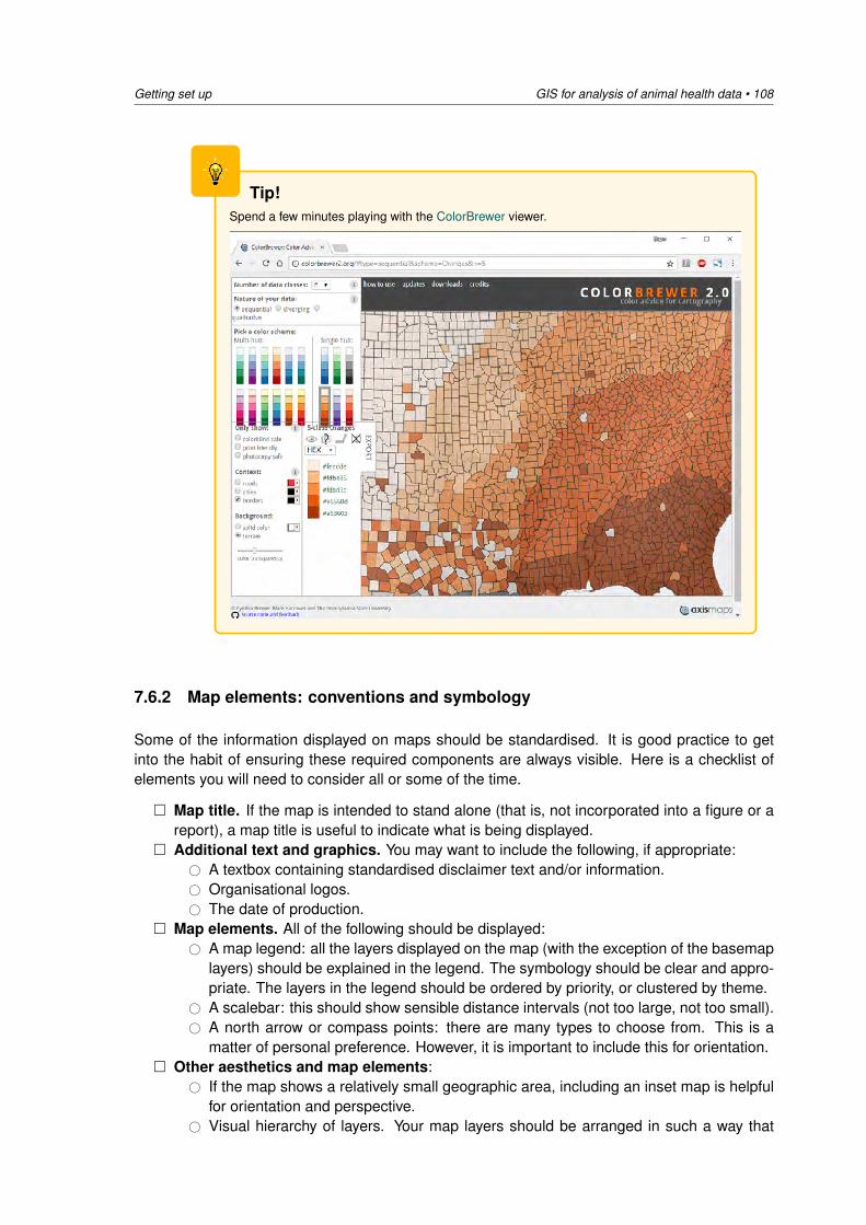
Getting set up GIS for analysis of animal health data • 108
Tip!Spend a few minutes playing with the ColorBrewer viewer.
7.6.2 Map elements: conventions and symbology
Some of the information displayed on maps should be standardised. It is good practice to getinto the habit of ensuring these required components are always visible. Here is a checklist ofelements you will need to consider all or some of the time.
� Map title. If the map is intended to stand alone (that is, not incorporated into a figure or areport), a map title is useful to indicate what is being displayed.
� Additional text and graphics. You may want to include the following, if appropriate:# A textbox containing standardised disclaimer text and/or information.# Organisational logos.# The date of production.
� Map elements. All of the following should be displayed:# A map legend: all the layers displayed on the map (with the exception of the basemap
layers) should be explained in the legend. The symbology should be clear and appro-priate. The layers in the legend should be ordered by priority, or clustered by theme.
# A scalebar: this should show sensible distance intervals (not too large, not too small).# A north arrow or compass points: there are many types to choose from. This is a
matter of personal preference. However, it is important to include this for orientation.� Other aesthetics and map elements:
# If the map shows a relatively small geographic area, including an inset map is helpfulfor orientation and perspective.
# Visual hierarchy of layers. Your map layers should be arranged in such a way that

109 • GIS for analysis of animal health data Getting set up
they are logically and sensibly displayed.# You may want to include frames around your map and map elements (legend etc.),
adjust the opacity, and so forth.# All text on your map should be readable. This means that the font / typeface you
use must be consistent and readable (Arial or Times New Roman are always safechoices); and the text size must be appropriate.
� Use a replicable template. Using the Composer Manager (see below), you can developtemplates which are pre-populated with these elements. This can save time and effort.
7.6.3 Generating map output using the Print Composer
The Print Composer is what we use to generate and export printable maps showing a specifiedregion, including the additional and conventional map symbology and annotations mentionedabove. It is not particularly intuitive or user-friendly, and many people struggle to master it effec-tively. However, it’s worth some time and effort to do so, as it can save much time later on.
Let’s continue with the basemap we developed previously, and imagine we want to display cattle
density. To create a Print Composer, click on the New Print Composer icon, and enter thename of the composer you are creating. You can create and save multiple print composers foreach QGIS project you are working on, or geographic sections within one project.
The Composer preview screen now opens. The following buttons provide functionality that youwill find yourself using frequently:
Icon Function
Select / Move item
Move item content
Add new map
Add image
Add new label
Add new legend
Add new scalebar
Export as image
Zoom full
Refresh view
Follow these steps to develop the Print Composer (don’t be afraid to experiment if you are notfamiliar with this):
• Click on Add new map and drag out a map area. QGIS will try to fill this area with the mapextent in you main screen.
• Click on Move item content to reposition the area you want to include in your map.• Click on Select / move item to adjust your canvas size.• Other fine-tuning and options for adjustment are given under the Composition and Item
properties tabs.• You can add a legend and a scalebar.
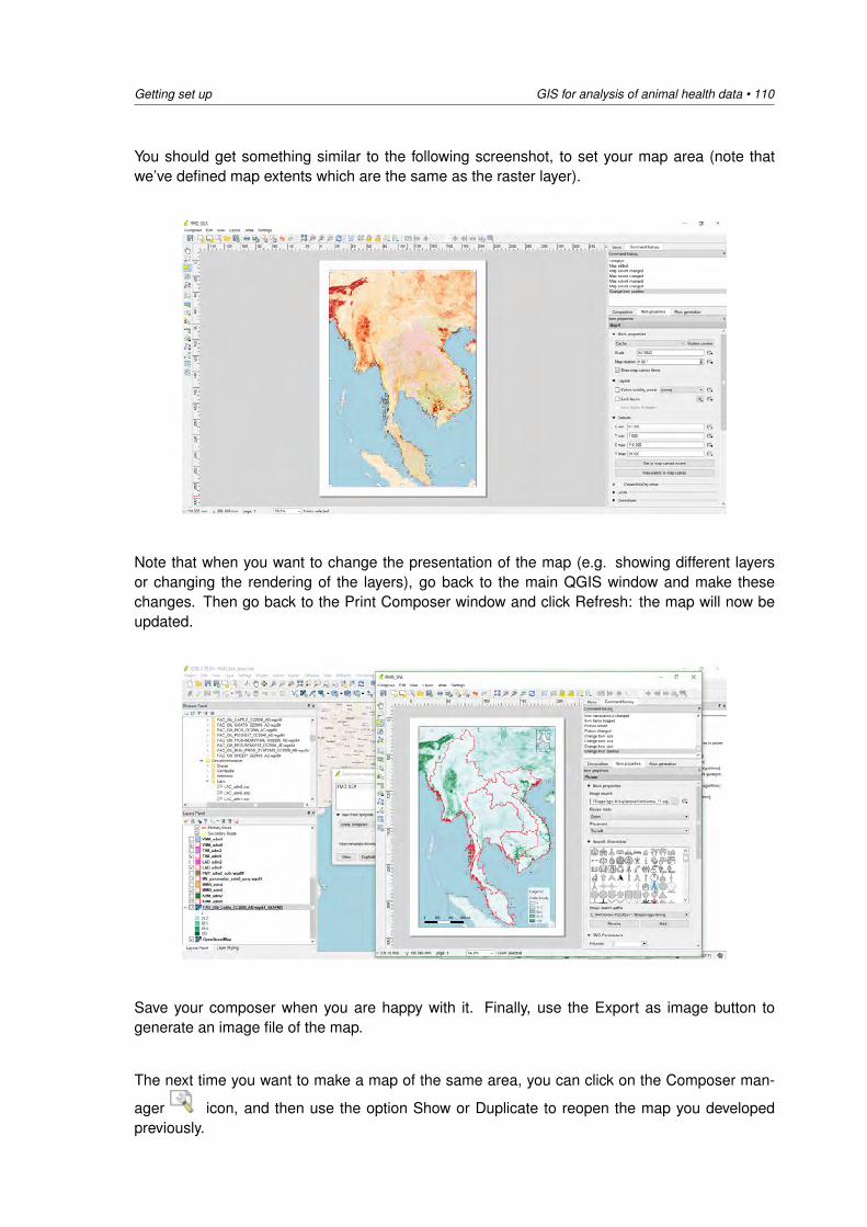
Getting set up GIS for analysis of animal health data • 110
You should get something similar to the following screenshot, to set your map area (note thatwe’ve defined map extents which are the same as the raster layer).
Note that when you want to change the presentation of the map (e.g. showing different layersor changing the rendering of the layers), go back to the main QGIS window and make thesechanges. Then go back to the Print Composer window and click Refresh: the map will now beupdated.
Save your composer when you are happy with it. Finally, use the Export as image button togenerate an image file of the map.
The next time you want to make a map of the same area, you can click on the Composer man-
ager icon, and then use the option Show or Duplicate to reopen the map you developedpreviously.
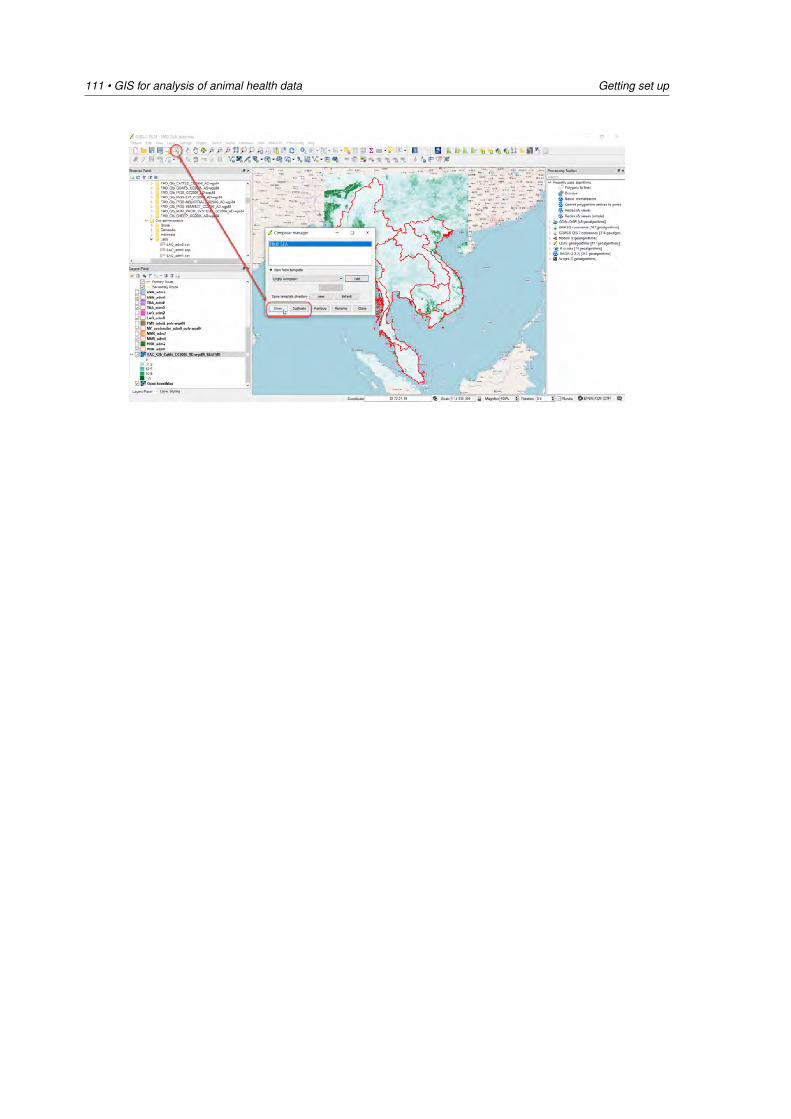
111 • GIS for analysis of animal health data Getting set up
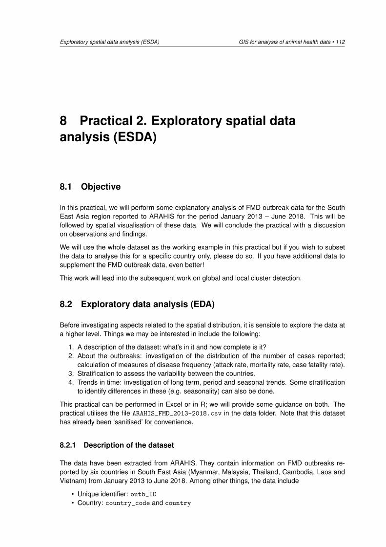
Exploratory spatial data analysis (ESDA) GIS for analysis of animal health data • 112
8 Practical 2. Exploratory spatial dataanalysis (ESDA)
8.1 Objective
In this practical, we will perform some explanatory analysis of FMD outbreak data for the SouthEast Asia region reported to ARAHIS for the period January 2013 – June 2018. This will befollowed by spatial visualisation of these data. We will conclude the practical with a discussionon observations and findings.
We will use the whole dataset as the working example in this practical but if you wish to subsetthe data to analyse this for a specific country only, please do so. If you have additional data tosupplement the FMD outbreak data, even better!
This work will lead into the subsequent work on global and local cluster detection.
8.2 Exploratory data analysis (EDA)
Before investigating aspects related to the spatial distribution, it is sensible to explore the data ata higher level. Things we may be interested in include the following:
1. A description of the dataset: what’s in it and how complete is it?2. About the outbreaks: investigation of the distribution of the number of cases reported;
calculation of measures of disease frequency (attack rate, mortality rate, case fatality rate).3. Stratification to assess the variability between the countries.4. Trends in time: investigation of long term, period and seasonal trends. Some stratification
to identify differences in these (e.g. seasonality) can also be done.
This practical can be performed in Excel or in R; we will provide some guidance on both. Thepractical utilises the file ARAHIS_FMD_2013-2018.csv in the data folder. Note that this datasethas already been ‘sanitised’ for convenience.
8.2.1 Description of the dataset
The data have been extracted from ARAHIS. They contain information on FMD outbreaks re-ported by six countries in South East Asia (Myanmar, Malaysia, Thailand, Cambodia, Laos andVietnam) from January 2013 to June 2018. Among other things, the data include
• Unique identifier: outb_ID• Country: country_code and country

113 • GIS for analysis of animal health data Exploratory spatial data analysis (ESDA)
• Outbreak location coordinates: latitude and longitude
• Administrative units: province, district, subdistrict and epiunitname
• Outbreak duration: startdate, resolveddate and duration; month and year
• Agent details: diagnosis_type and serotype
• Affected species: species• Epidemiological units of interest: atrisk, cases and died
Partial data on other variables are present, but these are not likely to be useful.
8.2.2 EDA in Excel
Use pivot tables to create summary tables showing the numbers of reported outbreaks:
• per species• per country• per year and per month
What additional variables would you consider adding?
Use the pivot tables to make charts showing:
• the distribution of the numbers of reported cases (histograms)• the numbers of cases reported per month for the entire period• the numbers of cases reported per calendar month
You may wish to stratify these per country.
You will find that while pivot tables are a very useful feature of Excel, aggregating the data andformatting it in such a way that the charts we are interested in are not necessarily easy (or evenpossible) to perform. For this reason, it can be preferable to use specialised statistical softwaresuch as R to perform this data manipulation and chart generation.
8.2.3 EDA using R
You will find an R script file in the data folder which will perform some analyses on the data, andgenerate some graphics.
The boxplots, barplots and time series plots are shown in Figures 8.1 to 8.4.
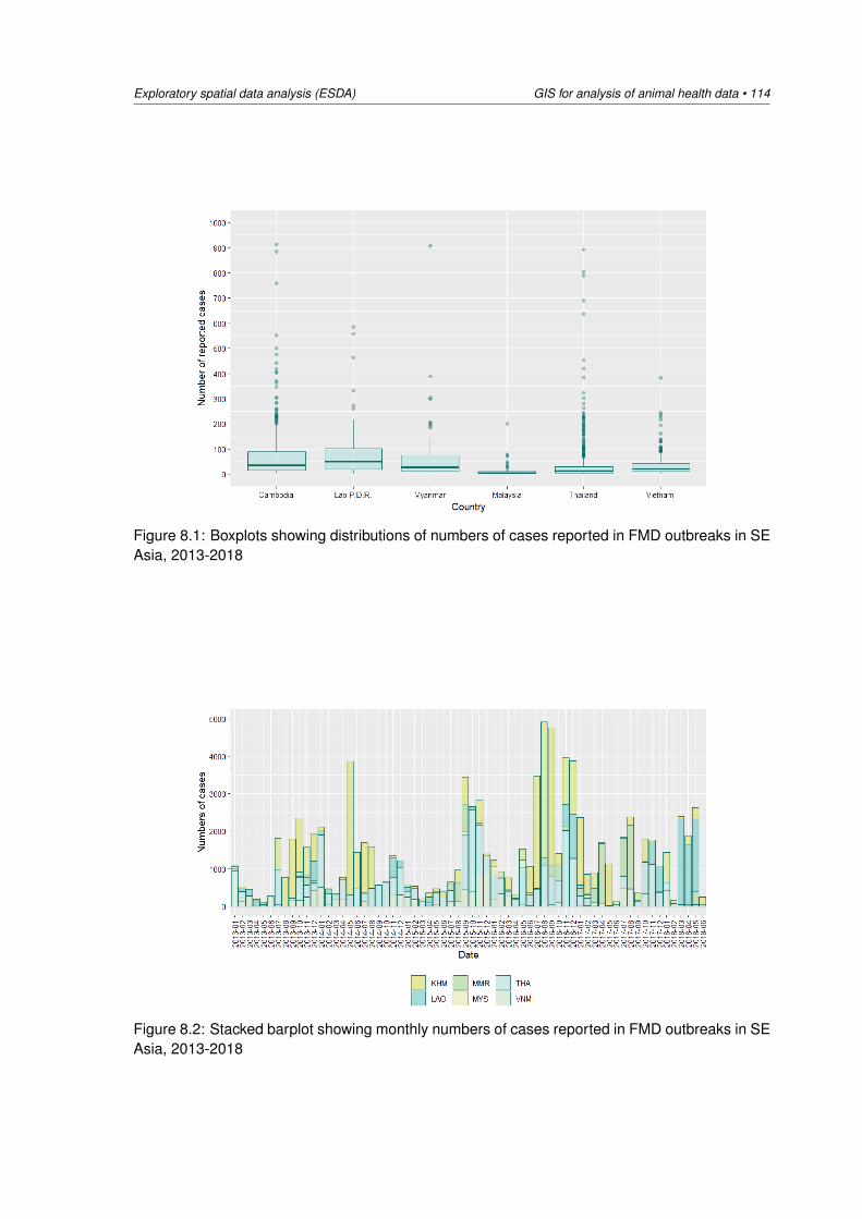
Exploratory spatial data analysis (ESDA) GIS for analysis of animal health data • 114
Figure 8.1: Boxplots showing distributions of numbers of cases reported in FMD outbreaks in SEAsia, 2013-2018
Figure 8.2: Stacked barplot showing monthly numbers of cases reported in FMD outbreaks in SEAsia, 2013-2018
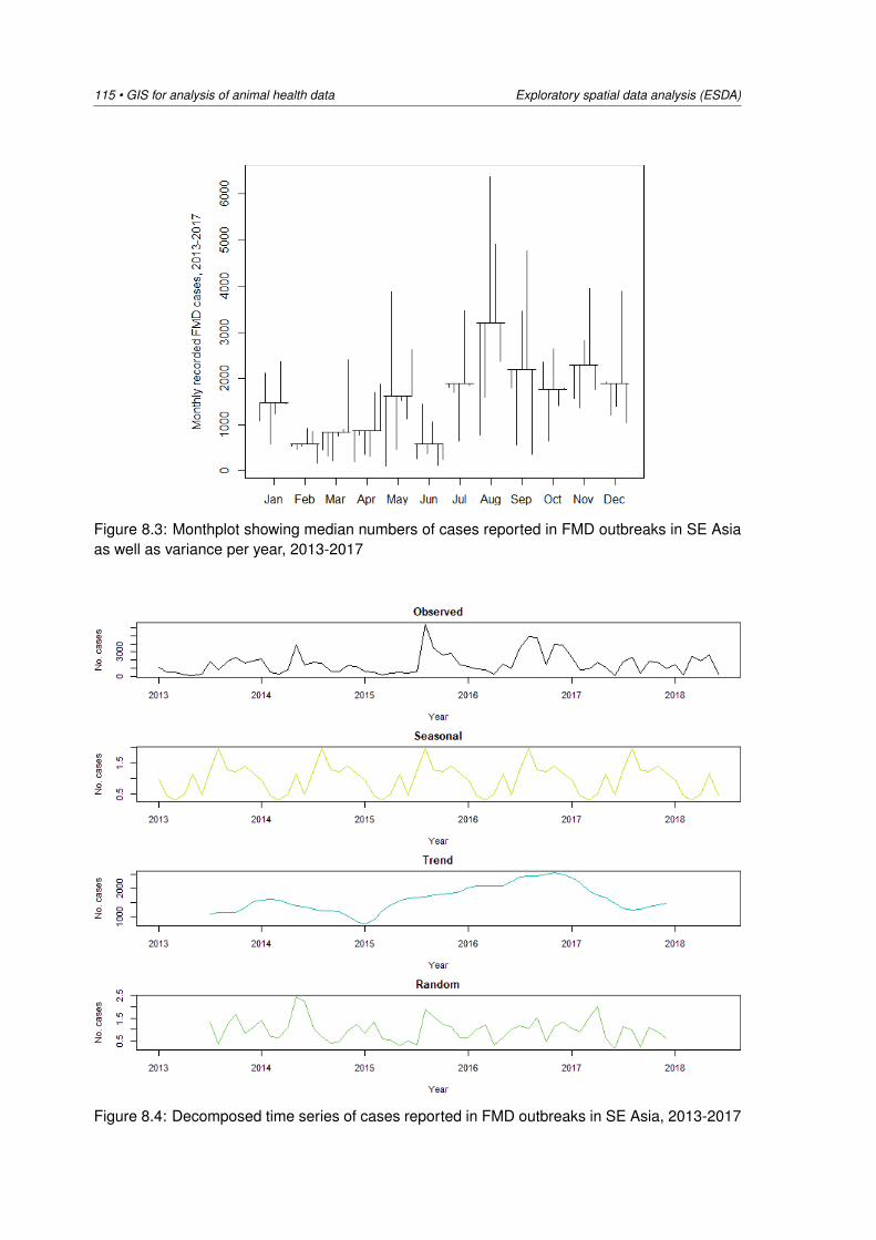
115 • GIS for analysis of animal health data Exploratory spatial data analysis (ESDA)
Figure 8.3: Monthplot showing median numbers of cases reported in FMD outbreaks in SE Asiaas well as variance per year, 2013-2017
Figure 8.4: Decomposed time series of cases reported in FMD outbreaks in SE Asia, 2013-2017
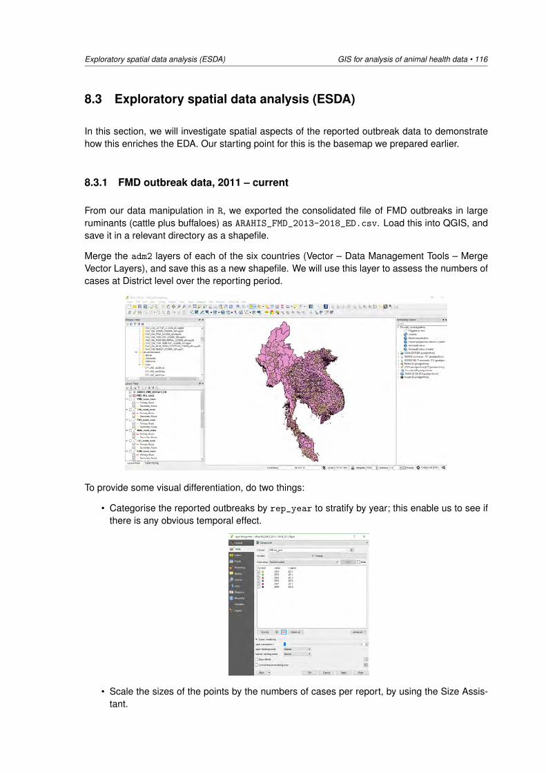
Exploratory spatial data analysis (ESDA) GIS for analysis of animal health data • 116
8.3 Exploratory spatial data analysis (ESDA)
In this section, we will investigate spatial aspects of the reported outbreak data to demonstratehow this enriches the EDA. Our starting point for this is the basemap we prepared earlier.
8.3.1 FMD outbreak data, 2011 – current
From our data manipulation in R, we exported the consolidated file of FMD outbreaks in largeruminants (cattle plus buffaloes) as ARAHIS_FMD_2013-2018_ED.csv. Load this into QGIS, andsave it in a relevant directory as a shapefile.
Merge the adm2 layers of each of the six countries (Vector – Data Management Tools – MergeVector Layers), and save this as a new shapefile. We will use this layer to assess the numbers ofcases at District level over the reporting period.
To provide some visual differentiation, do two things:
• Categorise the reported outbreaks by rep_year to stratify by year; this enable us to see ifthere is any obvious temporal effect.
• Scale the sizes of the points by the numbers of cases per report, by using the Size Assis-tant.
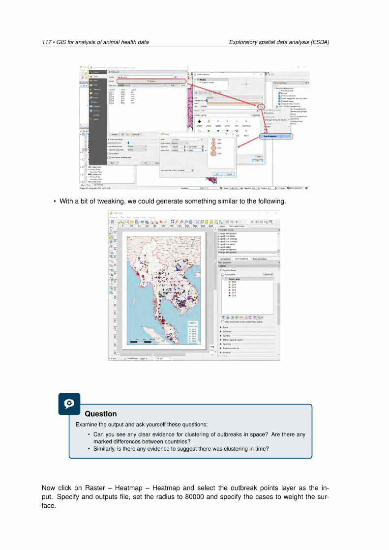
117 • GIS for analysis of animal health data Exploratory spatial data analysis (ESDA)
• With a bit of tweaking, we could generate something similar to the following.
QuestionExamine the output and ask yourself these questions:
• Can you see any clear evidence for clustering of outbreaks in space? Are there anymarked differences between countries?
• Similarly, is there any evidence to suggest there was clustering in time?
Now click on Raster – Heatmap – Heatmap and select the outbreak points layer as the in-put. Specify and outputs file, set the radius to 80000 and specify the cases to weight the sur-face.
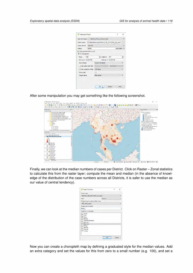
Exploratory spatial data analysis (ESDA) GIS for analysis of animal health data • 118
After some manipulation you may get something like the following screenshot.
Finally, we can look at the median numbers of cases per District. Click on Raster – Zonal statisticsto calculate this from the raster layer; compute the mean and median (in the absence of knowl-edge of the distribution of the case numbers across all Districts, it is safer to use the median asour value of central tendency).
Now you can create a choropleth map by defining a graduated style for the median values. Addan extra category and set the values for this from zero to a small number (e.g. 100), and set a
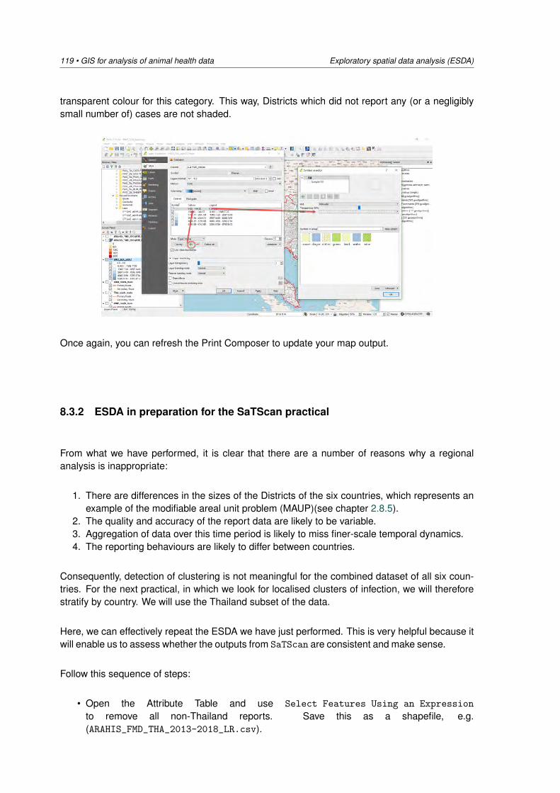
119 • GIS for analysis of animal health data Exploratory spatial data analysis (ESDA)
transparent colour for this category. This way, Districts which did not report any (or a negligiblysmall number of) cases are not shaded.
Once again, you can refresh the Print Composer to update your map output.
8.3.2 ESDA in preparation for the SaTScan practical
From what we have performed, it is clear that there are a number of reasons why a regionalanalysis is inappropriate:
1. There are differences in the sizes of the Districts of the six countries, which represents anexample of the modifiable areal unit problem (MAUP)(see chapter 2.8.5).
2. The quality and accuracy of the report data are likely to be variable.3. Aggregation of data over this time period is likely to miss finer-scale temporal dynamics.4. The reporting behaviours are likely to differ between countries.
Consequently, detection of clustering is not meaningful for the combined dataset of all six coun-tries. For the next practical, in which we look for localised clusters of infection, we will thereforestratify by country. We will use the Thailand subset of the data.
Here, we can effectively repeat the ESDA we have just performed. This is very helpful because itwill enable us to assess whether the outputs from SaTScan are consistent and make sense.
Follow this sequence of steps:
• Open the Attribute Table and use Select Features Using an Expression
to remove all non-Thailand reports. Save this as a shapefile, e.g.(ARAHIS_FMD_THA_2013-2018_LR.csv).
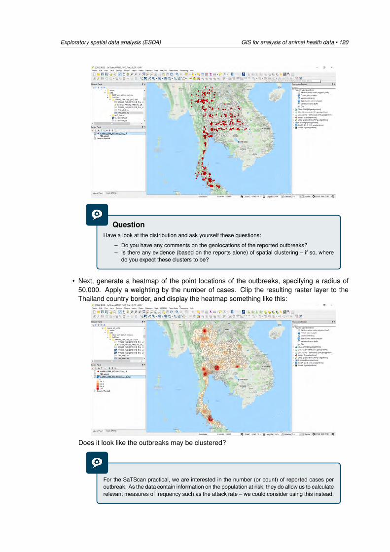
Exploratory spatial data analysis (ESDA) GIS for analysis of animal health data • 120
QuestionHave a look at the distribution and ask yourself these questions:
– Do you have any comments on the geolocations of the reported outbreaks?– Is there any evidence (based on the reports alone) of spatial clustering – if so, where
do you expect these clusters to be?
• Next, generate a heatmap of the point locations of the outbreaks, specifying a radius of50,000. Apply a weighting by the number of cases. Clip the resulting raster layer to theThailand country border, and display the heatmap something like this:
Does it look like the outbreaks may be clustered?
For the SaTScan practical, we are interested in the number (or count) of reported cases peroutbreak. As the data contain information on the population at risk, they do allow us to calculaterelevant measures of frequency such as the attack rate – we could consider using this instead.
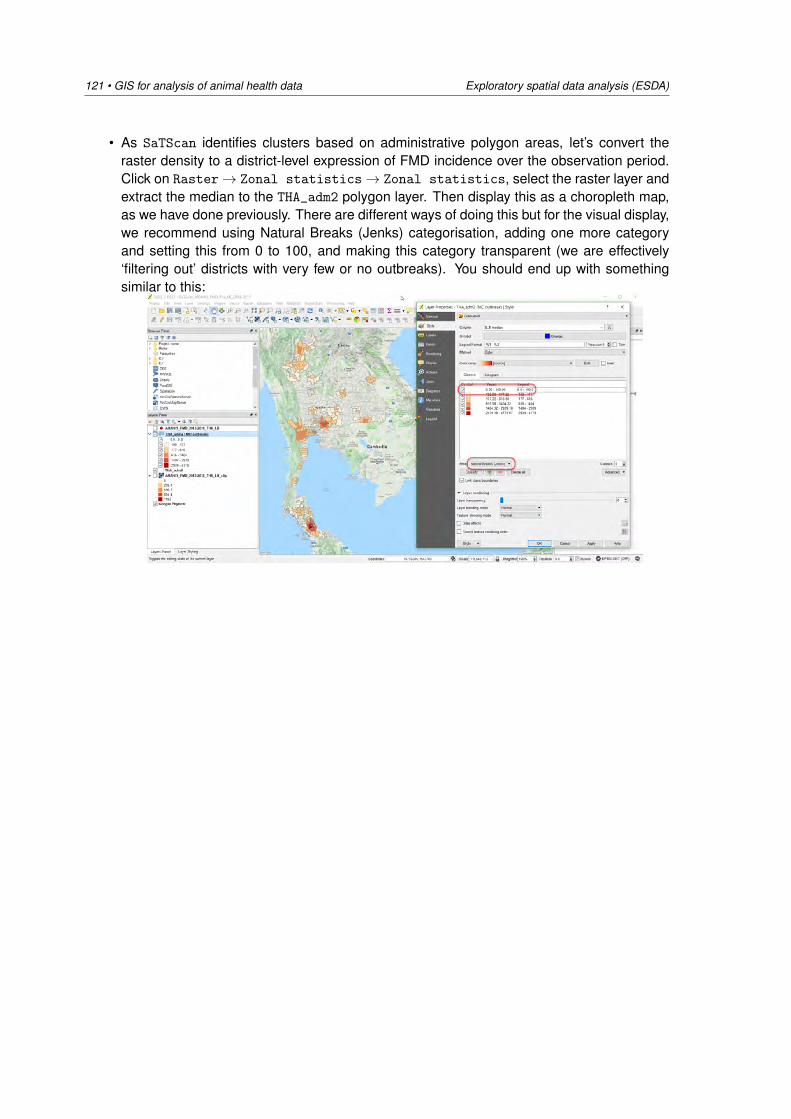
121 • GIS for analysis of animal health data Exploratory spatial data analysis (ESDA)
• As SaTScan identifies clusters based on administrative polygon areas, let’s convert theraster density to a district-level expression of FMD incidence over the observation period.Click on Raster→ Zonal statistics→ Zonal statistics, select the raster layer andextract the median to the THA_adm2 polygon layer. Then display this as a choropleth map,as we have done previously. There are different ways of doing this but for the visual display,we recommend using Natural Breaks (Jenks) categorisation, adding one more categoryand setting this from 0 to 100, and making this category transparent (we are effectively‘filtering out’ districts with very few or no outbreaks). You should end up with somethingsimilar to this:

Space-time cluster scanning using SaTScan GIS for analysis of animal health data • 122
9 Practical 4. Space-time cluster scanningusing SaTScan
9.1 Objective
SaTScan is free software that analyses spatial, temporal and space-time data using the spatial,temporal, or space-time scan statistics. It is designed to detect spatial or space-time diseaseclusters, and to determine if these are statistically significant. For an overview of the computa-tional methodology, refer to the resources provided in this course; we won’t go into any detailshere.
In this practical, we will use the purely spatial scan statistic to analyse the geographical distri-bution of reported Foot-and-Mouth Disease (FMD) cases in Thailand over the period 2013 to2018, and determine if there are any statistically significant geographical clusters of FMD. Inother words, we will determine if there are any geographical areas with more FMD cases thanwould be expected if the risk of incidence of FMD was evenly distributed across the country. Wewill be using SaTScan for the computation but we will perform data editing and visualisation inQGIS.
We will conclude the practical by interpreting our results, the requirements in terms of data avail-ability and accuracy, and assessing the usefulness of the technique.
As more advanced exercises, we will assess whether there is evidence of longer-term spatio-temporal clustering (stratification by calendar year) or short-term spatio-temporal clustering (strat-ification by season). You may tackle these later if you do not have sufficient time during thecourse.
9.2 Data required
You will find the data in the relevant folder. These include the following files:
1. ARAHIS extract of FMD outbreaks for the period January 2013 to June 2018.2. For the purely spatial analysis, these data will be subsetted to Thailand reports only, for the
entire period, and aggregated to District.3. For the spatiotemporal analysis, we will use the subset of Thailand reports for the calendar
years 2013 to 2017.
We should have already performed some ESDA on these data – if not, refer to Chapter8.3.2.
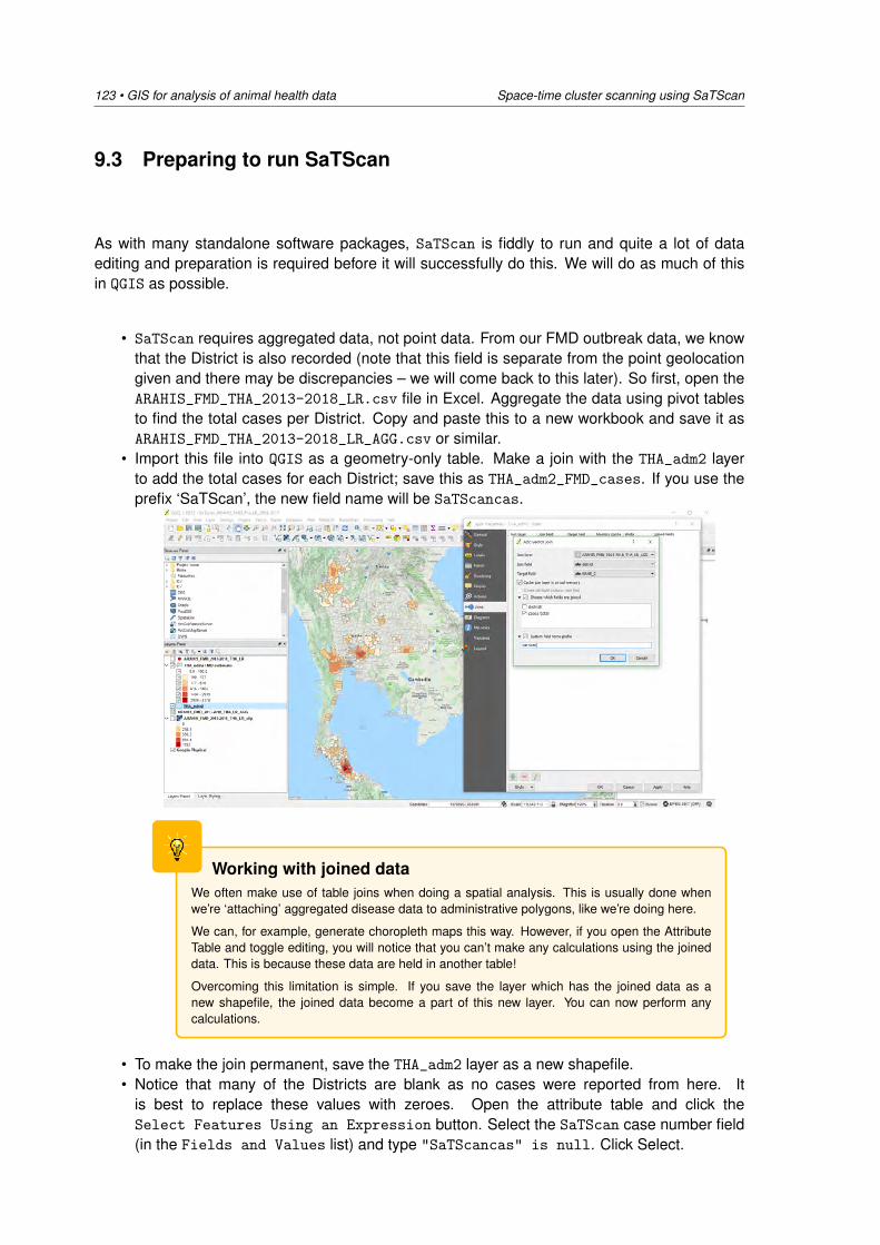
123 • GIS for analysis of animal health data Space-time cluster scanning using SaTScan
9.3 Preparing to run SaTScan
As with many standalone software packages, SaTScan is fiddly to run and quite a lot of dataediting and preparation is required before it will successfully do this. We will do as much of thisin QGIS as possible.
• SaTScan requires aggregated data, not point data. From our FMD outbreak data, we knowthat the District is also recorded (note that this field is separate from the point geolocationgiven and there may be discrepancies – we will come back to this later). So first, open theARAHIS_FMD_THA_2013-2018_LR.csv file in Excel. Aggregate the data using pivot tablesto find the total cases per District. Copy and paste this to a new workbook and save it asARAHIS_FMD_THA_2013-2018_LR_AGG.csv or similar.
• Import this file into QGIS as a geometry-only table. Make a join with the THA_adm2 layerto add the total cases for each District; save this as THA_adm2_FMD_cases. If you use theprefix ‘SaTScan’, the new field name will be SaTScancas.
Working with joined dataWe often make use of table joins when doing a spatial analysis. This is usually done whenwe’re ‘attaching’ aggregated disease data to administrative polygons, like we’re doing here.
We can, for example, generate choropleth maps this way. However, if you open the AttributeTable and toggle editing, you will notice that you can’t make any calculations using the joineddata. This is because these data are held in another table!
Overcoming this limitation is simple. If you save the layer which has the joined data as anew shapefile, the joined data become a part of this new layer. You can now perform anycalculations.
• To make the join permanent, save the THA_adm2 layer as a new shapefile.• Notice that many of the Districts are blank as no cases were reported from here. It
is best to replace these values with zeroes. Open the attribute table and click theSelect Features Using an Expression button. Select the SaTScan case number field(in the Fields and Values list) and type "SaTScancas" is null. Click Select.
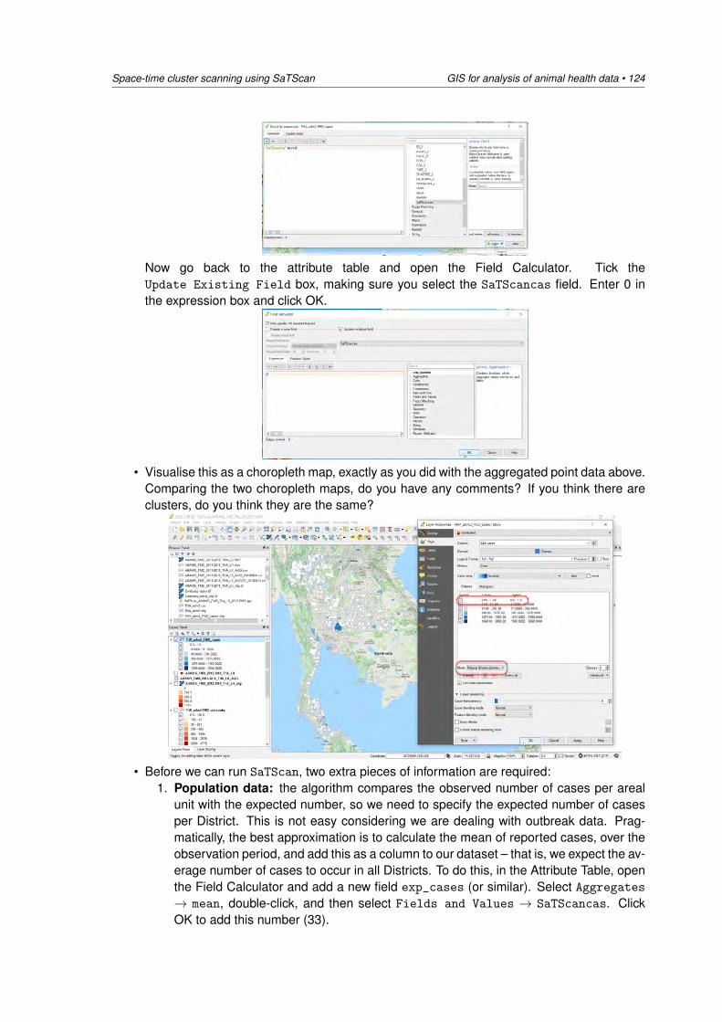
Space-time cluster scanning using SaTScan GIS for analysis of animal health data • 124
Now go back to the attribute table and open the Field Calculator. Tick theUpdate Existing Field box, making sure you select the SaTScancas field. Enter 0 inthe expression box and click OK.
• Visualise this as a choropleth map, exactly as you did with the aggregated point data above.Comparing the two choropleth maps, do you have any comments? If you think there areclusters, do you think they are the same?
• Before we can run SaTScan, two extra pieces of information are required:1. Population data: the algorithm compares the observed number of cases per areal
unit with the expected number, so we need to specify the expected number of casesper District. This is not easy considering we are dealing with outbreak data. Prag-matically, the best approximation is to calculate the mean of reported cases, over theobservation period, and add this as a column to our dataset – that is, we expect the av-erage number of cases to occur in all Districts. To do this, in the Attribute Table, openthe Field Calculator and add a new field exp_cases (or similar). Select Aggregates→ mean, double-click, and then select Fields and Values → SaTScancas. ClickOK to add this number (33).
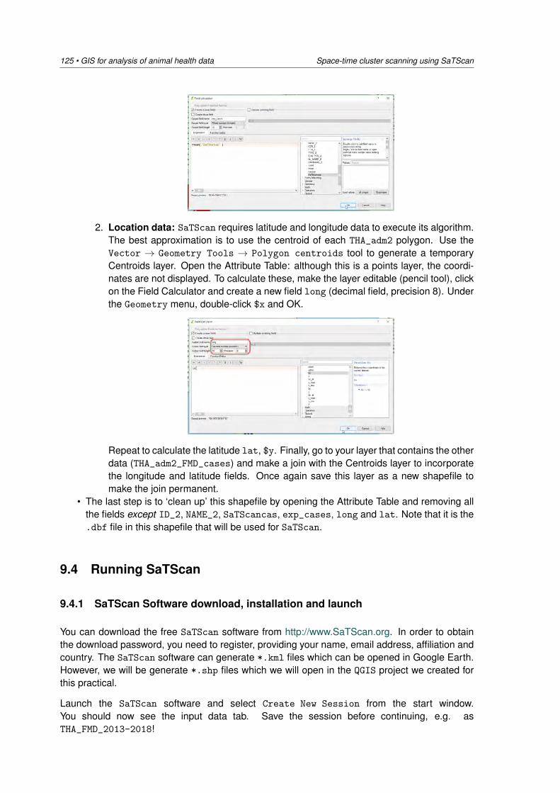
125 • GIS for analysis of animal health data Space-time cluster scanning using SaTScan
2. Location data: SaTScan requires latitude and longitude data to execute its algorithm.The best approximation is to use the centroid of each THA_adm2 polygon. Use theVector → Geometry Tools → Polygon centroids tool to generate a temporaryCentroids layer. Open the Attribute Table: although this is a points layer, the coordi-nates are not displayed. To calculate these, make the layer editable (pencil tool), clickon the Field Calculator and create a new field long (decimal field, precision 8). Underthe Geometry menu, double-click $x and OK.
Repeat to calculate the latitude lat, $y. Finally, go to your layer that contains the otherdata (THA_adm2_FMD_cases) and make a join with the Centroids layer to incorporatethe longitude and latitude fields. Once again save this layer as a new shapefile tomake the join permanent.
• The last step is to ‘clean up’ this shapefile by opening the Attribute Table and removing allthe fields except ID_2, NAME_2, SaTScancas, exp_cases, long and lat. Note that it is the.dbf file in this shapefile that will be used for SaTScan.
9.4 Running SaTScan
9.4.1 SaTScan Software download, installation and launch
You can download the free SaTScan software from http://www.SaTScan.org. In order to obtainthe download password, you need to register, providing your name, email address, affiliation andcountry. The SaTScan software can generate *.kml files which can be opened in Google Earth.However, we will be generate *.shp files which we will open in the QGIS project we created forthis practical.
Launch the SaTScan software and select Create New Session from the start window.You should now see the input data tab. Save the session before continuing, e.g. asTHA_FMD_2013-2018!
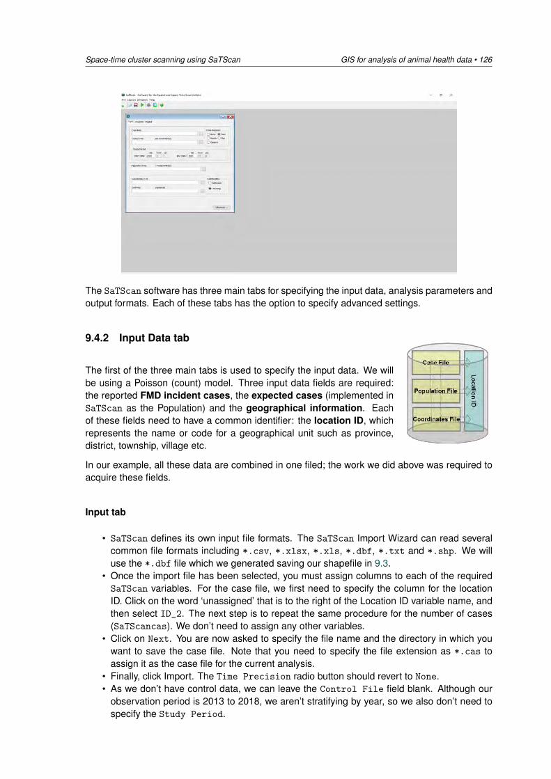
Space-time cluster scanning using SaTScan GIS for analysis of animal health data • 126
The SaTScan software has three main tabs for specifying the input data, analysis parameters andoutput formats. Each of these tabs has the option to specify advanced settings.
9.4.2 Input Data tab
The first of the three main tabs is used to specify the input data. We willbe using a Poisson (count) model. Three input data fields are required:the reported FMD incident cases, the expected cases (implemented inSaTScan as the Population) and the geographical information. Eachof these fields need to have a common identifier: the location ID, whichrepresents the name or code for a geographical unit such as province,district, township, village etc.
In our example, all these data are combined in one filed; the work we did above was required toacquire these fields.
Input tab
• SaTScan defines its own input file formats. The SaTScan Import Wizard can read severalcommon file formats including *.csv, *.xlsx, *.xls, *.dbf, *.txt and *.shp. We willuse the *.dbf file which we generated saving our shapefile in 9.3.
• Once the import file has been selected, you must assign columns to each of the requiredSaTScan variables. For the case file, we first need to specify the column for the locationID. Click on the word ‘unassigned’ that is to the right of the Location ID variable name, andthen select ID_2. The next step is to repeat the same procedure for the number of cases(SaTScancas). We don’t need to assign any other variables.
• Click on Next. You are now asked to specify the file name and the directory in which youwant to save the case file. Note that you need to specify the file extension as *.cas toassign it as the case file for the current analysis.
• Finally, click Import. The Time Precision radio button should revert to None.• As we don’t have control data, we can leave the Control File field blank. Although our
observation period is 2013 to 2018, we aren’t stratifying by year, so we also don’t need tospecify the Study Period.
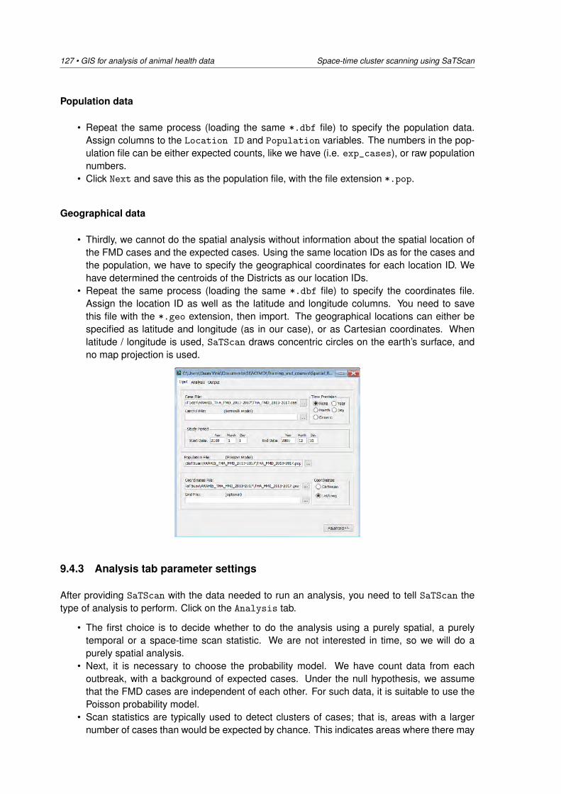
127 • GIS for analysis of animal health data Space-time cluster scanning using SaTScan
Population data
• Repeat the same process (loading the same *.dbf file) to specify the population data.Assign columns to the Location ID and Population variables. The numbers in the pop-ulation file can be either expected counts, like we have (i.e. exp_cases), or raw populationnumbers.
• Click Next and save this as the population file, with the file extension *.pop.
Geographical data
• Thirdly, we cannot do the spatial analysis without information about the spatial location ofthe FMD cases and the expected cases. Using the same location IDs as for the cases andthe population, we have to specify the geographical coordinates for each location ID. Wehave determined the centroids of the Districts as our location IDs.
• Repeat the same process (loading the same *.dbf file) to specify the coordinates file.Assign the location ID as well as the latitude and longitude columns. You need to savethis file with the *.geo extension, then import. The geographical locations can either bespecified as latitude and longitude (as in our case), or as Cartesian coordinates. Whenlatitude / longitude is used, SaTScan draws concentric circles on the earth’s surface, andno map projection is used.
9.4.3 Analysis tab parameter settings
After providing SaTScan with the data needed to run an analysis, you need to tell SaTScan thetype of analysis to perform. Click on the Analysis tab.
• The first choice is to decide whether to do the analysis using a purely spatial, a purelytemporal or a space-time scan statistic. We are not interested in time, so we will do apurely spatial analysis.
• Next, it is necessary to choose the probability model. We have count data from eachoutbreak, with a background of expected cases. Under the null hypothesis, we assumethat the FMD cases are independent of each other. For such data, it is suitable to use thePoisson probability model.
• Scan statistics are typically used to detect clusters of cases; that is, areas with a largernumber of cases than would be expected by chance. This indicates areas where there may
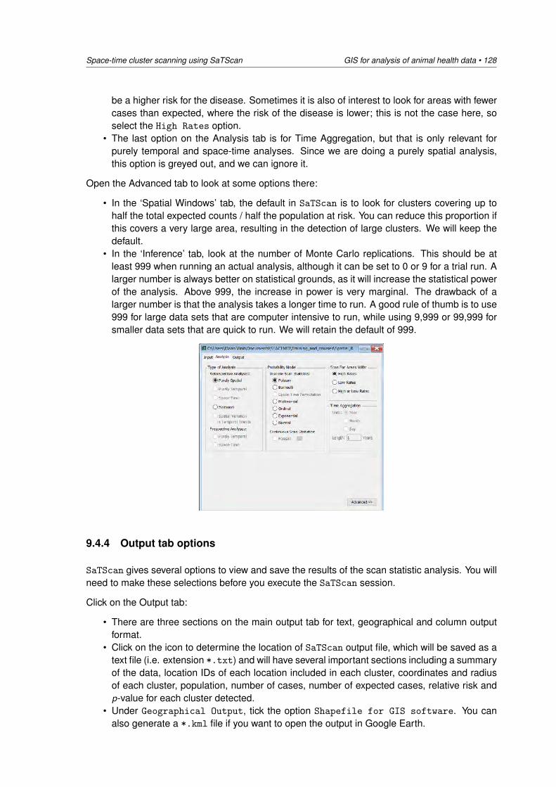
Space-time cluster scanning using SaTScan GIS for analysis of animal health data • 128
be a higher risk for the disease. Sometimes it is also of interest to look for areas with fewercases than expected, where the risk of the disease is lower; this is not the case here, soselect the High Rates option.
• The last option on the Analysis tab is for Time Aggregation, but that is only relevant forpurely temporal and space-time analyses. Since we are doing a purely spatial analysis,this option is greyed out, and we can ignore it.
Open the Advanced tab to look at some options there:
• In the ‘Spatial Windows’ tab, the default in SaTScan is to look for clusters covering up tohalf the total expected counts / half the population at risk. You can reduce this proportion ifthis covers a very large area, resulting in the detection of large clusters. We will keep thedefault.
• In the ‘Inference’ tab, look at the number of Monte Carlo replications. This should be atleast 999 when running an actual analysis, although it can be set to 0 or 9 for a trial run. Alarger number is always better on statistical grounds, as it will increase the statistical powerof the analysis. Above 999, the increase in power is very marginal. The drawback of alarger number is that the analysis takes a longer time to run. A good rule of thumb is to use999 for large data sets that are computer intensive to run, while using 9,999 or 99,999 forsmaller data sets that are quick to run. We will retain the default of 999.
9.4.4 Output tab options
SaTScan gives several options to view and save the results of the scan statistic analysis. You willneed to make these selections before you execute the SaTScan session.
Click on the Output tab:
• There are three sections on the main output tab for text, geographical and column outputformat.
• Click on the icon to determine the location of SaTScan output file, which will be saved as atext file (i.e. extension *.txt) and will have several important sections including a summaryof the data, location IDs of each location included in each cluster, coordinates and radiusof each cluster, population, number of cases, number of expected cases, relative risk andp-value for each cluster detected.
• Under Geographical Output, tick the option Shapefile for GIS software. You canalso generate a *.kml file if you want to open the output in Google Earth.
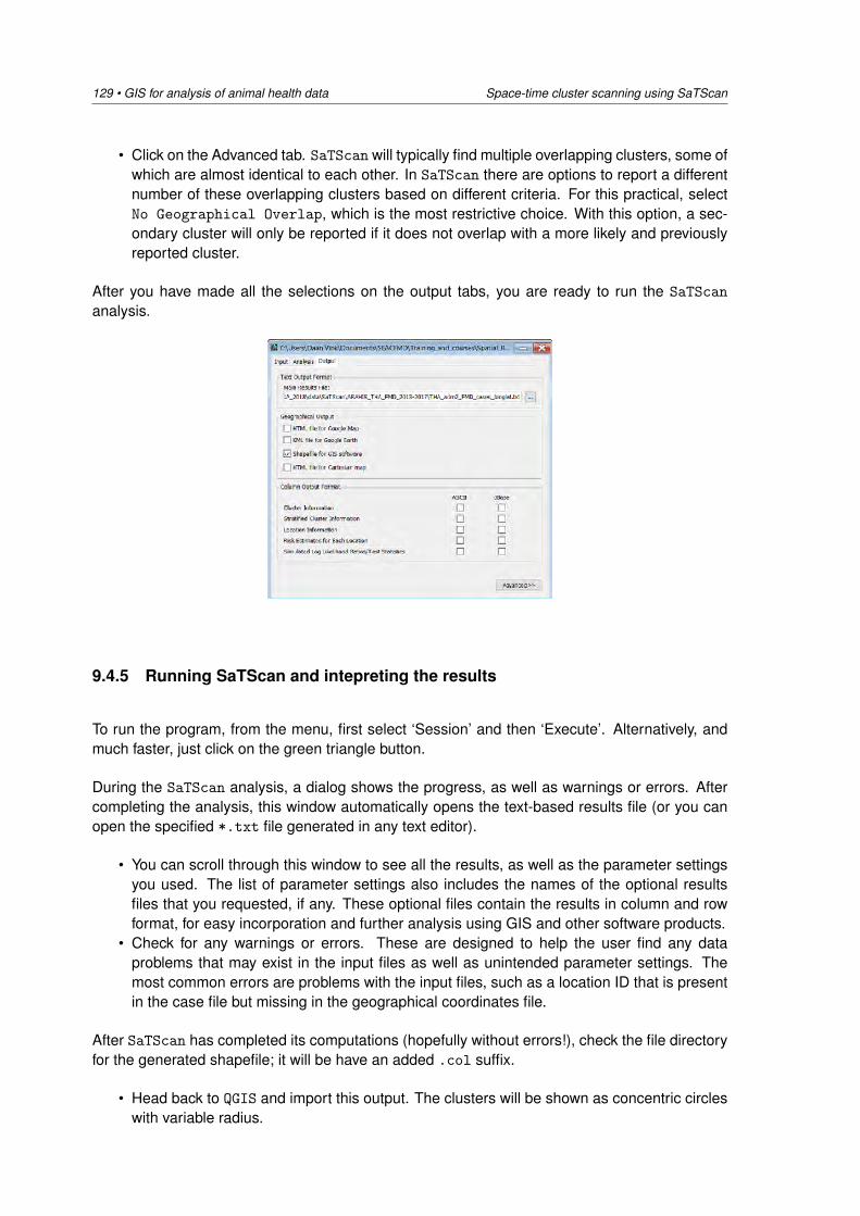
129 • GIS for analysis of animal health data Space-time cluster scanning using SaTScan
• Click on the Advanced tab. SaTScan will typically find multiple overlapping clusters, some ofwhich are almost identical to each other. In SaTScan there are options to report a differentnumber of these overlapping clusters based on different criteria. For this practical, selectNo Geographical Overlap, which is the most restrictive choice. With this option, a sec-ondary cluster will only be reported if it does not overlap with a more likely and previouslyreported cluster.
After you have made all the selections on the output tabs, you are ready to run the SaTScan
analysis.
9.4.5 Running SaTScan and intepreting the results
To run the program, from the menu, first select ‘Session’ and then ‘Execute’. Alternatively, andmuch faster, just click on the green triangle button.
During the SaTScan analysis, a dialog shows the progress, as well as warnings or errors. Aftercompleting the analysis, this window automatically opens the text-based results file (or you canopen the specified *.txt file generated in any text editor).
• You can scroll through this window to see all the results, as well as the parameter settingsyou used. The list of parameter settings also includes the names of the optional resultsfiles that you requested, if any. These optional files contain the results in column and rowformat, for easy incorporation and further analysis using GIS and other software products.
• Check for any warnings or errors. These are designed to help the user find any dataproblems that may exist in the input files as well as unintended parameter settings. Themost common errors are problems with the input files, such as a location ID that is presentin the case file but missing in the geographical coordinates file.
After SaTScan has completed its computations (hopefully without errors!), check the file directoryfor the generated shapefile; it will be have an added .col suffix.
• Head back to QGIS and import this output. The clusters will be shown as concentric circleswith variable radius.
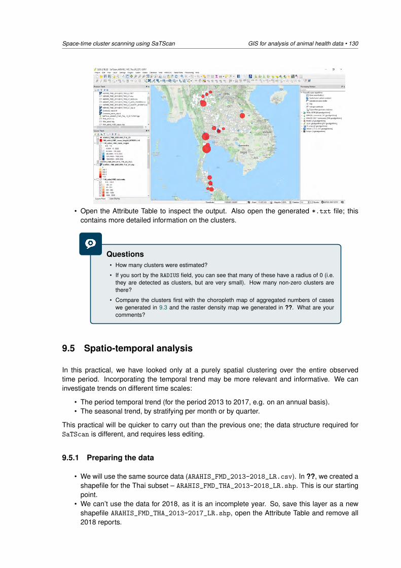
Space-time cluster scanning using SaTScan GIS for analysis of animal health data • 130
• Open the Attribute Table to inspect the output. Also open the generated *.txt file; thiscontains more detailed information on the clusters.
Questions• How many clusters were estimated?
• If you sort by the RADIUS field, you can see that many of these have a radius of 0 (i.e.they are detected as clusters, but are very small). How many non-zero clusters arethere?
• Compare the clusters first with the choropleth map of aggregated numbers of caseswe generated in 9.3 and the raster density map we generated in ??. What are yourcomments?
9.5 Spatio-temporal analysis
In this practical, we have looked only at a purely spatial clustering over the entire observedtime period. Incorporating the temporal trend may be more relevant and informative. We caninvestigate trends on different time scales:
• The period temporal trend (for the period 2013 to 2017, e.g. on an annual basis).• The seasonal trend, by stratifying per month or by quarter.
This practical will be quicker to carry out than the previous one; the data structure required forSaTScan is different, and requires less editing.
9.5.1 Preparing the data
• We will use the same source data (ARAHIS_FMD_2013-2018_LR.csv). In ??, we created ashapefile for the Thai subset – ARAHIS_FMD_THA_2013-2018_LR.shp. This is our startingpoint.
• We can’t use the data for 2018, as it is an incomplete year. So, save this layer as a newshapefile ARAHIS_FMD_THA_2013-2017_LR.shp, open the Attribute Table and remove all2018 reports.
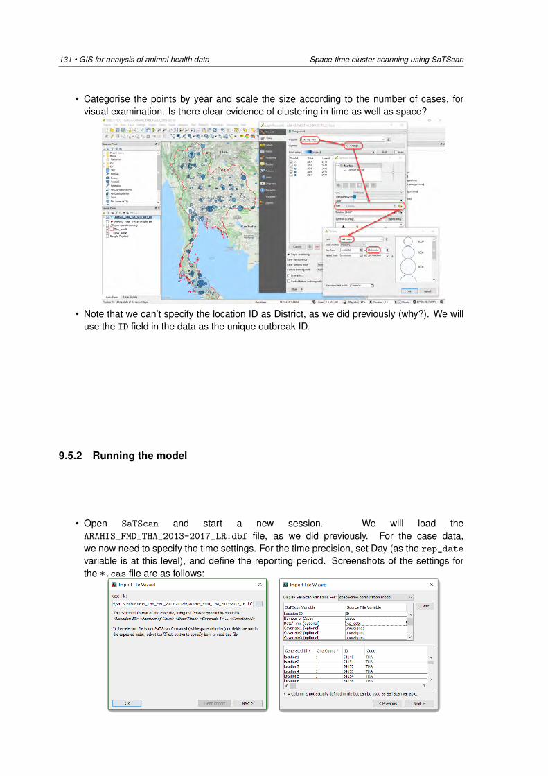
131 • GIS for analysis of animal health data Space-time cluster scanning using SaTScan
• Categorise the points by year and scale the size according to the number of cases, forvisual examination. Is there clear evidence of clustering in time as well as space?
• Note that we can’t specify the location ID as District, as we did previously (why?). We willuse the ID field in the data as the unique outbreak ID.
9.5.2 Running the model
• Open SaTScan and start a new session. We will load theARAHIS_FMD_THA_2013-2017_LR.dbf file, as we did previously. For the case data,we now need to specify the time settings. For the time precision, set Day (as the rep_date
variable is at this level), and define the reporting period. Screenshots of the settings forthe *.cas file are as follows:
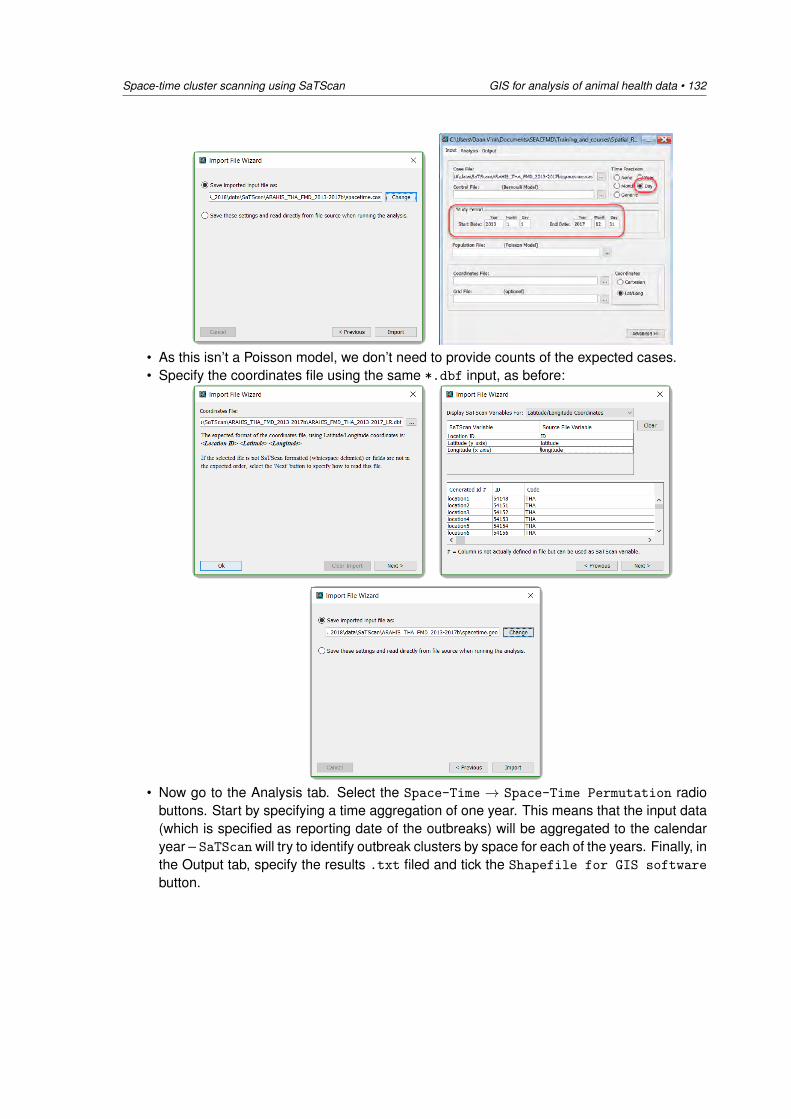
Space-time cluster scanning using SaTScan GIS for analysis of animal health data • 132
• As this isn’t a Poisson model, we don’t need to provide counts of the expected cases.• Specify the coordinates file using the same *.dbf input, as before:
• Now go to the Analysis tab. Select the Space-Time → Space-Time Permutation radiobuttons. Start by specifying a time aggregation of one year. This means that the input data(which is specified as reporting date of the outbreaks) will be aggregated to the calendaryear – SaTScan will try to identify outbreak clusters by space for each of the years. Finally, inthe Output tab, specify the results .txt filed and tick the Shapefile for GIS software
button.
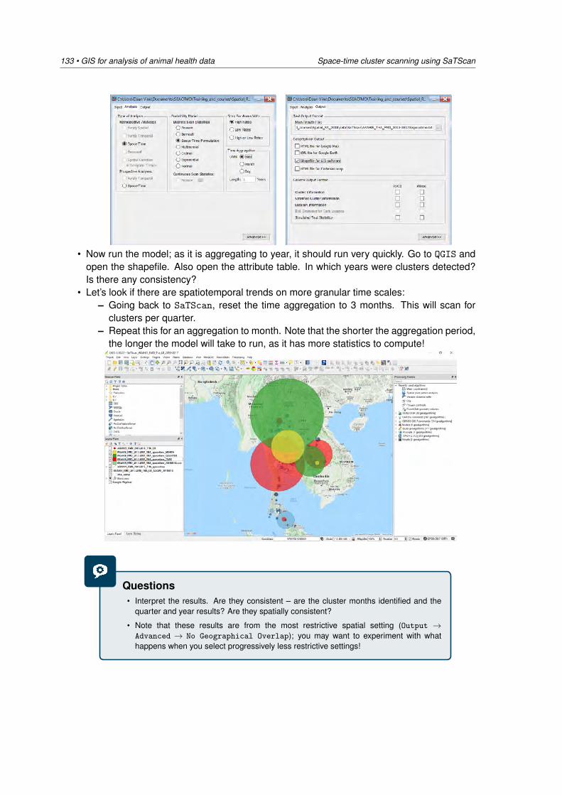
133 • GIS for analysis of animal health data Space-time cluster scanning using SaTScan
• Now run the model; as it is aggregating to year, it should run very quickly. Go to QGIS andopen the shapefile. Also open the attribute table. In which years were clusters detected?Is there any consistency?
• Let’s look if there are spatiotemporal trends on more granular time scales:– Going back to SaTScan, reset the time aggregation to 3 months. This will scan for
clusters per quarter.– Repeat this for an aggregation to month. Note that the shorter the aggregation period,
the longer the model will take to run, as it has more statistics to compute!
Questions• Interpret the results. Are they consistent – are the cluster months identified and the
quarter and year results? Are they spatially consistent?
• Note that these results are from the most restrictive spatial setting (Output →Advanced → No Geographical Overlap); you may want to experiment with whathappens when you select progressively less restrictive settings!

Spatial risk assessment using QGIS GIS for analysis of animal health data • 134
10 Practical 5a. Spatial risk assessmentusing QGIS
10.1 Objective
In this practical, we will demonstrate how to implement knowledge-driven spatial risk assessmentto generate a risk surface for FMD in cattle in Malaysia. Refer to Chapter 6 for backgroundinformation.
To save time, we will use the outputs of an MCDA exercise performed previously to inform themultipliers required for our Weighted Linear Combination (WLC). We will implement this WLCusing different spatial layers. Ultimately, the objective is to identify potential high-risk areas forFMD – disease ‘hot spots’.
The MCDA exercise was performed to elicit information on the relative influence of each of thesefactors on the occurrence of FMD outbreaks. This is knowledge-driven: it relies on expert opinion,both for the selection of the spatial risk factors as well as the estimation of their relative impor-tance. If we had appropriate data and evidence from literature, a more quantitative (data-driven)approach would be preferable.
From the MCDA exercise, the following spatial risk factors were identified:
• Direct contacts of livestock during grazing.• Livestock movements following legal trade.• Illegal or unregulated livestock movements.• Contact of ruminants with pigs.• Contact of livestock with feral or wild-living pigs.
10.2 Spatial layers and data
A summary of the spatial data sets required for these analyses is provided in Table 10.1. We havemade various assumptions to perform this analysis; this exercise is crude, but demonstrates amethodology which could be refined.
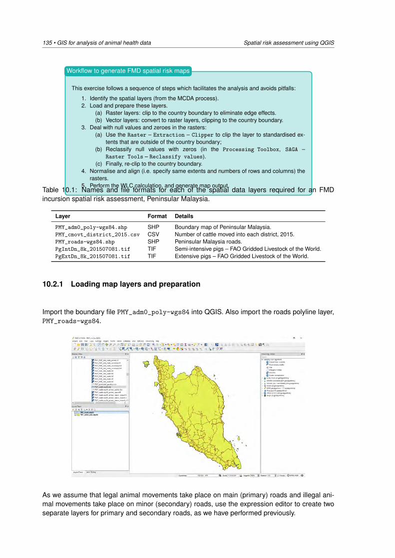
135 • GIS for analysis of animal health data Spatial risk assessment using QGIS
This exercise follows a sequence of steps which facilitates the analysis and avoids pitfalls:
1. Identify the spatial layers (from the MCDA process).2. Load and prepare these layers.
(a) Raster layers: clip to the country boundary to eliminate edge effects.(b) Vector layers: convert to raster layers, clipping to the country boundary.
3. Deal with null values and zeroes in the rasters:(a) Use the Raster – Extraction – Clipper to clip the layer to standardised ex-
tents that are outside of the country boundary;(b) Reclassify null values with zeros (in the Processing Toolbox, SAGA –
Raster Tools – Reclassify values).(c) Finally, re-clip to the country boundary.
4. Normalise and align (i.e. specify same extents and numbers of rows and columns) therasters.
5. Perform the WLC calculation, and generate map output.
Workflow to generate FMD spatial risk maps
Table 10.1: Names and file formats for each of the spatial data layers required for an FMDincursion spatial risk assessment, Peninsular Malaysia.
Layer Format Details
PMY_adm0_poly-wgs84.shp SHP Boundary map of Peninsular Malaysia.PMY_cmovt_district_2015.csv CSV Number of cattle moved into each district, 2015.PMY_roads-wgs84.shp SHP Peninsular Malaysia roads.PgIntDn_8k_201507081.tif TIF Semi-intensive pigs – FAO Gridded Livestock of the World.PgExtDn_8k_201507081.tif TIF Extensive pigs – FAO Gridded Livestock of the World.
10.2.1 Loading map layers and preparation
Import the boundary file PMY_adm0_poly-wgs84 into QGIS. Also import the roads polyline layer,PMY_roads-wgs84.
As we assume that legal animal movements take place on main (primary) roads and illegal ani-mal movements take place on minor (secondary) roads, use the expression editor to create twoseparate layers for primary and secondary roads, as we have performed previously.
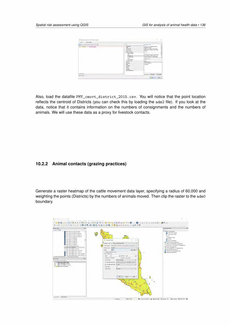
Spatial risk assessment using QGIS GIS for analysis of animal health data • 136
Also, load the datafile PMY_cmovt_district_2015.csv. You will notice that the point locationreflects the centroid of Districts (you can check this by loading the adm2 file). If you look at thedata, notice that it contains information on the numbers of consignments and the numbers ofanimals. We will use these data as a proxy for livestock contacts.
10.2.2 Animal contacts (grazing practices)
Generate a raster heatmap of the cattle movement data layer, specifying a radius of 60,000 andweighting the points (Districts) by the numbers of animals moved. Then clip the raster to the adm0
boundary.
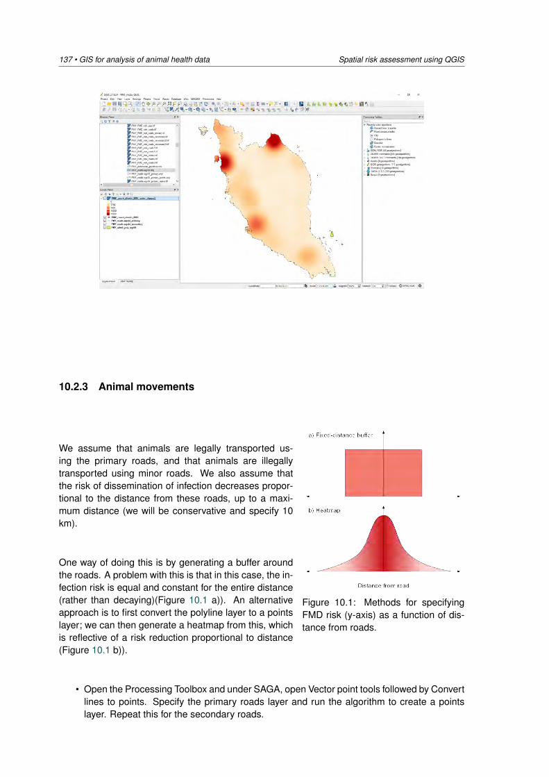
137 • GIS for analysis of animal health data Spatial risk assessment using QGIS
10.2.3 Animal movements
Figure 10.1: Methods for specifyingFMD risk (y-axis) as a function of dis-tance from roads.
We assume that animals are legally transported us-ing the primary roads, and that animals are illegallytransported using minor roads. We also assume thatthe risk of dissemination of infection decreases propor-tional to the distance from these roads, up to a maxi-mum distance (we will be conservative and specify 10km).
One way of doing this is by generating a buffer aroundthe roads. A problem with this is that in this case, the in-fection risk is equal and constant for the entire distance(rather than decaying)(Figure 10.1 a)). An alternativeapproach is to first convert the polyline layer to a pointslayer; we can then generate a heatmap from this, whichis reflective of a risk reduction proportional to distance(Figure 10.1 b)).
• Open the Processing Toolbox and under SAGA, open Vector point tools followed by Convertlines to points. Specify the primary roads layer and run the algorithm to create a pointslayer. Repeat this for the secondary roads.
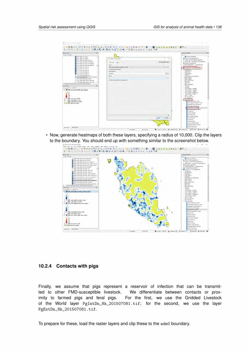
Spatial risk assessment using QGIS GIS for analysis of animal health data • 138
• Now, generate heatmaps of both these layers, specifying a radius of 10,000. Clip the layersto the boundary. You should end up with something similar to the screenshot below.
10.2.4 Contacts with pigs
Finally, we assume that pigs represent a reservoir of infection that can be transmit-ted to other FMD-susceptible livestock. We differentiate between contacts or prox-imity to farmed pigs and feral pigs. For the first, we use the Gridded Livestockof the World layer PgIntDn_8k_201507081.tif; for the second, we use the layerPgExtDn_8k_201507081.tif.
To prepare for these, load the raster layers and clip these to the adm0 boundary.
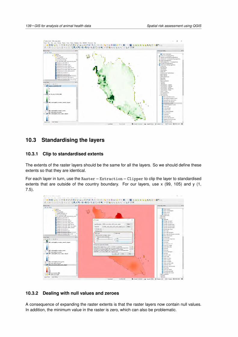
139 • GIS for analysis of animal health data Spatial risk assessment using QGIS
10.3 Standardising the layers
10.3.1 Clip to standardised extents
The extents of the raster layers should be the same for all the layers. So we should define theseextents so that they are identical.
For each layer in turn, use the Raster – Extraction – Clipper to clip the layer to standardisedextents that are outside of the country boundary. For our layers, use x (99, 105) and y (1,7.5).
10.3.2 Dealing with null values and zeroes
A consequence of expanding the raster extents is that the raster layers now contain null values.In addition, the minimum value in the raster is zero, which can also be problematic.
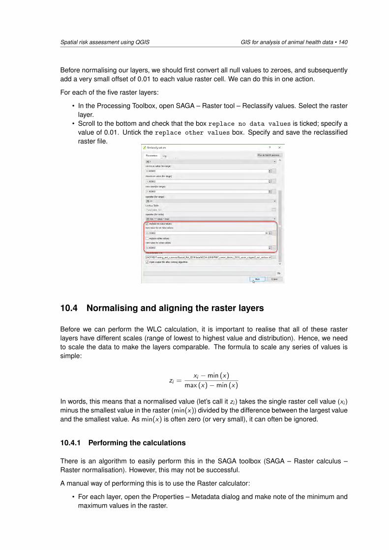
Spatial risk assessment using QGIS GIS for analysis of animal health data • 140
Before normalising our layers, we should first convert all null values to zeroes, and subsequentlyadd a very small offset of 0.01 to each value raster cell. We can do this in one action.
For each of the five raster layers:
• In the Processing Toolbox, open SAGA – Raster tool – Reclassify values. Select the rasterlayer.
• Scroll to the bottom and check that the box replace no data values is ticked; specify avalue of 0.01. Untick the replace other values box. Specify and save the reclassifiedraster file.
10.4 Normalising and aligning the raster layers
Before we can perform the WLC calculation, it is important to realise that all of these rasterlayers have different scales (range of lowest to highest value and distribution). Hence, we needto scale the data to make the layers comparable. The formula to scale any series of values issimple:
zi =xi −min (x)
max (x)−min (x)
In words, this means that a normalised value (let’s call it zi ) takes the single raster cell value (xi )minus the smallest value in the raster (min(x)) divided by the difference between the largest valueand the smallest value. As min(x) is often zero (or very small), it can often be ignored.
10.4.1 Performing the calculations
There is an algorithm to easily perform this in the SAGA toolbox (SAGA – Raster calculus –Raster normalisation). However, this may not be successful.
A manual way of performing this is to use the Raster calculator:
• For each layer, open the Properties – Metadata dialog and make note of the minimum andmaximum values in the raster.
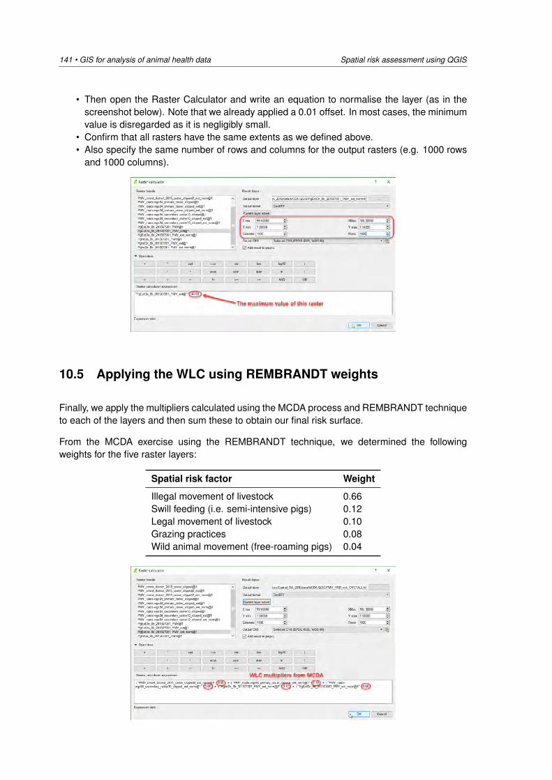
141 • GIS for analysis of animal health data Spatial risk assessment using QGIS
• Then open the Raster Calculator and write an equation to normalise the layer (as in thescreenshot below). Note that we already applied a 0.01 offset. In most cases, the minimumvalue is disregarded as it is negligibly small.
• Confirm that all rasters have the same extents as we defined above.• Also specify the same number of rows and columns for the output rasters (e.g. 1000 rows
and 1000 columns).
10.5 Applying the WLC using REMBRANDT weights
Finally, we apply the multipliers calculated using the MCDA process and REMBRANDT techniqueto each of the layers and then sum these to obtain our final risk surface.
From the MCDA exercise using the REMBRANDT technique, we determined the followingweights for the five raster layers:
Spatial risk factor Weight
Illegal movement of livestock 0.66Swill feeding (i.e. semi-intensive pigs) 0.12Legal movement of livestock 0.10Grazing practices 0.08Wild animal movement (free-roaming pigs) 0.04
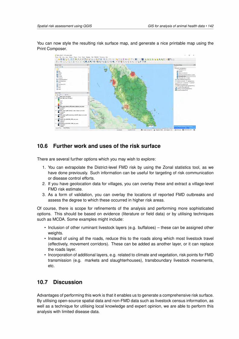
Spatial risk assessment using QGIS GIS for analysis of animal health data • 142
You can now style the resulting risk surface map, and generate a nice printable map using thePrint Composer.
10.6 Further work and uses of the risk surface
There are several further options which you may wish to explore:
1. You can extrapolate the District-level FMD risk by using the Zonal statistics tool, as wehave done previously. Such information can be useful for targeting of risk communicationor disease control efforts.
2. If you have geolocation data for villages, you can overlay these and extract a village-levelFMD risk estimate.
3. As a form of validation, you can overlay the locations of reported FMD outbreaks andassess the degree to which these occurred in higher risk areas.
Of course, there is scope for refinements of the analysis and performing more sophisticatedoptions. This should be based on evidence (literature or field data) or by utilising techniquessuch as MCDA. Some examples might include:
• Inclusion of other ruminant livestock layers (e.g. buffaloes) – these can be assigned otherweights.
• Instead of using all the roads, reduce this to the roads along which most livestock travel(effectively, movement corridors). These can be added as another layer, or it can replacethe roads layer.
• Incorporation of additional layers, e.g. related to climate and vegetation, risk points for FMDtransmission (e.g. markets and slaughterhouses), transboundary livestock movements,etc.
10.7 Discussion
Advantages of performing this work is that it enables us to generate a comprehensive risk surface.By utilising open-source spatial data and non-FMD data such as livestock census information, aswell as a technique for utilising local knowledge and expert opinion, we are able to perform thisanalysis with limited disease data.

143 • GIS for analysis of animal health data Spatial risk assessment using QGIS
However, we need to also be aware of the limitations and dangers of doing this:
• Subjective nature of expert elicitation to perform MCDA and determine the WLC.• Limitations in the data: old or inaccurate census figures (or interpolated spatial data such
as in this case); underreporting (poor or biased disease data).• It is possible to generate an authoritative-looking map which may be taken at too much
value by decision-makers. It is very difficult to assess the accuracy of the outputs. It ispossible to perform the analysis in such a way as to suggest hotspots exist, whereas in factthe true risk may be much more homogeneous (e.g. in an endemic setting).

Spatial risk assessment using R GIS for analysis of animal health data • 144
11 Practical 5b. Spatial risk assessmentusing R
11.1 Objective
In this practical, we will demonstrate how to implement knowledge-driven spatial risk assessmentto generate a risk surface for FMD in cattle in Myanmar. Refer to Chapter 6 for backgroundinformation.
Outputs of an MCDA exercise performed previously with stakeholder groups identified: (1) graz-ing practices; (2) legal animal movement; (3) the presence of backyard (semi-intensively man-aged) pigs; (4) illegal animal movement; and (5) wild animal movement as contributors to the riskof FMD incursions in South East Asian countries.
Our task now is to retrieve appropriate spatial data for each of these risk factors and to manipulatethat data into a format suitable for spatial risk analysis. Subsequently, we will use the multipliersrequired for our Weighted Linear Combination (WLC) tp develop an FMD incursion risk map forPeninsular Malaysia for the purpose of illustration.
We will be performing this exercise using R. You will be able to follow the sequence of steps andrun the code to obtain the outputs. We will compare these outputs to those obtained using QGIS,and discuss the pros and cons of using the different software packages.
11.2 Spatial layers and data
A summary of the spatial data sets required for these analyses is provided in Table 11.1.Table 11.1: Names and file formats for each of the spatial data layers required for an FMDincursion spatial risk assessment, Peninsular Malaysia.
Layer Format Details
PMY_adm0_poly-wgs84.shp SHP Boundary map of Peninsular Malaysia.PMY_cmovt_district_2015.csv CSV Number of cattle moved into each district, 2015.PMY_roads-wgs84.shp SHP Peninsular Malaysia primary roads.PgIntDn_8k_201507081.tif TIF Semi-intensive pigs – FAO Gridded Livestock of the World.PMY_roads-wgs84.shp SHP Peninsular Malaysia secondary roads.PgExtDn_8k_201507081.tif TIF Extensive pigs – FAO Gridded Livestock of the World.
11.2.1 Preparing for the analysis
You will find an R script file in the data folder which will perform some analyses on the data, andgenerate some graphics.
Load the required packages for this exercise and set your working directory:

145 • GIS for analysis of animal health data Spatial risk assessment using R
l i b r a r y ( r a s t e r ) ; l i b r a r y ( rgda l ) ; l i b r a r y ( ggp lo t2 ) ; l i b r a r y ( s p a t s t a t ) ;l i b r a r y ( maptools ) ; l i b r a r y ( rgeos ) ; l i b r a r y ( RColorBrewer ) ; l i b r a r y (RODBC) ;l i b r a r y ( t i d y r ) ; l i b r a r y ( dp l y r ) ; l i b r a r y ( psych )
setwd ( ”C:\\Users\\User name\\Documents \\ . . .\\ data\\MCDA R\\ ” )
11.2.2 Loading map layers
Our boundary map of Peninsular Malaysia is projected in latitude longitude format. Because partsof our analysis involve thinking in terms of distance we project the data to Cartesian coordinatesso that distance is expressed in metres (or kilometres) as opposed to decimal degrees. Retrievethe EPSG code for the UTM 48N projection for Malaysia:
EPSG <− make EPSG( )EPSG[ grep ( ” 48N” , EPSG$note ) , 1 : 2 ]
11.2.3 Boundary map
The EPSG code for UTM 48N is 32648. Load the Malaysian boundary map and reproject to UTM48N:
mypol . l l <− readOGR( dsn = getwd ( ) , l a ye r = ”PMY adm0 poly−wgs84 ” )mypol . l l e x t <− ex ten t ( mypol . l l )mypol . utm <− spTransform ( mypol . l l , CRS( ” + i n i t =epsg :32648 ” ) )
Our analyses (later) will involve some of the functions used by the spatstat package. Create anobservation window for spatstat:
mypol .w <− as ( as ( mypol . utm , ” Spat ia lPo lygons ” ) , ” owin ” )
Dilate the observation window by 1 km:
mypol .w <− d i l a t i o n ( mypol .w, 1000)
11.2.4 Animal movements (by road)
To quantify risk associated with legal and illegal animal movement we will use the Malaysian roadshape file downloaded from the GADM database of Global Administrative Areas:
myroad . l l <− readOGR( dsn = getwd ( ) , l a ye r = ”PMY roads−wgs84 ” )myroad . utm <− spTransform ( myroad . l l , CRS( ” + i n i t =epsg :32648 ” ) )
Clip the road spatial data layer to ensure they’re all within the boundaries of PeninsularMalaysia:
myroad . utm <− crop ( x = myroad . utm , y = mypol . utm )
Plot to check:
windows ( ) ; plot ( mypol . utm )plot ( myroad . utm , add = TRUE)
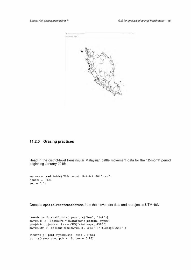
Spatial risk assessment using R GIS for analysis of animal health data • 146
11.2.5 Grazing practices
Read in the district-level Pensinsular Malaysian cattle movement data for the 12-month periodbeginning January 2015:
mymov <− read . table ( ”PMY cmovt d i s t r i c t 2015. csv ” ,header = TRUE,sep = ” , ” )
Create a spatialPointsDataframe from the movement data and reproject to UTM 48N:
coords <− S p a t i a l P o i n t s (mymov[ , c ( ” lon ” , ” l a t ” ) ] )mymov. l l <− Spat ia lPointsDataFrame ( coords , mymov)p r o j 4 s t r i n g (mymov. l l ) <− CRS( ” + i n i t =epsg :4326 ” )mymov. utm <− spTransform (mymov. l l , CRS( ” + i n i t =epsg :32648 ” ) )
windows ( ) ; plot ( mybord . shp , axes = TRUE)points (mymov. utm , pch = 16 , cex = 0.75)
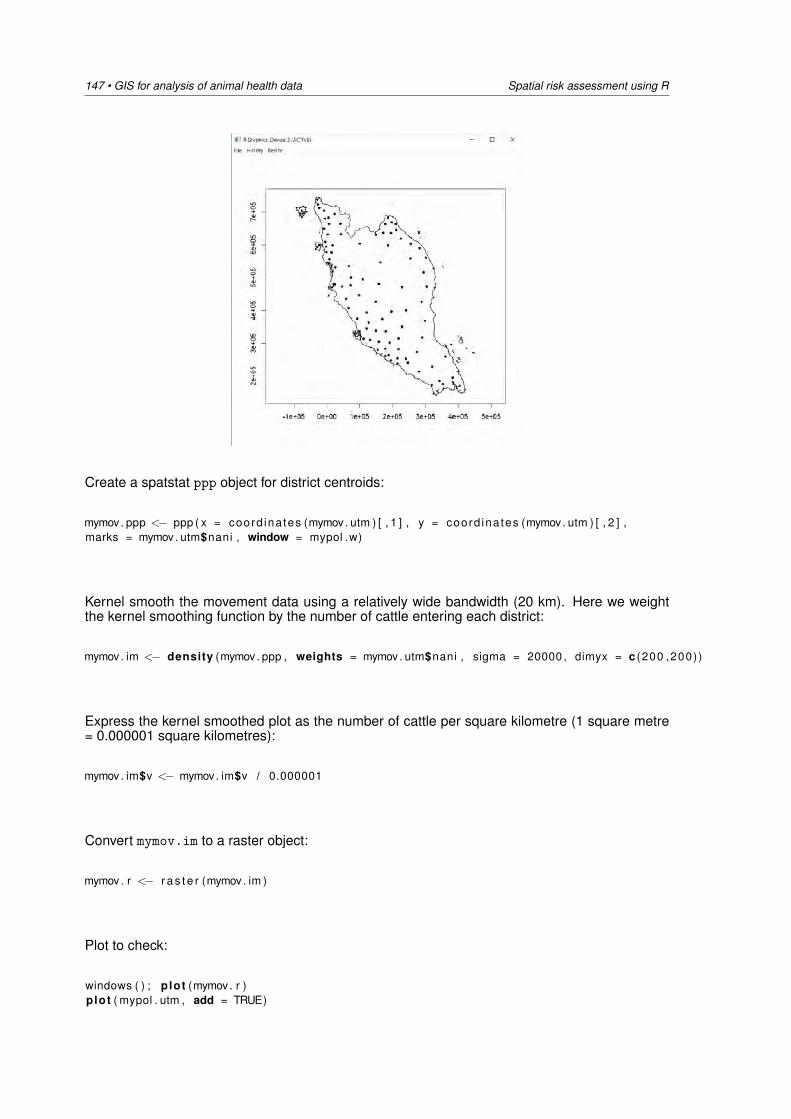
147 • GIS for analysis of animal health data Spatial risk assessment using R
Create a spatstat ppp object for district centroids:
mymov. ppp <− ppp ( x = coord ina tes (mymov. utm ) [ , 1 ] , y = coord ina tes (mymov. utm ) [ , 2 ] ,marks = mymov. utm$nani , window = mypol .w)
Kernel smooth the movement data using a relatively wide bandwidth (20 km). Here we weightthe kernel smoothing function by the number of cattle entering each district:
mymov. im <− density (mymov. ppp , weights = mymov. utm$nani , sigma = 20000 , dimyx = c (200 ,200) )
Express the kernel smoothed plot as the number of cattle per square kilometre (1 square metre= 0.000001 square kilometres):
mymov. im$v <− mymov. im$v / 0.000001
Convert mymov.im to a raster object:
mymov. r <− r a s t e r (mymov. im )
Plot to check:
windows ( ) ; plot (mymov. r )plot ( mypol . utm , add = TRUE)
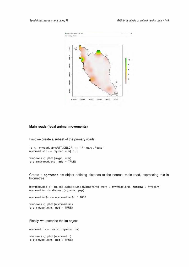
Spatial risk assessment using R GIS for analysis of animal health data • 148
Main roads (legal animal movements)
First we create a subset of the primary roads:
i d <− myroad . utm$RTT DESCRI == ” Primary Route ”mymroad . shp <− myroad . utm [ id , ]
windows ( ) ; plot ( mypol . utm )plot (mymroad . shp , add = TRUE)
Create a spatstat im object defining distance to the nearest main road, expressing this inkilometres:
mymroad . psp <− as . psp . Spat ialLinesDataFrame ( from = mymroad . shp , window = mypol .w)mymroad . im <− distmap (mymroad . psp )
mymroad . im$v <− mymroad . im$v / 1000
windows ( ) ; plot (mymroad . im )plot ( mypol . utm , add = TRUE)
Finally, we rasterise the im object:
mymroad . r <− r a s t e r (mymroad . im )
windows ( ) ; plot (mymroad . r )plot ( mypol . utm , add = TRUE)
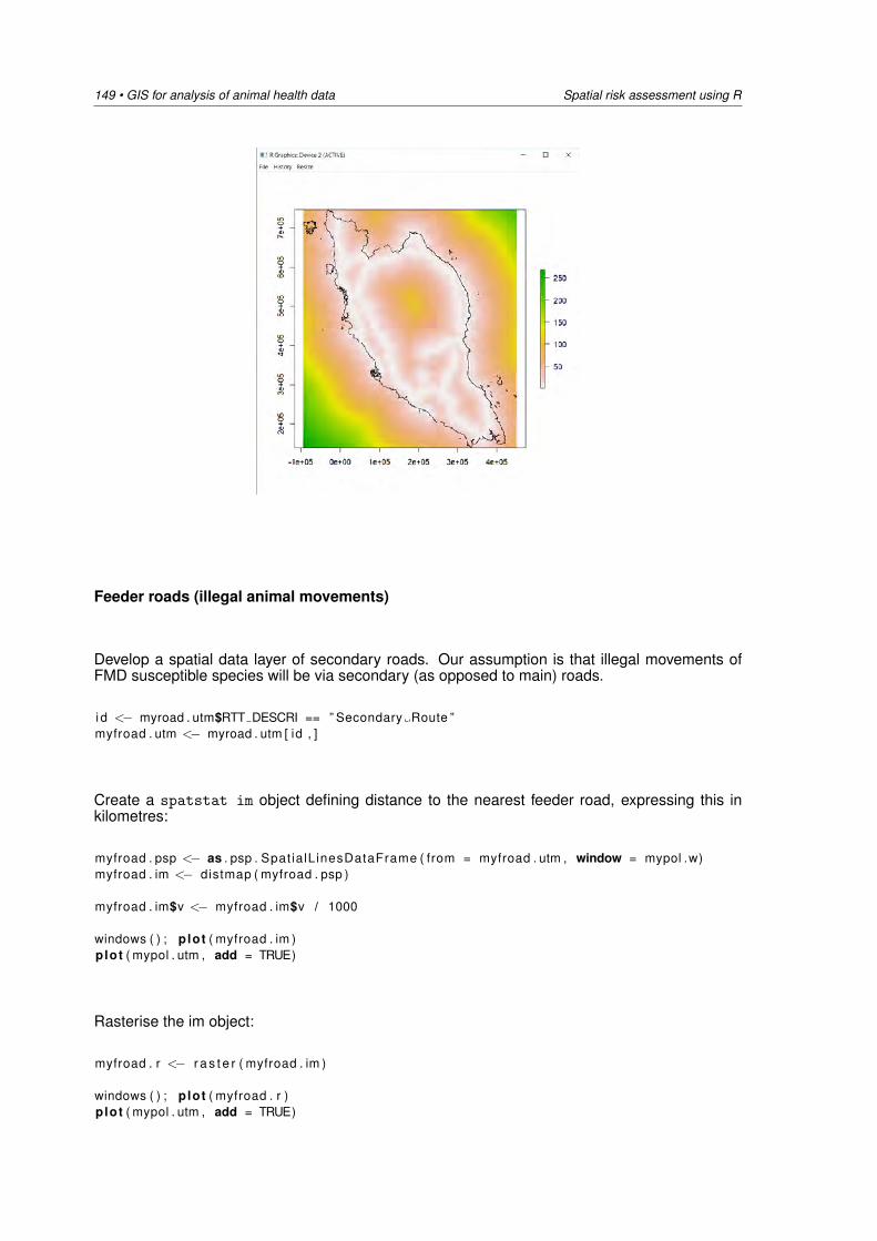
149 • GIS for analysis of animal health data Spatial risk assessment using R
Feeder roads (illegal animal movements)
Develop a spatial data layer of secondary roads. Our assumption is that illegal movements ofFMD susceptible species will be via secondary (as opposed to main) roads.
i d <− myroad . utm$RTT DESCRI == ” Secondary Route ”myfroad . utm <− myroad . utm [ id , ]
Create a spatstat im object defining distance to the nearest feeder road, expressing this inkilometres:
myfroad . psp <− as . psp . Spat ialLinesDataFrame ( from = myfroad . utm , window = mypol .w)myfroad . im <− distmap ( myfroad . psp )
myfroad . im$v <− myfroad . im$v / 1000
windows ( ) ; plot ( myfroad . im )plot ( mypol . utm , add = TRUE)
Rasterise the im object:
myfroad . r <− r a s t e r ( myfroad . im )
windows ( ) ; plot ( myfroad . r )plot ( mypol . utm , add = TRUE)
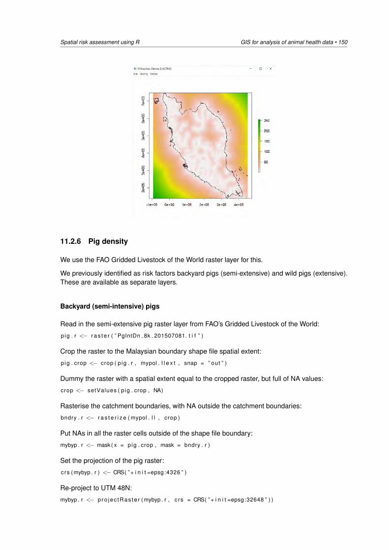
Spatial risk assessment using R GIS for analysis of animal health data • 150
11.2.6 Pig density
We use the FAO Gridded Livestock of the World raster layer for this.
We previously identified as risk factors backyard pigs (semi-extensive) and wild pigs (extensive).These are available as separate layers.
Backyard (semi-intensive) pigs
Read in the semi-extensive pig raster layer from FAO’s Gridded Livestock of the World:
p ig . r <− r a s t e r ( ” PgIntDn 8k 201507081. t i f ” )
Crop the raster to the Malaysian boundary shape file spatial extent:
p ig . crop <− crop ( p ig . r , mypol . l l e x t , snap = ” out ” )
Dummy the raster with a spatial extent equal to the cropped raster, but full of NA values:
crop <− setValues ( p ig . crop , NA)
Rasterise the catchment boundaries, with NA outside the catchment boundaries:
bndry . r <− r a s t e r i z e ( mypol . l l , crop )
Put NAs in all the raster cells outside of the shape file boundary:
mybyp . r <− mask ( x = p ig . crop , mask = bndry . r )
Set the projection of the pig raster:
crs ( mybyp . r ) <− CRS( ” + i n i t =epsg :4326 ” )
Re-project to UTM 48N:
mybyp . r <− pro jec tRas te r ( mybyp . r , c rs = CRS( ” + i n i t =epsg :32648 ” ) )
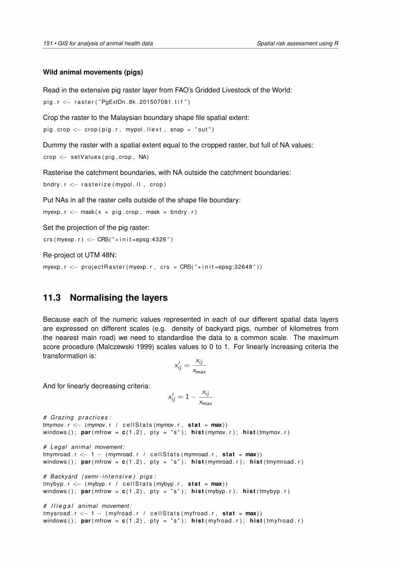
151 • GIS for analysis of animal health data Spatial risk assessment using R
Wild animal movements (pigs)
Read in the extensive pig raster layer from FAO’s Gridded Livestock of the World:
p ig . r <− r a s t e r ( ” PgExtDn 8k 201507081. t i f ” )
Crop the raster to the Malaysian boundary shape file spatial extent:
p ig . crop <− crop ( p ig . r , mypol . l l e x t , snap = ” out ” )
Dummy the raster with a spatial extent equal to the cropped raster, but full of NA values:
crop <− setValues ( p ig . crop , NA)
Rasterise the catchment boundaries, with NA outside the catchment boundaries:
bndry . r <− r a s t e r i z e ( mypol . l l , crop )
Put NAs in all the raster cells outside of the shape file boundary:
myexp . r <− mask ( x = p ig . crop , mask = bndry . r )
Set the projection of the pig raster:
crs ( myexp . r ) <− CRS( ” + i n i t =epsg :4326 ” )
Re-project ot UTM 48N:
myexp . r <− pro jec tRas te r ( myexp . r , c rs = CRS( ” + i n i t =epsg :32648 ” ) )
11.3 Normalising the layers
Because each of the numeric values represented in each of our different spatial data layersare expressed on different scales (e.g. density of backyard pigs, number of kilometres fromthe nearest main road) we need to standardise the data to a common scale. The maximumscore procedure (Malczewski 1999) scales values to 0 to 1. For linearly increasing criteria thetransformation is:
x ′i j =xi j
xmax
And for linearly decreasing criteria:x ′i j = 1−
xi jxmax
# Grazing p r a c t i c e s :tmymov . r <− (mymov. r / c e l l S t a t s (mymov. r , stat = max ) )windows ( ) ; par ( mfrow = c ( 1 , 2 ) , p ty = ” s ” ) ; hist (mymov. r ) ; hist ( tmymov . r )
# Legal animal movement :tmymroad . r <− 1 − (mymroad . r / c e l l S t a t s (mymroad . r , stat = max ) )windows ( ) ; par ( mfrow = c ( 1 , 2 ) , p ty = ” s ” ) ; hist (mymroad . r ) ; hist ( tmymroad . r )
# Backyard ( semi−i n t e n s i v e ) p igs :tmybyp . r <− ( mybyp . r / c e l l S t a t s ( mybyp . r , stat = max ) )windows ( ) ; par ( mfrow = c ( 1 , 2 ) , p ty = ” s ” ) ; hist ( mybyp . r ) ; hist ( tmybyp . r )
# I l l e g a l animal movement :tmysroad . r <− 1 − ( myfroad . r / c e l l S t a t s ( myfroad . r , stat = max ) )windows ( ) ; par ( mfrow = c ( 1 , 2 ) , p ty = ” s ” ) ; hist ( myfroad . r ) ; hist ( tmyfroad . r )
Spatial risk assessment using R GIS for analysis of animal health data • 152
# Wild animal movement :tmyexp . r <− ( myexp . r / c e l l S t a t s ( myexp . r , stat = max ) )windows ( ) ; par ( mfrow = c ( 1 , 2 ) , p ty = ” s ” ) ; hist ( myexp . r ) ; hist ( tmyexp . r )
11.4 Resampling of processed rasters
A spatial raster data set can be thought of as a data matrix with a defined number of rows andcolumns. Because our intent is to combine each of the risk factor data layers, it is important thatthey uniform in terms of the number of rows and columns. The GIS technique ‘resampling’ is theprocess used to align one raster data set with another. For this example we will re-sample eachof the input rasters to the dimensions of the tmymroad.r raster layer.
# Check the dimensions o f each r a s t e r i n tu rn and re−sample , i f necessary . What i s ther e s o l u t i o n o f the c a t t l e movement r a s t e r l aye r ?tmymov . r
# Answer : 200 200. Resample tmymov . r to match tmymroad . r :tmymov . rrtmymov . r <− resample ( x = tmymov . r , y = tmymroad . r , method = ” ngb ” )
# Legal animal movement . A l l OK.tmymroad . r
# Backyard ( semi−i n t e n s i v e ) p igs :tmybyp . rrtmybyp . r <− resample ( x = tmybyp . r , y = tmybcross . r , method = ” ngb ” )
# I l l e g a l animal movement . A l l OK.tmyfroad . r
# Wild animal movement :tmyexp . rrtmyexp . r <− resample ( x = tmyexp . r , y = tmybcross . r , method = ” ngb ” )
11.5 Multicriteria decision analysis (MCDA)
Read in the pairwise comparison responses from each of the 30 participants:
dat <− read . table ( ”SEACFMD i n c u r s i o n r i s k s . csv ” , header = TRUE, sep = ” , ” )
Create a matrix to capture the responses from each of the participants. Set row and columnnumber for each factor:
dat$row <− 0; dat$col <− 0
dat$row [ dat$ f a c t o r a == ” Grazing p r a c t i c e s ” ] <− 1dat$row [ dat$ f a c t o r a == ” Legal animal movements ” ] <− 2dat$row [ dat$ f a c t o r a == ” S w i l l feed ing ” ] <− 3dat$row [ dat$ f a c t o r a == ” I l l e g a l animal movements ” ] <− 4dat$row [ dat$ f a c t o r a == ” Wild animal movement ” ] <− 5
dat$col [ dat$ f a c t o r b == ” Grazing p r a c t i c e s ” ] <− 1dat$col [ dat$ f a c t o r b == ” Legal animal movements ” ] <− 2dat$col [ dat$ f a c t o r b == ” S w i l l feed ing ” ] <− 3dat$col [ dat$ f a c t o r b == ” I l l e g a l animal movements ” ] <− 4
153 • GIS for analysis of animal health data Spatial risk assessment using R
dat$col [ dat$ f a c t o r b == ” Wild animal movement ” ] <− 5
i d <− c ( ) ; count ry <− c ( ) ; factor <− c ( ) ; nmean <− c ( )
Loop through each of the responses provided by each of the 30 participants and, for each of thefive FMD incursion risk factors, calculate the REMBRANDT weights:
who <− unique ( dat$ i d )
for ( i i n 1 : length (who ) ){tmp <− subset ( dat , subset = i d == who [ i ] )
# Create a 5 * 5 mat r i x :r v a l <− data . frame ( matrix ( rep (0 , t imes = 25) , nrow = 5 ) )
for ( j i n 1 :nrow ( tmp ) ){r v a l [ tmp$row [ j ] , tmp$col [ j ] ] <− tmp$score [ j ]r v a l [ tmp$col [ j ] , tmp$row [ j ] ] <− −tmp$score [ j ]
}
colnames ( r v a l ) <− c ( ” graz ” , ” lmov ” , ” s w i l l ” , ” imov ” , ” w i l d ” )rownames ( r v a l ) <− c ( ” graz ” , ” lmov ” , ” s w i l l ” , ” imov ” , ” w i l d ” )
# Gamma t rans fo rma t i on :r v a l <− exp ( r v a l * log ( 2 ) )
# Take the geometr ic mean of each row :r v a l $gmean <− apply ( r va l , MARGIN = 1 , FUN = function ( x ) geometr ic .mean( x ,na . rm = TRUE) )
# Normalise the data :r v a l $nmean <− r v a l $gmean / sum( r v a l $gmean)
i d <− c ( id , who [ i ] )count ry <− c ( country , as . character ( tmp$count ry [ 1 ] ) )factor <− c ( factor , rownames ( r v a l ) )nmean <− c (nmean , r v a l $nmean)
}
r v a l <− data . frame ( id , country , factor , nmean , rank )r v a l $ factor <− factor ( r v a l $factor , labels = c ( ” Grazing p r a c t i c e s ” , ” I l l e g a lanimal movements ” , ” Legal animal movements ” , ” S w i l l feed ing ” , ” Wild animalmovement ” ) )
Make a box and whisker plot showing the distribution of REMBRANDT weights for each FMDincursion risk factor:
windows ( ) ; ggp lo t ( data = rva l , aes ( x = factor , y = nmean ) ) +geom boxplot ( width = 0.25) +x lab ( ” I ncu rs ion r i s k f a c t o r ” ) +y lab ( ” Re la t i ve weight ” ) +geom j i t t e r ( width = 0 .1 ) +coord f l i p ( )
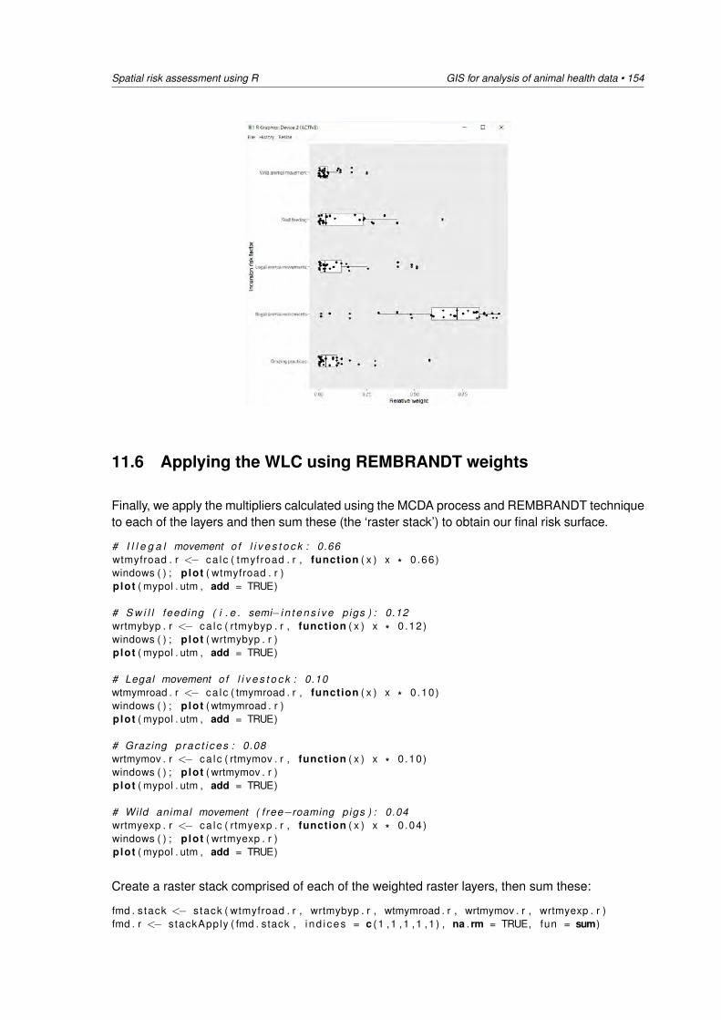
Spatial risk assessment using R GIS for analysis of animal health data • 154
11.6 Applying the WLC using REMBRANDT weights
Finally, we apply the multipliers calculated using the MCDA process and REMBRANDT techniqueto each of the layers and then sum these (the ‘raster stack’) to obtain our final risk surface.
# I l l e g a l movement o f l i v e s t o c k : 0.66wtmyfroad . r <− ca lc ( tmyfroad . r , function ( x ) x * 0.66)windows ( ) ; plot ( wtmyfroad . r )plot ( mypol . utm , add = TRUE)
# S w i l l feed ing ( i . e . semi−i n t e n s i v e p igs ) : 0.12wrtmybyp . r <− ca lc ( rtmybyp . r , function ( x ) x * 0.12)windows ( ) ; plot ( wrtmybyp . r )plot ( mypol . utm , add = TRUE)
# Legal movement o f l i v e s t o c k : 0.10wtmymroad . r <− ca lc ( tmymroad . r , function ( x ) x * 0.10)windows ( ) ; plot ( wtmymroad . r )plot ( mypol . utm , add = TRUE)
# Grazing p r a c t i c e s : 0.08wrtmymov . r <− ca lc ( rtmymov . r , function ( x ) x * 0.10)windows ( ) ; plot ( wrtmymov . r )plot ( mypol . utm , add = TRUE)
# Wild animal movement ( f ree−roaming pigs ) : 0.04wrtmyexp . r <− ca lc ( rtmyexp . r , function ( x ) x * 0.04)windows ( ) ; plot ( wrtmyexp . r )plot ( mypol . utm , add = TRUE)
Create a raster stack comprised of each of the weighted raster layers, then sum these:
fmd . s tack <− stack ( wtmyfroad . r , wrtmybyp . r , wtmymroad . r , wrtmymov . r , wrtmyexp . r )fmd . r <− stackApply ( fmd . stack , i nd i ces = c (1 ,1 ,1 ,1 ,1 ) , na . rm = TRUE, fun = sum)
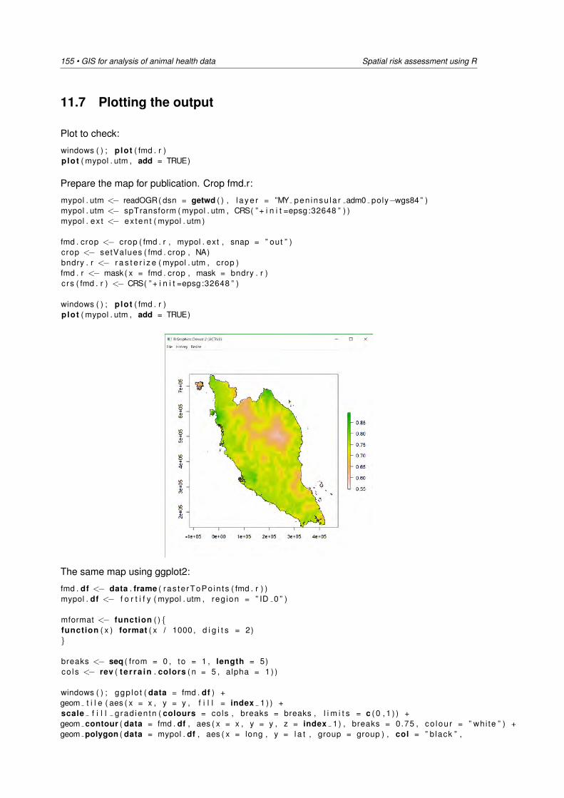
155 • GIS for analysis of animal health data Spatial risk assessment using R
11.7 Plotting the output
Plot to check:
windows ( ) ; plot ( fmd . r )plot ( mypol . utm , add = TRUE)
Prepare the map for publication. Crop fmd.r:
mypol . utm <− readOGR( dsn = getwd ( ) , l a ye r = ”MY pen insu la r adm0 poly−wgs84 ” )mypol . utm <− spTransform ( mypol . utm , CRS( ” + i n i t =epsg :32648 ” ) )mypol . ex t <− ex ten t ( mypol . utm )
fmd . crop <− crop ( fmd . r , mypol . ext , snap = ” out ” )crop <− setValues ( fmd . crop , NA)bndry . r <− r a s t e r i z e ( mypol . utm , crop )fmd . r <− mask ( x = fmd . crop , mask = bndry . r )c rs ( fmd . r ) <− CRS( ” + i n i t =epsg :32648 ” )
windows ( ) ; plot ( fmd . r )plot ( mypol . utm , add = TRUE)
The same map using ggplot2:
fmd . df <− data . frame ( ras te rToPo in ts ( fmd . r ) )mypol . df <− f o r t i f y ( mypol . utm , reg ion = ” ID 0 ” )
mformat <− function ( ){function ( x ) format ( x / 1000 , d i g i t s = 2)}
breaks <− seq ( from = 0 , to = 1 , length = 5)co ls <− rev ( t e r ra in . colors ( n = 5 , alpha = 1 ) )
windows ( ) ; ggp lo t ( data = fmd . df ) +geom t i l e ( aes ( x = x , y = y , f i l l = index 1 ) ) +scale f i l l g rad ien tn ( colours = cols , breaks = breaks , l i m i t s = c ( 0 , 1 ) ) +geom contour ( data = fmd . df , aes ( x = x , y = y , z = index 1) , breaks = 0.75 , co lour = ” whi te ” ) +geom polygon ( data = mypol . df , aes ( x = long , y = l a t , group = group ) , col = ” b lack ” ,
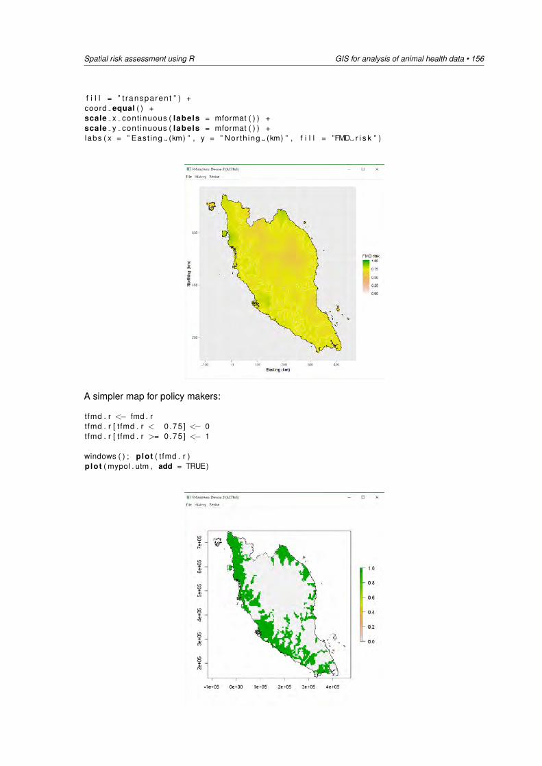
Spatial risk assessment using R GIS for analysis of animal health data • 156
f i l l = ” t ransparen t ” ) +coord equal ( ) +scale x cont inuous ( labels = mformat ( ) ) +scale y cont inuous ( labels = mformat ( ) ) +labs ( x = ” East ing (km) ” , y = ” Nor th ing (km) ” , f i l l = ”FMD r i s k ” )
A simpler map for policy makers:
t fmd . r <− fmd . rt fmd . r [ t fmd . r < 0 .75 ] <− 0tfmd . r [ t fmd . r >= 0 .75 ] <− 1
windows ( ) ; plot ( t fmd . r )plot ( mypol . utm , add = TRUE)
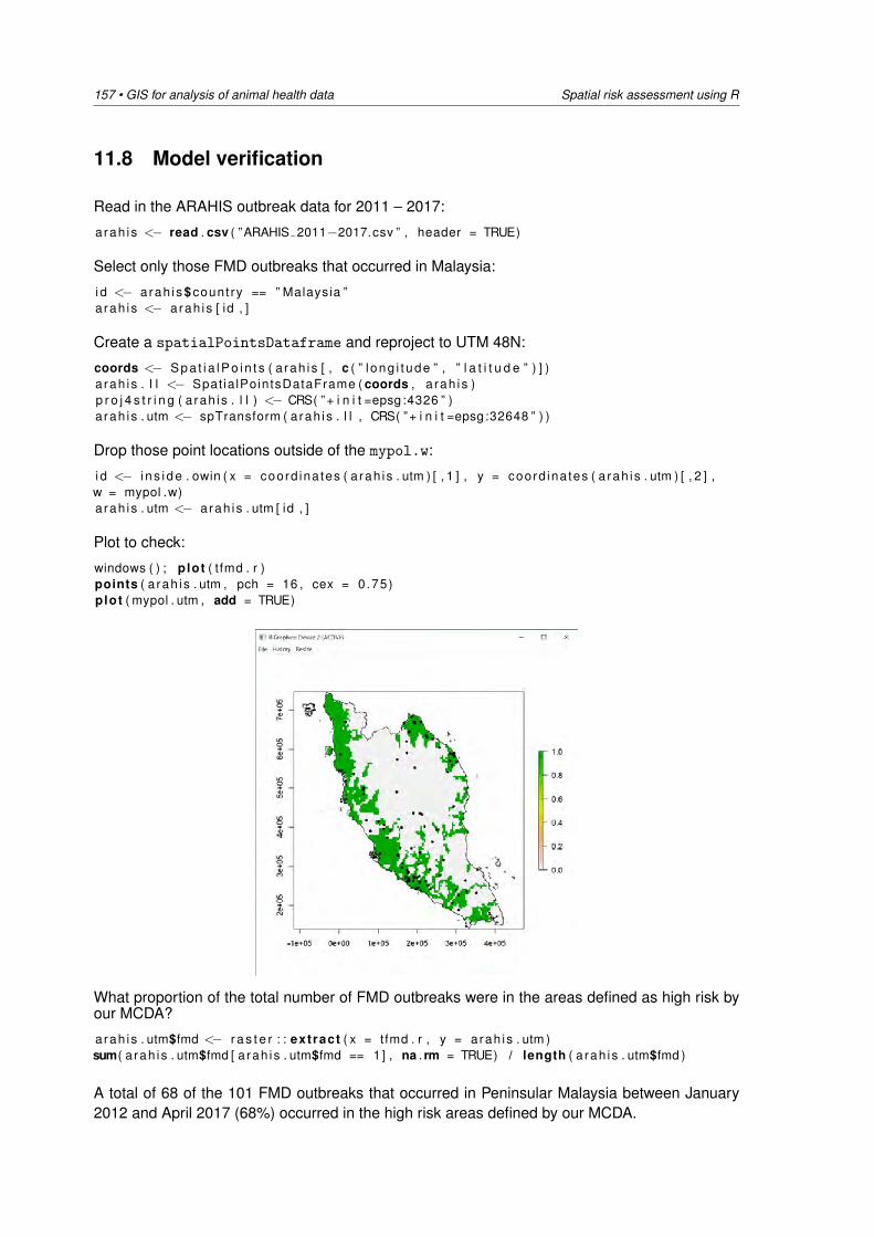
157 • GIS for analysis of animal health data Spatial risk assessment using R
11.8 Model verification
Read in the ARAHIS outbreak data for 2011 – 2017:
arah is <− read . csv ( ”ARAHIS 2011−2017.csv ” , header = TRUE)
Select only those FMD outbreaks that occurred in Malaysia:
i d <− arah is $count ry == ” Malaysia ”a rah is <− arah is [ id , ]
Create a spatialPointsDataframe and reproject to UTM 48N:
coords <− S p a t i a l P o i n t s ( a rah is [ , c ( ” l ong i t ude ” , ” l a t i t u d e ” ) ] )a rah is . l l <− Spat ia lPointsDataFrame ( coords , a rah is )p r o j 4 s t r i n g ( a rah is . l l ) <− CRS( ” + i n i t =epsg :4326 ” )a rah is . utm <− spTransform ( arah is . l l , CRS( ” + i n i t =epsg :32648 ” ) )
Drop those point locations outside of the mypol.w:
i d <− i n s i d e . owin ( x = coord ina tes ( a rah is . utm ) [ , 1 ] , y = coord ina tes ( a rah is . utm ) [ , 2 ] ,w = mypol .w)a rah is . utm <− arah is . utm [ id , ]
Plot to check:
windows ( ) ; plot ( t fmd . r )points ( a rah is . utm , pch = 16 , cex = 0.75)plot ( mypol . utm , add = TRUE)
What proportion of the total number of FMD outbreaks were in the areas defined as high risk byour MCDA?
arah is . utm$fmd <− r a s t e r : : extract ( x = tfmd . r , y = arah is . utm )sum( a rah is . utm$fmd [ a rah is . utm$fmd == 1 ] , na . rm = TRUE) / length ( a rah is . utm$fmd )
A total of 68 of the 101 FMD outbreaks that occurred in Peninsular Malaysia between January2012 and April 2017 (68%) occurred in the high risk areas defined by our MCDA.

Investigation of spatial clustering in R GIS for analysis of animal health data • 158
12 Practical 6. Investigation of spatialclustering in R
12.1 Preliminaries and acknowledgements
12.1.1 R software set-up
The setup for analysis in this document uses a “Project” in “RStudio” . RStudio is a softwareinterface to R, that is, R is opened when you open R Studio and you interact with R throughRStudio. RStudio provides tools for working with R which help the analyst in many ways, includingproviding “Projects” to aid file organisation.
File organisation and folder structure is a personal preference, but a basic structure with informa-tive names which suits many purposes is:
• “MyProjectName” folder– “Code” sub folder– “Data” sub folder– “Docs” sub folder
This structure will work with the following code for accessing the data that are provided below.(Note that the sub folders are all on the same “level”).
Create a new project in the following steps:
1. Open R studio
2. Click in on “File- New Project. . . ”
3. Choose to create a “New Directory” if none already exists, or “Existing Directory” if onealready exists (for example, the “Code” directory)
4. Browse to and create a new directory, or just browse to the directory you want, and thenclick “Create Directory”
Create a new .R file from which you run your code, and save and name it appropriately e.g.“MyRFile.R” (you must add the “.R” extension manually). R code is identified in the shaded rows,and can be copied from this PDF into the upper left window in R Studio, and run from there.
Note that code or text which is preceded on a line with a “#” character is ignored by R. Thesecomments are used to organise the structure of the exercises and briefly explain what is hap-pening to aid understanding. Some code is commented out for the sake of brevity, but you areencouraged to run these (and create your own in addition) to aid your understanding.

159 • GIS for analysis of animal health data Investigation of spatial clustering in R
The data for the exercises first needs to be copied into the directory chosen to store it (“Data” inthis case). You are now ready to go.
R packages and base R itself, are frequently updated. The authors do this to fix bugs and addnew features, which is great. Unfortunately, sometimes the code in the updates “breaks” old codethat previously worked. Therefore, if your versions of R or the packages used in the following codeeither predate those used to produce the accompanying exercises, or sometime in the future ifyou return to these code and they don’t work, then one reason for the problem may be that thesoftware versions don’t match. If you can’t fix the problem, you can install the versions that aredefined in 2.4 at the end of the last content chapter.
12.1.2 Exercises and getting on-line help
Alongside the notes are exercises and questions to check the student’s understanding of theprinciples and application of the learnt methods. Additional “extension” exercise are available todevelop further skills and understanding.
You are encouraged to use the ‘help’ resources in R to understand the functions. If the functionused are in packages loaded at the start of the exercise (using the ‘library’ function), then simplytyping “?function-name” in the “Console” screen (usually lower left screen in R Studio) will bringup the help page for that function in the “Help” tab (usually lower right window in R Studio).When R functions are referred to in this document, the package in which they are located isindicated first, followed by a colon (:), and then the function name, for example ‘graphics::plot’.Cited references and additional other helpful resources for learning spatial epidemiology at theintroductory level are found the Bibliography at the end of this document.
12.1.3 Data sets used with these notes and exercises
Extensive use is made of different data sets in the exercises. These data are from three mainsources- R packages, other public on-line sources, and from previous spatial epidemiology orGIS course. The data from R packages are simply imported into the work space by loadingthe relevant library with the ‘library’ function, then using the ‘data’(data set name) function. Anexplanation of how the data were obtained and a description of the fields is available by usingthe ‘help?’ function as previously described, with the name of the data set in parentheses be-side it. These data are from a variety of scientific fields, with a few human and animal healthexamples.
The second group of data sets was obtained from the website for the book “Veterinary Epidemio-logic Research” (Dohoo, Martin, and Stryhn 2009) and relate to the relevant Chapters 25 and 26.These data represent the results of surveillance for avian influenza (AI) between 2004 and 2006in a region in northern Vietnam, extracted from a larger data set of the whole country, and carrythe prefix “viet” in their. Several spatial data sets are available for different administrative levels,including coordinates of communes (actually the centroids of their areas) and attribute data onwhether or not the commune experienced one or more outbreak of AI in the surveillance period.Further information on these data are available in Pfeiffer et al. (2007)
Finally, we borrow from other datasets used in a previous course which is acknowledged below.The “cheshire” data set contains locations of farms and dates of infection with foot-and-mouthdisease in the 2001 outbreak in the UK county of that name. The Scottish lip cancer data set
Investigation of spatial clustering in R GIS for analysis of animal health data • 160
(“SC lip cancer”) consists of spatial polygon files of the districts in that country, and attributes ofthe number of cases of that cancer and the population in each district.
The exercises are designed to introduce methods and stimulate your thinking about them. Theyare not complete analyses in themselves, and may not even be the best or only approach to theanalytical problem. A deeper understand than can be taught in a course can only come frompracticing the methods and further reading on the subjects, and better still conducting your ownresearch!
12.1.4 Acknowledgements
Many of the data exercises (and material for the accompanying presentation) originate from MarkStevenson’s comprehensive notes “Investigation of Spatial Patterns of Animal Disease” providedfor the Introductory Spatial Epidemiology course in “118.817 Advanced analysis of epidemiologicdata” held at Massey University 13 - 17 Nov 2017, and I want to acknowledge his work that hascontributed to these notes.
References
Dohoo, I., W. Martin, and H. Stryhn. 2009. Veterinary Epidemiologic Research. 2nd ed. AtlanticVeterinary College Inc., Charlottetown, Canada.
Pfeiffer, D.U., P.Q. Minh, V. Martin, M. Epprecht, and M.J. Otte. 2007. “An Analysis of theSpatial and Temporal Patterns of Highly Pathogenic Avian Influenza Occurrence in Vietnam UsingNational Surveillance Data.” Veterinary Journal 174 (2): 302–9. https://doi.org/10.1016/j.tvjl.2007.05.010.
12.2 Investigation of spatial clustering in R
12.2.1 Background and definitions
Investigation of possible clusters of disease is a core role of epidemiologists that aims to provideinformation on the causes of disease and means for it’s control and prevention. Analysis ofthe spatial and temporal patterns of disease occurrence provide a quantitative description ofthe apparent problem and possible new insights into the cause of the disease that might haveotherwise been unnoticed with other methods.
Many factors may determine the spatial distribution of disease occurrence, such as the densityand species of animal populations, movement and trade in these populations, geographic andclimatic factors that affect the animals, their environment or disease vector species, or existingdisease control programmes. Due consideration of these factors is important when applyingmethods to evaluate clustering of disease.
The history of methods to detect clusters of disease has grown since the 1980’s out of increasedconcerns about actual or potential adverse environmental effects on public health, for examplefrom nuclear power stations. However, many diseases will show geographic (and possibly tem-poral) clustering for other reasons that are associated with the disease, and not the one postu-lated. Hence, in some situations diseases may appear to cluster, even when the known aetiologydoesn’t suggest it should be observed.

161 • GIS for analysis of animal health data Investigation of spatial clustering in R
Reasons for studying disease clustering:
• In epidemiological study of aetiology of disease• In public/population health disease surveillance• In response to disease cluster (outbreak) alarms to evaluate whether further investigations
are warranted
In each setting, it is important to account for the population at risk in the study, as the distributionof cases may just reflect the underlying population distribution.
Study of disease aetiology
Differential disease rates in large scale or localised geographic areas have long been used tostudy disease aetiology. The same methods can be used to detect areas with high rates ofdisease in which to conduct further epidemiologic studies (especially cohort studies for whichit is important to enrol subjects with a relatively increased risk of disease to achieve sufficientstatistical power in a cost-efficient way).
A key feature of these methods for purely spatial or space-time data is that they are able topinpoint the location of clusters. However, the interest may alternatively be in general nature ofdistribution of disease, for example, to understand whether the disease is likely to be infectious(may exhibit both space-time interaction and spatial clustering), or has risk factors that vary ge-ographically (only spatial clustering). When assessing the association between geographic riskvariables and disease risk in an ecological analysis, it is important to adjust for any spatial auto-correlation not explained by the known variables. When individual subject exposure is unavailableor unknown, focused cluster tests can be used to move from pure hypothesis to established riskfactors and the conduct of further epidemiologic studies.
Population surveillance
The detection of clusters of disease with known risk factors may prompt a public health responsewhere those factors can be reduced or removed, for example from water-borne diseases or en-vironmental pollution. Additionally, geographic areas with high mortality rates may be searchedfor, and adjustment made for the distribution of incidence instead of the population at risk, tothereby identify areas of substandard treatment or screening. Alternatively, areas of reduced riskmay indicate successful treatment or screening programmes from which others can learn, or theymay alternately reflect areas of under-reporting of cases.
Response to disease cluster alarms
These are more commonplace in the human public health setting, for example for leukemia in-cidence around nuclear power stations, or clusters of cases of swine flu (in humans) in 2009 oroutbreaks of meningitis.
Definitions of clustering
• When the exact extent or form of the clusters to be studied are unknown, a cluster is:– ” a geographically bounded group of occurrences of sufficient size and concentration
to be unlikely to have occurred by chance” (Knox 1989 cited in @Lawson1999)

Investigation of spatial clustering in R GIS for analysis of animal health data • 162
– or less formally- an area within the study region of significant elevated risk– also known as a ‘hot-spot’
• When the extent or form of the cluster has been previously defined, a cluster occurs when– the study region displays a pre-specified cluster structure
Other relevant statistical concepts
• A spatial process is stationary when the dependence between measurements of the same(outcome) variable is the same for all locations in the study area
• A spatial process is isotropic when it is affected by distance from a location, but the effectis the same in all directions
• A first-order effect describes large-scale variations in the mean of the same variable acrossthe study region
• A second-order effects describes small-scale variation due to interactions between neigh-bours
12.2.2 Methods to investigate clustering of disease
A range of methods exist to investigate spatial and temporal clustering of disease because ofthe various data types that might be obtained from epidemiologic studies, and because no singlemethod is clearly superior to the alternatives. Cluster evaluation methods are clearly useful toassess whether an excess of cases have occurred to inform further responses. However, severalproblems are likely to be met when attempting to evaluate clustering:
• Cases of disease may be rare or distributed over an extended period of time, which meansthat they may not be detected
• Information on the population at risk may be unavailable or of poor quality• The background occurrence of disease in the population may be unknown
The types of clustering methods have been defined by Besag and Newell (1991) andTango (1999):
• General, global or non-specific clustering detection methods– An analysis of the overall clustering tendency of a disease in a study region, regard-
less of where that clustering is located– Analogous to assessment of autocorrelation– Assesses the overall or global aspects of clustering– These methods do not estimate the spatial locations of clusters– Assumes that the disease process is the same (stationary) throughout the study re-
gion and therefore give no indication of local variability of clustering– Most easily interpreted when applied to regions where the factors that determine dis-
ease occurrence are relatively uniform• Localised non-focused spatial cluster detection methods
– Aim to define the location and intensity of any clusters if they exist• Localised focused spatial cluster detection methods
– Examine clusters of pre-defined characteristics and their extent around a pre-determined focus point
– Examples of focused local clustering methods are mainly from putative sources ofhealth hazard for humans from environmental contamination, but can be applied in

163 • GIS for analysis of animal health data Investigation of spatial clustering in R
the veterinary setting, for example with infectious diseases to putative sources suchas livestock markets or transport routes
It is important to consider the structure of hypotheses that could include clustering componentsin any analysis of geographic health data. If the disease of interest naturally clusters (beyondthat explained by the background population), then this form of clustering should be investigated.This form of clustering may arise from unobserved covariates and should be considered as het-erogeneity, and can often be modeled through the use of random effects. Additionally, closeattention needs to be paid to the assumptions and methods of the models to verify that they areappropriate for the study data and research question. In particular, when optional parametersneed to be specified for the method, these should be chosen a priori on the basis of the biologyof the disease being studied and possibly also on what other authors have published, so as not to‘adjust’ the method to obtain a pre-determined result. Unfortunately, guidance in the literature isnot always available or clear for each situation the analyst encounters, so these methods shouldbe used with caution.
Global methods to investigate clustering or autocorrelation
Ripley’s K-function difference
• Spatial data: Point• Data needed: Coordinates of point locations of cases and controls (or population at risk)• How test works:
– Calculates the number of events of the same type occurring within a certain distanceof a randomly-chosen case
– When spatial autocorrelation is present then events of the same type are likely to be incloser proximity to one another, and for small distances, K will be larger than expected
– Assumes a stationary point process and that the direction to neighbour does not affectthe spatial process (isotropy), but options exist is software for inhomogenous pointprocess data
– Reflects the second-order effects of a spatial process– Edge effects can be adjusted with a choice of methods– Because the variance of the K function increases with distance, it is recommended
that the pre-defined distance scale for the function is no more than one third of thelinear extent of the study area or half the length of the shorter side of the rectangularstudy area
– Therefore this test is most suitable for testing clustering over a relatively small extentof the study region
– Spatial heterogeneity of population at risk (or controls) is accounted for by use of adifference function (cases - controls)
– Results are visualised in a plot of the K against distance, which should have aparabola shape if process CSR
* Expresses the scaled expected number of excess cases occurring at a givendistance from a random case
* Significance of difference tested by Monte Carlo simulation which also allowsstatistical inference in presence of non-stationarity
* Any deviation of the difference function above the envelope formed by the upperand lower bounds of the expected difference indicates significant clustering ofcases
Investigation of spatial clustering in R GIS for analysis of animal health data • 164
– Difference function also estimates the spatial extent or distance over which clusteringoccurs, but the extent must be small in relation to the whole study region
• References: Ripley (1977), Diggle and Chetwynd (1991), Waller and Gotway (2004)
Ex 6.1
## K-function difference library(smacpod) data(grave) # load data levels(grave$marks) # checklevels of marks attribute to ensure that cases are correctly ordered plot(grave) kd1 = kdest(grave)plot(kd1, iso ˜ r, ylab = “difference”, legend = FALSE, main = “”) kd2 = kdest(grave, nsim = 99,level = 0.8) # Simulate to create envelope plot(kd2, ylim = c(-2e+06, 6e+06), legend = TRUE)## The two bands are each for the minimum and maximum differences between the cases andcontrols, ## respectively ## Statistical test for clustering using difference in K functions pval <-kdplus.test(kd2) pval$pvalue detach(package:smacpod)
Q 6.1 How would you interpret the test result? Does it agree with your first visual impression ofthe data in the plot? Is there evidence in the data of clustering of cases, and over what range ofdistances?
A “by hand” calculation of the K-function difference from previous the previous K-function exerciseusing epi.incin data is shown below. The explicit steps help understand how the test works
##For bivariate data, estimate separate point patterns for cases and controls ## and calculatethe difference of the K-functions ## Peaks or troughs in the plot above or below the simula-tion confidence envelope ## are evidence of clustering or regularity, respectively data(epi.incin);dat.df <- epi.incin dat.df$status <- factor(dat.df$status, levels = c(0,1), labels = c(“Neg”, “Pos”))names(dat.df)[3] <- “Status” dat.w <- convexhull.xy(x = dat.df[,1], y = dat.df[,2]) dat.w <- di-lation(dat.w, r = 1000) coords <- matrix(c(dat.w$bdry[[1]]$x, dat.w$bdry[[1]]$y), ncol = 2, by-row = FALSE) pol <- Polygon(coords, hole = FALSE) pol <- Polygons(list(pol),1) pol <- Spa-tialPolygons(list(pol)) pol.spdf <- SpatialPolygonsDataFrame(Sr = pol, data = data.frame(id =1), match.ID = TRUE) pol.map <- fortify(pol.spdf) dat.ppp <- ppp(x = dat.df[,1], y = dat.df[,2],marks = factor(dat.df[,3]), window = dat.w) ## Estimate the area of the study region: lenx <-max(dat.df$xcoord) - min(dat.df$xcoord); lenx leny <- max(dat.df$ycoord) - min(dat.df$ycoord);leny ## The study area is 17960 x 16550 metres. Compute the K-function and plot it: r <-seq(from = 0, to = 1000, by = 10) pos.kenv <- envelope(split(dat.ppp)$Pos, fun = Kest, r = r,nrank = 2, nsim = 99, verbose = FALSE) neg.kenv <- envelope(split(dat.ppp)$Neg, fun = Kest,r = r, nrank = 2, nsim = 99, verbose = FALSE) pos.ggplot <- ggplot(data = pos.kenv, aes(x =r, y = obs)) + geom line() + geom ribbon(aes(ymin = lo, ymax = hi), colour = “#cccccc”, alpha= 0.25) + geom line(data = pos.kenv, aes(x = r, y = theo), col = “red”, linetype = “dashed”) +ylab(“K(r)”) + theme(aspect.ratio = 1) neg.ggplot <- ggplot(data = neg.kenv, aes(x = r, y = obs))+ geom line() + geom ribbon(aes(ymin = lo, ymax = hi), colour = “#cccccc”, alpha = 0.25) +geom line(data = neg.kenv, aes(x = r, y = theo), col = “red”, linetype = “dashed”) + ylab(“K(r)”) +theme(aspect.ratio = 1) grid.arrange(pos.ggplot, neg.ggplot, ncol = 2) kdif.spat <- data.frame(r =r, obs = pos.kenv$obs - neg.kenv$obs, theo = pos.kenv$theo - neg.kenv$theo, lo = pos.kenv$lo -neg.kenv$lo, hi = pos.kenv$hi - neg.kenv$hi) ## Plot the results: ggplot(data = kdif.spat, aes(x =r, y = obs)) + geom line() + geom ribbon(aes(ymin = lo, ymax = hi), colour = “#cccccc”, alpha =0.25) + geom hline(yintercept = 0, linetype = 2) + ylim(-3E06, 3E06) + labs(x = “Distance (m)”, y= “K-function difference”)
Extension exercise 6.1
## Load Vietnam AI data library(foreign); library(sp); library(spatstat) library(ggplot2); li-brary(ggforce); library(smacpod) commune.d <- read.dta(“..//Data//commune-d.dta”) dat.c.all.df<- data.frame(xcoord = commune.d$x coord, ycoord = commune.d$y coord, status = com-
165 • GIS for analysis of animal health data Investigation of spatial clustering in R
mune.d$infected) dat.c.all.df$status <- factor(dat.c.all.df$status, levels = c(“No”, “Yes”), la-bels = c(“Neg”, “Pos”)) summary(dat.c.all.df) ## Create observation window dat.c.all.w <-convexhull.xy(x = dat.c.all.df$xcoord, y = dat.c.all.df$ycoord) dat.c.all.w <- dilation(dat.c.all.w,r = 1) ## Create a ppp objects for positive and negative communes: pos.ppp <- ppp(x= dat.c.all.df$xcoord[dat.c.all.df$status == “Pos”], y = dat.c.all.df$ycoord[dat.c.all.df$status ==“Pos”], window = dat.c.all.w) neg.ppp <- ppp(x = dat.c.all.df$xcoord[dat.c.all.df$status == “Neg”],y = dat.c.all.df$ycoord[dat.c.all.df$status == “Neg”], window = dat.c.all.w) ## Plot data coords <-matrix(c(dat.c.all.w$bdry[[1]]$x, dat.c.all.w$bdry[[1]]$y), ncol = 2, byrow = FALSE) pol <- Poly-gon(coords, hole = FALSE) pol <- Polygons(list(pol),1) pol <- SpatialPolygons(list(pol)) pol.spdf<- SpatialPolygonsDataFrame(Sr = pol, data = data.frame(id = 1), match.ID = TRUE) pol.map<- fortify(pol.spdf) g <- ggplot() + geom point(data = dat.c.all.df, aes(x = xcoord, y = ycoord,colour = status, shape = status), alpha = 0.5) + geom polygon(data = pol.map, aes(x = long, y =lat, group = group), col = “black”, fill = “transparent”) + scale shape manual(values = c(1, 16)) +scale colour manual(values = c(“royalblue”, “red”)) + labs(x = “Easting (km)”, y = “Northing (km)”,fill = “status”) + coord equal() g ## Combine positive and negative communes com.ppp <- ppp(x= dat.c.all.df$xcoord, y = dat.c.all.df$ycoord, window = dat.c.all.w, marks = dat.c.all.df$status)levels(com.ppp$marks) # check levels of marks attribute to ensure that cases are correctly or-dered # plot(com.ppp) Uninformative because of over-plotting ## Run K difference test kd1 =kdest(com.ppp) plot(kd1, iso ˜ r, ylab = “difference”, legend = FALSE, main = “”) # Simulate tocreate envelope- use only 19 sims to shorten processing time kd2 = kdest(com.ppp, nsim = 19,level = 0.8) plot(kd2, legend = TRUE) ## The two bands are each for the minimum and maximumdifferences between the cases and controls, ## respectively ## Statistical test for clustering usingdifference in K functions pval <-kdplus.test(kd2) pval$pvalue
Cuzick-and-Edwards’ k-nearest neighbour test
• Spatial data: Point• Data needed: Coordinates of point locations of cases and controls• How test works:
– Accounts for heterogeneous distribution of population at risk by comparing co-ordinates of cases and controls
– Requires a pre-determined scale parameter k which defines the number of nearest-neighbours (may be > 1)
– Null hypothesis is that nearest neighbour to a randomly-selected case is just as likelyto be a control as another case
– Test statistic is number of cases that are nearest neighbours to each individual case-when cases are clustered, the nearest neighbour to a case will tend to be near toanother case
– Assumes controls were randomly selected from same source population as cases– If controls are selected on basis of potential confounding variables (for example by
matching) then their effect can be adjusted for– May also be used with aggregated areal data
• References: Cuzick and Edwards (1990)
## Cuzick-and-Edward’s k-nearest neighbour test—- qnn.test(com.ppp, q = 1:5) # Search up to5 nearest neighbours detach(package:smacpod)
Extn. Q 6.1 Is their evidence of spatial clustering of cases in this data set, and over what dis-tances? Do the test results agree?
Investigation of spatial clustering in R GIS for analysis of animal health data • 166
Moran’s I test for autocorrelation Spatial data: Areal data with continuous or ordinal attributeData needed: Areal aggregated data, neighbour matrix (optionally with weights) How test works:- Commonly-used test for global clustering - Originally developed for event counts within sub-regions, but typically used now with standardised measures such as rates because of differencesin sizes of populations at risk in different sub-regions - Can also be applied to Bernoulli (0/1) dataand residuals from a regression model - Assesses the similarity between pairs in their deviationfrom the global mean - Neighbouring values that are similar result in a positive I, and conversely ifdifferent, I is negative - A positive value of I implies clustering, and a negative value dispersion orrepulsion - The expected value of I is 1/(N1) 1 / ( N 1 ) where N N = the number of points in thestudy, and approaches zero when N N increases - If used for proportion data, the population-sizeweighting is lost, and therefore, a population-adjusted statistic , Odens Ipop I p o p that accountsfor the population, is preferred - Test results are sensitive to the form of neighbour graph andweights, therefore check against Monte Carlo test results - Assumptions: - If analysing onlycount data the population at risk should be evenly distributed over the study region - If diseaseproportions or rates are used and sub-region populations differ, then the assumption of constantvariance of the measured attribute will be violated. One option to account for this includes Oden’smethod (Oden 1995, an adaptation of Moran’s I) - First order or spatial trends are absent in thestudy region - The correlation between sub-regions are the same in all directions, that is, thedata are isotropic - Weights matrix is symmetric (see spdep::moran.test for solution when it isn’t)- A useful additional method is to create a ‘spatial correlogram’ to investigate the spatial lag ordistance over which autocorrelation occurs - Moran’s I (or Geary’s C- see below) is calculatedfor different distances or spatial lags and plotted against those same lags or distances - Theresults should be interpreted with caution from a spatial correlogram if there are few remainingincluded observations when the spatial lag order increases - Also, the adjacent values in theseplots are correlated, and therefore correlations at greater lags should be cautiously considered -References: Moran (1950), Cliff and Ord (1981), Assuno and Reis (1999), Ward and Carpenter(2000)
Ex 6.2
library(rgdal); library(ggmap); library(ggplot2); library(epiR); library(classInt); li-brary(RColorBrewer); library(plyr) library(rgeos); library(sp); library(maptools); library(spdep)## Import data file. Districts are numbered consecutively from 1 to 56. ## Retrieve dis-ease event details: sclip.df <- read.table(“..//Data//SC lip cancer.csv”, header = TRUE, sep= “,”) #head(sclip.df) ## The disease event table uses the same district numeric codes asthe shape file ## Calculate the standardised morbidity ratio, its standard error and 95%confidence interval: exp <- (sum(sclip.df$obs) / sum(sclip.df$pop)) * sclip.df$pop smr <-round(epi.conf(as.matrix(cbind(sclip.df$obs, exp)), ctype = “smr”), digits = 2) sclip.df <-cbind(sclip.df, exp, smr) names(sclip.df)[c(7:10)] <- c(“smr”, “smr.se”, “smr.lci”, “smr.uci”) ##Im-port polygon shapefile: scpol.shp <- readOGR(dsn = “..//Data”, layer = “SC districts-LL”, verbose= FALSE) scpol.shp@data$DISTRICT ## Convert polygons to a data frame for plotting usingfortify: scpol.df <- fortify(scpol.shp, region = “ID”) scpol.df$id <- as.numeric(scpol.df$id) ## Joincolumns from scpol.shp@data to scpol.df: scpol.df <- join(x = scpol.df, y = scpol.shp@data) ##Merge columns from sclip.df to scpol.df: scpol.df <- merge(x = scpol.df, y = sclip.df, by.x = “id”,by.y = “id”) ## Create fixed class intervals for plotting ppal <- brewer.pal(n = 5, name = “Reds”) q<- classIntervals(sclip.df$smr, n = 5, style = “fixed”, fixedBreaks = c(0, 1, 2, 4, 10, Inf)) qColours<- findColours(q, ppal) ## Gradient scale choropleth map using ggplot: ggplot(data = scpol.df)+ geom polygon(aes(x = long, y = lat, group = group, fill = smr)) + geom path(aes(x = long, y =lat, group = group), colour = “grey”, size = 0.25) + scale fill gradientn(limits = c(0, 10), colours =brewer.pal(n = 5, “Reds”), guide = “colourbar”) + labs(x = “Longitude”, y = “Latitude”, fill = “Lipcancer SMR”) + theme(legend.position = c(0.2, 0.8), legend.background = element rect(colour =
167 • GIS for analysis of animal health data Investigation of spatial clustering in R
NA, fill = NA)) + coord map() ## We begin by creating queen contiguity neighbours. ## Tractssharing boundary points are defined as neighbours. ## The poly2nb function accepts a Spa-tialPolygonsDataFrame as its (first) argument: scpol.01nb <- poly2nb(scpol.shp, queen = TRUE)plot(scpol.shp, border = “#7f7f7f”); plot(scpol.01nb, coords, add = TRUE) ## Check neighboursof individual districts: id <- 11; neigh <- unlist(scpol.01nb[id]) col <- rep(“white”, times = 56)col[id] <- “red”; col[neigh] <- “yellow” plot(scpol.shp, col = col, border = “#7f7f7f”, axes = TRUE)## Now define second order neighbours: sc.nblag <- nblag(scpol.01nb, maxlag = 2) scpol.02nb<- sc.nblag[[2]] class(scpol.02nb) <- NULL ## And again, check the neighbours of individualdistricts: id <- 11; neigh <- unlist(scpol.02nb[id]) col <- rep(“white”, times = 56) col[id] <- “red”;col[neigh] <- “yellow” plot(scpol.shp, col = col, border = “#7f7f7f”, axes = TRUE) ## Sometimes itmight of interest to identify cumulative neighbours: sc.cnblag <- nblag cumul(nblags = sc.nblag)## And plot to check: id <- 11; neigh <- unlist(sc.cnblag[id]) col <- rep(“white”, times = 56) col[id]<- “red”; col[neigh] <- “yellow” plot(scpol.shp, col = col, border = “#7f7f7f”) ## Create spatialweights for defined neighbours ## Row-standardised- sum of weights of neighbours add to 1scpol.02nb<- nb2listw(scpol.01nb, style = “W”) scpol.02nb ## Binary weights- 1 for neighbours, 0for non-neighbours scpol.03nb <- nb2listw(scpol.01nb, style = “B”) scpol.03nb ## General binaryweights use the glist argument to include extra a priori ## information about spatial relationshipsbetween ## areas. Here we allow the weight to be inversely proportional to distance. coords <-coordinates(scpol.shp) # Define coordinates of polygon centroids dsts <- nbdists(scpol.01nb,coords) idw <- lapply(dsts, function(x) 1/(x/10000)) scpol.04nb <- nb2listw(scpol.01nb, glist= idw, style = “B”) scpol.04nb ## Finally, weight matrices can be imported as a *.gal file(written from GeoDa). ## If you are using a GeoDa generated ## *.gal file make sure the rowordering of your data is the same as the order ## in which polygons are listed in the shape## file of your study area. scpol.01nb <- read.gal(“..//Data//SC districts BNG.gal”) coords<- coordinates(scpol.shp) plot(scpol.shp, border = “#7f7f7f”, axes = FALSE) plot(scpol.01nb,coords, add = TRUE) title(main = “GAL order 1 links with first nearest neighbours in red”)col.knn <- knearneigh(coords, k = 1) plot(knn2nb(col.knn), coords, add = TRUE, col = “red”,length = 0.08) ## Run Moran’s I test with and without simulation and plot spatial correlogrammoran.test(sclip.df$obs, listw = scpol.02nb) EBImoran.mc(sclip.df$obs, sclip.df$exp, listw =scpol.02nb, nsim = 999) plot(sp.correlogram(scpol.01nb, sclip.df$obs, order = 3, method =“I”))
Q. 6.2 Is there evidence of global spatial autocorrelation and over what number of neighbouringdistricts? Are these results consistent with the choropleth map of standardised morbidity ratiospreviously plotted in 6.1?
Extension exercise 6.2
## Global spatial clustering of areal data- Morans I test for autocorrelation—- ## Load re-quired packages library(rgdal); library(ggmap); library(ggplot2); library(epiR); library(classInt);library(RColorBrewer); library(plyr) library(rgeos); library(sp); library(maptools); library(spdep)library(DCluster) ## Import data on 117 districts with number of communes and num-ber affected with AI in any year viet dist.shp <- readOGR(dsn = “..//Data”, layer =“viet district poly”, verbose = FALSE) summary(viet dist.shp) # summary of recordsin data frame str(viet dist.shp@data) ## Convert No commune from factor to integerviet dist.shp@data$No commune <- as.integer(viet dist.shp@data$No commune) ## Cre-ate id variable in viet district.shp for districts id <- data.frame(id = 1:nrow(viet dist.shp@data))viet dist.shp@data <- cbind(viet dist.shp@data, id) summary(viet dist.shp) ## Estimate SMR ofeach district for plotting ## Calculate the number of expected infected communes, the standard-ised morbidity ratio, ## its standard error and 95% confidence interval from the data attributesexp <- (sum(viet dist.shp@data$All AI) / sum(as.integer(viet dist.shp@data$No commune))) *
Investigation of spatial clustering in R GIS for analysis of animal health data • 168
as.integer(viet dist.shp@data$No commune) smr<- round(epi.conf(as.matrix(cbind(viet dist.shp@data$All AI,exp)), ctype = “smr”), digits = 2) viet dist ai.df <- data.frame(id = 1:nrow(viet dist.shp@data),exp, smr) names(viet dist ai.df)[c(3:6)] <- c(“smr”, “smr.se”, “smr.lci”, “smr.uci”) obs<- viet dist.shp@data$All AI pop <- viet dist.shp@data$No commune viet dist ai.df <-cbind(viet dist ai.df, obs, pop) summary(viet dist ai.df) ## Plot SMR with sp.plot ## Createcut-points and transform SMR into categorical variable cat.smr <- cut(viet dist ai.df$smr,breaks = c(0, 0.0000001, 0.5, 1, 2, 5, Inf), include.lowest = TRUE, right = FALSE, dig.lab = 2)levels(cat.smr) <- c( “0”, “0 - 0.5”, “0.5 - 1”, “1 - 2”, “2 - 5”, “5+”) summary(cat.smr) #Create adataframe with all the information needed for the map plotting and further analysis map.cat.smr<- data.frame(id = viet dist.shp@data$id , exp = exp, cat.smr = cat.smr) summary(map.cat.smr)#Merge the categorised SMR for each sub-region with the spatial polygon into a new shape fileviet dist smr.shp <- merge(viet dist.shp , map.cat.smr, by.x = “id”, by.y = “id”) ## Plot with spplot## Greyscale spplot(obj = viet dist smr.shp, zcol = “cat.smr”, col.regions = gray(seq(0.9,0.1,length=6)), asp=1) ## Colourscale gradient scale my.palette <- brewer.pal(n = 7, name= “OrRd”) spplot(viet dist smr.shp, zcol = “cat.smr”, col.regions = my.palette) rm(cat.smr,map.cat.smr, my.palette) ## Create neighbours and weights ## define district centroids co-ords <- coordinates(viet dist.shp) ## Create queen contiguity neighbours. viet dist.01nb <-poly2nb(viet dist.shp, queen = TRUE) plot(viet dist.shp, border = “#7f7f7f”, axes = TRUE);plot(viet dist.01nb, coords, add = TRUE) summary(viet dist.01nb) ## 1 district without link (anisland) which(card(viet dist.01nb) == 0) # id = 117 id <- 117; neigh <- unlist(viet dist.01nb[id])col <- rep(“white”, times = 117) col[id] <- “red”; col[neigh] <- “yellow” plot(viet dist.shp, col =col, border = “#7f7f7f”, axes = TRUE) rm(id, neigh, col) ## Identify nearest neighbour (this maybe artificial as don’t know boat connections. . . ) id <- 82; neigh <- unlist(viet dist.01nb[id]) col<- rep(“white”, times = 117) col[id] <- “red” plot(viet dist.shp, col = col, border = “#7f7f7f”, axes= TRUE) # No neighbour link to island rm(id, neigh, col) ## Manually add a link to the islandsdisrict not automatically connected viet dist.01nb[82] viet dist.01nb[117] viet dist.01nb[[82]]=as.integer(sort(c(viet dist.01nb[[82]], 117))) viet dist.01nb[[117]]= as.integer(82) ## Check editsummary(viet dist.01nb) which(card(viet dist.01nb) == 0) # id = 0 i.e. no districts withoutneighbours id <- 117; neigh <- unlist(viet dist.01nb[id]) col <- rep(“white”, times = 117) col[id]<- “red”; col[neigh] <- “yellow” plot(viet dist.shp, col = col, border = “#7f7f7f”, axes = TRUE)# neighbour link created rm(id, neigh, col) ## Weights ## Row standardised viet dist.02nb<- nb2listw(viet dist.01nb, style = “W”, zero.policy = TRUE) ## Binary weights viet dist.03nb<- nb2listw(viet dist.01nb, style = “B”, zero.policy = TRUE) ## General binary weights usethe glist argument to include extra a priori ## information about spatial relationships be-tween ## areas. Here we allow the weight to be inversely proportional to distance. dsts<- nbdists(viet dist.01nb, coords) idw <- lapply(dsts, function(x) 1/(x/100)) viet dist.04nb <-nb2listw(viet dist.01nb, glist = idw, style = “B”, zero.policy = TRUE) ## Run Moran’s I tests,Moran scatterplot and spatial correlogram moran.test(viet dist ai.df$smr, listw = viet dist.02nb,zero.policy = TRUE) moran.mc(viet dist ai.df$smr, listw = viet dist.02nb, nsim = 999, zero.policy= TRUE) plot(sp.correlogram(viet dist.01nb, viet dist ai.df$smr, order = 5, method = “I”))
Extn. Q 6.2 Do the test results support the SMR plots and what you know about the biology ofthe disease? Do the tests as applied violate any assumption?
Geary’s C autocorrelation (or contiguity ratio) statistic
• Spatial data type: Areal• Data needed: Counts of observed or expected number of cases, or residuals from regres-
sion model, spatial weights matrix (for some software implementations)• How test works:
169 • GIS for analysis of animal health data Investigation of spatial clustering in R
– A weighted estimate of spatial autocorrelation that considers similarities betweenpairs of sub-regions as defined by the neighbourhood matrix (unlike Moran’s I whichconsiders all the defined neighbours)
– The test statistic varies between 0 (perfect positive autocorrelation) and 2 (perfectnegative autocorrelation)
– Note that the test is sensitive to the assumptions used in the form of neighbour re-lationships and spatial weights (notably for non-symmetric weights more so than forMoran’s I), but that solutions exist for these problems (see spdep::geary.test)
• References: Geary (1954)
Getis and Ord’s global G test for spatial autocorrelation
• Spatial data type: Areal data• Data needed: Number of cases and population at risk in each sub-region of study area• How test works:
– Measures overall concentration or lack of concentration of all pairs of points within adistance of each other
– G test may be used in conjunction with I test to reveal any patterns not revealed bythe latter
– Inappropriate for regression residuals, use cautiously when distance between sub-regions compartively small or large
• References: Cliff and Ord (1981)
Tango’s statistic (excess events test, EET) for general clustering
• Spatial data type: Areal• Data needed: Count of observed and expected number of cases in a sub-region, neigh-
bours list with spatial weights• How test works
– Measures the difference between the observed and expected rate of cases in eachsub-region
– Weights the differences by the distance between the sub-regions so that smaller dis-tances have greater weighting
– Requires a predetermined value for the scale over which clustering occurs (whichmay not be known) which in turn makes the test more sensitive to clustering over thatdistance
– This creates problems of both multiple testing when comparing different values for thescale parameter, and of ‘picking winners’
– These problems addresse with Tango’s maximum excess events test (MEET)• References: Tango (1995), Tango (2000)
Ex. 6.3
## Global spatial clustering- Tango’s statistic—- ## Create data in form required for test ## Cre-ate data frame of observed and expected number of infected communes + locations coords<- coordinates(viet dist.shp) viet.df <- data.frame(Observed = viet dist.shp@data$All AI, Ex-pected = exp, x = coords[, 1], y = coords[, 2]) summary(viet.df) ## Use previously-created neigh-bour lists tango.stat(viet.df, viet dist.02nb) tango.test(Observed˜offset(log(Expected)), viet.df,model=“poisson”, R=99, list=viet dist.02nb)
Investigation of spatial clustering in R GIS for analysis of animal health data • 170
Extn. Q. 6.3 Do the results of Tango’s test agree with those of the Moran’s I test? If not, whatreasons might explain these findings?
Localised non-focused spatial cluster detection
Spatial clustering may be investigated in three different dimensions (linear, point and area) andwhere for a range of different data types: case-control or case and population count data, di-chotomous, categorical, rank or continuous). Each test was primarily developed to be used withone data type, but it its possible to aggregate point to areal data, and possibly areal to point data(by using areal centroids). However, the scanning methods for point data are less suitable forareal data as sub-regions may not neatly fall within the scanning circle.
Randomness of runs and sign test This test is appropriate when investigating linear clusters,for example when the event locations refer to a road or coastline, or row of pens or hutches:
• Appropriate for linearly distributed, case-control data• Runs are adjacent similar points• More runs equates to greater clustering
Besag and Newell’s statistic for spatial clustering
• Spatial data type: Areal• Data needed: Number of cases and population at risk in each sub-region of study area• How test works:
– Investigates whether clusters of cases in a region exist greater than a pre-determinednumber k k (usually 2 - 10 for rare diseases)
– May use Poisson or negative binomial distributions– At every area where a case was detected, the number of neighbouring regions re-
quired to reach k k is counted– If number of regions required to reach k k is fewer than expected, then it is identified
as a cluster– Drawbacks of this test
* Need to define cluster size before testing- a value that is too small may not iden-tify larger clusters, or a value too large may falsely identify clusters by chance;therefore care needs to be applied when setting k k
* The potentially large number of clusters tested introduces the problem of multipletesting and Type I error
• References: (Besag and Newell 1991)
Getis-Ord localG spatial statistics
• Spatial data type: Areal• Data needed: Counts of cases and population at risk aggregated by sub-region within study
region, spatial neighbour matrix with spatial weights or distance-based measures• How test works
– Used for detection of localised clusters (in a diagnostic sense)– Measures the degree of association that result from the concentration of weighted
points (centroids of areas) and all other weighted points within a predefined radiusfrom the original weighted point

171 • GIS for analysis of animal health data Investigation of spatial clustering in R
– The local estimate of spatial autocorrelation is compared with a global average toidentify ‘hotspots’
• References: Getis and Ord (1992), Ord and Getis (1995)
Local Moran’s I statistic
• Spatial data type: Areal data• Data needed: Count of cases by sub-regions, a neigbourhood matrix with spatial weights• How test works
– The global Moran’s I statistic is decomposed into local Moran’s I values of spatialautocorrelation around each sub-region
– A local indicator of spataital association (LISA) statistic is calculated for each zonebased on the neighbour weights object
– Indicates clusters of local autocorrelation (similar or dissimilar disease frequency)– May be used to investigate outliers in global spatial patterns by use of a ‘Moran scat-
terplot’
* X-axis represents the standardised local value for the sub-region
* Y-axis represents the weighted average of the standardised neighbouring values
* The location of the points in the 4 quadrats of the plot indicates the type of clus-tering mechanism for each point
· Lower-left (low-low) and and upper-right (high-high) quadrats indicate clus-tering
· Upper-left (low-high) and lower-right (high-low) are dissimilar to their neigh-bours
· The slope of a linear regression line fitted to the data represents theMoran’s I statistic
• References: Anselin (1995)
Extn. Ex. 6.4
## Localised non-focused spatial cluster detection- Local Moran’s I statistic—- resI <- local-moran(x = smr$est, listw = viet dist.02nb) hist(resI[,5]) # Distribution of p-values for significanceof clustering around locations mean(resI[,1]) # Mean statistic moran.plot(x = smr$est, listw =viet dist.02nb) rm(resI)
Extn. Q. 6.4 Interpret the findings from these tests in light of your other findings?
Kulldorff’s spatial scan test
• Spatial data type: Areal or point• Data needed: Polygons of areal units, counts of cases and either controls or population at
risk, or dichotomous infection status• How test works:
– Theoretical circular window placed on map of all study locations (centroids of arealunits)
– A scanning window of increasing radius is placed around one of many possible cen-troids by sequentially aggregating nearest neighbour areas to create zones
– Window radius may vary to a defined upper limit (up to 50% of study population rec-ommended)
– For each window the risk of disease is compared with that outside the window
Investigation of spatial clustering in R GIS for analysis of animal health data • 172
– If using case-control data, controls should be selected from same source populationas cases
– Significance measures estimated by Monte Carlo sampling– Data may be either Bernoulli (cases and controls) or Poisson (the number of cases
and the population at risk)– Adjusts for heterogeneity of population at risk by indirect adjustment to calculate the
expected number of cases for each location– Test may be used as complement to a global clustering method– The test can be used to detect clusters with increased, decreased or both increased
and decreased incidence of disease– Reports most significant most likely and secondary clusters
• References: Kulldorff and Nagarwalla (1995), Kulldorff (1997)
Extn. Ex. 6.5
## Kulldorff’s spatial scan test (point data)—- library(smacpod) res<- spscan.test(com.ppp, case= 2, nsim = 99, alpha = 0.05, maxd = 75, cl = NULL, longlat = FALSE) ## Collect results ina dataframe for plotting xcoords <- c(res$clusters[[1]]$coords[1], res$clusters[[2]]$coords[1],res$clusters[[3]]$coords[1], res$clusters[[4]]$coords[1], res$clusters[[5]]$coords[1]) ycoords<- c(res$clusters[[1]]$coords[2], res$clusters[[2]]$coords[2], res$clusters[[3]]$coords[2],res$clusters[[4]]$coords[2], res$clusters[[5]]$coords[2]) radius <- c(res$clusters[[1]]$r,res$clusters[[2]]$r, res$clusters[[3]]$r, res$clusters[[4]]$r, res$clusters[[5]]$r) res.spscan.df<- data.frame(xcoords = xcoords, ycoords = ycoords, radius = radius) g + geom circle(aes(x0= xcoords, y0 = ycoords, r = radius), data = res.spscan.df) rm(xcoords, ycoords, radius)detach(package:smacpod) ## Kulldorff’s spatial scan test (areal data)—- library(smerc)out.s = scan.test(coords = coords, cases = viet dist smr.shp@data$All AI, pop =viet dist smr.shp@data$No commune, nsim = 49, alpha = 0.05, lonlat = FALSE) ## Num-ber of significant clusters identified length(out.s$clusters) ## 3 ## Plot clusters starting withmost significant id <- out.s$clusters[[1]]$locids col <- rep(“white”, times = 117) col[id] <- “red”plot(viet dist.shp, col = col, border = “#7f7f7f”, axes = FALSE) rm(id) ## Plot clusters startingwith next most significant id <- out.s$clusters[[2]]$locids col[id] <- “orange” plot(viet dist.shp, col= col, border = “#7f7f7f”, add = TRUE) ## Plot clusters starting with next most significant id <-out.s$clusters[[3]]$locids col[id] <- “orange” plot(viet dist.shp, col = col, border = “#7f7f7f”, add= TRUE)
Extn. Q. 6.5 How are the results of the 2 tests similar or dissimilar? Give reasons for youranswers.
Flexibly-shaped spatial scan test
• Spatial data type: Areal• Data needed: Counts of cases and population at risk for each areal unit• How test works
– As for Kulldorff’s spatial scan statistic, except uses both circular and non-circularsearch windows by amalgamating areal units
– Need to define maximum number of regions (< 30) to include in a cluster– The power to detect circular clusters is less than that of Kulldorff’s spatial scan statis-
tic, but is able to detect non-circular clusters that cannot be captured by any circularwindow
– Has a high positive predictive value for the detected significant most-likely cluster• References: Tango and Takahashi (2005)
173 • GIS for analysis of animal health data Investigation of spatial clustering in R
Extn. Ex. 6.6
## Localised non-focused spatial cluster detection- Flexibly Shaped Spatial ScanTest—- ## Create binary spatial adjacency matrix from queen neighbours list objectviet dist.01nb.bm <- nb2mat(viet dist.01nb, style = “B”) out.f <- flex.test(coords = co-ords, cases = viet dist smr.shp@data$All AI, pop = viet dist smr.shp@data$No commune,w = viet dist.01nb.bm, alpha = 0.05, k = 10) ## Number of significant clusters identifiedlength(out.f$clusters) ## 6 plot(viet dist.shp, col = color.clusters(out.f))
Extn. Q. 6.6 Is there agreement between the different tests on the same data? How would youinterpret them?
Localised focused spatial cluster detection
Several methods are available in R packages for detecting localised and focused clusters of dis-ease, but because these are less-frequently applied in animal health settings, only one is men-tioned in detail. For further information, the reader is referred to Stone’s test (Stone 1988 and im-plemented in DCluster::stone.test), Lawson-Waller test (Lawson 1993 and implemented in spat-stat::berman.test),
Kulldorff and Nagarwalla’s statistic for spatial clustering
• Spatial data type: Areal data, aggregated counts of cases and population for sub-regions,Bernoulli or Poisson data
• Data needed:• How test works:
– Pre-define a location for the point source of cluster and the maximum proportion ofpopulation in the study region to include in circular window of investigation
– Data set created so that sub-region of interest is in the first row– Subsequent rows sorted in ascending order of distance to the centre of the sub-region
of interest– Should not be used if point source is determined from the data itself
• References: Kulldorff and Nagarwalla (1995), Ward and Carpenter (2000)
Other methods for cluster detection
Temporal scan statistic
• Data needed: Count of cases by time• How test works:
– Originally proposed by Naus (1966) for use in stable population and analogous tospatial scan statistic
– The test statistic is the maximum number of cases in a predefined “window” of timefound by scanning all time series or that interval in the study
– Generalised to account for temporal trends in the population size and incorporated inthe SaTScan software
– Test most sensitive when the scanning window of similar interval as duration of clus-ters
– Recommended to set scanning window on basis of disease patterns, and subjectivityof this setting can affect test results
Investigation of spatial clustering in R GIS for analysis of animal health data • 174
• References: Kulldorff (2018)
Dynamic minimum spanning tree scan test
• Spatial data type: Areal• Data needed: Counts of cases and population at risk for each areal unit• How test works
– Similar to other scan methods– Identifies only non-overlapping clusters– Pre-define the proportion of the population and the maximum radius to consider in
each zone• References: Assuno et al. (2006)
12.2.3 Session information
The following code prints a summary of the operating system and versions of R and packagesused in compiling this document. This information is useful for checking whether different pack-age version numbers are responsible for any failure of the scripts to run or to debug other codeerrors.
sessionInfo() ## R version 3.5.1 (2018-07-02) ## Platform: x86 64-w64-mingw32/x64 (64-bit)## Running under: Windows 7 x64 (build 7601) Service Pack 1 ## ## Matrix products: default## ## locale: ## [1] LC COLLATE=English New Zealand.1252 ## [2] LC CTYPE=English NewZealand.1252 ## [3] LC MONETARY=English New Zealand.1252 ## [4] LC NUMERIC=C ##[5] LC TIME=English New Zealand.1252 ## ## attached base packages: ## [1] stats graph-ics grDevices utils datasets methods base ## ## other attached packages: ## [1] kableEx-tra 0.9.0 readxl 1.1.0 ## ## loaded via a namespace (and not attached): ## [1] Rcpp 0.12.19rstudioapi 0.8 xml2 1.2.0 ## [4] knitr 1.20 magrittr 1.5 hms 0.4.2 ## [7] munsell 0.5.0 rvest 0.3.2viridisLite 0.3.0 ## [10] colorspace 1.3-2 R6 2.3.0 rlang 0.2.2 ## [13] httr 1.3.1 stringr 1.3.1tools 3.5.1 ## [16] xfun 0.3 htmltools 0.3.6 yaml 2.2.0 ## [19] rprojroot 1.3-2 digest 0.6.17 tib-ble 1.4.2 ## [22] crayon 1.3.4 bookdown 0.7 readr 1.1.1 ## [25] evaluate 0.11 rmarkdown 1.10stringi 1.1.7 ## [28] compiler 3.5.1 pillar 1.3.0 cellranger 1.1.0 ## [31] scales 1.0.0 back-ports 1.1.2 pkgconfig 2.0.2
References
Knox, E.G. 1989. “Detection of Clusters.” In Methodology of Enquiries into Disease Clustering,edited by P. Elliot, 17–20. London School of Hygiene; Tropical Medicine, Biological Journal of theLinnean Society of London.
Besag, J., and J. Newell. 1991. “The Detection of Clusters in Rare Diseases.” Journal of the RoyalStatistical Society Series A-Statistics in Society 154 (1): 143–55. https://doi.org/%7B10.2307/2982708%7D.
Tango, T. 1999. “Comparison of General Tests for Spatial Clustering.” In Disease Mappingand Risk Assessment for Public Health, edited by Andrew Lawson, Annibale Biggeri, DankmarBohning, Emmanuel Lesaffre, Jean-Francois Viel, and Roberto Bertollini. John Wiley & Sons,Ltd, Chichester, United Analyst (Cambridge, United Kingdom). https://www.ebook.de/de/product/4253210/lawson_disease_mapping_risk_assessment.html.

175 • GIS for analysis of animal health data Investigation of spatial clustering in R
Ripley, B.D. 1977. “Spatial Patterns.” Journal of the Royal Statistical Society Series B 39 (2):172–212.
Diggle, P.J., and A.G. Chetwynd. 1991. “Second-Order Analysis of Spatial Clusteringfor Inhomogeneous Populations.” Biometrics 47 (3): 1155–63. https://doi.org/10.2307/
2532668.
Waller, L.A., and C.A. Gotway. 2004. Applied Spatial Statistics. John Wiley& Sons. https://www.ebook.de/de/product/3606503/waller_gotway_applied_spatial_statistics.html.
Cuzick, J., and R. Edwards. 1990. “Spatial Clustering for Inhomogenous Populations (with Dis-cussion).” Journal of the Royal Statistical Society Series B 52 (1): 73–104.
Oden, N. 1995. “Adjusting Moran’s I for Population Density.” Statistics in Medicine 14 (1): 17–26. https://doi.org/10.1002/sim.4780140104.
Moran, P.A.P. 1950. “Notes on Continuous Stochastic Phenomena.” Biometrika 37: 17–23.
Cliff, A.D., and J.K. Ord. 1981. Spatial Processes: Models and Applications. Pion, London,UK.
Assuno, R.M., and E.A. Reis. 1999. “A New Proposal to Adjust Moran’s I for Popu-lation Density.” Statistics in Medicine 18 (16): 2147–62. https://doi.org/10.1002/(SICI)1097-0258(19990830)18:16<2147::AID-SIM179>3.0.CO;2-I.
Ward, M.P., and T.E. Carpenter. 2000. “Techniques for Analysis of Disease Clustering inSpace and in Time in Veterinary Epidemiology.” Preventive Veterinary Medicine 45 (3-4): 257–84. https://doi.org/10.1016/S0167-5877(00)00133-1.
Geary, R.C. 1954. “The Contiguity Ratio and Statistical Mapping.” The Incoporated Statistician 5(3): 115–45.
Tango, T. 1995. “A Class of Tests for Detecting ‘General’ and ‘Focused’ Clustering ofRare Diseases.” Statistics in Medicine 14 (21-22): 2323–34. https://doi.org/10.1002/sim.4780142105.
Tango, T. 2000. “A Test for Spatial Disease Clustering Adjusted for Multiple Testing.” Statisticsin Medicine19 (2): 191–204. https://doi.org/10.1002/(SICI)1097-0258(20000130)19:2<191::AID-SIM281>3.0.CO;2-Q.
Getis, A., and J.K. Ord. 1992. “The Analysis of Spatial Association by Use of DistanceStatistics.” Geographical Analysis 24 (3): 189–206. https://doi.org/10.1111/j.1538-4632.1992.tb00261.x.
Ord, J.K., and A. Getis. 1995. “Local Spatial Autocorrelation Statistics: Distributional Issuesand an Application.” Geographical Analysis 27 (4): 286–306. https://doi.org/10.1111/j.1538-4632.1995.tb00912.x.
Anselin, L. 1995. “Local Indicators of Spatial Association—Lisa.” Geographical Analysis 27 (2):93–115. https://doi.org/10.1111/j.1538-4632.1995.tb00338.x.
Kulldorff, M., and N. Nagarwalla. 1995. “Spatial Disease Clusters: Detection andInference.” Statistics in Medicine 14 (8): 799–810. https://doi.org/10.1002/sim.
4780140809.
Kulldorff, M. 1997. “A Spatial Scan Statistic.” Communications in Statistics - Theory and Meth-ods 26 (6): 1481–96. https://doi.org/10.1080/03610929708831995.
Investigation of spatial clustering in R GIS for analysis of animal health data • 176
Tango, T., and K. Takahashi. 2005. “A Flexibly Shaped Spatial Scan Statistic for Detect-ing Clusters.” International Journal of Health Geographics 4. https://doi.org/10.1186/
1476-072X-4-11.
Stone, R.A. 1988. “Investigations of Excess Environmental Risks Around Putative Sources: Sta-tistical Problems and a Proposed Test.” Statistics in Medicine 7 (6): 649–60. https://doi.org/10.1002/sim.4780070604.
Lawson, A.B. 1993. “On the Analysis of Mortality Events Associated with a Prespecified FixedPoint.” Journal of the Royal Statistical Society. Series A, (Statistics in Society) 156 (3): 363–77. https://doi.org/10.2307/2983063.
Naus, J.I. 1966. “Power Comparison of Two Tests of Non-Random Clustering.” Technometrics 8(3): 493–517. https://doi.org/10.1080/00401706.1966.10490382.
Kulldorff, M. 2018. “SaTScan- Software for Spatial, Temporal and Space-Time Scan Statis-tics.” https://www.satscan.org/.
Assuno, R., M. Costa, A. Tavares, and S. Ferreira. 2006. “Fast Detection of Arbitrarily ShapedDisease Clusters.” Statistics in Medicine 25 (5): 723–42. https://doi.org/10.1002/sim.
2411.