Embed Size (px)
Citation preview

GEOG 487 Lesson 7: Step-by-Step Activity; Author: Rachel Kornak, GISP. Updated 3/12/2018. Page 1 of 27 © 1999-2017 The Pennsylvania State University.
GEOG 487 Lesson 7: Step-by-Step Activity
Part I: Review the Relevant Data Layers and Organize the Map Document
In Part I, we will review the data and organize the map document for analysis.
1. Unzip the Data for Use in ArcMap
a. Unzip the Lesson 7 data in your L7 folder. Since all of the data is included in this zip file,
you do not need to worry about how you unzip the data.
b. Familiarize yourself with the contents of the data included with this zip file. Refer to the
Lesson Data section for additional information.
2. Organize the Map Document and Familiarize Yourself with the Study Area
Since all of the datasets used in this lesson have the same projection, we do not have to be
concerned with the order in which we load the data.
a. Start ArcMap and make sure the Spatial Analyst extension is on. Create a new map and
save it in your L7 folder.
b. Add the "Study_Boundary," "Management_Units," and "Roads07" feature classes from
the "L7Data.mdb" geodatabase located in your L7Data folder.
c. Change the symbology of the layers as follows: Study_Boundary – hollow red line; Management_Units – unique colors by ‘Use’; Roads07 – black line.
d. Rearrange the layers so the study area boundary is on top and the roads are on the bottom.
e. Explore the attribute tables of the three feature classes. f. Update your Environment Settings: workspace to your L7 folder, output coordinates,
mask, and extent to "Same as Layer Study_Boundary," cell size to 100 meters, and
uncheck the “Build Pyramids” box.
g. Add the "Imagery with Labels" ArcGIS Basemap to your map and drag it below the boundaries. Notice the location of the study boundary in relation to the country of Cameroon and the Congo Basin.
h. Save your map. You may want to turn off the basemap to improve map loading speed for the rest of the lesson.
How many of the management units are used for logging? What about conservation?
Using the "Imagery with Labels" layer, can you see the approximate extent of the rainforests located in the Congo Basin? What kind of details can you see in the forest if you zoom in very close?
GEOG 487 Lesson 7: Step-by-Step Activity; Author: Rachel Kornak, GISP. Updated 3/12/2018. Page 2 of 27 © 1999-2017 The Pennsylvania State University.
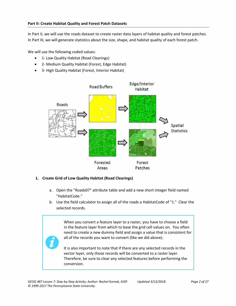
Part II: Create Habitat Quality and Forest Patch Datasets
In Part II, we will use the roads dataset to create raster data layers of habitat quality and forest patches.
In Part III, we will generate statistics about the size, shape, and habitat quality of each forest patch.
We will use the following coded values:
• 1- Low Quality Habitat (Road Clearings)
• 2- Medium Quality Habitat (Forest, Edge Habitat)
• 3- High Quality Habitat (Forest, Interior Habitat)
1. Create Grid of Low Quality Habitat (Road Clearings)
a. Open the "Roads07" attribute table and add a new short integer field named
"HabitatCode."
b. Use the field calculator to assign all of the roads a HabitatCode of "1." Clear the
selected records.
When you convert a feature layer to a raster, you have to choose a field in the feature layer from which to base the grid cell values on. You often need to create a new dummy field and assign a value that is consistent for all of the records you want to convert (like we did above).
It is also important to note that if there are any selected records in the vector layer, only those records will be converted to a raster layer. Therefore, be sure to clear any selected features before performing the conversion.
GEOG 487 Lesson 7: Step-by-Step Activity; Author: Rachel Kornak, GISP. Updated 3/12/2018. Page 3 of 27 © 1999-2017 The Pennsylvania State University.
The data type of the field you choose is very important. For example, if you choose a numerical field that contains decimal values, the resultant grid will not have an attribute table. However, if you choose an integer field, the resultant raster will have an attribute table. If you choose a text field, ArcGIS will automatically assign each unique text value an integer code in a new field named "VALUE."
The new raster layer will be created based on all defined Spatial Analyst environment settings. Always check these settings before converting features to a raster to avoid potentially undesirable results.
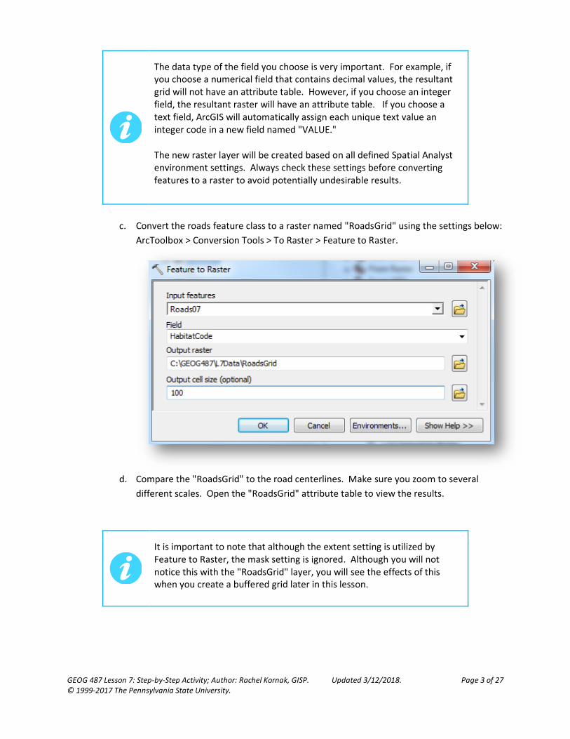
c. Convert the roads feature class to a raster named "RoadsGrid" using the settings below:
ArcToolbox > Conversion Tools > To Raster > Feature to Raster.
d. Compare the "RoadsGrid" to the road centerlines. Make sure you zoom to several
different scales. Open the "RoadsGrid" attribute table to view the results.
It is important to note that although the extent setting is utilized by Feature to Raster, the mask setting is ignored. Although you will not notice this with the "RoadsGrid" layer, you will see the effects of this when you create a buffered grid later in this lesson.

GEOG 487 Lesson 7: Step-by-Step Activity; Author: Rachel Kornak, GISP. Updated 3/12/2018. Page 4 of 27 © 1999-2017 The Pennsylvania State University.
Make sure you have the correct answer before moving on to the next step.
The "RoadsGrid" raster should have the following information. If your data does not match this, go back and redo the previous step.
2. Create Edge Effects Grid
Remember from the Background Information section that edge effects can occur up to 2 km
from roads. We will consider all areas 2 km from roads as "edge habitat" and areas farther than
2 km from roads as "interior habitat." To do this, we need to create a buffer of the road
centerlines.
a. Create a 2 km buffer of the road centerlines (Main Toolbar > Geoprocessing > Buffer)
using the settings below. Save the file inside the Lesson 7 geodatabase.

GEOG 487 Lesson 7: Step-by-Step Activity; Author: Rachel Kornak, GISP. Updated 3/12/2018. Page 5 of 27 © 1999-2017 The Pennsylvania State University.
b. Compare the buffer to the road centerlines. You may want to use the measuring tool to
double check your buffer is the correct width.
c. Add a new short integer field named "HabCode" to the "Roads07_Buffer" feature class
and assign it a value of "2" using the field calculator. The value of "2" corresponds to
medium quality habitat (forested areas within 2 km of a road).
d. Convert the road buffer to a grid named "EdgeGrid" based on the "HabCode" field. Be
sure to pay attention to the cell size.
e. Compare the "EdgeGrid" raster to the "Roads07" and "Roads07_Buffer" datasets.
Notice how the conversion tool did not follow the mask setting, as the raster cells with
values extrude beyond the study area boundary. It may be easier to see the effect if
you assign values of NoData in the EdgeGrid raster a color as we did in previous lessons.
Make sure you have the correct answer before moving on to the next step.
The "EdgeGrid" raster should have the following information. If your data does not match this, go back and redo the previous step.

GEOG 487 Lesson 7: Step-by-Step Activity; Author: Rachel Kornak, GISP. Updated 3/12/2018. Page 6 of 27 © 1999-2017 The Pennsylvania State University.
3. Create Interior Forests Grid
a. Reclassify the "EdgeGrid" using the settings below. Name the output grid
"InteriorGrid."
b. Compare the "InteriorGrid" raster layer to the "EdgeGrid" and "RoadsGrid" layers.
Notice how we were able to "flip" the areas with NoData. It is easier to see the effect if
you turn off all of the layers except the Roads, InteriorGrid, and Study Boundary. It’s
important that you choose appropriate mask and extent settings when using this
technique.
Did the Reclassify Tool honor the mask and extent settings? Hint: Compare the InteriorGrid and EdgeGrid rasters along the study area boundary.

GEOG 487 Lesson 7: Step-by-Step Activity; Author: Rachel Kornak, GISP. Updated 3/12/2018. Page 7 of 27 © 1999-2017 The Pennsylvania State University.
Make sure you have the correct answer before moving on to the next step.
The "InteriorGrid" grid should have the following information. If your data does not match this, go back and redo the previous step.
4. Create Final Habitat Quality Grid
In steps 1, 2, and 3, we created three individual grids, one for each level of habitat quality. To
continue the analysis, we need a way to merge all of the data sets into one grid. The Mosaic to
New Raster tool in ArcToolbox allows you to mosaic multiple raster data layers together by
stacking them on top of one another. The values in the output raster will be determined based
on the order the files are specified during the mosaic. Cells will first be assigned according to
the cell values in the first input raster; all remaining null values will be filled in with the middle
input raster, and so on. We want the roads to be on top of the stack, the edge habitat in the
middle, and the forests on the bottom.
a. Go to ArcToolbox > Data Management Tools > Raster > Raster Dataset > Mosaic to New
Raster and enter the settings as shown on the next page. Name the new grid
"HabMosaic." When adding the input rasters, pay attention to the order in which you
add them. Along with the output location and the raster dataset name, you will need to
assign a cell size and number of bands. The number of bands refers to a color map.
Since we are not dealing with multiple band data, enter "1" to identify the new raster
dataset as a single band layer. As mentioned above, we want the raster to be created
based on a hierarchy from first to last. Therefore, we need to set the Mosaic Operator
to "FIRST" so that the analysis runs as intended. You can leave the Mosiac Colormap
Mode setting to "FIRST" since we are dealing with single band data.
This tool does not honor the Output extent environment settings. If you
want a specific extent for your output raster, consider using the Clip tool.
You can either clip the input rasters prior to using this tool, or clip the
output of this tool.

GEOG 487 Lesson 7: Step-by-Step Activity; Author: Rachel Kornak, GISP. Updated 3/12/2018. Page 8 of 27 © 1999-2017 The Pennsylvania State University.

GEOG 487 Lesson 7: Step-by-Step Activity; Author: Rachel Kornak, GISP. Updated 3/12/2018. Page 9 of 27 © 1999-2017 The Pennsylvania State University.
Make sure you have the correct answer before moving on to the next step.
The "HabMosaic" raster should have the following information. If your data does not match this, go back and redo the previous step.
What value was assigned to areas with roads, since they have data in both the "RoadsGrid" and "EdgeGrid" rasters?
Which habitat type (roads, edge, or interior) covers the majority of the study area?
How can you calculate the area of each habitat type?
b. Notice that the some edges of the "HabMosaic" grid fall outside of the study boundary.
As mentioned earlier, this is because the Mosaic to New Raster tool does not utilize the
extent environment settings. Therefore, we need to "clip" the data to the extent of our
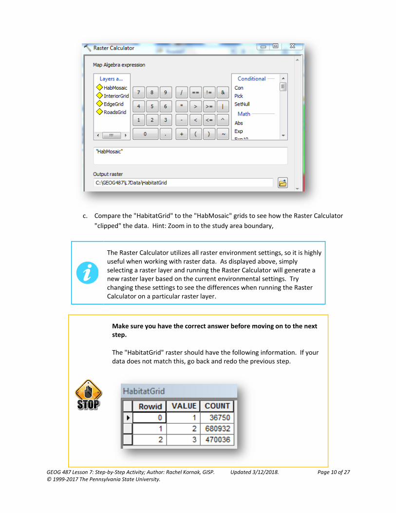
study boundary. To do this, we will use the Raster Calculator. Open the Raster
Calculator (ArcToolbox > Spatial Analyst Tools > Map Algebra > Raster Calculator), click
the "HabMosaic" grid to enter it into the expression window, set the output raster as
"HabitatGrid" and click OK to run the expression.
GEOG 487 Lesson 7: Step-by-Step Activity; Author: Rachel Kornak, GISP. Updated 3/12/2018. Page 10 of 27 © 1999-2017 The Pennsylvania State University.
c. Compare the "HabitatGrid" to the "HabMosaic" grids to see how the Raster Calculator
"clipped" the data. Hint: Zoom in to the study area boundary,
The Raster Calculator utilizes all raster environment settings, so it is highly useful when working with raster data. As displayed above, simply selecting a raster layer and running the Raster Calculator will generate a new raster layer based on the current environmental settings. Try changing these settings to see the differences when running the Raster Calculator on a particular raster layer.
Make sure you have the correct answer before moving on to the next step.
The "HabitatGrid" raster should have the following information. If your data does not match this, go back and redo the previous step.

GEOG 487 Lesson 7: Step-by-Step Activity; Author: Rachel Kornak, GISP. Updated 3/12/2018. Page 11 of 27 © 1999-2017 The Pennsylvania State University.
5. Create Grid of Forested Areas
We now have one grid with values showing the range of habitat quality within the study area.
The next step is to create a grid of forested areas, which we need to create the forest
fragments. We will use the "RoadsGrid" raster we created in Part II Step 1 to create a new grid
representing forested areas (cells that are NOT roads).
a. Reclassify "RoadsGrid" using the settings below:
b. Compare the "ForestGrid" raster to the "RoadsGrid" raster.
Make sure you have the correct answer before moving on to the next step.
The "ForestGrid" raster should have the following information. If your data does not match this, go back and redo the previous step. You may need to adjust for the Mask and Processing Extent here as well.

GEOG 487 Lesson 7: Step-by-Step Activity; Author: Rachel Kornak, GISP. Updated 3/12/2018. Page 12 of 27 © 1999-2017 The Pennsylvania State University.
6. Create Grid of Individual Forest Patches
a. Examine the "ForestGrid" attribute table. Notice there is not a way to distinguish
groups of contiguous cells from one another. We need to be able to do this to
determine which cells belong to the same forest patch.
b. To accomplish this, we will use the RegionGroup tool. RegionGroup is an operation that
takes adjacent cells with the same value and assigns them a unique value. So, in
essence, it creates a grid with groups of cells similar to polygons in a shapefile. This is an
important operation, since it enables further analysis with expressions and operations
that require grouped regions, such as calculating the area and width of forest patches.
c. Go to ArcToolbox > Spatial Analyst Tools > Generalization > Region Group, select
"ForestGrid" as the input raster, name the output raster "ForestPatches", leave the
number of neighbors to use as "FOUR", the zone grouping method as "WITHIN",
uncheck the "Add link field to output", leave the excluded value setting , and click OK.
d. Compare the ForestPatches attribute table to the ForestGrid attribute table. Notice
how the attribute table now has multiple rows, one for each forest patch. The "Rowid"
and "VALUE" fields both contain unique ID numbers for each contiguous forest patch.
The "COUNT" field shows the number of cells in each forest patch.

GEOG 487 Lesson 7: Step-by-Step Activity; Author: Rachel Kornak, GISP. Updated 3/12/2018. Page 13 of 27 © 1999-2017 The Pennsylvania State University.
Make sure you have the correct answer before moving on to the next step.
The "ForestPatches" grid should have the following information. If your data does not match this, go back and redo the previous step.
e. The "VALUE" field is very important, since it uniquely identifies each forest patch.
However, the default name assigned by the computer is not very meaningful. It would
be very easy to forget what it means later on. It’s also easy to confuse the "VALUE" and
"Rowid" field, since they contain similar numbers.
f. To prevent these issues, let’s create a more meaningful attribute to keep track of the
forest patches. Add a new short integer field named "ForestID" to the "ForestPatches"
attribute table. Populate it with the numbers in the "VALUE" field.
g. Change the symbology to "unique values" based on the "ForestID" field. Notice how
groups of contiguous cells are now considered one unit. Also notice how the default
colors assigned by ArcMap are not very meaningful. We will address this later in the
lesson.
h. The "COUNT" field is also very important, since it tells us how many cells are within
each forest patch. As we saw in Lesson 5, we can use the number of cells and size of
each cell to calculate area values.
i. Add a new float field to the "ForestPatches" attribute table named "AREA_SQM." Use
the field calculator to populate the field.

GEOG 487 Lesson 7: Step-by-Step Activity; Author: Rachel Kornak, GISP. Updated 3/12/2018. Page 14 of 27 © 1999-2017 The Pennsylvania State University.
Why did we use the number "100" to calculate the area?
Make sure you have the correct answer before moving on to the next step.
The "ForestPatches" grid should have the following information. If your data does not match this, go back and redo the previous step.
How many individual forest patches are there? Which forest patch is the largest? Which forest patch is the smallest? Why do you think there are so many patches with an area of exactly 10,000 sq m?

GEOG 487 Lesson 7: Step-by-Step Activity; Author: Rachel Kornak, GISP. Updated 3/12/2018. Page 15 of 27 © 1999-2017 The Pennsylvania State University.
Part III: Calculate Spatial Statistics of Forest Patches
In Part III, we will use two Spatial Analyst tools to bring together the raster layers we created in Part I
(habitat quality) and Part II (forest patches). Zonal Geometry calculates several geometry measures,
such as area and thickness, for zones in a raster. We will use it to generate a table of statistics about the
size and shape of each forest patch. We will also use the Zonal Histogram Tool to tabulate the number
of cells of each habitat type within each forest patch and management unit.
1. Calculate the Geometry of Each Forest Patch
a. Go to ArcToolbox > Spatial Analyst Tools > Zonal > Zonal Geometry as Table. Use the
settings shown below. Name the table "PatchGeometry.dbf" and save it in your L7
folder. Make sure to include the .dbf file extension.
Make sure you have the correct answer before moving on to the next step.
The "PatchGeometry" table should have the following information. If your data does not match this, go back and redo the previous step.

GEOG 487 Lesson 7: Step-by-Step Activity; Author: Rachel Kornak, GISP. Updated 3/12/2018. Page 16 of 27 © 1999-2017 The Pennsylvania State University.
Which field in the "PatchGeometry" table is the equivalent to the "ForestID" field? What are the units of the fields "AREA," "PERIMETER," and "THICKNESS"? What do the values in the fields "XCENTROID," "YCENTROID," "MAJORAXIS," "MINORAXIS", and "ORIENTATION" mean?
b. Add a new short integer field named "ForestID" and populate it with the values in the
"VALUE" field using the field calculator. This step will make it easier to compare the
Patch Geometry table with other outputs later in the lesson.
c. Add three new float fields named “TotAreaSQM,” “PerimeterM, and “ThicknessM.”
Calculate them to equal the values in “AREA,”PERIMETER,” and THICKNESS,”
respectively. This will help us remember the units of the calculations later on.
2. Calculate Habitat Statistics by Forest Patch
The Zonal Histogram tool will create a summary table that contains one row for each unique
value in the "Value raster" and one column for each unique value in the "Zone dataset." The tool
will calculate the total number of cells for each combination of unique row and column. The
tool can also create a graph based on the output table, which we are going to skip.
a. Open the Zonal Histogram tool (ArcToolbox > Spatial Analyst Tools > Zonal > Zonal
Histogram). Use the settings below and click "OK." Make sure to add the .dbf
extension.

GEOG 487 Lesson 7: Step-by-Step Activity; Author: Rachel Kornak, GISP. Updated 3/12/2018. Page 17 of 27 © 1999-2017 The Pennsylvania State University.
b. Open the "Habitat_by_Patch" table. The "LABEL" field contain values equivalent to the
"Rowid" field within "ForestPatches." The "VALUE_2" field contains the number of cells
of edge habitat for each forest patch. The "VALUE_3" field contains the number of cells
of interior habitat for each forest patch (Remember that we used codes of 1, 2, and 3 to
represent the different habitat types throughout the lesson).
c. These field names are not very intuitive, and we may forget what they mean later on.
Let’s add a few new meaningful fields to address this potential problem.
d. Add a new short integer field called "ForestID" to the "Habitat_by_Patch" table. Use
the field calculator to populate it with the values in the “LABEL” field.
e. Add two new float fields named "Edge_SQM" and "Int_SQM." Calculate the fields as
shown below (# of cells * cell length * cell width):
f. Remember from Lesson 4 that it is a lot easier to compare multiple area values if you
use percent of total area instead of actual area values. Add two new short integer fields
named "PctTotEdge" and "PctTotInt." Calculate the fields as shown below. Notice the
100 in the equation is used to create a percent value and is not related to the 100 value
we used in step e, which corresponds to the length and width of the raster cells.

GEOG 487 Lesson 7: Step-by-Step Activity; Author: Rachel Kornak, GISP. Updated 3/12/2018. Page 18 of 27 © 1999-2017 The Pennsylvania State University.
Make sure you have the correct answer before moving on to the next step.
The "Habitat_by_Patch" table should have the following information. If your data does not match this, go back and redo the previous step.
3. Calculate Habitat Statistics by Management Unit
a. Use the Zonal Histogram Tool to determine the amount of each habitat type by
management unit as shown in the example below: Don’t forget the file extension.
What do numbers in the "LABEL" field of the "Habitat_by_MU" mean? Which management unit "use" has the most roads?

GEOG 487 Lesson 7: Step-by-Step Activity; Author: Rachel Kornak, GISP. Updated 3/12/2018. Page 19 of 27 © 1999-2017 The Pennsylvania State University.
b. Add a new text field (length 20) named “Habitat.” Use the field calculator and the
information below to update the new field.
• 1 - Low Quality Habitat (Road Clearings)
• 2 - Medium Quality Habitat (Forest, Edge Habitat)
• 3 - High Quality Habitat (Forest, Interior Habitat)
c. Add two new float fields named “LogSQM” and “ConsSQM.” Add two new short integer
fields named “PctTotLog” and “PctTotCons.” Calculate them using the technique we
used in Step 2 e and f.
Make sure you have the correct answer before moving on to the next step.
The "Habitat_by_MU" table should have the following values. If your data does not match this, go back and redo the previous step.
4. Join Forest Patches to Geometry Table
a. Since we no longer need the forest patches to be in raster format, let’s convert them to
a shapefile so they are easier to use.
b. Convert the "ForestPatches" grid to a polygon shapefile using the settings below:
ArcToolbox > Conversion Tools > From Raster > Raster to Polygon.

GEOG 487 Lesson 7: Step-by-Step Activity; Author: Rachel Kornak, GISP. Updated 3/12/2018. Page 20 of 27 © 1999-2017 The Pennsylvania State University.
c. Open the attribute table of the new shapefile. Notice how the "ForestID" values match
those in the GRIDCODE field.
d. Add a new short integer field named "FORESTID" and populate it with the values in the
"GRIDCODE" field.
Make sure you have the correct answer before moving on to the next step.
The "forestpatchpoly" shapefile should have the following information. If your data does not match this, go back and redo the previous step. Note that this table has been sorted based on "ForestID".

GEOG 487 Lesson 7: Step-by-Step Activity; Author: Rachel Kornak, GISP. Updated 3/12/2018. Page 21 of 27 © 1999-2017 The Pennsylvania State University.
e. Join the "PatchGeometry" and "Habitat_by_Patch" tables to the "forestpatchpoly"
shapefile using the link fields shown below.
f. Open the attribute table to make sure the joins worked properly. Notice how it is hard
to view the attributes we are most interested in since there are so many fields.
g. Right click on the "forestpatchpoly " shapefile > Properties > Fields, and click the "Turn
all fields off" icon on the top left side. Add the check boxes back to the eight fields
listed below and click "OK."
• ForestID
• TotAreaSQM
• PerimeterM
• ThicknessM
• Edge_SQM
• Int_SQM
• PctTotEdge
• PctTotInt
h. Open the attribute table. Notice how it is much easier to interpret the results now.
i. To make the joins and table design permanent, export the "forestpatchpoly" to a new
shapefile in your Lesson 7 folder named “Final_Forest_Patches.shp.”
j. Add the new shapefile to your map when prompted. Examine the attribute table.

GEOG 487 Lesson 7: Step-by-Step Activity; Author: Rachel Kornak, GISP. Updated 3/12/2018. Page 22 of 27 © 1999-2017 The Pennsylvania State University.
5. Calculate the Edge to Area Ratio of each Forest Patch
a. Calculate the edge to area ratio for each for patch. Add a new double field named
"EdgetoArea." Calculate it as shown below. Note: we are going to multiply the result by
"100" to make the values easier to compare.
Why is there such a large range of values for the edge to area ratio results?
How would the results of the analysis change if we used a larger or smaller cell size?
Make sure you have the correct answer before moving on to the next step.
The "Final_Forest_Patches" attribute table should have the following information. If your data does not match this, go back and redo the previous step.
Notice how the default outputs from many of the Spatial Analyst tools are not very easy to understand. It’s worth the time to create more intuitive fields, units, and names while you are doing the analysis. That way you can easily interpret your results later on and share them with others in a meaningful format.

GEOG 487 Lesson 7: Step-by-Step Activity; Author: Rachel Kornak, GISP. Updated 3/12/2018. Page 23 of 27 © 1999-2017 The Pennsylvania State University.
Part IV: Share Your Results
In Part IV, we will finalize our map in ArcGIS Desktop, then share it as a feature service and web map in
ArcGIS Online. As a final step, you will combine this map with the output from the Advanced Activity
into a web application.
1. Prepare Your Map to Publish in ArcGIS Online
a. When you publish your map to ArcGIS Online, it preserves many of the features such as
the extent and visible datasets. Let’s begin by removing all of the data we do not want
to include on our final map. Remove the base map, all of the data sets, and all of the
tables (you may need to switch to the List by Source view in the Table of Contents) from
your map except the following: Final_Forest_Patches, Study_Boundary, Roads07, and
Management_Units. Save your map.
b. Remove the underscores from the file names in the Table of Contents.
c. Change the symbology of the Final Forest Patches to Quantities > Graduated Colors
based on the PctTotEdge field. Select a color scheme and number of classes you think
best represent the message you want to convey about the results. You may want to
consult the Color Brewer website we covered in Lesson 1 for tips.
d. Update the labels in the Table of Contents so the numbers in the Final Forest Patches
make sense to your viewers. (What are the units? What’s being shown?)
e. Change the symbology of the management units to hollow outlines with a unique color
for each “Use.”
f. Review your map. Ask yourself the following questions: 1) What are the main
messages I am trying to convey with my map? (Remember, you want to show the
relationship between logging and forest health.) 2) Does my map design communicate
these messages clearly? 3) Will someone unfamiliar with my analysis be able to use my
map to make a decision? Make any changes you think are necessary and save your
map.
2. Share Your Results as a Map Service on ArcGIS Online
a. Go to File > Sign In. Log on to your account.
b. Go to File > Share As > Service > Publish a service. Make sure the connection says “My
Hosted Services (Penn State Online Geospatial Education). You need to be logged in to
see this option (File > Sign In).
c. Name the service “YourFirstName_LastName_L7.” Make sure there are no spaces in
the name.
d. Keep all of the defaults in the Parameters, Tiled Mapping, Caching, and Advanced
Settings sections.
GEOG 487 Lesson 7: Step-by-Step Activity; Author: Rachel Kornak, GISP. Updated 3/12/2018. Page 24 of 27 © 1999-2017 The Pennsylvania State University.
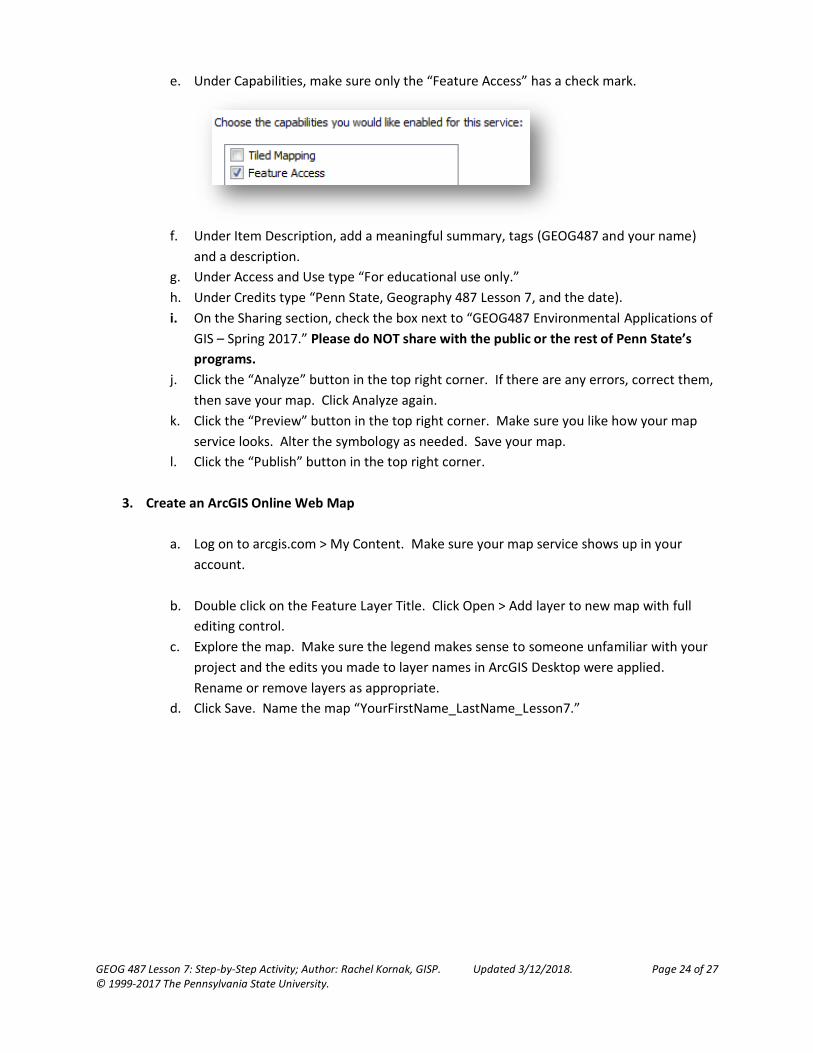
e. Under Capabilities, make sure only the “Feature Access” has a check mark.
f. Under Item Description, add a meaningful summary, tags (GEOG487 and your name)
and a description.
g. Under Access and Use type “For educational use only.”
h. Under Credits type “Penn State, Geography 487 Lesson 7, and the date).
i. On the Sharing section, check the box next to “GEOG487 Environmental Applications of
GIS – Spring 2017.” Please do NOT share with the public or the rest of Penn State’s
programs.
j. Click the “Analyze” button in the top right corner. If there are any errors, correct them,
then save your map. Click Analyze again.
k. Click the “Preview” button in the top right corner. Make sure you like how your map
service looks. Alter the symbology as needed. Save your map.
l. Click the “Publish” button in the top right corner.
3. Create an ArcGIS Online Web Map
a. Log on to arcgis.com > My Content. Make sure your map service shows up in your
account.
b. Double click on the Feature Layer Title. Click Open > Add layer to new map with full
editing control.
c. Explore the map. Make sure the legend makes sense to someone unfamiliar with your
project and the edits you made to layer names in ArcGIS Desktop were applied.
Rename or remove layers as appropriate.
d. Click Save. Name the map “YourFirstName_LastName_Lesson7.”

GEOG 487 Lesson 7: Step-by-Step Activity; Author: Rachel Kornak, GISP. Updated 3/12/2018. Page 25 of 27 © 1999-2017 The Pennsylvania State University.
e. Share your map with the class as shown below (the group name will show the current
semester as well). Notice the short URL listed in the “Link to this map.”
ArcGIS online creates a shorter URL that redirects to the actual (and very long) URL of your map or application. It is easier to share the shortened URL on social media and through email. To access the short URL, open the map in the ArcGIS.com map viewer > Share.
Notice that this is not the same as the Share button on the Details page.
GEOG 487 Lesson 7: Step-by-Step Activity; Author: Rachel Kornak, GISP. Updated 3/12/2018. Page 26 of 27 © 1999-2017 The Pennsylvania State University.
f. Save your map again. Go to My Content. Click on the three-dot icon next to your map >
View item details. Edit the information on the page that opens as follows:
a. Summary: One sentence about what the map shows.
b. Description: 3-4 sentences describing the main trends in the results. For
example: Where are the best habitat areas located (conservation of logging
management units)? What is the overall habitat health like in the study area?
c. Access and Use Constraints: Type “For educational use only.”
d. Tags: “GEOG487” and your name.
e. Credits: Penn State, Geography 487 Lesson 7, date, and the name of any
classmates’ maps you used as a reference while creating your own.
f. Save your changes.
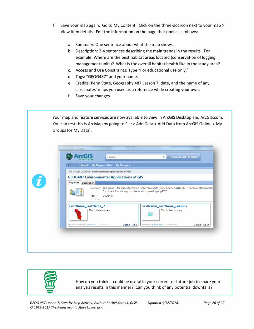
Your map and feature services are now available to view in ArcGIS Desktop and ArcGIS.com.
You can test this is ArcMap by going to File > Add Data > Add Data from ArcGIS Online > My
Groups (or My Data).
How do you think it could be useful in your current or future job to share your analysis results in this manner? Can you think of any potential downfalls?

GEOG 487 Lesson 7: Step-by-Step Activity; Author: Rachel Kornak, GISP. Updated 3/12/2018. Page 27 of 27 © 1999-2017 The Pennsylvania State University.
That’s it for the required portion of the Lesson 7 Step-by-Step Activity. Please consult the Lesson
Checklist for instructions on what to do next.
Try one or more of the optional activities listed below.
• Explore the Global Forest Watch Interactive Mapping Website
Many of the data sets we will use in the lesson were originally created by Global Forest Watch. Explore their website at http://www.wri.org/gfw2.
• Explore the USGS Global Visualization Viewer website
Landsat satellite images were used to digitize the roads data we used in this lesson.
You can read more about Landsat data on NASA’s website:
http://landsat.gsfc.nasa.gov/data/. As of October 2008, Landsat data is available for
free to the public. It can be viewed and downloaded from the USGS Global
Visualization Viewer website at: http://glovis.usgs.gov/next/.
Note: Try This Activities are voluntary and are not graded, though I encourage you to complete the
activity and share comments about your experience on the lesson message board.