Embed Size (px)
Citation preview
Geochemical patterns in the soils of Zeeland

Nederlandse Geografische Studies 330
Geochemical patterns in the soils of Zeeland
Natural variability versus anthropogenic impact
J. Spijker
Utrecht, 2005
Koninklijk Nederlands Aardkundig Genootschap/Faculteit Geowetenschappen Universiteit Utrecht

This publication is identical to a thesis submitted in partial fullfilment of the requirementsfor the degree of Doctor of Philosophy (Ph.D.) at Utrecht University, The Netherlands.
Promotor: Prof. Dr. P.A. BurroughFaculteit Geowetenschappen, Universiteit Utrecht
Co-promotores: Dr. P.F.M. Van GaansFaculteit Geowetenschappen, Universiteit UtrechtDr. S.P. VriendFaculteit Geowetenschappen, Universiteit Utrecht
This research was financially supported by the Provincie Zeeland
ISBN 90-6809-370-3
Copyright © J. Spijker, p/a Faculteit Geowetenschappen, Universiteit Utrecht, 2005
Niets uit deze uitgave mag worden vermenigvuldigd en/of openbaar gemaakt door middelvan druk, fotokopie of op welke andere wijze dan ook zonder voorafgaande schriftelijketoestemming van de uitgevers.
All rights reserved. No part of this publication may be reproduced in any form, byphotoprint, microfilm or any other means, without written permission by the publishers.
Printed in the Netherlands by Labor Grafimedia b.v. - Utrecht
Cover: silhouettes of the Zeeland landscape, after a photograph of R. Sluiter.

Suivre l’etoilePeu m’importent mes chances
Peu m’importe le tempsOu ma desesperance
Et puis lutter toujoursSans questions ni repos
La Quete, Jacques Brel


Contents
1 Introduction 15
1.1 History and approaches to soil management in the Netherlands . . . . . . . 16
1.2 Soil quality and so called “soil quality maps” . . . . . . . . . . . . . . . . 18
1.3 Aim of this thesis . . . . . . . . . . . . . . . . . . . . . . . . . . . . . . . 18
1.4 Outline of this thesis . . . . . . . . . . . . . . . . . . . . . . . . . . . . . 19
2 Geology and pedology of Zeeland 21
2.1 Introduction . . . . . . . . . . . . . . . . . . . . . . . . . . . . . . . . . . 21
2.2 Basic geographic information . . . . . . . . . . . . . . . . . . . . . . . . . 22
2.3 Geology of Zeeland . . . . . . . . . . . . . . . . . . . . . . . . . . . . . . 23
2.3.1 Pleistocene period: terrestrial phase . . . . . . . . . . . . . . . . . 24
2.3.2 Forming of the Basal Peat . . . . . . . . . . . . . . . . . . . . . . 24
2.3.3 Calais deposits, first inundation . . . . . . . . . . . . . . . . . . . 25
2.3.4 Holland Peat . . . . . . . . . . . . . . . . . . . . . . . . . . . . . 25
2.3.5 Duinkerke deposits . . . . . . . . . . . . . . . . . . . . . . . . . . 25
2.4 Human activities . . . . . . . . . . . . . . . . . . . . . . . . . . . . . . . 27
2.4.1 Dikes and embankments . . . . . . . . . . . . . . . . . . . . . . . 27
2.4.2 Peat excavation . . . . . . . . . . . . . . . . . . . . . . . . . . . . 29
2.4.3 Parceling and land reconstruction . . . . . . . . . . . . . . . . . . 29
2.4.4 Agricultural inputs . . . . . . . . . . . . . . . . . . . . . . . . . . 30
2.5 Landscape and soil geomorphology . . . . . . . . . . . . . . . . . . . . . 30
2.5.1 Heartlands . . . . . . . . . . . . . . . . . . . . . . . . . . . . . . 32
2.5.2 Channel ridges and creeks . . . . . . . . . . . . . . . . . . . . . . 33
2.5.3 Accretion polders . . . . . . . . . . . . . . . . . . . . . . . . . . . 35
2.5.4 Groundwater . . . . . . . . . . . . . . . . . . . . . . . . . . . . . 36
2.6 Summary and conclusion . . . . . . . . . . . . . . . . . . . . . . . . . . . 38
7
3 Natural and anthropogenic patterns of covariance and spatial variability ofminor and trace elements in agricultural topsoil 41
3.1 Introduction . . . . . . . . . . . . . . . . . . . . . . . . . . . . . . . . . . 41
3.2 Materials and methods . . . . . . . . . . . . . . . . . . . . . . . . . . . . 42
3.2.1 Area . . . . . . . . . . . . . . . . . . . . . . . . . . . . . . . . . . 42
3.2.2 Spatial variance and sampling theory . . . . . . . . . . . . . . . . 43
3.2.3 Sampling and chemical analysis . . . . . . . . . . . . . . . . . . . 45
3.2.4 Data analysis . . . . . . . . . . . . . . . . . . . . . . . . . . . . . 46
3.3 Results and discussion . . . . . . . . . . . . . . . . . . . . . . . . . . . . 48
3.4 Conclusions . . . . . . . . . . . . . . . . . . . . . . . . . . . . . . . . . . 56
4 Sampling and analyses for a regional environmental soil geochemical survey 61
4.1 Introduction . . . . . . . . . . . . . . . . . . . . . . . . . . . . . . . . . . 61
4.2 Material and methods . . . . . . . . . . . . . . . . . . . . . . . . . . . . . 62
4.2.1 Study area . . . . . . . . . . . . . . . . . . . . . . . . . . . . . . . 62
4.2.2 General research approach . . . . . . . . . . . . . . . . . . . . . . 64
4.2.3 Field sampling . . . . . . . . . . . . . . . . . . . . . . . . . . . . 65
4.2.4 Sample preparation . . . . . . . . . . . . . . . . . . . . . . . . . . 66
4.2.5 Chemical analyses . . . . . . . . . . . . . . . . . . . . . . . . . . 67
4.2.6 Precision and accuracy . . . . . . . . . . . . . . . . . . . . . . . . 68
4.2.7 Outliers . . . . . . . . . . . . . . . . . . . . . . . . . . . . . . . . 70
4.2.8 Parametric levelling . . . . . . . . . . . . . . . . . . . . . . . . . 70
4.3 Results and interpretation . . . . . . . . . . . . . . . . . . . . . . . . . . . 72
4.3.1 Precision . . . . . . . . . . . . . . . . . . . . . . . . . . . . . . . 72
4.3.2 Accuracy . . . . . . . . . . . . . . . . . . . . . . . . . . . . . . . 73
4.3.3 Outliers . . . . . . . . . . . . . . . . . . . . . . . . . . . . . . . . 74
4.3.4 Parametric levelling of data . . . . . . . . . . . . . . . . . . . . . 75
4.3.5 Comparison between XRF and ICP-MS . . . . . . . . . . . . . . . 76
4.3.6 Parameter selection and summary statistics . . . . . . . . . . . . . 78
4.4 Discussion and conclusions . . . . . . . . . . . . . . . . . . . . . . . . . . 82
5 Enrichment and natural variability versus anthropogenic impact 95
5.1 Introduction . . . . . . . . . . . . . . . . . . . . . . . . . . . . . . . . . . 95
5.2 The Zeeland geochemical soil data . . . . . . . . . . . . . . . . . . . . . . 97
5.3 Concepts and methods . . . . . . . . . . . . . . . . . . . . . . . . . . . . 97
8
5.3.1 Assessing enrichments and baselines in attribute space . . . . . . . 97
5.3.2 Spatial representation and spatial anomalies . . . . . . . . . . . . . 104
5.4 Results and interpretation . . . . . . . . . . . . . . . . . . . . . . . . . . . 105
5.4.1 Univariate statistics for the Zeeland topsoil data. . . . . . . . . . . 105
5.4.2 Univariate comparison with reference data and legal threshold levels 107
5.4.3 Correlation and regression with Al . . . . . . . . . . . . . . . . . . 113
5.4.4 Spatial patterns of topsoil enrichments . . . . . . . . . . . . . . . . 118
5.5 General discussion and conclusions . . . . . . . . . . . . . . . . . . . . . 123
6 Regional diffuse geochemical patterns and processes 129
6.1 Introduction . . . . . . . . . . . . . . . . . . . . . . . . . . . . . . . . . . 129
6.2 Material and methods . . . . . . . . . . . . . . . . . . . . . . . . . . . . . 130
6.2.1 Study area and geochemical topsoil data . . . . . . . . . . . . . . . 130
6.2.2 Principal component analysis . . . . . . . . . . . . . . . . . . . . 131
6.2.3 Fuzzy c-means clustering . . . . . . . . . . . . . . . . . . . . . . . 133
6.2.4 Statistical software packages . . . . . . . . . . . . . . . . . . . . . 134
6.3 Results and interpretation . . . . . . . . . . . . . . . . . . . . . . . . . . . 134
6.3.1 Principal components analysis . . . . . . . . . . . . . . . . . . . . 134
6.3.2 Anthropogenic subprocesses . . . . . . . . . . . . . . . . . . . . . 138
6.3.3 Fuzzy clustering . . . . . . . . . . . . . . . . . . . . . . . . . . . 139
6.4 General discussion and conclusions . . . . . . . . . . . . . . . . . . . . . 144
7 Assessment of regional DDT concentrations in the soils of Zeeland 149
7.1 Introduction . . . . . . . . . . . . . . . . . . . . . . . . . . . . . . . . . . 149
7.2 DDT, properties and history . . . . . . . . . . . . . . . . . . . . . . . . . 150
7.3 Study area . . . . . . . . . . . . . . . . . . . . . . . . . . . . . . . . . . . 151
7.4 Method . . . . . . . . . . . . . . . . . . . . . . . . . . . . . . . . . . . . 152
7.4.1 Collection of data . . . . . . . . . . . . . . . . . . . . . . . . . . . 152
7.4.2 Basic statistical analysis . . . . . . . . . . . . . . . . . . . . . . . 153
7.4.3 Analysis of variance . . . . . . . . . . . . . . . . . . . . . . . . . 154
7.4.4 Regional variability . . . . . . . . . . . . . . . . . . . . . . . . . . 154
7.4.5 Comparison with external data and normative values . . . . . . . . 155
7.4.6 DDT breakdown . . . . . . . . . . . . . . . . . . . . . . . . . . . 155
7.5 Results . . . . . . . . . . . . . . . . . . . . . . . . . . . . . . . . . . . . . 156
7.5.1 Data merging and selection . . . . . . . . . . . . . . . . . . . . . . 156
9
7.5.2 Exploratory statistics . . . . . . . . . . . . . . . . . . . . . . . . . 157
7.5.3 Local and regional variability . . . . . . . . . . . . . . . . . . . . 159
7.5.4 Regional overview . . . . . . . . . . . . . . . . . . . . . . . . . . 161
7.5.5 Comparison with external data and normative values . . . . . . . . 162
7.5.6 DDT breakdown . . . . . . . . . . . . . . . . . . . . . . . . . . . 166
7.6 Discussion and conclusions . . . . . . . . . . . . . . . . . . . . . . . . . . 167
8 Synthesis 171
8.1 Methods used . . . . . . . . . . . . . . . . . . . . . . . . . . . . . . . . . 171
8.2 Achievements of this study . . . . . . . . . . . . . . . . . . . . . . . . . . 172
8.3 Implications . . . . . . . . . . . . . . . . . . . . . . . . . . . . . . . . . . 174
Bibliography 175
Abstract - Geochemical patterns in the soils of Zeeland, natural variability versusanthropogenic impact 185
Samenvatting - Geochemische patronen in de bodems van Zeeland, natuurlijkevariabiliteit versus antropogene impact 193
Dankwoord 203
Curriculum Vitae 205
10
Figures
2.1 Topography of Zeeland . . . . . . . . . . . . . . . . . . . . . . . . . . . . . . . . 22
2.2 Pictures of the landscape of Zeeland. Both pictures were taken in Zeeuws-Vlaanderen. 23
2.3 Simplified geological cross section of Zeeland . . . . . . . . . . . . . . . . . . . . 24
2.4 Simplified geology of the Duinkerke deposits . . . . . . . . . . . . . . . . . . . . 26
2.5 History of embankment . . . . . . . . . . . . . . . . . . . . . . . . . . . . . . . . 28
2.6 Historical usage of P and K fertilisers . . . . . . . . . . . . . . . . . . . . . . . . 31
2.7 Landscape typology . . . . . . . . . . . . . . . . . . . . . . . . . . . . . . . . . . 32
2.8 Simplified soil map of Zeeland . . . . . . . . . . . . . . . . . . . . . . . . . . . . 33
2.9 Digital elevation model of Zeeland . . . . . . . . . . . . . . . . . . . . . . . . . . 34
2.10 Schematic cross section of the origin of ridge inversion of tidal channels . . . . . . 35
2.11 Excerpt from digital elevation model showing pool areas . . . . . . . . . . . . . . 36
2.12 Excerpt from digital elevation model showing channel ridges . . . . . . . . . . . . 37
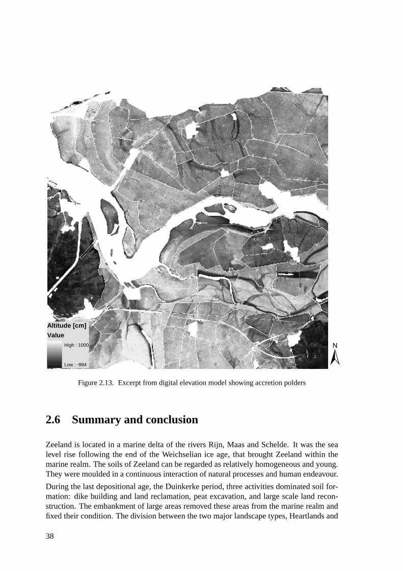
2.13 Excerpt from digital elevation model showing accretion polders . . . . . . . . . . . 38
3.1 Location map . . . . . . . . . . . . . . . . . . . . . . . . . . . . . . . . . . . . . 43
3.2 Stacking of levels of variation design . . . . . . . . . . . . . . . . . . . . . . . . . 44
3.3 Stacking of levels of sample design . . . . . . . . . . . . . . . . . . . . . . . . . . 46
3.4 Contribution of the hierarchical variance components . . . . . . . . . . . . . . . . 53
3.5 Summary of cumulative spatial variance patterns . . . . . . . . . . . . . . . . . . 58
3.6 Variance Ratios . . . . . . . . . . . . . . . . . . . . . . . . . . . . . . . . . . . . 59
4.1 Topography of Zeeland . . . . . . . . . . . . . . . . . . . . . . . . . . . . . . . . 63
4.2 Sample locations per survey . . . . . . . . . . . . . . . . . . . . . . . . . . . . . 67
4.3 Principal concepts of levelling . . . . . . . . . . . . . . . . . . . . . . . . . . . . 71
4.4 Example of levelling of Ga . . . . . . . . . . . . . . . . . . . . . . . . . . . . . . 77
4.5 Comparison between selected elements from the XRF and ICP-MS . . . . . . . . . 81
4.6 Histograms for selected elements and oxides analysed in the topsoil samples . . . . 85
5.1 Map of Zeeland with sample locations . . . . . . . . . . . . . . . . . . . . . . . . 98
11

5.2 Cumulative probability plots of a selection of components . . . . . . . . . . . . . 106
5.3 Regional distribution of a selection of components expected not to be influenced byhuman processes . . . . . . . . . . . . . . . . . . . . . . . . . . . . . . . . . . . 108
5.4 Regional distribution of a selection of elements expected to be influenced by humanprocesses . . . . . . . . . . . . . . . . . . . . . . . . . . . . . . . . . . . . . . . 109
5.5 Ratio of median values for Zeeland topsoil and the average upper continental crust 110
5.6 Ratio of median values for the Zeeland topsoil and the median of the subsoil . . . . 112
5.7 Ratio of median values and legal threshold value . . . . . . . . . . . . . . . . . . 114
5.8 Scatter plots of Al2O3 versus selected elements . . . . . . . . . . . . . . . . . . . 116
5.9 Box plots of the enrichment ratio e . . . . . . . . . . . . . . . . . . . . . . . . . . 120
5.10 Spatial pattern of the enrichment for selected elements . . . . . . . . . . . . . . . 121
5.11 Spatial representation of the contamination index . . . . . . . . . . . . . . . . . . 123
5.12 Spatial pattern of the ratio with the S-value for selected elements . . . . . . . . . . 124
6.1 Topography of Zeeland and sampling locations . . . . . . . . . . . . . . . . . . . 131
6.2 Scree plot of the eigenvalues from the first 8 of 30, unrotated, components . . . . . 135
6.3 PCA loading plots . . . . . . . . . . . . . . . . . . . . . . . . . . . . . . . . . . . 137
6.4 Regional distribution of rotated factor scores . . . . . . . . . . . . . . . . . . . . . 139
6.5 FCMC centroids of the scaled data. . . . . . . . . . . . . . . . . . . . . . . . . . . 141
6.6 Box and Whisker plots of the distribution of the 8 elements for each cluster . . . . 142
6.7 Box and Whisker plots of the distribution of selected elements for each cluster . . . 143
6.8 Regional distribution of the FCMC memberships of the sample locations. . . . . . 144
7.1 Topography of Zeeland . . . . . . . . . . . . . . . . . . . . . . . . . . . . . . . . 152
7.2 Selected sample locations from the soil information systems of Zeeland . . . . . . 158
7.3 Boxplots of log scaled concentration ∑DDx by survey . . . . . . . . . . . . . . . . 160
7.4 Cumulative frequency plot concentration ∑DDx . . . . . . . . . . . . . . . . . . . 161
7.5 Variance versus approximate scale . . . . . . . . . . . . . . . . . . . . . . . . . . 163
7.6 Semivariogram of the regional ∑DDx concentrations . . . . . . . . . . . . . . . . 164
7.7 Regional overview of ∑DDx concentrations . . . . . . . . . . . . . . . . . . . . . 165
7.8 Relation of organic matter (TOC) and ∑DDx . . . . . . . . . . . . . . . . . . . . . 166
7.9 Relation between DDT, its isomers DDE and DDD, and the number of half-times . 168
12
Tables
3.1 Statistical summary after outlier replacement of the geochemical data for the clayeytop soils of Zeeland . . . . . . . . . . . . . . . . . . . . . . . . . . . . . . . . . . 48
3.2 Varimax rotated principal component factor loadings . . . . . . . . . . . . . . . . 50
3.3 Correlations of concentrations of elements, not included in the PCA-V . . . . . . . 50
3.4 Relative percentages of the variance components for each level and their total . . . 51
3.5 Fuzzy cluster memberships . . . . . . . . . . . . . . . . . . . . . . . . . . . . . . 56
3.6 Relation between covariance structure (PCA-V) and the clustered UANOVA vari-ance patterns . . . . . . . . . . . . . . . . . . . . . . . . . . . . . . . . . . . . . 57
4.1 Year, region and number of sample locations . . . . . . . . . . . . . . . . . . . . . 66
4.2 Attributes analysed per survey and method . . . . . . . . . . . . . . . . . . . . . . 69
4.3 Average precision for ICP-MS . . . . . . . . . . . . . . . . . . . . . . . . . . . . 73
4.4 Average precision for XRF . . . . . . . . . . . . . . . . . . . . . . . . . . . . . . 74
4.5 Accuracy of the XRF analyses . . . . . . . . . . . . . . . . . . . . . . . . . . . . 74
4.6 Accuracy of the ICP-MS analyses . . . . . . . . . . . . . . . . . . . . . . . . . . 75
4.7 Number of outliers . . . . . . . . . . . . . . . . . . . . . . . . . . . . . . . . . . 76
4.8 Results of the levelling for the XRF data . . . . . . . . . . . . . . . . . . . . . . . 78
4.9 Results of the levelling for the ICP-MS data . . . . . . . . . . . . . . . . . . . . . 79
4.10 Differences and correlations between elements analysed by both XRF and ICP-MS 80
4.11 Selected elements . . . . . . . . . . . . . . . . . . . . . . . . . . . . . . . . . . . 80
4.12 Statistical summary of the geochemical data for the topsoil of Zeeland. . . . . . . . 86
4.13 Statistical summary of the geochemical data for the subsoil of Zeeland. . . . . . . 90
5.1 Elements selected from the Zeeland dataset . . . . . . . . . . . . . . . . . . . . . 97
5.2 Statistical concepts for assessing enrichments and baselines . . . . . . . . . . . . . 99
5.3 S values and regression parameters . . . . . . . . . . . . . . . . . . . . . . . . . . 104
5.4 Percentiles of Zeeland topsoil . . . . . . . . . . . . . . . . . . . . . . . . . . . . . 107
5.5 Pearson correlation with topsoil Al2O3 . . . . . . . . . . . . . . . . . . . . . . . . 115
5.6 Regression constants of the regression of subsoil concentrations . . . . . . . . . . 119
13
5.7 Enrichment ratios in the topsoil . . . . . . . . . . . . . . . . . . . . . . . . . . . . 119
5.8 Enrichment differences for the topsoil . . . . . . . . . . . . . . . . . . . . . . . . 120
6.1 Varimax rotated factorloadings and communalities . . . . . . . . . . . . . . . . . 136
6.2 Robust correlation of other elements with PCA factor scores . . . . . . . . . . . . 138
6.3 Correlation of anthropogenic elements . . . . . . . . . . . . . . . . . . . . . . . . 140
6.4 Median values for each FCMC cluster . . . . . . . . . . . . . . . . . . . . . . . . 145
7.1 Databases and survey area used for merged dataset . . . . . . . . . . . . . . . . . 157
7.2 Summary values for ∑DDx and total organic carbon . . . . . . . . . . . . . . . . . 159
7.3 Results ANOVA on the replicated samples . . . . . . . . . . . . . . . . . . . . . . 162
7.4 Percentage of sample points exceeding the S-value. . . . . . . . . . . . . . . . . . 165
7.5 Selected ∑DDx vaues from other areas. . . . . . . . . . . . . . . . . . . . . . . . 169
14
1 Introduction
“As knowledge increases, and as the earth becomes more crowded, geo-chemical information is becoming an increasingly significant factor in deci-sions affecting the management of the overall environment. Ultimately thisinformation affects human survival.”
Darnley (1995)
It is widely understood that the geochemical environment plays a profound role in the ex-istence of life on earth. A large part of this geochemical environment is the thin layerbetween the earth crust and the atmosphere. Yet, Bridges and van Baren (1997) alreadyargued that the significance of this thin layer, also called soil, is not always sufficiently ap-preciated, despite its vital role for human well-being. As they summarise, this natural bodyof mineral, animal, and plant organic matter forms a critical link between the inanimaterocks and minerals and the living plants and animals.
Soil, especially its biogenic content, can affect the biosphere by its role in global cli-matic processes. The bidirectional relations between consumption and production of CO2 ,CH4 and N2O can directly influence climatic changes (Mosier, 1998). More directly, soilsalso play a major role in human health. Mineral nutrients are, mainly, transfered fromsoil to humans by plant and animal foods. Deficiencies, excesses, or imbalances in thisdietary source can have deleterious influences. Such influences can occur on rather large,even global, scale; for example the atmospheric transport of persistent organic pollutants ofsoils from moderate climatic areas to colder areas, were the cold conditions cause precip-itation of the pollutants and subsequent uptake in the local food chain (Abrahams, 2002).These examples of the close relation between soil, health, and global sustainability confirmthat soil plays a critical role as a major interface in our environment and that soil qualitycan be an important indicator for sustainable environmental management (Doran, 2002).
Soil quality, as defined by Karlen et al. (1997), is ”the capacity of a specific kind of soil tofunction, within natural or managed boundaries, to sustain plant and animal productivity,maintain or enhance water and air quality, and support human health and habitation”. Soilquality is often described in terms of physical (texture, thickness of topsoil layer, waterholding capacity), chemical (organic C, Total N, pH, extractable N, P, K) and biological(biomass, soil respiration) parameters (Wienhold et al., 2004). An evaluation of the vari-ous quality indicators and their change over time may dentify if sustainable managementis reached or that soil quality is aggrading/degrading. The type of soil informaton to be
15
evaluated depends of course on the function of the soil, be it a natural ecosystem, foodproduction, or just the base for building (Nortcliff, 2002). The framework and criteria forevaluation often depend on policy choices by relevant authorities or organisations.
This thesis is concerned with obtaining an overview of general (geo)chemical soil quality,within the framework of diffuse anthropogenic pollution and sustainable soil managementin the Netherlands.
1.1 History and approaches to soil management in theNetherlands
Within the Netherlands soil quality assessment and related monitoring in part follow athematic approach, as for example soil acidification, effects of manure and fertilizer use,salinization, or other effects of hydrological management. These thematically based ac-tivities are divided between regional authorities, and often subject to evolving politicalinterests and influence at this level (Busink & Postma, 2000; Mol et al., 2001). The other,in some ways more consistent and georeferenced approach to obtain soil quality informa-tion is rooted in the Dutch soil sanitation and soil management legislation. To place thepresent study into context, this latter approach and its history are explained below. Mostof the following is derived from the good and extensive description by de Roo (2003) ofthe history of Dutch environmental policy and legislation, and their influence on (spatial)planning.
A major event which instigated environmentalism and seeded the first ideas about soilmanagement in the Netherlands was the discovery of severe soil pollution at Lekkerkerk in1980. During a new housing development chemical waste was used as building material tolevel the soil. The dumping of the waste, containing substances such as xylene and toluenecausing the area to be uninhabitable, resulted in an unprecedented scandal. This, however,was just a tip of the iceberg, as many cases of soil pollution followed. This increase in casesof soil pollution led in 1983 to the Soil Remediation (interim) Act, which later resulted inthe Soil Remediation Guidelines (Dutch: Leidraad bodemsanering) (VROM, 1999), andthese guidelines defined legal limits which were the foundation of soil remediation untilthe 1990s. A major concern resulting from the Soil Remediation Guidelines was that thesoil should be remediated until the soil was “clean”, i.e. below the threshold values definedin the guidelines. This resulted in a tremendous increase in costs and stagnation of spatialplanning as spatial development and building of houses was by law not allowed to proceeduntil the conditions of the guidelines were met. The soils, after remediation, should be freeof contaminants and able to support many functions. This led, for example, into clean soilpatches within historically diffusely contaminated urban areas, hence wasting effort andmoney.
Objections to the guidelines, cost increase and stagnating spatial development, led to arevision of the soil remediation policy at the beginning of the 1990s, resulting in threemajor developments. The first was the development of ‘active soils management’, which
16
should provide authorities during their spatial planning and decision making with up-to-date information about the soil condition. Also powers and tasks were decentralised tolower authorities This should help the remediation efforts, which were until then frustatedby a lack of advance information. Another development was the changeover from theold system of legal limits to a system of limits based on actual risks. With these newlimits the urgency of remediation could be assessed and the necessity of remediation wasnot determined by the nature of the pollution but by its seriousness. With the ‘urgency’,together with the third development that the government would in principle not pay the billfor clean-up, pressure could be put on the parties responsible for soil remediation. Withthe new Soil Protection Act of the mid 1990s, which could enforce parties to remediate,soil remediation became a responsibility of society, hence spreading the effort and costs ofurgent soil remediation.
Another major implication originated from the second half of the 1990s. The awarenessgrew that for a more coordinated, instead of consecutive, soil policy, integration of remedi-ation measures and spatial development policies was necessary. Soil management movedtowards a more decentralised, integrated, and market dynamic policy. Therefore reliableinformation about the nature and extent of soil contamination was needed, as this informa-tion can be used to make agreements with non governmental parties involved in the spatialplanning. This coordination also led to the function oriented approach which implied itwas not necessary to remediate the soil until it was ”clean” but that the remediation effortcould be location specific supporting the future function of the soil (de Roo, 2003).
One of the necessities of the new policy was information about the condition of the soil andthe extent of contaminated sites. The government acknowledged this in the third nationalenvironmental policy plan (NEPP 3) (VROM, 1997). Their wish was to obtain an overviewof the country wide soil quality and to provide of soil management methods. Their goal wasto tackle the soil pollution problems, especially the costs and efforts of remediation, within25 years. In 2002 the stepping stones (Dutch: Stappenplan Landsdekkend Beeld 2005)towards this country wide overview were presented and two major tracks were discerned.One track was the inventory of existing polluted sites and the second track aimed at soilmanagement and soil quality. This information should provide a country wide overview ofthe soil quality to facilitate large scale spatial development. This is were the ‘active soilmanagement policy’ returns. This policy should lead to the realisation of sustainable soilmanagement and to adequately and efficiently manage existing soil contamination so as toprevent frustation of spatial planning operations (Leenaers et al., 1999).
The purpose of the country wide overview was also to re-evaluate the existing soil back-ground values and how these relate to the existing legal limits. The observation that partof these legal limits were within the range of considered natural background values urgedthe need for insight in actual soil values. These values should then also provide in a newreference for soil remediation (Leenaers et al., 1999).
17
1.2 Soil quality and so called “soil quality maps”
One of the major tools in fulfilling the country wide overview of the soil quality and sup-porting active soil management are the so called “soil quality maps” (Dutch: bodemk-waliteits kaarten). The interim guidelines for such maps (Dutch: Interim-RichtlijnBodemkwaliteitskaarten) were presented in 1999 (VROM, 1999; van der Gaast et al., 1998;van Lienen et al., 2000). The starting point of the guidelines was the Building Material De-cree (Eikelboom et al., 2001). This came into full operation in 1999, describing the qualitycriteria for building material, which according to the decree includes soil, used as land fillor site preparation material. This decree should prevent materials being exposed in the sur-face environment that leach potential contaminating compounds. (Eikelboom et al., 2001).
The aim of the soil quality maps is to indicate if soil, used in terms of the decree as buildingmaterial, originating from an area was “clean” relative to the legal limits and therefore dis-pensated to be transported to another area. Without such maps and dispensation, each ship-ment of soil needs to be extensively surveyed to see if it is “clean”, substantially increasingthe costs of spatial development (Anonymous, 1999; van Lienen et al., 2000). When soilis not clean, it is generally not allowed to be used as building material, so spreading ofcontamination is prevented.
Besides the use as a dispensation tool, from the information of the soil quality maps thecountry wide overview of contaminated sites and re-evaluation of background levels couldalso be obtained and these should facilitate active soil management and sustainable soil useas well (Leenaers et al., 1999). However, due to the urgent need for spatial developmentand increasing soil transport the latter has become less obvious.
The current Dutch soil quality maps, based on the building material decree, are aimed toindicate or predict when “soil quality” exceeds certain legal limits. Since these limits in-dicate the risk of soil pollution they are actually “soil pollution risk maps” (van der Gaastet al., 1998; Swartjes, 1999). Also, according to the guideline, soils are grouped based ontheir soil concentrations of environmental priority compounds relative to the legal limits(VROM, 1999). This reduces the soil quality, usually not including other biological, phys-ical and chemical soil indicators, to a black and white concept: legal limits are exceededor not. Therefore, in my opinion, the current soil quality maps are neither the means ofproviding the new background values as wished by the NEPP 3 nor do they facilitate sus-tainable soil management. However, they are still suitable for fulfilling the country wideoverview of contaminated sites and facilitate enforcement of the building material decree.
1.3 Aim of this thesis
Despite the changeover from curative measurements and remediation to prevention of con-tamination, the evolution from soil quality maps to soil pollution risk maps is not surprising.The aim of Dutch soil policy is still to reduce remediation costs and prevent stagnation ofspatial development. The next step towards sustainability seems, yet, a small one. An
18
overview of soil background values as reference is a basic need as a starting point for sus-tainable management. However, to provide the overview of soil background values andassess the impact of anthropogenic processes on the natural soil composition, another ap-proach is needed.
This thesis aims at assessing patterns in geochemical soil composition and distinguishingnatural variability from anthropogenic impact. The variability is assessed in geographicalspace, where the spatial interaction of soil components takes place, and in attribute space,where interaction between soil constituents is exposed. Patterns from both spaces can thenbe related to processes influencing the soil composition.
Based on these patterns, and related processes, anthropogenic influence can be distin-guished from natural variability. This can provide tools and information to support thewide overview as required by the NEPP 3.
The chosen study area for this research is the Province of Zeeland, in the south west ofthe Netherlands. The large rural area of young Holocene deposits with a rich human his-tory makes it a suitable area for testing the main hypothesis that human influence leaves adistinct and quantifiable pattern, based on variability within the geographical and attributespace of the soil composition.
1.4 Outline of this thesis
This thesis is addressed in 6 chapters and a synthesis. Each chapter is written to stand onits own and can be read more or less independently of the others.
To understand soil geochemistry in an area it is necessary to understand the factors thatdetermine the geochemical variability. In the next chapter a description is given of theresearch area, the rural part of the province of Zeeland. It is shown how both geologicaland pedological processes, and human activities have influenced the soils and shaped thelandscape. This information is the basis on which a regional geochemical survey can berealized. In such a survey interest focuses on regional features and this is only useful whensmall scale variability does not dominate the observed regional patterns. In chapter 3 it ishypothesised that distinct spatial patterns of variability exists for groups of data related toanthropogenical or geochemical processes. This requires that the sampling strategy shouldanticipate those different patterns in variability by using composite or single samples.
In chapter 4 the process of obtaining a province wide geochemical dataset is described.This dataset should contain information on pristine soil composition and information howthis composition is altered by human processes. The noise level in such a dataset should beas low as possible so the large variety of different processes can be discerned at a adequatelevel of significance. Also, sources of variance and their magnitude should be determined.While chapter 3 focusses on field scale variability, chapter 4 examines analytical sources ofvariance and bias. The final dataset presented in chapter 4 should provide a true referencedataset, which is suitable for environmental and geochemical assessment within a regionalcontext.
19

For environmental legislation and soil management policies it is essential to have a goodoverview of the present day soil composition. Although the above dataset presents a refer-ence of actual soil values it is assumed that these values are imprinted by human activities.In chapter 5 it is hypothesised that this anthropogenic imprint can be established using ageo- chemical baseline that comprises the natural variability in soil composition. Since nostandard approach exists, this chapter shows different approaches which differ in degreeof complexity and efficacy. The assessment started in chapter 5 continues in chapter 6,where the question as to what extent the human contribution determines the regional soilcomposition, is discussed. It is supposed that the anthropogenic imprint on the soils resultsin distinguishable regions were specific human processes have a relevant contribution tothe soil composition. If such regions exist then they can be important for the zoning of soilpollution risk maps.
The first six chapters focus on inorganic geochemical soil composition based on a speciallycollected dataset. From a practical point of view it is also interesting to obtain some knowl-edge about levels of organic polutants in soil, such as persistent organic pesticides, as theyimpose certain environmental risks and are a concern of the local authorities. In chapter7 the occurrence of DDT in the Zeeland soils is assessed based on data derived from soilinformation systems associated with soil quality maps. The extent of the contaminationby DDT residues, relative to legal limits and values obtained from other areas, and vari-ability are studied. Besides insight into the DDT residue concentrations, this chapter alsodemonstrates the level of suitability of data from soil information systems for a regionaland environmental assessment.
20
2 Geology and pedology of Zeeland
2.1 Introduction
Zeeland (Sea-land) is probably the most intriguing Dutch province within the Delta of therivers Rijn, Maas, and Schelde∗. Its name testifies of the sea as the primary element in itsformation and history, which had full play up to the end of the 20th century. However, itwas not only nature that formed the province, people also had a substantial influence on thelandscape. Their biggest struggle was to keep what was threatened to be taken by the sea, acontinuing battle against the rising water. The final victory, more or less, was considered tobe gained with the completion of the “Delta works” in 1989. Due to the mix of the worksof Mother Nature and Man, the province is unique in the Netherlands and Europe. Theintriguing part is the complex interaction between natural and human processes togetherwith a rich human history.
A description of the research area of this study, that aims to unravel the factors that de-termine the Zeeland soil geochemical variability, should therefore address both the naturaland human history of the province. Geology is undoubtedly a key natural factor in soilformation and soil composition. Variation in parent material is expected to be responsiblefor the larger part of the geochemical variability. With respect to human activities, interestis in the local processes that led to the current landscape, soil morphology, and possiblysoil chemistry. Understanding the parent materials and human activities provides insightinto the patterns of variation of Zeeland soils. Given this prior information, assumptionscan then be made on which to base the realization of the geochemical soil survey and hy-potheses can be formed to explain the features encountered in the resulting data.
It is thus the aim of this chapter to give an overview of both the geological/pedologicalhistory and the human activities in the province, and to summarize the major landscapeunits resulting from their interaction. Since the geochemical soil survey concentrates onthe rural area of Zeeland, this overview will have the same focus. The information for thisoverview has been taken from soil studies which were performed as part of soil mapping(STIBOKA, 1964, 1967, 1980; van der Sluis et al., 1965; Bazen, 1987; Pleijter & Wal-lenburg, 1994) and the Dutch Geological Survey (Zagwijn, 1991; Vos & van Heeringen,1997). No new research was done to append or validate the already available data.
∗Rhine, Meuse and Scheldt respectively, in this thesis the Dutch names are used
21
Figure 2.1. Topography of Zeeland, showing names (italic) of the peninsula’s and areas, and somecities (bold)
2.2 Basic geographic information
The location and topography of Zeeland are given in figure 2.1. Zeeland is located in thesouth-west of the Netherlands, along the coast of the North Sea and bordering Belgium.Besides the main land of Zeeuws-Vlaanderen it consists of several islands and peninsulas.
The general landscape of Zeeland is a relatively flat and open country of polders withdikes and villages on the horizon. Illustrations of this landscape are shown in figure 2.2.The province has a maritime-climate resulting in moderate summers and winters. Annual
22
Figure 2.2. Pictures of the landscape of Zeeland. Both pictures were taken in Zeeuws-Vlaanderen.
rainfall varies from 750-800mm, which is close to the annual rainfall for the Netherlandsas a whole. Evaporation is about 600-615mm a year. The average temperature is around10.1-10.4°C, which is the highest for the Netherlands (Heijboer & Nellestijn, 2002). Themild temperature and the fact that the province has the largest number of yearly sun hoursmakes it popular with tourists
The total area of Zeeland, about 2930km2, is divided into 1440km2 for agriculture,120km2 for nature of which 30km2 are forest, and 240km2 for other purposes such asbuildings, recreation and industry. Almost 1140km2 is water. This roughly means that onethird of the province is water and 80% of the remainder is agricultural area. The larger partof the agricultural area (980km2) is arable land, while only 150km2 are meadows. Themain crops are corn, root- and tuberous plants. Livestock is usually sheep and to a lesserextent cattle. Despite its large areal extension and subsequent important role in shapingthe landscape, the economic role of agriculture is marginal. Only 4% of the added valueis earned from agriculture and fisheries and under 7% of the labour is in the agriculturalsector (http://www.zeeland.nl/zeeland/).
2.3 Geology of Zeeland
A simplified geological cross section through Zeeland is depicted in figure 2.3. The entiresection consists of non-consolidated sediments, mainly of Holocene marine origin (West-land Formation). A chronological description of the deposits is given below.
23
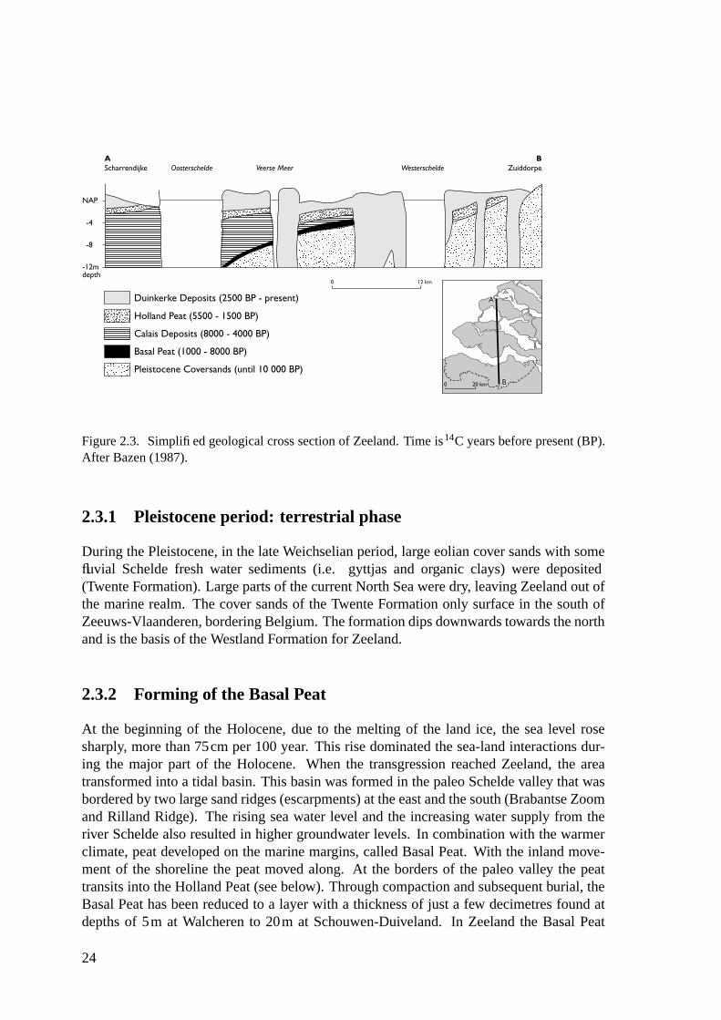
Figure 2.3. Simplified geological cross section of Zeeland. Time is14C years before present (BP).After Bazen (1987).
2.3.1 Pleistocene period: terrestrial phase
During the Pleistocene, in the late Weichselian period, large eolian cover sands with somefluvial Schelde fresh water sediments (i.e. gyttjas and organic clays) were deposited(Twente Formation). Large parts of the current North Sea were dry, leaving Zeeland out ofthe marine realm. The cover sands of the Twente Formation only surface in the south ofZeeuws-Vlaanderen, bordering Belgium. The formation dips downwards towards the northand is the basis of the Westland Formation for Zeeland.
2.3.2 Forming of the Basal Peat
At the beginning of the Holocene, due to the melting of the land ice, the sea level rosesharply, more than 75cm per 100 year. This rise dominated the sea-land interactions dur-ing the major part of the Holocene. When the transgression reached Zeeland, the areatransformed into a tidal basin. This basin was formed in the paleo Schelde valley that wasbordered by two large sand ridges (escarpments) at the east and the south (Brabantse Zoomand Rilland Ridge). The rising sea water level and the increasing water supply from theriver Schelde also resulted in higher groundwater levels. In combination with the warmerclimate, peat developed on the marine margins, called Basal Peat. With the inland move-ment of the shoreline the peat moved along. At the borders of the paleo valley the peattransits into the Holland Peat (see below). Through compaction and subsequent burial, theBasal Peat has been reduced to a layer with a thickness of just a few decimetres found atdepths of 5m at Walcheren to 20m at Schouwen-Duiveland. In Zeeland the Basal Peat
24
does not outcrop.
2.3.3 Calais deposits, first inundation
Around 6000-3000BC tidal channels emerged where most of the peat was removed by ero-sion, these were filled in with clay deposits, the Calais deposits. During this period theinfluence of the sea diminished and a coastal barrier system developed. Behind this bar-rier, (lagunal) basins formed in which clayey sediments deposited, while the tidal channelsconsisted of more sandy sediments. The decline in sea level tipped the balance betweensea level rise and filling of the basin. As a result the tidal area filled up, the tidal channelsdecreased in size and the coastal barrier could expand laterally until only two major tidalinlets were left, positioned around the current openings of the Westerschelde and Ooster-schelde. At present, outcrops of the Calais deposits are only found at Schouwen-Duivelandin an area called the “Prunje” east of Serooskerke (see figure 2.1). It otherwise is usuallyfound at depths of 1.5-4.5m. In Zeeuws-Vlaanderen, due to the higher elevation, the Calaisdeposit is absent.
2.3.4 Holland Peat
Due to the attenuation of the sea level rise and the shrinking of the tidal channels, drainageconditions deteriorated, and behind the now almost closed coastal barrier, only some open-ings were left by rivers, a new peat landscape emerged. It gradually changed from brackishto freshwater, due to the fresh water supply of the Schelde. The quantities of nutrientsdiminished though, and the peat flora changed from eutrophic to oligotrophic vegetation.Only along the Schelde did the peat stay eutrophic. The peat landscape was crossed byseveral streams of which the Oosterschelde was the largest one. These streams kept ac-tive openings in the coastal barrier through which the sea could gain influence on theland again. Holland Peat is found almost everywhere in Zeeland, unless it is excavatedor eroded, in a layer with a thickness ranging from 0.5-2.0m usually within a few metresfrom the surface. During excavations in the Middle Ages most of the peat was removed onSchouwen-Duiveland and Walcheren.
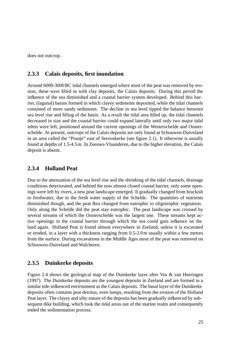
2.3.5 Duinkerke deposits
Figure 2.4 shows the geological map of the Duinkerke layer after Vos & van Heeringen(1997). The Duinkerke deposits are the youngest deposits in Zeeland and are formed in asimilar tide-influenced environment as the Calais deposits. The basal layer of the Duinkerkedeposits often contains peat detritus, even lumps, resulting from the erosion of the HollandPeat layer. The clayey and silty nature of the deposits has been gradually influenced by sub-sequent dike building, which took the tidal areas out of the marine realm and consequentlyended the sedimentation process.
25
0 5 102.5 Km
GeologyChannel deposits >1250 ADChannel deposits <1250 ADNo deposits, Pleistocene sandsCover layer, clay/sand
Figure 2.4. Simplified geology of the Duinkerke deposits, after Zagwijn (1991); Vos & van Heerin-gen (1997)
During the earliest embankments (1000-1200AD) heavy clays were deposited due to thequiet marine environment, resulting in the so called Heartland areas (Dutch: Oud- en Mid-delland). The quiet environment and slow sedimentation rates are presumably also thecause of the observed decalcified nature of the sediments. Moreover, these areas, so called“schorren” or “poelen” were often overgrown by vegetation. This source of organic mate-rial led to a reducing environment in the sediments.
Areas embanked after 1200AD are called Newlands; these are areas much closer to thetidal channels in which more fine sand, silt, and shell debris were deposited due to the
26
more turbulent environment. The type of embanked environment also gradually changed.First, mostly the accretions alongside the already existing dikes were embanked; later onalso the large tidal channels were closed. These were usually areas with barely any, orno, vegetation. Decalcification is much less than in the Heartlands due to the higher shellcontent and younger age.
A former geological model, describing the transgressive and regressive phases and result-ing in a subdivision of the Duinkerke deposits as 0 to IIIb layers, is nowadays consideredinvalid. Reasons for this, as given by Vos & van Heeringen (1997), are that the describedtransgressive phases are not synchronous in space, are insufficiently proved, and sometimesare incorrectly dated. However, this model is frequently referenced in pedologic descrip-tions of Zeeland that originate from before the invalidation of the model and it is thereforementioned here for completeness.
2.4 Human activities
Indications of the first human presence in Zeeland date back to Late Neolithic Ages(3100-2100BC), while during the Middle Roman Age (circa 100BC-100AD) the areawas already densely populated. However, these early inhabitants of Zeeland were barelyresponsible for the formation of the present day landscape. The most dramatic changesoccurred with the advancement of industry and technology. From the studied literatureit appears that there have been three major processes since the Middle Ages: 1) the dikebuilding and reclamation of the area, 2) the excavation of the Holland and Basal peat, and3) the reparceling of the agricultural land and Modern Time land reconstructions after themost recent floods (STIBOKA, 1964, 1967, 1980; van der Sluis et al., 1965; Bazen, 1987;Pleijter & Wallenburg, 1994; Vos & van Heeringen, 1997). I further consider that the soilsare influenced by input of metals and organic compounds from agricultural activities andatmospheric deposition. Although the latter is not often recognised from the literature de-scribing the landscape and soil geomorphology, it is generally accepted that such influencesare ubiquitously present in soils.
2.4.1 Dikes and embankments
Around 1000AD the first dikes were raised but it was not until the 12th century AD whenthe inhabitants started the systematic embankment of large areas such as the island of Beve-land (see figure 2.5 Rijkswaterstaat (1971)). The early dikes primarily defended the Heart-lands against the continuous threat of the sea and the regular storm surges during thesetimes. These dikes were relatively low since the elevation of the salt marshes was about1.5m above sea level. From the 13th century onwards the dike building becomes more of-fensive. The salt marshes outside the first embankments, sometimes newly formed, werealso reclaimed. These dikes were also motivated by the need for agricultural land and thegrowing prosperity due to the trading with Vlaanderen and England. It was this prosper-ity and the rise of abbeys that resulted in more political influence and money to invest in
27
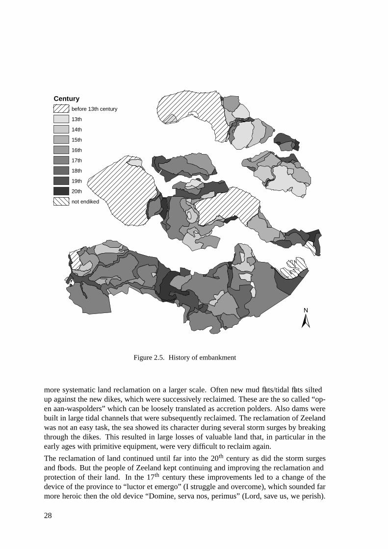
Centurybefore 13th century
13th
14th
15th
16th
17th
18th
19th
20th
not endiked
Figure 2.5. History of embankment
more systematic land reclamation on a larger scale. Often new mud flats/tidal flats siltedup against the new dikes, which were successively reclaimed. These are the so called “op-en aan-waspolders” which can be loosely translated as accretion polders. Also dams werebuilt in large tidal channels that were subsequently reclaimed. The reclamation of Zeelandwas not an easy task, the sea showed its character during several storm surges by breakingthrough the dikes. This resulted in large losses of valuable land that, in particular in theearly ages with primitive equipment, were very difficult to reclaim again.
The reclamation of land continued until far into the 20th century as did the storm surgesand floods. But the people of Zeeland kept continuing and improving the reclamation andprotection of their land. In the 17th century these improvements led to a change of thedevice of the province to “luctor et emergo” (I struggle and overcome), which sounded farmore heroic then the old device “Domine, serva nos, perimus” (Lord, save us, we perish).
28

The last two floods, one induced by the allied forces during World War II in Walcheren andthe other the great flood of 1953, resulted in large land reconstruction works. The dramaticflood of 1953, when 1835 people perished, forced the Dutch government to start the DeltaWorks, an impressive engineering project in which the dikes were raised and the large opensea arms were closed with dams (Goemans & Visser, 1987). With the completion of theDelta Works in 1988 Zeeland reached its present form.
2.4.2 Peat excavation
The exploitation of peat, mainly the Holland peat, started in the Roman Age but it is theexcavation during the Late Middle Ages that most influenced the present landscape. Theareas from which the peat was excavated were mostly located in the at present pool areas.
While the peat was used for fuel during the Roman Age, the Holland Peat became moresalty and covered by a thin layer of marine sediments due to the frequent floodings and in-undations of the peat landscape. The peat layers were then exploited for their salt content.Exploitation of the peat (“darinckdelven” or “moerneren” and refinement of the salt (“sel-nering” took place until prohibition in the 15th century. The process involved removing thecover sediment layer and digging out the peat. By burning the peat and mixing the asheswith sea water, and subsequent refining of the salt in lead, copper and iron pans, the valu-able salt was obtained. The excavations, both within and outside reclaimed areas, resultedin a lowering of the surface level by about 1m, which endangered such areas by makingthem even more vulnerable to floods. This was one of the main reasons for the prohibition.Moreover, the exploited areas were left behind in a bad state, as the surface level loweringwas highly variable at short distances. The resulting “hollebollig” (concave/convex) land-scape has short scale fluctuating soil moisture, and soil moisture salt content, and very poordrainage.
2.4.3 Parceling and land reconstruction
The allotment of the (agricultural) land among the inhabitants differed between the Heart-lands and the Newlands. The early farmers of the Heartlands started on the grounds of thesandy channel ridges, which were easier to rework with their primitive equipment, resultingin irregular and patchy patterns of parcels. In the Newlands the parceling was more rational.A cooperative group of people would buy the salt marshes and reclaim the area. The newpolder was then divided into the mainland, high quality grounds, and in the “volgerland”,lower quality ground. Each participant in the cooperative group then obtained parcels onboth kinds of ground, or was paid money if no mainland grounds could be obtained. Thisresulted in a more regular, block wise, parceling. By inheritance, sales, and other changesover time, the parcels became divided later into smaller and smaller areas.
The last floods during World War II and 1953 caused severe destruction. This led to largescale land reconstruction works that reparceled the agricultural land, leading to a betterorganised landscape. New, straight roads were built and ditches were replaced. Also the
29
“hollebollig” landscape, with its low agricultural value, was reworked. The cover layer wasremoved and the underlying layers leveled. The cover layer was then placed back. In largeareas, mainly those where peat excavations had occurred, this disturbed the soil profile ofthe subsoil but kept the upper layer intact.
2.4.4 Agricultural inputs
The intensification of agriculture, facilitated by the large scale land reconstructions, ini-tially also led to an increase in the usage of fertilisers and pesticides as compared to pre-war levels. This increase was subsequently reduced due to more environmental awarenessand governmental regulations in the last part of the 20th century (RIVM, 2004). Based onhistorical statistics figure 2.6 shows an example of the usage of P and K inorganic fertilisersfor the Netherlands.
Some fertilisers are known to contain substantial amounts of heavy metals like Cd, Pb, Cu,and Zn (de Lopez Camelo et al., 1997; Gimeno-Garcıa et al., 1996; Nash et al., 2003). Theaccumulation of these heavy metals in soils has also been recognised in the Netherlandsand for some parts of Zeeland (Groot et al., 2001; van Drecht et al., 1996; RIVM, 2004).Residues of persistent organochlorine pesticides, such as DDT, γ-HCH, and Dieldrin, arefound as a heritage from the past. It is not uncommon that the values of organochlorinepesticides in Dutch soil exceed legal permissible limits (Groot et al., 2001; RIVM, 2004).Besides local input by agricultural practice, atmospheric deposition from sometimes re-mote sources may also contribute to the deposition of organochlorine pesticide (Rovinskyet al., 1995; Villa et al., 2003) and heavy metals (Koeleman et al., 1999). Although theseprocesses are not specific to the Zeeland region, in fact some of them are global, they areexpected to exert a major influence on the (geo)chemical soil composition of Zeeland.
2.5 Landscape and soil geomorphology
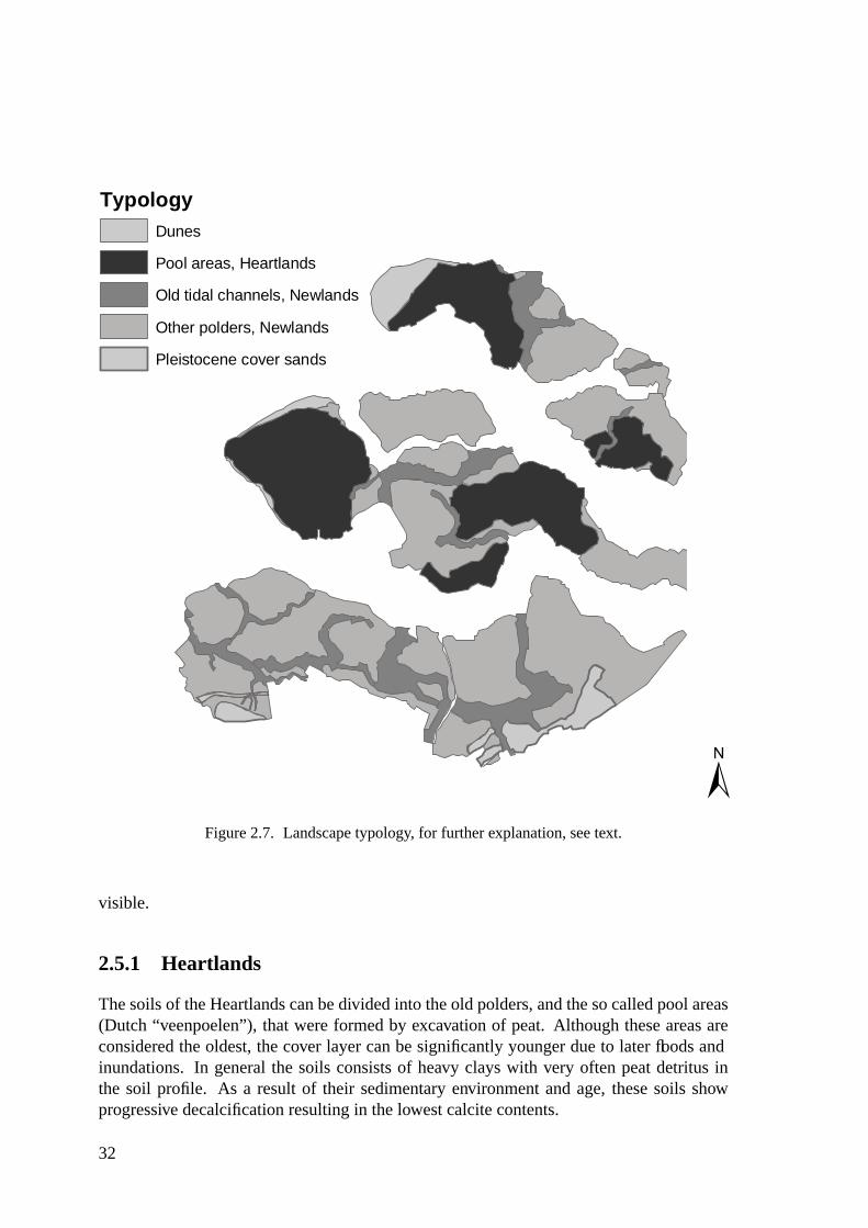
The final geomorphology of Zeeland is a result of both the natural and human processes asdescribed above. While varied and sometimes complex, they resulted in only a few majorlandscape types and associated soil types that will be outlined in some detail below: theHeartlands, channel ridges, and accretion polders (“op- en aanwaspolders”) Dunes, beachsands, the small area of Pleistocene sands in the south of Zeeland, and areas outside thedikes are left out of this description since they are not within the focus of the geochem-ical research. A brief description of the major groundwater systematics will be given tocomplement this section.
The relevant major landscape types are depicted in figure 2.7 (Halfwerk, 1996). Whilethe classification differs from that based on the invalidated Duinkerke 0 to IIIb regressionmodel (see §2.3.5) the major features are the same. The oldest pool areas are mainly formedby the Heartlands the Newlands are subdivided into polders and large tidal channels.
The soils of Zeeland have developed on marine clay deposits and according to the classi-
30
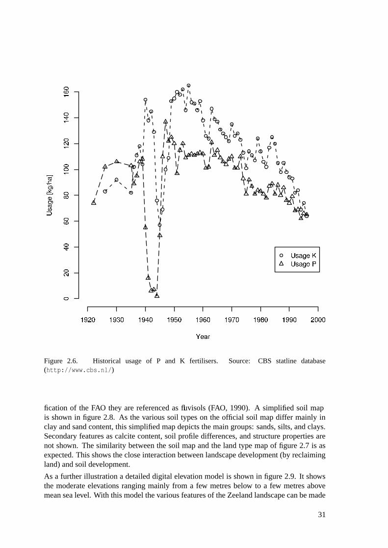
Figure 2.6. Historical usage of P and K fertilisers. Source: CBS statline database(http://www.cbs.nl/)
fication of the FAO they are referenced as fluvisols (FAO, 1990). A simplified soil mapis shown in figure 2.8. As the various soil types on the official soil map differ mainly inclay and sand content, this simplified map depicts the main groups: sands, silts, and clays.Secondary features as calcite content, soil profile differences, and structure properties arenot shown. The similarity between the soil map and the land type map of figure 2.7 is asexpected. This shows the close interaction between landscape development (by reclaimingland) and soil development.
As a further illustration a detailed digital elevation model is shown in figure 2.9. It showsthe moderate elevations ranging mainly from a few metres below to a few metres abovemean sea level. With this model the various features of the Zeeland landscape can be made
31
TypologyDunes
Pool areas, Heartlands
Old tidal channels, Newlands
Other polders, Newlands
Pleistocene cover sands
Figure 2.7. Landscape typology, for further explanation, see text.
visible.
2.5.1 Heartlands
The soils of the Heartlands can be divided into the old polders, and the so called pool areas(Dutch “veenpoelen”), that were formed by excavation of peat. Although these areas areconsidered the oldest, the cover layer can be significantly younger due to later floods andinundations. In general the soils consists of heavy clays with very often peat detritus inthe soil profile. As a result of their sedimentary environment and age, these soils showprogressive decalcification resulting in the lowest calcite contents.
32
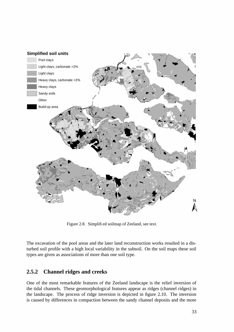
Simplified soil unitsPool clays
Light clays, carbonate >2%
Light clays
Heavy clays, carbonate >2%
Heavy clays
Sandy soils
Other
Build−up area
Figure 2.8. Simplified soilmap of Zeeland, see text.
The excavation of the pool areas and the later land reconstruction works resulted in a dis-turbed soil profile with a high local variability in the subsoil. On the soil maps these soiltypes are given as associations of more than one soil type.
2.5.2 Channel ridges and creeks
One of the most remarkable features of the Zeeland landscape is the relief inversion ofthe tidal channels. These geomorphological features appear as ridges (channel ridges) inthe landscape. The process of ridge inversion is depicted in figure 2.10. The inversionis caused by differences in compaction between the sandy channel deposits and the more
33
Altitude [cm]
ValueHigh : 1000
Low : −994
12
3
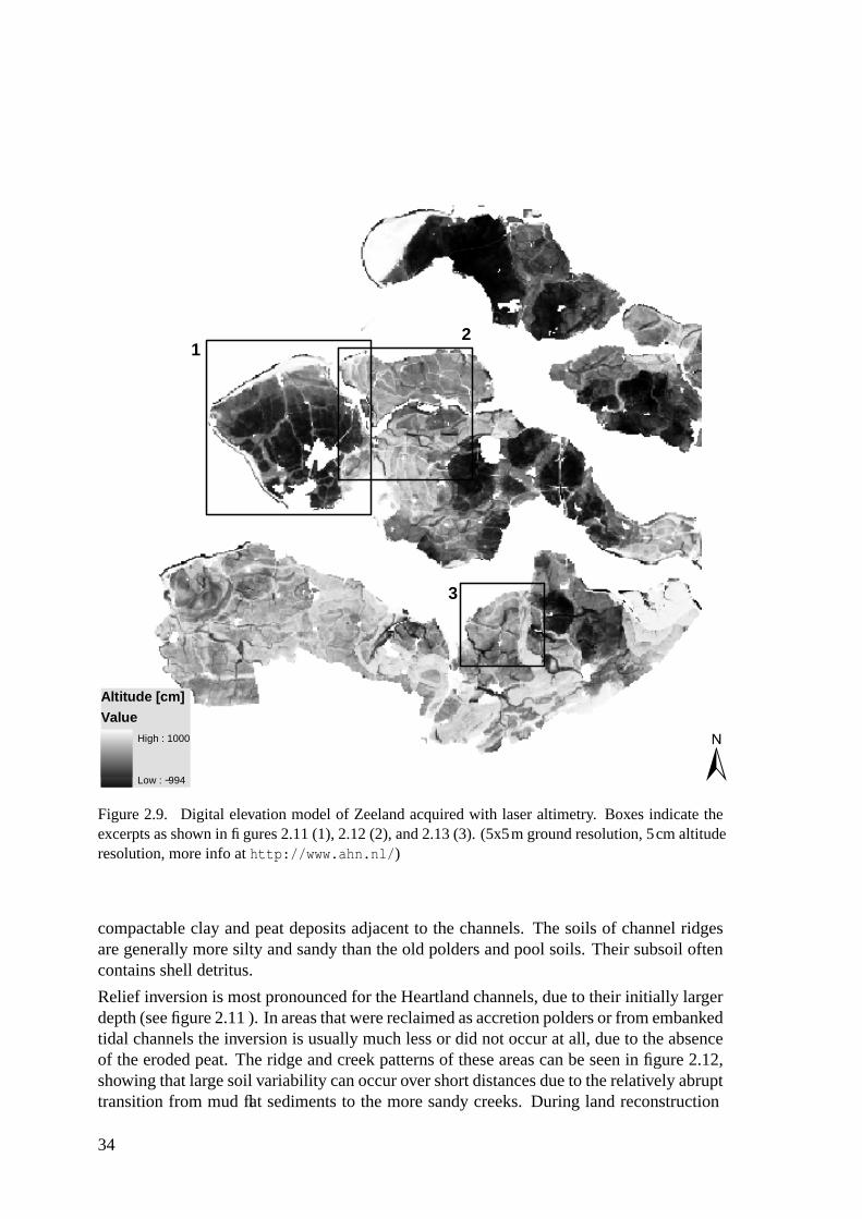
Figure 2.9. Digital elevation model of Zeeland acquired with laser altimetry. Boxes indicate theexcerpts as shown in figures 2.11 (1), 2.12 (2), and 2.13 (3). (5x5m ground resolution, 5cm altituderesolution, more info at http://www.ahn.nl/)
compactable clay and peat deposits adjacent to the channels. The soils of channel ridgesare generally more silty and sandy than the old polders and pool soils. Their subsoil oftencontains shell detritus.
Relief inversion is most pronounced for the Heartland channels, due to their initially largerdepth (see figure 2.11 ). In areas that were reclaimed as accretion polders or from embankedtidal channels the inversion is usually much less or did not occur at all, due to the absenceof the eroded peat. The ridge and creek patterns of these areas can be seen in figure 2.12,showing that large soil variability can occur over short distances due to the relatively abrupttransition from mud flat sediments to the more sandy creeks. During land reconstruction
34
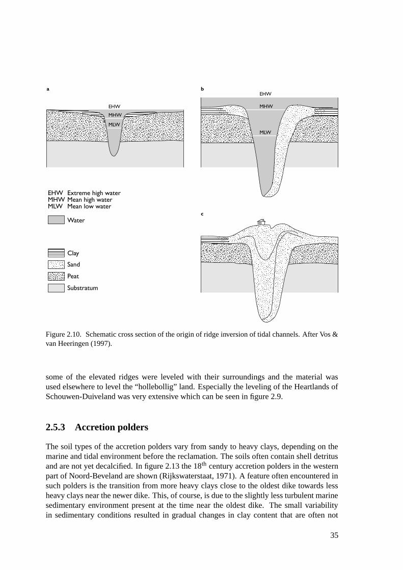
Figure 2.10. Schematic cross section of the origin of ridge inversion of tidal channels. After Vos &van Heeringen (1997).
some of the elevated ridges were leveled with their surroundings and the material wasused elsewhere to level the “hollebollig” land. Especially the leveling of the Heartlands ofSchouwen-Duiveland was very extensive which can be seen in figure 2.9.
2.5.3 Accretion polders
The soil types of the accretion polders vary from sandy to heavy clays, depending on themarine and tidal environment before the reclamation. The soils often contain shell detritusand are not yet decalcified. In figure 2.13 the 18th century accretion polders in the westernpart of Noord-Beveland are shown (Rijkswaterstaat, 1971). A feature often encountered insuch polders is the transition from more heavy clays close to the oldest dike towards lessheavy clays near the newer dike. This, of course, is due to the slightly less turbulent marinesedimentary environment present at the time near the oldest dike. The small variabilityin sedimentary conditions resulted in gradual changes in clay content that are often not
35
Altitude [cm]
ValueHigh : 1000
Low : −994
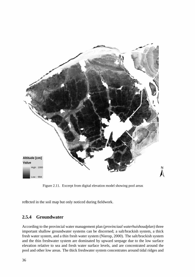
Figure 2.11. Excerpt from digital elevation model showing pool areas
reflected in the soil map but only noticed during fieldwork.
2.5.4 Groundwater
According to the provincial water management plan (provinciaal waterhuishoudplan) threeimportant shallow groundwater systems can be discerned; a salt/brackish system, a thickfresh water system, and a thin fresh water system (Nierop, 2000). The salt/brackish systemand the thin freshwater system are dominated by upward seepage due to the low surfaceelevation relative to sea and fresh water surface levels, and are concentrated around thepool and other low areas. The thick freshwater system concentrates around tidal ridges and
36

Altitude [cm]
ValueHigh : 1000
Low : −994
Figure 2.12. Excerpt from digital elevation model showing channel ridges
higher elevated areas, the main direction of flow is determined by infiltration. The excessof water due to seepage and rainfall is removed towards the sea by a system of ditchesand channels using pumping-stations. The phreatic level varies from close to the surfacedown to a depth of 2m (Rijkswaterstaat, 1971). Regulation of the groundwater level isimportant for agriculture. As the input of freshwater cannot be controlled by fresh waterinlets because of the generally brackish surface water, water levels are kept higher in winterto provide a buffer against drier periods in summer.
37
Altitude [cm]
ValueHigh : 1000
Low : −994
Figure 2.13. Excerpt from digital elevation model showing accretion polders
2.6 Summary and conclusion
Zeeland is located in a marine delta of the rivers Rijn, Maas and Schelde. It was the sealevel rise following the end of the Weichselian ice age, that brought Zeeland within themarine realm. The soils of Zeeland can be regarded as relatively homogeneous and young.They were moulded in a continuous interaction of natural processes and human endeavour.
During the last depositional age, the Duinkerke period, three activities dominated soil for-mation: dike building and land reclamation, peat excavation, and large scale land recon-struction. The embankment of large areas removed these areas from the marine realm andfixed their condition. The division between the two major landscape types, Heartlands and
38
Newlands, is based on the embankment history. The relatively elevated Heartlands weremainly embanked in the Middle Ages as defensive measures against the sea, while the New-lands were reclaimed in later periods to acquire new agricultural land. As a consequencethe soils of the Heartlands are mainly fairly heavy clays, while most of the Newlands aremore sandy and silty. Especially in the Heartlands, large areas of peat were excavated,leaving behind an area of low agricultural value with an uneven surface and short rangefluctuating moisture content. This, amongst other factors, led to major land reconstructionworks, initiated after the two last catastrophic inundations of 1944 and 1953, in which thetopsoil was removed and the subsoil leveled, after which the topsoil was replaced. Thisresulted in a variable subsoil with a relatively homogeneous topsoil.
Considering the fact that soils of Zeeland are in general developed in from marine claydeposits, it can be expected that a main source of geochemical variability is the varyingclay content. The natural pattern of creek ridges and pool areas already creates relativelyabrupt transitions. As local homogeneity or gradual variation may be further disturbed bythe extensive human works, variability in soil composition is expected to be still higherthan is directly evident from the soil map. Each (embanked) area with its own history,both sedimentary and human, may have its own pattern of soil variability. Given the factthat 80% of terrestrial Zeeland is used for agriculture, nearly 70% of which is arable land,human processes related to fertilisation and pesticide use are further expected to have in-fluenced soil composition. This will result in elevated concentrations of so called “heavymetals” (Cd, Cu, Pb, and Zn) and persistent organochlorine pesticide residues. Finally,atmospheric inputs should also be considered as contributing to soil geochemistry.
39

3 Natural and anthropogenic patternsof covariance and spatial variabilityof minor and trace elements in agri-cultural topsoil
3.1 Introduction
Soil contamination is one of the major environmental issues within the Netherlands. Thegovernment, in its Third National Environmental Policy Plan (VROM, 1997), has calledfor a nationwide assessment of soil quality before the year 2005. The two tracks of the as-sessment include: 1; the stock of contaminated sites that need remediation, a job intendedto be carried out to completion within the coming two decades; and 2; the general or “dif-fuse” soil quality. This second track of the assessment concentrates on making accessibleand integrating available data on soil quality in support of soil protection policy and spatialplanning.
As a consequence of stricter environmental legislation regarding building materials(VROM, 1999), municipal and provincial authorities recently have been putting much ef-fort into the draft of so called soil pollution risk maps (in Dutch: BodemKwaliteitsKaartenor BKKs)(van der Gaast et al., 1998; van Lienen et al., 2000). These maps show the levelsof priority chemicals relative to their legal thresholds in soil. A legally ascertained mapallows dispensation of some of the clauses in the legislation regarding the effort needed tocertify that soil that is transported to and from the area is legally “clean”. The data collectedwithin the BKK-scope will also provide an important input into track 2 of the nationwidesoil quality assessment.
In view of the large commitment of financial and human resources dedicated to soil qualityassessment, the need was felt for a more scientific evaluation of soil quality and the benefitof soil quality maps, alongside the governmental tracks. One of the issues requiring furtherattention is the quality of soil quality maps, in respect of spatial variability and samplingprocedures.
In print as: Spijker, J., Vriend, S.P., Van Gaans, P.F.M., 2005, “Natural and anthropogenic patterns ofcovariance and spatial variability of minor and trace elements in agricultural topsoil”, Geoderma.
41
In the Netherlands environmental soil surveys are usually based on sampling designs thatuse composite samples. The Dutch standard for soil sampling (NNI, 1999b) details therequired procedure of such a design. This standard is based in part on agricultural practiceand requirements for soil remediation research, and as such aims at a local rather than aregional scale. For reasons of comparability (the very first aim of a standard) and efficientuse of existing data, the same design is also used in the BKK procedure and other moreregional studies. For example in the geochemical soil survey for the province of Zeelandon which most of this thesis will be based, samples consisted of a composite of 15-20subsamples taken from a field area of about 100 m · 100 m, at a density of approximatelyone sample per 3 to 9 km2. The aim of this general Zeeland study is the (multivariate)characterization of the inorganic soil composition within the rural areas, both for naturallyoccurring and for anthropogenically enriched elements, like the so called “heavy metals”(Cd, Cu, Pb, Sb, Sn, and Zn). Given this context, expectations regarding the advantagesof error reduction through composite sampling, based on experience and expert judgmentin daily operation of remediation surveys, might be false.
The benefits of the reduction in variance through compositing depend on the spatial vari-ation pattern and the spatial scale of interest. If interest is mainly in regional patternscompositing will only be useful when local variability is large, including in relation to an-alytical variance (i.e. variance associated with chemical analysis). If local features are ofinterest, compositing may be generally more relevant. The aim of this chapter is to estimatethe variability related to spatial scale and sampling procedure for a wide range of elementsin the topsoil of Zeeland. The hypothesis is that distinct spatial patterns of variability ex-ist for groups of elements that are geochemically or anthropogenically related and whosevariability depends on common factors and processes. The relative benefit of compositingmay then be different for different groups of elements, which indicate that the quality ofsoil quality maps may have to be viewed differently depending on the desired application.
3.2 Materials and methods
3.2.1 Area
The chosen study area, the peninsula of Walcheren/Zuid Beveland, is located in theprovince of Zeeland, in the south-west of the Netherlands, see figure 3.1. The geologicalprocesses and human activities responsible for soil variability in this area are representativefor Zeeland, and probably for similar deltaic areas around the world. The polder-landscapeof the study area mainly consists of marine clay deposits (Duinkerke deposits) which arepart of the Holocene Westland formation (Vos & van Heeringen, 1997). The Holocenealternation of marine clay deposits and peat deposits was caused by a sequence of trans-gressive and minor regressive events since the end of the last glacial period of the Pleis-tocene (see also chapter 2). The peninsula has a history of flooding and land-reclamationthat continued until the 20th century. The area is divided into two major marine clay land-types based on their age of reclamation and relative altitude: Heartlands and Newlands.
42

Walcheren Zuid−Beveland
LocationsLocations unbalanced design HeartlandsLocations unbalanced design NewlandsLocations general Zeeland survey
Figure 3.1. Location map of the study area Walcheren/Beveland in Zeeland, the Netherlands, withsample sites.
The Heartlands originated as an alternation between salt-marshes and peat in the periodbetween 500-1200 AD. During the various floods large tidal inlets formed that were subse-quently filled with marine sand. The peat was excavated for the production of salt, resultingin pools which were later filled with heavy marine clays. These pool-clays are not very wellsuited for cultivation, but drainage and re-allotment improved this situation. A landscapedeveloped with a variable, sometimes disturbed, soil profile of heavy clay and sometimessparse peat fragments, cut by the sandy inlets. Due to the settling of the peat layers analtitude inversion occurred and the sand ridges are now about 1-1.5 m above the clay areas.The Newlands are of later origin than the Heartlands and in general were not used for peatexcavation. The soil profile is less disturbed and consists of sandy marine clay deposits(Bazen, 1987). Soils of both land-types can be classified as fluvisols and are mainly usedfor farming.
3.2.2 Spatial variance and sampling theory
The total observed variance of a soil characteristic is in principal a summation of variancecomponents that each can be attributed to a specific source. For example the variabilityin lime content in soil can, amongst others, be attributed to variation in the parent mate-rial and to variation in the extent of leaching with fresh water (Sposito, 1989). For the
43
heavy metals in topsoil an anthropogenic source of variance can be expected. Of course anunavoidable additional source is analytical error. In the simplest form of Analysis of Vari-ance (ANOVA) the “within” variance obtained through replicate sampling within e.g; onetype of parent material is considered as noise. If, from an F-test, the variance “between”different parent materials is significantly larger than the pooled “within” variance, parentmaterial is concluded to be an additional source of variability.
In soil science, or in geological sciences in general, the total variance can often be viewedas being composed of spatial components. The well-known semivariogram displays thecumulative variance as a function of increasing distance (e.g. Journel & Huijbregts (1981)).A discrete version of this spatial variance pattern can be obtained through an ANOVA basedon a hierarchical nested sampling design with different distances as subclasses or levels(Webster, 1985; Miesch, 1975).
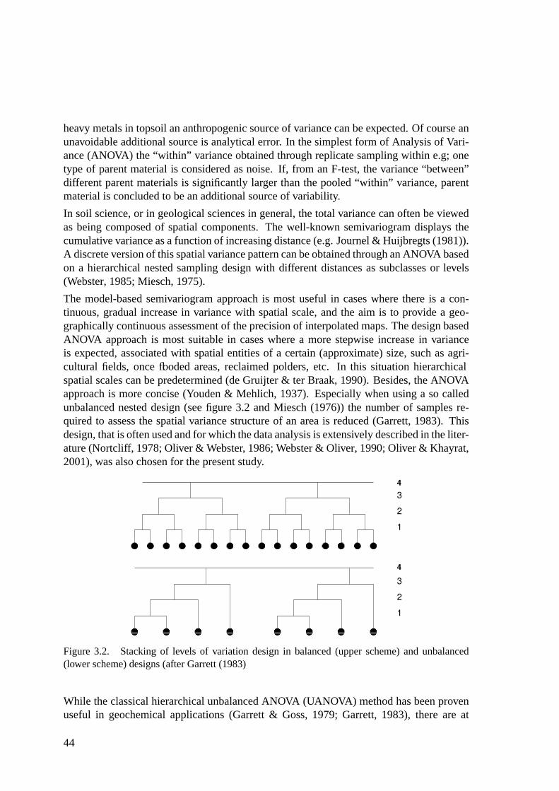
The model-based semivariogram approach is most useful in cases where there is a con-tinuous, gradual increase in variance with spatial scale, and the aim is to provide a geo-graphically continuous assessment of the precision of interpolated maps. The design basedANOVA approach is most suitable in cases where a more stepwise increase in varianceis expected, associated with spatial entities of a certain (approximate) size, such as agri-cultural fields, once flooded areas, reclaimed polders, etc. In this situation hierarchicalspatial scales can be predetermined (de Gruijter & ter Braak, 1990). Besides, the ANOVAapproach is more concise (Youden & Mehlich, 1937). Especially when using a so calledunbalanced nested design (see figure 3.2 and Miesch (1976)) the number of samples re-quired to assess the spatial variance structure of an area is reduced (Garrett, 1983). Thisdesign, that is often used and for which the data analysis is extensively described in the liter-ature (Nortcliff, 1978; Oliver & Webster, 1986; Webster & Oliver, 1990; Oliver & Khayrat,2001), was also chosen for the present study.
Figure 3.2. Stacking of levels of variation design in balanced (upper scheme) and unbalanced(lower scheme) designs (after Garrett (1983)
While the classical hierarchical unbalanced ANOVA (UANOVA) method has been provenuseful in geochemical applications (Garrett & Goss, 1979; Garrett, 1983), there are at
44
present many other methods for estimating variance components for an unbalanced design,such as maximum likelihood, restricted maximum likelihood and a principal componentsbased method (Searle et al., 1992; Khatree et al., 1997). The main disadvantage of theclassical UANOVA, as seen by most authors, is the possibility of negative estimates forone or more of the variance components. Some go as far as calling this feature “awkwardand embarrassing” (Searle et al., 1992), and therefore disapprove of the method. The ad-vantages of (U)ANOVA, however, are clarity, simplicity, and robustness. More advancedmethods such as Restricted Maximum Likelihood may be highly sensitive to whether ornot an additional level of spatial scale is discerned (as in our case for example the divisionin Heartland and Newland) or not.
The possibility of negative estimates for variance components was not considered an in-surmountable problem in this study. Negative estimates occur when the estimate for thebetween group variance is smaller than the estimate for the within group variance or, inspatial terms, when the calculated variance at a certain scale between units of a finer scaleis smaller than the calculated variance within these finer scaled units. While in principleimpossible (except for zonal features), a negative estimate can always occur if the realvalue is close to zero. Negative estimates thus can be substituted by zero. This method isgenerally accepted and performs well, also compared to more advanced methods (Pettitt &McBratney, 1993; Khatree et al., 1997).
The aim of this study is not to determine absolute values for the individual variance compo-nents of single elements, but to distinguish general patterns of spatial variance for groupsof related elements. The simplicity and robustness of the UANOVA are therefore preferredover the sophistication, but sensitivity, of the more advanced methods.
3.2.3 Sampling and chemical analysis
For both Heartlands and Newlands eight locations were randomly selected in the marineclay deposits of the rural area of the peninsula resulting in 16 locations (see figure 3.1).Five local and two regional levels of variance were chosen. At each sample location singlesoil samples were collected at five specific distances, in a random direction from a basesample. The seven levels/distances thus investigated matched respectively the variabilityfor a duplicate sample (1 m), at short distance (30 m), within the sample field (100 m),between neighbouring fields (300 m), at kilometre level (1000 m), between locations (re-gional), and Heartlands vs. Newlands (landtype). This sampling scheme is illustrated infigure 3.3. Heartland sand ridges were avoided to exclude large differences in soil typewithin one location.
The resulting 96 samples were taken with a hand auger from the plough layer. If this layercould not be distinguished, the samples were taken from the depth range 5-20 cm. Afterdrying at 40°C, grinding down to approximately 50 µm, and a hot aqua-regia digestion, thesamples were analyzed by ICP-MS, together with 13 randomly selected duplicates at theanalytical (within-sample) level. The following elements were determined: As, Ag, Au,B, Ba, Be, Bi , Ca, Cd, Ce, Cr, Cs, Cu, Dy, Er , Eu, Fe, Ga, Gd, Hf, Ho, La, Li , Lu,
45

Figure 3.3. Stacking of levels of the sample design for this research. For each landtype the designof one location is shown
Mg, Mn, Mo, Nb, Nd, Ni , Pb, Pr , Pt , Rb, Re, Sb, Sc, Se, Sm, Sn, Sr , Ta, Tb, Th, Ti ,Tl , Tm, U, Y, Yb, Zn, Zr .
As pointed out by among others Walsh et al. (1997) in case of an acid leach such as aquaregia there are few recognized reference materials available that can be used for methodvalidation. Moreover, the focus of this chapter is on variance and covariance, for whichprecision rather than accuracy is the priority issue. Accuracy was therefore assumed to bejust as good as that attained in the general Zeeland study, for which part overlap with XRFdata and comparison with ISE standards was available (van Dijk & Houba, 2000).
3.2.4 Data analysis
The data were first examined for analytical errors. From the duplicate analysis the relativeerror was calculated using
v =sx·100% (3.1)
Where v is the error relative to the overal mean x and the standard deviation s. The lattercalculated with
s =
√∑n
i=1(xi1− xi2)2
2n(3.2)
where the standard deviation is calculated from n duplicates with values xi1 and xi2. Ele-ments with large relative error were excluded from further statistical analysis.
Outliers are defined as values larger than the 3rd quartile plus 2 times the interquartilerange, This procedure is equivalent to calculating the fences for box and whiskers plotsaccording to Tukey (1977), except that for the inner fences the value of 2 was chosen
46
above the original value of 1.5 to compensate for possible positive skewness. This kindof Winsoring of the extremes was applied to prevent them from having undue influenceon the UANOVA analysis. Outliers were replaced by a random sample from the upper(4th) quartile from the same distribution of the same element without outliers since theUANOVA poorly handles missing values. Listwise deletion obviously is not desired. Therandom replacement instead of a fixed maximum value ensures remaining variance alsobetween outliers. We prefer this procedure over a logaritmic or similar transformation sincethe character of the statistical distribution of the variance components may also be scaledependent. In the case of just the sporadic outlier we do not assume that this replacementmethod adversely influences the distribution of the data.
For the UANOVA, the program of Garrett & Goss (1980) was used, to identify for eachelement which spatial scale/level contributes most to the overall variance and to show therelative contribution of each level. To identify groups of elements with similar spatialvariability patterns a fuzzy c-means clustering (Bezdek et al., 1984; Vriend et al., 1988;Urbat et al., 1997) was performed on the UANOVA results. Due to the random selectionof the analytical duplicates, independent of the UANOVA scheme, analytical variance isnot incorporated in the UANOVA model. Moreover, it was felt that the analytical varianceshould not play an explicit role in the fuzzy clustering of the UANOVA results.
The assumed reduction of variance of a composite sample design, as used in the generalZeeland study, in respect to a single sample design as used here, was assessed with an F-test. Thirty-three samples from the general Zeeland study that cover the same area as that ofthe single sample design, although with a different sampling pattern (see figure 3.1), wereselected and their overall variance was calculated. From the single sample design only thebase sample and the 1000 m sample were selected, resulting in 32 samples in total. Usingthe 1000 m sample as well, the number and hence the spatial spread of locations, matchthose of the general Zeeland study.
Since the aim of this study is to distinguish general patterns of spatial variances of groupsof related elements, it is also interesting to consider their covariance patterns. Of coursethese may also vary with spatial scale. Interest here is focussed on regional features sospecifically the covariance at the overall (regional) level was considered. To this end aprincipal components analysis with varimax rotation (PCA-V;Davis (2002); Reimann et al.(2002)) was applied to the dataset. To provide sufficient dimensionality, defined as the ratiobetween the number of cases and variables (i.e. elements) used, a selection of representativeelements was made for the PCA. Due to collinearity, it is not necessary to include allelements that are expected to be mainly related to one factor such as parent material. Forinstance, one or two rare earth elements (REE) will suffice instead of all REE, increasingthe dimensionality. To check the assumption that the elements that are not included in thePCA-V are still explained by the factor model, the correlation with the PCA-V factorscoreswas studied. For the same reason of sufficient dimensionality, robust versions of PCA, thatuse only a subset of the cases, were not deemed adequate here. It was assumed that theWinsorising/replacement of the outliers sufficed to obtain a stable factor model.
47
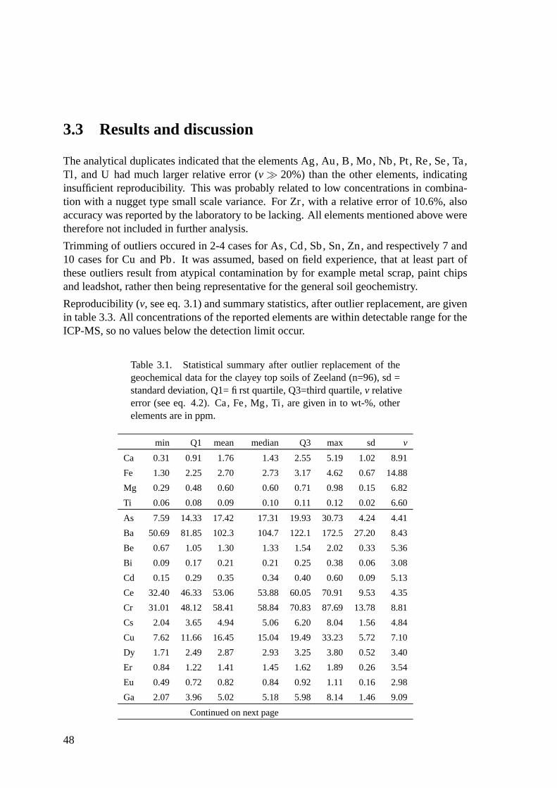
3.3 Results and discussion
The analytical duplicates indicated that the elements Ag, Au, B, Mo, Nb, Pt , Re, Se, Ta,Tl , and U had much larger relative error (v� 20%) than the other elements, indicatinginsufficient reproducibility. This was probably related to low concentrations in combina-tion with a nugget type small scale variance. For Zr, with a relative error of 10.6%, alsoaccuracy was reported by the laboratory to be lacking. All elements mentioned above weretherefore not included in further analysis.
Trimming of outliers occured in 2-4 cases for As, Cd, Sb, Sn, Zn, and respectively 7 and10 cases for Cu and Pb. It was assumed, based on field experience, that at least part ofthese outliers result from atypical contamination by for example metal scrap, paint chipsand leadshot, rather then being representative for the general soil geochemistry.
Reproducibility (v, see eq. 3.1) and summary statistics, after outlier replacement, are givenin table 3.3. All concentrations of the reported elements are within detectable range for theICP-MS, so no values below the detection limit occur.
Table 3.1. Statistical summary after outlier replacement of thegeochemical data for the clayey top soils of Zeeland (n=96), sd =standard deviation, Q1= first quartile, Q3=third quartile, v relativeerror (see eq. 4.2). Ca, Fe, Mg, Ti , are given in to wt-%, otherelements are in ppm.
min Q1 mean median Q3 max sd v
Ca 0.31 0.91 1.76 1.43 2.55 5.19 1.02 8.91
Fe 1.30 2.25 2.70 2.73 3.17 4.62 0.67 14.88
Mg 0.29 0.48 0.60 0.60 0.71 0.98 0.15 6.82
Ti 0.06 0.08 0.09 0.10 0.11 0.12 0.02 6.60
As 7.59 14.33 17.42 17.31 19.93 30.73 4.24 4.41
Ba 50.69 81.85 102.3 104.7 122.1 172.5 27.20 8.43
Be 0.67 1.05 1.30 1.33 1.54 2.02 0.33 5.36
Bi 0.09 0.17 0.21 0.21 0.25 0.38 0.06 3.08
Cd 0.15 0.29 0.35 0.34 0.40 0.60 0.09 5.13
Ce 32.40 46.33 53.06 53.88 60.05 70.91 9.53 4.35
Cr 31.01 48.12 58.41 58.84 70.83 87.69 13.78 8.81
Cs 2.04 3.65 4.94 5.06 6.20 8.04 1.56 4.84
Cu 7.62 11.66 16.45 15.04 19.49 33.23 5.72 7.10
Dy 1.71 2.49 2.87 2.93 3.25 3.80 0.52 3.40
Er 0.84 1.22 1.41 1.45 1.62 1.89 0.26 3.54
Eu 0.49 0.72 0.82 0.84 0.92 1.11 0.16 2.98
Ga 2.07 3.96 5.02 5.18 5.98 8.14 1.46 9.09
Continued on next page
48

Table 3.1 – continued from previous page
min Q1 mean median Q3 max sd v
Gd 2.35 3.32 3.86 3.95 4.38 5.11 0.71 3.20
Hf 0.41 0.58 0.70 0.71 0.82 0.99 0.15 5.78
Ho 0.31 0.46 0.53 0.54 0.60 0.72 0.10 7.63
La 14.35 21.95 25.20 25.91 28.84 34.45 4.75 3.82
Li 12.85 21.98 29.38 30.55 36.04 50.52 9.01 5.34
Lu 0.10 0.15 0.17 0.17 0.19 0.23 0.03 5.81
Mn 141.6 233.1 308.2 291.6 370.8 542.0 95.19 8.24
Nd 14.16 19.92 22.91 23.26 26.02 30.44 4.14 4.09
Ni 7.60 15.19 18.62 19.31 22.61 29.83 5.26 4.31
Pb 11.54 21.51 27.03 26.96 30.70 50.19 7.61 3.07
Pr 3.63 5.29 6.05 6.12 6.88 8.09 1.11 5.46
Rb 32.45 50.97 66.36 66.00 79.90 105.4 18.56 5.50
Sb 0.27 0.35 0.42 0.42 0.47 0.65 0.08 9.89
Sc 3.70 5.98 7.50 7.62 8.90 11.53 1.91 8.51
Sm 2.76 3.90 4.46 4.53 5.08 5.89 0.81 3.88
Sn 1.16 1.74 2.19 2.07 2.50 3.95 0.61 4.41
Sr 37.12 53.23 69.86 65.25 87.95 124.3 21.19 3.51
Tb 0.33 0.47 0.54 0.55 0.61 0.73 0.10 3.48
Th 3.73 5.55 6.53 6.65 7.53 8.76 1.29 4.56
Tm 0.11 0.17 0.19 0.19 0.21 0.25 0.03 5.53
Y 8.32 12.13 13.86 14.19 15.76 18.76 2.59 5.09
Yb 0.73 1.08 1.22 1.27 1.40 1.66 0.23 5.48
Zn 34.86 61.62 74.26 73.12 86.32 131.6 20.53 5.21
Twenty representative elements were selected for the PCA-V, resulting in a dimensionalityof 4.8, and the results are shown in table 3.2. For the elements not included in the PCA-V,correlations with the PCA-V factorscores are given in table 3.3 for the first factor. Correla-tions with scores of other factors were substantially lower, all less than 0.3. This confirmsthat the elements not included in the PCA-V are indeed highly correlated with one of thefactors. The first rotated factor accounts for 47.6% of the total variance within the model.Elements with high factor loadings on this factor are mostly clay related natural elements,i.e. not influenced by human interference. The second factor accounts for 14% of the fac-tor model variance and has high loadings for Ca and Sr and moderate loadings for As, Cu,Mg, and Mn. This factor represents the primarily natural variation in carbonate contentof the soils. The elements As and Mn are possibly partly related to pH-dependent redoxprocesses. The third factor has high loadings for the possibly anthropogenically influencedelements Cd, Pb, Sb, Sn, and to lesser extent Zn, Bi , and Cu. The factors have been
49
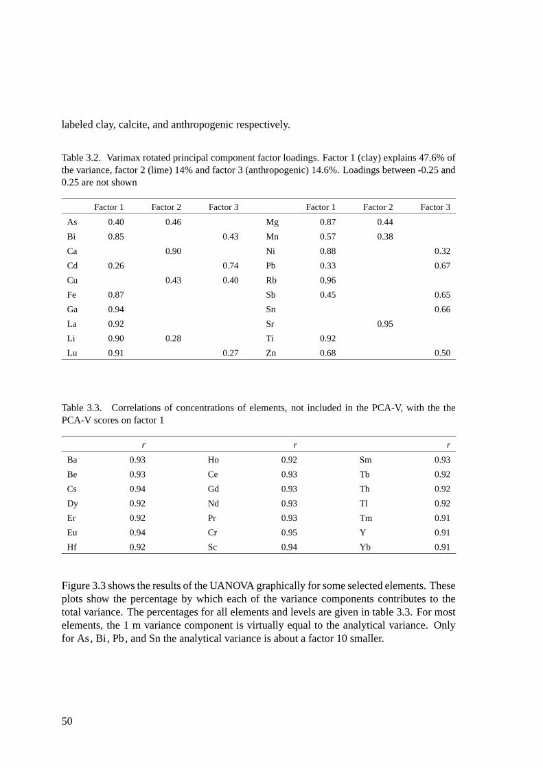
labeled clay, calcite, and anthropogenic respectively.
Table 3.2. Varimax rotated principal component factor loadings. Factor 1 (clay) explains 47.6% ofthe variance, factor 2 (lime) 14% and factor 3 (anthropogenic) 14.6%. Loadings between -0.25 and0.25 are not shown
Factor 1 Factor 2 Factor 3 Factor 1 Factor 2 Factor 3
As 0.40 0.46 Mg 0.87 0.44
Bi 0.85 0.43 Mn 0.57 0.38
Ca 0.90 Ni 0.88 0.32
Cd 0.26 0.74 Pb 0.33 0.67
Cu 0.43 0.40 Rb 0.96
Fe 0.87 Sb 0.45 0.65
Ga 0.94 Sn 0.66
La 0.92 Sr 0.95
Li 0.90 0.28 Ti 0.92
Lu 0.91 0.27 Zn 0.68 0.50
Table 3.3. Correlations of concentrations of elements, not included in the PCA-V, with the thePCA-V scores on factor 1
r r r
Ba 0.93 Ho 0.92 Sm 0.93
Be 0.93 Ce 0.93 Tb 0.92
Cs 0.94 Gd 0.93 Th 0.92
Dy 0.92 Nd 0.93 Tl 0.92
Er 0.92 Pr 0.93 Tm 0.91
Eu 0.94 Cr 0.95 Y 0.91
Hf 0.92 Sc 0.94 Yb 0.91
Figure 3.3 shows the results of the UANOVA graphically for some selected elements. Theseplots show the percentage by which each of the variance components contributes to thetotal variance. The percentages for all elements and levels are given in table 3.3. For mostelements, the 1 m variance component is virtually equal to the analytical variance. Onlyfor As, Bi , Pb, and Sn the analytical variance is about a factor 10 smaller.
50
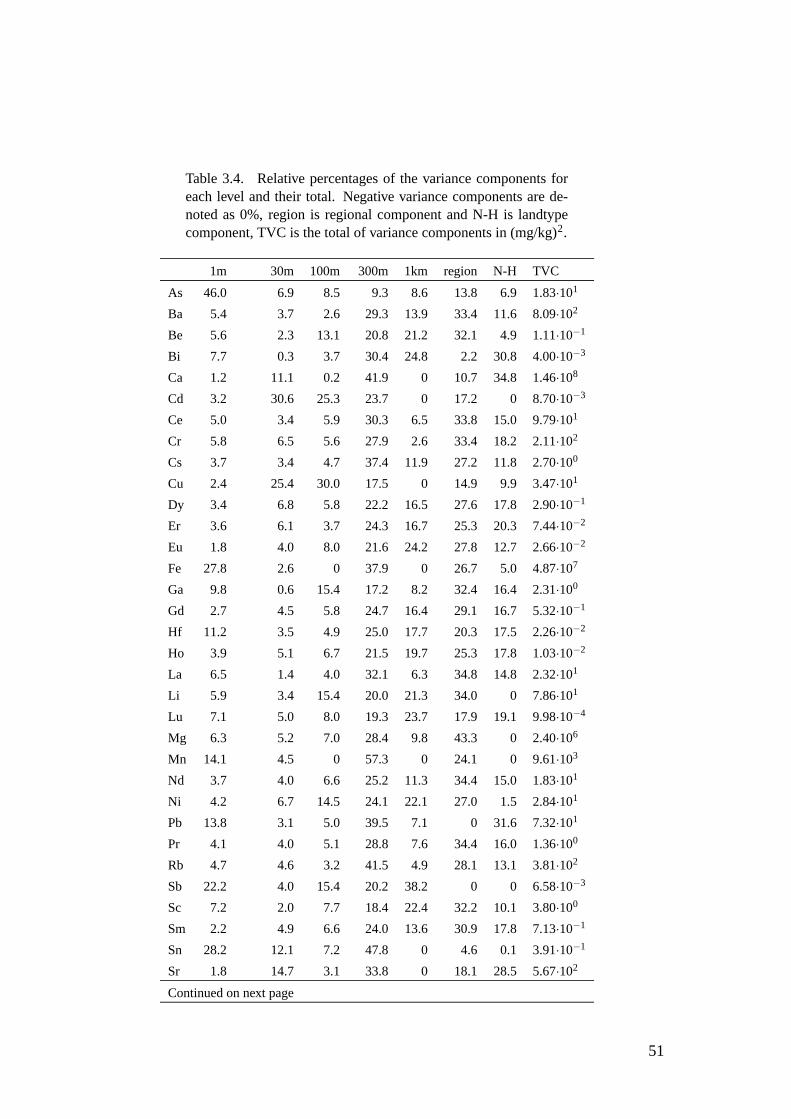
Table 3.4. Relative percentages of the variance components foreach level and their total. Negative variance components are de-noted as 0%, region is regional component and N-H is landtypecomponent, TVC is the total of variance components in (mg/kg)2.
1m 30m 100m 300m 1km region N-H TVC
As 46.0 6.9 8.5 9.3 8.6 13.8 6.9 1.83·101
Ba 5.4 3.7 2.6 29.3 13.9 33.4 11.6 8.09·102
Be 5.6 2.3 13.1 20.8 21.2 32.1 4.9 1.11·10−1
Bi 7.7 0.3 3.7 30.4 24.8 2.2 30.8 4.00·10−3
Ca 1.2 11.1 0.2 41.9 0 10.7 34.8 1.46·108
Cd 3.2 30.6 25.3 23.7 0 17.2 0 8.70·10−3
Ce 5.0 3.4 5.9 30.3 6.5 33.8 15.0 9.79·101
Cr 5.8 6.5 5.6 27.9 2.6 33.4 18.2 2.11·102
Cs 3.7 3.4 4.7 37.4 11.9 27.2 11.8 2.70·100
Cu 2.4 25.4 30.0 17.5 0 14.9 9.9 3.47·101
Dy 3.4 6.8 5.8 22.2 16.5 27.6 17.8 2.90·10−1
Er 3.6 6.1 3.7 24.3 16.7 25.3 20.3 7.44·10−2
Eu 1.8 4.0 8.0 21.6 24.2 27.8 12.7 2.66·10−2
Fe 27.8 2.6 0 37.9 0 26.7 5.0 4.87·107
Ga 9.8 0.6 15.4 17.2 8.2 32.4 16.4 2.31·100
Gd 2.7 4.5 5.8 24.7 16.4 29.1 16.7 5.32·10−1
Hf 11.2 3.5 4.9 25.0 17.7 20.3 17.5 2.26·10−2
Ho 3.9 5.1 6.7 21.5 19.7 25.3 17.8 1.03·10−2
La 6.5 1.4 4.0 32.1 6.3 34.8 14.8 2.32·101
Li 5.9 3.4 15.4 20.0 21.3 34.0 0 7.86·101
Lu 7.1 5.0 8.0 19.3 23.7 17.9 19.1 9.98·10−4
Mg 6.3 5.2 7.0 28.4 9.8 43.3 0 2.40·106
Mn 14.1 4.5 0 57.3 0 24.1 0 9.61·103
Nd 3.7 4.0 6.6 25.2 11.3 34.4 15.0 1.83·101
Ni 4.2 6.7 14.5 24.1 22.1 27.0 1.5 2.84·101
Pb 13.8 3.1 5.0 39.5 7.1 0 31.6 7.32·101
Pr 4.1 4.0 5.1 28.8 7.6 34.4 16.0 1.36·100
Rb 4.7 4.6 3.2 41.5 4.9 28.1 13.1 3.81·102
Sb 22.2 4.0 15.4 20.2 38.2 0 0 6.58·10−3
Sc 7.2 2.0 7.7 18.4 22.4 32.2 10.1 3.80·100
Sm 2.2 4.9 6.6 24.0 13.6 30.9 17.8 7.13·10−1
Sn 28.2 12.1 7.2 47.8 0 4.6 0.1 3.91·10−1
Sr 1.8 14.7 3.1 33.8 0 18.1 28.5 5.67·102
Continued on next page
51
Table 3.4 – continued from previous page
1m 30m 100m 300m 1km region N-H TVC
Tb 3.0 3.3 8.0 20.6 21.3 26.2 17.7 1.06·10−2
Th 4.0 2.4 6.0 30.4 12.4 27.2 17.5 1.82·100
Ti 8.2 6.4 4.8 15.8 4.0 34.1 26.7 3.03·104
Tm 4.9 5.8 5.9 20.1 21.6 23.2 18.5 1.25·10−3
Y 3.7 6.1 8.6 18.6 16.8 26.6 19.6 6.99·100
Yb 8.2 2.3 6.9 18.8 24.3 21.2 18.5 5.42·10−2
Zn 3.3 8.2 5.7 37.9 8.2 6.1 30.7 5.13·102
After fuzzy c-means clustering with varying numbers of clusters and visual inspection ofall the plots, the output of the UANOVA was divided into 3 groups. The plots shownin figure 3.3 are representatives of each group. The first group (figure 3.3, Eu) shows agradual increase of the variance with distance, with about equal contributions of the fourhighest levels. The second group (figure 3.3, Mg) shows a similar increase except thatthe contributions at the 1000 m level and the landtype level are lower than the 300 m andregional level. Both groups have in common that the major increase in variance is at thelast four levels, i.e. distances larger then the field scale (300m). The third group (figure 3.3,Cd) shows a more irregular pattern which is different for each element within the group.They have in common that the largest increase occurs at the first three levels, i.e within thefield scale. The clusters are respectively labeled gradual 1, gradual 2, and irregular. Thecluster memberships are given in table 3.5. The gradual 1 cluster contains the heavy REE,Sc and Y whereas gradual 2 contains the light REE and clay/feldspar related elements.The irregular cluster combines Ca and Sr, heavy metals, and redox sensitive elements.
Figure 3.5 gives an overview of all the measured elements and their variance patterns.For clarity only the cumulative variance is plotted against the distance. From this figurethe difference between the three types of variation patterns becomes clear. In general thecurves of gradual 2 are less smooth as those of gradual 1, with a clear inflection at the300 m level. The elements of the irregular cluster show a steep ascending curve for shortdistances which flattens towards larger distances. This underlines that the major part of thetotal variance for these elements occurs at the field scale.
Table 3.6 shows the relation between the covariance structure, derived from the PCA-Vand the three spatial variance patterns. In general the elements with high loadings on theclay PCA-V factor, or that are highly correlated with this factor, are grouped in the first twoclusters (gradual 1 & 2). For these elements the contribution of the small scale varianceto the total variance is relatively small. Thus observed regional variance, whether or notcomposite samples are collected, will indeed be largely caused by regional features. It isremarkable that while both light and heavy REE have high correlations with the clay factorin the PCA-V, they cluster separately based on their spatial variance patterns.
All the elements with high loadings on the anthropogenic and redox/lime factor of the
52
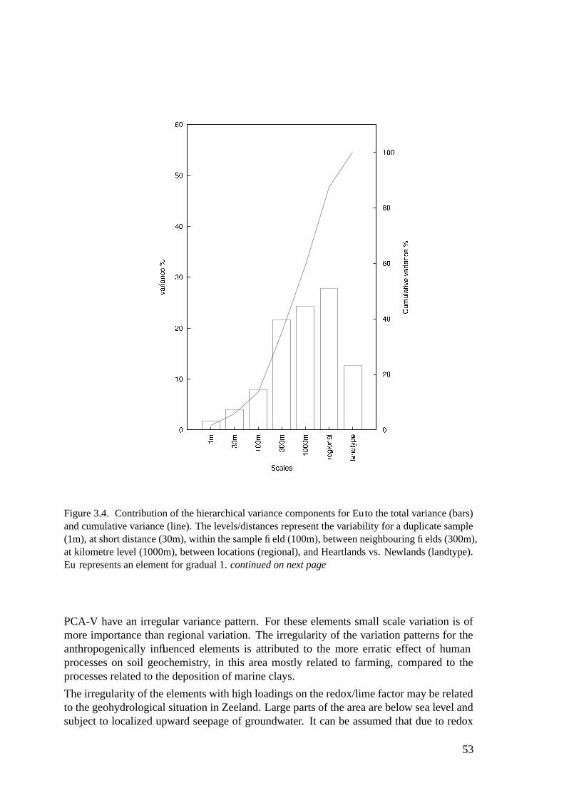
Figure 3.4. Contribution of the hierarchical variance components for Euto the total variance (bars)and cumulative variance (line). The levels/distances represent the variability for a duplicate sample(1m), at short distance (30m), within the sample field (100m), between neighbouring fields (300m),at kilometre level (1000m), between locations (regional), and Heartlands vs. Newlands (landtype).Eu represents an element for gradual 1. continued on next page
PCA-V have an irregular variance pattern. For these elements small scale variation is ofmore importance than regional variation. The irregularity of the variation patterns for theanthropogenically influenced elements is attributed to the more erratic effect of humanprocesses on soil geochemistry, in this area mostly related to farming, compared to theprocesses related to the deposition of marine clays.
The irregularity of the elements with high loadings on the redox/lime factor may be relatedto the geohydrological situation in Zeeland. Large parts of the area are below sea level andsubject to localized upward seepage of groundwater. It can be assumed that due to redox
53
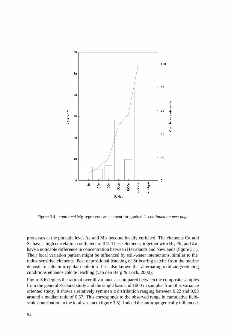
Figure 3.4. continued Mg represents an element for gradual 2. continued on next page
processes at the phreatic level As and Mn become locally enriched. The elements Ca andSr have a high correlation coefficient of 0.9. These elements, together with Bi , Pb, and Zn,have a noticable difference in concentration between Heartlands and Newlands (figure 3.1).Their local variation pattern might be influenced by soil-water interactions, similar to theredox sensitive elements. Post depositional leaching of Sr bearing calcite from the marinedeposits results in irregular depletion. It is also known that alternating oxidizing/reducingconditions enhance calcite leaching (van den Berg & Loch, 2000).
Figure 3.6 depicts the ratio of overall variance as compared between the composite samplesfrom the general Zeeland study and the single base and 1000 m samples from this varianceoriented study. It shows a relatively symmetric distribution ranging between 0.22 and 0.93around a median ratio of 0.57. This corresponds to the observed range in cumulative field-scale contribution to the total variance (figure 3.5). Indeed the anthropogenically influenced
54
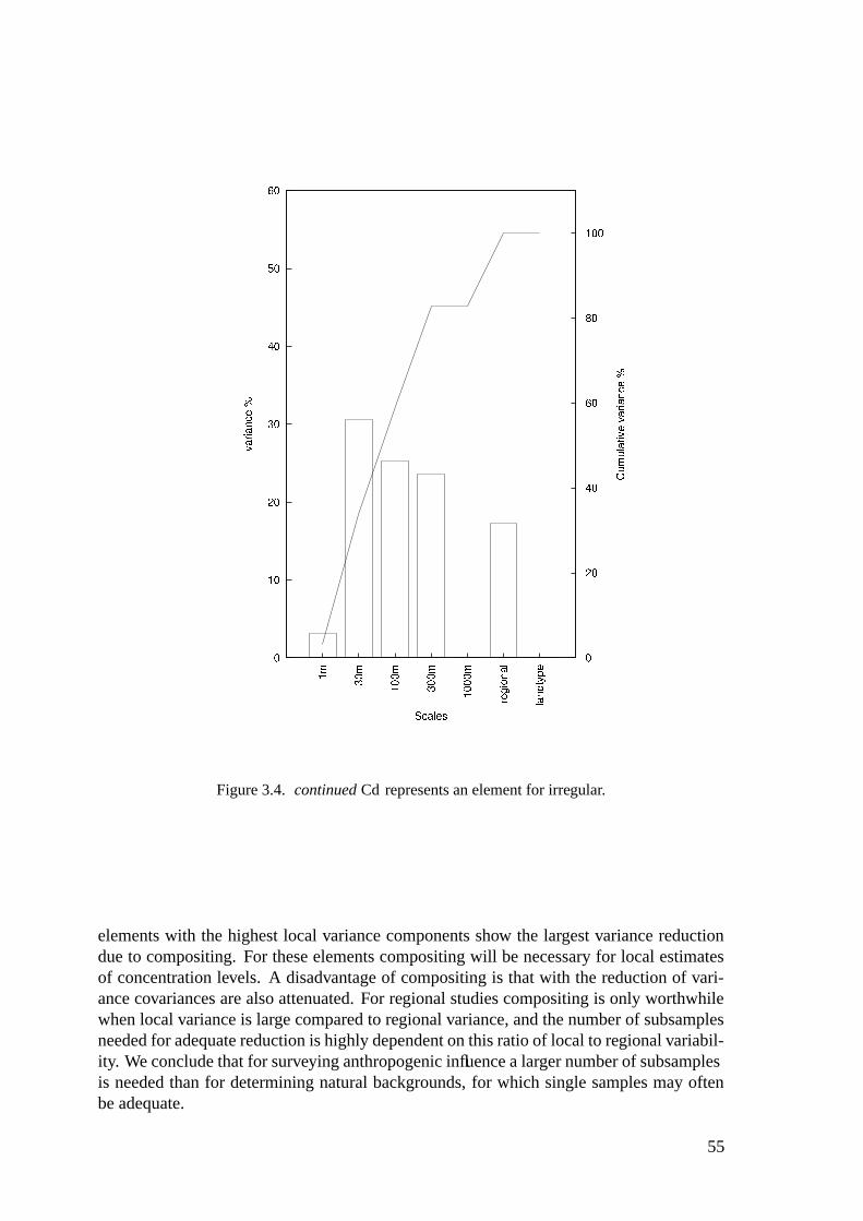
Figure 3.4. continued Cd represents an element for irregular.
elements with the highest local variance components show the largest variance reductiondue to compositing. For these elements compositing will be necessary for local estimatesof concentration levels. A disadvantage of compositing is that with the reduction of vari-ance covariances are also attenuated. For regional studies compositing is only worthwhilewhen local variance is large compared to regional variance, and the number of subsamplesneeded for adequate reduction is highly dependent on this ratio of local to regional variabil-ity. We conclude that for surveying anthropogenic influence a larger number of subsamplesis needed than for determining natural backgrounds, for which single samples may oftenbe adequate.
55
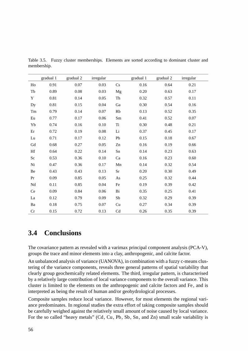
Table 3.5. Fuzzy cluster memberships. Elements are sorted according to dominant cluster andmembership.
gradual 1 gradual 2 irregular gradual 1 gradual 2 irregular
Ho 0.91 0.07 0.03 Cs 0.16 0.64 0.21
Tb 0.89 0.08 0.03 Mg 0.20 0.63 0.17
Y 0.81 0.14 0.05 Th 0.32 0.57 0.11
Dy 0.81 0.15 0.04 Ga 0.30 0.54 0.16
Tm 0.79 0.14 0.07 Rb 0.13 0.52 0.35
Eu 0.77 0.17 0.06 Sm 0.41 0.52 0.07
Yb 0.74 0.16 0.10 Ti 0.30 0.48 0.21
Er 0.72 0.19 0.08 Li 0.37 0.45 0.17
Lu 0.71 0.17 0.12 Pb 0.15 0.18 0.67
Gd 0.68 0.27 0.05 Zn 0.16 0.19 0.66
Hf 0.64 0.22 0.14 Sn 0.14 0.23 0.63
Sc 0.53 0.36 0.10 Ca 0.16 0.23 0.60
Ni 0.47 0.36 0.17 Mn 0.14 0.32 0.54
Be 0.43 0.43 0.13 Sr 0.20 0.30 0.49
Pr 0.09 0.85 0.05 As 0.25 0.32 0.44
Nd 0.11 0.85 0.04 Fe 0.19 0.39 0.42
Ce 0.09 0.84 0.06 Bi 0.35 0.25 0.41
La 0.12 0.79 0.09 Sb 0.32 0.29 0.39
Ba 0.18 0.75 0.07 Cu 0.27 0.34 0.39
Cr 0.15 0.72 0.13 Cd 0.26 0.35 0.39
3.4 Conclusions
The covariance pattern as revealed with a varimax principal component analysis (PCA-V),groups the trace and minor elements into a clay, anthropogenic, and calcite factor.
An unbalanced analysis of variance (UANOVA), in combination with a fuzzy c-means clus-tering of the variance components, reveals three general patterns of spatial variability thatclearly group geochemically related elements. The third, irregular pattern, is characterisedby a relatively large contribution of local variance components to the overall variance. Thiscluster is limited to the elements on the anthropogenic and calcite factors and Fe, and isinterpreted as being the result of human and/or geohydrological processes.
Composite samples reduce local variance. However, for most elements the regional vari-ance predominates. In regional studies the extra effort of taking composite samples shouldbe carefully weighed against the relatively small amount of noise caused by local variance.For the so called “heavy metals” (Cd, Cu, Pb, Sb, Sn, and Zn) small scale variability is
56
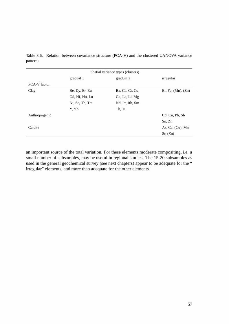
Table 3.6. Relation between covariance structure (PCA-V) and the clustered UANOVA variancepatterns
Spatial variance types (clusters)
gradual 1 gradual 2 irregular
PCA-V factor
Clay Be, Dy, Er, Eu Ba, Ce, Cr, Cs Bi, Fe, (Mn), (Zn)
Gd, Hf, Ho, Lu Ga, La, Li, Mg
Ni, Sc, Tb, Tm Nd, Pr, Rb, Sm
Y, Yb Th, Ti
Anthropogenic Cd, Cu, Pb, Sb
Sn, Zn
Calcite As, Ca, (Cu), Mn
Sr, (Zn)
an important source of the total variation. For these elements moderate compositing, i.e. asmall number of subsamples, may be useful in regional studies. The 15-20 subsamples asused in the general geochemical survey (see next chapters) appear to be adequate for the “irregular” elements, and more than adequate for the other elements.
57

Ho Tb Y Dy Tm Eu
Yb Er Lu Gd Hf Sc
Ni Be
0
0
Pr Nd Ce
La Ba Cr Cs Mg Th
Ga Rb Sm Ti Li
0
0
Pb Zn Sn Ca Mn Sr
As Fe Bi Sb Cu Cd
Figure 3.5. Summary of cumulative spatial variance patterns as estimated with UANOVA. Thecumulative variance as percentage of the total variance on the y-axis is plotted against the distanceon the x-axis. For x-axis scale see figure 3.3. The distances of the regional and landtype levels werein these figures arbitrary set at 3000 m and 5000 m. The order of the plot is from high membershipsin the gradual 1 cluster (Ho to Be), via high memberships in the gradual 2 cluster (Pr to Li) to highmemberships in the irregular cluster (Pb to Cd).
58

Variance ratio
Ele
men
ts
cdsn
ticu
sbzn
smer
cafe
hocs
lisr
dypr
ndth
ybtm
rbeu
crtb
yni
mg
asbe
celu
laba
gdbi
mn
sc
0.1 0.5 1.0 1.5
Figure 3.6. Variance ratios between composite samples and single samples (F-statistic; circle), andits 95 % confidence interval (line). 33 samples selected from the general Zeeland study employingcomposite sampling, and 32 samples from the single sample design, base and 1000 m sample.
59

4 Sampling and analyses for a regionalenvironmental soil geochemical sur-vey
4.1 Introduction
To manage and safeguard the environment one needs primary knowledge about its statusand condition. For terrestrial life, including the human species, the biosphere is stronglydependent upon the chemistry of the earth’s surface layer. Soils form a fundamental com-ponent of this layer, hence knowledge of the distribution of major and trace elements insoils, and their mutual relations in spatial as well as attribute space, are of major concernfor understanding our environment. The basic factors that determine the composition ofsoils are: 1) geogenic/pedogenic origin, 2) the vertical redistribution through soil formingprocesses, and 3) the ubiquitous spread of anthropogenic substances as the consequenceof diffuse entry into the soil. In geochemistry the original composition is often assessedby means of a baseline, while divergence from this baseline may then be related to humaninfluence.
For the Dutch situation this baseline is expressed by in legal background threshold values(Dutch: “Streefwaarden”) that form the backbone of the Dutch legal framework of permis-sible limits for soil quality and soil remediation (see also chapter 1). These legal valueswere derived in a search for true soil background values in a survey of natural areas, un-der the assumption that these were not significantly influenced by man and thus could beconsidered as relatively clean. Van der Meent et al. (1990) calls this method of acquiringbackground values disputable since it is hard to establish criteria for a “relatively cleanarea”. Their suggestion is to use preanthropogenic deposits for determining backgroundconcentrations or use scientific deduction. They also consider that natural background con-centrations for the Dutch situation do not exist. However, Bolviken et al. (1996) pointedout that pristine, preanthropogenic material can be found and sampled everywhere. Ageochemical survey with an appropriate sampling design can provide both influenced andpristine soil material. A comparison between the two then offers a diagnosis tool on thestate of a major environmental quality: the soil geochemistry.
This chapter focuses on how to obtain a consistent, high quality, and province-wide dataset
61
that contains both information about pristine soil composition, i.e. the natural composition,and information on how the soil is influenced by human processes. From such a datasetgeochemical baselines can be derived as well as a quantification of the imprint by man. Theuse of the dataset for a baseline, hence as a reference dataset, demands that the methods areextensively described so a proper evaluation of their efficacy and a comparison with otherdata can be made. Of course, accuracy and precision are of the utmost importance. Todiscern a large variety of different processes at an adequate level of significance, throughrelations between soil attributes and in geographical space, it is necessary to keep the levelof noise as low as possible. One of the major concerns is to correct for bias caused byhaving different surveys spaced in time. Due to necessary re-calibrations and unavoidablechanges in laboratory practice and apparatus, such biases are virtually unavoidable. Toanticipate to these changes a new method of parametric levelling is used based on sets ofbetween survey duplicates (BSD) and linear regression.
From the complete dataset with all measured soil attributes a -still sizable- set of soil chem-ical attributes was selected, based on their affirmed high accuracy and precision, and no oronly random missing values. Thus the desired georeferenced, consistent, and high qualitydataset for the entire area studied was created. This dataset will be optimal for statisti-cal analysis and environmental assessment for legal authorities. The remainder of the at-tributes measured may, when used with prudence and competence, still provide importantadditional insight into the soil geochemical patterns and processes.
4.2 Material and methods
4.2.1 Study area
This research focuses on defining and distinguishing natural and anthropogenic geochemi-cal patterns in soil. The province of Zeeland was chosen for this study because it is an agri-cultural area with a relatively small variability in soil types that are of a young, Holocene,age. Because of the low permeability, high adsorption capacity of the clayey soils, andtheir relatively young age, vertical transport through natural soil forming processes or an-thropogenic input is expected to be minimal. Thus, the presence of a pristine soil layer atdepth may be reasonably assumed.
The province of Zeeland belongs largely to the Holocene estuary at the outlet of the riversRijn, Maas and Schelde∗, see figure 4.1. It consists of the mainland of Zeeuws-Vlaanderen,bordering Belgium, and several islands/peninsulas that have a long and rich history of landreclamation and inundation. Inundation of reclaimed land was partly related to the rise ofaverage sea-level in the first half of the last millennium. However, both natural and humaninduced flooding have occurred until recent times. Examples are the strategic flooding ofWalcheren near the end of the Second World War, and the great storm flood of 1953 thatinundated large parts of Zeeland. The history of land reclamation through dike building is
∗In this thesis Dutch names are used for the rivers Rhine, Meuse and Scheldt respectively
62

Figure 4.1. Topography of Zeeland, showing names of peninsula’s and areas (italic), and somecities (bold)
complicated, resulting in a geographically complex polder-landscape.
The Holocene geology and pedology of Zeeland have been extensively described in chapter2 of this thesis. In summary the major soil types of Zeeland are immature marine claydeposits ranging from heavy clays (clay fraction >25%) to sandy tidal inlet and tidal flats(clay fraction <7%). The Zeeland landscape is divided into Heartlands, the oldest and firstreclaimed areas with often very heavy pool-clays, and Newlands, younger areas with moresandy clay soils. The elevation of the field level, relative to the Dutch average sea levelNAP, ranges from about 1.5m for channel ridges to -1.3m for the pool clay areas. Land useis mainly agricultural and in the Newlands is characterised by its larger scale and intensive
63
artificial drainage.
4.2.2 General research approach
Examples of geochemical baseline studies are common in modern geochemistry (see forexample de Vos et al. (1996); Gregorauskiene & Kadunas (1997); Salminen & Tarvainen(1995); Burenkov et al. (1999); Cocker (1999); Rapant et al. (1999); Ferreira et al. (2001);Singh et al. (2001)), chiefly based on practices of exploration geochemistry. As Hale &Kuhnel (1997) explain, the classical purpose of exploration geochemistry, finding metal-liferous ore bodies, can be transferred to the inventory of contaminated soils. Yet, thereare important differences, e.g. looking for a single element stationary ore body as com-pared to a possibly mobile multi-element contamination of soil and the huge difference intime scales of both phenomena. Also for natural geochemical anomalies the underlyingprocess or cause is often known or can be deduced from mineral relationships, while thisis much less the case for contaminated soils. The causes of contamination, the interactionwith soil constituents, and the relation between contaminating elements are often not wellunderstood. Still the basic geochemical techniques are the same and approaches known ingeochemistry are now considered very useful in the environmental field (Nikkarinen et al.,1996; Selinus & Esbensen, 1995).
Examples of environmental geochemical studies include the assessment of a backgroundby using overbank samples (Swennen & van de Sluys, 2002). Here older, deeper, fluvialdeposits are used as pristine material, and the relatively modern top sediments to assessthe anthropogenic influence. This approach of using deeper sediments as pristine materialhas also been successfully applied in other studies and different soil types (Blaser et al.,2000; Wilcke et al., 1998; Sterckeman et al., 2004). The specific choices for sampling andanalytical procedures to be used in this study are based on several considerations.
Most of the earlier mentioned geochemical baseline and/or environmental studies are gen-erally limited to a small group of trace elements, notably the so called heavy metals (Cd,Cr, Cu, Ni , Pb, Zn) and As. Although those usually constitute the environmental prior-ity elements, broadening the analytical focus with major components like Al2O3 , Fe2O3 ,CaO, and trace elements such as Rb, Ga, Sr , and the rare earth elements (REE), will resultin a better understanding not only of the human effect but of the natural composition andrelations in the soil as well.
To make efficient use of the multi-element approach, detection limits for all elementsshould be sufficiently low so as to stringently reduce the number of measurements belowthe detection limit, since they will weaken and complicate data interpretation and statisticalanalysis.
To serve as a reference dataset, sampling and analytical methods should be at least partly inline with the current Dutch practice in assessments for soil sanitation permits and soil qual-ity statements. This chiefly implies that composite samples are collected and that chemicalanalysis is preferably based on an aqua regia leach.
Current state of the art analytical techniques with high throughput that allow measurement
64

of a large number of major, minor, and trace elements including the REE, are InductivelyCoupled Plasma-Mass Spectrometry (ICP-MS) and X-ray Fluorescence (XRF). EspeciallyICP-MS ensures low detection limits for a wide range of trace elements. While XRF pro-vides the total content of an element in a sample, ICP-MS is always based on (partial)sample decomposition. The efficacy of the decomposition or leach depends on the chosenmedium and exact procedure followed, and on the binding of the specific element in thesample matrix. Hot aqua-regia sample decomposition was chosen to comply with to thedesired comparability with Dutch standard procedures. A known limitation of this methodis the underestimation of concentrations of some metals due to resistance to the acid attackand resulting in a partial leach (Scancar et al., 2000; Tsolakidou et al., 2002). The overlapin elements between XRF and ICP-MS can be used as an supplementary check on analyti-cal quality, and for some elements the difference between results may give some indicationon their mineralogy.
One of the difficulties in soil analysis is sample inhomogeneity, which can result in lowreproducibility and high variability of the measured values. Therefore homogenisation ofthe samples needs special attention, both at the field sampling stage and when subsamplingfor chemical analysis, in order to reduce this source of variability as much as possible.Variance due to inhomogeneity is dependent on grain size and mineralogy, and thus variesfrom element to element. Especially trace elements that form their own minerals, such asZr, may suffer from the so called nugget effect (see also Chapter 3), which can only bereduced by increasing the weight of the analytical sample or reducing the grain size bymilling.
As analytical variance and minor inaccuracies are inevitable properties of measured data,knowledge of the size of these errors is needed to allow any geochemical data interpretation.Therefore, for both the XRF and ICP-MS methods several duplicate samples and standardswere analysed together with the samples. These included the between survey duplicates(BSD) for the purpose of levelling, i.e. eliminating the bias caused by separately analysingthe different surveys that were widely spaced in time. Moreover, data were screened foranomalous values at all stages of the analytical procedure.
4.2.3 Field sampling
The samples were collected in 4 field surveys between 1996 and 2003. Sampling followeda geographically and pedologically stratified random procedure, with a density varyingfrom 1 location per 1km2 in the first survey, up to 1 per 10km2 in the later surveys. Thevariation in density was based on improved knowledge about local and regional variation(see chapter 3) and a change from a local to a more regional focus with later surveys. Theexact sample location within a randomly selected target site depended on permission of thelandowner.
Focus was on rural areas, so built up zones and the dunes were excluded. Obvious potentialpoint sources of pollution (industrial sites, junk yards, grave yards, orchards) were avoidedas well. Soil types covering only a small area of the province were also disregarded.
65
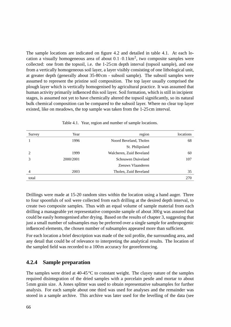
The sample locations are indicated on figure 4.2 and detailed in table 4.1. At each lo-cation a visually homogeneous area of about 0.1 ·0.1km2, two composite samples werecollected: one from the topsoil, i.e. the 1-25cm depth interval (topsoil sample), and onefrom a vertically homogeneous soil layer, a layer visibly consisting of one lithological unit,at greater depth (generally about 35-80cm - subsoil sample). The subsoil samples wereassumed to represent the pristine soil composition. The top layer usually comprised theplough layer which is vertically homogenised by agricultural practice. It was assumed thathuman activity primarily influenced this soil layer. Soil formation, which is still in incipientstages, is assumed not yet to have chemically altered the topsoil significantly, so its naturalbulk chemical composition can be compared to the subsoil layer. Where no clear top layerexisted, like on meadows, the top sample was taken from the 1-25cm interval.
Table 4.1. Year, region and number of sample locations.
Survey Year region locations
1 1996 Noord Beveland, Tholen 68
St. Philipsland
2 1999 Walcheren, Zuid Beveland 60
3 2000/2001 Schouwen Duiveland 107
Zeeuws Vlaanderen
4 2003 Tholen, Zuid Beveland 35
total 270
Drillings were made at 15-20 random sites within the location using a hand auger. Threeto four spoonfuls of soil were collected from each drilling at the desired depth interval, tocreate two composite samples. Thus with an equal volume of sample material from eachdrilling a manageable yet representative composite sample of about 300g was assured thatcould be easily homogenised after drying. Based on the results of chapter 3, suggesting thatjust a small number of subsamples may be preferred over a single sample for anthropogenicinfluenced elements, the chosen number of subsamples appeared more than sufficient.
For each location a brief description was made of the soil profile, the surrounding area, andany detail that could be of relevance to interpreting the analytical results. The location ofthe sampled field was recorded to a 100m accuracy for georeferencing.
4.2.4 Sample preparation
The samples were dried at 40-45°C to constant weight. The clayey nature of the samplesrequired disintegration of the dried samples with a porcelain pestle and mortar to about5mm grain size. A Jones splitter was used to obtain representative subsamples for furtheranalysis. For each sample about one third was used for analyses and the remainder wasstored in a sample archive. This archive was later used for the levelling of the data (see
66
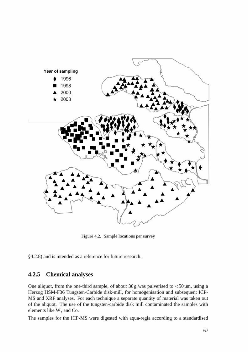
Year of samplingYear of sampling
Figure 4.2. Sample locations per survey
§4.2.8) and is intended as a reference for future research.
4.2.5 Chemical analyses
One aliquot, from the one-third sample, of about 30g was pulverised to <50µm, using aHerzog HSM-F36 Tungsten-Carbide disk-mill, for homogenisation and subsequent ICP-MS and XRF analyses. For each technique a separate quantity of material was taken outof the aliquot. The use of the tungsten-carbide disk mill contaminated the samples withelements like W, and Co.
The samples for the ICP-MS were digested with aqua-regia according to a standardised
67
method of the Dutch Geological Survey. A subsample of 250mg of the milled 30g aliquotwas leached with 6 ml ultra-pure hydrochloric acid and 2 ml ultra-pure nitric acid anddigested in a closed Teflon vessel in a microwave oven (Milestone 1200 Mega ) for 13minat 600W and 17min at 300W. After a cooling period of 10 to 20 minutes another 2ml ofnitric acid was added and the hydrochloric acid was removed through evaporation. For thispart, due to changes in the laboratory, an evaporator (survey 1 and 2), a sand bath (survey3), and a aluminum block (survey 4) were used as heat sources in the different surveys.The solution was quantitatively transferred into polyethylene flasks and diluted to 50mlwith demineralised water. From this volume an aliquot was 5 times diluted, together withan internal standard (In) and submitted for ICP-MS analysis.
For the XRF method 10g of the milled sample was mixed with wax tablets and pressedin a Herzog HTP-S and analysed, using α-correction for major elements and Comptonbackscatter correction for trace elements. A new XRF apparatus was installed betweensurveys 2 and 3.
Table 4.2 lists the elements that were determined by each method. Due to enhancementsin the laboratory and the possibility to analyse more elements the set of parameters wasextended after the first survey, and to a smaller extent after the third survey.
4.2.6 Precision and accuracy
During all stages of the chemical analysis data integrity was closely watched by meansof comparison between XRF and ICP-MS results, duplicate comparison, drift plots, etc.Given the large number of attributes determined, these a priori attempts to eliminate grossanalytical errors focused on the key attributes like the major oxides and the priority heavymetals.
Precision of the analytical results within a survey was estimated through duplicate analysisof some 15% of the ICP-MS samples, and about 4% of the XRF samples as this method isknown to be more precise. For each ICP duplicate a new subsample was decomposed byaqua regia, for each XRF duplicate a new subsample was ground and pressed into a tablet.
The precision was calculated with
s =
√∑n
i=1(xi1− xi2)2
2n(4.1)
v =sx·100% (4.2)
where v is the error relative to the mean (x) of the duplicates and s is the standard deviationwith (xi1− xi2) the difference between the n sets of duplicates.
Reference ISE samples (van Dijk & Houba, 2000), that were treated in the same way as thesamples, were used to check on accuracy. Comparison of laboratory performance with therecommended values of the international standards for XRF results is relatively straight-forward, as these represent total concentrations. Since for some elements the aqua regia
68
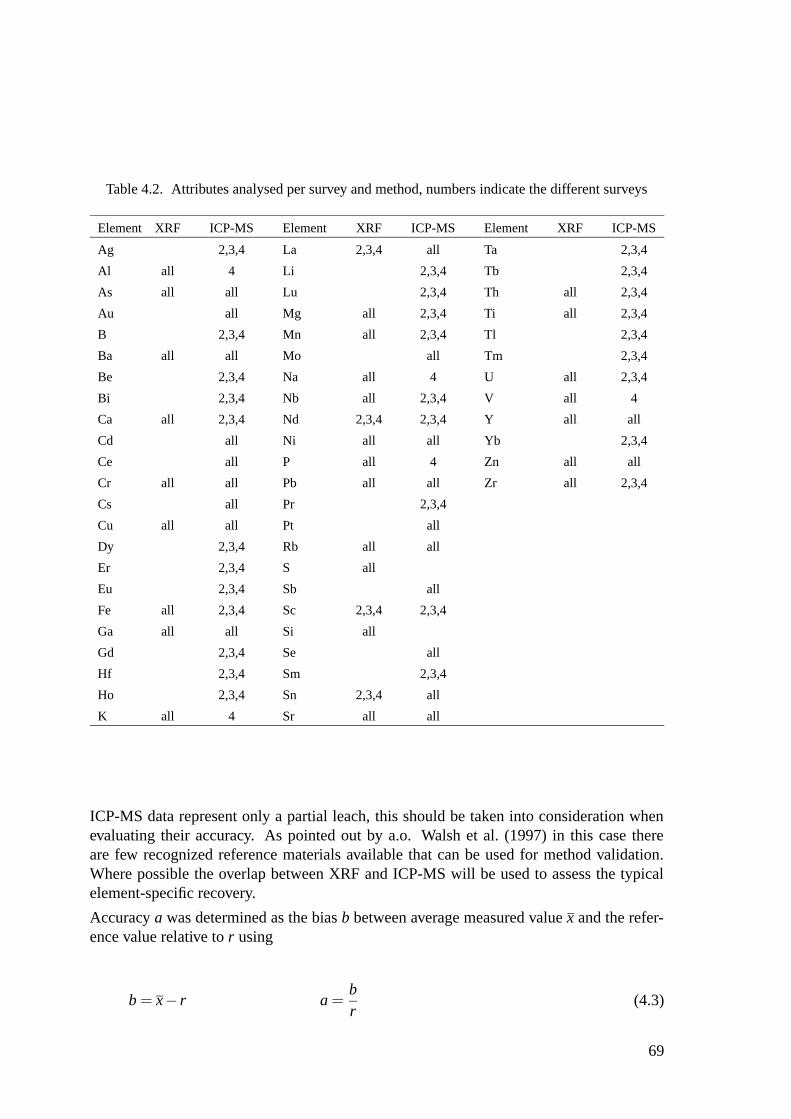
Table 4.2. Attributes analysed per survey and method, numbers indicate the different surveys
Element XRF ICP-MS Element XRF ICP-MS Element XRF ICP-MS
Ag 2,3,4 La 2,3,4 all Ta 2,3,4
Al all 4 Li 2,3,4 Tb 2,3,4
As all all Lu 2,3,4 Th all 2,3,4
Au all Mg all 2,3,4 Ti all 2,3,4
B 2,3,4 Mn all 2,3,4 Tl 2,3,4
Ba all all Mo all Tm 2,3,4
Be 2,3,4 Na all 4 U all 2,3,4
Bi 2,3,4 Nb all 2,3,4 V all 4
Ca all 2,3,4 Nd 2,3,4 2,3,4 Y all all
Cd all Ni all all Yb 2,3,4
Ce all P all 4 Zn all all
Cr all all Pb all all Zr all 2,3,4
Cs all Pr 2,3,4
Cu all all Pt all
Dy 2,3,4 Rb all all
Er 2,3,4 S all
Eu 2,3,4 Sb all
Fe all 2,3,4 Sc 2,3,4 2,3,4
Ga all all Si all
Gd 2,3,4 Se all
Hf 2,3,4 Sm 2,3,4
Ho 2,3,4 Sn 2,3,4 all
K all 4 Sr all all
ICP-MS data represent only a partial leach, this should be taken into consideration whenevaluating their accuracy. As pointed out by a.o. Walsh et al. (1997) in this case thereare few recognized reference materials available that can be used for method validation.Where possible the overlap between XRF and ICP-MS will be used to assess the typicalelement-specific recovery.
Accuracy a was determined as the bias b between average measured value x and the refer-ence value relative to r using
b = x− r a =br
(4.3)
69
4.2.7 Outliers
Outliers can occur due to an anomalous sample or due to analytical error. In the first casethe sample may originate from a location with high concentrations of a certain elementor elements. These elevated concentrations, either caused by natural or human processes,can denote a local soil feature, another possibility is the incidence of small, non visible,amounts of allochtonous material like flakes of paint, pieces of leadshot, metal scraps, etc.in a subsample (van Gaans & Vriend, 1996). The grinding and homogenisation of thesample may than contaminate the entire sample. Outliers caused by analytical error canhave various causes that are usually hard to account for. A repeated analysis can disclosesuch outliers but for many elements the overlap between the ICP-MS and XRF can be used.If an ICP-MS analysis shows an outlier for a certain element while the XRF does not, it isvery likely that this outlier is an analytical effect.
Outliers were defined as values larger then the 3rd quartile value plus several times theinterquartile range according to
x> P75 + f · (P75−P25) (4.4)
This procedure is equivalent to calculating the fences for box and whiskers plots accordingto Tukey (1977). In this formula P denotes a percentile and x is the measured value. Thefactor f , usually set at 1.5 for inner fences, was set to 2, making allowance for a possibleskewness. If equation 4.4, with f = 2, is applied to the normal distribution virtually nooutliers exist, while for a log normal distribution data about 5% will be identified as outlierscaused by the large tail of a theoretic log normal distribution. Outliers were not removedfrom the dataset but marked as such so they can be treated separately.
4.2.8 Parametric levelling
Since the time span between the 4 surveys was several years (see table 4.1) it is inevitablethat small, but systematic shifts will have occurred between the different data subsets.These shifts are caused by changes in procedures, fluctuations in calibration and/or per-formance of the analytical instruments etc., and are unavoidable in laboratories that keepimproving analytical performance. Instead of consolidating the method for years it is betterto anticipate these changes so expected bias can be compensated. The shifts, although smalland within acceptable analytical precision for individual parameters, can have a negativeinfluence on multivariate relations. For example, covariability may shift from one subsetto another, thereby weakening the relation in the overall dataset. Artificial groups can alsoresult from these artifacts (Rutten, 2004).
To level, or eliminate, these small differences so called Between Survey Duplicates (BSD)were used. One survey was chosen as the reference and about 15 to 20 samples from thisreference survey were reanalysed in the analytical batches during the other surveys. Theother surveys were then corrected by means of shift and multiplier values based on an
70

6 7 8 9 10 11 12
46
810
12
reference sample
dupl
icat
e sa
mpl
e
unlevelledlevelled
Figure 4.3. Principal concepts of levelling. The circles show the deviation from the y = x line, as aresult of shifting. The triangles show the same data after correction
ordinary least square linear regression equation derived from the set of BSD.
This method was chosen above well known methods like regression of quantiles (Daneshfar& Cameron, 1998; Darnley et al., 1995) or correction based on the reference samples used.The advantage of this method is that the levelling is based on a, for the area, representativerange of measured values.
Figure 4.3 shows the procedure of the BSD levelling for an example dataset. Due to asystematic shift the data measured in a second batch are shifted away from the y = x line.If the outcome of the analyses only differs due to analytical variability then the points would
71
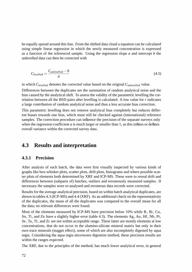
be equally spread around this line. From the shifted data cloud a equation can be calculatedusing simple linear regression in which the newly measured concentration is expressedas a function of the referenced sample. Using the regression slope a and intercept b theunlevelled data can then be corrected with
Clevelled =Cunlevelled−b
a(4.5)
in which Clevelled denotes the corrected value based on the original Cunlevelled value.
Differences between the duplicates are the summation of random analytical noise and thebias caused by the analytical shift. To assess the validity of the parametric levelling the cor-relation between all the BSD pairs after levelling is calculated. A low value for r indicatesa large contribution of random analytical noise and thus a less accurate bias correction.
This parametric levelling does not remove analytical bias completely but reduces differ-ent biases towards one bias, which must still be checked against (international) referencesamples. The correction procedure can influence the precision of the separate surveys onlywhen the regression coefficient a is much larger or smaller than 1, as this inflates or deflatesoverall variance within the corrected survey data.
4.3 Results and interpretation
4.3.1 Precision
After analysis of each batch, the data were first visually inspected by various kinds ofgraphs like box-whisker plots, scatter plots, drift plots, histograms and where possible scat-ter plots of elements both determined by XRF and ICP-MS. These were to reveal drift anddifferences between (subparts of) batches, outliers and erroneously measured samples. Ifnecessary the samples were re-analysed and erroneous data records were corrected.
Results for the average analytical precision, based on within batch analytical duplicates, areshown in tables 4.3 (ICP-MS) and 4.4 (XRF). As an additional check on the representativityof the duplicates, the mean of all the duplicates was compared to the overall mean for allthe data; no relevant differences were found.
Most of the elements measured by ICP-MS have precision below 10% while B, Bi , Cu,Sn, Ti , and Zn have a slightly higher error (table 4.3). The elements Ag, Au, Hf, Nb, Pt ,Se, Ta, Tl , and Zr are not within acceptable range. These latter are mostly elements at lowconcentrations, that do not occur in the alumino-silicate mineral matrix but only in theirown trace minerals (nugget effect), some of which are also incompletely digested by aquaregia. Considering the aqua regia microwave digestion method, these precision results arewithin the ranges expected.
The XRF, due to the principles of the method, has much lower analytical error, in general
72
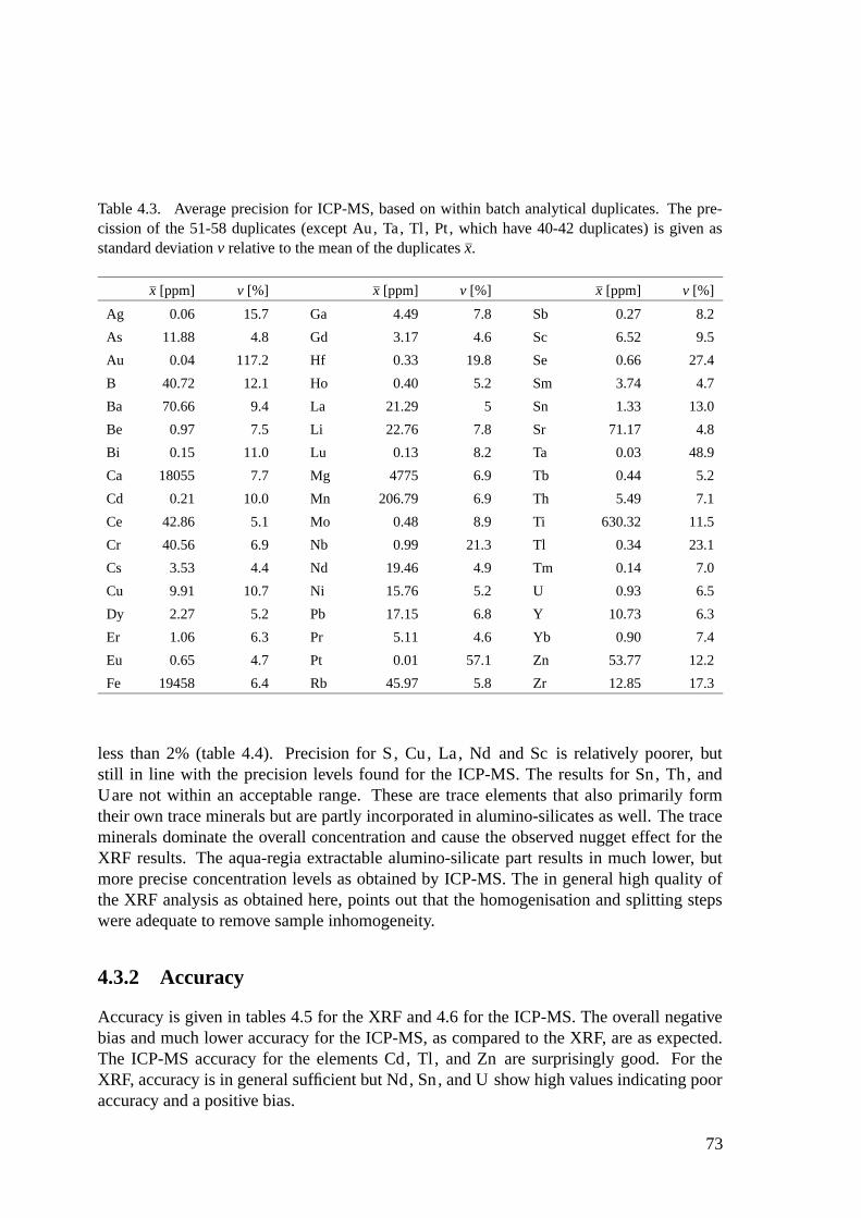
Table 4.3. Average precision for ICP-MS, based on within batch analytical duplicates. The pre-cission of the 51-58 duplicates (except Au, Ta, Tl , Pt , which have 40-42 duplicates) is given asstandard deviation v relative to the mean of the duplicates x.
x [ppm] v [%] x [ppm] v [%] x [ppm] v [%]
Ag 0.06 15.7 Ga 4.49 7.8 Sb 0.27 8.2
As 11.88 4.8 Gd 3.17 4.6 Sc 6.52 9.5
Au 0.04 117.2 Hf 0.33 19.8 Se 0.66 27.4
B 40.72 12.1 Ho 0.40 5.2 Sm 3.74 4.7
Ba 70.66 9.4 La 21.29 5 Sn 1.33 13.0
Be 0.97 7.5 Li 22.76 7.8 Sr 71.17 4.8
Bi 0.15 11.0 Lu 0.13 8.2 Ta 0.03 48.9
Ca 18055 7.7 Mg 4775 6.9 Tb 0.44 5.2
Cd 0.21 10.0 Mn 206.79 6.9 Th 5.49 7.1
Ce 42.86 5.1 Mo 0.48 8.9 Ti 630.32 11.5
Cr 40.56 6.9 Nb 0.99 21.3 Tl 0.34 23.1
Cs 3.53 4.4 Nd 19.46 4.9 Tm 0.14 7.0
Cu 9.91 10.7 Ni 15.76 5.2 U 0.93 6.5
Dy 2.27 5.2 Pb 17.15 6.8 Y 10.73 6.3
Er 1.06 6.3 Pr 5.11 4.6 Yb 0.90 7.4
Eu 0.65 4.7 Pt 0.01 57.1 Zn 53.77 12.2
Fe 19458 6.4 Rb 45.97 5.8 Zr 12.85 17.3
less than 2% (table 4.4). Precision for S, Cu, La, Nd and Sc is relatively poorer, butstill in line with the precision levels found for the ICP-MS. The results for Sn, Th, andUare not within an acceptable range. These are trace elements that also primarily formtheir own trace minerals but are partly incorporated in alumino-silicates as well. The traceminerals dominate the overall concentration and cause the observed nugget effect for theXRF results. The aqua-regia extractable alumino-silicate part results in much lower, butmore precise concentration levels as obtained by ICP-MS. The in general high quality ofthe XRF analysis as obtained here, points out that the homogenisation and splitting stepswere adequate to remove sample inhomogeneity.
4.3.2 Accuracy
Accuracy is given in tables 4.5 for the XRF and 4.6 for the ICP-MS. The overall negativebias and much lower accuracy for the ICP-MS, as compared to the XRF, are as expected.The ICP-MS accuracy for the elements Cd, Tl , and Zn are surprisingly good. For theXRF, accuracy is in general sufficient but Nd, Sn, and U show high values indicating pooraccuracy and a positive bias.
73
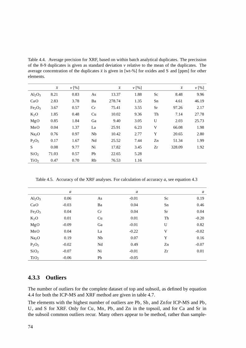
Table 4.4. Average precision for XRF, based on within batch analytical duplicates. The precissionof the 8-9 duplicates is given as standard deviation v relative to the mean of the duplicates. Theaverage concentration of the duplicates x is given in [wt-%] for oxides and S and [ppm] for otherelements.
x v [%] x v [%] x v [%]
Al2O3 8.21 0.83 As 13.37 1.88 Sc 8.48 9.96
CaO 2.83 3.78 Ba 278.74 1.35 Sn 4.61 46.19
Fe2O3 3.67 0.57 Cr 75.41 3.55 Sr 97.26 2.17
K2O 1.85 0.48 Cu 10.02 9.36 Th 7.14 27.78
MgO 0.85 1.84 Ga 9.40 3.05 U 2.03 25.73
MnO 0.04 1.37 La 25.91 6.23 V 66.08 1.98
Na2O 0.76 0.97 Nb 10.42 2.77 Y 20.65 2.80
P2O5 0.17 1.67 Nd 25.52 7.44 Zn 51.34 1.99
S 0.08 9.77 Ni 17.82 3.45 Zr 328.09 1.92
SiO2 71.03 0.57 Pb 22.65 5.28
TiO2 0.47 0.70 Rb 76.53 1.16
Table 4.5. Accuracy of the XRF analyses. For calculation of accuracy a, see equation 4.3
a a a
Al2O3 0.06 As -0.01 Sc 0.19
CaO -0.03 Ba 0.04 Sn 0.46
Fe2O3 0.04 Cr 0.04 Sr 0.04
K2O 0.01 Cu 0.01 Th -0.20
MgO -0.09 Ga -0.01 U 0.82
MnO 0.04 La -0.22 V -0.02
Na2O 0.19 Nb 0.07 Y 0.16
P2O5 -0.02 Nd 0.49 Zn -0.07
SiO2 -0.07 Ni -0.01 Zr 0.01
TiO2 -0.06 Pb -0.05
4.3.3 Outliers
The number of outliers for the complete dataset of top and subsoil, as defined by equation4.4 for both the ICP-MS and XRF method are given in table 4.7.
The elements with the highest number of outliers are Pb, Sb, and Znfor ICP-MS and Pb,U, and S for XRF. Only for Cu, Mn, Pb, and Zn in the topsoil, and for Ca and Sr inthe subsoil common outliers recur. Many others appear to be method, rather than sample-
74
Table 4.6. Accuracy of the ICP-MS analyses. For calculation of accuracy a, see equation 4.3
a a a
Ag -0.60 Ga -0.61 Sb -0.55
Al -0.73 K -0.81 Sc -0.42
As -0.14 La -0.33 Se -0.96
B -0.73 Li -0.15 Sn -0.63
Ba -0.85 Mg -0.17 Sr -0.42
Be -0.53 Mn -0.21 Th -0.22
Bi -0.98 Mo -0.77 Tl 0.05
Ca -0.33 Na -0.97 U -0.37
Cd 0.03 Nb -0.84 V -0.38
Ce -0.21 Nd 0.11 Y -0.52
Cr -0.50 Ni -0.09 Zn 0.05
Cu -0.27 P -0.16 Zr -0.97
Fe -0.27 Pb -0.22
specific, indicating analytical error.
The elements Pb, Zn, and Cu are known contaminants and the presence of samples withanomalous high concentrations is a first indication of anthropogenic altering of the topsoil.As no comparison between ICP-MS and XRF is possible for Cd, P, and S this could betrue for these elements as well. The anomalies for CaO and Sr in the subsoil may berelated to a concentration of shell fragments which were regularly found in the subsoilduring sampling.
In view of the size of the total dataset and the regional objectives of the overall survey,these outliers are negligible and can be simply omitted in the regional characterisation.
4.3.4 Parametric levelling of data
Survey 3 was chosen as the reference survey for the BSD because in this sampling roundthe largest number of samples were analysed. Hence, the smallest possible number ofsamples needed to be corrected. Moreover, the new XRF apparatus was already in use forthis survey. The choice for survey 3 therefore also facilitates comparison with future data.An example of the levelling is given in figure 4.4 in which Ga, as measured on the XRF, islevelled towards the reference.
The overall correlations between the BSD after the parametric levelling are given in tables4.8 and 4.9. From these tables it is clear that for the XRF the correlations are higher thanfor the ICP-MS. For the XRF the elements Sn, Th, and U have low correlations, which isin accordance with their low precision (table 4.4). In general the correlations are between
75
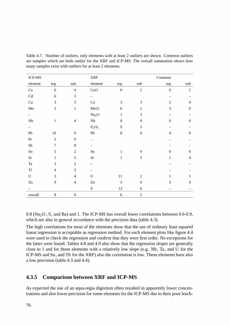
Table 4.7. Number of outliers, only elements with at least 2 outliers are shown. Common outliersare samples which are both outlier for the XRF and ICP-MS. The overall summation shows howmany samples exist with outliers for at least 2 elements.
ICP-MS XRF Common
element top sub element top sub top sub
Ca 6 4 CaO 0 2 0 2
Cd 6 3 – – –
Cu 3 3 Cu 3 3 2 0
Mn 3 1 MnO 6 1 3 0
– Na2O 1 3 – –
Nb 1 4 Nb 0 0 0 0
– P2O5 9 5 – –
Pb 10 0 Pb 8 0 4 0
Pr 2 0 – – –
Sb 7 8 – – –
Sn 5 2 Sn 1 0 0 0
Sr 1 5 Sr 1 5 1 4
Ta 3 2 – – –
Tl 4 3 – – –
U 3 4 U 11 2 1 1
Zn 9 4 Zn 3 0 3 0
– S 12 6 – –
overall 8 6 6 2
0.8 (Na2O , S, and Ba) and 1. The ICP-MS has overall lower correlations between 0.6-0.9,which are also in general accordance with the precision data (table 4.3).
The high correlations for most of the elements show that the use of ordinary least squaredlinear regression is acceptable as regression method. For each element plots like figure 4.4were used to check the regression and confirm that they were first order. No exceptions forthe latter were found. Tables 4.8 and 4.9 also show that the regression slopes are generallyclose to 1 and for those elements with a relatively low slope (e.g. Nb, Ta, and U for theICP-MS and Sn, and Th for the XRF) also the correlation is low. These elements have alsoa low precision (table 4.3 and 4.4).
4.3.5 Comparison between XRF and ICP-MS
As expected the use of an aqua-regia digestion often resulted in apparently lower concen-trations and also lower precision for some elements for the ICP-MS due to their poor leach-
76
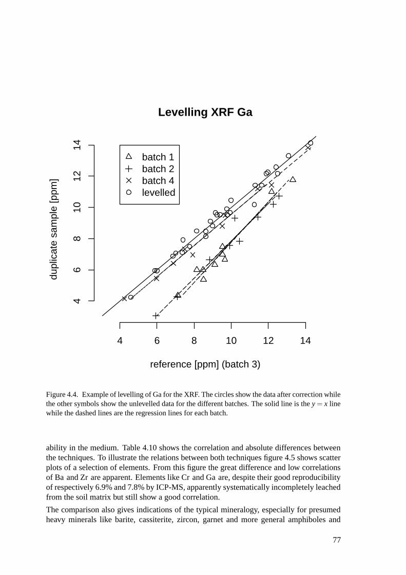
Levelling XRF Ga
reference [ppm] (batch 3)
dupl
icat
e sa
mpl
e [p
pm]
4 6 8 10 12 14
46
810
1214
batch 1batch 2batch 4levelled
Figure 4.4. Example of levelling of Ga for the XRF. The circles show the data after correction whilethe other symbols show the unlevelled data for the different batches. The solid line is the y = x linewhile the dashed lines are the regression lines for each batch.
ability in the medium. Table 4.10 shows the correlation and absolute differences betweenthe techniques. To illustrate the relations between both techniques figure 4.5 shows scatterplots of a selection of elements. From this figure the great difference and low correlationsof Ba and Zr are apparent. Elements like Cr and Ga are, despite their good reproducibilityof respectively 6.9% and 7.8% by ICP-MS, apparently systematically incompletely leachedfrom the soil matrix but still show a good correlation.
The comparison also gives indications of the typical mineralogy, especially for presumedheavy minerals like barite, cassiterite, zircon, garnet and more general amphiboles and
77

Table 4.8. Results of the levelling for the XRF data. r is the correlation coefficient and a is theslope of the linear regression
Element r a Element r a
Al2O3 1 1.02 La 0.97 1.13
CaO 0.97 0.98 Nb 0.96 0.96
Fe2O3 1 1.01 Nd 0.93 0.86
K2O 1 0.99 Ni 0.98 0.98
MgO 0.96 0.93 Pb 0.96 0.98
MnO 0.89 0.82 Rb 1 1
Na2O 0.75 0.61 Sc 0.95 1
P2O5 0.99 0.99 Sn 0.19 0.28
S 0.82 0.59 Sr 0.91 0.83
SiO2 0.90 0.92 Th 0.46 0.64
TiO2 0.97 1 U 0.51 0.81
As 0.98 0.98 V 0.99 1.01
Ba 0.84 0.83 Y 0.96 0.97
Cr 0.93 0.91 Zn 0.97 0.91
Cu 0.99 0.94 Zr 0.96 1
Ga 0.99 0.98
pyroxenes. Figure 4.5 shows that heavy mineral associated elements like Ba, Zr , Ga, Cr,Sc, and to a lesser extent Ni , have lower values by ICP-MS than on the XRF. Apparently,they only partially leach in an aqua regia solution (Scancar et al., 2000; Tsolakidou et al.,2002). For Ba and Zr poor correlations exist while for Cr, Ga, and Ni they are better.The main distinction is that Ba and Zr are very poorly leached by aqua regia (respectivelyabout 25% and 3%), and mainly occur outside the alumino-silicate matrix. Their totalconcentration as measured by XRF thus will not be correlated to Al2O3 , in contrast to theirICP measured aqua regia leached part.
A good example of the benefits of comparing two methods is Zn. This shows unexpectedoverall enrichment in the ICP-MS extract compared to the XRF together with several ICP-MS outliers. After consultation with the laboratory staff it was inferred that the extensivereconstruction activities in the building over the past years apparently have generated a Znenriched fine dust that continues to contaminate the air quality in the laboratory.
4.3.6 Parameter selection and summary statistics
Selection of parameters for a final, optimal dataset was based on the following criteria:no, or only sporadic missing values, satisfactory precision and accuracy, and in case of
78

Table 4.9. Results of the levelling for the ICP-MS data, r is the correlation coefficient and a is theslope of the linear regression
Element r a Element r a
As 0.86 0.94 Mn 0.78 0.80
Ba 0.74 0.70 Mo 0.46 0.35
Be 0.89 0.90 Nb 0.42 0.40
B 0.67 0.81 Nd 0.79 0.76
Bi 0.85 0.82 Ni 0.90 0.90
Ca 0.88 1.04 Pb 0.76 0.88
Cd 0.83 0.90 Pr 0.80 0.83
Ce 0.82 0.86 Rb 0.90 0.90
Cr 0.91 0.92 Sb 0.77 0.81
Cs 0.85 0.90 Sc 0.72 0.70
Cu 0.64 0.77 Sm 0.81 0.82
Dy 0.76 0.72 Sn 0.64 0.75
Er 0.76 0.72 Sr 0.92 0.94
Eu 0.68 0.73 Tb 0.77 0.72
Fe 0.87 0.89 Th 0.76 0.81
Ga 0.87 0.88 Ti 0.68 0.64
Gd 0.77 0.73 Tm 0.73 0.68
Ho 0.77 0.73 U 0.66 0.63
La 0.84 0.85 Y 0.84 0.85
Li 0.87 0.86 Yb 0.72 0.64
Lu 0.62 0.53 Zn 0.67 0.72
Mg 0.89 0.92
overlap between XRF and ICP-MS: preferably optimal precision and accuracy, but alsocompatibility with the standard Dutch practice of aqua-regia extraction.
The first criterion results in rejection of a number of parameters that were not analysed inthe first survey: Ag, B, Be, Bi , Li , Sc, Ta, Tl , and most of the REE. Of these Ag, Taand Tl also suffer from poor precision. Other elements that are rejected because of un-satisfactory precision/accuracy are Au, Pt , and Se. In the comparison between XRF andICP-MS for optimal precision and accuracy, XRF is favoured for most elements, except forSn, which has a higher reproducibility by ICP-MS. For Ba which has a large differencebetween ICP-MS and XRF (table 4.10), the ICP-MS analyses were chosen to be more com-patible with other Dutch research. For most other elements that have satisfactory precisionfor both XRF and ICP-MS, method bias is relatively small (4.10).
Table 4.11 summarises the 31 parameters selected for the optimal dataset (n=270). The
79
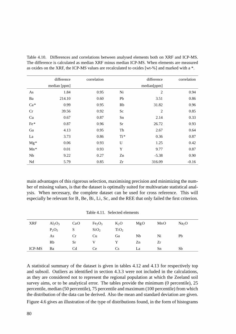
Table 4.10. Differences and correlations between analysed elements both on XRF and ICP-MS.The difference is calculated as median XRF minus median ICP-MS. When elements are measuredas oxides on the XRF, the ICP-MS values are recalculated to oxides [wt-%] and marked with a *.
difference correlation difference correlation
median [ppm] median[ppm]
As 1.84 0.95 Ni 2 0.94
Ba 214.10 0.60 Pb 3.51 0.86
Ca* 0.99 0.95 Rb 31.82 0.96
Cr 39.56 0.92 Sc 2 0.85
Cu 0.67 0.87 Sn 2.14 0.33
Fe* 0.87 0.96 Sr 26.72 0.93
Ga 4.13 0.95 Th 2.67 0.64
La 3.73 0.86 Ti* 0.36 0.87
Mg* 0.06 0.93 U 1.25 0.42
Mn* 0.01 0.93 Y 9.77 0.87
Nb 9.22 0.27 Zn -5.38 0.90
Nd 5.79 0.85 Zr 316.09 -0.16
main advantages of this rigorous selection, maximising precision and minimizing the num-ber of missing values, is that the dataset is optimally suited for multivariate statistical anal-ysis. When necessary, the complete dataset can be used for cross reference. This willespecially be relevant for B, Be, Bi , Li , Sc, and the REE that only failed the first criterion.
Table 4.11. Selected elements
XRF Al2O3 CaO Fe2O3 K2O MgO MnO Na2O
P2O5 S SiO2 TiO2
As Cr Cu Ga Nb Ni Pb
Rb Sr V Y Zn Zr
ICP-MS Ba Cd Ce Cs La Sn Sb
A statistical summary of the dataset is given in tables 4.12 and 4.13 for respectively topand subsoil. Outliers as identified in section 4.3.3 were not included in the calculations,as they are considered not to represent the regional population at which the Zeeland soilsurvey aims, or to be analytical error. The tables provide the minimum (0 percentile), 25percentile, median (50 percentile), 75 percentile and maximum (100 percentile) from whichthe distribution of the data can be derived. Also the mean and standard deviation are given.
Figure 4.6 gives an illustration of the type of distributions found, in the form of histograms
80
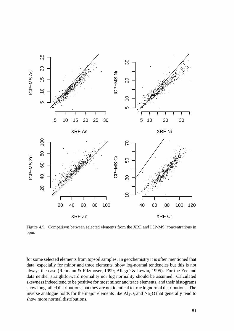
XRF As
ICP
−M
S A
s
5 10 15 20 25 30
510
1520
25
XRF Zn
ICP
−M
S Z
n
20 40 60 80 100
2040
6080
100
XRF Ni
ICP
−M
S N
i5 10 20 30
510
2030
XRF Cr
ICP
−M
S C
r
40 60 80 100 120
1030
5070
Figure 4.5. Comparison between selected elements from the XRF and ICP-MS, concentrations inppm.
for some selected elements from topsoil samples. In geochemistry it is often mentioned thatdata, especially for minor and trace elements, show log-normal tendencies but this is notalways the case (Reimann & Filzmoser, 1999; Allegre & Lewin, 1995). For the Zeelanddata neither straightforward normality nor log normality should be assumed. Calculatedskewness indeed tend to be positive for most minor and trace elements, and their histogramsshow long tailed distributions, but they are not identical to true lognormal distributions. Theinverse analogue holds for the major elements like Al2O3 and Na2O that generally tend toshow more normal distributions.
81
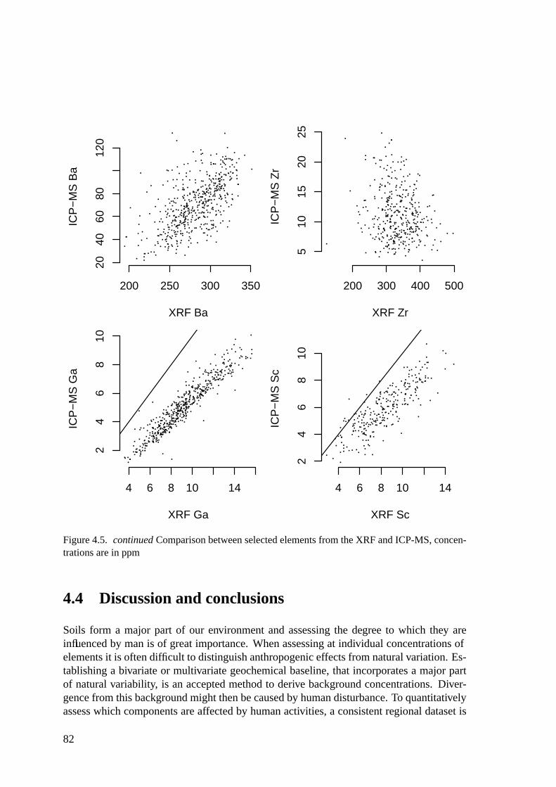
XRF Ba
ICP
−M
S B
a
200 250 300 350
2040
6080
120
XRF Ga
ICP
−M
S G
a
4 6 8 10 14
24
68
10
XRF Zr
ICP
−M
S Z
r200 300 400 500
510
1520
25
XRF Sc
ICP
−M
S S
c
4 6 8 10 14
24
68
10
Figure 4.5. continued Comparison between selected elements from the XRF and ICP-MS, concen-trations are in ppm
4.4 Discussion and conclusions
Soils form a major part of our environment and assessing the degree to which they areinfluenced by man is of great importance. When assessing at individual concentrations ofelements it is often difficult to distinguish anthropogenic effects from natural variation. Es-tablishing a bivariate or multivariate geochemical baseline, that incorporates a major partof natural variability, is an accepted method to derive background concentrations. Diver-gence from this background might then be caused by human disturbance. To quantitativelyassess which components are affected by human activities, a consistent regional dataset is
82
needed where special attention is paid to quantifying data quality. This chapter documentsthe construction of such a dataset for the province of Zeeland.
The sampling design was aimed at sampling present-day soil and pristine soil concentra-tions by sampling an influenced topsoil layer and an assumed pre-anthropogenic deepersubsoil layer. Based on earlier results (see chapter 3) the minimum sampling density of 1sample per 1-10km2 was regarded sufficient for obtaining a regional overview of the soilchemical composition in Zeeland. The analytical methods used (ICP-MS with aqua regiadigestion and XRF on pressed powder tablets) and the broad group of elements measured(major elements like Al2O3 and Fe2O3 , anthropogenically affected elements like Cd, Pb,Sb, trace elements like the REE) resulted in a data set of 87, partly overlapping, parame-ters. Each group of elements is thought to provide specific information on natural variation,human influence, or their interaction, as will the comparison between top and subsoil.
The comparison allowed by the overlap in measured parameters between ICP-MS and XRFshows a low extraction efficiency by aqua regia especially for elements like Ba, Zr , Ga, Cr,Sc, and Ni, which probably are partly related to the presence of heavy minerals containingthese elements to various degrees. The parameter overlap can also be used to determine ifoutliers are true anomalous samples or caused by analytical error. The elements Cu, Mn,Pb, and Zndisplay outliers in the topsoil data common to both techniques, which is anindication that these are (anthropogenic) anomalies.
Precision was estimated by analysing about 15% of the ICP-MS samples and about 4%of the XRF samples in duplicate. The smaller number of duplicates for the XRF wasconsidered sufficient since this method is known to be far more reproducible than the aqua-regia ICP-MS method. The better XRF reproducibility is indeed confirmed by the resultsfor analytical variance, which is in general lower for the XRF (0.5-10% relative to themean) than for the ICP-MS (5-13% relative). Exceptions are Th, U, and Snas measured byXRF and Ag, Au, Nb, Pt , Se, Ta, Tl , and Zr for ICP-MS; their low precision is ascribedto nugget effects. The analytical variability is generally smaller than the local samplingvariance as found in chapter 3, and therefore adequate for the desired regional evaluation ofsoil concentrations. The number of outliers found in the data also appears quite acceptable,as from a total of 270 samples a maximum of 10 outliers for Pb is found.
In this study the levelling of the data based on Between Survey Duplicates (BSD) provedto be a good method to eliminate subsurvey biases. The fact that BSD levelling uses a setof samples that has the full range of element composition and concentration present, and isthus representative of the total survey, makes this method preferable to corrections solelybased on analytical standards. The levelling uses ordinary linear regression, which wasconfirmed to be adequate in view of high correlations between the BSD duplicate pairs anda visual check on the linearity of the relation. The higher precision for the XRF also leadsto higher correlations for the parametric levelling.
Based on the precision and accuracy a selection was made of 31 parameters that were mea-sured in all surveys, and hence for virtually all locations and soil depths. This selectionis thus optimised for multivariate statistical analysis by maximizing data quality and min-imizing the number of missing values. This optimal dataset is limited compared to all the
83
data analysed, but still comprises a sufficient subset of major, minor, and trace elements forenvironmental assessment of the soils of Zeeland. It is intended to form the core for all mul-tivariate statistical and geochemical analysis, from which cross reference to the completedata set can still be made.
Summary statistics show that for most of the parameters neither a normal nor a lognormaldistribution should be assumed. Although most major elements tend to a more or lessnormal distribution, while most minor and trace elements are positively skewed, deviationsfrom the standard type distributions are apparent. Suspected contaminants like Cd, Sb, As,Pb and Zn are more skewed than other trace elements.
The data collection exercise documented in this chapter shows that, the use of state of theart analytical methods and appropriate use of international standard samples and withinsurvey, as well as between surveys, sample duplicates are all prerequisites for obtaining atrue reference dataset suitable for environmental and geochemical assessment of soil withina regional context.
84
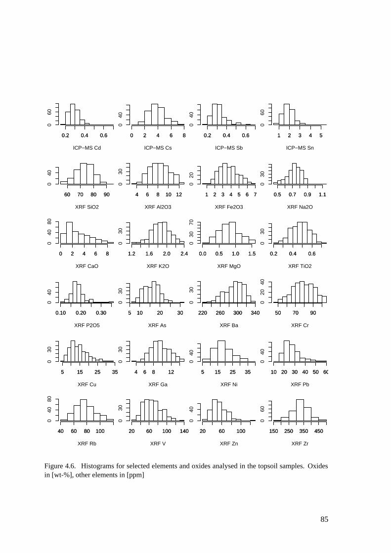
ICP−MS Cd
0.2 0.4 0.6
060
0.2 0.4 0.6
ICP−MS Cs
Fre
quen
cy
0 2 4 6 8
040
0 2 4 6 8
ICP−MS Sb
Fre
quen
cy
0.2 0.4 0.6
040
0.2 0.4 0.6
ICP−MS Sn
Fre
quen
cy
1 2 3 4 5
060
1 2 3 4 5
XRF SiO2
60 70 80 90
040
60 70 80 90
XRF Al2O3
Fre
quen
cy
4 6 8 10 12
030
4 6 8 10 12
XRF Fe2O3
Fre
quen
cy
1 2 3 4 5 6 70
201 2 3 4 5 6 7
XRF Na2O
Fre
quen
cy
0.5 0.7 0.9 1.1
030
0.5 0.7 0.9 1.1
XRF CaO
0 2 4 6 8
040
80
0 2 4 6 8
XRF K2O
Fre
quen
cy
1.2 1.6 2.0 2.4
030
1.2 1.6 2.0 2.4
XRF MgO
Fre
quen
cy
0.0 0.5 1.0 1.5
030
70
0.0 0.5 1.0 1.5
XRF TiO2
Fre
quen
cy0.2 0.4 0.6
030
0.2 0.4 0.6
XRF P2O5
0.10 0.20 0.30
040
0.10 0.20 0.30
XRF As
Fre
quen
cy
5 10 20 30
030
5 10 20 30
XRF Ba
Fre
quen
cy
220 260 300 340
030
220 260 300 340
XRF Cr
Fre
quen
cy
50 70 90
020
40
50 70 90
XRF Cu
5 15 25 35
030
5 15 25 35
XRF Ga
Fre
quen
cy
4 6 8 12
030
4 6 8 12
XRF Ni
Fre
quen
cy
5 15 25 35
040
5 15 25 35
XRF Pb
Fre
quen
cy
10 20 30 40 50 60
040
10 20 30 40 50 60
XRF Rb
40 60 80 100
040
80
40 60 80 100
XRF V
Fre
quen
cy
20 60 100 140
030
20 60 100 140
XRF Zn
Fre
quen
cy
20 60 100
040
20 60 100
XRF Zr
Fre
quen
cy
150 250 350 450
060
150 250 350 450
Figure 4.6. Histograms for selected elements and oxides analysed in the topsoil samples. Oxidesin [wt-%], other elements in [ppm]
85
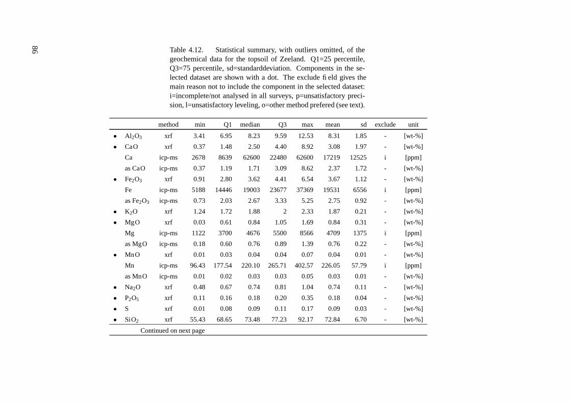
Table 4.12. Statistical summary, with outliers omitted, of thegeochemical data for the topsoil of Zeeland. Q1=25 percentile,Q3=75 percentile, sd=standarddeviation. Components in the se-lected dataset are shown with a dot. The exclude field gives themain reason not to include the component in the selected dataset:i=incomplete/not analysed in all surveys, p=unsatisfactory preci-sion, l=unsatisfactory leveling, o=other method prefered (see text).
method min Q1 median Q3 max mean sd exclude unit
• Al2O3 xrf 3.41 6.95 8.23 9.59 12.53 8.31 1.85 - [wt-%]
• CaO xrf 0.37 1.48 2.50 4.40 8.92 3.08 1.97 - [wt-%]
Ca icp-ms 2678 8639 62600 22480 62600 17219 12525 i [ppm]
as CaO icp-ms 0.37 1.19 1.71 3.09 8.62 2.37 1.72 - [wt-%]
• Fe2O3 xrf 0.91 2.80 3.62 4.41 6.54 3.67 1.12 - [wt-%]
Fe icp-ms 5188 14446 19003 23677 37369 19531 6556 i [ppm]
as Fe2O3 icp-ms 0.73 2.03 2.67 3.33 5.25 2.75 0.92 - [wt-%]
• K2O xrf 1.24 1.72 1.88 2 2.33 1.87 0.21 - [wt-%]
• MgO xrf 0.03 0.61 0.84 1.05 1.69 0.84 0.31 - [wt-%]
Mg icp-ms 1122 3700 4676 5500 8566 4709 1375 i [ppm]
as MgO icp-ms 0.18 0.60 0.76 0.89 1.39 0.76 0.22 - [wt-%]
• MnO xrf 0.01 0.03 0.04 0.04 0.07 0.04 0.01 - [wt-%]
Mn icp-ms 96.43 177.54 220.10 265.71 402.57 226.05 57.79 i [ppm]
as MnO icp-ms 0.01 0.02 0.03 0.03 0.05 0.03 0.01 - [wt-%]
• Na2O xrf 0.48 0.67 0.74 0.81 1.04 0.74 0.11 - [wt-%]
• P2O5 xrf 0.11 0.16 0.18 0.20 0.35 0.18 0.04 - [wt-%]
• S xrf 0.01 0.08 0.09 0.11 0.17 0.09 0.03 - [wt-%]
• SiO2 xrf 55.43 68.65 73.48 77.23 92.17 72.84 6.70 - [wt-%]
Continued on next page
86

Table 4.12 – continued from previous page
method min Q1 median Q3 max mean sd exclude unit
• TiO2 xrf 0.24 0.41 0.48 0.55 0.71 0.48 0.09 - [wt-%]
Ti icp-ms 357.81 577.24 653.32 721.81 939.14 643.01 108.47 i [ppm]
as TiO2 icp-ms 0.06 0.09 0.11 0.12 0.15 0.10 0.02 - [wt-%]
Ag icp-ms 0.04 0.06 0.07 0.08 0.13 0.07 0.02 i [ppm]
• As xrf 6.95 12.62 15.86 18.35 30.11 15.70 3.83 - [ppm]
As icp-ms 5.45 10.98 13.98 16.22 25.60 13.89 3.59 o [ppm]
Au icp-ms 0 0.01 0.02 0.05 0.15 0.03 0.03 p [ppm]
B icp-ms 11.70 28.78 39.31 47.05 69.30 38.94 12.35 i [ppm]
Ba xrf 221.80 274.73 291.32 304.74 334.70 289.78 20.95 o [ppm]
• Ba icp-ms 27.91 57.02 72.69 85.91 126.32 72.56 19.61 - [ppm]
Be icp-ms 0.31 0.76 0.96 1.14 1.73 0.97 0.28 i [ppm]
Bi icp-ms 0.07 0.14 0.17 0.22 0.36 0.18 0.06 i [ppm]
• Cd icp-ms 0.18 0.26 0.29 0.33 0.56 0.30 0.06 - [ppm]
• Ce icp-ms 24.07 36.71 41.45 46.87 56.86 41.46 6.70 - [ppm]
• Cr xrf 49.60 69.30 78.10 87.73 103.50 78.14 12.60 - [ppm]
Cr icp-ms 14.12 31.37 37.37 45.27 66.22 38.38 10 o [ppm]
• Cs icp-ms 0.81 2.86 3.59 4.47 7.92 3.75 1.28 - [ppm]
• Cu xrf 5.16 10.36 12.93 16.67 27.44 13.87 4.76 - [ppm]
Cu icp-ms 5.10 9.41 11.35 14.02 23.14 11.95 3.64 o [ppm]
Dy icp-ms 1.23 2.02 2.37 2.66 3.45 2.34 0.44 i [ppm]
Er icp-ms 0.56 0.93 1.11 1.24 1.59 1.09 0.20 i [ppm]
Eu icp-ms 0.34 0.60 0.70 0.81 1.05 0.70 0.14 i [ppm]
• Ga xrf 3.92 8.03 9.39 11.03 14.71 9.55 2.14 - [ppm]
Ga icp-ms 1.49 4.07 5.19 6.31 9.78 5.31 1.60 o [ppm]
Continued on next page
87
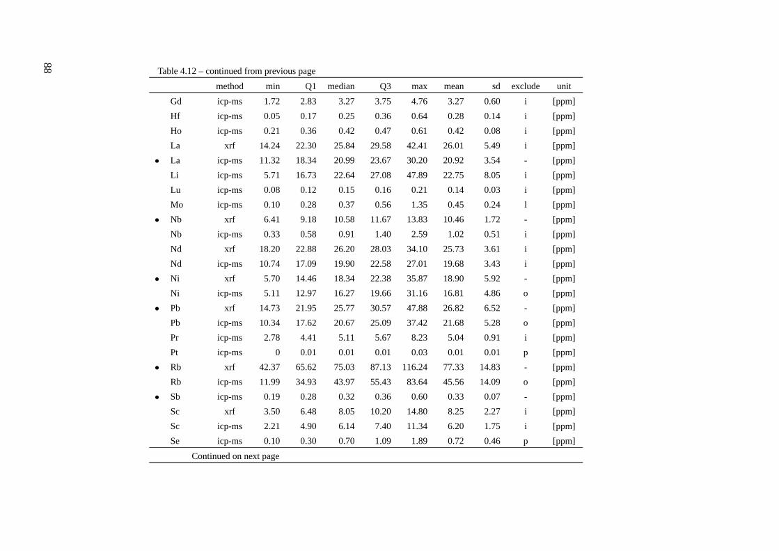
Table 4.12 – continued from previous page
method min Q1 median Q3 max mean sd exclude unit
Gd icp-ms 1.72 2.83 3.27 3.75 4.76 3.27 0.60 i [ppm]
Hf icp-ms 0.05 0.17 0.25 0.36 0.64 0.28 0.14 i [ppm]
Ho icp-ms 0.21 0.36 0.42 0.47 0.61 0.42 0.08 i [ppm]
La xrf 14.24 22.30 25.84 29.58 42.41 26.01 5.49 i [ppm]
• La icp-ms 11.32 18.34 20.99 23.67 30.20 20.92 3.54 - [ppm]
Li icp-ms 5.71 16.73 22.64 27.08 47.89 22.75 8.05 i [ppm]
Lu icp-ms 0.08 0.12 0.15 0.16 0.21 0.14 0.03 i [ppm]
Mo icp-ms 0.10 0.28 0.37 0.56 1.35 0.45 0.24 l [ppm]
• Nb xrf 6.41 9.18 10.58 11.67 13.83 10.46 1.72 - [ppm]
Nb icp-ms 0.33 0.58 0.91 1.40 2.59 1.02 0.51 i [ppm]
Nd xrf 18.20 22.88 26.20 28.03 34.10 25.73 3.61 i [ppm]
Nd icp-ms 10.74 17.09 19.90 22.58 27.01 19.68 3.43 i [ppm]
• Ni xrf 5.70 14.46 18.34 22.38 35.87 18.90 5.92 - [ppm]
Ni icp-ms 5.11 12.97 16.27 19.66 31.16 16.81 4.86 o [ppm]
• Pb xrf 14.73 21.95 25.77 30.57 47.88 26.82 6.52 - [ppm]
Pb icp-ms 10.34 17.62 20.67 25.09 37.42 21.68 5.28 o [ppm]
Pr icp-ms 2.78 4.41 5.11 5.67 8.23 5.04 0.91 i [ppm]
Pt icp-ms 0 0.01 0.01 0.01 0.03 0.01 0.01 p [ppm]
• Rb xrf 42.37 65.62 75.03 87.13 116.24 77.33 14.83 - [ppm]
Rb icp-ms 11.99 34.93 43.97 55.43 83.64 45.56 14.09 o [ppm]
• Sb icp-ms 0.19 0.28 0.32 0.36 0.60 0.33 0.07 - [ppm]
Sc xrf 3.50 6.48 8.05 10.20 14.80 8.25 2.27 i [ppm]
Sc icp-ms 2.21 4.90 6.14 7.40 11.34 6.20 1.75 i [ppm]
Se icp-ms 0.10 0.30 0.70 1.09 1.89 0.72 0.46 p [ppm]
Continued on next page
88
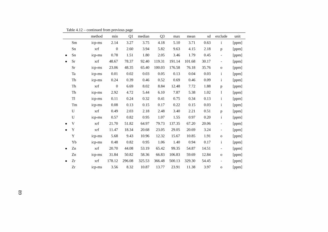
Table 4.12 – continued from previous page
method min Q1 median Q3 max mean sd exclude unit
Sm icp-ms 2.14 3.27 3.75 4.18 5.10 3.71 0.63 i [ppm]
Sn xrf 0 2.60 3.94 5.82 9.63 4.15 2.18 p [ppm]
• Sn icp-ms 0.78 1.51 1.80 2.05 3.46 1.79 0.45 - [ppm]
• Sr xrf 48.67 78.37 92.40 119.31 191.14 101.68 30.17 - [ppm]
Sr icp-ms 23.06 48.35 65.40 100.03 176.58 76.18 35.76 o [ppm]
Ta icp-ms 0.01 0.02 0.03 0.05 0.13 0.04 0.03 i [ppm]
Tb icp-ms 0.24 0.39 0.46 0.52 0.69 0.46 0.09 i [ppm]
Th xrf 0 6.69 8.02 8.84 12.48 7.72 1.88 p [ppm]
Th icp-ms 2.92 4.72 5.44 6.10 7.87 5.38 1.02 l [ppm]
Tl icp-ms 0.11 0.24 0.32 0.41 0.75 0.34 0.13 i [ppm]
Tm icp-ms 0.08 0.13 0.15 0.17 0.22 0.15 0.03 i [ppm]
U xrf 0.49 2.03 2.18 2.48 3.40 2.21 0.51 p [ppm]
U icp-ms 0.57 0.82 0.95 1.07 1.55 0.97 0.20 i [ppm]
• V xrf 21.70 51.82 64.97 79.73 137.35 67.20 20.06 - [ppm]
• Y xrf 11.47 18.34 20.68 23.05 29.05 20.69 3.24 - [ppm]
Y icp-ms 5.68 9.43 10.96 12.32 15.67 10.85 1.91 o [ppm]
Yb icp-ms 0.48 0.82 0.95 1.06 1.40 0.94 0.17 i [ppm]
• Zn xrf 20.70 44.08 53.19 65.42 99.35 54.87 14.51 - [ppm]
Zn icp-ms 31.84 50.82 58.36 66.83 106.83 59.69 12.84 o [ppm]
• Zr xrf 178.12 296.08 325.53 366.48 500.13 329.30 54.45 - [ppm]
Zr icp-ms 3.56 8.32 10.87 13.77 23.91 11.38 3.97 o [ppm]
89

Table 4.13. Statistical summary, with outliers omitted, of thegeochemical data for the subsoil of Zeeland. Q1=25 percentile,Q3=75 percentile, sd=standdardeviation. Components in the se-lected dataset are shown with a dot. The exclude field gives themain reason not to include the component in the selected dataset:i=incomplete/not analysed in all surveys, p=unsatisfactory preci-sion, l=unsatisfactory leveling, o=other method prefered (see text).
method min 25-prec. median 75-perc. max mean sd exclude unit
• Al2O3 xrf 2.58 5.54 7.23 9.30 13.29 7.49 2.51 - [wt-%]
• CaO xrf 0.52 2.80 3.94 5.27 10.70 4.05 1.90 - [wt-%]
Ca icp-ms 2961 15277 22772 30486 63723 24390 12716 i [ppm]
as CaO 0.41 2.10 3.14 4.20 8.77 3.36 1.75 - [wt-%]
• Fe2O3 xrf 0.51 2.08 2.99 4.13 7.39 3.20 1.40 - [wt-%]
Fe icp-ms 2123 11304 16094 23571 43678 17680 8425 i [ppm]
as Fe2O3 0.30 1.59 2.26 3.31 6.14 2.49 1.18 - [wt-%]
• K2O xrf 0.96 1.54 1.69 1.94 2.61 1.75 0.31 - [wt-%]
• MgO xrf 0.04 0.46 0.77 1.06 1.67 0.80 0.40 - [wt-%]
Mg icp-ms 1022 3332 4565 5803 8615 4571 1742 i [ppm]
as MgO 0.17 0.54 0.74 0.94 1.40 0.74 0.28 - [wt-%]
• MnO xrf 0.01 0.02 0.03 0.04 0.07 0.03 0.01 - [wt-%]
Mn icp-ms 69.21 133.20 174.54 210.69 387.79 177.79 58.39 i [ppm]
as MnO 0.01 0.02 0.02 0.03 0.05 0.02 0.01 - [wt-%]
• Na2O xrf 0.50 0.69 0.75 0.81 1.02 0.75 0.10 - [wt-%]
• P2O5 xrf 0.01 0.07 0.09 0.11 0.32 0.09 0.04 - [wt-%]
• S xrf 0 0.05 0.06 0.08 0.17 0.06 0.03 - [wt-%]
• SiO2 xrf 54.93 68.96 73.26 77.96 89.31 73.56 6.59 - [wt-%]
Continued on next page
90
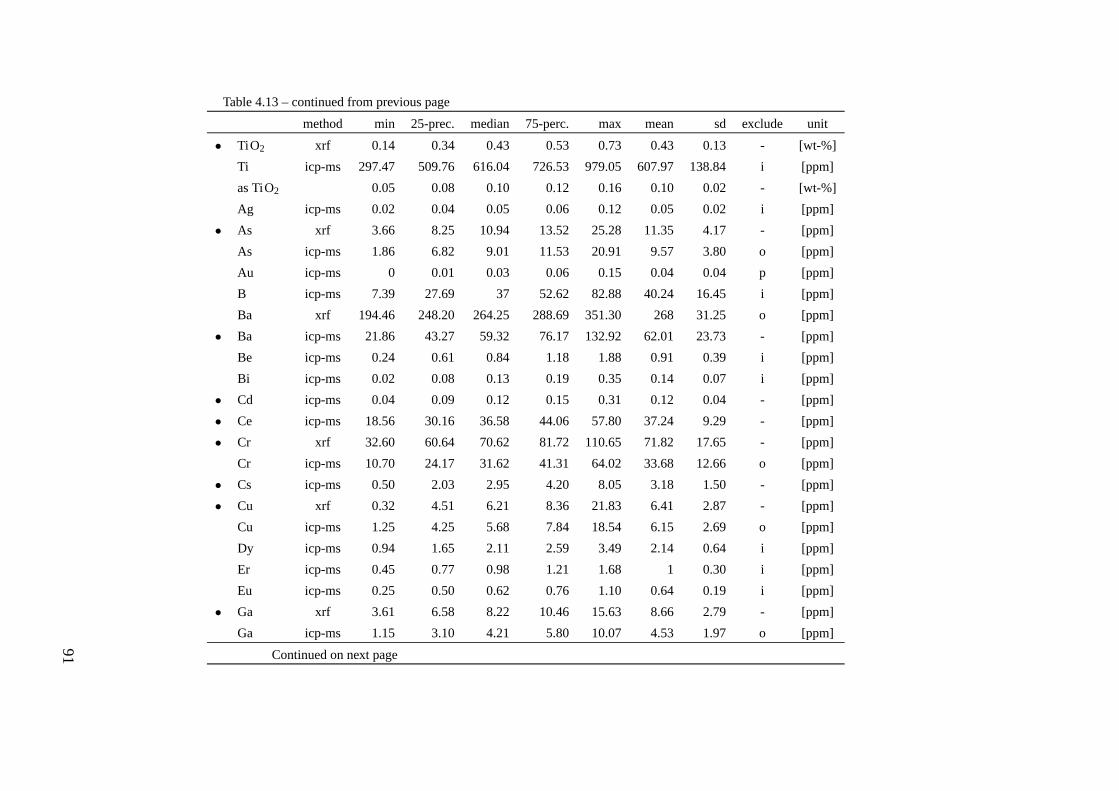
Table 4.13 – continued from previous page
method min 25-prec. median 75-perc. max mean sd exclude unit
• TiO2 xrf 0.14 0.34 0.43 0.53 0.73 0.43 0.13 - [wt-%]
Ti icp-ms 297.47 509.76 616.04 726.53 979.05 607.97 138.84 i [ppm]
as TiO2 0.05 0.08 0.10 0.12 0.16 0.10 0.02 - [wt-%]
Ag icp-ms 0.02 0.04 0.05 0.06 0.12 0.05 0.02 i [ppm]
• As xrf 3.66 8.25 10.94 13.52 25.28 11.35 4.17 - [ppm]
As icp-ms 1.86 6.82 9.01 11.53 20.91 9.57 3.80 o [ppm]
Au icp-ms 0 0.01 0.03 0.06 0.15 0.04 0.04 p [ppm]
B icp-ms 7.39 27.69 37 52.62 82.88 40.24 16.45 i [ppm]
Ba xrf 194.46 248.20 264.25 288.69 351.30 268 31.25 o [ppm]
• Ba icp-ms 21.86 43.27 59.32 76.17 132.92 62.01 23.73 - [ppm]
Be icp-ms 0.24 0.61 0.84 1.18 1.88 0.91 0.39 i [ppm]
Bi icp-ms 0.02 0.08 0.13 0.19 0.35 0.14 0.07 i [ppm]
• Cd icp-ms 0.04 0.09 0.12 0.15 0.31 0.12 0.04 - [ppm]
• Ce icp-ms 18.56 30.16 36.58 44.06 57.80 37.24 9.29 - [ppm]
• Cr xrf 32.60 60.64 70.62 81.72 110.65 71.82 17.65 - [ppm]
Cr icp-ms 10.70 24.17 31.62 41.31 64.02 33.68 12.66 o [ppm]
• Cs icp-ms 0.50 2.03 2.95 4.20 8.05 3.18 1.50 - [ppm]
• Cu xrf 0.32 4.51 6.21 8.36 21.83 6.41 2.87 - [ppm]
Cu icp-ms 1.25 4.25 5.68 7.84 18.54 6.15 2.69 o [ppm]
Dy icp-ms 0.94 1.65 2.11 2.59 3.49 2.14 0.64 i [ppm]
Er icp-ms 0.45 0.77 0.98 1.21 1.68 1 0.30 i [ppm]
Eu icp-ms 0.25 0.50 0.62 0.76 1.10 0.64 0.19 i [ppm]
• Ga xrf 3.61 6.58 8.22 10.46 15.63 8.66 2.79 - [ppm]
Ga icp-ms 1.15 3.10 4.21 5.80 10.07 4.53 1.97 o [ppm]
Continued on next page
91
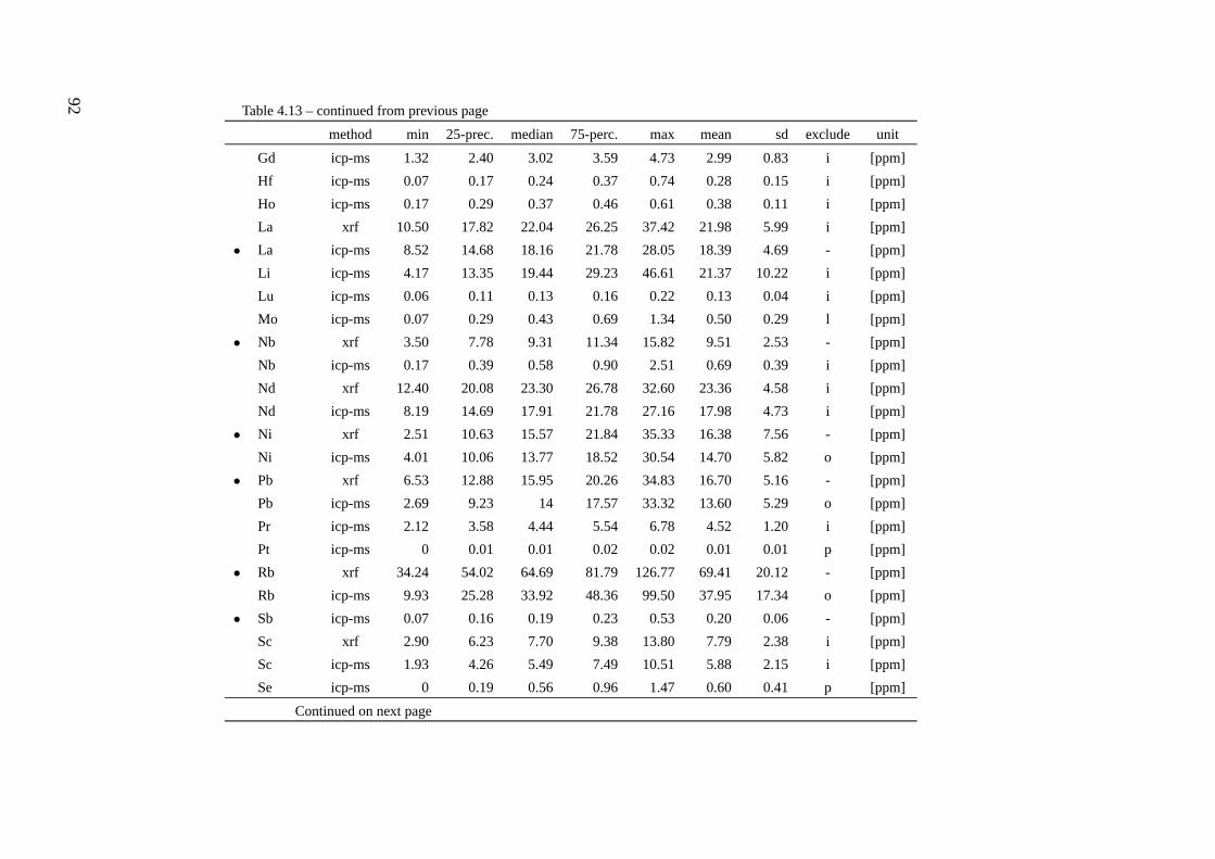
Table 4.13 – continued from previous page
method min 25-prec. median 75-perc. max mean sd exclude unit
Gd icp-ms 1.32 2.40 3.02 3.59 4.73 2.99 0.83 i [ppm]
Hf icp-ms 0.07 0.17 0.24 0.37 0.74 0.28 0.15 i [ppm]
Ho icp-ms 0.17 0.29 0.37 0.46 0.61 0.38 0.11 i [ppm]
La xrf 10.50 17.82 22.04 26.25 37.42 21.98 5.99 i [ppm]
• La icp-ms 8.52 14.68 18.16 21.78 28.05 18.39 4.69 - [ppm]
Li icp-ms 4.17 13.35 19.44 29.23 46.61 21.37 10.22 i [ppm]
Lu icp-ms 0.06 0.11 0.13 0.16 0.22 0.13 0.04 i [ppm]
Mo icp-ms 0.07 0.29 0.43 0.69 1.34 0.50 0.29 l [ppm]
• Nb xrf 3.50 7.78 9.31 11.34 15.82 9.51 2.53 - [ppm]
Nb icp-ms 0.17 0.39 0.58 0.90 2.51 0.69 0.39 i [ppm]
Nd xrf 12.40 20.08 23.30 26.78 32.60 23.36 4.58 i [ppm]
Nd icp-ms 8.19 14.69 17.91 21.78 27.16 17.98 4.73 i [ppm]
• Ni xrf 2.51 10.63 15.57 21.84 35.33 16.38 7.56 - [ppm]
Ni icp-ms 4.01 10.06 13.77 18.52 30.54 14.70 5.82 o [ppm]
• Pb xrf 6.53 12.88 15.95 20.26 34.83 16.70 5.16 - [ppm]
Pb icp-ms 2.69 9.23 14 17.57 33.32 13.60 5.29 o [ppm]
Pr icp-ms 2.12 3.58 4.44 5.54 6.78 4.52 1.20 i [ppm]
Pt icp-ms 0 0.01 0.01 0.02 0.02 0.01 0.01 p [ppm]
• Rb xrf 34.24 54.02 64.69 81.79 126.77 69.41 20.12 - [ppm]
Rb icp-ms 9.93 25.28 33.92 48.36 99.50 37.95 17.34 o [ppm]
• Sb icp-ms 0.07 0.16 0.19 0.23 0.53 0.20 0.06 - [ppm]
Sc xrf 2.90 6.23 7.70 9.38 13.80 7.79 2.38 i [ppm]
Sc icp-ms 1.93 4.26 5.49 7.49 10.51 5.88 2.15 i [ppm]
Se icp-ms 0 0.19 0.56 0.96 1.47 0.60 0.41 p [ppm]
Continued on next page
92
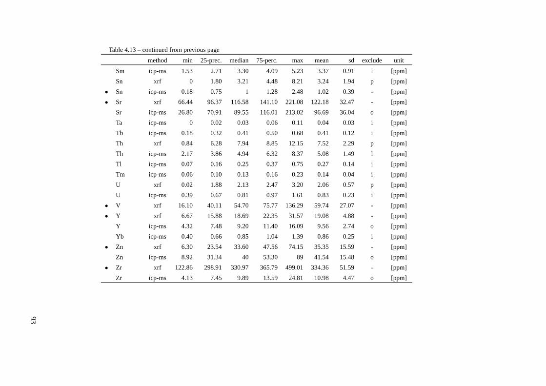
Table 4.13 – continued from previous page
method min 25-prec. median 75-perc. max mean sd exclude unit
Sm icp-ms 1.53 2.71 3.30 4.09 5.23 3.37 0.91 i [ppm]
Sn xrf 0 1.80 3.21 4.48 8.21 3.24 1.94 p [ppm]
• Sn icp-ms 0.18 0.75 1 1.28 2.48 1.02 0.39 - [ppm]
• Sr xrf 66.44 96.37 116.58 141.10 221.08 122.18 32.47 - [ppm]
Sr icp-ms 26.80 70.91 89.55 116.01 213.02 96.69 36.04 o [ppm]
Ta icp-ms 0 0.02 0.03 0.06 0.11 0.04 0.03 i [ppm]
Tb icp-ms 0.18 0.32 0.41 0.50 0.68 0.41 0.12 i [ppm]
Th xrf 0.84 6.28 7.94 8.85 12.15 7.52 2.29 p [ppm]
Th icp-ms 2.17 3.86 4.94 6.32 8.37 5.08 1.49 l [ppm]
Tl icp-ms 0.07 0.16 0.25 0.37 0.75 0.27 0.14 i [ppm]
Tm icp-ms 0.06 0.10 0.13 0.16 0.23 0.14 0.04 i [ppm]
U xrf 0.02 1.88 2.13 2.47 3.20 2.06 0.57 p [ppm]
U icp-ms 0.39 0.67 0.81 0.97 1.61 0.83 0.23 i [ppm]
• V xrf 16.10 40.11 54.70 75.77 136.29 59.74 27.07 - [ppm]
• Y xrf 6.67 15.88 18.69 22.35 31.57 19.08 4.88 - [ppm]
Y icp-ms 4.32 7.48 9.20 11.40 16.09 9.56 2.74 o [ppm]
Yb icp-ms 0.40 0.66 0.85 1.04 1.39 0.86 0.25 i [ppm]
• Zn xrf 6.30 23.54 33.60 47.56 74.15 35.35 15.59 - [ppm]
Zn icp-ms 8.92 31.34 40 53.30 89 41.54 15.48 o [ppm]
• Zr xrf 122.86 298.91 330.97 365.79 499.01 334.36 51.59 - [ppm]
Zr icp-ms 4.13 7.45 9.89 13.59 24.81 10.98 4.47 o [ppm]
93

5 Enrichment and natural variabilityversus anthropogenic impact
5.1 Introduction
For the Netherlands it is often claimed that natural soils, i.e. soils without anthropogenicinfluence, do not exist anymore (e.g. van der Meent et al. (1990)) . It is believed that overtime almost every part of the country has been subjected to the activities of people (seealso chapter 2). Despite this extensive influence, Dutch soils are statutorily divided intoclean (i.e. non-polluted) and polluted. The National Environmental Policy Plan (VROM,1997) states that the inventory of polluted and non-polluted soils must be completed by2005. The background values in Dutch soils will then be re-evaluated based on the set ofnon-polluted soils. However, this approach has some serious drawbacks. With rigid legalthresholds defining the difference between non-polluted and polluted soil samples, the linebetween the two categories of samples is extremely narrow. Moreover, the causal link maybe missing completely. Furthermore, in view of the widespread anthropogenic influence,the set of non-polluted soil samples will undoubtedly be affected to some extent.
For the Netherlands, soil pollution is defined in environmental legislation. The basis ofthese normative values is taken from a study of Edelman (1984) that established back-ground values based on soil samples from relatively clean areas. This study was latercriticised by van der Meent et al. (1990) because of the poor definition of “relatively cleanareas”. In the Netherlands one can, or even must, speak of soil pollution when a measuredvalue exceeds the legal threshold. Even a minor difference in measured concentration canflip the result from non polluted to polluted. This comparison of rigid values does notincorporate any information about variability and uncertainty in both measured and norma-tive value, reducing the outcome of the test to a boolean result. The latter has indeed beenevidenced by some soil sanitation projects in residential areas, where individual front andback yards were assessed for the need of sanitation. One garden might be considered cleanwhile the neighbouring garden could be polluted, resulting in a highly patchy pattern ofpolluted and non-polluted yards (pers. comm.). Although the rigid approach is apparentlyeffective for addressing legal issues, it does not necessarily reflect reality, which is thatmost soils are altered to some degree by human influence.
To solve the problem, altered elevated concentrations levels should be recognised regard-
95
less of whether the high values are caused by pollution or natural variation. One wayto do this is to compare the data with an unaltered, pristine, reference. In the field ofgeochemistry this often comprises a geochemical baseline that defines the natural back-ground. (Salminen & Tarvainen, 1997; Matschullat et al., 2000). Salminen & Grego-rauskiene (2000) provide an overview of different definitions for such a baseline. Theirmain points are that a geochemical baseline should describe the natural variation of an ele-ment in a particular natural material and should not be considered as a single value but as afluctuating reference surface over a wider area. They also noted that finer material, such asclay, has a different range of element abundances than other material. Hence a geochemi-cal baseline should incorporate the differences in parent material and underlying geogenic(and biogeochemical) processes.
If deviations from a geochemical background can be coherently discerned, the questionstill to be answered is if they should be called “pollution”. Pollution, in a more zealouscontext, is the destroying of purity or sanctity, while another meaning is simple “makingdirty”. But when is the purity of the soil destroyed or has someone made it dirty? Isdisturbing the soil, but leaving the bulk chemistry intact, also pollution? And what aboutthe use of fertiliser and other enhancements? This “disturbs” the chemical compositionof the soil, i.e. making it dirty, but is usually considered as an improvement instead of adestruction. Considering the multitude of human induced alterations to the soil that maylead to increased concentration levels, and considering the problems of defining pollutionor its synonym contamination, it is probably better to speak of enrichment. This term,which in fact describes what actually happened, will therefore be used in this thesis.
For the province of Zeeland (south-west Netherlands), the question of how to distinguishbetween natural and human induced geochemical patterns, was the reason to initiate thepresent geochemical soil survey. This study aims at establishing the anthropogenic imprinton the soil using a geochemical baseline that comprises the natural variability in soil com-position. Results should give a more precise insight in the state of enrichment (pollution),of the soils, and form a firm base for the soil and environmental protection policies of theprovince.
The use of a natural baseline for background values may seem much more obvious than theuse of just a legal threshold but the question remains how to derive such a baseline frompresent-day, thus influenced, soil data. While chapter 4 described the sampling and ana-lytical requirements, here focus is on data analysis and interpretation. Several (statistical)techniques that vary in complexity and accuracy are available to fulfill the aim of this study.As, among others, Salminen & Gregorauskiene (2000) have shown no best method existsfor establishing a baseline, no commonly agreed method for calculating human influenceexists either. From the point of view of the end user, the local government, a simple methodwithout the requirement for many (extra) data is preferred. From a scientific point of view,explained variability is of more importance than simplicity. The method must supply a re-alistic, accurate background value, and a more complex method, using relevant additionaldata, might be required. This chapter illustrates several techniques that permit the deter-mination of which components are enriched and how enrichments may be quantified. Thedifferences, degree of complexity, and efficacy of these methods will be discussed.
96
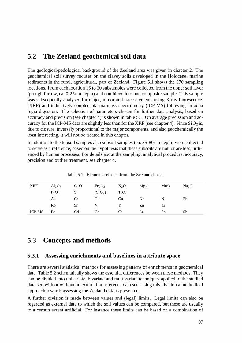
5.2 The Zeeland geochemical soil data
The geological/pedological background of the Zeeland area was given in chapter 2. Thegeochemical soil survey focuses on the clayey soils developed in the Holocene, marinesediments in the rural, agricultural, part of Zeeland. Figure 5.1 shows the 270 samplinglocations. From each location 15 to 20 subsamples were collected from the upper soil layer(plough furrow, ca. 0-25cm depth) and combined into one composite sample. This samplewas subsequently analysed for major, minor and trace elements using X-ray fluorescence(XRF) and inductively coupled plasma-mass spectrometry (ICP-MS) following an aquaregia digestion. The selection of parameters chosen for further data analysis, based onaccuracy and precision (see chapter 4) is shown in table 5.1. On average precission and ac-curacy for the ICP-MS data are slightly less than for the XRF (see chapter 4). Since SiO2 is,due to closure, inversely proportional to the major components, and also geochemically theleast interesting, it will not be treated in this chapter.
In addition to the topsoil samples also subsoil samples (ca. 35-80cm depth) were collectedto serve as a reference, based on the hypothesis that these subsoils are not, or are less, influ-enced by human processes. For details about the sampling, analytical procedure, accuracy,precision and outlier treatment, see chapter 4.
Table 5.1. Elements selected from the Zeeland dataset
XRF Al2O3 CaO Fe2O3 K2O MgO MnO Na2O
P2O5 S (SiO2) TiO2
As Cr Cu Ga Nb Ni Pb
Rb Sr V Y Zn Zr
ICP-MS Ba Cd Ce Cs La Sn Sb
5.3 Concepts and methods
5.3.1 Assessing enrichments and baselines in attribute space
There are several statistical methods for assessing patterns of enrichments in geochemicaldata. Table 5.2 schematically shows the essential differences between these methods. Theycan be divided into univariate, bivariate and multivariate techniques applied to the studieddata set, with or without an external or reference data set. Using this division a methodicalapproach towards assessing the Zeeland data is presented.
A further division is made between values and (legal) limits. Legal limits can also beregarded as external data to which the soil values can be compared, but these are usuallyto a certain extent artificial. For instance these limits can be based on a combination of
97
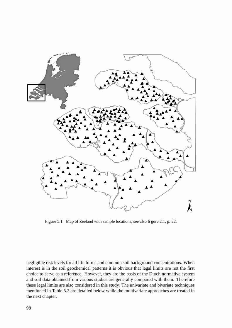
Figure 5.1. Map of Zeeland with sample locations, see also figure 2.1, p. 22.
negligible risk levels for all life forms and common soil background concentrations. Wheninterest is in the soil geochemical patterns it is obvious that legal limits are not the firstchoice to serve as a reference. However, they are the basis of the Dutch normative systemand soil data obtained from various studies are generally compared with them. Thereforethese legal limits are also considered in this study. The univariate and bivariate techniquesmentioned in Table 5.2 are detailed below while the multivariate approaches are treated inthe next chapter.
98
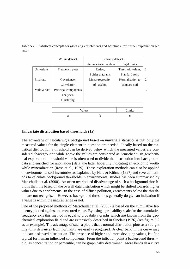
Table 5.2. Statistical concepts for assessing enrichments and baselines, for further explanation seetext.
Within dataset Between datasets
reference/external data legal limits
Univariate Frequency plots Ratios, Threshold values, 1
Spider diagrams Standard soils
Bivariate Covariance, Linear regression Normalisation to 2
Correlation of baseline standard soil
Multivariate Principal components – – 3
analyses,
Clustering
Values Limits
a b c
Univariate distribution based thresholds (1a)
The advantage of calculating a background based on univariate statistics is that only themeasured values for the single element in question are needed. Ideally based on the sta-tistical distribution a threshold can be derived below which the measured values are con-sidered “background” while above the values are considered as “enriched”. In geochem-ical exploration a threshold value is often used to divide the distribution into backgrounddata and enriched (or anomalous) data, the latter hopefully indicating an economic worth-while mineralization (Rose et al., 1979). These exploration methods can also be appliedin environmental soil inventories as explained by Hale & Kuhnel (1997) and several meth-ods to calculate background thresholds in environmental studies has been summarised byMatschullat et al. (2000). An often overlooked disadvantage of such a background thresh-old is that it is based on the overall data distribution which might be shifted towards highervalues due to enrichments. In the case of diffuse pollution, enrichments below the thresh-old are not recognised. However, background thresholds generally do give an indication ifa value is within the natural range or not.
One of the proposed methods of Matschullat et al. (2000) is based on the cumulative fre-quency plotted against the measured value. By using a probability scale for the cumulativefrequency axis this method is equal to probability graphs which are known from the geo-chemical exploration field and are extensively described in Sinclair (1976) (see figure 5.2as an example). The advantage of such a plot is that a normal distribution plots as a straightline, thus deviances from normality are easily recognised. A clear bend in the curve mayindicate a skewed distribution. The presence of higher and more deviating values, is oftentypical for human influenced components. From the inflection point a background thresh-old, as concentration or percentile, can be graphically determined. More bends in a curve
99
may indicate multi-modality. Determining the bends in the plots graphically, results insome subjectivity towards the chosen percentile. In contrast, an arbitrary choice, althoughobjective, might not reflect the optimal threshold. For example, in the Netherlands the90-percentile, or P90, is an arbitrary level which is often used (van der Gaast et al., 1998).
Comparison with standard data or other reference data (1b)
An often used method to judge if measured values are anomalous or enriched is to comparethem with global average values like that for the average upper continental crust (UCC)(Wedepohl, 1995). Despite the differences between average crust and soil material, theUCC is a good reference for element composition, especially for immature soils such asfound in Zeeland. A ratio of about one between measured and global UCC value indicatesno deviation from the global average while ratios much larger or smaller than one indicatean anomaly. Anomalies with ratios larger than one can be considered as enriched towardsthe global average, irrespective of the fact whether this enrichment is caused by naturalprocesses (like the enrichment of more mobile elements in weathering products) or causedby enrichment due to human input.
Another approach is to use reference values from pristine soils of the same area. The greatadvantage is that the reference soils have then been subjected to the same natural processesas the soils of interest, yet not subjected to human influence (Facchinelli et al., 2001; Shotyket al., 2001). In this case a ratio different than one might indicate anthropogenic influence.The data collected for this research (see chapter 4) therefore incorporate subsoil samples,under the assumption that these are chemically less or not disturbed by man. The means ormedians of this subsoil data set can then be used as a local reference value comprising thegeochemical background.
Using global averages or local references has as drawback that the actual field values arecompared with a single value only, neglecting natural and sampling variance. A single ratiohas limited value without any information about variability. Therefore also the ratios of the2nd and 4th quartile of the data will be calculated to provide insight in the variability.
Legal thresholds (1c)
The same method, as with the “real” global averages or local backgrounds, of calculat-ing ratios can be applied to legal limits like the Dutch legal threshold values (Dutch:“Streefwaarden” or S) (VROM, 1994; Swartjes, 1999). For the Dutch situation disadvan-tages of this technique are that legal threshold limits are defined, besides organic com-pounds, for only 16 elements (As, Ba, Be, Cd, Cr, Co, Cu, Hg, Pb, Mo, Ni, Sb, Se, Ta,V, Zn), and that their derivation is not well documented in international literature. For Sn,a legal limit is lacking, only an indicative value can be derived from regression parameters(see below). Besides the value for S, an intervention value is defined that signals the levelof severe pollution (Dutch: “Interventiewaarde” or I). This level is based on risk ratherthen on background soil composition, and it will not be further considered in this study(Swartjes, 1999).
100
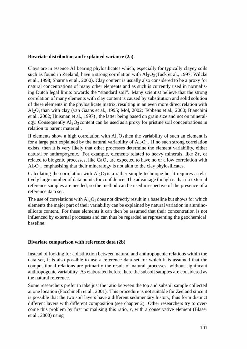
Bivariate distribution and explained variance (2a)
Clays are in essence Al bearing phylosilicates which, especially for typically clayey soilssuch as found in Zeeland, have a strong correlation with Al2O3 (Tack et al., 1997; Wilckeet al., 1998; Sharma et al., 2000). Clay content is usually also considered to be a proxy fornatural concentrations of many other elements and as such is currently used in normalis-ing Dutch legal limits towards the “standard soil”. Many scientist believe that the strongcorrelation of many elements with clay content is caused by substitution and solid solutionof these elements in the phylosilicate matrix, resulting in an even more direct relation withAl2O3 than with clay (van Gaans et al., 1995; Mol, 2002; Tebbens et al., 2000; Bianchiniet al., 2002; Huisman et al., 1997) , the latter being based on grain size and not on mineral-ogy. Consequently Al2O3 content can be used as a proxy for pristine soil concentrations inrelation to parent material .
If elements show a high correlation with Al2O3 then the variability of such an element isfor a large part explained by the natural variability of Al2O3 . If no such strong correlationexists, then it is very likely that other processes determine the element variability, eithernatural or anthropogenic. For example, elements related to heavy minerals, like Zr, orrelated to biogenic processes, like CaO, are expected to have no or a low correlation withAl2O3 , emphasising that their mineralogy is not akin to the clay phylosilicates.
Calculating the correlation with Al2O3 is a rather simple technique but it requires a rela-tively large number of data points for confidence. The advantage though is that no externalreference samples are needed, so the method can be used irrespective of the presence of areference data set.
The use of correlations with Al2O3 does not directly result in a baseline but shows for whichelements the major part of their variability can be explained by natural variation in alumino-silicate content. For these elements it can then be assumed that their concentration is notinfluenced by external processes and can thus be regarded as representing the geochemicalbaseline.
Bivariate comparison with reference data (2b)
Instead of looking for a distinction between natural and anthropogenic relations within thedata set, it is also possible to use a reference data set for which it is assumed that thecompositional relations are primarily the result of natural processes, without significantanthropogenic variability. As elaborated before, here the subsoil samples are considered asthe natural reference.
Some researchers prefer to take just the ratio between the top and subsoil sample collectedat one location (Facchinelli et al., 2001). This procedure is not suitable for Zeeland since itis possible that the two soil layers have a different sedimentary history, thus form distinctdifferent layers with different composition (see chapter 2). Other researchers try to over-come this problem by first normalising this ratio, r, with a conservative element (Blaseret al., 2000) using
101

r =(x
y)top
(xy)sub
(5.1)
in which x is the element of interest normalised to the conservative element y. This methodalways requires 4 measurements for calculating an enrichment. Furthermore the covariancebetween x, y for both soil depths must be studied closely to prevent spurious results (van derWeijden, 2002).
Another method uses linear relations with clay or Al2O3 content, or any other soil or sed-iment parameter that is known not to be influenced, or conservative (Bauer et al., 1992;Bauer & Bor, 1995). As does the calculation of the direct within data set correlation de-scribed above, this method requires a sufficiently large number of reference data points forconfidence, and of course a good correlation between the element considered and the pre-dictor variable used. In this thesis the subsoil data set with the outliers omitted is used asundisturbed reference. Sulfur, due to the relatively large number of outliers, was excluded.Linear equations were derived in which the estimated concentration (Cest) of each elementin the topsoil was expressed as a function of Al2O3 content using
Cest = Al2O3 ·a + b (5.2)
where a and b are the slope and intercept from the regression analysis based on the subsoildata, and Al2O3 is the measured concentration in the topsoil sample.
A significant deviation of the actually measured concentration from the calculated valueis evidence of an enrichment caused by processes other than natural variability inclay/phylosilicate content, which is calculated as
e =Ctop
Cest(5.3)
where Ctop is the analysed topsoil sample concentration of the element considered. Com-pared to equation 5.1, this method only requires 2 components analysed once the regressionparameters are established.
It was decided to use ordinary least squares (OLS) regression. Although some researchersconsider “better” regression techniques in geochemistry, e.g. Szava-Kovats (2002), thesetechniques are usually trying to minimise the influence of outliers and to compensate forthe error in the independent variable. Since the outliers had already been omitted from thesubsoil data set and considering the analytical error of only 0.8% (see table 4.4, p. 74) forAl2O3 I presume that OLS regression is adequate.
Although theoretically the possibility of depletion of anthropogenically influenced com-ponents does exist, it is not very likely in young marine clayey areas such as Zeeland. If
102
depletion occurred, for example due to acidification of the soil, the situation would easilybe recognised. Depletion due to weathering is not considered, except for calcite relatedcomponents. Because of the very young age of the Zeeland soils the differences betweentop and subsoil caused by weathering are expected to be negligible, and within the boundsof sampling and analytical noise.
From the enrichments e, and after establishing that the enrichments are of anthropogenicorigin, it is possible to calculate a contamination degree d (Rapant et al., 1999). This degreeindicates the amount of contamination caused by a group of n elements by calculating theaverage enrichment using
d =1n
i=1
∑n
ei (5.4)
Soil type dependent legal threshold (2c)
According to the normative framework, Dutch legal threshold values are dependent on thesoil type using clay content (grain size <2µm) and organic matter content as the primarydistinctive soil properties for all Dutch soil types (VROM, 1994). Threshold values aregiven as maximum permissible levels for sustainable soil quality (S) and are based on aso called standard soil containing 25% clay and 10% organic matter. Using the dictatedequation
s = S · α +Cβ + Oγα + 25β + 10γ
(5.5)
the given value S can be recalculated to the soil dependent value s using the measuredorganic matter (%O) and clay (%C) content of that soil (VROM, 1994). The regressionparameters α, β, and γ, are also provided by the normative framework. In principle the Svalues are valid only for concentrations determined in aqua-regia extracts, while here mostelements are analysed by XRF, giving total concentrations. For most elements the discrep-ancy is negligible except for Ba and V. For Ba, therefore, ICP-MS data were selected butfor V precision with ICP-MS was poor. Thus V is omitted from the comparison with S.
As noted earlier, only for 16 inorganic elements are legal threshold available. Most ofthe Dutch soil surveys within the scope of environmental law or practice, are standardisedtowards them. Data are often expressed as either the ratio of the measured values and thesoil dependent threshold limit or as the equivalent concentration in standard soil, as it isbelieved that such a standardisation facilitates comparison between areas and surveys.
103
Table 5.3. S values and regression (α, β, γ) parameters (see equation 5.5) for relevant elements.S-value for Sn derived from regression parameters, no official value given. For Sb no regressionparameters are given (VROM, 1994).
α β γ S value
As 15 0.4 0.4 29
Cd 0.4 0.007 0.021 0.8
Cr 50 2 0 100
Cu 15 0.6 0.6 36
Ni 10 1 0 35
Pb 50 1 1 85
Sb - - - 3
Sn 4 0.6 0 19
Zn 50 3 1.5 140
5.3.2 Spatial representation and spatial anomalies
In addition to discerning geochemical baselines and enrichments in attribute space, plottinggeochemical soil data in geographical space might reveal regional patterns or anomalies.Regional patterns are usually visible as spatial groups of points with similar values indi-cating regional features of the soil composition. Anomalies would be single points witha divergent value compared with other surrounding points, denoting either a depletion or,as expected for Zeeland, an enrichment compared to the surroundings. These anomaliesmight not occur as such in attribute space because the data point is not at the extreme of thedistribution but only in comparison with spatially neighbouring samples.
If no mathematical or geostatistical spatial model for each point in geographical space isassumed, only values related to the sampled locations can be plotted. To make the valuegraphically visible symbols will be used for which the size varies with the magnitude of theattribute concerned. Examples of such symbol maps already exist (Reimann et al., 2002;Bounessah & Atkin, 2003; McGrath & Zhang, 2003). The size function should preferablybe continuous, suitable to differentiate between high and low values, and should adjustto the observed frequency distribution of the attribute. Therefore the plotting method ofthe Geological Survey of Finland was adopted (Gustavson et al., 1997), which is basedon bubble plots for which the bubble size is an exponential function which monotonicallyincreases with the cumulative distribution. This bubble size function is designed for geo-chemical variables which follow a positively skewed or log normal distribution, emphasis-ing the upper values. This function can be regarded as a variant of the univariate cumulativefrequency distribution, where the bubble size shows the position of the data point withinthe distribution, small sizes corresponding with values in the lower part and large sizescorresponding with values in the upper tail.
104
5.4 Results and interpretation
5.4.1 Univariate statistics for the Zeeland topsoil data.
Cumulative frequencies
Figure 5.2 shows the cumulative frequency distributions of 12 selected components to-gether with the 90-percentile (P90). Some components like Al2O3 and Rb have straight,somewhat S-shaped, curves while other components like Cd, P2O5 , and Sb have a clearbend, and a steeper slope, at the top. This suggests that the latter have a deviation towardshigher values and might be locally enriched. The components La and Na2O have clear out-liers around the P99 showing that this technique can be used also to detect outliers. Fromthe almost straight line of components like Al2O3 and Fe2O3 it can be concluded that theirdistribution follows the normal distribution and that it is likely that they are uninfluencedby anthropogenic processes.
The component P2O5 shows that the bend in the top of the curve starts around the P90 pointsuggesting that the P90 value is a reasonable boundary for distinguishing enriched, influ-enced soil for this component. For Cd, Cu and Sb the P80 or P85 seem more appropriate(see table 5.4). For the assumed non influenced elements, e.g. Al 2O3 , Fe2O3 , and Rb, theP90 definitely is an underestimation of the maximum background level, which theoreticallyis the P100, the P99 is used instead. This shows that the P90, as used in Dutch practice, ispartly useful but only if the corresponding cumulative frequency plot is studied as well.Preferably the percentile should be adjusted in accordance with the plot. Using an arbitraryvalue, there is a clear risk of over- or underestimating the background threshold.
The P90, P95, and P99 values for all the elements are given in table 5.4. The optimal thresh-old is determined by choosing the optimal percentile based on the bends in the cumulativefrequency plots (plots are not shown). Despite the subjectivity of this method, within the5% resolution adopted, the results obtained are adequate.
The use of the cumulative plots is helpful in indicating which elements show anomaliesrelative to a normal distribution. While this method is very simple and easy to apply, itgives no indication if a component is anthropogenically enriched or not. Also it does notrecognise enrichments which occur within the range of the normal distributed uninfluenceddata, e.g. some concentrations on the lower end of the distribution can be substantiallyenriched without changing the relation in the cumulative frequency plots. If all the samplesare enriched, e.g. by diffuse contamination, then this is not revealed in the CDF plots aswell.
Spatial representation
The regional distributions of the same elements as selected for figure 5.2, are illustrated infigure 5.3 and 5.4. Figure 5.3 depicts elements that are expected not to be influenced by hu-man processes and figure 5.4 shows the elements that are probably influenced by man. The
105
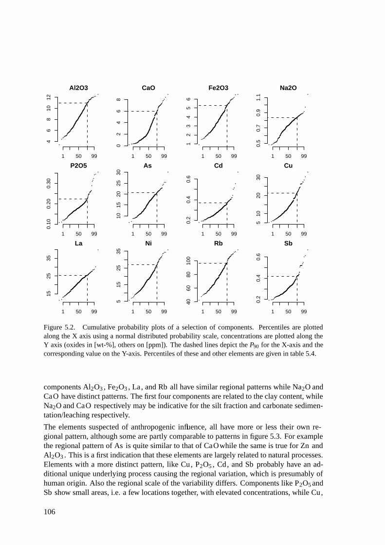
Al2O3
1 50 99
46
810
12
CaO
1 50 99
02
46
8
Fe2O3
1 50 99
12
34
56
Na2O
1 50 99
0.5
0.7
0.9
1.1
P2O5
1 50 99
0.10
0.20
0.30
As
1 50 99
1015
2025
30
Cd
1 50 99
0.2
0.4
0.6
Cu
1 50 99
510
2030
La
1 50 99
1525
35
Ni
1 50 99
515
2535
Rb
1 50 99
4060
8010
0
Sb
1 50 99
0.2
0.4
0.6
Figure 5.2. Cumulative probability plots of a selection of components. Percentiles are plottedalong the X axis using a normal distributed probability scale, concentrations are plotted along theY axis (oxides in [wt-%], others on [ppm]). The dashed lines depict the P90 for the X-axis and thecorresponding value on the Y-axis. Percentiles of these and other elements are given in table 5.4.
components Al2O3 , Fe2O3 , La, and Rb all have similar regional patterns while Na2O andCaO have distinct patterns. The first four components are related to the clay content, whileNa2O and CaO respectively may be indicative for the silt fraction and carbonate sedimen-tation/leaching respectively.
The elements suspected of anthropogenic influence, all have more or less their own re-gional pattern, although some are partly comparable to patterns in figure 5.3. For examplethe regional pattern of As is quite similar to that of CaOwhile the same is true for Zn andAl2O3 . This is a first indication that these elements are largely related to natural processes.Elements with a more distinct pattern, like Cu, P2O5 , Cd, and Sb probably have an ad-ditional unique underlying process causing the regional variation, which is presumably ofhuman origin. Also the regional scale of the variability differs. Components like P2O5 andSb show small areas, i.e. a few locations together, with elevated concentrations, while Cu,
106

Table 5.4. Percentiles of the data of Zeeland topsoil. Optimal threshold percentiles, determinedgraphically, are noted in bold face. If no optimal threshold is given, then it is below the P90 andshown below the table
Element P90 P95 P99 Element P90 P95 P99
Al2O3 10.94 11.56 12.05 Cs 5.46 6.23 6.90
CaO 5.99 6.91 7.93 Cu 21.44 24.26 29.14
Fe2O3 5.32 5.60 6.15 Ga 12.53 13.36 14.54
K2O 2.14 2.21 2.31 La 25.36 26.52 28.55
MgO 1.27 1.37 1.54 Nb 12.71 13.06 13.64
MnO 0.06 0.06 0.08 Ni 27.08 30.35 33.94
Na2O 0.84 0.86 0.90 Pb 37 42.48 55
P2O5 0.22 0.26 0.34 Rb 96.74 105.17 111.25
S 0.14 0.17 0.26 Sb 0.42 0.51 0.71
TiO2 0.60 0.62 0.67 Sn 2.38 2.59 3.95
As 20.67 21.64 24.81 Sr 146.02 158.66 182.99
Ba 100.87 108.51 116.12 V 95.62 102.01 114.67
Cd 0.37 0.40 0.59 Y 24.40 25.30 26.54
Ce 50.83 52.19 55.91 Zn 74.51 80.07 98.84
Cr 94.82 99.28 102.60 Zr 394.05 422.05 466.05
P80: Cu(18.93ppm). P85: Cd(0.35ppm), Sb(0.36ppm)
As, and Zn show more regional features.
5.4.2 Univariate comparison with reference data and legal thresholdlevels
The upper continental crust
Figure 5.5 depicts the ratio of the median values of the concentrations as measured for theZeeland soils and those given for the upper continental crust (UCC) (Wedepohl, 1995).
In this comparison, for Ba the XRF values are used instead of the much lower ICP-MSdata, as the UCC is also based on total concentrations. Compared to the UCC and theoverall pattern the elements As, Cd, Cr, Pb, and Zrare relatively enriched while especiallyNa, and to a lesser extent Ca, K, Mg, Mn, and Sr are depleted. Most other elements liebetween a ratio of about 0.5 and 1.0. The Zeeland soils on average appear somewhat lessaluminous and ferromagnesian than the UCC.
The elements Pb and Cd are known as contaminants in fertiliser (de Lopez Camelo et al.,1997; Gimeno-Garcıa et al., 1996; Nash et al., 2003) and to be constituents of atmospheric
107

Al2O312.539.89
8.27
Fe2O36.544.534.083.61
Na2O0.970.80.770.74
CaO8.924.693.492.43
Rb116.2488.5781.6675.05
La30.2
24.0322.6221.27
Figure 5.3. Regional distribution of a selection of components expected not to be influenced byhuman processes
deposition of traffic exhausts (Parkpian et al., 2003). It is expected that these processes,fertilization and atmospheric deposition, are at least partially responsible for the enrichmentcompared to the upper continental crust. Natural processes, like mineralisations of theseelements, are not very likely for Zeeland. Ratios with the UCC from sedimentary studies
108
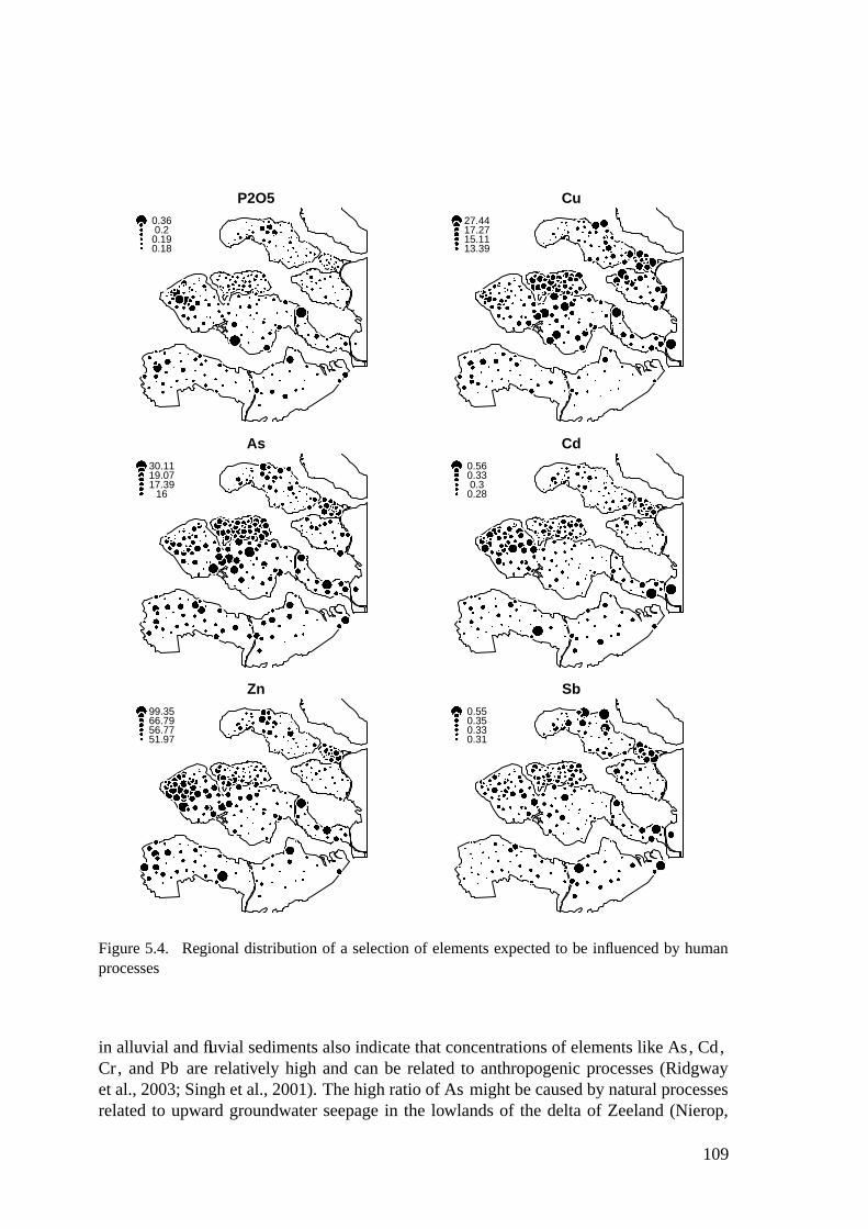
P2O50.360.20.190.18
As30.1119.0717.39
16
Zn99.3566.7956.7751.97
Cu27.4417.2715.1113.39
Cd0.560.330.3
0.28
Sb0.550.350.330.31
Figure 5.4. Regional distribution of a selection of elements expected to be influenced by humanprocesses
in alluvial and fluvial sediments also indicate that concentrations of elements like As, Cd,Cr, and Pb are relatively high and can be related to anthropogenic processes (Ridgwayet al., 2003; Singh et al., 2001). The high ratio of As might be caused by natural processesrelated to upward groundwater seepage in the lowlands of the delta of Zeeland (Nierop,
109
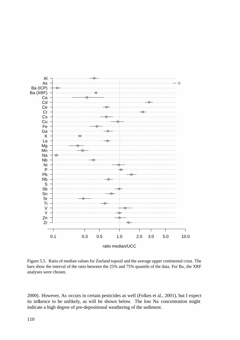
ratio median/UCC
ZrZnYVTiSrSnSb
SRbPb
PNi
NbNaMnMgLaK
GaFeCuCsCrCeCdCa
Ba (XRF)Ba (ICP)
AsAl
0.1 0.3 0.5 1.0 2.0 3.0 5.0 10.0
Figure 5.5. Ratio of median values for Zeeland topsoil and the average upper continental crust. Thebars show the interval of the ratio between the 25% and 75% quantile of the data. For Ba, the XRFanalyses were chosen.
2000). However, As occurs in certain pesticides as well (Folkes et al., 2001), but I expectits influence to be unlikely, as will be shown below. The low Na concentration mightindicate a high degree of pre-depositional weathering of the sediment.
110
In figure 5.6 the ratio between the medians of the top and subsoil samples is shown. Theratio for Al (1.13) is depicted by a vertical line and shows that the topsoil has a higher Alcontent. This suggests that the topsoil consists of heavier clays, which can be attributedto a more quiet marine environment and the sedimentation of the finest fraction during thereclamation of the Zeeland polders. This confirms that a direct, local, comparison betweentopsoil and subsoil concentration for Zeeland would indeed be unsuitable, and that at leasta normalisation according to equation 5.1 would be required.
The elements As, Cd, Cu, P, Pb, S, Sb, Sn, and Zn are clearly enriched compared to thesubsoil and, according to Senesi et al. (1999), can be related to anthropogenic activities.CaO and Sr are depleted from the topsoil. Assuming that the CaO content is mostly deter-mined by the calcite content of the soils it can be inferred that this depletion is caused byweathering. In general the element Sr is highly correlated with Ca in marine environmentsand often a replacement for Ca in calcite, hence Sr is depleted together with CaO.
Most of the other elements are close to the line round the 1.13 ratio. This suggest thatthese elements are closely related to the Al and clay content, and are not anthropogenicallyenriched in the Zeeland topsoil.
Comparing the local subsoil reference with the global UCC reference shows that the Crand Zr enrichments found for Zeeland compared to the UCC are probably a natural phe-nomenon, related to a typical heavy mineral association. The high topsoil/subsoil ratio forCu is not supported by the ratio of about 1.0 with the UCC, for this element the UCC isapparently an over-estimation of the Zeeland natural background. Given the fact that theAs content of the subsoil is relatively close to that of the topsoil, in relation to the enrich-ment of the Zeeland soils in comparison to the UCC, it appears that at least part of the Asenrichment is due to natural processes.
While the global UCC reference highlights the regional features and facilitates comparisonwith other areas, the local reference indeed provides much more insight into the (anthro-pogenic) nature of the enrichments found.
Legal thresholds
To compare the data with the legal threshold values, the ratio between the median topsoilvalues and the standard threshold value were calculated and depicted in figure 5.7. A com-parison with soil specific threshold values is presented as well, based on the standard soilcontaining 25% clay and 10% organic matter using equation 5.5. Since no clay and organicmatter values were available in the geochemical dataset, the clay content was estimatedusing the relation between Al2O3 and clay content obtained from another study in Zeeland(data not shown)∗ and the median clay content was used for the calculation. Organic mat-ter was set at the median organic matter value from the same data set†. The smaller bars,as compared to figure 5.5 and 5.6, are caused by the higher values of the legal trhesholdvalues, resulting in much smaller ratios. Exceedance of the soil specific threshold values is
∗The relation used is 4.76 · [Al2O3]−15.47 and derived from the data set of chapter 7, n=35†Median value organic matter is 3%
111
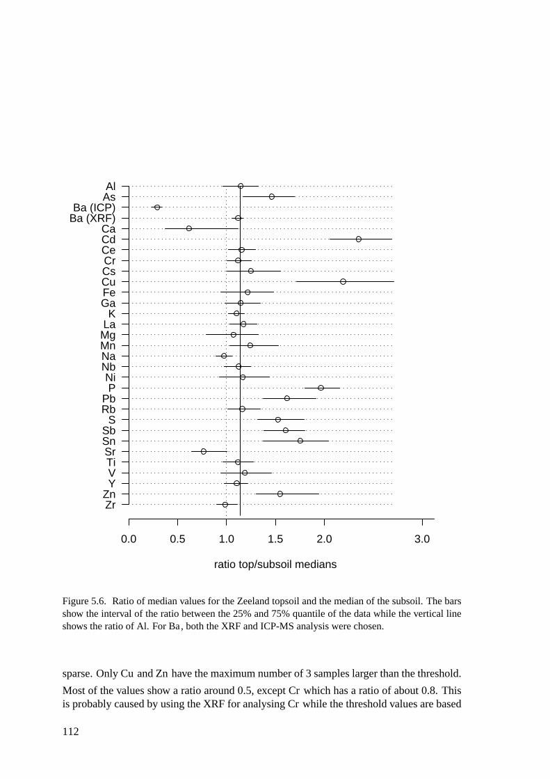
ratio top/subsoil medians
ZrZnYVTiSrSnSbS
RbPbPNi
NbNaMnMgLaK
GaFeCuCsCrCeCdCa
Ba (XRF)Ba (ICP)
AsAl
0.0 0.5 1.0 1.5 2.0 3.0
Figure 5.6. Ratio of median values for the Zeeland topsoil and the median of the subsoil. The barsshow the interval of the ratio between the 25% and 75% quantile of the data while the vertical lineshows the ratio of Al. For Ba, both the XRF and ICP-MS analysis were chosen.
sparse. Only Cu and Zn have the maximum number of 3 samples larger than the threshold.
Most of the values show a ratio around 0.5, except Cr which has a ratio of about 0.8. Thisis probably caused by using the XRF for analysing Cr while the threshold values are based
112

on aqua regia leached digested samples (see chapter 4). This may also be the cause ofthe slightly higher ratio for Ni . Both Ni and Cr show a ratio between top and subsoilcomparable to that of Al2O3 , suggesting that there is no anthropogenic enrichment. WhileZeeland is less aluminous than the UCC, Ni and Cr are comparatively much higher, whichfor Cr was already ascribed in chapter 4 to its incorporation in heavy minerals. For Sband Sn the reverse is found, a slightly higher ratio for the comparison between top andsubsoil, while having a lower ratio compared to the legal threshold. Both Sb and Sn wereanalysed by ICP-MS using an aqua regia extraction, and were not found to be regionallylow in Zeeland compared to the UCC. This suggests that, in comparison to the other priorityelements, the legal thresholds for Sb and Sn are relatively high compared to their naturalbackground in Zeeland.
For all elements it is clear that the legal threshold values are substantially higher than themedian values found in the topsoils. This shows that the legal threshold value is not suitableto reveal the moderate, yet evident, enrichment in the topsoil of Zeeland.
5.4.3 Correlation and regression with Al
Explained variance versus natural variability
The Pearson correlation of the elements with Al2O3 is given in table 5.5. Most of theelements have a positive correlation with Al2O3 which more or less confirms the closelyrelated ratios in figure 5.6; only Na2O and Zr have a negative correlation. The correlationsof CaOand Srare not significantly different from zero. However, the correlation betweenCaOand Sr is 0.953 supporting that they both are the result of (biogenic) calcite precip-itation and dissolution (pre- and post-depositional). The components P2O5 , Cd, Cu, Pb,S, Sb, and Sn are slightly less correlated with Al2O3 . These are also elements that areenriched in the topsoil according to figure 5.6. Both enrichment and lesser correlation withsoil mineralogy proxies are suggesting that the soil concentrations of these elements areindeed altered by human processes.
Relation with Al content
To study the variability and concentrations due to natural mineralogical variability the mea-sured values were plotted against the concentration of Al2O3 . Figure 5.8 shows scatter plotsof selected elements versus Al2O3 , that illustrate the different types of relations found.Both topsoil and subsoil relations are depicted for clarity.
Cadmium, as best example, shows two distinct groups: a group of topsoil samples and agroup of subsoil samples. The latter has lower Cd values and less residual variance thanthe first. If higher Cd concentration are caused by anthropogenic input, it can be assumedthat this occurs more erratically than natural processes and thus causes higher variability inthe influenced soil horizons. In chapter 3 it was already shown that presumed contaminantshave a higher spatial variability than non contaminants. The other elements that also show
113
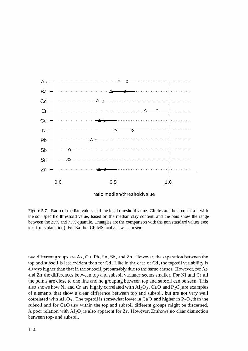
ratio median/thresholdvalue
Zn
Sn
Sb
Pb
Ni
Cu
Cr
Cd
Ba
As
0.0 0.5 1.0
Figure 5.7. Ratio of median values and the legal threshold value. Circles are the comparison withthe soil specific threshold value, based on the median clay content, and the bars show the rangebetween the 25% and 75% quantile. Triangles are the comparison with the non standard values (seetext for explanation). For Ba the ICP-MS analysis was chosen.
two different groups are As, Cu, Pb, Sn, Sb, and Zn. However, the separation between thetop and subsoil is less evident than for Cd. Like in the case of Cd, the topsoil variability isalways higher than that in the subsoil, presumably due to the same causes. However, for Asand Zn the differences between top and subsoil variance seems smaller. For Ni and Cr allthe points are close to one line and no grouping between top and subsoil can be seen. Thisalso shows how Ni and Cr are highly correlated with Al2O3 . CaO and P2O5 are examplesof elements that show a clear difference between top and subsoil, but are not very wellcorrelated with Al2O3 . The topsoil is somewhat lower in CaO and higher in P2O5 than thesubsoil and for CaOalso within the top and subsoil different groups might be discerned.A poor relation with Al2O3 is also apparent for Zr . However, Zrshows no clear distinctionbetween top- and subsoil.
114
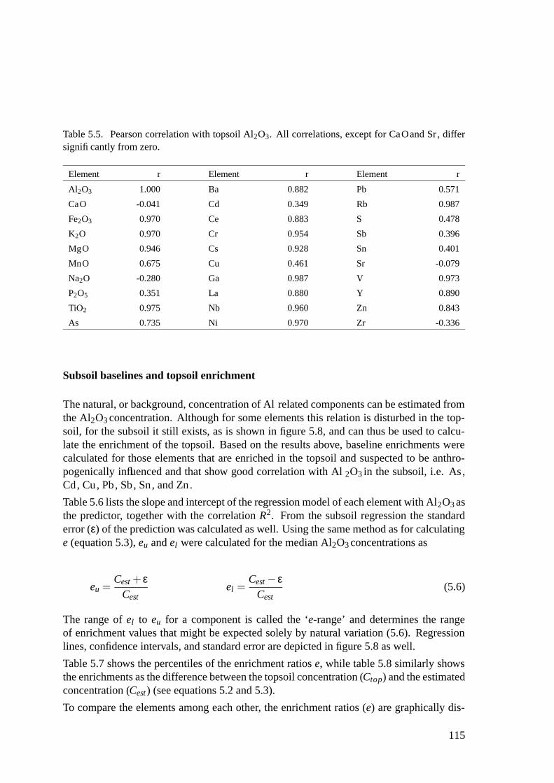
Table 5.5. Pearson correlation with topsoil Al2O3. All correlations, except for CaOand Sr, differsignificantly from zero.
Element r Element r Element r
Al2O3 1.000 Ba 0.882 Pb 0.571
CaO -0.041 Cd 0.349 Rb 0.987
Fe2O3 0.970 Ce 0.883 S 0.478
K2O 0.970 Cr 0.954 Sb 0.396
MgO 0.946 Cs 0.928 Sn 0.401
MnO 0.675 Cu 0.461 Sr -0.079
Na2O -0.280 Ga 0.987 V 0.973
P2O5 0.351 La 0.880 Y 0.890
TiO2 0.975 Nb 0.960 Zn 0.843
As 0.735 Ni 0.970 Zr -0.336
Subsoil baselines and topsoil enrichment
The natural, or background, concentration of Al related components can be estimated fromthe Al2O3 concentration. Although for some elements this relation is disturbed in the top-soil, for the subsoil it still exists, as is shown in figure 5.8, and can thus be used to calcu-late the enrichment of the topsoil. Based on the results above, baseline enrichments werecalculated for those elements that are enriched in the topsoil and suspected to be anthro-pogenically influenced and that show good correlation with Al 2O3 in the subsoil, i.e. As,Cd, Cu, Pb, Sb, Sn, and Zn.
Table 5.6 lists the slope and intercept of the regression model of each element with Al2O3 asthe predictor, together with the correlation R2. From the subsoil regression the standarderror (ε) of the prediction was calculated as well. Using the same method as for calculatinge (equation 5.3), eu and el were calculated for the median Al2O3 concentrations as
eu =Cest + ε
Cestel =
Cest− εCest
(5.6)
The range of el to eu for a component is called the ‘e-range’ and determines the rangeof enrichment values that might be expected solely by natural variation (5.6). Regressionlines, confidence intervals, and standard error are depicted in figure 5.8 as well.
Table 5.7 shows the percentiles of the enrichment ratios e, while table 5.8 similarly showsthe enrichments as the difference between the topsoil concentration (Ctop) and the estimatedconcentration (Cest) (see equations 5.2 and 5.3).
To compare the elements among each other, the enrichment ratios (e) are graphically dis-
115

As
4 6 8 10 12
510
2030
Cd
4 6 8 10 12
0.1
0.3
0.5
Cr
4 6 8 10 12
4060
8010
0
Cu
4 6 8 10 12
05
1020
Figure 5.8. Scatter plots of Al2O3 versus selected elements. Black dots are subsoil samples, crossesare topsoil samples. Al2O3 is on the x-axis, elements are on the y-axis. Regression lines are drawnfor the subsoil data with confidence intervals (inner dashed lines) and standard error (outer dashedlines).continued at next page
played in figure 5.9. These box plots show clearly that Cd and Cu are more enriched thanthe other elements. The range of e for the natural subsoil variation (table 5.6) is for theseelements below the P25 showing that their enrichment is substantially higher than can beexpected from natural (or random) variability. This again suggests that artificial fertilizerusage is a major process that influenced the Zeeland soils. The elements Pb, Sb, and Sn areless enriched, the upper limit of enrichment caused by natural variability lies between theP25 and the median topsoil enrichment. Zn and As have the smallest enrichment ratios and
116
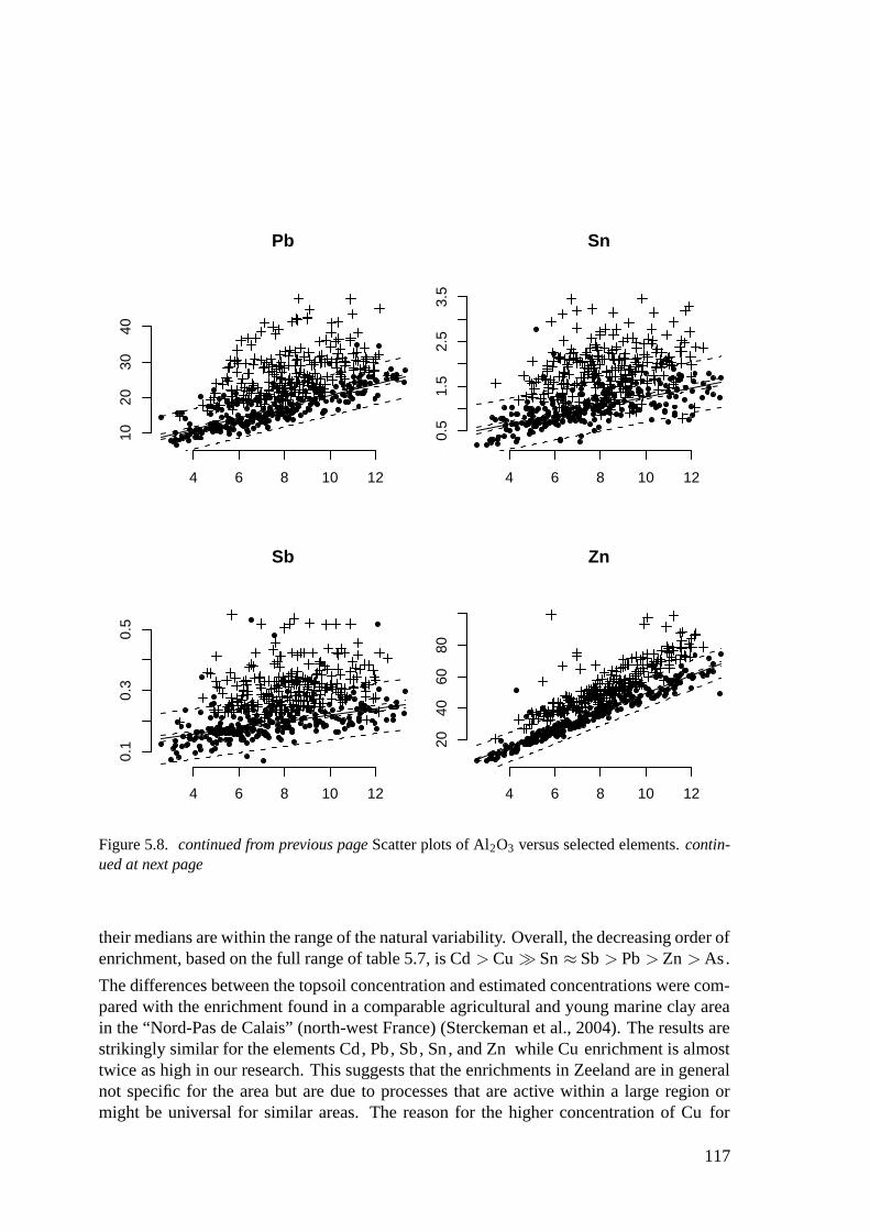
Pb
4 6 8 10 12
1020
3040
Sb
4 6 8 10 12
0.1
0.3
0.5
Sn
4 6 8 10 12
0.5
1.5
2.5
3.5
Zn
4 6 8 10 12
2040
6080
Figure 5.8. continued from previous page Scatter plots of Al2O3 versus selected elements. contin-ued at next page
their medians are within the range of the natural variability. Overall, the decreasing order ofenrichment, based on the full range of table 5.7, is Cd > Cu � Sn ≈ Sb > Pb > Zn >As.
The differences between the topsoil concentration and estimated concentrations were com-pared with the enrichment found in a comparable agricultural and young marine clay areain the “Nord-Pas de Calais” (north-west France) (Sterckeman et al., 2004). The results arestrikingly similar for the elements Cd, Pb, Sb, Sn, and Zn while Cu enrichment is almosttwice as high in our research. This suggests that the enrichments in Zeeland are in generalnot specific for the area but are due to processes that are active within a large region ormight be universal for similar areas. The reason for the higher concentration of Cu for
117
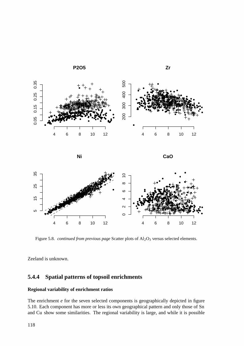
P2O5
4 6 8 10 12
0.05
0.15
0.25
0.35
Ni
4 6 8 10 12
515
2535
Zr
4 6 8 10 12
200
300
400
500
CaO
4 6 8 10 12
02
46
810
Figure 5.8. continued from previous page Scatter plots of Al2O3 versus selected elements.
Zeeland is unknown.
5.4.4 Spatial patterns of topsoil enrichments
Regional variability of enrichment ratios
The enrichment e for the seven selected components is geographically depicted in figure5.10. Each component has more or less its own geographical pattern and only those of Snand Cu show some similarities. The regional variability is large, and while it is possible
118

Table 5.6. Regresion constants and R2 of the regression of subsoil concentrations of selected ele-ments as a function of Al2O3 . a is the slope and b is the intercept of the regression. The e rangegives the range of enrichment based on the upper and lower limits of the regression standard errorof prediction.
Element a b R2 e range
As 1.44 0.56 0.77 0.51-1.49
Cd 0.0074 0.072 0.29 0.57-1.43
Cu 0.80 0.48 0.64 0.62-1.38
Pb 1.58 4.76 0.65 0.63-1.37
Sb 0.011 0.12 0.29 0.57-1.43
Sn 0.086 0.40 0.42 0.49-1.51
Zn 5.73 -7.84 0.90 0.67-1.33
Table 5.7. Enrichment ratios in the topsoil, The minimum (min), 25-percentile (25 perc.), median,75 percentile (75 perc.), and the maximum (max) ratio are given
element min 25 perc. median 75 perc. max
As 0.63 1.07 1.22 1.46 2.23
Cd 1.10 1.93 2.14 2.39 6.66
Cu 1.01 1.53 1.86 2.46 5.9
Pb 1 1.27 1.41 1.71 4.19
Sb 0.85 1.33 1.50 1.72 5.21
Sn 0.56 1.25 1.56 1.88 5.16
Zn 1.07 1.25 1.33 1.45 4.62
to distinguish subregions they are less well expressed as the spatial patterns of the noninfluenced elements (compare figure 5.3). Considering the enrichment of these elementsas anthropogenic this lesser regional correlation can be explained by the probably rathererratic human processes.
The spatial pattern of the overall contamination index d is shown in figure 5.11. Some lo-cations show high index values but in general they lie around a ratio of 2. From a regionalperspective the areas in the north-east of Zeeland (Schouwen-Duiveland, St. Philipsland,Tholen) seem to be more enriched, followed by Noord-Beveland and Zuid-Beveland. Be-sides regions with high values some local anomalies also can be seen, which compriseseveral enriched elements (compare figure 5.8).
119
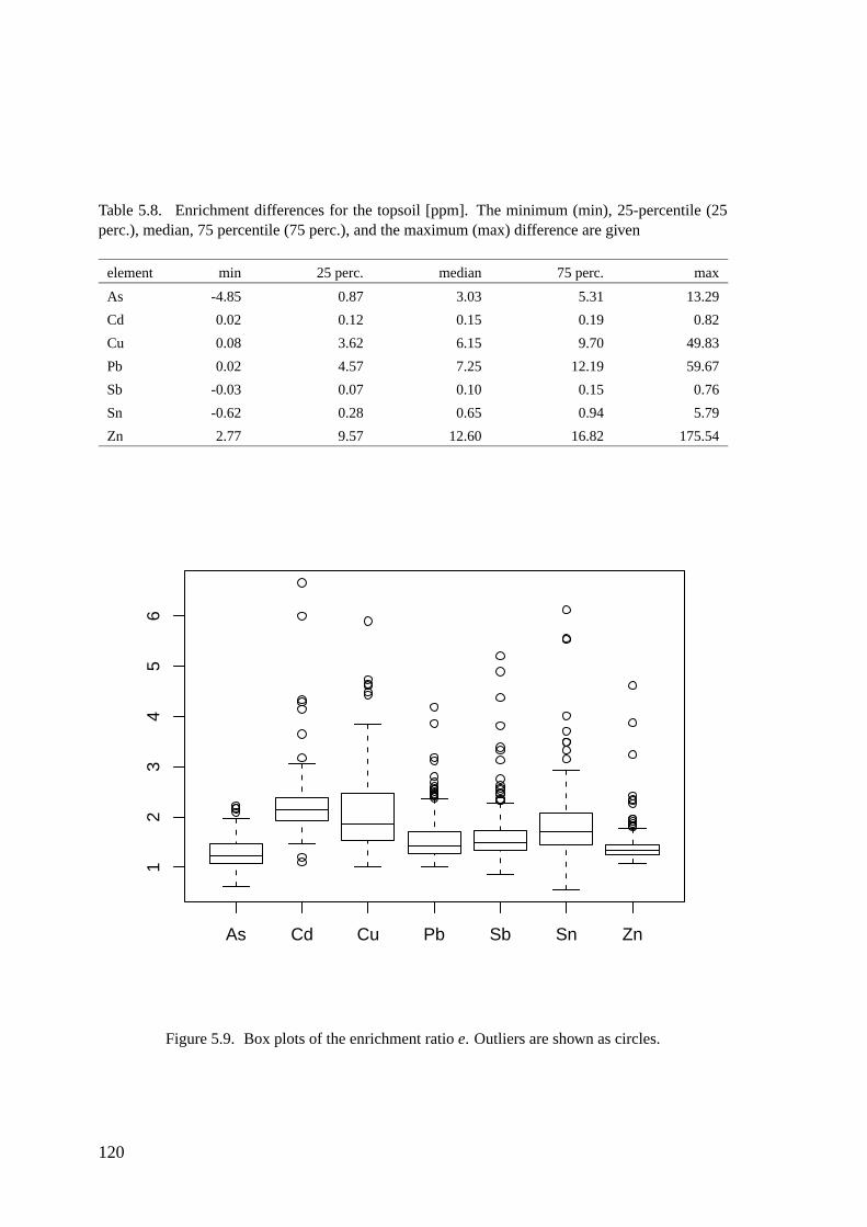
Table 5.8. Enrichment differences for the topsoil [ppm]. The minimum (min), 25-percentile (25perc.), median, 75 percentile (75 perc.), and the maximum (max) difference are given
element min 25 perc. median 75 perc. max
As -4.85 0.87 3.03 5.31 13.29
Cd 0.02 0.12 0.15 0.19 0.82
Cu 0.08 3.62 6.15 9.70 49.83
Pb 0.02 4.57 7.25 12.19 59.67
Sb -0.03 0.07 0.10 0.15 0.76
Sn -0.62 0.28 0.65 0.94 5.79
Zn 2.77 9.57 12.60 16.82 175.54
As Cd Cu Pb Sb Sn Zn
12
34
56
Figure 5.9. Box plots of the enrichment ratio e. Outliers are shown as circles.
120

As2.231.571.481.41.291.22
Cd6.662.592.422.342.252.14
Cu5.92.842.572.312.081.87
Pb4.191.961.771.61.481.41
Figure 5.10. Spatial pattern of the enrichment for selected elements. Gray dots have an enrichmentwithin the natural variability of the subsoil. See table 5.7. continued on next page
Ratios with legal thresholds
It is also possible to calculate the ratios with the soil specific legal threshold level. Againcalculation is based on equation 5.5 and table 5.3. For the value of clay C and organicmatter O the same values are used as in §5.4.2. The results are shown for completeness infigure 5.12.
Since both the enrichment e and the ratio with the soil specific threshold s are based onthe variation in Al2O3(a constant value is taken for O) the resemblance between figures5.10 and 5.12 is evident. However, the intercept for calculating s is larger (see table 5.3),
121

Sb5.211.951.751.651.581.5
Sn6.122.342.121.971.841.7
Zn4.621.531.481.421.381.33
Figure 5.10. continued Spatial pattern of the enrichment for selected elements. Gray dots have anenrichment within the natural variability of the subsoil. See table 5.7.
and as a consequence the relative range of s-values is generally much smaller, resulting inenrichment maps that are still very similar to the element maps themselves. Exceptions areCd, for which the relative effects of dividing by Cest or s are similar, and Sn, for whichthe relative range in s-values is much larger then the range in Cest , due to the steep slopeassociated with the clay-content.
A more important difference is that for the enrichment e the extent of enrichment values,that can be expected from natural variability is known through the standard error of theprediction. This variability is a distinct property of the linear regression model underlyingthe calculation of e while the legal threshold values is just a rigid, though normalised for
122
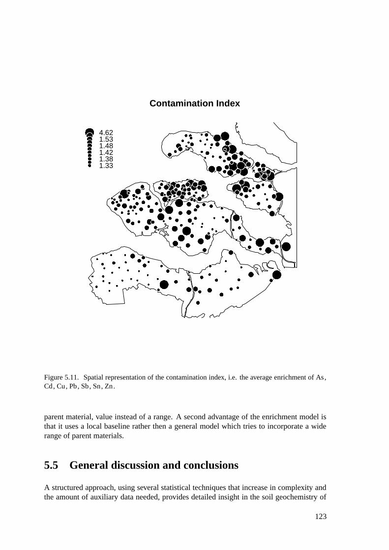
Contamination Index
4.621.531.481.421.381.33
Figure 5.11. Spatial representation of the contamination index, i.e. the average enrichment of As,Cd, Cu, Pb, Sb, Sn, Zn.
parent material, value instead of a range. A second advantage of the enrichment model isthat it uses a local baseline rather then a general model which tries to incorporate a widerange of parent materials.
5.5 General discussion and conclusions
A structured approach, using several statistical techniques that increase in complexity andthe amount of auxiliary data needed, provides detailed insight in the soil geochemistry of
123

As1.010.760.70.670.640.61
ratio S
Cd1.390.540.50.490.470.45
ratio S
Cu1.420.640.560.520.470.42
ratio S
Pb0.980.440.40.370.340.33
ratio S
Figure 5.12. Spatial pattern of the ratio with the soil specific s-value for selected elements. contin-ued on next page
Zeeland. This approach first of all shows which components are influenced by, most likely,anthropogenic processes. Then, this anthropogenic imprint can be quantified based on their(mutual) relation with non-influenced soil components.
Cumulative frequency plots are a good aid to show at a glance which elements have anoma-lous concentrations. From these plots percentiles can be derived dividing anomalous datafrom background. The use of the value corresponding to the P90, an often used standardpercentile in Dutch soil surveys, as a threshold for assumed to be influenced elements mightbe a responsible choice, but only if the corresponding cumulative distribution plots are stud-ied and justify the choice. In this study most (trace) elements are chiefly associated with
124
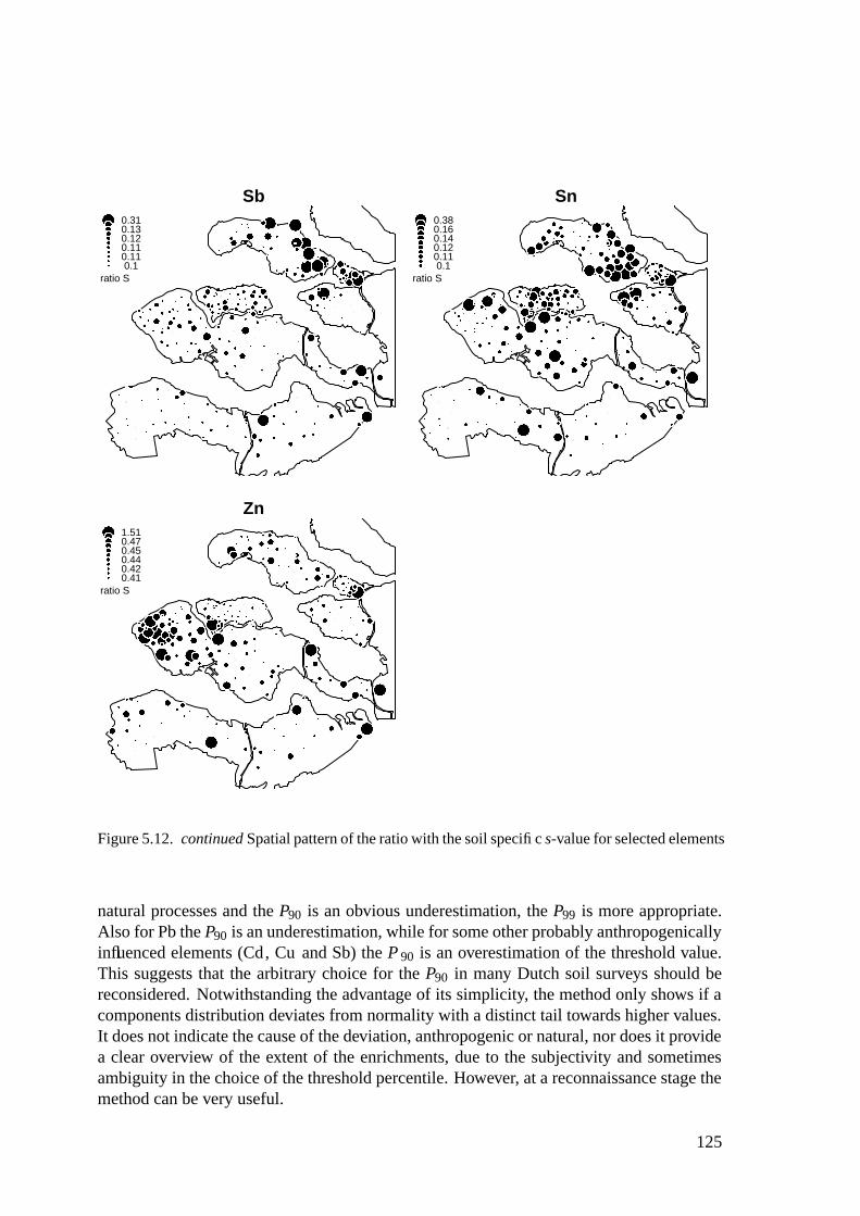
Sb0.310.130.120.110.110.1
ratio S
Sn0.380.160.140.120.110.1
ratio S
Zn1.510.470.450.440.420.41
ratio S
Figure 5.12. continued Spatial pattern of the ratio with the soil specific s-value for selected elements
natural processes and the P90 is an obvious underestimation, the P99 is more appropriate.Also for Pb the P90 is an underestimation, while for some other probably anthropogenicallyinfluenced elements (Cd, Cu and Sb) the P 90 is an overestimation of the threshold value.This suggests that the arbitrary choice for the P90 in many Dutch soil surveys should bereconsidered. Notwithstanding the advantage of its simplicity, the method only shows if acomponents distribution deviates from normality with a distinct tail towards higher values.It does not indicate the cause of the deviation, anthropogenic or natural, nor does it providea clear overview of the extent of the enrichments, due to the subjectivity and sometimesambiguity in the choice of the threshold percentile. However, at a reconnaissance stage themethod can be very useful.
125
The spatial distribution of elements with low threshold percentiles (P80 to P90) and sus-pected of human influence, shows regional variability that differs distinctly from the moreor less similar patterns that emerge for elements related to natural processes like variabilityin clay/Al2O3 . This indicates that these probably influenced elements indeed have a moreunique process underlying their regional variability.
Calculation of median ratios, with the upper continental crust (UCC), median subsoil con-centrations, and legal limits, is an easy method to determine which elements are enrichedcompared to the reference used. Ratios with the UCC indicate that As, Cd, Cr, Pb, andZr are relatively enriched. For As it is assumed that this enrichment is partially caused bythe low lying deltaic environment of Zeeland, Cr and Zr could be related to heavy mineralconcentrations, while the other elements might be enriched due to, for example, fertiliserusage and/or traffic exhaust. Depleted elements are Ba, Ca, K, Mg, Mn, Na, and Sr,which are assumed to be a natural regional feature. On average, the Zeeland soils also ap-pear somewhat less aluminous and ferromagnesian than the UCC. The ratios based on thesubsoil show that the elements As, Cd, Cu, P, Pb, S, Sb, Sn, and Zn are enriched. Theseare all elements for which enrichments can be related to anthropogenic activities. The ra-tios with the official legal limits for Dutch soil, often used as reference values, show ratiosof about 0.5-0.8, with the higher ratios (Cr, Ni) probably caused by the better analyticalperformance of the XRF method used as compared to the prescribed aqua-regia extraction.Even the P99 of the ratios, based on median clay values, are still below one for all elements.
The implications of the ratio results are basically twofold: 1) the area of Zeeland coveredin this study is clean as regarding the governmental regulations and 2) the legal thresholdlimits are an overestimation of soil background concentrations, already including (minor)anthropogenic enrichments. They are thus less suitable as a reference value for a study intonatural and anthropogenic geochemical patterns, and the ratios with the local reference(subsoil data) are preferred for identifying the influenced elements and determining theextent of their enrichment.
The correlation with Al2O3 is easily calculated and proved to be very useful to indicateelements which are possibly altered by human processes. The elements P2O5 , Cd, Cu,Pb, S, Sb, and Sn show relatively low correlations with Al2O3 in the topsoil comparedto other elements and are also enriched in the topsoil. CaO, MnO, Na2O , and Sr showrelatively low, or negative, correlations with Al2O3 and are not enriched in the topsoil. Thecorrelations confirm the similarities observed in the spatial distributions of the elements.
Overall higher correlations with Al2O3 in the reference subsoil confirm the hypothesisthat the subsoil can be regarded as a pristine, non-influenced, reference. A graphicalrepresentation of the relation between the various elements and Al2O3 for both topsoiland subsoil clearly depicts the relative addition in the topsoil. Using a linear regres-sion model based on the subsoil data the extent of the enrichment was quantified foreach topsoil sample. When expressed as the ratio between observed concentration andcalculated baseline concentration, the elements in order of decreasing enrichment areCd > Cu � Sn ≈ Sb > Pb > Zn > As. These enrichments are in line with data foundfor a similar area in the north of France, except for Cu, which is relatively higher in theZeeland topsoils. Spatial distribution patterns of the enrichment ratios show that for most
126

influenced elements regional variability is high and that hardly any spatial or mutual re-gional relations appear. The overall regional perspective provided by the contaminationindex shows that some areas in the north-east and centre of Zeeland on average are slightlymore enriched.
Using the subsoil regression as a baseline has many advantages above the current Dutchpractice of calculating a fixed legal threshold value, though corrected for clay and organicmatter content. The natural random variability in baseline concentrations, expressed as thestandard error of the regression, is a property of the model. This contrasts with the legalthreshold value, which is just a rigid value with no range given. Also the regression modelprovides a local baseline, specifically suited for the parent soil material of Zeeland, whichobviously should be preferred over a general model that tries to include all possible soiltypes. Compared to all other techniques presented, this subsoil regression baseline methodgives the most profound insight into 1) the geological/pedological pattern of geochemicalvariability, 2) random natural variation, and 3) the anthropogenic imprint on the Zeelandsoil. These advantages definitely outweigh the greater complexity of the procedure.
127

6 Regional diffuse geochemical pat-terns and processes
6.1 Introduction
From the perspective of environmental management it can be useful to identify areas inwhich the soil geochemistry is more influenced by human processes than others. For ex-ample, given that soil in the Netherlands and elsewhere is often used as site preparation andbuilding material, the further spreading of contaminants can be curtailed when soil with acertain degree of enrichment of anthropogenic components is not used elsewhere. The cur-rent policy in the Netherlands regarding regional mapping of human influence is to createrisk maps of soil pollution (van der Gaast et al., 1998) in which areas can be comparedbased on whether or not permissible limits are exceeded. However, this method considersneither the interactions between polluting substances nor how their concentrations relate tonatural levels in the soil.
It is well known that soil composition is the result of both natural and human influences,and is thus a summation of separate processes, such as sedimentary deposition, weatheringof calcite and other minerals, input by manuring, or atmospheric deposition. This multi-dimensional space comprises interactions over the region and between soil components,both interactions generally being expressed in the form of observable patterns, like theintercorrelation between different elements and/or spatial variability over an area. Thesepatterns thus represent an important key for assessing the condition of soils, especially if adistinction can be made between human induced and natural patterns.
The previous chapters show that, given a dedicated sampling design and analytical proce-dures, it is possible with univariate and bivariate statistical techniques to make a distinc-tion between sites dominated by natural or anthropogenic processes. This distinction wasbased on the comparision with threshold and reference values or explained variance usingno more than than two variables. Although such a small dimensional space may give anindication of the underlying processes, a larger dimensional, multivariate, space must beconsidered to fully understand the soil composition. This multidimensional space can bedivided into attribute space, in which processes among chemical components play a part,and geographical space in which the interaction of these processes between sample loca-tions is assessed. Ultimately, this answers the question as to what combination of which
129

processes occur where, thereby providing a practically useful explanation of the processesthat causes geochemical soil variability.
In this chapter I focus on the extent to which human contributions actually affect the re-gional soil composition compared to natural variability. Using the same data as in chapter5, the processes or factors determining the regional variability, both in attribute and ge-ographical space are assessed. The regional expression of the interaction of human andanthropogenic processes is further evaluated, to see if regions may be distinguished wherespecific human processes have had an effect on the soil composition.
The general covariance structure of the data was studied using principal component analy-sis (PCA) to reveal the processes within attribute space. Groups of covarying geochemicalcomponents, may indicate certain processes. To assess which processes explain featuresin geographical space, clustering techniques were used to identify groups of sample pointswith similar properties. Due to the expectation that each pattern is a combination of dif-ferent processes and the general multivariate nature of geochemical data, fuzzy c-meansclustering (FCMC) was chosen (Vriend et al., 1988).
6.2 Material and methods
6.2.1 Study area and geochemical topsoil data
The study area belongs largely to a Holocene estuary and consists of the mainland ofZeeuws Vlaanderen, bordering Belgium, and several islands/peninsulas that have a longhistory of land reclamation and inundation. The Holocene geology and pedology of Zee-land have been extensively described in chapter 2 of this thesis. In summary the major soiltypes of Zeeland are immature marine clay deposits ranging from heavy clays (clay frac-tion larger then 25%) to sandy tidal inlet and tidal flats (clay fraction <7%). The Zeelandlandscape is divided into Heartlands, the oldest and first reclaimed areas with often veryheavy pool-clays, and Newlands, younger areas with more sandy clay soils. The elevationof the field level, relative to the Dutch average sea level NAP, ranges from about 1.5m forchannel ridges to -1.3m for the pool clay areas. Land use is mainly agricultural and in theNewlands is characterised by its larger scale and intensive artificial drainage.
Figure 6.1 depicts the 270 sample locations where geochemical data were obtained. Eachsample is a composite of 15 to 20 subsamples from the upper soil layer (about 0-30cm),usually the plough furrow. The samples were analysed by X-ray fluorescence (XRF) inpressed powder tablet or, after aqua-regia digestion, by inductively coupled plasma-massspectrometry (ICP-MS). The analysis aimed at maximising the number of parameters andfrom these a selection was made based on accuracy, precision and minimum of missingvalues. For details about the sampling, analytical methods and the selection procedure, seechapter 4 and table 4.11 (p. 80).
130

Figure 6.1. Topography of Zeeland and sampling locations. Names of peninsula’s and areas initalic, cities in bold
6.2.2 Principal component analysis
To discern the controlling processes in attribute space principal component analysis (PCA),also called principal factor analysis, was used which is based on the major axes in a datacloud. These axes are derived from the covariance matrix by extracting the eigenvectorsand subsequently deriving a matrix with factor loadings with an a priori chosen numberof factors. Subsequently, to maximise the variance of the loadings on the factors, varimaxrotation was applied (Davis, 2002). A principal component, or factor, is assumed to rep-resent a controlling process or feature, that captures a specific relevant source of variance.
131

PCA can reduce the number of variables of the multivariate dataset to a few factors thatmay be indicative for certain geochemical processes. Factor analysis is widely used in geo-chemistry and usually with success (Reimann et al., 2002; Bianchini et al., 2002; Chork &Salminen, 1993; van Helvoort, 2003; Mol, 2002). The method has its controversies thoughand three well known are: 1) the choice of the underlying method for the factor analy-sis: principal factor analysis or maximum likelihood; 2) the choice of which elements toinclude and the number of initial factors for the analysis; and 3) normality of the data isassumed while this most often is not the case (Reimann et al., 2002; van Helvoort, 2003).
It was shown by Reimann et al. (2002) that for geochemical data principal factor analysis,based on the eigenvector structure is a better solution than maximum likelihood. Theyconsidered that as the maximum likelihood depended even more on normally distributeddata than PCA, its use increases the chance of misleading results.
For the desired number of variables or geochemical components compared to the number ofcases, the so called dimensionality, there is no standard rule of thumb. If p is the number ofvariables and n is the number of cases than p should be substantially smaller than n. Giventhe many available suggestions for p and n (e.g. n> p2,n> 9p,n> 3p, etc.) (Davis, 2002;Reimann et al., 2002) The dimensionality in the present dataset, where p = 30 and n = 270,here defined as p/n, can be considered as sufficient.
The data used for this study can be regarded as “near-normal” (compare figure 4.6, p. 85and 5.2, p. 106), with some elements displaying a certain amount of positive skewness andoutliers, that might have an adverse effect on a standard PCA analysis. As presented byPison et al. (2003) using a robust technique for PCA overcomes these adverse effects. Thistechnique is based on deriving a robust covariance matrix using the minimum covariancedeterminant (MCD) algorithm of Rousseeuw & van Driessen (1999). This MCD algorithmtries to find a subset of observations whose classical covariance matrix has the lowest deter-minant, thus the highest covariances for all variables. This reduces the influence of outlierswhich usually result in lower covariances for most variables. Following Pison et al. (2003),0.75n of the datapoints were used to calculate the robust covariance matrix, allowing amaximum of 0.25n of outliers without effect on the estimation of the covariance matrix.Standardisation of data to compensate for the difference in units and magnitude for bothXRF (wt-% and ppm) and ICP-MS (ppm) is also provided by using the robust correla-tion matrix. To prevent indeterminacy effects on the XRF data, SiO2 was omitted from thedataset.
The number of factors in principle is determined by a combination of the Kaiser/Guttmancriterion (only factors with eigenvalues larger than 1 are incorporated in the model) andgeochemical interpretability. Also scree plots are used, in which the eigenvalue is plottedagainst component number, to evaluate if a factor is relevant or not. It is known that limitingthe set of factors with the Kaiser/Guttman criterion may be too crude and factors witheigenvalues just smaller than 1 should be at least evaluated for their relevancy (e.g. vanHelvoort (2003)). Besides, a subselection of elements related to one factor can be used fora second PCA to gain insight if this factor comprises more than one process.
Additionally, the covariance structure of the components not included in the selected
132

dataset was estimated by calculating the correlation of these components with the PCAfactor scores.
To provide insight in the regional variability of the processes inferred from the patterns inattribute space, the factor scores are spatially depicted. This may reveal which areas areparticularly influenced by certain processes (Tao, 1998; Reimann et al., 2002). For spatialplotting of map attributes, the same plotting method as in chapter 5,based on the methodsof Gustavson et al. (1997), is used.
6.2.3 Fuzzy c-means clustering
Although spatial presentations of PCA factor scores can reveal their regional variation,they only show the effects of the processes related to each of the factors, not the interactionbetween the processes. Yet, at each location the overall geochemistry is determined by asummation of the different processes described by the PCA. This interaction in geograph-ical space is not revealed since the PCA is used for separating the processes regardless oftheir spatial location. The PCA procedure in principle results in independent (i.e. uncorre-lated in the overall attribute space) processes, yet at each location they have some specificrelation. To see if these interacting processes have a regional pattern, the sample locationswith similar properties can be grouped together with a clustering technique.
Since the degree of interaction of the different processes varies gradually from one locationto the other it is not expected that the grouping will result in clear, well separated clustersin attribute space but rather in dense areas in a continuous data cloud. Due to this expectedfuzziness it was chosen to use fuzzy c-means clustering (FCMC). This technique has provedto be very useful in the field of soil science and geochemistry. (Vriend et al., 1988; Haneschet al., 2001; McBratney & Odeh, 1997; Burrough et al., 1997; Kramar, 1995). With FCMCthe interest is not to assign samples, or cases, unambiguously to a group but rather to give asimilarity to each group in the cluster model. This similarity is expressed as a membershipvalue ranging from 0, no similarity, to 1, identical to the cluster centre. The memberships ofa sample for all clusters sum up to one. The advantage of this technique is that intermediatecases, falling in between clusters, can be recognized and are not forced into just one cluster.Outliers contribute equally to all clusters and since the calculation of the cluster centres usesa weighted membership, outliers have hardly any adverse influence on the final result.
The choice of elements for FCMC is more delicate then for PCA. Simply selecting all ele-ments may result in additional noise for the clustering algorithm, but also that just one ma-jor process, e.g. parent material, determines the outcome of the clustering. Considering thatthe PCA differentiates the major processes determining the geochemical soil composition,then elements with high loadings on the corresponding factors should be representative forthese processes. To prevent that the variability of one process alone will determine theoutcome of the FCMC, a moderately equal number of elements of each factor is thereforeselected.
The results of the FCMC are geographically plotted by using the cluster membership as theattribute for the maps, again using the approach of Gustavson et al. (1997). A sample was
133

regarded to belong to one cluster when exceeding a threshold value according to
T hreshold = 0.7 ·highest membership> next highest membership (6.1)
If the location did not meet this condition the location was regarded as belonging to morethan one cluster.
6.2.4 Statistical software packages
Both multivariate analyses (PCA and FCMC) were applied using S-Plus and the R statis-tical software (Venables & Ripley, 2002; R Development Core Team, 2004). Using R, forthe FCMC the cmeans function from the e1071 library was used and for the robust covari-ance matrix the MCD version of the cov.rob routine from the MASS library was used.For the PCA an R implementation, based on the S-Plus princomp function was applied forextracting the eigenvalues and calculating the factor loadings, rotation was provided by thevarimax function.
6.3 Results and interpretation
6.3.1 Principal components analysis
The first 8 eigenvalues, as extracted from the robust correlation matrix of the selected com-ponents included in the optimal dataset (see chapter 4), are plotted in figure 6.2. The first4 components were considered to be geochemically relevant. They explain 76.6% of thetotal variability in all 30 components selected . The factor loadings are listed in table 6.1and plotted in figure 6.3.
The first rotated factor explains the major part, 50.4%, of the variance and has the highestloadings for geogenic elements like Al2O3 , TiO2 , Ce, La, Nb, and Y. Most additionalelements, like the REE, are also related to this factor (table 6.2). It is interpreted as repre-senting natural variability in the pristine soil composition. The component Al2O3 is relatedto Al-bearing phylosilicates and known to have a close relationship with clay (Tack et al.,1997; Wilcke et al., 1998; Sharma et al., 2000). Many other elements are primarily influ-enced by the variability in clay content of the parent material and load high on this factor aswell (van Gaans et al., 1995; Mol, 2002; Tebbens et al., 2000; Bianchini et al., 2002; Huis-man et al., 1997). This relation has already been demonstrated in chapter 5. Relatively highloadings on this component were also found for the elements Cr, Ni , Zn, which within theDutch situation are usually regarded as potential contaminants, but here the PCA indicatesotherwise.
The second rotated factor, explaining 10.3% of the variance, shows high loadings of around0.9 for CaO and Sr, with minor loadings for Mgand Mn. This factor was interpreted asrepresenting the variability in carbonate content
134
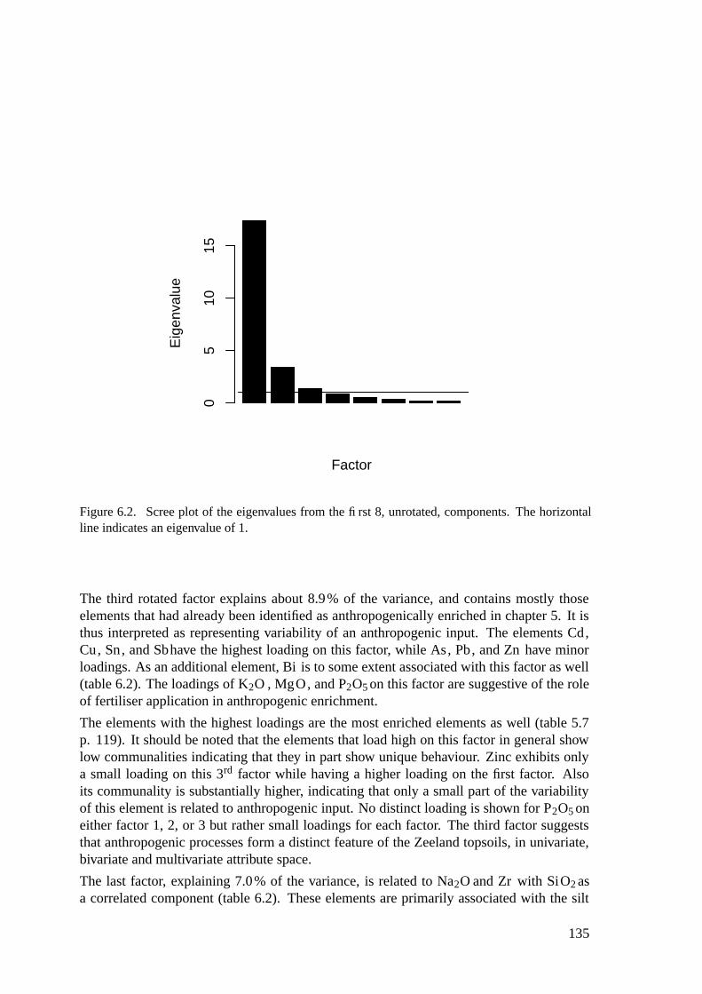
Factor
Eig
enva
lue
05
1015
Figure 6.2. Scree plot of the eigenvalues from the first 8, unrotated, components. The horizontalline indicates an eigenvalue of 1.
The third rotated factor explains about 8.9% of the variance, and contains mostly thoseelements that had already been identified as anthropogenically enriched in chapter 5. It isthus interpreted as representing variability of an anthropogenic input. The elements Cd,Cu, Sn, and Sbhave the highest loading on this factor, while As, Pb, and Zn have minorloadings. As an additional element, Bi is to some extent associated with this factor as well(table 6.2). The loadings of K2O , MgO, and P2O5 on this factor are suggestive of the roleof fertiliser application in anthropogenic enrichment.
The elements with the highest loadings are the most enriched elements as well (table 5.7p. 119). It should be noted that the elements that load high on this factor in general showlow communalities indicating that they in part show unique behaviour. Zinc exhibits onlya small loading on this 3rd factor while having a higher loading on the first factor. Alsoits communality is substantially higher, indicating that only a small part of the variabilityof this element is related to anthropogenic input. No distinct loading is shown for P2O5 oneither factor 1, 2, or 3 but rather small loadings for each factor. The third factor suggeststhat anthropogenic processes form a distinct feature of the Zeeland topsoils, in univariate,bivariate and multivariate attribute space.
The last factor, explaining 7.0% of the variance, is related to Na2O and Zr with SiO2 asa correlated component (table 6.2). These elements are primarily associated with the silt
135
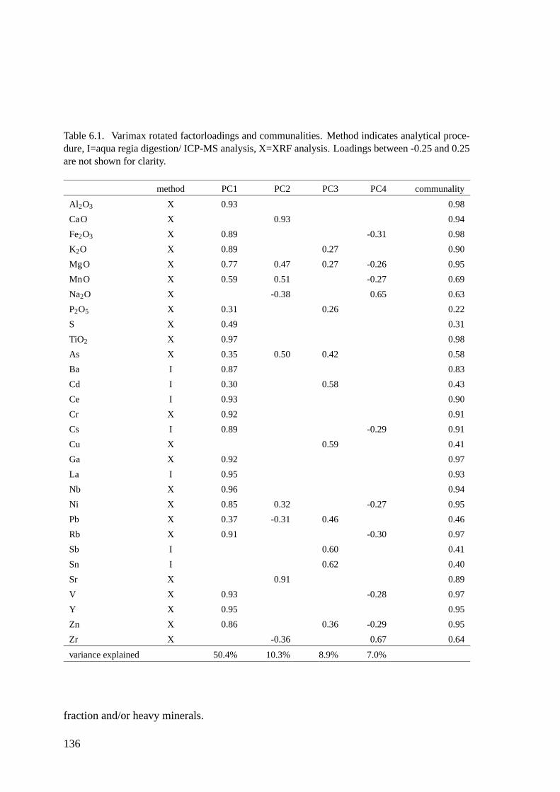
Table 6.1. Varimax rotated factorloadings and communalities. Method indicates analytical proce-dure, I=aqua regia digestion/ ICP-MS analysis, X=XRF analysis. Loadings between -0.25 and 0.25are not shown for clarity.
method PC1 PC2 PC3 PC4 communality
Al2O3 X 0.93 0.98
CaO X 0.93 0.94
Fe2O3 X 0.89 -0.31 0.98
K2O X 0.89 0.27 0.90
MgO X 0.77 0.47 0.27 -0.26 0.95
MnO X 0.59 0.51 -0.27 0.69
Na2O X -0.38 0.65 0.63
P2O5 X 0.31 0.26 0.22
S X 0.49 0.31
TiO2 X 0.97 0.98
As X 0.35 0.50 0.42 0.58
Ba I 0.87 0.83
Cd I 0.30 0.58 0.43
Ce I 0.93 0.90
Cr X 0.92 0.91
Cs I 0.89 -0.29 0.91
Cu X 0.59 0.41
Ga X 0.92 0.97
La I 0.95 0.93
Nb X 0.96 0.94
Ni X 0.85 0.32 -0.27 0.95
Pb X 0.37 -0.31 0.46 0.46
Rb X 0.91 -0.30 0.97
Sb I 0.60 0.41
Sn I 0.62 0.40
Sr X 0.91 0.89
V X 0.93 -0.28 0.97
Y X 0.95 0.95
Zn X 0.86 0.36 -0.29 0.95
Zr X -0.36 0.67 0.64
variance explained 50.4% 10.3% 8.9% 7.0%
fraction and/or heavy minerals.
136
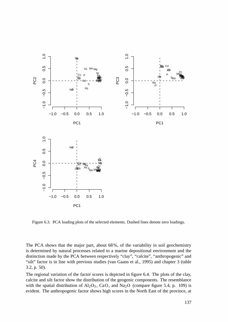
PC1
PC
2 AlTiFe
Mn
Ca
Mg
Na
KP
S
As
Cu
Pb
Zn
Ni
CrV
Sr
RbGa
Zr
YNbBaLaCeCdSb CsSn
−1.0 −0.5 0.0 0.5 1.0
−1.
0−
0.5
0.0
0.5
1.0
PC1
PC
3 AlTiFeMn
CaMg
Na
KPS
AsCu
PbZnNiCrVSr RbGa
Zr
YNbBa
LaCe
CdSb
Cs
Sn
−1.0 −0.5 0.0 0.5 1.0
−1.
0−
0.5
0.0
0.5
1.0
PC1
PC
4
Al
Ti
FeMnCa Mg
Na
KP
SAs
CuPb
ZnNi
Cr
VSr
RbGa
Zr
Y
Nb
Ba
LaCe
Cd
SbCs
Sn
−1.0 −0.5 0.0 0.5 1.0
−1.
0−
0.5
0.0
0.5
1.0
Figure 6.3. PCA loading plots of the selected elements. Dashed lines denote zero loadings.
The PCA shows that the major part, about 68%, of the variability in soil geochemistryis determined by natural processes related to a marine depositional environment and thedistinction made by the PCA between respectively “clay”, “calcite”, “anthropogenic” and“silt” factor is in line with previous studies (van Gaans et al., 1995) and chapter 3 (table3.2, p. 50).
The regional variation of the factor scores is depicted in figure 6.4. The plots of the clay,calcite and silt factor show the distribution of the geogenic components. The resemblancewith the spatial distribution of Al2O3 , CaO, and Na2O (compare figure 5.4, p. 109) isevident. The anthropogenic factor shows high scores in the North East of the province, at
137
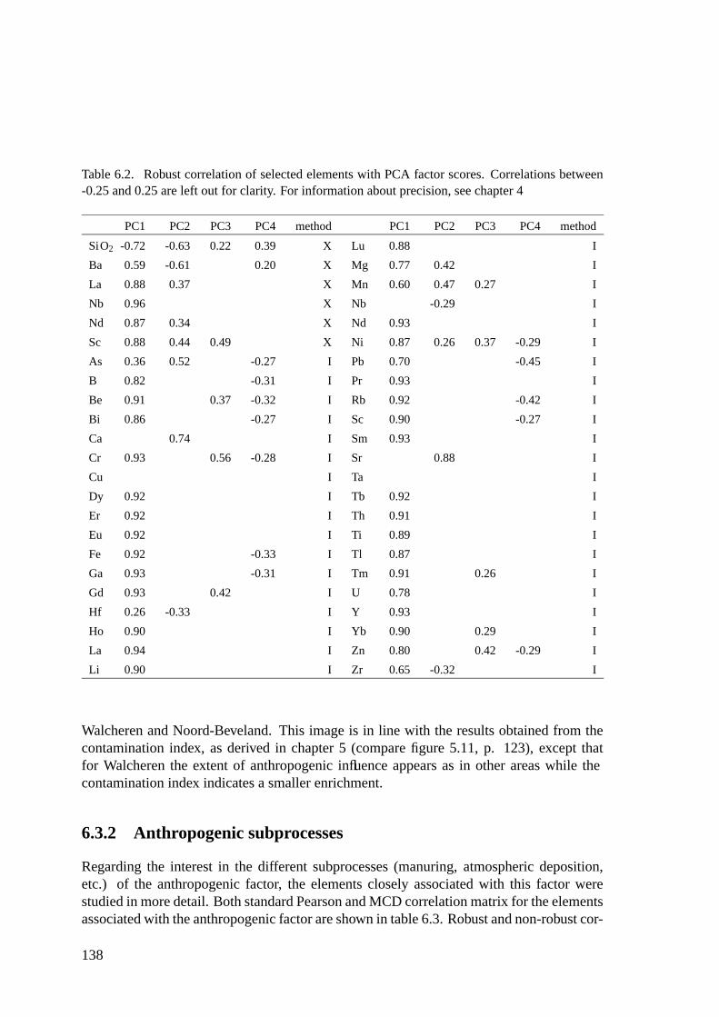
Table 6.2. Robust correlation of selected elements with PCA factor scores. Correlations between-0.25 and 0.25 are left out for clarity. For information about precision, see chapter 4
PC1 PC2 PC3 PC4 method PC1 PC2 PC3 PC4 method
SiO2 -0.72 -0.63 0.22 0.39 X Lu 0.88 I
Ba 0.59 -0.61 0.20 X Mg 0.77 0.42 I
La 0.88 0.37 X Mn 0.60 0.47 0.27 I
Nb 0.96 X Nb -0.29 I
Nd 0.87 0.34 X Nd 0.93 I
Sc 0.88 0.44 0.49 X Ni 0.87 0.26 0.37 -0.29 I
As 0.36 0.52 -0.27 I Pb 0.70 -0.45 I
B 0.82 -0.31 I Pr 0.93 I
Be 0.91 0.37 -0.32 I Rb 0.92 -0.42 I
Bi 0.86 -0.27 I Sc 0.90 -0.27 I
Ca 0.74 I Sm 0.93 I
Cr 0.93 0.56 -0.28 I Sr 0.88 I
Cu I Ta I
Dy 0.92 I Tb 0.92 I
Er 0.92 I Th 0.91 I
Eu 0.92 I Ti 0.89 I
Fe 0.92 -0.33 I Tl 0.87 I
Ga 0.93 -0.31 I Tm 0.91 0.26 I
Gd 0.93 0.42 I U 0.78 I
Hf 0.26 -0.33 I Y 0.93 I
Ho 0.90 I Yb 0.90 0.29 I
La 0.94 I Zn 0.80 0.42 -0.29 I
Li 0.90 I Zr 0.65 -0.32 I
Walcheren and Noord-Beveland. This image is in line with the results obtained from thecontamination index, as derived in chapter 5 (compare figure 5.11, p. 123), except thatfor Walcheren the extent of anthropogenic influence appears as in other areas while thecontamination index indicates a smaller enrichment.
6.3.2 Anthropogenic subprocesses
Regarding the interest in the different subprocesses (manuring, atmospheric deposition,etc.) of the anthropogenic factor, the elements closely associated with this factor werestudied in more detail. Both standard Pearson and MCD correlation matrix for the elementsassociated with the anthropogenic factor are shown in table 6.3. Robust and non-robust cor-
138
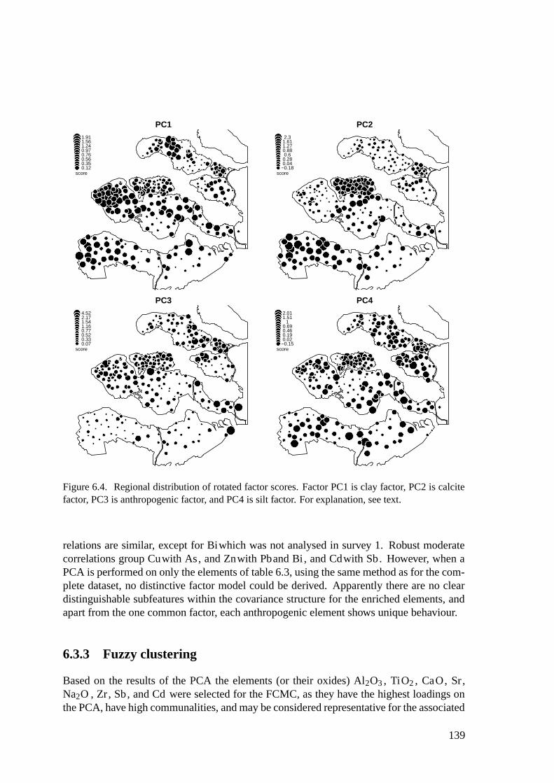
PC11.911.561.240.970.760.560.350.12
score
PC22.3
1.611.270.880.6
0.280.04
−0.18score
PC34.522.171.541.160.770.520.330.07
score
PC42.011.51
10.690.460.190.02
−0.15score
Figure 6.4. Regional distribution of rotated factor scores. Factor PC1 is clay factor, PC2 is calcitefactor, PC3 is anthropogenic factor, and PC4 is silt factor. For explanation, see text.
relations are similar, except for Biwhich was not analysed in survey 1. Robust moderatecorrelations group Cuwith As, and Znwith Pband Bi, and Cdwith Sb. However, when aPCA is performed on only the elements of table 6.3, using the same method as for the com-plete dataset, no distinctive factor model could be derived. Apparently there are no cleardistinguishable subfeatures within the covariance structure for the enriched elements, andapart from the one common factor, each anthropogenic element shows unique behaviour.
6.3.3 Fuzzy clustering
Based on the results of the PCA the elements (or their oxides) Al2O3 , TiO2 , CaO, Sr ,Na2O , Zr, Sb, and Cd were selected for the FCMC, as they have the highest loadings onthe PCA, have high communalities, and may be considered representative for the associated
139

Table 6.3. Correlation of anthropogenic elements. Upper part are MCD robust correlations, lowerpart are standard Pearsons correlations. All standard Pearsons correlations differ significantly from0.
As Bi Cd Cu P Pb Sb Sn Zn
As 0.08 0.32 0.58 0.38 0.21 0.42 0.48 0.50
Bi 0.54 0.26 -0.11 0.24 0.54 -0.02 -0.03 0.55
Cd 0.38 0.61 0.26 0.40 0.43 0.58 0.37 0.49
Cu 0.53 0.31 0.22 0.29 0.27 0.16 0.44 0.31
P 0.42 0.37 0.40 0.29 0.26 0.28 0.23 0.47
Pb 0.23 0.55 0.56 0.33 0.26 0.27 0.32 0.65
Sb 0.39 0.31 0.54 0.03 0.28 0.34 0.41 0.40
Sn 0.34 0.42 0.38 0.29 0.18 0.34 0.33 0.37
Zn 0.51 0.88 0.66 0.34 0.52 0.62 0.35 0.35
process. For convenience they are called respectively “clay elements” (Al , Ti), “calciteelements” (Ca, Sr), “silt elements” (Na, Zr), and “anthropogenic elements” (Sb, Cd). Thedata were scaled to equal range after removal of extreme values larger then 3 times theinterquartile range plus the third quartile (see equation 4.4, p. 70, f = 3). For determiningthe number of FCMC clusters the partition coefficient (F) and partition entropy (H) criteria(Vriend et al., 1988; Bezdek et al., 1984) were used together with a priori knowledge of thesoils and earlier results presented in this thesis. A systematic approach was applied to varythe number of clusters between 2 and 6, and varying the fuzziness (q-value) from 1.2 to 1.7trying to maximise F and minimise H. This resulted in an optimal model with 4 clustersand a q of 1.3.
The cluster centroids of the scaled data are shown in figure 6.5. The variability in centroidsis high for the elements for the clay, calcite, and silt elements, while it is much smaller,especially between clusters 1,3, and 4 for the anthropogenic elements.
Figure 6.6 shows box-and-whisker plots of the concentrations of the components groupedby cluster. In this crisp presentation, the samples are assigned to the cluster for whichthey have the highest membership. This shows a gradual decrease in concentrations forthe clay elements from cluster 1 to 4, with the largest gap between clusters 2 and 3. Thecalcite factor elements have significantly higher concentrations in cluster 1 and 3, and lowerconcentrations in cluster 2 and 4. The silt factor elements show a more or less moderateincrease in concentrations from cluster 1 to 4, which confirms the inverse relation betweenclay and silt. Here two major gaps appear between cluster 1 and 2, and between cluster3 and 4. The FCMC apparently divides the samples into 1) calcareous heavy clays, 2)non-calcareous heavy clays, 3) moderately calcareous silty clays, and 4) non-calcareoussilts.
The anthropogenic elements (Cd and Sb) barely show differences between clusters, except
140
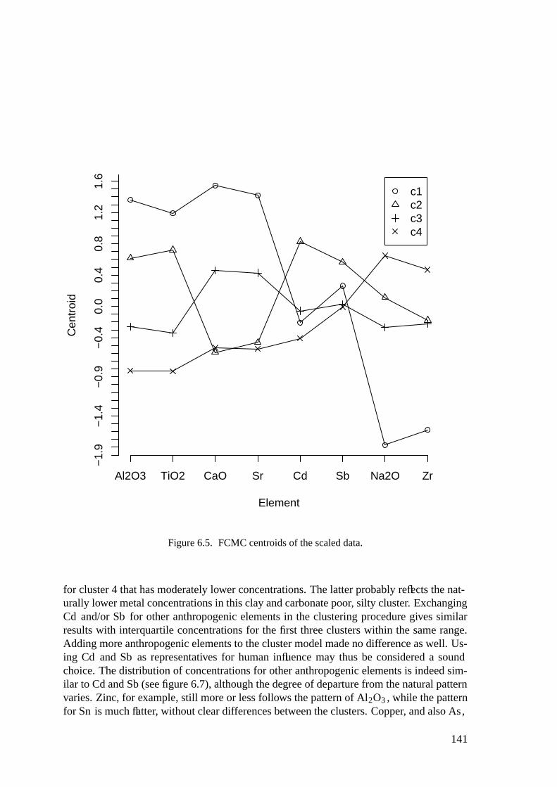
Element
Cen
troi
d
Al2O3 TiO2 CaO Sr Cd Sb Na2O Zr
−1.
9−
1.4
−0.
9−
0.4
0.0
0.4
0.8
1.2
1.6
c1c2c3c4
Figure 6.5. FCMC centroids of the scaled data.
for cluster 4 that has moderately lower concentrations. The latter probably reflects the nat-urally lower metal concentrations in this clay and carbonate poor, silty cluster. ExchangingCd and/or Sb for other anthropogenic elements in the clustering procedure gives similarresults with interquartile concentrations for the first three clusters within the same range.Adding more anthropogenic elements to the cluster model made no difference as well. Us-ing Cd and Sb as representatives for human influence may thus be considered a soundchoice. The distribution of concentrations for other anthropogenic elements is indeed sim-ilar to Cd and Sb (see figure 6.7), although the degree of departure from the natural patternvaries. Zinc, for example, still more or less follows the pattern of Al2O3 , while the patternfor Sn is much flatter, without clear differences between the clusters. Copper, and also As,
141
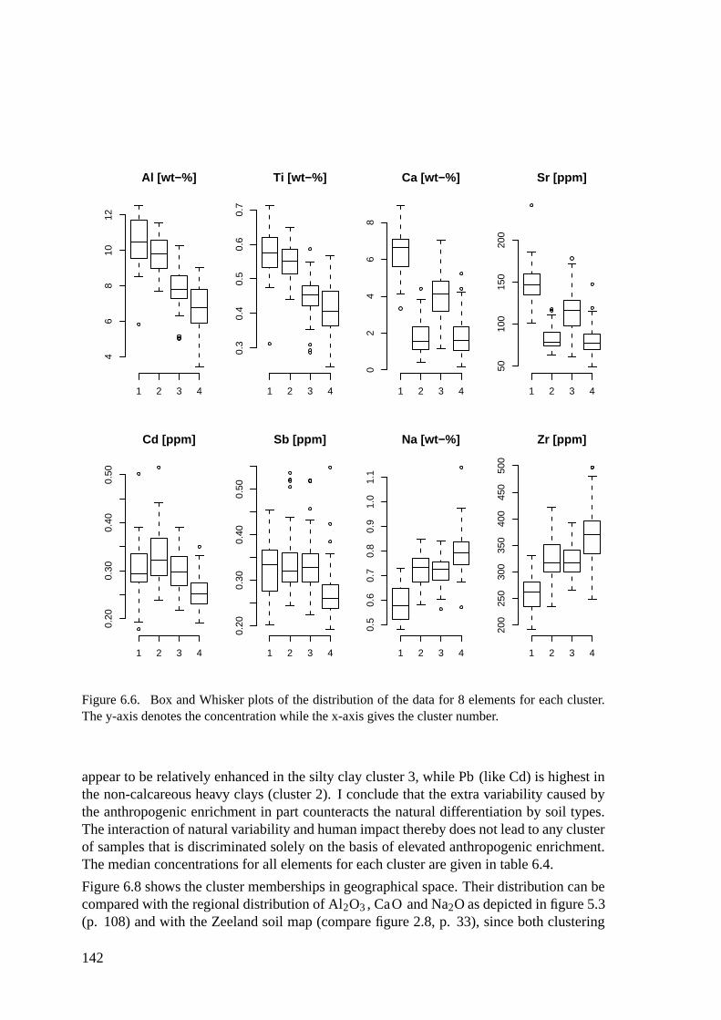
46
810
12
1 2 3 4
Al [wt−%]
1 2 3 4
0.3
0.4
0.5
0.6
0.7
Ti [wt−%]
1 2 3 4
02
46
8
Ca [wt−%]
1 2 3 4
5010
015
020
0
Sr [ppm]
1 2 3 4
0.20
0.30
0.40
0.50
Cd [ppm]
1 2 3 4
0.20
0.30
0.40
0.50
Sb [ppm]
1 2 3 4
0.5
0.6
0.7
0.8
0.9
1.0
1.1
Na [wt−%]
1 2 3 4
200
250
300
350
400
450
500
Zr [ppm]
Figure 6.6. Box and Whisker plots of the distribution of the data for 8 elements for each cluster.The y-axis denotes the concentration while the x-axis gives the cluster number.
appear to be relatively enhanced in the silty clay cluster 3, while Pb (like Cd) is highest inthe non-calcareous heavy clays (cluster 2). I conclude that the extra variability caused bythe anthropogenic enrichment in part counteracts the natural differentiation by soil types.The interaction of natural variability and human impact thereby does not lead to any clusterof samples that is discriminated solely on the basis of elevated anthropogenic enrichment.The median concentrations for all elements for each cluster are given in table 6.4.
Figure 6.8 shows the cluster memberships in geographical space. Their distribution can becompared with the regional distribution of Al2O3 , CaO and Na2O as depicted in figure 5.3(p. 108) and with the Zeeland soil map (compare figure 2.8, p. 33), since both clustering
142
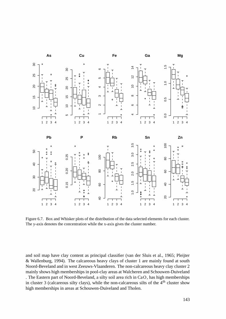
1015
2025
30
1 2 3 4
As
1 2 3 4
510
1520
2530
Cu
1 2 3 4
12
34
56
Fe
1 2 3 4
46
810
1214
Ga
1 2 3 4
0.0
0.5
1.0
1.5
Mg
1 2 3 4
2030
4050
Pb
1 2 3 4
0.15
0.20
0.25
P
1 2 3 4
4060
8010
0
Rb
1 2 3 4
1.0
1.5
2.0
2.5
3.0
3.5
Sn
1 2 3 4
2040
6080
100
Zn
Figure 6.7. Box and Whisker plots of the distribution of the data selected elements for each cluster.The y-axis denotes the concentration while the x-axis gives the cluster number.
and soil map have clay content as principal classifier (van der Sluis et al., 1965; Pleijter& Wallenburg, 1994). The calcareous heavy clays of cluster 1 are mainly found at southNoord-Beveland and in west Zeeuws-Vlaanderen. The non-calcareous heavy clay cluster 2mainly shows high memberships in pool-clay areas at Walcheren and Schouwen-Duiveland. The Eastern part of Noord-Beveland, a silty soil area rich in CaO, has high membershipsin cluster 3 (calcareous silty clays), while the non-calcareous silts of the 4th cluster showhigh memberships in areas at Schouwen-Duiveland and Tholen.
143
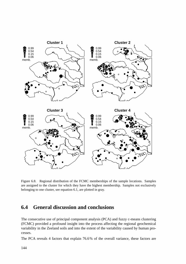
Cluster 10.990.540.150.06
memb.
Cluster 20.990.540.150.06
memb.
Cluster 30.990.540.150.06
memb.
Cluster 40.990.540.150.06
memb.
Figure 6.8. Regional distribution of the FCMC memberships of the sample locations. Samplesare assigned to the cluster for which they have the highest membership. Samples not exclusivelybelonging to one cluster, see equation 6.1, are plotted in gray.
6.4 General discussion and conclusions
The consecutive use of principal component analysis (PCA) and fuzzy c-means clustering(FCMC) provided a profound insight into the process affecting the regional geochemicalvariability in the Zeeland soils and into the extent of the variability caused by human pro-cesses.
The PCA reveals 4 factors that explain 76.6% of the overall variance, these factors are
144
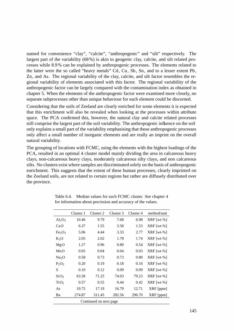
named for convenience “clay”, “calcite”, “anthropogenic” and “silt” respectively. Thelargest part of the variability (68%) is akin to geogenic clay, calcite, and silt related pro-cesses while 8.9% can be explained by anthropogenic processes. The elements related tothe latter were the so called “heavy metals” Cd, Cu, Sb, Sn, and to a lesser extent Pb,Zn, and As. The regional variability of the clay, calcite, and silt factor resembles the re-gional variability of elements associated with this factor. The regional variability of theanthropogenic factor can be largely compared with the contamination index as obtained inchapter 5. When the elements of the anthropogenic factor were examined more closely, noseparate subprocesses other than unique behaviour for each element could be discerned.
Considering that the soils of Zeeland are clearly enriched for some elements it is expectedthat this enrichment will also be revealed when looking at the processes within attributespace. The PCA confirmed this, however, the natural clay and calcite related processesstill comprise the largest part of the soil variability. The anthropogenic influence on the soilonly explains a small part of the variability emphasising that these anthropogenic processesonly affect a small number of inorganic elements and are really an imprint on the overallnatural variability.
The grouping of locations with FCMC, using the elements with the highest loadings of thePCA, resulted in an optimal 4 cluster model mainly dividing the area in calcareous heavyclays, non-calcareous heavy clays, moderately calcareous silty clays, and non calcareoussilts. No clusters exist where samples are discriminated solely on the basis of anthropogenicenrichment. This suggests that the extent of these human processes, clearly imprinted onthe Zeeland soils, are not related to certain regions but rather are diffusely distributed overthe province.
Table 6.4. Median values for each FCMC cluster. See chapter 4for information about precission and accuracy of the values.
Cluster 1 Cluster 2 Cluster 3 Cluster 4 method/unit
Al2O3 10.46 9.79 7.68 6.98 XRF [wt-%]
CaO 6.37 1.55 3.58 1.53 XRF [wt-%]
Fe2O3 5.06 4.44 3.33 2.77 XRF [wt-%]
K2O 2.05 2.02 1.78 1.74 XRF [wt-%]
MgO 1.27 0.96 0.80 0.54 XRF [wt-%]
MnO 0.05 0.04 0.04 0.03 XRF [wt-%]
Na2O 0.58 0.73 0.73 0.80 XRF [wt-%]
P2O5 0.20 0.19 0.18 0.16 XRF [wt-%]
S 0.10 0.12 0.09 0.09 XRF [wt-%]
SiO2 63.58 71.25 74.03 79.23 XRF [wt-%]
TiO2 0.57 0.55 0.44 0.42 XRF [wt-%]
As 19.75 17.19 16.79 12.71 XRF [ppm]
Ba 274.87 311.45 282.56 296.70 XRF [ppm]
Continued on next page
145
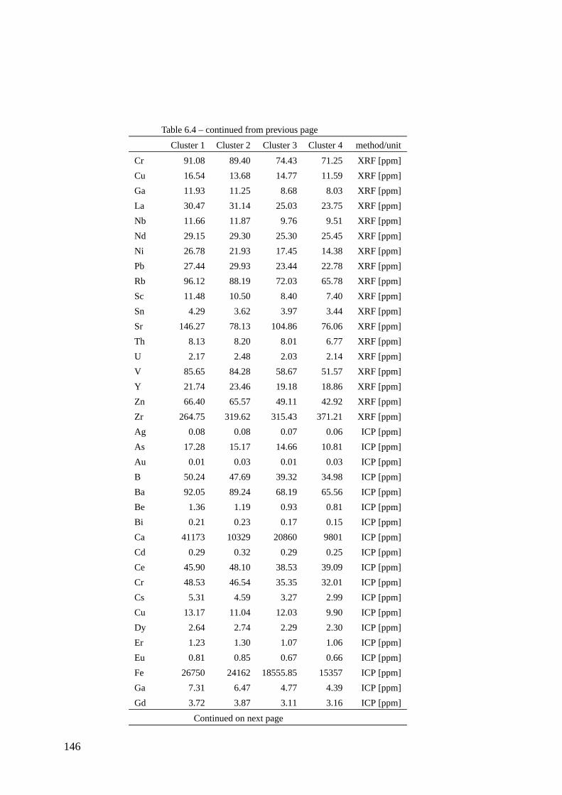
Table 6.4 – continued from previous page
Cluster 1 Cluster 2 Cluster 3 Cluster 4 method/unit
Cr 91.08 89.40 74.43 71.25 XRF [ppm]
Cu 16.54 13.68 14.77 11.59 XRF [ppm]
Ga 11.93 11.25 8.68 8.03 XRF [ppm]
La 30.47 31.14 25.03 23.75 XRF [ppm]
Nb 11.66 11.87 9.76 9.51 XRF [ppm]
Nd 29.15 29.30 25.30 25.45 XRF [ppm]
Ni 26.78 21.93 17.45 14.38 XRF [ppm]
Pb 27.44 29.93 23.44 22.78 XRF [ppm]
Rb 96.12 88.19 72.03 65.78 XRF [ppm]
Sc 11.48 10.50 8.40 7.40 XRF [ppm]
Sn 4.29 3.62 3.97 3.44 XRF [ppm]
Sr 146.27 78.13 104.86 76.06 XRF [ppm]
Th 8.13 8.20 8.01 6.77 XRF [ppm]
U 2.17 2.48 2.03 2.14 XRF [ppm]
V 85.65 84.28 58.67 51.57 XRF [ppm]
Y 21.74 23.46 19.18 18.86 XRF [ppm]
Zn 66.40 65.57 49.11 42.92 XRF [ppm]
Zr 264.75 319.62 315.43 371.21 XRF [ppm]
Ag 0.08 0.08 0.07 0.06 ICP [ppm]
As 17.28 15.17 14.66 10.81 ICP [ppm]
Au 0.01 0.03 0.01 0.03 ICP [ppm]
B 50.24 47.69 39.32 34.98 ICP [ppm]
Ba 92.05 89.24 68.19 65.56 ICP [ppm]
Be 1.36 1.19 0.93 0.81 ICP [ppm]
Bi 0.21 0.23 0.17 0.15 ICP [ppm]
Ca 41173 10329 20860 9801 ICP [ppm]
Cd 0.29 0.32 0.29 0.25 ICP [ppm]
Ce 45.90 48.10 38.53 39.09 ICP [ppm]
Cr 48.53 46.54 35.35 32.01 ICP [ppm]
Cs 5.31 4.59 3.27 2.99 ICP [ppm]
Cu 13.17 11.04 12.03 9.90 ICP [ppm]
Dy 2.64 2.74 2.29 2.30 ICP [ppm]
Er 1.23 1.30 1.07 1.06 ICP [ppm]
Eu 0.81 0.85 0.67 0.66 ICP [ppm]
Fe 26750 24162 18555.85 15357 ICP [ppm]
Ga 7.31 6.47 4.77 4.39 ICP [ppm]
Gd 3.72 3.87 3.11 3.16 ICP [ppm]
Continued on next page
146
Table 6.4 – continued from previous page
Cluster 1 Cluster 2 Cluster 3 Cluster 4 method/unit
Hf 0.24 0.35 0.23 0.22 ICP [ppm]
Ho 0.48 0.50 0.40 0.41 ICP [ppm]
La 23.58 23.99 19.88 19.48 ICP [ppm]
Li 32.75 26.89 21.57 18.30 ICP [ppm]
Lu 0.17 0.17 0.14 0.15 ICP [ppm]
Mg 6549.81 5266.79 4710.06 3928.54 ICP [ppm]
Mn 311.60 229.09 227.63 187.15 ICP [ppm]
Mo 0.47 0.64 0.33 0.29 ICP [ppm]
Nb 0.57 0.66 0.60 0.57 ICP [ppm]
Nd 22.27 22.82 19.05 18.64 ICP [ppm]
Ni 22.35 19.82 15.35 13.45 ICP [ppm]
Pb 24.43 24.67 18.83 18.60 ICP [ppm]
Pr 5.58 5.68 4.81 4.70 ICP [ppm]
Pt 0.01 0.01 0.01 0.01 ICP [ppm]
Rb 62.61 56.20 40.15 38.29 ICP [ppm]
Sb 0.33 0.31 0.33 0.25 ICP [ppm]
Sc 7.89 7.66 5.97 5.60 ICP [ppm]
Se 0.41 0.98 0.34 0.64 ICP [ppm]
Sm 4.07 4.24 3.55 3.52 ICP [ppm]
Sn 2.08 1.96 1.92 1.60 ICP [ppm]
Sr 130.99 55.38 82.91 51.59 ICP [ppm]
Ta 0.03 0.02 0.03 0.02 ICP [ppm]
Tb 0.53 0.54 0.44 0.44 ICP [ppm]
Th 5.91 6.26 5.13 5.15 ICP [ppm]
Ti 702.83 727.14 630.68 620.85 ICP [ppm]
Tl 0.36 0.35 0.26 0.28 ICP [ppm]
Tm 0.17 0.18 0.14 0.14 ICP [ppm]
U 1.06 1.09 0.94 0.93 ICP [ppm]
Y 12.12 12.90 10.37 10.22 ICP [ppm]
Yb 1.09 1.11 0.92 0.94 ICP [ppm]
Zn 70.08 64.91 55.15 51.26 ICP [ppm]
Zr 11.97 14.26 10.12 9.44 ICP [ppm]
147


7 Assessment of regional DDT concen-trations in the soils of Zeeland
7.1 Introduction
Since the 1940s the organochlorine pesticide DDT has been used in western Europe, anddespite its ban in the 1970s its legacy is still present as residues in the soil compartment. Forseveral decades its risks for the environment have been acknowledged (Organisation, 1989;Edwards, 1970) and this makes it important to have a good overview of the occurrences ofDDT in our environment. Especially for soil, as a major environmental compartment, andbeing both a source and a sink, knowledge about DDT residue concentrations is vital toevaluate the ecotoxicological risk of our notorious legacy. One of the questions in such anevaluation is whether the DDT residue level is part of the ubiquitous global background oris the result of more local features.
Studies in the Arctic and Antarctic, glaciers, tundras, i.e. pristine areas from where it canbe assumed that DDT was not actively applied, show significant concentrations in soils,sediment and water (Rovinsky et al., 1995; Harner et al., 1999; Villa et al., 2003; Politovet al., 2000). Most of these studies regard marine and atmospheric transport as the maintransportation mechanisms of DDT. Considering this ubiquitous occurrence of DDT onecan assume the existence of a global DDT background. However, this background is neithergeogenic nor biogenic but solely anthropogenic and there are no reasons to assume that anatural source of DDT exists.
Knowledge about DDT residue concentrations can be provided by large scale regional soilsurveys, for example, as are common in geochemistry (Darnley, 1995; Bolviken et al.,1996) However, examples of large scale surveys aimed at organochlorine pesticides (OCP),including DDT, are scarce (Gong et al., 2004). More often soil surveys aimed at DDTconcentrations are regional and have a limited number of samples, usually about 10 to 50samples (e.g. Covaci et al. (2001); Kim & Smith (2001)). When speculating about thereasons why OCP surveys are as yet less common than geochemical surveys, both wouldhave similar environmental goals (Darnley, 1995), the time, complexity, and effort that areneeded for the analytical determination of OCP, appear likely culprits.
Also within the Netherlands interest in the general level of organochlorine pesticides occur-rence in soil exists, but only small parts of the country have been sampled and the number
149
of samples is usually limited (Groot et al., 2001). A country wide, or even regional scale,survey of DDT concentrations does not yet exist, despite the fact that at the local scale DDToccurrence in soils frequently results in legal issues (e.g. building permits, sale of land).
An alternative approach to obtain regional information about DDT or other contaminantsis to use existing data. A larger regional assessment can be obtained by combining datafrom several subregions, which are gathered over the years (Licht & Tarvainen, 1996).Ideally, these data should have been sampled and analysed using standardised methods tominimise survey and analytical bias. Even then the combined dataset may still suffer frombias caused by different choices during survey and analytical procedures. However, byacknowledging the presence of bias, the data may still provide relevant information, andusing limited resources and effort an indication can be obtained if larger or more detailedstudies are necessary.
In the Netherlands, municipal and provincial authorities are currently putting much effortin drafting so called soil pollution risk maps (van der Gaast et al., 1998; van Lienen et al.,2000). These maps are used for environmental legislation, building permits, and permits fortransport of (non-polluted) soil and are to some extent standardised regarding sampling anddetermination of chemical composition (VROM, 1999; Eikelboom et al., 2001). The datafor these maps are held in soil information systems (SIS) and include some informationabout OCP, including DDT and residues.
This study aims at providing a regional assessment of current DDT residue concentrations,variability, and degradation for the province of Zeeland. Data from several separate SISdata are merged. By comparing the concentrations with legal limits and data from otherareas the extent of contamination will be assessed, providing insight into whether the con-centrations are just part of the ubiquitous background or exceeding those. The geographicaldistribution of the DDT residue levels might indicate patterns, if any, that possibly relateto distinct processes. In addition, the data integration excercise will assess the value of thecombined SIS for regional environmental policy and may lead to recommendations to the(local) authorities for further research and monitoring.
7.2 DDT, properties and history
DDT∗, and its metabolites DDE† and DDD‡ are well known as contaminants in our presentday environment (Braune et al., 1999). The physiochemical properties of these substancesmake them a real environmental threat as they are resistant to breakdown, easily takenin by organisms, and are readily absorbed on to the soil (organic) matrix, and they havehazardous effects on aquatic and terrestrial organisms (Organisation, 1989; Zitko, 2003).Soil can both be a sink and a long-term source for exposure to DDT. This not only affectssoil biota (Megharaj et al., 1999) but can also affect larger organisms (Zitko, 2003). Al-
∗1,1,1-trichloro-2,2-bis(p-chlorophenyl)ethane†1,1-dichloro-2,2-bis(p-chlorophenyl)ethylene‡1,1-dichloro-2,2-bis(p-chlorophenyl)ethane
150

though absorption is often assumed, DDT is also reported as soil-bound and unextractableby solvents (Singh & Agarwal, 1992).
The metabolites DDE and DDD are formed by the breakdown of DDT. It is assumed thatthe degradation of DDT in aerobic soils procedes relatively slowly, with reported half-lifesranging between 20 to 30 years (Howard, 1991; Dimond & Owen, 1996)
DDT has been in use since the beginning of the 20th century, as part of a larger group ofOCP that were seen as new state of the art methods to engineer nature. It was not untilthe emotional call in the book “Silent Spring” (Carson, 1962) that awareness about thedeleterious effects of pesticide usage in society was raised. Since the beginning of the1970s DDT usage has been banned in most industrialised countries, in the NetherlandsDDT has not been allowed since 1973.
DDT, DDE and DDD each have two different isomers depending on the position of thephenyl-bound chlorine. When data for the individual isomers are presented they will bereported as p, p-DDT and o, p-DDT (or p, p-DDE/o, p-DDE, and p, p-DDD/o, p-DDD).When purity is unknown the simple abreviations DDT, DDE, and DDD will be used in ageneral sense. All isomers and metabolites together will be referred to as DDx in a generalsense or ∑DDx when quantitively indicating the sum of all concentrations.
7.3 Study area
The location of the study area is shown in figure 7.1. The province of Zeeland is located inthe south-west of the Netherlands along the coast of the North Sea. Besides the mainlandof Zeeuws-Vlaanderen, it consists of several islands and peninsulas. The area is the resultof a continuous shaping by the marine environment and human activity. It has been moreextensively described in chapter 2.
Zeeland has an agricultural land use history where crop farming has long been the mostimportant factor. Nowadays the total area of 2930km2 consists of 1140km2 water and1440km2 agricultural area. Common crops are corn, root- and tuberous plants while live-stock are mostly sheep and some cattle. In the 20th century the economy shifted towardsmore industrial and service activities and today only 4% of the economic revenues aregained from agriculture even though it still encompasses the largest geographical area (seealso chapter 2). Based on communications with the provincial authorities, it is known thatDDT has been used for pest control for several years in Zeeland, especially in orchards.This usage ended in the mid 1960s. Still the concentrations of DDT and derivatives ex-isting in the soil is of concern for local authorities. The legal limits, set up by the Dutchgovernment, are often exceeded, resulting in litigations.
151
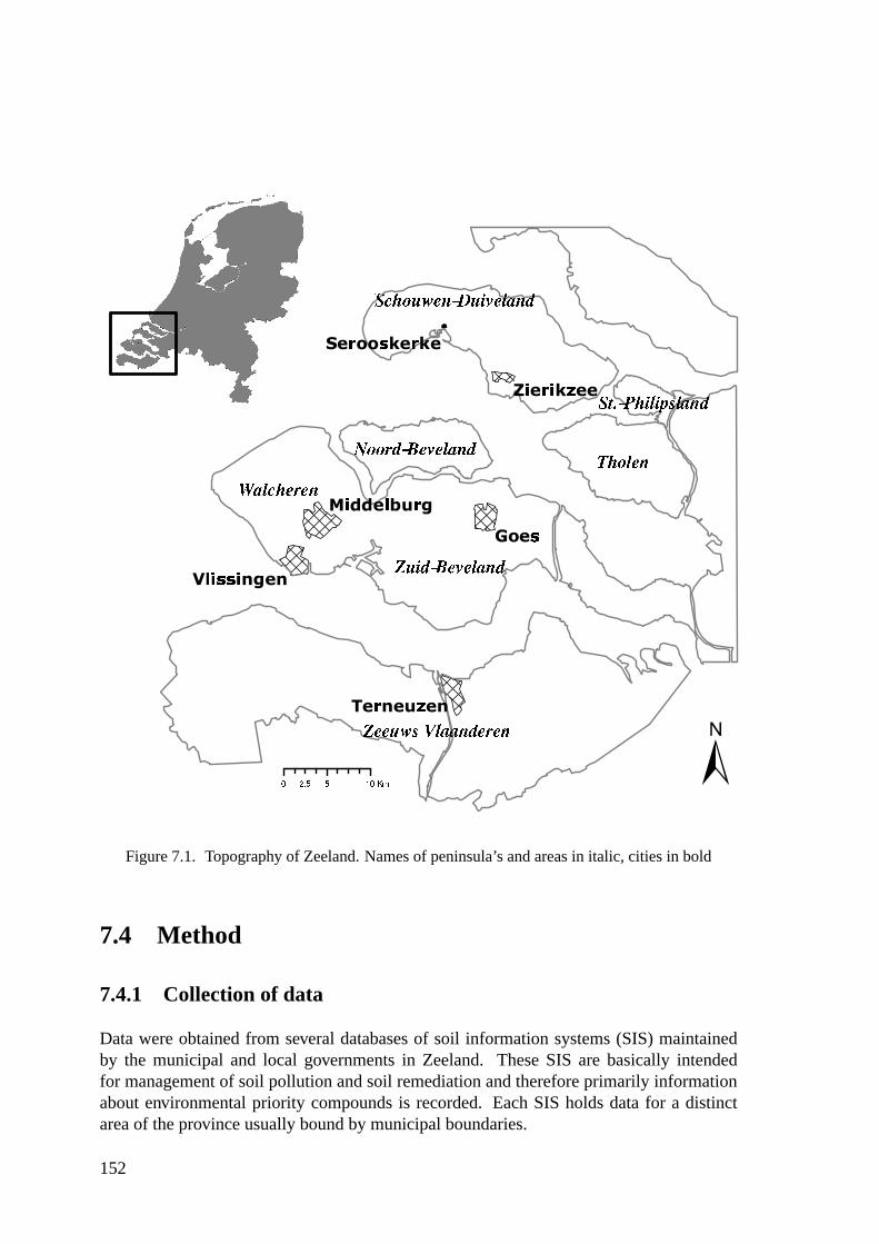
Figure 7.1. Topography of Zeeland. Names of peninsula’s and areas in italic, cities in bold
7.4 Method
7.4.1 Collection of data
Data were obtained from several databases of soil information systems (SIS) maintainedby the municipal and local governments in Zeeland. These SIS are basically intendedfor management of soil pollution and soil remediation and therefore primarily informationabout environmental priority compounds is recorded. Each SIS holds data for a distinctarea of the province usually bound by municipal boundaries.
152
The available databases were merged and only topsoil (0-50cm depth) data from rural ar-eas, mainly agricultural land, were selected. These georeferenced data comprise severalinorganic parameters like priority metals, and organic parameters such as polycyclic aro-matic hydrocarbons, polychlorinated biphenyls and OCP including DDx. Some databasescontained replicate samplings which will be used to assess the variability at different sam-pling scales.
Sampling and analytical methods are generally based on national standards for which theNEN 5740 standard for sampling (NNI, 1999b) and the NEN 5734 standard for OCP anal-ysis (NNI, 1999a) are the most relevant in this context. The sampling in general comprisestaking composite samples containing about 10 to 20 subsamples, taken from a distinct rangefrom the soil profile. Depending on the purpose, scale, and if contamination is expected ornot, the number of subsamples and sampling density varies. The depth range of the samplesusually varies from 1-30cm to 1-50cm depth for the topsoil and a second sample from adepth of 50-100cm.
The OCP analysis, according to NEN 5734, is based on a wet extraction with acetoneand petroleum ether. The extracts are dried with anhydrous Na2SO4 and eluted over analuminum oxide column. Subsequent gas-chromatographic analysis, mostly with a mass-spectrometric detector, is used for detection of the residues. The chemical analyses aremostly carried out in commercial laboratories.
Although standard methods are used, small deviations are to be expected due to differentinterpretations of the protocol or adaptations to local circumstances, during both survey-ing and laboratory analysis. These departures are usually not recorded in the datasets. Nomethod to compensate for the resulting bias is used since neither control samples wereavailable nor were analytical standards reported in the SIS. Other known methods for re-moving bias between datasets are not suitable due to the low number of samples per survey(Daneshfar & Cameron, 1998; Darnley, 1995).
7.4.2 Basic statistical analysis
The statistical analysis should provide insight in the ranges of DDx concentrations, whilebeing robust against the expected high variability within the data, many outliers, and cen-sored data below the detection limit occurr. Considering the possible bias between thedifferent datasets, the analysis should also provide some basic insight into the differencesbetween the datasets.
Univariate data exploration techniques, such as cumulative distribution frequency (CDF)plots, were used to provide the necessary insight in the statistical DDx distributions. WithCDF plots, in which the data are plotted against the data percentiles on a probability scale,the type of data distribution is determined and possible outliers can be identified. Thistechnique has already been demonstrated in chapter 5 and has been also used by otherauthors (Sinclair, 1976; Matschullat et al., 2000; Bounessah & Atkin, 2003). Standardhistograms were viewed as well.
Since outliers might denote important features, such as areas with more extensive DDT
153
usage, they are as important as the bulk of the data. Therefore outliers are treated sepa-rately when necessary. The CDF plots were used to find a threshold value above which avalue should be regarded as an outlier. This threshold value is the percentile where a clearinflection in the CDF curve occurs.
When replacement of censored data, i.e. values below the detection limit, was necessarythey were replaced by a value of 0.7 times the detection limit.
7.4.3 Analysis of variance
The observed variability of DDT and its derivatives in soil comes from several sources. Forexample variability in application, degree of breakdown, transport trough the soil column,together with the variability caused by sampling and analytical procedures may all con-tribute to the total variability. In chapter 3 it is already shown how the contribution of localscale variability can influence the regional variability. If the local variability is relativelyhigh then it is to be expected that observed regional patterns are mainly caused by localfeatures instead of true regional processes.
In some datasets replicate samples exist, i.e. some areas or fields were purposely sampledmore than once within a survey, or samples were analysed by two different laboratories.The occasional replicates in the dataset were used to calculate local variance (i.e. fieldscale)and this can be compared with the overall regional variance. Using an analysis of variance(ANOVA) the variance components can be calculated, which explain the contribution ofeach level of variance to the total variance (Youden & Mehlich, 1937; Nortcliff, 1978;Oliver & Webster, 1986; Webster & Oliver, 1990; Searle et al., 1992). For the ANOVA andcalculation of the variance components the raov function of S-PLUS was used (Venables& Ripley, 2002).
Since not all datasets have a sampling design suitable for ANOVA, and considering theinterest in the overall spatial variance as well, an experimental semivariogram was calcu-lated by using all available data (Journel & Huijbregts, 1981). By using the range of thevariogram the extent of the local semivariance can be compared to the regional one and itcan be assessed how far local noise determines the observed regional variability. The semi-variogram was calculated using the Gstat program (Pebesma & Wesseling, 1998). BothANOVA and semivariance can provide insight into how the observed regional variabilityshould be interpreted.
7.4.4 Regional variability
To reveal spatial DDx patterns over the region of Zeeland, the concentrations were plottedusing symbol maps. From these, groups or areas with similar concentrations can be dis-cerned. Spatial anomalies, single samples with anomalous concentrations compared to thesurrounding samples, can be recognised as well. Examples of symbol maps, for which thesize of the symbol varies with the associated attribute can be found in Bounessah & Atkin(2003) and Reimann & Filzmoser (1999). In chapter 5 (§5.3.2) the plotting method of
154
the Geological Survey of Finland is described and demonstrated (Gustavson et al., 1997),which will also be used here.
7.4.5 Comparison with external data and normative values
Considering that there is no natural, geogenic, background for DDx it is more difficult toevaluate the soil concentrations of Zeeland than in the case of potentially toxic metals. Toput the data in perspective, values found in other areas, mostly outside the Netherlands,are compared with those found in Zeeland. Although it is expected that the sampling andanalytical methods of the other studies will often differ from those for the current study,the comparison will still point out the relative magnitude of the DDT contamination ofZeeland.
The values are obtained from literature for areas which were presumed to be to some extentcomparable to Zeeland or from pristine areas where it can be assumed that no DDT appli-cation has occurred. It is recognised that the probable differences in soil lithology and soilecology also will lead to differences in ecotoxicological risk between areas.
In the Netherlands it is standard practice to compare DDx values with soil specific legal lim-its to judge the extent of the contamination, using the limits as a standard reference. Theselimits are provided by the Dutch normative framework (VROM, 1994; Swartjes, 1999) andinclude a threshold value (S, or “Streefwaarde”), which is the maximum permissible levelfor sustainable soil quality, and an intervention value (I or “Interventiewaarde”) which in-dicates the level of severe pollution. These values apply to a so called standard soil, asdefined in the framework, containing 25% of clay and 10% organic matter (VROM, 1994).The S and I values for standard soil for ∑DDx are 0.01mg/kg and 4mg/kg respectively.For pesticides the normative framework requires correction for the actual organic mattercontent in the soil according to
s = S · O10
(7.1)
Here S is the value for standard soils and s is the soil specific legal limit normalisedon percentage organic matter, O (VROM, 1994). The comparison of DDx concentra-tions against these limits does not take into account sample and analytical variability andthis can make deciding between a “clean” soil (concentration < S) and “polluted” soil(concentration > S) a chance event.
7.4.6 DDT breakdown
If the extent of DDT breakdown calculated from the actually observed values in Zeeland formetabolic and remaining DDT is less than expected under local circumstances, comparedwith a half-life of 20-30 year (Howard, 1991; Dimond & Owen, 1996), then the DDTbreakdown has evolved more slowly then expected, or fresh application has occurred. Also,
155
it indicates that the Zeeland soils will be a source of DDx components for a longer periodthan probably anticipated. Presuming that DDT was banned at the beginning of the 1970sit can be expected that DDT breakdown should now be at a level of at least 1 half-life time.
As no single validated value for DDT half-life exists, the exact time elapsed since its appli-cation cannot be assessed. However, from the molar ratio between DDT and its breakdownproducts, DDE and DDD, it can be calculated how many half-lifes ( t
T12
) have passed. As-
suming exponential decay the formula
tT1
2
=ln( [DDE+DDD]
DDT + 1)
ln(2)(7.2)
can be used, as was suggested by van Gaans et al. (1995).
As DDE is the major breakdown product under aerobic conditions, which is the predom-inating condition in soils, DDE is likely to be the predominant metabolite to be found inZeeland.
7.5 Results
7.5.1 Data merging and selection
It became apparent that neither a common standard nor a well described method was usedwhen recording the data in the different databases. The recording of the data itself wasregularly quite minimal. For instance, in many datasets only a sum DDT value was recordedinstead of separate values for DDT, DDE, and DDD. Information about which isomer wasdetermined (o, p or p, p) was even more scarce. In general, neither information aboutsampling strategy nor analytical procedure or laboratory was available. Therefore it wasdecided to use the data “as is” and not to make assumptions about the differences betweenthe methods.
From the initial merged dataset, locations within the rural area of the province were se-lected, and from each location the sample, if any, for which DDT, DDD, DDE or ∑DDxwas determined, was selected. Locations known to be orchards were left out, as these weresuspected of showing divergently higher values. This resulted in a final selection from 7databases and 30-60 samples per database (table 7.1). The sample locations are reasonablywell distributed over the province although not every area is covered (figure 7.2).
All surveys, except surveys 1 and 3, were derived from datasets related to local pollutionrisk maps. Surveys 2, 5, and 6 were distinct surveys specifically aimed at creating a pol-lution risk map while surveys 4 and 7 are in themselves already a combination of severalsubsurveys with different aims.
Survey 1 had a somewhat different sampling design than proposed by the standardised de-sign according to the NEN 5740. A composite topsoil sample, consisting of 5 randomly
156
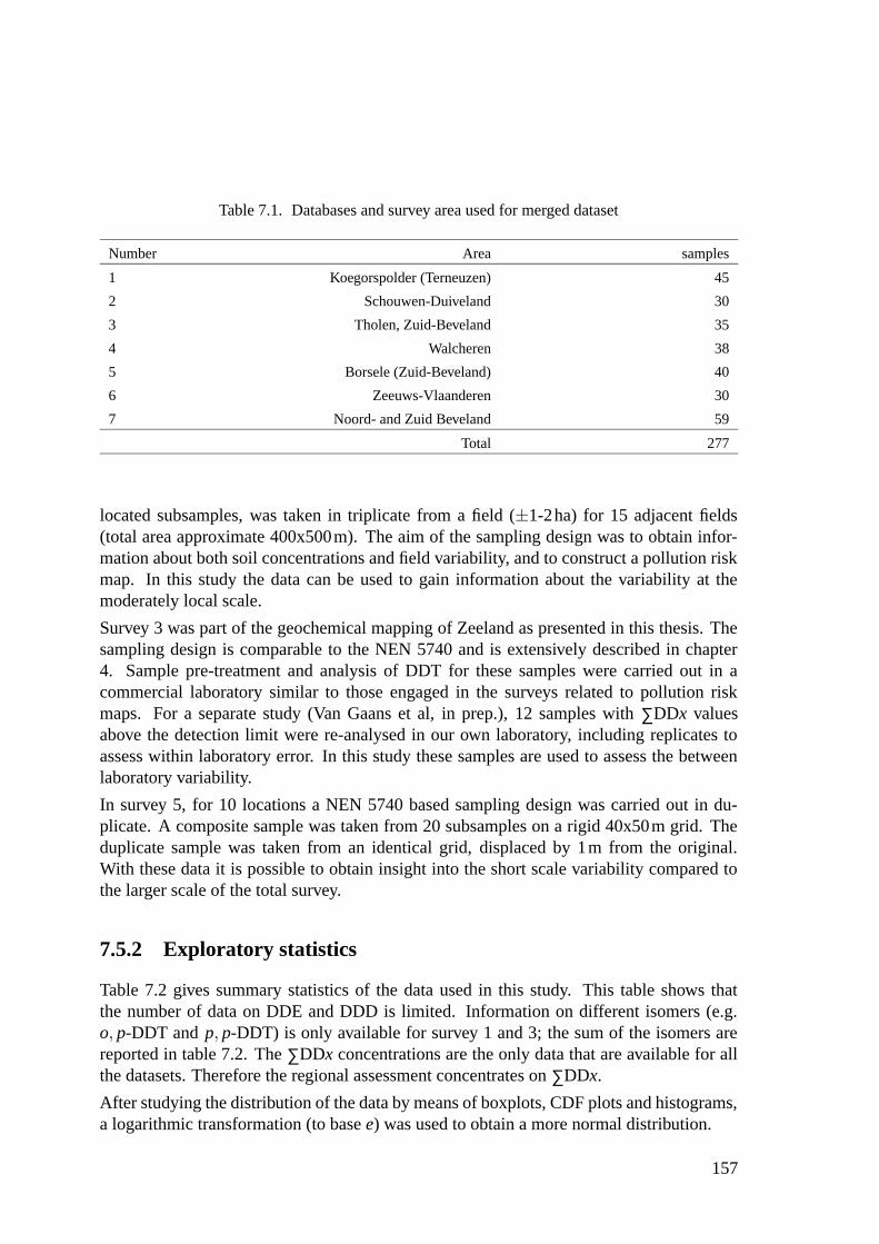
Table 7.1. Databases and survey area used for merged dataset
Number Area samples
1 Koegorspolder (Terneuzen) 45
2 Schouwen-Duiveland 30
3 Tholen, Zuid-Beveland 35
4 Walcheren 38
5 Borsele (Zuid-Beveland) 40
6 Zeeuws-Vlaanderen 30
7 Noord- and Zuid Beveland 59
Total 277
located subsamples, was taken in triplicate from a field (±1-2ha) for 15 adjacent fields(total area approximate 400x500m). The aim of the sampling design was to obtain infor-mation about both soil concentrations and field variability, and to construct a pollution riskmap. In this study the data can be used to gain information about the variability at themoderately local scale.
Survey 3 was part of the geochemical mapping of Zeeland as presented in this thesis. Thesampling design is comparable to the NEN 5740 and is extensively described in chapter4. Sample pre-treatment and analysis of DDT for these samples were carried out in acommercial laboratory similar to those engaged in the surveys related to pollution riskmaps. For a separate study (Van Gaans et al, in prep.), 12 samples with ∑DDx valuesabove the detection limit were re-analysed in our own laboratory, including replicates toassess within laboratory error. In this study these samples are used to assess the betweenlaboratory variability.
In survey 5, for 10 locations a NEN 5740 based sampling design was carried out in du-plicate. A composite sample was taken from 20 subsamples on a rigid 40x50m grid. Theduplicate sample was taken from an identical grid, displaced by 1m from the original.With these data it is possible to obtain insight into the short scale variability compared tothe larger scale of the total survey.
7.5.2 Exploratory statistics
Table 7.2 gives summary statistics of the data used in this study. This table shows thatthe number of data on DDE and DDD is limited. Information on different isomers (e.g.o, p-DDT and p, p-DDT) is only available for survey 1 and 3; the sum of the isomers arereported in table 7.2. The ∑DDx concentrations are the only data that are available for allthe datasets. Therefore the regional assessment concentrates on ∑DDx.
After studying the distribution of the data by means of boxplots, CDF plots and histograms,a logarithmic transformation (to base e) was used to obtain a more normal distribution.
157
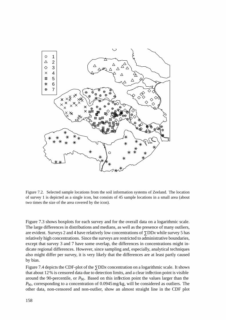
1234567
Figure 7.2. Selected sample locations from the soil information systems of Zeeland. The locationof survey 1 is depicted as a single icon, but consists of 45 sample locations in a small area (abouttwo times the size of the area covered by the icon).
Figure 7.3 shows boxplots for each survey and for the overall data on a logarithmic scale.The large differences in distributions and medians, as well as the presence of many outliers,are evident. Surveys 2 and 4 have relatively low concentrations of ∑DDx while survey 5 hasrelatively high concentrations. Since the surveys are restricted to administrative boundaries,except that survey 3 and 7 have some overlap, the differences in concentrations might in-dicate regional differences. However, since sampling and, especially, analytical techniquesalso might differ per survey, it is very likely that the differences are at least partly causedby bias.
Figure 7.4 depicts the CDF-plot of the ∑DDx concentration on a logarithmic scale. It showsthat about 12% is censored data due to detection limits, and a clear inflection point is visiblearound the 90-percentile, or P90. Based on this inflection point the values larger than theP90, corresponding to a concentration of 0.0945mg/kg, will be considered as outliers. Theother data, non-censored and non-outlier, show an almost straight line in the CDF plot
158
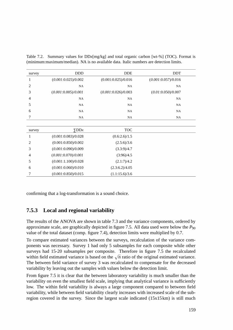
Table 7.2. Summary values for DDx[mg/kg] and total organic carbon [wt-%] (TOC). Format is(minimum:maximum/median). NA is no available data. Italic numbers are detection limits.
survey DDD DDE DDT
1 (0.001 :0.025)/0.002 (0.001:0.025)/0.016 (0.001 :0.057)/0.016
2 NA NA NA
3 (0.001 :0.005)/0.001 (0.001 :0.026)/0.003 (0.01 :0.050)/0.007
4 NA NA NA
5 NA NA NA
6 NA NA NA
7 NA NA NA
survey ∑DDx TOC
1 (0.001 :0.083)/0.028 (0.6:2.6)/1.5
2 (0.001:0.850)/0.002 (2.5:6)/3.6
3 (0.001 :0.090)/0.009 (3.3:9)/4.7
4 (0.001 :0.070)/0.001 (3:96)/4.5
5 (0.001 :1.100)/0.028 (2.1:7)/4.2
6 (0.001 :0.060)/0.010 (2.3:6.2)/4.05
7 (0.001 :0.850)/0.015 (1.1:15.6)/3.6
confirming that a log-transformation is a sound choice.
7.5.3 Local and regional variability
The results of the ANOVA are shown in table 7.3 and the variance components, ordered byapproximate scale, are graphically depicted in figure 7.5. All data used were below the P90
value of the total dataset (comp. figure 7.4), detection limits were multiplied by 0.7.
To compare estimated variances between the surveys, recalculation of the variance com-ponents was necessary. Survey 1 had only 5 subsamples for each composite while othersurveys had 15-20 subsamples per composite. Therefore in figure 7.5 the recalculatedwithin field estimated variance is based on the
√n ratio of the original estimated variance.
The between field variance of survey 3 was recalculated to compensate for the decreasedvariability by leaving out the samples with values below the detection limit.
From figure 7.5 it is clear that the between laboratory variability is much smaller than thevariability on even the smallest field scale, implying that analytical variance is sufficientlylow. The within field variability is always a large component compared to between fieldvariability, while between field variability clearly increases with increased scale of the sub-region covered in the survey. Since the largest scale indicated (15x15km) is still much
159
Survey
Sum
DD
x [m
g/kg
]
1 2 3 4 5 6 7 T
0.00
10.
050
0.50
0
Figure 7.3. Boxplots of log scaled concentration ∑DDx by survey. The upper dashed line denotesthe overall P90 (see figure 7.4) and the lower dashed line the legal, non soil specific, S limit. Thetotal of all surveys together is shown in the last (T) boxplot.
smaller than the province as a whole, overall variance is expected to be even larger.
Comparing the variability of the concentrations of ∑DDx to the variability of inorganiccompounds, e.g. As and metals like Pb, Cd, Zn as obtained in chapter 3, it is clear thatthe variability of ∑DDx is substantially larger. Given the fact that the samples from thestudy described in chapter 3 are single samples, while the samples from the datasets of thisstudy are composite samples, it can be expected that the actual small scale variance is evenhigher.
For the calculation of the semivariogram of the log transformed concentrations ∑DDx out-liers were removed based on the P90. It is expected that these outliers result in an overesti-mation of the regional semivariance. The influence of censored values below the detectionlimits was assessed by both calculating the semivariance with and without these values.The censored values might result in an underestimation due to lack of variability betweenthese samples. However, such samples indicate very low or absent ∑DDx concentrationswhich are an important feature of the regional variability. Therefore it was decided to cal-culate the semivariogram both with censored data, replaced by 0.7 times the detection limit,and without the censored data.
The calculated variogram is given in figure 7.6 and it shows that the nugget effect for the
160
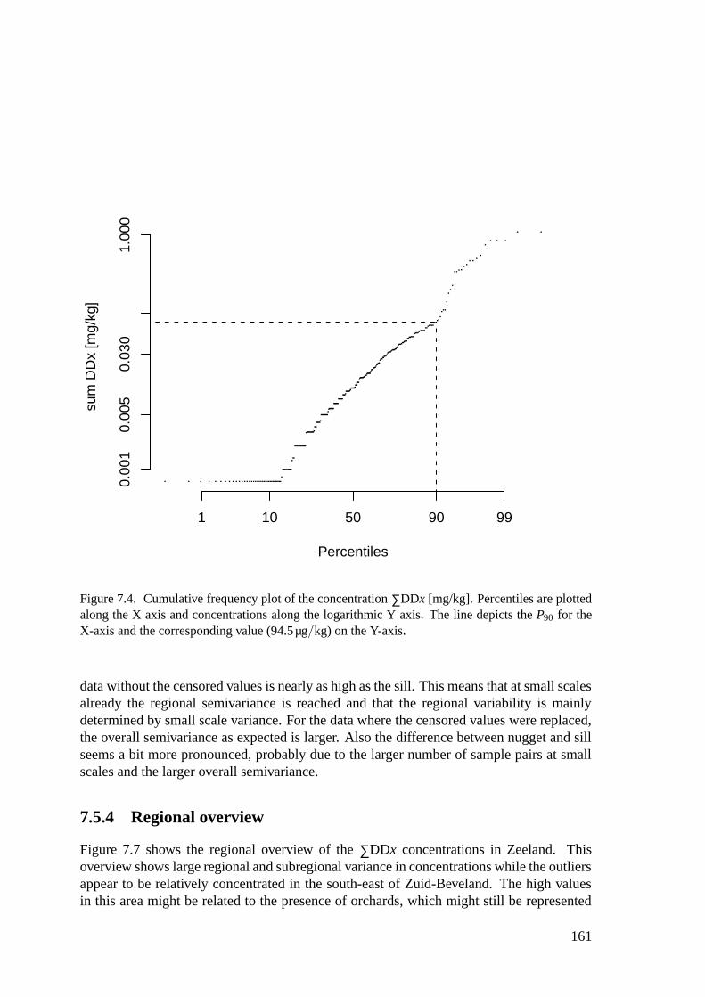
Percentiles
sum
DD
x [m
g/kg
]
1 10 50 90 99
0.00
10.
005
0.03
01.
000
Figure 7.4. Cumulative frequency plot of the concentration ∑DDx [mg/kg]. Percentiles are plottedalong the X axis and concentrations along the logarithmic Y axis. The line depicts the P90 for theX-axis and the corresponding value (94.5µg/kg) on the Y-axis.
data without the censored values is nearly as high as the sill. This means that at small scalesalready the regional semivariance is reached and that the regional variability is mainlydetermined by small scale variance. For the data where the censored values were replaced,the overall semivariance as expected is larger. Also the difference between nugget and sillseems a bit more pronounced, probably due to the larger number of sample pairs at smallscales and the larger overall semivariance.
7.5.4 Regional overview
Figure 7.7 shows the regional overview of the ∑DDx concentrations in Zeeland. Thisoverview shows large regional and subregional variance in concentrations while the outliersappear to be relatively concentrated in the south-east of Zuid-Beveland. The high valuesin this area might be related to the presence of orchards, which might still be represented
161
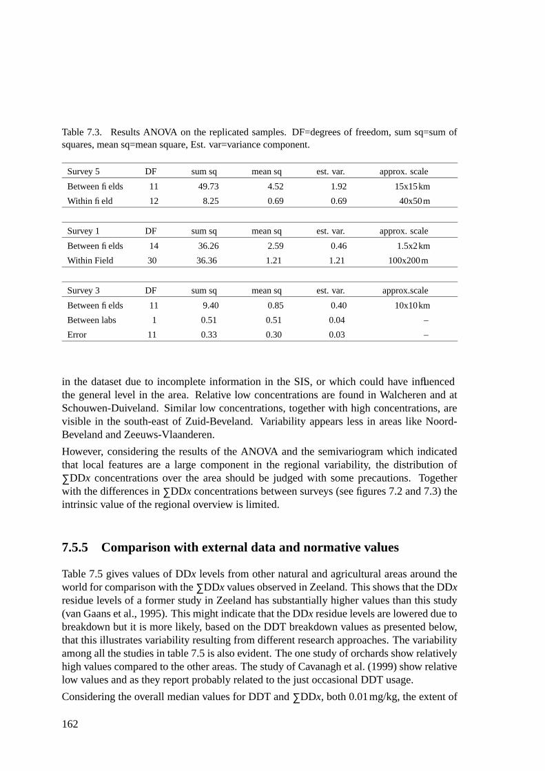
Table 7.3. Results ANOVA on the replicated samples. DF=degrees of freedom, sum sq=sum ofsquares, mean sq=mean square, Est. var=variance component.
Survey 5 DF sum sq mean sq est. var. approx. scale
Between fields 11 49.73 4.52 1.92 15x15km
Within field 12 8.25 0.69 0.69 40x50m
Survey 1 DF sum sq mean sq est. var. approx. scale
Between fields 14 36.26 2.59 0.46 1.5x2km
Within Field 30 36.36 1.21 1.21 100x200m
Survey 3 DF sum sq mean sq est. var. approx.scale
Between fields 11 9.40 0.85 0.40 10x10km
Between labs 1 0.51 0.51 0.04 –
Error 11 0.33 0.30 0.03 –
in the dataset due to incomplete information in the SIS, or which could have influencedthe general level in the area. Relative low concentrations are found in Walcheren and atSchouwen-Duiveland. Similar low concentrations, together with high concentrations, arevisible in the south-east of Zuid-Beveland. Variability appears less in areas like Noord-Beveland and Zeeuws-Vlaanderen.
However, considering the results of the ANOVA and the semivariogram which indicatedthat local features are a large component in the regional variability, the distribution of∑DDx concentrations over the area should be judged with some precautions. Togetherwith the differences in ∑DDx concentrations between surveys (see figures 7.2 and 7.3) theintrinsic value of the regional overview is limited.
7.5.5 Comparison with external data and normative values
Table 7.5 gives values of DDx levels from other natural and agricultural areas around theworld for comparison with the ∑DDx values observed in Zeeland. This shows that the DDxresidue levels of a former study in Zeeland has substantially higher values than this study(van Gaans et al., 1995). This might indicate that the DDx residue levels are lowered due tobreakdown but it is more likely, based on the DDT breakdown values as presented below,that this illustrates variability resulting from different research approaches. The variabilityamong all the studies in table 7.5 is also evident. The one study of orchards show relativelyhigh values compared to the other areas. The study of Cavanagh et al. (1999) show relativelow values and as they report probably related to the just occasional DDT usage.
Considering the overall median values for DDT and ∑DDx, both 0.01mg/kg, the extent of
162
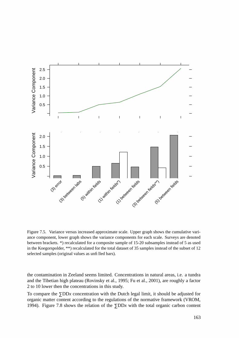
Var
ianc
e C
ompo
nent
(5) b
etwee
n fie
lds
(3) b
etwee
n fie
lds**)
(1) b
etwee
n fie
lds
(1) w
ithin
fields
*)
(5) w
ithin
fields
(3) b
etwee
n lab
s
(3) e
rror
0.5
1.0
1.5
2.0
Var
ianc
e C
ompo
nent
0.5
1.0
1.5
2.0
2.5
Figure 7.5. Variance versus increased approximate scale. Upper graph shows the cumulative vari-ance component, lower graph shows the variance components for each scale. Surveys are denotedbetween brackets. *) recalculated for a composite sample of 15-20 subsamples instead of 5 as usedin the Koegorspolder, **) recalculated for the total dataset of 35 samples instead of the subset of 12selected samples (original values as unfilled bars).
the contamination in Zeeland seems limited. Concentrations in natural areas, i.e. a tundraand the Tibetian high plateau (Rovinsky et al., 1995; Fu et al., 2001), are roughly a factor2 to 10 lower then the concentrations in this study.
To compare the ∑DDx concentration with the Dutch legal limit, it should be adjusted fororganic matter content according to the regulations of the normative framework (VROM,1994). Figure 7.8 shows the relation of the ∑DDx with the total organic carbon content
163
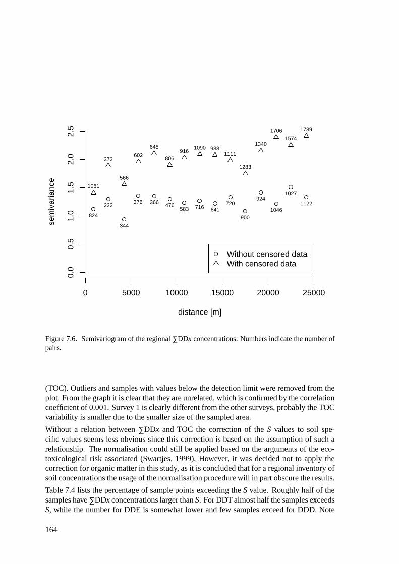
824
222
344
376 366 476583 716 641
720
900
924
1046
1027
1122
distance [m]
sem
ivar
ianc
e
0 5000 10000 15000 20000 25000
0.0
0.5
1.0
1.5
2.0
2.5
1061
372
566
602
645
806916
1090 9881111
1283
1340
1706
1574
1789
Without censored dataWith censored data
Figure 7.6. Semivariogram of the regional ∑DDx concentrations. Numbers indicate the number ofpairs.
(TOC). Outliers and samples with values below the detection limit were removed from theplot. From the graph it is clear that they are unrelated, which is confirmed by the correlationcoefficient of 0.001. Survey 1 is clearly different from the other surveys, probably the TOCvariability is smaller due to the smaller size of the sampled area.
Without a relation between ∑DDx and TOC the correction of the S values to soil spe-cific values seems less obvious since this correction is based on the assumption of such arelationship. The normalisation could still be applied based on the arguments of the eco-toxicological risk associated (Swartjes, 1999), However, it was decided not to apply thecorrection for organic matter in this study, as it is concluded that for a regional inventory ofsoil concentrations the usage of the normalisation procedure will in part obscure the results.
Table 7.4 lists the percentage of sample points exceeding the S value. Roughly half of thesamples have ∑DDx concentrations larger than S. For DDT almost half the samples exceedsS, while the number for DDE is somewhat lower and few samples exceed for DDD. Note
164
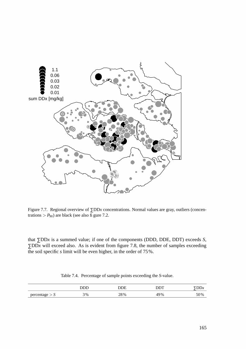
1.10.060.030.020.01
sum DDx [mg/kg]
Figure 7.7. Regional overview of ∑DDx concentrations. Normal values are gray, outliers (concen-trations > P90) are black (see also figure 7.2.
that ∑DDx is a summed value; if one of the components (DDD, DDE, DDT) exceeds S,∑DDx will exceed also. As is evident from figure 7.8, the number of samples exceedingthe soil specific s limit will be even higher, in the order of 75%.
Table 7.4. Percentage of sample points exceeding the S-value.
DDD DDE DDT ∑DDx
percentage > S 3% 28% 49% 50%
165

0.00
10.
005
0.05
00.
500
0 2 4 6 8
TOC [wt−%]
Sum
DD
x [m
g/kg
]
1234567
Figure 7.8. Relation of organic matter (TOC) and ∑DDx with outliers and not detected valuesnot shown. The solid line depicts the S value while the dashed line shows the soil specific s. Thecorrelation coefficient r is 0.001
7.5.6 DDT breakdown
For survey 1 and 5 not only is the ∑DDx available but also the separate parameters for DDT,DDE and DDD (both o,p and p,p), their relation is plotted in figure 7.9. This shows a strongcorrelation (r=0.935) between DDT and DDE and, using the medians, a DDE:DDT ratioof 0.5. The relation between DDT and DDD is less evident. For estimating the number ofhalf-lifes passed censored data were recalculated using equation 7.2.
By calculating a tT1
2
for each available sample, a range of values is obtained. The P25,
median, and P75 are 0.4, 0.6, and 0.8 respectively. It appears that the higher DDT valuestend to a t
T12
of 0.5, while lower values have higher tT1
2
(figure 7.2). This indicates that the
residue level is only about one half to two-thirds tT1
2
and implies that the breakdown is not
at the expected rate or that DDT applications occurred after the ban in 1973. The latter,
166
however, is very unlikely at such a large scale.
7.6 Discussion and conclusions
The combination of the different SIS derived datasets resulted in a database that can beused for a regional assessment. However, the differences between the surveys, although ingeneral based on the same sampling and analytical standards, are evident in the data. It ishard to determine if these differences denote differences in true ∑DDx soil values or thatthey are largely caused by the slight variations in field and laboratory methods.
The ∑DDx concentrations as found in Zeeland are comparable to those in similar agricul-tural areas, and based on these values there is no reason to believe that the current levelof DDT contamination is more severe than can be expected for an agricultural area. Com-pared to pristine areas the level in Zeeland is about a factor 2 to 10 higher, which indicatesZeeland can be regarded as enriched compared to a general ubiquitous ∑DDx background.Despite that the values are within a normal range for agricultural areas, the standard soilnormative threshold value S is exceeded for roughly half the cases and the soil specificvalue s in even more cases, which may result in litigations.
The relatively large contribution of local scale variability to the overall variability of ∑DDxconcentrations implies that a regional overview has limited value since most of the observedvariance can be regarded as noise caused by small scale features. This is both indicated bythe analysis of variance on replicate samples and by the nugget effect of the calculatedsemivariance.
Given both small scale variability and between survey bias, a final regional overview willcontain large uncertainties. Despite that large scale features appear visible, like the rela-tively higher concentrations in the south of Zuid-Beveland which are presumably caused bythe presence of orchards, these should be judged with caution. Extreme caution is neededwhen the values are compared with (soil specific) legal limits. Due to the uncertainty causedby the various sources of variability, such comparison might have very limited value.
The degradation level of DDT residues indicates that the Zeeland soils will remain a sourcefor ∑DDx longer than expected. Since it is not assumed that new applications of DDT willoccur, the monitoring of DDT residue levels could be cautionary. The most important issuewhich should be addressed is the reduction of variability in the monitoring data. Probablythe largest reduction can be obtained in more standardisation of field survey procedures, re-ducing the between survey bias. The small scale variance may be assessed by increasing thenumber of subsamples and sampling on smaller scales but this might be less cost-effectivethen reducing the between survey bias. However, policy and regulation based on these datashould always incorporate the uncertainties as a result of the remaining variability.
167
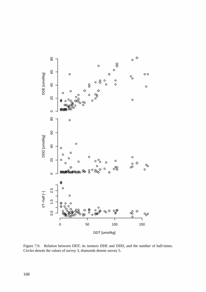
DD
E [u
mol
/kg]
020
4060
80
DD
D [u
mol
/kg]
020
4060
80
DDT [umol/kg]
t/T−
half
[−]
0 50 100 150
0.5
1.5
2.5
Figure 7.9. Relation between DDT, its isomers DDE and DDD, and the number of half-times.Circles denote the values of survey 3, diamonds denote survey 5.
168
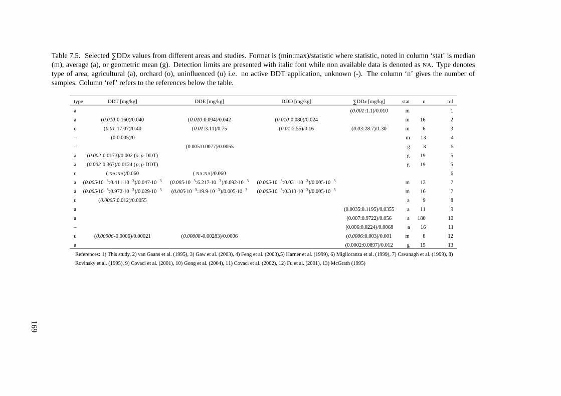
Table 7.5. Selected ∑DDx values from different areas and studies. Format is (min:max)/statistic where statistic, noted in column ‘stat’ is median(m), average (a), or geometric mean (g). Detection limits are presented with italic font while non available data is denoted as NA. Type denotestype of area, agricultural (a), orchard (o), uninfluenced (u) i.e. no active DDT application, unknown (-). The column ‘n’ gives the number ofsamples. Column ‘ref’ refers to the references below the table.
type DDT [mg/kg] DDE [mg/kg] DDD [mg/kg] ∑DDx [mg/kg] stat n ref
a (0.001 :1.1)/0.010 m 1
a (0.010 :0.160)/0.040 (0.010 :0.094)/0.042 (0.010 :0.080)/0.024 m 16 2
o (0.01 :17.07)/0.40 (0.01 :3.11)/0.75 (0.01 :2.55)/0.16 (0.03 :28.7)/1.30 m 6 3
– (0:0.005)/0 m 13 4
– (0.005:0.0077)/0.0065 g 3 5
a (0.002 :0.0173)/0.002 (o, p-DDT) g 19 5
a (0.002 :0.367)/0.0124 (p, p-DDT) g 19 5
u ( NA:NA)/0.060 ( NA:NA)/0.060 6
a (0.005·10−3:0.411·10−3)/0.047·10−3 (0.005·10−3:6.217·10−3)/0.092·10−3 (0.005·10−3:0.031·10−3)/0.005·10−3 m 13 7
a (0.005·10−3:0.972·10−3)/0.029·10−3 (0.005·10−3:19.9·10−3)/0.005·10−3 (0.005·10−3:0.313·10−3)/0.005·10−3 m 16 7
u (0.0005 :0.012)/0.0055 a 9 8
a (0.0035:0.1195)/0.0355 a 11 9
a (0.007:0.9722)/0.056 a 180 10
– (0.006:0.0224)/0.0068 a 16 11
u (0.00006 -0.0006)/0.00021 (0.00008 -0.00283)/0.0006 (0.0006 :0.003)/0.001 m 8 12
a (0.0002:0.0897)/0.012 g 15 13
References: 1) This study, 2) van Gaans et al. (1995), 3) Gaw et al. (2003), 4) Feng et al. (2003),5) Harner et al. (1999), 6) Miglioranza et al. (1999), 7) Cavanagh et al. (1999), 8)
Rovinsky et al. (1995), 9) Covaci et al. (2001), 10) Gong et al. (2004), 11) Covaci et al. (2002), 12) Fu et al. (2001), 13) McGrath (1995)
169

8 Synthesis
The aim of this thesis is to assess how patterns in the geochemical soil composition canbe used to distinguish natural variability from anthropogenic impact both in attribute andgeographical space. The patterns found in this study are related to processes determiningvariability in soil composition, including variability caused by human influence. The manysoil quality indicators presented can be used as a first initiative for sustainable managementof soil quality.
In the following I will evaluate the methods used, the achievements of this study, and givean overview of the implications of the results, together with possible future applications.
8.1 Methods used
The methods used in this study are in general based on state of the art analytical meth-ods combined with well established statistical techniques from the field of geochemicalsurveying and exploration. With the use of X-ray fluorescence spectrometry (XRF) andinductively coupled plasma mass spectrometry (ICP-MS) a broad range of elements couldbe analysed on many samples. For future comparison with data obtained from regular en-vironmental Dutch soil surveys, the ICP-MS samples were leached using a hot aqua-regiasolution. Both multi-element techniques were specifically chosen to broaden the analyti-cal focus with major components, trace elements, and the rare earth elements (REE). Thiswide range of components can be obtained with minimal extra effort compared to a smallerselection such as environmental priority metals. This resulted in a better understanding ofnot only the human effect but also of the natural composition and relations in the soil.
By using both techniques some overlap between measured components occurred, whichwas useful to obtain extra information about analytical quality and bias. Due to the differentapproaches of the techniques, partial aqua-regia leach for ICP-MS and total analysis forXRF, some basic mineralogical information was also obtained.
Using well established statistical techniques for data analysis has the advantage that possi-bilities and limitations are well known and that many examples are available. This makesthe techniques more transparent to the researcher and easily explainable to users. How-ever, more complex methods have not been avoided, such as robust principal componentsanalysis, so long as they provide a true advantage over standard techniques.
171
The methodology of this study incorporated several techniques to obtain information aboutthe accuracy, variability and bias on analytical and sampling scales and, if applicable, meth-ods to reduce noise and bias. It is essential to be able to distinguish the contribution ofgeochemical soil variability from that due to chemical analysis and sampling.
8.2 Achievements of this study
It was expected from the history of Zeeland that the soil contained slightly elevated concen-trations of so called “heavy metals” (Cd, Cu, Pb, and Zn) compared to pristine backgroundconcentration levels. Also persistent organochlorine pesticide residues were expected to bepresent. This is confirmed in this study.
It was shown that the spatial variability of the heavy metals, Fe, and calcite related com-ponents, has a relatively large contribution of local scale variance. This means that forthese components small scale variability is an important source of the total variation andcompositing for these elements is considered useful. For most other elements the regionalvariance predominates, reducing the need for compositing.
The main part of this study comprises the geochemical characterisation of the province. Themain hypotheses were that 1) based on insight into the natural variability the anthropogenicimprint could be recognised and 2) the subsoil is suitable for obtaining a geochemical base-line as a reference to calculate the anthropogenic impact. An additional question studiedwas if the imprint results in spatially distinct areas where specific human processes havehad a relevant contribution to the soil composition.
To test these hypotheses a dataset of 31 chemical components was selected from the overalldataset of 83 components, based on precision, accuracy and completeness. For this dataseta measurement was available for each variable at each location and for each depth, topsoiland subsoil. The dataset still comprised major, minor, and trace elements, providing a ref-erence for a wide range of components. It formed the core for the geochemical assessmentof the soils of Zeeland.
To determine the anthropogenic imprint it is necessary to have a reference, or baseline,comprising the natural soil composition. For the Netherlands it was believed that no goodbaseline existed (van der Meent et al., 1990), and reference values like the legal thresholdvalues are not considered representative for natural soil composition. When a true baselineis available, deviations from this baseline can be attributed to separate processes. Hu-man processes, for example the local application of fertilisers or atmospheric deposition ofcontaminants from remote areas, will in general lead to increased concentration levels, orenrichment, of certain components. Using a baseline, such enrichment can be determinedand the extent of the influence of the associated process can be assessed.
A good method for many elements to obtain a baseline is the use of the relation with Al2O3 .The correlation of an element with Al2O3 can indicate if the element is uninfluenced by hu-man processes. Overall higher correlations with Al2O3 in the subsoil in Zeeland confirmthe hypothesis that the subsoil can be used as a pristine, non-influenced, reference. Using
172
a regression model based on the subsoil relation of an element with Al2O3 , the extent ofthe enrichment of the topsoil can be quantified both in absolute terms and as ratio withthe subsoil baseline. The enrichment can be assessed using individual enrichments of soilcomponents or by the average enrichment, called the contamination index, of all compo-nents with elevated concentration. Despite the presence of enrichments for many elementsthe legal threshold level is not exceeded, thus the soils may be regarded as legally cleanwith regard to inorganic components. This implies also that the legal threshold values arenot a suitable reference for natural background soil concentrations. Compared to all othertechniques illustrated in chapter 5, the subsoil regression baseline method gives the bestinsight into 1) the geological/pedological pattern of geochemical variability, 2) randomnatural variation, and 3) the anthropogenic imprint on Zeeland soils.
The use of the above described baseline provides enrichments for individual elements basedon the covariability with only one other variable. To fully understand the soil factors thatdetermine the variability in soil composition a more multidimensional space must be con-sidered. Multi-element covariability (principal component analysis) revealed four mainfactors that can be related to clay, calcite, silt and anthropogenic processes. The naturalclay and calcite related processes comprise the largest part of the overall soil variability.The anthropogenic factor explains only a small part of the overall variability emphasisingthat these anthropogenic processes are really an imprint on the overall natural variability.Yet, for individual elements such as Sn, the antropogenic factor may explain up to about40% of the variance.
The regional patterns of both the contamination index and the scores on the anthropogenicfactor show many similarities. However, since the anthropogenic factor explains the vari-ability caused by human processes based on the total soil composition while the contam-ination index is an average of ratios from a few bivariate relations, I prefer the former.Nevertheless, enrichments or the contamination index can be quantified as concentrationsof individual components or average of more componenents, making it easier to comparethem with normative values and values from other areas.
When the samples in attribute space are grouped, i.e. based on their similarity with respectto interactions between the processes distinguised, no spatial regions emerge where sam-ples are discriminated solely on the basis of anthropogenic enrichment. This suggests thatthe extent of the human imprint on the Zeeland soil, is not related to certain regions butrather is distributed diffusely over the province.
Using the techniques and experience from the former chapters, chapter 7 gave an assess-ment of DDT residue levels based on separate datasets provided by the local authorities.Compared with other areas, the DDT residue concentrations in Zeeland are such that thereis no reason to believe that the DDT contamination is more severe than can be expectedof an agricultural area. The extent of the values compared to uninfluenced areas is abouta factor 2 to 10 higher, indicating that values for Zeeland must be regarded as enrichedcompared to the non-natural ubiquitous DDT residue background.
Unfortunately, a regional assessment of DDT residue values is hampered by the large con-tribution of small scale (sampling) variance. This means that for a regional overview the
173
observed variance is largly influenced by local scale noise. Together with the clear differ-ences between the sub datasets, this implies that the regional variability should be judgedwith caution, despite the fact that large scale features are still visible.
8.3 Implications
The collection of soil quality data over time is a prerequisite of sustainable management.With a dynamic assessment the direction and magnitude of change can be evaluated (Wien-hold et al., 2004). This study showed that with the use of state of the art analytical tech-niques and well established methods from geochemistry, a profound insight can be obtainedin a single survey into the natural soil composition and how it is influenced by human pro-cesses. This both provides methods to obtain a reference for natural soil composition andto quantify the anthropogenic imprint. It is shown in this study that the framework of le-gal limits does neither provides such a reference nor is able to detect subtle anthropogenicenrichment. This, in a way, is remarkable considering that this framework is also usedfor the building material decree and related to soil pollution risk maps that should preventspreading of contaminants. I therefore suggest that references for soil composition shouldbe derived from (local) baselines rather then legal limits. When obtaining such a baseline,quantification of the variability due to sampling and analytical procedures, and methods toreduce or compensate bias between sub-surveys are as important as the baseline itself. Ifmulti-element techniques are used, as most laboratories do, focus should not only be on en-vironmental priority components but also on components which might provide informationabout natural geochemical soil composition and variability.
Soil pollution risks appear to be, as defined in the Dutch normative framework, mainlydetermined by DDT residues. Unfortunately, the on average low concentrations in soil,complex analytical determination, and high small-scale variability result in large uncertain-ties concerning the regional variability of this component. Consequently, to obtain a moretrustworthy georeferenced overview of DDT residue levels, more effort aimed at reductionof variance and bias should be put in the assessment of this component.
The question remains what “soil quality” should mean for the Dutch situation and whichindicators to use. The definition of soil quality as given by Karlen et al. (1997): “thecapacity of a specific kind of soil to function, within natural or managed boundaries, tosustain plant and animal productivity, maintaining or enhance water and air quality, andsupport human health and habitation”, clearly implies not only a characterisation, but anevaluation against certain criteria as well. The so called “soil quality maps”, as used in theNetherlands to facilitate spatial development, clearly do not provide information about soilquality as envisaged by Karlen et al. (1997), despite their name. Therefore, one of the goalsto reach sustainable soil management should be a reconsideration of what is understood by“soil quality”. Only then it is possible to define which soil quality indicators should beassessed. The reference data and methods provided in this study could be a starting pointfor obtaining such indicators, finally leading towards sustainable soil management.
174
Bibliography
ABRAHAMS, P. W. (2002), Soils: their implications to human health. Science of the Total Environ-ment 291, pp. 1–32.
ALLEGRE, C. J. & E. LEWIN (1995), Scaling Laws and geochemical distributions. Earth and Plan-etary Science Letters 132, pp. 1–12.
ANONYMOUS (1999), Vrijstellingsregeling grondverzet. Staatscourant 180.BAUER, I. & J. BOR (1995), Lithogene, geogene und anthropogene Schwermetallgehalte von
Loßboden an den Beispielen von Kupfer, Zink, Nickel, Blei, Quecksilber und Cadmium. MainzerGeowiss. Mitt. 24, pp. 47–70.
BAUER, I., V. M. SPRENGER & J. BOR (1992), Die Berechnung lithogener und geogener Schwer-metallgehalte von Loßboden am Beispiel von Kupfer, Zink und Blei. Mainzer Geowiss. Mitt. 21,pp. 7–34.
BAZEN, M. (1987), Bodemkaart van Nederland 1:50.000. Toelichting bij de kaartbladen 48 OostMiddelburg en 49 West Bergen op Zoom. Stichting bodemkartering, Wageningen.
BEZDEK, J. C., R. EHRLICH & W. E. FULL (1984), FCM; The fuzzy c-means clustering algorithm.Computer & Geosciences 10, pp. 191–203.
BIANCHINI, G., R. LAVIANO, S. LOVO & C. VACCARO (2002), Chemical-mineralogical charac-terisation of clay sediments around Ferrara (Italy): a tool for an environmental analysis. AppliedClay Science 21, pp. 165–176.
BLASER, P., S. ZIMMERMANN, J. LUSTER & W. SHOTYK (2000), Critical examination of traceelement enrichments and depletions in soils: As, Cr, Cu, Ni, Pb, and Zn in Swiss forest soils.Science of the Total Environment 249, pp. 257–280.
BOLVIKEN, B., J. BOGEN, A. DEMETRIADES, W. DE VOS, J. EBBING, R. HINDEL,M. LANGEDAL, J. LOCUTERA, P. O’CONNOR, R. T. OTTESEN, E. PULKKINEN, R. SALMI-NEN, O. SCHERMANN, R. SWENNEN, J. VAN DER SLUYS & T. VOLDEN (1996), Regionalgeochemical mapping of Western Europe towards the year 2000. Journal of Geochemical Explo-ration 56, pp. 141–166.
BOUNESSAH, M. & B. P. ATKIN (2003), An application of exploratory analysis (EDA) as a ro-bust non-parametric technigue for geochemical mapping in a semi-arid climate. Applied Geo-chemistry 18, pp. 1185–1195.
BRAUNE, B., D. MUIR, B. DEMARCH, M. GAMBERG, K. POOLE, R. CURRIE, M. DODD,W. DUSCHENKO, J. EAMER, B. ELKIN, M. EVANS, S. GRUNDY, C. HEBERT, R. JOHN-STONE, K. KIDD, B. KOENIG, L. LOCKHART, H. MARSHALL, K. REIMER, J. ANDERSON
& L. SHUTT (1999), Spatial and temporal trends of contaminants in the Canadian Arctic fresh-water and terrestrial ecosytems: a review. Science of the Total Environment , pp. 145–207.
BRIDGES, E. M. & J. H. V. VAN BAREN (1997), Soil: an overlooked, undervalued and vital partof the human environment. The Environmentalist 17, pp. 15–20.
175

BURENKOV, E. K., A. A. GOLOVIN, I. MOROZOVA & E. I. FILATOV (1999), Multi-purposegeochemical mapping (1:1,000,000) as a basis for the integrated assessment of natural resourcesand ecological problems. Journal of Geochemical Exploration 66, pp. 159–172.
BURROUGH, P. A., P. F. M. VAN GAANS & R. HOOTSMANS (1997), Continuous classificationsin soil survey: spatial correlation, confusion and boundaries. Geoderma 77, pp. 115–135.
BUSINK, E. R. V. & S. POSTMA (2000), Provincial soil-quality monitoring networks in the Nether-lands as an instrument for environmental protection. Netherlands Journal of Geosciences 4, pp.429–440.
CARSON, R. (1962), Silent Spring. Houghton Mifflin Company, Boston.CAVANAGH, J. E., K. A. BURNS, G. J. BRUNSKILL & R. J. COVENTRY (1999), Organochlo-
rine pesticide residues in soils and sediments of the Herbert and Burdekin River regions, NorthQueensland: implications for contamination of the Great Barrier Reef. Marina pollution Bulletin39, pp. 367–375.
CHORK, C. Y. & R. SALMINEN (1993), Interpreting exploration geochemical data from Out-okumpu, FInland: A MVE-robust factor analysis. Journal of Geochemical Exploration 48, pp.1–20.
COCKER, M. D. (1999), Geochemical mapping in Georgia, USA: a tool for environmental studies,geologic mapping and mineral exploration. Journal of Geochemical Exploration 67, pp. 345–360.
COVACI, A., C. HURA & P. SCHEPENS (2001), Selected persistent organochlorine pollutants inRomania. Science of the Total Environment 280, pp. 143–152.
COVACI, A., P. MANIRAKIZA & P. SCHEPENS (2002), Persistent organochlorine pollutants insoils from Belgium, Italy, Greece, and Romania. Environmental Contamination and Toxicology68, pp. 97–103.
DANESHFAR, B. & E. CAMERON (1998), Leveling geochemical data between map sheets. Journalof Geochemical Exploration 63, pp. 189–201.
DARNLEY, A., A. BJORKLAND, B. BØLVIKEN, N. GUSTAVSSON, P. V. KOVAL, J. A. PLANT,A. STEENFELT, M. TAUCHID & X. XUEJING (1995), A global geochemical database for envi-ronmental and resource management. Final Report of IGCP Project 259, Unesco Publishing.
DARNLEY, A. G. (1995), International geochemical mapping, a review. Journal of GeochemicalExploration 55, pp. 5–10.
DAVIS, J. C. (2002), Statistics and Data Analysis in Geology. John Wiley and Sons, New York.DE GRUIJTER, J. J. & C. J. F. TER BRAAK (1990), Model-Free Estimation from Spatial Samples:
A Reappraisal of Classical Sampling Theory. Mathematical Geology 22, pp. 407–415.DE LOPEZ CAMELO, L. G., S. R. DE MIGUEZ & L. MARBAN (1997), Heavy metals input with
phosphate fertilizers used in Argentina. Science of the Total Environment 204, pp. 245–250.DE ROO, G. (2003), Environmental planning in the Netherlands: Too good to be true. Ashgate,
Hampshire.DE VOS, W., J. EBBING, R. HINDEL, J. SCHALICH, R.SWENNEN & I. V. KEER (1996), Geochem-
ical mapping based on overbank sediments in the heavily industrialised border area of Belgium,Germany and the Netherlands. Journal of Geochemical Exploration 56, pp. 91–104.
DIMOND, J. B. & R. B. OWEN (1996), Long-term residue of DDT compounds in forest soils inMaine. Environmental Pollution 92, pp. 227–230.
DORAN, J. W. (2002), Soil health and global sustainability: translating science into practice. Agri-culture, Ecosystems and Environment 88, pp. 119–127.
EDELMAN, T. (1984), Achtergrondgehalten van stoffen in de bodem. Staatsuitgeverij, Den Haag.EDWARDS, C. A. (1970), Persistent pesticides in the environment. CRC monoscience series, But-
terworths, London.
176
EIKELBOOM, R. T., E. RUWIEL & J. J. J. M. GOUMANS (2001), The Building Material Decree:an example of a Dutch regulation based on the potential impact of materials on the environment.Waste Management 21, pp. 295–302.
FACCHINELLI, A., E. SACCHI & L. MALLEN (2001), Multivariate statistical and GIS-based ap-proach to identify heavy metal sources in soils. Environmental Pollution 114, pp. 313–324.
FAO (1990), FAO-UNESCO soil map of the world, revised legend. Soils Bulletin 60, FAO, Rome.FENG, K., B. Y. YU, D. M. GE, M. H. WONG, X. C. WANG & Z. H. CAO (2003), Organo-
chlorine pesticide (DDT and HCH) residues in the Taihu Lake Region and its movement in soil-water system; I. Field survey of DDT and HCH residues in ecosystems of the region. Chemo-sphere 50, pp. 683–687.
FERREIRA, A., M. M. INACIO, P. MORGADO, M. J. BATISTA, L. FERREIRA, V. PEREIRA &M. S. PINTO (2001), Low-density geochemical mapping in Portugal. Applied Geochemistry 16,pp. 1323–1331.
FOLKES, D. J., T. E. KEUHSTER & R. A. LITLE (2001), Contributions of pesticide use to urbanbackground concentrations of arsenic in Denver, Colorado, U.S.A. Environmental Forensics 2,pp. 127–139.
FU, S., S. CHU & S. XU (2001), Organochlorine pesticide residue in soils from Tibet. Bulletin ofEnvironmental Contamination and Toxicology 2001, pp. 171–177.
GARRETT, R. G. (1983), Sampling Methodology. In: R. J. Howarth, ed., Handbook of explorationgeochemistry. Volume 2: statistics and data analysis in geochemical prospecting, Elsevier Sci-ence.
GARRETT, R. G. & T. I. GOSS (1979), The Evaluation of Sampling and Analytical variation inRegional Geochemical Surveys. In: J. R. Watterson & P. K. Theobald, eds., Geochemical Explo-ration 1978, Association of Exploration Geochemists, Rexdale.
GARRETT, R. G. & T. I. GOSS (1980), Uanova: A FORTRAN IV program for unbalanced nestedanalysis of variance. Computer & Geosciences 6, pp. 35–60.
GAW, S. K., G. PALMER, N. D. KIM & A. L. WILKINS (2003), Preliminary evidence that copperinhibits the degradation of DDT to DDE in pip and stonefruit orchard soils in the Aucklandregion, New Zealand. Environmental pollution 122, pp. 1–5.
GIMENO-GARCIA, E., V. ANDRUE & R. BOLUDA (1996), Heavy metals incidence in the applica-tion of inorganic fertilizers and pesticides to rice farming soils. Environmental Pollution 92, pp.19–25.
GOEMANS, T. & T. VISSER (1987), The Delta Project; The Netherlands experience with amegaproject for flood protection. Technology in Society 9, pp. 97–111.
GONG, Z. M., S. TAO, F. L. XU, R. DAWSON, W. X. LIU, Y. H. CUI, J. CAO, X. J. WANG,W. R. SHEN, W. J. ZHANG, B. P. QING & R. SUN (2004), Level and distribution of DDT insurface soils from Tianjin, China. Chemosphere 54, pp. 1247–1253.
GREGORAUSKIENE, V. & V. KADUNAS (1997), Experience and goals of geochemical mapping forenvironmental protection in Lithuania. Journal of Geochemical Exploration 60, pp. 67–76.
GROOT, M. S. M., J. J. B. BRONSWIJK & T. V. VAN LEEUWEN (2001), Landelijk meetnetbodemkwaliteit, resultaten 1996. rapport nr. 714801026, Rijksinstitiuut voor Volksgezondheiden Milieu.
GUSTAVSON, N., E. LAMPIO & T. TARVAINEN (1997), Visualisation of geochemical data on mapsat the Geological Survey of Finland. Journal of Geochemical Exploration 59, pp. 197–207.
HALE, M. & R. KUHNEL (1997), Exploration of contaminated soils and sediments. Applied ClayScience 11, pp. 373–380.
HALFWERK, W. (1996), Natuur in Zeeland, tussen Zee en Zoom (Nature in Zeeland, between sea
177
and zoom). De Koperen Tuin, Goes.HANESCH, M., R. SCHOLGER & M. J. DEKKERS (2001), The application of fuzzy c-means cluster
analysis and non-linear mapping to a soil data set for the detection of polluted sites. PhysicalChemical Earth 26, pp. 885–891.
HARNER, T., J. L. WIDEMAN, L. M. M. JANTUNEN, T. F. BIDLEMAN & W. J. PARKHURST
(1999), Residues of organochlorine pesticides in Alabama soils. Environmental Pollution 106,pp. 323,332.
HEIJBOER, D. & J. NELLESTIJN (2002), Klimaatatlas van Nederland: de normaalperiode 1971-2000. Elmar, Rijswijk.
HOWARD, P. H. (1991), Environmental degradation rates. Lewis Publishers, Michigan.HUISMAN, D. J., F. J. H. VERMEULEN, J. BAKER, A. VELDKAMP, S. B. KROONENBERG &
G. T. KLAVER (1997), A geological interpretation of heavy metal concentrations in soils andsediments in the southern Netherlands. Journal of Geochemical Exploration 59, pp. 163–174.
JOURNEL, A. G. & C. J. HUIJBREGTS (1981), Mining Geostatistics. Academic Press, London.KARLEN, D. L., M. J. MAUSBACH, J. W. DORAN, R. G. CLINE, R. F. HARRIS & G. E. SCHU-
MAN (1997), Soil quality: a concept, definition, and framework for evaluation. Journal Soil Sci-ence Society of America 61, pp. 4–10.
KHATREE, R., D. N. NAIK & R. L. MASON (1997), Estimation of variance components in staggerdnested designs. Journal of Applied Statistics 24, pp. 395–408.
KIM, J.-H. & A. SMITH (2001), Distribution of organochlorine pesticides in soils from SouthKorea. Chemosphere 43, pp. 137–140.
KOELEMAN, M., W. J. VAN DER LAAK & H. IETSWAART (1999), Dispersion of PAH and heavymetals along motorways in the Netherlands: an overview. Science of the Total Environment 235,pp. 347–349.
KRAMAR, U. (1995), Application of limited fuzzy clusters to anomaly recognition in complexgeological environments. Journal of Geochemical Exploration 55, pp. 81–92.
LEENAERS, H., J. DE BOER, D. BOELS., M. HOOGERWERF & A. WEENK (1999), Bodemk-waliteitsbeeld 2005: de lokale en regionale informatiebehoefte. Tech. Rep.
LICHT, O. A. B. & T. TARVAINEN (1996), Multipurpose geochemical maps produced by integra-tion of geochemical exploration data sets in The Parana Shield, Brazil. Journal of GeochemicalExploration 56, pp. 167–182.
MATSCHULLAT, J., R. OTTENSTEIN & C. REIMANN (2000), Geochemical background - can wecalculate it? Environmental Geology 39, pp. 990–1000.
MCBRATNEY, A. B. & I. O. A. ODEH (1997), Application of fuzzy sets in soils science: fuzzylogic, fuzzy measurements and fuzzy decisions. Geoderma 77, pp. 85–113.
MCGRATH, D. (1995), Organic micropollutant and trace element pollution of Irish soils. Scienceof the Total Environment 164, pp. 125–133.
MCGRATH, D. & C. ZHANG (2003), Spatial distribution of soil organic carbon concentrations ingrassland of Ireland. Applied Geochemistry 18, pp. 1629–1639.
MEGHARAJ, M., H. L. BOUL & J. H. THIELE (1999), Effects of DDT and its metabolites on soilalgae and enzymatic activity. Biol Fertil Soils 29, pp. 130–134.
MIESCH, A. T. (1975), Variograms and variance components in geochemistry and ore evaluation.In: E. H. T. Whitten, ed., Quantative studies in the geological sciences - A memoir in honor ofWilliam C. Krumbein, vol. 142 of Geological Society of America.
MIESCH, A. T. (1976), Geochemical survey of Missouri: methods of sampling, laboratory analysisand statistical reduction of data. U.S. Geol. survey prof. paper .
MIGLIORANZA, K. S. B., J. E. A. DE MORENO, V. J. MORENO, M. L. OSTERRIETH & A. H.
178
ESCALANTE (1999), Fate of organochlorine pesticides in soils and terrestial biota of Los Padrespond watershed, Argentina. Environmental Pollution 105, pp. 91–99.
MOL, G. (2002), Soil acidification monitoring in the Netherlands. Ph.D. thesis, Faculty of EarthSciences, Utrecht University.
MOL, G., S. P. VRIEND & P. F. M. VAN GAANS (2001), Environmental monitoring in the Nether-lands: past developments and future challenges. Environmental Monitoring and Assessment 68,pp. 313–335.
MOSIER, A. R. (1998), Soil processes and global change. Biol. Fertil. Soils 27, pp. 221–229.NASH, D., D. HALLIWELL, M. HANNAH, L. CLEMOW & B. WEBB (2003), Phosporus and se-
lected metals mobilized from two commercial fertilizers into overland flow during border irriga-tion. Nutrient Cycling in Agroecosystems 67, pp. 255–264.
NIEROP, T. M. (2000), Samen slim met water; Waterhuishoudplan 2001-2007. Tech. Rep., Provin-cie Zeeland.
NIKKARINEN, M., E. KAUNISKANGAS & K. NENONEN (1996), Use of geological and geochem-ical data for the derivation of maps for environmental planning in Iisalmi, Finland. Applied Geo-chemistry 11, pp. 261–270.
NNI (1999a), NEN 5734: Bepaling van het gehalte PCB’s en OCB’s in grond. Tech. Rep., Neder-lands Normalisatie Instituut (NNI).
NNI (1999b), NEN 5740: Bodem-onderzoeksstrategie bij verkennend onderzoek. Tech. Rep., Ned-erlands Normalisatie Instituut (NNI).
NORTCLIFF, S. (1978), Soil Variability and Reconnaissance Soil Mapping: A Statistical Study inNorfolk. Journal of Soil science 29, pp. 403–418.
NORTCLIFF, S. (2002), Standardisation of soil quality attributes. Agriculture, Ecosystems and En-vironment 88, pp. 161–168.
OLIVER, M. A. & A. L. KHAYRAT (2001), A geostatistical investigation of the spatial variation ofradon in soil. Computer & Geosciences 27, pp. 939–957.
OLIVER, M. A. & R. WEBSTER (1986), Combining nested and linear sampling for determingthe scale and form of spatial variation of regionalized vaiables. Geographical Analysis 18, pp.227–242.
ORGANISATION, W. H. (1989), Environmental Health Criteria 83. DDT and its derivates- Environ-mental aspects. Tech. Rep.
PARKPIAN, P., S. T. LEONG, P. LAORTANAKUL & N. THUNTHAISONG (2003), Regional monitor-ing of lead and cadmium contamination in a tropical grazing land site, Thailand. EnvironmentalMnitoring and Assessment 85, pp. 157–173.
PEBESMA, E. J. & C. G. WESSELING (1998), Gstat: A program for geostatistical modelling,prediction and simulation. Computer & Geosciences 24, pp. 17–31.
PETTITT, A. N. & A. B. MCBRATNEY (1993), Sampling Designs for Estimating Spatial VarianceCOmponents. Applied Statistics 42, pp. 185–209.
PISON, G., P. J. ROUSSEEUW, P. FILZMOSER & C. CROUX (2003), Robust factor analyses. Journalof Multivariate Analysis 84, pp. 145–172.
PLEIJTER, G. & C. WALLENBURG (1994), Bodemkaart van Nederland 1:50.000. Toelichtingbij de kaartbladen 42 West en 42 Oost Zierikzee, 47/48 West Cadzand/Middelburg. DLO-Staringcentrum, Wageningen.
POLITOV, S. V., Y. A. ANOKHIN & N. N. SURNINA (2000), Organochlorine pesticides and poly-chlorinated biphenyls in the environment of the Baikal region. Aquatic Ecosystems Health andManagement 3, pp. 235–238.
R DEVELOPMENT CORE TEAM (2004), R: A language and environment for statistical com-
179

puting. R Foundation for Statistical Computing, Vienna, Austria. ISBN 3-900051-00-3, URLhttp://www.R-project.org.
RAPANT, S., M. RAPOSOVA, D. BODIS, K. MARSINA & I. SLANINKA (1999), Environmental-geochemical mapping program in the Slovak Republic. Journal of Geochemical Exploration 66,pp. 151–158.
REIMANN, C. & P. FILZMOSER (1999), Normal and lognormal data distribution in geochemistry:death of a myth. Consequences for the statistical treatment of geochemical and environmentaldata. Environmental Geology 39, pp. 1001–1014.
REIMANN, C., P. FILZMOSER & R. G. GARRETT (2002), Factor analysis applied to regionalgeochemical data: problems and possibilities. Applied Geochemistry 17, pp. 185–206.
RIDGWAY, J., N. BREWARD, W. J. LANGSTON, R. LISTER, J. G. REES & S. M. ROWLATT
(2003), Distinguishing between natural and anthropogenic sources of metals entering the IrishSea. Applied Geochemistry 18, pp. 283–309.
RIJKSWATERSTAAT (1971), Beschrijving van de provincie Zeeland behorende bij de water-staatskaart. Tech. Rep., Directie Algemene Dienst van de Rijkswaterstaat.
RIVM (2004), Milieu- en Natuurcompendium. Tech. Rep., RIVM-MNP, Bilthoven; CBS, DenHaag; Stichting DLO, Wageningen. URL http://www.milieuennatuurcompendium.nl.
ROSE, A. W., H. E. HAWKES & J. S. WEBB (1979), Geochemistry in mineral exploration. Aca-demic Press, London.
ROUSSEEUW, P. J. & K. VAN DRIESSEN (1999), A fast algorithm for the minimum covariancedeterminant estimator. Technometrics 41, pp. 212–223.
ROVINSKY, F., B. PASTUKHOV, Y. BOUYVOLOV & L. BURTSEVA (1995), Present day state ofbackground pollution of the natural environment in the Russian Arctic in the region of the UST-Lena Reserve. Science of the Total Environment 160/161, pp. 193–199.
RUTTEN, K. (2004), een vergelijking van de geochemie en bodemkunde van Zeeland. Master’sthesis, Utrecht University, department of geosciences.
SALMINEN, R. & V. GREGORAUSKIENE (2000), Consideration regarding the definition of ageochmical baseline of elements in the surficial meterials in areas differing in basic geology.Applied Geochemistry 15, pp. 647–653.
SALMINEN, R. & T. TARVAINEN (1995), Geochemical mapping and databases in Finland. Journalof Geochemical Exploration 55, pp. 321–27.
SALMINEN, R. & T. TARVAINEN (1997), The problem of defining geochemical baselines. A casestudy of selected elements and geological materials in Finland. Journal of geochemical explo-ration 60, pp. 91–98.
SCANCAR, J., R. MILACIC & M. HORVAT (2000), Comparison of various digestion and extractionprocedures in analysis of heavy metals in sediments. Water, Air and Soil Pollution 118, pp. 87–99.
SEARLE, S. R., G. CASELLA & C. E. MCCULLOCH (1992), Variance Components. John Wiley &Sons.
SELINUS, O. S. & K. ESBENSEN (1995), Separating anthropogenic from natural anomalies inenvironmental geochemistry. Journal of Geochemical Exploration 55, pp. 55–66.
SENESI, G. S., G. BALDASSARRE, N. SENESI & B. RADINA (1999), Trace elements inputs intosoils by anthropogenic activities and implications for human health. Chemosphere 39, pp. 343–377.
SHARMA, V. K., K. B. RHUDY, J. C. CARGILL, M. E. TACKER & F. G. VAZQUEZ (2000), Metalsand grain size distributions in soil of the middle Rio Grande basin, Texas USA. EnvironmentalGeoloy 39, pp. 698–704.
180
SHOTYK, W., D. WEISS, J. D. KRAMERS, R. FREI, A. K. CHEBURKIN, M. GLOOR & S. REESE
(2001), Geochemistry of the peat bog at Etang de la Gruere, Jura Mountains, Switserland, and itsrecord of atmospheric Pb and lithogenic trace metals (Sc, Ti, Y, Zr, and REE) since 12,370 14Cyr BP. Geochmica et Cosmochimica Acta 65, pp. 2337–2360.
SINCLAIR, A. J. (1976), Applications of probability graphs in mineral exploration. Association ofExploration Geochemists.
SINGH, D. K. & H. C. AGARWAL (1992), Chemical release and nature of soil-bound DDT-residues. Journal of Agricultural Food Chemistry 40, pp. 1713–1716.
SINGH, M., G. MULLER & I. B. SING (2001), Geogenic distribution and baseline concentration ofheavy metals in sediments of the Ganges River, India. Journal of Geochemical Exploration 80,pp. 1–17.
SPOSITO, G. (1989), The Chemistry of Soils. Oxford University Press.STERCKEMAN, T., F. DOUAY, D. BAIZE, H. FOURRIER, N. PROIX & C. SCHVARTZ (2004),
Factors affecting trace element concentrations in soils developed on recent maine deposits fromNorthern France. Applied Geochemistry 19, pp. 89–103.
STIBOKA (1964), Bodemkaart van Nederland 1:50.000. Toelichting bij kaartblad 43 West Willem-stad. Stichting voor Bodemkartering, Wageningen.
STIBOKA (1967), Bodemkaart van Nederland 1:50.000. Toelichting bij kaartblad 53 Sluis en 54West Terneuzen. Stichting voor Bodemkartering, Wageningen.
STIBOKA (1980), Bodemkaart van Nederland 1:50.000. Toelichting bij kaartblad 54 OostTerneuzen, 55 Hulst en het Zeeuws-Vlaamse deel van de kaartbladen 48 Oost Middelburg, 49West Bergen op Zoom. Sluis en 54 West Terneuzen. Stichting voor Bodemkartering, Wagenin-gen.
SWARTJES, F. A. (1999), Risk-based assessment of soil and groundwater quality in the netherlands:standards and remediation urgency. Risk Analysis 19, pp. 1235–1249.
SWENNEN, R. & J. VAN DE SLUYS (2002), Anthropogenic impact on sediment composition andgeochemistry in vertical overbank profiles of river alluvium from Belgium and Luxembourg.Journal of Geochemical Exploration 75, pp. 93–105.
SZAVA-KOVATS, R. C. (2002), Outlier-resistant errors-in-variables regression: anomaly recogni-tion and grain-size correction in stream sediments. Applied Geochemistry 17, pp. 1149–1157.
TACK, F. M. G., M. G. VERLOO, L. VANMECHELEN & E. V. RANST (1997), Baseline concentra-tion levels of trace elements as a function of clay and organic carbon contents in soils in Flanders(Belgium). Science of the Total Environment 201, pp. 113–123.
TAO, S. (1998), Factor score mapping of soil trace element contents for the Shenzen Area. Water,Air and Soil Pollution 102, pp. 415–425.
TEBBENS, L. A., A. VELDKAMP & S. B. KROONENBERG (2000), Natural compossitional varia-tion of the river Meuse (Maas) suspended load: a 13 ka bulk geochemical record from the upperKreftenheye and Betuwe Formations in Northern Limburg. Geologie en Mijnbouw/NetherlandsJournal of Geosciences 79, pp. 391–409.
TSOLAKIDOU, A., J. B. I GARRIGOS & V. KILIKOGLOU (2002), Assessment of dissolution tech-niques for the analysis of ceramic samples by plasma spectrometry. Analytca Chimica Acta 474,pp. 177–188.
TUKEY, J. W. (1977), Exploratory data analysis. Addison-Wesley, Philipines.URBAT, M., M. J. DEKKERS & S. P. VRIEND (1997), Fuzzy c-means clustering as an aid in the
interpretation of the natural remanent magnetization in various types of sediments. In: G. V.Pawlowsky, ed., Proceedings of IAMG ’97: Third annual conference of the International Asso-ciation for Mathematical Geology.
181
VAN DEN BERG, G. A. & J. P. G. LOCH (2000), Decalcification of soils subject to periodic water-logging. Journal of Soil Science 51, pp. 27–33.
VAN DER GAAST, N., H. LEENAERS & J. ZEGWAARD (1998), The grey areas in soil pollutionrisk mapping. The distinction between cases of soil pollution and increased background levels.Journal of Hazardous Materials 61, pp. 249–255.
VAN DER MEENT, D., T. ALDENBERG, J. H. CANTON, C. A. M. VAN GESTEL & W. SLOOFF
(1990), Desire for Levels. rapport nr 670101002, Rijksinstitiuut voor Volksgezondheid en Milieu.VAN DER SLUIS, P., G. G. STEUR & I. OVAA (1965), De bodem van Zeeland, Toelichting bij blad
7 bodemkaart van Nederland, schaal 1:200.000. Stiboka, Wageningen.VAN DER WEIJDEN, C. H. (2002), Pitfalls of normalization of marine geochemical data using a
common divisor. Marine Geology 184, pp. 167–187.VAN DIJK, D. & V. J. G. HOUBA (2000), Homogenity and Stability of Materials Distributed Whitin
the Wageningen Evaluating Programmes for Analytical Laboratories. Communications in SoilScience and Plant Analysis 31, pp. 1745–1756.
VAN DRECHT, G., L. J. M. BOUMANS, D. FRATERS, H. F. R. REIJNDERS & W. VAN DUIJVEN-BODEN (1996), Landelijke beelden van diffuse metaalbelasting van de bodem en de metaalge-halten in de bovengrond, alsmede de relatie tussen gehalten en belasting. rapport nr. 714801006,Rijksinstitiuut voor volksgezondheid en milieu.
VAN GAANS, P. F. M., S. P. VRIEND, S. BLEYERVELD, G. SCHRAGE & A. J. VOS (1995),Assessing Enviromental Soil Quality in Rural Areas, a base line study in the Province of Zeeland,the Netherlands and reflections on soil monitoring network design. Enviromental Monitoring andAssesment 34, pp. 73–102.
VAN GAANS, P. M. & S. P. VRIEND (1996), PAK en de verspreiding van onderhoudsbaggerspecieover landbouwpercelen. Tech. Rep. ISBN 90-71577-96-1.
VAN HELVOORT, P. J. (2003), Complex confining layers. A physical and geochemical chracter-ization of heterogeneous unconsolidated fluvial deposits using a facies-based approach. Ph.D.thesis, Dutch geographical Studies.
VAN LIENEN, F., G. FRAPPORTI & A. STEIN (2000), Construction of maps for soil recycling inregional infrastructural works integrating soil-quality laws. Netherlands Journal of Geosciences4, pp. 449–457.
VENABLES, W. N. & B. D. RIPLEY (2002), Modern Applied Statistics with S. Fourth Edition.Springer.
VILLA, S., M. VIGHI, V. MAGGI, A. FINIZIO & E. BOLZACCHINI (2003), Historical trends oforganochlorine pesticides in an alpine glacier. Journal of Atmospheric Chemistry 46, pp. 295–311.
VOS, P. C. & R. M. VAN HEERINGEN (1997), Holocene geology and occupation history of theProvince of Zeeland (SW Netherlands). In: M. M. Fischer, ed., Holocene evolution of Zeeland(SW Netherlands), vol. 59 of Medelingen Nederlands Instituut voor Toegepaste geowetenschap-pen, Netherlands institute of appplied geosciences TNO.
VRIEND, S. P., P. F. M. VAN GAANS, J. MIDDELBURG & A. DE NIJS (1988), The application offuzzy c-means cluster analysis and non-linear mapping to geochemical datasets: examples fromPortugal. Applied Geochemistry 3, pp. 213–224.
VROM (1994), circulaire streef en interventiewaarden. rapport nr. DBO/0749013, Ministerie vanVROM.
VROM (1997), Nationaal milieubeleidsplan 3. Tech. Rep., Ministry of Housing, Spatial Planningand the Environment, The Netherlands.
VROM (1999), Interim Richtlijn. Opstellen en toepassen bodemkwaliteitskaarten in het kader van
182
de Vrijstellingsregeling grondverzet. Beleidsstuk, Ministerie van VROM.WALSH, J. N., R. GILL & M. F. THIRLWALL (1997), Dissolution procedures for geological and en-
vironmental samples. In: Modern analytical geochemistry, an introduction to quantitative chem-ical analysis for earth, environmental and materials scientists., Addison Wesley Longman Ltd,Harlow, UK, pp. 29–40.
WEBSTER, R. (1985), Quantitative spatial analysis of soil in the field. In: Stewart, ed., Advancesin Soil Sciences, vol. 3, Springer Verlag.
WEBSTER, R. & M. A. OLIVER (1990), Statistical methods in soils and land resource survey.Oxford University Press.
WEDEPOHL, K. H. (1995), The composition of the continental crust. Geochemica CosmochemicaActa 59, pp. 1217–1232.
WIENHOLD, B. J., S. ANDREWS & D. L. KARLEN (2004), Soil quality: a review of the scienceand experiences in the USA. Environmental Geochemistry and Health 26, pp. 89–95.
WILCKE, W., S. MULLER, N. KANCHANAKOOL & W. ZECH (1998), Urban soil contamination inBangkok: heavy metal and aluminium partitioning in topsoils. Geoderma 86, pp. 211–228.
YOUDEN, W. J. & A. MEHLICH (1937), Selection of efficient methods for soil sampling. Contr.Boyce Thompson Inst. Plant. Res. 9, pp. 59–70.
ZAGWIJN, W. H. (1991), Nederland in het Holoceen. Staatsuitgeverij, Den Haag.ZITKO, V. (2003), Chlorinated pesticides: Aldrin, DDT, Endrin, Dieldrin, Mirex. In: H. Fiedler,
ed., Persistent Organic Pollutants, Springer-Verlag, Berlin Heidelberg.
183

Abstract - Geochemical patterns in thesoils of Zeeland, natural variability ver-sus anthropogenic impact
Chapter 1. Introduction
The close relation between soil, health, and global sustainability confirm that soil plays acritical role as a major interface in our environment and that soil quality can be an importantindicator for sustainable environmental management.
This thesis is concerned with obtaining an overview of general (geo)chemical soil quality,within the framework of diffuse anthropogenic pollution and sustainable soil managementin the Netherlands. It aims at assessing patterns in the geochemical soil composition anddistinguishing the natural variability from the anthropogenic impact. The variability isassessed in geographical space, in which the spatial interaction of soil components takesplace, and in attribute space, the space where interaction between soil constituents is ex-posed. Patterns from both spaces can then be related to processes influencing the soilcomposition.
Based on these patterns, and related processes, anthropogenic influence can be distin-guished from natural variability. This can provide tools and information which can bepart of the country wide overview needed as required by the Dutch government in theirnational environmental policy plan (NEPP 3).
The Province of Zeeland in the south west of the Netherlands was the area chosen for thisresearch. The large rural area of young Holocene deposits and rich human history makeit a suitable area for testing the main hypothesis that human influence leaves a distinctand quantifiable pattern of soil pollutants, based on variability within the geographical andattribute space of the soil composition.
Chapter 2. Geology and pedology of Zeeland
Zeeland is located in the marine delta of the rivers Rijn, Maas en Schelde. It was the sealevel rise following the end of the Weichselian ice age that brought Zeeland within the
185
marine realm. The soils of Zeeland can be regarded as relatively homogeneous and young.They were moulded in a continuous interaction of natural processes and human endeavour.
Considering the fact that soils of Zeeland are in general developed in marine clay deposits,it can be expected that a main source of geochemical variability is the varying clay content.The natural pattern of creek ridges and pool grounds creates relatively abrupt transitions.As local homogeneity or gradual variation may be further disturbed by extensive humanactivity, variability in soil composition is expected to be still higher than is directly evi-dent from the soil map. Each (embanked) area with its own history, both sedimentary andhuman, may have its own pattern of soil variability. Given the fact that 80% of terres-trial Zeeland is used for agriculture, nearly 70% of which is arable land, human processesrelated to fertilisation and pesticide use are further expected to have influenced soil com-position. This will result in elevated concentrations of so called “heavy metals” (Cd, Cu,Pb, and Zn) and persistent organochlorine pesticide residues. Finally, atmospheric inputsshould also be considered as contributing to soil geochemistry.
Chapter 3. Natural and anthropogenic patterns of covari-ance and spatial variability of minor and trace elements inagricultural topsoil
The aim of this chapter was to analyze the sources of variation in soil geochemical com-position related to spatial scale and sampling procedure. Apart from an intrinsic interest,research was motivated by practical questions regarding sampling strategies, using singleor composite samples, for regional soil surveys. An unbalanced nested sampling design,based on single samples, was implemented at Walcheren/Zuid-Beveland. The sampleswere digested with aqua regia and analyzed by ICP-MS. The resulting data for 40 elementswere examined through principal component analysis in combination with varimax rota-tion (PCA-V), unbalanced analysis of variance (UANOVA) and a fuzzy c-means clusteringof the UANOVA results. The increase in noise when using single samples was further as-sessed through comparison with results of a previous study in the area based on compositesamples. The three factors of the PCA-V are interpreted as being the results of natural,human, and geohydrological processes. The UANOVA analysis distinguishes three spatialvariance patterns. Two groups show a gradual increase of variance with distance and con-tain respectively clay/feldspar related elements and heavy rare earth elements. The thirdgroup encompasses all anthropogenically and geohydrologically influenced elements witha larger part of the variance at small scales.
In general regional variance predominates over local variance and the extra effort of com-positing is of limited value for a regional survey. However, environmental priority metalslike Cd, Cu, Pb, Sb, Sn and Zn, were found to have larger local variance components. Forthese elements compositing is relatively more beneficial.
186
Chapter 4. Sampling and analyses for a regional environ-mental soil geochemical survey
When assessing soil composition for individual concentrations of elements it is often diffi-cult to distinguish anthropogenic effects from natural variation. Establishing a bivariate ormultivariate geochemical baseline, that incorporates a major part of natural variability, is anaccepted method to derive background concentrations. Divergence from this backgroundmight then be caused by human disturbance. To quantitatively assess which componentsare affected by human activities, a consistent regional dataset is needed where special at-tention is paid to quantifying data quality. This chapter documents the construction of sucha dataset for the province of Zeeland.
The sampling design was aimed at sampling present-day soil and pristine soil concentra-tions by sampling an influenced topsoil layer and an assumed pre-anthropogenic deepersubsoil layer at a density of 1 sample per 1-10km2. The analytical methods used (ICP-MS with aqua regia digestion and XRF on pressed powder tablets) and the broad groupof elements measured (major elements like Al2O3 and Fe2O3 , anthropogenically affectedelements like Cd, Pb, Sb, trace elements like the REE) resulted in a data set of 87, partlyoverlapping, parameters. Each group of elements is thought to provide specific informationon natural variation, human influence, or their interaction, as will the comparison betweentop and subsoil.
Precision was estimated by analysing about 15% of the ICP-MS samples and about 4% ofthe XRF samples in duplicate. The reproducibility is in general better for the XRF (0.5-10% relative to the mean) than for the ICP-MS (5-13% relative). The analytical variabilityis generally smaller than the local sampling variance as found in chapter 3, and thereforeadequate for the desired regional evaluation of soil concentrations. The number of outliersfound in the data also appears quite acceptable.
In this study the levelling of the data from each survey, based on Between Survey Dupli-cates (BSD), proved to be a good method to eliminate subsurvey biases. The fact that BSDlevelling uses a set of samples that has the full range of element composition and concen-tration present, and is thus representative of the total survey, makes this method preferableto corrections based solely on analytical standards.
Based on the precision and accuracy a selection was made of 31 parameters that were mea-sured in all surveys, and hence were sampled for virtually all locations and soil depths. Thisselection is thus optimised for multivariate statistical analysis by maximizing data qualityand minimizing the number of missing values. This optimal dataset is limited comparedto all the data analysed, but still comprises a sufficient subset of major, minor, and traceelements for environmental assessment of the soils of Zeeland. It is intended to form thecore for all multivariate statistical and geochemical analysis, from which cross reference tothe complete data set can still be made.
Summary statistics show that for most of the parameters neither a normal nor a lognormaldistribution should be assumed. Although most major elements tend to a more or less
187
normal distribution, while most minor and trace elements are positively skewed, deviationsfrom the standard type distributions are apparent. Suspected contaminants like Cd, Sb, As,Pb and Zn are more skewed than other trace elements.
Chapter 5. Enrichment and natural variability versus an-thropogenic impact
Chapter 5 adopts a structured approach, using several statistical techniques that increasein complexity and the amount of auxiliary data needed. This approach provides detailedinsight in the soil geochemistry of Zeeland. It first shows which components are most likelyinfluenced by anthropogenic processes. Then, this anthropogenic imprint can be quantifiedbased on their relation with non-influenced soil components.
Cumulative frequency plots are a good aid to show at a glance which elements have anoma-lous concentrations. From these plots percentiles can be derived thereby dividing anoma-lous data from background. The use of the value corresponding to the P90, an often usedstandard percentile in Dutch soil surveys, as a baseline or threshold for assumed to be in-fluenced elements might be a responsible choice, but only if the corresponding cumulativedistribution plots are studied. In this study most (trace) elements are chiefly associated withnatural processes and the P90 is an obvious underestimation, the P99 is more appropriate.Also for Pb the P90 is an underestimation, while for some other probably anthropogenicallyinfluenced elements (Cd, Cu and Sb) the P 90 is an overestimation of the threshold value.This suggests that the arbitrary choice for the P90 in many Dutch soil surveys should bereconsidered. Notwithstanding the advantage of its simplicity, the method only shows if acomponents distribution deviates from normality with a distinct tail towards higher values.It does not show the nature of the deviation, anthropogenic or natural, nor does it providea clear overview of the extent of the enrichments, due to the subjectivity and sometimesambiguity in the choice of the threshold percentile. However, at a reconnaissance stage themethod can be very useful.
The spatial distribution of elements with low threshold percentiles (P80 to P90) and sus-pected of human influence, shows regional variability that differs distinctly from the moreor less similar patterns that emerge for elements related to natural processes like variabilityin clay/Al2O3 . This indicates that these probably influenced elements indeed have a singleprocess underlying their regional variability.
Calculation of median ratios, with the upper continental crust (UCC), median subsoil con-centrations, and legal limits, is an easy method to determine which elements are enrichedcompared to the reference used. Ratios with the UCC indicate that As, Cd, Cr, Pb, andZr are relatively enriched. For As it is assumed that this enrichment is partially caused bythe low lying deltaic environment of Zeeland, Cr and Zr could be related to heavy mineralconcentrations, while the other elements might be enriched due to fertiliser usage and/ortraffic exhaust. Depleted elements are Ba, Ca, K, Mg, Mn, Na, and Sr, which is assumedto be a natural regional feature. On average, the Zeeland soils also appear somewhat less
188
aluminous and ferromagnesious than the UCC. The ratios based on the subsoil show thatthe elements As, Cd, Cu, P, Pb, S, Sb, Sn, and Zn are enriched. These are all elements forwhich enrichments can usually be related to anthropogenic activities. The ratios with theofficial legal limits for Dutch soil, often used as reference values, show ratios of about 0.5-0.8, with the higher ratios (Cr, Ni) probably caused by the better analytical performance ofthe XRF method used as compared to the prescribed aqua-regia extraction. Even the P99 ofthe ratios, based on median clay values, are still below one for all elements.
The implications of the ratio results are basically twofold: 1) the area of Zeeland coveredby this study is clean as regarding the governmental regulations and 2) the legal thresholdlimits are an overestimation of soil background concentrations, already including (minor)anthropogenic enrichments. They are thus less suitable as a reference value for a study intonatural and anthropogenic geochemical patterns, and the ratios with the local reference(subsoil data) are preferred for identifying the influenced elements and determining theextent of their enrichment.
The correlation with Al2O3 is easily calculated and proved to be very useful to indicateelements which are possibly altered by human processes. The elements P2O5 , Cd, Cu,Pb, S, Sb, and Sn show relatively low correlations with Al2O3 in the topsoil comparedto other elements and are also enriched in the topsoil. CaO, MnO, Na2O , and Sr showrelatively low, or negative, correlations with Al2O3 but are not enriched in the topsoil. Thecorrelations confirm the similarities observed in the spatial distribution of the elements.
Overall higher correlations with Al2O3 in the reference subsoil confirm the hypothesisthat the subsoil can be regarded as a pristine, non-influenced, reference. A graphicalrepresentation of the relation between the various elements and Al2O3 for both topsoiland subsoil clearly depicts the relative addition in the topsoil. Using a linear regres-sion model based on the subsoil data the extent of the enrichment was quantified foreach topsoil sample. When expressed as the ratio between observed concentration andcalculated baseline concentration, the elements in order of decreasing enrichment areCd > Cu � Sn ≈ Sb > Pb > Zn > As. These enrichments are in line with data foundfor a similar area in the north of France, except for Cu, which is relatively higher in theZeeland topsoils. Spatial distribution patterns of the enrichment ratios show that for mostinfluenced elements regional variability is high and that hardly any spatial or mutual re-gional relations appear. The overall regional perspective provided by the contaminationindex shows that some areas in the north-east and centre of Zeeland are slightly more en-riched on average.
Using the subsoil regression as a baseline has many advantages above the current Dutchpractice of calculating a fixed legal threshold value, though corrected for clay and organicmatter content. The natural random variability in baseline concentrations, expressed as thestandard error of the regression, is a property of the model. This contrasts with the legalthreshold value, which is just a rigid value with no range given. Also the regression modelprovides a local baseline, specifically suited for the parent soil material of Zeeland, whichobviously should be preferred over a general model that tries to include all possible soiltypes. Compared to all other techniques presented, this subsoil regression baseline methodgives the most profound insight into 1) the geological/pedological pattern of geochemical
189
variability, 2) random natural variation, and 3) the anthropogenic imprint on the Zeelandsoil. These advantages definitely outweigh the greater complexity of the procedure.
Chapter 6. Regional diffuse geochemical patterns and pro-cesses
In this chapter I focus on the extent to which the human contributions actually affect theregional soil composition compared to the natural variability. Using the same data as inchapter 5, the processes or factors determining the regional variability, both in attribute andgeographical space are assessed. The regional expression of the interaction of human andanthropogenic processes is further evaluated, to see if regions may be distinguished wherespecific human processes have had an effect on the soil composition.
The general covariance structure of the data was studied using robust principal compo-nent analysis (PCA) with varimax rotation to reveal the processes within attribute space.Groups of covarying geochemical components, may indicate certain processes. To assesswhich processes explain features in geographical space, clustering techniques were usedto identify groups of sample points with similar properties. Due to the expectation thateach pattern is a combination of different processes and the general multivariate nature ofgeochemical data, fuzzy c-means clustering (FCMC) was chosen.
The consecutive use of principal component analysis and fuzzy c-means clustering pro-vided a profound insight into the processes affecting the regional geochemical variabilityin the Zeeland soils and into the extent of the variability caused by human processes.
The PCA reveals 4 factors that explain 76.6% of the overall variance, these factors arenamed for convenience “clay”, “calcite”, “anthropogenic” and “silt” respectively. Thelargest part of the variability (68%) is akin to geogenic clay, calcite, and silt related pro-cesses while 8.9% can be explained by anthropogenic processes. The elements related tothe latter were the so called “heavy metals” Cd, Cu, Sb, Sn, and to a lesser extent Pb,Zn, and As. The regional variability of the clay, calcite, and silt factor resembles the re-gional variability of elements associated with this factor. The regional variability of theanthropogenic factor can be largely compared with the contamination index as obtained inchapter 5. When the elements of the anthropogenic factor were examined more closely, noseparate subprocesses could be discerned other than unique behaviour for each element.
Considering that the soils of Zeeland are clearly enriched for some elements it is to beexpected that this enrichment will also be revealed when looking at the processes withinattribute space. The PCA confirmed this, but, the natural clay and calcite related processesstill comprise the largest part of the soil variability. The anthropogenic influence on the soilonly explains a small part of the variability emphasising that these anthropogenic processesonly affect a small number of inorganic elements and are really an imprint on the overallnatural variability.
The grouping of locations with FCMC, using the elements with the highest loadings of thePCA, resulted in an optimal 4 cluster model mainly dividing the area in calcareous heavy
190
clays, non-calcareous heavy clays, moderately calcareous silty clays, and non calcareoussilts. No clusters exist where samples are discriminated solely on the basis of anthropogenicenrichment. This suggests that the extent of these human processes, clearly imprinted onthe Zeeland soils, are not related to certain regions but rather are diffusely distributed overthe province.
Chapter 7. Assessment of regional DDT concentrations inthe soils of Zeeland
This chapter aims at providing a regional assessment of current DDT residue concentra-tions, variability, and degradation for the province of Zeeland. Based on a merging of sev-eral separate soil information systems (SIS) data, and comparing the concentrations withlegal limits and data from other areas allowed the extent of contamination to be assessed,providing insight into whether the concentrations are just part of the ubiquitous backgroundor exceed them. The geographical distribution of the DDT residue levels might indicatepatterns, if any, that possibly relate to distinct processes. In addition, the data integrationexcercise may help assess the value of the combined SIS for regional environmental pol-icy and may lead to recommendations for the (local) authorities for further research andmonitoring.
The combination of the different SIS derived datasets resulted in a database that can beused for a regional assessment. However, the differences between the surveys, althoughin general based on the same sampling and analytical standards, are evident. It is hard todetermine if these differences denote differences in true DDT soil values or that they arelargely caused by the slight variations in surveying and laboratory methods.
The ∑DDx concentrations (sum of the concentrations of all DDT isomers and metabolites)as found in Zeeland are comparable to those in similar agricultural areas, and based onthese values there is no reason to believe that the current level of DDT contamination ismore severe than can be expected for an agricultural area. Compared to pristine areasthe level in Zeeland is about a factor 2 to 10 higher, which indicates that Zeeland can beregarded as enriched compared to a general ubiquitous ∑DDx background. Despite thatthe values are within a normal range for agricultural areas, the standard soil normativethreshold value S is exceeded for roughly half the cases and the soil specific value s in evenmore cases, which may result in litigations.
The relatively large contribution of local scale variability to the overall variability of ∑DDxconcentrations implies that a regional overview has limited value since most of the observedvariance can be regarded as noise caused by small scale features. This is both indicated bythe analysis of variance on replicate samples and by the nugget effect of the calculatedsemivariance.
Given both small scale variability and between survey bias, a final regional overview willcontain large uncertainties. Despite that large scale features appear visible, like the rela-tively higher concentrations in the south of Zuid-Beveland which are presumably caused by
191
the presence of orchards, these should be judged with caution. Extreme caution is neededwhen the values are compared with (soil specific) legal limits. Due to the uncertainty causedby the various sources of variability, such comparison might have very limited value.
The degradation level of DDT residues indicates that the Zeeland soils will remain a sourcefor ∑DDx longer than expected. Since it is not assumed that new applications of DDT willoccur, the monitoring of DDT residue levels could be cautionary. The most important issuewhich should be addressed is the reduction of variability in the monitoring data. Probablythe largest reduction can be obtained in more standardisation of surveying, reducing thebetween survey bias. The small scale variance may be assessed by increasing the numberof subsamples and sampling on smaller scales but this might be less cost-effective thenreducing the between survey bias. However, policy based on these data should alwaysincorporate the uncertainties as a result of the remaining variability.
Chapter 8. Synthesis
This study showed that with the use of state of the art analytical techniques and well es-tablished methods from geochemistry, much insight can be obtained from a single surveyinto the natural soil composition and how it is influenced by human processes. This bothprovides methods to obtain a reference for natural soil composition and to quantify theanthropogenic imprint. It is shown in this study that the framework of legal limits neitherprovides such reference nor is it able to detect subtle anthropogenic enrichment. This, ina way, is remarkable considering that this framework is also used for the building materialdecree and related to soil pollution risk maps that should prevent spreading of contam-inants. I therefore suggest that references for soil composition should be derived from(local) baselines rather then legal limits. When obtaining such a baseline, quantification ofthe variability due to sampling and analytical procedures, and methods to reduce or com-pensate bias between sub-surveys are as important as the baseline itself. If multi-elementtechniques are used, like most laboratories do, focus should not only be on environmen-tal priority components but also on components which might provide information aboutnatural geochemical soil composition and variability.
Soil pollution risks in Zeeland appear to be, as defined in the Dutch normative frame-work, mainly determined by DDT residues. Unfortunately, the low average concentrationsin soil, complex analytical determination, and large small-scale variability result in largeuncertainties towards the regional variability of this component. Consequently, to obtaina more trustworthy georeferenced overview of DDT residue levels, more effort aimed atreduction of variance and bias should be put in the assessment of this component.
The question remains what “soil quality” should mean for the Dutch situation and whichindicators to use. In this chapter it is argued that one of the goals to reach sustainable soilmanagement should be a reconsideration of what is understood by “soil quality”. Only thenit is possible to define which soil quality indicators should be assessed. The reference dataand methods provided in this study could be a starting point for obtaining such indicators,finally leading towards sustainable soil management.
192
Samenvatting - Geochemische patronenin de bodems van Zeeland, natuurlijkevariabiliteit versus antropogene impact
Hoofdstuk 1. Introductie
De sterke band tussen bodem, gezondheid en algemene duurzaamheid bevestigt dat de bo-dem een belangrijke rol speelt als grensvlak tussen milieu-compartimenten en dat bodem-kwaliteit een belangrijke potentiele indicator is voor het duurzaam beheer van ons milieu.
Dit proefschrift wil een overzicht geven van de algemene (geo)chemische bodemkwaliteitin de provincie Zeeland, binnen het kader van diffuse antropogene vervuiling en duurzaambodembeheer in Nederland. Het voornaamste doel daarbij is om de natuurlijke variabiliteitin de geochemische bodemsamenstelling te onderscheiden van antropogene beınvloeding.De totale variabiliteit is geevalueerd in zowel de geografische ruimte, waar de ruimtelij-ke interactie tussen de bodem-componenten plaatsvindt, alsook in de eigenschappen- ofattribuut-ruimte, waarin die interactie eveneens tot uitdrukking komt. Patronen in beideruimten kunnen dan gerelateerd worden aan processen die van invloed zijn op de bodem-samenstelling. Gebaseerd op deze patronen en de daaraan gerelateerde processen kan deantropogene invloed worden onderscheiden van de natuurlijke variabiliteit. Dit voorziet ininformatie en gereedschappen ten nutte van het in het Nationaal Milieubeleids Plan 3 vande Nederlandse regering beoogde landelijk beeld van de algemene bodemkwaliteit.
De provincie Zeeland heeft een omvangrijk landelijk gebied, bestaand uit jonge Holoceneafzettingen, en kent een rijke historie. Hierdoor is dit een bij uitstek geschikt gebied om dehoofdhypothese bij dit onderzoek te testen: dat menselijke invloed leidt tot onderscheidbareen kwantificeerbare patronen in bodemsamenstelling, in termen van ruimtelijke variabiliteiten onderlinge samenhang tussen bodem-componenten.
Hoofdstuk 2. Geologie en pedologie van Zeeland
Zeeland is gesitueerd in de mariene delta van de rivieren Rijn, Maas en Schelde. Door dezeespiegelstijging aan het einde van de laatste grote ijstijd, het Weichsel, kwam Zeeland
193
in de greep van de zee. De bodems van Zeeland kunnen worden beschouwd als relatiefhomogeen en jong. Zij zijn gevormd in een continue interactie van natuurlijke processenen menselijke ambities.
De bodems van Zeeland zijn in het algemeen ontwikkeld in mariene klei-afzettingen. Hetligt daarom in de verwachting dat variatie in het kleigehalte de belangrijkste omstandigheidis die de geochemische variatie bepaalt. Het natuurlijke patroon van kreekruggen en poel-gronden creeert hierin al relatief abrupte overgangen. Homogeniteit of graduele variatiebinnen dergelijke eenheden kan verder fysiek zijn verstoord door menselijke activiteiten.Waarschijnlijk is de variabiliteit in de bodemsamenstelling daarom hoger dan direct blijktuit de bodemkaart. Elk bedijkt gebied heeft zijn eigen geschiedenis, zowel menselijk alssedimentair, en daarmee een eigen, uniek patroon van bodemvariatie. Daarnaast kan ver-wacht worden, gezien het feit dat 80% van het Zeeuwse landoppervlak in gebruik is voorde landbouw, waarvan 70% voor akkerbouw, dat gebruik van bemestings- en bestrijdings-middelen de variabiliteit in de bodem verder hebben beınvloed. Hierbij zullen met nameverhoogde concentraties van zogenaamde “zware metalen” (Cd, Cu, Pb en Zn) en res-tanten van persistente organochloor bestrijdingsmiddelen optreden. Als laatste moet ookatmosferische toevoer worden beschouwd als bijdrage aan de bodemgeochemie.
Hoofdstuk 3. Natuurlijke en antropogene covariantie pa-tronen en ruimtelijke variabiliteit van sporenelementen inde bovenlaag van landbouwgronden
Het doel van dit hoofdstuk is om de mate van geochemische variabiliteit in de bodemsa-menstelling te analyseren als functie van de ruimtelijke schaal en de bemonsteringspro-cedure (wel of geen mengmonsters). Het onderzoek was ingegeven door vragen uit depraktijk aangaande bemonsteringsstrategien voor regionale bodemonderzoeken. Een zoge-naamde ongebalanceerde geneste bemonsteringsstrategie, met enkelvoudige monsters, isuitgevoerd op Walcheren en Zuid-Beveland. Hierbij worden series van monster-paren op(exponentieel) oplopende afstand (schaal) gecreeerd. De toename in ruis-variatie door ge-bruik van enkelvoudige monsters is onderzocht door vergelijking met de resultaten van eeneerdere studie in het gebied op basis van mengmonsters.
De monsters zijn opgelost in koningswater en geanalyseerd met ICP-MS. De resulteren-de data (40 elementen) zijn onderzocht met behulp van principaal component analyse incombinatie met een varimax rotatie (PCA-V), ongebalanceerde variantie-analyse (UANO-VA) en fuzzy c-means clusteranalyse op de UANOVA resultaten. De drie factoren vande PCA-V representeren variabiliteit ten gevolge van respectievelijk natuurlijke, menselij-ke en geohydrologische processen. De UANOVA analyse onderscheidt drie patronen vanruimtelijke variantie. Twee groepen laten een graduele toename zien van de variantie metde afstand. De ene groep bevat klei/veldspaat gerelateerde elementen inclusief de lichterelantaniden of zeldzame aarden, de andere groep bevat de zwaardere zeldzame aarden. Dederde groep bevat alle antropogene en geohydrologisch beınvloede elementen. Voor deze
194
laatste groep treedt een groter deel van de variatie al op lokale schaal op.
In het algemeen domineert de regionale variantie over de lokale variantie en de extra in-spanning die het nemen van mengmonsters vraagt blijkt van beperkte waarde voor eenregionaal onderzoek. Echter, prioritaire metalen zoals Cd, Cu, Pb, Sb, Sn en Zn, hebbeneen relatief grotere locale variantie-component. Voor deze elementen is het nemen vanmengmonsters relatief gezien gunstiger.
Hoofdstuk 4. Bemonstering en analyse voor een regionalemilieukundig geochemisch bodemonderzoek
Het onderkennen van antropogene effecten (aanrijking) ten opzichte van mogelijke natuur-lijke variabiliteit op basis van waargenomen concentraties van individuele elementen isuiterst moeilijk. Het vaststellen van een bi-variate of multi-variate geochemische referentie(baseline) is daarom een algemeen geaccepteerde methode om achtergrondwaarden vast testellen. Hierbij wordt een eventuele aanrijking relatief beschouwd ten opzichte van anderebodemchemische kenmerken die een groot deel van de natuurlijke variabiliteit beschrijven.Een afwijkingen ten opzichte van de aldus bepaalde achtergrond is dan te interpreteren alsmogelijk veroorzaakt door menselijke verstoring. Om op die manier kwantitatief te on-derzoeken welke componenten zijn beınvloed door menselijke activiteiten is dan wel eenconsistente regionale multivariate dataset nodig, die ook aan hoge eisen betreffende be-trouwbaarheid en juistheid moet voldoen. Dit hoofdstuk documenteert de constructie vanzo’n dataset voor de provincie Zeeland.
De bemonsteringsstrategie was gericht op het bemonsteren van zowel hedendaagse als oor-spronkelijke, onbeınvloede bodemconcentraties. De bemonsteringsdichtheid bedroeg 1 lo-catie per 1-10km2 en zowel de beınvloede bovenlaag van de bodem als een dieper gelegen,verondersteld pre-antropogene, laag werden bemonsterd. De gebruikte analyse-technieken(ICP-MS met koningswater-ontsluiting en XRF met tabletten) en de brede groep geme-ten elementen (hoofdelementen zoals Al2O3 en Fe2O3 , antropogene beınvloede elementenzoals Cd, Pb,Sb, sporenelementen zoals de lantaniden) resulteerde in een dataset van 87,gedeeltelijk overlappende, parameters. Van elke groep elementen, alsook van de vergelij-king tussen de bovenlaag en diepere bodem, wordt verwacht dat zij specifieke informatiekunnen leveren over natuurlijke variatie, menselijke invloed of hun interactie.
De betrouwbaarheid (precisie, reproduceerbaarheid) van de bepalingen is geschat door 15%van de ICP-MS monsters en circa 4% van de XRF monsters in duplo te analyseren. Dereproduceerbaarheid is in het algemeen beter voor de XRF (0.5-10% relatief) dan voor deICP-MS (5-13% relatief). Deze analytische variabiliteit is in het algemeen kleiner dan delokale veld-variantie zoals gevonden in hoofdstuk 3 en daarmee adequaat voor de gewensteregionale evaluatie van de bodemconcentraties. De dataset bleek slechts een beperkt aantalonverklaarde uitbijters te bevatten, wat eveneens als zeer acceptabel is beoordeeld.
In deze studie is het corrigeren van de data, gebaseerd op “Between Survey Duplicates”(BSD) een goede methode gebleken om systematische afwijkingen tussen de verschil-
195
lende meetrondes in het totale bodemonderzoek te elimineren. De BSD methode maaktgebruik van een deelverzameling van de monsters die de volledige bandbreedte in element-concentraties beslaat, en dus representatief is voor het onderzoek. De BSD methode ver-dient daarmee de sterke voorkeur boven correctie-methoden gebaseerd op alleen analyti-sche standaarden.
Op basis van de geraamde precisie en juistheid van analyse is uit het totaal aan parameterseen selectie gemaakt van 31 parameters, die bovendien zijn bepaald in elke meetronde endus voor alle locaties en bodemlagen. Door het op deze manier maximaliseren van dekwaliteit van de data en het minimaliseren van het aantal ontbrekende waarden is dezeselectie optimaal voor multivariate statistische analyse. Deze optimale dataset bevat nogsteeds voldoende diversiteit in hoofd- en sporenelementen voor de gewenste milieukundigebeoordeling van de bodems van Zeeland. Hij vormt derhalve de gewaarborgde kern vooralle data-analyses, waarbij echter nog steeds gerefereerd kan worden aan de totale dataset.
Statistische kengetallen laten zien dat de meeste parameters niet de standaard normale oflognormale verdeling volgen. Hoewel de meeste hoofdelementen neigen naar een min ofmeer normale distributie, en de meeste sporenelementen scheef verdeeld zijn naar de ho-gere concentraties, zijn afwijkingen van de standaardverdeling overduidelijk. Mogelijkecontaminanten zoals Cd, Sb, As, Pb en Zn zijn meer scheef verdeeld dan andere sporen-elementen.
Hoofdstuk 5. Aanrijking en natuurlijke variabiliteit versusantropogene impact
Voor het bepalen en kwantificeren van antropogene beınvloeding wordt een gestructureer-de aanpak gevolgd, gebruik makend van diverse statistische technieken die toenemen incomplexiteit en het gebruik van extra data. Deze aanpak verschaft gedetailleerd inzicht inde bodemgeochemie van Zeeland. Hij laat ten eerste zien welke componenten zeer waar-schijnlijk zijn beınvloed door menselijke activiteit. Vervolgens blijkt deze antropogeneinvloed gekwantificeerd te kunnen worden, gebaseerd op een relatie met niet beınvloedebodem-componenten.
Cumulatieve frequentie grafieken zijn een goede hulp om in een oogopslag te zien welkeelementen voor een deel van de monsters een afwijkende concentratie hebben. Uit dezegrafieken kunnen in principe percentielen in de frequentieverdeling worden afgeleid diede grens vormen tussen achtergrond en afwijkende data. Een veel gebruikte standaard bijNederlands bodemonderzoek is om de waarde corresponderend met de P90 te kiezen alsreferentie- of drempelwaarde voor potentieel beınvloede elementen. Dit is echter alleenverantwoord als ook de bijbehorende cumulatieve frequentie grafieken worden bestudeerd.In deze studie zijn de meeste (sporen) elementen voornamelijk geassocieerd met natuurlij-ke processen en de P90 is een overduidelijke onderschatting, de P99 is meer geschikt. Ookvoor Pb is de P90 een onderschatting, terwijl voor sommige andere waarschijnlijk antropo-geen beınvloede elementen (Cd, Cu en Sb) de P90 een overschatting van de drempelwaarde
196
is. Dit suggereert dat de arbitraire keuze voor de P90 in veel Nederlandse bodemonderzoe-ken in heroverweging genomen moet worden. De cumulatieve frequentie methode heefthet voordeel van haar eenvoud, maar laat alleen zien of de statistische frequentie verdelingvan een bodemcomponent al of niet afwijkt van normaliteit met een duidelijk neiging naarhogere waarden. De methode geeft geen aanwijzing voor de aard van de afwijking, natuur-lijk of antropogeen. Ook wordt geen duidelijk beeld voorzien van de mate van aanrijkingdoor de subjectiviteit en soms ambivalentie in de keuze van de drempelwaarde. Echter ineen verkennende fase kan deze methode zeer bruikbaar zijn.
De ruimtelijke verdeling van de elementen met lage drempelwaarden (P80 tot P90), en waar-schijnlijk beınvloed door de mens, laat een variabiliteit zien die duidelijk afwijkt van de minof meer overeenkomende ruimtelijke patronen die de elementen laten zien die gerelateerdzijn aan natuurlijke processen, zoals de variabiliteit in klei-gehalte. Dit duidt erop dat voordeze mogelijk beınvloede elementen een uniek proces ten grondslag ligt aan de regionalevariabiliteit.
Berekening van mediane ratio’s met de standaardwaarden voor de buitenste continenta-le korst (upper continental crust, UCC), met de mediane waarden zoals bepaald voor dediepere Zeeuwse bodem, en met de wettelijke Streefwaarden, is een eenvoudige methodeom te bepalen welke elementen aangerijkt zijn in vergelijking tot de gebruikte referentie.Ratio’s met de UCC duiden erop dat As, Cd, Cr, Pben Zr relatief aangerijkt zijn. VoorAs wordt aangenomen dat deze aanrijking deels wordt veroorzaakt door de laag gelegendeltaısche positie van Zeeland. Cr en Zr kunnen gerelateerd worden aan concentraties vanzware mineralen, terwijl de ander elementen mogelijk zijn aangerijkt door kunstmestge-bruik en/of uitstoot van verkeer. Relatief verarmde elementen zijn Ba, Ca, K, Mg, Mn,Naen Sr, waarvan wordt aangenomen dat dit een natuurlijke regionale eigenschap is voorZeeland. Gemiddeld lijkt het dat de Zeeuwse bodems iets armer in Al en Fe is dan deUCC. De ratio’s gebaseerd op de diepere bodem laten zien dat de elementen As, Cd, Cu,P, Pb, S, Sb, Snen Zn aangerijkt zijn. Dit zijn allemaal elementen waarvoor aanrijkingin het algemeen gerelateerd kan worden aan antropogene activiteiten. De ratio’s met deStreefwaarden, vaak gebruikt als referentiewaarde voor de mate van verontreiniging, latenwaarden zien tussen de 0.5-0.8. Hierbij worden de hogere ratio’s (Cr , Ni) waarschijnlijkveroorzaakt door de hogere analytische opbrengst van de XRF totaal-methode in vergelij-king met de koningswater extractie. Zelfs de P99 van de ratio’s gebaseerd op Streefwaardenvoor het mediane klei-gehalte in Zeeland, zijn lager dan 1 voor alle elementen.
De implicaties van de ratio-resultaten zijn tweeledig: 1) het landelijk gebied in Zeelandzoals beschouwd in deze studie is schoon volgens wettelijke maatstaven en 2) de Streef-waarden, die duidelijk een zekere algemene(lichte) mate van antropogene aanrijkingen alincorporeren, zijn een overschatting van de natuurlijke achtergrondwaarden in de bodem.Zij zijn dus minder geschikt als referentiewaarden in een studie naar natuurlijke en antro-pogene geochemische patronen. De ratio’s met de lokale referentie (data van de dieperebodem) hebben de voorkeur bij de identificatie van de beınvloede elementen en het vast-stellen van de mate van aanrijking.
De correlatie met Al2O3 is eenvoudig te berekenen en is zeer bruikbaar gebleken om ele-menten te duiden die mogelijk zijn beınvloed door menselijk processen. De componenten
197
P2O5 , Cd, Cu, Pb, S, Sben Sn laten, vergeleken met andere elementen, een relatief lagerecorrelatie zien met Al2O3 in de bovenlaag van de bodem en zijn ook aangerijkt ten opzichtevan de diepere bodem. CaO, MnO, Na2O en Sr laten een relatief lage, of negatieve cor-relatie zien met Al2O3 maar zijn niet aangerijkt in de bovenlaag. De correlaties bevestigende overeenkomsten zoals waargenomen in de ruimtelijke patronen van de elementen.
De in het algemeen hogere correlaties met Al2O3 in de diepere bodem bevestigen de hy-pothese dat de laatste kan worden beschouwd als een oorspronkelijke, niet beınvloede,referentie. Een grafische weergave van de relatie tussen de verschillende elementen enAl2O3 voor zowel de bovenlaag als de diepere bodem laat duidelijk de relatieve aanrij-king van de bovenlaag zien. Door gebruik te maken van een lineair regressiemodel ge-baseerd op alle data van de diepere bodem, kan de mate van aanrijking in de boven-laag voor iedere afzonderlijke locatie gekwantificeerd worden. De elementen in volgordevan afnemende aanrijking, uitgedrukt als de gemiddelde of mediane ratio tussen de wer-kelijk gemeten waarde en de uit de regressievergelijking berekende referentiewaarde, isCd > Cu � Sn ≈ Sb > Pb > Zn > As. Deze mate van aanrijking komt overeen met datauit een vergelijkbaar gebied in het noorden van Frankrijk, behalve voor Cu dat in Zeelandrelatief meer is aangerijkt. Ruimtelijke verdelingspatronen van de aanrijkings-ratio’s latenzien dat voor de meeste beınvloede elementen de regionale variabiliteit groot is en dat nau-welijks enige ruimtelijke of onderlinge relaties voorkomen. Het algemene regionale beeldzoals blijkend uit de gesommeerde contaminatie-index laat zien dat sommige gebieden inhet noord-oosten en midden van Zeeland relatief meer zijn aangerijkt.
De regressie met de diepere bodem als referentie biedt veel voordelen ten opzichte vande huidige Nederlandse praktijk van het vergelijken met de vaste Streefwaarden, ofschoongecorrigeerd voor klei en organisch stof gehalte. De natuurlijke willekeurige variabiliteitin de referentie-concentratie, uitgedrukt als de standaardfout van de regressie, is een viahet regressiemodel bepaald kenmerk. Dit contrasteert met de wettelijke Streefwaarde, dieslechts n getal zonder bandbreedte geeft. Tevens voorziet het regressiemodel in een lokalereferentie, specifiek voor het natuurlijke bodemmateriaal van Zeeland, hetgeen zeker devoorkeur verdient boven een algemeen model dat probeert alle mogelijke bodemtypen teomvatten. Vergeleken met de andere technieken, geeft de regressie met de diepere bodemals referentie het meest diepgaand inzicht in 1) de geologische/pedologische patronen ingeochemische variabiliteit, 2) de willekeurige natuurlijke variatie en 3) de antropogeneaanrijking van de Zeeuwse bodem. De nadelen van de grotere complexiteit wegen niet optegen bovengenoemde voordelen van deze methode.
Hoofdstuk 6. Regionale diffuse geochemische patronen enprocessen
In dit hoofdstuk concentreer ik me op de mate waarin de menselijke bijdrage werkelijkde regionale bodemsamenstelling beınvloedt in vergelijking met de natuurlijk variabiliteit.Gebruik makend van dezelfde data als in hoofdstuk 5 worden de processen en factoren, die
198
de regionale variabiliteit in de geografische en attribuut ruimte bepalen, onderzocht. Deregionale expressie van de interactie van menselijke en natuurlijke processen wordt naderbekeken om te zien of er regio’s te onderscheiden zijn waar specifieke menselijke processeneffect hebben gehad op de bodemsamenstelling.
De algemene covariantiestructuur van de data wordt bestudeerd met behulp van principaalcomponent analyse (PCA) om zo processen in de attribuut-ruimte te laten zien. De groepe-ring van onderling covarierende geochemische componenten vormt aanwijzingen voor deaard van deze processen. Een clustering-techniek is gebruikt om groepen van monsterpun-ten met gelijke eigenschappen te identificeren, om zo de relatie tussen de geıdentificeerdeprocessen en locatie in de geografische ruimte te leggen. Een fuzzy clustering (FCMC)werd gekozen omdat verwacht werd dat het uiteindelijke totale patroon een combinatie ofoverlap is van verschillende processen.
Het achtereenvolgende gebruik van PCA en FCMC leverde een duidelijk inzicht in de pro-cessen die van invloed zijn op de regionale geochemische bodemsamenstelling in Zeelanden in de mate van de variabiliteit veroorzaakt door de mens.
De PCA onthult 4 factoren die 76.6% van de variantie verklaren. Deze factoren zijn voorhet gemak “klei”, “calciet”, “antropogeen” en “silt” genoemd. Het grootste gedeelte vande variabiliteit (68%) is gerelateerd aan de geogene klei, calciet en silt gerelateerde pro-cessen terwijl 8.9% verklaard kan worden met antropogene processen. De elementen diegerelateerd zijn aan het laatste zijn de zogenaamde “zware metalen” Cd, Cu, Sb, Snenin mindere mate Pb, Znen As. De regionale variabiliteit van de klei, calciet en silt facto-ren komt overeen met de regionale variabiliteit van de specifieke elementen die aan dezerespectieve factoren geassocieerd zijn. De regionale variabiliteit van de antropogene fac-tor kan grotendeels worden vergeleken met die van de contaminatie index zoals verkregenin hoofdstuk 5. Wanneer de elementen op de antropogene factor nader worden bekekenkunnen geen aparte subprocessen onderscheiden worden, anders dan uniek gedrag van elkelement.
Gegeven de al eerder aangetoonde aanrijking van de bovenlaag van de Zeeuwse bodemsmet sommige elementen, is het te verwachten dat dit ook naar voren komt bij het bekijkenvan proces-gerelateerde patronen in de attribuut-ruimte. De PCA bevestigde dit inderdaad,maar de klei en calciet gerelateerde processen bepalen nog steeds het grootste gedeelte vande variabiliteit in bodemsamenstelling. De antropogene invloed op de bodemsamenstellingverklaart slechts een klein deel van de totale variabiliteit. Dit benadrukt dat deze antro-pogene processen slechts een klein aantal anorganische elementen beınvloeden en maar inbeperkte mate de al aanwezige, natuurlijke variabiliteit vergroten.
Het groeperen van de locaties met behulp van FCMC, gebruik makend van die elementendie door de PCA werden geıdentificeerd als meest karakteristiek voor de verschillende pro-cessen, resulteerde in een optimaal 4-cluster model. Hiermee werd het gebied hoofdzake-lijk opgedeeld in kalkrijke klei, kalkarme klei, matig kalkhoudende siltige klei en kalkarmesilt. Er zijn geen clusters van monsters gevonden die kunnen worden onderscheiden op spe-cifiek antropogene aanrijking. Dit suggereert dat deze menselijke processen, waarvan deinvloed duidelijk aanwezig is in de Zeeuwse bodems, niet gerelateerd zijn aan specifieke
199
regio’s maar eerder diffuus verspreid zijn over de provincie.
Hoofdstuk 7. Beoordeling van de regionale DDT concentra-ties in de bodems van Zeeland
Dit hoofdstuk tracht te voorzien in een regionale beoordeling van de DDT-problematiekin de Provincie Zeeland betreffende huidige resterende DDT concentraties, variabiliteiten afbraak. De data zijn samengevoegd uit een aantal verschillende bodem informatiesystemen (soil information systems, SIS). Vergelijking van de concentraties met wettelijkenormen en gegevens uit andere gebieden maken het mogelijk de mate van vervuiling tebeoordelen. Dit laatste geeft inzicht of de concentraties slechts een onderdeel zijn vande alomtegenwoordige achtergrond of deze overstijgen. Ook de geografische verdelingvan de restant DDT waarden laat mogelijk patronen zien die kunnen duiden op bepaaldeprocessen. Daarnaast kan het integreren van de DDT data helpen om de waarde van degecombineerde SIS voor regionaal milieukundig beleid te bepalen, mogelijk leidend totaanbevelingen voor de (lokale) autoriteiten voor toekomstig onderzoek en monitoring.
De combinatie van de uit de diverse SIS betrokken sub-datasets resulteerde in een data-base die kon worden gebruikt voor een regionale beoordeling. De verschillen tussen deafzonderlijke datasets zijn echter overduidelijk, ondanks dat ze in het algemeen allemaalgebaseerd zijn op dezelfde bemonsterings- en analyse-voorschriften. Het is moeilijk tebepalen of deze verschillen duiden op reele verschillen in DDT concentraties of dat zijngrotendeels worden veroorzaakt door de te verwachten kleine variaties in bemonsterings-en laboratorium-methoden.
De ∑DDx concentratie (som van de concentraties van alle DDT isomeren en metabolie-ten) zoals gevonden in Zeeland zijn vergelijkbaar met die in overeenkomstige agrarischegebieden. Er is daarom geen reden om aan te nemen dat het huidige niveau van DDTcontaminatie ernstiger is dan wat verwacht mag worden voor een agrarisch gebied. Ver-geleken met niet beınvloede gebieden is het niveau in Zeeland een factor 2-10 hoger waterop duidt dat Zeeland beschouwd kan worden als aangerijkt ten opzichte van de wereld-wijd aanwezige achtergrond. Alhoewel de waarden dus binnen een normale bandbreedtevallen voor agrarische gebieden, wordt de ongecorrigeerde streefwaarde S in de helft vande gevallen overschreden en de (voor lutum en organsich stof) gecorrigeerde streefwaardes in nog meer gevallen, wat kan leiden tot wettelijke problemen.
De relatief grote bijdrage van de variabiliteit op lokale schaal aan de totale variabiliteit vande ∑DDx concentraties houdt in dat een ruimtelijk regionaal beeld van beperkte waarde isaangezien het grootste gedeelte van de waargenomen regionale variantie beschouwd kanworden als ruis, veroorzaakt door kleinschalige processen of factoren. Dit volgt zoweluit de variantie-analyse op herhaald uitgevoerde bemonsteringen, als uit het grote “nuggeteffect” in de berekende semivariantie.
Gegeven de kleinschalige variabiliteit en de afwijkingen tussen de verschillende datasets,zal het uiteindelijke ruimtelijke beeld grote onzekerheden bevatten. Ondanks dat grootscha-
200
lige kenmerken zichtbaar lijken te zijn, zoals hogere concentraties in het zuiden van Zuid-Beveland die waarschijnlijk worden veroorzaakt door de aanwezigheid van boomgaarden,zullen deze met voorzichtigheid moeten worden beoordeeld. Extreme voorzichtigheid isnodig als de waarden worden vergeleken met de (gecorrigeerde) streefwaarde. Door degrote onnauwkeurigheid veroorzaakt door de diverse foutbronnen heeft zo’n toetsing zeerbeperkte waarde.
Het lage niveau van afbraak van DDT, zoals blijkend uit de verhouding tussen metabo-lieten en restant-DDT, duiden erop dat de Zeeuwse bodems een bron blijven voor ∑DDxvoor een langere tijd dan mogelijk verwacht. Aangezien niet wordt aangenomen dat nu nogtoepassing van DDT plaatsvindt zal het monitoren van het DDT niveau vooral een inzichtverschaffend karakter kunnen hebben. Het belangrijkste punt dat aandacht behoeft is hetterugdringen van de ruis-variabiliteit. Waarschijnlijk kan de grootste reductie behaald wor-den door het verder standaardiseren van de bemonstering, wat de systematische verschillentussen de individuele onderzoeken vermindert. De invloed van de kleinschalige variabili-teit kan aangepakt worden door het vergroten van het aantal submonsters of het verhogenvan de mosnterdichtheid, maar dit is wellicht minder kosten-effectief. Van belang is dat hetbeleid, gebaseerd op de huidige of betere data, altijd rekening zal moeten houden met degegeven onzekerheden als gevolg van de resterende variabiliteit.
Hoofdstuk 8, Synthese
Deze studie heeft laten zien dat door het gebruik van state-of-the-art analytische techniekenen bewezen methoden uit de geochemie, veel inzicht verkregen kan worden in onderzoeknaar de natuurlijke bodemsamenstelling en hoe deze wordt beınvloed door menselijke pro-cessen. De aanpak voorziet in zowel een methode om een referentie voor natuurlijke bo-demwaarden te krijgen als om de menselijke invloed te kwantificeren. Het raamwerk vanwettelijke normen voorziet niet in een dergelijke referentie, en is niet in staat om subtieleantropogene invloeden te onderscheiden. Dit raamwerk voldoet voor zover toegepast in hetkader van de bodemsanering, maar het gebruik van de Streefwaarde als basisnorm voor hetbouwstoffenbesluit en gerelateerde bodemkwaliteitskaarten die het verspreiden van conta-minanten tegen moet gaan, ligt minder voor de hand. Daarom suggereer ik dat in dat gevalde referentie voor “schone” bodem zou moeten worden afgeleid van een lokale referentieen niet van wettelijk normen. Bij het verkrijgen van zo’n referentie zijn het kwantificerenvan de variabiliteit ten gevolge van bemonstering en analytische procedures, en methodenom afwijkingen tussen separate onderzoeken te reduceren of te compenseren, net zo be-langrijk als de referentie zelf. Indien multi-element technieken worden gebruikt, zoals demeeste laboratoria al doen, dan zal er niet alleen aandacht moeten worden geschonken aande prioritaire componenten maar ook aan componenten die mogelijk informatie verschaffenover de natuurlijk geochemische samenstelling en variabiliteit.
Bodemkwaliteit (of beter vervuilingsrisico) in Zeeland lijkt, volgens de Nederlandse wet-telijke normen, voornamelijk bepaald te worden door restanten DDT. Helaas resulteert degemiddeld lage concentratie, grote kleinschalige variabiliteit en complexe analytische me-
201

thode in een hoge bepalings-onzekerheid met betrekking tot deze component. Voor hetverkrijgen van een meer betrouwbaar “georeferenced” beeld van de DDT niveaus zal meerinspanning gericht moeten worden op het verminderen van variantie en afwijking tussenonderzoeken.
De vraag blijft wat “bodemkwaliteit” betekent voor de Nederlandse situatie en welke indi-catoren daarvoor gebruikt moeten worden. In dit hoofdstuk is beargumenteerd dat een vande doelen om duurzaam bodembeleid te bereiken een heroverweging en verbreding vanhet begrip “bodemkwaliteit” zou moeten zijn. Alleen dan is het mogelijk om te bepalenwelke, probleem-specifieke, bodemkwaliteitsindicatoren moeten worden beoordeeld. Dereferentie-data en methoden uit deze studie kunnen een startpunt vormen voor het verkrij-gen van zulke indicatoren, uiteindelijk leidend tot duurzaam beheer van de bodem.
202
Dankwoord
“Goed, dit doen we dus nooit meer”, het was het enige waar ik aan kon denken terwijlik een voor een de blaadjes van de eerste complete versie van dit proefschrift uit de zachtzoemende printer haalde. Het is een vreemde gewaarwording om datgene waar je maandenaan geschreven hebt opeens vorm te zien krijgen in een bijna eindeloos pak papier.
Onderzoek doen is leuk, een beetje data vinden, er wat met spelen, dan wat verstandigedingen zeggen over de uitkomsten en daar vervolgens eens stevig over discusieren. Het gaatbijna allemaal vanzelf maar dan komt het schrijven. . . Toch is niets leuker dan de ideeen uitje onderzoek aan de wereld te presenteren. Waarbij ik me meteen besef dat daarmee dediscussie pas echt begint.
Ondertussen heeft de printer overuren gedraaid en het eindresultaat ligt nu voor u. Of-schoon mijn naam onder het werk staat is dit niet het resultaat van een persoon. Een Noor-se professor heeft mij ooit uitgelegd dat promoveren een redelijke egoıstische bezigheid is.Ofschoon ik het deels met hem eens ben, heb ik me daar niet bij willen neerleggen. Onder-zoek doen en promoveren is in mijn ogen geen werk voor een solist maar het heeft inputen feedback nodig van meerdere personen. Daarom ben ik heel blij dat een groot aantalmensen heeft bijgedragen door middel van discussies en opmerkingen of simpelweg wildeluisteren hoewel zij soms totaal niet begrepen waar ik het over had.
Als eerste wil natuurlijk mijn co-promotores bedanken, Pauline van Gaans en SimonVriend. De vele, soms langdurige, onderlinge discussies hebben grotendeels de ideeenuit dit proefschrift gevormd. Daarbij hebben hun vele opmerkingen over de verschillen-de versies van de manuscripten (soms misschien wat teveel versies) veel bijgedragen aanhet eindresultaat. Mijn promotor, Peter Burrough, wil ik met name danken voor de bij-drage in de laatse fase van dit proefschrift. Het was heel verhelderend hoe hij als iemandzonder directe geochemische achtergrond naar het manuscript heeft gekeken en dit heeftbecommentarieerd.
Natuurlijk heeft ook de Provincie Zeeland, en met name Ad Vos, een heel belangrijkebijdrage geleverd aan dit onderzoek. Met name de input van Ad maakte het mogelijk omop de hoogte te blijven van wat speelde binnen de (Zeeuwse) bodemwereld en om enkeleideeen uit dit proefschrift in de praktijk uit te proberen.
Wat voor paaseieren geldt, geldt ook voor ons: een AiO is geen AiO. Mijn mede AiO’s,Grishja, Marc en met name mijn ex-kamergenoot Pieter-Jan ben ik ook dankbaar. Naasthet feit dat het altijd leuk is om over elkaars werk te discusieren zijn dergelijke collega’s
203
ook nuttig om wat minder wetenschappelijke informatie uit te wisselen. Varierend van dekwaliteit van de Spar koffie tot het uiten van de diverse frustaties die altijd in de loop vaneen promotie op duiken.
Dit onderzoek was er niet geweest zonder data en de data was er niet geweest zonder la-boratorium. De diverse medewerkers van het geochemische laboratorium van TNO-NITGen de UU, Gerard, Bertil, Hans, Erik, Dineke, Rob en Kathrin wil ik graag bedanken voorhun bijdrage aan de chemische analyses. Tijdens het onderzoek is temeer gebleken dat eengoede band met het laboratorium direct bijdraagt aan de kwaliteit van de data. Daarnaastwil ik Jerfaas de Jong bedanken voor de eerste gegevens voor dit onderzoek en de hulp bijhet verzamelen van de gegevens voor hoofdstuk 3. Tijdens de veldwerken voor de surveys3 en 4 ben ik bijgestaan door mijn “boorslaven”: Atilla, Joris, Sander, Vincent, Janneke,Helene en Johan. Niets is zo mooi als een ander voor je te zien werken, voor dat beeld benik hen dan ook zeker dankbaar.
Vanzelfsprekend mag ik de rest van mijn collega’s op het departement (of afdeling, vak-groep, al naar gelang welke organisatorische vernieuwing men gebruikt) fysische geografieook niet vergeten, met z’n allen zorgden ze voor een prettige en motiverende werksfeer.Aan het obligate rijtje namen waag ik mij niet, dan vergeet ik er geheid een. Toch maakik direct een paar uitzonderingen. Eentje voor de buren: Kor, Derk-Jan, de Jopies (Hansa-kwast en de Sluitersnuiter) en m’n huidige kamergenoot Reinder; hun gesjouw met koffieheeft mij op cruciale momenten wakker gehouden. Eentje voor Edzer, Maarten ZvE, enThom voor de vele adviezen. En als laatste voor hen die in stilte veel van het onderzoekondersteund hebben, de mensen van de werkplaats, materiaaluitleen, secretariaat en FG-lab.
De afgelopen jaren heb ik veel ondersteuning gekregen van mijn vrienden, bewust of onbe-wust hebben zij bijgedragen aan veel goede ideeen voor mijn promotie en voor de periodeer na. Mijn ouders ben ik vooral dankbaar voor de steun tijdens mijn studie en ontwikke-ling. Zonder hen was ik nooit zover gekomen. Lieve Marije, jou wil ik vooral bedankenvoor je geduld wanneer ik me weer had vastgebeten in dit onderzoek en al die fijne mo-menten als je me wist los te schudden.
Job Spijker
204
Curriculum Vitae
I was born in IJmuiden, the Netherlands, on January 13, 1973. I graduated secondaryschool in 1992 and started my professional education at the chemistry faculty of the Hoge-school Alkmaar. During my qualification for chemical engineer I studied the implicationsof the use of herbicides on the production of drinking water. In 1996 I started my studyat the geochemistry department of the faculty of Earth Sciences at the Utrecht University,specialising in environmental geochemistry. For my master graduation I studied the varia-bility of soil composition on various spatial scales, the latest results are presented in chapter3 of this thesis. From 2000 to 2005 I worked on my Ph.D. at the department of physicalgeography of the Utrecht University.
205