Embed Size (px)
Citation preview

GeoBUGS User ManualVersion 1.2, September 2004
Andrew Thomas1 Nicky Best2 Dave Lunn2 Richard Arnold3 David Spiegelhalter4
1 Rolf Nevanlinna InstituteP.O. Box 4 (Yliopistonkatu 5)FIN-00014 University of Helsinki
Finland
2 Department of Epidemiology & Public Health,Imperial College School of Medicine,Norfolk Place,London W2 1PG, UK
3 School of Mathematical and Computing SciencesVictoria University,P. O. Box 600, Wellington,New Zealand
4 MRC Biostatistics Unit,Institute of Public Health,Robinson Way,Cambridge CB2 2SR, UK
e-mail: bugs@ m rc-bsu.cam .ac.uk [general]ant@ rni.helsinki.fi [technical]
internet: http://www.mrc-bsu.cam.ac.uk/bugs
Contents
Introduction
Changes from GeoBUGS 1.1Beta
Importing map polygon files
Exporting maps from GeoBUGS into Splus format
Producing adjacency matrices
Editing adjacency matrices
��

Producing maps
User-specified cut-points and shading
Identifying individual areas on a map
Copying and saving maps
Spatial distributions
Temporal distributions
Examples
Appendix 1: Technical details of Structured Multivariate Gaussian andConditional Autoregressive (CAR) models and hyperprior specification
Appendix 2: Technical details of the Poisson-gamma Spatial Moving Averageconvolution model
References
Introduction [top]
GeoBUGS is an add-on module to WinBUGS which provides an interface for:∗∗∗∗ producing maps of the output from disease mapping and other spatial models∗∗∗∗ creating and manipulating adjacency matrices that are required as input for the conditional autoregressive
models available in WinBUGS 1.4 for carrying out spatial smoothing.
Version 1.2 of GeoBUGS contains map files for∗∗∗∗ Districts in Scotland (called Scotland)∗∗∗∗ Wards in a London Health Authority (called London_HA)∗∗∗∗ Counties in Great Britain (called GB_Counties)∗∗∗∗ Departements in France (called France)∗∗∗∗ Nomoi in Greece (called Greecenomoi)∗∗∗∗ Districts in Belgium (called Belgium)∗∗∗∗ Communes in Sardinia (called Sardinia)∗∗∗∗ Subquarters in Munich (called Munich)∗∗∗∗ A 15 x 15 regular grid (called Elevation)∗∗∗∗ Wards in West Yorkshire (UK) (called WestYorkshire)∗∗∗∗ A 4 x 4 regular grid (called Forest)∗∗∗∗ A grid of 750 m2 grid cells covering the town of Huddersfield and surroundings in northern England (calledHuddersfield_750m_grid)
A list of the area IDs for each map and the order in which the areas are stored in the map file can be obtainedusing the export Splus command.
GeoBUGS 1.2 also has facilities for importing user-defined maps reading polygon formats from Splus,ArcInfo and Epimap, plus a link to a program written by Yue Cui for importing ArcView shape files.
��
��
��
��

Changes from GeoBUGS 1.1Beta [top]
∗∗∗∗ New distributions:- spatial.disc- pois.conv- mv.car
∗∗∗∗ New examples:- spatial moving average model applied to forest biodiversity and disease mapping examples- multivariate spatial modelling using multivariate intrinsic CAR and shared component models for
mapping multiple diseases- temporal smoothing of daily air pollution measurements using a random walk prior
∗∗∗∗ Problems and bugs fixed:- no restriction on dimension of vector that can be fitted using the spatial.exp distribution when used in
conjunction with spatial.exp.pred.uni (previously vector was restricted to have length < 100)- sum-to-zero constraint in car.normal and car.l1 distributions is fixed (previous method for imposing the
constraint did not always give a mean of exactly zero)- problem with selecting areas using adjacency tool for regular grid maps is fixed
Importing map polygon files [top]
Polygon files can be imported into GeoBUGS from a variety of other packages:∗∗∗∗ Splus∗∗∗∗ ArcInfo∗∗∗∗ Epimap∗∗∗∗ ArcView
Import files are text files containing:∗∗∗∗ Number of regions in the map∗∗∗∗ List of labels for each region, with corresponding ID number∗∗∗∗ List of x and y co-ordinates for each polygon, plus the polygon label
The different GeoBUGS import formats are designed to follow as closely as possible the format in which Splus,ArcInfo and EpiMap export polygons, respectively. However, some manual editing of the polygon files exportedfrom these various packages is also necessary before they can be read into GeoBUGS.
The following simple map is used to illustrate the different import formats. The map contains 3 areas (labelledarea 1, area 2 and area 3); area 1 consists of 2 separate polygons, while areas 2 and 3 consist of one polygoneach.

Splus format [top]
map:3xScale: 1000yScale: 1000
1 area12 area23 area3
area1 0 2area1 1 2area1 1 3area1 0 3NA NA NAarea1 2 1area1 4 1area1 4 3area1 2 3NA NA NAarea2 0 0area2 2 0area2 2 1area2 0 1NA NA NAarea3 2 0area3 3 0area3 3 1area3 2 1
END
The Splus import file is in three parts:
The first line contains the key word 'map' (lower case) followed by a colon and an integer, N, where N is thenumber of distinct areas in the map (note that one area can consist of more than one polygon). The 2nd and3rd lines are optional, and can be used to specify the units for the map scale. By default, GeoBUGS assumesthat the polygon coordinates are measured in metres. If the coordinates are measured in kilometres, say, thenspecify xScale and yScale to be 1000. GeoBUGS will then multiply all polygon co-ordinates by xScale andyScale as appropriate before storing the map file. If xScale and yScale are not specified, then the default units(metres) are assumed.
The next part of the import file is a 2 column list giving:
(column 1) the numeric ID of the area - this must be a unique integer between 1 and N; the areas should belabelled in the same order as the corresponding data for that area appears in the model.(column 2) the area label - this must start with a character, and can be a maximum of 79 alphanumericcharacters (no spaces allowed)
The final part of the import file is a 3 column list giving the co-ordinates of the polygons. The format is:
(col 1) the label of the area to which the polygon belongs(col 2) x-coordinate(col 3) y-xoordinate
The polygon coordinates can be listed either clockwise or anticlockwise. Polygons should be separated by arow of NA's
The import file should end with the key word: END

Note: Brad Carlin has a link on his web page to an Splus program called poly.S to extract polygons for anystate in the United States in the appropriate format for loading into GeoBUGS(http://www.biostat.umn.edu/~brad/software.html)
ArcInfo format [top]
map:3xScale: 1000yScale: 1000
1 area12 area23 area3
regions99 area1103 area1210 area2211 area3END
99 0 00 21 21 30 3END103 0 02 14 14 32 3END210 0 00 02 02 10 1END211 0 02 03 03 12 1ENDEND
The ArcInfo import file is in four parts:
The first 2 parts are the same as the Splus format.
The third part begins with a line containing the key word 'regions' (lower case). Below this is a 2 column listgiving:
(column 1) an integer label corresponding to the integer label for one of the polygons listed in the final part ofthe import file. Each polygon should have a unique integer label, but this can be arbitrary (i.e. labels don't needto start at 1 or be consecutive). If using the ArcInfo command UNGENERATE to export a set of polygons, thisis the integer label that ArcInfo automatically attaches to each polygon.

(column 2) the area label to which the polygon with that integer ID belongs. Note, if an area contains more thanone polygon, then each polygon ID should be listed on a separate line and given the same area label (e.g.,area1 in the above example).
There should be as many rows in this part of the file as there are polygons. This will be equal to or greater thanthe number of distinct areas in the map.
The final part of the import file gives the co-ordinates of the polygons. The format for each polygon is:
(row 1, column 1) the integer ID for the polygon (this should correspond to one of the integer IDs listed in theprevious part of the import file).(row 1, columns 2 and 3) if the polygon file has been exported directly from ArcInfo, these 2 numbers usuallygive the centroid of the polygon. However, they are not used by GeoBUGS, so can be arbitrary.Subsequent rows contain a 2-column list of numbers giving the x- and y-coordinates of the poly. The polygoncoordinates can be listed either clockwise or anticlockwise.
Polygons should be separated by a line containing the key word END.
The final row of the import file should also contain the key word END
Epimap format [top]
map:3xScale: 1000yScale: 1000
1 area12 area23 area3
area1, 40, 21, 21, 30, 3area1, 42, 14, 14, 32, 3area2, 40, 02, 02, 10, 1area3, 42, 03, 03, 12, 1END
The Epimap import file is in three parts:
The first 2 parts are the same as the Splus format.
The third gives the polygon co-ordinates. The format for each polygon is:
(row 1, column 1) the label of the area to which the polygon belongs.

(row 1, column 2) the number of vertices in the polygon (note the comma separator)Subsequent rows contain a 2-column list of numbers giving the x- and y-coordinates of the poly, separated by acomma. The polygon coordinates can be listed either clockwise or anticlockwise.
The final row of the import file should contain the key word END
ArcView format [top]
GeoBUGS does not have an option for loading ArcView shape files directly. However, Ms Yue Cui at theUniversity of Minnesota has written programs in Splus and R for converting shape files into the GeoBUGSSplus format so that they can be loaded in GeoBUGS (http://www.biostat.umn.edu/~yuecui/).
Loading a polygon file into GeoBUGS [top]
Open the polygon file as a separate text file in WinBUGS 1.4Beta and select the appropriate import option fromthe Map menu. (To try loading the example map files above, first copy them to a separate file, and focus thewindow containing this file). If the map has been loaded correctly, a Save As dialog box will appear, promptingyou to enter a name for the map file. By default, the map file will be saved in the M aps/M ap subdirectory ofyour WinBUGS14Beta program, with a .m ap extension. You can view this map by selecting Open from theFile menu (go to the M aps/M ap subdirectory and select file type: m ap file (*.m ap). You will need to exitWinBUGS and re-start before the new map will appear on the pull-down list of avaialble maps in the Map Tooland Adjacency Tool of the Map menu.
Exporting maps from GeoBUGS into Splus format [top]
Focus the window containing the map in GeoBUGS and select Export Splus from the Map menu. This willwrite the map in Splus format to a new window. This command can be used to obtain the list of area IDs andthe order in which they are specified in the GeoBUGS map (see top part of export file).
Producing adjacency matrices [top]
GeoBUGS includes an option to produce a data file containing the adjacency matrix for any map loaded on thesystem. This file is in a format required by the car.normal, car.l1 and mv.car conditional autoregressivedistributions available in the WinBUGS 1.4 program.
∗∗∗∗ Select the Adjacency Tool option from the Map menu.
∗∗∗∗ Select the name of the map you wish to draw from the pull-down menu labelled Map and click on adjmap. The selected map will then appear in a window.
∗∗∗∗ Typing the ID number of a region in the bottom white box and clicking shw region will cause the specifiedregion to be highlighted in red on the map; its neighbours (defined to be any region adjacent to the redregion) are highlighted in green. A region and its neighbours can also be highlighted by positioning themouse cursor over the required region on the map and clicking with the left button.
∗∗∗∗ Click on the adj matrix button to produce a text file containing the adjacency matrix in a form suitable for

loading as data into WinBUGS for use with the car.normal, car.l1 and mv.car distributions. (Seeappendix 1 for further details about these three distributions).
Note: when calculating which areas are adjacent to which others, GeoBUGS includes a 'tolerance' zone of0.1 metres. This tolerance zone should not lead to spurious neighbours unless you forget to appropriatelyscale your distance units in the polygon file using the xScale and yScale options, or your map covers atiny geographic region (in which case, artificially re-scaling the distance units for your map shouldovercome any problems).
Editing adjacency matrices [top]
To remove a region from the set of neighbours for a specific area:
∗∗∗∗ Highlight the specific area in red on the map;
∗∗∗∗ Place the mouse cursor over the region to be removed from the set of neighbours for the red area;
∗∗∗∗ Hold down the Ctrl key while clicking with the left mouse button. The removed area will no longer behighlighted in green.
To add a region to the set of neighbours for a specific area:
∗∗∗∗ Highlight the specific area in red on the map;
∗∗∗∗ Place the mouse cursor over the region to be added to the set of neighbours for the redarea;∗∗∗∗ Hold down the Ctrl key while clicking with the left mouse button. The additional area will then become
highlighted in green.
Once you have finished editing the set of neighbours for each region on your map,create the new adjacency matrix by clicking on the adj matrix button.
Producing maps [top]
Note: in order to produce a map of the mean or other summary statistic of the posterior distribution of astochastic variable, you must have already set a samples or summary monitor for that parameter and havecarried out some updates.
To produce a map:
∗∗∗∗ Select the Mapping Tool option from the Map menu.

∗∗∗∗ Select the name of the map you wish to draw from the pull-down menu labelled Map.
∗∗∗∗ Type the name of the variable to be mapped in the white box labelled Variable.
∗∗∗∗ If the variable is data (e.g. the raw SMR, expected counts E, or a covariate) pick the value option in thepull down menu labelled Quantity and then click the plot button: a map shaded according to the values ofthe variable will now appear.
∗∗∗∗ If the variable is a stochastic quantity (e.g. the relative risks) there are various options which you canselect from the Quantity menu:
− if you have monitored the variable by setting a summary monitor, then you must select themean(summary) option from this menu, as only the posterior means are stored by the summarymonitor;
− if you have monitored the variable by setting a samples monitor (which stores the full posterior sample),you can select any of the remaining options from the Quantity menu:mean(sample) will map the posterior means of the variable;percentile will plot posterior quantiles of the variable - if you select this option, you must then type therequired percentile in the box labelled quantile;prob greater will map the posterior probability that the value of the variable is greater than or equal tothe specified threshold, which you must type in the box labelled threshold;prob less will map the posterior probability that the value of the variable is less than or equal to thespecified threshold, which you must type in the box labelled threshold;
When you have selected the quantity you want to map, click the plot button to display the map.
∗∗∗∗ The numbers in brackets shown on the map legend give the number of areas classified in each categoryon the map.
Fig 1. GeoBUGS map of SMRs for Scottish Lip Cancer data (see Examples section for further details)
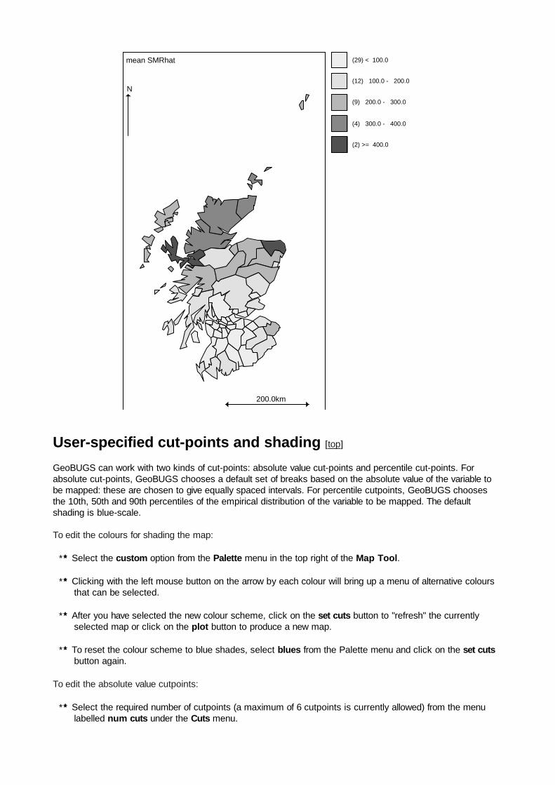
User-specified cut-points and shading [top]
GeoBUGS can work with two kinds of cut-points: absolute value cut-points and percentile cut-points. Forabsolute cut-points, GeoBUGS chooses a default set of breaks based on the absolute value of the variable tobe mapped: these are chosen to give equally spaced intervals. For percentile cutpoints, GeoBUGS choosesthe 10th, 50th and 90th percentiles of the empirical distribution of the variable to be mapped. The defaultshading is blue-scale.
To edit the colours for shading the map:
∗∗∗∗ Select the custom option from the Palette menu in the top right of the Map Tool.
∗∗∗∗ Clicking with the left mouse button on the arrow by each colour will bring up a menu of alternative coloursthat can be selected.
∗∗∗∗ After you have selected the new colour scheme, click on the set cuts button to "refresh" the currentlyselected map or click on the plot button to produce a new map.
∗∗∗∗ To reset the colour scheme to blue shades, select blues from the Palette menu and click on the set cutsbutton again.
To edit the absolute value cutpoints:
∗∗∗∗ Select the required number of cutpoints (a maximum of 6 cutpoints is currently allowed) from the menulabelled num cuts under the Cuts menu.
(29) < 100.0
(12) 100.0 - 200.0
(9) 200.0 - 300.0
(4) 300.0 - 400.0
(2) >= 400.0
mean SMRhat
200.0km
N

∗∗∗∗ Type the required values of the cutpoints in the appropriate boxes labelled cut 1, cut 2 etc.
∗∗∗∗ Click on the set cuts button to "refresh" the currently selected map or click on the plot button to produce anew map.
To produce maps using cutpoints based on percentiles:
∗∗∗∗ Select the percentile option rather than abs value option for the cutpoints on the left of the Map Tool.
∗∗∗∗ Click on the plot button to produce a new map. The default is to set the cutpoints to the 10th, 50th and90th percentiles of the empirical distribution of values to be mapped.
∗∗∗∗ To display the absolute values corresponding to these percentiles on the map legend:− reselect the abs value option for cutpoints;− click on the get cuts button - the absolute values corresponding to the percentiles should now be
displayed in the Cuts boxes on the right of the Map Tool− click on the set cuts button - the legend labels on the map should now display the absolute values of the
cutpoints.
To use the same set of cutpoints for multiple maps:
∗∗∗∗ Select the window with the map containing the cutpoints you wish to use.∗∗∗∗ Click on the get cuts button - the cutpoints used for the selected map should now be displayed in the Cuts
boxes on the right of the Map Tool.∗∗∗∗ Select the window with the map whose cutpoints you wish to change.∗∗∗∗ Click on the set cuts button - the map should now be updated using the new cutpoints.
Some current limitations:
∗∗∗∗ It is not possible to save user-defined colour schemes once you quit GeoBUGS.
Identifying individual areas on a map [top]
The index, label and value of an individual area on the map can be found by placing the cursor over the area ofinterest on the map and clicking with the left mouse button. The index (i.e. ID number i of the area, wherei=1,...,Number of areas), area label (given in the polygon file) and value of variable currently being mapped forthe selected area will be shown in left of the grey bar at the bottom of the WinBUGS program window.
Copying and saving maps [top]
Maps produced using the GeoBUGS map tool can be copied and pasted into other Microsoft Windows softwaresuch as Word and PowerPoint. In WinBUGS 1.4, this can only be done if the map is plotted in the log file (butnot in a separate window) - select 'Output options' from the 'Options' menu and click on 'log' rather than 'window'before plotting the map. To select the map, click anywhere on the map to focus it (a blue border should thenappear around the figure); then select 'Copy' from the 'Edit' menu (or Crtl-C). Then paste into the appropriateWord or PowerPoint file etc. To save the map as a postscript file, you will need to install a postscript print driveron your PC, then select 'Print' from the 'File' menu, check the 'print to file' box, and then select 'Print'.
If you produce the map in a window rather than the log file, you can save the map as a WinBUGS .odcdocument; this will allow you to re-open the map within WinBUGS 1.4 and re-edit the cutpoints and colours ifyou wish. Unfortunately there is a bug which means that log files containing maps cannot be saved as .odcfiles and re-opened.

Spatial distributions [top]
See appendices for further tecnhical details about the various spatial distributions implemented in GeoBUGS
1.2.
car.normal and car.l1 [top]
The intrinsic Gaussian CAR prior distribution is specified using the distribution car.normal for the vector ofrandom varables S = ( S1, ....., SN ). A robust version of this model is available, which assumes a doubleexponential (Laplace) rather than Gaussian distribution: this is called car.l1. The syntax for these distributionsis as follows:
S[1:N] ~ car.normal(adj[], weights[], num[], tau)S[1:N] ~ car.l1(adj[], weights[], num[], tau)
where:
adj[] : A vector listing the ID numbers of the adjacent areas for each area (this is a sparse representation ofthe full adjacency matrix for the study region, and can be generated using the Adjacency Tool from the Mapmenu in GeoBUGS.weights[] : A vector the same length as adj[] giving unnormalised weights associated with each pair of areas.For the CAR model described above, taking Cij = 1 (equivalently Wij = 1/ ni ) if areas i and j are neighbours and
0 otherwise, gives a vector of 1's for weights[].num[] : A vector of length N (the total number of areas) giving the number of neighbours ni for each area.
tau : A scalar argument representing the precision (inverse variance) parameter of the Gaussian CAR prior, orthe inverse scale parameter of the Laplace prior (for the latter model, the variance = 2 / tau2).
The first 3 arguments must be entered as data (it is currently not possible to allow the weights to be unknown);the final variable tau is usually treated as unknown and so is assigned a prior distribution. The data variablesnum and adj may be created by the adj matrix option of the GeoBUGS Adjacency Tool as described above.The variable weights must be created by the user, and must be a vector the same length as adj. A commonchoice is to set all the weights equal to 1 since this gives the standard Besag, York and Mollie (1991) CARmodel (see section on intrinsic CAR models in Appendix 1 for further discussion of weights). The easiest wayto do this is to create a loop in your WinBUGS model code:
for(j in 1:sumNumNneigh) { weights[j] <- 1}
where sumNumNneigh is the length of adj and is also output by the adj matrix option of the GeoBUGSAdjacency Tool .
Important things to check when using the car.normal or car.l1 distributions:∗∗∗∗ The car.normal and car.l1 distributions use unnormalised weights (see section on intrinsic CAR models
in Appendix 1).∗∗∗∗ An area cannot be specified as its own neighbour so make sure the ID number of the area itself does not
appear in as one of its list of neighbours in the adj vector. GeoBUGS does not check for this, so it is theuser's responsibility.
∗∗∗∗ The weights must be symmetric ( Wij = Wji ). GeoBUGS does carry out a check for this and returns an
error message if non-symmetric weights are detected.∗∗∗∗ Take care with priors on tau, and be prepared to carry out sensitivity analysis to this choice.∗∗∗∗ The car.normal and car.l1 distributions are parameterised to include a sum-to-zero constraint on the
random effects. This means that you must also include a separate intercept term in your model, whichMUST be assigned an improper uniform prior using the dflat() distribution.
∗∗∗∗ Because the car.normal and car.l1 distributions are improper, they can only be used as prior distributions,and not as a likelihood.

car.proper [top]
The proper Gaussian CAR prior distribution is specified using the distribution car.proper for the vector ofrandom variables S = ( S1, ....., SN ). The syntax for this distributions is as follows:
S[1:N] ~ car.proper(mu[], C[], adj[], num[], M[], tau, gamma)
where:
mu[] : A vector giving the mean for each area (this can either be entered as data, assigned a prior distribution,or specified deterministically within the model code).C[] : A vector the same length as adj[] giving normalised weights associated with each pair of areas (seesections on conditional specification and proper CAR priors in Appendix 1). Note that this differs from theintrinsic car.normal or car.l1 distributions, where unnormalised weights should be specified.adj[] : A vector listing the ID numbers of the adjacent areas for each area (this is a sparse representation ofthe full adjacency matrix for the study region, and can be generated using the Adjacency Tool from the Mapmenu in GeoBUGS.num[] : A vector of length N (the total number of areas) giving the number of neighbours ni for each area.
M[] : A vector of length N giving the diagonal elements Mii of the conditional variance matrix (see sections on
conditional specification and proper CAR priors in Appendix 1)tau : A scalar parameter representing the overall precision (inverse variance) parameter.gamma : A scalar parameter representing the overall degree of spatial dependence. This parameter isconstrained to lie between bounds given by the inverse of the minimum and maximum eigenvalues of the matrixM-1/2 C M1/2 (see appendix 1). GeoBUGS 1.2 contains two deterministic functions for calculating these bounds(or they can be calculated externally to GeoBUGS and input by the user):
min.bound(C[], adj[], num[], M[])max.bound(C[], adj[], num[], M[])
where the arguments are the same as the corresponding vectors used as arguments to the car.properdistribution.
Important things to check when using the car.proper distribution:
∗∗∗∗ C, adj, num and M must be entered as data (it is currently not possible to allow C to be unknown); numand adj may be created by the adj matrix option of the GeoBUGS Adjacency Tool as described above.The Lips example shows a (slightly clumsy) way of creating the C and M vectors within the WinBUGSmodel code; alternatively, these can be created externally to GeoBUGS and read in as data.
∗∗∗∗ The car.proper distribution uses normalised weights C (see section on proper CAR priors in Appendix 1).∗∗∗∗ An area cannot be specified as its own neighbour so make sure the ID number of the area itself does not
appear in as one of its list of neighbours in the adj vector. GeoBUGS does not check for this, so it is theuser's responsibility.
∗∗∗∗ The symmetry constraint Cij Mjj = Cji Mii must be satisfied. GeoBUGS does carry out a check for this and
returns an error message if lack of symmetry is detected.∗∗∗∗ Take care with priors on tau, and be prepared to carry out sensitivity analysis to this choice.
∗∗∗∗ Take care with priors on gamma: you must ensure that the prior is constrained between the appropriatebounds. Besag, York and Mollie (1991) suggest that gamma needs to be close to its upper bound before itreflects reasonable spatial dependence, so you may want to try informative priors to represent this, and beprepared to carry out sensitivity analysis.
spatial.exp and spatial.disc [top]
Bayesian Gaussian kriging models (multivariate Gaussian distribution with covariance matrix expressed as aparametric function of distance between pairs of points - e.g. see Diggle, Tawn and Moyeed, 1998 andAppendix 1) can be specified using the distributions spatial.exp or spatial.disc for the vector of random

variables S = ( S1, ....., SN ). The syntax for this distributions is as follows:
S[1:N] ~ spatial.exp(mu[], x[], y[], tau, phi, kappa)S[1:N] ~ spatial.disc(mu[], x[], y[], tau, alpha)
where:
mu[] : A vector giving the mean for each area (this can either be entered as data, assigned a prior distribution,or specified deterministically within the model code).x[] and y[] : Vectors of length N giving the x and y coordinates of the location of each point, or the centroid ofeach areatau : A scalar parameter representing the overall precision (inverse variance) parameter.
Two options are available for specifying the form of the covariance matrix: the powered exponential function andthe 'disc' function (see section on Joint Specification in Appendix 1).
The powered exponential function is implemented using the spatial.exp distribution and has 2 parameters:phi : A scalar parameter representing the rate of decline of correlation with distance between points. Note thatthe magnitude of this parameter will depend on the units in which the x and y coordinates of each location aremeasured (e.g. metres, km etc.).kappa : A scalar parameter controlling the amount of spatial smoothing. This is constrained to lie in the interval[0, 2).
The disc function is implemented using the spatial.disc distribution and has 1 parameter:alpha : A scalar parameter representing the radius of the 'disc' centred at each (x, y) location. Note that themagnitude of this parameter will depend on the units in which the x and y coordinates of each location aremeasured (e.g. metres, km etc.).
Warning: These models can be very slow for even moderate sized datasets (the algorithm is of order N3)!Experience to date also suggests that it may be better to hierarchically centre this model. For example,consider the following two alternative parameterisations of the same model:
Non-hierarchically centredfor (i in 1:N){
y[i] ~ dnorm(S[i], gamma)mu[i] <- alpha+beta*z[i]
}S[1:N] ~ spatial.exp(mu[], x[], y[], tau, phi,1)
Hierarchically centredfor (i in 1:N){
y[i] ~ dnorm(S[i], gamma)S[i] <- alpha+beta*z[i] + W[i]mu[i]<-0
}W[1:N] ~ spatial.exp(mu[], x[], y[], tau, phi,1)
In some simulated examples, the non-hierarchically centred parameterisation has produced incorrect results,while the hierarchically centred parameterisation gives sensible answers. This may be a feature of the single-site updating schemes used in WinBUGS, so interpret your results with care!(Thanks to Alan Gelfand, Shanshan Wu and Alex Schmidt for noting this problem).
Experience also suggests that there is often very little information in the data about the values of theparameters of the powered exponential (i.e. phi and kappa) or disc (i.e. alpha) functions. We thereforerecommend that reasonably informative priors are used, or that the values are fixed a priori, based on eithersubstantive knowledge or exploratory analysis using e.g. variograms.
spatial.pred and spatial.unipred [top]
Spatial interpolation or prediction at arbitrary locations can be carried out using the spatial.pred orspatial.unipred functions, in conjunction with fitting either the spatial.exp or spatial.disc model to a set ofobserved data. spatial.pred carries out joint or simultaneous prediction at a set of target locations, whereasspatial.unipred carries out single site prediction. The difference is that the single site prediction yieldsmarginal prediction intervals (i.e. ignoring correlation between prediction locations) whereas joint predictionyields simultaneous prediction intervals for the set of target locations (which will tend to be narrower than themarginal prediction intervals). The predicted means should be the same under joint or single site prediction. Thedisadvantage of joint prediction is that it is very slow (the computational time is of order P3, where P is thenumber of prediction sites). The syntax for these predictive distributions is:
Joint prediction:T[1:P] ~ spatial.pred(mu.T[], x.T[], y.T[], S[])
Single site prediction:for(j in 1:P) {
T[j] ~ spatial.unipred(mu.T[j], x.T[j], y.T[j], S[])}
where:
P : Scalar giving the number of prediction locationsmu.T[] : vector of length P (or scalar for single site version) specifying the mean for each prediction location(this should be specified in the same way as the mean for the observed data S).x.T] and y.T[] : Vectors of length P (or scalars for single site version) giving the x and y coordinates of thelocation of each prediction pointS : The vector of observations to which either the spatial.exp or spatial.disc model has been fitted.
pois.conv [top]
A conjugate Poisson-gamma spatial moving average distribution can be specified for non-negative countsdefined on a spatial lattice (i.e. discrete geographical partition), using the distribution pois.conv. This is adiscrete version of the Poisson-gamma random field model of Wolpert and Ickstadt (1998) and Best et al(2000a). The basic syntax for this distribution is as follows:
S ~ dpois.conv(mu[])
where S is a non-negative scalar parameter defined at some (usually spatial) location, and mu[] is a vector oflength J representing the influence of a set of gamma distributed latent parameters at each of J differentlocations on the value of S. Hence mu[] must be defined as a convolution of gamma random variables:
for (j in 1 : J) {mu[j] <- gamma[j] * k[j]
gamma[j] ~ dgamma(a, b)}
where k[j] is a spatial kernel or spatial 'weight' depending on some measure of distance or spatial proximitybetween the jth latent location and the location of S, and a and b are hyperparameters to be specified (seeAppendix 2 for further discussion of this distribution, including suitable kernel functions). Usually, k[] iscalculated externally and read into WinBUGS as data; alternatively, if k[] depends on unknown parameters, itmay be defined as part of the BUGS code and re-computed at each MCMC iteration. However, this is likely toslow down the sampling within WinBUGS by many orders of magnitude, so is not recommended for modelswith large numbers of latent parameters (i.e. J large).
More typically, the distribution will be used for each element of a vector of counts defined on a spatial lattice ofN regions, using the following syntax:
for (i in 1:N) {S[i] ~ dpois.conv(mu[i, ])for (j in 1 : J) {
mu[i, j] <- gamma[j] * k[i, j]}
}where the latent gamma[j] parameters are defined as above, and k[,] is now an N x J matrix with elements k[i,j]representing the 'weight' or contribution of the latent gamma random variable at location j to the expected valueof S at location i.
Conditional on mu, the S[i] have independent Poisson distributions with mean = Σ j mu[i, j].
Note that the model may be extended to include observed covariates as well as latent variables in the Poissonmean - see example 6.
mv.car [top]
The multivariate intrinsic Gaussian CAR prior distribution is specified using the distribution mv.car for the p xN matrix of random varables S , where columns of S represent the spatial units (areas) and rows represent thevariables (it is important to ensure the dimensions of S are specified the correct way round). The syntax for thisdistribution is as follows:
S[1:p, 1:N] ~ mv.car(adj[], weights[], num[], omega[ , ])
where:
adj[] : A vector listing the ID numbers of the adjacent areas for each area (this is a sparse representation ofthe full adjacency matrix for the study region, and can be generated using the Adjacency Tool from the Mapmenu in GeoBUGS.weights[] : A vector the same length as adj[] giving unnormalised weights associated with each pair of areas.For the CAR model described above, taking Cij = 1 (equivalently Wij = 1/ ni ) if areas i and j are neighbours and
0 otherwise, gives a vector of 1's for weights[].num[] : A vector of length N (the total number of areas) giving the number of neighbours ni for each area.
omega[ , ] : A p x p matrix representing the precision (inverse variance) matrix of the multivariate intrinsicGaussian CAR prior.
The first 3 arguments must be entered as data (it is currently not possible to allow the weights to be unknown);the final variable omega is usually treated as unknown and so is assigned a prior distribution (which must be aWishart distribution). The data variables num and adj may be created by the adj matrix option of theGeoBUGS Adjacency Tool as described above. The variable weights must be created by the user, and mustbe a vector the same length as adj. A common choice is to set all the weights equal to 1 since this gives themultivariate equivalent of the standard Besag, York and Mollie (1991) CAR model (see sections onintrinsic CAR models and multivariate intrinsic CAR models in Appendix 1 for further discussion of weights).The easiest way to do this is to create a loop in your WinBUGS model code:
for(j in 1:sumNumNneigh) { weights[j] <- 1}
where sumNumNneigh is the length of adj and is also output by the adj matrix option of the GeoBUGSAdjacency Tool .
Important things to check when using the mv.car distribution:
∗∗∗∗ The mv.car distribution uses unnormalised weights, as for the car.normal distribtion.∗∗∗∗ An area cannot be specified as its own neighbour so make sure the ID number of the area itself does not
appear in as one of its list of neighbours in the adj vector. GeoBUGS does not check for this, so it is theuser's responsibility.
∗∗∗∗ The weights must be symmetric ( Wij = Wji ). GeoBUGS does carry out a check for this and returns an
error message if non-symmetric weights are detected.∗∗∗∗ Take care with priors on omega, and be prepared to carry out sensitivity analysis to this choice.∗∗∗∗ The mv.car distribution is parameterised to include a sum-to-zero constraint on the random effects. This
means that you must also include separate intercept terms in your model for each of the p variables, whichMUST be assigned improper uniform priors using the dflat() distribution.
∗∗∗∗ An alternative unconstrained version of the multivariate CAR prior is available in WinBUGS 1.4, calledmv.car.uncon. The syntax is the same as for mv.car.
∗∗∗∗ Because the mv.car (and mv.car.uncon) distribution is improper, it can only be used as a priordistribution, and not as a likelihood.
∗∗∗∗ Please regard the mv.car and mv.car.uncon distributions as beta-test versions. If you encounter anyproblems using either distribution, please report these to [email protected]
Temporal distributions [top]
Using car.normal as a random walk prior for temporal smoothing [top]
In one dimension, the intrinsic Gaussian CAR distribution reduces to a Gaussian random walk (seee.g.Fahrmeir and Lang, 2001). Assume we have a set of temporally correlated random effects θt, t=1,..., T
(where T is the number of equally-spaced time points). In the simplest case of a random walk of order 1,RW(1), we may write
θt | θ−t ~ Normal ( θt+1, φ) for t = 1
~ Normal ( (θt-1 + θt+1)/2, φ / 2 ) for t = 2, ...., T-1
~ Normal ( θt-1, φ) for t = T
where θ−t denotes all elements of θθθθ except the θt. This is equivalent to specifying
θt | θ−t ~ Normal ( Σk Ctk θk, φ Mtt) for t = 1, ..., T
where Ctk = Wtk / Wt+, Wt+ = Σ k Wtk and Wtk = 1 if k = (t-1) or (t+1) and 0 otherwise; Mtt = 1/Wt+. Hence the
RW(1) prior may be fitted using the car.normal distribution in WinBUGS, with appropriate specification of theweight and adjacency matrices, and num vector (see example 9)
A second order random walk prior is defined as
θt | θ−t ~ Normal ( 2θt+1 − θt+2, φ) for t = 1
~ Normal ( (2θt-1 + 4θt+1 − θt+2)/5, φ / 5 ) for t = 2
~ Normal ( (−θt-2 + 4θt-1 + 4θt+1 − θt+2)/6, φ / 6 ) for t = 3, ...., T-2
~ Normal ( (−θt-2 + 4θt-1 + 2θt+1)/5, φ / 5 ) for t = T-1
~ Normal ( −θt-2+ 2θt-1, φ) for t = T
Again this is equivalent to specifying
θt | θ−t ~ Normal ( Σk Ctk θk, φ Mtt) for t = 1, ..., T
where Ctk is defined as above, but this time with Wtk = −1 if k = (t-2) or (t+2), Wtk = 4 if k = (t-1) or (t+1) and t in
(3, T-2), Wtk = 2 if k = (t-1) or (t+1) and t = 2 or T-1, Wtk = 0 otherwise; Mtt = 1/Wt+.
Note that if the observed time points are not equally spaced, it is necessary to include missing values (NA) forthe intermediate time points (see example 9).
Examples [top]
1. Conditional Autoregressive (CAR) models for disease mapping: Lip cancer in
Scotland [top]
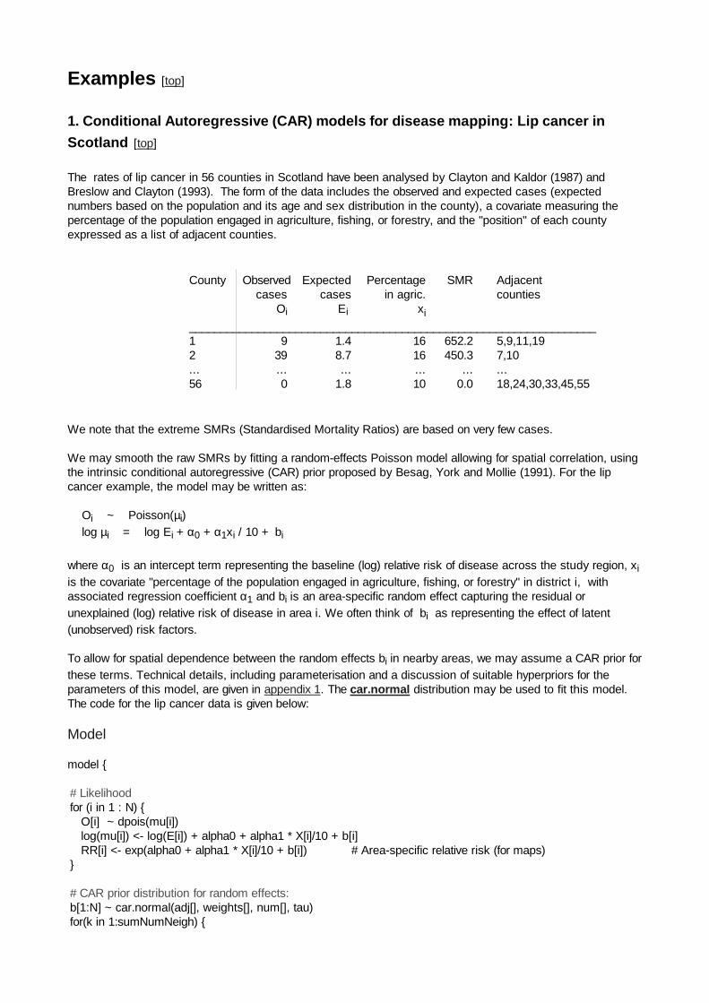
The rates of lip cancer in 56 counties in Scotland have been analysed by Clayton and Kaldor (1987) andBreslow and Clayton (1993). The form of the data includes the observed and expected cases (expectednumbers based on the population and its age and sex distribution in the county), a covariate measuring thepercentage of the population engaged in agriculture, fishing, or forestry, and the "position'' of each countyexpressed as a list of adjacent counties.
County Observed Expected Percentage SMR Adjacentcases cases in agric. counties
Oi Ei xi
_________________________________________________________________1 9 1.4 16 652.2 5,9,11,192 39 8.7 16 450.3 7,10... ... ... ... ... ...56 0 1.8 10 0.0 18,24,30,33,45,55
We note that the extreme SMRs (Standardised Mortality Ratios) are based on very few cases.
We may smooth the raw SMRs by fitting a random-effects Poisson model allowing for spatial correlation, usingthe intrinsic conditional autoregressive (CAR) prior proposed by Besag, York and Mollie (1991). For the lipcancer example, the model may be written as:
Oi ~ Poisson(µi)log µi = log Ei + α0 + α1xi / 10 + bi
where α0 is an intercept term representing the baseline (log) relative risk of disease across the study region, xi
is the covariate "percentage of the population engaged in agriculture, fishing, or forestry" in district i, withassociated regression coefficient α1 and bi is an area-specific random effect capturing the residual orunexplained (log) relative risk of disease in area i. We often think of bi as representing the effect of latent(unobserved) risk factors.
To allow for spatial dependence between the random effects bi in nearby areas, we may assume a CAR prior forthese terms. Technical details, including parameterisation and a discussion of suitable hyperpriors for theparameters of this model, are given in appendix 1. The car.normal distribution may be used to fit this model.The code for the lip cancer data is given below:
Model
model {
# Likelihoodfor (i in 1 : N) {
O[i] ~ dpois(mu[i])log(mu[i]) <- log(E[i]) + alpha0 + alpha1 * X[i]/10 + b[i]RR[i] <- exp(alpha0 + alpha1 * X[i]/10 + b[i]) # Area-specific relative risk (for maps)
}
# CAR prior distribution for random effects:b[1:N] ~ car.normal(adj[], weights[], num[], tau)for(k in 1:sumNumNeigh) {

weights[k] <- 1}
# Other priors:alpha0 ~ dflat()alpha1 ~ dnorm(0.0, 1.0E-5)tau ~ dgamma(0.5, 0.0005) # prior on precisionsigma <- sqrt(1 / tau) # standard deviation
}
Data click on one of the arrows to open data
Note that the data for the adjacency matrix (variables adj, num and SumNumNeigh) have been generatedusing the adj matrix option of the Adjacency Tool menu in GeoBUGS. By default, this treats islands ashaving no neighbours, and so the three areas representing the Orkneys, Shetland and the Outer Hebridesislands in Scotland have zero neighbours. You can edit the adjacency map of Scotland to include these areasas neighbours if you wish. The car.normal distribution sets the value of bi equal to zero for areas i that are
islands. Hence the posterior relative risks for the Orkneys, Shetland and the Outer Hebrides in the presentexample will just depend on the overall baseline rate α0 and the covariate xi. Alternatively, you could specify a
convolution prior for the area-specific random effects (Besag, York and Mollie 1991) which partitions the overallrandom effect for each area into the sum of a spatial component plus a non-spatial component. In this model,the islands will just have a non-spatial term for the random effect. See example on lung cancer in a LondonHealth Authority for details of this model.
Inits click on one of the arrows to open initial values
Note that the initial values for elements 6, 8 and 11 of the vector b are set to NA since these correspond to thethree islands (Orkneys, Shetland and the Outer Hebrides). The values of b are set to zero by the car.normalprior for these 3 areas, and so they are not stochastic nodes.
2. Convolution priors: Lung cancer in a London Health Authority [top]
This example has been modified from a London Health Authority annual report. The theme of the report wasinequality in health and the aim was to investiagte links between poverty and ill health. To investigate thisissue, the Health Authority carried out a series of disease mapping studies at census ward level. There are 44wards in the Health Authority in this example. The data are simulated observed and exepected counts of lungcancer incidence in males aged 65 and over living in the Health Authority region; a ward level index of socio-economic devprivation is also available.
We fit the following model, allowing a convolution prior for the random effects:
Oi ~ Poisson(µi)log µi = log Ei + α + β deprivi + bi + hi
where deprivi is the devprivation covariate, bi are spatial random effects assigned a CAR prior, and we introduce
a second set of random effects hi for which we assume an exchangeable Normal prior. The random effect foreach area is thus the sum of a spatially structured component bi and an unstructured component hi . This istermed a convolution prior (Besag, York and Mollie 1991; Mollie 1996). Besag, York and Mollie argue that thismodel is more flexible than assume only CAR random effects, since it allows the data to decide how much ofthe residual disease risk is due to spatially structured variation, and how much is unstructured over-dispersion.
The code for this model is given below.
Model
� �
� �

model {
for (i in 1 : N) {# LikelihoodO[i] ~ dpois(mu[i])log(mu[i]) <- log(E[i]) + alpha + beta * depriv[i] + b[i] + h[i]RR[i] <- exp(alpha + beta * depriv[i] + b[i] + h[i]) # Area-specific relative risk (for maps)
# Exchangeable prior on unstructured random effectsh[i] ~ dnorm(0, tau.h)
}
# CAR prior distribution for spatial random effects:b[1:N] ~ car.normal(adj[], weights[], num[], tau.b)for(k in 1:sumNumNeigh) {
weights[k] <- 1}
# Other priors:alpha ~ dflat()beta ~ dnorm(0.0, 1.0E-5)tau.b ~ dgamma(0.5, 0.0005)sigma.b <- sqrt(1 / tau.b)tau.h ~ dgamma(0.5, 0.0005)sigma.h <- sqrt(1 / tau.h)
}
Data click on one of the arrows to open data
Inits click on one of the arrows to open initial values
3. Proper CAR model: Lip cancer revisited [top]
This example illustrates the use of the proper CAR distribution (car.proper) rather than the intrinsic CARdistribution for the area-specific random effects in the Lip cancer example (9.1). We use the definition of the Cand M matrices proposed by Cressie and colleagues (see section on proper CAR models in Appendix 1).
Model
model {
# Set up 'data' to define spatial dependence structure# =====================================for(i in 1 : N) {
m[i] <- 1/E[i] # scaling factor for variance in each cell}
# The vector C[] required as input into the car.proper distribution is a vector respresention# of the weight matrix with elements Cij. The first J1 elements of the C[] vector contain the# weights for the J1 neighbours of area i=1; the (J1+1) to J2 elements of the C[] vector contain# the weights for the J2 neighbours of area i=2; etc.# To set up this vector, we need to define a variable cumsum, which gives the values of J1,# J2, etc.; we then set up an index matrix pick[,] with N columns corresponding to the# i=1,...,N areas, and with the same number of rows as there are elements in the C[] vector# (i.e. sumNumNeigh). The elements C[ (cumsum[i]+1):cumsum[i+1] ] correspond to
� �
� �
# the set of weights Cij associated with area i, and so we set up ith column of the matrix pick[,]# to have a 1 in all the rows k for which cumsum[i] < k <= cumsum[i+1], and 0's elsewhere.# For example, let N=4 and cumsum=c(0,3,5,6,8), so area i=1 has 3 neighbours, area i=2 has 2# neighbours, area i=3 has 1 neighbour and area i=4 has 2 neighbours. The the matrix pick[,] is:# pick# 1, 0, 0, 0,# 1, 0, 0, 0,# 1, 0, 0, 0,# 0, 1, 0, 0,# 0, 1, 0, 0,# 0, 0, 1, 0,# 0, 0, 0, 1,# 0, 0, 0, 1,## We can then use the inner product (inprod(,)) function in WinBUGS and the kth row of pick to# select which area corresponds to the kth element in the vector C[]; likewise, we can use inprod(,)# and the ith column of pick to select the elements of C[] which correspond to area i.## Note: this way of setting up the C vector is somewhat convoluted!!!! In future versions, we hope the# GeoBUGS adjacency matrix tool will be able to dump out the relevant vectors required. Alternatively,# the C vector could be created using another package (e.g. Splus) and read into WinBUGS as data.#cumsum[1] <- 0for(i in 2:(N+1)) {
cumsum[i] <- sum(num[1:(i-1)])}for(k in 1 : sumNumNeigh) {
for(i in 1:N) {pick[k,i] <- step(k - cumsum[i] - epsilon) * step(cumsum[i+1] - k)# pick[k,i] = 1 if cumsum[i] < k <= cumsum[i=1]; otherwise, pick[k,i] = 0
}C[k] <- sqrt(E[adj[k]] / inprod(E[], pick[k,])) # weight for each pair of neighbours
}epsilon <- 0.0001
# Model# =====
# Likelihoodfor (i in 1 : N) {
O[i] ~ dpois(mu[i])log(mu[i]) <- log(E[i]) + S[i]
RR[i] <- exp(S[i]) # Area-specific relative risktheta[i] <- alpha
}
# Proper CAR prior distribution for spatial random effects:S[1:N] ~ car.proper(theta[], C[], adj[], num[], m[], prec, gamma)
# Other priors:alpha ~ dnorm(0, 0.0001)prec ~ dgamma(0.5, 0.0005) # prior on precisionv <- 1/prec # variancesigma <- sqrt(1 / prec) # standard deviation
gamma.min <- min.bound(C[], adj[], num[], m[])gamma.max <- max.bound(C[], adj[], num[], m[])gamma ~ dunif(gamma.min, gamma.max)
}
Data click on one of the arrows to open data
Initial values Click on one of the arrows for the initial values
4. Bayesian kriging and spatial prediction: Surface elevation [top]
The data for this example are taken from Diggle and Riberio (2000) (and came originally from Davis (1973)). Thedata file contains the variables height, x and y, giving surface elevation at each of 52 locations (x, y) within a310-foot square. The unit of distance is 50 feet, whereas one unit of height represents 10 feet of elevation. AGaussian kriging model can be fitted to these data in WinBUGS 1.4 using either the spatial.exp or spatial.discdistributions. The data file also contains a set of locations x.pred and y.pred representing a 15 x 15 grid of
points at which we wish to predict surface elevation. Predictions can be obtained using either the spatial.predor spatial.unipred predictive distributions in WinBUGS 1.4
Model
model {
# Spatially structured multivariate normal likelihoodheight[1:N] ~ spatial.exp(mu[], x[], y[], tau, phi, kappa) # exponential correlation function# height[1:N] ~ spatial.disc(mu[], x[], y[], tau, alpha) # disc correlation function
for(i in 1:N) {mu[i] <- beta
}
# Priorsbeta ~ dflat()tau ~ dgamma(0.001, 0.001)sigma2 <- 1/tau
# priors for spatial.exp parametersphi ~ dunif(0.05, 20) # prior range for correlation at min distance (0.2 x 50 ft) is 0.02 to 0.99
# prior range for correlation at max distance (8.3 x 50 ft) is 0 to 0.66kappa ~ dunif(0.05,1.95)
# priors for spatial.disc parameter# alpha ~ dunif(0.25, 48) # prior range for correlation at min distance (0.2 x 50 ft) is 0.07 to 0.96
# prior range for correlation at max distance (8.3 x 50 ft) is 0 to 0.63
# Spatial prediction
# Single site predictionfor(j in 1:M) {
height.pred[j] ~ spatial.unipred(beta, x.pred[j], y.pred[j], height[])}
# Only use joint prediction for small subset of points, due to length of time it takes to runfor(j in 1:10) { mu.pred[j] <- beta }height.pred.multi[1:10] ~ spatial.pred(mu.pred[], x.pred[1:10], y.pred[1:10], height[])
}
Data Click on one of the arrows for the data
� �
� �
� �

Initial valuesClick on one of the arrows for inital values for spatial.exp modelClick on one of the arrows for inital values for spatial.disc model
The GeoBUGS map tool can be used to produce an approximate map of the posterior mean predicted surfaceelevation. It is not possible to map point locations using GeoBUGS. However, a map file called elevation isalready loaded in the GeoBUGS Map Tool --- this is a 15 x 15 grid with the centroids of the grid cellcorresponding to the locations of each of the prediction points. You can use this to produce a map of theposterior mean (or other posterior summaries) of the vector of predicted values height.pred.
5. Poisson-gamma spatial moving average (convolution) model: Distribution of
hickory trees in Duke forest [top]
Ickstadt and Wolpert (1998) and Wolpert and Ickstadt (1998) analyse the spatial distribution of hickory trees (asubdominant species) in a 140 metre x 140 metre research plot in Duke Forest, North Carolina, USA, with theaim of investigating the regularity of the distribution of trees: spatial clustering would reveal that thesubdominant species is receding from, or encroaching into, a stand recovering from a disturbance,while regularity would suggest a more stable and undisturbed recent history.
The data comprise counts of trees, Yi, in each of i=1,...,16 30m x 30m quadrats (each having area Ai = 900
m2) on a 4x4 grid covering the research plot (excluding a 10m boundary region to minimise edge effects),together with the x and y co-ordinates of the centroid of each plot (relative to the south-west corner of theresearch plot). Ickstadt and Wolpert (1998) fit a Poisson-gamma spatial moving average model as follows:
Yi ~ Poisson( µ i ) i = 1,...,16
µ i = Ai * λ i
λ i = Σj kij γ j
where γ j can be thought of as latent unobserved risk factors associated with locations or sub-regions of the
study region indexed by j, and kij is a kernel matrix of 'weights' which depend on the distance or proximity
between latent location j and quadrat i of the study region (see Appendix 2 for further details of this convolutionmodel). Ickstadt and Wolpert (1998) take the locations of the latent γ j to be the same as the partition of the
study region used for the observed data i.e. j = 1,....16 with latent sub-region j being the same as quadrat i ofthe study region. Note that it is not necessary for the latent partition to be the same as the observed partition -see example 6. The γ j are assigned independent gamma prior distributions
γ j ~ Gamma(α, β) j = 1,....,16.
Ickstadt and Wolpert (1998) consider two alternative kernel functions: an adjacency-based kernel and adistance-based kernel. The adjacency based kernel is defined as:
kij = 1 if i = j
kij = exp(θ2)/ni if j is a nearest neighbour of i (only north-south and east-west neighbours considered)
and ni is the number of neighbours of area i
kij = 0 otherwise
The distance based kernel is defined as:
kij = exp(− [dij / exp(θ2)]2) where dij is the distance between the centroid of areas i and j
For both kernels, the parameter exp(θ2) reflects the degree of spatial dependence or clustering in the data, with
large values of θ2 suggesting spatial correlation and irregular distribution of hickory trees.
� �
� �
Ickstadt and Wolpert (1998) elicit expert prior opinion concerning the unknown hyperparameters θ0 = log(α), θ1
= −log(β) and θ2 and translate this information into Normal prior distributions for θ0, θ1 and θ2.
This model may be implemented in WinBUGS 1.4 using the pois.conv distribution. The code is given below.
Model
model {
# likelihoodfor (i in 1:N) {
Y[i] ~ dpois.conv(mu[i,])for (j in 1:J) {
mu[i, j] <- A[i] * lambda[i, j]lambda[i, j] <- k[i, j] * gamma[j]
}}
# priors (see Ickstadt and Wolpert (1998) for details of prior elicitation)for (j in 1:J) {
gamma[j] ~ dgamma(alpha, beta)}alpha <- exp(theta0)beta <- exp(-theta1)
theta0 ~ dnorm(-0.383, 1)theta1 ~ dnorm(-5.190, 1)theta2 ~ dnorm(-1.775, 1) # prior on theta2 for adjacency-based kernel# theta2 ~ dnorm(1.280, 1) # prior on theta2 for distance-based kernel
# compute adjacency-based kernelfor (i in 1:N) { # Note N = J in this example (necessary for adjacency-based kernel)
k[i, i] <- 1for (j in 1:J) {
d[i, j] <- sqrt((x[i] - x[j])*(x[i] - x[j]) + (y[i] - y[j])*(y[i] - y[j])) # distance between areas i and j# (only needed to help compute# nearest neighbour weights;# alternatively, read matrix w from file)
w[i, j] <- step(30.1 - d[i, j]) # nearest neighbour weights:# areas are 30 sq m, so any pair of areas with# centroids > 30m apart are not nearest neighbours# (0.1 added to account for numeric imprecision in d)
}for (j in (i+1):J) {
k[i, j] <- w[i, j] * exp(theta2) / (sum(w[i,]) - 1)k[j, i] <- w[j, i] * exp(theta2) / (sum(w[j,]) - 1)
}}
# alternatively, compute distance-based kernel# for (i in 1:N) {# k[i, i] <- 1# for (j in 1:J) {# d[i, j] <- sqrt((x[i] - x[j])*(x[i] - x[j]) + (y[i] - y[j])*(y[i] - y[j])) # distance between areas i and j# }# for (j in (i+1):J) {# k[i, j] <- exp(-pow(d[i, j]/exp(theta2), 2))# k[j, i] <- exp(-pow(d[j, i]/exp(theta2), 2))
# }# }
# summary quantities for posterior inferencefor (i in 1:N) {
density[i] <- sum(lambda[i, ]) # smoothed density of hickory trees (per sq metre) in area iobs.density[i] <- Y[i]/A[i] # observed density of hickory trees (per sq metre) in area i
}spatial.effect <- exp(theta2) # large values indicate strong spatial dependence;
# spatial.effect -> 0 indicates spatial independence}
Data click on one of the arrows to open data
Initial values click on one of the arrows to open initial values
Results
Assuming adjacency-based kernel (equivalent to Ickstadt and Wolpert's model MS):node mean sd MC error 2.5% median 97.5% start samplespatial.effect 0.2856 0.1793 0.009916 0.04003 0.2588 0.7088 10001 10000theta0 -0.6121 0.4562 0.02313 -1.519 -0.6084 0.228 10001 10000theta1 -5.111 0.5088 0.0179 -6.046 -5.133 -4.05 10001 10000theta2 -1.487 0.7497 0.04143 -3.218 -1.352 -0.3441 10001 10000
Ickstadt and Wolpert report a posterior mean (sd) of 0.281 (0.156) for the spatial effect, exp(θ2), from theiranalysis using a 4x4 partition of the study region (Table 1.3).
Assuming distance-based kernel (equivalent to Ickstadt and Wolpert's model MD):node mean sd MC error 2.5% median 97.5% start samplespatial.effect 8.042 7.474 0.5676 0.5371 4.684 23.9 20001 20000theta0 -0.297 0.5198 0.02996 -1.533 -0.2463 0.5766 20001 20000theta1 -5.276 0.522 0.01989 -6.197 -5.308 -4.157 20001 20000theta2 1.563 1.108 0.06682 -0.6216 1.544 3.174 20001 20000
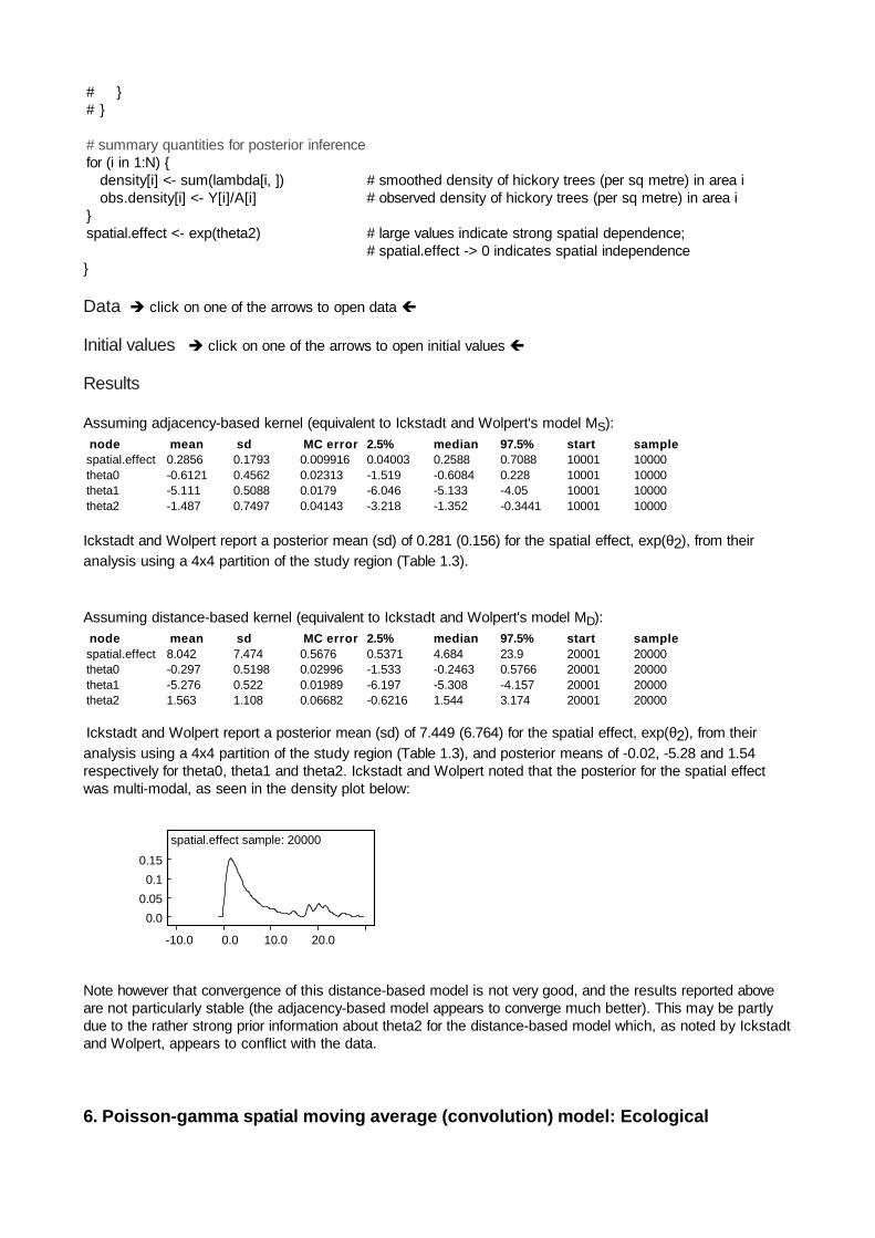
Ickstadt and Wolpert report a posterior mean (sd) of 7.449 (6.764) for the spatial effect, exp(θ2), from theiranalysis using a 4x4 partition of the study region (Table 1.3), and posterior means of -0.02, -5.28 and 1.54respectively for theta0, theta1 and theta2. Ickstadt and Wolpert noted that the posterior for the spatial effectwas multi-modal, as seen in the density plot below:
Note however that convergence of this distance-based model is not very good, and the results reported aboveare not particularly stable (the adjacency-based model appears to converge much better). This may be partlydue to the rather strong prior information about theta2 for the distance-based model which, as noted by Ickstadtand Wolpert, appears to conflict with the data.
6. Poisson-gamma spatial moving average (convolution) model: Ecological
� �
� �
spatial.effect sample: 20000
-10.0 0.0 10.0 20.0
0.0
0.05
0.1
0.15
regression of air pollution and respiratory illness in children [top]
Best et al (2000b) applied the Poisson-gamma convolution model to a small-area ecological regressionanalysis of traffic-related air pollution and respiratory illness in children living in the Huddersfield region ofnorthern England. They carried out two analyses, one using a partition of the study region into 427administrative enumeration districts, and the other partitioning the region into 605 regular 750m2 grid cells. Herewe consider the latter partition of the study region. The following data were available:
Yi = number of cases of self-reported frequent cough amongst children aged 7-9 in each of the i=1,..., 605
areas (750 m2 grid cells)popi = (estimated) population of 7-9 year old children in each area, based on pro-rated 1991 enumeration
district census counts. (Note that this leads to <1 child per area in some areas, due to the pro-ratasplit; counts are also divided by 100, to give rates per 100 children).
NO2i = average annual nitrogen dioxide concentration in each area, measured in µg m-3 above the baseline
concentration for the study region of approximately 20µg m-3
Best et al (2000b) fitted an indentity-link spatial moving average Poisson regression model:
Yi ~ Poisson( µ i )
µ i = popi * λ i
λ i = β0 + β1 NO2i + β2 Σj kij γ j
where γ j can be thought of as latent unobserved risk factors associated with locations or sub-regions of the
study region indexed by j. These locations or sub-regions are typically defined by the user, and are chosen torepresent a partition of the region that is appropriate for capturing unmeasured spatial variation in the diseaserate. Best et al (2000b) define the latent γ j parameters on a 12 x 8 grid of approx 3km2 quadrats covering the
Huddersfield study region. kij are then the elements of a 605 x 96 Gaussian kernel matrix, with
kij = 1 / (2π ρ2) exp(−dij2 / 2ρ2)
where dij represents the Euclidean distance between the centroid of area i of the study region and the location
of the jth latent factor. Note that if the latent factors are defined on sub-regions rather than points, it is preferableto integrate the above kernel over the latent sub-region (i.e. over all possible distances between the centroid ofarea i and all locations within the latent sub-region) - the Splus / R function given in the data file belowimplements this integration when computing the kernel matrix. ρ > 0 is a distance scale governing how rapidlythe kernel weights (i.e. the influence of the jth latent factor on the disease risk in the ith area) decline withincreasing distance. Best et al (2000b) fix ρ = 1 km. By fixing ρ, the kernel matrix can be pre-computedoutside of WinBUGS (see link in the data file for Splus / R code for doing this), thus simplifying theimplementation. It is possible to treat ρ as uncertain (see example 5), but this entails calculating the elementskij at each MCMC interation within the BUGS code: this leads to big increases in computation time for all but
very small study regions and latent grids. (Note that since the overall scale parameter of the Gaussian kernel iscommon to all elements kij it can be factored out of the externel calculation of the kernel, and included as an
uncertain parameter (here called β2) in the BUGS model.
Independent gamma prior distributions are assumed for the uncertainty quantities β0, β1, β2 and γ j as this
enables the MCMC sampler to exploit conjugacy with the Poisson likelihood.
See Best et al (2000b) for full details and interpretation of the model, and Appendix 2 for further technicalinformation about the Poisson-gamma model.
The code for this model is given below.
Model
model {

# Likelihoodfor (i in 1 : I) {
Y[i] ~ dpois.conv(mu[i, ]) # convolution likelihood:# Y[i] ~ Poisson( sum_ j { mu[i, j] } )# where mu[i, j] = pop[i] * lambda[i, j] and# pop[i] = (standardised) population (in 100's) in area i# lambda[i, j] = disease rate in area i attributed to jth 'source', where# the sources include both observed and latent covariates.
for (j in 1 : J) {k1[i, j] <- ker[i, j] / prec # rescale kernel matrixlambda[i, j] <- beta2 * gamma[j] * k1[i, j] # jth 'source' (jth latent spatial grid cell)
}lambda[i,J+1] <- beta0 # (J+1)th 'source' (overall intercept; represents background rate)lambda[i,J+2] <- beta1 * NO2[i] # (J+2)th 'source' (effect of observed NO2 covariate in area i)
# Note: if additional covariates have been measured, these# should be included in the same way as NO2, giving terms# lambda[i, J+3], lambda[i, J+4],.....etc.
for (j in 1 : J+2) {mu[i, j] <- lambda[i, j] * pop[i]
}}
# Priors# See Table 22.1 in Best et al. (2000b) for further details.
# Priors for latent spatial grid cell (gamma) parameters:## Assume gamma_j ~ gamma(a, t)## Prior shape parameter for gamma distn on gamma[j]'s will change in proportion to the size of# the latent grid cells, to ensure aggregation consistency. The prior inverse scale parameter for# gamma distn on gamma[j]'s stays constant across different partitions, but depends on the# units used to measure the area of the latent grid cells: here we are assuming 'area' is in# sq kilometres, and we take tauG = 1 (per km^2) which corresponds to assuming that our prior# guess at the value of the gamma[j]'s is based on 'observing' about# 1 * (area of study region = 30*20km^2) = 600# 'prior points' over the study region.
alphaG <- tauG * area # Note: area of latent grid cells is read in from data filetauG <- 1
for (j in 1 : J) {gamma[j] ~ dgamma(alphaG, tauG)
}
# Priors for beta coefficients:## Assume priors on each beta are of the form beta ~ gamma(a, t).## Here, parameter of the prior are chosen by setting the prior mean to give an equal number of cases# allocated to each of the 3 'sources' (baseline, NO2 and latent), i.e.# prior mean = a / t = a * 3 * Xbar / Ybar,# where Ybar is the overall disease rate in number of cases per unit population,# and Xbar is the population-weighted mean of covariate X.## We also take shape parameter a = 0.575, since this gives the ratio of the 90th : 10th percentile# of the prior distn = 100, which is suitably diffuse.
YBAR <- sum(Y[])/sum(pop[]) # mean number of cases per unit population
NO2BAR <- inprod(NO2[], pop[]) / sum(pop[]) # population-weighted mean NO2
alpha0<- 0.575 # Shape parameter for Intercept (beta0)tau0 <- 3 * alpha0 / YBAR # Inverse scale parameter for Intercept (beta0)alpha1<- 0.575 # Shape parameter for effect of NO2 (beta1)tau1 <- 3 * alpha1 * NO2BAR / YBAR # Inverse scale parameter for effect of NO2 (beta1)alpha2 <- 0.575 # Shape parameter for Latent coefficient (beta2)tau2 <- 3 * alpha2 / YBAR # Inverse scale parameter for Latent coefficient (beta2)
beta0 ~ dgamma(alpha0, tau0)beta1 ~ dgamma(alpha1, tau1)beta2 ~ dgamma(alpha2, tau2)
# Summary quantities for posterior inferencefor(i in 1:I) {
RATE[i] <- sum(mu[i, ])/pop[i] # Overall disease rate in area iLATENT[i] <- beta2 * inprod(k1[i,], gamma[]) # Rate associated with latent spatial factor in area i
}
# Expected rate (number of cases per unit population) attributed to each source# (see Table 22.2 in Best et al (2000b) )rate.base <- beta0 # Background (overall baseline) rate per 100 populationrate.no2 <- beta1 * inprod(pop[], NO2[]) / sum(pop[]) # Number of cases per 100 population attributed
# to NO2 = beta1 * population-weighted mean value# of NO2 across the study region.
rate.latent <- inprod(pop[], LATENT[]) / sum(pop[]) # Number of cases per 100 population attributed to# latent sources = beta2 * population-weighted mean# value of the latent spatial factor (sum_j k_ij gamma_j)
# Percentage of cases attributed to each source:Total <- rate.base + rate.no2 + rate.latentPC.base <- rate.base / Total * 100 # % cases attributed to baseline riskPC.no2 <- rate.no2 / Total * 100 # % cases attributed to NO2 exposurePC.latent <- rate.latent / Total * 100 # % cases attributed to latent spatial factors
}
Data Click here for the data file
Initial values Click here for the initial values
Results
A 10000 iteration burn-in followed by a further 20000 updates gave the following results
node mean sd MC error 2.5% median 97.5% start samplePC.base 6.674 8.565 0.6041 0.01874 3.805 32.94 10000 20001PC.latent 74.95 13.99 0.9768 41.11 76.09 97.39 10000 20001PC.no2 18.38 10.92 0.7131 0.4521 18.08 41.31 10000 20001rate.base 0.6806 0.8744 0.06162 0.001946 0.3872 3.376 10000 20001rate.latent 7.641 1.452 0.09948 4.203 7.748 10.01 10000 20001rate.no2 1.874 1.115 0.07273 0.04625 1.843 4.223 10000 20001
These differ slightly from those in Best et al (2000b) Table 22.2 since the data in this example have beenrandomly perturbed for confidentiality. However, the picture is broadly similar, with 1.84 (95% interval 0.046 to4.2) cases per 100 population attributed to NO2 exposure, 7.75 (95% interval 4.2 to 10.0) cases per 100population attributed to latent spatially varying risk factors and the remaining 0.39 (95% iterval 0.0019 to 3.4)cases per 100 population attributed to the (spatially constant) baseline risk.
� �
� �
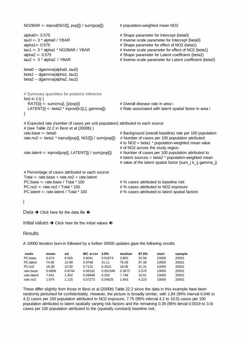
A map showing the posterior mean rate (per 100 population) of frequent cough attributed to the latent riskfactors (cf Fig 22.6b in Best et al, 2000b) in each area in the study region is show below. The relevant map fileis available from the GeoBUGS 1.2 map tool and is called Huddersfield_750m_grid.
7. Intrinsic multivariate CAR prior for mapping multiple diseases: Oral cavity cancer
and lung cancer in West Yorkshire, UK [top]
This example illustrates the use of the multivariate CAR prior distribution for joint mapping of two diseases. Thedata represent observed and age and sex standardised expected counts of incidenct cases of oral cavity andlung cancer in each of 126 electoral wards in the West Yorkshire region of England between 1986 and 1991.Some of the counts have been randomly peturbed by a small amount for confidentiality.
Since both outcomes are rare, the mortality counts Yik for cancer k (k=1, 2) in area i (i=1,126) are assumed tofollow independent Poisson distributions, conditional on an unknown mean µik
Yik ~ Poisson(µik)log µik = log Eik + αk + Sik
whereEik is the age and sex standardised expected count for cancer k in area i, αk is an intercept termrepresenting the baseline (log) relative risk of cancer k across the study region, and Sik is the area- and cancer-specific log relative risk of death. For cancer k, we assume that these log relative risks are spatially correlatedacross areas, and within area i, we assume that the log relative risks for cancer 1 (oral cavity) and cancer 2(lung) are also correlated due to dependence on shared area-level unmeasured risk factors. We represent thesecorrelation assumptions using an intrinsic bivariate CAR prior for the 2 x 126 dimensional matrix of Sik values.Technical details of this prior distribution are given in appendix 1. The mv.car distribution may be used to fitthis model. The WiNBUGS code is given below:
Model
model {# Likelihoodfor (i in 1:Nareas) {
(82) < 6.5
(90) 6.5 - 7.0
(181) 7.0 - 7.5
(111) 7.5 - 8.0
(141) >= 8.0
(samples)means for LATENT
10.0km
N
for (k in 1:Ndiseases) {Y[i, k] ~ dpois(mu[i, k])log(mu[i, k]) <- log(E[i, k]) + alpha[k] + S[k, i] # Note dimension of S is reversed:
# rows=k, cols=i because mv.car# assumes rows represent variables# (diseases) and columns represent# observations (areas).
}# The GeoBUGS map tool can only map vectors, so need to create separate vector# of quantities to be mapped, rather than an array (i.e. RR[i,k] won't work!)RR1[i] <- exp(alpha[1] + S[1,i]) # area specific relative risk for disease 1 (oral)RR2[i] <- exp(alpha[2] + S[2,i]) # area specific relative risk for disease 2 (lung)
}
# MV CAR prior for the spatial random effectsS[1:Ndiseases, 1:Nareas] ~ mv.car(adj[], weights[], num[], omega[ , ]) # MVCAR priorfor (i in 1:sumNumNeigh) { weights[i] <- 1 }
# Other priorsfor (k in 1:Ndiseases) {
alpha[k] ~ dflat()}omega[1:Ndiseases, 1:Ndiseases] ~ dwish(R[ , ], Ndiseases) # Precision matrix of MVCARsigma2[1:Ndiseases, 1:Ndiseases] <- inverse(omega[ , ]) # Covariance matrix of MVCARsigma[1] <- sqrt(sigma2[1, 1]) # conditional SD of S[1,] (oral cancer)sigma[2] <- sqrt(sigma2[2, 2]) # conditional SD of S[2,] (lung cancer)corr <- sigma2[1, 2] / (sigma[1] * sigma[2]) # within-area conditional correlation
# between oral and lung cancers.}
Data Click here for the data file
Initial values Click here for the initial values
Results
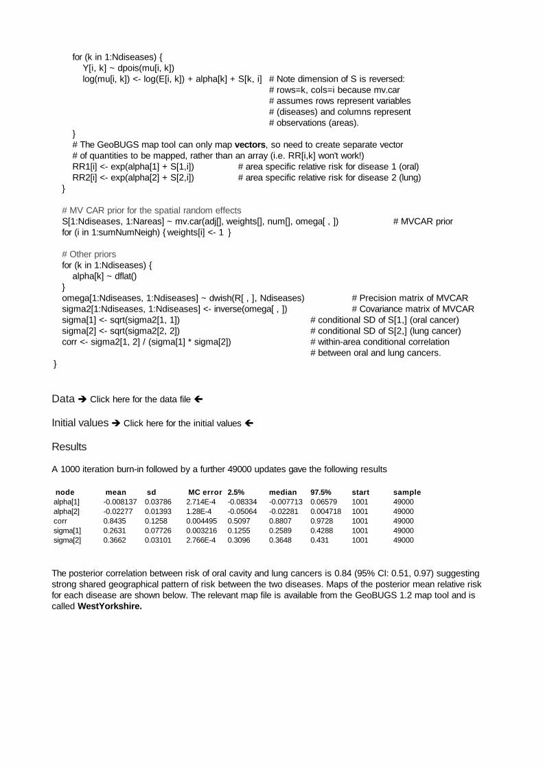
A 1000 iteration burn-in followed by a further 49000 updates gave the following results
node mean sd MC error 2.5% median 97.5% start samplealpha[1] -0.008137 0.03786 2.714E-4 -0.08334 -0.007713 0.06579 1001 49000alpha[2] -0.02277 0.01393 1.28E-4 -0.05064 -0.02281 0.004718 1001 49000corr 0.8435 0.1258 0.004495 0.5097 0.8807 0.9728 1001 49000sigma[1] 0.2631 0.07726 0.003216 0.1255 0.2589 0.4288 1001 49000sigma[2] 0.3662 0.03101 2.766E-4 0.3096 0.3648 0.431 1001 49000
The posterior correlation between risk of oral cavity and lung cancers is 0.84 (95% CI: 0.51, 0.97) suggestingstrong shared geographical pattern of risk between the two diseases. Maps of the posterior mean relative riskfor each disease are shown below. The relevant map file is available from the GeoBUGS 1.2 map tool and iscalled WestYorkshire.
� �
� �
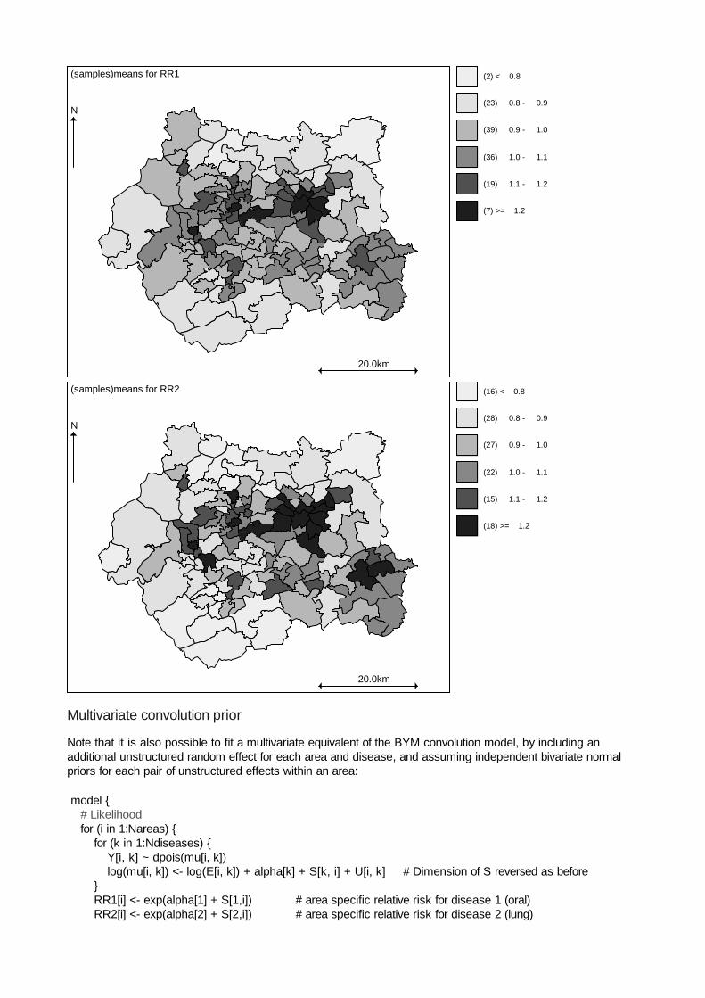
Multivariate convolution prior
Note that it is also possible to fit a multivariate equivalent of the BYM convolution model, by including anadditional unstructured random effect for each area and disease, and assuming independent bivariate normalpriors for each pair of unstructured effects within an area:
model {# Likelihoodfor (i in 1:Nareas) {
for (k in 1:Ndiseases) {Y[i, k] ~ dpois(mu[i, k])log(mu[i, k]) <- log(E[i, k]) + alpha[k] + S[k, i] + U[i, k] # Dimension of S reversed as before
}RR1[i] <- exp(alpha[1] + S[1,i]) # area specific relative risk for disease 1 (oral)RR2[i] <- exp(alpha[2] + S[2,i]) # area specific relative risk for disease 2 (lung)
(2) < 0.8
(23) 0.8 - 0.9
(39) 0.9 - 1.0
(36) 1.0 - 1.1
(19) 1.1 - 1.2
(7) >= 1.2
(samples)means for RR1
20.0km
N
(16) < 0.8
(28) 0.8 - 0.9
(27) 0.9 - 1.0
(22) 1.0 - 1.1
(15) 1.1 - 1.2
(18) >= 1.2
(samples)means for RR2
20.0km
N
}
# MV CAR prior for the spatial random effectsS[1:Ndiseases, 1:Nareas] ~ mv.car(adj[], weights[], num[], omega[ , ]) # MVCAR priorfor (i in 1:sumNumNeigh) { weights[i] <- 1 }
# Bivariate normal prior for unstructured random effects within each areafor (i in 1:Nareas) {
U[i, 1:Ndiseases] ~ dmnorm(zero[], tau[ , ]) # Unstructured multivariate normal}
# Other priorsfor (k in 1:Ndiseases) {
alpha[k] ~ dflat()}omega[1:Ndiseases, 1:Ndiseases] ~ dwish(R[ , ], Ndiseases) # Precision matrix of MVCARsigma2[1:Ndiseases, 1:Ndiseases] <- inverse(omega[ , ]) # Covariance matrix of MVCAR
sigma[1] <- sqrt(sigma2[1, 1]) # conditional SD of S[1,] (oral cancer)sigma[2] <- sqrt(sigma2[2, 2]) # conditional SD of S[2,] (lung cancer)corr <- sigma2[1, 2] / (sigma[1] * sigma[2]) # within-area conditional correlation between spatial
# component of variation in oral and lung cancers.
tau[1:Ndiseases, 1:Ndiseases] ~ dwish(Q[ , ], Ndiseases) # Precision matrix of MV Normalsigma2.U[1:2, 1:2] <- inverse(tau[ , ]) # Covariance matrix of MV Normal
sigma.U[1] <- sqrt(sigma2.U[1, 1])sigma.U[2] <- sqrt(sigma2.U[2, 2])corr.U <- sigma2.U[1, 2] / (sigma.U[1] * sigma.U[2]) # within-area correlation between unstructured
# component of variation in oral and lung cancers
# within-area conditional correlation between total random effect (i.e. spatial+unstructured components)# for oral cancer and for lung cancercorr.sum <- (sigma2[1, 2] + sigma2.U[1, 2]) /
(sqrt(sigma2[1, 1] + sigma2.U[1, 1]) * sqrt(sigma2[2, 2] + sigma2.U[2, 2]))
}
Data Click here for the data file
Initial values Click here for the initial values
Results
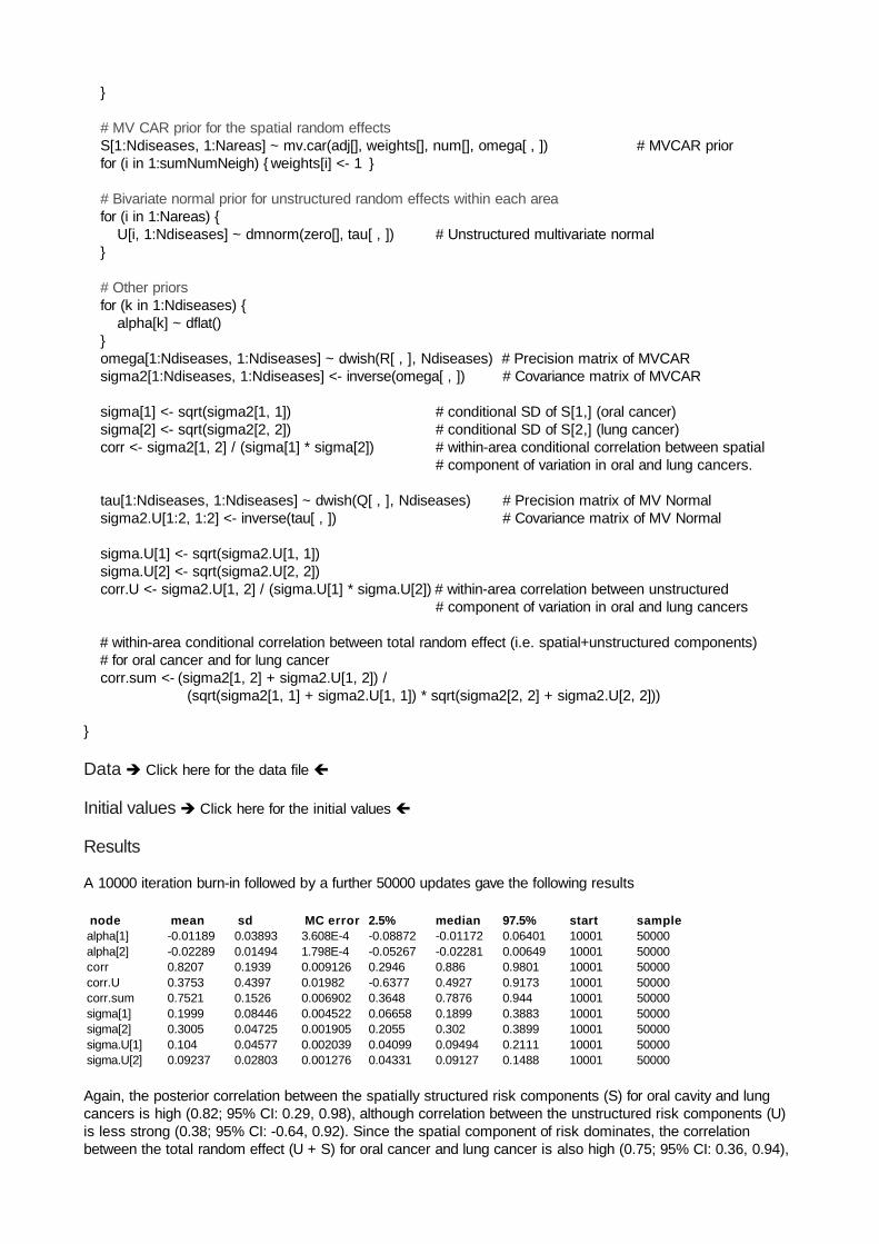
A 10000 iteration burn-in followed by a further 50000 updates gave the following results
node mean sd MC error 2.5% median 97.5% start samplealpha[1] -0.01189 0.03893 3.608E-4 -0.08872 -0.01172 0.06401 10001 50000alpha[2] -0.02289 0.01494 1.798E-4 -0.05267 -0.02281 0.00649 10001 50000corr 0.8207 0.1939 0.009126 0.2946 0.886 0.9801 10001 50000corr.U 0.3753 0.4397 0.01982 -0.6377 0.4927 0.9173 10001 50000corr.sum 0.7521 0.1526 0.006902 0.3648 0.7876 0.944 10001 50000sigma[1] 0.1999 0.08446 0.004522 0.06658 0.1899 0.3883 10001 50000sigma[2] 0.3005 0.04725 0.001905 0.2055 0.302 0.3899 10001 50000sigma.U[1] 0.104 0.04577 0.002039 0.04099 0.09494 0.2111 10001 50000sigma.U[2] 0.09237 0.02803 0.001276 0.04331 0.09127 0.1488 10001 50000
Again, the posterior correlation between the spatially structured risk components (S) for oral cavity and lungcancers is high (0.82; 95% CI: 0.29, 0.98), although correlation between the unstructured risk components (U)is less strong (0.38; 95% CI: -0.64, 0.92). Since the spatial component of risk dominates, the correlationbetween the total random effect (U + S) for oral cancer and lung cancer is also high (0.75; 95% CI: 0.36, 0.94),
� �
� �
again suggesting strong shared geographical pattern of risk between the two diseases.
8. Shared component model for mapping multiple diseases: Oral cavity cancer and
lung cancer cancer in West Yorkshire, UK [top]
Knorr-Held and Best (2001) analysed data on mortality from oral cavity and oesophageal cancer in Germanyusing a shared component model. This model is similar in spirit to conventional factor analysis, and partitionsthe geographical variation in two diseases into a common (shared) component (φφφφ), and two disease-specific(residual) components (ψψψψ1 and ψψψψ2). Making the rare disease assumption, the likelihood for each disease isassumed to be independent Poisson, conditional on an unknown mean µik
Yik ~ Poisson(µik)log µi1 = log Ei1 + α1 + φi∗δ + ψi1
log µi2 = log Ei2 + α2 + φi /δ + ψi2
where Yik and Eik are the observed and age/sex standardised expected counts for cancer k in area irespectively, αk is an intercept term representing the baseline (log) relative risk of cancer k across the studyregion, and δ is a scaling factor to allow the risk gradient associated with the shared component to be differentfor each disease (this is in some sense similar to the factor loadings in conventional factor analysis - seeKnorr-Held and Best (2001) for more details). Each of the three components (φφφφ, ψψψψ1 and ψψψψ2) is assumed to bespatially structured with zero mean; the components are assumed to be independent of each other. Knorr-Heldand Best (2001) used a spatial partition model as a prior for each component. In this example, we fit a similarmodel, but assume an BYM convolution prior for each component. Here we consider the data from example 7on incidence of oral cavity cancer and lung cancer in 126 electoral wards in the West Yorkshire region ofEngland:
model {
# Likelihoodfor (i in 1:Nareas) {
for (k in 1:Ndiseases) {Y[i,k] ~ dpois(mu[i,k])log(mu[i,k]) <- log(E[i,k]) + alpha[k] + eta[i, k]
}}
for(i in 1:Nareas) {# Define log relative risk in terms of disease-specific (psi) and shared (phi) random effectseta[i,1] <- phi[i] *delta + psi[1, i] # changed order of k and i index for psieta[i,2] <- phi[i] /delta + psi[2, i] # (needed because car.normal assumes right hand index is areas)
}
# Spatial priors (BYM) for the disease-specific random effectsfor (k in 1:Ndiseases) {
for (i in 1:Nareas) {psi[k, i] <- U.sp[k, i] + S.sp[k, i] # convolution prior = sum of unstructured and spatial effectsU.sp[k, i] ~ dnorm(0, tau.unstr[k]) # unstructured disease-specific random effects
}S.sp[k,1:Nareas] ~ car.normal(adj[], weights[], num[], tau.spatial[k]) # spatial disease-specific effects
}# Spatial priors (BYM) for the shared random effectsfor (i in 1:Nareas) {
phi[i] <- U.sh[i] + S.sh[i] # convolution prior = sum of unstructured and spatial effectsU.sh[i] ~ dnorm(0, omega.unstr) # unstructured shared random effects
}S.sh[1:Nareas] ~ car.normal(adj[], weights[], num[], omega.spatial) # spatial shared random effects
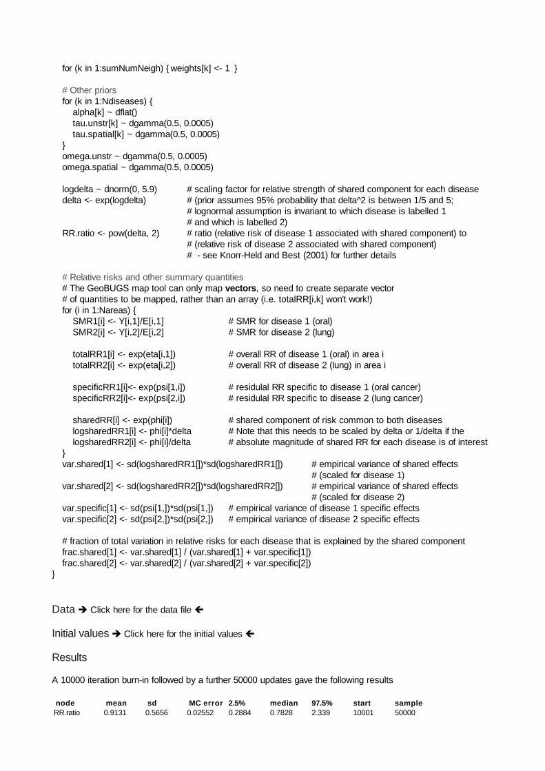
for (k in 1:sumNumNeigh) { weights[k] <- 1 }
# Other priorsfor (k in 1:Ndiseases) {
alpha[k] ~ dflat()tau.unstr[k] ~ dgamma(0.5, 0.0005)tau.spatial[k] ~ dgamma(0.5, 0.0005)
}omega.unstr ~ dgamma(0.5, 0.0005)omega.spatial ~ dgamma(0.5, 0.0005)
logdelta ~ dnorm(0, 5.9) # scaling factor for relative strength of shared component for each diseasedelta <- exp(logdelta) # (prior assumes 95% probability that delta^2 is between 1/5 and 5;
# lognormal assumption is invariant to which disease is labelled 1# and which is labelled 2)
RR.ratio <- pow(delta, 2) # ratio (relative risk of disease 1 associated with shared component) to# (relative risk of disease 2 associated with shared component)# - see Knorr-Held and Best (2001) for further details
# Relative risks and other summary quantities# The GeoBUGS map tool can only map vectors, so need to create separate vector# of quantities to be mapped, rather than an array (i.e. totalRR[i,k] won't work!)for (i in 1:Nareas) {
SMR1[i] <- Y[i,1]/E[i,1] # SMR for disease 1 (oral)SMR2[i] <- Y[i,2]/E[i,2] # SMR for disease 2 (lung)
totalRR1[i] <- exp(eta[i,1]) # overall RR of disease 1 (oral) in area itotalRR2[i] <- exp(eta[i,2]) # overall RR of disease 2 (lung) in area i
specificRR1[i]<- exp(psi[1,i]) # residulal RR specific to disease 1 (oral cancer)specificRR2[i]<- exp(psi[2,i]) # residulal RR specific to disease 2 (lung cancer)
sharedRR[i] <- exp(phi[i]) # shared component of risk common to both diseaseslogsharedRR1[i] <- phi[i]*delta # Note that this needs to be scaled by delta or 1/delta if thelogsharedRR2[i] <- phi[i]/delta # absolute magnitude of shared RR for each disease is of interest
}var.shared[1] <- sd(logsharedRR1[])*sd(logsharedRR1[]) # empirical variance of shared effects
# (scaled for disease 1)var.shared[2] <- sd(logsharedRR2[])*sd(logsharedRR2[]) # empirical variance of shared effects
# (scaled for disease 2)var.specific[1] <- sd(psi[1,])*sd(psi[1,]) # empirical variance of disease 1 specific effectsvar.specific[2] <- sd(psi[2,])*sd(psi[2,]) # empirical variance of disease 2 specific effects
# fraction of total variation in relative risks for each disease that is explained by the shared componentfrac.shared[1] <- var.shared[1] / (var.shared[1] + var.specific[1])frac.shared[2] <- var.shared[2] / (var.shared[2] + var.specific[2])
}
Data Click here for the data file
Initial values Click here for the initial values
Results
A 10000 iteration burn-in followed by a further 50000 updates gave the following results
node mean sd MC error 2.5% median 97.5% start sampleRR.ratio 0.9131 0.5656 0.02552 0.2884 0.7828 2.339 10001 50000
� �
� �
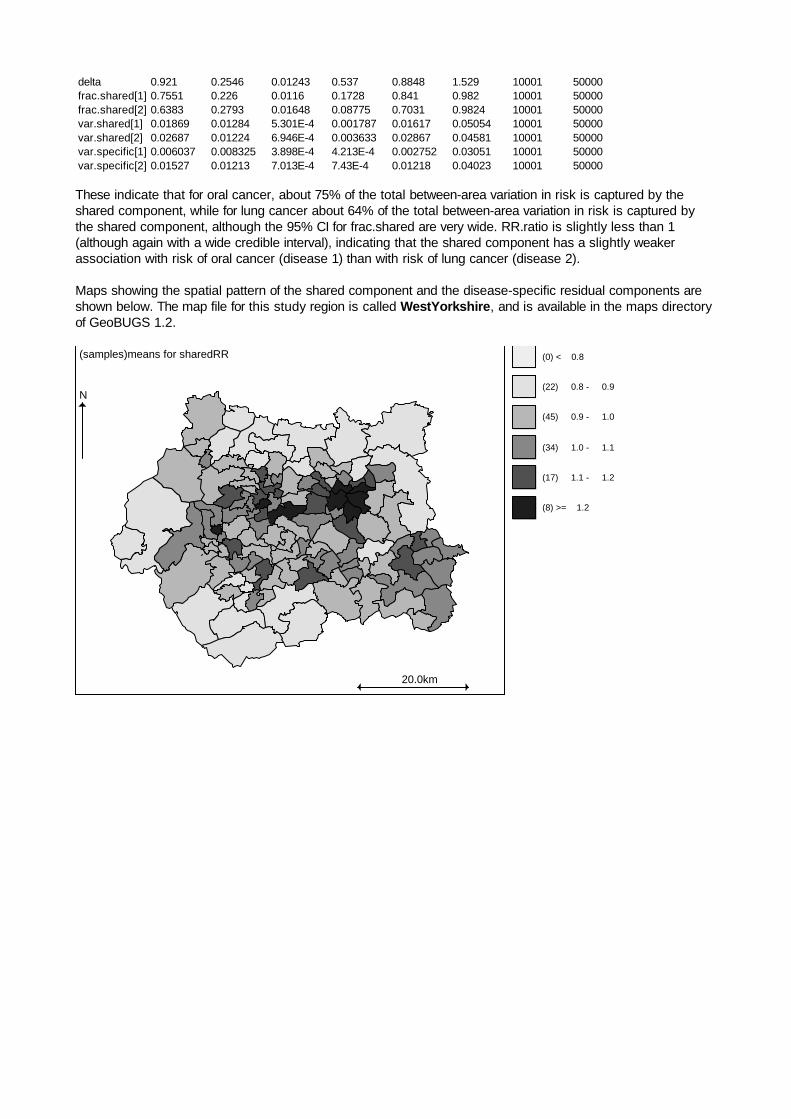
delta 0.921 0.2546 0.01243 0.537 0.8848 1.529 10001 50000frac.shared[1] 0.7551 0.226 0.0116 0.1728 0.841 0.982 10001 50000frac.shared[2] 0.6383 0.2793 0.01648 0.08775 0.7031 0.9824 10001 50000var.shared[1] 0.01869 0.01284 5.301E-4 0.001787 0.01617 0.05054 10001 50000var.shared[2] 0.02687 0.01224 6.946E-4 0.003633 0.02867 0.04581 10001 50000var.specific[1] 0.006037 0.008325 3.898E-4 4.213E-4 0.002752 0.03051 10001 50000var.specific[2] 0.01527 0.01213 7.013E-4 7.43E-4 0.01218 0.04023 10001 50000
These indicate that for oral cancer, about 75% of the total between-area variation in risk is captured by theshared component, while for lung cancer about 64% of the total between-area variation in risk is captured bythe shared component, although the 95% CI for frac.shared are very wide. RR.ratio is slightly less than 1(although again with a wide credible interval), indicating that the shared component has a slightly weakerassociation with risk of oral cancer (disease 1) than with risk of lung cancer (disease 2).
Maps showing the spatial pattern of the shared component and the disease-specific residual components areshown below. The map file for this study region is called WestYorkshire, and is available in the maps directoryof GeoBUGS 1.2.
(0) < 0.8
(22) 0.8 - 0.9
(45) 0.9 - 1.0
(34) 1.0 - 1.1
(17) 1.1 - 1.2
(8) >= 1.2
(samples)means for sharedRR
20.0km
N
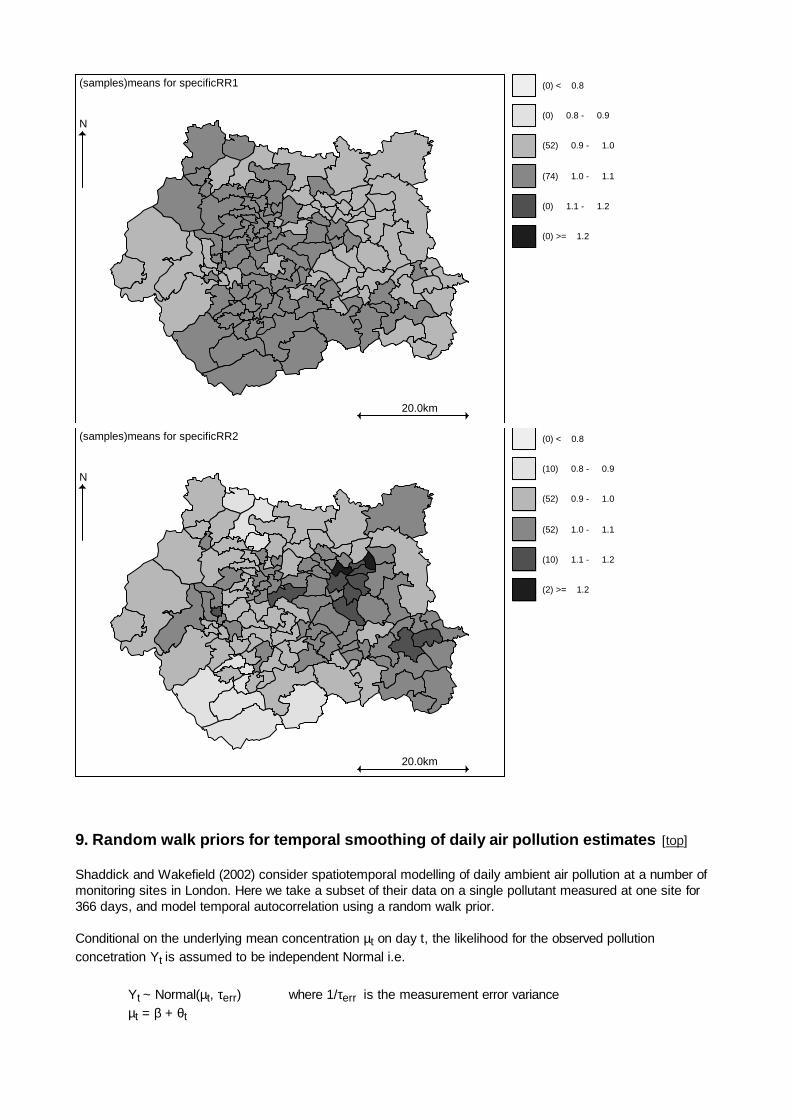
9. Random walk priors for temporal smoothing of daily air pollution estimates [top]
Shaddick and Wakefield (2002) consider spatiotemporal modelling of daily ambient air pollution at a number ofmonitoring sites in London. Here we take a subset of their data on a single pollutant measured at one site for366 days, and model temporal autocorrelation using a random walk prior.
Conditional on the underlying mean concentration µt on day t, the likelihood for the observed pollutionconcetration Yt is assumed to be independent Normal i.e.
Yt ~ Normal(µt, τerr) where 1/τerr is the measurement error varianceµt = β + θt
(0) < 0.8
(0) 0.8 - 0.9
(52) 0.9 - 1.0
(74) 1.0 - 1.1
(0) 1.1 - 1.2
(0) >= 1.2
(samples)means for specificRR1
20.0km
N
(0) < 0.8
(10) 0.8 - 0.9
(52) 0.9 - 1.0
(52) 1.0 - 1.1
(10) 1.1 - 1.2
(2) >= 1.2
(samples)means for specificRR2
20.0km
N
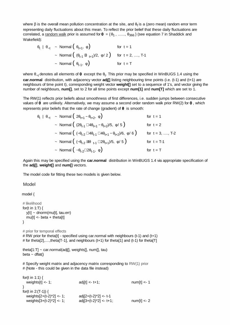
where β is the overall mean pollution concentration at the site, and θt is a (zero mean) random error termrepresenting daily fluctuations about this mean. To reflect the prior belief that these daily fluctuations arecorrelated, a random walk prior is assumed for θθθθ = {θ1 , ......, θ366 } (see equation 7 in Shaddick andWakefield):
θt | θ−t ~ Normal ( θt+1, φ ) for t = 1
~ Normal ( (θt-1 + θt+1)/2, φ / 2 ) for t = 2, ...., T-1
~ Normal ( θt-1, φ) for t = T
where θ−t denotes all elements of θθθθ except the θt. This prior may be specified in WinBUGS 1.4 using the
car.normal distribution, with adjacency vector adj[] listing neighbouring time points (i.e. (t-1) and (t+1) areneighbours of time point t), corresponding weight vector weight[] set to a sequence of 1's, and vector giving thenumber of neighbours, num[], set to 2 for all time points except num[1] and num[T] which are set to 1.
The RW(1) reflects prior beliefs about smoothness of first differences, i.e. sudden jumps between consecutivevalues of θθθθ are unlikely. Alternatively, we may assume a second order random walk prior RW(2) for θθθθ , whichrepresents prior beliefs that the rate of change (gradient) of θθθθ is smooth:
θt | θ−t ~ Normal ( 2θt+1 − θt+2, φ) for t = 1
~ Normal ( (2θt-1 + 4θt+1 − θt+2)/5, φ / 5 ) for t = 2
~ Normal ( (−θt-2 + 4θt-1 + 4θt+1 − θt+2)/6, φ / 6 ) for t = 3, ...., T-2
~ Normal ( (−θt-2 + 4θt-1 + 2θt+1)/5, φ / 5 ) for t = T-1
~ Normal ( −θt-2+ 2θt-1, φ) for t = T
Again this may be specified using the car.normal distribution in WinBUGS 1.4 via appropriate specification ofthe adj[], weight[] and num[] vectors.
The model code for fitting these two models is given below.
Model
model {
# likelihoodfor(t in 1:T) {
y[t] ~ dnorm(mu[t], tau.err)mu[t] <- beta + theta[t]
}
# prior for temporal effects# RW prior for theta[t] - specified using car.normal with neighbours (t-1) and (t+1)# for theta[2],....,theta[T-1], and neighbours (t+1) for theta[1] and (t-1) for theta[T]
theta[1:T] ~ car.normal(adj[], weights[], num[], tau)beta ~ dflat()
# Specify weight matrix and adjacency matrix corresponding to RW(1) prior# (Note - this could be given in the data file instead)
for(t in 1:1) {weights[t] <- 1; adj[t] <- t+1; num[t] <- 1
}for(t in 2:(T-1)) {
weights[2+(t-2)*2] <- 1; adj[2+(t-2)*2] <- t-1weights[3+(t-2)*2] <- 1; adj[3+(t-2)*2] <- t+1; num[t] <- 2
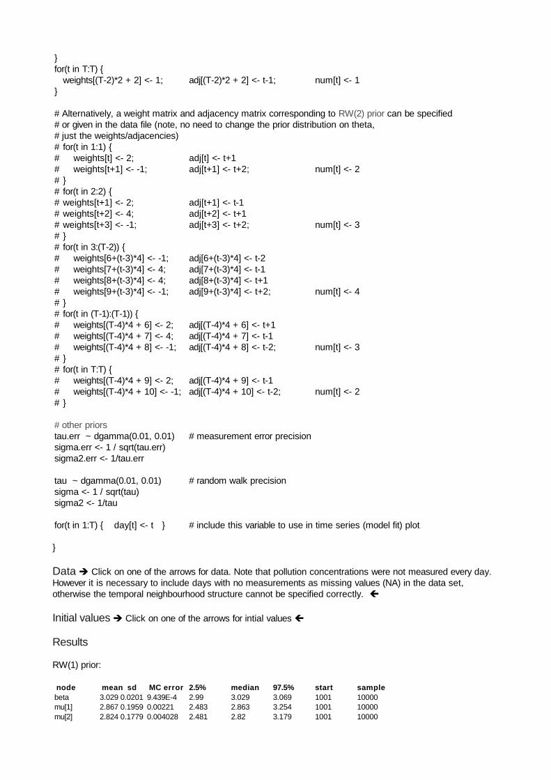
}for(t in T:T) {
weights[(T-2)*2 + 2] <- 1; adj[(T-2)*2 + 2] <- t-1; num[t] <- 1}
# Alternatively, a weight matrix and adjacency matrix corresponding to RW(2) prior can be specified# or given in the data file (note, no need to change the prior distribution on theta,# just the weights/adjacencies)# for(t in 1:1) {# weights[t] <- 2; adj[t] <- t+1# weights[t+1] <- -1; adj[t+1] <- t+2; num[t] <- 2# }# for(t in 2:2) {# weights[t+1] <- 2; adj[t+1] <- t-1# weights[t+2] <- 4; adj[t+2] <- t+1# weights[t+3] <- -1; adj[t+3] <- t+2; num[t] <- 3# }# for(t in 3:(T-2)) {# weights[6+(t-3)*4] <- -1; adj[6+(t-3)*4] <- t-2# weights[7+(t-3)*4] <- 4; adj[7+(t-3)*4] <- t-1# weights[8+(t-3)*4] <- 4; adj[8+(t-3)*4] <- t+1# weights[9+(t-3)*4] <- -1; adj[9+(t-3)*4] <- t+2; num[t] <- 4# }# for(t in (T-1):(T-1)) {# weights[(T-4)*4 + 6] <- 2; adj[(T-4)*4 + 6] <- t+1# weights[(T-4)*4 + 7] <- 4; adj[(T-4)*4 + 7] <- t-1# weights[(T-4)*4 + 8] <- -1; adj[(T-4)*4 + 8] <- t-2; num[t] <- 3# }# for(t in T:T) {# weights[(T-4)*4 + 9] <- 2; adj[(T-4)*4 + 9] <- t-1# weights[(T-4)*4 + 10] <- -1; adj[(T-4)*4 + 10] <- t-2; num[t] <- 2# }
# other priorstau.err ~ dgamma(0.01, 0.01) # measurement error precisionsigma.err <- 1 / sqrt(tau.err)sigma2.err <- 1/tau.err
tau ~ dgamma(0.01, 0.01) # random walk precisionsigma <- 1 / sqrt(tau)sigma2 <- 1/tau
for(t in 1:T) { day[t] <- t } # include this variable to use in time series (model fit) plot
}
Data Click on one of the arrows for data. Note that pollution concentrations were not measured every day.However it is necessary to include days with no measurements as missing values (NA) in the data set,otherwise the temporal neighbourhood structure cannot be specified correctly.
Initial values Click on one of the arrows for intial values
Results
RW(1) prior:
node mean sd MC error 2.5% median 97.5% start samplebeta 3.029 0.0201 9.439E-4 2.99 3.029 3.069 1001 10000mu[1] 2.867 0.1959 0.00221 2.483 2.863 3.254 1001 10000mu[2] 2.824 0.1779 0.004028 2.481 2.82 3.179 1001 10000
�
�
� �
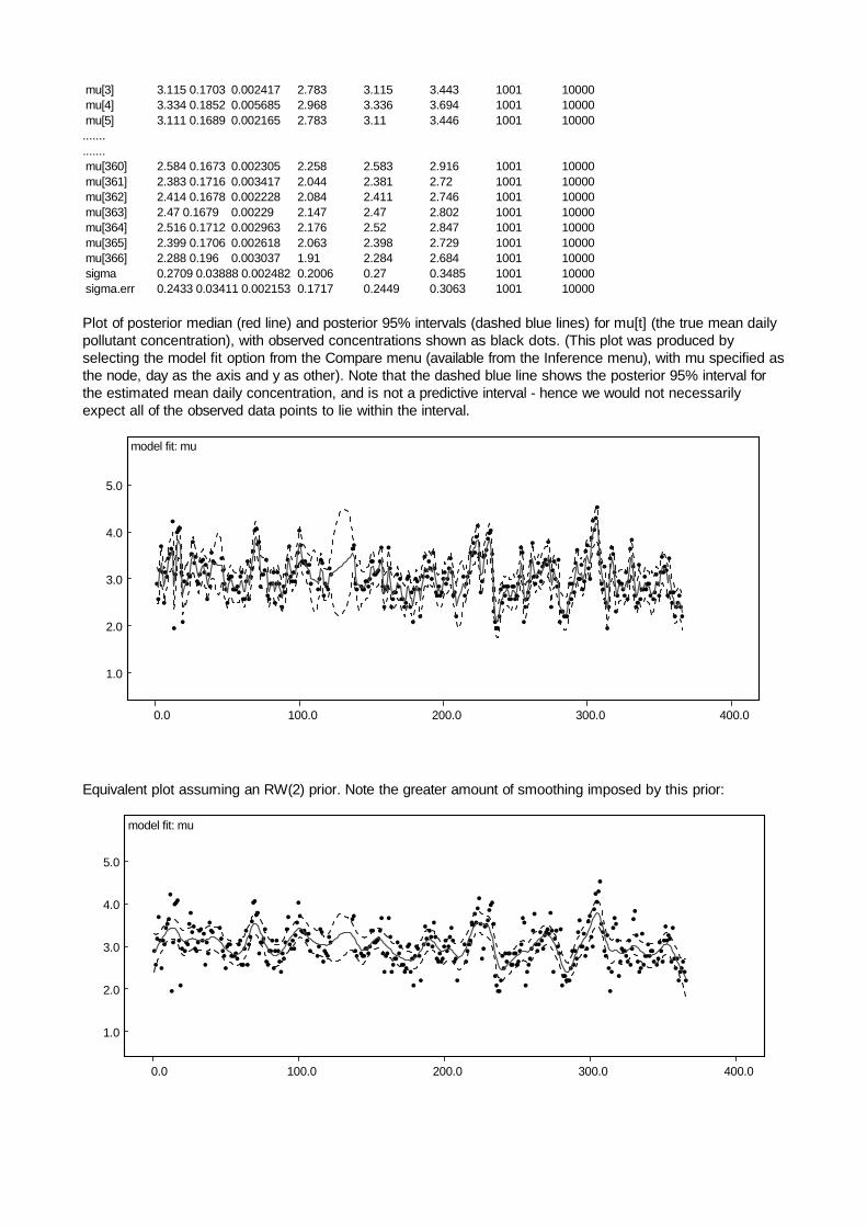
mu[3] 3.115 0.1703 0.002417 2.783 3.115 3.443 1001 10000mu[4] 3.334 0.1852 0.005685 2.968 3.336 3.694 1001 10000mu[5] 3.111 0.1689 0.002165 2.783 3.11 3.446 1001 10000..............mu[360] 2.584 0.1673 0.002305 2.258 2.583 2.916 1001 10000mu[361] 2.383 0.1716 0.003417 2.044 2.381 2.72 1001 10000mu[362] 2.414 0.1678 0.002228 2.084 2.411 2.746 1001 10000mu[363] 2.47 0.1679 0.00229 2.147 2.47 2.802 1001 10000mu[364] 2.516 0.1712 0.002963 2.176 2.52 2.847 1001 10000mu[365] 2.399 0.1706 0.002618 2.063 2.398 2.729 1001 10000mu[366] 2.288 0.196 0.003037 1.91 2.284 2.684 1001 10000sigma 0.2709 0.03888 0.002482 0.2006 0.27 0.3485 1001 10000sigma.err 0.2433 0.03411 0.002153 0.1717 0.2449 0.3063 1001 10000
Plot of posterior median (red line) and posterior 95% intervals (dashed blue lines) for mu[t] (the true mean dailypollutant concentration), with observed concentrations shown as black dots. (This plot was produced byselecting the model fit option from the Compare menu (available from the Inference menu), with mu specified asthe node, day as the axis and y as other). Note that the dashed blue line shows the posterior 95% interval forthe estimated mean daily concentration, and is not a predictive interval - hence we would not necessarilyexpect all of the observed data points to lie within the interval.
Equivalent plot assuming an RW(2) prior. Note the greater amount of smoothing imposed by this prior:
model fit: mu
0.0 100.0 200.0 300.0 400.0
1.0
2.0
3.0
4.0
5.0
model fit: mu
0.0 100.0 200.0 300.0 400.0
1.0
2.0
3.0
4.0
5.0
Appendix 1: Technical details of Structured MultivariateGaussian and Conditional Autoregressive (CAR) models andhyperprior specification. [top]
(Note: for clarity of exposition, we parameterise the Normal distribution in terms of the mean and variance in thefollowing discussion. However, WinBUGS parameterisation of the CAR and structured MVN models is in termsof the mean and precision as usual.)
Assume we have a set of area-specific spatially correlated Gaussian data or random effects Si, i=1,..., N
(where N is the number of areas in the study region). Suppose their joint distribution may be expressed asfollows:
S ~ MVN(µµµµ, vΣΣΣΣ)
where S = ( S1, ....., SN ), MVN denotes the N-dimensional multivariate normal distribution, µµµµ is the 1 x Nmean vector, v > 0 controls the overall variability of the Si and ΣΣΣΣ is an N x N positive definite matrix.
Joint specification [top]
We may assume a parametric form for the elements of the between-area correlation matrix:Σij = f(dij; θ)
where dij = distance between areas i and j. WinBUGS 1.4 allows two options for the funtion f(.) (see Richardson
(1992) for further details of these functions):
1. Powered exponential family
f(dij; φ, κ) = exp[−(φdij)κ ] where φ> 0, κ in (0, 2]
The parameter φ controls the rate of decline of correlation with distance:
φ large −> rapid decayφsmall −> slow decay
One possible strategy for specifying a prior for φ is to choose a uniform distribution between φmin and φmax
where φmin and φmax are chosen to give a sensible range of values for correlations both at a distance equal to
the maximum distance between any pair of areas in the study region, and at a distance equal to the minimumdistance between any pair of areas in the study. For example, if the minimum distance is 1 km (say), and themaximum distance is 20 km (say), then values of φmin = 0.04 and φmax = 5 would give a diffuse but plausible
prior range of correlations (assuming κ = 1) between 0.007 and 0.96 at a distance of 1 km, and between 0 and0.45 at a distance of 20 km. Note that it is advisable to choose a value of φmin that prevents the correlation at
the maximum distance between observations in the study region from being too high, since this can lead toidentifiability problems between the overall mean, µµµµ, of the spatial random variables and the correlationparameter, φ.
The parameter κ controls the amount by which spatial variations in the data are smoothed. Large values of κlead to greater smoothing, with κ = 2 corresponding to the Gaussian correlation function (although the resultingcovariance matrix is nearly singular). It is often difficult to learn much about this parameter, so unless there is agood reason for believing otherwise, it is usually advisable to set κ = 1 a priori.
2. Disc model
f(dij; α) = 2 / π * {cos−1 (dij /α) − [(dij /α)(1 − (dij2 /α2))]1/2 } for dij < α
= 0 for dij > α
The parameter α controls the rate of decline of correlation with distance:
α large −> slow decayα small −> rapid decay
The disc function leads to an approximately linear decrease in correlation with increasing distance, withcorrelation declining to zero at a distance equal to α. Again, it is advisable to choose a prior for α that prevents
the correlation at the maximum distance between observations in the study region from being too high, sincethis can lead to identifiability problems between the overall mean, µµµµ, of the spatial random variables and thecorrelation parameter, α. An upper prior bound on α equal to a small multiple of the maximum distance in thestudy region is therefore a sensible 'default' choice. The minimum value allowed a priori for α should also bechosen carefully since values of α less than the minimum distance between observations in the study regionwill not be identifiable.
Exploratory analysis using variograms maybe be helpful to help chose an appropriate specification for thecorrelation function and associated parameters.
Conditional specification [top]
By writing the between-area covariance matrix in the following form:vΣΣΣΣ = v(I - γ C)-1 M
where I = N x N identity matrixM = N x N diagonal matrix, with elements Mii proportional to the conditional variance of Si | Sj
C = N x N weight matrix, with elements Cij reflecting spatial association between areas i and jγ = controls overall strength of spatial dependence
and using standard multivariate normal theory (e.g. Johnson and Kotz, 1972; Besag and Kooperberg, 1995),the joint multivariate Gaussian model can be expressed in the form of a set of conditional distributions
Si | S−i ~ Normal (µ i + Σj γ Cij (sj −µ i), φ Mii ),
(here Σj denotes summation over j=1 to N, not covariance matrix, and S−i denotes all the elements of S except Si)
From a modelling perspective, use of the joint formulation requires specification of the elements of thecovariance matrix ΣΣΣΣ (see above), while use of the conditional formulation reduces to specification of thematrices C and M and the spatial dependence parameter γ. Various constraints are needed on the values of C,M and γ in order to ensure that ΣΣΣΣ is symmetric positive definite:
∗∗∗∗ ΣΣΣΣ is only symmetric if Cij Mjj = Cji Mii
∗∗∗∗ Var( Si | Sj ) = vMii > 0 so Mii must be > 0
∗∗∗∗ To ensure S is positive definite, γ must lie between γ min and γ max where γ min-1 and γ max-1 are the smallest
and largest eigenvalues of M-1/2 C M1/2
∗∗∗∗ In practice, we often expect positive spatial dependence, so constrain prior for γ to be between 0 and γ max
∗∗∗∗ γ = 0 implies no spatial dependence
Intrinsic CAR model [top]
Besag, York and Mollie (1991) propose an intrinsic version of this CAR model in which the covariance matrix ΣΣΣΣis not positive definite. Their model corresponds to choosing Cij = 1/ni if areas i and j are adjacent and Cij = 0
otherwise (with Cii also set to 0), Mii = 1/ni, and setting γ = γ max which turns out to always be 1 with this
particular choice of Cij and Mii. Here, ni is the number of areas which are adjacent to area i. Comparison with
the equations above shows that this leads to the following model for the conditional distribution of Si | S−i :
Si | S−i ~ Normal ( S.bari , v / ni )

where S.bari = Σ j in δiSj / ni and δi denotes the set of labels of the "neighbours" of area i. Hence Si has a
normal distribution with conditional mean given by the average of the neighbouring Sj 's and conditional varianceinversely proportional to the number of neighbours ni . Note that an equivalent specification is take
unnormalised weights Wij = 1 if areas i and j are adjacent and Wij = 0 otherwise, and set Cij = Wij / Wi+ where
Wi+ = Σ j Wij. The car.normal and (car.l1) distributions in GeoBUGS requires the user to specify
unnormalised weights.
Since the CAR model defined above is improper (the overall mean of the Si is not defined), it can only be usedas a prior distribution for spatially distributed random effects, and not as a likelihood for data. It is oftenconvenient to assume that suchrandom effects have zero mean. Besag and Kooperberg (1995) show thatconstraining the random effects to sum to zero and specifying a separate intercept term with a locationinvariant Uniform(-infty, +infty) prior is equivalent to the unconstrained parameterisation with no separateintercept. WinBUGS 1.4 includes a distribution called dflat() which corresponds to an improper (flat) prior onthe whole real line. This prior must always be used for the intercept term in a model including CAR randomeffects.
We must also specify prior distributions for the overall variance parameter v. As usual in WinBUGS, thecar.normal (and car.l1) distributions are parameterised in terms of the precision τ = 1/v . Care is needed whenchoosing a prior for τ since the posterior variance of the random effects can be quite sensitive. One option is agamma distribution with shape and inverse scale parameters both equal to 0.01. This has a mean of 0.01/0.01= 1 and a large variance of 0.01/(0.01)2 = 100; however, this tends to place most of the prior mass away fromzero (on the scale of the random effects standard deviation), and so in situations when the true spatialdependence between areas is negligible (i.e. standard deviation close to zero) this may induce artefactualspatial structure in the posterior. Kelsall and Wakefield (1999) suggest an alternative gamma(0.5, 0.0005) priorfor the precision parameter of the spatial random effects in a CAR model. This expresses the prior belief thatthe random effects standard deviation is centered around 0.05 with a 1% prior probability of being smaller than0.01 or larger than 2.5.
Proper CAR model [top]
If γ is constrained to lie in the interval (γ min , γ max ) where γ min-1 and γ max-1 are the smallest and largest
eigenvalues of M-1/2 C M1/2 as defined above, rather than being fixed to its maximum as in the intrinsic CAR,then the resulting distribution is proper provided the constraints on C and M are still satisfied. The choice Cij =
1/ni if areas i and j are adjacent and Cij = 0 otherwise (with Cii also set to 0) and Mii = 1/ni, where ni is the
number of areas which are adjacent to area i is still valid for the proper CAR. In the context of disease mappingCressie and Chan (1989) and Stern and Cressie (1999) choose an alternative parameterisation:
Mii = 1/Ei (the inverse of the expected count or population size in area i)
Cij = (Ej / Ei)1/2 for neighbouring areas i, j and 0 otherwise
Multivariate intrinsic CAR model [top]
Assume we have a multivariate p-dimensional vector of spatially correlated Gaussian data or random effects ineach area, Si = (S1i , S2i,....., Spi )', i=1,..., N. The CAR models discussed above extend naturally to amultivariate setting by replacing the univariate Gaussian conditional distribution for Si | Sj with a multivariateconditional distribution. In the case of the intrinsic CAR prior with 0-1 adjacency weights as used by Besag,York and Mollie (1991), and taking the case of p=2 for simplicity, this gives:
Si | (S1(−i), S2(−i)) ~ Bivariate Normal (S.bari , V / ni ),
(here (S1(−i), S2(−i)) denotes the elements of the 2 x N matrix S excluding the ith area (column))
where S.bari = (S.bari1 , S.bari2) with S.barip = Σ j in δiSjp / ni and, as in the univariate case, δi and ni denote
the set of labels of the "neighbours" of area i and the number of neighbours, respectively. V is a 2 x 2covariance matix with diagonal elements v11 and v22 representing the conditional variances of S1 and S2

respectively, and off-diagonal element v12 representing the (conditional) within-area covariance between S1 and
S2. In general Si has a p-dimensional multivariate normal distribution with pth element of the conditional mean
vector given by the average of the neighbouring Sjp 's and conditional covariance matrix inversely proportional tothe number of neighbours ni, with pth diagonal element representing the conditional variance of the pth
component of S and off-diagonal elements representing the conditional covariances between each pair of the pelements of S.
Gelfand and Vounatsou (2003) discuss a multivariate generalisation of the proper version of CAR distribution,but only the improper intrinsic multivariate CAR is currently implemented in WinBUGS.
Appendix 2: Technical details of the Poisson-gamma SpatialMoving Average convolution model . [top]
Spatial moving average models are a flexible class of models that have been used to describe continuousspatial processes, particularly in geostatistical applications. Such models are constructed by integrating asimple two-dimensional random noise process (for example, a grid of iid Gaussian random variables) with asmoothing kernel that is a function of distance and, possibly, location. The kernel can be thought of as adevice to `smear out' the random noise process in two-dimensional space to give a smooth surface.
Spatial moving average models have been developed primarily for continuous spatial processes and arecurrently not implementable in WinBUGS 1.4. However, Ickstadt and Wolpert (1998) and Best et al (2000b)proposed a discrete version of a gamma moving average process, for use in identity-link Poisson regressionmodels. Suppose we have a set of area-specific spatially correlated Poisson count data (or random effects) Si,
i=1,..., N (where N is the number of areas in the study region). Ickstadt and Wolpert (1998) and Best et al(2000b) model spatial dependence at the level of the Poisson mean, and assume that the counts Si are
conditionally independent given this mean:
Si ~ Poisson( λ i )
The model for each λ i is constructed by specifying an arbitrary grid of latent iid gamma random variables γ j
(j=1,...,J where J is the total number of grid cells defining the latent process) covering the study region. Theseare then convolved with a kernel matrix whose elements, kij, represent the relative contribution of the latent
variable in grid cell j to the Poisson mean in area i:
λ i = Σ j γ j * kij
Best et al (2000b) assume an isotropic, stationary Gaussian kernel function (although other kernel forms areeasily accommodated, such as an adjacency-based kernel - see example 5):
kij = τ / (2π ρ2) exp(−dij2 / 2ρ2)
where τ can be thought of as a scale factor for the λ's, dij is the distance between the centroid of area i and
the centroid of latent grid cell j, and ρ is the spatial range parameter governing how rapidly the influence ofthe latent gamma random variables on the area-specific Poisson means declines with distance.
One interpretation of Poisson-gamma moving average model is to view the gamma random variables asrepresenting the location and magnitude of unmeasured risk factors, and the area-specific Poisson means λ i
as representing the cumulative effect of these risk factors in each area, weighted by their distance from thearea according to the kernel 'weights' kij.
The model may be extended to include observed covariates and an offset adjustment (e.g. to account fordifferent populations in different areas). Observed covariates are included as additive terms in the linearpredictor λ i as in a standard identity link Poisson regression:
λ i = Σ k β k Xik + Σ j γ j * kij
where Xik is the value of the kth observed covariate in area i. Note that due to the identity link, all covariatesand regression coefficients must take positive values, yielding an interpretation as additive excess risk factors.The latent terms θi = Σ j γ j * kij may then be thought of as a spatial (non-negative) random effect for area i.
Adjustment for an offset - say the population living in each area, Ni - is easily achieved by setting
λ i = pi Ni
pi = Σ k β k Xik + Σ j γ j * kij
Note that Best et al (2004) discuss how to standardise the offset Ni for different age and sex distributions
within each area in an epidemiological application of these models.
Estimation of the pois.conv distribution is carried out in WinBUGS 1.4 using a data augmentation scheme toexploit the Poisson-gamma conjugacy of the full conditionals for the γ j parameters (see Ickstadt and Wolpert(1998) and Best et al (2000b) for details). It is also a good idea to assume gamma prior distributions for anyother uncertain parameters in the linear predictor λ i (e.g. the β k parameters above) to exploit this conjugacy,
although it is possible to assume any suitable prior distribution with positive support for these otherparameters. Hyperprior specification is discussed in detail by Ickstadt and Wolpert (1998) and Best et al(2000b). Note however that the prior shape (a) and precision (b) parameters of the latent gamma variablesshould be chosen such that γ j has prior mean proportional to the area of the jth latent grid cell. This makesthe model spatially extensible in the sense that any partition of the latent gamma random variables will lead toidentical probability distributions for the kernel-weighted sums Σ j γ j * kij.
References [top]
Besag, J., York, J. and Mollie, A. (1991). Bayesian image restoration, with two applications in spatialstatistics. Annals of the Institute of Statistical Mathematics, 43, 1--59, (With discussion).
Besag, J. and Kooperberg, C.L. (1995). On conditional and intrinsic autoregressions. Biometrika, 82, 733--746.
Best, N.G., Richardson, S. and Thomson, A. (2004). A comparison of Bayesian spatial models for diseasemapping. Statistical Methods in Medical Research (to appear).
Best, N.G., Ickstadt, K.and Wolpert, R.L. (2000a). Spatial Poisson regression for health and exposure datameasured at disparate resolutions. Journal of the American Statistical Association, 95, 1076-1088.
Best, N.G., Ickstadt, K., Wolpert, R.L. and Briggs, D.J. (2000b). Combining models of health and exposuredata: the SAVIAH study. In Spatial Epidemiology: Methods and Applications. P. Elliott, J.C. Wakefield, N.G.Best and D.J. Briggs (eds), Oxford: Oxford University Press, p. 393-414.
Clayton, D.G and Kaldor, J. (1987). Empirical Bayes estimates of age-standardized relative risks for use indisease mapping. Biometrics, 43, 671--681.
Cressie, N.A. and Chan, N.H. (1989). Spatial modeling of regional variables. Journal of the AmericanStatistical Association, 84, 393--401.
Diggle, P.J., Tawn, J.A. and Moyeed, R.A. (1998). Model-based geostatistics. Applied Statistics, 47, 299-350.
Fahrmeir, L. and Lang, S. (2001). Bayesian inference for generlaized additive mixed models based on Markovrandom field priors. Applied Statistics, 50, 201-220.
Gelfand, A. and Vounatsou, P. (2003). Proper multivariate conditional autoregressive models for spatial dataanalysis. Biostatistics, 4, 11-25.

Ickstadt, K. and Wolpert, R.L. (1998). Multiresolution assessment of forest inhomogeneity. In Case Studies inBayesian Statistics, Volume 3. Lecture Notes in Statistics, 121. C. Gatsonis, J.S. Hodges, R.E. Kass, R.McCulloch, P. Rossi and N.D. Singpurwalla (eds), New York: Springer-Verlag, p. 371-386.
Johnson, N.L. and Kotz, S. (1972). Distributions in Statistics: continuous multivariate. Wiley: New York.
Kelsall, J.E. and Wakefield, J.C. (1999). Discussion of "Bayesian models for spatially correlated disease andexposure data", by Best et al. In Bayesian Statistics 6. J.M. Bernardo, J.O. Berger, A.P. Dawid and A.F.M.Smith (eds), Oxford: Oxford University Press, p. 151.
Knorr-Held L. and Best N.G. (2001). A shared component model for joint and selective clustering of twodiseases. Journal of the Royal Statistical Society, Series A.
Mollie, A. (1996). Bayesian mapping of disease. In Markov Chain Monte Carlo in Practice. W.R. Gilks, S.Richardson and D.J. Spiegelhalter (eds.), New York: Chapman & Hall, pp. 359--379.
Richardson, S. (1992). Statistical methods for geographical correlation studies. In Geographical andEnvironmental Epidemiology. P. Elliott, J. Cuzick, D. English and R. Stern (eds.), Oxford: Oxford UniversityPress, p. 181-204.
Shaddick, G. and Wakefield, J. (2002). Modelling daily multivariate pollutant data at multiple sites. AppliedStatistics, 51, 351-372.
Stern, H.S. and Cressie, N.A. (1999). Inference for extremes in disease mapping. In Disease mapping and riskassessment for public health. A. Lawson, A. Biggeri, D. Bohning, E. Lesaffre, J-F. Viel and R. Bertollini (eds.),Chichester: Wiley, p. 63--84.
Wakefield, J.C., Best, N.G., and Waller, L.A. (2000). Bayesian Approaches to Disease Mapping. In SpatialEpidemiology: Methods and Applications. P. Elliott, J.C. Wakefield, N.G. Best and D.J. Briggs (eds), Oxford:Oxford University Press, p. 104-127.
Wolpert, R.L. and Ickstadt, K. (1998). Poisson/Gamma random field models for spatial statistics. Biometrika,85, 251-267.