GEOARCHAEOLOGICAL ANALYSIS OF A NORTHWEST COAST PLANK HOUSE:

FORMATION PROCESSES AT THE DIONISIO POINT SITE

By

JAMES PATRICK DOLAN

A thesis submitted in partial fulfillment ofthe requirements for the degree of

MASTER OF ARTS IN ANTHROPOLOGY

WASHINGTON STATE UNIVERSITYDepartment of Anthropology

DECEMBER 2009

To the Faculty of Washington State University

The members of the Committee appointed to examine the thesis of JAMES PATRICK DOLAN find it satisfactory and recommend that it be accepted.

Melissa Goodman-Elgar Ph.D., Chair

Colin Grier, Ph.D.

Robert Ackerman, Ph.D.

ii

ACKNOWLEDGMENTS

I would like to thank foremost my committee. This thesis would not have

been possible without their patience and guidance. I would like to thank M.

Goodman-Elgar, C. Grier, and R. Ackerman for everything that they have done to

make this possible. I would also like to thank my family and friends for their

endless support.

iii

GEOARCHAEOLOGICAL ANALYSIS OF A NORTHWEST COAST PLANK HOUSE:

FORMATION PROCESSES AT THE DIONISIO POINT SITE

Abstract

by James Patrick Dolan, M.A.Washington State University

December 2009

Chair: Melissa Goodman-Elgar

Since the later 19th century, the societies of the Northwest Coast have been recognized as

complex hunter-gatherers. Archaeological research into the pre-contact history of these societies

has been characterized as divided into two discussions, one concerning the evolutionary history

of a complex hunting and gathering economies, and the other the rise of inequality. Increasingly,

prehistoric plank house deposits are being seen as a nexus of these two research themes,

providing archaeologists with the opportunity to explore the integration of ecology, economy,

social organization, and culture at the local level. Research of this nature has typically focused

on the spatial organization of evidence of production and consumption activities through stone

tool, bone tool, and faunal remain analyses. This study broadens this research by focusing on

plank house deposits as sedimentary data sets.

iv

The goal of this study is to present the results of geoarchaeological analyses that

demonstrate that we can establish better links between models of plank house formation

processes and archaeological data through quantitative methods based in the soil and

sedimentary sciences. To this end, sediment samples were collected from confirmed house

deposits at a major Marpole phase village site at Dionisio Point on Galiano Island in

southwestern British Columbia. Using current models of plank house cultural formation

processes and the extensive ethnographic record for the region, a model of the sedimentary

signatures of several plank house architectural features was generated. This permitted the

prediction of expected values for a series of geoarchaeological assays. Laboratory

determinations were compared to model expectations. Soil texture, organic matter enrichment,

inorganic carbonate enrichment, and electrical conductivity were proximate measures of the

presence and intensity of human activity, permitting the differentiation of house from non-house

deposits as well as features internal to these structures. House features, as expected, reflected a

range of non-cultural formation processes that could not be directly assessed through the artifact

assemblage. Moreover, sediments demonstrated that cultural formation processes varied within

these deposits between functionally analogous features. This variation is best identified as

reflecting socio-economic differentiation of the family units that made up the household.

v

Table of Contents

List of Tables.........................................................................................................................viii

List of Figures..........................................................................................................................x

....................................................................................................Chapter One: Introduction 1

................................................................................................Chapter Two: Dionisio Point 16

.............................................................................The Dionisio Point Site: Prior Excavations 19

.......................................................Dionisio Point in a Regional Archaeological Perspective 26

.............................................................Chapter Three: A Geoarchaeological Framework 29

.................................................................................................................Analytical Variables 30

.........................................................................................................................Natural Setting 36

........................................................................................................Geoarchaeological Model 45

...................................................................................Chapter Four: Methods and Results 60

...................................................................................................................................Methods 67

.....................................................................................................................................Results 72

.....................................................................................................Chapter Five: Discussion 90

.................................................................................Cultural Stratigraphy at Dionisio Point 103

......................................................Identifying formation processes of plank house features 104

................................Implications for socio-economic reconstruction shed-roof households 130

.......................................................................Prospects for Geoarchaeological Prospection 133

..............................................................Chapter Six: Conclusions and Future Research 135

..........................................................................................................................Appendices 141

............................................................................................................Appendix A: Methods 142

.......................................................................................Appendix B: Sample Descriptions 149

...................................................................Appendix C: Laser Particle Size Analyzer Data 156

.....................................................................................Appendix D: Hydrometer Raw Data 161

.........................................................................................Appendix E: Hydrometer Results 168

.....................................................................................Appendix F: Loss-On-Ignition Data 180

..............................................................Appendix G: Electrical Conductivity and pH Data 184

........................................................................................................................Bibliography 186

vii

List of Tables

Title Page

Table 3.1 Comparison of Canadian and Standard U.S. Wentworth- 32 Uddon grain-size classification systems

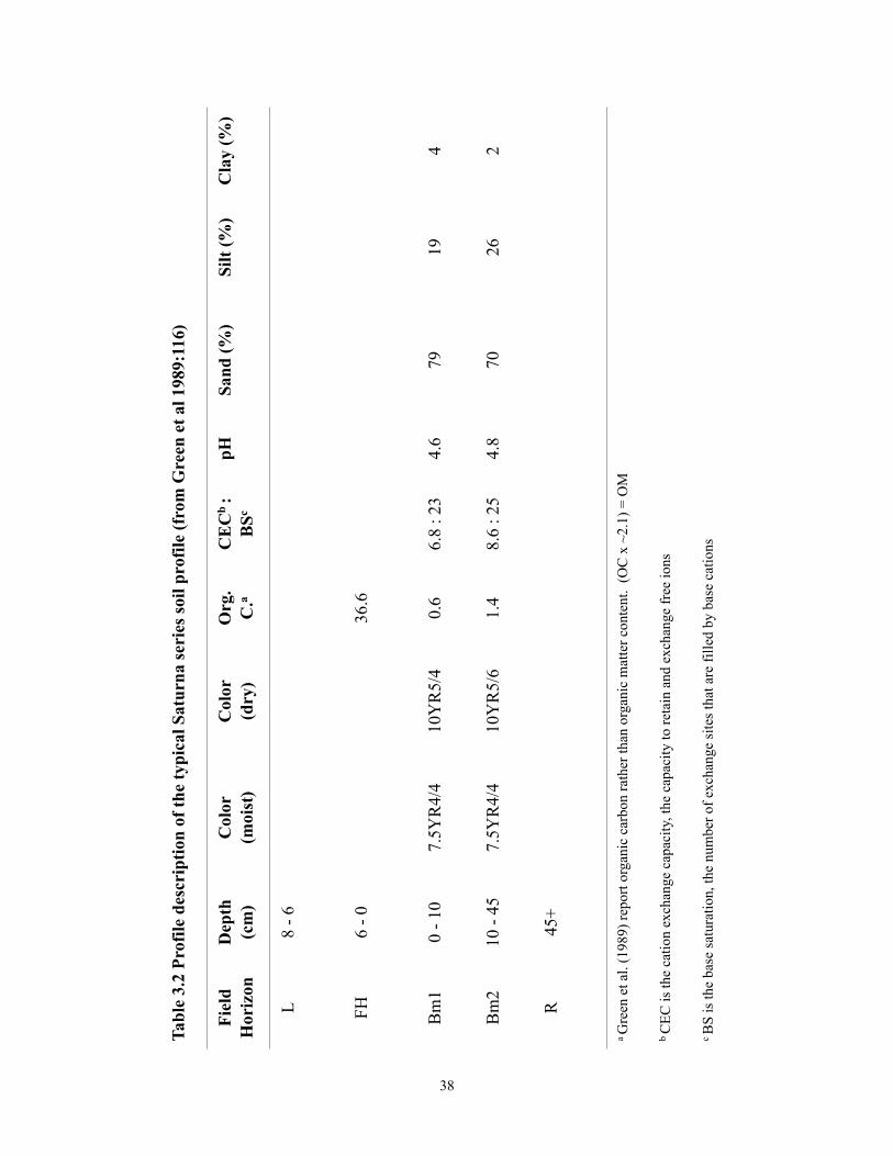
Table 3.2 Profile description of the typical Saturna series soil 38 profile (from Green et al 1989:116)

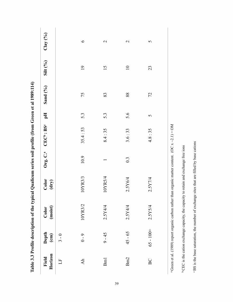
Table 3.3 Profile description of the typical Qualicum series 39 soil profile (from Green et al 1989:114)

Table 3.4 Expectations of natural soil characteristics 44

Table 3.5 Cultural versus natural sample geoarchaeological expectations 57

Table 4.1 Generalized descriptions of site stratigraphy 66 (from Grier 2001:102-130)

Table 4.2 Feature Descriptions for Layer A (from DPHAP field notes) 68

Table 4.3 Feature Descriptions for Layer B/C (from DPHAP field notes) 69

Table 4.4 Methods and precision error margins used in this analysis 71

Table 4.5 Natural Samples 73

Table 4.6 Summary statistics of natural controls with the addition of 97M21 78

Table 4.7 Cultural Samples 79

Table 4.8: Mean and standard deviations of cultural strata 81 sedimentary characteristics

Table 5.1 Cultural layer A versus the natural data set difference of means 92 and difference medians tests

Table 5.2 Cultural layer B versus the natural data set difference of means 92 and difference medians tests

viii

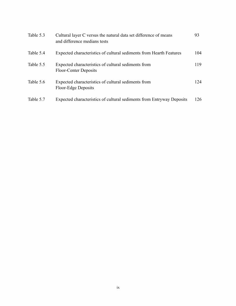
Table 5.3 Cultural layer C versus the natural data set difference of means 93 and difference medians tests

Table 5.4 Expected characteristics of cultural sediments from Hearth Features 104

Table 5.5 Expected characteristics of cultural sediments from 119 Floor-Center Deposits

Table 5.6 Expected characteristics of cultural sediments from 124 Floor-Edge Deposits

Table 5.7 Expected characteristics of cultural sediments from Entryway Deposits 126

ix

List of Figures

Title Page

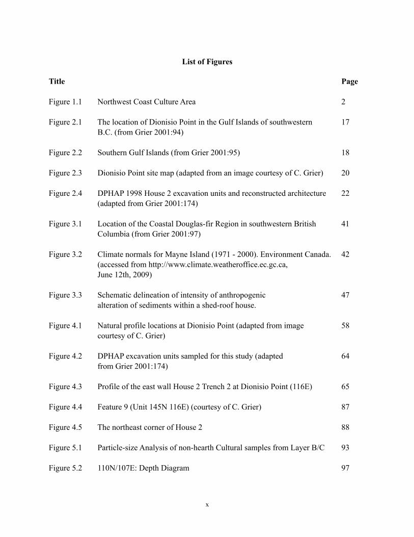
Figure 1.1 Northwest Coast Culture Area 2

Figure 2.1 The location of Dionisio Point in the Gulf Islands of southwestern 17 B.C. (from Grier 2001:94)

Figure 2.2 Southern Gulf Islands (from Grier 2001:95) 18

Figure 2.3 Dionisio Point site map (adapted from an image courtesy of C. Grier) 20

Figure 2.4 DPHAP 1998 House 2 excavation units and reconstructed architecture 22 (adapted from Grier 2001:174)

Figure 3.1 Location of the Coastal Douglas-fir Region in southwestern British 41 Columbia (from Grier 2001:97)

Figure 3.2 Climate normals for Mayne Island (1971 - 2000). Environment Canada. 42 (accessed from http://www.climate.weatheroffice.ec.gc.ca, June 12th, 2009)

Figure 3.3 Schematic delineation of intensity of anthropogenic 47 alteration of sediments within a shed-roof house.

Figure 4.1 Natural profile locations at Dionisio Point (adapted from image 58 courtesy of C. Grier)

Figure 4.2 DPHAP excavation units sampled for this study (adapted 64 from Grier 2001:174)

Figure 4.3 Profile of the east wall House 2 Trench 2 at Dionisio Point (116E) 65

Figure 4.4 Feature 9 (Unit 145N 116E) (courtesy of C. Grier) 87

Figure 4.5 The northeast corner of House 2 88

Figure 5.1 Particle-size Analysis of non-hearth Cultural samples from Layer B/C 93

Figure 5.2 110N/107E: Depth Diagram 97

x

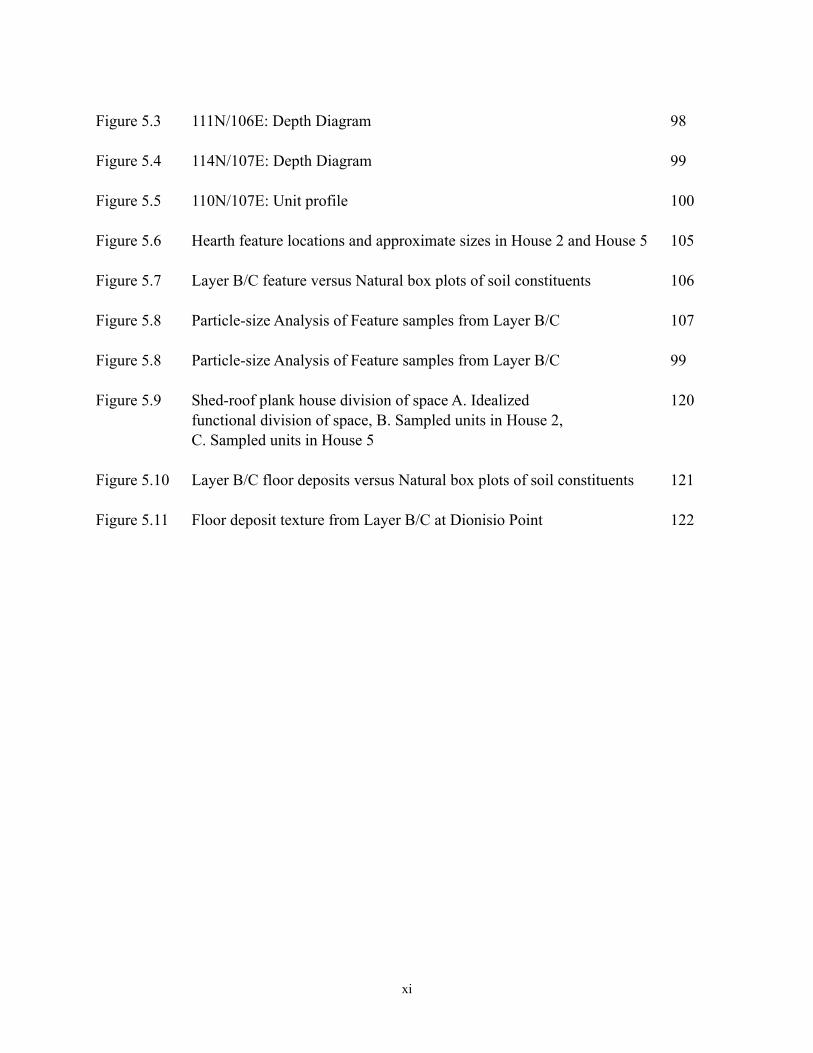
Figure 5.3 111N/106E: Depth Diagram 98

Figure 5.4 114N/107E: Depth Diagram 99

Figure 5.5 110N/107E: Unit profile 100

Figure 5.6 Hearth feature locations and approximate sizes in House 2 and House 5 105

Figure 5.7 Layer B/C feature versus Natural box plots of soil constituents 106

Figure 5.8 Particle-size Analysis of Feature samples from Layer B/C 107

Figure 5.8 Particle-size Analysis of Feature samples from Layer B/C 99

Figure 5.9 Shed-roof plank house division of space A. Idealized 120 functional division of space, B. Sampled units in House 2, C. Sampled units in House 5

Figure 5.10 Layer B/C floor deposits versus Natural box plots of soil constituents 121

Figure 5.11 Floor deposit texture from Layer B/C at Dionisio Point 122

xi

Chapter One: Introduction

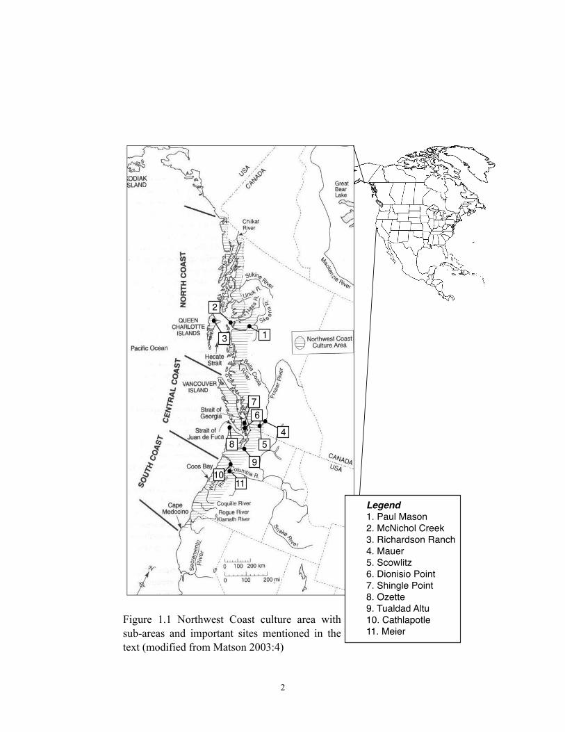
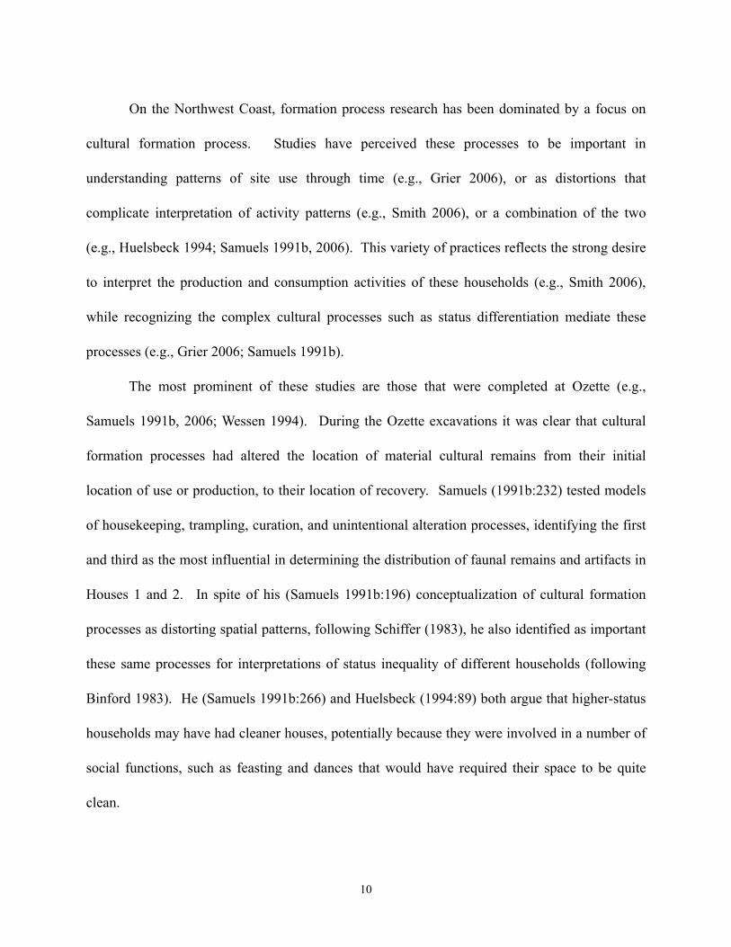
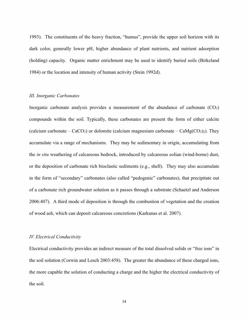
The archaeological record of the Northwest Coast of North America (Figure 1.1) provides one of

the world’s best opportunities to study the relationship between the emergence of large,

multifamily households and institutionalized social inequality in small-scale foraging societies.

The principal reason for this is the region’s large, lengthy, and well-preserved record of house

deposits. Approximately 4,000 years ago, large plank house-like structures appeared in the

Fraser River Valley of southwestern British Columbia. The nature of these structure is unclear;

they are followed by a 2,000 year hiatus in plank house occupation on the Central Coast. At the

beginning of the Marpole phase (2400 - 1400 B.P.) they reappear in this sub-area, often in the

context of large multi-house villages. They continue through following Gulf of Georgia phase

(1400 B.P. - Contact) and into the post-contact period (e.g., Ames and Maschner 1999:159-161;

Barnett 1955) as both as seasonal and year-round habitations.

The changes in house and household size and structure that appear during the Marpole

phase indicate a shift in social organization (Grier 2006:97). They are also coincident with

several other lines of data that suggest that social differentiation had, by this time, become

institutionalized in this area. These include the emergence of a regional mortuary tradition

centered around prominent tumuli and cairn burials (e.g., Lepofsky et al. 2000; Thom 1995),

differential access to valuable grave goods, particularly by children and sub-adults, indicating

ascribed rather than achieved status (e.g., Burley and Knusel 1989), and the emergence of a

regional artistic tradition associated with high-status goods that may be associated with the

construction of a regional elite identity (e.g., Grier 2003).

1

2

13

4

5

6

7

8

9

10

2

11

Legend

1. Paul Mason

2. McNichol Creek

3. Richardson Ranch

4. Mauer

5. Scowlitz

6. Dionisio Point

7. Shingle Point

8. Ozette

9. Tualdad Altu

10. Cathlapotle

11. Meier

Figure 1.1 Northwest Coast culture area with sub-areas and important sites mentioned in the text (modified from Matson 2003:4)

Household archaeologists have recently begun to explore how Northwest Coast

household organization was related to these processes (Chatters 1989; Coupland 1988, 2006;

Grier 2003, 2006a); that is, what it may mean that dramatic changes in household and house size

were coevolutionary with dramatic changes in the nature of social differentiation. The principal

means of operationalizing this has been through intrasite spatial analysis of artifacts and faunal

remains. Archaeologists have primarily targeted the spatial distribution of formed tools (Chatters

1989; Coupland 1988, 2006; Coupland et al. 2003; Grier 2006a; Samuels 2006) and faunal

remains (Chatters 1989; Huelsbeck 1994; Wessen 1994) as means of reconstructing social,

economic, and political relationships in these corporate groups (Grier 2006a:97). However, a

weakness of these analyses has been their oftentimes informal treatment of what most

archaeologists know commonly as cultural formation processes and non-cultural formation

processes (Schiffer 1983), those processes that can be defined, for the moment, that distort the

archaeological context from its original cultural systemic context.

I argue that Northwest Coast household archaeologists have rarely taken full advantage of

the data coded into the most ubiquitous data set in plank house deposits, the sediment. This

means that the processes that led to feature formation and alteration have been left largely

unproblematized. Initial steps steps taken towards understanding these formation processes have

for the most part not been sustained. Consequently, feature identification has frequently been

informal, running the risk of uncritical reconstruction of plank house architecture, and as so

many interpretations of household social, economic, and political organization rest on proper

architectural reconstruction (e.g., Coupland et al. 2009; Grier 2006b; Marshall 1989), uncritical

reconstruction of households themselves.

3

The goal of this study is the examination of the sedimentary characteristics of pre-contact

Northwest Coast plank house features and the processes by which they were formed. To

accomplish this, I drew on a data set from two plank house deposits at the Marpole phase village

component of the Dionisio Point site on Galiano Island in southwestern British Columbia.

Excavations at the site in 1997 and 1998 sampled two large Marpole phase plank houses. During

these excavations, artifact, faunal, botanical, and sedimentary materials were collected.

Sediment was sampled from a variety of architectural features, such as hearths, floors, benches,

and entryways. These features were identified during excavation, by their form, contents, and

context. Analysis of the lithic, bone tool, sumptuary goods (Grier 2006a), and faunal (Ewonus

2006; Lukowski and Grier 2009) components has already generated interpretations of the social,

economic, and architectural character of these structures.

This situation provides a unique opportunity to evaluate the fit of formation process

model expectations derived from existing archaeological and ethnographic data to the empirical

results of an analysis of plank house features. The methods used are geoarchaeological, focusing

on in-field qualitative soil description and quantitative laboratory-based bulk sediment analyses.

The methods used were able to assess the cultural and non-cultural formation processes that

created and altered these features during their use and following site abandonment.

The objective of this chapter is to briefly review the development of household

archaeological on the Northwest Coast, specifically focusing on studies that have attempted to

reconstruct patterns of social inequality within households with the objective of understanding

their long-term evolutionary relationship. This discussion reveals the bias present in these

studies towards the reconstruction of activities rather than cultural or non-cultural formation

4

processes. Geoarchaeological analysis of archaeological sediments has presented as a means by

which the nature and effects of some of these processes can be assessed.

Northwest Coast Household Archaeology

The earliest plank house excavations on the Northwest Coat were undertaken between the

late 1960s and the early 1980s. These projects included excavations at the proto-historic

Richardson Ranch site on Haida Gwaii (Fladmark 1973), the 4,500 year-old Mauer Site in the

Lower Fraser River Valley (LeClair 1976; Schaepe 2003), and the proto-historic Ozette village

site on the Pacific coast of Washington State (Samuels 1991a, 1994; Wechel 2005). All of these

projects were innovative in their approach to Northwest Coast archaeology, which up until this

time had focused on the excavation of shell middens towards the reconstruction of cultural

historical sequences (e.g., Mtichell 1971a), or long-term cultural ecological trends (e.g.,

Fladmark 1975; Matson 1976). The innovations of these projects were principally conceptual

and methodological. First and foremost, they recognized the plank house as a significant

empirical unit deserving further research. Second, they established methods that continue to be

used to effectively collect household data, focusing on the intrasite spatial analysis of the

distribution of cultural remains between and within plank house deposits.

Yet, in spite of the innovations of these sites, these projects did not make as significant a

contribution to our theoretical understanding of the early relationship between households and

social inequality on the Northwest Coast, as none of them made explicit the possible connection

between the appearance of plank houses and evidence of institutionalized social inequality. This

connection was not made until several years later (e.g., Ames 1985; Coupland 1985, 1988).

5

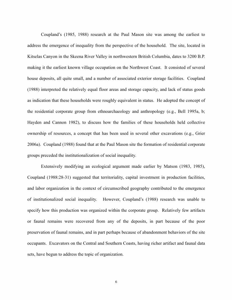
Coupland’s (1985, 1988) research at the Paul Mason site was among the earliest to

address the emergence of inequality from the perspective of the household. The site, located in

Kitselas Canyon in the Skeena River Valley in northwestern British Columbia, dates to 3200 B.P.

making it the earliest known village occupation on the Northwest Coast. It consisted of several

house deposits, all quite small, and a number of associated exterior storage facilities. Coupland

(1988) interpreted the relatively equal floor areas and storage capacity, and lack of status goods

as indication that these households were roughly equivalent in status. He adopted the concept of

the residential corporate group from ethnoarchaeology and anthropology (e.g., Bell 1995a, b;

Hayden and Cannon 1982), to discuss how the families of these households held collective

ownership of resources, a concept that has been used in several other excavations (e.g., Grier

2006a). Coupland (1988) found that at the Paul Mason site the formation of residential corporate

groups preceded the institutionalization of social inequality.

Extensively modifying an ecological argument made earlier by Matson (1983, 1985),

Coupland (1988:28-31) suggested that territoriality, capital investment in production facilities,

and labor organization in the context of circumscribed geography contributed to the emergence

of institutionalized social inequality. However, Coupland’s (1988) research was unable to

specify how this production was organized within the corporate group. Relatively few artifacts

or faunal remains were recovered from any of the deposits, in part because of the poor

preservation of faunal remains, and in part perhaps because of abandonment behaviors of the site

occupants. Excavators on the Central and Southern Coasts, having richer artifact and faunal data

sets, have begun to address the topic of organization.

6

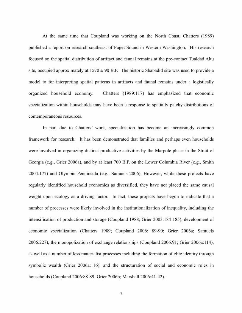
At the same time that Coupland was working on the North Coast, Chatters (1989)

published a report on research southeast of Puget Sound in Western Washington. His research

focused on the spatial distribution of artifact and faunal remains at the pre-contact Tualdad Altu

site, occupied approximately at 1570 ± 90 B.P. The historic Sbabadid site was used to provide a

model to for interpreting spatial patterns in artifacts and faunal remains under a logistically

organized household economy. Chatters (1989:117) has emphasized that economic

specialization within households may have been a response to spatially patchy distributions of

contemporaneous resources.

In part due to Chatters’ work, specialization has become an increasingly common

framework for research. It has been demonstrated that families and perhaps even households

were involved in organizing distinct productive activities by the Marpole phase in the Strait of

Georgia (e.g., Grier 2006a), and by at least 700 B.P. on the Lower Columbia River (e.g., Smith

2004:177) and Olympic Penninsula (e.g., Samuels 2006). However, while these projects have

regularly identified household economies as diversified, they have not placed the same causal

weight upon ecology as a driving factor. In fact, these projects have begun to indicate that a

number of processes were likely involved in the institutionalization of inequality, including the

intensification of production and storage (Coupland 1988; Grier 2003:184-185), development of

economic specialization (Chatters 1989; Coupland 2006: 89-90; Grier 2006a; Samuels

2006:227), the monopolization of exchange relationships (Coupland 2006:91; Grier 2006a:114),

as well as a number of less materialist processes including the formation of elite identity through

symbolic wealth (Grier 2006a:116), and the structuration of social and economic roles in

households (Coupland 2006:88-89; Grier 2006b; Marshall 2006:41-42).

7

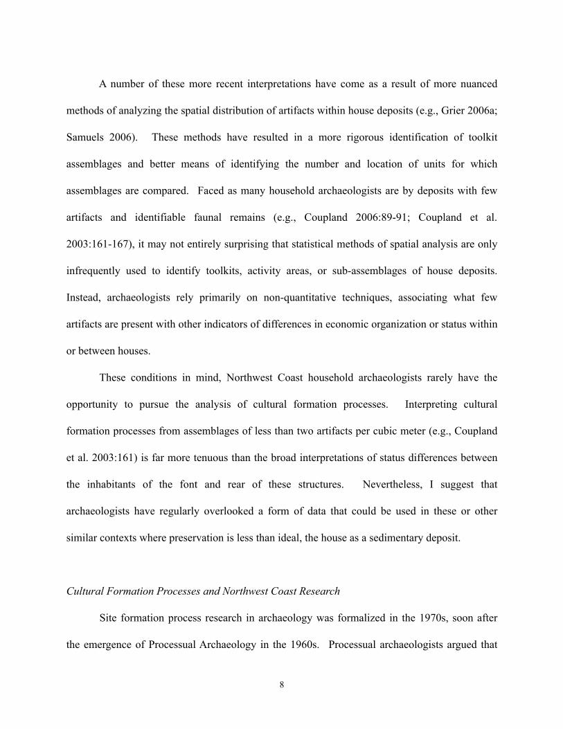
A number of these more recent interpretations have come as a result of more nuanced

methods of analyzing the spatial distribution of artifacts within house deposits (e.g., Grier 2006a;

Samuels 2006). These methods have resulted in a more rigorous identification of toolkit

assemblages and better means of identifying the number and location of units for which

assemblages are compared. Faced as many household archaeologists are by deposits with few

artifacts and identifiable faunal remains (e.g., Coupland 2006:89-91; Coupland et al.

2003:161-167), it may not entirely surprising that statistical methods of spatial analysis are only

infrequently used to identify toolkits, activity areas, or sub-assemblages of house deposits.

Instead, archaeologists rely primarily on non-quantitative techniques, associating what few

artifacts are present with other indicators of differences in economic organization or status within

or between houses.

These conditions in mind, Northwest Coast household archaeologists rarely have the

opportunity to pursue the analysis of cultural formation processes. Interpreting cultural

formation processes from assemblages of less than two artifacts per cubic meter (e.g., Coupland

et al. 2003:161) is far more tenuous than the broad interpretations of status differences between

the inhabitants of the font and rear of these structures. Nevertheless, I suggest that

archaeologists have regularly overlooked a form of data that could be used in these or other

similar contexts where preservation is less than ideal, the house as a sedimentary deposit.

Cultural Formation Processes and Northwest Coast Research

Site formation process research in archaeology was formalized in the 1970s, soon after

the emergence of Processual Archaeology in the 1960s. Processual archaeologists argued that

8

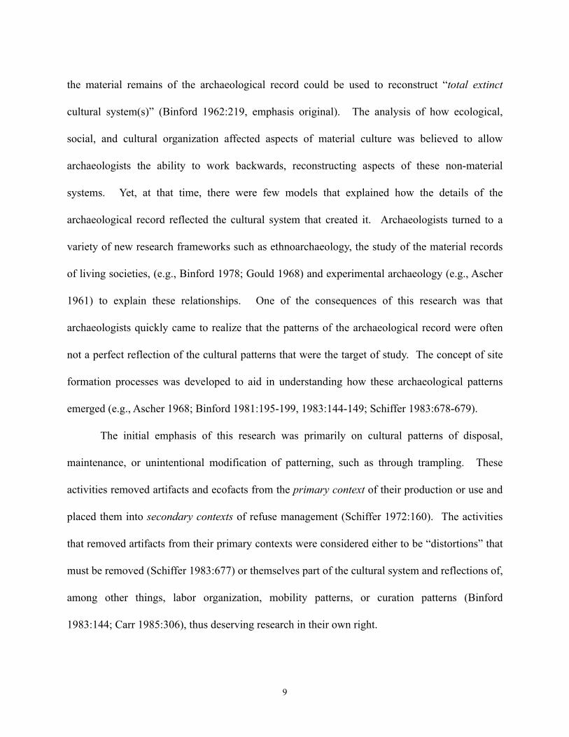
the material remains of the archaeological record could be used to reconstruct “total extinct

cultural system(s)” (Binford 1962:219, emphasis original). The analysis of how ecological,

social, and cultural organization affected aspects of material culture was believed to allow

archaeologists the ability to work backwards, reconstructing aspects of these non-material

systems. Yet, at that time, there were few models that explained how the details of the

archaeological record reflected the cultural system that created it. Archaeologists turned to a

variety of new research frameworks such as ethnoarchaeology, the study of the material records

of living societies, (e.g., Binford 1978; Gould 1968) and experimental archaeology (e.g., Ascher

1961) to explain these relationships. One of the consequences of this research was that

archaeologists quickly came to realize that the patterns of the archaeological record were often

not a perfect reflection of the cultural patterns that were the target of study. The concept of site

formation processes was developed to aid in understanding how these archaeological patterns

emerged (e.g., Ascher 1968; Binford 1981:195-199, 1983:144-149; Schiffer 1983:678-679).

The initial emphasis of this research was primarily on cultural patterns of disposal,

maintenance, or unintentional modification of patterning, such as through trampling. These

activities removed artifacts and ecofacts from the primary context of their production or use and

placed them into secondary contexts of refuse management (Schiffer 1972:160). The activities

that removed artifacts from their primary contexts were considered either to be “distortions” that

must be removed (Schiffer 1983:677) or themselves part of the cultural system and reflections of,

among other things, labor organization, mobility patterns, or curation patterns (Binford

1983:144; Carr 1985:306), thus deserving research in their own right.

9

On the Northwest Coast, formation process research has been dominated by a focus on

cultural formation process. Studies have perceived these processes to be important in

understanding patterns of site use through time (e.g., Grier 2006), or as distortions that

complicate interpretation of activity patterns (e.g., Smith 2006), or a combination of the two

(e.g., Huelsbeck 1994; Samuels 1991b, 2006). This variety of practices reflects the strong desire

to interpret the production and consumption activities of these households (e.g., Smith 2006),

while recognizing the complex cultural processes such as status differentiation mediate these

processes (e.g., Grier 2006; Samuels 1991b).

The most prominent of these studies are those that were completed at Ozette (e.g.,

Samuels 1991b, 2006; Wessen 1994). During the Ozette excavations it was clear that cultural

formation processes had altered the location of material cultural remains from their initial

location of use or production, to their location of recovery. Samuels (1991b:232) tested models

of housekeeping, trampling, curation, and unintentional alteration processes, identifying the first

and third as the most influential in determining the distribution of faunal remains and artifacts in

Houses 1 and 2. In spite of his (Samuels 1991b:196) conceptualization of cultural formation

processes as distorting spatial patterns, following Schiffer (1983), he also identified as important

these same processes for interpretations of status inequality of different households (following

Binford 1983). He (Samuels 1991b:266) and Huelsbeck (1994:89) both argue that higher-status

households may have had cleaner houses, potentially because they were involved in a number of

social functions, such as feasting and dances that would have required their space to be quite

clean.

10

Recently, Smith (2006) discussed similar processes at the Meier and Cathlapotle sites in

northwestern Oregon. His analysis focused on the evidence of intrasite differences in production

activities present in the distribution of different kinds of use wear. He looked at curation,

maintenance, and trampling. Testing these models of cultural formation processes, he confirmed

that the distribution his sample of over 1,000 tools was from primary rather than secondary

deposits. Since, he was not interested on the cultural meaning of formation processes, he

focused on them primarily as distortions of the archaeological record, rather than as aspects of

the cultural system.

Unfortunately, while both of these studies are model formation process research projects,

pragmatically neither can act as models for most household archaeology on the Northwest Coast.

The Ozette site, the Meier site, and the Cathlapolte site are all unusual for their rich

archaeological assemblages, contrary to the situation experienced by many other excavators as

argued above. Few excavators are able to address the influence of housekeeping, curation, or

trampling at their sites because the artifact data are simply too coarse. I argue, as I have above,

that the analysis of archaeological sediments permits archaeologists to address many of these

models without relying solely on the artifacts or faunal remains found on their sites. However, to

accomplish this goal, household archaeologists will have to adopt methods that have, up until

now, not been used for this purpose, such as geoarchaeology.

Natural Formation Processes and Northwest Coast Archaeology

Geoarchaeology, the study of geological problems in the archaeological record (Hasan

1980:267), developed as a distinct sub-field in archaeology much in tandem with site formation

11

process research (e.g., Butzer 1982: 98; Schiffer 1983:676). In part, this was recognition of the

fact the geoarchaeological methods are appropriate for this kind of research. They view the

aarchaeological deposit in one sense as an aggregation of particles, the analysis of which

provides information on their source, transportation agent, and the depositional environment

(Stein 2001:44). They also work at a scale appropriate to archaeological research questions

(Stein 1993). Until recently, in formation process research, the focus of geoarchaeological

analysis were the archaeological effects of post-depositional processes. However, archaeological

sediments in house deposits are predominantly cultural in origin. Schiffer (1983:690) and Stein

(1987:378) have both advocated the treatment of humans as agents in geological processes on

archaeological sites, effectively bringing cultural formation processes in geoarchaeological

research. A number of geoarchaeological techniques now exist for addressing questions of

cultural formation processes (e.g., Matthewes et al. 1997; Middleton and Price 1996; Sánchez

Vizcaino and Cañabate 1999).

Geoarchaeological investigations have long been a part of archaeology on the Northwest

Coast. They have been used predominantly in two capacities. First, in the geomorphological

reconstructions of past landscapes, particularly with reference to changing sea-levels during the

Holocene. Secondly, they have been used in the reconstruction of site formation processes,

focusing on post-depositional alteration of the archaeological record. Rarely have quantitative

geoarchaeological methods been applied to plank houses, nor have they focused on cultural site

formation processes. One of the arguments of this study is that household archaeologists

regularly use geoarchaeological methods informally, and often without exploring their full

relevance to plank house architecture, or household organization.

12

Landscape-scale geoarchaeology projects are far more prominent in Northwest Coast

archaeology than those that focus on site formation processes. They tend to focus on sea-level

reconstruction (e.g., Fedje and Christiansen 1999; Fladmark 1975; Josenhans et al. 1995;

Josenhans et al. 1997). These studies have generated information on one of the most interesting

periods of human history in the region, its initial occupation, but share little more than their

methods of geomorphological analysis with household geoarchaeology research.

Stein (1992a) has been one of the most vocal proponents of using geoarchaeological

methods to address site formation processes. Much of her work has focused on midden analysis

(e.g., Stein 1992b). The methods she uses rely upon high-resolution sampling within cultural

deposits and the use of a wide range of geophysical (e.g., Dalan et al. 1992), geochemical (e.g.,

Linse 1992, Stein 1992b), and other geoanalytical techniques. Her emphasis in using these

techniques in site formation process research has been on revealing how cultural patterns may in

some cases reflect natural formation processes. While her methods have been focused on natural

formation processes, they are appropriate to cultural formation processes, and the scale of

household archaeological research. A number of her techniques have been adopted in this study.

As stated above, the kinds of quantitative natural formation analyses advocated by Stein

(1992a) have been rare in household archaeology on the Northwest Coast. Perhaps

unsurprisingly, those excavations that have been most explicit in their analysis of natural

formation processes have been those that are also the most prominent in their study of cultural

formation processes. Smith’s (2006) research stands out as the most explicit testing of post-

depositional processes in household archaeology. He analyzed evidence of water sorting, wind

sorting, and bioturbation, coming to the conclusion that they had not significantly affected the

13

distribution of artifacts at Meier or Cathlapotle. These processes were assessed, much as Stein

(1987) advocated, by the use of geoarchaeological techniques designed to identify geological

processes.

The goal of this project, as stated above, is to study both natural formation processes and

cultural formation processes in plank house deposits through their archaeological sediments. The

latter, which has not been attempted before. The process is different than typical cultural

formation processes studies in that there are no models of how these cultural sediments should

behave. Archaeologists who study cultural formation processes through the lens of artifacts, are

able to rely upon a long history of experimental research. Geoarchaeological experiments used

to study cultural formation processes are exceedingly rare, and are often targeted at agro-pastoral

communities (e.g., MacPhail et al. 2003). No such projects have been undertaken on the

Northwest Coast.

1. Assessment of current models of cultural formation processes in prehistoric plank

houses. How well does the observed geoarchaeological data from Dionisio Point match

the expectations generated by an ethnographic model? What are the discrepancies and

why might they exist? What does this suggest about the applicability of current models

of cultural formation processes in prehistoric shed-roof houses?

2. Utility of feature analysis for interpreting the socio-economic organization of pre-

Contact households. Do features provide data not available from artifact data sets? If

they do, what do these tell us about the inhabitants of these dwellings?

3. Implications for prospection methods on the Coast. Does the analysis suggest that

there is a possibility of identifying some or all of the architectural contexts defined in

14

Chapter Three? Which are most easily discriminated and which are the most difficult to

define? What are the implications of these results for further excavations at Dionisio

Point and for sites elsewhere?

This thesis is divided into six chapters. Chapter Two provides a brief overview of the

Dionisio Point site, where the data used in this study were collected, as well as a summary of

Dionisio Point and the Marpole phase in the emergence of large plank houses in Strait of

Georgia. Chapter Three is separated into three sections that together comprise the

geoarchaeological model the fit of which is measured by the results of the field and laboratory

analysis. A section of this chapter is devoted to the variables used, a second to a discussion of

the local environment, and the third to the ethnographic and archaeological data used to develop

the cultural formation process model itself. Chapter Four discusses the data set, methods, and

results of the analysis. Chapter Five presents the interpretations of these results and discusses

their implications for household archaeology and the site formation process research in the

region. Chapter Six summarizes the findings and presents conclusions and potential directions

for future work.

15

Chapter Two: Dionisio Point

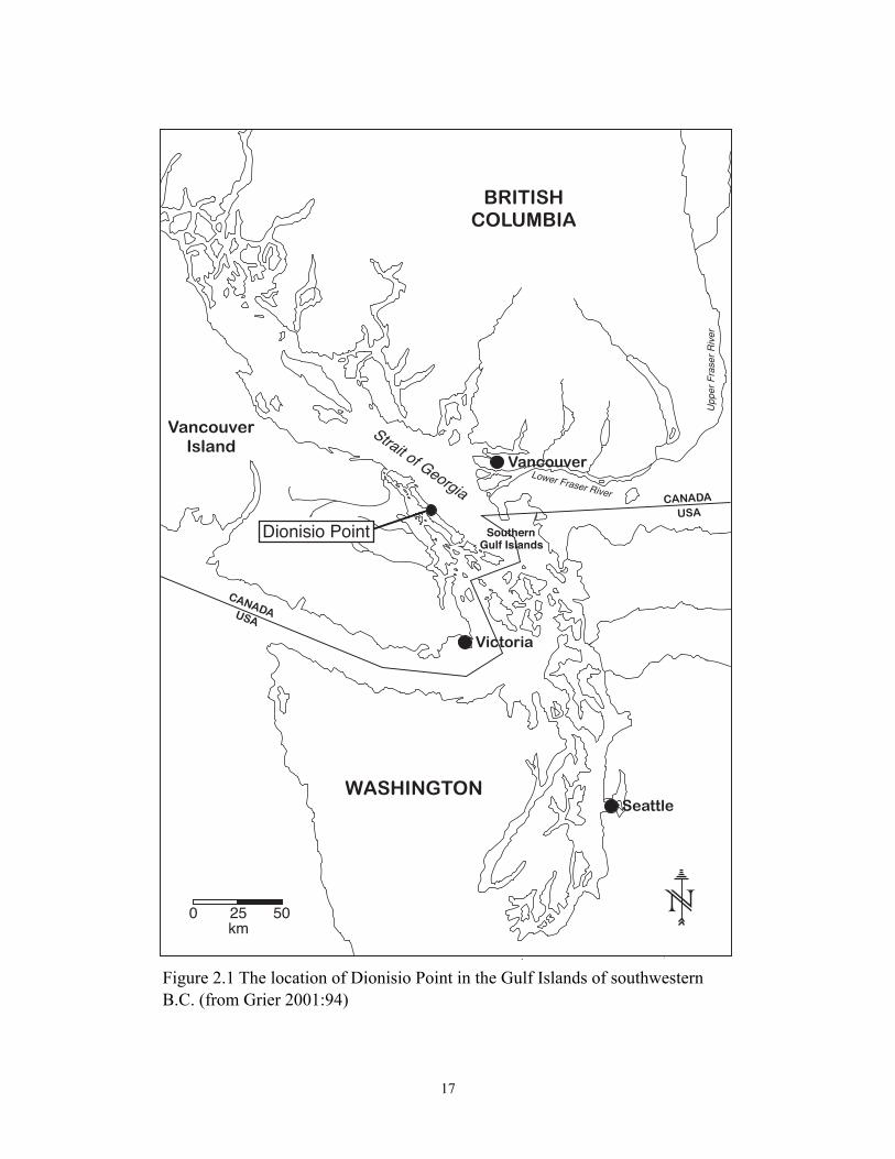
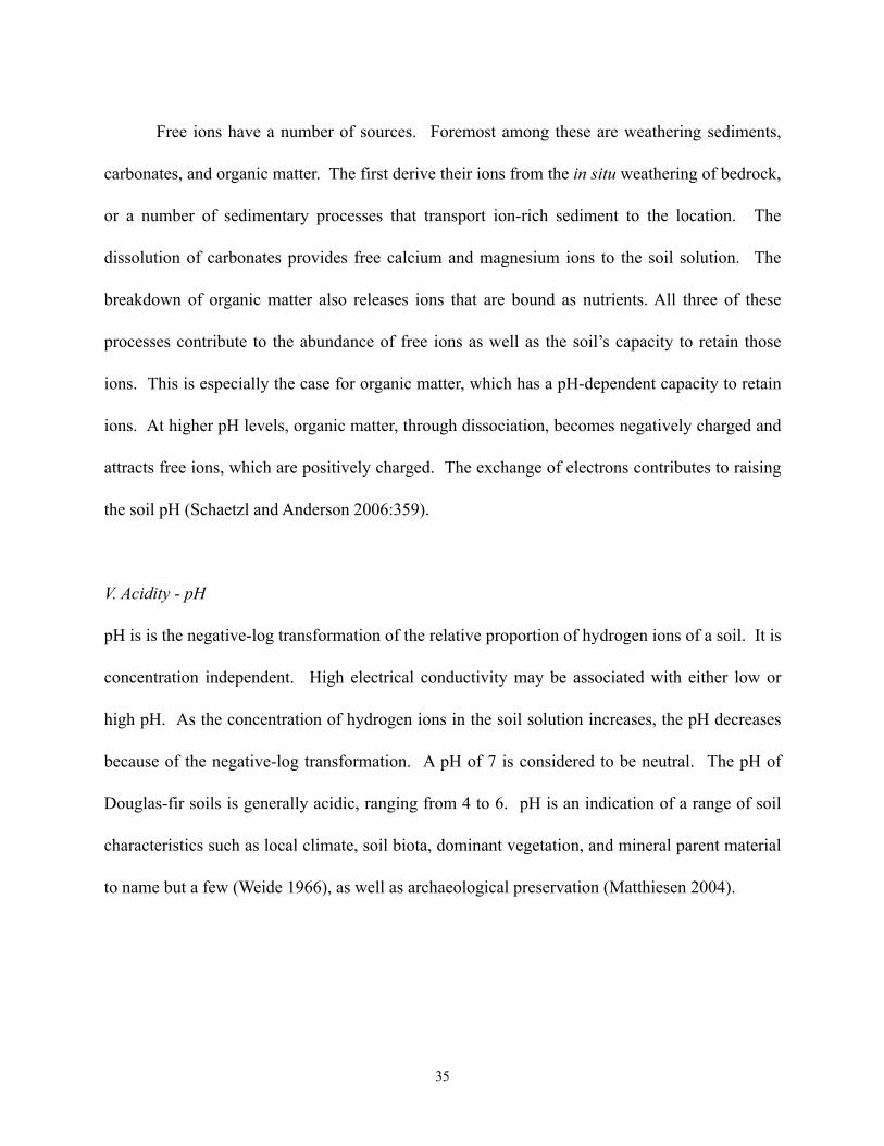
The Dionisio Point Site is located on the northern end of Galiano Island, one of the southern Gulf

Islands of southwestern British Columbia (Figure 2.1). The southern Gulf Islands are located

within the Strait of Georgia, the body of water that separates the mainland of British Columbia

from Vancouver Island. Galiano Island is one of the outer Gulf Islands, furthest from Vancouver

Island. The view from the eastern side of Galiano provides an unimpeded vista of British

Columbia’s Lower Mainland and the Fraser River Delta. Looking west one can see Kuper Island

and Thetis Island, and beyond them the rising mountains of Vancouver Island.

Galiano Island is one of the largest of the southern Gulf Islands, measuring some 30 km

from end to end and 3 km across at its widest point. It follows the trend shared by all of the

southern Gulf Islands of being oriented roughly parallel to the Vancouver Island coastline. This

orientation has been determined by the tectonic systems that underlie the Gulf of Georgia,

generating the geological setting of the Gulf Islands over the past 50 million years (Johnstone

2006).

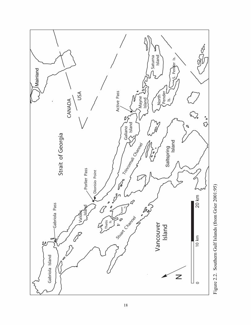
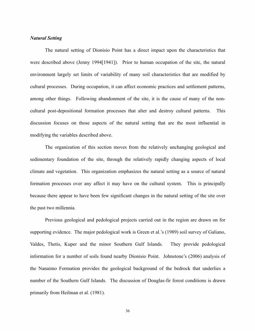
To the northwest of Galiano Island lies Valdes Island, separated by Porlier Pass (Figure

2.2). To the southeast lies Mayne Island separated by Active Pass. These highly turbulent passes

are extraordinarily abundant resource patches (Grier 2001:99). Urchin (Strongylocentrotus sp.)

is plentiful along with a variety of other shellfish, as are a number of marine mammals including

seals (Phocidae), sea lions (Ottaridae), and more rarely orcas (Orcinus orca). Salmon are not

abundant in this location, though schools of predominantly coho (Oncorhynchus kisutch) and

pink (O. gorbuscha) salmon are seasonally present in the waters during their migrations to the

mainland or Vancouver Island (Grier 2001:99; Kew 1992). Along with Gabriola Pass to the

16

17

0 25 50km

Strait of Georgia

re

viR r

es

arF r

ep

pU

Lower Fraser River

Southern

Gulf Islands

Dionisio Point

Figure 2.1 The location of Dionisio Point in the Gulf Islands of southwestern B.C. (from Grier 2001:94)

18

Straitof

Geo

rgia

Gab

riola

Pass

Vanc

ouver

Island

Valdes Island

Galiano Island

Porlier

Pass

Dionisio

Point

Gab

riola

Island

Thetis Is.

Kupe

r Is.

Activ

ePa

ss

Mayne

Island

Saturna

Island

North

Pend

erIs.

S.Pe

nder

Is.

CANAD

A USA

010

km

N

Stuart

Channel

Trincomali

Channel

Figu

re 2

.2.

Sout

hern

Gul

f Isl

ands

(fro

m G

rier 2

001:

95)

Mai

nlan

d

north of Valdes Island, these two passes are the only breaks in the outer Gulf Islands that allow

direct maritime movement between southeastern Vancouver Island and the mainland.

The Dionisio Point Site: Prior Excavations

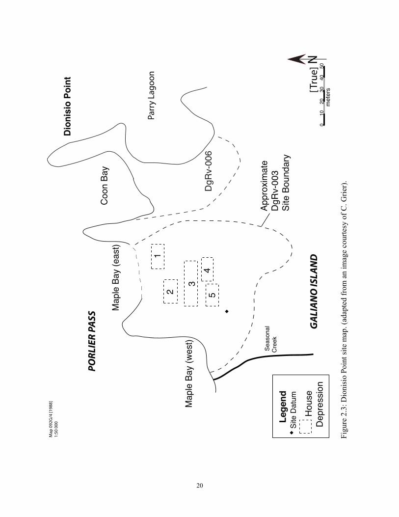
The northwestern tip of Galiano Island is broken by a series of erosional embayments.

Evidence of pre-contact human activity has been found in all of these locations (Grier 2001:93).

The Dionisio Point site (DgRv-003) is the largest of these sites. It is made up of two

components. The stratigraphically lower and earlier of these is a Marpole phase village

composed of five house depressions, visible from the surface of the site. This component

overlies culturally sterile Pleistocene glacial drift deposits. The upper, later component is a late

Marpole phase, or Transitional Gulf of Georgia phase (1400 - 1000 B.P.) seasonal resource

exploitation camp and lacks evidence of permanent architecture (Grier 2006a:101). Recent

excavations have revealed evidence of a plank house contemporary with these later deposits at

the nearby DgRv-006 site, in Coon Bay (Grier and McLay 2007:Figure 4), suggesting a shift in

settlement patterns between these two phases. The western boundary of the site is a sandstone

bluff and beyond that a perennial creek. The eastern boundary is a similar sandstone ridge, and

beyond that DgRv-006 and Parry Lagoon (Figure 2.3).

The earliest excavations at the site were undertaken by Mitchell (1971b) in 1964 as part

of his validation of the Gulf of Georgia cultural historical sequence. Excavations were limited to

several test units, one of which was located within House 2, and focused almost exclusively on

the lithic assemblage. The site was revisited during 1997 and 1998 for the Dionisio Point

Household Archaeology Project (DPHAP) by Grier (2001; 2003; 2006a). The goal of the

19

20

Coon B

ay

Maple

Bay (

west)

Maple

Bay (

east)

POR

LIER

PA

SS

GA

LIA

NO

ISLA

ND

Ap

pro

xim

ate

Dg

Rv-0

03

Site

Bo

un

da

ry

Map

092

G/4

[198

8]1:

50 0

00

2

3

4 5

[Tru

e] N

10

20

30

40

Site D

atu

m

Le

ge

nd

Parr

y La

goon

Dio

nis

io P

oin

t

050

me

ters

Ho

use

De

pre

ssio

n

1

Se

aso

na

l

Cre

ek

Dg

Rv-0

06

Figu

re 2

.3: D

ioni

sio

Poin

t site

map

. (ad

apte

d fr

om a

n im

age

cour

tesy

of C

. Grie

r).

DPHAP was to test the hypothesis that households were socio-economically internally

differentiated units. Initial testing of two house depressions (House 2 and House 5) in 1997 led

to extensive excavations in House 2 in 1998. During two field seasons, 77 m2 of House 2 and 4

m2 of House 5 were excavated. The excavation of approximately 40% of House 2 resulted in the

recovery of a relatively large lithic and bone artifact assemblage , debitage (Grier 2001:111), and

faunal assemblage (Ewonus 2006).

A suite of radiocarbon age determinations place the Marpole phase village occupation

between 1770±70 to 1440±60 B.P. (Grier 2006a:100). This range represents the maximum

possible length of occupation from presently-dated contexts. The probability distribution of

radiocarbon dates indicates that the occupation may have lasted no longer than 50 years. Yet, the

large amount of anthropogenic sediment (~50 cm) deposited during this time suggests that a 200

year occupation between 1680 and 1460 B.P. is a reasonable estimate (Grier 2006a:101). Given

a possible life-span of 50 to 80 years for a Northwest Coast plank house (Ames 1996:145), this

200 year occupation may represent three or four rebuilding episodes, and as many as eight

generations of inhabitants (Grier 2006a:101).

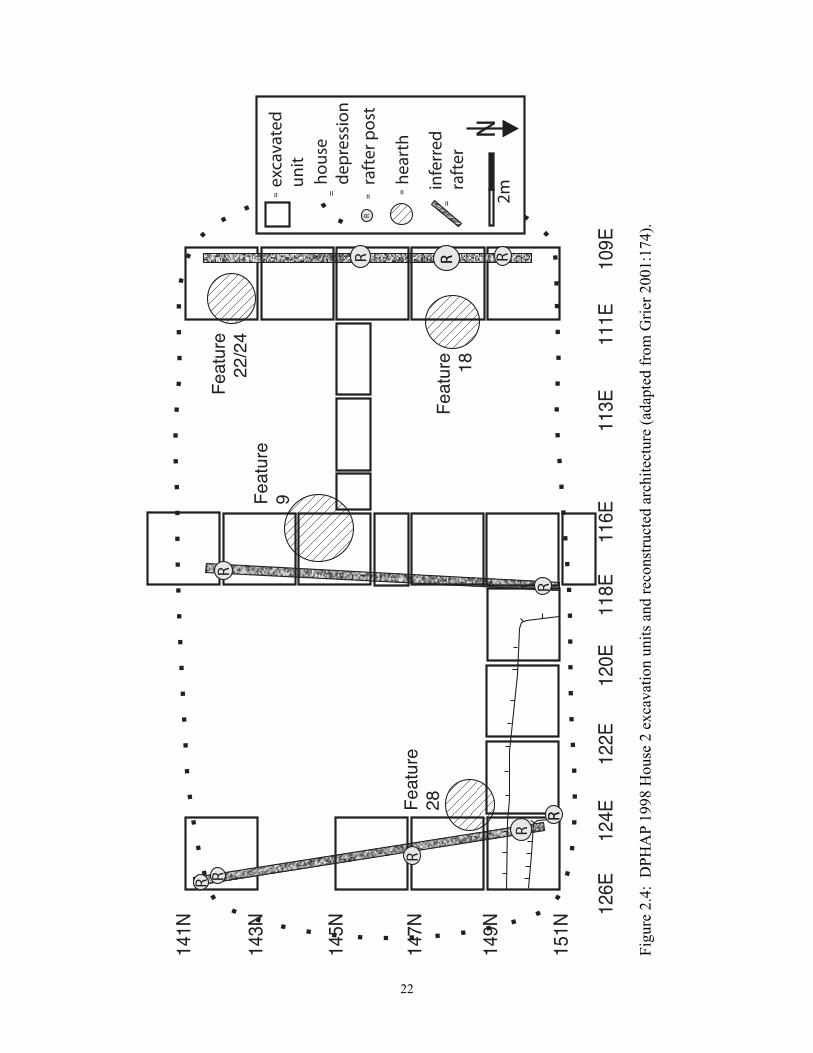
Grier (2006a, 2006b) has argued that spatial patterning in the data set reflects socio-

economic differentiation of space within the house. It appears that the families inhabiting the

west, center and eastern portions of the house were distinct socio-economic units organized

within a wider corporate context. Each was associated with toolkits for a different suite of

productive tasks, suggesting that these families may have been involved in organizing household

production in these activities (Grier 2001:224; 2006a:108-110). The families inhabiting the

domestic area around the eastern hearth (Feature 28) (Figure 2.4), appear to have been

21

22

RR RR

R

R

RR

R

R

RRF

eatu

re

22/2

4

Featu

re 18

Featu

re

9

Featu

re

28

=

=

=R

=

exca

vate

d un

itho

use

depr

essio

n

N

=

rafte

r pos

t

hear

th

infe

rred

rafte

r

2m

141N

143N

145N

147N

149N

151N

126E

124E

122E

120E

118E

116E

113E

111E

109E

Figu

re 2

.4:

DPH

AP

1998

Hou

se 2

exc

avat

ion

units

and

reco

nstru

cted

arc

hite

ctur

e (a

dapt

ed fr

om G

rier 2

001:

174)

.

differentiated from others by their involvement in marine hunting and fishing. The relative

abundance of chipped-stone and projectile points in the western portion of House 2 suggests that

the families living around Features 22/24 and 18 were focused on terrestrial hunting. The

domestic area around Feature 9, in the center of the house, has a scarcity of production-related

artifacts (Grier 2001:256), but the bulk of the sumptuary goods (slate beads, anthropomorphic

stone bowls, and labrets)(Grier 2006a:113). The abundance and variety of sumptuary goods

concentrated within the central part of the house illustrate status-related differences between the

resident family and those occupying either the eastern or western portions of the house, neither

of which have comparable assemblages.

Spatial variation in production activity toolkits and the location of sumptuary goods,

provides strong evidence that the use of space within House 2 was affected by variation in socio-

economic status, a pattern noted in the ethnographic record of the area (e.g., Suttles 1991), more

so than differences in the functional use of space (Grier 2006a:101). Regional similarities in the

stylistic attributes of the sumptuary goods recovered predominantly from the central of the house

(Grier 2006a:110), suggest that the inhabitants of this area were likely the social “core” of the

household and were involved in the accelerated construction of a regional elite identity that

accelerated during the Marpole Phase (Grier 2003; 2006b).

Ewonus (2006) recently completed a quantitative analysis of a portion of the faunal data

set from nine units in House 2 at Dionisio Point and has presented a different interpretation of

the Marpole phase seasonality and socio-economic structure. He has suggested that the

relatively high taxonomic diversity of the faunal assemblage indicates a seasonal mixed-

economy, typically associated with a spring aggregation rather than a winter village (e.g.

23

Coupland 1991). Moreover, he claims that the low abundance of salmon and the species

recovered (O. gorbuscha), identified through ancient-DNA analysis of five vertebrae, is evidence

of infrequent, fresh, local capture rather than stored resources transported from other locations

(Ewonus 2006:72).

This argument is based on two common models of salmon use on the coast. First, it is

often argued that these large communities would have difficulty persisting through the scarcity of

the winter season without these abundant, storable resources (e.g. Coupland 1991; Matson 1992),

and thus House 2 having few salmon was probably not a winter village. The weakness with this

argument is that salmon, while not the most abundant fish (NISP = 440), are comparable in

number to dogfish (Squalus sp., NISP = 590) and rockfish (Sebastes sp., NISP = 590). Given

that no other house excavation data are presented by Ewonus (2006), is it difficult to confirm that

these numbers are “low”. The aDNA identification of all five salmon vertebrae as sockeye (O.

nerka), commonly considered to be poor fish for storing because of their high fat content, might

suggest that salmon were taken locally and eaten fresh. Notably, a subsequent analysis of a

larger number of salmon vertebrae (Lukowski and Grier 2009), demonstrates greater diversity

than identified by Ewonus’ study and does not support a reliance solely upon sockeye.

Following patterns identified in the ethnographic record (e.g., Barnett 1955) and

suggested archaeological records (e.g., Burley 1988; Coupland 1991), Ewonus (2006:85) argues

that the various portions of House 2 were likely not inhabited contemporaneously; that families

occupied the plank house throughout the spring, arriving as family-units rather than en masse.

He (Ewonus 2006:85) maintains that having arrived at Dionisio Point and having their own

domestic hearths around the perimeter of the structure, family-units used the central hearth as a

24

communal space, an interpretation he supports by pointing towards the relatively low density of

faunal remains recovered from the central hearth.

The contrast between the Grier’s (2006a) and Ewonus’ (2006) interpretations is in part

indicative of the complexity of plank house deposits and the difficulties Northwest Coast

archaeologists face in attempting to integrate different data sets, particularly in light of our

imprecise models of what artifact and faunal assemblages from seasonal habitations should look

like archaeologically. Part of this may be because they are based on different forms of

information, Grier’s (2003, 2006a) on production and sumptuary data in both a local and regional

context, and Ewonus’ (2006) on a subset of the consumption data. Both Barnett (1955:242) and

Suttles (1951:272) identify extensive intrahousehold sharing of food resources, significantly

obscuring the consumption data for each family.

Given the concerns raised above regarding Ewonus’ (2006) interpretations of seasonality

and house occupation based on questionable salmon data and uncritical models, I am inclined to

read the faunal data in light of Grier’s (2006a) reconstruction of the socio-economic

differentiation of space in House 2. For example, the higher proportion of fish remains in the

eastern portion of the house (64% of the total fish remains) (Ewonus 2006:46), agrees quite well

with Grier’s (2006a) interpretation of the inhabitants of this domestic space as organizing marine

hunting and fishing if they tended to consume greater amounts of their own produce than other

families. More pertinent to this study is Ewonus’ (2006:57) identification of fewer faunal

remains in the central portion of the house, which he attributes to a possible functional difference

in this part of the house compared to either the eastern or western portion. I argue that given that

we understand so little about cultural formation processes in House 2, we cannot discount the

25

possibility that this area was treated differently by the inhabitants, while it broadly remained

functionally analogous to the east and west. As suggested by the conclusions of this study, it is

not clear that archaeologists can assume that different families did not maintain their domestic

spaces differently (cf. Huelsbeck 1994:57).

Dionisio Point in a Regional Archaeological Perspective

The Marpole Phase in the Strait of Georgia shows both cultural change and continuity

from the preceding Locarno Beach Phase (3300 - 2400 B.P.). There are a number of similarities,

such as the continuation of microblade technologies, the use of labrets (though at a lower

frequency), earspools, certain forms of net-sinkers, and a number of bone needles and awls

(Burley 1980:36). These similarities have all but silenced early arguments that the Marpole

phase represents an intrusive culture from the Fraser Canyon, either in the movement of people

or of ideas (Mitchell 1971a).

There are a number of obvious changes between these two phases. Lithic technological

organization transitions from predominantly chipped to ground stone tool kits. Large celts,

nipple-topped stone hand mauls, widespread stone sculpture similar in style to ethnographic

materials, and fixed unilaterally barbed harpoon heads are added to the material culture. The

emergence of ascribed inequality is suggested by the replacement of labrets by cranial

deformation as a status marker (Ames 1995:166), and burial with lavish grave goods (Burley and

Knusel 1989). Most notably there is the earliest direct evidence of ethnographic-style large

plank houses on the southwest British Columbia coast (Matson and Coupland 1995:201-9).

26

The recent analysis of faunal remains from a number of sites in the region has provided

support for a connection between the Marpole Phase and the emergence a salmon-storage based

economy (e.g., Matson 1992), which may have been necessary to support large sedentary winter

villages (Ames 1996). However, while salmon rises to dominance, notably more clearly in some

data sets (e.g., Matson 1992) than in others, a number of other economic pursuits remain

important and a range of terrestrial and marine faunal were taken on a regular basis (e.g.,

Ewonus 2006). This “focal economy” (Ames and Maschner 1999:25-26) may reflect

increasingly complex relationships between household-level and family-level economic practices

(e.g., Chatters 1989; Grier 2006a).

The earliest consistent evidence of large houses in the Strait of Georgia dates to the

beginning of the Marpole phase at 2400 B.P. (Burley 1980:63; Matson and Coupland 1995:209 -

211; Mitchell 1971a:53). Discussions of earlier household organization in the region are

complicated by the lack of evidence of large house depressions from the previous Locarno Beach

phase (Burley 1980:30), though the necessary tools appear to have been part of the toolkit at this

time (Mitchell 1971a:59). However, while large house depressions have not been found,

evidence of much smaller structures has been identified at a number of sites (Matson 2008:164).

A small (5 x 6 m) depression at the Hoko River Wet/Dry site is one of the better reported

examples, and appears to have been a seasonal spring dwelling (Matson and Coupland 1995:169)

dating to approximately 2700 B.P. At the Crescent Beach site, a distinctive stratigraphic feature

has been suggested to be a Locarno phase winter pithouse (3010±85 B.P.) (Matson 2008:161).

Identification of this feature is insecure as it lacks an associated hearth feature, presumably

necessary in a winter structure, and has uncertain evidence of post features. If this feature does

27

represent a structure its small size (approximately 19 m2) confirms the fact that large houses and

presumably large households are a Marpole phase phenomenon.

Two very early structures have been identified on the British Columbia mainland in the

Upper Fraser River Valley, one at Hatzic Rock and another at the Mauer site, both potentially

dating to between 4500 - 3300 B.P. The Mauer site has been determined to be a house based on

the evidence of hearth and post features, and associated lithic data set (Schaepe 2003:152). The

long period of time between the abandonment of the two structures and the emergence of villages

during the Marpole Phase (2400 - 1400 B.P.) during which no conclusive evidence for winter

dwellings exists at any of the 28 reported Locarno Beach components (Matson and Coupland

1995:157), makes it difficult to constructively address the influence of the former in the

historical development of plank house villages. As noted above, it is not until the Marpole Phase

that house depressions aggregated in villages begin to appear. Nonetheless, only six Marpole-

age components have evidence of such structures (Grier 2001:105). Of these, only two have

received extensive excavation: Dionisio Point, and Tualdad Altu.

28

Chapter Three: A Geoarchaeological Framework

The previous chapter provided a brief overview of the history of archaeological work at

the Dionisio Point site and its place in the development of large plank houses on the Central

Coast. The purpose of this chapter is to create an archaeological model of Northwest Coast

plank house formation processes that can be evaluated by geoarchaeological analytical method.

Archaeological, paleoenvironmental, and ethnographic data are discussed, framed within the

geoarchaeological variables selected for this study.

To allow plank house geoarchaeological signatures to be analyzed in the sedimentary

record, three conditions must be met. First, a suite of variables must be identified that record the

past activities of households and yet are resistant to post-depositional alteration, either in form or

location. A suite of methods must then be selected that can accurately and precisely measure

these variables. Achieving this goal represents a recursive exercise as variables are selected,

tested, kept or discarded.

The second condition is that natural sources of variability are assessed. Natural

environmental conditions are responsible for the range of natural formation processes that cause

post-depositional alteration of cultural patterning; they introduce new material into the

archaeological site that transform and transport existing materials, or remove them altogether.

This process-based model was made explicit by Simonson (1959), is widely used in the soil

sciences (Schaetzl and Anderson 2006:320), and is adopted for this study. Dramatic changes in

the natural environment may elicit behavioral responses. Determining that the natural

environment has not significantly changed over the occupation of the site removes this source of

variability.

29

The third condition is that a model of past human activities must be generated from

which to evaluate patterns in the field and laboratory determined on the selected variables.

Unlike the analysis of other data sets, such as lithics or faunal remains, geoarchaeological

analysis of cultural formation processes relies on data that cannot be uniquely linked to

anthropogenic sources (Butzer 1982:81-82). Models of natural and anthropogenic formation

processes are therefore necessary evaluative tools and must be combined with other material data

sets. Archaeological collections from Dionisio Point provide an opportunity to satisfy these three

conditions.

Analytical Variables

The methodology of this project is derived from the sedimentological and pedological

sciences. Geologists, geomorphologists, and pedologists regularly use sedimentary texture, the

analysis of particle-size distributions, in palaeoenvironmental research. Pedologists, those

scientists who study the formation of soils, add to this a range of techniques that allow them to

describe the processes involved in soil genesis. In fact, in spite of the thousands of soil families

described in both the American (Soil Survey Staff 2006) and Canadian (Soil Classification

Working Group 2006) soil systems, the complexities of pedogenesis (soil formation) are due to

the interactions of a limited number of soil components and formation factors (e.g., Jenny

1994[1941]). By implication, these character of interactions can reveal a great deal of

information about the genesis of any particular soil. This project draws on a number of those

methods.

30

A suite of bulk sediment analyses were selected to address the anthropogenic and

geogenic factors that contributed to the geoarchaeological record of House 2 and House 5 at the

Dionisio Point site. These are low resolution analyses in that they measure only the changes in

major soil constituents. They lack the precision necessary to analyze soil constituents that form

the minor and trace proportions of a sample. While it is, for example, possible to measure each

ionic element individually using titration (e.g., Cook and Heizer 1965) or inductively-coupled

plasma mass-spectrometry (e.g., Middleton 2004), the anthropological meaning of their

individual concentrations is not necessarily clear (Butzer 1982:82). Both of these methods also

require large comparative data sets that are beyond the scope of this study. While the resolution

of the analyses used here is comparatively low, the methods are appropriate to the data resolution

of this study, are simple and straight-forward to apply and interpret and thus can be used in all

projects with access to minimal laboratory equipment, and are supported by decades of use in the

archaeological sciences (Butzer 1982; Deetz and Dethlefsen 1963; Weide 1966).

This project uses five methods common to pedological research: soil texture, organic

matter content (OM), inorganic carbonate content (IC), electrical conductivity (EC) and pH.

They form a standard suite used to characterize soil properties and differentiate anthropogenic

from natural processes. Each is briefly described below.

I. Particle-Size Analysis

Soil texture breaks the continuum of grain sizes down into a number of size classes and sub-

classes. The classes used in the Canadian and Standard U.S. Wentworth-Uddon systems are

presented in Table 3.1.

31

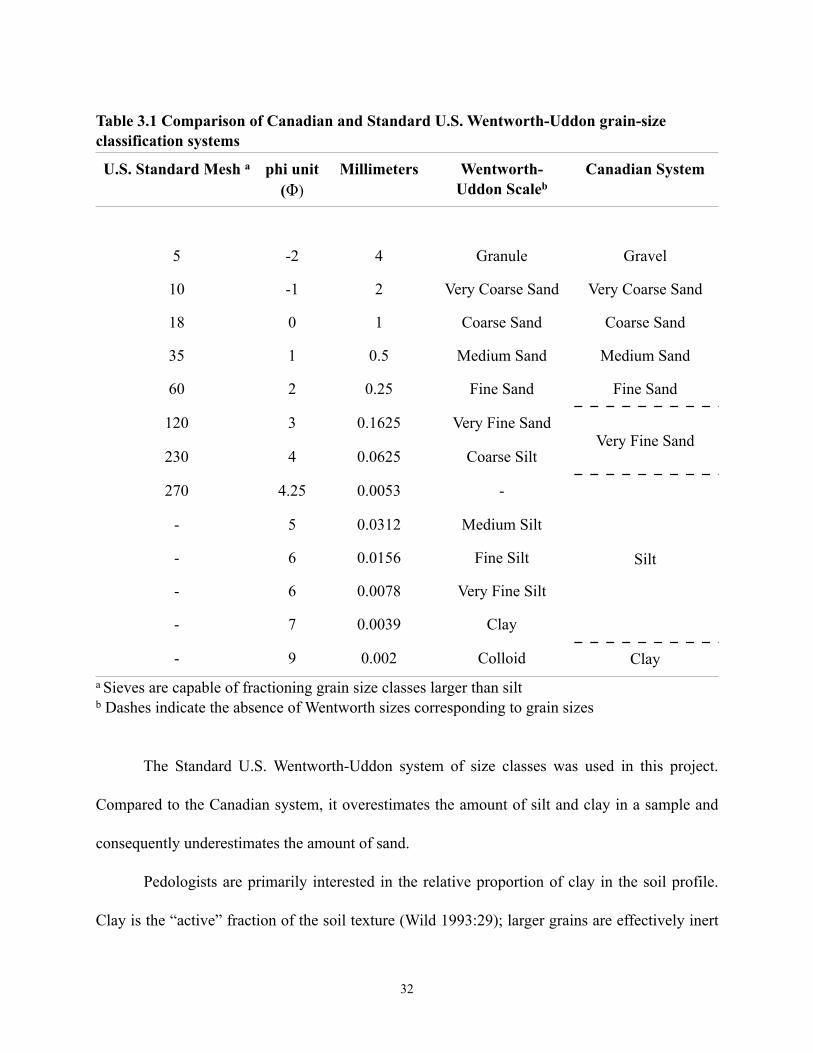
Table 3.1 Comparison of Canadian and Standard U.S. Wentworth-Uddon grain-size classification systems

U.S. Standard Mesh a phi unit(Φ)

Millimeters Wentworth-Uddon Scaleb

Canadian System

5 -2 4 Granule Gravel

10 -1 2 Very Coarse Sand Very Coarse Sand

18 0 1 Coarse Sand Coarse Sand

35 1 0.5 Medium Sand Medium Sand

60 2 0.25 Fine Sand Fine Sand

120 3 0.1625 Very Fine SandVery Fine Sand

230 4 0.0625 Coarse Silt

270 4.25 0.0053 -

Silt

- 5 0.0312 Medium Silt

- 6 0.0156 Fine Silt

- 6 0.0078 Very Fine Silt

- 7 0.0039 Clay

- 9 0.002 Colloid Claya Sieves are capable of fractioning grain size classes larger than siltb Dashes indicate the absence of Wentworth sizes corresponding to grain sizes

The Standard U.S. Wentworth-Uddon system of size classes was used in this project.

Compared to the Canadian system, it overestimates the amount of silt and clay in a sample and

consequently underestimates the amount of sand.

Pedologists are primarily interested in the relative proportion of clay in the soil profile.

Clay is the “active” fraction of the soil texture (Wild 1993:29); larger grains are effectively inert

32

with respect to soil chemical characteristics. Many labile soil constituents, such as free ions and

carbonates, are rapidly leached in coarse-textured deposits for this reason. Clay minerals, which

are often highly charged particles, readily adsorb nutrients and form organic-mineral complexes

that protect organic matter from decomposition. Nevertheless, coarse-textured soils impart some

characteristics to the soil. They accentuate the visible characteristics of humus, a constituent of

organic matter, particularly its apparent depth. Coarse-textured soils, having a lower surface area

to volume ratio are more easily coated by humus, suggesting deeper organic matter penetration

than might truly exist (Schaetzl 1991).

Finally, the texture of a sedimentary deposit can reveal the provenience (origin), mode of

transportation and mode of deposition of the sedimentary materials that for the deposit. This can

be important in understanding past climates (e.g., Butzer and Harris 2007) as well as

geomorphological changes to landscapes following human habitation that might bias or obscure

the archaeological record (e.g., Field and Banning 1998).

II. Organic Matter

In natural soils, organic matter is derived primarily from the death and decomposition of local

vegetation and biota that live both on and in the soil (Brady and Weil 2002:500). The

accumulation of dead organic matter on the surface and in the subsurface, forms the primary

source of food for a wide range of faunal and fungal communities. As they consume, digest, and

excrete organic matter, these communities convert it from a particulate “light fraction” composed

of macroscopic vegetal debris, to a relatively homogeneous “heavy fraction” composed of a

variety of acids, fats, waxes, and other microscopic and sub-microscopic derivatives (Wild

33

1993). The constituents of the heavy fraction, “humus”, provide the upper soil horizon with its

dark color, generally lower pH, higher abundance of plant nutrients, and nutrient adsorption

(holding) capacity. Organic matter enrichment may be used to identify buried soils (Birkeland

1984) or the location and intensity of human activity (Stein 1992d).

III. Inorganic Carbonates

Inorganic carbonate analysis provides a measurement of the abundance of carbonate (CO3)

compounds within the soil. Typically, these carbonates are present the form of either calcite

(calcium carbonate – CaCO3) or dolomite (calcium magnesium carbonate – CaMg(CO3)2). They

accumulate via a range of mechanisms. They may be sedimentary in origin, accumulating from

the in situ weathering of calcareous bedrock, introduced by calcareous eolian (wind-borne) dust,

or the deposition of carbonate rich bioclastic sediments (e.g., shell). They may also accumulate

in the form of “secondary” carbonates (also called “pedogenic” carbonates), that precipitate out

of a carbonate rich groundwater solution as it passes through a substrate (Schaetzl and Anderson

2006:407). A third mode of deposition is through the combustion of vegetation and the creation

of wood ash, which can deposit calcareous concretions (Karkanas et al. 2007).

IV. Electrical Conductivity

Electrical conductivity provides an indirect measure of the total dissolved solids or “free ions” in

the soil solution (Corwin and Lesch 2003:458). The greater the abundance of these charged ions,

the more capable the solution of conducting a charge and the higher the electrical conductivity of

the soil.

34

Free ions have a number of sources. Foremost among these are weathering sediments,

carbonates, and organic matter. The first derive their ions from the in situ weathering of bedrock,

or a number of sedimentary processes that transport ion-rich sediment to the location. The

dissolution of carbonates provides free calcium and magnesium ions to the soil solution. The

breakdown of organic matter also releases ions that are bound as nutrients. All three of these

processes contribute to the abundance of free ions as well as the soil’s capacity to retain those

ions. This is especially the case for organic matter, which has a pH-dependent capacity to retain

ions. At higher pH levels, organic matter, through dissociation, becomes negatively charged and

attracts free ions, which are positively charged. The exchange of electrons contributes to raising

the soil pH (Schaetzl and Anderson 2006:359).

V. Acidity - pH

pH is is the negative-log transformation of the relative proportion of hydrogen ions of a soil. It is

concentration independent. High electrical conductivity may be associated with either low or

high pH. As the concentration of hydrogen ions in the soil solution increases, the pH decreases

because of the negative-log transformation. A pH of 7 is considered to be neutral. The pH of

Douglas-fir soils is generally acidic, ranging from 4 to 6. pH is an indication of a range of soil

characteristics such as local climate, soil biota, dominant vegetation, and mineral parent material

to name but a few (Weide 1966), as well as archaeological preservation (Matthiesen 2004).

35

Natural Setting

The natural setting of Dionisio Point has a direct impact upon the characteristics that

were described above (Jenny 1994[1941]). Prior to human occupation of the site, the natural

environment largely set limits of variability of many soil characteristics that are modified by

cultural processes. During occupation, it can affect economic practices and settlement patterns,

among other things. Following abandonment of the site, it is the cause of many of the non-

cultural post-depositional formation processes that alter and destroy cultural patterns. This

discussion focuses on those aspects of the natural setting that are the most influential in

modifying the variables described above.

The organization of this section moves from the relatively unchanging geological and

sedimentary foundation of the site, through the relatively rapidly changing aspects of local

climate and vegetation. This organization emphasizes the natural setting as a source of natural

formation processes over any affect it may have on the cultural system. This is principally

because there appear to have been few significant changes in the natural setting of the site over

the past two millennia.

Previous geological and pedological projects carried out in the region are drawn on for

supporting evidence. The major pedological work is Green et al.’s (1989) soil survey of Galiano,

Valdes, Thetis, Kuper and the minor Southern Gulf Islands. They provide pedological

information for a number of soils found nearby Dionisio Point. Johnstone’s (2006) analysis of

the Nanaimo Formation provides the geological background of the bedrock that underlies a

number of the Southern Gulf Islands. The discussion of Douglas-fir forest conditions is drawn

primarily from Heilman et al. (1981).

36

Parent Material

The geology of Galiano Island is the Cretaceous age (90 - 65 mya) Nanaimo Formation,

which underlies many of the Gulf Islands (Johnstone 2006). This formation is composed of a

series of bedded sandstones, siltstones, and fine mudstones. In many places, including Dionisio

Point, the softer materials have eroded away leaving the harder sandstone beds exposed.

According to Johnstone’s (2006:31-36) description of Nanaimo Formation non-clastic sandstone

facies, these deposits vary in terms of their texture (coarse to medium grained), and bedding

(swalley cross-stratified to hummocky cross-stratified deposits). This indicates that the initial

mode of deposition of these bedsets was marine. Cementation is achieved by hematite and clay

rather than carbonates, though detrital calcite is present (Johnstone 2006:130). Weathering of

this material has resulted in the development of thin sandy, carbonate poor soils in many areas

around the site. The characteristics of these soils, the Saturna series, which are the primary soils,

are presented in Table 3.2.

Also overlying the Nanaimo Formation are a number of glacial drift deposits, laid down

during the late Pleistocene/early Holocene Fraser (Wisconsin) glaciation (30,000 - 10,000 B.P.)

(Clague and James 2002:71). Where these sediments have not eroded away, often in topographic

depressions, they form deposits more than 1 m thick. Much like the Saturna sediments, these

glacial sediments are predominantly sandy, with a slightly higher proportion of silt and clay.

They also have slightly higher coarse clast content (25 - 50% by weight). The characteristics of

soils that form in these sediments, called Qualicum soils are presented in Table 3.3. Soil surveys

in the region have identified this sediment at Dionisio Point (Green et al. 1989:22), where it

forms the secondary sediment in the immediate area of the site.

37

38

Tabl

e 3.

2 Pr

ofile

des

crip

tion

of th

e ty

pica

l Sat

urna

seri

es so

il pr

ofile

(fro

m G

reen

et a

l 198

9:11

6)

Fiel

d H

oriz

onD

epth

(c

m)

Col

or(m

oist

)C

olor

(dry

)O

rg.

C.a

CE

Cb

: B

ScpH

Sand

(%)

Silt

(%)

Cla

y (%

)

L8

- 6

FH6

- 036

.6

Bm

10

- 10

7.5Y

R4/

410

YR

5/4

0.6

6.8

: 23

4.6

7919

4

Bm

210

- 45

7.5Y

R4/

410

YR

5/6

1.4

8.6

: 25

4.8

7026

2

R45

+

a G

reen

et a

l. (1

989)

repo

rt or

gani

c ca

rbon

rath

er th

an o

rgan

ic m

atte

r con

tent

. (O

C x

~2.

1) =

OM

b C

EC is

the

catio

n ex

chan

ge c

apac

ity, t

he c

apac

ity to

reta

in a

nd e

xcha

nge

free

ions

c B

S is

the

base

satu

ratio

n, th

e nu

mbe

r of e

xcha

nge

site

s tha

t are

fille

d by

bas

e ca

tions

39

Tabl

e 3.

3 Pr

ofile

des

crip

tion

of th

e ty

pica

l Qua

licum

seri

es so

il pr

ofile

(fro

m G

reen

et a

l 198

9:11

4)

Fiel

d H

oriz

onD

epth

(c

m)

Col

or(m

oist

)C

olor

(dry

)O

rg. C

.aC

EC

b : B

ScpH

Sand

(%)

Silt

(%)

Cla

y (%

)

LF3

- 0

Ah

0 - 9

10

YR

3/2

10Y

R3/

310

.935

.4 :

535.

375

196

Bm

19

- 45

2.5Y

4/4

10Y

R5/

41

8.4

: 35

5.3

8315

2

Bm

245

- 65

2.5Y

4/4

2.5Y

6/4

0.3

3.6

: 33

5.6

8810

2

BC

65 -

100+

2.5Y

5/4

2.5Y

7/4

4.8

: 35

572

235

a G

reen

et a

l. (1

989)

repo

rt or

gani

c ca

rbon

rath

er th

an o

rgan

ic m

atte

r con

tent

. (O

C x

~2.

1) =

OM

b C

EC is

the

catio

n ex

chan

ge c

apac

ity, t

he c

apac

ity to

reta

in a

nd e

xcha

nge

free

ions

c B

S is

the

base

satu

ratio

n, th

e nu

mbe

r of e

xcha

nge

site

s tha

t are

fille

d by

bas

e ca

tions

Parent materials impart various characteristics to soils, many of which should be evident

from the above discussion. The soils around Dionisio Point are necessarily sand, with little

amounts of silt and clay. Any shifts in the texture of on-site sediments indicates either human

activity or natural alluvial or colluvial addition of finer sediments. They also can impart a

number of mineral elements to soils, such as calcium or potassium that directly affect a number

of other soil characteristics. However, there are two reasons to expect that few mineral elements

found in soils are sedimentary in origin. Firstly, based on Johnstone’s (2006) study I would

expect few carbonates will be present in local soils (also Green et al. 1989:114, 116). Secondly,

the coarse texture of the parent material means that natural soils are rapidly leached

Modern and Holocene Climatic Setting

The Douglas-fir Region extends approximately from Bella Coola in British Columbia to

the Oregon – California border (Franklin 1981:92). It characterizes much of the Northwest

region of the Coast-Cascade Mountain chain. The area around Dionisio Point falls within the

much more accurate and spatially delimited Coastal Douglas-fir zone of the Biogeoclimatic

Ecosystem Classification System, developed specifically for British Columbia (Meidinger and

Pojar 1991) (Figure 3.1). This zone is found exclusively on the southeastern coast of Vancouver

Island and a number of the Gulf Islands. Elevation is typically less than 150 m. In the case of the

Gulf Islands, this places them within the rain shadow of the Olympic Mountains (~2400 m asl)

and the spine of Vancouver Island (~2200 m asl) (Meidinger and Pojar 1991:82). Consequently,

the Gulf Islands are among the sunniest (1400 h per year) and warmest (> 200 frost free days per

year) areas in Canada (Green et al. 1989:16). Annual climatic data from 1971 to 2000 for Mayne

40

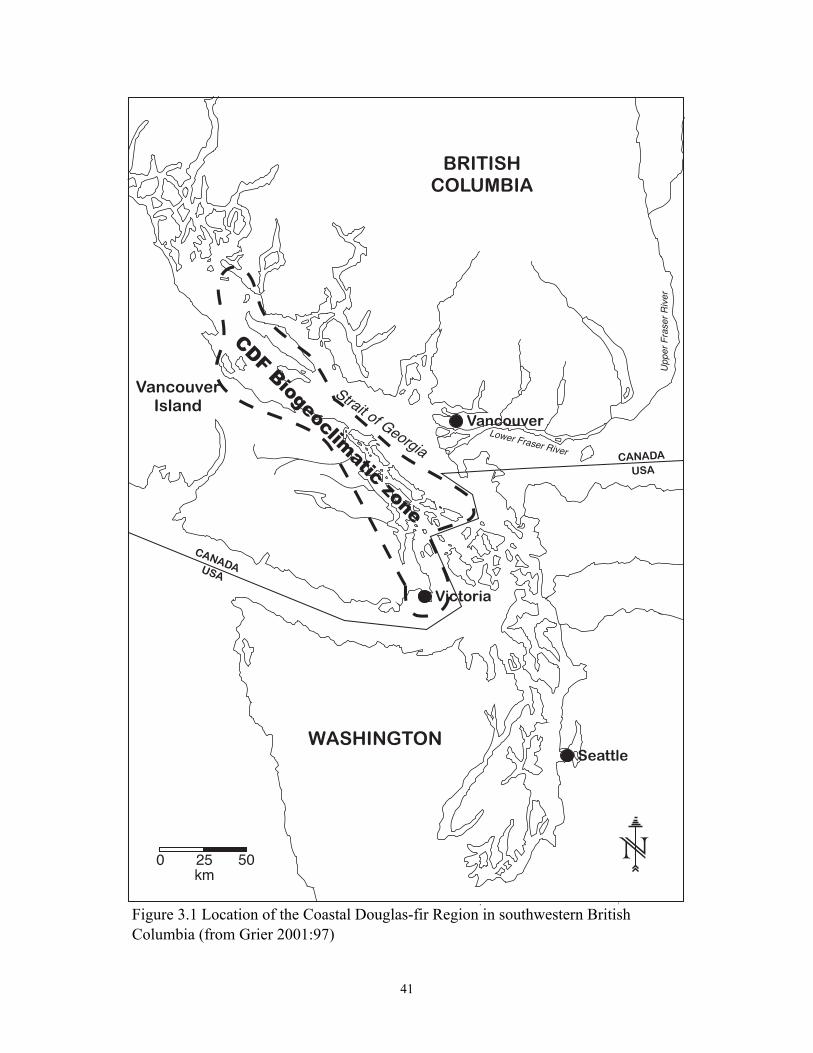
41

0 25 50km

Strait of Georgia

re

viR r

es

arF r

ep

pU

Lower Fraser River

Figure 3.1 Location of the Coastal Douglas-fir Region in southwestern British Columbia (from Grier 2001:97)

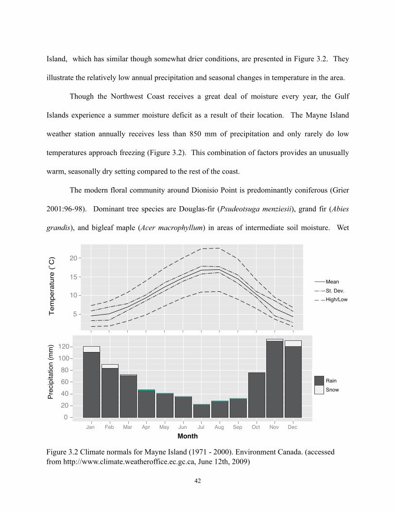
Island, which has similar though somewhat drier conditions, are presented in Figure 3.2. They

illustrate the relatively low annual precipitation and seasonal changes in temperature in the area.

Though the Northwest Coast receives a great deal of moisture every year, the Gulf

Islands experience a summer moisture deficit as a result of their location. The Mayne Island

weather station annually receives less than 850 mm of precipitation and only rarely do low

temperatures approach freezing (Figure 3.2). This combination of factors provides an unusually

warm, seasonally dry setting compared to the rest of the coast.

The modern floral community around Dionisio Point is predominantly coniferous (Grier

2001:96-98). Dominant tree species are Douglas-fir (Psudeotsuga menziesii), grand fir (Abies

grandis), and bigleaf maple (Acer macrophyllum) in areas of intermediate soil moisture. Wet

42

Month

Pre

cip

ita

tio

n (

mm

)

0

20

40

60

80

100

120

Jan Feb Mar Apr May Jun Jul Aug Sep Oct Nov Dec

Rain

Snow

Te

mp

era

ture

(˚C) 20

15

10

5

Mean

St. Dev.

High/Low

Figure 3.2 Climate normals for Mayne Island (1971 - 2000). Environment Canada. (accessed from http://www.climate.weatheroffice.ec.gc.ca, June 12th, 2009)

swales contain western redcedar (Thuja plicata). Arbutus (Arbutus menziesii) are present in dry

locations. Understory vegetation is dominated by salal (Gaultheria shallon), dull Oregon-grape

(Mahonia nervosa), and ocean spray (Holodiscus discolor). In restricted pockets, and in at least

one location next to Dionisio Point, Garry oak (Quercus garryana ) still thrives locally.

In a typical Douglas-fir forest floor, organic matter is composed primarily of humus,

woody debris, needles, and branches, contributing a decreasing amount of organic matter to the

soil in that order (Youngberg 1981:140). They do not require high concentrations of soil

nutrients, analogous to the ions measured by electrical conductivity, for fertility (Heilman

1981:130). Conifers are typically “base cation cyclers”. Their litter is nutrient rich, but many of

these nutrients are quickly taken up by the tree before they can be leached into the subsoil.

Modern climatic conditions appear to have prevailed over at least the past two millennia

(Brown and Hebda 2002; Zhang and Hebda 2005). Late Pleistocene – Holocene (~12,000 B.P.

to present) climatic reconstructions that focus on the Gulf Islands of British Columbia are

currently unavailable. However, reconstructions based on palynological evidence are available

for nearby southern Vancouver Island (Brown and Hebda 2002). They (Brown and Hebda 2002)

found that relative precipitation was tracked by the ratio between two coniferous species:

Douglas-fir and Western Hemlock. The Douglas-fir - Western Hemlock Index for the location

most similar to Dionisio Point in terms of its protection from high annual precipitation (East

Sook Fen, 45 km south of Dionisio Point), shows a gradual trend towards increasing moisture

and cooling temperatures over the Holocene (Brown and Hebda 2002:359). Modern conditions

appear to have been achieved by 2000 B.P. and have not significantly changed since that time.

43

Finer resolution data are available from an analysis of 706 Douglas-fir growth-ring

records collected from a drowned forest at Heal Lake, 17 km northeast of East Sook Fen (Zhang

and Hebda 2005). Sub-centennial changes in the climate were pronounced prior to 4000 B.P. but

over the following four millennia climatic change were relatively muted (Zhang and Hebda

2005:3), supporting Brown and Hebda’s (2002) reconstruction of Late Holocene climatic

climatic variability. These studies demonstrate that few significant climatic changes have

occurred within the past two millennia, and in particular over the 300 years of site occupation.

Below (Table 3.4) formalized expectations are presented for the natural samples, derived from

the above discussion. These characteristics are favorable for the recognition of cultural

sediments and the reconstruction of cultural formation process; the cultural and natural samples

vary inversely in most characteristics. Cultural samples are expected, for reasons explained a

length below, to have enriched organic matter contents, electrical conductivity, inorganic

carbonates, and finer texture.

Table 3.4 Expectations of natural soil characteristics

Variable Expectation

Texture Sandy

Organic Matter Moderate to Low below the surface horizon

Inorganic Carbonates Very Low

Electrical Conductivity Low below the surface horizon

pH 4 - 6

44

Geoarchaeological Model

The final section of this chapter focuses on the construction of a model of the

geoarchaeological characteristics of several architectural features identified at Dionisio Point. As

first mentioned in the introduction to this project, this method is slightly different than that used

in most formation process studies on the Northwest Coast. It draws on ethnographic and

archaeological data from the Northwest Coast to generate expectations for the analytical

variables presented at the opening of this chapter. It is separated into two parts. The first

presents ethnographic data on the Coast Salish shed-roof plank house, the architectural form that

dominated the Strait Of Georgia area at the time of Contact. The second discusses a number of

geoarchaeological expectations derived from these ethnographic data in light of archaeological

models that are currently used in the Strait of Georgia and elsewhere on the Northwest Coast.

The use of “geo-ethnoarchaeological” analogues has become increasingly common in

geoarchaeological activity area research (e.g., Knudson et al. 2004; Middleton 2004; Shahack-

Gross et al. 2003). In these studies, modern sites where contemporary cultural processes can be

observed are studied for comparison with archaeological data. Unfortunately, these approaches

are not feasible in the case of the Northwest Coast. Few post-contact-era houses have survived

in a form that allows them to be ethnoarchaeological analogues to archaeological data (e.g.,

Mackie and Williamson 2003).

Facing this reality, archaeologists in the region have tried to unravel the complexity of

house deposits by combining archaeological analysis with local and regional ethnographic data.

The utility of this approach has been questioned by archaeologists in light of the demographic

and socio-economic effects of Contact (e.g., Burley 1980:59-63) or who are generally suspect of

45

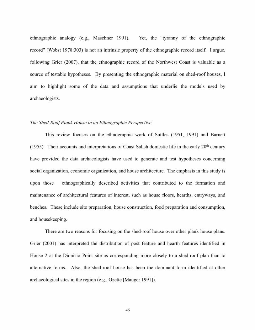
ethnographic analogy (e.g., Maschner 1991). Yet, the “tyranny of the ethnographic

record” (Wobst 1978:303) is not an intrinsic property of the ethnographic record itself. I argue,

following Grier (2007), that the ethnographic record of the Northwest Coast is valuable as a

source of testable hypotheses. By presenting the ethnographic material on shed-roof houses, I

aim to highlight some of the data and assumptions that underlie the models used by

archaeologists.

The Shed-Roof Plank House in an Ethnographic Perspective

This review focuses on the ethnographic work of Suttles (1951, 1991) and Barnett

(1955). Their accounts and interpretations of Coast Salish domestic life in the early 20th century

have provided the data archaeologists have used to generate and test hypotheses concerning

social organization, economic organization, and house architecture. The emphasis in this study is

upon those ethnographically described activities that contributed to the formation and

maintenance of architectural features of interest, such as house floors, hearths, entryways, and

benches. These include site preparation, house construction, food preparation and consumption,

and housekeeping.

There are two reasons for focusing on the shed-roof house over other plank house plans.

Grier (2001) has interpreted the distribution of post feature and hearth features identified in

House 2 at the Dionisio Point site as corresponding more closely to a shed-roof plan than to

alternative forms. Also, the shed-roof house has been the dominant form identified at other

archaeological sites in the region (e.g., Ozette [Mauger 1991]).

46

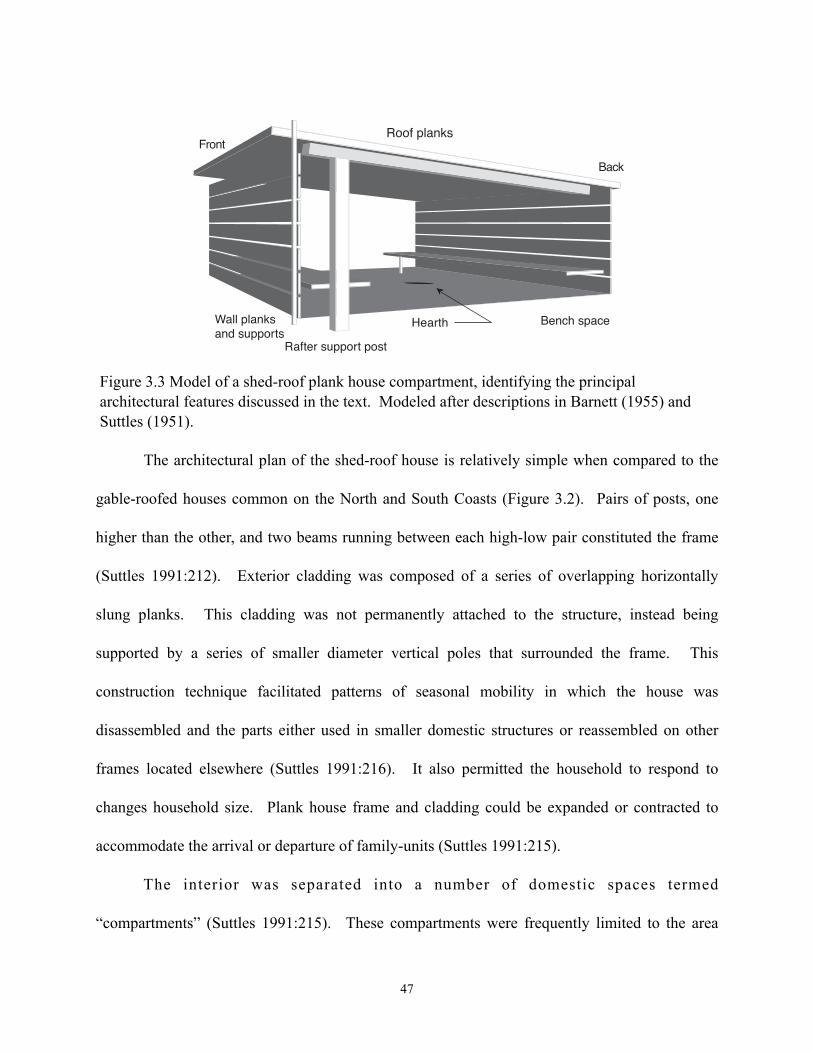
The architectural plan of the shed-roof house is relatively simple when compared to the

gable-roofed houses common on the North and South Coasts (Figure 3.2). Pairs of posts, one

higher than the other, and two beams running between each high-low pair constituted the frame

(Suttles 1991:212). Exterior cladding was composed of a series of overlapping horizontally

slung planks. This cladding was not permanently attached to the structure, instead being

supported by a series of smaller diameter vertical poles that surrounded the frame. This

construction technique facilitated patterns of seasonal mobility in which the house was

disassembled and the parts either used in smaller domestic structures or reassembled on other

frames located elsewhere (Suttles 1991:216). It also permitted the household to respond to

changes household size. Plank house frame and cladding could be expanded or contracted to

accommodate the arrival or departure of family-units (Suttles 1991:215).

The interior was separated into a number of domestic spaces termed

“compartments” (Suttles 1991:215). These compartments were frequently limited to the area

47

Figure 3.3 Model of a shed-roof plank house compartment, identifying the principal architectural features discussed in the text. Modeled after descriptions in Barnett (1955) and Suttles (1951).

Bench space

Roof planks

Rafter support post

Wall planks

and supports

Back

Front

Hearth

between two sets of house posts along the length of the structure (Suttles 1991:215). Thus a

shed-roof house with six house posts in three pairs is thought to have contained four families.

Each domestic space was used by a nuclear or extended family, and had a hearth and storage area

(Suttles 1991:215). Hearths lacked any associated furniture and could be readily moved when

necessary. Stores were kept in the rafters, which allowed the house to act as an enormous smoke

box (Ames 1996; Suttles 1991) and in boxes under sleeping platforms.

Platforms, approximately 1.5 m in width (Suttles 1951:258) and approximately 20 - 70

cm high (Barnett 1955:37; Samuels 1991:108), extended around the parts of or the whole of the

interior perimeter of the house. It is likely that the shape, size, and distribution of these features

were variable and tailored to suit the needs of the household. These may have constituted the

only permanent furniture in the structures (Barnett 1955:38). Ethnographers are unanimous in

describing the floor as earthen (Suttles 1991:214) or unplanked (Barnett 1955:38). Inhabitants

may have used mats to protect themselves from the cold and possibly somewhat damp sediment.

It appears from the ethnographic record that the location of the entryway could be quite

variable. Suttles (1991) identifies it as typically found in the long wall that faced the beach.

Mauger (1991:157) suggests that it may not have had a permanent location in some shed-roof

plank houses, and being little more than a gap in the horizontal wall planking facilitated their

relation. In some instances, the entryways were extraordinarily complex, formed of a convoluted

web of planks and posts. Some may have had extensive defensive mechanisms (Suttles

1991:219), hinged doors, or wind-breaks (Mauger 1991:157).

The ethnographic data suggests that several architectural features that can be productively

assessed from the geoarchaeological record. Floors, hearths, benches, and post features are all

48

candidates; they may leave permanent signatures that are identifiable by their color, texture or

microscopic characteristics. Entryways are also features that may leave identifiable

geoarchaeological traces due to their presumed association with housekeeping practices; all

refuse that is not incorporated into the floor or bench features, must be transported through the

entryway to exterior middens. Past discussions of plank house cultural formation processes have

highlighted many of these same features. The following section discusses how these features

have been treated by past models of cultural formation processes, and contrasts these with

geoarchaeological expectations that are tested in this study.

Archaeological Models of Plank House Features

The geoarchaeological model draws on the preceding discussion of the ethnographic

literature to identify architectural features that may leave a geoarchaeological signature. The

discussion covers the anthropogenic alteration of the site prior to habitation, and the behaviors

that may have contributed to the development of house floors, hearth, benches and entryways

identified in the geoarchaeological record. Post features samples were unavailable for analysis

from the Dionisio Point site and are not addressed here.

Pre-habitation site alteration

Few archaeologists systematically treat pre-habitation site alteration as a cultural

formation process because they concentrate on materials deposited after site-preparation.

However, accounting for these processes is a necessary step in geoarchaeological analysis as

they alter the distribution of on-site natural sediments. The preparation of the site for a plank

49

house construction resulted in the formation of a series of three stable terraces (Grier

2001:104,106), a practice also noted among the ethnographic Coast Salish (Barnett 1955:43, 51;

Suttles 1991:214). Each of these terraces is 2 to 3 m in height, suggesting that many cubic

meters of material was redistributed from the back of would-be house floors to the front.

This large-scale movement of sediment bodes well for the recovery of signatures of

habitation activities. Soil constituents may be variable within a small area due to varying

vegetation cover, as pect, and infiltration. The character of the underlying sediment, however, is

fairly homogenous (Green et al. 1989) because it is only indirectly affected by these factors and

predominantly reflects the characteristics of the parent material. Thus, the inversion and

effective elimination of the forest soil removed one of the sources of variability that might

confuse our interpretations of later activities. Comparison of on-site and off-site signatures is,

therefore, primarily concerned with changes that occurred after site abandonment.

Hearth Deposits

I have chosen to begin with hearths for three reasons. First, if the dominant sources of

organic matter, free ions, and fine sediments in the house are the preservation, preparation and

consumption of food, these features should be the most enriched in the deposit, and thus should

be readily “visible” in their geoarchaeological signatures. Second, with few exceptions, hearths

are considered to be fundamental to the identification of plank house deposits. Third, hearths

have also been regularly used to infer the number of families in a house (e.g. Grier 2006a),

household social organization (Coupland et al. 2009), as well as the social status of the

household (Samuels 1991b).

50

Few cultural or non-cultural formation process models presently exist to explain the

characteristics of plank house hearth features. The common conceptualization of these features

is that they functioned principally as domestic facilities, used to process food, give light, and

provide heat. Drawing on the ethnographic record, it has been suggested that some hearths

functioned as purely ceremonial facilities, and others purely domestic facilities. This argument

has been supported with evidence that some hearths were treated differently than others,

particularly by their location and size (Samuels 1991b:266). How far into the past this model

can be used is unclear, particularly in light of evidence that ceremonial function appear to have

been vested in specific families within the household as opposed to the entire household itself

(e.g., Grier 2006a:114). Samuels (1991b) analysis of different size grades of faunal remains,

excluding shell fish, has suggested that food waste may have been deposited directly into hearths

after it was consumed in Houses 1 and 2 at the Ozette site.

When compared to natural samples, in the context of all other deposits in the plank house,

hearths should have the highest enrichment in organic matter, the highest concentration of free

ions (electrical conductivity), and the highest pH. Organic matter in this context is derived

primarily from food and fuel residues. Food prepared around the hearth may have deposited oils,

or particulate organic matter into the feature increasing its organic matter content. Carbonized

wood fuel would also contribute to localized organic matter enrichment.

Wood ash, in sites in drier environments has been demonstrated to cause increased free

ion content, particularly in the form of potassium (Marwick 2005:1361; Middleton and Price

1996:678; Weide 1966). Similar increases in forested environments have been identified in

forestry studies, but they have also noted that in these latter environments, presumably because

51

of nutrient uptake, coarse soils, and higher precipitation, these effects are only temporary.

However, none of these studies the effects of ash disappear completely during their projects,

suggesting that slight, localized signatures may still be present in archaeological deposits.

Increased pH is a consequence of the deposition of free ions by ash, and has been noted in other

archeological contexts (e.g., Marwick 2005:1361; Weide 1966).

Inorganic carbonate enrichment in hearths likely represents the in situ deposition of

shellfish remains following either processing or consumption, the leaching of carbonates from

nearby shell deposits, or from detrital calcite phytolithis formed by the combustion of wood fuel.

Wood phytoliths likely contributes to a slight increase in carbonates in hearths, but it is unlikely

that this results in a significant increase over the characteristics of the natural samples.

Significant carbonate enrichment is probably only the result of either the first or the second

process. It is, however, possible that phytoliths could contribute to slight increases in silt and

clay content. Sedimentary analyses of ash texture has demonstrated that particles can range from

clay to sand in size, the modality determined by the species of fuel plant, part of the plan, and

temperature of the fire. One study of commercially produced wood ash demonstrates that as

much as 50% are less than 100 µm or smaller, quite close to the 62.5 µm is the division between

sand in silt used in this study (Demeyer et al. 2001:288). Given these characteristics, different

temperatures of fires may also be reflected in grain size distributions.

House Floors

The term house floor, for many plank house deposits in the Strait of Georgia is something

of a misnomer. Expect for rare occurrences of prepared floors (e.g., Lepofsky et al.

52

2000:398-399; Samuels 1991b:191), excavations have failed to locate evidence of well-

preserved living floor strata traceable across an entire deposit (e.g., Grier 2001; Matson 2003).

This is indirect support for the argument that pre-contact plank houses lacked planked floors,

much like their post-contact representatives. However, it also means that few studies have dealt

directly with the cultural formation process that create and affect house floor deposits or their

assemblages.

Where floor formation processes have been discussed is in those excavations where

discrete floors have been preserved, such as at the Ozette site (e.g., Huelsbeck 1994; Samuels

1991b). These discussions focus on the differential disturbance of primary deposits as a result of

three processes: housekeeping, trampling, and curation (Samuels 1991b:232). These processes

were suggested to affect the distribution of both artifacts and faunal remains in Houses 1, 2, and

5 at the site. Artifacts were much more likely to be curated by house occupations (Samuels

1991b:244), while faunal material appear to have reflected in situ processing locations as well as

housekeeping practices (Sameusls 1991b:262). These processes, as I argue in the introduction,

are most commonly addressed through the distributions of artifacts and faunal remains, both of

which can be scarce at some sites. Sedimentary analysis, while not as sensitive as artifact

remains, can provide an alternative data set.

Spatial analyses of floor assemblages have supported the argument that space in most

pre-contact plank house deposits was redundant; that the house was not divided into functional

areas, but that each compartment was used as a domestic space by an individual family (Grier

2006a). This suggests that the additions made to most floor areas were broadly similar. Should

this be the case, it is likely that anthropogenic additions were dominated by residues from food

53

production and consumption (e.g., Samuels 1991b), and tool production. Many of these

residues, and particularly food residues, would have been difficult to remove from floors and

would have, over time, accumulated in large amounts.

The incorporation of large amounts of organic matter would alter the floors pH and

electrical conductivity. Organic matter typically has the affect of lowering pH through the

production of organic acids. However, much like hearth deposits, this process was likely

mediated by the incorporation of byproducts of wood fuel combustion that result in increased

electrical conductivity and increased pH.

Once again, much like hearth deposits, inorganic carbonates have only two significant

anthropogenic sources: marine shell and opal phytoliths. Shell deposition within houses has

been demonstrated in deposits at Ozette (Wessen 1994), but otherwise appears to be a rare

occurrence on the coast.

Bench Deposits

Ethnographic data on benches suggests that their size and layout were variable (Barnett

1955:37; cf. Suttles 1951:258, 1991:213), although there is consensus that it was used for

sleeping, socializing, and storage. In spite of this structural variability, these deposits have been

located in several excavations in the Strait of Georgia. They have been identified through two

kinds of evidence. First, benches have been inferred from the presence of substantial post

features that area associated with the frame of the structure but are not clearly rafter support

beams. They are frequently smaller than rafter supports and are located approximately a bench-

width away from the edge of the structure (Grier 2001:166-178; Mauger 1991:105).

54

Alternatively, changes in microtopography and texture have been used to identify bench deposits.

Grier (2001:179) at the Dionisio Point site, and Lepofsky et al. (2000:398-399), at the Scowlitz

site, have both identified benches based on gravelly, step-like features located in the edges of the

deposit. Matson (2003:88) has suggested that loose black sediment around a portion of one of

the compartments in the Shingle Point house represents a bench deposit.

The variety of data used suggests that archaeologists use several models to identify and

interpret bench deposits in plank houses on the Central Coast. Many draw on Hayden and

Cannon’s (1982) discussion of benches as out-of-the-way places where valued artifacts may be

kept and subsequently lost, or where, through size-sorting processes, larger artifacts and faunal

remains will differentially accumulate through daily maintenance processes. The data Matson

(2003:88) cites in identifying bench deposits suggests that this area was not trampled, and further

implies that organic matter of some kind accumulated in this area, perhaps in the form of

material transported from the center of the house floor.

If these features were created during initial preparation of the deposit by the piling of

sediment around the perimeter of the house, the characteristics of these deposits should appear to

be quite similar to those identified for natural samples. However, if as has been suggested,

benches were locations where sediment accumulated during the occupation of the house, they

may have characteristics quite different from the natural samples. If food resources were stored

in these locations, I would expect that they would be enriched in organic matter, much as Matson

(2003:88) identified at Shingle Point. Moreover, if they were locations where material

accumulated, either intentionally or unintentionally, as Matson (2003:88) suggests, they may also

contain traces of sediments generated by other features, and therefore appear to be moderately

55

enriched in, for example, electrical conductivity and have slightly finer texture than non-bench

floor deposits if hearth sediments were transported there. However, if bench space was not used

for the storage of goods, nor did material accumulate there from cleaning activities,

characteristics may be quite similar to those of non-bench floor deposits.

Entryways

As discussed in above, entryways have been poorly defined in both ethnographic and

archaeological contexts. When archaeologists have identified these deposits it has been through

two lines of data. First, entryways have been identified through “smears” of faunal material new

walls (e.g., Huelsbeck 1994). It is argued that these patterns are the result of debris being moved

out of the house. The long-term accumulation of faunal remains suggests that the house

entryway was rarely, if ever, moved during the occupation of the structure. The second line of

evidence is the presence of clusters of large numbers of post features near the edge of deposits.

Following ethnographic descriptions of fortified doorways in some shed-roof plank houses, some

archaeologists have interpreted these feature clusters as parts of these defencive mechanisms.

The sedimentary signature of entryways may be quite subtle. It likely tracks the same

disposal processes that were identified at the Ozette site. I expect that many of the waste

materials removed from houses were organic in origin, such as food and fuel waste. The overall

patterns should be similar to those of floors and hearths. However, because the activities that

generate these wastes are concentrated in other parts of the house, it is probable that the signature

here will be considerably weaker.

Expectations

56

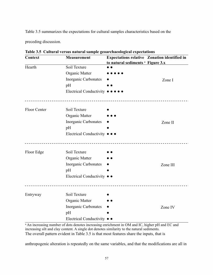
Table 3.5 summarizes the expectations for cultural samples characteristics based on the

preceding discussion.

Table 3.5 Cultural versus natural sample geoarchaeological expectationsContext Measurement Expectations relative

to natural sediments aZonation identified in Figure 3.x

Hearth Soil Texture ● ●

Zone I

Organic Matter ● ● ● ● ●Inorganic Carbonates ●pH ● ●Electrical Conductivity ● ● ● ● ●

Floor Center Soil Texture ●

Zone IIOrganic Matter ● ● ●Inorganic Carbonates ●pH ●Electrical Conductivity ● ● ●

Floor Edge Soil Texture ● ●

Zone IIIOrganic Matter ● ●Inorganic Carbonates ●pH ●Electrical Conductivity ● ●

Entryway Soil Texture ●

Zone IVOrganic Matter ● ●Inorganic Carbonates ●pH ●Electrical Conductivity ● ●

a An increasing number of dots denotes increasing enrichment in OM and IC, higher pH and EC and increasing silt and clay content. A single dot denotes similarity to the natural sediments.The overall pattern evident in Table 3.5 is that most features share the inputs, that is

anthropogenic alteration is repeatedly on the same variables, and that the modifications are all in

57

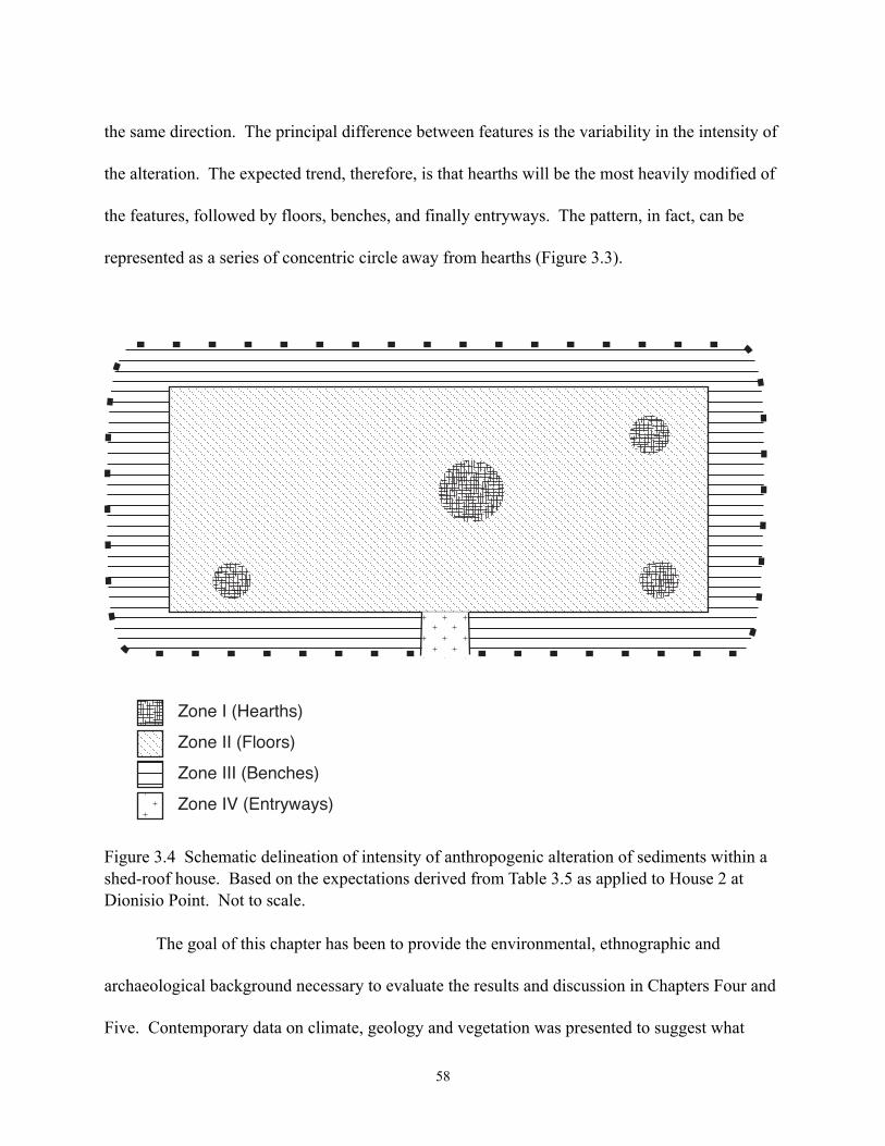
the same direction. The principal difference between features is the variability in the intensity of

the alteration. The expected trend, therefore, is that hearths will be the most heavily modified of

the features, followed by floors, benches, and finally entryways. The pattern, in fact, can be

represented as a series of concentric circle away from hearths (Figure 3.3).

!"#$%&%'($)*+,-.

!"#$%&&%'/0""*-.%

!"#$%&&&%'1$#2,$-.

!"#$%&3%'4#+*56)5-.

Figure 3.4 Schematic delineation of intensity of anthropogenic alteration of sediments within a shed-roof house. Based on the expectations derived from Table 3.5 as applied to House 2 at Dionisio Point. Not to scale.

The goal of this chapter has been to provide the environmental, ethnographic and

archaeological background necessary to evaluate the results and discussion in Chapters Four and

Five. Contemporary data on climate, geology and vegetation was presented to suggest what

58

might be expected from natural samples collected from around the Dionisio Point site.

Ethnographic and archaeological data pertaining to shed-roof plank house architecture and

feature formation processes were identified to provide a basis for evaluating the cultural samples

selected for this study. The implications of these three data sets for our archaeological models of

plank houses and plank house formation processes will be raised throughout the remainder of

this study.

59

Chapter Four: Methods and Results

This study focuses on the bulk sediment analysis of two data sets. The first of these is an

archival collection of bulk sediment samples generated in 1997 and 1998 by the Dionisio Point

Household Archaeology Project (DPHAP). These samples were collected from locations in

House 2 and House 5 at the Dionisio Point site. The second data set is a series of bulk samples

of non-anthropogenically altered sediments and soils from locations around the Dionisio Point

site.

In the following discussion, natural strata are labeled according to pedological

conventions, using capitalized Roman letters. However, the cultural strata at Dionisio Point

have, in the past, been labeled using the same range of letters. Rather change conventions for

either of these data sets, I have retained these label, but refer to a pedological stratum as a

“horizon” and a cultural stratum a “layer”.

Natural Samples

In 2007, eight off-site “natural” samples were collected at Dionisio Point. These samples

were collected from three locations within the Dionisio Point Provincial Park boundaries, but

outside of the known village area (Figure 4.1) and attempted to capture the range of variability of

geology and vegetation in the area. Samples were collected from the organic-mineral “A”

horizon, the illuvial “B” horizon, and the parent material “C” horizon. Where a clear boundary

between the B and C horizon was absent, the label B/C was used. When possible, the overlying

organic litter “L/F” horizon was excluded. One sample (SS200702) was discarded after it

became clear that it had partially sampled the litter horizon. Samples consisted of 500 g of

60

sediment, which were collected on May 22nd. 2007 and were transported to the Geoarchaeology

lab at Washington State University for analysis.

Natural Sample Profile 1:

The first of the sampling locations was approximately 40 m south of the Marpole village

site datum, at 10 m asl. It consisted of a 50 by 50 cm unit 53 cm deep. The in-field description

of the profile indicates the presence of a 12 cm thick litter horizon (L/F), composed of

undecomposed to partially decomposed twigs, needles, and woody material. This horizon

directly overlay a weakly formed illuvial B horizon that was grayish brown (10YR5/3) from 0 to

20 cm below surface and a dark yellowish brown (10YR4/4) B/C horizon from 21 to 53 cm

below surface. The field identification of the texture was loose gravelly sand. Below the litter

horizon, there were a few fine roots. Samples were collected from each of these three horizons.

Natural Sample Profile 2:

The second unit was located approximately 100 m southeast of the site datum, at 10 m

asl. It consisted of a 50 by 50 cm unit 30 cm deep. The in-field description of the profile

indicates the presence of an approximately 10 cm thick litter horizon (L/F). This horizon directly

overlay a weakly formed B horizon that was dark brown (10YR3/3) from 0 to 20 cm below

surface, and a brown (10YR5/3) B/C horizon from 21 to 31 cm below surface. The field

identification of the texture was a loose gravelly sand. Below the litter horizon there were a few

fine roots. Samples were collected from both the B and B/C horizons.

61

Natural Sample Profile 3:

The third unit was located approximately 180 m east-northeast of the site datum, on the

erosional west bank of Parry Lagoon. The elevation was between 1 and 2 m asl. The in-field

description of the profile indicates that there was a 26 cm thick black (10YR2/1) A horizon

developing under short grasses. The A horizon directly overlay a thick dark grayish brown

(10YR3/2) B horizon from 26 to 70 cm below surface. The samples collected from the B

horizon were located adjacent to one another. The B horizon contained evidence of dark

yellowish brown (10YR3/6) mottles (oxidized, iron-rich accumulations) or root casts, both these

and the presumed in situ soil were sampled. The field identification of the texture was loose

sand. There were a few fine roots in the B horizon. Samples were collected from the A horizon

and B horizon soils and mottles/root casts.

Cultural Samples

During the DPHAP excavations, sediment samples were collected with the goal of

activity area research. Every 10 cm cultural layer in each 1 m2 or 4 m2 excavation unit was

represented by the collection of a single sample. When features were encountered, they were

sampled as a single unit, except when the feature was quite large. Feature 9, the approximately

1.5 m3 central hearth in House 2, for example, generated several samples. Each of these samples

was approximately 4 liters in volume

At the time of this study, 52 cultural samples were appropriate to the kind of research

questions and methods pursued here. This data set consisted of forty-four on-site matrix samples

selected from the 1997 excavations in addition to eight on-site sediment samples from the 1998

62

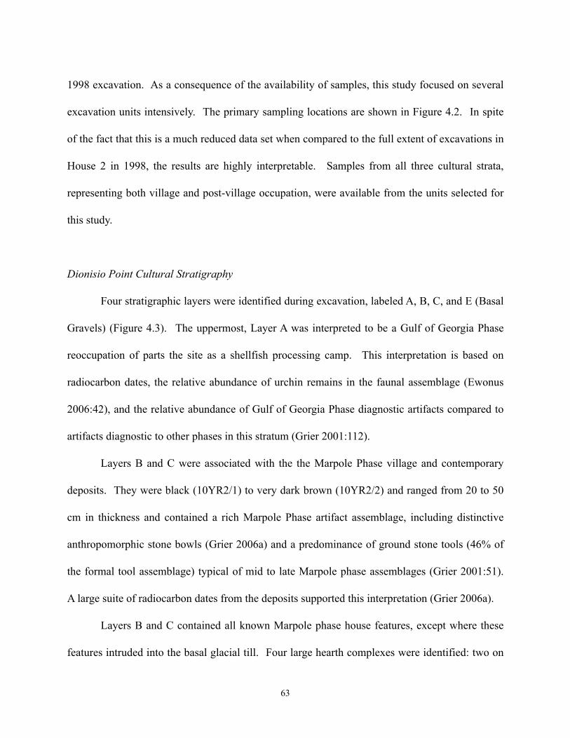
1998 excavation. As a consequence of the availability of samples, this study focused on several

excavation units intensively. The primary sampling locations are shown in Figure 4.2. In spite

of the fact that this is a much reduced data set when compared to the full extent of excavations in

House 2 in 1998, the results are highly interpretable. Samples from all three cultural strata,

representing both village and post-village occupation, were available from the units selected for

this study.

Dionisio Point Cultural Stratigraphy

Four stratigraphic layers were identified during excavation, labeled A, B, C, and E (Basal

Gravels) (Figure 4.3). The uppermost, Layer A was interpreted to be a Gulf of Georgia Phase

reoccupation of parts the site as a shellfish processing camp. This interpretation is based on

radiocarbon dates, the relative abundance of urchin remains in the faunal assemblage (Ewonus

2006:42), and the relative abundance of Gulf of Georgia Phase diagnostic artifacts compared to

artifacts diagnostic to other phases in this stratum (Grier 2001:112).

Layers B and C were associated with the the Marpole Phase village and contemporary

deposits. They were black (10YR2/1) to very dark brown (10YR2/2) and ranged from 20 to 50

cm in thickness and contained a rich Marpole Phase artifact assemblage, including distinctive

anthropomorphic stone bowls (Grier 2006a) and a predominance of ground stone tools (46% of

the formal tool assemblage) typical of mid to late Marpole phase assemblages (Grier 2001:51).

A large suite of radiocarbon dates from the deposits supported this interpretation (Grier 2006a).

Layers B and C contained all known Marpole phase house features, except where these

features intruded into the basal glacial till. Four large hearth complexes were identified: two on

63

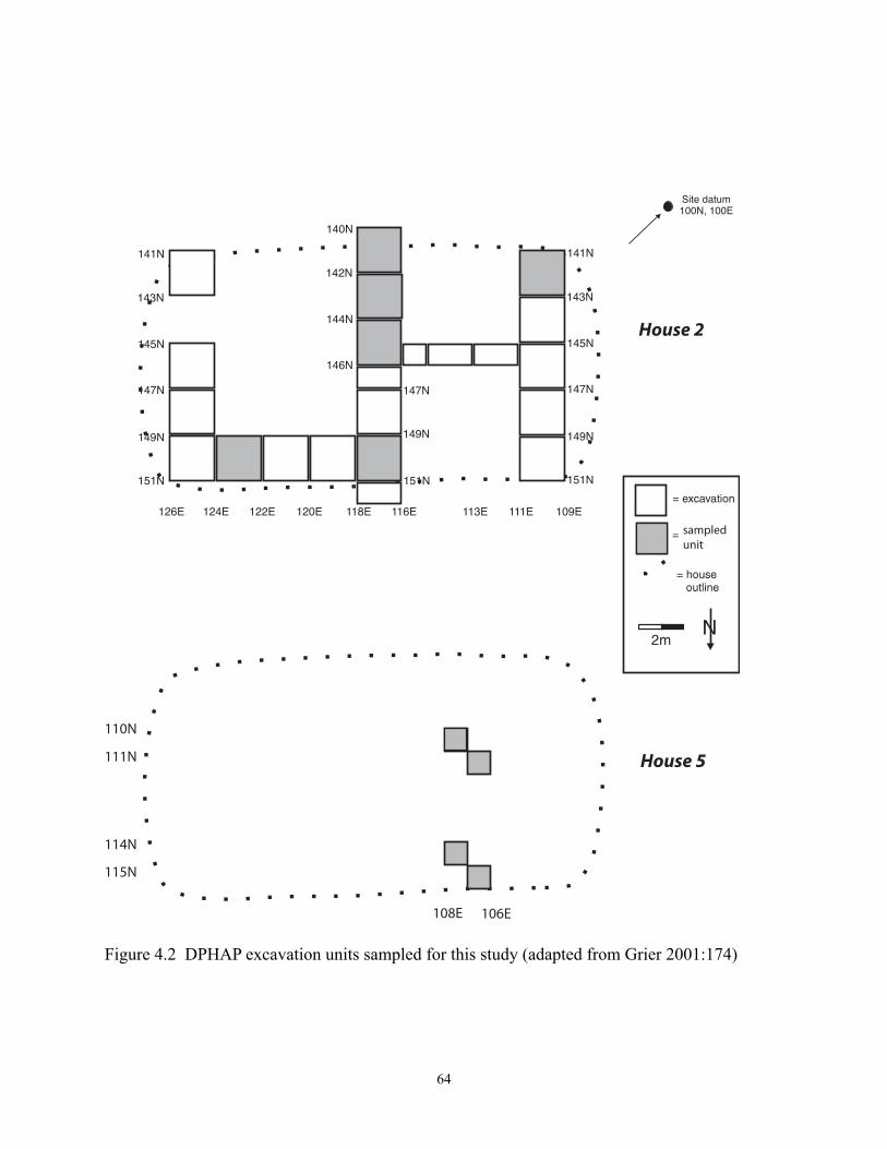
64

141N

143N

145N

147N

149N

151N

141N

143N

145N

147N

149N

151N

140N

142N

144N

146N

147N

149N

151N

126E 124E 122E 120E 118E 116E 113E 111E 109E

Site datum

100N, 100E

sampledunit

110N

111N

114N

115N

106E108E

House 2

House 5

Figure 4.2 DPHAP excavation units sampled for this study (adapted from Grier 2001:174)

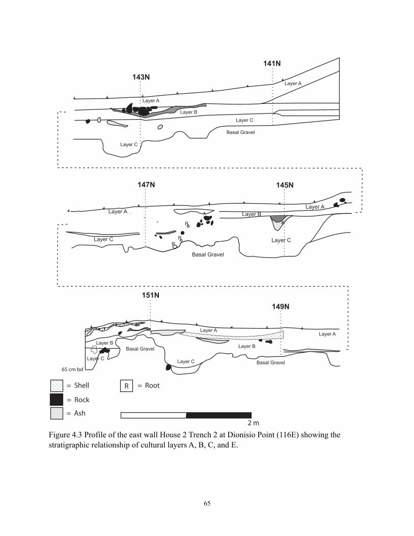
65

Layer B

Layer C

Layer A

Layer A

Layer C

Basal Gravel

141N

143N

R

R

R

R

Layer C

Layer A Layer B

Layer C

Layer A

Basal Gravel

145N147N

Layer B

Layer A

Layer C

Basal GravelLayer B

Layer C

Layer A

Basal Gravel

149N

151N

R= Shell

= Rock

= Ash

= Root

2 m

65 cm bd

Figure 4.3 Profile of the east wall House 2 Trench 2 at Dionisio Point (116E) showing the stratigraphic relationship of cultural layers A, B, C, and E.

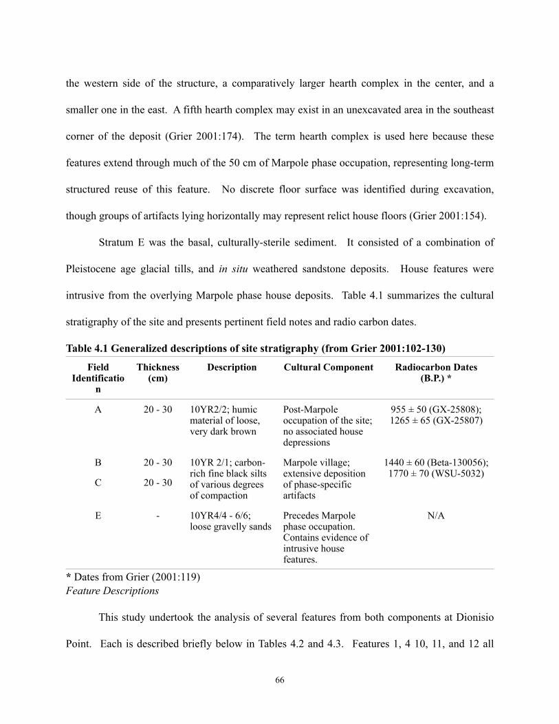
the western side of the structure, a comparatively larger hearth complex in the center, and a

smaller one in the east. A fifth hearth complex may exist in an unexcavated area in the southeast

corner of the deposit (Grier 2001:174). The term hearth complex is used here because these

features extend through much of the 50 cm of Marpole phase occupation, representing long-term

structured reuse of this feature. No discrete floor surface was identified during excavation,

though groups of artifacts lying horizontally may represent relict house floors (Grier 2001:154).

Stratum E was the basal, culturally-sterile sediment. It consisted of a combination of

Pleistocene age glacial tills, and in situ weathered sandstone deposits. House features were

intrusive from the overlying Marpole phase house deposits. Table 4.1 summarizes the cultural

stratigraphy of the site and presents pertinent field notes and radio carbon dates.

Table 4.1 Generalized descriptions of site stratigraphy (from Grier 2001:102-130)

Field Identificatio

n

Thickness (cm)

Description Cultural Component Radiocarbon Dates (B.P.) *

A 20 - 30 10YR2/2; humic material of loose, very dark brown

Post-Marpole occupation of the site; no associated house depressions

955 ± 50 (GX-25808);1265 ± 65 (GX-25807)

B 20 - 30 10YR 2/1; carbon-rich fine black silts of various degrees of compaction

Marpole village; extensive deposition of phase-specific artifacts

1440 ± 60 (Beta-130056);1770 ± 70 (WSU-5032)

C 20 - 30

E - 10YR4/4 - 6/6; loose gravelly sands

Precedes Marpole phase occupation. Contains evidence of intrusive house features.

N/A

* Dates from Grier (2001:119)Feature Descriptions

This study undertook the analysis of several features from both components at Dionisio

Point. Each is described briefly below in Tables 4.2 and 4.3. Features 1, 4 10, 11, and 12 all

66

belong to the post-Marpole phase plank house occupation at the site. Feature 34, a possible rock

heating feature, is included in this component as it could not be securely associated with the

House occupation either structurally or stratigraphically. Features 2, 9, 16, 24, and 28 were

located within the Marpole village occupation Layers B and C.

Methods

67

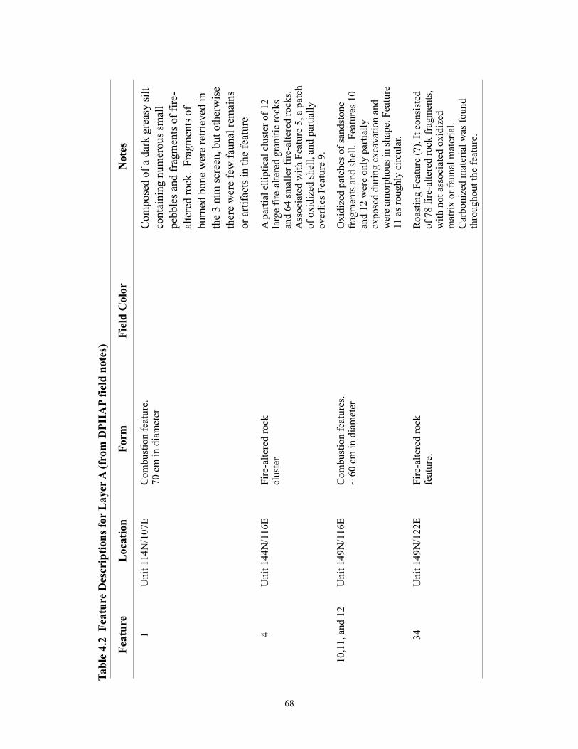
68

Feat

ure

Loc

atio

nFo

rmFi

eld

Col

orN

otes

1U

nit 1

14N

/107

EC

ombu

stio

n fe

atur

e.

70 c

m in

dia

met

erC

ompo

sed

of a

dar

k gr

easy

silt

cont

aini

ng n

umer

ous s

mal

l pe

bble

s and

frag

men

ts o

f fire

-al

tere

d ro

ck.

Frag

men

ts o

f bu

rned

bon

e w

ere

retri

eved

in

the

3 m

m sc

reen

, but

oth

erw

ise

ther

e w

ere

few

faun

al re

mai

ns

or a

rtifa

cts i

n th

e fe

atur

e m

atrix

.4

Uni

t 144

N/1

16E

Fire

-alte

red

rock

cl

uste

rA

par

tial e

llipt

ical

clu

ster

of 1

2 la

rge

fire-

alte

red

gran

itic

rock

s an

d 64

smal

ler f

ire-a

ltere

d ro

cks.

Ass

ocia

ted

with

Fea

ture

5, a

pat

ch

of o

xidi

zed

shel

l, an

d pa

rtial

ly

over

lies F

eatu

re 9

.

10,1

1, a

nd 1

2U

nit 1

49N

/116

EC

ombu

stio

n fe

atur

es.

~ 60

cm

in d

iam

eter

Oxi

dize

d pa

tche

s of s

ands

tone

fr

agm

ents

and

shel

l. F

eatu

res 1

0 an

d 12

wer

e on

ly p

artia

lly

expo

sed

durin

g ex

cava

tion

and

wer

e am

orph

ous i

n sh

ape.

Fea

ture

11

as r

ough

ly c

ircul

ar.

34U

nit 1

49N

/122

EFi

re-a

ltere

d ro

ck

feat

ure.

Roa

stin

g Fe

atur

e (?

). It

cons

iste

d of

78

fire-

alte

red

rock

frag

men

ts,

with

not

ass

ocia

ted

oxid

ized

m

atrix

or f

auna

l mat

eria

l.

Car

boni

zed

mat

eria

l was

foun

d th

roug

hout

the

feat

ure.

Tabl

e 4.

2 F

eatu

re D

escr

iptio

ns fo

r L

ayer

A (f

rom

DPH

AP

field

not

es)

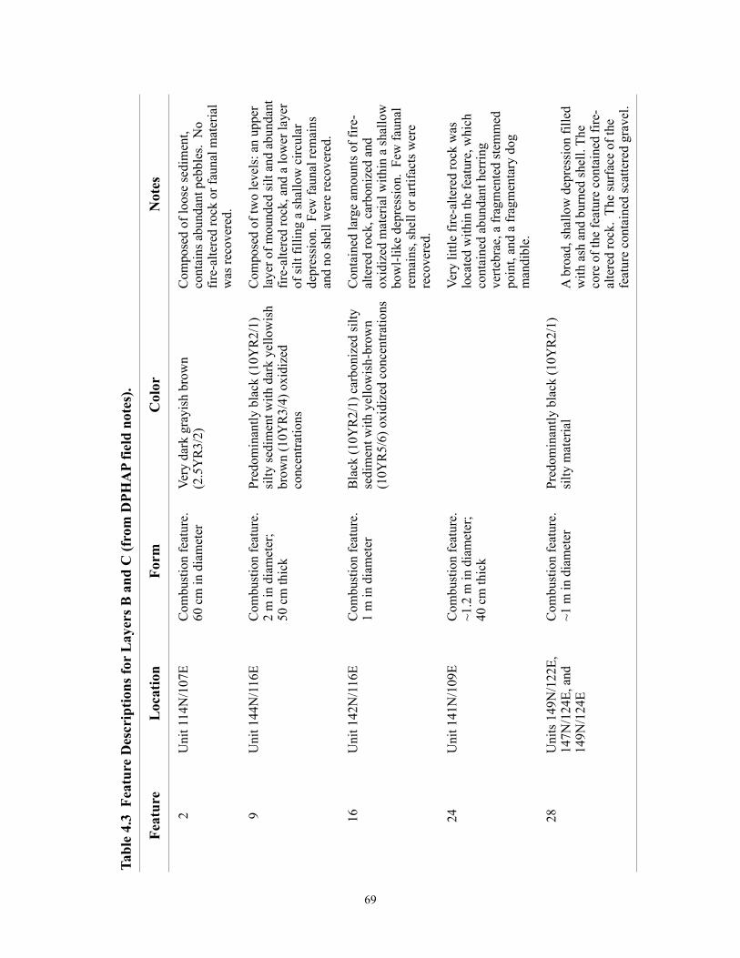
69

Feat

ure

Loc

atio

nFo

rmC

olor

Not

es

2U

nit 1

14N

/107

EC

ombu

stio

n fe

atur

e.

60 c

m in

dia

met

erVe

ry d

ark

gray

ish

brow

n (2

.5Y

R3/

2)C

ompo

sed

of lo

ose

sedi

men

t, co

ntai

ns a

bund

ant p

ebbl

es.

No

fire-

alte

red

rock

or f

auna

l mat

eria

l w

as re

cove

red.

9U

nit 1

44N

/116

EC

ombu

stio

n fe

atur

e.

2 m

in d

iam

eter

; 50

cm

thic

k

Pred

omin

antly

bla

ck (1

0YR

2/1)

si

lty se

dim

ent w

ith d

ark

yello

wis

h br

own

(10Y

R3/

4) o

xidi

zed

conc

entra

tions

Com

pose

d of

two

leve

ls: a

n up

per

laye

r of m

ound

ed si

lt an

d ab

unda

nt

fire-

alte

red

rock

, and

a lo

wer

laye

r of

silt

fillin

g a

shal

low

circ

ular

de

pres

sion

. Fe

w fa

unal

rem

ains

an

d no

shel

l wer

e re

cove

red.

16U

nit 1

42N

/116

EC

ombu

stio

n fe

atur

e.

1 m

in d

iam

eter

Bla

ck (1

0YR

2/1)

car

boni

zed

silty

se

dim

ent w

ith y

ello

wis

h-br

own

(1

0YR

5/6)

oxi

dize

d co

ncen

tratio

ns

Con

tain

ed la

rge

amou

nts o

f fire

-al

tere

d ro

ck, c

arbo

nize

d an

d ox

idiz

ed m

ater

ial w

ithin

a sh

allo

w

bow

l-lik

e de

pres

sion

. Fe

w fa

unal

re

mai

ns, s

hell

or a

rtifa

cts w

ere

reco

vere

d.

24U

nit 1

41N

/109

EC

ombu

stio

n fe

atur

e.

~1.2

m in

dia

met

er;

40 c

m th

ick

Very

littl

e fir

e-al

tere

d ro

ck w

as

loca

ted

with

in th

e fe

atur

e, w

hich

co

ntai

ned

abun

dant

her

ring

verte

brae

, a fr

agm

ente

d st

emm

ed

poin

t, an

d a

frag

men

tary

dog

m

andi

ble.

28U

nits

149

N/1

22E,

14

7N/1

24E,

and

14

9N/1

24E

Com

bust

ion

feat

ure.

~1

m in

dia

met

erPr

edom

inan

tly b

lack

(10Y

R2/

1)

silty

mat

eria

lA

bro

ad, s

hallo

w d

epre

ssio

n fil

led

with

ash

and

bur

ned

shel

l. Th

e co

re o

f the

feat

ure

cont

aine

d fir

e-al

tere

d ro

ck.

The

surf

ace

of th

e fe

atur

e co

ntai

ned

scat

tere

d gr

avel

.

Tabl

e 4.

3 F

eatu

re D

escr

iptio

ns fo

r L

ayer

s B a

nd C

(fro

m D

PHA

P fie

ld n

otes

).

All samples were run through a series of standardized bulk sediment analyses. Samples

were subsampled to 500g and dry-screened on a Ro-Tap to whole-Φ units (see Table 2.2).

Visible particulate organic matter was removed from the < 4 Φ fraction. For particle-size

analyses, carbonates removed with 1N HCl, diluted in de-ionized H2O, left overnight and the

supernatant removed. Salts were removed with de-ionized H2O, left overnight, and the

supernatant removed. Organic matter was removed from the samples with 30% H2O2, which was

allowed to digest overnight and the supernatant was removed. The high concentration of H2O2

was necessary because of visibly high organic matter content of all cultural samples. Soil texture

was determined with either a Malvern Mastersizer “S” Laser Particle-Size Analyzer or

hydrometer following Gee and Orr (1986) and Day (1965).

The amount of organic matter enrichment and inorganic carbonate enrichment in each

sample was determined through loss-on-ignition (LOI) modified from Stein (1984). Samples

were initially dried to 105ºC. Combustion of organic matter was completed by heating each

sample to 550ºC for four hours. Combustion of inorganic carbonates was completed by further

heating each sample to 950ºC for two hours. Organic matter and inorganic carbonate

measurements are presented in percent by weight to the nearest ten-thousandth of a gram. pH

was determined on a 1:1 aqueous slurry measured with a Beckman 300 Series pH meter.

Electrical conductivity was determined on a 1:1 aqueous slurry measured with an Exstik EC400

Conductivity meter. Electrical conductivity measurements are presented in microseimens per

centimeter (µS/cm).

All of these methods evaluate sediment/soil characteristics that are considered to be

proximate measures of degree and kind of human activity as described in Chapter Three.

70

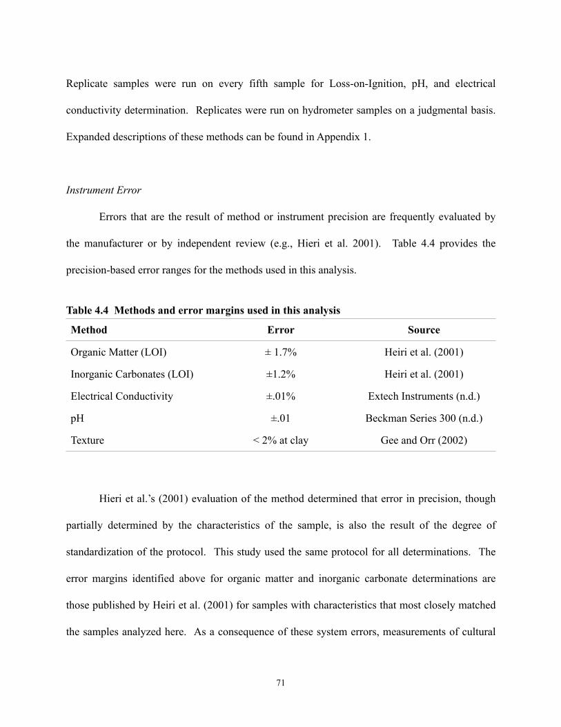
Replicate samples were run on every fifth sample for Loss-on-Ignition, pH, and electrical

conductivity determination. Replicates were run on hydrometer samples on a judgmental basis.

Expanded descriptions of these methods can be found in Appendix 1.

Instrument Error

Errors that are the result of method or instrument precision are frequently evaluated by

the manufacturer or by independent review (e.g., Hieri et al. 2001). Table 4.4 provides the

precision-based error ranges for the methods used in this analysis.

Table 4.4 Methods and error margins used in this analysis

Method Error Source

Organic Matter (LOI) ± 1.7% Heiri et al. (2001)

Inorganic Carbonates (LOI) ±1.2% Heiri et al. (2001)

Electrical Conductivity ±.01% Extech Instruments (n.d.)

pH ±.01 Beckman Series 300 (n.d.)

Texture < 2% at clay Gee and Orr (2002)

Hieri et al.’s (2001) evaluation of the method determined that error in precision, though

partially determined by the characteristics of the sample, is also the result of the degree of

standardization of the protocol. This study used the same protocol for all determinations. The

error margins identified above for organic matter and inorganic carbonate determinations are

those published by Heiri et al. (2001) for samples with characteristics that most closely matched

the samples analyzed here. As a consequence of these system errors, measurements of cultural

71

sample characteristics must exceed these error margins to be considered meaningful. pH and

electrical conductivity error rates have been published by the manufacturer. Human error is the

greatest source of erroneous measurements for particle size analysis, particularly when using the

hydrometer method. All measurements were taken by myself and only after extensive practice

with replicates of samples with known texture.

Results

Bulk Analysis of Natural Samples

The following discussion presents the results of the bulk analysis of the natural samples

from Profiles 1, 2, and 3. Table 4.5 presents the profile, field horizon identification, and

laboratory determination for all 8 samples. Note that while SS200702 is presented here, it is not

used in later analyses. The sample was collected from the litter horizon in Profile 1 and is not

comparable to any context in the cultural data set. The addition of sample 97M21 in Table 4.6,

from the DPHAP matrix archive acts as a replacement for SS200702. The laboratory determined

characteristics of this sample are comparable to those collected from off-site. Descriptions of all

samples can be found in Appendix 2.

Table 4.5 Natural Samples Bulk Sediment Characteristics

72

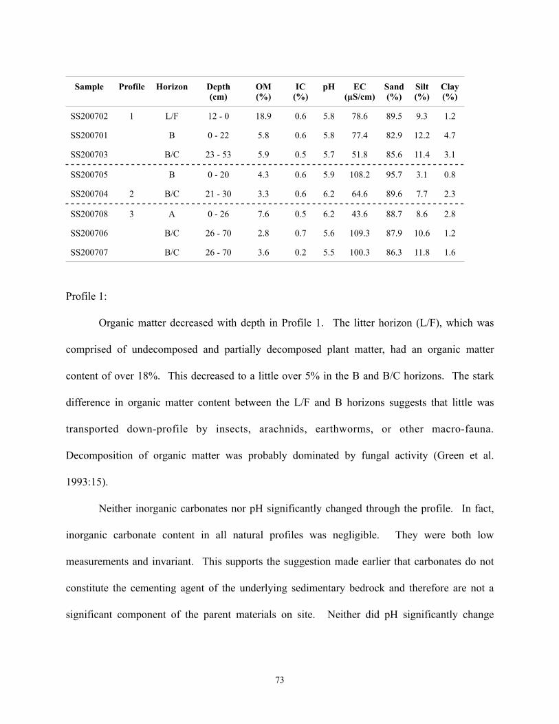
Sample Profile Horizon Depth (cm)

OM (%)

IC (%)

pH EC (µS/cm)

Sand (%)

Silt (%)

Clay (%)

SS200702 1 L/F 12 - 0 18.9 0.6 5.8 78.6 89.5 9.3 1.2

SS200701 B 0 - 22 5.8 0.6 5.8 77.4 82.9 12.2 4.7

SS200703 B/C 23 - 53 5.9 0.5 5.7 51.8 85.6 11.4 3.1

SS200705 B 0 - 20 4.3 0.6 5.9 108.2 95.7 3.1 0.8

SS200704 2 B/C 21 - 30 3.3 0.6 6.2 64.6 89.6 7.7 2.3

SS200708 3 A 0 - 26 7.6 0.5 6.2 43.6 88.7 8.6 2.8

SS200706 B/C 26 - 70 2.8 0.7 5.6 109.3 87.9 10.6 1.2

SS200707 B/C 26 - 70 3.6 0.2 5.5 100.3 86.3 11.8 1.6

Profile 1:

Organic matter decreased with depth in Profile 1. The litter horizon (L/F), which was

comprised of undecomposed and partially decomposed plant matter, had an organic matter

content of over 18%. This decreased to a little over 5% in the B and B/C horizons. The stark

difference in organic matter content between the L/F and B horizons suggests that little was

transported down-profile by insects, arachnids, earthworms, or other macro-fauna.

Decomposition of organic matter was probably dominated by fungal activity (Green et al.

1993:15).

Neither inorganic carbonates nor pH significantly changed through the profile. In fact,

inorganic carbonate content in all natural profiles was negligible. They were both low

measurements and invariant. This supports the suggestion made earlier that carbonates do not

constitute the cementing agent of the underlying sedimentary bedrock and therefore are not a

significant component of the parent materials on site. Neither did pH significantly change

73

throughout the profile. pH values were comparable to those measured by Green et al. (1989:116)

for soils similar to those in the study area.

As measured by electrical conductivity, free ions decreased with depth. Elevated

electrical conductivity recorded in the horizon B was likely due to leaching of nutrients from the

organic horizon that immediately overlay it. The approximately 25 µS/cm decrease between

horizon B and B/C was due to its relative distance from the litter horizon. Fewer free ions were

added to horizon B/C and most were rapidly leached from the profile.

The soil texture of profile was classified as a loamy sand. The relative sand content

decreased with depth in the profile, while silt and clay both increased. Down profile movement

of fine sediment is a process identified in many natural soils (Birkeland 1984). This is likely the

process that is responsible for changes in texture with depth in this profile.

Profile 2:

Profile 2 showed a pattern that was, overall, similar to that noted for Profile 1, with the

exception that the L/F horizon was not sampled in this profile. Organic matter decreased by 1%

through the profile. The inorganic carbonate content showed no change through the profile. The

0.3 pH increase between the B and B/C horizons was within the error margin of the instrument.

The approximately 43 µS/cm decrease in electrical conductivity between the two horizons was

probably the result of pedogenic processes. Free ions accumulated in the B horizon, but were

extensively leached in the layer B/C horizon. Higher absolute electrical conductivity values in

this profile, when contrasted with Profile 1, were the result of additional free ions derived from

the chemical and physical weathering of a nearby sandstone ridge in combination with forest

74

litter. The soil texture of profile was classified as sand. The textural changes between horizons

was likely the result of the same processes responsible for this pattern in the first profile.

Profile 3:

Profile 3 had high organic matter content in the surface layer that decreased with depth

from 7.6 to 2.8%. A substantial A horizon had formed as a result of both local topography and

vegetation. The profile was found at the foot of a gentle grassy slope and collected far more

water and sediments, and received more subsoil biomass, than did the other profiles in this data

set. Inorganic carbonates did not show significant change with depth. The 0.5% difference in

inorganic carbonate enrichment between the two B/C samples was within the error margin of the

protocol. SS200707 was collected from a suspected mottle (an iron-oxide concentration) that

was properly identified as a root cast in the laboratory.

The decrease in pH through the profile cannot be readily explained. The surface sample

contained no greater inorganic carbonate enrichment than lower samples nor did it have higher

free ion concentration, both of which would act to mediate acidification. I would also expect the

higher organic matter concentration at the soil surface to contribute to increased acidification.

The measurement may reflect relatively minor pedogenic processes which are not accounted for

in this analysis.

Electrical conductivity showed an increase with depth from 43.6 to 109.3 µS/cm. This

was the reverse of the pattern in either of the other natural profiles and there were several

contributing factors that are unique to the location of this profile. First, the pattern of increasing

electrical conductivity with depth reflected the local absence of base-cycling coniferous forest

75

vegetation. Second, analysis of the B/C samples suggests that sample SS200707 may have been

collected from a root cast that could have promoted local through-flow of water from the surface.

Finally, sea water can be an abundant source of free ions either via submergence of the profile or

sea spray (Essington 2003:501). The latter was likely the dominant process in the case of Profile

3. It appears that sea spray had deposited more free ions in the B/C than the A horizon.

All three samples were classified as sand. The changes in texture were minor. The less

than 3% decrease in sand and as much as 1.2% decrease in clay with depth through the profile

was balanced by a 2% or more increase in silt. It is likely that the decrease in sand was the result

of the downward mobilization of fine sediments has in Profile 1 and 2.

Natural Sample Analysis

Excluding sample SS200702 in Profile 1 from the comparison, the soil characteristics of

the natural samples were highly consistent. As expected from Green et al.’s (1989) discussion of

Qualicum and Saturna soils, and field observations made during this study, these soils strongly

reflected the local bedrock and glacial parent material, and the local coniferous forest vegetation

community.

Organic matter content (mean= 4.8%, s = 1.7) was both relatively low and invariant.

Variability was predominantly a reflection of local vegetation. The higher organic matter content

of the surface sample in Profile 3, relative to other natural samples, was due to local A horizon

formation. A horizons did not form in other profiles where semi-closed forest conditions

prevailed.

76

The near-absence of inorganic carbonates (mean = 0.5%, s = 0.2) was a reflection of the

near absence of carbonates in either glacial (Green et al. 1989) or sandstone (Johnstone 2006)

parent materials found in the area and the acidic conditions of the forest solum (combined A and

B horizons). Without carbonates, which act to slow the process of acidification, and because

conifers reabsorb many of nutrients they deposit as litter, pH levels in the natural soils in the area

were moderately acid. At these these levels (mean = 5.9, s = 0.3), these soils would be

characterized as “moder soils”, indicating that decomposition was largely due to fungal activity

(Green et al. 1993:15).

Electrical conductivity showed the greatest variation between samples, ranging from 43.6

to 109.3 µS/cm (mean = 79.3 µS/cm, s = 21.2). This was not unexpected, free ions are the most

mobile of all the soil constituents measured in this analysis (via leaching and cycling) and

variation over a few centimeters within any profile was expected. The sea-spray affected

samples in the subsurface horizons in Profile 3 inflated the average electrical conductivity of the

natural soils. All samples were classified as loamy sand or sand. Sand content for every sample

was greater than 80% (mean = 87.6%, s = 4.0), silt less than 13% (mean = 9.8%, s = 3.3), and

clay less than 5% (mean = 2.4%, s = 1.3).

For the purpose of later analyses, the tendencies and variation in the natural samples were

summarized by their mean and standard deviation. These statistics are calculated with the

addition of sample 97M21, a sample collected from the basal gravels, presented below in Table

4.6. This sample is part of the archaeological data set, and although it was collected from the

sterile sediments beneath House 2 it corresponds so closely to the natural samples that it has been

included in that data set.

77

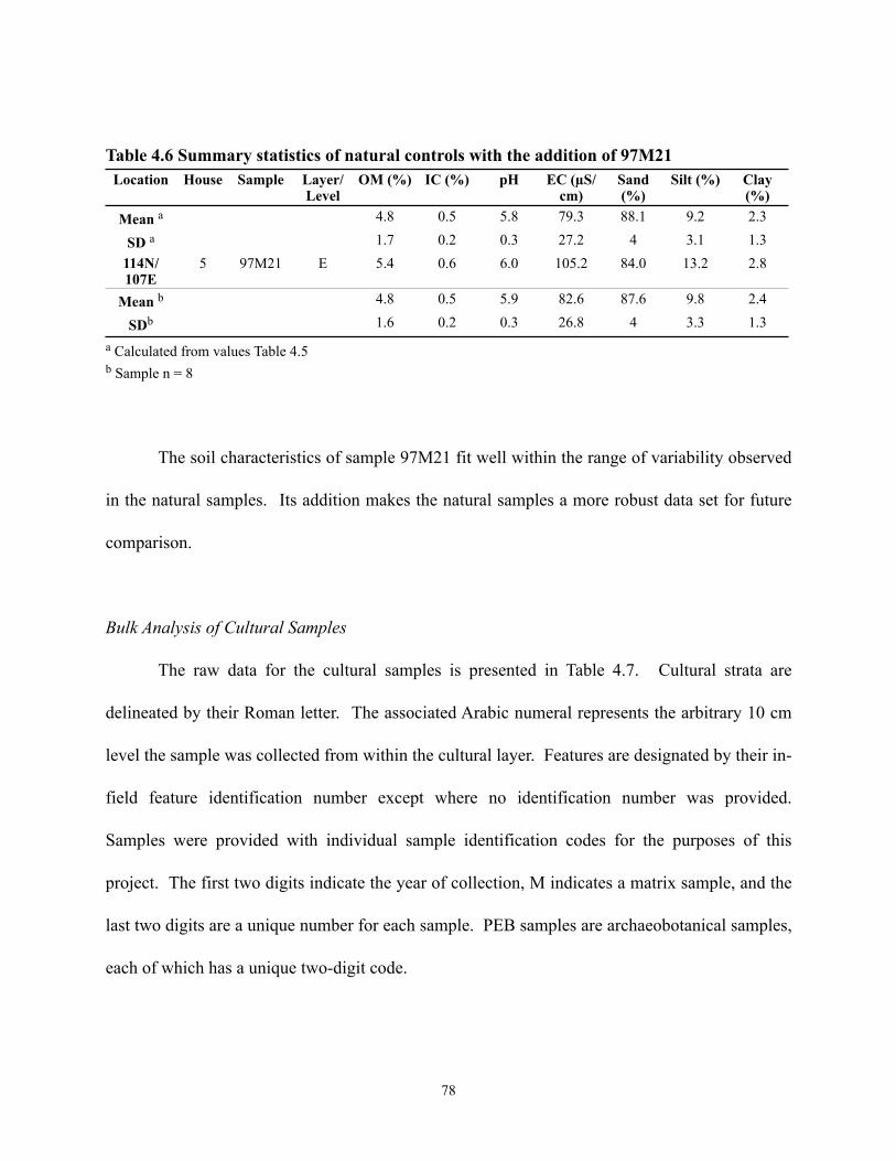
Table 4.6 Summary statistics of natural controls with the addition of 97M21Location House Sample Layer/

LevelOM (%) IC (%) pH EC (µS/

cm)Sand (%)

Silt (%) Clay (%)

Mean a 4.8 0.5 5.8 79.3 88.1 9.2 2.3

SD a 1.7 0.2 0.3 27.2 4 3.1 1.3114N/107E

5 97M21 E 5.4 0.6 6.0 105.2 84.0 13.2 2.8

Mean b 4.8 0.5 5.9 82.6 87.6 9.8 2.4

SDb 1.6 0.2 0.3 26.8 4 3.3 1.3a Calculated from values Table 4.5b Sample n = 8

The soil characteristics of sample 97M21 fit well within the range of variability observed

in the natural samples. Its addition makes the natural samples a more robust data set for future

comparison.

Bulk Analysis of Cultural Samples

The raw data for the cultural samples is presented in Table 4.7. Cultural strata are

delineated by their Roman letter. The associated Arabic numeral represents the arbitrary 10 cm

level the sample was collected from within the cultural layer. Features are designated by their in-

field feature identification number except where no identification number was provided.

Samples were provided with individual sample identification codes for the purposes of this

project. The first two digits indicate the year of collection, M indicates a matrix sample, and the

last two digits are a unique number for each sample. PEB samples are archaeobotanical samples,

each of which has a unique two-digit code.

78

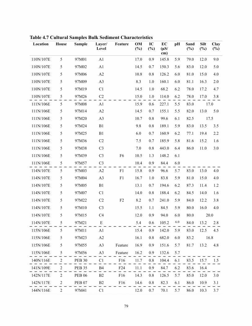
Table 4.7 Cultural Samples Bulk Sediment CharacteristicsLocation House Sample Layer/

LevelFeature OM

(%)IC

(%)EC (µS/cm)

pH Sand (%)

Silt (%)

Clay (%)

110N/107E

110N/107E

110N/107E

110N/107E

110N/107E

110N/107E

111N/106E

111N/106E

111N/106E

111N/106E

111N/106E

111N/106E

111N/106E

111N/106E

111N/106E

114N/107E

114N/107E

114N/107E

114N/107E

114N/107E

114N/107E

114N/107E

114N/107E

115N/106E

115N/106E

115N/106E

115N/106E

140N/116E

141N/109E

142N/117E

142N/117E

144N/116E

5 97M01 A1 17.0 0.9 145.8 5.9 79.0 12.0 9.0

5 97M02 A1 14.5 0.7 150.3 5.6 83.0 12.0 5.0

5 97M06 A2 10.8 0.8 126.2 6.0 81.0 15.0 4.0

5 97M09 A3 8.3 1.0 160.1 6.0 81.1 16.3 2.0

5 97M19 C1 14.5 1.0 68.2 6.2 78.0 17.2 4.7

5 97M26 C2 15.0 1.0 114.0 6.2 78.0 17.0 3.8

5 97M08 A1 15.9 0.6 227.1 5.5 83.0 17.0

5 97M14 A2 14.5 0.7 155.1 5.5 82.0 13.0 5.0

5 97M20 A3 10.7 0.8 99.6 6.1 82.5 17.5

5 97M24 B1 9.8 0.8 189.1 5.9 83.0 13.5 3.5

5 97M25 B1 6.0 0.7 160.9 6.2 77.1 19.4 2.2

5 97M36 C2 7.5 0.7 185.9 5.8 81.6 15.2 1.6

5 97M38 C3 7.0 0.8 443.0 6.4 86.0 11.0 3.0

5 97M39 C3 F6 10.5 1.3 148.2 6.1

5 97M57 C3 10.4 0.9 84.4 6.0

5 97M03 A2 F1 15.8 0.9 96.6 5.7 83.0 13.0 4.0

5 97M04 A3 F1 16.7 1.0 83.8 5.9 81.0 15.0 4.0

5 97M05 B1 13.1 0.7 194.6 6.2 87.3 11.4 1.2

5 97M07 C1 14.0 0.8 188.4 6.2 84.5 14.0 1.6

5 97M22 C2 F2 8.2 0.7 241.0 5.9 84.0 12.2 3.8

5 97M10 C3 15.5 1.1 84.5 5.9 80.0 16.0 4.0

5 97M15 C4 12.0 0.9 94.0 6.0 80.0 20.0

5 97M21 E 5.4 0.6 105.2 6.0 84.0 13.2 2.8

5 97M11 A1 15.4 0.9 142.0 5.9 83.0 12.5 4.5

5 97M23 A2 16.1 0.8 682.0 6.0 83.2 16.8

5 97M55 A3 Feature 16.9 0.9 151.6 5.7 81.7 13.2 4.8

5 97M56 A3 Feature 16.2 0.9 132.6 5.7

2 PEB 30 C1 F16 11.7 0.8 104.4 6.1 83.5 15.7 1.5

2 PEB 35 B4 F24 11.1 0.9 84.7 6.2 83.6 16.4

2 PEB 06 B2 F16 14.3 0.8 126.5 5.7 85.0 12.0 3.0

2 PEB 07 B2 F16 14.6 0.8 82.3 6.1 86.0 10.9 3.1

2 97M41 C1 12.0 0.7 70.1 5.7 86.0 10.3 3.7

79

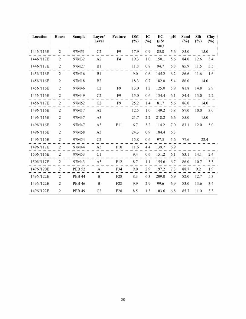
Location House Sample Layer/Level

Feature OM (%)

IC (%)

EC (µS/cm)

pH Sand (%)

Silt (%)

Clay (%)

144N/116E

144N/117E

144N/117E

145N/116E

145N/116E

145N/116E

145N/116E

145N/117E

149N/116E

149N/116E

149N/116E

149N/116E

149N/116E

149N/117E

150N/116E

150N/117E

149N/120E

149N/122E

149N/122E

149N/122E

2 97M51 C2 F9 17.9 0.9 85.8 5.6 85.0 15.0

2 97M32 A2 F4 19.3 1.0 150.1 5.6 84.0 12.6 3.4

2 97M27 B1 11.8 0.8 94.7 5.8 85.9 11.5 3.5

2 97M16 B1 9.0 0.6 145.2 6.2 86.6 11.6 1.6

2 97M18 B2 18.3 0.7 182.0 5.4 86.0 14.0

2 97M46 C2 F9 13.0 1.2 125.0 5.9 81.8 14.8 2.9

2 97M49 C2 F9 15.0 0.6 134.4 6.1 84.4 13.0 2.2

2 97M52 C2 F9 25.2 1.4 81.7 5.6 86.0 14.0

2 97M17 A2 12.5 1.0 149.2 5.8 87.0 10.0 3.0

2 97M37 A3 21.7 2.2 218.2 6.6 85.0 15.0

2 97M47 A3 F11 6.7 3.2 114.2 7.0 83.1 12.0 5.0

2 97M58 A3 24.3 0.9 184.4 6.3

2 97M54 C2 15.8 0.6 97.3 5.6 77.6 22.4

2 97M44 A3 F10 11.6 4.4 139.7 6.9

2 97M53 C1 9.4 0.6 151.2 6.1 83.1 14.1 2.4

2 97M43 A3 F12 8.7 1.1 155.6 6.7 86.0 10.7 3.3

2 PEB 52 A F34 9.0 2.9 197.2 7.3 88.7 9.2 1.9

2 PEB 44 B F28 8.3 6.3 209.0 6.9 82.0 12.7 5.3

2 PEB 46 B F28 9.9 2.9 99.6 6.9 83.0 13.6 3.4

2 PEB 49 C2 F28 8.5 1.3 103.6 6.8 85.7 11.0 3.3

80

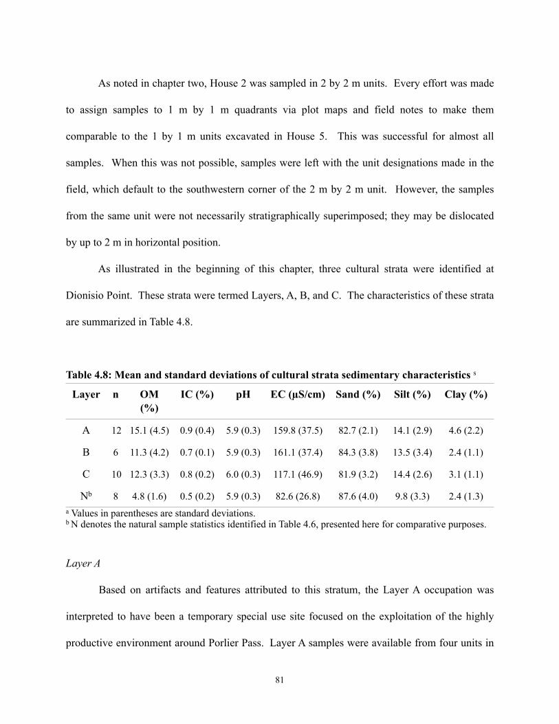
As noted in chapter two, House 2 was sampled in 2 by 2 m units. Every effort was made

to assign samples to 1 m by 1 m quadrants via plot maps and field notes to make them

comparable to the 1 by 1 m units excavated in House 5. This was successful for almost all

samples. When this was not possible, samples were left with the unit designations made in the

field, which default to the southwestern corner of the 2 m by 2 m unit. However, the samples

from the same unit were not necessarily stratigraphically superimposed; they may be dislocated

by up to 2 m in horizontal position.

As illustrated in the beginning of this chapter, three cultural strata were identified at

Dionisio Point. These strata were termed Layers, A, B, and C. The characteristics of these strata

are summarized in Table 4.8.

Table 4.8: Mean and standard deviations of cultural strata sedimentary characteristics s

Layer n OM (%)

IC (%) pH EC (µS/cm) Sand (%) Silt (%) Clay (%)

A 12 15.1 (4.5) 0.9 (0.4) 5.9 (0.3) 159.8 (37.5) 82.7 (2.1) 14.1 (2.9) 4.6 (2.2)

B 6 11.3 (4.2) 0.7 (0.1) 5.9 (0.3) 161.1 (37.4) 84.3 (3.8) 13.5 (3.4) 2.4 (1.1)

C 10 12.3 (3.3) 0.8 (0.2) 6.0 (0.3) 117.1 (46.9) 81.9 (3.2) 14.4 (2.6) 3.1 (1.1)

Nb 8 4.8 (1.6) 0.5 (0.2) 5.9 (0.3) 82.6 (26.8) 87.6 (4.0) 9.8 (3.3) 2.4 (1.3)a Values in parentheses are standard deviations.b N denotes the natural sample statistics identified in Table 4.6, presented here for comparative purposes.

Layer A

Based on artifacts and features attributed to this stratum, the Layer A occupation was

interpreted to have been a temporary special use site focused on the exploitation of the highly

productive environment around Porlier Pass. Layer A samples were available from four units in

81

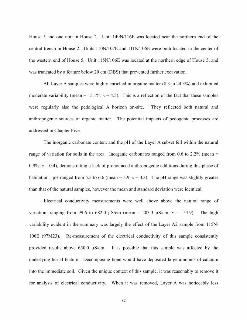
House 5 and one unit in House 2. Unit 149N/116E was located near the northern end of the

central trench in House 2. Units 110N/107E and 111N/106E were both located in the center of

the western end of House 5. Unit 115N/106E was located at the northern edge of House 5, and

was truncated by a feature below 20 cm (DBS) that prevented further excavation.

All Layer A samples were highly enriched in organic matter (8.3 to 24.3%) and exhibited

moderate variability (mean = 15.1%; s = 4.5). This is a reflection of the fact that these samples

were regularly also the pedological A horizon on-site. They reflected both natural and

anthropogenic sources of organic matter. The potential impacts of pedogenic processes are

addressed in Chapter Five.

The inorganic carbonate content and the pH of the Layer A subset fell within the natural

range of variation for soils in the area. Inorganic carbonates ranged from 0.6 to 2.2% (mean =

0.9%; s = 0.4), demonstrating a lack of pronounced anthropogenic additions during this phase of

habitation. pH ranged from 5.5 to 6.6 (mean = 5.9; s = 0.3). The pH range was slightly greater

than that of the natural samples, however the mean and standard deviation were identical.

Electrical conductivity measurements were well above above the natural range of

variation, ranging from 99.6 to 682.0 µS/cm (mean = 203.3 µS/cm; s = 154.9). The high

variability evident in the summary was largely the effect of the Layer A2 sample from 115N/

106E (97M23). Re-measurement of the electrical conductivity of this sample consistently

provided results above 650.0 µS/cm. It is possible that this sample was affected by the

underlying burial feature. Decomposing bone would have deposited large amounts of calcium

into the immediate soil. Given the unique context of this sample, it was reasonably to remove it

for analysis of electrical conductivity. When it was removed, Layer A was noticeably less

82

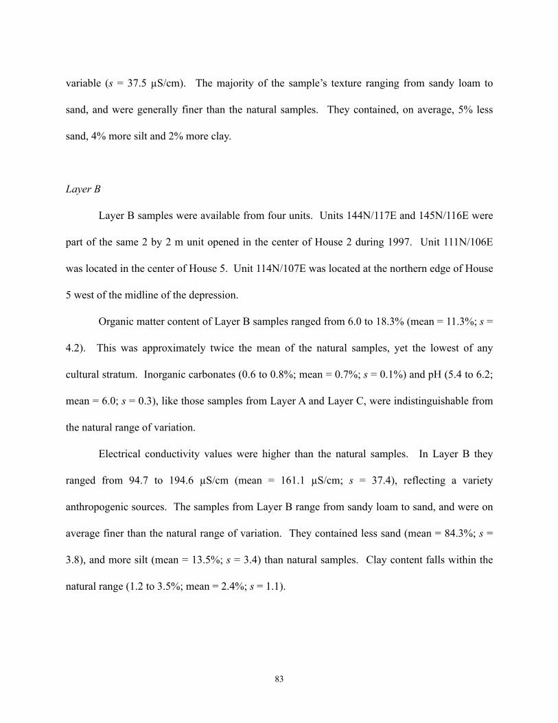
variable (s = 37.5 µS/cm). The majority of the sample’s texture ranging from sandy loam to

sand, and were generally finer than the natural samples. They contained, on average, 5% less

sand, 4% more silt and 2% more clay.

Layer B

Layer B samples were available from four units. Units 144N/117E and 145N/116E were

part of the same 2 by 2 m unit opened in the center of House 2 during 1997. Unit 111N/106E

was located in the center of House 5. Unit 114N/107E was located at the northern edge of House

5 west of the midline of the depression.

Organic matter content of Layer B samples ranged from 6.0 to 18.3% (mean = 11.3%; s =

4.2). This was approximately twice the mean of the natural samples, yet the lowest of any

cultural stratum. Inorganic carbonates (0.6 to 0.8%; mean = 0.7%; s = 0.1%) and pH (5.4 to 6.2;

mean = 6.0; s = 0.3), like those samples from Layer A and Layer C, were indistinguishable from

the natural range of variation.

Electrical conductivity values were higher than the natural samples. In Layer B they

ranged from 94.7 to 194.6 µS/cm (mean = 161.1 µS/cm; s = 37.4), reflecting a variety

anthropogenic sources. The samples from Layer B range from sandy loam to sand, and were on

average finer than the natural range of variation. They contained less sand (mean = 84.3%; s =

3.8), and more silt (mean = 13.5%; s = 3.4) than natural samples. Clay content falls within the

natural range (1.2 to 3.5%; mean = 2.4%; s = 1.1).

83

Layer C

Layer C samples were available from six units. Unit 144N/116E was located in the

center of House 2. Units 149N/116E and 140N/116E were located at opposite ends of the central

trench in House 2. The former was at the northern and the latter at the southern end. Unit 110N/

107E and 111N/106E were located in the center of House 5. Unit 114N/116E was located at the

northern edge of House 2, west of the midline of the structure.

The organic matter content of these samples ranged from 7.0 to 15.8% (mean = 12.2%; s

= 3.3), nearly three times that of the natural samples. Variation between Layer C and Layer B

was less than the error introduced by the laboratory methods. Inorganic carbonates ranged from

0.6 to 1.1% (mean = 0.8%; s = 0.2). This range and tendency and that of pH measurements (5.6

to 6.4, mean = 6.0; s = 0.3) were well within the natural range of variation. Electrical

conductivity was enriched compared to the natural samples, ranging from 68.2 to 443.0 µS/cm

(mean = 149.7 µS/cm; s = 112.1). Layer C samples ranged from sandy loam to sand in texture.

They were finer than the natural samples, containing less sand (mean = 81.5%; s = 3.3), more silt

(mean = 14.3%; s = 2.6) and comparable amounts of clay.

Features

Feature analysis is taken up separately in this chapter because of the dramatic variability

that is evident in the results presented in Table 4.7. The variables that are important to feature

analysis are not the same as those important to the analysis of non-feature cultural samples.

Specifically inorganic carbonates play a larger role in the discussion of features than they do

above.

84

Two groups of features were analyzed in this study, one from Layer A and and another

from Layer B/C. They are taken up separately below. No attempt was made to statistically

average the feature characteristics from either the entire class of data or from any one feature.

Samples are too small from any one feature, and combining features conflates evidence of

between feature variability that is important for further analysis.

Layer A

The features attributed to the post-Marpole occupation of the site were quite diverse in

form and function. Several appeared to be hearths. Features 1 and 4 were in situ hearth features

with fire-altered rock arrangements, ash and carbonized sediment. Three samples were available

from these two features, which share consistent characteristics. All three were enriched in

organic matter relative to the natural background. Organic matter content ranged from 15.8 to

19.3%, more than three times the natural average. Inorganic carbonate content was similar to the

natural samples (0.9%), as was the pH (5.7 to 5.9). Electrical conductivity was the most

variable, exceeding the natural range (83.8 to 150.1 µS/cm). The texture of the samples was

sandy loam to loamy sand, indicating less sand and more silt (12.6 to 15%) than natural samples.

Features 10, 11 and 12 formed a complex of oxidized sandstone/shell features in unit

149N/116E. The range of organic matter enrichment (6.7 to 11.6%) partially exceeded the

natural range. The inorganic carbonate content was unusual in that was significantly higher than

the natural range (1.1 to 4.4%) as was pH (6.7 to 7.0). Electrical conductivity partially

overlapped with the range of the natural samples (114.2 to 155.6 µS/cm). Texture was available

85

for only two of the samples, both of which were loamy sands, quite similar to the natural samples

apart from their higher clay content (3.3 to 5.0%).

Feature 34 was located across two units, 149N/120E and 140N/122E. It may have been

an intrusive roasting or rock heating feature associated with the post-Marpole village occupation.

One sample was available from this feature. Organic matter (8.9%) was twice that of the natural

samples. Inorganic carbonate content was significantly higher (2.9%) than the natural samples as

was electrical conductivity values (197.2 µS/cm). This feature had the highest pH determination

of any sample in the cultural data set (7.3). The texture was loamy sand and fell well within the

range of natural variation.

Layers B and C

The second group of feature samples were all attributed to the Marpole village

component of the site. They were hearths or hearth-like features. In spite of their formal

similarity, there was a wide range of variation between them. Features 9, 24, and 28 were

interpreted as domestic hearths. Feature 9 was the central hearth in House 2, Feature 24 was the

domestic hearth in the southwestern domestic area of the same structure, and Feature 28 the

domestic hearth in the northeastern domestic area. The sedimentary characteristics of these three

features were quite heterogeneous.

Feature 9 (Figure 4.4) was highly enriched in organic matter (12.9 to 25.2%). Inorganic

carbonates fell within the natural variation (0.6 to 1.4%), as did pH (5.6 to 6.1). Electrical

conductivity partially exceeded the natural range of variation (85.8 to 134.4 µS/cm). Full

textural analyses were available for two of the samples, one of which was a sandy loam and the

86

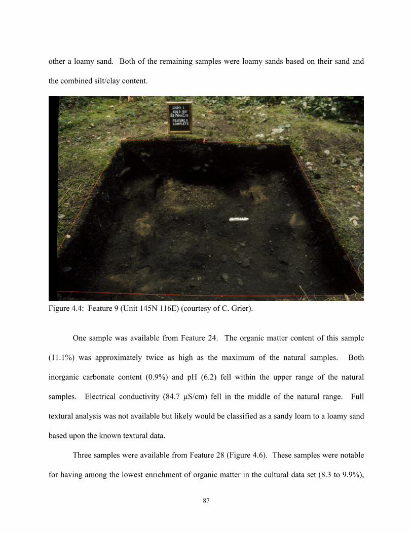
other a loamy sand. Both of the remaining samples were loamy sands based on their sand and

the combined silt/clay content.

Figure 4.4: Feature 9 (Unit 145N 116E) (courtesy of C. Grier).

One sample was available from Feature 24. The organic matter content of this sample

(11.1%) was approximately twice as high as the maximum of the natural samples. Both

inorganic carbonate content (0.9%) and pH (6.2) fell within the upper range of the natural

samples. Electrical conductivity (84.7 µS/cm) fell in the middle of the natural range. Full

textural analysis was not available but likely would be classified as a sandy loam to a loamy sand

based upon the known textural data.

Three samples were available from Feature 28 (Figure 4.6). These samples were notable

for having among the lowest enrichment of organic matter in the cultural data set (8.3 to 9.9%),

87

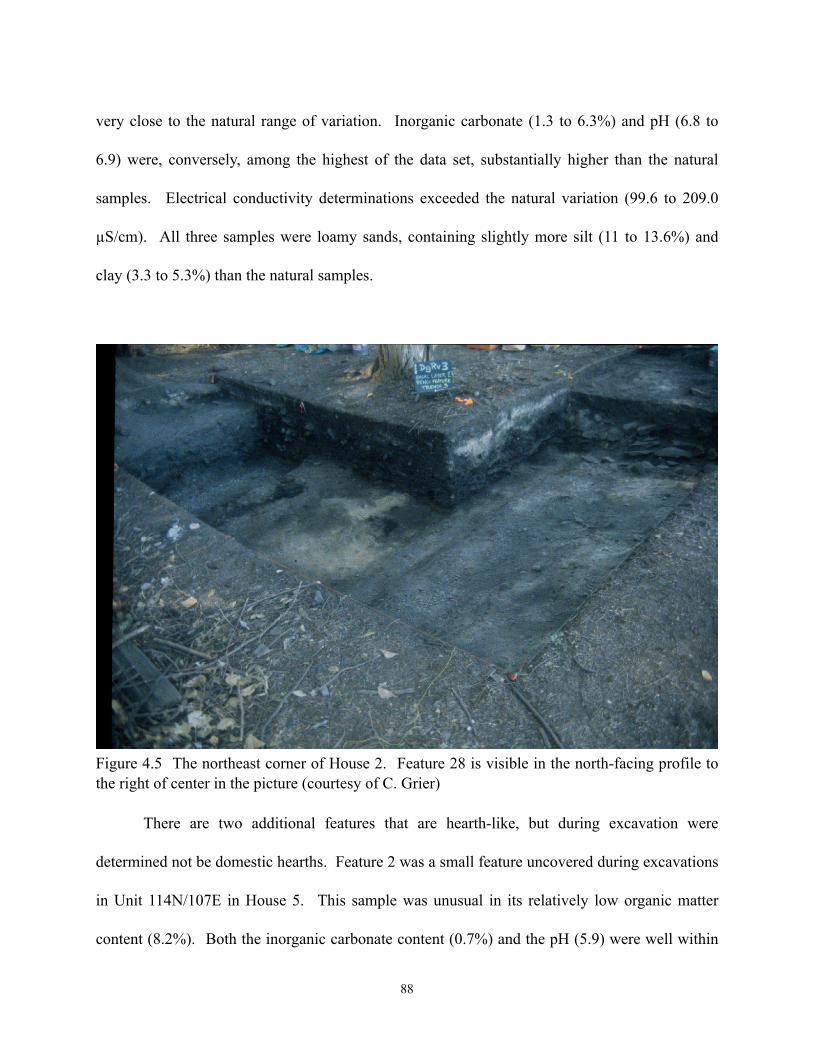
very close to the natural range of variation. Inorganic carbonate (1.3 to 6.3%) and pH (6.8 to

6.9) were, conversely, among the highest of the data set, substantially higher than the natural

samples. Electrical conductivity determinations exceeded the natural variation (99.6 to 209.0

µS/cm). All three samples were loamy sands, containing slightly more silt (11 to 13.6%) and

clay (3.3 to 5.3%) than the natural samples.

Figure 4.5 The northeast corner of House 2. Feature 28 is visible in the north-facing profile to the right of center in the picture (courtesy of C. Grier)

There are two additional features that are hearth-like, but during excavation were

determined not be domestic hearths. Feature 2 was a small feature uncovered during excavations

in Unit 114N/107E in House 5. This sample was unusual in its relatively low organic matter

content (8.2%). Both the inorganic carbonate content (0.7%) and the pH (5.9) were well within

88

the natural range. The electrical conductivity determination was among the highest in the

cultural data set (241.0 µS/cm), well outside the upper limit of the natural range. The texture of

the sample was loamy sand, containing more silt (12.2%) and slightly more clay (3.8%) than the

natural range.

Feature 16 was unusual in that it was the sole large hearth-like feature that first appeared

in Layer B, rather than C. It was located in Unit 142N/116E at the rear of House 2. Organic

matter content was enriched relative to the natural samples (11.7 to 14.6%). Inorganic

carbonates (0.7 to 0.8%), pH (5.7 to 6.1) and electrical conductivity (82.3 to 126.5 µS/cm) on the

other hand either fell entirely within or only slightly exceeded the natural range of variation.

Sample texture ranged from sandy loam to loamy sand, containing more silt (10.9 to 15.7%) than

natural samples.

Summary

The differences between the natural and cultural samples demonstrates that an anthropogenic

signal has been preserved in the Dionisio Point sedimentary record in organic matter content,

electrical conductivity and particle-size, particularly in the Layer B/C Marpole village

component. Some of the values generated by these analyses suggest further that the processes

that have created and affected the two cultural components of the site might be different,

especially in terms of the affects of modern-day natural inputs and pedogenic processes as

discussed below. The broader trends in these patterns are explored in the following chapter.

89

Chapter Five: Discussion

The previous chapter presented the results of the analyses of this study. Several

interesting patterns were suggested by these data. Among these was the strong evidence that an

anthropogenic pattern has been preserved in the sediments in Houses 2 and 5 at Dionisio Point.

Variability in this pattern further suggested that the various architectural contexts of shed-roof

houses, identified in Chapter 3, have discrete formation processes. The goal of this chapter is to

discuss these patterns, their implications for assessing natural formation processes at Dionsio

Point, and most importantly the evidence they provide that specific cultural formation process

have been preserved in these deposits.

This chapter is divided into five sections. The first summarizes the results presented in

the previous chapter. It assesses the utility of the methods that were used for distinguishing the

archaeological samples from the natural samples. The second describes the evidence that

supports the interpretation of geoarchaeological patterning at Dionisio Point as anthropogenic

rather than pedogenic. The third presents an evaluation of the cultural models presented in

Chapter Three through the lens of the geoarchaeological record. The fourth is a discussion of

how these models can help us understand the plank house socio-economy, using Dionisio Point

as an example. The final section evaluates the potential utility of these methods for plank house

feature prospection in the archaeological record of the Strait Of Georgia region. These five

sections follow the three research themes that were identified in the introduction to this study.

90

Research Themes:

1. Assessment of current models of cultural formation processes in prehistoric plank

houses. How well does the observed geoarchaeological data from Dionisio Point match

the expectations generated by an ethnographic model? What are the discrepancies and

why might they exist? What does this suggest about the applicability of current models

of cultural formation processes in prehistoric shed-roof houses?

2. Utility of feature analysis for interpreting the socio-economic organization of pre-

Contact households. Do features provide data not available from artifact data sets? If

they do, what do these tell us about the inhabitants of these dwellings?

3. Implications for prospection methods on the Coast. Does the analysis suggest that

there is a possibility of identifying some or all of the architectural contexts defined in

Chapter Three? Which are most easily discriminated and which are the most difficult to

define? What are the implications of these results for further excavations at Dionisio

Point and for sites elsewhere?

Evaluating Results – Utility of the Methods

The results presented in the previous chapter suggested that the methods used in this

analysis effectively identified differences between the cultural and natural sample data sets.

Tables 5.1, 5.2, and 5.3 present the results of statistical analyses of the differences between

natural samples and each of the cultural strata identified at the site. Only non-feature samples

were used in this analysis. Feature samples would in all cases likely accentuate any differences,

but would at the same time be more difficult to normalize and thus would require the use of less

robust tests of significance. Two-group difference of means tests were used in all cases where

91

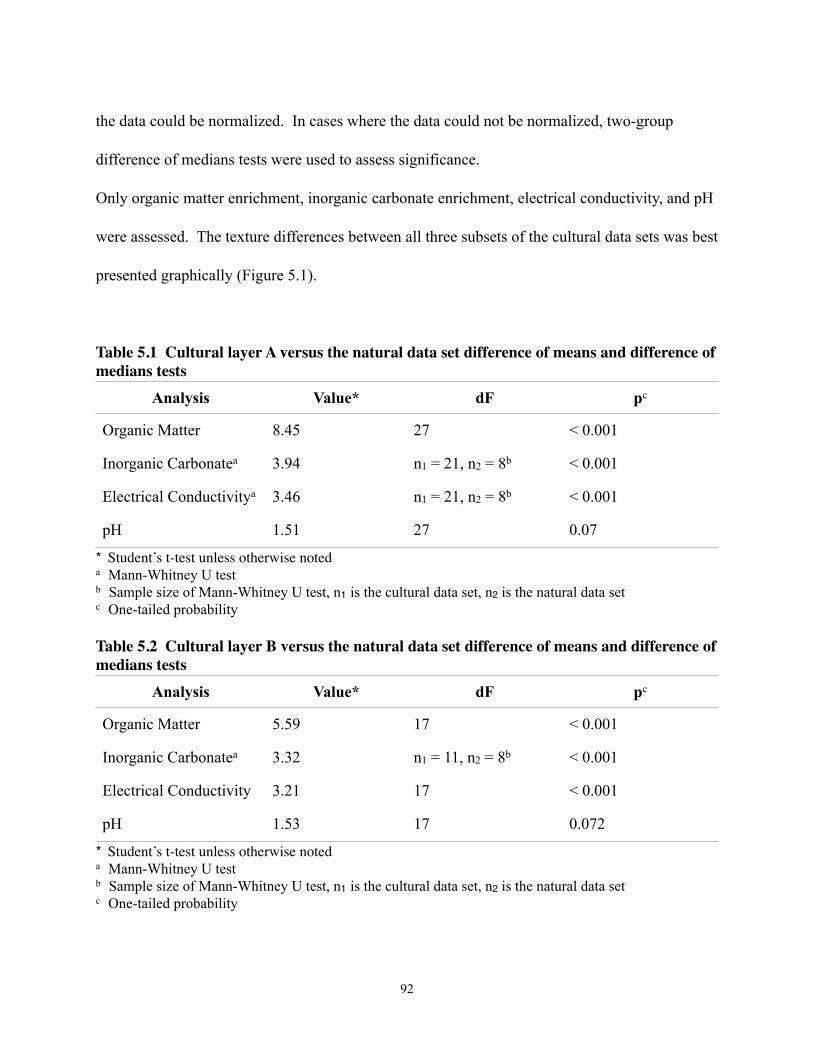
the data could be normalized. In cases where the data could not be normalized, two-group

difference of medians tests were used to assess significance.

Only organic matter enrichment, inorganic carbonate enrichment, electrical conductivity, and pH

were assessed. The texture differences between all three subsets of the cultural data sets was best

presented graphically (Figure 5.1).

Table 5.1 Cultural layer A versus the natural data set difference of means and difference of medians tests

Analysis Value* dF pc

Organic Matter 8.45 27 < 0.001

Inorganic Carbonatea 3.94 n1 = 21, n2 = 8b < 0.001

Electrical Conductivitya 3.46 n1 = 21, n2 = 8b < 0.001

pH 1.51 27 0.07

* Student’s t-test unless otherwise noteda Mann-Whitney U testb Sample size of Mann-Whitney U test, n1 is the cultural data set, n2 is the natural data setc One-tailed probability

Table 5.2 Cultural layer B versus the natural data set difference of means and difference of medians tests

Analysis Value* dF pc

Organic Matter 5.59 17 < 0.001

Inorganic Carbonatea 3.32 n1 = 11, n2 = 8b < 0.001

Electrical Conductivity 3.21 17 < 0.001

pH 1.53 17 0.072

* Student’s t-test unless otherwise noteda Mann-Whitney U testb Sample size of Mann-Whitney U test, n1 is the cultural data set, n2 is the natural data setc One-tailed probability

92

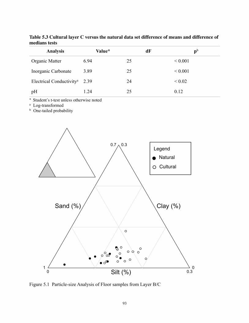
Table 5.3 Cultural layer C versus the natural data set difference of means and difference of medians tests

Analysis Value* dF pb

Organic Matter 6.94 25 < 0.001

Inorganic Carbonate 3.89 25 < 0.001

Electrical Conductivitya 2.39 24 < 0.02

pH 1.24 25 0.12

* Student’s t-test unless otherwise noteda Log-transformedb One-tailed probability

93

0.7 0.3

Sand (%)

10 Silt (%) 0.3

0

Clay (%)

Legend

NaturalCultural

Figure 5.1 Particle-size Analysis of Floor samples from Layer B/C

Legend

Cultural

Natural

The pattern presented in all three subsets of the cultural data set is clear. Several analyses

discriminated well between the natural and cultural data sets. Organic matter enrichment and

electrical conductivity were significantly higher in the cultural data set than the natural data set.

In no subset was pH significantly different between from the natural data set. Inorganic

carbonate enrichment in all three subsets was significantly higher in the cultural data than the

natural data. However, this difference never exceeded the error margin for the protocols used in

the analysis and, thus, these values cannot be considered to be archaeologically meaningful.

Differences in texture were not statistically verified, but suggest that the cultural samples trend

towards being finer than the natural samples. The difference in this case consists almost entirely

in trade-offs between the sand and silt content. Clay does not vary by more than 2%.

Returning to the models laid out in Chapter Three, these overall patterns were expected

from the kinds of activities that were discussed. It should be noted that these statistical patterns

only described trends in the overall data set. Therefore, neither inorganic carbonate content nor

pH were discounted from further study if the values for individual samples exceeded the error

margin and the natural range. This was the case for several feature samples, which would have

been swamped by the non-features samples in a statistical analysis. However, in spite of the fact

that these patterns match the expectations, it is possible that they are not anthropogenic. This is

discussed below.

Evaluating Results – Pedogenic versus Anthropogenic Processes

The previous section demonstrated that cultural samples were significantly different from

natural samples on a number of variables, specifically organic matter and electrical conductivity.

94

Texture variation, although not statistically tested, were consistently different between the two

data sets. However, it is not clear from the previous section whether or not the processes that

contributed to these patterns were natural or cultural. That is, are these patterns the result of

human activity during the occupation of the Dionisio Point site, or are they primarily the result of

natural, post-depositional processes?

Stein’s (1992c) discussion of anthropogenic versus pedogenic sources of organic matter

at archaeological sites is a useful heuristic for this discussion. She raised the issue of identifying

which of these two sources was dominant in the formation of organic matter in any given

archaeological deposit. She described three settings where, in a profile:

• Organic matter is entirely anthropogenic

• Organic matter is entirely pedogenic

• Pedogenic organic matter has formed in an anthropogenic matrix

Clearly, the danger that is faced is the interpretation as cultural, signatures that are natural

in origin. While she (Stein 1992c) directs her attention towards organic matter content, all of the

geoarchaeological signatures in this study could have been affected in the same manner.

The statistical analyses presented above demonstrate that the signatures are not the result

of the natural, pedogenic formation of any of the measured constituents, with the exception of

pH. The question that remains is whether or not the patterns were directly cultural or whether

they were only indirectly cultural. In the first case, interpretations can be made on the present

results. In the latter, the anthropogenic signatures are masked by natural signatures. If the

95

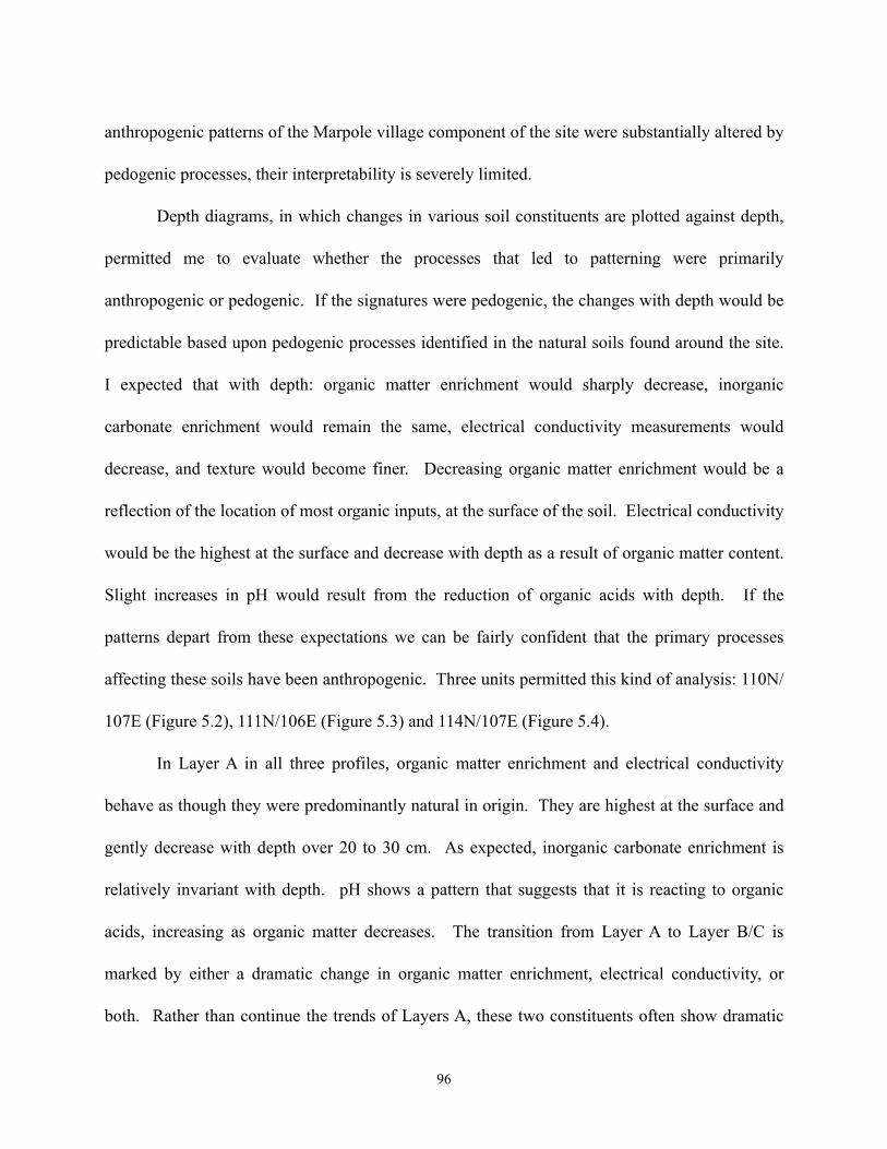
anthropogenic patterns of the Marpole village component of the site were substantially altered by

pedogenic processes, their interpretability is severely limited.

Depth diagrams, in which changes in various soil constituents are plotted against depth,

permitted me to evaluate whether the processes that led to patterning were primarily

anthropogenic or pedogenic. If the signatures were pedogenic, the changes with depth would be

predictable based upon pedogenic processes identified in the natural soils found around the site.

I expected that with depth: organic matter enrichment would sharply decrease, inorganic

carbonate enrichment would remain the same, electrical conductivity measurements would

decrease, and texture would become finer. Decreasing organic matter enrichment would be a

reflection of the location of most organic inputs, at the surface of the soil. Electrical conductivity

would be the highest at the surface and decrease with depth as a result of organic matter content.

Slight increases in pH would result from the reduction of organic acids with depth. If the

patterns depart from these expectations we can be fairly confident that the primary processes

affecting these soils have been anthropogenic. Three units permitted this kind of analysis: 110N/

107E (Figure 5.2), 111N/106E (Figure 5.3) and 114N/107E (Figure 5.4).

In Layer A in all three profiles, organic matter enrichment and electrical conductivity

behave as though they were predominantly natural in origin. They are highest at the surface and

gently decrease with depth over 20 to 30 cm. As expected, inorganic carbonate enrichment is

relatively invariant with depth. pH shows a pattern that suggests that it is reacting to organic

acids, increasing as organic matter decreases. The transition from Layer A to Layer B/C is

marked by either a dramatic change in organic matter enrichment, electrical conductivity, or

both. Rather than continue the trends of Layers A, these two constituents often show dramatic

96

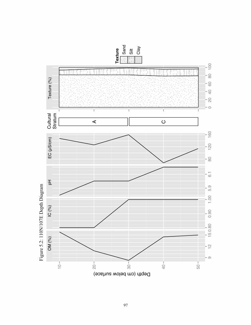
97

Depth (cm below surface)

50

40

30

20

10

91

21

50

.80

0.9

01

.00

5.9

6.1

80

12

01

60

OM

(%

)IC

(%

)p

HE

C (

µS

/cm

)

02

04

06

08

01

00

Texture

Sa

nd

Silt

Cla

y

T

extu

re (

%)

Cu

ltu

ral

Str

atu

m

A C

Figu

re 5

.2: 1

10N

/107

E D

epth

Dia

gram

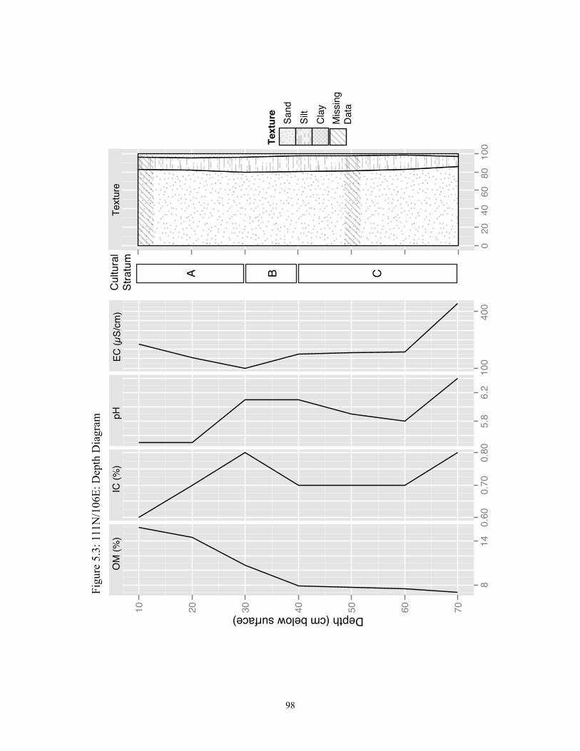
98

Depth (cm below surface) 70

60

50

40

30

20

10

814

0.6

00.7

00.8

05.8

6.2

100

400

OM

(%

)IC

(%

)pH

EC

(µ

S/c

m)

020

40

60

80

100

Texture

Sand

Silt

Cla

y

Textu

re

Mis

sin

g

Data

Cultura

l

Str

atu

m

A B C

Figu

re 5

.3: 1

11N

/106

E: D

epth

Dia

gram

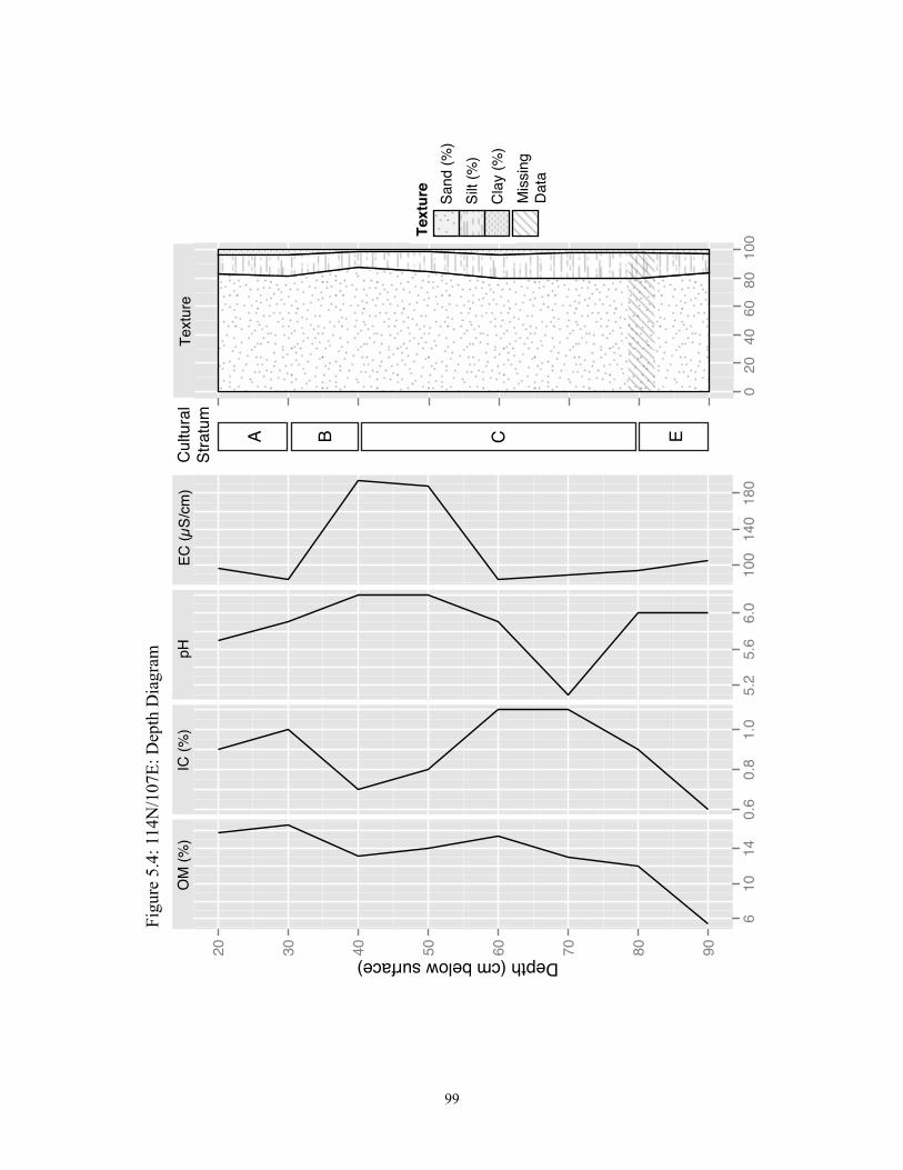
99

Depth (cm below surface) 90

80

70

60

50

40

30

20

61

01

40

.60

.81

.05

.25

.66

.01

00

14

01

80

OM

(%

)IC

(%

)p

HE

C (

µS

/cm

)

02

04

06

08

01

00

Texture

Sa

nd

(%

)

Silt

(%

)

Cla

y (

%)

Te

xtu

re

Mis

sin

g

Da

ta

Cultura

l

Str

atu

m

A B C E

Figu

re 5

.4: 1

14N

/107

E: D

epth

Dia

gram

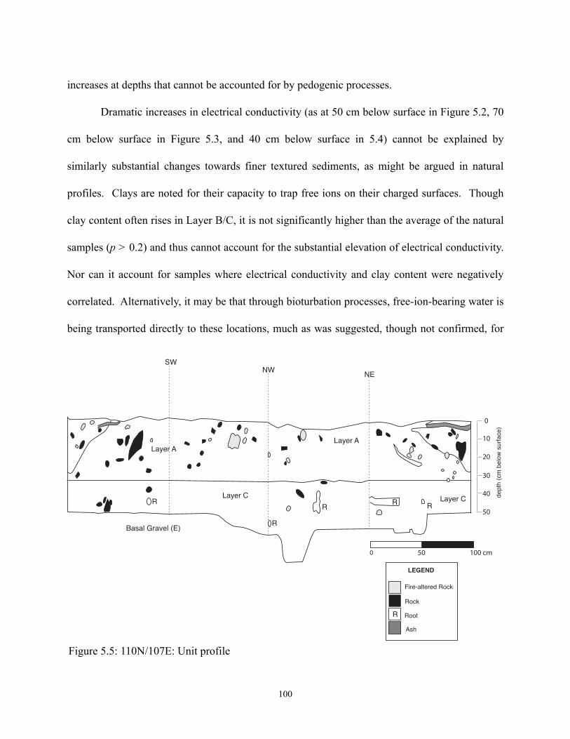
increases at depths that cannot be accounted for by pedogenic processes.

Dramatic increases in electrical conductivity (as at 50 cm below surface in Figure 5.2, 70

cm below surface in Figure 5.3, and 40 cm below surface in 5.4) cannot be explained by

similarly substantial changes towards finer textured sediments, as might be argued in natural

profiles. Clays are noted for their capacity to trap free ions on their charged surfaces. Though

clay content often rises in Layer B/C, it is not significantly higher than the average of the natural

samples (p > 0.2) and thus cannot account for the substantial elevation of electrical conductivity.

Nor can it account for samples where electrical conductivity and clay content were negatively

correlated. Alternatively, it may be that through bioturbation processes, free-ion-bearing water is

being transported directly to these locations, much as was suggested, though not confirmed, for

100

Layer A

Layer C

Layer A

Layer C

Basal Gravel (E)

R

R

RR

R

SWNW

NE

0

10

20

30

40

50

de

pth

(cm

be

low

su

rfa

ce

)

50 100 cm0

R

Fire-altered Rock

Rock

Root

Ash

LEGEND

Figure 5.5: 110N/107E: Unit profile

samples in the Natural Profile 3. These may be the result of root intrusion or faunalturbation.

However, as argued for organic matter deposition, below, it does not appear likely that site-wide

patterns of sediment characteristics can be attributed to either flora or fauna. The primary source

of free ions, measured by electrical conductivity, was likely not natural.

Dramatic increases in organic matter enrichment (as at 40 cm below surface in Figure 5.2

and 60 cm below surface in Figure 5.4) cannot be explained by pedogenic processes. Natural

sources of organic matter at depth are limited primarily to forms of bioturbation. At Dionisio

Point, the roots of coniferous forest species have been noted to follow the transition from Layer

C to the glacial tills, probably because nutrients are rapidly leached from sediments at greater

depths. Profile drawings record the presence of roots in Layers B and C (Figure 5.5). However,

roots at these depths were rare, small-diameter (less than 5 to 10 cm) lateral branching roots.

There are two reasons to doubt that roots are the cause of organic matter enrichment. First it is

unlikely that roots would result in systematic increase in organic matter enrichment across all

samples. Second, organic matter enrichment in the units described by Figures 5.2 and 5.4 begins

at least 10 cm above this transitional layer. Faunalturbation of surficial organic matter to great

deapths either by earthworms (e.g., Stein 1983), or by larger soil fauna is unlikely. Organic

matter processing is typically completed by fungal mats in moder soils (Green et al 199).

Natural samples showed no signs of faunal disturbance. Pedogenic or bioturbation processes

likely do not account for these rises in organic matter at depth in the lower cultural strata. The

principal source, therefore, is probably anthropogenic.

Changes in pH and inorganic carbonate content below Layer A (also the A horizon)

appear to be responses to more than simply pedogenic processes. In Figures 5.2 and 5.3, the

101

relationship between the two characteristics, as expected from a natural profile, is positive.

However, the changes in inorganic carbonate content in these levels are minor, as is suggested to

be the case for entire site by the statistical analyses in the previous section. In Figure 5.4, the

two vary inversely. This appears to be the result of anthropogenic alteration of the sediments.

The pH measurements below 30 cm below surface in the unit described in Figure 5.2 rise with

increasing organic matter enrichment. This is contrary to what would be expected from a natural

system, organic matter enrichment typically being positively associated with organic matter-

driven acidification. The positive relationship between these two variables in this unit suggests

that the organic matter at this depth is old, inert material rather than material transported down

from the surface. However, given the low absolute variation in either pH or inorganic carbonate

enrichment these patterns are suggestive rather than conclusive. It is not possible to use either

pH or inorganic carbonate enrichment independent of other variables, expect where they are

dramatically higher than the natural range of variation, to interpret cultural formation processes.

Taking into account the occupational history of the site and the expected correlations

between organic matter, electrical conductivity, and human activity, the gross trends seen in these

profiles are indicative of anthropogenic modification. The decrease in organic matter through

Layer A (0 to 30 cm below surface) may be an indication of pedogenic processes, yet the rise in

Layer B/C (> 30 cm below surface) is a reflection of high organic input during Marpole phase

occupation. Mirroring of the organic matter content by the electrical conductivity is expected

under conditions of organic-driven acidification.

102

Cultural Stratigraphy at Dionisio Point

Until this point the cultural stratigraphy at Dionisio Point has been treated as having three

distinct cultural layers overlying a culturally-sterile glacial till. However, Grier (2006a) has

interpreted cultural strata Layer B and Layer C as representing the deposition of a single

occupational phase of the Marpole phase village component of the site. This aggregation was

not challenged by Ewnous’ (2006) analysis of the faunal remains of the site; artifacts,

architecture, and faunal remains all suggest that these two layers represent a single phase of

occupation.

This occupation was probably punctuated by seasonal and perhaps longer periods of

abandonment. The stability of the material record through these two strata supports their

treatment as a single unit, both in terms of the artifact assemblage and complex of features,

which do not substantially change their spatial position during this period. This consistency in

spatial arrangement applies to the architectural layout of the house, in terms of hearth and post

features (Grier 2006a:105), as well as artifact distributions (Grier 2006a:111).

Based on the data presented above in Tables 5.2, 5.3, the depth diagrams, and the

descriptions of both Layers B and C, there is no geoarchaeological reason to dispute the

aggregation of these two cultural strata into a single unit suggested by the artifact analysis.

These strata have similar trends when compared to the natural range of variation. A possible

exception is the difference in electrical conductivity measurements. Layer C’s average electrical

conductivity was nearer the natural range than Layer B (though even then it is significantly

different [t = 1.8; df = 1,15; p < 0.05]).

103

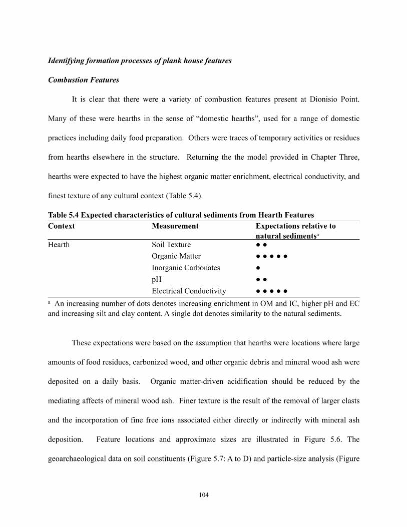
Identifying formation processes of plank house features

Combustion Features

It is clear that there were a variety of combustion features present at Dionisio Point.

Many of these were hearths in the sense of “domestic hearths”, used for a range of domestic

practices including daily food preparation. Others were traces of temporary activities or residues

from hearths elsewhere in the structure. Returning the the model provided in Chapter Three,

hearths were expected to have the highest organic matter enrichment, electrical conductivity, and

finest texture of any cultural context (Table 5.4).

Table 5.4 Expected characteristics of cultural sediments from Hearth FeaturesContext Measurement Expectations relative to

natural sedimentsa

Hearth Soil Texture ● ●Organic Matter ● ● ● ● ●Inorganic Carbonates ●pH ● ●Electrical Conductivity ● ● ● ● ●

a An increasing number of dots denotes increasing enrichment in OM and IC, higher pH and EC and increasing silt and clay content. A single dot denotes similarity to the natural sediments.

These expectations were based on the assumption that hearths were locations where large

amounts of food residues, carbonized wood, and other organic debris and mineral wood ash were

deposited on a daily basis. Organic matter-driven acidification should be reduced by the

mediating affects of mineral wood ash. Finer texture is the result of the removal of larger clasts

and the incorporation of fine free ions associated either directly or indirectly with mineral ash

deposition. Feature locations and approximate sizes are illustrated in Figure 5.6. The

geoarchaeological data on soil constituents (Figure 5.7: A to D) and particle-size analysis (Figure

104

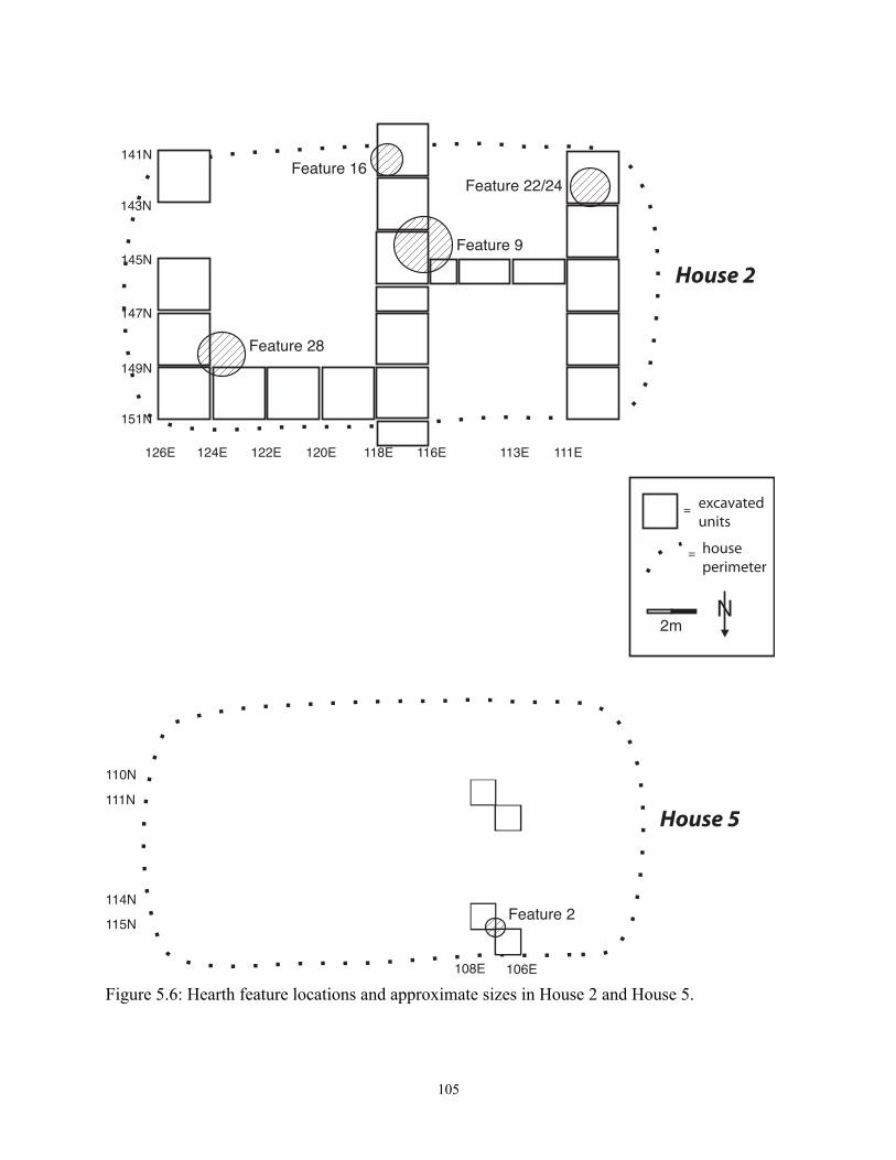
105

houseperimeter

excavatedunits

110N

111N

114N

115N

106E108E

House 5

Feature 2

141N

143N

145N

147N

149N

151N

126E 124E 122E 120E 118E 116E 113E 111E

House 2Feature 9

Feature 16

Feature 28

Feature 22/24

Figure 5.6: Hearth feature locations and approximate sizes in House 2 and House 5.

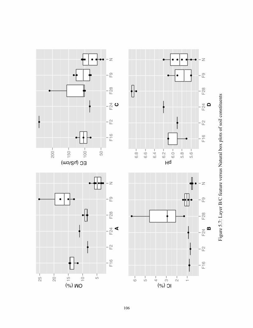
106

Feature

OM

●● ●

●

●

●● ●

●● ●●

●● ● ●● ●●●

510152025

F16

F2F24

F28

F9N

Feature

EC

● ●●

●

●

● ●●

● ●●●

● ●● ●●● ● ●50100

150

200

F16

F2F24

F28

F9N

Feature

IC

●

●●●●

●

● ● ●

●● ● ●● ●●●●● ●●

123456

F16

F2F24

F28

F9N

Feature

pH

●●●

●

●

●● ●

●●●●

● ●●● ● ● ●●

5.6

5.8

6.0

6.2

6.4

6.6

6.8

F16

F2F24

F28

F9N

A B

C D

OM (%) IC (%)

EC (µS/cm) pH

Figu

re 5

.7: L

ayer

B/C

feat

ure

vers

us N

atur

al b

ox p

lots

of s

oil c

onst

ituen

ts

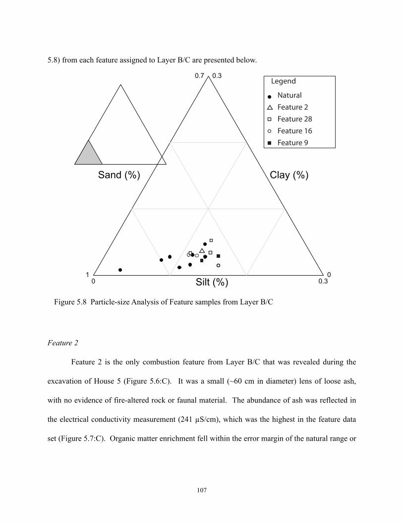
5.8) from each feature assigned to Layer B/C are presented below.

Feature 2

Feature 2 is the only combustion feature from Layer B/C that was revealed during the

excavation of House 5 (Figure 5.6:C). It was a small (~60 cm in diameter) lens of loose ash,

with no evidence of fire-altered rock or faunal material. The abundance of ash was reflected in

the electrical conductivity measurement (241 µS/cm), which was the highest in the feature data

set (Figure 5.7:C). Organic matter enrichment fell within the error margin of the natural range or

107

0.7 0.3

Sand (%)

10 Silt (%) 0.3

0

Clay (%)

Legend

NaturalFeature 2Feature 28Feature 16Feature 9

Figure 5.8 Particle-size Analysis of Feature samples from Layer B/C

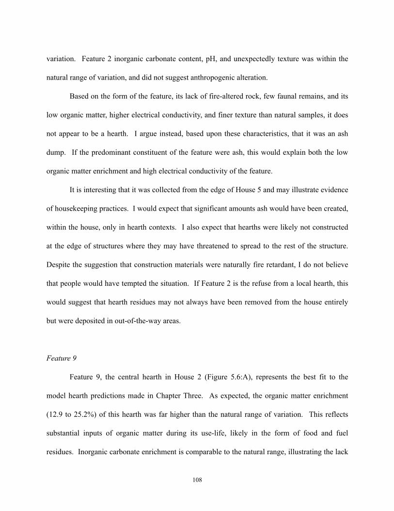
variation. Feature 2 inorganic carbonate content, pH, and unexpectedly texture was within the

natural range of variation, and did not suggest anthropogenic alteration.

Based on the form of the feature, its lack of fire-altered rock, few faunal remains, and its

low organic matter, higher electrical conductivity, and finer texture than natural samples, it does

not appear to be a hearth. I argue instead, based upon these characteristics, that it was an ash

dump. If the predominant constituent of the feature were ash, this would explain both the low

organic matter enrichment and high electrical conductivity of the feature.

It is interesting that it was collected from the edge of House 5 and may illustrate evidence

of housekeeping practices. I would expect that significant amounts ash would have been created,

within the house, only in hearth contexts. I also expect that hearths were likely not constructed

at the edge of structures where they may have threatened to spread to the rest of the structure.

Despite the suggestion that construction materials were naturally fire retardant, I do not believe

that people would have tempted the situation. If Feature 2 is the refuse from a local hearth, this

would suggest that hearth residues may not always have been removed from the house entirely

but were deposited in out-of-the-way areas.

Feature 9

Feature 9, the central hearth in House 2 (Figure 5.6:A), represents the best fit to the

model hearth predictions made in Chapter Three. As expected, the organic matter enrichment

(12.9 to 25.2%) of this hearth was far higher than the natural range of variation. This reflects

substantial inputs of organic matter during its use-life, likely in the form of food and fuel

residues. Inorganic carbonate enrichment is comparable to the natural range, illustrating the lack

108

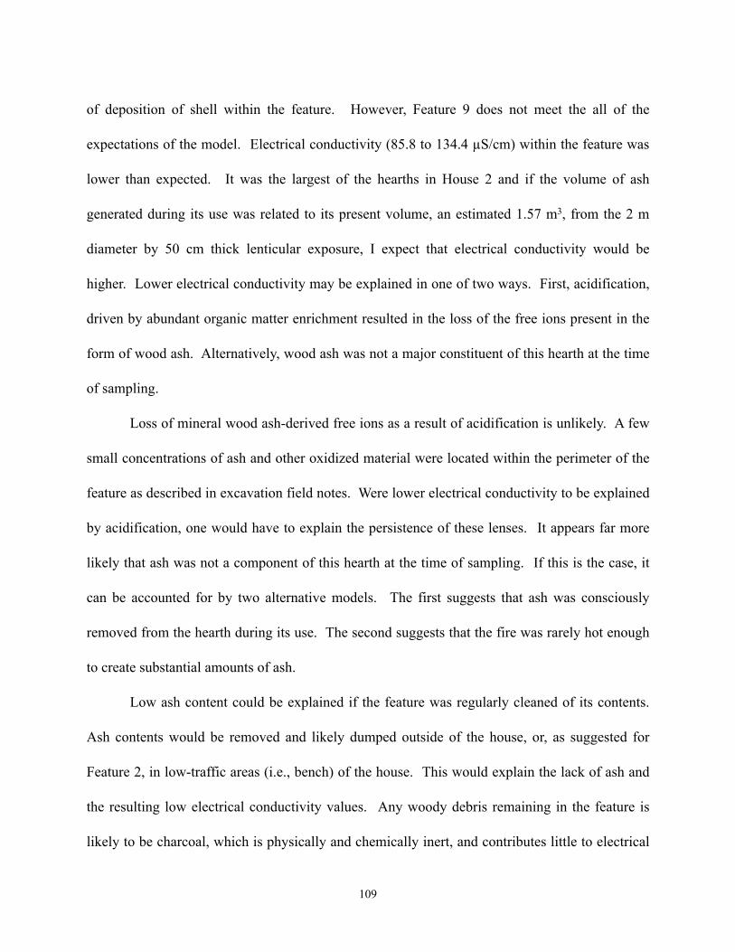
of deposition of shell within the feature. However, Feature 9 does not meet the all of the

expectations of the model. Electrical conductivity (85.8 to 134.4 µS/cm) within the feature was

lower than expected. It was the largest of the hearths in House 2 and if the volume of ash

generated during its use was related to its present volume, an estimated 1.57 m3, from the 2 m

diameter by 50 cm thick lenticular exposure, I expect that electrical conductivity would be

higher. Lower electrical conductivity may be explained in one of two ways. First, acidification,

driven by abundant organic matter enrichment resulted in the loss of the free ions present in the

form of wood ash. Alternatively, wood ash was not a major constituent of this hearth at the time

of sampling.

Loss of mineral wood ash-derived free ions as a result of acidification is unlikely. A few

small concentrations of ash and other oxidized material were located within the perimeter of the

feature as described in excavation field notes. Were lower electrical conductivity to be explained

by acidification, one would have to explain the persistence of these lenses. It appears far more

likely that ash was not a component of this hearth at the time of sampling. If this is the case, it

can be accounted for by two alternative models. The first suggests that ash was consciously

removed from the hearth during its use. The second suggests that the fire was rarely hot enough

to create substantial amounts of ash.

Low ash content could be explained if the feature was regularly cleaned of its contents.

Ash contents would be removed and likely dumped outside of the house, or, as suggested for

Feature 2, in low-traffic areas (i.e., bench) of the house. This would explain the lack of ash and

the resulting low electrical conductivity values. Any woody debris remaining in the feature is

likely to be charcoal, which is physically and chemically inert, and contributes little to electrical

109

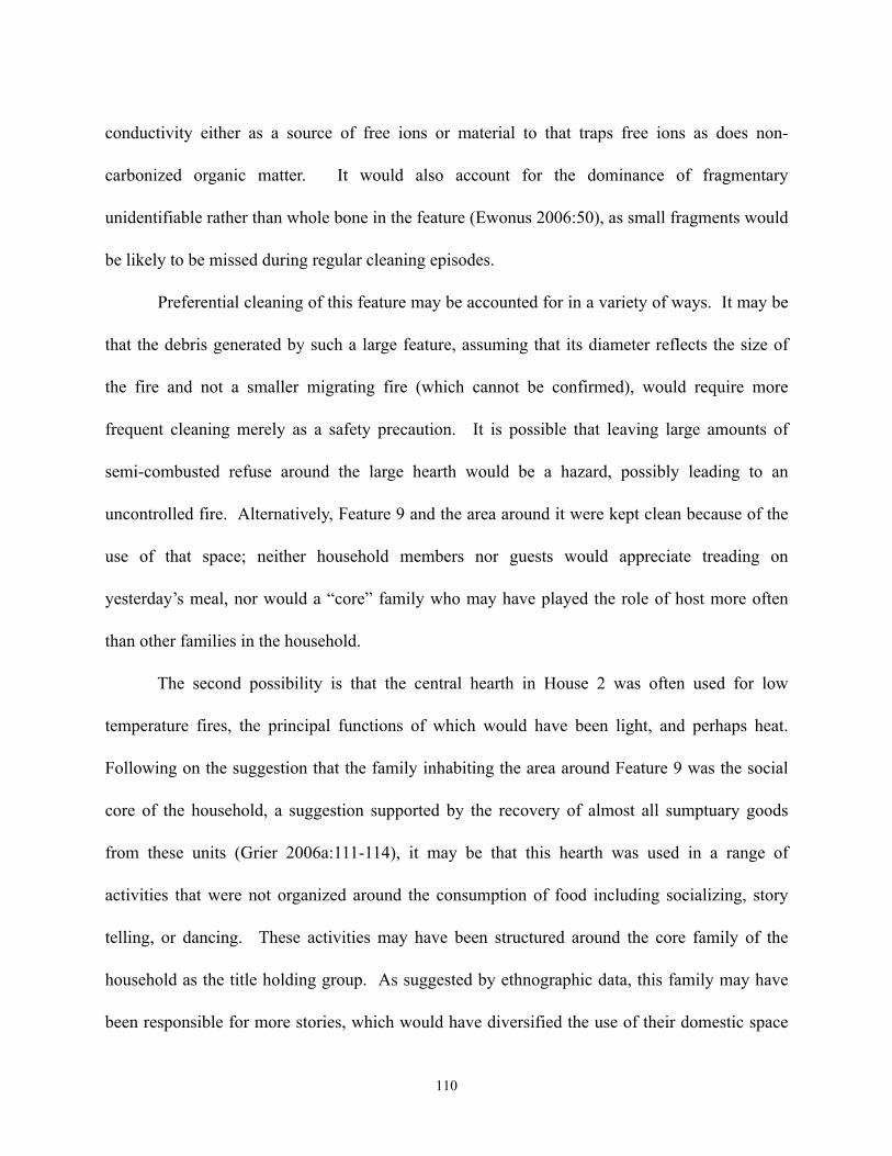
conductivity either as a source of free ions or material to that traps free ions as does non-

carbonized organic matter. It would also account for the dominance of fragmentary

unidentifiable rather than whole bone in the feature (Ewonus 2006:50), as small fragments would

be likely to be missed during regular cleaning episodes.

Preferential cleaning of this feature may be accounted for in a variety of ways. It may be

that the debris generated by such a large feature, assuming that its diameter reflects the size of

the fire and not a smaller migrating fire (which cannot be confirmed), would require more

frequent cleaning merely as a safety precaution. It is possible that leaving large amounts of

semi-combusted refuse around the large hearth would be a hazard, possibly leading to an

uncontrolled fire. Alternatively, Feature 9 and the area around it were kept clean because of the

use of that space; neither household members nor guests would appreciate treading on

yesterday’s meal, nor would a “core” family who may have played the role of host more often

than other families in the household.

The second possibility is that the central hearth in House 2 was often used for low

temperature fires, the principal functions of which would have been light, and perhaps heat.

Following on the suggestion that the family inhabiting the area around Feature 9 was the social

core of the household, a suggestion supported by the recovery of almost all sumptuary goods

from these units (Grier 2006a:111-114), it may be that this hearth was used in a range of

activities that were not organized around the consumption of food including socializing, story

telling, or dancing. These activities may have been structured around the core family of the

household as the title holding group. As suggested by ethnographic data, this family may have

been responsible for more stories, which would have diversified the use of their domestic space

110

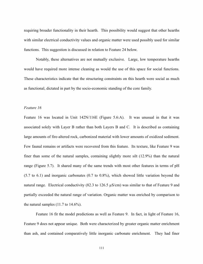
requiring broader functionality in their hearth. This possibility would suggest that other hearths

with similar electrical conductivity values and organic matter were used possibly used for similar

functions. This suggestion is discussed in relation to Feature 24 below.

Notably, these alternatives are not mutually exclusive. Large, low temperature hearths

would have required more intense cleaning as would the use of this space for social functions.

These characteristics indicate that the structuring constraints on this hearth were social as much

as functional, dictated in part by the socio-economic standing of the core family.

Feature 16

Feature 16 was located in Unit 142N/116E (Figure 5.6:A). It was unusual in that it was

associated solely with Layer B rather than both Layers B and C. It is described as containing

large amounts of fire-altered rock, carbonized material with lower amounts of oxidized sediment.

Few faunal remains or artifacts were recovered from this feature. Its texture, like Feature 9 was

finer than some of the natural samples, containing slightly more silt (12.9%) than the natural

range (Figure 5.7). It shared many of the same trends with most other features in terms of pH

(5.7 to 6.1) and inorganic carbonates (0.7 to 0.8%), which showed little variation beyond the

natural range. Electrical conductivity (82.3 to 126.5 µS/cm) was similar to that of Feature 9 and

partially exceeded the natural range of variation. Organic matter was enriched by comparison to

the natural samples (11.7 to 14.6%).

Feature 16 fit the model predictions as well as Feature 9. In fact, in light of Feature 16,

Feature 9 does not appear unique. Both were characterized by greater organic matter enrichment

than ash, and contained comparatively little inorganic carbonate enrichment. They had finer

111

texture than any other feature and partially exceeded the natural range of variation. The location

of this hearth nearby Feature 9 may suggest that it was subject to a similar intensity of cleaning,

accounting for their comparable characteristics.

Feature 24

Feature 24 was located in Unit 141N/109E (Figure 5.6A). It has been interpreted to be

the domestic hearth in the southwestern corner of House 2. It was partially uncovered during

excavation in the northeastern corner of the unit. It was approximately 1.2 m in diameter and 40

cm thick (~ 0.45 m3). Very little fire-altered rock was found within the feature, which contained

a fragmented stemmed point, abundant herring vertebrae, and a fragmentary dog mandible. Few

of the geoarchaeological characteristics of this feature were particularly notable. It had organic

matter enrichment higher than the natural range of variation (11.1%). Yet, all other constituents

were well within the natural range, making further interpretation difficult (Figure 5.7:B to D).

This feature was raised above as a having similar characteristics to Feature 9, which was

argued to derive its characteristics from a combination of broad functionality and more intensive

maintenance. Grier (2006a:112) identified the location of the second stone bowl recovered from

House 2 as Unit 141N/109E, the same unit where this hearth is located. Although this hearth is

not of the same size as Feature 9, it is possible that the family that occupied it was also involved

in social activities. However, given the small sample, and few sumptuary goods, this conclusion

must remain tentative.

112

Feature 28

Feature 28, was the large domestic hearth found in the northeastern corner of House 2

(Figure 5.6:A). In the DPHAP field notes it was described as a large hearth feature dominated by

ashy, brown (10YR4/3), burned shell matrix sitting in a shallow depression. The center of the

feature was noted to have a patch of burned black (10YR2/1) sediment.

The chemical and physical signature of this feature corresponds quite closely to the field

description. The dominance of ash in the feature matrix was reflected by the organic matter

content, which was substantially lower than any of the other combustion features (8.3 to 9.9%)

(Figure 5.7: A). The abundance of shell was readily visible in its inorganic carbonate enrichment

(1.3 to 6.3%) and pH (6.8 to 6.9) data, both of which were higher than the natural range of

variation (Figure 5.7:B, D). The inorganic carbonate values generated by this feature were the

highest of any sample and have the widest range. When they were compared to the remainder of

the cultural data set, it was evident that the feature’s carbonates originated in the shell content of

the feature matrix. This abundant shell-derived carbonate had an appreciable effect on the

feature’s electrical conductivity (84.7 to 209.0 µS/cm), which was also the high in the data set

(Figure 5.7: C). Notably, the features that most closely match the characteristics of Feature 28

were Features 10, 11, and 12 from Layer A, all three of which were interpreted to be shellfish

roasting features.

Feature 28 has been interpreted to be a domestic hearth based on its location, near the

bench area zone in the northeast corner of House 2, and its size, at least 1.2 m in diameter. The

density of faunal material is higher in this area than in any other area of the house (Ewonus

2006:Table 5, 6, 7, and 8) and the artifacts suggest marine-focused subsistence activities (Grier

113

2006a:108-109). The preponderance of evidence suggests that this is a domestic space. It is

unlikely that this hearth was functionally different than other hearths in the house, despite its

unique characteristics. This was not “the shellfish roasting hearth” in the house that was used by

all families for that specific purpose. The variability in this feature is likely a reflection of the

socio-economic practices of the domestic group that inhabited this area of the house. The

consumption of shellfish is generally described as a low-status activity in spite of archaeologists’

attempts to de-stigmatize it (e.g., Moss 1993). The abundance of shellfish in this domestic area

may suggest the presence of a low-status domestic group, particularly in light of the absence of

any sumptuary items in these units. It has been argued (Samuels 1991b:202), following

ethnographic evidence, that low-status families may have had imperatives to keep their domestic

space clean. Thus, the combined evidence of shellfish consumption and a relatively “messier”

compartment indicates that this family may not have enjoyed the same status as the families

occupying either the areas around Feature 9 or Feature 24, a point driven home by the lack of

sumptuary goods around Feature 28.

Feature Summary

The preceding discussion of feature samples from the DPHAP collection revealed that

there was far greater variability in the hearth feature samples than was predicted by the model

presented in Chapter Three. It appears that two factors controlled the geoarchaeological

signatures of these features, their faunal content and their treatment during use. The fact that this

variability was finite and that three distinct categories of signatures were evident, even with this

limited sample size suggests that variation was meaningfully patterned:

114

1. High organic matter. Low conductivity features characterized by large amounts of

charcoal, little ash and low pH values.

2. High ash content. Electrical conductivity higher than combustion features without ash,

pH slightly higher. These can be distinguished from floor deposits by their unusually low

organic matter content.

3. High ash content, with significant shell contribution. At Dionisio Point these samples

were readily recognizable by substantially higher inorganic carbonates.

The causes of this variation were, in at least one case (Feature 2) identified to be

functional. Feature 2 suggests that, in some cases, features designated to be “hearths” in the

field, may be other types of features entirely. Functional variability in hearth features has been

suggested in past archaeological investigations (e.g., Samuels 1991b). However, this has often

targeted large hearths has ceremonial rather than domestic. This study makes no such

suggestion. The functional variability that is being discussed here is in the much smaller,

ephemeral features found in House 2 and likely other structures. A functional analysis of these

smaller features has not been undertaken in the published literature, archaeologists regularly

focusing on larger hearth features.

There are two capacities in which this kind of functional analysis could be useful. The

first in the functional interpretation of space. In a number of excavations architectural feature

identification, such as door, or bench feature identification is unclear. It may be possible to use

the identification of smaller features to infer the architectural nature of these features from

indirect evidence. Aggregations of ash dumps may, for example, identify low-traffic areas as

115

suggested above. This study was not able to pursue this line of research at length as a result of

the small data set, but indications are that it may be productive to pursue sampling of small

features for this purpose.

This feature analysis also suggests that variation in the social constraints on individual

families may affect the nature of hearth features. Inasmuch as domestic activities varied between

family-units, the nature of domestic hearths could be quite variable. The functional model

suggests that the same domestic groups use different hearths for different functions. Thus

domestic hearths and ceremonial hearths are mutually exclusive classes of features. The social

model is distinguished by arguing that, where the evidence supports the presence of a domestic

space around the hearth, that inter-hearth variability is the result of the socio-economic status of

these groups. That is, all hearths may be domestic hearths, but high status families may be

engaged in activities that require them to treat their domestic hearth differently.

Features 9 and 28 are the best examples, in this data set, of domestic hearths that appear

to have been treated in quite different manners as a consequence of differences in social status.

As argued above, Feature 9 sedimentary characteristics indicate that it was predominantly

composed of inert organic matter at the time of sampling. The low electrical conductivity values

recorded for it were surprising in the context of the hearth model presented in Chapter Three.

However, in light of the artifact analysis previously undertaken for this compartment, the low

electrical conductivity, suggested to reflect low ash content, is explicable as a reflection of the

domestic requirements of the high-status “core” family that inhabited the area around it.

Ethnographically, the title-holding core of the household was responsible for hosting other

households in a number of social activities. In House 2 at Dionisio Point, the distribution of

116

sumptuary goods within the central compartment, surrounding Feature 9 suggests that this family

enjoyed greater ability to gain access to these goods (Grier 2006a:114). The possession of these

goods was likely related to elite identity (Grier 2003), and very likely were involved in the

activities centered around Feature 9, the same activities that required this space to be maintained

to a greater degree than the spaces around it.

Feature 28 has been suggested to be the domestic hearth of a low-status family based on

the abundance of shellfish, a low-status food ethnographically, and the far density of faunal

debris found in this location. The predominance of shellfish in this location was evident in the

inorganic carbonate content of the sediment samples. Wether shellfish were in fact a low-status

resource at the time that House 2 at Dionisio Point was occupied is not clear. However, if they

were it would explain both the greater degree of “messyness” of this part of the house, that is the

higher density of most data sets, as well as the absence of an sumptuary goods.

These two very different hearth signatures suggest that social differentiation was recorded

in these features. The alternative that these were functionally different structures is difficult to

maintain in light of the domestic artifacts located around Feature 9 (Grier 2001). Nor can it be

simply argued that Feature 28 was the shellfish-roasting hearth in the house. These socially

determined constraints on the use of space should be of interest to archaeologists who are

attempting to address questions of the emergence of social differentiation in households.

Differences in the treatment of space should be coevolutionary with the activities that alter the

distribution of sumptuary goods, and may be appropriate to assess when artifact assemblages are

not appropriate for these kinds of questions.

117

Floor Contexts

Three different floors contexts were presented in this analysis: Center, Edge (Bench), and

Entryway. These contexts were chosen to reflect important aspects of the ethnographic and

archaeological models of shed-roof house architecture. Figure 5.9, illustrates an idealized model

of the functional division of space within the ethnographic shed-roof plank house (B), and the

units that were sampled from House 2 (B) and House 5 (C). Variability of soil constituents

between the three types of floor deposits is presented in Figure 5.10 (A to D), and results of the

particle-size analysis in Figure 5.11.

Comparison of the soil constituents revealed that there were few significant differences

between the three floor contexts. pH and inorganic carbonates failed to exceed the natural range

of variation. The electrical conductivity of all three samples exceeded the natural range but was

broadly similar between contexts as was organic matter, though samples clustered slightly

differently.

Center Deposits

Table 5.5 presents the expectations for Center samples. Center samples were collected

from Unit 144N/116E of House 2, and Units 110N/106E and 111N/107E House 5. The Center

deposits within the plank house are the open space that surrounds domestic hearths and was used

for a variety of activities. Barring post-depositional alteration, patterning of floor residues will

reflect the amount of time that debris was allowed to remain in contact with the floor surface.

Samuels (1991b) and Huelsbeck (1994) argue for a similar process in the macroscopic artifact

and faunal record at Ozette. The model presented in Chapter Three predicts that floor deposits

118

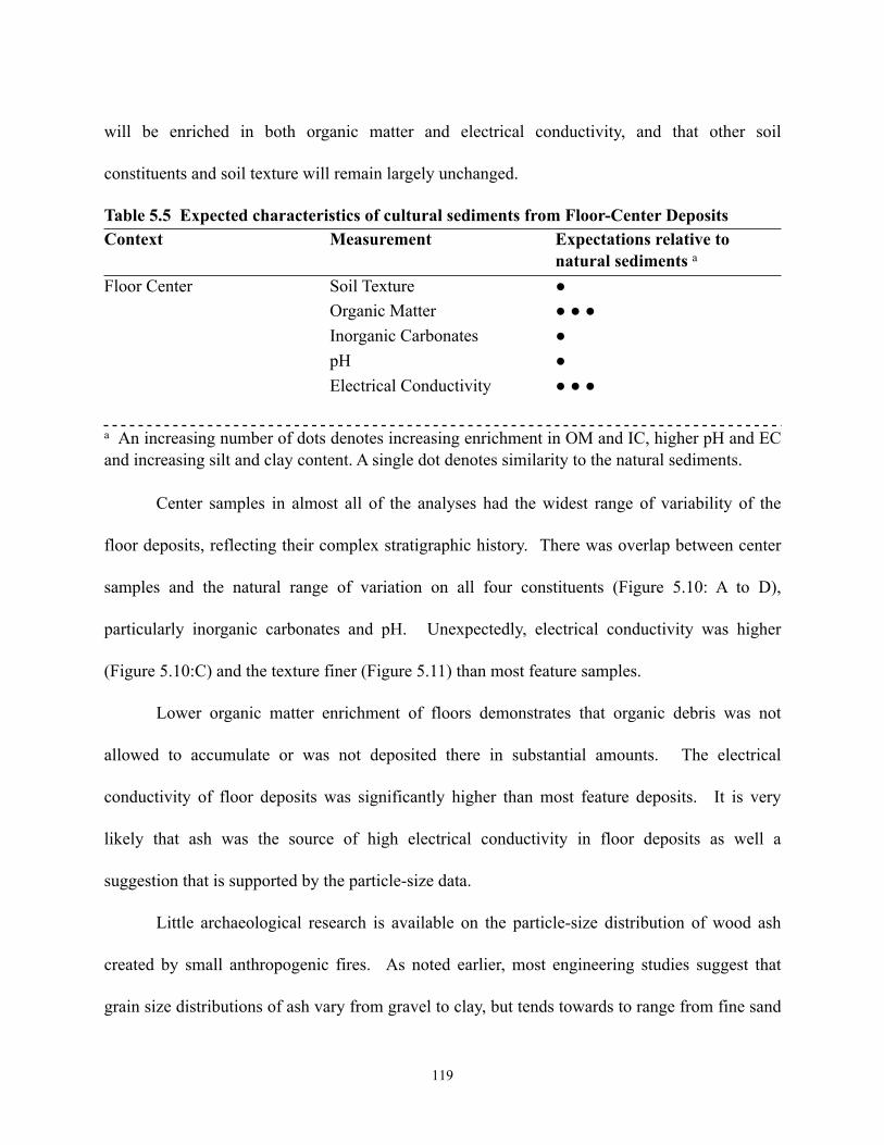
will be enriched in both organic matter and electrical conductivity, and that other soil

constituents and soil texture will remain largely unchanged.

Table 5.5 Expected characteristics of cultural sediments from Floor-Center DepositsContext Measurement Expectations relative to

natural sediments a

Floor Center Soil Texture ●Organic Matter ● ● ●Inorganic Carbonates ●pH ●Electrical Conductivity ● ● ●

a An increasing number of dots denotes increasing enrichment in OM and IC, higher pH and EC and increasing silt and clay content. A single dot denotes similarity to the natural sediments.

Center samples in almost all of the analyses had the widest range of variability of the

floor deposits, reflecting their complex stratigraphic history. There was overlap between center

samples and the natural range of variation on all four constituents (Figure 5.10: A to D),

particularly inorganic carbonates and pH. Unexpectedly, electrical conductivity was higher

(Figure 5.10:C) and the texture finer (Figure 5.11) than most feature samples.

Lower organic matter enrichment of floors demonstrates that organic debris was not

allowed to accumulate or was not deposited there in substantial amounts. The electrical

conductivity of floor deposits was significantly higher than most feature deposits. It is very

likely that ash was the source of high electrical conductivity in floor deposits as well a

suggestion that is supported by the particle-size data.

Little archaeological research is available on the particle-size distribution of wood ash

created by small anthropogenic fires. As noted earlier, most engineering studies suggest that

grain size distributions of ash vary from gravel to clay, but tends towards to range from fine sand

119

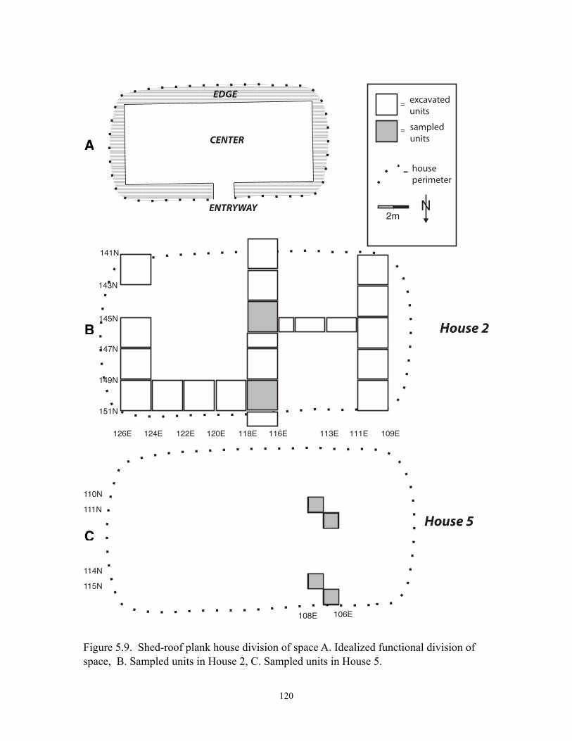
120

Figure 5.9. Shed-roof plank house division of space A. Idealized functional division of space, B. Sampled units in House 2, C. Sampled units in House 5.

houseperimeter

excavatedunits

sampledunitsCENTER

EDGE

ENTRYWAY

110N

111N

114N

115N

106E108E

House 5

141N

143N

145N

147N

149N

151N

126E 124E 122E 120E

House 2

118E 116E 113E 111E 109E

A

B

C

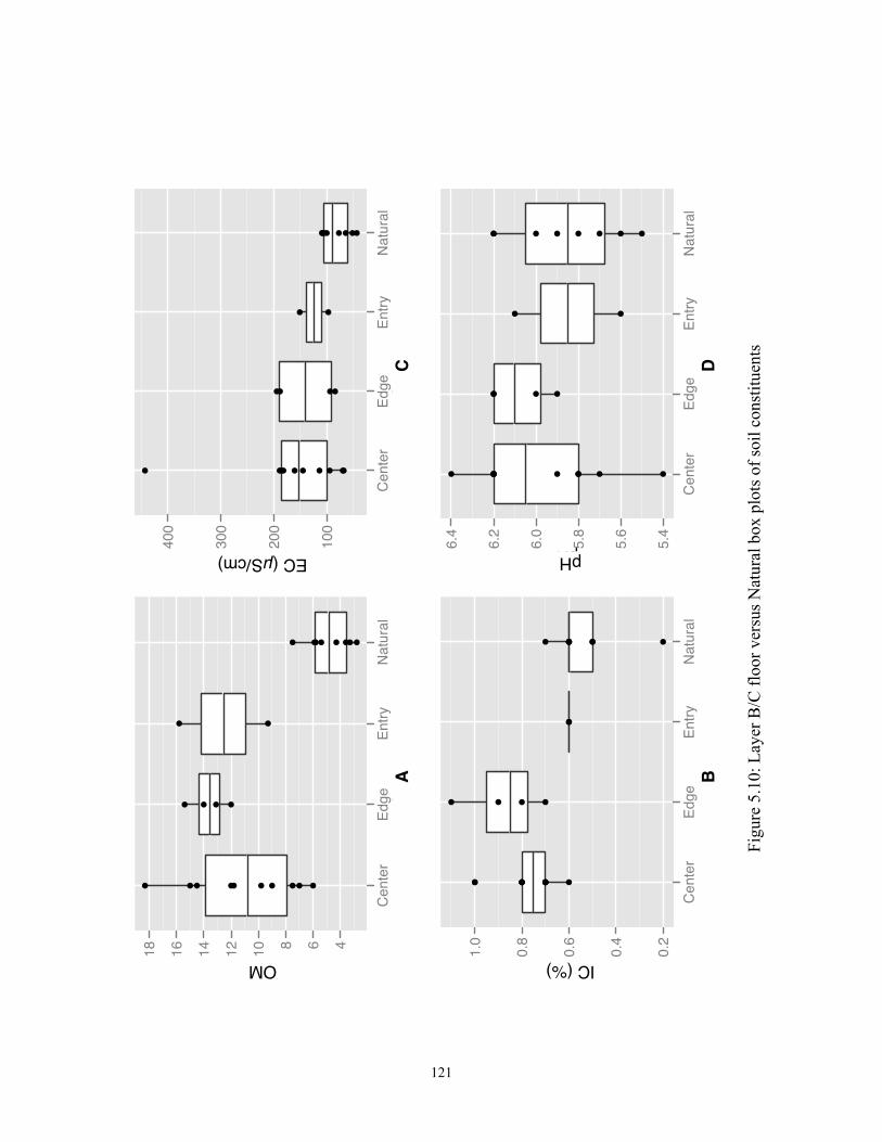
121

Context

OM

● ●● ●● ● ●● ● ●

●●● ●

●●

●● ● ●● ●●●

4681012141618

Center

Edge

Entry

Natural

Context

IC

●●

●

● ●● ●●● ●● ●●

●●● ●

●●● ●●●●● ●●

0.2

0.4

0.6

0.8

1.0

Center

Edge

Entry

Natural

Context

EC

● ● ● ●●● ●●●●●

● ● ●●

● ●● ●● ●●● ● ●

100

200

300

400

Center

Edge

Entry

Natural

Context

pH●● ●● ●● ●● ●●

●● ●●

● ●

● ●●● ● ● ●●

5.4

5.6

5.8

6.0

6.2

6.4

Center

Edge

Entry

Natural

A B

C D

OM IC (%)

Figu

re 5

.10:

Lay

er B

/C fl

oor v

ersu

s Nat

ural

box

plo

ts o

f soi

l con

stitu

ents

EC (µS/cm) pH

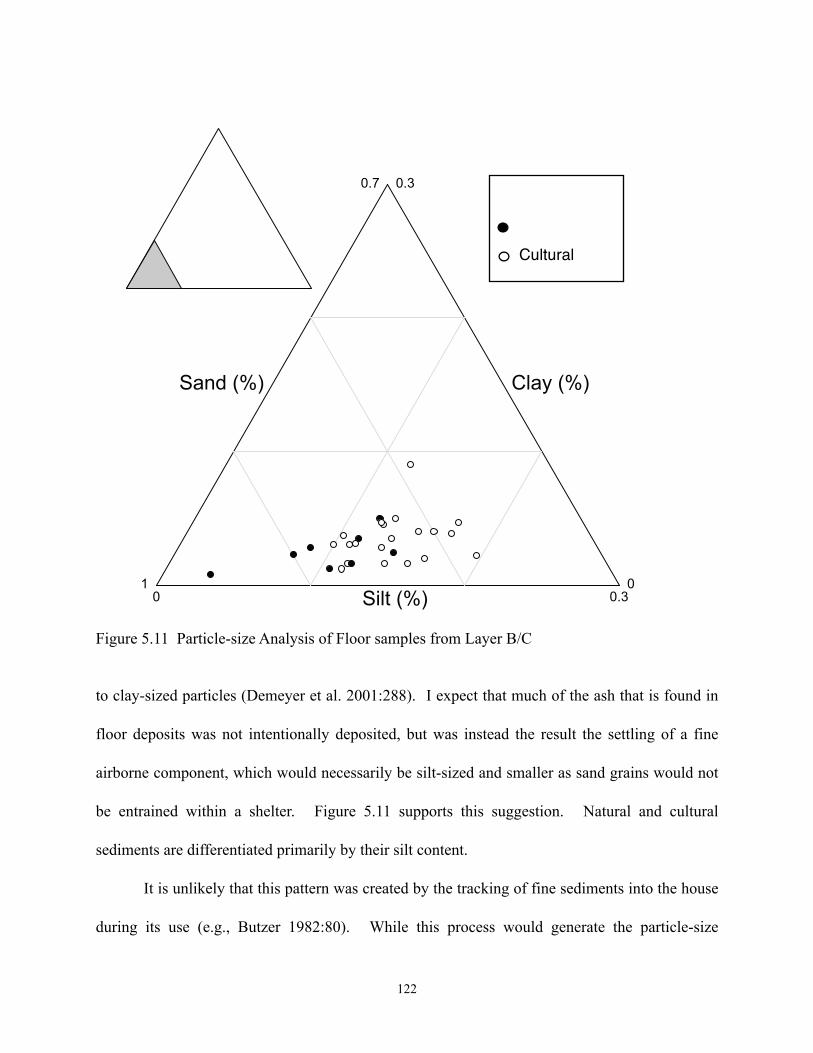
to clay-sized particles (Demeyer et al. 2001:288). I expect that much of the ash that is found in

floor deposits was not intentionally deposited, but was instead the result the settling of a fine

airborne component, which would necessarily be silt-sized and smaller as sand grains would not

be entrained within a shelter. Figure 5.11 supports this suggestion. Natural and cultural

sediments are differentiated primarily by their silt content.

It is unlikely that this pattern was created by the tracking of fine sediments into the house

during its use (e.g., Butzer 1982:80). While this process would generate the particle-size

122

0.7 0.3

Sand (%)

10 Silt (%) 0.3

0

Clay (%)

Legend

NaturalCultural

Figure 5.11 Particle-size Analysis of Floor samples from Layer B/C

Cultural

distribution patterns noted in Figure 5.11, mineral silt additions cannot fully account for the

significantly higher electrical conductivity patterns noted in Figure 5.9 (C). Some of the natural

samples with equivalent silt content were shown to have lower electrical conductivity values.

Local organic matter enrichment could account for increased electrical conductivity, but does not

explain the grain size differences. It is more likely that ash or a derivative of wood combustion

connected to ash is the primary cause of elevated electrical conductivity (e.g., Weide 1996),

indicating that ash is an important constituent of the matrix of Center deposits.

It is not difficult to envision a number of practices that would have tracked ash

throughout the house, as occupants moved around their domestic space. Feature 2, evidence of

an episode of hearth cleaning, demonstrates that ash could be and was moved around the house.

Hoever, housekeeping practices were probably ineffective at removing fine ash residues, perhaps

suggested by the slightly finer texture of Feature 2 as compared to floor deposits.

Ethnographically, fine residues were managed by regularly moistening the floor (Suttles

1951:313). However, the electrical conductivity values from Dionisio Point illustrate how

effectively these materials could become incorporated into floor deposits.

Edge Deposits

As mentioned in Chapter Three, archaeological evidence of benches has often been

lacking during the excavation of prehistoric structures. Evidence of post features (Mauger

1991:105), changes in soil color, and changes in texture, for example, have been used to suggest

the presence of bench features (e.g. Grier 2001:166-178; Lepofsky et al. 2000:398-399; Matson

2003:88). Under many circumstances, it is difficult to either confirm or deny their existence;

123

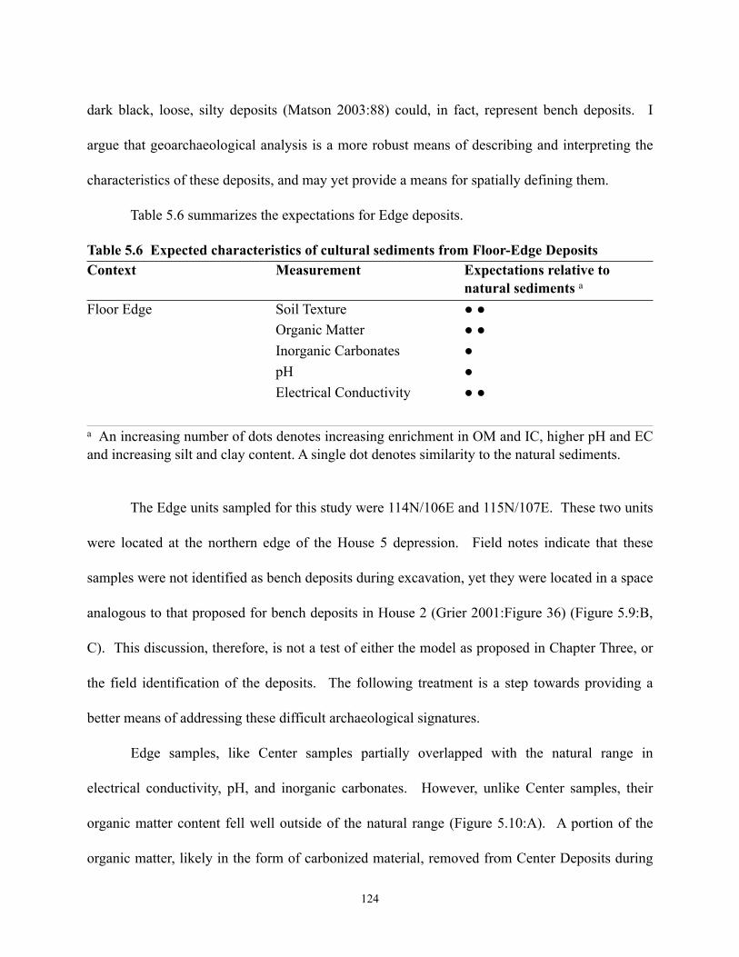
dark black, loose, silty deposits (Matson 2003:88) could, in fact, represent bench deposits. I

argue that geoarchaeological analysis is a more robust means of describing and interpreting the

characteristics of these deposits, and may yet provide a means for spatially defining them.

Table 5.6 summarizes the expectations for Edge deposits.

Table 5.6 Expected characteristics of cultural sediments from Floor-Edge DepositsContext Measurement Expectations relative to

natural sediments a

Floor Edge Soil Texture ● ●Organic Matter ● ●Inorganic Carbonates ●pH ●Electrical Conductivity ● ●

a An increasing number of dots denotes increasing enrichment in OM and IC, higher pH and EC and increasing silt and clay content. A single dot denotes similarity to the natural sediments.

The Edge units sampled for this study were 114N/106E and 115N/107E. These two units

were located at the northern edge of the House 5 depression. Field notes indicate that these

samples were not identified as bench deposits during excavation, yet they were located in a space

analogous to that proposed for bench deposits in House 2 (Grier 2001:Figure 36) (Figure 5.9:B,

C). This discussion, therefore, is not a test of either the model as proposed in Chapter Three, or

the field identification of the deposits. The following treatment is a step towards providing a

better means of addressing these difficult archaeological signatures.

Edge samples, like Center samples partially overlapped with the natural range in

electrical conductivity, pH, and inorganic carbonates. However, unlike Center samples, their

organic matter content fell well outside of the natural range (Figure 5.10:A). A portion of the

organic matter, likely in the form of carbonized material, removed from Center Deposits during

124

cleaning activities was deposited in Edge deposits. Comparison of the feature (Figure 5.7) and

non-feature (Figure 5.10) box plots reveals that Edge deposits contain a median organic matter

content comparable to Feature 9, supporting the suggestion that some portion of the domestic

debris generated by a family accumulated beneath benches. The discussion of Feature 2 has

already illustrated the possibility that ash was dumped along the edge of house deposits,

conceivably beneath benches. It appears that Feature 2 could simply be a specific example of a

more generalized process of housekeeping and maintenance. Alternatively, benches in the

ethnographic literature were storage locations as well as sleeping quarters and social space

(Suttles 1991). A pattern of higher organic matter enrichment, higher electrical conductivity

determinations, similar to that suggested above to be the result of housekeeping, could also be

the result of the in situ degradation of materials kept in this location. Unfortunately, the methods

used here are unable to resolve between these two alternatives. Both processes may have been

active and coexistent. Yet, until we develop better means of identifying the specific sources of

organic matter or electrical conductivity, the more influential of these two processes cannot be

determined.

The suggestion that Edge samples have been affected because of their proximity to

exterior shell middens can be abandoned. Shell middens would generate both higher electrical

conductivity and organic matter enrichment. However, I would expect there to be a similar

increase in inorganic carbonate content in the form of calcium carbonate. This is not the case.

Calcium carbonate is known to degrade under acidic conditions and should leach into the

surrounding matrix (Stein 1992b). The ~0.2% difference between the median inorganic

125

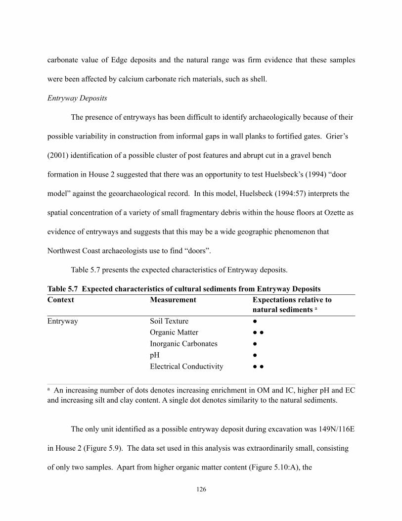
carbonate value of Edge deposits and the natural range was firm evidence that these samples

were been affected by calcium carbonate rich materials, such as shell.

Entryway Deposits

The presence of entryways has been difficult to identify archaeologically because of their

possible variability in construction from informal gaps in wall planks to fortified gates. Grier’s

(2001) identification of a possible cluster of post features and abrupt cut in a gravel bench

formation in House 2 suggested that there was an opportunity to test Huelsbeck’s (1994) “door

model” against the geoarchaeological record. In this model, Huelsbeck (1994:57) interprets the

spatial concentration of a variety of small fragmentary debris within the house floors at Ozette as

evidence of entryways and suggests that this may be a wide geographic phenomenon that

Northwest Coast archaeologists use to find “doors”.

Table 5.7 presents the expected characteristics of Entryway deposits.

Table 5.7 Expected characteristics of cultural sediments from Entryway DepositsContext Measurement Expectations relative to

natural sediments a

Entryway Soil Texture ●Organic Matter ● ●Inorganic Carbonates ●pH ●Electrical Conductivity ● ●

a An increasing number of dots denotes increasing enrichment in OM and IC, higher pH and EC and increasing silt and clay content. A single dot denotes similarity to the natural sediments.

The only unit identified as a possible entryway deposit during excavation was 149N/116E

in House 2 (Figure 5.9). The data set used in this analysis was extraordinarily small, consisting

of only two samples. Apart from higher organic matter content (Figure 5.10:A), the

126

characteristics of Entryway samples partially overlapped with the natural range of variation. The

electrical conductivity of the Entryway sample was slightly higher than the natural range. The

median pH and inorganic carbonate content of the Entryway samples were among the lowest in

the data set, overlapping extensively with the natural range.

These characteristics are largely indistinguishable from the Edge deposits. The similarity

between these two cultural contexts should not be taken to suggest that the Entryway samples

were, in fact, drawn from bench deposits. First, the Edge samples cannot be verified to be drawn

from bench deposits themselves, and second, it is largely a working hypothesis that these two

contexts should have different signatures. Higher-than-expected electrical conductivity and

organic matter content of these samples results not only because material is being removed from

inside, but because, unintentionally, material is being brought in from outside (Butzer 1982:80).

The past treatment of plank houses as closed systems may largely stem from the kinds of

data sets that have been analyzed. Archaeologists studying tools or faunal remains rarely need to

address the possibility that materials are being unintentionally tracked into structures. However,

for microscopic data sets, this is a possible cultural formation process (Butzer 1980:82). Organic

matter and minerals that contribute to electrical conductivity could and likely were tracked into

these structures. The discussion of Center deposits above has already demonstrated evidence this

process in the “tracking-in” of large amounts of silt. These materials would be trampled into the

floor deposits around the entryway preserving them there and generating a geoarchaeological

signature similar to that of Edge deposits.

All of this suggests that Huelsbeck’s (1994) method of using faunal materials for the

identification of doors does not work for bulk sediment analysis. Entryways and Edges are

127

simply too similar to be differentiated on these five analytical variables. Importantly, Huelsbeck

(1994) had a very high resolution data set at his disposal, and had the opportunity to pick up

patterns that this data set could not. It may be that will a more intensive geoarchaeological

sampling strategy could differences between these two contexts.

Floor Summary

In the cultural model in Chapter Three it is suggested that the primary source of

variability within floor deposits, here including Center, Edge and Entryway samples, was

housekeeping practices. While activities surrounding food preparation, consumption and storage

were responsible for introducing the large amounts of organic matter and mineral wood ash to

these deposits that elevated them above the natural background, it was the intentional and

unintentional re-deposition of these materials via housekeeping that ultimately led to the patterns

recorded geoarchaeologically.

This is best seen in the variability between Center and Edge (bench) deposits. It is

evident from the differences in organic matter content between the two spaces that human

activities either preferentially removed organic matter in the former or deposited in the latter (or

both). I believe that a combination of the two is the most accurate interpretation of the

geoarchaeological data. As has been previously argued, the unintentional tracking-in of fine

sediment would not be sufficient to result in the ~ 4% drop in organic matter content between

Edge and Center deposits. Nor can we attribute accumulation of large amounts of organic matter

to the proximity of Edge deposits to middens (though the in situ decomposition of stored

materials may have made a contribution to the geoarchaeological signature). Further support for

128

a model of organic matter re-deposition away from Center deposits and into Edge deposits is

found in two places. First, the characteristics of Edge deposits are best matched by hearth debris.

I am, therefore, certain that bench areas were sometimes, if not always, the location of the

accumulation of domestic debris through the cleaning of domestic areas. The second source of

evidence is less strong, but is potentially more telling. Comparison of non-feature and feature

samples from Layer B/C in Unit 144N/116E, the only unit where substantial numbers of samples

are available for both, reveals that though organic matter overlaps between the two, it is notably

different (Figure 5.10). I suggest that this is because floor areas were regularly cleaned.

The data set used in this analysis is, however, unable to address variation in housekeeping

practices through either one of the houses sampled at Dionisio Point. Variation in the density of

faunal remains within House 2 has been interpreted to reflect functional variation in the use of

space (Ewonus 2006:85). The central compartment, in this interpretation, is argued to be a

communal space used by several families living around it. An alternative interpretation is that

different areas of the house were subject to different degrees of housekeeping during their

occupation. Smith (2006) has argued that lithic debris was removed from high-traffic areas

around hearths. This same argument could be extended to a range of debris, including faunal

materials. If the domestic area in the central compartment of House 2 was occupied by the elite

core of the household, that space may have had cause to be cleaned more frequently. The elite

family may have hosted more feasts, or possibly may have reproduced its status in part by

keeping a cleaner domestic space than the remaining domestic groups in the house.

This interpretation of the geoarchaeological evidence has implications for the

reconstruction of plankhouse economic organization. Huelsbeck (1994:57) suggests that there is

129

no reason to expect differential cleaning of domestic spaces within a plankhouse, as this would

constitute little more than pushing the dirt around the room. Huelsbeck’s (1994) model assumes

a high level of household social integration in the prehistoric shed-roof household. However,

ethnographically while the families shared in a number of activities, both economic and social,

they were distinct units and were largely responsible for their own space (Suttles 1991:214).

Grier (2006b:148) has recently illustrated the underlying tensions that existed in the shed-roof

household between the social elite “core” family and the “tenant” families that had been attracted

to it, the former wanting to attract the best labor and the latter desiring to be part of the best

household.

While Huelsbeck (1994) marshals both ethnographic and archaeological material to

support his argument, the model of within-household uniformity in maintenance practices does

not appear to apply to Dionisio Point. This has important implications for the reconstruction of

household socio-economic activities from artifact and faunal data. The possibility that some

shed-roof compartments were differentially treated by their occupants forms the basis for

economic reconstruction of household organization. However, archaeologists have only recently

paid appropriate attention to the complicated cultural formation processes that these deposits

represent (Grier 2006a; Smith 2004). If differential maintenance is a spatially consistent practice

through time, archaeologists must look for evidence of it, such as presented here, prior to

interpreting results based on artifact or faunal data sets.

Implications for socio-economic reconstruction shed-roof households

130

The distribution of artifacts and faunal remains within plank house deposits represents the

end result of a complex pattern of domestic and non-domestic activities. Geoarchaeological data

reflects a similar complexity of activities, but it is often more difficult to link patterns to specific

behaviors. Attempts to integrate these data sets have proven to be neither simple nor straight-

forward (e.g., Ewonus 2006; Grier 2006a) and yet a holistic approach is necessary to account for

the complex nature of plank house remains. This study has succeeded in addressing present

models of the processes that generate the features that we use to identify plank house deposits:

hearths, floor, and bench deposits.

None of the formation process models presented in Chapter Three were found to wholly

or accurately describe the characteristics of features identified at Dionisio Point. In large part

this is because these models were unable to address variability in the data set. Previous

examinations of artifacts and architecture at Dionisio Point in combination with the data

presented here suggest that this variability was generated by social as well as functional

constraints. Which of these was dominant in any one spatial content within a plank house, at

least in this data set, was not random; social and functional variability follow patterns.

Variability between domestic areas is primarily a function of variability of social status

(privileges and obligations) between the domestic groups that occupied the plank house. That is,

higher-status and lower-status families were seen to use and treat their space differently. The

variability within any one of these domestic areas, however, was partially a consequence of the

functional divisions of space into floor, bench, and hearth deposits. These interpretations suggest

that household archaeologists need to continue to analyze the internal economic and social

organization of plank house households in the context of the concept of the corporate group.

131

Under the broad definition of corporate groups as groups that share inalienable rights to

property, they exist at various social and political scales, ranging from small-scale hunter-

gatherer communities, to nuclear families, and the citizenry of nation-states (Bell 1995a:826). It

is important to keep this variability in mind when we think of corporate groups on the Northwest

Coast. Under a fairly inflexible conceptualization of this unit, it might be difficult to understand

how a corporate group could show evidence of patterned variability in consumption debris; a

corporate group is an economic unit that by definition grants access to resources for all members.

Under this definition the variability that we see in housekeeping practices within the households

at Dionisio Point is not explicable. However, I think that it is useful to point out that household

archaeological work on the Northwest Coast has repeatedly revealed that Marpole phase

households were not simple corporate groups (e.g., Chatters 1989; Grier 206a). Corporate group

rights appear to, at this time. exist alongside emergent individual property rights.

Ethnographic and ethnohistoric examples of this pattern exist in agropastoral

communities, in which leadership ranges from the ephemeral to the enduring. Archaeologists

studying this development have looked to these communities for insight, often identifying socio-

economic processes as the basis for change. The production of an economic surplus (Hayden

1995), intensification of production (Johnson and Earle 2000; Price and Brown 1985),

development of economic specialization (Cobb 2000), and the monopolization of exchange

relationships (Spencer 1994; Wiessner 2002) have all been interpreted as causal forces. Many of

these same processes have been explored on the Northwest Coast (see Chapter One).

The importance of the residential corporate group in this discussion is the central role that

it can play as both the social and economic setting for the emergence of inequality. Ethnographic

132

and, increasingly, archaeological evidence suggests that residential corporate groups form

coherent economic units in small-scale societies. The social and economic settings for the

emergence of inequality involve the same core group of individuals as suggested by the

importance of the kinship ethic that dominates socio-economic relationships in many of these

societies (Cobb 1993:46-49). Household archaeology is one of the ways in which Northwest

Coast archaeologists can enter and contribute constructively to this wider discussion.

Prospects for Geoarchaeological Prospection

One of the goals at the outset of this study was to establish geoarchaeological signatures

of plank house features for the purposes of prospecting for houses prior to or in lieu of

excavation. The southwestern coast of British Columbia contains an large number of dense shell

middens, some of which were plank house villages in the past. Excavation techniques are unable

to test the large areas of the shell midden necessary to identify the presence of plank house

features (Ames et al. 1992; Bulakis-Onat 1985; Lyman 1991). It was hoped that this study would

provide a means for assigning geoarchaeological samples to various specific features. However,

during analysis of the data set, it became clear that the bulk sediment methods used here were not

able to provide the discrimination between contexts that is necessary to distinguish floors from

hearths or benches. One need only compare the results of organic matter and electrical

conductivity analyses for each context to see that there are large areas of overlap (Figure 5.11).

Where the results of this study may be most effective is in terms of prospection at

Dionisio Point and nearby sites. The natural sources of variability are not so great that the

conclusions presented here would not apply to other houses at the site. Implications for feature

133

identification through the geoarchaeological signature have been presented throughout this

discussion. Two facts are evident from the discussion of combustion feature signatures above:

1. Combustion features are the location of the highest anthropogenic inputs in the houses,

be those inputs organic matter or inorganic carbonates

2. These additions create extreme values that are readily picked up by the analyses used

in this study. The implication of the presence of distinct hearth signatures, is that hearths

and their associated domestic spaces can be found in buried plankhouses from fairly

small matrix samples (e.g. < 10 g).

There is convincing evidence that these signals will hold for the remaining houses at Dionisio

Point. However, the signatures cannot be exported wholesale to other sites with visibly different

natural and, conceivably, different cultural formation processes.

134

Chapter Six: Conclusions and Future Research

Indigenous households seasonally occupied large post-and-beam plank houses on the Northwest

Coast as early as 4500 B.P. These houses form long-term records of the domestic and non-

domestic activities of their occupants and have been shown to preserve these records for

millennia. This study demonstrates that geoarchaeological analyses of bulk sediment samples

can be a fruitful data set to pursue alongside artifacts, faunal, and botanical remains.

Furthermore, it may be able to identify patterns in the use of space when these other data sets are

lacking.

The approach used was successful in assessing the validity of present models of cultural

formation processes In contrast to models that emphasize variability in housekeeping processes

at the household level (e.g., Huelsbeck 1994), this study supports a model in which social

differentiation between families within houses is likely an important variable in these activities.

This has a number of methodological implications, the most immediate are for the analysis of the

spatial distribution of artifacts and ecofacts. Archaeologists working on the coast have treated

this process with due caution as a great deal of interpretive weight is placed on the spatial

association of features and artifacts. The complex cultural processes that move cultural materials

from locations of primary to secondary and tertiary deposition have been rigorously studied in

this context (Ames et al. 1992; Grier 2006a; Samuels 1991b; Smith 2006). However, it remains

difficult to associate specific artifacts with their original locations of production, use or discard,

and it may be that geoarchaeological materials provides a means of addressing this weakness. .

Geoarchaeologists working elsewhere have demonstrated that microresidues of activities

preserved in sedimentary deposits are more resistant to change and relocation following

135

deposition (King 2008:1225), and thus are more directly related to the location where the

associated activities took place. This is true only in part for the data used here. The evidence

suggests that very fine microresidues may remain in place and become trampled into house

floors, such was the case for very fine ash residues that have raised the electrical conductivity of

House 2 and House 5 floor deposits at Dionisio Point. One of the strengths of this bulk analysis

was that sediments could often be traced from their origins to their place of final deposition.

Ash, for example, produced presumably in domestic hearths, could be traced to locations along

the interior wall of both House 2 and House 5, the former showing evidence of general free ion

enrichment and the latter evidence of a spatially discrete ash dump. These methods may be used,

therefore, to reconstruct the potential pathways that other data sets may take as a result of

housekeeping activities, much as Ames et al. (1992) and Smith (2006) have attempted at the

Meier site.

Geoarchaeological analysis was also successfully used to address questions specific to

Dionisio Point. The anthropogenic signal of the central hearth feature in House 2 revealed that

differences in maintenance rather than in use were responsible for the low density of faunal

remains recovered from in and around it. This, minimally, does not support the argument that the

center compartment of the house was functionally different from the others. When combined

with interpretations from the artifact and architectural data sets, there is strong evidence that this

was a domestic space rather than solely a ceremonial hearth. This does not preclude the hearth

from also being used for ceremonial purposes. If, as Grier argues, Dionisio Point was a winter

village, ceremony would likely have played a large role in the activities of the inhabitants

(Barnett 1955; Suttles 1991). Subsistence during the long, cold winter months was based on

136

stored goods on the Northwest Coast and ceremonial activities dominated the calendar (Ames

and Maschner 1999:123).

This project was less successful at addressing its original research goal of providing a

means of geoarchaeologically identifying architectural features in Northwest Coast plank houses.

Two factors affected its success. First, of the analytical variables chosen, only three: particle-

size, organic matter and electrical conductivity, were found to differentiate most cultural contexts

from the natural background, and second, those variables that were significantly different

between the cultural and natural deposits suggested but did not provide robust means of

differentiating between kinds of cultural deposits, such as hearths, floors or entryways. These

results may be most useful during future research at Dionisio Point.

Finally, it should be recalled that the data set used in this analysis was archival. Large

archival sedimentary data sets have been generated from some of the most important excavations

in British Columbia’s archaeological history, such as the Marpole site at the mouth of the Fraser

River, or the Pender Canal site on the Gulf Islands. Little has been done with these data sets

since their collection. This study demonstrates the utility of these kinds of collections when

methods and research questions operate at the same resolution. If these methods are developed

to the point that a post-feature or hearth signal can be generated for these sites, analysis of these

archival collections will provide a fruitful data set for research.

Future Research

This project has had a number of implications for excavations at Dionisio Point as well as

the use of geoarchaeological methods more widely on the Northwest Coast. The project was,

137

admittedly, a pilot study. Several future research directions present themselves as a result of this

work.

Many of the conclusions of this study are based upon samples that represent broad

vertical and/or horizontal contexts. Several complex features, for example, are represented by a

single sample. Higher resolution sampling strategies are necessary in these complex house

deposits. However, they must be research-directed. I advocate for the use of mixed strategies,

focused on the range of methods that are being used. Organic matter enrichment and electrical

conductivity were found to be important indicators of human activity in this study. Neither of

these methods requires a large amount of sediment. Large numbers of small samples could be

rapidly collected across an activity area. In fact, electrical conductivity can be measured on site

with a portable meter, increasing the volume and speed of data collection. Particle-size analysis,

on the other hand, consumes a large amount of sediment. Sampling strategies for this kind of

analysis should focus on taking fine-resolution column samples systematically across the house

floor. These need not be in every unit as textural differences are likely not that drastic. Finally,

features should be sampled at the finest possible resolution. Bulk samples conflate the record of

individual events. In particular, variability within features may be quite high. The averaging

affect of bulk sediments results in the loss of a great deal of information.

This project was also based on a limited set of bulk sedimentary geoarchaeological

methods. These are the simplest of a large array of methods that currently exist in the field that

could be used to more specifically pinpoint formation processes. Two of these may be applicable

to Northwest Coast plankhouse data sets. The first is soil micromorphology, the study of soil

monoliths at the microscopic level. This method has been used successfully in a range of

138

environments to address questions of floor deposit formation, hearth function (Mallol et al.

2007), and post-depositional alteration (Courty et al. 1989; Goldberg and MacPhail 2006).

However, this should be directed toward sites that have finer soils. Sandy soils, such as those

identified at Dionisio Point do not preserve microstructure well. It may also be useful in hearth

contexts where laminae of ash and carbonized material are often recorded in field notes and

profiles.

The second method, multi-elemental characterization of deposits, may also be a technique

worth exploring in terms of its ability to identify feature from surface sediments (Entwistle et al.

2000). It is unlikely that it would provide a meaningful source of information within the vertical

house deposits at Dionisio Point as they rarely contain a floor in the common sense. At sites

where a prepared floor is present, geochemical identification of bench versus floor deposits may

be a quick and inexpensive means of achieving a fuller understanding of the architectural layout

of the house.

There are also other techniques that are broadly characterized as geoarchaeological that

may be useful in the interpretation of formation processes. Chief among these, given the

evidence of large number of productive activities that took place within plank houses (e.g.

Chatters 1989; Grier 2006a; Smith 2006), is microdebitage analysis (Metcalf and Heath 1990).

Using samples very similar to those used in bulk sedimentary analysis, a microdebitage analysis

could provide another means of tracking housekeeping activities. Such an analysis is not simple,

but would provide a very useful data set for supplementing small artifact assemblages.

Finally, subsurface prospection may be best undertaken with traditional geophysical

methods, particularly magnetometry and resistivity. If the goal is the mapping of subsurface

139

features prior to excavation, these may provide the most expedient methods currently available.

Matson (2003) successfully undertook a resistivity survey of Shingle Point prior to excavation

and was able to more carefully select excavation units based upon its results. Many

archaeologists may be satisfied with identifying the location of buried hearths, to confirm the

positive identification of a plank house and to locate all of the domestic spaces.

Geoarchaeology, like archaeobotany on the Northwest Coast, has been under-utilized in

the excavation of pre-contact plank houses. During this time, a suite of methods have been

developed in other parts of the world that can and should be successfully applied to the

Northwest Coast data. If we are going to learn what pre-contact plank house households were

(Ames 2006), and provide new and exciting research into the larger academic community, we are

going to have to expand our range of analytical methods and theory to bring us up to speed with

archaeologists who have have been working with domestic structures for far longer than we.

140

Appendices

141

Appendix A: Methods

142

Methods

The methods used in this analysis are those used in any basic soil science field and laboratory

analysis. They are intended to capture many of the basic characteristics of a soil such as:

acidification, fertility, texture, nutrients, and genesis. The original application of many of these

variously qualitative or quantitative assessments was agricultural. As such, the formation of any

given soil was considered to be primarily pedological, or “natural”. The use of these methods in

archaeological context requires that we rethink the methods as well as the results, such that they

are altered or corrected to fit our models of soil genesis that contain an explicitly anthropogenic

developmental pathway.

Initial sample separation was achieved though the fractional shovelling technique

(Gerlach et al. 2002). Each bulk sample was separated into five equal piles by consecutively

“shovelling” approximately 10g of sample into each pile until the original sample was entirely

split. One of the sub-samples was retained for futher analysis. The remaining sub-samples were

re-aggregated and stored.

Soil Texture

Particle size analysis, or granulometry, was determined using two different techniques. A

number of the samples were assessed using a Malvern Mastersizer S laser particle size analyzer.

The remaining samples were assessed through hydrometer analysis. Table x indicates how each

sample’s texture was recorded. The two methods diverge in a number of details and so are

described separately below.

143

Laser Particle Size Analysis

Laser particle size analysis measures the three dimensional shape and size of each grain

introduced to the unit. It is the most accurate means of collecting grain size data on sediments

smaller than 4Φ (D = < 0.002mm). 100g samples of ≤ -1Φ (D = < 2mm) sediment were dry-

sieved for a minimum of 10 minutes on Ro-Tap machines through standard Wentworth size-class

sieves, removing sediment at every whole-Φ unit. For samples with coarser-grained textures,

larger samples were sieved (up to 200g). 5g of sediment from the <1Φ fraction were collected

for carbonate pre-treatment and organic matter digestion. Material from each whole-Φ screen

was retained and weighed to the nearest tenth of a gram.

Low carbonate samples were treated in warm, dionized water for a period of 24 hours.

High carbonate samples were treated with 10mL 0.5M NaOAc, heated to 75°C for 1 hour and let

sit for 24 hours. Samples were centrifuged and the supernatant poured off.

All samples were pre-treated for high organic matter content. Treatment included

digestion in 5ml 30% H2O2 buffered with < 1 ml glacial acetic acid for 24 hours. If organic

matter was not digested at this time, the treatment was repeated until digestion was complete.

Complete digestion was assessed based on the abundance and color of effervescence at the

surface of the sample. Low abundance and white effervescence, as opposed to brown or black,

were taken as indication of complete organic matter digestion. Samples were centrifuged and the

supernatant poured off.

All samples were then dispersed in 10mL Na(PO3)6 prior to texture determination to

deflocculate clays. Approximately 3 – 5ml aliquots were introduced to the Malvern Mastersizer

S unit using a Malvern Hydro SM small volume dispersion unit and mixed with a volume of

144

deionized water until the appropriate ratio of sample to water was reached. 5000 passes were

made on each sample. Data was output to an excel spreadsheet and grain sizes assessed at 0.25Φ

intervals. Computation within excel provided the silt and clay proportions for each sample

which were then added to the weight data from the initial dry-sieving to calculate the whole-

sample proportion of sand, silt and clay.

Hydrometer Analysis

The following hydrometer method is an unmodified use of Huckleberry (WSU lab notes).

Hydrometer analysis requires a much larger sample than does laser particle size analysis and is

based on fundamentally different principles. Hydrometer analysis depends on the rate at which a

grain of a given size and density falls through a laminar fluid. The rate of descent is calculated

for an idealized spherical grain of quartz, inasmuch as grains diverge from this assumption, the

hydrometer may introduce minor error. The hydrometer measures the

Initial sample weights ranged from 200g to over 600g depending on the proportion of

sediment < 1Φ (D < 0.62mm). Samples were dry-sieved on a Ro-Tap machine through standard

Wentworth size-class sieves for a minimum of 10 minutes and each whole-Φ sub-sample was

collected and weighed separately. 50g of the < 1 Φ was collected and separated. Each of the 50g

samples was dried in (brand) oven at 105°C for a minimum of 12 hours to remove moisture.

Each was then reweighed to measure the amount of moisture loss. Prior to carbonate and organic

matter digestion, macroscopic organic matter was removed with tweezers and the aid of a hand

lens.

145

Carbonates were digested with 10 ml of HCl for a period of at least 8 hours. Samples

were allowed to settle and the supernatant was pipetted off. Soluble salts were removed with a

deionized water rinse and again allowed to settle for a period of at least 8 hours. Sample organic

matter was digested in 0.5ml glacial acetic acid, 20ml H2O2, and 80ml deionized water. Samples

were allowed to sit for a period of at least 12 hours. If organic matter was not digested at this

time, the treatment was repeated until digestion was complete. Complete digestion was assessed

based on the abundance and color of effervescence at the surface of the sample. Low abundance

and white effervescence, as opposed to brown or black, were taken as indication of complete

organic matter digestion. If possible the supernatant was pipetted off of the sample. Otherwise,

the sample was centrifuged and the supernatant poured off.

Samples were dispersed in 100ml of Na(PO3)6 and mixed for a minimum of 10 minutes

to ensure complete sample dispersion. Each sample was then introduced to a 1000ml settling

tube and filled to the 1000ml mark with deionized water. The sample was plunged 15 times, the

plunger rinsed and removed. If bubbles were present on the surface prior to hydrometer

introduction, a small amount of 50% isopropyl alcohol was added to break the surface tension.

Hydrometer measurements were taken 40 second, 4 minutes, 60 minutes and 120 minutes after

the withdrawal of the plunger. Each time the hydrometer was introduced to the settling tube,

lowered as close as possible to the expected reading and then released, making sure not to allow

the hydrometer bulb to contact the sides of the settling tube. The reading was taken and the

hydrometer removed, cleaned and lain aside. For each hydrometer measurement, the sample

temperature was taken in degrees Celsius; the hydrometer measurements are finely tuned to

146

specific sample temperatures, the real temperature was used to adjust hydrometer measurements

in the final calculation.

Hydrometer measurements and temperature measurements were introduced into an excel

spreadsheet that calculated the proportion of sand, silt and clay in the sample. The proportions

were multiplied by the sample weight and the resulting weights used to calculate the total sample

proportion of sand, silt and clay, including the information from the dry-sieve analysis.

Loss-on-Ignition

Loss-on-ignition assays were conducted on all samples. Every fifth sample was

replicated. 10g of sediment < - 1 Φ was collected from a larger sample of variable weight dry-

sieved for a minimum of 10 minutes in a Ro-Tap machine through standard Wentworth size-class

sieves. Sample weights were measured on one of two analytical balances (Ohaus) to the nearest

0.0000g. Samples were heated to 105°C for 12 hours, to remove soil moisture. Each sample

was then heated to 550°C for 4 hours to remove organic matter and 950°C for 2 hours to remove

inorganic carbonates. The sample was weighed between each heating to determine the

proportion of each of these constituents in the sample.

Electrical Conductivity

Electrical Conductivity (EC) was measured for all samples. Samples were made into a 1:1

aqueous paste in a 15mL container. An Exstik EC400 Conductivity meter was used to measure

EC. Results are provided in dS/cm.

147

pH

The same sample prepared for EC was used to measure soil pH. A Beckman 300 Series pH

meter was used to retrieve soil pH from all samples to the nearest 0.00 pH unit, with an error of ±

0.01 pH units.

148

Appendix B: Sample Descriptions

149

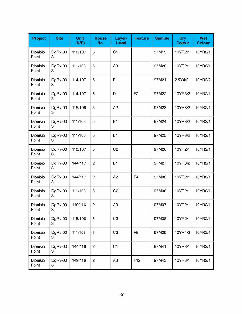
Project Site Unit (N/E)

House No.

Layer/Level

Feature Sample Dry Colour

Wet Colour

Dionisio Point

DgRv-003

110/107 5 C1 97M19 10YR2/1 10YR2/1

Dionisio Point

DgRv-003

111/106 5 A3 97M20 10YR2/1 10YR2/1

Dionisio Point

DgRv-003

114/107 5 E 97M21 2.5Y4/2 10YR2/2

Dionisio Point

DgRv-003

114/107 5 D F2 97M22 10YR3/2 10YR2/1

Dionisio Point

DgRv-003

115/106 5 A2 97M23 10YR3/2 10YR2/1

Dionisio Point

DgRv-003

111/106 5 B1 97M24 10YR3/2 10YR2/1

Dionisio Point

DgRv-003

111/106 5 B1 97M25 10YR3/2 10YR2/1

Dionisio Point

DgRv-003

110/107 5 C2 97M26 10YR2/1 10YR2/1

Dionisio Point

DgRv-003

144/117 2 B1 97M27 10YR3/2 10YR2/1

Dionisio Point

DgRv-003

144/117 2 A2 F4 97M32 10YR2/1 10YR2/1

Dionisio Point

DgRv-003

111/106 5 C2 97M36 10YR2/1 10YR2/1

Dionisio Point

DgRv-003

149/116 2 A3 97M37 10YR2/1 10YR2/1

Dionisio Point

DgRv-003

115/106 5 C3 97M38 10YR2/1 10YR2/1

Dionisio Point

DgRv-003

111/106 5 C3 F6 97M39 10YR4/2 10YR2/1

Dionisio Point

DgRv-003

144/116 2 C1 97M41 10YR3/1 10YR2/1

Dionisio Point

DgRv-003

149/116 2 A3 F12 97M43 10YR3/1 10YR2/1

150

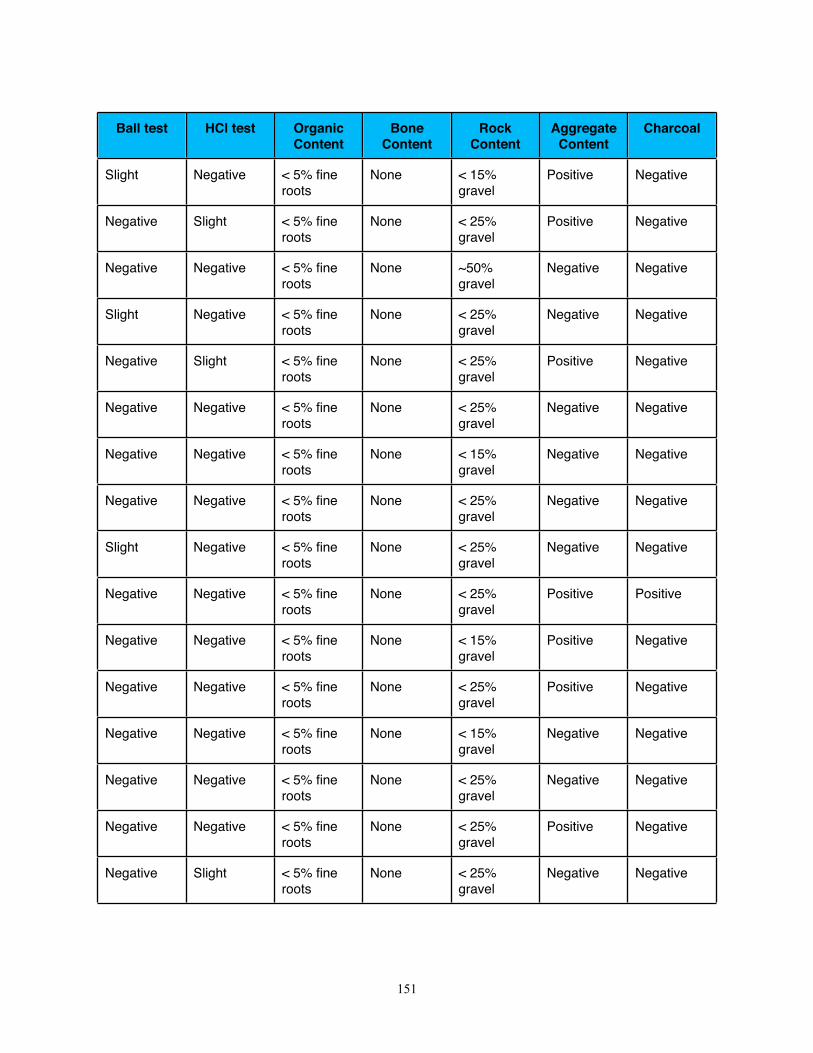
Ball test HCl test Organic Content

Bone Content

Rock Content

Aggregate Content

Charcoal

Slight Negative < 5% fine roots

None < 15% gravel

Positive Negative

Negative Slight < 5% fine roots

None < 25% gravel

Positive Negative

Negative Negative < 5% fine roots

None ~50% gravel

Negative Negative

Slight Negative < 5% fine roots

None < 25% gravel

Negative Negative

Negative Slight < 5% fine roots

None < 25% gravel

Positive Negative

Negative Negative < 5% fine roots

None < 25% gravel

Negative Negative

Negative Negative < 5% fine roots

None < 15% gravel

Negative Negative

Negative Negative < 5% fine roots

None < 25% gravel

Negative Negative

Slight Negative < 5% fine roots

None < 25% gravel

Negative Negative

Negative Negative < 5% fine roots

None < 25% gravel

Positive Positive

Negative Negative < 5% fine roots

None < 15% gravel

Positive Negative

Negative Negative < 5% fine roots

None < 25% gravel

Positive Negative

Negative Negative < 5% fine roots

None < 15% gravel

Negative Negative

Negative Negative < 5% fine roots

None < 25% gravel

Negative Negative

Negative Negative < 5% fine roots

None < 25% gravel

Positive Negative

Negative Slight < 5% fine roots

None < 25% gravel

Negative Negative

151

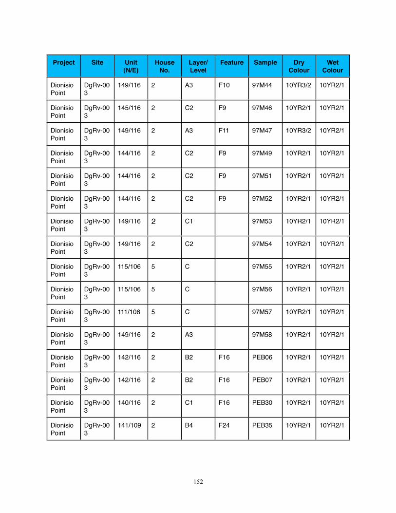
Project Site Unit (N/E)

House No.

Layer/Level

Feature Sample Dry Colour

Wet Colour

Dionisio Point

DgRv-003

149/116 2 A3 F10 97M44 10YR3/2 10YR2/1

Dionisio Point

DgRv-003

145/116 2 C2 F9 97M46 10YR2/1 10YR2/1

Dionisio Point

DgRv-003

149/116 2 A3 F11 97M47 10YR3/2 10YR2/1

Dionisio Point

DgRv-003

144/116 2 C2 F9 97M49 10YR2/1 10YR2/1

Dionisio Point

DgRv-003

144/116 2 C2 F9 97M51 10YR2/1 10YR2/1

Dionisio Point

DgRv-003

144/116 2 C2 F9 97M52 10YR2/1 10YR2/1

Dionisio Point

DgRv-003

149/116 2 C1 97M53 10YR2/1 10YR2/1

Dionisio Point

DgRv-003

149/116 2 C2 97M54 10YR2/1 10YR2/1

Dionisio Point

DgRv-003

115/106 5 C 97M55 10YR2/1 10YR2/1

Dionisio Point

DgRv-003

115/106 5 C 97M56 10YR2/1 10YR2/1

Dionisio Point

DgRv-003

111/106 5 C 97M57 10YR2/1 10YR2/1

Dionisio Point

DgRv-003

149/116 2 A3 97M58 10YR2/1 10YR2/1

Dionisio Point

DgRv-003

142/116 2 B2 F16 PEB06 10YR2/1 10YR2/1

Dionisio Point

DgRv-003

142/116 2 B2 F16 PEB07 10YR2/1 10YR2/1

Dionisio Point

DgRv-003

140/116 2 C1 F16 PEB30 10YR2/1 10YR2/1

Dionisio Point

DgRv-003

141/109 2 B4 F24 PEB35 10YR2/1 10YR2/1

152

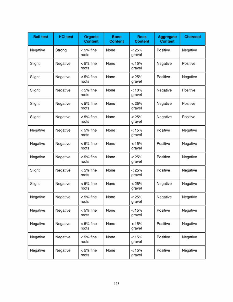
Ball test HCl test Organic Content

Bone Content

Rock Content

Aggregate Content

Charcoal

Negative Strong < 5% fine roots

None < 25% gravel

Positive Negative

Slight Negative < 5% fine roots

None < 15% gravel

Negative Positive

Slight Negative < 5% fine roots

None < 25% gravel

Positive Negative

Slight Negative < 5% fine roots

None < 10% gravel

Negative Positive

Slight Negative < 5% fine roots

None < 25% gravel

Negative Positive

Slight Negative < 5% fine roots

None < 25% gravel

Negative Positive

Negative Negative < 5% fine roots

None < 15% gravel

Positive Negative

Negative Negative < 5% fine roots

None < 15% gravel

Positive Negative

Negative Negative < 5% fine roots

None < 25% gravel

Positive Negative

Slight Negative < 5% fine roots

None < 25% gravel

Positive Negative

Slight Negative < 5% fine roots

None < 25% gravel

Negative Negative

Negative Negative < 5% fine roots

None < 25% gravel

Negative Negative

Negative Negative < 5% fine roots

None < 15% gravel

Positive Negative

Negative Negative < 5% fine roots

None < 15% gravel

Positive Negative

Negative Negative < 5% fine roots

None < 15% gravel

Positive Negative

Negative Negative < 5% fine roots

None < 15% gravel

Positive Negative

153

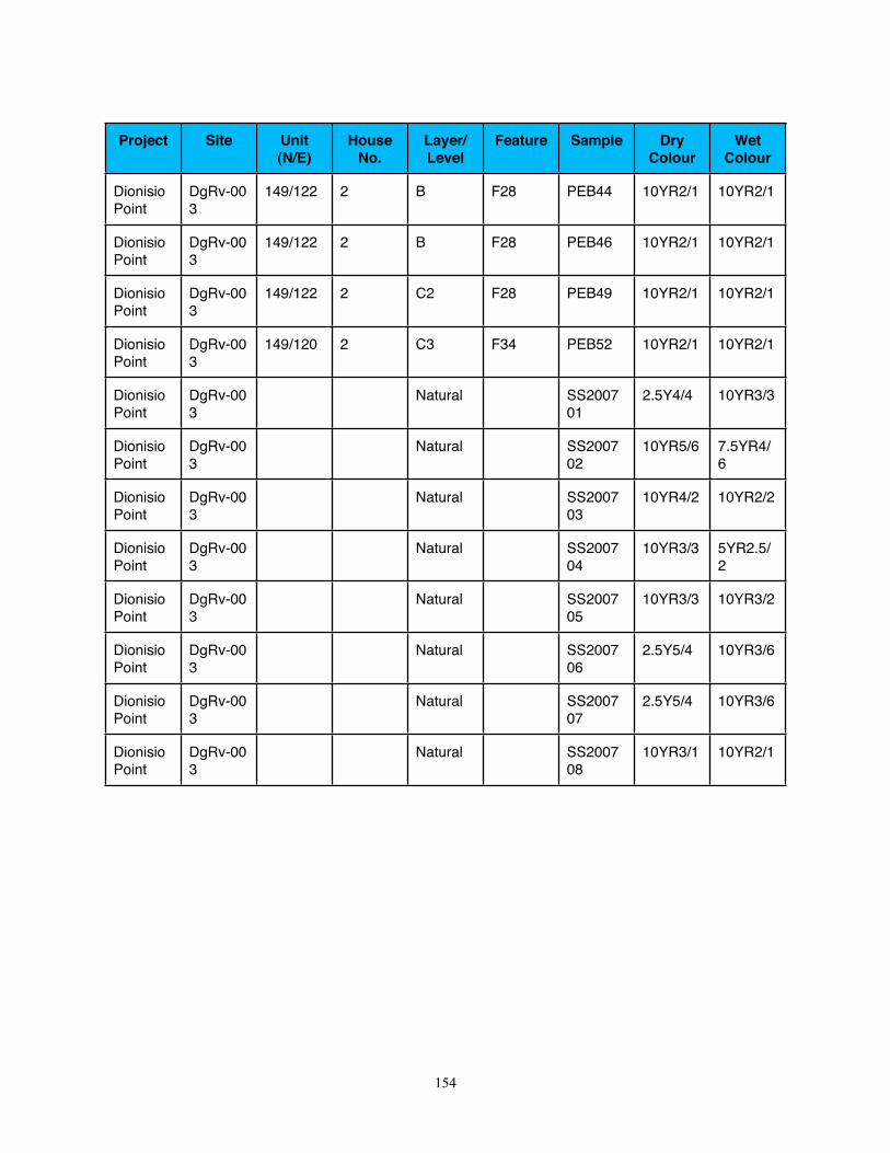
Project Site Unit (N/E)

House No.

Layer/Level

Feature Sample Dry Colour

Wet Colour

Dionisio Point

DgRv-003

149/122 2 B F28 PEB44 10YR2/1 10YR2/1

Dionisio Point

DgRv-003

149/122 2 B F28 PEB46 10YR2/1 10YR2/1

Dionisio Point

DgRv-003

149/122 2 C2 F28 PEB49 10YR2/1 10YR2/1

Dionisio Point

DgRv-003

149/120 2 C3 F34 PEB52 10YR2/1 10YR2/1

Dionisio Point

DgRv-003

Natural SS200701

2.5Y4/4 10YR3/3

Dionisio Point

DgRv-003

Natural SS200702

10YR5/6 7.5YR4/6

Dionisio Point

DgRv-003

Natural SS200703

10YR4/2 10YR2/2

Dionisio Point

DgRv-003

Natural SS200704

10YR3/3 5YR2.5/2

Dionisio Point

DgRv-003

Natural SS200705

10YR3/3 10YR3/2

Dionisio Point

DgRv-003

Natural SS200706

2.5Y5/4 10YR3/6

Dionisio Point

DgRv-003

Natural SS200707

2.5Y5/4 10YR3/6

Dionisio Point

DgRv-003

Natural SS200708

10YR3/1 10YR2/1

154

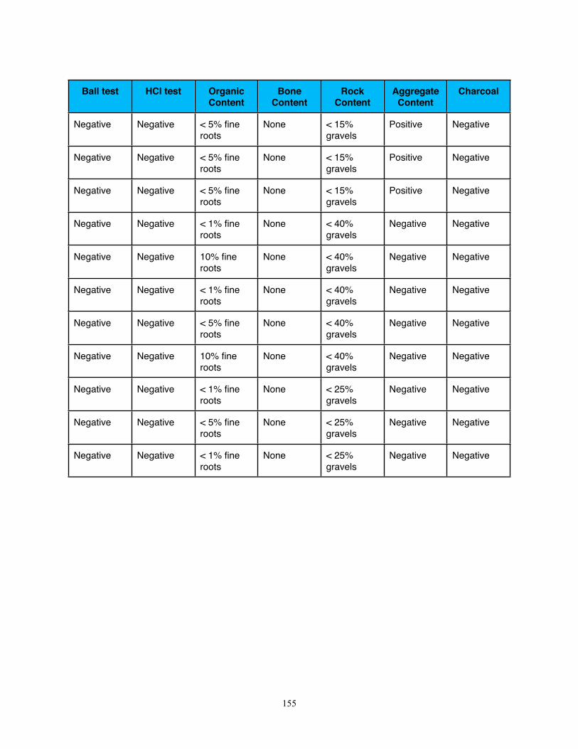
Ball test HCl test Organic Content

Bone Content

Rock Content

Aggregate Content

Charcoal

Negative Negative < 5% fine roots

None < 15% gravels

Positive Negative

Negative Negative < 5% fine roots

None < 15% gravels

Positive Negative

Negative Negative < 5% fine roots

None < 15% gravels

Positive Negative

Negative Negative < 1% fine roots

None < 40% gravels

Negative Negative

Negative Negative 10% fine roots

None < 40% gravels

Negative Negative

Negative Negative < 1% fine roots

None < 40% gravels

Negative Negative

Negative Negative < 5% fine roots

None < 40% gravels

Negative Negative

Negative Negative 10% fine roots

None < 40% gravels

Negative Negative

Negative Negative < 1% fine roots

None < 25% gravels

Negative Negative

Negative Negative < 5% fine roots

None < 25% gravels

Negative Negative

Negative Negative < 1% fine roots

None < 25% gravels

Negative Negative

155

Appendix C: Laser Particle Size Analyzer Data

156

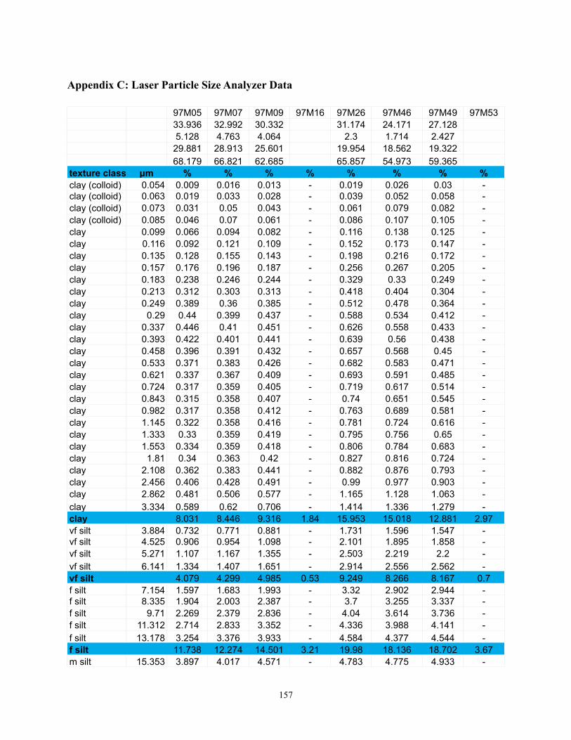
Appendix C: Laser Particle Size Analyzer Data

97M05 97M07 97M09 97M16 97M26 97M46 97M49 97M5333.936 32.992 30.332 31.174 24.171 27.1285.128 4.763 4.064 2.3 1.714 2.427

29.881 28.913 25.601 19.954 18.562 19.32268.179 66.821 62.685 65.857 54.973 59.365

texture class µm % % % % % % % %clay (colloid) 0.054 0.009 0.016 0.013 - 0.019 0.026 0.03 -clay (colloid) 0.063 0.019 0.033 0.028 - 0.039 0.052 0.058 -clay (colloid) 0.073 0.031 0.05 0.043 - 0.061 0.079 0.082 -clay (colloid) 0.085 0.046 0.07 0.061 - 0.086 0.107 0.105 -clay 0.099 0.066 0.094 0.082 - 0.116 0.138 0.125 -clay 0.116 0.092 0.121 0.109 - 0.152 0.173 0.147 -clay 0.135 0.128 0.155 0.143 - 0.198 0.216 0.172 -clay 0.157 0.176 0.196 0.187 - 0.256 0.267 0.205 -clay 0.183 0.238 0.246 0.244 - 0.329 0.33 0.249 -clay 0.213 0.312 0.303 0.313 - 0.418 0.404 0.304 -clay 0.249 0.389 0.36 0.385 - 0.512 0.478 0.364 -clay 0.29 0.44 0.399 0.437 - 0.588 0.534 0.412 -clay 0.337 0.446 0.41 0.451 - 0.626 0.558 0.433 -clay 0.393 0.422 0.401 0.441 - 0.639 0.56 0.438 -clay 0.458 0.396 0.391 0.432 - 0.657 0.568 0.45 -clay 0.533 0.371 0.383 0.426 - 0.682 0.583 0.471 -clay 0.621 0.337 0.367 0.409 - 0.693 0.591 0.485 -clay 0.724 0.317 0.359 0.405 - 0.719 0.617 0.514 -clay 0.843 0.315 0.358 0.407 - 0.74 0.651 0.545 -clay 0.982 0.317 0.358 0.412 - 0.763 0.689 0.581 -clay 1.145 0.322 0.358 0.416 - 0.781 0.724 0.616 -clay 1.333 0.33 0.359 0.419 - 0.795 0.756 0.65 -clay 1.553 0.334 0.359 0.418 - 0.806 0.784 0.683 -clay 1.81 0.34 0.363 0.42 - 0.827 0.816 0.724 -clay 2.108 0.362 0.383 0.441 - 0.882 0.876 0.793 -clay 2.456 0.406 0.428 0.491 - 0.99 0.977 0.903 -clay 2.862 0.481 0.506 0.577 - 1.165 1.128 1.063 -clay 3.334 0.589 0.62 0.706 - 1.414 1.336 1.279 -clay 8.031 8.446 9.316 1.84 15.953 15.018 12.881 2.97vf silt 3.884 0.732 0.771 0.881 - 1.731 1.596 1.547 -vf silt 4.525 0.906 0.954 1.098 - 2.101 1.895 1.858 -vf silt 5.271 1.107 1.167 1.355 - 2.503 2.219 2.2 -vf silt 6.141 1.334 1.407 1.651 - 2.914 2.556 2.562 -vf silt 4.079 4.299 4.985 0.53 9.249 8.266 8.167 0.7f silt 7.154 1.597 1.683 1.993 - 3.32 2.902 2.944 -f silt 8.335 1.904 2.003 2.387 - 3.7 3.255 3.337 -f silt 9.71 2.269 2.379 2.836 - 4.04 3.614 3.736 -f silt 11.312 2.714 2.833 3.352 - 4.336 3.988 4.141 -f silt 13.178 3.254 3.376 3.933 - 4.584 4.377 4.544 -f silt 11.738 12.274 14.501 3.21 19.98 18.136 18.702 3.67m silt 15.353 3.897 4.017 4.571 - 4.783 4.775 4.933 -

157

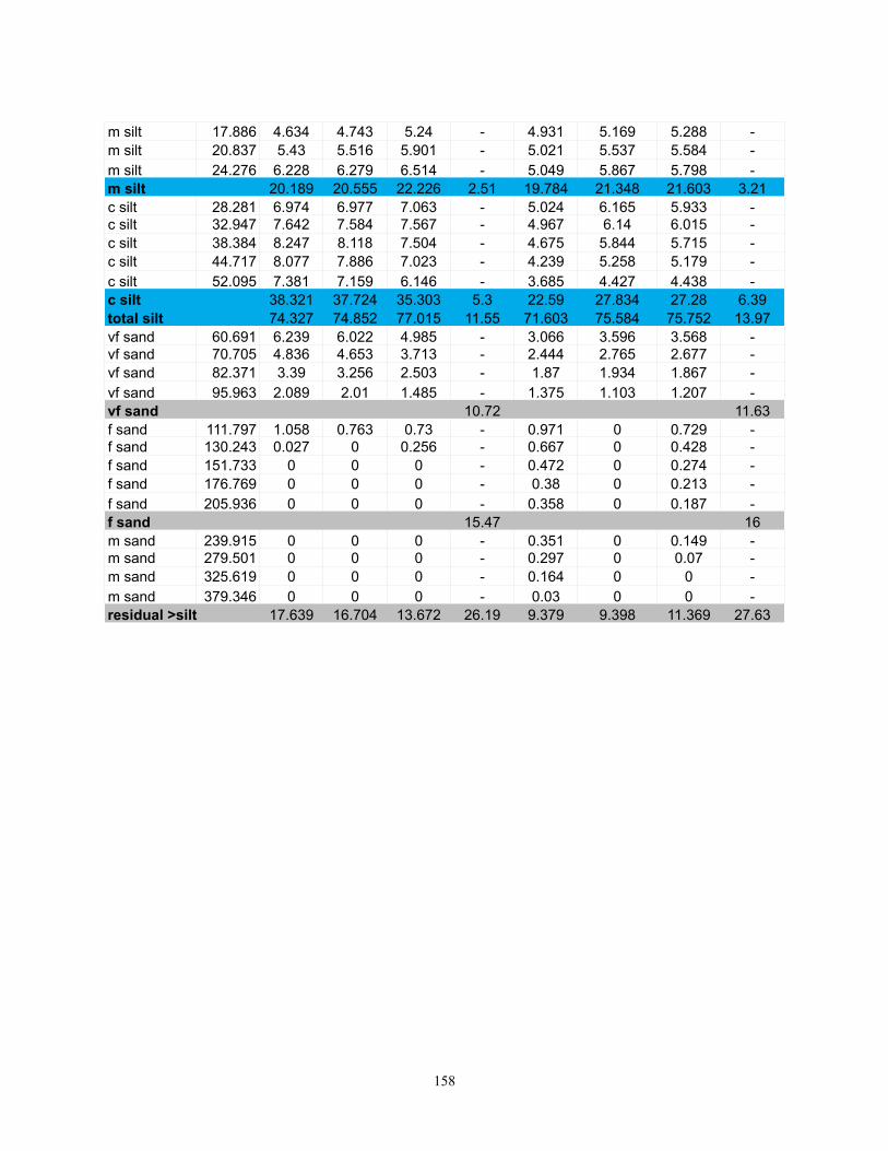
m silt 17.886 4.634 4.743 5.24 - 4.931 5.169 5.288 -m silt 20.837 5.43 5.516 5.901 - 5.021 5.537 5.584 -m silt 24.276 6.228 6.279 6.514 - 5.049 5.867 5.798 -m silt 20.189 20.555 22.226 2.51 19.784 21.348 21.603 3.21c silt 28.281 6.974 6.977 7.063 - 5.024 6.165 5.933 -c silt 32.947 7.642 7.584 7.567 - 4.967 6.14 6.015 -c silt 38.384 8.247 8.118 7.504 - 4.675 5.844 5.715 -c silt 44.717 8.077 7.886 7.023 - 4.239 5.258 5.179 -c silt 52.095 7.381 7.159 6.146 - 3.685 4.427 4.438 -c silt 38.321 37.724 35.303 5.3 22.59 27.834 27.28 6.39total silt 74.327 74.852 77.015 11.55 71.603 75.584 75.752 13.97vf sand 60.691 6.239 6.022 4.985 - 3.066 3.596 3.568 -vf sand 70.705 4.836 4.653 3.713 - 2.444 2.765 2.677 -vf sand 82.371 3.39 3.256 2.503 - 1.87 1.934 1.867 -vf sand 95.963 2.089 2.01 1.485 - 1.375 1.103 1.207 -vf sand 10.72 11.63f sand 111.797 1.058 0.763 0.73 - 0.971 0 0.729 -f sand 130.243 0.027 0 0.256 - 0.667 0 0.428 -f sand 151.733 0 0 0 - 0.472 0 0.274 -f sand 176.769 0 0 0 - 0.38 0 0.213 -f sand 205.936 0 0 0 - 0.358 0 0.187 -f sand 15.47 16m sand 239.915 0 0 0 - 0.351 0 0.149 -m sand 279.501 0 0 0 - 0.297 0 0.07 -m sand 325.619 0 0 0 - 0.164 0 0 -m sand 379.346 0 0 0 - 0.03 0 0 -residual >siltresidual >silt 17.639 16.704 13.672 26.19 9.379 9.398 11.369 27.63

158

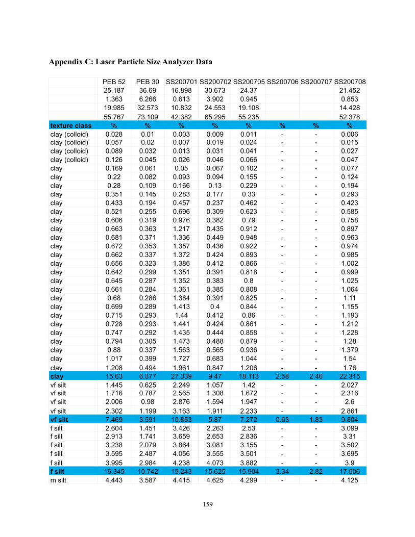
Appendix C: Laser Particle Size Analyzer Data

PEB 52 PEB 30 SS200701 SS200702 SS200705 SS200706 SS200707 SS20070825.187 36.69 16.898 30.673 24.37 21.4521.363 6.266 0.613 3.902 0.945 0.853

19.985 32.573 10.832 24.553 19.108 14.42855.767 73.109 42.382 65.295 55.235 52.378

texture class % % % % % % % %clay (colloid) 0.028 0.01 0.003 0.009 0.011 - - 0.006clay (colloid) 0.057 0.02 0.007 0.019 0.024 - - 0.015clay (colloid) 0.089 0.032 0.013 0.031 0.041 - - 0.027clay (colloid) 0.126 0.045 0.026 0.046 0.066 - - 0.047clay 0.169 0.061 0.05 0.067 0.102 - - 0.077clay 0.22 0.082 0.093 0.094 0.155 - - 0.124clay 0.28 0.109 0.166 0.13 0.229 - - 0.194clay 0.351 0.145 0.283 0.177 0.33 - - 0.293clay 0.433 0.194 0.457 0.237 0.462 - - 0.423clay 0.521 0.255 0.696 0.309 0.623 - - 0.585clay 0.606 0.319 0.976 0.382 0.79 - - 0.758clay 0.663 0.363 1.217 0.435 0.912 - - 0.897clay 0.681 0.371 1.336 0.449 0.948 - - 0.963clay 0.672 0.353 1.357 0.436 0.922 - - 0.974clay 0.662 0.337 1.372 0.424 0.893 - - 0.985clay 0.656 0.323 1.386 0.412 0.866 - - 1.002clay 0.642 0.299 1.351 0.391 0.818 - - 0.999clay 0.645 0.287 1.352 0.383 0.8 - - 1.025clay 0.661 0.284 1.361 0.385 0.808 - - 1.064clay 0.68 0.286 1.384 0.391 0.825 - - 1.11clay 0.699 0.289 1.413 0.4 0.844 - - 1.155clay 0.715 0.293 1.44 0.412 0.86 - - 1.193clay 0.728 0.293 1.441 0.424 0.861 - - 1.212clay 0.747 0.292 1.435 0.444 0.858 - - 1.228clay 0.794 0.305 1.473 0.488 0.879 - - 1.28clay 0.88 0.337 1.563 0.565 0.936 - - 1.379clay 1.017 0.399 1.727 0.683 1.044 - - 1.54clay 1.208 0.494 1.961 0.847 1.206 - - 1.76clay 15.63 6.877 27.339 9.47 18.113 2.58 2.46 22.315vf silt 1.445 0.625 2.249 1.057 1.42 - - 2.027vf silt 1.716 0.787 2.565 1.308 1.672 - - 2.316vf silt 2.006 0.98 2.876 1.594 1.947 - - 2.6vf silt 2.302 1.199 3.163 1.911 2.233 - - 2.861vf silt 7.469 3.591 10.853 5.87 7.272 0.63 1.83 9.804f silt 2.604 1.451 3.426 2.263 2.53 - - 3.099f silt 2.913 1.741 3.659 2.653 2.836 - - 3.31f silt 3.238 2.079 3.864 3.081 3.155 - - 3.502f silt 3.595 2.487 4.056 3.555 3.501 - - 3.695f silt 3.995 2.984 4.238 4.073 3.882 - - 3.9f silt 16.345 10.742 19.243 15.625 15.904 3.34 2.82 17.506m silt 4.443 3.587 4.415 4.625 4.299 - - 4.125

159

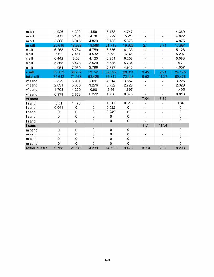
m silt 4.926 4.302 4.59 5.188 4.747 - - 4.369m silt 5.411 5.104 4.76 5.722 5.21 - - 4.622m silt 5.866 5.945 4.823 6.183 5.673 - - 4.875m silt 20.646 18.938 18.588 21.718 19.929 2.1 3.71 17.991c silt 6.268 6.754 4.759 6.536 6.133 - - 5.128c silt 6.62 7.461 4.532 6.78 6.32 - - 5.207c silt 6.442 8.03 4.123 6.951 6.208 - - 5.083c silt 5.868 8.473 3.529 6.535 5.734 - - 4.7c silt 4.954 7.989 2.798 5.797 4.916 - - 4.057c silt 30.152 38.707 19.741 32.599 29.311 3.45 2.91 24.175total silt 74.612 71.978 68.425 75.812 72.416 9.52 11.27 69.476vf sand 3.829 6.981 2.011 4.814 3.857 - - 3.226vf sand 2.691 5.605 1.276 3.722 2.729 - - 2.329vf sand 1.708 4.229 0.68 2.66 1.697 - - 1.495vf sand 0.979 2.853 0.272 1.738 0.875 - - 0.818vf sand 7.04 8.86f sand 0.51 1.478 0 1.017 0.315 - - 0.34f sand 0.041 0 0 0.522 0 - - 0f sand 0 0 0 0.249 0 - - 0f sand 0 0 0 0 0 - - 0f sand 0 0 0 0 0 - - 0f sand 11.1 11.34m sand 0 0 0 0 0 - - 0m sand 0 0 0 0 0 - - 0m sand 0 0 0 0 0 - - 0m sand 0 0 0 0 0 - - 0residual >silt 9.758 21.146 4.239 14.722 9.473 18.14 20.2 8.208

160

Appendix D: Hydrometer Raw Data

161

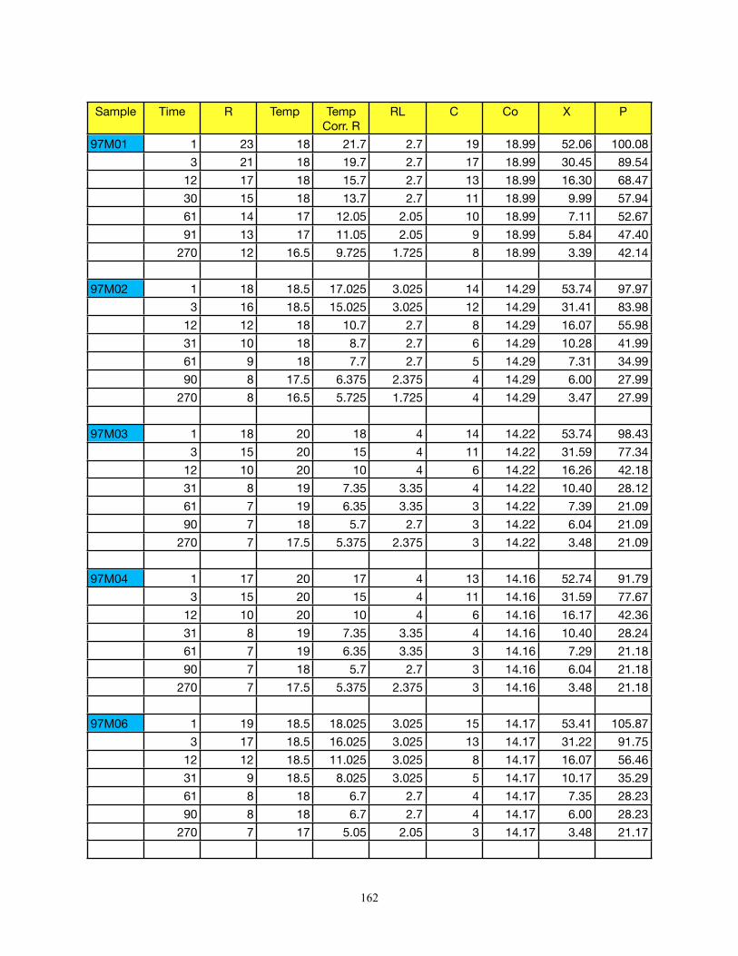
Sample Time R Temp Temp Corr. R

RL C Co X P

97M01 1 23 18 21.7 2.7 19 18.99 52.06 100.08

3 21 18 19.7 2.7 17 18.99 30.45 89.54

12 17 18 15.7 2.7 13 18.99 16.30 68.47

30 15 18 13.7 2.7 11 18.99 9.99 57.94

61 14 17 12.05 2.05 10 18.99 7.11 52.67

91 13 17 11.05 2.05 9 18.99 5.84 47.40

270 12 16.5 9.725 1.725 8 18.99 3.39 42.14

97M02 1 18 18.5 17.025 3.025 14 14.29 53.74 97.97

3 16 18.5 15.025 3.025 12 14.29 31.41 83.98

12 12 18 10.7 2.7 8 14.29 16.07 55.98

31 10 18 8.7 2.7 6 14.29 10.28 41.99

61 9 18 7.7 2.7 5 14.29 7.31 34.99

90 8 17.5 6.375 2.375 4 14.29 6.00 27.99

270 8 16.5 5.725 1.725 4 14.29 3.47 27.99

97M03 1 18 20 18 4 14 14.22 53.74 98.43

3 15 20 15 4 11 14.22 31.59 77.34

12 10 20 10 4 6 14.22 16.26 42.18

31 8 19 7.35 3.35 4 14.22 10.40 28.12

61 7 19 6.35 3.35 3 14.22 7.39 21.09

90 7 18 5.7 2.7 3 14.22 6.04 21.09

270 7 17.5 5.375 2.375 3 14.22 3.48 21.09

97M04 1 17 20 17 4 13 14.16 52.74 91.79

3 15 20 15 4 11 14.16 31.59 77.67

12 10 20 10 4 6 14.16 16.17 42.36

31 8 19 7.35 3.35 4 14.16 10.40 28.24

61 7 19 6.35 3.35 3 14.16 7.29 21.18

90 7 18 5.7 2.7 3 14.16 6.04 21.18

270 7 17.5 5.375 2.375 3 14.16 3.48 21.18

97M06 1 19 18.5 18.025 3.025 15 14.17 53.41 105.87

3 17 18.5 16.025 3.025 13 14.17 31.22 91.75

12 12 18.5 11.025 3.025 8 14.17 16.07 56.46

31 9 18.5 8.025 3.025 5 14.17 10.17 35.29

61 8 18 6.7 2.7 4 14.17 7.35 28.23

90 8 18 6.7 2.7 4 14.17 6.00 28.23

270 7 17 5.05 2.05 3 14.17 3.48 21.17

162

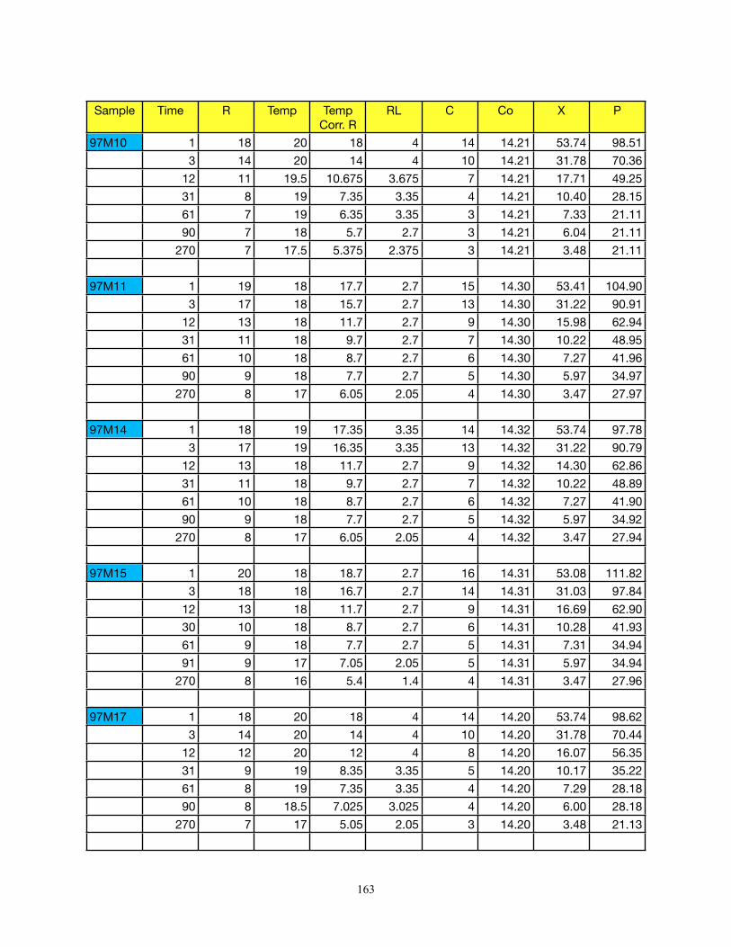
Sample Time R Temp Temp Corr. R

RL C Co X P

97M10 1 18 20 18 4 14 14.21 53.74 98.51

3 14 20 14 4 10 14.21 31.78 70.36

12 11 19.5 10.675 3.675 7 14.21 17.71 49.25

31 8 19 7.35 3.35 4 14.21 10.40 28.15

61 7 19 6.35 3.35 3 14.21 7.33 21.11

90 7 18 5.7 2.7 3 14.21 6.04 21.11

270 7 17.5 5.375 2.375 3 14.21 3.48 21.11

97M11 1 19 18 17.7 2.7 15 14.30 53.41 104.90

3 17 18 15.7 2.7 13 14.30 31.22 90.91

12 13 18 11.7 2.7 9 14.30 15.98 62.94

31 11 18 9.7 2.7 7 14.30 10.22 48.95

61 10 18 8.7 2.7 6 14.30 7.27 41.96

90 9 18 7.7 2.7 5 14.30 5.97 34.97

270 8 17 6.05 2.05 4 14.30 3.47 27.97

97M14 1 18 19 17.35 3.35 14 14.32 53.74 97.78

3 17 19 16.35 3.35 13 14.32 31.22 90.79

12 13 18 11.7 2.7 9 14.32 14.30 62.86

31 11 18 9.7 2.7 7 14.32 10.22 48.89

61 10 18 8.7 2.7 6 14.32 7.27 41.90

90 9 18 7.7 2.7 5 14.32 5.97 34.92

270 8 17 6.05 2.05 4 14.32 3.47 27.94

97M15 1 20 18 18.7 2.7 16 14.31 53.08 111.82

3 18 18 16.7 2.7 14 14.31 31.03 97.84

12 13 18 11.7 2.7 9 14.31 16.69 62.90

30 10 18 8.7 2.7 6 14.31 10.28 41.93

61 9 18 7.7 2.7 5 14.31 7.31 34.94

91 9 17 7.05 2.05 5 14.31 5.97 34.94

270 8 16 5.4 1.4 4 14.31 3.47 27.96

97M17 1 18 20 18 4 14 14.20 53.74 98.62

3 14 20 14 4 10 14.20 31.78 70.44

12 12 20 12 4 8 14.20 16.07 56.35

31 9 19 8.35 3.35 5 14.20 10.17 35.22

61 8 19 7.35 3.35 4 14.20 7.29 28.18

90 8 18.5 7.025 3.025 4 14.20 6.00 28.18

270 7 17 5.05 2.05 3 14.20 3.48 21.13

163

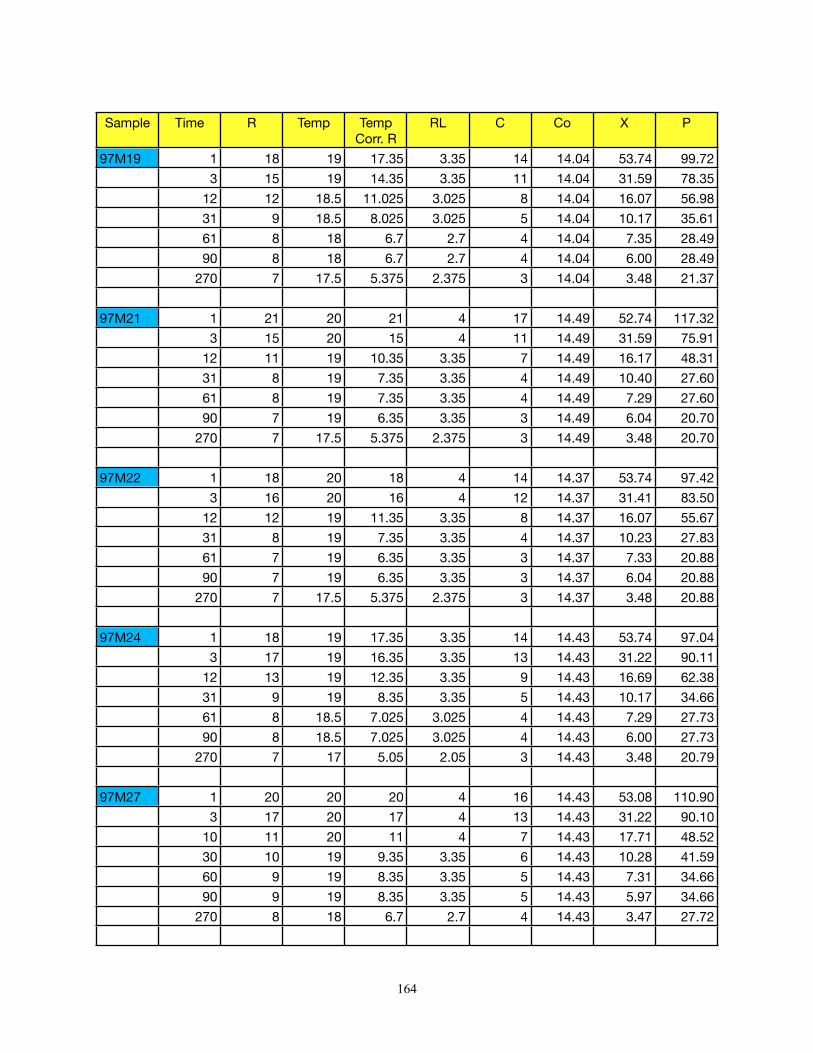
Sample Time R Temp Temp Corr. R

RL C Co X P

97M19 1 18 19 17.35 3.35 14 14.04 53.74 99.72

3 15 19 14.35 3.35 11 14.04 31.59 78.35

12 12 18.5 11.025 3.025 8 14.04 16.07 56.98

31 9 18.5 8.025 3.025 5 14.04 10.17 35.61

61 8 18 6.7 2.7 4 14.04 7.35 28.49

90 8 18 6.7 2.7 4 14.04 6.00 28.49

270 7 17.5 5.375 2.375 3 14.04 3.48 21.37

97M21 1 21 20 21 4 17 14.49 52.74 117.32

3 15 20 15 4 11 14.49 31.59 75.91

12 11 19 10.35 3.35 7 14.49 16.17 48.31

31 8 19 7.35 3.35 4 14.49 10.40 27.60

61 8 19 7.35 3.35 4 14.49 7.29 27.60

90 7 19 6.35 3.35 3 14.49 6.04 20.70

270 7 17.5 5.375 2.375 3 14.49 3.48 20.70

97M22 1 18 20 18 4 14 14.37 53.74 97.42

3 16 20 16 4 12 14.37 31.41 83.50

12 12 19 11.35 3.35 8 14.37 16.07 55.67

31 8 19 7.35 3.35 4 14.37 10.23 27.83

61 7 19 6.35 3.35 3 14.37 7.33 20.88

90 7 19 6.35 3.35 3 14.37 6.04 20.88

270 7 17.5 5.375 2.375 3 14.37 3.48 20.88

97M24 1 18 19 17.35 3.35 14 14.43 53.74 97.04

3 17 19 16.35 3.35 13 14.43 31.22 90.11

12 13 19 12.35 3.35 9 14.43 16.69 62.38

31 9 19 8.35 3.35 5 14.43 10.17 34.66

61 8 18.5 7.025 3.025 4 14.43 7.29 27.73

90 8 18.5 7.025 3.025 4 14.43 6.00 27.73

270 7 17 5.05 2.05 3 14.43 3.48 20.79

97M27 1 20 20 20 4 16 14.43 53.08 110.90

3 17 20 17 4 13 14.43 31.22 90.10

10 11 20 11 4 7 14.43 17.71 48.52

30 10 19 9.35 3.35 6 14.43 10.28 41.59

60 9 19 8.35 3.35 5 14.43 7.31 34.66

90 9 19 8.35 3.35 5 14.43 5.97 34.66

270 8 18 6.7 2.7 4 14.43 3.47 27.72

164

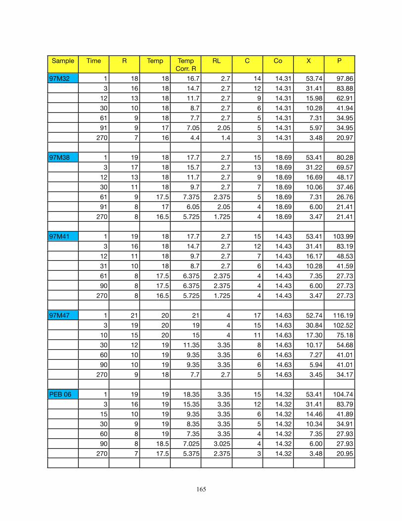
Sample Time R Temp Temp Corr. R

RL C Co X P

97M32 1 18 18 16.7 2.7 14 14.31 53.74 97.86

3 16 18 14.7 2.7 12 14.31 31.41 83.88

12 13 18 11.7 2.7 9 14.31 15.98 62.91

30 10 18 8.7 2.7 6 14.31 10.28 41.94

61 9 18 7.7 2.7 5 14.31 7.31 34.95

91 9 17 7.05 2.05 5 14.31 5.97 34.95

270 7 16 4.4 1.4 3 14.31 3.48 20.97

97M38 1 19 18 17.7 2.7 15 18.69 53.41 80.28

3 17 18 15.7 2.7 13 18.69 31.22 69.57

12 13 18 11.7 2.7 9 18.69 16.69 48.17

30 11 18 9.7 2.7 7 18.69 10.06 37.46

61 9 17.5 7.375 2.375 5 18.69 7.31 26.76

91 8 17 6.05 2.05 4 18.69 6.00 21.41

270 8 16.5 5.725 1.725 4 18.69 3.47 21.41

97M41 1 19 18 17.7 2.7 15 14.43 53.41 103.99

3 16 18 14.7 2.7 12 14.43 31.41 83.19

12 11 18 9.7 2.7 7 14.43 16.17 48.53

31 10 18 8.7 2.7 6 14.43 10.28 41.59

61 8 17.5 6.375 2.375 4 14.43 7.35 27.73

90 8 17.5 6.375 2.375 4 14.43 6.00 27.73

270 8 16.5 5.725 1.725 4 14.43 3.47 27.73

97M47 1 21 20 21 4 17 14.63 52.74 116.19

3 19 20 19 4 15 14.63 30.84 102.52

10 15 20 15 4 11 14.63 17.30 75.18

30 12 19 11.35 3.35 8 14.63 10.17 54.68

60 10 19 9.35 3.35 6 14.63 7.27 41.01

90 10 19 9.35 3.35 6 14.63 5.94 41.01

270 9 18 7.7 2.7 5 14.63 3.45 34.17

PEB 06 1 19 19 18.35 3.35 15 14.32 53.41 104.74

3 16 19 15.35 3.35 12 14.32 31.41 83.79

15 10 19 9.35 3.35 6 14.32 14.46 41.89

30 9 19 8.35 3.35 5 14.32 10.34 34.91

60 8 19 7.35 3.35 4 14.32 7.35 27.93

90 8 18.5 7.025 3.025 4 14.32 6.00 27.93

270 7 17.5 5.375 2.375 3 14.32 3.48 20.95

165

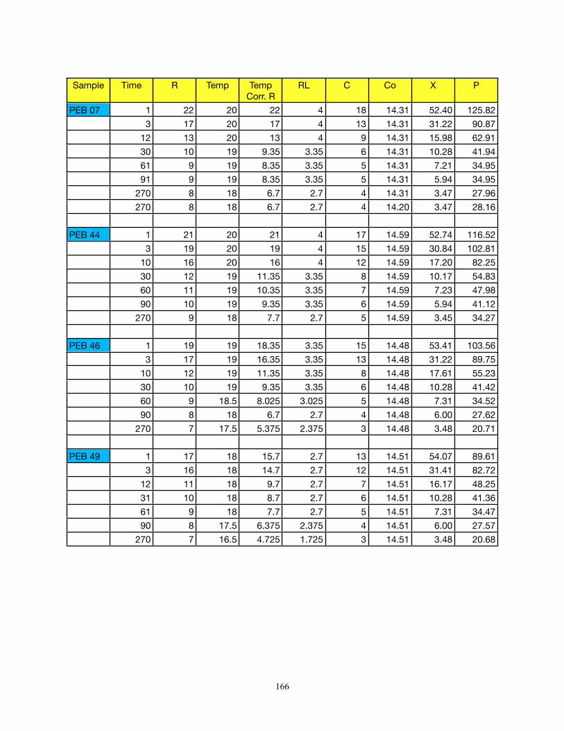
Sample Time R Temp Temp Corr. R

RL C Co X P

PEB 07 1 22 20 22 4 18 14.31 52.40 125.82

3 17 20 17 4 13 14.31 31.22 90.87

12 13 20 13 4 9 14.31 15.98 62.91

30 10 19 9.35 3.35 6 14.31 10.28 41.94

61 9 19 8.35 3.35 5 14.31 7.21 34.95

91 9 19 8.35 3.35 5 14.31 5.94 34.95

270 8 18 6.7 2.7 4 14.31 3.47 27.96

270 8 18 6.7 2.7 4 14.20 3.47 28.16

PEB 44 1 21 20 21 4 17 14.59 52.74 116.52

3 19 20 19 4 15 14.59 30.84 102.81

10 16 20 16 4 12 14.59 17.20 82.25

30 12 19 11.35 3.35 8 14.59 10.17 54.83

60 11 19 10.35 3.35 7 14.59 7.23 47.98

90 10 19 9.35 3.35 6 14.59 5.94 41.12

270 9 18 7.7 2.7 5 14.59 3.45 34.27

PEB 46 1 19 19 18.35 3.35 15 14.48 53.41 103.56

3 17 19 16.35 3.35 13 14.48 31.22 89.75

10 12 19 11.35 3.35 8 14.48 17.61 55.23

30 10 19 9.35 3.35 6 14.48 10.28 41.42

60 9 18.5 8.025 3.025 5 14.48 7.31 34.52

90 8 18 6.7 2.7 4 14.48 6.00 27.62

270 7 17.5 5.375 2.375 3 14.48 3.48 20.71

PEB 49 1 17 18 15.7 2.7 13 14.51 54.07 89.61

3 16 18 14.7 2.7 12 14.51 31.41 82.72

12 11 18 9.7 2.7 7 14.51 16.17 48.25

31 10 18 8.7 2.7 6 14.51 10.28 41.36

61 9 18 7.7 2.7 5 14.51 7.31 34.47

90 8 17.5 6.375 2.375 4 14.51 6.00 27.57

270 7 16.5 4.725 1.725 3 14.51 3.48 20.68

166

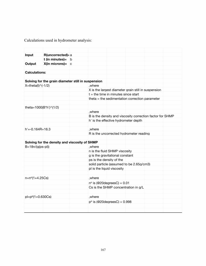
Calculations used in hydrometer analysis:

Input R(uncorrected)=at (in minutes)= b

Output X(in microns)= c

Calculations:Calculations:

Solving for the grain diameter still in suspensionSolving for the grain diameter still in suspensionSolving for the grain diameter still in suspensionSolving for the grain diameter still in suspensionX=theta(t)^(-1/2)X=theta(t)^(-1/2) ,where

X is the largest diameter grain still in suspensionX is the largest diameter grain still in suspensionX is the largest diameter grain still in suspensionX is the largest diameter grain still in suspensiont = the time in minutes since startt = the time in minutes since startt = the time in minutes since starttheta = the sedimentation correction parametertheta = the sedimentation correction parametertheta = the sedimentation correction parametertheta = the sedimentation correction parameter

theta=1000(B*h')^(1/2)theta=1000(B*h')^(1/2),whereB is the density and viscosity correction factor for SHMPB is the density and viscosity correction factor for SHMPB is the density and viscosity correction factor for SHMPB is the density and viscosity correction factor for SHMPB is the density and viscosity correction factor for SHMPh' is the effective hydrometer depthh' is the effective hydrometer depthh' is the effective hydrometer depth

h'=-0.164R+16.3h'=-0.164R+16.3 ,whereR is the uncorrected hydrometer readingR is the uncorrected hydrometer readingR is the uncorrected hydrometer readingR is the uncorrected hydrometer reading

Solving for the density and viscosity of SHMPSolving for the density and viscosity of SHMPSolving for the density and viscosity of SHMPSolving for the density and viscosity of SHMPB=18n/(g(ps-pl))B=18n/(g(ps-pl)) ,where

n is the fluid SHMP viscosityn is the fluid SHMP viscosityn is the fluid SHMP viscosityg is the gravitational constantg is the gravitational constantg is the gravitational constantps is the density of the ps is the density of the solid particle (assumed to be 2.65g/cm3)solid particle (assumed to be 2.65g/cm3)solid particle (assumed to be 2.65g/cm3)solid particle (assumed to be 2.65g/cm3)pl is the liquid viscositypl is the liquid viscosity

n=no(1+4.25Cs)n=no(1+4.25Cs) ,where

no is (@20degreesC) = 0.01no is (@20degreesC) = 0.01no is (@20degreesC) = 0.01Cs is the SHMP concentration in g/LCs is the SHMP concentration in g/LCs is the SHMP concentration in g/LCs is the SHMP concentration in g/L

pl=pp(1+0.630Cs)pl=pp(1+0.630Cs) ,where

po is (@20degreesC) = 0.998po is (@20degreesC) = 0.998po is (@20degreesC) = 0.998

167

Appendix E: Hydrometer Results

185

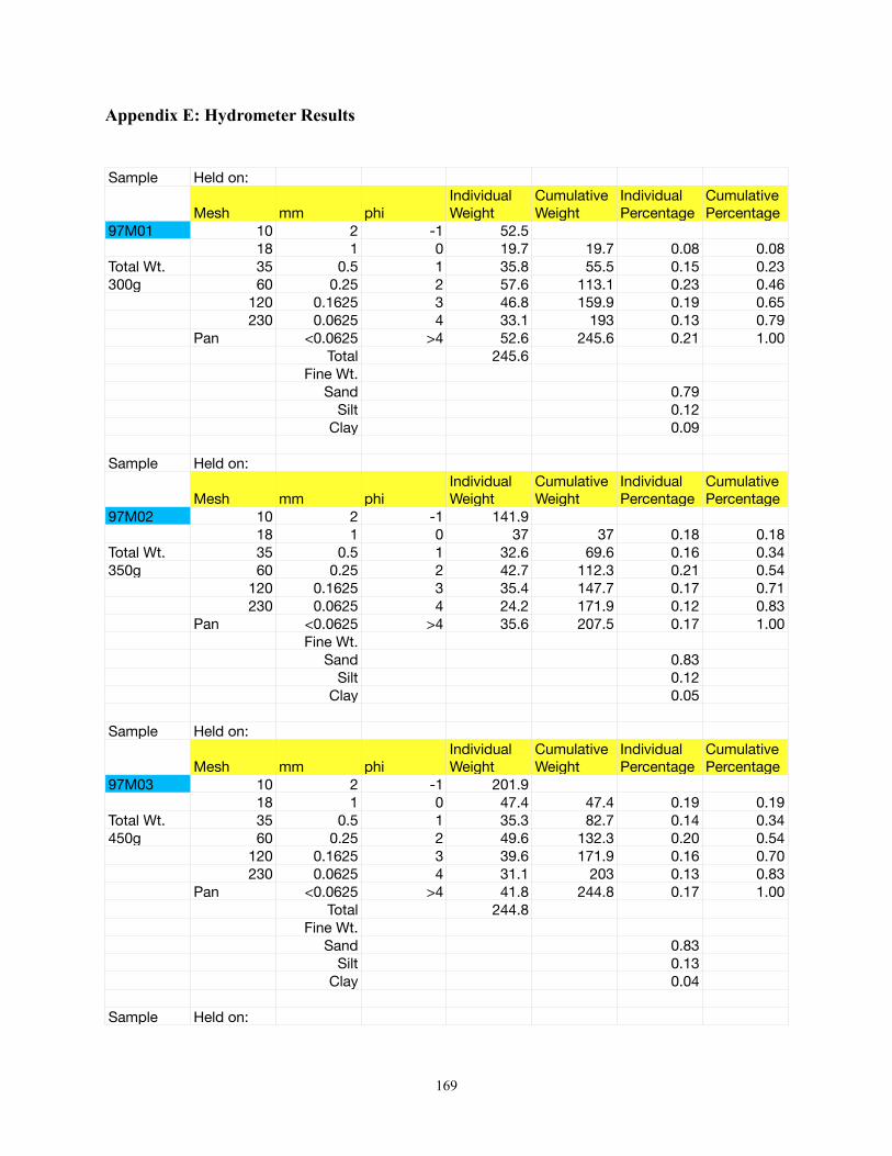
Sample Held on:

Mesh mm phiIndividual Weight

Cumulative Weight

Individual Percentage

Cumulative Percentage

97M01 10 2 -1 52.518 1 0 19.7 19.7 0.08 0.08

Total Wt. 35 0.5 1 35.8 55.5 0.15 0.23300g 60 0.25 2 57.6 113.1 0.23 0.46

120 0.1625 3 46.8 159.9 0.19 0.65230 0.0625 4 33.1 193 0.13 0.79

Pan <0.0625 >4 52.6 245.6 0.21 1.00Total 245.6

Fine Wt.Sand 0.79

Silt 0.12Clay 0.09

Sample Held on:

Mesh mm phiIndividual Weight

Cumulative Weight

Individual Percentage

Cumulative Percentage

97M02 10 2 -1 141.918 1 0 37 37 0.18 0.18

Total Wt. 35 0.5 1 32.6 69.6 0.16 0.34350g 60 0.25 2 42.7 112.3 0.21 0.54

120 0.1625 3 35.4 147.7 0.17 0.71230 0.0625 4 24.2 171.9 0.12 0.83

Pan <0.0625 >4 35.6 207.5 0.17 1.00Fine Wt.

Sand 0.83Silt 0.12

Clay 0.05

Sample Held on:

Mesh mm phiIndividual Weight

Cumulative Weight

Individual Percentage

Cumulative Percentage

97M03 10 2 -1 201.918 1 0 47.4 47.4 0.19 0.19

Total Wt. 35 0.5 1 35.3 82.7 0.14 0.34450g 60 0.25 2 49.6 132.3 0.20 0.54

120 0.1625 3 39.6 171.9 0.16 0.70230 0.0625 4 31.1 203 0.13 0.83

Pan <0.0625 >4 41.8 244.8 0.17 1.00Total 244.8

Fine Wt.Sand 0.83

Silt 0.13Clay 0.04

Sample Held on:

Appendix E: Hydrometer Results

169

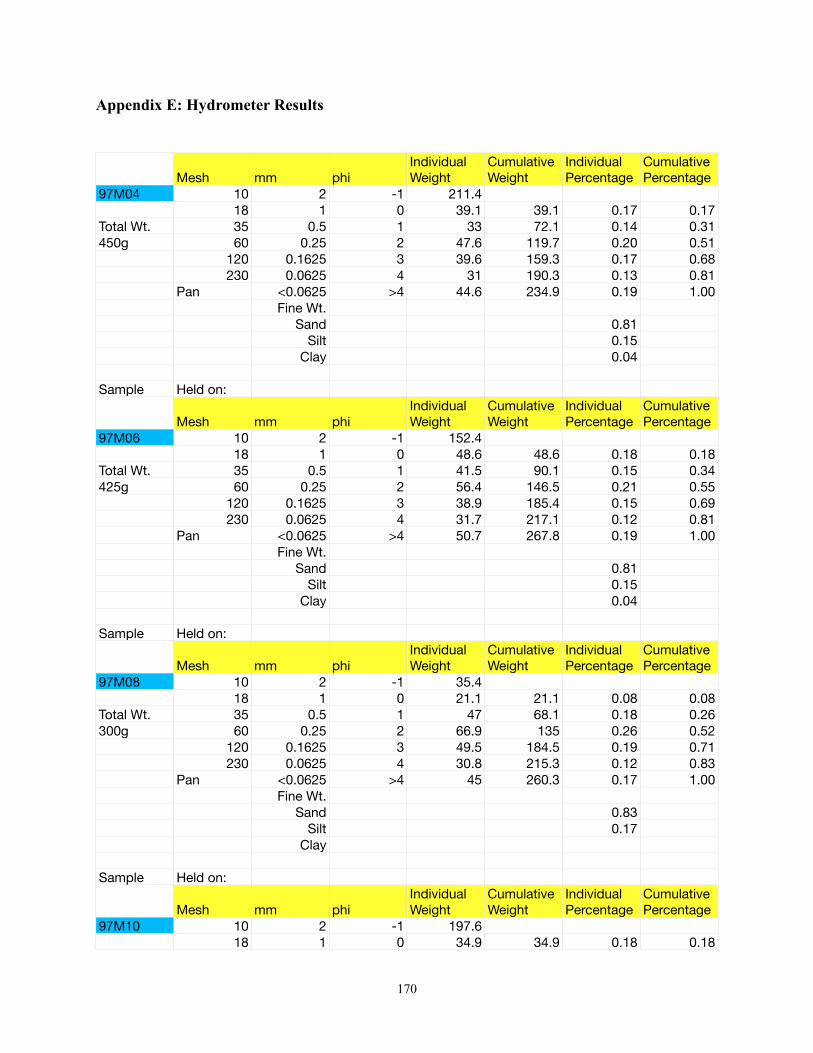
Mesh mm phiIndividual Weight

Cumulative Weight

Individual Percentage

Cumulative Percentage

97M04 10 2 -1 211.418 1 0 39.1 39.1 0.17 0.17

Total Wt. 35 0.5 1 33 72.1 0.14 0.31450g 60 0.25 2 47.6 119.7 0.20 0.51

120 0.1625 3 39.6 159.3 0.17 0.68230 0.0625 4 31 190.3 0.13 0.81

Pan <0.0625 >4 44.6 234.9 0.19 1.00Fine Wt.

Sand 0.81Silt 0.15

Clay 0.04

Sample Held on:

Mesh mm phiIndividual Weight

Cumulative Weight

Individual Percentage

Cumulative Percentage

97M06 10 2 -1 152.418 1 0 48.6 48.6 0.18 0.18

Total Wt. 35 0.5 1 41.5 90.1 0.15 0.34425g 60 0.25 2 56.4 146.5 0.21 0.55

120 0.1625 3 38.9 185.4 0.15 0.69230 0.0625 4 31.7 217.1 0.12 0.81

Pan <0.0625 >4 50.7 267.8 0.19 1.00Fine Wt.

Sand 0.81Silt 0.15

Clay 0.04

Sample Held on:

Mesh mm phiIndividual Weight

Cumulative Weight

Individual Percentage

Cumulative Percentage

97M08 10 2 -1 35.418 1 0 21.1 21.1 0.08 0.08

Total Wt. 35 0.5 1 47 68.1 0.18 0.26300g 60 0.25 2 66.9 135 0.26 0.52

120 0.1625 3 49.5 184.5 0.19 0.71230 0.0625 4 30.8 215.3 0.12 0.83

Pan <0.0625 >4 45 260.3 0.17 1.00Fine Wt.

Sand 0.83Silt 0.17

Clay

Sample Held on:

Mesh mm phiIndividual Weight

Cumulative Weight

Individual Percentage

Cumulative Percentage

97M10 10 2 -1 197.618 1 0 34.9 34.9 0.18 0.18

Appendix E: Hydrometer Results

170

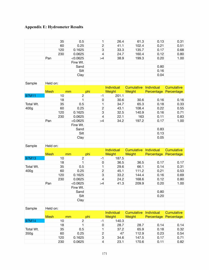
35 0.5 1 26.4 61.3 0.13 0.3160 0.25 2 41.1 102.4 0.21 0.51

120 0.1625 3 33.3 135.7 0.17 0.68230 0.0625 4 24.7 160.4 0.12 0.80

Pan <0.0625 >4 38.9 199.3 0.20 1.00Fine Wt.

Sand 0.80Silt 0.16

Clay 0.04

Sample Held on:

Mesh mm phiIndividual Weight

Cumulative Weight

Individual Percentage

Cumulative Percentage

97M11 10 2 -1 201.118 1 0 30.6 30.6 0.16 0.16

Total Wt. 35 0.5 1 34.7 65.3 0.18 0.33400g 60 0.25 2 43.1 108.4 0.22 0.55

120 0.1625 3 32.5 140.9 0.16 0.71230 0.0625 4 22.1 163 0.11 0.83

Pan <0.0625 >4 34.2 197.2 0.17 1.00Fine Wt.

Sand 0.83Silt 0.13

Clay 0.05

Sample Held on:

Mesh mm phiIndividual Weight

Cumulative Weight

Individual Percentage

Cumulative Percentage

97M13 10 2 -1 187.518 1 0 36.5 36.5 0.17 0.17

Total Wt. 35 0.5 1 29.6 66.1 0.14 0.31400g 60 0.25 2 45.1 111.2 0.21 0.53

120 0.1625 3 33.2 144.4 0.16 0.69230 0.0625 4 24.2 168.6 0.12 0.80

Pan <0.0625 >4 41.3 209.9 0.20 1.00Fine Wt.

Sand 0.80Silt 0.20

Clay

Sample Held on:

Mesh mm phiIndividual Weight

Cumulative Weight

Individual Percentage

Cumulative Percentage

97M14 10 2 -1 140.318 1 0 28.7 28.7 0.14 0.14

Total Wt. 35 0.5 1 37.2 65.9 0.18 0.32350g 60 0.25 2 47 112.9 0.23 0.54

120 0.1625 3 34.6 147.5 0.17 0.71230 0.0625 4 23.1 170.6 0.11 0.82

Appendix E: Hydrometer Results

171

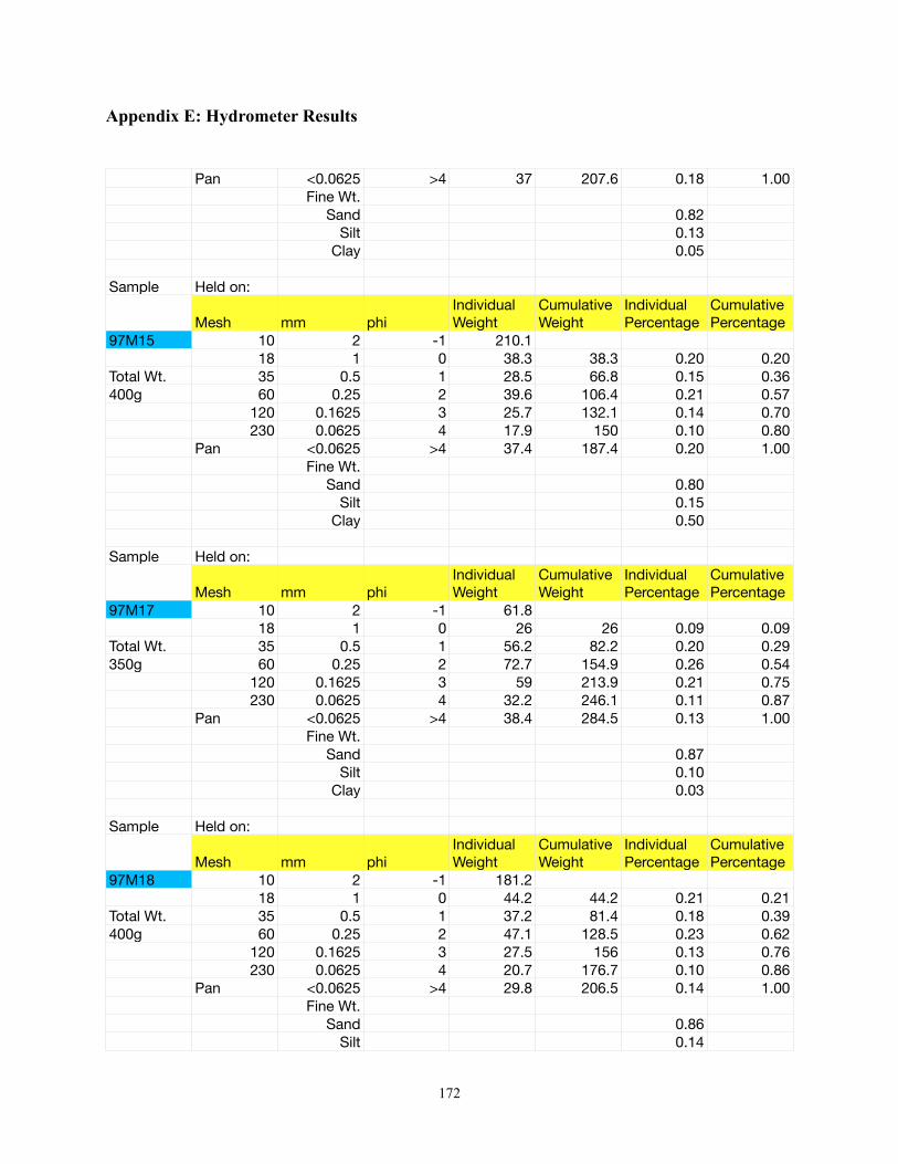
Pan <0.0625 >4 37 207.6 0.18 1.00Fine Wt.

Sand 0.82Silt 0.13

Clay 0.05

Sample Held on:

Mesh mm phiIndividual Weight

Cumulative Weight

Individual Percentage

Cumulative Percentage

97M15 10 2 -1 210.118 1 0 38.3 38.3 0.20 0.20

Total Wt. 35 0.5 1 28.5 66.8 0.15 0.36400g 60 0.25 2 39.6 106.4 0.21 0.57

120 0.1625 3 25.7 132.1 0.14 0.70230 0.0625 4 17.9 150 0.10 0.80

Pan <0.0625 >4 37.4 187.4 0.20 1.00Fine Wt.

Sand 0.80Silt 0.15

Clay 0.50

Sample Held on:

Mesh mm phiIndividual Weight

Cumulative Weight

Individual Percentage

Cumulative Percentage

97M17 10 2 -1 61.818 1 0 26 26 0.09 0.09

Total Wt. 35 0.5 1 56.2 82.2 0.20 0.29350g 60 0.25 2 72.7 154.9 0.26 0.54

120 0.1625 3 59 213.9 0.21 0.75230 0.0625 4 32.2 246.1 0.11 0.87

Pan <0.0625 >4 38.4 284.5 0.13 1.00Fine Wt.

Sand 0.87Silt 0.10

Clay 0.03

Sample Held on:

Mesh mm phiIndividual Weight

Cumulative Weight

Individual Percentage

Cumulative Percentage

97M18 10 2 -1 181.218 1 0 44.2 44.2 0.21 0.21

Total Wt. 35 0.5 1 37.2 81.4 0.18 0.39400g 60 0.25 2 47.1 128.5 0.23 0.62

120 0.1625 3 27.5 156 0.13 0.76230 0.0625 4 20.7 176.7 0.10 0.86

Pan <0.0625 >4 29.8 206.5 0.14 1.00Fine Wt.

Sand 0.86Silt 0.14

Appendix E: Hydrometer Results

172

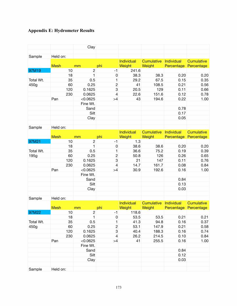
Clay

Sample Held on:

Mesh mm phiIndividual Weight

Cumulative Weight

Individual Percentage

Cumulative Percentage

97M19 10 2 -1 241.618 1 0 38.3 38.3 0.20 0.20

Total Wt. 35 0.5 1 29.2 67.5 0.15 0.35450g 60 0.25 2 41 108.5 0.21 0.56

120 0.1625 3 20.5 129 0.11 0.66230 0.0625 4 22.6 151.6 0.12 0.78

Pan <0.0625 >4 43 194.6 0.22 1.00Fine Wt.

Sand 0.78Silt 0.17

Clay 0.05

Sample Held on:

Mesh mm phiIndividual Weight

Cumulative Weight

Individual Percentage

Cumulative Percentage

97M21 10 2 -1 1.318 1 0 38.6 38.6 0.20 0.20

Total Wt. 35 0.5 1 36.6 75.2 0.19 0.39195g 60 0.25 2 50.8 126 0.26 0.65

120 0.1625 3 21 147 0.11 0.76230 0.0625 4 14.7 161.7 0.08 0.84

Pan <0.0625 >4 30.9 192.6 0.16 1.00Fine Wt.

Sand 0.84Silt 0.13

Clay 0.03

Sample Held on:

Mesh mm phiIndividual Weight

Cumulative Weight

Individual Percentage

Cumulative Percentage

97M22 10 2 -1 118.618 1 0 53.5 53.5 0.21 0.21

Total Wt. 35 0.5 1 41.3 94.8 0.16 0.37450g 60 0.25 2 53.1 147.9 0.21 0.58

120 0.1625 3 40.4 188.3 0.16 0.74230 0.0625 4 26.2 214.5 0.10 0.84

Pan <0.0625 >4 41 255.5 0.16 1.00Fine Wt.

Sand 0.84Silt 0.12

Clay 0.03

Sample Held on:

Appendix E: Hydrometer Results

173

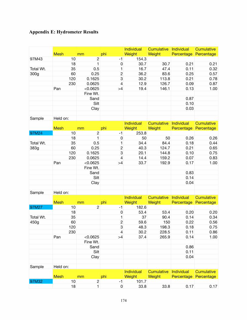
Mesh mm phiIndividual Weight

Cumulative Weight

Individual Percentage

Cumulative Percentage

97M43 10 2 -1 154.318 1 0 30.7 30.7 0.21 0.21

Total Wt. 35 0.5 1 16.7 47.4 0.11 0.32300g 60 0.25 2 36.2 83.6 0.25 0.57

120 0.1625 3 30.2 113.8 0.21 0.78230 0.0625 4 12.9 126.7 0.09 0.87

Pan <0.0625 >4 19.4 146.1 0.13 1.00Fine Wt.

Sand 0.87Silt 0.10

Clay 0.03

Sample Held on:

Mesh mm phiIndividual Weight

Cumulative Weight

Individual Percentage

Cumulative Percentage

97M24 10 2 -1 253.818 1 0 50 50 0.26 0.26

Total Wt. 35 0.5 1 34.4 84.4 0.18 0.44383g 60 0.25 2 40.3 124.7 0.21 0.65

120 0.1625 3 20.1 144.8 0.10 0.75230 0.0625 4 14.4 159.2 0.07 0.83

Pan <0.0625 >4 33.7 192.9 0.17 1.00Fine Wt.

Sand 0.83Silt 0.14

Clay 0.04

Sample Held on:

Mesh mm phiIndividual Weight

Cumulative Weight

Individual Percentage

Cumulative Percentage

97M27 10 2 -1 182.618 0 53.4 53.4 0.20 0.20

Total Wt. 35 1 37 90.4 0.14 0.34450g 60 2 59.6 150 0.22 0.56

120 3 48.3 198.3 0.18 0.75230 4 30.2 228.5 0.11 0.86

Pan <0.0625 >4 37.4 265.9 0.14 1.00Fine Wt.

Sand 0.86Silt 0.11

Clay 0.04

Sample Held on:

Mesh mm phiIndividual Weight

Cumulative Weight

Individual Percentage

Cumulative Percentage

97M32 10 2 -1 101.718 1 0 33.8 33.8 0.17 0.17

Appendix E: Hydrometer Results

174

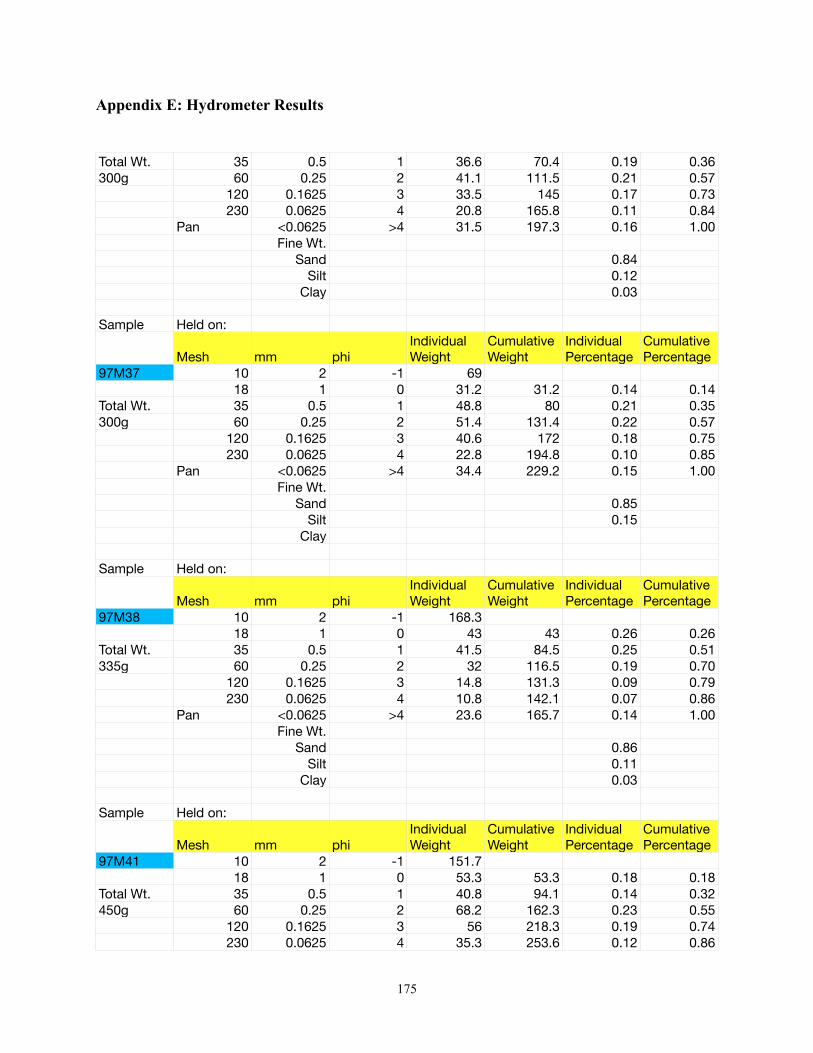
Total Wt. 35 0.5 1 36.6 70.4 0.19 0.36300g 60 0.25 2 41.1 111.5 0.21 0.57

120 0.1625 3 33.5 145 0.17 0.73230 0.0625 4 20.8 165.8 0.11 0.84

Pan <0.0625 >4 31.5 197.3 0.16 1.00Fine Wt.

Sand 0.84Silt 0.12

Clay 0.03

Sample Held on:

Mesh mm phiIndividual Weight

Cumulative Weight

Individual Percentage

Cumulative Percentage

97M37 10 2 -1 6918 1 0 31.2 31.2 0.14 0.14

Total Wt. 35 0.5 1 48.8 80 0.21 0.35300g 60 0.25 2 51.4 131.4 0.22 0.57

120 0.1625 3 40.6 172 0.18 0.75230 0.0625 4 22.8 194.8 0.10 0.85

Pan <0.0625 >4 34.4 229.2 0.15 1.00Fine Wt.

Sand 0.85Silt 0.15

Clay

Sample Held on:

Mesh mm phiIndividual Weight

Cumulative Weight

Individual Percentage

Cumulative Percentage

97M38 10 2 -1 168.318 1 0 43 43 0.26 0.26

Total Wt. 35 0.5 1 41.5 84.5 0.25 0.51335g 60 0.25 2 32 116.5 0.19 0.70

120 0.1625 3 14.8 131.3 0.09 0.79230 0.0625 4 10.8 142.1 0.07 0.86

Pan <0.0625 >4 23.6 165.7 0.14 1.00Fine Wt.

Sand 0.86Silt 0.11

Clay 0.03

Sample Held on:

Mesh mm phiIndividual Weight

Cumulative Weight

Individual Percentage

Cumulative Percentage

97M41 10 2 -1 151.718 1 0 53.3 53.3 0.18 0.18

Total Wt. 35 0.5 1 40.8 94.1 0.14 0.32450g 60 0.25 2 68.2 162.3 0.23 0.55

120 0.1625 3 56 218.3 0.19 0.74230 0.0625 4 35.3 253.6 0.12 0.86

Appendix E: Hydrometer Results

175

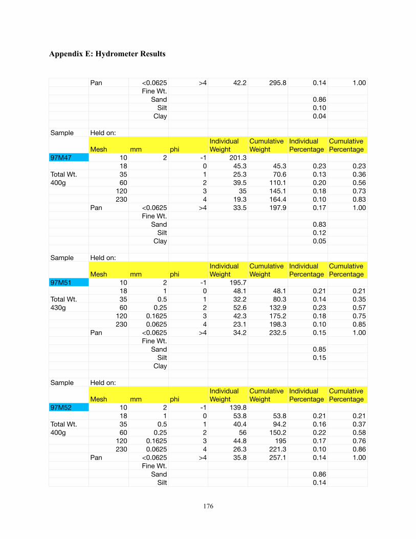
Pan <0.0625 >4 42.2 295.8 0.14 1.00Fine Wt.

Sand 0.86Silt 0.10

Clay 0.04

Sample Held on:

Mesh mm phiIndividual Weight

Cumulative Weight

Individual Percentage

Cumulative Percentage

97M47 10 2 -1 201.318 0 45.3 45.3 0.23 0.23

Total Wt. 35 1 25.3 70.6 0.13 0.36400g 60 2 39.5 110.1 0.20 0.56

120 3 35 145.1 0.18 0.73230 4 19.3 164.4 0.10 0.83

Pan <0.0625 >4 33.5 197.9 0.17 1.00Fine Wt.

Sand 0.83Silt 0.12

Clay 0.05

Sample Held on:

Mesh mm phiIndividual Weight

Cumulative Weight

Individual Percentage

Cumulative Percentage

97M51 10 2 -1 195.718 1 0 48.1 48.1 0.21 0.21

Total Wt. 35 0.5 1 32.2 80.3 0.14 0.35430g 60 0.25 2 52.6 132.9 0.23 0.57

120 0.1625 3 42.3 175.2 0.18 0.75230 0.0625 4 23.1 198.3 0.10 0.85

Pan <0.0625 >4 34.2 232.5 0.15 1.00Fine Wt.

Sand 0.85Silt 0.15

Clay

Sample Held on:

Mesh mm phiIndividual Weight

Cumulative Weight

Individual Percentage

Cumulative Percentage

97M52 10 2 -1 139.818 1 0 53.8 53.8 0.21 0.21

Total Wt. 35 0.5 1 40.4 94.2 0.16 0.37400g 60 0.25 2 56 150.2 0.22 0.58

120 0.1625 3 44.8 195 0.17 0.76230 0.0625 4 26.3 221.3 0.10 0.86

Pan <0.0625 >4 35.8 257.1 0.14 1.00Fine Wt.

Sand 0.86Silt 0.14

Appendix E: Hydrometer Results

176

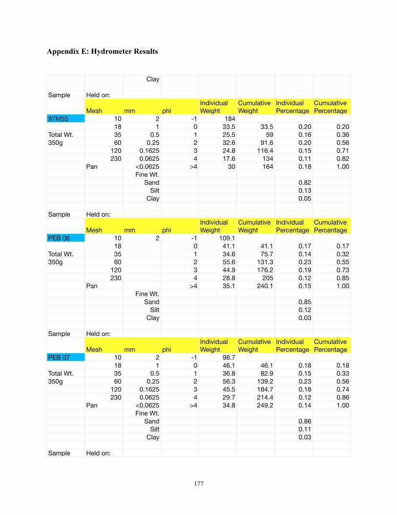
Clay

Sample Held on:

Mesh mm phiIndividual Weight

Cumulative Weight

Individual Percentage

Cumulative Percentage

97M55 10 2 -1 18418 1 0 33.5 33.5 0.20 0.20

Total Wt. 35 0.5 1 25.5 59 0.16 0.36350g 60 0.25 2 32.6 91.6 0.20 0.56

120 0.1625 3 24.8 116.4 0.15 0.71230 0.0625 4 17.6 134 0.11 0.82

Pan <0.0625 >4 30 164 0.18 1.00Fine Wt.

Sand 0.82Silt 0.13

Clay 0.05

Sample Held on:

Mesh mm phiIndividual Weight

Cumulative Weight

Individual Percentage

Cumulative Percentage

PEB 06 10 2 -1 109.118 0 41.1 41.1 0.17 0.17

Total Wt. 35 1 34.6 75.7 0.14 0.32350g 60 2 55.6 131.3 0.23 0.55

120 3 44.9 176.2 0.19 0.73230 4 28.8 205 0.12 0.85

Pan >4 35.1 240.1 0.15 1.00Fine Wt.

Sand 0.85Silt 0.12

Clay 0.03

Sample Held on:

Mesh mm phiIndividual Weight

Cumulative Weight

Individual Percentage

Cumulative Percentage

PEB 07 10 2 -1 98.718 1 0 46.1 46.1 0.18 0.18

Total Wt. 35 0.5 1 36.8 82.9 0.15 0.33350g 60 0.25 2 56.3 139.2 0.23 0.56

120 0.1625 3 45.5 184.7 0.18 0.74230 0.0625 4 29.7 214.4 0.12 0.86

Pan <0.0625 >4 34.8 249.2 0.14 1.00Fine Wt.

Sand 0.86Silt 0.11

Clay 0.03

Sample Held on:

Appendix E: Hydrometer Results

177

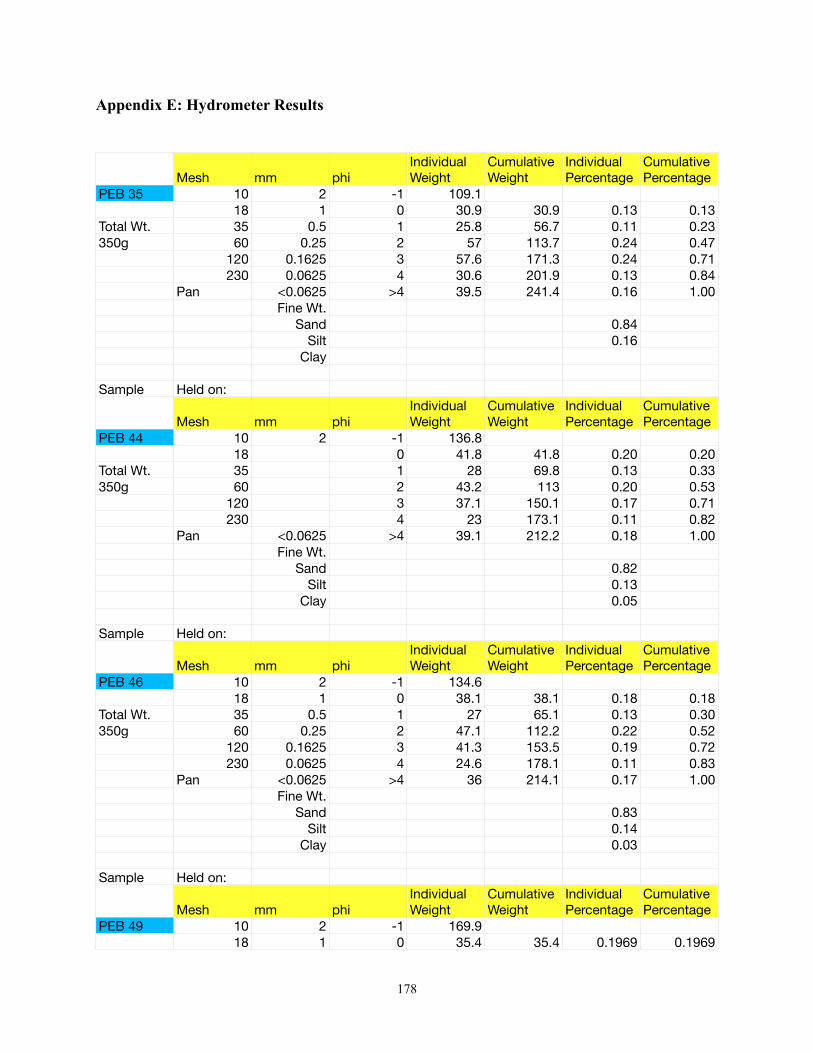
Mesh mm phiIndividual Weight

Cumulative Weight

Individual Percentage

Cumulative Percentage

PEB 35 10 2 -1 109.118 1 0 30.9 30.9 0.13 0.13

Total Wt. 35 0.5 1 25.8 56.7 0.11 0.23350g 60 0.25 2 57 113.7 0.24 0.47

120 0.1625 3 57.6 171.3 0.24 0.71230 0.0625 4 30.6 201.9 0.13 0.84

Pan <0.0625 >4 39.5 241.4 0.16 1.00Fine Wt.

Sand 0.84Silt 0.16

Clay

Sample Held on:

Mesh mm phiIndividual Weight

Cumulative Weight

Individual Percentage

Cumulative Percentage

PEB 44 10 2 -1 136.818 0 41.8 41.8 0.20 0.20

Total Wt. 35 1 28 69.8 0.13 0.33350g 60 2 43.2 113 0.20 0.53

120 3 37.1 150.1 0.17 0.71230 4 23 173.1 0.11 0.82

Pan <0.0625 >4 39.1 212.2 0.18 1.00Fine Wt.

Sand 0.82Silt 0.13

Clay 0.05

Sample Held on:

Mesh mm phiIndividual Weight

Cumulative Weight

Individual Percentage

Cumulative Percentage

PEB 46 10 2 -1 134.618 1 0 38.1 38.1 0.18 0.18

Total Wt. 35 0.5 1 27 65.1 0.13 0.30350g 60 0.25 2 47.1 112.2 0.22 0.52

120 0.1625 3 41.3 153.5 0.19 0.72230 0.0625 4 24.6 178.1 0.11 0.83

Pan <0.0625 >4 36 214.1 0.17 1.00Fine Wt.

Sand 0.83Silt 0.14

Clay 0.03

Sample Held on:

Mesh mm phiIndividual Weight

Cumulative Weight

Individual Percentage

Cumulative Percentage

PEB 49 10 2 -1 169.918 1 0 35.4 35.4 0.1969 0.1969

Appendix E: Hydrometer Results

178

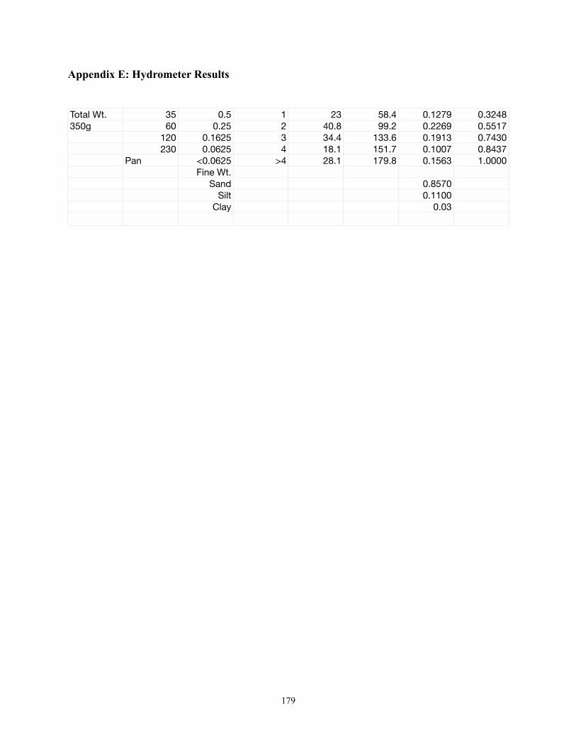
Total Wt. 35 0.5 1 23 58.4 0.1279 0.3248350g 60 0.25 2 40.8 99.2 0.2269 0.5517

120 0.1625 3 34.4 133.6 0.1913 0.7430230 0.0625 4 18.1 151.7 0.1007 0.8437

Pan <0.0625 >4 28.1 179.8 0.1563 1.0000Fine Wt.

Sand 0.8570Silt 0.1100

Clay 0.03

Appendix E: Hydrometer Results

179

Appendix F: Loss-On-Ignition Data

180

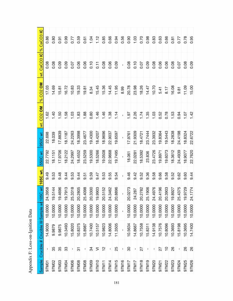
181

Sam

ple

Cru

cibl

e #

Cru

cibl

e W

t.Sam

ple

wt.1

05C

wt.

105C

wt.

550C

wt

950C

wt

wt.

CO

2 O

M%

CO

2 O

Mw

t. C

aCO

3 IC

% C

aCO

3 IC

97M

01-

14.9

030

10.0

000

24.3

958

9.49

22.7

792

22.6

981.

6217

.03

0.08

0.86

97M

0235

9.98

7910

.000

019

.514

49.

5318

.115

118

.039

1.40

14.6

90.

080.

80

97M

0335

9.98

7510

.000

019

.469

69.

4817

.970

617

.883

91.

5015

.81

0.09

0.91

97M

0433

10.3

493

10.0

000

19.7

913

9.44

18.2

122

18.1

187

1.58

16.7

20.

090.

99

97M

06-

15.8

020

10.0

000

25.3

318

9.53

24.2

997

24.2

263

1.03

10.8

30.

070.

77

97M

0831

10.8

375

10.0

000

20.2

805

9.44

18.4

552

18.3

998

1.83

19.3

30.

060.

59

97M

08-

15.8

987

10.0

000

25.4

098

9.51

23.5

259

23.4

677

1.88

19.8

10.

060.

61

97M

0934

10.7

400

10.0

000

20.3

300

9.59

19.5

300

19.4

300

0.80

8.34

0.10

1.04

97M

10V

I10

.515

710

.000

019

.990

39.

4718

.526

618

.420

71.

4615

.45

0.11

1.12

97M

1112

10.9

823

10.0

000

20.5

152

9.53

19.0

508

18.9

696

1.46

15.3

60.

080.

85

97M

14-

14.8

006

10.0

000

24.3

462

9.55

22.9

668

22.9

037

1.38

14.4

50.

060.

66

97M

1525

11.3

505

10.0

000

20.8

896

9.54

19.7

495

19.6

597

1.14

11.9

50.

090.

94

97M

16-

--

--

--

-8.

99-

0.56

97M

1730

10.5

634

10.0

000

20.0

273

9.46

18.0

6117

.976

11.

9720

.78

0.08

0.90

97M

17-

14.8

667

10.0

000

24.2

879.

4222

.028

121

.930

92.

2623

.98

0.10

1.03

97M

1827

10.7

558

10.0

000

20.2

782

9.52

18.5

392

18.4

721

1.74

18.2

60.

070.

70

97M

19-

15.8

311

10.0

000

25.1

906

9.36

23.8

3623

.744

41.

3514

.47

0.09

0.98

97M

20-

14.9

138

10.0

000

24.4

976

9.58

23.4

726

23.3

932

1.03

10.7

00.

080.

83

97M

2127

10.7

576

10.0

000

20.4

196

9.66

19.8

971

19.8

364

0.52

5.41

0.06

0.63

97M

2210

10.8

096

10.0

000

20.3

903

9.58

19.6

073

19.5

443

0.78

8.17

0.06

0.66

97M

2326

10.3

693

10.0

000

19.8

927

9.52

18.3

612

18.2

838

1.53

16.0

80.

080.

81

97M

24-

15.8

198

10.0

000

25.4

375

9.62

24.4

939

24.4

198

0.94

9.81

0.07

0.77

97M

2526

10.3

695

10.0

000

19.9

729

9.60

18.9

077

18.8

324

1.07

11.0

90.

080.

78

97M

2626

14.7

400

10.0

000

24.1

774

9.44

22.7

620

22.6

722

1.42

15.0

00.

090.

95

App

endi

x F:

Los

s-on

-Igni

tion

Dat

a

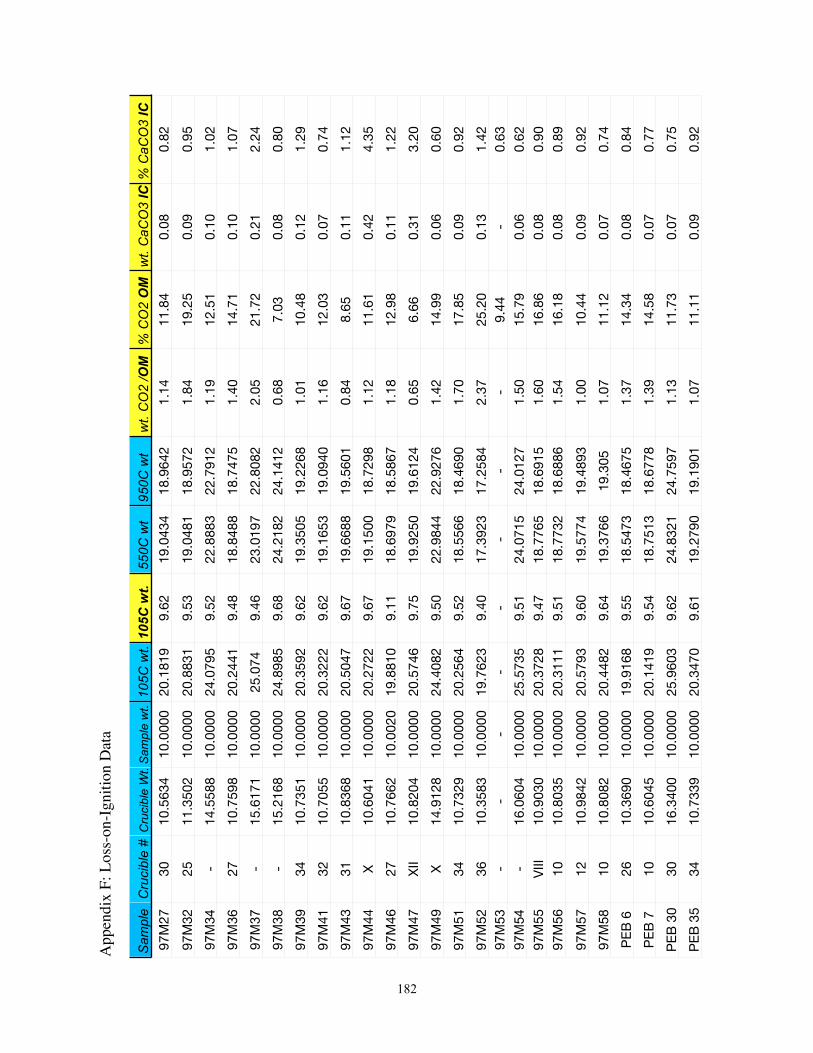
182

Sam

ple

Cru

cibl

e #

Cru

cibl

e W

t.S

ampl

e w

t.10

5C w

t.10

5C w

t.55

0C w

t95

0C w

tw

t. C

O2

/OM

% C

O2

OM

wt.

CaC

O3

IC%

CaC

O3

IC97

M27

3010

.563

410

.000

020

.181

99.

6219

.043

418

.964

21.

1411

.84

0.08

0.82

97M

3225

11.3

502

10.0

000

20.8

831

9.53

19.0

481

18.9

572

1.84

19.2

50.

090.

95

97M

34-

14.5

588

10.0

000

24.0

795

9.52

22.8

883

22.7

912

1.19

12.5

10.

101.

02

97M

3627

10.7

598

10.0

000

20.2

441

9.48

18.8

488

18.7

475

1.40

14.7

10.

101.

07

97M

37-

15.6

171

10.0

000

25.0

749.

4623

.019

722

.808

22.

0521

.72

0.21

2.24

97M

38-

15.2

168

10.0

000

24.8

985

9.68

24.2

182

24.1

412

0.68

7.03

0.08

0.80

97M

3934

10.7

351

10.0

000

20.3

592

9.62

19.3

505

19.2

268

1.01

10.4

80.

121.

29

97M

4132

10.7

055

10.0

000

20.3

222

9.62

19.1

653

19.0

940

1.16

12.0

30.

070.

74

97M

4331

10.8

368

10.0

000

20.5

047

9.67

19.6

688

19.5

601

0.84

8.65

0.11

1.12

97M

44X

10.6

041

10.0

000

20.2

722

9.67

19.1

500

18.7

298

1.12

11.6

10.

424.

35

97M

4627

10.7

662

10.0

020

19.8

810

9.11

18.6

979

18.5

867

1.18

12.9

80.

111.

22

97M

47X

II10

.820

410

.000

020

.574

69.

7519

.925

019

.612

40.

656.

660.

313.

20

97M

49X

14.9

128

10.0

000

24.4

082

9.50

22.9

844

22.9

276

1.42

14.9

90.

060.

60

97M

5134

10.7

329

10.0

000

20.2

564

9.52

18.5

566

18.4

690

1.70

17.8

50.

090.

92

97M

5236

10.3

583

10.0

000

19.7

623

9.40

17.3

923

17.2

584

2.37

25.2

00.

131.

4297

M53

--

--

--

--

9.44

-0.

6397

M54

-16

.060

410

.000

025

.573

59.

5124

.071

524

.012

71.

5015

.79

0.06

0.62

97M

55V

III10

.903

010

.000

020

.372

89.

4718

.776

518

.691

51.

6016

.86

0.08

0.90

97M

5610

10.8

035

10.0

000

20.3

111

9.51

18.7

732

18.6

886

1.54

16.1

80.

080.

89

97M

5712

10.9

842

10.0

000

20.5

793

9.60

19.5

774

19.4

893

1.00

10.4

40.

090.

92

97M

5810

10.8

082

10.0

000

20.4

482

9.64

19.3

766

19.3

051.

0711

.12

0.07

0.74

PE

B 6

2610

.369

010

.000

019

.916

89.

5518

.547

318

.467

51.

3714

.34

0.08

0.84

PE

B 7

1010

.604

510

.000

020

.141

99.

5418

.751

318

.677

81.

3914

.58

0.07

0.77

PE

B 3

030

16.3

400

10.0

000

25.9

603

9.62

24.8

321

24.7

597

1.13

11.7

30.

070.

75

PE

B 3

534

10.7

339

10.0

000

20.3

470

9.61

19.2

790

19.1

901

1.07

11.1

10.

090.

92

App

endi

x F:

Los

s-on

-Igni

tion

Dat

a

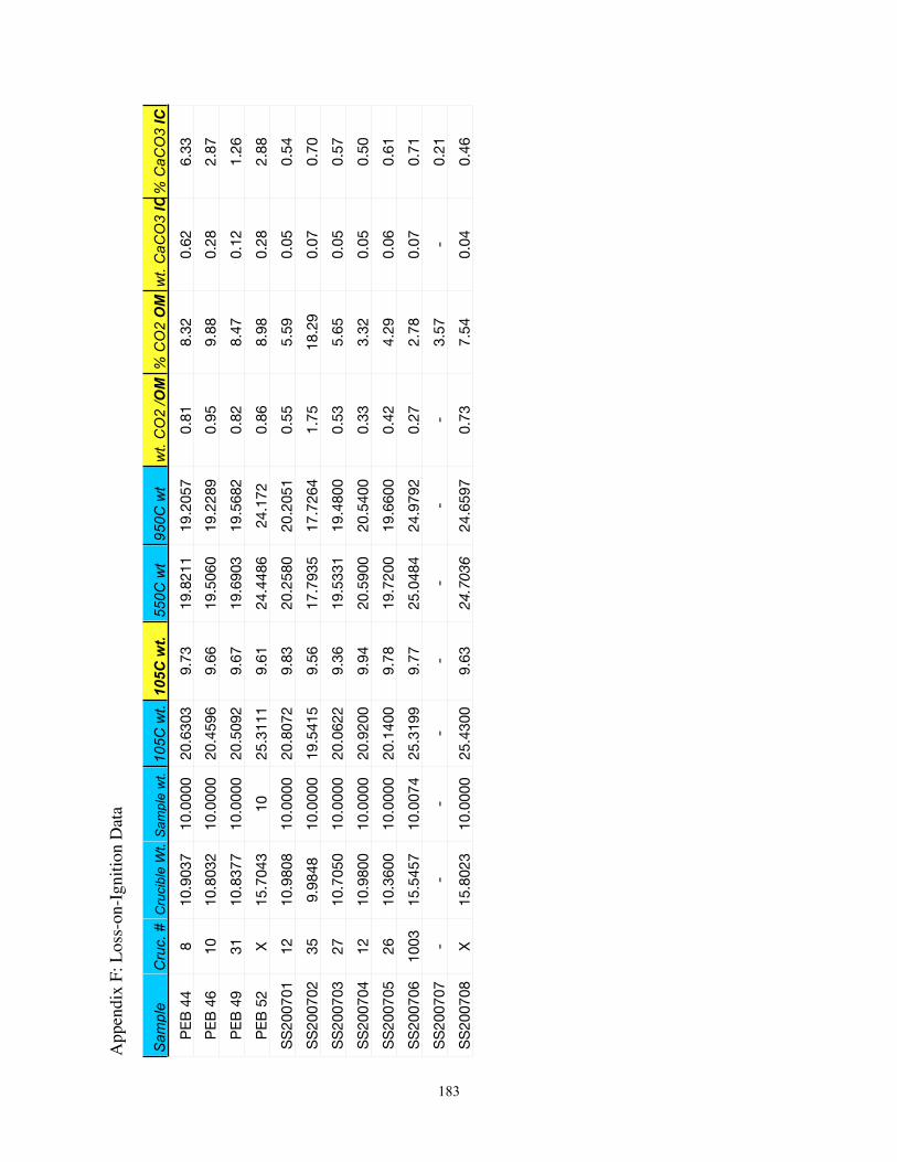
183

Sam

ple

Cru

c. #

Cru

cibl

e W

t.S

ampl

e w

t.10

5C w

t.10

5C w

t.55

0C w

t95

0C w

tw

t. C

O2

/OM

% C

O2

OM

wt.

CaC

O3

IC%

CaC

O3

IC

PE

B 4

48

10.9

037

10.0

000

20.6

303

9.73

19.8

211

19.2

057

0.81

8.32

0.62

6.33

PE

B 4

610

10.8

032

10.0

000

20.4

596

9.66

19.5

060

19.2

289

0.95

9.88

0.28

2.87

PE

B 4

931

10.8

377

10.0

000

20.5

092

9.67

19.6

903

19.5

682

0.82

8.47

0.12

1.26

PE

B 5

2X

15.7

043

1025

.311

19.

6124

.448

624

.172

0.86

8.98

0.28

2.88

SS

2007

0112

10.9

808

10.0

000

20.8

072

9.83

20.2

580

20.2

051

0.55

5.59

0.05

0.54

SS

2007

0235

9.98

4810

.000

019

.541

59.

5617

.793

517

.726

41.

7518

.29

0.07

0.70

SS

2007

0327

10.7

050

10.0

000

20.0

622

9.36

19.5

331

19.4

800

0.53

5.65

0.05

0.57

SS

2007

0412

10.9

800

10.0

000

20.9

200

9.94

20.5

900

20.5

400

0.33

3.32

0.05

0.50

SS

2007

0526

10.3

600

10.0

000

20.1

400

9.78

19.7

200

19.6

600

0.42

4.29

0.06

0.61

SS

2007

0610

0315

.545

710

.007

425

.319

99.

7725

.048

424

.979

20.

272.

780.

070.

71

SS

2007

07-

--

--

--

-3.

57-

0.21

SS

2007

08X

15.8

023

10.0

000

25.4

300

9.63

24.703

624

.659

70.

737.

540.

040.

46

App

endi

x F:

Los

s-on

-Igni

tion

Dat

a

Appendix G: Electrical Conductivity and pH Data

Appendix G: Electrical Conductivity and pH Data

184

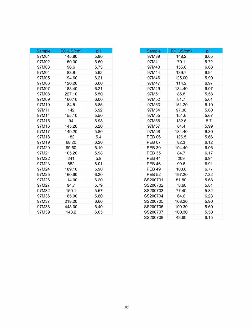
Sample EC (µS/cm) pH Sample EC (µS/cm) pH97M01 145.80 5.90 97M39 148.2 6.0597M02 150.30 5.60 97M41 70.1 5.7297M03 96.6 5.73 97M43 155.6 6.6897M04 83.8 5.92 97M44 139.7 6.9497M05 194.60 6.21 97M46 125.00 5.9097M06 126.20 6.00 97M47 114.2 6.9797M07 188.40 6.21 97M49 134.40 6.0797M08 227.10 5.50 97M51 85.8 5.5897M09 160.10 6.00 97M52 81.7 5.6197M10 84.5 5.85 97M53 151.20 6.1097M11 142 5.92 97M54 97.30 5.6097M14 155.10 5.50 97M55 151.6 5.6797M15 94 5.98 97M56 132.6 5.797M16 145.20 6.20 97M57 84.4 5.9997M17 149.20 5.80 97M58 184.40 6.3097M18 182 5.4 PEB 06 126.5 5.6697M19 68.20 6.20 PEB 07 82.3 6.1297M20 99.60 6.10 PEB 30 104.40 6.0697M21 105.20 5.98 PEB 35 84.7 6.1797M22 241 5.9 PEB 44 209 6.9497M23 682 6.01 PEB 46 99.6 6.9197M24 189.10 5.90 PEB 49 103.6 6.7797M25 160.90 6.20 PEB 52 197.20 7.3297M26 114.00 6.20 SS200701 51.80 5.6897M27 94.7 5.79 SS200702 78.60 5.8197M32 150.1 5.57 SS200703 77.40 5.8297M36 185.90 5.80 SS200704 64.6 6.2397M37 218.20 6.60 SS200705 108.20 5.9097M38 443.00 6.40 SS200706 109.30 5.6097M39 148.2 6.05 SS200707 100.30 5.50

SS200708 43.60 6.15

185

Bibliography

Ames, Kennth M.1985 Hierarchies, stress, and logistical strategies among hunter-gatherers in Northwestern North America. In Prehistoric Hunter-Gatherers: The Emergence of Cultural Complexity, edited by T. D. Price and J. A. Brown, pp. 155 - 180. Academic Press, Orlando.

1995 Chiefly Power and Household Production on the Northwest Coast. In Foundations of Social Inequality, edited by T. D. Price and G. M. Feinman, pp. 155 - 187. Plenum Press. New York.

1996 Life in the Big House: Household labor and dwelling size on the Northwest Coast. In People Who Lived in Big Houses: Archaeological Perspectives on Large Domestic Structures, edited by Gary Coupland and E. B. Banning, pp. 131 - 150. Monographs in World Archaeology No. 27. Prehistory Press. Wisconsin.

Ames, Kenneth M. and Herbert D. G. Maschner1999 Peoples of the Northwest Coast: Their Archaeology and Prehistory. Thames and Hudson, London.

Ames, Kenneth M., Doria F. Raetz, Stephen Hamilton, Christine McAfee1992 Household Archaeology of a Southern Northwest Coast Plank House. Journal of Field Archaeology 19(3):275 - 290.

Ascher, Robert1961 Experimental Archaeology. American Anthropologist 63(4):793 - 816.

1968 Time’s Arrow and the Archaeology of a Contemporary Community. In Settlement Archaeology, edited by K. C. Chang, pp. 43 - 52. National Press Books, Palo Alto.

Barnett, Homer G.1955 The Coast Salish of British Columbia. University of Oregon Monographs. Studies in Anthropology no. 4. Eugene.

Bell, Duran1995a On the Nature of Sharing: Beyond the Range of Methodological Individualism. Current Anthropology 36:826 - 830.

1995b The Structure of Rights in the Context of Private Property. Journal of Socio-Economics 24(4):607 - 622.

186

Binford, Lewis R.1978 Nunamiut Ethnoarchaeology. Academic Press, New York.

1981 Behavioral Archaeology and the “Pompeii Premise”. Journal of Anthropological Archaeology 37(3):195 - 208.

1983 In Pursuit of the Past. Thames and Hudson, New York.

Birkeland, Peter W. 1984 Soils and Geomorphology. Oxford University Press, New York.

Brady, Nyle C. and Ray R. Weil. 2002 The Nature and Properties of Soils, 13th ed.

Brown, Kevin J. and Richard J. Hebda 2002 Origin, Development and Dynamics of Coastal Temperate Conifer Rainforests of

Southern Vancouver Island, Canada. Canadian Journal of Forest Research 32(2):353 - 372.

Burley, David V.1980 Marpole: Anthropological Reconstructions of a Prehistoric Northwest Culture Type. Department of Archaeology. Simon Fraser University Publication No. 8. Burnaby.

1988 Senewélets: Culture History of the Nanaimo Coast Salish and the False Narrows Midden. Royal British Columbia Museum Memoir no. 2. Victoria.

Burley, David V., and Christopher Knusel1989 Burial Patterns and Archaeological Interpretation: Problems in the Recognition of Ranked Society in the Coast Salish Region. Paper presented at the conference: Development of Hunting-Fishing-Gathering Maritime Societies along the West Coast of North America. Seattle.

Butzer, Karl1982 Archaeology as Human Ecology: Method and Theory for a Contextual Approach. Cambridge University Press, Cambridge.

Butzer, Karl and Sarah E. Harris 2007 Geoarchaeological approaches to the environmental history of Cyprus: explication and critical evaluation. Journal of Archaeological Science 34:1932 - 1952.

187

Carr, Christopher1985 Intrasite Spatial Analysis. In For Concordance in Archaeological Analysis: Bridging Data Structure, Quantitative Technique, and Theory, edited by C. Carr, pp. 297 - 473. University of Arkansas. Kansas City.

Chatters, James C.1989 The Antiquity of Economic Differentiation within Households in the Puget Sound, Northwest Coast. In Households and Communities, edited by S. MacEachern, D. J. Archer and R. D. Gavin, pp. 168 - 178. The University Calgary Archaeological Association, Calgary.

Clague, John J. and Thomas S. James 2002 History and isostatic effects of the last ice sheet in southern British Columbia.

Quaternary Science Reviews 21:71 - 87.

Cobb, Charles R. 1993 Archaeological Approaches to the Political Economy of Nonstratified. In Archaeological Method and Theory, edited by M. B. Schiffer, pp. 43 - 100, vol. 5. University of Arizona Press, Tuscon.

2000. Specialization, exchange, and power in small-scale societies andchiefdoms. In From Quarry to Cornfield: The Political Economy of Mississippian Hoe Production, edited by C. R. Cobb, pp. 19 - 46. University of Alabama Press, Tuscaloosa.

Cook, S. F. and R. F. Heizer 1965 Studies on the Chemical Analysis of Archaeological Sites. University of California Publications in Anthropology No. 2. Berkley.

Corwin, D. L. and S. M. Lesch 2003 Application of Soil Electrical Conductivity to Precision Agriculture: Theory,

Principles, and Guidelines. Agronomy Journal 95(3):455 - 471.

Coupland, Gary1985 Household Variability and Status Differentiation as Kitselas Canyon. Canadian Journal of Archaeology 9:39 - 56.

1988 Prehistoric Culture Change at Kitselas Canyon. National Museum of Man, Mercury Series, Archaeological Survey of Canada Paper no. 138. Ottawa.

1991 The Point Grey Site: a Marpole Spring Village Component. Canadian Journal of Archaeology 15:73 - 96.

188

2006 A Chief’s House Speaks: Communicating Power on the Northern Northwest Coast. In Household Archaeology on the Northwest Coast, edited by E. A. Sobel, D. A. Gahr and K. M. Ames, pp. 80 - 96. International Monographs in Prehistory, Archaeology Series No. 18. Ann Arbor.

Coupland, Gary, Terence Clark and Amanda Palmer2009 Hierarchy, Communalism, and the Spatial Order of Northwest Coast Plank Houses: A Comparative Study. American Antiquity, p.77 - 106.

Coupland, Gary, Roger H. Colton, Rebecca Case2003 Preliminary Analysis of Socio Economic Organization at the McNichol Creek Site, British Columbia. In Emerging from the Mist, edited by G. Coupland, R. G. Matson and Q. Mackie. pp. 152 - 169. UBC Press, Vancouver.

Courty, Marie-Agnes, Paul Goldberg, and Richard I. MacPhail1989 Soils and Micromorphology in Archaeology. Cambridge University Press, Cambridge.

Dalan, Rinita A., J. M. Musser and Julie K. Stein1992 Geophysical Exploration of a Shell Midden. In Deciphering a Shell Midden, edited by J. K. Stein, pp. 43 - 59. Academic Press, San Diego.

Deetz, James and Edwin Dethlefsen 1963 Soil pH as a Tool in Archaeological Site Interpretation. American Antiquity 29(2):242 - 243.

Demeyer, A. J. C. Voundi Nkana, and M. G. Verloo2001 Characteristics of Wood Ash and Influence on Soil Properties and Nutrient Uptake: An Overview. Bioresource Technology 77:287-295.

Entwistle, J. A., K. J. W. McCaffery and R. A. Dodgshon 2007` Geostatistics and Multi-Elemental Analysis of Soils to Interpret Land-Use History

in the Hebrides Scotland. Geoarchaeology: An International Journal 22:319 - 415.

Essington, Michael E.2003 Soil and Water Chemistry: An Integrative Approach. CRC Press. Boca Rotan.

Ewonus, Paul A.2006 The Social Archaeology of a Plankhouse in Perspective. Unpublished M.A. Thesis, Department of Anthropology, McMaster University, Hamilton, ON.

189

Expert Committee 1982 The Canada Soil Information System: Manual for Describing Soils in the Field,

Ottawa.

Field, John, and E. B. Banning1998 Hillslope Processes and Archaeology in Wadi Ziqlab, Jordan. Geoarchaeology 13(6):595 - 616.

Fedje, Daryl and Tina Christiansen1999 Modeling Paleoshorelines and Locating Early Holocene Coastal Sites in Haida Gwaii. American Antiquity 64(4):635 - 652.

Fladmark, Knut1973 The Richardson Ranch Site: A 19th Century Haida House. In Historical Archaeology in Northwestern North America, edited by R.M. Getty and K. Fladmark, pp. 53 - 95. Archaeological Association of the University of Calgary, Calgary.

1975 A paleoecological model for Northwest Coast prehistory. National Museum of Man, Mercury Series, Archaeological Survey of Canada Paper no. 43. Ottawa.

Gee, G. W. and D. Orr2002 Particle Size Analysis. In Methods of Soil Analysis Part 4: Physical Methods, edited by J. H. Dane and G. C. Topp, pp. 255 - 293. Soil Sci. Soc. Am. Monograph 9, SSSA, Madison.

Gerlach, Robert W., David E. Dobb, Gregory A. Raab and John M. Nocerino 2002 Gy Sampling theory in environmental studies. 1. Assessing soil splitting

protocols. Journal of Chemometrics 16:321 - 328.

Goldberg, Paul and Richard I. MacPhail 2006 Practical and Theoretical Geoarchaeology. Blackwell Publishing, Oxford.

Gould, Richard A.1968 Living Archaeology: The Ngatatjara of Western Australia. Southwestern Journal of Anthropology 24(2):101 - 122.

Green, A. J., van Vliet L. J. P. and E. A. Kenney 1989 Soils of the Gulf Islands of British Columbia vol. 3: Soils of Galiano, Valdes,

Thetis, Kuper and lesser Islands. British Columbia Soil Survey, Vancouver.

190

Green, R. N., R. L. Trowbridge and K. Klinka 1993 Towards a Taxonomic Classification of Humus Forms. Forest Science Monograph

29. Society of American Foresters.

Grier, Colin F.2001 The Social Economy of a Prehistoric Northwest Coast Plankhouse. Unpublished Ph.D. Dissertation, Department of Anthropology, Arizona State University, Tempe, AZ.

2003 Dimensions of Regional Interaction in the Prehistoric Gulf of Georgia. In Emerging from the Mist, edited by G. Coupland, R.G. Matson and Q. Mackie. pp. 170 - 187. UBC Press. Vancouver.

2006a Temporality in Northwest Coast Households. In Household Archaeology on the Northwest Coast, edited by E. A. Sobel, D. A. Gahr and K. M. Ames, pp. 97 - 119. International Monographs in Prehistory, Archaeology Series No. 18. Ann Arbor.

2006b Political Dimensions of Monumental Residences on the Northwest Coast of North America. In Palaces and Power in the Americas: From Peru to the Northwest Coast, edited by J. J. Christie and P. J. Sarro, pp 141 - 165. University of Texas Press, Austin.

2007 Consuming the Recent for Constructing the Ancient: The Role of Ethnography in Coast Salish Archaeological Interpretation. In Be Of Good Mind: Essays on the Coast Salish, edited by B.G. Miller, pp. 282 - 307. UBC Press, Vancouver.

Grier, Colin F., and Eric McLay2007 Archaeological Inventory of DgRv-006 Dionisio Point Provincial Park, Galiano Island. Report on file with the Archaeological Branch. Victoria [Heritage Permit 2007-144].

Hassan, Fekri A.1980 Geoarchaeology: The Geologist and Archaeology. American Antiquity 44(2):267 - 270.

Hayden, Brian1995 Pathways to Power: Principles for Creating Socioeconomic Inequalities. In Foundations of Social Inequality, edited by T. D. Price and G. M. Feinman, pp. 15 - 86. Plenum Press, New York.

Hayden, Brian and Audrey Cannon1982 The Corporate Group as an Archaeological Unit. Journal of Anthropological Archaeology 1:132 - 158.

191

1983 Where the Garbage Goes: Refuse Disposal in the Maya Highlands. Journal of Anthropological Archaeology 2:117 - 163.

Heilman, Paul E., Harry W. Anderson, and David M. Baumgartner (editors) 1981 Forest Soils of the Douglas-fir Region. Washington State University Cooperative

Extension Service, Pullman.

Heiri, Oliver, André F. Lotter, and Gerry Lemcke2001 Loss-On-Ignition as a Method for Estimating Organic and Carbonate Content in Sediments: Reproducibility and Comparability of Results. Journal of Palaelimnology 25:101 - 110.

Huelsbeck, David R.1994 Mammals and fish in the subsistence economy of Ozette. In Ozette Archaeological Project Research Reports, Vol. II: Fauna, edited by Stephen R. Samuels, pp. 17 - 92. WSU Department of Anthropology Reports of Research No. 68. National Parks Service, Northwest Regional Office, Seattle.

Jenny, Hans 1994 [1941] Factors of Soil Formation: A System of Quantitative Pedology. Dover

Press, New York.

Johnson, Allen and Timothy Earle2000 The Evolution of Human Societies from Foraging Group to Agrarian State. Stanford University Press, Stanford.

Johnstone, Patrick D. 2006 Geology of the Upper Cretaceous Nanaimo Group, Southernmost Gulf Islands

and Adjacent Saanich Penninsula, Southwestern British Columbia. Unpublished M.Sc. Thesis, Department of Earth Sciences, Simon Fraser University, Burnaby.

Josenhans, Heiner W., Daryl W. Fedje, Kim W. Conway, and J Vaughn Barrie1995 Post Glacial Sea Levels on the Western Canadian Continental Shelf: Evidence for Rapid Change, Extensive Subaerial Exposure, and Early Human Habitation. Marine Geology 125:73 - 94.

Josenhans, Heiner W., Daryl W. Fedje, Reinhardt Pienitz, and John Southon1997 Early Humans and Rapidly Changing Holocene Sea Levels in the Queen Charlotte Islands-Hecate Strait, British Columbia, Canada. Science N.S. 277:71 - 74.

192

Karkanas, Panagiotis, Ruth Shahack-Gross, Avner Ayalon, Mira Bar-Matthews, Ran Barkai, Amos Frumkin, Avi Gopher, and Mary C. Stiner

2007 Evidence for Habitual Use of Fire at the End of the Lower Paleolithic: Site-Formation Processes at Qesem Cave, Israel. Journal of Archaeological Science 53:197 - 212.

Kew, Michael1992 Salmon availability, technology, and cultural adaptation in the Fraser River watershed. In A Complex Culture of the British Columbia Plateau: Traditional Stl’átl’imx Resource Use, edited by Brian Hayden, pp. 177 - 221. University of British Columbia Press, Vancouver.

Knudson, Kelly J., Lisa Frink, Brian W. Hoffman, T. Douglas Price2004 Chemical Characterization of Arctic Soils: Activity Area Analysis in Contemporary Yup'ik Fish Camps Using ICP-MS. Journal of Archaeological Science 31:443 - 456.

LeClair, R.1976 Investigations at the Mauer site near Aggasiz. In Current Research Reports, Department of Anthropology, Simon Fraser University Publication No. 3, edited by Roy L . Carlson, pp. 33 - 42. Simon Fraser University, Burnaby.

Lepofsky, Dana, Michael Blake, Douglas Brown, Sandra Morrison, Nicole Oakes, and Natasha Lyons

2000 The Archaeology of the Scowlitz Site, SW British Columbia. Journal of Field Archaeology 27(4):391 - 416.

Linse, Angela R. 1992 Is Bone Safe in a Shell Midden? In Deciphering A Shell Midden, edited by J. K.

Stein, pp. 327 - 346. Academic Press, San Diego.

Lukowksi, Susan, and Colin F. Grier 2009 Archaeological Investigations of Household Economics at the Dionisio Point Site,

southwestern British Columbia, Canada. Poster presented at 74th Annual Meeting of the Society for American Archaeology. Atlanta.

Lyman, R. Lee1991 Prehistory of the Oregon Coast: The Effects of Excavation Strategies and

Assemblage Size on Archaeological Inquiry. Orlando, Academic Press.

193

Mackie, Alexander P. and Laurie Williamson2003 Nuu-chah-nulth Houses: Structural Remains and Cultural Depressions on Southwestern Vancouver Island. In Emerging from the Mist, edited by G. Coupland, R.G. Matson and Q. Mackie. pp. 105 - 151. UBC Press, Vancouver.

MacPhail, Richard I., G. M. Cruise, Michael J. Allen, Johan Linderholm, and Peter Reynolds2003 Archaeological soil and pollen analysis of experimental house floor deposits; with special reference to Butser Ancient Farm, Hampshire, UK. Journal of Archaeological Science 31(2):175 - 191.

Mallol, Carolina, Frank W. Marlowe, Brian M. Wood, and Claire C. Porter2007 Earth, Wind, and Fire: Ethnoarchaeological Signals of Hadza Fires. Journal of Archaeological Science 34:2035 - 2052.

Marshall, Yvonne1989 The House in Northwest Coast, Nuu-Chah-Nulth, Society: The Material Structure of Political Action. In Household and Communities, edited by S. MacEachern, D. J. W. Archer, and R. D. Garvin, pp. 15 - 12. The University of Calgary Archaeological Association, Calgary.

2006 Houses and Domestication on the Northwest Coast. In Household Archaeology on the Northwest Coast, edited by E. A. Sobel, D. A. Gahr and K. M. Ames, pp. 37 - 56. International Monographs in Prehistory, Archaeology Series No. 18. Ann Arbor.

Marwick, Ben2005 Element Concentrations and Magnetic Susceptibility of Anthrosols: Indicators of Prehistoric Human Occupation in the Inland Pilbara, Western Australia. Journal of Archaeological Science 32: 1357 - 1368.

Maschner, Herbert D. G.1991 The Emergence of Cultural Complexity on the West Coast of North America. Antiquity 65:921 - 923

Matson, R. G.1976 The Glenrose Cannery Site. Canadian National Museum, Archaeology Survey of Canada Paper, Mercury Series no. 52, Ottawa.

1983 Intensification and the Development of Cultural Complexity: The Northwest versus the Northeast Coast. In The Evolution of Maritime Cultures on the Northeast and Northwest Coasts of North America, edited by R. J. Nash, pp. 124 - 148. Department of Archaeology Occaisional Paper no. 11. Simon Fraser University, Burnaby.

194

1985. The relationship between sedentism and status inequalities among hunters and gatherers. In Status, Structure and Stratification: Current Archaeological Reconstructions, pp. 245 - 252. University of Calgary, Calgary.

1992 The Evolution of Northwest Coast Subsistence. In Long-term Subsistence Change in Prehistoric North America, edited by D. R. Croes, R. A. Hawkins and B. L. Isaac, pp. 367 - 428. Research in Economic Anthropology Supplement 6. Greenwich.

2003 The Coast Salish House: Lessons from Shingle Point, Valdes Island, British Columbia. In Emerging from the Mist; Studies in Northwest Coast Culture History, edited by R.G. Matson, Gary Coupland and Quentin Mackie, pp 76 - 104. University of British Columbia Press, Vancouver.

2008 The Crescent Beach site and the Place of the Locarno Beach Phase. Manuscript on file with the Laboratory of Archaeology, University of British Columbia. Vancouver.

Matson, R.G. and Gary Coupland 1995 The Prehistory of the Northwest Coast. Academic Press, Orlando.

Matthews, Wendy, C. A. I. French, T. Lawrence, D. F. Cutler, and M. K. Jones1997 Microstratigraphic traces of site formation processes and human activities. World Archaeology 29(2):281 - 308.

Matthiesen, Henning 2004 In Situ Measurement of Soil pH. Journal of Archaeological Science 31:1373 -

1381.

Mauger, Jeffery E.1991 Shed-roof Houses at Ozette and in a Regional Perspective. In Ozette Archaeological Project Research Reports Volume One: House Structure and Floor Midden. pp. 29 - 175. Reports of Investigations 63, Washington State University Department of Anthropology. Pullman and National Parks Service, Seattle.

Meidinger, Dellis Vern and Jim Pojar 1991 Ecosystems of British Columbia. Special Report Series 6. Ministry of Forests,

Victoria.

Middleton, William D. 2004 Identifying Chemical Activity Residues on Prehistoric House Floors: A

Methodology and Rationale for Multi-Elemental Characterization of a Mild Acid Extract of Anthropogenic Sediments. Archaeometry 46:47 - 65.

195

Middleton, William D. and T. Douglas Price1996 Identification of Activity Areas by Multi-Element Characterization of Sediments from Modern and Archaeological House Floors Using Inductively Coupled Plasma-atomic Emission Spectroscopy. Journal of Archaeological Science 23:673 - 687.

Mitchell, Donald H. 1971a Archaeology of the Gulf of Georgia Area, a Natural Region and its Culture Types.

Syesis 4 (Supplement 1). The British Columbia Provincial Museum, Victoria, BC.

1971b The Dionisio Point Site and Gulf Island Culture History. Syesis 4:145 - 168. 1983 Seasonal Settlements, Village Aggregations, and Political Autonomy on the

Central Northwest Coast. In The Development of Political Organization in Native North America, edited by E. Tooker and M. Fried, pp. 97 - 107. Washington, D.C.

Price, T. Douglas and James A. Brown1985 Prehistoric Hunter-Gatherers: The Emergence of Cultural Complexity. Academic Press, New York.

Samuels, Stephen R. 1991a Ozette Archaeological Project Research Reports Volume One: House Structure

and Floor Midden. Reports of Investigations. Washington State Department of Anthropology, Seattle.

1991b Patterns in Ozette Floor Middens: Reflections of Social Units. In Ozette Archaeological Project Research Reports Volume One: House Structure and Floor Midden, edited by S. R. Samuels, pp. 175 - 270. Reports of Investigations. Washington State Department of Anthropology, Seattle.

1994 Ozette Archaeological Project Research Reports Volume Two: Fauna. Reports of Investigations. Washington State Department of Anthropology, Seattle.

2006 Households at Ozette. In Household Archaeology on the Northwest Coast, edited by E. Sobel, A. Trieu and K. Ames, pp. 200 - 232. International Monographs in Prehistory, Ann Arbor.

Sánchez Vizcaíno, Alberto and María L. Cañabate1999 Identification of Activity Areas by Soil Phosphorous and Organic Matter Analysis in Two Rooms of the Iberian Sanctuary “Cerro El Pajarillo”, Geoarchaeology 14(1):47 - 62.

196

Schaepe, David2003 Validating the Maurer House. In Archaeology of Coastal British Columbia: Essays in Honour of Professor Phillip M. Hobler, edited by R. L. Carlson, pp. 113 - 152. Archaeology Press, Simon Fraser University, Burnaby.

Schaetzl, Randall1991 Factors Affecting the Formation of Dark, Thick Epipedons Beneath Forest Vegetation, Michigan, USA. Soil Science Society of America Journal 56:1538 - 1545.

Schaetzl, Randall and Sharon Anderson 2005 Soils: Genesis and Geomorphology. Cambridge University Press, Cambridge.

Schiffer, Michael B.1972 Archaeological Context and Systemic Context. American Antiquity 37(2):156 - 165.

1983 Toward the Identification of Formation Processes. American Antiquity 48(4):675-706.

Shahack-Gross, Ruth, Fiona Marshall, Kathleen Ryan and Steve Weiner 2004 Reconstruction of spatial organization in abandoned Maasai settlements:

implications for site structure in the Pastoral Neolithic of East Africa. Journal of Archaeological Science 31(10):1395 - 1411.

Smith, Cameron M.2004 The Social Organization of Production in Three Protohistoric Lower-Columbia River Plank Houses. Unpublished PhD dissertation. Department of Anthropology, Simon Fraser University. Burnaby, B.C.

2006 The Formation Processes of Lower Columbia River Plankhouse Site. In Household Archaeology on the Northwest Coast, edited by E. Sobel, A. Trieu-Gahr, and K. Ames, pp. 233 - 269. International Monographs in Prehistory, Ann Arbor.

Soil Classification Working Group 1998 The Canadian System of Soil Classification, Third Ed. National Research Council Press, Ottawa.

Spencer, Charles S.1994 Factional Ascendence, Dimensions of Leadership, and the Development of Centralized Authority. In Factional Competition and Political Development in the New World, edited by E. Brumfiel and J. Fox, pp. 31 - 43. Cambridge University Press, Cambridge.

197

Stein, Julie K. 1983 Earthworm Activity: A Source of Potential Disturbances of Archaeological

Sediments. American Antiquity 48(2):277 - 289.

1984 Organic Matter and Carbonates in Archaeological Sites. Journal of Field Archaeology 11:239 - 246

1992a Deciphering a Shell Midden. Academic Press. San Diego.

1992b Sediment Analysis of the British Camp Shell Midden. In Deciphering a Shell Midden, edited by J. K. Stein, pp. 135 - 162. Academic Press, San Diego.

1992d Organic Matter in Archaeological Contexts. In Soils, Landscape Evolution, and Human Occupation, edited by V. T. Holliday, pp. 193 - 216. Smithsonian Institution Press, Washington D.C.

1993 The Issue of Scale in Archaeology, Geosciences, and Geoarchaeology. In Effects of Scale on Archaeology and Geoscientific Perspectives, edited by J. K. Stein and A. R. Linse, pp. 1 - 10. Geological Society of America, Special Paper no. 283.

2001 A Review of Site Formation Processes and Their Relevance to Geoarchaeology. In Earth Sciences and Archaeology, edited by P. Goldberg, V. T. Holliday, and C. R. Ferring, pp. 37 - 51. Kluwer Academic/Plenum Publishers, New York.

Suttles, Wayne P.1951 Economic life of the coast Salish of Haro and Rosario Straits. M.A. Thesis. Department of Anthropology, Washington State University.

1991 The Shed-Roof House. In A Time of Gathering: Native Heritage in Washington State, edited by R. K. Wright, pp. 212 - 222. University of Washington Press, Seattle.

Thom, Brian1995 The Dead and the Living: Burial Mounds and Cairns and the Development of Social Classes in the Gulf of Georgia Region. Unpublished M.A. Thesis. Department of Anthropology and Sociology. University of British Columbia. Vancouver, B.C.

Wechel, David L.2005 Ozette Archaeological Project Research Reports Volume Three: Ethnobotany and Wood Technology. Reports of Investigations. Washington State Department of Anthropology, Seattle.

198

Weide, D.L. 1966 Soil pH as a guide to archaeological investigations. In Archaeological Survey Annual Report, pp. 155 - 163. Department of Anthropology, University of California, Los Angeles.

Wessen, Gary1994 Subsistence patterns as reflected by the invertebrate remains recovered at the Ozette site. In Ozette Archaeological Project Research Reports, Vol. II: Fauna, edited by Stephen R. Samuels, pp. 93 - 196. WSU Department of Anthropology Reports of Research No. 68. National Parks Service, Northwest Regional Office, Seattle.

Wiessner, Polly2002 The Vines of Complexity: Egalitarian Struactures and the Institutionalization of Inequality among the Enga. Current Anthropology 43(2):233 - 269.

Wild, Alan 1993 Soils and the Environment: An Introduction. Cambridge University Press,

Cambridge.

Youngberg, C. T. 1981 Organic Matter of Forest Soils. In Forest Soils of the Douglas-fir Region, edited

by P. E. Heilman, H. W. Anderson and D. M. Baumgartner, pp. 137 - 144. Washington State University Cooperative Extension Service, Pullman.

Zhang, Qi-Bin and Richard J. Hebda 2005 Abrupt climate change and variability in the past four millennia of the

southern Vancouver Island, Canada. Geophysical Research Letters 32 L16708.

199