Embed Size (px)
Citation preview
1
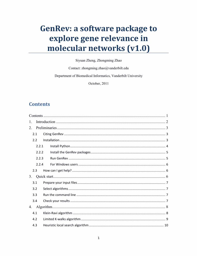
GenRev: a software package to explore gene relevance in
molecular networks (v1.0) Siyuan Zheng, Zhongming Zhao
Contact: [email protected]
Department of Biomedical Informatics, Vanderbilt University
October, 2011
Contents Contents .............................................................................................................................. 1
1. Introduction ................................................................................................................. 2
2. Preliminaries ................................................................................................................ 3
2.1 Citing GenRev .................................................................................................................. 3
2.2 Installation ....................................................................................................................... 3
2.2.1 Install Python ........................................................................................................... 4
2.2.2 Install the GenRev packages .................................................................................... 5
2.2.3 Run GenRev ............................................................................................................. 5
2.2.4 For Windows users .................................................................................................. 6
2.3 How can I get help? ......................................................................................................... 6
3. Quick start.................................................................................................................... 6
3.1 Prepare your input files ................................................................................................... 7
3.2 Select algorithms ............................................................................................................. 7
3.3 Run the command line .................................................................................................... 7
3.4 Check your results ........................................................................................................... 7
4. Algorithm..................................................................................................................... 8
4.1 Klein-Ravi algorithm ........................................................................................................ 8
4.2 Limited K-walks algorithm ............................................................................................... 9
4.3 Heuristic local search algorithm .................................................................................... 10
2
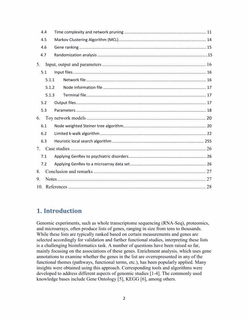
4.4 Time complexity and network pruning ......................................................................... 11
4.5 Markov Clustering Algorithm (MCL) .............................................................................. 14
4.6 Gene ranking ................................................................................................................. 15
4.7 Randomization analysis ……………………………………………………………………………………………..15
5. Input, output and parameters ..................................................................................... 16
5.1 Input files ....................................................................................................................... 16
5.1.1 Network file ........................................................................................................... 16
5.1.2 Node information file ............................................................................................ 17
5.1.3 Terminal file ........................................................................................................... 17
5.2 Output files .................................................................................................................... 17
5.3 Parameters .................................................................................................................... 18
6. Toy network models .................................................................................................. 20
6.1 Node weighted Steiner tree algorithm.......................................................................... 20
6.2 Limited k-walk algorithm ............................................................................................... 22
6.3 Heuristic local search algorithm .................................................................................. 255
7. Case studies ............................................................................................................... 26
7.1 Applying GenRev to psychiatric disorders ..................................................................... 26
7.2 Applying GenRev to a microarray data set .................................................................... 26
8. Conclusion and remarks ............................................................................................ 27
9. Notes .......................................................................................................................... 27
10. References ................................................................................................................. 28
1. Introduction
Genomic experiments, such as whole transcriptome sequencing (RNA-Seq), proteomics, and microarrays, often produce lists of genes, ranging in size from tens to thousands. While these lists are typically ranked based on certain measurements and genes are selected accordingly for validation and further functional studies, interpreting these lists is a challenging bioinformatics task. A number of questions have been raised so far, mainly focusing on the associations of these genes. Enrichment analysis, which uses gene annotations to examine whether the genes in the list are overrepresented in any of the functional themes (pathways, functional terms, etc.), has been popularly applied. Many insights were obtained using this approach. Corresponding tools and algorithms were developed to address different aspects of genomic studies [1-4]. The commonly used knowledge bases include Gene Ontology [5], KEGG [6], among others.

3
The high throughput biological molecular networks contain association information for thousands of genes in the form of direct and indirect interactions, thus providing promising alternative to interpret a set of genes. In these networks, nodes typically represent genes, while edges represent their interactions. In a variety of molecular networks, such as protein-protein interaction networks, genetic interaction networks, regulatory networks, interactions often hint at close functional associations between genes. Previous reports have revealed many novel insights into these networks [7-8]. Recently, many studies have utilized them to examine biological patterns, discover biomarkers [9-10].The advantage of using network approaches is obvious. Rather than reporting enriched pathways or function categories by the enrichment analysis based tools, network approaches generate subnetworks. Subnetworks can show gene interactions, community structures, and other information in a systematic framework. Hub nodes or bottleneck nodes, which may not be seen in the original gene list, can be prioritized in the network as key connecting components in the network. This is a very useful feature, considering that many disease-driving genes do not show significant signals within certain experiment platforms, but they may contribute as a major risk to disease by a set of genes interaction with each other.
A number of algorithms have been reported to address the subnetwork extraction problem [11-12], but there are few standalone software packages designed for large networks. Here, we present GenRev, a Python package, to assist the users for subnetwork extraction from any whole network. In the current version, GenRev implements three network search algorithms including Klein-Ravi algorithm [13], limited k-walk algorithm [14] and a heuristic local search algorithm [15]. All three algorithms use a list of genes as input to query a large network, and then return a subnetwork which connects the input genes. The input genes are called terminals or seeds. We will use these two terms interchangeably in this document. GenRev also includes an analysis module that currently includes the MCL algorithm [16] and a gene ranking function.
2. Preliminaries
2.1 Citing GenRev Please cite “GenRev: http://bioinfo.mc.vanderbilt.edu/GenRev.html."
2.2 Installation GenRev is implemented in Python programming language (http://www. python.org/). It uses the NetworkX library (http://networkx.lanl.gov/) [17] as a foundation for graph data structures. NumPy package (http://numpy.scipy.org/) is used for numerical operations. In this part, we will briefly introduce how to install the Python and the third party packages.
GenRev was developed in Python 2.6, NetworkX 1.3 and NumPy 1.3. Users should be particularly cautious of the Python version, because from version 3.0, Python will have some grammar changes with the previous versions. Since Python is independent with operating systems, GenRev is an OS free package. However, it should be noted that

4
GeneRev is primarily developed and tested in Linux and is much more convenient to use in Linux.
2.2.1 Install Python Python is a free programming language, and it is embedded in most Linux systems, if not all. Before installing your own Python, users can check the version of their default Python in shell using the command
~$ python -V If reinstallation is needed, download Python at http://www.python.org/download/releases/2.6.6/.
Decompress the source file first,
~$ tar -xzvf Python2.6.6.tgz
Then, enter this directory:
~$ cd Python2.6.6
You will need proper permissions to install Python to local directory.
~$ ./configure –-prefix=/my_directory/
~$ make
~$ make install
Python will then be installed to that directory. To add your Python directory to the system path, go to the home directory, edit the .bashrc file
~$ vi .bashrc
Add the Python installation directory to path
export PATH=/my_directory/:$PATH
Or you can add alias to your Python in .bashrc
alias python=/my_directory/bin/python
Save the .bashrc file, then
source .bashrc

5
Now type python –V to check your Python version.
2.2.2 Install the packages Download NetworkX package at http://networkx.lanl.gov/download.html. Decompress the zip file following the commands below.
~$ tar -xcvf networkx-1.3.tar.gz
~$ cd networkx-1.3/
~$ python setup.py install
Similarly, one can install the NumPy package. The download address for NumPy is http://sourceforge.net/projects/numpy/files/NumPy/.
2.2.3 Run GenRev Download GenRev from http://bioinfo.mc.vanderbilt.edu/GenRev.html. Unzip the file by command
~$ tar -xzvf GenRev1.0.tar.gz
In the GenRev directory, you will find an executive file called GenRev. If this file does not have executive permission, use the following command to add it.
~$ chmod +x GenRev
To add GenRev to the system path, go to home directory, edit .bashrc
~$ export PATH=$PATH:/where your GenRev is/
Then
~$ source .bashrc
Now, test your GenRev, type
~$ GenRev –h
If installed properly, the help document can be printed out to your screen.
To test GenRev, go to your GenRev directory, follow the commands below
~$ cd testdata/
~$ GenRev –a steiner –g lesmis.net –t lesmis.terminal

6
A message will be shown to report the status of calculation and where the result files are written.
2.2.4 For Windows users Because GenRev is a command line package, one has to call GenRev in the MS-DOS environment.
To install Python in Windows, download Python Windows installer at http://www.python.org/download/releases/2.6.6/.
Then, add Python to your system path. Here is a simple tutorial on how to add system paths in Windows.
http://publib.boulder.ibm.com/iseries/v5r2/ic2924/books/5445775168.htm
Restart the console. Once the path addition is successful, you can type Python in your MS-DOS console.
Install NetworkX (http://networkx.lanl.gov/download/networkx/) and NumPy (http://sourceforge.net/projects/numpy/files/NumPy/).
If both packages are installed successfully, you can import them in your Python environment.
>>> import networkx
>>> import numpy
Download GenRev at http://bioinfo.mc.vanderbilt.edu/GenRev.html
Unzip the file to local directory. In MS-DOS, enter the GenRev directory. Run
python GenRev –a steiner –g testdata\lesmis.net –t testdata\lesmis.terminal
Unlike the Linux system, users have to explicitly call GenRev with Python in Windows. Since it is more convenient to run GenRev in the Linux system, we will assume the users are using Linux in the following document.
2.3 How can I get help? For helps and feedbacks, send email to Dr. Zhongming Zhao [email protected].
3. Quick start
Here is a quick start example.

7
3.1 Prepare your input files Prepare your input files according to the directions in section 6. Basically, all input files are text, white space delimited files and are easy to prepare. The network file contains two columns, with each line representing an interaction. In terminal file, each line represents a node. Additionally, you can find examples in the directory testdata/. Network files have a .net suffix, node score files have a .score suffix and terminal files have a .terminal suffix.
3.2 Select algorithms GenRev has three algorithm options: “steiner”, “heuristic” and “kwalk”. “steiner” refers to the Klein-Ravi algorithm, which is an approximation algorithm for the node weighted Steiner tree problem [13]. “heuristic” refers to the heuristic local search algorithm first proposed by Chuang et al. [15]. “kwalk” refers to the limited k-walk algorithm proposed by Dupont et al. [14]. It is important for the users to accurately specify one of them. Note that when “heuristic” is specified, the node score file is a must to run GenRev correctly.
3.3 Run the command line To view a full list of parameters, type
$ GenRev –h
GenRev needs the users to input at least a network file (parameter -g) and a terminal file (parameter -t). Node score file is also needed for the “heuristic” algorithm.
For demonstration, one can enter the testdata directory. An example command line is:
$ nohup GenRev -a steiner -g lesmis.net -t lesmis.terminal >log.txt 2>&1 &
Report messages or error messages will be written to log.txt.
3.4 Check your results GenRev will automatically create an output directory for result files, unless the users specify a location with the “-o” parameter. When running GenRev, the output directory will be printed to the screen (standard out) by default. The default directory name will be formatted as GenRev_analysis01202011_3, which, in this instance, means the third time running GenRev on 01/20/2011. If a user specified directory has already exists, GenRev will report output error. Output files are formatted for Cytoscape network analysis and visualization platform [18]. Users can load the network file and node and edge attribute files to Cytoscape for visualizations.
For details of the result files, see section 6.3.

8
4. Algorithm
In this section, we will briefly introduce the algorithms that GenRev implements. For different algorithms, we may use the interchangeable terms “terminal” or “seed” to denote the user input gene lists.
4.1 Klein-Ravi algorithm In graph theory, the notion of connecting a set of nodes in a graph is the Steiner tree problem. In the classical Steiner tree problem, the network is typically edge weighted graphs. In biological studies, genes are often scored instead of their interactions. Therefore, a variant of the classical Steiner tree problem, the node weighted Steiner tree problem, fits our questions more naturally. The goal of node weighted Steiner tree problem is, given each node a weight in graph and a set of terminals, how can we find a subnetwork linking all terminals while keeping the weight of the subnetwork minimum? Network score is the sum of scores of its nodes. From the definition, the algorithms for node weighted Steiner tree problem seeks connections that have a small cost by nature. However, in most biological studies, genes are often scored proportional to properties of interest. For example, a larger fold change of gene expression indicates a bigger probability of real functional relevance to the phenotypic differences. Therefore, a transformation is needed before we can apply any algorithm for this problem. To this end, GenRev transforms the user input gene scores internally into node cost by
𝐺𝑒𝑛𝑒 𝑐𝑜𝑠𝑡 = 1 �𝑔𝑒𝑛𝑒 𝑠𝑐𝑜𝑟𝑒⁄
Since the exact solution to this problem is NP-hard, many approximation algorithms were proposed. In GenRev, we implemented one of them proposed by P. Klein and R. Ravi [13]. We call it Klein-Ravi algorithm.
The algorithm assumes that the terminals have zero cost for generality. Initially every terminal is a tree itself. The algorithm uses a greedy strategy to iteratively merge the trees into larger trees until there is only one tree. In GenRev, besides this greedy search strategy, we also initialize the algorithm in a slightly different way. Instead of setting each terminal as a tree, we first map terminals to the network to see if they have any direct interactions. If some terminals can form a connected graph, then the graph will be used as an initial tree.
The iteration of the algorithm selects a non-tree node and a subset of at least two of the current trees to minimize the ratio
𝑛𝑜𝑑𝑒 𝑐𝑜𝑠𝑡 + 𝑠𝑢𝑚 𝑜𝑓 𝑑𝑖𝑠𝑡𝑎𝑛𝑐𝑒 𝑡𝑜 𝑡𝑟𝑒𝑒𝑠𝑛𝑢𝑚𝑏𝑒𝑟 𝑜𝑓 𝑡𝑟𝑒𝑒𝑠
The minimum ratio defined above is called quotient cost. Distance along a path is the sum of the node costs in the path but does not include the cost of the end nodes. Once a node is selected, the shortest path is used to merge node and trees into one.
This algorithm is implemented in the NWSteiner module in GenRev. For more details of the algorithm, please refer to the original paper [13].

9
4.2 Limited K-walks algorithm The limited K-walks algorithm was proposed by P. Dupont et al. in 2006 [14]. The algorithm simulates random walks on a graph by the Markov Chain model. The relevance of an edge and a node in relation to the seed genes is evaluated by the expected times random walk passes starting from one seed to any of the others. Here, we briefly introduce the mathematics of this algorithm. A detailed elaboration can be found in the original paper.
A graph can be described as an adjacency matrix, where 𝑋𝑖𝑗 is the connectivity between vertex 𝑖 and vertex 𝑗. Markov chain is used to model a graph, with each node as a state at time 𝑡. 𝑃𝑖𝑗 denotes the possibility of transiting from vertex 𝑖 to vertex 𝑗 and can be calculated as 𝑃𝑖𝑗 = 𝑎𝑖𝑗
𝑑𝑖 where 𝑎𝑖𝑗 is the edge score between 𝑖 and 𝑗 and 𝑑𝑖 is the degree of
vertex 𝑖. If Markov chain has a set of absorbing states (denoted as K, e. g. terminals in GenRev), and the random walk starts from node x, the modified transition would be
𝑃𝑖𝑗𝑥 = �1 𝑖𝑓 𝑖 ∈ 𝐾\{𝑥} 𝑎𝑛𝑑 𝑖 = 𝑗0 𝑖𝑓 𝑖 ∈ 𝐾\{𝑥} 𝑎𝑛𝑑 𝑖 ≠ 𝑗
𝑃𝑖𝑗 𝑜𝑡ℎ𝑒𝑟𝑤𝑖𝑠𝑒�
Then the transition matrix is rearranged to
𝑃 = � 𝑄𝑥 𝑅𝑥
0 𝐼�𝑥
Where 𝑄𝑥 denotes the (𝑛 − 𝑘 + 1) × (𝑛 − 𝑘 + 1) matrix for transient states, 𝑅𝑥 is a (𝑛 − 𝑘 + 1) × (𝑘 − 1) matrix, for transition probability from transient states to absorbing states. 𝐼 is identity matrix.
After 𝑙 steps, the transition matrix is ( 𝑄𝑥 )𝑙, so [( 𝑄𝑥 )𝑙]𝑥𝑖 defines the probability of transiting from 𝑥 to 𝑖 in 𝑙 steps.
Let expectation of 𝑛(𝑥, 𝑖) is the expected number of times of the transition events from 𝑥 to 𝑖 for any time index 𝑙, which can be calculated as
𝐸[𝑛(𝑥, 𝑖)] = �𝑃[𝑋𝑙 = 𝑖|𝑋0 = 𝑥]∞
𝑙=0
= �[( 𝑄𝑥 )𝑙]𝑥𝑖
∞
𝑙=0
= [𝐼 − 𝑄𝑥 ]𝑥𝑖−1
𝑁𝑥 = [𝐼 − 𝑄𝑥 ]−1 is called fundamental matrix.
The edge passage time 𝑒(𝑥, 𝑖, 𝑗) is calculated as
𝐸[𝑒(𝑥, 𝑖, 𝑗)] = �𝑁𝑥𝑖𝑥 𝑃𝑖𝑗 𝑖𝑓 𝑖 ∈ 𝑉\𝐾𝑥 ,
𝑁𝑖𝑖𝑥 𝑃𝑖𝑗 𝑖𝑓 𝑥 = 𝑖 𝑎𝑛𝑑 𝑖 ∈ 𝐾,𝑥
0 𝑖𝑓 𝑥 ≠ 𝑖 𝑎𝑛𝑑 𝑗 ∈ 𝐾.
�
If the random walks are limited to a maximal walk length to 𝐿𝑚𝑎𝑥, the expected passage times can be computed as
10
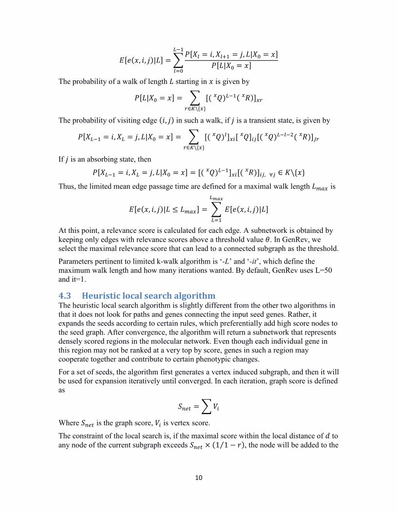
𝐸[𝑒(𝑥, 𝑖, 𝑗)|𝐿] = �𝑃[𝑋𝑙 = 𝑖,𝑋𝑙+1 = 𝑗, 𝐿|𝑋0 = 𝑥]
𝑃[𝐿|𝑋0 = 𝑥]
𝐿−1
𝑙=0
The probability of a walk of length 𝐿 starting in 𝑥 is given by
𝑃[𝐿|𝑋0 = 𝑥] = � [( 𝑄𝑥 )𝐿−1( 𝑅𝑥 )]𝑥𝑟𝑟∈𝐾\{𝑥}
The probability of visiting edge (𝑖, 𝑗) in such a walk, if 𝑗 is a transient state, is given by
𝑃[𝑋𝐿−1 = 𝑖,𝑋𝐿 = 𝑗, 𝐿|𝑋0 = 𝑥] = � [( 𝑄𝑥 )𝑙]𝑥𝑖[ 𝑄𝑥 ]𝑖𝑗[( 𝑄𝑥 )𝐿−𝑙−2( 𝑅𝑥 )]𝑗𝑟𝑟∈𝐾\{𝑥}
If 𝑗 is an absorbing state, then
𝑃[𝑋𝐿−1 = 𝑖,𝑋𝐿 = 𝑗, 𝐿|𝑋0 = 𝑥] = [( 𝑄𝑥 )𝐿−1]𝑥𝑖[( 𝑅𝑥 )]𝑖𝑗, ∀𝑗 ∈ 𝐾\{𝑥}
Thus, the limited mean edge passage time are defined for a maximal walk length 𝐿𝑚𝑎𝑥 is
𝐸[𝑒(𝑥, 𝑖, 𝑗)|𝐿 ≤ 𝐿𝑚𝑎𝑥] = � 𝐸[𝑒(𝑥, 𝑖, 𝑗)|𝐿]𝐿𝑚𝑎𝑥
𝐿=1
At this point, a relevance score is calculated for each edge. A subnetwork is obtained by keeping only edges with relevance scores above a threshold value 𝜃. In GenRev, we select the maximal relevance score that can lead to a connected subgraph as the threshold.
Parameters pertinent to limited k-walk algorithm is ‘-L’ and ‘-it’, which define the maximum walk length and how many iterations wanted. By default, GenRev uses L=50 and it=1.
4.3 Heuristic local search algorithm The heuristic local search algorithm is slightly different from the other two algorithms in that it does not look for paths and genes connecting the input seed genes. Rather, it expands the seeds according to certain rules, which preferentially add high score nodes to the seed graph. After convergence, the algorithm will return a subnetwork that represents densely scored regions in the molecular network. Even though each individual gene in this region may not be ranked at a very top by score, genes in such a region may cooperate together and contribute to certain phenotypic changes.
For a set of seeds, the algorithm first generates a vertex induced subgraph, and then it will be used for expansion iteratively until converged. In each iteration, graph score is defined as
𝑆𝑛𝑒𝑡 = �𝑉𝑖
Where 𝑆𝑛𝑒𝑡 is the graph score, 𝑉𝑖 is vertex score.
The constraint of the local search is, if the maximal score within the local distance of 𝑑 to any node of the current subgraph exceeds 𝑆𝑛𝑒𝑡 × (1 1 − 𝑟⁄ ), the node will be added to the
11
network. Otherwise, the expansion stops. 𝑟 is score increment rate, For a node with score 𝑣𝑖 and a subgraph with score 𝑆𝑛𝑒𝑡, the score increment rate is defined as
𝑟 =𝑣𝑖
𝑣𝑖 + 𝑆𝑛𝑒𝑡
Because 𝑣𝑖 and 𝑆𝑛𝑒𝑡 are positive values, 𝑟 has a range of (0, 1).
Shortest path will be used to link the node to networks. By default, the local distance 𝑑 is set to 2 and the increment rate 𝑟 is 0.1. User can change the two parameters by “-d” and “-r” options when running GenRev.
Note that the network score is defined as the sum of all nodes’ scores. Other scoring themes are available too in previous reports [19-20]. In GenRev, we select sum method to ensure the convergence of network expansion because the sum method will let the network scores increase linearly. With a pre-specified 𝑟, the threshold score for including a new node therefore keeps increasing too. Eventually when the threshold reaches a value that no more nodes can fulfill, the expansion converges.
4.4 Time complexity and network pruning Suppose network size (number of edges) is 𝑚, network order (number of nodes) is 𝑛, and the number of seeds is 𝑠. According to Faust et al. [12], time complexity of the Klein-Ravi algorithm is 𝜃(𝑛2 log𝑛 + 𝑛𝑚 + 𝑛𝑠3 log 𝑠). For limited k-walk algorithm, time complexity is 𝜃(𝑠𝑚𝐿) where 𝐿 is the maximum walk length. If the network is dense, time complexity can reach the upper bound 𝜃(𝑠𝑛2𝐿). For big networks such as the human protein interaction network (more than 10,000 nodes from the current PINA version), the run time can be very long.
To reduce the computation time, an effective approach is to prune the large networks to smaller networks. In GenRev, we introduce a parameter called “pruning factor”. The ground for this operation is that gene functional distance is negatively correlated with their network distance [21]. In other words, if two genes have a long distance in the network, even though they are connected by a path, their functional associations might be weak. In our application, we aim to find functional associated genes with the terminal genes. Following the above theory, if genes are “too far” from these terminals, they might be less informative in connecting the terminals, even if they are indispensable in these connections. Therefore, it is plausible to prune these nodes from the large network to generate a more compact but yet informative network. Such a network pruning will reduce the search space on the graph without loss of much information.
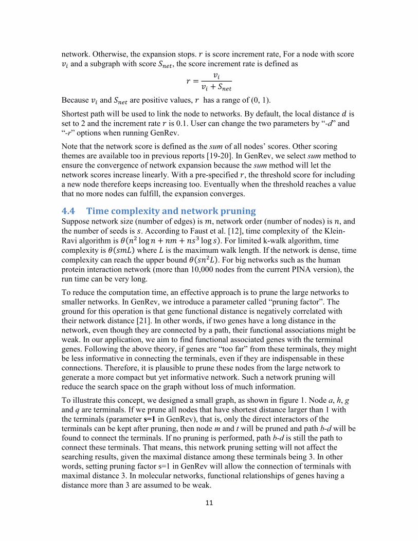
To illustrate this concept, we designed a small graph, as shown in figure 1. Node a, h, g and q are terminals. If we prune all nodes that have shortest distance larger than 1 with the terminals (parameter s=1 in GenRev), that is, only the direct interactors of the terminals can be kept after pruning, then node m and t will be pruned and path b-d will be found to connect the terminals. If no pruning is performed, path b-d is still the path to connect these terminals. That means, this network pruning setting will not affect the searching results, given the maximal distance among these terminals being 3. In other words, setting pruning factor s=1 in GenRev will allow the connection of terminals with maximal distance 3. In molecular networks, functional relationships of genes having a distance more than 3 are assumed to be weak.
12
If there is another node c between b and d, then this setting will prune c and consequently split the terminals into two separate networks, e.g. {a, b, h} and {g, d, q}. Otherwise if no pruning is conducted, path b-c-d will be identified and the distance between {a, h} and {g, q} will be 4. If we put the terminals into the network context, it is apparent that {a, b, h} and {g, d, q} belong to different modules. While c is an obvious bridge for the two modules, exclusion of c by pruning will nevertheless allow the re-discovery of the two modules by identifying b and d for terminal set {a, h} and {g, q} respectively.
By default, GenRev sets the pruning factor to 1 to include the paths within shortest path length 3 among the terminals. However, considering there are all kinds of user-defined networks, GenRev allows the users to specify this parameter in the command line by parameter s.
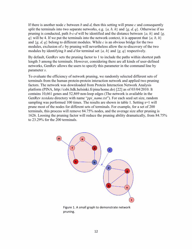
To evaluate the efficiency of network pruning, we randomly selected different sets of terminals from the human protein-protein interaction network and applied two pruning factors. The network was downloaded from Protein Interaction Network Analysis platform (PINA, http://csbi.ltdk.helsinki.fi/pina/home.do) [22] as of 03/04/2010. It contains 10,661 genes and 52,869 non-loop edges (The network is available in the GenRev testdata directory with name “ppi_name.txt”). For each seed set size, random sampling was performed 100 times. The results are shown in table 1. Setting s=1 will prune most of the nodes for different sets of terminals. For example, for a set of 200 terminals, this process will remove 84.75% nodes, and the average size after pruning is 1626. Loosing the pruning factor will reduce the pruning ability dramatically, from 84.75% to 23.29% for the 200 terminals.
Figure 1. A small graph to demonstrate network pruning.
13
Network pruning percentage
s=1 s=2 seeds number order stdv prune% order stdv prune%
50 504 100 95.27% 5760 438 45.97% 100 913 149 91.44% 7040 283 33.96% 200 1626 173 84.75% 8178 156 23.29% 500 3169 180 70.27% 9253 68 13.21%
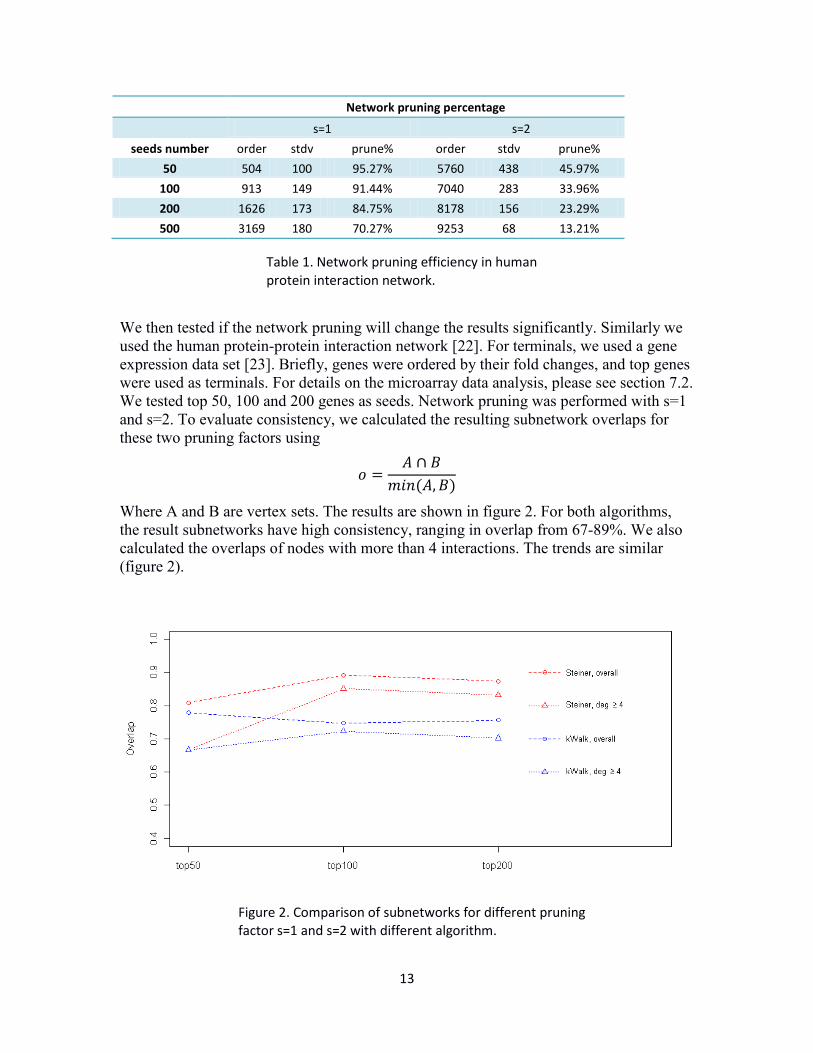
We then tested if the network pruning will change the results significantly. Similarly we used the human protein-protein interaction network [22]. For terminals, we used a gene expression data set [23]. Briefly, genes were ordered by their fold changes, and top genes were used as terminals. For details on the microarray data analysis, please see section 7.2. We tested top 50, 100 and 200 genes as seeds. Network pruning was performed with s=1 and s=2. To evaluate consistency, we calculated the resulting subnetwork overlaps for these two pruning factors using
𝑜 =𝐴 ∩ 𝐵
𝑚𝑖𝑛(𝐴,𝐵)
Where A and B are vertex sets. The results are shown in figure 2. For both algorithms, the result subnetworks have high consistency, ranging in overlap from 67-89%. We also calculated the overlaps of nodes with more than 4 interactions. The trends are similar (figure 2).
Table 1. Network pruning efficiency in human protein interaction network.
Figure 2. Comparison of subnetworks for different pruning factor s=1 and s=2 with different algorithm.

14
One concern is that network pruning may disperse the terminals into disjoint parts in the result subnetworks because many nodes would be removed while they might be indispensible to connect the terminals. To address this concern, we calculated the percentage of the giant components to the resultant subnetworks (table 2). In most cases, giant components take over 90% of the whole result network. The pruning factor setting seems not impact this value much. In other words, even the strongest pruning will allow the connection of the vast majority of the terminals. This is expected because many of deregulated genes are hypothesized to be under co-regulations of some transcriptional programs or other mechanisms. These functional associations predispose them within close neighborhoods in networks.
algorithm terminal s1 s2 Klein-Ravi 50 94.55% 94.74% Klein-Ravi 100 95.33% 96.46% Klein-Ravi 200 97.60% 98.23%
kwalk 50 88.68% 57.41% kwalk 100 96.06% 93.57% kwalk 200 97.83% 94.31%
By network pruning, software run time is greatly improved (table 3). The test was done in a Linux server with 2.6 GHz CPU and 16 Gb memory.
Klein-Ravi kWalk terminals s=1 s=2 s=1 s=2 top50 7 sec 6 min 25 sec 2.8 h top100 68 sec 38 min 8 min 17.6 h top200 8 min 116 min 42 min 53.4 h
Since the heuristic local search algorithm is very fast, network pruning is not applicable to it in GenRev.
4.5 Markov Clustering Algorithm (MCL) By default, GenRev applies MCL algorithm (http://www.micans.org/mcl/) [16] to the resultant subnetworks to identify modules if the subnetworks are not too big. A modular view of the subnetwork enables the users to quickly inspect the results and discover complexes or pathways revealed by the network. Modularity, a measurement of how good the division is by MCL, is provided. Though originally created to quantify graph clustering, it is able to show how modular a graph is. It ranges from -1 to 1. A value of 0 indicates that the modular structure is no longer than would be expected by chance. Positive values indicate the modularity is larger than random.
Table 3. Run time for algorithms and pruning factors.
Table 2. The ratio of connected nodes in the result subnetworks for different pruning factor.

15
The MCL algorithm iterates two operations called expansion and inflation, respectively. In GenRev, we implemented a prototype of this algorithm and restricted the input network order (number of nodes) to be less than 500. Otherwise if the network order is larger, this analysis procedure will be omitted. In GenRev, the MCL inflation factor is set to 2.
For more information about MCL, please visit http://www.micans.org/mcl/ and the original paper.
4.6 Gene ranking To help biologists prioritize genes, GenRev provides gene rankings by default. Genes in the resultant subnetwork are ranked by three measurements: degree, betweenness and score.
While the grounds for ranking genes by score are obvious, ranking by degree and betweenness serves a way to prioritize genes by their topological importance in the network. Previous studies reported that hub genes (high degree) and bottleneck genes (high betweenness) in gene networks are more important for cell survivals [24-26]. It is important to note that the ranking only reflects the gene's position in the subnetwork rather than the global network. This is one of GenRev's initiatives that highlight genes in a context dependent manner. Top 20 genes are returned for each measurement in GenRev.
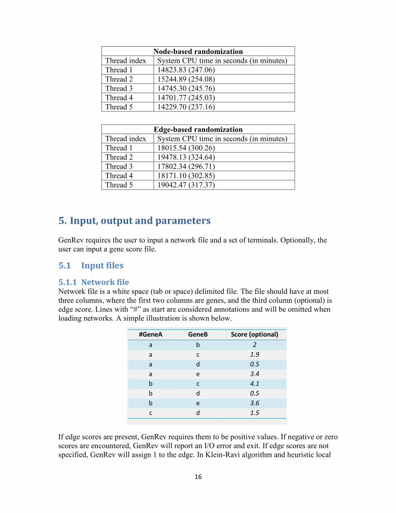
4.7 Randomization analysis We provided two ways of randomization strategies to evaluate the results; they were implemented in R scripts. First, we wrote an R script that implemented an edge-based randomization process based on Milo et al. [27]. This randomization process keeps the degree of each node while the edges are permuted, thus, the topological characteristics of the original network could be preserved.
Second, for the seeds (genes) whose node weights are available, we implemented a randomization process to permute node weights based on Chuang et al. [15]. This node-based normalization strategy is intended to build the null distribution by permute the status of node weights. Specifically for the score-guided subnetwork search methods, e.g., the heuristic local search method, this node weight randomization analysis is important to evaluate the results from randomness.
We applied both randomization strategies to our HCC dataset. For each strategy, we performed 1000 randomization subsets, split to 5 threads. The input genes are the same 200 top genes from our test dataset. All the other parameters are the same in randomization as in the real case, i.e., the heuristic local search algorithm was used with default parameters. We run it in a Linux server (Intel core 2, 3.0 GHz CPU and 16 GB memory) with five threads. It took ~5 hours to complete the edge-based normalization using the heuristic local search algorithm, with a total computational time ~1542 minutes for all threads. For the node-based randomization, it took less time (~4 hours for each thread and ~20.5 hours in total). In the real applications, both R scripts can be executed in parallel to save computational time.
16
Node-based randomization Thread index System CPU time in seconds (in minutes) Thread 1 14823.83 (247.06) Thread 2 15244.89 (254.08) Thread 3 14745.30 (245.76) Thread 4 14701.77 (245.03) Thread 5 14229.70 (237.16)
Edge-based randomization Thread index System CPU time in seconds (in minutes) Thread 1 18015.54 (300.26) Thread 2 19478.13 (324.64) Thread 3 17802.34 (296.71) Thread 4 18171.10 (302.85) Thread 5 19042.47 (317.37)
5. Input, output and parameters
GenRev requires the user to input a network file and a set of terminals. Optionally, the user can input a gene score file.
5.1 Input files
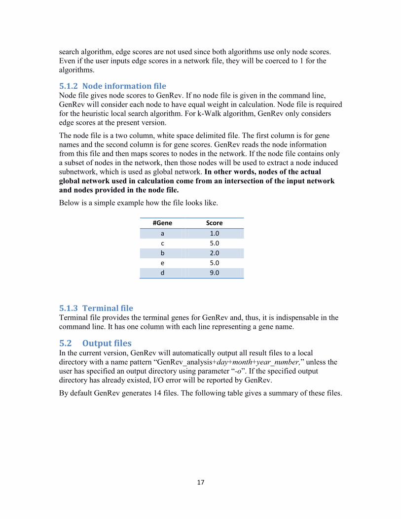
5.1.1 Network file Network file is a white space (tab or space) delimited file. The file should have at most three columns, where the first two columns are genes, and the third column (optional) is edge score. Lines with “#” as start are considered annotations and will be omitted when loading networks. A simple illustration is shown below.
If edge scores are present, GenRev requires them to be positive values. If negative or zero scores are encountered, GenRev will report an I/O error and exit. If edge scores are not specified, GenRev will assign 1 to the edge. In Klein-Ravi algorithm and heuristic local
#GeneA GeneB Score (optional) a b 2 a c 1.9 a d 0.5 a e 3.4 b c 4.1 b d 0.5 b e 3.6 c d 1.5
17
search algorithm, edge scores are not used since both algorithms use only node scores. Even if the user inputs edge scores in a network file, they will be coerced to 1 for the algorithms.
5.1.2 Node information file Node file gives node scores to GenRev. If no node file is given in the command line, GenRev will consider each node to have equal weight in calculation. Node file is required for the heuristic local search algorithm. For k-Walk algorithm, GenRev only considers edge scores at the present version.
The node file is a two column, white space delimited file. The first column is for gene names and the second column is for gene scores. GenRev reads the node information from this file and then maps scores to nodes in the network. If the node file contains only a subset of nodes in the network, then those nodes will be used to extract a node induced subnetwork, which is used as global network. In other words, nodes of the actual global network used in calculation come from an intersection of the input network and nodes provided in the node file. Below is a simple example how the file looks like.
5.1.3 Terminal file Terminal file provides the terminal genes for GenRev and, thus, it is indispensable in the command line. It has one column with each line representing a gene name.
5.2 Output files In the current version, GenRev will automatically output all result files to a local directory with a name pattern “GenRev_analysis+day+month+year_number,” unless the user has specified an output directory using parameter “-o”. If the specified output directory has already existed, I/O error will be reported by GenRev.
By default GenRev generates 14 files. The following table gives a summary of these files.
#Gene Score a 1.0 c 5.0 b 2.0 e 5.0 d 9.0

18
File Name Annotation summary.txt Overview of the current run terminals.txt Terminals used in calculation global_net.sif SIF format for global network global_edge_cat.eda Edge categorization for global network global_edge_score.eda Edge scores for global network global_node_cat.noa Node categorization for global network global_node_score.noa Node scores for global network sub_net.sif SIF format for subnetwork sub_edge_cat.eda Edge categorization for subnetwork sub_edge_score.eda Edge scores for subnetwork sub_node_cat.noa Node categorization for subnetwork sub_node_score.noa Node scores for subnetwork modules.txt Modules for subnetwork by MCL gene_rank.txt Gene ranking for subnetwork
The summary.txt file gives a summary of the current GenRev calculation. The module.txt and gene_rank.txt files give clustering analysis and gene ranking analysis result. If ‘-cl’ is set to FALSE, graph clustering analysis will be omitted.
GenRev does not provide network visualization. Instead, it generates SIF format files so the users can use the Cystoscape software [18] to visualize the networks. GenRev also generates node and edge attribution files (.noa and .eda files), thus allowing the users to load these files into Cytoscape and set different visual properties for the attributes. Files with ‘global’ prefix are global network related files used in the calculation, and files with ‘sub’ prefix are the extracted subnetwork related files.
Under several circumstances, GenRev will automatically adjust the input data for the selected algorithm. For example, even though each edge has different scores in the large network, GenRev will coerce the edge scores to be equal when running the Klein-Ravi Steiner algorithm. In other words, the “real” networks in computations may be different with the user input networks. To help the users check with their data, the “global” files in the result directory provide the “real” networks and their attributes. Meanwhile, nodes in large network are categorized into “terminal”, “linker” and “other”. Similarly edges are categorized into “subnetwork” and “other”. The users can use these attributes to visualize subnetworks in the large network.
In subnetworks, edges are categorized into “terminal_terminal”, “terminal_linker” and “linker_linker” to describe edges with different sources of end nodes. Nodes are categorized into “terminal” and “linker”.
If MCL is called, modules.txt file will be present in the result directory. This is a result file for graph clustering analysis to the subnetwork, not the large network. Each line denotes a module. Modularity is computed according to its definition [28].
5.3 Parameters To view GenRev parameters, type ‘GenRev -help’ in command line.

19
All parameters in GenRev are listed below. -h Show all parameters.
-v Show the current version of GenRev.
-a Algorithm selection. Three algorithms are available, please specify one of
'heuristic', 'steiner', 'kwalk' for your selection. Note there are some
algorithm specific parameters.
-s The pruning factor. Default is 1. Set to F if no network pruning
is wanted. This factor defines how GenRev reduces the global network to a
more compact, but yet informative network.
-g The network file path. Network file is space or tab delimited. The first
two columns are vertices, the third column is edge score. Larger score
indicate more close relations. This edge column is optional. If omitted,
all edges are thought to have equal scores of 1.
-n The node score file. Node file is space or tab delimited. The first column
is node name, and the second column is node score. Node scores should be
positive. This file is optional. If omitted, all nodes are thought to have
equal scores of 1.
-t The terminal nodes file. In GenRev, the input genes for subnetwork
extraction are called terminals. This file is of single column, with each
line is a node name.
-d Set the search radius in heuristic local search algorithm. Only valid when
algorithm parameter set to 'heuristic'. Default value is 2. It should set to
positive integers.
-r Set the network score increment rate. Default is 0.1, range is (0,1). Only
valid for heuristic algorithm.
-L Set the maximal walk length in limited k-walk algorithm. Default is 50. It
should set to be positive integers.
-it Set the iteration times for k-walk algorithm. Default is 1.
-cl If MCL clustering will be applied. Default if True. Alternative option is False.
If result network have more than 500 nodes, -cl is automatically set to F.
-o The output directory for the analysis results. If omitted, GenRev will
automatically create output directory in the current location.
In the following, we will elaborate on some algorithm specific parameters.

20
-s The pruning factor. This parameter defines whehter and how the network pruning is done. Assuming it is set to 𝑣, then the 𝑣 orders of the seeds (nodes with shortest distance less or equal to 𝑣 to the seeds) are kept while others are pruned to reduce the search space on the graph. By default s is 1. If no network pruning is needed, set s to False. Note that without network pruning, the runtime may be very long for large networks. See section 4 for more details.
-d This parameter is specific to heuristic local search algorithm and defines the local search radius. If d=1, then the direct neighbors of the seed graph will be examined. Similarly, if d=2, the neighbors of order 2 will be examined. Though in theory the users can set d to whatever value, we recommend setting d at no more than 2, because if two genes have a relation intermediated by the other two genes, their relations might be weak.
-r This is a score increment rate defined in the heuristic local search algorithm, with the equation shown below.
𝑟 =𝑉𝑖
𝑉𝑖 + 𝑆𝑔
Where 𝑉𝑖 is the maximum node score within the d distance and 𝑆𝑔 is the current network score. If 𝑉𝑖 is much larger than 𝑆𝑔, 𝑟 will get close to 1. Oppositely, 𝑟 gets closer to 0. By default, GenRev sets 𝑟 to 0.1, but the users can change it by setting “-r” parameter.
-L This parameter defines the maximum walk length in the limited k-walk algorithm. The default value is 50.
-it It defines how many iterations GenRev will run the limited k-walk algorithm. By default, GenRev will run it 1 time (iteration=1), but if this parameter is set to other values (e.g., 2), GenRev will iteratively run this algorithm by using the nodes in the resultant subnetwork from the previous run as terminals.
6. Toy network models
In this part, we will demonstrate the three algorithm implementations in GenRev with some toy models.
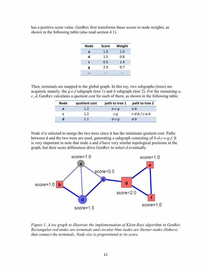
6.1 Klein-Ravi algorithm. First, we use a simple graph to show how the algorithm works. In the graph shown in figure 1, red nodes are terminals and blue nodes are so called Steiner nodes, which connect the terminals. We also call these nodes “linkers”. Grey nodes are not included in the resultant subnetwork. We keep them here for demonstration purpose only. Each node
21
has a positive score value. GenRev first transforms these scores to node weights, as shown in the following table (also read section 4.1).
Node Score Weight a 1.0 1.0 d 1.5 0.8 c 0.5 1.4 g 2.0 0.7 … … …
Then, terminals are mapped to the global graph. In this toy, two subgraphs (trees) are acquired, namely, the g-e-f subgraph (tree 1) and b subgraph (tree 2). For the remaining a, c, d, GenRev calculates a quotient cost for each of them, as shown in the following table.
Node quotient cost path to tree 1 path to tree 2 a 1.2 a-c-g a-b c 1.2 c-g c-d-b / c-a-b d 1.1 d-c-g d-b
Node d is selected to merge the two trees since it has the minimum quotient cost. Paths between d and the two trees are used, generating a subgraph consisting of b-d-c-e-g-f. It is very important to note that node a and d have very similar topological positions in the graph, but their score differences drive GenRev to select d eventually.
Figure 1. A toy graph to illustrate the implementation of Klein-Ravi algorithm in GenRev. Rectangular red nodes are terminals and circular blue nodes are Steiner nodes (linkers) that connect the terminals. Node size is proportional to its score.
22
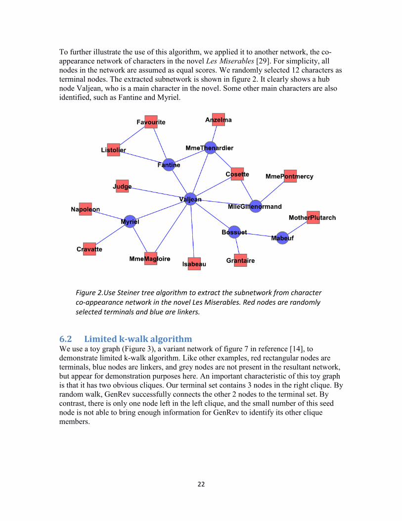
To further illustrate the use of this algorithm, we applied it to another network, the co-appearance network of characters in the novel Les Miserables [29]. For simplicity, all nodes in the network are assumed as equal scores. We randomly selected 12 characters as terminal nodes. The extracted subnetwork is shown in figure 2. It clearly shows a hub node Valjean, who is a main character in the novel. Some other main characters are also identified, such as Fantine and Myriel.
6.2 Limited k-walk algorithm We use a toy graph (Figure 3), a variant network of figure 7 in reference [14], to demonstrate limited k-walk algorithm. Like other examples, red rectangular nodes are terminals, blue nodes are linkers, and grey nodes are not present in the resultant network, but appear for demonstration purposes here. An important characteristic of this toy graph is that it has two obvious cliques. Our terminal set contains 3 nodes in the right clique. By random walk, GenRev successfully connects the other 2 nodes to the terminal set. By contrast, there is only one node left in the left clique, and the small number of this seed node is not able to bring enough information for GenRev to identify its other clique members.
Figure 2.Use Steiner tree algorithm to extract the subnetwork from character co-appearance network in the novel Les Miserables. Red nodes are randomly selected terminals and blue are linkers.

23
It is interesting to compare the differences between the Klein-Ravi algorithm and limited k-walk algorithm. While k-walks can pick up other clique members (f and h), the Klein-Ravi algorithm can only find f. This difference stems from the Klein-Ravi algorithm seeking to find the minimum number of nodes to connect terminals, while k-walk seeks to find the most relevant nodes in the information flow from terminal to terminal. It is very difficult to compare the superiority of the two algorithms since both have advantages and disadvantages. The Klein-Ravi algorithm can highlight the most important hubs, while missing some important information, especially regarding the modular structure of biological networks. The limited k-walk algorithm, on the other hand, may result in very comprehensive networks that makes the interpretation challenging.
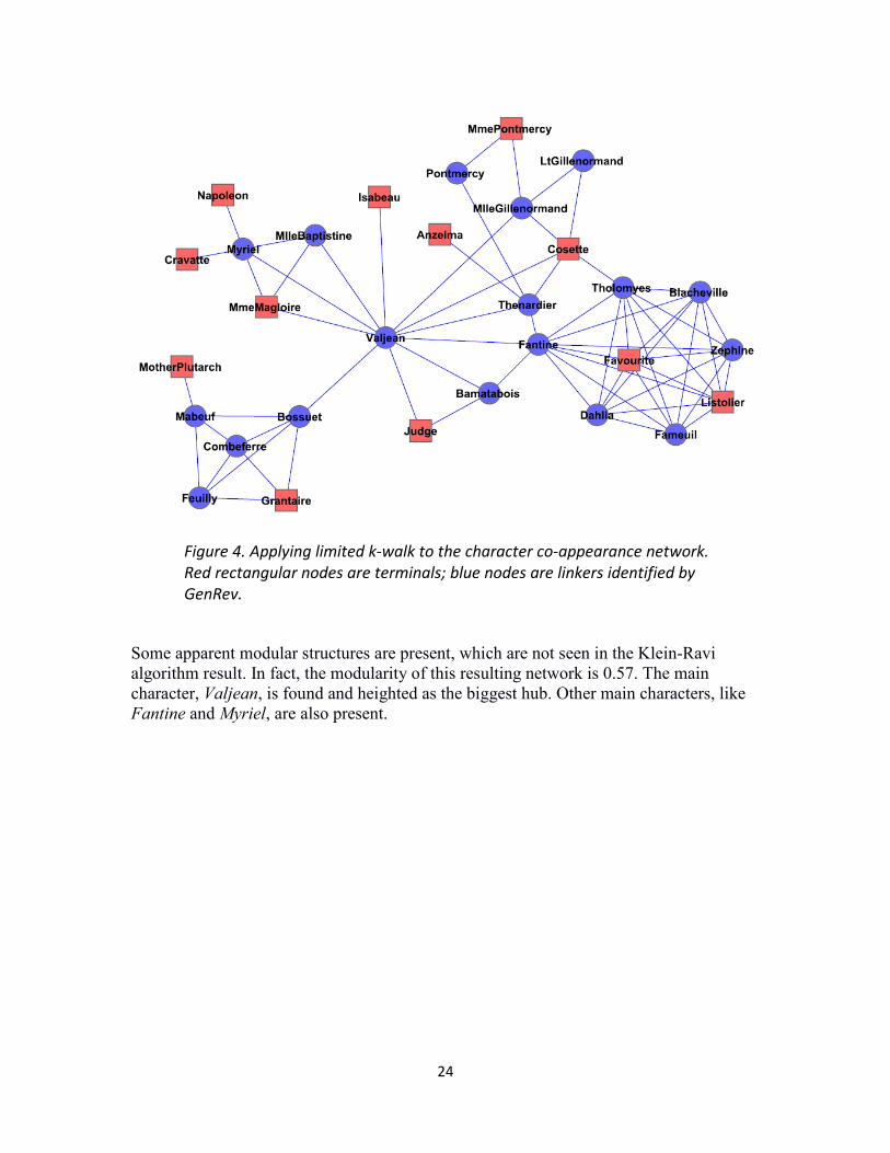
To give one more example of this algorithm, we run the same terminals to the Les Miserables character network using the same terminals. Result network is shown in figure 4.
Figure 3.Relevance subnetwork by limited k-walk algorithm. Red rectangular nodes are terminals, blue nodes are linkers, grey nodes are present just for illustration.
24
Some apparent modular structures are present, which are not seen in the Klein-Ravi algorithm result. In fact, the modularity of this resulting network is 0.57. The main character, Valjean, is found and heighted as the biggest hub. Other main characters, like Fantine and Myriel, are also present.
Figure 4. Applying limited k-walk to the character co-appearance network. Red rectangular nodes are terminals; blue nodes are linkers identified by GenRev.
25
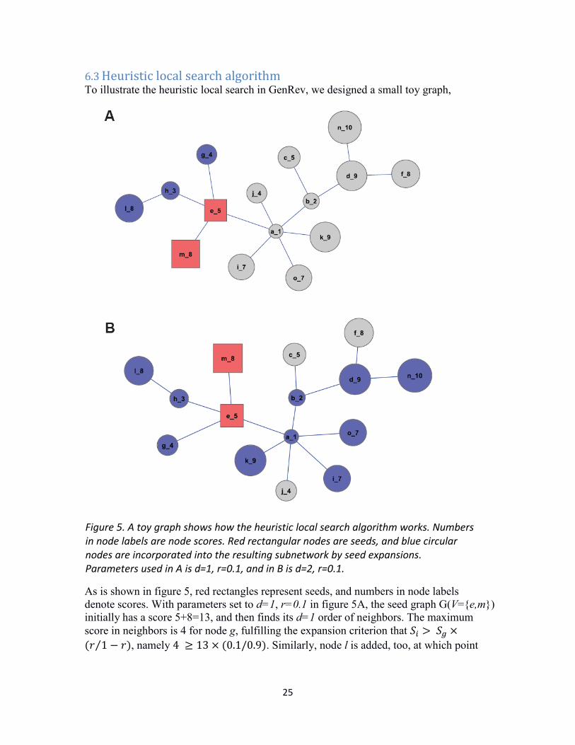
6.3 Heuristic local search algorithm To illustrate the heuristic local search in GenRev, we designed a small toy graph,
As is shown in figure 5, red rectangles represent seeds, and numbers in node labels denote scores. With parameters set to d=1, r=0.1 in figure 5A, the seed graph G(V={e,m}) initially has a score 5+8=13, and then finds its d=1 order of neighbors. The maximum score in neighbors is 4 for node g, fulfilling the expansion criterion that 𝑆𝑖 > 𝑆𝑔 ×(𝑟 1 − 𝑟⁄ ), namely 4 ≥ 13 × (0.1/0.9). Similarly, node l is added, too, at which point
Figure 5. A toy graph shows how the heuristic local search algorithm works. Numbers in node labels are node scores. Red rectangular nodes are seeds, and blue circular nodes are incorporated into the resulting subnetwork by seed expansions. Parameters used in A is d=1, r=0.1, and in B is d=2, r=0.1.
26
no addition meets the 𝑟 restriction. If the searching radius is set to d=2, the expansion will be more aggressive, resulting in a much bigger network (figure 5B).
7. Case studies
7.1 Applying GenRev to psychiatric disorders We had applied an early version of GenRev to psychiatric disorder studies. In a schizophrenia study, we used the Klein-Ravi algorithm to extract a schizophrenia network, and subsequently compared this network to the cancer specific network [10]. We showed that the schizophrenia genes are weakly connected and distribute peripherally in the network. For details, please refer to our original paper [10].
In another study, we used a set of genes localized in a set of significant copy number variation regions and a set of genes annotated to be related with epilepsy in HuGE as terminals, and aimed to construct epilepsy specific subnetworks [9]. The copy number variation data comes from a recent study [30]. The epilepsy related genes from HuGE were determined by a page search with key term “epilepsy”. Using these two sets of terminals, we constructed two subnetworks. By comparing the two networks, we identified 20 genes in common, and then we assigned them high priority candidates for epilepsy. We then used microarray data to evaluate their expression patterns. Two of them, CHRNA1 and GABRA1, are differentially expressed genes. We project that they can be used as biomarkers, or potentially therapeutic targets. For details, please refer to our paper [9].
7.2 Applying GenRev to a microarray data set We analyzed a microarray data set to illustrate GenRev. The data set was downloaded from NCBI Gene Expression Omnibus (GEO) database [31]. The authors used Affymetrix Human Genome U133 plus 2.0 arrays to characterize the stage differences of hepatitis C virus (HCV) induced hepatocellular carcinoma (HCC) [23]. Specifically their findings provided a comprehensive molecular portrait of genomic changes in progressive HCV-related HCC.
To re-analyze this data, we first categorized the samples into precancerous and cancerous groups. Precancerous samples consist of normal, cirrhosis and dysplastic liver samples, and cancerous samples consist of early and advanced stage HCC samples. We excluded 3 samples from cirrhotic liver tissue of patients without HCC. Since this data set had been already normalized when it was submitted to GEO, no more normalization was performed in our analysis. For genes with more than one probe set in the array platform, we used the strongest signal in each sample to collapse those probe sets.
To run GenRev, we calculated expression fold changes for each gene between the two groups at the logarithm scale. Negative values were transformed to their absolute values. Genes were then ranked decreasingly. Protein interaction network from PINA [22] was used as the large network. As of 03/04/2010, the PINA platform contained 10,661 unique nodes and 52,869 edges. Each node represents a gene product (i.e., protein encoded by the gene) and each edge represents an interaction between the two linked nodes.
27
The top 200 genes were used as terminals. Three algorithms were run respectively. Ranking genes by their degrees revealed that a cell cycle regulator, CDK1, was the largest hub protein (with most interactions) in all resulting networks. Previous studies have reported that CDK1 is a very important component in the HCV core protein mediated deregulation in HCC [32]. A pilot study reported that inhibition of CDK1 could decrease tumor growth and is a potential therapy for hepatoblastoma tumors and some other tumors [33]. In this example, GenRev prioritized it as hub protein in networks. In the microarray data set, this gene ranked 66th by fold change. Using gene expression alone, this gene may be missed. However, GenRev shows that the networks bring additional information and eventually lead to its identification.
Many other genes were also prioritized, such as UBB, TP53, GRB2 and others. It is not surprising to see TP53 in the lists because it is widely recognized as a tumor gene [34]. UBB is known to participate in the protein degradation. Recently it is reported to be a regulatory gene in cancer [35]. GRB2 is also observed relevant with HCC [36].
Please visit http://bioinfo.mc.vanderbilt.edu/GenRev.html for complete results.
8. Conclusion and remarks
A key task in biomedical informatics research is to understand the underpinning mechanisms of diseases and identify causal genes. While many technologies produce lists of genes that show changes at certain layers of the cellular system, interpreting these lists is challenging. The large scale networks shed lights on this task because we can understand these gene lists in network context. GenRev was developed under this premise. It allows the users to input a list of genes as seeds to extract relevance networks, which may then be used to study the functional associations among those seed genes and prioritize specific genes from their topological structures and scores.
By its three algorithms, GenRev guarantees to generate gene relevance networks. The next step would be how to interpret the networks and give insights into their functions. In the current version, GenRev provides clustering analysis and gene ranking analysis. However, we are aware that collaborative efforts are necessary to the successful creation of a high quality tool. We welcome feedbacks from GenRev users.
9. Notes
Part of GenRev (the node weighted Steiner tree algorithm) was implemented while Dr. S. Zheng was a Ph.D. student in the Shanghai Institute for Biological Sciences under the mentorship of Dr. Yixue Li and Dr. Pei Hao. Members in the Bioinformatics and Systems Medicine Laboratory in Vanderbilt, particularly Drs. Peilin Jia and Jingchun Sun provided numerous helpful discussion and suggestions for the development of GenRev. Dr. Peilin Jia also provided randomization R scripts that are available on the GenRev website.
28
10. References
[1] T. Beissbarth, T.P. Speed, GOstat: find statistically overrepresented Gene Ontologies within a group of genes, Bioinformatics 20 (2004) 1464-1465.
[2] S. Zheng, J. Sheng, C. Wang, X. Wang, Y. Yu, Y. Li, A. Michie, J. Dai, Y. Zhong, P. Hao, et al., MPSQ: a web tool for protein-state searching, Bioinformatics 24 (2008) 2412-2413.
[3] A. Subramanian, P. Tamayo, V.K. Mootha, S. Mukherjee, B.L. Ebert, M.A. Gillette, A. Paulovich, S.L. Pomeroy, T.R. Golub, E.S. Lander, et al., Gene set enrichment analysis: a knowledge-based approach for interpreting genome-wide expression profiles, Proc Natl Acad Sci U S A 102 (2005) 15545-15550.
[4] B. Zhang, S. Kirov, J. Snoddy, WebGestalt: an integrated system for exploring gene sets in various biological contexts, Nucleic Acids Res 33 (2005) W741-748.
[5] M. Ashburner, C.A. Ball, J.A. Blake, D. Botstein, H. Butler, J.M. Cherry, A.P. Davis, K. Dolinski, S.S. Dwight, J.T. Eppig, et al., Gene ontology: tool for the unification of biology. The Gene Ontology Consortium, Nat Genet 25 (2000) 25-29.
[6] M. Kanehisa, S. Goto, M. Furumichi, M. Tanabe, M. Hirakawa, KEGG for representation and analysis of molecular networks involving diseases and drugs, Nucleic Acids Res 38 (2010) D355-360.
[7] A.L. Barabasi, R. Albert, Emergence of scaling in random networks, Science 286 (1999) 509-512.
[8] V. Spirin, L.A. Mirny, Protein complexes and functional modules in molecular networks, Proc Natl Acad Sci U S A 100 (2003) 12123-12128.
[9] P. Jia, J.M. Ewers, Z. Zhao, Prioritization of epilepsy associated candidate genes by convergent analysis, PLoS One 6 (2011) e17162
[10] J. Sun, P. Jia, A.H. Fanous, E. van den Oord, X. Chen, B.P. Riley, R.L. Amdur, K.S. Kendler, Z. Zhao, Schizophrenia gene networks and pathways and their applications for novel candidate gene selection, PLoS One 5 (2010) e11351.
[11] M.S. Scott, T. Perkins, S. Bunnell, F. Pepin, D.Y. Thomas, M. Hallett, Identifying regulatory subnetworks for a set of genes, Mol Cell Proteomics 4 (2005) 683-692.
[12] K. Faust, P. Dupont, J. Callut, J. van Helden, Pathway discovery in metabolic networks by subgraph extraction, Bioinformatics 26 (2010) 1211-1218.
[13] P. Klein, R. Ravi, A nearly best-possible approximation algorithm for node-weighted Steiner trees., Journal of Algorithms 19 (1995) 104-115.
[14] P. Dupont, J. Callut, G. Dooms, J.N. Monette, Y. Deville, Relevant subgraph extraction from random walks in a graph., Research report UCL/FSA/INGI 2006-07 (2006).
[15] H.Y. Chuang, E. Lee, Y.T. Liu, D. Lee, T. Ideker, Network-based classification of breast cancer metastasis, Mol Syst Biol 3 (2007) 140.
[16] S.v. Dongen, Graph clustering by flow simulation, PhD thesis, University of Utrecht, May 2000 (2000).
[17] A.H. Aric, A.S. Daniel, J.S. Pieter, Exploring network structure, dynamics, and function using NetworkX, Proceedings of the 7th Python in Science Conference (SciPy2008) (2008) 11-15.
29
[18] M.S. Cline, M. Smoot, E. Cerami, A. Kuchinsky, N. Landys, C. Workman, R. Christmas, I. Avila-Campilo, M. Creech, B. Gross, et al., Integration of biological networks and gene expression data using Cytoscape, Nat Protoc 2 (2007) 2366-2382.
[19] T. Ideker, O. Ozier, B. Schwikowski, A.F. Siegel, Discovering regulatory and signalling circuits in molecular interaction networks, Bioinformatics 18 Suppl 1 (2002) S233-240.
[20] S. Nacu, R. Critchley-Thorne, P. Lee, S. Holmes, Gene expression network analysis and applications to immunology, Bioinformatics 23 (2007) 850-858.
[21] R. Sharan, I. Ulitsky, R. Shamir, Network-based prediction of protein function, Mol Syst Biol 3 (2007) 88.
[22] J. Wu, T. Vallenius, K. Ovaska, J. Westermarck, T.P. Makela, S. Hautaniemi, Integrated network analysis platform for protein-protein interactions, Nat Methods 6 (2009) 75-77.
[23] E. Wurmbach, Y.B. Chen, G. Khitrov, W. Zhang, S. Roayaie, M. Schwartz, I. Fiel, S. Thung, V. Mazzaferro, J. Bruix, et al., Genome-wide molecular profiles of HCV-induced dysplasia and hepatocellular carcinoma, Hepatology 45 (2007) 938-947.
[24] H. Yu, P.M. Kim, E. Sprecher, V. Trifonov, M. Gerstein, The importance of bottlenecks in protein networks: correlation with gene essentiality and expression dynamics, PLoS Comput Biol 3 (2007) e59.
[25] X. He, J. Zhang, Why do hubs tend to be essential in protein networks?, PLoS Genet 2 (2006) e88.
[26] H. Jeong, S.P. Mason, A.L. Barabasi, Z.N. Oltvai, Lethality and centrality in protein networks, Nature 411 (2001) 41-42.
[27] R. Milo, S. Shen-Orr, S. Itzkovitz, N. Kashtan, D. Chklovskii, U. Alon, Network motifs: simple building blocks of complex networks, Science 298 (2002) 824-827.
[28] M.E. Newman, Fast algorithm for detecting community structure in networks, Phys Rev E Stat Nonlin Soft Matter Phys 69 (2004) 066133.
[29] D.E. Knuth, The Stanford GraphBase: A Platform for Combinatorial Computing, Addison-Wesley, Reading, MA (1993).
[30] E.L. Heinzen, R.A. Radtke, T.J. Urban, G.L. Cavalleri, C. Depondt, A.C. Need, N.M. Walley, P. Nicoletti, D. Ge, C.B. Catarino, et al., Rare deletions at 16p13.11 predispose to a diverse spectrum of sporadic epilepsy syndromes, Am J Hum Genet 86 707-718.
[31] T. Barrett, D.B. Troup, S.E. Wilhite, P. Ledoux, C. Evangelista, I.F. Kim, M. Tomashevsky, K.A. Marshall, K.H. Phillippy, P.M. Sherman, et al., NCBI GEO: archive for functional genomics data sets--10 years on, Nucleic Acids Res 39 (2011) D1005-1010.
[32] A. Spaziani, A. Alisi, D. Sanna, C. Balsano, Role of p38 MAPK and RNA-dependent protein kinase (PKR) in hepatitis C virus core-dependent nuclear delocalization of cyclin B1, J Biol Chem 281 (2006) 10983-10989.
[33] A. Goga, D. Yang, A.D. Tward, D.O. Morgan, J.M. Bishop, Inhibition of CDK1 as a potential therapy for tumors over-expressing MYC, Nat Med 13 (2007) 820-827.

30
[34] C. Caron de Fromentel, T. Soussi, TP53 tumor suppressor gene: a model for investigating human mutagenesis, Genes Chromosomes Cancer 4 (1992) 1-15.
[35] P. Wu, Y. Tian, G. Chen, B. Wang, L. Gui, L. Xi, X. Ma, Y. Fang, T. Zhu, D. Wang, et al., Ubiquitin B: an essential mediator of trichostatin A-induced tumor-selective killing in human cancer cells, Cell Death Differ 17 (2010) 109-118.
[36] S.Y. Yoon, M.J. Jeong, J. Yoo, K.I. Lee, B.M. Kwon, D.S. Lim, C.E. Lee, Y.M. Park, M.Y. Han, Grb2 dominantly associates with dynamin II in human hepatocellular carcinoma HepG2 cells, J Cell Biochem 84 (2001) 150-155.