Theoretical Population Biology 87 (2013) 62–74

Contents lists available at SciVerse ScienceDirect

Theoretical Population Biology

journal homepage: www.elsevier.com/locate/tpb

Genotype imputation in a coalescent model withinfinitely-many-sites mutationLucy Huang a, Erkan O. Buzbas b, Noah A. Rosenberg b,∗

a Center for Computational Medicine and Bioinformatics, University of Michigan, Ann Arbor, MI 48109, USAb Department of Biology, Stanford University, Stanford, CA 94305, USA

a r t i c l e i n f o

Article history:Available online 16 October 2012

Keywords:CoalescentImputationPopulation divergence

a b s t r a c t

Empirical studies have identified population-genetic factors as important determinants of the propertiesof genotype-imputation accuracy in imputation-based disease association studies. Here, we develop asimple coalescentmodel of three sequences thatweuse to explore the theoretical basis for the influence ofthese factors on genotype-imputation accuracy, under the assumption of infinitely-many-sites mutation.Employing a demographicmodel in which two populations diverged at a given time in the past, we derivethe approximate expectation and variance of imputation accuracy in a study sequence sampled fromone of the two populations, choosing between two reference sequences, one sampled from the samepopulation as the study sequence and the other sampled from the other population. We show that, underthis model, imputation accuracy—as measured by the proportion of polymorphic sites that are imputedcorrectly in the study sequence—increases in expectation with the mutation rate, the proportion of themarkers in a chromosomal region that are genotyped, and the time to divergence between the studyand reference populations. Each of these effects derives largely from an increase in information availablefor determining the reference sequence that is genetically most similar to the sequence targeted forimputation. We analyze as a function of divergence time the expected gain in imputation accuracy inthe target using a reference sequence from the same population as the target rather than from the otherpopulation. Together with a growing body of empirical investigations of genotype imputation in diversehuman populations, our modeling framework lays a foundation for extending imputation techniques tonovel populations that have not yet been extensively examined.

© 2012 Elsevier Inc. All rights reserved.

1. Introduction

The field of humangenetics has recentlywitnessed an explosionin the number of published genome-wide association (GWA)studies, revealing hundreds of novel disease-associated genes(Donnelly, 2008; Manolio et al., 2008; Hindorff et al., 2009,2011). The considerable potential of GWA studies—which examinethousands to millions of genetic markers in samples of unrelatedindividuals with the goal of uncovering genotype–phenotypecorrelations—to ultimately improve humanhealth has beenwidelyrecognized (e.g., Hardy and Singleton, 2009; Manolio, 2010;Stranger et al., 2011).

Among factors contributing to the success of GWA studies hasbeen the advent of genotype-imputation methods that use chro-mosomal segments shared among subjects to predict, or impute,genotypes at marker positions not directly measured in individ-ual GWA studies (Li et al., 2006; Nicolae, 2006; Browning andBrowning, 2007; Marchini et al., 2007; Servin and Stephens, 2007).

∗ Corresponding author.E-mail address: noahr@stanford.edu (N.A. Rosenberg).

0040-5809/$ – see front matter© 2012 Elsevier Inc. All rights reserved.doi:10.1016/j.tpb.2012.09.006

In imputation studies, the haplotypes of ‘‘reference’’ individualsthat have been genotyped at a higher density than GWA individ-uals targeted for imputation often serve as template sequences onthe basis of which unknown genotypes in the targets are inferred.Because imputation increases the number of markers that canbe interrogated for disease associations and permits larger sam-ple sizes by enabling data sets typed on different platforms to bemerged, it can increase the statistical power of GWA studies (e.g.,Li et al., 2009; Marchini and Howie, 2010). This important rolefor imputation is likely to persist as technology advances; whenwhole-genome sequencing of at least a portion of GWA samplesbecomes routinely feasible, the power of sequence-based GWAstudies can be improved by imputation in genotyped individualsusing sequenced individuals as templates (Li et al., 2011).

Recent studies have empirically examined the determinantsof genotype-imputation accuracy in globally distributed humanpopulations (Guan and Stephens, 2008; Pei et al., 2008; Huanget al., 2009, 2011; Li et al., 2009; Fridley et al., 2010; Surakka et al.,2010). These investigations have shown that, in imputation-basedGWA studies, population-genetic factors play an important role indetermining levels of imputation accuracy attainable in a studypopulation. Factors such as the level of linkage disequilibrium in

L. Huang et al. / Theoretical Population Biology 87 (2013) 62–74 63

a study population and the degree of genetic similarity betweena study population and a reference population whose membersserve as templates have been found in imputation experiments tobe prominent drivers of imputation accuracy (Egyud et al., 2009;Huang et al., 2009, 2011; Paşaniuc et al., 2010; Shriner et al., 2010).Though empirical work on genotype imputation has providedsome understanding of the population-genetic factors that affectimputation accuracy, theoretical work exploring the influence ofthese factors on imputation accuracy has been limited.

A theoretical approach to studying genotype imputation un-der a population-genetic model offers the potential for produc-ing a variety of insights. First, by obtaining expressions for themean and the variance of the imputation accuracy as a functionof population-genetic parameters, we can explain patterns of im-putation accuracy observed in empirical studies in terms of thepopulation-genetic factors that affect the underlying genealogicalrelationship between study and reference individuals. Second, us-ing simple expressions, imputation accuracy can be evaluatedwithless computation than in simulation-based approaches, enablinginvestigators to predict imputation accuracy under a model ratherthan implement computationally intensive simulations. Third,unlike targeted simulations specific to particular populations ofinterest, a general modeling framework can be adapted for organ-isms beyond humans in which imputation-based association stud-ies and large-scale genomic resources have begun to emerge (e.g.,Atwell et al., 2010; Druet et al., 2010; Kirby et al., 2010; Badke et al.,2012; Hickey et al., 2012).

Jewett et al. (2012) introduced a theoretical model for eva-luating imputation accuracy as a function of population-geneticparameters. Using a coalescent framework, they analyticallystudied the effect of reference-panel size on imputation accuracy,aswell as the degree towhich the use of reference haplotypes fromthe same population as a target sequence (an ‘‘internal’’ referencepanel) improves the accuracy of imputation compared to the useof reference haplotypes from a separate population (an ‘‘external’’reference panel). In order to incorporate a large sample size inobtaining their analytical results, however, Jewett et al. (2012) didnot account for randomness in themutation process. Instead, theirtreatment of mutation amounted to an assumption that mutationis a deterministic process, in which mutations accumulate alonga genealogical branch in direct proportion to the branch length.Consequently, under this assumption, the best template forimputation is always a haplotypewhose coalescence timewith thetarget sequence on which genotypes are to be imputed is smallest.

Here, we consider a coalescent model of genotype imputationthat, at the cost of examining only a small sample size, allows forrandomness in the imputation process resulting from the stochas-ticity of mutation. Assuming the infinitely-many-sites mutationmodel, we derive the approximate expectation and variance ofimputation accuracy under a straightforward imputation scheme,conditioning on amutation parameter (θ ), a proportion of markersgenotyped in a given length of a chromosome (p), and a time to di-vergence between the target population and an external referencepopulation (td). As in Jewett et al. (2012), our derivations accountfor randomness in the genealogy by considering the distribution ofgenealogies under a model in which study and reference individ-uals are sampled from two populations that diverged at time td inthe past. We pose the following questions: (1) What are the influ-ences of θ, p, and td on the expectation and variance of imputationaccuracy? (2) What is the expected gain in imputation accuracy ina study sequence targeted for imputation by using a reference se-quence from the same population as the target rather than from adifferent population? Answers to these questions provide informa-tion on the factors that affect genotype-imputation accuracy, withimplications for the design of imputation-based association stud-ies and the expansion of genomic databases.

2. Theory

In this section, we introduce a theoretical framework thatpermits the computation of the approximate expectation andvariance of imputation accuracy in a target sequence on thebasis of one of two reference sequences. The framework hasfour parts: a coalescent model for the genealogical relationshipsamong lineages, a mutation model, a decision rule that guides theselection of the reference sequence for the imputation, and animputation scheme that specifies how the imputation is performedand its accuracy evaluated. The computations employ threeapproximations, including a Monte Carlo step for the evaluationof certain integrals.

2.1. A coalescent model

Consider two populations P1 and P2 that diverged from an an-cestral population PA at time td in the past. Further, consider threehaploid individuals—a study individual targeted for imputation(henceforth simply identified as a target and denoted by I) and tworeference individuals (denoted by R1 and R2). Individuals R1 and Iare from population P1, and individual R2 is from population P2. Ina diploid organism, the haploid individuals can be viewed as singlehaplotypes.

For the set of three individuals, let G denote a labeled genetree topology. We denote the times during which three and twolineages exist in the genealogy, and the divergence time betweenpopulations P1 and P2, by T3, T2, and td, respectively. We assumethat the diploid effective population size, denoted by Ne, is thesame for populations P1, P2, and PA. All times aremeasured in unitsof 2Ne generations. For convenience, we refer toG as the genealogyand use the notation T = (T3, T2, td).

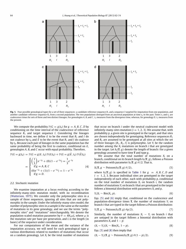
The genealogy G can have one of four possible genealogicaltypes G (Fig. 1): three in which the first coalescence event occursmore anciently than the population-divergence time td (g =

A, B, C), and one in which the first coalescence occurs morerecently than td (g = D). For each type, we label the externalbranches for the lineages of reference individuals R1 and R2 andtarget individual I by 1, 2, and 3, respectively (Fig. 1). We examinethe genealogy backward in time, combining the external andinternal branches immediately descended from the root into onebranch that takes on the label for the external branch. Thus, forinstance, branch 2 in genealogy A has length td + t3 + 2t2. Notethat, as shown in Fig. 1, in genealogies A, B, and C, t3 measuresfrom td back in time, whereas, in genealogy D, t3 measures fromthe present.

Under standard coalescent theory, the time (in units of 2Negenerations) for k lineages in a population to coalesce to k − 1lineages follows an exponential distribution with parameter

k2

(Kingman, 1982a,b). For our model of sequences R1, R2, and I , theprobability density function of T2 for genealogies g = A, B, C,D is

fT2(t2|G = g, td) = e−t2 , g = A, B, C,D. (1)

For g = A, B, C , the probability density function of T3 is

fT3(t3|G = g, td) = 3e−3t3 , g = A, B, C . (2)

For genealogy D, however, the lineages for reference sequenceR1 and target sequence I are constrained to coalesce no moreanciently than the divergence time td. Thus, the probability densityfunction for the time T3 during which all three lineages exist is

fT3(t3|G = D, td) =e−t3

1 − e−td1{t3<td}, (3)

where 1{B} is the indicator function that takes a value of 1 ifcondition B holds and is 0 otherwise.

64 L. Huang et al. / Theoretical Population Biology 87 (2013) 62–74

Fig. 1. Four possible genealogical types for a set of three sequences: a candidate reference sequence R1 and a sequence I targeted for imputation from one population, andanother candidate reference sequence R2 from a second population. The two populations diverged from an ancestral population at time td in the past. Times t3 and t2 arecoalescence times for sets of three and two distinct lineages. For genealogies A, B, and C, t3 measures from the divergence time, whereas, for genealogy D, t3 measures fromthe present.

We compute the probability P(G = g|td) for g = A, B, C,D byconditioning on the time interval of the coalescence of referencesequence R1 and target sequence I . Considering the lineagesbackward in time, we define E to be the event that R1 and I donot coalesce by td and E to be the event that R1 and I do coalesceby td. Because each pair of lineages in the same population has thesame probability of being the first to coalesce, conditional on E ,genealogies A, B, and C occur with equal probability. Therefore,

P(G = g|td) = P(G = g|E, td) P(E |td) + P(G = g|E, td) P(E |td)

=

13

e−td + (0)(1 − e−td) =

13e−td

if g = A, B, C(0)e−td + (1)(1 − e−td) = 1 − e−td

if g = D.

(4)

2.2. Stochastic mutation

We examine imputation at a locus evolving according to theinfinitely-many-sites mutation model, with no recombination(Watterson, 1975). We consider only the polymorphic sites in asample of three sequences, ignoring all sites that are not poly-morphic in the sample. Under the infinitely-many-sites model, thenumber of polymorphic sites in a sample is the same as the numberof mutations in its gene genealogy, and we use the terms ‘‘poly-morphic sites’’ and ‘‘mutations’’ interchangeably. We denote thepopulation-scaled mutation parameter by θ = 4NeµL, where µ isthe mutation rate per base per generation, and L is the length (inbases) of the sequence under consideration.

For our computations of the mean and the variance of theimputation accuracy, we will need for each genealogical type gvarious distributions related to numbers of mutations that occuron a random genealogy. Let Xi be the total number of mutations

that occur on branch i under the neutral coalescent model withinfinitely-many-sites mutation (i = 1, 2, 3). We assume that, withprobability p, a given site is genotyped in the target, and that sitesare chosen independently for genotyping. Reference sequences R1and R2 are assumed to be genotyped at all sites at which the setof three lineages {R1, R2, I} is polymorphic. Let Yi be the randomnumber among the Xi mutations on branch i that are genotypedin the target. Let hi(T; g) denote the length of branch i for a givengenealogy assumed to have time T and type g .

We assume that the total number of mutations Xi on abranch, conditional on its branch length hi(T; g), follows a Poissondistribution with parameter hi(T; g) θ/2. That is,

Xi|T, g ∼ Poisson(hi(T; g) θ/2), (5)

where hi(T; g) is specified in Table 1 for g = A, B, C,D andi = 1, 2, 3. Because individual sites are genotyped in the targetindependently of each other, each with probability p, conditionalon the total number of mutations Xi on branch i, the randomnumber ofmutations Yi on branch i that are genotyped in the targetfollows a binomial distribution with parameters Xi and p,

Yi|Xi ∼ Bin(Xi, p). (6)

Eqs. (5) and (6) imply that, conditional on the coalescence andpopulation-divergence times T, the number of mutations Yi onbranch i that are typed in the target follows a Poisson distribution:

Yi|T, g ∼ Poisson(hi(T; g) θp/2). (7)

Similarly, the number of mutations Xi − Yi on branch i thatare untyped in the target follows a binomial distribution withparameters Xi and 1 − p:

(Xi − Yi)|Xi ∼ Bin(Xi, 1 − p). (8)

Eqs. (5) and (8) then imply that

(Xi − Yi)|T, g ∼ Poisson(hi(T; g) θ(1 − p)/2). (9)

L. Huang et al. / Theoretical Population Biology 87 (2013) 62–74 65

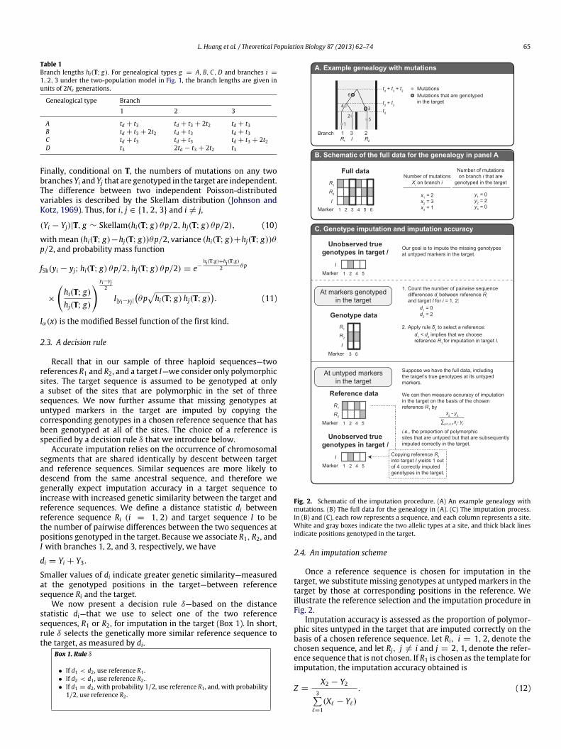
Table 1Branch lengths hi(T; g). For genealogical types g = A, B, C,D and branches i =

1, 2, 3 under the two-population model in Fig. 1, the branch lengths are given inunits of 2Ne generations.

Genealogical type Branch1 2 3

A td + t3 td + t3 + 2t2 td + t3B td + t3 + 2t2 td + t3 td + t3C td + t3 td + t3 td + t3 + 2t2D t3 2td − t3 + 2t2 t3

Finally, conditional on T, the numbers of mutations on any twobranchesYi andYj that are genotyped in the target are independent.The difference between two independent Poisson-distributedvariables is described by the Skellam distribution (Johnson andKotz, 1969). Thus, for i, j ∈ {1, 2, 3} and i = j,

(Yi − Yj)|T, g ∼ Skellam(hi(T; g) θp/2, hj(T; g) θp/2), (10)

withmean (hi(T; g)−hj(T; g))θp/2, variance (hi(T; g)+hj(T; g))θp/2, and probability mass function

fSk(yi − yj; hi(T; g) θp/2, hj(T; g) θp/2) = e−hi(T;g)+hj(T;g)

2 θp

×

hi(T; g)hj(T; g)

yi−yj2

I|yi−yj|θphi(T; g) hj(T; g)

. (11)

Iα(x) is the modified Bessel function of the first kind.

2.3. A decision rule

Recall that in our sample of three haploid sequences—tworeferences R1 and R2, and a target I—we consider only polymorphicsites. The target sequence is assumed to be genotyped at onlya subset of the sites that are polymorphic in the set of threesequences. We now further assume that missing genotypes atuntyped markers in the target are imputed by copying thecorresponding genotypes in a chosen reference sequence that hasbeen genotyped at all of the sites. The choice of a reference isspecified by a decision rule δ that we introduce below.

Accurate imputation relies on the occurrence of chromosomalsegments that are shared identically by descent between targetand reference sequences. Similar sequences are more likely todescend from the same ancestral sequence, and therefore wegenerally expect imputation accuracy in a target sequence toincrease with increased genetic similarity between the target andreference sequences. We define a distance statistic di betweenreference sequence Ri (i = 1, 2) and target sequence I to bethe number of pairwise differences between the two sequences atpositions genotyped in the target. Because we associate R1, R2, andI with branches 1, 2, and 3, respectively, we have

di = Yi + Y3.

Smaller values of di indicate greater genetic similarity—measuredat the genotyped positions in the target—between referencesequence Ri and the target.

We now present a decision rule δ—based on the distancestatistic di—that we use to select one of the two referencesequences, R1 or R2, for imputation in the target (Box 1). In short,rule δ selects the genetically more similar reference sequence tothe target, as measured by di.

Box 1. Rule δ

• If d1 < d2 , use reference R1 .• If d2 < d1 , use reference R2 .• If d1 = d2 , with probability 1/2, use reference R1 , and, with probability

1/2, use reference R2 .

Fig. 2. Schematic of the imputation procedure. (A) An example genealogy withmutations. (B) The full data for the genealogy in (A). (C) The imputation process.In (B) and (C), each row represents a sequence, and each column represents a site.White and gray boxes indicate the two allelic types at a site, and thick black linesindicate positions genotyped in the target.

2.4. An imputation scheme

Once a reference sequence is chosen for imputation in thetarget, we substitute missing genotypes at untyped markers in thetarget by those at corresponding positions in the reference. Weillustrate the reference selection and the imputation procedure inFig. 2.

Imputation accuracy is assessed as the proportion of polymor-phic sites untyped in the target that are imputed correctly on thebasis of a chosen reference sequence. Let Ri, i = 1, 2, denote thechosen sequence, and let Rj, j = i and j = 2, 1, denote the refer-ence sequence that is not chosen. If R1 is chosen as the template forimputation, the imputation accuracy obtained is

Z =X2 − Y2

3ℓ=1

(Xℓ − Yℓ)

. (12)

66 L. Huang et al. / Theoretical Population Biology 87 (2013) 62–74

Alternatively, if R2 is chosen as the template, then the imputationaccuracy is

Z =X1 − Y1

3ℓ=1

(Xℓ − Yℓ)

. (13)

In both cases, the numerator isXj−Yj, because, under the infinitely-many-sites mutation model, polymorphic sites produced bymutations on the branch for reference sequence Rj are exactlywhere reference Ri and target I have identical genotypes. Thus, tocount the number of sites imputed correctly in the target whenusing reference sequence Ri, one simply counts the number ofmutations on the branch for reference sequence Rj that are notgenotyped in the target but that are imputed. The denominator3

ℓ=1(Xℓ − Yℓ) corresponds to the total number of untypedpolymorphic sites in the target that are subsequently imputed; inthe case that

3ℓ=1(Xℓ − Yℓ) = 0, Z is undefined because there are

no genotypes to impute.

2.5. Expectation and variance of imputation accuracy

At sites genotyped in both reference and target sequences, thenumber di of pairwise differences between reference Ri (i = 1, 2)and target I is observable. Given d1 and d2, we apply rule δ in Box1 to select a reference sequence for imputing missing genotypesat untyped markers in the target. In this section, conditioning onthe model parameters—the mutation parameter θ , the proportionp of polymorphic sites genotyped in the target, and the population-divergence time td—we derive the approximate expectation andvariance of imputation accuracy Z by averaging over all possiblegenealogical types G and coalescence times T3 and T2.

To compute the expectation E[Z |θ, p, td], we consider threepossible scenarios that can occur when we apply rule δ to agenealogy: reference sequence R1 is selected as the templatesequence for imputation in target sequence I because d1 < d2,reference sequence R2 is selected because d1 > d2, and a choiceis made randomly between references R1 and R2 because d1 = d2.Let S1 be the scenario in which d1 < d2 (i.e., Y1 − Y2 < 0), letS2 be the scenario in which d1 > d2 (i.e., Y1 − Y2 > 0), and letS3 be the scenario in which d1 = d2 (i.e., Y1 − Y2 = 0). We canobtain E[Z |θ, p, td] by taking a weighted average of its expectationconditional on the genealogical type g and the scenario Sw , whereg = A, B, C,D and w = 1, 2, 3, and where the weight is the jointprobability of the genealogical type G = g and the scenario Sw:

E[Z |θ, p, td]

=

g=A,B,C,D

3w=1

E[Z |g, Sw, θ, p, td] P(g, Sw|θ, p, td). (14)

We first derive the conditional expectations E[Z |g, Sw, θ, p, td]and the probabilities P(g, Sw|θ, p, td) for g = A, B, C,D andw = 1, 2, 3, andwe then obtain the expectationE[Z |θ, p, td] usingEq. (14).

Many quantities in Sections 2.5.1 and 2.5.2 are conditioned onθ, p, and td, but, for notational convenience, these parameters aresuppressed.

2.5.1. Derivation of E[Z |g, Sw] in Eq. (14)Let B be a Bernoulli random variable with parameter 1/2. For

any genealogical type g , we can write the expectation E[Z |g, Sw]

under a specific scenario Sw for w = 1, 2, 3:

E[Z |g, Sw]

=

E

Xj − Yj3

ℓ=1(Xℓ − Yℓ)

g, Sw

if w = 1, 2, where j = 3 − w

E

BX2 − Y2

3ℓ=1

(Xℓ − Yℓ)

+ (1 − B)X1 − Y1

3ℓ=1

(Xℓ − Yℓ)

g, Sw

if w = 3.

(15)

We make two approximations to obtain an expression forE[Z |g, Sw]. First, we use the first-order Taylor approximation thattreats the expectation of a quotient as a quotient of expectations;although this approximation is not accurate in general, we willsee later that, in our analysis, it is not unreasonable. Next, weapproximate E[Xi − Yi|g, Sw] by E[Xi − Yi|g]; this approximationamounts to assuming for i ∈ {1, 2, 3} that the number of untypedmutations on branch i is independent of which reference is closerto the target at sites genotyped in the target. Although thesequantities are not independent, we will see that this assumptionis also reasonable.

Applying the approximations, for g = A, B, C,D andw ∈ {1, 2},

E[Z |g, Sw] = E

Xj − Yj3

ℓ=1(Xℓ − Yℓ)

g, Sw

≈

E[Xj − Yj|g, Sw]

E

3ℓ=1

(Xℓ − Yℓ)|g, Sw

≈

E[Xj − Yj|g]

E

3ℓ=1

(Xℓ − Yℓ)|g , (16)

where j = 3 − w. For g = A, B, C,D and w = 3,

E[Z |g, Sw]

=12

E

X2 − Y23

ℓ=1(Xℓ − Yℓ)

g, Sw

+ E

X1 − Y13

ℓ=1(Xℓ − Yℓ)

g, Sw

≈12

E[X2 − Y2|g]

E

3ℓ=1

(Xℓ − Yℓ)|g +

E[X1 − Y1|g]

E

3ℓ=1

(Xℓ − Yℓ)|g . (17)

In Eqs. (16) and (17), for g = A, B, C,D and i = 1, 2, 3,the expectation E[Xi − Yi|g] can be found by conditioning onthe coalescence times T3 and T2 and then integrating over theirdistributions:

E[Xi − Yi|g]

=

∞

t2=0

a

t3=0E[Xi − Yi|t3, t2, g] fT3,T2(t3, t2|g) dt3 dt2. (18)

L. Huang et al. / Theoretical Population Biology 87 (2013) 62–74 67

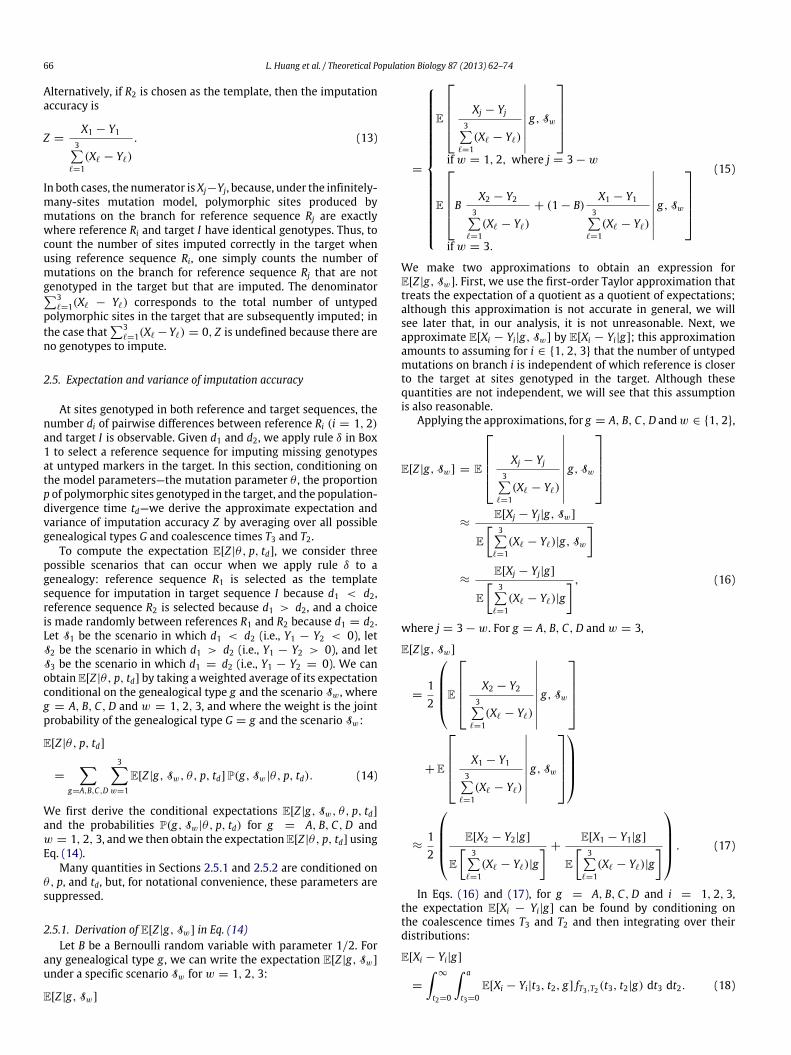
Table 2Mean numbers of untyped mutations E[Xi − Yi|g], for genealogical types g =

A, B, C,D and branches i = 1, 2, 3. The definitions of E◦, E×, E� , and E√—each ofwhich is a function of θ, p, and td—appear in Eqs. (23)–(26).

Genealogical type Branch1 2 3

A E◦ E× E◦

B E× E◦ E◦

C E◦ E◦ E×

D E� E√ E�

The upper limit of the inner integral depends on the genealogicaltype:

a =

∞ if g = A, B, Ctd if g = D.

(19)

The formula for the expectation of a Poisson random variablegives

E[Xi − Yi|t3, t2, g] = hi(T; g) θ(1 − p)/2. (20)

In any genealogy, by the independence of coalescence times underthe coalescent model,

fT3,T2(t3, t2|g) = fT3(t3|g) fT2(t2|g). (21)

Using Eqs. (1)–(3),

fT3,T2(t3, t2|g) =

3e−3t3−t2 if g = A, B, Ce−t3−t2

1 − e−td1{t3<td} if g = D.

(22)

Considering all 12 choices of (g, i) with g = A, B, C,D and i = 1,2, 3, the 12 cases in Eq. (18) evaluate to four possible quantities,which we denote as follows:

E◦ =16θ(1 − p)(3td + 1) (23)

E× =16θ(1 − p)(3td + 7) (24)

E� =12θ(1 − p)

1 − (td + 1)e−td

1 − e−td

(25)

E√ =12θ(1 − p)

2td + 1 − (td + 1)e−td

1 − e−td

. (26)

Table 2 indicates which among the 12 integrals equal E◦, E×, E�,and E√.

We can then insert the appropriate quantities from Eqs. (23)–(26) into Eqs. (16) and (17) to obtain the 12 terms E[Z |g, Sw]

that appear in Eq. (14) (Table 3). This completes the derivation ofE[Z |g, Sw].

2.5.2. Derivation of P(g, Sw) in Eq. (14)We obtain the probability P(g, Sw) by jointly considering the

marginal distribution of g and the conditional distribution of Sw

given a genealogical type G = g:

P(g, Sw) = P(g) P(Sw|g). (27)

The probability P(g) is given in Eq. (4). As in the derivation ofE[Xi − Yi|g], to compute P(Sw|g), we condition on the coalescencetimes T3 and T2 and then integrate over their distributions:

P(Sw|g) =

∞

t2=0

a

t3=0P(Sw|t3, t2, g) fT3,T2(t3, t2|g) dt3 dt2, (28)

Table 3The computation of E[Z |g, Sw] for g = A, B, C,D and w = 1, 2, 3. Each initialexpression is obtained using Eqs. (16) and (17), and then simplified using Eqs. (23)–(26).

Quantity Initial expression Simplified expression

E[Z |A, S1]E×

2E◦+E×

3td+79td+9

E[Z |B, S1]E◦

2E◦+E×

3td+19td+9

E[Z |C, S1]E◦

2E◦+E×

3td+19td+9

E[Z |D, S1]E√

2E�+E√

2td+1−(td+1)e−td

2td+3−3(td+1)e−td

E[Z |A, S2]E◦

2E◦+E×

3td+19td+9

E[Z |B, S2]E×

2E◦+E×

3td+79td+9

E[Z |C, S2]E◦

2E◦+E×

3td+19td+9

E[Z |D, S2]E�

2E�+E√

1−(td+1)e−td

2td+3−3(td+1)e−td

E[Z |A, S3]E◦+E×

2(2E◦+E×)

3td+49td+9

E[Z |B, S3]E◦+E×

2(2E◦+E×)

3td+49td+9

E[Z |C, S3]E◦

2E◦+E×

3td+19td+9

E[Z |D, S3]E�+E√

2(2E�+E√)

(td+1)(1−e−td )

2td+3−3(td+1)e−td

where fT3,T2(t3, t2|g) is calculated with Eq. (22) and a is given inEq. (19). In principle, P(Sw|t3, t2, g) can be obtained by consideringthe difference Y1 − Y2 and using Eq. (11):

P(S1|t3, t2, g)

=

∞y1=0

∞y2=y1+1

fSk(y1 − y2; h1(T; g) θp/2, h2(T; g) θp/2) (29)

P(S2|t3, t2, g)

=

∞y2=0

∞y1=y2+1

fSk(y1 − y2; h1(T; g) θp/2, h2(T; g) θp/2) (30)

P(S3|t3, t2, g) = fSk(0; h1(T; g) θp/2, h2(T; g) θp/2). (31)

In practice, the sums are unwieldy, and, instead of computingthem, we use a Monte Carlo approach to evaluate Eq. (28), as de-scribed in Section 3. This completes the derivation of the expecta-tion E[Z |θ, p, td] in Eq. (14).

2.5.3. Derivation of Var[Z |θ, p, td]Var[Z |θ, p, td] is obtained as

Var[Z |θ, p, td] = E[Z2|θ, p, td] − E[Z |θ, p, td]2, (32)

where E[Z |θ, p, td] has already been derived (Eq. (14)). It remainsto evaluate E[Z2

|θ, p, td].As in the derivation of E[Z |θ, p, td], we obtain E[Z2

|θ, p, td] byconditioning on the genealogical type g and the scenario Sw:

E[Z2|θ, p, td]

=

g=A,B,C,D

3w=1

E[Z2|g, Sw, θ, p, td] P(g, Sw|θ, p, td). (33)

For g = A, B, C,D and w = 1, 2, 3,

E[Z2|g, Sw, θ, p, td]

= Var[Z |g, Sw, θ, p, td] + E[Z |g, Sw, θ, p, td]2. (34)

We again suppress θ, p, and td. The probability P(g, Sw) inEq. (33) and the expectation E[Z |g, Sw] in Eq. (34) have alreadybeen derived (Eqs. (27), (16), (17)). To obtain an expression forVar[Z |g, Sw] in Eq. (34), we apply the same two approximationsused for obtaining E[Z |g, Sw] in Section 2.5.1. The first-order

68 L. Huang et al. / Theoretical Population Biology 87 (2013) 62–74

Taylor-series approximation for the variance Var[Z |g, Sw] (Casellaand Berger, 2001, p. 245) is followed by an additional approxima-tion that disregards the dependence on Sw .

Applying the approximations, for g = A, B, C,D andw ∈ {1, 2},

Var[Z |g, Sw] = Var

Xj − Yj3

ℓ=1(Xℓ − Yℓ)

g, Sw

≈

E[Xj − Yj|g, Sw]

E

3ℓ=1

(Xℓ − Yℓ)|g, Sw

2

×

Var[Xj − Yj|g, Sw]

E[Xj − Yj|g, Sw]2+

Var

3

ℓ=1(Xℓ − Yℓ)|g, Sw

E

3

ℓ=1(Xℓ − Yℓ)|g, Sw

2

−

2Cov

Xj − Yj,

3ℓ=1

(Xℓ − Yℓ)|g, Sw

E[Xj − Yj|g, Sw] E

3

ℓ=1(Xℓ − Yℓ)|g, Sw

≈

E[Xj − Yj|g]

E

3

ℓ=1(Xℓ − Yℓ)|g

2

×

Var[Xj − Yj|g]E[Xj − Yj|g]2

+

Var

3

ℓ=1(Xℓ − Yℓ)|g

E

3

ℓ=1(Xℓ − Yℓ)|g

2

−

2Cov

Xj − Yj,

3ℓ=1

(Xℓ − Yℓ)|g

E[Xj − Yj|g] E

3

ℓ=1(Xℓ − Yℓ)|g

, (35)

where j = 3 − w. For g = A, B, C,D and w = 3,

Var[Z |g, Sw]

= Var

BX2 − Y2

3ℓ=1

(Xℓ − Yℓ)

+ (1 − B)X1 − Y1

3ℓ=1

(Xℓ − Yℓ)

g, Sw

= E

B

X2 − Y23

ℓ=1(Xℓ − Yℓ)

+ (1 − B)X1 − Y1

3ℓ=1

(Xℓ − Yℓ)

2 g, Sw

− E

BX2 − Y2

3ℓ=1

(Xℓ − Yℓ)

+ (1 − B)X1 − Y1

3ℓ=1

(Xℓ − Yℓ)

g, Sw

2

. (36)

Because B is Bernoulli, B2= B, (1−B)2 = (1−B), and B(1−B) = 0.

Using the independence of B from the imputation accuracy Z , wecan simplify Eq. (36) to

Var[Z |g, S3] =12

Var

X2 − Y23

ℓ=1(Xℓ − Yℓ)

g, S3

+Var

X1 − Y13

ℓ=1(Xℓ − Yℓ)

g, S3

+14

E

X2 − Y23

ℓ=1(Xℓ − Yℓ)

g, S3

− E

X1 − Y13

ℓ=1(Xℓ − Yℓ)

g, S3

2

. (37)

When w = 1, Z = (X2 − Y2)/3

ℓ=1(Xℓ − Yℓ), and whenw = 2, Z = (X1 − Y1)/

3ℓ=1(Xℓ − Yℓ) (Eqs. (12) and (13)). As

we have elsewhere used an approximation that, conditional on agenealogical type g , terms Xi − Yi do not depend on whether wis equal to 1, 2, or 3 (Eqs. (16) and (17)), we here make a similarapproximation that, conditional on g, (Xi − Yi)/

3ℓ=1(Xℓ − Yℓ)

does not depend on Sw . Thus, instead of conditioning on w = 3,we can condition on w = 1 or w = 2. If w = 3 is replacedwith w = 1 for terms E[(X2 − Y2)/

3ℓ=1(Xℓ − Yℓ)|g, Sw] and

Var[(X2 − Y2)/3

ℓ=1(Xℓ − Yℓ)|g, Sw], and with w = 2 for termsE[(X1 −Y1)/

3ℓ=1(Xℓ −Yℓ)|g, Sw] and Var[(X1 −Y1)/

3ℓ=1(Xℓ −

Yℓ)|g, Sw], we obtain

Var[Z |g, S3] ≈Var[Z |g, S1] + Var[Z |g, S2]

2

+(E[Z |g, S1] − E[Z |g, S2])

2

4. (38)

This approximation reduces Var[Z |g, S3] to simpler computationsconditional on S1 and S2.

In Eq. (35), for g = A, B, C,D and i = 1, 2, 3, the expectationE[Xi − Yi|g] is computed using Eqs. (18)–(19), and the varianceVar[Xi − Yi|g] can be found using the conditional variance iden-tity (Casella and Berger, 2001, p. 167). Applying the identity, con-ditioning on the coalescence times T3 and T2, and integrating overthe coalescence-time distributions, we have

Var[Xi − Yi|g] = E[Var[Xi − Yi|t3, t2, g]]+Var[E[Xi − Yi|t3, t2, g]]

=

∞

t2=0

a

t3=0Var[Xi − Yi|t3, t2, g]

× fT3,T2(t3, t2|g) dt3 dt2

+

∞

t2=0

a

t3=0(E[Xi − Yi|t3, t2, g]

− E[Xi − Yi|g])2 fT3,T2(t3, t2|g) dt3 dt2. (39)

In Eq. (39), the upper limit a of the inner integral is given in Eq. (19),and the joint density function fT3,T2(t3, t2|g) is evaluated using

L. Huang et al. / Theoretical Population Biology 87 (2013) 62–74 69

Table 4Variances of the number of untypedmutations Var[Xi−Yi|g], for genealogical typesg = A, B, C,D and branches i = 1, 2, 3. The definitions of V◦, V×, V� , and V√ – eachof which is a function of θ, p, and td – appear in Eqs. (41)–(44).

Genealogical type Branch1 2 3

A V◦ V× V◦

B V× V◦ V◦

C V◦ V◦ V×

D V� V√ V�

Eq. (22). The formula for the variance of a Poisson random variablegives,

Var[Xi − Yi|t3, t2, g] = E[Xi − Yi|t3, t2, g]= hi(T; g) θ(1 − p)/2, (40)

where hi(T; g) appears in Table 1. Consequently, in Eq. (39), thefirst term is E[Var[Xi − Yi|t3, t2, g]] = E[E[Xi − Yi|t3, t2, g]] =

E[Xi − Yi|g], which has already been obtained in Eq. (18).For the second term in Eq. (39), the expectations E[Xi −

Yi|t3, t2, g] and E[Xi − Yi|g] are given in Eqs. (20) and (18),respectively. Considering all 12 choices of (g, i)with g = A, B, C,Dand i = 1, 2, 3, the 12 cases in Eq. (39) evaluate to four possiblequantities:

V◦ =16θ(1 − p)(3td + 1) +

136

θ2(1 − p)2 (41)

V× =16θ(1 − p)(3td + 7) +

3736

θ2(1 − p)2 (42)

V� =12θ(1 − p)

1 − (td + 1)e−td

1 − e−td

+14θ2(1 − p)2

1 − 2e−td − t2d e

−td + e−2td

1 − 2e−td + e−2td

(43)

V√ =12θ(1 − p)

2td + 1 − (td + 1)e−td

1 − e−td

+14θ2(1 − p)2

5 − 10e−td − t2d e

−td + 5e−2td

1 − 2e−td + e−2td

. (44)

Table 4 indicates which among the 12 integrals equal V◦, V×, V�,and V√.

To complete the calculation of Var[Z |g, Sw], we compute thecovariance Cov(Xj − Yj,

3ℓ=1(Xℓ − Yℓ)|g) in Eq. (35). For any

genealogy, conditional on the coalescence times T3 and T2, (Xi−Yi)and (Xj − Yj) are independent for any i and jwith j = i. Then

Cov

Xj − Yj,

3ℓ=1

(Xℓ − Yℓ)

g

= Var[Xj − Yj|g], (45)

which has been obtained in Eq. (39).For g = A, B, C,D, we obtain the eight terms Var[Z |g, S1]

and Var[Z |g, S2] in Eq. (33) by inserting the appropriate quantitiesfrom Eqs. (23)–(26) and (41)–(44) into Eq. (35). We obtain theremaining four terms Var[Z |g, S3] using Eq. (38) (Table 5). Theresulting quantities are unwieldy, and we do not list the fullexpressions for Var[Z |g, Sw]. This completes the derivation ofE[Z2

|θ, p, td] and thus of Var[Z |θ, p, td].

3. Methods of computation and simulation

To calculate the expectation E[Z |θ, p, td] (Eq. (14)), we com-puted E[Z |g, Sw, θ, p, td] using Eqs. (16) and (17). We obtained

Table 5The computation of Var[Z |g, Sw] for g = A, B, C,D and w = 1, 2, 3. Each initialexpression is obtained using Eqs. (35) and (38), and then simplified using Eqs.(23)–(26) and (41)–(44). We omit the simplified expressions, as they are unwieldy.

Quantity Initial expression

Var[Z |A, S1]

E×

2E◦+E×

2 V×

E2×

+2V◦+V×

(2E◦+E×)2−

2V×

E×(2E◦+E×)

Var[Z |B, S1]

E◦

2E◦+E×

2V◦

E2◦+

2V◦+V×

(2E◦+E×)2−

2V◦

E◦(2E◦+E×)

Var[Z |C, S1]

E◦

2E◦+E×

2V◦

E2◦+

2V◦+V×

(2E◦+E×)2−

2V◦

E◦(2E◦+E×)

Var[Z |D, S1]

E√

2E�+E√

2 V√

E2√+

2V�+V√

(2E�+E√)2−

2V√

E√(2E�+E√)

Var[Z |A, S2]

E◦

2E◦+E×

2V◦

E2◦+

2V◦+V×

(2E◦+E×)2−

2V◦

E◦(2E◦+E×)

Var[Z |B, S2]

E×

2E◦+E×

2 V×

E2×

+2V◦+V×

(2E◦+E×)2−

2V×

E×(2E◦+E×)

Var[Z |C, S2]

E◦

2E◦+E×

2V◦

E2◦+

2V◦+V×

(2E◦+E×)2−

2V◦

E◦(2E◦+E×)

Var[Z |D, S2]

E�

2E�+E√

2V�

E2�+

2V�+V√

(2E�+E√)2−

2V�

E�(2E�+E√)

Var[Z |A, S3]

Var[Z |A,S1]+Var[Z |A,S2]

2 +(E[Z |A,S1]−E[Z |A,S2])2

4

Var[Z |B, S3]Var[Z |B,S1]+Var[Z |B,S2]

2 +(E[Z |B,S1]−E[Z |B,S2])2

4

Var[Z |C, S3]Var[Z |C,S1]+Var[Z |C,S2]

2 +(E[Z |C,S1]−E[Z |C,S2])2

4

Var[Z |D, S3]Var[Z |D,S1]+Var[Z |D,S2]

2 +(E[Z |D,S1]−E[Z |D,S2])2

4

Monte Carlo estimates of P(Sw|g, θ, p, td) included in the expres-sion for P(g, Sw|θ, p, td), using 105 draws from the Skellam distri-bution defined in Eq. (11). Each of these drawswas obtained by firstsampling t3 and t2 from their respective distributions, conditionalon g (and td). Next, we evaluated the difference between two simu-lated Poisson randomvariables,with parameters h1(T; g) θp/2 andh2(T; g) θp/2, respectively. These Poisson variates were sampledusing the GNU Scientific Library function gsl_ran_Poisson.Thus, the expectation was obtained using three approximations: aTaylor approximation, an approximation that disregards a depen-dence on Sw , and a Monte Carlo approximation for integrals asso-ciated with the Skellam distribution.

The computation of the variance Var[Z |θ, p, td] used someof the same approximations used in evaluating the meanE[Z |θ, p, td]. The variance computation incorporated the two stepsof approximation for E[Z |g, Sw, θ, p, td]. Additionally, the sameMonte Carlo samples of P(Sw|g, θ, p, td) employed in evaluatingthe mean were used in the variance computation. Beyond theTaylor approximation and omission of the conditioning on Sw thatwere required in obtaining the mean, the variance computationapplied corresponding approximations in obtaining E[Z2

|g, Sw,

θ, p, td].Given θ, p, and td, we also performed stochastic simulations

under the coalescent to estimate the mean and the variance of theimputation accuracy by summing over all simulations, employingMonte Carlo integration as described in Box 2 with M = 105

simulation replicates. To verify the expressions for E[Z |θ, p, td]and Var[Z |θ, p, td] in Eqs. (14) and (32), we then compared thesimulated means and variances of the imputation accuracy to ourformula-based estimates.

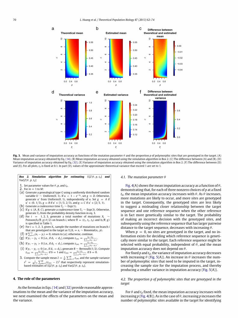
Fig. 3 shows the mean and the variance of the imputationaccuracy computed both using our formulas and using the simu-lations. For the parameter values that we considered, the theoret-ical approximations of E[Z |θ, p, td] obtained using Eq. (14) closelymatch the simulated mean imputation accuracy (Fig. 3, top row).Except when θ is small and p is large, the theoretical estimates ofVar[Z |θ, p, td] obtained using Eq. (32) closely match the simulatedvariances (Fig. 3, bottom row).

70 L. Huang et al. / Theoretical Population Biology 87 (2013) 62–74

Fig. 3. Mean and variance of imputation accuracy as functions of the mutation parameter θ and the proportion p of polymorphic sites that are genotyped in the target. (A)Mean imputation accuracy obtained by Eq. (14). (B) Mean imputation accuracy obtained using the simulation algorithm in Box 2. (C) The difference between (A) and (B). (D)Variance of imputation accuracy obtained by Eq. (32). (E) Variance of imputation accuracy obtained using the simulation algorithm in Box 2. (F) The difference between (D)and (E). For all plots, td is fixed at 0.1. In part (D), values of the approximate theoretical variance that exceed 1 are set to 1.

Box 2. Simulation algorithm for estimating E[Z |θ, p, td] andVar[Z |θ, p, td]

1. Set parameter values for θ , p, and td .2. Form = 1 toM:(a) Generate a genealogical type G using a uniformly distributed random

variable U ∼ Uniform(0, 1). If u < 1 − e−td , set g = D. Otherwise,generate u′ from Uniform(0, 1), independently of u. Set g = A ifu′

∈ (0, 1/3), g = B if u′∈ [1/3, 2/3), and g = C if u′

∈ [2/3, 1).(b) Generate a coalescence time T2 ∼ Exp(1).(c) If g ∈ {A, B, C}, generate a coalescence time T3 ∼ Exp(3). Otherwise,

generate T3 from the probability density function in eq. 3.(d) For i = 1, 2, 3, generate a total number of mutations Xi ∼

Poisson(hi(T; g) θ/2) on branch i, where T = (t3, t2, td) and hi(T; g)is specified in Table 1.

(e) For i = 1, 2, 3, given Xi , sample the number of mutations on branch ithat are genotyped in the target as Yi|Xi = xi ∼ Binomial(xi, p).

(f) If3

i=1(xi − yi) = 0, return to (a); otherwise, continue.(g) If y1 − y2 < 0 (i.e., if d1 < d2), compute z(m) =

x2−y23ℓ=1(xℓ−yℓ)

.

(h) If y1 − y2 > 0 (i.e., if d2 < d1), compute z(m) =x1−y13

ℓ=1(xℓ−yℓ).

(i) If y1 − y2 = 0 (i.e., if d1 = d2), generate B ∼ Bernoulli(1/2). Computez(m) =

x2−y23ℓ=1(xℓ−yℓ)

if b = 1 and z(m) =x1−y13

ℓ=1(xℓ−yℓ)if b = 0.

3. Compute the sample mean z =1M

Mm=1 z(m) and the sample variance

s2 =1

M−1

Mm=1(z(m) − z)2 that respectively represent simulation-

based estimates of E[Z |θ, p, td] and Var[Z |θ, p, td].

4. The role of the parameters

As the formulas in Eqs. (14) and (32) provide reasonable approx-imations to the mean and the variance of the imputation accuracy,we next examined the effects of the parameters on the mean andthe variance.

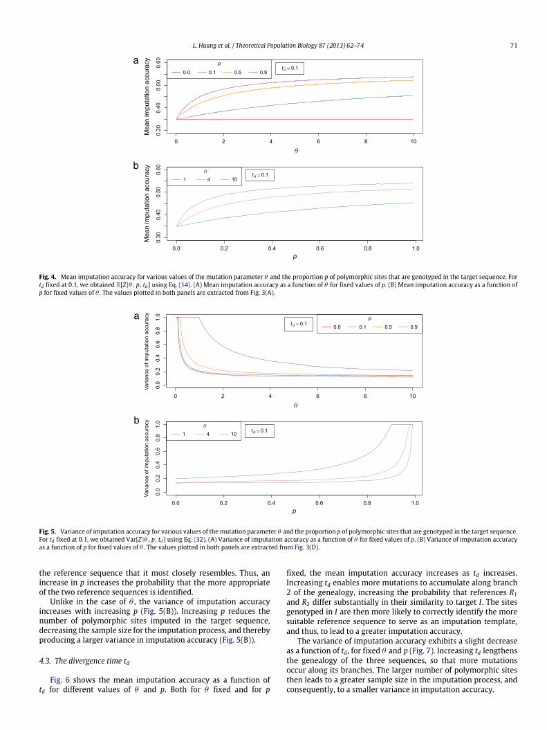
4.1. The mutation parameter θ

Fig. 4(A) shows themean imputation accuracy as a function of θ ,demonstrating that, for each of three nonzero choices of p at a fixedtd, the mean imputation accuracy increases with θ . As θ increases,more mutations are likely to occur, and more sites are genotypedin the target. Consequently, the genotyped sites are less likelyto suggest a misleading closer relationship between the targetsequence and one reference sequence when the other referenceis in fact more genetically similar to the target. The probabilityof making an incorrect decision with the genotyped sites, andsubsequently using the reference sequence that has larger pairwisedistance to the target sequence, decreases with increasing θ .

When p = 0, no sites are genotyped in the target, and no in-formation exists for deciding which reference sequence is geneti-cally more similar to the target. Each reference sequence might beselected with equal probability, independent of θ , and the meanimputation accuracy does not depend on θ .

For fixed p and td, the variance of imputation accuracy decreaseswith increasing θ (Fig. 5(A)). An increase in θ increases the num-ber of polymorphic sites that need to be imputed in the target, in-creasing the sample size for the imputation process, and therebyproducing a smaller variance in imputation accuracy (Fig. 5(A)).

4.2. The proportion p of polymorphic sites that are genotyped in thetarget

For θ and td fixed, themean imputation accuracy increases withincreasing p (Fig. 4(B)). As in the case of θ , increasing p increases thenumber of polymorphic sites available in the target for identifying

L. Huang et al. / Theoretical Population Biology 87 (2013) 62–74 71

Fig. 4. Mean imputation accuracy for various values of the mutation parameter θ and the proportion p of polymorphic sites that are genotyped in the target sequence. Fortd fixed at 0.1, we obtained E[Z |θ, p, td] using Eq. (14). (A) Mean imputation accuracy as a function of θ for fixed values of p. (B) Mean imputation accuracy as a function ofp for fixed values of θ . The values plotted in both panels are extracted from Fig. 3(A).

Fig. 5. Variance of imputation accuracy for various values of the mutation parameter θ and the proportion p of polymorphic sites that are genotyped in the target sequence.For td fixed at 0.1, we obtained Var[Z |θ, p, td] using Eq. (32). (A) Variance of imputation accuracy as a function of θ for fixed values of p. (B) Variance of imputation accuracyas a function of p for fixed values of θ . The values plotted in both panels are extracted from Fig. 3(D).

the reference sequence that it most closely resembles. Thus, anincrease in p increases the probability that the more appropriateof the two reference sequences is identified.

Unlike in the case of θ , the variance of imputation accuracyincreases with increasing p (Fig. 5(B)). Increasing p reduces thenumber of polymorphic sites imputed in the target sequence,decreasing the sample size for the imputation process, and therebyproducing a larger variance in imputation accuracy (Fig. 5(B)).

4.3. The divergence time td

Fig. 6 shows the mean imputation accuracy as a function oftd for different values of θ and p. Both for θ fixed and for p

fixed, the mean imputation accuracy increases as td increases.Increasing td enables more mutations to accumulate along branch2 of the genealogy, increasing the probability that references R1and R2 differ substantially in their similarity to target I . The sitesgenotyped in I are then more likely to correctly identify the moresuitable reference sequence to serve as an imputation template,and thus, to lead to a greater imputation accuracy.

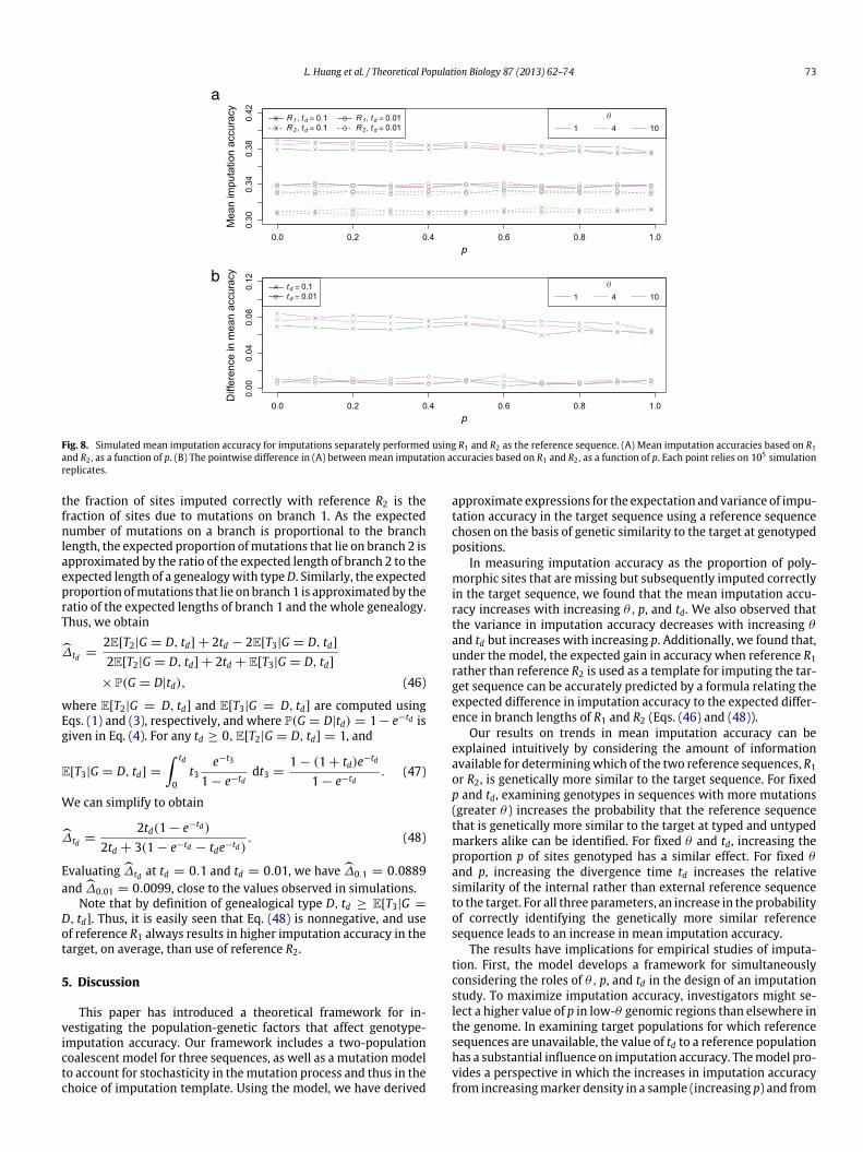
The variance of imputation accuracy exhibits a slight decreaseas a function of td, for fixed θ and p (Fig. 7). Increasing td lengthensthe genealogy of the three sequences, so that more mutationsoccur along its branches. The larger number of polymorphic sitesthen leads to a greater sample size in the imputation process, andconsequently, to a smaller variance in imputation accuracy.

72 L. Huang et al. / Theoretical Population Biology 87 (2013) 62–74

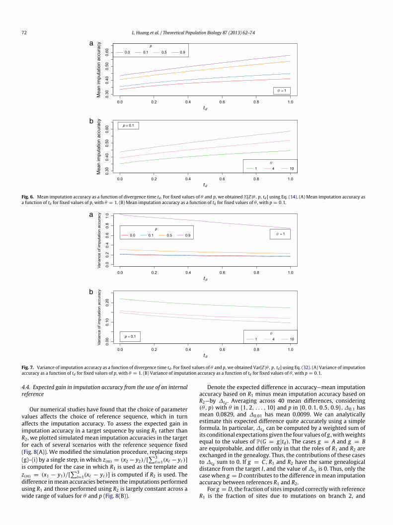
Fig. 6. Mean imputation accuracy as a function of divergence time td . For fixed values of θ and p, we obtained E[Z |θ, p, td] using Eq. (14). (A) Mean imputation accuracy asa function of td for fixed values of p, with θ = 1. (B) Mean imputation accuracy as a function of td for fixed values of θ , with p = 0.1.

Fig. 7. Variance of imputation accuracy as a function of divergence time td . For fixed values of θ and p, we obtained Var[Z |θ, p, td] using Eq. (32). (A) Variance of imputationaccuracy as a function of td for fixed values of p, with θ = 1. (B) Variance of imputation accuracy as a function of td for fixed values of θ , with p = 0.1.

4.4. Expected gain in imputation accuracy from the use of an internalreference

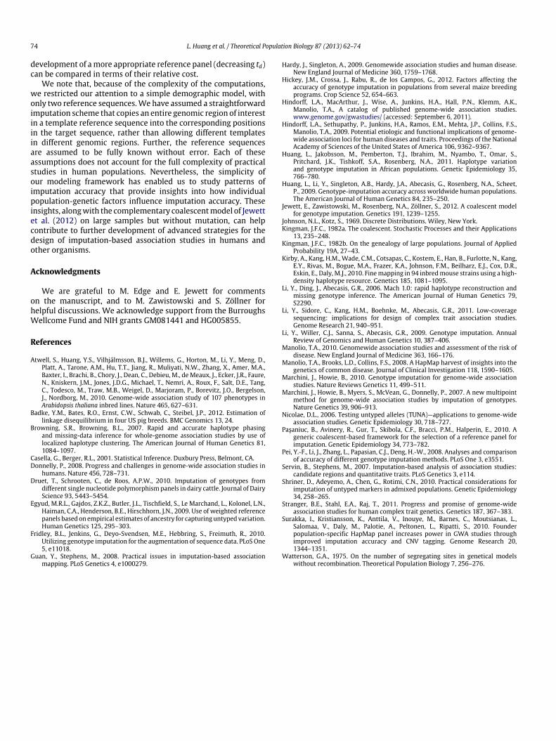
Our numerical studies have found that the choice of parametervalues affects the choice of reference sequence, which in turnaffects the imputation accuracy. To assess the expected gain inimputation accuracy in a target sequence by using R1 rather thanR2, we plotted simulated mean imputation accuracies in the targetfor each of several scenarios with the reference sequence fixed(Fig. 8(A)). We modified the simulation procedure, replacing steps(g)–(i) by a single step, in which z(m) = (x2 − y2)/[

3ℓ=1(xℓ − yℓ)]

is computed for the case in which R1 is used as the template andz(m) = (x1 − y1)/[

3i=1(xℓ − yℓ)] is computed if R2 is used. The

difference inmean accuracies between the imputations performedusing R1 and those performed using R2 is largely constant across awide range of values for θ and p (Fig. 8(B)).

Denote the expected difference in accuracy—mean imputationaccuracy based on R1 minus mean imputation accuracy based onR2—by ∆td . Averaging across 40 mean differences, considering(θ, p) with θ in {1, 2, . . . , 10} and p in {0, 0.1, 0.5, 0.9}, ∆0.1 hasmean 0.0829, and ∆0.01 has mean 0.0099. We can analyticallyestimate this expected difference quite accurately using a simpleformula. In particular, ∆td can be computed by a weighted sum ofits conditional expectations given the four values of g , withweightsequal to the values of P(G = g|td). The cases g = A and g = Bare equiprobable, and differ only in that the roles of R1 and R2 areexchanged in the genealogy. Thus, the contributions of these casesto ∆td sum to 0. If g = C, R1 and R2 have the same genealogicaldistance from the target I , and the value of ∆td is 0. Thus, only thecase when g = D contributes to the difference inmean imputationaccuracy between references R1 and R2.

For g = D, the fraction of sites imputed correctlywith referenceR1 is the fraction of sites due to mutations on branch 2, and

L. Huang et al. / Theoretical Population Biology 87 (2013) 62–74 73

Fig. 8. Simulated mean imputation accuracy for imputations separately performed using R1 and R2 as the reference sequence. (A) Mean imputation accuracies based on R1and R2 , as a function of p. (B) The pointwise difference in (A) between mean imputation accuracies based on R1 and R2 , as a function of p. Each point relies on 105 simulationreplicates.

the fraction of sites imputed correctly with reference R2 is thefraction of sites due to mutations on branch 1. As the expectednumber of mutations on a branch is proportional to the branchlength, the expected proportion ofmutations that lie on branch 2 isapproximated by the ratio of the expected length of branch 2 to theexpected length of a genealogywith typeD. Similarly, the expectedproportion ofmutations that lie on branch1 is approximated by theratio of the expected lengths of branch 1 and the whole genealogy.Thus, we obtain

∆td =2E[T2|G = D, td] + 2td − 2E[T3|G = D, td]2E[T2|G = D, td] + 2td + E[T3|G = D, td]

× P(G = D|td), (46)

where E[T2|G = D, td] and E[T3|G = D, td] are computed usingEqs. (1) and (3), respectively, and where P(G = D|td) = 1− e−td isgiven in Eq. (4). For any td ≥ 0, E[T2|G = D, td] = 1, and

E[T3|G = D, td] =

td

0t3

e−t3

1 − e−tddt3 =

1 − (1 + td)e−td

1 − e−td. (47)

We can simplify to obtain

∆td =2td(1 − e−td)

2td + 3(1 − e−td − tde−td). (48)

Evaluating ∆td at td = 0.1 and td = 0.01, we have ∆0.1 = 0.0889and ∆0.01 = 0.0099, close to the values observed in simulations.

Note that by definition of genealogical type D, td ≥ E[T3|G =

D, td]. Thus, it is easily seen that Eq. (48) is nonnegative, and useof reference R1 always results in higher imputation accuracy in thetarget, on average, than use of reference R2.

5. Discussion

This paper has introduced a theoretical framework for in-vestigating the population-genetic factors that affect genotype-imputation accuracy. Our framework includes a two-populationcoalescent model for three sequences, as well as a mutation modelto account for stochasticity in themutation process and thus in thechoice of imputation template. Using the model, we have derived

approximate expressions for the expectation and variance of impu-tation accuracy in the target sequence using a reference sequencechosen on the basis of genetic similarity to the target at genotypedpositions.

In measuring imputation accuracy as the proportion of poly-morphic sites that are missing but subsequently imputed correctlyin the target sequence, we found that the mean imputation accu-racy increases with increasing θ, p, and td. We also observed thatthe variance in imputation accuracy decreases with increasing θand td but increases with increasing p. Additionally, we found that,under the model, the expected gain in accuracy when reference R1rather than reference R2 is used as a template for imputing the tar-get sequence can be accurately predicted by a formula relating theexpected difference in imputation accuracy to the expected differ-ence in branch lengths of R1 and R2 (Eqs. (46) and (48)).

Our results on trends in mean imputation accuracy can beexplained intuitively by considering the amount of informationavailable for determiningwhich of the two reference sequences, R1or R2, is genetically more similar to the target sequence. For fixedp and td, examining genotypes in sequences with more mutations(greater θ ) increases the probability that the reference sequencethat is genetically more similar to the target at typed and untypedmarkers alike can be identified. For fixed θ and td, increasing theproportion p of sites genotyped has a similar effect. For fixed θand p, increasing the divergence time td increases the relativesimilarity of the internal rather than external reference sequenceto the target. For all three parameters, an increase in the probabilityof correctly identifying the genetically more similar referencesequence leads to an increase in mean imputation accuracy.

The results have implications for empirical studies of imputa-tion. First, the model develops a framework for simultaneouslyconsidering the roles of θ, p, and td in the design of an imputationstudy. To maximize imputation accuracy, investigators might se-lect a higher value of p in low-θ genomic regions than elsewhere inthe genome. In examining target populations for which referencesequences are unavailable, the value of td to a reference populationhas a substantial influence on imputation accuracy. Themodel pro-vides a perspective in which the increases in imputation accuracyfrom increasingmarker density in a sample (increasing p) and from

74 L. Huang et al. / Theoretical Population Biology 87 (2013) 62–74

development of amore appropriate reference panel (decreasing td)can be compared in terms of their relative cost.

We note that, because of the complexity of the computations,we restricted our attention to a simple demographic model, withonly two reference sequences.We have assumed a straightforwardimputation scheme that copies an entire genomic region of interestin a template reference sequence into the corresponding positionsin the target sequence, rather than allowing different templatesin different genomic regions. Further, the reference sequencesare assumed to be fully known without error. Each of theseassumptions does not account for the full complexity of practicalstudies in human populations. Nevertheless, the simplicity ofour modeling framework has enabled us to study patterns ofimputation accuracy that provide insights into how individualpopulation-genetic factors influence imputation accuracy. Theseinsights, alongwith the complementary coalescentmodel of Jewettet al. (2012) on large samples but without mutation, can helpcontribute to further development of advanced strategies for thedesign of imputation-based association studies in humans andother organisms.

Acknowledgments

We are grateful to M. Edge and E. Jewett for commentson the manuscript, and to M. Zawistowski and S. Zöllner forhelpful discussions. We acknowledge support from the BurroughsWellcome Fund and NIH grants GM081441 and HG005855.

References

Atwell, S., Huang, Y.S., Vilhjálmsson, B.J., Willems, G., Horton, M., Li, Y., Meng, D.,Platt, A., Tarone, A.M., Hu, T.T., Jiang, R., Muliyati, N.W., Zhang, X., Amer, M.A.,Baxter, I., Brachi, B., Chory, J., Dean, C., Debieu, M., deMeaux, J., Ecker, J.R., Faure,N., Kniskern, J.M., Jones, J.D.G., Michael, T., Nemri, A., Roux, F., Salt, D.E., Tang,C., Todesco, M., Traw, M.B., Weigel, D., Marjoram, P., Borevitz, J.O., Bergelson,J., Nordborg, M., 2010. Genome-wide association study of 107 phenotypes inArabidopsis thaliana inbred lines. Nature 465, 627–631.

Badke, Y.M., Bates, R.O., Ernst, C.W., Schwab, C., Steibel, J.P., 2012. Estimation oflinkage disequilibrium in four US pig breeds. BMC Genomics 13, 24.

Browning, S.R., Browning, B.L., 2007. Rapid and accurate haplotype phasingand missing-data inference for whole-genome association studies by use oflocalized haplotype clustering. The American Journal of Human Genetics 81,1084–1097.

Casella, G., Berger, R.L., 2001. Statistical Inference. Duxbury Press, Belmont, CA.Donnelly, P., 2008. Progress and challenges in genome-wide association studies in

humans. Nature 456, 728–731.Druet, T., Schrooten, C., de Roos, A.P.W., 2010. Imputation of genotypes from

different single nucleotide polymorphismpanels in dairy cattle. Journal of DairyScience 93, 5443–5454.

Egyud, M.R.L., Gajdos, Z.K.Z., Butler, J.L., Tischfield, S., Le Marchand, L., Kolonel, L.N.,Haiman, C.A., Henderson, B.E., Hirschhorn, J.N., 2009. Use of weighted referencepanels basedon empirical estimates of ancestry for capturinguntyped variation.Human Genetics 125, 295–303.

Fridley, B.L., Jenkins, G., Deyo-Svendsen, M.E., Hebbring, S., Freimuth, R., 2010.Utilizing genotype imputation for the augmentation of sequence data. PLoS One5, e11018.

Guan, Y., Stephens, M., 2008. Practical issues in imputation-based associationmapping. PLoS Genetics 4, e1000279.

Hardy, J., Singleton, A., 2009. Genomewide association studies and human disease.New England Journal of Medicine 360, 1759–1768.

Hickey, J.M., Crossa, J., Rabu, R., de los Campos, G., 2012. Factors affecting theaccuracy of genotype imputation in populations from several maize breedingprograms. Crop Science 52, 654–663.

Hindorff, L.A., MacArthur, J., Wise, A., Junkins, H.A., Hall, P.N., Klemm, A.K.,Manolio, T.A., A catalog of published genome-wide association studies.www.genome.gov/gwastudies/ (accessed: September 6, 2011).

Hindorff, L.A., Sethupathy, P., Junkins, H.A., Ramos, E.M., Mehta, J.P., Collins, F.S.,Manolio, T.A., 2009. Potential etiologic and functional implications of genome-wide association loci for human diseases and traits. Proceedings of the NationalAcademy of Sciences of the United States of America 106, 9362–9367.

Huang, L., Jakobsson, M., Pemberton, T.J., Ibrahim, M., Nyambo, T., Omar, S.,Pritchard, J.K., Tishkoff, S.A., Rosenberg, N.A., 2011. Haplotype variationand genotype imputation in African populations. Genetic Epidemiology 35,766–780.

Huang, L., Li, Y., Singleton, A.B., Hardy, J.A., Abecasis, G., Rosenberg, N.A., Scheet,P., 2009. Genotype-imputation accuracy across worldwide human populations.The American Journal of Human Genetics 84, 235–250.

Jewett, E., Zawistowski, M., Rosenberg, N.A., Zöllner, S., 2012. A coalescent modelfor genotype imputation. Genetics 191, 1239–1255.

Johnson, N.L., Kotz, S., 1969. Discrete Distributions. Wiley, New York.Kingman, J.F.C., 1982a. The coalescent. Stochastic Processes and their Applications

13, 235–248.Kingman, J.F.C., 1982b. On the genealogy of large populations. Journal of Applied

Probability 19A, 27–43.Kirby, A., Kang, H.M., Wade, C.M., Cotsapas, C., Kostem, E., Han, B., Furlotte, N., Kang,

E.Y., Rivas, M., Bogue, M.A., Frazer, K.A., Johnson, F.M., Beilharz, E.J., Cox, D.R.,Eskin, E., Daly, M.J., 2010. Finemapping in 94 inbredmouse strains using a high-density haplotype resource. Genetics 185, 1081–1095.

Li, Y., Ding, J., Abecasis, G.R., 2006. Mach 1.0: rapid haplotype reconstruction andmissing genotype inference. The American Journal of Human Genetics 79,S2290.

Li, Y., Sidore, C., Kang, H.M., Boehnke, M., Abecasis, G.R., 2011. Low-coveragesequencing: implications for design of complex trait association studies.Genome Research 21, 940–951.

Li, Y., Willer, C.J., Sanna, S., Abecasis, G.R., 2009. Genotype imputation. AnnualReview of Genomics and Human Genetics 10, 387–406.

Manolio, T.A., 2010. Genomewide association studies and assessment of the risk ofdisease. New England Journal of Medicine 363, 166–176.

Manolio, T.A., Brooks, L.D., Collins, F.S., 2008. A HapMap harvest of insights into thegenetics of common disease. Journal of Clinical Investigation 118, 1590–1605.

Marchini, J., Howie, B., 2010. Genotype imputation for genome-wide associationstudies. Nature Reviews Genetics 11, 499–511.

Marchini, J., Howie, B., Myers, S., McVean, G., Donnelly, P., 2007. A new multipointmethod for genome-wide association studies by imputation of genotypes.Nature Genetics 39, 906–913.

Nicolae, D.L., 2006. Testing untyped alleles (TUNA)—applications to genome-wideassociation studies. Genetic Epidemiology 30, 718–727.

Paşaniuc, B., Avinery, R., Gur, T., Skibola, C.F., Bracci, P.M., Halperin, E., 2010. Ageneric coalescent-based framework for the selection of a reference panel forimputation. Genetic Epidemiology 34, 773–782.

Pei, Y.-F., Li, J., Zhang, L., Papasian, C.J., Deng, H.-W., 2008. Analyses and comparisonof accuracy of different genotype imputation methods. PLoS One 3, e3551.

Servin, B., Stephens, M., 2007. Imputation-based analysis of association studies:candidate regions and quantitative traits. PLoS Genetics 3, e114.

Shriner, D., Adeyemo, A., Chen, G., Rotimi, C.N., 2010. Practical considerations forimputation of untyped markers in admixed populations. Genetic Epidemiology34, 258–265.

Stranger, B.E., Stahl, E.A., Raj, T., 2011. Progress and promise of genome-wideassociation studies for human complex trait genetics. Genetics 187, 367–383.

Surakka, I., Kristiansson, K., Anttila, V., Inouye, M., Barnes, C., Moutsianas, L.,Salomaa, V., Daly, M., Palotie, A., Peltonen, L., Ripatti, S., 2010. Founderpopulation-specific HapMap panel increases power in GWA studies throughimproved imputation accuracy and CNV tagging. Genome Research 20,1344–1351.

Watterson, G.A., 1975. On the number of segregating sites in genetical modelswithout recombination. Theoretical Population Biology 7, 256–276.