Embed Size (px)
Citation preview

Genomic Selection in the era of Genome sequencing
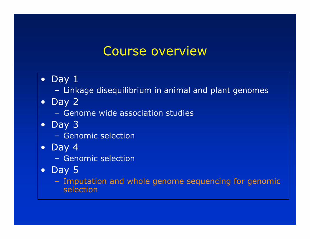
Course overview
• Day 1– Linkage disequilibrium in animal and plant genomes
• Day 2– Genome wide association studies
• Day 3 – Genomic selection
• Day 4 – Genomic selection
• Day 5– Imputation and whole genome sequencing for genomic selection

Imputation
• Why impute?
• Approaches for imputation
• Factors affecting accuracy of imputation
• How can imputation give you more power?
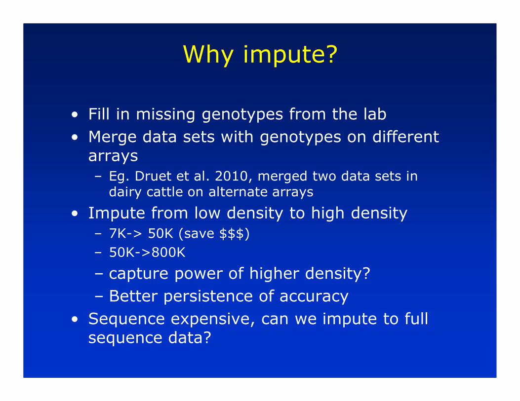
Why impute?
• Fill in missing genotypes from the lab
• Merge data sets with genotypes on different arrays
– Eg. Druet et al. 2010, merged two data sets in dairy cattle on alternate arrays
• Impute from low density to high density
– 7K-> 50K (save $$$)
– 50K->800K
– capture power of higher density?
– Better persistence of accuracy
• Sequence expensive, can we impute to full sequence data?
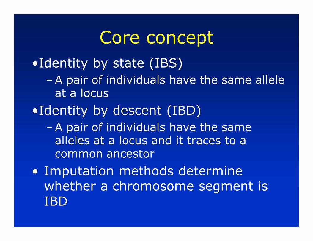
Core concept
•Identity by state (IBS)
–A pair of individuals have the same allele at a locus
•Identity by descent (IBD)
–A pair of individuals have the same alleles at a locus and it traces to a common ancestor
• Imputation methods determine whether a chromosome segment is IBD

Core concept 2
• Any individuals in a population may share a proportion of their genome identical by descent (IBD)
– IBD segments are the same and have originated in a common ancestor
•The closer the relationship the longer the IBD segments
–Pedigree relationships

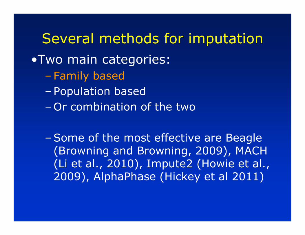
Several methods for imputation
•Two main categories:
–Family based
–Population based
–Or combination of the two
–Some of the most effective are Beagle (Browning and Browning, 2009), MACH (Li et al., 2010), Impute2 (Howie et al., 2009), AlphaPhase (Hickey et al 2011)
Several methods for imputation
•Two main categories:
–Family based
–Population based
–Or combination of the two
–Some of the most effective are Beagle (Browning and Browning, 2009), MACH (Li et al., 2010), Impute2 (Howie et al., 2009), AlphaPhase (Hickey et al 2011)

Finding an IBD segment
0 22 0 2 20
00 2 0 2 2 2
Sire
0 ?2 0 2 2?
?2 ? 0 0 2 0
Progeny

0 22 0 2 20
02 2 0 2 2 2
Sire
0 ?2 0 2 2?
?2 ? 0 0 2 0
Progeny
IBD segment

0 22 0 2 20
02 2 0 2 2 2
Sire
0 22 0 2 20
?2 ? 0 0 2 0
Progeny

Relationships
Sire Dam
Proband
Progeny
Maternal
Relatives
Paternal
Relatives
Long range phasing

Relationships
Sire Dam
Proband
Progeny
Maternal
Relatives
Paternal
Relatives
Long range phasing

Several methods for imputation
•Two main categories:
–Family based
–Population based (exploits LD)
–Or combination of the two
–Some of the most effective are Beagle (Browning and Browning, 2009), MACH (Li et al., 2010), Impute2 (Howie et al., 2009), AlphaPhase (Hickey et al 2011)
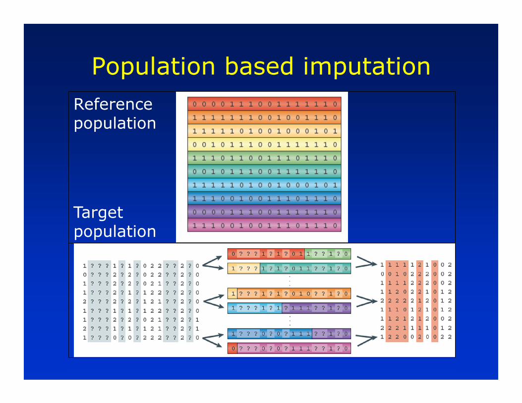
Population based imputation
Reference population
Target population

Population based imputation
• Hidden Markov Models
–Has “hidden states”
– For target individuals these are “map” of reference haplotypes that have been inherited
– Imputation problem is to derive genotype probabilities given hidden states, sparse genotypes, recombination rates, other population parameters

Population based imputation
• Hidden Markov Models
– Example with reference haplotypes
• 011
• 010
• 101
• 001
– What are possible genotypes?

Population based imputation
• Hidden Markov Models
fastPHASE BEAGLE

Imputation accuracy
• Depends on –Size of reference set
• bigger the better!
–Density of markers • extent of LD, effective population size
–Frequency of SNP alleles
–Genetic relationship to reference

Imputation accuracy sheep
• Density of markers (extent of LD)– In Dairy cattle
• 3K -> 50K accuracy 0.93
• 7K -> 50K accuracy 0.98
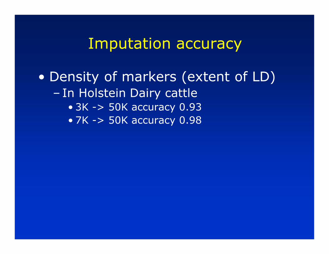
Imputation accuracy
• Density of markers (extent of LD)– In Holstein Dairy cattle
• 3K -> 50K accuracy 0.93
• 7K -> 50K accuracy 0.98

Illumina Bovine HD array
• We genotyped
— 898 Holstein heifers
— 47 Holstein Key ancestor bulls
— 67 Jersey Key ancestor bulls
• After (stringent) QC 634,307 SNPs

Imputation 50K -> 800K
• Holsteins
Cross validation % Correct
Heifers only 1 96.7%
2 96.7%
Average 96.7%
Heifers 1 97.8%
using key 2 97.7%
ancestors Average 97.7%

Imputation 50K -> 800K
• Jerseys
Cross validation % Correct
1 95.2%
2 95.5%
3 95.3%
4 95.6%
5 96.2%
Average 95.6%

Imputation accuracy
• Rare alleles?

Imputation accuracy
• Relationship to reference?

Imputation of full sequence data
• Effect of map errors?

Why more power with imputation
• High accuracies of imputation demonstrate that we can infer haplotypes of animal genotyped with e.g. 3K accurately
• But potentially large number of haplotypes
• With imputed data can test single snp, only use 1 degree of freedom, rather than number of haplotypes

Why more power with imputation
• Weigel et al. (2010)

Using sequence data in genomic selection and GWAS
• Motivation
• Characteristics of sequence data
• Which individuals to sequence?
• Imputation of full sequence data
• Methods for genomic prediction with full sequence data
• Examples–GWAS in Rice, Cattle

Using sequence data in genomic selection and GWAS
• Motivation–Genome wide association study
• Straight to causative mutation
–Genomic selection (all hypotheses!)• No longer have to rely on LD, causative mutation actually in data set– Higher accuracy of prediction?
• Better prediction across breeds?– Assumes same QTL segregating in both breeds
– No longer have to rely on SNP-QTL associations holding across breeds
• Better persistence of accuracy across generations

Using sequence data in genomic selection and GWAS
• Motivation
• Characteristics of sequence data
• Which individuals to sequence?
• Imputation of full sequence
• Methods for genomic prediction with full sequence data
• Examples–GWAS in Rice, Cattle

Sequence data
• Generates reads of DNA approx. 100 base pair (bp) length
• Reads are aligned to a reference genome– Or they could be assembled de novo
– Assigns each read a location on genome
• Reads have an error rate!– One error per read
• Information is base pair (ACTG) + Quality score for each base– PHRED score = -10*log10(error rate)
• 0.01 error rate = Q20
• 0.001 error rate = Q30
• 0.0001 error rate = Q40

Read depth
•Each sequenced animal is aligned separately to reference
– .bam files are created
•Read depth or fold coverage
Genome
Read depth 7Read depth 5Read

Importance of read depth
• Consider a heterozygous locus (animal carries 2 different alleles)
– 50/50 chance of observing each allele in every read
• If read depth is low, it is possible to not observe an allele and therefore call a het locus homozygous
– Read depth 5 � 0.55 = 0.03125
Genome
1211212
1
1
1
11
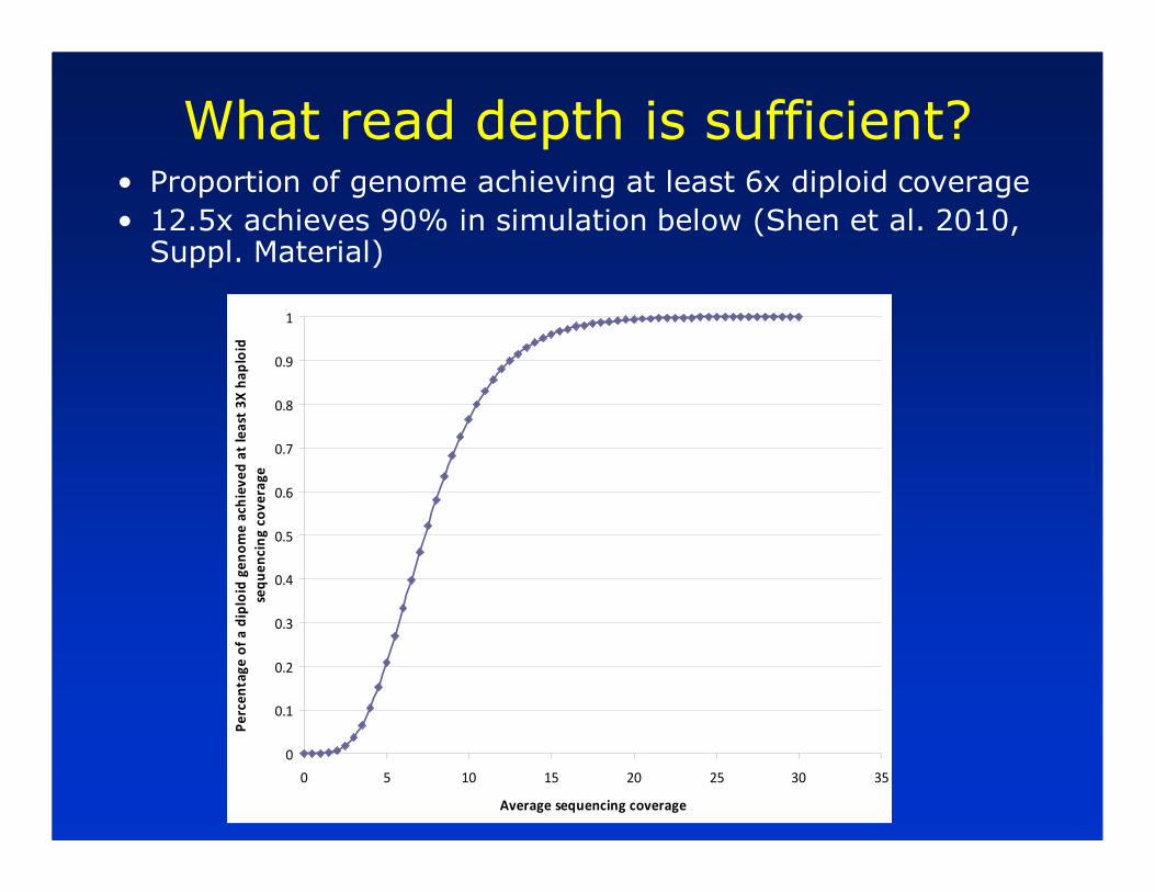
What read depth is sufficient?• Proportion of genome achieving at least 6x diploid coverage
• 12.5x achieves 90% in simulation below (Shen et al. 2010, Suppl. Material)
0
0.1
0.2
0.3
0.4
0.5
0.6
0.7
0.8
0.9
1
0 5 10 15 20 25 30 35
Average sequencing coverage
Pe
rce
nta
ge
of
a d
iplo
id g
en
om
e a
ch
iev
ed
at
lea
st 3
X h
ap
loid
seq
ue
nc
ing
co
ve
rag
e
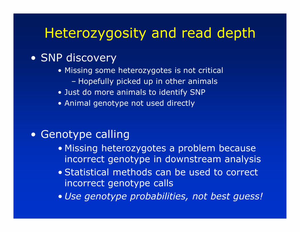
Heterozygosity and read depth
• SNP discovery• Missing some heterozygotes is not critical
– Hopefully picked up in other animals
• Just do more animals to identify SNP
• Animal genotype not used directly
• Genotype calling
•Missing heterozygotes a problem because incorrect genotype in downstream analysis
• Statistical methods can be used to correct incorrect genotype calls
•Use genotype probabilities, not best guess!

Identification of variants
• Program SAMtools
• stacks aligned bam files of multiple animals
• Calls variants and calculates quality/confidence statistics for calls
• http://samtools.sourceforge.net/mpileup.shtml
Genome
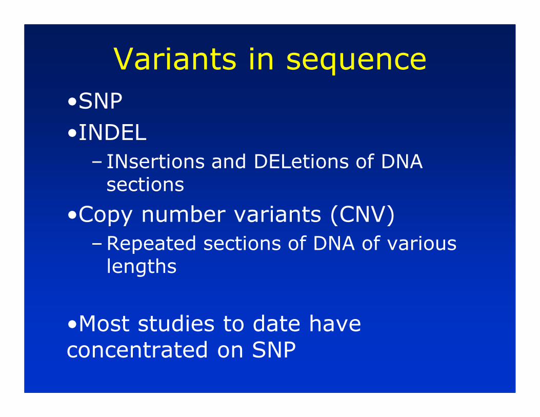
Variants in sequence
•SNP
•INDEL
– INsertions and DELetions of DNA sections
•Copy number variants (CNV)
–Repeated sections of DNA of various lengths
•Most studies to date have concentrated on SNP

Filtering of variants
• Reasons for filters:
• Number of artefacts of the sequencing process that lead to falsely identified variants
• Little evidence for a variant
–Quality scores low
• Reasons against filters:
• Real variants may be lost
–Low frequency SNP often have lower quality scores
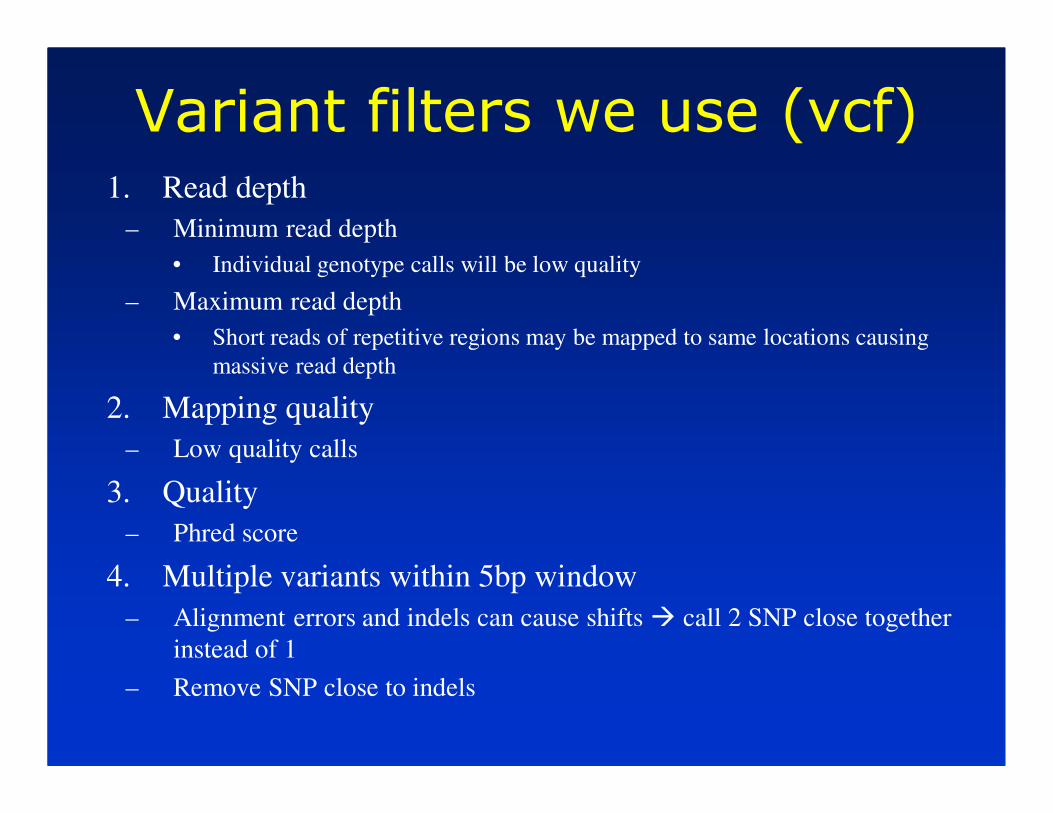
Variant filters we use (vcf) 1. Read depth
– Minimum read depth
• Individual genotype calls will be low quality
– Maximum read depth
• Short reads of repetitive regions may be mapped to same locations causing
massive read depth
2. Mapping quality
– Low quality calls
3. Quality
– Phred score
4. Multiple variants within 5bp window
– Alignment errors and indels can cause shifts � call 2 SNP close together
instead of 1
– Remove SNP close to indels

Phred quality scores (Q)
• Related to base-calling error probabilities.
Expressed in a range from 0 to 999 in our data.
• Probabilities are calculated by the following
formula:
• e.g. Phred of 30 = error rate of 0.001
• Phred of 20 = error rate of 0.01
• Result is probability of each genotype at each
variant eg. AA=0.95 AT=0.05 TT=0.00
• Use these in BEAGLE!
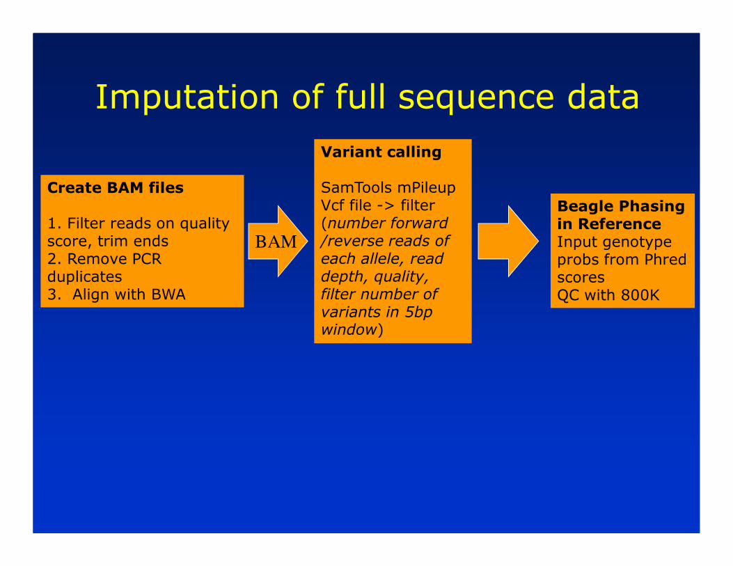
Imputation of full sequence data
Create BAM files
1. Filter reads on quality score, trim ends2. Remove PCR duplicates3. Align with BWA
Variant calling
SamTools mPileupVcf file -> filter (number forward /reverse reads of each allele, read depth, quality, filter number of variants in 5bp window)
Beagle Phasing in ReferenceInput genotype probs from Phred scoresQC with 800K
BAM

Differences between SNP chip and sequence
• SNP chip– Sample of SNP
– Higher minor allele frequency
– Limited linkage disequilibrium depending on number of SNP
• Sequence– Contains most variants
• SNP, indels, CNVs, etc
– Allele frequency matches underlying causative variant frequency
– Causative variants included
– High linkage disequilibrium between variants
Using sequence data in genomic selection and GWAS
• Motivation
• Characteristics of sequence data
• Which individuals to sequence?
• Imputation of full sequence
• Methods for genomic prediction with full sequence data
• Examples–GWAS in Rice, Cattle
Which individuals to sequence?
• Those which capture greatest genetic diversity?
• Select set of individuals which are likely to capture highest proportion of unique chromosome segments

Which individuals to sequence?
• Let total number of individuals in population be n, number of individuals that can be sequenced be m.
• A = average relationship matrix among nindividuals, from pedigree

Animal Sire Dam
1 0 0
2 0 0
3 0 0
4 1 2
5 1 2
6 1 3
Pedigree
Animal 1 Animal 2 Animal 3 Animal 4 Animal 5 Animal 6
Animal 1 1
Animal 2 0 1
Animal 3 0 0 1
Animal 4 0.5 0.5 0 1
Animal 5 0.5 0.5 0 0.5 1
Animal 6 0.5 0 0.5 0.25 0.25 1
Animals 6 is a half sib of 4 and 5
• An example A matrix……..

Which individuals to sequence?
• Let total number of individuals in population be n, number of individuals that can be sequenced be m.
• A = average relationship matrix among n individuals, from pedigree
• c is a vector of size n, which for each animal has the average relationship to the population (eg. Sum up the elements of Adown the column for individual i)

Which individuals to sequence?
• If we choose a group of m animals for sequencing, how much of the diversity do they capture
• pm = Am-1cm
– Where Am is the sub matrix of A for the mindividuals, and cm is the elements of the cvector for the m individuals
• Proportion of diversity = pm’1n
Which individuals to sequence?
• Example
Which individuals to sequence?
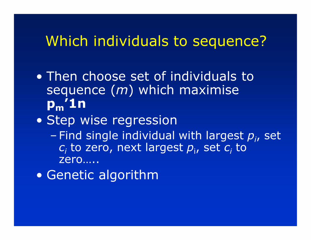
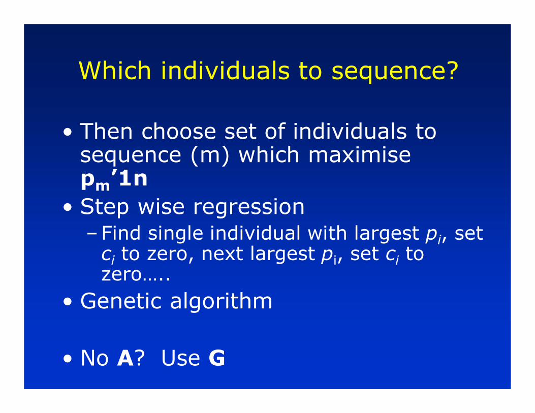
• Then choose set of individuals to sequence (m) which maximise pm’1n
• Step wise regression–Find single individual with largest pi, set ci to zero, next largest pi, set ci to zero…..
• Genetic algorithm

Which individuals to sequence?
• Poll Dorset sheep
0.00
0.05
0.10
0.15
0.20
0.25
0.30
0.35
0.40
0.45
0 10 20 30 40 50 60 70 80
Rams sequenced, ranked from most influential
Pro
port
ion
of ge
ne
tic d
ive
rsity c
aptu
red
Which individuals to sequence?
• Then choose set of individuals to sequence (m) which maximise pm’1n
• Step wise regression–Find single individual with largest pi, set ci to zero, next largest pi, set ci to zero…..
• Genetic algorithm
• No A? Use G

Using sequence data in genomic selection and GWAS
• Motivation
• Characteristics of sequence data
• Which individuals to sequence?
• Imputation of full sequence data
• Methods for genomic prediction with full sequence data
• Examples–GWAS in Rice, Cattle
Imputation of full sequence data
• Two groups of individuals–Sequenced individuals: reference population
– Individuals genotyped on SNP array: target individuals
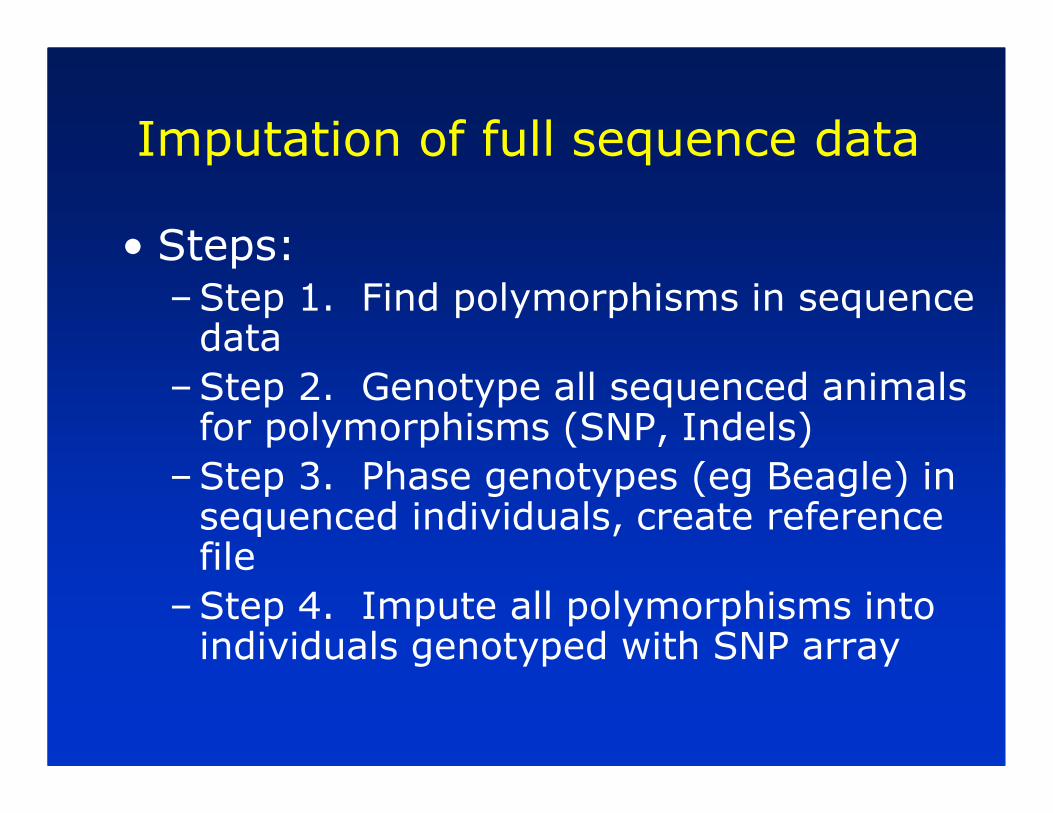
Imputation of full sequence data
• Steps:–Step 1. Find polymorphisms in sequence data
–Step 2. Genotype all sequenced animals for polymorphisms (SNP, Indels)
–Step 3. Phase genotypes (eg Beagle) in sequenced individuals, create reference file
–Step 4. Impute all polymorphisms into individuals genotyped with SNP array

Imputation of full sequence data
Create BAM files
1. Filter reads on quality score, trim ends2. Remove PCR duplicates3. Align with BWA
Variant calling
SamTools mPileupVcf file -> filter (number forward /reverse reads of each allele, read depth, quality, filter number of variants in 5bp window)
Beagle Phasing in ReferenceInput genotype probs from Phred scoresQC with 800K
BAM
Reference file for imputation
Beagle Imputation in Target
SNP array data in target population
Analysis
Genome wide association
Genomic selection
Genotype probabilities

Imputation of full sequence data
• How accurate?

Imputation 50K -> 800K
• Holsteins
Cross validation % Correct
Heifers only 1 96.7%
2 96.7%
Average 96.7%
Heifers 1 97.8%
using key 2 97.7%
ancestors Average 97.7%
Using sequence data in genomic selection and GWAS
• Motivation
• Characteristics of sequence data
• Which individuals to sequence?
• Imputation of full sequence data
• Methods for genomic prediction with full sequence data
• Examples–GWAS in Rice, Cattle

Methods for genomic prediction with full sequence
• 14 million SNPs in Holstein Friesian cattle?
• Which method is most appropriate
• Priors–BLUP (GBLUP) -> all SNPs in LD with QTL, very small effects
–BayesA -> some SNPs have moderate to large effects, rest very small
–BayesB -> many SNPs have zero effect, some have small to moderate effect?

Methods for genomic prediction with full sequence
• Meuwissen and Goddard 2010–Simulated population with full sequence data, ~ 900 mutations chosen to be QTL
–Used BLUP and BayesB to predict GEBV
Meuwissen, Goddard (2010) Genetics 185:623

Methods for genomic prediction with full sequence
• Meuwissen and Goddard 2010–Simulated population with full sequence data, ~ 900 mutations chosen as QTL
–Used BLUP and BayesB to predict GEBV
–Large advantage of BayesB over BLUP• Prior matches their simulated data -> only 900 QTL amongst millions of SNP
–3% advantage of having mutation in data
–Real data??

Methods for genomic prediction with full sequence
• Meuwissen and Goddard 2010–Better persistence of accuracy over generations

Genomic selection methods for GWAS?

Using sequence data in genomic selection and GWAS
• Motivation
• Characteristics of sequence data
• Which individuals to sequence?
• Imputation of full sequence data
• Methods for genomic prediction with full sequence data
• Examples–GWAS in Rice, Cattle
GWAS with sequence
GWAS with sequence
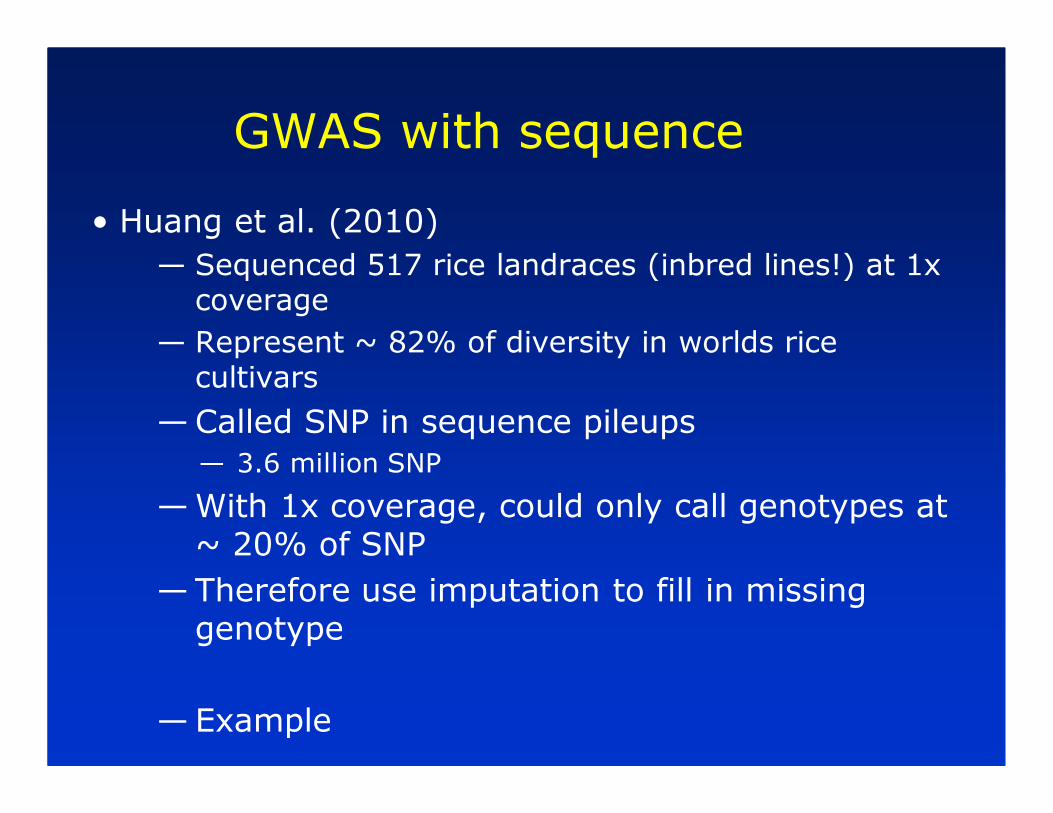
• Huang et al. (2010)
— Sequenced 517 rice landraces (inbred lines!) at 1x coverage
— Represent ~ 82% of diversity in worlds rice cultivars
—Called SNP in sequence pileups
— 3.6 million SNP
—With 1x coverage, could only call genotypes at ~ 20% of SNP
—Therefore use imputation to fill in missing genotype
—Example

GWAS with sequence
• Huang et al. (2010)
• Extent of LD
GWAS with sequence
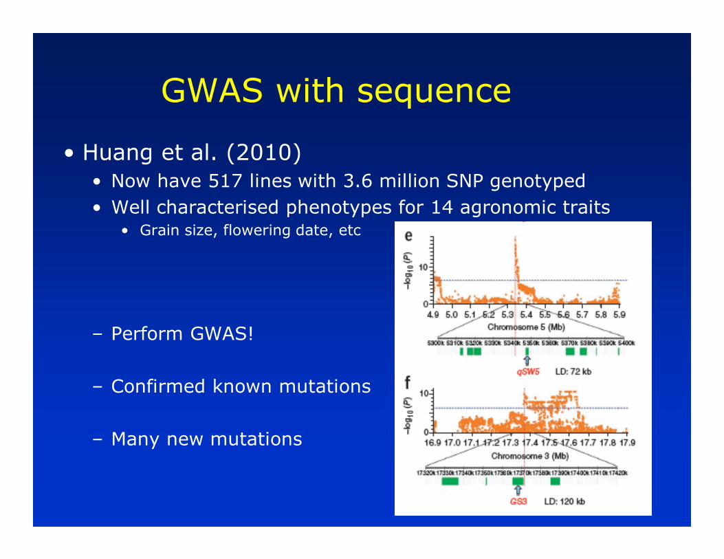
• Huang et al. (2010)
• Now have 517 lines with 3.6 million SNP genotyped
• Well characterised phenotypes for 14 agronomic traits• Grain size, flowering date, etc
– Perform GWAS!
– Confirmed known mutations
– Many new mutations
GWAS with sequence
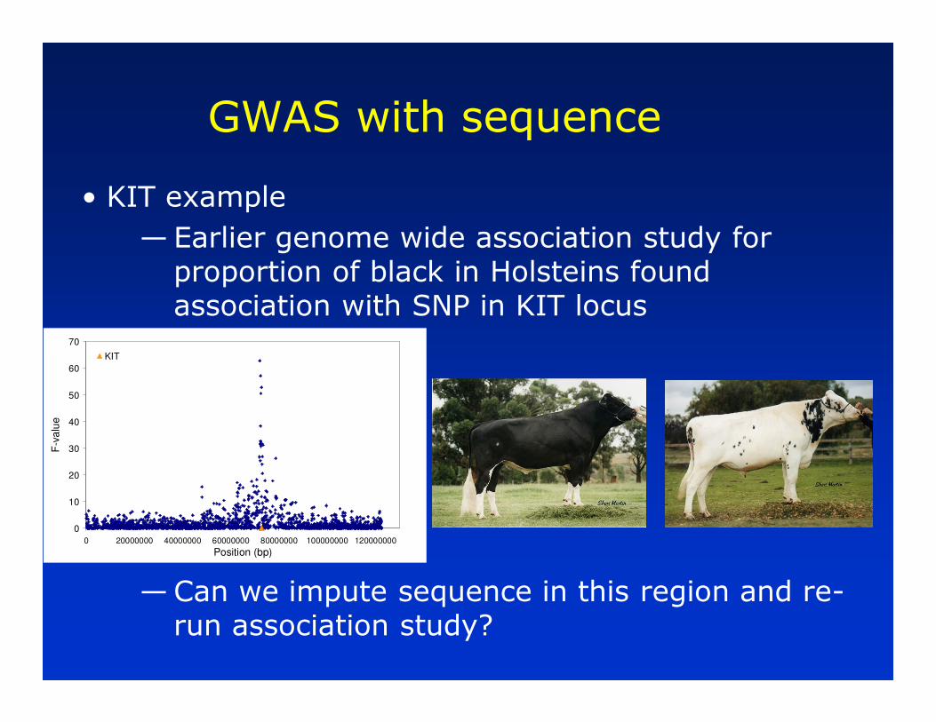
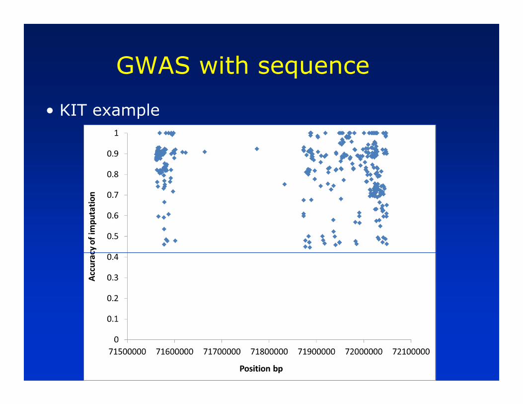
• KIT example
—Earlier genome wide association study for proportion of black in Holsteins found association with SNP in KIT locus
—Can we impute sequence in this region and re-run association study?
0
10
20
30
40
50
60
70
0 20000000 40000000 60000000 80000000 100000000 120000000
Position (bp)
F-v
alu
e
KIT

GWAS with sequence
Average fold coverage Filtered SNPsConcordance
with 800KPICKARD-ACRES VIC KAI 10.4 3,061,950GLENAFTON ENHANCER 10.9 2,934,805 99.9%
BUSHLEA WAVES FABULON 11.3 4,249,998 97.4%
HANOVERHILL STARBUCK 12.5 3,237,681 97.9%
BIS-MAY S-E-L MOUNTAIN ET 12.6 3,009,463 98.5%
SHOREMAR PERFECT STAR 13.6 2,985,205ROYBROOK STARLITE 14.9 3,421,859 97.6%
TOPSPEED H POTTER 15.0 3,839,627LOCHAVON RAMESES 16.2 3,986,520BRAEDALE GOLDWYN 17.2 3,559,227 97.9%
CARENDA GRAVITY 17.8 4,331,849 96.8%ONKAVALE GRIFFLAND MIDAS 22.5 3,742,799

Imputation of full sequence data
Create BAM files
1. Filter reads on quality score, trim ends2. Remove PCR duplicates3. Align with BWA
Variant calling
SamTools mPileupVcf file -> filter (number forward /reverse reads of each allele, read depth, quality, filter number of variants in 5bp window)
Beagle Phasing in ReferenceInput genotype probs from Phred scoresQC with 800K
BAM
Reference file for imputation
Beagle Imputation in Target
SNP array data in target population
Analysis
Genome wide association
Genomic selection
Genotype probabilities

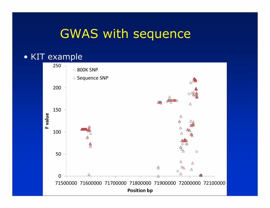
GWAS with sequence
• KIT example
— In sequenced bulls, compile list of SNPs/Indels in KIT region (352/20)
— Call genotypes for the 372 variants in the 12 bulls
— Use this as reference file for imputing the 372 variants in 697 bulls with % black phenotype (from 800K) data
— Run association study on the 372 variants imputed
in 697 bulls
GWAS with sequence
• KIT example
GWAS with sequence
• KIT example

1000 bull genomes on the cloud
• We will all need “reference” population of many sequenced bulls to impute from
— SNP, indel and CNV genotypes
— The more bulls the better!
• We propose a project where we each upload our sequence files (BAM) for each bull to a shared server
• Run SNP/indel/CNV calling software every new 100 bulls uploaded
• Contributors can download SNP/indel/CNV genotype file on all bulls to use for imputation anytime
• Partners welcome!
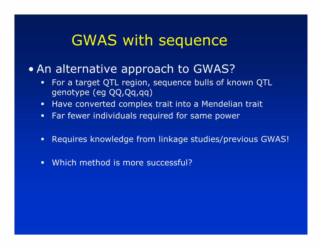
GWAS with sequence
• An alternative approach to GWAS?� For a target QTL region, sequence bulls of known QTL
genotype (eg QQ,Qq,qq)
� Have converted complex trait into a Mendelian trait
� Far fewer individuals required for same power
� Requires knowledge from linkage studies/previous GWAS!
� Which method is more successful?

Quality of reference genomes?
• Cattle
– Bovine build 4.2
– Annotated • But many genes no assigned function
– No Y chromosome yet, X is messy
– ~ 9.5 million putative SNP in dbSNP
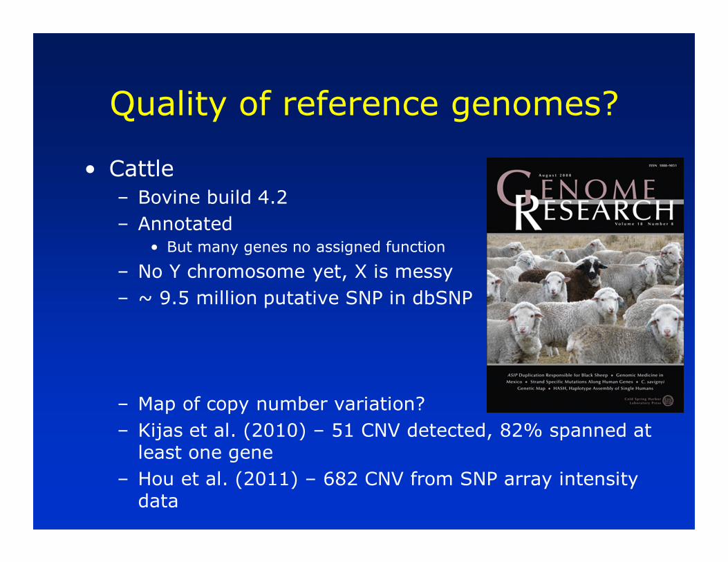
Quality of reference genomes?
• Cattle
– Bovine build 4.2
– Annotated • But many genes no assigned function
– No Y chromosome yet, X is messy
– ~ 9.5 million putative SNP in dbSNP
– Map of copy number variation?
– Kijas et al. (2010) – 51 CNV detected, 82% spanned at least one gene
– Hou et al. (2011) – 682 CNV from SNP array intensity data

• Potential of whole genome sequence data
– Enable genome wide association study -> straight to causative mutation
– Genomic selection
• No longer have to rely on LD, causative mutation actually in data set, Higher accuracy of prediction?, Better persistence of accuracy across generations
Conclusions

• Potential of whole genome sequence data
– Enable genome wide association study -> straight to causative mutation
– Genomic selection
• No longer have to rely on LD, causative mutation actually in data set, Higher accuracy of prediction?, Better persistence of accuracy across generations
• Choose individuals to sequence based on genetic contribution to population?
• Imputation of target population genotyped with SNP arrays
– Caution with low frequency alleles, relationship to reference
• Large collaborative projects required for bovine/plant communities?
Conclusions