Genomic Selection Accuracy using Historical Data Generated ... Selection Accuracy using Historical Data . ... Soil and Crop Science, C117 Plant ... effects for some or all markers

Genomic Selection Accuracy using Historical Data

Generated in a Wheat Breeding Program

Eric Storlie and Gilles Charmet*

G. Charmet, INRA UMR GDEC 234 av du Brézet 63100 Clermont-Ferrand, France,

63100 ; E. Storlie, Colorado State University, Soil and Crop Science, C117 Plant Science,

Fort Collins CO 80523. *Corresponding author ([email protected])

Abbreviations: BL, Bayesian LASSO; BRR, Bayesian Ridge Regression; CV, cross-

validation; BLUP best linear unbiased predictor; GEBV, genomic estimate of breeding

value; GB, genomic relationship best linear unbiased predictor; GS, genomic selection;

RRB, ridge regression best linear unbiased predictor

Abstract

Cross-Validation methods (CV) were designed to simulate Genomic Selection (GS) for

yield in a wheat breeding program with data of 318 genotypes grown over an 11 year

period at 6 locations in France. Two methods, CVSWO (Cross-Validation-Specific-

WithOut location as factor) and CVSW (Cross-Validation-Specific-With location as

factor), included 11 folds, each comprising genotypes grown during a specific year and

each representing target populations, while the remaining folds comprising genotypes

The Plant Genome: Posted 1 Mar. 2013; doi: 10.3835/plantgenome2013.01.0001

mailto:[email protected]

grown during the other ten years represented training populations. These methods were

compared with CVRWO (Cross-Validation-Random-WithOut) and CVRW (Cross-

Validation-Random-With location as factor), designed to simulate standard CV, while

retaining the structure of the first two CV methods; the same 318 genotypes were used to

create 11 folds, each comprising randomly-selected genotypes. Results suggest the

accuracy of the CV methods using specifically-selected genotypes (rM = 0.20) based on

years grown, were significantly less than methods using randomly-selected genotypes (rM

= 0.40 - 0.50). These results imply wheat yield is more difficult to predict for unknown,

futuristic years than standard CV methods suggest. An alternative measure of accuracy

based on predicted genotypic ranks, termed Predicted Rank Conversion (PRC) was

implemented for the purpose of improving accuracies and reducing the differences

between CV methods.


Introduction

Plant Genomic Selection (GS) investigations have suggested the possibility of predicting

breeding value of traits with a dense and uniform set of molecular markers. The impetus

behind GS is the convenience of predicting the performance of crop plants without the

usual drudgery of field tests at multiple locations over several years. Genomic Selection,

though, may not replace the need for field tests and may take a more integrative role in a

wheat breeding program. Heffner et al. (2010) suggested two years could be eliminated

from field trials, and parents might be selected in three rather than four years for

subsequent breeding cycles.

Small grain GS empirical studies include barley, maize and wheat (Albrecht et al., 2011;

Burgueño et al., 2012; Crossa et al., 2010; Heffner et al., 2011; Heslot et al., 2012;

Lorenzana and Bernardo, 2009; Poland, 2012; Zhao et al., 2012; Zhong et al., 2009).

Heffner et al. (2011) analysed 374 wheat genotypes, grown at 3 locations over 2 years,

genotyped with 1158 DArT markers and phenotyped for 13 traits using four statistical

models – RRB, BayesA, BayesB and BayesC – for Genomic Estimated Breeding Values

(GEBV); prediction accuracies were 28% greater than marker assisted selection and 5%

less accurate than phenotypic selection. Crossa et al. (2010) analysed 599 wheat

genotypes, grown in 4 mega-environments, genotyped with 1279 DArT markers and

phenotyped for yield using three statistical models - RRB, BL and RKHS (Reproducing

Kernel Hilbert Space) - with marker and/or pedigree information for GEBV.


The statistical models make different assumptions about marker numbers and effects,

possibly affecting GEBV and prediction accuracies of different data sets. Several

statistical models estimate marker effects for some or all markers in a dataset, including –

BayesA, BayesB, BL, BRR and RRB (Meuwissen et al., 2001; Park and Casella, 2008;

Pérez et al., 2010; Whitaker et al., 2000). Two models, RRB and BRR assume there are

many QTLs with small effects (Pérez et al., 2010); one model, BayesB, assumes many

QTL with no effects and a few QTLs with some, possibly large effects (Meuwissen et al.,

2001); two models, BayesA and BL, assume many QTLs have small effects and a few

QTLs have large effects (Meuwissen et al., 2001; Pérez et al., 2010). At least one model,

GB, derives genetic relationships from markers and estimates breeding values from the

relationship matrix using a BLUP animal model (VanRaden, 2008), though the basis of

GB is similar to RRB (Piepho, 2009). Each model derives genotypic and phenotypic

information from the entire training population for an estimation of marker effects. The

training and target populations comprise individuals genotyped with the same markers

and may consist of any number of individuals grown at any number of sites during any

number of years.

Accuracies are measured as correlations between the observed and predicted phenotypes

using a Cross-Validation method; the CV method randomly partitions the genotypes into

folds and isolates folds as target populations, while omitting the target’s phenotypic data.

The remaining folds of genotypes with their phenotypic data intact are utilized as the

training dataset; this process is repeated for each fold (Crossa et al., 2010). Standard CV


methods have reported correlations between predicted and observed yields up to 0.61 in

wheat (Crossa et al., 2010) and 0.74 in maize (Albrecht et al., 2012). Burgueño et al.

(2012) altered the CV method to more closely mimic the use of GS in a breeding

program, which will have new, untested genotypes, and their results suggest the accuracy

of predictions is reduced without some field testing by up to 31%. A breeding program

would ultimately hope to eliminate field testing and rely on GS predictions, and this

should be possible for some traits of some organisms. For example, some dairy breeding

companies have relied on GS predictions to reveal a young bull’s merit, and already some

bulls have been marketed with GEBV and no pedigree-testing information (Hayes et al.,

2009).

Quantitative traits strongly influenced by genotype x environment (GxE) interactions,

such as wheat yield, would be more difficult to predict due the change of varietal ranks.

Heffner et al. (2009) reasoned GS accuracies would be stable, despite GxE effects, due to

a breeder’s intentional and unintentional selection of alleles appropriate for a particular

region. Crossa et al. (2010) indicated marker effects differed in different environments,

implying GxE or, more specifically, QxE (QTL x Environment) was the cause. Some

genotypes are more resistant to GxE effects than others. For example, in the CSU

(Colorado State University) winter wheat breeding program, some top ranked varieties,

like Byrd and Snowmass, are predictably high yielders from year to year, location to

location. A breeding program tends to select for this consistency after 3 years of yield


trials. If the consistently high yields are a predictable trait, accuracies may improve if the

top ranked genotypes are isolated for analysis.

This investigation analysed elite French winter wheat genotypes (breeding lines) grown

during an eleven year period at six locations with four statistical models to simulate the

use of GS in wheat breeding program to determine the accuracy of predicting

uncharacterized genotypes in a futuristic growing season. Another objective was to

determine if the measure of accuracy would improve by ranking the genotypes and

retaining only the top-ranked genotypes.

Materials and Methods

Population

Yield data was taken from 318 elite winter wheat genotypes developed by INRA in the

applied breeding programme from crosses between varieties and elite breeding genotypes

and grown over ten years at six locations with two replications in France. Each genotype

was grown for an average of 3.3 years between 2000 and 2010. These genotypes were

developed in the “continuous improvement program” involving 300 crosses each year

between breeding genotypes and recently registered varieties. Wheat plants from the F2

to F4 generations were bulked into families with about 2000 plants per cross, and the F5

grains from selected spikes were sown in single rows using a classical pedigree design.


Bulked grains of F6 genotypes were sown in two replicated trials with randomized 6-10

m² plots in a single location. The best F7 and the most advanced F8- F9 genotypes were

evaluated in a network of 8-10 locations with 4 replications, according to their precocity

group. For a more balanced design, data from 6 locations - Clermont-Ferrand (CF),

Dijon (DI), Estrées-Mons (EM), Le Moulon (LM), Lusignan (LU) and Rennes (RE) -

were used due to a more balanced genotypic representation. Therefore, 30-50 new

genotypes were entered into the most advanced evaluation network. Some genotypes

were evaluated 1-3 years before the best were registered. Since breeding genotypes were

used as genitors one time, sufficient phenotypic data are available during the selection

cycle. In this study, genotypes had been evaluated in the complete multisite network

between 2000 and 2010. There were 318 genotypes after discarding genotypes with

incomplete data. The Parents of the 318 lines are for half of them the recently registered

French varieties and for the second half breeding lines from former generations of the

program. Therefore they belong to the same breeding group and are not or little

genetically structured (i.e. in subgroups). However, they are related to each other, with

an average coefficient of co-ancestry of 0.22 (range of 0 to 0.98, i.e. a few lines are quite

similar, likely derived from the same F4 plant), which might suggest that co-ancestry

based methods should be efficient.


Statistical models for GEBV

The single-environment linear, statistical models of this investigation may be described,

yi= μ+∑j = 1

p

xij β j+εi i= (1,. .. ,n) [1]

where yi is the phenotype of the ith individual, μ is the overall mean, xij is the marker

covariate of the ith individual and jth marker, βj is a regression coefficient of the jth marker

and εi the residual. The statistical models – RRB, BRR and BL - estimated marker

effects for each of the markers in the training population and used these marker effects to

calculate GEBV for genotypes in the target population. Ridge Regression BLUP (RRB)

used maximum-likelihood solutions for mixed models (Endelman, 2011); it assumed

markers had random effects, a common variance and effects that were equally shrunken

towards zero using a penalty parameter - λ2=σ2e/σ2

g, where σ2e is the residual variance

and σ2g is the marker effect variance (Piepho, 2009). Bayesian Ridge Regression (BRR)

uses a Gaussian prior distribution with a variance common to each marker effect (de los

Campos and Pérez, 2010; Pérez et al., 2010). The prior residual variance and degree of

freedom were Sε=4.5, dfε=3, respectively, and the prior variance of marker effects were

SβR=.009, dfβR=3. Estimates of lambda were based on a heritability, h2= 0.37. The

number of iterations used as burn-in was 20,000 and the number of iterations made in the

Gibbs sampler was 60,000. Bayesian LASSO (BL) uses a Gaussian prior distribution

with a marker-specific prior variance for a differential shrinkage of each marker effect


(de los Campos and Pérez, 2010; Pérez et al., 2010). The prior residual variance and

degree of freedom were Sε=4.5, dfε=3, respectively, and the prior variance of marker

effects were SβL=.009, dfβR=3. Estimates of lambda were based on a heritability, h2=

0.37 The number of iterations used as burn-in was 20,000 and the number of iterations

made in the Gibbs sampler was 60,000. G-BLUP (GB) assumes pedigree relationships in

the training population, based on marker genotypes, and then estimates breeding values

using a BLUP animal model (Henderson, 1975; Costner, 2010). Piepho (2009) showed

GB and RRB are similar.

Data analysis

Marker genotypes were produced with 2236 Diversity Array Technology (Triticarte Pty.

Ltd, Canberra, Australia: http://www.triticarte.com.au); genotypes were scored as ‘1’ for

‘present’ and ‘0’ for ‘absent’.

The R package, Linear mixed effects models using S4 classes (lme4), was used to

estimate variance components for heritability described, y = μ + E + g + ε, where y is a

response vector, E a fixed “environment (i.e. year x location) effect parameter, g a

random genotypic effect vector and ε, a per observation noise term (Bates et al. 2011).

Genomic Estimates of BV were derived from 318 genotypes, each used with four Cross-

Validation methods (Table 1): the Cross-Validation methods described in Table 1 were

designed to compare methods that predict yields of genotypes selected specifically for


http://www.triticarte.com.au/

years grown with and without location as factor (CVSWO and CVRW) with methods that

predict yields of genotypes selected randomly with and without location as factor

(CVRWO and CVRW). For each CV method, genotypes were separated into 11 folds,

one fold for each of 11 growing seasons from 2000 to 2010. The folds were composed of

randomly - or specifically - selected genotypes with regression coefficients derived with

and without location as factor (Table 1). The difference between CVSW and CVSWO

was an estimation of mean yield for each location (CVSW) or an estimation of mean

yield without regarding location as an explanatory variable. For example, if genotypes 1-

62 were grown during the year 2000, they comprised one fold and this fold could be the

target population predicted by the training population comprising the other ten folds; this

fold, in turn, may be part of the training population in another cross-validation analysis.

Linear regression coefficients were derived from the genotypes “With” or “Without”

location as a factor using a linear model [1], lm, (R Development Core Team 2011).

Cross-Validation-Random-With location as factor (CVRW) and Cross-Validation-

Random-Without location as factor (CVRWO) included the same fold numbers and sizes

as CVSW and CVSWO, but the folds comprised randomly-selected genotypes grown

during any of 11 years. For example, genotypes 1-10, 50-60, 100-110, 150-160, 200-210

and 250-262 may have been grown during any of the years and would have been placed

in any fold with any other genotypes. Again, linear regression coefficients were derived

from the genotypes “with” or “without” location as a factor using a linear model [1], lm.


Each line was grown for an average of 3.3 years, though each line was represented in

only one fold and could not be part of both the training and target populations. The fold

compositions were inflexible due to the basis of CVSW and CVSWO, which comprised

genotypes grown during specific years and could only be grouped amongst genotypes

grown during the same year; therefore, the folds could not be re-assembled and re-

analysed in a re-sampling procedure. CVRW and CVRWO were not re-sampled, as well,

in order to align the CV methods as closely as possible.

The Pearson correlation coefficient, r, measured the degree of correlation between the

observed phenotype and predicted breeding values, expressed as rM, marker-based

prediction accuracy (Heffner et al. 2011; Heslot et al. 2012). A t-test compared the

prediction accuracies of the four models using CVSWO vs. CVRWO and CVSW vs.

CVRW. Bargraphs and linegraphs represent means and error bars represent SD; graphs

were produced with the R Package ‘sciplot’ (Morales 2010).


Predicted Rank Conversion

An alternative to Pearson correlations, termed Predicted Rank Conversion (PRC),

ranked the predicted yields of genotypes for methods, CVSWO and CVRWO, and

selected the top 10 percent and compared these predicted ranks with the observed ranks

and converted the predicted 10 percent in terms of their observed rankings. For example,

if the number one predicted genotype was actually ranked number 12/100, this genotype

was scored a rank of 0.12, because it was assumed, in a breeding program, the top 10

percent of predicted genotypes would be selected for further development, and the logic

of the conversion was to set the predicted genotypes in terms of their observed rankings;

so, in this example, the number one genotype would probably have been selected for

further development, when actually, the number 12 genotype was selected. All top ten

percent predicted ranks were converted to observed ranks, and an average score was

calculated for CVSWO and CVRWO. The best possible score was estimated from a

perfect match between the predicted and observed ranks and classified under the “BEST”

model.


Results and discussion

Prediction Accuracy of Cross-Validation Methods

The historical wheat data described in Materials and Methods was used to gain insight

into the utility of GS for breeding wheat. The objective was to determine if there were

differences in prediction accuracies, which may have implications for appropriate GS

models for wheat. The methods were compared for prediction accuracies, and the results

suggest significant differences for each comparison (Figs. 1 and 2, respectively): the CV

methods based on randomly-selected genotypes were more accurate than methods based

on specifically-selected genotypes. The four statistical models produced very similar

results.

Crossa et al. (2010) concluded certain markers had different effects at different locations,

suggesting they were influenced by QxE. The objective of deriving regression

coefficients from each location, CVRW and CVSW, was to determine if accuracies were

more consistent when location was a factor and was used to estimate prediction

accuracies, rather than deriving coefficients when location was not a factor. In most

cases, accuracies decreased for the methods using specifically-selected genotypes at each

location (Figs. 4, and 5). A t-test indicates differences between the methods at 4

locations and no differences at 2 locations (supplemental Table S4), suggesting yields

were less predictable at some locations – CF, DI, LM and LU – and were more


predictable at other locations, EM and RE, during an 11 year period. One interpretation

of this result highlights the regional differences and possible inherent predictabilities of

some regions due to more consistent climates; Rennes, RE, for instance has an oceanic

climate, buffering plants from temperature and precipitation extremes.

The measure of accuracy for these initial results was a correlation, rM, between predicted

and observed yields, which included all observations in the analysis. Wheat breeders,

however, typically rank candidate genotypes and select the top percentage for further

evaluations. In an attempt to simulate a breeding program, the Predicted Rank

Conversion (PRC) measurement was evaluated to determine if accuracies changed for the

CV methods. Only, Cross-Validation methods, CVRWO and CVSWO, were compared

graphically and by method t-test, and again, differences were significant (Fig. 3).

Cross-Validation Accuracy

The decreased prediction accuracies between the CV methods were the result of

predictions based on genotypes grown during one specific year, rather than 1-11 random,

non-specific years. This alteration of genotypic selection caused changes in the relative

order of genotypes, according to predicted yields. An interaction effect may explain the

change of genotypic order, and a reasonable interaction to implicate is a QTL x

Environment interaction (QxE). When the training and target populations comprised

randomly-selected genotypes (CVRWO and CVRW) marker effects were estimated from

genotypes representing each year of the target population, and the prediction accuracies


were rM = 0.50 and 0.40, respectively, but when the target population comprised

specifically-selected genotypes (CVSWO and CVSW) marker effects were estimated in

the training population from genotypes with no growing years in common with the target

population, and prediction accuracies decreased to rM=0.20 and 0.21, respectively. If the

environmental conditions induced specific marker effects for each year, these year-

specific effects were not available for CVSWO and CVSW, due to the target population

containing all the genotypes grown during one year – this is analogous to a real breeding

program that would predict the value of genotypes for futuristic, unknown years.

Cross-Validation methods using training populations comprising genotypes grown during

single years was not used for GEBV in the current investigation. However, Heffner et al.

(2011) used the same genotypes grown in 2008 and 2009 for training and target

populations, respectively, to predict yields using the statistical model, Bayes A, and

prediction accuracies were rM=0.22; the current study had a similar result with CVSWO

and CVSW, indicating accuracies did not improve with a training population comprising

the same genotypes grown during a single year for the training and target populations.

The results of Heffner et al. (2011) also include a phenotypic correlation, rp=0.20, for the

phenotypic yield of each year, suggesting phenotypic selection offers no advantage over

GS, when the predictor and predicted populations are grown for one year.

In practical terms, according to these results, a plant breeder would realize low prediction

accuracies when using training populations comprising genotypes grown over several


years to predict the yield of genotypes grown for one year at one or six locations. A

classical breeding program, described by Heffner et al. (2010), would subject F5-derived

genotypes to three years and, at least, three locations for yield trials. In the current study,

the mean yield for each genotype was estimated from an average of 3.3 years of growth

at six locations, and these genotypes represent genotypes a breeding program may strive

to predict using statistical models; a plant breeder using GS may hope to replace 3 years

and, at least, 3 locations with GEBV to predict the best genotypes if these predictions

could be as reliable and accurate as classical methods.

The difficulty predicting uncharacterized genotypes may be partly addressed with

parameter adjustments: investigations involving simulations have determined the most

controllable parameters are training population sizes and marker numbers (Goddard

2009; Hayes et al. 2009). Regarding marker numbers, Poland et al. (2012) used over 41k

SNPs in 254 wheat genotypes and indicated there were no accuracy differences with

1827 SNPs. Regarding training population size, a few recent studies have concluded

population size was an important variable determining prediction accuracies in wheat,

maize and barley (Heffner et al. 2011; Iwata and Jannink 2011; Zhao et al. 2011).

Heffner et al. (2011) calculated a training population for wheat should be of a size,

~12,000 for rM = 0.90, similar to an estimation by Hayes et al. (2009) for dairy cows.


Crossa et al. (2010) described the relationship between CV correlation and square root

(sqrt) of heritability h as Cor(gi,yi) having an upper limit of (σ2g + ni

-1 σ2ε)-(1/2)σg < h

(where yi is the average performance of the ith line, gi is the genetic value of the ith

genotype, ni is the number of replicates of the ith genotype and εi is a model residual),

indicating correlations may be greater than h for replicated data, because this sqrt of

heritability is higher than heritability defined for a single replicate level. For the

population of the current investigation, CVRWO, Cor(gi,yi) = rM=~0.50 and h= 0.61

(Table 2); accordingly, the models were accurate for the CV methods, though genetic

variation remains to be captured for all CV methods. The relationship between

correlation, rM, and sqrt of heritability may be a guide for the identification of an optimal

marker density and training population size for GS, possibly defined empirically through

a balance between prediction accuracy and economic cost of materials and methods.

In the previous sections, prediction accuracies were based on correlations, rM, between

predicted and observed yields of respective genotypes. This measurement was

expeditious but included some unused information in a breeding program. A plant

breeding program, for example, may seek to identify the top ten percent of progeny

derived from a parental cross. The top ten percent could be the primary focus of GS, as

well, if they were isolated from the GEBV analysis and featured for purposes of

comparing models, markers and populations. The impetus for evaluating other

measurements of accuracy was to optimize accuracies. It is possible the correlation

measurement of accuracy includes less predictable genotypes, those more prone to GxE


effects, while the top-ranked genotypes may be more consistent across environments and

typically selected under conventional breeding methods.

An alternative measurement, termed Predicted Rank Conversion (PRC) in Materials and

Methods, converts the predicted top ten percent of genotypes in terms of observed

genotypic ranks. A PRC measurement would more directly connect to the objectives of a

breeding program than correlations involving all predicted genotypes (including 90% of

the genotypes a breeding program would not consider). A PRC would allow a breeder to

establish a limit, a PRC range of confident predictions. Predicted Rank Conversion was

used to compare methods CVRWO and CVSWO, but the differences were significant

(Fig. 3), as with correlations, rM. The PRC, however, indicates the average observed

rank predicted by each model: with method CVRWO, the average observed rank was in

the top 21 percent of the population predicted by RRB. This average over ten years

included 66 genotypes predicted in the top 10 percent; thirty-four of these genotypes had

observed yields that were equal to or less than 10 percent of the population rank, and the

remaining 32 (48%) genotypes had observed yields greater than 10 percent (data not

shown); a plant breeder using GS would have selected 48 percent of predicted genotypes

that were greater than the top 10 percentage of ranks. The lowest possible score would be

an average of 0.06, equivalent to a perfect correlation (Fig. 3), and the worst possible

average score would be an average of 0.94 (data not shown).


Conclusion

Cross-Validation methods (CVSWO and CVSW) were designed to simulate GS in a

breeding program using historical data of 318 genotypes for the assemblage of 11 folds,

each comprising genotypes grown during a specific year. Specifically-selected genotypes

for each of 11 folds had one year in common – they all grew during the same year – and

were used as a target populations while the remaining genotypes were used as the training

populations. These CV methods were compared with methods, CVRWO and CVRW,

designed to simulate more standard CV methods using the 318 genotypes for an

assemblage of 11 folds, each comprising randomly-selected genotypes; these methods are

more expeditious and flexible, due to the sampling possibilities. The methods, CVSWO

and CVSW, had lower prediction accuracies for the trait, yield, of this investigation. The

only differences between CVSWO vs. CVRWO and CVSW vs. CVRW were the fold

genotypic compositions. These results have implications for a wheat breeding program

seeking to utilize the predictive capabilities of GS, because results suggest accuracies for

predicting yield are rM=0.20 and probably not useful for reliably predicting the best

genotypes. One explanation for the reduced accuracies may be a QxE effect changing the

performance of some genotypes in different environments and making them less

predictable. If some genotypes are less affected by QxE effects and tend to emerge near

the top of rankings, due to consistently high yields, then predictability may be improved

if the top-ranked genotypes were isolated for estimates of accuracy. The Predicted Rank

Conversion (PRC) was designed as an alternative measure of accuracy to determine if


accuracies might be improved following the approach of plant breeding programs by

selecting the top ranked genotypes and discarding the others. However, the difference

between CVRWO and CVSWO was significant.

The low accuracies revealed by GS for predicting genotypes separated according to

years may be a shared problem with phenotypic selection (Heffner et al. 2011), which

also had low accuracies, rp=0.20. Employing GS, a breeding program may seek a

reduction of years and locations for testing F5-derived genotypes, as described by

Heffner et al. (2010). The prediction of traits using GS is measured against classical

breeding methods, stated as a correlation between the two methods, rM=0.20, a measure

of accuracy. As discussed in the first section, this correlation can be, at least, the sqrt of

heritability. With a much larger training population, a greater marker density, the

incorporation of QxE information in models, GS may address the poor accuracies for

predicting yield in wheat.


References

Albrecht, T., V. Wimmer, H-J. Auinger, M. Erbe, C. Knaak, M. Ouzunova, H. Simianer,

and C-C. Schön. 2011. Genome-based prediction of testcross values in maize. Theor.

Appl. Genet. 123:339-350.

Bates, D., M. Maechler, and B. Bolker. 2011. Linear mixed-effects models using s4

classes: package lme4. Available at http://lme4.r-forge.r-project.org/. (Accessed 12

September 2011).

Burgueño, J., G. de los Campos, K. Weigel, and J. Crossa. 2012. Genomic prediction of

breeding values when modelling genotype x environment interaction using pedigree and

dense molecular markers. Crop Sci. 52:707-719.

Costner, A. 2010. Pedigree functions: package pedigree. Available at

http://cran.r-project.org/web/packages/pedigree/pedigree.pdf. (Accessed 22 February

2011).

Crossa, J., G. de los Campos, P. Pérez, D. Gianola, J. Burgueño, J.L Araus, D. Makumbi,

R.P. Singh, S. Dreisigacker, J. Yan, V. Arief, M. Banziger, and H-J. Braun. 2010.

Prediction of genetic values of quantitative traits in plant breeding using pedigree and

molecular markers. Genetics 186:713-724.


http://lme4.r-forge.r-project.org/

http://cran.r-project.org/web/packages/pedigree/pedigree.pdf

de los Campos, and G., P. Pérez. 2010. Bayesian linear regression: package BLR.

Available at http://cran.r-project.org/web/packages/BLR/index.html. (Accessed 15

September 2010).

Endelman, J. 2011. Genomic selection and association analysis: package rrBLUP.

Available at http://cran.r-project.org/web/packages/rrBLUP/index.html. (Accessed 2

October 2011).

Goddard,M.E.2009. Genomic selection: prediction of accuracy and maximisation of long

term response. Genetica. 136:245-257>

Hayes, B.J., P.J. Bowman, A.J. Chamberlain, and M.E. Goddard. 2009. Invited review:

Genomic selection in dairy cattle: progress and challenges. J. Dairy Sci. 92:433-443.

Heffner, E.L., J-L. Jannink, and M.E. Sorrells. 2011. Genomic selection accuracy using

multifamily prediction models in a wheat breeding program. The Plant Genome. 4:65-75.

Heffner, E.L., M.E. Sorrells, and J-L. Jannink. 2009. Genomic selection for crop

improvement. Crop Sci. 49:1-12.


http://cran.r-project.org/web/packages/BLR/index.html

http://cran.r-project.org/web/packages/rrBLUP/index.html

Heffner, E.L., A.J. Lorenz, J-L. Jannink, and M.E. Sorrells. 2010. Plant breeding with

genomic selection: gain per unit time and cost. Crop Sci. 50:1681-1690.

Henderson C.R.1975. Best linear unbiased prediction under a selection model. Biometrics

31:423–447

Heslot, N., H-P. Yang, M.E. Sorrells, and J-L. Jannink. 2012. Genomic selection in plant

breeding: a comparison of models. Crop Sci. 52:146-160.

Iwata, H., and J-L. Jannink. 2011. Accuracy of genomic selection prediction in barley

breeding programs: a simulation study based on the real single nucleotide polymorphism

data of barley breeding lines. Crop Sci. 51:1915-1927.

Lorenzana, R.E., and R. Bernardo. 2009. Accuracy of genotypic value predictions for

marker-based selection in biparental plant populations. Theor. Appl. Genet. 120:151-161.

Morales, M. 2010. Scientific graphing functions for factorial designs: package sciplot.

Available at http://cran.r-project.org/bin/windows64/contrib/2.11/check/sciplot-

check.log. (Accessed 20 July 2011).

Meuwissen, T.H.E., B.J. Hayes, and M.E. Goddard. 2001 Prediction of total genetic

value using genome-wide dense marker maps. Genetics. 157:1819-1829.


http://cran.r-project.org/bin/windows64/contrib/2.11/check/sciplot-check.log

http://cran.r-project.org/bin/windows64/contrib/2.11/check/sciplot-check.log

Park, T., and G. Casella. 2008. The bayesian LASSO. J. Am. Stat. Assoc. 103:681-686.

Pérez, P., G. de los Campos, J. Crossa, and D. Gianola. 2010. Genomic-enabled

prediction based on molecular markers and pedigree using the Bayesian Linear

Regression Package in R. Plant Gen. 3:106-116. doi: 10.3835/plantgenome2010.04.0005

Piepho, H.P. 2009. Ridge regression and extensions for genomewide selection in maize.

Crop Sci. 49:1165-1175.

Poland, J., Endelman, J., Dawson, J., Rutkoski, J., Wu, S., Manes, Y., Dreisigacker, S.,

Crossa, J., Sánchez-Villeda, H., Sorrells, M., and Jannink J-L. 2012. Genomic Selection

in Wheat Breeding using Genotyping-by-Sequencing. Plant Gen. 5:103-113.

doi: 10.3835/plantgenome2012.06.0006

R Development Core Team. 2011. R: A language and environment for statistical

computing. R Foundation for Statistical Computing, Vienna, Austria.

Whittaker, J.C., C. Haley, and R. Thompson. 1997. Optimal weighting of information in

marker-assisted selection. Genet. Res. 69:137-144.


Zhao, Y., M. Gowda, W. Liu, T. Wurschum, H.P. Maurer, F.H. Longin, N. Ranc, and

J.C. Reif. 2012. Accuracy of genomic selection in European maize elite breeding

populations. Thoer. Appl. Genet. 123: DOI: 10.1007/s00122-011-1745-y

Zhong, S.Q., J.C.M. Dekkers, R.L. Fernando, and J-L. Janink. 2009. Factors affecting

accuracy from genomic selection in populations derived from multiple inbred lines: a

barley case study. Genetics 182:355-364.

VanRaden, P.M. 2008. Efficient methods to compute genomic predictions. J, Dairy Sci.

91: 4414-4423.

Acknowledgements

We thank the reviewers, Laurence Moreau, Alain Charcosset, Jacques Bordes, Mathieu

Bogart and Xinran Li for helpful suggestions.





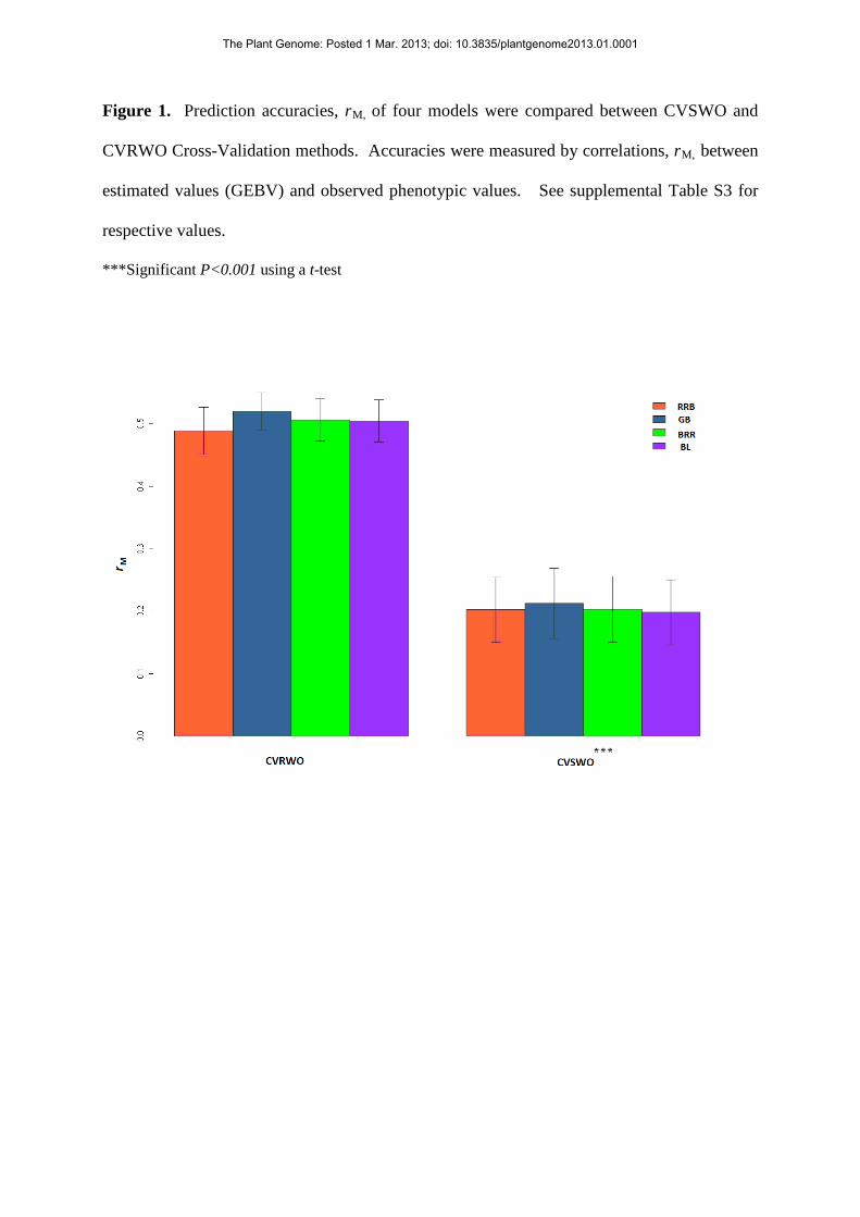
Figure 1. Prediction accuracies, rM, of four models were compared between CVSWO and

CVRWO Cross-Validation methods. Accuracies were measured by correlations, rM, between

estimated values (GEBV) and observed phenotypic values. See supplemental Table S3 for

respective values.

***Significant P<0.001 using a t-test


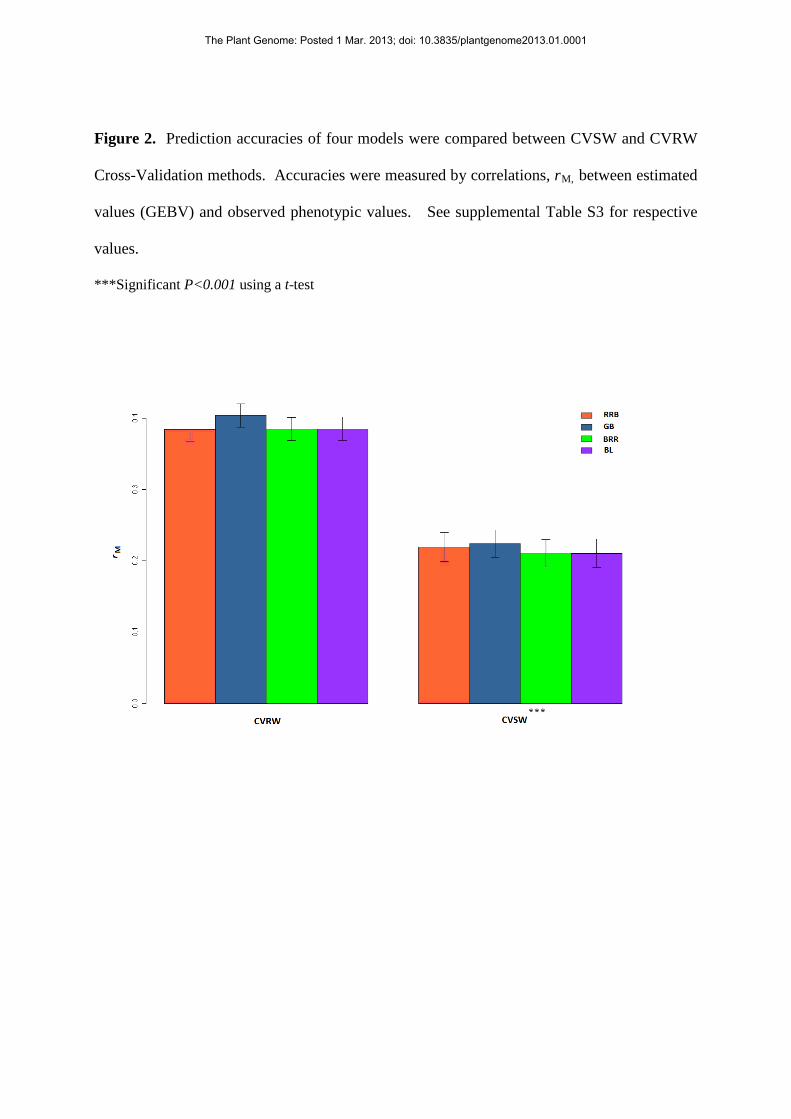
Figure 2. Prediction accuracies of four models were compared between CVSW and CVRW

Cross-Validation methods. Accuracies were measured by correlations, rM, between estimated

values (GEBV) and observed phenotypic values. See supplemental Table S3 for respective

values.



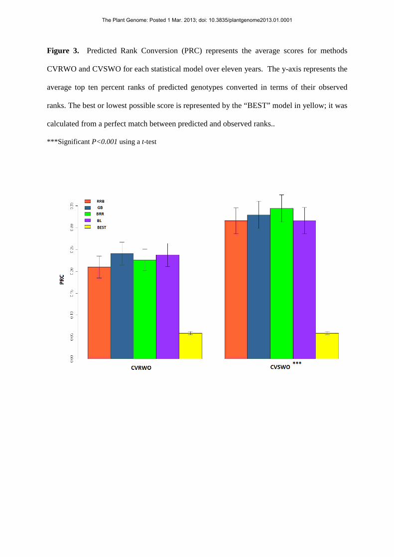
Figure 3. Predicted Rank Conversion (PRC) represents the average scores for methods

CVRWO and CVSWO for each statistical model over eleven years. The y-axis represents the

average top ten percent ranks of predicted genotypes converted in terms of their observed

ranks. The best or lowest possible score is represented by the “BEST” model in yellow; it was

calculated from a perfect match between predicted and observed ranks..



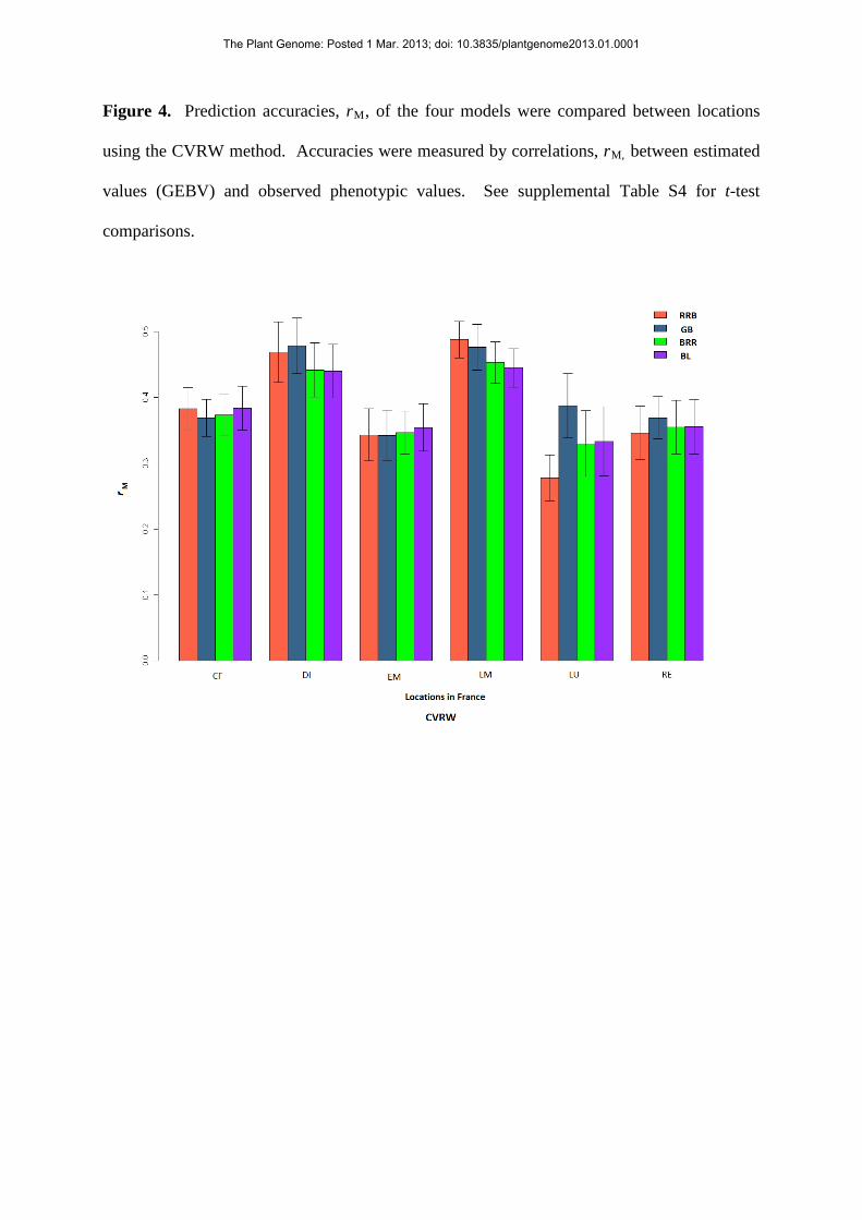
Figure 4. Prediction accuracies, rM, of the four models were compared between locations

using the CVRW method. Accuracies were measured by correlations, rM, between estimated

values (GEBV) and observed phenotypic values. See supplemental Table S4 for t-test

comparisons.


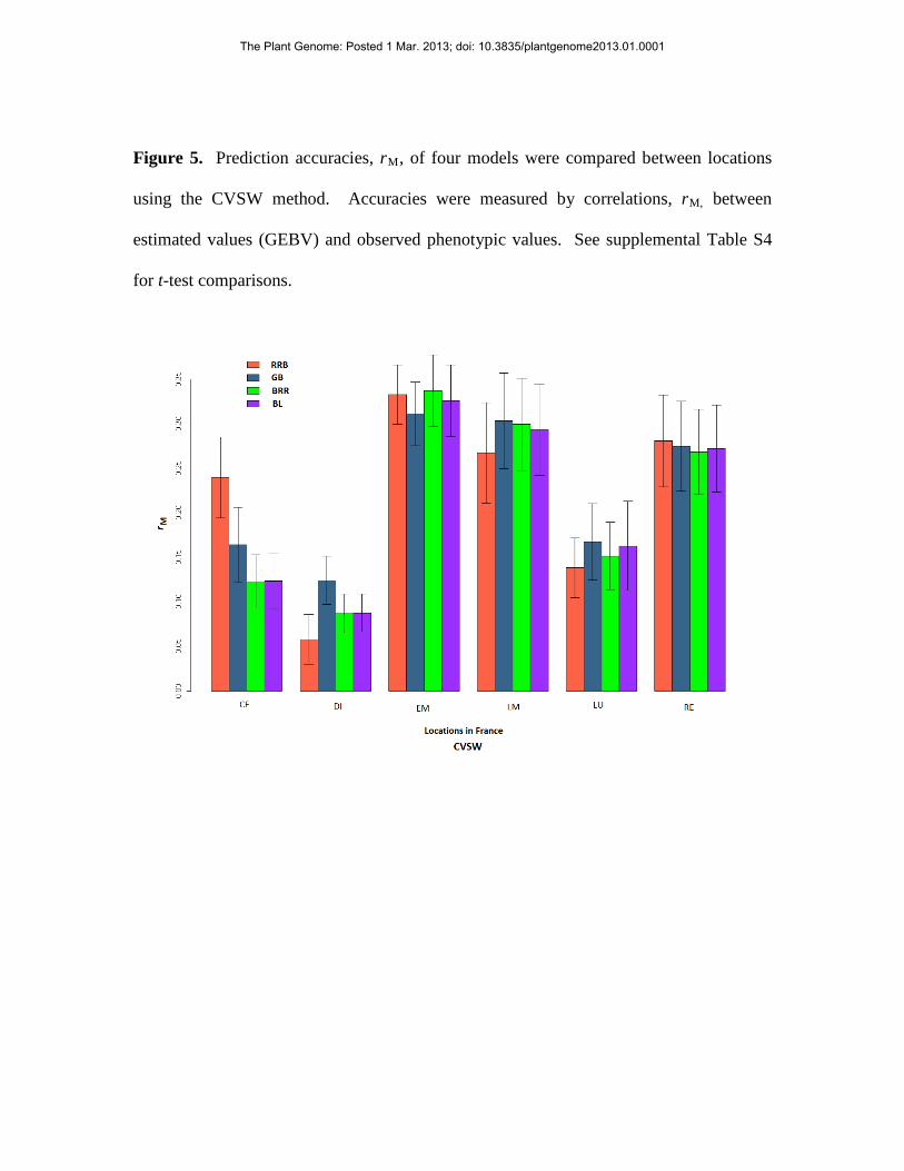
Figure 5. Prediction accuracies, rM, of four models were compared between locations

using the CVSW method. Accuracies were measured by correlations, rM, between

estimated values (GEBV) and observed phenotypic values. See supplemental Table S4

for t-test comparisons.


Documents

Genomic Selection Accuracy using Historical Data Generated ... Selection Accuracy using Historical Data . ... Soil and Crop Science, C117 Plant ... effects for some or all markers