“Genome-wide association study identifies 74 loci

associated with educational attainment”

Table of contents

Supplementary Methods ......................................................................................................................... 3

1 Methods GWA study ...................................................................................................................... 3

1.1 STUDY OVERVIEW ...................................................................................................... 3

1.2 PHENOTYPE DEFINITION ............................................................................................. 3 1.3 GENOTYPING AND IMPUTATION .................................................................................. 4

1.4 ASSOCIATION ANALYSES ............................................................................................ 4 1.5 QUALITY CONTROL ..................................................................................................... 6 1.6 META-ANALYSIS ...................................................................................................... 11 1.7 WITHIN-SAMPLE REPLICATION ................................................................................. 13

1.8 OUT-OF-SAMPLE REPLICATION ................................................................................. 14 1.9 COMBINED META-ANALYSIS OF DISCOVERY AND REPLICATION COHORTS

(N = 405,072) ....................................................................................................................... 16 1.10 PUBLICLY AVAILABLE SUMMARY STATISTICS .......................................................... 16

2 Testing for Population Stratification ............................................................................................ 19

2.1 BACKGROUND ........................................................................................................... 19

2.2 WF-GWAS SIGN TEST ............................................................................................. 20 2.3 LD SCORE INTERCEPT TEST ...................................................................................... 22

2.4 DECOMPOSITION OF THE VARIANCE OF THE POLYGENIC SCORE—THEORY .............. 23 2.5 DECOMPOSITION OF THE VARIANCE OF THE POLYGENIC SCORE—RESULTS ............. 30 2.6 SIGNIFICANCE OF THE POLYGENIC SCORES IN A WF REGRESSION ............................ 30

3 Genetic Overlap............................................................................................................................ 33

3.1 INTRODUCTION ......................................................................................................... 33 3.2 ESTIMATING GENETIC OVERLAP ............................................................................... 34 3.3 ENRICHMENT ANALYSIS AND LOOK-UP OF LEAD SNPS IN GWAS FOR OTHER

PHENOTYPES ......................................................................................................................... 46

4 Biological Annotation .................................................................................................................. 59

4.1 LOOK-UP OF NONSYNONYMOUS STATUS, EQTL EFFECTS, ASSOCIATIONS WITH

OTHER PHENOTYPES, AND PREDICTED GENE FUNCTIONS ..................................................... 62

4.2 ENRICHMENT ANALYSIS AND FINE-MAPPING OF GWAS SIGNALS WITH FGWAS ...... 68 4.3 FUNCTIONAL PARTITION OF HERITABILITY WITH GREML ....................................... 74 4.4 FUNCTIONAL PARTITION OF HERITABILITY USING STRATIFIED LD SCORE

REGRESSION ......................................................................................................................... 77 4.5 PRIORITIZATION OF GENES, PATHWAYS, AND TISSUES/CELL TYPES WITH DEPICT . 82

4.6 ENRICHMENT OF LOCI BY GENES IMPLICATED IN SYNDROMIC DISORDERS .............. 96 4.7 TEMPORAL EXPRESSION PATTERN OF GENES PRIORITIZED BY DEPICT ................. 102

5 Polygenic Prediction .................................................................................................................. 105

5.1 METHODS ............................................................................................................... 105 5.2 DISCUSSION ............................................................................................................ 106

6 Mediation ................................................................................................................................... 109

6.1 THEORY AND METHODS .......................................................................................... 109 6.2 CAVEATS ................................................................................................................ 110 6.3 STANDARD ERRORS FOR INDIRECT EFFECTS ........................................................... 110 6.4 DATA ...................................................................................................................... 111 6.5 RESULTS ................................................................................................................. 112

7 Gene-environment Interactions .................................................................................................. 115

7.1 INTRODUCTION ....................................................................................................... 115

7.2 COHORT ANALYSIS ................................................................................................. 115 7.3 ASCERTAINMENT BIAS ............................................................................................ 116 7.4 DISCUSSION ............................................................................................................ 116

Supplementary Notes .......................................................................................................................... 121

8 Author Contributions.................................................................................................................. 121

9 Additional acknowledgments ..................................................................................................... 132

Supplementary Methods

1 Methods GWA study

1.1 Study Overview

We examined two phenotypes: a continuous variable measuring the number of years of

schooling completed (EduYears, N = 293,723) and an indicator variable for college completion

(College, N = 280,007). All analyses were performed at the cohort level according to a pre-

specified and publicly archived analysis plan. Summary statistics provided by cohorts were

uploaded to a central server and subsequently meta-analyzed. The lead PI of each cohort

affirmed that the results contributed to the study were based on analyses approved by the local

Research Ethics Committee and/or Institutional Review Board responsible for overseeing

research. All participants provided written informed consent. Supplementary Table 1.1

provides basic information about the participating cohorts.

Our Analysis Plan was preregistered at https://osf.io/paj9m/. With one exception, the analyses

reported here follow the original plan. The exception is that the original plan treated EduYears

and College symmetrically whereas throughout the manuscript, we treat EduYears as the

primary variable and de-emphasize College. After circulation of the Analysis Plan to our

cohorts, a paper was posted on bioRxiv showing that the genetic correlation between the two

measures is very high, with the point estimate suggesting a perfect genetic correlation1.

Previously, we had considered as plausible the possibility that College would have better power

for detecting associations at the upper end of the distribution of EduYears. However, since

College is constructed by dichotomizing EduYears, the very high genetic correlation suggests

that the College phenotype is for all intents and purposes merely a coarsening of the EduYears

phenotype.

Hence, we reasoned in light of this new evidence that attempts to detect associations with

EduYears are likely to be better powered, regardless of whether or not the effect is stronger at

the upper end of the distribution of EduYears. To eliminate (or at least minimize) concerns

about data mining, we made the decision to promote EduYears to the primary phenotype before

quality-control work had begun in earnest. After the decision to make EduYears the primary

phenotype was made, we performed the quality control sequentially. In the first stage, we

completed the quality control of the EduYears variable, froze the meta-analysis, and announced

to all analysts responsible for follow-up work that their work would be based on the pooled-

sex EduYears results. We subsequently turned to the College quality control.

1.2 Phenotype Definition

Subjects in our cohorts are heterogeneous in terms of birth cohort and country of birth, and

hence they were educated under a diverse set of educational systems. Moreover, the survey

questions that were used to evaluate subjects’ educational qualifications are not identical across

cohorts. To maximize comparability across samples, we use as a standard the 1997

International Standard Classification of Education (ISCED) of the United Nations Educational,

Scientific and Cultural Organization2. Specifically, we map each major educational

qualification that it is possible to attain in a specific country into one of seven harmonized

ISCED categories. To construct our primary outcome variable, EduYears, we impute a years-

of-education equivalent for each ISCED category using the mapping shown in Supplementary

Table 1.2. Following Rietveld et al.3, we also analyzed the binary outcome, College, which

takes the value 1 for subjects with an ISCED level equal to 5 or more (and 0 otherwise).

The study-specific phenotype measurements and distributions are summarized in

Supplementary Table 1.3. With the exceptions of STR and HBCS, whose variables are derived

from official register data on educational attainment, the studies relied on surveys to measure

educational attainment.

1.3 Genotyping and Imputation

Genotyping was performed using a range of common, commercially available genotyping

arrays. Study analysts were encouraged to impute markers from all 23 chromosomes using the

1000 Genomes project (1kGp) March 2012 version 3 release (hereafter, 1000G) as reference

panel, the most recently released haplotype version available when the Analysis Plan was

circulated. Given the well-known challenges in imputing markers on the X chromosome,

cohorts who could only supply results for autosomal markers were also invited to participate.

Supplementary Table 1.4 provides study-specific details on genotyping platform, pre-

imputation quality-control filters applied to the genotype data, subject-level exclusion criteria,

imputation software used, the reference sample used for imputation (haplotype release date and

whether imputation was done using European-ancestry sample or the full 1000G-sample) and

whether the cohort supplied us with results from the X chromosome. As the table shows, the

overwhelming majority of cohorts followed the recommendation to impute their data against

the March 2012 version 3 release of the 1000G panel. The exceptions are (i) SardiNIA, which

used its own reference panel constructed from sequencing data available for about 2000

individuals in their sample4; (ii) Rush, whose imputation was based on the December 2010

haplotype release; and (iii) a handful of cohorts who began imputation relatively late and used

more recent releases that were not available at the time that the Analysis Plan was written and

circulated.

1.4 Association Analyses

1.4.1 EduYears Analyses

Cohorts were asked to estimate this regression equation for each measured SNP (we drop the

SNP subscript j here to avoid notational clutter):

(1) 𝐸𝑑𝑢𝑌𝑒𝑎𝑟𝑠 = 𝛽0 + 𝛽1 𝑆𝑁𝑃 + 𝑷𝑪 𝜸 + 𝑩 𝜶 + 𝑿 𝜽 + 𝜖,

where SNP is the allele dose of the SNP; PC is a vector of the first ten principal components

of the variance-covariance matrix of the genotypic data, estimated after the removal of genetic

outliers; B is a vector of standardized controls, including a third-order polynomial in age, an

indicator for being female, and their interactions; and X is a vector of study-specific controls.

Specifically, in X, study analysts were encouraged to include dummy variables for major events

such as wars or policy changes that may have affected access to education in their specific

sample. Mixed-sex cohorts were additionally asked to upload separate regression results for

men and women.

1.4.2 College Analyses

The College specification is analogous to the EduYears specification. Cohorts uploaded either

coefficient estimates from a linear probability model or from a logistic regression model.

Linear Regression. The linear model can be written as

(2) 𝐶𝑜𝑙𝑙𝑒𝑔𝑒 = 𝛽0,lin + 𝛽1,lin 𝑆𝑁𝑃 + 𝑷𝑪 𝜸lin + 𝑩 𝜶lin + 𝑿 𝜽lin + 𝜖lin,

where 𝐶𝑜𝑙𝑙𝑒𝑔𝑒 is an indicator variable equal to one for individuals who completed college, the

other variables are defined as above, and the subscript “lin” indicates that the variables

correspond to the linear probability model. The parameter 𝛽1,lin is the average change in the

fraction of subjects whose value of 𝐶𝑜𝑙𝑙𝑒𝑔𝑒 is equal to one associated with being endowed

with one more copy of the reference allele, after linear adjustment for the covariates.

Logistic Regression. Most participating cohorts uploaded coefficient estimates from the

logistic regression model,

(3) 𝑃(𝐶𝑜𝑙𝑙𝑒𝑔𝑒 = 1|𝑆𝑁𝑃, 𝑷𝑪, 𝜶, 𝑿) =

1

1 + 𝑒−(𝛽0,log+𝛽1,log 𝑆𝑁𝑃+𝑷𝑪 𝜸log+𝑩 𝜶log+𝑿 𝜽log),

where the subscript “log” is used to label coefficients from the logistic model. In this model,

the parameter 𝛽1,log can be interpreted as follows: controlling for the covariates, the odds of

having completed college is increased by a factor of 𝑒𝛽1,log for each increase of one copy of the

reference allele.

1.4.3 Sample Selection Criteria

Only individuals satisfying the following criteria were eligible for inclusion in the estimation

sample:

a. Educational attainment was measured when the subject was 30 years of age or older.

b. The subject passed the cohort’s standard quality controls, which typically include

removal of subjects who are genetic outliers (to mitigate stratification concerns) and

subjects with poor genotyping rates.

c. The subject is of European ancestry, and the subject’s mother tongue is the same as the

main language in the country of the cohort.

d. All relevant covariates are available for the subject.

1.4.4 Study-Specific Details

Supplementary Table 1.5 provides study-specific details on the analysis. Column 2 shows the

association software used by each study analyst. The EduYears analyses are based on summary

statistics from all 64 samples listed in Supplementary Table 1.1. Of the 64 samples, whose

combined sample size is N=293,723, 5 were from single-sex cohorts, and 59 contained pooled

results from mixed-sex cohorts (who additionally uploaded separate results for men and

women).

The College analyses were based on results from 52 of the 64 EduYears samples. The combined

sample size of these 52 cohorts is N=280,007. One small cohort, LBC1921, is excluded

because it did not upload College results. The cohort analyst determined that the low fraction

of college-educated individuals (1-5%) and the small sample would not yield reliable estimates

of the standard errors. Indeed, because analytical standard errors may not be reliably estimated

in small samples when the dependent variable is rare, we restrict our final analysis to cohorts

with a combined sample size (𝑁𝑡𝑜𝑡) of at least 500 and at least 100 cases (𝑁𝑐𝑎𝑠𝑒𝑠). We also

drop one family-based cohort (ERF) and one isolate (ORCADES) because the estimated

standard errors of the logistic regression coefficients did not account for the sample relatedness

(in both cases, the standard errors from their EduYears did account for relatedness). Column 3

of Supplementary Table 1.5 reports if a given sample was included in the College analyses and

also explains why, in two samples, the EduYears sample size is not identical to the College

sample size.

Column 4 reports whether the cohorts omitted any of the basic control variables recommended

in the Analysis Plan in their specification. For example, some cohorts dropped higher-order

polynomials in birth year because collinearity was causing problems in model estimation.

Column 5 lists extra controls included by the cohorts in the vector X, such as controls for

cohort-specific events that may have impacted the education system in the cohort.

Several cohorts contain samples with related subjects. The Analysis Plan encouraged cohorts

that include related subjects to estimate mixed linear models (MLMs)5,6. To facilitate their

implementation, the Analysis Plan contained a supplement with sample code for MLM

estimation written for the software GCTA7. Conceptually, the estimation of MLM models

involves two steps: (i) the genome-wide data are used to estimate the degree of genetic

similarity between each pair of individuals in the sample, and (ii) unlike in standard regression

where the covariance of the error term (in an educational attainment regression) between any

two individuals is assumed to be zero, the covariance is fitted as an increasing linear function

of the individuals’ genetic similarity. In other words, to the extent that two individuals are more

recently descended from a common ancestor (as very accurately measured by overall genetic

similarity)—and thus are more likely to be similar on unobserved environmental factors—these

individuals are treated as correlated observations.

Many cohorts that include related subjects have developed strategies for ensuring that the

standard errors correctly account for relatedness. Column 6 of Supplementary Table 1.5 reports

whether the estimated standard errors were adjusted for family relatedness and provides

information about the adjustment used. The details vary by software. For example, QIMR

estimated a model implemented in the software Merlin Offline8, in which the variance-

covariance matrix of the phenotypes of members of the same family is assumed to have a

particular structure according to which resemblance between relatives is induced by the

additive effects of their shared genes. Some cohorts made no adjustment for non-independence

but instead sought to restrict the estimation samples to conventionally unrelated individuals.

For example, 23andMe restrict their estimation sample to conventionally unrelated individuals

by ensuring that no pair of participants in the final estimation sample share more than 700

centimorgans of their genome identical-by-descent9.

1.5 Quality Control

We closely followed the quality-control protocol used in the GIANT consortium’s most recent

study of height10. The protocol, implemented by the software EasyQC, is described in detail by

Winkler et al.11. EasyQC calculates a range of test statistics that are valuable for identifying

possible sources of error in uploaded summary statistics. It also outputs a harmonized set of

graphs, described below, that can be visually inspected to identify problems with data or

analysis. Below, we describe the quality-control filters that were applied to the uploaded files.

We then describe a subset of several additional diagnostic tests that the files were required to

pass before being included in the meta-analysis.

1.5.1 Quality Control Filters

Cohorts were asked to provide results according to a specific file format. For each genetic

marker (which, in the uploaded results, included not just SNPs, but also indels and structural

variants), cohorts were asked to supply the marker’s chromosome and base-pair position, its rs

number, its effect allele, its other allele, the effect allele frequency, the estimated regression

coefficient (beta), the estimated standard error, and a P-value uncorrected for genomic control.

For genotyped markers, the study analyst was asked to supply us with the Hardy-Weinberg P-

value. For imputed markers, we requested information about the imputation quality provided

by default by the software used. We also asked study analysts what imputation and association

software was used.

From the uploaded files, we filtered out the following markers:

1. If the data were imputed against the September or December 2013 releases of the 1000

Genomes Phase 1 haplotypes provided by the software IMPUTE2, we drop the

730+199 SNPs whose strands were incorrectly aligned in these releases.a

2. We drop a marker if neither an effect allele nor other allele is supplied. We also drop a

marker if any of the following variables are missing: effect allele frequency, beta,

standard error, P-value, imputation accuracy (if the marker is imputed), or the

imputed/genotyped indicator. For variables that can only take on some restricted range

of values, we drop the marker if the value of the variable falls outside the permissible

range. For example, P-values have to lie within the unit interval, and binary variables

can only take on a value of 0 or 1.b

3. The analytical standard errors computed by genetic-association software packages are

known to be unreliable in small samples, especially for low-frequency variants11. To

guard against spurious associations with low-frequency markers in small samples, we

dropped a marker from a cohort if its minor allele count (MAC) was below 25. We also

drop markers that explain more than 5% of variance in EduYears, two order of

magnitudes larger than the effects that should be considered plausible based on the

findings in Rietveld et al.3.c,d For each SNP 𝑗, we approximate the variance explained

by 𝑅𝑗2 ≈

2 𝑀𝐴𝐹𝑗 (1−𝑀𝐴𝐹𝑗) ��𝑗2

��𝑦2 .

a The announcement is available on https://mathgen.stats.ox.ac.uk/impute/impute_v2.html#whats_new b Four College cohorts reported P-values from likelihood-ratio (LR) tests in which the test-statistic is defined as 𝜒𝑂𝐵𝑆

2 =

−2𝑙𝑛 (𝐿0

𝐿1), where 𝐿0 is the log-likelihood of the full model and 𝐿1 is the log-likelihood of a restricted model in which the

coefficient for SNP j restricted to equal 0. Under the null hypothesis that 𝛽𝑗 = 0, the statistic is approximately distributed

𝜒2(1). Remaining cohorts conducted hypotheses-testing using conventional Wald tests in which the P-value is derived from

the fact that the distribution of the test-statistic 𝑍𝑂𝐵𝑆 =��

𝑠��(��) is approximately 𝑁(0,1). The two tests are asymptotically

equivalent, but may deliver different answers in finite samples. We err on the side of caution by dropping SNPs from the LR-

test cohorts that fail to satisfy the inequality |𝜒𝑂𝐵𝑆

2 .

𝑍𝑂𝐵𝑆2 − 1| < 0.1.

c Standard practice is to drop SNPs with estimated betas whose absolute value exceeds some threshold considered to represent

an implausibly large effect11. Rather than select a single 𝛽 threshold, we decided to apply a more flexible filter that is not

sensitive to the measurement scale of the dependent variable and allows the 𝛽 threshold to vary by allele frequency. The latter

is desirable because what constitutes a plausible effect size depends on the allele frequency. To illustrate using the example of

height, an effect of 15 cm per allele need not indicate a quality-control problem for very low-frequency variants; in fact rare

polymorphisms with effects of that magnitude have been identified27. However, for common variants, effects of that magnitude

are impossible (the implied R2 would exceed 100% for any realistic value of the sample variance of height). To verify that the

number of SNPs dropped due to the R2 filter is not alarmingly high, we reran the filtering of the cohort-level EduYears results

files with the R2 filter applied last. We found that the R2 filter, after applying standard quality-control filters, does not remove

any SNPs in any of the 44 largest cohorts (combined N = 278,528). The filter removes a small number of SNPs in ten of the

remaining 20 cohorts: LBC1936 (9 SNPs dropped), INGI-CARL (64), THISEAS (225), H2000 Controls (16), Hypergenes

(1), H2000 Cases (2), MoBa (566), OGP (2300), COPSAC2000 (8561). In a logistic regression model, the estimated proportion

of variance explained by SNP 𝑗 is defined as 2 𝑀𝐴𝐹𝑗 (1 − 𝑀𝐴𝐹𝑗) ��𝑗,log2 .

d For cohorts that report marginal effects from linear probability models, it is necessary to transform the estimated linear-

probability coefficient ��𝑗,lin into a quantity that is comparable to ��𝑗,log as estimated from a logistic model. We use the

approximation ��𝑗,lin ≈ 𝑓(1 − 𝑓)��𝑗,log, where 𝑓 is the fraction of the sample with a college degree. The approximation is

4. We drop markers with low imputation-quality metrics. The exact definition of the

quality metrics vary by software. In cohorts that supplied us with the Rsq variable

generated by the imputation software MaCH12, we use a threshold of 0.6. In cohorts

that supplied us with the INFO variable generated by the imputation software

IMPUTE213, we used a threshold of 0.7. These thresholds are stricter than those that

have typically been used in previous studies predating the availability of the 1000G

reference panel. We used the stricter thresholds because evaluations have shown that

the conventional thresholds (in the range 0.3-0.4) do not filter out all badly imputed

rare variants in 1000G data4. The MACH-Rsq and IMPUTE2-INFO thresholds we use

were proposed by Pistis et al.4 for variants with minor allele frequency below 1%. For

transparency, and to err on the side of conservatism, we apply these thresholds to all

markers. Finally, for cohorts that supplied us with PLINK’s imputation-accuracy

measure (info), we follow Winkler et al.’s11 recommendation of using a threshold of

0.8.

5. We drop non-autosomal SNPs, indels, or structural variants. We drop the indels and

structural variants because they are often poorly imputed and hence difficult to align,

and we drop X-chromosome markers because they are analyzed separately.

6. If a cohort supplied us with an rs number, we use the reference file provided by

EasyQCe to identify the marker’s chromosome-position ID (ChrPosID). If a cohort only

supplied information about the genetic position (chromosome and base pair) of the

SNP, we generate a chromosome-position ID (ChrPosID) by horizontally concatenating

the chromosome number and the base pair position. We subsequently drop duplicated

markers based on ChrPosID, or markers whose ChrPosID’s are unavailable in the 1000

Genomes phase 1 European panel (The 1000 Genomes Project Consortium 2012) that

we use to identify potential strand problems. In this step, SNPs that cannot be

successfully aligned due to allele mismatch with the reference panel are also removed.

Having applied filters 1-6 to cohort-level summary statistics, we examined how many SNPs

were dropped in each filtering step. Whenever an unusual number of markers were being

dropped, we flagged the cohort as potentially having an error in the uploaded results file. The

issue was discussed with the cohort-level analyst and resolved through a new QC iteration.

1.5.2 EasyQC Diagnostics

We conducted several additional diagnostic checks after applying the filters described

previously. Below, we describe the four most important of these. Winkler et al.11 contains a

comprehensive discussion of how these four diagnostic tests are useful for identifying a number

of potential problems and their possible underlying causes.

accurate for ��𝑗,lin small. Hence, we drop marker j if 2 𝑀𝐴𝐹𝑗 (1 − 𝑀𝐴𝐹𝑗) ��𝑗,log

2 > 0.05 (logistic model) or 2 𝑀𝐴𝐹𝑗 (1 −

𝑀𝐴𝐹𝑗) (��𝑗,lin

��(1−��))2

> 0.05 (linear probability model).

e http://homepages.uni-

regensburg.de/~wit59712/easyqc/1000g/rsmid_map.1000G_ALL_p1v3.merged_mach_impute.v1.txt.gz,

accessed on 22 June 2015.

Diagnostic Test #1. Allele Frequency Plots (AF Plots)

We looked for errors in allele frequencies and strand orientations by visually inspecting a plot

of the sample allele frequency of filtered SNPs against the frequency in the 1000 Genomes

phase 1 version 3 European panel14.

Diagnostic Test #2. P-value vs Z-score Plots (PZ Plots)

We verified that the reported P-values are consistent with the P-values implied by the

coefficient estimates and standard errors in the results file.

Diagnostic Test #3. Quantile-Quantile Plots (QQ Plots)

We visually inspected the cohort-level QQ plots to look for evidence of unaccounted-for

stratification.

Diagnostic Test #4. Predicted vs Reported Standard Error Plots (PRS Plots)

We investigated if the standard errors reported in the EduYears files are roughly consistent

with the reported sample size, allele frequency, and phenotype distribution. Winkler et al.11

propose a similar diagnostic (the SE-N Plots), which is based on following approximation to

the standard error of a coefficient estimated by OLS

(4) (𝑠. 𝑒. )𝑗 ≈

��𝑌

√𝑁∙

1

√2 𝑀𝐴𝐹𝑗 (1 − 𝑀𝐴𝐹𝑗)

,

where ��𝑌 is the standard deviation of the dependent variable, 𝑀𝐴𝐹𝑗 is the minor allele

frequency of SNP j, and N is the sample size. We used Equation (4) to generate a predicted

standard error for 50,000 randomly sampled SNPs. We then plotted these predicted standard

errors against the reported standard errors. Since the assumptions underlying Equation (4)—

independent observations, no other controls are included in the regression, and no estimation

error that is due to imputation uncertainty—do not hold exactly, the main purpose of the plot

is detect substantial discrepancies between the reported and actual size of the estimation sample

or errors in phenotype transformation. Specifically, we visually inspected the plot to ensure

that the standard errors were of approximately the predicted magnitude and that there were no

major outliers.

When examining the standard errors in the College files, we proceeded similarly, albeit using

an analytical approximation for the standard error of the coefficient from a logistic regression

when appropriate. The approximation is

(5) (𝑠. 𝑒. )𝑗 ≈

1

√𝑁∙

1

√2 𝑓(1 − 𝑓) 𝑀𝐴𝐹𝑗 (1 − 𝑀𝐴𝐹𝑗)

where 𝑓 denotes the fraction of college graduates in the sample.

1.5.3 SNP Exclusions

Our meta-analyses are based on files that have been filtered according to the six QC-filter steps

described above and that have passed the four diagnostic tests. Supplementary Table 1.6 shows,

for each of the cohorts contributing to our pooled EduYears analysis, the number of SNPs in

the originally uploaded results files, the number of SNP exclusions in each of the six steps, and

the number of SNPs remaining after the full set of QC steps were applied. Supplementary Table

1.7 shows the analogous numbers for College. All subsequent analyses are based on the set of

SNPs remaining after these exclusions.

1.5.4 Genomic Control Factors

The last column of Supplementary Tables 1.6 and 1.7 shows the genomic control factor, λGC15

,

from each sample. With the exception of deCODE, whose standard protocol is to apply

genomic control to the standard errors before uploading results, the reported genomic control

factors are all computed using untransformed standard errors. For EduYears, the unweighted

average λGC is 1.02, with a range from 0.95-1.15 and a median of 1.01. For College, the

corresponding numbers are 1.01, 0.93-1.13, and 1.01. Supplementary Tables 1.6 and 1.7 also

report the inflation factor used by deCODE to inflate their standard errors prior to uploading

the results.

1.5.5 Additional Diagnostics

Here, we summarize the results from three additional diagnostic tests of the cleaned results

files.

1.5.5.1 Cohort-Level 𝐹𝑠𝑡 Statistics

𝐹𝑠𝑡 is a frequently used measure of between-population genetic differentiation. We estimated

𝐹𝑠𝑡 using summary data on cohort-level allele frequencies using an approach described by

Weir16. For each cohort, we calculated the 𝐹𝑠𝑡 relative to the European-ancestry individuals in

the 1000G sample14. We sampled 30,000 quasi-independent markers with minor allele

frequencies greater than 0.05 in the European-ancestry subjects. We computed the 𝐹𝑠𝑡 of each

SNP and averaged over the 30,000 markers to get an overall measure of 𝐹𝑠𝑡 in the cohort.

Because our reference sample is European, an unusually high level of 𝐹𝑠𝑡 may be an indication

that a cohort inadvertently failed to remove genetic outliers or a sign of genotyping or

imputation problems.

In Weir16, the equation for estimating 𝐹𝑠𝑡 is

(6) 𝐹𝑠𝑡 =

𝑟(𝑟 − 1)∑ 𝑛𝑖

𝑟𝑖=1

[∑ 𝑛𝑖𝑟𝑖=1 (𝑝𝑖 − ��)2]

��(1 − ��)

where r is the number of populations in the sample, 𝑛𝑖 is the number of individuals in the

sample from population 𝑖, 𝑝𝑖 is the sample minor allele frequency of the SNP in the sample in

population 𝑖, and �� is the weighted average frequency across populations in the sample. Since

in our case 𝑟 = 2, Equation (6) specializes to

(7) 𝐹𝑠𝑡 =

2𝑁 [𝑛1(𝑝1 − ��)2 + 𝑛2(𝑝2 − ��)2]

��(1 − ��)

where 𝑁 = 𝑛1 + 𝑛2, and �� =𝑛1

𝑁𝑝1 +

𝑛2

𝑁𝑝2 is the mean allele frequency. For most EA cohorts,

the average 𝐹𝑠𝑡 value was below 0.004, which agrees well with previous reports that 𝐹𝑠𝑡 is

around 0.004 between European nations17. The largest 𝐹𝑠𝑡, a value of 0.02, was observed for

the cohort OGP-Talana. It is known that the central-eastern Sardinia region, Ogliastra, has been

secluded from the surrounding regions for most of its history. Such isolation is expected to

generate an unusually high 𝐹𝑠𝑡.18 Although the possibility of technical problems for genotype

calling or imputation cannot be ruled out, the observed 𝐹𝑠𝑡 values indicate that the quality of

the reported genotype data is consistent with observed differences in sample allele frequencies

between populations, and there is no evidence that cohorts are derived from non-European

ancestry. Supplementary Table 1.8 summarizes the 𝐹𝑠𝑡 results from our 64 samples.

1.5.5.2 𝜆meta Test for Genetic Effects for Each Pair of Cohorts

We computed a second diagnostic summary statistic, 𝜆meta, which can help identify a number

of problems, including unknown sample overlap between cohorts (which would violate the

assumption of independence underlying the meta-analysis). Given a pair of cohorts and a locus,

𝜆meta is defined as

(8) 𝜆meta ≡(𝑏1 − 𝑏2)

2

𝜎𝑏1

2 + 𝜎𝑏2

2 .

where 𝑏𝑖 and 𝜎𝑏𝑖

2 are the reported allelic effect and sampling variance of the number of minor

alleles in cohort 𝑖 ∈ {1, 2}. If the two cohorts are independent and if the genetic correlation of

the phenotype across the two cohorts is 1, then the expected value of 𝜆meta across loci is 1. If

the cohorts overlap substantially, then the reported effect sizes are too similar, and therefore

the numerator is smaller than the denominator, leading to 𝜆meta < 1. Conversely, if there is too

much heterogeneity in the estimated effect sizes for a pair of cohorts, either because the

phenotypes are not the same or because results are not reported for the same allele, then 𝜆meta

> 1. Hence this statistic is a useful QC metric to detect deviations in the reported summary

statistics for a pair of cohorts from the assumed null hypothesis of independence and

homogeneity. In our data, the average value of 𝜆meta is only slightly greater than 1 (see

Supplementary Table 1.8), suggesting no overall deviation from expectation.

1.5.5.3 Tests of Allele Misalignment

We supplemented our visual inspection of the allele frequency plots with two additional tests

of allele misalignment. First, we generated a pruned set of SNPs from the deCODE summary

statistics whose P-value for the test of association with EduYears was smaller than 0.01. For

each of our other samples, we calculated the frequency with which the estimated effects had

the same sign as in the deCODE results. In all but one of the cohorts with a sample size above

5,000, the fraction of coefficient signs that aligned with deCODE exceeded 50% (see

Supplementary Table 1.9).

Second, we used LD Score regression19 to estimate the genetic correlation between EduYears

in each of our samples and EduYears in deCODE. The estimator often failed to converge,

especially for smaller cohorts, but of the 21 estimates obtained, all but one are in the predicted

(positive) direction. The negative estimated genetic correlation is for the cohort Rush-MAP: it

is -0.29 but has a large standard error (s.e. = 0.70). Given that Rush-MAP passes all other

diagnostics, it is likely that the negative estimate is a chance outcome due to sampling

variability. The estimated genetic correlations are shown in Supplementary Table 1.10.

1.6 Meta-Analysis

We used the software program METAL20 to conduct sample-size-weighted meta-analysis of

all SNPs that passed the quality-control thresholds. Prior to running the meta-analyses, we

applied a single correction for genomic control to the cohort-level summary statistics. A total

of 9,256,490 autosomal SNPs were meta-analyzed using data in the 64 filtered EduYears files,

and 9,280,749 autosomal SNPs were meta-analyzed using data in the 52 filtered College files.f

1.6.1 EduYears (N = 293,723)

We used sample-size-weighted meta-analysis in our primary analyses because the method is

more robust to errors in variable scaling at the cohort level. As a robustness check, we also

conducted a secondary meta-analysis of EduYears with inverse-variance weighting. Consistent

with the results from our many diagnostic tests, the results were highly similar, suggesting that

the scale of measurement was successfully harmonized across cohorts. The correlation between

the two sets of P-values obtained using the two methods was 0.91. We conducted sample-size-

weighted sex-stratified meta-analyses of EduYears as another robustness check to see whether

the results differ for men and women.

Extended Data Fig. 1 shows the quantile-quantile plot of the P-value distributions for the

pooled-sex meta-analysis. As is expected under polygenicity, the plots show strong evidence

of P-value inflation (𝜆𝐺𝐶 = 1.28). In Supplementary Information section 3, we use a variety

of tools, including LD Score regression19 and various tests of within-family association, to

quantify how much of this inflation can plausibly be attributed to unaccounted-for stratification

biases. The results from these analyses consistently suggest that unaccounted-for stratification

biases are unlikely to account for more than a modest share of the observed inflation in the 𝜆𝐺𝐶

in the pooled EduYears analysis. Forest plots of the EduYears-associated SNPs (not shown)

provide little evidence that the estimated effects are driven by a small number of outlier cohorts,

cohorts from a given region, or by one of the sexes (see Supplementary Table 1.11 for the

heterogeneity I2 statistics and P-values for the lead SNPs).

To select independent genome-wide significant SNPs from our primary EduYears results, we

first grouped the GWAS results into “clumps” as follows. The SNP with the smallest P-value

was chosen as the lead SNP in its clump. All SNPs less than 500 kb away from this lead SNP,

in LD with it to the extent r2 > 0.1, and with an association P-value smaller than 10-6 were

assigned to this clump. The next clump was greedily formed around the SNP with the next

smallest P-value not already assigned to the first clump. This process was iterated until no

SNPs remained with P-value < 5×10-8. The end result was 77 approximately independent

clumps, each centered around, and represented by, a genome-wide significant SNP.

Next, we checked the long-range LD between these 77 approximately independent SNPs

without imposing any restriction on distance (except for residing on the same chromosome). If

the r2 between two SNPs is greater than 0.5, we merged the corresponding clumps and assigned

the SNP with smaller P-value to represent that locus. This step resulted in 74 approximately

independent loci, each represented by a genome-wide significant SNP. The PLINK tool version

1.921 and 1000 Genomes Project phase 1 genotyping data22 (from 268 individuals with

European ancestry) was used to perform clumping and calculating r2 between a pair of SNPs.

Supplementary Table 1.11 shows the EduYears pooled-sex and sex-stratified association

results for these 74 approximately-independent genome-wide significant SNPs.

To help gauge the magnitude of the estimated effects, we used a well-known approximation to

compute unstandardized regression coefficients from the METAL output obtained from the

sample-size-weighted meta-analysis:

(9) ��𝑗 ≈ 𝑧𝑗 ��𝑌

√2𝑁𝑗 𝑀𝐴𝐹𝑗 (1 − 𝑀𝐴𝐹𝑗)

f SNPs with a sample size less than 100,000 (3,074,494 SNPs in EduYears, and 3,161,722 SNPs in College) were excluded

from the meta-analyses.

for SNP j with minor allele frequency MAFj, sample size Nj, METAL z-statistic zj, and standard

deviation of the phenotype ��𝑌. For a derivation, see the SOM in Rietveld et al.3. Extended Data

Fig. 2a shows effects in standard-deviation units of the SNP with lowest P-value in each of the

74 loci, ordered from largest to smallest. Consistent with the findings in Rietveld et al.3, the

estimated effects of most common variants are in the range 0.02-0.04 SD, implying that an

additional allele of the education-increasing allele is associated with approximately 0.5 to 1.5

months of additional schooling. The minor allele frequency of the SNP with the largest effect

size in SD-units is 0.04.

1.6.2 College (N = 280,007)

Overall, the results are similar to those from the EduYears analyses, but with higher P-values

(consistent with the hypothesis that the College variable is a noisier measure of educational

attainment than the EduYears variable). If we apply the procedure described previously to

determine the number of approximately independent SNPs reaching genome-wide

significance, we find 34 such SNPs (compared to 74 in the EduYears meta-analysis). Of these,

24 reach genome-wide significance in the EduYears analyses, and 27 are within 500kb distance

and in LD with an EduYears lead SNP to the extent r2 > 0.1. Supplementary Table 1.12 shows

the association results for these 34 approximately independent genome-wide significant SNPs

from the College meta-analysis and the EduYears lead SNPs in the same locus, if any.

1.7 Within-Sample Replication

Following the suggestion of a referee, we attempted to replicate the genome-wide associations

reported in our previous GWAS of EA3 in the new cohorts that were added to this study.

Conversely, we also examined if the SNPs that reach genome-wide significance in a meta-

analysis of the new cohorts replicate in the Rietveld et al. cohorts.

1.7.1 Cohort Overlap with Rietveld et al. (2013)

The analyses of EduYears in Rietveld et al.3 were based on a discovery sample of 101,069

individuals and a combined sample (discovery + replication) of 126,559 individuals. Some of

the cohorts that contributed to the Rietveld et al. study did not participate in the present study

(N = 13,981). Overall, the combined sample size of the Rietveld et al. cohorts that contributed

to our study is N = 126,413 individuals. This number exceeds the difference between 126,559

and 13,981 because some of the original Rietveld et al. cohorts completed additional

genotyping since 2013, and were hence able to contribute larger samples to the current study.

1.7.2 Methods in Within-Sample Replication Analyses

Rietveld et al. reported three genome-wide significant SNPs in their discovery sample, all of

which replicated in their replication sample. These three SNPs also yielded lower P-values in

the “combined” (discovery + replication) sample. In a meta-analysis of the combined sample,

four additional SNPs reached genome-wide significance. Of these, five were genome-wide

significant in the EduYears analyses. The remaining two only reached genome-wide

significance in the analyses of College, but both had P-values just shy of genome-wide

significance in the combined-sample EduYears analysis. Given our decision to make EduYears

the primary phenotype, and to facilitate comparisons of effect sizes, we attempt to replicate all

of the seven original associations in our meta-analyses of the EduYears variable. To examine

if the seven associations replicate in our new cohorts, we split our overall sample into two

subsamples comprising: (1) cohorts that participated in Rietveld et al.3 and (2) all new cohorts

that were added to the current study. In what follows we refer to the former as the “Rietveld

Cohorts” and the latter as the “New Cohorts.” We refer to the combined-sample meta-analysis

results reported by Rietveld et al.3 as the “Rietveld et al. (2013) Cohorts.”

1.7.3 Within-Sample Replication Results

Supplementary Table 1.13 reports the results of the replication analysis. In the upper panel, we

report for the seven SNPs, their standardized effect sizes, standard errors, and P-values. We

report these statistics from three separate meta-analyses of EduYears conducted in: (i) the

Rietveld et al. (2013) Cohorts (ii) the Rietveld Cohorts, and (iii) the New Cohorts. The

reference allele is chosen to be the allele associated with higher values of EduYears in Rietveld

et al.’s analysis (2013).

Given the high degree of overlap between cohorts in the previous EA meta-analysis3 and the

Rietveld Cohorts, the similarity of the effect-size estimates is unsurprising. Reassuringly, the

sign of the estimated coefficient in the New Cohorts is always in the predicted direction, and

for all but one of the seven SNPs we can reject the null hypothesis of no effect at the 5%

significance level (two SNPs, rs4851266 and rs9320913, reach genome-wide significant also

in the replication sample). For six of the seven SNPs, the 95% confidence intervals for the

estimated effect sizes overlap across the Rietveld Cohorts and the New Cohorts.

To further examine replicability, we examined if SNPs that reach genome-wide significance in

a meta-analysis of the New Cohorts replicate in the Rietveld Cohorts. Applying the pruning

algorithm described in Supplementary Information section 1.6.1 to meta-analysis results for

the New Cohorts resulted in 14 approximately independent SNPs. The results from this

replication analyses are reported in Panel B of Supplementary Table 1.13. The results are

similar to those of the replication of the associations from the Rietveld Cohorts in the New

Cohorts: the signs align for all 14 SNPs, and 12 SNP replicate at P-value < 0.05 in the Rietveld

Cohorts (none of them at genome-wide significance, but 5 at P-value < 10-5).

In the two replication analyses, the average effects in the replication samples are about 35%

smaller than the estimated effect of the genome-wide significant association, roughly consistent

with the degree of inflation one would expect from a Winner’s Curse correction of the sort

described and performed in the next subsection.

1.8 Out-of-Sample Replication

Between the time when we submitted our manuscript for publication and when we received the

referee reports, we gained access to the first wave of UK Biobank (UKB) data.23,24 Here, we

report the results from a replication analysis of the 74 lead SNPs that emerged from our GWAS

meta-analysis of EduYears.

1.8.1 Methods in Out-of-Sample Replication Analyses

Our out-of-sample replication analyses uses data from the interim release of the UKB data and

closely follows the methodological best practices recommended in the documentation that has

been made publicly available through the UKB website23. Following the “exemplary GWAS”

described in the documentation, we restrict the analysis to the subsample of N = 112,338

conventionally unrelated individuals with “White British” ancestry. Dropping a small number

of observations with missing phenotypic data leaves us with our final estimation (N = 111,349).

Details on genotyping, pre-imputation quality control, and imputation of the interim release

data have been documented extensively elsewhere25.

Supplementary Table 1.14 provides additional details on the UKB analysis, including

information about phenotype construction, sample demographics, association software, and the

regression specification we estimate. As recommended by the UKB, we control for genotyping

array in all analyses and use the software SNPTEST with the “–method expected” option

specified. We applied exactly the same quality-control filters as in our main analyses to the

UKB results file.

Because two of the 74 lead SNPs are missing from the quality-controlled UKB results file, we

replaced them with nearby proxies. Specifically, we replaced lead SNP rs8005528 with

rs8008779 (r2 = 0.69) and lead SNP rs192818565 with rs55943044 (r2 = 0.93). In both cases,

the proxy was selected by choosing from the pooled discovery sample the lowest p-value SNP

within 500 kb of the original lead SNP, restricting the search to SNPs available in the UKB

data.

1.8.2 UKB Replication Results

Supplementary Table 1.15 and Extended Data Fig. 4 report the results. Of the 74 lead SNPs,

72 have the anticipated sign in the replication sample, and 52 replicate at the 5% level (always

with an effect size in the anticipated direction). Of the 52 SNPs, 7 reach genome-wide

significance in the replication sample.

Under the null model that each of the lead SNPs are null in both the discovery and replication

data, we would expect 50% of the SNPs (37 SNPs) to have a concordant sign in the discovery

and replication samples, we would expect 5% (3.7 SNPs) to be significant at the 5% level, and

we would expect 0.000005% (3.7×10−6 SNPs) to be genome-wide significant.

We can construct P-values associated with these results, noting that the number of SNPs that

have a concordant sign or that are above a certain significance level is distributed as a

Binomial(74, π) where π is the expected fraction of concordant or significant SNPs reported in

the previous paragraph. Given that we are specifically interested in an increase in concordance

or significance, we use a one-sided test. The P-value associated with the sign concordance is

then 1.47×10−19, the P-value associated with the number of SNPs significant at the 5% level is

2.68×10−50, and the P-value associated with the number of genome-wide significant SNPs is

1.41×10−42.

We can additionally measure the replicability of the GWAS estimates generally by assessing

the genetic correlation between the discovery and replication samples. We estimate this using

bivariate LD Score regression. (Details of estimating genetic correlation using LD Score

regression, including the reference panel used to produce LD Scores, are in Supplementary

Information section 3.2.2.) We estimate a genetic correlation of 0.946 (SE = 0.021). These

results, along with the P-values reported above, suggest that the GWAS coefficients estimated

in this paper in general, and the estimates of the 74 lead SNPs in particular, are highly

replicable.

1.8.3 Expected Replication Record

To benchmark this replication record under a natural alternative hypothesis (as opposed to the

expected replication under the null hypothesis calculated above), we calculated the expected

degree of replication given the meta-analysis results, the sample size in the meta-analysis, and

the sample size of the replication sample. To do this, we conducted a Bayesian Winner’s Curse

correction described in a previous study of cognitive performance (Rietveld et al., 201426, SI

pp. 7-13). We assume a diffuse prior (in the notation of the original paper, 𝜏2 → ∞), and we

treat the winners’-curse-adjusted estimates as the vector of true underlying parameters, 𝜷.

Below, we denote the vector of standard errors from our meta-analysis and the UKB replication

by 𝝈GWAS and 𝝈UKB, respectively. The probability that SNP i has a matching sign across the

two analyses is

𝑃(match𝑖) = Φ(−|𝛽𝑖|

𝜎GWAS,𝑖)Φ(−

|𝛽𝑖|

𝜎UKB,𝑖) + [1 − Φ(−

|𝛽𝑖|

𝜎GWAS,𝑖)] [1 − Φ(−

|𝛽𝑖|

𝜎UKB,𝑖)],

where Φ(⋅) is the standard normal cumulative distribution function. Similarly, the probability

that the UKB estimate for SNP i is significant at the 𝛼-level is

𝑃(sig𝑖) = Φ(−|𝛽𝑖|

𝜎GWAS,𝑖+ Φ−1 (

𝛼

2)) + [1 − Φ(−

|𝛽𝑖|

𝜎GWAS,𝑖− Φ−1 (

𝛼

2))].

Since the lead SNPs are (approximately) independent, the expected number of SNPs with

matching signs in the discovery and replication analyses is simply

∑𝑃(match𝑖).

𝑖

And the expected number of SNPs meeting the threshold 𝛼 is

∑𝑃(sig𝑖).

𝑖

Applying the above methodology, we find that 71.4 of the 74 SNPs are expected to have

matching signs, 40.3 SNPs are expected to be significant at the 5% level, and 0.6 SNPs are

expected to be genome-wide significant. The observed numbers are, respectively, 72, 51 and

7. The replication record of the lead SNPs in the UKB is hence somewhat stronger than

predicted by the power calculations.

1.9 Combined Meta-Analysis of Discovery and Replication Cohorts (N

= 405,072)

Using procedures identical to those described in SI Section 1.6, we conducted a meta-analysis

of the EduYears phenotype, combining the results from our discovery cohorts (N = 293,723)

and the results from the UKB replication cohort (N = 111,349). Expanding the overall sample

size to N = 405,072 increases the number of approximately independent genome-wide

significant loci from 74 to 162.

Supplementary Table 1.16 provides information about the lead SNPs in each of these loci.

1.10 Publicly Available Summary Statistics

Summary statistics from our EduYears analyses are available for download at

http://www.thessgac.org.

IRB restrictions for the 23andMe cohort (N = 76,155) limit the number of SNPs for which

results may be posted publicly to a maximum of 10,000. We therefore provide the results from

a meta-analysis of all discovery and replication cohorts except 23andMe (N = 328,917) for the

full set of all SNPs passing QC filters.

For a restricted set of SNPs, we also provide results from meta-analyses which include the

23andMe cohort. Specifically, we provide summary statistics for 5,000 SNPs each from the

meta-analysis of (i) all discovery cohorts (N = 293,723) and (ii) the pooled discovery and

replication samples (N = 405,072). The SNPs are selected by iterating the clumping algorithm

described in SI Section 1.6 5,000 times, thus generating 5,000 independent loci. We report

summary statistics for the SNP with lowest p-value in each locus.

References

1. Bulik-Sullivan, B. et al. An atlas of genetic correlations across human diseases and traits.

Nat. Genet. 47, 1236–1241 (2015).

2. UNESCO. International Standard Classification of Education ISCED 1997. (2006). at

<http://www.unesco.org/education/information/nfsunesco/doc/isced_1997.htm>

3. Rietveld, C. A. et al. GWAS of 126,559 individuals identifies genetic variants associated

with educational attainment. Science 340, 1467–71 (2013).

4. Pistis, G. et al. Rare variant genotype imputation with thousands of study-specific

whole-genome sequences: implications for cost-effective study designs. Eur. J. Hum.

Genet. 23, 975–983 (2015).

5. Kang, H. M. et al. Variance component model to account for sample structure in

genome-wide association studies. Nat. Genet. 42, 348–54 (2010).

6. Yang, J., Zaitlen, N. A, Goddard, M. E., Visscher, P. M. & Price, A. L. Advantages and

pitfalls in the application of mixed-model association methods. Nat. Genet. 46, 100–6

(2014).

7. Yang, J., Lee, S. H., Goddard, M. E. & Visscher, P. M. GCTA: a tool for genome-wide

complex trait analysis. Am. J. Hum. Genet. 88, 76–82 (2011).

8. Chen, W.-M. & Abecasis, G. R. Family-based association tests for genomewide

association scans. Am. J. Hum. Genet. 81, 913–926 (2007).

9. Eriksson, N. et al. Web-based, participant-driven studies yield novel genetic

associations for common traits. PLoS Genet. 6, e1000993 (2010).

10. Wood, A. R. et al. Defining the role of common variation in the genomic and biological

architecture of adult human height. Nat. Genet. 46, 1173–1186 (2014).

11. Winkler, T. W. et al. Quality control and conduct of genome-wide association meta-

analyses. Nat. Protoc. 9, 1192–212 (2014).

12. Li, Y., Willer, C. J., Ding, J., Scheet, P. & Abecasis, G. R. MaCH: using sequence and

genotype data to estimate haplotypes and unobserved genotypes. Genet. Epidemiol. 34,

816–834 (2010).

13. Marchini, J., Howie, B., Myers, S., McVean, G. & Donnelly, P. A new multipoint

method for genome-wide association studies by imputation of genotypes. Nat. Genet.

39, 906–913 (2007).

14. The 1000 Genomes Project Consortium. An integrated map of genetic variation from

1,092 human genomes. Nature 491, 56–65 (2012).

15. Devlin, B. & Roeder, K. Genomic control for association studies. Biometrics 55, 997–

1004 (1999).

16. Weir, B. S. Genetic Data Analysis (Sinauer, 1990).

17. Novembre, J. et al. Genes mirror geography within Europe. Nature 456, 98–101 (2008).

18. Pistis, G. et al. High differentiation among eight villages in a secluded area of Sardinia

revealed by genome-wide high density SNPs analysis. PLoS One 4, e4654 (2009).

19. Bulik-Sullivan, B. et al. LD Score Regression Distinguishes Confounding from

Polygenicity in Genome-Wide Association Studies. Nat. Genet. 47, 291–295 (2015).

20. Willer, C. J., Li, Y. & Abecasis, G. R. METAL: fast and efficient meta-analysis of

genomewide association scans. Bioinformatics 26, 2190–2191 (2010).

21. Chang, C. C. et al. Second-generation PLINK: rising to the challenge of larger and richer

datasets. Gigascience 4, 7 (2015).

22. Abecasis, G. R. et al. An integrated map of genetic variation from 1,092 human

genomes. Nature 491, 56–65 (2012).

23. UK Biobank. Genotyping and Quality Control of UK Biobank, a Large-Scale,

Extensively Phenotyped Prospective Resource: Information for Researchers. Interim

Data Release. (2015). at <http://www.ukbiobank.ac.uk/wp-

content/uploads/2014/04/UKBiobank_genotyping_QC_documentation-web.pdf>

24. Sudlow, C. et al. UK Biobank: An open access resource for identifying the causes of a

wide range of complex diseases of middle and old age. PLoS Med. 12, e1001779 (2015).

25. Marchini, J. et al. Genotype Imputation and Genetic Association Studies of UK Biobank:

Interim Data Release. (2015). at

<https://biobank.ctsu.ox.ac.uk/crystal/docs/impute_ukb_v1.pdf>

26. Rietveld, C. A. et al. Common Genetic Variants Associated with Cognitive Performance

Identified Using Proxy-Phenotype Method. Proc. Natl. Acad. Sci. USA. 111, 13790–

13794 (2014).

2 Testing for Population Stratification

2.1 Background

Population stratification is a major concern in genetic-association studies. It can severely bias

the estimates for causal variants, or worse, lead to false positives. This can occur if a particular

variant of a SNP is more common in one subpopulation than another and if there are mean

differences in the phenotype of interest between subpopulations due to factors that do not

involve that SNP. Such factors could be either:

1. Non-genetic factors. These include cultural or environmental factors; the mechanism

through which confounding can arise is illustrated by the famous chopsticks example1.

2. Genetic factors that do not involve the particular SNP of interest. The GWAS estimate

for a SNP will be biased if that SNP varies in frequency across subpopulations and if

other causal SNPs also vary in frequency across subpopulations (and are thus in LD

with the SNP of interest within the entire population). Note that a bias could arise even

if the particular SNP of interest is in perfect linkage equilibrium (LE) within each

subpopulation with all causal SNPs that differ in frequency across subpopulations and

if there are no mean differences in phenotype due to non-genetic reasons.

To make this discussion precise, we analyze a simple linear model for a quantitative trait 𝑦𝑖 for

individual 𝑖:

(1) 𝑦𝑖 = ∑ 𝑥𝑖𝑘𝑏𝑘𝑝𝑘=1 + 𝑃𝑖 + 𝜀𝑖,

where 𝑥𝑖𝑘 is individual 𝑖’s genotype at SNP 𝑘, 𝑝 is the number of SNPs in the genome, 𝑃𝑖 is a

fixed effect corresponding to the environmental effect of being in the individual’s

subpopulation, and 𝜀𝑖 is the residual and is independent of 𝑥𝑖. Each estimate ��𝑗 from a GWAS

corresponds to the linear projection of the trait onto the genotype at a single SNP 𝑗. That is, using E∗(∙ | ∙) to denote the linear-projection operator,

E∗(𝑦𝑖|𝑥𝑖𝑗) = E∗(∑ 𝑥𝑖𝑘𝑏𝑘𝑝𝑘=1 + 𝑃𝑖 + 𝜀𝑖|𝑥𝑖𝑗) = 𝛽𝑗𝑥𝑖𝑗,

where

(2) 𝛽𝑗 = 𝑏𝑗 + ∑ E∗(𝑥𝑖𝑘|𝑥𝑖𝑗)𝑘≠𝑗 𝑏𝑘 + E∗(𝑃𝑖|𝑥𝑖𝑗).

If 𝑥𝑖𝑗 is stratified by subpopulation and if nongenetic factors (i.e., 𝑃𝑖) vary by subpopulation,

then E∗(𝑃𝑖|𝑥𝑖𝑗) ≠ 0, causing 𝛽𝑗 to differ systematically from 𝑏𝑗. This difference corresponds

to the first bias described above. Similarly, if 𝑥𝑖𝑗 is stratified by subpopulation and so is a set

of causal SNPs with nonzero 𝑏𝑘’s, then E∗(𝑥𝑖𝑘|𝑥𝑖𝑗) ≠ 0 for those 𝑘 SNPs—even if the SNPs

are in perfect LE within subpopulations (e.g., even if they are on different chromosomes). This

effect will be aggregated across all causal SNPs in the genome that differ in frequency across

subpopulations. It is the second source of bias due to population stratification described above.

Several methods have been proposed to correct for these biases and thereby reduce the risk of

false positives due to population stratification. These include controlling for the top principal

components of the genetic-relatedness matrix (GRM) in the analysis or estimating mixed-linear

models. Indeed, almost all cohorts in this GWAS of EduYears followed one or the other of

these strategies. Nonetheless, there is still some concern that residual stratification could

remain. This possibility is particularly concerning in large GWA studies such as this one, where

the effects of even a very small amount of stratification bias may be comparable in magnitude

to the estimated SNP effect sizes.

This document presents the theory and associated results of the methods we employ to assess

whether our GWAS estimates reflect the effects of true polygenic signals or those of population

stratification. These methods are a sign test (Supplementary Information section 2.2), the LD

Score intercept method (2.3), a decomposition of the variance of the estimated polygenic score

(2.4 and 2.5), and a regression of EduYears on the polygenic score using only within-family

variation (2.6).

2.2 WF-GWAS Sign Test

As a first-order consideration, we would like to know if our results are entirely driven by

stratification or if our GWAS results in fact capture some true genetic signal. A simple sign

test—based on comparing the signs of the GWAS estimates to those of the estimates from a

WF analysis—is robust to violations of the many assumptions required for the other tests

presented below. If a SNP has no true genetic effect, then the signs of the GWAS and WF

estimates will be independent and will be concordant with 50% probability. Hence, if

significantly more than 50% of the GWAS estimates for the lead SNPs have concordant signs

with the corresponding WF estimates, it is strong evidence that at least some of the lead SNPs

uncovered by the GWAS are truly causal. We describe this test more precisely below.

A GWAS estimate for SNP 𝑗, ��𝑗, can be decomposed as

��𝑗 = 𝛽𝑗 + 𝑠𝑗 + 𝑈𝑗 ,

where 𝛽𝑗 is the true underlying GWAS parameter for SNP 𝑗, 𝑠𝑗 is the associated bias due to

stratification, and 𝑈𝑗 is the sampling variance of the estimate with E(𝑈𝑗) = 0. Since WF

estimates of 𝛽𝑗 are robust to stratification, a WF estimate for SNP 𝑗 can similarly be

decomposed as

��𝑊𝐹,𝑗 = 𝛽𝑗 + 𝑉𝑗,

where 𝑉𝑗 is the sampling variance of the estimates with E(𝑉𝑗) = 0. Note that if ��𝑗 and ��𝑊𝐹,𝑗

are estimated in independent samples, then 𝑈𝑗 and 𝑉𝑗 will be uncorrelated.

Under the null hypothesis that 𝛽𝑗 = 0 for all 𝑗, the probability that ��𝑗 and ��𝑊𝐹,𝑗 have

concordant signs is 50%. Therefore, denoting by 𝐶 the random variable that corresponds to the

count of how many times the signs match for the two estimates, under the null hypothesis,

𝐶~Binomial(0.5, 𝑆),

where 𝑆 is the number of SNPs tested. For a given 𝑆 and ��, we can then calculate the P-value

for a one-sided test that 𝐶 ≥ �� under the null hypothesis. We call this test “the sign test.”

The sign test makes virtually no assumptions other than the independence of 𝑈𝑗 and 𝑉𝑗, which

can be ensured by calculating our two estimates in non-overlapping samples. Moreover, this

test is robust to bias due to the Winner’s Curse since the Winner’s Curse biases estimates away

from zero, therefore not altering the sign. On the other hand, this test is not informative about

how much stratification there is. It is possible to imagine scenarios where there is a large

amount of stratification in our estimates but where the sign test would nevertheless reject the

null hypothesis, as long as a sufficient number of SNPs have a moderate causal effect. In

summary, rejecting the null hypothesis in the sign test constitutes strong evidence that at least

some of the identified SNPs are truly causal, but other tests with stronger assumptions are

needed to quantify how much stratification there is.

For our analysis, we calculate the WF estimates of the effects of each lead SNP on EduYears

using pooled results from the QIMR, STR, MCTFR, and NTR cohorts, combined using an

inverse-variance weighted meta-analysis. For the GWAS estimates, we omit these five cohorts

and perform a meta-analysis of the remaining cohorts. Thus, the WF estimates are based on a

sample size of 5,506 sibling pairs, and the GWAS estimates have a sample size of 271,360

individuals.

Of the 74 lead SNPs, 66 are present in all five datasets used to calculate the WF estimates. Of

these 66 SNPs, 41 (62%) had GWAS and WF estimates with concordant signs. This

corresponds to a P-value of 0.032 in a one-sided test; we thus reject the null that the 66 genome-

wide significant SNPs are all false positives arising due to stratification.

Although the sign test is statistically significant, the ultimate fraction of matching signs may

seem small given the sample sizes available. Using the coefficients from our replication

sample, we can estimate the expected number of matching signs under two assumptions: (i) the

coefficients we estimate in the UKB equal the true underlying parameter value vector, 𝜷; and

(ii) the true within-family parameter values are equal to the true population parameter values

𝜷 (e.g., there is no bias due to population stratification). Then using the standard errors from

the WF analysis, 𝝈𝑊𝐹, and from the GWAS, 𝝈𝐺𝑊𝐴𝑆, we can calculate the probability that SNP

i would have the same sign in a WF and GWAS analysis as

𝑃(match𝑖) =Φ(−|𝛽𝑖|

𝜎𝐺𝑊𝐴𝑆,𝑖)Φ(−

|𝛽𝑖|

𝜎𝑊𝐹,𝑖) + [1 −Φ(−

|𝛽𝑖|

𝜎𝐺𝑊𝐴𝑆,𝑖)] [1 −Φ (−

|𝛽𝑖|

𝜎𝑊𝐹,𝑖)].

Since these SNPs are (approximately) independent, we then can calculate the expected number

of matching signs as

∑𝑃(match𝑖),

𝑖

with a variance of

∑𝑃(match𝑖)[1 − 𝑃(match𝑖)].

𝑖

By this approach we find that the expected number of matching signs is 49.7 out of 66 with a

95% confidence interval from 43.2 SNPs to 56.1 SNPs. Thus the actual number of signs aligned

(41 signs) is smaller than expected under the null hypothesis. We therefore reject the joint

hypothesis that assumptions (i) and (ii) above both hold.

This discrepancy could be explained by stratification, heterogeneous effects, or some mix of

both. We do not think we can convincingly quantify to what extent each of the two factors

drives the result. On the one hand, there is clear evidence that the genetic effects are indeed

heterogeneous. For example, estimates of the genetic correlation with deCODE are

overwhelmingly below 1.00 (Supplementary Table 1.10) and the predictive power of the score

varies by cohort in the STR sample (Supplementary Table 7.1 and Supplementary Information

section 7). On the other hand, the LD Score regression results in the following subsection

suggest that there is some stratification. We therefore view the sign test as providing useful

supporting evidence, but overall less informative and definitive than the LD Score regression

results, which quantify the degree to which the results are affected by stratification.

2.3 LD Score Intercept Test

Following the approach described in Bulik-Sullivan et al.2, we use the LDSC software to

estimate the intercept in a LD Score regression to assess if our results exhibit signs of

population stratification. This approach uses GWAS summary statistics for all measured SNPs.

Unlike the Genomic Control (GC) method, which assumes that confounding bias (e.g., due to

population stratification and cryptic relatedness) is responsible for inflation in the GWAS chi-

square statistics, the LD Score regression method can disentangle inflation that is due to a true

polygenic signal throughout the genome (which affects the slope of the LD Score regression)

from inflation that is due to confounding biases such as cryptic relatedness and population

stratification (which affects the intercept of the regression).

Formally, the LD Score regression intercept method is based on the relationship

𝐸[𝜒𝑗2] =

𝑁ℎ2ℓ𝑗

𝑀+ 𝑁𝑎 + 1,

where 𝜒𝑗2 = 𝑁��𝑗

2 is the chi-square statistic from the GWAS for SNP j, N is sample size, ℓ𝑗 is

the LD Score of SNP j, ℎ2/𝑀 is the average heritability explained per SNP, and a is a term that

measures the contribution of confounding biases.

Bulik-Sullivan et al. show that: this relationship holds under a polygenic model, the intercept

of the regression minus one (i.e., Na) is an estimator of the contribution of confounding bias to

the inflation of the chi-square statistics, and the intercept equals one (i.e., Na is equal to 0)

under a model without confounding biases.

We used the LDSC software to estimate the regression of the chi-square statistics on ℓ𝑗 and to

test whether the estimate of the intercept is significantly different from 1. We use the

“eur_w_ld_chr/” files of LD Scores calculated by Finucane et al.3 and made available on

https://github.com/bulik/ldsc/wiki/Genetic-Correlation. These LD Scores were computed with

genotypes from the European-ancestry samples in the 1000 Genomes Project using only

HapMap3 SNPs. Only HapMap3 SNPs with MAF > 0.01 were included in the LD Score

regression.

As described in Supplementary Information section 1.6, we applied GC at the cohort level

before running the meta-analysis to produce our main GWAS estimates. However, because GC

will tend to bias the intercept of the LD Score regression downward, we did not apply GC to

the summary statistics we used to estimate the LD Score regression. Furthermore, we excluded

the deCODE cohort from the analysis because the cohort-level regression estimates for

deCODE did not correct for the high level of relatedness in the sample (their standard procedure

is to apply GC). Consequently, including the estimates from deCODE would very likely have

led to an intercept that is considerably upward biased. This procedure—estimating the LD

Score regression with summary statistics that were not GC’d and excluding the deCODE

cohort—allows us to interpret the estimated LD Score regression intercept as an unbiased

measure of the amount of stratification there is in the sample, aside from deCODE, that we

used for the GWAS.

Running the LD Score regression on these data, we estimate an intercept of 1.0491 (Extended

Data Fig. 3a), which is significantly larger than 1 (the standard error reported by the LDSC

software is 0.0091). By comparison, the mean 𝜒2 statistics for all the SNPs in the LD Score

regression is 1.5966. This suggests that there is some confounding bias (due to population

stratification, cryptic relatedness, or other confounds) but that it accounts for only a small part

of the inflation in the chi-square statistics. Thus, the inflation is largely attributable to true

polygenic signal throughout the genome.

We note that the amount of inflation due to confounding bias is likely to be even smaller in our

main GWAS results (e.g., in the estimates for the genome-wide significant SNPs) because, as

mentioned above, genomic control was applied at the cohort level for that main GWASg.

2.4 Decomposition of the Variance of the Polygenic Score—Theory

As a complement to a number of tests that assess if there is population stratification in their

data, Wood et al.5 developed a method to quantify the extent to which the variance of a

polygenic score (constructed from GWAS estimates) in an independent validation sample is

affected by population stratification in that validation sample. To do so, they decompose the

variance of the score into expressions that correspond to the variance due to true genetic effects,

the variance due to estimation error, and the variance due to population stratification in the

independent validation sample.

g Though genomic control is overly conservative, using it should make little difference for all but the larger cohorts in our

sample4. To verify this, we re-ran the meta-analysis without the cohort-level genomic control correction and instead applied

GC at the meta-analysis level using the LDSC intercept (1.05) as the correction factor. The results changed very little. To be

specific, the total count of genome-wide significant SNPs remained 74, the same number we obtained with cohort-level

genomic control. The only changes were that one lead SNP on chr2 (rs4851251) was replaced by another SNP (rs72819174)

in the same locus (because rs4851251 no longer had the lowest P-value SNP in the locus), one lead SNP on chr3 (rs112634398)

fell just below the genome-wide significance threshold, and one SNP on chr16 (rs1007883) rose just above the genome-wide

significance threshold. The remaining 72 lead SNPs were identical.

Below, we present a more general derivation of their method, where we relax some implicit

assumptions they made. In particular:

- We relax the assumption that 𝑔 (the total genetic effects of all SNPs) and 𝑆 (the bias in the

predictor �� due to population stratification in the GWAS sample) are uncorrelatedh;

- Our formula for the sibling correlation between two SNPs that are in linkage disequilibrium

accounts for the effect of population stratification;

- We model the estimation error terms’ variances and covariances (𝑉𝑒 and 𝐶𝑒 in Wood et al.)

slightly differentlyi.

We obtain equations that are similar to Equations 13-16 in Wood et al. but contain a number

of additional terms. Some of these additional terms are likely to be small, but the magnitude of

some other terms may be more difficult to assess (because the terms are difficult to interpret).

If those additional terms are all relatively small, the crux of the Wood et al. derivations and the

analyses underlying the results presented in Supplementary Table 2.1 still hold.

2.4.1 The True Genetic Score

We begin with a model that is similar to Wood et al.’s:

(3) 𝑦 = 𝑔 + 𝑃 + 𝜀,

where, as in Wood et al., 𝑔 = ∑ 𝑥𝑖𝑏𝑖𝑖 is the genetic score of an individual, and 𝜀 is the residual.

The difference from Wood et al. is that we explicitly model 𝑃, the effect of population

stratification. (To be precise, 𝑃 is a subpopulation-level fixed effect: 𝑃𝑝 = 𝑃𝑝′ if persons 𝑝 and

𝑝′ are from the same subpopulation.) The new term 𝑃 may be correlated with 𝑔, but 𝜀 captures

sampling variation and is thus independent of both 𝑃 and 𝑔.

We define 𝑦1, 𝑦2, 𝑔1, and 𝑔2 to be the respective phenotypes and genotypes for sibling pairs.

Using this notation, we see that

(4) Var(𝑔) = ∑ Cov(𝑥𝑖, 𝑥𝑗)𝑏𝑖𝑏𝑗𝑖,𝑗

and

(5) Cov(𝑔1, 𝑔2) = ∑ Cov(𝑥1𝑖, 𝑥2𝑗)𝑏𝑖𝑏𝑗𝑖,𝑗

Note that the covariance between two SNPs, i and j, comes from two sources: LD and

population stratification. The former, which we define as Cov𝐿𝐷(𝑥𝑖, 𝑥𝑗)—or the population

covariance between a pair of SNPs due to LD—arises due to fact that nearby SNPs tend to be

inherited together. It will be equal to zero when 𝑥𝑖 and 𝑥𝑗 are in LE. The population-

stratification source of covariance, which we define as Cov𝑝𝑜𝑝(𝑥𝑖, 𝑥𝑗), arises because certain

SNPs will be more common in certain subpopulations. Thus

(6) Cov(𝑥𝑖, 𝑥𝑗) = Cov𝐿𝐷(𝑥𝑖, 𝑥𝑗) + Cov𝑝𝑜𝑝(𝑥𝑖, 𝑥𝑗).

h Wood et al. do not model S directly but they assume that b is independent of their variable e; this assumption is justified if

there is no bias in the predictor �� due to population stratification in the GWAS sample (among other possible justifications for

this assumption). i Our 𝑉𝑒 term is a sum over all pairs of SNPs that are in LD with one another, whereas the 𝑉𝑒 term in Wood et al. is a sum of

over all SNPs.

As we show in the Box at the end of this subsection, the covariance between two SNPs in two

siblings is

(7) Cov(𝑥1𝑖, 𝑥2𝑗) =1

2Cov𝐿𝐷(𝑥𝑖, 𝑥𝑗) + Cov𝑝𝑜𝑝(𝑥𝑖, 𝑥𝑗).

This expression generalizes the special cases that

Cov(𝑥1𝑖, 𝑥2𝑗) = Cov𝑝𝑜𝑝(𝑥𝑖, 𝑥𝑗)

when SNP 𝑖 and 𝑗 are in LE and that

Cov(𝑥1𝑖, 𝑥2𝑗) =1

2Var𝐿𝐷(𝑥𝑖) + Var𝑝𝑜𝑝(𝑥𝑖)

when 𝑖 = 𝑗. (Note that Equation 7 is different than the equivalent equation in Wood et al., who

omit the Cov𝑝𝑜𝑝(𝑥𝑖, 𝑥𝑗) term for SNPs that are in LD.) The intuition behind Equation 7 is that

since siblings share on average half of their parents’ DNA, the cross-sibling covariance due to

LD is cut in half. On the other hand, since each sibling-pair’s parents are from the same

subpopulation, the covariance due to population structure will not be diminished when

comparing siblings.

2.4.2 The Estimated Polygenic Score

Using bold to denote vectors of SNPs, we define �� as the estimate of 𝒃 obtained from the

GCTA-COJO method. Given that there may be bias due to stratification in our estimate of 𝒃,

it may be expressed as

(8) �� = 𝒃 + 𝒔 + 𝒆,

where 𝒔 is the bias in the estimate of 𝒃 due to population stratification, and 𝒆 is the estimation

error due to sampling variation. The polygenic score for 𝑦 can be calculated in an independent

validation sample as

�� = ∑𝑥𝑖��𝑖

𝑖

= 𝑔 + 𝑆 + 𝐸,

where 𝑆 ≡ ∑ 𝑥𝑖𝑠𝑖𝑖 and 𝐸 ≡ ∑ 𝑥𝑖𝑒𝑖𝑖 . We note that 𝐸 is independent of 𝑔 and 𝑆 but that 𝑔 and 𝑆

may not be independent from one another (for instance, if the true genetic effect 𝑔 is correlated

across subpopulations with the non-genetic subpopulation effect on the phenotype (𝑃)).

To simplify our derivations, we now adopt a notational convention: for any vectors 𝜶 and 𝜷,

𝑉𝛼𝛽,𝐿𝐷 ≡ ∑ Cov𝐿𝐷(𝑥𝑖, 𝑥𝑗)𝛼𝑖𝛽𝑗 | SNPs are in LD

𝑖,𝑗

𝐶𝛼𝛽,𝐿𝐷 ≡ ∑ Cov𝐿𝐷(𝑥𝑖, 𝑥𝑗)𝛼𝑖𝛽𝑗 | SNPs are not in LD

𝑖,𝑗

𝑉𝛼𝛽,𝑝𝑜𝑝 ≡ ∑ Cov𝑝𝑜𝑝(𝑥𝑖 , 𝑥𝑗)𝛼𝑖𝛽𝑗 | SNPs are in LD

𝑖,𝑗

𝐶𝛼𝛽,𝑝𝑜𝑝 ≡ ∑ Cov𝑝𝑜𝑝(𝑥𝑖 , 𝑥𝑗)𝛼𝑖𝛽𝑗 | SNPs are not in LD

𝑖,𝑗

.

We note that 𝐶𝛼𝛽,𝐿𝐷 is always zero by construction. As in Wood et al., we want to estimate the

following quantities:

𝑉𝑔 ≡ 𝑉𝑏𝑏,𝐿𝐷 + 𝑉𝑏𝑏,𝑝𝑜𝑝

𝐶𝑔 ≡ 𝐶𝑏𝑏,𝐿𝐷 + 𝐶𝑏𝑏,𝑝𝑜𝑝 = 𝐶𝑏𝑏,𝑝𝑜𝑝

𝑉𝑒 ≡ 𝑉𝑒𝑒,𝐿𝐷 + 𝑉𝑒𝑒,𝑝𝑜𝑝

𝐶𝑒 ≡ 𝐶𝑒𝑒,𝐿𝐷 + 𝐶𝑒𝑒,𝑝𝑜𝑝 = 𝐶𝑒𝑒,𝑝𝑜𝑝.

We also define two new quantities:

𝑉𝑠 ≡ 𝑉𝑠𝑠,𝐿𝐷 + 𝑉𝑠𝑠,𝑝𝑜𝑝

𝐶𝑠 ≡ 𝐶𝑠,𝐿𝐷 + 𝐶𝑠𝑠,𝑝𝑜𝑝 = 𝐶𝑠𝑠,𝑝𝑜𝑝.

Using these conventions, we can derive the following equalities using (6) and (7):

Var(𝑔) = 𝑉𝑏𝑏,𝐿𝐷 + 𝑉𝑏𝑏,𝑝𝑜𝑝 + 𝐶𝑏𝑏,𝑝𝑜𝑝

Cov(𝑔1, 𝑔2) =1

2𝑉𝑏𝑏,𝐿𝐷 + 𝑉𝑏𝑏,𝑝𝑜𝑝 + 𝐶𝑏𝑏,𝑝𝑜𝑝

Var(𝑆) = 𝑉𝑠𝑠,𝐿𝐷 + 𝑉𝑠𝑠,𝑝𝑜𝑝 + 𝐶𝑠𝑠,𝑝𝑜𝑝

Cov(𝑆1, 𝑆2) =1

2𝑉𝑠𝑠,𝐿𝐷 + 𝑉𝑠𝑠,𝑝𝑜𝑝 + 𝐶𝑠𝑠,𝑝𝑜𝑝

Var(𝐸) = 𝑉𝑒𝑒,𝐿𝐷 + 𝑉𝑒𝑒,𝑝𝑜𝑝 + 𝐶𝑒𝑒,𝑝𝑜𝑝

Cov(𝐸1, 𝐸2) =1

2𝑉𝑒𝑒,𝐿𝐷 + 𝑉𝑒𝑒,𝑝𝑜𝑝 + 𝐶𝑒𝑒,𝑝𝑜𝑝

Cov(𝑔, 𝑆) = 𝑉𝑏𝑠,𝐿𝐷 + 𝑉𝑏𝑠,𝑝𝑜𝑝 + 𝐶𝑏𝑠,𝑝𝑜𝑝

Cov(𝑔1, 𝑆2) =1

2𝑉𝑏𝑠,𝐿𝐷 + 𝑉𝑏𝑠,𝑝𝑜𝑝 + 𝐶𝑏𝑠,𝑝𝑜𝑝.

2.4.3 Re-deriving Equations 13-16 from Wood et al.

Wood et al. estimate 𝑉𝑔, 𝑉𝑒, and 𝐶𝑔 + 𝐶𝑒 with the following formulae:

��𝑔 ≡ Cov(∆𝑦, ∆��) (Wood et al. Equation 13);

��𝑒 ≡ Var(∆��) − ��𝑔 = Var(∆��) − Cov(∆𝑦, ∆��) (Wood et al. Equation 14);

��𝑔 + ��𝑒 ≡ 2Cov(��1, ��2) − Var(��) (Wood et al. Equation 15 & 16).

Using the more generalized model we present here, we can calculate what these formulae are

in fact estimating. We begin by calculating

��𝑔 = Cov(∆𝑦, ∆��)

= Cov(∆𝑔 + ∆𝜀, ∆𝑔 + ∆𝑆 + ∆𝐸) = Var(∆𝑔) + Cov(∆𝑔, ∆𝑆) = 2Var(𝑔) − 2Cov(𝑔1, 𝑔2) + 2Cov(𝑔, 𝑆) − 2Cov(𝑔1, 𝑆2)

= 𝑉𝑏𝑏,𝐿𝐷 + 𝑉𝑏𝑠,𝐿𝐷

= 𝑉𝑔 + [𝑉𝑏𝑠,𝐿𝐷 − 𝑉𝑏𝑏,𝑝𝑜𝑝].

Next, we have

��𝑒 = Var(∆��) − Cov(∆𝑦, ∆��) = Var(∆𝑔 + ∆𝑠 + ∆𝐸) − (𝑉𝑏𝑏,𝐿𝐷 + 𝑉𝑏𝑠,𝐿𝐷)

= Var(∆𝑔) + Var(∆𝑠) + Var(∆𝐸) + 2Cov(∆𝑔, ∆𝑠) − (𝑉𝑏𝑏,𝐿𝐷 + 𝑉𝑏𝑠,𝐿𝐷)

= (2Var(𝑔) − 2Cov(𝑔1, 𝑔2)) + (2Var(𝑆) − 2Cov(𝑆1, 𝑆2)) + (2Var(𝐸) − 2Cov(𝐸1, 𝐸2))

+ (4Cov(𝑔, 𝑆) − 4Cov(𝑔1, 𝑆2)) − (𝑉𝑏𝑏,𝐿𝐷 + 𝑉𝑏𝑠,𝐿𝐷)

= 𝑉𝑏𝑏,𝐿𝐷 + 𝑉𝑠𝑠,𝐿𝐷 + 𝑉𝑒𝑒,𝐿𝐷 + 2𝑉𝑏𝑠,𝐿𝐷 − 𝑉𝑏𝑏,𝐿𝐷 − 𝑉𝑏𝑠,𝐿𝐷 = 𝑉𝑠𝑠,𝐿𝐷 + 𝑉𝑒𝑒,𝐿𝐷 + 𝑉𝑏𝑠,𝐿𝐷

= 𝑉𝑒 + 𝑉𝑠 + [𝑉𝑏𝑠,𝐿𝐷 − 𝑉𝑒𝑒,𝑝𝑜𝑝 − 𝑉𝑠𝑠,𝑝𝑜𝑝].

Further,

��𝑔 + ��𝑒 = 2Cov(��1, ��2) − Var(��)

= 2Cov(𝑔1 + 𝑆1 + 𝐸1, 𝑔2 + 𝑆2 + 𝐸2) − Var(𝑔 + 𝑠 + 𝐸) = 2Cov(𝑔1, 𝑔2) + 2Cov(𝑆1, 𝑆2) + 2Cov(𝐸1, 𝐸2) + 4Cov(𝑔1, 𝑆2) − Var(𝑔) − Var(𝑆)

− Var(𝐸) − 2Cov(𝑔, 𝑆) = 𝑉𝑏𝑏,𝐿𝐷 + 2𝑉𝑏𝑏,𝑝𝑜𝑝 + 2𝐶𝑏𝑏,𝑝𝑜𝑝 + 𝑉𝑠𝑠,𝐿𝐷 + 2𝑉𝑠𝑠,𝑝𝑜𝑝 + 2𝐶𝑠𝑠,𝑝𝑜𝑝 + 𝑉𝑒𝑒,𝐿𝐷 + 2𝑉𝑒𝑒,𝑝𝑜𝑝

+ 2𝐶𝑒𝑒,𝑝𝑜𝑝 + 2𝑉𝑏𝑠,𝐿𝐷 + 4𝑉𝑏𝑠,𝑝𝑜𝑝 + 4𝐶𝑏𝑠,𝑝𝑜𝑝 − 𝑉𝑏𝑏,𝐿𝐷 − 𝑉𝑏𝑏,𝑝𝑜𝑝 − 𝐶𝑏𝑏,𝑝𝑜𝑝

− 𝑉𝑠𝑠,𝐿𝐷 − 𝑉𝑠𝑠,𝑝𝑜𝑝 − 𝐶𝑠𝑠,𝑝𝑜𝑝 − 𝑉𝑒𝑒,𝐿𝐷 − 𝑉𝑒𝑒,𝑝𝑜𝑝 − 𝐶𝑒𝑒,𝑝𝑜𝑝 − 2𝑉𝑏𝑠,𝐿𝐷 − 2𝑉𝑏𝑠,𝑝𝑜𝑝

− 2𝐶𝑏𝑠,𝑝𝑜𝑝

= 𝑉𝑏𝑏,𝑝𝑜𝑝 + 𝐶𝑏𝑏,𝑝𝑜𝑝 + 𝑉𝑠𝑠,𝑝𝑜𝑝 + 𝐶𝑠𝑠,𝑝𝑜𝑝 + 𝑉𝑒𝑒,𝑝𝑜𝑝 + 𝐶𝑒𝑒,𝑝𝑜𝑝 + 2𝑉𝑏𝑠,𝑝𝑜𝑝 + 2𝐶𝑏𝑠,𝑝𝑜𝑝

= 𝐶𝑔 + 𝐶𝑒 + 𝐶𝑠 + [2𝐶𝑏𝑠,𝑝𝑜𝑝 + 𝑉𝑏𝑏,𝑝𝑜𝑝 + 𝑉𝑠𝑠,𝑝𝑜𝑝 + 𝑉𝑒𝑒,𝑝𝑜𝑝 + 2𝑉𝑏𝑠,𝑝𝑜𝑝].

In summary, we have

(9) ��𝑔 = 𝑉𝑔 + [𝑉𝑏𝑠,𝐿𝐷 − 𝑉𝑏𝑏,𝑝𝑜𝑝]

(10) ��𝑒 = 𝑉𝑒 + 𝑉𝑠 + [𝑉𝑏𝑠,𝐿𝐷 − 𝑉𝑒𝑒,𝑝𝑜𝑝 − 𝑉𝑠𝑠,𝑝𝑜𝑝]

(11) ��𝑔 + ��𝑒 = 𝐶𝑔 + 𝐶𝑒 + 𝐶𝑠 + [2𝐶𝑏𝑠,𝑝𝑜𝑝 + 𝑉𝑏𝑏,𝑝𝑜𝑝 + 𝑉𝑠𝑠,𝑝𝑜𝑝 + 𝑉𝑒𝑒,𝑝𝑜𝑝 + 2𝑉𝑏𝑠,𝑝𝑜𝑝]Cg +

Ce = Cg + Ce + Cs

2.4.4 Discussion

The original analysis in Equations 1-20 of Wood et al. aimed “to quantify the fraction of

phenotypic variance explained by SNPs selected from the GCTA-COJO analyses of the meta-

analysis data … and to quantify the accuracy of predicting height using these selected SNPs.”

In this paper, we use this analysis to produce Supplementary Table 2.1.

In light of the above derivations, it may still be possible to interpret these figures in the spirit

of Wood et al. if the new terms that now appear on RHS of Equations (9)-(11) can either (i) be

assumed to be very small or (ii) be given a meaningful interpretation. We make the following

observations:

Observation 1: the 𝑉..,𝑝𝑜𝑝 terms represent the amount of variance associated with the SNPs

that are in LD that is due to population structure. In European-ancestry populations such as

those from which our data are drawn, 𝐹𝑠𝑡 has been estimated to be small6, which may

suggest that the 𝑉..,𝑝𝑜𝑝 terms are small. If we can assume these 𝑉..,𝑝𝑜𝑝 terms to be small

relative to the other terms, Equations (9)-(11) simplify significantly, to:

(9*) ��𝑔 = 𝑉𝑔 + [𝑉𝑏𝑠,𝐿𝐷]

(10*) ��𝑒 = 𝑉𝑒 + 𝑉𝑠 + [𝑉𝑏𝑠,𝐿𝐷]

(11*) ��𝑔 + ��𝑒 = 𝐶𝑔 + 𝐶𝑒 + 𝐶𝑠 + [2𝐶𝑏𝑠,𝑝𝑜𝑝]

Observation 2: defining 𝒆′ ≡ 𝒆 + 𝒔, 𝑉𝑒′ ≡ 𝑉𝑒 + 𝑉𝑠, and 𝐶𝑒′ ≡ 𝐶𝑒 + 𝐶𝑠, we can express

these equations as:

(9**) ��𝑔 = 𝑉𝑔 + [𝑉𝑏𝑠,𝐿𝐷]

(10**) ��𝑒 = 𝑉𝑒′ + [𝑉𝑏𝑠,𝐿𝐷]

(11**) ��𝑔 + ��𝑒 = 𝐶𝑔 + 𝐶𝑒′ + [2𝐶𝑏𝑠,𝑝𝑜𝑝]

Here, 𝒆′ is the estimation error in 𝒃 due to both population stratification and sampling

variationj; it is unfortunately not possible to disentangle these two sources of estimation

error with this method.

Observation 3: the 𝑉𝑏𝑠,𝐿𝐷 and 𝐶𝑏𝑠,𝑝𝑜𝑝 terms capture the correlation between 𝑔 and 𝑆 (the

bias in �� due to population stratification). It is possible to imagine conditions under which

these terms would not be small. For instance, if subpopulations with a larger average 𝑔 tend

to have a higher 𝑃 (i.e., a better environment for the trait 𝑦), then 𝑔 and 𝑆 will tend to be

positively correlated. However, it is also possible to imagine conditions under which these

terms would be small or zero; in particular, if the score �� is not biased by population

stratification, then 𝑆 = 0 and 𝑉𝑏𝑠,𝐿𝐷 = 𝐶𝑏𝑠,𝑝𝑜𝑝 = 0. In practice, it is difficult to assess how

large the 𝑉𝑏𝑠,𝐿𝐷 and 𝐶𝑏𝑠,𝑝𝑜𝑝 terms are our data.

Hence, we see that the estimators ��𝑔, ��𝑒, and ��𝑔 + ��𝑒 in Fig. 2 in Wood et al. and

Supplementary Table 2.1 in this paper will be unbiased estimates (or nearly so) of 𝑉𝑔, 𝑉𝑒′, and

𝐶𝑔 + 𝐶𝑒′ if (1) we can assume the 𝑉..,𝑝𝑜𝑝 terms to be small; (2) we properly interpret ��𝑒 and

��𝑒 as estimates of 𝑉𝑒′ and 𝐶𝑒′; and (3) the 𝑉𝑏𝑠,𝐿𝐷 and 𝐶𝑏𝑠,𝑝𝑜𝑝 terms are small.

It is important to note that large estimates of 𝐶𝑔 and 𝐶𝑒 do not imply that the score and the

estimates from the GWAS are biased due to population stratification; indeed, ��𝑔 and ��𝑒 do not

depend on 𝑆 (the bias in the predictor �� due to population stratification in the GWAS sample)

and may be sizeable even when 𝑆 = 0. 𝐶𝑔 captures the extent to which Var(𝑔) is inflated due

to the real effects of SNPs that are not in LD but are correlated in the independent validation

sample owing to population stratification in that sample.

As we show in Supplementary Information section 2.6, if 𝐶𝑔 or 𝐶𝑒 are nonzero and even if the

score is unbiased (𝑆 = 0), the estimate of the coefficient on the score in an individual-level

j Our 𝑉𝑒

′ and 𝐶𝑒′ terms are slightly different from Wood et al.’s 𝑉𝑒 and 𝐶𝑒 terms because the sum in 𝑉𝑒

′ is over all SNPs that are

in LD and the sum in 𝐶𝑒′ is over all SNPs that are not in LD.

regression of the phenotype 𝑦 on the score will be different from the corresponding estimate in

a WF regression.

PROOF that Cov(𝑥1𝑖, 𝑥2𝑗) =1

2Cov𝐿𝐷(𝑥𝑖 , 𝑥𝑗) + Cov𝑝𝑜𝑝(𝑥𝑖, 𝑥𝑗).

Let 𝑥𝑖 = 𝑋𝑖𝐹 + 𝑋𝑖

𝑀, where 𝑋𝑖𝐹 and 𝑋𝑖

𝑀 are the alleles inherited from the father 𝐹 and the

mother 𝑀, who are in the same subpopulation (we assume no assortative mating).

Observe that

Cov𝐿𝐷(𝑥𝑖 , 𝑥𝑗) = Cov𝐿𝐷(𝑋𝑖𝐹 + 𝑋𝑖

𝑀, 𝑋𝑗𝐹 + 𝑋𝑗

𝑀)

= Cov𝐿𝐷(𝑋𝑖𝐹 , 𝑋𝑗

𝐹) + Cov𝐿𝐷(𝑋𝑖𝑀 , 𝑋𝑗

𝑀) = 2Cov𝐿𝐷(𝑋𝑖, 𝑋𝑗)

and that

Cov𝑝𝑜𝑝(𝑥𝑖, 𝑥𝑗) = Cov𝑝𝑜𝑝(𝑋𝑖𝐹 + 𝑋𝑖

𝑀, 𝑋𝑗𝐹 + 𝑋𝑗

𝑀)

= Cov𝑝𝑜𝑝(𝑋𝑖𝐹 , 𝑋𝑖

𝐹) + Cov𝑝𝑜𝑝(𝑋𝑖𝑀, 𝑋𝑖

𝑀) + 2Cov𝑝𝑜𝑝(𝑋𝑖𝐹, 𝑋𝑖

𝑀) = 4Cov𝑝𝑜𝑝(𝑋𝑖 , 𝑋𝑗)

(since M and F are from the same subpopulation).

It follows that

Cov(𝑥1𝑖, 𝑥2𝑗) = Cov(𝑋1𝑖𝐹 + 𝑋1𝑖

𝑀 , 𝑋2𝑗𝐹 + 𝑋2𝑗

𝑀)

= Cov(𝑋1𝑖𝐹 , 𝑋2𝑗

𝐹 ) + Cov(𝑋1𝑖𝑀 , 𝑋2𝑗

𝑀) + 2Cov(𝑋1𝑖𝐹 , 𝑋2𝑗

𝑀)

= 2Cov(𝑋1𝑖𝐹 , 𝑋2𝑗

𝐹 ) + 2Cov𝑝𝑜𝑝(𝑋𝑖, 𝑋𝑗)

= 2𝐸[𝑋1𝑖𝐹 ∙ 𝑋2𝑗

𝐹 ] + 2Cov𝑝𝑜𝑝(𝑋𝑖, 𝑋𝑗)

= 2 (

12Cov(𝑋1𝑖

𝐹 , 𝑋2𝑗𝐹 |𝑋1𝑖

𝐹 , 𝑋2𝑗𝐹 are from same grandparent)

+12Cov(𝑋1𝑖

𝐹 , 𝑋2𝑗𝐹 |𝑋1𝑖

𝐹 , 𝑋2𝑗𝐹 are from diff. grandparent)

) +1

2Cov𝑝𝑜𝑝(𝑥𝑖, 𝑥𝑗)

= (Cov(𝑋𝑖𝐹 , 𝑋𝑗

𝐹) + Cov𝑝𝑜𝑝(𝑋𝑖, 𝑋𝑗)) +1

2Cov𝑝𝑜𝑝(𝑥𝑖 , 𝑥𝑗)

= ((Cov𝐿𝐷(𝑋𝑖, 𝑋𝑗) + Cov𝑝𝑜𝑝(𝑋𝑖, 𝑋𝑗)) + Cov𝑝𝑜𝑝(𝑋𝑖, 𝑋𝑗)) +1

2Cov𝑝𝑜𝑝(𝑥𝑖, 𝑥𝑗)

=1

2Cov𝐿𝐷(𝑥𝑖, 𝑥𝑗) + Cov𝑝𝑜𝑝(𝑥𝑖, 𝑥𝑗).

The equality on the second line follows from the fact that

Cov(𝑋1𝑖𝐹 , 𝑋2𝑗

𝐹 )=Cov(𝑋1𝑖𝑀 , 𝑋2𝑗

𝑀), and the equality on the third line holds because the

variables are assumed to have mean zero.

2.5 Decomposition of the Variance of the Polygenic Score—Results

To estimate ��𝑔, 𝑉��, and ��𝑔 + ��𝑒 as per Equations 13-16 from Wood et al., we used data on DZ

twins from the Swedish Twin Registry (STR). There are 3515 DZ twins with both genotype

and EA phenotype data, and the phenotypic correlation between DZ twins is 0.414, before

adjustments for age and sex. The phenotype EduYears was adjusted for age in each gender

group in each cohort separately and then standardized. The genotypes of all the individuals

were imputed to 1000G reference panels. We estimated the principal components (PCs) from

all the common variants on HapMap3 using GCTA7,8. We constructed polygenic scores (also

known as “genetic predictors”) using the variants selected by GCTA-COJO and using their

effect sizes re-estimated by GCTA-COJO. Supplementary Information section 5 provides more

details on how the polygenic scores were constructed.

We estimated ��𝑔, 𝑉��, and ��𝑔 + ��𝑒 using polygenic scores calculated with sets of SNPs meeting

several different threshold P-values (5 × 10−8, 5 × 10−7, 5 × 10−6, 5 × 10−5, 5 × 10−4)

without adjusting for the PCs. We then replicated this analysis, this time adjusting the

polygenic scores for the first 10 PCs.

Supplementary Table 2.1 show that ��𝑔 + ��𝑒 is very small regardless of whether the predictor

is adjusted for PCs or not. As discussed in the preceding subsection, if we can assume that the

𝑉..,𝑝𝑜𝑝 terms are small (Observation 1), if we interpret ��𝑒 as an estimator of 𝐶𝑒′ = 𝐶𝑒 + 𝐶𝑠

(Observation 2), and if we can assume that the 𝑉𝑏𝑠,𝐿𝐷 and 𝐶𝑏𝑠,𝑝𝑜𝑝 terms are small (Observation

3), the results thus suggest that population structure in the STR does not account for much of

the variance of the polygenic score.

2.6 Significance of the Polygenic Scores in a WF regression

To test the robustness of our all-SNPs polygenic score and of the polygenic scores calculated

with sets of SNPs meeting several different threshold P-values (5 × 10−8, 5 × 10−7, 5 × 10−6,

5 × 10−5, 5 × 10−4), we estimated WF regressions of EduYears on each polygenic score in

samples that are independent from those used to construct the scores. Details of how these

scores were constructed are found in Supplementary Information section 5. For each WF

regression, we also compared the estimated coefficient on the polygenic score to the

corresponding coefficient from individual-level regressions.

Formally, let y denote the phenotype EduYears. As Wood et al. show, if we estimate the

regression 𝑦 = ��𝛽 + 𝜀 (where 𝑦 is EduYears, �� is the polygenic score, and 𝜀 is the error term)

in an independent replication sample of individuals, then

��𝐿𝑒𝑣𝑒𝑙𝑠 =Cov(𝑦,��)

Var(��)=

𝑉𝑔+𝐶𝑔

𝑉𝑔+𝑉𝑒+𝐶𝑔+𝐶𝑒.

(We assume, as Wood et al. implicitly do, that 𝑆 = 0 and that Cov(𝑔, 𝑃) = 0.)

However, if we estimate this regression using only the WF variation, �� = ��𝛽 + 𝜀 (where �� =

Δ𝑦 and �� = Δ��), then

��𝑊𝐹 =Cov(��,��)

Var(��)=

𝑉𝑔

𝑉𝑔+𝑉𝑒.

(We assume, as Wood et al. implicitly do, that 𝑆 = 0 and that the 𝑉..,𝑝𝑜𝑝 terms are negligible).

Thus, we see that if 𝐶𝑔 or 𝐶𝑒 are nonzero and even if the score is unbiased (𝑆 = 0), the estimate

of the coefficient on the score in an individual-level regression of 𝑦 on the score will be

different from the corresponding estimate in a WF regression. As Supplementary Table 2.1

shows, estimates of 𝐶𝑔 are quite sizeable relative to estimates of 𝑉𝑔 for the scores based on less

significant SNPs, so we expect to see ��𝑊𝐹 to be smaller relative to ��𝐿𝑒𝑣𝑒𝑙𝑠 for the scores based

on less significant SNPs.

Importantly, because we estimated both the individual-level and the WF regressions in samples

that are independent of those used to construct the score, the estimates ��𝑊𝐹 and ��𝐿𝑒𝑣𝑒𝑙𝑠 will

differ from zero if and only if the scores capture at least some true effects of the SNPs.

For both our all-SNPs polygenic score and the polygenic scores calculated with sets of SNPs

meeting several different threshold P-values, we estimated individual-level and WF

regressions in the subset of DZ twin pairs in the STR, controlling for age, age squared, and

gender. To make the estimated coefficients directly comparable, we used the exact same sample

of DZ twin pairs for all regressions. There were 2,722 DZ twin pairs with both genotype and

EA phenotype data.

Extended Data Fig. 3b and Supplementary Table 2.2 report the results. For every polygenic

score, the estimated coefficient on the polygenic score from the WF regression is statistically

distinguishable from zero, further confirming that our GWAS uncovered some true polygenic

signal. As expected, the estimated individual-level coefficient is significantly larger than the

WF coefficient for the scores based on less significant SNPs, which is consistent with 𝐶𝑔 being

sizeable for those scores in the STR.k Thus, these results indicate that the score captures true

polygenic signal but do not allow us to draw firm conclusions about the extent to which the

score is biased due to population stratification.

(We note that it is difficult to compare the R2’s from the individual-level and WF regressions,

since the R2 from the latter depends on both the covariance between the polygenic scores and

between the error terms within twin pairs, which are not known quantities; for that reason, we

refrain from doing such a comparison.)

References

1. Hamer, D. H. Beware the chopsticks gene. Mol. Psychiatry 5, 11–13 (2000).

2. Bulik-Sullivan, B. et al. LD Score regression distinguishes confounding from

polygenicity in genome-wide association studies. Nat. Genet. 47, 291–295 (2014).

k We note, however, that there are other possible explanations for the wedge between the individual-level and WF coefficients.

For example, if the polymorphic sites that affect EduYears operate partly by making one’s household more amenable to its

members’ pursuit of education, or if parents tend to either attenuate or accentuate differences between their children, then the

individual-level and WF coefficients will differ.

3. Finucane, H. K. et al. Partitioning heritability by functional category using GWAS

summary statistics. Nat. Genet. 47, 1228-1235.

4. Yang, J. et al. Genomic inflation factors under polygenic inheritance. Eur. J. Hum.

Genet. 19, 807–812 (2011).

5. Wood, A. R. et al. Defining the role of common variation in the genomic and biological

architecture of adult human height. Nat. Genet. 46, 1173–1186 (2014).

6. McEvoy, B. P. et al. Geographical structure and differential natural selection among

North European populations. Genome Res. 19, 804–814 (2009).

7. Yang, J., Lee, S. H., Goddard, M. E. & Visscher, P. M. GCTA: a tool for genome-wide

complex trait analysis. Am. J. Hum. Genet. 88, 76–82 (2011).

8. Price, A. L. et al. Principal components analysis corrects for stratification in genome-

wide association studies. Nat. Genet. 38, 904–909 (2006).

3 Genetic Overlap

3.1 Introduction

Previous work using twin data suggests that educational attainment may share genetic

pathways in common with other phenotypes1–5. Here, we follow our pre-registered analysis

plan (https://osf.io/p95cq/) to explore such relationships further using GWAS results.

As a first step, we estimate genetic overlap between EA and several other phenotypes. We

define genetic overlap as the degree to which common regions of the genome are associated

with different traits, i.e., the extent to which multiple phenotypes are associated with the same

underlying genetic variants. Instead of relying on family data or individual-level genetic data,

we estimate genetic overlap using the LD Score Regression procedure developed by Bulik-

Sullivan et al6. Note that this procedure does not require that the GWAS samples are

independent. In addition, we develop another SNP-based estimate of genetic overlap based on

different assumptions that requires GWAS results from independent samples as inputs. This

new measure of genetic overlap is conceptually similar, but not identical, to the measure

estimated in bivariate GREML7. We compare the different measures of genetic overlap

theoretically and empirically.

Next, we systematically investigate evidence of genetic overlap between EA and phenotypes

related to (1) mental health and psychometric traits (including general cognitive performance

and neuroticism), (2) brain anatomy, and (3) anthropometric traits. Henceforth, we refer to

these phenotypes collectively as “MHBA” phenotypes. We chose to include in the analysis

phenotypes for which the phenotypic correlation between EA and the trait has previously been

establishedl and GWAS summary statistics of the trait are available in the public domain. The

final list of phenotypes includes: Alzheimer’s disease8, bipolar disorder9, schizophrenia10,

cognitive performance11,12, neuroticism13, volumes of subcortical brain regions and total

intracranial volume14,m, BMI15, and height16. The links we used to access the GWAS results for

these traits are listed in Supplementary Table 3.1.

We complement our estimates of SNP-based genetic overlap by looking up the lead (i.e.,

genome-wide significant) EA-associated SNPs in the GWAS results for the MHBA

phenotypes.

l Evidence for phenotypic correlation with EA has previously been reported for Alzheimer’s disease70–77, bipolar disorder19,20,55,

schizophrenia52,54,55,59,78,60, cognitive performance12,79,80, neuroticism32,81,82, hippocampus83,84, caudate85, brain volume4,86–88,

BMI37–41, and height89–94. m The ENIGMA214 GWAS summary statistics that were available to us also included the amygdala. However, we omit the

amygdala from our analyses because estimates of genetic overlap between EA and amygdala volume result in a negative

heritability estimate, whereas heritability estimates should, by definition, be restricted to the 0-1 interval. Because the estimated

heritability is negative, both estimates of genetic overlap we report are undefined for this phenotype. The obtained estimate is

imprecisely estimated, suggesting that the negative sign may be due to lack of statistical power in the original GWA study.

3.2 Estimating Genetic Overlap

3.2.1 An Approach Based on Z-statistics from GWAS Meta-Analysis in Independent

Samples

There are several ways that one might measure genetic overlap. Below we define a measure

based on the correlation of SNPs’ (true) effect sizes for two traits. We then develop an

asymptotically unbiased estimator of our genetic-overlap parameter that is only a function of

GWAS summary statistics. Advantages of our measure include: (1) it has a straightforward

interpretation (it is the correlation of GWAS parameters), (2) it requires only GWAS summary

statistics (not individual-level data), and (3) it is computationally fast to estimate.

3.2.1.1 Theoretical Framework

In order to define our measure, we let 𝑌𝑖 and 𝑍𝑖, denote the values of two phenotypes for some

individual 𝑖. Projecting these phenotypes onto a constant and the genotype for a single SNP 𝑗 gives us the population parameters corresponding to a GWAS analysis (i.e., a set of univariate

regressions). More precisely, for each SNP 𝑗, consider the population regressions

𝑌𝑖 = 𝛽0,𝑗 + 𝑔𝑖,𝑗𝛽𝑗 + 𝜀𝑌𝑖𝑗

𝑍𝑖 = 𝛼0,𝑗 + 𝑔𝑖,𝑗𝛼𝑗 + 𝜀𝑍𝑖𝑗,

where 𝑔𝑖,𝑗 is the genotype of SNP 𝑗 for individual 𝑖 as measured by the allele count for a

particular reference allele at the locus. Let Var(𝜀𝑌𝑖𝑗) = 𝜎𝑌𝑗2 and Var(𝜀𝑍𝑖𝑗) = 𝜎𝑍𝑗

2 . Define 𝜷 to

be the vector of all of the 𝛽𝑗’s, 𝜶 to be the vector of all of the 𝛼𝑗’s, and 𝒈𝑖 to be the vector of

all of the 𝑔𝑖,𝑗’s, where all the vectors have length 𝑝. Finally, denote the variance-covariance

matrix of 𝒈𝑖 by Ω𝒈, and let 𝑫𝒈 denote the matrix of diagonal entries of Ω𝒈.

We define our measure of genetic overlap to be

𝑟 ≡𝜷′𝑫𝒈𝜶

√𝜷′𝑫𝒈𝜷𝜶′𝑫𝒈𝜶

.

We note that this measure is independent of whether or not the genotypes are measured in

standard-deviation units. To see this, suppose we calculate our measure using as the

transformed genotypes ��𝑖,𝑗 ≡ 𝑔𝑖,𝑗/𝐷𝑗𝑗1/2

. In that case, the model becomes

𝑌𝑖 = 𝛽0,𝑗 + (��𝑖,𝑗)(𝐷𝑗𝑗1/2

𝛽𝑗) + 𝜀𝑌𝑖𝑗

𝑍𝑖 = 𝛼0,𝑗 + (��𝑖,𝑗)(𝐷𝑗𝑗1/2

𝛼𝑗) + 𝜀𝑍𝑖𝑗.

Defining �� ≡ 𝑫𝒈1/2

𝜷 and �� ≡ 𝑫𝒈1/2

𝜶, we calculate 𝑟 to be

𝑟 =��′��

√��′����′��

,

where 𝑫𝑔 vanishes from the expression because it is now the identity matrix. This value of 𝑟

is clearly the same as before.

There are at least two ways to interpret this measure:

1. It is the correlation of the effect sizes �� and �� that are associated with genotypes

measured in standard-deviation units. To be precise, it is the “uncentered correlation”:

the formula used for correlation when the variables have mean zero (even though �� and

�� may not have mean zero). Below, we discuss some justifications for uncenteredness.

2. Alternatively, it may be thought of as a weighted, uncentered correlation of 𝜷 and 𝜶

that gives greater weight to (𝛽𝑗, 𝛼𝑗) pairs that correspond to SNPs whose genotypes

have greater variance.

Note that our measure of genetic overlap, 𝑟, has some intuitive properties: the genetic overlap

of a trait with itself is equal to one, the genetic overlap of two traits that share no associated

SNPs is equal to zero, and the genetic overlap of two traits where every SNP has an opposite

effect is negative one.

Our measure also has the property that 𝐸[𝛼𝑗|𝑟, 𝛽𝑗] = 𝐶𝑟𝛽𝑗, where 𝐶 is a scaling constant equal

to the ratio of the variance of 𝛼𝑗 to the variance of 𝛽𝑗. That is, if two traits exhibit high genetic

overlap as measured by 𝑟 and one trait is strongly associated with some SNP, then the other

trait will also be likely to be associated with that SNP—and the predicted magnitude of the

association is a linear function of the magnitude of the association for the first trait.

As noted above, our measure of genetic overlap is an uncentered correlation. The choice of

using an uncentered correlation was made for both practical and theoretical reasons. While the

magnitudes of 𝛽𝑗 and 𝛼𝑗 (the effect sizes corresponding to SNP 𝑗) are constant, their signs are

determined by the arbitrary choice of reference allele. Using the uncentered correlation makes

𝑟 invariant to the choice of reference allele for each SNP, which is a desirable property of a

genetic overlap parameter.n As a theoretical justification for this property, if we think of each

𝛽𝑗 and 𝛼𝑗 as random variables that have fixed magnitudes but whose reference allele is random

with an equal chance of being either allele, the expected value of 𝛽𝑗 and 𝛼𝑗 will indeed be zero.

We further highlight that 𝑟 is a population parameter and not a sample statistic (since it is a

function of population parameters). In the following subsection, we will discuss how one might

estimate the parameter 𝑟 using GWAS data.

n Imagine that we switch reference allele at SNP 𝑗. This will flip the sign of 𝛽𝑗 and 𝛼𝑗 . Using an uncentered correlation, this

transformation of 𝑟 will cancel itself out since every instance of 𝛽𝑗 and 𝛼𝑗 is either squared or multiplied with each other. If

we instead used a centered correlation, switching the reference allele would not only flip the sign of the relevant 𝛽𝑗 and 𝛼𝑗 , but

it would also cause the mean of 𝜷 and 𝜶 to shift slightly. The impact of this shift on 𝑟 would depend on how 𝛽𝑗 , 𝛼𝑗 , the mean

of 𝜷, and the mean of 𝜶 all compare to one another.

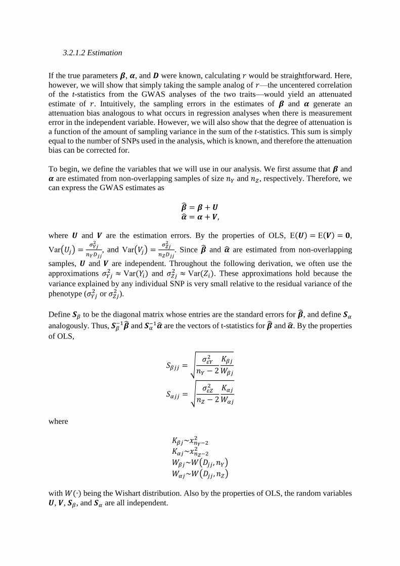
3.2.1.2 Estimation

If the true parameters 𝜷, 𝜶, and 𝑫 were known, calculating 𝑟 would be straightforward. Here,

however, we will show that simply taking the sample analog of 𝑟—the uncentered correlation

of the t-statistics from the GWAS analyses of the two traits—would yield an attenuated

estimate of 𝑟. Intuitively, the sampling errors in the estimates of 𝜷 and 𝜶 generate an

attenuation bias analogous to what occurs in regression analyses when there is measurement

error in the independent variable. However, we will also show that the degree of attenuation is

a function of the amount of sampling variance in the sum of the t-statistics. This sum is simply

equal to the number of SNPs used in the analysis, which is known, and therefore the attenuation

bias can be corrected for.

To begin, we define the variables that we will use in our analysis. We first assume that 𝜷 and

𝜶 are estimated from non-overlapping samples of size 𝑛𝑌 and 𝑛𝑍, respectively. Therefore, we

can express the GWAS estimates as

�� = 𝜷 + 𝑼 �� = 𝜶 + 𝑽,

where 𝑼 and 𝑽 are the estimation errors. By the properties of OLS, E(𝑼) = E(𝑽) = 𝟎,

Var(𝑈𝑗) =𝜎𝑌𝑗

2

𝑛𝑌𝐷𝑗𝑗, and Var(𝑉𝑗) =

𝜎𝑍𝑗2

𝑛𝑍𝐷𝑗𝑗. Since �� and �� are estimated from non-overlapping

samples, 𝑼 and 𝑽 are independent. Throughout the following derivation, we often use the

approximations 𝜎𝑌𝑗2 ≈ Var(𝑌𝑖) and 𝜎𝑍𝑗

2 ≈ Var(𝑍𝑖). These approximations hold because the

variance explained by any individual SNP is very small relative to the residual variance of the

phenotype (𝜎𝑌𝑗2 or 𝜎𝑍𝑗

2 ).

Define 𝑺𝛽 to be the diagonal matrix whose entries are the standard errors for ��, and define 𝑺𝛼

analogously. Thus, 𝑺𝛽−1�� and 𝑺𝛼

−1�� are the vectors of t-statistics for �� and ��. By the properties

of OLS,

𝑆𝛽𝑗𝑗 = √𝜎𝜀𝑌

2

𝑛𝑌 − 2

𝐾𝛽𝑗

𝑊𝛽𝑗

𝑆𝛼𝑗𝑗 = √𝜎𝜀𝑍

2

𝑛𝑍 − 2

𝐾𝛼𝑗

𝑊𝛼𝑗

where

𝐾𝛽𝑗~𝑥𝑛𝑌−22

𝐾𝛼𝑗~𝑥𝑛𝑍−22

𝑊𝛽𝑗~𝑊(𝐷𝑗𝑗 , 𝑛𝑌)

𝑊𝛼𝑗~𝑊(𝐷𝑗𝑗 , 𝑛𝑍)

with 𝑊(∙) being the Wishart distribution. Also by the properties of OLS, the random variables

𝑼, 𝑽, 𝑺𝛽, and 𝑺𝛼 are all independent.

With this setup, first note that a naïve estimator of 𝑟 is

��𝑛𝑎𝑖𝑣𝑒 =��′𝑺𝛽

−1𝑺𝛼−1��

√(��′𝑺𝛽−2��)(��′𝑺𝛼

−2��)

.

We see that the denominator will contain expressions of the form ��𝑗2. Since these expressions

include estimation error, they will be larger in expectation than their population analogue 𝛽𝑗.

The naïve estimator would therefore suffer from an attenuation bias: |𝐸(��𝑛𝑎𝑖𝑣𝑒)| < |𝑟|.

We instead use as our estimator an adjusted version of the naïve estimator, in which the number

of SNPs in our analysis, 𝑝, is subtracted from each term in the denominator:

�� =��′𝑺𝛽

−1𝑺𝛼−1��

√(��′𝑺𝛽−2�� − 𝑝)(��′𝑺𝛼

−2�� − 𝑝)

,

Intuitively, the amount of measurement error in each SNP’s estimated coefficient ��𝑗 is its

standard error, 𝑆𝛽𝑗𝑗. Put more formally, ��𝑗2 will, in expectation, overestimate 𝛽𝑗

2 by the amount

𝑆𝛽𝑗𝑗2 . Thus, the squared estimated coefficient measured in standard-deviation units, ��𝑗

2/𝑆𝛽𝑗𝑗2 ,

will overestimate 𝛽𝑗2/𝑆𝛽𝑗𝑗

2 by 1. Adding up across the SNPs in the analysis gives a total amount

of error of p. Thus, subtracting p debiases the estimate of the first term in the denominator.

Similarly for the second term.

In what follows, we prove asymptotic unbiasedness of �� formally. To begin:

E(��) = E

[ ��′𝑺𝛽

−1𝑺𝛼−1��

√(��′𝑺𝛽−2�� − 𝑝)(��′𝑺𝛼

−2�� − 𝑝)]

= E

[ (𝜷′ + 𝑼′)𝑺𝛽

−1𝑺𝛼−1(𝜶 + 𝑽)

√[(𝜷′ + 𝑼′)𝑺𝛽−2(𝜷 + 𝑼) − 𝑝][(𝜶′ + 𝑽′)𝑺𝛼

−2(𝜶 + 𝑽) − 𝑝]]

= E

[ 𝜷′𝑺𝛽

−1𝑺𝛼−1𝜶 + 𝑼′𝑺𝛽

−1𝑺𝛼−1𝜶 + 𝜷′𝑺𝛽

−1𝑺𝛼−1𝑽 + 𝑼′𝑺𝛽

−1𝑺𝛼−1𝑽

√(𝜷′𝑺𝛽−2𝜷 + 2𝑼′𝑺𝛽

−2𝜷 + 𝑼′𝑺𝛽−2𝑼 − 𝑝)(𝜶′𝑺𝛼

−2𝜶 + 2𝑽′𝑺𝛼−2𝜶 + 𝑽′𝑺𝛼

−2𝑽 − 𝑝)]

.

From here, we use the conventional approximations E (𝐴

√𝐵) ≈ E(𝐴)𝐸 (

1

√𝐵) ≈

E(𝐴)

√E(𝐵). The

precision of these approximations is inversely related to the variances of 𝐴 and 𝐵. Since the

variance in 𝐴 and 𝐵 declines as the sample size increases, these approximations will

asymptotically become arbitrarily good. With these considerations in mind, we continue our

derivation:

E(��) ≈E(𝜷′𝑺𝛽

−1𝑺𝛼−1𝜶 + 𝑼′𝑺𝛽

−1𝑺𝛼−1𝜶 + 𝜷′𝑺𝛽

−1𝑺𝛼−1𝑽 + 𝑼′𝑺𝛽

−1𝑺𝛼−1𝑽)

√E[(𝜷′𝑺𝛽−2𝜷 + 2𝑼′𝑺𝛽

−2𝜷 + 𝑼′𝑺𝛽−2𝑼 − 𝑝)(𝜶′𝑺𝛼

−2𝜶 + 2𝑽′𝑺𝛼−2𝜶 + 𝑽′𝑺𝛼

−2𝑽 − 𝑝)]

=𝜷′E(𝑺𝛽

−1𝑺𝛼−1)𝜶 + E(𝑼′)E(𝑺𝛽

−1𝑺𝛼−1)𝜶 + 𝜷′E(𝑺𝛽

−1𝑺𝛼−1)E(𝑽) + E(𝑼′)E(𝑺𝛽

−1𝑺𝛼−1)E(𝑽)

√(𝜷′E(𝑺𝛽−2)𝜷 + 2E(𝑼′)E(𝑺𝛽

−2)𝜷 + E(𝑼′𝑺𝛽−2𝑼) − 𝑝)[𝜶′E(𝑺𝛼

−2)𝜶 + 2E(𝑽′)E(𝑺𝛼−2)𝜶 + E(𝑽′𝑺𝛼

−2𝑽) − 𝑝]

=𝜷′E(𝑺𝛽

−1𝑺𝛼−1)𝜶

√[𝜷′E(𝑺𝛽−2)𝜷 + E(𝑼′𝑺𝛽

−2𝑼) − 𝑝][𝜶′E(𝑺𝛼−2)𝜶 + E(𝑽′𝑺𝛼

−2𝑽) − 𝑝]

.

The second line follows from the independence of 𝑼 and 𝑽, and the third uses E(𝑼) = E(𝑽) =𝟎.

To complete this derivation, we must evaluate each of these expectations. By the

properties of the random variables defined above, we have

E(𝑆𝛽𝑗−1𝑆𝛼𝑗

−1) = E (√𝑛𝑌 − 2

𝜎𝜀𝑌2

𝑊𝛽𝑗

𝐾𝛽𝑗√

𝑛𝑍 − 2

𝜎𝜀𝑍2

𝑊𝛼𝑗

𝐾𝛼𝑗)

= √(𝑛𝑌 − 2)(𝑛𝑍 − 2)

𝜎𝜀𝑌2 𝜎𝜀𝑍

2 E (√𝑊𝛽𝑗) E (√1

𝐾𝛽𝑗) E(√𝑊𝛼𝑗)E (√

1

𝐾𝛼𝑗)

= √(𝑛𝑌 − 2)(𝑛𝑍 − 2)

𝜎𝜀𝑌2 𝜎𝜀𝑍

2 (Г (

𝑛𝑌

2 +12)

√2Г (𝑛𝑌

2)

√𝐷𝑗𝑗)(Г (

𝑛𝑌 − 22 −

12)

√2Г (𝑛𝑌 − 2

2 ))(

Г (𝑛𝑍

2 +12)

√2Г (𝑛𝑍

2)

√𝐷𝑗𝑗)(Г (

𝑛𝑍 − 22 −

12)

√2Г (𝑛𝑍 − 2

2 ))

= √(𝑛𝑌 − 2)(𝑛𝑍 − 2)

𝜎𝜀𝑌2 𝜎𝜀𝑍

2 (Г (

𝑛𝑌

2 +12)

√2Г (𝑛𝑌

2 ))(

Г (𝑛𝑌 − 2

2 −12)

√2Г (𝑛𝑌 − 2

2 ))(

Г (𝑛𝑍

2 +12)

√2Г(𝑛𝑍

2 ))(

Г (𝑛𝑍 − 2

2 −12)

√2Г (𝑛𝑍 − 2

2 ))𝐷𝑗𝑗

→ √(𝑛𝑌 − 2)(𝑛𝑍 − 2)

𝜎𝜀𝑌2 𝜎𝜀𝑍

2 (√𝑛𝑌) (√1

𝑛𝑌 − 2) (√𝑛𝑍) (√

1

𝑛𝑍 − 2)𝐷𝑗𝑗

= √𝑛𝑌𝑛𝑍

𝜎𝜀𝑌2 𝜎𝜀𝑍

2 𝐷𝑗𝑗 .

In these lines of algebra, the second equality follows from the independence of each of these

random variables. The approximation uses lim𝑥→∞

Г(𝑥+𝛼)

Г(𝑥)𝑥𝛼 = 1. This calculation implies that

E(𝑆𝛽𝑗−1𝑆𝛼𝑗

−1) → √𝑛𝑌𝑛𝑍

𝜎𝜀𝑌2 𝜎𝜀𝑍

2 𝐷𝑗𝑗 .

Also using independence, we have

E(𝑆𝛽𝑗−2) = E (

𝑛𝑌 − 2

𝜎𝜀𝑌2

𝑊𝛽𝑗

𝐾𝛽𝑗)

=𝑛𝑌 − 2

𝜎𝜀𝑌2 E(𝑊𝛽𝑗)E (

1

𝐾𝛽𝑗)

=𝑛𝑌 − 2

𝜎𝜀𝑌2 (𝑛𝑌𝐷𝑗𝑗) (

1

𝑛 − 4)

=(𝑛𝑌 − 2)𝑛𝑌

(𝑛𝑌 − 4)𝜎𝜀𝑌2 𝐷𝑗𝑗

→𝑛𝑌

𝜎𝜀𝑌2 𝐷𝑗𝑗 .

and

E(𝑆𝛼𝑗−2) =

(𝑛𝑍 − 2)𝑛𝑍

(𝑛𝑍 − 4)𝜎𝜀𝑍2 𝐷𝑗𝑗

→𝑛𝑍

𝜎𝜀𝑍2 𝐷𝑗𝑗 ,

which imply

E(𝑆𝛽−2) → (

𝑛𝑌

𝜎𝜀𝑌2 𝐷𝑔)

E(𝑆𝛼−2) → (

𝑛𝑌

𝜎𝜀𝑌2 𝐷𝑔).

Lastly,

E(𝑈𝑗2𝑆𝛽𝑗

−2) = E(𝑈𝑗2)E(𝑆𝛽𝑗

−2)

=𝜎𝜀𝑌

2

𝑛𝑌𝐷𝑗𝑗

(𝑛𝑌 − 2)𝑛𝑌

(𝑛𝑌 − 4)𝜎𝜀𝑌2 𝐷𝑗𝑗

=(𝑛𝑌 − 2)

(𝑛𝑌 − 4)

→ 1,

and

E(𝑉𝑗2𝑆𝛼𝑗

−2) =(𝑛𝑌 − 2)

(𝑛𝑌 − 4)

→ 1.

It follows from these last two asymptotic results that

E(𝑼′𝑺𝛽−2𝑼) ≈ E(𝑽′𝑺𝛼

−2𝑽) → 𝑝.

where (as a reminder) 𝑝 is the number of SNPs in 𝜷 and 𝜶.

Substituting all of these asymptotic values from above,

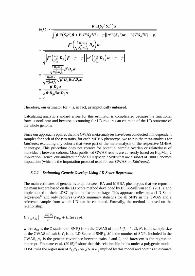
E(��) ≈𝜷′E(𝑺𝛽

−1𝑺𝛼−1)𝜶

√[𝜷′E(𝑺𝛽−2)𝜷 + E(𝑼′𝑺𝛽

−2𝑼) − 𝑝][𝜶′E(𝑺𝛼−2)𝜶 + E(𝑽′𝑺𝛼

−2𝑽) − 𝑝]

≈

𝜷′ (√𝑛𝑌𝑛𝑍

𝜎𝜀𝑌2 𝜎𝜀𝑍

2 𝑫𝑔)𝜶

√[𝜷′ (𝑛𝑌

𝜎𝜀𝑌2 𝑫𝑔)𝜷 + 𝑝 − 𝑝] [𝜶′ (

𝑛𝑍

𝜎𝜀𝑍2 𝑫𝑔)𝜶 + 𝑝 − 𝑝]

=√

𝑛𝑌𝑛𝑍

𝜎𝜀𝑌2 𝜎𝜀𝑍

2 𝜷′𝑫𝑔𝜶

√𝑛𝑌𝑛𝑍

𝜎𝜀𝑌2 𝜎𝜀𝑍

2 √𝜷′𝑫𝑔𝜷𝜶′𝑫𝑔𝜶

=𝜷′𝑫𝑔𝜶

√𝜷′𝑫𝑔𝜷𝜶′𝑫𝑔𝜶

= 𝑟.

Therefore, our estimator for 𝑟 is, in fact, asymptotically unbiased.

Calculating analytic standard errors for this estimator is complicated because the functional

form is nonlinear and because accounting for LD requires an estimate of the LD structure of

the whole genome.

Since our approach requires that the GWAS meta-analyses have been conducted in independent

samples for each of the two traits, for each MHBA phenotype, we re-run the meta-analysis for

EduYears excluding any cohorts that were part of the meta-analysis of the respective MHBA

phenotype. This procedure does not correct for potential sample overlap or relatedness of

individuals between cohorts. Most published GWAS results are currently based on HapMap 2

imputation. Hence, our analyses include all HapMap 2 SNPs that are a subset of 1000 Genomes

imputation (which is the imputation protocol used for our GWAS on EduYears).

3.2.2 Estimating Genetic Overlap Using LD Score Regression

The main estimates of genetic overlap between EA and MHBA phenotypes that we report in

the main text are based on the LD Score method developed by Bulik-Sullivan et al. (2015)6 and

implemented in their LDSC python software package. This approach relies on an LD Score

regression17 and only requires GWAS summary statistics for all SNPs in the GWAS and a

reference sample from which LD can be estimated. Formally, the method is based on the

relationship:

𝐸[𝑧1𝑗𝑧2𝑗] =√𝑁1𝑁2

𝑀ℓ𝑗𝜌𝑔 + 𝐼𝑛𝑡𝑒𝑟𝑐𝑒𝑝𝑡,

where 𝑧𝑘𝑗 is the Z-statistic of SNP j from the GWAS of trait k (k = 1, 2), Nk is the sample size

of the GWAS of trait k, ℓj is the LD Score of SNP j, M is the number of SNPs included in the

GWAS, 𝜌𝑔 is the genetic covariance between traits 1 and 2, and Intercept is the regression

intercept. Finucane et al. (2015)18 show that this relationship holds under a polygenic model.

LDSC runs the regression of ��1𝑗��2𝑗 on √𝑁1𝑁2ℓj implied by this model and obtains an estimate

of 𝜌𝑔 from the estimated regression slope coefficient. It also runs separate LD Score regressions

for traits 1 and 2 and estimates their heritability parameters ℎ𝑔12 and ℎ𝑔2

2 as the estimated

regression slope coefficients. Finally, it uses all of these estimates to compute the genetic

correlation as

𝑟𝐿�� = ��𝑔

√ℎ𝑔12 ℎ𝑔2

2

.

As Bulik-Sullivan et al.6 note, the genetic covariance and heritability estimates from LDSC

will be biased if genomic control (GC) correction has been applied at any stage to the GWAS

summary statistics. However, the biases cancel out in the calculation of 𝑟𝐿��, so as an estimator

𝑟𝐿�� is not biased. (Below, we do not report estimates of heritability obtained with LDSC

because they are biased.)

We use the “eur_w_ld_chr/” files of LD Scores calculated by Finucane et al. (2015)18 and made

available on https://github.com/bulik/ldsc/wiki/Genetic-Correlation. These LD Scores were

computed with genotypes from the European-ancestry samples in the 1000 Genomes Project

using only HapMap3 SNPs. In our LD Score regressions, we include only HapMap3 SNPs

with MAF > 0.01 to restrict the analyses to SNPs that are likely to be imputed with reasonable

accuracy across all cohorts that contributed to the meta-analyses.

The standard errors are estimated (by the LDSC software) using a block jackknife over SNPs.

As such, they should be interpreted as the variability of the estimate holding the sample

constant but drawing a new set of SNPs. This is in contrast to the conventional interpretation

of standard errors, which measure the variability of the estimate holding the covariates constant

but drawing new sets of individuals. Ideally we would have standard errors that represent the

latter, but it is unclear how one might obtain such estimates with the available data. For this

reason, we report the block jackknife errors as in Bulik-Sullivan et al.6, but we note that they

may be only loosely related to conventional standard errors.

3.2.3 Results

In Fig. 2 in the main text, we report the estimates of genetic overlap from the LD Score

regression, along with 95% confidence intervals. In Supplementary Table 3.1, we report

estimation results from both methods described above. Cognitive performance shows the

strongest genetic overlap with EduYears (r = 0.82 & rLD = 0.75). We also find substantial

genetic overlap for mental health phenotypes, in particular for neuroticism (-0.37 & -0.41),

Alzheimer’s disease (-0.20 & -0.31), and bipolar disorder (0.25 & 0.28). The positive genetic

overlap between EduYears and bipolar disorder is noteworthy given that the phenotypic

correlation is negative19,20.

Furthermore, we see substantial positive genetic overlap for intracranial volume (0.39 & 0.34)

and height (0.16 & 0.13), as well as a strong negative overlap for BMI (-0.44 & -0.26).

Note that the two methods yield identical signs for all MHBA phenotypes, except those which

have estimates close to zero (accumbens, hippocampus, pallidum). Furthermore, the estimated

coefficients from both methods are almost perfectly correlated (r = 0.97). Note also that our

results are consistent with those of Bulik-Sullivan et al.6 for the phenotypes we study in

common. (The phenotypes studied here, but not in Bulik-Sullivan et al.6, are cognitive

performance, neuroticism, and the seven brain volume phenotypes.)

3.2.4 Comparing the Measures of Genetic Overlap

We will compare three measures of genetic overlap: (1) 𝑟, our new measure defined above; (2)

𝑟𝐿𝐷, the measure derived from the LD Score regression; and (3) the correlation of the true

polygenic scores for the corresponding traits (i.e., the polygenic scores that would be estimated

in an infinite sample). These methods differ from one another in the way they deal with LD,

although they are equivalent under some assumptions, as we show below.

For two traits 𝑦𝑖 and 𝑧𝑖, we define �� and �� as the respective vectors of true SNP coefficients in

a model that fits all of the SNPs at once. That is,

𝑦𝑖 = ��𝑖�� + 𝑒𝑦𝑖

𝑧𝑖 = ��𝑖�� + 𝑒𝑧𝑖,

where ��𝑖 is the standardized genotype vector of individual 𝑖, and 𝑒𝑦𝑖 and 𝑒𝑧𝑖

are the residuals

of these models. Throughout, we use tildes over variables to denote standardized variables, the

coefficients associated with standardized variables (note that these are different from

standardized coefficients), and the variances and covariances associated with standardized

variables. As before, we define Ω as the variance-covariance matrix of ��𝑖.

3.2.4.1 The 𝑟 Measure of Genetic Overlap

Since our genotypes are standardized, 𝑟 can be expressed as

𝑟 =��′��

√��′����′��

.

Applying the equation for the OLS estimator, �� and �� have the simple relationship

�� = [diag(��)]−1

Cov(��𝑖, 𝑦𝑖)

= Cov(��𝑖, 𝑦𝑖) = ����−1Cov(��𝑖, 𝑦𝑖)

= ����.

Similarly,

�� = ����.

Using these substitutions, we have

𝑟 =��′��2��

√��′��2����′��2��.

3.2.4.2 The 𝑟𝐿𝐷 Measure of Genetic Overlap

Under the assumption that the effect sizes ��𝑗, ��𝑗 are random and independent from each other

and from the allele frequency and LD structure of their corresponding SNP—assumptions

maintained by Bulik-Sullivan et al.6 throughout their derivations—it can be shown that 𝑟𝐿𝐷 can

be expressed as

𝑟𝐿𝐷 =Cov(��𝑗, ��𝑗)

√Var(��𝑗)Var(��𝑗)

=��′��

√��′����′��.

This equation can be rewritten as

𝑟𝐿𝐷 =��′��0��

√��′��0����′��0��,

where ��0 is the identity matrix.

3.2.4.3 The Correlation Between True Polygenic Scores

Lastly, we note that the correlation of true polygenic scores is

𝑟𝑃𝐺 =Cov(��𝑖��, ��𝑖��)

√Var(��𝑖��)Var(��𝑖��)

=��′Var(��𝑖)��

√��′Var(��𝑖)����′Var(��𝑖)��

=��′����

√��′������′����,

or equivalently,

𝑟𝑃𝐺 =��′��1��

√��′��1����′��1��.

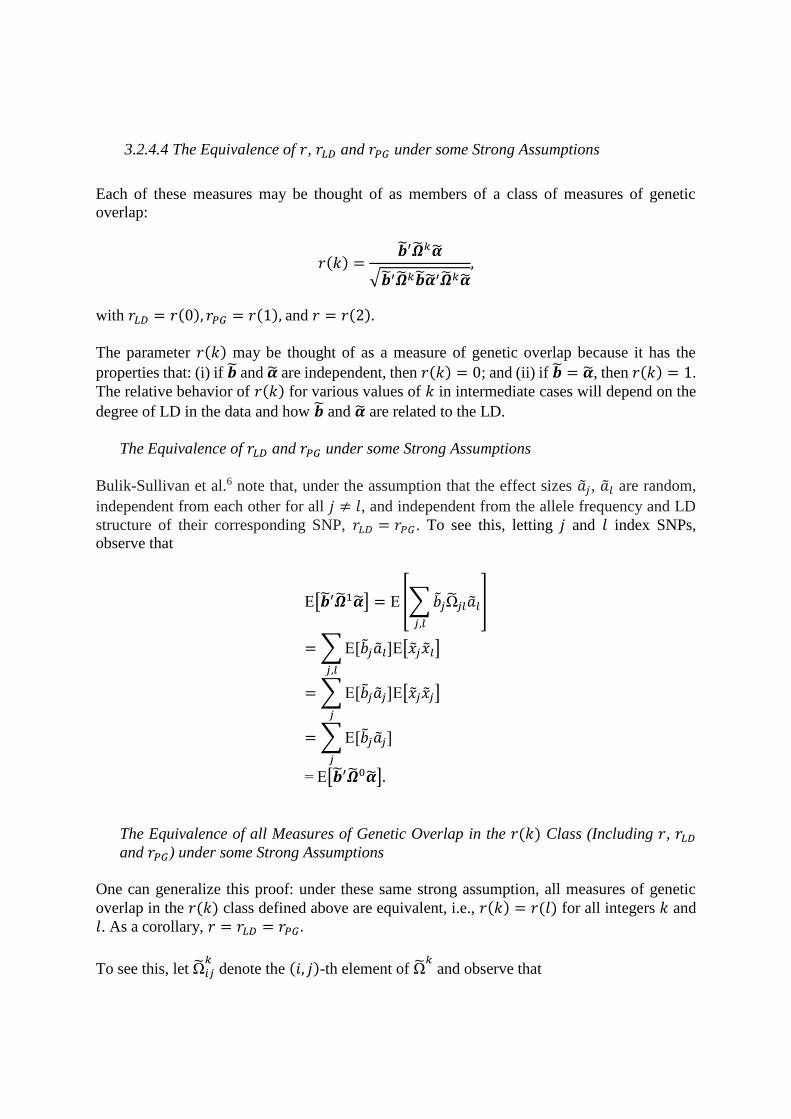
3.2.4.4 The Equivalence of 𝑟, 𝑟𝐿𝐷 and 𝑟𝑃𝐺 under some Strong Assumptions

Each of these measures may be thought of as members of a class of measures of genetic

overlap:

𝑟(𝑘) =��′��𝑘��

√��′��𝑘����′��𝑘��,

with 𝑟𝐿𝐷 = 𝑟(0), 𝑟𝑃𝐺 = 𝑟(1), and 𝑟 = 𝑟(2).

The parameter 𝑟(𝑘) may be thought of as a measure of genetic overlap because it has the

properties that: (i) if �� and �� are independent, then 𝑟(𝑘) = 0; and (ii) if �� = ��, then 𝑟(𝑘) = 1.

The relative behavior of 𝑟(𝑘) for various values of 𝑘 in intermediate cases will depend on the

degree of LD in the data and how �� and �� are related to the LD.

The Equivalence of 𝑟𝐿𝐷 and 𝑟𝑃𝐺 under some Strong Assumptions

Bulik-Sullivan et al.6 note that, under the assumption that the effect sizes ��𝑗, ��𝑙 are random,

independent from each other for all 𝑗 ≠ 𝑙, and independent from the allele frequency and LD

structure of their corresponding SNP, 𝑟𝐿𝐷 = 𝑟𝑃𝐺. To see this, letting 𝑗 and 𝑙 index SNPs,

observe that

E[��′��1��] = E [∑��𝑗Ω𝑗𝑙��𝑙

𝑗,𝑙

]

= ∑ E[��𝑗��𝑙]E[��𝑗��𝑙]

𝑗,𝑙

= ∑ E[��𝑗��𝑗]E[��𝑗��𝑗]

𝑗

= ∑ E[��𝑗��𝑗]

𝑗

= E[��′��0��].

The Equivalence of all Measures of Genetic Overlap in the 𝑟(𝑘) Class (Including 𝑟, 𝑟𝐿𝐷

and 𝑟𝑃𝐺) under some Strong Assumptions

One can generalize this proof: under these same strong assumption, all measures of genetic

overlap in the 𝑟(𝑘) class defined above are equivalent, i.e., 𝑟(𝑘) = 𝑟(𝑙) for all integers 𝑘 and

𝑙. As a corollary, 𝑟 = 𝑟𝐿𝐷 = 𝑟𝑃𝐺 .

To see this, let Ω𝑖𝑗𝑘

denote the (𝑖, 𝑗)-th element of Ω𝑘 and observe that

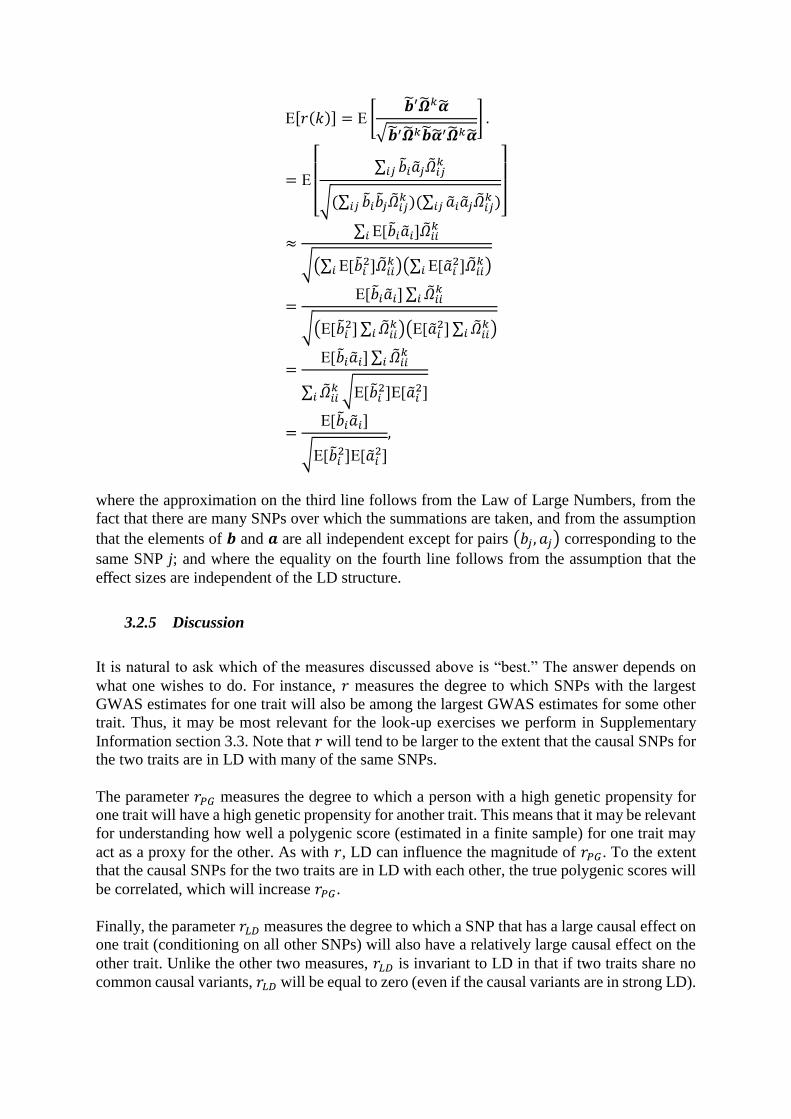
E[𝑟(𝑘)] = E [��′��𝑘��

√��′��𝑘����′��𝑘��] .

= E

[ ∑ ��𝑖��𝑗��𝑖𝑗

𝑘𝑖𝑗

√(∑ ��𝑖��𝑗��𝑖𝑗𝑘

𝑖𝑗 )(∑ ��𝑖��𝑗��𝑖𝑗𝑘

𝑖𝑗 )]

≈∑ E[��𝑖��𝑖]��𝑖𝑖

𝑘𝑖

√(∑ E[��𝑖2]��𝑖𝑖

𝑘𝑖 )(∑ E[��𝑖

2]��𝑖𝑖𝑘

𝑖 )

=E[��𝑖��𝑖] ∑ ��𝑖𝑖

𝑘𝑖

√(E[��𝑖2] ∑ ��𝑖𝑖

𝑘𝑖 )(E[��𝑖

2] ∑ ��𝑖𝑖𝑘

𝑖 )

=E[��𝑖��𝑖] ∑ ��𝑖𝑖

𝑘𝑖

∑ ��𝑖𝑖𝑘

𝑖 √E[��𝑖2]E[��𝑖

2]

=E[��𝑖��𝑖]

√E[��𝑖2]E[��𝑖

2]

,

where the approximation on the third line follows from the Law of Large Numbers, from the

fact that there are many SNPs over which the summations are taken, and from the assumption

that the elements of 𝒃 and 𝒂 are all independent except for pairs (𝑏𝑗 , 𝑎𝑗) corresponding to the

same SNP j; and where the equality on the fourth line follows from the assumption that the

effect sizes are independent of the LD structure.

3.2.5 Discussion

It is natural to ask which of the measures discussed above is “best.” The answer depends on

what one wishes to do. For instance, 𝑟 measures the degree to which SNPs with the largest

GWAS estimates for one trait will also be among the largest GWAS estimates for some other

trait. Thus, it may be most relevant for the look-up exercises we perform in Supplementary

Information section 3.3. Note that 𝑟 will tend to be larger to the extent that the causal SNPs for

the two traits are in LD with many of the same SNPs.

The parameter 𝑟𝑃𝐺 measures the degree to which a person with a high genetic propensity for

one trait will have a high genetic propensity for another trait. This means that it may be relevant

for understanding how well a polygenic score (estimated in a finite sample) for one trait may

act as a proxy for the other. As with 𝑟, LD can influence the magnitude of 𝑟𝑃𝐺. To the extent

that the causal SNPs for the two traits are in LD with each other, the true polygenic scores will

be correlated, which will increase 𝑟𝑃𝐺.

Finally, the parameter 𝑟𝐿𝐷 measures the degree to which a SNP that has a large causal effect on

one trait (conditioning on all other SNPs) will also have a relatively large causal effect on the

other trait. Unlike the other two measures, 𝑟𝐿𝐷 is invariant to LD in that if two traits share no

common causal variants, 𝑟𝐿𝐷 will be equal to zero (even if the causal variants are in strong LD).

This is easily seen in that 𝑟𝐿𝐷 is not a function of 𝛀 or of any variables that are correlated with

𝛀.

3.3 Enrichment Analysis and Look-up of Lead SNPs in GWAS for Other

Phenotypes

3.3.1 Test for Joint Enrichment of the 74 Lead SNPs for the MHBA Phenotypes

For each of the 14 MHBA phenotypes (sources are listed in Supplementary Table 3.1), we

compared the observed enrichment of our 74 lead SNPs to the expected degree of enrichment

from 74 randomly chosen SNPs with similar allele frequencies.

Because the GWAS results files for some of the phenotypes do not include all 74 lead SNPs,

we began by generating a set of candidate proxies for each of the lead SNPs. We used the

clumping procedure described in Supplementary Information section 1.6.1 to identify all SNPs

in the lead SNP’s clump. We then retained from each clump the 25 SNPs whose LD with the

lead SNP was greatest. This procedure yielded us a list of at most 25 candidate proxies for each

lead SNP.

The following procedure was then used to implement the test:

1. For each phenotype, we generated a list of lead/proxy SNPs. If a lead SNP was directly

available in the phenotype’s results file, it was used. If not, we replaced it with the

highest-LD candidate proxy available in the phenotype’s results file. If none of the

candidate proxies was available in the results file, no proxy was used for that lead SNP

for that phenotype. Because we have 14 phenotypes and 74 lead SNPs, we looked up a

total of 14 × 74 = 1,036 SNPs in the results files. The lead SNP itself was available 783

times, a proxy was available 237 times (mean r2 with lead SNP is 0.90), and only in 16

cases we identified neither the lead SNP nor a candidate proxy (at most 4 cases for a

given phenotype).

2. For each phenotype in turn, we used the software SNPsnap21 to generate 10,000

matched SNP vectors with allele frequency distributions similar to that of the vector

of lead/proxy SNPs. Specifically, the SNPs in each matching vector were drawn

randomly conditional on having a minor allele frequency that deviated from the MAF

of the lead/proxy SNP by at most one percentage point. We dropped a small number

of lead/proxy SNPs that were not available in the SNPsnap database (for a given

phenotype, the number of SNPs not recognized by SNPsnap never exceeded 4).

3. For each phenotype, the SNPsnap output is a matrix whose rows correspond to the

available proxy/lead SNPs and each of whose 10,000 columns contains a vector of

matched SNPs. We eliminated from the matrix any SNPs that were not available in the

phenotype’s results file, iteratively replacing cells containing non-available SNPs with

a missing value and shifting the row vector leftward to fill in missing values. Then, we

kept only the first 500 column vectors of the matrix. By construction, this matrix only

contained SNPs available in the phenotype’s result file.

4. For each phenotype, our test statistic is the mean squared Z-statistic of the lead/proxy

SNPs. The observed test statistic was calculated excluding SNPs for which (i) the lead

SNP and its candidate proxies were all unavailable in the phenotype’s results file, or

(ii) the lead/proxy SNP was not recognized by SNPsnap. To generate an empirical null

distribution, we calculated the test statistic (the mean squared Z-statistic of the SNPs)

in each of the 500 vectors from step (3). We then calculated the empirical P-value as

the percentile of the null distribution at which the observed test statistic falls.

3.3.2 SNP Look-up and Proxy-Phenotype Analysis

We have just described how the lead SNPs (or the best available proxies) were tested jointly

for association with each of the 14 MHBA phenotypes. Here, we test the same SNPs

individually for association with the same 14 phenotypes.

For each phenotype, we looked up the P-value of each lead/proxy SNPs (whose construction

was described in the previous subsection). The results from this analysis are shown in

Supplementary Table 3.2. We consider two P-value thresholds. The first threshold corrects for

both the number of lead SNPs (74) as well as the number of MHBA phenotypes (14): this P-

value threshold is 0.05 / (74 × 14) = 4.83 × 10-5. (For simplicity, we corrected for 74 SNPs here

and below even for phenotypes for which we tested fewer than 74 SNPs due to missing

lead/proxy SNPs in the phenotype’s result file.) The SNPs whose P-values satisfy this stricter

threshold are color-coded in green in Supplementary Table 3.2, so we refer to them as “green

SNPs” in what follows. Our second threshold corrects only for the number of SNPs: 0.05 / 74

= 6.76 × 10-4. SNPs reaching this threshold (but not the stricter threshold) are color-coded in

yellow and referred to as “yellow SNPs.”

For each yellow SNP, we investigated whether it is in a genomic region harboring SNPs

previously reported to reach genome-wide significance in that phenotype’s GWAS. To this

end, we identified the set of LD partners of each yellow SNP, defined as SNPs within 1000kb

whose pairwise LD with the yellow SNP exceeds a r2 of 0.1. We estimated the pairwise r2

using the European-ancestry 1000 Genomes Project phase 1 genotyping data22. We then

examined whether the lead/proxy SNP or any of its LD partners reached genome-wide

significance in the phenotype’s GWAS. If none did, we classified the SNP as “prioritized.” We

followed the same procedure with the green SNPs. Using this procedure, we found that 10 of

the 25 SNPs labeled as either green or yellow are prioritized. Of the 15 green SNPs, we found

that 3 are prioritized (one for hippocampus and two for height; see Supplementary Tables 3.2,

3.3, and 3.4).

A concern about these results is that the EduYears and MHBA phenotype samples are not

independent. Sample overlap biases the look-up exercise toward finding a significant effect on

the MHBA phenotype because of the phenotypic correlations between each of the MHBA

phenotypes and EduYears. To test the robustness of our findings to this concern, we ran

restricted EduYears meta-analyses dropping overlapping cohorts. The color gray in

Supplementary Table 3.2 flags lead SNPs that no longer reach genome-wide significance in

the meta-analysis of EduYears after we excluded cohorts that overlap with the cohorts included

in the phenotype’s GWAS. Of the 10 prioritized SNPs, 4 reached genome-wide significance

even in the restricted GWAS without sample overlap (one for each of height, hippocampus,

ICV, and schizophrenia).

3.3.3 Results

Extended Data Fig. 5 shows the Q-Q plots of the lead/proxy SNPs for the MHBA phenotypes

(as defined in Supplementary Information section 3.1).

The test for joint enrichment of the SNPs (Supplementary Information section 3.3.1) yields

significant P-values at the 0.05 level for the following phenotypes: Alzheimer’s (P = 0.026),

bipolar (P < 0.002), BMI (P = 0.004), cognitive performance (P < 0.002), height (P = 0.006),

hippocampus (P = 0.008), intracranial volume (P = 0.006), neuroticism (P < 0.002), and

schizophrenia (P < 0.002). We found no significant enrichment for accumbens, caudate,

pallidum, putamen, and thalamus. Note, however, that our statistical power to detect

associations is a function of the sample size of the MHBA phenotype meta-analyses and of the

reliability of phenotypic measurement. Only relatively modest sample sizes were available for

the brain anatomy phenotypes14 (N < 13,000 for subcortical regions), and measurement of

subcortical volumes is notoriously prone to measurement error.

We identified which of the significant associations with MHBA phenotypes are prioritized, as

described in Supplementary Information section 3.3.2. One of the two SNPs that passes

Bonferroni correction for cognitive performance in our look-up (rs9320913 on chr 6) is in high

LD with rs1487441, which was previously reported by Rietveld et al. (2014)12 (r2 = 0.905

according to the 1000 Genomes Pilot 1 reference panel)23, and therefore we do not consider it

to be a prioritized association.o In addition, one EA lead SNP that passes Bonferroni correction

for intracranial volume (rs192818565) tags the only previously identified locus14,24, and thus

we also do not consider this finding to be a prioritized association. Supplementary Table 3.3

summarizes the main findings of our look-up exercise.

We identify prioritized SNP associations for: Alzheimer’s disease (rs7945718), BMI

(rs56231335), cognitive performance (rs12682297), height (rs10496091, rs113520408,

rs9537821), hippocampus (rs4500960), intracranial volume (rs12969294), neuroticism

(rs12969294), and schizophrenia (rs11588857). Extended Data Fig. 6 shows examples of

regional association plots of the prioritized SNPs for cognitive performance, hippocampus,

intracranial volume, and neuroticism. We picked these four examples because very few

genome-wide significant SNPs have been reported for these traits until now. Regional

association plots for the remaining prioritized SNPs are available on http://ssgac.org/Data.php.

Several of our EA lead SNPs are related to more than one MHBA phenotype. For example,

rs12969294 is a prioritized SNP for both intracranial volume and neuroticism, rs4500960 is

prioritized for hippocampus volume and was previously identified as being associated with

schizophrenia, and rs7945718 is prioritized for Alzheimer’s here and was identified earlier as

a height SNP.

o Rietveld et al. (2014)12 reported several SNP associations with cognitive performance using a similar approach as we use

here (with educational attainment as a “proxy phenotype”). However, they used a different set of education-associated SNPs

(based on Rietveld et al. 201380 and a P-value threshold of 10-5 instead of the 5×10-8 threshold used here). The three SNPs that

survived Bonferroni correction in their analysis have the following P-values in our current meta-analysis of EduYears, after

we exclude the second-stage cohorts used in Rietveld et al. (2014): rs1487441 on chr 6 (P = 1.1×10-16), rs7923609 on chr 10

(P = 8.13×10-6), and rs2721173 on chr 8 (P = 3.22×10-7).

Consistent with our finding sign concordance with EduYears less than 50%, we find negative

correlation of SNP coefficients with EduYears for Alzheimer’s, BMI, and neuroticism.

Consistent with their sign concordance greater than 50%, we find positive correlation of SNP

coefficients for cognitive performance, intracranial volume, and height (although for height,

the sign conconcordance is not statistically distinguishable from 50%). An intriguing pattern is

found for schizophrenia, which has a positive but near-zero estimated genetic correlation (rLD

= 0.08 with P = 3.2×10-4) and a nearly equal percentage of concordant SNPs and discordant

SNPs among the set of 74 that we tested (51% concordant)—and yet, as reported above, the

enrichment of association of these SNPs for schizophrenia is strong (P < 0.002). We now turn

to potential explanations for this result and discuss related literature.

3.3.4 Discussion

Our work builds on earlier epidemiological research using genetically informative designs3–

5,25–29.

First, our results corroborate earlier findings that the genetic contribution to the positive

relationship between cognitive performance and EA is substantial, but not perfect1,30,31.

Second, earlier studies found that neuroticism is a powerful negative predictor of achievement

across various domains including job performance, academic achievement, and performance

on tests of cognitive performance, partly through test anxiety32–36. The strong negative genetic

overlap between EA and neuroticism suggests that SNPs associated with EA may be good

candidates for association with neuroticism.

Third, our finding of a negative genetic correlation between EA and BMI corroborates earlier

evidence from twin studies suggesting that the negative relationship between EA and BMI37–41

is partially due to common genetic factors2,25,42. A possible hypothesis to explain this finding

is that the genetic effects on BMI may be partially mediated by individual differences in self-

control, impulsivity, and reward sensitivity43–48, which are also linked to learning and academic

achievement45–48. Interestingly, the most recent GWAS on BMI found that genes associated

with BMI are much more strongly expressed in the nervous system and sense organs than in

the digestive system15. However, future research is needed to better understand the mechanisms

underlying these findings.

Fourth, our results also relate to a literature on the relationship between cognitive performance

and brain size. A recent meta-analysis of published and unpublished studies on this topic

identified 88 articles involving overall more than 8,000 individuals49. The meta-analysis

reported a significant positive association (r = 0.24) but concluded that this estimate is too high

due to publication bias. Furthermore, twin studies have found that the association between brain

volume and cognitive performance is partly due to common genetic effects4,26. Although we

report results on intracranial instead of brain volumep and overlap with EA rather than cognitive

performance, the strong positive genetic overlap of EA with both cognitive performance and

intracranial volume corroborates the earlier twin-study findings that their moderate positive

phenotypic association is partly due to a shared genetic component.

Fifth, our results relate to ongoing research on schizophrenia and bipolar disorder. Earlier work

has demonstrated links between these mental disorders on the one hand, and school

p Brain volume and intracranial volume are highly positively correlated, but in contrast to brain volume, intracranial volume

remains roughly constant during adult life95.

performance, cognitive performance, creativity, and educational attainment on the other.

Although these latter measures are related to each other and share a genetic basis, the

phenotypic and genetic correlations between them are far from perfect30,50,51. Furthermore, their

relationship with schizophrenia and bipolar disorder is rather complex and possibly U-shaped.

On the one hand, low cognitive performance and low school performance have been reported

as risk factors for schizophrenia and bipolar disorder19,52–55. For example, evidence from a

large, population-based Swedish Multi-Generation Register suggests a weak negative

correlation (-0.11) between IQ and psychosis (a term referring to mental disorders including

both schizophrenia and bipolar disorder)5. Furthermore, Stefansson et al. (2013)28 demonstrate

that rare copy-number variants that are known to cause schizophrenia also predict lower

cognitive performance in healthy individuals.

On the other hand, a higher prevalence of psychosis among individuals high in cognitive

performance and creativity has been frequently reported56–58, and polygenic risk scores for

bipolar disorder and schizophrenia have been reported to predict creativity in independent

samples29. This suggests that some genetic variants that increase the risk for psychosis may

also have positive effects on cognitive performance.

The relationship between educational attainment and schizophrenia specifically is similarly

complex. Although early-onset schizophrenia is associated with school dropout59, Kremen et

al. (2006)60 find no clear relationship between educational attainment and risk of schizophrenia.

More generally, the relationship between education and schizophrenia appears to depend on

age at onset, duration, and severity of the disease, factors that often are not measured61. The

failure to account for these factors in many empirical studies may contribute to the relatively

weak or even seemingly contradictory results.

As suggested by Craddock et al. (2009)62, it is possible that the clinical diagnoses of

schizophrenia and bipolar disorder mask several disease subtypes that are caused by different

biological mechanisms. This is one possible interpretation of our results for schizophrenia: The

strong enrichment for association of our EA lead SNPs with schizophrenia, combined with a

nearly equal percentage of concordant and discordant associations of our lead SNPs with these

mental disorders, could point to different sub-types of schizophrenia that are lumped together

by the current disease classification system. Alternatively, it may be that SNPs that are

associated with schizophrenia happen to be in LD with SNPs that are associated with

educational attainment simply because both sets of SNPs are primarily located in genes or

genomic regions that are expressed in the brain. Such co-localization would generate a

haphazard pattern of sign concordance. Follow-up research will need to differentiate between

these different interpretations of our results.

Sixth, our results relate to ongoing research in cognitive neuroscience that aims to identify how

specific cognitive processes are mapped to neural substrates and brain structures. Visuomotor

abilities63, visuospatial64 and verbal-working memory65, executive functions66, motivation and

reward processing67,68, and social skills69 have all been linked to EA. Thus, brain structures that

influence performance of these cognitive functions could be related to EA. Viewed from that

perspective, it might be surprising that our 95% confidence intervals rule out even a moderately

sized genetic correlation between EA and the volumes of the six sub-cortical structures we

tested. However, our results do not exclude the possibilities that (a) a significant phenotypic

relationship between EA and anatomical features of these sub-cortical regions may exist; (b)

with greater statistical power, we could statistically distinguish from zero the magnitude of

genetic correlation with these sub-cortical volumes (especially given the relatively low

statistical power as discussed in Supplementary Information section 3.3.3); (c) SNPs associated

with EA may still be enriched for association with the sub-cortical volumes investigated here,

as we indeed found for hippocampus; and (d) substantial genetic correlations may exist

between EA and other brain structures that are not investigated here (e.g., cortical volume,

fronto-parietal network, and white matter).

Finally, our look-up results confirmed that EA is a useful “proxy phenotype”12 to study the

genetic architecture of brain volume phenotypes. This is particularly noteworthy because only

very few SNPs associated with brain volume phenotypes have been discovered. Specifically,

the largest GWAS meta-analysis on brain volume phenotypes to date14 reports two genome-

wide significant SNPs for hippocampus and only one for intracranial volume. Our results

prioritized additional SNPs for hippocampus (rs4500960 on chr 2, with a discordant sign of the

effect) and intracranial volume (rs12969294 on chr 18, concordant sign). Furthermore, an

additional EA lead SNP that passes Bonferroni correction (rs192818565) tags the only

previously identified locus for intracranial volume14,24.

For neuroticism, the largest GWAS meta-analysis to date13 reports one genome-wide-

significant SNP. Our look-up exercise prioritizes a second SNP, rs12969294 on chr 18

(discordant sign).

We find various interesting patterns that warrant future investigation. Several SNPs that are

associated with an increased chance to obtain higher education are also associated with an

increased likelihood of bipolar disorder or schizophrenia. For schizophrenia, several of these

SNPs that have sign-concordant effects with EA survive Bonferroni correction (rs11588857,

rs2245901, rs2992632, rs6739979, rs7306755), and one of them has not previously been

identified yet as a schizophrenia variant (rs11588857). Furthermore, one of the three prioritized

height SNPs we identify has sign-discordant effects on height and EA (rs113520408).

References

1. Calvin, C. et al. Multivariate genetic analyses of cognition and academic achievement

from two population samples of 174,000 and 166,000 school children. Behav. Genet.

42, 699–710 (2012).

2. Della Bella, S. & Lucchini, M. Education and BMI: a genetic informed analysis. Qual.

Quant. (2014).

3. Silventoinen, K., Krueger, R. F., Bouchard, T. J., Kaprio, J. & McGue, M. Heritability

of body height and educational attainment in an international context: comparison of

adult twins in Minnesota and Finland. Am. J. Hum. Biol. 16, 544–555 (2004).

4. Posthuma, D. et al. The association between brain volume and intelligence is of genetic

origin. Nat. Neurosci. 5, 83–84 (2002).

5. Fowler, T., Zammit, S., Owen, M. J. & Rasmussen, F. A population-based study of

shared genetic variation between premorbid IQ and psychosis among male twin pairs

and sibling pairs from Sweden. Arch. Gen. Psychiatry 69, 460–466 (2012).

6. Bulik-Sullivan, B. et al. An atlas of genetic correlations across human diseases and traits.

Nat. Genet. 47, 1236–1241 (2015).

7. Lee, S. H., Yang, J., Goddard, M. E., Visscher, P. M. & Wray, N. R. Estimation of

pleiotropy between complex diseases using single-nucleotide polymorphism-derived

genomic relationships and restricted maximum likelihood. Bioinformatics 28, 2540–

2542 (2012).

8. Lambert, J. C. et al. Meta-analysis of 74,046 individuals identifies 11 new susceptibility

loci for Alzheimer’s disease. Nat. Genet. 45, 1452–1458 (2013).

9. Psychiatric GWAS Consortium Bipolar Disorder Working Group. Large-scale genome-

wide association analysis of bipolar disorder identifies a new susceptibility locus near

ODZ4. Nat. Genet. 43, 977–983 (2011).

10. Ripke, S. et al. Biological insights from 108 schizophrenia-associated genetic loci.

Nature 511, 421–427 (2014).

11. Benyamin, B. et al. Childhood intelligence is heritable, highly polygenic and associated

with FNBP1L. Mol. Psychiatry 19, 1–6 (2013).

12. Rietveld, C. A. et al. Common genetic variants associated with cognitive performance

identified using the proxy-phenotype method. Proc. Natl. Acad. Sci. USA 111, 13790–

13794 (2014).

13. De Moor, V. D. B. et al. Genome-wide association study identifies novel locus for

neuroticism and shows polygenic association with Major Depressive Disorder. JAMA

Psychiatry 72, 642–650 (2015).

14. Hibar, D. P. et al. Common genetic variants influence human subcortical brain

structures. Nature 520, 224–229 (2015).

15. Locke, A. E. et al. Genetic studies of body mass index yield new insights for obesity

biology. Nature 518, 197–206 (2015).

16. Wood, A. R. et al. Defining the role of common variation in the genomic and biological

architecture of adult human height. Nat. Genet. 46, 1173–1186 (2014).

17. Bulik-Sullivan, B. K. et al. LD Score regression distinguishes confounding from

polygenicity in genome-wide association studies. Nat. Genet. 47, 291–295 (2015).

18. Finucane, H. K. et al. Partitioning heritability by functional category using GWAS

summary statistics. Nat. Genet. 47, 1228-1235.

19. Glahn, D. C., Bearden, C. E., Bowden, C. L. & Soares, J. C. Reduced educational

attainment in bipolar disorder. J. Affect. Disord. 92, 309–312 (2006).

20. Robinson, L. J. et al. A meta-analysis of cognitive deficits in euthymic patients with

bipolar disorder. J. Affect. Disord. 93, 105–115 (2006).

21. Pers, T. H., Timshel, P. & Hirschhorn, J. N. SNPsnap: a Web-based tool for

identification and annotation of matched SNPs. Bioinformatics 31, 418–20 (2015).

22. Abecasis, G. R. et al. An integrated map of genetic variation from 1,092 human

genomes. Nature 491, 56–65 (2012).

23. Institute, B. SNAP - SNP annotation and proxy search. at

<https://www.broadinstitute.org/mpg/snap/ldsearchpw.php> (2015)

24. Ikram, M. A. et al. Common variants at 6q22 and 17q21 are associated with intracranial

volume. Nat. Genet. 44, 539–544 (2012).

25. Silventoinen, K., Sarlio-Lahteenkorva, S., Koskenvuo, M., Lahelma, E. & Kaprio, J.

Effect of environmental and genetic factors on education-associated disparities in weight

and weight gain: a study of Finnish adult twins. Am J Clin Nutr 80, 815–822 (2004).

26. Posthuma, D. et al. Genetic correlations between brain volumes and the WAIS-III

dimensions of verbal comprehension, working memory, perceptual organization, and

processing speed. Twin Res. 6, 131–139 (2012).

27. Lencz, T. et al. Molecular genetic evidence for overlap between general cognitive ability

and risk for schizophrenia: a report from the Cognitive Genomics consorTium

(COGENT). Mol. Psychiatry 19, 168–174 (2014).

28. Stefansson, H. et al. CNVs conferring risk of autism or schizophrenia affect cognition

in controls. Nature 505, 361–366 (2013).

29. Power, R. A. et al. Polygenic risk scores for schizophrenia and bipolar disorder predict

creativity. Nat. Neurosci. 18, 953–955 (2015).

30. Thompson, L. A., Detterman, D. K. & Plomin, R. Associations between cognitive

abilities and scholastic achievement: Genetic overlap but environmental differences.

Psychol. Sci. 2, 158–165 (1991).

31. Greven, C. U., Harlaar, N., Kovas, Y., Chamorro-Premuzic, T. & Plomin, R. More than

just IQ: school achievement is predicted by self-perceived abilities-but for genetic rather

than environmental reasons. Psychol. Sci. 20, 753–762 (2009).

32. Lynn, R. & Gordon, I. E. The relation of neuroticism and extraversion to intelligence

and educational attainment. Br. J. Educ. Psychol. 31, 194–203 (1961).

33. McKenzie, J., Taghavi-Khonsary, M. & Tindell, G. Neuroticism and academic

achievement: the Furneaux Factor as a measure of academic rigour. Pers. Individ. Dif.

29, 3–11 (2000).

34. Gallagher, D. J. Personality, coping, and objective outcomes: extraversion, neuroticism,

coping styles, and academic performance. Pers. Individ. Dif. 21, 421–429 (1996).

35. Phillips, J. B. & Endler, N. S. Academic examinations and anxiety: the interaction model

empirically tested. J. Res. Pers. 16, 303–318 (1982).

36. Debusscher, J., Hofmans, J. & De Fruyt, F. The curvilinear relationship between state

neuroticism and momentary task performance. PLoS One 9, e106989 (2014).

37. Karnehed, N., Rasmussen, F., Hemmingsson, T. & Tynelius, P. Obesity and attained

education: cohort study of more than 700,000 Swedish men. Obesity 14, 1421–1428

(2006).

38. Chandola, T., Deary, I. J., Blane, D. & Batty, G. D. Childhood IQ in relation to obesity

and weight gain in adult life: the National Child Development (1958) Study. Int. J. Obes.

30, 1422–1432 (2006).

39. Lawlor, D. A., Clark, H., Davey Smith, G. & Leon, D. A. Childhood intelligence,

educational attainment and adult body mass index: findings from a prospective cohort

and within sibling-pairs analysis. Int. J. Obes. 30, 1758–1765 (2006).

40. Roskam, A.-J. R. et al. Comparative appraisal of educational inequalities in overweight

and obesity among adults in 19 European countries. Int. J. Epidemiol. 39, 392–404

(2010).

41. Caird, J. et al. Childhood obesity and educational attainment: A systematic review.

(EPPI-Centre, Social Science Research Unit, Institute of Education, University of

London)

<http://eprints.ioe.ac.uk/16316/1/Caird_et_al._2011._Childhood_obesity_and_educati

onal_attainment._a_systematic_review.pdf> (2011).

42. Vermeiren, A. P. A. et al. Do genetic factors contribute to the relation between education

and metabolic risk factors in young adults? A twin study. Eur. J. Public Health 23, 986–

991 (2012).

43. Nasser, J. A., Gluck, M. E. & Geliebter, A. Impulsivity and test meal intake in obese

binge eating women. Appetite 43, 303–307 (2004).

44. Franken, I. H. A. & Muris, P. Individual differences in reward sensitivity are related to

food craving and relative body weight in healthy women. Appetite 45, 198–201 (2005).

45. Tangney, J. P., Baumeister, R. F. & Boone, A. L. High self-control predicts good

adjustment, less pathology, better grades, and interpersonal success. J. Pers. 72, 271–

324 (2004).

46. Duckworth, A. L. & Seligman, M. E. P. Self-discipline outdoes IQ in predicting

academic performance of adolescents. Psychol. Sci. 16, 939–944 (2005).

47. O’Doherty, J. P. Reward representations and reward-related learning in the human brain:

insights from neuroimaging. Curr. Opin. Neurobiol. 14, 769–776 (2004).

48. Reynolds, J. N., Hyland, B. I. & Wickens, J. R. A cellular mechanism of reward-related

learning. Nature 413, 67–70 (2001).

49. Pietschnig, J., Penke, L., Wicherts, J. M., Zeiler, M. & Voracek, M. Meta-analysis of

associations between human brain volume and intelligence differences: how strong are

they and what do they mean? SSRN Electron. J. (2014). doi:10.2139/ssrn.2512128

50. Bartels, M., Rietveld, M. J. H., Van Baal, G. C. M. & Boomsma, D. I. Heritability of

educational achievement in 12-year-olds and the overlap with cognitive ability. Twin

Res. 5, 544–553 (2012).

51. Tambs, K., Sundet, J. M., Magnus, P. & Berg, K. Genetic and environmental

contributions to the covariance between occupational status, educational attainment, and

IQ: a study of twins. Behav. Genet. 19, 209–222 (1989).

52. Osler, M., Lawlor, D. A. & Nordentoft, M. Cognitive function in childhood and early

adulthood and hospital admission for schizophrenia and bipolar disorders in Danish men

born in 1953. Schizophr. Res. 92, 132–141 (2007).

53. Jones, P. Child developmental risk factors for adult schizophrenia in the British 1946

birth cohort. Lancet 344, 1398–1402 (1994).

54. Loewenstein, D. A., Czaja, S. J., Bowie, C. R. & Harvey, P. D. Age-associated

differences in cognitive performance in older patients with schizophrenia: a comparison

with healthy older adults. Am. J. Geriatr. Psychiatry 20, 29–40 (2012).

55. MacCabe, J. H. et al. Scholastic achievement at age 16 and risk of schizophrenia and

other psychoses: a national cohort study. Psychol. Med. 38, 1133–1140 (2008).

56. Kyaga, S. et al. Mental illness, suicide and creativity: 40-year prospective total

population study. J. Psychiatr. Res. 47, 83–90 (2013).

57. Kyaga, S. et al. Creativity and mental disorder: family study of 300,000 people with

severe mental disorder. Br. J. Psychiatry 199, 373–379 (2011).

58. Juda, A. The relationship between highest mental capacity and psychic abnormalities.

Am. J. Psychiatry 106, 296–307 (1949).

59. Isohanni, I. et al. Educational consequences of mental disorders treated in hospital. A

31-year follow-up of the Northern Finland 1966 Birth Cohort. Psychol. Med. 31, 339–

349 (2001).

60. Kremen, W. S. et al. A discordant twin study of premorbid cognitive ability in

schizophrenia. J. Clin. Exp. Neuropsychol. 28, 208–224 (2006).

61. Resnick, S. M. Matching for education in studies of schizophrenia. Arch. Gen.

Psychiatry 49, 246 (1992).

62. Craddock, N., O’Donovan, M. C. & Owen, M. J. Psychosis genetics: modeling the

relationship between schizophrenia, bipolar disorder, and mixed (or ‘schizoaffective’)

psychoses. Schizophr. Bull. 35, 482–490 (2009).

63. Keogh, B. K. & Smith, C. E. Visuo-motor ability for school prediction: a seven-year

study. Percept. Mot. Skills 25, 101–110 (1967).

64. Holmes, J., Adams, J. W. & Hamilton, C. J. The relationship between visuospatial

sketchpad capacity and children’s mathematical skills. Eur. J. Cogn. Psychol. 20, 272–

289 (2008).

65. Gathercole, S. E., Pickering, S. J., Knight, C. & Stegmann, Z. Working memory skills

and educational attainment: evidence from national curriculum assessments at 7 and 14

years of age. Appl. Cogn. Psychol. 18, 1–16 (2004).

66. St Clair-Thompson, H. L. & Gathercole, S. E. Executive functions and achievements in

school: shifting, updating, inhibition, and working memory. Q. J. Exp. Psychol. 59, 745–

59 (2006).

67. Dweck, C. S. Motivational processes affecting learning. Am. Psychol. 41, 1040–1048

(1986).

68. Zimmerman, B. J., Bandura, A. & Martinez-Pons, M. Self-motivation for academic

attainment: the role of self-efficacy beliefs and personal goal setting. Am. Educ. Res. J.

29, 663–676 (1992).

69. Lleras, C. Do skills and behaviors in high school matter? The contribution of

noncognitive factors in explaining differences in educational attainment and earnings.

Soc. Sci. Res. 37, 888–902 (2008).

70. Stern, Y. Influence of education and occupation on the incidence of Alzheimer’s disease.

JAMA J. Am. Med. Assoc. 271, 1004–1010 (1994).

71. Stern, Y. Cognitive reserve. Neuropsychologia 47, 2015–2028 (2009).

72. Stern, Y. Cognitive reserve in ageing and Alzheimer’s disease. Lancet. Neurol. 11,

1006–1012 (2012).

73. Scarmeas, N., Albert, S. M., Manly, J. J. & Stern, Y. Education and rates of cognitive

decline in incident Alzheimer’s disease. J. Neurol. Neurosurg. Psychiatry 77, 308–316

(2006).

74. Ott, A. et al. Prevalence of Alzheimer’s disease and vascular dementia: association with

education. The Rotterdam study. BMJ 310, 970–973 (1995).

75. Kemppainen, N. M. et al. Cognitive reserve hypothesis: Pittsburgh Compound B and

fluorodeoxyglucose positron emission tomography in relation to education in mild

Alzheimer’s disease. Ann. Neurol. 63, 112–118 (2008).

76. Paradise, M., Cooper, C. & Livingston, G. Systematic review of the effect of education

on survival in Alzheimer’s disease. Int. Psychogeriatr. 21, 25–32 (2009).

77. Andel, R., Vigen, C., Mack, W. J., Clark, L. J. & Gatz, M. The effect of education and

occupational complexity on rate of cognitive decline in Alzheimer’s patients. J. Int.

Neuropsychol. Soc. 12, 147–152 (2006).

78. Swartz, M. S. et al. Substance use in persons with schizophrenia: baseline prevalence

and correlates from the NIMH CATIE study. J. Nerv. Ment. Dis. 194, 164–172 (2006).

79. Davies, G. et al. Genetic contributions to variation in general cognitive function: a meta-

analysis of genome-wide association studies in the CHARGE consortium (N=53 949).

Mol. Psychiatry 20, 183–192 (2015).

80. Rietveld, C. A. et al. GWAS of 126,559 individuals identifies genetic variants associated

with educational attainment. Science 340, 1467–1471 (2013).

81. Bogg, T. & Vo, P. T. Openness, neuroticism, conscientiousness, and family health and

aging concerns interact in the prediction of health-related Internet searches in a

representative U.S. sample. Front. Psychol. 5(370), 1–10 (2014).

82. Lewis, G. et al. Socio-economic status, standard of living, and neurotic disorder. Int.

Rev. Psychiatry 15, 91–96 (2009).

83. Piras, F., Cherubini, A., Caltagirone, C. & Spalletta, G. Education mediates

microstructural changes in bilateral hippocampus. Hum. Brain Mapp. 32, 282–289

(2011).

84. Noble, K. G. et al. Hippocampal volume varies with educational attainment across the

life-span. Front. Hum. Neurosci. 6, 307 (2012).

85. Grazioplene, R. G. et al. Subcortical intelligence: caudate volume predicts IQ in healthy

adults. Hum. Brain Mapp. 36, 1407–1416 (2014).

86. Cheong, J. L. Y. et al. Contribution of brain size to IQ and educational

underperformance in extremely preterm adolescents. PLoS One 8, e77475 (2013).

87. MacLullich, A. M. J. et al. Intracranial capacity and brain volumes are associated with

cognition in healthy elderly men. Neurology 59, 169–174 (2002).

88. McDaniel, M. Big-brained people are smarter: a meta-analysis of the relationship

between in vivo brain volume and intelligence. Intelligence 33, 337–346 (2005).

89. Magnusson, P. K. E., Rasmussen, F. & Gyllensten, U. B. Height at age 18 years is a

strong predictor of attained education later in life: cohort study of over 950,000 Swedish

men. Int. J. Epidemiol. 35, 658–663 (2006).

90. Cinnirella, F., Piopiunik, M. & Winter, J. Why does height matter for educational

attainment? evidence from German children. Econ. Hum. Biol. 9, 407–418 (2011).

91. Case, A. & Paxson, C. Stature and status: height, ability, and labor market outcomes.

NBER Bull. Aging Heal. (2006).

92. Case, A. & Paxson, C. Height, health, and cognitive function at older ages. Am. Econ.

Rev. 98, 463–467 (2008).

93. Guven, C. & Lee, W. S. Height and cognitive function at older ages: is height a useful

summary measure of early childhood experiences? Health Econ. 22, 224–233 (2013).

94. Szklarska, A., Kozieł, S., Bielicki, T. & Malina, R. M. Influence of height on attained

level of education in males at 19 years of age. J. Biosoc. Sci. 39, 575–582 (2007).

95. Courchesne, E. et al. Normal brain development and aging: quantitative analysis at in

vivo MR imaging in healthy volunteers. Radiology 216, 672–682 (2000).

4 Biological Annotation

In this section we describe, in greater detail than in the main text, the results from a number of

analyses designed to elucidate the biological mechanisms through which DNA variation in our

implicated genomic regions might influence educational attainment. Our treatment is much

more extensive than in our previous reports because of the substantial increase in sample size,

the novel bioinformatic techniques developed in the interim, and our intention to provide a

walk-through of our methods and results that is accessible to readers who lack a biological

background but are willing to consult appropriate resources for non-specialists when necessary.

Each of the following subsections describes a particular method of biological analysis and the

specific results yielded in the present application. At the outset, however, we provide some

broad introductory material.

The word gene has several distinct meanings across different subfields of genetics. Originally,

in classical and population genetics, a gene was an indivisible token of hereditary material that

could occupy a specific locus (discrete location in the genome). The genes at a particular locus

might fall into distinct classes, called alleles. Adopting this terminology, we can say that an

individual’s genome carries two genes at each locus, one inherited from each parent, possibly

of the same allelic type (in which case the individual is said to be homozygous at the locus) or

different allelic types (heterozygous).

In most of this paper, however, we use gene in a more modern sense: a contiguous region of

the type genome (e.g., the “human genome”), spanning many base pairs, whose expression or

transcription leads to a particular biological product—typically a messenger RNA (mRNA)

transcript, the translation of which leads to the production of a protein. Proteins are the basic

structural and functional units of the cell; examples of proteins include subunits of

neurotransmitter receptors, enzymes catalyzing metabolic processes such as the breakdown of

neurotransmitter in the synaptic cleft, and transporters that enable a presynaptic neuron to

reabsorb neurotransmitter that has just been released. Since locus is also used nowadays to

designate a region encompassing many base pairs, it is preferable to adopt a different term to

single out a point-like location in the genome. We use the term site for this purpose; the term

variant is also often used in the literature to refer to a polymorphic site, although we avoid this

term because it often shades into a synonym of allele. The latter term is still used in modern

genetics to specify a distinct class of base pairs that can occupy a particular site; the different

possible alleles at a single-nucleotide polymorphic (SNP) site are the familiar G, C, T, and A.

Note that non-expressed portions of the genome that do not encode proteins or other products

for use in the cell are not genes at all in the modern sense (although the base pairs inherited by

the offspring that reside at such locations are still genes in the classical sense). If two regions

of the genome are known to be genes because they are transcribed into mRNA at certain times

in certain cell types, then the gene-barren region between them is often called “intergenic.”

A nonsynonymous SNP—which necessarily lies within a gene—changes the composition and

biological properties of the encoded protein. Such a SNP might do this if the two alleles specify

distinct types of amino acids to be incorporated into the final protein sequence. Another

possibility is that one allele is a stop signal leading to termination of transcription. A SNP or

other type of polymorphic site outside of a gene can only have a phenotypic effect by affecting

the regulation of the gene product in some manner. (The illustration that follows is indeed

merely illustrative; many mechanisms of gene regulation are still not well understood.) A SNP

far from a gene when the chromosome is treated as a one-dimensional string may actually lie

in an enhancer that can be close to the transcription start site in the three-dimensional reality

of the cell nucleus, and the specific allele present at such a SNP may affect the binding of the

various proteins that must assemble at the start site to initiate the expression of the gene.

Regulation refers to the modulation of gene expression’s timing, abundance, or cell-type

specificity by such mechanisms, and it is in fact likely that most GWAS signals are due to sites

affecting regulation as opposed to encoding differences in protein composition. Gene

expression itself can be directly measured by assaying the abundance in the cell of mRNA

transcripts that map to a given gene, and indeed we make use of several databases recording

the results of such measurements in our various analyses.

In the GWAS literature, the term locus has come to mean a stretch of the genome centered on

a SNP showing the strongest evidence of association within a broader region. A locus in this

sense is variously defined in terms of physical distance (e.g., ±250 kilobases), genetic distance

(recombination probability), or decay of linkage disequilibrium. Two SNPs are in linkage

disequilibrium (LD) if they are correlated—that is, if the allele present at one site tends to be

found in the same chromosomes as a particular allele at the other. Indeed, a standard measure

of LD between two sites, r2, is simply the squared Pearson correlation between counts of the

respective reference alleles within phased haplotypes.

This background suffices to motivate the biological questions that arise in the interpretation of

GWAS results and the means by which these questions might be tentatively addressed. For

starters, since a GWAS locus typically contains many other SNPs in LD with the defining lead

SNP and with each other, it is natural to ask: which of these SNPs is the actual causal site

responsible for the downstream phenotypic variation? Many SNPs in the genome appear to be

biologically inert—neither encoding differences in protein composition nor affecting gene

regulation—and a lead GWAS SNP may fall into this category and nonetheless show the

strongest association signal as a result of statistical noise or happenstance LD with multiple

causal sites. Fortunately, much is known from external sources of data about whether variation

at a particular site is likely to have biological consequences, and exploiting these resources is

our general strategy for fine-mapping loci: nominating individual sites that may be causally

responsible for the GWAS signals. Descriptions of genomic sites or regions based on external

sources of data are known as annotations, and readers will not go far astray if they interpret

this term rather literally (as referring to a note of explanation or comment added to a text in

one of the margins). If we regard the type genome as the basic text, then annotations are

additional comments describing the structural or functional properties of particular sites or the

regions in which they reside. For example, all nonsynonymous sites that influence protein

structures might be annotated as such. An annotation can be far more specific than this; for

instance, all sites that fall in a regulatory region active in the fetal liver might bear an annotation

to this effect.

A given causal site will exert its phenotypic effect through altering the composition of a gene

product or regulating its expression. Conceptually, once a causal site has been identified or at

least nominated, the next question to pursue is the identity of the mediating gene. In practice,

because only a handful of genes at most will typically overlap a GWAS locus, we can make

some progress toward answering this question without precise knowledge of the causal site.

The difficulty of the problem, however, should still not be underestimated. It is natural to

assume that a lead GWAS SNP lying inside the boundaries of a particular gene must reflect a

causal mechanism involving that gene itself, but in certain cases such a conclusion would be

premature. It is possible for a causal SNP lying inside a certain gene to exert its phenotypic

effect by regulating the expression of a nearby gene or for several genes to intervene between

the SNP and its regulatory target.

Supplementary Table 4.1 ranks each gene overlapping a DEPICT-defined locus by the number

of discrete evidentiary items favoring that gene (see Supplementary Information section 4.5 for

details regarding DEPICT). These lines of evidence are taken from a number of our analyses

to be detailed in the following subsections. Our primary tool for gene prioritization is DEPICT,

which can be used to calculate a P-value and associated FDR for each gene. It is important to

keep in mind, however, that a gene-level P-value returned by DEPICT refers to the tail

probability under the null hypothesis that random sampling of loci can account for annotations

and patterns of co-expression shared by the focal gene with genes in all other GWAS-identified

loci. Although it is very reasonable to expect that genes involved in the same phenotype do

indeed share annotations and patterns of co-expression, it may be the case that certain causal

genes do not conform to this expectation and thus fail to yield low DEPICT P-values. This is

why we do not rely on DEPICT alone but also the other lines of evidence described in the

caption of Supplementary Table 4.1.

The products of genes do not work in isolation to construct and maintain whole organisms.

Rather, multiple gene products participate in a particular pathway that serves a distinct

biological function. (The term pathway appears to be derived from the chains of

causal/temporal arrows often used in illustrations of unfolding cellular processes.) If one

considers neural signaling, it becomes clear that several gene products are needed to construct

ion channels, reuptake transporters, neurotransmitter receptors, and so forth. On the basis of

massive experimental evidence, biologists have constructed catalogs of pathways defined at

different levels of organization, each containing several proteins or other gene products. We

make heavy use of these catalogs here; in essence, we single out a pathway as likely to be

particularly important in the biology of the phenotype if it encompasses an unusually large

number of genes overlapping our GWAS loci.

Pathways are often defined in a manner that spans different tissue or cell types. For example,

a particular pathway may involve a ligand (signaling molecule) that is found in both the nervous

and digestive systems. Prioritizing particular tissues is conceptually parallel to prioritizing

pathways, and we employ similar methods for both types of biological follow-up.

To summarize, our biological analyses seek provisional answers to the following questions:

1. Which polymorphic sites in our GWAS loci are the actual causal sites responsible for

downstream variation in EduYears?

2. Which genes (protein-coding regions of the genome) mediate the effects of the causal

sites on EduYears?

3. Which biological pathways contribute to variation in cognitive performance and other

psychological attributes affecting EduYears?

4. Once certain biological mechanisms are implicated, can we determine the tissues and

cell types where they are active?

The method-specific subsections are arranged in an order that very roughly addresses these

questions in turn.

4.1 Look-up of Nonsynonymous Status, eQTL Effects, Associations with

other Phenotypes, and Predicted Gene Functions

4.1.1 Overview

Here we conduct a number of follow-up analyses that are now routinely used to gain some

biological insight into GWAS results. We document the sites among the lead SNPs taken

forward from our GWAS of EduYears (or sites in strong LD with those SNPs) that fall into one

of the following three classes: (1) nonsynonymous SNPs that alter the composition of the

protein encoded by a gene, (2) eQTLs that are associated with the abundance of mRNA

transcript in whole blood or in tissue from three distinct brain regions, and (3) SNPs associated

with other phenotypes in large-scale GWAS. A notable finding is that a top EduYears-

associated SNP is concordantly associated with head circumference in infants. As an additional

look-up exercise, we used the Gene Network tool to ascertain the predicted functions of our

prioritized genes and the tissues in which these genes are expressed.

4.1.2 Background

A subset of SNPs within a list of top GWAS SNPs—or, alternatively, SNPs in strong LD with

the top SNPs—may be highlighted as promising candidates for causality if they fall within a

class of sites that are more likely to have phenotypic effects. One such class consists of

nonsynonymous SNPs. It is now believed that a majority of GWAS signals across all studied

phenotypes are owed to causal sites that are regulatory rather than coding1,2, but nevertheless a

SNP is much more likely to have some phenotypic effect if it is coding2,3.

Another promising class of sites consists of expression quantitative trait loci (eQTLs), which

in this context can be defined as SNPs that have been shown to be associated with the

abundance of one or more mRNA transcripts. eQTLs are thus promising candidates for

regulating the expression of their corresponding genes. A greater quantity of transcript does

not invariably lead to greater abundance of the corresponding protein in the cell, and it is the

latter that is of biological significance. Typically, however, the correlation between gene

expression and protein concentration is ~0.654.

If an eQTL and its regulated gene are relatively close to each other in the genome, the eQTL is

said to act in cis (as opposed to in trans), although refinements of this terminology are also in

use5. eQTLs are identified in studies that are analogous to GWAS, except that the phenotypes

are gene expression (mRNA transcript levels) rather than high-level traits. The effect sizes of

eQTLs and hence the statistical power to detect them are fairly sizable because of the short

causal chain from variation in regulatory DNA sequence to the expression of the regulated

gene, although it is almost certainly the case that many thousands of eQTLs remain to be

detected5. SNPs associated with complex traits in GWAS are more likely to be eQTLs than

other SNPs with similar minor allele frequencies that are also assayed by genotyping chips6.

To pick out candidates for causal sites giving rise to our GWAS signals, we determined whether

any lead EduYears-associated SNPs are in LD with nonsynonymous SNPs or eQTLs (or are

themselves sites of these two types).

We also determined whether any of our lead SNPs has emerged as a top signal in GWAS of

other phenotypes. EduYears shows extensive genetic overlap with many other traits

(Supplementary Information section 3), and identifying candidates for the genomic sites at the

heads of the causal forks or chains responsible for these genetic correlations is another

promising means of shedding light on underlying biological and behavioral mechanisms.

4.1.3 Nonsynonymous Sites in Strong LD with Lead EduYears-Associated SNPs

We used the tool HaploReg

(http://www.broadinstitute.org/mammals/haploreg/haploreg_v3.php) to identify

nonsynonymous SNPs in strong LD (r2 ≥ 0.6) with at least one of the 74 lead SNPs associated

with EduYears. In total we identified 17 such SNPs, including two of our lead SNPs themselves

(Supplementary Table 4.1.1).

rs11588857 resides within LRRN2, which encodes a leucine-rich repeat found in neurons;

proteins in this family are often involved in cell-cell adhesion. According to the Gene Network

tool (to be described later in the subsection), LRRN2 is predicted to be active in several neural

pathways, including SYNAPSE ORGANIZATION, POSITIVE REGULATION OF NERVOUS SYSTEM

DEVELOPMENT, and REGULATION OF TRANSMISSION OF NERVE IMPULSE.

rs35761247 resides in COL7A1, which encodes a product incorporated into collagen (the main

structural element of connective tissues such as tendons and ligaments). This gene does not

seem to be a promising a priori candidate for affecting EduYears, and in fact our various

sources of evidence point to other genes in the region where this SNP is found (Supplementary

Table 4.1). It is possible that the causal site responsible for this association signal is in LD with

this particular nonsynonymous SNP.

4.1.4 Blood cis-eQTL Look-up

We conducted gene expression analyses of whole peripheral blood from a total of 2,360

unrelated individuals: 1,240 individuals from the Fehrmann cohort measured with the Illumina

HT12v3 platform7; 229 individuals from the Fehrmann cohort measured with the Illumina

H8v2 platform7; and 891 individuals from EGCUT8.

The analysis of the Fehrmann samples was confined to the SNPs shared by the Illumina

HumanHap300, HumanHap370, and 610 Quad SNP genotyping platforms. SNPs with MAF <

0.05, call rate < 0.95, or HWE P-value < 0.001 were excluded from further analysis. In the

EGCUT sample, duplicates were used to assess genotyping reproducibility. The per-individual

call rate had to be at least 0.95 for individuals to be included in subsequent analyses. Closely

related individuals were identified using the proportion of the genome shared identical by

descent (IBD), and the relative with the lower call rate was removed. SNPs with MAF < 0.01,

call rate < 0.99, or HWE P-value < 1×10−5 were excluded from further analysis. Data were

harmonized by imputation to dosages using the 1000 Genomes March 2012 combined

reference panel.

In each sample the following additional steps were taken. Gene expression data were quantile

normalized to the median distribution and subsequently log2 transformed. Probe and individual

means were centered to zero. (A “probe” is an element of a microarray designed to capture a

specified mRNA transcript.) Gene expression data were then corrected for possible population

structure by linear regression on the first four multidimensional scaling components derived

from the genotypic data. We residualized the resulting variables on the projections of the

individuals on the first 40 principal components (PCs) derived from the probe covariance

matrix of the expression data that did not show evidence of association with any genotype

meeting the P-value threshold corresponding to FDR < 0.05 (see below). Any expression PC

showing a significant association with a SNP might represent a biologically meaningful effect

of the SNP on the expression of multiple genes, and therefore it is important not to remove

such PCs.

cis-eQTL mapping was performed as described elsewhere9, with one difference: we deemed a

SNP a potential cis-eQTL when the distance between the SNP and the midpoint of the probe

was smaller than 1Mb, instead of smaller than 250kb. The precise upper bound on the distance

between a cis-eQTL and its regulatory target is a matter of arbitrary definition at this point5,

and we elected to relax the required proximity.

We only included probes that were present on the HT12v3 platform. We only tested SNP-probe

pairs when the SNP passed quality control in at least two of the three samples. We tested the

associations between the genotype dosages of the lead 74 SNPs from our GWAS meta-analysis

of EduYears and the gene expression values. The three datasets, each weighted by sample size,

were subsequently meta-analyzed. We then permuted the sample labels and repeated this

analysis 100 times. We set the FDR to 0.05, using the permuted datasets to ascertain the null

distribution of the nominal P-value.

An apparent cis-eQTL effect may often be the result of a nearby causal SNP in high LD with

the query SNP. In order to determine whether the lead EduYears SNPs have independent cis-

eQTL effects or are merely markers for nearby causal SNPs, we performed a conditional

analysis. Using the procedure described above, we first determined which SNP shows the

strongest cis-eQTL effect for each probe associated with any of the 74 lead EduYears SNPs.

After partialing out the effect of the strongest cis-eQTL using linear regression, we repeated

the tests of association between the EduYears SNPs and the highlighted probes. The

significance threshold corresponding to FDR < 0.05 was again estimated with 100

permutations.

We applied the above-described methodology to our 74 top EduYears SNPs and found that 33

SNPs were significant cis-eQTLs for 72 genes (98 array probes; the number of probes for

mRNA transcripts can be greater than the number of corresponding genes because various

splicing and editing mechanisms can lead a given gene to produce several distinct transcripts).

None of our EduYears SNPs was identified as the strongest cis-eQTL for its probe. 14 SNPs

did show an independent effect on expression after conditioning on the best cis-eQTL for the

given probe.

The effect sizes and P-values of those lead EduYears SNPs proving to be significant blood cis-

eQTLs are presented in Supplementary Table 4.1.2.

4.1.5 Brain cis-eQTL Look-up

To determine whether any of the lead EduYears SNPs are associated with gene expression

levels in human neural tissue, we utilized data from the Harvard Brain Tissue Research Center.

The total sample of 742 individuals is comprised of 376 late-onset Alzheimer’s disease patients

(LOAD), 193 Huntington’s disease patients (HD), and 173 individuals without a known

neurological disorder (healthy). The resource contains data on expression levels obtained from

postmortem brains and measured in three distinct regions: dorsolateral prefrontal cortex, visual

cortex, and cerebellum. Although it is reasonable to expect that causal sites affecting

educational attainment will enrich brain-specific cis-eQTLs, we note that the sample size of

our blood dataset is ~3 times larger.

The extensive quality control and probe-data normalization steps are described in detail

elsewhere10. After these steps, 39,579 probes were taken forward as dependent variables for

subsequent eQTL analysis. We eliminated SNPs exhibiting MAF < 0.01, HWE P-value < 10−6,

or call rate < 0.95. After applying these filters, 838,958 SNPs remained. For each probe we

used a Kruskal-Wallis test to test all SNPs within 1Mb of the corresponding gene’s

transcription start site for association with expression level. To take into account the complex

correlation structure of this dataset, we estimated an empirical FDR: the ratio of the average

number of eQTLs meeting a candidate threshold in datasets with randomly permuted sample

labels to the number of eQTLs meeting that same threshold in the original dataset. Since the

number of tests was large, the empirical null distribution converged after a relatively small

number of permutation runs; thus, we used ten permutation runs to estimate the empirical FDR.

We focus on the associations that survived after constraining the empirical FDR to be less than

0.10 (which corresponds to a nominal P-value cutoff of approximately 5×10−5).

Supplementary Table 4.1.3 lists the relevant effect sizes, P-values, LD measures, and brain

regions. In short, of our 74 lead EduYears SNPs, 15 (as represented by 28 LD proxies) were

significant cis-eQTLs for 25 probes (which happen to represent exactly 25 genes). We observed

eQTLs (counting lead EduYears SNPs and not proxies) active in all three brain areas: 13 in

dorsolateral prefrontal cortex, 11 in visual cortex, and 12 in cerebellum. Most of the apparent

effects were observed in all samples, except rs12987662 (its proxy rs6722241 significant in

LOAD only), rs572016 (its proxy rs3213566 significant in LOAD only), and rs1043209 (its

proxy rs11157390 significant in HD only). Since these inconsistencies may be due to

inadequate statistical power, we did not use them as a basis for deprioritization.

4.1.6 GWAS Look-up

Consulting the NHGRI GWAS catalog (http://www.genome.gov/gwastudies), we extracted

previously reported significant GWAS signals within a 500kb radius of any lead EduYears-

associated SNP and also in LD with this focal SNP to the extent r2 ≥ 0.6 (1000 Genomes CEU).

We excluded traits studied in our proxy-phenotype analysis (Supplementary Information

section 3). To be clear, we are looking here for EduYears SNPs or LD partners of such SNPs

reaching genome-wide significance in a GWAS of any trait.

We found that 6 of our 74 lead EduYears SNPs are (in close proximity to) signals reaching the

significance threshold P < 5×10−8 in other published GWAS. Supplementary Table 4.1.4 lists

the results. Perhaps the most interesting overlap occurs at rs7306755, which is in strong LD (r2

= 0.99) with a SNP associated with head circumference in infants. Looking up the proxy SNP

in our meta-analysis results, we found that the effect signs are concordant; the allele associated

with increased EduYears is also associated with increased head circumference. In our proxy-

phenotype analysis, the lead SNP is also concordantly associated with intracranial volume in

adults, although not significantly so (P = 0.33).

In contrast to infant head circumference and those traits studied in our proxy-phenotype

analysis, the cancers and autoimmune disorders in Supplementary Table 4.1.4 for the most part

offer little a priori reason to invoke a connection with cognition or personality. Results such

as these, obtained from GWAS of apparently unrelated phenotypes, may contribute to the

debate over the extent and evolutionary importance of pleiotropy11. One possibility is that a

relatively small fraction of polymorphic sites are functional, implying that many sites are

necessarily pleiotropic if polygenicity is the rule, but that effects on two traits are often

discordant and thus do not necessarily lead to a sizable genetic correlation. Any inferences

from such results, however, must be tentative in the absence of knowledge regarding the precise

causal sites responsible for these GWAS signals. For instance, a SNP with apparent effects on

two distinct traits may be tagging a causal site affecting one trait and an entirely different causal

site affecting the other trait. However, even if the most that can be said at present is that

functional SNPs tend to reside in the same genomic regions, the findings are still relevant to

the discussion of pleiotropy, which becomes the limit of a more general investigation into the

effects of linkage and LD on natural selection and neutral variation12.

4.1.7 Using Co-Expression to Predict Gene Function

We used a recently developed method (implemented by Fehrmann et al.13 and more extensively

described in Supplementary Information section 4.5) to gain insight into the functions of the

genes prioritized by DEPICT, our chief tool for gene nomination. We queried the co-expression

database described by ref. 13 (http://www.genenetworki.nl:8080/GeneNetwork/mgi.html) with

each of our DEPICT-prioritized genes (Supplementary Table 4.1). After using the symbol of

the focal gene as the search term, we recorded all results listed under Gene Ontology (GO)14

biological process, cellular compartment, and molecular function that were indicated to be

statistically significant. We also recorded the analogous results that were listed under the

Reactome15 and Kyoto Encyclopedia of Genes and Genomes (KEGG)16 pathways. We then

recorded all tissues, organs, and cell types (“tissues”) where the area under the receiver

operating characteristic curve (AUC) with respect to the discriminating power of measured

gene expression exceeds 0.80. The AUC in each case was derived from the difference between

the samples of the focal tissue and all other tissues in the distribution of the query gene’s

expression level, as determined by text-mining the descriptions provided by experimenters who

uploaded expression data to the Gene Expression Omnibus (GEO). Note that the tissue/cell

type labels taken from the Medical Subject Headings (MeSH) database can refer to different

levels of a hierarchy and therefore are not mutually exclusive in application.

We hasten to add that this look-up exercise cannot produce results as comprehensive as those

of DEPICT when this latter tool is used to highlight biological pathways and tissues

(Supplementary Tables 4.5.1 and 4.5.2). The advantage of the Gene Network look-up is ease

of use and the provision of some intuition regarding the output of the more sophisticated

DEPICT procedures described in Supplementary Information section 4.5.

The results of the look-up exercise can be found in Supplementary Table 4.1.5, which lists the

10 most frequently occurring search results yielded by each data source and their respective

counts. It is immediately apparent that the table is dominated by terms related to the brain.

Many of the terms concern transmission of signals across the synapse, the junction between

two neurons typically consisting of the axon terminal, a dendritic spine, and the extracellular

cleft between terminal and spine. (An axon is the output cable of a neuron; a dendrite is a short

protrusion extending from a neuron, along which messages from other neurons are conveyed

to the cell body.) Glutamate is the excitatory neurotransmitter most commonly used to relay

messages across the synapse, and many of the synaptic terms single out this ligand in particular

(e.g., GLUTAMATE RECEPTOR ACTIVITY). These results recapitulate the findings from our earlier

study of cognitive performance17. There are a number of terms concerning neural development,

including NEURON CELL-CELL ADHESION, TELENCEPHALON DEVELOPMENT, AXON GUIDANCE,

and NOTCH SIGNALING PATHWAY. Another noteworthy trend is the presence of many terms

related to chromatin modification (e.g., CHROMATIN REMODELING COMPLEX). Although tissue-

specific gene expression per se is not employed by DEPICT to prioritize genes, the most

frequently returned tissues where DEPICT-prioritized genes are more highly expressed than in

other tissues are all neural. The three most frequent terms are PREFRONTAL CORTEX, FRONTAL

LOBE, and HIPPOCAMPUS.

References

1. 1000 Genomes Project Consortium. A map of human genome variation from

population-scale sequencing. Nature 467, 1061–1073 (2010).

2. Gusev, A. et al. Partitioning heritability of regulatory and cell-type-specific variants

across 11 common diseases. Am. J. Hum. Genet. 95, 535–552 (2014).

3. Finucane, H. K. et al. Partitioning heritability by functional category using GWAS

summary statistics. Nat. Genet. 47, 1228-1235.

4. Vogel, C. & Marcotte, E. M. Insights into the regulation of protein abundance from

proteomic and transcriptome analyses. Nat. Genet. Rev. 13, 227–232 (2012).

5. Albert, F. W. & Kruglyak, L. The role of regulatory variation in complex traits and

disease. Nat. Genet. Rev. 16, 197–212 (2015).

6. Nicolae, D. L. et al. Trait-associated SNPs are more likely to be eQTLs: annotation

to enhance discovery from GWAS. PLoS Genet. 6, e1000888 (2010).

7. Fehrmann, R. N. S. et al. Trans-eQTLs reveal that independent genetic variants

associated with a complex phenotype converge on intermediate genes, with a major

role for the HLA. PLoS Genet. 7, e1002197 (2011).

8. Metsplau, A. The Estonian Genome Project. Drug Dev. Res. 62, 97–101 (2004).

9. Westra, H.-J. et al. MixupMapper: Correcting sample mix-ups in genome-wide

datasets increases power to detect small genetic effects. Bioinformatics 27, 2104–

2111 (2011).

10. Zhang, B. et al. Integrated systems approach identifies genetic nodes and networks

in late-onset Alzheimer’s disease. Cell 153, 707–720 (2013).

11. Wagner, G. P. & Zhang, J. The pleiotropic structure of the genotype-phenotype

map: the evolvability of complex organisms. Nat. Rev. Genet. 12, 204–213 (2011).

12. Good, B. H., Walczak, A. M., Neher, R. A. & Desai. M. M. Genetic diversity in the

interference selection limit. PLoS Genet. 10, e1004222 (2014).

13. Fehrmann, R. N. S. et al. Gene expression analysis identifies global gene dosage

sensitivity in cancer. Nat. Genet. 47, 115–125 (2015).

14. Ashburner, M. et al. Gene ontology: tool for unification of biology. Nat. Genet. 25,

25–29 (2000).

15. Croft, D. et al. Reactome: a database of reactions, pathways and biological

processes. Nucleic Acids Res. 39, D691–D697 (2010).

16. Kanehisa, M., Goto, S. Sato, Y., Furumichi, M. & Tanabe, M. KEGG for integration

and interpretation of large-scale molecular data sets. Nucleic Acids Res. 40, D109–

D817 (2014).

17. Rietveld, C. A. et al. Common genetic variants associated with cognitive

performance identified using the proxy-phenotype method. Proc. Natl. Acad. Sci.

USA 111, 13790–13794 (2014).

4.2 Enrichment Analysis and Fine-Mapping of GWAS Signals with fgwas

4.2.1 Overview

We briefly describe the intuition behind fgwas, a method for using GWAS results and

functional-genomic data to (1) identify the types of polymorphic sites in the genome that are

most likely to influence a trait and (2) use this information to fine-map GWAS loci and identify

additional loci. We then describe an application of this method to our GWAS of EduYears. The

annotations that most improve the probability of an association between a genomic region and

EduYears are those that indicate gene regulatory regions in the fetal brain. This pattern of

enrichment has not previously been observed in applications of fgwas to 18 other phenotypes.

Furthermore, on the assumption that a single causal SNP is responsible for a given association

signal, we use the functional enrichments to identify 17 SNPs with a strong probability of

causality.

4.2.2 Background

A GWAS can be used to assess, for millions of polymorphic sites in the genome, the evidence

that the genotype at the site is associated with the phenotype. In general, when deciding if the

evidence for association meets some threshold of statistical significance, each site is treated in

the same way—that is, we set some threshold (typically, P < 5×10−8) and consider all sites

passing this threshold to be significant.

However, a priori we know that some SNPs are more likely to be associated with the phenotype

than others; for example, it is often assumed that nonsynonymous SNPs are more likely to

influence phenotypes than sites that fall far from all known genes. So a P-value of 5×10−7, say,

though not typically considered significant at the genome-wide level, might merit a second

look if the SNP in question is nonsynonymous.

Formalizing this intuition can be done with Bayesian statistics, which combines the strength of

evidence in favor of a hypothesis (in our case, that a genomic site is associated with a

phenotype) with the prior probability of the hypothesis. Deciding how to set this prior is often

subjective. However, if many hypotheses are being tested (for example, if there are thousands

of nonsynonymous polymorphisms in the genome), then the prior can be estimated from the

data themselves using what is called “empirical Bayes” methodology. For example, if it turns

out that SNPs with low P-values tend to be nonsynonymous sites rather than other types of

sites, then the prior probability of true association is increased at all nonsynonymous sites. In

this way a nonsynonymous site that otherwise falls short of the conventional significance

threshold can become prioritized once the empirically estimated prior probability of association

is taken into account. Note that such favorable reweighting of sites within a particular class is

not set a priori, but is learned from the GWAS results themselves.

In our case, we split the genome into approximately independent blocks and estimate the prior

probability that each block contains a causal SNP that influences the phenotype and (within

each block) the conditional prior probability that each individual SNP is the causal one. Each

such probability is allowed to depend on annotations describing structural or functional

properties of the genomic region or the SNPs within it. We can then empirically estimate to

extent to each annotation predicts association with the focal phenotype. For a complete

description of the fgwas method, see ref. 1.

4.2.3 Methods

For application to the GWAS of EduYears, we used the same set of 450 annotations as ref. 1;

these are available at https://github.com/joepickrell/1000-genomes. The annotations include

elements of gene structure (e.g., nonsynonymous sites, untranslated regions following stop

signals), several hundred genomic regions identified as DNase hypersensitive in a variety of

tissues and cell lines2,3, and segmentations of the genome in the six ENCODE cell lines4. A

segmentation in this sense is a partition of the genome that uses a hidden Markov model or

similar mathematical construct to assign a somewhat high-level “state” to each segment of the

partition. The states are inferred from the correlation structure of low-level features such as

histone marks and transcription factors. The states in the segmentations based on the ENCODE

data were learned in an unsupervised fashion—meaning that the methods were not initially

trained on portions of the genome already labeled with a priori state-like annotations—but can

be interpreted post hoc as regions of the genome that (in a given cell type) are:

1. targets of the transcription-regulating protein CTCF;

2. enhancers (regions that bind transcription factors);

3. promoter flankers (regions near the transcription start sites of actively expressed genes);

4. repressed chromatin (regions where transcription factors are prevented from binding);

5. transcribed regions, including exons and introns;

6. active transcription start sites; and

7. weak enhancers.

The segmentations were performed on each cell line independently, but the outputs are

somewhat similar due to the biology shared across different tissues.

Since DNase I hypersensitive regions will feature prominently in our results, it is worthwhile

to describe them here. (In the literature these are commonly referred to as DNase I

hypersensitive “sites.” In keeping with our reservation of this term for atomic positions in the

genome, however, we will use the alternative “regions.”) At any given time, in any given cell,

much of the DNA making up the genome is tightly wound around spool-like proteins known

as histones; collectively, the DNA, histones, and other proteins and RNA packaged together in

this way are called chromatin. In those parts of the genome known as DNase I hypersensitive

regions, the DNA is readily degraded by the enzyme DNase I. A finding of DNase I

hypersensitivity is often taken as evidence of regulatory mechanisms having unpacked the

chromatin and thereby exposed the constituent DNA to transcription factors and other proteins

involved in gene expression. Whether a specific genomic region is DNase I hypersensitive

depends on the cellular and temporal context, as regulatory mechanisms target a level of gene

expression appropriate to the cell type and developmental stage.

We labeled each of the ~9 million SNPs in our GWAS of EduYears with any of the 450

annotations for which it qualified; note that several of these annotations refer to independent

replicates of the same experiments. We then ran fgwas as described in ref. 1 with two

exceptions. First, instead of splitting the genome into blocks containing equal numbers of

SNPs, we split it into approximately independent blocks identified from patterns of linkage

disequilibrium in the 1000 Genomes Project European-ancestry populations (using the –bed

flag)5. Second, we needed to set a prior variance of effect size to calculate the Bayes factor

measuring the evidence in favor of association and previously had used a fixed value of 0.1.

Here, we averaged over three Bayes factors calculated with prior variances equaling 0.01, 0.1,

and 0.5.

4.2.4 Single-Annotation Models

Shown in Extended Data Fig. 7a are the top 50 annotations when considering each individually,

ordered so that the annotations that most improve the likelihood of the model are at the top.

The individual annotation that most improves the model likelihood is DNASE (FETAL BRAIN)

(4.69-fold increase in odds of association; 95% confidence interval 2.89–7.07). Several

independent replicates of the experiments assaying DNase I hypersensitivity in the fetal brain

are also referred to by the top annotations. (We have no adult brain tissues in this database.

Each of the experiments assaying DNase I hypersensitive regions in the fetal brain was

performed independently.) Furthermore, in line with 18 other phenotypes previously analyzed

with fgwas, transcriptionally repressed chromatin is significantly depleted of SNPs associated

with EduYears. Note that in the analyses applying these exact same annotations to the GWAS

of the 18 other traits, we did not see any trait enriched by SNPs residing in genomic regions

that are DNase I hypersensitive in the brain.

4.2.5 Combined Model

Many sites in the genome satisfy criteria for multiple annotations, and it is of interest to

determine the independent contribution of each annotation in a manner analogous to multiple

regression. Using forward selection and cross-validation to avoid overfitting1, we built a

combined model including the effects of multiple annotations. Extended Data Fig. 7b displays

the results of the combined model that maximizes the cross-validation likelihood. In the

combined model are annotations referring to transcription in HepG2 (a cell line derived from

the liver of a patient with hepatocellular carinoma) and HeLa (a cell line derived from a

cancerous cervix). Crucially, the model-selection procedure retained two different annotations

referring to DNase I hypersensitive regions identified in the fetal brain.

4.2.6 Reweighted GWAS and Fine Mapping

We reweighted the GWAS results using the functional-genomic results described above. Using

a regional posterior probability of association (PPA) greater than 0.90 as the cutoff, we

identified 102 regions likely to harbor a causal SNP with respect to EduYears (Extended Data

Fig. 7c and Supplementary Table 4.2.1). All but two of our 74 lead EduYears-associated SNPs

fall within one of these 102 regions. The exceptions are rs3101246 and rs2837992, which

attained PPA > 0.80 (Extended Data Fig. 7c). In previous applications of fgwas, the majority

of novel loci that attained the equivalent of genome-wide significance only upon reweighting

later attained the conventional P < 5×10−8 in larger cohorts1.

Within each region attaining PPA > 0.90, each SNP received a conditional posterior probability

of being the causal SNP (under the assumption that there is just one causal SNP in the region).

The method of assigning this latter posterior probability is similar to that of ref. 6, except that

the input Bayes factors are reweighted by annotation-dependent and hence SNP-varying prior

probabilities. In essence, the likelihood of causality at an individual SNP derives from its Bayes

factor with respect to phenotypic association (which is monotonically related to the P-value

under reasonable assumptions), whereas the prior probability is derived from any empirical

genome-wide tendency for the annotations borne by the SNP to predict evidence of association.

Thus, the SNP with the largest posterior probabilities of causality tend to exhibit among the

strongest P-values within their loci and functional annotations that predict association

throughout the genome. Note that proper calibration of this posterior probability requires that

all potential causal sites have been either genotyped or imputed, which may not be the case in

our application; we did not include difficult-to-impute non-SNP sites such as

insertions/deletions in the GWAS meta-analysis. With this caveat in mind, we identified 17

regions where fine mapping amassed over 50 percent of the posterior probability on a single

SNP (Supplementary Table 4.2.2). Of our 74 lead EduYears SNPs, 9 are good candidates for

being the causal sites driving their association signals. One of our top SNPs, rs4500960, is in

nearly perfect LD with the causal candidate rs2268894 (and is indeed the second most likely

causal SNP in this region according to fgwas). The causal candidate rs6882046 is within 75kb

of two lead SNPs on chromosome 5 (rs324886 and rs10061788), but no two of these three

SNPs show strong LD. Interestingly, the remaining 6 causal candidates lie in genomic regions

that only attain the equivalent of genome-wide significance upon Bayesian reweighting. Of the

17 causal candidates, 9 lie in regions that are DNase I hypersensitive in the fetal brain.

4.2.7 Conditional Analysis of Correlated Annotations

In 4.2.5, we reported an analysis that controls for correlations across a number of different

annotations. Specifically, we used forward selection and cross-validation to select multiple

annotations to be included in a combined model. The results, displayed in Extended Data Fig.

7b, are consistent with our conclusion that the annotation DNASE (FETAL BRAIN) is an important

predictor of whether a SNP is significantly associated with EduYears in our meta-analysis.

Here, we report an additional analysis to probe the robustness of our conclusions. The goal of

this analysis is to test to what extent each annotation included in our combined model is robust

to controlling for other annotations, including other annotations that may be correlated with it.

Following ref. 1, for each annotation included in the combined model in Extended Data Fig.

7b (hereafter, called the “annotation of interest”), we tested whether adding that annotation to

a model that controls for another annotation (hereafter, called the “other annotation”)

significantly improves the fit of the model. Specifically, for each annotation of interest, we (i)

estimated a model replacing the annotation of interest with the other annotation; (ii) fixing the

coefficient of the other annotation, we added the annotation of interest back to the model and

estimated its coefficient; and (iii) we examined whether the improvement in the model’s

likelihood was statistically significant (i.e., P < 0.05). For every annotation of interest, we

repeated this procedure using as the other annotation each of the (other) 50 most significant

annotations from the one-annotation-only analysis that were not included in the combined

model. By examining which other annotations eliminate the statistical significance of the

annotation of interest, we can assess whether particular confounds might be driving the

presence of DNASE (FETAL BRAIN) in the combined model.

The results of this robustness check are shown in Supplementary Table 4.2.3. In summarizing

these results, we concentrate on the two instances (i.e., experimental replicates) of DNASE

(FETAL BRAIN) as the annotations of interest, since their importance is the primary result of this

analysis.

Here we list the “other annotations” that eliminate the statistical significance of DNASE (FETAL

BRAIN). To be more precise, the “other annotations” such that adding one of the instances of

the DNASE (FETAL BRAIN) did not generate a significant improvement in model fit (P > 0.05)

were:

Another instance of DNASE (FETAL BRAIN). This finding is unsurprising since different

instances of DNASE (FETAL BRAIN) are highly correlated with each other. It also does

not bear on the question of whether DNase I hypersensitivity in the fetal brain is

confounded by a different genomic feature.

One of the several annotations related to transcription in embryonic stem cells. In this

case, DNASE (FETAL BRAIN) only barely becomes insignificant (P < 0.06), so it does

not appear that these annotations drive our finding about DNASE (FETAL BRAIN).

One experimental replicate of DNASE (FETAL MUSCLE). In this case also, DNASE

(FETAL BRAIN) only barely becomes insignificant (P = 0.07). We conclude that DNASE

(FETAL MUSCLE) does not seem to drive our finding about DNASE (FETAL BRAIN).

Experimental replicates of DNASE (FETAL LUNG). In these cases, the P-value of DNASE

(FETAL BRAIN) gets as large as 0.13. Thus, from a statistical perspective, DNASE

(FETAL LUNG) is the strongest candidate for a confounder, although it is not obvious to

us how to interpret it biologically. In any case the lung is a rather heterogeneous tissue

where DNase I hypersensitivity has previously been found to predict association with

height1, another perhaps unlikely phenotype.

One of several annotations related to DNase I hypersensitivity in neural progenitor

cells. These annotations implicate early brain development just as DNASE (FETAL

BRAIN) does. Therefore, while this finding raises the question of which of these

correlated annotations is responsible for the signal we observe, it does not call into

question the substantive conclusion from this analysis that early brain development is

implicated.

We interpret these results taken altogether as broadly supporting the robustness of our

conclusion: DNase I hypersensitivity in the fetal brain (or in progenitors of brain cells) is an

important predictor of whether a SNP is associated with EduYears, although it is conceivable

that the finding is instead driven by DNASE (FETAL LUNG).

4.2.8 Analysis of the Roadmap Epigenomics data

To confirm the enrichment of regions annotated as related to gene regulation in the brain, we

turned to a separate set of annotations based on data from the Roadmap Epigenomics

Consortium7.

The annotations are based on genome segmentations in 127 cell lines/types from

https://sites.google.com/site/anshulkundaje/projects/epigenomeroadmap. In these

segmentations, each region of the genome in each cell line/type falls into one of 15 categories

according to the pattern of histone marks in the region. We labeled each SNP in the 1000

Genomes Project with any of the 1,905 annotations, defined by cell lines/types and pattern of

histone marks, for which it qualified. We additionally included SYNONYMOUS and

NONSYNONYMOUS as annotations. (Synonymous SNPs are single-nucleotide polymorphic sites

within protein-coding genes that do not affect the composition of the protein as a result of

redundancy in the mapping of DNA triplets to amino acids.) This dataset lacks an annotation

referring directly to a positive result from an experimental assay of DNase I hypersensitivity

in the brain. It does contain excellent proxies for this annotation such as the brain-specific

extent of transcription and whether a region is a brain-specific enhancer; a frequent cause of

DNase I hypersensitivity is the regulatory exposure of transcription start sites and enhancers to

the machinery of gene expression. We then performed the same analyses as in our treatment of

the earlier dataset, except using this set of 1,907 annotations instead of the previous set of 450.

All 530 statistically significant (P < 0.05) annotations are given in Supplemental Table 4.2.4.

Again, the most significant annotations refer to cell lines/types that are neural in nature. In

particular, the four most significant annotations that improve the odds of association with

EduYears are WEAK TRANSCRIPTION (FETAL BRAIN FEMALE) (6.27-fold increase in odds of

association; 95% confidence interval 3.43–11.25), WEAK TRANSCRIPTION (FETAL BRAIN MALE)

(6.05-fold increase in odds of association; 95% confidence interval 3.35–10.75), ENHANCERS

(FETAL BRAIN MALE) (10.74-fold increase in odds of association; 95% confidence interval 5.49–

19.22), and WEAK TRANSCRIPTION (BRAIN DORSOLATERAL PREFRONTAL CORTEX) (4.67-fold

increase in odds of association; 95% confidence interval 2.67–8.02). We also replicated the

observation that genomic regions annotated as transcriptionally repressed (QUIESCENT/LOW)

are depleted of SNPs associated with EduYears.

References

1. Pickrell, J. K. Joint analysis of functional genomic data and genome-wide association

studies of 18 human traits. Am. J. Hum. Genet. 94, 559–573 (2014).

2. Maurano, M. T. et al. Systematic localization of common disease-associated variation

in regulatory DNA. Science 337, 1190–1195 (2012).

3. Thurman, R. E. et al. The accessible chromatin landscape of the human genome.

Nature, 489, 75–82 (2012).

4. Hoffman M. M. et al. Integrative annotation of chromatin elements from ENCODE

data. Nucleic Acids Res. 41, 827–841 (2013).

5. Beriza, T. & Pickrell, J. K. Approximately independent linkage disequilibrium blocks

in human populations. bioRxiv (Cold Spring Harbor Labs Journals, 2015).

http://dx.doi.org/10.1101/020255

6. Maller, J. B. et al. Bayesian refinement of association signals for 14 loci in 3 diseases.

Nat. Genet. 44, 1294–1301 (2012).

7. Roadmap Epigenomics Consortium et al. Integrative analysis of 111 reference human

epigenomes. Nature 518, 317–339 (2015).

4.3 Functional Partition of Heritability with GREML

4.3.1 Overview

By applying genetic-relatedness-matrix REML to pooled data from the Health and Retirement

Study, the Rotterdam Study, and the Swedish Twin Registry, we partitioned the SNP-based

heritability of EduYears between (1) coding and non-coding regions of the genome and (2)

regions of the genome that are DNase I hypersensitive regions in different cell types.

Partitioned heritability estimates indicated that EduYears-associated SNPs enrich

nonsynonymous sites and regions that are DNase I hypersensitive in both blood cells and the

brain. Only the enrichment of regions that are DNase I hypersensitive in blood, however, was

statistically significant. A likely explanation for the typical failure of enrichment to reach

significance is that available SNPs in our analysis poorly represent nonsynonymous sites and

DNase I hypersensitive regions and thus lead to biased heritability estimates.

4.3.2 Background

Explanations of genomic-relatedness-matrix restricted maximum likelihood (GREML), at

various levels of formality, have been given in previous publications1–4. We followed the

method developed by ref. 5 and estimated the extent to which the heritable variance of

EduYears enriches coding SNPs and also SNPs residing in regions that are DNase I

hypersensitive in particular cell types. Partitioning heritability in this way can help to elucidate

the biological mechanisms through which genetic variation affects the phenotype of interest.

4.3.3 Data and Methods

The investigators of the Rotterdam Study (RS) I and II genotyped their samples with the

Illumina-550K chip; RS III, the Illumina-610K-Quad; the Swedish Twin Registry (STR), the

HumanOmniExpress-12v1-A; and the Health and Retirement Study (HRS), the Illumina-

Omni2.5-Beadchip. In all cohorts, the worldwide 1000 Genomes (1000G) phase I reference

sample was used for imputation.

From the 1000G SNPs we selected the subset of available autosomal HapMap3 SNPs with an

imputation r² above 70%. We rounded the dosages to best-guess genotypes. In each cohort we

performed quality control (QC) on the best-guess genotypes, excluding all SNPs meeting any

of the following criteria: MAF < 0.01, Hardy-Weinberg equilibrium P < 0.01, and missingness

greater than 0.05. We also excluded individuals missing more than 5 percent of their calls.

After QC we merged the five cohorts. This procedure yielded a merged dataset consisting of

1,062,589 SNPs available in all cohorts. The total number of individuals in the merged set was

29,765.

In each cohort we corrected EduYears for age, squared age, and gender. The resulting residuals

were standardized within cohort. In the merged dataset we selected individuals with non-

missing measurements of the control and outcome variables. In addition, from each twinship

in the pooled data, we selected at most one twin. The sample size remaining after these steps

was 26,180.

We applied a second round of QC to the merged data, with the same thresholds applied at the

cohort level. This led to 1,052,745 SNPs. To this final set of markers and individuals, we

applied GCTA to construct the genetic-relatedness-matrix (GRM) and calculate its

eigendecomposition. From this decomposition we retained the first 20 principal components.

Finally, we included cohort dummies as additional controls. Pairs of individuals with a genetic

relatedness greater than 0.025 were excluded. This relatedness cutoff led to a final sample of

20,450 individuals.

In the taxonomy of ref. 5, SNPs are assigned to six different categories (i.e., nonsynonymous,

UTR, promoter, DNase I hypersensitive regions, intronic, and intergenic). We adopted the data

sources of ref. 5 but for simplicity collapsed all SNPs in the five noncoding categories. This

classification yielded 16,565 coding and 1,036,180 noncoding SNPs. For each of the two

categories, we constructed a GRM. In essence, we modeled the matrix of phenotypic products

as a linear combination of GRMs. The variance component weighting each GRM corresponds

to the SNP-based additive genetic variance attributable to the particular class of SNPs (e.g.,

coding).

We carried out another partitioning analysis by constructing three (partially overlapping)

subsets, containing SNPs located in regions that are DNase I hypersensitive in blood cells,

brain cells, and other cell types respectively. For each subset we constructed a GRM based on

the SNPs in the subset, a GRM based on SNPs located in regions that are DNase I

hypersensitive region in some cells but not in the cell type under consideration, and a GRM

based on SNPs outside any region ever observed to be DNase I hypersensitive. We

subsequently used GREML with three variance components to estimate the respective

contributions to heritability made by three types of SNPs.

We note that the GREML procedure we employ can produce biased estimates if the SNPs with

nonzero partial regression coefficients are not representative of the entire category with respect

to LD, but the magnitude of any such bias is likely to be small and in any case lead to

underestimates of univariate quantities4,6. Bivariate quantities are not likely to be affected.

4.3.4 Partitioned Heritability Results

Supplementary Table 4.3.1 shows the results of our GREML partitions. Turning first to the

partition between coding and non-coding SNPs, one can see that noncoding SNPs explain the

bulk of the genetic variation. This is not surprising since coding SNPs are outnumbered by a

factor of ~60. The enrichment statistic—defined as the proportion of heritability captured by a

set of SNPs divided by the proportion of SNPs in that set—suggests that coding SNPs are

enriched by ~3-fold; however, using a likelihood-ratio test, we found that this statistic is not

significantly greater than one.

Similarly, in our partitions between SNPs in regions that are DNase I hypersensitive in a

particular cell type and other SNPs, there appears to be enrichment of regions that are DNase I

hypersensitive regions in blood and the brain, but only the ~2-fold enrichment of blood is

statistically significant.

The lack of statistical significance is likely to be driven by the poor representation of causal

SNPs in enriched regions by our subset of HapMap3 SNPs. In more detail, we must consider

that the SNP-based heritability captured by genotyping chips is already near the asymptote

once the number of SNPs is about 400K1,7, which is a small subset of the roughly 8 million

SNPs in European populations where both alleles are common. Therefore, when attempting to

partition a fixed SNP-based heritability with a reduced subset of all common SNPs, the true

heritability contributed by a SNP that bears a particular annotation but is missing from the

panel must be captured by other SNPs in LD, and these proxy SNPs will often fall in other

functional categories; this will tend to reduce the estimated heritability accounted for by SNPs

in enriched regions (and to increase the estimated heritability accounted for by SNPs in

impoverished regions). For instance, the very numerous classes of SNPs that are not DNase I

hypersensitive in the brain will appear to capture more of the fixed SNP-based heritability than

these classes actually contribute, because many of their SNPs tag DNase I hypersensitive

regions that are not well represented in the panel. Ref. 5 noted that DNase I hypersensitive

regions are especially prone to a misallocation of their SNP-based heritability to other regions

when panels of SNPs smaller than 1000G are used.

Rather than attempting to remedy this limitation, we turned to stratified LD Score regression,

a novel method for partitioning heritability that is not constrained in this manner. Stratified LD

Score regression is the subject of the next subsection.

References

1. Yang, J. et al. Common SNPs explain a large proportion of the heritability for human

height. Nat. Genet. 42, 565–569 (2010).

2. Visscher, P. M., Yang, J. & Goddard, M. G. A commentary on ‘Common SNPs explain

a large proportion of the heritability for human height.’ Twin Res. Hum. Genet. 13, 517–

524 (2010).

3. Rietveld, C. A. et al. Molecular genetics and subjective well-being. Proc. Natl. Acad.

Sci. USA 110, 96962-9697 (2013).

4. Lee, J. J. & Chow, C. C. Conditions for the validity of SNP-based heritability

estimation. Hum. Genet. 133, 1011–1022 (2014).

5. Gusev, A. et al. Partitioning heritability of regulatory and cell-type-specific variants

across 11 common disease. Am. J. Hum. Genet. 95, 535–552 (2014).

6. Speed, D. et al. Improved heritability estimation from genome-wide SNPs. Am. J. Hum.

Genet. 91, 1011–1021 (2012).

7. Vattikuti, S., Guo, J. & Chow, C. C. Heritability and genetic correlations explained by

common SNPs for metabolic syndrome traits. PLoS Genet. 8, e1002637 (2012).

4.4 Functional Partition of Heritability Using Stratified LD Score

Regression

4.4.1 Overview

By performing multiple regression of GWAS association chi-square statistics on stratified LD

Scores, each corresponding to how well the focal SNP tags other SNPs within a functional

category (e.g., nonsynonymous, DNase I hypersensitive region), we can estimate the

percentage of the trait’s total SNP-based heritability ascribable to SNPs residing in each

category. Application of this method to our GWAS of EduYears leads to results that in some

ways are similar to those obtained from analyses of other phenotypes; for instance, we find that

regions of the genome that are evolutionarily conserved in mammals account for a

disproportionate share of heritable variance, whereas regions that are transcriptionally

repressed are depleted of contributions to heritability. In line with some other previously

analyzed phenotypes but not others, EduYears owes an enriched share of its heritability to

regions associated with histones that are marked specifically in cell types constituting the

central nervous system.

4.4.2 Background

Stratified LD Score regression is based on the relationship

𝑬[𝝌𝒋𝟐] = 𝑵∑𝝉𝒄𝓵(𝒋, 𝒄) + 𝑵𝒂 + 𝟏,

𝑪

𝒄

where 𝜒𝑗2 = 𝑁��𝑗

2 is the GWAS chi-square statistic for SNP j, N is the sample size, c indexes

the functional categories (which do not have to be disjoint), ℓ(𝑗, 𝑐) is the stratified LD Score

of SNP j with respect to functional category 𝑐, 𝜏𝑐 is the average contribution to heritability of

a SNP due to its membership in category 𝑐, and a is a term that measures the contribution of

confounding biases such as cryptic relatedness and population stratification. A derivation of

this equation is given by ref. 1. To be clear,

𝓵(𝒋, 𝒄) ≔ ∑ 𝒓𝒋𝒌𝟐

𝒌∈ 𝓒𝒄

,

where 𝒞𝑐 denotes the set of SNPs in the cth functional category (c = 1, …, C). Thus, the

stratified LD Score of SNP j with respect to category 𝑐 is the sum of j’s linkage disequilibrium

(LD) measures with respect to all SNPs in category 𝑐. In the case that the functional categories

are disjoint, the sum of SNP j’s stratified LD Scores is equal to its total LD Score

(Supplementary Information section 2.3). In stratified LD Score regression, however, the

categories need not be disjoint. The case of SNPs belonging to more than one category is

analogous to multiple regression with correlated predictor variables; Crow and Kimura2 give

an insightful description of the correlation between two variables in terms of discrete

“elements” shared in common between them.

To estimate the heritability ascribable to various functional categories, the multiple regression

of 𝜒𝑗2 on the ℓ(𝑗, 𝑐)’s implied by the above relationship is used to estimate the 𝜏𝑐’s; the squared

coefficient of SNP j in the regression of the phenotype on the SNP is assumed to equal, on

average, Var(𝛽𝑗) = ∑ 𝜏𝑐𝑐:𝑗∈𝒞𝑐 (i.e., it is assumed that the SNPs bearing the same functional

annotations as SNP j have an average squared regression coefficient equal to the sum of the

𝜏𝑐’s over the categories to which these SNPs belong); and the heritability ascribable to

functional category 𝑐 is calculated as

ℎ2(𝒞𝑐) = ∑ Var(𝛽𝑗)

𝑗∈𝒞𝑐

.

Enrichment is then calculated for each category as the fraction of the total heritability captured

by the category divided by the fraction of SNPs in that category. The simulations reported in

ref. 1 indicate that this method of assigning heritability to functional categories is superior to

GREML because it renders a large number of categories computationally tractable. Another

advantage is that can be applied to meta-analysis summary statistics without requiring

individual-level data.

Note that, as ref. 1 mentions, this method of partitioning heritability works even when Genomic

Control (GC) has been applied to the summary statistics of some cohorts in the meta-analysis,

even though the GC correction makes it impossible to estimate the heritability for any specific

category or the total heritability. As ref. 1 puts it, “[t]his is because GC correction introduces a

multiplicative error into estimates of both ℎ2(𝒞𝑐) and ℎ2, but the two multiplicative errors are

equal, and cancel out in the ratio.”

To partition the SNP-based heritability of EduYears with our GWAS meta-analysis results, we

followed exactly the same procedure described in ref. 1. We used the stratified LD Scores

calculated from the European-ancestry samples in the 1000 Genomes Project (1000G), but in

the regressions themselves took forward only the EduYears chi-square statistics of the ~1.1

million HapMap3 SNPs with minor allele frequency (MAF) > 0.05; the LD Scores of SNPs

with low MAFs introduce a great deal of sampling variation. The predictor variables in the

“baseline” model consisted of one category consisting of all SNPs, 24 main annotations, 500bp

windows around regions qualifying for each of these 24 annotations, and 100bp windows

around ChIP-seq peaks (regions that are DNase hypersensitive or associated with histones

bearing the marks H3K4me1, H3K4me3, or H3K9ac). There were thus 53 predictor variables

in total. The windows encompassing regions of interest were included to prevent SNPs bearing

a particular annotation from capturing heritability due to neighboring sites.

It is worth pointing out that, unlike GREML, stratified LD Score regression does not suffer

from the misallocation of heritability described in Supplementary Information section 4.3.

Under the model, all that is needed for the accuracy of a heritability partition is the accurate

estimation of the 𝜏𝑐’s; this is ensured by the standard identification condition in least-squares

regression, which in our case requires that that the residual terms in the regression model be

uncorrelated with the stratified LD Scores. The results reported in ref. 3—in particular the

finding of close-to-zero correlations between total LD Scores and Fst (a measure of genetic

differentiation among subpopulations) at various geographical scales—bears out the

plausibility of this condition. Furthermore, since the stratified LD Scores themselves are

calculated from essentially all 1000G SNPs where both alleles are common in Europeans (a

superset of the SNPs employed in the regression), the variables on the right-hand side of the

LD Score regression equation are accurately quantified for the purpose of partitioning the

genetic variance caused or tagged by SNPs where both alleles are common.

It is of interest to determine the heritability contributed by SNPs located in regions that are

especially likely to regulate gene expression in cells of a certain type (e.g., cartilage

progenitors, liver, adipose nuclei, pancreatic islets, frontal lobe, angular gyrus). Gene

expression is often facilitated or repressed as a result of mechanisms triggered by histone or

chromatin marks: posttranslational modifications of histones that alter their interaction with

the DNA wound around them. There are a number of annotations referring to histone marks in

the baseline model, but the SNPs in each corresponding category are a union of SNPs located

in regions associated with the defining mark in any cell type. To gain tissue-level resolution,

we followed the analysis of ref. 1 by grouping 220 distinct types of histone marks—defined by

both mark and cell type—into 10 broad tissue types (ADRENAL/PANCREAS, CENTRAL NERVOUS

SYSTEM, CARDIOVASCULAR, CONNECTIVE/BONE, GASTROINTESTINAL,

IMMUNE/HEMATOPOIETIC, KIDNEY, LIVER, SKELETAL MUSCLE, and OTHER). We then added each

of these 10 tissue annotations to the baseline model, one at a time, and assessed the magnitude

and statistical significance of the enrichment thus observed. To benchmark these results, we

downloaded the summary statistics of three recent GWAS meta-analyses of height4, body mass

index (BMI)5, and waist-to-hip ratio adjusted for BMI (WHR)6

(http://www.broadinstitute.org/collaboration/giant/index.php) and applied the tissue-level

analysis to these phenotypes. The sample sizes employed in these three meta-analyses are

similar to our own and therefore enable an informative comparison.

4.4.3 Results

Supplementary Table 4.4.1 gives the results from estimating the parameters of the baseline

model. For now we focus on the enrichment statistics. To correct for multiple hypothesis

testing, we adjusted the significance threshold with a Bonferroni correction for 62 two-sided

tests of 52 annotations in the baseline model and 10 tissue types; the resulting significance

threshold is P < 0.05/62 = 8.1×10−4. It can be seen that 10 baseline annotations met this

threshold. Indeed, 23 annotations met the conventional threshold P < 0.05, more than 7 times

as many as expected if the enrichment statistics of the baseline annotations are all null.

The functional category exhibiting the most quantitatively substantial and statistically

significant enrichment corresponds to regions that are evolutionarily conserved in mammals

(~15-fold). Evolutionarily conserved regions of the genome accumulate base-pair substitutions

differentiating distinct species more slowly than predicted by a model of selective neutrality,

which implies that mutations in such regions tend to have phenotypic effects that are visible to

natural selection. The enrichment of evolutionarily conserved regions by the SNP-based

heritability of EduYears is in line with a strong trend observed in previous applications of

stratified LD Score regression to 16 other phenotypes1. Also consistent with these previous

applications is the depletion of heritability from regions that are predicted to be

transcriptionally repressed (~0.9-fold).

The functional category showing the strongest enrichment after evolutionarily conserved

regions corresponds to regions associated with the histone mark H3K9ac (~5.6-fold). The

nomenclature used to classify histone marks indicates the precise nature of a given

modification. In this case, the particular type of histone is H3, the type of the modified amino

acid is lysine (which has the abbreviation K), the position of the modified amino acid within

the protein is 9, and the modification undergone is acetylation. The acetylation of lysine acts

to reduce the electrical attraction between DNA and the histone residue, which may facilitate

the expression of genes embedded in the DNA through a number of mechanisms. Indeed, a

common theme of the significant annotations is residence upstream of protein-coding genes

and likely regulation of their expression (TRANSCRIPTION START SITE, FANTOM5 ENHANCER, 5-

PRIME UTR, FETAL DNASE I HYPERSENSITIVE, WEAK ENHANCER).

We found that nonsynonymous SNPs account for roughly 3.5 times as much variance as

expected from the sheer number of SNPs alone, but this enrichment was not statistically

significant (P = 0.158). The average phenotype analyzed in ref. 1 was found to exhibit more

than 7-fold enrichment of nonsynonymous SNPs. Although our current estimation precision

does not allow us to rule out enrichment of this magnitude, we can at least say that the genetic

architecture of EduYears does not stand out as particularly enriched by nonsynonymous sites.

We confirmed that EduYears-associated SNPs enrich regions that are DNase I hypersensitive

in fetal tissue (Supplementary Table 4.4.1), although the annotation in this analysis refers to

the union of regions that are DNase I hypersensitive in any fetal tissue (as opposed to just the

brain). It should be pointed out that the point estimate of 2.361 is only marginally significant.

The enrichment factor is slightly smaller when we consider the superset of SNPs including all

those lying either directly in a region found to be DNase I hypersensitive in fetal tissue or

within 500bp of such a region, but this factor is very highly significant because of the greater

number of SNPs qualifying for these extended regions and hence smaller standard error (P =

2.3×10−6). If we take the point estimates at face value, they suggest that SNPs lying very close

to a peak of assayed DNase I hypersensitivity are only somewhat less enriched by EduYears

heritable variance than SNPs lying directly within such a peak.

Extended Data Fig. 8a and Supplementary Table 4.4.2 display the results of the tissue-level

analysis. It is the enrichment of the central nervous system that is strongest and most

statistically significant when the phenotype is EduYears (~3-fold). When all four traits are

considered simultaneously, a striking trend becomes evident. Every bar graph in Extended Data

Fig. 8a corresponding to a tissue type, with one exception, resembles a flight of stairs ascending

from left to right; these tissues are more enriched by WHR and height than by EduYears and

BMI. The one exception is the central nervous system, the bar graph of which resembles a

flight of stairs descending from left to right as a result of this tissue type being most enriched

by EduYears. The fact that it is BMI whose enrichment profile most closely resembles that of

EduYears is explicable in light of the nontrivial magnitude of the genetic correlation between

these two traits (Fig. 2 and Supplementary Table 3.1).

Most of the enrichments in Extended Data Fig. 8a are greater than one because we did not carry

out a true partition. Many SNPs are associated with histone marks observed in multiple tissues,

and thus the addition of each tissue type to the baseline model one at a time can lead to the

positive enrichment of all types. It is thus of interest to examine the 𝜏𝑐 of each tissue, which

corresponds to the expected change in the square of a SNP’s GWAS marginal regression

coefficient (the regression being on the standardized genotype) for each unit change in the

SNP’s tissue-specific stratified LD Score. Since each 𝜏𝑐 is a partial regression coefficient in

the stratified LD Score regression model, the just-described change reflects statistical control

of the 52 variables in the baseline model. The 𝜏𝑐’s are given in the final column of

Supplementary Table 4.4.2. In contrast to the enrichments, which all deviate from one in the

positive direction, the signs of the 𝜏𝑐’s are both positive and negative. For instance, when the

phenotype is EduYears, the only positive estimated 𝜏𝑐’s belong to CENTRAL NERVOUS SYSTEM

(34.27×10−9), ADRENAL/PANCREAS (14.16×10−9), and IMMUNE/HEMATOPOIETIC (3.49×10−9).

When the phenotype is height, we see a markedly different pattern; now all estimated 𝜏𝑐’s are

positive with one exception, which is CENTRAL NERVOUS SYSTEM (−56.47×10−9).

We offer the following interpretation of the 𝜏𝑐’s for the sake of concreteness, although it should

be kept in mind that the validity of the interpretation depends on the quality of the baseline

annotations as statistical controls and the structural assumptions of LD Score regression (e.g.,

the absence of any relationship between MAF and contributed heritability). Suppose that we

have two SNPs that are identical in all respects except for the tissues where their associated

histones are marked; for instance, they may be both noncoding, both located in an

evolutionarily conserved region, both more than 500bp from a region that is DNase I

hypersensitive in fetal tissue, and so forth. Also suppose that they both tag no other SNPs (total

LD Score = 1); this means that each SNP’s GWAS regression coefficient (𝛽𝑗) is in fact

proportional to its average effect of gene substitution (“true” causal effect)7,8. If the SNP-based

heritability of EduYears is 0.20 (the estimate reported by ref. 9), then each of the ~10 million

SNPs where both alleles are common in Europeans makes an average contribution to this

heritability of 2×10−8.

Each squared average effect of gene substitution is equal to a linear combination of the 𝜏𝑐’s,

where the weights are indicators of the annotations. Suppose that the baseline annotations of

our two matched SNPs are indicative of phenotypic impact and thus predict twice the typical

squared average effect. If one SNP’s histone is marked only in the central nervous system while

the other SNP’s histone is marked only in gastrointestinal tissue (𝜏GI = −23.44×10−9), then the

squared average effects of the two SNPs are predicted to equal ~7.4×10−8 and 1.7×10−8

respectively. The SNP located in a stretch of DNA wound around a histone modified only in

the central nervous system thus accounts for more nearly 4.5 times as much EduYears variance

as a matched SNP whose histone is modified only in the digestive system.

To put this example in perspective, suppose now that we switch the phenotype from EduYears

to height, where we have 𝜏GI = 46.97×10−9. Starting with a SNP-based heritability of height

equal to 0.50 (the GREML estimate reported by ref. 4), we can repeat the exercise above and

find that a SNP associated with a histone modified only in the digestive system accounts for

nearly 3.5 times as much variance as that of a matched SNP modified only in the central

nervous system. If we use connective/bone in the place of gastrointestinal tissue in our exercise

(𝜏C/B = 223.19×10−9), we find that a SNP associated with a histone modified only in

connective/bone tissue accounts for nearly 7.5 times as much height variance as a matched

SNP whose tissue-level annotations refer only to the central nervous system.

References

1. Finucane, H. K. et al. Partitioning heritability by functional category using GWAS

summary statistics. Nat. Genet. 47, 1228-1235.

2. Crow, J. F. & Kimura, M. Introduction to Population Genetics Theory (Harper and

Row, 1970).

3. Bulik-Sullivan et al. LD Score regression distinguishes confounding from

polygenicity in genome-wide association studies. Nat. Genet. 47, 291–295 (2015).

4. Wood et al. Defining the role of common variation in the genomic and biological

architecture of adult human height. Nat. Genet. 46, 1173–1186 (2014).

5. Shungin et al. New genetic loci link adipose and insulin biology to body fat

distribution. Nature 518, 187–196 (2015).

6. Locke et al. Genetic studies of body mass index yield new insights for obesity

biology. Nature 518, 197–206 (2015).

7. Fisher, R. A. Average excess and average effect of a gene substitution. Ann.

Eugenics 11, 53–63 (1941).

8. Lee, J. J. & Chow, C. C. The causal meaning of Fisher’s average effect. Genet. Res.

95, 89–109 (2013).

9. Rietveld, C. A. et al. GWAS of 126,559 individuals identifies genetic variants

associated with educational attainment. Science 340, 1467–1471 (2013).

4.5 Prioritization of Genes, Pathways, and Tissues/Cell Types with

DEPICT

4.5.1 Overview

Here we describe Data-driven Expression Prioritized Integration for Complex Traits (DEPICT,

www.broadinstitute.org/depict)1, a tool that employs data from massive numbers of

experiments measuring gene expression to (1) prioritize candidates for the genes whose

products are altered or regulated by the DNA sites responsible for GWAS signals; (2) highlight

biological pathways and sets of functionally related genes (henceforth “gene sets”) enriched by

multiple GWAS signals; and (3) identify tissues and cell types where prioritized genes are

highly expressed. DEPICT has been described in previous publications, but here we aim to

give a walk-through that is accessible to social scientists and neuroscientists.

As a brief preview of what we find, in our GWAS of EduYears, DEPICT returns robust

nominations of gene sets pertaining to the central nervous system and neural tissues. More

specifically, the gene sets matter for many of the stages of brain development following the

induction of the head: the proliferation of neural progenitor cells, the differentiation of neurons

from the progenitors, the migration of newly born neurons to the different layers of the cortex,

the projection of axons from neurons to their signaling targets, the sprouting of dendrites and

their spines to meet incoming axons, and neuronal signaling and synaptic plasticity throughout

the lifespan.

4.5.2 Background

In the GWAS literature, the term locus has come to mean a stretch of the genome centered on

a SNP showing the strongest evidence of association within a broader region. It is common for

the locus centered on a lead SNP to contain several genes, and in such cases picking out the

specific gene whose product is involved in the biology of the focal phenotype poses a serious

challenge. Addressing this problem of prioritizing genes in a principled and comprehensive

fashion is a primary motivation of DEPICT. Another application—which in fact turns out not

depend on the correct nomination of individual genes—is to highlight sets of functionally

related genes and tissues/cell types enriched by GWAS signals.

4.5.3 Gene Function Prediction for Gene Set Reconstitution

The initial input to DEPICT consists of results gathered from 77,840 microarray experiments

across hundreds of studies, each measuring the expression levels of 19,997 genes (the number

of genes covered by the Affymetrix platforms; see ref. 2 for details). Such an experiment

measures the expression levels of all genes covered by the microarray platform, in order to

study the effects of certain treatments, diseases, or developmental cues. Each of the 77,840

experiments thus reports the quantities of mRNA transcripts mapping to each of the 19,997

genes, in response to a certain set of conditions. One of the microarrays may have measured

levels of gene expression in a certain cell type exposed to heat shock; another may have

measured levels of gene expression in a certain cell type just after its initial differentiation from

a progenitor cell type. The experiments were performed on different mammalian species: two

of the platforms were designed for human, whereas one was designed for mouse and another

for rat.

After appropriate renormalization, the gene-by-gene correlation matrix derived from the subset

of microarray experiments performed with each species-specific platform was subjected to

principal components analysis (PCA). PCA is a common technique for clustering similar

experimental units according to their projections on continuous components (linear

combinations of the attributes). For example, psychologists often use PCA to convert a test-

by-examinee matrix of test scores into a test-by-component matrix of “loadings”; those tests

with large loadings on the same components tend to show higher correlations with each other.

The same principle applies to the work of Fehrmann et al.2 used in DEPICT; the PCA leads to

a gene-by-component matrix of loadings, and those genes with large loadings on the same

components tend to show similar levels of expression across microarray experiments.

Cronbach’s α was used to determine the reliability of each component (henceforth

“transcriptional component” or “TC”). This measure of reliability has historically been

important in the theory and practice of psychological measurement3. The “total score” in this

computation of Cronbach’s α is the loading-weighted sum of measured expression levels over

all genes, and a given “item score” is the product of the loading and the expression level. A

higher value indicates tighter co-expression of the genes with large loadings on the TC; that is,

the expression levels of all genes with loadings on a highly reliable TC tend to rise or fall

together across distinct experiments, implicating the products of these genes in shared biology.

Applying a threshold of α > 0.70 to the reliability measures led to the retention of 777 and 377

TCs from the respective human platforms, 677 TCs from the mouse platform, and 375 TCs

from the rat platform. The total number of TCs was thus 2,206.

At this point the DEPICT pipeline had a 19,997×2,206 matrix of loadings. Pers et al.1 then

adopted 14,461 predefined gene sets taken comprehensively from several bioinformatic

databases, including Gene Ontology (GO, http://amigo.geneontology.org/amigo)4, the Kyoto

Encyclopedia of Genes and Genomes (KEGG, http://www.genome.jp/kegg/)5, Reactome

(http://www.reactome.org/)6, the Mouse Phenome Database within the Mouse Genome

Informatics project (MP, http://phenome.jax.org/)7, and the InWeb database8. (An example of

a gene set is all genes placed by the curators of GO in the category FOREBRAIN DEVELOPMENT.

The MP database is relevant because most human genes have orthologs in mice as a result of

common descent from a primordial mammalian ancestor.) For each gene set and TC, a t-test of

the mean difference between the TC loadings of genes within the set and all other genes was

calculated. A large mean difference indicates that the loadings of genes on the focal TC are

informative with respect to membership in the predefined gene set. The result of this processing

step was a 14,461×2,206 matrix of t-statistics.

An analogy to the use of PCA in differential psychology may be helpful. Whereas the first

principal component (PC) extracted from a test-by-examinee matrix of scores typically

corresponds to the general factor of cognitive performance (g), the second PC can often be

interpreted as a “bipolar factor,” on which tests measuring verbal ability have loadings of one

sign and tests measuring spatial ability have loadings of the other sign. If the constructors of

the test battery deliberately intended to measure spatial ability with some subset of the tests,

they might perform a t-test of the mean difference in second-PC loadings between those tests

putatively measuring spatial ability and all other tests. A large mean difference indicates that

the second PC does indeed correspond in some way to the desired spatial factor. Note that in

the context of DEPICT, the P-values yielded by the t-tests need not be interpreted in terms of

Type 1 error. The t-statistics are simply a means of quantifying the correspondences that exist

between a priori gene sets and TCs empirically derived from gene co-expression data.

The final step was the calculation of the correlation between the ith gene’s TC loadings (the ith

row of the gene-by-TC matrix) and the jth predefined gene set’s t-statistics (the jth row of the

gene set-by-TC matrix). To avoid circularity in cases where a particular gene was part of a

predefined gene set, that gene was left out from the gene set, the gene set’s t-statistic for each

TC was recomputed, and the correlation between the gene’s TC loadings and the gene set’s t-

statistics was calculated. The P-value corresponding to each correlation was converted to a Z-

statistic, and the resulting 19,997×14,461 gene-by-gene-set matrix of Z-statistics was the final

output of the pipeline. Because each entry of the gene-by-gene-set matrix is quantitative, a

given entry will often represent the weight of evidence or the centrality of the gene to the set

with more precision than the all-or-nothing a priori classifications. For this reason we call a

given gene’s row of Z-scores in the gene-by-gene-set matrix its memberships in reconstituted

gene sets. (Incidentally, the statistical significance of the correlation between a gene’s TC

loadings and a gene set’s t-statistics is used by the web-based Gene Network tool to determine

whether a GO, KEGG, or Reactome category should be returned to a user entering the gene as

a search term. Recall that we used these search results to construct Supplementary Table 4.1.5.

Ref. 9 describes how the significance threshold is chosen to satisfy FDR < 0.05.)

Returning to our analogy between DEPICT and a potentially parallel use in differential

psychology, we can think of what it means for a newly designed test to have a high membership

score with respect to a test battery originally purporting to measure spatial ability. The new test

must have high loadings on PCs that strongly differentiate the original spatial tests from other

tests and low loadings on PCs that do not make this discrimination. Suppose that there is

another PC of smaller eigenvalue, on which tests of perceptual speed have high loadings (while

the original spatial tests have inconsistent or uniformly low loadings). Then the new test—

despite a high loading on the spatial PC—cannot have a high membership score if it also has a

loading of large absolute value on the perceptual PC. In light of the small residual correlations

remaining between the original tests measuring spatial ability and perceptual speed after the

outer products of the higher PCs have been removed from the correlation matrix, the new test

is too strongly correlated with the tests of perceptual speed to qualify as a good member of a

reconstituted spatial battery. Similarly, in order for a gene to be a strong member of a

reconstituted gene set (e.g., the GO category FOREBRAIN DEVELOPMENT), it must not only be

co-expressed with genes that are heavily weighted in those linear combinations of microarray

measurements successfully distinguishing FOREBRAIN DEVELOPMENT genes from others, but

also fail to exhibit residual co-expression with genes that are heavily weighted in other

combinations.

If a gene is a highly ranked member of a gene set to which it does not nominally belong, we

have evidence of “hidden biology”: a participation of the gene’s product in a particular

biological pathway—or a localization of the product in a particular cell component or tissue

type—that was not previously recognized. Because a high rank must derive from a correlation

between loadings of genes and t-statistics of gene sets across thousands of TCs, this approach

to uncovering such hidden biology takes advantage of co-expression patterns that can be

extremely subtle.

To summarize, a reconstituted gene set is initially seeded by a category found in one of the

databases cited earlier. Co-expression of genes across many thousands of microarray

experiments is the basis for replacing binary membership scores on the part of genes with

quantitative weights. By boosting the membership scores of some genes from zero to a positive

value, this latter step effectively brings many genes into the gene set with the following

property: they were not included in the original set by the scientists curating the database of

origin, but nevertheless share subtle patterns of co-expression with many of the seed members.

Pers et al. have shown that gene sets known to be biologically relevant to the phenotype are

much more likely to be prioritized when they are reconstituted and employed by DEPICT than

when the original sets are employed by other GWAS enrichment-analysis tools1. (Interestingly,

the performance of these other tools can be improved by supplying the reconstituted gene sets

as input in place of the original sets.) The reconstituted gene sets are the basis for our

nomination of genes and gene sets, applications to which we now turn.

4.5.4 Gene Prioritization

Any particular locus centered on a SNP may contain multiple genes. By exploiting the fact that

genes involved in a particular phenotype tend to be co-expressed and share similar annotations

in bioinformatic databases, DEPICT can nominate a gene whose product is likely to be altered

or regulated by the causal site in the locus. At a given locus where a gene must be nominated,

DEPICT calculates the average correlation between each gene’s vector of memberships in

reconstituted gene sets and the corresponding vectors of genes lying in all n−1 other significant

GWAS loci. Each of these correlations is converted to a Z-statistic, and a gene with a high Z-

statistic may then be nominated as the mediator of the SNP’s phenotypic effect. The empirical

mean and standard deviation of the Z-statistic under the null hypothesis is obtained by drawing

a random set of n−1 loci (each centered on a SNP reaching the chosen significance threshold

in one of 200 simulated GWAS of a non-heritable phenotype and constrained to match its

corresponding actual GWAS locus in gene density), recalculating the focal gene’s Z-statistic

with the reconstituted memberships of the genes in the matched loci, and repeating this whole

process until 500 Z-statistics are in hand. The gene’s prioritization P-value is derived from its

actual Z-statistic after this has been adjusted in light of its empirical mean and standard

deviation under the null hypothesis. The FDR associated with a given gene’s P-value is

obtained by dividing the number of times the P-value is exceeded in simulated GWAS of non-

heritable phenotypes by the DEPICT-determined rank of the gene in the actual GWAS results

and normalizing by the number of simulations.

4.5.5 Reconstituted Gene Set Prioritization

It is also valuable to prioritize a subset of the reconstituted gene sets themselves, since the sets

often correspond to entire biological pathways and cell components that may be better

characterized as a whole than many individual genes. For each reconstituted gene set, DEPICT

sums the Z-statistics in its column of the gene-by-gene-set matrix corresponding to genes

contained in the n GWAS loci and then tests the significance of the resulting enrichment

statistic by repeatedly sampling random sets of n loci (matched to the actual GWAS loci by

gene density) from the entire genome to estimate the empirical mean and standard deviation of

the enrichment statistic’s null distribution. These estimates are used to calculate a P-value.

Simulated GWAS of randomly generated non-heritable phenotypes are used to estimate the

FDR associated with any given P-value threshold for declaring that the genes within a set

enrich the loci centered on high-ranking SNPs in the actual GWAS results.

Simulations have shown the P-values returned by DEPICT’s procedures for prioritizing

reconstituted gene sets and individual genes are uniformly distributed when the phenotype is

non-heritable1. In non-null cases matching by gene density may actually be a conservative

procedure; see Supplementary Information section 4.6 for discussion.

The application of DEPICT to a GWAS meta-analysis with as large a sample size as ours can

be expected to return a long list of reconstituted gene sets, and many pairs of these sets will

have vectors of membership scores that are positively correlated. To clarify the interpretation

of the results, it is therefore useful to partition the significant reconstituted gene sets into

clusters. For this purpose DEPICT employs the Affinity Propagation algorithm10, which also

selects an exemplar for each cluster. Reconstituted gene sets that are members of the same

cluster tend to be more highly correlated with each other than with members of other clusters.

In our judgment the exemplary reconstituted gene set giving its name to the cluster typically

better represents the cluster as a whole than the member gene set with the lowest enrichment

P-value.

4.5.6 Tissue/Cell Type Prioritization

DEPICT determines whether the genes overlapping GWAS loci are expressed more highly in

a particular tissue or cell type than other genes, on average, by employing a gene-by-tissue

matrix that is conceptually similar to the gene-by-gene-set matrix.

We downloaded normalized RNA-Seq gene expression data from the GTEx project11 (pilot

release, 01/31/2013, patch 1). We further processed the RNA-Seq data by winsorizing values

larger than 50 reads per kilobase of transcript per million reads mapped (RPKM) to 50 (as

previously done in ref. 12) and transforming all values to log2(1+RPKM) values. (The RPKM

unit thus corresponds to the relative abundance of sequenced RNA transcripts mapped to the

given gene.) After discarding genes either not covered by DEPICT or showing no variance

across tissues, we ended up with 19,414 genes. We discarded tissues with fewer than 10

samples and computed the median expression level of each gene in each of the remaining 37

tissues. We used the resulting 19,414×37 gene-by-tissue matrix of normalized scores in the

place of the matrix derived from microarray samples accompanying the standard version of

DEPICT1.

The algorithm for identifying columns of the matrix (tissues or cell types) that are significantly

enriched by the expression of genes overlapping EduYears-associated loci is conceptually

identical to the one used to prioritize reconstituted gene sets.

4.5.7 Parameters Used in DEPICT

Scripts from GitHub were used to run all analyses (https://github.com/DEPICTdevelopers; the

version at 139 commits). We included as input all SNPs reaching the DEPICT default P <

1×10−5 in the GWAS meta-analysis of EduYears. Many of our analyses suggest that SNPs

attaining this significance threshold are unlikely to be false positives due wholly to residual

stratification (Extended Data Fig. 3). DEPICT was run with the default settings:

1. independently associated SNPs were defined as those showing LD to the extent r2

< 0.1 and located more than 500kb apart;

2. an independent associated locus was defined as the genomic region encompassing

all SNPs in LD with the defining independent SNP to the extent r2 > 0.5;

3. associated loci with overlapping genes were merged;

4. SNPs within the major histocompatibility complex region (chromosome 6, base

pairs 25,000,000 through 35,000,000) were excluded; and

5. 500 sets of matched SNPs were used to calculate each P-value; 50 replications were

used for FDR estimation; normalized expression data from 77,840 Affymetrix

microarrays were used for the reconstitution of gene sets; and 14,461 reconstituted

gene sets were used for the enrichment analysis.

The source code to identify independent signals and loci can be found at

https://github.com/perslab/gwas-snps-loci. The DEPICT locus-construction steps resulted in

273 independent loci. After removing genes not covered by DEPICT, we were left with 685

genes (Supplementary Table 4.1). A gene is not covered by DEPICT if no mRNA transcripts

mapping to the gene can be assayed by an Affymetrix probe in a manner that reliably survives

quality control.

4.5.8 Validation of the Significant Reconstituted Gene Sets

Supplementary Table 4.5.1 lists the 283 reconstituted gene sets (pathways or cell components)

where genes in the EduYears loci are disproportionately found (FDR < 0.05). For each

significantly enriched gene set, Supplementary Table 4.5.1 also gives the 20 genes in the

EduYears loci with the highest membership scores.

It is possible for the reconstitution of a gene set to reweight certain seed members unfavorably

and thus alter the meaning of the set. For this reason we tested the validity of the gene sets upon

reconstitution by examining the average membership score of the original seed genes. To

benchmark these 283 average scores, we compared each of them to the average membership

scores of seed genes from 300 randomly selected gene sets in the DEPICT inventory that did

not achieve significance in our study of EduYears. We chose to use nonsignificant gene sets as

benchmarks because many pairs of significant gene sets are highly correlated and thus

especially likely to share many seed genes. We discovered that two of these benchmark gene

sets were exact duplicates despite their different identifiers and removed one.

The second-to-last column of Supplementary Table 4.5.1 gives the fraction of the 299 randomly

chosen gene sets whose seed members have a higher average membership score with respect

to the reconstituted version of the focal gene set than the seed members of the focal gene set

itself. An evident pattern is that the majority of the gene sets that fare badly according to this

benchmark are protein-protein interaction (PPI) networks taken from the InWeb database. A

protein-protein interaction network is a group of proteins whose members can maintain

physical contact with a given focal protein, and it is perhaps surprising that gene sets of this

nature appear not to retain their meanings upon the application of a reconstitution method based

on gene co-expression. In contrast, just about all of the significant gene sets taken from GO,

KEGG, Reactome, and MP appear to mean much the same thing after the reconstitution, as

their seed members are usually outscored by few or none of the 299 random gene sets. A

notable exception is the MP category DECREASED FEAR-RELATED RESPONSE.

The last column of Supplementary Table 4.5.1 gives the fraction of the 299 randomly chosen

gene sets in which the seed members of the focal set have a higher average membership than

in the focal set itself. This measure has a somewhat different interpretation than the first one

discussed above. Whereas the first measure is analogous to an assessment of whether the

original residents of a building are still “at home” in that building after an entire neighborhood

has been redeveloped, the second is analogous to an assessment of whether the original

residents are now a better fit for some other building. This measure, however, also singles out

many of the PPI gene sets as potentially problematic.

Rather than proposing a biological interpretation of this pattern, we instead pass over the PPI

gene sets in our subsequent discussion, which will be organized by clusters of closely related

gene sets, and proceed roughly from northwest to southeast in Fig. 3. We acknowledge that

aspects of our discussion below are somewhat arbitrary; for instance, many genes discussed in

the context of one category are also seed or high-ranking reconstituted members of a category

discussed separately, and many undoubtedly important genes and pathways are not even

mentioned. The reader should therefore treat the narrative summary below as representing a

necessarily partial and limited view that is nevertheless useful as a way of framing what may

otherwise be an overwhelming collection of facts. For brevity, we omit all clusters without at

least one member set attaining P < 1×10−6.

4.5.9 Significant Genes and Gene Sets

DENDRITIC SPINE ORGANIZATION is named after the GO pathway defined as “a process that is

carried out at the cellular level which results in the assembly, arrangement of constituent parts,

or disassembly of a dendritic spine. A dendritic spine is a specialized protrusion from a

neuronal dendrite and is involved in synaptic transmission.” When an extending axon makes

contact with a dendrite in the course of development, the contact triggers the growth of

mushroom-shaped spines from the dendrite that support various proteins needed in synaptic

communication. This process depends on signaling between membrane-bound ligands called

ephrins and receptors localized to dendrites13. One of these receptors is the product encoded by

the DEPICT-prioritized gene EPHA5.

DENDRITE is named after a rather large and heterogeneous GO category; this 19-set cluster has

the same character as its exemplar and is thus difficult to summarize. We will start by

mentioning some prominent genes that are seed or high-ranking reconstituted members of at

least one member gene set. GRIN2A encodes an ionotropic glutamate receptor, emerges as a

top DEPICT-prioritized member of several gene sets in the cluster, and was a highly prioritized

gene in the most recent GWAS of schizophrenia14. GRM3 encodes a metabotropic glutamate

receptor, emerges as one of the top DEPICT-prioritized members of reconstituted DENDRITIC

SHAFT, and was also a highly prioritized schizophrenia gene. HCN1, which ends about 70kb

from the lead EduYears SNP rs4493682, emerges as a highly ranked member of IMPAIRED

SYNAPTIC PLASTICITY. This gene encodes a dendrite-localized hyperpolarization-activated ion

channel, which acts to stabilize the dendritic membrane potential in the face of both excitatory

and inhibitory input. It has recently been found that HCN1 harbors sites where de novo

mutations cause a syndrome characterized by epilepsy, intellectual disability, and autism

spectrum disorder15. Note that HCN1 was not present in the lists of syndromic genes used to

generate Extended Data Fig. 9b. The identification of these genes and their pathways/cell

components confirms our nomination of synaptic communication, mediated especially by the

neurotransmitter glutamate, in our previous study of cognitive performance16.

Many of our genes are implicated in the formation and movement of vesicles, which are fluid-

filled sacs responsible for transporting cargo between cellular locations. In a neuron the most

important vesicles enclose neurotransmitters; these vesicles reside in the axon terminal and

release their contents out into the synaptic cleft upon the opening of voltage-gated calcium

channels. (Note that VOLTAGE-GATED CALCIUM CHANNEL COMPLEX is one of our clusters.) The

protein components of these synaptic vesicles are manufactured in the neuronal cell body and

transported to the axon terminal along cytoskeletal tracks known as microtubules. Vesicles in

neurons can contain important cargo other than neurotransmitter, and a plausible example in

our results is supplied by NBEA, a high-ranking member of DENDRITIC SHAFT. The expression

of this gene is essential in the dendritic contribution to synapse formation, perhaps because of

a critical role in transporting ionotropic glutamate receptors and other key proteins from their

sites of manufacture in the cell body to their dendritic destinations17. Another possible example

is given by NEGR1, which encompasses the lead EduYears SNP rs34305371. Strongly

implicated in obesity18, this gene is a high-ranking member of TRAFFICKING OF AMPA

RECEPTORS (i.e., transport of ionotropic glutamate receptors). Finally, we have the closest gene

to the lead EduYears SNP rs11712056, CAMKV (formerly known as 1G5), about which little

is apparently known except that its product is often found in association with vesicles19.

CAMKV is the gene in our DEPICT-defined loci with the second highest membership score

with respect to TRAFFICKING OF AMPA RECEPTORS.

AXONOGENESIS is named after the GO category referring to “the morphogenesis or creation of

shape or form of the developing axon,” and its important member gene set AXON GUIDANCE is

the GO pathway defined as “the chemotaxis process that directs the migration of an axon

growth cone to a specific target site in response to a combination of attractive and repulsive

cues.” (The KEGG and Reactome instances of AXON GUIDANCE are also covered by DEPICT

and returned as significantly enriched. A growth cone is a paddle-shaped structure at the end

of an extending axon that simultaneously moves toward the target while lengthening the axon

trailing behind it. The GO cell compartment GROWTH CONE is a significantly enriched member

of the cluster DENDRITE. Growing dendrites also form growth cones, albeit smaller ones that

are less well studied.) The process of axon growth is truly a marvel of nature, analogous to a

railroad track extending autonomously to a distant but highly specific address by following

local cues only. A class of proteins known as netrins plays a critical role in this process by

diffusing from targets and boundaries; a growing axon will move either toward or away from

a higher concentration of netrin. The DEPICT-prioritized gene DCC encodes a netrin receptor

expressed in growing axons and often leading them toward critical crossover points at the

midline of the body20. Another DEPICT-prioritized gene, SEMA6D, belongs to the large family

encoding semaphorins, which typically act as repulsive guidance cues by binding to receptors

on growth cones and bringing about a temporary halt. Recent studies suggest that the SEMA6D

protein can either attract or repel axons, depending on the extracellular context21.

Microtubules serve as internal scaffolds of axon growth, extending onward at the end pointing

away from the cell body of the originating neuron. MAPT, the gene encompassing the lead

EduYears SNP rs192818565, encodes a member of the microtubule-associated protein (MAP)

family that is not present in dendrites but active in the distal ends of axons. The special

combination of stability and flexibility required by extending microtubules in axonogenesis is

owed to microtubule-associated protein tau (MAPT), and MAPT itself is a highly ranked

member of reconstituted GROWTH CONE, SITE OF POLARIZED GROWTH, AXON, ABNORMAL AXON

GUIDANCE, AXON GUIDANCE (REACTOME), and CRMPS IN SEMA3A SIGNALING. Tangles of

hyperphosphorylated MAPT are often observed in the neurons of patients with Alzheimer’s

disease (AD), although whether these tangles are a correlate/consequence of AD pathogenesis

or a cause is uncertain22. De novo mutations of MAPT have been observed in patients suffering

from frontotemporal dementia and parkinsonism.

SIGNALING BY ROBO RECEPTOR is named after a Reactome pathway centered on a type of

receptor active in growth cones extending toward the same side of the body. The ligands of

Robo receptors are the Slit proteins, which are secreted by midline cells for the purpose of

repelling axons that have already crossed the midline. The DEPICT-prioritized gene SLITRK1

belongs to a family of genes whose products share much sequence homology with Slit proteins,

and it shows strong membership in SIGNALING BY ROBO RECEPTOR and several members of the

AXONOGENESIS cluster. A number of studies have implicated SLITRK1 in various aspects of

synapse formation, including the development of both axons and dendrites23,24.

The first axon to reach a particular address in the nervous system is sometimes called a pioneer.

Follower axons have a somewhat easier time because they can rely on guidance provided by

molecules on the surface of the pioneer. Another term for bundles or tracts of axons is fascicles,

and thus axons that grow together are said to be fasciculated. The DEPICT-prioritized gene

CELSR3 (which starts ~70kb from the lead EduYears SNP rs35761247) is a seed member of

AXONOGENESIS retaining a high membership score, and it encodes a transmembrane protein

implicated in fasciculation. The inactivation of CELSR3 in mice leads to selective anomalies

of several major axonal tracts, including a disconnection of the neocortex from subcortical

areas25. Another DEPICT-prioritized gene, PCDH17, stops ~100kb from the lead EduYears

SNP rs9537821 and exhibits strong memberships in ABNORMAL AXON GUIDANCE, AXON

GUIDANCE (REACTOME), and AXON GUIDANCE (KEGG). It has recently been found that when both

fasciculated axons express this gene, the clustered PCDH17 recruits other molecules that

shepherd the growth cone of the follower along its way26. Knocking out PCDH17 in mice leads

to a reduction in the size and integrity of the amygdala-to-hypothalamus axonal tract.

ABNORMAL CEREBRAL CORTEX MORPHOLOGY is named after the MP category defined to include

genes that, when knocked out or otherwise targeted in mice, lead to a “structural anomaly …

on the surface of the cerebral hemisphere that develops from the telencephalon and folds into

gyri.” Because of the moderate genetic correlation between EduYears and intracranial volume

(Fig. 2 and Supplementary Table 3.1), it is worthwhile to single out the most significantly

enriched member set, DECREASED BRAIN SIZE, the seeds of which can lead to a reduction of

brain weight or volume when targeted. The DEPICT-prioritized members FOXP2 and TBR1

encode transcription factors that are active during neural development, and assays of both

factors may be used to determine the stage of neuronal migration and the layer of cortex

affected by an experimental perturbation of brain size or structure27–29. FOXP2 was the first

gene to be implicated in language, and it has undergone two nonsynonymous substitutions in

the human lineage since its divergence from other primates30,31. (We note, however, that at

least one small-sample study has failed to find a relationship between SNPs in FOXP2 and

human brain structure32.) The DEPICT-prioritized member ZIC2 can mutate to cause

holoprosencephaly (failure of the forebrain to develop into two hemispheres) in both mice and

humans and microcephaly (abnormally small brain size) in humans, although the precise

mechanism of action involving the putative transcription factor encoded by this gene remains

to be elucidated33. Our lead EduYears SNP rs12646808 is ~4kb from the end of the seed gene

HTT, where mutations in the form of expanding trinucleotide repeats are responsible for

Huntington’s disease. The normal (“wild-type”) form of the protein huntingtin has many

functions that are not well understood, but it has been found that a drastic reduction of its levels

in mice leads to disruptions of neurogenesis and malformations of the cortex34. Several

DEPICT-prioritized genes have even stronger reconstituted memberships in DECREASED BRAIN

SIZE than the seed genes just mentioned; these include the gene closest to the lead EduYears

SNP rs9320913, POU3F2 (known until recently as BRN2), which was prioritized in our

previous study of cognitive performance16. Like FOXP2 and TBR1, POU3F2 is a transcription

factor that appears to regulate its target genes in a particular class of neurons during and after

their radial migration to their destined cortical layers35,36.

FOREBRAIN DEVELOPMENT is named after the GO pathway defined as “the process whose

specific outcome is the progression of the forebrain over time, from its formation to the mature

structure.” The seed members of the gene sets in this cluster that are prioritized by DEPICT

(TBR1, FOXP2, ZIC2, POU3F2, DCC, EPHA5, GRIN2A) have nearly all been mentioned

already. The names of certain sets—ABNORMAL TELENCEPHALON DEVELOPMENT, CENTRAL

NERVOUS SYSTEM NEURON DIFFERENTIATION, CEREBRAL CORTEX CELL MIGRATION—serve to

emphasize the many different contiguous stages of brain development implicated by our

GWAS of EduYears. So far we have discussed relatively later stages, such as the inside-out

migration of increasingly later-born cortical neurons to more outward layers, the wiring of the

axon-dendrite architecture connecting different neurons, and synaptic communication and

plasticity (the latter occurring throughout life). We will shortly turn to evidence that implicates

the earlier events comprising the differentiation of neurons from progenitor cells.

SIGNALING BY EGFR is named after the Reactome pathway centered on the epidermal growth

factor receptor (EGFR, formerly ErbB1). EGFR is a member of a family that also includes

ErbB2, ErbB3, and ErbB4. Upon binding their ligands, these transmembrane receptors activate

a cascade of processes including cell proliferation, inhibition of apoptosis (programmed cell

death), and migration. The member set SIGNALING BY EGFR IN CANCER was the most

significantly enriched pathway in a recent GWAS of intracranial volume37. This pathway is

active in many aspects of brain development, one of which is the development of glial cells—

non-neuronal cells in the brain that perform a variety of supportive functions such as the

insulation of axons, supply of nutrients and oxygen, and removal of waste products, although

there continue to be suggestive reports of astrocytic glial cells performing some information-

processing role in humans38. Glioblastoma is the most common malignant primary brain tumor

diagnosed in human adults, and the majority of cases are characterized by somatic mutations

in both the EGFR and phosphatidylinositol 3-kinase (PI3K) pathways. (Two PI3K pathways

attained significance in the GWAS of intracranial volume, and in our own results the gene set

PI3K EVENTS IN ERBB4 SIGNALING is a significant member of the SIGNALING BY EGFR cluster.)

The coordinated overexpression of genes in these two pathways yields up to a 50-fold

overproduction of glial cells in the brains of Drosophila larva39. A naïve inference from these

results would be that the functioning of a brain consisting of more neurons may be improved

by a concomitantly larger “support staff” of glial cells. Whatever the merit of this interpretation,

we can say that the pathways represented by these reconstituted gene sets are of some

importance in EduYears, given the many genes in Supplementary Table 4.1 with very low

DEPICT prioritization P-values and strong memberships in at least one of these sets (PPP6R2,

MEF2C, USP33, ZSWIM6, SBNO1, PLK2). Although not prioritized by DEPICT, ERBB3

starts ~57kb from the lead EduYears SNP rs2456973 and is nominated as a causal EduYears

gene by three other lines of evidence, including the significant Gene Network search results

REGULATION OF ACTION POTENTIAL IN NEURON and AXON ENSHEATHMENT.

NPBAF COMPLEX is named after the GO cellular component defined as “a SWI/SNF-type

complex that is found in neural stem or progenitor cells.” First discovered in yeast, SWI/SNF

is a chromatin remodeler composed of several gene products, and its function is to dissociate

targeted segments of DNA from their nucleosomes in order to expose enhancers to transcription

factors. (If a corepressor complex binds to the SWI/SNF-like complex, then the complex as a

whole may down-regulate gene expression.) The human ortholog is called BAF; the prefixes

es, np, and n stand for embryonic stem, neural progenitor, and neuronal respectively. During

the development of the mammalian nervous system, each BAF complex swaps out certain

subunits and thus becomes the next type of complex in the sequence. These switches appear to

occur in all cells becoming neurons, indicating that they are a fundamental component of

abandoning the multipotent condition and committing to a neuronal fate40. A recent study of

mice found that knocking out SMARCC2 (also known as BAF170), whose product is a subunit

of npBAF, increases the pool of progenitor cells and ultimately the size of the cortex;

conversely, overexpressing this gene in transgenic mice leads to a reduction in the number of

cortical neurons41. The underlying mechanism appears to be competition between the products

of SMARCC2 and SMARCC1 (also known as BAF155) for occupancy of the BAF complex.

Thus, for instance, knockout of SMARCC2 leads to the retention of SMARCC1 in the BAF

complex and a greater supply of progenitor cells capable of producing multiple neuronal

lineages. Of the genes in this study showing significantly different expression levels in the

knockout mice, 35 have gene symbols coinciding with those in our list of DEPICT-prioritized

genes (OR ≈ 1.8), including TBR1, FOXP2, FOXO6, ZIC2, MAPT, DCC, SEMA6D, EPHA5,

CELSR3, CAMKV, ZSWIM6, and PLK2.

SMARCC1 itself is prioritized by DEPICT and lies ~800kb upstream from a group of 4 lead

EduYears SNPs on chromosome 3 that define a locus including CELSR3; SMARCC1 itself is

the gene closest to a DEPICT-defined independent SNP falling short of P < 5×10−8. The

DEPICT-prioritized gene SMARCA2 (also known as BAF190) encodes one of the two proteins

that can fill the role of the core ATPase subunit of the BAF complex, and its start site lies

~270kb upstream of the lead EduYears SNP rs1871109.

We come now to the final cluster of reconstituted gene sets in our narrative summary,

TRANSCRIPTION COFACTOR ACTIVITY, which is named after the GO molecular function defined

as “interacting selectively and non-covalently with a regulatory transcription factor and also

with the basal transcription machinery in order to modulate transcription.” This large and

diverse cluster includes TRANSCRIPTION COACTIVATOR ACTIVITY (the most significantly

enriched gene set in the entire analysis), TRANSCRIPTION FACTOR BINDING, CHROMATIN

REMODELING COMPLEX, TRANSCRIPTION COREPRESSOR ACTIVITY, RNA POLYMERASE II

TRANSCRIPTION COFACTOR ACTIVITY, and CHROMATIN BINDING. The names of the constituent

gene sets broadly refer to transcriptional regulation and chromatin remodeling, pathways that

have been implicated in studies of neuropsychiatric disorders40,42–43. Indeed, our discussion of

the other clusters has already made it plain that EduYears depends on the action of many

transcription factors and chromatin remodelers. The exemplars of TRANSCRIPTION COFACTOR

ACTIVITY and HISTONE ACETYLTRANSFERASE COMPLEX are highly correlated. In contrast to the

BAF complex, which displaces histones, the histone acetyltransferase complex marks histones

with acetyl groups while leaving them in place; the end result of greater DNA accessibility is

similar.

Given that so many of the genes discussed above in relation to brain size and structure are seed

members of one or more sets in the TRANSRIPTION COFACTOR ACTIVITY cluster (TBR1, FOXP2,

ZIC2, POU3F2, SMARCA2, SMARCC1), we are not surprised to find the MP category

INCREASED BRAIN SIZE placed here as well. The top DEPICT-prioritized member of this set is

NFIB, which encodes a transcription factor that can be deleted in mice to produce deficits in

the differentiation of neurons from their progenitors (reviewed in ref. 44).

4.5.10 Significant Tissues

Extended Data Fig. 8b and Supplementary Table 4.5.2 gives the results of applying DEPICT

to the GTEx expression data. There are 13 neural tissues in this analysis, and it happens that

they are also the 13 most significantly enriched tissues—and, in fact, the only tissues clearing

the threshold FDR < 0.05.

4.5.11 Comparison with Other Phenotypes

DEPICT has now been applied in enough large-scale GWAS to motivate an overview of its

results across phenotypes. Supplementary Table 4.5.3 provides the results of a coarse

comparison. The column reporting prioritized gene sets gives the terms constituting the 20 most

significant instances after excluding InWeb PPI subnetworks and the MP category DECREASED

FEAR-RELATED RESPONSE, although in all applications far more than 20 gene sets showed low

P-values and FDRs.

The comparison shows that DEPICT is not biased toward the nomination of terms related to

the central nervous system. For example, when applied to the latest GWAS of height, DEPICT

highlighted gene sets such as CHORDATE EMBRYONIC DEVELOPMENT, DECREASED EMBRYO SIZE,

SKELETAL SYSTEM DEVELOPMENT, and CARTILAGE DEVELOPMENT; when applied to Crohn’s

disease (an autoimmune disorder), the most significant gene sets included REGULATION OF

IMMUNE RESPONSE, T-CELL ACTIVATION, and RESPONSE TO CYTOKINE STIMULATION.

References

1. Pers, T. H. et al. Biological interpretation of genome-wide association studies

using predicted gene functions. Nat. Commun. 6, 5890 (2015).

2. Fehrmann, R. S. N. et al. Gene expression analysis identifies global gene dosage

sensitivity in cancer. Nat. Genet. 47, 115–125 (2015).

3. McDonald, R. P. Test Theory: A Unified Approach (Erlbaum, 1999).

4. Ashburner, M. et al. Gene ontology: tool for the unification of biology. Nat.

Genet. 25, 25–29 (2000).

5. Kanehisa, M., Goto, S., Sato, Y., Furumichi, M. & Tanabe, M. KEGG for

integration and interpretation of large-scale molecular data sets. Nucleic Acids

Res. 40, D109–D114 (2012).

6. Croft, D. et al. Reactome: a database of reactions, pathways and biological

processes. Nucleic Acids Res. 39, D691–D697 (2010).

7. Bogue, M. A., Grubb, S. C., Maddatu, T. P. & Bult, C. J. Mouse Phenome

Database (MPD). Nucleic Acids Res. 35, D643–D649 (2007).

8. Lage, K. et al. A human phenome-interactome network of protein complexes

implicated in genetic disorders. Nat. Biotechnol. 25, 309–316 (2007).

9. Cvejic, A. et al. SMIM1 underlies the Vel blood group and influences red blood

cell traits. Nat. Genet. 45, 542–545 (2013).

10. Frey, B. J. & Dueck, D. Clustering by passing messages between data points.

Science 315, 972–976 (2007).

11. GTEx Consortium. The Genotype-Tissue Expression (GTEx) pilot analysis:

multitissue gene regulation in humans. Science 348, 648–660 (2015).

12. Purcell, S. M. et al. A polygenic burden of rare disruptive mutations in

schizophrenia. Nature 506, 185–190 (2014).

13. Akaneya, Y. et al. Ephrin-A5 and EphA5 interaction induces synaptogenesis

during early hippocampal development. PLoS ONE, 5, e12486 (2010).

14. Ripke, S. et al. Biological insights from 108 schizophrenia-associated loci. Nature

511, 421–427 (2014).

15. Nava, C. et al. De novo mutations in HCN1 cause early infantile epileptic

encephalopathy. Nat. Genet. 46, 640–645 (2014).

16. Rietveld, C. A. et al. Common genetic variants associated with cognitive

performance identified using the proxy-phenotype method. Proc. Natl. Acad. Sci.

USA 111, 13790–13794 (2014).

17. Miller, A. C., Voelker, L. H., Shah, A. N. & Moens, C. B. Neurobeachin is

required postsynaptically for electrical and chemical synapse formation. Curr.

Biol. 25, 16–28 (2015).

18. Locke, A. E et al. Genetic studies of body mass index yield new insights for

obesity biology. Nature 518, 197–206 (2015).

19. Godbout, M. et al. IG5: a calmodulin-binding, vesicle-associated, protein kinase-

like protein enriched in forebrain neurites. J. Neurosci. 14, 1–13 (1994).

20. Stein, E., Zou, Y., Poo, M. & Tessier-Lavigne, M. Binding of DCC by netrin-1 to

mediate axon guidance independent of adenosine A2B receptor activation. Science

291, 1976–1982 (2001).

21. Dudanova, I. & Klein, R. Integration of guidance cues: parallel signaling and

cross talk. Trends Neurosci. 36, 295–304 (2013).

22. Goedert, M. & Spillantini, M. G. A century of Alzheimer’s disease. Science 314,

777–781 (2006).

23. Aruga, J. & Mikoshiba, K. Identification and characterization of Slitrk, a novel

neuronal transmembrane protein family controlling neurite outgrowth. Mol. Cell.

Neurosci. 24, 117–129 (2003).

24. Abelson, J. F. et al. Sequence variants in SLITRK1 are associated with Tourette’s

syndrome. Science 310, 317–320 (2005).

25. Tissir, F., Bar, I., Jossin, Y. De Backer, O. & Goddinet, A. M. Protocadherin

Celsr3 is crucial in axonal tract development. Nat. Neurosci. 8, 451–457 (2005).

26. Hayashi, S. et al. Protocadherin-17 mediates collective axon extension by

recruiting actin regulator complexes to interaxonal contacts. Dev. Cell 30, 673–

687 (2014).

27. Chenn, A. & Walsh, C. A. Regulation of cerebral cortical size by control of cell

cycle exit in neural precursors. Science 297, 365–369 (2002).

28. Shen, Q. et al. The timing of cortical neurogenesis is encoded within lineages of

individual progenitor cells. Nat. Neurosci. 9, 743–751 (2006).

29. Silver, D. L. et al. The exon junction complex Magoh controls brain size by

regulating neural stem cell division. Nat. Neurosci. 13, 551–558 (2010).

30. Enard, W. et al. Molecular evolution of FOXP2, a gene involved in speech and

language. Nature 418, 869–872 (2002).

31. Van der Lely, H. K. J. & Pinker, S. The biological basis of language: insight from

developmental grammatical impairments. Trends Cogn. Sci. 18, 586–595 (2014).

32. Hoogman, M. et al. Assessing the effects of common variation in the FOXP2 gene

on human brain structure. Front. Hum. Neurosci. 8, 473 (2014).

33. Warr, N. et al. Zic2-associated holoprosencephaly is caused by a transient defect

in the organizer region during gastrulation. Hum. Mol. Genet. 17, 2986–2996

(2008).

34. Cattaneo, E., Zuccato, C. & Tartari, M. Normal huntington function: an alternative

approach to Huntington’s disease. Nat. Rev. Neurosci. 6, 919–930 (2005).

35. McEvilly, R. J. et al. Transcriptional regulation of cortical neuron migration by

POU domain factors. Science 295, 1528–1532 (2002).

36. Lancaster, M. A. et al. Cerebral organoids model human brain development and

microcephaly. Nature 501, 373–379 (2013).

37. Hibar, D. P. et al. Common genetic variants influence human subcortical brain

structures. Nature 520, 224–229 (2015).

38. Han, X. et al. Forebrain engraftment by human glial progenitor cells enhances

synaptic plasticity and learning in adult mice. Cell Stem Cell 12, 342–353 (2013).

39. Read, R. D., Cavenee, W. K., Furnari, F. B. & Thomas, J. B. A Drosophila model

for EGFR-Ras and PI3K-dependent human glioma. PLoS Genet. 5, e1000374

(2009).

40. Ronan, J. L, Wei, W. & Crabtree, G. R. From neural development to cognition:

unexpected roles for chromatin. Nat. Rev. Genet. 14, 347–359 (2013).

41. Tuoc, T. C. et al. Chromatin regulation by BAF170 controls cerebral cortical size

and thickness. Dev. Cell 25, 256–269 (2013).

42. De Rubeis et al. Synaptic, transcriptional and chromatin genes disrupted in

autism. Nature 515, 209–215 (2014).

43. Network and Pathway Analysis Subgroup of the Psychiatric Genomics

Consortium. Psychiatric genome-wide association study analyses implicate

neuronal, immune and histone pathways. Nat. Neurosci. 18, 199–209 (2015).

44. Piper, M. et al. NFIB-mediated repression of the epigenetic factor Ezh2 regulates

cortical development. J. Neurosci. 34, 2921–2930 (2014).

4.6 Enrichment of Loci by Genes Implicated in Syndromic Disorders

4.6.1 Overview

Common variants of small effect and de novo mutations of large effect, affecting the same trait

(or closely related traits), often map to the same genes. Here we determined whether the genes

implicated by our GWAS meta-analysis of common variants associated with EduYears also

tend to be genes containing sites where de novo mutations are known or believed to cause one

of three syndromic forms of impaired cognitive function (intellectual disability, autism

spectrum disorder, schizophrenia). Our two distinct approaches to testing enrichment

consistently indicate that EduYears-associated loci are indeed enriched by genes where de novo

mutations have been implicated in these syndromic disorders. The biological insights obtained

from studies of these disorders thus have some applicability to educational attainment.

4.6.2 Background

Some large-scale GWAS have found that loci centered on “common SNPs” (where the

frequencies of both alleles are at least moderate) tend to contain genes where de novo mutations

produce large and deleterious effects on related traits. For example, the Psychiatric Genomics

Consortium’s most recent GWAS of schizophrenia (SCZ) found that their top loci show

substantial overlap with genes where de novo mutations may have large effects on SCZ itself,

autism spectrum disorder (ASD), and intellectual disability (ID)1.

We looked for a similar pattern in loci defined by SNPs associated with EduYears in our GWAS

meta-analysis. We will call ID, ASD, and SCZ syndromic forms of impaired cognitive function

because these disorders (especially when caused by de novo mutations) often co-occur with

other physical and behavioral symptoms, although it should be kept in mind that this term is

often restricted to forms of these disorders that invariably co-occur with such symptoms.

Intellectual disability is defined as a combination of very low cognitive performance (as

assessed with a validated psychometric instrument) and poor adaptation to the social and

practical challenges of everyday life, arising before the onset of adulthood. We have already

demonstrated that common SNPs give rise to a strong genetic correlation between cognitive

performance and EduYears (Fig. 2 and Supplementary Table 3.1). Postmortem studies of

human brains and animal models of ID-causing conditions such as fetal alcohol exposure

implicate perturbed neuronal migration and dendritic abnormalities in the etiology of this

syndrome2,3. Autism spectrum disorder refers to a number of diseases sharing in common the

symptoms of impaired social skills and excessive interest in narrow and repetitive pursuits. It

is usually diagnosed at a young age; many forms of ASD are characterized by delayed language

and poor cognitive performance. Schizophrenia is a disorder of thought characterized by

delusions, hallucinations, and withdrawal from social interactions, and it is often accompanied

by gross brain abnormalities such as the reduced volume of particular regions. Unlike ID and

ASD, SCZ is typically diagnosed in late adolescence or early adulthood.

We now briefly describe the two complementary approaches that we used to test enrichment

of EduYears-associated loci by genes where de novo mutations have been implicated in the

syndromic diseases described above. In the first approach, we took forward the set of genes

nominated by DEPICT for involvement in EduYears and examined the respective intersections

of this set with syndromic genes for ID, ASD, and SCZ. Because DEPICT’s nominations at

different loci are not independent, it is difficult to test the statistical significance of the resulting

enrichment statistics. For this reason we determined whether DEPICT is more likely to

prioritize syndromic genes for ID, ASD, and SCZ when the GWAS phenotype is EduYears

rather than body mass index (BMI)4, height5, or waist-to-hip ratio adjusted for BMI (WHR)6.

All three of these anthropometric traits have been recently interrogated by DEPICT in GWAS

meta-analyses employing sample sizes comparable to ours.

In the second approach, we determined whether genes centered on SNPs attaching the threshold

P < 5×10−8 loci show an unusually large intersection with syndromic genes when compared to

sets of loci randomly drawn from across the genome but constrained to match certain properties

of the GWAS loci. While this latter approach has the advantage of enabling the calculation of

empirical P-values, it may be overly conservative in that any inherent difference between

EduYears and other phenotypes in a property used for selecting matched loci (e.g., gene density

near causal sites) may produce “control groups” that are spuriously similar to the EduYears

loci themselves.

4.6.3 DEPICT-nominated Genes for the Four GWAS Phenotypes

Our Supplementary Table 4.1 lists all 146 genes that were prioritized by DEPICT for EduYears

(FDR < 0.05). Supplementary Table 24 of ref. 4 lists the 202 genes with valid symbols that

were similarly prioritized by DEPICT for BMI; Supplementary Table 16 of ref. 5, the 649

genes for height; and finally Supplementary Table 21 of ref. 6, the 31 genes for WHR.

4.6.4 Constructing the Lists of Syndromic Genes

The list of ID genes was constructed from Supplementary Table 10 of ref. 7. The authors of

this study located a larger set of putative ID genes in a systematic literature review and database

search. They then listed the subset of genes found to contain de novo mutations in at least five

ID patients. This original list contained 528 gene symbols. After using the SNPsnap database

(http://www.broadinstitute.org/mpg/snpsnap/database_download.html)8 to map the gene

symbols to Ensembl identifiers, we discarded all symbols without a match. We then eliminated

all genes mapping to the X chromosome. Recall that we did not include the X chromosome in

our GWAS meta-analysis (nor did any of the GWAS of anthropometric traits). Removing genes

on the X chromosome is particularly important in our case because this chromosome is greatly

enriched by ID genes. These processing steps produced a list of 431 genes.

Our lists of ASD and SCZ genes were derived from the information in Supplementary Tables

1 and 2 of ref. 9. The authors of this study listed all genes found to contain a de novo mutation

in ASD and SCZ probands participating in recently published exome-sequencing studies. We

filtered these lists so as to include only genes whose mutations fall in the following categories

of nonsynonymous sites: CODON-DELETION, CODON-INSERTION, SPLICE, FRAMESHIFT,

MISSENSE, NONSENSE, and START-LOST. We then followed exactly the same procedure that we

used to clean the list of ID genes. These processing steps produced lists consisting of 713 ASD

and 646 SCZ genes respectively.

As a negative control, we looked at the intersection of genes implicated in GWAS with genes

containing sites where mutations are believed to cause disorders of abnormal skeletal growth

(SKEL) such as Marfan syndrome. The list of SKEL genes was taken from Supplementary

Table 9 of ref. 5; the GIANT Consortium investigators compiled this list by searching the

Online Mendelian Inheritance in Man database with the keywords SHORT STATURE,

OVERGROWTH, SKELETAL DYSPLASIA, and BRACHYDACTYLIC. Applying the same cleaning

procedure described above led to a list of 232 genes.

We used the odds ratio as the measure of overlap between the relevant sets of syndromic and

DEPICT-nominated genes. At this step we excluded all genes not covered by DEPICT from

the lists of syndromic genes. The set of genes populating the 2×2 tables in this analysis thus

consisted of the 16,133 autosomal protein-coding genes covered by DEPICT.

When we use the traits examined in other large-scale GWAS as a benchmark, the conceptual

experiment is to examine how the association between syndromic and GWAS-implicated genes

varies as we fix the sample size within a range (more or less between 225,000 and 340,000

individuals) but vary the target phenotype of the GWAS. If the association between the GWAS

phenotype and a particular syndromic disorder is strongest when the phenotype is EduYears,

the claim for the biological significance of the association is substantiated.

4.6.5 Finding Matches for Loci Defined by SNPs Reaching P < 5×10−8

To perform our benchmarking exercise without relying on DEPICT’s nominations of genes,

we retrieved the respective lists of independent strictly significant SNPs (P < 5×10−8) from the

GWAS results of the four phenotypes under consideration. We subsequently used the tool

SNPsnap (http://www.broadinstitute.org/mpg/snpsnap/)8 to obtain lists of genes contained

within the locus of each SNP. By default, SNPsnap drops SNPs whose chromosomal

coordinates cannot be identified and SNPs in the human leukocyte antigen (HLA) region. After

the exclusion of SNPs not recognized by SNPsnap, we were left with 676 height SNPs (21

dropped), 94 BMI SNPs (3 dropped), 70 EduYears SNPs (4 dropped), and 47 WHR SNPs (2

dropped). We used SNPsnap’s default settings to define a locus (𝑟2 > 0.5) and the odds ratio

as the measure of overlap between the set of syndromic genes and genes overlapping loci

centered on strictly significant SNPs. When calculating odds ratios, we constrained each gene

to contribute a single count even if it overlapped more than one locus. The set of genes

populating the 2×2 tables in this analysis consisted of the 19,484 autosomal protein-coding

genes covered by SNPsnap.

We also used SNPsnap to test the significance of a given overlap between syndromic and

GWAS-implicated genes. For each combination of GWAS phenotype and syndromic disorder,

we started with the n lead SNPs identified by the GWAS that are also recognized by SNPsnap.

We calculated the number of genes in each of the loci defined by these SNPs that appear in the

relevant list of syndromic genes. (We allowed a given gene to contribute to the counts of more

than one locus. If independent SNPs associated with a phenotype in a GWAS tend to cluster

near a given syndromic gene, this phenomenon is clearly of biological importance.) We then

randomly generated 2,000 sets of n SNPs, where the ith member of each set was selected to

match the ith SNP taken forward from the given GWAS (i = 1, …, n) in certain respects.

Procedurally, we used the 1000 Genomes European Phase 3 reference panel and the default

SNPsnap matching criteria (MAF ± 0.05, gene density ± 50%, distance to nearest gene ± 50%,

and number of LD buddies ± 50% using 𝑟2 > 0.5). For each set of matched SNPs generated

under these settings, we calculated the difference between the vector of syndromic gene counts

in the actual GWAS loci and the vector of counts in the matched loci. The mean of this

difference vector can be interpreted as the average difference in syndromic genes per locus

between the GWAS loci and their matches. We counted the number of these means falling

below zero and divided the count by 2,000 to obtain the empirical one-sided P-value.

Because functional regions of the genome differ systematically from biologically inert regions

in properties such as gene and SNP density, the fact that EduYears-associated SNPs are the

output of a GWAS disqualifies the unconstrained random selection of SNPs as an appropriate

null model of randomness. A GWAS of any trait whatsoever is more likely to yield loci

encompassing ID genes (say) than unconstrained random selection. Our matching procedure is

therefore an attempt to generate random sets of SNPs resembling those likely to yielded by a

GWAS or some other study of genome function. This attempt to use the focal GWAS itself to

supply the values of the biologically relevant matching parameters might fail if the genetic

architecture of the trait under consideration is unusual—for example, because the density of

genes in the loci centered on the causal sites is even higher than what is found in a typical

functional region. Nevertheless we note that the basic approach implemented in SNPsnap has

been frequently employed; see ref. 8 for citations of relevant studies. Since the number of SNPs

is constant across random realizations, the SNPsnap approach implicitly titrates the sample size

of the hypothetical GWAS-like studies to yield a fixed number of significant hits.

4.6.6 Results

The intersections of DEPICT-nominated EduYears genes with the respective sets of genes

implicated in ID, ASD, and SCZ are given in Extended Data Fig. 9c and Supplementary Table

4.1. The results of our analyses are given in Supplementary Table 4.6.1.

Extended Data Fig. 9b displays the results of our primary analysis relying on DEPICT-

nominated genes. The odds ratio corresponding to the intersection between EduYears-

associated genes and ID genes (~4.2) is more than twice as large as when the GWAS

phenotypes are anthropometric in nature. The trend for ASD is similar but less marked, whereas

EduYears and SCZ genes do not seem to exhibit a biologically significant intersection. It is

possible that de novo SNP mutations (as opposed to copy number variants10) tend not make a

consistently signed joint contribution to cognitive performance and SCZ liability. Our null

finding with respect to SCZ should not be taken as definitive, however, since it is our list of

SCZ genes that likely contains the largest fraction of false positives. This list is not as well

curated as the list of ID genes, and de novo SNP mutations increasing SCZ liability have not

been confidently identified in subsequent studies.

As a robustness check, we recalculated the ASD odds ratios using a list of ASD genes published

after the initiation of our bioinformatic pipeline11. The authors of this exome-sequencing study

calculated an FDR associated with each gene in their ranked list, enabling the selection of a

high-confidence subset. Taking forward only the 107 ASD genes satisfying FDR < 0.05, we

found odds ratios of 5.31 for EduYears, 2.84 for BMI, 1.81 for height, and 0 for WHR. Since

this list is about 6 times smaller than our primary list of ASD genes drawn from ref. 9, the

intersections are very small and thus do not lead to smooth changes in the corresponding odds

ratios with size. For instance, the intersection of EduYears and the high-confidence ASD set

contains only SRPK2, QRICH1, TBR1, and BCL11A. Nevertheless it is reassuring that the latter

three genes are also members of our primary ASD list.

The intersections between the GWAS-implicated genes and the SKE genes exhibit a

dramatically different pattern. The SKEL odds ratios for EduYears and BMI are both smaller

than one. In contrast, genes implicated in GWAS of height and WHR show substantial overlap

with genes where de novo mutations can lead to syndromic disorders of skeletal growth. The

stark contrast between ID and SKEL genes in Extended Data Fig. 9b highlights the specific

connection of ID to EduYears and suggests that de novo mutations at the relevant sites are

responsible for severe disturbances of the biology underlying cognitive performance.

The secondary analysis employing all genes in loci centered on lead SNPs (P < 5×10−8)

produced broadly similar results (Supplementary Table 4.6.1). EduYears is again the trait

whose GWAS-implicated genes are most likely to harbor sites where mutations are known or

suspected to cause ID and ASD, and height and WHR are again the traits showing the tightest

connections to genes where mutations can cause SKEL. The SNPsnap P-values track the

relevant odds ratios closely. (The P-values are also influenced by the numbers of significant

SNPs and putative syndromic genes. Note that if several independent SNPs are near the same

syndromic gene, then it is possible in Supplementary Table 4.6.1 for a “top loci” odds ratio to

be less than one and for the corresponding one-sided P-value to be less than 0.50.) In particular,

the overlap of genes near EduYears lead SNPs with genes where de novo mutations have been

linked to the syndromic disorders ID (P = 0.006), ASD (P < 0.001), and SCZ (P = 0.156) range

from suggestive to highly significant.

References

1. Ripke S. et al. Biological insights from 108 schizophrenia-associated genetic loci.

Nature 511, 421–427 (2014).

2. Nelson, D. L. in Vogel and Motulsky’s Human Genetics: Problems and Approaches

(eds. Speicher, M. R., Antonarakis, S. E. & Motulsky, A. G.) 663–680 (Springer,

2010).

3. Fahrbach, S. E. Development Neuroscience: A Concise Introduction (Princeton

Univ. Press, 2013).

4. Locke, A. E. et al. Genetic studies of body mass index yield new insights for obesity

biology. Nature 518, 197–206 (2015).

5. Wood, A. R. et al. Defining the role of common variation in the genomic and

biological architecture of adult human height. Nat. Genet. 46, 1173–1186 (2014).

6. Shungin, D. et al. New genetic loci link adipose and insulin biology to body fat

distribution. Nature 518, 187–196 (2015).

7. Gilissen, C. et al. Genome sequencing identifies major causes of severe intellectual

disability. Nature 511, 344–347 (2014).

8. Pers, T. H., Timshel, P. & Hirschhorn, J. N. SNPsnap: a Web-based tool for

identification and annotation of matched SNPs. Bioinformatics 31, 418–420 (2015).

9. Fromer, M. et al. De novo mutations in schizophrenia implicate synaptic networks.

Nature 506, 179–184 (2014).

10. Stefansson, H. et al. CNVs conferring risk of autism or schizophrenia affect

cognition in controls. Nature 505, 361–366 (2014).

11. De Rubeis, S. et al. Synaptic, transcriptional and chromatin genes disrupted in

autism. Nature 515, 209–215 (2014).

4.7 Temporal Expression Pattern of Genes Prioritized by DEPICT

4.7.1 Overview

The expression level of a gene typically varies across time, partly depending on the extent to

which the gene product is needed at a particular point in development. We investigated the

variation in brain-specific expression levels of EduYears-associated genes (as prioritized by

DEPICT) across time points ranging from early fetal stages to adulthood. We have previously

applied our method to results from a GWAS of schizophrenia and found that genes prioritized

for that disorder tend to be more highly expressed in the brain than non-prioritized genes

throughout the lifespan—but particularly during postnatal development (Pers et al. in

progress). In contrast, when we applied our method to the present GWAS of EduYears, we

found that the prioritized genes tend to be more highly expressed in the brain throughout the

lifespan but particularly during prenatal development.

4.7.2 Background

Genes exhibit variable expression levels throughout life. For instance, since few new neurons

are generated from progenitor cells in human adults, one might expect the expression levels of

genes involved in neurogenesis to be high during early developmental stages and then to

decline. Conversely, one might expect genes whose expression within neurons is modulated by

second messengers during episodes of learning and memory formation to remain highly

expressed during adulthood.

Previous studies have measured gene expression levels in a number of human brain regions at

different stages ranging from early prenatal development (~9 weeks after conception) to

adulthood (~20 to 60 years of age)1,2. Typically these studies use laser microdissection to

isolate distinct brain regions in postmortem brain samples from clinically unremarkable donors.

Afterwards, gene expression levels are quantified using microarray- or sequencing-based

technologies. Data from such studies can be consulted in order to determine whether the genes

prioritized by GWAS results (e.g., by DEPICT) tend to be preferentially expressed at particular

points in development. Any trend uncovered by such an analysis must be interpreted cautiously.

For instance, the temporal expression pattern of the most highly prioritized genes found in early

GWAS with smaller sample sizes may differ from those of genes found in later GWAS with

larger sample sizes (which have the resolution to detect associations of smaller magnitude

reflecting potentially distinct biology). Also, the gene expression data may be confounded by

differences in RNA integrity between brain regions and factors related to the individual such

as cause of death. Nevertheless elevated expression levels during a particular temporal window

tentatively support the inference that developmental events occurring during that window play

some role in producing the phenotypic variation observed at the time of assessment.

4.7.3 Gene Expression Normalization and Analysis

For previous work, Pers et al. downloaded normalized BrainSpan Developmental

Transcriptome RNA-Seq data (see URLs; download date October 31, 2014). We further

processed the RNA-Seq data by winsorizing all genes with more than 50 reads per kilobase of

transcript per million reads (RPKM) to a value of 50 and transforming to log2(1+RPKM). In

total 4,586 genes were affected by winsorizing (~2% of the expression values).

The downloaded datasets contained measurements of each gene’s expression levels in 26

different brain regions (primary auditory cortex, amygdaloid complex, cerebellum, and so on)

at 12 developmental stages (prenatal, infancy, and so on). Supplementary Table 4.7.1 provides

each individual’s stage at death and donated brain regions. The developmental stages were

defined using the BrainSpan Developmental Transcriptome technical white paper, release

October 2013 v.5 (see the URLs listed at the end of this subsection). For each combination of

individual donor and brain region, we computed the median expression level in log2(1+RPKM)

of (1) all genes prioritized by DEPICT for EduYears and (2) all genes in the human genome

captured in the dataset. In order to summarize the expression of prioritized genes across all

regions, we then computed each individual’s mean of the regional median expression levels.

The mean of this latter quantity over all individuals representing a given developmental stage

was taken as the stage’s essential data point. The expression data and source code to compute

the temporal expression profiles and carry out the accompanying statistical tests can be found

at https://github.com/perslab/temporal-brain-expression.

To assess whether DEPICT-prioritized genes were more highly expressed prenatally or

postnatally, we used a paired t-test to calculate the significance of this contrast (the linear

combination of stage means giving weight +1/6 to each of the prenatal stages and −1/6 to each

of the postnatal stages). We performed Levene’s test of homogeneous variance across stages

and could not reject this assumption. We therefore used a pooled estimate of the variance in

the t-test. Although linear mixed models offer a potentially more powerful means of

aggregating the data and testing any trend over time, we chose to proceed with our simpler

method in accordance with the plotting of the data in Extended Data Fig. 9a.

4.7.4 Results

The 146 genes prioritized for EduYears (including those without gene symbols in

Supplementary Table 4.1) exhibited higher expression levels during prenatal development

(fold-change 1.36, P = 6.02×10−8).

Extended Data Fig. 9a displays the time course of gene expression in finer detail. The red curve

represents the average median expression levels of the DEPICT-prioritized EduYears genes as

function of time, beginning with 8 weeks after conception and ending with adulthood (>20

years). (The induction of the head occurs about 4 weeks after conception in humans.) The error

bars represent 95% confidence intervals based on the pooled estimate of the within-stage

variance. For comparison, the black curve represents the average median expression levels of

all genes, which by the nature of the normalization should remain close to zero. We can see

that the prioritized genes exhibit above-background levels of expression in the brain at every

point of development. Expression levels are highest very early in development, however, and

then decline through birth and remain below the earlier levels throughout adulthood. Each of

the gray curves represents expression of the prioritized genes in a specific brain region as a

function of time, and we can see that most of them track the global trend.

We have extensively tested and ruled out the possibility that DEPICT is biased toward the

prioritization of genes that are highly expressed at particular time points (Pers et al. in

progress). Moreover, a previous application of our method found that genes prioritized by

DEPICT for schizophrenia exhibit higher levels of expression postnatally, which demonstrates

that our result in the case of EduYears cannot easily be ascribed to an artifact.

There is one potential confound that we are able to address with the available data. We can

imagine that if EduYears causal genes are more highly expressed throughout life in a particular

brain region that has been donated exclusively by individuals who died before birth, then the

downward trend of the red curve in Extended Data Fig. 9a might be due to this confounding.

However, the visual appearance of the gray curves in Extended Data Fig. 9a suggests that this

type of confounding is not a concern, and we can formally support this impression by testing

only those brain regions donated by individuals representing all 12 developmental stages. There

are 6 such regions—the amygdaloid complex, hippocampus, inferolateral temporal cortex,

anterior cingulate (medial prefrontal) cortex, orbitofrontal cortex, and ventrolateral prefrontal

cortex (Supplementary Table 4.7.1). It happens that these regions are known to subserve higher

cognitive functions such as learning, memory, thinking, reasoning, decision making, and

executive monitoring3.

We inspected the detailed temporal trajectories of these 6 brain regions and found that each

one resembles the red curve in Extended Data Fig. 9a. Because some developmental stages at

this regional level are represented by a single donor, we tested the significance of the downward

trend over time by permuting the stage labels and determining how often the higher mean

expression level measured in the “prenatal” donors exceeds the difference actually observed.

When tested individually, each of the 6 brain regions achieved an empirical one-sided P <

0.001.

URLs BrainSpan Developmental Transcriptome gene expression data:

http://www.brainspan.org/static/download.html

BrainSpan Developmental Transcriptome technical white paper – stage definition: http://help.brain-map.org/display/devhumanbrain/Documentation

References

1. Colantuoni, C. et al. Temporal dynamics and genetic control of transcription in

the human prefrontal cortex. Nature 478, 519–523 (2011).

2. Kang, H. J. et al. Spatio-temporal transcriptome of the human brain. Nature 478,

483–489 (2011).

3. Gazzaniga, M. S. The Cognitive Neurosciences (MIT Press, 2009).

5 Polygenic Prediction

We performed out-of-sample prediction using the cohorts STR and HRS as holdout samples.

The score for each cohort was constructed using meta-analytic results from our EduYears

sample with the cohort omitted.

5.1 Methods

We employed two different methods to construct the polygenic scores for STR and HRS,

depending on the P-value threshold. First, for a range of threshold P-values—5×10−8, 5×10−7,

5×10−6, 5×10−5, 5×10−4—we used the top EduYears-associated SNPs selected from a

conditional-joint (COJO) analysis1,q conducted in the software GCTA2, using the estimates

from a meta-analysis excluding STR and HRS, respectively. The results for the SNPs selected

by GCTA-COJO at the P-threshold of 5×10−8, using HRS as a reference sample for LD

estimation, are reported in Supplementary Table 5.1. The scores were constructed using

PLINK3.

Second, for the threshold P-value of 1, the effect sizes from the original meta-analysis were

used as weights to construct the score (i.e., the GWAS coefficients that were estimated via

univariate regression, rather than GCTA-COJO coefficients from multiple regression)r. At this

threshold, we constructed two scores: one using all SNPs (both directly genotyped and

imputed) and one using only the directly genotyped SNPs. (We did not originally intend to

construct a score using only the directly genotyped SNPs, but post hoc analyses revealed that

it had greater explanatory power.) The number of SNPs included in the score at each P-value

threshold in each analysis are shown in Supplementary Table 5.2.

The genotypes of all the individuals have been imputed to the 1000G reference panel. Using

GCTA2 and all the common variants on HapMap3, we estimated ten principal components

(PCs) in each of the STR and HRS cohorts. Note that we computed the HRS PCs ourselves

using the European-only subsample described above (rather than using those provided by the

HRS).

We followed two similar but distinct approaches to estimate the predictive power of all these

polygenic scores in samples of unrelated individuals in the STR and the HRS. We prefer the

first approach of estimating incremental R2, but we also report the second because it has been

used in prior GWAS research. The two approaches also differ slightly in their samples due to

different methods of dropping unrelated individuals.

q In the COJO analysis, SNPs are selected through a step-wise model selection procedure that finds a set of SNPs

where each SNP meets some specified P-value threshold conditional on all of the other SNPs in the set, and no

SNP can be added that meets the P-value threshold conditional on the SNPs in the selected set. Using a reference

data set drawn from the same population, the coefficients that arise from this analysis may be thought of as

approximately equal to what would be estimated if the selected model were directly estimated with individual-

level data. r The COJO analysis only works when the number of analyzed SNPs is smaller than the number of individuals in

the reference dataset because COJO involves inverting the variance-covariance matrix of the genotypes estimated

from the reference data. When the number of SNPs in the analysis (which is all SNPs when the P-value threshold

is 1) is greater than the sample size, this inverse is not defined.

Approach 1

For the STR cohort, we randomly selected one sibling per family to include in the analysis (the

HRS cohort is not family-based, so the individuals are unrelated). In the HRS, only the

individuals of European ancestry, as reported in the HRS quality control documentation4, were

included in the analyses. This left 10,810 and 8,641 individuals in the STR and HRS,

respectively.

For each score, we first regressed EduYears on sex, birth year, squared birth year, and the first

10 PCs. Then we estimated the same regression with the score as an additional covariate, and

we calculated the incremental R2 from including the score in the regression.

The results of this approach are shown in Supplementary Table 5.2.

Approach 2

For both the STR and the HRS cohorts, we selected samples of unrelated individuals based on

the estimated genetic relatedness from common SNPs using a relatedness threshold of 0.05. In

the HRS, only the samples of European ancestry, as reported the HRS quality control

documentation4, were included in the analyses. This left 9,339 and 8,538 unrelated individuals

in the STR and HRS, respectively.

The dependent variable was constructed as follows: for each cohort and sex, we regressed

EduYears on age and standardized the resulting residuals (so they have mean 0 and variance

1).

We regressed the standardized EduYears residuals on the residuals resulting from regressing

the polygenic score on the first 10 PCs.

The results of this approach are reported in Supplementary Table 5.2.

5.2 Discussion

The results from both approaches show that prediction accuracy increases as more SNPs are

used to construct the score, with the maximum predictive power achieved when using all the

genotyped SNPs (with Approach 1). In that case, the weighted average across the two cohorts

of the incremental R2 is ~3.85%. Interestingly, the score based on only the genotyped SNPs

explains a larger share of the variance than the score based on all SNPs in both the STR and

the HRS cohorts, although the differences are not significant. (The standard errors and

confidence intervals for the incremental R2 estimates were estimated with the bootstrap method,

with 1,000 bootstrap samples.)

A possible reason for this difference is that the set of all SNPs contains a larger share of SNPs

with low minor allele frequencies (MAF) than the set of genotyped SNPs. For example, in the

HRS dataset, 11.6% of the SNPs in the set of all SNPs have MAF between 0.01 and 0.02, and

16.4% have MAF between 0.02 and 0.05, versus 1.5% and 5.7%, respectively, for the set of

genotyped SNPs. If the effect sizes of the low-MAF SNPs tend to be similar to those of the

other SNPs, then the estimates of the former will be less precise relative to their explanatory

power since the standard errors of estimates of effect sizes are larger for low-MAF SNPs. In

that case, they will thus tend to add noise to the score based on all SNPs and to reduce its

explanatory power. However, it is not clear whether the effect sizes of the low-MAF SNPs are

generally similar to those of the other SNPs, and it is in fact often assumed that rare SNPs have

relatively larger effect sizes (see, e.g., the LD Score regression framework5). Furthermore,

given that the differences in the estimates of the incremental R2 are not significant, the

differences could also simply be due to sampling variation.

The magnitude of predictive power that we observe is less than one might have expected on

the basis of statistical genetics calculations6 and GCTA-GREML estimates of “SNP

heritability” from individual cohorts. Indeed, Rietveld et al. (2013)7 reported GCTA-GREML

estimates of SNP heritability for each of two cohorts (STR and QIMR), and the mean estimate

was 22.4%. Assuming that 22.4% is in fact the true SNP heritability, the calculations outlined

in the SOM of Rietveld et al. (pp. 22-23) generate a prediction of R2 = 11.0% for a score

constructed from the GWAS estimates of this paper and of R2 = 6.1% for a score constructed

from the combined (discovery + replication cohorts, but excluding the validation cohorts)

GWAS sample of N = ~117,000-119,000 in Rietveld et al.—substantially higher than the

3.85% that we achieve here (with the score based on all genotyped SNPs) and the 2.2% Rietveld

et al. achieved, respectively.

These discrepancies between the scores’ predicted and estimated R2 may be due to the failure

of some of the assumptions underlying the calculation of the predicted R2.

An alternative (or additional) explanation is that the true SNP heritability for the GWAS sample

pooled across cohorts is lower than 22.4%. That would be the case if the true GWAS

coefficients differ across cohorts, perhaps due to heterogeneity in phenotype measurement or

gene-by-environment interactions. If so, then a polygenic score constructed from the pooled

GWAS sample would be expected to have lower predictive power in an individual cohort than

implied by the calculations above. Based on that reasoning, the R2 of 2.2% observed by

Rietveld et al. (2013) could be rationalized by assuming that the proportion of variance

accounted for by common variants across the pooled Rietveld cohorts is only 12.7%6. (We

obtain a similar estimate, 11.5% with a standard error of 0.45%, when we use LD Score

regression5 to estimate the SNP heritability using our pooled-sample meta-analysis results from

this paper, excluding deCODE and without GC. While we believe this estimate is based on

cohort results without GC, it is biased downward if any cohort in fact applied GC.) If we

assume that the 12.7% is valid also for the cohorts considered in this study, we would predict

an R2 equal to 4.5%, somewhat higher than we observe in HRS and STR but much closer.

However, the degree of correlation in coefficients across cohorts appears to be relatively high

(Supplementary Table 1.10 reports estimates of the genetic correlation between selected

cohorts and deCODE; although the correlation estimates vary a lot across cohorts, they tend to

be large for the largest cohorts, and the weighted average is 0.76). We do not know whether a

pooled-cohort SNP heritability of 12.7% or lower can be reconciled with the observed degree

of correlation in coefficients across cohorts.

References

1. Yang, J. et al. Conditional and joint multiple-SNP analysis of GWAS summary statistics

identifies additional variants influencing complex traits. Nat. Genet. 44, 369–375

(2012).

2. Yang, J., Lee, S. H., Goddard, M. E. & Visscher, P. M. GCTA: a tool for genome-wide

complex trait analysis. Am. J. Hum. Genet. 88, 76–82 (2011).

3. Chang, C. C. et al. Second-generation PLINK: rising to the challenge of larger and richer

datasets. GigaScience 4, 7 (2015).

4. Health and Retirement Study. Quality Control Report for Genotypic Data.

<http://hrsonline.isr.umich.edu/sitedocs/genetics/HRS_QC_REPORT_MAR2012.pdf>

(2012).

5. Bulik-Sullivan, B. K. et al. LD Score regression distinguishes confounding from

polygenicity in genome-wide association studies. Nat. Genet. 47, 291–295 (2015).

6. Daetwyler, H. D., Villanueva, B. & Woolliams, J. A. Accuracy of predicting the genetic

risk of disease using a genome-wide approach. PLoS One 3, e3395 (2008).

7. Rietveld, C. A. et al. GWAS of 126,559 individuals identifies genetic variants associated

with educational attainment. Science 340, 1467–1471 (2013).

6 Mediation

As reported above in Supplementary Information section 5, the polygenic score (PGS) for

EduYears constructed from all SNPs (imputed and directly genotyped) is significantly

associated with EduYears, with predictive power 𝑅2 ≈ 2.7% and 𝑅2 ≈ 3.8% in the Swedish

Twin Registry and the Health and Retirement Study, respectively. To examine the channels

that may underlie this association, we conduct mediation analyses with potential mediating

variables that are measured in STR and HRS: cognitive function and several personality traits.

Our earlier GWAS of EA1 provided evidence from STR that the association between the PGS

and EA is mediated by cognitive performance. Here, we conduct a more powerful version of

that analysis using the more predictive PGS made possible by the larger GWAS reported here.

We also extend the earlier analysis by considering additional potential mediators, by including

controls for potential confounding variables, by using an extended STR dataset (relative to the

earlier paper), and by conducting the analyses in HRS in addition to STR.

6.1 Theory and Methods

We build on Baron and Kenny’s (1986)2 standard regression approach to mediation analysis,

extending their framework to accommodate multiple mediating variables and covariates.

We estimate the following population regression model:

(1) 𝐸∗[𝑌|𝑋,𝑴, 𝑪] = 𝜃0 + 𝜃1𝑋 + 𝜽2′ 𝑴 + 𝜽3

′ 𝑪

𝐸∗[𝑀𝑘|𝑋, 𝑪] = 𝛽0𝑘 + 𝛽1𝑘𝑋 + 𝜷2𝑘′ 𝑪 for each 𝑘 = 1…𝑚,

where 𝐸∗[𝐴|𝐵] denotes the linear projection of A onto B, Y is the dependent variable of interest

(in our case, EduYears), X is the independent variable (in our case, the PGS), 𝑴 =[𝑀1, … ,𝑀𝑚] is a vector of mediating variables, and 𝑪 is a vector of covariates (throughout,

we use bolded capitalized letters to denote vectors). Supplementary Table 6.1 illustrates the

main pathways of interest in the model. According to the model, a change in X induces a

change in 𝑀𝑘, and a change in 𝑀𝑘 in turns induces a change in Y. It is in that sense that 𝑴 =

[𝑀1, … ,𝑀𝑚] mediates part of the relationship between X and Y.

We can re-write model (1) in reduced form as a function of X and 𝐶 only:

𝐸∗[𝑌|𝑋, 𝑪] = 𝐸∗[𝐸∗[𝑌|𝑋,𝑴, 𝑪]|𝑋, 𝑪] = 𝐸∗[𝑌|𝑋, 𝐸∗[𝑴|𝑋, 𝑪], 𝑪] = 𝜃0 + 𝜃1𝑋 + 𝜽2

′ 𝐸∗[𝑴|𝑋, 𝑪] + 𝜽3′ 𝑪

= 𝜃0 + 𝜃1𝑋 + [𝜃21(𝛽01 + 𝛽11𝑋 + 𝜷21′ 𝑪) + ⋯+ 𝜃2𝑚(𝛽0𝑚 + 𝛽1𝑚𝑋 + 𝜷2𝑚

′ 𝑪)] + 𝜽3′ 𝑪

= (𝜃0 + 𝜃21𝛽01 + ⋯+ 𝜃2𝑚𝛽0𝑚) + (𝜃1 + 𝜃21𝛽11 + ⋯+ 𝜃2𝑚𝛽1𝑚)𝑋 + (𝜽3′ + 𝜃21𝜷21 + ⋯

+ 𝜃2𝑚𝜷2𝑚)𝑪 = 𝛾0 + 𝛾1𝑋 + 𝜸2

′ 𝑪,

where 𝛾0 ≡ 𝜃0 + 𝜃21𝛽01 + ⋯+ 𝜃2𝑚𝛽0𝑚,

𝛾1 ≡ 𝜃1 + 𝜃21𝛽11 + ⋯+ 𝜃2𝑚𝛽1𝑚,

and 𝜸2′ ≡ 𝜽3

′ + 𝜃21𝜷21 + ⋯+ 𝜃2𝑚𝜷2𝑚.

We refer to 𝛾1 = (𝜃1 + 𝜽2′ 𝜷1) as the total effect of X on Y, to 𝜃1 as the direct effect of X on Y,

to 𝜽2′ 𝜷1 = 𝜃21𝛽11 + ⋯+ 𝜃2𝑚𝛽1𝑚 as the total indirect effect, and to 𝜃2𝑘𝛽1𝑘 as the partial

indirect effect due to variable 𝑀𝑘. The total effect is equal to the sum of the direct effect and

the total indirect effect. The direct effect captures the extent to which Y changes when X

increased by one unit, with 𝑴 held fixed. The total indirect effect captures the extent to which

Y changes when X is held fixed but the mediating variables are changed to the levels they would

have attained had X increased by one unit; it quantifies the part of the total effect mediated by

𝑴.

We wish to test:

𝐻0: 𝜃1 = 0 (direct effect: Does X have a direct effect on Y after controlling for 𝑴?);

𝐻0′ : 𝜽2

′ 𝜷1 = 0 (total indirect effect: Does 𝑴 mediate part of the effect of X on Y?); and

𝐻0,𝑘′′ : 𝜃2𝑘𝛽1𝑘 = 0, 𝑘 = 1…𝑚 (partial indirect effects: For each k, does 𝑀𝑘 mediate the

effect of X on Y?).

6.2 Caveats

We emphasize that any conclusion drawn from these hypothesis tests is contingent on model

(1) being correctly specified. (For a broader discussion of conceptual and identification issues

in mediation analysis, see VanderWeele and Vansteelandt, 20093.) Among other assumptions,

the model posits that all effects are linear and that there are no interactions between 𝑴 and X.

Crucially, the model also assumes that (i) any observed correlation between X and 𝑴 (after

controlling for 𝑪) is due to a causal effect of X on 𝑴, and (ii) any observed correlation between

𝑴 and Y (after controlling for 𝑪 and 𝑿) is due to a causal effect of 𝑴 on Y, and not the other

way around. In the analyses below, (i) is plausible (𝑋 is the PGS of educational attainment and

is determined at conception), but (ii) is unlikely to always hold: many of the mediating variables

were measured after the realization of educational attainment Y, so reverse causality is a

possibility. To help mitigate this latter concern, we consider only mediating variables that are

known to be relatively stable through life.

With these caveats in mind, below we estimate models in which X is the PGS for EduYears

(hereafter, simply PGS), Y is educational attainment (EduYears), and 𝑴 contains a variable for

cognitive performance and variables that measure personality traits. The analyses control for

birth year and, where applicable, also gender.

6.3 Standard Errors for Indirect Effects

The standard errors of the direct effects are delivered directly from the regression output. To

obtain the standard errors of the indirect effects, we use the delta method. Define 𝑓(𝜽2; 𝜷1) ≡𝜽2

′ 𝜷1. Applying the delta method,

𝑉𝑎��(��2′ ��1) = 𝑉𝑎�� (𝑓(��2; ��1)) ≈

𝜕𝑓(��2; ��1)′

𝜕([𝜽2; 𝜷1])𝑉𝑎��(��2; ��1)

𝜕𝑓(��2; ��1)

𝜕([𝜽2; 𝜷1])

= [��1; ��2]′

(𝑉𝑎�� (��2) 0

0 𝑉𝑎�� (��1)) [��1; ��2]

= ��1′ 𝑉𝑎��(��2)��1 + ��2

′ 𝑉𝑎��(��1)��2.

The standard error is the square root of this quantity.

6.4 Data

We conduct mediation analyses based on this framework in two separate samples: the Swedish

Twin Registry (STR) and the Health and Retirement Study (HRS). Both analyses examine the

extent to which cognitive performance and a set of personality variables mediate the effect of

PGS on EduYears.

The Swedish Twin Registry (STR) is a large, population-based twin registry4. 14,726

individuals born between 1911 and 1958, including slightly more than 7,000 males, were

successfully genotyped as part of the TwinGene project. We conduct the analysis in the males-

only subsample because data for cognitive performance, which comes from conscription

records, are available only for males.

We use data from all males who have been successfully genotyped. Information on the sex of

the participants is from the pedigree file. The participant’s birth year is from the SALT

Questionnaire Administration Data. Educational attainment information is from the 2005 data

of Statistics Sweden and transformed into the EduYears variable using the ISCED scale. In

cases where the education level from the 2005 data is missing, the level from the 1990 data is

used.

We use three mediating variables from the STR: cognitive performance, Rotter locus of control,

and behavioral inhibition. For cognitive performance, men in the sample were matched to

conscription data provided by the Military Archives of Sweden. Men were required by law to

participate in military conscription around the age of 18. We use the stanine scores of four

subtests of logical, verbal, spatial, and technical ability. Following Rietveld et al. (2014)5, we

use the first principal component of these four stanine scores as the measure of cognitive

performance. The two personality variables come from the SALTY survey, which was

conducted between 2008 and 2010. As we discuss further below, the personality variables were

measured long after individuals completed their education, thus raising concerns of reverse

causality. The locus of control scale classifies individuals along a single dimension capturing

the degree to which they feel they control the outcomes of events. The variable is a sum score,

constructed from a questionnaire consisting of 12 questions. This score is coded such that a

higher value corresponds to greater belief in one’s own responsibility for one’s fate. Behavioral

inhibition is a subjective measure designed to capture how an individual responds to novel

social situations. The behavioral inhibition variable is a sum score, constructed from a

questionnaire consisting of 16 questions regarding inhibition. The scores are coded such that a

higher value corresponds to more inhibition.

The Health and Retirement Study (HRS) is a longitudinal panel study that surveys a

representative sample of approximately 20,000 Americans over the age of 50 every two years6

(http://hrsonline.isr.umich.edu/). All individuals were born between 1900 and 1974, with more

than 95% born in 1953 or earlier. DNA samples of a subsample of the HRS participants have

been collected between 2006 and 2008. As recommended in the HRS documentation, we

restrict the analysis to 8,652 unrelated individuals of European ancestry to reduce confounding

by ethnicity and close relatedness.

All variables, except for the Big Five personality traits, are retrieved from the RandHRS public

dataset, version L. The EduYears variable is based on the highest degree attained. In cases

where degree data are missing, we use self-reported years of education.

We use six mediating variables from the HRS: cognitive performance and a variable for each

of the Big Five personality traits (Agreeableness, Neuroticism, Extraversion, Conscientious,

Openness to Experience). In this dataset, all six mediating variables were measured long after

education was completed, raising concerns of reverse causality, as we discuss below. The

cognition measure is the average of measures from waves 3-10. In each of these waves, the

cognition measure is a sum score of immediate and delayed word recall tasks, as well as

counting, naming, and vocabulary tasks. The Big Five personality variables are the average of

the personality measures in the RandHRS FAT files from the years 2006, 2008, and 2010.

These measures are in turn based on 26 items in the 2006 and 2008 waves and 31 items in the

2010 wave.

For both STR and HRS, we used the polygenic score constructed using all SNPs (imputed as

well as directly genotyped) as our PGS variable. Supplementary Information section 5 provides

more details on how the polygenic scores were constructed. We standardized PGS as well as

all mediating variables for the analysis. We present summary statistics for all variables used in

these analyses in Supplementary Table 6.2.

6.5 Results

The results are reported in Supplementary Tables 6.3 and 6.4. In both the STR and the HRS,

cognitive performance significantly mediates the effect of PGS on EduYears; in the HRS,

Openness to Experience is also a significant mediator. The indirect effects for the other

mediating variables are not significants.

The results for cognitive performance are similar across STR and HRS. In both datasets, a one-

standard deviation increase in PGS is associated with ~0.6-0.7 more years of education, and a

one-standard deviation increase in cognitive performance is associated with ~0.15 more years

of education. In both datasets, the direct effect (𝜃1) of PGS on EduYears is ~0.3-0.4 and the

total indirect effect (𝜷1𝜽2) is ~0.19-0.31. This implies that a one-standard-deviation increase

in PGS is associated with ~0.3-0.4 more years of education, keeping the mediating variables

constant, and that changing the mediating variables to the levels they would have attained had

PGS increased by one standard deviation (but keeping PGS fixed) increases years of education

by ~0.19-0.31 years. Lastly, in both datasets, the partial indirect effect (𝜃21𝛽11) of cognitive

performance is large and very significant: the estimates are equal to 0.29 and 0.14—or 42%

and 23% of the total effect (𝛾1)—in STR and HRS, respectively.

The results also suggest that a one-standard deviation increase in Openness to Experience is

associated with ~0.06 more years of education, and the estimated partial indirect effect for

Openness to Experience is equal to 0.04—or 7% of the total effect (𝛾1).

s In STR, the indirect effects of locus of control and behavioral inhibition are significant, but only at the 10% level; in HRS,

the indirect effect for conscientiousness is significant, but only at the 5% level. These P-values do not account for the multiple

hypotheses we test, and these associations would not remain significant after correction for multiple hypotheses testing, so we

ignore them in the remainder of this discussion.

We note that the total effect (𝛾1) is slightly different from the sum of the direct effect (𝜃1) and

the total indirect effect (𝜷1𝜽2) because there are differences in the sets of observations used in

the various regressions due to missing data.

As noted above, an important caveat to these results is the potential concern of reverse

causality. For instance, it is possible that PGS impacts EduYears independently of Openness to

Experience or that EduYears also impacts Openness to Experience, in addition to or instead of

the other way around.

In the STR results, reverse causality is unlikely to be much of a problem because many

individuals completed their education at age 18 or later, and thus EduYears was determined

after cognitive performance was measured. As a robustness check, we repeated the mediation

analysis with the STR data after dropping individuals who completed less than 13 years of

education—i.e., dropping those who finished their education prior to taking the cognitive

performance tests. Reassuringly, we continue to find that cognitive performance is a strongly

significant mediating variable.

Our result that cognitive performance mediates the relationship between PGS and EduYears

reinforces our results with the polygenic scores from the earlier EA GWAS1. Our result that

Openness to Experience is also a significant mediating variable is consistent with the literature

on personality and educational attainment. Openness to Experience is often defined by two

factors emphasizing distinct types of experience, internal (aesthetics, fantasy, feelings) and

external (actions, ideas, values), and the latter has been found to be correlated with academic

performance7,8.

References

1. Rietveld, C. A. et al. GWAS of 126,559 individuals identifies genetic variants associated

with educational attainment. Science 340, 1467–1471 (2013).

2. Baron, R. M. & Kenny, D. A. The moderator–mediator variable distinction in social

psychological research: Conceptual, strategic, and statistical considerations. J. Pers.

Soc. Psychol. 51, 1173–1182 (1986).

3. VanderWeele, T. & Vansteelandt, S. Conceptual issues concerning mediation,

interventions and composition. Stat. Interface 2, 457–468 (2009).

4. Lichtenstein, P. et al. The Swedish Twin Registry in the third millennium: an update.

Twin Res. Hum. Genet. 9, 875–882 (2012).

5. Rietveld, C. A. et al. Common genetic variants associated with cognitive performance

identified using the proxy-phenotype method. Proc. Natl. Acad. Sci. USA 111, 13790–4

(2014).

6. Juster, T. F. & Suzman, R. An overview of the Health and Retirement Study. J. Hum.

Resour. 20, 7–56 (1995).

7. Poropat, A. E. A meta-analysis of the five-factor model of personality and academic

performance. Psychol. Bull. 135, 322–338 (2009).

8. Von Stumm, S., Hell, B. & Chamorro-Premuzic, T. The hungry mind: intellectual

curiosity is the third pillar of academic performance. Perspect. Psychol. Sci. 6, 574–588

(2011).

7 Gene-environment Interactions

7.1 Introduction

Previous twin-based research has found that genetic effects on education vary across

environmental contexts1,2, but few studies have examined interactions with directly measured

EA-associated genotypes. Here, we provide an exploratory analysis of how the predictive

power of our all-SNPs (including both imputed and directly genotyped SNPs) score varies by

birth cohort in the Swedish Twins Registry (STR, birth year range 1929–1958). These cohorts

made educational decisions in substantially different environments as Swedish institutions,

norms and policy evolved over the course of the twentieth century, and hence changes in the

effects of the PGS may reflect interactions with these environmental changes. Our cohort-based

strategy for studying gene-by-environment (G×E) interactions is in the spirit of Rosenquist et

al. (2015)3, who found that the strength of the well-known genetic association with body mass

index varied by birth cohort.

7.2 Cohort Analysis

In our analyses, we divide our sample into six groups based on their year of birth. Each group

spans five birth years, with the oldest spanning 1929-1933 and the youngest spanning 1954-

1958. Within each group, we separately estimate the following regression:

𝐸𝑑𝑢𝑌𝑒𝑎𝑟𝑠𝑖 = 𝛽0 + 𝛽1𝑃𝐺𝑆𝑖 + 𝛽2𝑆𝑒𝑥𝑖 + 𝜇𝑖𝑏 + 𝜇𝑖

𝑏,𝑚𝑎𝑙𝑒 + ∑𝛽𝑗𝑝𝑐𝑃𝐶𝑖𝑗

20

𝑗=1

+ 𝜀𝑖 (1)

where 𝑖 indexes individuals and 𝑗 indexes principal components of the genetic data. We use a

PGS standardized to have mean 0 and standard deviation 1 based on the GWAS meta-analysis

results excluding the STR. Since the STR was genotyped with two arrays (Supplementary

Table 1.4), a natural concern is the possibility of batch effects that might drive differences in

the PGS score (or its correlation with EduYears) across the two waves. We therefore only

include in our all-SNP score SNPs with minor allele frequency above 1% and whose imputation

accuracy exceeds 95% in both samples. This restriction does not meaningfully affect the

predictive power of the PGS: we continue to find R2 ≈ 2.6% in the full STR sample with this

revised version of the PGS. In addition to the PGS, we control for sex, a vector of birth-year

effects (𝜇𝑖𝑏), interactions between sex and birth-year effects (𝜇𝑖

𝑏,𝑚𝑎𝑙𝑒) and the first 20 principal

components of the genetic data.

Supplementary Table 7.1 reports the estimated coefficient on PGS from each of these

regressions. The results suggest that the association between the PGS and EduYears is

decreasing across the cohorts. The coefficient estimate for those born in the late 1950s is less

than 60 percent of the size of the corresponding estimate for those born in the early 1930s. This

difference in effect size between the oldest and youngest cohorts is statistically significant: in

a regression specification in which the PGS is interacted with separate indicators for the birth-

year groups defined above and the oldest cohort is used as the omitted category, the interaction

between the PGS and the youngest cohort has P-value 0.004. We also pool data on all cohorts

and estimate an equation that includes a linear interaction between birth year (BirthYr, treated

as a continuous variable) and the PGS:

𝐸𝑑𝑢𝑌𝑒𝑎𝑟𝑠𝑖 = 𝛽0 + 𝛽1𝑃𝐺𝑆𝑖 + 𝛽1𝑎𝑃𝐺𝑆𝑖 × 𝐵𝑖𝑟𝑡ℎ𝑌𝑟𝑖 + 𝛽2𝑆𝑒𝑥𝑖 + 𝜇𝑖𝑏 + 𝜇𝑖

𝑏,𝑚𝑎𝑙𝑒 + ∑ 𝛽𝑗𝑝𝑐

𝑃𝐶𝑖𝑗

20

𝑗=1

+ 𝜀𝑖 (2)

Column 7 of Supplementary Table 7.1 reports the estimated coefficient on PGS and the

interaction between the PGS and BirthYr. To facilitate interpretation, the BirthYr variable is

recoded to the 0-1 range, where 0 is equal to 1929 and 1 is equal to 1958. The interaction term

is negative, statistically significant (P = 0.004), and implies that the effect of the PGS for the

oldest cohort in the sample (born in 1929) is almost twice as large as the effect among those

born in 1958.

We also report the incremental R2 associated with the PGS for the specifications in

Supplementary Table 7.1. In the younger cohorts, the distribution in education is compressed

and hence has smaller variance, and the PGS explains a smaller (yet non-trivial) share of the

variance than in the older cohorts. However, the decline in R2 is less pronounced than the

decline of the regression coefficient.

7.3 Ascertainment Bias

A plausible concern is that the effects we observe could be explained by non-trivial

ascertainment bias (also called sample-selection effects) due to differential mortality by

education and the PGS score. Since individuals had to survive into the 2000s in order to be

genotyped, the older birth cohorts in our analysis include individuals who lived longer on

average than their cohort peers. If individuals with low values of the PGS and high educational

attainment (or high values of the PGS and low attainment) faced higher mortality rates, then

we could be finding a larger relationship between the PGS and EduYears in these cohorts

because of differential mortality.

We believe this scenario is unlikely. A large literature finds that education is positively

associated with longevity4. Thus, it seems plausible that the PGS exerts a positive effect on

longevity (independent of education). In that case, individuals with low educational attainment

and low values of the PGS would face the highest mortality rates in our population. In that

case, ascertainment bias would work to attenuate the relationship between the PGS and

EduYears. The bias would be greater for the older cohorts, causing us to underestimate the

decline in the importance of genetic factors.

7.4 Discussion

The Swedish twin cohorts we study grew up during a period in which the Swedish schooling

system underwent dramatic changes. Here, we describe some of these changes, provide

descriptive analyses of how their timing relates to the falling predictive power of the score, and

compare our results to those in the previous literature.

Sweden’s most important reform during the period of study was introduced in the 1950s and

1960s when, like many other European countries, a new comprehensive schooling system was

put in place. The main components of this reform were an extension of mandatory schooling

from seven to nine years, elimination of the lower level in secondary school, and postponement

of tracking from around 10 years of age until the age of 16. The Swedish comprehensive school

reform was gradually rolled out across the country’s municipalities between 1949 and 1962 as

part of an extensive evaluation program. Thus, for an extended period of time, pupils belonging

to the same age cohort but living in different municipalities, and pupils living in the same

municipality but from adjacent age cohorts, were assigned to different school systems5. The

effects of the reform have been evaluated in a number of papers. One striking and robust finding

is that the reform had a positive impact on the adult earnings of children from low-SES

households6.

Another set of reforms sought to increase equality of outcomes and opportunity by increasing

the availability of high schools, colleges, and universities. The expansion of the non-

compulsory school system in Sweden gained momentum in the first decades of the twentieth

century. The increasing geographic spread of lower secondary schools halted in the 1940s as

the comprehensive school reform made this level of schooling saturated, whereas the expansion

in the number of upper secondary schools continued well into the 1980s. Additionally, the

availability of higher education increased sharply as new colleges and universities opened, first

in the mid-1960s, and later following a major educational reform in 19776,7.

The lower panel of Supplementary Table 7.1 presents some descriptive statistics relating the

evolution of Swedish education reforms to the declining role of the PGS. The first row in the

lower panel presents the share of pupils in each birth-cohort group that was exposed to the

comprehensive school reformt. The oldest cohort that was exposed to the reform program was

born in 1938 (and started the fifth grade in 1949). From a modest start, where only a handful

of municipalities were selected for the first year of assessment (1949/1950), the number of

municipalities joining the evaluation program grew steadily. The youngest cohort in which

some pupils still attended the old school system was born in 1955 (i.e., they started school in

1962 when the parliament decided to permanently introduce the nine-year comprehensive

school).

The following three rows report average distance between the individual’s home and nearest

(i) lower secondary school, (ii) upper secondary school, and (iii) college or university. These

indicators are based on recently collected data that have not previously been usedu. We note

several features of these data. First, the average distance to secondary schools and colleges and

universities decreased significantly over the time period during which the individuals in the

STR sample came of school age. Second, the initiation of the comprehensive school reform

signaled the gradual dismantling of the old system with a lower secondary stage. Third, as

discussed above, the expansion of the number of lower secondary schools preceded the

expansion of upper secondary schools and, later, colleges and universitiesv.

t To construct a reform-status indicator for each individual in our sample, we use information on birth municipality for those

born 1938 to 1942 as a proxy for home municipality when aged 13. For those born during 1943 to 1958, we instead use home

municipality according to the census in 1960. We are grateful to Helena Holmlund for sharing the data and code used for

creating this indicator5.

uThe distance measures are constructed using information about the birth parish of the individuals in the STR sample in

combination with data on the presence and exact location of lower secondary schools, upper secondary schools, and

colleges/universities in each year from 1905 to 2000 across the approximately 2,500 parishes in Sweden. To create the distance

measures, we make the following assumptions about the individuals: (i) the individuals start lower secondary school at age 13,

secondary school at age 16, and college/university at age 20; (ii) the birth parish is the same as the residential parish when

aged 13, 16, and 20; and (iii) all individuals in a parish are assumed to live at the location of the parish church. Given these

assumptions, the lower secondary school distance score for individual i born in year t is defined as the distance between the

location of the birth parish church and the location of the nearest lower secondary school in year t+13. The distance scores for

upper secondary school and college/university are defined analogously. v Due to the use of birth parish as the basis for the distance measures, there is an artificial increase in the average distance to

the nearest school for individuals born 1947 and later. Until 1946, birth parish is defined as the parish in which an individual

is born in the Swedish registers. Children born from 1947 onward were instead assigned the mother’s residential parish as birth

parish. Since the number of mothers who gave birth at a maternity ward grew steadily during the first half of the twentieth

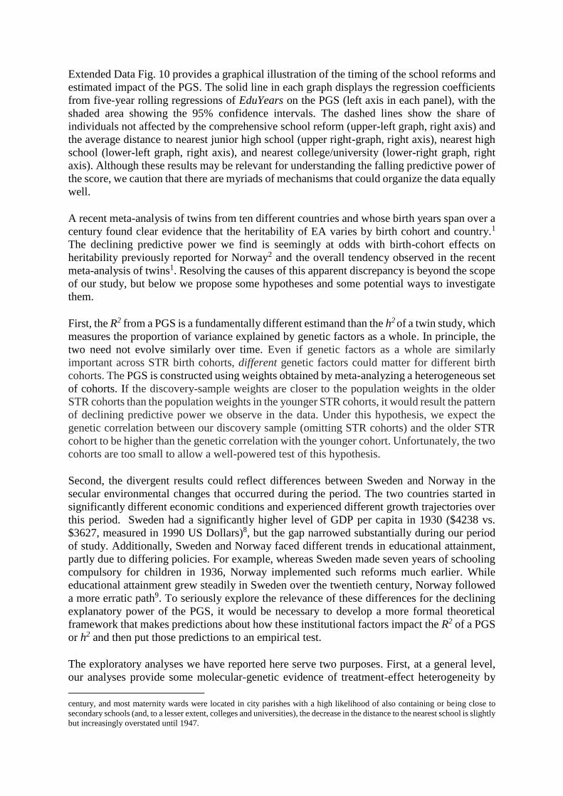
Extended Data Fig. 10 provides a graphical illustration of the timing of the school reforms and

estimated impact of the PGS. The solid line in each graph displays the regression coefficients

from five-year rolling regressions of EduYears on the PGS (left axis in each panel), with the

shaded area showing the 95% confidence intervals. The dashed lines show the share of

individuals not affected by the comprehensive school reform (upper-left graph, right axis) and

the average distance to nearest junior high school (upper right-graph, right axis), nearest high

school (lower-left graph, right axis), and nearest college/university (lower-right graph, right

axis). Although these results may be relevant for understanding the falling predictive power of

the score, we caution that there are myriads of mechanisms that could organize the data equally

well.

A recent meta-analysis of twins from ten different countries and whose birth years span over a

century found clear evidence that the heritability of EA varies by birth cohort and country.1

The declining predictive power we find is seemingly at odds with birth-cohort effects on

heritability previously reported for Norway2 and the overall tendency observed in the recent

meta-analysis of twins1. Resolving the causes of this apparent discrepancy is beyond the scope

of our study, but below we propose some hypotheses and some potential ways to investigate

them.

First, the R2 from a PGS is a fundamentally different estimand than the h2 of a twin study, which

measures the proportion of variance explained by genetic factors as a whole. In principle, the

two need not evolve similarly over time. Even if genetic factors as a whole are similarly

important across STR birth cohorts, different genetic factors could matter for different birth

cohorts. The PGS is constructed using weights obtained by meta-analyzing a heterogeneous set

of cohorts. If the discovery-sample weights are closer to the population weights in the older

STR cohorts than the population weights in the younger STR cohorts, it would result the pattern

of declining predictive power we observe in the data. Under this hypothesis, we expect the

genetic correlation between our discovery sample (omitting STR cohorts) and the older STR

cohort to be higher than the genetic correlation with the younger cohort. Unfortunately, the two

cohorts are too small to allow a well-powered test of this hypothesis.

Second, the divergent results could reflect differences between Sweden and Norway in the

secular environmental changes that occurred during the period. The two countries started in

significantly different economic conditions and experienced different growth trajectories over

this period. Sweden had a significantly higher level of GDP per capita in 1930 ($4238 vs.

$3627, measured in 1990 US Dollars)8, but the gap narrowed substantially during our period

of study. Additionally, Sweden and Norway faced different trends in educational attainment,

partly due to differing policies. For example, whereas Sweden made seven years of schooling

compulsory for children in 1936, Norway implemented such reforms much earlier. While

educational attainment grew steadily in Sweden over the twentieth century, Norway followed

a more erratic path9. To seriously explore the relevance of these differences for the declining

explanatory power of the PGS, it would be necessary to develop a more formal theoretical

framework that makes predictions about how these institutional factors impact the R2 of a PGS

or h2 and then put those predictions to an empirical test.

The exploratory analyses we have reported here serve two purposes. First, at a general level,

our analyses provide some molecular-genetic evidence of treatment-effect heterogeneity by

century, and most maternity wards were located in city parishes with a high likelihood of also containing or being close to

secondary schools (and, to a lesser extent, colleges and universities), the decrease in the distance to the nearest school is slightly

but increasingly overstated until 1947.

birth cohort. We do not think it is appropriate to make general inferences about how the PGS

interacts with birth cohort from a study of a single country. Second, our analyses help lay a

foundation for future, rigorous studies on G×E interactions. Despite enormous enthusiasm,

progress in molecular G×E studies of behavioral traits has been disappointing10. There is now

strong evidence that the false-positive rate in the G×E literature is high: systematic evaluations

find that only about one in four positive findings replicate and that there is clear evidence of

publication bias4. The editor of the field journal Behavior Genetics recently concluded that the

G×E literature is “full of reports that have not stood up to rigorous replication”11. It is widely

understood that a major cause of the disappointing replication record is that most studies have

been dramatically underpowered10,12. The PGS used here may help mitigate this problem, as it

has explanatory power at least an order of magnitude greater than that of single polymorphisms

whose variation has been credibly linked to behavioral phenotypes. Therefore, the PGS we

develop in this paper may prove to be valuable for follow-up studies examining in greater detail

how, and ultimately why, different environmental factors amplify or dampen genetic effects.

References

1. Branigan, A. R., McCallum, K. J. & Freese, J. Variation in the heritability of educational

attainment: an international meta-analysis. Soc. Forces 92, 109–140 (2013).

2. Heath, A., Berg, K., Eaves, L. & Solaas, M. Education policy and the heritability of

educational attainment. Nature 314, 734–736 (1985).

3. Rosenquist, J. N. et al. Cohort of birth modifies the association between FTO genotype

and BMI. Proc. Natl. Acad. Sci. USA 112, 354–359 (2015).

4. Cutler, D. M., Lleras-Muney, A. & Vogl, T. in Oxford Handb. Heal. Econ. (Glied, S. &

Smith, P. C.) 124–163 (Oxford Univ. Press, 2011).

5. Holmlund, H. A Researcher’s Guide to the Swedish Compulsory School Reform.

<http://eprints.lse.ac.uk/19382/1/A_Researcher%27s_Guide_to_the_Swedish_Compul

sory_School_Reform.pdf> (2008).

6. Meghir, C. & Palme, M. Educational reform, ability, and family background. Am. Econ.

Rev. 95, 414–424 (2005).

7. Erikson, R. & Jonsson, J. O. Ursprung och utbildning. Social snedrekrytering till högre

studier. Huvudbetänkande av Utredningen om den sociala snedrekryteringen till högre

studier, SOU 1993:85. (Fritzes offentliga publikationer, 1993).

8. The Maddison-Project, http://www.ggdc.net/maddison/maddison-project/home.htm,

(2013).

9. Lindbekk, T. School reforms in Norway and Sweden, and the redistribution of

educational attainments. Scand. J. Educ. Res. 37, 129–149 (1993).

10. Duncan, L. E. & Keller, M. C. A Critical review of the first 10 years of candidate gene-

by-environment interaction research in psychiatry. Am. J. Psychiatry 168, 1041–1049

(2011).

11. Hewitt, J. K. Editorial policy on candidate gene association and candidate gene-by-

environment interaction studies of complex traits. Behav. Genet. 42, 1–2 (2012).

12. Rietveld, C. A. et al. Replicability and robustness of GWAS for behavioral traits.

Psychol. Sci. 25, 1975–1986 (2014).

Supplementary Notes

8 Author Contributions

Daniel Benjamin, David Cesarini, Tõnu Esko, Magnus Johannesson, Philipp Koellinger, and

Peter Visscher designed and oversaw the study.

The lead analyst responsible for quality control and meta-analyses was Aysu Okbay. She was

assisted by Guo-Bo Chen, Mark Fontana, Tune Pers, and Niels Rietveld.

Jonathan Beauchamp, Patrick Turley, Peter Visscher, and Jian Yang developed and applied

methods to test for population stratification. Zhihong Zhu and Jian Yang provided guidelines

to the cohorts for conducting mixed linear model association analyses.

The genetic overlap analyses were conducted by Mark Fontana and Patrick Turley, and

Jonathan Beauchamp and Patrick Turley developed the analyses of new and existing methods.

Tõnu Esko and James Lee organized and oversaw the bioinformatics analyses, which were

conducted by Jonathan Beauchamp (LD Score partitioning), Johannes H. Brandsma

(enrichment by genes containing de novo causal mutations), Valur Emilsson (brain eQTL),

Mark Fontana (LD Score partitioning), Lude Franke (blood eQTL), Fleur Meddens (Gene

Network, HaploReg, and GWAS catalog look-ups), Geert Meddens (Gene Network look-ups),

Tune Pers (DEPICT, temporal expression), Joe Pickrell (fgwas), Raymond A. Poot (enrichment

by genes containing de novo causal mutations), Pascal Timshel (temporal expression,

enrichment by genes containing de novo causal mutations), Ronald de Vlaming (GREML

partitioning), and Harm-Jan Westra (blood eQTL). James Lee led the writing of the results of

the bioinformatics analyses.

Polygenic-prediction analyses were conducted by Jonathan Beauchamp, Mark Fontana, Peter

Visscher, and Jian Yang.

Jonathan Beauchamp conducted the mediation analyses.

Dalton Conley, Steven F. Lehrer, Karl-Oskar Lindgren, Sven Oskarsson, and Kevin Thom

conducted the analysis of gene×environment interactions.

Replication analyses in the UK Biobank were carried out by Mark Fontana and Niels Rietveld.

Besides the contributions explicitly listed above, Ronald de Vlaming, Mark Fontana, James

Lee, and Niels Rietveld conducted additional analyses for several subsections, including

quality control, population stratification, and genetic overlap. Niels Rietveld prepared the

majority of figures. Olga Rostapshova helped with coordinating among the participating

cohorts.

The Advisory Board of the SSGAC (Dalton Conley, George Davey Smith, Tõnu Esko, Albert

Hofman, Robert Krueger, David Laibson, Sarah Medland, Michelle Meyer, and Peter Visscher)

supported the project in a variety of important ways.

All authors contributed to and critically reviewed the manuscript. Jonathan Beauchamp, Jake

Gratten, James Lee, and Patrick Turley made especially major contributions to the writing and

editing.

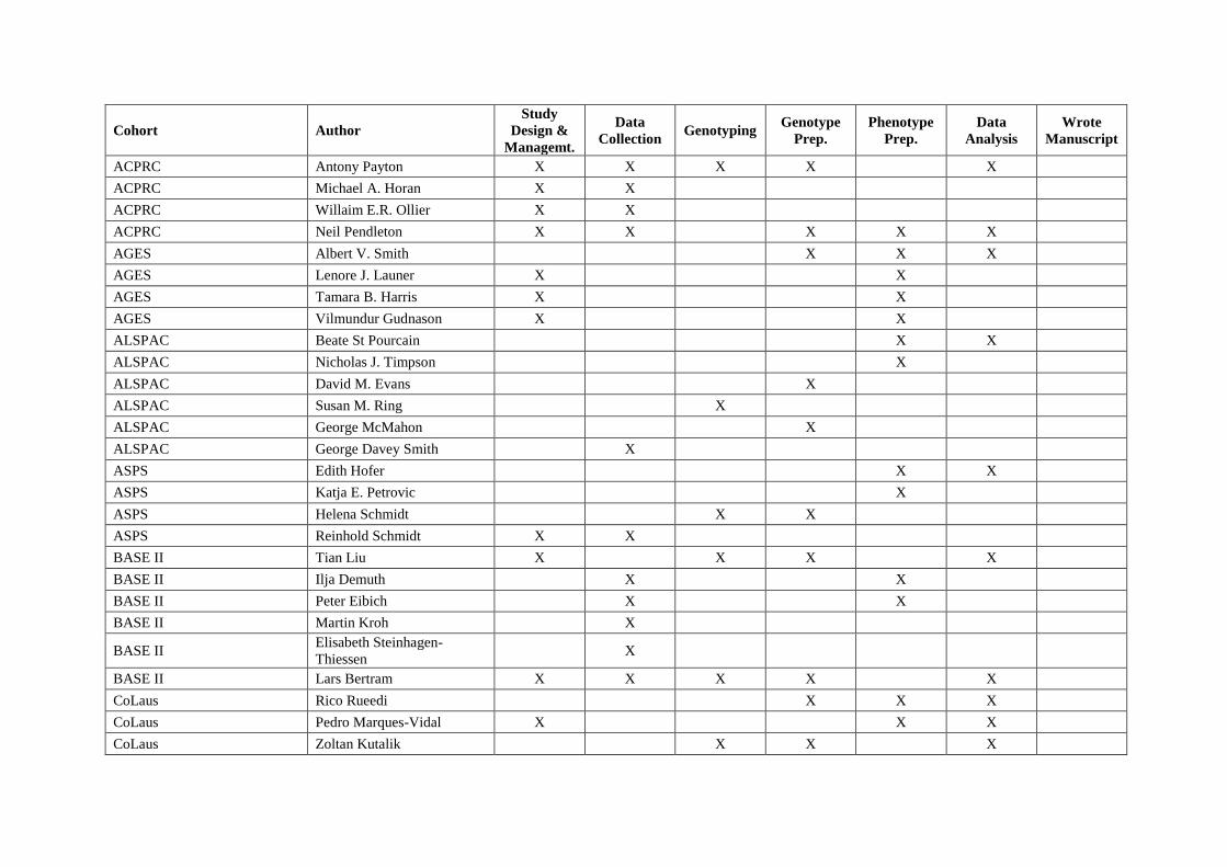
Cohort Author

Study

Design &

Managemt.

Data

Collection Genotyping

Genotype

Prep.

Phenotype

Prep.

Data

Analysis

Wrote

Manuscript

ACPRC Antony Payton X X X X X

ACPRC Michael A. Horan X X

ACPRC Willaim E.R. Ollier X X

ACPRC Neil Pendleton X X X X X

AGES Albert V. Smith X X X

AGES Lenore J. Launer X X

AGES Tamara B. Harris X X

AGES Vilmundur Gudnason X X

ALSPAC Beate St Pourcain X X

ALSPAC Nicholas J. Timpson X

ALSPAC David M. Evans X

ALSPAC Susan M. Ring X

ALSPAC George McMahon X

ALSPAC George Davey Smith X

ASPS Edith Hofer X X

ASPS Katja E. Petrovic X

ASPS Helena Schmidt X X

ASPS Reinhold Schmidt X X

BASE II Tian Liu X X X X

BASE II Ilja Demuth X X

BASE II Peter Eibich X X

BASE II Martin Kroh X

BASE II Elisabeth Steinhagen-

Thiessen X

BASE II Lars Bertram X X X X X

CoLaus Rico Rueedi X X X

CoLaus Pedro Marques-Vidal X X X

CoLaus Zoltan Kutalik X X X

CoLaus Peter Vollenweider X X X

COPSAC2000 Tarunveer S. Ahluwalia X X X

COPSAC2000 Johannes Waage X

COPSAC2000 Klaus Bønnelykke X X X

COPSAC2000 Hans Bisgaard X X X

CROATIA-Korčula Jonathan Marten X X

CROATIA-Korčula Ivana Kolcic X

CROATIA-Korčula Igor Rudan X

CROATIA-Korčula Ozren Polasek X X X

CROATIA-Split Veronique Vitart X

CROATIA-Vis Alan F. Wright X X

deCODE Gudmar Thorleifsson X

deCODE Gyda Bjornsdottir X

deCODE Bjarni Gunnarsson X

deCODE Bjarni V. Halldórsson X

deCODE Augustine Kong X

deCODE Unnur Thorsteinsdottir X X X

deCODE Kari Stefansson X

DHS Juergen Wellmann X X

DHS Klaus Berger X X X X

DHS Peter Lichtner X

EGCUT Evelin Mihailov X

EGCUT Reedik Mägi X

EGCUT Lili Milani X

EGCUT Andres Metspalu X X X

EGCUT Tõnu Esko X X X

ERF Sven J. van der Lee X X

ERF Najaf Amin X X

ERF Cornelia M. van Duijn X X X X

FamHS Aldi T. Kraja X X

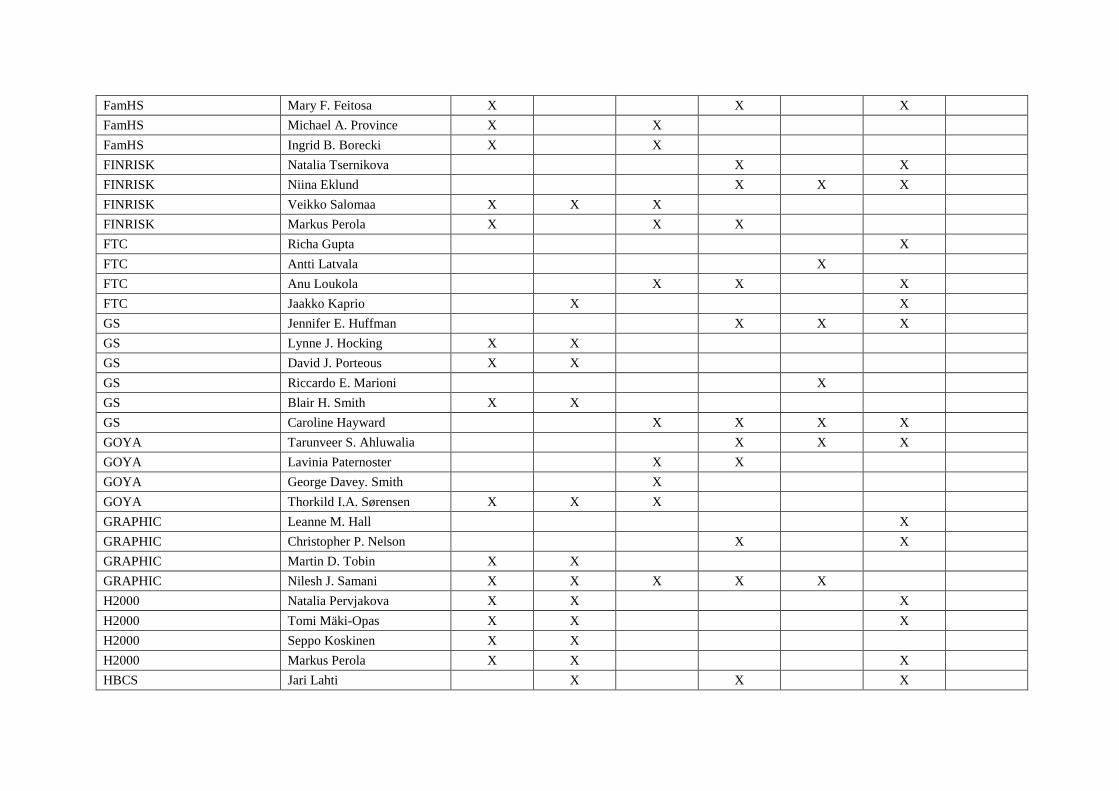
FamHS Mary F. Feitosa X X X

FamHS Michael A. Province X X

FamHS Ingrid B. Borecki X X

FINRISK Natalia Tsernikova X X

FINRISK Niina Eklund X X X

FINRISK Veikko Salomaa X X X

FINRISK Markus Perola X X X

FTC Richa Gupta X

FTC Antti Latvala X

FTC Anu Loukola X X X

FTC Jaakko Kaprio X X

GS Jennifer E. Huffman X X X

GS Lynne J. Hocking X X

GS David J. Porteous X X

GS Riccardo E. Marioni X

GS Blair H. Smith X X

GS Caroline Hayward X X X X

GOYA Tarunveer S. Ahluwalia X X X

GOYA Lavinia Paternoster X X

GOYA George Davey. Smith X

GOYA Thorkild I.A. Sørensen X X X

GRAPHIC Leanne M. Hall X

GRAPHIC Christopher P. Nelson X X

GRAPHIC Martin D. Tobin X X

GRAPHIC Nilesh J. Samani X X X X X

H2000 Natalia Pervjakova X X X

H2000 Tomi Mäki-Opas X X X

H2000 Seppo Koskinen X X

H2000 Markus Perola X X X

HBCS Jari Lahti X X X

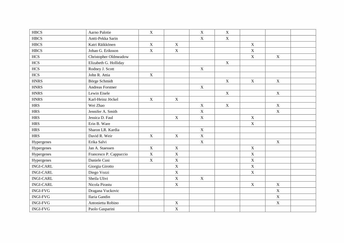
HBCS Aarno Palotie X X X

HBCS Antti-Pekka Sarin X X

HBCS Katri Räikkönen X X X

HBCS Johan G. Eriksson X X X

HCS Christopher Oldmeadow X X

HCS Elizabeth G. Holliday X

HCS Rodney J. Scott X

HCS John R. Attia X

HNRS Börge Schmidt X X X

HNRS Andreas Forstner X

HNRS Lewin Eisele X X

HNRS Karl-Heinz Jöckel X X

HRS Wei Zhao X X X

HRS Jennifer A. Smith X X

HRS Jessica D. Faul X X X

HRS Erin B. Ware X

HRS Sharon LR. Kardia X

HRS David R. Weir X X X

Hypergenes Erika Salvi X X

Hypergenes Jan A. Staessen X X X

Hypergenes Francesco P. Cappuccio X X X

Hypergenes Daniele Cusi X X X

INGI-CARL Giorgia Girotto X X

INGI-CARL Diego Vozzi X X

INGI-CARL Sheila Ulivi X X

INGI-CARL Nicola Pirastu X X X

INGI-FVG Dragana Vuckovic X

INGI-FVG Ilaria Gandin X

INGI-FVG Antonietta Robino X X

INGI-FVG Paolo Gasparini X

KORA Clemens Baumbach X

KORA Konstantin Strauch X

KORA Thomas Meitinger X

KORA Christa Meisinger X

KORA Christian Gieger X

LBC Sarah E. Harris X X X X X

LBC Gail Davies X X X

LBC David CM. Liewald X X

LBC Ian J. Deary X X

LifeLines Peter J. van der Most X

LifeLines Judith M. Vonk X X

LifeLines Behrooz Z. Alizadeh X X X

LifeLines Ute Bultmann X X

LifeLines Behrooz Z. Alizadeh X X X X X

LifeLines Rudolf A. de Boer X X X X X

LifeLines H Marike. Boezen X X X X X

LifeLines Marcel Bruinenberg X X X X X

LifeLines Lude Franke X X X X X

LifeLines Pim van. der Harst X X X X X

LifeLines Hans L. Hillege X X X X X

LifeLines Melanie M. van der Klauw X X X X X

LifeLines Gerjan Navis X X X X X

LifeLines Johan Ormel X X X X X

LifeLines Dirkje S. Postma X X X X X

LifeLines Judith G.M. Rosmalen X X X X X

LifeLines Joris P. Slaets X X X X X

LifeLines Harold Snieder X X X X X

LifeLines Ronald P. Stolk X X X X X

LifeLines Bruce H.R. Wolffenbuttel X X X X X

LifeLines Cisca Wijmenga X X X X X

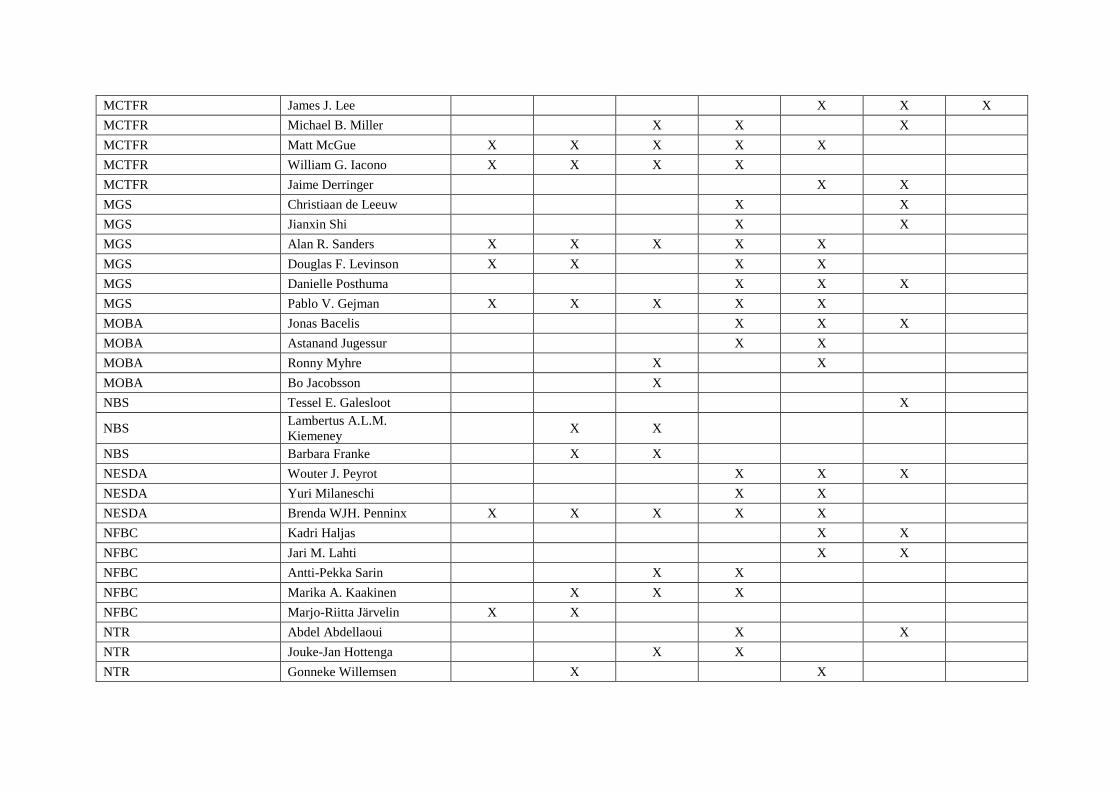
MCTFR James J. Lee X X X

MCTFR Michael B. Miller X X X

MCTFR Matt McGue X X X X X

MCTFR William G. Iacono X X X X

MCTFR Jaime Derringer X X

MGS Christiaan de Leeuw X X

MGS Jianxin Shi X X

MGS Alan R. Sanders X X X X X

MGS Douglas F. Levinson X X X X

MGS Danielle Posthuma X X X

MGS Pablo V. Gejman X X X X X

MOBA Jonas Bacelis X X X

MOBA Astanand Jugessur X X

MOBA Ronny Myhre X X

MOBA Bo Jacobsson X

NBS Tessel E. Galesloot X

NBS Lambertus A.L.M.

Kiemeney X X

NBS Barbara Franke X X

NESDA Wouter J. Peyrot X X X

NESDA Yuri Milaneschi X X

NESDA Brenda WJH. Penninx X X X X X

NFBC Kadri Haljas X X

NFBC Jari M. Lahti X X

NFBC Antti-Pekka Sarin X X

NFBC Marika A. Kaakinen X X X

NFBC Marjo-Riitta Järvelin X X

NTR Abdel Abdellaoui X X

NTR Jouke-Jan Hottenga X X

NTR Gonneke Willemsen X X

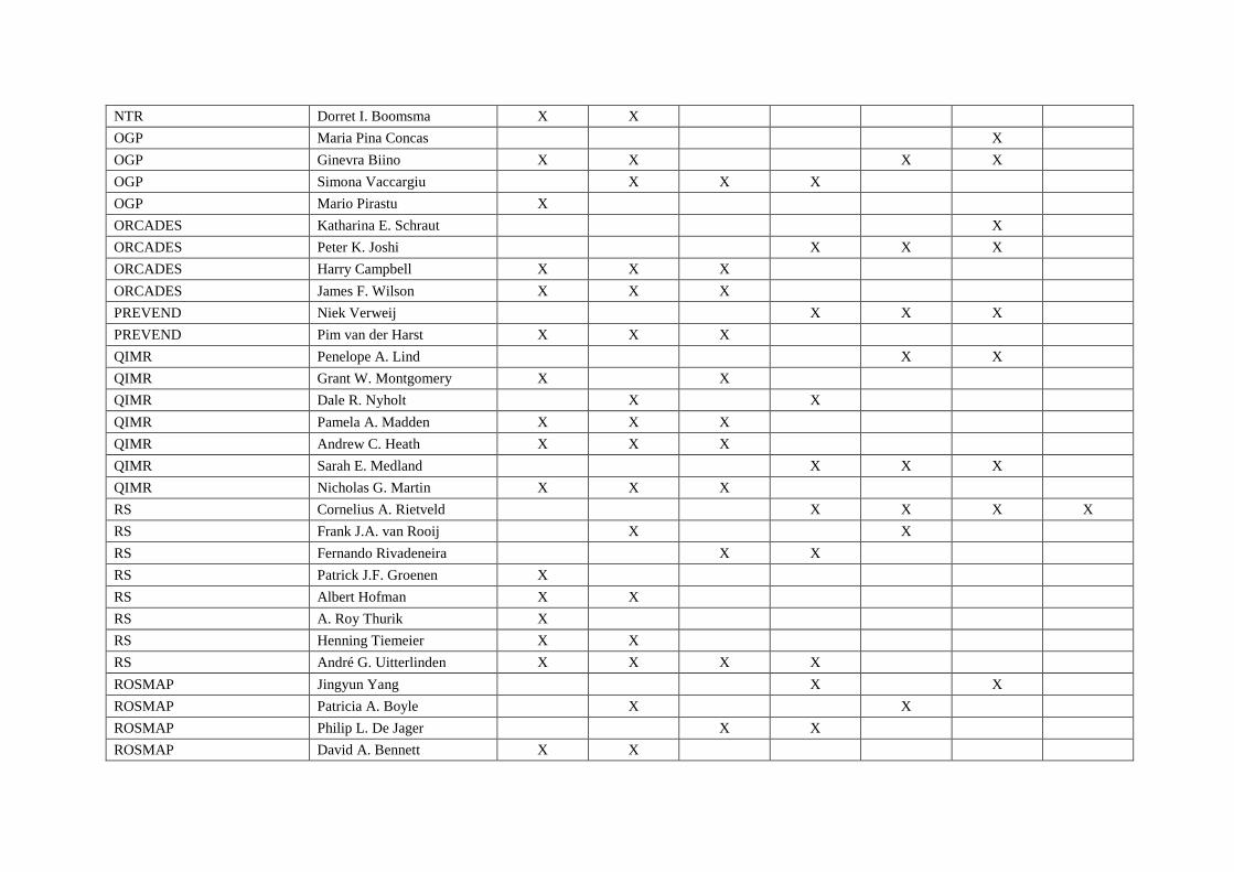
NTR Dorret I. Boomsma X X

OGP Maria Pina Concas X

OGP Ginevra Biino X X X X

OGP Simona Vaccargiu X X X

OGP Mario Pirastu X

ORCADES Katharina E. Schraut X

ORCADES Peter K. Joshi X X X

ORCADES Harry Campbell X X X

ORCADES James F. Wilson X X X

PREVEND Niek Verweij X X X

PREVEND Pim van der Harst X X X

QIMR Penelope A. Lind X X

QIMR Grant W. Montgomery X X

QIMR Dale R. Nyholt X X

QIMR Pamela A. Madden X X X

QIMR Andrew C. Heath X X X

QIMR Sarah E. Medland X X X

QIMR Nicholas G. Martin X X X

RS Cornelius A. Rietveld X X X X

RS Frank J.A. van Rooij X X

RS Fernando Rivadeneira X X

RS Patrick J.F. Groenen X

RS Albert Hofman X X

RS A. Roy Thurik X

RS Henning Tiemeier X X

RS André G. Uitterlinden X X X X

ROSMAP Jingyun Yang X X

ROSMAP Patricia A. Boyle X X

ROSMAP Philip L. De Jager X X

ROSMAP David A. Bennett X X

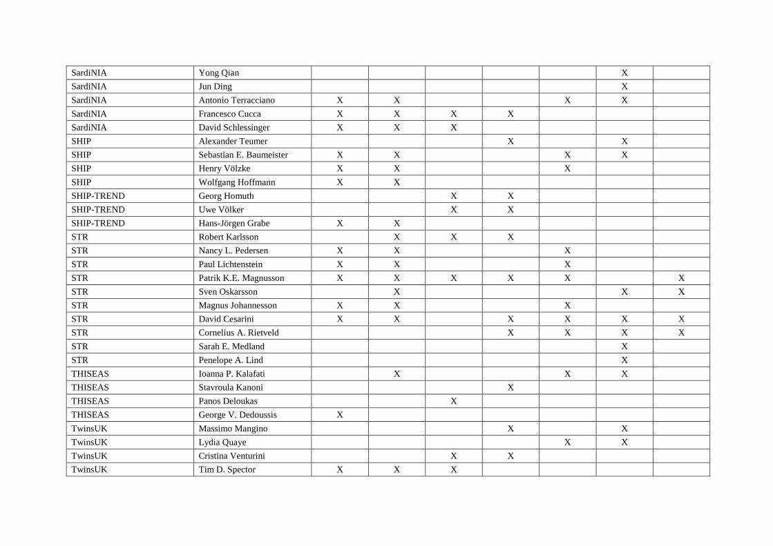
SardiNIA Yong Qian X

SardiNIA Jun Ding X

SardiNIA Antonio Terracciano X X X X

SardiNIA Francesco Cucca X X X X

SardiNIA David Schlessinger X X X

SHIP Alexander Teumer X X

SHIP Sebastian E. Baumeister X X X X

SHIP Henry Völzke X X X

SHIP Wolfgang Hoffmann X X

SHIP-TREND Georg Homuth X X

SHIP-TREND Uwe Völker X X

SHIP-TREND Hans-Jörgen Grabe X X

STR Robert Karlsson X X X

STR Nancy L. Pedersen X X X

STR Paul Lichtenstein X X X

STR Patrik K.E. Magnusson X X X X X X

STR Sven Oskarsson X X X

STR Magnus Johannesson X X X

STR David Cesarini X X X X X X

STR Cornelius A. Rietveld X X X X

STR Sarah E. Medland X

STR Penelope A. Lind X

THISEAS Ioanna P. Kalafati X X X

THISEAS Stavroula Kanoni X

THISEAS Panos Deloukas X

THISEAS George V. Dedoussis X

TwinsUK Massimo Mangino X X

TwinsUK Lydia Quaye X X

TwinsUK Cristina Venturini X X

TwinsUK Tim D. Spector X X X

58BC-WTCCC and DIL Momoko Horikoshi X

58BC-WTCCC and DIL Christine Power X X X

58BC-WTCCC and DIL Elina Hyppönen X X X

YFS Olli Raitakari X X X X

YFS Mika Kähönen X X X

YFS Liisa Keltigangas-Järvinen X X X

YFS Terho Lehtimäki X X X X X X

23andMe, Inc. Nicholas A. Furlotte X

23andMe, Inc. Joyce Y. Tung X

23andMe, Inc. David A. Hinds X

9 Additional acknowledgments

ACPRC (Age and Cognitive Performance Research Cohort) – Phenotype collection in the

Age and Cognitive Performance Research Cohort (ACPRC) Manchester and Newcastle

Longitudinal Studies of Aging was supported by Social Science Research Council, Medical

Research Council, Economic and Social Research Council, Research into Ageing, Wellcome

Trust and Unilever plc. Genotyping of the cohort was supported by the UK’s Biotechnology

and Biological Sciences Research Council (BB.F022441/1) and analysis supported by the Joint

Research Council MRC Late Life Health and Wellbeing fRaill project (MRC G100137/1).

External researchers can discuss access to the data from this study by contacting Dr Neil

Pendleton at neil.pendleton@manchester.ac.uk.

AGES (Age, Gene/Environment Susceptibility-Reykjavik Study) – AGES is funded by

NIH contract N01-AG-12100, the NIA Intramural Research Program, Hjartavernd (the

Icelandic Heart Association), and the Althingi (the Icelandic Parliament). Genotyping was

conducted at the NIA IRP Laboratory of Neurogenetics. Researchers interested in using the

AGES data must obtain approval from the AGES study group. Researchers using the data are

required to follow the terms of a research agreement between them and the AGES investigators.

In accordance with Icelandic law, individual level data cannot be released to external

investigators, only summary GWAS results. Investigators interested in collaboration can work

on individual data at the Icelandic Heart Association site. For further information contact Prof.

V. Gudnason (v.gudnason@hjarta.is).

ALSPAC (Avon Longitudinal Study of Parents and Children) – We are extremely grateful

to all the families who took part in this study, the midwives for their help in recruiting them,

and the whole ALSPAC team, which includes interviewers, computer and laboratory

technicians, clerical workers, research scientists, volunteers, managers, receptionists and

nurses. The Centre National de Génotypage (CNG) carried out DNA genotyping on the

Illumina Human660W-Quad array, and genotypes were called with Illumina GenomeStudio

supported by the Wellcome Trust (WT088806). The UK Medical Research Council and the

Wellcome Trust (Grant ref: 102215/2/13/2) and the University of Bristol provide core support

for ALSPAC. This work was also supported by the Medical Research Council Integrative

Epidemiology Unit (MC_UU_12013/1-9). This publication is the work of the authors and they

will serve as guarantors for the contents of this paper. ALSPAC summary data will be published

on the data repository at data.bris.ac.uk. Please note that the study website contains details of

all the data that is available through a fully searchable data dictionary. Ethical approval for the

study was obtained from the ALSPAC Ethics and Law Committee and the Local Research

Ethics Committees.

ASPS (Austrian Stroke Prevention Study) – The research reported in this article was funded

by the Austrian Science Fond (FWF) grant number P20545-P05 and P13180. The Medical

University of Graz supports the databank of the ASPS. The authors thank the staff and the

participants of the ASPS for their valuable contributions. The data file of ASPS regarding all

analyses of this manuscript can be provided to external researchers upon request.

BASE-II (The Berlin Aging Study II) – BASE-II has been funded by the German Federal

Ministry of Education and Research (BMBF) and has been formally divided into four

subprojects: “Psychology & Project Coordination and Database” (Max Planck Institute for

Human Development [MPIB], grant number 16SV5837), “Survey Methods and Social

Science” (German Institute for Economic Research and Socioeconomic Panel [SOEP/DIW],

grant number 16 SV5537), Medicine and Geriatrics (Charité – Universitätsmedizin, Berlin

[Charité], grant number 16SV5536K), and “Molecular Genetics” (Max Planck Institute for

Molecular Genetics, now University of Lübeck [MPIMG-ULBC], grant number 16SV5538).

External scientists can apply to the Steering Committee of BASE-II for data access. Although

the data are available for other parties are scientific data and not personal contact data, the

scientific data are subject to a security level as if they were personal data to ensure that the

BASE-II Steering Committee sufficiently protects the large volume of data collected from each

BASE-II participant. All existing variables are documented in a handbook. Contact: Katrin

Schaar, scientific coordinator, schaar@mpib-berlin.mpg.de.

CoLaus (Cohorte Lausannoise) – The CoLaus study was and is supported by research grants

from GlaxoSmithKline, the Faculty of Biology and Medicine of Lausanne, and the Swiss

National Science Foundation (grants 33CSCO-122661, 33CS30-139468 and 33CS30-148401).

The authors also express their gratitude to the participants in the Lausanne CoLaus study and

to the investigators who have contributed to the recruitment, in particular research nurses

Yolande Barreau, Anne-Lise Bastian, Binasa Ramic, Martine Moranville, Martine Baumer,

Marcy Sagette, Jeanne Ecoffey and Sylvie Mermoud for data collection. We would also like to

thank Gérard Waeber, Vincent Mooser and Dawn Waterworth, co-PIs of the study. Researchers

must obtain approval from the Steering Committee of the CoLaus Study and from the

Institutional Ethics Committee of the University in Lausanne, Switzerland. Researchers using

the data are required to follow the terms of an Assistance Agreement containing a number of

clauses designed to ensure protection of privacy and compliance with relevant laws. For further

information go to www.colaus.ch or contact Peter Vollenweider

(peter.vollenweider@chuv.ch).

COPSAC2000 (Copenhagen Prospective Studies on Asthma in Children) – We greatly

acknowledge the private and public research funding allocated to COPSAC and listed on

www.copsac.com, with special thanks to The Lundbeck Foundation; Danish State Budget;

Danish Council for Strategic Research; The Danish Council for Independent Research and The

Capital Region Research Foundation as core supporters. The funding agencies did not have

any influence on study design, data collection and analysis, decision to publish or preparation

of the manuscript. No pharmaceutical company was involved in the study. We gratefully

express our gratitude to the participants of the COPSAC2000 cohort study for all their support

and commitment. We also acknowledge and appreciate the unique efforts of the COPSAC

research team. External researchers who wish to obtain access to COPSAC2000’s data or EA2

results may contact Tarunveer Singh Ahluwalia (tarun.ahluwalia@dbac.dk).

CROATIA_Korcula (Croatia Korcula) – We would like to acknowledge the invaluable

contributions of the recruitment team in Korcula, the administrative teams in Croatia and

Edinburgh and the people of Korcula. The CROATIA-Korcula study was funded by grants

from the Medical Research Council (UK), European Commission Framework 6 project

EUROSPAN (Contract No. LSHG-CT-2006-018947), FP7 project BBMRI-LPC (grant

313010), Ministry of Science, Education and Sports of the Republic of Croatia (grant 108-

1080315-0302) and the Croatian Science Foundation (grant 8875). External researchers who

wish to obtain access to CROATIA-Korcula’s data or EA2 results may contact Ozren Polasek,

ozren.polasek@mefst.hr.

deCODE (deCODE Genetics) – All deCODE collaborators in this study are employees of

deCODE Genetics/Amgen, Inc. External researchers who wish to obtain access to data or EA2

results may contact Gudmar Thorleifsson gudmar.thorleifsson@decode.is.

DHS (Dortmund Health Study) – The collection of sociodemographic and clinical data in the

Dortmund Health Study was supported by the German Migraine & Headache Society (DMKG)

and by unrestricted grants of equal share from Almirall, Astra Zeneca, Berlin Chemie,

Boehringer, Boots Health Care, Glaxo-Smith-Kline, Janssen Cilag, McNeil Pharma, MSD

Sharp & Dohme and Pfizer to the University of Muenster. Blood collection in the Dortmund

Health Study was done through funds from the Institute of Epidemiology and Social Medicine

University of Muenster. Genotyping for the Human Omni Chip was supported by the German

Ministry of Education and Research (BMBF, grant no. 01ER0816). Researchers interested in

using DHS data are required to sign and follow the terms of a Cooperation Agreement that

includes a number of clauses designed to ensure protection of privacy and compliance with

relevant laws. For further information, contact Klaus Berger (bergerk@uni-muenster.de).

EGCUT (Estonian Genome Center) – EGCUT received targeted financing from Estonian

Research Council grant IUT20-60, Center of Excellence in Genomics (EXCEGEN) and

University of Tartu (SP1GVARENG). We acknowledge EGCUT technical personnel,

especially Mr V. Soo and S. Smit. Data analyzes were carried out in part in the High

Performance Computing Center of University of Tartu. For more information, please contact

Tõnu Esko (tesko@broadinstitute.org).

ERF (Erasmus Rucphen Family Study) – The ERF study as a part of EUROSPAN (European

Special Populations Research Network) was supported by European Commission FP6 STRP

grant number 018947 (LSHG-CT-2006-01947) and also received funding from the European

Community's Seventh Framework Programme (FP7/2007-2013)/grant agreement HEALTH-

F4-2007-201413 by the European Commission under the programme "Quality of Life and

Management of the Living Resources" of 5th Framework Programme (no. QLG2-CT-2002-

01254). High-throughput analysis of the ERF data was supported by joint grant from

Netherlands Organization for Scientific Research and the Russian Foundation for Basic

Research (NWO-RFBR 047.017.043). Exome sequencing analysis in ERF was supported by

the ZonMw grant (project 91111025). We are grateful to all study participants and their

relatives, general practitioners and neurologists for their contributions and to P. Veraart for her

help in genealogy, J. Vergeer for the supervision of the laboratory work and P. Snijders for his

help in data collection. Najaf Amin is supported by the Netherlands Brain Foundation (project

number F2013(1)-28). The ERF study genome-wide array data and phenotype data (age and

gender) is archived in European Genome-Phenome Database (EGA). The study is archived in

the DAC named Erasmus Rucphen Family Study with the accession code: EGAS00001001134.

Researchers who wish to use other phenotypic data of the Erasmus Rucphen Family Study

must seek approval from the management team of the Erasmus Rucphen Family study. They

are advised to contact the study PI, professor Cornelia van Duijn (c.vanduijn@erasmusmc.nl).

FamHS (Family Heart Study) – Family Heart Study is supported in part by NIDDK grant

1R01DK8925601 (IBB). Data and results are available directly from the investigators (contact

IBB).

FINRISK (FINRISK) – The FINRISK cohorts have been mainly funded by budgetary funds

from the National Institute for Health and Welfare. Additional funding has been obtained from

the Academy of Finland (grant # 139635 and #269517), The EU FP7 under grant agreements

nr. 313010 (BBMRI-LPC), nr. 305280 (MIMOmics), and nr. 261433 (BioSHaRE-EU), the

Yrjö Jahnsson Foundation, the Juho Vainio Foundation and from the Finnish Foundation for

Cardiovascular Research. Data used for this study can be made available on request to the

FINRISK Management Group according to the given ethical guidelines and Finnish legislation.

FTC (Finnish Twin Registry) – We warmly thank the participating twin pairs and their family

members for their contribution. We would like to express our appreciation to the skilled study

interviewers A-M Iivonen, K Karhu, H-M Kuha, U Kulmala-Gråhn, M Mantere, K Saanakorpi,

M Saarinen, R Sipilä, L Viljanen, and E Voipio. Anja Häppölä and Kauko Heikkilä are

acknowledged for their valuable contribution in recruitment, data collection, and data

management. Antti-Pekka Sarin and Samuli Ripatti are acknowledged for genotype quality

control and imputation. Phenotyping and genotyping of the Finnish twin cohorts has been

supported by the Academy of Finland Center of Excellence in Complex Disease Genetics

grants 213506, 129680; the Academy of Finland grants 100499, 205585, 118555, 141054,

265240, 263278 and 264146 (to prof. Jaakko Kaprio); NIH Grant DA12854 (to prof. Pamela

A.F. Madden, Department of Psychiatry, Washington University School of Medicine, Saint

Louis, MO, USA); Sigrid Juselius Foundation (to prof. Jaakko Kaprio); Global Research

Award for Nicotine Dependence, Pfizer Inc. (to prof. Jaakko Kaprio), the Wellcome Trust

Sanger Institute, Hinxton, Cambridge, UK; and the Broad Institute, Cambridge, MA, USA.

Association analyses and genotype imputation were run at the ELIXIR Finland node hosted at

CSC - IT Center for Science for ICT resources. Researchers interested in using FTC data must

obtain approval from the Data Access Committee (DAC) of the Institute for Molecular

Medicine Finland (FIMM). For more details please contact the chair of the FIMM DAC

(hannele.laivuori@helsinki.fi). Note that anonymized individual level data can only be released

after study has been approved by Research Ethics Committee of University of Helsinki and

must be carried out in collaboration with FTC investigators. To ensure protection of privacy

and compliance with national data protection legislation, a data use/transfer agreement is

needed, the content and specific clauses of which will depend on the nature of the requested

data. For further information please contact Jaakko Kaprio (jaakko.kaprio@helsinki.fi).

GS (Generation Scotland) – Generation Scotland received core funding from the Chief

Scientist Office of the Scottish Government Health Directorate CZD/16/6 and the Scottish

Funding Council HR03006. Genotyping of the GS:SFHS samples was carried out by the

Genetics Core Laboratory at the Wellcome Trust Clinical Research Facility, Edinburgh,

Scotland and was funded by the UK’s Medical Research Council. Ethics approval for the study

was given by the NHS Tayside committee on research ethics (reference 05/S1401/89). We are

grateful to all the families who took part, the general practitioners and the Scottish School of

Primary Care for their help in recruiting them, and the whole Generation Scotland team, which

includes interviewers, computer and laboratory technicians, clerical workers, research

scientists, volunteers, managers, receptionists, healthcare assistants and nurses. Information on

applications for access to Generation Scotland data can be found at

http://www.generationscotland.org.

GOYA (Genetics of Overweight Young Adults) - This study was conducted as part of the

activities of the Danish Obesity Research Centre (DanORC, www.danorc.dk) and the MRC

centre for Causal Analyses in Translational Epidemiology (MRC CAiTE), and the Gene-diet

Interactions in Obesity project (GENDINOB, www.gendinob.dk). LP was supported by and

the genotyping for GOYA was funded by the Wellcome Trust (WT 084762MA). LP was

supported by a Medical Council New Investigator Award (MRC G0800582 to DME). We

thank all the participants of the study. TSA was also funded by the GENDINOB project and

acknowledges the same. External researchers who wish to obtain access to GOYA (male) data

or EA2 results may contact Tarunveer Singh Ahluwalia (tarun.ahluwalia@dbac.dk or

veertarun@gmail.com).

GRAPHIC (Genetic Regulation of Arterial Pressure in Humans in the Community) –

Recruitment and genotyping for the GRAPHIC cohort were funded by the British Heart

Foundation (BHF). NJS holds a Chair funded by the BHF and is a UK National Institute for

Health Research (NIHR) Senior Investigator. CPN is supported by the BHF. MDT holds a

Medical Research Council Senior Clinical Fellowship (G0902313). LMH is supported by the

NIHR Leicester Cardiovascular Biomedical Research Unit. External researchers who wish to

obtain access to GRAPHIC data or EA2 results may contact Prof. Nilesh Samani

(njs@le.ac.uk).

Health 2000 – The Health 2000 Study was mainly funded from the budget of the National

Institute for Health and Welfare (THL). Additional funding was received from the Finnish

Centre for Pensions, the Social Insurance Institution of Finland, the Local Government

Pensions Institution, the National Research and Development Centre for Welfare and Health,

the Finnish Dental Association, the Finnish Dental Society, Statistics Finland, the Finnish

Institute for Occupational Health, The Finnish Work Environment Fund, the UKK Institute for

Health Promotion Research and the Occupational Safety and Health Fund of the State Sector.

The data used for this study can be made available on request to the Health 2000/2011 scientific

committee according to the ethical and research guidelines (www.terveys2011.info/aineisto)

as well as Finnish legislation.

HBCS (Helsinki Birth Cohort Study) – We thank all study participants as well as everybody

involved in the Helsinki Birth Cohort Study. Helsinki Birth Cohort Study has been supported

by grants from the Academy of Finland, the Finnish Diabetes Research Society, Folkhälsan

Research Foundation, Novo Nordisk Foundation, Finska Läkaresällskapet, Signe and Ane

Gyllenberg Foundation, University of Helsinki, Ministry of Education, Ahokas Foundation,

Emil Aaltonen Foundation. Researchers interested in using HBCS data must obtain approval

from the Steering Committee of the Helsinki Birth Cohort Study. Researchers using the data

are required to follow the terms in a number of clauses designed to ensure protection of privacy

and compliance with relevant Finnish laws. For further information, contact Johan Eriksson

(johan.eriksson@helsinki.fi).

HCS (Hunter Community Study) – The authors would like to thank the men and women

participating in the HCS as well as all the staff, investigators and collaborators who have

supported or been involved in the project to date. The University of Newcastle provided $300

000 from its Strategic Initiatives Fund, and $600 000 from the Gladys M Brawn Senior

Research Fellowship scheme; the Vincent Fairfax Family Foundation, a private philanthropic

trust, provided $195 000; The Hunter Medical Research Institute provided media support

during the initial recruitment of participants; and Dr Anne Crotty, Prof. Rodney Scott and

Associate Prof. Levi provided financial support towards freezing costs for the long-term

storage of participant blood samples. External researchers may request data access from Chris

Oldmeadow, Elizabeth Holliday or John Attia by email.

HNRS (Heinz Nixdorf Recall Study) – The Heinz Nixdorf Recall Study thank the Heinz

Nixdorf Foundation (Germany), the German Federal Ministry of Research and Education and

projects SI 236/8-1 and SI 236/9-1 from the German Research Council for the generous support

of this study. We acknowledge the support of the Sarstedt AG & Co. (Nümbrecht, Germany)

for laboratory equipment. The genotyping was partially supported by the German Federal

Ministry of Education and Research (BMBF) through the Integrated Network IntegraMent

(Integrated Understanding of Causes and Mechanisms in Mental Disorders), under the auspices

of the e:Med Programme (grant 01ZX1314A). We are indebted to all study participants and to

the dedicated personnel of the study centre of the Heinz Nixdorf Recall study. Advisory Board:

Meinertz T, Hamburg, Germany (Chair); Bode C, Freiburg, Germany; de Feyter PJ, Rotterdam,

Netherlands; Güntert B, Hall i.T., Austria; Gutzwiller F, Bern, Switzerland; Heinen H, Bonn,

Germany; Hess O, Bern, Switzerland; Klein B, Essen, Germany; Löwel H, Neuherberg,

Germany; Reiser M, Munich, Germany; Schwaiger M, Munich, Germany; Steinmüller C,

Bonn, Germany; Theorell T, Stockholm, Sweden; Willich SN, Berlin, Germany. External

researchers can send their inquiry to boerge.schmidt@uk-essen.de to get access to the study

results.

HRS (Health and Retirement Study) – HRS is supported by the National Institute on Aging

(NIA U01AG009740). The genotyping was funded separately by the National Institute on

Aging (RC2 AG036495, RC4 AG039029). Our genotyping was conducted by the NIH Center

for Inherited Disease Research (CIDR) at Johns Hopkins University. Genotyping quality

control and final preparation of the data were performed by the Genetics Coordinating Center

at the University of Washington. Genotype data can be accessed via the database of Genotypes

and Phenotypes (dbGaP, http://www.ncbi.nlm.nih.gov/gap, accession number

phs000428.v1.p1). Researchers who wish to link genetic data with other HRS measures that

are not in dbGaP, such as educational attainment, must apply for access from HRS. See the

HRS website (http://hrsonline.isr.umich.edu/gwas) for details.

HYPERGENES - The European Union (FP7-HEALTH-F4-2007-201550-HYPEREGENS,

HEALTH-2011.2.4.2-2-EU-MASCARA, HEALTH-F7-305507 HOMAGE and the European

Research Council Advanced Researcher Grant-2011-294713-EPLORE). InterOmics project

(PB05 MIUR-CNR Italian Flagship Project). The Fonds voor Wetenschappelijk Onderzoek

Vlaanderen, Ministry of the Flemish Community, Brussels, Belgium (G.0881.13 and

G.088013). External researchers can discuss access to the data from this study by contacting

Daniele Cusi (daniele.cusi@unimi.it).

INGI-CARL, INGI-FVG (Italian Network of Genetic Isolates—Carlantino, Friuli

Venezia Giulia) – We would like to acknowledge the following funds: Italian Ministry of

Health RC n.1/2014 Linea 3. Access to our data is usually available upon request. For more

information, please contact Dragana Vuckovic (dragana.vuckovic@burlo.trieste.it).

The KORA research platform (KORA, Cooperative Research in the Region of Augsburg)

– KORA was initiated and financed by the Helmholtz Zentrum München - German Research

Center for Environmental Health, which is funded by the German Federal Ministry of

Education and Research and by the State of Bavaria. Furthermore, KORA research was

supported within the Munich Center of Health Sciences (MC Health), Ludwig-Maximilians-

Universität, as part of LMUinnovativ. External researchers can apply for KORA data or our

EA2.0 results via our KORA.PASST project application self-service tool at https://helmholtz-

muenchen.managed-otrs.com/otrs/customer.pl.

LBC (Lothian Birth Cohort) – We thank the cohort participants and team members who

contributed to these studies. Phenotype collection in the Lothian Birth Cohort 1921 was

supported by the UK’s Biotechnology and Biological Sciences Research Council (BBSRC),

The Royal Society, and The Chief Scientist Office of the Scottish Government. Phenotype

collection in the Lothian Birth Cohort 1936 was supported by Age UK (The Disconnected

Mind project). Genotyping of the cohorts was funded by the BBSRC. The work was

undertaken by The University of Edinburgh Centre for Cognitive Ageing and Cognitive

Epidemiology, part of the cross council Lifelong Health and Wellbeing Initiative

(MR/K026992/1). Funding from the BBSRC and Medical Research Council (MRC) is

gratefully acknowledged. The raw data collected in the course of our research with human

participants is available upon request (please contact, by e-mail, Professor Ian Deary, at the

University of Edinburgh, and ask for a ‘Lothian Birth Cohort Data Request Form’). The process

is facilitated by a full-time Lothian Birth Cohort database manager. Such proposals, when

approved, are conducted in collaboration with appropriate members of the Lothian Birth Cohort

study team.

LifeLines (LifeLines) – Expanded Banner or Group Author: Behrooz Z Alizadeh (1), Rudolf

A de Boer (2), H Marike Boezen (1), Marcel Bruinenberg (3), Lude Franke (4), Pim van der

Harst (2), Hans L Hillege (1,2), Melanie M van der Klauw (5), Gerjan Navis (6), Johan Ormel

(7), Dirkje S Postma (8), Judith GM Rosmalen (7), Joris P Slaets (9), Harold Snieder (1),

Ronald P Stolk (1), Bruce HR Wolffenbuttel (5), Cisca Wijmenga (4).

(1) Department of Epidemiology, University of Groningen, University Medical Center

Groningen, The Netherlands

(2) Department of Cardiology, University of Groningen, University Medical Center

Groningen, The Netherlands

(3) LifeLines Cohort Study, University of Groningen, University Medical Center Groningen,

The Netherlands

(4) Department of Genetics, University of Groningen, University Medical Center Groningen,

The Netherlands

(5) Department of Endocrinology, University of Groningen, University Medical Center

Groningen, The Netherlands

(6) Department of Internal Medicine, Division of Nephrology, University of Groningen,

University Medical Center Groningen, The Netherlands

(7) Interdisciplinary Center of Psychopathology of Emotion Regulation (ICPE), Department of

Psychiatry, University of Groningen, University Medical Center Groningen, The Netherlands

(8) Department of Pulmonology, University of Groningen, University Medical Center

Groningen, The Netherlands

(9) University Center for Geriatric Medicine, University of Groningen, University Medical

Center Groningen, The Netherlands

The LifeLines Cohort Study, and generation and management of GWAS genotype data for the

LifeLines Cohort Study is supported by the Netherlands Organization of Scientific Research

NWO (grant 175.010.2007.006), the Economic Structure Enhancing Fund (FES) of the Dutch

government, the Ministry of Economic Affairs, the Ministry of Education, Culture and Science,

the Ministry for Health, Welfare and Sports, the Northern Netherlands Collaboration of

Provinces (SNN), the Province of Groningen, University Medical Center Groningen, the

University of Groningen, Dutch Kidney Foundation and Dutch Diabetes Research Foundation.

We thank Behrooz Z. Alizadeh, Annemieke Boesjes, Marcel Bruinenberg, Noortje Festen, Pim

van der Harst, Ilja Nolte, Lude Franke, Mitra Valimohammadi for their help in creating the

GWAS database, and Rob Bieringa, Joost Keers, René Oostergo, Rosalie Visser, Judith Vonk

for their work related to data-collection and validation. The authors are grateful to the study

participants, the staff from the LifeLines Cohort Study and the contributing research centers

delivering data to LifeLines and the participating general practitioners and pharmacists. All

data and samples collected by LifeLines are available to scientific researchers worldwide. It is

also possible to prospectively collect additional data and samples in a selected group of

LifeLines participants in an add-in study. Researchers can apply for data, samples or an add-

on study by filling in the application form for research and submitting the completed form

through our data catalogue, together with a selection of the requested data. Please contact dr.

Salome Scholtens at s.scholtens@umcg.nl, when you may need more specific information.

MCTFR (The Minnesota Center for Twin and Family Research) – MCTFR was supported

in part by USPHS Grants from the National Institute on Alcohol Abuse and Alcoholism

(AA09367 and AA11886), the National Institute on Drug Abuse (DA05147, DA13240, and

DA024417), and the National Institute on Mental Health (MH066140). William Iacono was

supported in part by a grant from the National Institute on Drug Abuse (DA 036216). GWAS

and phenotypic data for MCTFR subjects who provided consent to place their data in a public

repository are deposited into the database of Genotypes and Phenotypes (dbGaP,

www.ncbi.nlm.nih.gov/gap) under phs000620. For further information, please contact Matt

McGue (mcgue001@umn.edu).

MGS (Molecular Genetics of Schizophrenia) - We thank the study participants of the

Molecular Genetics of Schizophrenia (MGS). MGS was mainly supported by R01MH059571,

R01MH081800, and U01MH079469 (to P.V.G.); and other NIH grants for other MGS sites

(R01MH067257 to N.G.B., R01MH059588 to B.J.M., R01MH059565 to R.F., R01MH059587

to F.A., R01MH060870 to W.F.B., R01MH059566 to D.W.B., R01MH059586 to J.M.S.,

R01MH061675 to D.F.L., R01MH060879 to C.R.C., U01MH046276 to C.R.C., and

U01MH079470 to D.F.L). GWAS and phenotypic data for all MGS subjects are deposited into

the database of Genotypes and Phenotypes (dbGaP, www.ncbi.nlm.nih.gov/gap) under

phs000021 and phs000167.

MoBa (Mother and Child Cohort of NIPH) - This work was supported by grants from the

Norwegian Research Council (FUGE 183220/S10, FRIMEDKLI-05 ES236011), Swedish

Medical Society (SLS 2008-21198), Jane and Dan Olsson Foundations and Swedish

government grants to researchers in the public health service (ALFGBG-2863, ALFGBG-

11522, ALFGBG-426411) Sahlgrenska University Hospital, Gothenburg, Sweden, and the

European Community’s Seventh Framework Programme (FP7/2007-2013), grant agreement

HEALTH-F4-2007-201413. The Norwegian Mother and Child Cohort Study was also

supported by the Norwegian Ministry of Health and the Ministry of Education and Research,

NIH/NIEHS (contract no N01-ES-75558), NIH/NINDS (grant no.1 UO1 NS 047537-01 and

grant no.2 UO1 NS 047537-06A1), and the Norwegian Research Council/FUGE (grant no.

151918/S10). We are grateful to all the participating families in Norway who take part in this

ongoing cohort study. For further information, contact the principal investigator of MoBa, Per

Magnus (per.magnus@fhi.no).

NESDA (Netherlands Study of Depression and Anxiety) – We acknowledge financial

support from the Geestkracht program of ZonMW (10-000-1002); matching funds from

universities and mental health care institutes involved in NESDA; Center for Medical Systems

Biology (NWO Genomics), Neuroscience Campus Amsterdam. Genotyping was funded by the

Genetic Association Information Network (GAIN) of the Foundation for the US National

Institutes of Health. Genotype data were obtained from dbGaP

(http://www.ncbi.nlm.nih.gov/dbgap, accession number phs000020.v1.p1). Researchers

interested in using the NESDA data must obtain approval from the NESDA study group.

Researchers using the data are required to follow the signed terms of a research agreement

between them and the NESDA investigators. Note that individual level data cannot be released

to external investigators, only summary GWAS results. For further information contact

B.W.J.H. Penninx (b.penninx@vumc.nl).

NFBC1966 (Northern Finland Birth Cohorts (1966 Cohort)) – We thank Professor Paula

Rantakallio (launch of NFBC1966 and initial data collection), Ms Sarianna Vaara (data

collection), Ms Tuula Ylitalo (administration), Mr Markku Koiranen (data management), Ms

Outi Tornwall and Ms Minttu Jussila (DNA biobanking). This work was supported by the

Academy of Finland [project grants 104781, 120315, 129418, Center of Excellence in Complex

Disease Genetics and Public Health Challenges Research Program (SALVE)], University

Hospital Oulu, Biocenter, University of Oulu, Finland (75617), the European Commission

[EURO-BLCS, Framework 5 award QLG1-CT-2000-01643], The National Heart, Lung and

Blood Institute [5R01HL087679-02] through the SNP Typing for Association with Multiple

Phenotypes from Existing Epidemiologic Data (STAMPEED) program [1RL1MH083268-01],

The National Institute of Health/The National Institute of Mental Health [5R01MH63706:02],

European Network of Genomic and Genetic Epidemiology (ENGAGE) project and grant

agreement [HEALTH-F4-2007-201413], and the Medical Research Council, UK [G0500539,

G0600705, PrevMetSyn/ Public Health Challenges Research Program (SALVE)]. Researchers

interested in using NFBC1966 data must obtain approval from the Ethical Committee of

Northern Ostrobothnia Hospital District and from the Data and Publication Committee of the

Northern Finland Birth Cohorts. Researchers using the data are required to follow The

Declaration of Helsinki and rules of practice containing a number of clauses designed to ensure

protection of privacy and compliance with relevant laws. For further information, contact

Marjo-Riitta Jarvelin (m.jarvelin@imperial.ac.uk).

NBS (The Nijmegen Biomedical Study) – NBS is a population-based survey conducted at the

Department for Health Evidence, and the Department of Laboratory Medicine of the Radboud

university medical center. Principal investigators of the Nijmegen Biomedical Study are

Lambertus Kiemeney, André Verbeek, Dorine Swinkels and Barbara Franke. The Nijmegen

Biomedical Study (NBS) data are managed by the NBS project team and are available upon

request; see www.nijmegenbiomedischestudie.nl for an overview of the data available in this

study. Current practical coordinator of the NBS is dr. T.E. Galesloot. Readers can contact her

to request the data (Tessel.Galesloot@radboudumc.nl).

NTR (Netherlands Twin Register) – We would like to thank all the twins and family members

for their participation. This work was supported by the Netherlands Organization for Scientific

Research (NWO: MagW/ZonMW grants 904-61-090, 985-10-002,904-61-193,480-04-004,

400-05-717, Addiction-31160008 Middelgroot-911-09-032, Spinozapremie 56-464-14192),

Biobanking and Biomolecular Resources Research Infrastructure (BBMRI –NL, 184.021.007),

the VU University’s Institute for Health and Care Research (EMGO+ ) and Neuroscience

Campus Amsterdam (NCA), the European Science Council (ERC Advanced, 230374), the

Avera Institute for Human Genetics, Sioux Falls, South Dakota (USA) and the National

Institutes of Health (NIH, R01D0042157-01A). Part of the genotyping was funded by the

Genetic Association Information Network (GAIN) of the Foundation for the US National

Institutes of Health (NIMH, MH081802) and by the Grand Opportunity grants

1RC2MH089951-01 and 1RC2 MH089995-01 from the NIMH. Part of the analyses were

carried out on the Genetic Cluster Computer (http://www.geneticcluster.org), which is

financially supported by the Netherlands Scientific Organization (NWO 480-05-003), the

Dutch Brain Foundation, and the department of Psychology and Education of the VU

University Amsterdam. For access to NTR results, please contact Abdel Abdellaoui at

a.abdellaoui@vu.nl or Dorret I. Boomsma at di.boomsma@vu.nl.

OGP (Ogliastra Genetic Park) – We thank the Ogliastra population and all the individuals

who participated in this study. We are very grateful to the municipal administrators for their

collaboration to the project and for economic and logistic support. This research was supported

by grant from the Italian Ministry of Education, University and Research (MERIT

RBNE08NKH7_007). For more information and for access to results please contact Mario

Pirastu at pirastu@igp.cnr.it or Maria Pina Concas at m.p.concas@irgb.cnr.it.

ORCADES (The Orkney Complex Disease Study) – ORCADES was supported by the Chief

Scientist Office of the Scottish Government, the Royal Society, the MRC Human Genetics

Unit, Arthritis Research UK and the European Union framework program 6 EUROSPAN

project (contract no. LSHG-CT-2006-018947). DNA extractions were performed at the

Wellcome Trust Clinical Research Facility in Edinburgh. We would like to acknowledge the

invaluable contributions of Lorraine Anderson and the research nurses in Orkney, the

administrative team in Edinburgh and the people of Orkney. Further information and

association summary statistics are available from orkney@ed.ac.uk.

PREVEND (Prevention of Renal and Vascular Endstage Disease) – PREVEND genetics is

supported by the Dutch Kidney Foundation (Grant E033), the EU project grant GENECURE

(FP-6 LSHM CT 2006 037697), the National Institutes of Health (grant 2R01LM010098), The

Netherlands organisation for health research and development (NWO-Groot grant

175.010.2007.006, NWO VENI grant 916.761.70, ZonMw grant 90.700.441), and the Dutch

Inter University Cardiology Institute Netherlands (ICIN). For more information, contact

PREVEND’s PI Pim van der Harst p.van.der.harst@umcg.nl.

QIMR (Queensland Institute of Medical Research) – Funding was provided by the

Australian National Health and Medical Research Council (241944, 339462, 389927, 389875,

389891, 389892, 389938, 442915, 442981, 496739, 552485, 552498), the Australian Research

Council (A7960034, A79906588, A79801419, DP0770096, DP0212016, DP0343921), the FP-

5 GenomEUtwin Project (QLG2-CT-2002-01254), and the U.S. National Institutes of Health

(NIH grants AA07535, AA10248, AA13320, AA13321, AA13326, AA14041, DA12854,

MH66206). A portion of the genotyping on which the QIMR study was based (Illumina 370K

scans) was carried out at the Center for Inherited Disease Research, Baltimore (CIDR), through

an access award to the authors’ late colleague Dr. Richard Todd (Psychiatry, Washington

University School of Medicine, St Louis). Imputation was carried out on the Genetic Cluster

Computer, which is financially supported by the Netherlands Scientific Organization (NWO

480-05-003). N.W.H.M was supported by a PhD scholarship from the ANZ trust. S.E.M., is

supported by the Australian Research Council (ARC) Fellowship Scheme. Dale R. Nyholt is

supported by the Australian Research Council (ARC) Future Fellowship (FT0991022) and

National Health and Medical Research Council (NHMRC) Research Fellowship

(APP0613674) Schemes. The funders had no role in study design, data collection and analysis,

decision to publish, or preparation of the manuscript. Researchers interested in using QIMR

data can contact Nick Martin (Nick.Martin@qimrberghofer.edu.au) and Sarah Medland

(medlandse@gmail.com).

RS (Rotterdam Study) – The generation and management of GWAS genotype data for the

Rotterdam Study is supported by the Netherlands Organisation of Scientific Research NWO

Investments (nr. 175.010.2005.011, 911-03-012). This study is funded by the Research Institute

for Diseases in the Elderly (014-93-015; RIDE2), the Netherlands Genomics Initiative

(NGI)/Netherlands Organisation for Scientific Research (NWO) project nr. 050-060-810. We

thank Pascal Arp, Mila Jhamai, Marijn Verkerk, Lizbeth Herrera and Marjolein Peters for their

help in creating the GWAS database, and Karol Estrada and Maksim V. Struchalin for their

support in creation and analysis of imputed data. The Rotterdam Study is funded by Erasmus

Medical Center and Erasmus University, Rotterdam, Netherlands Organization for the Health

Research and Development (ZonMw), the Research Institute for Diseases in the Elderly

(RIDE), the Ministry of Education, Culture and Science, the Ministry for Health, Welfare and

Sports, the European Commission (DG XII), and the Municipality of Rotterdam. The authors

are grateful to the study participants, the staff from the Rotterdam Study and the participating

general practitioners and pharmacists. Some of the statistical analyses were carried out on the

Genetic Cluster Computer (http://www.geneticcluster.org) which is financially supported by

the Netherlands Scientific Organization (NWO 480-05-003 PI: Posthuma) along with a

supplement from the Dutch Brain Foundation and the VU University Amsterdam. Researchers

who wish to use data of the Rotterdam Study must obtain approval from the Rotterdam Study

Management Team. They are advised to contact the PI of the Rotterdam Study, Dr Albert

Hofman (a.hofman@erasmusmc.nl).

RUSH (The Rush Memory and Aging Project, and Religious Orders Study) is supported

by NIA Grants R01AG15819, R01AG17917, R01AG33678, and the Translational Genomics

Research Institute. The Rush Religious Orders Study is supported by NIA Grants

P30AG10161, R01AG15819 and R01AG30146, and the Translational Genomics Research

Institute. We thank the study participants and the staff of the Rush Alzheimer’s Disease Center.

To obtain data from the Rush Alzheimer's Disease Center (RADC), please submit a request

through the RADC research website: https://www.radc.rush.edu/res/ext/home.htm.

SardiNIa (SardinNIA Study of Aging) - The SardiNIA study thanks the many individuals

who generously participated in this study, the Mayors and citizens of the Sardinian towns

involved, the head of the Public Health Unit ASL4, and the province of Ogliastra for their

volunteerism and cooperation. In addition, we are grateful to the Mayor and the administration

in Lanusei for providing and furnishing the clinic site. This work was supported by the

Intramural Research Program of the National Institute on Aging (NIA), National Institutes of

Health (NIH), with contracts NO1-AG-1–2109 and HHSN271201100005C. For more

information, contact Francesca Cucca (francesco.cucca@irgb.cnr.it) or David Schlessinger

(SchlessingerD@grc.nia.nih.gov).

SHIP (Study of Health in Pomerania) – SHIP is part of the Community Medicine Research

net of the University of Greifswald, Germany, which is funded by the Federal Ministry of

Education and Research (grants no. 01ZZ9603, 01ZZ0103, and 01ZZ0403), the Ministry of

Cultural Affairs as well as the Social Ministry of the Federal State of Mecklenburg-West

Pomerania, and the network ‘Greifswald Approach to Individualized Medicine (GANI_MED)’

funded by the Federal Ministry of Education and Research (grant 03IS2061A). Genome-wide

data have been supported by the Federal Ministry of Education and Research (grant no.

03ZIK012) and a joint grant from Siemens Healthcare, Erlangen, Germany and the Federal

State of Mecklenburg- West Pomerania. The University of Greifswald is a member of the

Caché Campus program of the InterSystems GmbH. The SHIP and SHIP-TREND data and

results may be accessed via a data transfer application online at: https://fvcm.med.uni-

greifswald.de/cm_antrag/ (support by email: transfer@uni-greifswald.de).

STR (Swedish Twin Registry) – The Jan Wallander and Tom Hedelius Foundation (P2012-

0002:1), the Ragnar Söderberg Foundation (E9/11), The Swedish Research Council (421-2013-

1061), the Ministry for Higher Education, The Swedish Research Council (M-2205-1112),

GenomEUtwin (EU/QLRT-2001-01254; QLG2-CT-2002-01254), NIH DK U01-066134, The

Swedish Foundation for Strategic Research (SSF). Researchers interested in using STR data

must obtain approval from the Swedish Ethical Review Board and from the Steering

Committee of the Swedish Twin Registry. Researchers using the data are required to follow

the terms of an Assistance Agreement containing a number of clauses designed to ensure

protection of privacy and compliance with relevant laws. For Further information, contact

Patrik Magnusson (Patrik.magnusson@ki.se).

THISEAS (The Hellenic study of Interactions between SNPs & Eating in Atherosclerosis

Susceptibility) – Recruitment for THISEAS was partially funded by a research grant (PENED

2003) from the Greek General Secretary of Research and Technology; we thank all the

dieticians and clinicians for their contribution to the project. The genotyping was funded by

the Wellcome Trust. We like to thank the members of the WTSI GenotypingFacility in

particular Sarah Edkins and Cordelia Langford. Researchers interested in using the THISEAS

data must obtain approval from the THISEAS study group. Researchers using the data are

required to follow the terms of a research agreement between them and the THISEAS

investigators. Note that individual level data cannot be released to external investigators, only

summary GWAS results. For further information contact George Dedoussis (dedousi@hua.gr).

TwinsUK (St. Thomas’ UK Adult Twin Registry) – The study was funded by the Wellcome

Trust; European Community’s Seventh Framework Programme (FP7/2007-2013). The study

also receives support from the National Institute for Health Research (NIHR) BioResource

Clinical Research Facility and Biomedical Research Centre based at Guy's and St Thomas'

NHS Foundation Trust and King's College London. Tim Spector is an ERC Advanced

Researcher. SNP Genotyping was performed by The Wellcome Trust Sanger Institute and

National Eye Institute via NIH/CIDR.

To obtain access to TwinsUK data please follow our data access policy

(http://www.twinsuk.ac.uk/data-access/submission-procedure/).TwinsUK EA2.0 summary

results are available on request to the corresponding author of the paper.

WTCCC-58BC and DIL (The Wellcome Trust Case Control Consortium (1958 Birth

Cohort) and Diabetes and Inflammation Laboratory) – DNA collection was funded by

MRC grant G0000934 and cell-line creation by Wellcome Trust grant 068545/Z/02. This

research used resources provided by the Type 1 Diabetes Genetics, a collaborative clinical

study sponsored by the National Institute of Diabetes and Digestive and Kidney Diseases

(NIDDK), National Institute of Allergy and Infectious Diseases, National Human Genome

Research Institute, National Institute of Child Health and Human Development, and Juvenile

Diabetes Research Foundation International (JDRF) and supported by U01 DK062418. This

study makes use of data generated by the Wellcome Trust Case-Control Consortium. A full list

of investigators who contributed to generation of the data is available from the Wellcome Trust

Case-Control Consortium website. Funding for the project was provided by the Wellcome

Trust under the award 076113. Great Ormond Street Hospital/University College London,

Institute of Child Health receives a proportion of funding from the Department of Health's

National Institute for Health Research (NIHR) ('Biomedical Research Centres' funding).

Written consent was obtained from participants for the use of information in medical studies.

The 45-year biomedical survey and genetic studies were approved by the South-East Multi-

Centre Research Ethics Committee (ref: 01/1/44) and the joint UCL/UCLH Committees on the

Ethics of Human Research (Ref: 08/H0714/40). The individual-level genotype and phenotype

data for WTCCC-58BC and DIL (T1DGC) can be applied for through the data access

committee at http://www2.le.ac.uk/projects/birthcohort/1958bc/available-resources.

YFS (The Cardiovascular Risk in Young Finns Study) – The Young Finns Study has been

financially supported by the Academy of Finland: grants 134309 (Eye), 126925, 121584,

124282, 129378 (Salve), 117787 (Gendi), and 41071 (Skidi); the Social Insurance Institution

of Finland; Kuopio, Tampere and Turku University Hospital Medical Funds (grant X51001

for T.L.); Juho Vainio Foundation; Paavo Nurmi Foundation; Finnish Foundation of

Cardiovascular Research (T.L.); Finnish Cultural Foundation; Tampere Tuberculosis

Foundation (T.L.); Emil Aaltonen Foundation (T.L.); and Yrjö Jahnsson Foundation (T.L.).

The expert technical assistance in the statistical analyses by Irina Lisinen, Ville Aalto and Mika

Helminen are gratefully acknowledged. Researchers interested in using the YFS data must

obtain approval from the YFS study group. Researchers using the data are required to follow

the terms of a research agreement between them and the YFS investigators. For further

information contact Olli Raitakari (olli.raitakari@utu.fi).

23andMe, Inc. – We would like to thank the customers and employees of 23andMe for making

this work possible. This work was supported by the National Human Genome Research

Institute of the National Institutes of Health (grant number R44HG006981).

Individual acknowledgments - Valur Emilsson acknowledges the Icelandic Research Fund

(130547-051) for financial support. Danielle Posthuma and Christian de Leeuw acknowledge

financial support from The Netherlands Organization for Scientific Research (NWO VICI 453-

14-005, NWO Complexity 645-000-003). Antony Payton acknowledges financial support from

the Central Manchester Foundation Trust for genotype imputation. Niels Rietveld gratefully

acknowledges funding from the Netherlands Organization for Scientific Research (NWO Veni

grant 016.165.004). Philipp Koellinger gratefully acknowledges funding from the European

Research Council (ERC consolidator grant 647648 EdGe).