The Cooper Union for the Advancement of Science and Art

Albert Nerken School of Engineering

Department of Electrical Engineering

Genetic Synthesis of Broadband,

Low-Frequency Antennas,

with Applications to

Radio Astronomy

by

Neil Zimmerman

A thesis submitted in partial fulfillment

of the requirements of the degree of

Master of Engineering

May 2006

Professor Toby Cumberbatch

Advisor

The Cooper Union

for the

Advancement of Science and Art

Albert Nerken School of Engineering

This thesis was prepared under the direction of the Candidate’s Thesis

Advisor and has received approval. It was submitted to the Dean of the

School of Engineering and the full Faculty, and was approved as partial

fulfillment of the requirements of the degree of Master of Engineering.

Dean, School of Engineering — Date

Prof. Cumberbatch — Date

Candidate’s Thesis Advisor

Acknowledgements

Of all the outstanding faculty at Cooper Union with whom I have had the fortune of studying,

my advisor, Professor Toby Cumberbatch, has had an incomparable impact on my develop-

ment. During my tuition as an undergraduate, he brought the best out of my classmates

and I, challenging us with far more than circuit problems. He continues to set an example

of sincere dedication to humanitarian ideals that is all too rare in academia.

The inspiration for this thesis comes from my internship in the summer of 2003, working

at the Haystack Observatory with Brian Corey and Eric Kratzenberg. In particular, Eric

encouraged me to continue exploring new antenna designs, and his guidance over the course

of this project was invaluable.

Besides my fellow Cooper students, I will miss the companionship of the staff, especially

Jeff Hakner and Glenn Gross. Thanks for keeping me company during those late nights in

the lab.

Finally, I am greatly indebted to the free software community, which provided me with

several tools that helped me carry out this research. Special thanks go to the radio hobbyists

who contributed to the antenna simulation and data extraction programs I used: Neoklis

Kyriazis, Jeroen Vreeken, and Pieter-Tjerk de Boer.

i

Abstract

The next generation of low-frequency radio astronomy interferometers will place great de-

mands on the bandwidths of wire antennas. To explore novel antenna designs that meet

this challenge, a genetic algorithm has been developed which optimizes the geometry of a

given wire template with respect to cascaded noise temperature over the frequency band

of operation. The application of this method to the binary tree dipole results in a novel

antenna with promising noise matching characteristics.

ii

Contents

1 Statement of Problem 1

1.1 Low-Frequency Radio Astronomy . . . . . . . . . . . . . . . . . . . . . . . . 1

1.2 The Epoch of Reionization . . . . . . . . . . . . . . . . . . . . . . . . . . . . 4

1.3 Low-Frequency Interferometers . . . . . . . . . . . . . . . . . . . . . . . . . 9

1.4 The Role of the Dipole Interferometer Element . . . . . . . . . . . . . . . . . 14

2 Broadband Antennas 17

2.1 Antenna Basics . . . . . . . . . . . . . . . . . . . . . . . . . . . . . . . . . . 17

2.2 The Bow-tie: A Traditional Broadband Dipole . . . . . . . . . . . . . . . . . 21

2.3 Fractal Geometry . . . . . . . . . . . . . . . . . . . . . . . . . . . . . . . . . 29

2.4 The Electrical Properties of Fractal Conductors . . . . . . . . . . . . . . . . 31

2.5 The Tree Fractal Dipole . . . . . . . . . . . . . . . . . . . . . . . . . . . . . 34

3 The Genetic Antenna Optimizer 37

3.1 Genetic Algorithms . . . . . . . . . . . . . . . . . . . . . . . . . . . . . . . . 37

3.2 Overview of the Genetic Algorithm . . . . . . . . . . . . . . . . . . . . . . . 39

3.3 Parallelization . . . . . . . . . . . . . . . . . . . . . . . . . . . . . . . . . . . 42

3.4 Initialization . . . . . . . . . . . . . . . . . . . . . . . . . . . . . . . . . . . . 44

3.5 Main Loop . . . . . . . . . . . . . . . . . . . . . . . . . . . . . . . . . . . . . 46

3.6 Implementation of the Binary Tree Antenna Species . . . . . . . . . . . . . . 53

4 Results and Analysis 56

iii

4.1 Optimizer Parameters . . . . . . . . . . . . . . . . . . . . . . . . . . . . . . 56

4.2 Bow-tie Dipole Solution . . . . . . . . . . . . . . . . . . . . . . . . . . . . . 59

4.3 Binary Tree Dipole Solution . . . . . . . . . . . . . . . . . . . . . . . . . . . 61

4.4 Conclusions . . . . . . . . . . . . . . . . . . . . . . . . . . . . . . . . . . . . 71

Bibliography 73

iv

List of Figures

1.1 Simulation of the evolution of emission features during EoR. From upper left to

lower right, the redshift is varied from 12.1 to 7.6. [1] . . . . . . . . . . . . . . . 8

1.2 Major contributions to the power spectrum of the EoR sky. [2] . . . . . . . . . . 9

1.3 New observatories planned to probe the EoR. [3] . . . . . . . . . . . . . . . . . 13

1.4 Layout of the MWA Low-Frequency Demonstrator. [4] . . . . . . . . . . . . . . . 14

1.5 MWA Low-Frequency Demonstrator antenna tile, situated in Mileura, Australia. [5] 14

1.6 MWA LFD Dual-Polarization Dipole. [4] . . . . . . . . . . . . . . . . . . . . . . 16

2.1 Basic dipole antenna. . . . . . . . . . . . . . . . . . . . . . . . . . . . . . . . . 19

2.2 Impedance response of a 1 meter dipole. . . . . . . . . . . . . . . . . . . . . . . 20

2.3 Model of the LFD’s bow-tie dipole. . . . . . . . . . . . . . . . . . . . . . . . . 22

2.4 Impedance Comparison between the LFD bow-tie dipole and the straight 1 m dipole. 26

2.5 Reflection coefficient plots. Top panel is a comparison between a bow-tie and a

straight dipole, and the bottom panel is just the bow-tie. . . . . . . . . . . . . . 27

2.6 Theoretical system temperature performance comparison between thin wire bow-tie

and straight dipole. . . . . . . . . . . . . . . . . . . . . . . . . . . . . . . . . . 28

2.7 Koch snowflake. [6] . . . . . . . . . . . . . . . . . . . . . . . . . . . . . . . . . 29

2.8 Gianvittorio Binary Tree Dipole. . . . . . . . . . . . . . . . . . . . . . . . . . . 35

2.9 |Γ| Comparison between a Gianvittorio binary tree and a straight dipole, tuned to

the same resonance. . . . . . . . . . . . . . . . . . . . . . . . . . . . . . . . . 36

3.1 Overall flowchart of the antenna optimizer. . . . . . . . . . . . . . . . . . . . . 41

v

3.2 Recombination algorithm flow chart. . . . . . . . . . . . . . . . . . . . . . . . . 49

3.3 Mutation algorithm flow chart. . . . . . . . . . . . . . . . . . . . . . . . . . . . 51

3.4 Example of an invalid mutation. . . . . . . . . . . . . . . . . . . . . . . . . . . 53

3.5 The encoding of a third-order binary tree dipole. . . . . . . . . . . . . . . . . . 54

4.1 Bow-tie genes. . . . . . . . . . . . . . . . . . . . . . . . . . . . . . . . . . . . 59

4.2 Bow-tie champion. . . . . . . . . . . . . . . . . . . . . . . . . . . . . . . . . . 60

4.3 TLNA/Tsys comparison between full and scaled-down bow-tie. . . . . . . . . . . . 61

4.4 Binary tree champion. . . . . . . . . . . . . . . . . . . . . . . . . . . . . . . . 62

4.5 TLNA/Tsys comparison between binary tree champion and bow-tie. . . . . . . . . 63

4.6 Impedance response comparison between binary tree champion and bow-tie. . . . 67

4.7 Close-up view of an outer branch tip capacitor. . . . . . . . . . . . . . . . . . . 68

4.8 Reactance of binary tree champion with modified branch tip capacitor. . . . . . . 68

4.9 Simplified binary tree champion with connected inner branch tips. . . . . . . . . 69

4.10 Normalized E-plane and H-plane power patterns at 150 MHz. . . . . . . . . . . . 69

4.11 Normalized E-plane and H-plane power patterns at 250 MHz. . . . . . . . . . . . 70

vi

Chapter 1

Statement of Problem

1.1 Low-Frequency Radio Astronomy

The range of wavelengths of light to which the human eye is tuned is a miniscule fraction

of the complete spectrum of electromagnetic radiation generated by the cosmos. The visible

region spans only one of over 50 octaves in frequency comprising the electromagnetic spec-

trum. Our handicap in this sense has been compared to taking a recording of a symphony

orchestra and removing all octaves of sound but middle C [7].

Despite the limited window of light with which natural selection left us, mankind relied

on it for millennia to gather knowledge about the universe beyond our physical reach. Tra-

ditional optical telescopes, while vastly improving the resolution and sensitivity of our view,

did not increase the width of this window. It was not until the 20th century, after the advent

of radio communication technology, that we began to detect electromagnetic radiation from

outside the visible spectrum. We have since created instruments to act as our eyes in other

regimes; today light is captured and studied at radio, submillimeter, infrared, ultraviolet,

x-ray, and gamma-ray wavelengths. Without fail, whenever a new region of the spectrum

is opened up, major astrophysical discoveries are made. The cosmic microwave background,

neutron stars, black holes, synchrotron nebulae, x-ray binaries, protostars, active galactic

nuclei, and gamma-ray bursts would each remain either theoretical entities or unimagined

were it not for the expansion of astronomy into non-visible wavelengths during the second

1

half of the last century [8].

Despite radio wavelengths being our first glimpse at non-visible light, several octaves of

the radio spectrum continue to elude astronomers. Efforts to observe at the lower frequency

end of the radio regime — corresponding to frequencies below around 300 million cycles

per second (MHz) or equivalently, wavelengths greater than 1 meter — are frustrated by an

alliance of technical and natural obstacles. Therefore, astronomers first built and perfected

radio telescopes to work at higher frequencies, typically employing a single large reflector to

focus radiation. However, they achieved higher sensitivity and resolution by combining the

signals from many such telescopes in phase. During the 1960s, interferometers composed

of large reflectors spread out over several kilometers were built. The most famous of these,

the Very Large Array (VLA) in New Mexico, was completed in 1980. The VLA is still

used today with spectacular success at frequencies up to 43 GHz [9]. In more recent years,

astronomers have created telescopes for yet higher frequencies, filling in the gap between

radio and infrared.

The VLA is outfitted with receivers that tune to as low as 74 MHz, but performance

here is unfavorable for objects demanding high angular resolution. The reason is concisely

expressed by the Rayleigh criterion:

sinθ = 1.22λ/D (1.1)

where θ is the minimum separation between features that can be resolved in an image given

a circular aperture of diameter D and observed wavelength λ [10]. If you tune your receiver

to larger and larger wavelengths using the same radio dish, the angular size of the details

you can resolve increases in direct proportion to λ. For a single filled aperture antenna, the

angle θ in the Rayleigh criterion is essentially referred to as the beam size or beamwidth of

a given radio telescope. For an interferometer, the same limit applies, except in this case

D is not the diameter of the aperture but rather the maximum baseline between antennas.

If we compare the beam size of the VLA at various frequencies, we see that in its widest

configuration (maximum D), the synthesized beamwidth increases from 1.4 arcseconds at 20

cm (1400 MHz) to 24 arcseconds at 400 cm (74 MHz).

2

However, diffraction limitation is not a major concern for certain observations, such as

the epoch of reionization observations which will be introduced later. Yet there is another

problem facing all astronomers who wish to form images at 74 MHz with a telescope like

the VLA. At frequencies this low, the ionosphere plays havoc with the paths of incident

radio waves. Air molecules, ionized by solar radiation, effectively produce a plasma at high

altitudes (90 km to 500 km). The plasma frequency of an ionized medium is given by

ν0 =e

2π

√

ne

ǫ0me(1.2)

where e is the electron charge, ne is the electron density, ǫ0 is the permittivity in a vacuum,

and me is the electron mass [11]. An incident wave below the plasma frequency is totally

reflected by the medium. The structure of the ionosphere is complicated by the fact that the

electron density varies with both geographic position and altitude on multiple time scales.

However, for a typical electron density of 1012 m−3 equation 1.2 gives a plasma frequency of

about 9 MHz. Therefore, radio astronomy below a few MHz can never be undertaken from

the surface of the Earth. The few satellites that have been equipped to observe below 1 MHz

have only done so with single wire antennas, consequently providing only coarse sampling of

the sky’s brightest features [12]. Although 74 MHz is far above the plasma frequency of the

ionosphere, there are scintillation effects that extend well above the plasma frequency, caused

by changes in the index of refraction over a light wave’s path through the ionosphere. Since

the magnitude of the phase shifts due to the ionosphere is proportional to λ2, the longer

wavelength signals are most severely distorted. However, the scintillation effects that have

slow-varying time components can be largely overcome using new wide field self-calibration

techniques [3], [13].

We mentioned above that certain observations do not need higher resolution than in-

terferometers like the VLA can offer. So, putting resolution needs aside, and assuming

ionosphere distortion can be calibrated out, what is wrong with our current interferometers

for low-frequency radio astronomy? The main limitation is sensitivity, or how faint an object

we can see. The most interesting science that we predict will come out of low-frequency radio

astronomy requires an order of magnitude greater telescope collecting area than even our

3

largest telescopes can offer now. In the next section we’ll show where this need arises.

1.2 The Epoch of Reionization

The most widely accepted model of the universe claims that as matter cooled after the

big bang due to expansion, the electrons and protons recombined to form neutral hydrogen

(see [14] and [15]). This happened when the universe was roughly 11000

th of its current size.

After this event, collisions between photons and electrons became far more scarce, so much

so that most of the photons continued travelling without interacting with any atoms. We see

these photons today as the well known cosmic microwave background (CMB), the relic of a

turning point in the universe’s history. The spectrum of the CMB is a near perfect blackbody,

telling us the exact temperature of the hot particle soup at the point where electrons and

photons fell out of thermal equilibrium. The “microwave” in the name is slightly misleading;

the spectrum does peak at a wavelength of 1.9 mm, but like a true blackbody, the power

is spread out over all frequencies. What followed the recombination is known as the cosmic

dark ages — the universe was relatively homogeneous, without any of the complex structure

that we see today, and the only light was the blackbody radiation that we now know as the

CMB.

Eventually, the newly formed hydrogen atoms, gathered by the force of gravity, formed

the first luminous structures: population III stars and quasars [3]. Stars behave as hot black-

bodies, and they output a continuum of light peaking in or near the visible wavelengths and

extending into the ultraviolet (UV) range. Quasars likewise provide a continuum spectrum

extending into UV frequencies. Only UV photons have enough energy to ionize hydrogen

(13.6 eV, corresponding to a wavelength of 912 A). Before these luminous bodies formed,

there were no photoionizing sources since the temperature of the blackbody spectrum of the

cosmic background (∼ 3000 K) was insufficient to provide enough UV light. The process

by which the first luminous structures ionized the surrounding hydrogen is called the epoch

of reionization because it caused the transition from a mostly neutral universe to a mostly

ionized one. To this day the universe remains mostly ionized. The ionized hydrogen is in be-

4

tween stars, gathered in hot clouds throughout the Milky Way and in other galaxies in what

is collectively known as the interstellar medium, and it fills the space in between galaxies

with a low density intergalactic medium.

As they travel over distances on the scale of galaxy separations, light waves stretch in

direct proportion with the expansion of the universe. Therefore, if the light that makes up

the CMB was emitted when the universe was 11000

th the size is it is now, then the wavelength

of each photon we see today was originally 11000

th the size it is now. Redshift, z, is a

unitless measure of the degree to which light waves have stretched since they were emitted.

Astronomers use z to mark how far back they are looking in time, and it is defined as follows.

Let te be the time of emission of a light wave. Suppose that at time te the universe was a

fraction of its current size given by a, a ≤ 1. Then redshift is defined such that z + 1 = 1a.

Therefore, light from our “neighborhood” (a = 1) — the neighboring Andromeda Galaxy,

for example — has a redshift z of zero. Higher z means further back in time.

The most compelling motivation for the push to low radio frequencies is the desire to

probe the cosmos during the epoch of reionization (EoR). The signal we can expect to use

is an indirect trace of the fraction of neutral hydrogen as a function of z. The total energy

of a hydrogen atom is greater when the magnetic moment of the electron is parallel to that

of the proton. Any ground state electron with such a parallel magnetic moment has a finite

but extremely small probability of flipping its quantum spin, thereby reversing the magnetic

moment. Since switching to an anti-parallel magnetic moment decreases the total energy

of the atom, it emits a photon at a wavelength of 21 cm. Given any one neutral hydrogen

atom, the expectation time to see this very rare hyperfine transition is 11 million years.

Fortunately, in many circumstances the column density of hydrogen in a given direction

from the observer is enormous enough that the emission associated with this transition is

detectable. Radio astronomers have observed 21 cm “spin-flip” radiation for over 50 years,

in the Milky Way and in surrounding galaxies [16].

The EoR corresponds to z ≃ 10, and therefore 21 cm emission from this period will

appear at a wavelength of (1 + z)21 cm ≃ 2 m, or a frequency of around 150 MHz. The

5

21 cm line EoR start EoR finish

Redshift = z 20 6

Light Travel Time (Gyr) 13.5 12.7

Wavelength (m) 4.4 1.5

Frequency (MHz) 70 200

Table 1.1: Hydrogen line wavelengths for EoR. Light travel times are based on a 13.7 Gyr-old flat

universe [17].

time span of reionization is debatable but popular estimates state the most critical range

as z = 20 to z = 6 [3]. This means that in order to map the entire reionization history, a

wide range of redshifts, and therefore wavelengths, needs to be observed. The corresponding

hydrogen line wavelengths are shown in Table 1.1.

In the context of radio astronomy, we use brightness temperature to refer to the intensity

of radiation at a given point in the sky. To understand why one would ever use temperature

to describe the intensity of light, consider the blackbody spectrum in the Rayleigh-Jeans

limit (hν ≪ kBT ),

B =2kBTν2

c2=

2kBT

λ2(1.3)

Here B is the brightness or intensity in SI units that describes the incident power per unit

of receiving area due to radiation from a unit of subtended angular area of the radiating

body per unit frequency (Watts m−2 rad−2 Hz−1). kB is Boltzmann’s constant, T is the

temperature of the body, and c is the speed of light [18]. Using temperature to describe

features in the sky is convenient because if the object of interest radiates like a blackbody,

then one can explain its spectrum with just one parameter — temperature — instead of

brightness at each frequency. For example, if you know that the CMB has a sky temperature

of ∼3 K, then you know the intensity you would observe at every frequency, assuming it

is a perfect blackbody. The Rayleigh-Jeans approximation is reasonably true for all radio

frequencies and certainly in the low-frequency regime.

Theoretical models claim that for z < 20, absorption of the CMB background radiation

6

at 21 cm by neutral hydrogen is negligible compared to the 21 cm emission [1]. Therefore the

21 cm signal from neutral hydrogen during the EoR will be observed as a brightness super-

imposed on the CMB continuum. An approximate formula for this brightness temperature

addition to the CMB, in units of mK, is given by

∆TB ≃ 7(1 + δ)xHI(1 + z)2. (1.4)

Here δ is the relative overdensity of a region, xHI is the fraction of neutral hydrogen, and z

is redshift [3]. Cosmological computer simulations have been used to estimate the statistical

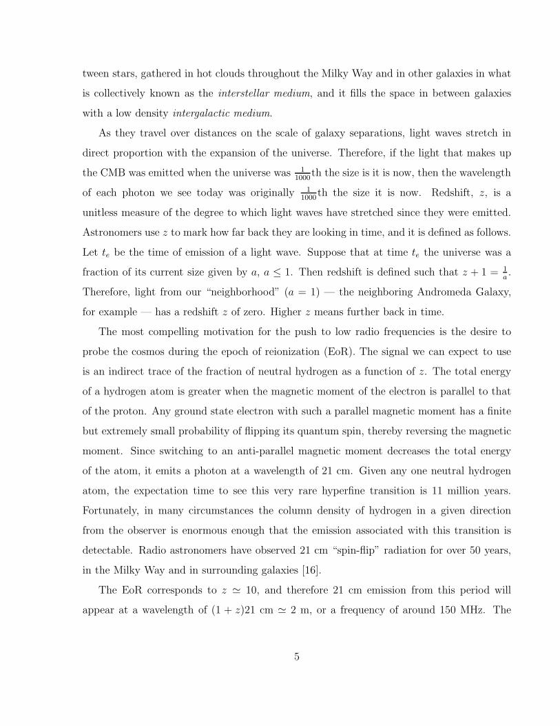
properties of the distribution of matter during the EoR. Figure 1.1 is one example of this,

demonstrating how a small section of the sky would appear at nine different wavelengths (or

redshifts), provided the telescope had unlimited resolution, sensitivity, and no foreground

confusion. Direct imaging of even the brightest of these features requires more sensitivity

than all but one observatory in the planning stage can offer (the Square Kilometer Array) [1].

However, what we can hope to determine within ten years is the angular power spectrum of

these brightness fluctuations.

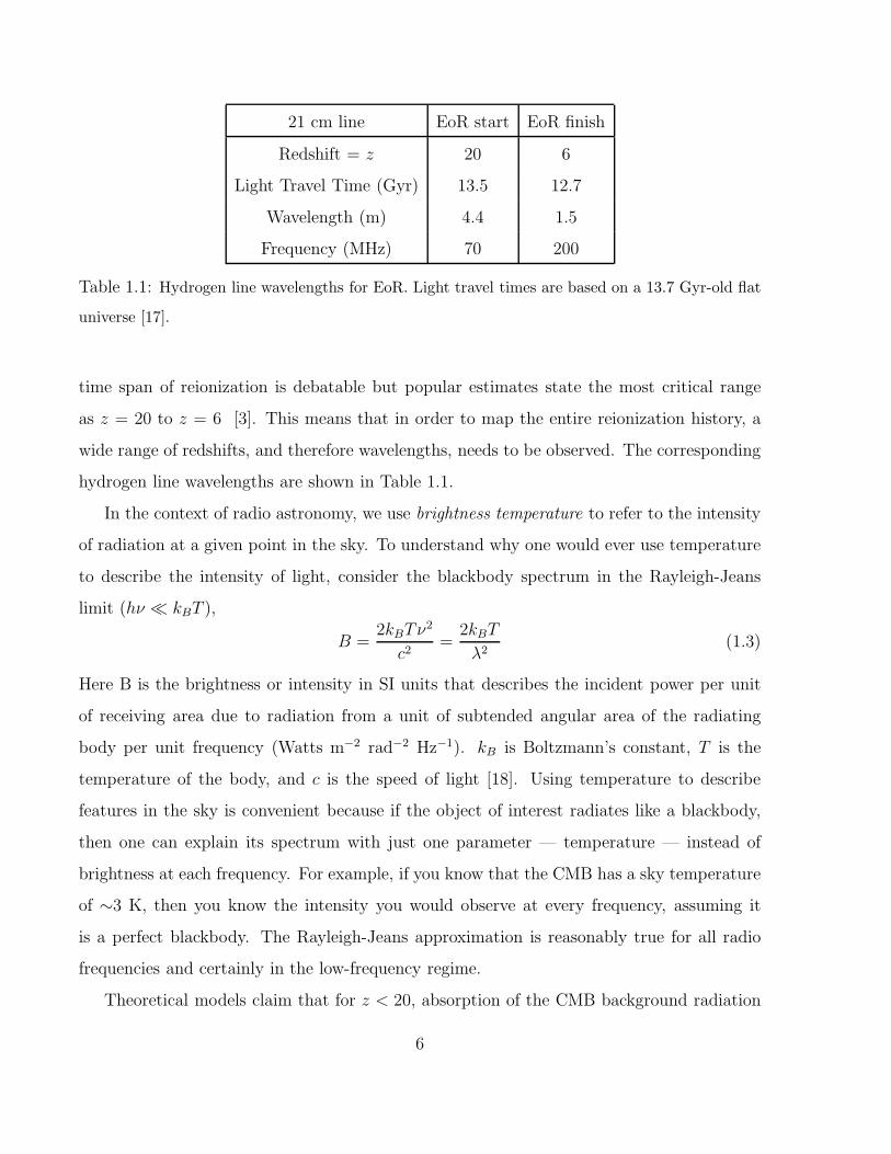
Figure 1.2 shows estimates of two major contributions to the power spectrum of the EoR

sky at a redshift of z = 10, as plotted by Miguel Morales and collaborators. The abscissa is

given in units of antenna baseline length. In the field of radio interferometry it is conventional

to translate the wavenumbers of fluctuations in the sky into the correspondingly matched

baselines. The essential relationship to understand is that the lower baselines correspond

to wider scale structure and higher baselines correspond to smaller angular scale. Another

important thing to understand about this plot is that the relative amplitudes of the curves

are extremely uncertain; only their shapes are particularly meaningful for discussion. The

dashed curve indicates how matter should be distributed as a function of angular scale

at this particular epoch, based on a favored cosmological model. We expect the observed

power spectrum to be similar to this curve, with perturbations determined by the reionization

history. The solid line relates to one of those deviations; it is the theoretical contribution

of Stromgren spheres to the power spectrum. A Stromgren sphere is a region where a

luminous body such as a star or a quasar has ionized the surrounding hydrogen with UV

7

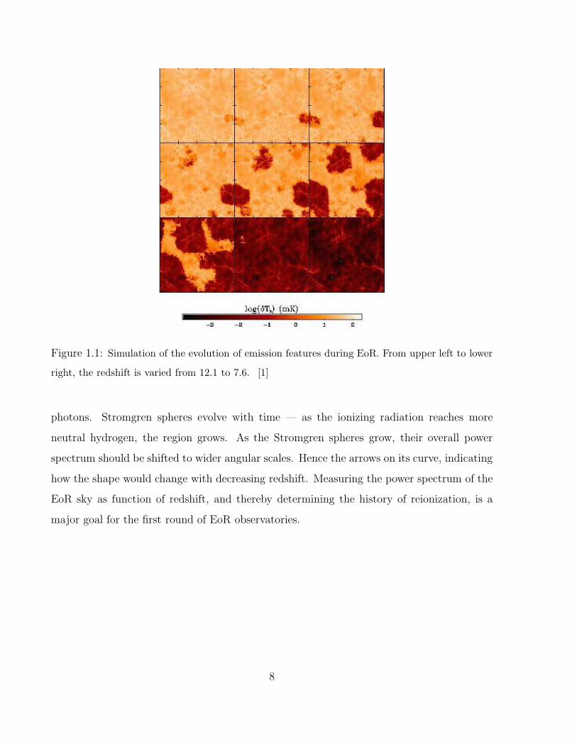
Figure 1.1: Simulation of the evolution of emission features during EoR. From upper left to lower

right, the redshift is varied from 12.1 to 7.6. [1]

photons. Stromgren spheres evolve with time — as the ionizing radiation reaches more

neutral hydrogen, the region grows. As the Stromgren spheres grow, their overall power

spectrum should be shifted to wider angular scales. Hence the arrows on its curve, indicating

how the shape would change with decreasing redshift. Measuring the power spectrum of the

EoR sky as function of redshift, and thereby determining the history of reionization, is a

major goal for the first round of EoR observatories.

8

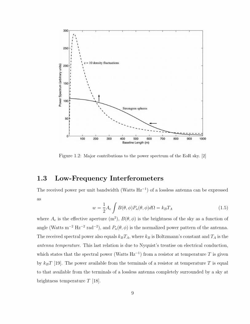
Figure 1.2: Major contributions to the power spectrum of the EoR sky. [2]

1.3 Low-Frequency Interferometers

The received power per unit bandwidth (Watts Hz−1) of a lossless antenna can be expressed

as

w =1

2Ae

∫

B(θ, φ)Pn(θ, φ)dΩ = kBTA (1.5)

where Ae is the effective aperture (m2), B(θ, φ) is the brightness of the sky as a function of

angle (Watts m−2 Hz−2 rad−2), and Pn(θ, φ) is the normalized power pattern of the antenna.

The received spectral power also equals kBTA, where kB is Boltzmann’s constant and TA is the

antenna temperature. This last relation is due to Nyquist’s treatise on electrical conduction,

which states that the spectral power (Watts Hz−1) from a resistor at temperature T is given

by kBT [19]. The power available from the terminals of a resistor at temperature T is equal

to that available from the terminals of a lossless antenna completely surrounded by a sky at

brightness temperature T [18].

9

Combining equations 1.5 and 1.3, the expression for brightness in terms of temperature,

results in

TA =Ae

λ2

∫

Ts(θ, φ)Pn(θ, φ)dΩ (1.6)

Suppose the antenna is placed in free space, surrounded in all directions by an empty sky

except for a single source of brightness Ts subtending a solid angle of Ωs. If the main beam of

the antenna is centered on the source, and the source extent is small enough that Pn(θ, φ) ≃ 1

across the source, then

TA ≃ AeTsΩs

λ2(1.7)

The sensitivity of a radio telescope is limited by the noise introduced by the conduc-

tivity losses and impedance mismatch between the antenna and the receiver, as well as the

noise added to the signal by the receiver. The equivalent noise temperature, defined by

the summation of these effects and the antenna temperature, is conventionally denoted by

Tsys. Given a length of time of observation, the minimum antenna temperature that can be

distinguished from system noise is given by

∆TAmin=

KsTsys√∆νt

(1.8)

where Ks is a constant of order unity depending on the receiver mode, Tsys is the system

temperature (K), ∆νt is the predetection bandwidth multiplied by the total integration

time [18].

The minimum detectable antenna temperature is not as interesting as the minimum

detectable source temperature. Combining equations 1.8 and 1.7, it is apparent that the

minimum detectable source temperature is

Tsmin=

λ2KsTsys

AeΩs

√∆νt

. (1.9)

This expression is true not only for a single antenna radio telescope but also for an inter-

ferometer. In the latter case, Ae is the sum of the collecting areas of the array components.

From 1.9 it is clear that the minimum temperature of a detectable source is inversely pro-

portional to collecting area of the array. Unfortunately, the financial budget of a project

typically limits Ae more than any other characteristic of the instrument.

10

Tsys has a lower limit set by foreground noise caused by synchrotron emission in our own

galaxy. The strength of the noise varies strongly with frequency and direction; it is brightest

towards the center of the galaxy, and it increases steeply with wavelength. The synchrotron

foreground brightness temperature can be approximated by

Tsky ≃ (60 ± 20)λ2.55 K (1.10)

for a region of sky away from the galactic plane [20]. Because of the foreground, the antenna

temperature, and therefore the system temperature, will always be on the order of 100

K for low-frequency observations. This is unlike the case at higher frequencies where the

galactic synchrotron foreground is negligible. The engineer of an instrument operating at

GHz frequencies has the luxury of being able to reduce Tsys by an amount only limited by

state-of-the-art of microwave electronics in order compensate for small Ae. Placing a high-

end receiver on a low-frequency telescope, on the other hand, does not make sense when Tsys

will be large no matter what.

The need to produce a large aperture at low expense and the natural limitations on

Tsys lead to some defining features of the new low-frequency interferometers. One trait

is that instead of using parabolic reflectors like the VLA, they will use about 104 wire

dipole antennas. What are the tradeoffs between making an interferometer out of dipoles

versus paraboloids? A half-wavelength dipole provides a maximum effective aperture of

0.13λ2 [21]. Therefore, whether or not it is more cost-effective to divide the aperture into

dipoles versus paraboloids depends on the wavelength of interest. For example, to construct

an interferometer out of dipoles with a total aperture around that of the VLA (∼104 m2)

optimized for a wavelength of 10 cm requires 104

0.13(0.1)2= 8×106 dipoles. At that point, the

receiver for each antenna and the associated networking would make it more expensive than

approaching the problem with 30 parabolic reflectors, each on the order of 20 m in diameter.

However, at wavelengths on the order of one meter this is no longer the case; an array

containing 10,000 dipoles is feasible and several such projects are well underway.

The main disadvantage of a dipole interferometer compared to a paraboloid interferom-

eter is that it can never have the same wavelength versatility. The VLA is a prime example

11

of this, having the capability to observe over 9 octaves. This is because a paraboloid’s useful

frequency range is limited only by the surface precision of the reflector and the availability

of appropriate feeds and receivers. On the other hand, a dipole can only be operated up to a

certain frequency before the main beam becomes narrow and the entire power pattern shows

multiple lobes. Furthermore, the effective aperture of a dipole is proportional to the square

of the wavelength. However, the scientific objectives of an interferometer dedicated to low

frequencies are compelling enough to justify this limitation. The areas of research possible

with a low-frequency interferometer extend beyond the cosmology example highlighted in

this chapter, and include extragalactic surveys, Milky Way surveys, galactic transient phe-

nomena, high-energy cosmic rays, pulsars, extrasolar planet detection, solar physics, and

geophysics [22].

The functional advantages of a dipole interferometer over a paraboloid interferometer

are considerable. One benefit is that mechanical steering can replaced by signal processing.

Parabolic antennas have inherently narrow beams that must be physically steered to the

target. Dipole antennas, on the other hand, have wide beams, and pointing can be accom-

plished by applying the appropriate phases to the individual signals in either hardware or

software. The wide beam of a dipole offers the ability to image more of the sky at once than

a conventional paraboloid interferometer could allow. Having a large field of view vastly

improves the efficiency of observing campaigns that depend on surveying large areas of the

sky, like probing the EoR.

A second major advantage of an array composed of many dipoles as opposed to a rela-

tively small number of paraboloids is that the apertures can be distributed more smoothly.

The purpose of interferometry is to synthesize one aperture much greater than that of any

individual element. The synthesized beam of an interferometer is the Fourier transform of

the spatial sampling of the area over which the antennas are placed. As the area of the array

is increasingly filled, the better it approximates a true aperture, and the lower the unwanted

sidelobes are in the beam pattern.

The table in figure 1.3 is extracted from a recent review article on new low-frequency

12

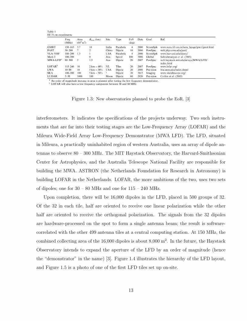
Figure 1.3: New observatories planned to probe the EoR. [3]

interferometers. It indicates the specifications of the projects underway. Two such instru-

ments that are far into their testing stages are the Low-Frequency Array (LOFAR) and the

Mileura Wide-Field Array Low-Frequency Demonstrator (MWA LFD). The LFD, situated

in Mileura, a practically uninhabited region of western Australia, uses an array of dipole an-

tennas to observe 80 – 300 MHz. The MIT Haystack Observatory, the Harvard-Smithsonian

Center for Astrophysics, and the Australia Telescope National Facility are responsible for

building the MWA. ASTRON (the Netherlands Foundation for Research in Astronomy) is

building LOFAR in the Netherlands. LOFAR, the more ambitious of the two, uses two sets

of dipoles; one for 30 – 80 MHz and one for 115 – 240 MHz.

Upon completion, there will be 16,000 dipoles in the LFD, placed in 500 groups of 32.

Of the 32 in each tile, half are oriented to receive one linear polarization while the other

half are oriented to receive the orthogonal polarization. The signals from the 32 dipoles

are hardware-processed on the spot to form a single antenna beam; the result is software-

correlated with the other 499 antenna tiles at a central computing station. At 150 MHz, the

combined collecting area of the 16,000 dipoles is about 8,000 m2. In the future, the Haystack

Observatory intends to expand the aperture of the LFD by an order of magnitude (hence

the “demonstrator” in the name) [3]. Figure 1.4 illustrates the hierarchy of the LFD layout,

and Figure 1.5 is a photo of one of the first LFD tiles set up on-site.

13

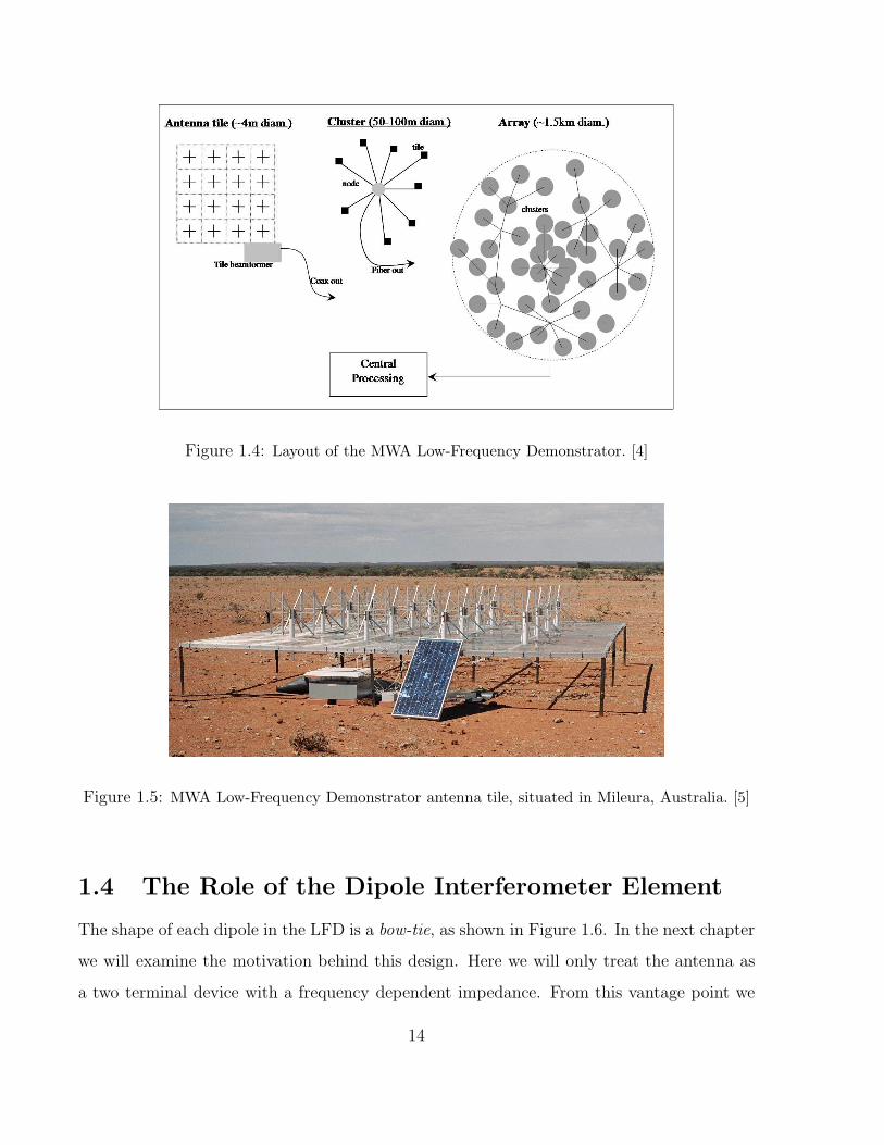
Figure 1.4: Layout of the MWA Low-Frequency Demonstrator. [4]

Figure 1.5: MWA Low-Frequency Demonstrator antenna tile, situated in Mileura, Australia. [5]

1.4 The Role of the Dipole Interferometer Element

The shape of each dipole in the LFD is a bow-tie, as shown in Figure 1.6. In the next chapter

we will examine the motivation behind this design. Here we will only treat the antenna as

a two terminal device with a frequency dependent impedance. From this vantage point we

14

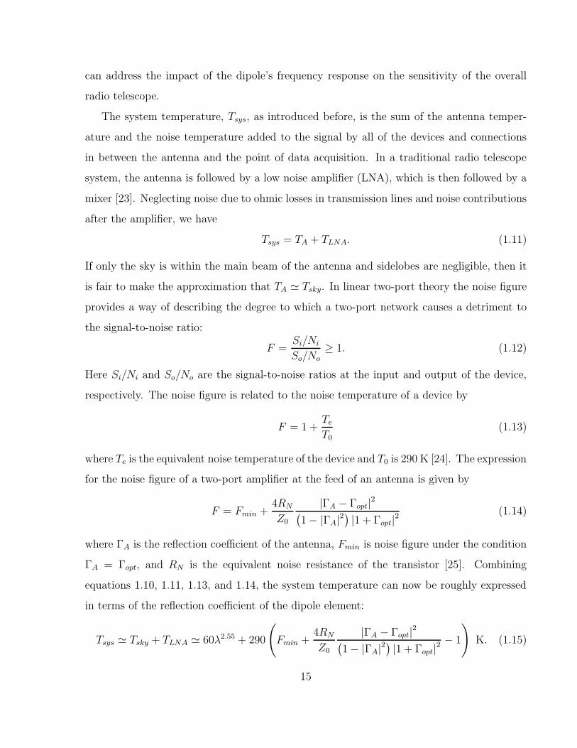
can address the impact of the dipole’s frequency response on the sensitivity of the overall

radio telescope.

The system temperature, Tsys, as introduced before, is the sum of the antenna temper-

ature and the noise temperature added to the signal by all of the devices and connections

in between the antenna and the point of data acquisition. In a traditional radio telescope

system, the antenna is followed by a low noise amplifier (LNA), which is then followed by a

mixer [23]. Neglecting noise due to ohmic losses in transmission lines and noise contributions

after the amplifier, we have

Tsys = TA + TLNA. (1.11)

If only the sky is within the main beam of the antenna and sidelobes are negligible, then it

is fair to make the approximation that TA ≃ Tsky. In linear two-port theory the noise figure

provides a way of describing the degree to which a two-port network causes a detriment to

the signal-to-noise ratio:

F =Si/Ni

So/No≥ 1. (1.12)

Here Si/Ni and So/No are the signal-to-noise ratios at the input and output of the device,

respectively. The noise figure is related to the noise temperature of a device by

F = 1 +Te

T0

(1.13)

where Te is the equivalent noise temperature of the device and T0 is 290 K [24]. The expression

for the noise figure of a two-port amplifier at the feed of an antenna is given by

F = Fmin +4RN

Z0

|ΓA − Γopt|2(

1 − |ΓA|2)

|1 + Γopt|2(1.14)

where ΓA is the reflection coefficient of the antenna, Fmin is noise figure under the condition

ΓA = Γopt, and RN is the equivalent noise resistance of the transistor [25]. Combining

equations 1.10, 1.11, 1.13, and 1.14, the system temperature can now be roughly expressed

in terms of the reflection coefficient of the dipole element:

Tsys ≃ Tsky + TLNA ≃ 60λ2.55 + 290

(

Fmin +4RN

Z0

|ΓA − Γopt|2(

1 − |ΓA|2)

|1 + Γopt|2− 1

)

K. (1.15)

15

Since 0 ≤ |ΓA| ≤ 1, Tsys in equation 1.15 increases monotonically with |ΓA − Γopt|.Therefore, we arrive at the result that in order to optimize the sensitivity of an interferometer,

given control only over the properties of the dipole, we must minimize |ΓA − Γopt|. ΓA is

related to the impedance of the antenna, ZA, by

ΓA =ZA − Z0

ZA + Z0(1.16)

where Z0 is the characteristic impedance of the system.

The investigation that follows in this thesis can be summarized as a systematic approach

to finding a new dipole design that minimizes Tsys across the range of frequencies typical of

a low-frequency interferometer like the MWA LFD.

Figure 1.6: MWA LFD Dual-Polarization Dipole. [4]

16

Chapter 2

Broadband Antennas

2.1 Antenna Basics

The function of an antenna is to transform a free-space wave to a guided wave, or vice

versa [26]. An antenna is often modeled as a two-terminal network whose impedance, ZA, is

the ratio of voltage to current at its terminals, or feed. Like a circuit element, the impedance

of an antenna is a complex-valued function of frequency. In general, the value of this function

depends not only on the structure of the antenna but the environment surrounding it. This

is because the impedance presented by an antenna changes due to electromagnetic coupling

with objects around it such as ground or other antennas [27]. The term self-impedance is

used to describe the impedance in the case where the structure is in empty space, free from

any such external effects. For simplicity, any reference to the impedance of an antenna

beyond this point will implicitly mean the self-impedance.

In receiving mode, the antenna extracts energy from incident radiation and delivers it to

the network connected to its terminals. Consider an antenna subject to an electromagnetic

field, with a load of impedance ZL connected across its feed. The antenna may be replaced

by a Thevenin equivalent. Then, by the reciprocity theorem of linear circuits ([28]), the

impedance associated with this Thevenin equivalent must be ZA in order to be consistent

with the two-port equivalent in the transmitting case. The root-mean-square current ILrms

17

in the load is given by

ILrms=

Vrms

ZL + ZA

. (2.1)

Furthermore, the maximum power is delivered to the load when RL = RA and XL = −XA,

or ZL = Z∗

A [29]. The effective aperture of an antenna is defined by the ratio of the power

delivered to the load, WL = I2Lrms

RL, to the incident power density, S (W/m2):

Aeff =WL

S[21]. (2.2)

Effective aperture is therefore dependent on the match between the antenna and the load.

Unfortunately, in radio astronomy literature, effective aperture is always stated with the

implicit assumption of a conjugate impedance match – this includes most references in the

first chapter. What they really mean is the maximum effective aperture, which is equation 2.2

in the case that the LNA is conjugately matched to the antenna. The expressions such as the

one for minimum detectable source temperature, equation 1.9, are valid with maximum Aeff

so long as impedance mismatch is taken into account in the Tsys term, as in equation 1.11. It is

also important to note that although conjugate matching results in the maximum power being

delivered from the antenna to the load, it is not optimum for minimizing Tsys. The derivation

leading to equation 1.14 demonstrated that the optimal match is such that ΓA = Γopt, which

depends on the amplifier following the antenna. This seemingly contradictory result is often

encountered in the design of microwave amplifier circuits [25].

Now that we have the meaning of antenna impedance and understand how it effects the

performance of a radio telescope, we can examine how an actual antenna behaves. Consider

a sinusoidal voltage generator, each terminal of which is connected to a thin wire as in

Figure 2.1. The oscillations of charges in the wires excited by the voltage source will produce

radiation at the same frequency as the applied signal. This is the simplest form of a dipole

antenna. A travelling wave of current propagates from the generator to the end of each wire.

When it reaches the end, there is a reflection with a 180 degree phase reversal, and the sum

of the outbound and inbound waves forms a standing wave across the antenna. When the

length of the antenna, l is equal to half of the wavelength, λ, of the travelling current wave

in the conductor, the reflected wave constructively interferes with the outbound one [30].

18

This produces a maximum in the magnitude of the current standing wave at the near end

of each wire. The same resonance also occurs when l is equal to a larger odd multiple of

λ2. Another interesting case occurs when l ≪ λ. Then, there is not enough spatial variation

in the travelling wave for appreciable interference to take place between the reflected and

outbound waves, and the magnitude of the overall current oscillation falls off approximately

linearly with distance from the center.

At this point it is useful to introduce radiation resistance, Rr, which in general is not

the same as RA. Its definition is also dependent on the type of antenna being considered.

For a thin dipole, the current distribution is sinusoidal, and Rr is defined through the power

emitted in transmitting mode, Wemit, given the amplitude of the standing wave of current

on the dipole, I0, such that:

Wemit =I20

2Rr [31]. (2.3)

Since ZA is defined by the current at the terminals of the antenna, RA will be different from

Rr if the current distribution peaks away from the center of the dipole. Such is the case

when destructive interference between the outbound and inbound travelling current waves

occurs at the feed, for example when l = 34λ. For a dipole of length l ≤ λ/4 the current

maximum always occurs at the feed and so Rr = RA. In general, the two-terminal resistance

and the radiation resistance of a dipole are related by

I2A

2RA =

I20

2Rr (2.4)

where IA is the current amplitude at the feed of the dipole and I0 is the amplitude of the

standing wave of current on the dipole [31].

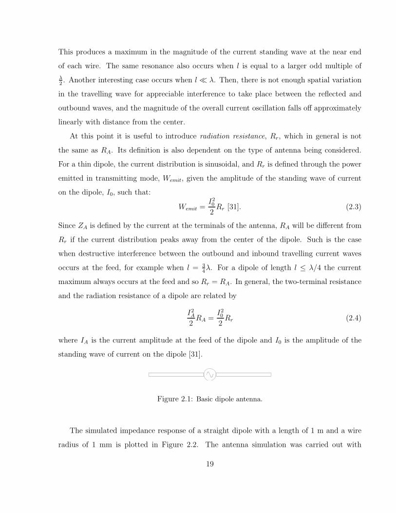
Figure 2.1: Basic dipole antenna.

The simulated impedance response of a straight dipole with a length of 1 m and a wire

radius of 1 mm is plotted in Figure 2.2. The antenna simulation was carried out with

19

nec2c (described later) [32]. The plot, and all the others hereafter printed in this thesis,

were generated with a combination of Perl (v5.8.7) and Gnuplot (4th Berkeley Distribution)

scripts [33], [34]. The solid curve is the resistance, corresponding to the vertical scale on

the left side of the plot, and the dashed curve is the reactance, corresponding to the right

scale. Frequency is varied along the horizontal axis from 75 MHz to 300 MHz. Notice that

the reactance goes to zero around 140 MHz, which corresponds to a wavelength just over

twice the total length of the dipole. The reason the resonance is at 140 MHz and not 150

MHz is due to the lower propagation speed of electromagnetic waves inside the conductor.

In practice the reactance of a dipole of length l vanishes for a free space wavelength between

about 2.08l and 2.13l, the exact value depending on the thickness of the wire. Conversely,

to resonate at a free space wavelength λ, l should be between 0.47λ and 0.48λ [35].

0

200

400

600

800

1000

1200

1400

1600

1800

2000

100 150 200 250 300-1200

-1000

-800

-600

-400

-200

0

200

400

600

800

1000

Res

ista

nce

Rea

ctan

ce

Frequency (MHz)

Straight 1 m Dipole Impedance

ResistanceReactance

Figure 2.2: Impedance response of a 1 meter dipole.

It is preferable to operate a dipole at or near the half-wave resonance because the low

reactance allows a good match to the characteristic impedance of the transmission line in

between the feed and the amplifier, which is generally either 50 Ω or 75 Ω. In fact, 75 Ω is

not an arbitrary standard for characteristic impedance — it is the approximate value of the

impedance of a dipole antenna when l = λ/2 [35].

20

2.2 The Bow-tie: A Traditional Broadband Dipole

As long as the structure under consideration is a perfect conductor, then the wavelength

of the solutions to Maxwell’s equations will scale in proportion to a change in scale of the

structure [36]. This summarizes the approach taken to the concept of frequency-independent

antennas starting in the 1950s. V. H. Rumsey hypothesized that an antenna whose geom-

etry is defined only by angles would be frequency-independent. To define a structure only

be angles means that the radius is unbounded, and therefore a truly frequency-independent

antenna is impossible to construct. However, a truncated version could still possess great

bandwidth. For example, work along these lines by DuHamel and Isbell led to the devel-

opment of log periodic structures, which possess multiple-octave bandwidths. However, log

periodic arrays lack the wide main beam of a dipole [37]. Recall that having a wide main

beam in the elements of an MWA LFD-style low-frequency interferometer is critical in order

to facilitate electronic steering and a wide field of view. In the next section we will see how

Rumsey’s original idea resurfaced years later with the first fractal antennas.

Even before Rumsey had outlined the formal criterion for an ideal frequency-independent

antenna, J. D. Kraus graphically demonstrated in his 1950 text how successively crude

approximations to a truncated self-scaling structure can form practical broadband antennas.

With each step, the antenna is easier to build, but consequently has narrower bandwidth.

One of Kraus’ antennas is a kind of planar dipole, derived from a two-wire self-scaling

transmission line. It is known in the field as a bow-tie, composed of two oppositely facing,

solid triangular sheets [37]. To ease the fabrication, the triangles of the bow-tie can be

constructed with a wire frame instead of solid sheets.

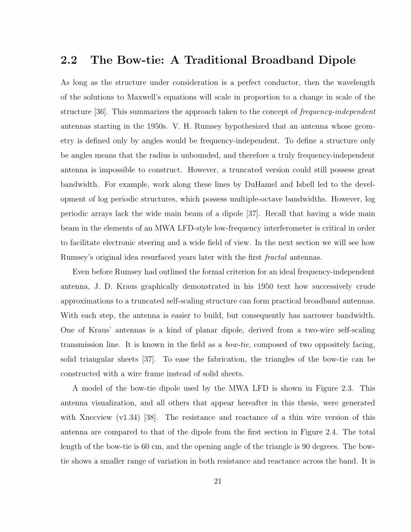
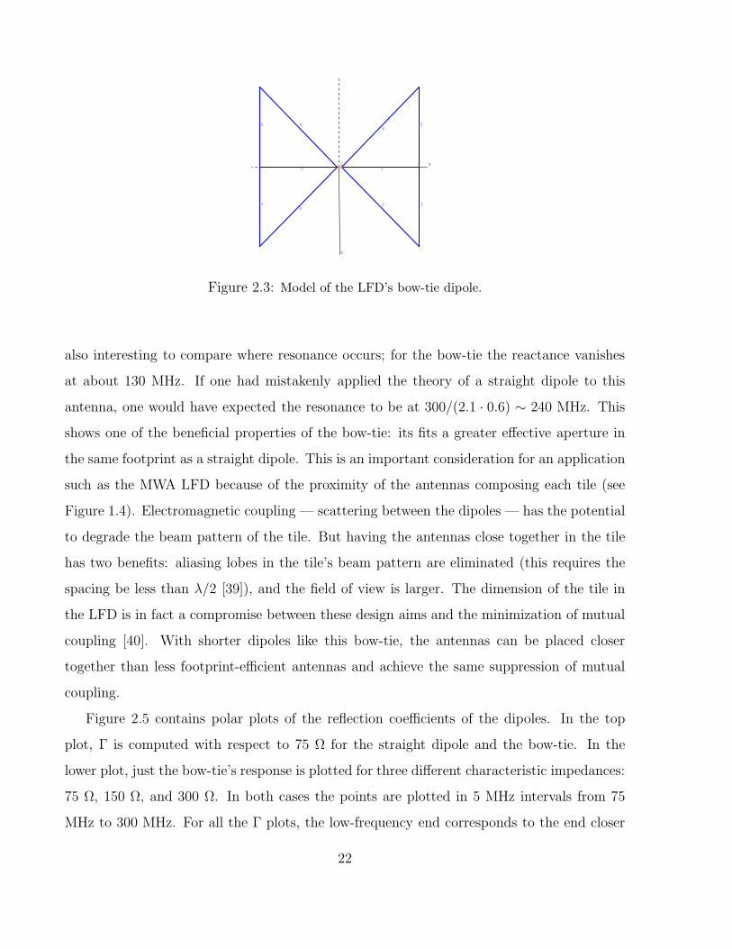
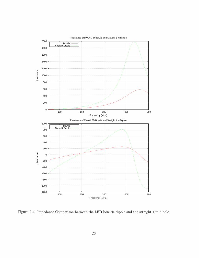
A model of the bow-tie dipole used by the MWA LFD is shown in Figure 2.3. This

antenna visualization, and all others that appear hereafter in this thesis, were generated

with Xnecview (v1.34) [38]. The resistance and reactance of a thin wire version of this

antenna are compared to that of the dipole from the first section in Figure 2.4. The total

length of the bow-tie is 60 cm, and the opening angle of the triangle is 90 degrees. The bow-

tie shows a smaller range of variation in both resistance and reactance across the band. It is

21

X

YZ

2 3

4

5

1

6

7

89

5

Figure 2.3: Model of the LFD’s bow-tie dipole.

also interesting to compare where resonance occurs; for the bow-tie the reactance vanishes

at about 130 MHz. If one had mistakenly applied the theory of a straight dipole to this

antenna, one would have expected the resonance to be at 300/(2.1 · 0.6) ∼ 240 MHz. This

shows one of the beneficial properties of the bow-tie: its fits a greater effective aperture in

the same footprint as a straight dipole. This is an important consideration for an application

such as the MWA LFD because of the proximity of the antennas composing each tile (see

Figure 1.4). Electromagnetic coupling — scattering between the dipoles — has the potential

to degrade the beam pattern of the tile. But having the antennas close together in the tile

has two benefits: aliasing lobes in the tile’s beam pattern are eliminated (this requires the

spacing be less than λ/2 [39]), and the field of view is larger. The dimension of the tile in

the LFD is in fact a compromise between these design aims and the minimization of mutual

coupling [40]. With shorter dipoles like this bow-tie, the antennas can be placed closer

together than less footprint-efficient antennas and achieve the same suppression of mutual

coupling.

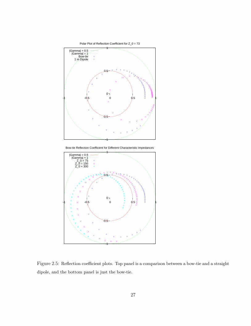
Figure 2.5 contains polar plots of the reflection coefficients of the dipoles. In the top

plot, Γ is computed with respect to 75 Ω for the straight dipole and the bow-tie. In the

lower plot, just the bow-tie’s response is plotted for three different characteristic impedances:

75 Ω, 150 Ω, and 300 Ω. In both cases the points are plotted in 5 MHz intervals from 75

MHz to 300 MHz. For all the Γ plots, the low-frequency end corresponds to the end closer

22

Antenna < |Γ| > < TLNA

Tsys>

Straight Dipole 0.76 0.38

LFD Bow-tie 0.65 0.20

Table 2.1: Comparison of mean |Γ| and mean TLNA

Tsys

to the outer boundary of the plot. In all cases this is the part of the band where the match

is poorest, because of the low resistance of any dipole that is much smaller than λ; RA is

expected to fall as 1λ2 at wavelengths much longer than the antenna [31].

The bow-tie resistance at resonance is 28 Ω, significantly lower than any of the charac-

teristic impedances, and as a consequence its Γ curve never passes through the origin like

that of the straight dipole. However, on average most of the bow-tie’s points are closer to

the origin. This is quantitatively shown in Table 2.1, where the computed mean values of

the Γ responses are listed for Z0 = 75 Ω.

As was concluded in the first chapter, what ultimately controls the performance of an

interferometer of fixed aperture is the system temperature. However, in order to compute

TLNA, the amplifier parameters RN and Fmin must be set (see equation 1.14). Through

correspondence with Eric Kratzenberg, a research engineer at the MIT Haystack Observatory,

we obtained enough information about the LNA circuit being employed in the MWA LFD

to set reasonable values. Most importantly, although the characteristic impedance of the

MWA LFD is 75 Ω, the amplifier is configured as a differential pair, where the base of each

transistor is connected to one terminal of the antenna. The circuit analysis of a differential

pair shows that such a configuration effectively doubles the impedance presented to the source

(see e.g. [41]). Therefore before solving for the system temperature, the impedance of the

antenna, ZA, should be halved under these circumstances. The device used in the differential

pair is the Avago Technologies ATF-54143, a pseudomorphic high electron mobility transistor

(pHEMT).

The manufacturer’s data for the ATF-54143 when VDS = 3 V and IDS = 80 mA indicates

that for the frequencies under consideration, Fmin and RN are essentially constant. The data

23

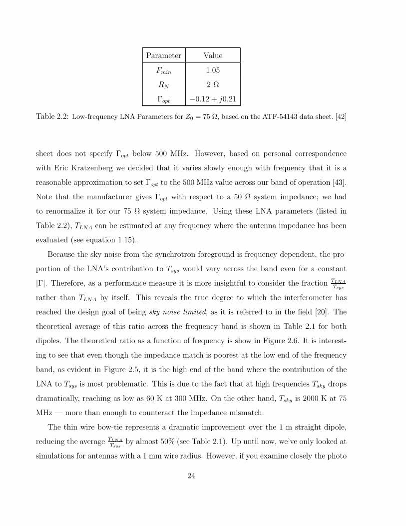
Parameter Value

Fmin 1.05

RN 2 Ω

Γopt −0.12 + j0.21

Table 2.2: Low-frequency LNA Parameters for Z0 = 75 Ω, based on the ATF-54143 data sheet. [42]

sheet does not specify Γopt below 500 MHz. However, based on personal correspondence

with Eric Kratzenberg we decided that it varies slowly enough with frequency that it is a

reasonable approximation to set Γopt to the 500 MHz value across our band of operation [43].

Note that the manufacturer gives Γopt with respect to a 50 Ω system impedance; we had

to renormalize it for our 75 Ω system impedance. Using these LNA parameters (listed in

Table 2.2), TLNA can be estimated at any frequency where the antenna impedance has been

evaluated (see equation 1.15).

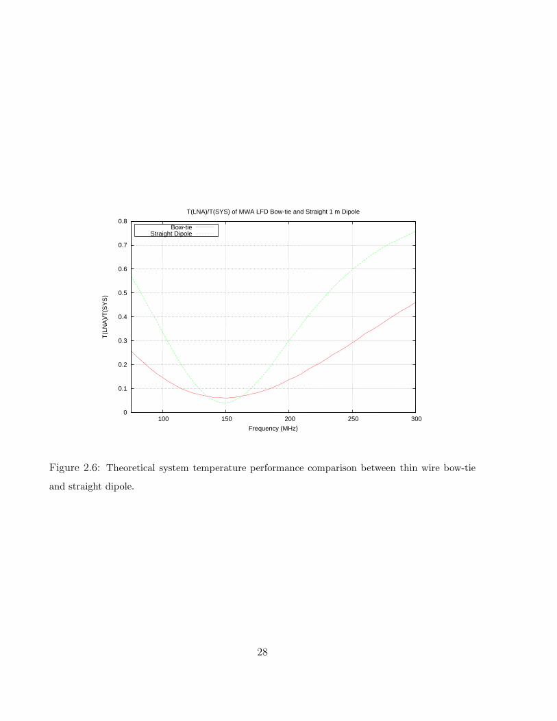
Because the sky noise from the synchrotron foreground is frequency dependent, the pro-

portion of the LNA’s contribution to Tsys would vary across the band even for a constant

|Γ|. Therefore, as a performance measure it is more insightful to consider the fraction TLNA

Tsys

rather than TLNA by itself. This reveals the true degree to which the interferometer has

reached the design goal of being sky noise limited, as it is referred to in the field [20]. The

theoretical average of this ratio across the frequency band is shown in Table 2.1 for both

dipoles. The theoretical ratio as a function of frequency is show in Figure 2.6. It is interest-

ing to see that even though the impedance match is poorest at the low end of the frequency

band, as evident in Figure 2.5, it is the high end of the band where the contribution of the

LNA to Tsys is most problematic. This is due to the fact that at high frequencies Tsky drops

dramatically, reaching as low as 60 K at 300 MHz. On the other hand, Tsky is 2000 K at 75

MHz — more than enough to counteract the impedance mismatch.

The thin wire bow-tie represents a dramatic improvement over the 1 m straight dipole,

reducing the average TLNA

Tsysby almost 50% (see Table 2.1). Up until now, we’ve only looked at

simulations for antennas with a 1 mm wire radius. However, if you examine closely the photo

24

in Figure 1.6, you’ll see that the wires are significantly thicker than 2 mm – closer to 2 cm, in

fact. Thicker wires add to the durability of the structure, which in practice will be exposed to

the elements for several years. Increasing the radius of the conductor also decreases the range

over which both the resistance and reactance of the antenna vary with frequency, thereby

improving the bandwidth [44]. The MWA LFD antenna, constructed with u-channel sections,

benefits from this fact. However, we found that solutions from our simulator, nec2c, were not

robust for antennas with large wire radius. More specifically, the results of the simulation

were very sensitive to the user-specified segmentation of the structure. Since the accuracy of

those simulations is questionable, we do not bother presenting calculations of TLNA

Tsysfor the

thick wire case. Still, it is a useful design variable to keep in mind.

Revisiting the plot of Figure 2.6, we see that the performance of the MWA LFD bow-tie

is excellent for low frequencies. Nevertheless, above 225 MHz, TLNA

Tsysexceeds 0.2 and grows

linearly, approaching the noise contribution of the sky. Is there another dipole shape that

can further decrease TLNA?

25

0

200

400

600

800

1000

1200

1400

1600

1800

2000

100 150 200 250 300

Res

ista

nce

Frequency (MHz)

Resistance of MWA LFD Bowtie and Straight 1 m Dipole

BowtieStraight Dipole

-1200

-1000

-800

-600

-400

-200

0

200

400

600

800

1000

100 150 200 250 300

Rea

ctan

ce

Frequency (MHz)

Reactance of MWA LFD Bowtie and Straight 1 m Dipole

BowtieStraight Dipole

Figure 2.4: Impedance Comparison between the LFD bow-tie dipole and the straight 1 m dipole.

26

-1

-0.5

0

0.5

1

-1 -0.5 0 0.5 1

Polar Plot of Reflection Coefficient for Z_0 = 73

|Gamma| = 0.5|Gamma| = 1

Bow-tie1 m Dipole

-1

-0.5

0

0.5

1

-1 -0.5 0 0.5 1

Bow-tie Reflection Coefficient for Different Characteristic Impedances

|Gamma| = 0.5|Gamma| = 1

Z_0 = 75Z_0 = 150Z_0 = 300

Figure 2.5: Reflection coefficient plots. Top panel is a comparison between a bow-tie and a straight

dipole, and the bottom panel is just the bow-tie.

27

0

0.1

0.2

0.3

0.4

0.5

0.6

0.7

0.8

100 150 200 250 300

T(L

NA

)/T

(SY

S)

Frequency (MHz)

T(LNA)/T(SYS) of MWA LFD Bow-tie and Straight 1 m Dipole

Bow-tieStraight Dipole

Figure 2.6: Theoretical system temperature performance comparison between thin wire bow-tie

and straight dipole.

28

2.3 Fractal Geometry

A fractal is a figure which displays the same geometrical motif at arbitrarily large and

small scales. There is no concise mathematical definition of a fractal, as the typical cri-

teria commonly associated with them — self-similarity, dimension — have multiple valid

meanings [45]. Instead of addressing the overall theory of fractal geometry, we will start by

describing a specific category of fractals which are particularly useful in engineering due to

their ease of generation and friendliness to data structure encoding.

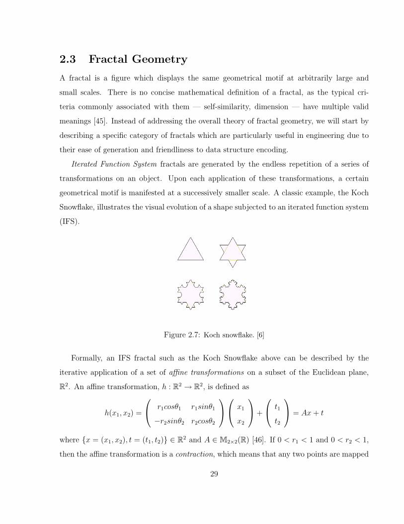
Iterated Function System fractals are generated by the endless repetition of a series of

transformations on an object. Upon each application of these transformations, a certain

geometrical motif is manifested at a successively smaller scale. A classic example, the Koch

Snowflake, illustrates the visual evolution of a shape subjected to an iterated function system

(IFS).

Figure 2.7: Koch snowflake. [6]

Formally, an IFS fractal such as the Koch Snowflake above can be described by the

iterative application of a set of affine transformations on a subset of the Euclidean plane,

R2. An affine transformation, h : R

2 → R2, is defined as

h(x1, x2) =

r1cosθ1 r1sinθ1

−r2sinθ2 r2cosθ2

x1

x2

+

t1

t2

= Ax + t

where x = (x1, x2), t = (t1, t2) ∈ R2 and A ∈ M2×2(R) [46]. If 0 < r1 < 1 and 0 < r2 < 1,

then the affine transformation is a contraction, which means that any two points are mapped

29

closer together than they were before the transformation. The union of a family of M affine

transformations is a Hutchinson operator, H(S), denoted

H(S) =

M⋃

i=1

hi(S)

where S ⊂ R2 [47]. If every affine transformation contained in the Hutchinson operator is

a contraction, then the repeated application of H to any set S ⊂ R2, the generator, results

in a convergence to F ⊂ R2, known as the attractor set of the IFS [48]. By definition, F is

invariant under H , so that F = H(F ). The subset of R2 resulting from the jth application

of H to S can be denoted as Hj(S), j ≥ 1. At a fixed j

Hj(S) =⋃

Qj

hi1(hi2(· · · (hij (S)) · · · )).

Here Qj is the set of all ordered sequences (i1, . . . , ij) of length j with 1 ≤ ik ≤ M [49]. For

example, the subset resulting from the second iteration of H on the generator S, H2(S), is

the union h1(h1(S)) ∪ h1(h2(S)) ∪ h2(h1(S)) ∪ h2(h2(S)). As j increases, Hj(S) resembles

the attractor set F more and more closely.

A special case of an affine transformation is a similitude or similarity transformation, for

which

A =

rcosθ −rsinθ

rsinθ rcosθ

[46]

This is intuitively understood as an operator that never stretches a shape in one direction

more than the other — there is merely scaling and rotation caused by A and translation

caused by the vector t. When the Hutchinson operator is composed of only similarity trans-

formations, then the attractor is a self-similar fractal. Self-similar fractals such as the Koch

curve have the remarkable property that looking at a given piece, no matter how closely

examined, gives no hint as to the scale of your window. More generally, r1 6= r2, and an

affine transformation can map a square to a parallelogram, for example. In this case the

attractor of the IFS is a self-affine fractal. On a self-affine fractal, the motifs present at

different scales may be distinguishable.

30

The jth iteration of the IFS, Hj(S), is an approximation of the attractor/fractal set,

commonly referred to as a prefractal [49], or from a physical standpoint, a bandlimited

fractal [50].

The consideration of random variations in the IFS opens up an enormous range of pos-

sibilities to add to our definition of a fractal. In particular, one can imagine mapping the

entries of the transformation matrix to probability distributions, from which slight varia-

tions in the motif will result at each iteration. The imposition of random variations on

a self-similar IFS results in what is often referred to as statistical self-similarity, or more

loosely, a random fractal.

2.4 The Electrical Properties of Fractal Conductors

The first investigation into the interaction of electromagnetic waves with fractal boundaries

was lead by Dwight L. Jaggard’s group at the University of Pennsylvania in the late 1980s;

this work is summarized in [50] and expounded upon in [51]. In the mid 1990s the first

publications detailing results of antennas constructed in the shape of prefractals appeared;

these early efforts were independently lead by Carles Puente at the Universitat Politecnica

de Catalunya in Spain and Nathan Cohen in the United States [52], [53]. There are two

main features of prefractal antennas demonstrated by these pioneers that have stimulated

continued research in this field. First, prefractal antennas offer inherent multiband resonance

without the appendage of reactive networks. Second, certain prefractal antennas take up

significantly less space in comparison to conventional antennas resonating at the same given

wavelength. Furthermore, it became apparent that previous successful efforts to create

frequency-independent structures, such as log-periodic arrays and spiral antennas, can all be

described within the framework of fractal geometry [53].

Puente et al. have offered a theoretical explanation for the multiple resonances of self-

similar fractal shapes, which we will now paraphrase [47]. The approach relies on the same

scaling properties of Maxwell’s equations that were used by Rumsey and his contemporaries.

31

First, a binary valued index function is defined by

G(x1, x2) =

1 if (x1, x2) ∈ S

0 if (x1, x2) 6∈ S

where S is the usual initial subset of the Euclidean plane that is to be transformed. A

translation of points in S can be described using convolution with a Dirac delta function:

G(x1 − x10, x2 − x20

) = G(x1, x2) ∗ δ(x1 − x10, x2 − x20

)

where (x10, x20

) is the new resulting point. A Hutchinson operator containing M similarity

translations can be represented as

H(G(x1, x2)) =

M∑

i=1

G(rix1i, rix2i

) ∗ δ(x1 − x1i, x2 − x2i

)

where 0 < r < 1. If the scaling factor is the same for each of the M contractions, so that

ri = r, then this can be further simplified to

H(G(x1, x2)) = G(rx1, rx2) ∗ IF (x1, x2) where IF (x1, x2) =

M∑

i=1

δ(x1 − x1i, x2 − x2i

)

and IF stands for iterator function. For the nth application of the iterator function, we will

have

Gn(x1, x2) = G(rnx1, rnx2) ∗ IF (rn−1x1, r

n−1x2) ∗ · · · ∗ IF (x1, x2)

= G(rnx1, rnx2)

n−1⊗

j=0

IF (rjx1, rjx2)

where⊗

denotes the convolution operator. For large n, G(rnx1, rnx2) converges, and it will

be just as valid for the original G(x1, x2) to have been an impulse function. This way, the

attractor set F can be described as

F (x1, x2) =

∞⊗

j=0

IF (rjx1, rjx2)

F is self-similar in the same manner as the set theory of description from the previous section.

However, F is finite and thus not truly self-scalable, in which case an identical motif would

32

appear at arbitrarily small and large scales. The finite size of F means that it has an upper

limit to the scale of repetition of the iterative function. This is fixed by redefining the limits

of the convolution operator for Gn and F :

Gn(x1, x2) =n−1⊗

j=−(n−1)

IF (rjx1, rjx2) and F (x1, x2) =

∞⊗

j=−∞

IF (rjx1, rjx2)

Now the attractor is self-scalable since

F (rpx1, rpx2) =

∞⊗

j=−∞

IF (rj+px1, rj+px2)

and letting k = j + p, this simplifies to

∞⊗

k=−∞

IF (rkx1, rkx2) = F (x1, x2)

The geometric motif of such a self-similar structure repeats logarithmically according to the

scaling factor r. Likewise the wavelengths of the currents and fields for such a structure repeat

in a log-periodic fashion in accordance with the scaling principle of Maxwell’s equations [47].

The assumptions that have been made do not correspond to a realizable structure, because

the scales of the iterator functions represented in the fabrication will always have a lower

and upper bound. However, in practice a finite prefractal antenna can approximate this

frequency-periodic behavior to the extent that the IFS iterations are physically realized, as

demonstrated by the experiments of Puente et al.

Notice that even though this proof predicts multiple resonances, Puente et al. do not

claim that a fractal antenna can offer a response that is resonant over the scale of an oc-

tave rather than at discretely-spaced narrow bands. One might suppose that an IFS with a

scaling factor r approaching unity would offer this solution, by shrinking the period between

resonances. However, even in the case that a structure with a near unity r is realized, the

structure’s efficacy as an antenna is in no way guaranteed. Therefore, without experimenta-

tion it is uncertain whether or not the above argument is meaningful for an application that

is broadband rather than multiband.

33

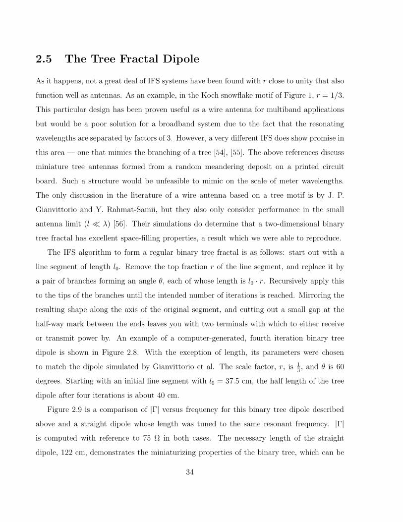
2.5 The Tree Fractal Dipole

As it happens, not a great deal of IFS systems have been found with r close to unity that also

function well as antennas. As an example, in the Koch snowflake motif of Figure 1, r = 1/3.

This particular design has been proven useful as a wire antenna for multiband applications

but would be a poor solution for a broadband system due to the fact that the resonating

wavelengths are separated by factors of 3. However, a very different IFS does show promise in

this area — one that mimics the branching of a tree [54], [55]. The above references discuss

miniature tree antennas formed from a random meandering deposit on a printed circuit

board. Such a structure would be unfeasible to mimic on the scale of meter wavelengths.

The only discussion in the literature of a wire antenna based on a tree motif is by J. P.

Gianvittorio and Y. Rahmat-Samii, but they also only consider performance in the small

antenna limit (l ≪ λ) [56]. Their simulations do determine that a two-dimensional binary

tree fractal has excellent space-filling properties, a result which we were able to reproduce.

The IFS algorithm to form a regular binary tree fractal is as follows: start out with a

line segment of length l0. Remove the top fraction r of the line segment, and replace it by

a pair of branches forming an angle θ, each of whose length is l0 · r. Recursively apply this

to the tips of the branches until the intended number of iterations is reached. Mirroring the

resulting shape along the axis of the original segment, and cutting out a small gap at the

half-way mark between the ends leaves you with two terminals with which to either receive

or transmit power by. An example of a computer-generated, fourth iteration binary tree

dipole is shown in Figure 2.8. With the exception of length, its parameters were chosen

to match the dipole simulated by Gianvittorio et al. The scale factor, r, is 13, and θ is 60

degrees. Starting with an initial line segment with l0 = 37.5 cm, the half length of the tree

dipole after four iterations is about 40 cm.

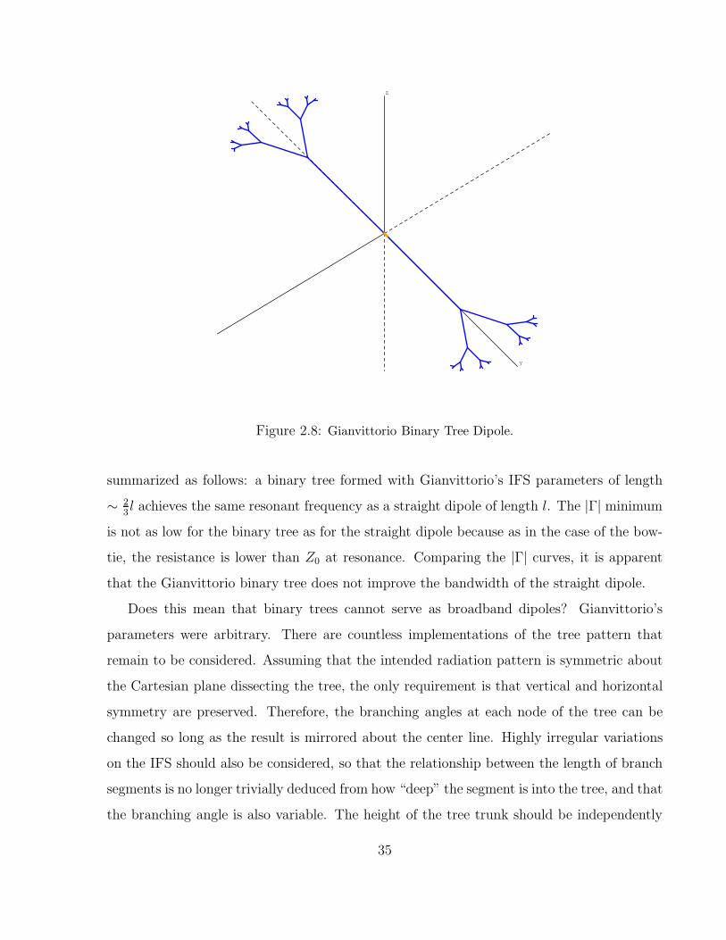
Figure 2.9 is a comparison of |Γ| versus frequency for this binary tree dipole described

above and a straight dipole whose length was tuned to the same resonant frequency. |Γ|is computed with reference to 75 Ω in both cases. The necessary length of the straight

dipole, 122 cm, demonstrates the miniaturizing properties of the binary tree, which can be

34

Y

Z

Figure 2.8: Gianvittorio Binary Tree Dipole.

summarized as follows: a binary tree formed with Gianvittorio’s IFS parameters of length

∼ 23l achieves the same resonant frequency as a straight dipole of length l. The |Γ| minimum

is not as low for the binary tree as for the straight dipole because as in the case of the bow-

tie, the resistance is lower than Z0 at resonance. Comparing the |Γ| curves, it is apparent

that the Gianvittorio binary tree does not improve the bandwidth of the straight dipole.

Does this mean that binary trees cannot serve as broadband dipoles? Gianvittorio’s

parameters were arbitrary. There are countless implementations of the tree pattern that

remain to be considered. Assuming that the intended radiation pattern is symmetric about

the Cartesian plane dissecting the tree, the only requirement is that vertical and horizontal

symmetry are preserved. Therefore, the branching angles at each node of the tree can be

changed so long as the result is mirrored about the center line. Highly irregular variations

on the IFS should also be considered, so that the relationship between the length of branch

segments is no longer trivially deduced from how “deep” the segment is into the tree, and that

the branching angle is also variable. The height of the tree trunk should be independently

35

0

0.1

0.2

0.3

0.4

0.5

0.6

0.7

0.8

0.9

1

80 90 100 110 120 130 140 150 160

|Gam

ma|

Frequency (MHz)

|Gamma| of Gianvittorio Binary Tree and Straight Dipole

Binary TreeStraight Dipole

Figure 2.9: |Γ| Comparison between a Gianvittorio binary tree and a straight dipole, tuned to the

same resonance.

adjustable as well. These allowances leave freedom for the possibility of finding an optimum

tree pattern is not actually fractal at all.

The sheer enormity of combinations of variables suggests that a brute force, trial-and-

error method is hopeless in fully exploring the space of valid solutions. Rather, an automated

approach of learned, adaptive evaluation of candidates appears far more likely to succeed.

36

Chapter 3

The Genetic Antenna Optimizer

3.1 Genetic Algorithms

A genetic algorithm autonomously searches a space of parameter vectors for optimal values

based on a specified metric of goodness. It falls under a category known as evolutionary

algorithms, which mimic biological processes in order to address optimization problems.

Darwinian selection rules are used to combine and propagate the most successful traits from

a pool of iteratively generated candidates [57].

Although implementations may vary widely in complexity and philosophy as demanded

by particular applications, the general procedure followed by many programmers is as fol-

lows. First, a scheme must be created that encodes all the relevant free parameters of the

problem into a vector whose function is analogous to that of an organism’s chromosome. The

algorithm begins with an initial population, created by setting the genes of each member,

contained in individual chromosomes, to random values. After this initialization stage, the

algorithm enters a loop which repeats until a condition set by the user is met. This condition

is either the completion of a certain number of generations or the achievement of a certain

figure of merit by one of the candidates.

During each iteration of this loop, several actions are performed in succession: (i) The

goodness of each member of the current population is evaluated using a global metric. The

rankings of goodness are translated into probabilities of survival. (ii) Based on the eval-

37

uations, a schematic is created to describe how the next population will be formed. The

schematic specifies one of three modes for each replacement: elite, recombination, or muta-

tion. (iii) Following the schematic, the replacement population is generated, overwriting the

old population.

The details of step (ii) are the heart of the genetic algorithm, and due to the wide variety

of implementations, they cannot be explained without a loss of generality. Therefore, we will

only describe our method. An elite chromosome is one that has a high enough goodness that

it is passed on to the next generation unmodified. Usually only a very small portion of the

population (< 5%) is created in this way. Recombination, on the other hand, is much more

important because it results in new combinations of parameters being tested. In recom-

bination, two vectors are stochastically selected in accordance with their assigned survival

probabilities. Therefore, the vector with the highest goodness has the greatest chance of

being selected, and so on. Such a mode of selection is referred to as roulette selection. Re-

combination results in a new replacement vector created with parameters that are a mixture

of the two roulette-selected vectors. Consider a simple case where each parameter vector

consists of a string of four values, so that the two selected vectors may be symbolically rep-

resented as abcd and pqrs. The simplest way to produce a new vector through recombination

is to randomly choose from either of the two parent values for each parameter. This way,

the offspring could turn out to be abrd or pbcs, for example. Lastly, mutation is the way

in which new gene values are added to the pool. In our algorithm, we begin mutation by

setting the replacement vector equal to the parent vector. Then we add a random variable

with a Gaussian distribution to each gene.

In practice, the average goodness value of the population rises quickly from the initial

population, and in later iterations decelerates as the algorithm converges on a single vector.

As there is considerable freedom in the design of the algorithm, there is no guaranteed best

choice of characteristics such as population size, likelihood of recombination, likelihood of

mutation, or method of recombination. All of these require tweaking based on trial runs.

As an example of the effects these variables have on the execution, it has been noted that

38

if too much favoritism is given to the fittest vectors of the population, then the solution

may get stuck approaching a local peak instead of exploring other regions of the parameter

landscape, where far better solutions may remain [57]. Therefore, it is beneficial not to map

the worst members of the population to miniscule survival probabilities.

The genetic algorithm is non-deterministic, and therefore multiple runs may result in

different champions. In comparison with other optimization methods, the genetic algorithm

performs slowly. This is because unlike other algorithms that keep just one candidate after

each iteration, a genetic algorithm carries a full population throughout the execution. Each

member that is the result of a modification needs to be evaluated, which is typically the

most computationally expensive part of the algorithm. Nevertheless, for certain classes of

problems they have demonstrated excellent results. Antenna engineering is one such field

where they have repeatedly been shown to be applicable [58], [59], [60]. In such a problem,

the parameters to be optimized might be the geometry of the antenna, the placement and

value of discrete loads on the antenna structure, or the phase and magnitude of excitations

applied to an array of antenna elements. The goodness of a given design might be defined

relative to the impedance response or radiation pattern.

3.2 Overview of the Genetic Algorithm

In order to search for an improved dipole meeting the demands of the MWA LFD, a genetic

algorithm was developed. The scope of our algorithm is limited to the optimization of

impedance response. Radiation pattern is an important factor of the design – ideally, the

dipole will have a wide main beam to allow the tile to be steered over a large area of the

sky without great losses in sensitivity. However, from the beginning of the experiment we

reasoned that a substantial improvement in the frequency response (as described in Chapter

2) would be interesting enough in and of itself regardless of the resulting radiation pattern.

In case an antenna with an excellent response were found, the algorithm could be expanded

to incorporate the evaluation of radiation pattern in a future project; if not, then the wasted

effort would have been minimized.

39

In order to evaluate the response of each candidate antenna, we chose to have our algo-

rithm call Numerical Electromagnetics Code 2 (NEC-2), a free program that is commonly

used in antenna research. The bare-bones philosophy of NEC-2 is well suited to the task

because rather than having a graphical user interface, it runs directly on UNIX shell com-

mands, leaving results in a specified ASCII file. NEC was created at Lawrence Livermore

Laboratory in 1981, a successor in a line of several antenna simulators created under US

military funding [61]. Its source code was later released to the public domain, with added

features, as NEC-2 [62]. Like its predecessors, NEC-2 allows the user to define a conducting

structure composed of wires and smooth surfaces along with voltage/current generators and

incident plane waves, and solves for the current distribution. For a pure thin wire structure

(wire radius ≪ wavelength), NEC-2 solves an electric field integral equation for the currents

using the method of moments. The impedance looking in from any signal generators is com-

puted for a specified array of frequencies and listed in the output file. The far field radiation

pattern is also described at these frequencies if the relevant flag is set in the input file. There

are many free versions of NEC-2 available on the web with slightly different features. We

use nec2c (version rxq-0.2), a port of NEC-2 from Fortran to C, last released May 2004 [32].

The one modification we made to nec2c’s source code before inclusion in our experiment was

the removal of all output to stdout in order to not waste resources on I/O and fill up the

terminal with unnecessary information. Our “silent” version of nec2c is hereafter referred to

as nec2cSilent.

The NEC-2 input file describing a 1 meter straight dipole is listed here:

CM 1 meter dipole antenna

CE

GW 1 50 0.0 0.0 0.0 0.0 0.50 0.0 0.001

GX 1 010

GE 0

FR 0 46 0 0 75.0 5.0 0 0 0 0

EX 0 1 1 0 1 0 0 0 0 0

XQ 0

EN

In the original implementation of NEC, each line above corresponded to a different punch

40

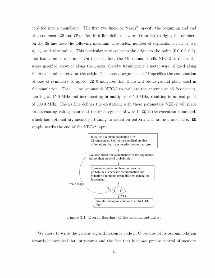
card fed into a mainframe. The first two lines, or “cards”, specify the beginning and end

of a comment (CM and CE). The third line defines a wire. From left to right, the numbers

on the GW line have the following meaning: wire index, number of segments, x1, y1, z1, x2,

y2, z2, and wire radius. This particular wire connects the origin to the point (0.0, 0.5, 0.0),

and has a radius of 1 mm. On the next line, the GX command tells NEC-2 to reflect the

wires specified above it along the y-axis, thereby forming one 1 meter wire, aligned along

the y-axis and centered at the origin. The second argument of GX specifies the combination

of axes of symmetry to apply. GE 0 indicates that there will be no ground plane used in

the simulation. The FR line commands NEC-2 to evaluate the antenna at 46 frequencies,

starting at 75.0 MHz and incrementing in multiples of 5.0 MHz, resulting in an end point

of 300.0 MHz. The EX line defines the excitation; with these parameters NEC-2 will place

an alternating voltage source at the first segment of wire 1. XQ is the execution command,

which has optional arguments pertaining to radiation pattern that are not used here. EN

simply marks the end of the NEC-2 input.

Tournament selection based on survivalprobabilites; stochastic recombination andmutation operations create the next generation.Increment i.

Evaluate metric for each member of the population,and set their survival probabilities.

Initialize a random population of NChromosomes. Set I to the specified numberof iterations. Set i, the iteration counter, to zero.

"main loop"

No

Yes

i == I?

Print the champion antenna to an NEC file.Exit.

Figure 3.1: Overall flowchart of the antenna optimizer.

We chose to write the genetic algorithm source code in C because of its accommodation

towards hierarchical data structures and the fact that it allows precise control of memory

41

resources. Throughout our work we used the GNU C compiler (gcc) version 3.2.2 [63]. A

flowchart illustrating the overall concept of the algorithm is shown in Figure 3.1.

In the genetic algorithm, there are three data structure hierarchies that act in tandem,

each one critical at different stages in the program. The top structure of the first hierarchy

is a type called NecInData. The NecInData type fulfills the purpose of storing raw infor-

mation for reading and writing NEC-2 formatted files. The translation of an instance of an

NecInData structure to a file understandable by NEC-2 is trivial; it is a matter of dumping

strings and numbers in the appropriate order, following the NEC-2 command syntax illus-

trated earlier in this section. It contains all the information needed to simulate an antenna

except for its actual geometry. A second hierarchy, CartMap, contains information about

how many wires there are in the antenna, and where they each begin and end. It contains

the actual Cartesian coordinates of the line segments defining the structure. Together, the

NecInData and CartMap give all of the necessary values needed to write an NEC-2 input file.

However, if the antenna being optimized has a certain motif, such as a tree, then a

structure which specifies every line segment with floating point Cartesian coordinates would

be very wasteful, and would not lend itself well to the actual genetic operations. For these

purposes a chromosome data structure is used, whose definition is specific to each type

of antenna. It contains only the parameters of the antenna that are subject to genetic

operations. These parameters act as the genes of the chromosome. Each one is stored in

a single byte (specified in C by the type unsigned char), with a range of [0, 127]. The

chromosome data structures will be revisited later on in the context of the specific antenna

shapes being optimized.

3.3 Parallelization

Midway through the development of the algorithm, we decided that it would be worth-

while to parallelize the code, in order to divide the computational load associated with the

electromagnetic simulations amongst an arbitrary number of workstations. Local Area Mul-

ticomputer (LAM) is a free implementation of the Message Passing Interface (MPI), and it

42

contained all the tools needed for this purpose [64]. MPI is an industry standard describing

routines by which identical, concurrently executing programs can share data during exe-

cution [65]. We compiled and configured LAM/MPI version 7.1.1 in a home directory on

the Electrical Engineering Department’s Integrated Circuit Engineering (ICE) workstation

cluster. Each ICE workstation has an Intel Pentium IV 3.2 GHz CPU, 1 GByte of RAM,

and runs the Fedora GNU/Linux operating system with kernel version 2.4.20-8. Because the

ICE cluster has a network file system, a user’s home directory as seen from each machine

maps to the same disk storage. Therefore, the entire ICE cluster is ready to run parallel

programs after a single home directory installation of LAM/MPI.

LAM/MPI includes an application program interface (API), which is the library of func-

tions that we call in our genetic algorithm to pass data between copies of the program running

on different nodes of the cluster. A number of executable tools are included along with the

API, of which the most important for us are: mpicc, lamboot, and mpirun. mpicc is a gcc

compiler “wrapper” that hides the long series of compiler flags and library links needed to

produce an executable MPI application. Therefore, compiling the source of a program using

MPI functions can be as simple as merely entering the command “mpicc myprogram.c”.

Before the executable can be run, the LAM run-time environment must be started from any

one of the cluster workstations with the lamboot command. One argument of lamboot is

a file containing a list of network addresses corresponding to the machines that will each

become a node of the cluster. These can be any machines on which LAM/MPI and auto-

matic ssh key authentication have been configured. Therefore, a LAM/MPI cluster need not

necessarily consist of homogeneous hardware on an ethernet. In our experiment, however,

the ∼10 workstations of the ICE cluster were deemed sufficient. Typically one wants to em-

ploy the entire cluster started with lamboot; in this case we enter “mpirun N myprogram”

at the shell prompt to begin the parallel execution. In the default LAM architecture there

is no master node; however, mpirun must be called from the same machine that completed

lamboot.

43

3.4 Initialization

A header file named commonvar.h contains the definitions of the data structures that are

common to all the antenna optimizers. It also contains a long list of preprocessor directives

that specify parameters that can be varied between runs, such as the total population size

and the number of generations to run the algorithm for. In the spirit of modularity, the

data structure definitions and preprocessor directives specific to a given antenna species are

stored in separate files (e.g. tree.h).

The initialization statements of the main function of the genetic algorithm are listed

below. The code is taken from the binary tree optimizer, but between the antenna species

there is only a slight variation in the names of the data types and variables.

TreeParArray TPop;

CartParArray CartPop;

ChromTok *PhoneBook;

NecInData Props;

RegenInstruc *Schem;

TreeChrom *Lobby;

unsigned int InDisp[PTot];

These statements create instances of several data structures. The TreeParArray is a

parallel array of tree chromosomes. This structure is parallel because it facilitates the division

of its elements among the nodes of the cluster, so that each machine only “sees” its own part

of the array. The CartParArray is similar to the TreeParArray except that it is an array

of Cartesian antenna maps. Phonebook, an array of type ChromTok, is another structure for

which only one instance is created in the entire program. It functions as a global directory

of the entire population, storing the following information for each member: the home node,

the local index on that node, the global index, and the metric associated with its evaluation.

The NecInData structure is used to store the input parameters for NEC-2. Schem, a pointer

to a structure of type RegenInstruc, holds the place of the instructions that specify the

operations that transform the current generation into the next. Lobby functions as a holding

cell, pointing to tree chromosomes that are either on their way out to be delivered to a fellow

44

node or have just arrived at the local node. InDisp is an array whose function is also related

to transferring chromosomes between nodes.

The function calls of the initialization stage are listed below.

create_tree_par_array(&TPop);

create_cart_par_array(&CartPop);

alloc_chromtok_array(&PhoneBook);

alloc_instruc_set(&Schem, TPop.LocalSize);

alloc_tree_array(&Lobby, 2*TPop.LocalSize);

init_pop(&TPop, &CartPop, &Props);

The first two calls initialize the parallel data structures in a very similar manner. Inside

these functions, memory is allocated for the structures making up the array. Also, each node

is assigned the range of global population indices that it controls throughout the algorithm.

The following three functions (all of whose names begin with alloc) allocate memory for

the data structure instances specified in their arguments. The memory is allocated locally,

and the amount requested on a node is dependent on the share of the population that has

been assigned to it. The population shares will not be exactly equal if the number of nodes

in the cluster does not divide evenly into the total population. The last function, init pop,

does much more than the housekeeping that has been done up until this point.

From random numbers, init pop fills the empty population with individual antennas

that meet the definition of the species being optimized. For each member of the population,

a sequence of random gene values composing a chromosome is generated. If these genes

result in a valid structure, then it will move on to create the next member of the population.

If not, it repeats the generation of a sequence of random genes until a valid member has

been initialized. Depending on the algorithm parameters, this process can easily take over

100 tries for a given member. The first condition that is tested to discriminate a valid

structure is to check that the structure falls within the boundaries specified in the algorithm

input parameters, for example a 60 cm × 60 cm square. If the structure is a tree antenna,

then a second condition must be checked – that none of the branch wires cross each other.

The algorithm to check for wire-crossing is revisited later on in further detail during the

discussion on the genetic operations, as it is also needed to check newly derived antennas.

45

3.5 Main Loop

Here is the main loop of the genetic algorithm, with only some minor debugging and logging

statements excluded for clarity:

for(GenCounter = 0; GenCounter <= GENERATIONS; GenCounter++)

if(GenCounter > 0)

create_schem(Schem, TPop, CartPop, PhoneBook);

exchange_pop(Lobby, InDisp, Schem, TPop);

regen_pop(Lobby, InDisp, Schem, &TPop, &CartPop);

write_pop(CartPop, Props);

sort_pop(CartPop, PhoneBook, Props);

The optimizer is essentially complete once this loop has gone through the number of iter-

ations specified by the user in the algorithm input parameters, GENERATIONS. GENERATIONS

is on the order of 100 for most runs. On the first pass through the main loop, the regener-

ation code block is skipped, because the antennas of the initial population have yet to be

evaluated. The write pop function writes NEC-2 input files based on the Cartesian map ar-

ray, CartPop, and the NEC-2 properties structure, Props. sort pop is a long, multi-layered

function that accomplishes three major tasks. First, it calls nec2cSilent on each of the input

files created by write pop. The total execution time of the genetic optimizer is dominated

by the wait for nec2cSilent to finish evaluating the entire population. Keep in mind that

each node of the cluster is only running NEC-2 on their own subset of the population – this

division of labor is the entire goal of the parallelization. Next, a function inside sort pop

parses the output files left by nec2cSilent to evaluate the goodness of each antenna in their

local subset, assigning each one a metric. The metrics and their associated antennas are

sorted using a parallel quicksort routine, and the results are stored in PhoneBook. The ele-

ments of the PhoneBook are ordered by metric, so that PhoneBook[0] indicates where the

champion chromosome is, what its local and global indices are, and what its metric is.

On the second pass through the main loop, and every pass thereafter, the regeneration

46

block is executed. The first function, create schem, forms the scheme of regeneration, and

its inner workings are as follows. First, each member of the population is assigned a roulette

area that will define its probability of being selected during the upcoming genetic operations.

The roulette area is proportional to 1/√

rank + 1, where rank is an integer in the range

[0, POPULATION−1] and lower rank is better. Next, two parameters defined by the user in the

input header file of the algorithm come into play, ELITE FRAC and CROSS FRAC. ELITE FRAC is

a floating point value in the range [0, 1] that specifies how much of the population will survive

as elites. This is typically a relatively small value such as 0.01. CROSS FRAC indicates the

percentage of the non-elite population that will be regenerated through recombination (also

known as crossover) instead of mutation. In the final trials of our experiment, CROSS FRAC

was set to 0.5.

Next, a loop is entered that selects the mode of regeneration of each new member of

the population. Suppose that i is the iteration counter of this loop. If the rank of the

ith member of the old population is low enough to place it in the top ELITE FRAC×100

percentage of the population, then a regeneration mode flag in Schem[i] is set to a value that

tells the algorithm to pass the ith member on to the next generation unmodified. If the ith

member is not elite, then a random number decides whether the mode will be recombination

or mutation, making use of CROSS FRAC to control the likelihood of the respective outcomes.

If the random number lands in the range mapped to a recombination instruction, two

parent members are stochastically selected from the global population. The likelihood of a

chromosome being selected is proportional to the roulette area assigned to it at the beginning

of the function. The populations used in this experiment are large enough (on the order of

100) that no provision is made to prevent the selection of identical parents. In addition to

the regeneration mode being set to the nominal recombination value, the home node and

the local and global indices of each parent are stored in Schem[i]. If the random number

chooses a mutation instruction (the only other possibility allowed), then only one parent is

selected, with the same roulette method as for the individual recombination parents. Again,

the relevant information needed for carrying out the regeneration is stored in Schem[i].

47

In the process described above, the parents of the new ith member are selected from

the global pool of chromosomes. This means that members will need to be transported

from one node to another in order for each node to carry out its share of the regeneration

instructions. exchange pop is the function that serves this purpose. To do this in the

most efficient manner, each node determines two matrices: one specifying the incoming

chromosomes and one specifying the outgoing chromosomes. In such a matrix, the column

indicates the node that is being considered. Then, each column contains the local indices of

the chromosomes that are being transported to or from that column’s node. The length of

the columns will generally be uneven because create schem makes no attempt to equally

distribute the flux between nodes. The data structure allocated before the main loop, Lobby,

serves as the intermediate storage space for outgoing and incoming chromosomes, which

are passed between nodes using a number of calls to MPI library functions. Once the

requested chromosomes have been moved to the Lobby structures of the expectant nodes,

exchange pop’s job is done.

The last main loop function to be described is the core of the genetic algorithm, regen pop.

It has the instructions it needs, thanks to create schem, and it has the data it needs, thanks

to exchange pop. Inside regen pop is a loop that overwrites each spot of the old population

one at a time. At iteration i, the first step is to check the mode of regeneration and act

accordingly. If the mode is elite, a flag is raised in the Cartesian map associated with the

member indicating that the antenna does not need to be reevaluated later on in sort pop.

Since both the Cartesian map and the chromosome remain the same, nothing else need be

done before advancing to the next member. If the mode is recombination, then the recom-

bination function is called on the two parents. Lastly, if the mode is mutation, then the

mutation function is called on the mutation parent. These last two functions are worth

exploring in detail.

Figure 3.2 is a flow chart illustrating the algorithm of the recombination function. The

shaded bubbles indicate the two possible exits. As a starting point, the first of the two

parents, ParentOne, is copied to Dummy. Dummy serves as a test bed of different combinations

48

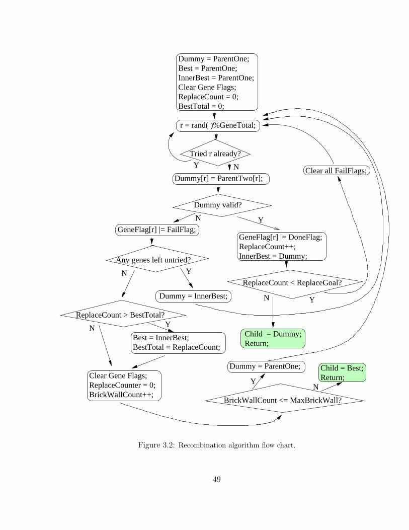
Tried r already?

Dummy[r] = ParentTwo[r];

Dummy valid?

Y

ReplaceCount++;InnerBest = Dummy;

GeneFlag[r] |= DoneFlag;

Clear all FailFlags;

Dummy = ParentOne;Best = ParentOne;InnerBest = ParentOne;Clear Gene Flags;ReplaceCount = 0;BestTotal = 0;

GeneFlag[r] |= FailFlag;

Any genes left untried?

ReplaceCount < ReplaceGoal?

Dummy = InnerBest;

Dummy = ParentOne;

Best = InnerBest;BestTotal = ReplaceCount;

Clear Gene Flags;

BrickWallCount++;ReplaceCounter = 0;

ReplaceCount > BestTotal?Y

BrickWallCount <= MaxBrickWall?

Y N

YN

N

N Y

NY

r = rand( )%GeneTotal;

N

Child = Dummy;Return;

Child = Best;Return;

Figure 3.2: Recombination algorithm flow chart.

49

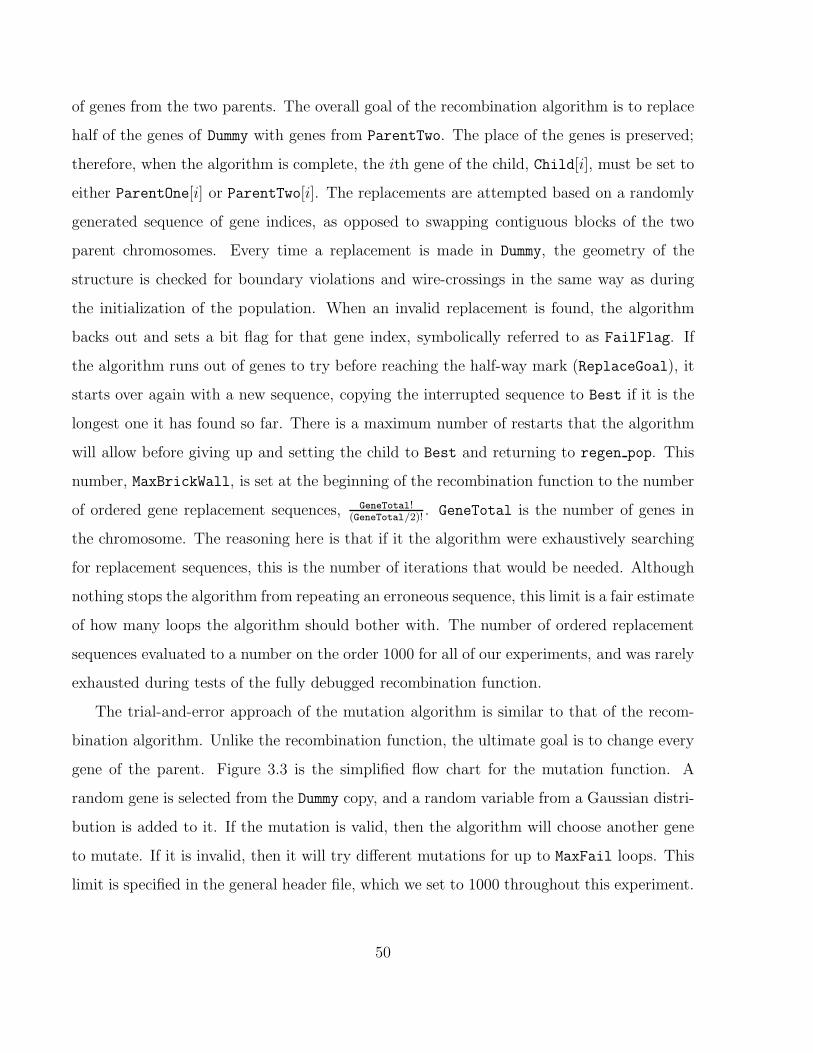
of genes from the two parents. The overall goal of the recombination algorithm is to replace

half of the genes of Dummy with genes from ParentTwo. The place of the genes is preserved;

therefore, when the algorithm is complete, the ith gene of the child, Child[i], must be set to

either ParentOne[i] or ParentTwo[i]. The replacements are attempted based on a randomly

generated sequence of gene indices, as opposed to swapping contiguous blocks of the two

parent chromosomes. Every time a replacement is made in Dummy, the geometry of the

structure is checked for boundary violations and wire-crossings in the same way as during

the initialization of the population. When an invalid replacement is found, the algorithm

backs out and sets a bit flag for that gene index, symbolically referred to as FailFlag. If

the algorithm runs out of genes to try before reaching the half-way mark (ReplaceGoal), it

starts over again with a new sequence, copying the interrupted sequence to Best if it is the

longest one it has found so far. There is a maximum number of restarts that the algorithm

will allow before giving up and setting the child to Best and returning to regen pop. This

number, MaxBrickWall, is set at the beginning of the recombination function to the number

of ordered gene replacement sequences, GeneTotal!(GeneTotal/2)!

. GeneTotal is the number of genes in

the chromosome. The reasoning here is that if it the algorithm were exhaustively searching

for replacement sequences, this is the number of iterations that would be needed. Although

nothing stops the algorithm from repeating an erroneous sequence, this limit is a fair estimate

of how many loops the algorithm should bother with. The number of ordered replacement

sequences evaluated to a number on the order 1000 for all of our experiments, and was rarely

exhausted during tests of the fully debugged recombination function.

The trial-and-error approach of the mutation algorithm is similar to that of the recom-

bination algorithm. Unlike the recombination function, the ultimate goal is to change every

gene of the parent. Figure 3.3 is the simplified flow chart for the mutation function. A

random gene is selected from the Dummy copy, and a random variable from a Gaussian distri-

bution is added to it. If the mutation is valid, then the algorithm will choose another gene

to mutate. If it is invalid, then it will try different mutations for up to MaxFail loops. This

limit is specified in the general header file, which we set to 1000 throughout this experiment.

50

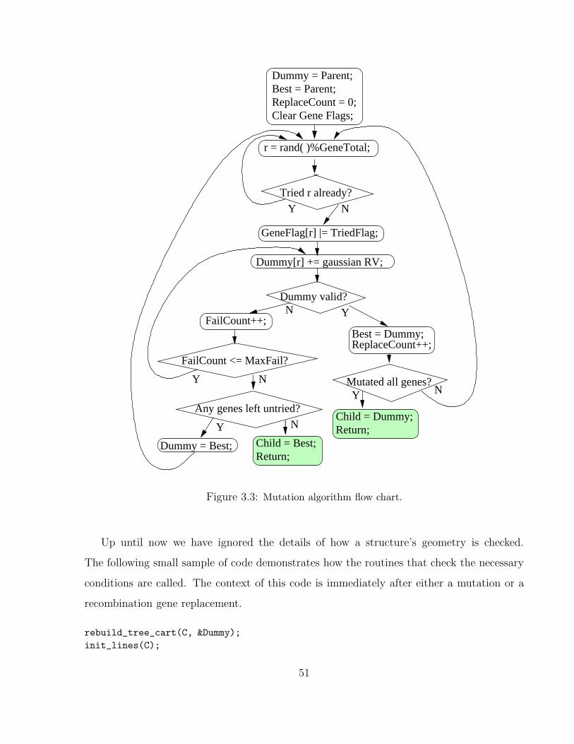
r = rand( )%GeneTotal;

FailCount++;

Dummy = Parent;Best = Parent;ReplaceCount = 0;Clear Gene Flags;

Tried r already?

GeneFlag[r] |= TriedFlag;

Dummy[r] += gaussian RV;

Dummy valid?

FailCount <= MaxFail?

Any genes left untried?

Dummy = Best;

Mutated all genes?

ReplaceCount++;Best = Dummy;

Y

N Y

NY

N

Y N

Child = Best;Return;

Y N

Child = Dummy;Return;

Figure 3.3: Mutation algorithm flow chart.

Up until now we have ignored the details of how a structure’s geometry is checked.

The following small sample of code demonstrates how the routines that check the necessary

conditions are called. The context of this code is immediately after either a mutation or a

recombination gene replacement.

rebuild_tree_cart(C, &Dummy);

init_lines(C);

51

BoundResult = check_bound(*C);

if(BoundResult == 0)

GeomResult = check_geom(C);

if(GeomResult == 0)

GeneFlag[r] |= DoneFlag;

copy_tree(Dummy, &InnerBest);

ReplaceCount++;

.

.

.

The functions rebuild tree cart and init lines translate the Dummy, of type chro-

mosome, into a Cartesian map. The function check bound looks at the Cartesian map and

makes sure that the antenna fits within the two-dimensional boundaries given by the user in

the general header file, and that none of the nodes have crossed over a plane of symmetry.

The result is stored in BoundResult; its value is zero if there is no boundary violation. If

the boundary check passed, then the Cartesian map is scrutinized further by the function

check geom. Like check bound, it returns zero if the structure meets its requirements.

check geom checks for several problems. One is the unintentional intersection of wires.

Consider the scenario shown in Figure 3.4, a close-up view of a wire antenna before and

after a mutation. When a node is moved, so is every wire attached to it. Here, when Node

#1 is moved, it results in the attached wires a and b crossing wire d. Besides drastically

changing the electrical nature of the structure, crossing wires in this manner would result in

highly inaccurate results from NEC-2. This is because NEC-2 will not allow current to flow

between conductors unless the points where the conductors touch are themselves defined as

wire endpoints [61]. In other words, new nodes would have to be created at the intersection

points for the results to be meaningful. While not an implausible feature, the size of the

chromosome structures would explode as the algorithm progressed through the generations,

accumulating more and more crossings. In addition, recombination would be complicated

by the fact that members of the population would each have different numbers of nodes.

Therefore, our genetic algorithm does not allow new wire intersections to form.

52

2 2

11

wire a

wire b

wire cwire d

wire a

wire b

wire cwire d

Figure 3.4: Example of an invalid mutation.

A second unwanted outcome, closely related to the first, is the unlikely but serious situ-

ation of wires overlapping as a result of mutation. In that case, since the wires are parallel,

there is no solution for an intersection point, so it must be addressed separately from the

first criterion. Thirdly, a more subtle problem relates to the distance between wires. The

NEC user manual suggests that unconnected segments remain several wire radii apart for the

best accuracy. Because of this, there should be a minimal separation condition between each

node and all of the wires unattached to it. Despite the simplicity with which these problems

are visually demonstrated, the complexity of their analytical detection makes check geom

one of the longest functions of the entire program.

3.6 Implementation of the Binary Tree Antenna Species

Figure 3.5 is a diagram of a third-order binary tree illustrating how the information needed

to construct the antenna is reduced to a sequence of genes. There are two implied axes of

symmetry represented by dashed lines. Therefore, the entire structure is actually the union

of the reflections about the vertical and horizontal axes. This way, not only is the symmetry

of the dipole preserved, but the size of the encoded structure is reduced. A simple approach

is taken to storing the information necessary to reconstruct the shape. Each node is assigned

a pair of angles and a pair of radii, which fully describe the branch segments that grow from

it. The exception to this is the first branch node, situated on top of the trunk, where only

53

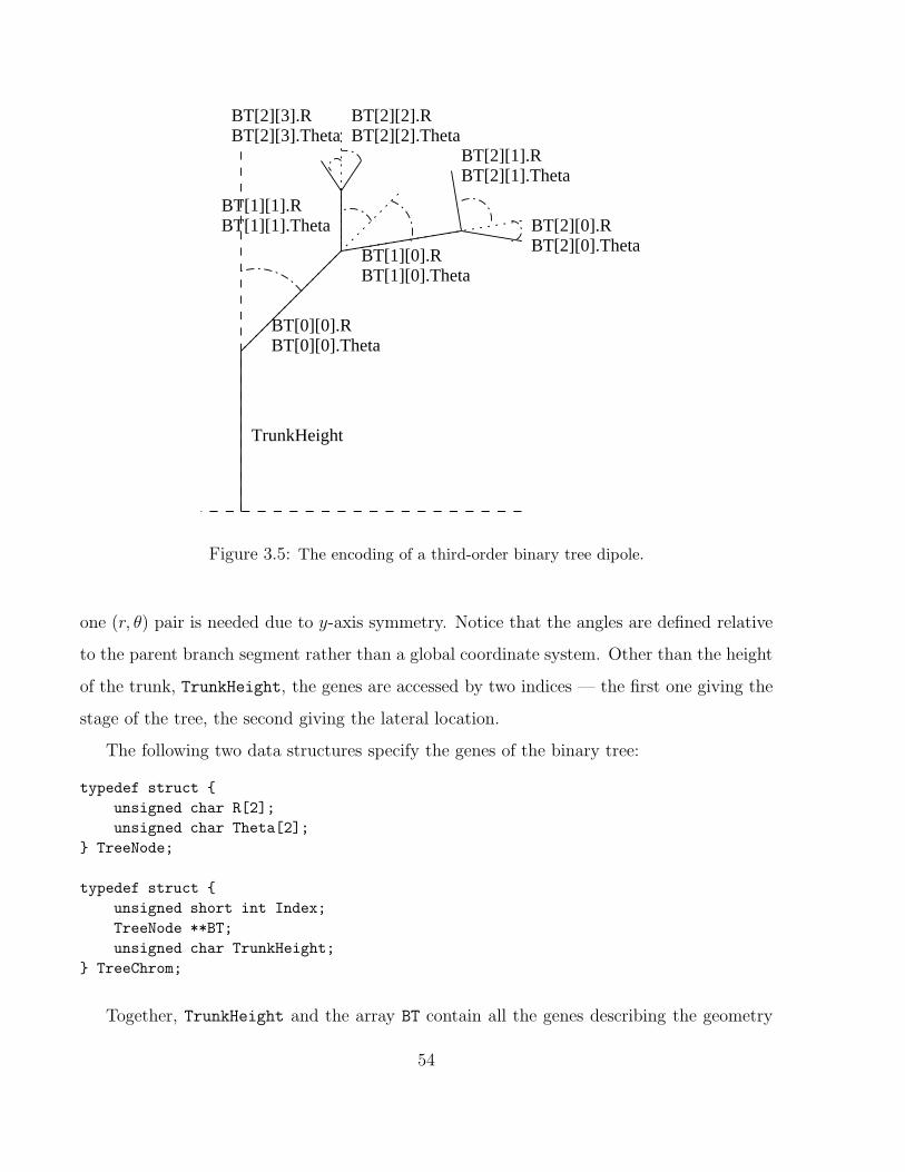
TrunkHeight

BT[2][1].RBT[2][1].Theta

BT[0][0].ThetaBT[0][0].R

BT[1][0].RBT[1][0].Theta

BT[2][0].ThetaBT[2][0].R

BT[2][2].RBT[2][2].Theta

BT[2][3].RBT[2][3].Theta

BT[1][1].ThetaBT[1][1].R

Figure 3.5: The encoding of a third-order binary tree dipole.

one (r, θ) pair is needed due to y-axis symmetry. Notice that the angles are defined relative

to the parent branch segment rather than a global coordinate system. Other than the height

of the trunk, TrunkHeight, the genes are accessed by two indices — the first one giving the

stage of the tree, the second giving the lateral location.

The following two data structures specify the genes of the binary tree:

typedef struct

unsigned char R[2];

unsigned char Theta[2];

TreeNode;

typedef struct

unsigned short int Index;

TreeNode **BT;

unsigned char TrunkHeight;

TreeChrom;

Together, TrunkHeight and the array BT contain all the genes describing the geometry

54

of the binary tree. The memory that BT references is allocated during init pop; the amount

given for each “row” of BT is determined by the number of branching levels specified by the

user. An Mth order binary tree, M ≥ 0, has 2M − 1 (r, θ) pairs, which results in a total

of 2M+1 − 1 genes when the trunk height is counted. Through most of the experiment, a

third-order binary tree was chosen to be optimized (15 genes), as a compromise between the

design flexibility offered by many branch levels and the prohibitive cost of manufacturing a

more complex shape. Each θ has a range of (0, π), and each r has a range of [RMIN, RMAX],

where RMIN and RMAX are defined in the input header file. The actual geometric values of r

and θ are each mapped to a 7-bit value with a range of [0,127], stored in variables of type

unsigned char.

55

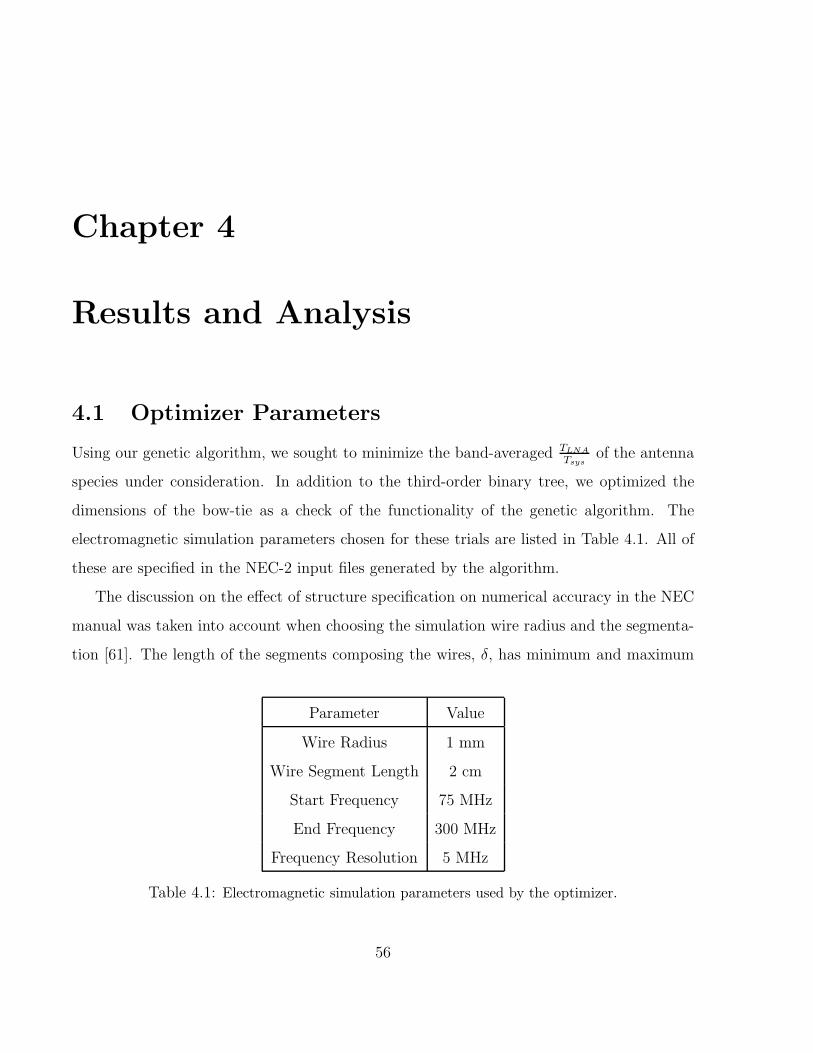
Chapter 4

Results and Analysis

4.1 Optimizer Parameters

Using our genetic algorithm, we sought to minimize the band-averaged TLNA

Tsysof the antenna

species under consideration. In addition to the third-order binary tree, we optimized the

dimensions of the bow-tie as a check of the functionality of the genetic algorithm. The

electromagnetic simulation parameters chosen for these trials are listed in Table 4.1. All of

these are specified in the NEC-2 input files generated by the algorithm.

The discussion on the effect of structure specification on numerical accuracy in the NEC

manual was taken into account when choosing the simulation wire radius and the segmenta-

tion [61]. The length of the segments composing the wires, δ, has minimum and maximum

Parameter Value

Wire Radius 1 mm

Wire Segment Length 2 cm

Start Frequency 75 MHz

End Frequency 300 MHz

Frequency Resolution 5 MHz

Table 4.1: Electromagnetic simulation parameters used by the optimizer.

56

recommended values based on the wavelengths over which the structure is excited. The man-

ual urges the user to observe the range 10−3λmax < δ < 0.1λmin. Considering the frequency

range [75, 300] MHz, this implies that we should have 0.004 m < δ < 0.1 m. We wanted the

optimizer to have the ability to consider features on the scale of centimeters. However, the

execution time increases dramatically for small segment sizes. Empirically, we found that

the NEC-2 execution time was proportional to the cube of the inverse of the segment length.

Therefore, as a compromise between speed and design flexibility we settled on a segment

length of 2 cm.

The choice of wire radius was dependent on the choice of segment length; the NEC

manual states that a high ratio of segment length to wire radius is beneficial to the accuracy

of the results, and that a ratio δ/r ∼ 10 is sufficient. However, as discussed in Section 2.2, we

found that the solutions for thick wire (1 cm radius) antennas were not robust to variations

in segmentation, even when this ratio was respected. Consequently, we used a 1 mm radius

throughout our experiment. Although in practice a larger wire radius would be used, we

reasoned that the effect of wire radius on TLNA would be systematic for a given antenna

species.

Originally we intended to use a relatively coarse frequency sampling during the evalua-

tion of the antennas: 11 points spaced 22.5 MHz apart. However, during early runs we found

narrowband features in the impedance responses of some of the algorithm’s offspring, whose

alignment could easily throw the optimization off course. Therefore, we decreased the fre-

quency resolution to 5 MHz, resulting in 46 simulation points in total. Not all features can be

satisfactorily sampled for some antennas, but at least their presence is immediately evident

when examining the results. Fortunately, the final metric we employed did not propagate

antennas with such narrowband response features.

The overall parameters of the genetic algorithm used during the final trials are shown

in Table 4.2. As stated before, the metric used in sorting the offspring is their average

TLNA

Tsys. To obtain the metric, the algorithm first halves the antenna impedance read from the

nec2cSilent output file, because of the differential pair configuration of the LNA (see Section

57

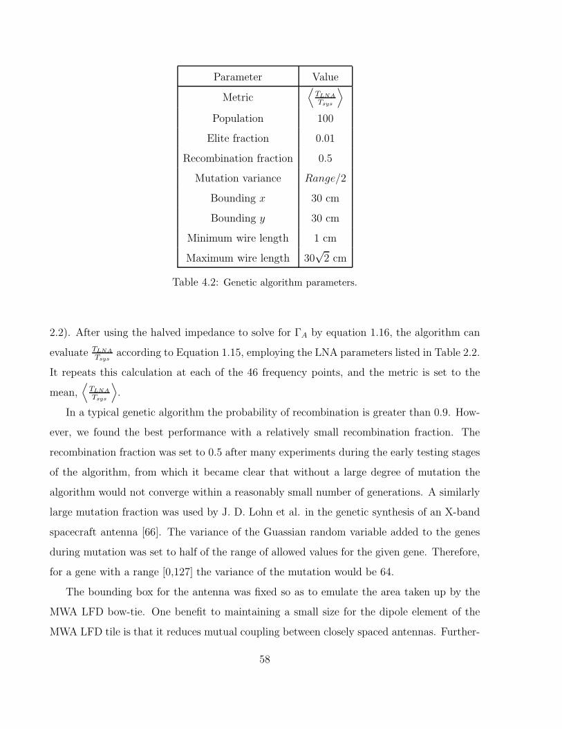
Parameter Value

Metric⟨

TLNA

Tsys

⟩

Population 100

Elite fraction 0.01

Recombination fraction 0.5

Mutation variance Range/2

Bounding x 30 cm

Bounding y 30 cm

Minimum wire length 1 cm

Maximum wire length 30√

2 cm

Table 4.2: Genetic algorithm parameters.

2.2). After using the halved impedance to solve for ΓA by equation 1.16, the algorithm can

evaluate TLNA

Tsysaccording to Equation 1.15, employing the LNA parameters listed in Table 2.2.

It repeats this calculation at each of the 46 frequency points, and the metric is set to the

mean,⟨

TLNA

Tsys

⟩

.

In a typical genetic algorithm the probability of recombination is greater than 0.9. How-

ever, we found the best performance with a relatively small recombination fraction. The

recombination fraction was set to 0.5 after many experiments during the early testing stages

of the algorithm, from which it became clear that without a large degree of mutation the

algorithm would not converge within a reasonably small number of generations. A similarly

large mutation fraction was used by J. D. Lohn et al. in the genetic synthesis of an X-band

spacecraft antenna [66]. The variance of the Guassian random variable added to the genes

during mutation was set to half of the range of allowed values for the given gene. Therefore,

for a gene with a range [0,127] the variance of the mutation would be 64.

The bounding box for the antenna was fixed so as to emulate the area taken up by the

MWA LFD bow-tie. One benefit to maintaining a small size for the dipole element of the

MWA LFD tile is that it reduces mutual coupling between closely spaced antennas. Further-

58

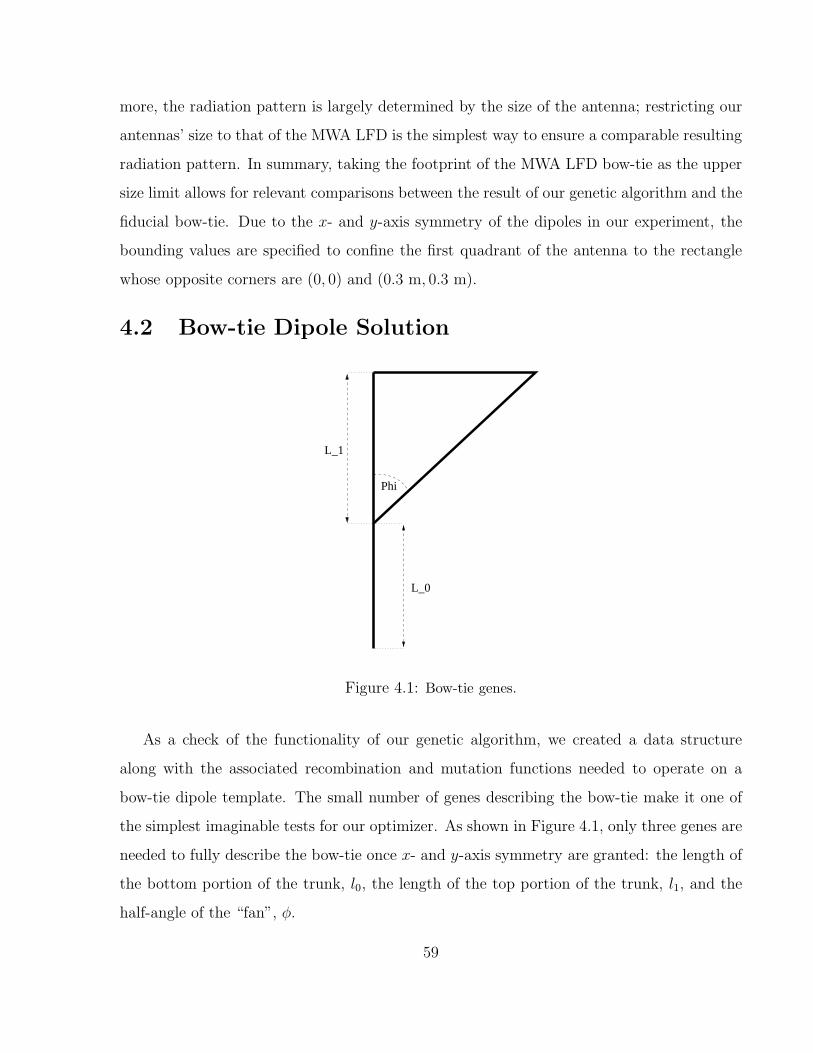
more, the radiation pattern is largely determined by the size of the antenna; restricting our

antennas’ size to that of the MWA LFD is the simplest way to ensure a comparable resulting

radiation pattern. In summary, taking the footprint of the MWA LFD bow-tie as the upper

size limit allows for relevant comparisons between the result of our genetic algorithm and the

fiducial bow-tie. Due to the x- and y-axis symmetry of the dipoles in our experiment, the

bounding values are specified to confine the first quadrant of the antenna to the rectangle

whose opposite corners are (0, 0) and (0.3 m, 0.3 m).

4.2 Bow-tie Dipole Solution

Phi

L_1

L_0

Figure 4.1: Bow-tie genes.

As a check of the functionality of our genetic algorithm, we created a data structure

along with the associated recombination and mutation functions needed to operate on a

bow-tie dipole template. The small number of genes describing the bow-tie make it one of

the simplest imaginable tests for our optimizer. As shown in Figure 4.1, only three genes are

needed to fully describe the bow-tie once x- and y-axis symmetry are granted: the length of

the bottom portion of the trunk, l0, the length of the top portion of the trunk, l1, and the

half-angle of the “fan”, φ.

59

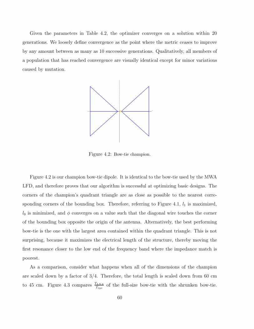
Given the parameters in Table 4.2, the optimizer converges on a solution within 20

generations. We loosely define convergence as the point where the metric ceases to improve

by any amount between as many as 10 successive generations. Qualitatively, all members of

a population that has reached convergence are visually identical except for minor variations

caused by mutation.

X

YZ

Figure 4.2: Bow-tie champion.

Figure 4.2 is our champion bow-tie dipole. It is identical to the bow-tie used by the MWA

LFD, and therefore proves that our algorithm is successful at optimizing basic designs. The

corners of the champion’s quadrant triangle are as close as possible to the nearest corre-

sponding corners of the bounding box. Therefore, referring to Figure 4.1, l1 is maximized,

l0 is minimized, and φ converges on a value such that the diagonal wire touches the corner

of the bounding box opposite the origin of the antenna. Alternatively, the best performing

bow-tie is the one with the largest area contained within the quadrant triangle. This is not

surprising, because it maximizes the electrical length of the structure, thereby moving the

first resonance closer to the low end of the frequency band where the impedance match is

poorest.

As a comparison, consider what happens when all of the dimensions of the champion

are scaled down by a factor of 3/4. Therefore, the total length is scaled down from 60 cm

to 45 cm. Figure 4.3 compares TLNA

Tsysof the full-size bow-tie with the shrunken bow-tie.

60

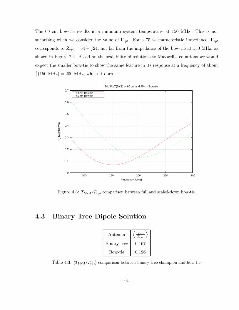
The 60 cm bow-tie results in a minimum system temperature at 150 MHz. This is not

surprising when we consider the value of Γopt. For a 75 Ω characteristic impedance, Γopt

corresponds to Zopt = 54 + j24, not far from the impedance of the bow-tie at 150 MHz, as

shown in Figure 2.4. Based on the scalability of solutions to Maxwell’s equations we would

expect the smaller bow-tie to show the same feature in its response at a frequency of about

43(150 MHz) = 200 MHz, which it does.

0

0.1

0.2

0.3

0.4

0.5

0.6

0.7

100 150 200 250 300

T(L

NA

)/T

(SY

S)

Frequency (MHz)

T(LNA)/T(SYS) of 60 cm and 45 cm Bow-tie

60 cm Bow-tie45 cm Bow-tie

Figure 4.3: TLNA/Tsys comparison between full and scaled-down bow-tie.

4.3 Binary Tree Dipole Solution

Antenna⟨

TLNA

Tsys

⟩

Binary tree 0.167

Bow-tie 0.196

Table 4.3: 〈TLNA/Tsys〉 comparison between binary tree champion and bow-tie.

61

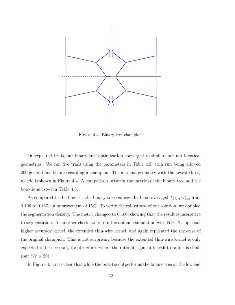
YZ

Figure 4.4: Binary tree champion.

On repeated trials, our binary tree optimization converged to similar, but not identical

geometries. We ran five trials using the parameters in Table 4.2, each run being allowed

200 generations before recording a champion. The antenna geometry with the lowest (best)

metric is shown in Figure 4.4. A comparison between the metrics of the binary tree and the

bow-tie is listed in Table 4.3.

As compared to the bow-tie, the binary tree reduces the band-averaged TLNA/Tsys from

0.196 to 0.167, an improvement of 15%. To verify the robustness of our solution, we doubled

the segmentation density. The metric changed to 0.166, showing that the result is insensitive

to segmentation. As another check, we re-ran the antenna simulation with NEC-2’s optional

higher accuracy kernel, the extended thin-wire kernel, and again replicated the response of

the original champion. This is not surprising because the extended thin-wire kernel is only

expected to be necessary for structures where the ratio of segment length to radius is small

(our δ/r is 20).

In Figure 4.5, it is clear that while the bow-tie outperforms the binary tree at the low end

62

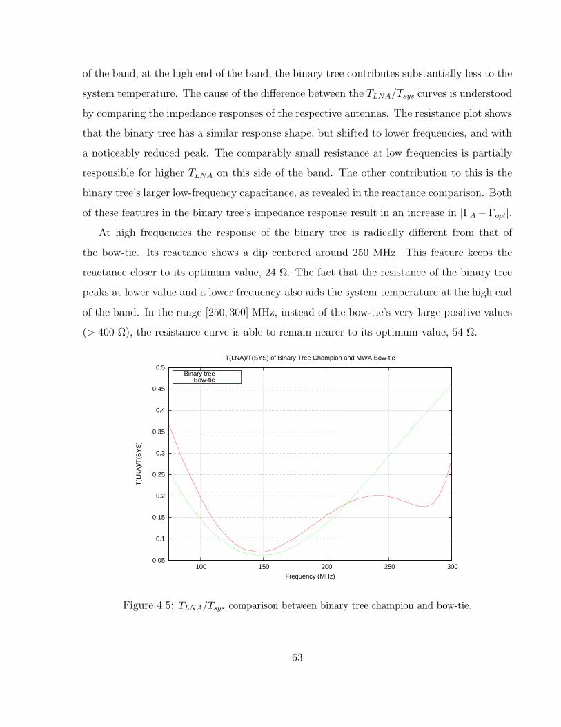
of the band, at the high end of the band, the binary tree contributes substantially less to the

system temperature. The cause of the difference between the TLNA/Tsys curves is understood

by comparing the impedance responses of the respective antennas. The resistance plot shows

that the binary tree has a similar response shape, but shifted to lower frequencies, and with

a noticeably reduced peak. The comparably small resistance at low frequencies is partially

responsible for higher TLNA on this side of the band. The other contribution to this is the

binary tree’s larger low-frequency capacitance, as revealed in the reactance comparison. Both

of these features in the binary tree’s impedance response result in an increase in |ΓA −Γopt|.At high frequencies the response of the binary tree is radically different from that of

the bow-tie. Its reactance shows a dip centered around 250 MHz. This feature keeps the

reactance closer to its optimum value, 24 Ω. The fact that the resistance of the binary tree

peaks at lower value and a lower frequency also aids the system temperature at the high end

of the band. In the range [250, 300] MHz, instead of the bow-tie’s very large positive values

(> 400 Ω), the resistance curve is able to remain nearer to its optimum value, 54 Ω.

0.05

0.1

0.15

0.2

0.25

0.3

0.35

0.4

0.45

0.5

100 150 200 250 300

T(L

NA

)/T

(SY

S)

Frequency (MHz)

T(LNA)/T(SYS) of Binary Tree Champion and MWA Bow-tie

Binary treeBow-tie

Figure 4.5: TLNA/Tsys comparison between binary tree champion and bow-tie.

63

The geometry of the binary-tree champion, displayed in Figure 4.4, is worth analyzing.

Most conspicuously, the algorithm has formed the outer branch tips into a structure that

recalls the profile of a parallel plate capacitor, blown up in Figure 4.7. Given the combination

of the branching nature of the binary tree and its two axes of symmetry, finding pairs of

roughly parallel wire segments spanning the feed is not surprising. Such wire segment pairs,

having locally constant and opposite electric potentials, will necessarily possess a capacitance.

However, the fact that the algorithm has effectively minimized the separation between this

set of branch tips and its mirrored image suggests that the capacitance has a dominant role

in the evolution of their positioning.

For an antenna there exists no method to isolate the contribution of various sections of

the structure to the frequency response, even in an approximate manner as is typically done

with linear circuits composed of discrete components. However, we can make an order of

magnitude calculation to determine if the branch tip capacitor described above could play

a significant role in the response of the antenna. The capacitance per unit length of two

parallel wires is given by

C/l =πǫ0

cosh−1(D/2a)[67]. (4.1)

ǫ0 is the permittivity of free space, D is the separation between the wires, and a is the radius

of the wires. Based on the geometry of the binary tree, we set a = 1 mm and D = 2 cm.

The two capacitors on each side of the dipole axis are effectively in parallel. Therefore, using

the sum of their lengths, 10 cm, we arrive at C ≃ 1 pF.

The magnitude of a capacitor’s impedance equals that of a resistor of value R at an

angular frequency ωc = 1/(RC). If we presuppose that this frequency occurs around 250

MHz, and set R to its value at this frequency, 200 Ω, then we have a capacitance of 3 pF.

Because this is within reasonable agreement with the capacitance we determined through

physical arguments, it is plausible for this branch tip capacitor to play a significant role in

the shape of the response of the binary tree at the high end of the frequency band. We made

another check of this hypothesis by observing how the response changes when the separation

between opposite sides of the capacitor is increased from 2 cm to 4 cm. Increasing D should

64

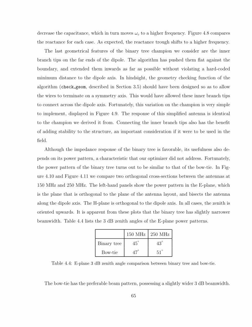
decrease the capacitance, which in turn moves ωc to a higher frequency. Figure 4.8 compares

the reactance for each case. As expected, the reactance trough shifts to a higher frequency.

The last geometrical features of the binary tree champion we consider are the inner

branch tips on the far ends of the dipole. The algorithm has pushed them flat against the

boundary, and extended them inwards as far as possible without violating a hard-coded

minimum distance to the dipole axis. In hindsight, the geometry checking function of the

algorithm (check geom, described in Section 3.5) should have been designed so as to allow

the wires to terminate on a symmetry axis. This would have allowed these inner branch tips

to connect across the dipole axis. Fortunately, this variation on the champion is very simple

to implement, displayed in Figure 4.9. The response of this simplified antenna is identical

to the champion we derived it from. Connecting the inner branch tips also has the benefit

of adding stability to the structure, an important consideration if it were to be used in the

field.

Although the impedance response of the binary tree is favorable, its usefulness also de-

pends on its power pattern, a characteristic that our optimizer did not address. Fortunately,

the power pattern of the binary tree turns out to be similar to that of the bow-tie. In Fig-

ure 4.10 and Figure 4.11 we compare two orthogonal cross-sections between the antennas at

150 MHz and 250 MHz. The left-hand panels show the power pattern in the E-plane, which

is the plane that is orthogonal to the plane of the antenna layout, and bisects the antenna

along the dipole axis. The H-plane is orthogonal to the dipole axis. In all cases, the zenith is

oriented upwards. It is apparent from these plots that the binary tree has slightly narrower

beamwidth. Table 4.4 lists the 3 dB zenith angles of the E-plane power patterns.

150 MHz 250 MHz

Binary tree 45

43

Bow-tie 47

51

Table 4.4: E-plane 3 dB zenith angle comparison between binary tree and bow-tie.

The bow-tie has the preferable beam pattern, possessing a slightly wider 3 dB beamwidth.

65

A wider beamwidth allows the interferometer to survey a greater area of the sky at once. On

the other hand, it also means that there is less rejection of man-made interference, which is

likely to arrive from large zenith angles. Because of this interference, the ideal beam would

be a step function that becomes null at zenith angles greater than 60

[43].

66

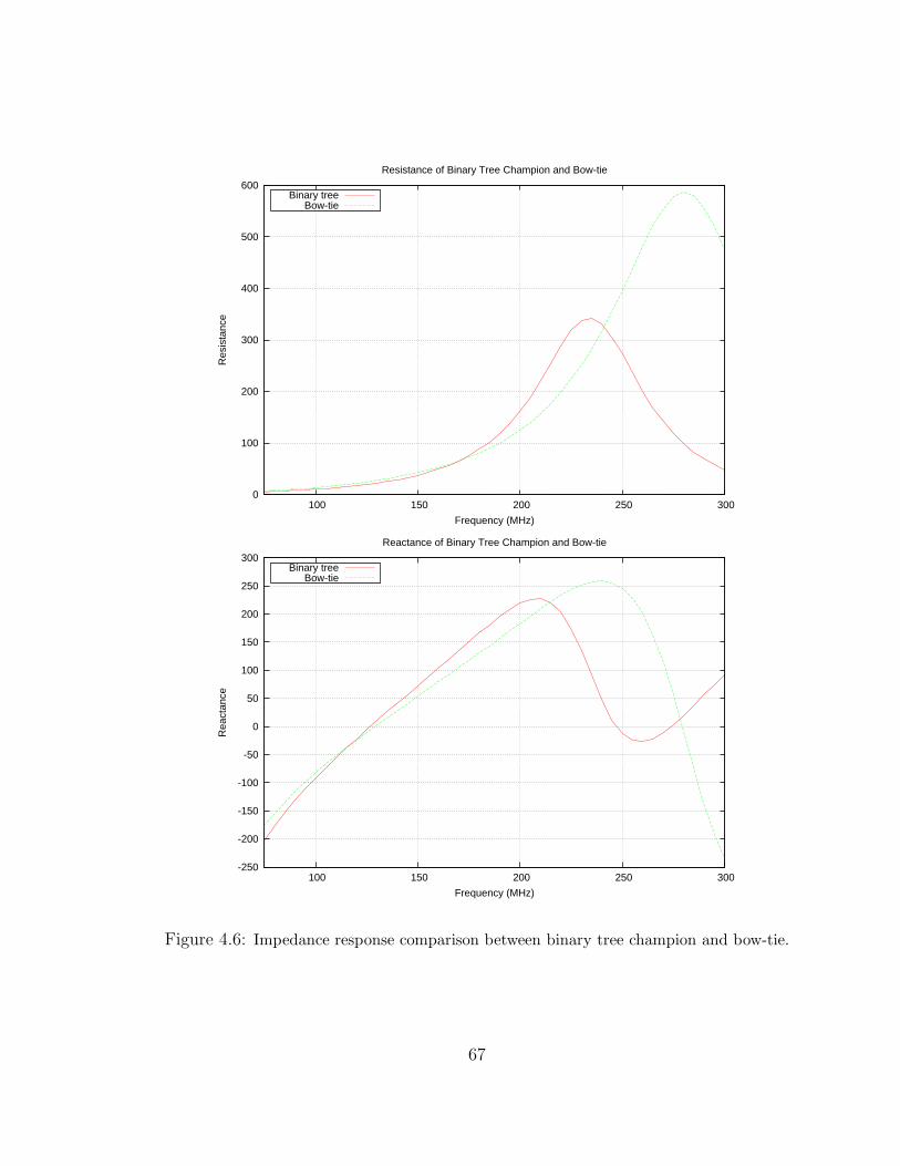
0

100

200

300

400

500

600

100 150 200 250 300

Res

ista

nce

Frequency (MHz)

Resistance of Binary Tree Champion and Bow-tie

Binary treeBow-tie

-250

-200

-150

-100

-50

0

50

100

150

200

250

300

100 150 200 250 300

Rea

ctan

ce

Frequency (MHz)

Reactance of Binary Tree Champion and Bow-tie

Binary treeBow-tie

Figure 4.6: Impedance response comparison between binary tree champion and bow-tie.

67

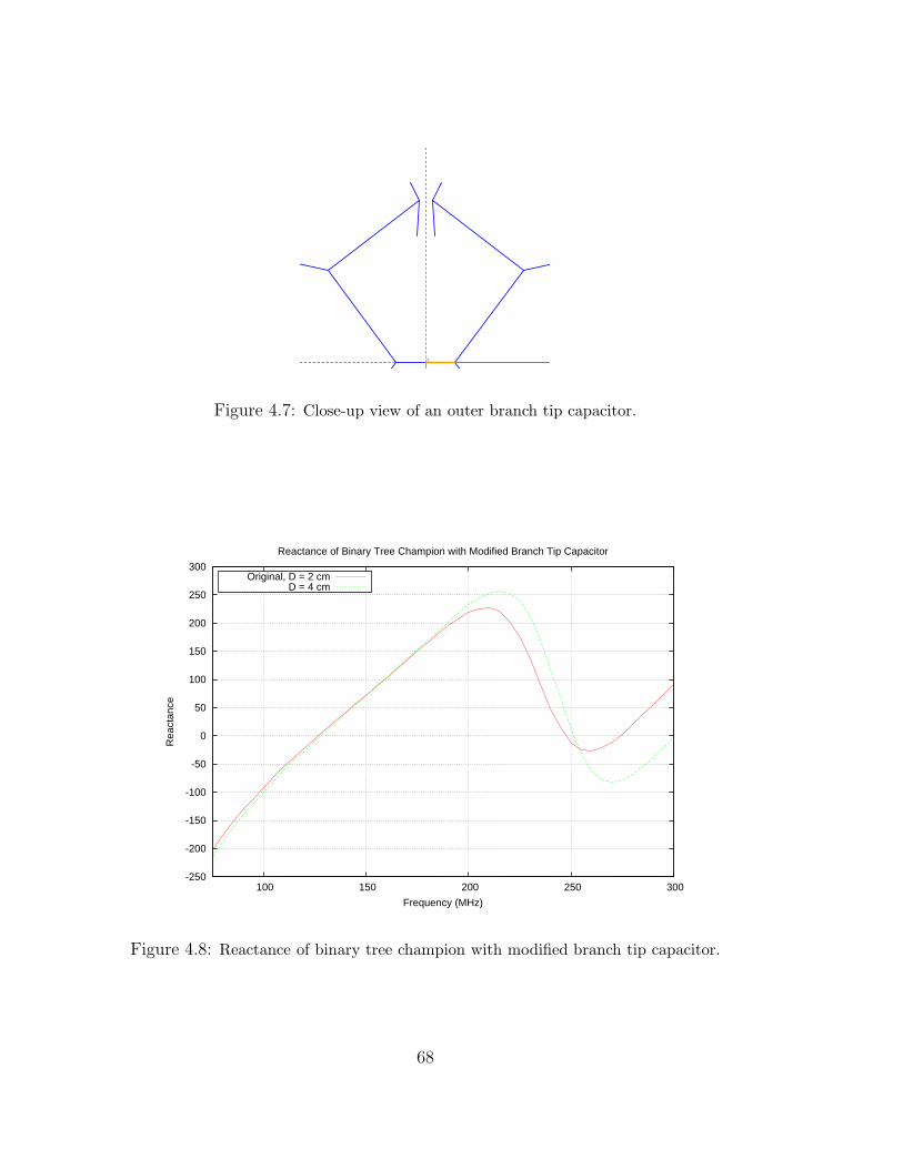
Z

Figure 4.7: Close-up view of an outer branch tip capacitor.

-250

-200

-150

-100

-50

0

50

100

150

200

250

300

100 150 200 250 300

Rea

ctan

ce

Frequency (MHz)

Reactance of Binary Tree Champion with Modified Branch Tip Capacitor

Original, D = 2 cmD = 4 cm

Figure 4.8: Reactance of binary tree champion with modified branch tip capacitor.

68

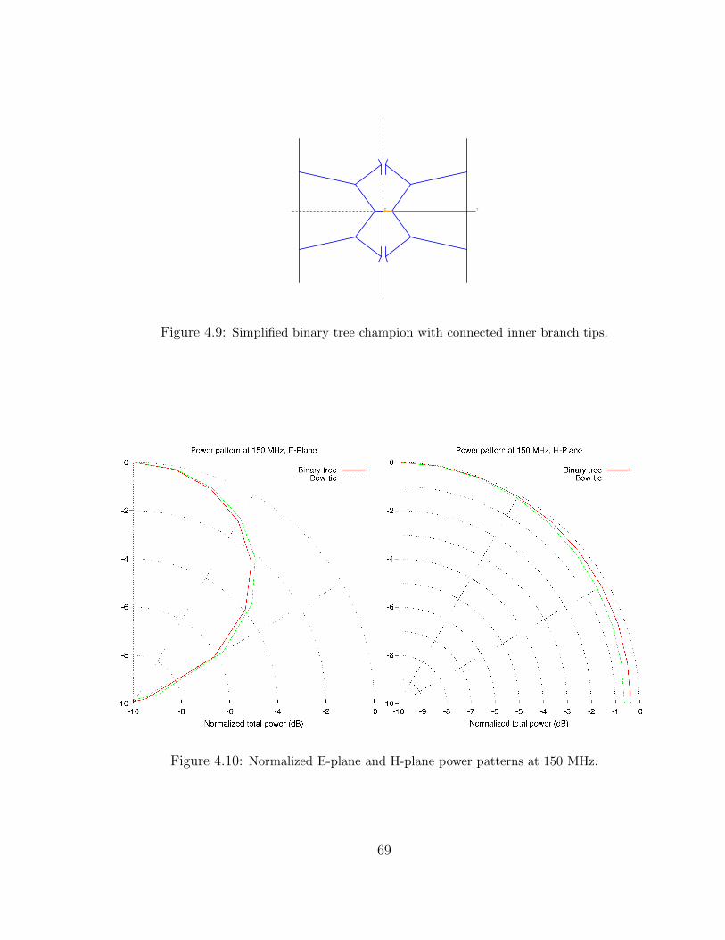
YZ

Figure 4.9: Simplified binary tree champion with connected inner branch tips.

Figure 4.10: Normalized E-plane and H-plane power patterns at 150 MHz.

69

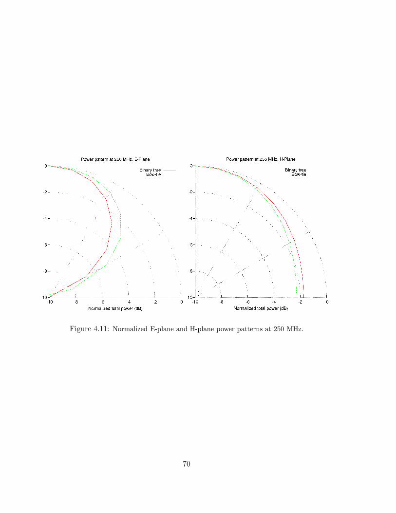
Figure 4.11: Normalized E-plane and H-plane power patterns at 250 MHz.

70

4.4 Conclusions

Our binary tree solution demonstrates the efficacy of using a genetic algorithm to optimize

the geometry of an antenna over a wide range of frequencies. Under idealized conditions,

our algorithm succeeded in improving on the overall noise match of the fiducial broadband

dipole, the MWA LFD bow-tie. Unfortunately, the binary tree does not decrease the sys-

tem temperature at the low end of the frequency band, which contains the main scientific

objective of the MWA, EoR observations. Recall that the redshifted 21 cm signal appears

at frequencies under 200 MHz for z > 6. Nevertheless, numerous other scientific objectives

are aided by the improved noise match at the high frequency end. These include surveys for

radio transients from high energy astrophysical phenomena, observations of pulsars and the

interstellar medium, and cosmic ray air shower detections [4].

In our simulations the antenna exists in free space, with no scattering off of surrounding

surfaces to perturb the response. The impact of structures in the vicinity of the antenna,

including the ground screen and the surrounding tile elements, is the largest unknown char-

acteristic of our binary tree champion. More comprehensive simulations that determine the

radiation pattern and the impedance response while taking these factors into account could

improve the confidence of the genetic algorithm solution. Ultimately, the evaluation would

be best carried out with field measurements of a prototype.

Another factor we have neglected in our comparison is the ease of construction. The bow-

tie is clearly easier to produce, consisting solely of equally-sized 45

triangles. On the other

hand, the binary tree’s outer branch tips are unterminated wires, requiring more careful

fabrication. The features of the branch tip capacitors are small, of order 1 cm, and likely

the most difficult part to reproduce precisely. Furthermore, as demonstrated in Figure 4.8,

the performance of the binary tree is highly sensitive to the positioning of these branch tips.

Here, a mere 2 cm shift in the placement resulted in a substantially different impedance

response. The fine-tuned nature of the branch tip capacitors may be the largest flaw in the

design of the binary tree champion. However, if construction obstacles could be overcome,

they pose a dramatic improvement at the high frequency end of the operation band.

71

The most intriguing question that our results raise is whether or not branch tip capacitors

could be added to the bow-tie shape to provide the same benefits as they do to the binary

tree. Extensions to our genetic algorithm could be developed to optimize a bow-tie/tree

hybrid species. Conceivably, this hybrid could offer the best of both worlds — the low end

noise match of the bow-tie and the high end noise match of the binary tree.

Lastly, it is interesting to note that the solutions of our genetic algorithm possess no

fractal properties. This is not surprising, because Gianvittorio’s fractal binary trees showed

no bandwidth improvement in this regime of electrical length. However, unlike in his ex-

periment, we did not form our trees by ad hoc prescription of branching angle and scaling

factor. Instead, we left the entire parameter space open for unbiased exploration. Yet, no

tree with the self-scaling regularity of a fractal evolved out of our populations. Therefore, it

is a compelling and more generalized reinforcement of his demonstration that regular fractal

trees do not offer bandwidth improvement outside of the small antenna limit.

The results of our experiment, and the antenna optimizer we created along the way will

prove useful in the final design stages of the Mileura Wide Field array, and possibly other

instruments of its kind. Binary trees are just one of countless templates that our algorithm

can be applied to; other antenna species, particularly a hybrid of the bow-tie and the binary

tree, could offer even more promising properties.

72

Bibliography

[1] S. Furlanetto, “Observing the reionization epoch through 21-centimetre radiation,”

Monthly Notices of the Royal Astronomical Society, vol. 347, no. 1, pp. 187–195, 2004.

[2] M. F. Morales, “Toward epoch of reionization measurements with wide-field radio ob-

servations,” The Astrophysical Journal, vol. 615, no. 1, pp. 7–18, 2004.

[3] C. L. Carilli, “HI 21cm probes of reionization, and beyond,” New Astronomy Reviews,

vol. 50, pp. 162–172, 2006.

[4] MIT Haystack Observatory, “The LFD Technical Design – Overview.” http://web.

haystack.mit.edu/arrays/MWA/LFD/tech_design/index.html, 15 March 2005. Re-

trieved 13 March 2006.

[5] J. D. Bowman, “The sensitivity of first-generation epoch of reionization observatories

and their potential for differentiating theoretical power spectra,” The Astrophysical

Journal, vol. 638, no. 1, pp. 20–26, 2006.

[6] Wikipedia: The Free Encyclopedia, “Koch curve.” http://en.wikipedia.org/wiki/

Koch_curve, 12 Jan 2005, 22:56 UTC. Retrieved 17 Jan 2005.

[7] D. Helfand, “Seeing the Whole Symphony.” http://ccnmtl.columbia.edu/projects/

helfand/, May 2003. Retrieved 26 Feb 2006.

[8] M. Rowan-Robinson, “Astrophysics and cosmology: the golden age,” Physics World,

December 1999. Retrieved 26 Feb 2006.

73

[9] NRAO, “An Overview of the Very Large Array.” http://www.vla.nrao.edu/genpub/

overview/, May 2003. Retrieved 26 Feb 2006.

[10] C. R. Nave, “The Rayleigh Criterion.” http://hyperphysics.phy-astr.gsu.edu/

Hbase/phyopt/raylei.html#c1, December 2005. Retrieved 26 Feb 2006.

[11] J. D. Kraus, Radio Astronomy, ch. 5. Cygnus-Quasar Books, 1986.

[12] J. K. Alexander, “Low frequency cosmic noise observations of the constitution of the

local system,” Astronomy and Astrophysics, vol. 6, p. 476, 1979.

[13] C. Lonsdale, “Calibration Approaches.” ftp://web.haystack.edu/pub/lofar/015.

pdf, December 2003. LOFAR Memo.

[14] S. Dodelson, Modern Cosmology. Academic Press, 2003.

[15] J. A. Peacock, Cosmological Physics. Cambridge University Press, 1999.

[16] J. D. Kraus, Radio Astronomy, ch. 8. Cygnus-Quasar Books, 1986.

[17] N. Wright, “Ned Wright’s Javascript Cosmology Calculator.” http://www.astro.ucla.

edu/~wright/CosmoCalc.html, 13 Aug 2003, 18:59 UTC. Retrieved 13 Mar 2006.

[18] J. D. Kraus, Radio Astronomy, ch. 3. Cygnus-Quasar Books, 1986.

[19] H. Nyqust, “Thermal agitation of electrical charge in conductors,” Phys. Rev., vol. 32,

pp. 110–113, 1928.

[20] J. D. Bregman, “Concepts for a Sky Noise Limited Low Frequency Array,” Perspec-

tives on Radio Astronomy: Technologies for Large Antenna Arrays, Proceedings of the

Conference held at the ASTRON Institute in Dwingeloo on 12-14 April 1999, 2000.

[21] J. D. Kraus, Antennas, ch. 3. McGraw-Hill, 1950.

[22] M. P. van Haarlem, “Lofar scientific applications.” http://www.lofar.org/archive/

science/LOFAR_SciApp_1.0.pdf, July 2001. ASTRON technical memo.

74

[23] J. D. Kraus, Radio Astronomy, ch. 7. Cygnus-Quasar Books, 1986.

[24] D. M. Pozar, Microwave Engineering, Second Edition, ch. 10. John Wiley and Sons,

1998.

[25] D. M. Pozar, Microwave Engineering, Second Edition, ch. 11. John Wiley and Sons,

1998.

[26] J. D. Kraus, Antennas, ch. 1. McGraw-Hill, 1950.

[27] J. D. Kraus, Antennas, ch. 10. McGraw-Hill, 1950.

[28] W. H. Hayt, Jr., Engineering Circuit Analysis, Fifth Edition, ch. 15. McGraw-Hill,

1993.

[29] C. A. Balanis, Antenna Theory, Third Edition, ch. 2. John Wiley and Sons, 2005.

[30] C. A. Balanis, Antenna Theory, Third Edition, ch. 1. John Wiley and Sons, 2005.

[31] J. D. Kraus, Antennas, ch. 5. McGraw-Hill, 1950.

[32] N. Kyriazis, “nec2c.” http://www.si-list.org/swindex2.html, 2005 Jun 6.

[33] The Perl Institute, “The Perl Directory.” http://www.perl.org, 2006 Apr 23.

[34] T. Williams, “Gnuplot.” http://www.gnuplot.info, 2004 Apr.

[35] C. A. Balanis, Antenna Theory, Third Edition, ch. 4. John Wiley and Sons, 2005.

[36] R. E. Collin, Antenna Theory, Part 2, pp. 350–351. McGraw-Hill, Inc., 1969.

[37] C. A. Balanis, Antenna Theory, Third Edition, ch. 11. John Wiley and Sons, 2005.

[38] P.-T. de Boer, “Xnecview.” http://wwwhome.cs.utwente.nl/~ptdeboer/ham/

software.html, 2006 Apr 5.

[39] A. Rogers, “The sensitivity of a sky noise dominated array.” ftp://web.haystack.

edu/pub/lofar/001.pdf, January 2000. MIT Haystack Observatory Technical Memo.

75

[40] B. Corey, “Report on Antenna and Station Design Discussion Group: Discussions and

Conclusions.” http://web.haystack.edu/lofar/pres/parallel_antenna.pdf, Oc-

tober 2001. LOFAR Technical Meeting.

[41] D. A. Neamen, Electronic Circuit Analysis and Design, ch. 11. McGraw-Hill, 2001.

[42] Avago Technologies, “ATF-54143.” http://www.avagotech.com. Retrieved 15 Apr

2006.

[43] E. Kratzenberg, Apr 2006. Personal correspondence.

[44] C. A. Balanis, Antenna Theory, Third Edition, ch. 9. John Wiley and Sons, 2005.

[45] Wikipedia: The Free Encyclopedia, “Fractal.” http://en.wikipedia.org/wiki/

Fractal, 6 Jan 2005, 17:40 UTC. Retrieved 25 Jan 2005.

[46] M. Barnsley, Fractals Everywhere, ch. 3. Academic Press, Inc., Boston, 1988.

[47] C. Puente, “Fractal-shaped antennas,” in Frontiers in Electromagnetics (D. H. Werner,

ed.), ch. 2, IEEE Press, 2000.

[48] H. Peitgen, Chaos and Fractals, New Frontiers in Science, ch. 5. W.H. Freeman and

Company, New York, 2004.

[49] K. Falconer, Fractal Geometry: Mathematical Foundations and Applications, ch. 9. John

Wiley & Sons, Ltd., Chichester, 1990.

[50] D. Jaggard, “On fractal electrodynamics,” in Recent Advances in Electromagnetic The-

ory (H. Kritikos, ed.), ch. 6, Springer-Verlag, New York, 1990.

[51] D. Jaggard, “Fractal electrodynamics: Surfaces and superlattices,” in Frontiers in Elec-

tromagnetics (D. H. Werner, ed.), ch. 1, IEEE Press, 2000.

[52] C. Puente IEEE Electronics Letters, vol. 32, pp. 1–2, January 1996.

[53] N. Cohen, “Fractal antennas: Part 1,” Communications Quarterly, Summer 1995.

76

[54] C. Puente, “Multiband properties of a fractal tree antenna generated by electrochemical

deposition,” IEEE Electronics Letters, vol. 32, pp. 2298–2299, December 1996.

[55] M. Sindou, “Multiband and wideband properties of printed fractal branched antennas,”

IEEE Electronics Letters, vol. 35, pp. 181–182, February 1999.

[56] J. P. Gianvittorio IEEE Antennas and Propagation Magazine, vol. 44, February 2002.

[57] Wikipedia: The Free Encyclopedia, “Genetic algorithm.” http://en.wikipedia.org/

wiki/Genetic_algorithm, 2005 Jan 18, 02:48 UTC. Retrieved 2005 Jan 23.

[58] R. Haupt, “Adaptive crossed dipole antennas using a genetic algorithm,” IEEE Trans-

actions on Antennas and Propagation, vol. 52, pp. 1976–1982, Aug 2004.

[59] E. Altshuler, “An ultrawide-band impedance-loaded genetic antenna,” IEEE Transac-

tions on Antennas and Propagation, vol. 52, pp. 3147–3151, Nov 2004.

[60] A. Kerkhoff, “Design and analysis of planar monopole antennas using a genetic algo-

rithm approach,” IEEE Transactions on Antennas and Propagation, vol. 52, pp. 2709–

2718, Oct 2004.

[61] No author, “User’s Manual for NEC.” http://www.nec2.org/, 9 Sep 2002. Retrieved

19 Feb 2005.

[62] D. Adler, “Information on the history and availability of NEC-MOM codes for PCs

and UNIX,” Applied Computational Electromagnetics Society Newsletter, vol. 8, no. 3,

pp. 8–10.

[63] The Free Software Foundation, “GCC Home Page.” http://gcc.gnu.org, 2006 Mar 3.

Retrieved 2006 Apr 8.

[64] Indiana University, “LAM/MPI Parallel Computing.” http://www.lam-mpi.org, 2006

Mar 12. Retrieved 2006 Apr 8.

77

[65] “MPI Documents.” http://www.mpi-forum.org/docs/docs.html, 2005 May 4. Re-

trieved 2006 Apr 8.

[66] J. D. Lohn, “Evolutionary Design of an X-Band Antenna for NASA’s Space Technology 5

Mission,” Proc. 2004 IEEE Antenna and Propagation Society International Symposium

and USNC/URSI National Radio Science Meeting, vol. 3, pp. 2313–2316, 2004.

[67] D. M. Pozar, Microwave Engineering, Second Edition, ch. 2. John Wiley and Sons,

1998.

78