Embed Size (px)
Citation preview
Genetic Endowments and Wealth Inequality∗
Daniel Barth† Nicholas W. Papageorge‡ Kevin Thom§
Abstract: We show that genetic endowments linked to educational attainment stronglyand robustly predict wealth at retirement. The estimated relationship is not fully explainedby flexibly controlling for education and labor income. We therefore investigate a host of ad-ditional mechanisms that could account for the gene-wealth gradient, including inheritances,mortality, risk preferences, portfolio decisions, beliefs about the probabilities of macroeco-nomic events, and planning horizons. We provide evidence that genetic endowments relatedto human capital accumulation are associated with wealth not only through educationalattainment and labor income, but also through a facility with complex financial decision-making.
Keywords: Wealth, Inequality, Portfolio Decisions, Beliefs, Education and Genetics.JEL Classification: D14, D31, G11, H55, I24, J24.
∗First version: February 27, 2017. This version: July 11, 2019. We thank Aysu Okbay for constructingand sharing some of the polygenic scores used for HRS respondents. We are also grateful for helpful commentsfrom Robert Barbera, Daniel Belsky, Lee Benham, Jess Benhabib, Daniel Benjamin, Daniel Bennett, AlbertoBisin, Christopher Carroll, David Cesarini, Gabriella Conti, Stephanie DeLuca, Manasi Deshpande, WeiliDing, Benjamin Domingue, Steven Durlauf, Jon Faust, Titus Galama, Barton Hamilton, Bruce Hamilton,Joseph Hotz, Steven Lehrer, George-Levi Gayle, Robin Lumsdaine, Shelly Lundberg, Luigi Pistaferri, RobertPollak, Paul Romer, Simone Schaner, Stephan Siegel, Matthew Shapiro, Dan Silverman, Jonathan Skinner,Rachel Thornton, Robert Topel, Jasmin Wertz, Robert Willis, Jonathan Wright, and Basit Zafar, alongwith seminar participants at CESR, Clemson, CUNY - Baruch College, Dartmouth, Duke, Johns Hopkins,Michigan, Penn State, Rochester, Stony Brook, UCLA, UCSB, UNC-Chapel Hill, UW-Milwaukee, Williamand Mary, Bates White, the Inter-American Development Bank, the Bureau of Economic Analysis, the 2016HCEO Conference on Genetics and Social Science, the 2nd Annual Empirical Microeconomics Conferenceat ASU, the 2017 NBER Cohort Studies meetings, the 2017 North American summer meetings of theEconometric Society, 2017 NBER Institute (Aging), and the 2017 PAA Meetings. We acknowledge excellentresearch assistance from Andrew Gray, Emma Kalish, Oscar Volpe and Matthew Zahn. Finally, the authorswould like to note that a previous version of this paper was circulated with the title “Genetic Ability, Wealthand Financial Decision-Making.” The usual caveats apply.
†University of Southern California. Email: [email protected].‡Johns Hopkins University, IZA and NBER. Email: [email protected].§University of Wisconsin - Milwaukee. Email: [email protected].
1
main manuscript Click here to access/download;Manuscript;GENX_JPE_MAIN.tex
Copyright The University of Chicago 2019. Preprint (not copyedited or formatted). Please use DOI when citing or quoting. DOI: 10.1086/705415
This content downloaded from 154.059.124.171 on August 01, 2019 01:48:53 AMAll use subject to University of Chicago Press Terms and Conditions (http://www.journals.uchicago.edu/t-and-c).
1 Introduction
Wealth inequality in the United States and many other countries is substantial and growing
(Saez and Zucman, 2014; Jones, 2015). Income inequality explains only part of this phe-
nomenon. After controlling for lifetime income, there remains significant heterogeneity in
household wealth at retirement (Venti and Wise, 1998). Existing research attributes some of
this variation to differences in fertility and other demographic choices (Scholz and Seshadri,
2007), differences in savings rates, and heterogeneity in the returns to wealth generated by
different investment decisions (Benhabib, Bisin, and Zhu, 2011; Calvet, Campbell, and So-
dini, 2007). Yet, the factors that produce differences in wealth accumulation are not fully
understood. Learning more about these factors is important because policies are likely to
have different effects depending on the origins of wealth inequality.
In this paper, we explore the relationship between genetic factors and household wealth.
Our measure of genetic variation is a linear index of genetic markers, or polygenic score, as-
sociated with years of schooling. Polygenic scores have been constructed to predict a number
of outcomes, and the score we use is specific to educational attainment. We demonstrate
an economically large and statistically significant empirical relationship between the poly-
genic score and household wealth at retirement. We also document relationships between
the score and a number of underlying factors relevant for wealth accumulation, including
financial decisions and beliefs about the macroeconomy. Our results suggest that the ge-
netic transmission of traits related to wealth may be one component of the intergenerational
persistence of wealth (Charles and Hurst, 2003; De Nardi, 2004; Benhabib, Bisin, and Zhu,
2011; Black, Devereux, and Salvanes, 2005). They also suggest that an understanding of the
intergenerational transmission of economic outcomes that does not account for the role of
genetics is likely to be incomplete, possibly overstating the importance of other factors such
as parental investments and financial transfers.
We begin by establishing a robust relationship between household wealth in retirement
2
Copyright The University of Chicago 2019. Preprint (not copyedited or formatted). Please use DOI when citing or quoting. DOI: 10.1086/705415
This content downloaded from 154.059.124.171 on August 01, 2019 01:48:53 AMAll use subject to University of Chicago Press Terms and Conditions (http://www.journals.uchicago.edu/t-and-c).
and the average polygenic score within the household. A one standard deviation increase
in the score is associated with a 25 percent increase in household wealth (approximately
$165,347 at the median wealth, in 2010 dollars). The relationship between the polygenic
score and wealth is present across time and education groups. Measures of educational
attainment, including years of education and completed degrees, explain over two thirds of
this relationship. Using detailed income data from the Social Security Administration (SSA)
as well as self-reported labor earnings from the HRS, we find that labor income can explain
less than half of the gene-wealth relationship that remains. After conditioning on lifetime
income and household education, we find that a one standard deviation increase in the score
is associated with a 5 percent increase in household wealth (approximately $28,741 at the
median).
Next, we explore additional mechanisms that may explain the gene-wealth gradient.
Because individuals receive their genes from their parents, we first examine factors related to
intergenerational transfers. We show that the polygenic score is positively related to parental
education, which may proxy for transfers and advantageous family environments. We do
not find a statistically significant relationship between higher scores and the probability
of receiving an inheritance, nor with the size of the inheritance conditional on receiving
one. The gene-wealth gradient remains economically large and statistically significant after
controlling for both parental education and the size and incidence of inheritances.
We also consider savings behavior and portfolio choice as possible mechanisms through
which genetic factors might operate. While the HRS is not well-suited for a direct analysis
of savings rates, we examine whether previously documented determinants of savings are
associated with the polygenic score. We find that higher individual polygenic scores predict
lower objective probabilities of death as well as subjective beliefs about mortality, which may
motivate higher savings rates in anticipation of longer lifespans.1 We also document an as-1This is related to the findings of Cronqvist and Siegel (2015), who use a twins design to study a genetic
basis for savings behavior. However, they find that genes related to savings do not operate through genesrelated to education, but instead through time preference and self control because of genetic correlationsbetween savings, smoking, and obesity.
3
Copyright The University of Chicago 2019. Preprint (not copyedited or formatted). Please use DOI when citing or quoting. DOI: 10.1086/705415
This content downloaded from 154.059.124.171 on August 01, 2019 01:48:53 AMAll use subject to University of Chicago Press Terms and Conditions (http://www.journals.uchicago.edu/t-and-c).
sociation between an individual’s polygenic score and measures of risk tolerance constructed
from responses to hypothetical income and wealth gambles, which may affect both the sav-
ings rate and how savings are invested. This is consistent with previous research suggesting
a genetic basis for risk preferences (Cesarini et al., 2009). We find strong evidence that
households with different scores differ in how they save. In particular, we find that higher
polygenic-score households are more likely to invest in the stock market, and this appears
to play a particularly important role in mediating the relationship between the score and
wealth.
Motivated by the findings on stock market participation, we next analyze aspects of fi-
nancial decision-making that might give rise to differences in investment behavior. We show
that lower polygenic scores are associated with beliefs about the probabilities of macroeco-
nomic events that are less accurate relative to objective benchmarks. Lower scores are also
associated with a greater propensity to believe that these events will occur with probabilities
of 0 percent or 100 percent (a phenomenon we refer to as “extreme beliefs”). Large devia-
tions between subjective and objective probabilities may reflect difficulty with probabilistic
thinking. We also find that higher polygenic score households report longer planning hori-
zons for financial decisions. This may indicate that these households are more patient, or
that they are more comfortable with complex and abstract decision problems and therefore
adopt longer planning horizons.
While we do not observe returns directly, our results provide a possible genetic micro-
foundation for the persistent differences in returns to wealth posited in a new wave of theo-
retical work. This line of research argues that cross-sectional heterogeneity in the returns to
wealth is required to match the basic features of the wealth distribution (Benhabib, Bisin,
and Zhu, 2011; Benhabib and Bisin, 2016). This argument is supported by a growing em-
pirical literature that finds substantial heterogeneity in such returns (Fagereng et al., 2016;
Benhabib, Bisin, and Luo, 2015; Bach, Thiemann, and Zucco, 2015). Much of this het-
erogeneity persists over time, with some individuals earning consistently higher returns to
4
Copyright The University of Chicago 2019. Preprint (not copyedited or formatted). Please use DOI when citing or quoting. DOI: 10.1086/705415
This content downloaded from 154.059.124.171 on August 01, 2019 01:48:53 AMAll use subject to University of Chicago Press Terms and Conditions (http://www.journals.uchicago.edu/t-and-c).
wealth (Fagereng et al., 2016). If the genetic gradient we study emerges from different re-
turns to wealth brought on by differences in financial decision-making and beliefs about the
macroeconomy, then relatively straightforward policy tools such as stronger public pension
schemes may help to reduce wealth inequality stemming from genetic variation. This is espe-
cially relevant given the dramatic shift away from defined-benefit retirement plans towards
options that give individuals greater financial autonomy (Poterba and Wise, 1998).
To explore this issue, our final set of results examines how the polygenic score interacts
with a policy relevant variable: pensions. Because defined-benefit pensions offer recipients
a guaranteed stream of income without requiring them to make choices about contribution
rates or asset composition, such plans should reduce differences in wealth that arise from skill
in financial decision-making. We find that the gene-wealth gradient is over four times as large
for the subset of households who do not participate in defined-benefit pension plans. This
exercise is useful for two reasons. First, it offers compelling support for the hypothesis that
financial decisions may be a source of the gene-wealth gradient. Second, it also highlights a
potentially important policy consideration. While more flexible plans like 401(k) accounts
grant individuals greater freedom in planning for retirement, they may also reduce the welfare
of those who find it more difficult to navigate complex financial choices.
This study relates to the literature on endowments, economic traits, and household
wealth. One strand of this work examines how various measures of “ability,” such as IQ
or cognitive test scores, predict household wealth and similar outcomes (Grinblatt, Kelo-
harju, and Linnainmaa, 2011; Grinblatt et al., 2015; Lillard and Willis, 2001).2 However,
parental investments and other environmental factors can directly affect test performance,
making it difficult to use test scores to separate the effects of endowed traits from endogenous
human capital investments. In contrast, genetic measures are predetermined if not exoge-2As we discuss in greater detail in Section 2, when describing the genetic endowments examined in this
paper we purposefully avoid the term “ability” because it is likely overly simplistic and imprecise. Forexample, the term does not emphasize multidimensionality of skill. The genetic endowments we study,which predict educational attainment, may capture some types of cognitive skill, but may also capture ahost of other factors, such as personality or socio-emotional skills.
5
Copyright The University of Chicago 2019. Preprint (not copyedited or formatted). Please use DOI when citing or quoting. DOI: 10.1086/705415
This content downloaded from 154.059.124.171 on August 01, 2019 01:48:53 AMAll use subject to University of Chicago Press Terms and Conditions (http://www.journals.uchicago.edu/t-and-c).
nous. That is, while polygenic scores are correlated with environmental factors, they are not
directly manipulated by environments and investments in the same way as test scores.
A second strand of this literature focuses on genetic endowments, and seeks to esti-
mate their collective importance using twin studies. Twin studies have shown that genes
play a non-trivial role in explaining financial behavior such as savings and portfolio choices
(Cronqvist and Siegel, 2014, 2015; Cesarini et al., 2010).3 However, while twin studies can
decompose the variance of an outcome into genetic and non-genetic contributions, they do
not identify which particular markers influence economic outcomes.4 This makes it more
difficult to study the mechanisms through which genetic factors operate, or how they inter-
act with environments. Moreover, it is typically impossible to apply twin methods to large
and nationally representative longitudinal studies, such as the HRS, which offer some of the
richest data on household wealth and related behavioral traits.
The remainder of this paper is organized as follows. Section 2 provides details on the
genetic index used in this paper. Section 3 describes the data and provides details on key vari-
ables. Section 4 presents our main results on the relationship between the average household
polygenic score and household wealth. Section 5 explores a host of possible mechanisms that
can explain the gene-wealth gradient, including standard factors established in the literature
along with measures of financial decision-making. Section 6 concludes.3For example, using the Swedish Twin Registry, Cesarini et al. (2010) demonstrate that about 25% of
individual variation in portfolio risk is attributable to genetic variation while Cronqvist and Siegel (2015)show that 35% of variation in the propensity to save has a genetic basis. It is worth mentioning, however,that these estimates may be biased upward if identical twins face more similar family environments than donon-identical twins (Fagereng et al., 2015).
4Variance decomposition exercises such as twins studies treat genes as unobserved factors. Testing hy-potheses about specific mechanisms is conceptually possible using information on twins. In practice, learningabout interactions between observed and unobserved factors is generally difficult and relies on modeling as-sumptions and requires large amounts of data to permit stratification by each potential mediating factor.
6
Copyright The University of Chicago 2019. Preprint (not copyedited or formatted). Please use DOI when citing or quoting. DOI: 10.1086/705415
This content downloaded from 154.059.124.171 on August 01, 2019 01:48:53 AMAll use subject to University of Chicago Press Terms and Conditions (http://www.journals.uchicago.edu/t-and-c).
2 Molecular Genetic Data and Economic Analysis
Following recent developments in behavioral genetics, we investigate the relationship between
genetic factors related to educational attainment and household wealth by using a linear
index known as a polygenic score. In this section, we first provide details on the construction
of the polygenic score, and then discuss what this approach can add to economic analysis.
Our description of genetic data and related empirical techniques are intentionally informal;
throughout this section, we provide citations for more rigorous and detailed treatments of
this material. Moreover, we note that much of the background information presented here
on the human genome follows Beauchamp et al. (2011) and Benjamin et al. (2012).
2.1 The Human Genome
DNA (deoxyribonucleic acid) molecules contain instructions that allow organisms to develop,
grow, and function. The human genome consists of 23 pairs of DNA molecules called chro-
mosomes, with an individual inheriting one copy of a chromosome from each parent. A DNA
molecule is shaped like a double-helix ladder, where each “rung” is formed by one of two
possible nucleotide pairs: adenine-thymine (AT), or a guanine-cytosine (GC). The genetic
index that we study in this paper is constructed to measure variation in these nucleotide
pairs. Since each location in the genome can feature one of two possible molecules, it is
sometimes said that “the code of life is written in binary.”
Across the entire human genome, there are approximately 3 billion locations featuring
nucleotide base pair molecules. However, differences across people in these base pairs is
observed at less than 1% of these locations.5 Variation in the base pair molecules at a
particular location is referred to as a single-nucleotide polymorphism (SNP, pronounced
“snip”). Because individuals inherit two sets of chromosomes — one from each parent —
at each SNP an individual can have either two AT’s, two GC’s, or one AT and one GC.5Other forms of genetic variation exist. Such variation is typically referred to as structural variation and
may include deletions, insertions, and copy-number variations (Feuk, Carson, and Scherer, 2006).
7
Copyright The University of Chicago 2019. Preprint (not copyedited or formatted). Please use DOI when citing or quoting. DOI: 10.1086/705415
This content downloaded from 154.059.124.171 on August 01, 2019 01:48:53 AMAll use subject to University of Chicago Press Terms and Conditions (http://www.journals.uchicago.edu/t-and-c).
Genetic data thus most commonly take the form of a series of count variables indicating
the number of copies of the reference molecule (AT’s or GC’s, depending on the location
and conventions), possessed by an individual at each SNP: 0, 1, or 2. A central task in
behavioral genetics involves determining which, if any, of these SNP variables are associated
with behavioral outcomes.
2.2 GWAS and Polygenic Scores
Twins studies account for much of the existing literature on genetics and economic behaviors.
A standard twins methodology estimates the fraction of the variance of a particular outcome
attributable to genetic factors by comparing the outcomes of identical (monozygotic) twins
and fraternal (dizygotic) twins. While identical twins share nearly all genetic markers in
common, fraternal twins will share only about 50 percent of these markers. Twins stud-
ies often assume the following data generating process for an outcome of interest, Yif , for
individual i in family f :
Yif = Ai + Cf + Ei. (1)
Here Ai represents an additive genetic component, Cf represents common environmental
factors affecting all individuals in family f , and Ei represents unique environmental factors
affecting individual i. Differences in the covariance of Yif between identical and fraternal
twins allow one to identify the heritability of this outcome, which is the fraction of the
variance of Yif accounted for by genetic differences: V ar(Ai)V ar(Yif ) . Existing twins studies deliver
heritability estimates of around 40% for education (Branigan, McCallum, and Freese, 2013).6
While twins studies provide an estimate of how much genetic factors collectively matter
for explaining variation in a given trait, they do not reveal which specific SNPs are relevant.
By contrast, Genome Wide Association Studies (GWAS) estimate associations between in-
dividual SNPs and outcomes of interest. A GWAS typically proceeds by gathering data6Approaches that use adoptee studies provide similar but often lower estimates of heritability of education.
See e.g., Sacerdote (2011) for a review.
8
Copyright The University of Chicago 2019. Preprint (not copyedited or formatted). Please use DOI when citing or quoting. DOI: 10.1086/705415
This content downloaded from 154.059.124.171 on August 01, 2019 01:48:53 AMAll use subject to University of Chicago Press Terms and Conditions (http://www.journals.uchicago.edu/t-and-c).
on J observable SNPs, {SNPij}Jj=1, and estimating J separate regressions similar to the
following:
Yi = µX ′i + βjSNPij + ϵij, (2)
where SNPij ∈ {0, 1, 2} measures the number AT’s or GC’s (again depending on convention)
possessed by individual i for SNP j, and Xi is a vector of control variables. Separate
regressions for each SNP are estimated because in practice, one typically has many more
genotyped SNPs than observations in a discovery sample.
The J individual regressions in a GWAS produce a set of coefficients{β̂j
}J
j=1— one
for each SNP — with associated standard errors and p-values. Researchers interested in
studying individual genetic markers typically focus on those SNPs exhibiting the strongest
GWAS associations. Since traits like education are likely influenced by a large number of
genetic markers, each with possibly small influences, the βj estimated from (2) are often
used to construct polygenic scores — indices formed by a linear combination of the GWAS
coefficients. A polygenic score for a trait or outcome of interest is given by:
PGSi =J∑
j=1β̃jSNPi. (3)
where the β̃j in Equation (3) are versions of the β̂j coefficients estimated from Equation (2)
that are adjusted to account for correlations between SNPs. There are many ways to perform
this correction, and a detailed discussion of various methods is outside the scope of this paper.
The polygenic score we use follows the Bayesian LDpred procedure of Vilhjalmsson (2015),
which has been shown to perform better out of sample than other methods (Okbay et al.,
2016), and we refer the reader to that study for details.
As shown in Equation (3), a polygenic score is simply a linear combination of SNPs and
their effect sizes. While relatively few SNPs are likely to achieve genome wide significance7
7Given the large number of regression equations being estimated, correction for multiple hypothesis
9
Copyright The University of Chicago 2019. Preprint (not copyedited or formatted). Please use DOI when citing or quoting. DOI: 10.1086/705415
This content downloaded from 154.059.124.171 on August 01, 2019 01:48:53 AMAll use subject to University of Chicago Press Terms and Conditions (http://www.journals.uchicago.edu/t-and-c).
— a stringent threshold for the statistical significance of a single βj that accounts for multiple
hypothesis testing and other factors — many polygenic scores include all SNPs included in
the GWAS. In the case of educational attainment, previous studies have shown that a score
using all SNPs produces better out-of-sample prediction than polygenic scores that use only
genome wide significant SNPs (Okbay et al., 2016). In the context of Equation (1), the
polygenic score can be thought of as the best SNP-based linear predictor of the common
genetic component Ai.
2.3 The EA Score
GWAS have traditionally focused on medical or health-related outcomes, such as smoking
(Bierut, 2010; Thorgeirsson et al., 2010) and obesity (Locke et al., 2015). However, the
increasing availability of genetic data has made it possible to perform well-powered GWAS
for behavioral traits with more distant relationships to underlying biological mechanisms. In
particular, a series of landmark studies have delivered the first GWAS associations between
individual SNPs and educational attainment, specifically years of schooling (Rietveld et al.,
2013; Okbay et al., 2016; Lee et al., 2018). Existing work shows that polygenic scores for
educational attainment based on these GWAS predict labor market outcomes, including
earnings (Papageorge and Thom, 2018), and other measures of adult success (Belsky et al.,
2016), even after controlling for completed education.
In this paper, we study a polygenic score based on the educational attainment GWAS
results from Lee et al. (2018), which featured a discovery sample of over 1.1 million people.8
testing has been a key concern in this literature. For the purposes of determining whether an individualSNP-outcome association is statistically significant, the literature has adopted stringent p-value thresholds.A benchmark threshold for genome wide significance is p < 5×10⁻⁸. Stringent thresholds were developed inpart as a response to earlier methods used to measure gene-outcome associations using so-called candidategenes, which are genes that the researcher believes may be implicated in an outcome arising from knowledgeof biological processes. This approach suffered from false positives due to an uncorrected multiple-hypothesistesting problem (Benjamin et al., 2012).
8Specifically, the score is based on GWAS associations for 1,104,681 SNPs that pass the inclusion criteriadocumented in a set of technical notes provided in Okbay, Benjamin, and Visscher (2018). The score isconstructed with the LDpred method, using parameters outlined in Okbay, Benjamin, and Visscher (2018).
10
Copyright The University of Chicago 2019. Preprint (not copyedited or formatted). Please use DOI when citing or quoting. DOI: 10.1086/705415
This content downloaded from 154.059.124.171 on August 01, 2019 01:48:53 AMAll use subject to University of Chicago Press Terms and Conditions (http://www.journals.uchicago.edu/t-and-c).
Importantly, HRS data are not used to estimate the GWAS associations{β̂j
}J
j=1for this
score, so every analysis in this study is an out-of-sample exercise.9
Prediction results from Lee et al. (2018) suggest that this score explains approximately
10.6 percent of the variation of years of schooling in the Health and Retirement Study. In
what follows, we refer to this score as the Educational Attainment, or EA score.10 It is
reasonable to suspect that genetic endowments related to educational attainment may affect
biological processes related to cognition that facilitate learning. Indeed, pathway analyses
suggest that several of the SNPs most heavily tied to educational attainment are linked
to biological processes known to be involved in brain development and cognitive processes
(Lee et al., 2018; Okbay et al., 2016). Further, there is evidence of a high correlation
between SNPs related to educational attainment and those associated with cognition (Okbay
et al., 2016).11 Results from Belsky et al. (2016) suggest that an earlier polygenic score
for educational attainment predicts cognitive test scores for children in elementary school.
However, it is important to note that the GWAS associations can reflect a range of traits
— both cognitive and non-cognitive — that affect educational attainment through diverse
mechanisms. We refrain from using the term “ability” when we refer to the EA score as
it is likely too simplistic and may lead to the mischaracterization of the EA score as solely
capturing cognitive function.
2.4 Interpretational Issues
Several caveats apply to the interpretation of variation in polygenic scores, and correlations
between polygenic scores and outcomes. First, it is difficult to assign a causal interpretation
to the estimated relationship between the score and outcomes. In particular, variation in the9Details on genetic data used in this paper, along with instructions on how to obtain them, are found at
the following URL: http://hrsonline.isr.umich.edu/index.php?p=shoavail&iyear=ZE.10We maintain this nomenclature to distinguish this polygenic score from others that have been constructed
to summarize genetic endowments related to different outcomes, such as depression, smoking, or subjectivewell-being.
11Bulik-Sullivan et al. (2015) consider a host of other related traits, but uses results from an earlier GWAS.
11
Copyright The University of Chicago 2019. Preprint (not copyedited or formatted). Please use DOI when citing or quoting. DOI: 10.1086/705415
This content downloaded from 154.059.124.171 on August 01, 2019 01:48:53 AMAll use subject to University of Chicago Press Terms and Conditions (http://www.journals.uchicago.edu/t-and-c).
polygenic score may reflect differences in environments or parental investments rather than
differences in genetic factors across individuals. Parents not only provide their children with
genetic material, but also with the environments in which they are raised. It is therefore
possible that higher polygenic scores could be associated with higher education and wealth
largely through parental choices. We explore this point in greater detail when discussing our
main findings.
Second, estimation error in the β̂j GWAS coefficients will generate measurement error
in the polygenic score relative to a theoretical true genetic component Ai. In general, we
expect this measurement error to attenuate the relationship between a polygenic score and
an outcome.12 As larger GWAS are conducted, the explanatory power of EA scores should
in principle approach the theoretical upper bound, which is the heritability of educational
attainment.
A third interpretational issue is related to functional form assumptions in the construction
of polygenic scores. Polygenic scores like those in Equation 3 assume additively separable,
linear relationships between SNPs and an outcome of interest. Of course, there may be
nonlinearities and interactions between SNPs that would not be captured by this relationship.
The presence of such departures from linearity may be one reason why polygenic scores tend
to under-estimate the contribution of genetic factors relative to twins studies (Zuk et al.,
2012).
Another concern is that associations between particular SNPs and an outcome of interest
could reflect population stratification — that is, differences associated with characteristics
of historical ancestry groups rather than biology at the individual level. For example, if a
particular variant is more common in a specific ancestry group (e.g. Southern Europeans),
then an observed association between this SNP and the outcome might reflect a combination
of the biological function of the SNP and the common environment or social norms shared12It is possible to use information about the heritability of education to provide an approximate correction
for this kind of measurement error. If we assume measurement error is classical, doing this would increasethe magnitude of the associations we estimate. Since this type of correction is valid only under strongassumptions about measurement error, we refrain from performing this exercise.
12
Copyright The University of Chicago 2019. Preprint (not copyedited or formatted). Please use DOI when citing or quoting. DOI: 10.1086/705415
This content downloaded from 154.059.124.171 on August 01, 2019 01:48:53 AMAll use subject to University of Chicago Press Terms and Conditions (http://www.journals.uchicago.edu/t-and-c).
by this ancestry group. A common approach to control for such confounding effects is to
include the first K principal components of the full matrix of SNP data in the GWAS
control set Xi. In samples with ancestry differences, principal components have been shown
to capture geographic variation, and therefore serve as controls for ancestral commonality
(Price et al., 2006). Stated differently, the principal components help to control for ethnic
background factors that would be absorbed by family fixed effects in research designs that
exploit within-family variation. Unless otherwise noted, the first 10 principal components
are always included in our empirical analyses.
A related concern is that GWAS results tend to best replicate in samples with a similar
ancestral composition as the GWAS discovery sample. For this reason, we only consider
individuals of genetic European ancestry as categorized by the HRS.13 The score that we
study was constructed using results from a sample of individuals of European ancestry, and
previous work has shown that polygenic scores based on GWAS of genetic Europeans lack
predictive power, and in some cases can generate bizarre predictions, when applied to non-
European sub-samples. For example, applying a polygenic score for height discovered on a
sample of individuals of European descent predicts very low average height relative to the
observed distribution if applied to individuals of African descent (Martin et al., 2017).14 It
would thus be inappropriate to use this polygenic score for education to make predictions
about individuals who are not of European descent.13As part of the genetic data release, the HRS calculates polygenic scores and principal components that
are specific to European ancestry groups. The HRS defines individuals of European ancestry as “... allself-reported non-Hispanic whites that had [principal component] loadings within ± one standard deviationsof the mean for eigenvectors 1 and 2 in the [principal components] analysis of all unrelated study subjects.”(Ware et al., 2018)
14The authors write, “the African populations sampled are genetically predicted to be considerably shorterthan all Europeans and minimally taller than East Asians, which contradicts empirical observations (p. 7)”
13
Copyright The University of Chicago 2019. Preprint (not copyedited or formatted). Please use DOI when citing or quoting. DOI: 10.1086/705415
This content downloaded from 154.059.124.171 on August 01, 2019 01:48:53 AMAll use subject to University of Chicago Press Terms and Conditions (http://www.journals.uchicago.edu/t-and-c).
3 The HRS Sample and Key Economic Variables
This section describes the definition of our analytic sample and the construction of key
variables used in our analyses. We also address possible issues that arise from sample se-
lection. Alternative samples and variables are discussed alongside the presentation of our
main results in Section 4, although we note here that our main results are robust to a host
of reasonable alternatives.
3.1 Sample Construction
The Health and Retirement Study (HRS) is a longitudinal study that follows Americans
over age 50 and their partners. Surveys began in 1992 and occur every two years. The HRS
collected genetic samples from just under 20,000 individuals over the course of four waves
(2006, 2008, 2010, 2012). Our sample includes only those genotyped in the 2006 and 2008
waves, since the polygenic score we use has not yet been constructed for the 2010 and 2012
waves.
Our main analysis sample includes all households with at least one individual classified as
a genetic European by the Health and Retirement Study. We drop households in which any
member self-identifies as non-white. We further restrict our sample to include only retired
households in years 1996, 1998, and 2002-2010.15 We also include only those households
with one or two members, and exclude households where both members are of the same sex
because such households may have faced unique circumstances during their primary wealth-
accumulation years. Finally, to minimize selection bias related to mortality, we include
only household-year observations in which both members are between 65 and 75 years old.
Our restriction aims to balance concerns about measurement error in wealth with concerns15A household is categorized as “retired” if every member of the household is either not working for pay
or reports that they are retired. This raises the possibility that some households are included in the samplebecause they are unemployed, even if they are not retired. This is unlikely to affect our sample given the ageof the HRS respondents. The years 1992, 1994, and 2000 are excluded due to the incomparable measurementof components of wealth such as “dormant” retirement accounts — accounts that have accumulated benefitsthat reside with former employers.
14
Copyright The University of Chicago 2019. Preprint (not copyedited or formatted). Please use DOI when citing or quoting. DOI: 10.1086/705415
This content downloaded from 154.059.124.171 on August 01, 2019 01:48:53 AMAll use subject to University of Chicago Press Terms and Conditions (http://www.journals.uchicago.edu/t-and-c).

about selection biases that arise if too many observations are excluded from the analysis. The
resulting analytic sample includes 2,590 households and 5,701 household-year observations,
with responses supplied for an average of 2.2 waves.
3.2 Education and Income
Table 1 provides summary statistics for key variables used in the main analyses. On av-
erage, the men in the sample were born two years before the women. While the mean
years of education is similar for both men and women, the standard deviation is larger for
men. Relatedly, men are more likely to have both high degree outcomes (College, MA, and
Professional Degrees), and low degree outcomes (No Degree, GED).
Labor income is computed at the household level. Our primary source of earned income
data comes from the Respondent Cross-Year Summary Earnings data set in the HRS. These
data link individuals in the HRS to income data available through the Master Earnings File
(MEF) maintained by the Social Security Administration (SSA). The MEF is constructed
using data from employers’ reports as well as Internal Revenue Service records including
W-2 forms and other annual tax figures. The data include “regular wages and salaries, tips,
self-employment income, and deferred compensation” (Olsen and Hudson, 2009).16 The Re-
spondent Cross-Year Summary Earnings provides annual MEF income totals for individuals
over the period 1951-2013.
Our baseline income measure is the sum of all earned income in the MEF associated
with a household for all available years through 2010, converted to 2010 dollars. This may
include earnings from deceased spouses that are not directly observed in the HRS.17 Table 1
summarizes the distribution of lifetime household income. The median household earned a16Olsen and Hudson (2009) offer a detailed discussion of the evolution of the MEF, including the variety
of records used to construct annual income in the file, as well as an account of how the kinds of incomeincluded in the MEF changed over time.
17For each year, we add observed earnings for an individual with any earnings reported for a deceasedspouse in the Deceased Spouse Cross-Year Summary Earnings data set. After converting annual totals toreal 2010 dollars, we then sum up all person-year income observations for each person in a household upthrough 2010.
15
Copyright The University of Chicago 2019. Preprint (not copyedited or formatted). Please use DOI when citing or quoting. DOI: 10.1086/705415
This content downloaded from 154.059.124.171 on August 01, 2019 01:48:53 AMAll use subject to University of Chicago Press Terms and Conditions (http://www.journals.uchicago.edu/t-and-c).
total of $2.26 million. Lifetime income has a mean of just over $2.3 million with a standard
deviation of just over $1.4 million.
One shortcoming of the SSA income data is that it is top-coded at the maximum taxable
amount for Social Security payroll taxes. Table 1 shows that, on average, a household has
over 12 years in which labor income is top-coded for at least one household member. As a
partial solution, in cases where earnings are top-coded, we use Current Population Survey
(CPS) data to impute the mean income for people earning at least the top-coded level in
that year for the period 1961-2010 (Ruggles et al., 2018). In Section 4, along with our main
results, we discuss the robustness of our results to alternative income measures, including
self-reported HRS income variables that are not top-coded, but only record contemporaneous
income.
3.3 Household Wealth
The HRS contains rich and detailed information on household wealth. Unfortunately, data
related to household retirement wealth and stock market participation pose various chal-
lenges. Values of defined contribution plans from previous jobs are not asked in every wave;
stock allocations in defined contribution plans are only asked in certain waves and only for
plans associated with the current employer; and expected defined-benefit pension income is
asked only of plans at the current employer. In some cases, such issues may be relatively
unimportant. However, because this paper studies heterogeneity in wealth for elderly house-
holds, having a complete picture of retirement assets is of fundamental importance. While
some data issues have no hope of being resolved, our sample comprises households for whom
wealth data are most likely to be both accurate and comprehensive.
Our measure of total wealth is designed to encompass all components of household wealth.
Our data include the present value of all pension, annuity, and social security income, which
come from the RAND HRS income files, as well as the net value of housing (including primary
and secondary residences as well as investment property), the net value of private businesses
16
Copyright The University of Chicago 2019. Preprint (not copyedited or formatted). Please use DOI when citing or quoting. DOI: 10.1086/705415
This content downloaded from 154.059.124.171 on August 01, 2019 01:48:53 AMAll use subject to University of Chicago Press Terms and Conditions (http://www.journals.uchicago.edu/t-and-c).
and vehicles, all financial assets including cash, checking accounts, savings accounts, CDs,
stocks and stock mutual funds, bonds and bond mutual funds, trusts, and other financial
assets, less the net value of non-housing debt. Each of these are taken from the RAND HRS
wealth files.18 Further, we include the account value of all defined contribution retirement
plans.19 We exclude the value of insurance policies from our wealth measure.20 All monetary
values are measured in 2010 dollars. Unless otherwise noted we winsorize the log of real total
household wealth at the 1st and 99th percentiles.
We note that our measure of wealth includes both marketable securities, such as stocks
which can be easily sold at publicly available prices, and non-marketable assets such as
social security income. Our measure of wealth is therefore intended to capture the overall
financial security of households rather than the market value of household assets. Our results
are qualitatively unchanged if we limit household wealth to exclude retirement income and
housing, which can be interpreted as the market value of households’ pure financial assets.
Table 1 also contains summary statistics that describe the distribution of household
wealth across all household-year observations in our sample. Although the median value
of wealth is roughly $593,640, the mean of $900,170 ($838,046 after winsorizing) indicates
substantial skewness. Indeed, the 10th percentile of wealth is $168,740, whereas wealth at
the 90th percentile is $1.7 million. The last three rows of Table 1 provide the median values
of wealth after excluding housing and retirement accounts (defined contribution accounts
as well as the present value of defined-benefit pensions and Social Security), separately, as
well as their sum. The median value of wealth after excluding housing and pensions is
approximately 15 percent of the baseline median. Additional details about the construction
of the wealth and income measures, as well as summary statistics for the distribution of18When calculating the present discounted value of annuity, social security, and defined-benefit pension
income, we follow Yogo (2016) and assume a 1.5% guaranteed rate of return, discounted by the probabilityof death in each year conditional on age, cohort and gender of the financial respondent as determined by theSocial Security life tables.
19Plans that are maintained either at previous employers for working households, or are still maintainedby the previous employer for retired households, are referred to by the HRS as “dormant plans.”
20Without further details on the structure or terms of specific insurance products it is difficult to estimatea market value for these items.
17
Copyright The University of Chicago 2019. Preprint (not copyedited or formatted). Please use DOI when citing or quoting. DOI: 10.1086/705415
This content downloaded from 154.059.124.171 on August 01, 2019 01:48:53 AMAll use subject to University of Chicago Press Terms and Conditions (http://www.journals.uchicago.edu/t-and-c).
income, wealth, and other relevant variables are provided in Appendix A.
3.4 The EA Score in the HRS Sample
Since our unit of analysis is the household, we use the average EA score within households
as our measure of genetic endowments. Hereafter, we use the term EA score to refer to
the household average unless otherwise noted. Figure 1 plots the smoothed distribution
of the EA score for our analytic sample. The score is normalized to have mean zero and
variance of one, and is approximately normally distributed. Table 2 presents evidence of
the raw relationships between the EA score and several key human capital measures and
outcomes. Panel A of Table 2 presents the mean of education (years of schooling) and
parental education, separately for men and women, by quartiles of the EA score distribution.
Column [5] reports the difference between values in the first and fourth quartiles, while
Column [6] reports the associated p-value. All three education measures are strongly and
monotonically increasing in the EA score; women in the fourth quartile have nearly two
more years of schooling than those in the first quartile, whereas men in the fourth quartile
have nearly 2.4 more years than those in the first quartile. We again note that HRS data
were not used in the construction of the score, so the relationship between the EA score and
education documented in Table 2 constitutes an out-of-sample exercise. Similar patterns
exist for parental education; individuals from households with higher EA scores tend to have
parents with more education.
3.5 Sample Selection
We highlight two possible sources of selection bias in our sample: a) selection into genotyping,
and b) selection based on retirement behavior and mortality outcomes. Appendix A provides
summary statistics on differences between genotyped and non-genotyped HRS respondents.
On average, genotyped individuals belong to older birth cohorts. Moreover, women and
18
Copyright The University of Chicago 2019. Preprint (not copyedited or formatted). Please use DOI when citing or quoting. DOI: 10.1086/705415
This content downloaded from 154.059.124.171 on August 01, 2019 01:48:53 AMAll use subject to University of Chicago Press Terms and Conditions (http://www.journals.uchicago.edu/t-and-c).
individuals with more education are more likely to agree to the collection of genetic data.
Genotyped men, and individuals with lower levels of educational attainment may also be
positively selected on unobserved factors that increase the likelihood of agreeing to the
collection of biological data. If higher levels of education are associated with greater rates
of participation, individuals with low EA scores who are genotyped may have higher than
average values of other human capital traits. This form of selection bias could attenuate
positive associations between the EA score and education or other related outcomes in our
sample.
A second source of selection bias is linked to the criteria for inclusion in our sample. We
limit our sample to retired households because defined benefit pension flows are important
components of wealth for many households in the HRS, and they can only be measured
for households that are retired and drawing these benefits. Including younger (non-retired)
households would increase the size of our sample, but would introduce more measurement
error in household wealth. However, restricting the sample to retired households may intro-
duce selection bias if the EA score is associated with the timing of retirement.
In Table 3, we assess selection in our analytical sample by examining the relationship
between the EA score and demographic characteristics that should be uncorrelated with the
score in the absence of sample selection. Specifically, we divide individuals into quartiles
based on their individual EA scores and report the fraction of males, average birth year,
and average age for each quartile. Sex and birth year are measured cross-sectionally, while
we include all person-year observations when calculating statistics for age. In Panel A we
examine these patterns in our analytical sample, which includes all retired households with
members aged 65-75. We indeed find selection on all three demographic variables. High EA
individuals (fourth quartile) are 4.5% more likely to be male than low EA score individuals
(first quartile). Because the SNPs used to construct the EA score are not found on sex
chromosomes, the slightly higher representation of men in the fourth quartile of the EA
score must result from selection. We also note that higher EA score individuals are more
19
Copyright The University of Chicago 2019. Preprint (not copyedited or formatted). Please use DOI when citing or quoting. DOI: 10.1086/705415
This content downloaded from 154.059.124.171 on August 01, 2019 01:48:53 AMAll use subject to University of Chicago Press Terms and Conditions (http://www.journals.uchicago.edu/t-and-c).
likely to belong to older birth cohorts, and are more likely to be observed at old ages. These
age and cohort differences are likely to arise if individuals with higher EA scores live longer
on average (which we explore in Section 5), and are therefore more likely to survive to be
genotyped and less likely to die and exit the panel. While these differences are statistically
significant, they appear to be modest in size. The average difference in birth year between
the fourth and first quartiles is 1.2 years, while the average differences in age is 0.33 years.
The remaining panels of Table 3 display selection patterns for alternate samples. Panel
B considers a sample of retired households with a wider range of ages (55-85). In this
larger retired sample, there are substantially greater birth year and age differences between
high and low EA score individuals compared to our analytical sample in Panel A. Panels C
and D examine patterns among samples that include all households regardless of retirement
status, for different age ranges (50-75 and ≤ 85, respectively). As one would expect, the
samples that include all households feature smaller differences in these characteristics across
EA score quartiles. However, the magnitudes of these differences are similar and relatively
modest across alternate samples. Restricting our sample to retired households balances
concerns about sample selection and measurement error.
4 The EA Score and Wealth
4.1 Main Association
Figure 2 provides visual evidence of the association between the EA score and wealth. The
top panel of Figure 2 plots the unconditional, nonparametric (Lowess) relationship between
the log of total household wealth and the average household EA score in our sample. The
relationship between the EA score and wealth is increasing for normalized values of the EA
score between -2 and 1 (over 80% of the sample), although it flattens and even declines
somewhat after an EA score of 1. The size of the wealth differences are economically large;
moving from an EA score of -1 to 1 implies a change in log wealth of approximately 0.48, or
20
Copyright The University of Chicago 2019. Preprint (not copyedited or formatted). Please use DOI when citing or quoting. DOI: 10.1086/705415
This content downloaded from 154.059.124.171 on August 01, 2019 01:48:53 AMAll use subject to University of Chicago Press Terms and Conditions (http://www.journals.uchicago.edu/t-and-c).
the equivalent of over $200,000.
The second panel of Figure 2 examines whether the relationship between the EA score
and wealth holds within education groups. We plot the relationship separately for households
in which at least one member has at least some college, and those in which all members have
at most a high school degree. In both education subsamples, the relationship between the
EA score and wealth is positive and substantial for EA scores between -2 and 1. For values
of the EA score greater than 1 the relationship becomes flat (or even negative) for more
educated households.
Panel B of Table 2 presents the (unconditional) mean of both total household income and
household wealth for each EA score quartile. While total labor income is a cross-sectional
measure with at most one observation per household, households may contribute multiple
household-year observations for wealth. Panel B establishes our first main result: household
wealth is strongly increasing in the EA score. A household in the fourth quartile of the
household-average EA score has over $475,000 more wealth in retirement than those in the
first quartile. The EA score also exhibits a large and statistically significant relationship with
household income; households in the first quartile earned $2.13 million over their working
lives compared to $2.51 million for those in the fourth quartile.
Figure 2 and Table 2 offer compelling evidence that the EA score and wealth are positively
associated. We examine this relationship more formally in Table 4, which reports results
from regressing log household wealth on the EA score for specifications with various sets
of controls. Standard errors are clustered at the family level.21 Column [1] shows the
unconditional relationship between the EA score and the log of household wealth with no
additional covariates. A one standard deviation increase in the EA score is associated with
24.6% greater wealth, and this result is highly statistically significant. In Column [2], we
add basic controls for age (separately for males and females in each household), birth year21Multiple households could be linked in our data if a once-married couple divorces or separates to become
two distinct households. In such a case, the individuals in the divorced household would belong to threedistinct households in our data, but just one family.
21
Copyright The University of Chicago 2019. Preprint (not copyedited or formatted). Please use DOI when citing or quoting. DOI: 10.1086/705415
This content downloaded from 154.059.124.171 on August 01, 2019 01:48:53 AMAll use subject to University of Chicago Press Terms and Conditions (http://www.journals.uchicago.edu/t-and-c).
(separately for males and females), sex of the financial respondent, calendar time, and family
structure.22 Throughout the paper, these constitute our “standard controls.” The inclusion of
standard controls has only a modest effect on the coefficient on the EA score, which remains
large and highly significant. In Column [3], we include the first 10 principal components of
the genetic data and allow coefficients to vary for male and female household members.23
These variables are intended to approximate family fixed-effects as explained in Section 2
(Benjamin et al., 2012). The principal components reduce the EA score coefficient from
0.221 to 0.218, and it remains statistically significant.
In Column [4] of Table 4 we add controls for years of schooling for each member of the
household. Including years of schooling significantly reduces the size of the gene-wealth gra-
dient, decreasing the coefficient to 0.085. This is unsurprising; the EA score was developed
based on years of schooling, and education undoubtedly affects income and wealth accu-
mulation over the life cycle. It is important to note, however, that the coefficient remains
statistically and economically significant even after controlling for years of schooling. A
coefficient of 0.085 suggests a one standard deviation increase in the genetic score is associ-
ated with approximately 8.5% greater wealth during retirement. In Column [5], we include
more flexible measures of education. Instead of the simple count of years of schooling for
each member, we include the following: a complete set of dummy variables for each year
of schooling for the male household member, dummies for every highest completed degree
for the male household member, interactions between all male education dummies and an22We add the following: a set of dummies for every possible age for the male household member, interacted
with an indicator for a male only household, a complete set of dummies for every possible age for the femalehousehold member, interacted with an indicator for female only households, complete sets of dummies formale and female birth years, also interacted with indicators for male only and female only householdsrespectively, dummies for calendar year, an indicator for male financial respondent, and dummies for a maleonly household and female only household. We note that the age variables are constructed even for deceasedhousehold members. The appendix contains robustness exercises that explicitly control for the years sincethe death of a household member.
23We include the first 10 principal components for the male household respondent, along with interactionswith a dummy for being in a male only household, the first 10 principal components for the female household,along with interactions with a dummy variable for being in a female only household, and separate dummiesindicating missing genetic data for the male and female household members, respectively. The principalcomponents for individuals who are not genotyped are set to zero.
22
Copyright The University of Chicago 2019. Preprint (not copyedited or formatted). Please use DOI when citing or quoting. DOI: 10.1086/705415
This content downloaded from 154.059.124.171 on August 01, 2019 01:48:53 AMAll use subject to University of Chicago Press Terms and Conditions (http://www.journals.uchicago.edu/t-and-c).
indicator for male-only households, an identical set of dummies for the female household
member, and a full set of interactions between the male and female years of schooling dum-
mies and degree dummies. We refer to this set as “full education controls”. Including the full
set of education controls reduces the EA score coefficient to 0.070. Even in this specification
the coefficient remains highly statistically significant.
In Column [6], we include the standard controls and principle components and add
controls for labor income. In particular, we include the total of lifetime earnings for the
household from the SSA data described in Section 3. Controlling for income reduces the
coefficient on the EA score from 0.218 to 0.179, which remains statistically significant. In
Column [7], we add the full set of education variables along with income and other controls.
The results are consistent with Columns [5] and [6]. The coefficient on the EA score is
0.047, (p-value = 0.03), suggesting that a one standard deviation increase in the EA score
is associated with 4.7% greater wealth.
Table 4 indicates that the EA score is associated with wealth even after controlling flexibly
for completed schooling and degree type. One interpretation of this result is that the score
measures genetic traits that promote wealth independently of any effects on the acquisition
of human capital. However, it could also be that the education variables in the HRS are
measured with error, or do not fully reflect the educational investments associated with
genetic factors. If so, then the remaining genetic gradient in Column [7] may simply result
from the effects of unobserved human capital investments rather than genetic factors. In
particular, our control set does not include measures of school quality, which has been studied
as a potentially important dimension of educational investment (Behrman and Birdsall,
1983).24
Given results linking higher quality teachers to higher adult earnings (Chetty, Friedman,24Recent evidence on school quality is mixed. Some papers show evidence that charter schools and schools
with more funding improve outcomes on test scores and post-secondary educational outcomes (Deminget al., 2014; Jackson, Johnson, and Persico, 2015; Angrist et al., 2016) and reducing racial achievement gaps(Dobbie and Fryer Jr, 2011). Other work shows that the impact of higher school quality is very small onceselection into more prestigious schools is accounted for (Abdulkadiroğlu, Angrist, and Pathak, 2014). SeeCard and Krueger (1996) for a survey of earlier literature on school quality effects.
23
Copyright The University of Chicago 2019. Preprint (not copyedited or formatted). Please use DOI when citing or quoting. DOI: 10.1086/705415
This content downloaded from 154.059.124.171 on August 01, 2019 01:48:53 AMAll use subject to University of Chicago Press Terms and Conditions (http://www.journals.uchicago.edu/t-and-c).
and Rockoff, 2014), observed lifetime earnings may contain information about the quality
of schools that an individual attended. Since controlling for lifetime earnings attenuates
the relationship between the EA score and wealth, higher values of the polygenic score
may be associated with access to better quality schooling. However, controlling for lifetime
income causes the coefficient on the polygenic score to shrink by at most one third, leaving
a substantial unexplained gradient. Nonetheless, measurement error in income is still a
concern. It may be that complete measures of income that do not suffer from top-coding or
reporting biases fully account for the gene-wealth gradient once education (even improperly
measured) is included. While we assess the robustness of our results to various income
specifications below, the reader should interpret our results with these potential measurement
issues in mind.
4.2 Robustness
Figure 2 and Table 4 show a strong, economically large relationship between the average
household EA score and household wealth. In Table 5, we provide results from alternative
specifications that address three potentially important choices in the formation of our main
sample: the use of the average household EA score, the restriction to retired households,
and the use of income data from the SSA. For each, we repeat the specifications in Columns
[5] and [7] from Table 4.
Our measure of genetic endowments is the household average EA score. Averages can
mask important differences across households depending on the degree of assortative mating
and the structure of intra-household decision-making. In Appendix B, we find modest evi-
dence of assortative mating; couples’ EA scores are correlated with a coefficient of ρ = 0.137,
although we cannot reject random matching once we condition on education.
If EA scores are not highly correlated across individuals within a household, this raises
the question of whose score matters. The intra-household division of tasks and financial
decision-making may have a meaningful effect on our results. A reasonable hypothesis is
24
Copyright The University of Chicago 2019. Preprint (not copyedited or formatted). Please use DOI when citing or quoting. DOI: 10.1086/705415
This content downloaded from 154.059.124.171 on August 01, 2019 01:48:53 AMAll use subject to University of Chicago Press Terms and Conditions (http://www.journals.uchicago.edu/t-and-c).
that an individual’s EA score should matter more if they assume more financial responsibility
within the household. In Columns [1] and [2] of Table 5, we replace the average household
EA score with separate individual scores for the financial respondent (FR), who answers
financial questions on behalf of the household, and non-financial respondent (NFR). The
average individual EA score for the FR is 0.09, while it is -0.04 for the NFR, suggesting
modest differences between the EA scores of the FR and NFR. If, for example, the FR has sole
responsibility for the financial decisions of the household, the FR’s EA score may have a larger
association with wealth than the household average score. Alternatively, complementarities
would imply that conditional on the FR’s EA score, a higher EA score of the NFR could
also associate with greater wealth.25 Columns [1] and [2] show that the FR score is more
predictive than the NFR’s score. While the coefficient on the NFR score remains positive
even conditioning on the FR score (0.023 and 0.019 for the two specifications, respectively),
it is statistically indistinguishable from zero at conventional levels. In other words, once we
condition on household income and both spouses’ education along with the FR score, the
NFR score no longer predicts household wealth.
In Columns [3] and [4] of Table 5, we relax the retirement requirement and include
both retired and non-retired households. For non-retired households with defined-benefit
pensions, economic resources are understated since we do not include expectations of future
defined-benefit income. Compared to individuals in our main analytic sample, this sample
includes individuals that are younger, more highly educated (by at least a third of a year of
schooling for both men and women) and exhibit higher lifetime income ($2.4 million versus
$2.3 million for our baseline sample). The coefficients on the EA score in columns [3] and [4]
are 0.079 and 0.057, similar to our main results in Table 4, and remain highly statistically
significant. This suggests our restriction to retired households is not an important factor
driving the relationship between the EA score and wealth. Nonetheless, we maintain the
retirement restriction for our main sample to ensure completeness of the wealth data and to25This could occur if partners exchange information, a point made in Benham (1974) who studies the
benefits of women’s education for the household.
25
Copyright The University of Chicago 2019. Preprint (not copyedited or formatted). Please use DOI when citing or quoting. DOI: 10.1086/705415
This content downloaded from 154.059.124.171 on August 01, 2019 01:48:53 AMAll use subject to University of Chicago Press Terms and Conditions (http://www.journals.uchicago.edu/t-and-c).
facilitate our analysis of the gene-wealth gradient within defined-benefit pension participation
in Section 5.
Finally, in Columns [5] and [6], we consider the log of the household’s average self-
reported labor income in the HRS as an additional control.26 For this specification, we
necessarily restrict the sample to households that are ever observed in the HRS with at
least one working member, since this is required to obtain an in-sample measure of total
income. The self-reported income data in the HRS are not subject to top-coding like the
SSA data. However, because the HRS is a sample of elderly Americans, this necessarily
means that HRS labor income is observed toward the end of the life-cycle or not at all.
These differences are meaningful. Average annual household income in our sample based on
HRS data is $57,769 and the correlation coefficient between the log of this HRS average and
the log of total income using SSA data is 0.32. Column [5] presents the coefficient on the EA
score once we restrict the sample to households with non-missing HRS income. The results
in Column [6] indicate that both the SSA and HRS income variables independently predict
wealth. Nevertheless, the estimated coefficient on the EA score is 0.044 (p-val = 0.058)
when both income measures are included — similar to the baseline estimates in Column [7]
of Table 4.
In Appendix C we provide numerous robustness tests for the main association between
the EA score and wealth documented in Table 4. Additional summary statistics, including
those relevant for this section and later analyses, are included in Appendix A.2. In separate
analyses, we test the importance of sample selection by using HRS sampling weights, using
only one household-year per sample, and by restricting analyses to only “coupled” households
— i.e., those where two members are observed for at least one household-year observation.
We also examine robustness to alternate sample definitions with different age restrictions, as
well as those that include non-retirees. Additional specifications control for more complicated26Specifically, for each member of the household, we consider only years in which they are not retired and
report working for pay. We add up real income for each household within a particular year, and averageacross available years in the HRS up through 2010.
26
Copyright The University of Chicago 2019. Preprint (not copyedited or formatted). Please use DOI when citing or quoting. DOI: 10.1086/705415
This content downloaded from 154.059.124.171 on August 01, 2019 01:48:53 AMAll use subject to University of Chicago Press Terms and Conditions (http://www.journals.uchicago.edu/t-and-c).
functions of household income, including the number of years with top-coded income, and use
alternate definitions of household wealth that exclude retirement and housing wealth. We
also examine robustness to the use of different versions of the EA score, and to the inclusion
of more extensive controls including cognitive ability, number of children, the death of a
household member, and years since retirement. Generally, results in Table 4 are robust to
these exercises.
4.3 Transfers and Parental Education
A likely candidate to explain the remaining portion of the gene-wealth gradient is parental
transfers that are not captured by completed education or earned income. Individuals inherit
their genetic material from their parents, and those parents shape childhood environments.
Thus, differences in the EA score could reflect not only differences in genetic factors that
promote educational attainment but also environmental factors that affect education and
other outcomes regardless of one’s genes. As evidence of this possibility, Lee et al. (2018)
find that associations between SNPs and educational attainment tend to be smaller using
only within-family variation as opposed to within and across family variation. Moreover,
Kong et al. (2018) show that even those SNPs carried by parents that are not passed on to
children are correlated with children’s outcomes, presumably through parental environments.
Indeed, one of the largest challenges in interpreting variation in the EA score comes from
gene-environment correlations. An important limitation of our analyses is that we are not
able to cleanly separate the association between the EA score and wealth into genetic and
environmental components.
In Table 6, we examine the extent to which the transfer of resources from parents to
children — either indirectly through more advantageous environments as proxied by parental
education, or directly through monetary bequests — can explain the gene-wealth gradient.27
27In Appendix A, we provide additional summary statistics on these variables. We also show that aftercontrolling for respondent education, the EA score is unrelated to the likelihood of receiving an inheritanceor the size of the inheritance conditional on receiving one. Unsurprisingly, parental education is correlated
27
Copyright The University of Chicago 2019. Preprint (not copyedited or formatted). Please use DOI when citing or quoting. DOI: 10.1086/705415
This content downloaded from 154.059.124.171 on August 01, 2019 01:48:53 AMAll use subject to University of Chicago Press Terms and Conditions (http://www.journals.uchicago.edu/t-and-c).
Roughly 40% of households report receiving an inheritance and among those who do, the
average amount is approximately $160,617. Average fathers’ and mothers’ education for the
household are 9.47 years and 9.95, respectively.
In Column [1] of Table 6, we provide a baseline specification that repeats Column [5] of
Table 4 and includes the standard controls, principal components, and full education controls.
In Column [2], we include an indicator for ever receiving an inheritance in the HRS data, and
the log of total inheritances received by all members of the household while in the HRS. The
log inheritance variable is set to zero for households that do not receive an inheritance. As
expected, inheritances are highly correlated with household wealth. However, the inclusion
of inheritances changes the coefficient on the EA score only marginally, from 0.070 to 0.064.
Next, we include years of schooling for each parent of each member of the household, along
with a set of dummy variables indicating missing values for these variables. The education
of the father of the female member of the household appears to be related to wealth, but the
inclusion of parental education as a control once again reduces the coefficient on the EA score
only slightly. In Column [4], we include both parental education controls and the log of the
sum of lifetime inheritances. The inclusion of the full set of proxies for parental investments
reduces the coefficient on the EA score to 0.058, implying a one-standard deviation increase
in the EA score increases total wealth by 5.8%, and remains statistically significant at the
5% level.
The results in Table 6 show that the remaining portion of the gene-wealth gradient does
not fall substantially when we include additional parental background variables intended to
capture direct and indirect transfers. It may be the case that parental investments are largely
captured by respondents’ completed education and labor income. These results suggest
that the EA-score wealth correlation may in part be driven by additional mechanisms not
examined in this section. We address potential alternative mechanisms in the following
section.with higher EA scores even after we control for respondents’ education.
28
Copyright The University of Chicago 2019. Preprint (not copyedited or formatted). Please use DOI when citing or quoting. DOI: 10.1086/705415
This content downloaded from 154.059.124.171 on August 01, 2019 01:48:53 AMAll use subject to University of Chicago Press Terms and Conditions (http://www.journals.uchicago.edu/t-and-c).
5 Additional Mechanisms
This section considers possible channels beyond income, education and parental transfers
through which the EA score may relate to wealth. Specifically, we investigate risk aversion,
mortality (which could affect savings), and investment decisions such as stock market partic-
ipation, home ownership, and business ownership. We also consider how the EA score relates
to different dimensions of financial decision-making, including beliefs about macroeconomic
events and reported planning horizons. Finally, we show differences in the gene-wealth gra-
dient depending on whether individuals receive income from defined-benefit pensions. A
complete set of summary statistics for each potential mechanism are provided in Appendix
A, but we provide means when analyzing each potential mechanism below. We also provide
means for outcome variables in each corresponding table.
5.1 Mortality
One way in which wealth may be related to genetic endowments is through longevity, which
has been shown to be correlated with genetic variants linked to education (Marioni et al.,
2016). If individuals with higher individual EA scores expect to live longer, they may
endogenously save more to finance these additional years of consumption. Furthermore,
longer expected lives may lead to longer investment horizons, which may affect the mix of
assets in household portfolios. We therefore examine whether the score is associated with
realized and expected longevity in our sample. We forgo a direct analysis of savings rates
because the HRS consumption and expenditure data are only available for a small sub-sample
of households, which may leave tests to detect differences in savings rates underpowered.
Further, given the age of the sample, the data do not include the prime working (and
saving) years of the household, which are likely the most informative for such an analysis.28
28In results available from the authors, we show that the EA score is not related savings (as measured byconsumption and expenditures as a portion of income). We do not present these results because of the dataissues outlined above.
29
Copyright The University of Chicago 2019. Preprint (not copyedited or formatted). Please use DOI when citing or quoting. DOI: 10.1086/705415
This content downloaded from 154.059.124.171 on August 01, 2019 01:48:53 AMAll use subject to University of Chicago Press Terms and Conditions (http://www.journals.uchicago.edu/t-and-c).
The one-year mortality rate in our sample (excluding years before genotyping) is 0.04.
The average subjective probability of living to 75 years old, for individuals in our analytic
sample is approximately 67 percent. We begin our analyses by directly estimating the
empirical relationship between the individual’s EA score and mortality. Since here we are
studying individual mortality outcomes, we use the individual’s own personal EA score
as opposed to the household average score. We construct an indicator variable equal to
one if the individual dies in the next year, and estimate a linear probability model of the
likelihood of dying in a particular year as a function of the individual’s EA score, the principal
components, and dummy variables for age, birth year, years of schooling, and degree. We
restrict this regression to person-years in which an individual was between the ages of 50
and 90, and we drop years before an individual was genotyped. Table 7 provides the results
of this regression. In Column [1] we include both females and males in the sample, and find
that a one standard deviation increase in the individual’s EA score is associated with a 0.3
percentage point decline in the one-year mortality rate. Columns [2] and [3] consider females
and males separately. The estimated association for females implies a 0.5 percentage point
decline in the mortality rate for every one-standard deviation increase in the EA score. We
find no relationship for males.
We also consider beliefs about mortality. In principle, objective mortality should only
affect behavior if individuals expect to live longer. In this sense, beliefs about mortality
are perhaps the more relevant mechanism linking genetic endowments to wealth. The HRS
repeatedly asks individuals to provide their subjective beliefs for the probability that they
will live to the age of 75. In Column [4], we regress this subjective belief on the individual EA
score, our standard controls, and the full set of education controls in a sample of individuals
aged 50-65. We do not find a significant association between the EA score and the level of this
subjective probability. We also estimate this regression for females and males separately in
Columns [5] and [6], and find that for females a one standard deviation rise in the individual’s
EA score predicts a 0.66 percentage point rise in reported beliefs about living to age 75.
30
Copyright The University of Chicago 2019. Preprint (not copyedited or formatted). Please use DOI when citing or quoting. DOI: 10.1086/705415
This content downloaded from 154.059.124.171 on August 01, 2019 01:48:53 AMAll use subject to University of Chicago Press Terms and Conditions (http://www.journals.uchicago.edu/t-and-c).
For males, the relationship is negative and statistically insignificant. In total, we find a
non-trivial relationship between the EA score and mortality rates, but no association with
expected mortality. This may offer some evidence that part of the gene-wealth gradient
arises from the prospect of greater longevity.
5.2 Risk Aversion
We next examine if the EA score is associated with differences in how households save. A
well-established source of heterogeneity in household wealth is returns to risky endeavors,
such as participation in risky asset markets or business ownership. One mechanism that
may therefore relate the EA score to wealth is aversion to risk. To examine the relationship
between risk aversion and the EA score, we use questions in the HRS designed to elicit
measures of risk tolerance based on hypothetical income and wealth gambles. Generally,
these questions pose hypothetical scenarios in which the respondent faces a choice between
a guaranteed endowment of wealth or stream of income, or a 50-50 gamble that will result
in a permanent increase or decrease in that endowment or income. Specifically, respondents
are asked to choose between two jobs: “The first would guarantee your current total family
income for life. The second is possibly better paying, but the income is also less certain.
There is a 50-50 chance the second job would double your total lifetime income and a 50-
50 chance that it would cut it by X.” The series replaces X with a set of possible income
losses: ten percent, twenty percent, one-third, one-half, or seventy five percent. Additionally,
respondents are asked one of two hypothetical wealth gambles with a similar structure. One
is based on an inherited business worth one million dollars today, or that may be sold in
one month with a 50-50 chance of being worth two million dollars or X. The other is based
on an immediate inheritance worth one million dollars, with the potential to participate in
a risky business venture that has a 50-50 chance of doubling in value or falling in value by
X. In each case, X varies by the same proportions as the hypothetical income gamble.
Based on the responses to these hypothetical gambles, each respondent can be grouped
31
Copyright The University of Chicago 2019. Preprint (not copyedited or formatted). Please use DOI when citing or quoting. DOI: 10.1086/705415
This content downloaded from 154.059.124.171 on August 01, 2019 01:48:53 AMAll use subject to University of Chicago Press Terms and Conditions (http://www.journals.uchicago.edu/t-and-c).
by the smallest downside for which they still reject the gamble. We create a dummy variable
for each gamble that takes a value of one if an individual always responds with a preference
for the guaranteed wealth or income. A value equal to one for this variable indicates the
highest degree of risk aversion permitted with this set of questions. 39% of respondents
comprise the most risk averse households, who would not take a 50-50 gamble that would
double their income or cut it by 10%. Alternatively, only 5% of respondents would take a
50-50 gamble where the downside is a 75% reduction in income.
In Column [1] of Table 8, the dependent variable is our binary indicator for the highest
degree of risk aversion based on the labor income gamble. We find a negative association
between the average household EA score and risk aversion — a one standard deviation
increase in the score is associated with a reduction in the probability of the most risk averse
response by 2.2 percentage points. In Columns [2] and [3], we use indicators for greatest
risk-aversion based on the inheritance and business risk questions as the dependent variables.
We find no statistically significant relationship between the EA score and risk aversion for
the inheritance question, but do find that the probability of a respondent giving the most
risk averse response for the business risk question is 2.7 percentage points lower for a one
standard deviation increase in the EA score, which is significant at the 0.05 level.
In Columns [4]-[6], we allow the outcome variable to be an ordered categorical variable
indicating the riskiest gamble that a respondent accepts. This variables can take one of six
values, with higher values corresponding to higher degrees of risk aversion. We estimate
an ordered probit model in these specifications, and report coefficients for the latent index.
Column [4] shows that the EA score is associated with a significant decrease in the latent
index for risk aversion for income. Columns [5] and [6] repeat the ordered probit estimation
for the inheritance and business wealth gambles, respectively. Again, we find no statistically
significant relationship between the EA score and risk aversion based on the hypothetical
inheritance wealth gambles, but do find a significant relationship with risk aversion for the
business wealth gamble.
32
Copyright The University of Chicago 2019. Preprint (not copyedited or formatted). Please use DOI when citing or quoting. DOI: 10.1086/705415
This content downloaded from 154.059.124.171 on August 01, 2019 01:48:53 AMAll use subject to University of Chicago Press Terms and Conditions (http://www.journals.uchicago.edu/t-and-c).
5.3 Stocks, Housing, and Business Ownership
Motivated by the relationship between the EA score and elicited measures of risk aversion, we
examine whether the EA score is related to stock market participation, business ownership,
and owning a home. Each of these asset classes is the subject of a well-established literature
highlighting their importance as a source of heterogeneity in wealth accumulation over the
life-cycle. Eighty-four percent of households own a house, while 8% own a business and 46%
own stocks.
Panel A of Table 9 regresses indicator variables for stock market participation, business
ownership, and home ownership on the average household EA score and our full set of
standard controls, including education variables. Columns [1]-[3] also include the log of total
lifetime household income from the SSA data as an additional control. In Column [1] we find
no statistically significant relationship between home ownership and the EA score, but we
do find a significant relationship between home ownership and lifetime earnings. In Column
[2] of Panel A, we find no relationship between business ownership and the EA score, nor
between business ownership and lifetime labor income. Column [3], however, shows a strong
positive association between the EA score and stock market participation. A one standard
deviation increase in the EA score is associated with a 5.2 percentage point increase in
the probability of owning stocks, and this coefficient is statistically significant at the 1%
level. Compared to an average rate of stock ownership of 46%, the coefficient suggests this
predicted increase in participation is also economically meaningful.
Of course, stock market participation is likely affected by accumulated wealth, which has
already been shown to strongly correlate with the EA score. This suggests that the rela-
tionships between the EA score and stock market participation may operate purely through
wealth. This possibility is addressed in Columns [4]-[6], which repeat the specifications in
Columns [1]-[3] but also include the log of financial wealth from the previous wave. Con-
sistent with the existing literature, we find that the coefficient on lagged wealth is large
and statistically significant for all three asset types. We continue to find no evidence of
33
Copyright The University of Chicago 2019. Preprint (not copyedited or formatted). Please use DOI when citing or quoting. DOI: 10.1086/705415
This content downloaded from 154.059.124.171 on August 01, 2019 01:48:53 AMAll use subject to University of Chicago Press Terms and Conditions (http://www.journals.uchicago.edu/t-and-c).
a relationship between the EA score and home or business ownership after controlling for
lagged wealth. However, the relationship between the EA score and stock ownership remains
significant and economically meaningful after controlling for lagged wealth. A one standard
deviation increase in the EA score is associated with a 4 percentage point higher likelihood of
owning stocks, with statistical significance at the 1% level. Because stocks have traditionally
offered substantially higher returns than other liquid securities such as money-market funds
or bonds, this may be an important factor for explaining the gene-wealth gradient, and may
also suggest that these genetic endowments provide a microfoundation for the persistent
differences in returns to wealth.
To examine the extent to which the important components of household saving — home,
business, and stock ownership — can be possible explanations for the association between
the EA score and wealth, we include each in regressions of wealth on the EA score and our
standard controls. Column [1] of Panel B in Table 9 establishes the baseline coefficient by
repeating the final specification in Table 4, but restricting the sample to those households
with non-missing values for the asset ownership variables. In Columns [2] and [3], we include
indicator variables for whether the household owns their home or has ever owned a business
during the sample. In both cases, the coefficient on the EA score declines to 0.046, but
remains statistically significant at the 5-percent level.
In Column [4] of Table 9, we include an indicator for stock ownership. This reduces the
coefficient on the EA score substantially, from 0.049 to 0.016, a reduction of roughly 67%.
Further, the coefficient becomes statistically insignificant. This suggests that stock market
participation may be an important explanatory factor for the gene-wealth gradient. However,
we caution against over-interpreting this result; in other samples with less severe age and
retirement restrictions, the coefficient on the EA score is larger and remains statistically
significant when stock market participation is controlled for, suggesting that stock market
participation is likely to be only one of potentially many relevant factors explaining the
relationship between the EA score and wealth.
34
Copyright The University of Chicago 2019. Preprint (not copyedited or formatted). Please use DOI when citing or quoting. DOI: 10.1086/705415
This content downloaded from 154.059.124.171 on August 01, 2019 01:48:53 AMAll use subject to University of Chicago Press Terms and Conditions (http://www.journals.uchicago.edu/t-and-c).
Finally, in Column [5], we include all three investment controls simultaneously. Together,
they reduce the coefficient on the EA score to 0.018, which is not statistically significant.
This offers preliminary evidence that investment decisions over the life-cycle, broadly defined,
may be an important mediator of the gene-wealth gradient. We again emphasize that these
results should be interpreted with care. For example, the empirical specifications in Panel B
of Table 9 may be biased by measurement error in the right-hand-side variables. However,
these results may be suggestive of possible relevant mechanisms relating the EA score to
wealth. Motivated by these findings, we next evaluate the extent to which the EA score is
related to financial decision-making.
5.4 Extreme Beliefs and Planning Horizons
An important element of financial decision-making is an assessment of the risks and uncer-
tainties associated with the macroeconomy and the payoffs to alternative financial choices.
Yet, inferring the likelihood of uncertain events can be difficult. Despite the typical as-
sumption of rational expectations, it has long been recognized that individuals may have
trouble forming accurate beliefs about probabilistic outcomes (Savage, 1954; Kahneman and
Tversky, 1972). Further, a well-documented challenge for prudent savings and investment
decisions is the complexity associated with intertemporal choices. Thinking about the dis-
tant future is difficult; as the planning horizon increases so too does the uncertainty around
financial needs, investment and employment opportunities, family composition, and a host
of other important considerations. In this section, we evaluate whether the EA score is
associated with an aptitude for abstract and complicated financial decisions.
Recent literature examines the role of subjective expectations in economic decisions such
as human capital investments (Wiswall and Zafar, 2015) and stock market participation
(Arrondel, Calvo Pardo, and Tas, 2014). Another set of papers demonstrates links between
subjective beliefs and investment behaviors that impact household wealth (Lillard and Willis,
35
Copyright The University of Chicago 2019. Preprint (not copyedited or formatted). Please use DOI when citing or quoting. DOI: 10.1086/705415
This content downloaded from 154.059.124.171 on August 01, 2019 01:48:53 AMAll use subject to University of Chicago Press Terms and Conditions (http://www.journals.uchicago.edu/t-and-c).
2001; Dominitz and Manski, 2007; Hudomiet, Kézdi, and Willis, 2011).29 Lumsdaine and
Potter van Loon (2017) study differences in how individuals report beliefs about stock market
returns, arguing that their findings reflect heterogeneity in individuals’ understanding of the
laws of probability. In related work Lusardi, Michaud, and Mitchell (2017) demonstrate that
heterogeneity in returns to savings, which are plausibly determined by financial knowledge,
can explain a substantial proportion of wealth inequality.
We begin by investigating whether the average household EA score is associated with
differences in beliefs about macroeconomic events that are relevant for financial choices. The
HRS data are uniquely well-suited for this analysis, as most respondents are repeatedly asked
to provide subjective probabilities of a range of events. Individuals are asked to provide a
probability on a scale of 0 to 100 for the following three macroeconomic events:
◦ Stock Market Goes Up: “By next year at this time, what is the percent chance that
mutual fund shares invested in blue chip stocks like those in the Dow Jones Industrial
Average will be worth more than they are today?”
◦ Economic Depression: “What do you think are the chances that the U.S. economy
will experience a major depression sometime during the next 10 years or so?”
◦ Double Digit Inflation: “And how about the chances that the U.S. economy will
experience double-digit inflation sometime during the next 10 years or so?”
First, we construct one (of possibly many) measures of “objectively correct” responses
to these questions. Our objective benchmark probability for the stock market going up in a
single year is 71 percent, which is the probability the S&P 500 increases in value in a given
year for the period 1992-2015. There is no common definition of an economic depression, but29Hurd (2009) provides a review of subjective probabilities reported in household surveys such as the
HRS. A number of researchers have used the HRS to study cognition, probabilistic thinking and investmentdecisions (Lillard and Willis, 2001; Kézdi and Willis, 2009, 2003). Another set of related studies focuses oncognitive decline and retirement decisions (Rohwedder and Willis, 2010; Kézdi and Willis, 2013; Delavandeet al., 2006; Delavande, Rohwedder, and Willis, 2008).
36
Copyright The University of Chicago 2019. Preprint (not copyedited or formatted). Please use DOI when citing or quoting. DOI: 10.1086/705415
This content downloaded from 154.059.124.171 on August 01, 2019 01:48:53 AMAll use subject to University of Chicago Press Terms and Conditions (http://www.journals.uchicago.edu/t-and-c).
clearly this refers to an unusually severe period of economic contraction. We use data from
the Federal Reserve Bank of Saint Louis on annual real GDP growth over the period 1948-
2016, and define an unusually severe contraction as a year with growth less than or equal to
-0.73 percent, which is the 25th percentile of the distribution of growth rates for negative-
growth years. Based on this metric, the unconditional probability of a severe contraction
is 4.4 percent per year, which implies a 36 percent probability for such an event over a 10
year period. Finally, the Bureau of Labor Statistics reports two years with double digit
inflation (1980, 1981) over the period 1958-2015. This implies an approximate probability
of 3.4 percent for double digit inflation in any year, or about a 29 percent chance for double
digit inflation over a 10 year period.30
Panel A of Table 10 provides estimates of the association between the average household
EA score and individual beliefs about the probabilities of these macroeconomic events. We
use the average household score rather than the individual EA score so as to be consistent
with our analysis in Section 5.3, and to avoid decisions about intra-household information
transfers. Our first measure is the absolute value of the deviation between the respondent’s
subjective probability and the objective probability. We regress this deviation on our stan-
dard controls and the EA score in Column [1]. For all three events, higher values of the
polygenic score are associated with a statistically significant reduction in the deviation be-
tween the respondent’s subjective probability and the objective probability. For example,
in Column [1] of Panel A, the coefficient estimate of -0.567 suggests that a one standard
deviation increase in the EA score is associated with a reduction in the deviation from the
objective stock market increase probability of over one half of one percentage point. Co-
efficients of -0.550 and -1.054 are estimated for the depression and double-digit inflation
questions, respectively.
Columns [2]-[4] of Panel A in Table 10 examine binary outcomes indicating whether30In results available from the authors, we show that main results relating the EA score to deviations
from objective probabilities remain qualitatively similar for reasonably large intervals around the objectiveprobabilities we use.
37
Copyright The University of Chicago 2019. Preprint (not copyedited or formatted). Please use DOI when citing or quoting. DOI: 10.1086/705415
This content downloaded from 154.059.124.171 on August 01, 2019 01:48:53 AMAll use subject to University of Chicago Press Terms and Conditions (http://www.journals.uchicago.edu/t-and-c).
respondents answered with specific focal probabilities (0, 50, and 100, respectively). Using
linear probability models, we relate these binary outcomes to the EA score. For all three
events, we observe the same pattern of association: the EA score is negatively associated with
providing a subjective probability indicating complete certainty (0 or 100), and is largely
uncorrelated with providing a focal probability of 50 percent. The magnitudes of these
associations are substantial. For example, findings on beliefs about a depression suggest
that a one standard deviation increase in the EA score is associated with a 0.5 percentage
point reduction in the probability of reporting a 0% probability that the economy will suffer
a major depression in the next 10 years. For comparison, 7% of individuals report a 0%
probability for this event. While we find no statistically significant association between the
EA score and reporting a 100% probability that the stock market will increase, we do find
a relationship between 100% beliefs about economic recessions and double-digit inflation.
These results suggest that individuals from households with lower polygenic scores are
more likely to report beliefs that are at odds with objective probabilities. Moreover, lower
scores are also associated with a greater tendency to report “extreme” beliefs. We next inves-
tigate whether the EA score is associated with the length of the financial planning horizon.
The complexity of economic decisions increases with their scope, and households may be
heterogeneous in the costliness of thinking about increasingly distant future periods. Those
for whom such considerations are relatively low-cost will endogenously consider longer hori-
zons. The HRS asks respondents about their planning horizons for spending and saving: “In
deciding how much of their (family) income to spend or save, people are likely to think about
different financial planning periods. In planning your (family’s) saving and spending, which
of the following time periods is most important to you (and your husband/wife/partner):
the next few months, the next year, the next few years, the next 5-10 years, or longer than
10 years?” 13% of respondents report planning horizons of less than 1 year. 12% have a
planning horizon of at least a year, but less than a few years. 30% have a planning horizon
of a few years, 34% indicate horizons in the range of 5-10 years, and 11% have planning
38
Copyright The University of Chicago 2019. Preprint (not copyedited or formatted). Please use DOI when citing or quoting. DOI: 10.1086/705415
This content downloaded from 154.059.124.171 on August 01, 2019 01:48:53 AMAll use subject to University of Chicago Press Terms and Conditions (http://www.journals.uchicago.edu/t-and-c).
horizons of more than 10 years.
In Panel B of Table 10, we test whether the EA score predicts planning horizon responses.
The dependent variable in Column [1] is a dummy variable equal to one if the planning
horizon is greater than a few months. The estimated coefficient is statistically significant,
and suggests that a one standard deviation in the EA score is associated with a 0.8 percentage
point increase in the probability of reporting a planning horizon longer than a few months.
Columns [2]-[4] repeat this exercise, but with dummies equal to one for increasingly longer
horizons. The dummy dependent variable in Column [2] is equal to one if the reported
horizon is “a few years”, in [3] if “5-10 years”, and in [4] if “longer than 10 years”. In all but
Column [4], the coefficient on the EA score is positive and significant at the 1% level. This
suggests that the EA score is predictive of longer planning horizons for all but the longest
horizon.
The results linking the length of the planning horizon to the EA score are consistent with
an interpretation that higher EA score households are better able to think about complex and
abstract decision problems. Alternatively, these results could be interpreted as an association
between the EA score and patience. However, in results available from the authors and using
the HRS questions designed to elicit patience parameters, we find little variation between
households that report the shortest and longest planning horizons. This suggests it is unlikely
that the planning horizon results are due to patience. Gabaix and Laibson (2017) provide
a theoretical foundation for our interpretation. They demonstrate that infinitely patient,
Bayesian households that receive noisy, unbiased signals about future events will behave as
if they are impatient. A consequence of their model is that households that receive more
precise signals will appear to behave as if they are more patient than others, even though
all households are equally (infinitely) patient.
In Appendix C, we provide several additional analyses. First, we use the cognitive test
score administered to HRS respondents to evaluate whether the gene-wealth gradient works
through cognition. In particular, we include the test score as an additional control and find
39
Copyright The University of Chicago 2019. Preprint (not copyedited or formatted). Please use DOI when citing or quoting. DOI: 10.1086/705415
This content downloaded from 154.059.124.171 on August 01, 2019 01:48:53 AMAll use subject to University of Chicago Press Terms and Conditions (http://www.journals.uchicago.edu/t-and-c).
that it does little to mediate the gene-wealth gradient. This is not surprising given why
and how the test is constructed: to capture cognitive decline through memory tasks and
simple factual questions. Second, it is possible that reported macroeconomic beliefs are not
related to individual behavior in a meaningful way, making these results interesting but not
particularly useful for understanding the potential underlying mechanisms linking the EA
score to financial decisions. This would be the case if either the HRS expectations questions
do a poor job of eliciting true beliefs about these economic events, or if the events themselves
were not relevant for the household’s choice problem. In Appendix B, we show that these
elicited beliefs do indeed predict relevant behaviors such as stock market participation, and
are associated with wealth. Further, excessive optimism about the stock market is actually
associated with greater wealth, likely due to an increase in participation. This suggests that
the direction of incorrect beliefs is important for their overall impact on wealth.
5.5 Pensions
One consequence of the apparent relationship between genetic endowments and financial
decisions is that individuals with low EA scores may benefit from outsourcing certain eco-
nomic choices, such as saving and investment decisions. Defined benefit pensions, which
may be provided by one’s employer, offer one form of outsourcing by providing an employee
a guaranteed stream of income in retirement without requiring the individual to choose the
contribution rate or underlying investment allocations. Defined benefit plans effectively re-
duce the impact of the household’s financial decisions on accumulated wealth by ensuring
a minimal level of resources at retirement. We investigate whether the reduced autonomy
associated with defined-benefit pensions alters the relationship between genetic ability and
wealth.31
Over half of households (57%) have a defined-benefit pension with an average present31Because we focus only on retired households, our definition of defined-benefit plan participation is
whether the household reports receiving income from a defined-benefit pension in that household-year. Wealso winsorize defined-benefit pension wealth at the 1st and 99th percentiles.
40
Copyright The University of Chicago 2019. Preprint (not copyedited or formatted). Please use DOI when citing or quoting. DOI: 10.1086/705415
This content downloaded from 154.059.124.171 on August 01, 2019 01:48:53 AMAll use subject to University of Chicago Press Terms and Conditions (http://www.journals.uchicago.edu/t-and-c).
discounted value of $234,021. One primary concern is that pension participation is not
randomly assigned. As a first step, we regress an indicator for defined-benefit pension par-
ticipation on the average household EA score. Column [1] of Table 11 shows that after
including our standard set of controls, there is no economically or statistically significant
relationship between the EA score and defined-benefit pension participation. Column [2]
shows that, conditional on participation in a defined-benefit pension plan, defined-benefit
pension wealth (the present value of pension income) is also unrelated to the EA score.
In general, selection into careers based on defined-benefit pension benefits appears to be
uncorrelated with the EA score after controlling for education.
Columns [3] and [4] of Table 11 investigate whether participation in a defined-benefit
plan mitigates the role of the EA score in wealth accumulation. Column [3] shows that the
coefficient on the EA score remains large and statistically significant when an indicator for
defined-benefit pension wealth is included.32 In Column [4], we also include an interaction
between the EA score and the pension-participation dummy. We also include interactions
between the pension-participation dummy and all principal components variables to account
for possible population stratification in obtaining defined-benefit pensions. The results are
striking. The coefficient on the interaction is negative and statistically significant, and is
economically large. For households that participate in a defined-benefit plan, the coefficient
on the EA score is 0.029, compared to 0.125 for households that do not participate in a
defined-benefit plan. Put differently, the relationship between the EA score and wealth is
over four times as large for households that have more autonomy over their savings and
investment choices. This offers strong evidence in support of the hypothesis that the gene-
wealth association documented in this paper is in part determined by a household’s difficulty
in making wise financial choices.32Note that the coefficient of 0.39 on the defined-pension dummy variable in Column [3] should not
be interpreted in isolation, since this specification also includes interactions between this dummy and theprincipal components of the genetic data.
41
Copyright The University of Chicago 2019. Preprint (not copyedited or formatted). Please use DOI when citing or quoting. DOI: 10.1086/705415
This content downloaded from 154.059.124.171 on August 01, 2019 01:48:53 AMAll use subject to University of Chicago Press Terms and Conditions (http://www.journals.uchicago.edu/t-and-c).
6 Conclusions
We study the genetic endowments linked to educational attainment, summarized as a linear
index called a polygenic score (EA score). Using data from the HRS, we demonstrate that
the average EA score in a household strongly and robustly predicts wealth at retirement. The
estimated gene-wealth gradient is not fully explained by flexibly controlling for education
and income, nor by parental transfers (bequests) and parents’ education, which may proxy
for parental investments. We find the EA score is related to risk preferences and mortality,
and strongly predicts stock ownership. Stock market participation appears to substantially
mediate the gene-wealth association. Lower EA scores are associated with less accurate
beliefs about macroeconomic probabilities, as well as shorter planning horizons. Finally, the
EA score is much more strongly related to wealth within a subsample of individuals who
do not receive defined-benefit pension benefits, and who presumably have greater autonomy
over their financial decisions.
The associations we report not only help us to explain the gene-wealth gradient, but may
also suggest why these particular genetic markers are associated with education. In partic-
ular, the finding that the EA score is related to probabilistic thinking, planning horizons,
and decision-making under uncertainty may be useful for understanding the sources of het-
erogeneity in human capital accumulation. However, we offer important caveats for such an
interpretation of these findings. First, measurement error in income, education, and parental
transfers may lead us to incorrectly ascribe part of the gene-wealth gradient to other factors
that would be unrelated if such variables were correctly measured. Second, genetic mea-
sures are likely endogenous to family environment, so one must be careful before assigning a
causal interpretation to the gene-outcome gradients that we observe. Third, the polygenic
score does not fully explain the amount of education that twin studies have suggested is
heritable. Future GWAS will likely estimate more precise genetic associations which could
lead to stronger empirical relationships between a polygenic score and completed schooling,
42
Copyright The University of Chicago 2019. Preprint (not copyedited or formatted). Please use DOI when citing or quoting. DOI: 10.1086/705415
This content downloaded from 154.059.124.171 on August 01, 2019 01:48:53 AMAll use subject to University of Chicago Press Terms and Conditions (http://www.journals.uchicago.edu/t-and-c).
and which could alter the empirical relationships documented here.
Economic research using information on genetic endowments is useful for understanding
what has heretofore been a form of unobserved heterogeneity that persists across generations.
Studies that ignore this type of heterogeneity when studying the intergenerational persistence
of economic outcomes, such as income or wealth, could place too much weight on other
mechanisms such as attained education or direct monetary transfers between parents and
children. The use of observed genetic information can therefore help economists to develop
a more accurate and complete understanding of inequality across generations.
Studying how genetic endowments implicated in one outcome, in this case education,
relate to other outcomes, such as wealth, leads to a more complete picture of how these en-
dowments function, including how they interact with policy-relevant environmental factors.
Our results on pensions and the gene-wealth gradient are an illustration of how environ-
mental factors can modify the relationship between genetic endowments and key economic
outcomes. This is one example of what is often referred to as a gene by environment inter-
action.
Importantly, demonstrating a genetic basis for behavioral outcomes in no way precludes
the possibility of effective public policies. A better understanding of why individuals with
higher polygenic scores achieve better results may allow for a better design of policies and
educational environments that help to improve outcomes. For example, it may be that
children with lower polygenic scores begin to face challenges at particular ages or struggle
to meet specific educational milestones. In that case, we could better target educational
policies to help alleviate these roadblocks. In this manner, the future of genetic research
is likely to be just as concerned with nurture as it is with nature. In short, studying how
genes are connected to choices and behavior is important because it provides guidance for
creating the kinds of environments where everyone, regardless of genetic endowments, has
the opportunity to thrive.
43
Copyright The University of Chicago 2019. Preprint (not copyedited or formatted). Please use DOI when citing or quoting. DOI: 10.1086/705415
This content downloaded from 154.059.124.171 on August 01, 2019 01:48:53 AMAll use subject to University of Chicago Press Terms and Conditions (http://www.journals.uchicago.edu/t-and-c).
References
Abdulkadiroğlu, Atila, Joshua Angrist, and Parag Pathak. 2014. “The Elite Illusion:
Achievement Effects at Boston and New York Exam Schools.” Econometrica 82 (1):137–
196.
Angrist, Joshua D, Sarah R Cohodes, Susan M Dynarski, Parag A Pathak, and Christopher R
Walters. 2016. “Stand and Deliver: Effects of Boston’s Charter High Schools on College
Preparation, Entry, and Choice.” Journal of Labor Economics 34 (2):275–318.
Arrondel, Luc, Hector F Calvo Pardo, and Derya Tas. 2014. “Subjective Return Expecta-
tions, Information and Stock Market Participation: Evidence from France.” Manuscript,
University of Southampton.
Bach, Stefan, Andreas Thiemann, and Aline Zucco. 2015. “The Top Tail of the Wealth
Distribution in Germany, France, Spain, and Greece.” Discussion Paper no. 1502, DIW
Berlin.
Beauchamp, Jonathan P., David Cesarini, Magnus Johannesson, Matthijs J. H. M. van der
Loos, Philipp D. Koellinger, Patrick J.F. Groenen, James H. Fowler, J. Niels Rosenquist,
A. Roy Thurik, and Nicholas A. Christakis. 2011. “Molecular Genetics and Economics.”
Journal of Economic Perspectives 25 (4):57–82.
Behrman, Jere R and Nancy Birdsall. 1983. “The Quality of Schooling: Quantity Alone is
Misleading.” American Economic Review 73 (5):928–946.
Belsky, Daniel W., Terrie E. Moffitt, David L. Corcoran, Benjamin Domingue, HonaLee
Harrington, Sean Hogan, Renate Houts, Sandhya Ramrakha, Karen Sugden, Benjamin S.
Williams, Richie Poulton, and Avshalom Caspi. 2016. “The Genetics of Success: How
Single-Nucleotide Polymorphisms Associated with Educational Attainment Relate to Life-
Course Development.” Psychological Science 27:957–972.
44
Copyright The University of Chicago 2019. Preprint (not copyedited or formatted). Please use DOI when citing or quoting. DOI: 10.1086/705415
This content downloaded from 154.059.124.171 on August 01, 2019 01:48:53 AMAll use subject to University of Chicago Press Terms and Conditions (http://www.journals.uchicago.edu/t-and-c).
Benhabib, Jess and Alberto Bisin. 2016. “Skewed Wealth Distributions: Theory and Empir-
ics.” Working Paper no. 21924 (January), NBER, Cambridge, MA.
Benhabib, Jess, Alberto Bisin, and Mi Luo. 2015. “Wealth Distribution and Social Mobility
in the US: A Quantitative Approach.” Working Paper no. 21721 (November), NBER,
Cambridge, MA.
Benhabib, Jess, Alberto Bisin, and Shenghao Zhu. 2011. “The Distribution of Wealth and
Fiscal Policy in Economies with Finitely Lived Agents.” Econometrica 79 (1):123–157.
Benham, Lee. 1974. “Benefits of Women’s Education within Marriage.” Journal of Political
Economy 82 (2, Part 2):S57–S71.
Benjamin, Daniel J, David Cesarini, Christopher F Chabris, Edward L Glaeser, David I
Laibson, Vilmundur Guðnason, Tamara B Harris, Lenore J Launer, Shaun Purcell, Al-
bert Vernon Smith et al. 2012. “The Promises and Pitfalls of Genoeconomics.” Annual
Review of Economics 4:627–662.
Bierut, Laura Jean. 2010. “Convergence of Genetic Findings for Nicotine Dependence and
Smoking Related Diseases with Chromosome 15q24-25.” Trends in Pharmacological Sci-
ences 31 (1):46–51.
Black, Sandra E, Paul J Devereux, and Kjell G Salvanes. 2005. “Why the Apple Doesn’t
Fall Far: Understanding Intergenerational Transmission of Human Capital.” American
Economic Review 95 (1):437–449.
Branigan, Amelia R, Kenneth J McCallum, and Jeremy Freese. 2013. “Variation in the
Heritability of Educational Attainment: An International Meta-Analysis.” Social Forces
:109–140.
Bulik-Sullivan, Brendan, Hilary K Finucane, Verneri Anttila, Alexander Gusev, Felix R Day,
Po-Ru Loh, Laramie Duncan, John RB Perry, Nick Patterson, Elise B Robinson et al. 2015.
45
Copyright The University of Chicago 2019. Preprint (not copyedited or formatted). Please use DOI when citing or quoting. DOI: 10.1086/705415
This content downloaded from 154.059.124.171 on August 01, 2019 01:48:53 AMAll use subject to University of Chicago Press Terms and Conditions (http://www.journals.uchicago.edu/t-and-c).
“An Atlas of Genetic Correlations across Human Diseases and Traits.” Nature Genetics
47 (11):1236.
Calvet, Laurent E., John Y. Campbell, and Paolo Sodini. 2007. “Down or Out: Assess-
ing the Welfare Costs of Household Investment Mistakes.” Journal of Political Economy
115 (5):707–747.
Card, David and Alan B Krueger. 1996. “Labor Market Effects of School Quality: Theory
and Evidence.” Working Paper no. 5450 (February), NBER, Cambridge, MA.
Cesarini, David, Christopher T Dawes, Magnus Johannesson, Paul Lichtenstein, and Björn
Wallace. 2009. “Genetic Variation in Preferences for Giving and Risk Taking.” Quarterly
Journal of Economics 124 (2):809–842.
Cesarini, David, Magnus Johannesson, Paul Lichtenstein, Örjan Sandewall, and Björn Wal-
lace. 2010. “Genetic Variation in Financial Decision-Making.” The Journal of Finance
65 (5):1725–1754.
Charles, Kerwin Kofi and Erik Hurst. 2003. “The Correlation of Wealth across Generations.”
Journal of Political Economy 111 (6):1155–1182.
Chetty, Raj, John N. Friedman, and Jonah E. Rockoff. 2014. “Measuring the Impacts
of Teachers II: Teacher Value-Added and Student Outcomes in Adulthood.” American
Economic Review 104 (9):2633–2679.
Cronqvist, Henrik and Stephan Siegel. 2014. “The Genetics of Investment Biases.” Journal
of Financial Economics 113:215–234.
———. 2015. “The Origins of Savings Behavior.” Journal of Political Economy 123 (1):123–
169.
De Nardi, Mariacristina. 2004. “Wealth Inequality and Intergenerational Links.” Review of
Economic Studies 71 (3):743–768.
46
Copyright The University of Chicago 2019. Preprint (not copyedited or formatted). Please use DOI when citing or quoting. DOI: 10.1086/705415
This content downloaded from 154.059.124.171 on August 01, 2019 01:48:53 AMAll use subject to University of Chicago Press Terms and Conditions (http://www.journals.uchicago.edu/t-and-c).
Delavande, Adeline, Michael Perry, Robert Willis et al. 2006. “Probabilistic Thinking and
Early Social Security Claiming.” Working Paper no. 129, Michigan Retirement Research
Center.
Delavande, Adeline, Susann Rohwedder, and Robert J Willis. 2008. “Preparation for Re-
tirement, Financial Literacy and Cognitive Resources.” Working Paper no. 190, Michigan
Retirement Research Center.
Deming, David J, Justine S Hastings, Thomas J Kane, and Douglas O Staiger. 2014. “School
Choice, School Quality, and Postsecondary Attainment.” American Economic Review
104 (3):991–1013.
Dobbie, Will and Roland G Fryer Jr. 2011. “Are High-Quality Schools Enough to Increase
Achievement among the Poor? Evidence from the Harlem Children’s Zone.” American
Economic Journal: Applied Economics 3 (3):158–87.
Dominitz, Jeff and Charles F Manski. 2007. “Expected Equity Returns and Portfolio Choice:
Evidence from the Health and Retirement Study.” Journal of the European Economic
Association 5 (2-3):369–379.
Fagereng, Andreas, Luigi Guiso, Davide Malacrino, and Luigi Pistaferri. 2016. “Heterogene-
ity and Persistence in Returns to Wealth.” Working Paper no. 22822 (November), NBER,
Cambridge, MA.
Fagereng, Andreas, Magne Mogstad, Marte Rønning et al. 2015. “Why Do Wealthy Parents
Have Wealthy Children.” Statistics Norway, Discussion Papers 813.
Feuk, Lars, Andrew R. Carson, and Stephen W. Scherer. 2006. “Structural Variation in the
Human Genome.” Nature Reviews Genetics 7:85–97.
Gabaix, Xavier and David Laibson. 2017. “Myopia and Discounting.” Working Paper no.
23254 (March), NBER, Cambridge, MA.
47
Copyright The University of Chicago 2019. Preprint (not copyedited or formatted). Please use DOI when citing or quoting. DOI: 10.1086/705415
This content downloaded from 154.059.124.171 on August 01, 2019 01:48:53 AMAll use subject to University of Chicago Press Terms and Conditions (http://www.journals.uchicago.edu/t-and-c).
Grinblatt, Mark, Seppo Ikäheimo, Matti Keloharju, and Samuli Knüpfer. 2015. “IQ and
Mutual Fund Choice.” Management Science 62 (4):924–944.
Grinblatt, Mark, Matti Keloharju, and Juhani Linnainmaa. 2011. “IQ and Stock Market
Participation.” Journal of Finance 66 (6):2121–2164.
Hudomiet, Peter, Gábor Kézdi, and Robert J Willis. 2011. “Stock Market Crash and Ex-
pectations of American Households.” Journal of Applied Econometrics 26 (3):393–415.
Hurd, Michael D. 2009. “Subjective Probabilities in Household Surveys.” Annual Review of
Economics 1:543.
Jackson, C Kirabo, Rucker C Johnson, and Claudia Persico. 2015. “The Effects of School
Spending on Educational and Economic Outcomes: Evidence from School Finance Re-
forms.” Quarterly Journal of Economics 131 (1):157–218.
Jones, Charles I. 2015. “Pareto and Piketty: The Macroeconomics of Top Income and Wealth
Inequality.” The Journal of Economic Perspectives 29 (1):29–46.
Kahneman, Daniel and Amos Tversky. 1972. “Subjective Probability: A Judgment of Rep-
resentativeness.” In The Concept of Probability in Psychological Experiments. Springer,
25–48.
Kézdi, Gábor and Robert J Willis. 2003. “Who Becomes a Stockholder? Expectations,
Subjective Uncertainty, and Asset Allocation.” Manuscript, University of Michigan.
———. 2009. “Stock Market Expectations and Portfolio Choice of American Households.”
Manuscript, University of Michigan.
———. 2013. “Expectations, Aging and Cognitive Decline.” In Discoveries in the Economics
of Aging. University of Chicago Press, 305–337.
48
Copyright The University of Chicago 2019. Preprint (not copyedited or formatted). Please use DOI when citing or quoting. DOI: 10.1086/705415
This content downloaded from 154.059.124.171 on August 01, 2019 01:48:53 AMAll use subject to University of Chicago Press Terms and Conditions (http://www.journals.uchicago.edu/t-and-c).
Kong, Augustine, Gudmar Thorleifsson, Michael L Frigge, Bjarni J Vilhjalmsson, Alexander I
Young, Thorgeir E Thorgeirsson, Stefania Benonisdottir, Asmundur Oddsson, Bjarni V
Halldorsson, Gisli Masson et al. 2018. “The Nature of Nurture: Effects of Parental Geno-
types.” Science 359 (6374):424–428.
Lee, James J, Robbee Wedow, Aysu Okbay, Edward Kong, Omeed Maghzian, Meghan
Zacher, M Johannesson, PD Koellinger, P Turley, PM Visscher et al. 2018. “Gene Dis-
covery and Polygenic Prediction from a 1.1-Million-Person GWAS of Educational Attain-
ment.” Nature Genetics .
Lillard, Lee and Robert J Willis. 2001. “Cognition and Wealth: The Importance of Proba-
bilistic Thinking.” Working Paper no. 07, Michigan Retirement Research Center.
Locke, Adam E., Bratati Kahali, Sonja I. Berndt, Anne E. Justice, Tune H. Pers et al. 2015.
“Genetic Studies of Body Mass Index Yield New Insights for Obesity Biology.” Nature
518 (7538):197–206.
Lumsdaine, Robin L and Rogier J D Potter van Loon. 2017. “Do Survey Probabilities Match
Financial Market Beliefs?” Journal of Behavioral Finance, forthcoming.
Lusardi, Annamaria, Pierre-Carl Michaud, and Olivia S Mitchell. 2017. “Optimal Financial
Knowledge and Wealth Inequality.” Journal of Political Economy, forthcoming.
Marioni, Riccardo E, Stuart J Ritchie, Peter K Joshi, Saskia P Hagenaars, Aysu Okbay,
Krista Fischer, Mark J Adams, W David Hill, Gail Davies, Reka Nagy et al. 2016. “Genetic
Variants Linked to Education Predict Longevity.” Proceedings of the National Academy of
Sciences 113 (47):13366–13371.
Martin, Alicia R, Christopher R Gignoux, Raymond K Walters, Genevieve L Wojcik, Ben-
jamin M Neale, Simon Gravel, Mark J Daly, Carlos D Bustamante, and Eimear E Kenny.
2017. “Human Demographic History Impacts Genetic Risk Prediction across Diverse Pop-
ulations.” The American Journal of Human Genetics 100 (4):635–649.
49
Copyright The University of Chicago 2019. Preprint (not copyedited or formatted). Please use DOI when citing or quoting. DOI: 10.1086/705415
This content downloaded from 154.059.124.171 on August 01, 2019 01:48:53 AMAll use subject to University of Chicago Press Terms and Conditions (http://www.journals.uchicago.edu/t-and-c).
Okbay, Aysu, Jonathan P Beauchamp, Mark Alan Fontana, James J Lee, Tune H Pers,
Cornelius A Rietveld, Patrick Turley, Guo-Bo Chen, Valur Emilsson, S Fleur W Med-
dens et al. 2016. “Genome-Wide Association Study Identifies 74 Loci Associated with
Educational Attainment.” Nature 533 (7604):539–542.
Okbay, Aysu, Daniel Benjamin, and Peter Visscher. 2018. “SSGAC Educational Attainment:
GWAS and MTAG Polygenic Scores (Ver. 1.0).” SSGAC Educational Attainment: GWAS
and MTAG Polygenic Scores (Ver. 1.0).
Olsen, Anya and Russell Hudson. 2009. “Social Security Administration’s Master Earnings
File: Background Information.” Social Security Bulletin 69 (3). URL https://www.ssa.
gov/policy/docs/ssb/v69n3/v69n3p29.html.
Papageorge, Nicholas W and Kevin Thom. 2018. “Genes, Education and Labor Outcomes:
Evidence from the Health and Retirement Study.” Working Paper no. 25114 (September),
NBER, Cambridge, MA.
Poterba, James M and David A Wise. 1998. “Individual Financial Decisions in Retirement
Saving Plans and the Provision of Resources for Retirement.” In Privatizing Social Secu-
rity. University of Chicago Press, 363–401.
Price, Alkes L, Nick J Patterson, Robert M Plenge, Michael E Weinblatt, Nancy A Shadick,
and David Reich. 2006. “Principal Components Analysis Corrects for Stratification in
Genome-Wide Association Studies.” Nature Genetics 38 (8):904–909.
Rietveld, Cornelius A, Sarah E Medland, Jaime Derringer, Jian Yang, Tõnu Esko, Nicolas W
Martin, Harm-Jan Westra, Konstantin Shakhbazov, Abdel Abdellaoui, Arpana Agrawal
et al. 2013. “GWAS of 126,559 Individuals Identifies Genetic Variants Associated with
Educational Attainment.” Science 340 (6139):1467–1471.
Rohwedder, Susann and Robert J Willis. 2010. “Mental Retirement.” The Journal of Eco-
nomic Perspectives 24 (1):119–138.
50
Copyright The University of Chicago 2019. Preprint (not copyedited or formatted). Please use DOI when citing or quoting. DOI: 10.1086/705415
This content downloaded from 154.059.124.171 on August 01, 2019 01:48:53 AMAll use subject to University of Chicago Press Terms and Conditions (http://www.journals.uchicago.edu/t-and-c).
Ruggles, Steven, Sarah Floor, Ronald Goeken, Josiah Grover, Erin Meyer, Jose Pacas,
and Matthew Sobek. 2018. “IPUMS USA: Version 8.0 [dataset].” https://doi.org/
10.18128/D010.V8.0.
Sacerdote, Bruce. 2011. “Nature and Nurture Effects on Children’s Outcomes: What Have
We Learned from Studies of Twins and Adoptees?” In Handbook of Social Economics,
vol. 1. Elsevier, 1–30.
Saez, Emmanuel and Gabriel Zucman. 2014. “Wealth Inequality in the United States since
1913: Evidence from Capitalized Income Tax Data.” Working Paper no. 20625 (October),
NBER, Cambridge, MA.
Savage, L.J. 1954. The Foundations of Statistics. Wiley.
Scholz, John Karl and Ananth Seshadri. 2007. “Children and Household Wealth.” Working
Paper, University of Michigan.
Thorgeirsson, Thorgeir E, Daniel F Gudbjartsson, Ida Surakka, Jacqueline M Vink, Najaf
Amin, Frank Geller, Patrick Sulem, Thorunn Rafnar, Tõnu Esko, Stefan Walter et al.
2010. “Sequence Variants at CHRNB3-CHRNA6 and CYP2A6 Affect Smoking Behavior.”
Nature Genetics 42 (5):448–453.
Venti, Steven F and David A Wise. 1998. “The Cause of Wealth Dispersion at Retirement:
Choice or Chance?” American Economic Review 88 (2):185–191.
Vilhjalmsson, et al., Bjarni J. 2015. “Modeling Linkage Disequilibrium Increases Accuracy
of Polygenic Risk Scores.” The American Journal of Human Genetics 87:576–592.
Ware, Erin, Lauren Schmitz, Arianna Gard, and Jessica Faul. 2018. “HRS Polygenic Scores
- Release 3, 2006-2012 Genetic Data.” HRS Documentation Report.
Wiswall, Matthew and Basit Zafar. 2015. “Determinants of College Major Choice: Identifi-
cation Using an Information Experiment.” Review of Economic Studies 82 (2):791–824.
51
Copyright The University of Chicago 2019. Preprint (not copyedited or formatted). Please use DOI when citing or quoting. DOI: 10.1086/705415
This content downloaded from 154.059.124.171 on August 01, 2019 01:48:53 AMAll use subject to University of Chicago Press Terms and Conditions (http://www.journals.uchicago.edu/t-and-c).
Yogo, Motohiro. 2016. “Portfolio Choice in Retirement: Health Risk and the Demand for
Annuities, Housing, and Risky Assets.” Journal of Monetary Economics 80:17–34.
Zuk, Or, Eliana Hechter, Shamil R Sunyaev, and Eric S Lander. 2012. “The Mystery of
Missing Heritability: Genetic Interactions Create Phantom Heritability.” Proceedings of
the National Academy of Sciences 109 (4):1193–1198.
52
Copyright The University of Chicago 2019. Preprint (not copyedited or formatted). Please use DOI when citing or quoting. DOI: 10.1086/705415
This content downloaded from 154.059.124.171 on August 01, 2019 01:48:53 AMAll use subject to University of Chicago Press Terms and Conditions (http://www.journals.uchicago.edu/t-and-c).
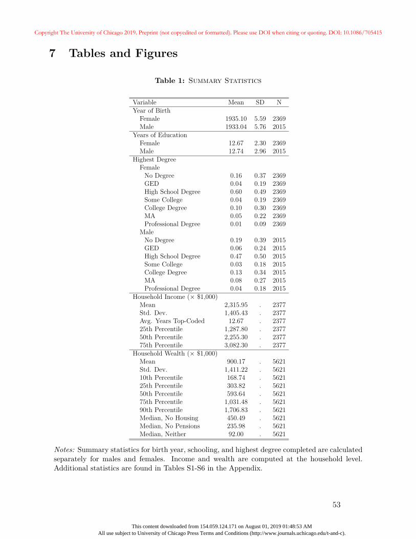
7 Tables and Figures
Table 1: Summary Statistics
Variable Mean SD NYear of Birth
Female 1935.10 5.59 2369Male 1933.04 5.76 2015
Years of EducationFemale 12.67 2.30 2369Male 12.74 2.96 2015
Highest DegreeFemale
No Degree 0.16 0.37 2369GED 0.04 0.19 2369High School Degree 0.60 0.49 2369Some College 0.04 0.19 2369College Degree 0.10 0.30 2369MA 0.05 0.22 2369Professional Degree 0.01 0.09 2369
MaleNo Degree 0.19 0.39 2015GED 0.06 0.24 2015High School Degree 0.47 0.50 2015Some College 0.03 0.18 2015College Degree 0.13 0.34 2015MA 0.08 0.27 2015Professional Degree 0.04 0.18 2015
Household Income (× $1,000)Mean 2,315.95 . 2377Std. Dev. 1,405.43 . 2377Avg. Years Top-Coded 12.67 . 237725th Percentile 1,287.80 . 237750th Percentile 2,255.30 . 237775th Percentile 3,082.30 . 2377
Household Wealth (× $1,000)Mean 900.17 . 5621Std. Dev. 1,411.22 . 562110th Percentile 168.74 . 562125th Percentile 303.82 . 562150th Percentile 593.64 . 562175th Percentile 1,031.48 . 562190th Percentile 1,706.83 . 5621Median, No Housing 450.49 . 5621Median, No Pensions 235.98 . 5621Median, Neither 92.00 . 5621
Notes: Summary statistics for birth year, schooling, and highest degree completed are calculatedseparately for males and females. Income and wealth are computed at the household level.Additional statistics are found in Tables S1-S6 in the Appendix.
53
Copyright The University of Chicago 2019. Preprint (not copyedited or formatted). Please use DOI when citing or quoting. DOI: 10.1086/705415
This content downloaded from 154.059.124.171 on August 01, 2019 01:48:53 AMAll use subject to University of Chicago Press Terms and Conditions (http://www.journals.uchicago.edu/t-and-c).
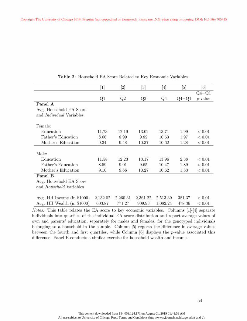
Table 2: Household EA Score Related to Key Economic Variables
[1] [2] [3] [4] [5] [6]Q4−Q1
Q1 Q2 Q3 Q4 Q4−Q1 p-valuePanel AAvg. Household EA Scoreand Individual Variables
Female:Education 11.73 12.19 13.02 13.71 1.99 < 0.01Father’s Education 8.66 8.99 9.82 10.63 1.97 < 0.01Mother’s Education 9.34 9.48 10.37 10.62 1.28 < 0.01
Male:Education 11.58 12.23 13.17 13.96 2.38 < 0.01Father’s Education 8.59 9.01 9.65 10.47 1.89 < 0.01Mother’s Education 9.10 9.66 10.27 10.62 1.53 < 0.01
Panel BAvg. Household EA Scoreand Household Variables
Avg. HH Income (in $1000) 2,132.02 2,260.31 2,361.22 2,513.39 381.37 < 0.01Avg. HH Wealth (in $1000) 603.87 771.27 909.93 1,082.24 478.36 < 0.01
Notes: This table relates the EA score to key economic variables. Columns [1]-[4] separateindividuals into quartiles of the individual EA score distribution and report average values ofown and parents’ education, separately for males and females, for the genotyped individualsbelonging to a household in the sample. Column [5] reports the difference in average valuesbetween the fourth and first quartiles, while Column [6] displays the p-value associated thisdifference. Panel B conducts a similar exercise for household wealth and income.
54
Copyright The University of Chicago 2019. Preprint (not copyedited or formatted). Please use DOI when citing or quoting. DOI: 10.1086/705415
This content downloaded from 154.059.124.171 on August 01, 2019 01:48:53 AMAll use subject to University of Chicago Press Terms and Conditions (http://www.journals.uchicago.edu/t-and-c).
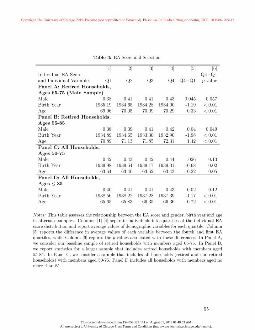
Table 3: EA Score and Selection
[1] [2] [3] [4] [5] [6]Individual EA Score Q4−Q1and Individual Variables Q1 Q2 Q3 Q4 Q4−Q1 p-valuePanel A: Retired Households,Ages 65-75 (Main Sample)Male 0.38 0.41 0.41 0.43 0.045 0.057Birth Year 1935.19 1934.65 1934.28 1934.00 -1.19 < 0.01Age 69.96 70.05 70.09 70.29 0.33 < 0.01Panel B: Retired Households,Ages 55-85Male 0.38 0.39 0.41 0.42 0.04 0.049Birth Year 1934.89 1934.65 1933.30 1932.90 -1.98 < 0.01Age 70.89 71.13 71.85 72.31 1.42 < 0.01Panel C: All Households,Ages 50-75Male 0.42 0.43 0.42 0.44 .026 0.13Birth Year 1939.98 1939.64 1939.17 1939.31 -0.68 0.02Age 63.64 63.40 63.62 63.43 -0.22 0.05Panel D: All Households,Ages ≤ 85Male 0.40 0.41 0.41 0.43 0.02 0.12Birth Year 1938.56 1938.22 1937.28 1937.39 -1.17 < 0.01Age 65.65 65.83 66.35 66.36 0.72 < 0.01
Notes: This table assesses the relationship between the EA score and gender, birth year and agein alternate samples. Columns [1]-[4] separate individuals into quartiles of the individual EAscore distribution and report average values of demographic variables for each quartile. Column[5] reports the difference in average values of each variable between the fourth and first EAquartiles, while Column [6] reports the p-values associated with these differences. In Panel A,we consider our baseline sample of retired households with members aged 65-75. In Panel B,we report statistics for a larger sample that includes retired households with members aged55-85. In Panel C, we consider a sample that includes all households (retired and non-retiredhouseholds) with members aged 50-75. Panel D includes all households with members aged nomore than 85.
55
Copyright The University of Chicago 2019. Preprint (not copyedited or formatted). Please use DOI when citing or quoting. DOI: 10.1086/705415
This content downloaded from 154.059.124.171 on August 01, 2019 01:48:53 AMAll use subject to University of Chicago Press Terms and Conditions (http://www.journals.uchicago.edu/t-and-c).
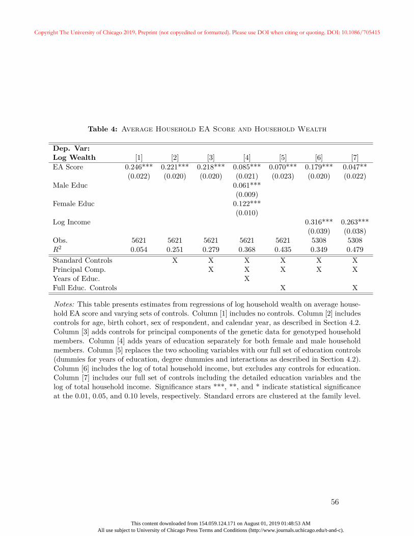
Table 4: Average Household EA Score and Household Wealth
Dep. Var:Log Wealth [1] [2] [3] [4] [5] [6] [7]EA Score 0.246*** 0.221*** 0.218*** 0.085*** 0.070*** 0.179*** 0.047**
(0.022) (0.020) (0.020) (0.021) (0.023) (0.020) (0.022)Male Educ 0.061***
(0.009)Female Educ 0.122***
(0.010)Log Income 0.316*** 0.263***
(0.039) (0.038)Obs. 5621 5621 5621 5621 5621 5308 5308R2 0.054 0.251 0.279 0.368 0.435 0.349 0.479Standard Controls X X X X X XPrincipal Comp. X X X X XYears of Educ. XFull Educ. Controls X X
Notes: This table presents estimates from regressions of log household wealth on average house-hold EA score and varying sets of controls. Column [1] includes no controls. Column [2] includescontrols for age, birth cohort, sex of respondent, and calendar year, as described in Section 4.2.Column [3] adds controls for principal components of the genetic data for genotyped householdmembers. Column [4] adds years of education separately for both female and male householdmembers. Column [5] replaces the two schooling variables with our full set of education controls(dummies for years of education, degree dummies and interactions as described in Section 4.2).Column [6] includes the log of total household income, but excludes any controls for education.Column [7] includes our full set of controls including the detailed education variables and thelog of total household income. Significance stars ***, **, and * indicate statistical significanceat the 0.01, 0.05, and 0.10 levels, respectively. Standard errors are clustered at the family level.
56
Copyright The University of Chicago 2019. Preprint (not copyedited or formatted). Please use DOI when citing or quoting. DOI: 10.1086/705415
This content downloaded from 154.059.124.171 on August 01, 2019 01:48:53 AMAll use subject to University of Chicago Press Terms and Conditions (http://www.journals.uchicago.edu/t-and-c).
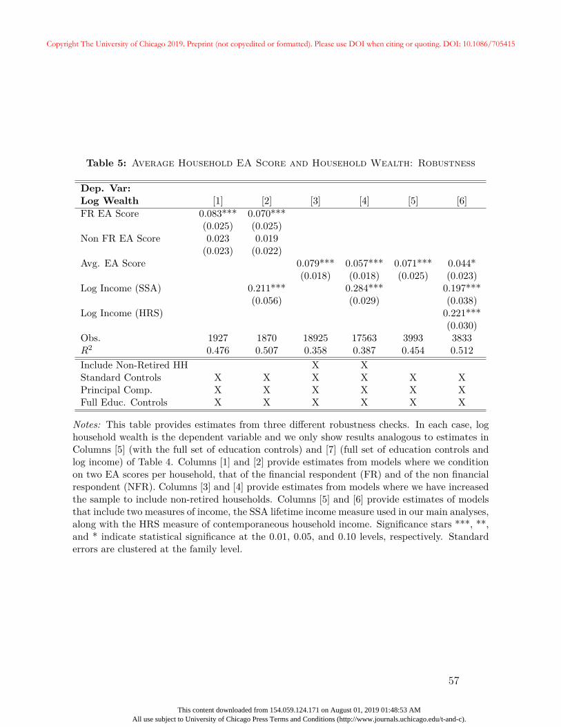
Table 5: Average Household EA Score and Household Wealth: Robustness
Dep. Var:Log Wealth [1] [2] [3] [4] [5] [6]FR EA Score 0.083*** 0.070***
(0.025) (0.025)Non FR EA Score 0.023 0.019
(0.023) (0.022)Avg. EA Score 0.079*** 0.057*** 0.071*** 0.044*
(0.018) (0.018) (0.025) (0.023)Log Income (SSA) 0.211*** 0.284*** 0.197***
(0.056) (0.029) (0.038)Log Income (HRS) 0.221***
(0.030)Obs. 1927 1870 18925 17563 3993 3833R2 0.476 0.507 0.358 0.387 0.454 0.512Include Non-Retired HH X XStandard Controls X X X X X XPrincipal Comp. X X X X X XFull Educ. Controls X X X X X X
Notes: This table provides estimates from three different robustness checks. In each case, loghousehold wealth is the dependent variable and we only show results analogous to estimates inColumns [5] (with the full set of education controls) and [7] (full set of education controls andlog income) of Table 4. Columns [1] and [2] provide estimates from models where we conditionon two EA scores per household, that of the financial respondent (FR) and of the non financialrespondent (NFR). Columns [3] and [4] provide estimates from models where we have increasedthe sample to include non-retired households. Columns [5] and [6] provide estimates of modelsthat include two measures of income, the SSA lifetime income measure used in our main analyses,along with the HRS measure of contemporaneous household income. Significance stars ***, **,and * indicate statistical significance at the 0.01, 0.05, and 0.10 levels, respectively. Standarderrors are clustered at the family level.
57
Copyright The University of Chicago 2019. Preprint (not copyedited or formatted). Please use DOI when citing or quoting. DOI: 10.1086/705415
This content downloaded from 154.059.124.171 on August 01, 2019 01:48:53 AMAll use subject to University of Chicago Press Terms and Conditions (http://www.journals.uchicago.edu/t-and-c).
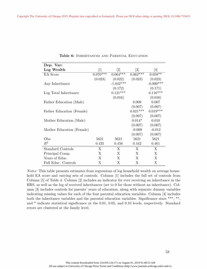
Table 6: Inheritances and Parental Education
Dep. Var:Log Wealth [1] [2] [3] [4]EA Score 0.070*** 0.064*** 0.062*** 0.058**
(0.023) (0.022) (0.023) (0.023)Any Inheritance -1.042*** -0.990***
(0.172) (0.171)Log Total Inheritance 0.121*** 0.116***
(0.016) (0.016)Father Education (Male) 0.009 0.007
(0.007) (0.007)Father Education (Female) 0.021*** 0.019***
(0.007) (0.007)Mother Education (Male) 0.014* 0.010
(0.007) (0.007)Mother Education (Female) -0.009 -0.012
(0.007) (0.007)Obs. 5621 5621 5621 5621R2 0.435 0.456 0.442 0.461Standard Controls X X X XPrincipal Comp. X X X XYears of Educ. X X X XFull Educ. Controls X X X X
Notes: This table presents estimates from regressions of log household wealth on average house-hold EA score and varying sets of controls. Column [1] includes the full set of controls fromColumn [5] of Table 4. Column [2] includes an indicator for ever receiving an inheritance in theHRS, as well as the log of received inheritances (set to 0 for those without an inheritance). Col-umn [3] includes controls for parents’ years of education, along with separate dummy variablesindicating missing values for each of the four parental education variables. Column [4] includesboth the inheritance variables and the parental education variables. Significance stars ***, **,and * indicate statistical significance at the 0.01, 0.05, and 0.10 levels, respectively. Standarderrors are clustered at the family level.
58
Copyright The University of Chicago 2019. Preprint (not copyedited or formatted). Please use DOI when citing or quoting. DOI: 10.1086/705415
This content downloaded from 154.059.124.171 on August 01, 2019 01:48:53 AMAll use subject to University of Chicago Press Terms and Conditions (http://www.journals.uchicago.edu/t-and-c).
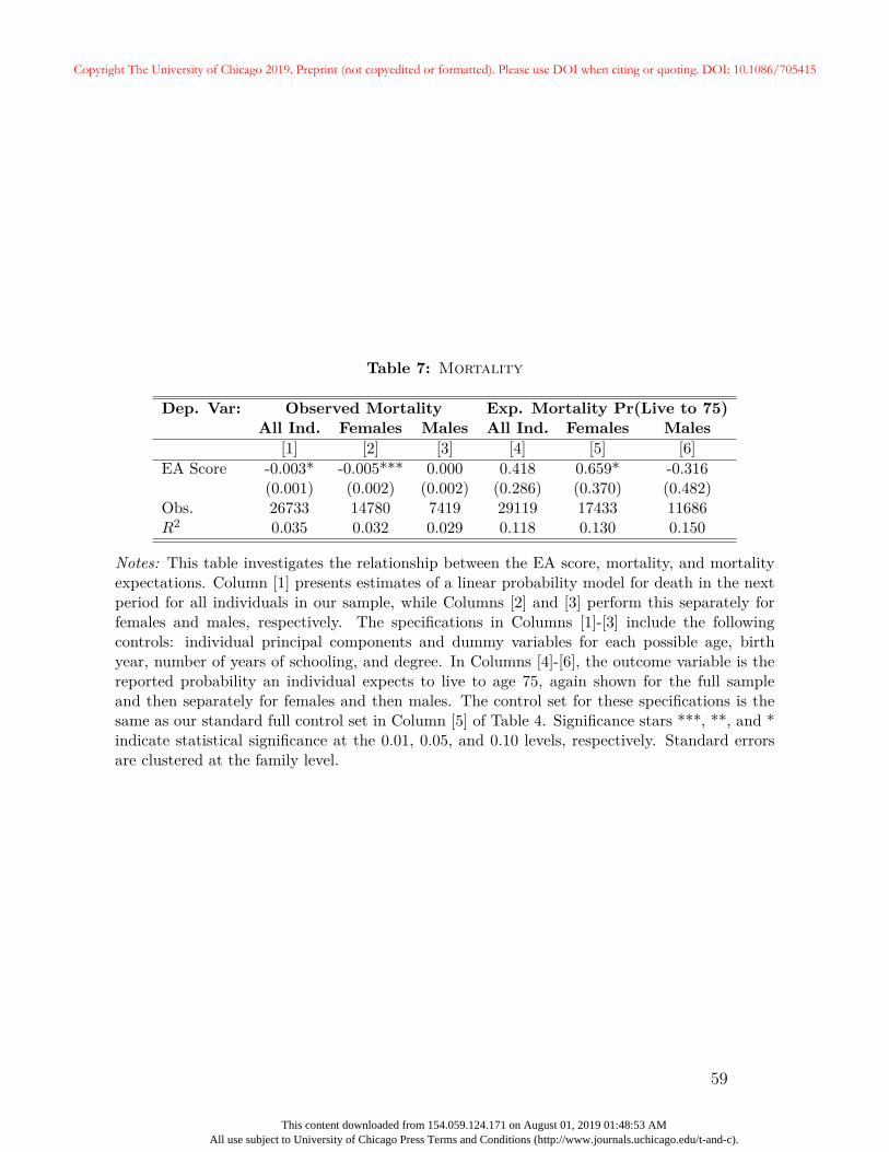
Table 7: Mortality
Dep. Var: Observed Mortality Exp. Mortality Pr(Live to 75)All Ind. Females Males All Ind. Females Males
[1] [2] [3] [4] [5] [6]EA Score -0.003* -0.005*** 0.000 0.418 0.659* -0.316
(0.001) (0.002) (0.002) (0.286) (0.370) (0.482)Obs. 26733 14780 7419 29119 17433 11686R2 0.035 0.032 0.029 0.118 0.130 0.150
Notes: This table investigates the relationship between the EA score, mortality, and mortalityexpectations. Column [1] presents estimates of a linear probability model for death in the nextperiod for all individuals in our sample, while Columns [2] and [3] perform this separately forfemales and males, respectively. The specifications in Columns [1]-[3] include the followingcontrols: individual principal components and dummy variables for each possible age, birthyear, number of years of schooling, and degree. In Columns [4]-[6], the outcome variable is thereported probability an individual expects to live to age 75, again shown for the full sampleand then separately for females and then males. The control set for these specifications is thesame as our standard full control set in Column [5] of Table 4. Significance stars ***, **, and *indicate statistical significance at the 0.01, 0.05, and 0.10 levels, respectively. Standard errorsare clustered at the family level.
59
Copyright The University of Chicago 2019. Preprint (not copyedited or formatted). Please use DOI when citing or quoting. DOI: 10.1086/705415
This content downloaded from 154.059.124.171 on August 01, 2019 01:48:53 AMAll use subject to University of Chicago Press Terms and Conditions (http://www.journals.uchicago.edu/t-and-c).
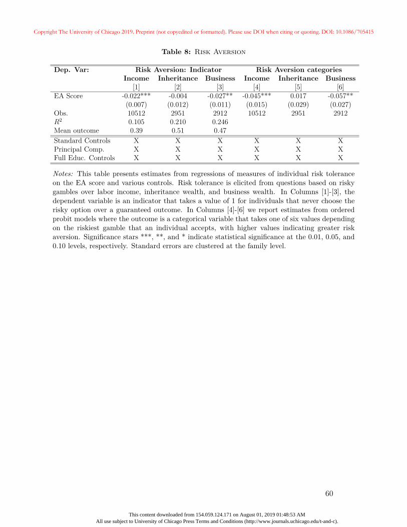
Table 8: Risk Aversion
Dep. Var: Risk Aversion: Indicator Risk Aversion categoriesIncome Inheritance Business Income Inheritance Business
[1] [2] [3] [4] [5] [6]EA Score -0.022*** -0.004 -0.027** -0.045*** 0.017 -0.057**
(0.007) (0.012) (0.011) (0.015) (0.029) (0.027)Obs. 10512 2951 2912 10512 2951 2912R2 0.105 0.210 0.246Mean outcome 0.39 0.51 0.47Standard Controls X X X X X XPrincipal Comp. X X X X X XFull Educ. Controls X X X X X X
Notes: This table presents estimates from regressions of measures of individual risk toleranceon the EA score and various controls. Risk tolerance is elicited from questions based on riskygambles over labor income, inheritance wealth, and business wealth. In Columns [1]-[3], thedependent variable is an indicator that takes a value of 1 for individuals that never choose therisky option over a guaranteed outcome. In Columns [4]-[6] we report estimates from orderedprobit models where the outcome is a categorical variable that takes one of six values dependingon the riskiest gamble that an individual accepts, with higher values indicating greater riskaversion. Significance stars ***, **, and * indicate statistical significance at the 0.01, 0.05, and0.10 levels, respectively. Standard errors are clustered at the family level.
60
Copyright The University of Chicago 2019. Preprint (not copyedited or formatted). Please use DOI when citing or quoting. DOI: 10.1086/705415
This content downloaded from 154.059.124.171 on August 01, 2019 01:48:53 AMAll use subject to University of Chicago Press Terms and Conditions (http://www.journals.uchicago.edu/t-and-c).
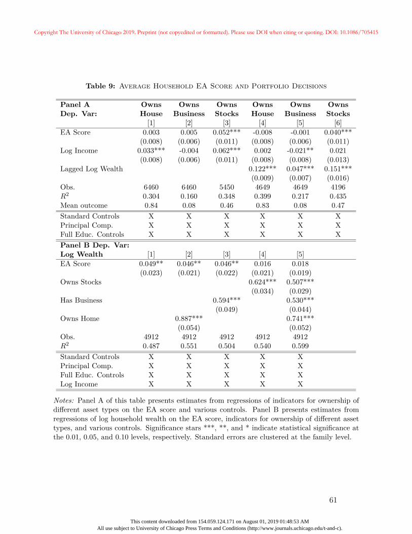
Table 9: Average Household EA Score and Portfolio Decisions
Panel A Owns Owns Owns Owns Owns OwnsDep. Var: House Business Stocks House Business Stocks
[1] [2] [3] [4] [5] [6]EA Score 0.003 0.005 0.052*** -0.008 -0.001 0.040***
(0.008) (0.006) (0.011) (0.008) (0.006) (0.011)Log Income 0.033*** -0.004 0.062*** 0.002 -0.021** 0.021
(0.008) (0.006) (0.011) (0.008) (0.008) (0.013)Lagged Log Wealth 0.122*** 0.047*** 0.151***
(0.009) (0.007) (0.016)Obs. 6460 6460 5450 4649 4649 4196R2 0.304 0.160 0.348 0.399 0.217 0.435Mean outcome 0.84 0.08 0.46 0.83 0.08 0.47Standard Controls X X X X X XPrincipal Comp. X X X X X XFull Educ. Controls X X X X X XPanel B Dep. Var:Log Wealth [1] [2] [3] [4] [5]EA Score 0.049** 0.046** 0.046** 0.016 0.018
(0.023) (0.021) (0.022) (0.021) (0.019)Owns Stocks 0.624*** 0.507***
(0.034) (0.029)Has Business 0.594*** 0.530***
(0.049) (0.044)Owns Home 0.887*** 0.741***
(0.054) (0.052)Obs. 4912 4912 4912 4912 4912R2 0.487 0.551 0.504 0.540 0.599Standard Controls X X X X XPrincipal Comp. X X X X XFull Educ. Controls X X X X XLog Income X X X X X
Notes: Panel A of this table presents estimates from regressions of indicators for ownership ofdifferent asset types on the EA score and various controls. Panel B presents estimates fromregressions of log household wealth on the EA score, indicators for ownership of different assettypes, and various controls. Significance stars ***, **, and * indicate statistical significance atthe 0.01, 0.05, and 0.10 levels, respectively. Standard errors are clustered at the family level.
61
Copyright The University of Chicago 2019. Preprint (not copyedited or formatted). Please use DOI when citing or quoting. DOI: 10.1086/705415
This content downloaded from 154.059.124.171 on August 01, 2019 01:48:53 AMAll use subject to University of Chicago Press Terms and Conditions (http://www.journals.uchicago.edu/t-and-c).
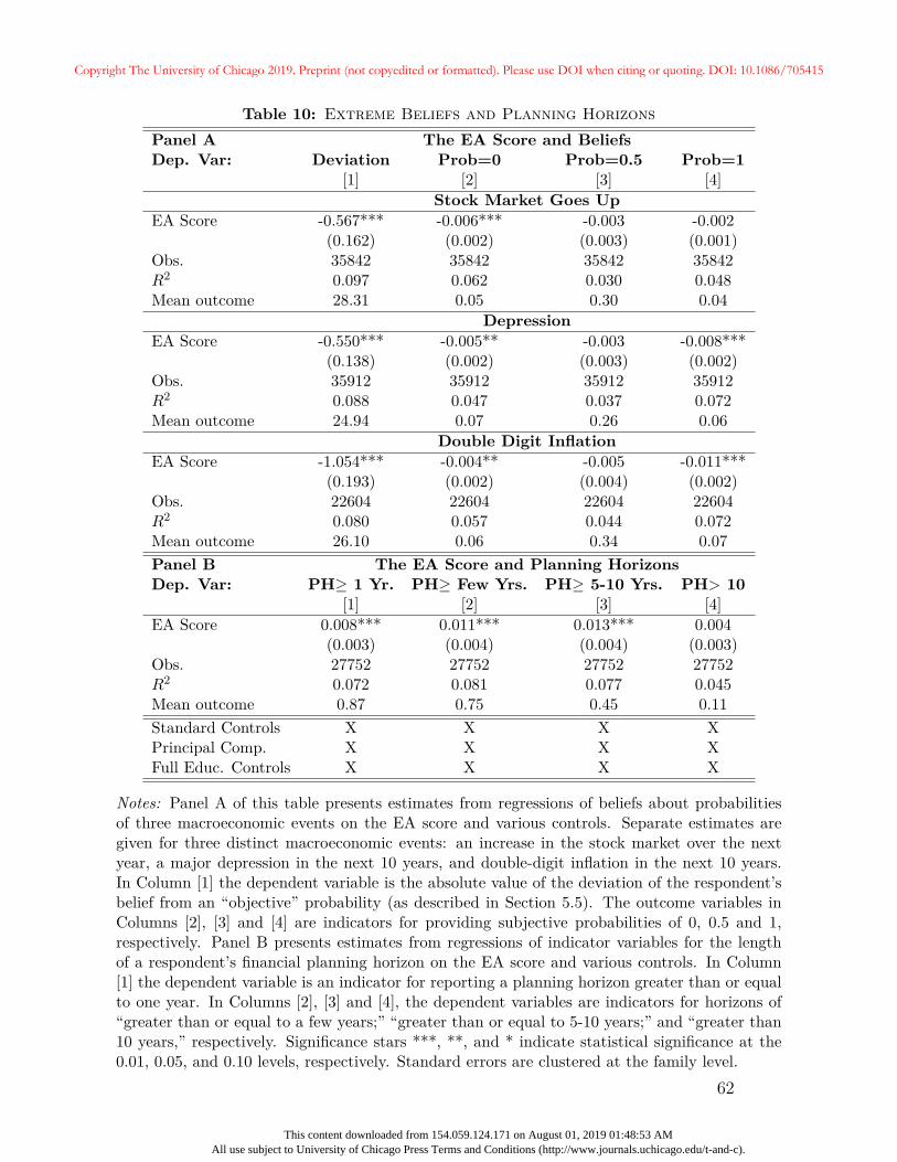
Table 10: Extreme Beliefs and Planning HorizonsPanel A The EA Score and BeliefsDep. Var: Deviation Prob=0 Prob=0.5 Prob=1
[1] [2] [3] [4]Stock Market Goes Up
EA Score -0.567*** -0.006*** -0.003 -0.002(0.162) (0.002) (0.003) (0.001)
Obs. 35842 35842 35842 35842R2 0.097 0.062 0.030 0.048Mean outcome 28.31 0.05 0.30 0.04
DepressionEA Score -0.550*** -0.005** -0.003 -0.008***
(0.138) (0.002) (0.003) (0.002)Obs. 35912 35912 35912 35912R2 0.088 0.047 0.037 0.072Mean outcome 24.94 0.07 0.26 0.06
Double Digit InflationEA Score -1.054*** -0.004** -0.005 -0.011***
(0.193) (0.002) (0.004) (0.002)Obs. 22604 22604 22604 22604R2 0.080 0.057 0.044 0.072Mean outcome 26.10 0.06 0.34 0.07Panel B The EA Score and Planning HorizonsDep. Var: PH≥ 1 Yr. PH≥ Few Yrs. PH≥ 5-10 Yrs. PH> 10
[1] [2] [3] [4]EA Score 0.008*** 0.011*** 0.013*** 0.004
(0.003) (0.004) (0.004) (0.003)Obs. 27752 27752 27752 27752R2 0.072 0.081 0.077 0.045Mean outcome 0.87 0.75 0.45 0.11Standard Controls X X X XPrincipal Comp. X X X XFull Educ. Controls X X X X
Notes: Panel A of this table presents estimates from regressions of beliefs about probabilitiesof three macroeconomic events on the EA score and various controls. Separate estimates aregiven for three distinct macroeconomic events: an increase in the stock market over the nextyear, a major depression in the next 10 years, and double-digit inflation in the next 10 years.In Column [1] the dependent variable is the absolute value of the deviation of the respondent’sbelief from an “objective” probability (as described in Section 5.5). The outcome variables inColumns [2], [3] and [4] are indicators for providing subjective probabilities of 0, 0.5 and 1,respectively. Panel B presents estimates from regressions of indicator variables for the lengthof a respondent’s financial planning horizon on the EA score and various controls. In Column[1] the dependent variable is an indicator for reporting a planning horizon greater than or equalto one year. In Columns [2], [3] and [4], the dependent variables are indicators for horizons of“greater than or equal to a few years;” “greater than or equal to 5-10 years;” and “greater than10 years,” respectively. Significance stars ***, **, and * indicate statistical significance at the0.01, 0.05, and 0.10 levels, respectively. Standard errors are clustered at the family level.
62
Copyright The University of Chicago 2019. Preprint (not copyedited or formatted). Please use DOI when citing or quoting. DOI: 10.1086/705415
This content downloaded from 154.059.124.171 on August 01, 2019 01:48:53 AMAll use subject to University of Chicago Press Terms and Conditions (http://www.journals.uchicago.edu/t-and-c).
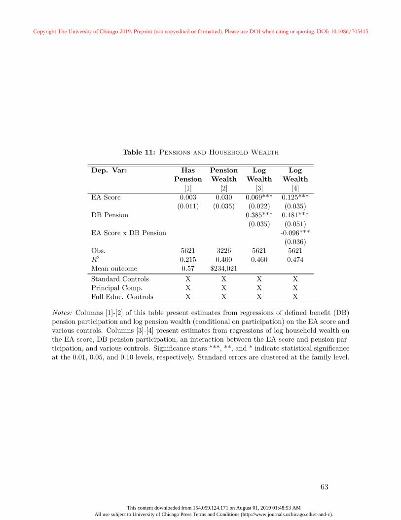
Table 11: Pensions and Household Wealth
Dep. Var: Has Pension Log LogPension Wealth Wealth Wealth
[1] [2] [3] [4]EA Score 0.003 0.030 0.069*** 0.125***
(0.011) (0.035) (0.022) (0.035)DB Pension 0.385*** 0.181***
(0.035) (0.051)EA Score x DB Pension -0.096***
(0.036)Obs. 5621 3226 5621 5621R2 0.215 0.400 0.460 0.474Mean outcome 0.57 $234,021Standard Controls X X X XPrincipal Comp. X X X XFull Educ. Controls X X X X
Notes: Columns [1]-[2] of this table present estimates from regressions of defined benefit (DB)pension participation and log pension wealth (conditional on participation) on the EA score andvarious controls. Columns [3]-[4] present estimates from regressions of log household wealth onthe EA score, DB pension participation, an interaction between the EA score and pension par-ticipation, and various controls. Significance stars ***, **, and * indicate statistical significanceat the 0.01, 0.05, and 0.10 levels, respectively. Standard errors are clustered at the family level.
63
Copyright The University of Chicago 2019. Preprint (not copyedited or formatted). Please use DOI when citing or quoting. DOI: 10.1086/705415
This content downloaded from 154.059.124.171 on August 01, 2019 01:48:53 AMAll use subject to University of Chicago Press Terms and Conditions (http://www.journals.uchicago.edu/t-and-c).
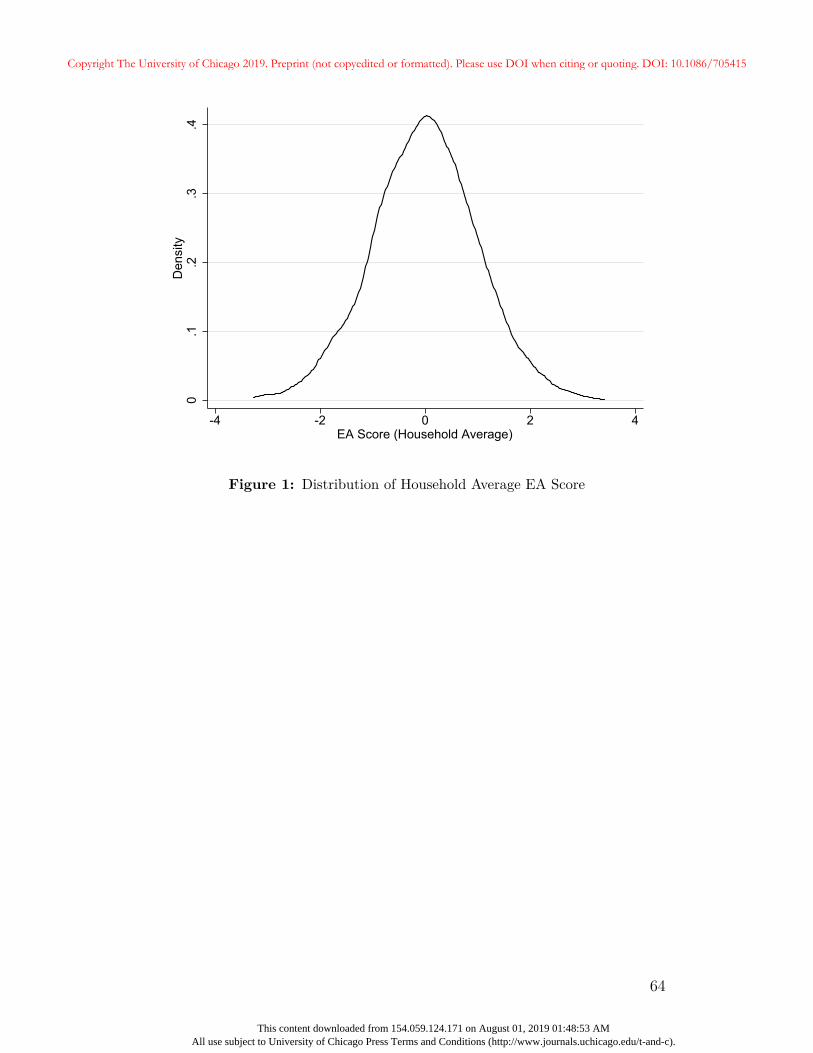
0.1
.2.3
.4D
ensi
ty
-4 -2 0 2 4EA Score (Household Average)
Figure 1: Distribution of Household Average EA Score
64
Copyright The University of Chicago 2019. Preprint (not copyedited or formatted). Please use DOI when citing or quoting. DOI: 10.1086/705415
This content downloaded from 154.059.124.171 on August 01, 2019 01:48:53 AMAll use subject to University of Chicago Press Terms and Conditions (http://www.journals.uchicago.edu/t-and-c).
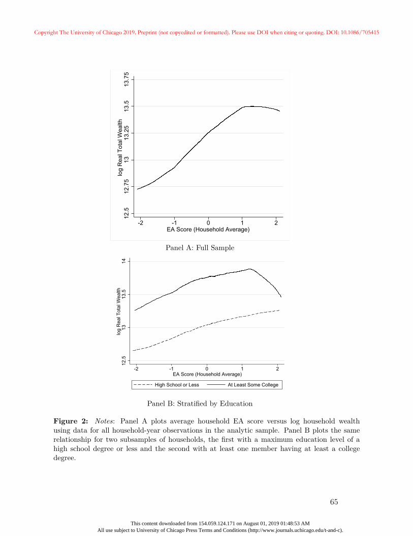
12.5
12.7
513
13.2
513
.513
.75
log
Rea
l Tot
al W
ealth
-2 -1 0 1 2EA Score (Household Average)
Panel A: Full Sample
12.5
1313
.514
log
Rea
l Tot
al W
ealth
-2 -1 0 1 2EA Score (Household Average)
High School or Less At Least Some College
Panel B: Stratified by Education
Figure 2: Notes: Panel A plots average household EA score versus log household wealthusing data for all household-year observations in the analytic sample. Panel B plots the samerelationship for two subsamples of households, the first with a maximum education level of ahigh school degree or less and the second with at least one member having at least a collegedegree.
65
Copyright The University of Chicago 2019. Preprint (not copyedited or formatted). Please use DOI when citing or quoting. DOI: 10.1086/705415
This content downloaded from 154.059.124.171 on August 01, 2019 01:48:53 AMAll use subject to University of Chicago Press Terms and Conditions (http://www.journals.uchicago.edu/t-and-c).
Online Appendix:“Genetic Endowments and Wealth Inequality”
By: Daniel Barth, Nicholas W. Papageorge and Kevin Thom1
A Wealth Data and Additional Summary Statistics
A.1 Retirement Wealth
The wealth data used in this paper are largely constructed from the RAND wealth andincome files. The RAND files are carefully cleaned and consistently coded by RAND Cor-portation and are available for public use. The RAND files have been used in both academicand industry publications, and ensure comparability and consistency across HRS waves andresearch projects. We refer the reader to the RAND codebook and documentation for furtherdetails.
One important shortcoming of the RAND wealth files is the exclusion of employer-sponsored retirement plan account balances. While the RAND wealth files do include thebalances of IRAs and other non-employer-sponsored plans, wealth accumulated in employer-sponsored 401k, 403(b), and other such accounts are not included. For households at ornear retirement, such accounts can be a significant source of wealth. Further, such accountsmay be the only vehicles through which households invest in the stock market, and mea-sures of stock market participation will understate true participation if these plans are notconsidered.
Unfortunately, data on employer-sponsored retirement plans are not asked in every wave,and are sometimes inconsistently coded across waves. The remainder of this section focuseson our methodology for coding retirement account balances and stock market participationinferred from those accounts. Broadly speaking, there are two types of retirement plans:defined-benefit plans, such as traditional pensions (which the HRS calls type A plans), anddefined contribution plans, such as 401k and 403(b) plans (which the HRS calls type Bplans). We discuss each type of plan in turn.
A.1.1 Defined Benefit Plans
To deal with issues arising from type A style retirement plans, our sample includes onlyhouseholds fully in retirement (households in which no member of the household is currentlyworking). We exclude working households because expected benefits from defined-benefit
1This version of the online appendix was generated on July 11, 2019.
1
Supplementary/Online-Only Appendix Click here to access/download;Supplementary/Online-OnlyAppendix;2017434 online appendix.pdf
Copyright The University of Chicago 2019. Preprint (not copyedited or formatted). Please use DOI when citing or quoting. DOI: 10.1086/705415
This content downloaded from 154.059.124.171 on August 01, 2019 01:48:53 AMAll use subject to University of Chicago Press Terms and Conditions (http://www.journals.uchicago.edu/t-and-c).
pension plans are likely to be both an important source of wealth and noisily measured. Forretired households, our assumption is that those who report receiving pension income wereincluded in defined-benefit pension plans at some point during their working lives, and thosewho do not receive pension income in retirement were not included in such plans. To theextent that households misreport pension income, for example if income from an annuityconverted from a 401k plan is reported as pension income, or if households have delayedreceiving pension benefits until some future date, our assignment of households participatingin type A plans will be biased. Further, because the household earns a guaranteed stream ofincome regardless of the underlying investments that support that income (and because wedo not observe these underlying investments), we do not consider a household’s participationin type A pension plans to be participation in the stock market.
We include retirement income in our household wealth measure by calculating the priceof an actuarially fair annuity based on the entirety of household retirement income, whichincludes pension income, annuity income, and income from social security. We follow Yogo(2016) by calculating the present discounted value of this income based on a 1.5% annualrisk-free rate of return, and discount income in each year by the probability of the recipientsurviving until that year.2 Specifically, we calculate the present value of retirement income,Pt, as:
Pt = Yt
T−t−1∑s=1
[s∏
u=1pt+uR−1
], (1)
where Yt is total retirement income, pt is the recipient’s survival probability in period t andis a function of gender, birth cohort, and age, and R = 1.015 is the annual risk-free rate ofreturn.
A.1.2 Defined Contribution Plans
Wealth in defined contribution style plans is a bit trickier. Households may have plansassociated with multiple previous employers. To calculate comprehensive measures of wealthand stock market participation, we would like to know both the balances and asset allocationsof all employer-sponsored type B plans from all previous jobs. Unfortunately, this is notalways possible.
In years 1996, 1998, and 2002-2010 (comprising even-numbered years), we have the high-est quality data on total balances in employer-sponsored type B retirement plans.3 In these
2We differ from Yogo (2016) in that we use the probability of death of the individual receiving the income,rather than of the female partner.
3In 2012, the pension data were changed to an entirely new format.
2
Copyright The University of Chicago 2019. Preprint (not copyedited or formatted). Please use DOI when citing or quoting. DOI: 10.1086/705415
This content downloaded from 154.059.124.171 on August 01, 2019 01:48:53 AMAll use subject to University of Chicago Press Terms and Conditions (http://www.journals.uchicago.edu/t-and-c).
years, our wealth data include balances of employer-sponsored plans that are still maintainedthrough that employer, and have not been converted to annuities or rolled over into IRAs.The HRS refers to such plans as dormant plans. Unfortunately, the value of dormant plansat employers prior to retirement are not asked in 1992, 1994, and 2000.
Dormant plans also present problems for measurement of stock market participation.While in years 2002-2010 the stock allocation within a respondent’s retirement plan at thecurrent employer is observable for working households, the stock allocation in dormant plansfor retired households is not. Thus, for retirement plans at current or former employers, onlystock market participation for plans at the current employer are included in our measureof stock market participation. Because our sample includes only retired households, stockmarket allocations at employer-sponsored plans contribute negligibly to our stock marketownership variable.
A.2 Additional Summary Statistics
This appendix provides additional summary statistics for the genotyped versus non-genotypedsamples, demographics by household structure, income and wealth, and the potential mech-anisms studied in Section 5. Table S1 documents differences in birth year, education, andother variables between the genotyped and non-genotyped samples. Genotyped individualstend to be older, more educated, and belong to wealthier households. Table S2 presents themean and standard deviation of demographic variables such as birth year, years of school-ing, and highest degree earned. These are reported for all households in our sample andseparately by household structure.
Panel A of Table S3 shows the distribution of lifetime labor earnings for all householdsand by household structure: coupled, male only, and female only households. Table S4shows the distribution of various measures of household wealth: total wealth, total wealthexcluding housing wealth, total wealth excluding the present value of retirement income, andtotal wealth excluding both retirement wealth and housing. Table S5 presents the mean,median, 75th percentile, and 90th percentile of each individual component of household wealthfor the full sample for all household-years. We also calculate the share of total real wealth ineach component for each household-year, and present the median and mean values of theseshares.
Table S6 shows summary statistics for the various mechanisms that may help to explainthe gene-wealth gradient. Panel A presents statistics on the fraction of households thatreceive an inheritance, the (total) amount of inheritances received for households that receivethem, and the household average of parental education (years of schooling). Panel B reports
3
Copyright The University of Chicago 2019. Preprint (not copyedited or formatted). Please use DOI when citing or quoting. DOI: 10.1086/705415
This content downloaded from 154.059.124.171 on August 01, 2019 01:48:53 AMAll use subject to University of Chicago Press Terms and Conditions (http://www.journals.uchicago.edu/t-and-c).
summary statistics related to mortality. In particular, we examine the annual death ratefor individuals in our main sample (excluding years before genotyping), and the subjectiveprobability of living until the age 75, which is elicited multiple times per individual. PanelC reports summary statistics for measures of risk aversion. Specifically, Panel C shows thefraction of households that fall within each risk aversion bin (based on the gambles theywould accept and reject) for the labor income gamble, the business wealth gamble, and theinheritance gamble. Panel D reports the mean and standard deviation of home ownership,business ownership, and stock market participation. Stock market participation includesequity investments in retirement accounts, mutual funds, or in individually held stocks.
Panel E of Table S6 reports summary statistics related to beliefs about macroeconomicevents: the probability the stock market appreciated over the following year, the deviation ofthis belief from the objective estimate based on historical data, and whether the respondentreports a belief of 0% or 100% (extreme beliefs), or of 50% (a focal belief that may repre-sent uncertainty). Similar statistics are reported for the likelihood of a major (economic)depression and double-digit inflation. Panel E also reports the distribution of the reportedfinancial planning horizon. Finally, panel F reports the fraction of households that receivedefined-benefit pension income, and the present discounted value of lifetime defined benefitincome.
4
Copyright The University of Chicago 2019. Preprint (not copyedited or formatted). Please use DOI when citing or quoting. DOI: 10.1086/705415
This content downloaded from 154.059.124.171 on August 01, 2019 01:48:53 AMAll use subject to University of Chicago Press Terms and Conditions (http://www.journals.uchicago.edu/t-and-c).
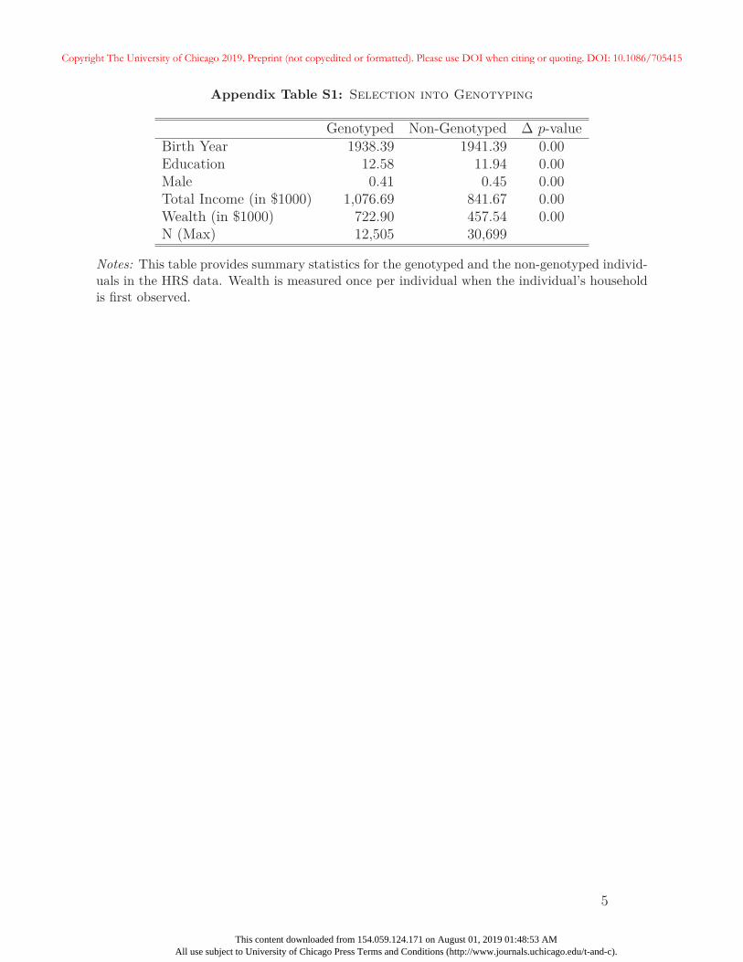
Appendix Table S1: Selection into Genotyping
Genotyped Non-Genotyped Δ p-valueBirth Year 1938.39 1941.39 0.00Education 12.58 11.94 0.00Male 0.41 0.45 0.00Total Income (in $1000) 1,076.69 841.67 0.00Wealth (in $1000) 722.90 457.54 0.00N (Max) 12,505 30,699
Notes: This table provides summary statistics for the genotyped and the non-genotyped individ-uals in the HRS data. Wealth is measured once per individual when the individual’s householdis first observed.
5
Copyright The University of Chicago 2019. Preprint (not copyedited or formatted). Please use DOI when citing or quoting. DOI: 10.1086/705415
This content downloaded from 154.059.124.171 on August 01, 2019 01:48:53 AMAll use subject to University of Chicago Press Terms and Conditions (http://www.journals.uchicago.edu/t-and-c).
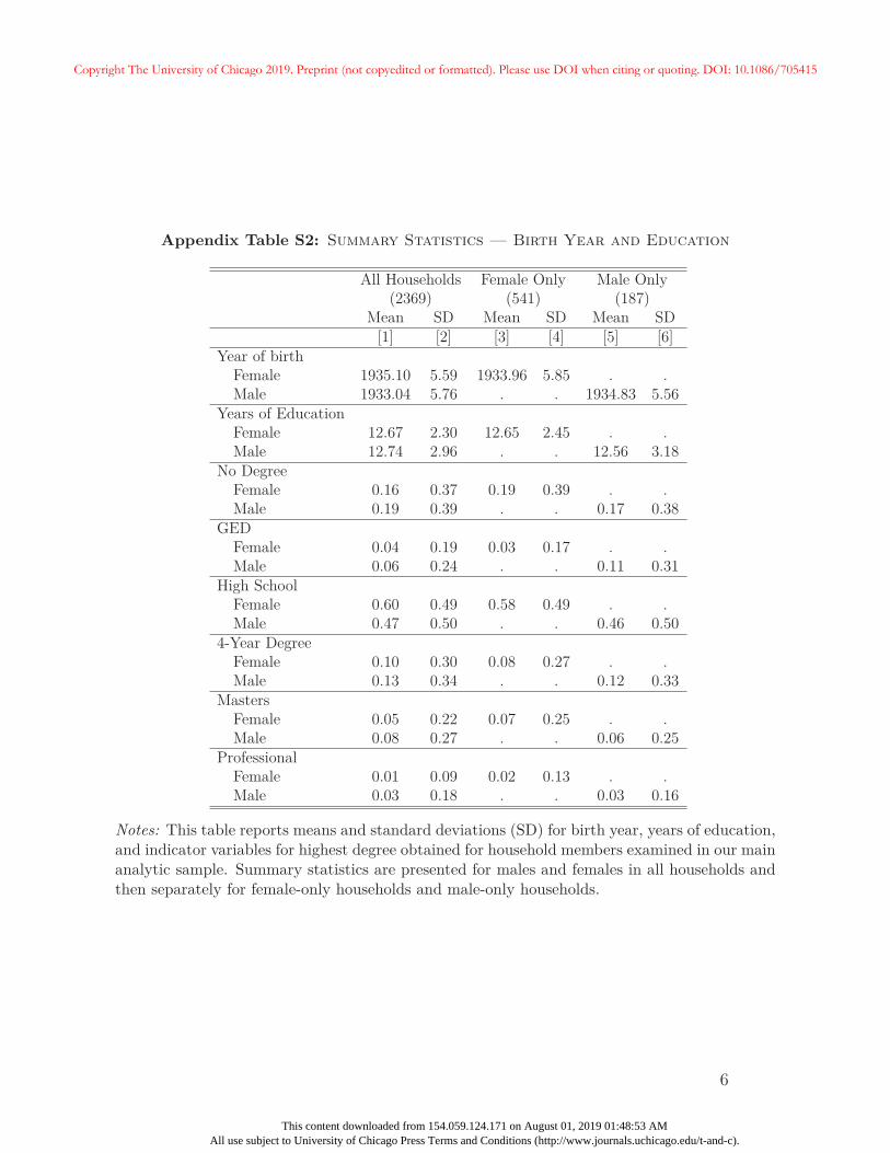
Appendix Table S2: Summary Statistics — Birth Year and Education
All Households Female Only Male Only(2369) (541) (187)
Mean SD Mean SD Mean SD[1] [2] [3] [4] [5] [6]
Year of birthFemale 1935.10 5.59 1933.96 5.85 . .Male 1933.04 5.76 . . 1934.83 5.56
Years of EducationFemale 12.67 2.30 12.65 2.45 . .Male 12.74 2.96 . . 12.56 3.18
No DegreeFemale 0.16 0.37 0.19 0.39 . .Male 0.19 0.39 . . 0.17 0.38
GEDFemale 0.04 0.19 0.03 0.17 . .Male 0.06 0.24 . . 0.11 0.31
High SchoolFemale 0.60 0.49 0.58 0.49 . .Male 0.47 0.50 . . 0.46 0.50
4-Year DegreeFemale 0.10 0.30 0.08 0.27 . .Male 0.13 0.34 . . 0.12 0.33
MastersFemale 0.05 0.22 0.07 0.25 . .Male 0.08 0.27 . . 0.06 0.25
ProfessionalFemale 0.01 0.09 0.02 0.13 . .Male 0.03 0.18 . . 0.03 0.16
Notes: This table reports means and standard deviations (SD) for birth year, years of education,and indicator variables for highest degree obtained for household members examined in our mainanalytic sample. Summary statistics are presented for males and females in all households andthen separately for female-only households and male-only households.
6
Copyright The University of Chicago 2019. Preprint (not copyedited or formatted). Please use DOI when citing or quoting. DOI: 10.1086/705415
This content downloaded from 154.059.124.171 on August 01, 2019 01:48:53 AMAll use subject to University of Chicago Press Terms and Conditions (http://www.journals.uchicago.edu/t-and-c).
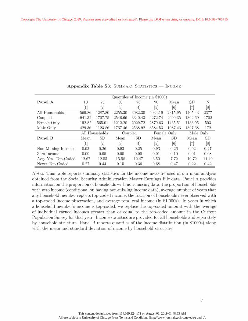
Appendix Table S3: Summary Statistics — Income
Quantiles of Income (in $1000)Panel A 10 25 50 75 90 Mean SD N
[1] [2] [3] [4] [5] [6] [7] [8]All Households 569.86 1287.80 2255.30 3082.30 4034.19 2315.95 1405.43 2377Coupled 941.32 1707.75 2546.66 3340.43 4272.74 2609.35 1362.69 1702Female Only 192.82 565.01 1212.20 2029.72 2870.63 1435.51 1133.95 503Male Only 429.36 1123.86 1767.46 2538.92 3584.53 1987.43 1397.68 172
All Households Coupled Female Only Male OnlyPanel B Mean SD Mean SD Mean SD Mean SD
[1] [2] [3] [4] [5] [6] [7] [8]Non-Missing Income 0.93 0.26 0.93 0.25 0.93 0.26 0.92 0.27Zero Income 0.00 0.05 0.00 0.00 0.01 0.10 0.01 0.08Avg. Yrs. Top-Coded 12.67 12.55 15.58 12.47 3.50 7.72 10.72 11.40Never Top Coded 0.27 0.44 0.15 0.36 0.68 0.47 0.22 0.42
Notes: This table reports summary statistics for the income measure used in our main analysisobtained from the Social Security Administration Master Earnings File data. Panel A providesinformation on the proportion of households with non-missing data, the proportion of householdswith zero income (conditional on having non-missing income data), average number of years thatany household member reports top-coded income, the fraction of households never observed witha top-coded income observation, and average total real income (in $1,000s). In years in whicha household member’s income is top-coded, we replace the top-coded amount with the averageof individual earned incomes greater than or equal to the top-coded amount in the CurrentPopulation Survey for that year. Income statistics are provided for all households and separatelyby household structure. Panel B reports quantiles of the income distribution (in $1000s) alongwith the mean and standard deviation of income by household structure.
7
Copyright The University of Chicago 2019. Preprint (not copyedited or formatted). Please use DOI when citing or quoting. DOI: 10.1086/705415
This content downloaded from 154.059.124.171 on August 01, 2019 01:48:53 AMAll use subject to University of Chicago Press Terms and Conditions (http://www.journals.uchicago.edu/t-and-c).
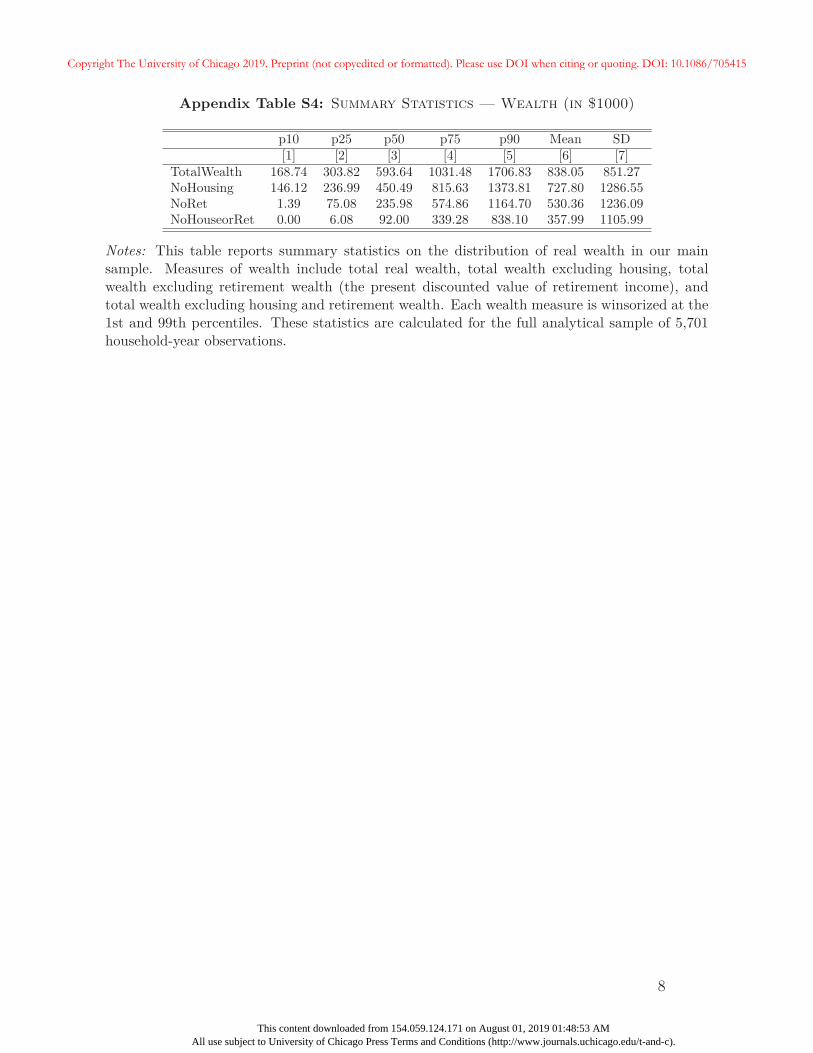
Appendix Table S4: Summary Statistics — Wealth (in $1000)
p10 p25 p50 p75 p90 Mean SD[1] [2] [3] [4] [5] [6] [7]
TotalWealth 168.74 303.82 593.64 1031.48 1706.83 838.05 851.27NoHousing 146.12 236.99 450.49 815.63 1373.81 727.80 1286.55NoRet 1.39 75.08 235.98 574.86 1164.70 530.36 1236.09NoHouseorRet 0.00 6.08 92.00 339.28 838.10 357.99 1105.99
Notes: This table reports summary statistics on the distribution of real wealth in our mainsample. Measures of wealth include total real wealth, total wealth excluding housing, totalwealth excluding retirement wealth (the present discounted value of retirement income), andtotal wealth excluding housing and retirement wealth. Each wealth measure is winsorized at the1st and 99th percentiles. These statistics are calculated for the full analytical sample of 5,701household-year observations.
8
Copyright The University of Chicago 2019. Preprint (not copyedited or formatted). Please use DOI when citing or quoting. DOI: 10.1086/705415
This content downloaded from 154.059.124.171 on August 01, 2019 01:48:53 AMAll use subject to University of Chicago Press Terms and Conditions (http://www.journals.uchicago.edu/t-and-c).
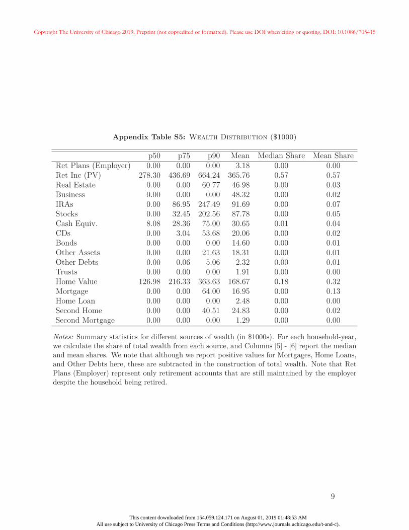
Appendix Table S5: Wealth Distribution ($1000)
p50 p75 p90 Mean Median Share Mean ShareRet Plans (Employer) 0.00 0.00 0.00 3.18 0.00 0.00Ret Inc (PV) 278.30 436.69 664.24 365.76 0.57 0.57Real Estate 0.00 0.00 60.77 46.98 0.00 0.03Business 0.00 0.00 0.00 48.32 0.00 0.02IRAs 0.00 86.95 247.49 91.69 0.00 0.07Stocks 0.00 32.45 202.56 87.78 0.00 0.05Cash Equiv. 8.08 28.36 75.00 30.65 0.01 0.04CDs 0.00 3.04 53.68 20.06 0.00 0.02Bonds 0.00 0.00 0.00 14.60 0.00 0.01Other Assets 0.00 0.00 21.63 18.31 0.00 0.01Other Debts 0.00 0.06 5.06 2.32 0.00 0.01Trusts 0.00 0.00 0.00 1.91 0.00 0.00Home Value 126.98 216.33 363.63 168.67 0.18 0.32Mortgage 0.00 0.00 64.00 16.95 0.00 0.13Home Loan 0.00 0.00 0.00 2.48 0.00 0.00Second Home 0.00 0.00 40.51 24.83 0.00 0.02Second Mortgage 0.00 0.00 0.00 1.29 0.00 0.00
Notes: Summary statistics for different sources of wealth (in $1000s). For each household-year,we calculate the share of total wealth from each source, and Columns [5] - [6] report the medianand mean shares. We note that although we report positive values for Mortgages, Home Loans,and Other Debts here, these are subtracted in the construction of total wealth. Note that RetPlans (Employer) represent only retirement accounts that are still maintained by the employerdespite the household being retired.
9
Copyright The University of Chicago 2019. Preprint (not copyedited or formatted). Please use DOI when citing or quoting. DOI: 10.1086/705415
This content downloaded from 154.059.124.171 on August 01, 2019 01:48:53 AMAll use subject to University of Chicago Press Terms and Conditions (http://www.journals.uchicago.edu/t-and-c).
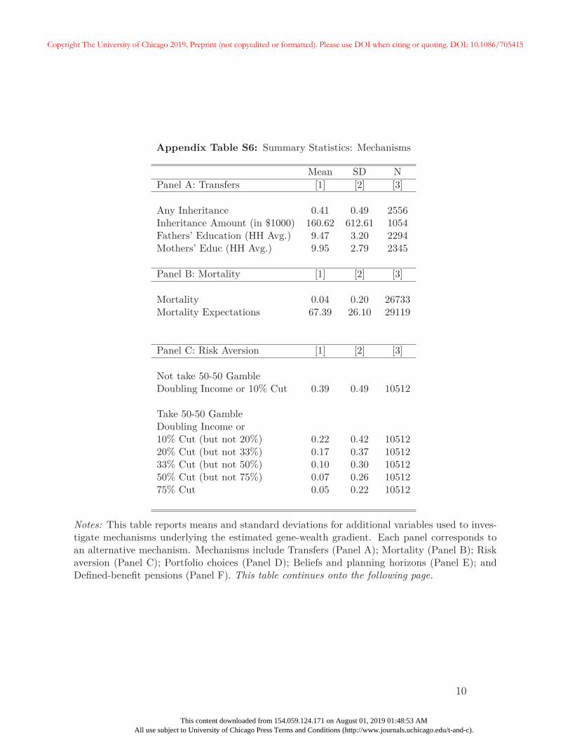
Appendix Table S6: Summary Statistics: Mechanisms
Mean SD NPanel A: Transfers [1] [2] [3]
Any Inheritance 0.41 0.49 2556Inheritance Amount (in $1000) 160.62 612.61 1054Fathers’ Education (HH Avg.) 9.47 3.20 2294Mothers’ Educ (HH Avg.) 9.95 2.79 2345
Panel B: Mortality [1] [2] [3]
Mortality 0.04 0.20 26733Mortality Expectations 67.39 26.10 29119
Panel C: Risk Aversion [1] [2] [3]
Not take 50-50 GambleDoubling Income or 10% Cut 0.39 0.49 10512
Take 50-50 GambleDoubling Income or10% Cut (but not 20%) 0.22 0.42 1051220% Cut (but not 33%) 0.17 0.37 1051233% Cut (but not 50%) 0.10 0.30 1051250% Cut (but not 75%) 0.07 0.26 1051275% Cut 0.05 0.22 10512
Notes: This table reports means and standard deviations for additional variables used to inves-tigate mechanisms underlying the estimated gene-wealth gradient. Each panel corresponds toan alternative mechanism. Mechanisms include Transfers (Panel A); Mortality (Panel B); Riskaversion (Panel C); Portfolio choices (Panel D); Beliefs and planning horizons (Panel E); andDefined-benefit pensions (Panel F). This table continues onto the following page.
10
Copyright The University of Chicago 2019. Preprint (not copyedited or formatted). Please use DOI when citing or quoting. DOI: 10.1086/705415
This content downloaded from 154.059.124.171 on August 01, 2019 01:48:53 AMAll use subject to University of Chicago Press Terms and Conditions (http://www.journals.uchicago.edu/t-and-c).
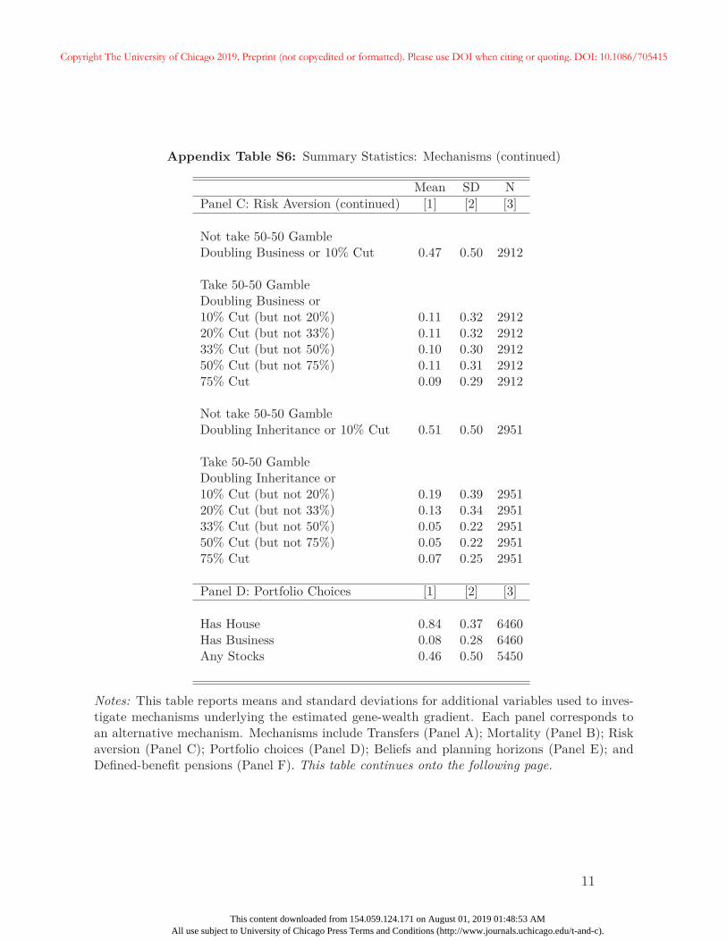
Appendix Table S6: Summary Statistics: Mechanisms (continued)
Mean SD NPanel C: Risk Aversion (continued) [1] [2] [3]
Not take 50-50 GambleDoubling Business or 10% Cut 0.47 0.50 2912
Take 50-50 GambleDoubling Business or10% Cut (but not 20%) 0.11 0.32 291220% Cut (but not 33%) 0.11 0.32 291233% Cut (but not 50%) 0.10 0.30 291250% Cut (but not 75%) 0.11 0.31 291275% Cut 0.09 0.29 2912
Not take 50-50 GambleDoubling Inheritance or 10% Cut 0.51 0.50 2951
Take 50-50 GambleDoubling Inheritance or10% Cut (but not 20%) 0.19 0.39 295120% Cut (but not 33%) 0.13 0.34 295133% Cut (but not 50%) 0.05 0.22 295150% Cut (but not 75%) 0.05 0.22 295175% Cut 0.07 0.25 2951
Panel D: Portfolio Choices [1] [2] [3]
Has House 0.84 0.37 6460Has Business 0.08 0.28 6460Any Stocks 0.46 0.50 5450
Notes: This table reports means and standard deviations for additional variables used to inves-tigate mechanisms underlying the estimated gene-wealth gradient. Each panel corresponds toan alternative mechanism. Mechanisms include Transfers (Panel A); Mortality (Panel B); Riskaversion (Panel C); Portfolio choices (Panel D); Beliefs and planning horizons (Panel E); andDefined-benefit pensions (Panel F). This table continues onto the following page.
11
Copyright The University of Chicago 2019. Preprint (not copyedited or formatted). Please use DOI when citing or quoting. DOI: 10.1086/705415
This content downloaded from 154.059.124.171 on August 01, 2019 01:48:53 AMAll use subject to University of Chicago Press Terms and Conditions (http://www.journals.uchicago.edu/t-and-c).
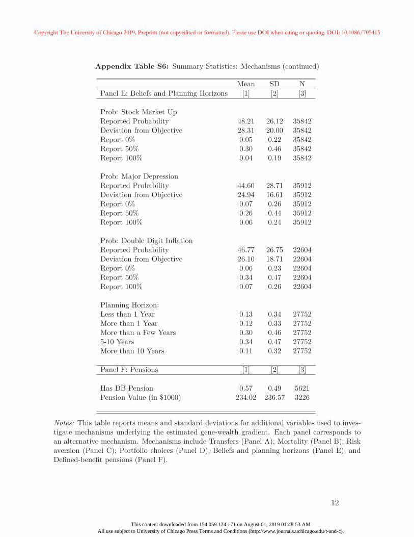
Appendix Table S6: Summary Statistics: Mechanisms (continued)
Mean SD NPanel E: Beliefs and Planning Horizons [1] [2] [3]
Prob: Stock Market UpReported Probability 48.21 26.12 35842Deviation from Objective 28.31 20.00 35842Report 0% 0.05 0.22 35842Report 50% 0.30 0.46 35842Report 100% 0.04 0.19 35842
Prob: Major DepressionReported Probability 44.60 28.71 35912Deviation from Objective 24.94 16.61 35912Report 0% 0.07 0.26 35912Report 50% 0.26 0.44 35912Report 100% 0.06 0.24 35912
Prob: Double Digit InflationReported Probability 46.77 26.75 22604Deviation from Objective 26.10 18.71 22604Report 0% 0.06 0.23 22604Report 50% 0.34 0.47 22604Report 100% 0.07 0.26 22604
Planning Horizon:Less than 1 Year 0.13 0.34 27752More than 1 Year 0.12 0.33 27752More than a Few Years 0.30 0.46 277525-10 Years 0.34 0.47 27752More than 10 Years 0.11 0.32 27752
Panel F: Pensions [1] [2] [3]
Has DB Pension 0.57 0.49 5621Pension Value (in $1000) 234.02 236.57 3226
Notes: This table reports means and standard deviations for additional variables used to inves-tigate mechanisms underlying the estimated gene-wealth gradient. Each panel corresponds toan alternative mechanism. Mechanisms include Transfers (Panel A); Mortality (Panel B); Riskaversion (Panel C); Portfolio choices (Panel D); Beliefs and planning horizons (Panel E); andDefined-benefit pensions (Panel F).
12
Copyright The University of Chicago 2019. Preprint (not copyedited or formatted). Please use DOI when citing or quoting. DOI: 10.1086/705415
This content downloaded from 154.059.124.171 on August 01, 2019 01:48:53 AMAll use subject to University of Chicago Press Terms and Conditions (http://www.journals.uchicago.edu/t-and-c).
B Additional Results
This appendix contains additional results referenced in the main text. Additional results arerelated to assortative mating, the relationship between the EA score and parental educationand inheritances, and the relationship between beliefs, the financial planning horizon, wealth,and stock market participation.
B.1 Assortative Mating
Table S7 provides the evidence for the extent of assortative mating in our sample. We restrictattention to households in which both spouses have EA scores. First, we sort both males andfemales into quartiles, respectively, based on their individual EA scores. We then calculatethe fraction of men in each male EA quartile within a given female EA quartile, and normalizeso that the columns sum to one.4 Panel A reports these distributions for individuals sortedby the raw, unadjusted value of their individual EA scores; Panel B reports distributionswhere individuals have been sorted based on the residual in a regression of their individualEA score on degree dummies and years of schooling. With perfect assortative mating, thematrices reported in Table S7 would be diagonal matrices, with 100% populating the diagonalentries and 0% populating the off-diagonal entries. Alternatively, random assignment wouldgenerate matrices with 25% for each entry.
We find some evidence of assortative mating, especially among the highest and lowestEA score quartiles. We find that 27.3% of women in the lowest individual EA score quartileare coupled with men in the lowest individual EA score quartile, compared to 26.9% coupledwith men in the second quartile, 28.5% coupled with men in the third quartile, and 17.3%coupled with men in the fourth quartile. Entries in the fourth quartile of females’ EA scoresshow similar patterns, with only 18.8% of the highest EA quartile women coupled with thehighest EA-quartile men, compared to 33.5% coupled with the highest EA quartile males.Although we are able to reject the random-assignment null hypothesis that all entries areequal to 25% (p < 0.001), the degree of assortative mating appears modest relative to thecounterfactual of perfect sorting. Indeed, while the within-couple correlation of years ofschooling is 0.52, the within-couple correlation of individual EA scores is only 0.14.
4This exercise closely follows Charles, Hurst, and Killewald (2013) (see their Table 5 on p. 61), whoexamine assortative mating on parents’ wealth.
13
Copyright The University of Chicago 2019. Preprint (not copyedited or formatted). Please use DOI when citing or quoting. DOI: 10.1086/705415
This content downloaded from 154.059.124.171 on August 01, 2019 01:48:53 AMAll use subject to University of Chicago Press Terms and Conditions (http://www.journals.uchicago.edu/t-and-c).
B.2 Transfers and Parental Education
In Table S8, we relate the EA score to inheritances. All regressions include our standardcontrols and full education controls, unless otherwise noted. In Column [1] of Table S8, weestimate a cross-sectional regression where the dependent variable is an indicator variableequal to one if the household has ever received an inheritance over the span of the sample.In Column [2] we estimate a cross-sectional regression where the dependent variable is thelog of the real dollar value of all inheritances received over the sample. Because the log oftotal inheritances is defined only for values greater than zero, this specification is equivalentto a regression of inheritance values conditional on receiving an inheritance. We find norelationship between the EA score and either the probability of receiving an inheritance orthe size of inheritance wealth conditional on receiving an inheritance.
Next, we regress different measures of parental education on the household’s average EAscore. In Column [3], the dependent variable is the average education of the fathers of bothhousehold members, and we include our standard controls but no measures of respondenteducation. Column [4] presents the same specification but with the average of mothers’education as the dependent variable. Results suggest the education of both parents arestrongly related to the household average EA score. In Columns [5] and [6], we investigatewhether the relationship between parental education and the EA score is entirely explainedby household members’ own education. In Column [5] the dependent variable is again averagefathers’ education, but we now include the full set of household education controls. Column[6] reports analogous coefficients with average mothers’ education as the dependent variable.The estimated coefficients on the EA score are reduced dramatically but remain statisticallysignificant for fathers’ education (and marginally significant for mothers’ education), whichindicates that household environments and other investments could play a role in wealthaccumulation beyond just educational attainment.
B.3 Macroeconomic Beliefs and Household Behavior
The results in Table 10 suggest that individuals with lower genetic scores are more likelyto report beliefs that are at odds with objective probabilities and are more likely to report“extreme” beliefs. It is possible, however, that these reported beliefs are not related to in-dividual behavior in a meaningful way, making these results interesting but not particularlyuseful for understanding the potential underlying mechanisms linking the EA score to finan-cial decisions. This would be the case if either the HRS expectations questions do a poorjob of eliciting true beliefs about these economic events, or if the events themselves were notrelevant for the household’s choice problem. Whether a longer financial planning horizon is
14
Copyright The University of Chicago 2019. Preprint (not copyedited or formatted). Please use DOI when citing or quoting. DOI: 10.1086/705415
This content downloaded from 154.059.124.171 on August 01, 2019 01:48:53 AMAll use subject to University of Chicago Press Terms and Conditions (http://www.journals.uchicago.edu/t-and-c).
associated with greater wealth is a similarly empirical question.Table S9 shows that some of these elicited measures do indeed predict relevant behaviors
such as stock market participation, and are associated with wealth. Column [1] regresses logwealth on indicators for whether the household ever reported an extreme belief for any of thethree macroeconomic expectations (stock market appreciation, severe recession, or double-digit inflation), and indicators for which financial planning horizon households report. Boththe financial planning horizon and stock market beliefs are related to accumulated wealth.Interestingly, excessive optimism about the stock market is actually associated with greaterwealth, likely due to an increase in participation. This suggests that the direction of incorrectbeliefs is important for their overall impact on wealth. Column [2] repeats this exercise butincludes the EA score as an additional control. The inclusion of the belief and planninghorizon variables reduces the coefficient on the EA score from 0.047 to 0.038.
In Columns [3] and [4] we repeat the specifications in Columns [1] and [2], but replacethe log wealth with stock market participation as the dependent variable. Consistent witheconomic theory, longer planning horizons are associated with greater stock market partic-ipation. Reassuringly, extreme optimistic beliefs are also positively associated with stockmarket participation, whereas extreme pessimistic beliefs are negatively (but statisticallyinsignificantly) related. Column [4] also shows that the positive relationship between theEA score and stock ownership documented in Table 9 remains after inclusion of belief andplanning horizon controls.
15
Copyright The University of Chicago 2019. Preprint (not copyedited or formatted). Please use DOI when citing or quoting. DOI: 10.1086/705415
This content downloaded from 154.059.124.171 on August 01, 2019 01:48:53 AMAll use subject to University of Chicago Press Terms and Conditions (http://www.journals.uchicago.edu/t-and-c).
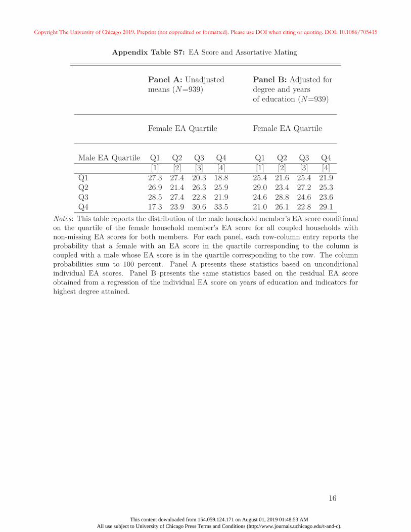
Appendix Table S7: EA Score and Assortative Mating
Panel A: Unadjusted Panel B: Adjusted formeans (N=939) degree and years
of education (N=939)
Female EA Quartile Female EA Quartile
Male EA Quartile Q1 Q2 Q3 Q4 Q1 Q2 Q3 Q4[1] [2] [3] [4] [1] [2] [3] [4]
Q1 27.3 27.4 20.3 18.8 25.4 21.6 25.4 21.9Q2 26.9 21.4 26.3 25.9 29.0 23.4 27.2 25.3Q3 28.5 27.4 22.8 21.9 24.6 28.8 24.6 23.6Q4 17.3 23.9 30.6 33.5 21.0 26.1 22.8 29.1
Notes: This table reports the distribution of the male household member’s EA score conditionalon the quartile of the female household member’s EA score for all coupled households withnon-missing EA scores for both members. For each panel, each row-column entry reports theprobability that a female with an EA score in the quartile corresponding to the column iscoupled with a male whose EA score is in the quartile corresponding to the row. The columnprobabilities sum to 100 percent. Panel A presents these statistics based on unconditionalindividual EA scores. Panel B presents the same statistics based on the residual EA scoreobtained from a regression of the individual EA score on years of education and indicators forhighest degree attained.
16
Copyright The University of Chicago 2019. Preprint (not copyedited or formatted). Please use DOI when citing or quoting. DOI: 10.1086/705415
This content downloaded from 154.059.124.171 on August 01, 2019 01:48:53 AMAll use subject to University of Chicago Press Terms and Conditions (http://www.journals.uchicago.edu/t-and-c).
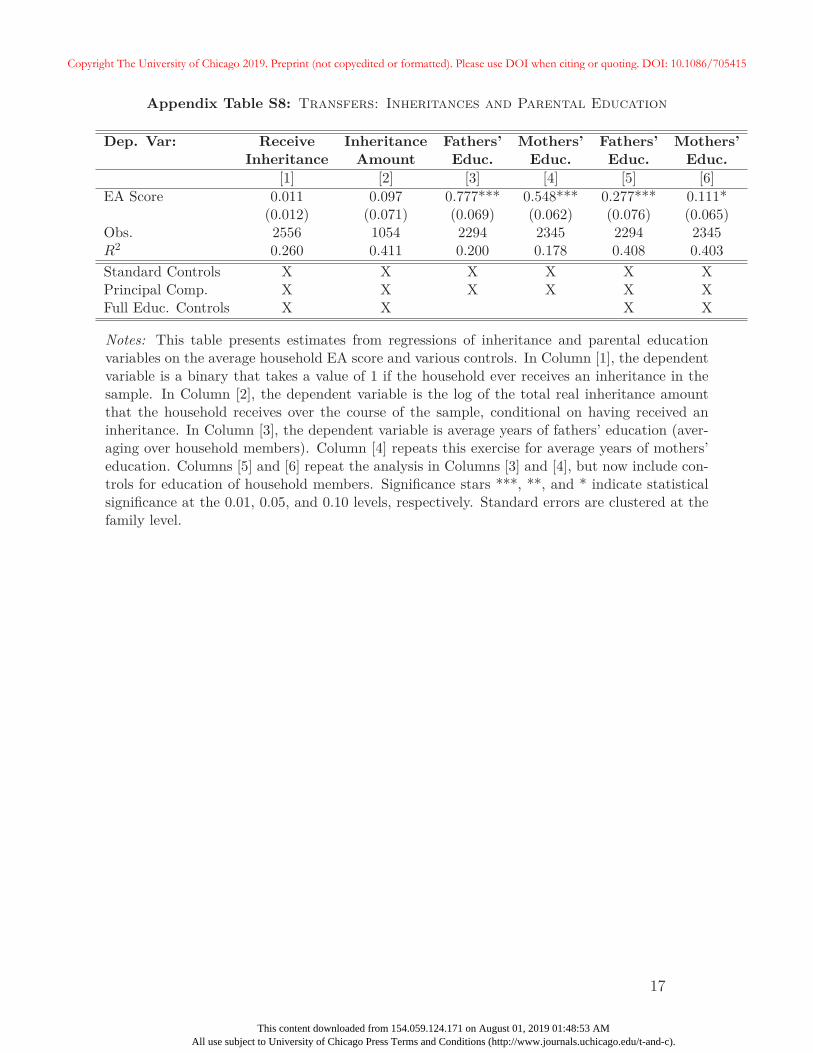
Appendix Table S8: Transfers: Inheritances and Parental Education
Dep. Var: Receive Inheritance Fathers’ Mothers’ Fathers’ Mothers’Inheritance Amount Educ. Educ. Educ. Educ.
[1] [2] [3] [4] [5] [6]EA Score 0.011 0.097 0.777*** 0.548*** 0.277*** 0.111*
(0.012) (0.071) (0.069) (0.062) (0.076) (0.065)Obs. 2556 1054 2294 2345 2294 2345R2 0.260 0.411 0.200 0.178 0.408 0.403Standard Controls X X X X X XPrincipal Comp. X X X X X XFull Educ. Controls X X X X
Notes: This table presents estimates from regressions of inheritance and parental educationvariables on the average household EA score and various controls. In Column [1], the dependentvariable is a binary that takes a value of 1 if the household ever receives an inheritance in thesample. In Column [2], the dependent variable is the log of the total real inheritance amountthat the household receives over the course of the sample, conditional on having received aninheritance. In Column [3], the dependent variable is average years of fathers’ education (aver-aging over household members). Column [4] repeats this exercise for average years of mothers’education. Columns [5] and [6] repeat the analysis in Columns [3] and [4], but now include con-trols for education of household members. Significance stars ***, **, and * indicate statisticalsignificance at the 0.01, 0.05, and 0.10 levels, respectively. Standard errors are clustered at thefamily level.
17
Copyright The University of Chicago 2019. Preprint (not copyedited or formatted). Please use DOI when citing or quoting. DOI: 10.1086/705415
This content downloaded from 154.059.124.171 on August 01, 2019 01:48:53 AMAll use subject to University of Chicago Press Terms and Conditions (http://www.journals.uchicago.edu/t-and-c).
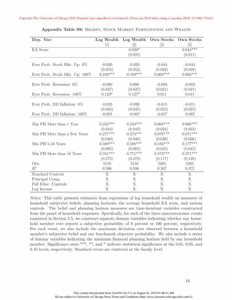
Appendix Table S9: Beliefs, Stock Market Participation and Wealth
Dep. Var: Log Wealth Log Wealth Own Stocks Own Stocks[1] [2] [3] [4]
EA Score 0.038* 0.044***(0.021) (0.011)
Ever Prob. Stock Mkt. Up: 0% -0.020 -0.020 -0.044 -0.044(0.053) (0.053) (0.028) (0.028)
Ever Prob. Stock Mkt. Up: 100% 0.169*** 0.169*** 0.069*** 0.068***
Ever Prob. Recession: 0% -0.000 0.000 -0.003 -0.003(0.037) (0.037) (0.021) (0.021)
Ever Prob. Recession: 100% 0.123* 0.127* 0.011 0.015
Ever Prob. DD Inflation: 0% -0.029 -0.026 -0.015 -0.011(0.045) (0.045) (0.025) (0.025)
Ever Prob. DD Inflation: 100% -0.095 -0.087 -0.017 -0.007
Min PH More than 1 Year 0.234*** 0.234*** 0.068*** 0.066***(0.043) (0.043) (0.024) (0.023)
Min PH More than a Few Years 0.277*** 0.273*** 0.078*** 0.071***(0.040) (0.040) (0.026) (0.026)
Min PH 5-10 Years 0.589*** 0.588*** 0.183*** 0.177***(0.085) (0.085) (0.045) (0.045)
Min PH More than 10 Years 0.761*** 0.771*** 0.373*** 0.371***(0.273) (0.278) (0.117) (0.120)
Obs. 5158 5158 5285 5285R2 0.506 0.506 0.367 0.372Standard Controls X X X XPrincipal Comp. X X X XFull Educ. Controls X X X XLog Income X X X X
Notes: This table presents estimates from regressions of log household wealth on measures ofhousehold subjective beliefs, planning horizons, the average household EA score, and variouscontrols. The belief and planning horizon measures are time-invariant variables constructedfrom the panel of household responses. Specifically, for each of the three macroeconomic eventsexamined in Section 5.5, we construct separate dummy variables indicating whether any house-hold member ever reports a subjective probability of 0 percent or 100 percent, respectively.For each event, we also include the maximum deviation ever observed between a householdmember’s subjective belief and our benchmark objective probability. We also include a seriesof dummy variables indicating the minimum financial planning horizon held by any householdmember. Significance stars ***, **, and * indicate statistical significance at the 0.01, 0.05, and0.10 levels, respectively. Standard errors are clustered at the family level.
18
Copyright The University of Chicago 2019. Preprint (not copyedited or formatted). Please use DOI when citing or quoting. DOI: 10.1086/705415
This content downloaded from 154.059.124.171 on August 01, 2019 01:48:53 AMAll use subject to University of Chicago Press Terms and Conditions (http://www.journals.uchicago.edu/t-and-c).
C Robustness
This appendix contains robustness tests that are largely based on the main associationsreported in Table 4. We examine robustness to the application of sampling weights, as wellas alternate sample definitions, measurements of household EA scores, income specifications,wealth definitions, and control sets.
C.1 Household Structure and EA Score
This section assesses the robustness of the main results presented in Table 4 to changes inthe sample definition, as well as changes in how we aggregate the EA score within two-person households. In Table S10, we address four possible selection issues that may affectthe main results. In Columns [1] and [2], we repeat specifications from Columns [5] and [7]in Table 4, but apply the HRS supplied sample weights. In Columns [3] and [4] we addresspotential selection bias from mortality including only one observation per household; thismay be important if wealthier people with higher EA scores live longer and are thereforedisproportionately represented in a full panel. In Columns [5] and [6], we restrict the sampleto only “coupled” households, in which the household has two members in at least one samplewave. We note that this sample may include household-year observations after a spouse hasdied. The results in Columns [1]-[6] all continue to demonstrate a economically large andstatistically significant association between the EA score and wealth. Finally, in Columns[7] and [8], we evaluate whether the maximum or minimum EA score is ultimately drivingthe main association. In these specifications, we restrict the sample to households with non-missing EA scores for both members. Estimates in these specifications are quite imprecise,and in both regressions we fail to reject the null hypothesis that the coefficients on bothscores are the same. The lack of precision here is likely driven by the fact that the samplesize is reduced dramatically when restricting to coupled households with two non-missingscores.
C.2 Alternate Definitions of Income
The income data described in Section 3.2 are based on data from the Social Security Admin-istration (SSA). The SSA data contain earnings information for most or all of respondents’working lives. This offers a clear advantage relative to the self-reported income measures inthe HRS, which only cover older ages. However, an important limitation of the SSA data is
19
Copyright The University of Chicago 2019. Preprint (not copyedited or formatted). Please use DOI when citing or quoting. DOI: 10.1086/705415
This content downloaded from 154.059.124.171 on August 01, 2019 01:48:53 AMAll use subject to University of Chicago Press Terms and Conditions (http://www.journals.uchicago.edu/t-and-c).
that they are top-coded at the taxable maximum amount for Social Security payroll taxes.5
Panel B of Table S3 presents summary statistics relevant for the SSA income measure andtop-coding. Across households, the average number of person-years with top-coded incomeobservations is 12.67 in our sample. Less than one-third (27%) of households are never top-coded. To partially correct for top-coding, we use Current Population Survey (CPS) datato calculate mean income for people earning at least the top-coded level in each year overthe period 1961-2010. We then replace the top coded amount in the SSA data with theconditional mean from the CPS data for each of these years.6
Table S11 presents estimates from specifications with a variety of alternative controls forlifetime household income. All specifications include the same set of controls as Column [7]in Table 4. Column [1] of S11 measures household income using the log of average householdincome observed within the HRS sample. Column [2] includes the log of total householdincome from the SSA (our standard measure), but also includes a complete set of dummyvariables for each possible number of top-coded years in the SSA earnings data. Column[3] is the same as Column [2], but further includes dummy variables for each quintile ofthe distribution of SSA earnings across households. Column [4] controls for lifetime incomeusing a quintic polynomial of the log of total household income from the SSA. Column [5] isthe same as our basic specification (Column [7] in Table 4), but drops households in whichany member is ever observed in two separate households (e.g., households that split dueto a divorce). This specification addresses concerns that lifetime income might be dividedacross households that separate. Finally, Column [6] controls for income using the log of theaverage of SSA earnings over the household’s 35 highest earning years. Across all of thesespecifications, we robustly estimate an economically large statistically significant coefficienton the EA score. Estimates of the coefficient on the EA score fall in a fairly narrow rangeof 0.041-0.061.
C.3 Alternative Definitions of Wealth
In this section, we repeat the analysis in Table 4 using different measures of household wealth.In Column [1] of Table S12, we use the measure of wealth provided by RAND, which does notinclude the present discounted value of retirement income or the retirement account balances
5This taxable maximum has changed substantially over time. In some years, especially in the 1960s and1970s, a substantial portion of households fall into this category since the maximum was fairly low. Forexample, in 1965 the maximum was $4,800 (which is about $38,000 in 2018 dollars).
6For example, if an individual earned $10,000 (nominal) in 1965, we would observe a top-coded incomeamount of $4,800 in the SSA file. The mean CPS income for those earning at least $4,800 in 1965 is $8,103so we would replace this individuals’ income (any 1965 SSA amount of at least $4,800) with $8,103, whichis approximately $56,096 in 2010 dollars.
20
Copyright The University of Chicago 2019. Preprint (not copyedited or formatted). Please use DOI when citing or quoting. DOI: 10.1086/705415
This content downloaded from 154.059.124.171 on August 01, 2019 01:48:53 AMAll use subject to University of Chicago Press Terms and Conditions (http://www.journals.uchicago.edu/t-and-c).
still held with employers. In Column [2], we use the measure of wealth used in our mainanalysis but subtract the net value of housing. In Column [3], we again use our main wealthmeasure, but subtract the present discounted value of defined-benefit pension, annuity, andsocial security income. In Column [4], we subtract both housing and retirement-incomewealth. Finally, in Column [5], we subtract the value of privately held businesses. In allspecifications the key patterns from our main results remain largely unchanged.
C.4 Sample Selection
Table S13 presents estimates of our basic results from Table 4 using four different possiblesample definitions. For each alternate sample, we present two specifications correspondingto Columns [5] and [7] in Table 4. Columns [1]-[2] of S13 present estimates from our baselinesample of retired households with members aged 65-75, which are reproduced from Table 4.To understand whether these results are affected by the retirement or age restrictions on thissample, we consider three other sample definitions. Columns [3]-[4] present estimates froma sample of retired households with members aged 55-85. Columns [5]-[6] present estimatesfrom a sample of all households regardless of retirement status with members aged 50-75,while the sample used in Columns [7]-[8] includes all households with members aged ≤ 85.Across all of these samples, we consistently estimate economically large and statisticallysignificant coefficients on the EA score in the range 0.047-0.084.
C.5 Alternative Scores
In Table S14, we examine whether the main association established in Table 4 is affectedby using alternate polygenic scores for educational attainment. For each alternative score,we construct a household average and replicate Column [7] of Table 4. The score usedin Column [1] is based on the Lee et al. (2018) GWAS (as is the main score used in ouranalysis). Since Lee et al. (2018) is the third in a series of GWAS on educational attainmentby the same consortium, it is referred to as the EA3 score. The version of the EA3 scorefeatured in Column [1] is not constructed with the LDpred method used to construct ourprimary score. Rather, this version is simply the sum of all SNPs weighted by their GWAScoefficients, and was released by the HRS for all genotyped waves. Consequently, this scoreis available for more households than the LDpred EA3 score, which was only calculated forindividuals genotyped in the 2006 and 2008 waves. In Column [1] we use this non-LDpredscore, but restrict the sample to households included in our main sample. We estimate acoefficient on the EA3 score of 0.038 in this specification. In Column [2], we use this scorefor all genotyped households (including individuals genotyped in the 2010 and 2012 waves),
21
Copyright The University of Chicago 2019. Preprint (not copyedited or formatted). Please use DOI when citing or quoting. DOI: 10.1086/705415
This content downloaded from 154.059.124.171 on August 01, 2019 01:48:53 AMAll use subject to University of Chicago Press Terms and Conditions (http://www.journals.uchicago.edu/t-and-c).
and estimate a coefficient of 0.044. The stability of the coefficient across these specificationssuggests that our main association is not greatly affected by the expansion of the genotypedsubsample over time.
Columns [3]-[4] estimate specifications based on a score built from the Okbay et al.(2016) GWAS results (referred to as EA2, since it was the second education GWAS by thisconsortium), which featured a discovery sample size of N = 293, 723. The score used inthese specifications is the all-SNP (non-LDpred) score released by the HRS. In column [3]we restrict the sample to households that are included in our main sample, while column[4] expands the sample to include household-year observations with individuals genotypedin the 2010 and 2012 waves. The coefficients estimated in these specifications are similar tothe coefficients estimated in Columns [1]-[2] using the EA3 scores. Finally, Columns [5]-[6]present results with the score based on the EA1 GWAS results from Rietveld et al. (2013),which featured a sample size of N = 126, 559. Column [5] presents results for an LDpredscore, while column [6] presents results from a score that sums all SNPs weighted by theirGWAS association sizes. Both scores exhibit a weak, statistically insignificant associationwith log households wealth.
C.6 Alternative Control Sets
In this section, we examine the robustness of the main results in Table 4 to the inclusion ofadditional controls. In Columns [1]-[2] of Panel A in Table S15, we add the average householdcognitive test score to our two baseline specifications (Columns [5] and [7] in Table 4). If thegene-wealth gradient in part arises from facility with complex decisions, a cognitive test scoremay explain much of the association captured by the EA score. However, the cognitive testscore in the HRS is designed to capture cognitive decline and is only moderately correlatedwith the EA score. The average household test score is 23.89 (out of a total of 35) withaverages for females and males of 24.40 and 23.22, respectively. Inclusion of the averagehousehold cognitive test score does not affect our main results. In Columns [3]-[4] of PanelA in Table S15, we include the maximum number of children associated with a householdmember. Higher EA score individuals may have more wealth at retirement due to havingfewer children. The average number of children in the full analytical sample is 3.70, andhouseholds with higher average EA scores have fewer children. For individuals with EAscores in the first quartile, the average number of children in their household is 3.90 (againusing the maximum observed for the household). For individuals with EA scores in thefourth quartile, the average is 3.34. However, inclusion of number of children leaves resultsunchanged.
22
Copyright The University of Chicago 2019. Preprint (not copyedited or formatted). Please use DOI when citing or quoting. DOI: 10.1086/705415
This content downloaded from 154.059.124.171 on August 01, 2019 01:48:53 AMAll use subject to University of Chicago Press Terms and Conditions (http://www.journals.uchicago.edu/t-and-c).
In Panel B of Table S15, we include controls for years since retirement and years since thedeath of a household member. Columns [1]-[2] modify our baseline specifications by addingseparate sets of dummy variables for the number of years that the male and female householdmembers have been retired, respectively. We interact these variables with dummies for male-only and female-only households, respectively. If higher EA score individuals retire laterthan respondents with lower scores, this could explain greater wealth accumulation. Thecoefficient in column [2] decreases some, and becomes marginally statistically insignificantat the 10% level (p-value of 0.108). The death of a household member may be associated witha spike in expenses related to end-of-life care, followed by a systematic change in householdconsumption and decision-making. Therefore, in Columns [3]-[4], we control for the deathof a household member by adding a full set of dummies for the number of years since themale and female household member has died, respectively. We also add an indicator fora coupled household that only has one member in it during a given year. The resultingcoefficient estimates are again similar to our baseline estimates. Finally, in Panel C, weestimate specifications in which we simultaneously include all of the additional controls fromPanels A and B. Adding all of these controls reduces the coefficient on the EA score, and incolumn [2] again becomes statistically insignificant.
23
Copyright The University of Chicago 2019. Preprint (not copyedited or formatted). Please use DOI when citing or quoting. DOI: 10.1086/705415
This content downloaded from 154.059.124.171 on August 01, 2019 01:48:53 AMAll use subject to University of Chicago Press Terms and Conditions (http://www.journals.uchicago.edu/t-and-c).
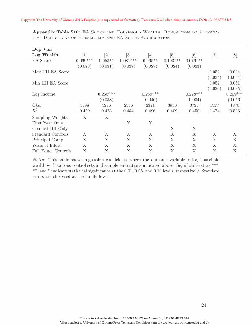
Appendix Table S10: EA Score and Household Wealth: Robustness to Alterna-
tive Definitions of Households and EA Score Aggregation
Dep Var:Log Wealth [1] [2] [3] [4] [5] [6] [7] [8]EA Score 0.069*** 0.053** 0.081*** 0.065** 0.103*** 0.076***
(0.023) (0.021) (0.027) (0.027) (0.024) (0.023)Max HH EA Score 0.052 0.034
(0.034) (0.034)Min HH EA Score 0.052 0.051
(0.036) (0.035)Log Income 0.265*** 0.259*** 0.228*** 0.209***
(0.038) (0.046) (0.034) (0.056)Obs. 5598 5286 2556 2371 3930 3723 1927 1870R2 0.429 0.473 0.454 0.496 0.409 0.450 0.474 0.506Sampling Weights X XFirst Year Only X XCoupled HH Only X XStandard Controls X X X X X X X XPrincipal Comp. X X X X X X X XYears of Educ. X X X X X X X XFull Educ. Controls X X X X X X X X
Notes: This table shows regression coefficients where the outcome variable is log householdwealth with various control sets and sample restrictions indicated above. Significance stars ***,**, and * indicate statistical significance at the 0.01, 0.05, and 0.10 levels, respectively. Standarderrors are clustered at the family level.
24
Copyright The University of Chicago 2019. Preprint (not copyedited or formatted). Please use DOI when citing or quoting. DOI: 10.1086/705415
This content downloaded from 154.059.124.171 on August 01, 2019 01:48:53 AMAll use subject to University of Chicago Press Terms and Conditions (http://www.journals.uchicago.edu/t-and-c).
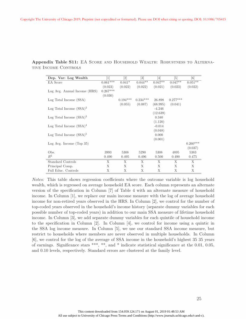
Appendix Table S11: EA Score and Household Wealth: Robustness to Alterna-
tive Income Controls
Dep. Var: Log Wealth [1] [2] [3] [4] [5] [6]EA Score 0.061*** 0.041* 0.044** 0.047** 0.047** 0.051**
(0.023) (0.022) (0.022) (0.021) (0.023) (0.022)Log Avg. Annual Income (HRS) 0.267***
(0.030)Log Total Income (SSA) 0.194*** 0.234*** 26.898 0.277***
(0.055) (0.087) (68.995) (0.041)Log Total Income (SSA)2 -4.246
(12.639)Log Total Income (SSA)3 0.340
(1.120)Log Total Income (SSA)4 -0.014
(0.048)Log Total Income (SSA)5 0.000
(0.001)Log Avg. Income (Top 35) 0.260***
(0.037)Obs. 3993 5308 5290 5308 4895 5383R2 0.490 0.495 0.496 0.500 0.490 0.475Standard Controls X X X X X XPrincipal Comp. X X X X X XFull Educ. Controls X X X X X X
Notes: This table shows regression coefficients where the outcome variable is log householdwealth, which is regressed on average household EA score. Each column represents an alternateversion of the specification in Column [7] of Table 4 with an alternate measure of householdincome. In Column [1], we replace our main income measure with the log of average householdincome for non-retired years observed in the HRS. In Column [2], we control for the number oftop-coded years observed in the household’s income history (separate dummy variables for eachpossible number of top-coded years) in addition to our main SSA measure of lifetime householdincome. In Column [3], we add separate dummy variables for each quintile of household incometo the specification in Column [2]. In Column [4], we control for income using a quintic inthe SSA log income measure. In Column [5], we use our standard SSA income measure, butrestrict to households where members are never observed in multiple households. In Column[6], we control for the log of the average of SSA income in the household’s highest 35 35 yearsof earnings. Significance stars ***, **, and * indicate statistical significance at the 0.01, 0.05,and 0.10 levels, respectively. Standard errors are clustered at the family level.
25
Copyright The University of Chicago 2019. Preprint (not copyedited or formatted). Please use DOI when citing or quoting. DOI: 10.1086/705415
This content downloaded from 154.059.124.171 on August 01, 2019 01:48:53 AMAll use subject to University of Chicago Press Terms and Conditions (http://www.journals.uchicago.edu/t-and-c).
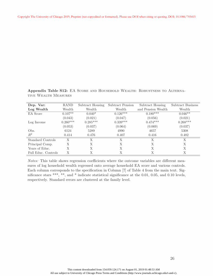
Appendix Table S12: EA Score and Household Wealth: Robustness to Alterna-
tive Wealth Measures
Dep. Var: RAND Subtract Housing Subtract Pension Subtract Housing Subtract BusinessLog Wealth Wealth Wealth Wealth and Pension Wealth WealthEA Score 0.107** 0.040* 0.126*** 0.180*** 0.046**
(0.043) (0.021) (0.047) (0.056) (0.021)Log Income 0.260*** 0.285*** 0.339*** 0.474*** 0.268***
(0.053) (0.037) (0.064) (0.069) (0.037)Obs. 6124 5289 4990 4657 5308R2 0.414 0.476 0.407 0.416 0.482Standard Controls X X X X XPrincipal Comp. X X X X XYears of Educ. X X X X XFull Educ. Controls X X X X X
Notes: This table shows regression coefficients where the outcome variables are different mea-sures of log household wealth regressed onto average household EA score and various controls.Each column corresponds to the specification in Column [7] of Table 4 from the main text. Sig-nificance stars ***, **, and * indicate statistical significance at the 0.01, 0.05, and 0.10 levels,respectively. Standard errors are clustered at the family level.
26
Copyright The University of Chicago 2019. Preprint (not copyedited or formatted). Please use DOI when citing or quoting. DOI: 10.1086/705415
This content downloaded from 154.059.124.171 on August 01, 2019 01:48:53 AMAll use subject to University of Chicago Press Terms and Conditions (http://www.journals.uchicago.edu/t-and-c).
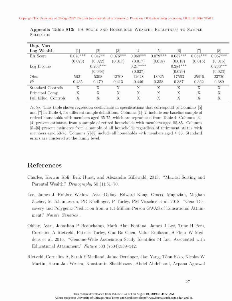
Appendix Table S13: EA Score and Household Wealth: Robustness to Sample
Selection
Dep. Var:Log Wealth [1] [2] [3] [4] [5] [6] [7] [8]EA Score 0.070*** 0.047** 0.076*** 0.060*** 0.079*** 0.057*** 0.084*** 0.067***
(0.023) (0.022) (0.017) (0.017) (0.018) (0.018) (0.015) (0.015)Log Income 0.263*** 0.217*** 0.284*** 0.233***
(0.038) (0.027) (0.029) (0.023)Obs. 5621 5308 13708 12628 18925 17563 25815 23720R2 0.435 0.479 0.413 0.446 0.358 0.387 0.362 0.389Standard Controls X X X X X X X XPrincipal Comp. X X X X X X X XFull Educ. Controls X X X X X X X X
Notes: This table shows regression coefficients in specifications that correspond to Columns [5]and [7] in Table 4, for different sample definitions. Columns [1]-[2] include our baseline sample ofretired households with members aged 65-75, which are reproduced from Table 4. Columns [3]-[4] present estimates from a sample of retired households with members aged 55-85. Columns[5]-[6] present estimates from a sample of all households regardless of retirement status withmembers aged 50-75. Columns [7]-[8] include all households with members aged ≤ 85. Standarderrors are clustered at the family level.
References
Charles, Kerwin Kofi, Erik Hurst, and Alexandra Killewald. 2013. “Marital Sorting andParental Wealth.” Demography 50 (1):51–70.
Lee, James J, Robbee Wedow, Aysu Okbay, Edward Kong, Omeed Maghzian, MeghanZacher, M Johannesson, PD Koellinger, P Turley, PM Visscher et al. 2018. “Gene Dis-covery and Polygenic Prediction from a 1.1-Million-Person GWAS of Educational Attain-ment.” Nature Genetics .
Okbay, Aysu, Jonathan P Beauchamp, Mark Alan Fontana, James J Lee, Tune H Pers,Cornelius A Rietveld, Patrick Turley, Guo-Bo Chen, Valur Emilsson, S Fleur W Med-dens et al. 2016. “Genome-Wide Association Study Identifies 74 Loci Associated withEducational Attainment.” Nature 533 (7604):539–542.
Rietveld, Cornelius A, Sarah E Medland, Jaime Derringer, Jian Yang, Tõnu Esko, Nicolas WMartin, Harm-Jan Westra, Konstantin Shakhbazov, Abdel Abdellaoui, Arpana Agrawal
27
Copyright The University of Chicago 2019. Preprint (not copyedited or formatted). Please use DOI when citing or quoting. DOI: 10.1086/705415
This content downloaded from 154.059.124.171 on August 01, 2019 01:48:53 AMAll use subject to University of Chicago Press Terms and Conditions (http://www.journals.uchicago.edu/t-and-c).

et al. 2013. “GWAS of 126,559 Individuals Identifies Genetic Variants Associated withEducational Attainment.” Science 340 (6139):1467–1471.
Yogo, Motohiro. 2016. “Portfolio Choice in Retirement: Health Risk and the Demand forAnnuities, Housing, and Risky Assets.” Journal of Monetary Economics 80:17–34.
28
Copyright The University of Chicago 2019. Preprint (not copyedited or formatted). Please use DOI when citing or quoting. DOI: 10.1086/705415
This content downloaded from 154.059.124.171 on August 01, 2019 01:48:53 AMAll use subject to University of Chicago Press Terms and Conditions (http://www.journals.uchicago.edu/t-and-c).
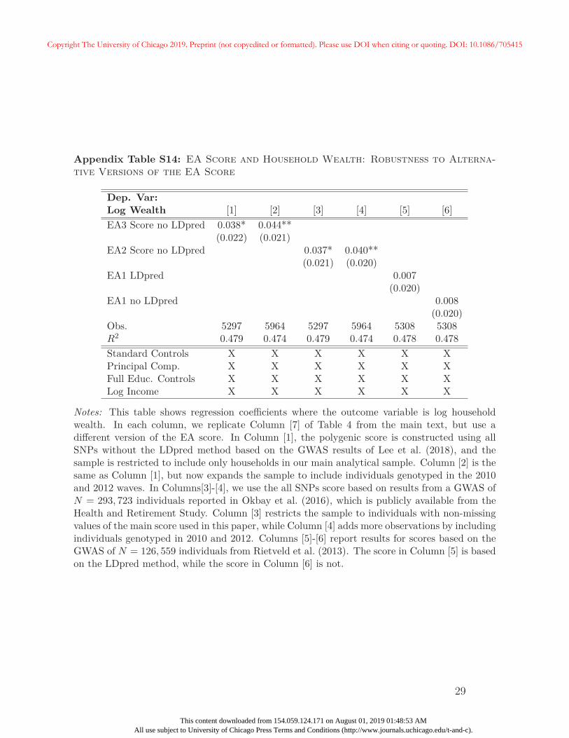
Appendix Table S14: EA Score and Household Wealth: Robustness to Alterna-
tive Versions of the EA Score
Dep. Var:Log Wealth [1] [2] [3] [4] [5] [6]EA3 Score no LDpred 0.038* 0.044**
(0.022) (0.021)EA2 Score no LDpred 0.037* 0.040**
(0.021) (0.020)EA1 LDpred 0.007
(0.020)EA1 no LDpred 0.008
(0.020)Obs. 5297 5964 5297 5964 5308 5308R2 0.479 0.474 0.479 0.474 0.478 0.478Standard Controls X X X X X XPrincipal Comp. X X X X X XFull Educ. Controls X X X X X XLog Income X X X X X X
Notes: This table shows regression coefficients where the outcome variable is log householdwealth. In each column, we replicate Column [7] of Table 4 from the main text, but use adifferent version of the EA score. In Column [1], the polygenic score is constructed using allSNPs without the LDpred method based on the GWAS results of Lee et al. (2018), and thesample is restricted to include only households in our main analytical sample. Column [2] is thesame as Column [1], but now expands the sample to include individuals genotyped in the 2010and 2012 waves. In Columns[3]-[4], we use the all SNPs score based on results from a GWAS ofN = 293, 723 individuals reported in Okbay et al. (2016), which is publicly available from theHealth and Retirement Study. Column [3] restricts the sample to individuals with non-missingvalues of the main score used in this paper, while Column [4] adds more observations by includingindividuals genotyped in 2010 and 2012. Columns [5]-[6] report results for scores based on theGWAS of N = 126, 559 individuals from Rietveld et al. (2013). The score in Column [5] is basedon the LDpred method, while the score in Column [6] is not.
29
Copyright The University of Chicago 2019. Preprint (not copyedited or formatted). Please use DOI when citing or quoting. DOI: 10.1086/705415
This content downloaded from 154.059.124.171 on August 01, 2019 01:48:53 AMAll use subject to University of Chicago Press Terms and Conditions (http://www.journals.uchicago.edu/t-and-c).
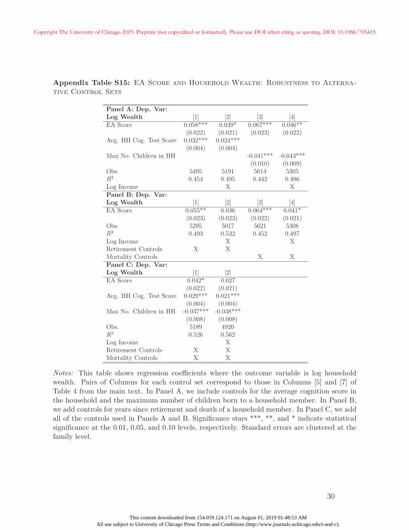
Appendix Table S15: EA Score and Household Wealth: Robustness to Alterna-
tive Control Sets
Panel A: Dep. Var:Log Wealth [1] [2] [3] [4]EA Score 0.058*** 0.039* 0.067*** 0.046**
(0.022) (0.021) (0.023) (0.022)Avg. HH Cog. Test Score 0.032*** 0.024***
(0.004) (0.004)Max No. Children in HH -0.041*** -0.043***
(0.010) (0.009)Obs. 5495 5191 5614 5305R2 0.454 0.495 0.442 0.486Log Income X XPanel B: Dep. Var:Log Wealth [1] [2] [3] [4]EA Score 0.055** 0.036 0.064*** 0.041*
(0.023) (0.023) (0.022) (0.021)Obs. 5295 5017 5621 5308R2 0.493 0.532 0.452 0.497Log Income X XRetirement Controls X XMortality Controls X XPanel C: Dep. Var:Log Wealth [1] [2]EA Score 0.042* 0.027
(0.022) (0.021)Avg. HH Cog. Test Score 0.029*** 0.021***
(0.004) (0.004)Max No. Children in HH -0.037*** -0.038***
(0.008) (0.008)Obs. 5189 4920R2 0.526 0.562Log Income XRetirement Controls X XMortality Controls X X
Notes: This table shows regression coefficients where the outcome variable is log householdwealth. Pairs of Columns for each control set correspond to those in Columns [5] and [7] ofTable 4 from the main text. In Panel A, we include controls for the average cognition score inthe household and the maximum number of children born to a household member. In Panel B,we add controls for years since retirement and death of a household member. In Panel C, we addall of the controls used in Panels A and B. Significance stars ***, **, and * indicate statisticalsignificance at the 0.01, 0.05, and 0.10 levels, respectively. Standard errors are clustered at thefamily level.
30
Copyright The University of Chicago 2019. Preprint (not copyedited or formatted). Please use DOI when citing or quoting. DOI: 10.1086/705415
This content downloaded from 154.059.124.171 on August 01, 2019 01:48:53 AMAll use subject to University of Chicago Press Terms and Conditions (http://www.journals.uchicago.edu/t-and-c).