Genetic CNN

Lingxi Xie, Alan YuilleCenter for Imaging Science, The Johns Hopkins University, Baltimore, MD, USA

198808xc@gmail.com alan.l.yuille@gmail.com

Abstract

The deep Convolutional Neural Network (CNN) is thestate-of-the-art solution for large-scale visual recognition.Following basic principles such as increasing the depthand constructing highway connections, researchers havemanually designed a lot of fixed network structures andverified their effectiveness.

In this paper, we discuss the possibility of learning deepnetwork structures automatically. Note that the numberof possible network structures increases exponentially withthe number of layers in the network, which inspires us toadopt the genetic algorithm to efficiently traverse this largesearch space. We first propose an encoding method torepresent each network structure in a fixed-length binarystring, and initialize the genetic algorithm by generatinga set of randomized individuals. In each generation, wedefine standard genetic operations, e.g., selection, mutationand crossover, to eliminate weak individuals and then gen-erate more competitive ones. The competitiveness of eachindividual is defined as its recognition accuracy, which isobtained via training the network from scratch and evaluat-ing it on a validation set. We run the genetic process on twosmall datasets, i.e., MNIST and CIFAR10, demonstratingits ability to evolve and find high-quality structures whichare little studied before. These structures are also trans-ferrable to the large-scale ILSVRC2012 dataset.

1. IntroductionVisual recognition is a fundamental task in computer

vision, implying a wide range of applications. Recently, thestate-of-the-art algorithms on visual recognition are mostlybased on the deep Convolutional Neural Network (CNN).Starting from the fundamental network model for large-scale image classification [17], researchers have been in-creasing the depth of the network [29], as well as designingnew inner structures [32][10] to improve recognition accu-racy. Although these modern networks have been shownto be efficient, we note that their structures are manuallydesigned, not learned, which limits the flexibility of the

approach.In this paper, we explore the possibility of automatically

learning the structure of deep neural networks. We considera constrained case, in which the network has a limitednumber of layers, and each layer is designed as a set of pre-defined building blocks such as convolution and pooling.Even under these limitations, the total number of possiblenetwork structures grows exponentially with the numberof layers. Therefore, it is impractical to enumerate all thecandidates and find the best one. Instead, we formulate thisproblem as optimization in a large search space, and applythe genetic algorithm to traversing the space efficiently.

The genetic algorithm involves constructing an initialgeneration of individuals (candidate solutions), and per-forming genetic operations to allow them to evolve in agenetic process. To this end, we propose an encodingmethod to represent each network structure by a fixed-length binary string. After that, we define several standardgenetic operations, i.e., selection, mutation and crossover,which eliminate weak individuals of the previous genera-tion and use them to generate competitive ones. The qualityof each individual is determined by its recognition accuracyon a reference dataset. Throughout the genetic process,we evaluate each individual (i.e., network structure) bytraining it from scratch. The genetic process comes to anend after a fixed number of generations.

It is worth emphasizing that the genetic algorithm iscomputationally expensive, because we need to conduct acomplete network training process for each generated indi-vidual. Therefore, we run the genetic process on two smalldatasets, i.e., MNIST and CIFAR10, and demonstrate itsability to find high-quality network structures. It is inter-esting to see that the generated structures, most of whichhave been less studied before, often perform better thanthe standard manually designed ones. Finally, we transferthe learned structures to large-scale experiments and verifytheir effectiveness.

The remainder of this paper is organized as follows.Section 2 briefly introduces related work. Section 3 il-lustrates the way of using the genetic algorithm to designnetwork structures. Experiments are shown in Section 4,

1

arX

iv:1

703.

0151

3v1

[cs

.CV

] 4

Mar

201

7

and conclusions are drawn in Section 5.

2. Related Work2.1. Convolutional Neural Networks

Image classification is a fundamental problem in com-puter vision. Recently, researcher have extended conven-tional classification tasks [18][7] into large-scale environ-ments such as ImageNet [5] and Places [44]. With the avail-ability of powerful computational resources (e.g., GPU),the Convolutional Neural Networks (CNNs) [17][29] haveshown superior performance over the conventional Bag-of-Visual-Words models [3][35][26].

CNN is a hierarchical model for large-scale visual recog-nition. It is based on the observation that a network withenough neurons is able to fit any complicated data distribu-tion. In past years, neural networks were shown effectivefor simple recognition tasks [20]. More recently, the avail-ability of large-scale training data (e.g., ImageNet [5]) andpowerful GPUs make it possible to train deep CNNs [17]which significantly outperform BoVW models. A CNNis composed of several stacked layers. In each of them,responses from the previous layer are convoluted with afilter bank and activated by a differentiable non-linearity.Hence, a CNN can be considered as a composite function,which is trained by back-propagating error signals definedby the difference between the supervision and predictionat the top layer. Recently, several efficient methods wereproposed to help CNNs converge faster and prevent over-fitting, such as ReLU activation [17], batch normaliza-tion [15], Dropout [11] and DisturbLabel [39]. Features ex-tracted from pre-trained neural networks can be generalizedto other recognition tasks [36][40].

Designing powerful CNN structures is an intriguingproblem. It is believed that deeper networks produce bet-ter recognition results [29][32]. But also, adding high-way information has been verified to be useful [10][42].Efforts are also made to add invariance into the networkstructure [38]. We find some work which uses stochas-tic [14] or dense [13] structures, but all these network struc-tures are deterministic (although stochastic operations areused in [14] to accelerate training and prevent over-fitting),which limits the flexibility of the models and thus inspiresus to automatically learn network structures.

2.2. Genetic Algorithm

The genetic algorithm is a metaheuristic inspired bythe process of natural selection. Genetic algorithms arecommonly used to generate high-quality solutions to op-timization and search problems [12][27][2][4] by relyingon bio-inspired operators such as mutation, crossover andselection.

A typical genetic algorithm requires two prerequisites,

i.e., a genetic representation of the solution domain, anda fitness function to evaluate each individual. A goodexample is the travelling-salesman problem (TSP) [9], afamous NP-complete problem which aims at finding theoptimal Hamiltonian path in a graph of N nodes. In thissituation, each feasible solution is represented as a permu-tation of {1, 2, . . . , N}, and the fitness function is the totalcost (distance) of the path. We will show later that deepneural networks can be encoded into a binary string.

The core idea of the genetic algorithm is to allow in-dividuals to evolve via some genetic operations. Popularoperations include selection, mutation, crossover, etc. Theselection process allows us to preserve strong individualswhile eliminating weak ones. The ways of performing mu-tation and crossover vary from case to case, often based onthe properties of the specific problem. For example, in theTSP problem with the permutation-based representation,a possible set of mutations is to change the order of twovisited nodes. These operations are also used in our work.

There is a lot of research in how to improve the per-formance of genetic algorithms, including performing lo-cal search [34] and generating random keys [30]. In ourwork, we show that the vanilla genetic algorithm workswell enough without these tricks. We also note that someprevious work applied the genetic algorithm to exploringefficient neural network architectures [41][31][1][6], butour work aims at learning the architecture of modern CNNs,which is not studied in these prior works.

3. Our Approach

This section presents a genetic algorithm for designingcompetitive network structures. First, we describe a wayof representing the network structure by a fixed-length bi-nary string. Next, several genetic operations are defined,including selection, mutation and crossover, so that we cantraverse the search space efficiently and find high-qualitysolutions.

Throughout this work, the genetic algorithm is onlyused to propose new network structures, the parame-ters and classification accuracy of each structure areobtained via standalone training-from-scratch.

3.1. Binary Network Representation

We provide a binary string representation for a networkstructure in a constrained case. We first note that manystate-of-the-art network structures [29][10] can be parti-tioned into several stages. In each stage, the geometric di-mensions (width, height and depth) of the layer cube remainunchanged. Neighboring stages are connected via a spatialpooling operation, which may change the spatial resolution.All the convolutional operations within one stage have thesame number of filters, or channels.

2

INPUTA1

A2

A3

A4A0 A5POOL1conv@32 pooling next stage

32 × 32 × 3 Code: 1-00-111 16 × 16 × 32

POOL1prev. stageB0 B1

B2

B3

B4

B5 B6POOL2conv@64 pooling

16 × 16 × 32 Code: 0-00-100-0101 8 × 8 × 64

Encoding Area

Encoding Area

Stage 1

Stage 2

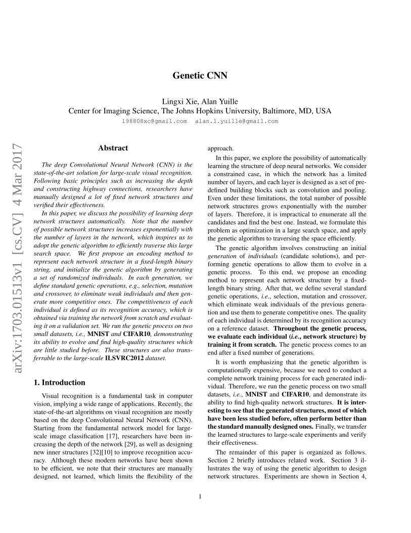
Figure 1. A two-stage network (S = 2, (K1,K2) = (4, 5)) and the encoded binary string (best viewed in color PDF). The default inputand output nodes (see Section 3.1.1) and the connections from and to these nodes are marked in red and green, respectively. We onlyencode the connections in the effective parts (regions with light blue background). Within each stage, the number of convolutional filtersis a constant (32 in Stage 1, 64 in Stage 2), and the spatial resolution remains unchanged (32 × 32 in Stage 1, 16 × 16 in Stage 2). Eachpooling layer down-samples the data by a factor of 2. ReLU and batch normalization are added after each convolution.

We borrow this idea to define a family of networks whichcan be encoded into fixed-length binary strings. A networkis composed of S stages, and the s-th stage, s = 1, 2, . . . , S,contains Ks nodes, denoted by vs,ks

, ks = 1, 2, . . . ,Ks.The nodes within each stage are ordered, and we onlyallow connections from a lower-numbered node to a higher-numbered node. Each node corresponds to a convolutionaloperation, which takes place after element-wise summingup all its input nodes (lower-numbered nodes that are con-nected to it). After convolution, batch normalization [15]and ReLU [17] are followed, which are verified efficient intraining very deep neural networks [29]. We do not encodethe fully-connected part of a network.

In each stage, we use 1 + 2 + . . .+ (Ks − 1) =12Ks (Ks − 1) bits to encode the inter-node connections.The first bit represents the connection between (vs,1, vs,2),then the following two bits represent the connection be-tween (vs,1, vs,3) and (vs,2, vs,3), etc. This process con-tinues until the last Ks − 1 bits are used to represent theconnection between vs,1, vs,2, . . . , vs,Ks−1 and vs,Ks

. For1 6 i < j 6 Ks, if the code corresponding to (vs,i, vs,j) is1, there is an edge connecting vs,i and vs,j , i.e., vs,j takesthe output of vs,i as a part of the element-wise summation,and vice versa.

Figure 1 illustrates two examples of network encod-ing. To summarize, a S-stage network with Ks nodes atthe s-th stage is encoded into a binary string with lengthL = 1

2

∑sKs (Ks − 1). Equivalently, there are in total

2L possible network structures. This number may be verylarge. In the CIFAR10 experiments (see Section 4.2), wehave S = 3 and (K1,K2,K3) = (3, 4, 5), therefore L = 19

and 2L = 524,288. It is computationally intractable toenumerate all these structures and find the optimal one(s).In the following parts, we adopt the genetic algorithm toefficiently explore good candidates in this large space.

3.1.1 Technical Details

To make every binary string valid, we define two defaultnodes in each stage. The default input node, denoted as vs,0,receives data from the previous stage, performs convolution,and sends its output to every node without a predecessor,e.g., vs,1. The default output node, denoted as vs,Ks+1,receives data from all nodes without a successor, e.g., vs,Ks ,sums up them, performs convolution, and sends its outputto the pooling layer. Note that the connections between theordinary nodes and the default nodes are not encoded.

There are two special cases. First, if an ordinary nodevs,i is isolated (i.e., it is not connected to any other ordinarynodes vs,j , i 6= j), then it is simply ignored, i.e., it is notconnected to the default input node nor the default outputnode (see the B2 node in Figure 1). This is to guaranteethat a stage with more nodes can simulate all structuresrepresented by a stage with fewer nodes. Second, if thereare no connections at a stage, i.e., all bits in the binary stringare 0, then the convolutional operation is performed onlyonce, not twice (one for the default input node and one forthe default output node).

3

conv layer

conv layer

conv layer

conv layer

conv layer

conv layer

conv layer conv layer

conv layer conv layer

conv layer conv layer

conv layer

conv layer

conv layer

conv layer

conv layer

conv layer

VGGNet𝐾 = 4

ResNet𝐾 = 4

Code: 1-01-001 Code: 1-01-101

DenseNet𝐾 = 4

Code: 1-11-111

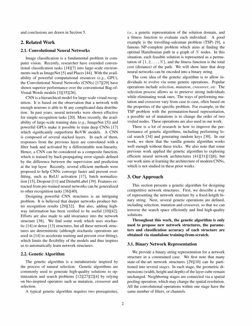
Figure 2. The basic building blocks of VGGNet [29] andResNet [10] can be encoded as binary strings defined in Sec-tion 3.1.

3.1.2 Examples and Limitations

Many popular network structures can be represented us-ing the proposed encoding scheme. Examples includeVGGNet [29], ResNet [10], and a modified variant ofDenseNet [13], which are illustrated in Figure 2.

Currently, only convolutional and pooling operations areconsidered, which makes it impossible to generate sometricky network modules such as Maxout [8]. Also, the sizeof convolutional filters is fixed within each stage, whichlimits our network from incorporating multi-scale informa-tion as in the inception module [32]. However, we note thatall the encoding-based approaches have such limitations.Our approach can be easily modified to include more typesof layers and more flexible inter-layer connections. Asshown in experiments, we can achieve competitive recogni-tion performance using merely these basic building blocks.

As shown in a recent published work using reinforce-ment learning to explore neural architecture [45], this typeof methods often require heavy computation to traversethe huge solution space. Fortunately, our method can beeasily generalized and scaled up, which is done via learningthe architecture on a small dataset and transfer the learnedinformation to large-scale datasets. Please refer to theexperimental part for details.

3.2. Genetic Operations

The flowchart of the genetic process is shown in Al-gorithm 1. It starts with an initialized generation of Nrandomized individuals. Then, we perform T rounds, orT generations, each of which consists of three operations,i.e., selection, mutation and crossover. The fitness functionof each individual is evaluated via training-from-scratch onthe reference dataset.

3.2.1 Initialization

We initialize a set of randomized models {M0,n}Nn=1. Eachmodel is a binary string with L bits, i.e., M0,n : b0,n ∈{0, 1}L. Each bit in each individual is independently sam-pled from a Bernoulli distribution: bl0,n ∼ B(0.5), l =1, 2, . . . , L. After this, we evaluate each individual (seeSection 3.2.4) to obtain their fitness function values.

As we shall see in Section 4.1.3, different strategies ofinitialization do not impact the genetic performance toomuch. Even starting with a naive initialization (all individ-uals are all-zero strings), the genetic process can discoverquite competitive structures with crossover and mutation.

3.2.2 Selection

The selection process is performed at the beginning of everygeneration. Before the t-th generation, the n-th individualMt−1,n is assigned a fitness function, which is defined asthe recognition rate rt−1,n obtained in the previous genera-tion or initialization. rt−1,n directly impacts the probabilitythat Mt−1,n survives the selection process.

We perform a Russian roulette process to determinewhich individuals survive. Each individual in the next gen-eration Mt,n is determined independently by a non-uniformsampling over the set {Mt−1,n}Nn=1. The probability ofsampling Mt−1,n is proportional to rt−1,n − rt−1,0, wherert−1,0 = minNn=1 {rt−1,n} is the minimal fitness functionvalue in the previous generation. This means that the bestindividual has the largest probability of being selected, andthe worst one is always eliminated. As the number ofindividuals N remains unchanged, each individual in theprevious generation may be selected multiple times.

3.2.3 Mutation and Crossover

The mutation process of an individual Mt,n involves flip-ping each bit independently with a probability qM. Inpractice, qM is often small, e.g., 0.05, so that mutation isnot likely to change one individual too much. This is topreserve the good properties of a survived individual whileproviding an opportunity of trying out new possibilities.

The crossover process involves changing two individualssimultaneously. Instead of considering each bit individu-ally, the basic unit in crossover is a stage, which is motivatedby the need to retain the local structures within each stage.Similar to mutation, each pair of corresponding stages areexchanged with a small probability qC.

Both mutation and crossover are implemented by anoverall flowchart (see Algorithm 1). The probabilities ofmutation and crossover for each individual (or pair) are pMand pC, respectively. We understand that there are manydifferent ways of mutation and crossover. As shown in

4

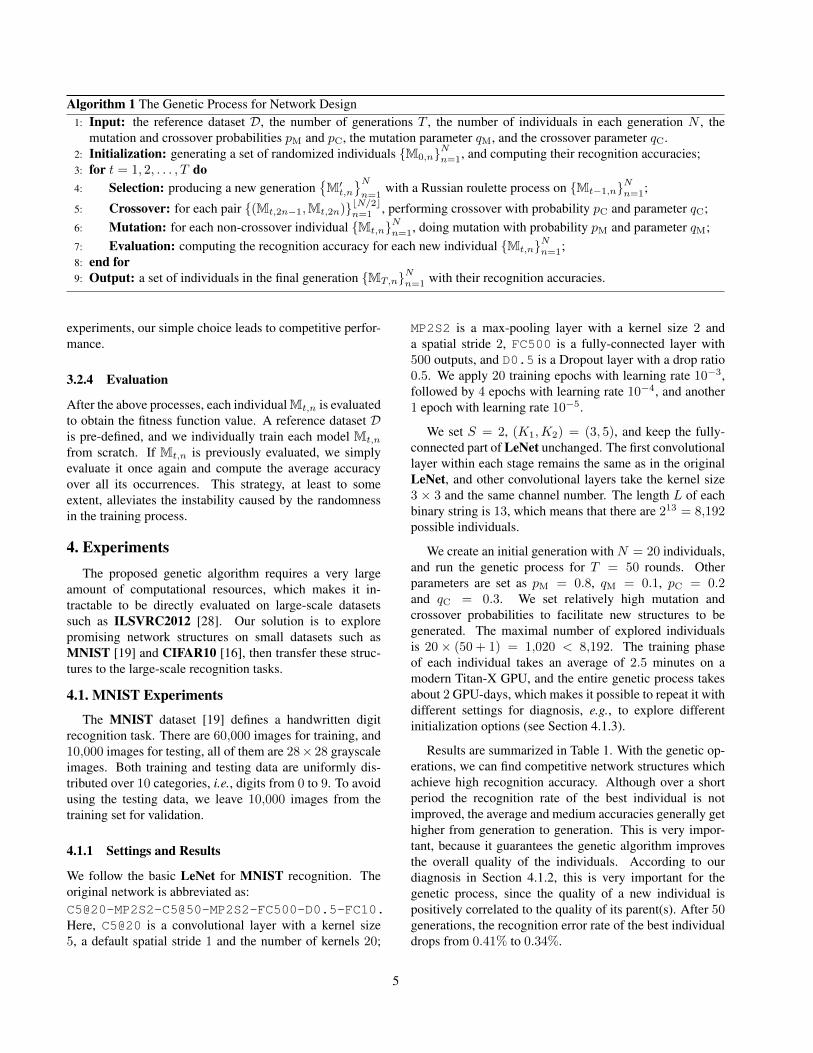
Algorithm 1 The Genetic Process for Network Design1: Input: the reference dataset D, the number of generations T , the number of individuals in each generation N , the

mutation and crossover probabilities pM and pC, the mutation parameter qM, and the crossover parameter qC.2: Initialization: generating a set of randomized individuals {M0,n}Nn=1, and computing their recognition accuracies;3: for t = 1, 2, . . . , T do4: Selection: producing a new generation

{M′t,n

}Nn=1

with a Russian roulette process on {Mt−1,n}Nn=1;

5: Crossover: for each pair {(Mt,2n−1,Mt,2n)}bN/2cn=1 , performing crossover with probability pC and parameter qC;

6: Mutation: for each non-crossover individual {Mt,n}Nn=1, doing mutation with probability pM and parameter qM;7: Evaluation: computing the recognition accuracy for each new individual {Mt,n}Nn=1;8: end for9: Output: a set of individuals in the final generation {MT,n}Nn=1 with their recognition accuracies.

experiments, our simple choice leads to competitive perfor-mance.

3.2.4 Evaluation

After the above processes, each individual Mt,n is evaluatedto obtain the fitness function value. A reference dataset Dis pre-defined, and we individually train each model Mt,n

from scratch. If Mt,n is previously evaluated, we simplyevaluate it once again and compute the average accuracyover all its occurrences. This strategy, at least to someextent, alleviates the instability caused by the randomnessin the training process.

4. ExperimentsThe proposed genetic algorithm requires a very large

amount of computational resources, which makes it in-tractable to be directly evaluated on large-scale datasetssuch as ILSVRC2012 [28]. Our solution is to explorepromising network structures on small datasets such asMNIST [19] and CIFAR10 [16], then transfer these struc-tures to the large-scale recognition tasks.

4.1. MNIST Experiments

The MNIST dataset [19] defines a handwritten digitrecognition task. There are 60,000 images for training, and10,000 images for testing, all of them are 28× 28 grayscaleimages. Both training and testing data are uniformly dis-tributed over 10 categories, i.e., digits from 0 to 9. To avoidusing the testing data, we leave 10,000 images from thetraining set for validation.

4.1.1 Settings and Results

We follow the basic LeNet for MNIST recognition. Theoriginal network is abbreviated as:C5@20-MP2S2-C5@50-MP2S2-FC500-D0.5-FC10.Here, C5@20 is a convolutional layer with a kernel size5, a default spatial stride 1 and the number of kernels 20;

MP2S2 is a max-pooling layer with a kernel size 2 anda spatial stride 2, FC500 is a fully-connected layer with500 outputs, and D0.5 is a Dropout layer with a drop ratio0.5. We apply 20 training epochs with learning rate 10−3,followed by 4 epochs with learning rate 10−4, and another1 epoch with learning rate 10−5.

We set S = 2, (K1,K2) = (3, 5), and keep the fully-connected part of LeNet unchanged. The first convolutionallayer within each stage remains the same as in the originalLeNet, and other convolutional layers take the kernel size3 × 3 and the same channel number. The length L of eachbinary string is 13, which means that there are 213 = 8,192possible individuals.

We create an initial generation with N = 20 individuals,and run the genetic process for T = 50 rounds. Otherparameters are set as pM = 0.8, qM = 0.1, pC = 0.2and qC = 0.3. We set relatively high mutation andcrossover probabilities to facilitate new structures to begenerated. The maximal number of explored individualsis 20× (50 + 1) = 1,020 < 8,192. The training phaseof each individual takes an average of 2.5 minutes on amodern Titan-X GPU, and the entire genetic process takesabout 2 GPU-days, which makes it possible to repeat it withdifferent settings for diagnosis, e.g., to explore differentinitialization options (see Section 4.1.3).

Results are summarized in Table 1. With the genetic op-erations, we can find competitive network structures whichachieve high recognition accuracy. Although over a shortperiod the recognition rate of the best individual is notimproved, the average and medium accuracies generally gethigher from generation to generation. This is very impor-tant, because it guarantees the genetic algorithm improvesthe overall quality of the individuals. According to ourdiagnosis in Section 4.1.2, this is very important for thegenetic process, since the quality of a new individual ispositively correlated to the quality of its parent(s). After 50generations, the recognition error rate of the best individualdrops from 0.41% to 0.34%.

5

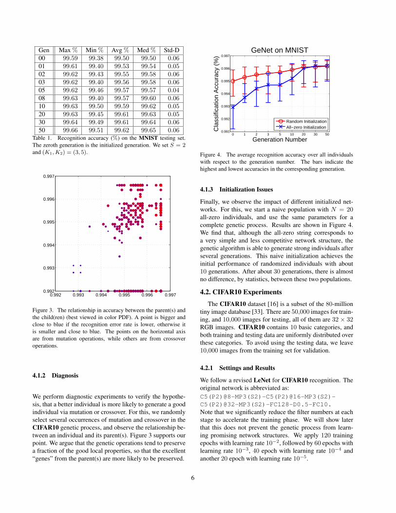
Gen Max % Min % Avg % Med % Std-D00 99.59 99.38 99.50 99.50 0.0601 99.61 99.40 99.53 99.54 0.0502 99.62 99.43 99.55 99.58 0.0603 99.62 99.40 99.56 99.58 0.0605 99.62 99.46 99.57 99.57 0.0408 99.63 99.40 99.57 99.60 0.0610 99.63 99.50 99.59 99.62 0.0520 99.63 99.45 99.61 99.63 0.0530 99.64 99.49 99.61 99.64 0.0650 99.66 99.51 99.62 99.65 0.06

Table 1. Recognition accuracy (%) on the MNIST testing set.The zeroth generation is the initialized generation. We set S = 2and (K1,K2) = (3, 5).

0.992 0.993 0.994 0.995 0.996 0.9970.992

0.993

0.994

0.995

0.996

0.997

Figure 3. The relationship in accuracy between the parent(s) andthe child(ren) (best viewed in color PDF). A point is bigger andclose to blue if the recognition error rate is lower, otherwise itis smaller and close to blue. The points on the horizontal axisare from mutation operations, while others are from crossoveroperations.

4.1.2 Diagnosis

We perform diagnostic experiments to verify the hypothe-sis, that a better individual is more likely to generate a goodindividual via mutation or crossover. For this, we randomlyselect several occurrences of mutation and crossover in theCIFAR10 genetic process, and observe the relationship be-tween an individual and its parent(s). Figure 3 supports ourpoint. We argue that the genetic operations tend to preservea fraction of the good local properties, so that the excellent“genes” from the parent(s) are more likely to be preserved.

0 1 2 3 5 10 20 30 500.991

0.992

0.993

0.994

0.995

0.996

0.997

Generation Number

Cla

ssifi

catio

n A

ccur

acy

(%)

GeNet on MNIST

Random InitializationAll−zero Initialization

Figure 4. The average recognition accuracy over all individualswith respect to the generation number. The bars indicate thehighest and lowest accuracies in the corresponding generation.

4.1.3 Initialization Issues

Finally, we observe the impact of different initialized net-works. For this, we start a naive population with N = 20all-zero individuals, and use the same parameters for acomplete genetic process. Results are shown in Figure 4.We find that, although the all-zero string corresponds toa very simple and less competitive network structure, thegenetic algorithm is able to generate strong individuals afterseveral generations. This naive initialization achieves theinitial performance of randomized individuals with about10 generations. After about 30 generations, there is almostno difference, by statistics, between these two populations.

4.2. CIFAR10 Experiments

The CIFAR10 dataset [16] is a subset of the 80-milliontiny image database [33]. There are 50,000 images for train-ing, and 10,000 images for testing, all of them are 32 × 32RGB images. CIFAR10 contains 10 basic categories, andboth training and testing data are uniformly distributed overthese categories. To avoid using the testing data, we leave10,000 images from the training set for validation.

4.2.1 Settings and Results

We follow a revised LeNet for CIFAR10 recognition. Theoriginal network is abbreviated as:C5(P2)@8-MP3(S2)-C5(P2)@16-MP3(S2)-C5(P2)@32-MP3(S2)-FC128-D0.5-FC10.Note that we significantly reduce the filter numbers at eachstage to accelerate the training phase. We will show laterthat this does not prevent the genetic process from learn-ing promising network structures. We apply 120 trainingepochs with learning rate 10−2, followed by 60 epochs withlearning rate 10−3, 40 epoch with learning rate 10−4 andanother 20 epoch with learning rate 10−5.

6

We keep the fully-connected part of the above networkunchanged, and set S = 3 and (K1,K2,K3) = (3, 4, 5).Similarly, the first convolutional layer within each stage re-mains the same as in the original LeNet, and other convolu-tional layers take the kernel size 3×3 and the same channelnumber. The length L of each binary string is 19, whichmeans that there are 219 = 524,288 possible individuals.

We create an initial generation with N = 20 individuals,and run the genetic process for T = 50 rounds. Otherparameters are set to be pM = 0.8, qM = 0.05, pC = 0.2and qC = 0.2. The mutation and crossover parameters qMand qC are set to be smaller because the strings becomelonger. The maximal number of explored individuals is20× (50 + 1) = 1,020 � 524,288. The training phase ofeach individual takes an average of 0.4 hour, and the entiregenetic process takes about 17 GPU-days.

We perform two individual genetic processes. The re-sults of one process are summarized in Table 2. As inthe MNIST experiments, all the important statistics (e.g.,average and median accuracies) grow from generation togeneration. We also report the best network structures inthe table, and visualize the best structures throughout thesetwo processes in Figure 5.

4.2.2 Comparison to Densely-Connected Nets

Under our encoding scheme, a straightforward way of net-work construction is to set all bits to be 1, which leads to anetwork in which any two layers within the same stage areconnected. This network produces a 76.84% recognitionrate, which is a little bit lower than those reported in Table 2.Considering that the densely-connected network requiresheavier computational overheads, we conclude that the ge-netic algorithm helps to find more effective and efficientstructures than the dense connections.

4.2.3 Observation

In Figure 5, we plot the the network structures learned fromtwo individual genetic processes. The structures learnedby the genetic algorithm are quite different from the manu-ally designed ones, although some manually designed localstructures are observed, like the chain-shaped networks,multi-path networks and highway networks. We emphasizethat these two networks are obtained by independent geneticprocesses, which demonstrates that our genetic process gen-erally converges to similar network structures.

4.3. CIFAR and SVHN Experiments

We apply the networks learned from the CIFAR10 ex-periments to more small-scale datasets. We test threedatasets, i.e., CIFAR10, CIFAR100 and SVHN. CI-FAR100 is an extension to CIFAR10 containing 100 finer-grained categories. It has the same numbers of training

0

1

2 3

4

0

1

2 3

4

5

0

1

2 3

4 5

6

0

1

2 3

4

0

1

2 3

4

5

0

1

2 3

4 5

6

Code: 1-01

Code: 1-01

Chain-ShapedNetworks

AlexNet VGGNet

Code: 0-01-100

Code: 1-01-100

Code: 0-11-

101-0001

Code: 0-11-

101-0001

Multiple-PathNetworks

GoogLeNet

HighwayNetworks

Deep ResNet

Figure 5. Two network structures learned from the two indepen-dent genetic processes (best viewed in color PDF).

and testing images as CIFAR10, and these images are alsouniformly distributed over 100 categories.

SVHN (Street View House Numbers) [25] is a largecollection of 32 × 32 RGB images, i.e., 73,257 trainingsamples, 26,032 testing samples, and 531,131 extra train-ing samples. We preprocess the data as in the previouswork [25], i.e., selecting 400 samples per category from thetraining set as well as 200 samples per category from theextra set, using these 6,000 images for validation, and theremaining 598,388 images as training samples. We also useLocal Contrast Normalization (LCN) for preprocessing [8].

We evaluate the best network structure in each genera-tion of the genetic process. We resume using a large numberof filters at each stage, i.e., the three stages and the firstfully-connected layer are equipped with 64, 128, 256 and1024 filters, respectively. The training strategy, include thenumbers of epochs and learning rates, remains the same asin the previous experiments.

7

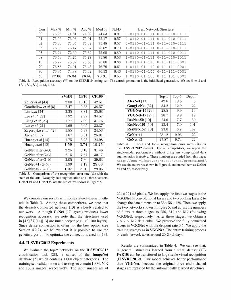
Gen Max % Min % Avg % Med % Std-D Best Network Structure00 75.96 71.81 74.39 74.53 0.91 0-01|0-01-111|0-11-010-011101 75.96 73.93 75.01 75.17 0.57 0-01|0-01-111|0-11-010-011102 75.96 73.95 75.32 75.48 0.57 0-01|0-01-111|0-11-010-011103 76.06 73.47 75.37 75.62 0.70 1-01|0-01-111|0-11-010-011105 76.24 72.60 75.32 75.65 0.89 1-01|0-01-111|0-11-010-001108 76.59 74.75 75.77 75.86 0.53 1-01|0-01-111|0-11-010-101110 76.72 73.92 75.68 75.80 0.88 1-01|0-01-110|0-11-111-000120 76.83 74.91 76.45 76.79 0.61 1-01|1-01-110|0-11-111-000130 76.95 74.38 76.42 76.53 0.46 1-01|0-01-100|0-11-111-000150 77.06 75.34 76.58 76.81 0.55 1-01|0-01-100|0-11-101-0001

Table 2. Recognition accuracy (%) on the CIFAR10 testing set. The zeroth generation is the initialized generation. We set S = 3 and(K1,K2,K3) = (3, 4, 5).

SVHN CF10 CF100Zeiler et.al [43] 2.80 15.13 42.51

Goodfellow et.al [8] 2.47 9.38 38.57

Lin et.al [24] 2.35 8.81 35.68

Lee et.al [22] 1.92 7.97 34.57

Liang et.al [23] 1.77 7.09 31.75

Lee et.al [21] 1.69 6.05 32.37

Zagoruyko et.al [42] 1.85 5.37 24.53

Xie et.al [37] 1.67 5.31 25.01

Huang et.al [14] 1.75 5.25 24.98

Huang et.al [13] 1.59 3.74 19.25

GeNet after G-00 2.25 8.18 31.46

GeNet after G-05 2.15 7.67 30.17

GeNet after G-20 2.05 7.36 29.63

GeNet #1 (G-50) 1.99 7.19 29.03

GeNet #2 (G-50) 1.97 7.10 29.05Table 3. Comparison of the recognition error rate (%) with thestate-of-the-arts. We apply data augmentation on all these datasets.GeNet #1 and GeNet #2 are the structures shown in Figure 5.

We compare our results with some state-of-the-art meth-ods in Table 3. Among these competitors, we note thatthe densely-connected network [13] is closely related toour work. Although GeNet (17 layers) produces lowerrecognition accuracy, we note that the structures usedin [42][37][14][13] are much deeper (e.g., 40–100 layers).Since dense connection is often not the best option (seeSection 4.2.2), we believe that it is possible to use thegenetic algorithm to optimize the connections used in [13].

4.4. ILSVRC2012 Experiments

We evaluate the top-2 networks on the ILSVRC2012classification task [28], a subset of the ImageNetdatabase [5] which contains 1,000 object categories. Thetraining set, validation set and testing set contain 1.3M, 50Kand 150K images, respectively. The input images are of

Top-1 Top-5 DepthAlexNet [17] 42.6 19.6 8GoogLeNet [32] 34.2 12.9 22VGGNet-16 [29] 28.5 9.9 16VGGNet-19 [29] 28.7 9.9 19ResNet-50 [10] 24.6 7.7 50ResNet-101 [10] 23.4 7.0 101ResNet-152 [10] 23.0 6.7 152

GeNet #1 28.12 9.95 22GeNet #2 27.87 9.74 22

Table 4. Top-1 and top-5 recognition error rates (%) onthe ILSVRC2012 dataset. For all competitors, we report thesingle-model performance without using any complicated dataaugmentation in testing. These numbers are copied from this page:http://www.vlfeat.org/matconvnet/pretrained/.We use the networks shown in Figure 5, and name them as GeNet#1 and #2, respectively.

224×224×3 pixels. We first apply the first two stages in theVGGNet (4 convolutional layers and two pooling layers) tochange the data dimension to 56×56×128. Then, we applythe two networks shown in Figure 5, and adjust the numbersof filters at three stages to 256, 512 and 512 (followingVGGNet), respectively. After these stages, we obtain a7 × 7 × 512 data cube. We preserve the fully-connectedlayers in VGGNet with the dropout rate 0.5. We apply thetraining strategy as in VGGNet. The entire training processof each network takes around 20 GPU-days.

Results are summarized in Table 4. We can see that,in general, structures learned from a small dataset (CI-FAR10) can be transferred to large-scale visual recognition(ILSVRC2012). Our model achieves better performancethan VGGNet, because the original three chain-shapedstages are replaced by the automatically learned structures.

8

5. ConclusionsThis paper applies the genetic algorithm to designing

the structure of deep neural networks. We first propose anencoding method to represent each network structure witha fixed-length binary string, then uses some popular geneticoperations such as mutation and crossover to explore thesearch space efficiently. Different initialization strategiesdo not make much difference on the genetic process. Weconduct the genetic algorithm with a relatively small refer-ence dataset (CIFAR10), and find that the generated struc-tures transfer well to other tasks, including the large-scaleILSVRC2012 dataset.

Despite the interesting results we have obtained, ouralgorithm suffers from several drawbacks. First, a largefraction of network structures are still unexplored, includingthose with non-convolutional modules like Maxout [8], andthe multi-scale strategy used in the inception module [32].Second, in the current work, the genetic algorithm is onlyused to explore the network structure, whereas the networktraining process is performed separately. It would be veryinteresting to incorporate the genetic algorithm to trainingthe network structure and weights simultaneously. Thesedirections are left for future work.

AcknowledgementsWe thank John Flynn, Wei Shen, Chenxi Liu and Siyuan

Qiao for instructive discussions.

References[1] J. Bayer, D. Wierstra, J. Togelius, and J. Schmidhuber.

Evolving Memory Cell Structures for Sequence Learning.International Conference on Artificial Neural Networks,2009.

[2] J. Beasley and P. Chu. A Genetic Algorithm for the Set Cov-ering Problem. European Journal of Operational Research,94(2):392–404, 1996.

[3] G. Csurka, C. Dance, L. Fan, J. Willamowski, and C. Bray.Visual Categorization with Bags of Keypoints. Workshop onStatistical Learning in Computer Vision, European Confer-ence on Computer Vision, 1(22):1–2, 2004.

[4] K. Deb, A. Pratap, S. Agarwal, and T. Meyarivan. A fastand elitist multiobjective genetic algorithm: Nsga-ii. IEEETransactions on Evolutionary Computation, 6(2):182–197,2002.

[5] J. Deng, W. Dong, R. Socher, L. Li, K. Li, and L. Fei-Fei. ImageNet: A Large-Scale Hierarchical Image Database.Computer Vision and Pattern Recognition, 2009.

[6] S. Ding, H. Li, C. Su, J. Yu, and F. Jin. EvolutionaryArtificial Neural Networks: A Review. Artificial IntelligenceReview, 39(3):251–260, 2013.

[7] L. Fei-Fei, R. Fergus, and P. Perona. Learning GenerativeVisual Models from Few Training Examples: An Incremen-tal Bayesian Approach Tested on 101 Object Categories.

Computer Vision and Image Understanding, 106(1):59–70,2007.

[8] I. Goodfellow, D. Warde-Farley, M. Mirza, A. Courville, andY. Bengio. Maxout networks. International Conference onMachine Learning, 2013.

[9] J. Grefenstette, R. Gopal, B. Rosmaita, and D. Van Gucht.Genetic Algorithms for the Traveling Salesman Problem.International Conference on Genetic Algorithms and theirApplications, 1985.

[10] K. He, X. Zhang, S. Ren, and J. Sun. Deep Residual Learn-ing for Image Recognition. Computer Vision and PatternRecognition, 2016.

[11] G. Hinton, N. Srivastava, A. Krizhevsky, I. Sutskever, andR. Salakhutdinov. Improving Neural Networks by Prevent-ing Co-adaptation of Feature Detectors. arXiv preprint,arXiv: 1207.0580, 2012.

[12] C. Houck, J. Joines, and M. Kay. A Genetic Algorithm forFunction Optimization: A Matlab Implementation. Techni-cal Report, North Carolina State University, 2009.

[13] G. Huang, Z. Liu, and K. Weinberger. Densely Con-nected Convolutional Networks. arXiv preprint, arXiv:1608.06993, 2016.

[14] G. Huang, Y. Sun, Z. Liu, D. Sedra, and K. Weinberger. DeepNetworks with Stochastic Depth. European Conference onComputer Vision, 2016.

[15] S. Ioffe and C. Szegedy. Batch Normalization: Accelerat-ing Deep Network Training by Reducing Internal CovariateShift. International Conference on Machine Learning, 2015.

[16] A. Krizhevsky and G. Hinton. Learning Multiple Layers ofFeatures from Tiny Images. Technical Report, University ofToronto, 1(4):7, 2009.

[17] A. Krizhevsky, I. Sutskever, and G. Hinton. ImageNetClassification with Deep Convolutional Neural Networks.Advances in Neural Information Processing Systems, 2012.

[18] S. Lazebnik, C. Schmid, and J. Ponce. Beyond Bags ofFeatures: Spatial Pyramid Matching for Recognizing NaturalScene Categories. Computer Vision and Pattern Recognition,2006.

[19] Y. LeCun, L. Bottou, Y. Bengio, and P. Haffner. Gradient-based Learning Applied to Document Recognition. Proceed-ings of the IEEE, 86(11):2278–2324, 1998.

[20] Y. LeCun, J. Denker, D. Henderson, R. Howard, W. Hub-bard, and L. Jackel. Handwritten Digit Recognition with aBack-Propagation Network. Advances in Neural InformationProcessing Systems, 1990.

[21] C. Lee, P. Gallagher, and Z. Tu. Generalizing PoolingFunctions in Convolutional Neural Networks: Mixed, Gated,and Tree. International Conference on Artificial Intelligenceand Statistics, 2016.

[22] C. Lee, S. Xie, P. Gallagher, Z. Zhang, and Z. Tu. Deeply-Supervised Nets. International Conference on Artificial In-telligence and Statistics, 2015.

[23] M. Liang and X. Hu. Recurrent Convolutional Neural Net-work for Object Recognition. Computer Vision and PatternRecognition, 2015.

[24] M. Lin, Q. Chen, and S. Yan. Network in Network. Interna-tional Conference on Learning Representations, 2014.

9

[25] Y. Netzer, T. Wang, A. Coates, A. Bissacco, B. Wu, andA. Ng. Reading Digits in Natural Images with UnsupervisedFeature Learning. NIPS Workshop on Deep Learning andUnsupervised Feature Learning, 2011.

[26] F. Perronnin, J. Sanchez, and T. Mensink. Improving theFisher Kernel for Large-scale Image Classification. Euro-pean Conference on Computer Vision, 2010.

[27] C. Reeves. A Genetic Algorithm for Flowshop Sequencing.Computers & Operations Research, 22(1):5–13, 1995.

[28] O. Russakovsky, J. Deng, H. Su, J. Krause, S. Satheesh,S. Ma, Z. Huang, A. Karpathy, A. Khosla, M. Bernstein,et al. ImageNet Large Scale Visual Recognition Challenge.International Journal of Computer Vision, pages 1–42, 2015.

[29] K. Simonyan and A. Zisserman. Very Deep ConvolutionalNetworks for Large-Scale Image Recognition. InternationalConference on Learning Representations, 2014.

[30] L. Snyder and M. Daskin. A Random-Key Genetic Al-gorithm for the Generalized Traveling Salesman Problem.European Journal of Operational Research, 174(1):38–53,2006.

[31] K. Stanley and R. Miikkulainen. Evolving Neural Networksthrough Augmenting Topologies. Evolutionary Computa-tion, 10(2):99–127, 2002.

[32] C. Szegedy, W. Liu, Y. Jia, P. Sermanet, S. Reed,D. Anguelov, D. Erhan, V. Vanhoucke, and A. Rabinovich.Going Deeper with Convolutions. Computer Vision andPattern Recognition, 2015.

[33] A. Torralba, R. Fergus, and W. Freeman. 80 Million TinyImages: A Large Data Set for Nonparametric Object andScene Recognition. IEEE Transactions on Pattern Analysisand Machine Intelligence, 30(11):1958–1970, 2008.

[34] N. Ulder, E. Aarts, H. Bandelt, P. van Laarhoven, andE. Pesch. Genetic Local Search Algorithms for the TravelingSalesman Problem. International Conference on ParallelProblem Solving from Nature, 1990.

[35] J. Wang, J. Yang, K. Yu, F. Lv, T. Huang, and Y. Gong.Locality-Constrained Linear Coding for Image Classifica-tion. Computer Vision and Pattern Recognition, 2010.

[36] L. Xie, R. Hong, B. Zhang, and Q. Tian. Image Classifi-cation and Retrieval are ONE. International Conference onMultimedia Retrieval, 2015.

[37] L. Xie, Q. Tian, J. Flynn, J. Wang, and A. Yuille. GeometricNeural Phrase Pooling: Modeling the Spatial Co-occurrenceof Neurons. European Conference on Computer Vision,2016.

[38] L. Xie, J. Wang, W. Lin, B. Zhang, and Q. Tian. To-wards Reversal-Invariant Image Representation. Interna-tional Journal on Computer Vision, 2016.

[39] L. Xie, J. Wang, Z. Wei, M. Wang, and Q. Tian. DisturbLa-bel: Regularizing CNN on the Loss Layer. Computer Visionand Patter Recognition, 2016.

[40] L. Xie, L. Zheng, J. Wang, A. Yuille, and Q. Tian. InterAc-tive: Inter-Layer Activeness Propagation. Computer Visionand Patter Recognition, 2016.

[41] X. Yao. Evolving Artificial Neural Networks. Proceedingsof the IEEE, 87(9):1423–1447, 1999.

[42] S. Zagoruyko and N. Komodakis. Wide Residual Networks.arXiv preprint, arXiv: 1605.07146, 2016.

[43] M. Zeiler and R. Fergus. Stochastic Pooling for Regulariza-tion of Deep Convolutional Neural Networks. InternationalConference on Learning Representations, 2013.

[44] B. Zhou, A. Lapedriza, J. Xiao, A. Torralba, and A. Oliva.Learning Deep Features for Scene Recognition Using PlacesDatabase. Advances in Neural Information Processing Sys-tems, 2014.

[45] B. Zoph and Q. Le. Neural architecture search with rein-forcement learning. International Conference on LearningRepresentations, 2017.

10