Genetic Algorithms in MATLAB - · PDF fileECON 457 – Final Project Monica Mow (V00706598) – B01 Genetic Algorithms in MATLAB A Selection of Classic Repeated

ECON457–FinalProject MonicaMow(V00706598)–B01

GeneticAlgorithmsinMATLABA Selection of Classic Repeated Games—from Chicken to the Battle of the Sexes

1

Introduction

In this project, I apply genetic algorithms in MATLAB to several two-player repeated

games. The games presented in the analysis are standard to the study of game theory in

economics and include the Prisoner’s Dilemma, Deadlock, Chicken, the Stag Hunt, the Battle of

the Sexes, Matching Pennies, Rock Paper Scissors, Choosing Sides, and a simple pure

coordination game. A description of these games and their outcomes is provided in the Economic

Model section. The experiments performed in this analysis use the textbook’s original setup as a

basis for formulating and calibrating several different simultaneous games that are often

referenced in introductory microeconomics courses and in the more technical game theoretical

literature. I have doubled the textbook’s original population size from eight to 16 in order to

achieve better convergence to equilibrium in the results. Although I have received only a limited

education in the area of game theory, I thought that this pairing of the economic model and the

computational method was quite interesting due to its simplicity and its useful contribution to

evolutionary game theory. Additionally, the results are consistent with the basic economic theory

of simultaneous games involving interactions between two players.

Economic Model

John von Neumann is unequivocally the father of modern game theory. He is best known

for his proof of the minimax theorem—that is, an individual can minimize his or her maximum

losses by employing a certain pair of strategies in a zero-sum game with perfect information. If

each player employs these strategies, the strategies are optimal; John von Neumann showed that

the players’ minimaxes are equal in absolute value and opposite in sign. Following von

Neumann is John Nash. He is best known for his development of non-cooperative game theory

and subsequent coining of the Nash equilibrium concept.

2

A Nash equilibrium is a solution to a non-cooperative game involving two or more

players, where each player knows the equilibrium strategies of their opponent, but does not

receive any gains from changing their own strategy unilaterally. The corresponding payoffs with

these particular strategies result in a pure strategy Nash equilibrium. At the equilibrium, each

player employs a strategy that is the best response to their opponent’s best response—a response

that provides the most favourable outcome to each respective player given the other player’s

strategies. As an example, in the game of Chicken, there is a Nash equilibrium at (Swerve,

Straight). This is shown in Figure 4a. Player 2 has no incentive to switch their strategy from

Straight to Swerve if Player 1 leaves their strategy unchanged. If Player 2 decided to swerve

while Player 1 chose to swerve, Player 2 would stand to lose one util or dollar (depending on the

interpretation of the payoff units). The experiment results are interpreted economically using

these game theory concepts. The results section also comments on the role of Nash equilibria in

the computational method applied in this model.

Basic Game Descriptions

In the Prisoner’s Dilemma, two criminals are arrested and brought in to a police station.

The police admit that they cannot charge either of them on the principal charge, but can charge

them for a lesser crime with a sentence of one year. They offer the following bargain to each of

the prisoners: if he testifies (defects) against (and incriminates) his partner, he will go free while

his partner will get five years for the principal charge. However, if both testify against and

incriminate each other, both prisoners will get two years in jail. The mutually most beneficial

action is dominated. In my formulation of the Prisoner’s Dilemma, the payoff of (Defect, Defect)

is less than the payoff of (Cooperate, Cooperate); we can interpret this as a prisoner’s utility

derived from a lower jail sentence.

The Deadlock game is numerically equivalent to the Prisoner’s Dilemma except that the

mutually most beneficial action is dominant—it is optimal and in the best interest for each of the

3

players to defect. This type of situation occurs when the two parties do not have any interest in

cooperating with one another, but would rather have the other compromise; it may be common to

diplomacy and international relations.

The game of Chicken involves two individuals driving along a single-lane stretch that

approaches a bridge; each player can swerve to avoid the other, letting them take the bridge

alone, or keep driving straight, risking a fatal head-on collision. The best strategy for each

individual is to keep driving straight, while the other person swerves. Therefore, the mutually

beneficial action is to play different strategies, which results in more than one Nash equilibrium.

The Stag Hunt differs from the aforementioned games because it contains two pure

strategy Nash equilibria with symmetric payoffs, one that is risk dominant (when both players

defect) and one that is payoff dominant (when both players cooperate). Formally, the game

involves two hunters. Each hunter can individually hunt a stag or a hare. If one hunts a stag, he

will require the other individual’s cooperation to succeed. However, if one hunts a hare, he can

succeed on his own, but a hare is worth less than a stag. Each player must act without knowing

the choice of the other, making this a simultaneous coordination game.

The Battle of the Sexes game involves a couple that was supposed to meet for a night out

at either the opera or a football game; neither can remember which event was the agreed upon

meeting place. The husband would prefer to go to the football game, while the wife would prefer

to go to the opera. However, both prefer to be in attendance together rather than alone. There are

two versions of this game—Version 2 introduces a “cost” (disutility) that accounts for the fact

that the husband and wife could each choose the event that is not their most preferred, while

Version 1 does not. The former is called “Battle of the Sexes 2”. The two pure strategy Nash

equilibria occur when both go to the opera and both go to the football game.

Matching Pennies is the two-strategy version of Rock Paper Scissors. It is also

mathematically equivalent to Odds and Evens. In this game, two individuals each have a penny.

4

Each must secretly turn the penny to heads or tails. If the faces of both pennies match, Player 1

keeps both pennies (and gains +1); if the faces do not match, Player 2 keeps both pennies (and

gains +1). There is no pure strategy Nash equilibrium in this game. Instead, the Nash equilibrium

is in mixed strategies when both players choose heads or tails with equal probabilities.

In Choosing Sides, two individuals are driving along a dirt road. One driver must swerve

to avoid the other to avoid a head-on collision. It does not matter which side they choose, as long

as it is the same side (both left or both right). The story that goes with Choosing Sides seems

mathematically equivalent to the Battle of the Sexes. However, when the two individuals

coordinate in Choosing Sides, they face an equal payoff structure. In the Battle of the Sexes, the

two individuals prefer a certain activity to the other. Choosing Sides is also different from the

Stag Hunt because it does not contain an activity that is “safer” than the other (i.e. one risks less

when hunting a hare instead of a stag). As a result, Choosing Sides contains two pure strategy

Nash equilibria that are Pareto efficient with equal payoffs.

The pure coordination game also differs from Choosing Sides because it contains only

one pure strategy Nash equilibrium. The two individuals in this game prefer the same Nash

equilibrium outcome, in which the payoff is the most mutually beneficial. In its classical

formulation, the two players can either go to a party or stay home. Both prefer going to the party

over staying at home, and both prefer to stay at home than engage in different activities. The

(Party, Party) outcome dominates the (Home, Home) outcome as the (Home, Home) outcome

dominates the non-coordinating outcomes (Party, Home) and (Home, Party).

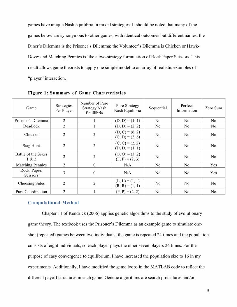
A summary of the simultaneous game characteristics is provided in Figure 1 below.

Games with two pure strategy Nash equilibria include Chicken, the Stag Hunt, Battle of the

Sexes, and Choosing Sides; games with only one pure strategy Nash equilibrium include the

Prisoner’s Dilemma, Deadlock, and the pure coordination game. Matching Pennies and Rock

Paper Scissors do not have any pure strategy Nash equilibria; due to their zero-sum nature, these

5

games have unique Nash equilibria in mixed strategies. It should be noted that many of the

games below are synonymous to other games, with identical outcomes but different names: the

Diner’s Dilemma is the Prisoner’s Dilemma; the Volunteer’s Dilemma is Chicken or Hawk-

Dove; and Matching Pennies is like a two-strategy formulation of Rock Paper Scissors. This

result allows game theorists to apply one simple model to an array of realistic examples of

“player” interaction.

Figure 1: Summary of Game Characteristics

Game Strategies Per Player

Number of Pure Strategy Nash

Equilibria

Pure Strategy Nash Equilibria Sequential Perfect

Information Zero Sum

Prisoner's Dilemma 2 1 (D, D) = (1, 1) No No No Deadlock 2 1 (D, D) = (2, 2) No No No

Chicken 2 2 (D, C) = (6, 2) (C, D) = (2, 6) No No No

Stag Hunt 2 2 (C, C) = (2, 2) (D, D) = (1, 1) No No No

Battle of the Sexes 1 & 2 2 2 (O, O) = (3, 2)

(F, F) = (2, 3) No No No

Matching Pennies 2 0 N/A No No Yes Rock, Paper,

Scissors 3 0 N/A No No Yes

Choosing Sides 2 2 (L, L) = (1, 1) (R, R) = (1, 1) No No No

Pure Coordination 2 1 (P, P) = (2, 2) No No No

Computational Method

Chapter 11 of Kendrick (2006) applies genetic algorithms to the study of evolutionary

game theory. The textbook uses the Prisoner’s Dilemma as an example game to simulate one-

shot (repeated) games between two individuals; the game is repeated 24 times and the population

consists of eight individuals, so each player plays the other seven players 24 times. For the

purpose of easy convergence to equilibrium, I have increased the population size to 16 in my

experiments. Additionally, I have modified the game loops in the MATLAB code to reflect the

different payoff structures in each game. Genetic algorithms are search procedures and/or

6

heuristics that mimic the process of natural selection and genetics; the rules of Darwin’s

“survival of the fittest” apply to this model in which individuals compete with one another and

the fittest individuals form a couple in order to give birth to the next generation.

The genetic algorithm presented in these models is quite realistic in that it makes use of

inheritance, mutation, crossover, and selection. Inheritance is evident in this model when the

chromosome, containing a string of genes, for each individual in a population may contain

similar genes to individuals in the populations from previous generations/runs. The mutation and

crossover operations also provide a simple representation of those that can be found in the

human race. Selection in the genetic algorithm is achieved by selecting the “best fit” agents in

the population—here; the “best fit” strategies are the ones with the highest payoffs. In order for

the genetic algorithm to begin, the genetic representation (the number of genes in each

chromosome) and fitness function need to be defined. After this, the genetic algorithm can

proceed to the following steps before finding a global optimum: initialization (generation of the

initial population given some deterministic or stochastic criteria), selection (again, given

deterministic or stochastic criteria), genetic operators (rate of mutation and the crossover

method), and termination (when the algorithm finds the local or global optimum).

7

Experiments

My formulation of the different simultaneous games acts as more of a calibration exercise

than an experiment; however, I think that this is still a useful extension to the economic and

computational model because it allows me to compare the convergence to the equilibrium

outcomes (if any) in each game. There are two main experiments carried out using the genetic

algorithm. The first extends the number of runs to 500 for games that fail to converge in 100

runs. The second uses a deterministic method to initialize the population (as opposed to a random

one) in order to start with a population consisting entirely of co-operators (a binary string of 24

ones); this requires changing the gene pool equation from genepool (k1) = ceil (rand*(2^clen)-1)

to genepool (k1) = (2^clen)-1 in the initpoprand_gagagme.m file.

The first experiment is carried out on Matching Pennies and Rock, Paper, Scissors and

the second experiment is conducted for the Prisoner’s Dilemma, Deadlock, Chicken, and the

Stag Hunt. Payoff matrices, graphs representing the fittest strategies, and a preliminary

description of the computational results are provided in the results section; a more detailed

analysis relating the economic theory to the model is provided in the Discussion section.

Generally, the strategy in the first column (Cooperate) of the payoff matrix corresponds to a one

in the chromosome string, while the strategy in the second column (Defect) corresponds to a zero

in the chromosome string. In each game and experiment, the population size, chromosome

length, and probability of mutation are held constant at 16, 24, and 0.7, respectively.

Results

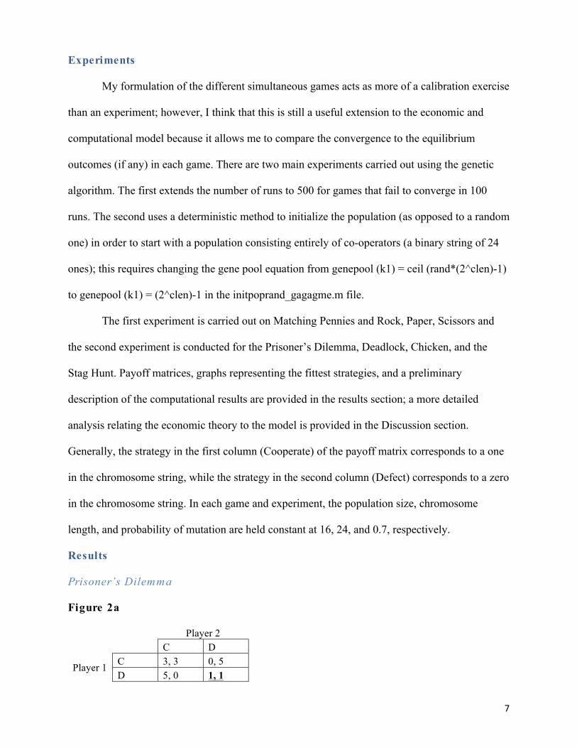
Prisoner’s Dilemma

Figure 2a

Player 2

C D

Player 1 C 3, 3 0, 5 D 5, 0 1, 1

8

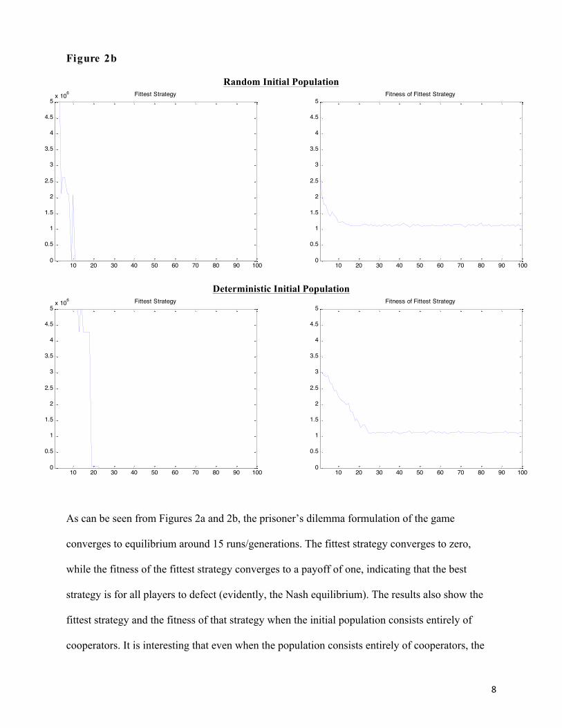
Figure 2b

Random Initial Population

Deterministic Initial Population

As can be seen from Figures 2a and 2b, the prisoner’s dilemma formulation of the game

converges to equilibrium around 15 runs/generations. The fittest strategy converges to zero,

while the fitness of the fittest strategy converges to a payoff of one, indicating that the best

strategy is for all players to defect (evidently, the Nash equilibrium). The results also show the

fittest strategy and the fitness of that strategy when the initial population consists entirely of

cooperators. It is interesting that even when the population consists entirely of cooperators, the

10 20 30 40 50 60 70 80 90 1000

0.5

1

1.5

2

2.5

3

3.5

4

4.5

5x 106 Fittest Strategy

10 20 30 40 50 60 70 80 90 1000

0.5

1

1.5

2

2.5

3

3.5

4

4.5

5Fitness of Fittest Strategy

10 20 30 40 50 60 70 80 90 1000

0.5

1

1.5

2

2.5

3

3.5

4

4.5


10 20 30 40 50 60 70 80 90 1000

0.5

1

1.5

2

2.5

3

3.5

4

4.5


9

fittest strategy still converges to defection, albeit more slowly (at around 20 runs) than under the

randomized initial population.

Deadlock

Figure 3a

Player 2

C D

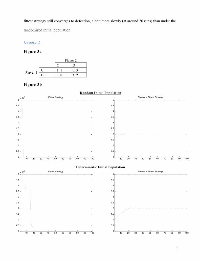
Player 1 C 1, 1 0, 3 D 3, 0 2, 2

Figure 3b



10 20 30 40 50 60 70 80 90 1000

0.5

1

1.5

2

2.5

3

3.5

4

4.5


10 20 30 40 50 60 70 80 90 1000

0.5

1

1.5

2

2.5

3

3.5

4

4.5


10 20 30 40 50 60 70 80 90 1000

0.5

1

1.5

2

2.5

3

3.5

4

4.5


10 20 30 40 50 60 70 80 90 1000

0.5

1

1.5

2

2.5

3

3.5

4

4.5


10

Figure 3b shows the convergence to the fittest strategy for the Deadlock game. Unlike in the

Prisoner’s Dilemma, the strategy converges to defection almost immediately, after about five

runs. It seems that because the Nash equilibrium strategy is also the most mutually beneficial

outcome, subsequent generations are able to adapt their strategies relatively quickly. When the

initial population is generated deterministically instead of randomly, consisting entirely of

cooperators, the fittest strategy reaches convergence after a larger number of runs, as is evident

in the Prisoner’s Dilemma.

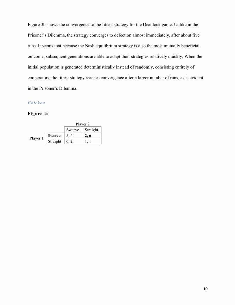
Chicken Figure 4a

Player 2

Swerve Straight

Player 1 Swerve 5, 5 2, 6 Straight 6, 2 1, 1

11

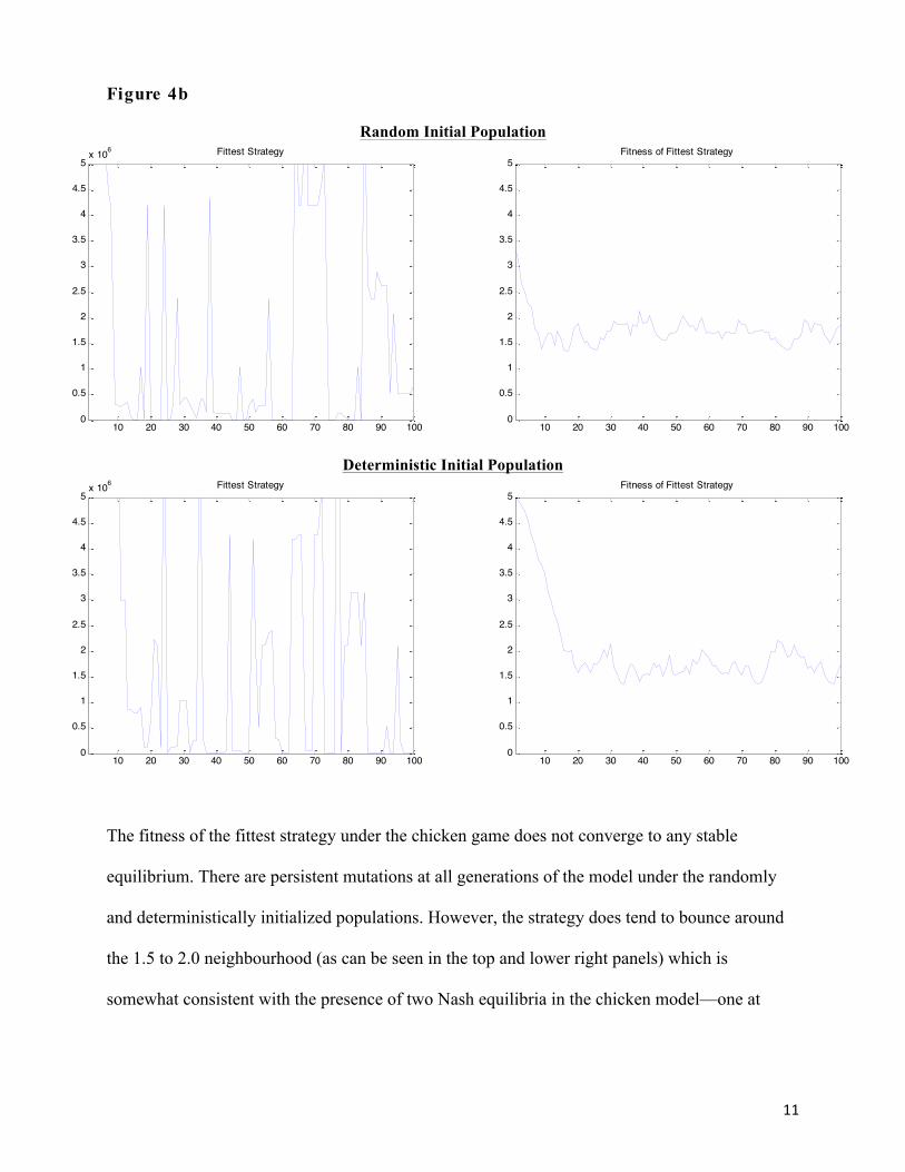
Figure 4b



The fitness of the fittest strategy under the chicken game does not converge to any stable

equilibrium. There are persistent mutations at all generations of the model under the randomly

and deterministically initialized populations. However, the strategy does tend to bounce around

the 1.5 to 2.0 neighbourhood (as can be seen in the top and lower right panels) which is

somewhat consistent with the presence of two Nash equilibria in the chicken model—one at

10 20 30 40 50 60 70 80 90 1000

0.5

1

1.5

2

2.5

3

3.5

4

4.5


10 20 30 40 50 60 70 80 90 1000

0.5

1

1.5

2

2.5

3

3.5

4

4.5


10 20 30 40 50 60 70 80 90 1000

0.5

1

1.5

2

2.5

3

3.5

4

4.5


10 20 30 40 50 60 70 80 90 1000

0.5

1

1.5

2

2.5

3

3.5

4

4.5


12

(Swerve, Straight) and one at (Straight, Swerve). It seems that a mixed strategy for each of the

players is the best response.

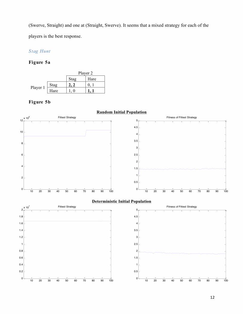
S tag Hunt Figure 5a

Player 2

Stag Hare

Player 1 Stag 2, 2 0, 1 Hare 1, 0 1, 1

Figure 5b



10 20 30 40 50 60 70 80 90 1000

2

4

6

8

10


10 20 30 40 50 60 70 80 90 1000

0.5

1

1.5

2

2.5

3

3.5

4

4.5


10 20 30 40 50 60 70 80 90 1000

0.2

0.4

0.6

0.8

1

1.2

1.4

1.6

1.8


10 20 30 40 50 60 70 80 90 1000

0.5

1

1.5

2

2.5

3

3.5

4

4.5


13

The convergence to the fittest strategy in the Stag Hunt game is relatively more stable; there is

only one significant mutation present at 70 runs. Under the randomized initial population, the

fitness of the fittest strategy is 1.5, indicating that the payoff to each individual is equal to the

average payoff between the two Nash equilibria [i.e. E (payoff) = 0.5(2) + 0.5(1) = 1.5]. In the

deterministic initial population simulation, the fittest strategy is for both parties to cooperate.

This result is not surprising as it reflects the theoretical basis of the Stag Hunt: if the players start

the game cooperating, they have no incentive to defect because they will only receive a payoff of

either zero or one.

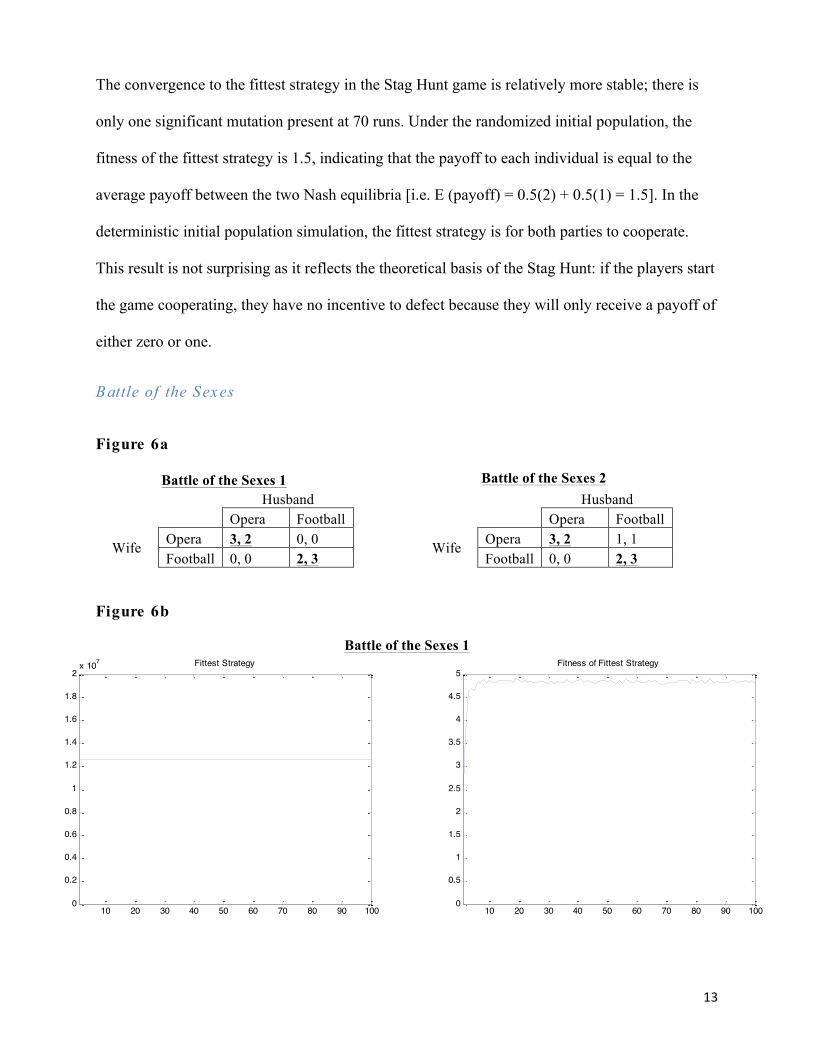
Battle of the Sexes

Figure 6a

Battle of the Sexes 1 Battle of the Sexes 2

Husband Husband

Opera Football Opera Football

Wife Opera 3, 2 0, 0 Wife Opera 3, 2 1, 1

Football 0, 0 2, 3 Football 0, 0 2, 3

Figure 6b

Battle of the Sexes 1

10 20 30 40 50 60 70 80 90 1000

0.2

0.4

0.6

0.8

1

1.2

1.4

1.6

1.8


10 20 30 40 50 60 70 80 90 1000

0.5

1

1.5

2

2.5

3

3.5

4

4.5


14

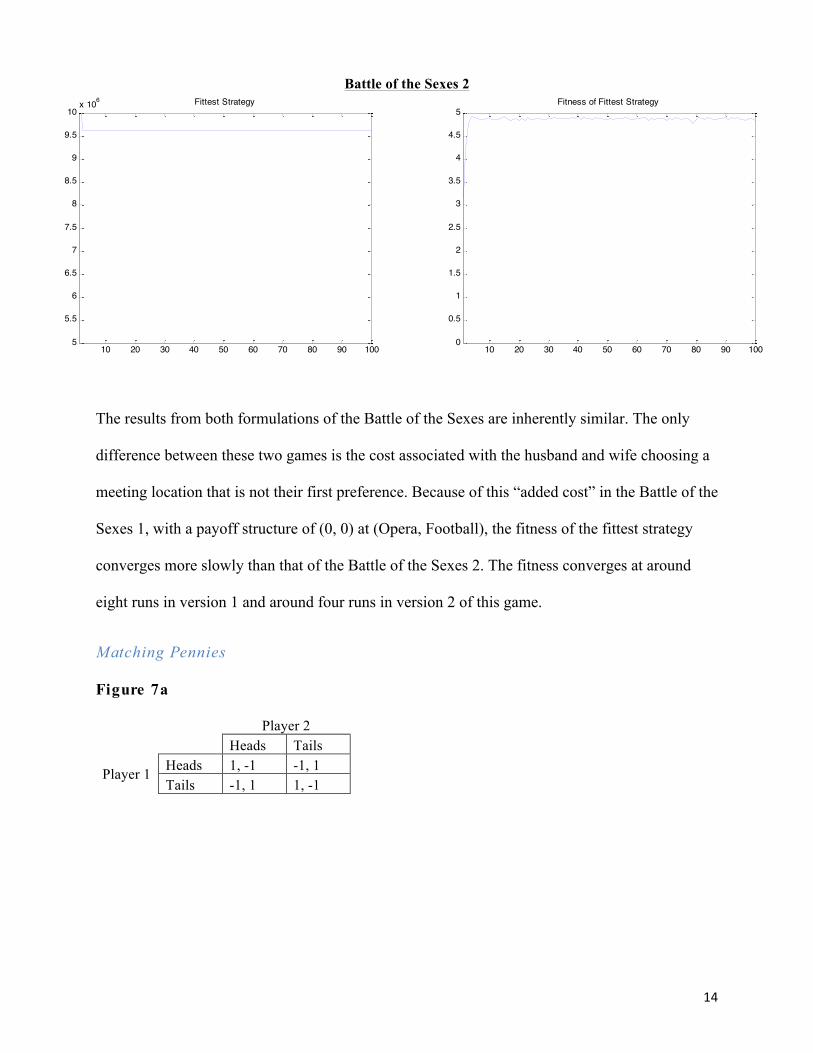
Battle of the Sexes 2

The results from both formulations of the Battle of the Sexes are inherently similar. The only

difference between these two games is the cost associated with the husband and wife choosing a

meeting location that is not their first preference. Because of this “added cost” in the Battle of the

Sexes 1, with a payoff structure of (0, 0) at (Opera, Football), the fitness of the fittest strategy

converges more slowly than that of the Battle of the Sexes 2. The fitness converges at around

eight runs in version 1 and around four runs in version 2 of this game.

Matching Pennies Figure 7a

Player 2

Heads Tails

Player 1 Heads 1, -1 -1, 1 Tails -1, 1 1, -1

10 20 30 40 50 60 70 80 90 1005

5.5

6

6.5

7

7.5

8

8.5

9

9.5


10 20 30 40 50 60 70 80 90 1000

0.5

1

1.5

2

2.5

3

3.5

4

4.5


15

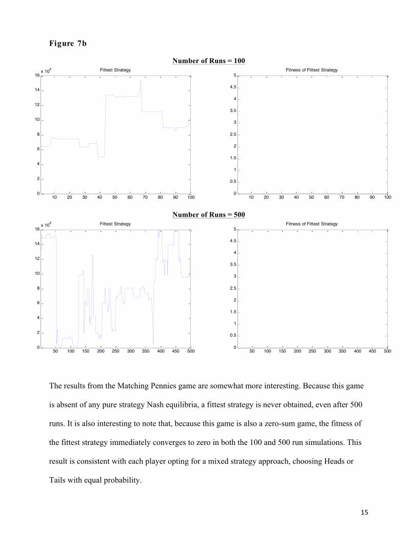
Figure 7b

Number of Runs = 100


The results from the Matching Pennies game are somewhat more interesting. Because this game

is absent of any pure strategy Nash equilibria, a fittest strategy is never obtained, even after 500

runs. It is also interesting to note that, because this game is also a zero-sum game, the fitness of

the fittest strategy immediately converges to zero in both the 100 and 500 run simulations. This

result is consistent with each player opting for a mixed strategy approach, choosing Heads or

Tails with equal probability.

10 20 30 40 50 60 70 80 90 1000

2

4

6

8

10

12

14


10 20 30 40 50 60 70 80 90 1000

0.5

1

1.5

2

2.5

3

3.5

4

4.5


50 100 150 200 250 300 350 400 450 5000

2

4

6

8

10

12

14


50 100 150 200 250 300 350 400 450 5000

0.5

1

1.5

2

2.5

3

3.5

4

4.5


16

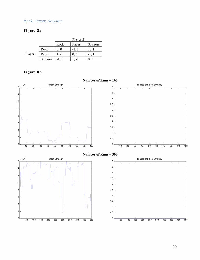
Rock , Paper, Scissors Figure 8a

Player 2

Rock Paper Scissors

Player 1 Rock 0, 0 -1, 1 1, -1 Paper 1, -1 0, 0 -1, 1 Scissors -1, 1 1, -1 0, 0

Figure 8b



10 20 30 40 50 60 70 80 90 1000

2

4

6

8

10

12

14


10 20 30 40 50 60 70 80 90 1000

0.5

1

1.5

2

2.5

3

3.5

4

4.5


50 100 150 200 250 300 350 400 450 5000

2

4

6

8

10

12

14


50 100 150 200 250 300 350 400 450 5000

0.5

1

1.5

2

2.5

3

3.5

4

4.5


17

The results from Rock, Paper, Scissors are almost identical to those from Matching Pennies. This

is because Rock, Paper, Scissors is the three-strategy version of Matching Pennies, thus,

containing the same game characteristics—a zero-sum game with no pure strategy Nash

equilibria and players employing a mixed strategy approach.

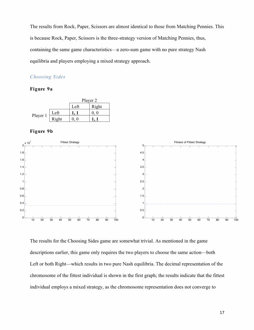
Choosing S ides Figure 9a

Player 2

Left Right

Player 1 Left 1, 1 0, 0 Right 0, 0 1, 1

Figure 9b

The results for the Choosing Sides game are somewhat trivial. As mentioned in the game

descriptions earlier, this game only requires the two players to choose the same action—both

Left or both Right—which results in two pure Nash equilibria. The decimal representation of the

chromosome of the fittest individual is shown in the first graph; the results indicate that the fittest

individual employs a mixed strategy, as the chromosome representation does not converge to

10 20 30 40 50 60 70 80 90 1000

0.2

0.4

0.6

0.8

1

1.2

1.4

1.6

1.8


10 20 30 40 50 60 70 80 90 1000

0.5

1

1.5

2

2.5

3

3.5

4

4.5


18

zero. In the second graph, we see that the fitness of this strategy converges to one, which reflects

the payoffs at the two equilibria.

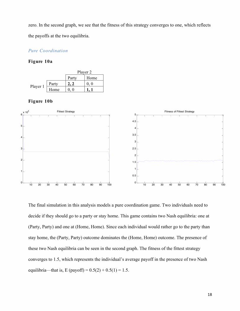
Pure Coordination Figure 10a

Player 2

Party Home

Player 1 Party 2, 2 0, 0 Home 0, 0 1, 1

Figure 10b

The final simulation in this analysis models a pure coordination game. Two individuals need to

decide if they should go to a party or stay home. This game contains two Nash equilibria: one at

(Party, Party) and one at (Home, Home). Since each individual would rather go to the party than

stay home, the (Party, Party) outcome dominates the (Home, Home) outcome. The presence of

these two Nash equilibria can be seen in the second graph. The fitness of the fittest strategy

converges to 1.5, which represents the individual’s average payoff in the presence of two Nash

equilibria—that is, E (payoff) = 0.5(2) + 0.5(1) = 1.5.

10 20 30 40 50 60 70 80 90 1000

1

2

3

4

5


10 20 30 40 50 60 70 80 90 1000

0.5

1

1.5

2

2.5

3

3.5

4

4.5


19

Discussion

Results and Economic Model/Computational Method

As is evident in the results presented above, modeling different games with a varying

number of Nash equilibria and corresponding “payoffs” or agent utility is particularly useful in

analyzing the path and time of strategy convergence. We can see that if a game contains two pure

strategy Nash equilibria, the path to convergence, as portrayed in the “Fittest Strategy” graphs, is

significantly more volatile than in games with only one Nash equilibrium. We can also see that

the fitness of this fittest strategy (the corresponding payoffs) tends to bounce between a specific

range, indicating a mixed strategy approach from the players. This type of model behaviour is

simulated in Chicken, the Stag Hunt, the Battle of the Sexes, Choosing Sides and the pure

coordination game.

When the game contains only one Nash equilibrium, as is the case of the Prisoner’s

Dilemma and Deadlock, the path to convergence in the strategy (defection) is more immediate.

Additionally, the fitness of this strategy quickly reduces to the corresponding matrix payoffs; for

example, the fitness of the fittest strategy quickly reduces to one in the Prisoner’s Dilemma and

two in Deadlock. When the game does not contain a Nash equilibrium, we can see that a “fittest

strategy” is not identified—the graph of the fittest strategy has several large deviations. This type

of game is modeled in Matching Pennies, or equivalently, in Rock, Paper, Scissors.

It seems that the formulation of the genetic algorithm has a strong influence on these

results. With each successive run, the “best fit” individual and corresponding chromosome string

survives simply because of its arbitrary fitness level (determined initially by the randomization

of the population and the binary representation). Since a player’s actions are determined

regardless of their opponent’s actions, the model simulates a situation in which it is in the best

interest of each individual agent to maximize their own payoff and ignore the most mutually

beneficial outcome. The introduction of chromosome crossover and mutation seem to have little

20

influence on maintaining a population of co-operators, unless the initial population consists

entirely of co-operators.

A dvantages and L imitations (of genetic algorithms in general)

Advantages

Genetic algorithms can solve a wide range of optimization problems as long as the

problem can be described over the “chromosome” encoding. Depending on the deterministic or

random aspects of the model, there may be several solutions to one problem, which provides

practitioners with many alternatives (but which could be seen as a disadvantage to some

researchers). There are many other advantages of genetic algorithms that allow for ease of

implementation: the problems applied to GAs can be multidimensional, non-differential, non-

continuous or non-parametric; bad proposals/solutions in the population are not an issue since

the algorithm is capable of discarding them; and the algorithm itself does not need to know the

rules/constraints of the problem, a feature which is particularly useful for loosely defined or

complex problems.

Limitations

One of the limitations of genetic algorithms is that they must use approximated fitness

levels to allow for computational efficiency. However, it has been found that the amalgamation

of several models with approximated fitness is still promising. Sometimes when the convex

problem is broken up into small parts, and these parts have become evolved, it is difficult to

prevent them from mutation especially if they are required to combine well with other parts. For

example, when designing a floor plan or an engine, it may be feasible to use genetic algorithms

to generate shapes or design fan blades, but not to design the entire structure of these items with

one algorithm. Additionally, the termination criterion is not clear in every problem since the

“best” solution only seems “best” when compared to the other surrounding solutions.

21

Specifically, in convex problems, the algorithm may get stuck in a local optimum instead of

reaching a global one; it does not know how to sacrifice short-term fitness for long-term fitness.

Further Research

As the games presented in this analysis are only one-shot (simultaneous) games, it would

be particularly interesting for game theory empiricists to model a sequential game, such as chess,

backgammon, tic-tac-toe, or Go. It would also be possible to model a simple, two-player

interaction game that consists of only two strategies: left and right. This type of game is provided

as an example in the introductory game theory portion of ECON 452 (Information and

Incentives). We used a decision tree with Player 1 as the “leader” and Player 2 as the “Follower”

to find the subgame perfect Nash equilibrium and the non-credible threat. In reference to the

game of Chicken, an example of a non-credible threat involves one of the drivers ripping the

steering wheel from their car. This action does not result in a credible threat since the wheel-

ripper’s opponent can always swerve knowing that the other has removed their steering wheel

and cannot possibly swerve. Although the player that has not yet removed their wheel has that

option, it is not a credible threat since it would require harming themselves, preventing the

combination of strategies (Straight, Straight).

Future researchers may wish to model the games presented here in a neural network

representation. They may also wish to model “learning” in the agents’ behaviour, as well as more

complex social interactions between the players with family, friends, or neighbours. As

mentioned in Kendrick (2006), including strategic thinking and behaviour—when a player’s

actions are reactions to the opponent’s past actions—in the players would not result in a

population of all defectors; the fittest strategy may converge to a population of all co-operators

or show complex cyclical behaviour.

22

Appendix – MATLAB Code

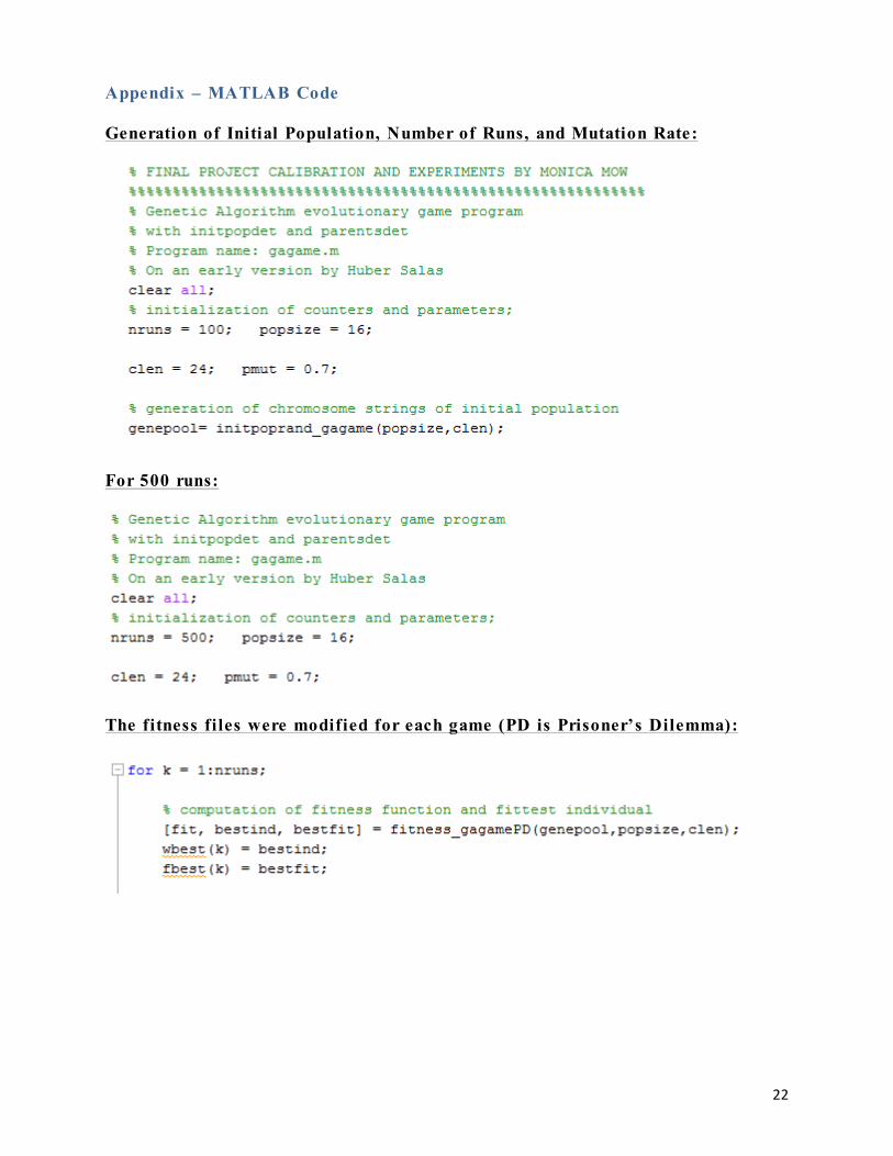
Generation of Initial Population, Number of Runs, and Mutation Rate:

For 500 runs:

The fitness files were modified for each game (PD is Prisoner’s Dilemma):

23

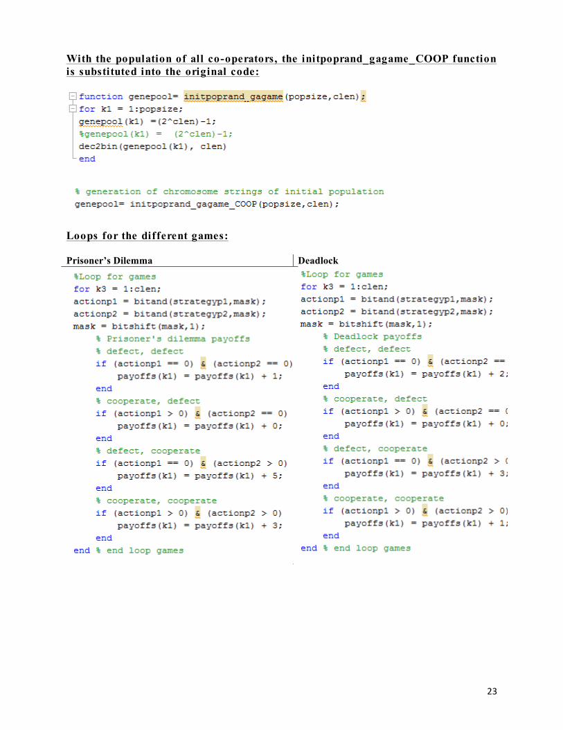
With the population of all co-operators, the initpoprand_gagame_COOP function is substituted into the original code:

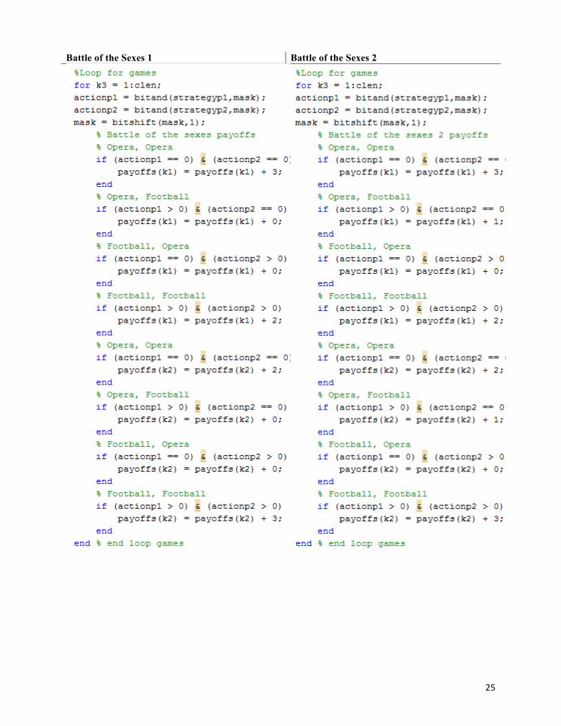
Loops for the different games:

Prisoner’s Dilemma Deadlock

24

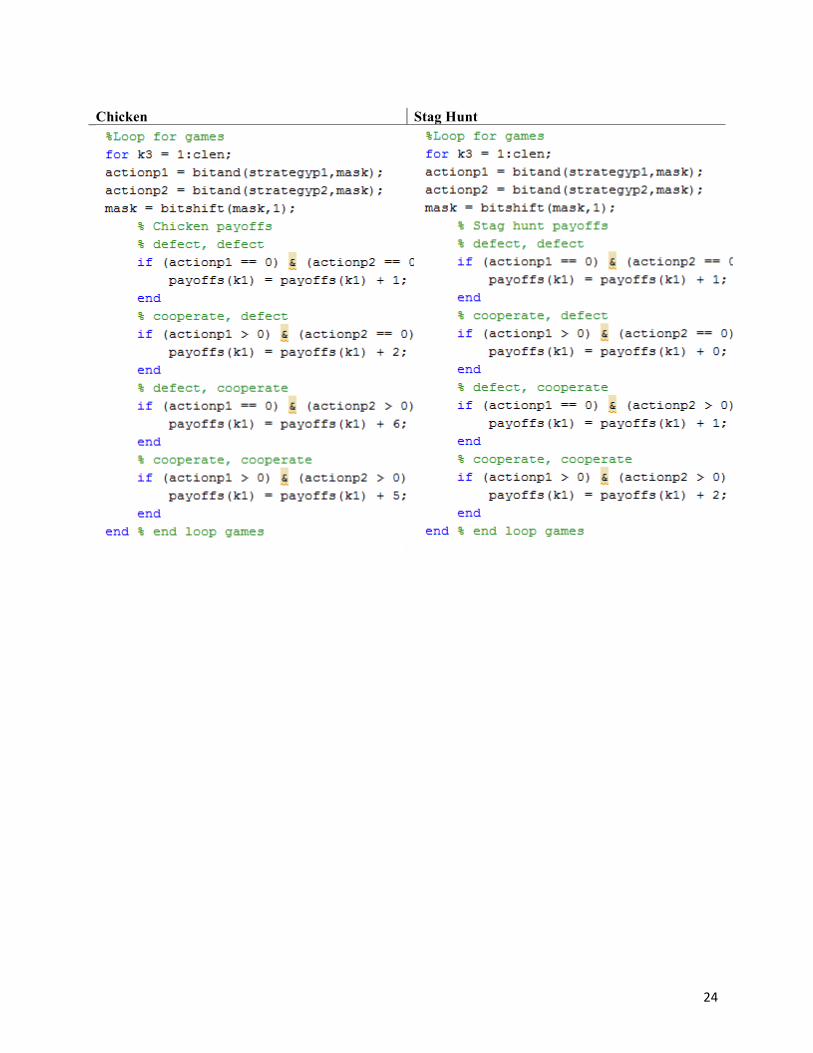
Chicken Stag Hunt

25

Battle of the Sexes 1 Battle of the Sexes 2

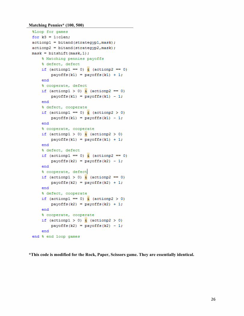
26

Matching Pennies* (100, 500)

*This code is modified for the Rock, Paper, Scissors game. They are essentially identical.

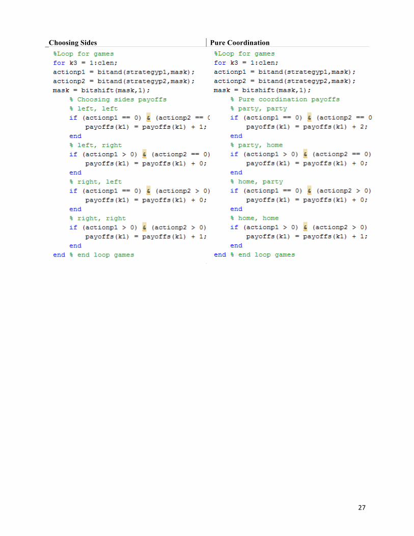
27

Choosing Sides Pure Coordination

Documents

Genetic Algorithms in MATLAB - · PDF fileECON 457 – Final Project Monica Mow (V00706598) – B01 Genetic Algorithms in MATLAB A Selection of Classic Repeated