Genetic Algorithms and Local Search

Darrell WhitleyComputer Science Department

Colorado State UniversityFort Collins, CO

225

https://ntrs.nasa.gov/search.jsp?R=19960047556 2018-05-10T02:10:48+00:00Z

GENETIC ALGORITHMSLOCAL SEARCH

Darrell WhitleyComputer Science Department

Colorado State UniversityFort Collins, CO 80523

whitley @ cs.colostate.edu(970) 491-5373

AND

ABSTRACT

The first part of this presentation is a tutorial level introduction to the principles of geneticsearch and models of simple genetic algorithms. The second half covers the combination of geneticalgorithms with local search methods to produce hybrid genetic algorithms. Hybrid algorithms can bemodeled within the existing theoretical framework developed for simple genetic algorithms.

An application of a hybrid to geometric model matching is given. The hybrid algorithm yields

results that improve on the current state-of-the-art for this problem.l

1Ross Beveridge collaborated in the geometric matching application. This work was supported by NSF grants IRI-9312748 and IRI-9503366 and by the Advanced Research Projects Agency (ARPA) under grant DAAH04-93-G-422monitored by the U.S. Army Research Office.

227

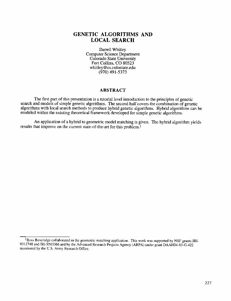
THE CANONICAL GENETIC ALGORITHM

In the canonical genetic algorithm, fitness is defined by: f,. / f where f_ is the evaluation

associated with string i, and f is the average evaluation of all the strings in the population. It is

helpful to view the execution of the genetic algorithm as a two-stage process. It starts with the currentpopulation. Selection is applied to the current population to create an intermediate population. Thenrecombination and mutation are applied to the intermediate population to create the next population.

F.

t _ 1 Generation _ t + 1

)producti, )n_ .,

Make I_i RelcombinatFi

m

Copieseach ofstring i

Performcrossat rate

Pc

on

1. Generate a random population of strings.

2. Evaluate all strings in the population.

3. Reproduce (duplicate) strings according tofitness.

4. Recombine strings according to the probabilityof crossover.

5. Repeat steps 2 to 4.

228

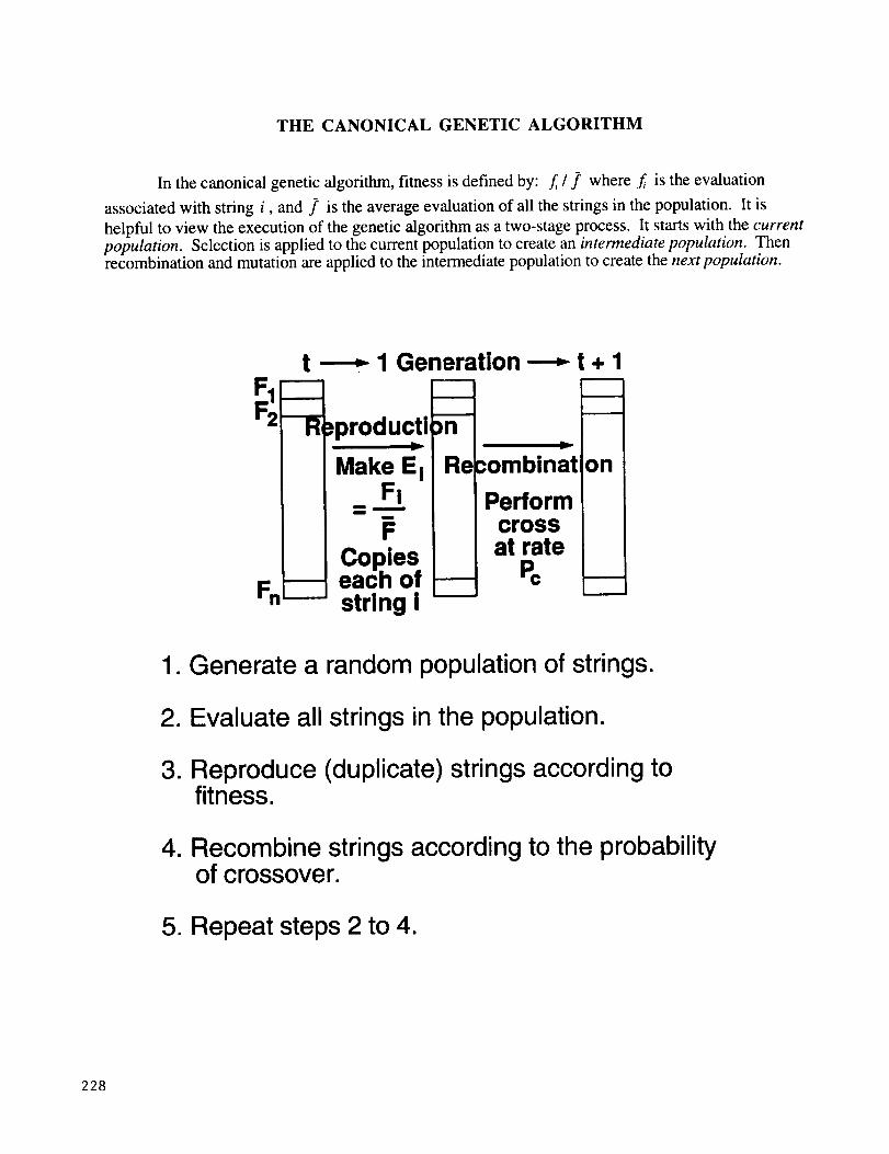
AN EXAMPLE OF HYPERPLANE PARTITIONING

A function over a single variable is plotted as a one-dimensional space, with functionmaximization as a goal. The hyperplane 0"***...** spans the first half of the space and 1"***...**spans the second half of the space. Since the strings in the 0"***...** partition are on average betterthan those in the 1"***...** partition, we would like the search to be proportionally biased toward thispartition. In the second graph the portion of the space corresponding to ** 1"*...** is shaded, whichalso highlights the intersection of 0"***...** and ** 1"*...**, namely, 0* 1"...**. Finally, in the thirdgraph, 0* 10"*...** is highlighted.

F(X)

0 K/2 K

Variable X

F(X_

K/8 K/4 K/2 K

Variable X

F{X}

K/8 K/4 K/2 K

Variable X

Figure 3 - A function and various partitions of hyperspace. Fitnessis scaled to a 0 to 1 range in this diagram.

229

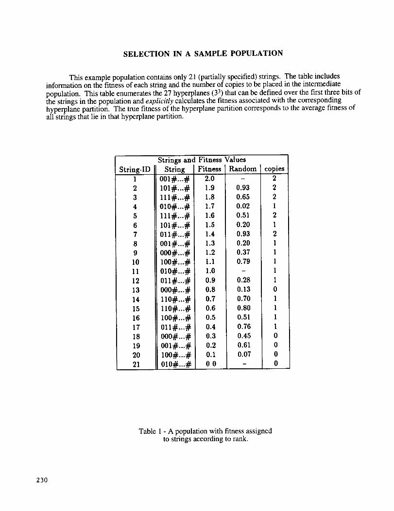
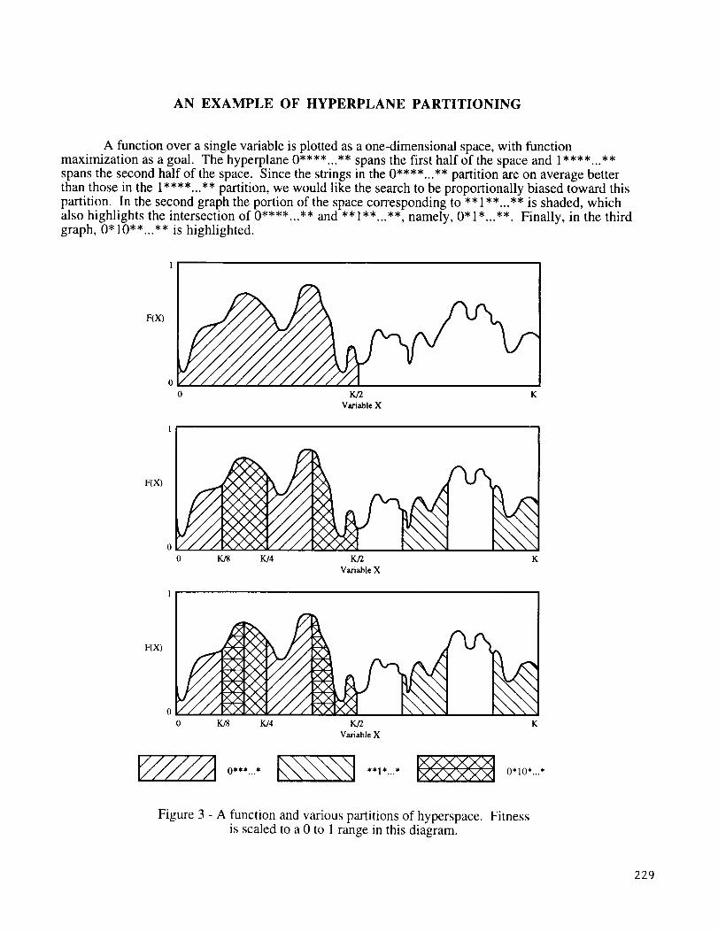
SELECTION IN A SAMPLE POPULATION

This example population contains only 21 (partially specified) strings. The table includesinformation on the fitness of each string and the number of copies to be placed in the intermediate

population. This table enumerates the 27 hyperplanes (33) that can be defined over the first three bits ofthe strings in the population and explicitly calculates the fitness associated with the correspondinghyperplane partition. The true fitness of the hyperplane partition corresponds to the average fitness ofall strings that lie in that hyperplane partition.

Strings and Fitness Values

String-ID [I String [Fitness Random I copies

1

2

3

4

5

6

7

8

9

10

11

12

13

14

15

16

17

18

19

20

21

001#...#

111#...#OLO#...#

2.0

1.9

1.8

1.7

111#...#

101:_...#

011#...#

001#...#

o00#...#100#...#

010#...#011#...#0o0#...#11o#...#11o#_.#lOO#...#011#...#

ooo#...#oo1#...#100#...#

010#...#

1.6

1.5

1.4

1.3

1.2

I.I

1.0

0.9

0.8

0.7

0.6

0.5

0.4

0.3

0.2

O.l

O0

0.93

0.65

0.02

0.51

0.20

0.93

0.20

0.37

0.79

0.28

0.13

0.70

0.80

0.51

0.76

0.45

0.61

0.07

m

2

2

2

1

2

1

2

1

1

1

1

1

0

1

1

1

1

0

0

0

0

Table 1 - A population with fitness assignedto strings according to rank.

230

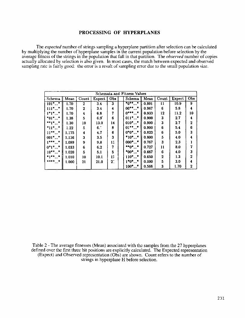
PROCESSING OF HYPERPLANES

The expected number of strings sampling a hyperplane partition after selection can be calculated

by multiplying the number of hyperplane samples in the current population before selection by the

average fitness of the strings in the population that fall in that partition. The observed number of copies

actually allocated by selection is also given. In most cases, the match between expected and observed

sampling rate is fairly good: the error is a result of sampling error due to the small population size.

Schenla

101"...*

111"...*1"1"...*

*01"...*

*11"...*

11"*...*

001"...*

1_... _

0"1"...*

10"*...*

...

Mean

1.70

1.70

1.70

1.38

1.30

1.22

1.175

1.136

1.089

1.033

1.020

1.0101.000

Count

2

2

4

5

10

5

4

3

9

6

5

10

21

I

Schemata and Fitness Values

Expect Obs Schema3.4 3 *0"*...*

3.4 4 00"*...*

6.8 7 0"**...*

6.9" 6 011"...*

13.0 14 010"...*

6.: 8 01"*...*

4.7 6 0"0"...*

3.5 3 *10'...*

9.8 11 000"...*

6.2 7 **0"...*

5.1 5 *00"...*

10.1 1_ 110"...*

21.0 2: l*0*...*

100"...*

Mean

0.991

0.967

0.933

0.900

0.900

0.900

0.833

0.800

0.767

0.727

0.667

0.650

0.600

0.566

Count Expect ObsII 10.9 9

6 5.8 4

12 11.2 I0

3 2.7 4

3 2.7 2

6 5.4 6

6 5.0 3

5 4.0 4

3 2.3 I

II 8.O 7

6 4.0 3

2 1.3 2

5 3.0 4

3 1.70 2

Table 2 - The average fitnesses (Mean) associated with the samples from the 27 hyperplanesdefined over the first three bit positions are explicitly calculated. The Expected representation

(Expect) and Observed representation (Obs) are shown. Count refers to the number of

strings in hyperplane H before selection.

231

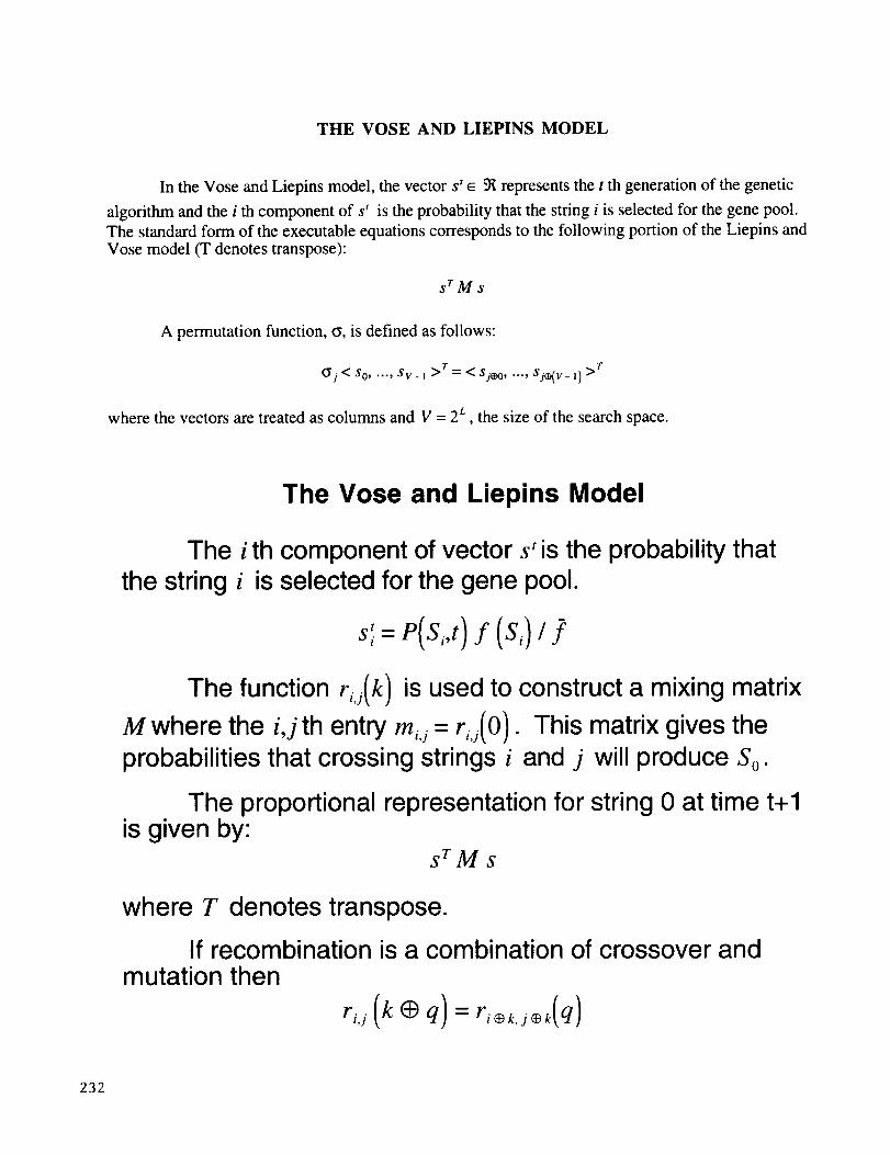
THE VOSE AND LIEPINS MODEL

In the Vose and Liepins model, the vector s' e 9_ represents the t th generation of the genetic

algorithm and the i th component of s' is the probability that the string i is selected for the gene pool.

The standard form of the executable equations corresponds to the following portion of the Liepins and

Vose model (T denotes transpose):

srMs

A permutation function, _, is defined as follows:

..., >T_i < So" Sv- l = < Silo, ..., sj_(v- 1)>r

where the vectors are treated as columns and V = 2 L , the size of the search space.

The Vose and Liepins Model

The i th component of vector s' is the probability that

the string i is selected for the gene pool.

s:- P(ai,t) f (Si) / :

The function ri,j(k) is used to construct a mixing matrix

M where the i,j th entry mij = rij(0). This matrix gives theprobabilities that crossing strings i and j will produce So.

The proportional representation for string 0 at time t+lis given by:

srMs

where T denotes transpose.

If recombination is a combination of crossover andmutation then

rij(k_q)=ri_,,2_,(q)

232

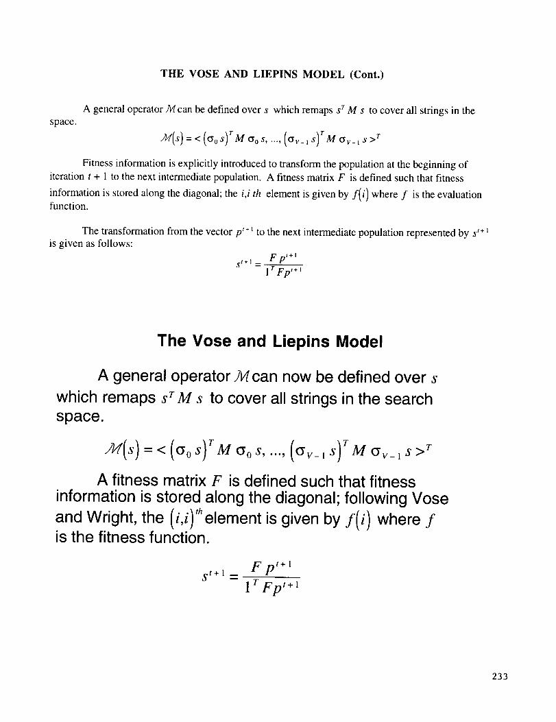
THE VOSE AND LIEPINS MODEL (Cont.)

space.

A general operator M can be defined over s which remaps s TM s to cover all strings in the

_(s) = < ("0s) _g'os ..... (,,v_, s) _M,,v_ts>r

Fitness information is explicitly introduced to transform the population at the beginning of

iteration t + I to the next intermediate population. A fitness matrix F is defined such that fitness

information is stored along the diagonal; the i,i th element is given by f(i) where f is the evaluationfunction.

The transformation from the vector p'+ _to the next intermediate population represented by s '÷ 1

is given as follows:

Fp' +lst+ 1 :

I r Fp,+ i

The Vose and Liepins Model

A general operator M can now be defined over s

which remaps s TM s to cover all strings in the searchspace.

=< s)Mo0s,..., is)T M Or-1 S >T

A fitness matrix F is defined such that fitnessinformation is stored along the diagonal; following Vose

and Wright, the (i,i)'helement is given by f(i) where fis the fitness function.

st+ 1F pt+ 1

1 r Fpt+l

233

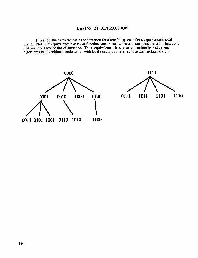
BASINS OF ATTRACTION

This slide illustrates the basins of attraction for a four-bit space under steepest ascent local

search. Note that equivalence classes of functions are created when one considers the set of functionsthat have the same basins of attraction. These equivalence classes carry over into hybrid genetic

algorithms that combine genetic search with local search, also referred to as Lamarckian search.

0000 1111

.,d>-..1000 0100 0111

0011 0101 1001 0110 1010 1100

1011 1101 1110

234

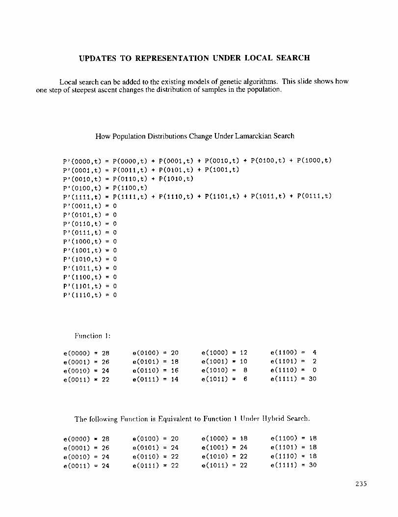
UPDATES TO REPRESENTATION UNDER LOCAL SEARCH

Local search can be added to the existing models of genetic algorithms. This slide shows how

one step of steepest ascent changes the distribution of samples in the population.

How Population Distributions Change Under Lamarckian Search

P'(0000,t) = P(0000,t) + P(0001,t) + P(0010,t) + P(0100,t) + P(1000,t)

P'(0001,t) = P(00tl,t) + P(0t0t,t) + P(t00l,t)

P'(OO10,t) : P(Ol10,t) + P(lO10,t)

P'(OlOO,t) = P(llOO,t)

P'(llll,t) : P(llll,t) + P(lllO,t) + P(llOl,t) + P(lO11,t) + P(Olll,t)

P'(OO11,t) : 0

P'(OlOl,t) = 0

P'(Ol10,t) = 0

P'(O111,t) = 0

P'(lOOO,t) : 0

P'(lOOl,t) : 0

P'(1OlO,t) = 0

P'(lOll,t) : 0

P'(ll00,t) : 0

P'(llO1,t) : 0

P'(1110,t) = 0

Function 1:

e(0000) : 28 e(0100) = 20 e(1000) : 12 e(ll00) : 4

e(0001) = 26 e(0101) : 18 e(1001) = 10 e(1101) = 2

e(O010) = 24 e(0110) : 16 e(1010) : 8 e(1110) : 0

e(0011) = 22 e(0111) = 14 e(1011) = 6 e(1111) = 30

The following Function is Equivalent to Function 1 Under ltybrid Search.

e(O000) : 28

e(O0Ol) = 26

e(O010) : 24

e(O011) = 24

e(OlO0) = 20

e(0101) : 24

e(0110) = 22

e(0111) = 22

e(lO00) : 18

e(lO01) = 24

e(1010) = 22

e(1011) = 22

e(llO0) : 18

e(llO1) = 18

e(1110) = 18

e(1111) = 30

235

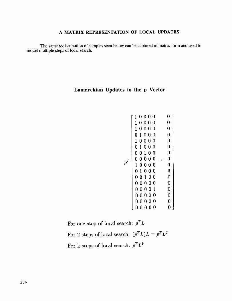
A MATRIX REPRESENTATION OF LOCAL UPDATES

The same redistribution of samples seen below can be captured in matrix form and used tomodel multiple steps of local search.

Lamarckian Updates to the p Vector

10000 0

10000 0

10000 0

01000 010000 0

01000 000100 0

00000 ...0

10000 0

01000 0

00100 0

00000 0

00001 0

00000 0

00000 0

00000 0

pT

For one step of local search: pTL

For 2 steps of local search: (pTL)L = pTL2

For k steps of local search: prLk

236

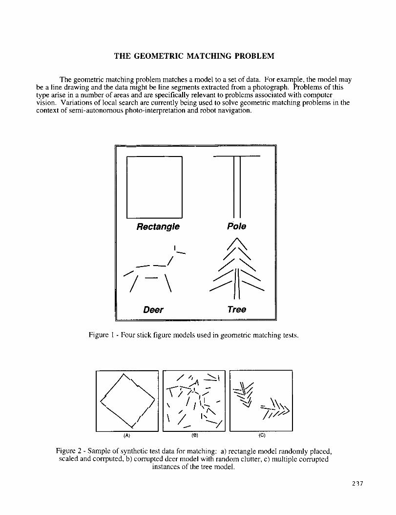
THE GEOMETRIC MATCHING PROBLEM

The geometric matching problem matches a model to a set of data. For example, the model maybe a line drawing and the data might be line segments extracted from a photograph. Problems of thistype arise in a number of areas and are specifically relevant to problems associated with computervision. Variations of local search are currently being used to solve geometric matching problems in thecontext of semi-autonomous photo-interpretation and robot navigation.

Rectangle Pole

I

I /

Deer Tree

Figure 1 - Four stick figure models used in geometric matching tests.

(AI (B) (C)

Figure 2 - Sample of synthetic test data for matching: a) rectangle model randomly placed,scaled and corrputed, b) corrupted deer model with random clutter, c) multiple corrupted

instances of the tree model.

237

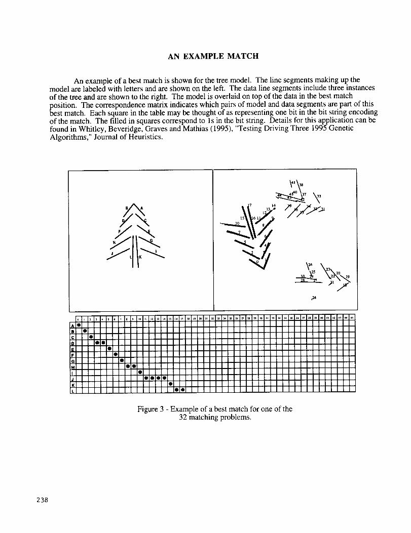
AN EXAMPLE MATCH

An example of a best match is shown for the tree model. The line segments making up themodel are labeled with letters and are shown on the left. The data line segments include three instances

of the tree and are shown to the right. The model is overlaid on top of the data in the best matchposition. The correspondence matrix indicates which pairs of model and data segments are part of thisbest match. Each square in the table may be thought of as representing one bit in the bit string encodingof the match. The filled in squares correspond to 1s in the bit string. Details for this application can befound in Whitley, Beveridge, Graves and Mathias (1995), "Testing Driving Three 1995 GeneticAlgorithms," Journal of Heuristics.

_ 17 1 13 14

--.-.az. W- 8/

g_

0 I

IAe

IDIEIF

I:hIJIKIL

ooe

O•

IIIIII

Figure 3 - Example of a best match for one of the32 matching problems.

238

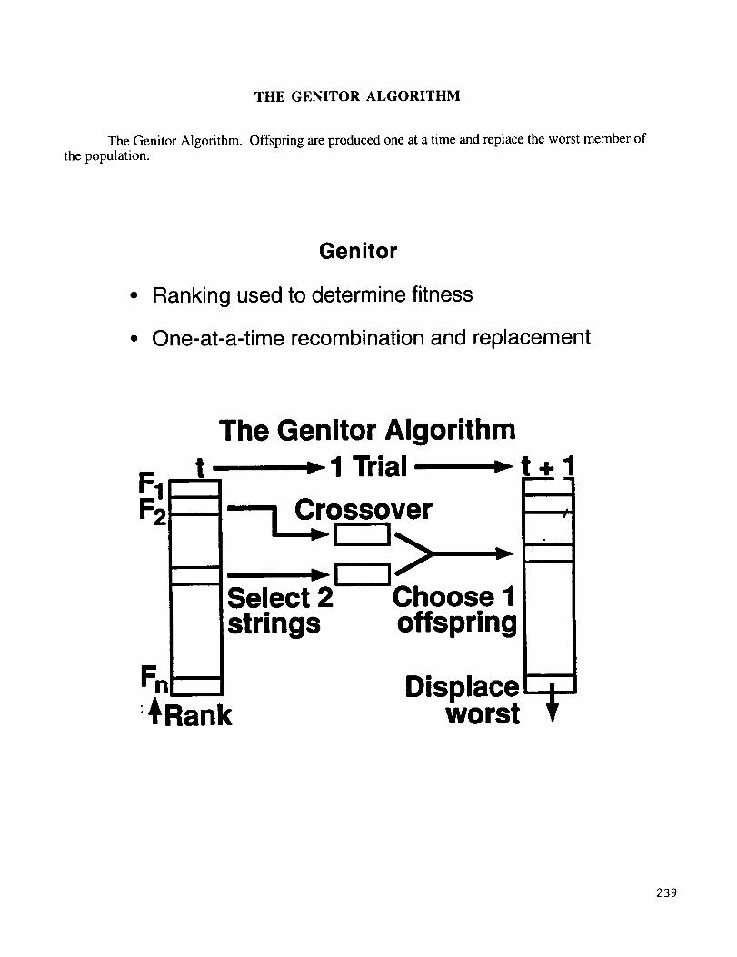
THE GENITOR ALGORITHM

The Genitor Algorithm. Offspring are produced one at a time and replace the worst member of

the population.

Genitor

• Ranking used to determine fitness

• One-at-a-time recombination and replacement

The Genitor Algorithm_ 1 Trial _t+l

Crossover

Select 2 Choose Istrings offspring

Displaceworst

239

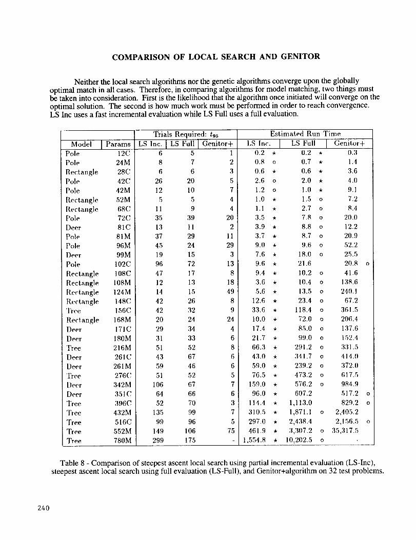
COMPARISON OF LOCAL SEARCH AND GENITOR

Neither the local search algorithms nor the genetic algorithms converge upon the globallyoptimal match in all cases. Therefore, in comparing algorithms for model matching, two things mustbe taken into consideration. First is the likelihood that the algorithm once initiated will converge on the

optimal solution. The second is how much work must be performed in order to reach convergence.LS Inc uses a fast incremental evaluation while LS Full uses a full evaluation.

Model I ParamsPole 12C

Pole 24M

Rectangle 28C

Pole 42C

Pole 42M

Rectangle 52M

Rectangle 68CPole 72C

Deer 81C

Pole 81 M

Pole 96M

Deer 99M

Pole 102C

Rectangle 108C

Rectangle 108M

Rectangle 124 M

Rectangle 148CTree 156C

Rectangle 168MDeer 171C

Deer 180M

'Free 216M

Deer 261C

Deer 261M

Tree 276C

Deer 342M

Deer 351C

Tree 396C

Tree 432M

Tree 516C

Tree 552M

Tree 780M

Trials Required: tgs

LS Inc. ] LS Full I Genitor+6 5 1

8 7 2

6 6 3

26 20 5

12 10 7

5 5 4

11 9 4

35 39 20

13 11 2

37 29 11

45 24 29

19 15 3

96 72 13

47 17 8

12 13 18

14 15 49

42 26 8

42 32 9

20 24 24

29 34 4

31 33 6

51 52 8

43 67 6

59 46 6

51 52 5

Estimated Run Time

LS Inc. I LS Full [ Genitor+

106 67

64 66

52 70

135 99

99 96

149 106

299 175

7 159.0

6 96.0

3 114.4

7 310.5

5 297.0

75 461.9

- 1,554.8

0.2 * 0.2 * 0.3

0.8 o 0.7 * 1.4

0.6 * 0.6 * 3.6

2.6 o 2.0 * 4.0

1.2 o 1.0 * 9.1

1.0 * 1.5 o 7.2

1.1 * 2.7 o 8.4

3.5 * 7.8 o 20.0

3.9 * 8.8 o 12.2

3.7 * 8.7 o 20.9

9.0 * 9.6 o 52.2

7.6 * 18.0 o 25.5

9.6 * 21.6 20.8

9.4 * 10.2 o 41.6

3.6 * 10.4 o 138.6

5.6 * 13.5 o 240.1

12.6 * 23.4 o 67.2

33.6 * 118.4 o 361.5

10.0 * 72.0 o 206.4

17.4 * 85.0 o 137.6

21.7 * 99.0 o 152.4

66.3 * 291.2 o 331.5

43.0 * 341.7 o 414.0

59.0 * 239.2 o 372.0

76.5 * 473.2 o 617.5

• 576.2 o 984.9

• 607.2 517.2

• 1,113.0 829.2

• 1,871.1 o 2,405.2

, 2,438.4 2,156.5

• 3,307.2 o 35,317.5

• 10,202.5 o

O

Table 8 - Comparison of steepest ascent local search using partial incremental evaluation (LS-Inc),steepest ascent local search using full evaluation (LS-Full), and Genitor+algorithm on 32 test problems.

240

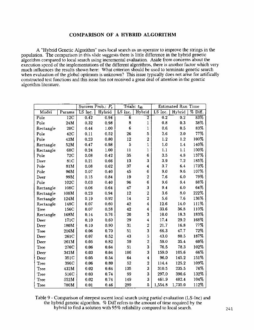
COMPARISON OF A HYBRID ALGORITHM

A "Hybrid Genetic Algorithm" uses local search as an operator to improve the strings in the

population. The comparison in this slide suggests there is little difference in the hybrid geneticalgorithm compared to local search using incremental evaluation. Aside from concerns about the

execution speed of the implementations of the different algorithms, there is another factor which verymuch influences the results shown here: What criterion should be used to terminate genetic search

when evaluation of the global optimum is unknown? This issue typically does not arise for artifically

constructed test functions and this issue has not received a great deal of attention in the genetic

algorithm literature.

Success Prob.: P, Trials: tgs Estimated Run Time

Model t ParamsPole 12C

Pole 24M

Rectangle 28C

Pole 42C

Pole 42M

Rectangle 52M

Rectangle 68CPole 72C

Deer 81C

Pole 81M

Pole 96M

Deer 99M

Pole 102C

Rectangle 108C

Rectangle 108M

Rectangle 124M

Rectangle 148CTree 156C

Rectangle 168M

Deer 171C

Deer 180M

Tree 216M

Deer 261C

Deer 261M

Tree 276C

Deer 342M

Deer 351 C

Tree 396C

Tree 432M

Tree 516C

Tree 552M

Tree 780M

LS Inc. I Hybrid LS Inc. [ Hybrid LS Inc. [ Hybrid ] % Diff.0.2 0.2 83%

0.8 0.3 38%

0.6 0.5 83%

2.6 2.0 77%

1.2 1.2 100%

1.0 1.4 140%

1.1 1.1 100%

3.5 4.8 137%

3.9 7.2 185%

3.7 6.4 173%

9.0 9.6 107%

7.6 6.0 79%

9.6 8.4 88%

9.4 6.0 64%

3.6 8.0 222%

5.6 7.6 136%

12.6 14.0 111%

33.6 36.8 110%

10.0 18.3 183%

17.4 29.2 168%

21.7 16.8 77%

66.3 47.7 72%

43.0 80.5 187%

59.0 35.4 60%

76.5 78.3 102%

159.0 105.6 66%

96.0 145.2 151%

114.4 125.2 109%

310.5 235.5 76%

297.0 390.6 132%

461.9 482.4 104%

1,554.8 1,735.0 112%

0.42 0.94

0.32 0.98

0.44 1.00

0.11 0.52

0.23 0.80

0.47 0.98

0.24 1.00

0.08 0.42

0.21 0.66

0.08 0.62

0.07 0.40

0.15 0.84

0.03 0.40

0.06 0.64

0.23 0.94

0.19 0.92

0.07 0.60

0.07 0.58

0.14 0.76

0.10 0.60

0.10 0.90

0.O6 0.70

0.07 0.52

0.05 0.82

0.06 0.64

0.03 0.64

0.05 0.54

0.06 0.80

0.02 0.64

0.03 0.74

0.O2 O.74

0.01 0.46

6 2

8 1

6 1

26 5

12 2

5 1

11 1

35 6

13 3

37 4

45 6

19 2

96 6

47 3

12 2

14 2

42 4

42 4

20 3

29 4

31 2

51 3

43 5

59 2

51 3

106 3

64 4

52 2

135 3

99 3

149 3

299 5

Table 9 - Comparison of steepest ascent local search using partial evaluation (LS-Inc) and

the hybrid genetic algorithm. % Diff refers to the amount of time required by the

hybrid to find a solution with 95% reliability compared to local search. 241

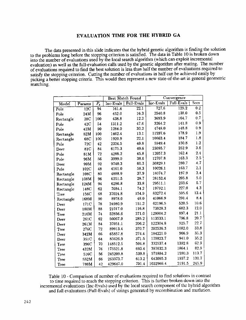
EVALUATION TIME FOR THE HYBRID GA

The data presented in this slide indicates that the hybrid genetic algorithm is finding the solution

to the problems long before the stopping criterion is satisfied. The data in Table 10 is broken downinto the number of evaluations used by the local search algorithm (which can exploit incremental

evaluation) as well as the full-evaluation calls used by the genetic algorithm after mating. The number

of evaluations required to find the best solution is less than half the number of evaluations required to

satisfy the stopping criterion. Cutting the number of evaluations in half can be achieved easily by

picking a better stopping criteria. This would then represent a new state-of-the-art in general geometric

matching.

Model I ParamsPole 12C

Pole 24M

Rectangle 28CPole 42C

Pole 42M

Rectangle 52M

Rectangle 68CPole 72C

Deer 81C

Pole 81M

Pole 96M

Deer 99M

Pole 102C

Rectangle 108C

Rectangle 108M

Rectangle 124M

Rectangle 148CTree 156C

Rectangle 168MDeer 171C

Deer 180M

Tree 216M

Deer 261C

Deer 261M

Tree 276C

Deer 342M

Deer 351C

Tree 396C

Tree 432M

Tree 516C

Tree 552M

Tree 780M

P, Best Match FoundInc-Evais I Full-Evals94 161.4

96 452.0

100 438.8

54 1311.2

90 1284.0

100 1462.4

I00 1920.9

42 2324.5

84 6175.3

72 4288.2

56 3999.0

92 9740.3

48 4161.0

80 4888.9

96 6251.5

94 6286.8

62 7684.1

68 37024.8

90 8978.0

78 24980.9

88 21017.0

74 52856.6

62 50067.9

84 37051.1

72 89913.4

66 65857.8

64 85626.9

70 148512.5

76 175521.8

56 245209.8

66 263373.7

42 429647.0

ConvergenceInc-Evals

22.1 727.6

16.3 2540.8

12.2 3693.9

47.6 3264.2

30.2 4748.0

13.1 11597.6

22.1 10663.4

49.8 5949.4

40.6 23095.7

45.8 12057.3

38.6 12707.8

60.3 30829.1

58.3 10026.1

37.9 18074.7

28.7 28152.4

33.8 29511.1

74.2 19792.1

154.9 83272.4

48.0 41066.9

151.2 62196.5

116.8 73928.3

271.0 129904.2

285.2 113533.1

206.2 122304.8

370.7 202536.3

274.4 184221.0

371.5 179823.7

504.8 332537.4

693.4 387632.3

539.8 571884.2

613.2 643095.3

701.4 1032966.4

I Full-Evalsl Secs129.2 0.2

138.0 0.5

164.7 0.7

141.8 0.9

148.8 0.9

178.9 1.9

184.7 1.8

150.8 1.2

252.9 3.6

162.4 2.4

163.3 2.5

280.7 4.7

163.7 2.1

197.9 3.4

205.8 5.0

233.6 5.7

227.0 4.3

505.6 13.4

291.4 8.4

520.5 10.6

602.3 12.0

897.4 21.1

796.8 20.7

925.7 22.7

1082.0 33.8

966.9 35.3

941.0 35.2

1392.8 62.9

1864.1 82.9

1590.3 113.7

1937.2 130.7

2191.5 245.9

Table 10 - Comparison of number of evaluations required to find solutions in contrast

to time required to reach the stopping criterion. This is further broken down into theincremental evaluations (Inc-Evals) used by the local search component of the hybrid algorithm

and full evaluations (Full-Evals) of strings generated by recombination and mutlation.

242

OTHER APPLICATIONS

• Navy Air-Plane Simulator SchedulingDeveloped by BBN using CSU algorithms

• Poor Prototype Warehouse Scheduler

A fast evaluation function is used thatapproximates warehouse operations which isorders of magnitude faster than a correspondingdetailed warehouse simulator.

Local methods yield poor results when theevaluation function is noisy or approximate, whilegenetic algorithms yield very good solutions.

• Artificial Genetically Grown NeuralNetworks

Neural networks are grown using celldevelopment processes for control applications.The grammar controlling the growth process isoptimized rather than the neural network itself.The resulting networks have outperformedtemporal difference methods on severalapplications.

• Seismic Data Interpretation

243