Embed Size (px)
Citation preview

Genetic Algorithm for theResource-Constrained Project SchedulingProblem Using Encoding with Scheduling
Mode ∗
Vu Thien Can,Department of Mathematics and Computer Science,
University of Ho Chi Minh City, Vietnam
Jacques A. Ferland,Departement d’informatique et de recherche operationnelle,
Universite de Montreal, Canada
Nguyen Huu Anh,Department of mathematics and Computer Science,
University of Ho Chi Minh City, Vietnam
December 6, 2004
∗This research was supported by NSERC grant (OGP 0008312) from Canada.
1
Abstract
In this paper we use genetic algorithms (GA) to deal with the Resource-Constrained Project Scheduling Problem (RCPSP ). We introduce a prior-ity value encoding (representation) to implement the GA for RCPSP . First,we follow up the approach of Alcaraz and Maroto [1] to introduce an addi-tional component in the encoding to indicate the scheduling mode (forwardor backward) used to generate the corresponding schedule. Furthermore, thenumerical results indicate that our methods is slightly better as far as so-lution quality is concerned and requires smaller solution time than the GAmethod proposed by Alcaraz and Maroto in [1] where an activity list encodingis used.Key words: genetic algorithm, resource-constrained project scheduling,metaheuristic.
1 Introduction
The Resource-Constrained Project Scheduling Problem (RCPSP ) is a clas-sical well-known problem where the activities of a project must be scheduledto minimize its makespan [7, 17, 22]. Several authors have suggested differentmethods to solve this problem. They can be classified into three categories.The exact methods [8, 9, 11, 26, 27] generate optimal solutions for smallsize problems (up to 60 activities). The heuristic procedures are the alter-native to deal with larger problems [3, 12, 20, 21, 24]. These methods areserial or parallel schedule generation schemes. The third category includesmetaheuristic methods like Tabu search [2, 28], simulated annealing [4, 5, 6],and genetic algorithm [1, 14, 19]. Recent numerical comparisons of thesemethods [1, 5, 15, 22] indicate that the three most efficient procedures are(in order) the genetic algorithms of Alcaraz and Maroto [1], the simulatedannealing method of Bouleimen and Lecocq [5, 6], and the genetic algorithmof Hartman [14].
To improve Hartman genetic algorithm [14] using an activity list encoding(representation) of the solution, Alcaraz and Maroto [1] introduce an addi-tional component in the encoding to indicate the scheduling mode (forwardor backward) used to generate the corresponding schedule. The numericalresults in [1] show the advantage of including the scheduling mode in theencoding. In this paper, to follow up this approach we present genetic algo-
2
rithms using priority value encoding with scheduling mode. The numericalresults indicate that the variant using an encoding with scheduling mode gen-erates better solutions than the variant where the encoding does not includethe scheduling mode. Furthermore, the results indicate that our genetic al-gorithm is slightly better as far as solution quality is concerned and requiressmaller solution time than the method proposed by Alcaraz and Maroto[1].
In Sections 2 and 3 we briefly summarize the descriptions of the RCPSPand of the genetic algorithm (GA) [10, 13, 18], respectively. In Section 4we specify the operators (selection, crossover, and mutation) and the cullingstrategy (used to generate the new current population) that we use to imple-ment the activity list or permutation based GAs. Then Section 5 includesthe modifications required to implement the GAs using activity list encod-ing with scheduling mode. Similarly we introduce the operators and theiradapted versions for the priority value based GAs and their variants using pri-ority value encoding with scheduling mode in Sections 6 and 7, respectively.Section 8 includes the numerical results and their analysis. Concluding re-marks are included in Section 9.
2 Problem description
In a Resource-Constrained Project Scheduling Problem (RCPSP ), we con-sider a project including n activities j = 1, 2, . . . , n to be scheduled underresource and precedence constraints. The time required to complete an ac-tivity j is specified in terms of an integer number dj of periods. It is alsoassumed that once initiated, any activity is completed without interruption.
On the one hand, the precedence constraints are induced by technologicalrequirements to impose that any activity j must be scheduled for executionafter the completion of all its immediate predecessors included in a set Pj.On the other hand, each activity j requires rjk units of resource k, k =1, 2, . . . , K, during each period of its execution. Hence resource constraintsare specified to limit the number of units of each resource k used in eachperiod t to the number Akt of units available.
The problem is to determine a starting period for each activity in orderto minimize the total duration (makespan) of the project while satisfyingthe precedence and resource constraints. Note that referring to Herroelenet al. classification in [16], this problem is denoted as m/1/cpm/Cmax, andreferring Brucker et al. notation in [7], as PS/prec/Cmax.
3
3 Genetic algorithm (GA) for RCPSP
Genetic algorithms (GA) [10, 13, 18] are population based techniques wherean evolutionary mechanism that mimics a biological mechanism based onselection and natural evolution principles, is used to transform a population(set) of solutions from one iteration (generation) to the next in order tolead the search into promising regions of the feasible domain. An initialpopulation G0 of m solutions is generated, and at each iteration, the sizeof the population remains the same. At each iteration three operators areapplied to generate a set of new offspring solutions : a selection operator, acrossover operator, and a mutation operator.
The selection operator is used to select an even number of (parent) solu-tions from the current population. Each parent-solution is selected accordingto some strategy. The parent-solutions are paired, and a crossover operatoris applied with some probability pcross to each paire of parent-solutions togenerate new feasible offspring-solutions inheriting interesting componentscontained in the parent-solutions. Then, a mutation operator is applied tomodify the components of each offspring-solution with a small probabilitypmut. The purpose of using such an operator is to promote diversity in thecurrent population of solutions. Finally, a culling strategy is used to de-termine a new population by selecting among the parent-solutions and theoffspring-solutions. The procedure is repeated until some stopping criterionis reached.
Now an essential feature of this solution approach is the encoding or repre-sentation of phenotype solutions into genotype vectors to which the differentoperators are applied. Several different encodings exist for the RCPSP , butwe limit our presentation to the activity list (permutation-based) encodinggiven in Hartmann [14] and Alcaraz and Maroto [1], and to a priority valueencoding quite similar to the priority value based encoding in Hartmann[14]. We also consider the corresponding encoding with scheduling mode asintroduced by Alcaraz and Maroto [1] for the activity list encoding .
4 Activity list or permutation based GA
Our presentation borrows heavily form [1]. In this first encoding, each indi-vidual in the population (genotype) is represented as a vector
[j1, j2, . . . , jn]
4

Figure 1: Project example having 8 activities.
corresponding to a permutation of the activities of the project. This permuta-tion satisfies the precedence constraints; i.e. for any index ji, i = 2, 3, . . . , n,
Pji⊂ {j1, j2, . . . , ji−1}.
Each genotype vector is decoded into a unique phenotype schedule accordingto the following serial scheduling scheme. Activity j1 is scheduled to start attime 0 (i.e. in the first period). Activity ji is the ith activity scheduled asearly as possible after its predecessors according to the ressources available.
To illustrate the serial scheduling scheme, consider the example illustratedin Figure 1 taken from [1] where the project includes 8 activities requiringone type of resource. Assume that A1t = 8 units of resource are available ineach period t. With each activity-node j, we associate the pair (dj, rj1). Thegenotype individual
[1, 2, 3, 4, 5, 6, 7, 8]
translates into the unique feasible (phenotype) schedule illustrated in figure2. It is interesting to note that the schedule in figure 2 corresponds also tothe genotype individual
[2, 1, 4, 3, 5, 7, 6, 8]
In [1] the genotype individuals in the initial population are generatedrandomly as follows. Starting with an empty vector, the next activity is
5
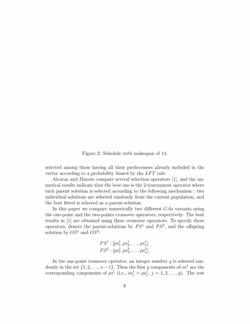
Figure 2: Schedule with makespan of 14.
selected among those having all their predecessors already included in thevector according to a probability biased by the LFT rule.
Alcaraz and Maroto compare several selection operators [1], and the nu-merical results indicate that the best one is the 2-tournament operator whereeach parent solution is selected according to the following mechanism : twoindividual solutions are selected randomly from the current population, andthe best fitted is selected as a parent-solution.
In this paper we compare numerically two different GAs variants usingthe one-point and the two-points crossover operators, respectively. The bestresults in [1] are obtained using these crossover operators. To specify theseoperators, denote the parent-solutions by PS1 and PS2, and the offspringsolution by OS1 and OS2:
PS1 : [ps11, ps
12, . . . , ps
1n]
PS2 : [ps21, ps
22, . . . , ps
2n].
In the one-point crossover operator, an integer number q is selected ran-domly in the set {1, 2, . . . , n−1}. Then the first q components of os1 are thecorresponding components of ps1 (i.e., os1
j = ps1j , j = 1, 2, . . . , q). The rest
6
of the activities os1q+1, os
1q+2, . . . , os
′n are selected in the order in which they
appear in the second parent-solution PS2; i.e., for j = q + 1, q + 2, . . . , n,
os1j = ps2
k where k is the smallest index such that
ps2k /∈ {os1
1, os12, . . . , os
1j−1}.
The second offspring-solution OS2 is determined by interchanging the rolesof PS1 and PS2.
In the two-points crossover operator, two integer numbers q1 < q2 areselected randomly in the set {1, 2, . . . , n}. Then the first q1 components ofOS1 are the corresponding ones of PS1 (i.e., os1
j = ps1j , j = 1, 2, . . . , q1).
The components q1 + 1, q1 + 2, . . . , q2 are selected in the order in which theyappear in the second-parent solution PS2; i.e. for j = q1 + 1, q1 + 2, . . . , q2,
os1j = ps2
k where k is the smallest index such that
ps2k /∈ {os1
1, os12, . . . , os
1j−1}.
Finally, the last components q2 + 1, q2 + 2, . . . , n, are selected in the order inwhich they appear in the first-parent solution PS1; i.e. for j = q2 + 1, q2 +2, . . . , n,
os1j = ps1
k where k is the smallest index such that
ps1k /∈ {os1
1, os12, . . . , os
1j−1}.
The second offspring-solution OS2 is determined by interchanging the rolesof PS1 and PS2.
For each pair of parent-solutions, the crossover operator is applied witha probability pcross. If the operator is not applied, then the parent-solutionsbecome their own offspring-solutions.
The mutation operator inducing the best results in [1] is an adaptation ofBoctor’s procedure [4] to generate neighbor solutions. Consider each activitysequentially. Determine randomly a new position in the genotype vector suchthat the precedence constraints are satisfied. Then the activity is moved tothis new position with a probability pmut.
Finally, the culling strategy is to replace the current population by theset of offspring-solutions to generate the new current population.
7
5 Activity list encoding with scheduling mode
In [1] Alcaraz and Maroto propose a variant of the activity list encodingwhere an additional component (n + 1) of the vector is used to indicate thescheduling mode forward or backward (f/b) used to decode the genotypevector into a (phenotype) schedule. The forward scheduling mode f is theserial scheduling scheme described before. The backward mode b is also aserial scheduling scheme where the last activity jn is first scheduled. Activityjn−i+1 is the ith activity scheduled as late as possible before its successorsaccording to the of resources available.
The initial population is generated as before. To determine the schedulingmode f/b of each individual, we evaluate the makespans of the two schedulesgenerated using the forward and the backward scheduling mode, respectively.The most fitted schedule (i.e., the schedule with the smallest makespan)induces the value f/b of the (n + 1)st component of the genotype vector.
The crossover operators are slightly modify to account for the schedulingmode. In the one-point crossover operator, if the first parent-solution PS1
mode is f , then OS1 is determined as before. Otherwise, if PS1 mode is b,then the last q components of OS1 are the corresponding components of ps1;i.e., os1
j = ps1j , j = q + 1, . . . , n). The rest of the activities os1
q, os1q−1, . . . , os
11
are selected in the order in which they appear in PS2; i.e. for j = q, q −1, . . . , 1,
os1j = ps2
k where k is the largest index such that
ps2k /∈ {os1
j+1, os1j+2, . . . , os
1n}.
Finally, the scheduling mode of OS1 is the same as PS1 (i.e., os1n+1 = ps1
n+1).The second offspring-solution OS2 is determined by interchanging the rolesof PS1 and PS2.
In the two-points crossover, if the first parent-solution PS1 mode is f ,then OS1 is determined as before. Otherwise, if PS1 mode is b, then thelast (n − q2) components of OS1 are the corresponding components of ps1
(i.e., os1j = ps1
j , j = q2 + 1, . . . , n). The components q1 + 1, . . . , q2 of OS1
are selected in the order in which they appear in the second parent-solutionPS2; i.e. for j = q2, q2 − 1, . . . , q1 + 1,
os1j = ps2
k where k is the largest index such that
ps2k /∈ {os1
j+1, os1j+2, . . . , os
1n}.
8
The first q1 components of OS1 are selected in the order in which they appearin PS1; i.e. for j = q1, . . . , 1
os1j = ps1
k where k is the largest index such that
ps1k /∈ {os1
j+1, os1j+2, . . . , os
1n}.
Finally, the scheduling mode of OS1 is the same as PS1 (i.e., os1n+1 = ps1
n+1).The second offspring solution OS2 is determined by interchanging the rolesof PS1 and PS2.
The same Boctor’s type mutation operator (applied to the first n compo-nents) and the same culling strategy are used in these GAs.
6 Priority value based GA
The priority value encoding presented in this section is quite similar to theone used in Hartmann [14] except that the values associated with the activi-ties in the genotype vector are integer values in the set {0, 1, . . . , n−1}. Thesmaller is the value associated with an activity, the higher is the priority toschedule it.
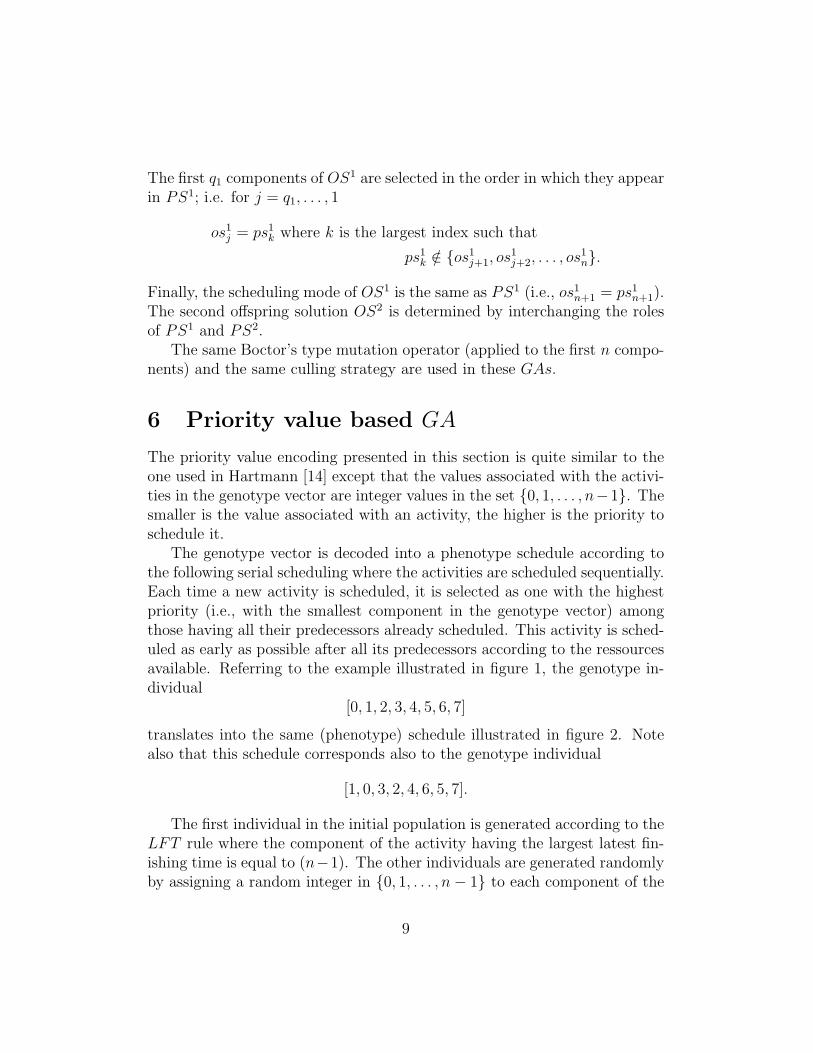
The genotype vector is decoded into a phenotype schedule according tothe following serial scheduling where the activities are scheduled sequentially.Each time a new activity is scheduled, it is selected as one with the highestpriority (i.e., with the smallest component in the genotype vector) amongthose having all their predecessors already scheduled. This activity is sched-uled as early as possible after all its predecessors according to the ressourcesavailable. Referring to the example illustrated in figure 1, the genotype in-dividual
[0, 1, 2, 3, 4, 5, 6, 7]
translates into the same (phenotype) schedule illustrated in figure 2. Notealso that this schedule corresponds also to the genotype individual
[1, 0, 3, 2, 4, 6, 5, 7].
The first individual in the initial population is generated according to theLFT rule where the component of the activity having the largest latest fin-ishing time is equal to (n−1). The other individuals are generated randomlyby assigning a random integer in {0, 1, . . . , n− 1} to each component of the
9
genotype vector. Thus it is possible for more than one activity to have thesame value in the vector.
In our implementation we use the following pseudo-elitist selection oper-ator. Each parent-solution is selected randomly in a subset of the currentpopulation obtained by eliminating the 25% less fitted solutions and the 25%best fitted solutions; i.e., this subset includes 50% of the current populationincluding the (so called) average best fitted solutions. Furthermore, in eachpair of parent-solutions, they are selected to be different.
An advantage of this encoding is to allow using the standard crossoveroperators. In this paper, we compare the variants using the one-point andthe uniform crossover operators, respectively. For the sake of completeness,recall that in the one-point crossover operator an integer number q is selectedrandomly in the set {1, 2, . . . , n − 1}. Then the first offspring-solution OS1
inherits its first q components from parent-solution PS1 and the rest of itscomponents from parent-solution PS2; i.e.
os1j =
{ps1
j j = 1, 2, . . . , q
ps2j j = q + 1, . . . , n.
The second offspring-solution is determined by interchanging the roles of PS1
and PS2.To implement the uniform crossover operator, we use a vector vb of di-
mension n where the value of each component is selected randomly to be 0or 1. The first offspring OS1 is generated as follows : for each j = 1, 2 . . . , n
os1j =
{ps1
j if vbj = 0
ps2j if vbj = 1.
The second offspring-solution OS2 is determined by interchanging the rolesof PS1 and PS2.
For each pair of parent-solutions, the crossover operator is also appliedwith a probability pcross, and the parent-solutions are their own offspring-solutions if the operator is not applied.
We use the following mutation operator. For each offspring-solutions, theoperator is applied with probability pmut. To apply the operator, we firstselect randomly an element α ∈ {0, 1, . . . , n − 1}. Then select randomly acomponent of the offspring-solution vector that has a value different from α,and replace it by α. Now, in the case where all components of the offspring
10

solution vector have a value equal to α, then select randomly a component tobe modified to the value α +1, if α < n− 1, or to the value α− 1, otherwise.
Finally the culling strategy uses a 2-tournament selection operator togenerate the new current population. Each individual of the new currentpopulation is selected as follows : two solutions are selected randomly inthe set including those in the current population and the offspring-solutions(i.e., the set includes 2n solutions), and the best fitted is included in the newcurrent population.
7 Priority value encoding with scheduling
mode
For the priority value encoding we can also apply the approach proposed byAlcaraz and Moroto in [1] and summarized in Section 5 where an (n+1) ad-ditional component of the genotype vector is used to indicate the schedulingmode forward or backward (f/b) used to decode it. The forward schedulingmode f is the serial scheduling scheme introduced above. The schedulingscheme is modified as follows in the backward mode b: each time a newactivity is scheduled, it is selected as one having the lowest priority amongthose having all their successors already scheduled. This activity is scheduledas late as possible before its successors according to the resources available.
The initial population is generated as before, and the scheduling mode ofeach solution is selected according to the fitness of the schedules generated.
The crossover operators (one-point and uniform) remain un changed. Thescheduling mode of OS1 is the one of PS1 (i.e., os1
n+1 = ps1n+1) if the number
of components that it inherits from PS1 is larger or equal to the number ofcomponents that it inherits from PS2. The scheduling mode of OS2 is thecomplementary one of OS1 (i.e., os2
n+1 = b(f) if os1n+1 = f(b)).
Finally, the same mutation operator and the same culling strategy areused in the corresponding GAs.
8 Numerical results
The numerical experimentation completed by Alcaraz and Maroto in [1] in-dicates that their GAs using the activity list encoding with scheduling mode
11
are the most efficient metaheuristic procedures when compared with simu-lated annealing [6], tabu search [2], adaptive sampling [21, 29] and other GAs[14, 25]. In this section we want to complete a similar experimentation tocompare the GAs using priority value encoding with the GAs of Alcaraz andMoroto.
Like Alcaraz and Moroto in [1], we are using the standard instances J30,J60 and J120 generated with the problem generator developed by Kolischet al. [23] that are available in the Project Scheduling Problem LIBraryPSPLIB (http:www.bwl.uni-kiel.de/Prod/psplib/). Each set J30 and J60includes 480 instances, and the set J120 includes 620 instances. For instancesin J30, the optimal values are known. For the instances in J60 and J120, bestknown upper bounds (best known solutions) are available. Furthermore, thenumerical results are obtained using a Pentium IBM-compatible computer598MHz, 128Mb Ram running under Windows XP.
Five different GAs are compared numerically. The first GA denoted CFAuses the priority value encoding (without scheduling mode) and the one-point crossover operator as described in Section 6. The other four GAs useencoding with scheduling mode. AM1 et AM2 denote the GAs proposedby Alcaraz and Moroto [1] as described in Section 5. They both use theactivity list encoding with scheduling mode, and the one-point and two-pointscrossover operator, respectively. Finally, the last two methods denoted CFA1and CFAU are the methods introduced in Section 7 using the priority valueencoding with scheduling mode, and the one-point and the uniform crossoveroperator, respectively. All these method are coded in Java.
In designing our numerical experimentation, we take advantage of thenumerical results obtained by Alcaraz and Moroto [1] to fixe most of theparameters. Hence, as in [1] we use the two stopping rules allowing a smallnumber of 20 iterations and an intermediate number of 50 iterations, respec-tively. But we also consider a third stopping rule allowing for a larger numberof 100 iterations. Note that in [1] the first two stopping rules are specified interms of number of schedules generated, but they are quite equivalent accord-ing to the population sizes m used. The parameters used are summarized inTable 1. The same parameters are used for the five methods compared.
12
In our experimentation, each instance is solved 20 times using the sameinitial population of solutions for each of the 20 runs, and we denote
B val : the value of the best solution generated
Aval : the average value of the 20 solutions generated
W val : the value of the worst solution generated.
Using these values, we compare the 5 methods according to the followingthree global criteria:
i) Percentage of deviation from the best solution (for problems in J30) orfrom the best known solution (for problems in J60 and in J120):
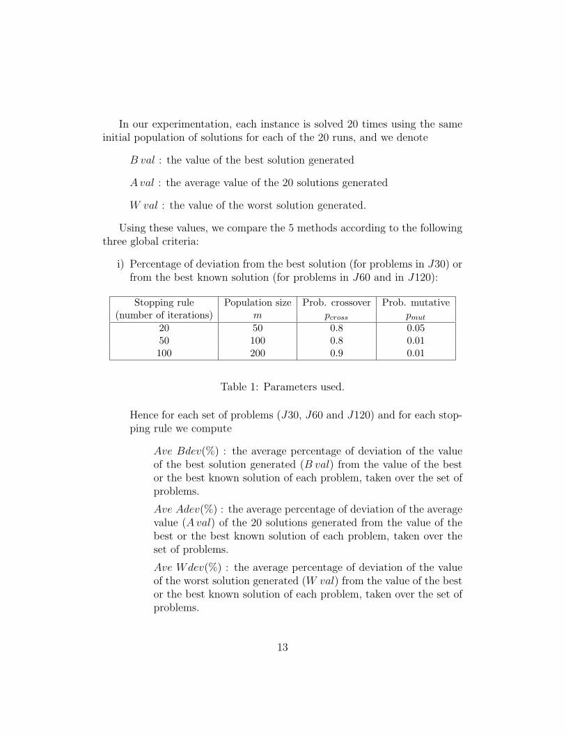
Stopping rule Population size Prob. crossover Prob. mutative(number of iterations) m pcross pmut
20 50 0.8 0.0550 100 0.8 0.01100 200 0.9 0.01
Table 1: Parameters used.
Hence for each set of problems (J30, J60 and J120) and for each stop-ping rule we compute
Ave Bdev(%) : the average percentage of deviation of the valueof the best solution generated (B val) from the value of the bestor the best known solution of each problem, taken over the set ofproblems.
Ave Adev(%) : the average percentage of deviation of the averagevalue (A val) of the 20 solutions generated from the value of thebest or the best known solution of each problem, taken over theset of problems.
Ave Wdev(%) : the average percentage of deviation of the valueof the worst solution generated (W val) from the value of the bestor the best known solution of each problem, taken over the set ofproblems.
13

ii) Number of instances where the value of the best known solution isachieved:
For each set of problems and for each stopping rule we compute:
NB1: the number of instances where the value of the best knownsolution is achieved at least once among the 20 solutions generated
NB20: the number of instances where the best known solution isachieved for all the 20 solutions generated.
OPT1(%) = NB1
(number of problems in the set)· 100
OPT20(%) = NB20
(number of problems in the set)· 100
iii) Average solution time (CPU):
For each set of problems and for each stopping rule we compute
Ave CPU(sec): average solution to solve one instance of theproblem set once.
The numerical results for the different criteria are summarized in Tables2, 3, and 4 for problems J30, J60, and J120, respectively. In these tables, acolumn and a row are associated with each method and with each criterion,respectively. Furthermore, each component of a table corresponding to apair (criterion, method) includes three different entries associated with thethree stopping rules where the number of iterations are 20, 50, and 100,respectively.
Note that referring to these tables, the four most important criteria arethe following : Ave ADev(%), OPT1(%), OPT20(%) and Ave CPU(sec). Theinterest in having the two additional criteria Ave BDev(%) and Ave WDev(%)is to indicate the average width of the interval including the values of the so-lutions for the different instances. As expected, for the three problems (J30,J60, J120) we observe that the width of this interval decreases in generalwith the number of iterations (stopping rule).
Let us first compare the results obtained with CFA and CFA1 to eval-uate the advantage of including the scheduling mode into the priority valueencoding. The results in Tables 2, 3,, and 4 clearly indicate the superiorityof the method CFA1 using scheduling mode. Now consider the results inTable 5 obtained from those in Tables 2, 3, and 4. In this table, for thestopping criterion with 100 iterations and for each problem set (J30, J60,
14

CFA AM1 AM2 CFA1 CFAUAve 0.397 0.265 0.254 0.229 0.447
Bdev(%) 0.205 0.122 0.188 0.101 0.2170.139 0.073 0.116 0.060 0.150
Ave 0.999 0.562 0.572 0.991 0.959Adev(%) 0.526 0.387 0.549 0.387 0.548
0.366 0.339 0.294 0.189 0.359Ave 1.811 0.964 0.953 2.730 1.573
Wdev(%) 0.965 0.492 1.070 0.491 0.9250.728 0.632 0.498 0.332 0.602
OPT1 83.75 89.79 90.21 80.42 83.54(%) 90.00 94.38 89.79 95.21 89.58
92.71 96.25 94.79 96.88 92.71OPT20 61.46 76.25 75.42 62.50 66.25(%) 72.71 82.50 71.04 82.50 72.92
75.83 78.83 82.50 86.88 80.42Ave CPU 0.1 0.2 0.2 0.3 0.3
(sec) 0.6 0.8 0.8 0.6 0.62.5 4 4 3 3
Table 2: Problems J30-global comparison
and J120) we indicate the percentage of improvement IAdev(%) of the av-erage of deviation AveAdev(%) from the value of the best known solution,the percentage of improvement I OPT1(%) in the number of problems wherethe value of the best known solution is achieved, and the percentage of in-crease in solution time ICPU(%) when the method CFA1 is used ratherthan CFA. The figures in Table 5 clearly indicate that the percentages ofimprovement in solution quality (IAdev(%) and I OPT1(%)) increase withthe size of the problems while percentage of the increase in solution time(ICPU(%)) decreases. These results confirm those of Alcaraz and Marotoin [1] to indicate the advantage of using scheduling mode in encoding.
Comparing the two methods with priority value encoding with schedulingmode CFA1 and CFAU (where the one-point and the uniform crossoveroperators are used, respectively), the results in Tables 2, 3, and 4 clearlyindicate the superiority of CFA1 over CFAU as far as solution quality isconcerned even if the average solution time is the same for both methods.
15

CFA AM1 AM2 CFA1 CFAUAve 1.795 1.187 0.802 0.799 1.958
Bdev(%) 1.036 0.408 0.555 0.407 1.4070.524 0.143 0.386 0.131 0.698
Ave 2.857 2.146 2.146 1.381 3.023Adev(%) 1.702 0.812 2.046 0.793 2.046
1.289 0.483 1.015 0.509 1.358Ave 4.101 3.050 1.874 1.924 4.028
Wdev(%) 2.466 1.270 11.893 1.284 2.9132.059 0.866 1.723 0.894 2.082
OPT1 67.29 76.46 84.17 85.63 69.38(%) 73.96 88.96 86.88 88.33 72.50
77.50 90.83 86.67 91.67 78.75OPT20 55.21 58.75 68.96 68.96 58.13(%) 63.54 73.13 38.75 72.50 64.58
62.92 72.92 65.21 73.33 65.42Ave CPU 0.6 0.7 0.7 0.5 0.5
(sec) 2 3 3 2.4 2.48 13 13 9 9
Table 3: Problems J60-global comparison
Similarly, if we refer to Tables 2, 3, and 4 to compare the two methodswith activity list encoding with scheduling mode AM1 and AM2 (where theone-point and the two-points crossover operators are used, respectively), wecan conclude that AM1 generates better results than AM2 using similarsolution time.
Now, we proceed to compare the methods AM1 and CFA1. First, con-sider the average percentage of deviation AveAdev(%). CFA1 generatessolutions with better Ave Adev(%) than AM1 for all problems J30, J60 andJ120 with the three stopping rules except for one case (J30 with 20 itera-tions). CFA1 is also better as far as the percentage OPT1(%) of instanceswhere the best known solution is achieved at least once among the 20 so-lutions generated. Indeed AM1 is better in only two cases (J30 with 20iterations and J60 with 50 iterations). Similar conclusions hold when weconsider the percentage OPT20(%).
Consider the results in Table 6 where for each problem we compare the
16
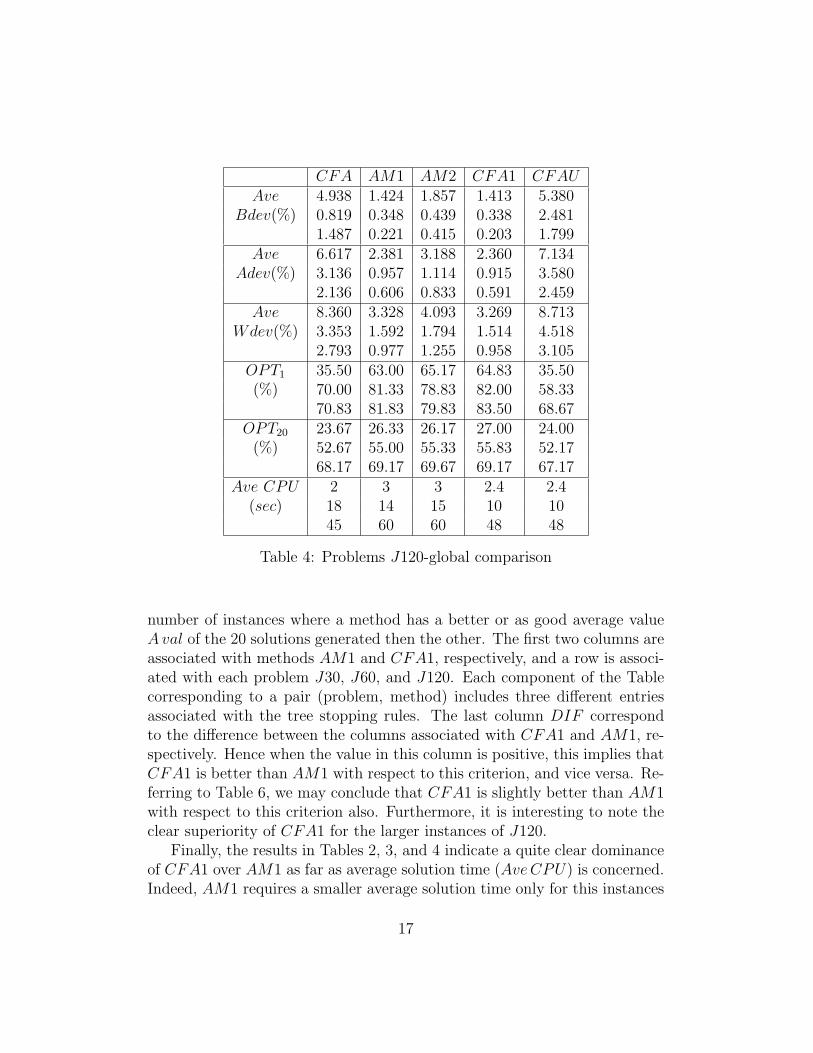
CFA AM1 AM2 CFA1 CFAUAve 4.938 1.424 1.857 1.413 5.380
Bdev(%) 0.819 0.348 0.439 0.338 2.4811.487 0.221 0.415 0.203 1.799
Ave 6.617 2.381 3.188 2.360 7.134Adev(%) 3.136 0.957 1.114 0.915 3.580
2.136 0.606 0.833 0.591 2.459Ave 8.360 3.328 4.093 3.269 8.713
Wdev(%) 3.353 1.592 1.794 1.514 4.5182.793 0.977 1.255 0.958 3.105
OPT1 35.50 63.00 65.17 64.83 35.50(%) 70.00 81.33 78.83 82.00 58.33
70.83 81.83 79.83 83.50 68.67OPT20 23.67 26.33 26.17 27.00 24.00(%) 52.67 55.00 55.33 55.83 52.17
68.17 69.17 69.67 69.17 67.17Ave CPU 2 3 3 2.4 2.4
(sec) 18 14 15 10 1045 60 60 48 48
Table 4: Problems J120-global comparison
number of instances where a method has a better or as good average valueAval of the 20 solutions generated then the other. The first two columns areassociated with methods AM1 and CFA1, respectively, and a row is associ-ated with each problem J30, J60, and J120. Each component of the Tablecorresponding to a pair (problem, method) includes three different entriesassociated with the tree stopping rules. The last column DIF correspondto the difference between the columns associated with CFA1 and AM1, re-spectively. Hence when the value in this column is positive, this implies thatCFA1 is better than AM1 with respect to this criterion, and vice versa. Re-ferring to Table 6, we may conclude that CFA1 is slightly better than AM1with respect to this criterion also. Furthermore, it is interesting to note theclear superiority of CFA1 for the larger instances of J120.
Finally, the results in Tables 2, 3, and 4 indicate a quite clear dominanceof CFA1 over AM1 as far as average solution time (Ave CPU) is concerned.Indeed, AM1 requires a smaller average solution time only for this instances
17

J30 J60 J120IAdev(%) 48.36 58.92 72.33I OPT1(%) 4.30 15.46 15.81I CPU(%) 16.67 11.11 6.25
Table 5: Percentage of improvement when using scheduling mode for thestopping criterion with 100 iterations
AM1 CFA1 DIF437 337 -100
J30 441 447 6401 455 54320 447 127
J60 414 436 -22430 420 -10392 414 22
J120 462 480 18503 527 24
Table 6: Pairwise comparison of AM1 and CAF1 with respect to the criterionADev(%)
in J30 when the stopping criterion is equal to 20 iterations. In all the othercases, the Ave CPU of AM1 is at least 20% (and reach up to 30%) largerthan for CFA1.
9 Conclusion
In this paper we follow up the nice idea due to Alcaraz and Maroto [1] ofincluding the scheduling mode into the activity list encoding of solutions tosolve the RCPSP with GAs. Our method use priority value encoding ratherthen activity list encoding. The numerical results indicate the superiority ofour method using scheduling mode (CFA1) over the one (CFA) withoutscheduling mode. This conclusion is consistent with the results in [1]. Thenfor the method of Alcaraz and Maroto, the numerical results indicate that,for the values of the parameters used, a one-point crossover operator (AM1)
18

seems more efficient than a two-points crossover operator (AM2). Similarly,for our method, a one-point crossover operator (CFA1) seems more efficientthan a uniform crossover operator (CFAU). Finally, comparing AM1 andCFA1, the numerical results indicate that CFA1 is slightly better as far assolution quality is concerned, and that the solution time for CFA1 is smaller,in general.
19
References
[1] J. Alcaraz, C. Maroto, A robust genetic algorithm for ressource alloca-tion in project scheduling. Annals of Operations Research, 102 (2001),83–109.
[2] T. Baar, P. Brucker, S. Knust, Tabu search algorithms for ressource-constrained project scheduling problems, in S. Voss, S. Martello, I. Os-man, C. Roucairol (Eds.), Metaheuristics : Advances and Trends inLocal Search Paradigms for Optimisation, Kluwer, 1997, pp. 1–18.
[3] F.F. Boctor, Some efficient multi-heuristic procedures for the ressource-constrained project scheduling problem, European Journal of Opera-tional Research, 49(1), (1990), 3–13.
[4] F.F. Boctor, Resource-constrained project scheduling by simulated an-nealing, International Journal of Production Research, 34 (8), (1996),2335–2351.
[5] K. Bouleimen, H. Lecocq, A new efficient simulated annealing algorithmfor the resource-constrained project scheduling problem and its multiplemode version, European Journal of Operational Research,, 149 (2003),268–281.
[6] K. Bouleimen, H. Lecocq, A new efficient simulated annealing algorithmfor the resource-constrained project scheduling problem, in: G. Bar-barosoglu, S. Karabati, L. Ozdamar, C. Ulasoy (Eds), Proceedings ofthe Sixth International Workshop on Project Management and Schedul-ing, Bogazici University Printing Office, Istanbul, 1998, pp. 19–22.
[7] P. Brucker, A. Drexl, R. Nohring, K. Neumann, E. Pesch, Resource-constrained project scheluding : Notation, models and methods, Euro-pean Journal of Operational Research, 112(1), (1999), 262–273.
[8] P. Brucker, S. Knust, A. Schoo, O. Thiele, A branch-and-bound algo-rithm for the resources-constrained project scheduling problem, Euro-pean Journal of Operational Research, 107, (1998), 272–288.
[9] N. Christofides, R. Alvarez-Valdes, J.M. Tamarit, Project schedulingwith resource constraints : A branch-and-bound approach, EuropeanJournal of Operational Research, 29(2), (1987), 262–273.
20
[10] L. Davis, Handbook of genetic algorithms, Van Nostrand Reinhold, NewYork, 1991.
[11] E. Demeulemeester, W. Herroelen, A branch-and-bound procedure forthe multiple resource-constrained project scheduling problem, Manage-ment Science, 38(12), (1992), 1803–1818.
[12] E. Demeulemeester, W. Herroelen, New benchmark results for theresource-constrained project scheduling problem, Management Science,43(11), (1995), 1485–1492.
[13] D.E. Goldberg, Genetic algorithms in search, optimization, and machinelearning, Addison Wesley, 1991.
[14] S. Hartmann, A competitive genetic algorithm for the resource-constrained project scheduling, Naval Research Logistics, 456,(1998),733–750.
[15] S. Hartmann, R. Kolisch, Experimental evaluation of state-of-the-artheuristics for the resource-constrained project scheduling problem, Eu-ropean Journal of Operational Research, 127, (2000), 394–407.
[16] W. Herroelen, E. Demeulemeester, B. De Reick, A classification schemefor project scheduling, In : J. Weglarz (Ed.), Project Scheduling : Re-cent Models, Algorithms and Applications, Kluwer Academic Publish-ers, Boston, 1999, pp. 1–26.
[17] W. Herroelen, E. Demeulemeester, B. De Reyck, Resource-constrainedproject scheluling – A survey of recent developments, Computers andOperations Research, 25(4), (1998), 279–302.
[18] J.H. Holland, Adaptation in natural and artificial systems, University ofMichigan Press, Ann Arbor, 1975.
[19] U. Kohlmorgen, H. Schmeck, K. Haase, Experiences with fine-grainedparallel genetic algorithms, Annals of Operations Research, 90, (1999),203–219.
[20] R. Kolisch, Efficient priority rule for the resource-constrained projectscheduling problem, Journal of Operational Management, 14, (1996),179–192.
21

[21] R. Kolisch, A. Drexl, Adaptative search for solving hard scheduling prob-lems, Naval Research Logistics, 43, (1996), 23–40.
[22] R. Kolisch, S. Hartmann, Heuristic algorithms for solving the resource-constrained project scheduling problem : Classification and computationanalysis, In : J. Weglarz (Ed.), Project Scheduling : Recent Models, Al-gorithms and Applications, Kluwer Academic Publishers, Boston, 1999,pp. 147–178.
[23] R. Kolisch, A. Sprecher, A. Drexl, Characterisation and generation of ageneral class of resource-constrained project scheduling problem, Man-agement Science, 41 (10), (1995), 1693–1703.
[24] J.K. Lee, Y.D. Kim, Search heuristics for the resource-constrainedproject scheduling problem, Journal of Operational Research Society,47(1996), 678–689.
[25] V.J. Leon, R. Balakrishman, Strenght and adaptability of problem-spacebased neighborhoods for resource-constrained scheduling, ORSpektrum,17, (1995), 173–182.
[26] A. Mingozzi, V. Maniezzo, S. Riccardelli, L. Bianco, An exact algo-rithm for project scheduling with resources constraints based on a newmathematical formulation, Management Science, 44, (1998), 714–729.
[27] J.H. Patterson, A comparison of exact approaches for solving the multi-ple constrained resource project scheduling problem, Management Sci-ence, 30(7), (1984), 854–867.
[28] E. Pinson, C. Prins, F. Rullier, Using tabu search for solving theresource-constrained project scheduling problem, In : Proceedings ofthe 4th International Workshop on Project Management and Schedul-ing, Leuven, Belgium, 1994, pp. 102–106.
[29] A. Schirmer, S. Riesenberg, Class-based control schemes forparametrized project scheduling heuristics, Working paper, Institutenfur Betriebswirtschaftslehre, Universitat Kiel, Kiel, Germany (1998).
22