Genetic Algorithm and Large Neighbourhood Search to Solve the Cell Formation Problem · 2010-09-07 · Genetic Algorithm and Large Neighbourhood Search to Solve the Cell Formation

___________________________

Genetic Algorithm and Large Neighbourhood Search to Solve the Cell Formation Problem Bouazza Elbenani Jacques A. Ferland Jonathan Bellemare August 2010 CIRRELT-2010-39

G1V 0A6

Bureaux de Montréal : Bureaux de Québec : Université de Montréal Université Laval C.P. 6128, succ. Centre-ville 2325, de la Terrasse, bureau 2642 Montréal (Québec) Québec (Québec) Canada H3C 3J7 Canada G1V 0A6 Téléphone : 514 343-7575 Téléphone : 418 656-2073 Télécopie : 514 343-7121 Télécopie : 418 656-2624

www.cirrelt.ca

Genetic Algorithm and Large Neighbourhood Search to Solve

the Cell Formation Problem

Bouazza Elbenani1, Jacques Ferland2,* Jonathan Bellemare2 1 Department of Computer Science, University Mohammed V, Avenue des Nations Unies, Agdal,

B.P. 554 Rabat-Chellah, Maroc 2 Interuniversity Research Centre on Enterprise Networks, Logistics and Transportation

(CIRRELT), and Department of Computer Science and Operations Research, Université de Montréal, C.P. 6128, succursale Centre-ville, Montréal, Canada H3C 3J7

Abstract. We first introduce a local search procedure to solve the cell formation problem

where each cell includes at least one machine and one part. The procedure applies

sequentially an intensification strategy to improve locally a current solution and a

diversification strategy destroying more extensively a current solution to recover a new

one. To search more extensively the feasible domain, a hybrid method is specified where

the local search procedure is used to improve each offspring solution generated with a

steady state genetic algorithm. The numerical results using 35 most widely used

benchmark problems indicate that the line search procedure can reduce to 1% the

average gap to the best-known solutions of the problems using an average solution time

of 0.64 seconds. The hybrid method can reach the best-known solution for 31 of the 35

benchmark problems, and improve the best-known solution of three others, but using

more computational effort.

Keywords. Cell formation problem, grouping efficiency, local search, destroy & recover

strategy, steady state genetic algorithm, uniform crossover.

Acknowledgements. This research was supported by the Natural Sciences and

Engineering Research Council of Canada (NSERC), grant (OGP0008312).

Results and views expressed in this publication are the sole responsibility of the authors and do not necessarily reflect those of CIRRELT. Les résultats et opinions contenus dans cette publication ne reflètent pas nécessairement la position du CIRRELT et n'engagent pas sa responsabilité. _____________________________

* Corresponding author: [email protected] Dépôt légal – Bibliothèque nationale du Québec, Bibliothèque nationale du Canada, 2010

© Copyright Elbenani, Ferland, Bellemare and CIRRELT, 2010

1. Introduction In group technology or in cellular manufacturing, a system including machines and parts are interacting. To maximize the efficiency of the system, a cell formation problem is solved in order to partition the system into subsystems that are as autonomous as possible in the sense that the interactions of the machines and the parts within a subsystem are maximized and that the interactions between machines and parts of other subsystems are reduced as much as possible. The cell formation problem is a NP hard optimization problem (Dimopoulos and Zalzala 2000). For this reason, several heuristic methods have been developed over the last forty years to generate good solutions in reasonable computational time. A very good survey of the methods is presented in Goncalves and Resende (2004) that review briefly the different methodologies used to solved the problem: cluster analysis, graph partitioning, mathematical programming, genetic (population based) algorithms, local search methods (tabu search, simulated annealing), and hybrids of these methods. The authors also indicate several references where the different methods are introduced. In this paper we introduce an approach similar to those in Goncalves and Resende (2004) and James et al. (2007). Our method is a hybrid integrating a Local Seach Algorithm (LSA) within a steady state Genetic Algorithm (GA) that are different from those used in Goncalves and Resende (2004) and James et al. (2007). The LSA includes two different procedures to intensify and diversify the search. They are applied successively for a fixed number of iterations. To intensify the search we modify successively the machines groups and the parts families until no modification can improve the current solution. To search more extensively the feasible domain, we partly destroy the current solution by selecting either a subset of machines or a subset of parts for which the assignment is modified. Then a recovering procedure allows generating a new solution by reassigning a new group to each machine or a new family to each part of the subset. The numerical results indicate that the LSA generates very good results using small computational time. But to improve even more the quality of the solution we use a hybrid method (HM) where each offspring solution generated with a steady state GA is improved with the LSA. The cell formation problem is described in Section 2. Additional constraints are included in our model insuring that each cell contains at least one machine and one part. The components of the LSA and of the GA are summarized in Sections 3 and 4, respectively. In Section 5, we compare the results obtained using the LSA and the HM with the best-known solutions for 35 benchmark problems commonly used by the authors to evaluate their methods. The LSA generate very good solutions in a short computational time, but the HM can reach the best known solution for 31 problems and improves the best-known solution for three other problems using reasonable computational time.

Genetic Algorithm and Large Neighbourhood Search to Solve the Cell Formation Problem

CIRRELT-2010-39 1

2. Problem formulation To formulate the cell formation problem, consider the following two sets

set of machines: 1, ,set of parts: 1, , .

I m i mJ n j n= == =

KK

The production incidence matrix ijA a⎡ ⎤= ⎣ ⎦ indicates the interactions between the machines and the parts:

1 if machine process part 0 otherwise.ij

i ja ⎧

= ⎨⎩

Furthermore, a part j may be processed by several machines. A production cell k ( )1, ,k K= K includes a subset (group) of machines kC I⊂ and a subset (family) of parts kF J⊂ . The problem is to determine a solution including K production cells

( ) ( ) ( ){ }1 1, = , , , ,K KC F C F C FK as autonomous as possible. Note that the K production cells induce partitions of the machines set and of the parts set:

{ }1 2 1 2

1 1

1 2

andand for all pairs of different cell indices and 1, ,

and .

K K

k k k k

C C I F F Jk k K

C C F Fφ φ

= =

∈

= =

UKU UKU

K

I I

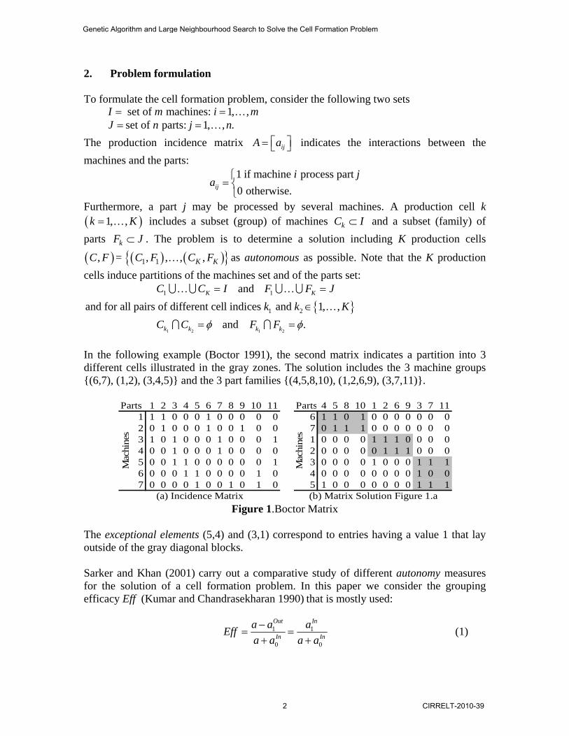
In the following example (Boctor 1991), the second matrix indicates a partition into 3 different cells illustrated in the gray zones. The solution includes the 3 machine groups {(6,7), (1,2), (3,4,5)} and the 3 part families {(4,5,8,10), (1,2,6,9), (3,7,11)}.

Figure 1.Boctor Matrix

The exceptional elements (5,4) and (3,1) correspond to entries having a value 1 that lay outside of the gray diagonal blocks. Sarker and Khan (2001) carry out a comparative study of different autonomy measures for the solution of a cell formation problem. In this paper we consider the grouping efficacy Eff (Kumar and Chandrasekharan 1990) that is mostly used:

1 1

0 0

Out In

In In

a a aEffa a a a−

= =+ +

(1)

Parts 1 2 3 4 5 6 7 8 9 10 11 Parts 4 5 8 10 1 2 6 9 3 7 111 1 1 0 0 0 1 0 0 0 0 0 6 1 1 0 1 0 0 0 0 0 0 02 0 1 0 0 0 1 0 0 1 0 0 7 0 1 1 1 0 0 0 0 0 0 03 1 0 1 0 0 0 1 0 0 0 1 1 0 0 0 0 1 1 1 0 0 0 04 0 0 1 0 0 0 1 0 0 0 0 2 0 0 0 0 0 1 1 1 0 0 05 0 0 1 1 0 0 0 0 0 0 1 3 0 0 0 0 1 0 0 0 1 1 16 0 0 0 1 1 0 0 0 0 1 0 4 0 0 0 0 0 0 0 0 1 0 07 0 0 0 0 1 0 0 1 0 1 0 5 1 0 0 0 0 0 0 0 1 1 1

Mac

hine

s

Mac

hine

s

(a) Incidence Matrix (b) Matrix Solution Figure 1.a


2 CIRRELT-2010-39

where 1 1

M P

iji j

a a= =

= ∑∑ denotes the total number of entries equal to 1 in the matrix A, 1Outa

denotes the number of exceptional elements, and 1 0and In Ina a are the numbers of one and of zero entries in the gray diagonal blocks, respectively. The objective function of the problem is maximizing Eff .

To formulate the mathematical formulation of the problem, we introduce the following binary variables:

{

{

for each pair 1, , ; 1, ,1 if machine belongs to cell 0 otherwise

for each pair 1, , ; 1, ,1 if part belongs to cell 0 otherwise.

ik

jk

i m k Ki kx

j n k Kj ky

= =

=

= =

=

K K

K K

To evaluate the objective function Eff, it is easy to verify that

( )

11 1 1

01 1 1

1 .

K m nout

ij ik jkk i j

K m nIn

ij ik jkk i j

a a a x y

a a x y

= = =

= = =

= −

= −

∑∑∑

∑∑∑

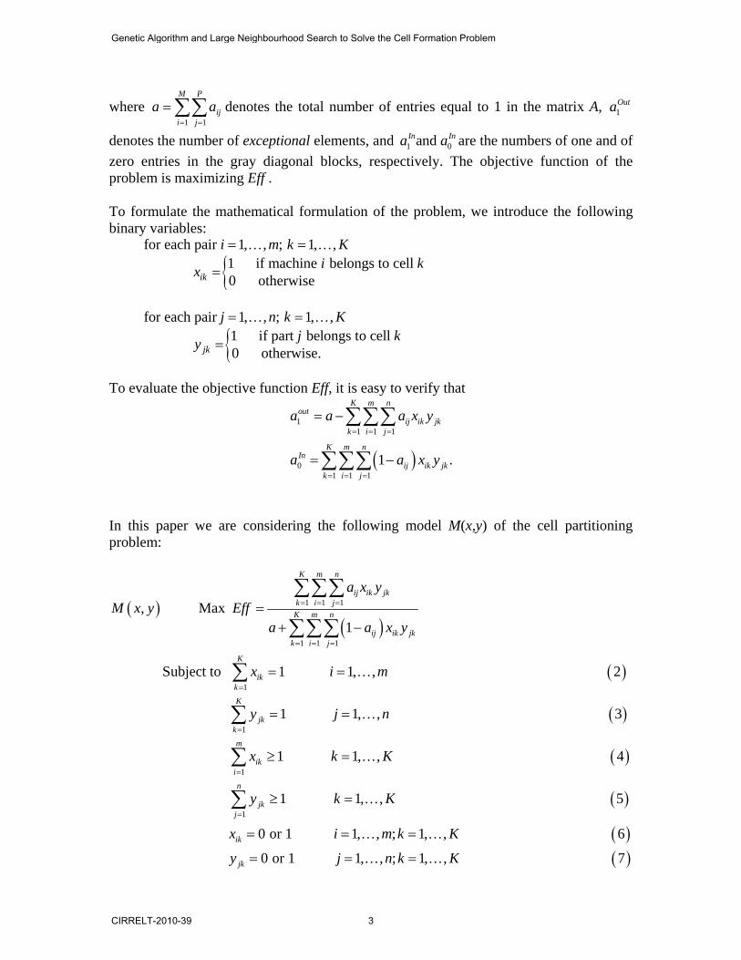
In this paper we are considering the following model M(x,y) of the cell partitioning problem:

( )( )

( )

( )

( )

( )

( )

1 1 1

1 1 1

1

1

1

1

, Max 1

Subject to 1 1, , 2

1 1, , 3

1 1, , 4

1 1, , 5

0 or 1 1, , ; 1, , 6

K m n

ij ik jkk i j

K m n

ij ik jkk i j

K

ikkK

jkkm

iki

n

jkj

ik

j

a x yM x y Eff

a a x y

x i m

y j n

x k K

y k K

x i m k K

y

= = =

= = =

=

=

=

=

=+ −

= =

= =

≥ =

≥ =

= = =

∑∑∑

∑∑∑

∑

∑

∑

∑

K

K

K

K

K K

( )0 or 1 1, , ; 1, , 7k j n k K= = =K K


CIRRELT-2010-39 3

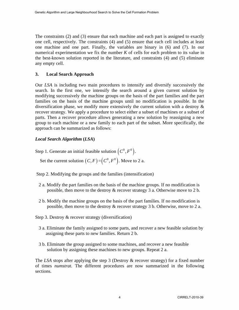
The constraints (2) and (3) ensure that each machine and each part is assigned to exactly one cell, respectively. The constraints (4) and (5) ensure that each cell includes at least one machine and one part. Finally, the variables are binary in (6) and (7). In our numerical experimentation we fix the number K of cells for each problem to its value in the best-known solution reported in the literature, and constraints (4) and (5) eliminate any empty cell. 3. Local Search Approach Our LSA is including two main procedures to intensify and diversify successively the search. In the first one, we intensify the search around a given current solution by modifying successively the machine groups on the basis of the part families and the part families on the basis of the machine groups until no modification is possible. In the diversification phase, we modify more extensively the current solution with a destroy & recover strategy. We apply a procedure to select either a subset of machines or a subset of parts. Then a recover procedure allows generating a new solution by reassigning a new group to each machine or a new family to each part of the subset. More specifically, the approach can be summarized as follows: Local Search Algorithm (LSA) Step 1. Generate an initial feasible solution ( )0 0,C F .

Set the current solution ( ),C F = ( )0 0,C F . Move to 2 a.

Step 2. Modifying the groups and the families (intensification) 2 a. Modify the part families on the basis of the machine groups. If no modification is possible, then move to the destroy & recover strategy 3 a. Otherwise move to 2 b. 2 b. Modify the machine groups on the basis of the part families. If no modification is possible, then move to the destroy & recover strategy 3 b. Otherwise, move to 2 a. Step 3. Destroy & recover strategy (diversification) 3 a. Eliminate the family assigned to some parts, and recover a new feasible solution by assigning these parts to new families. Return 2 b. 3 b. Eliminate the group assigned to some machines, and recover a new feasible solution by assigning these machines to new groups. Repeat 2 a. The LSA stops after applying the step 3 (Destroy & recover strategy) for a fixed number of times numstrat. The different procedures are now summarized in the following sections.


4 CIRRELT-2010-39

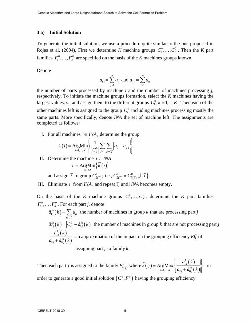
3 a) Initial Solution To generate the initial solution, we use a procedure quite similar to the one proposed in Rojas et al. (2004). First we determine K machine groups 0 0

1 , , KC CK . Then the K part families 0 0

1 , , KF FK are specified on the basis of the K machines groups known. Denote

1 1 and

n m

i ij j ijj i

a a a a= =

= =∑ ∑

the number of parts processed by machine i and the number of machines processing j, respectively. To initiate the machine groups formation, select the K machines having the largest values ia , and assign them to the different groups 0 , 1, .kC k K= K Then each of the other machines left is assigned to the group 0

kC including machines processing mostly the same parts. More specifically, denote INA the set of machine left. The assignments are completed as follows:

I. For all machines i INA∈ , determine the group

( )0

01, , 1

1ArgMink

k k

n

ij i jk K j i Ck

k i a aC= = ∈

⎧ ⎫⎪ ⎪= −⎨ ⎬⎪ ⎪⎩ ⎭

∑ ∑K

.

II. Determine the machine i INA∈ ( ){ }ArgMin

i INAi k i

∈=

and assign ( ) ( ) ( ) { }0 0 0 to group ; i.e., .k i k i k ii C C C i= U

III. Eliminate from i INA , and repeat I) until INA becomes empty. On the basis of the K machine groups 0 0

1 , , KC CK , determine the K part families 0 0

1 , , KF FK . For each part j, denote

( )0

1 the number of machines in group that are processing part k

Inj ij

i C

a k a k j∈

= ∑%

( ) ( )00 1 the number of machines in group that are not processing part In In

j k ja k C a k k j= −% %

( )( )

1

0

an approximation of the impact on the grouping efficiency of

assigning part to family .

Inj

Inj j

a kEff

a a k

j k

+

%

%

( ) ( ) ( )( )

10

1, , 0

Then each part is assigned to the family where ArgMax Inj

Ink jk K j j

a kj F k j

a a k=

⎧ ⎫⎪ ⎪= ⎨ ⎬+⎪ ⎪⎩ ⎭%

K

%%

%in

order to generate a good initial solution ( )0 0,C F having the grouping efficiency


CIRRELT-2010-39 5

( )( )

( )( )

11

01

.

nInj

jn

Inj

j

a k jEff

a a k j

=

=

=+

∑

∑

%%

%%

Note that if some family 0

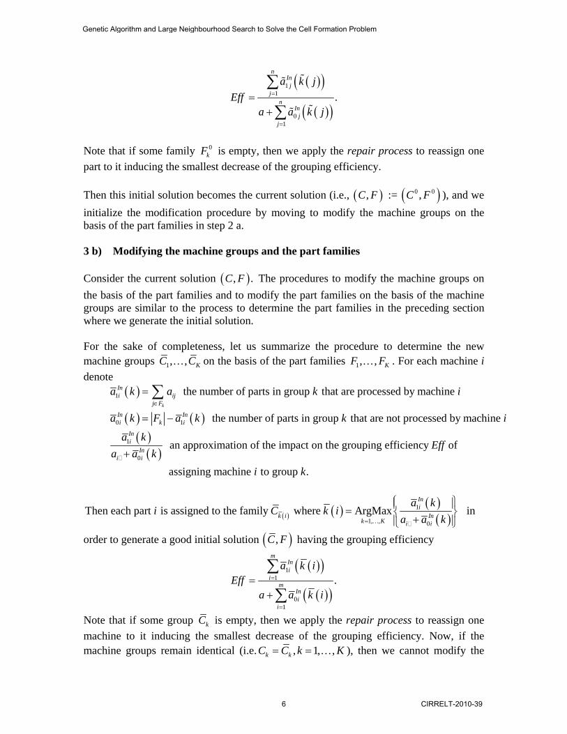
kF is empty, then we apply the repair process to reassign one part to it inducing the smallest decrease of the grouping efficiency. Then this initial solution becomes the current solution (i.e., ( ),C F := ( )0 0,C F ), and we initialize the modification procedure by moving to modify the machine groups on the basis of the part families in step 2 a. 3 b) Modifying the machine groups and the part families Consider the current solution ( ), .C F The procedures to modify the machine groups on the basis of the part families and to modify the part families on the basis of the machine groups are similar to the process to determine the part families in the preceding section where we generate the initial solution. For the sake of completeness, let us summarize the procedure to determine the new machine groups 1, , KC CK on the basis of the part families 1, , KF FK . For each machine i denote

( )1 the number of parts in group that are processed by machine k

Ini ij

j Fa k a k i

∈

= ∑

( ) ( )0 1 the number of parts in group that are not processed by machine In Ini k ia k F a k k i= −

( )( )

1

0


assigning machine to group .

Ini

Ini i

a kEff

a a ki k

+

( ) ( ) ( )( )

1

1, , 0

Then each part is assigned to the family where ArgMax Ini

k i Ink K i i

a ki C k i

a a k=

⎧ ⎫⎪ ⎪= ⎨ ⎬+⎪ ⎪⎩ ⎭K

in

order to generate a good initial solution ( ),C F having the grouping efficiency

( )( )

( )( )

11

01

.

mIni

im

Ini

i

a k iEff

a a k i

=

=

=+

∑

∑

Note that if some group kC is empty, then we apply the repair process to reassign one machine to it inducing the smallest decrease of the grouping efficiency. Now, if the machine groups remain identical (i.e. , 1, ,k kC C k K= = K ), then we cannot modify the


6 CIRRELT-2010-39

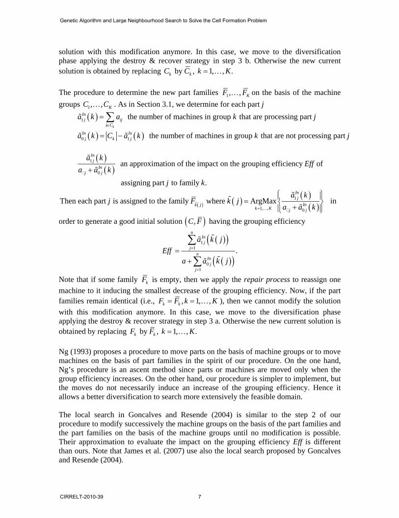
solution with this modification anymore. In this case, we move to the diversification phase applying the destroy & recover strategy in step 3 b. Otherwise the new current solution is obtained by replacing by , 1, , .k kC C k K= K The procedure to determine the new part families 1, , KF FK on the basis of the machine groups 1, , KC CK . As in Section 3.1, we determine for each part j

( )1 the number of machines in group that are processing part k

Inj ij

i Ca k a k j

∈

= ∑%

( ) ( )0 1 the number of machines in group that are not processing part In Inj k ja k C a k k j= −% %

( )( )

1

0


assigning part to family .

Inj

Inj j

a kEff

a a k

j k

+

%

%

( ) ( ) ( )( )

1

1, , 0

Then each part is assigned to the family where ArgMax Inj

Ink jk K j j

a kj F k j

a a k=

⎧ ⎫⎪ ⎪= ⎨ ⎬+⎪ ⎪⎩ ⎭%

K

%%%

in

order to generate a good initial solution ( ),C F having the grouping efficiency

( )( )

( )( )

11

01

.

nInj

jn

Inj

j

a k jEff

a a k j

=

=

=+

∑

∑

%%

%%

Note that if some family kF is empty, then we apply the repair process to reassign one machine to it inducing the smallest decrease of the grouping efficiency. Now, if the part families remain identical (i.e., , 1, ,k kF F k K= = K ), then we cannot modify the solution with this modification anymore. In this case, we move to the diversification phase applying the destroy & recover strategy in step 3 a. Otherwise the new current solution is obtained by replacing by , 1, , .k kF F k K= K Ng (1993) proposes a procedure to move parts on the basis of machine groups or to move machines on the basis of part families in the spirit of our procedure. On the one hand, Ng’s procedure is an ascent method since parts or machines are moved only when the group efficiency increases. On the other hand, our procedure is simpler to implement, but the moves do not necessarily induce an increase of the grouping efficiency. Hence it allows a better diversification to search more extensively the feasible domain. The local search in Goncalves and Resende (2004) is similar to the step 2 of our procedure to modify successively the machine groups on the basis of the part families and the part families on the basis of the machine groups until no modification is possible. Their approximation to evaluate the impact on the grouping efficiency Eff is different than ours. Note that James et al. (2007) use also the local search proposed by Goncalves and Resende (2004).


CIRRELT-2010-39 7

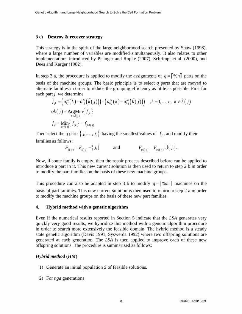
3 c) Destroy & recover strategy This strategy is in the spirit of the large neighborhood search presented by Shaw (1998), where a large number of variables are modified simultaneously. It also relates to other implementations introduced by Pisinger and Ropke (2007), Schrimpf et al. (2000), and Dees and Karger (1982). In step 3 a, the procedure is applied to modify the assignments of %q n= ⎡ ⎤⎢ ⎥ parts on the basis of the machine groups. The basic principle is to select q parts that are moved to alternate families in order to reduce the grouping efficiency as little as possible. First for each part j, we determine

( ) ( )( )( ) ( ) ( )( )( ) ( )

( )( )

{ }

( ){ } ( )

1 1 0 0 , 1, , ,

ArgMin

Min

In In In Injk j j j j

jkk k j

j jk jok jk k j

f a k a k j a k a k j k n k k j

ok j f

f f f

≠

≠

= − − − = ≠

=

= =

%

%

% % %% % % % K

Then select the q parts { }1, , qj jK having the smallest values of jf , and modify their families as follows:

( ) ( ) { } ( ) ( ) { }and .i i i ii ik j k j ok j ok jF F j F F j= − =% % % % U

Now, if some family is empty, then the repair process described before can be applied to introduce a part in it. This new current solution is then used to return to step 2 b in order to modify the part families on the basis of these new machine groups. This procedure can also be adapted in step 3 b to modify %q m= ⎡ ⎤⎢ ⎥ machines on the basis of part families. This new current solution is then used to return to step 2 a in order to modify the machine groups on the basis of these new part families. 4. Hybrid method with a genetic algorithm Even if the numerical results reported in Section 5 indicate that the LSA generates very quickly very good results, we hybridize this method with a genetic algorithm procedure in order to search more extensively the feasible domain. The hybrid method is a steady state genetic algorithm (Davis 1991, Syswerda 1992) where two offspring solutions are generated at each generation. The LSA is then applied to improve each of these new offspring solutions. The procedure is summarized as follows: Hybrid method (HM)

1) Generate an initial population S of feasible solutions.

2) For nga generations


8 CIRRELT-2010-39

• Select two parent solutions from S. • Perform a crossover operation to generate two new offspring solutions. • If necessary, apply the repair process to each offspring solution to insure that no

group or no family are empty. • Perform a mutation operation on each offspring solution with probability pm. • Apply the LSA to improve each offspring solution. • Update the population by keeping the best S solutions from the current

population and the two improved offspring solutions generated. To generate the initial population, we first introduce the solution generated by the LSA in S. Then each of the other solution in S is obtained according to the following procedure. First we decide to generate either the machine groups or the part families, each alternative having a probability of 0.5. If the first alternative is selected, then each machine i is assigned randomly to a group k. We also prevent that each group is not empty by applying a repair process to move a machine from the group including the most to the empty group. Then the part families are determined on the basis of these machine groups as in Section 3 a). The LSA is applied to improve the solution which is included in the population S. The procedure to complete the second alternative is similar. The role of machines and parts are exchanged. To complete the genetic algorithm, a proper encoding of the solutions is required. A feasible solution ( ) ( ) ( ){ }1 1, = , , , ,K KC F C F C FK is encoded as a vector having ( )n m+ components

( )1 1, , , , ,n mP P M MK K where is the index of the family including part , 1, ,

and is the index of the group including machine , 1, , .j

i

P j j n

M i i m

=

=

K

K

Note that this encoding is similar to the one used by Mahdavi et al. (2007). It is different from the Goncalves and Resende (2004) encoding involving only the machines, and from the James et al. (2007) encoding involving the parts, the machines, and the groups. Furthermore the genetic algorithm used in these two references is also different. Indeed a genetic algorithm with random keys and a group genetic algorithm due to Falkenauer (1998) are used by Goncalves and Resende (2004) and James et al. (2007), respectively. The two parent solutions are selected according to a tournament strategy. Four individuals are selected randomly from the population S, and the best of these solutions becomes the first parent solution. The second parent solution is selected similarly. To determine the two offspring solutions, a uniform crossover is completed. More specifically, suppose that the two parent solutions are

( )( )

1 1 1 11 1

2 2 2 21 1

, , , , ,

, , , , , .

n m

n m

P P M M

P P M M

K K

K K


CIRRELT-2010-39 9

Generate a crossover mask vector of bits having ( )n m+ elements

( )1 , 1, , , , .n n n mB B B B+ +K K

The offspring solutions ( )1 1, , , , , , 1, 2l l l ln mOP OP OM OM l =K K , are specified as follows:

1 1 2 2

1 2 2 1

1 1 2 2

1 2 2 1

for 1, , ,if 1, then and

if 0, then and

for 1, , ,if 1, then and

if 0, then and .

j j j j j

j j j j j

n i i i i i

n i i i i i

j nB OP P OP P

B OP P OP P

i mB OM M OM M

B OM M OM M+

+

=

= = =

= = =

=

= = =

= = =

K

K

A repair process is applied to introduce a part or a machine in any empty family or group. The mutation operator is also applied to modify slightly an offspring solution. Four different elements are selected randomly:

{ } { }{ } { }

a part 1, , a machine 1, ,

a family 1, , a group 1, , .

j n i m

k K k K

∈ ∈

∈ ∈

% K K

% K K

Then the part j% is moved to the family kF% , and the machine i to the group kC . Note that the elements are selected to avoid creating empty group or family. 5. Numerical results In this paper we consider 35 benchmark problems that are commonly used by authors to evaluate the efficiency of their methods. In table 1, for each problem we indicate the reference where it is specified (Problem source), its size (values of m, n, and K), the value of its best-known solution (Best-known solution), and one of the reference where the best-known solution is obtained (Best-known solution ref.). Note that we mentioned only one reference generating the best-known solution even if the solution has also been obtained with other solution method. Moreover the best-known can be found in the following references (Goncalves and Resende 2004, James et al. 2007, Luo and Tang 2009, Mahdavi et al. (2007), and Tunnukij and Hicks 2009) including the results obtained with different methods. The purpose of this analysis is to evaluate the efficiency of the procedures LSA and HM by comparing their values for the grouping efficiency Eff with the best-known values. Furthermore we compare the computational times of LSA and HM in order to see how it increases in order to improve the value of the grouping efficiency Eff. The numerical results are summarized in Table 2. The algorithms are coded in ++C , and the numerical tests are completed on a Personal Computer equipped with an AMD processor running at 2.002 GHz and having 2048 Kilobytes of central memory.


10 CIRRELT-2010-39

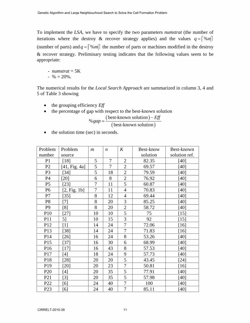
To implement the LSA, we have to specify the two parameters numstrat (the number of iterations where the destroy & recover strategy applies) and the values %q n= ⎡ ⎤⎢ ⎥

(number of parts) and %q m= ⎡ ⎤⎢ ⎥ the number of parts or machines modified in the destroy & recover strategy. Preliminary testing indicates that the following values seem to be appropriate:

- numstrat = 5K - % = 20%. The numerical results for the Local Search Approach are summarized in column 3, 4 and 5 of Table 3 showing

• the grouping efficiency Eff • the percentage of gap with respect to the best-known solution

( )( )

best-known solution%

best-known solutionEff

gap−

=

• the solution time (sec) in seconds.

Problem number

Problem source

m n K Best-know solution

Best-known solution ref.

P1 [18] 5 7 2 82.35 [40] P2 [41, Fig. 4a] 5 7 2 69.57 [40] P3 [34] 5 18 2 79.59 [40] P4 [20] 6 8 2 76.92 [40] P5 [23] 7 11 5 60.87 [40] P6 [2, Fig. 1b] 7 11 4 70.83 [40] P7 [35] 8 12 4 69.44 [40] P8 [7] 8 20 3 85.25 [40] P9 [8] 8 20 2 58.72 [40] P10 [27] 10 10 5 75 [15] P11 5] 10 15 3 92 [15] P12 [1] 14 24 7 72.06 [16] P13 [38] 14 24 7 71.83 [16] P14 [26] 16 24 8 53.26 [40] P15 [37] 16 30 6 68.99 [40] P16 [17] 16 43 8 57.53 [40] P17 [4] 18 24 9 57.73 [40] P18 [28] 20 20 5 43.45 [24] P19 [20] 20 23 7 50.81 [16] P20 [4] 20 35 5 77.91 [40] P21 [3] 20 35 5 57.98 [40] P22 [6] 24 40 7 100 [40] P23 [6] 24 40 7 85.11 [40]


CIRRELT-2010-39 11

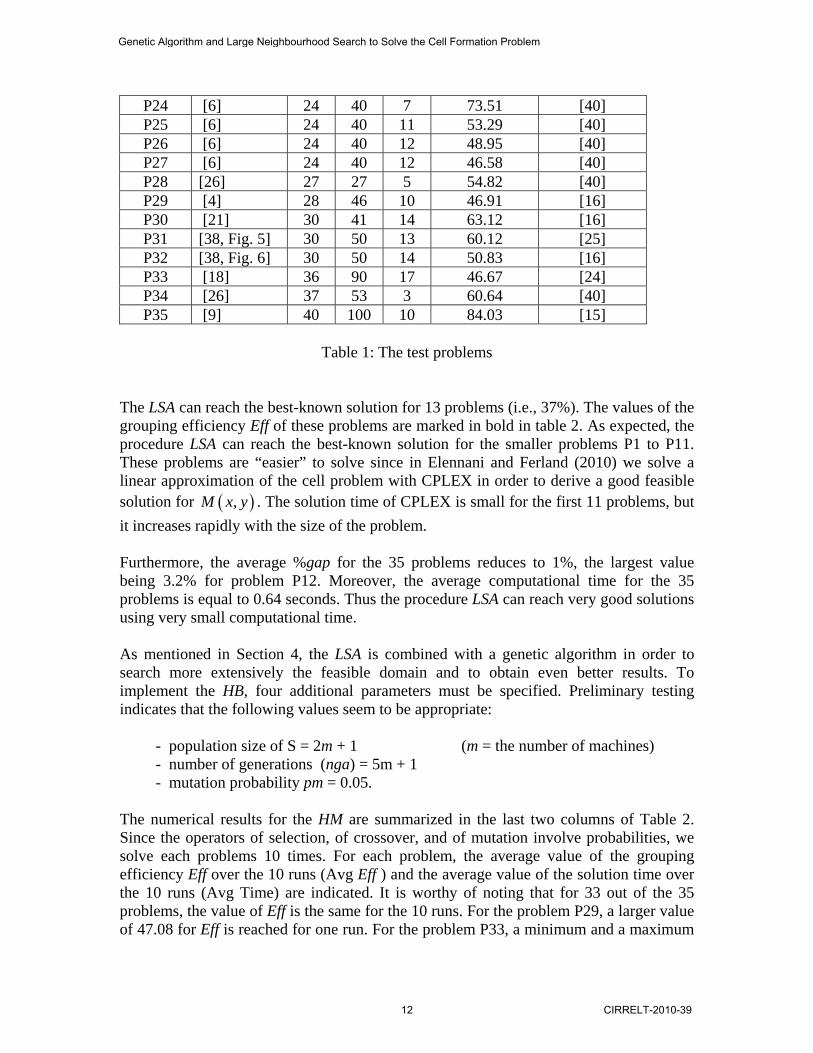
P24 [6] 24 40 7 73.51 [40] P25 [6] 24 40 11 53.29 [40] P26 [6] 24 40 12 48.95 [40] P27 [6] 24 40 12 46.58 [40] P28 [26] 27 27 5 54.82 [40] P29 [4] 28 46 10 46.91 [16] P30 [21] 30 41 14 63.12 [16] P31 [38, Fig. 5] 30 50 13 60.12 [25] P32 [38, Fig. 6] 30 50 14 50.83 [16] P33 [18] 36 90 17 46.67 [24] P34 [26] 37 53 3 60.64 [40] P35 [9] 40 100 10 84.03 [15]

Table 1: The test problems

The LSA can reach the best-known solution for 13 problems (i.e., 37%). The values of the grouping efficiency Eff of these problems are marked in bold in table 2. As expected, the procedure LSA can reach the best-known solution for the smaller problems P1 to P11. These problems are “easier” to solve since in Elennani and Ferland (2010) we solve a linear approximation of the cell problem with CPLEX in order to derive a good feasible solution for ( ),M x y . The solution time of CPLEX is small for the first 11 problems, but it increases rapidly with the size of the problem. Furthermore, the average %gap for the 35 problems reduces to 1%, the largest value being 3.2% for problem P12. Moreover, the average computational time for the 35 problems is equal to 0.64 seconds. Thus the procedure LSA can reach very good solutions using very small computational time. As mentioned in Section 4, the LSA is combined with a genetic algorithm in order to search more extensively the feasible domain and to obtain even better results. To implement the HB, four additional parameters must be specified. Preliminary testing indicates that the following values seem to be appropriate:

- population size of S = 2m + 1 (m = the number of machines) - number of generations (nga) = 5m + 1 - mutation probability pm = 0.05.

The numerical results for the HM are summarized in the last two columns of Table 2. Since the operators of selection, of crossover, and of mutation involve probabilities, we solve each problems 10 times. For each problem, the average value of the grouping efficiency Eff over the 10 runs (Avg Eff ) and the average value of the solution time over the 10 runs (Avg Time) are indicated. It is worthy of noting that for 33 out of the 35 problems, the value of Eff is the same for the 10 runs. For the problem P29, a larger value of 47.08 for Eff is reached for one run. For the problem P33, a minimum and a maximum


12 CIRRELT-2010-39

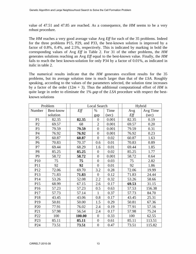
value of 47.51 and 47.85 are reached. As a consequence, the HM seems to be a very robust procedure. The HM reaches a very good average value Avg Eff for each of the 35 problems. Indeed for the three problems P15, P29, and P33, the best-known solution is improved by a factor of 0.8%, 0.4%, and 2.5%, respectively. This is indicated by marking in bold the corresponding values of Avg Eff in Table 2. For 31 of the other problems, the HM generates solutions reaching an Avg Eff equal to the best-known value. Finally, the HM fails to reach the best known-solution for only P34 by a factor of 0.01%, as indicated in italic in table 2. The numerical results indicate that the HM generates excellent results for the 35 problems, but its average solution time is much larger than that of the LSA. Roughly speaking, according to the values of the parameters selected, the solution time increases by a factor of the order (12m + 3). Thus the additional computational effort of HM is quite large in order to eliminate the 1% gap of the LSA procedure with respect the best-known solutions Problem Local Search Hybrid Number Best-know

solution Eff

% gap

Time (sec)

Avg Eff

Avg Time (sec)

P1 82.35 82.35 0 0.001 82.35 0.19 P2 69.57 68 2 0.001 69.57 0.20 P3 79.59 79.59 0 0.001 79.59 0.31 P4 76.92 76.92 0 0.001 76.92 0.23 P5 60.87 60.87 0 0.02 60.87 1.63 P6 70.83 70.37 0.6 0.01 70.83 0.89 P7 69.44 68.29 1.6 0.01 69.44 1.85 P8 85.25 85.25 0 0.02 85.25 1.77 P9 58.72 58.72 0 0.001 58.72 0.64 P10 75 75 0 0.03 75 2.82 P11 92 92 0 0.01 92 1.86 P12 72.06 69.70 3.2 0.28 72.06 19.99 P13 71.83 71.83 0 0.12 71.83 24.44 P14 53.26 52.08 2.2 0.32 53.26 58.66 P15 68.99 67.15 2.6 0.17 69.53 31.15 P16 57.23 57.23 0.5 0.63 57.53 156.38 P17 57.73 57.14 1 0.37 57.73 84.70 P18 43.45 43.06 0.8 0.17 43.45 25.31 P19 50.81 50.00 1.5 0.29 50.81 67.36 P20 77.91 76.02 2.4 0.19 77.91 57.16 P21 57.98 56.54 2.4 0.17 57.98 75.24 P22 100 100.00 0 0.33 100 62.55 P23 85.11 85.11 0 0.61 85.11 113.51 P24 73.51 73.51 0 0.47 73.51 115.82


CIRRELT-2010-39 13

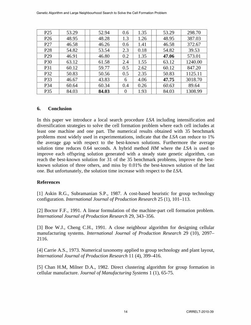
P25 53.29 52.94 0.6 1.35 53.29 298.70 P26 48.95 48.28 1.3 1.26 48.95 387.03 P27 46.58 46.26 0.6 1.41 46.58 372.67 P28 54.82 53.54 2.3 0.18 54.82 39.53 P29 46.91 46.80 0.2 1.35 47.06 573.01 P30 63.12 61.58 2.4 1.55 63.12 1240.00 P31 60.12 59.77 0.5 2.62 60.12 847.20 P32 50.83 50.56 0.5 2.35 50.83 1125.11 P33 46.67 43.83 6 4.06 47.75 3018.70 P34 60.64 60.34 0.4 0.26 60.63 89.64 P35 84.03 84.03 0 1.93 84.03 1308.99

6. Conclusion In this paper we introduce a local search procedure LSA including intensification and diversification strategies to solve the cell formation problem where each cell includes at least one machine and one part. The numerical results obtained with 35 benchmark problems most widely used in experimentations, indicate that the LSA can reduce to 1% the average gap with respect to the best-known solutions. Furthermore the average solution time reduces 0.64 seconds. A hybrid method HM where the LSA is used to improve each offspring solution generated with a steady state genetic algorithm, can reach the best-known solution for 31 of the 35 benchmark problems, improve the best-known solution of three others, and miss by 0.01% the best-known solution of the last one. But unfortunately, the solution time increase with respect to the LSA. References [1] Askin R.G., Subramanian S.P., 1987. A cost-based heuristic for group technology configuration. International Journal of Production Research 25 (1), 101–113. [2] Boctor F.F., 1991. A linear formulation of the machine-part cell formation problem. International Journal of Production Research 29, 343–356. [3] Boe W.J., Cheng C.H., 1991. A close neighbour algorithm for designing cellular manufacturing systems. International Journal of Production Research 29 (10), 2097–2116. [4] Carrie A.S., 1973. Numerical taxonomy applied to group technology and plant layout, International Journal of Production Research 11 (4), 399–416. [5] Chan H.M, Milner D.A., 1982. Direct clustering algorithm for group formation in cellular manufacture. Journal of Manufacturing Systems 1 (1), 65-75.


14 CIRRELT-2010-39

[6] Chandrasekharan M.P., Rajagopalan R., 1989. GROUPABILITY: an analysis of the properties of binary data matrices for group technology. International Journal of Production Research 27(6), 1035–1052. [7] Chandrasekharan M.P., Rajagopalan R., 1986a. MODROC: an extension of rank order clustering for group technology. International Journal of Production Research 24 (5), 1221–1233. [8] Chandrasekharan M.P., Rajagopalan R., 1986b. An ideal seed non-hierarchical clustering algorithm for cellular manufacturing, International Journal of Production Research 24 (2), 451–464. [9] Chandrasekharan M.P., Rajagopalan R., 1987. ZODIAC: an algorithm for concurrent formation of part-families and machine-cells. International Journal of Production Research 25 (6), 835–50. [10] Davis L, 1991. Handbook of Genetic Algorithms. New York: Van Nostrand Reinhold. [11] Dees Jr W.A., Karger P.G.,1982. Automated Rip-up and Reroute Techniques. Proceedings of the 19th Conference on Design Automation, New York: IEEE Press, 432–439. [12] Dimopoulos C, Zalzala A.M.S., 2000. Recent developments in evolutionary computations for manufacturing optimization: problems, solutions, and comparisons. IEEE Transactions on Evolutionary Computations 4, 93–113. [13] Elbenani B., Ferland J.A., 2010. An exact method for solving the manufacturing cell formation problem. Publication # 2010–37, CIRRELT, Université de Montréal, Montréal, Canada. [14] Falkenauer E., 1998. Genetic algorithms for grouping problems. New York: Wiley. [15]Goncalves J., Resende M.G.C., 2004. An evolutionary algorithm for manufacturing cell formation. Computers&Industrial Engineering 47, 247–273. [16] James T.J., Brown E.C., Keeling K.B., 2007. A hybrid Grouping Genetic Algorithm for the cell formation problem. Computers & Operations Research 34, 2059–2079. [17] King J.R., 1980. Machine-component grouping in production flow analysis: an approach using a rank order clustering algorithm. International Journal of Production Research 18, 213–232. [18] King J.R., Nakornchai V., 1982. Machine-component group formation in group technology: review and extension. International Journal of Production Research 20 (2), 117–133.


CIRRELT-2010-39 15

[19] Kumar C.S., Chandrasekharan M., 1990. Grouping efficiency: a quantitative criterion for goodness of block diagonal forms of binary matrices in group technology. International Journal of Production Research 28, 233–243. [20] Kumar K.R., Kusiak A., Vannelli A.,1986. Grouping of parts and components in flexible manufacturing systems. European Journal of Operational Research 24 (1986) 387–397. [21] Kumar K.R., Vannelli A., 1987. Strategic subcontracting for efficient disaggregated manufacturing. International Journal of Production Research 25 (12), 1715–1728. [22] Kusiak A. , Cho M., 1992. Similarity coefficient algorithm for solving the group technology problem. International Journal of Production Research 30 (11), 2633–2646. [23] Kusiak A., Chow W.S., 1987. Efficient solving of the group technology problem. Journal of Manufacturing Systems 6 (2), 117–124. [24] Luo L., Tang L., 2009. A hybrid approach of ordinal optimization and iterated local search for manufacturing cell formation. International Journal of Advance Manufacturing Technology 40, 362–372. [25] Mahdavi I. , Paydar M.M., Solimanpur M., Heidarzade A., 2009. Genetic algorithm approach for solving a cell formation problem in cellular manufacturing. Expert Systems with Applications 36, 6598–6604. [26] McCormick W.T., Schweitzer P.J., 1972. White T.W., Problem decomposition and data reorganization by a clustering technique. Operations Research 20, 993–1009. [27] Mosier C.T., Taube L., 1985. The facets of group technology and their impact on implementation. OMEGA 13 (5), 381–391. [28] Mosier C., Taube L., 1985. Weighted similarity measure heuristics for the group technology machine clustering problem. OMEGA 13 (6), 577–583. [29] Ng S., 1993. Worst-Case Analysis of an Algorithm for Cellular Manufacturing Systems. European Journal of Operational Research 69 (3), 384–398. [30] Pisinger D., Ropke S., 2007. A General Heuristic for Vehicle Routing Problems. Computers & Operations Research 34, 2403–2435. [31] Rojas W., Solar M., Chacon M., FerlandJ.A., 2004. An Efficient Genetic Algorithm to Solve the Manufacturing Cell Formation Problem. In : I.C. Parmee ed. Adaptive Computing in Design and Manufacture VI, , Springer-Verlag, 173–184.


16 CIRRELT-2010-39

[32] Sarker B., Khan M., 2001. A comparison of existing grouping efficiency measures and a new grouping efficiency measure. IIE Transactions 33, 11–27. [33] Schrimpf G., Schneider J., Stamm-Wilbrandt H., Dueck G., 2000. Record Breaking Optimization Results Using the Ruin and Recreate Principle. Journal of Computational Physics 159 (2), 139–171. [34] Seifoddini H., 1989. A note on the similarity coefficient method and the problem of improper machine assignment in group technology applications. International Journal of Production Research 27 (7), 1161–1165. [35] Seifoddini H., Wolfe P.M., 1986. Application of the similarity coefficient method in group technology. IIE Transactions 18 (3), 271–277. [36] Shaw P., 1998. Using Constraint Porgramming and Local Search Methods to Solve Vehicle Routing Problems. In: M. Maher, J.F. Puget eds., Fourth International Conference on Principles and Practice of Constraint Programming CP-98, Lecture Notes in Computer Science 1520, 417–431. [37] SrinivasanG. , Narendran T.T., Mahadevan B., 1990. An assignment model for the part-families problem in group technology. International Journal of Production Research 28 (1), 145–152. [38] Stanfel L.E., 1985. Machine clustering for economic production. Engineering Costs and Production Economics 9, 73–81. [39] Syswerda G., 1992. A Study of Reproduction in Generational and Steady-State Genetic Algorithms. In: G.J.E. Rawlings ed. Foundations of Genetic Algorithms. Morgan Kaufmann, San Mateo, CA, 94–101. [40] Tunnukij T., Hicks C., 2009. An Enhanced Genetic Algorithm for solving the cell formation problem. International Journal of Production research 47, 1989–2007. [41] Waghodekar P.H., Sahu S., 1984. Machine-component cell formation in group technology MACE. International Journal of Production Research 22, 937–948.


CIRRELT-2010-39 17

Documents

Genetic Algorithm and Large Neighbourhood Search to Solve the Cell Formation Problem · 2010-09-07 · Genetic Algorithm and Large Neighbourhood Search to Solve the Cell Formation