GENESIS support for ns and SSFNet

Anand SastryDepartment of Computer Science, RPI, Tory, NY 12180

February 8, 2003

Abstract

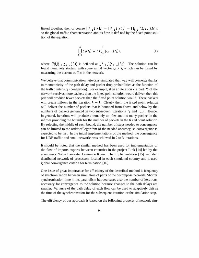
The complexity and dynamics of the Internet is driving the demand forscalable and efficient network simulation. Yet, parallelizing network sim-ulation at packet level does not work efficiently and therefore do not scaleto large number of processors because of tight synchronization between net-work components. To overcome this problem we designed a method in whicha large network is decomposed into parts and each part is simulated indepen-dently and concurrently with the others. These parts exchange informationperiodically about the packet delays and losses along the paths within eachpart. Each part iterates over the selected simulated time interval until theexchanged information changes less than the prescribed tolerance.

Each decomposed part may represent a subnet or a subdomain of theentire network, thereby mirroring the network structure in the simulation de-sign. The proposed method is independent of the specific simulator techniqueemployed to run simulators of the parts of the decomposed network. Hence,it is a general method for efficient parallelization of network simulation basedon convergence to the fixed point solution of inter-part traffic. The methodcan be used in all applications in which the speed of the simulation is ofessence, such as: on-line network simulation, network management, ad-hocnetwork design, emergency network planning, large network simulation ornetwork protocol verification under extreme conditions (large flows).

The paper describes this method we call Genesis(General Network Simu-lation Integration System), its implementation based on ns and SSFNet sim-ulator, and its performance for sample communication networks. We alsodescribe how Genesis has been ported to parallelize BGP (Border GatewayProtocol), with a goal to provide a novel outbound load-balancing techniqueusing BGP LOCAL PREF settings and aided by online simulation

1

1 Introduction

The major difficulty in simulating large networks at the packet level is the enor-mous computational power needed to execute all events that packets undergo inthe network [12]. The usual approach to providing required vast computationalresources relies on parallelization of an application to take advantage of a largenumber of processors running concurrently. Such parallelization does not workefficiently for network simulations at packet level because of tight synchroniza-tion between network components [11]. To overcome this difficulty, we designed amethod described in this paper, in which a large network is decomposed into partsand each part is simulated independently and simultaneously with the others. Eachpart represents a subnet or a subdomain of the entire network. These parts are con-nected to each other through edges that represent communication links existing inthe simulated network. In addition, we partition the total simulation time into sep-arate simulation time intervals selected in such a way that the traffic characteristicschange little during each time interval.

In the initial (zero) iteration of the simulation process, each part assumes on its ex-ternal in-links either no traffic, if this the the first simulated interval (alternatively,the initial external traffic may be defined by the real-time measurements of the sim-ulated network), or the traffic defined by the packet delays and drop rate defined inthe previous simulation time interval for external domains. Then, each part simu-lates its internal traffic, and computes the resulting outflow of packets through itsout-links.

Figure 1: Progress of the Simulation Execution

ii

In the subsequent�����

iteration, the inflow into each part from the other parts willbe generated based on the outflows measured by each part in the iteration

�����.

Once the inflows to each part in iteration�

are close enough to their counterpartsin the iteration

���, the iteration stops and the simulation either progresses to the

next simulation time interval or completes execution and produces the final results(see Figure 1).

More formally, consider a network � ����������� , where � is a set of nodes and �(a subset of Cartesian product ����� ), is a set of unidirectional links connectingthem (bidirectional links are simply represented as a pair of unidirectional links).Let ��������� � � ���"!#� be a disjoint partitioning of the nodes, each partition modeledby a simulator. For each subset �%$ , we can define a set of external out-links as& $ �'�)(*� $ ���� � � $ � , in-links as + $ �'�)(,��� � � $ �-��� $ , and local links as�.$/�0�)(�1$2���1$ .The purpose of a simulator 34$ , that models partition �%$ of the network, is to char-acterize traffic on the links in its partition in terms of a few parameters changingslowly compared to the simulation time interval. In the implementation presentedin this paper, we characterize each traffic as an aggregation of the flows, and eachflow is represented by the activity of its source and the packet delays and losseson the path from its source to the boundary of that part. Since the dynamics ofthe source can be faithfully represented by the copy of the source replicated to theboundary, the traffic is characterized by the packet delays and losses on the relevantpaths. Thanks to queuing at the routers and the aggregated effect of many flows onthe size of the queues, the path delays and packet drop rates change more slowlythan the traffic itself.

It should be noted that we are also experimenting with the direct method of rep-resenting the traffic on the external links as a self-similar traffic defined by a fewparameters. These parameters can be used to generate the equivalent traffic us-ing on-line traffic generator described in [17]. No matter which characterization ischosen, based on such characterization, the simulator can find the overall charac-terization of the traffic through the nodes of its subnet. Let 5768�:9;� be a vector oftraffic characterization of the links in set 9 in

�-th iteration. Each simulator can

be thought of as defining a pair of functions:

5�6<� & $=�.��>?$@�A5�6#B � ��+C$=�D�E�25�6<���F$:�.�HG?$��A5�6IB � ��+C$=�D�(or, symmetrically, 5I68��+C$J�E�K5�6L���.$J� can be defined in terms of 5M6IB � � & $=�D� .Each simulator can then be run independently of others, using the measured orpredicted values of 5I6<��+C$=� to compute its traffic. However, when the simulators are

iii

linked together, then of course � !$�� � 5�68��+ $ �*��� !$�� � 5�68� & $ �*��� !$�� � > $ �A5�6IB � ��+ $ �D� ,so the global traffic characterization and its flow is defined by the fixed point solu-tion of the equation.

!�$�� � 5�6L��+C$J�.�����

!�$�� � �A5�6IB � ��+C$J�D�E� (1)

where ����� !$�� � �A5�6IB � ��+C$:�D� is defined as � !$�� � >?$D�A5�6#B � ��+C$J�D� . The solution can befound iteratively starting with some initial vector 5 ��+C$J� , which can be found bymeasuring the current traffic in the network.

We believe that communication networks simulated that way will converge thanksto monotonicity of the path delay and packet drop probabilities as the function ofthe traffic intensity (congestion). For example, if in an iteration

�a part �2$ of the

network receives more packets than the fixed point solution would deliver, then thispart will produce fewer packets than the fixed point solution would. These packetswill create inflows in the iteration

��� �. Clearly then, the fixed point solution

will deliver the number of packets that is bounded from above and below by thenumbers of packets generated in two subsequent iterations + 6 and +�6� � . Hence,in general, iterations will produce alternately too few and too many packets in theinflows providing the bounds for the number of packets in the fixed point solution.By selecting the middle of each bound, the number of steps needed to convergencecan be limited to the order of logarithm of the needed accuracy, so convergence isexpected to be fast. In the initial implementations of the method, the convergencefor UDP traffic and small networks was achieved in 2 to 3 iterations.

It should be noted that the similar method has been used for implementation ofthe flow of imports-exports between countries in the project Link [14] led by theeconomics Noble Laureate, Lawrence Klein. The implementation [15] includeddistributed network of processors located in each simulated country and it usedglobal convergence criteria for termination [16].

One issue of great importance for efficiency of the described method is frequencyof synchronization between simulators of parts of the decompose network. Shortersynchronization time limits parallelism but decreases also the number of iterationsnecessary for convergence to the solution because changes to the path delays aresmaller. Variance of the path delay of each flow can be used to adaptively definethe time of the synchronization for the subsequent iteration or the simulation step.

The efficiency of our approach is based on the following property of network sim-

iv

ulation:

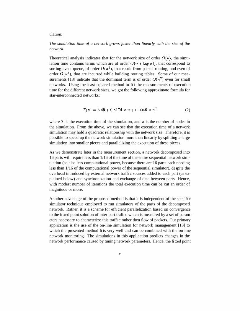
The simulation time of a network grows faster than linearly with the size of thenetwork.

Theoretical analysis indicates that for the network size of order& ��� � , the simu-

lation time contains terms which are of order& ����� ����� ��� �D� , that correspond to

sorting event queue, of order& ���#� , that result from packet routing, and even of

order& �����#� , that are incurred while building routing tables. Some of our mea-

surements [13] indicate that the dominant term is of order& ��� �� even for small

networks. Using the least squared method to fit the measurements of executiontime for the different network sizes, we got the following approximate formula forstar-interconnected networks:

� ��� � ���8����� � � ��� ��� ����� � � � � � ��� ��� (2)

where�

is the execution time of the simulation, and � is the number of nodes inthe simulation. From the above, we can see that the execution time of a networksimulation may hold a quadratic relationship with the network size. Therefore, it ispossible to speed up the network simulation more than linearly by splitting a largesimulation into smaller pieces and parallelizing the execution of these pieces.

As we demonstrate later in the measurement section, a network decomposed into16 parts will require less than 1/16 of the time of the entire sequential network sim-ulation (so also less computational power, because there are 16 parts each needingless than 1/16 of the computational power of the sequential simulator), despite theoverhead introduced by external network traffic sources added to each part (as ex-plained below) and synchronization and exchange of data between parts. Hence,with modest number of iterations the total execution time can be cut an order ofmagnitude or more.

Another advantage of the proposed method is that it is independent of the specificsimulator technique employed to run simulators of the parts of the decomposednetwork. Rather, it is a scheme for efficient parallelization based on convergenceto the fixed point solution of inter-part traffic which is measured by a set of param-eters necessary to characterize this traffic rather then flow of packets. Our primaryapplication is the use of the on-line simulation for network management [13] towhich the presented method fits very well and can be combined with the on-linenetwork monitoring. The simulations in this application predicts changes in thenetwork performance caused by tuning network parameters. Hence, the fixed point

v

solution found by our method is with high probability the point into which the realnetwork will evolve. However, this is a still an open issue under what conditionswe can guarantee that the fixed point solution is unique, and if it is not, when thesolution found by the method is the same as the point that the real network reaches.

The method can be used in all applications in which the speed of the simulation isof essence, such as:

� on-line network simulation,

� ad-hoc network design,

� emergency network planning,

� large network simulation,

� network protocol verification under extreme conditions (large flows).

2 Implementation

Our current simulation platform is the ns network simulator [3]. A simulationsis defined in ns by Tcl scripts which can also be used to interface the core of thesimulator. The kernel of the simulation system is written in C++. The ease ofadding extensions and rich suite of the network protocols made ns a popular andcommon, albeit not too efficient, platform for research in networking. Hence, webelieve that implementing our method within ns will enable others to experimentwith our system.

Our extensions to ns enable collaboration among individual parts into which thesimulated network is divided. Since network domains are convenient granules forsuch partitioning, we will refer to these parts as simulations domains or domainsin short. Each domain is simulated by a separate copy of ns running on a uniqueprocessor. The implementation specifics are described in the sections below.

2.1 New Features Added to ns

To accomplish per processor based domain simulation the following extensionwere added to ns.

vi

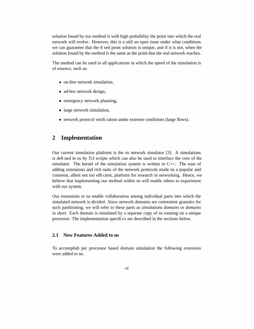
Figure 2: Active Domain with Connections to Other Domains

� The ability to suspend the simulation to enable exchange of data on pathdelays using message passing between processors simulating individual do-mains. During the simulation freeze, each individual simulation domain ex-changes information on packets generated and dropped along links leavingthe domain (cf. Figure 2).

The network in Figure 2 is split into three individual domains, named 1, 2and 3. Each of the domain simulations runs concurrently with the others andthey exchange information about the path delays incurred by packets leavingthe domain. The interval for exchange of this information is user config-urable (in the Tcl script). For example, each domain may run its individualsimulations for one second from � -th to � �;�

-st second of the simulationtime, and pause thereafter, Then, information about delays of packets leav-ing the domain during this time interval is passed onto the target domain towhich these packets are directed. If these delays differ significantly fromwhat was assumed in the target domain, the simulation of the time interval��� � � � � � is repeated. Otherwise, the simulation progresses to the time in-terval ��� � � � � ��� � . The threshold value of the difference between thecurrent delays and the previous ones under which the simulation is allowedto progress in time it is set by the user. This threshold impacts the speed ofthe simulation progress and defines the precision of the simulation results.

New event for the ns scheduler, Freeze is defined generically. It pauses thesimulation at intervals defined by the user. During the event execution, it ex-ecutes functions provided by the user in Freeze definition. On return, Freeze

vii

reactivates the simulation.

� The ability to record information about the delays and drop rate experiencedby the packets leaving the domain. Each delay measures the time expiredfrom the instance a packet leaves its source to the time it reaches the do-main boundary. Packet drop rates are computed for each flow separately.Also recorded is information about each packet source and its intended des-tination. Having this information enables us to replicate the source from theoriginal domain to the boundary of the target domain (sources in skeletons ofdomains 2 and 3 in Figure 2) and postpone an arrival of each packet producedby the replicated source at the domain boundary by the delay measured inthe source (and transient, if necessary) domains. Also, with probability de-fined by packet drop rates, packets are randomly dropped during the passageto the boundary of the destination domain (D boxes in Figure 2).

� The ability to define domain members and identify individual sources withinthe domain that generate packets intended for nodes external to the domain.This feature enables us to directly connect a source to the destination domainto which it sends packets. We refer to such replicated source as a fake sourceand to the link that connects it to the domain internal nodes as a fake link,as explained below. The domain is defined by the user using a Tcl levelcommand which takes as its parameters the nodes that the user marks asbelonging to the domain. Then, the simulation of this domain is created bydeactivating all domains external to the selected domain.

2.2 Details of modifications to ns

2.2.1 Domain definition: Domain is a Tcl-level scripting command that is usedto define the nodes which are part of the domain for the current simulation. In thefirst iteration of the simulation the traffic sources outside the domain are inactive.The traffic generated within the domain is recorded and the statistics calculated. Inthe following iterations, the sources active within other domains with a link to thedomain in question are activated.

When a domain declaration is made in the Tcl script, the nodes defined as a pa-rameter to this command are stored in the form of a list. Each time a new domainis defined, the new node list is added to a domain list (a list of lists). The userselected domain is made active. Any link with one end connected to a node in thisdomain and the other end connected to a node in another domain is defined as a

viii

cut-link. All packets sent on these links are collected for their delay and drop ratecomputation.

Source generators connected to sources outside the active domain are deactivated.This is done by a new Tcl script statement that attaches an inactive status to nodesoutside the active domain (cf. 2.2.3. Traffic Generator description below).

2.2.2 Connector: The connector performs the function of receiving, processingand then delivering the packets to the neighboring node or dropping the packets.A modification has been made to this connector class which now has the addedfunctionality of filtering out packets destined for the nodes outside the domain andstoring them for statistical data calculation.

A connector object is generally associated with a link. When a link is set up, thesimulator checks if this link connects nodes in different domains. If this is the case,this link is classified as a cross-link and the connector associated with this link ismodified to record packets flowing across it. Each such packet is either forwardedto the neighboring node or is marked as leaving the domain based on its destination.

2.2.3 Traffic Generator: TrafficGenerator Class is used to generate traffic flowsaccording to a timer. This class is modified, so that for the domain simulation, thetraffic sources can be activated or deactivated. Initially, at the start of the simula-tion, the traffic generator suppresses nodes outside the domain from generating anytraffic.

2.2.4 Fake Link: Fake links are used to connect the fake sources to a particularcross-link on the border of the destination domain. When a fake traffic source isconnected to a domain by a fake link, the packets generated by this source are sentinto the domain via the fake link and not the regular links which are set up by theuser network configuration file. The fake link adds a delay and, with certain prob-ability, drops the packet to simulate packet’s behavior during passage through theregular route. With the fake traffic sources and fake links, the statistical data fromthe simulation of another domain are collected, and the traffic to the destinationdomain is regenerated.

When a fake link is built, the source connector and the destination connector mustbe specified. A fake link shortens the route between the two connector objects.Each connector is identified by the nodes on both ends of it. Link connectors aremanaged in the border object as a link list. The flow id to build up a fake link isspecified, one fake link is used for one flow.

ix

Fake link is used to simulate a particular flow, so when the features (packet de-lay and drop rate) of this flow change, the fake link object needs to be updated.After updating the parameters of the fake link object, the performance of the cor-responding fake link changes immediately. Fake links themselves are managed inthe border object as a link list.

2.2.5 Connectors with Fake Targets: In the original version of ns, connectors aredefined as an NsObject with only a single neighbor. But our new ns simulationrequired this definition to be changed to build fake links to shortcut the routes fordifferent packet flows. These fake links are set up according to the network trafficflows and each flow from the fake sources will need a separate fake link. The flowsthat go through one source connector may reach different cross-link connectors atthe destination border, so there will be fake links connecting this connector to somedifferent connectors. Different flows going into one connector are sent to differentfake links, which are defined as fake targets here. Thus, the connector could nowbe defined as an NsObject with one neighbor and a list of fake targets. When thefake connection is enabled in a connector, this connector would have a list of fakelinks (fake targets), and would classify the incoming packets by flow id and sendthem to the correct destinations.

The connector class will maintain a list of fake targets. Once a new fake link is setup from this connector, it will be added to this connector’s fake target list (this isdone by the shortcut method defined in the Border class).

2.2.6 Border: Border is a new class added to the ns. It is the most importantclass in the domain simulation. A border object represents the active domain in thecurrent simulation. The main functionality of the border class includes:

� Initializing the current domain: setting up the current domain id, assigningnodes to different domains, setting up the date exchange etc.

� Collecting and maintaining information about the simulation objects, suchas a list of traffic source objects, a list of the connector objects and a list ofthe fake link objects maintained by the border object.

� Implementing and controlling the fake traffic sources: setting up and updat-ing fake links, etc.

The border object is set up first, and its reference its made available to all objects inthe simulation. A lot of other ns classes need to refer to the variables and methods

x

in the border object. The border class has an array which for each simulation objectstores the domain name to which this object belong. This information is collectedfrom domain description files that are created by the domain object implementa-tion. The names are created for the files assigned to each domain to store somepersistent data needed for inter-domain data exchange and restoration of the statefrom the checkpoint.

All traffic source objects created in the simulation are stored. These traffic sourcescan be deactivated or activated using the flow id. All the connector objects createdin the simulation are stored. These connectors are identified by the two nodes towhich they are connected. The connector information is used to create fake links.

The traffic sources outside the current active domain are deactivated while settingup the network and domains. When a fake link is set up for a flow, the traffic sourceof this flow will be reactivated. The border class searches the traffic source list tofind the object, and calls the reactivate() method of the matching source object toreactivate this flow.

When the border receives flow information from other domains, it will set up a fakelink for this flow, and initialize the parameter of the fake link using the receivedstatistical data. When setting up a fake link, it goes through the connector list tofind the source and the destination of the connector objects, and then shortcutsthe route between them by adding a fake target into the source connector. All thecreated fake link objects are stored in the border as a linked list ready for furtherupdate.

2.2.7 Checkpointing: This feature has been included in ns to enable the simulationto easily rerun over the same simulation time interval. We use diskless checkpoint-ing, in which each client process creates a child when it leaves a freeze point. Thechild is suspended, but preserves a state of the parent at the freeze time. The parentproceed to the next freeze point. Once there, the parent decides whether to returnto the previous state, in which case it unfreezes the child and then kills itself, orto continue the simulation to the next time interval, in which case the suspendedchild is killed. This method is efficient because the process memory is not dupli-cated initially; later only pages that become different for the parent and child areduplicated during execution of the parent. The only significant cost is the executionof fork statement creating a child, which however is several orders of magnitudesmaller than saving state to disk. More details have been provided in a separatesection later.

2.2.8 Synchronizing Individual Domain Simulations: Individual domain simu-

xi

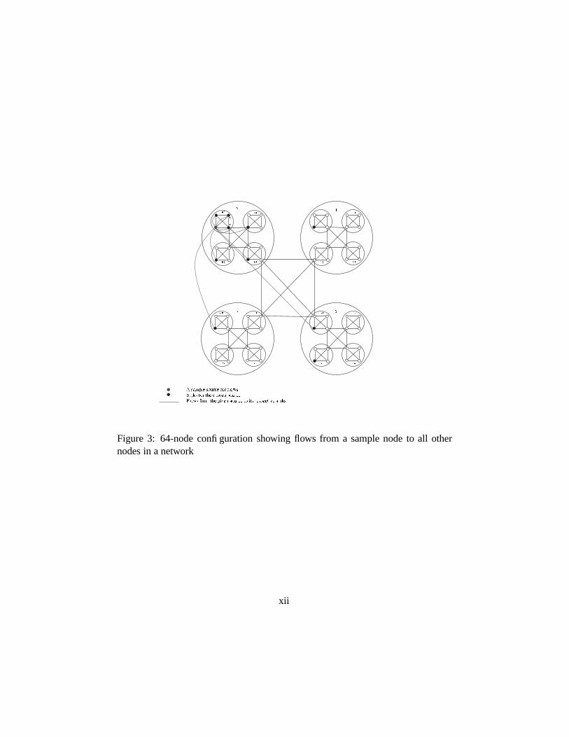
Figure 3: 64-node configuration showing flows from a sample node to all othernodes in a network

xii

lations are distributed across multiple processors using a client-server architecture.Multiple clients connect to a single server that handles the message passing be-tween them. The server is defined as a single process to avoid the overhead ofdealing with multiple threads and/or processes. The server uses two maps (datastructures). One map keeps track of the number of clients that have already sup-plied the delay data for the destination domain. The other map is toggled by clientsthat need to perform checkpointing. All messages to the server are preceded byMessage Identification Parameters which identify the state of the client. A deci-sion whether to checkpoint the current state or to restore the saved state is made bythe client based on the comparison of packet delays and drop rates in two subse-quent iterations.

A client indicates to the server whether it requires checkpointing in the contentsof the message itself. A client which has to checkpoint causes all other clients toblock until it has resent the data to the server and the server has delivered it to thedestination domain (in other words a domain on another machine). This is achievedby exchanging the maps at the end of each iteration during the simulation freeze.

The steps of collaboration of simulators and the server are shown in Figure 1.

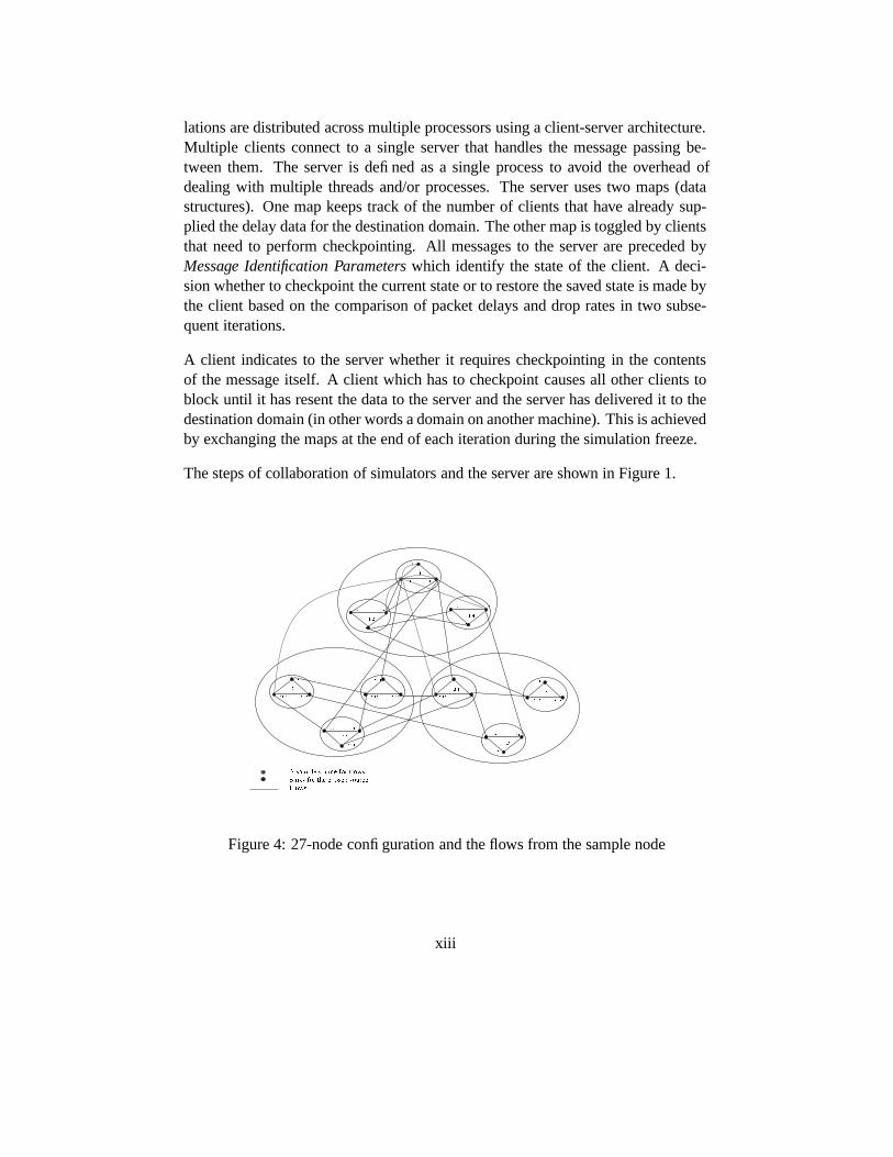
Figure 4: 27-node configuration and the flows from the sample node

xiii

3 Performance

We use two sample network configurations, one with 64 and the other with 27nodes to test the performance of our simulation method. Both of these networksare divided into classes of domains. The rate at which sources generate traffic arevaried to generate temporal congestion in the network, especially at the nodes atthe borders of the domains. All sources produce Constant Bit Rate (CBR) trafficwith constant packet size of 64 bytes.

The 64-node network is designed with a great deal of symmetry. The smallestdomain size is four nodes; there is full connectivity between these nodes. Foursuch domains together are considered as a larger domain in which there is fullconnectivity between the four sub-domains. Finally, four large domains are fullyconnected and form the entire network configuration (cf. Figure 3).

The 27-node network is a PINNI network [10] with a hierarchical structure. Itssmallest domain is composed of three nodes. Three such domains form a largerdomain and three large domains form the entire network (cf. Figure 4).

3.1 64-node network

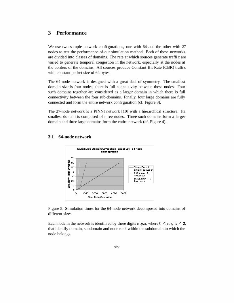
Figure 5: Simulation times for the 64-node network decomposed into domains ofdifferent sizes

Each node in the network is identified by three digits � ��� ��� , where���

�/��� ��� � � ,that identify domain, subdomain and node rank within the subdomain to which thenode belongs.

xiv

Each node has nine flows originating from it. In addition, each node also acts as asink to nine flows. The flows from a node � ��� ��� go to nodes:�/��� � � � �0� � � � �/��� � � � � � � � � � ��� � � � � � � � ��/� � � �0� � � � ��� �/� � � � � � � � ��� � � � � � � � � � ���� � �0� � � � ��� ��� � � � � � � � ��� ��� � � � � � � � ��� ���Thus, this configuration forms a hierarchical and symmetrical structure on whichthe simulation is tested for scalability and speedup.

In a set of measurements, the sources at the borders of domains produce packets atthe rate of 20000 packets/sec for half of the simulation time. The bandwidth of thelink is 1.5Mbps. Thus, certain links are definitely congested and congestion mayspread to some other links as well. For the other half of the simulation time, thesesources produce 1000 packets per second. Since such flows require less bandwidththan provided by the links connected to each source, congestion is not an issue. Allother sources produce packets at the rate of 100 packets/sec for the entire simula-tion. For these measurements we defined sources that produced only CBR trafficand the speedup was measured by comparing simulation times of domains to thesimulation time of the entire network (excluding synchronization time).

We measured speed up for this configuration over simulation of 60 seconds of traf-fic. The simulation interval was set at 14.9999 seconds, resulting in five freezes.The simulation speedup with 16 domains (each with size of four nodes) was ap-proximately 18, as shown in Table 1 and Figure 5. The decomposed simulationrequired at most two iterations to converge to the solution in each simulation timeinterval. Despite repetitive simulations over some of the intervals, the decomposedsimulations achieved superlinear speedup. The differences in the total number ofpackets in each flow, the number of dropped packets and the sizes of the queues atthe routers were well below 1% for all three different domain sizes.

3.2 27-node configuration

The network configuration shown in Figure 4, the PINNI network adopted from [10],consists of 27 nodes arranged into 3 different levels of domains containing three,nine and 27 nodes, respectively. Each node has six flows to other nodes in theconfiguration and is receiving six flows from other nodes. The flows from a node�/��� ��� can be expressed as:�/��� � � � �0� � � � �/��� � � � � � � � ��/� � � �0� � � �8��� �/� � � � � � � �8���� � �0� � � �8��� ��� � � � � � � �8��� ���

xv

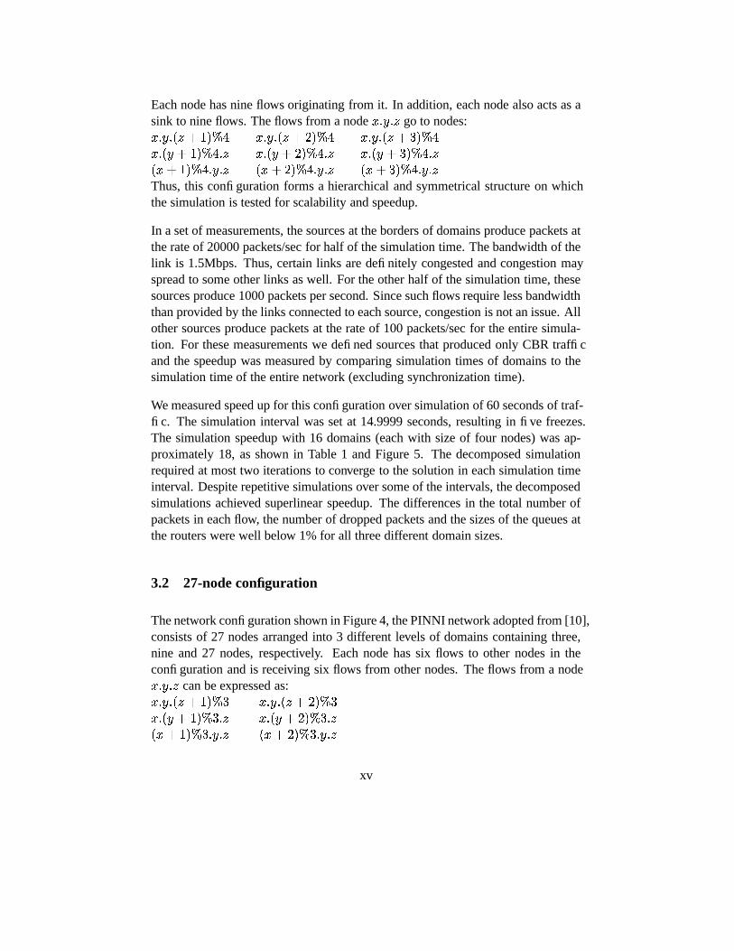
Figure 6: Simulation times for 27-node network decomposed into domains of dif-ferent sizes

size of domain 27-nodes 64-nodeslarge = 1 proc/domain 3885.5 1714.5medium = 3(4) procs/domains 729.5 414.7small = 9(16) procs/domains 341.9 95.1speed up for small domain 11.4 18.0

Table 1: Measurements results on IBM Netfinities (times are in seconds)

In these set of measurements, as above, the sources at the borders of domainsproduce packets at the rate of 20000 packets/sec for half of the simulation time.The bandwidth of the link is 1.5Mbps. Thus, congestion is definitely produced oncertain links shown above and congestion may be produced on certain other links.For the other half of the simulation, these sources produce 1000 packets whichis less than the total bandwidth of the links connected to each of them. All othersources produce packets at the rate of 100 packets/sec for the entire simulation. Wemeasured the speed up for this configuration over 60 seconds of simulated traffic.The simulation interval was set at 14.9999 seconds, resulting in five freezes.

The speedup of simulation with 9 domains was approximately 11 compared witha single network (sequential) run. The graphs of the results are shown in Figure 6and the numerical results are presented in Table 1. This configuration is less regularthen the 64-node configuration and as result, the number of iterations needed forconvergences varied from two to four. Despite that, the decomposed simulationsshowed superlinear speedup. The differences in the total number of packets in eachflow, the number of dropped packets and the sizes of the queues at the routers were

xvi

well below 1% for all three different domain sizes.

4 Checkpointing - What and Why?

Checkpointing is a new feature which has been added to mitigate the effect of largevariance in Average Delay calculations for each of the Fake Sources pumping datainto each domain.

This checkpointing routine is called when on comparing the current statistical dataof average delays more than 10 percent variance is found. This means that the data(delays and drop probabilities) used in the previous iteration was in error and thisdata is updated by the delays obtained in the current iteration.

We wanted to introduce this feature with the least amount of code restructur-ing as possible hence we are using the Unix Signal features which allows us tostop(suspend) and restart a process as explained in the following pages.

4.1 Some History

The original idea was to use third part libraries one of them being the DynamiteCheckpointing library since it was a transparent checkpointing library for Unix.

This library works by writing the address space of the process and its mappedshared libraries to a file. This is done when a process receives a signal USR1 whichis a user signal. This is also called preserving the memory image of the process.

This checkpointing file is an ELF executable which first loads the text and datasegment into the memory followed by the heap and stack segments respectively.

Once the loading has occurred siglongjmp is made to jump back to the checkpointsignal handler to restore the signal mask.

The state of the signal handlers are restored using the sigaction and the previouslyopen files are restored. When the signal handler returns, the operating systemrestores all CPU registers and the application resumes execution.

xvii

4.2 Current Checkpointing Implementation

Some drawbacks that were found in using the third party library were:

� The implementation depended on the image of the process address and dataspace being copied to an ELF executable which involves IO operations andutilizes a significant amount of disk space.

� Also this implementation of checkpointing depends on certain third party li-braries which are currently not widely supported by many operating systems.

Hence an alternative algorithm is listed below:

At the instant of Freeze:

� The main process forks a child process. This child process is suspended untilthe main process signals it to awaken.(This is currently implemented usingSIGSTOP and SIGCONT signals).

� The main process proceeds to the end of execution. At the point of the nextfreeze if the process needs to go back (ie. iterate) it sends a wake up sig-nal(SIGCONT) to the child process which originally in suspend (SIGSTOP)mode. Now this child process becomes the main process.

� If instead the process realizes that it can go ahead, it awakens the child pro-cess and kills it(SIGKILL).

Thus it can be observed that at any one point in execution time there is only oneprocess. These steps are repeated as per the number of freeze events required.

4.3 Advantages

The advantage of this technique is that we just keep a copy of the process in mem-ory in the child process and there is no need to resort to any IO.

xviii

5 BGP Extensions to SSFNet for Genesis support

5.1 Introduction

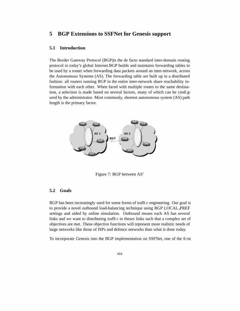
The Border Gateway Protocol (BGP)is the de facto standard inter-domain routingprotocol in today’s global Internet.BGP builds and maintains forwarding tables tobe used by a router when forwarding data packets around an inter-network, acrossthe Autonomous Systems (AS). The forwarding table are built up in a distributedfashion: all routers running BGP in the entire inter-network share reachability in-formation with each other. When faced with multiple routes to the same destina-tion, a selection is made based on several factors, many of which can be config-ured by the administrator. Most commonly, shortest autonomous system (AS) pathlength is the primary factor.

Figure 7: BGP between AS’

5.2 Goals

BGP has been increasingly used for some forms of traffic engineering. Our goal isto provide a novel outbound load-balancing technique using BGP LOCAL PREFsettings and aided by online simulation. Outbound means each AS has severallinks and we want to distributing traffic to theses links such that a complex set ofobjectives are met. These objective functions will represent more realistic needs oflarge networks like those of ISPs and defence networks than what is done today.

To incorporate Genesis into the BGP implementation on SSFNet, one of the first

xix

goals was to Domainize the flow of BGP messages ie. allow individual BGP routerson different processors to behave as if they are communicating directly with oneanother. What Genesis aims at achieving is to completely bypass direct commu-nication between the routers. The final goal being to harness the power of eachindividual processor while reducing the processing load per processor by disal-lowing all domains to activate. largeThis selective activation is what enables eachdomain simulation to converge faster.

BGP under Genesis To support simulation in which BGP changes impact back-ground traffic while preserving speed and scalability we use Genesis approach. Ourgoal was to port BGP to Genesis using SSFNET, and to measure the scalability andspeed of BGP simulation under Genesis.

Information Exchange Unlike TCP and UDP, the information exchanged betweenBGP Speakers (Peers) on the border routers are Route Withdrawals or Additions.So it is important to pass between Genesis domains information carried by thesemessages. This required a modification to the Farmer-Worker architecture to sup-port transfer of route information and not only the traffic characterization neededfor TCP and UDP flows.

Synchronization BGP Speakers involved in route exchanges have to be in themutually complimentary states of Send and Receive during the course of updatingtheir routing tables with new route information. Thus there is a need to maintain thestate of the simulation by recognizing when a BGP Speaker issues an update andwhich destination has to be in the Receive state at the same time. This is an issue inGenesis where each domain is simulated independently of the others and the onlymeans of maintaining the global state of any object is through the Farmer-Workerarchitecture.

5.3 Modification to the SSFNet BGP implementation - Mini Freeze

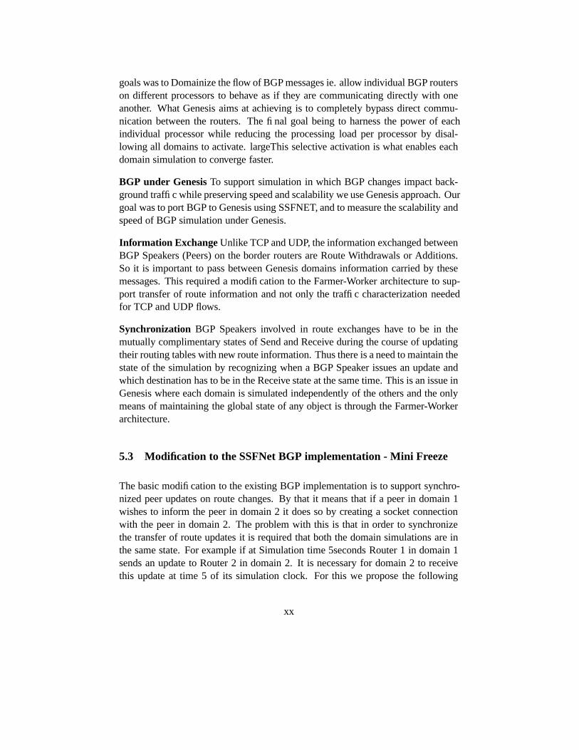
The basic modification to the existing BGP implementation is to support synchro-nized peer updates on route changes. By that it means that if a peer in domain 1wishes to inform the peer in domain 2 it does so by creating a socket connectionwith the peer in domain 2. The problem with this is that in order to synchronizethe transfer of route updates it is required that both the domain simulations are inthe same state. For example if at Simulation time 5seconds Router 1 in domain 1sends an update to Router 2 in domain 2. It is necessary for domain 2 to receivethis update at time 5 of its simulation clock. For this we propose the following

xx

Figure 8: Message Synchronization between BGP Peers

additions to the existing Genesis/BGP implementation:

Mini Freeze

Socket communication framework for transferring route update information acrossrouters in different domains to support the Mini Freeze event.

The Mini Freeze will be scheduled by the destination domain which contains therouter for which the update is the target. This is valid because parsing of the DMLfile containing the network model gives information as to the scheduled route up-date times.

So the source domain need not schedule a Mini Freeze since all it has to do is setupthe socket connection when router update is scheduled with an external peer entry.This is done when the peer entry calls its SendMsg() function in the BGPSessionclass for the peer entry.

The technique to implement the Mini Freeze would be to schedule the regular MiniFreeze event ahead of time based on the parameters returned from parsing the DMLfile. One of the issues to be discussed is that if the peer entry that schedules thisMini Freeze event does not receive a route update during the Freeze.

xxi

5.4 Reusability of existing Genesis classes to support BGP peer de-composition - Confirming simulation correctness

Once the update has been executed the thing that has to be taken care of is the de-lays in packets that has been affected by this route change. Consider the followingscenario:

At time � � = 5sec in domain 1 Router 1 advertises a route withdrawal in domain 1.Assume that the source in Domain 1 now uses route 2. As indicated in the figure.In Genesis we allow this source operation in domain 2 by means of a source proxy.We can get this route update to Domain 2 at time 5sec using the Mini Freeze event.But for Genesis to maintain correct simulation state we will have to have the sourceproxy indicate this delay for packets generated after 5 + t seconds.

DestinationSource

Domain 2Domain 1

Original Route

Changed Route

T=0..5

T=5..15

SP1

SP1

Collector 1

Copy Collector 1

SP1 − Source Proxy 1

T − Simulation Time

Figure 9: Design Model

To do this one novel way without much modification to the Genesis infrastructurewould be to create a Collector copy for each flow. This collector copy would be

xxii

used by the source proxy when the route goes down. This collector contains delaysfor packets following the modified route.

5.5 State Saving

State saving is a new feature added as an extension to support Genesis-based BGP.Currently we support only route updates as of writing this report. But other BGPmessages have also been incorporated which is outside the scope of this document.

State saving as an extension to BGP involves writing the update messages to file.Recording the following parameters:

� Freeze Time

� Message Contents (Update/Withdraw etc)

� AS Router ID

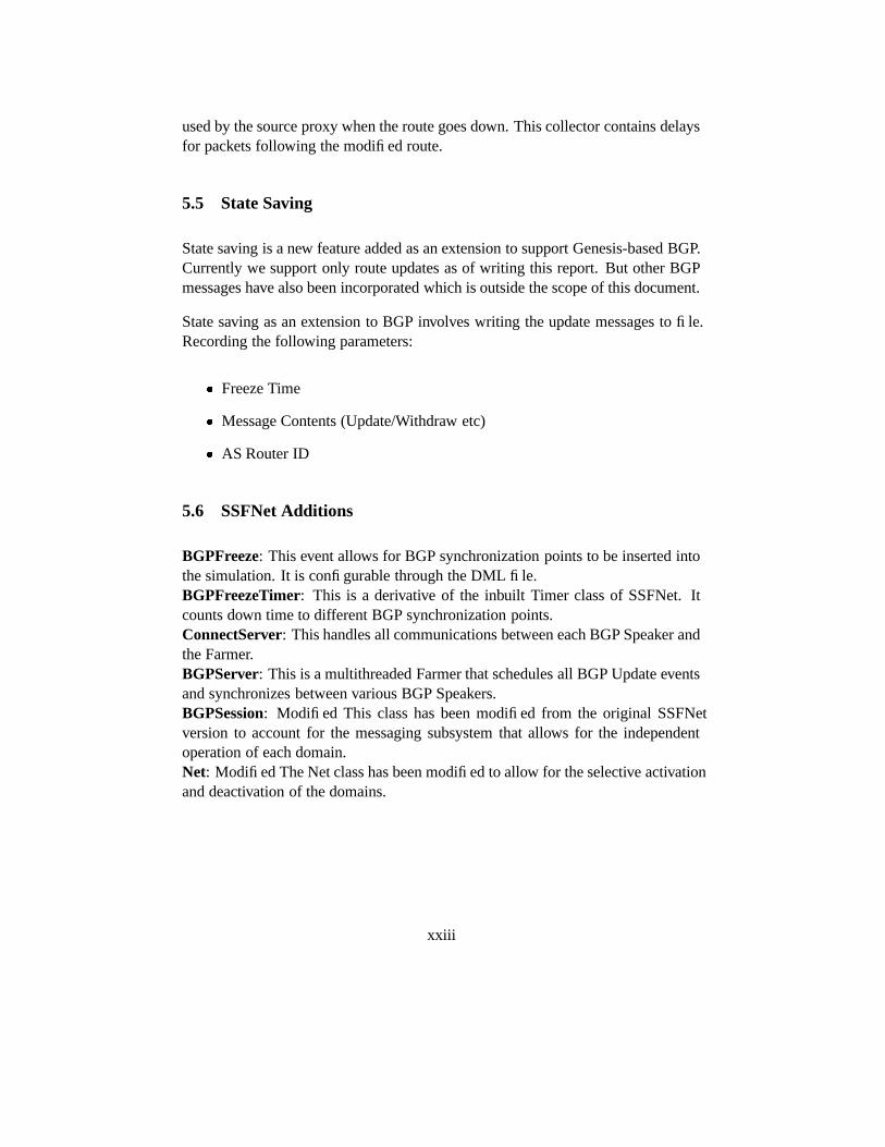
5.6 SSFNet Additions

BGPFreeze: This event allows for BGP synchronization points to be inserted intothe simulation. It is configurable through the DML file.BGPFreezeTimer: This is a derivative of the inbuilt Timer class of SSFNet. Itcounts down time to different BGP synchronization points.ConnectServer: This handles all communications between each BGP Speaker andthe Farmer.BGPServer: This is a multithreaded Farmer that schedules all BGP Update eventsand synchronizes between various BGP Speakers.BGPSession: Modified This class has been modified from the original SSFNetversion to account for the messaging subsystem that allows for the independentoperation of each domain.Net: Modified The Net class has been modified to allow for the selective activationand deactivation of the domains.

xxiii

6 Model verification through Self-Similarity

There has been some interest in experimentally observed self-similar, or long rangdependent, behavior in for instance local area network (LAN) traffic [1] and VBRvideo traffic.

The cause of self-similarity in traffic statistics in real networks is an open questionat present. It is the belief that many traffic flow control protocols are intrinsicallycapable of generating chaotic [2] behavior which are believed to be self-similar [?].

We in the last year have developed a distributed network simulation model GeN-eSIS (General Network Simulation Integration System) which allows for scalablemulti-domain real-time modeling of the network. This model addresses scalabilityat experiment design, network decomposition and network simulation levels [6].One major goal after proving that this network did indeed achieve almost super-linear speedup, was to validate this model.

Now we approached the problem of validation from two angles. One was exper-imentation - using ns [3] trace files to measure delays and drop rates of selectedflows, arrival rates of acknowledgment packets, arrival times and distribution ofpackets. The other was analytical - check simulated system behavior against knownsystem input/output behavior: for example confirm that a self similar nature of theaggregation of the TCP flow is preserved.

7 Models to verify self-similarity

The generally accepted argument for the “Poisson-like” nature of aggregated traf-fic, namely, that aggregate traffic becomes smoother (less bursty) as the number ofof traffic sources increses, has very little to do with reality. None of the commonlyused traffic models is able to capture the fractal-like behavior of self-similar traffic[1].

The general most accepted way to prove self-similarity is to measure the burstinessof traffic. This is identified by the ’Hurst Parameter’ [7]. In order to check forthe possible self-similarity of the traffic data, the following graphical tools can beapplied viz. variance time plots, pox plots of R/S, and periodogram plots. TheHurst Parameter H, when calculated for the average packet arrival time or jitter isclose to unity. This in turn implies the maximum possible degree of self-similarity.

xxiv

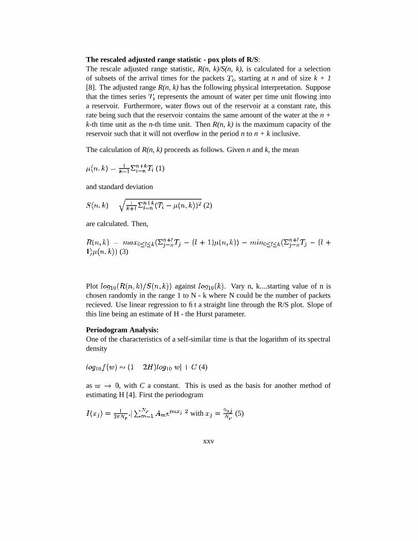
The rescaled adjusted range statistic - pox plots of R/S:The rescale adjusted range statistic, R(n, k)/S(n, k), is calculated for a selectionof subsets of the arrival times for the packets

� $ , starting at n and of size k + 1[8]. The adjusted range R(n, k) has the following physical interpretation. Supposethat the times series

� $ represents the amount of water per time unit flowing intoa reservoir. Furthermore, water flows out of the reservoir at a constant rate, thisrate being such that the reservoir contains the same amount of the water at the n +k-th time unit as the n-th time unit. Then R(n, k) is the maximum capacity of thereservoir such that it will not overflow in the period n to n + k inclusive.

The calculation of R(n, k) proceeds as follows. Given n and k, the mean

� ��� � � �.� �6� � ��� 6$�� � � $ (1)

and standard deviation

3-��� � � �.�� �6� � � � 6$�� � � � $ � � ��� � � �D� (2)

are calculated. Then,

� ��� � � ������ � � �� 6<� � � �� � � � � � ��� � � � � ��� � � �D� � ��� � � �� 6<� � � �� � � � � � ��� �� � � ��� � � �D� (3)

Plot ���IG8�� � � ��� � � ��� 3-��� � � �D� against ���IG8�� � � � . Vary n, k....starting value of n ischosen randomly in the range 1 to N - k where N could be the number of packetsrecieved. Use linear regression to fit a straight line through the R/S plot. Slope ofthis line being an estimate of H - the Hurst parameter.

Periodogram Analysis:One of the characteristics of a self-similar time is that the logarithm of its spectraldensity

���IG8���> ��� ��� � � � ��� �����IG8���� � � �"! (4)

as �$# �, with C a constant. This is used as the basis for another method of

estimating H [4]. First the periodogram

+ � � � �.� �&%('*) �+��, ' )- � � . -0/ $ -2143 � with � � � &% �'5) (5)

xxv

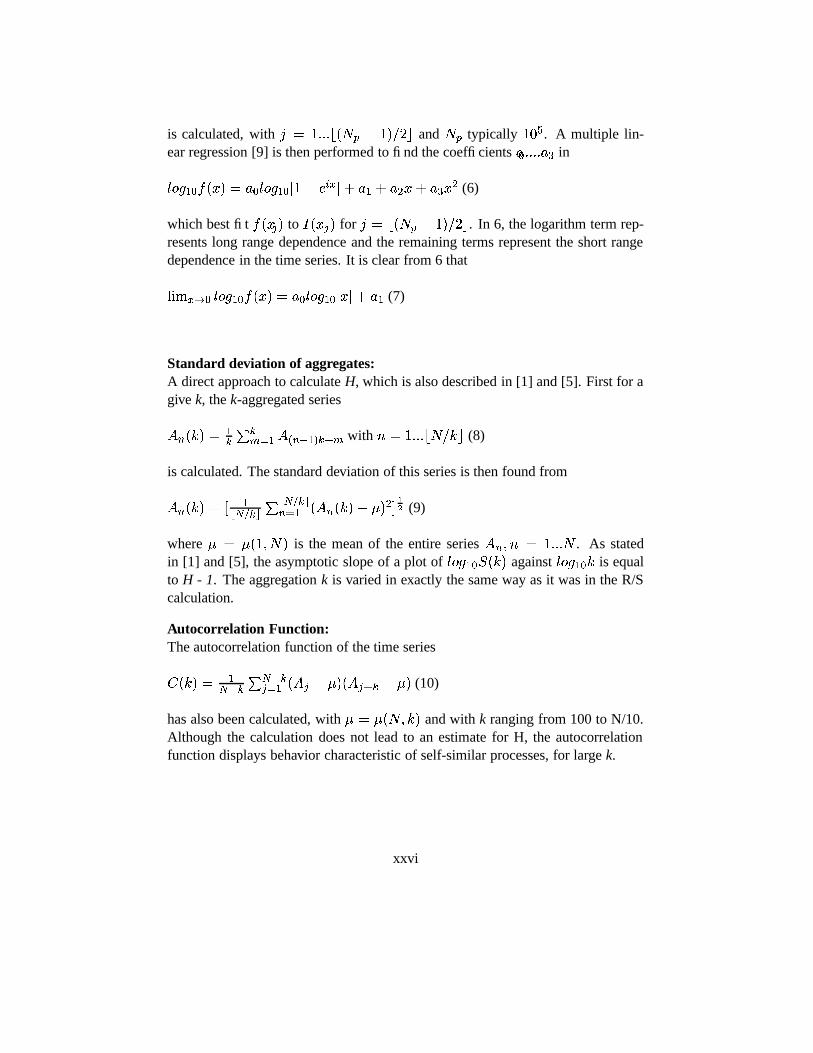
is calculated, with � � � � � ���@����� � � ��� ��� and ��� typically����

. A multiple lin-ear regression [9] is then performed to find the coefficients � ?� � � � � � in

���IG8���> � � �.� � ���IG<�� � � � / $ 1 � � � � � � �� � � � (6)

which best fit > � � � � to + � � � � for �,��@����� � � ��� ��� . In 6, the logarithm term rep-resents long range dependence and the remaining terms represent the short rangedependence in the time series. It is clear from 6 that

���� 1�� 5���#G8��#> � � � � � ���IG<�� � � � � � � (7)

Standard deviation of aggregates:A direct approach to calculate H, which is also described in [1] and [5]. First for agive k, the k-aggregated series

. � � � �F� �6 , 6- � � .�� � B ��� 6� - with ��� � � � ���A� � ��� (8)

is calculated. The standard deviation of this series is then found from

. � � � �F��� ��'�� 6�� ,

�'�� 6��� � � � . � � � � � � � ���� (9)

where � � � � � ��� � is the mean of the entire series . � � � � � � � � � . As statedin [1] and [5], the asymptotic slope of a plot of ���#G ��#3-� � � against ���IGL�� � is equalto H - 1. The aggregation k is varied in exactly the same way as it was in the R/Scalculation.

Autocorrelation Function:The autocorrelation function of the time series

! � � �.� �' B 6 , ' B 6� � � � . � � � �C� . � 6 � � � (10)

has also been calculated, with � � � ����� � � and with k ranging from 100 to N/10.Although the calculation does not lead to an estimate for H, the autocorrelationfunction displays behavior characteristic of self-similar processes, for large k.

xxvi

8 Test Network Configuration

n1

n2

r1 r2

n3

TCP Traffic

TCP Traffic

All links are 1.544 Mbit T−1, queues are droptail.

n4

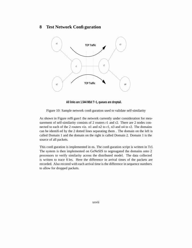
Figure 10: Sample network configuration used to validate self-similarity

As shown in Figure reffigure1 the network currently under consideration for mea-surement of self-similarity consists of 2 routers r1 and r2. There are 2 nodes con-nected to each of the 2 routers viz. n1 and n2 to r1, n3 and n4 to r2. The domainscan be identified by the 2 dotted lines separating them . The domain on the left iscalled Domain 1 and the domain on the right is called Domain 2. Domain 1 is thesource of all packets.

This configuration is implemented in ns. The configuration script is written in Tcl.The system is then implemented on GeNeSIS to segreagated the domains onto 2processors to verify similarity across the distributed model. The data collectedis written to trace files. Here the difference in arrival times of the packets arerecorded. Also recored with each arrival time is the difference in sequence numbersto allow for dropped packets.

xxvii

0

0.5

1

1.5

2

2.5

3

3.5

4

-0.5 0 0.5 1 1.5 2 2.5 3 3.5 4 4.5

log1

0[R

(n, k

)/S

(n, k

)]

log10(k)

Pox plot of R(n, k)/S(n, k) for a network, where k is the sample

f(x)’output’

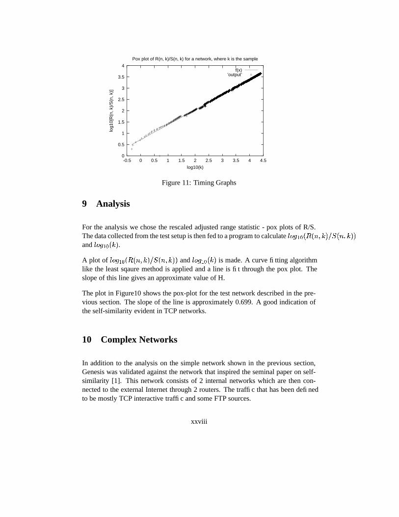
Figure 11: Timing Graphs

9 Analysis

For the analysis we chose the rescaled adjusted range statistic - pox plots of R/S.The data collected from the test setup is then fed to a program to calculate ���IG �� � � ��� � � ��� 3 ��� � � �D�and ���IG8�� � � � .A plot of ���IG8�� � � ��� � � ��� 3-��� � � �D� and ���IG8�� � � � is made. A curve fitting algorithmlike the least sqaure method is applied and a line is fit through the pox plot. Theslope of this line gives an approximate value of H.

The plot in Figure10 shows the pox-plot for the test network described in the pre-vious section. The slope of the line is approximately 0.699. A good indication ofthe self-similarity evident in TCP networks.

10 Complex Networks

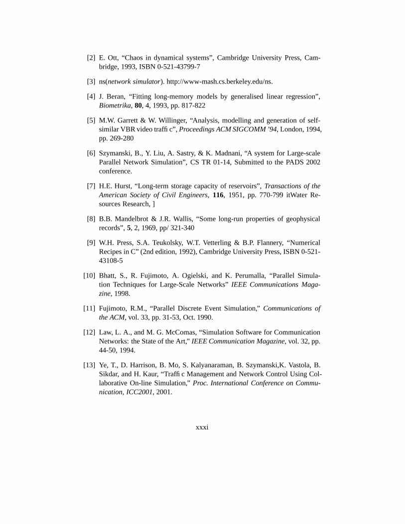
In addition to the analysis on the simple network shown in the previous section,Genesis was validated against the network that inspired the seminal paper on self-similarity [1]. This network consists of 2 internal networks which are then con-nected to the external Internet through 2 routers. The traffic that has been definedto be mostly TCP interactive traffic and some FTP sources.

xxviii

0

0.5

1

1.5

2

2.5

3

3.5

4

-1 -0.5 0 0.5 1 1.5 2 2.5 3 3.5 4 4.5

log1

0[R

(n, k

)/S

(n, k

)]

log10(k)

Pox plot of R(n, k)/S(n, k) for a network, where k is the sample

f(x)’output’

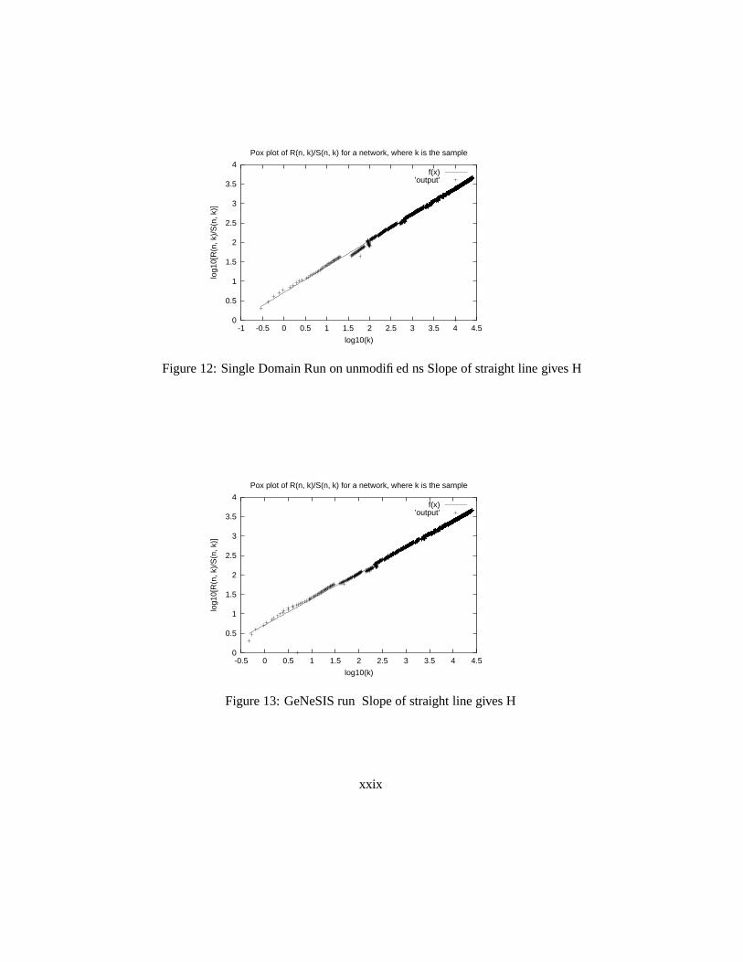
Figure 12: Single Domain Run on unmodified ns Slope of straight line gives H

0

0.5

1

1.5

2

2.5

3

3.5

4

-0.5 0 0.5 1 1.5 2 2.5 3 3.5 4 4.5

log1

0[R

(n, k

)/S

(n, k

)]

log10(k)

Pox plot of R(n, k)/S(n, k) for a network, where k is the sample

f(x)’output’

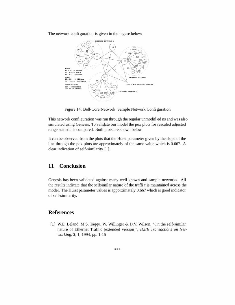
Figure 13: GeNeSIS run Slope of straight line gives H

xxix

The network configuration is given in the figure below:

n1n2

n3

n4

n5

n6

R1

R2

R3

n7

n8

n9

n10n11

n12

n13

n14 n15

n16

n17

n18

n19

n20

INTERNAL NETWORK 2

EXTERNAL NETWORK

L1

L2

L3

l1l2

l3

l4

l5

l6

l7

l8

l9

l10 l11

l12

l13

l14 l15l16

l17

l18

l19

l20l21

. . . ..

.

...

....

.

INTERNAL NETWORK 1

F1

NODESF1 − File Servern1..n20 − HostsR1..R3 − Routers

COULD ADD REST OF NETWORK

LINKSL1..L3 − 1.544Mbpsl1..l20 − 10−100Mbps

TRAFFIC TYPETCP − INTERACTIVEUDP OR FTP TRAFFIC

Figure 14: Bell-Core Network Sample Network Configuration

This network configuration was run through the regular unmodified ns and was alsosimulated using Genesis. To validate our model the pox plots for rescaled adjustedrange statistic is compared. Both plots are shown below.

It can be observed from the plots that the Hurst parameter given by the slope of theline through the pox plots are approximately of the same value which is 0.667. Aclear indication of self-similarity [1].

11 Conclusion

Genesis has been validated against many well known and sample networks. Allthe results indicate that the selfsimilar nature of the traffic is maintained across themodel. The Hurst parameter values is apporximately 0.667 which is good indicatorof self-similarity.

References

[1] W.E. Leland, M.S. Taqqu, W. Willinger & D.V. Wilson, “On the self-similarnature of Ethernet Traffic [extended version]”, IEEE Transactions on Net-working, 2, 1, 1994, pp. 1-15

xxx

[2] E. Ott, “Chaos in dynamical systems”, Cambridge University Press, Cam-bridge, 1993, ISBN 0-521-43799-7

[3] ns(network simulator). http://www-mash.cs.berkeley.edu/ns.

[4] J. Beran, “Fitting long-memory models by generalised linear regression”,Biometrika, 80, 4, 1993, pp. 817-822

[5] M.W. Garrett & W. Willinger, “Analysis, modelling and generation of self-similar VBR video traffic”, Proceedings ACM SIGCOMM ’94, London, 1994,pp. 269-280

[6] Szymanski, B., Y. Liu, A. Sastry, & K. Madnani, “A system for Large-scaleParallel Network Simulation”, CS TR 01-14, Submitted to the PADS 2002conference.

[7] H.E. Hurst, “Long-term storage capacity of reservoirs”, Transactions of theAmerican Society of Civil Engineers, 116, 1951, pp. 770-799 itWater Re-sources Research, ]

[8] B.B. Mandelbrot & J.R. Wallis, “Some long-run properties of geophysicalrecords”, 5, 2, 1969, pp/ 321-340

[9] W.H. Press, S.A. Teukolsky, W.T. Vetterling & B.P. Flannery, “NumericalRecipes in C” (2nd edition, 1992), Cambridge University Press, ISBN 0-521-43108-5

[10] Bhatt, S., R. Fujimoto, A. Ogielski, and K. Perumalla, “Parallel Simula-tion Techniques for Large-Scale Networks” IEEE Communications Maga-zine, 1998.

[11] Fujimoto, R.M., “Parallel Discrete Event Simulation,” Communications ofthe ACM, vol. 33, pp. 31-53, Oct. 1990.

[12] Law, L. A., and M. G. McComas, “Simulation Software for CommunicationNetworks: the State of the Art,” IEEE Communication Magazine, vol. 32, pp.44-50, 1994.

[13] Ye, T., D. Harrison, B. Mo, S. Kalyanaraman, B. Szymanski,K. Vastola, B.Sikdar, and H. Kaur, “Traffic Management and Network Control Using Col-laborative On-line Simulation,” Proc. International Conference on Commu-nication, ICC2001, 2001.

xxxi

[14] L.R. Klein, “Quantitative Studies of International Economic Relations,”Chapter The LINK Model of World Trade with Application to 1972-72, NorthHolland, Amsterdam, 1975.

[15] Y. Shi, N. Prywes, B. Szymanski and A. Pnueli, “Very high level concur-rent programming,” IEEE Trans. Software Engineering, SE-13:1038-1046,September 1989.

[16] B. Szymanski, Y. Shi and N. Prywes, “Synchronized distributed termination,”IEEE Trans. Software Engineering, SE-11:1136-1140, September 1987.

[17] M. Yuksel, B. Sikdar, K.S. Vastola and B. Szymanski, “Workload generationfor ns simulations of wide area networks and the internet,” Proc. Communi-cations Networks and Distributed Systems Modeling and Simulation Confer-ence, Pages 93-98, SCS Press, 2000.

xxxii