GENERIC RISK ASSESSMENT MODEL

FOR INDOOR AND OUTDOOR SPACE

SPRAYING OF INSECTICIDES

WHO Pesticide Evaluation SchemeDepartment of Control of Neglected Tropical DiseasesCluster of HIV/AIDS, Tuberculosis, Malaria and Neglected Tropical Diseases&Chemical SafetyDepartment of Public Health and EnvironmentCluster of Health Security and Environment

First Revision (February 2011)

Generic risk assessment model for indoor and outdoor space spraying

of insecticides

First revision (February 2011)

DEPARTMENT OF CONTROL OF NEGLECTED TROPICAL DISEASES HIV/AIDS, TUBERCULOSIS, MALARIA AND NEGLECTED TROPICAL DISEASES

WHO PESTICIDE EVALUATION SCHEME &

DEPARTMENT OF PUBLIC HEALTH AND ENVIRONMENT HEALTH SECURITY AND ENVIRONMENT

CHEMICAL SAFETY

WHO Library Cataloguing-in-Publication Data

Generic risk assessment model for indoor and outdoor space spraying of insecticides - 1st revision (February 2011).

1.Insecticides - toxicity. 2.Mosquito control. 3.Risk assessment - methods. 4.Environmental exposure. I.World Health Organization. II.WHO Pesticide evaluation scheme.

ISBN 978 92 4 150168 2 (NLM classification: WA 240)

© World Health Organization 2011

All rights reserved. Publications of the World Health Organization are available on the WHO web site (www.who.int) or can be purchased from WHO Press, World Health Organization, 20 Avenue Appia, 1211 Geneva 27, Switzerland (tel.: +41 22 791 3264; fax: +41 22 791 4857; e-mail: bookorders@who.int).

Requests for permission to reproduce or translate WHO publications – whether for sale or for noncommercial distribution – should be addressed to WHO Press through the WHO web site (http://www.who.int/about/licensing/copyright_form/en/index.html).

The designations employed and the presentation of the material in this publication do not imply the expression of any opinion whatsoever on the part of the World Health Organization concerning the legal status of any country, territory, city or area or of its authorities, or concerning the delimitation of its frontiers or boundaries. Dotted lines on maps represent approximate border lines for which there may not yet be full agreement.

The mention of specific companies or of certain manufacturers’ products does not imply that they are endorsed or recommended by the World Health Organization in preference to others of a similar nature that are not mentioned. Errors and omissions excepted, the names of proprietary products are distinguished by initial capital letters.

All reasonable precautions have been taken by the World Health Organization to verify the information contained in this publication. However, the published material is being distributed without warranty of any kind, either expressed or implied. The responsibility for the interpretation and use of the material lies with the reader. In no event shall the World Health Organization be liable for damages arising from its use.

WHO/HTM/NTD/WHOPES/2010.6 rev 1

iii

Contents

Acknowledgements .................................................................................................. v 

Acronyms and abbreviations .................................................................................. vi 

1. Introduction ..........................................................................................................1 

2. Purpose ................................................................................................................1 

3. Background ..........................................................................................................1 

3.1 Probabilistic vs. deterministic risk assessment models ....................... 2 

3.2 Essential elements of a human health risk assessment model ............. 3 

4. The human health risk assessment model .........................................................4 

4.1 Hazard assessment ....................................................................... 4 

4.1.1 Sources of data ................................................................... 4 

4.1.2 Types of health hazard data .................................................. 5 

4.1.3 Range of toxicity tests normally required for pesticide

approval ........................................................................... 6 

4.1.4 Evaluation of the toxicity information ..................................... 7 

4.1.5 Insecticides not recommended for use in space spraying ........... 8 

4.1.6 Other special considerations in hazard assessment ................... 8 

4.1.7 Dose–response assessment and setting of acceptable

exposure ........................................................................... 9 

4.2 Human exposure assessment ....................................................... 13 

4.2.1 General parameters for exposure assessment ........................ 15 

4.2.2 Algorithms used to estimate exposure and absorbed

dose caused by indoor or outdoor space spraying of

insecticides ..................................................................... 19 

4.2.3 Total exposure assessment ................................................. 25 

4.3 Risk characterization ................................................................... 26 

iv

5. The environmental risk assessment model ..................................................... 26 

5.1 Environmental exposure assessment ............................................. 28 

5.1.1 Air................................................................................... 28 

5.1.2 Soil ................................................................................. 30 

5.1.3 Surface water and aquatic sediment ..................................... 34 

5.2 Effects ...................................................................................... 37 

5.2.1 Aquatic organisms ............................................................. 37 

5.2.2 Soil organisms and soil function ........................................... 41 

5.2.3 Non-target terrestrial arthropods including honeybees ............ 43 

5.2.4 Terrestrial vertebrates ....................................................... 43 

5.2.5 Higher terrestrial plants ...................................................... 46 

6. Conclusions ....................................................................................................... 47 

7. Summary of the human health risk assessment model and a worked

example ............................................................................................................. 48 

8. Summary of the environmental risk assessment model and a worked

example ............................................................................................................. 56 

References ............................................................................................................ 60 

 

v

AcknowledgementsThe first draft of these generic models was prepared by a drafting committee appointed by the World Health Organization (WHO) and composed of Dr M. Mäkinen, Finnish Institute of Occupational Health, Kuopio, Finland; Dr T. Santonen, Finnish Institute of Occupational Health, Helsinki, Finland; Dr A. Aitio, private consultant, Helsinki, Finland; Dr S. Dobson OBE, Birchtree Consultants Ltd., Peterborough, UK; and Dr M. Zaim, WHO Pesticide Evaluation Scheme (WHOPES), Geneva, Switzerland. None of the drafting committee members declared an interest in the subject matter of these guidelines. The first draft of the guidelines was peer reviewed by individuals and institutions known for their expertise in the subject. The peer review group comprised Dr M. Baril, Institut de recherche Robert-Sauvé en santé et en sécurité au travail (IRSST), Montreal, Canada; Dr N. Besbelli, United Nations Environment Programme (UNEP), Geneva, Switzerland; Dr M. Birchmore, Syngenta Ltd., Basel, Switzerland; Dr L. Blake, Syngenta Ltd., Surrey, UK; Dr R. Brown, WHO Programme on Chemical Safety, Geneva, Switzerland; Dr H. Bouwman, School of Environmental Sciences and Development, North-West University, Potchefstroom, South Africa; Dr R. S. Chhabra, National Institute of Environmental Health Sciences, Research Triangle Park, NC, USA; Dr O. Hänninen, National Institute for Health and Welfare (THL), Kuopio, Finland; Dr M. Latham, Manatee County Mosquito Control District, Palmetto, FL, USA; Professor Dr G. A. Matthews, Imperial College, Ascot, UK; Dr D. J. Miller, Dr M. Crowley and Dr J. Evans, United States Environmental Protection Agency (USEPA), Office of Pesticide Programs, Health Effects Division, Washington DC, USA; Dr L. Patty, Bayer Environmental Science, Lyon, France; Dr L. Tomaska and Dr M. Bulters, Australian Commonwealth Department of Health, Office of Chemical Safety, Canberra, Australia; Dr C. Vickers, WHO Programme on Chemical Safety, Geneva, Switzerland; and Dr O. Yamada, French Agency for Environmental and Occupational Health Safety (Afsset), Maisons-Alfort, France. The above-mentioned drafting committee considered all comments received and prepared a second draft. This revised draft was reviewed and discussed at a WHO consultation held at the Finnish Institute of Occupational Health in Helsinki (Finland) on 23–25 June 2009. The experts appointed by WHO were Dr N. Besbelli, Dr H. Bouwman, Dr O. Hänninen, Dr M. Latham and Professor Dr G. A. Matthews. Dr C. Vickers (WHO Programme on Chemical Safety) and Dr M. Zaim (WHOPES) took part in reviewing the revised draft. None of the experts participating in the consultation declared an interest in the subject matter of these guidelines. Based on experience from use gathered since 2009, and also to make use of emerging new information, the document was revised in February 2011 by the original drafting committee. The WHO Departments of Control of Neglected Tropical Diseases and acknowledges the individuals and institutions listed above for their important contributions to this work. It also expresses its sincere thanks to Professor Matthews for his valuable support and technical advice in all phases of the drafting process. The financial support provided by the Bill & Melinda Gates Foundation is also gratefully acknowledged. The Department welcomes feedback on the guidelines and suggestions for improvement from national programmes, research institutions and industry in order to improve future editions.

vi

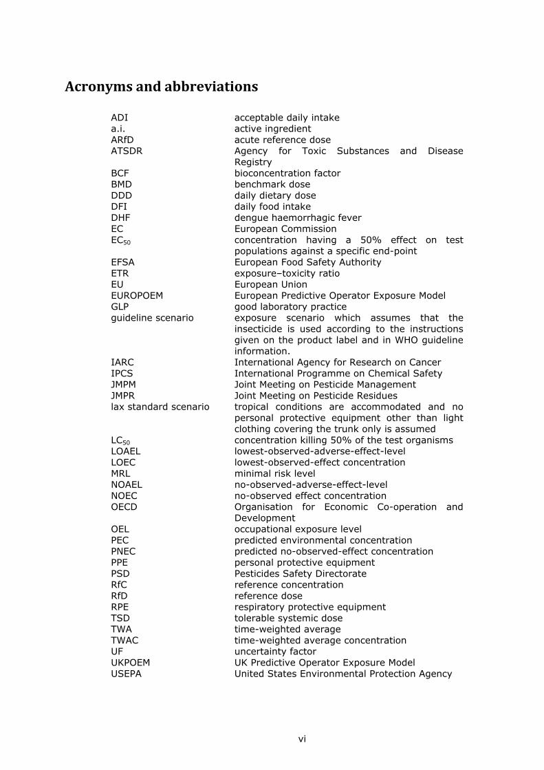
Acronymsandabbreviations

ADI acceptable daily intakea.i. active ingredientARfD acute reference doseATSDR Agency for Toxic Substances and Disease

RegistryBCF bioconcentration factorBMD benchmark doseDDD daily dietary doseDFI daily food intakeDHF dengue haemorrhagic fever EC European CommissionEC50 concentration having a 50% effect on test

populations against a specific end-pointEFSA European Food Safety AuthorityETR exposure–toxicity ratioEU European UnionEUROPOEM European Predictive Operator Exposure ModelGLP good laboratory practiceguideline scenario exposure scenario which assumes that the

insecticide is used according to the instructions given on the product label and in WHO guideline information.

IARC International Agency for Research on CancerIPCS International Programme on Chemical SafetyJMPM Joint Meeting on Pesticide ManagementJMPR Joint Meeting on Pesticide Residueslax standard scenario tropical conditions are accommodated and no

personal protective equipment other than light clothing covering the trunk only is assumed

LC50 concentration killing 50% of the test organismsLOAEL lowest-observed-adverse-effect-levelLOEC lowest-observed-effect concentrationMRL minimal risk levelNOAEL no-observed-adverse-effect-levelNOEC no-observed effect concentrationOECD Organisation for Economic Co-operation and

DevelopmentOEL occupational exposure levelPEC predicted environmental concentrationPNEC predicted no-observed-effect concentrationPPE personal protective equipmentPSD Pesticides Safety DirectorateRfC reference concentrationRfD reference doseRPE respiratory protective equipmentTSD tolerable systemic doseTWA time-weighted average TWAC time-weighted average concentrationUF uncertainty factorUKPOEM UK Predictive Operator Exposure ModelUSEPA United States Environmental Protection Agency

1

1.Introduction

Space spraying is the dissemination of small particles (less than 30 µm) that will remain airborne sufficiently long (usually not more than 30 minutes) to make contact with flying target species. Because this type of treatment is not intended to leave a residual deposit, it involves a very low dosage of insecticide. Sequential space-spray applications of insecticides are usually needed to control the emerging adult populations and are commonly used for vector-borne diseases such as dengue and malaria and in public health pest control programmes against nuisance mosquitoes and flies.

There are essentially two methods of creating a space spray – thermal and cold fogging, using portable, vehicle-mounted and aerial equipment. The formulations commonly used for such applications are hot fogging concentrates, ultra-low-volume liquids, oil-in-water emulsions and emulsifiable concentrates.

WHO has already published procedures for space-spray application of insecticides in public health (WHO, 2003), specifications for equipment to apply space sprays (WHO, 2006), and requirements, procedures and criteria for testing and evaluation of insecticides for space spraying (WHO, 2009a).

2.Purpose

This document provides a generic model that can be used for risk assessment of exposure to insecticide products applied as space treatment, both indoors and outdoors, against flying insect vectors and pests of public health importance. It aims to harmonize the risk assessment of such insecticides for public health use. The assessment considers both adults and children and people in the following specific categories:

– those preparing the spray; – those applying the spray; – residents who return to treated houses; and – bystanders who are present during an outdoor application.

In addition to human health risk assessment, aspects of ecological risk assessment need to be considered. In contrast to the former, ecological risk assessment characterizes the risk to populations of non-target organisms rather than to humans.

The structure of this document follows that of A generic risk assessment model for insecticide treatment and subsequent use of mosquito nets (WHO, 2004). Because risk assessment is a constantly evolving process, guidance is also subject to change. Readers are therefore advised to consider any newer guidance published by WHO and other authoritative sources.

3.Background

It is recommended that the risk assessments proposed for space spraying are not conducted de novo; risk assessments that have already been generated for the pesticides in the regulatory context of crop protection can be used as a starting point. Preference should be for international assessments, followed by peer-reviewed regional or national assessments;

2

risk assessments published in reputable journals would be a third possible source.

For each component of the risk assessment, the additional information – or modification of the existing assessment – likely to be needed will be identified and discussed. It is assumed that the generic guidance given here will be followed in parallel with one of the published regulatory schemes. These regulatory schemes are intended for guidance and none is wholly prescriptive; all state specifically that expert judgement is required. Similarly, expert judgment will be needed to determine the adjustments needed to make published risk assessments from regulation of pesticides suitable for the specific task of risk assessment of space spraying of insecticides indoors or outdoors.

3.1Probabilisticvs.deterministicriskassessmentmodels

Historically, exposure models have been based on point estimates. This deterministic approach has the advantage of simplicity and consistency. Risk characterization is relatively straightforward: the exposure estimate is compared with a health-based guidance value. The drawback of the deterministic approach is that it incorporates no information about the variability of real exposures. Likewise, there is no assessment of, or information about, the uncertainty in the exposure estimate.

The probabilistic technique offers a complementary modelling approach that incorporates variability of exposure. Probabilistic modelling uses distributions of values rather than single values. The advantage of the probabilistic technique is that it provides the probability of occurrence of exposure, which offers a sophisticated way of characterizing and communicating risk. Just as for deterministic models, however, the validity of the exposure estimate depends on the quality and extent of the input data and the reliability of the estimation algorithm.

Probabilistic methods have been used widely in North America in dietary exposure estimations (for example by the United States Environmental Agency, USEPA). Over the past few years, regulatory bodies and industry have also moved towards the use of probabilistic techniques in refining exposure estimates in occupational exposures (for example, in estimates produced by the United Kingdom’s Pesticides Safety Directorate). The European Commission and the OECD (Organisation for Economic Co-operation and Development) Working Group on Pesticides have prepared reports on the use of probabilistic methods for assessing operator exposure to plant protection products. In addition, use of probabilistic methods has been proposed for effects assessment (both for hazard identification and for assessment factors).

Problems in using probabilistic techniques lie principally in the following areas:

– the difficulty of using the models, – algorithm development; – collection of good-quality input distributions; – criteria for decision-making (what is an acceptable risk and what is

not); and – communicating the results to stakeholders.

3

Models that appear to be easily to understand and “user-friendly” will be published in the near future. Nevertheless, despite this apparent simplicity, it is critical that risk assessors and regulators remain fully aware of the pitfalls of modelling. They must have comprehensive knowledge of the principles of exposure assessment, and the techniques used to describe the exposure and risk – and thus be able to ask the right questions. Probabilistic modelling could, however, be used as a special technique in more complex situations or when deterministic assessments have identified exposures of concern (higher-tier assessments) (Nordic Council of Ministers, 2007).

WHO encourages anyone using the models published here to consider the probabilistic approach as an alternative, especially when higher-tier assessments are needed. Sophisticated probabilistic models are also being developed and may provide alternative ways setoff setting acceptable exposure levels in the future (WHO, 2009b).

3.2Essentialelementsofahumanhealthriskassessmentmodel

Comprehensive presentations on the principles of risk assessment can be found elsewhere in the scientific literature (e.g. WHO, 1999a); only a short summary is given here.

Hazard is defined as the inherent capacity of a chemical substance to cause adverse effects in humans and animals and to the environment. Risk is defined as the probability that a particular adverse effect will be observed under certain conditions of exposure or use. Risk characterization is the process of combining hazard and exposure information to describe the likelihood of occurrence and the severity of adverse effects associated with a particular exposure in a given population. The entire process of hazard assessment, exposure estimation and risk characterization is known as risk assessment. Management of uncertainties related to all natural processes, including processes related to risk assessment, is an essential part of a valid, good-quality risk assessment.

The subsequent process of risk management considers the risk assessment in parallel with any potential benefits, socioeconomic and political factors, the possibilities for risk reduction and other issues that are relevant in making operational decisions on the acceptability of a particular level of risk.

Risk assessments involve three steps:

1. Hazard assessment. Hazard assessment comprises hazard identification and hazard characterization, i.e. identification of the possible toxic effects of a substance, the dose/exposure levels at which those effects occur, and the dose/exposure levels below which no adverse effects are observed.

2. Exposure assessment. Exposure assessment may concern pesticide operators (applicators), residents of treated dwellings and users of other treated buildings, bystanders, domestic animals, wildlife and the environment. Exposure should be assessed in a “guideline scenario”, which assumes that the insecticide is used according to the instructions given on the product label and in WHO guideline information. A "lax standard scenario" takes into account the fact that in reality these instructions are not necessarily followed completely. Conservative, high end-point estimates of the default distributions are used as defaults. No

4

account is taken of intentional misuse. All relevant routes of exposure are covered.

3. Risk characterization. In the risk characterization step, estimates of exposure are compared with acceptable exposure levels previously defined in hazard assessment in all relevant exposure situations.

The various chapter of this report deal with specific information demands, data sources, uncertainties, discussion on vulnerable or sensitive subgroups, selection of default values and the underlying assumptions, etc.

4.Thehumanhealthriskassessmentmodel

4.1Hazardassessment

The purpose of human health hazard assessment is to identify:

– whether an agent may pose a health hazard to human health; and – the circumstances in which the hazard may be expressed (WHO,

1999a).

It involves the weight-of-evidence assessment of all available data on toxicity and on mode of action, and the establishment of dose–response curves and the threshold level below which the effects are no longer observed. The principles of human health hazard assessment are discussed in greater detail elsewhere (e.g. WHO, 1999a); they are largely the same, regardless of the class of chemical or its use pattern, differing only in, for example, data requirements. These principles have been summarized in an earlier WHO publication (WHO, 2004), which describes a generic risk assessment model for insecticide treatment and subsequent use of mosquito nets and which, with some updating, is used as a basis for the current text.

4.1.1Sourcesofdata

Hazard identification is based on gathering and analysing relevant data on the possible effects of the insecticide on humans. These data may include both toxicological (animal testing) and human data. It is recommended that, when available, authoritative risk assessments that have already been generated for the insecticides, e.g. in the regulatory context of crop protection, can be used as a starting point. These risk assessments usually contain all the relevant health hazard data available for the insecticide in question and are therefore important sources of data. Preference should be for international assessments, followed by peer-reviewed regional or national assessments; evaluations published in reputable, peer-reviewed journals are also possible sources.

Examples of this kind of authoritative evaluation are given in Table 1. Many can be accessed on the Internet, for example via OECD’s eChemPortal (http://webnet3.oecd.org/echemportal/).

When existing evaluations are used as a starting point, the original study reports should also be also consulted if they are identified as critical to the risk assessment. Literature searches should be conducted for any new published data, and any relevant unpublished studies should be evaluated and considered.

5

4.1.2Typesofhealthhazarddata

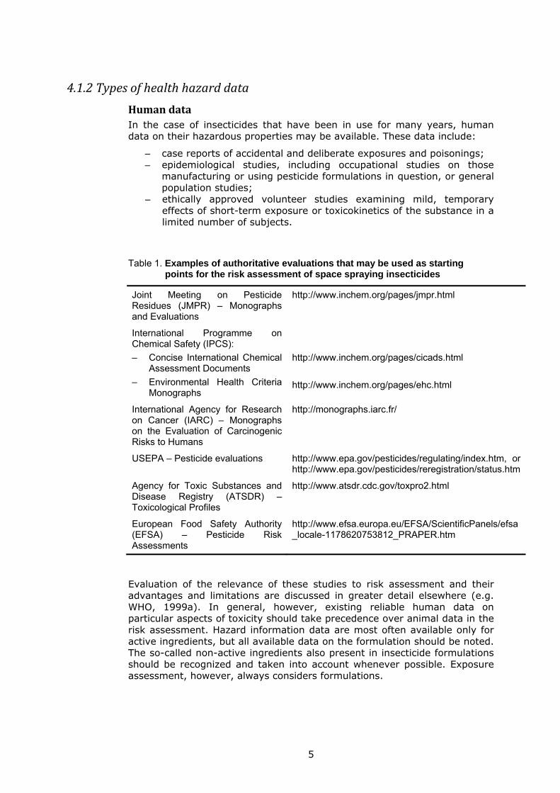
HumandataIn the case of insecticides that have been in use for many years, human data on their hazardous properties may be available. These data include:

– case reports of accidental and deliberate exposures and poisonings; – epidemiological studies, including occupational studies on those

manufacturing or using pesticide formulations in question, or general population studies;

– ethically approved volunteer studies examining mild, temporary effects of short-term exposure or toxicokinetics of the substance in a limited number of subjects.

Table 1. Examples of authoritative evaluations that may be used as starting points for the risk assessment of space spraying insecticides

Joint Meeting on Pesticide Residues (JMPR) – Monographs and Evaluations

http://www.inchem.org/pages/jmpr.html

International Programme on Chemical Safety (IPCS):

– Concise International Chemical Assessment Documents

– Environmental Health Criteria Monographs

http://www.inchem.org/pages/cicads.html

http://www.inchem.org/pages/ehc.html

International Agency for Research on Cancer (IARC) – Monographs on the Evaluation of Carcinogenic Risks to Humans

http://monographs.iarc.fr/

USEPA – Pesticide evaluations http://www.epa.gov/pesticides/regulating/index.htm, or http://www.epa.gov/pesticides/reregistration/status.htm

Agency for Toxic Substances and Disease Registry (ATSDR) – Toxicological Profiles

http://www.atsdr.cdc.gov/toxpro2.html

European Food Safety Authority (EFSA) – Pesticide Risk Assessments

http://www.efsa.europa.eu/EFSA/ScientificPanels/efsa_locale-1178620753812_PRAPER.htm

Evaluation of the relevance of these studies to risk assessment and their advantages and limitations are discussed in greater detail elsewhere (e.g. WHO, 1999a). In general, however, existing reliable human data on particular aspects of toxicity should take precedence over animal data in the risk assessment. Hazard information data are most often available only for active ingredients, but all available data on the formulation should be noted. The so-called non-active ingredients also present in insecticide formulations should be recognized and taken into account whenever possible. Exposure assessment, however, always considers formulations.

6

ExperimentaltoxicitydataFor many pesticides, the human database is very limited. In these cases hazard assessment is dependent on information from experimental animals and on in-vitro studies. For insecticides recently registered or reregistered for use by regulatory authorities, it is expected that comprehensive toxicology studies will have been conducted according to modern standards and good laboratory practice (GLP), using internationally accepted protocols for toxicological testing such as those published by OECD (OECD, 1987; http://www.oecd-ilibrary.org/environment/oecd-guidelines-for-the-testing-of-chemicals-section-4-health-effects_20745788), or the USEPA (latest update 2007: http://www.epa.gov/ocspp/pubs/frs/home/guidelin.htm ). For older pesticides animal toxicity data may be limited and may not encompass modern requirements (unless they have been recently evaluated in regulatory programmes intended to review old pesticides).

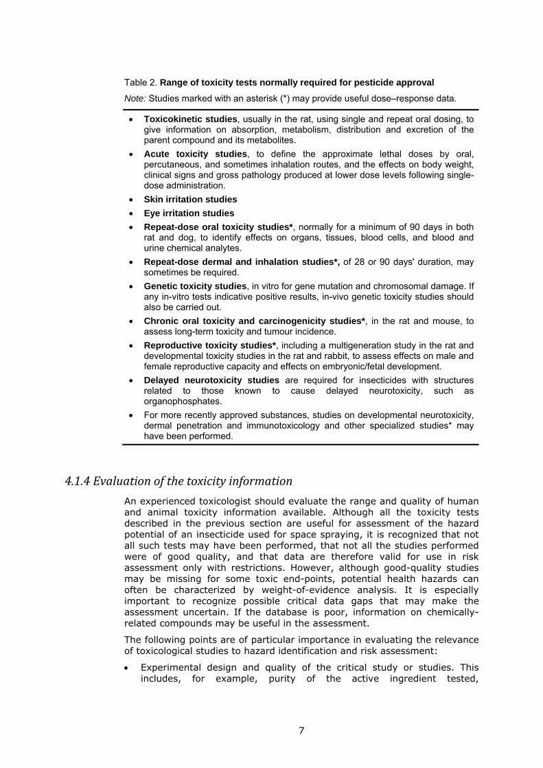
Like other chemicals, public health pesticides used in space spraying have the potential to cause a wide range of toxic effects. To identify the critical effects of the insecticide in question, a range of toxicity studies is usually needed. Although test requirements may vary to some extent with the country or region or with the precise use of the pesticide, the range of tests normally needed for health risk assessment, for example in regulatory approval of pesticides and biocides in OECD countries, is very similar (see Table 2).

It should be noted that toxicity test data are usually available only for pure substances, that is, for the active ingredients or solvents used in insecticide formulations rather than for the pesticide formulations themselves. Sometimes, however, some acute toxicity tests may also be performed with an insecticide formulation to ensure that the acute toxicity does not differ from that predicted on the basis of the tests or its individual components.

4.1.3Rangeoftoxicitytestsnormallyrequiredforpesticideapproval

In addition to these general requirements, information on dermal absorption will be useful in the assessment of a space treatment inside dwellings. Although space treatment is not expected to leave any residual deposit (surfaces are not intentionally sprayed), small droplets may be deposited on some surfaces within the dwellings to which inhabitants will be subsequently exposed. Further, inhalation toxicity studies may be of value in assessing risks to operators, who are subject to potential acute and repeated inhalation exposure.

Absorption of the insecticide by inhalation, ingestion and through the skin should be estimated in the hazard assessment. If no chemical-specific data exist, default values of 100% for inhalation and ingestion and 10% for the dermal route are used. It should be noted that while residents are usually exposed to the product as sprayed, that is, as a diluted solution, operators may be exposed to both the diluted product and the undiluted formulation. Dermal absorption may be different for these two. Thus, for mixing and loading, the absorption rate of the non-diluted formulation is to be used, while for other dermal exposure, that of the diluted spray is more appropriate (EC, 2002; WHO 2004).

7

Table 2. Range of toxicity tests normally required for pesticide approval

Note: Studies marked with an asterisk (*) may provide useful dose–response data.

Toxicokinetic studies, usually in the rat, using single and repeat oral dosing, to give information on absorption, metabolism, distribution and excretion of the parent compound and its metabolites.

Acute toxicity studies, to define the approximate lethal doses by oral, percutaneous, and sometimes inhalation routes, and the effects on body weight, clinical signs and gross pathology produced at lower dose levels following single-dose administration.

Skin irritation studies

Eye irritation studies

Repeat-dose oral toxicity studies*, normally for a minimum of 90 days in both rat and dog, to identify effects on organs, tissues, blood cells, and blood and urine chemical analytes.

Repeat-dose dermal and inhalation studies*, of 28 or 90 days' duration, may sometimes be required.

Genetic toxicity studies, in vitro for gene mutation and chromosomal damage. If any in-vitro tests indicative positive results, in-vivo genetic toxicity studies should also be carried out.

Chronic oral toxicity and carcinogenicity studies*, in the rat and mouse, to assess long-term toxicity and tumour incidence.

Reproductive toxicity studies*, including a multigeneration study in the rat and developmental toxicity studies in the rat and rabbit, to assess effects on male and female reproductive capacity and effects on embryonic/fetal development.

Delayed neurotoxicity studies are required for insecticides with structures related to those known to cause delayed neurotoxicity, such as organophosphates.

For more recently approved substances, studies on developmental neurotoxicity, dermal penetration and immunotoxicology and other specialized studies* may have been performed.

4.1.4Evaluationofthetoxicityinformation

An experienced toxicologist should evaluate the range and quality of human and animal toxicity information available. Although all the toxicity tests described in the previous section are useful for assessment of the hazard potential of an insecticide used for space spraying, it is recognized that not all such tests may have been performed, that not all the studies performed were of good quality, and that data are therefore valid for use in risk assessment only with restrictions. However, although good-quality studies may be missing for some toxic end-points, potential health hazards can often be characterized by weight-of-evidence analysis. It is especially important to recognize possible critical data gaps that may make the assessment uncertain. If the database is poor, information on chemically-related compounds may be useful in the assessment.

The following points are of particular importance in evaluating the relevance of toxicological studies to hazard identification and risk assessment:

Experimental design and quality of the critical study or studies. This includes, for example, purity of the active ingredient tested,

8

physicochemical properties (stability, etc.), size of the study (number of exposure groups, group sizes, sex, etc.), suitability of the exposure levels used, duration of exposure, extent of toxicological and statistical evaluation, relevancy of the route of exposure to humans, and whether the study adhered to established guidelines and GLP (WHO, 1999a).

Nature of the effects seen, their severity and sites, and whether they would be reversible on cessation of exposure.

Is it possible to identify dose–response relationship, no-observed-adverse-effect-level (NOAEL) and lowest-observed-adverse-effect-level (LOAEL)?

4.1.5Insecticidesnotrecommendedforuseinspacespraying

Compounds meeting the criteria of carcinogenicity, mutagenicity or reproductive toxicity categories 1A and 1B of the Globally harmonized system of classification and labelling of chemicals (United Nations, 2009; http://live.unece.org/trans/danger/publi/ghs/ghs_rev03/03files_e.html) can be regarded as highly hazardous pesticides (JMPM, 2008). The Joint Meeting on Pesticide Management (JMPM) has issued a general recommendation that pesticides meeting the criteria for highly hazardous pesticides should not be registered for use unless:

– a clear need is demonstrated; – there are no relevant alternatives based on risk–benefit analysis; and – control measures, as well as good marketing practices, are sufficient

to ensure that the product can be handled with acceptable risk to human health and the environment (JMPM, 2008).

It is suggested that this recommendation be followed in the case of space spraying as well. It is generally considered that compounds that are both genotoxic and carcinogenic are particularly likely to exert effects at very low doses: even if studies indicate apparent NOAELs, these should not be used for risk assessment. Moreover, an insecticide of high acute toxicity, meeting the criteria of classes Ia or Ib of the WHO recommended classification of pesticides by hazard (WHO, 2010), is not recommended for use in space spraying. However, it is the acute toxicity of the formulation, not just of the active ingredient, that should be taken into account, based on data relating to the formulation itself.

If both the active insecticide ingredient and the formulation have shown a high incidence of severe or irreversible adverse effects on human health or the environment, use of that particular insecticide may not be acceptable (JMPM, 2008).

4.1.6Otherspecialconsiderationsinhazardassessment

Interactions between insecticides and other constituents of theformulationIf two or more insecticides are used concurrently, possible toxicological interactions between those insecticides should be considered. Insecticides of the same class may produce additive toxic effects; organophosphates, for example, reduce acetylcholinesterase activity. Other forms of interaction include synergistic (supra-additive) and antagonistic effects, which may be

9

caused by different classes of pesticides, for example because of metabolic interactions. Unfortunately, reliable information is often unavailable, but knowledge of metabolic pathways or of receptor binding may sometimes help in identifying possible interactions.

Interactions may occur also between the active ingredient and the solvent used in the technical product. Moreover, impurities present in the technical product, e.g. in organophosphate products, may interact with the product and affect its final toxicity. Comprehensive specification of technical material (see http://www.who.int/whopes/quality) is thus of the utmost importance.

4.1.7Dose–responseassessmentandsettingofacceptableexposure

Dose–response assessment is an essential part of hazard assessment for deriving health-based guidance values and for the assessment of risks. There are different methods for dose-response assessment (WHO, 2009b). The standard NOAEL approach can be regarded as a simplified form of dose–response analysis, identifying a single dose assumed to be without appreciable adverse effects (WHO, 2009b). An important alternative approach is the benchmark dose method, based on the calculation of benchmark doses at which a particular level of response would occur (WHO, 2009b). Use of these approaches in the setting of acceptable exposure levels requires knowledge of the assumed shape of the dose–response curve. For some end-points, however, such as endocrine disruption, the shape of the dose–response curve is not very well understood, which limits use of these data in the risk assessment.

NOAELapproachFor most end-points it is generally recognized that there is a dose or concentration below which adverse effects do not occur; for these, an NOAEL and/or LOAEL can be identified. For genotoxicity and carcinogenicity mediated by genotoxic mechanisms, dose–response is considered to be linear, meaning that risk cannot be excluded at any exposure level.

The NOAEL and LOAEL values are study-specific dose level at which no effects or minimal effects, respectively, have been observed in toxicity studies (or, in some cases, in humans). The study design and the sensitivity of the test system can have a significant influence on NOAELs and LOAELs, which therefore represent only surrogates for the real no-effect and lowest-effect levels. Dose–response data and NOAELs/LOAELs can be obtained from repeated-dose toxicity studies, chronic toxicity/carcinogenicity studies, reproductive toxicity studies and some specialized toxicity studies. Human epidemiological studies, e.g. on occupationally exposed operators, may also provide useful dose–response data.

Different NOAELs/LOAELs are usually identified for different toxicities/end-points; they can be tabulated for each type of toxicity to help in identification of the critical end-point and the critical study (WHO, 2004). The lowest relevant NOAEL/LOAEL value should normally be used for risk characterization and the setting of acceptable exposure levels. It should be noted, however, that critical effects may not always be the same for different exposure scenarios. For example, for scenarios involving high-level acute exposure to acutely toxic insecticide, such as spraying of the insecticide, acute effects and irritation may be taken as critical effects,

10

whereas effects from long term/chronic studies should be considered in setting reference values for long-term low-level residual exposure of inhabitants via skin and hand–mouth contact.

The following additional points should be noted when identifying NOAEL/LOAEL for insecticides (WHO, 2010):

If irreversible toxicity is noted in any organs at higher dose levels than that at which the critical effect occurs, these levels should also be noted in case they may be relevant to the setting of tolerable exposure limits or to prediction of possible additional risks that may be present if certain exposures are exceeded.

In the case of insecticides such as carbamates and organophosphates, which act on specific and nonspecific cholinesterases, the dose levels that cause measurable effects, even if those effects are not considered “adverse”, should be noted. For example, while inhibition of plasma or brain butyrylcholinesterase serves mainly as an indicator of internal exposure, a statistically significant inhibition of 20% or more of brain or red blood cell acetylcholinesterase is considered to be of clear toxicological significance (JMPR, 1998).

There may be studies in which the lowest dose tested is a clear effect level and in which it is not possible to identify either an NOAEL or an LOAEL. In these cases, this lowest dose should be tabulated, noting that LOAEL and NOAEL may be significantly lower. Alternatively, the method for the derivation of benchmark dose can be used (see below).

If the highest dose tested is without any effect, it may be tabulated as the NOAEL noting that the true NOAEL may be significantly higher.

BenchmarkdosemodelWhen appropriate dose–response data are available, benchmark dose (BMD) can be used as an alternative to the NOAEL approach for setting acceptable exposure levels (WHO, 2009b). In contrast to NOAEL, which represents a single dose assumed to be without appreciable effect, BMD is based on data from the entire dose–response curve of the critical effect (WHO, 2009b). In the case of end-points with an assumed threshold level, a BMD can serve as a point of departure for setting acceptable exposure level in the same way as the NOAEL; similar uncertainty factors are applied. The BMD may also be helpful when low-dose extrapolation is needed, as in the case of carcinogenicity mediated by genotoxic mechanism when it is considered that the dose-response is linear. In these situations, BMD10 – representing a level with 10% response – is generally used as a starting point for low-dose linear extrapolation (WHO, 2009b).

Settingtolerablesystemicdoses:theuseofuncertaintyfactorsIn the setting of tolerable systemic dose levels (TSDs), critical NOAELs/LOAELs (or BMDs) are divided by uncertainty factors (UFs) to account for variability and different uncertainties:

TSD = N(L)OAEL/UF

A TSD is usually expressed in mg absorbed chemical/kg body weight per day.

11

Uncertainty factors should take account of uncertainties in the database, including interspecies and interindividual differences. Unless there are chemical-specific data to support the use of chemical-specific UFs (WHO, 2005a), the use of default UFs to account for these uncertainties is a standard approach in the setting of TSDs. If the critical NOAEL/LOAEL is derived from an animal study, a default UF of 10 is usually recommended to account for interspecies differences (WHO, 1994; WHO, 1999a). A default UF of 10 is also used to account for interindividual differences in the general population (WHO, 1994; WHO, 1999a). Contributors to the overall UF are normally multiplied because they are considered to be independent factors; the most commonly used default UF for the setting of TSDs for the general population is therefore 10 x 10 = 100 (WHO, 1994; WHO, 1999a). However, this default approach can be modified if appropriate chemical-specific toxicokinetic or toxicodynamic data exist that justify lower UFs for interspecies or interindividual differences. Moreover, if chemical-specific toxicokinetic or toxicodynamic data suggest higher interspecies or interindividual differences, the UFs should be modified accordingly. Further on chemical-specific adjustment factors may be found elsewhere (WHO, 2005a).

In some cases, the use of additional UFs is justified (Dourson, Knauf & Swartout, 1992; Herrman & Younes, 1999; Vermeire et al, 1999; WHO, 1999a; Dorne & Renwick, 2005; WHO, 2005a). Situations in which additional UFs should be considered include the following:

When LOAEL is used instead of NOAEL, an additional UF (e.g. 3 or 10) is usually incorporated.

When an NOAEL from a sub-chronic study (in the absence of chronic study) is used to derive a TSD for long-term exposure, an additional UF (often 10) is usually incorporated to take account of the attendant uncertainties.

If the critical NOAEL relates to serious, irreversible toxicity, such as developmental abnormalities or cancer induced by a non-genotoxic mechanism, especially if the dose–response is shallow (WHO, 1999a).

When there are exposed subgroups, which may be extra-sensitive to the effects of the compound (e.g. neonates because of the incompletely developed metabolism).

If the database is limited.

Smaller UFs may be considered in certain situations, including the following:

If the NOAEL/LOAEL is derived from human data, the UF for interspecies differences need not be taken into account.

If chemical-specific data on the toxicokinetics or toxicodynamics of the insecticide in either animals or humans are available, the default UF of 100 may be modified to reflect these data (see WHO, 2005a).

Typesof tolerableexposure limitsneeded for theriskassessmentofspacesprayingIn repeated exposure, such as that of an operator in space spraying, the most relevant reference value is the tolerable systemic dose for long-term

12

exposure, TSD (based on e.g., the ADI). For insecticides with marked acute toxicity, it is important, however, also to verify that the maximal daily exposure is acceptable; for this purpose, the tolerable systemic dose for acute exposure, TSDAC (based on e.g. ARfD) is used (Solecki et al., 2005).

Repeated exposure

For repeated exposure, such as that of operators a long-term tolerable systemic dose is needed.

The long-term TSD is usually based on systemic effects observed in long-term studies and is expressed as mg/kg body weight per day. For most insecticides, guidance values for long-term TSDs have already been set by international or national bodies; these include acceptable daily intakes (ADIs) set by JMPR or by the European Union, reference doses or concentrations (RfDs, RfCs) set by the USEPA, and minimal risk levels (MRLs) set by the ATSDR. While preference in the risk assessment for space spraying should be the ADIs set by WHO, guidance values set by other authoritative bodies can be used, especially in the absence of WHO guidelines, or when WHO guidelines no longer represent current knowledge.

Long-term TSDs are generally set on the basis of oral studies: chronic studies most commonly use the oral route and many values, such as the ADIs set by JMPR are intended primarily to control pesticide residue intake through the diet. However, operators and inhabitants of insecticide-treated dwellings are exposed also via skin contact and – especially when spraying does not follow the recommended procedures – by inhalation. All exposure routes must therefore be taken into account in estimating the total systemic exposure. Specifically, it should be noted that the JMPR/JECFA ADIs usually presume 100% gastrointestinal absorption; if actual data are available, the TSD (representing absorbed dose) should be derived from the ADI by considering the gastrointestinal absorption. On the other hand, it is important that TSDs also protect against possible local effects, for example on the respiratory tract.

In route-to-route extrapolation, one further issue worthy of note is the possibility of first-pass effect in oral exposure situations (EC, 2006). Parent compounds absorbed into the circulation of the gut are rapidly transported to the liver and may be extensively metabolized before reaching the systemic circulation (and possible target organs). Thus, systemic concentrations of parent compounds may be higher following dermal or inhalation exposure than following oral exposure.

Regional and national occupational exposure levels (OELs) may be available for public health pesticides. However, it should be noted that these values do not take into account skin exposure, which may be more significant than inhalation exposure in pesticide application. In addition, OELs are usually set on the assumption that the insecticide is used by adult, healthy workers exposed only for the duration of the working day or for shorter periods of time, and may thus reflect only the need to protect against local effects like irritation. UFs applied in the setting of OELs tend to be much smaller than those used in the setting of ADIs or ARfDs, or those recommended in this document. For these reasons, TSDs for operators are not recommended to be based on national or regional OELs.

13

Guidance values for short-term exposure

A guidance value for short-term (24-hour) dietary exposure to agricultural plant protection products has been set by JMPR for insecticides with significant acute toxicity such as acutely neurotoxic insecticides, including those with anticholinesterase activity (organophosphates and carbamates); these values are called acute reference doses (ARfD).

The acute reference dose (ARfD) is defined as the amount of a chemical, expressed on a body weight basis that can be ingested over a short period of time, such as one day, without appreciable risk to health (JMPR, 1998; Solecki et al., 2005)). It is derived similarly to the long-term ADI, using relevant human or animal studies of acute or short-term dosing. The critical NOAEL from such studies is used to derive the ARfD by application of a UF. If the data are based on animal data, an overall UF of 100 is quite commonly used unless chemical-specific information is available to support the use of a lower UF (see above).

For organophosphate and carbamates, inhibition of acetylcholinesterase in either red blood cells or brain, measured minutes to hours after dosing, is an appropriate parameter on which to base the guidance value for short-term exposure. For example, the ARfD for chlorpyriphos is based on a study in human volunteers, in which an NOAEL of 1 mg/kg body weight was identified for the inhibition of erythrocyte acetyl cholinesterase activity. Since the study was carried out in humans, no interspecies extrapolation was needed and an ARfD of 0.1 mg/kg was set using a UF of 10.

For space spraying, an tolerable systemic dose for acute exposure, TSDAC, derived from e.g. the ARfD, may be used in the risk assessment, notably for insecticides with significant acute toxicity, to take account of acute risks related to, for example, insecticide application, spillages and acute oral post-spraying exposure of residents.

For most common insecticides used for space spraying, an ARfD from JMPR is available for the derivation of the TSDAC. or JMPR has concluded that because of lack of significant acute toxicity, no ARfD is needed (JMPR, 2010) JMPR has also laid down principles for the derivation of ARfDs for agricultural pesticides (Solecki et al., 2005); these can be adjusted for insecticides used for space spraying when no authoritative acute reference dose is available.

4.2Humanexposureassessment

Exposure algorithms, default values and unit exposures, which describe the relationship between operational conditions and exposure, are taken from Standard operating procedures for residential exposure assessments (USEPA, 1997a, 2009), Exposure factors handbook (USEPA, 1997b) and Child-specific exposure factors handbook (USEPA, 2008), different agricultural field study databases and modelling approaches (European Predictive Operator Exposure Model (EUROPOEM, 2003); UK Predictive Operator Exposure Model (PSD, 2007). The defaults should be modified by the user of the models on a case-by-case basis and replaced with appropriate measured or otherwise improved point values or distributions, when applicable.

14

The ability of a pesticide to cause adverse health effects depends on the route of exposure (ingestion, inhalation, dermal contact), the frequency and duration of the exposure, the toxicity of the insecticide, and the inherent sensitivity of the exposed person. Exposure has also been seen to be strongly related to the actual amount of product or active ingredient handled and applied. Exposure assessment of space spraying therefore consists of several different scenarios for different target groups.

For the risk characterization, a total exposure estimate must be calculated by summing up all relevant exposure routes and pathways.

The exposure assessment described in this document should be considered as a first-tier approach. Whenever needed, higher-tier assessments with more complex methods should be used. For example, probabilistic risk assessment with quantification of uncertainties can be used to estimate risks in more detail. WHO has published guidance on exposure models and communicating uncertainties (WHO, 2005b; WHO, 2008).

Among the residents of the sprayed houses, unborn and newborn babies and children are of special concern because of their pattern of exposure, and possibly greater sensitivity to toxic chemical action. This document provides a rough means of assessing the risks to these sensitive groups, but additional, chemical-specific information is likely to greatly improve the accuracy of the risk assessments, especially in the case of unborn and newborn babies.

Assuming that properly calibrated and well-functioning equipment is used for spraying and that instructions, including safety precautions, are strictly followed, the exposure in space spraying should generally be low. However, optimum conditions do not always prevail during the spraying operations, and risk assessments that assume appropriate equipment and strict compliance with instructions may lead to an underestimation of the level of exposure. Unintentional misuse, however, is very difficult to take into account in models, and similar problems arise in trying to include the effect of using contaminated clothing, sweating of the skin, use of contaminated rags or towels to wipe the skin, etc. in the risk assessments. In most cases, these parameters are impossible to quantify. Moreover, the model does not take account of concurrent use of the insecticides for agricultural purposes. If the user of the models has any knowledge that suggests usage of risky equipment or work patterns, he or she is highly recommended to use that more case-dependent information as the source of default parameters.

It is the aim of this document to provide an estimate of the risks in:

– A guideline exposure scenario, that is, under optimal conditions; and – a lax standard scenario, which allows for some common deviations

from the instructions Malfunctioning equipment (leaks, variable and intermittent high spray pressure, equipment with the outer surface contaminated by the insecticide) may lead to very high exposure both by inhalation, and dermal (larger areas of skin exposed) routes. Such misuses are not covered in this risk assessment.

15

4.2.1Generalparametersforexposureassessment

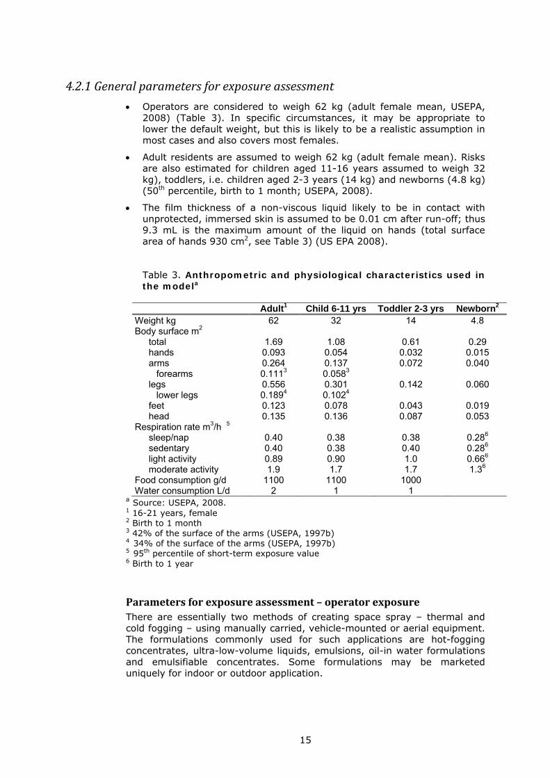
Operators are considered to weigh 62 kg (adult female mean, USEPA, 2008) (Table 3). In specific circumstances, it may be appropriate to lower the default weight, but this is likely to be a realistic assumption in most cases and also covers most females.

Adult residents are assumed to weigh 62 kg (adult female mean). Risks are also estimated for children aged 11-16 years assumed to weigh 32 kg), toddlers, i.e. children aged 2-3 years (14 kg) and newborns (4.8 kg) (50th percentile, birth to 1 month; USEPA, 2008).

The film thickness of a non-viscous liquid likely to be in contact with unprotected, immersed skin is assumed to be 0.01 cm after run-off; thus 9.3 mL is the maximum amount of the liquid on hands (total surface area of hands 930 cm2, see Table 3) (US EPA 2008).

Table 3. Anthropometric and physiological characteristics used in the modela

Adult1 Child 6-11 yrs Toddler 2-3 yrs Newborn2 Weight kg 62 32 14 4.8 Body surface m2 total 1.69 1.08 0.61 0.29 hands 0.093 0.054 0.032 0.015 arms 0.264 0.137 0.072 0.040 forearms 0.1113 0.0583 legs 0.556 0.301 0.142 0.060 lower legs 0.1894 0.1024 feet 0.123 0.078 0.043 0.019 head 0.135 0.136 0.087 0.053 Respiration rate m3/h 5 sleep/nap 0.40 0.38 0.38 0.286 sedentary 0.40 0.38 0.40 0.286 light activity 0.89 0.90 1.0 0.666 moderate activity 1.9 1.7 1.7 1.36 Food consumption g/d 1100 1100 1000 Water consumption L/d 2 1 1

a Source: USEPA, 2008. 1 16-21 years, female 2 Birth to 1 month 3 42% of the surface of the arms (USEPA, 1997b) 4 34% of the surface of the arms (USEPA, 1997b) 5 95th percentile of short-term exposure value 6 Birth to 1 year

Parametersforexposureassessment–operatorexposureThere are essentially two methods of creating space spray – thermal and cold fogging – using manually carried, vehicle-mounted or aerial equipment. The formulations commonly used for such applications are hot-fogging concentrates, ultra-low-volume liquids, emulsions, oil-in water formulations and emulsifiable concentrates. Some formulations may be marketed uniquely for indoor or outdoor application.

16

Treatments involving manually-carried equipment are used as an example in the following calculations since operators are more directly exposed to the insecticide. It is assumed that indoor space spraying using manually-carried thermal fogging equipment causes higher exposures than both outdoor spraying using vehicle-mounted sprayers and the application of cold fogs. It is further assumed that outdoor vehicle-mounted space spraying will not expose the operator who is protected by the cab of the vehicle and working upwind of the spray, although bystanders may be exposed.

A practitioner's guide for space spraying published by WHO describes in detail the appropriate spraying equipment and other issues that must be considered for safe and effective application of space-spray products (WHO, 2003). WHO has also published specifications for quality control of equipment used in such applications (WHO, 2006). In this exposure assessment, the guideline scenario assumes that both WHO recommendations and product label instructions are complied with, including the use of overalls. The lax standard scenario accommodates tropical conditions and thus assumes that protective clothing is not worn – only normal light clothing that covers the trunk.

The tasks that are considered to cause exposure to the operators are:

– mixing and loading; – application of the insecticide product by spraying with manually-

carried equipment and washing and maintenance of the spray equipment.

For operator exposure, the exposure duration is assumed to be 6 hours per day, 6 days a week, for a period of 6 months; 2 working hours per day are presumed to be spent in activities without exposure. This assumption is based on information provided to WHOPES by selected national programmes for control of vector-borne disease.

It is assumed that the correct maintenance procedures for the equipment are followed to ensure that there are no leakages occurring during the spraying operations; for example, leakages from the tap or valve, which has to be handled when starting and finishing the work, may specifically cause exposure of the hands.

Frequency of exposure in mixing and loading can be described by the number of tanks prepared per day. Tank size is assumed to be 5 litres. As an example, the tank is filled with a premixed insecticide formulation consisting of 1 part concentrate to 99 parts diluent oil (e.g. diesel oil). The label specifies a maximum of 200 mL of spray solution to be used per house, which is assumed to be 200 m3. Treatment of 60 houses per day – which is standard for this application – would require 12 litres of spray, meaning that the 5-litre tank is filled by a operator three times during the day.

The concentration of the spray liquid is to be checked from product labels or material safety data-sheets.

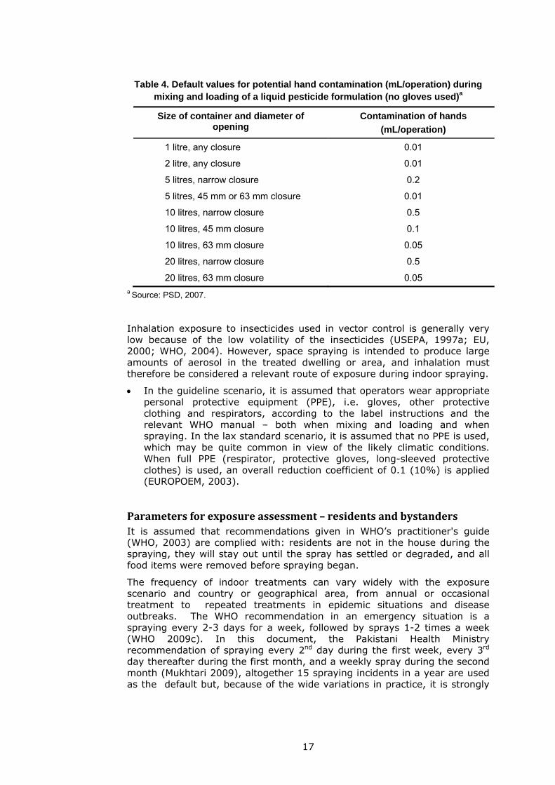
Hand contamination during filling of the tank is assumed to depend on the size of the product container and the diameter of the container opening. In the worst case, 0.5 mL of the product per tank-load is assumed to contaminate unprotected (no gloves) hands (UK POEM data: PSD, 2007); see Table 4.

17

Table 4. Default values for potential hand contamination (mL/operation) during mixing and loading of a liquid pesticide formulation (no gloves used)a

Size of container and diameter of opening

Contamination of hands

(mL/operation)

1 litre, any closure 0.01

2 litre, any closure 0.01

5 litres, narrow closure 0.2

5 litres, 45 mm or 63 mm closure 0.01

10 litres, narrow closure 0.5

10 litres, 45 mm closure 0.1

10 litres, 63 mm closure 0.05

20 litres, narrow closure 0.5

20 litres, 63 mm closure 0.05 a Source: PSD, 2007.

Inhalation exposure to insecticides used in vector control is generally very low because of the low volatility of the insecticides (USEPA, 1997a; EU, 2000; WHO, 2004). However, space spraying is intended to produce large amounts of aerosol in the treated dwelling or area, and inhalation must therefore be considered a relevant route of exposure during indoor spraying.

In the guideline scenario, it is assumed that operators wear appropriate personal protective equipment (PPE), i.e. gloves, other protective clothing and respirators, according to the label instructions and the relevant WHO manual – both when mixing and loading and when spraying. In the lax standard scenario, it is assumed that no PPE is used, which may be quite common in view of the likely climatic conditions. When full PPE (respirator, protective gloves, long-sleeved protective clothes) is used, an overall reduction coefficient of 0.1 (10%) is applied (EUROPOEM, 2003).

Parametersforexposureassessment–residentsandbystandersIt is assumed that recommendations given in WHO’s practitioner's guide (WHO, 2003) are complied with: residents are not in the house during the spraying, they will stay out until the spray has settled or degraded, and all food items were removed before spraying began.

The frequency of indoor treatments can vary widely with the exposure scenario and country or geographical area, from annual or occasional treatment to repeated treatments in epidemic situations and disease outbreaks. The WHO recommendation in an emergency situation is a spraying every 2-3 days for a week, followed by sprays 1-2 times a week (WHO 2009c). In this document, the Pakistani Health Ministry recommendation of spraying every 2nd day during the first week, every 3rd day thereafter during the first month, and a weekly spray during the second month (Mukhtari 2009), altogether 15 spraying incidents in a year are used as the default but, because of the wide variations in practice, it is strongly

18

recommended that local, case-specific data be used as well, whenever possible.

It is assumed that exposure of adults and older children occurs via the dermal route (touching contaminated surfaces in treated houses) or by ingestion of contaminated foodstuffs or water. The misuse of contaminated insecticide containers for storing drinking-water or food may also cause exposure via ingestion.

For indoor space spraying, it is assumed that residents follow the recommendations and remain out of their houses during treatment and for 30 minutes afterwards and are therefore not exposed by inhalation to the spray.

For truck application outdoors, it cannot be assumed that bystanders will not be exposed; the assumed exposure time is 15 minutes.

For surface contamination, and subsequent post-treatment dermal exposure to settled residue, it is assumed that surfaces are not intentionally sprayed but that the total volume of spray is ultimately deposited on horizontal surfaces of the house, including tables, work surfaces and the floor. For example, if the product label calls for 200 mL of diluted formulation (1 part formulation to 99 parts oil) to be sprayed in the house (10 m x 10 m x 2 m), the resulting deposition is 2 mL of diluted formulation/m2 of horizontal surface. This is considered to be a conservative assumption. In practice, especially with any wind outside the building, only about 50% of the droplets are eventually deposited on horizontal surfaces; most small droplets tend to escape through any openings. It is expected that the residue on the surfaces will decay or be carried away rapidly, so that the exposure is characteristically acute.

The body part surface areas are given in Table 3. For adults and children it is assumed that the head, upper extremities (hands and arms), lower legs and feet are exposed, the area exposed is thus 0.804 m2 for adults and 0.507 m2 for children. For toddlers (aged 2–3 years), the head, arms, hands, legs and feet (0.376 m2) are assumed to be exposed (USEPA, 1997a, 2008).

Ingestion exposure is the result of consuming contaminated foodstuff. It is assumed that food is not directly sprayed; rather, the contamination of food items is due to transfer of the insecticide from the sprayed surfaces to the food items. The surface area of food (daily intake) can be calculated from the daily volume of food eaten (1100, 1100 and 1000 g/d) for adults, children and toddlers (Table 3). The density of food is approximately 1 g/cm3, assuming that "food" is a cube of which one surface, i.e., volume to the power ⅔ is in contact with the shelf: the contaminated surface of food is 0.0107 for adults, 0.0107 for children, and 0.01 m2 for toddlers; half of food items are in contact with contaminated surfaces (the rest being in bags or otherwise wrapped). The default assumption for the amount available for transfer from contaminated surfaces to food items is 11% (95th percentile for hard surfaces, USEPA, 2009).

Toddlers frequently put different objects in their mouths and ingest soil or dust from contaminated hands. It is estimated that 11% of the insecticide on contact surfaces is transferred onto hands and that 10% of this goes from hands to mouth (USEPA, 2009). The hand area of a child aged 2–3 years is 0.032 m2 (USEPA, 2008).

19

While it clearly is misuse, it must be considered a possibility that empty insecticide packages are reused as food or water containers. This is especially important in the case of liquid products, which are often sold in sturdy plastic or metal containers; it is tempting to reuse these containers, against recommendations, for other purposes – most commonly to store water. Product-specific concentration, dilution factor (assumed 5% residue in USAID report (USAID, 2006)), water ingestion rate (2 litres/day for adults, 1 litre/day for children of both age groups (USEPA, 2008)), exposure duration of 1 day (assuming that a household uses one 38-litre container of water each day for drinking and other purposes) have been used as default parameters in the calculations. This is an acute exposure.

4.2.2 Algorithms used to estimate exposure and absorbed dose caused byindoororoutdoorspacesprayingofinsecticides

Operatorexposure

Mixing and loading insecticide formulation

In mixing and loading, inhalation exposure is not considered significant.

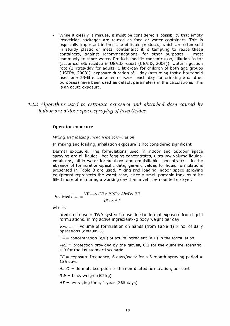
Dermal exposure. The formulations used in indoor and outdoor space spraying are all liquids –hot-fogging concentrates, ultra-low-volume liquids, emulsions, oil-in-water formulations and emulsifiable concentrates. In the absence of formulation-specific data, generic values for liquid formulations presented in Table 3 are used. Mixing and loading indoor space spraying equipment represents the worst case, since a small portable tank must be filled more often during a working day than a vehicle-mounted sprayer.

ATBW

EFAbsDPPECFVF

dermal

dosePredicted

where:

predicted dose = TWA systemic dose due to dermal exposure from liquid formulations, in mg active ingredient/kg body weight per day

VFdermal = volume of formulation on hands (from Table 4) × no. of daily operations (default, 3)

CF = concentration (g/L) of active ingredient (a.i.) in the formulation

PPE = protection provided by the gloves, 0.1 for the guideline scenario, 1.0 for the lax standard scenario

EF = exposure frequency, 6 days/week for a 6-month spraying period = 156 days

AbsD = dermal absorption of the non-diluted formulation, per cent

BW = body weight (62 kg)

AT = averaging time, 1 year (365 days)

20

Application of insecticide formulation, washing and maintenance of the spray equipment

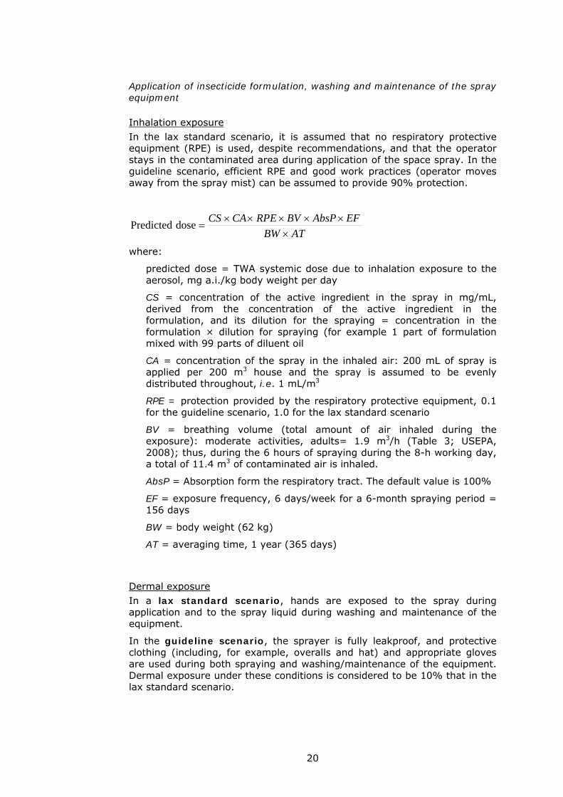
Inhalation exposure In the lax standard scenario, it is assumed that no respiratory protective equipment (RPE) is used, despite recommendations, and that the operator stays in the contaminated area during application of the space spray. In the guideline scenario, efficient RPE and good work practices (operator moves away from the spray mist) can be assumed to provide 90% protection.

ATBW

EFAbsPBVRPECACS

dosePredicted

where:

predicted dose = TWA systemic dose due to inhalation exposure to the aerosol, mg a.i./kg body weight per day

CS = concentration of the active ingredient in the spray in mg/mL, derived from the concentration of the active ingredient in the formulation, and its dilution for the spraying = concentration in the formulation × dilution for spraying (for example 1 part of formulation mixed with 99 parts of diluent oil

CA = concentration of the spray in the inhaled air: 200 mL of spray is applied per 200 m3 house and the spray is assumed to be evenly distributed throughout, i.e. 1 mL/m3

RPE = protection provided by the respiratory protective equipment, 0.1 for the guideline scenario, 1.0 for the lax standard scenario

BV = breathing volume (total amount of air inhaled during the exposure): moderate activities, adults= 1.9 m3/h (Table 3; USEPA, 2008); thus, during the 6 hours of spraying during the 8-h working day, a total of 11.4 m3 of contaminated air is inhaled.

AbsP = Absorption form the respiratory tract. The default value is 100%

EF = exposure frequency, 6 days/week for a 6-month spraying period = 156 days

BW = body weight (62 kg)

AT = averaging time, 1 year (365 days)

Dermal exposure In a lax standard scenario, hands are exposed to the spray during application and to the spray liquid during washing and maintenance of the equipment.

In the guideline scenario, the sprayer is fully leakproof, and protective clothing (including, for example, overalls and hat) and appropriate gloves are used during both spraying and washing/maintenance of the equipment. Dermal exposure under these conditions is considered to be 10% that in the lax standard scenario.

21

ATBW

AbsDEFPPECSVS

dermal

dosePredicted

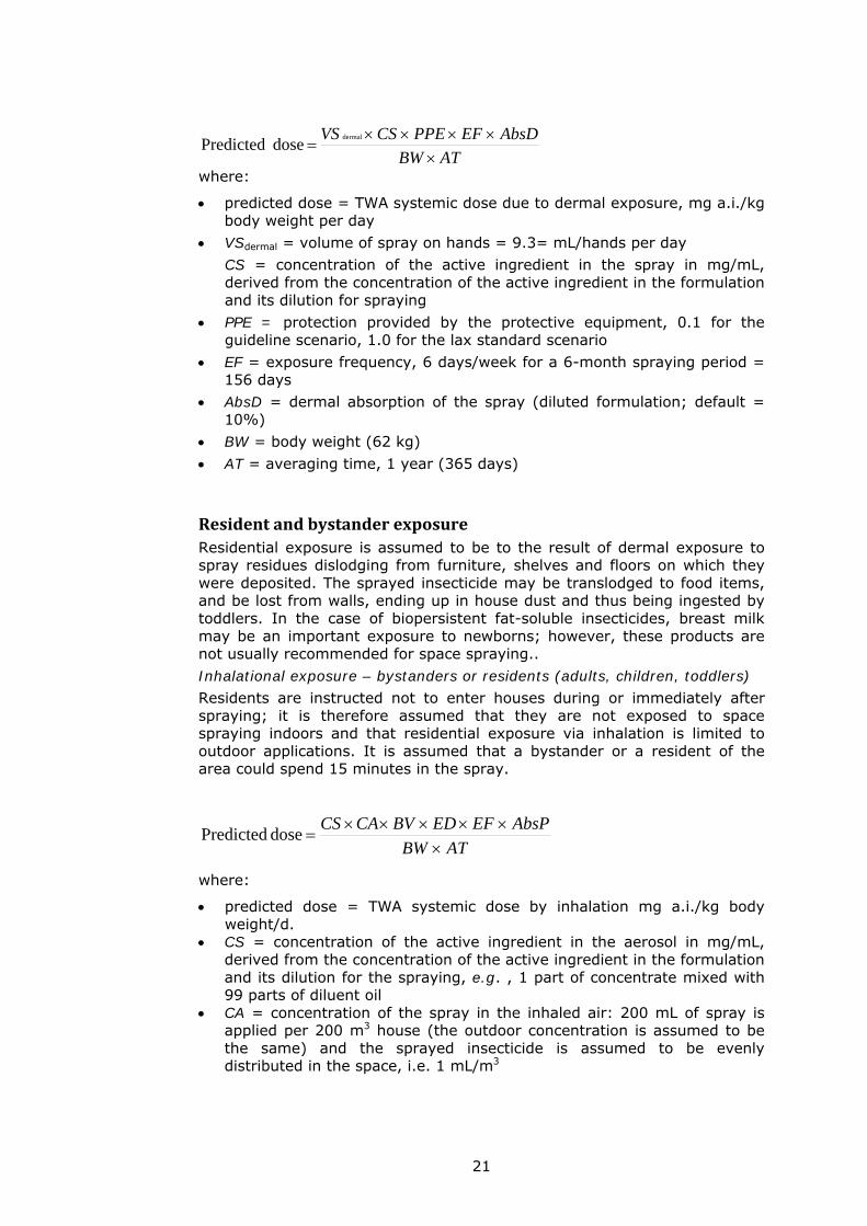
where:

predicted dose = TWA systemic dose due to dermal exposure, mg a.i./kg body weight per day

VSdermal = volume of spray on hands = 9.3= mL/hands per day CS = concentration of the active ingredient in the spray in mg/mL, derived from the concentration of the active ingredient in the formulation and its dilution for spraying

PPE = protection provided by the protective equipment, 0.1 for the guideline scenario, 1.0 for the lax standard scenario

EF = exposure frequency, 6 days/week for a 6-month spraying period = 156 days

AbsD = dermal absorption of the spray (diluted formulation; default = 10%)

BW = body weight (62 kg) AT = averaging time, 1 year (365 days)

ResidentandbystanderexposureResidential exposure is assumed to be to the result of dermal exposure to spray residues dislodging from furniture, shelves and floors on which they were deposited. The sprayed insecticide may be translodged to food items, and be lost from walls, ending up in house dust and thus being ingested by toddlers. In the case of biopersistent fat-soluble insecticides, breast milk may be an important exposure to newborns; however, these products are not usually recommended for space spraying.. Inhalational exposure – bystanders or residents (adults, children, toddlers) Residents are instructed not to enter houses during or immediately after spraying; it is therefore assumed that they are not exposed to space spraying indoors and that residential exposure via inhalation is limited to outdoor applications. It is assumed that a bystander or a resident of the area could spend 15 minutes in the spray.

ATBW

AbsPEFEDBVCACS

dose Predicted

where:

predicted dose = TWA systemic dose by inhalation mg a.i./kg body weight/d.

CS = concentration of the active ingredient in the aerosol in mg/mL, derived from the concentration of the active ingredient in the formulation and its dilution for the spraying, e.g. , 1 part of concentrate mixed with 99 parts of diluent oil

CA = concentration of the spray in the inhaled air: 200 mL of spray is applied per 200 m3 house (the outdoor concentration is assumed to be the same) and the sprayed insecticide is assumed to be evenly distributed in the space, i.e. 1 mL/m3

22

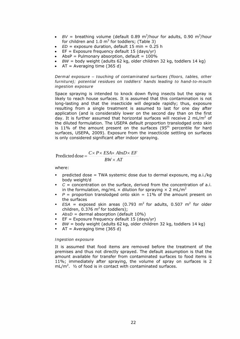
BV = breathing volume (default 0.89 m3/hour for adults, 0.90 m3/hour

for children and 1.0 m3 for toddlers; (Table 3) ED = exposure duration, default 15 min = 0.25 h EF = Exposure frequency default 15 (days/yr) AbsP = Pulmonary absorption, default = 100% BW = body weight (adults 62 kg, older children 32 kg, toddlers 14 kg) AT = Averaging time (365 d)

Dermal exposure – touching of contaminated surfaces (floors, tables, other furniture); potential residues on toddlers’ hands leading to hand-to-mouth ingestion exposure

Space spraying is intended to knock down flying insects but the spray is likely to reach house surfaces. It is assumed that this contamination is not long-lasting and that the insecticide will degrade rapidly; thus, exposure resulting from a single treatment is assumed to last for one day after application (and is considerably lower on the second day than on the first day. It is further assumed that horizontal surfaces will receive 2 mL/m2 of the diluted formulation. The USEPA default proportion translodged onto skin is 11% of the amount present on the surfaces (95th percentile for hard surfaces, USEPA, 2009). Exposure from the insecticide settling on surfaces is only considered significant after indoor spraying.

ATBW

EFAbsDESAPC

dose Predicted

where:

predicted dose = TWA systemic dose due to dermal exposure, mg a.i./kg body weight/d

C = concentration on the surface, derived from the concentration of a.i. in the formulation, mg/mL × dilution for spraying × 2 mL/m2

P = proportion translodged onto skin = 11% of the amount present on the surfaces

ESA = exposed skin areas (0.793 m2 for adults, 0.507 m2 for older children, 0.376 m2 for toddlers);

AbsD = dermal absorption (default 10%) EF = Exposure frequency default 15 (days/yr) BW = body weight (adults 62 kg, older children 32 kg, toddlers 14 kg) AT = Averaging time (365 d)

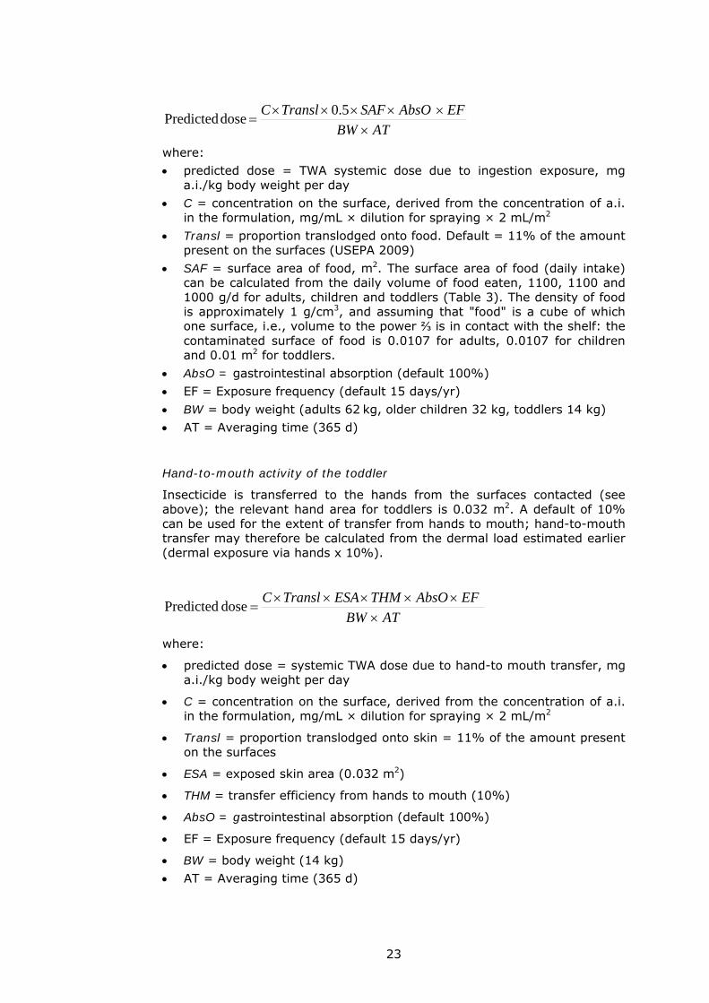
Ingestion exposure

It is assumed that food items are removed before the treatment of the premises and thus not directly sprayed. The default assumption is that the amount available for transfer from contaminated surfaces to food items is 11%; immediately after spraying, the volume of spray on surfaces is 2 mL/m2. ½ of food is in contact with contaminated surfaces.

23

ATBW

EFAbsOSAFTranslC

5.0

dose Predicted

where: predicted dose = TWA systemic dose due to ingestion exposure, mg

a.i./kg body weight per day C = concentration on the surface, derived from the concentration of a.i.

in the formulation, mg/mL × dilution for spraying × 2 mL/m2 Transl = proportion translodged onto food. Default = 11% of the amount

present on the surfaces (USEPA 2009) SAF = surface area of food, m2. The surface area of food (daily intake)

can be calculated from the daily volume of food eaten, 1100, 1100 and 1000 g/d for adults, children and toddlers (Table 3). The density of food is approximately 1 g/cm3, and assuming that "food" is a cube of which one surface, i.e., volume to the power ⅔ is in contact with the shelf: the contaminated surface of food is 0.0107 for adults, 0.0107 for children and 0.01 m2 for toddlers.

AbsO = gastrointestinal absorption (default 100%) EF = Exposure frequency (default 15 days/yr) BW = body weight (adults 62 kg, older children 32 kg, toddlers 14 kg) AT = Averaging time (365 d)

Hand-to-mouth activity of the toddler

Insecticide is transferred to the hands from the surfaces contacted (see above); the relevant hand area for toddlers is 0.032 m2. A default of 10% can be used for the extent of transfer from hands to mouth; hand-to-mouth transfer may therefore be calculated from the dermal load estimated earlier (dermal exposure via hands x 10%).

ATBW

EFAbsOTHMESATranslC

dose Predicted

where:

predicted dose = systemic TWA dose due to hand-to mouth transfer, mg a.i./kg body weight per day

C = concentration on the surface, derived from the concentration of a.i. in the formulation, mg/mL × dilution for spraying × 2 mL/m2

Transl = proportion translodged onto skin = 11% of the amount present on the surfaces

ESA = exposed skin area (0.032 m2)

THM = transfer efficiency from hands to mouth (10%)

AbsO = gastrointestinal absorption (default 100%)

EF = Exposure frequency (default 15 days/yr)

BW = body weight (14 kg) AT = Averaging time (365 d)

24

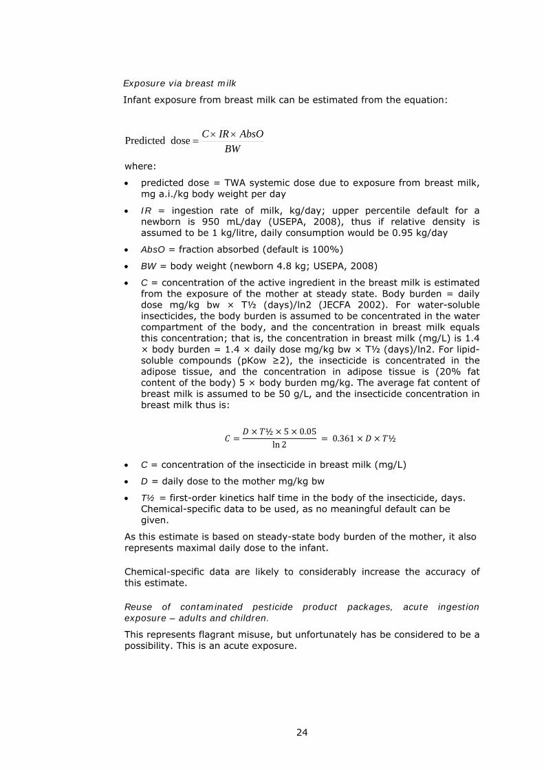
Exposure via breast milk

Infant exposure from breast milk can be estimated from the equation:

BW

AbsOIRC

dose Predicted

where:

predicted dose = TWA systemic dose due to exposure from breast milk, mg a.i./kg body weight per day

IR = ingestion rate of milk, kg/day; upper percentile default for a newborn is 950 mL/day (USEPA, 2008), thus if relative density is assumed to be 1 kg/litre, daily consumption would be 0.95 kg/day

AbsO = fraction absorbed (default is 100%)

BW = body weight (newborn 4.8 kg; USEPA, 2008)

C = concentration of the active ingredient in the breast milk is estimated from the exposure of the mother at steady state. Body burden = daily dose mg/kg bw × T½ (days)/ln2 (JECFA 2002). For water-soluble insecticides, the body burden is assumed to be concentrated in the water compartment of the body, and the concentration in breast milk equals this concentration; that is, the concentration in breast milk (mg/L) is 1.4 × body burden = 1.4 × daily dose mg/kg bw × T½ (days)/ln2. For lipid-soluble compounds (pKow ≥2), the insecticide is concentrated in the adipose tissue, and the concentration in adipose tissue is (20% fat content of the body) 5 × body burden mg/kg. The average fat content of breast milk is assumed to be 50 g/L, and the insecticide concentration in breast milk thus is:

½ 5 0.05ln 2

0.361 ½

C = concentration of the insecticide in breast milk (mg/L)

D = daily dose to the mother mg/kg bw

T½ = first-order kinetics half time in the body of the insecticide, days. Chemical-specific data to be used, as no meaningful default can be given.

As this estimate is based on steady-state body burden of the mother, it also represents maximal daily dose to the infant.

Chemical-specific data are likely to considerably increase the accuracy of this estimate.

Reuse of contaminated pesticide product packages, acute ingestion exposure – adults and children.

This represents flagrant misuse, but unfortunately has be considered to be a possibility. This is an acute exposure.

25

BW

WIRDFC dosePredicted

where:

predicted dose = systemic dose due to exposure from the misuse of a pesticide can as a drinking-water container, mg a.i./kg body weight

C = concentration of the a.i. in the formulation; chemical-specific data, mg a.i./litre

DF = dilution factor, approximately 1:20 volume/volume dilution, assumes 5% of insecticide residue in the emptied container, 0.05

WIR = water ingestion rate (2 litres/day for adults, 1 litre/day for children)

BW = body weight (adults 62 kg, older children 32 kg, toddlers 14 kg)

Ingestion exposure from contaminated foodstuffs grown in an area contaminated from space spraying – adults, children and toddlers

Insecticide sprayed in the air of a house or household area (e.g. garden) will also contaminate house dust, house floor materials and soil. Sweeping the house will transfer this contaminated material to the surrounding soil where vegetables and animals such as chickens might take up the insecticide. This could pose a significant route of human exposure if the pesticide is both persistent and bioaccumulative. In these circumstances, actual levels in these media and food items should be measured.

4.2.3Totalexposureassessment

Total exposure is calculated by summing the contributions via different routes. Any valid, chemical-specific data that are available should be used.

Exposure and risk should be calculated for operators, for residents (adults and children of different age groups) of the area that is being sprayed and for bystanders (visiting the area).

For the estimation of maximal daily exposure of the operator, (to be compared with the TSDAC, the total TWA exposure is multiplied by AT/EF = 365/156 = 2.34

For the estimation of maximal daily exposure of the residents, (to be compared with the TSDAC), the total TWA exposure is multiplied by AT/EF = 365/15 = 24.3

Space spraying treatments are not aimed at house surfaces, but some residues will inevitably be found – and there will therefore be some degree of post-application dermal exposure of residents of treated houses. However, because of the diversity of surface materials and differences in the persistence and decay of the active ingredients, this exposure is very difficult to estimate. Data on the decomposition of active ingredients are chemical-specific and not often available. This lack of information has traditionally also caused problems in assessing dermal exposure during re-entry activities in agricultural settings.

26

4.3Riskcharacterization

The aim of risk characterization is to evaluate the probability of adverse effects occurring under defined exposure conditions. In its simplest form, risk characterization consists of the comparison of estimate of total exposure with the TSD defined in the hazard assessment in all relevant exposure situations, that is, defining the ratio:.

When the insecticide has significant acute toxicity (e.g., JMPR or another organization has set an ARfD), the risk is also estimated for short-term exposure:

When these ratios are<1, the health risk is considered to be acceptable. When one or both of them are >1, there are possible health risks, and the planned use for space spraying may not be acceptable. In the case of operators, however, it may be possible to reduce the risk – for example by changing recommended operational conditions or the amount of active ingredient in the technical product. A risk–benefit analysis, in which the risks of potential toxicity are compared with potential health benefits (disease prevention), may be needed in some cases.

In the publication Generic risk assessment model for insecticide treatment and subsequent use of mosquito nets (WHO, 2004), another approach to risk characterization, based on MOE (margin of exposure) [called MOS, margin of safety, in that document], is described. However, this alternative approach has not been used to any significant extent and has therefore been omitted from the current document.

5.Theenvironmentalriskassessmentmodel

Environmental risk assessment is complex and multifaceted. Regional and national guidelines have been published yet there is no globally established system for environmental risk assessment. The published guidelines are all based on very similar premises though they differ considerably in detail; all are extensive, running to several hundred pages. This document does not cover the detail of such a scheme or propose a single scheme for international harmonization: any of the established schemes could form the starting point for environmental risk assessment associated with the public health use of pesticides. It does, however, cover the components of pesticide risk assessment schemes and the specific information likely to be needed for assessing the risk of outdoor space spraying to public health.

In the two areas of disease vector control covered in the generic models being published concurrently - larviciding and space spraying - there is commonality in the organisms likely to be exposed, although the primary application habitat (aquatic and terrestrial) and the method of application differ. Larvicides applied aerially over water will drift to expose soil organisms; insecticides applied over land in space spraying will drift to expose adjacent aquatic organisms. In summary, hazard is the same, exposure is different.

27

As in human health risk assessment, environmental risk assessment compares hazard, identified through hazard assessment, with exposure, calculated through exposure assessment, to provide risk characterization. However, environmental risk assessment seeks to characterize the risk to populations of organisms rather than to individual humans. In general, the mortality of individual organisms in the environment is naturally very high. To maintain stable populations over time, parents need to generate only two individuals over their lifetime which survive to reproduce. The very large numbers of offspring produced by many organisms in the wild reflect the considerable losses to predation, starvation and chance. The additional mortality caused acutely by pesticides would then be offset by density-dependent ecological factors; the reduced population following pesticide application would be less likely to be predated and less likely to starve. However, effects at the population level are complex to estimate and are often inferred from short-term testing.

For convenience, the components of pesticide environmental risk assessment in the European and Mediterranean Plant Protection Organization (EPPO) scheme (EPPO, 2003) are followed here, but this does not imply endorsement of one scheme over others. It is assumed throughout that good practice, as outlined by WHO (WHO, 2006) will be followed during the application of pesticides for outdoor space spraying.

The first stage for general pesticide regulatory risk assessment is to determine which components of the overall scheme are particularly relevant to the specific use(s) of the pesticide. This allows a logical progression through the series of components because output from one area is required as input to others. This progression can be similarly defined for public health use of space spraying and larviciding:

With the exception of granules applied to surface waters, all pesticides can become airborne during application and may become airborne following application by volatilization from water or soil. Possible exposure via deposition from the air is required as input to all other compartments, so this should be the starting point for risk assessment.

For outdoor space spraying, the pesticide will be intercepted by vegetation and then reach the soil. The mobility of the pesticide in soil determines the exposure of soil organisms; its presence in soil (together with residues on vegetation) determines the exposure of terrestrial vertebrates, both directly and indirectly via their food. Vertical movement through soil profiles determines the possible contamination of groundwater, and vertical and horizontal movement and surface run-off determine the indirect contamination of surface water.

Once the initial likely concentrations of pesticides in these different environmental compartments have been defined, persistence of the active ingredient in these compartments, together with information on repeat usage, allows longer-term estimates of likely concentrations to be derived.

Concentrations of pesticides, their distribution in different environmental compartments and the time course of their disappearance determine both the types of organisms that should be included in the comparison between exposure and effect and the type of effects information (acute or chronic) that is relevant to the particular exposure pattern for both soil and surface water.

28

Risk to organisms exposed through their food requires estimation of residues in different levels of food chains (from primary vegetation, through herbivore prey to predators). Information on the potential for bioaccumulation in food chains is also needed.

For all of the above, simple equations are available for estimating concentrations in environmental compartments, and standard test organisms are used to determine effect. In all cases, however, these focus on temperate conditions; the further information required to extrapolate exposure and effect estimates to tropical conditions is unlikely to be available for most pesticides.

The final stages of risk assessment for regulation of plant protection products would be refinement of the assessment and determination of appropriate risk management. The latter would require actual measurements of residue levels in the environment and/or field studies to confirm the level of effects. Neither of these is likely to be routinely available for the conditions pertinent to public health use of pesticides.

Environmental risk assessment for outdoor space spraying can be used to address four issues:

– the absolute risk to non-target organisms for each type of insecticide used;

– the relative risk of different pesticides; – the number of repeat applications likely to lead to risk to organisms

in the environment; – current best practice for the application of pesticides to minimize

risk.

5.1Environmentalexposureassessment

5.1.1Air

Pesticides may become airborne during the spraying process and, following application, by volatilization from soil, water and vegetation surfaces. The degree of spray drift is dependent on physical characteristics of spray application – the equipment used, the droplet size and the height above ground at which the spray is applied. Drift is usually expressed as a percentage of the applied dose of active ingredient that is likely to move outside the intended spraying area. If equipment and conditions remain constant for different insecticides, this proportion will remain constant.

The guidance on application of insecticides for vector control (WHO, 2003) specifies a maximum wind speed of 15 km/hour for application, equivalent to the maximum wind speed assumed in regulatory schemes. WHO guidance refers to the need to avoid overspraying of crops (although it is recognized that overspraying of rice paddies is required to kill mosquito larvae) and other direct sources of human contamination, which implies a maximum wind speed (WHO, 2006). It is therefore assumed that spraying would conform to plant protection product guidance in this respect.

However, outdoor space spraying for vector and public health pest control differs significantly from agricultural usage in that it is intended for spray droplets to stay airborne for as long as possible to kill flying insects. Aerial

29

application over rice paddies will give wider drift; at recommended wind speeds, the dose would fall to 1% within 100 metres (Hewitt et al., 2002; Teske et al., 2002) in the case of agricultural application but would be much higher in vector and public health pest control, with significant drift occurring over hundreds or thousands of metres.

The AGDRIFT (Hewitt et al., 2001) or AGDISP (Bilanin et al., 1989) aerial application models, developed by industry and government in the USA, should be used to determine the fraction of spray drift likely at the distance of the nearest significant surface water body to the application area. Temperature, humidity, etc. relevant to the geographical area of use should be input into the model.

Guidance values for spray drift are generally expressed as a percentage of the applied dose. They are tabulated for use in risk assessment according to crop type, crop growth stage of the crop and equipment types typical for the region. Values cannot, therefore, be directly transferred to public health applications. In general, the degree of spray drift increases with the energy applied by the equipment (hand-held back-pack spraying causes less drift than tractor-powered application) and with the height of the vegetation, or other surface, being sprayed. As a default for spray drift for space spraying, 10% is suggested (truck spraying, 8 km/h wind speed AGDISP, Bilanin et al., 1989).

Redistribution of deposited pesticide to the air after application can be considerable. Most studies in this area have concerned volatilization from soil surfaces; few studies have concerned plant surfaces and volatilization from water bodies has not been studied. The basic, worst-case assumptions for environmental risk assessment classify pesticides as being of high, medium or low relative volatility based on vapour pressure and Henry’s Law constant (a measure of the partition between air and water). Measured or estimated vapour pressure and Henry’s Law constant are requirements for pesticide registration and should be readily available in published regulatory assessments.

Henry’s Law constant (H) can be calculated from vapour pressure, water solubility, molecular weight and temperature:

)(K re temperatu )m (kg solubilitywater

)mol (kgweight molecular (Pa) pressurevapour 3-

1

RH

where R is the gas constant (in Pa m3 mol–1 K–1).

Correction can therefore be made for local temperature. Vapour pressure is expressed at 20 °C and adjustments for temperature are not possible without further data, which are unlikely to be available. Vapour pressure values are therefore likely to underestimate volatilization at ambient temperatures above 20 °C. However, this is not considered a major factor in the risk assessment.

Table 6 gives the classification criteria suggested for pesticides in the EPPO (2003) guidelines and suggested maximum daily loss by volatilization is a percentage of the applied dose in the first 24 hours after application.

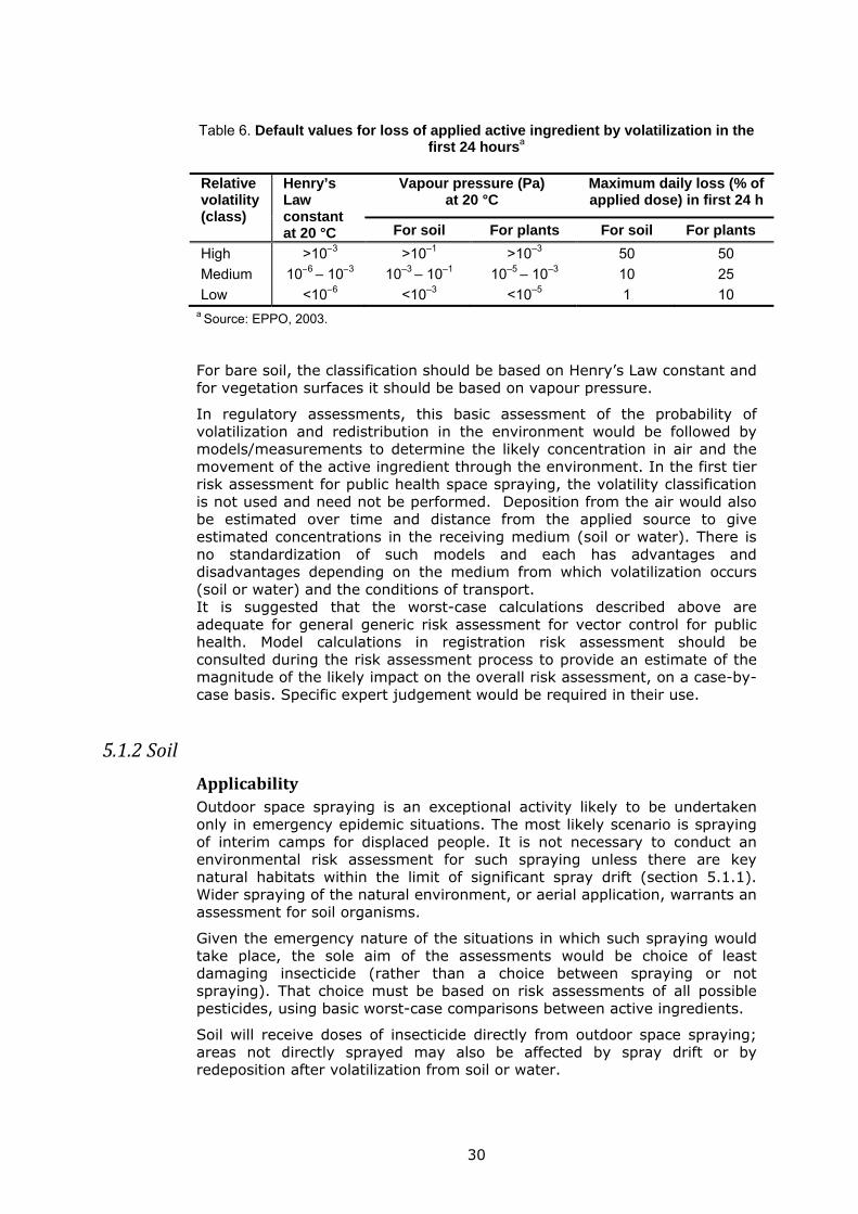
30

Table 6. Default values for loss of applied active ingredient by volatilization in the first 24 hoursa

Relative volatility (class)

Henry’s Law constant at 20 °C

Vapour pressure (Pa) at 20 °C

Maximum daily loss (% of applied dose) in first 24 h

For soil For plants For soil For plants

High >10–3 >10–1 >10–3 50 50

Medium 10–6 – 10–3 10–3 – 10–1 10–5 – 10–3 10 25

Low <10–6 <10–3 <10–5 1 10 a Source: EPPO, 2003.

For bare soil, the classification should be based on Henry’s Law constant and for vegetation surfaces it should be based on vapour pressure.

In regulatory assessments, this basic assessment of the probability of volatilization and redistribution in the environment would be followed by models/measurements to determine the likely concentration in air and the movement of the active ingredient through the environment. In the first tier risk assessment for public health space spraying, the volatility classification is not used and need not be performed. Deposition from the air would also be estimated over time and distance from the applied source to give estimated concentrations in the receiving medium (soil or water). There is no standardization of such models and each has advantages and disadvantages depending on the medium from which volatilization occurs (soil or water) and the conditions of transport. It is suggested that the worst-case calculations described above are adequate for general generic risk assessment for vector control for public health. Model calculations in registration risk assessment should be consulted during the risk assessment process to provide an estimate of the magnitude of the likely impact on the overall risk assessment, on a case-by-case basis. Specific expert judgement would be required in their use.

5.1.2Soil

ApplicabilityOutdoor space spraying is an exceptional activity likely to be undertaken only in emergency epidemic situations. The most likely scenario is spraying of interim camps for displaced people. It is not necessary to conduct an environmental risk assessment for such spraying unless there are key natural habitats within the limit of significant spray drift (section 5.1.1). Wider spraying of the natural environment, or aerial application, warrants an assessment for soil organisms.

Given the emergency nature of the situations in which such spraying would take place, the sole aim of the assessments would be choice of least damaging insecticide (rather than a choice between spraying or not spraying). That choice must be based on risk assessments of all possible pesticides, using basic worst-case comparisons between active ingredients.

Soil will receive doses of insecticide directly from outdoor space spraying; areas not directly sprayed may also be affected by spray drift or by redeposition after volatilization from soil or water.

31

The worst-case calculation of initial soil concentration assumes instantaneous uniform distribution in a stated depth of soil following application. Allowance is made for pesticide that does not reach the soil surface because it is intercepted by vegetation. (Vegetation is another source of exposure of organisms and is treated separately.) The next section outlines the basic calculation (EPPO, 2003) and suggests defaults.

Estimationofinitialconcentrationinsoil(worstcase)Ci = A x (1 – fi) x 106 / (I x 104 x d)

where:

Ci = initial concentration in soil (mg/kg soil)

A = application rate (kg/ha)

fi = fraction intercepted by vegetation

I = thickness of soil layer (metres); suggested default 0.1 m

d = bulk density of soil (kg/m3); suggested default 1500 kg/m3

The application rate (A) would be the recommended application rate for the formulation in direct overspray of the natural environment. If direct overspray can be excluded, default spray drift 10% (see above) may be used (Bilanin et al., 1989). Percentage interception equates, roughly, to percentage ground cover of the vegetation. A default value of 0.5 (50%) is suggested (Becker et al., 1999).

Risk for acute exposures of soil organisms would use this value.

For calculation of longer-term exposure risk, the half-life of the insecticide in soil must be known. This is a standard requirement for regulatory risk assessment and should be readily available. These standard biodegradation tests should have followed guidelines to determine the appropriate kinetics for the substance in the test soils. Aerobic degradation is the usual route relevant to risk assessment for soils (unless waterlogged soil is the norm in the area sprayed). Degradation is temperature-dependent and most test results will be reported for 20 °C. Adjustments can be made for other temperatures: in the European Union, a factor of 2.58 is used for 10 °C changes (normally applied for lower temperatures in Europe but can be used for increased temperature in the tropics) (EFSA, 2007).

Risk assessment for chronic exposure of soil organisms requires calculation of the concentration in soil (as a time-weighted average) over the same time period as used for exposure of standard organisms in chronic toxicity tests.

Calculationoftime‐weightedaverageconcentration(TWAC)insoil(worstcase)afterasingleapplication TWAC (mg/kg soil) = Ci x (DT50/(t x ln2)) x [1 – exp(-t x ln2/DT50)]

where:

Ci = initial concentration in soil (mg/kg soil) (from earlier calculations)

32

DT50 = half-life (days) from laboratory degradation tests (adjusted for local temperature)

t = time period of choice (days)

Risk calculations for chronic exposure of soil organisms would use this value.

For environmental risk assessment for soils it is important to determine whether the pattern of use of the insecticide leads to build-up of residues of the active ingredient. From any single application of insecticide, the concentration in soil at any specific time interval after application can be calculated according from the equation in the following section.

Calculationofconcentrationattimetafterasingleapplication Ct (mg/kg soil) = Ci x exp -(ln2/DT50 x t)

where:

Ci = initial concentration in soil (mg/kg soil) (from earlier calculations)

DT50 = half-life (days) from laboratory degradation tests (adjusted for local temperature)

t = time period of choice (days)

RepeatapplicationsFor repeat applications, concentrations in soil can be calculated over time, taking into account the overlap of residues remaining from previous applications with further spraying. The straightforward calculations assume a constant application rate and constant intervals between applications; in these circumstances, a steady state will be achieved over time. For irregular application intervals, each application would need to be calculated separately and the results added for overlap. The latter is likely to be the situation for vector control.

Repeat applications cause significantly increased (doubling) soil concentrations if the trough concentration (the concentration immediately before the next application) is ≥0.5 × Ci (i.e., if the total dissipation half-time is ≥ 2 × application interval, the worst case default of which is 7 days).

Calculation of upper and lower plateau concentrations for repeatapplicationatconstantrateandconstanttimeintervalLower plateau concentration (residue at the end of the nth application):

X

XXCR

ni

low

1

)1(

where:

Rlow = lower plateau concentration at the end of the nth application (mg/kg soil)

33

X = the proportion of the applied dose remaining after the first application

Ci = initial concentration following application of A (kg/ha)

n = the number of applications. As a contingency measure in dengue epidemics, WHO recommends space spraying every 1-2 weeks (WHO 1999b). As the dengue season may extend over 6 months, n in the worst case scenario and is approximately 20; this can therefore be used as the default number of applications.

Upper plateau concentration:

X

XCR

ni

high

1

)1(

For irregular application intervals or different application rates, the equation for the calculation of concentration Ct at time t after application should be used and overlapping calculated concentrations summed.

The remaining essential value required for soil is the adsorption coefficient Kd which measures the partition between the soil matrix and the interstitial water. This is an indicator of the likelihood of the pesticide leaching down through the soil to reach groundwater and of lateral movement through the soil. The value is often normalized to the organic matter fraction of the soil, the matrix in which most adsorption generally occurs. This is either expressed as KOM (for organic matter) or KOC (for organic carbon). The normalized value should be taken unless there is indication that organic material content of the relevant soils differs significantly from the default/measured values used in its calculation.

Residues of pesticides from the soil may be moved by rainfall and be carried by run-off to adjoining surface water. In the case of outdoor space spraying, where the objective is immediate knock-down of flying insects with no residual effect expected, the amount of insecticide deposited on soil will be much lower than that associated with agricultural spraying, so any run-off will be negligible. If it is felt that run-off could occur because of soil slope, there are models that might be used to assess the likelihood and extent of run-off (Beinat & van den Berg, 1996). If a risk is perceived, further information may be required to refine the risk assessment.

If local field studies are not available, the likely case, extrapolating to probable reality, could be based on the refinement level of regulatory risk assessment available from temperate countries. The field conditions of these refinement-level tests may be very different from those of vector control. Expert judgment is thus the only means of applying “correction” factors to the first, precautionary, estimates of risk.

Outdoor space spraying is clearly imperative as a means of preventing epidemic; the benefits therefore outweigh any risk to the environment. However, it is clearly an advantage to know the degree to which such environmental damage will occur and the time likely to be needed for environmental recovery. In such circumstances, it is suggested that a calculation be performed to predict the number of repeat applications that would lead to soil residues of concern at the worst-case and likely realistic assessment levels. Calculations are also suggested to estimate the time

34

taken for soil residues to fall to non-damaging levels after cessation of treatment.

Calculation of number of applications that would lead to soilconcentrationsofconcernThese calculations can be performed by iterations of the equations for upper and lower plateau concentrations presented above (or the results for overlapping irregular applications) until a concentration of concern is reached; this concentration is determined as a no-observed-effect concentration for soil organisms, derived in later stages of the risk assessment. The result would be expressed as a value of n (number of applications).

Calculation of time to return to non‐damaging concentrations aftercessationofsprayingOn cessation of spraying, the final estimate of soil concentration (plateau concentration equations using actual value for n) would be used as the starting concentration Ci for the equation for concentration at time t after application. The time period required to reach non-damaging concentrations would then be calculated iteratively.

5.1.3Surfacewaterandaquaticsediment

ApplicabilityOutdoor space spraying might overspray surface water or lead to exposure through spray drift; regular reapplication with typically daily intervals could lead to significant exposure.

Run-off from soil/vegetation application would represent another source of exposure for surface waters following outdoor space spraying, and this exposure might persist if high soil residues had built up from successive regular sprays.

Initial concentrations in surface water from spray drift during outdoor space spraying applications are given below.

Estimation of initial concentration in water from outdoor spacespraying(worstcase)–spraydriftCdrift = 100 × E x X/D

where:

Cdrift = initial concentration in water, µg/L

E = proportion of drift (default = 10%)

X = application rate (kg/ha)

D = water depth (metres; default = 0.5 m)

Risk for acute exposures of organisms living in the open water body would use this value.

35

As stated in section 5.1.2, run-off is usually not a problem in the case of space spraying for public health purposes; run-off need only be considered in cases in which the rainfall is heavy, the slope of the terrain is steep, and the soil is susceptible to run-off (clay, loam, silt). When needed, run-off estimates may be estimated as in Beinat & van den Berg (1996). Estimation should express potential run-off in percentage terms and lead to a calculation of concentration. Initial concentration following outdoor space spraying would then be the value from spray drift plus the value from run-off. For pesticides classified as highly volatile (see Table 6), an additional estimate of active ingredient in rainfall would be made.

Insecticide reaching surface water will partition between the water body and sediment (both bottom sediment and suspended particulates). This partitioning is key to understanding which organisms are likely to be exposed to the residues and therefore which compartment is relevant to the risk assessment.

Concentrations resulting (at equilibrium) from such partitioning are given below.

Estimation of concentrations in water and sediment followingpartitionequilibriumPartition coefficient:

Ks/l = Csed / Cwater

where:

Ks/l = sediment/water distribution coefficient (litres/kg)

Csed = concentration in sediment (mg/kg)

Cwater = concentration in water (mg/litre)

Fractions dissolved and sorbed:

Fdissolved = 1/(1 + Ks/l) and

Fsorbed = Ks/l/(1 + Ks/l)

Concentration:

Total emissions to the water/sediment compartment are divided by the estimated volume of the compartment.

Residues of insecticide in water will dissipate over time. Factors that may be relevant are: biodegradation (aerobic or anaerobic), advection, hydrolysis, photodegradation, sedimentation and resuspension.

As for soil, the biodegradation half-life should be available for the water/sediment compartment since it is a requirement for registration. Separate studies are conducted for this compartment (OECD, 1987) and should generate separate half-lives for the water, the sediment and the whole system.

Advection – transport in fluid – is relevant to the risk assessment if the water body receiving the insecticide is flowing or renewed (water being pumped into or out of the body).

36

Hydrolysis may be an important factor in dissipation and might also be included in the value for biodegradation; it is not necessarily measured separately in the test (using sterilized medium). Care must be taken if the pKa value for the substance is close to (within 1 unit) of the pH of the water; this might lead to significant dissociation of the substance into ionic species, which will affect both hydrolysis and the adsorption characteristics of the substance.

Photodegradation is often considered unlikely in registration assessments based on temperate regions but may be much more important in tropical areas. High turbidity in the receiving water will greatly reduce photodegradation.

Sedimentation is the loss of insecticide residue from the water body to sediment by adsorption to particulates which then fall to the bottom; sediment particles may also be resuspended following disturbance of bottom sediments by flow or other factors.

Concentration in the water body will dissipate as a result of any or all of these processes. The processes can be summed as rate constants, Kx, which can be calculated from half-life DT50 according to the general formula:

Kx = ln2/DT50

Total dissipation may then be estimated according to the following equation:

Dissipationfromthewaterbodyovertime(t)Ktotal_dissipation = (Kb + Ks – Kr + Kv + Kh + Kp) x Fw + Ka

where:

Ktotal_dissipation = total reaction rate constant for all processes together assuming first-order kinetic in days-1

Kb = rate constant for biodegradation (days-1)

Ks = rate constant for sedimentation (days-1)

Kr = rate constant for resuspension (days-1)

Kv = rate constant for volatilisation (days-1)

Kh = rate constant for hydrolysis (days-1)

Kp = rate constant for photodegradation (days-1)

Fw = fraction of dissolved substance

Ka = rate constant for advection (days-1)

Then:

Ct = Ci . e–Ktotal_dissipation x t

Ct = Ci x exp(-Ktotal dissipation x t)

where:

Ct = concentration at time t (mg/litre)

Ci = initial concentration from all sources (mg/litre)

t = time (days)

37

Comparison with acute toxicity test results can be made against concentration at time zero; comparison with chronic toxicity test results would be against a time-weighted average over t days calculated as:

1

where t is comparable with the time period of the chronic tests.

Dissipationfromthesedimentovertime(t)A comparable calculation can be made for dissipation from the sediment over time but only biodegradation and, possibly, sedimentation and resuspension would be relevant.

5.2Effects

5.2.1Aquaticorganisms

Acute tests on a range of aquatic organisms representing three trophic levels in aquatic ecosystems are an absolute requirement for registration of new pesticides and should be available as a minimum for all pesticides. Acute tests on microalgae, daphnids and fish are the common feature of all regulatory systems. For herbicides, an additional test on an aquatic macrophyte would normally be added; these tests, usually on the floating plant Lemna, are unlikely to be available for newer insecticides but have often been performed on older insecticides.

Testing should normally be done on the pesticide as the formulation that will be used in the field but this may not have been the case for older pesticides. Ideally, testing of both the pure active ingredient and the formulation should be available to indicate the toxicity caused by each component. Care should be taken with reported values from toxicity tests in which the concentrations tested substantially exceed the water solubility of the substance.

Small or minimal acute datasets can be handled for risk assessment only by using deterministic approaches. Comparison of the lowest reported LC50 (concentration killing 50% of the test organisms – the usual end-point for acute tests on animals) or EC50 (concentration having a 50% effect on test populations against a specific end-point – often growth or biomass and the usual end-point for algal tests) with the predicted (or measured) environmental concentration (PEC) gives a ratio, the exposure–toxicity ratio (ETR). The ETR is a measure of the margin between exposure and toxicity, a simple safety margin, and is normally expressed as a single ratio for the most sensitive species tested. Risk is thus completely dependent on a single data point, a single toxicity test result. Further tests will not affect the risk calculation provided that the new tests show lower sensitivity than the existing ones; however, a new test with a lower LC50 or EC50 will change the outcome.

Commonly, these simple ratios are used in regulatory systems to generate an initial classification of the pesticide and to inform the need for further testing.

38

It is suggested that ETRs are calculated for all three types of organism likely to be represented in the dataset – algae, fish and daphnids – plus other invertebrates if test results area available. Classification of the insecticide against unrelated organisms might then distinguish between different insecticides. Larvicidal application is likely to classify insecticides as high risk; outdoor space spraying is less likely to do so because of much lower exposure.

Exposure–toxicityratiosforacuteexposure(EPPO,2003)The ETR is derived by dividing the initial concentration in surface water (Ciw) by the lowest reported LC50 or EC50 for algae, invertebrates and fish, plus any other group of organisms for which acute toxicity test results are available. Results are tabulated.

For pesticides that dissipate rapidly from water, the TWAC would be more appropriate than initial concentration for deriving ETR.

If the ETR is low (<0.1 equivalent to a safety margin of 10), the value is classified as low acute risk.

If the ETR is moderate (0.1–1, equivalent to a safety margin between 10 and 0), the value is classified as medium risk.

If the ETR is high (>1, equivalent to an exceeded safety margin), the value is classified as high acute risk.

If any ETR is classified as indicating low acute risk, no further consideration is given to it in the risk assessment.

In regulatory systems, additional tests over a longer exposure period would be triggered by persistence of the pesticide in either water or sediment and/or medium to high acute risk classification. For older pesticides, many such tests were conducted outside the regulatory framework and published in scientific journals.

For older pesticides, existing schemes often did not distinguish between the media in which the pesticide was likely to partition; for these older active ingredients, tests will therefore be available on organisms that are unlikely to be exposed and unavailable for those that are likely to be exposed. Methods for extrapolation are available in this case. Modern regulatory systems would tailor requirements for longer-term toxicity tests to the most sensitive species and the appropriate medium (water or sediment) for the ultimate fate of the pesticide.

Chronic tests will thus be available for most pesticides that have been used for some time but may not be ideal for risk assessment or conform to modern guidelines. This does not make them unusable but increases the uncertainty of the resulting risk assessment.

Results of chronic tests would normally establish a no-observed-effect concentration (NOEC) rather than the effect concentrations determined in acute tests. In some cases no NOEC will have been established and a lowest-observed-effect concentration (LOEC) will be available instead.

The strict definition of “chronic” would be “over the lifetime of the organism”. Algal tests cover multiple generations of the algae, even for short-term exposure (typically 3–4 days), and these are often used in both acute and chronic toxicity assessments. The end-points in algal tests

39

(growth or biomass) are indications of population-level effects and would conform to an alternative definition of chronicity – relevance to population level. Chronic tests on daphnids are typically run over 28 days and would include two generations, fulfilling both definitions of chronicity. Some daphnid species can achieve the same number of generations in a much shorter time. “Chronic effects” on fish are commonly from tests conducted over shorter periods than would meet either definition. The decision on whether a fish test would be regarded as acute or chronic can have significant effects on the outcome of the risk assessment and should be made by an expert. Early life-stage tests, exposing fish from the egg stage through larval development to the juvenile, are often done as chronic tests. Longer-term fish tests that measure only survival are not usually considered as chronic. Tests measuring non-lethal end-points, for example enzyme systems (common for organophosphate insecticides) are not usually included in chronic risk assessment.

Ideally, chronic tests would involve species relevant to the environment local to the application under risk assessment. Most common test species are temperate and the tests will have been conducted at lower temperatures. Some tropical species are used in non-standard testing and might be available but should not be used in preference in risk assessment for space spraying; they should be examined for evidence of higher toxicity at higher temperature. It is unlikely that the dataset will be sufficiently large for confident predictions in this respect.

Classifications for chronic toxicity are then based on a recalculation of ETR, as for acute exposure.

Exposure–toxicityratiosforchronicexposureThe ETR is derived by dividing the RWAC in surface water over the time period of the chronic test by the lowest reported NOEC for algae, invertebrates and fish, plus any other group of organisms for which chronic toxicity test results are available to derive the ETR. Results are tabulated.

For pesticides that dissipate rapidly from water, the TWAC would be more appropriate than initial concentration for deriving ETR.

If the ETR is low (<0.1, equivalent to a safety margin of 10), the value is classified as low chronic risk.

If the ETR is moderate (0.1–0.2, equivalent to a safety margin between 10 and 5), the value is classified as medium risk.

If the ETR is high (>0.2, equivalent to a safety margin less than 5), the value is classified as high chronic risk.

Note: The risk assessor should be aware of the results of the partitioning calculations. If there is rapid or complete partitioning from water to sediment, the chronic risk assessment should concentrate on the latter medium.

Calculation of ETR would be based on calculated sediment concentration of the insecticide and tests on sediment-dwelling invertebrates. If sediment tests are not available, aquatic tests results may be compared with estimated interstitial water concentrations in sediment.

Biodegradation in the sediment should be taken into account in estimating exposure over the time period of the chronic test. Some partitioning out of

40

the water body will also affect the concentration in water over the period of a chronic test on a species living in the water body.

For larger datasets, a probabilistic approach can be taken, using all the available data to derive a predicted no-observed-effect concentration (PNEC) from a fitted distribution curve. This approach has not been widely applied to pesticide risk assessment but scientifically is the more desirable approach. A probabilistic distribution has the advantage that new single tests have little influence on the outcome. The complete dataset increases confidence that a realistic NOEC has been derived that is protective of a wide range of species.

In pesticide regulatory systems, strict criteria are usually applied to the use of the probabilistic approach (number of data points, number of trophic levels/representative groups of organisms, etc.). Only chronic NOECs are used as input for curve-fitting. In the present context, it is suggested that less strict criteria be established because the approach is useful in determining the degree of concern when headline ETRs indicate high risk.

In Australia and New Zealand, guidance on applying probabilistic approaches to risk assessment for water quality guidelines allows the application of factors to acute data to increase the number of chronic points available for curve-fitting. The number of tests required for the approach is also reduced. This less stringent guidance has been used in the WHO Concise International Chemical Assessment Document (CICAD) series and its use has been the subject of international peer-review in this context.

It is suggested that, if the dataset allows, distribution curves be fitted (log-logistic or comparable) for the full dataset and for the dataset without aquatic invertebrates. This should inform the final decision on risk to target (and related) and non-target organisms in vector control.

Fit a distribution curve to available chronic data (if sufficient areavailable) Derive values for concentration protective of 95% of species with an

error of 50% for all species and for non-target species (excluding invertebrates).

Bioaccumulation influences the perceived risk over longer time frames. Following estimation of chronic risk, account should be taken of indicative bioaccumulation in the test species or trophic level.

Bioaccumulation potential can be estimated from Pow, the octanol/water partition coefficient; this is commonly done for industrial chemicals where the availability of test data is limited. However, it is probable that bioaccumulation tests, at least in fish, will have been conducted for most pesticides. These experimental values should be used in preference in the risk assessment. A more precautionary approach is generally taken with pesticides than with industrial chemicals, and a ratio, at steady state, of 1000 for a BCF (bioconcentration factor: concentration in the test organism expressed as whole-body concentration/concentration in the test medium, usually water) is considered to be of concern.

41

Establishbioaccumulationpotential Estimate from log Kow: BCF = 0.048 x Pow

or preferably:

Obtain BCF from studies at least on fish. Classify as potentially bioaccumulative if BCF >1000.

The need for specific decisions on the suitability of species, the requirement for chronic testing, the interpretation of test results and whether or not probabilistic approaches can be applied is emphasized as a requirement for expert ecotoxicological input into the process in all regulatory systems. Input of expert judgement is also suggested here. The additional extrapolation from temperate to tropical conditions would also argue for specific expertise.

The availability of any further tests or field data should be established here. Mesocosm and field studies will indicate whether predicted worst-case ETRs are realistic.

5.2.2Soilorganismsandsoilfunction

Risk assessment for soil organisms is comparable to that for aquatic organisms; comparison is made between a predicted or measured concentration in soil and the results of toxicity tests. In addition to single-species toxicity testing, tests for generalized toxicity to soil microflora may be performed, measuring effects on nitrogen or carbon transformation processes in the soil.

Standard testing of soil organisms involves many fewer species than testing the aquatic environment. Earthworms are the most likely species to have been tested and the tests could be acute (lethality end-point) or chronic (reproductive end-point). Other organisms were seldom tested in the past and standard tests are unlikely to be available for older pesticides; non-standard tests might have been conducted and reported in the scientific literature. Tests that comply with international guidelines are often conducted in artificial soils to reduce variability; results are usually corrected to reflect differences in organic matter content between the artificial and natural soils. A correction factor of 2 is usually applied in Europe. However, this assumes that agricultural soils are neither very sandy nor very peaty; neither assumption can necessarily be made in the environment generally.

A wide range of soil function tests has been conducted in the past. Comparisons between different test methods suggest considerable variability, and interpretation of older tests therefore requires expert input.

Field tests on soil organisms are rare for older pesticides and are unlikely to be relevant to risk assessment in the context of disease vector control.

In general, ETRs are calculated as follows.

Estimationofexposure–toxicityratiosforsoilorganisms

Acute

Comparison is made between the initial concentration in soil, Ci, and acute LD50 from an earthworm test corrected for soil organic matter

42

(normally a factor of 2 is used but this should be determined by expert input).

If the ETR >0.2 (equivalent to a safety margin of 5), acute toxicity for earthworms is of concern.

Chronic

Comparison is made between the TWAC in soil over the time period of the chronic test and the chronic NOEC for reproduction in earthworms

A chronic test with measurement of reproductive success should give some indication of likely population effects in the field. The degree of concern for chronic effects on earthworms is based on the likelihood of effects persisting for more than one season or of substantial reduction in reproductive potential within a single season, estimated against toxicity test results and likely exposure over one season.

Further acute or chronic ETRs may be calculated if toxicity test results are available for other soil organisms.

Bioaccumulation in earthworms is considered of relevance to the risk assessment for soil organisms but is of interest principally in consideration of secondary poisoning in the food chain.

EstablishbioaccumulationpotentialforterrestrialorganismsThe bioconcentration factor is estimated from ooctanol/water partition coefficient (Pow):

BCF = (0.84 + 0.01Pow)/Foc Koc

where:

Pow = octanol/water partition coefficient

Foc = organic carbon content of the soil (default value is 0.02)

Koc = organic carbon adsorption coefficient

Ideally, however, BCF is obtained from studies on earthworms.

Significant bioaccumulation leads to consideration of risk by secondary poisoning to predators eating worms (see later).

Reasonablecut‐offvaluesforresultsonsoilfunctionThese tests should be conducted over an adequate period of time; early tests were often short-term. For valid test results on Carbon and Nitrogen transformation in soil:

If deviation from control is <25% at all time periods, the risk is considered to be negligible.

If deviation from control is <25% after 28 days, the risk is considered to be low.

If deviation from control is <25% between 42 and 100 days, the risk is considered to be medium.

If deviation from control is >25% after 100 days, the risk is considered to be high.

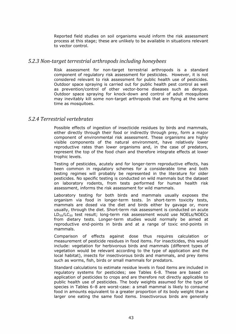
43

Reported field studies on soil organisms would inform the risk assessment process at this stage; these are unlikely to be available in situations relevant to vector control.

5.2.3Non‐targetterrestrialarthropodsincludinghoneybees

Risk assessment for non-target terrestrial arthropods is a standard component of regulatory risk assessment for pesticides. However, it is not considered relevant to risk assessment for public health use of pesticides. Outdoor space spraying is carried out for public health pest control as well as prevention/control of other vector-borne diseases such as dengue. Outdoor space spraying for knock-down and control of adult mosquitoes may inevitably kill some non-target arthropods that are flying at the same time as mosquitoes.

5.2.4Terrestrialvertebrates

Possible effects of ingestion of insecticide residues by birds and mammals, either directly through their food or indirectly through prey, form a major component of environmental risk assessment. These organisms are highly visible components of the natural environment, have relatively lower reproductive rates than lower organisms and, in the case of predators, represent the top of the food chain and therefore integrate effects at lower trophic levels.

Testing of pesticides, acutely and for longer-term reproductive effects, has been common in regulatory schemes for a considerable time and both testing regimes will probably be represented in the literature for older pesticides. No specific testing is conducted on wild mammals but the dataset on laboratory rodents, from tests performed for human health risk assessment, informs the risk assessment for wild mammals.

Laboratory testing for both birds and mammals usually exposes the organism via food in longer-term tests. In short-term toxicity tests, mammals are dosed via the diet and birds either by gavage or, more usually, through the diet. Short-term risk assessment is conducted on acute LD50/LC50 test result; long-term risk assessment would use NOELs/NOECs from dietary tests. Longer-term studies would normally be aimed at reproductive end-points in birds and at a range of toxic end-points in mammals.

Comparison of effects against dose thus requires calculation or measurement of pesticide residues in food items. For insecticides, this would include: vegetation for herbivorous birds and mammals (different types of vegetation would be relevant according to the type of application and the local habitat), insects for insectivorous birds and mammals, and prey items such as worms, fish, birds or small mammals for predators.

Standard calculations to estimate residue levels in food items are included in regulatory systems for pesticides; see Tables 6-8. These are based on application of pesticides to crops and are therefore not directly applicable to public health use of pesticides. The body weights assumed for the type of species in Tables 6–8 are worst-case: a small mammal is likely to consume food in amounts equivalent to a greater proportion of its body weight than a larger one eating the same food items. Insectivorous birds are generally

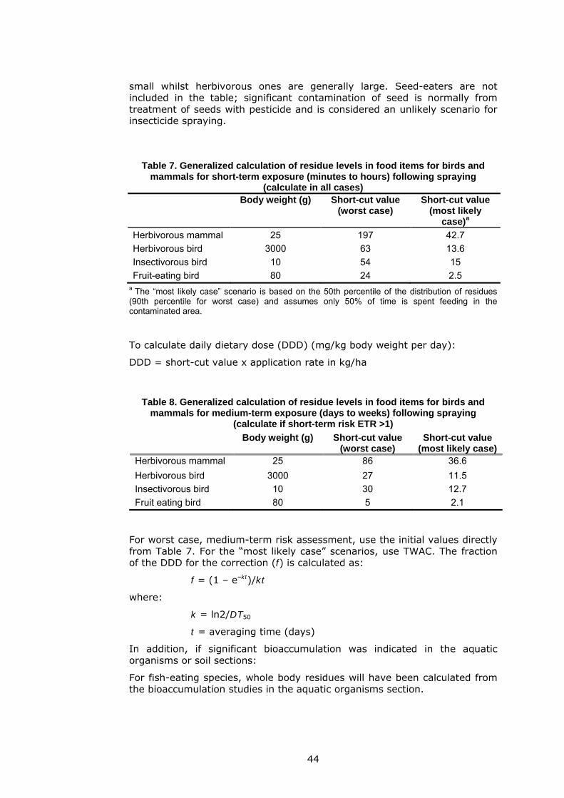
44

small whilst herbivorous ones are generally large. Seed-eaters are not included in the table; significant contamination of seed is normally from treatment of seeds with pesticide and is considered an unlikely scenario for insecticide spraying.

Table 7. Generalized calculation of residue levels in food items for birds and

mammals for short-term exposure (minutes to hours) following spraying (calculate in all cases)

Body weight (g)

Short-cut value (worst case)

Short-cut value (most likely

case)a

Herbivorous mammal 25 197 42.7

Herbivorous bird 3000 63 13.6

Insectivorous bird 10 54 15

Fruit-eating bird 80 24 2.5 a The “most likely case” scenario is based on the 50th percentile of the distribution of residues (90th percentile for worst case) and assumes only 50% of time is spent feeding in the contaminated area. To calculate daily dietary dose (DDD) (mg/kg body weight per day):

DDD = short-cut value x application rate in kg/ha

Table 8. Generalized calculation of residue levels in food items for birds and mammals for medium-term exposure (days to weeks) following spraying

(calculate if short-term risk ETR >1)

Body weight (g)

Short-cut value (worst case)

Short-cut value (most likely case)

Herbivorous mammal 25 86 36.6

Herbivorous bird 3000 27 11.5

Insectivorous bird 10 30 12.7

Fruit eating bird 80 5 2.1

For worst case, medium-term risk assessment, use the initial values directly from Table 7. For the “most likely case” scenarios, use TWAC. The fraction of the DDD for the correction (f) is calculated as:

f = (1 – e–kt)/kt

where:

k = ln2/DT50

t = averaging time (days)

In addition, if significant bioaccumulation was indicated in the aquatic organisms or soil sections:

For fish-eating species, whole body residues will have been calculated from the bioaccumulation studies in the aquatic organisms section.

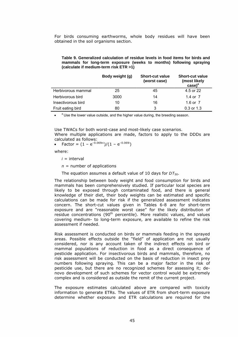
45

For birds consuming earthworms, whole body residues will have been obtained in the soil organisms section.

Table 9. Generalized calculation of residue levels in food items for birds and mammals for long-term exposure (weeks to months) following spraying (calculate if medium-term risk ETR >1)

Body weight (g)

Short-cut value (worst case)

Short-cut value (most likely

case)a Herbivorous mammal 25 45 4.5 or 22

Herbivorous bird 3000 14 1.4 or 7

Insectivorous bird 10 16 1.6 or 7

Fruit eating bird 80 3 0.3 or 1.3

a Use the lower value outside, and the higher value during, the breeding season.

Use TWACs for both worst-case and most-likely case scenarios. Where multiple applications are made, factors to apply to the DDDs are calculated as follows: Factor = (1 – e–0.069ni)/(1 – e–0.069i)

where:

i = interval

n = number of applications

The equation assumes a default value of 10 days for DT50.

The relationship between body weight and food consumption for birds and mammals has been comprehensively studied. If particular local species are likely to be exposed through contaminated food, and there is general knowledge of their diet, their body weights can be estimated and specific calculations can be made for risk if the generalized assessment indicates concern. The short-cut values given in Tables 6-8 are for short-term exposure and are “reasonable worst case” for the likely distribution of residue concentrations (90th percentile). More realistic values, and values covering medium- to long-term exposure, are available to refine the risk assessment if needed. Risk assessment is conducted on birds or mammals feeding in the sprayed areas. Possible effects outside the “field” of application are not usually considered, nor is any account taken of the indirect effects on bird or mammal populations of reduction in food as a direct consequence of pesticide application. For insectivorous birds and mammals, therefore, no risk assessment will be conducted on the basis of reduction in insect prey numbers following spraying. This can be a major factor in the risk of pesticide use, but there are no recognized schemes for assessing it; de- novo development of such schemes for vector control would be extremely complex and is considered as outside the remit of the current project. The exposure estimates calculated above are compared with toxicity information to generate ETRs. The values of ETR from short-term exposure determine whether exposure and ETR calculations are required for the

46

medium term; similarly, medium-term results indicate the need to consider long-term exposure. Indications of bioaccumulation from either the aquatic organisms section (fish) or the soil section (earthworms) would generate a requirement for risk assessment for fish-eating or worm-eating species; this is done for the medium-term exposure scenario and could be extended to the longer term if a risk were identified. Indications of bioaccumulation would be a log Pow >3 or BCF >1000.

Calculationofexposure–toxicityratiosforbirdsandmammals

Short-term exposure

The DDD values obtained above are divided by acute toxicity LD50 values.

Medium-term exposure

The DDD values are divided by lethality in short-term tests. For birds, the lethality end-point (LC50) is taken from a 5-day acute toxicity test; for mammals the end-point (NOEC) is taken from a 28-day rat study. In both cases, the value is converted from LC50 (mg/kg food) into LD50 (mg/kg body weight per day).

LD50 = LC50 x DFI/1000

where DFI = daily food intake (in g x 1000/body weight in g) Note: Applicability of the short-term dietary toxicity test in birds (5 days) for risk assessment has been called into question (Mineau et al., 1994). Results of the test are often a consequence of starvation because of repellency of the diet and should therefore be used with caution.

Long-term exposure

The DDD values obtained above are divided by non-lethal NOEC results from medium- to long-term tests (mammalian testing and avian reproductive testing). The NOEC is converted to NOED (mg/kg body weight per day). Uncertainty is related to the dataset available for mammals and birds. If only small numbers of tests results are available (one or two species, for example), an uncertainty factor – commonly 10 – is applied to the calculated ETR. If larger numbers of tests results are available, a probabilistic approach can be used to determine the appropriate NOEC, comparable to the approach described for aquatic organisms. The risk assessment result can be scaled against likely environmental risk only by reference to field studies on the appropriate organisms. The literature should be searched for such studies at this stage of the risk assessment.

5.2.5Higherterrestrialplants

It is proposed that risk assessment for higher terrestrial plants is not included; such effects are unlikely from exposure to insecticides used in public health.

47

6.Conclusions

The models described in this document are intended for first-tier risk assessments; when better validated models are available, they should be used. The default values presented here are meant to serve as examples; case- or substance-specific defaults or distributions for default parameters should be applied whenever available. In the interests of the transparency of the process, it is of utmost importance that the decisions taken are soundly and scientifically justified and accurately recorded.

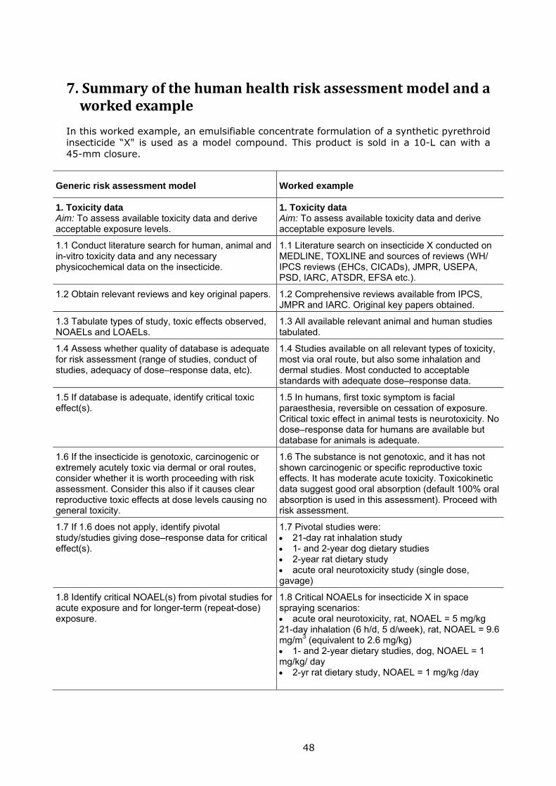
48

7.Summaryofthehumanhealthriskassessmentmodelandaworkedexample

In this worked example, an emulsifiable concentrate formulation of a synthetic pyrethroid insecticide “X" is used as a model compound. This product is sold in a 10-L can with a 45-mm closure.

Generic risk assessment model Worked example

1. Toxicity data Aim: To assess available toxicity data and derive acceptable exposure levels.

1. Toxicity data Aim: To assess available toxicity data and derive acceptable exposure levels.

1.1 Conduct literature search for human, animal and in-vitro toxicity data and any necessary physicochemical data on the insecticide.

1.1 Literature search on insecticide X conducted on MEDLINE, TOXLINE and sources of reviews (WH/ IPCS reviews (EHCs, CICADs), JMPR, USEPA, PSD, IARC, ATSDR, EFSA etc.).

1.2 Obtain relevant reviews and key original papers. 1.2 Comprehensive reviews available from IPCS, JMPR and IARC. Original key papers obtained.

1.3 Tabulate types of study, toxic effects observed, NOAELs and LOAELs.

1.3 All available relevant animal and human studies tabulated.

1.4 Assess whether quality of database is adequate for risk assessment (range of studies, conduct of studies, adequacy of dose–response data, etc).

1.4 Studies available on all relevant types of toxicity, most via oral route, but also some inhalation and dermal studies. Most conducted to acceptable standards with adequate dose–response data.

1.5 If database is adequate, identify critical toxic effect(s).

1.5 In humans, first toxic symptom is facial paraesthesia, reversible on cessation of exposure. Critical toxic effect in animal tests is neurotoxicity. No dose–response data for humans are available but database for animals is adequate.

1.6 If the insecticide is genotoxic, carcinogenic or extremely acutely toxic via dermal or oral routes, consider whether it is worth proceeding with risk assessment. Consider this also if it causes clear reproductive toxic effects at dose levels causing no general toxicity.

1.6 The substance is not genotoxic, and it has not shown carcinogenic or specific reproductive toxic effects. It has moderate acute toxicity. Toxicokinetic data suggest good oral absorption (default 100% oral absorption is used in this assessment). Proceed with risk assessment.

1.7 If 1.6 does not apply, identify pivotal study/studies giving dose–response data for critical effect(s).

1.7 Pivotal studies were: 21-day rat inhalation study 1- and 2-year dog dietary studies 2-year rat dietary study acute oral neurotoxicity study (single dose, gavage)

1.8 Identify critical NOAEL(s) from pivotal studies for acute exposure and for longer-term (repeat-dose) exposure.

1.8 Critical NOAELs for insecticide X in space spraying scenarios: acute oral neurotoxicity, rat, NOAEL = 5 mg/kg 21-day inhalation (6 h/d, 5 d/week), rat, NOAEL = 9.6 mg/m3 (equivalent to 2.6 mg/kg) 1- and 2-year dietary studies, dog, NOAEL = 1 mg/kg/ day 2-yr rat dietary study, NOAEL = 1 mg/kg /day

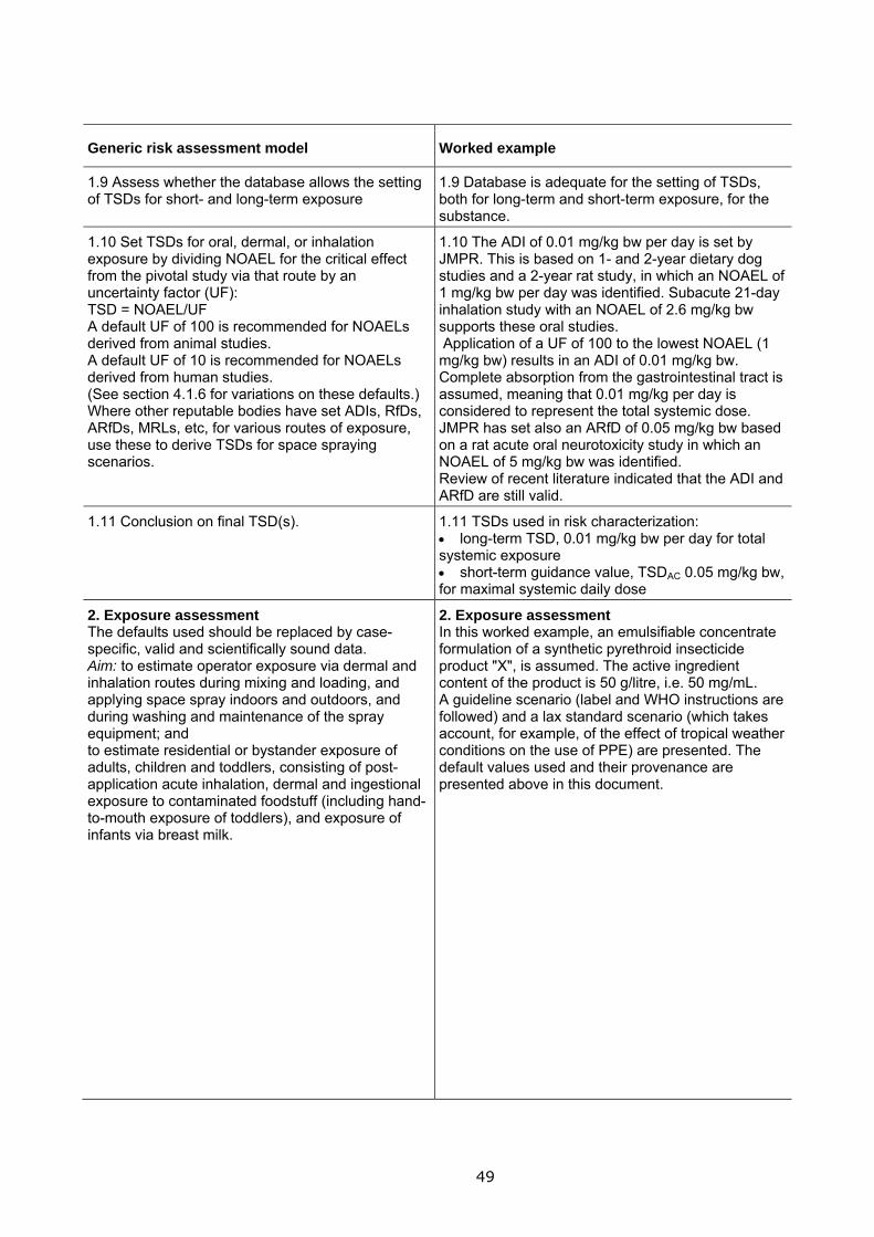
49

Generic risk assessment model Worked example

1.9 Assess whether the database allows the setting of TSDs for short- and long-term exposure

1.9 Database is adequate for the setting of TSDs, both for long-term and short-term exposure, for the substance.

1.10 Set TSDs for oral, dermal, or inhalation exposure by dividing NOAEL for the critical effect from the pivotal study via that route by an uncertainty factor (UF): TSD = NOAEL/UF A default UF of 100 is recommended for NOAELs derived from animal studies. A default UF of 10 is recommended for NOAELs derived from human studies. (See section 4.1.6 for variations on these defaults.) Where other reputable bodies have set ADIs, RfDs, ARfDs, MRLs, etc, for various routes of exposure, use these to derive TSDs for space spraying scenarios.

1.10 The ADI of 0.01 mg/kg bw per day is set by JMPR. This is based on 1- and 2-year dietary dog studies and a 2-year rat study, in which an NOAEL of 1 mg/kg bw per day was identified. Subacute 21-day inhalation study with an NOAEL of 2.6 mg/kg bw supports these oral studies. Application of a UF of 100 to the lowest NOAEL (1 mg/kg bw) results in an ADI of 0.01 mg/kg bw. Complete absorption from the gastrointestinal tract is assumed, meaning that 0.01 mg/kg per day is considered to represent the total systemic dose. JMPR has set also an ARfD of 0.05 mg/kg bw based on a rat acute oral neurotoxicity study in which an NOAEL of 5 mg/kg bw was identified. Review of recent literature indicated that the ADI and ARfD are still valid.

1.11 Conclusion on final TSD(s).

1.11 TSDs used in risk characterization: long-term TSD, 0.01 mg/kg bw per day for total systemic exposure short-term guidance value, TSDAC 0.05 mg/kg bw, for maximal systemic daily dose

2. Exposure assessment The defaults used should be replaced by case-specific, valid and scientifically sound data. Aim: to estimate operator exposure via dermal and inhalation routes during mixing and loading, and applying space spray indoors and outdoors, and during washing and maintenance of the spray equipment; and to estimate residential or bystander exposure of adults, children and toddlers, consisting of post-application acute inhalation, dermal and ingestional exposure to contaminated foodstuff (including hand-to-mouth exposure of toddlers), and exposure of infants via breast milk.

2. Exposure assessment In this worked example, an emulsifiable concentrate formulation of a synthetic pyrethroid insecticide product "X", is assumed. The active ingredient content of the product is 50 g/litre, i.e. 50 mg/mL. A guideline scenario (label and WHO instructions are followed) and a lax standard scenario (which takes account, for example, of the effect of tropical weather conditions on the use of PPE) are presented. The default values used and their provenance are presented above in this document.

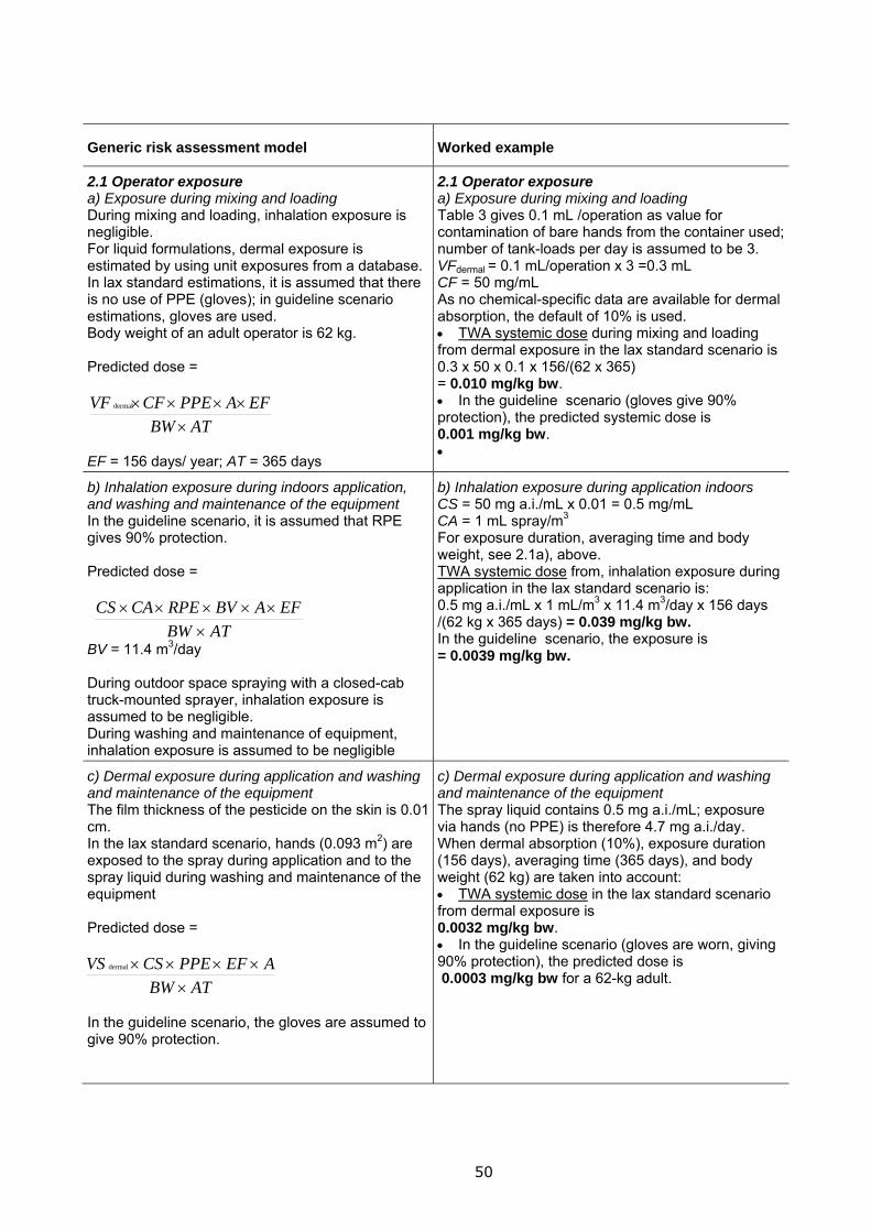
50

Generic risk assessment model Worked example

2.1 Operator exposure a) Exposure during mixing and loading During mixing and loading, inhalation exposure is negligible. For liquid formulations, dermal exposure is estimated by using unit exposures from a database. In lax standard estimations, it is assumed that there is no use of PPE (gloves); in guideline scenario estimations, gloves are used. Body weight of an adult operator is 62 kg. Predicted dose =

ATBW

EFAPPECFVF

dermal

EF = 156 days/ year; AT = 365 days

2.1 Operator exposure a) Exposure during mixing and loading Table 3 gives 0.1 mL /operation as value for contamination of bare hands from the container used; number of tank-loads per day is assumed to be 3. VFdermal = 0.1 mL/operation x 3 =0.3 mL CF = 50 mg/mL As no chemical-specific data are available for dermal absorption, the default of 10% is used. TWA systemic dose during mixing and loading from dermal exposure in the lax standard scenario is 0.3 x 50 x 0.1 x 156/(62 x 365) = 0.010 mg/kg bw. In the guideline scenario (gloves give 90% protection), the predicted systemic dose is 0.001 mg/kg bw.

b) Inhalation exposure during indoors application, and washing and maintenance of the equipment In the guideline scenario, it is assumed that RPE gives 90% protection. Predicted dose =

ATBW

EFABVRPECACS

BV = 11.4 m3/day During outdoor space spraying with a closed-cab truck-mounted sprayer, inhalation exposure is assumed to be negligible. During washing and maintenance of equipment, inhalation exposure is assumed to be negligible

b) Inhalation exposure during application indoors CS = 50 mg a.i./mL x 0.01 = 0.5 mg/mL CA = 1 mL spray/m3 For exposure duration, averaging time and body weight, see 2.1a), above. TWA systemic dose from, inhalation exposure during application in the lax standard scenario is: 0.5 mg a.i./mL x 1 mL/m3 x 11.4 m3/day x 156 days /(62 kg x 365 days) = 0.039 mg/kg bw. In the guideline scenario, the exposure is = 0.0039 mg/kg bw.

c) Dermal exposure during application and washing and maintenance of the equipment The film thickness of the pesticide on the skin is 0.01 cm. In the lax standard scenario, hands (0.093 m2) are exposed to the spray during application and to the spray liquid during washing and maintenance of the equipment Predicted dose =

ATBW

AEFPPECSVS

dermal

In the guideline scenario, the gloves are assumed to give 90% protection.

c) Dermal exposure during application and washing and maintenance of the equipment The spray liquid contains 0.5 mg a.i./mL; exposure via hands (no PPE) is therefore 4.7 mg a.i./day. When dermal absorption (10%), exposure duration (156 days), averaging time (365 days), and body weight (62 kg) are taken into account: TWA systemic dose in the lax standard scenario from dermal exposure is 0.0032 mg/kg bw. In the guideline scenario (gloves are worn, giving 90% protection), the predicted dose is 0.0003 mg/kg bw for a 62-kg adult.

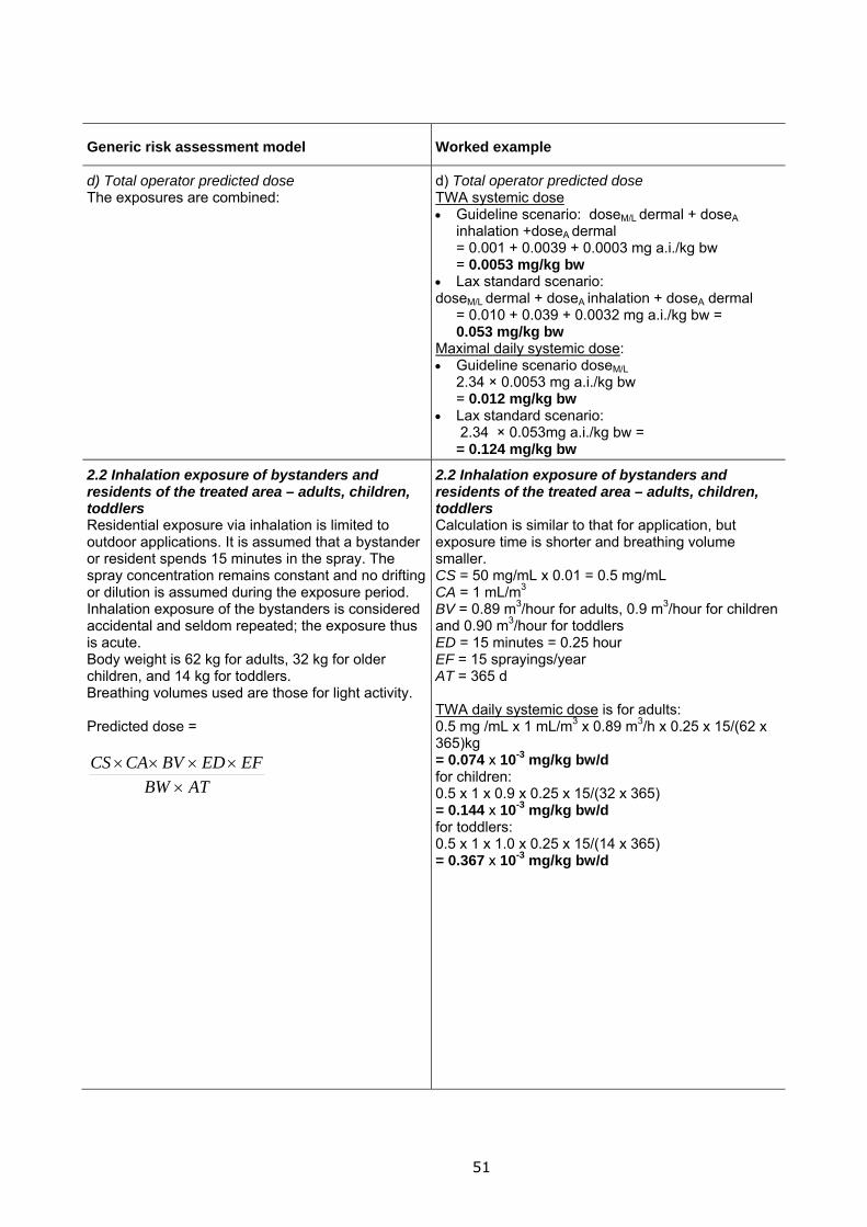
51

Generic risk assessment model Worked example

d) Total operator predicted dose The exposures are combined:

d) Total operator predicted dose TWA systemic dose Guideline scenario: doseM/L dermal + doseA

inhalation +doseA dermal = 0.001 + 0.0039 + 0.0003 mg a.i./kg bw = 0.0053 mg/kg bw

Lax standard scenario: doseM/L dermal + doseA inhalation + doseA dermal

= 0.010 + 0.039 + 0.0032 mg a.i./kg bw = 0.053 mg/kg bw

Maximal daily systemic dose: Guideline scenario doseM/L

2.34 × 0.0053 mg a.i./kg bw = 0.012 mg/kg bw

Lax standard scenario: 2.34 × 0.053mg a.i./kg bw = = 0.124 mg/kg bw

2.2 Inhalation exposure of bystanders and residents of the treated area – adults, children, toddlers Residential exposure via inhalation is limited to outdoor applications. It is assumed that a bystander or resident spends 15 minutes in the spray. The spray concentration remains constant and no drifting or dilution is assumed during the exposure period. Inhalation exposure of the bystanders is considered accidental and seldom repeated; the exposure thus is acute. Body weight is 62 kg for adults, 32 kg for older children, and 14 kg for toddlers. Breathing volumes used are those for light activity. Predicted dose =

ATBW

EFEDBVCACS

2.2 Inhalation exposure of bystanders and residents of the treated area – adults, children, toddlers Calculation is similar to that for application, but exposure time is shorter and breathing volume smaller. CS = 50 mg/mL x 0.01 = 0.5 mg/mL CA = 1 mL/m3 BV = 0.89 m3/hour for adults, 0.9 m3/hour for children and 0.90 m3/hour for toddlers ED = 15 minutes = 0.25 hour EF = 15 sprayings/year AT = 365 d TWA daily systemic dose is for adults: 0.5 mg /mL x 1 mL/m3 x 0.89 m3/h x 0.25 x 15/(62 x 365)kg = 0.074 x 10-3 mg/kg bw/d for children: 0.5 x 1 x 0.9 x 0.25 x 15/(32 x 365) = 0.144 x 10-3 mg/kg bw/d for toddlers: 0.5 x 1 x 1.0 x 0.25 x 15/(14 x 365) = 0.367 x 10-3 mg/kg bw/d

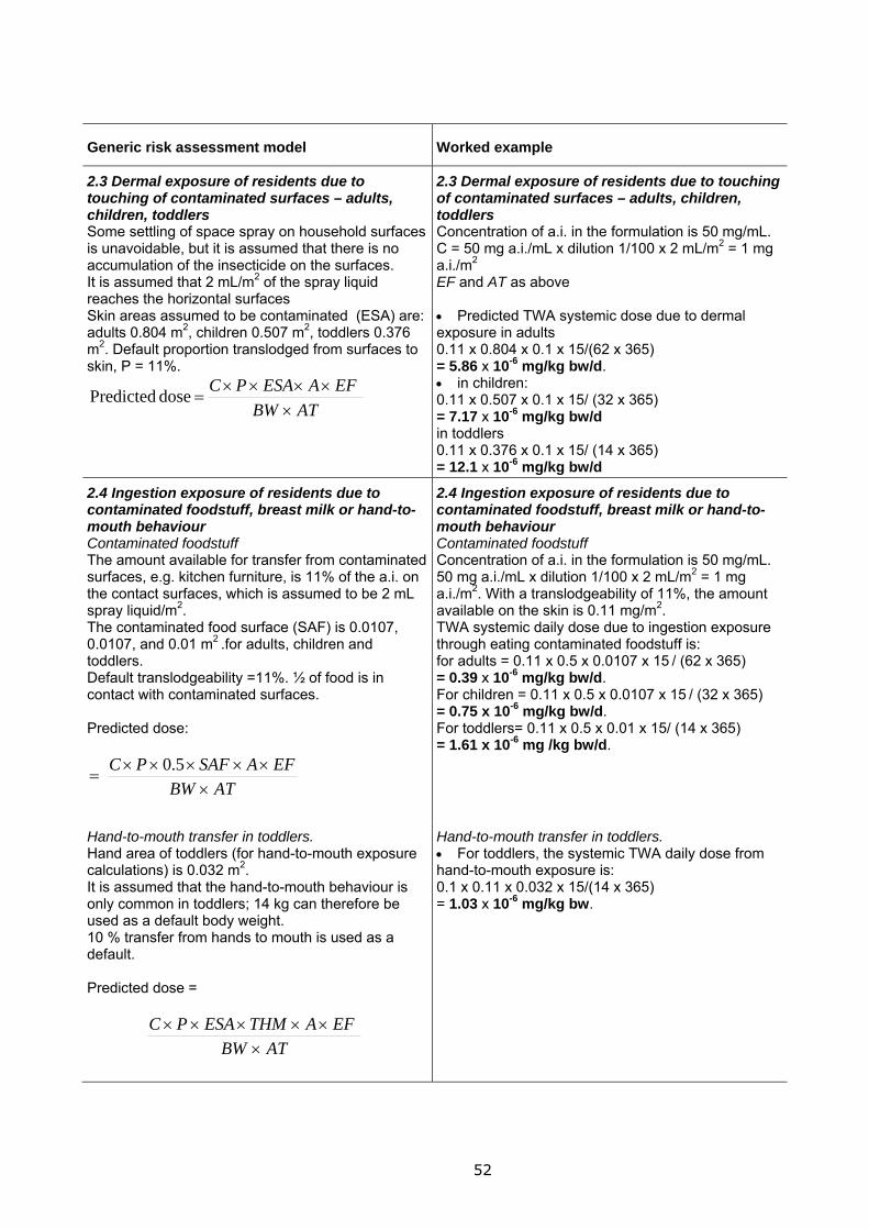
52

Generic risk assessment model Worked example

2.3 Dermal exposure of residents due to touching of contaminated surfaces – adults, children, toddlers Some settling of space spray on household surfaces is unavoidable, but it is assumed that there is no accumulation of the insecticide on the surfaces. It is assumed that 2 mL/m2 of the spray liquid reaches the horizontal surfaces Skin areas assumed to be contaminated (ESA) are: adults 0.804 m2, children 0.507 m2, toddlers 0.376 m2. Default proportion translodged from surfaces to skin, P = 11%.

ATBW

EFAESAPC

dose Predicted

2.3 Dermal exposure of residents due to touching of contaminated surfaces – adults, children, toddlers Concentration of a.i. in the formulation is 50 mg/mL. C = 50 mg a.i./mL x dilution 1/100 x 2 mL/m2 = 1 mg a.i./m2

EF and AT as above Predicted TWA systemic dose due to dermal exposure in adults 0.11 x 0.804 x 0.1 x 15/(62 x 365) = 5.86 x 10-6 mg/kg bw/d. in children: 0.11 x 0.507 x 0.1 x 15/ (32 x 365) = 7.17 x 10-6 mg/kg bw/d in toddlers 0.11 x 0.376 x 0.1 x 15/ (14 x 365) = 12.1 x 10-6 mg/kg bw/d

2.4 Ingestion exposure of residents due to contaminated foodstuff, breast milk or hand-to-mouth behaviour Contaminated foodstuff The amount available for transfer from contaminated surfaces, e.g. kitchen furniture, is 11% of the a.i. on the contact surfaces, which is assumed to be 2 mL spray liquid/m2. The contaminated food surface (SAF) is 0.0107, 0.0107, and 0.01 m2 .for adults, children and toddlers. Default translodgeability =11%. ½ of food is in contact with contaminated surfaces. Predicted dose:

ATBW

EFASAFPC

5.0

2.4 Ingestion exposure of residents due to contaminated foodstuff, breast milk or hand-to-mouth behaviour Contaminated foodstuff Concentration of a.i. in the formulation is 50 mg/mL. 50 mg a.i./mL x dilution 1/100 x 2 mL/m2 = 1 mg a.i./m2. With a translodgeability of 11%, the amount available on the skin is 0.11 mg/m2. TWA systemic daily dose due to ingestion exposure through eating contaminated foodstuff is: for adults = 0.11 x 0.5 x 0.0107 x 15 / (62 x 365) = 0.39 x 10-6 mg/kg bw/d. For children = 0.11 x 0.5 x 0.0107 x 15 / (32 x 365) = 0.75 x 10-6 mg/kg bw/d. For toddlers= 0.11 x 0.5 x 0.01 x 15/ (14 x 365) = 1.61 x 10-6 mg /kg bw/d.

Hand-to-mouth transfer in toddlers. Hand area of toddlers (for hand-to-mouth exposure calculations) is 0.032 m2. It is assumed that the hand-to-mouth behaviour is only common in toddlers; 14 kg can therefore be used as a default body weight. 10 % transfer from hands to mouth is used as a default. Predicted dose =

ATBW

EFATHMESAPC

Hand-to-mouth transfer in toddlers. For toddlers, the systemic TWA daily dose from hand-to-mouth exposure is: 0.1 x 0.11 x 0.032 x 15/(14 x 365) = 1.03 x 10-6 mg/kg bw.

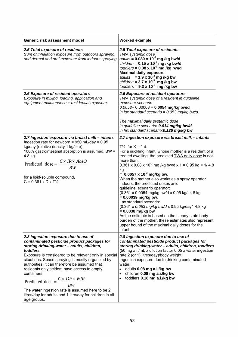
53

Generic risk assessment model Worked example

2.5 Total exposure of residents Sum of inhalation exposure from outdoors spraying, and dermal and oral exposure from indoors spraying

2.5 Total exposure of residents TWA systemic dose adults = 0.080 x 10-3 mg /kg bw/d children = 0.15 x 10-3 mg /kg bw/d toddlers = 0.38 x 10-3 mg /kg bw/d Maximal daily exposure adults = 1.9 x 10-3 mg /kg bw children = 3.7 x 10-3 mg /kg bw toddlers = 9.3 x 10-3 mg /kg bw

2.6 Exposure of resident operators Exposure in mixing. loading, application and equipment maintenance + residential exposure

2.6 Exposure of resident operators TWA systemic dose of a resident in guideline exposure scenario 0.0053+ 0.00008 = 0.0054 mg/kg bw/d in lax standard scenario = 0.053 mg/kg bw/d. The maximal daily systemic dose in guideline scenario: 0.014 mg/kg bw/d in lax standard scenario:0.126 mg/kg bw

2.7 Ingestion exposure via breast milk – infants Ingestion rate for newborn = 950 mL/day = 0.95 kg/day (relative density 1 kg/litre). 100% gastrointestinal absorption is assumed, BW = 4.8 kg.

BW

AbsOIRC

dose Predicted

for a lipid-soluble compound, C = 0.361 x D x T½

2.7 Ingestion exposure via breast milk – infants T½ for X = 1 d. For a suckling infant, whose mother is a resident of a treated dwelling, the predicted TWA daily dose is not more than: 0.361 x 0.08 x 10-3 mg /kg bw/d x 1 × 0.95 kg × 1/ 4.8 kg = 0.0057 x 10-3 mg/kg bw. When the mother also works as a spray operator indoors, the predicted doses are: guideline scenario operator: (0.361 x 0.0054 mg/kg bw/d x 0.95 kg/ 4.8 kg = 0.00039 mg/kg bw. Lax standard scenario: (0.361 x 0.053 mg/kg bw/d x 0.95 kg/day/ 4.8 kg = 0.0038 mg/kg bw As the estimate is based on the steady-state body burden of the mother, these estimates also represent upper bound of the maximal daily doses for the infant.

2.8 Ingestion exposure due to use of contaminated pesticide product packages for storing drinking-water – adults, children, toddlers Exposure is considered to be relevant only in special situations. Space spraying is mostly organized by authorities; it can therefore be assumed that residents only seldom have access to empty containers.

BW

WIRDFC dosePredicted

The water ingestion rate is assumed here to be 2 litres/day for adults and 1 litre/day for children in all age groups.

2.8 Ingestion exposure due to use of contaminated pesticide product packages for storing drinking-water – adults, children, toddlers(50 mg a.i./mL x dilution factor 0.05 x water ingestion rate 2 (or 1) litres/day)/body weight Ingestion exposure due to drinking contaminated water: adults 0.08 mg a.i./kg bw children 0.08 mg a.i./kg bw toddlers 0.18 mg a.i./kg bw

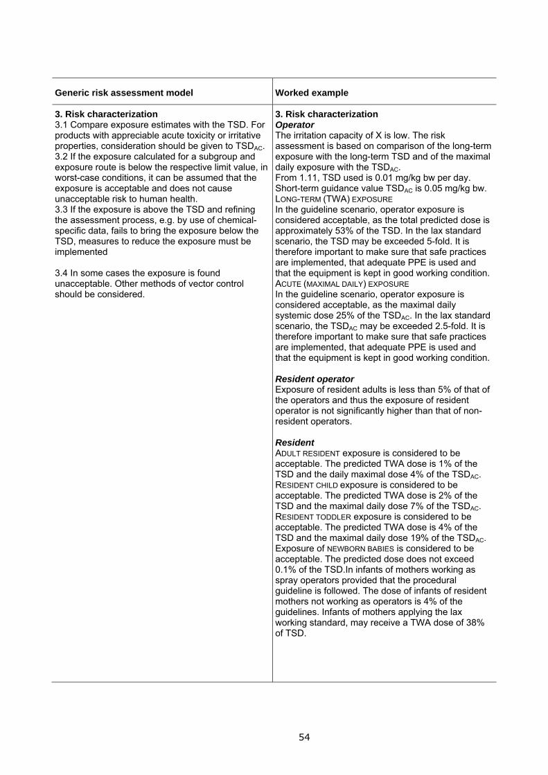
54

Generic risk assessment model Worked example

3. Risk characterization 3.1 Compare exposure estimates with the TSD. For products with appreciable acute toxicity or irritative properties, consideration should be given to TSDAC. 3.2 If the exposure calculated for a subgroup and exposure route is below the respective limit value, in worst-case conditions, it can be assumed that the exposure is acceptable and does not cause unacceptable risk to human health. 3.3 If the exposure is above the TSD and refining the assessment process, e.g. by use of chemical-specific data, fails to bring the exposure below the TSD, measures to reduce the exposure must be implemented 3.4 In some cases the exposure is found unacceptable. Other methods of vector control should be considered.

3. Risk characterization Operator The irritation capacity of X is low. The risk assessment is based on comparison of the long-term exposure with the long-term TSD and of the maximal daily exposure with the TSDAC. From 1.11, TSD used is 0.01 mg/kg bw per day. Short-term guidance value TSDAC is 0.05 mg/kg bw. LONG-TERM (TWA) EXPOSURE In the guideline scenario, operator exposure is considered acceptable, as the total predicted dose is approximately 53% of the TSD. In the lax standard scenario, the TSD may be exceeded 5-fold. It is therefore important to make sure that safe practices are implemented, that adequate PPE is used and that the equipment is kept in good working condition. ACUTE (MAXIMAL DAILY) EXPOSURE In the guideline scenario, operator exposure is considered acceptable, as the maximal daily systemic dose 25% of the TSDAC. In the lax standard scenario, the TSDAC may be exceeded 2.5-fold. It is therefore important to make sure that safe practices are implemented, that adequate PPE is used and that the equipment is kept in good working condition. Resident operator Exposure of resident adults is less than 5% of that of the operators and thus the exposure of resident operator is not significantly higher than that of non-resident operators. Resident ADULT RESIDENT exposure is considered to be acceptable. The predicted TWA dose is 1% of the TSD and the daily maximal dose 4% of the TSDAC. RESIDENT CHILD exposure is considered to be acceptable. The predicted TWA dose is 2% of the TSD and the maximal daily dose 7% of the TSDAC. RESIDENT TODDLER exposure is considered to be acceptable. The predicted TWA dose is 4% of the TSD and the maximal daily dose 19% of the TSDAC. Exposure of NEWBORN BABIES is considered to be acceptable. The predicted dose does not exceed 0.1% of the TSD.In infants of mothers working as spray operators provided that the procedural guideline is followed. The dose of infants of resident mothers not working as operators is 4% of the guidelines. Infants of mothers applying the lax working standard, may receive a TWA dose of 38% of TSD.

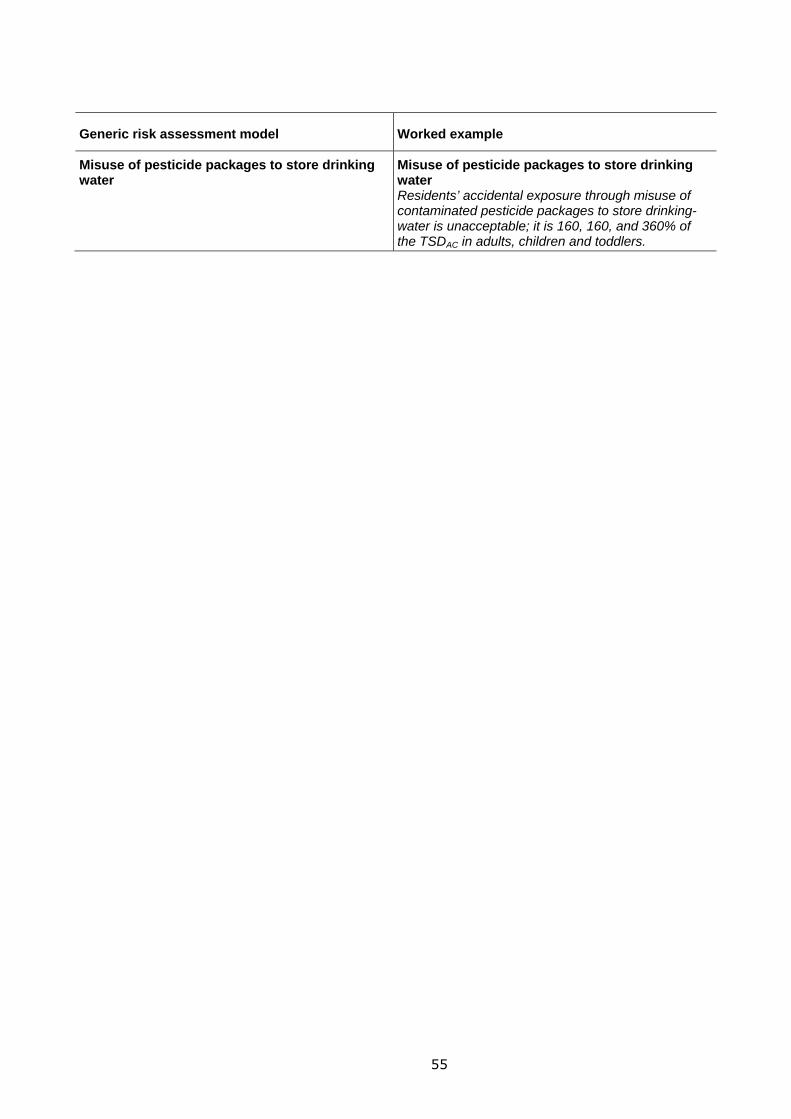
55

Generic risk assessment model Worked example

Misuse of pesticide packages to store drinking water

Misuse of pesticide packages to store drinking water Residents’ accidental exposure through misuse of contaminated pesticide packages to store drinking-water is unacceptable; it is 160, 160, and 360% of the TSDAC in adults, children and toddlers.

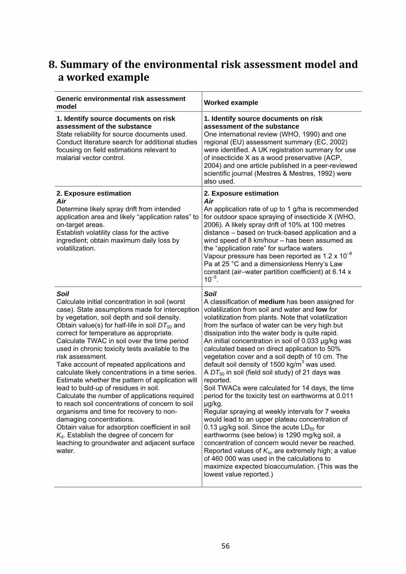
56

8.Summaryoftheenvironmentalriskassessmentmodelandaworkedexample

Generic environmental risk assessment model

Worked example

1. Identify source documents on risk assessment of the substance State reliability for source documents used. Conduct literature search for additional studies focusing on field estimations relevant to malarial vector control.

1. Identify source documents on risk assessment of the substance One international review (WHO, 1990) and one regional (EU) assessment summary (EC, 2002) were identified. A UK registration summary for use of insecticide X as a wood preservative (ACP, 2004) and one article published in a peer-reviewed scientific journal (Mestres & Mestres, 1992) were also used.

2. Exposure estimation Air Determine likely spray drift from intended application area and likely “application rates” to on-target areas. Establish volatility class for the active ingredient; obtain maximum daily loss by volatilization.

2. Exposure estimation Air An application rate of up to 1 g/ha is recommended for outdoor space spraying of insecticide X (WHO, 2006). A likely spray drift of 10% at 100 metres distance – based on truck-based application and a wind speed of 8 km/hour – has been assumed as the “application rate” for surface waters. Vapour pressure has been reported as 1.2 x 10–8 Pa at 25 °C and a dimensionless Henry’s Law constant (air–water partition coefficient) at 6.14 x 10–5.

Soil Calculate initial concentration in soil (worst case). State assumptions made for interception by vegetation, soil depth and soil density. Obtain value(s) for half-life in soil DT50 and correct for temperature as appropriate. Calculate TWAC in soil over the time period used in chronic toxicity tests available to the risk assessment. Take account of repeated applications and calculate likely concentrations in a time series. Estimate whether the pattern of application will lead to build-up of residues in soil. Calculate the number of applications required to reach soil concentrations of concern to soil organisms and time for recovery to non-damaging concentrations. Obtain value for adsorption coefficient in soil Kd. Establish the degree of concern for leaching to groundwater and adjacent surface water.

Soil A classification of medium has been assigned for volatilization from soil and water and low for volatilization from plants. Note that volatilization from the surface of water can be very high but dissipation into the water body is quite rapid. An initial concentration in soil of 0.033 µg/kg was calculated based on direct application to 50% vegetation cover and a soil depth of 10 cm. The default soil density of 1500 kg/m3 was used. A DT50 in soil (field soil study) of 21 days was reported. Soil TWACs were calculated for 14 days, the time period for the toxicity test on earthworms at 0.011 µg/kg. Regular spraying at weekly intervals for 7 weeks would lead to an upper plateau concentration of 0.13 µg/kg soil. Since the acute LD50 for earthworms (see below) is 1290 mg/kg soil, a concentration of concern would never be reached. Reported values of Koc are extremely high; a value of 460 000 was used in the calculations to maximize expected bioaccumulation. (This was the lowest value reported.)

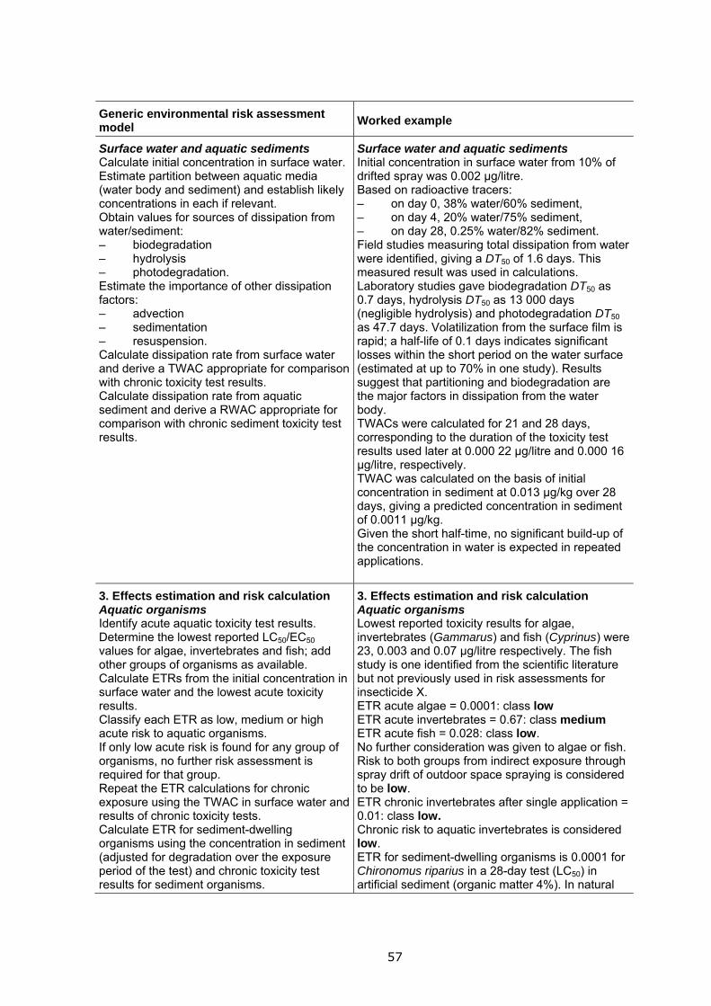
57

Generic environmental risk assessment model

Worked example

Surface water and aquatic sediments Calculate initial concentration in surface water. Estimate partition between aquatic media (water body and sediment) and establish likely concentrations in each if relevant. Obtain values for sources of dissipation from water/sediment: – biodegradation – hydrolysis – photodegradation. Estimate the importance of other dissipation factors: – advection – sedimentation – resuspension. Calculate dissipation rate from surface water and derive a TWAC appropriate for comparison with chronic toxicity test results. Calculate dissipation rate from aquatic sediment and derive a RWAC appropriate for comparison with chronic sediment toxicity test results.

Surface water and aquatic sediments Initial concentration in surface water from 10% of drifted spray was 0.002 µg/litre. Based on radioactive tracers: – on day 0, 38% water/60% sediment, – on day 4, 20% water/75% sediment, – on day 28, 0.25% water/82% sediment. Field studies measuring total dissipation from water were identified, giving a DT50 of 1.6 days. This measured result was used in calculations. Laboratory studies gave biodegradation DT50 as 0.7 days, hydrolysis DT50 as 13 000 days (negligible hydrolysis) and photodegradation DT50 as 47.7 days. Volatilization from the surface film is rapid; a half-life of 0.1 days indicates significant losses within the short period on the water surface (estimated at up to 70% in one study). Results suggest that partitioning and biodegradation are the major factors in dissipation from the water body. TWACs were calculated for 21 and 28 days, corresponding to the duration of the toxicity test results used later at 0.000 22 µg/litre and 0.000 16 µg/litre, respectively. TWAC was calculated on the basis of initial concentration in sediment at 0.013 µg/kg over 28 days, giving a predicted concentration in sediment of 0.0011 µg/kg. Given the short half-time, no significant build-up of the concentration in water is expected in repeated applications.

3. Effects estimation and risk calculation Aquatic organisms Identify acute aquatic toxicity test results. Determine the lowest reported LC50/EC50 values for algae, invertebrates and fish; add other groups of organisms as available. Calculate ETRs from the initial concentration in surface water and the lowest acute toxicity results. Classify each ETR as low, medium or high acute risk to aquatic organisms. If only low acute risk is found for any group of organisms, no further risk assessment is required for that group. Repeat the ETR calculations for chronic exposure using the TWAC in surface water and results of chronic toxicity tests. Calculate ETR for sediment-dwelling organisms using the concentration in sediment (adjusted for degradation over the exposure period of the test) and chronic toxicity test results for sediment organisms.

3. Effects estimation and risk calculation Aquatic organisms Lowest reported toxicity results for algae, invertebrates (Gammarus) and fish (Cyprinus) were 23, 0.003 and 0.07 µg/litre respectively. The fish study is one identified from the scientific literature but not previously used in risk assessments for insecticide X. ETR acute algae = 0.0001: class low ETR acute invertebrates = 0.67: class medium ETR acute fish = 0.028: class low. No further consideration was given to algae or fish. Risk to both groups from indirect exposure through spray drift of outdoor space spraying is considered to be low. ETR chronic invertebrates after single application = 0.01: class low. Chronic risk to aquatic invertebrates is considered low. ETR for sediment-dwelling organisms is 0.0001 for Chironomus riparius in a 28-day test (LC50) in artificial sediment (organic matter 4%). In natural

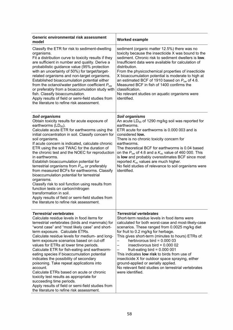
58

Generic environmental risk assessment model

Worked example

Classify the ETR for risk to sediment-dwelling organisms. Fit a distribution curve to toxicity results if they are sufficient in number and quality. Derive a probabilistic guidance value (95% protection with an uncertainty of 50%) for target/target-related organisms and non-target organisms. Established bioaccumulation potential either from the octanol/water partition coefficient Pow or preferably from a bioaccumulation study with fish. Classify bioaccumulation. Apply results of field or semi-field studies from the literature to refine risk assessment.

sediment (organic matter 12.5%) there was no toxicity because the insecticide X was bound to the sediment. Chronic risk to sediment dwellers is low. Insufficient data were available for calculation of distribution. From the physicochemical properties of insecticide X bioaccumulation potential is moderate to high at an estimated BCF of 1910 based on Pow of 4.6. Measured BCF in fish of 1400 confirms the classification. No relevant studies on aquatic organisms were identified.

Soil organisms Obtain toxicity results for acute exposure of earthworms (LD50). Calculate acute ETR for earthworms using the initial concentration in soil. Classify concern for soil organisms. If acute concern is indicated, calculate chronic ETR using the soil TWAC for the duration of the chronic test and the NOEC for reproduction in earthworms. Establish bioaccumulation potential for terrestrial organisms from Pow or preferably from measured BCFs for earthworms. Classify bioaccumulation potential for terrestrial organisms. Classify risk to soil function using results from function tests on carbon/nitrogen transformation in soil. Apply results of field or semi-field studies from the literature to refine risk assessment.

Soil organisms An acute LD50 of 1290 mg/kg soil was reported for earthworms. ETR acute for earthworms is 0.000 003 and is considered low. There is no chronic toxicity concern for earthworms. The theoretical BCF for earthworms is 0.04 based on the Pow of 4.6 and a Koc value of 460 000. This is low and probably overestimates BCF since most reported Koc values are much higher. No field studies of relevance to soil organisms were identified.

Terrestrial vertebrates Calculate residue levels in food items for terrestrial vertebrates (birds and mammals) for “worst case” and “most likely case” and short-term exposure. Calculate ETRs. Calculate residue levels for medium- and long-term exposure scenarios based on cut-off values for ETRs at lower time periods. Calculate ETR for fish-eating and earthworm-eating species if bioaccumulation potential indicates the possibility of secondary poisoning. Take repeat applications into account. Calculate ETRs based on acute or chronic toxicity test results as appropriate for succeeding time periods. Apply results of field or semi-field studies from the literature to refine risk assessment.

Terrestrial vertebrates Short-term residue levels in food items were calculated for both worst-case and most-likely-case scenarios. These ranged from 0.0025 mg/kg diet for fruit to 0.2 mg/kg for herbage. This gives short-term (minutes to hours) ETRs of: – herbivorous bird = 0.000 03 – insectivorous bird = 0.000 02 – fruit-eating bird = 0.000 001 This indicates low risk to birds from use of insecticide X for outdoor space spraying, either ground-applied or aerially applied. No relevant field studies on terrestrial vertebrates were identified.

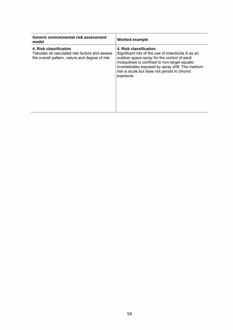
59

Generic environmental risk assessment model

Worked example

4. Risk classification Tabulate all calculated risk factors and assess the overall pattern, nature and degree of risk.

4. Risk classification Significant risk of the use of insecticide X as an outdoor space spray for the control of adult mosquitoes is confined to non-target aquatic invertebrates exposed by spray drift. The medium risk is acute but does not persist to chronic exposure.

60

References

Becker FA et al. (1999). The degree of ground coverage by arable crops as a help in estimating the amount of spray solution intercepted by the plants. Nachrichtenblatt des deutschen Pflanzenschutzdienstes, 51(9):237–242.

Beinat E, van den Berg R (1996) EUPHIDS, a decision support system for the admission of pesticides. National Institute of Public Health and the Environment, Bilthoven, The Netherlands. Available at: http://www.feweb.vu.nl/gis/education/Euphids3/finalrep.pdf

Dorne J-LC M, Renwick AG (2005). The refinement of uncertainty/safety factors in risk assessment by the incorporation of data on toxicokinetic variability in humans. Toxicological Sciences, 86(1):20–26.

Dourson ML, Knauf LA, Swartout JC (1992). On reference dose (RfD) and its underlying toxicity data base. Toxicology and Industrial Health, 8(3):171–189.

EC (2002). Technical Notes for Guidance on Annex I – inclusion. Technical Notes for Guidance in Support of Directive 98/8/EC of the European Parliament and the Council concerning the placing of biocidal products on the market. Principles and practical procedures for the inclusion of active substances in Annexes I, IA and IB. Ispra, Italy. Brussels, European Commission (available at: available at: http://ecb.jrc.ec.europa.eu/biocides/).

EC (2003). Technical guidance document in support of the risk assessment Directive (93/67/EEC) for new substances notified in accordance with the requirements of Council Directive 67/548/EEC. Brussels, European Commission.

EC (2006). Guidance for the setting and application of Acceptable Operator Exposure Levels (AOELs) (working document). Brussels, European Union (available at: http://ec.europa.eu/food/plant/protection/resources/7531_rev_10.pdf).

EFSA (2007). Scientific Opinion of the Panel on Plant Protection Products and their Residues on a request from EFSA related to the default Q10 value used to describe the temperature effect on transformation rates of pesticides in soil. EFSA Journal, 622, 1-32.

EPPO (2003). EPPO standards: Environmental risk assessment scheme for plants protection products. Paris, European and Mediterranean Plant Protection Organization. (Bulletin OEPP/EPPO). Available at: http://archives.eppo.org/EPPOStandards/era.htm

EU (2000). Guidance on data requirements for active substances and biocidal products. Technical guidance document in support of Directive 98/8/EC of the European Parliament and of the Council concerning the placing of biocidal products on the market. Brussels, European Union.

61

EUROPOEM II (2003). The development, maintenance and dissemination of a European Predictive Operator Exposure Model (EUROPOEM) database. A EUROPOEM II Database and Harmonised Model, FAIR3-CT96-1406. Carshalton, England, TNO-BIBRA International.

FAO (2002). World agriculture: towards 2015/2030. Summary report: long-term perspectives, the outlook for agriculture. Rome, Food and Agriculture Organization of the United Nations (available at: http://www.fao.org/docrep/004/Y3557E/Y3557E00.HTM).

Ganzelmeier H et al. (1995). Studies on the spray drift of plant protection products: results of a test program carried out throughout the Federal Republic of Germany. Berlin, Blackwell Wissenshafts Verlag.

Herrman JL, Younes M (1999). Background to the ADI/TDI/PTWI. Regulatory Toxicology and Pharmacology, 30:S109–S113.

Hewitt AJ et al. (2002). Development of the spray drift task force database for aerial applications. Environmental Toxicology and Chemistry, 21(3):648–658.

JMPM (2008). Recommendations of the 2nd FAO/WHO Joint Meeting on Pesticide Management and 4th Session of the FAO Panel of Experts on Pesticide Management, Geneva, 6–8 October 2008. Rome, Food and Agriculture Organization of the United Nations (available at: http://www.fao.org/fileadmin/templates/agphome/documents/Pests_Pesticides/Code/Recommendations08_01.pdf).

JMPR (1998). Report of the Joint Meeting of the FAO Panel of Experts on Pesticide Residues and the Environment and the WHO Core Assessment Group, Rome 21–30 September 1998. Geneva, World Health Organization (available at www.who.int/pcs/jmpr/jmpr.htm.).

JMPR (2010) of IPCS and other WHO pesticide evaluations and summary of toxicological evaluations performed by the Joint Meeting on Pesticide Residues (JMPR) through 2009 Tenth Edition. Available at: http://www.who.int/ipcs/publications/jmpr/jmpr_pesticide/en/index.html

Matthews GA (2001). Dermal exposure of hands to pesticides. In: Maibach HI, ed. Toxicology of skin pp. 179-182. Philadelphia, Taylor and Francis:179–182.

Mestres R, Mestres G (1992) Deltamethrin – uses and environmental safety. Reviews of Environmental Contamination and Toxicology, 124:1–18.

Mineau P et al. (1994). A critique of the avian 5-day dietary test (LC50) as the basis of avian risk assessment. Ottawa, Canadian Wildlife Service (Technical Report Series 215).

Najera JA, Zaim M (2002). Malaria vector control – decision-making criteria and procedures for judicious use of insecticides. World Health Organization, Geneva (available at: WHO/CDS/WHOPES/2002.5).

62

Mukhtari M (2009) Guidelines for dengue vector(s) control during outbreaks/emergencies. Directorate of malaria control, Ministry of Health, Islamabad. Available at: http://malariar7.com.pk/documents/pdfs/Dengue_Vetcor_control.pdf

Nantel G (1999). Carbohydrates in human nutrition. Food, nutrition and agriculture, 24. Rome, Food and Agriculture Organization of the United Nations (available at: http://www.fao.org/docrep/X2650T/X2650T02.HTM).

Nordic Council of Ministers (2007). Probabilistic exposure assessment methods in Chemical Safety Assessments (REACH). Copenhagen, Nordic Council of Ministers (TemaNord 2007:563; available at: http://www.norden.org/en/publications/publications/2007-563).

OECD (1987). Guidelines for the testing of chemicals (and subsequent revisions). Paris, Organisation for Economic Cooperation and Development (available at: www.oecd.org/env/testguidelines).

PSD (2007). UK Predictive Operator Exposure Model (POEM): a user’s guide. York, England, Pesticides Safety Directorate (available at: http://www.pesticides.gov.uk/approvals.asp?id=2427).

Solecki R et al. (2005) Guidance on setting of acute reference dose (ARfD) for pesticides. Food and Chemical Toxicology, 43:1569-1593.

Teske ME et al. (2002). AgDRIFT: a model for estimating near-field spray drift from aerial applications. Environmental Toxicology and Chemistry, 21(3):659–671.

United Nations (2009). Globally harmonized system of classification and labelling of chemicals. New York, United Nations (available at: http://www.unece.org/trans/danger/publi/ghs/ghs_rev03/03files_e.html).

USAID (2006). Integrated vector management programs for malaria vector control. Programmatic Environmental Assessment. Washington, DC, United States Agency for International Development (prepared by RTI International).

USEPA (1995). The use of the benchmark dose approach health risk assessment. Washington, DC, United States Environmental Protection Agency (EPA/630/R-94/007).

USEPA (1997a). Standard operating procedures (SOPs) for residential exposure assessments. Washington, DC, United States Environmental Protection Agency, Office of Science Coordination and Policy (available at: www.epa.gov/oscpmont/sap/meetings/1997/september/sopindex.htm).

USEPA (1997b). Exposure factors handbook. Washington, DC, United States Environmental Protection Agency, Office of Research and Development (available at: http://cfpub.epa.gov/ncea/cfm/recordisplay.cfm?deid=12464).

63

USEPA (2008). Child-specific exposure factors handbook (final report). United States Environmental Protection Agency, Office of Research and Development (available at: http://cfpub.epa.gov/ncea/cfm/recordisplay.cfm?deid=199243).

USEPA (2009). Draft Technical Guidelines. Standard operating procedures (SOPs) for residential pesticide exposure assessments. Submitted to the FIFRA Advisory Panel For Review and Comment October 6-9, 2009. Office of Pesticide Programs, Office of Prevention, Pesticides, and Toxic Substances, U.S. Environmental Protection Agency, Washington, D.C.

Vermeire T, et al. (1999). Assessment factors for human health risk assessment: a discussion paper. Critical Reviews in Toxicology, 29(5):439–490.

WHO (1990). Equipment for vector control, 3rd ed. Geneva, World Health Organization.

WHO (1994). Assessing human health risks of chemicals: derivation of guidance values for health-based exposure limits. Geneva, World Health Organization (Environmental Health Criteria 170, available at: www.inchem.org/documents/ehc/ehc/ehc170.htm).

WHO (1999a). Principles for the assessment of risks to human health from exposure to chemicals. Geneva, World Health Organization (Environmental Health Criteria 210; available at: www.inchem.org/documents/ehc/ehc/ehc210.htm).

WHO (1999b). Regional Guidelines on Dengue/DHF Prevention and Control ( Regional Publication 29/1999 ) WHO Regional Office for South-East Asia available at: http://www.searo.who.int/en/Section10/Section332/Section554.htm

WHO (2003). Space spray application of insecticides for vector and public health pest control – a practitioner’s guide. Geneva, World Health Organization (WHO/CDS/WHOPES/GCDPP/2003.5; available at: whqlibdoc.who.int/hq/2003/WHO_CDS_WHOPES_GCDPP_2003.5.pdf).

WHO (2004). Generic risk assessment model for insecticide treatment and subsequent use of mosquito nets. Geneva, World Health Organization (available at: http://whqlibdoc.who.int/hq/2004/WHO_PCS_04.1.pdf).

WHO (2005a). Chemical-specific adjustment factors for interspecies differences and human variability: guidance document for use of data in dose/concentration-response assessment. Geneva, World Health Organization (IPCS Harmonization Project Document, No. 2; available at: http://whqlibdoc.who.int/publications/2005/9241546786_eng.pdf).

WHO (2005b). Principles of characterizing and applying human exposure models. Geneva, World Health Organization (IPCS Harmonization Project Document, No. 3; available at: http://whqlibdoc.who.int/publications/2005/9241563117_eng.pdf).

64

WHO (2006). Equipment for vector control: specification guidelines. Geneva, World Health Organization (WHO/CDS/NTD/WHOPES/GCDPP/2006.5; available at: http://whqlibdoc.who.int/hq/2006/WHO_CDS_NTD_WHOPES_2006.5_eng.pdf).

WHO (2008). Uncertainty and data quality in exposure assessment. Part 1: Guidance document on characterizing and communicating uncertainty in exposure assessment. Geneva, World Health Organization (IPCS Harmonization Project Document No. 6; available at: www.who.int/ipcs/methods/harmonization/areas/uncertainty%20.pdf).

WHO (2009a). Guidelines for efficacy testing of insecticides for indoor and outdoor ground-applied space spray applications. Geneva, World Health Organization (WHO/CDS/NTD/WHOPES/2009.2; available at: http://whqlibdoc.who.int/hq/2009/WHO_HTM_NTD_WHOPES_2009.2_eng.pdf).

WHO (2009b). Principles for modelling dose–response for the risk assessment of chemicals. Geneva, World Health Organization (Environmental Health Criteria 239; available at: http://whqlibdoc.who.int/publications/2009/9789241572392_eng.pdf).

WHO (2009c) Dengue Guidelines for diagnosis, treatment and prevention. New edition. Available at: http://whqlibdoc.who.int/publications/2009/9789241547871_eng.pdf

WHO (2010). WHO recommended classification of pesticides by hazard and guidelines to classification. Geneva, World Health Organization (available at: http://whqlibdoc.who.int/publications/2010/9789241547963_eng.pdf).

GENERIC RISK ASSESSMENT MODEL

FOR INDOOR AND OUTDOOR SPACE

SPRAYING OF INSECTICIDES

WHO Pesticide Evaluation SchemeDepartment of Control of Neglected Tropical DiseasesCluster of HIV/AIDS, Tuberculosis, Malaria and Neglected Tropical Diseases&Chemical SafetyDepartment of Public Health and EnvironmentCluster of Health Security and Environment

First Revision (February 2011)