Embed Size (px)
Citation preview
Available online at www.sciencedirect.com
Journal of Computational Physics 227 (2007) 353–375
www.elsevier.com/locate/jcp
Generator estimation of Markov jump processes q
P. Metzner *, E. Dittmer, T. Jahnke, Ch. Schutte
Institute of Mathematics II, Free University of Berlin, Arnimallee 6, D-14195 Berlin, Germany
Received 8 March 2007; received in revised form 26 July 2007; accepted 27 July 2007Available online 14 August 2007
Abstract
Estimating the generator of a continuous-time Markov jump process based on incomplete data is a problem whicharises in various applications ranging from machine learning to molecular dynamics. Several methods have been devisedfor this purpose: a quadratic programming approach (cf. [D.T. Crommelin, E. Vanden-Eijnden, Fitting timeseries by con-tinuous-time Markov chains: a quadratic programming approach, J. Comp. Phys. 217 (2006) 782–805]), a resolventmethod (cf. [T. Muller, Modellierung von Proteinevolution, PhD thesis, Heidelberg, 2001]), and various implementationsof an expectation-maximization algorithm ([S. Asmussen, O. Nerman, M. Olsson, Fitting phase-type distributions via theEM algorithm, Scand. J. Stat. 23 (1996) 419–441; I. Holmes, G.M. Rubin, An expectation maximization algorithm fortraining hidden substitution models, J. Mol. Biol. 317 (2002) 753–764; U. Nodelman, C.R. Shelton, D. Koller, Expectationmaximization and complex duration distributions for continuous time Bayesian networks, in: Proceedings of the twenty-first conference on uncertainty in AI (UAI), 2005, pp. 421–430; M. Bladt, M. Sørensen, Statistical inference for discretelyobserved Markov jump processes, J.R. Statist. Soc. B 67 (2005) 395–410]). Some of these methods, however, seem to beknown only in a particular research community, and have later been reinvented in a different context. The purpose of thispaper is to compile a catalogue of existing approaches, to compare the strengths and weaknesses, and to test their perfor-mance in a series of numerical examples. These examples include carefully chosen model problems and an application to atime series from molecular dynamics.� 2007 Elsevier Inc. All rights reserved.
MSC: 60C40; 60J22; 60J75; 60J35; 60M05
PACS: 02.30.Zz; 02.50.Ga; 05.45.Tp; 36.20.Ey
Keywords: Markov jump process; Generator estimation; Embedding problem; EM-algorithm; Maximum likelihood
0021-9991/$ - see front matter � 2007 Elsevier Inc. All rights reserved.
doi:10.1016/j.jcp.2007.07.032
q Supported by the DFG Research Center MATHEON ‘‘Mathematics for Key Technologies’’ (FZT86) in Berlin.* Corresponding author.
E-mail addresses: [email protected] (P. Metzner), [email protected] (E. Dittmer), [email protected] (T.Jahnke), [email protected] (Ch. Schutte).
354 P. Metzner et al. / Journal of Computational Physics 227 (2007) 353–375
1. Introduction
Let {X(t), t P 0} be a continuous-time Markov jump process on a finite state space S @ {1, . . .,d}. Onlytime-homogeneous Markov processes will be considered, i.e. we assume that
PðX ðt þ sÞ ¼ jjX ðtÞ ¼ iÞ ¼ PðX ðsÞ ¼ jjX ð0Þ ¼ iÞ
for all states i, j 2 S and all t,s P 0. The transition matrix of {X(t), t P 0} is the time-dependent matrixP ðtÞ ¼ ðpijðtÞÞi;j 2 Rd�d ; pijðtÞ ¼ PðX ðtÞ ¼ jjX ð0Þ ¼ iÞ
containing the transition probabilities pij(t). If the limit
L ¼ limt!0
PðtÞ � Idt
exists, then the transition matrix can be expressed as the matrix exponential
P ðtÞ ¼ expðtLÞ ¼X1k¼0
tk
k!Lk
and L is called the infinitesimal generator of the Markov process fX ðtÞ; t P 0g. A matrix L 2 Rd�d generates acontinuous-time Markov process if and only if all off-diagonal entries are nonnegative and the sum over eachrow equals zero. The set of generators will be denoted by
G ¼ L ¼ ðlijÞi;j 2 Rd�d : lij P 0 for all i 6¼ j; lii ¼ �Xj 6¼i
lij
( ): ð1Þ
In this article, we consider the problem of how to determine the generator if only a finite samplingY = {y0 = X(t0), . . .,yN = X(tN)} of a process at discrete times t0, t1, . . ., tN is available. Several difficulties mustbe taken into account. First, from a finite number of samples it is impossible to tell if the underlying process isactually Markovian. Second, it is not clear if the observed data originates indeed from discrete samples of acontinuous-time Markov chain with some generator L, or rather from a discrete-time Markov chain whichcannot be embedded into a time-continuous counterpart. In the latter case, a generator does not exist becausethe transition matrix of the discrete chain does not belong to the set
P ¼ fP 2 Rd�d : there is a L 2 G such that P ¼ expðLÞg:
It is well-known that P is a subset of all stochastic matrices, but the so-called embedding problem, i.e. the ques-tion what characterizes the elements of P, is widely open for d > 3 (cf. [1,2] and references therein). A thirddifficulty is the fact that the matrix exponential function is not injective if the eigenvalues of the generatorare complex. Hence, some matrices P 2 P can be represented as P ¼ expðLÞ ¼ expðLÞ with two different gen-erators L 6¼ L. And finally, the question whether the time points tn of the observations are equidistant plays animportant role. In case of a constant time lag s = tn+1 � tn an estimate of the transition matrix P(s) is availableby counting the number of transitions between each pair of states, but in case of variable time lags the sampleddata is typically not sufficient for reasonable approximations of the transition matrix.Due to these problems the above question has to be modified: how can we find the generator that ‘‘agrees best’’with a finite observation Y = {y0 = X(t0), . . .,yN = X(tN)} of a process? Several methods have been proposed forthis purpose [2,19,18,3,1], but since the problem has been investigated in the context of rather different applica-tions, some of these papers apparently remained unknown outside the corresponding research community orwere at least not cited. Some methods have later been reinvented, such as the expectation-maximization algo-rithm introduced in [19] in 1996 and later by [1] in 2005. This may partly be due to the fact that even the termi-nology varies largely form paper to paper – for example, the generator is often called (transition) rate matrix (cf.[18]), substitution matrix (cf. [20]), intensity matrix (cf. [1]), or ‘‘matrix of transition intensities’’ (cf. [17]).
In this article, we present a concise – but not necessarily complete – review of approaches to generator esti-mation. We explain how each method works, discuss their pros and cons, evaluate their performance bynumerical examples, and explain in which sense the ‘‘agreement’’ of the approximative generator with the datahas to be understood in each case. In Section 2, we briefly sketch the resolvent method advocated, e.g., in [3].
P. Metzner et al. / Journal of Computational Physics 227 (2007) 353–375 355
However, since the output of this method is in general not a generator matrix, it will later be excluded from thecomparison. Section 3 resumes the quadratic programming approach introduced in [2]. In Section 4, we dis-cuss several methods for the computation of maximum likelihood estimators and the expectation-maximiza-tion algorithms proposed, e.g., in [19,17,18,1]. Furthermore, we derive a version of the EM-algorithm which isadapted to the reversible case. Numerical examples are presented in Section 5. The performance of the meth-ods is illustrated by carefully chosen model problems and by an application to a large system arising frommolecular dynamics. In the last section, we discuss and summarize the numerical results and give an outlookon a generalization of an enhanced expectation-maximization method to the case of varying time lags.
2. Resolvent method
For any generator L 2 G the parameter-dependent matrix
RðaÞ ¼ ðaI � LÞ�1; a > 0 ð2Þ
is called the resolvent of L. The inverse exists for all a > 0 since the real parts of the eigenvalues of a generatorL 2 G are non-positive. An alternative formula representing the resolvent in terms of the transition matrixP(t) = exp(tL) is given by the Laplace transform
RðaÞ ¼Z 1
0
expð�atÞP ðtÞdt; a > 0: ð3Þ
The existence of the integral is due to the fact that iP(t)i = 1 for all t P 0, and the equivalence of (3) and (2)follows from
ðaI � LÞRðaÞ ¼ �Z 1
0
d
dtðexpð�atÞP ðtÞÞdt ¼ I :
The main idea of the resolvent method is to approximate the resolvent using its integral representation (3) andthen to estimate the underlying generator via the identity
L ¼ aId � R�1ðaÞ: ð4Þ
Computing the integral in (3), however, requires an approximation of the transition matrix P(t). Suppose thatthe process X(t) has been observed at equidistant time points tn = ns with some fixed time lag s > 0 andn = 0, . . .,N. LetcðkÞij ¼XN�k
n¼0
vðX ðtnÞ ¼ iÞvðX ðtnþkÞ ¼ jÞ ð5Þ
be the number of observed transitions from state i to state j within the time interval of length ks. Here andbelow, v denotes the characteristic function. The matrix CðkÞ ¼ ðcðkÞij Þi;j 2 Nd�d is called the frequency matrixwith respect to the time interval [0,ks], and a simple estimate eP ðkÞ � P ðtkÞ is provided by
eP ðkÞ ¼ ~pðkÞij
� �i;j
with entries ~pðkÞij ¼cðkÞijPdj¼1cðkÞij
: ð6Þ
In the approach of [5,3] these estimates are used to approximate P(t) in the interval [tn,tn+1] by linearinterpolation:
P ðtÞ � PðtnÞ þ ðt � tnÞP ðtnþ1Þ � P ðtnÞ
s� eP ðnÞ þ ðt � tnÞ
eP ðnþ1Þ � eP ðnÞs
:
Substituting this into the integral representation (3) gives
RðaÞ ¼Xm�1
n¼0
Z tnþ1
tn
expð�asÞP ðsÞdsþZ 1
tm
expð�asÞP ðsÞds
�Xm�1
n¼0
Z tnþ1
tn
expð�asÞ eP ðnÞ þ ðs� tnÞeP ðnþ1Þ � eP ðnÞ
s
!dsþ
Z 1
tm
expð�asÞP ðtmÞds: ð7Þ
356 P. Metzner et al. / Journal of Computational Physics 227 (2007) 353–375
Since all integrals in (7) can be solved analytically, this yields an approximation eRðaÞ � RðaÞ to the resolvent.If eRðaÞ is invertible, then Eq. (4) yields an estimate eLðaÞ ¼ aId � eR�1ðaÞ for the generator. Of course, the esti-mate depends on the particular choice of a, but the optimal value of a can be determined by a maximum like-lihood approach; see [5,3] for details.
It can easily be shown that for any a the entries ~lðaÞii of the estimated generator eLðaÞ satisfy the condition~lðaÞii ¼ �
Pj 6¼i
~lðaÞij . However, eLðaÞ is in general not a generator in the sense of (1), because eLðaÞ can contain neg-ative or even complex off-diagonal elements. This happens if some of the estimated transition matrices eP ðnÞ donot belong to the set P. In [3], this obstacle did not appear because the resolvent method was applied to prob-lems where the transition matrices could assumed to be calibrated (i.e. close to identity in some sense). In ageneral situation, however, the fact that eLðaÞ 62 G is a severe drawback of the resolvent method.
3. Quadratic optimization method
In contrast to the resolvent method, the approach introduced by Crommelin and Vanden-Eijnden [2] yieldsan estimate that does belong to the set G: As in the previous chapter, first an approximative transition matrixeP ð1Þ � P ðt1Þ ¼ P ðsÞ is computed by Eq. (6). Now suppose an eigendecomposition
eP ð1Þ ¼ UKU�1 ð8Þ with a diagonal matrix K = diag(k1, . . .,kd) containing the eigenvalues exists, and that kk 6¼ 0 for all k. (Notethat U�1 can be obtained without explicit matrix inversion since its rows are the left eigenvectors of eP ð1Þ.)Then, the matrix eL ¼ UZU�1 with Z ¼ diagðz1; . . . ; zdÞ; zk ¼logðkkÞs
ð9Þ
can be defined, and the approximative transition matrix can be expressed in terms of the matrix exponential
expðseLÞ ¼ expðU logðKÞU�1Þ ¼ UKU�1 ¼ eP ð1Þ:
In spite of this relation, eL cannot be considered as a reasonable estimate for the generator because eL 62 G inmany cases. In order to find an estimate with the correct structural properties, Crommelin and Vanden-Eijn-den propose to compute the generator eL 2 G which agrees best with the eigendecomposition (9). This is moti-vated by the fact that many properties of a continuous-time Markov chain (such as, e.g., its stationarydistribution) depend strongly on the eigenvalues and eigenvectors of its generator. Therefore, in [2] the gen-erator is estimated by solving the quadratic minimization problemeLQP ¼ arg minL2G
Xd
k¼1
ðakjU�1k L� zkU�1
k j2 þ bkjLU k � zkU kj2 þ ckjU�1
k LU k � zkj2Þ ð10Þ
where Uk denotes the kth column of U, U�1k is the kth row of U�1, and
ak ¼ akjzkU�1k j�2; bk ¼ bkjzkUkj�2 and ck ¼ ckjzkj�2
are weights with suitably chosen coefficients ak, bk, ck. The problem (10) can be solved with a standard qua-dratic optimizer such as the Matlab quadprog command after reformulating (10) as
eLQP ¼ arg minL2G
1
2hL;HLi þ hF ; Li þ E0
with a tensor H 2 Rd�d�d�d and a matrix F 2 Rd�d ; see [2] for details. If d is so large that the tensor H cannotbe stored, the problem (10) can still be solved with quadprog, but this requires a function for the evaluationof Hv for arbitrary v without composing H explicitly.
4. The maximum likelihood method
In this section, we explain in detail the maximum likelihood method introduced in [19] and elaborated fur-ther in [1]. The idea behind the maximum likelihood estimation (MLE) method is to find a generator eL suchthat it maximizes the discrete likelihood of the given time series.
P. Metzner et al. / Journal of Computational Physics 227 (2007) 353–375 357
4.1. Continuous and discrete likelihood functions
The basis objects in the MLE-method is the continuous and discrete likelihood function. Suppose that theMarkov jump process X(t) has been observed continuously in a certain time interval [0,T]. Let the randomvariable Ri(T) be the time the process spent in state i before time T
RiðT Þ ¼Z T
0
vðX ðsÞ ¼ iÞds
and denote by Nij(T) the number of transitions from state i to state j in the time interval [0, T]. The continuous
time likelihood function Lc of an observed trajectory {Xt: 0 6 t 6 T} is given by [1]
LcðLÞ ¼Yd
i¼1
Yj 6¼i
lNijðT Þij expð�lijRiðT ÞÞ; L ¼ ðlijÞ: ð11Þ
By definition, the maximum likelihood estimator (MLE) eL maximizes the likelihood function (11). Exploitingthe monotonicity of the log-function, eL is also the maximizer of
logLcðLÞ ¼Xd
i¼1
Xj 6¼i
½NijðT Þ logðlijÞ � lijRiðT Þ�; ð12Þ
i.e. eL is the null of the partial derivatives of logLcðLÞ with respect to lij and the Hessian matrix of logLcðLÞevaluated at eL is negative definite. A short calculation shows
o logLcðeLÞolij
¼ 0() ~lij ¼N ijðT ÞRiðT Þ
ð13Þ
and
o logLcðeLÞolijolkl
¼ �N ijðT Þ~l2
ij
vðði; jÞ ¼ ðk; lÞÞ:
In the case where the process has only been observed at discrete time points 0 = t0 < t1 < . . . < tN = T the dis-
crete log-likelihood function Ld of a time series Y = {y0 = X(t0), . . .,yN = X(tN)} is given in terms of the tran-sition matrix P(t) = exp(tL)
LdðLÞ ¼Yn�1
k¼0
½pyk ;ykþ1ðskÞ� ð14Þ
where sk = tk+1 � tk is the time lag between two consecutive observations and pyk ;ykþ1ðskÞ is the probability that
the process makes a transition from state yk to the state yk+1 in time sk. The discrete likelihood function (14)simplifies further under the assumption that the time lags sk = s are constant for s > 0,
LdðLÞ ¼Yd
i;j¼1
½pijðsÞ�cij ð15Þ
where cij ¼ cð1Þij is the frequency of transitions from state i to state j in the discrete time Markov chainY = {y0, . . .,yN} (compare (5)). Even for this simplified case, the derivative of (15) with respect to the entriesof L
o
oLlogLdðLÞ ¼
X1n¼1
Xn
k¼1
sn
n!ðLTÞk�1ZðLTÞn�k with Z ¼ ðzijÞi;j2S ; zij ¼ cij= expðsLÞij
has such a complicated form that the null cannot be found analytically. Hence no analytical expression for theMLE with respect to L is available.
358 P. Metzner et al. / Journal of Computational Physics 227 (2007) 353–375
4.2. Likelihood approach revisited
In the likelihood approach, a generator eL for a given time series is determined such that eL maximizes thediscrete likelihood function (14) for the time series. As pointed out in the previous section the discrete likeli-hood function Ld does not permit an analytical maximum likelihood estimator. On the other hand, the MLE(13) for a continuous time observation can be obtained analytically but for an incomplete observation theinformation between two consecutive observations is hidden and, hence, the observables Ri(T) and Nij(T)are unknown. In this situation the expectation-maximization algorithm (EM-algorithm) is a natural choicebecause it allows iteratively to approximate a local maximum of Ld by computing the expectation values ofRi(T) and Nij(T) given the data and a generator guess. To be more precise, an iteration in the EM-algorithmconsists of an expectation step (E-step) and a maximization step (M-step). In the E-step, the conditional expec-tations of the unknown parts in (11) with respect to the given data and a current guess eL of the MLE are com-puted, i.e. EeL ½RiðT ÞjY � and EeL ½N ijðT ÞjY �. In the maximization step, a new ‘‘guess’’ of a MLE is constructed viathe maximizer (13) by replacing again the unobserved parts by their respective conditional expectations.
To formalize things, define the conditional log-likelihood function
GðL; eLÞ ¼ EeL ½logLcðLÞjY � ð16Þ
where EeL denotes the conditional expectation with respect to a generator eL. Then, the EM-algorithm basicallyworks as presented in Algorithm 1.
Algorithm 1 General EM-algorithm
Input: Time series Y = {y0 = X(t0), . . .,yN = X(tN)}, initial guess of generator L0.Output: MLE eL.
(1) Set eL :¼ L0.(2) Expectation step (E-step):
Compute the function GðL; eLÞ.
(3) Maximization step (M-Step): eL ¼ arg maxLGðL; eLÞ (4) Go to Step (2).Let eL0; eL1; eL2; . . . be a sequence of generators obtained via the EM-algorithm. Dempster, Laird, and Rubinproved in [6] that an increase in G implies an increase in the discrete likelihood function
LdðeLkþ1ÞP LdðeLkÞ:
For our particular likelihood function (11) we obtainGðL; L0Þ ¼Xd
i¼1
Xj 6¼i
logðlijÞEL0½NijðT ÞjY � �
Xd
i¼1
Xj 6¼i
lijEL0½RiðT ÞjY � ð17Þ
and, consequently, the maximizer of (17) is given by
~lij ¼EL0½N ijðT ÞjY �
EL0½RiðT ÞjY �
for all i 6¼ j: ð18Þ
The non-trivial task which remains is to evaluate the conditional expectations EL0½NijðT ÞjY � and EL0
½RiðT ÞjY �,respectively. The first step towards their computation is the observation that by the Markov property, thehomogeneity of the Markov jump process and a constant time lag s the conditional expectations in (17)can be expressed as sums
EL0½RiðT ÞjY � ¼
Xd
k¼1
Xd
l¼1
cklEL0RiðsÞjX ðsÞ ¼ l;X ð0Þ ¼ k½ �;
EL0½N ijðT ÞjY � ¼
Xd
k¼1
Xd
l¼1
cklEL0½NijðsÞjX ðsÞ ¼ l;X ð0Þ ¼ k�:
ð19Þ
P. Metzner et al. / Journal of Computational Physics 227 (2007) 353–375 359
Next, the conditional expectations in the right hand sides in (19) can be decomposed further by using theidentities
EL½RiðtÞjX ðtÞ ¼ l;X ð0Þ ¼ k� ¼ EL RiðtÞvðX ðtÞ ¼ lÞjX ð0Þ ¼ k½ �pklðtÞ
;
EL½NijðtÞjX ðtÞ ¼ l;X ð0Þ ¼ k� ¼EL N ijðtÞvðX ðtÞ ¼ lÞjX ð0Þ ¼ k� �
pklðtÞ:
ð20Þ
Finally, the authors in [19,1] realized that the auxiliary functions defined by
MiklðtÞ :¼ EL½RiðtÞvðX ðtÞ ¼ lÞjX ð0Þ ¼ k�;
F ijklðtÞ :¼ EL½NijðtÞvðX ðtÞ ¼ lÞjX ð0Þ ¼ k�
ð21Þ
satisfy systems of ordinary differential equations (ODEs). For example, let i,j 2 S be fixed. Then the vectorsMi
kðtÞ ¼ ðMik1ðtÞ; . . . ;Mi
kdðtÞÞ and F ijk ðtÞ ¼ ðF
ijk1ðtÞ; . . . ; F ij
kdðtÞÞ satisfy the two systems of ODEs
d
dtMi
kðtÞ ¼ MikðtÞLþ Ai
kðtÞ; Mikð0Þ ¼ 0 with Ai
kðtÞ ¼ pkiðtÞei;
d
dtF ij
k ðtÞ ¼ F ijk ðtÞLþ Aij
k ðtÞ; F ijk ð0Þ ¼ 0 with Aij
k ðtÞ ¼ lijpkiðtÞej;
ð22Þ
where ei and ej are the i-th and j-th unit vectors. To summarize, the computation of the function GðL; eLÞ in theE-step reduces to solving the systems of ODEs given in (22). Solving these ODEs numerically, however, causesprohibitive computational costs when the number of states of the system is large. Another option is to approx-imate the matrix-exponentials which are involved in the analytic solutions of (22)
MikðtÞ ¼
Z t
0
AikðsÞ expððt � sÞLÞds;
F ijk ðtÞ ¼
Z t
0
Aijk ðsÞ expððt � sÞLÞds
ð23Þ
via the so-called uniformization method [7]. Choose a = maxi=1,. . .,d{ � lii}, and define B = I + a�1L. Then,e.g., MiðtÞ ¼ ðMi
klðtÞÞk;l2S is given by
MiðtÞ ¼ expð�atÞa�1X1n¼0
ðatÞnþ1
ðnþ 1Þ!Xn
j¼0
BjðeieTi ÞBn�j:
with eTi denoting the transpose of the unit vector ei. However, this expansion is fairly time consuming and for
high dimensional matrices intractable. Moreover, the infinite sum has to be cut off at a finite n which entailsinaccuracies. In the next subsection, we show how the left hand sides in (20) can be computed in an more effi-cient way. To end this subsection we finally state the resulting EM-algorithm 2 due to [19,1].
Algorithm 2 MLE-method according to [19,1]
Input: Time series Y = {y0 = X(t0), . . .,yN = X(tN)}, initial guess of generator L0.
Output: MLE eL.
(1) Set eL :¼ L0.(2) E-step: Compute for i,j,l,k = 1, . . .,d the conditional expectations
EeL ½RiðsÞjX ðsÞ ¼ l;X ð0Þ ¼ k�,EeL ½NijðsÞjX ðsÞ ¼ l;X ð0Þ ¼ k�; i 6¼ j via (22), (20)
and
EeL ½RiðT ÞjY � and EeL ½NijðT ÞjY � via (19).
(3) M-Step: Setup the next MLE eL of the generator by
Ee½N ijðT ÞjY �=Ee½RiðT ÞjY �; i 6¼ j(
~lij ¼ L L
�P
k 6¼i~lik; otherwise:
(4) Go to Step (2).
360 P. Metzner et al. / Journal of Computational Physics 227 (2007) 353–375
4.3. Enhanced computation of the maximum likelihood estimator
It was shown in [4] that the conditional expectations EL½NijðtÞjX ðtÞ ¼ l;X ð0Þ ¼ k� and EL½RiðtÞjX ðtÞ ¼ l;X ð0Þ ¼ k� can analytically be expressed in terms of the generator L. Recalling the notation of the transitionmatrix P(s) = exp(sL), the following identities have been proved
EL RiðtÞjX ðtÞ ¼ l;X ð0Þ ¼ k½ � ¼ 1
pklðtÞ
Z t
0
pkiðsÞpilðt � sÞds;
EL½N ijðtÞjX ðtÞ ¼ l;X ð0Þ ¼ k� ¼ lij
pklðtÞ
Z t
0
pkiðsÞpjlðt � sÞds:
ð24Þ
In [18], the Holmes and Rubin derived explicit formulas for the integrals in (24) by using theeigendecomposition
L ¼ UDkU�1 ð25Þ
of the generator L. Here, the columns of the matrix U consist of all eigenvectors to the corresponding eigen-values of L in the diagonal matrix Dk = diag(k1, . . .,kd). Consequently, the expression of the transition matrixP(t) simplifies to
P ðtÞ ¼ expðtLÞ ¼ U expðtDkÞU�1
and we finally end up with a closed form expression of the integrals in (24), that is
Z t0
pabðsÞpcdðt � sÞds ¼Xd
p¼1
uapu�1pb
Xd
q¼1
ucqu�1qd WpqðtÞ ð26Þ
where the symmetric matrix W(t) = (Wpq(t))p,q2S is defined as
WpqðtÞ ¼tetkp if kp ¼ kq
etkp�etkq
kp�kqif kp 6¼ kq:
(ð27Þ
In many cases, computing the conditional expectations explicitly via the eigendecomposition leads to a con-siderable speed-up of the method. Therefore, this alternative will be referred to as the enhanced MLE-method.For the convenience of the reader, this method is summarized in Algorithm 3. In a single iteration step, d2
conditional expectations have to be computed where each one is decomposed into d2 conditional expectations.Hence, the computational cost of a single iteration step in the Algorithms 2 and 3 is Oðd4 � T EÞ where T E de-notes the computational cost to compute a single conditional expectation in the E-Step. In many applications,the frequency matrix C is sparse, i.e., if jCj = j{cij : cij > 0, i,j 2 S}j denotes the number of positive entries in C
then jCj � d2. In this case the computational cost in both algorithms for a single iteration reduces toOðjCj2 � T EÞ. The numerical considerations in [1] lead to a total computational cost per iteration in Algorithm2 of at least Oðd6Þ. According to the closed form expressions for the expectations (26), the computational costof a single iteration in the enhanced MLE-method (Algorithm 3) is Oðd5Þ which is achieved by a simulta-neously computation of the unknowns via matrix multiplication. For example, define for a fixed i 2 S the ma-trix Mi
kl ¼ EL½RiðsÞjX ðsÞ ¼ l;X ð0Þ ¼ k�. Let U�1i denote the ith row of the matrix U�1 and Ui the ith column of
U. Then Mi can be computed by
Mi ¼ U ½ðU�1i U iÞ �W�U�1
where A * B is the Hadamard (entrywise) product of two matrices A and B.
P. Metzner et al. / Journal of Computational Physics 227 (2007) 353–375 361
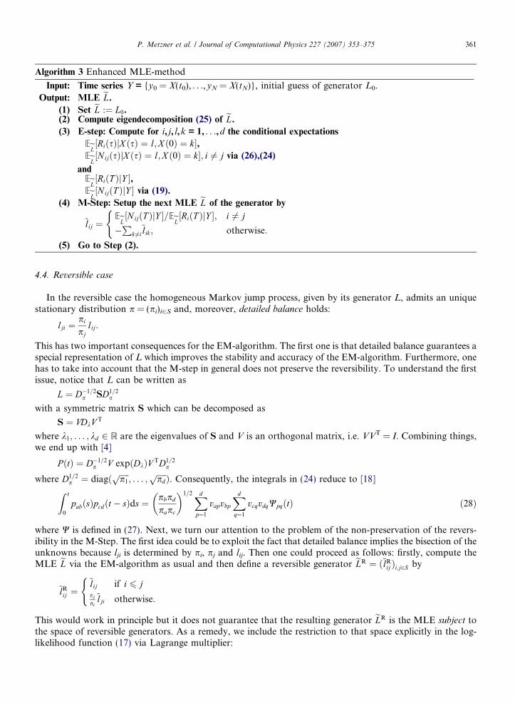
Algorithm 3 Enhanced MLE-method
Input: Time series Y = {y0 = X(t0), . . .,yN = X(tN)}, initial guess of generator L0.
Output: MLE eL.
(1) Set eL :¼ L0.(2) Compute eigendecomposition (25) of eL.
(3) E-step: Compute for i, j, l,k = 1, . . .,d the conditional expectations
EeL ½RiðsÞjX ðsÞ ¼ l;X ð0Þ ¼ k�,EeL ½NijðsÞjX ðsÞ ¼ l;X ð0Þ ¼ k�; i 6¼ j via (26),(24)
andEeL ½RiðT ÞjY �,EeL ½NijðT ÞjY � via (19).
(4) M-Step: Setup the next MLE eL of the generator by
Ee½N ijðT ÞjY �=Ee½RiðT ÞjY �; i 6¼ j(
~lij ¼ L L
�P
k 6¼i~lik; otherwise:
(5) Go to Step (2).
4.4. Reversible case
In the reversible case the homogeneous Markov jump process, given by its generator L, admits an uniquestationary distribution p = (pi)i2S and, moreover, detailed balance holds:
lji ¼pi
pjlij:
This has two important consequences for the EM-algorithm. The first one is that detailed balance guarantees aspecial representation of L which improves the stability and accuracy of the EM-algorithm. Furthermore, onehas to take into account that the M-step in general does not preserve the reversibility. To understand the firstissue, notice that L can be written as
L ¼ D�1=2p SD1=2
p
with a symmetric matrix S which can be decomposed as
S ¼ VDkV T
where k1; . . . ; kd 2 R are the eigenvalues of S and V is an orthogonal matrix, i.e. VVT = I. Combining things,we end up with [4]
P ðtÞ ¼ D�1=2p V expðDkÞV TD1=2
p
where D1=2p ¼ diagð ffiffiffiffiffip1
p; . . . ;
ffiffiffiffiffipdp Þ. Consequently, the integrals in (24) reduce to [18]
Z t0
pabðsÞpcdðt � sÞds ¼ pbpd
papc
� �1=2Xd
p¼1
vapvbp
Xd
q¼1
vcqvdqWpqðtÞ ð28Þ
where W is defined in (27). Next, we turn our attention to the problem of the non-preservation of the revers-ibility in the M-Step. The first idea could be to exploit the fact that detailed balance implies the bisection of theunknowns because lji is determined by pi, pj and lij. Then one could proceed as follows: firstly, compute theMLE eL via the EM-algorithm as usual and then define a reversible generator eLR ¼ ð~lR
ij Þi;j2S by
~lRij ¼
~lij if i 6 jpj
pi~lji otherwise:
(
This would work in principle but it does not guarantee that the resulting generator eLR is the MLE subject tothe space of reversible generators. As a remedy, we include the restriction to that space explicitly in the log-likelihood function (17) via Lagrange multiplier:
362 P. Metzner et al. / Journal of Computational Physics 227 (2007) 353–375
GRðL; L0Þ ¼ GðL; L0Þ þXd
i¼1
Xd
j>i
lijðpilij � pjljiÞ:
Performing the usual steps, we end up with the MLE eLR, given by
~lRij ¼
EL0NijðT ÞjY� �
�lijpi þ EL0½RiðT ÞjY �
; i < j
pipj
~lRij ; otherwise
8><>: ð29Þ
where the Lagrange multiplier can be determined by
lij ¼EL0½RjðT ÞjY �
pjEL0½NjiðT ÞjY �
� EL0½RiðT ÞjY �
piEL0½N ijðT ÞjY �
� � EL0
½NijðT ÞjY � � EL0½NjiðT ÞjY �
EL0½NijðT ÞjY � þ EL0
½NjiðT ÞjY �
: ð30Þ
Combining both issues leads to Algorithm 4.
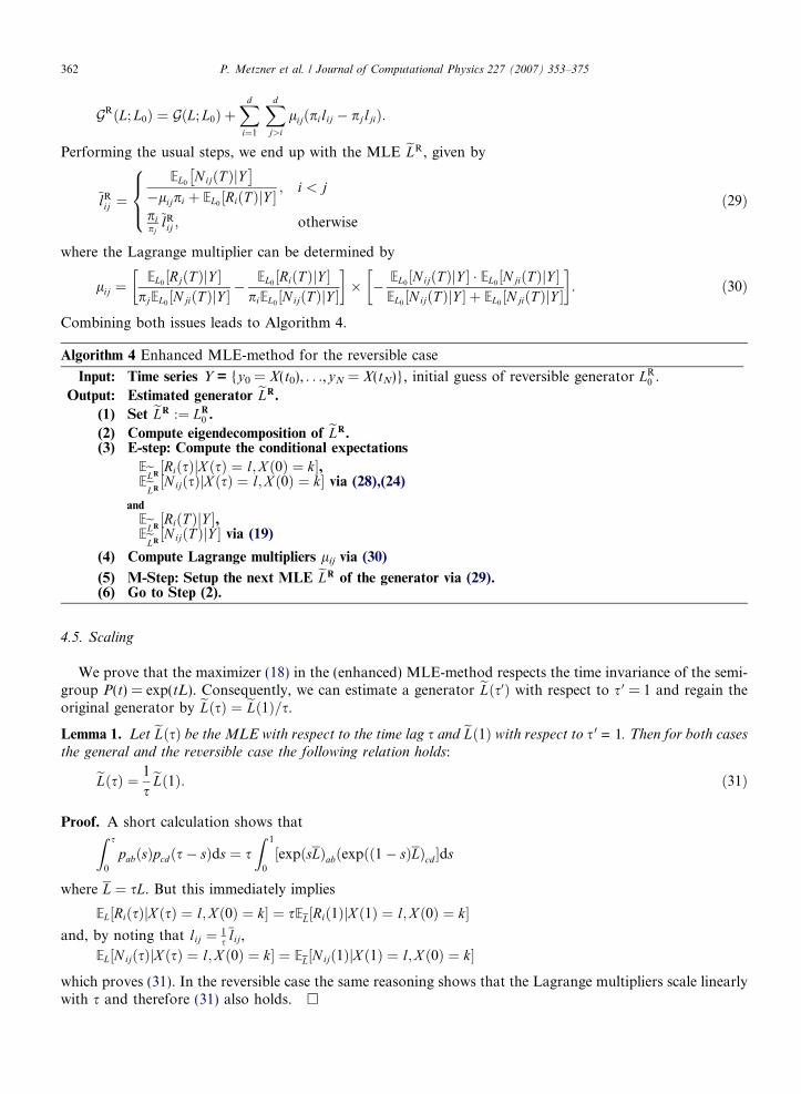
Algorithm 4 Enhanced MLE-method for the reversible case
Input: Time series Y = {y0 = X(t0), . . .,yN = X(tN)}, initial guess of reversible generator LR0 .
Output: Estimated generator eLR.
(1) Set eLR :¼ LR0 .
(2) Compute eigendecomposition of eLR.(3) E-step: Compute the conditional expectations
EeLR½RiðsÞjX ðsÞ ¼ l;X ð0Þ ¼ k�,
EeLR½N ijðsÞjX ðsÞ ¼ l;X ð0Þ ¼ k� via (28),(24)
and
EeLR½RiðT ÞjY �,
EeLR½N ijðT ÞjY � via (19)
(4) Compute Lagrange multipliers lij via (30)
(5) M-Step: Setup the next MLE eLR of the generator via (29).(6) Go to Step (2).
4.5. Scaling
We prove that the maximizer (18) in the (enhanced) MLE-method respects the time invariance of the semi-group P(t) = exp(tL). Consequently, we can estimate a generator eLðs0Þ with respect to s 0 = 1 and regain theoriginal generator by eLðsÞ ¼ eLð1Þ=s.
Lemma 1. Let eLðsÞ be the MLE with respect to the time lag s and eLð1Þ with respect to s 0 = 1. Then for both cases
the general and the reversible case the following relation holds:
eLðsÞ ¼ 1seLð1Þ: ð31Þ
Proof. A short calculation shows that
Z s0
pabðsÞpcdðs� sÞds ¼ sZ 1
0
½expðsLÞabðexpðð1� sÞLÞcd �ds
where L ¼ sL. But this immediately implies
EL½RiðsÞjX ðsÞ ¼ l;X ð0Þ ¼ k� ¼ sEL½Rið1ÞjX ð1Þ ¼ l;X ð0Þ ¼ k�
and, by noting that lij ¼ 1s�lij,
EL½N ijðsÞjX ðsÞ ¼ l;X ð0Þ ¼ k� ¼ EL½N ijð1ÞjX ð1Þ ¼ l;X ð0Þ ¼ k�
which proves (31). In the reversible case the same reasoning shows that the Lagrange multipliers scale linearlywith s and therefore (31) also holds. h
P. Metzner et al. / Journal of Computational Physics 227 (2007) 353–375 363
4.6. Enhanced MLE-method vs. MLE-method
The eigendecomposition approach has several advantages compared to the numerical considerations pro-posed in [1]. Let d be the dimension of the discrete state space. As explained in Section 4.2, the computationalcost is reduced to Oðd5Þ thanks to the closed form expression (26). Moreover, there is no longer an explicitdependency on the length of the time series. The second advantage is the exact computation of the conditionalexpectations involved in the E-step of the EM-algorithm. The steps which introduce numerical errors are theeigendecomposition and the computation of U�1. As before, the explicit inversion of U can be avoided by con-sidering the left eigenvectors of eL. We are aware that the eigendecomposition of non-symmetric matrices canbe ill-conditioned, but any reliable numerical solver should indicate this. Nevertheless, the computational costof both steps ðOðd3ÞÞ and their numerical stability are superior compared to any numerical approximationscheme for solving the ODEs in (22).
5. Numerical examples
5.1. Preparatory considerations
In order to compare the performance of the quadratic programming approach (QP) and the maximum like-lihood method (MLE), these approaches are now applied to a series of model problems. A comparison withthe resolvent method is omitted because, as we have seen above, this method does not respect the generatorconstraints and produces invalid estimates eL 62 G when no generator exists. A rather straightforward testwould proceed as follows:
(1) Choose an arbitrary generator L 2 G and a time lag s.(2) Compute the corresponding transition matrix P(s) = exp(sL).(3) Produce a time series Y = {y0 = X(t0), . . .,yN = X(tN)} by sampling from P(s).(4) Pass this data to each of the two methods and compute an estimate eL � L.(5) Compare the errors of the two approaches.
Although such a test seems to be somewhat reasonable, we will not use this procedure. The reason for ourrefusal is the fact that the time series produced in step 3 is just a single realization. Hence, the result of this testis random, too, and applying the test several times to the methods yields different results even though the inputL remains unchanged. In fact, both methods are affected by the sampling error
kP ðsÞ � bP k with P ¼ ðpijÞi;j and pij ¼cijPdj¼1cij
: ð32Þ
(Here and below, i Æ i denotes the matrix 2-norm.) Roughly speaking, the sampling error indicates how well thefrequency matrix of a time series ‘‘represents’’ the underlying transition matrix. In the limit N!1 one mayexpect the sampling error to vanish, but for a finite number of observations the deviation can be considerable.Since the outcome of a numerical method cannot be better than the input data, the error of both methods arebounded from below by the sampling error.
Therefore, our numerical experiments are designed in a different way:
(1) (a) Choose a generator L 2 G and a time lag s and compute the corresponding transition matrixP(s) = exp(sL),
or
(b) choose a transition matrix P. This allows to test the performance of the methods in situations whereno underlying generator exists. In this case, the time lag does not matter, and we can set s = 1.
(2) Define a virtual frequency matrix by multiplying each row of the transition matrix P(s) with the corre-sponding entry of the stationary distribution p = (pi),i 2 S and the length N of the (virtual) time series:
cij ¼ roundðNpipijÞ: ð33Þ
364 P. Metzner et al. / Journal of Computational Physics 227 (2007) 353–375
This is the frequency matrix which, up to rounding errors, reflects the underlying transition matrix in anoptimal way.
(3) Based on the virtual frequency matrix, define the virtual transition matrix
bP virt ¼ ðpijÞi;j and pij ¼cijPdj¼1cijð34Þ
and compute an estimate eL � L for the generator.(4) For both methods, compute and compare the errors:
(a) keL � Lk (only if L is available, i.e. if variant (a) of step 1 was used).(b) kP ðsÞ � expðseLÞk.(c) kbP virt � expðseLÞk with bP virt defined in (34).
The advantage of this approach to numerical experiments is illustrated by a simple example in Appendix A,cf. Section A.2.
Of course, the choice of the initial value L0 for the MLE-method is crucial for the convergence. If the matrixlogarithm of bP virt exists, then a good initial value L0 can easily be obtained by taking the absolute values of theoff-diagonal entries of logðbP virtÞ=s and setting the diagonal entries to the corresponding negative row sums,respectively.
5.2. Transition matrix with underlying generator
In a first example we follow variant (a) of step 1 and consider the generator
L¼
�4:293 0:678 0:301 0:819 0:592 0:149 0:543 0:411 0:774 0:023
0:033 �3:833 0:633 0:260 0:636 0:878 0:485 0:527 0:147 0:231
0:857 0:995 �5:466 0:704 0:532 0:021 0:441 0:920 0:148 0:845
0:682 0:499 0:005 �4:691 0:208 0:923 0:626 0:379 0:639 0:726
0:801 0:430 0:816 0:082 �4:268 0:632 0:077 0:638 0:093 0:694
0:917 0:829 0:690 0:875 0:241 �5:584 0:544 0:173 0:928 0:383
0:388 0:116 0:981 0:077 0:720 0:632 �4:667 0:785 0:485 0:479
0:472 0:598 0:069 0:741 0:400 0:753 0:270 �4:435 0:163 0:967
0:088 0:221 0:045 0:125 0:394 0:769 0:291 0:776 �3:495 0:783
0:925 0:398 0:740 0:443 0:411 0:808 0:822 0:342 0:131 �5:022
0BBBBBBBBBBBBBBBBBBBBB@
1CCCCCCCCCCCCCCCCCCCCCA
2G:
ð35Þ
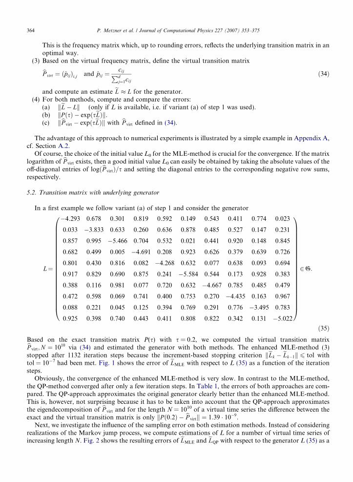
Based on the exact transition matrix P(s) with s = 0.2, we computed the virtual transition matrixbP virt;N ¼ 1010 via (34) and estimated the generator with both methods. The enhanced MLE-method (3)stopped after 1132 iteration steps because the increment-based stopping criterion keLk � eLk�1k 6 tol withtol = 10�7 had been met. Fig. 1 shows the error of eLMLE with respect to L (35) as a function of the iterationsteps.Obviously, the convergence of the enhanced MLE-method is very slow. In contrast to the MLE-method,the QP-method converged after only a few iteration steps. In Table 1, the errors of both approaches are com-pared. The QP-approach approximates the original generator clearly better than the enhanced MLE-method.This is, however, not surprising because it has to be taken into account that the QP-approach approximatesthe eigendecomposition of bP virt and for the length N = 1010 of a virtual time series the difference between theexact and the virtual transition matrix is only kP ð0:2Þ � bP virtk ¼ 1:39 � 10�9.
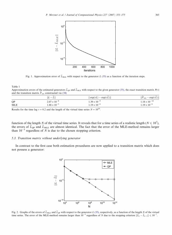
Next, we investigate the influence of the sampling error on both estimation methods. Instead of consideringrealizations of the Markov jump process, we compute estimations of L for a number of virtual time series ofincreasing length N. Fig. 2 shows the resulting errors of eLMLE and eLQP with respect to the generator L (35) as a
200 400 600 800 1000
10
10
100
iterations
Fig. 1. Approximation error of eLMLE with respect to the generator L (35) as a function of the iteration steps.
Table 1Approximation errors of the estimated generators eLQP and eLMLE with respect to the given generator (35), the exact transition matrix P(s)and the transition matrix bP virt constructed via (34)
kL� eLk k expðsLÞ � expðseLÞk kbP virt � expðseLÞkQP 2.07 · 10�8 1.39 · 10�9 1.18 · 10�14
MLE 1.88 · 10�5 1.19 · 10�6 1.19 · 10�6
Results for the time lag s = 0.2 and the length of the virtual time series N = 1010.
P. Metzner et al. / Journal of Computational Physics 227 (2007) 353–375 365
function of the length N of the virtual time series. It reveals that for a time series of a realistic length (N 6 107),the errors of eLQP and eLMLE are almost identical. The fact that the error of the MLE-method remains largerthan 10�5 regardless of N is due to the chosen stopping criterion.
5.3. Transition matrix without underlying generator
In contrast to the first case both estimation procedures are now applied to a transition matrix which doesnot possess a generator:
104 106 108 1010 101210
10
100
N
MLE
QP
Fig. 2. Graphs of the errors of eLMLE and eLQP with respect to the generator L (35), respectively, as a function of the length N of the virtualtime series. The error of the MLE-method remains larger than 10�5 regardless of N due to the stopping criterion keLk � eLk�1k 6 10�7.
TableApproconstr
QPMLE
Result
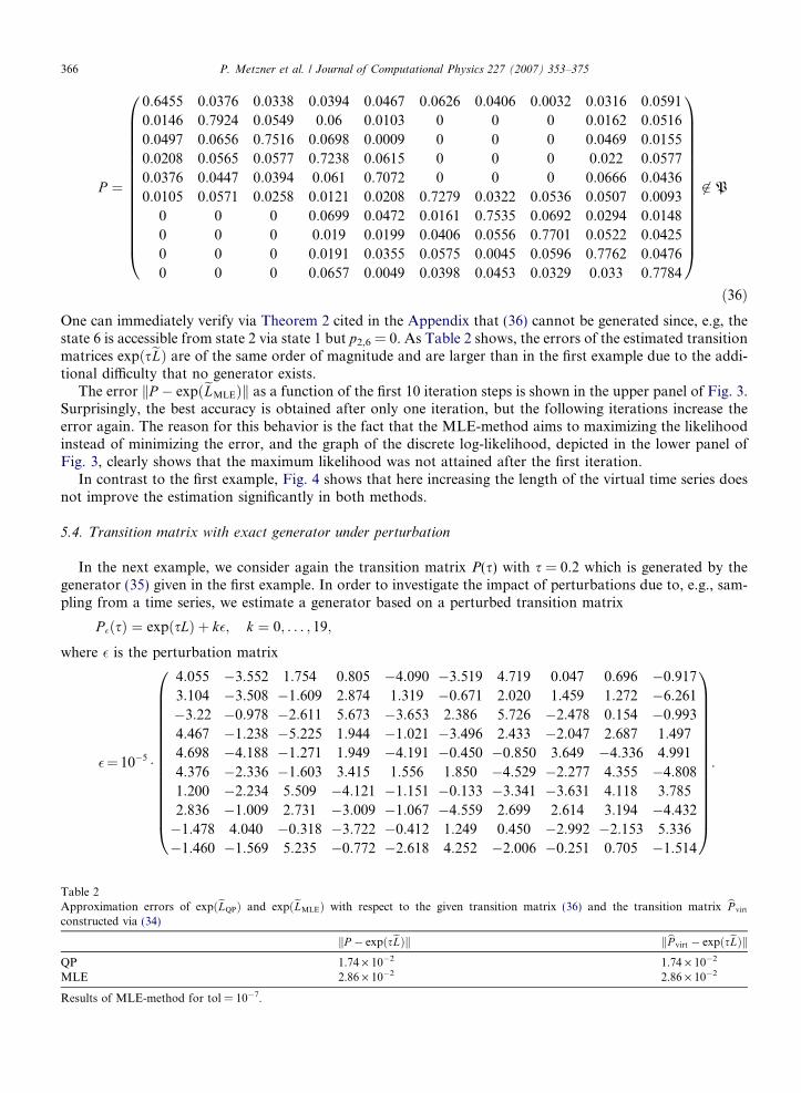
366 P. Metzner et al. / Journal of Computational Physics 227 (2007) 353–375
P ¼
0:6455 0:0376 0:0338 0:0394 0:0467 0:0626 0:0406 0:0032 0:0316 0:0591
0:0146 0:7924 0:0549 0:06 0:0103 0 0 0 0:0162 0:0516
0:0497 0:0656 0:7516 0:0698 0:0009 0 0 0 0:0469 0:0155
0:0208 0:0565 0:0577 0:7238 0:0615 0 0 0 0:022 0:0577
0:0376 0:0447 0:0394 0:061 0:7072 0 0 0 0:0666 0:0436
0:0105 0:0571 0:0258 0:0121 0:0208 0:7279 0:0322 0:0536 0:0507 0:0093
0 0 0 0:0699 0:0472 0:0161 0:7535 0:0692 0:0294 0:0148
0 0 0 0:019 0:0199 0:0406 0:0556 0:7701 0:0522 0:0425
0 0 0 0:0191 0:0355 0:0575 0:0045 0:0596 0:7762 0:0476
0 0 0 0:0657 0:0049 0:0398 0:0453 0:0329 0:033 0:7784
0BBBBBBBBBBBBBBB@
1CCCCCCCCCCCCCCCA62 P
ð36Þ
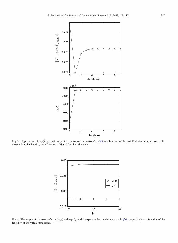
One can immediately verify via Theorem 2 cited in the Appendix that (36) cannot be generated since, e.g, thestate 6 is accessible from state 2 via state 1 but p2,6 = 0. As Table 2 shows, the errors of the estimated transitionmatrices expðseLÞ are of the same order of magnitude and are larger than in the first example due to the addi-tional difficulty that no generator exists.The error kP � expðeLMLEÞk as a function of the first 10 iteration steps is shown in the upper panel of Fig. 3.Surprisingly, the best accuracy is obtained after only one iteration, but the following iterations increase theerror again. The reason for this behavior is the fact that the MLE-method aims to maximizing the likelihoodinstead of minimizing the error, and the graph of the discrete log-likelihood, depicted in the lower panel ofFig. 3, clearly shows that the maximum likelihood was not attained after the first iteration.
In contrast to the first example, Fig. 4 shows that here increasing the length of the virtual time series doesnot improve the estimation significantly in both methods.
5.4. Transition matrix with exact generator under perturbation
In the next example, we consider again the transition matrix P(s) with s = 0.2 which is generated by thegenerator (35) given in the first example. In order to investigate the impact of perturbations due to, e.g., sam-pling from a time series, we estimate a generator based on a perturbed transition matrix
P �ðsÞ ¼ expðsLÞ þ k�; k ¼ 0; . . . ; 19;
where � is the perturbation matrix
�¼ 10�5 �
4:055 �3:552 1:754 0:805 �4:090 �3:519 4:719 0:047 0:696 �0:917
3:104 �3:508 �1:609 2:874 1:319 �0:671 2:020 1:459 1:272 �6:261
�3:22 �0:978 �2:611 5:673 �3:653 2:386 5:726 �2:478 0:154 �0:993
4:467 �1:238 �5:225 1:944 �1:021 �3:496 2:433 �2:047 2:687 1:497
4:698 �4:188 �1:271 1:949 �4:191 �0:450 �0:850 3:649 �4:336 4:991
4:376 �2:336 �1:603 3:415 1:556 1:850 �4:529 �2:277 4:355 �4:808
1:200 �2:234 5:509 �4:121 �1:151 �0:133 �3:341 �3:631 4:118 3:785
2:836 �1:009 2:731 �3:009 �1:067 �4:559 2:699 2:614 3:194 �4:432
�1:478 4:040 �0:318 �3:722 �0:412 1:249 0:450 �2:992 �2:153 5:336
�1:460 �1:569 5:235 �0:772 �2:618 4:252 �2:006 �0:251 0:705 �1:514
0BBBBBBBBBBBBBBB@
1CCCCCCCCCCCCCCCA:
2ximation errors of expðeLQPÞ and expðeLMLEÞ with respect to the given transition matrix (36) and the transition matrix bP virt
ucted via (34)
kP � expðseLÞk kbP virt � expðseLÞk1.74 · 10�2 1.74 · 10�2
2.86 · 10�2 2.86 · 10�2
s of MLE-method for tol = 10�7.
0 2 4 6 80.024
0.026
0.028
0.03
0.032
iterations
0 2 4 6 8
x 109
iterations
Fig. 3. Upper: error of expðeLMLEÞ with respect to the transition matrix P in (36) as a function of the first 10 iteration steps. Lower: thediscrete log-likelihood Ld as a function of the 10 first iteration steps.
104 106 1080.015
0.02
0.025
0.03
N
MLE
QP
Fig. 4. The graphs of the errors of expðeLMLEÞ and expðeLQPÞ with respect to the transition matrix in (36), respectively, as a function of thelength N of the virtual time series.
P. Metzner et al. / Journal of Computational Physics 227 (2007) 353–375 367
368 P. Metzner et al. / Journal of Computational Physics 227 (2007) 353–375
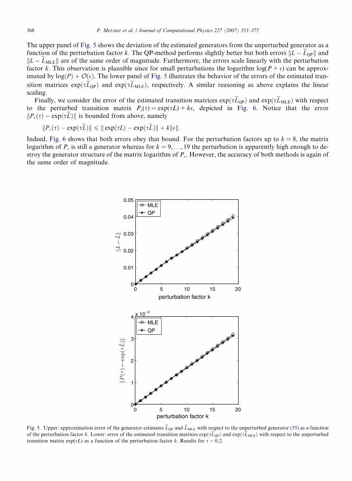
The upper panel of Fig. 5 shows the deviation of the estimated generators from the unperturbed generator as afunction of the perturbation factor k. The QP-method performs slightly better but both errors kL� eLQPk andkL� eLMLEk are of the same order of magnitude. Furthermore, the errors scale linearly with the perturbationfactor k. This observation is plausible since for small perturbations the logarithm log(P + �) can be approx-imated by logðP Þ þOð�Þ. The lower panel of Fig. 5 illustrates the behavior of the errors of the estimated tran-
sition matrices expðseLQPÞ and expðseLMLEÞ, respectively. A similar reasoning as above explains the linearscaling.
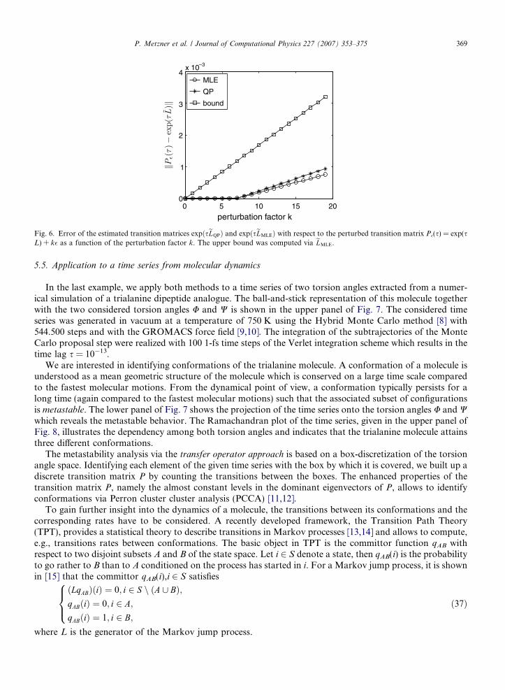
Finally, we consider the error of the estimated transition matrices expðseLQPÞ and expðseLMLEÞ with respectto the perturbed transition matrix P�(s) = exp(sL) + k�, depicted in Fig. 6. Notice that the errorkP �ðsÞ � expðseLÞk is bounded from above, namely
Fig. 5.of thetransit
kP �ðsÞ � expðseLÞk 6 k expðsLÞ � expðseLÞk þ kk�k:
Indeed, Fig. 6 shows that both errors obey that bound. For the perturbation factors up to k = 8, the matrixlogarithm of P� is still a generator whereas for k = 9, . . ., 19 the perturbation is apparently high enough to de-stroy the generator structure of the matrix logarithm of P�. However, the accuracy of both methods is again ofthe same order of magnitude.0 5 10 15 200
0.01
0.02
0.03
0.04
0.05
perturbation factor k
MLE
QP
0 5 10 15 200
1
2
3
4 x 10
perturbation factor k
MLE
QP
Upper: approximation error of the generator estimates eLQP and eLMLE with respect to the unperturbed generator (35) as a functionperturbation factor k. Lower: error of the estimated transition matrices expðseLQPÞ and expðseLMLEÞ with respect to the unperturbedion matrix exp(sL) as a function of the perturbation factor k. Results for s = 0.2.
0 5 10 15 200
1
2
3
4x 10
perturbation factor k
MLE
QP
bound
Fig. 6. Error of the estimated transition matrices expðseLQPÞ and expðseLMLEÞ with respect to the perturbed transition matrix P�(s) = exp(sL) + k� as a function of the perturbation factor k. The upper bound was computed via eLMLE.
P. Metzner et al. / Journal of Computational Physics 227 (2007) 353–375 369
5.5. Application to a time series from molecular dynamics
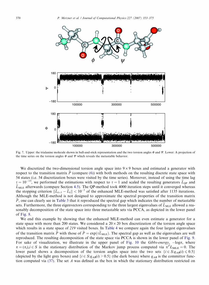
In the last example, we apply both methods to a time series of two torsion angles extracted from a numer-ical simulation of a trialanine dipeptide analogue. The ball-and-stick representation of this molecule togetherwith the two considered torsion angles U and W is shown in the upper panel of Fig. 7. The considered timeseries was generated in vacuum at a temperature of 750 K using the Hybrid Monte Carlo method [8] with544.500 steps and with the GROMACS force field [9,10]. The integration of the subtrajectories of the MonteCarlo proposal step were realized with 100 1-fs time steps of the Verlet integration scheme which results in thetime lag s = 10�13.
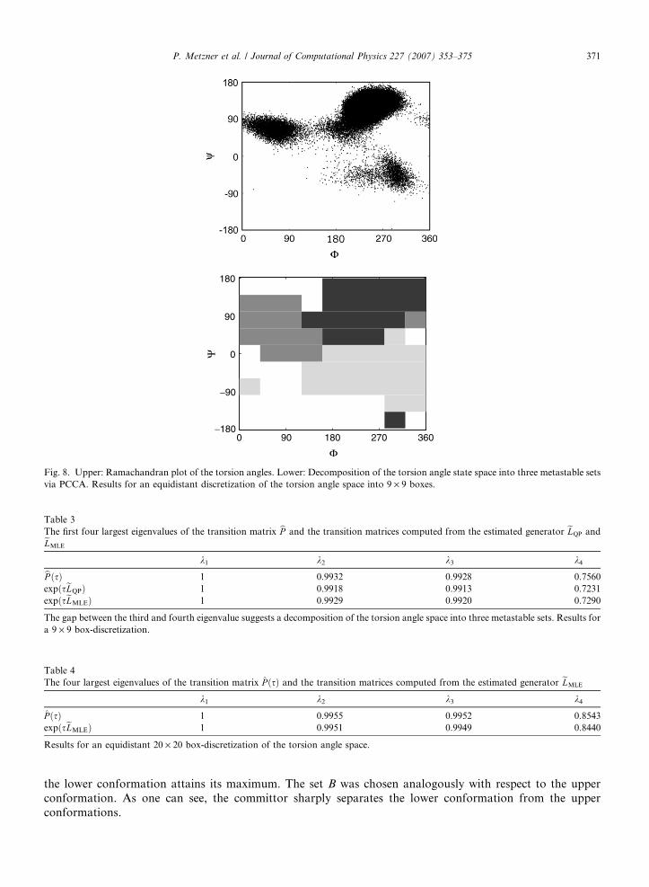
We are interested in identifying conformations of the trialanine molecule. A conformation of a molecule isunderstood as a mean geometric structure of the molecule which is conserved on a large time scale comparedto the fastest molecular motions. From the dynamical point of view, a conformation typically persists for along time (again compared to the fastest molecular motions) such that the associated subset of configurationsis metastable. The lower panel of Fig. 7 shows the projection of the time series onto the torsion angles U and Wwhich reveals the metastable behavior. The Ramachandran plot of the time series, given in the upper panel ofFig. 8, illustrates the dependency among both torsion angles and indicates that the trialanine molecule attainsthree different conformations.
The metastability analysis via the transfer operator approach is based on a box-discretization of the torsionangle space. Identifying each element of the given time series with the box by which it is covered, we built up adiscrete transition matrix P by counting the transitions between the boxes. The enhanced properties of thetransition matrix P, namely the almost constant levels in the dominant eigenvectors of P, allows to identifyconformations via Perron cluster cluster analysis (PCCA) [11,12].
To gain further insight into the dynamics of a molecule, the transitions between its conformations and thecorresponding rates have to be considered. A recently developed framework, the Transition Path Theory(TPT), provides a statistical theory to describe transitions in Markov processes [13,14] and allows to compute,e.g., transitions rates between conformations. The basic object in TPT is the committor function qAB withrespect to two disjoint subsets A and B of the state space. Let i 2 S denote a state, then qAB(i) is the probabilityto go rather to B than to A conditioned on the process has started in i. For a Markov jump process, it is shownin [15] that the committor qAB(i),i 2 S satisfies8
ðLqABÞðiÞ ¼ 0; i 2 S n ðA [ BÞ;qABðiÞ ¼ 0; i 2 A;
qABðiÞ ¼ 1; i 2 B;
><>: ð37Þ
where L is the generator of the Markov jump process.
100000 300000 500000
0
180
100000 300000 500000
0
180
Fig. 7. Upper: the trialanine molecule shown in ball-and-stick representation and the two torsion angles U and W. Lower: A projection ofthe time series on the torsion angles U and W which reveals the metastable behavior.
370 P. Metzner et al. / Journal of Computational Physics 227 (2007) 353–375
We discretized the two-dimensional torsion angle space into 9 · 9 boxes and estimated a generator withrespect to the transition matrix bP (compare (6)) with both methods on the resulting discrete state space with54 states (i.e. 54 discretization boxes were visited by the time series). Moreover, instead of using the time lags = 10�13, we performed the estimations with respect to s = 1 and scaled the resulting generators eLQP andeLMLE afterwards (compare Section 4.5). The QP-method took 4000 iteration steps until it converged whereasthe stopping criterion keLkþ1 � eLkk < 10�3 of the enhanced MLE-method was satisfied after 1135 iterations.Although the MLE-method is not designed to approximate the spectral properties of the transition matrixbP , one can clearly see in Table 3 that it reproduced the spectral gap which indicates the number of metastablesets. Furthermore, the three eigenvectors corresponding to the three largest eigenvalues of eLMLE allowed a rea-sonably decomposition of the state space into three metastable sets via PCCA, as depicted in the lower panelof Fig. 8.
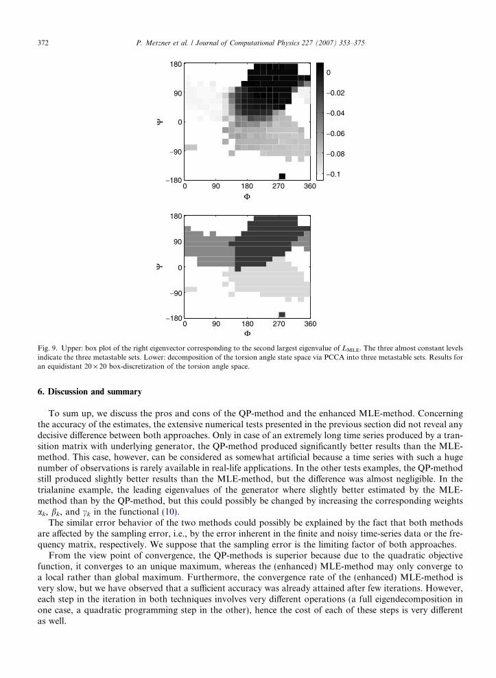
We end this example by showing that the enhanced MLE-method can even estimate a generator for astate space with more than 200 states. We considered a 20 · 20 box discretization of the torsion angle spacewhich results in a state space of 219 visited boxes. In Table 4 we compare again the four largest eigenvalues
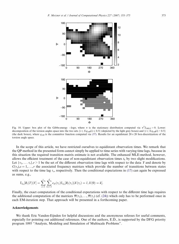
of the transition matrix bP with those of eP ¼ expðseLMLEÞ. The spectral gap as well as the eigenvalues are wellreproduced. The resulting decomposition of the state space via PCCA is shown in the lower panel of Fig. 9.For sake of visualization, we illustrate in the upper panel of Fig. 10 the Gibbs-energy, �logp, wherep = (pi),i 2 S is the stationary distribution of the Markov jump process computed via pTLMLE = 0. Thelower panel shows a decomposition of the torsion angles space into the two sets {i 2 S:qAB(i) 6 0.5}(depicted by the light grey boxes) and {i 2 S:qAB(i) > 0.5} (the dark boxes) where qAB is the committor func-tion computed via (37). The set A was defined as the box in which the stationary distribution restricted on
0 90 180 270 360
0
90
180
Fig. 8. Upper: Ramachandran plot of the torsion angles. Lower: Decomposition of the torsion angle state space into three metastable setsvia PCCA. Results for an equidistant discretization of the torsion angle space into 9 · 9 boxes.
Table 3The first four largest eigenvalues of the transition matrix bP and the transition matrices computed from the estimated generator eLQP andeLMLE
k1 k2 k3 k4bP ðsÞ 1 0.9932 0.9928 0.7560expðseLQPÞ 1 0.9918 0.9913 0.7231expðseLMLEÞ 1 0.9929 0.9920 0.7290
The gap between the third and fourth eigenvalue suggests a decomposition of the torsion angle space into three metastable sets. Results fora 9 · 9 box-discretization.
Table 4The four largest eigenvalues of the transition matrix P ðsÞ and the transition matrices computed from the estimated generator eLMLE
k1 k2 k3 k4
P ðsÞ 1 0.9955 0.9952 0.8543expðseLMLEÞ 1 0.9951 0.9949 0.8440
Results for an equidistant 20 · 20 box-discretization of the torsion angle space.
P. Metzner et al. / Journal of Computational Physics 227 (2007) 353–375 371
the lower conformation attains its maximum. The set B was chosen analogously with respect to the upperconformation. As one can see, the committor sharply separates the lower conformation from the upperconformations.
0 90 180 270 360
0
90
1800
0 90 180 270 360
0
90
180
Fig. 9. Upper: box plot of the right eigenvector corresponding to the second largest eigenvalue of LMLE. The three almost constant levelsindicate the three metastable sets. Lower: decomposition of the torsion angle state space via PCCA into three metastable sets. Results foran equidistant 20 · 20 box-discretization of the torsion angle space.
372 P. Metzner et al. / Journal of Computational Physics 227 (2007) 353–375
6. Discussion and summary
To sum up, we discuss the pros and cons of the QP-method and the enhanced MLE-method. Concerningthe accuracy of the estimates, the extensive numerical tests presented in the previous section did not reveal anydecisive difference between both approaches. Only in case of an extremely long time series produced by a tran-sition matrix with underlying generator, the QP-method produced significantly better results than the MLE-method. This case, however, can be considered as somewhat artificial because a time series with such a hugenumber of observations is rarely available in real-life applications. In the other tests examples, the QP-methodstill produced slightly better results than the MLE-method, but the difference was almost negligible. In thetrialanine example, the leading eigenvalues of the generator where slightly better estimated by the MLE-method than by the QP-method, but this could possibly be changed by increasing the corresponding weightsak, bk, and ck in the functional (10).
The similar error behavior of the two methods could possibly be explained by the fact that both methodsare affected by the sampling error, i.e., by the error inherent in the finite and noisy time-series data or the fre-quency matrix, respectively. We suppose that the sampling error is the limiting factor of both approaches.
From the view point of convergence, the QP-methods is superior because due to the quadratic objectivefunction, it converges to an unique maximum, whereas the (enhanced) MLE-method may only converge toa local rather than global maximum. Furthermore, the convergence rate of the (enhanced) MLE-method isvery slow, but we have observed that a sufficient accuracy was already attained after few iterations. However,each step in the iteration in both techniques involves very different operations (a full eigendecomposition inone case, a quadratic programming step in the other), hence the cost of each of these steps is very differentas well.
0 90 180 270 360
0
90
180
2
4
6
8
10
12
0 90 180 270 360
0
90
180
Fig. 10. Upper: box plot of the Gibbs-energy �logpi where p is the stationary distribution computed via pTLMLE = 0. Lower:decomposition of the torsion angles space into the two sets {i 2 S:qAB(i) 6 0.5} (depicted by the light grey boxes) and {i 2 S:qAB(i) > 0.5}(the dark boxes), where qAB is the committor function computed via (37). Results for an equidistant 20 · 20 box-discretization of thetorsion angle space.
P. Metzner et al. / Journal of Computational Physics 227 (2007) 353–375 373
In the scope of this article, we have restricted ourselves to equidistant observation times. We remark thatthe QP-method in the presented form cannot simply be applied to time series with varying time lags, because inthis situation the required transition matrix estimate is not available. The enhanced MLE-method, however,allows the efficient treatment of the case of non-equidistant observation times tk by two slight modifications.Let {s1, . . . sr},r > 1 be the set of the different observation time lags with respect to the data Y and denote byC(ss),s = 1, . . ., r the associated frequency matrices which provide the number of transitions between stateswith respect to the time lag ss, respectively. Then the conditional expectations in (17) can again be expressedas sums, e.g.,
EL0½RiðT ÞjY � ¼
Xr
s¼1
Xd
k;l¼1
cklðssÞEL0½RiðssÞjX ðssÞ ¼ l;X ð0Þ ¼ k�:
Finally, the exact computation of the conditional expectations with respect to the different time lags requiresthe additional computation of the matrices W(s1), . . .,W(sr) (cf. (24)) which only has to be performed once ineach EM-iteration step. That approach will be presented in a forthcoming paper.
Acknowledgements
We thank Eric Vanden-Eijnden for helpful discussions and the anonymous referees for useful comments,especially for pointing out additional references. One of the authors, E.D., is supported by the DFG priorityprogram 1095 ‘‘Analysis, Modeling and Simulation of Multiscale Problems’’.
374 P. Metzner et al. / Journal of Computational Physics 227 (2007) 353–375
Appendix A
A.1. Two theorems on the existence of generators
The following Theorems are found in [16]. They give sufficient conditions for the existence of a generator ofa given transition matrix.
Theorem 2. Let P be a transition matrix and suppose that
(a) det(P) 6 0, or
(b) detðP Þ >Q
ipii, or(c) there are states i and j such that j is accessible from i, but pij = 0.
Then, there is no generator L 2 G such that P = exp(L).
Theorem 3. Let P be a transition matrix.
(a) If detðP Þ > 12, then P has at most one generator.
(b) If detðPÞ > 12
and kP � Ik < 12
(using any operator norm), then the only possible generator for P is the prin-
cipal branch of the logarithm of P.
(c) If P has distinct eigenvalues and det(P) > e�p, then the only possible generator for P is the principal branch
of the logarithm of P.
A.2. A simple example illustrating the effect of sampling errors
This example illustrates the influence of the sampling error on the optimal generator estimate; cf. the dis-cussion in Section 5.1. The transition matrix of the generator
L ¼�0:2 0:2
0:2 �0:2
� �
with respect to the time lag s = 1 isPðsÞ ¼0:8352 0:1648
0:1648 0:8352
� �:
Suppose that sampling according to the transition matrix produces the time series
time, tn
0 1 2 3 4 5 6 7 8 9 10 state, X(tn) 1 1 2 2 1 1 1 1 2 2 2such that the corresponding frequency matrix is
C ¼4 2
3 1
� �:
According to this data, the transition matrix seems to be
bP ¼ 2=3 1=3
3=4 1=4
� �ðA:1Þ
and since bP ¼ expðbLÞ with
bL � �0:5003 0:5003
0:3752 �0:3752
� �2 G ðA:2Þ
P. Metzner et al. / Journal of Computational Physics 227 (2007) 353–375 375
the best result we can expect to obtain based on the time series is bL instead of L. The errors kbP � Pk � 0:2670and kbL � Lk � 0:4916 are caused by the time series and cannot be avoided by the two methods. However,these errors decrease if, according to the second test procedure, the frequency matrix is replaced by the virtualfrequency matrix (33). Since in our example the stationary distribution is p = (0.5,0.5), one obtains
C ¼4 1
1 4
� �:
The corresponding transition matrix
bP virt ¼0:8 0:2
0:2 0:8
� �
is obviously a better approximation of the true transition matrix P than (A.1), and the generator estimateeL ¼ logðbP virtÞ ��0:2554 0:2554
0:2554 �0:2554
� �
is evidently better than (A.2). In fact, the new errors are only kP � bP virtk � 0:0703 and kL� eLk � 0:1108.References
[1] M. Bladt, M. Sørensen, Statistical inference for discretely observed Markov jump processes, J.R. Statist. Soc. B 67 (2005) 395–410.[2] D.T. Crommelin, E. Vanden-Eijnden, Fitting timeseries by continuous-time Markov chains: a quadratic programming approach, J.
Comp. Phys. 217 (2006) 782–805.[3] T. Muller, Modellierung von Proteinevolution, PhD thesis, Heidelberg, 2001.[4] A. Hobolth, J.L. Jensen, Statistical inference in evolutionary models of DNA sequences via the EM algorithm, Statistical
Applications in Genetics and Molecular Biology 4 (2005) Article 18.[5] T. Muller, R. Spang, M. Vingron, Estimating amino acid substitution models: A comparison of Dayhoff’s estimator, the resolvent
approach and a maximum likelihood method, Mol. Biol. Evol. 19 (2002) 8–13.[6] A.P. Dempster, N.M. Laird, D.B. Rubin, Maximum likelihood from incomplete data via the EM algorithm, J.R. Statist. Soc. 39
(1977) 1–38.[7] M.F. Neuts, Algorithmic Probability: a Collection of Problems, Chapman and Hall, 1995.[8] A. Brass, B.J. Pendleton, Y. Chen, B. Robson, Hybrid Monte Carlo simulations theory and initial comparison with molecular
dynamics, Biopolymers 33 (1993) 1307–1315.[9] H.J.C. Berendsen, D. van der Spoel, R. van Drunen, Gromacs: a message-passing parallel molecular dynamics implementation,
Comp. Phys. Comm. 91 (1995) 43–56.[10] E. Lindahl, B. Hess, D. van der Spoel, Gromacs 3.0: a package for molecular simulation and trajectory analysis, J. Mol. Mod. 7
(2001).[11] P. Deuflhard, W. Huisinga, A. Fischer, Ch. Schutte, Identification of almost invariant aggregates in reversible nearly uncoupled
Markov chains, Lin. Alg. Appl. 315 (2000) 39–59.[12] F. Cordes, M. Weber, J. Schmidt-Ehrenberg, Metastable conformations via successive Perron-Cluster Cluster analysis of dihedrals,
ZIB-Report 02-40 (2002).[13] E. Weinan, Vanden-Eijnden, Towards a theory of transition paths, J. Stat. Phys. 123 (2006) 503–523.[14] P. Metzner, C. Schutte, E. Vanden-Eijnden, Illustration of transition path theory on a collection of simple examples, J. Chem. Phys.
125 (2006) 084110.[15] P. Metzner, Ch. Schutte, E. Vanden-Eijnden, Transition path theory for Markov jump processes, submitted for publication.[16] R.B. Israel, J.S. Rosenthal, J.Z. Wei, Finding generators for Markov chains via empirical transition matrices with applications to
credit ranking, Mathematical Finance 11 (2001) 245–265.[17] U. Nodelman, C.R. Shelton, D. Koller, Expectation maximization and complex duration distributions for continuous time Bayesian
networks, in: Proceedings of the Twenty-first Conference on Uncertainty in AI (UAI), 2005, pp. 421–430.[18] I. Holmes, G.M. Rubin, An expectation maximization algorithm for training hidden substitution models, J. Mol. Biol. 317 (2002)
753–764.[19] S. Asmussen, O. Nerman, M. Olsson, Fitting phase-type distributions via the EM algorithm, Scand. J. Stat. 23 (1996) 419–441.[20] L. Arvestad, W.J. Bruno, Estimation of reversible substitution matrices from multiple pairs of sequences, J. Mol. Evol. 45 (1997) 696–
703.

![Chapter 1Reversible Jump Markov chain Monte arXiv:1001 ... · arXiv:1001.2055v1 [stat.ME] 13 Jan 2010 Chapter 1Reversible Jump Markov chain Monte Carlo Yanan Fan and Scott A. Sisson](https://img.pdfslide.us/doc/110x75/5e3ef07316231b2e3e667f90/chapter-1reversible-jump-markov-chain-monte-arxiv1001-arxiv10012055v1-statme.jpg)


![ONLINE LEARNING AND OPTIMIZATION OF MARKOV JUMP … · control problem of Markov jump linear systems with unknown parameters [5]–[7]. In this paper, we study the online learning](https://img.pdfslide.us/doc/110x75/5f0925f37e708231d42574dc/online-learning-and-optimization-of-markov-jump-control-problem-of-markov-jump-linear.jpg)