Research Division Federal Reserve Bank of St. Louis Working Paper Series

Generational Policy and the Macroeconomic Measurement of Tax Incidence

Juan Carlos Conesa and

Carlos Garriga

Working Paper 2009-003A

http://research.stlouisfed.org/wp/2009/2009-003.pdf

January 2009

FEDERAL RESERVE BANK OF ST. LOUIS Research Division

P.O. Box 442 St. Louis, MO 63166

______________________________________________________________________________________

The views expressed are those of the individual authors and do not necessarily reflect official positions of the Federal Reserve Bank of St. Louis, the Federal Reserve System, or the Board of Governors.

Federal Reserve Bank of St. Louis Working Papers are preliminary materials circulated to stimulate discussion and critical comment. References in publications to Federal Reserve Bank of St. Louis Working Papers (other than an acknowledgment that the writer has had access to unpublished material) should be cleared with the author or authors.

1

Generational Policy and the Macroeconomic Measurement of Tax

Incidence1

Juan Carlos Conesa

Universitat Autònoma de Barcelona

Carlos Garriga

Federal Reserve Bank of St. Louis

January 2009

Abstract

In this paper we show that the generational accounting framework used in macroeconomics to measure tax

incidence can, in some cases, yield inaccurate measurements of the tax burden across age cohorts. This

result is very important for policy evaluation, because it shows that the selection of tax policies designed to

change generational imbalances could be misleading. We illustrate this problem in the context of a Social

Security reform where we show how fiscal policy can affect the intergenerational gap across cohorts

without impacting the distribution of welfare. We provide a more accurate procedure that only measures

changes in generational imbalances derived from policies with real effects.

Keywords: Generational Accounting, Ramsey Taxation

J.E.L. codes: E62, H21

1 The authors thank the following for useful comments: Costas Azariadis, Tim Kehoe, Chris Phelan, and seminar participants at

ITAM, Alicante, Spain; European University Institute, Bern, Edingurgh, the 2008 meetings of the SED, Banco de España, Central

Bank Hungary, European Central Bank, CERGE-EI. Judith Ahlers and George Fortier provided great editorial comments. Juan Carlos

Conesa acknowledges financial support from Ministerio de Educación (No. SEJ2006-02879), from Generalitat de Catalunya (No.

SGR01-00029), Barcelona Economics, and Consolider. Carlos Garriga acknowledges support from the National Science Foundation

(grant No. SES-0649374). The views expressed herein do not necessarily reflect those of the Federal Reserve Bank of St. Louis, or the

Federal Reserve System. The authors can be reached via e-mail at JuanCarlos.Conesa@uab.es, and Carlos.Garriga@stls.frb.org.

1. INTRODUCTION

The recent financial crises in the United States will leave a huge hole in

taxpayers’ pockets. The collapse of the investment banking sector and insurance

companies, the two largest housing finance entities, and part of the auto industry has

required an unprecedented response from the Treasury and the Federal Reserve. The cost

of bailout programs designed to restore confidence in the economy have been estimated

as 60 percent of gross domestic product (GDP). The magnitude of this figure—in

conjunction with the current deficit—has overshadowed the known economic challenges

that we face in upcoming years: namely, the imbalance in outlays and incoming revenue

for social insurance programs (Social Security and Medicare) caused by the reduction in

fertility and the increase in life expectancy. This is in addition to the effects on the labor

markets.

The magnitude of these fiscal adjustments can assessed by looking at projected

demographics and the distribution of the tax burden across different age cohorts; but,

ultimately, policies must by established by considering intergenerational equity (fairness

in taxing and benefiting different generations) and economic efficiency.

Thus, before determining who will pay the tax bill for social insurance programs,

how much is needed, and the best tax instruments to raise the revenue, we must

accurately measure the tax burden or tax incidence of different individuals over time.

This measurement then can be used to (i) identify the individuals who are currently

bearing the cost of the tax bill and (ii) changes in the tax burden implied by alternative

tax regimes. Our paper provides a new and simple metric to measure tax incidence across

different age cohorts over time.

2

The most popular approach to the measurement of generational tax incidence is

the generational accounting framework developed by Auerback, Gokhale, and Kotlikoff

(1991).2 The accounting procedure requires rewriting the government’s intertemporal

budget constraint in terms of the fiscal incidence and the transfer programs received by

each generation. Assuming that taxes and transfers remain unchanged, these authors

calculate the net tax burden that future generations must bear to achieve long-term

balance in the government budget constraint. Any structural change in the tax policy must

be captured by a change in the fiscal incidence and transfers received by each generation;

this requirement implies a different measurement for present and future generations.

The advantage of the accounting framework is that the tax burden is relatively

easy to compute because it does not require specific assumptions about individual

preferences, technology, and market structure.3 It is sufficient to determine an

intertemporal discount rate so the tax burden paid by future generations can be directly

compared with the current ones. This ease of computation explains the widespread use

for policy analysis in practice (Board of Governors, Department of the Treasury, World

Bank) to assess the burden of future demographics or the impact of policy reforms. Two

limitations of the generational accounting framework are that it ignores the impact of

taxation on economic activity, and omits the welfare gains and losses resulting from

fiscal reforms. To address these criticisms, Fehr and Kotlikoff (1996) measured the fiscal

2 Staff economists at the Board of Governors developed a similar approach: a stylized model to measure the impact of population aging on living standards measured using consumption growth. For example, Bernanke (2006) summarizes the findings of Elmendorf and Sheiner (2000) and Sheiner, Sichel, and Slifman (2006) and proposes different alternatives to deal with the demographic transition. 3 Welfare analysis provides an alternative method to measure tax incidence. This approach requires specific assumptions about preferences and technology and is based entirely on individual optimizing behavior and market clearing conditions. Conesa and Garriga (2008b) use optimal fiscal policy to design the best possible response to demographic shocks.

3

incidence implied by the generational accounting method in a dynamic general

equilibrium life cycle model. They found that generational accounts match the evolution

of welfare changes for each cohort, but err with regard to the magnitudes of the change.

The authors argue that the bias is quantitatively small when the capital-to-output ratio

that determines the equilibrium interest rate and wage rates changes little.

In this paper, we show that the generational accounting framework used in

macroeconomics to measure tax incidence can, in some cases, yield inaccurate

measurements of the tax burden across age cohorts. This result is very important for

policy evaluation, because it shows that the selection of tax policies designed to change

generational imbalances could be misleading. We illustrate these issues in the context of

tax reforms (i.e. Social Security reform, or tax substitution) where we show how fiscal

policy can affect the intergenerational gap measured by the generational accounts without

impacting the distribution of consumption, hours worked, and utility. Although cohort

costs, measured via the generational accounts, are different, in terms of welfare for the

individual they are in fact equivalent. We argue that this is a more fundamental problem

with the measure of tax incidence proposed by Auerbach et al. (1991).

Our paper’s main contribution is the development of a robust alternative

measurement approach based on the same principles and equally simple in its

implementation. To solve the aforementioned problems we base the measurement of the

tax burden on the consumer intertemporal budget constraint and the notion of effective

tax distortions from Ramsey taxation. This concept, instead of considering the statutory

definition of taxes (i.e., labor income tax, consumption tax, and capital income tax), uses

the notion of tax wedge that distorts relative prices from the marginal rate of

4

transformation. In the absence of distortions, the value of the wedge is one and prices

reflect the marginal rates of transformation. The measurement based on the intertemporal

budget constraint eliminates the complication of computing the tax treatment of capital

income taxation. This intertemporal distortion is embedded in the effective relative price

of consumption over time. To illustrate the magnitude of the bias we use a standard life

cycle model and compare the generational accounts implied by the baseline model with

the ones associated with a Pareto-neutral Social Security reform (as in Conesa and

Garriga, 2008a). We find that the bias using the measurement provided by Auerbach et

al. (1991) is quantitatively large: The numerical simulations suggest that it can be as high

as 15 percent across Pareto-neutral reforms and much larger compared with our

alternative measurement procedure. We complete the analysis by providing an empirical

illustration that compares the measurements obtained by Kotlikoff (2002) with our

definition of generational accounts. We find that the magnitude of the bias is similar to

the one obtained in the numerical simulations.

The remainder of the paper is organized as follows. In section 2, we briefly

summarize the methodology of generational accounting and its applications. In section 3,

we prove our main result in the context of a dynamic general equilibrium model. In

section 4, we develop a quantitative policy reform to illustrate the discrepancies in

generational accounts, and then provide an empirical illustration for the U.S. economy. In

section 5, we summarize the findings and provide our conclusions.

5

2. GENERATIONAL ACCOUNTING

The generational accounting framework was developed by Auerbach, Gokhale,

and Kotlikoff (1991) with the objective of measuring the generational incidence of tax

policy independent of fiscal taxonomy labels (see Kotlikoff, 1992, 2001, for a full

description of the methodology). The approach compares the lifetime (net of transfers)

tax bills between present and future cohorts;, this approach is regularly used to measure

the generational impact of changes in fiscal policy. All the different tax burden measures

can be compared independent of the method used to calculate fiscal deficits. An

important aspect of generational accounting is the impact of the evolution of population

demographics in the government budget constraint and the measurement of generational

imbalances. The ultimate goal is to prescribe tax policies that could correct any

imbalance, so all generations bear a similar tax burden.4

Methodology

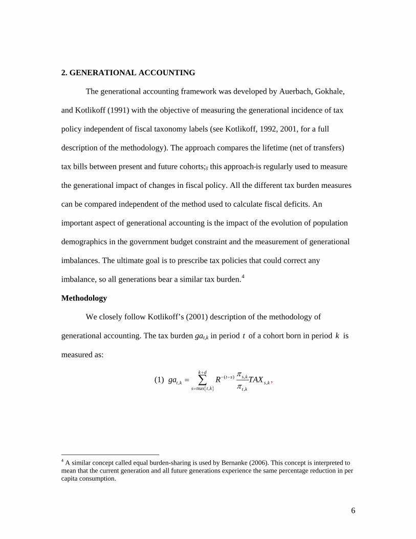
We closely follow Kotlikoff’s (2001) description of the methodology of

generational accounting. The tax burden gat,k in period t of a cohort born in period k is

measured as:

(1) { }

,( ), ,

max , ,

,k d

s kt st k s k

s t k t k

ga R TAXππ

+− −

=

= ∑

4 A similar concept called equal burden-sharing is used by Bernanke (2006). This concept is interpreted to mean that the current generation and all future generations experience the same percentage reduction in per capita consumption.

6

where ,s kTAX is taxes net of transfers paid at time t by the cohort born in period , k R is

a discount factor, , / ,s k t kπ π denotes the fraction of individuals surviving at time , and d

represents the life expectancy of a cohort.

s

Therefore, equation (1) represents the present value of the average amount of

taxes paid by the survivors of cohort members born at time . The tax term includes total

taxes paid minus transfer payments of different forms. If we are calculating the

generational account implied by a model, all these elements are clearly specified.

However, if we are using data as input, the process is a bit more involved (Auerbach,

Kotlikoff, and Gokhale, 2001, provide a detailed description of how to map the data into

the generational accounts), because it includes expenditures in health care, education, and

other forms of transfer programs. However, it does not impute to any specific cohort the

value of government expenditure in goods and services. The main reason for this

limitation is the difficulty in assigning the benefit of government purchases to different

generations.

k

5

The government intertemporal budget constraint can then be reinterpreted in

terms of generational accounts as follows:

(2) , ,, ,

0 1 1

dt s t s t s t s

t t s t t s tt s

s s

Gs s s

gaga B

μR R

μ∞ ∞

+ + + + +− −

= =

+ = +∑ ∑=∑ , 1, 2,...t = ,

where ,t kμ denotes the measure of individuals in period t of cohorts born at time k . The

term gat,t-s represents the per capita generational account in period t for a generation born

in period t-s. The first term on the left-hand side of equation (2) captures the existing

5 By contrast, welfare analysis can measure the benefits of government purchases when they enter in the production function or in the utility function in the form of public goods.

7

cohorts, whereas the second term adds the generational accounts of unborn cohorts

discounted at a rate R . The term on the right-hand side represents the amount of

outstanding government debt tB (financial liabilities minus the sum of the government’s

financial assets and market value of public enterprises) and the value of present and

future government expenditures. The term Gt+s represents the level of government

expenditure in period t+s.

The choice of the discount rate R merits special attention because it influences

the generational accounts for present and future generations. The choice becomes even

more problematic in the presence of varying rates or uncertainty because it would require

the use of the term structure or the use of some specific stochastic discount factor to

adjust for risk. Moreover, in the presence of incomplete markets, risk adjustment should

be cohort specific. However, in standard practice a benchmark constant discount rate is

used to represent the results under alternative constant discount rates. Assuming a

constant discount rate can be restrictive because the capital-to-output ratio that ultimately

determines interest rates may vary in the presence of demographic shocks, or due to

different policy regimes.

Generational Accounts Imbalances

Given the tax burden for the current generations and the sequence of future

expenditures, it is possible to calculate as a residual the tax payments of future

generations. In the presence of imbalances it is possible to compute which policy changes

(and paid by which generation) are necessary to restore sustainability.

Another important element is the impact of demographic changes on the

imbalance of generational accounts. Consequently, population growth of future

8

generations can reduce imbalances, whereas population aging can exacerbate a larger tax

burden on currently young or future cohorts.

Generational accounts are used extensively in the literature to measure fiscal

imbalances associated with various tax reforms. For example Gokhale, et al., (2000)

analyze the U.S. use of the long-term projections of the Congressional Budget Office.

These authors use a 4 percent discount rate and 2.2 percent of productivity growth and

find that future generations will face a lifetime burden that is 41.6 percent higher than the

existing generations. They propose five alternative policies. The first is a 31 percent

permanent increase in federal and personal corporate income taxes. The second is a 12

percent raise of all federal, state, and local taxes. The third policy requires cutting all

transfers programs (Social Security, Medicare, Medicaid, food stamps, unemployment

insurance benefits, housing support, and so on) by 21.9 percent. The final two options

require the reduction of all government expenditures by 21 percent or federal

expenditures by 66.3 percent. Other applications include a switch from income to

consumption taxation (as in Altig et al., 2001), or Social Security privatization (as in

Kotlikoff, Smetters, and Walliser, 2001). The methodology has also been applied to other

countries such as the United Kingdom (as in Cardarelli, Kotlikoff, and Sefton, 2000). For

an international study, see Kotlikoff and Raffelheuschen, (1991).

3. THE MEASUREMENT OF TAX INCIDENCE

This section begins with two examples in a simple framework. Each example

considers standard policy reforms suggested in the literature, such as redistributive

policy, or the substitution of consumption taxes by income taxes. We show that these

alternative fiscal policies could generate the same household allocation and welfare, but

9

give rise to different measures of tax incidence using the standard generational

accounting procedure. We then develop this argument more formally using a fairly

general overlapping generations model with production. The model illustrates how the

generational accounts can be biased because they are not robust to the choice of tax

instruments. The model can also be used to derive an alternative tax burden measurement

based on the consumer intertemporal budget constraint. This new measure is equally

simple in its implementation and is robust to the choice of tax instruments. We describe

these steps in detail.

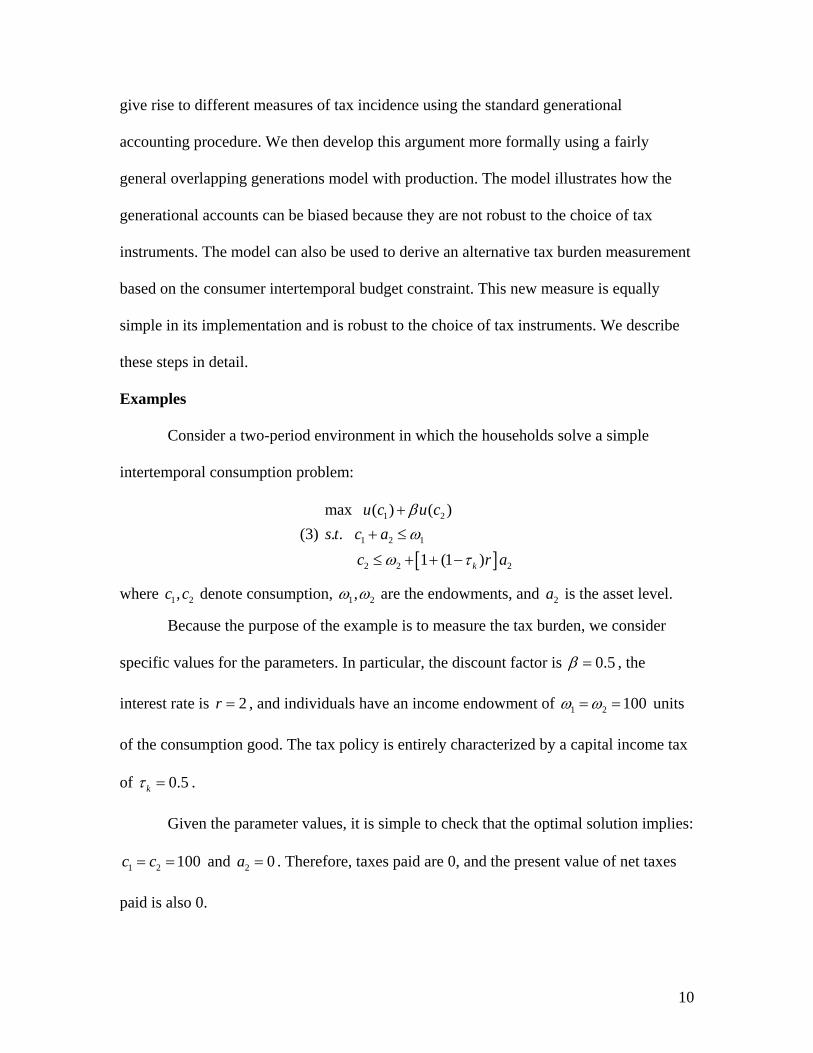
Examples

Consider a two-period environment in which the households solve a simple

intertemporal consumption problem:

(3)

[ ]

1 2

1 2 1

2 2

max ( ) ( ). .

1 (1 )k

u c u cs t c a

c r 2a

βω

ω τ

++ ≤

≤ + + −

where denote consumption, 1 2,c c 1 2,ω ω are the endowments, and is the asset level. 2a

Because the purpose of the example is to measure the tax burden, we consider

specific values for the parameters. In particular, the discount factor is 0.5β =

1 2

, the

interest rate is , and individuals have an income endowment of 2r = 100ω ω= = units

of the consumption good. The tax policy is entirely characterized by a capital income tax

of 0.5kτ = .

Given the parameter values, it is simple to check that the optimal solution implies:

and . Therefore, taxes paid are 0, and the present value of net taxes

paid is also 0.

1 2 100c c= = 2 0a =

10

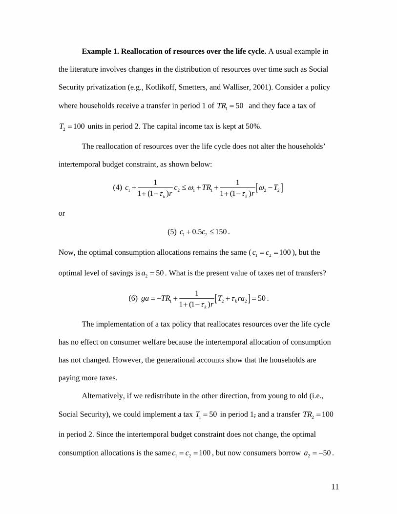
Example 1. Reallocation of resources over the life cycle. A usual example in

the literature involves changes in the distribution of resources over time such as Social

Security privatization (e.g., Kotlikoff, Smetters, and Walliser, 2001). Consider a policy

where households receive a transfer in period 1 of 1 50TR = and they face a tax of

units in period 2. The capital income tax is kept at 50%. 2 100T =

The reallocation of resources over the life cycle does not alter the households’

intertemporal budget constraint, as shown below:

(4) [ ]1 2 1 11 1

1 (1 ) 1 (1 )k k

c c TRr r

ω ωτ τ

+ ≤ + ++ − + − 2 2T−

or

(5) 1 20.5 150c c+ ≤ .

Now, the optimal consumption allocations remains the same ( 1 2 100c c= = ), but the

optimal level of savings is . What is the present value of taxes net of transfers? 2 50a =

(6) [ ]1 21 50

1 (1 ) kk

ga TR T rar

ττ

= − + + =+ − 2 .

The implementation of a tax policy that reallocates resources over the life cycle

has no effect on consumer welfare because the intertemporal allocation of consumption

has not changed. However, the generational accounts show that the households are

paying more taxes.

Alternatively, if we redistribute in the other direction, from young to old (i.e.,

Social Security), we could implement a tax 1 50T = in period 1, and a transfer

in period 2. Since the intertemporal budget constraint does not change, the optimal

consumption allocations is the same c c

2 100TR =

1 2 100= = , but now consumers borrow . 2 50a = −

11

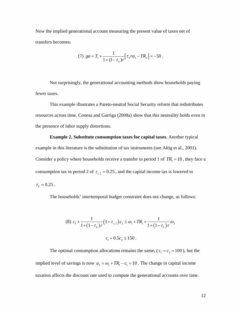
Now the implied generational account measuring the present value of taxes net of

transfers becomes:

(7) [ ]1 21 50

1 (1 ) kk

ga T ra TRrτ

τ= + − = −

+ − 2 .

Not surprisingly, the generational accounting methods show households paying

fewer taxes.

This example illustrates a Pareto-neutral Social Security reform that redistributes

resources across time. Conesa and Garriga (2008a) show that this neutrality holds even in

the presence of labor supply distortions.

Example 2. Substitute consumption taxes for capital taxes. Another typical

example in this literature is the substitution of tax instruments (see Altig et al., 2001).

Consider a policy where households receive a transfer in period 1 of , they face a

consumption tax in period 2 of

1 10TR =

,2 0.25cτ = , and the capital income tax is lowered to

0.25kτ = .

The households’ intertemporal budget constraint does not change, as follows:

(8) ( ) ( ) ( )1 ,2 2 1 1

1 111 1 1 1c

k k

c c TRr r 2τ ω ω

τ τ+ + ≤ + +

+ − + −

1 20.5 150c c+ ≤ .

The optimal consumption allocations remains the same, ( 1 2 100c c= = ), but the

implied level of savings is now 2 1 1 1 10a TR cω= + − = . The change in capital income

taxation affects the discount rate used to compute the generational accounts over time.

12

The present value of taxes net of transfers, discounted by the new after-tax interest rate,

, is as follows: ( )1 k rτ− =1.5

(9) ( )1 ,2 2

1 21 1 c k

k

ga TR c rarτ τ

τ⎡ ⎤= − + + =⎣ ⎦+ − 2 ;

but, if we were to use the original discounting, it would be

(10) ( )1 ,2 2

1 51 1 c k

k

ga TR c rarτ τ

τ⎡ ⎤= − + + =⎣ ⎦+ − 2 .

Again, consumption—and hence, welfare—do not change, but the tax burden, as

measured by generational accounting, increases.

Notably, all of these examples share two common features: alternative fiscal

policies redistribute taxes/transfers over the life cycle, and households respond optimally

by changing their level of savings. Because the return on savings is taxed, redistribution

of the tax burden over the life cycle changes the present value of taxes paid. If, on the

contrary, we were to exclude capital income taxes from our calculation of the tax burden,

we could immediately see that generational accounting would not change in any of these

examples. Now we establish these results in a more general setup.

A Standard Life Cycle Model

Generations live for I periods. Preferences of an individual born in period t are

represented by a time-separable utility function of the following form:

(11) 1, 1 , 1

1( , ) ( ,1 )

It t i

i t i i t ii

U c l u c lβ −+ − +

=

= −∑ − ,

where and denote consumption and hours worked of individuals of age ,j tc ,j tl j at time

. An individual’s subjective discount rate is denoted byt β . The utility function is

assumed to be twice continuously differentiable, strictly concave, monotonically

13

increasing in consumption and leisure, and satisfies the standard Inada conditions. At

each time point households are endowed with one divisible unit of time that can be used

for work and leisure. One unit of time of a household of age i transforms into iε units of

labor input. The time-invariant endowment profile of efficiency units of labor over the

life cycle is denoted by 1{ ,..., }Iε ε ε=

,i ta

tr

.

Individuals supply their labor services and assets in competitive markets. Then,

individuals receive a competitive wage, , per efficiency unit of labor supplied in period

. They also hold assets, , in the form of physical capital or government bonds in

exchange for a market rental rate, . Clearly, the return of both investments must be the

same if households are to hold both types of assets. We denote the transfer payments

received by cohort

tw

t

j as . Notice that this allows transfers to change over the life

cycle.

,j tm

, )t tL

6

We assume that markets are complete. Therefore, households are allowed to trade

assets to smooth consumption over the life cycle. Two potential extensions from the

standard model are possible: (i) the introduction of intragenerational heterogeneity, and

(ii) the introduction of mortality risk with or without annuity markets. The findings in this

paper do not depend on either of these model features.

The production possibility frontier is represented by a constant returns to scale

technology, Y F , that transforms units of capital and efficiency units of (t K= tK

6 We are not restricting the sign of government transfer programs for workers and retirees. This is not relevant since the focus of the paper is the measurement of tax incidence over different cohorts, not the distortionary effect of different tax instruments on these individuals.

14

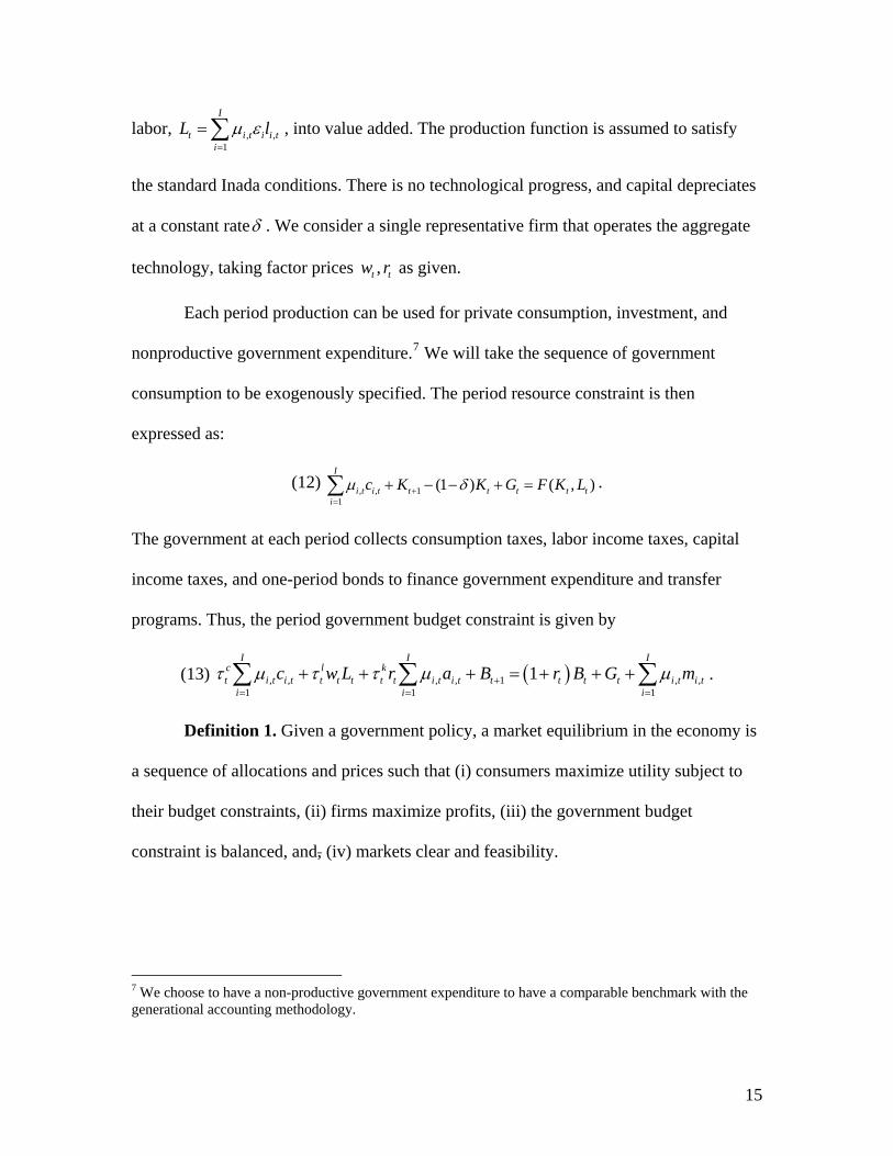
labor, , ,1

I

t i t ii

L i tlμ ε=

=∑ , into value added. The production function is assumed to satisfy

the standard Inada conditions. There is no technological progress, and capital depreciates

at a constant rateδ . We consider a single representative firm that operates the aggregate

technology, taking factor prices as given. ,t tw r

, ,i t i tc K

t tL τ+ +∑ ∑

Each period production can be used for private consumption, investment, and

nonproductive government expenditure.7 We will take the sequence of government

consumption to be exogenously specified. The period resource constraint is then

expressed as:

(12) . 1

1

(1 ) ( , )I

t t t t ti

K G F K Lμ δ+=

+ − − + =∑

The government at each period collects consumption taxes, labor income taxes, capital

income taxes, and one-period bonds to finance government expenditure and transfer

programs. Thus, the period government budget constraint is given by

(13) . ( ), , 1 , ,1 1

1I I

c l kt t t t i t i t t t t t i t i t

i ic w r a B r B G mτ μ μ+

= =

+ = + + +1

I

i=∑, ,t i t iτ μ

Definition 1. Given a government policy, a market equilibrium in the economy is

a sequence of allocations and prices such that (i) consumers maximize utility subject to

their budget constraints, (ii) firms maximize profits, (iii) the government budget

constraint is balanced, and, (iv) markets clear and feasibility.

7 We choose to have a non-productive government expenditure to have a comparable benchmark with the generational accounting methodology.

15

Model Generational Accounts

To construct the generational accounts for each cohort, we must determine the net

tax outlets (taxes minus transfers properly discounted) for each generation. In our model

environment the generational accounting of every newborn generation is given by

(14) 11 , 1 1 1 , 1 1 1 , 1 , 1

1

Ic l kt i

t t i i t i t i t i i i t i t i t i i t i i t ii t

qga c w l r a mq

τ τ ε τ+ −+ − + − + − + − + − + − + − + − + −

=

⎡ ⎤= + +⎣ ⎦∑ − ,

where and 1 1q = 11 , 2,3,...

1 (1 )t t kt t

q q trτ−= =

+ −.

There is also an equivalent expression for the cohorts already born. The generational

accounts are not a total lifetime bill, but, rather, remaining lifetime bills. As a

consequence the accounts are positive for young and middle age cohorts, but negative for

older cohorts.

In contrast with the empirical applications, the theoretical model offers a natural discount

rate because the market clearing interest rate can be used.8 However, it is important to

remark that individual generational accounts are just a metric to measure tax incidence

and are not necessarily related to the equilibrium in the model. In equilibrium, the

government intertemporal budget constraint is always satisfied. However, the implied

individual generational accounts and imbalances need not be consistent with the

government budget constraint unless the market discount rate is used. We simply use the

model to generate data that then are used to measure tax incidence by constructing

generational accounts.

8 Consequently, the long-run effects of demographic shocks or policy changes will affect future discount rates through changes in the capital-to-output ratio. This efficiency effect is usually not captured when the generational accounts are computed directly from the data, and the discount rate is fixed.

16

4. BIAS IN THE MEASUREMENT OF TAX INCIDENCE WITH STANDARD

GENERATIONAL ACCOUNTING

To illustrate the measurement bias of the tax incidence implied by the

generational accounts, it is useful to state and prove a well-known equivalence result. We

then use this equivalence to show that the generational accounting measurements are not

identical across equivalent tax policies.

Proposition 1. Let be a feasible fiscal policy, and let {ˆˆ ˆ( , , )m Bτ }, , 1ˆ ˆˆ( , ) ,I

i t i t i tc l K= be

the resulting allocation. Then, there exists a fiscal policy ( and a distribution of

assets such that {

, , )m Bτ %% %

,( )Ii t ia =% 1 }, , 1

ˆˆ( , ) ,Ii t i t ic l =

ˆtK

) ,τ% %

is the equilibrium allocation corresponding to

. Moreover, the associated generational accounts would in general differ

between policy and policy ( .

( ,τ% % , )m B%

ˆˆ ˆ( , ,m Bτ , )m B%

Proof. Any equilibrium allocation must satisfy the following first-order

conditions:

( ), 1 1

1,

1 1 11

c ci t i kt i

t i t ic ci t i t i

ur

uτ ττ

+ − + −+ +

+ + +

+ ⎡ ⎤= + −⎣ ⎦+, 1,..., 1i I= −

, 1 11

, 1 1

11

l li t i t i

t i ic ci t i t i

uw

uτ ετ

+ − + −+ −

+ − + −

−− =

+, 1,..., ri i=

( ) ( )1 1 , 1 1 1 1 , 1 1 ,1 1 1

1 1I I I

c lt i t i i t i t i t i t i i i t i t i i t i

i i iq c q w l qτ τ ε+ − + − + − + − + − + − + − + − + −

= = =

+ = − +∑ ∑ ∑ 1m .

Clearly, more than one policy can implement the same allocation because there are 2* I

equations and 4* I fiscal variables to determine a given an allocation.

Given an alternative fiscal policy, assets can then be constructed directly from the

sequential budget constraints. Notice that aggregate wealth would then change, and as a

17

consequence, government debt changes because the aggregate capital stock is unchanged.

Finally, the new level of government debt must necessarily balance the government

budget constraint by Walras’ law.

In general, the associated generational accounts measurement would change, even

though allocations and welfare are the same. To see that the generational accounts must

change for at least one generation, recall equation (2):

, ,, ,

0 1 1

dt s t s t s t s t s

t t s t t s ts ss s s

ga Gga Bμ

R Rμ

∞ ∞+ + + + +

− −= =

+ = +∑ ∑ ∑=

1,2,...t, = .

Notice that because aggregate debt in general changes across equivalent policies, the

right-hand side of the equation must change for some . Therefore, the left-hand side

must change as well.■

t

This result has two important implications.9 From the positive point of view, the

measurement of tax incidence implied by generational accounts does not provide an

accurate description (or invariant metric) of generational imbalances of the effective tax

burden faced by different cohorts. From a normative point of view, the evaluation of tax

policies based on the distribution of tax burden for different age cohorts could be

misleading of the true cost for each cohort. Our results show that we could be evaluating

the implied tax incidence of different policies on different cohorts and using the

generational accounts to conclude that one policy performs better than another.

Nevertheless, these policies could be equivalent from the household perspective, but the

9 A few remarks are relevant to the proposition. First, notice that the different tax reforms consistent with the proposition might imply a change in statutory tax rates (with the same effective tax wedges), a change in the magnitudes of intergenerational transfers, or both. Second, the result still holds in the presence of borrowing constraint of some form. The proof is very general and holds in a larger class of economies that include uncertainty and certain forms of market frictions. It is sufficient to have a non-empty set of equivalent policies.

18

generational accounts would lead to a different conclusion. This should be clear from the

examples in Section 3 that show the influence of tax reform in generational accounts

imbalances.

Correcting the Bias in Generational Accounting

A major problem in using generational accounts to measure generational

imbalances is the tax treatment of savings. The main result from Proposition 1 states that

any equivalent tax policy that requires a different distribution of asset holdings that

include claims on capital and government debt will lead to different generational

accounts.

One way to avoid this problem is to measure tax incidence using the intertemporal

budget constraint and effective rather than nominal tax distortions. The idea is very

simple: If the tax policies are equivalent, the intertemporal budget constraints must be the

same; otherwise, consumption-leisure plans would differ. Given this condition, then, we

should measure the magnitude of all the effective taxes paid using the consolidated

budget constraint and not what is recorded in the government accounting books. This

alternative procedure can be described as follows. Consider the sequential budget

constraint:

(15) . ( )( ) ( )

1 1 , 1 1 1,

1 1 1 , 1 1 1 1 , 1 1 ,

1

1 1 1

ct i t i i t i t i i t i

l kt i t i t i i i t i t i t i t i i t i t i i t i

q c q a

q w l q r a q

τ

τ ε τ

+ − + − + − + − + +

+ − + − + − + − + − + − + − + − + − + −

+ + =

⎡ ⎤− + + − +⎣ ⎦ 1m

1Define and ( )1 1 1 ct i t i t iq q τ+ − + − + −= +% 1

11

111

lt i

t i ct i

τφτ

+ −+ −

+ −

−− =

+.

19

Newborn households’ intertemporal budget constraint can be written as follows:

(16) ( ) , 11 , 1 1 1 1 , 1

1 1 1

11

I Ii t i

t i i t i t i t i t i i i t i ci i t i

mq c q w lφ ε

τ+ −

+ − + − + − + − + − + −= = + −

⎡ ⎤= − +⎢ ⎥+⎣ ⎦

∑ ∑% % .

Notice that the difference between the market value of labor income and consumption,

valued at the effective price of consumption goods, is denoted as:

(17) ( ) , 11 1 , 1 , 1 1 1 1 , 1

1 1 11

I Ii t i

t i t i i i t i i t i t i t i t i i i t i ci i t i

mq w l c q w lε φ ε

τ+ −

+ − + − + − + − + − + − + − + −= = + −

⎡ ⎤− = −⎢ ⎥+⎣ ⎦

∑ ∑% % .

Undoing the transformation of variables in the right-hand side of equation 17, we arrive

at our proposal for measuring tax incidence across cohorts:

(18) ( )11 1 1 , 1 ,

1

IIBC c lt it t i t i t i i i t i

i t

qGA w l mq

τ τ ε+ −+ − + − + − + − + −

=1i t i

⎡ ⎤= + −⎣ ⎦∑ .

Notice that two equivalent policies must satisfy the following first-order conditions (and

the intertemporal budget constraint):

(19) , 1 1

1,

ci t i t ici t i t i

u qu q

+ − + −

+ + +

=%

%

and

(20) ( ), 11 1

, 1

1li t i

t i t i ici t i

uw

uφ ε+ −

+ − + −+ −

− = − .

It is then clear that equivalent policies should therefore generate the same fiscal burden as

measured by equation (18), because the relative price of consumption across periods, the

effective taxation of the consumption-leisure margin, and the effective present value of

transfers must be the same across equivalent policies.

Thus, we have provided an alternative measurement of tax incidence that is robust

to the choice of tax instruments to decentralize a given allocation. Moreover, it is even

20

simpler in practice, as shown in the following direct comparison (equation 21) between

our proposal and the standard procedure (equation 22):

(21) ( )11 1 1 , 1 ,

1

IIBC c lt it t i t i t i i i t i

i t

qGA w l mq

τ τ ε+ −+ − + − + − + − + −

=1i t i

⎡ ⎤= + −⎣ ⎦∑

versus

(22) 11 , 1 1 1 , 1 1 1 , 1 , 1

1

Ic l kt i

t t i i t i t i t i i i t i t i t i i t i i t ii t

qga c w l r a mq

τ τ ε τ+ −+ − + − + − + − + − + − + − + − + −

=

⎡ ⎤= + +⎣ ⎦∑ − .

Notice that the same procedure could be used for currently existing cohorts. The

only difference is that for these cohorts the taxation of currently existing wealth holdings

should be included as effective taxation, while this is not the case for newborns born with

zero assets.

5. QUANTITATIVE ASSESSMENT OF THE TAX INCIDENCE BIAS

In this section we measure the potential size of the tax incidence bias and compare

it to with our proposed robust measure. In general, it is difficult to characterize the

equilibrium path and the optimal decision rules for a given tax policy. In the absence of a

closed-form solution, we use numerical methods to simulate the policy reforms and

compute the implied generational accounts.

As an illustration, we perform a Pareto-neutral Social Security privatization that

transforms the unfunded system into a funded one with private accounts following

Conesa and Garriga (2008a). The tax incidence bias can be measured as the difference

between the implied generational accounts across Social Security regimes and by

comparing the magnitudes with the robust measure.

21

Parameterization

Next we determine the choice of functional forms and parameters for the model

simulation.

Functional forms. We pose a standard log utility function between consumption

and leisure:

(24) ( , ) ln (1 ) ln(1 )u c l c lγ γ= + − − ,

where γ represents the consumption share on the utility function.

The aggregate technology is Cobb-Douglas with constant returns to scale:

(25) 1( , )F K L K Lα α−= ,

where α represents the capital income share in output. We assume that capital

depreciates at a constant rate δ and there is no exogenous technological growth.

Population structure and income. A model period is equivalent to one year.

Given our period choice, we assume households live for 65 periods, so that the

economically active life of a household starts at age 20 and we assume that households

die with certainty at age 85. In the benchmark economy, households retire in period 45

(equivalent to age 65 in years). Finally, we normalize the mass of households to be 1. We

assume that households are endowed with one unit of time. The lifetime profile of

efficiency units is constructed using Current Population Survey (CPS) data.

Government policy. The level of government expenditure is exogenously

specified as 20 percent of output. Revenues come from two sources: (i) capital and labor

income taxes and (ii) consumption taxes. In addition, the government runs a pay-as-you-

go Social Security system in the benchmark policy scenario. We assume that the tax on

capital income is 33 percent, Social Security contributions are 10.5 percent, and

22

consumption taxes are 5 percent. The labor income tax is chosen to balance the

government budget given the target level of outstanding government debt.

Given the assumptions on the functional forms, endowments, and tax rates, we

jointly solve for the equilibrium and the parameterization using the minimum distance

method. Table 1 defines the parameter values and the targets.

We want our economy to match three empirical targets. First, we define aggregate

capital as the level of fixed assets in the Bureau of Economic Analysis statistics, giving

an implied capital-to-output ratio of 3.00. Our second target is the average number of

hours worked over the life cycle, with an average of one-third of the time of households

allocated to market activities. The third target is an investment-to-output ratio of 16

percent. In addition, we fix government debt (defined as federal, state, and local) with an

implied ratio to GDP of 0.50, and the ratio of government expenditure to GDP at 0.20.

Our three targets determine the value of three parameters: the discount factor, the

consumption share in the utility function, and the depreciation rate. In addition, the labor

income tax is endogenously determined from the government’s budget constraint given

the ratios of government debt and expenditure to GDP.

A Pareto-Neutral Social Security Reform

The fiscal reform we examine follows Conesa and Garriga (2008a), and it

illustrates the measurement discrepancies generated by the standard procedure of

generational accounting. The goal is to implement a privatization of the Social Security

system while maintaining the level of distortions from the baseline economy.10 The

timing of events works as follows. We assume that at time 1 the economy is in steady

10 Clearly, it is possible to achieve better policy results optimizing distortions as in Conesa and Garriga (2008a) that use optimal fiscal policy to do precisely that.

23

state with an unfunded Social Security system. The contributions made by the young

generate an entitlement to a future benefit retirement, which constitutes an implicit debt

of the Social Security Administration towards them. On retirement, these retirees receive

their claims.

The reform is implemented at 2t = . The government eliminates pensions, giving

compensatory transfers to all households. These household-specific transfers are financed

with government debt. The privatization effectively transforms the implicit debt of the

Social Security system into explicit debt, but real allocations and welfare remain

unchanged. The resulting distribution of wealth is different, since now Social Security

implicit claims are transformed into explicit assets in the hands of households. Figure 1

compares both distributions of wealth.

The asset distribution under the funded system is always above the unfunded one,

since now workers use the proceedings from Social Security contributions to invest in

private savings accounts. The youngest cohort receives as a transfer an initial level of

assets that is equivalent to the net present value of Social Security transfers. This number

ensures that the consumer intertemporal budget constraint is satisfied. The difference

between the newly issued government bonds and the initial outstanding government debt

determines the implicit debt of the Social Security system. Figure 2 represents the net

taxes paid over the life cycle in these two equivalent policy regimes.

Under the unfunded Social Security system, the entire tax burden is placed on

individuals age 65 and younger. Retired households pay consumption and capital income

taxes, but in net terms they receive resources (their pensions). Under the new regime,

retired households do not receive a transfer from the government, and they are fully taxed

24

for the interest earned in the retirement accounts. Despite the differences in the amount of

taxes paid, the welfare distribution is the same across tax regimes. Using the net taxes

paid and the relative size of each cohort, we can compute the generational accounts of

each cohort based on their age. Figure 3 summarizes the model implied generational

accounts for these two equivalent Social Security regimes using the standard approach.

Notice that the standard generational accounting procedure is not invariant

between these two equivalent policy regimes because the two top curves in Figure 3 do

not lie on top of each other. To the contrary, the implied values have a bias that can be as

high as 15 percent for the young and middle-aged cohorts. The bias is driven purely by

the fact that government bond holdings are larger in the funded regime, while they are not

net wealth. Because capital income (coming from holding government debt or financial

assets) is taxed, the imputed tax burden varies across the two policy regimes. However,

the proceedings from selling the government bonds are by construction equal to the

transfers received from the Social Security system. The distinction is that under the

equivalent policy, transfers are computed as a taxable asset and a liability for the

government that remains forever, whereas in the other case as a net transfer from the

government and funded by workers’ contributions (but an implicit liability for the

government). Next, we compare this standard measurement with our proposed robust

measure for generational accounts.

The generational accounting procedure we propose is based on the intertemporal

households’ budget constraint and therefore accounts only for the tax treatment of capital

and consumption insofar as they affect the relative price of consumption across time.

Also, the measure only considers the effective distortion in the labor supply net of the

25

government transfers received in the corresponding period. As a consequence, the new

measure predicts a lower tax burden for all households except households in their last

period.

Notice the large bias of the previous two generational accounts (GA) (“GA

Funded” and “GA Unfunded”) compared with the proposed generational accounting

metric based on the intertemporal budget constraint. We claim that our proposed new

metric is not only robust to the choice of tax instruments, but it is also easier to calculate

because it requires less information.

An Empirical Illustration

The previous results were illustrations with data generated from a model. Now we

complete the analysis by comparing the measurement of tax incidence according to our

proposed procedure with the measurement by Kotlikoff (2002, table 1). Kotlikof’s table

reports the generational accounts of males in the United States in 1998, measured in

thousands of dollars, under the assumptions of a 4% discount rate and a 2.2% growth

rate.

Figure 4 illustrates the quantitative difference between the original methodology

and our proposal. We use the numbers reported in Kotlikoff’s table 1 (2002) to construct

our alternative measure. We subtract the capital income taxes that all cohorts would have

to pay in the future and include only the taxation of initial wealth holdings. A simple

comparison shows that the effective taxation of the existing cohorts in 1998 is much

lower than with the traditional methodology. The results are very consistent with the

findings implied by the model. In particular, the model and the data estimates suggest that

the zero crossing point should be delayed 10 years.

26

5. CONCLUSION

The current financial crisis is taking a huge toll on government deficits. In

addition, current estimates anticipate that in 25 years the U.S. economy will have twice as

many retirees but only 20 percent more workers. This demographic transition surely will

have an important effect on the government budget unless the benefits from Social

Security and Medicare are reduced. The determination of which cohorts will bear the cost

is important, but first agreement on how to measure generational imbalances is needed.

We show that the standard generational accounting procedure yields an inaccurate

measurement of tax burden imbalances across cohorts. We find that it is possible to

construct tax policy reforms consistent with the same pattern of consumption, work

effort, and utility across generations, but yielding different tax burden measurements than

those obtained with generational accounting. This result is very important for policy

evaluation because it shows that the selection of tax policies based on generational

accounts can be biased. We quantify the potential bias introduced by the methodology at

the same time that we provide a robust alternative, equally simple in its implementation.

27

REFERENCES

Altig, D., L.J. Kotlikoff, K. Smetters, and J. Walliser. (2001). “Simulating Fundamental

Tax Reform.” American Economic Review, June 2001, pp. 574-95.

Auerbach, A.J., and L.J. Kotlikoff. (1987). Dynamic Fiscal Policy. Cambridge:

Cambridge University Press.

Auerbach, A.J., J. Gokahale, and L.J. Kotlikoff. (1991). “Generational Accounts: A

Meaningful Alternative to Deficit Accounting,” in D. Bradford, Ed., Tax Policy

and the Economy, vol. 5, pp. 55-110. Cambridge, MA: MIT Press.

Bernanke, B. (2006). “The Coming Demographic Transition: Will We Treat Future

Generations Fairly?” Presented at the Washington Economic Club, Washington,

DC, October 4, 2006;

www.federalreserve.gov/newsevents/speech/bernanke20061004a.htm

Cardarelli, R., L.J. Kotlikoff, and J. Sefton. (2000). “Generational Accounting in the

UK.” Economic Journal, 110(467), pp. 547-74.

Conesa, J.C., and C. Garriga. (2008a). “Optimal Fiscal Policy in the Design of Social

Security Reforms.” International Economic Review 49(1), pp. 291-318.

Conesa, J.C., and C. Garriga. (2008b). “Optimal Response to a Transitory Demographic

Shock,” in De Menil, G., R. Fenge and P. Pestieau, Eds. Pension Strategies in

Europe and the United States, pp. 87-113. CESifo-MIT Press. Cambridge, MA.

Elmendorf, D., and L. Sheiner (2000). “Should America Save for Its Old Age? Fiscal

Policy, Population Aging, and National Saving.” Journal of Economic

Perspectives, 14, pp. 57-74.

28

Fehr, H., and Kotlikoff, L.J. (1996). “Generational Accounting in General Equilibrium.”

FinanzArchiv, 53(4), pp. 1-27.

Gokhale, J., B. Page, J. Potter, and J. Sturrock. (2000). “Generational Accounts for the

U.S.—An Update.” American Economic Review, 90(2), pp. 293-96.

Kotlikoff, L.J. (1992). Generational Accounting: Knowing Who Pays, and When, for

What We Spend. The Free Press. New York.

Kotlikoff, L.J. (2002). “Generational Policy,” in Auerbach, A.J., and M. Feldstein, Eds.,

Handbook of Public Economics, pp. 1983-1932. Amsterdam: North Holland.

Kotlikoff, L.J., K. Smetters, and J. Walliser. (2001). “Distributional Effects in a General

Equilibrium Analysis of Social Security,” in M. Feldestein and J. Liebman, eds.,

The Distributional Effects of Social Security Reform. Chicago: University of

Chicago Press.

Kotlikoff, L.J., and B. Raffelheuschen (1991). “Generational Accounting Around the

Globe.” American Economic Review, 89, pp. 161-66.

Sheiner, L., D., Sichel, and L. Slifman (2006). “A Primer on the Macroeconomic

Consequences of Population Aging.” Finance and Economics Discussion Series

Working Paper, Board of Governors of the Federal Reserve System, Division of

Research and Statistics, September 2006;

http://www.federalreserve.gov/pubs/feds/2007/200701/200701pap.pdf.

29

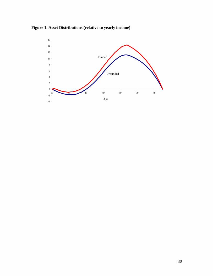
Figure 1. Asset Distributions (relative to yearly income)

-4

-2

0

2

4

6

8

10

12

14

16

20 30 40 50 60 70 80

Funded

Unfunded

Age

30

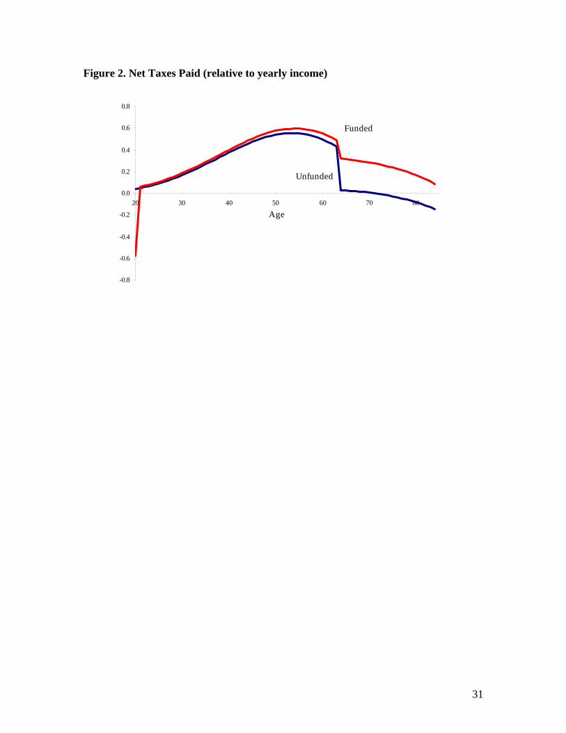
Figure 2. Net Taxes Paid (relative to yearly income)

-0.8

-0.6

-0.4

-0.2

0.0

0.2

0.4

0.6

0.8

20 30 40 50 60 70 80

Funded

Unfunded

Age

31

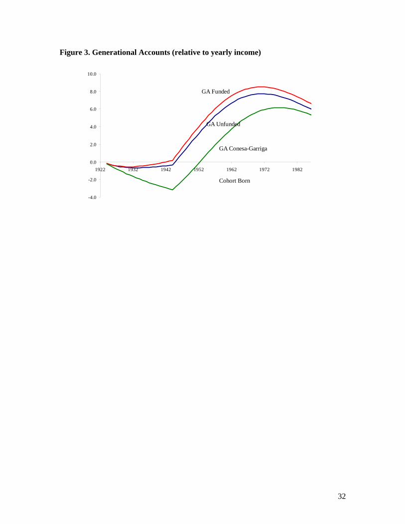
Figure 3. Generational Accounts (relative to yearly income)

-4.0

-2.0

0.0

2.0

4.0

6.0

8.0

10.0

1922 1932 1942 1952 1962 1972 1982

GA Funded

GA Unfunded

Cohort Born

GA Conesa-Garriga

32

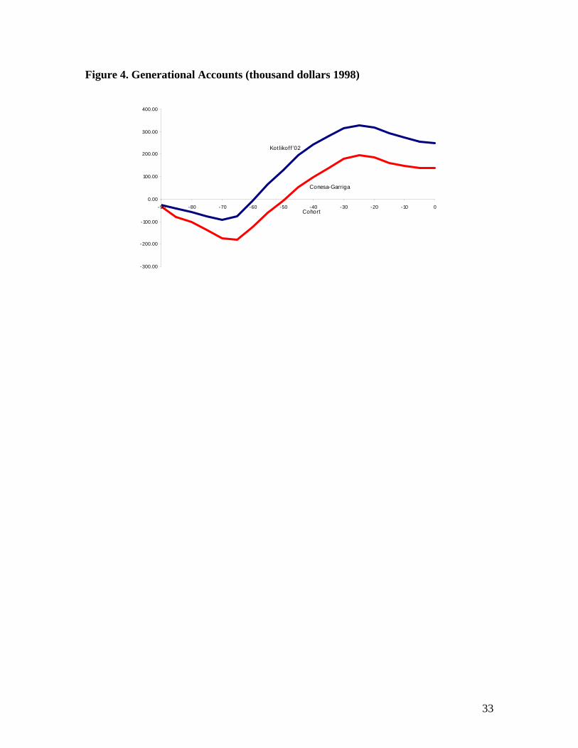
Figure 4. Generational Accounts (thousand dollars 1998)

-300.00

-200.00

-100.00

0.00

100.00

200.00

300.00

400.00

-90 -80 -70 -60 -50 -40 -30 -20 -10 0

Kotlikoff '02

Conesa-Garriga

Cohort

33

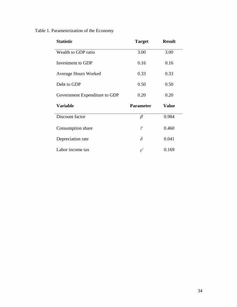
Table 1. Parameterization of the Economy

Statistic Target Result

Wealth to GDP ratio 3.00 3.00

Investment to GDP 0.16 0.16

Average Hours Worked 0.33 0.33

Debt to GDP 0.50 0.50

Government Expenditure to GDP 0.20 0.20

Variable Parameter Value

Discount factor β 0.984

Consumption share γ 0.460

Depreciation rate δ 0.041

Labor income tax lτ 0.169

34