icfi.com1

Generation Asset Valuation with Operational Constraints – A Trinomial Tree Approach

Andrew L. Liu

ICF International

September 17, 2008

icfi.com2

Outline

• Power Plants’ Optionality -- Intrinsic vs. Extrinsic Values

• Power and natural gas price processes

• Tree-based approach to value path-dependent optionsCase study: a combined-cycle unit as an option

• Parameter estimation and numerical results

• Caveat and summary

icfi.com3

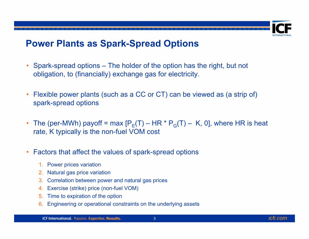
Power Plants as Spark-Spread Options

• Spark-spread options – The holder of the option has the right, but not obligation, to (financially) exchange gas for electricity.

• Flexible power plants (such as a CC or CT) can be viewed as (a strip of) spark-spread options

• The (per-MWh) payoff = max [PE(T) – HR * PG(T) – K, 0], where HR is heat rate, K typically is the non-fuel VOM cost

• Factors that affect the values of spark-spread options

1. Power prices variation2. Natural gas price variation3. Correlation between power and natural gas prices4. Exercise (strike) price (non-fuel VOM)5. Time to expiration of the option6. Engineering or operational constraints on the underlying assets

icfi.com4

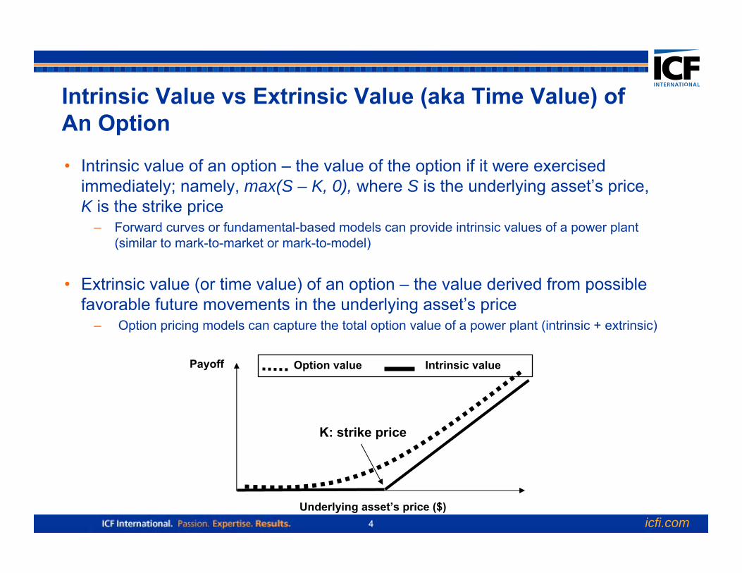
Intrinsic Value vs Extrinsic Value (aka Time Value) of An Option

• Intrinsic value of an option – the value of the option if it were exercised immediately; namely, max(S – K, 0), where S is the underlying asset’s price, K is the strike price

– Forward curves or fundamental-based models can provide intrinsic values of a power plant (similar to mark-to-market or mark-to-model)

• Extrinsic value (or time value) of an option – the value derived from possible favorable future movements in the underlying asset’s price

– Option pricing models can capture the total option value of a power plant (intrinsic + extrinsic)

Option value Intrinsic valuePayoff

Underlying asset’s price ($)

K: strike price

icfi.com5

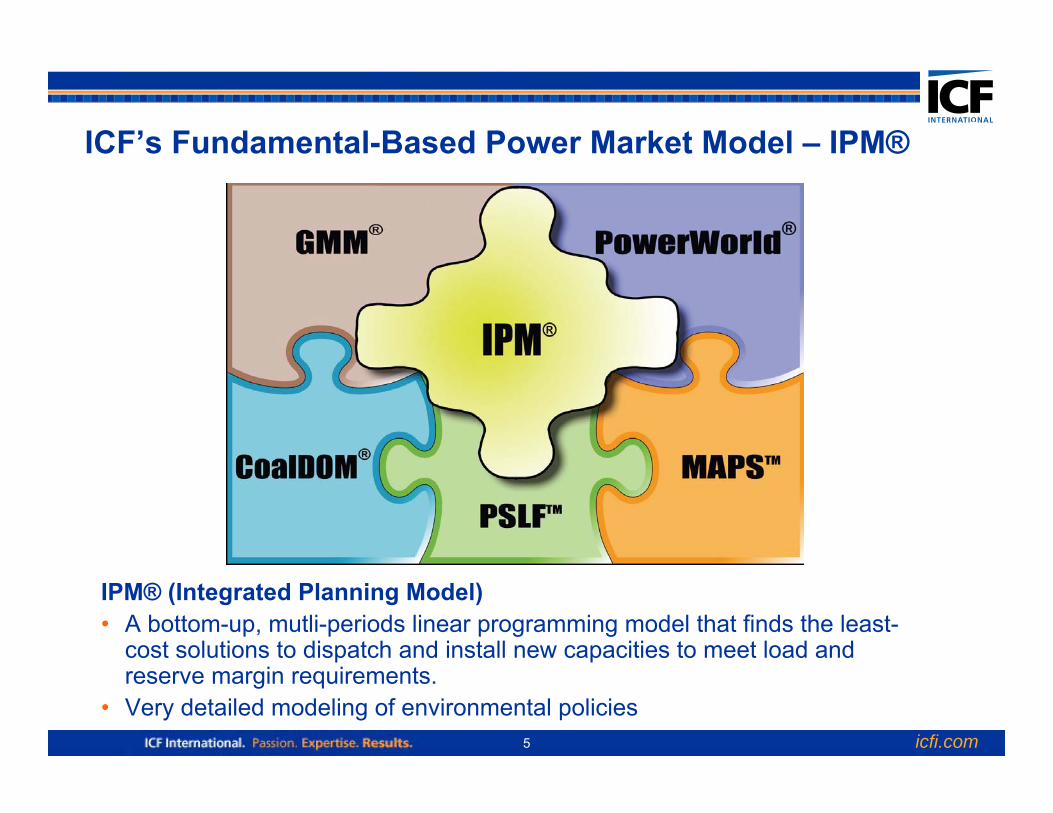
ICF’s Fundamental-Based Power Market Model – IPM®

IPM® (Integrated Planning Model) • A bottom-up, mutli-periods linear programming model that finds the least-

cost solutions to dispatch and install new capacities to meet load and reserve margin requirements.

• Very detailed modeling of environmental policies

icfi.com6

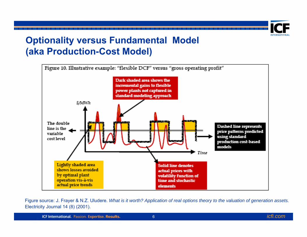
Optionality versus Fundamental Model (aka Production-Cost Model)

Figure source: J. Frayer & N.Z. Uludere. What is it worth? Application of real options theory to the valuation of generation assets.Electricity Journal 14 (8) (2001).

icfi.com7

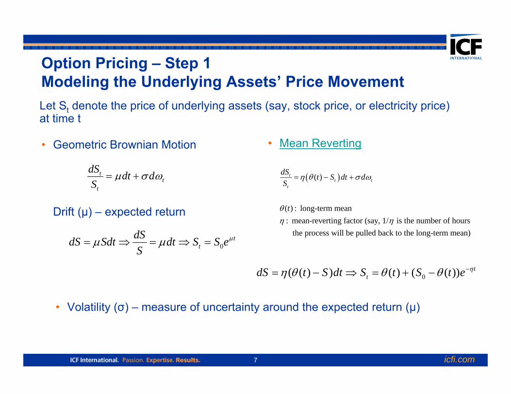
Option Pricing – Step 1Modeling the Underlying Assets’ Price Movement

0t

tdSdS Sdt dt S S eS

μμ μ= ⇒ = ⇒ =

tt

t

dS dt dS

μ σ ω= +

• Geometric Brownian Motion

Drift (μ) – expected return

• Mean Reverting

Let St denote the price of underlying assets (say, stock price, or electricity price) at time t

( )( )

( ) : long-term mean: mean-reverting factor (say, 1/ is the number of hours

the process will be pulled back to the long-term mean)

tt t

t

dS t S dt dS

t

η θ σ ω

θη η

= − +

0( ( ) ) ( ) ( ( )) ttdS t S dt S t S t e ηη θ θ θ −= − ⇒ = + −

• Volatility (σ) – measure of uncertainty around the expected return (μ)

icfi.com8

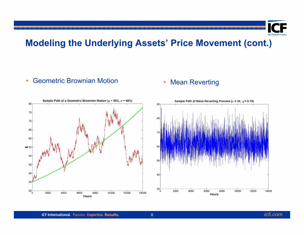
Modeling the Underlying Assets’ Price Movement (cont.)

• Geometric Brownian Motion • Mean Reverting

icfi.com9

Historical Power/Natural Gas Prices, and Spark Spread

icfi.com10

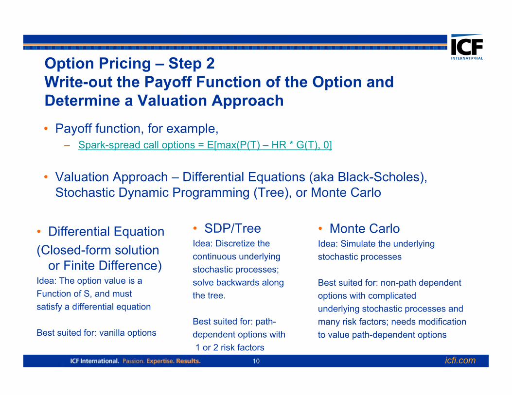
Option Pricing – Step 2Write-out the Payoff Function of the Option and Determine a Valuation Approach

• Payoff function, for example,– Spark-spread call options = E[max(P(T) – HR * G(T), 0]

• Valuation Approach – Differential Equations (aka Black-Scholes), Stochastic Dynamic Programming (Tree), or Monte Carlo

• SDP/TreeIdea: Discretize the continuous underlying stochastic processes; solve backwards along the tree.

Best suited for: path-dependent options with1 or 2 risk factors

• Differential Equation(Closed-form solution

or Finite Difference)Idea: The option value is a Function of S, and must satisfy a differential equation

Best suited for: vanilla options

• Monte CarloIdea: Simulate the underlying stochastic processes

Best suited for: non-path dependent options with complicated underlying stochastic processes and many risk factors; needs modification to value path-dependent options

icfi.com11

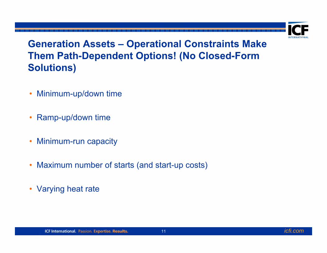
Generation Assets – Operational Constraints Make Them Path-Dependent Options! (No Closed-Form Solutions)

• Minimum-up/down time

• Ramp-up/down time

• Minimum-run capacity

• Maximum number of starts (and start-up costs)

• Varying heat rate

icfi.com12

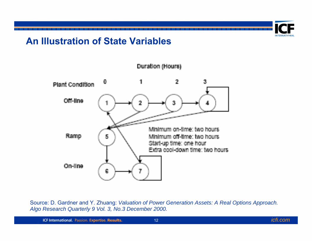
An Illustration of State Variables

Source: D. Gardner and Y. Zhuang: Valuation of Power Generation Assets: A Real Options Approach. Algo Research Quarterly 9 Vol. 3, No.3 December 2000.

icfi.com13

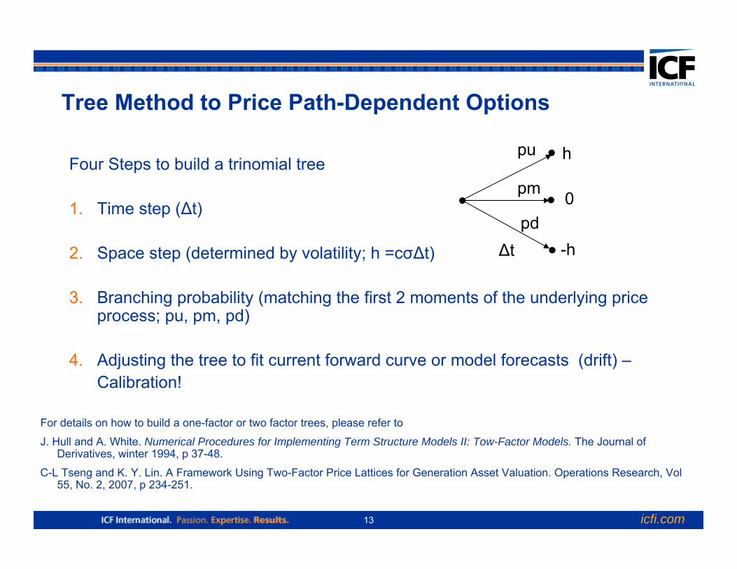
Tree Method to Price Path-Dependent Options

Four Steps to build a trinomial tree

1. Time step (Δt)

2. Space step (determined by volatility; h =cσΔt)

3. Branching probability (matching the first 2 moments of the underlying price process; pu, pm, pd)

4. Adjusting the tree to fit current forward curve or model forecasts (drift) –Calibration!

For details on how to build a one-factor or two factor trees, please refer to

J. Hull and A. White. Numerical Procedures for Implementing Term Structure Models II: Tow-Factor Models. The Journal of Derivatives, winter 1994, p 37-48.

C-L Tseng and K. Y. Lin. A Framework Using Two-Factor Price Lattices for Generation Asset Valuation. Operations Research, Vol55, No. 2, 2007, p 234-251.

h

0

-hΔt

pu

pm

pd

icfi.com14

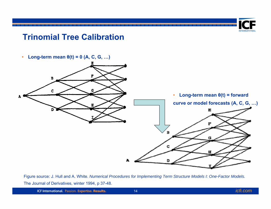
Trinomial Tree Calibration

Figure source: J. Hull and A. White. Numerical Procedures for Implementing Term Structure Models I: One-Factor Models.

The Journal of Derivatives, winter 1994, p 37-48.

• Long-term mean θ(t) = 0 (A, C, G, …)

• Long-term mean θ(t) = forwardcurve or model forecasts (A, C, G, …)

icfi.com15

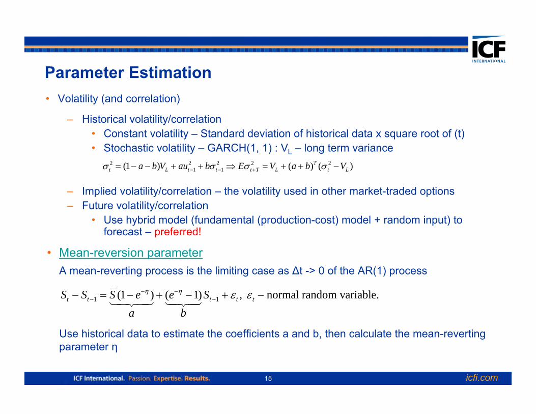
Parameter Estimation• Volatility (and correlation)

– Historical volatility/correlation• Constant volatility – Standard deviation of historical data x square root of (t)• Stochastic volatility – GARCH(1, 1) : VL – long term variance

– Implied volatility/correlation – the volatility used in other market-traded options– Future volatility/correlation

• Use hybrid model (fundamental (production-cost) model + random input) to forecast – preferred!

2 2 2 2 21 1(1 ) ( ) ( )T

t L t t t T L t La b V au b E V a b Vσ σ σ σ− − += − − + + ⇒ = + + −

• Mean-reversion parameter A mean-reverting process is the limiting case as Δt -> 0 of the AR(1) process

Use historical data to estimate the coefficients a and b, then calculate the mean-reverting parameter η

1 1(1 ) ( 1) , normal random variable.t t t t tS S S e e Sa b

η η ε ε− −− −− = − + − + −

icfi.com16

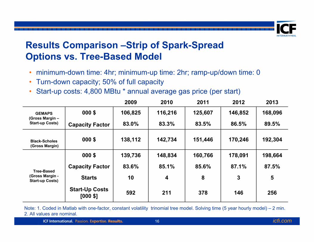
Results Comparison –Strip of Spark-Spread Options vs. Tree-Based Model• minimum-down time: 4hr; minimum-up time: 2hr; ramp-up/down time: 0 • Turn-down capacity; 50% of full capacity • Start-up costs: 4,800 MBtu * annual average gas price (per start)

Note: 1. Coded in Matlab with one-factor, constant volatility trinomial tree model. Solving time (5 year hourly model) – 2 min. 2. All values are nominal.

256146378211592Start-Up Costs [000 $]

538410Starts

87.5%87.1%85.6%85.1%83.6%Capacity Factor

198,664178,091160,766148,834139,736000 $

Tree-Based (Gross Margin -Start-up Costs)

192,304170,246151,446142,734138,112000 $Black-Scholes(Gross Margin)

89.5%86.5%83.5%83.3%83.0%Capacity Factor

168,096146,852125,607116,216106,825000 $GEMAPS (Gross Margin –Start-up Costs)

20132012201120102009

icfi.com17

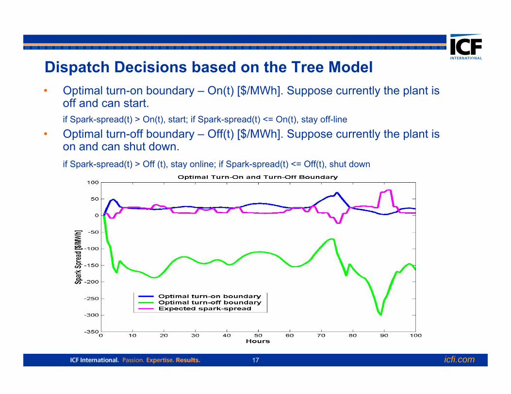
Dispatch Decisions based on the Tree Model• Optimal turn-on boundary – On(t) [$/MWh]. Suppose currently the plant is

off and can start.if Spark-spread(t) > On(t), start; if Spark-spread(t) <= On(t), stay off-line

• Optimal turn-off boundary – Off(t) [$/MWh]. Suppose currently the plant is on and can shut down.if Spark-spread(t) > Off (t), stay online; if Spark-spread(t) <= Off(t), shut down

icfi.com18

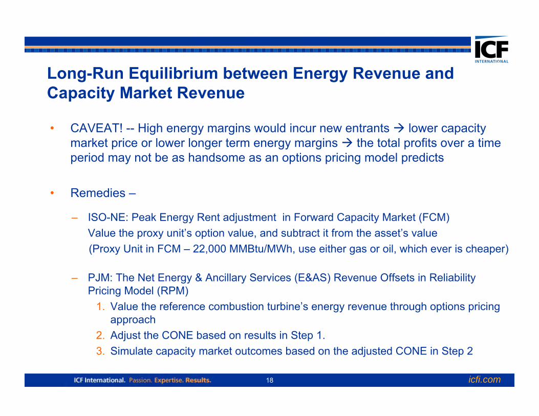
Long-Run Equilibrium between Energy Revenue and Capacity Market Revenue

• CAVEAT! -- High energy margins would incur new entrants lower capacity market price or lower longer term energy margins the total profits over a time period may not be as handsome as an options pricing model predicts

• Remedies –

– ISO-NE: Peak Energy Rent adjustment in Forward Capacity Market (FCM)Value the proxy unit’s option value, and subtract it from the asset’s value (Proxy Unit in FCM – 22,000 MMBtu/MWh, use either gas or oil, which ever is cheaper)

– PJM: The Net Energy & Ancillary Services (E&AS) Revenue Offsets in Reliability Pricing Model (RPM)

1. Value the reference combustion turbine’s energy revenue through options pricing approach

2. Adjust the CONE based on results in Step 1.3. Simulate capacity market outcomes based on the adjusted CONE in Step 2

icfi.com19

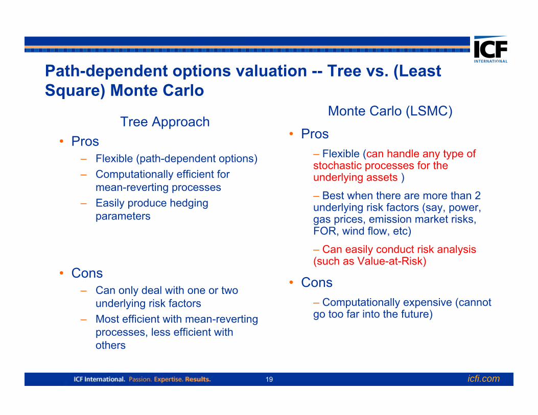
Path-dependent options valuation -- Tree vs. (Least Square) Monte Carlo

Tree Approach• Pros

– Flexible (path-dependent options)– Computationally efficient for

mean-reverting processes– Easily produce hedging

parameters

• Cons– Can only deal with one or two

underlying risk factors– Most efficient with mean-reverting

processes, less efficient with others

Monte Carlo (LSMC)

• Pros– Flexible (can handle any type of stochastic processes for the underlying assets )

– Best when there are more than 2 underlying risk factors (say, power, gas prices, emission market risks, FOR, wind flow, etc)

– Can easily conduct risk analysis (such as Value-at-Risk)

• Cons– Computationally expensive (cannot go too far into the future)

icfi.com20

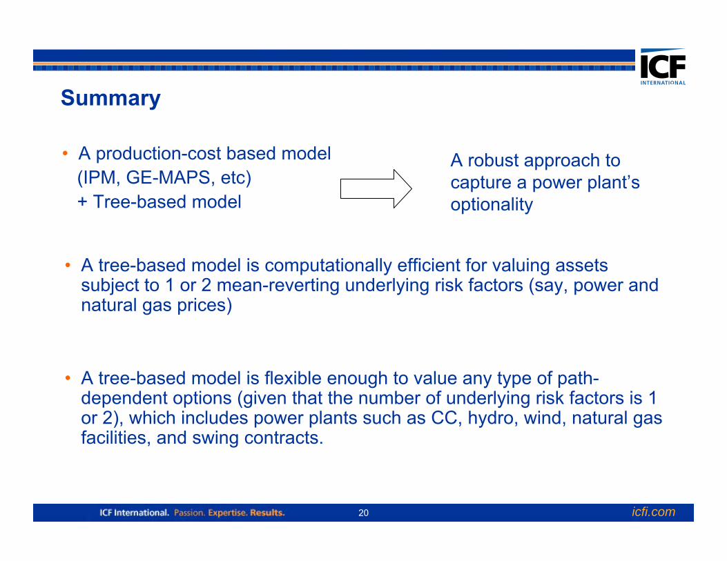
Summary

• A production-cost based model (IPM, GE-MAPS, etc) + Tree-based model

A robust approach to capture a power plant’s optionality

• A tree-based model is computationally efficient for valuing assets subject to 1 or 2 mean-reverting underlying risk factors (say, power and natural gas prices)

• A tree-based model is flexible enough to value any type of path-dependent options (given that the number of underlying risk factors is 1 or 2), which includes power plants such as CC, hydro, wind, natural gas facilities, and swing contracts.