Generating Synthetic Persian Music

Sahar Arshi1 and Darryl N. Davis2

Department of Computer Science University of Hull, UK

HU6 7RX 1S.Arshi@2014.hull.ac.uk, 2D.N.Davis@hull.ac.uk

Abstract. The research described here reflects our initial experiments in pro-ducing synthetic traditional Persian Music. Liquid Persian Music (LPM) is an assisting software capable of producing audio output. Equipped with cellular automata (CA) as a creative computational intelligence model and pattern recognition rules, it can produce novel musical material. This enables the explo-ration of new dimensions of music. Navigating in the LPM musical search space can be considered as a problem suitable for evolutionary algorithms. To help constraining the search space to desired musical classes, a fitness function based on a machine learning tool has been introduced to the problem. The fit-ness function is a support vector machine trained with features extracted from Persian music and LPM random sequences. The features are based on Zipf’s law proportions as one of the measurable universals for characterizing the aes-thetical aspects occurring in natural phenomena. The search is guided towards following the power law proportions from Persian music during the GA evolu-tion. The details of this approach are presented in the paper. The article con-cludes with an overview of the future work.

Keywords. audio software, machine learning, synthetic traditional Persian Mu-sic.

1 Introduction

Archaeological discoveries, on primary musical instruments, suggest that the human’s natural tendency towards music has a long history. These musical instruments are usually made from elementary materials (for example, skin, bones and wood) (Rault, 2000). The first humans were affected by natural sounds as well as thunderstorm, rain sound, water flow, sound of animals, etc. They were trying to use the power of sounds to express meanings and communicate. The invention of musical notes are more as-signed to a random process, where the first people gained different effects by chang-ing the physical factors in a sound producing media, for example by changing the length of an excited string (Khaleghi, 2013). The formation of musical octaves and tunings for many musical instruments continued through trial and error. Mathemati-cians, for example Pythagoras (Farhat, 1990), helped classify the mathematical pro-portions between notes and make the process more methodological. These had great

impact on the progression of what we have today as musical systems. This process has also benefited from cultural transmutations. New forms of musical instruments have been introduced to different countries and been customized to dif-ferent cultures and tastes. For instance Santur, the hammered dulcimer is a famous Persian musical instrument whose invention is assigned to Farabi the Persian scien-tist. There are different versions of Santur around the world, for example the Kam-boujfi from India, Yangqin from China, Butterfly from Britain, Macper from Ostrish, Santorini from Greece, Zither from United States (Sadie & Tyrrell, 2001). Some of the musical instruments are described as evolutions of previous versions. For example the Piano follows the same string excitation mechanism as a hammered dulcimer and can be considered as a modern version of the traditional hammered dulcimer. Like-wise, musical systems have undergone similar evolutionary processes and gradually became as an inseparable parts of various cultural signatures. With the advent of computational and artificial intelligence tools, the search for new music, and musical forms, can be advanced at a greater pace; with the possibility of truly novel forms emerging. Boden classifies creativity into two main groups according to the novelty of their origins. These are historical and psychological types of creativity. The P-creativity refers to the type of creativity that is new to the person who created it, no matter how many times it has happened before. However, the historical type of creativity. by definition, has never occurred before. For instance, undergraduate students imple-menting the perceptron algorithm are performing P-creativity; they may come to new ideas and concepts which have been already discovered. However a PhD student should come up with a new idea in their thesis, whether in methodology or in the nature of the produced knowledge, which is H-creative. Various musical genres have been revolutionized and continue to be developed; there-fore they can be categorized as H-creativity from many respects. However, once new styles are introduced, the artists or authors are likely to explore the same creativity space. Maintaining the previous established musical concepts, makes the productions likely to be considered as P-creativity types. For instance what are considered as con-sonant and dissonant chords and the related rules for chord progressions remain the same throughout newly composed music. Similarly, composing Persian traditional music is followed in one of the existing Dastgāh. Dastgāh are musical modal systems in traditional Persian music. The Dastgāh concept determines both the title for a group of individual pieces with their characteristic modal identity and the primary mode in each group. Each Dastgāh consists of individual melodies called Gushé, which vary in length and importance. The number of musical Gushe have not exceeded the ones collected by Moussa Maroufi from old musical references about a century ago (Farhat, 1990). However, many of the Gushe have been forgotten or altered through history as well, in a way that only the names of those pieces are available from an-cient Persian literatures (Khaleghi, 2013). The Dastgāh concept has been developed throughout history embedding ancient spir-itual messages and conceptual meanings. This introduces them as complex structures and musical novices are often encouraged to stick to the available framework as a requirement for advancing to higher levels. Compositions are often suspended until

the mastery of the Dastgāh itself; at the time when the artist gains a deep perception of Dastgāh concept and Gushe meaning. The description of the related concepts are often limited to words in range of emotional expressions. Therefore composition in Dastgāh music is often reliant on the emergence of great masters who intuitively un-derstand the complexity of traditional Persian music. However, these compositions are still exploring musical forms within quite constrained musical spaces, while there are various other musical possibilities, beyond these constraints, that transcend these traditional forms. There is the controversy of how the computational creativity experiments in the area of music art can generate quality music, particularly as they are in their early stages of development. This is particularly the case with Dastgāh where most current traditional musical pieces are regarded as masterpieces. The research in computational creativity is strongly interconnected to cognitive sciences and psychology. While there are so many unresolved questions in those areas, there is the hope that these types of exper-iments unveil some of the answers or at least lead to new approaches for making the underlying nature of cognitive and creative processes more tangible. It should be emphasized that the creativity space for producing music is, to all intents, infinite. The aim is to find the proper means for exploring those spaces. The fact is that there are human composers, machines that can create and compose, and human composers who use machines to create. If it is accepted that the computer can produce the desired music, then there would be the dispute that the composing machines would supersede their human counterparts. The process of introducing novel musical systems with their related musical theory can be considered as a historical type of creativity. Exploring the possibility of creat-ing novel Persian Dastgāh musical systems by help of computational intelligence tools is one of the ultimate goals of this project. However, a question that comes into mind is how to produce a novel style of music which can be associated with tradition-al Persian music. There is always the possibility that the search space gives new types of music which does not belong to any specific genre, and are quite new in many respects. If the search space is constrained to specific compositional rules, there is the hope that the new type of music generated possesses the essential and key features of a desired musical style or class. Liquid Persian Music (LPM) is a Cellular Automata (CA) based audio generator. Different pattern matching rules extract features from CA progression and update the parameters of a synthesizer for producing musical effects as an output. Various con-figurations of the system produce different voices which resemble musical motives in many respects (Arshi & Davis, 2016). The problem of sequencing those musical mo-tives in a musical manner can been treated as an optimization problem. Previous ex-periments (Arshi & Davis, 2015, 2016) have guided us towards a computational framework for aesthetical navigation in LPM musical search space. It has been em-phasized that the search space shall be divided to different multi-optimization prob-lems on the basis of melodic structure and psychoacoustics. In this paper sequencing LPM voices based on the first criteria is discussed. The first optimization problem have been conducted for evolving LPM voices according to the power law propor-tions extracted from the melodic structure of Persian music.

In this paper the details of an experiment for evolving musical voices on the basis of extracted Zipf’s features from Persian pop music is described. In section two some background fundamentals relevant to the current research approach are reported. Sec-tion three is engaged in the detailed description of LPM software developed in previ-ously conducted experiments. The core component of the current paper is presented in the fourth section. This part consists of the design of genotypes, and genetic algorithm operators based on the achieved framework. The fitness function and its feature con-text is explained on a step by step basis relying on some data mining fundamentals. This section is accompanied by the results of the experiment. The paper is concluded with a discussion section, and a portrayal of future research directions.

2 Background Fundamentals

Here we present a brief overview of the approach taken in this study and outline the key technologies employed.

2.1 Algorithmic Composition

Computer Music benefits from multi interdisciplinary research in computing technol-ogy, sound synthesis, musicology, music theory, digital signal processing, psychoa-coustics, and acoustics. CSIRAC built by Pearcy and Beard in 1951 (Doornbusch, 2005) is the first computer to play the popular music of the time. Further develop-ments took place by introducing composer machines by such people as Lejaren Hiller (Hiller & Isaacson, 1979). The current computer music practices revolves around approaches for innovating algorithmic composition techniques which are often con-ducted for various purposes. Most of the developments to date contribute to the mechanization of music production to varying degrees, as well as style imitation and assisting human composers in the process of music creation, exploration of the behav-iour of the algorithms themselves, attributing natural phenomena to music, and study-ing the cognitive behaviour of creativity (McCormack, 2007). Applied methodologies in algorithmic composition can be categorized in four groups (Fernández & Vico, 2013), namely: knowledge-based systems, machine learning, evolutionary algorithms, and computational intelligence (e.g. cellular automata). Un-like the three former categories, computational intelligence methods contribute to human domain knowledge (Arshi & Davis, 2016; Fernández & Vico, 2013) for pro-ducing musical material. This potential for creativity makes them well suited for ex-ploring new dimensions of music.

2.2 Cellular Automata

Cellular automata (CA) are discrete dynamical systems whose invention dates back to 1940’s when Von Neumann was experimenting with a system capable of reproduc-tion, comparable in certain respects with biological breeding (Burks, 1970). CA con-sists of elementary identical components whose interactions provoke global complex

behaviour in the system output (Wolfram, 2002). Cellular automata exhibiting myriad genres of behaviour have been targeted as a creative tool for artists. By increasing the number of states and neighbourhood size, the state space expands exponentially, in a way that the normal life expectancy of a human is not adequate for navigating through all these patterns. Cellular automata as an emergent machine can have various artistic applications. In music domain it has been widely used for the extraction of overall conformation for composition, MIDI sequencing, and sound synthesis (Burraston & Edmonds, 2005). Some of the early models of musical cellular automata include Beyls CA Explorer, and CAM developed by Millen (Burraston et al., 2004). Other popular cellular autom-ata musical systems are CAMUS and Chaosynth (Miranda, 2001; Miranda, 2002). CAMUS exploits Game of Life and Demon Cyclic Space, and uses a Cartesian space mapping to MIDI for achieving musical triplets. Chaosynth is based on the chemical reactions of a catalyst. It is a cellular automata sound generator with an underlying granular sound synthesis basis. However, the produced tones do not resemble musical acoustical voices, they are sometimes reminiscent of the natural sounds flow as well as the sound of waterfalls, or insects (Miranda, 2001).

2.3 Genetic Algorithm

Genetic Algorithms (GA) are a class of Evolutionary Algorithms inspired by natural selection (Darwin, 1906). They are employed in areas of search and optimization. Previous applications of GAs imply their success in problem solving for domains with widespread solution spaces (Buckles & Petry, 1992). Therefore, it can be considered a well suited candidate in music composition, with its almost infinite possible combina-tions of musical elements. However, in order to guide the search and constrain the musical search space, one can tailor fitness functions which fulfil musical aesthetical aspects or adhere to certain musical tastes (Burton & Vladimirova, 1999). A population of individuals are randomly initialized in a mating pool. Candidate solu-tions are coded as genotypes and are continually evolved in each nascent generation. The solutions contribute to crossover and mutation operations according to their fit-ness function. This assessment guarantees the survival of the most competent genes and raises the expectancy of convergence to optimal solutions. The reproduction op-eration consists of the selection of parents as the fittest individuals for breeding, which then undergo crossover and mutation operations. In crossover, individual par-ents are selected and their genes are transmitted to each other by swapping, in a mean-ingful manner. Mutation is a low-probability operation and involves changing a gene in the genotype (Goldberg, 1989). It can help the search by avoiding being entrapped in local solution spaces. The algorithm stops when a pre-specified goal has been satis-fied or some sort of limitations such as time or number of generations has been reached (Burton & Vladimirova, 1999). In previous applications, evolutionary algorithms have been widely used for compos-ing melodies, and harmonizing pre-specified melodies. The fitness function can be

interactive or autonomous. In interactive fitness functions a human user evaluates the candidate individuals in the population. These fitness functions usually contribute to user fatigue and should be used in domains where other fitness functions are unable to gain the desired results. The other types of fitness assessment usually rely on the ap-plication of machine learning methods (Fernández & Vico, 2013). Horner and Goldberg (1991) are one of the first to present the application of genetic algorithms in algorithmic composition. Thematic bridging is a composition method; starting from an initial pattern, the system goes into a series of evolutionary processes to transform to the final pattern. The GA individuals are the transformation operators and the fitness function is evaluated as the distance to the target pattern. The sequenc-es of the generated patterns are the output of the system. In GenJam, Biles (2014) devised an evolutionary algorithm for generating Jazz melodies. Later, he used an artificial neural network (ANN) to automate the task of evaluation to overcome the interactive fitness function bottleneck. However, the ANN failed to extend the evalua-tions to cases other than what was in its training set (Fernández & Vico, 2013). In (Lo, 2012), n-gram models, Zipf’s law, and information entropy are applied as trainable fitness functions in a series of experiments. Musical samples are used to train an N-gram classifier which is later applied as the fitness function in a random mutation hill climber. These fitness functions evaluate sequences of pitches, and the genetic opera-tors are employed as tools for search space navigation. Later in the same work evolu-tionary algorithms are applied to evolve cellular automata as a music generator.

2.4 Support Vector Machines

2.4.1 Genetic Algorithm

Support vector machines (SVM) are popular machine learning tools which are used widely in classification and regression applications (Vapnik, 1995). In the following some principles and formulations for SVM have been adopted from various resources in this area (Burges, 1998; Cristianini & Shawe-Taylor, 2000; Smola & Schölkopf, 2004; Steinwart & Christmann, 2008; Theodoridis, 2009; Vapnik, 1998). Support vector machines have very good performance in solving problems with small samples of data, while effectively avoiding high number of dimensions (Yin et al., 2015). Ker-nel functions are an important attribute of SVM which can be used where the data are not linearly separable. The Kernel functions are designed to map the data points to a higher dimensional space, where they can be linearly differentiated. The Kernel func-tion should contribute to Mercer condition (Cristianini & Shawe-Taylor, 2000). The differentiating hyper-plane can be formulated as

푓(푥) = 푤 푋 + 푏 푤 ∈ 푋, 푏 ∈ 푅 1

where w is the normal vector to the hyper-plane and b is the bias. Suppose we have N training samples as (푋 ,푦 ), …, (푋 ,푦 ). Where 푋 are the d-dimensional vectors,

and 푦 = 0,1 are the two class labels. The aim is to find a (d-1)-dimensional hyper-plane to discriminate between the data samples. Support vectors are the training data closest to the discriminating hyperplane. The distance between the support vectors (on both sides of the hyperplane) and the hyperplane are referred to as margins. Finding the maximum margin is the key to generalizing the trained system for classifying new data samples. The problem of finding the optimum hyperplane can be considered as an optimization problem for achieving the maximum margin, while making sure the training samples are placed on the correct sides of the discriminating hyper-plane. Support vectors are places on canonical hyper-planes |푤 푋 + 푏| = 1. Since ‖ ‖ obtains the distance between vector X and the discriminating hyperplane, the distance between the support vectors and the hyperplane is determined as ‖ ‖. Therefore, max-imizing the margin is equivalent to minimizing‖푤‖. The optimization constraints can be represented as

푚푖푛푖푚푖푧푒12‖푤‖

푠푢푏푗푒푐푡푡표 푦 − 푤 푋 + 푏 ≤ 0푤 푋 − 푦 + 푏 ≤ 0

2

Support vector machine problem can be formulated as a Lagrangian optimization with the help of classical method of Lagrange multipliers, where finding the optimal 푤 ,푏 is the ultimate goal. The solution is calculated in the context of quadratic program-ming problem which is described for the regression case in the following section.

2.4.2 Support Vector regression Model

Support vector regression model maintains the same principles as support vector ma-chines with slight differences. Support vector machines obtain zero or one values as the label of classes for new upcoming samples in both soft and hard problems. How-ever, in the current research, real numbers between zero and one are more desirable as fitness function values for utilization in the genetic algorithm. In traditional linear regression, the problem is to map a linear function 푓(푥) =푤 푋 + 푏 to the data samples in least squares sense as

푚푖푛 (푦 − 푤 푋 + 푏) 3

This is only valid where a linear function can be well mapped to the data. If data are not linearly distributed, they can be transformed to a higher dimensional space, where a linear function can be mapped to them. Since the upcoming samples are not neces-sarily placed on the regression line, the concept of margins are introduced to the prob-lem (Wang & Gao, 2012). The bigger the margin, the higher the generalization capa-bility of the trained support vector model to new data.

A support vector regression1 problem can be considered as an 휀 − 푆푉 machine, where the objective is to find a function f that has a maximum of 휀deviation from 푦 for each training sample 푋 and is as flat as possible simultaneously. The 휀 − 푆푉 regres-sion problem can be formulated as:

푚푖푛푖푚푖푧푒12‖푤‖

푠푢푏푗푒푐푡푡표: 푦 − 푤 푋 + 푏 ≤ 휀푤 푋 − 푦 + 푏 ≤ 휀

4

Slack variables ξ , ξ∗ > 0 are introduced to the optimization problem to handle the cases where the 휀 precision assumption is neglected. The optimization problem in its primal form can be written as:

푚푖푛푖푚푖푧푒12‖푤‖ + 퐶 (ξ + ξ∗ )

Subject to: 푦 − 푤 푋 + 푏 ≤ 휀 + ξ푤 푋 − 푦 + 푏 ≤ 휀 + ξ∗

5

where 퐶 > 0 is a constant compromization value between the flatness of 푓(푥) and how the alteration from 휀 are tolerated. The primal problem can be transformed to its dual version by utilizing Wolfe duality theorem and Lagrange multipliers. This makes the problem easier to solve. The solu-tion to the problem can be considered as determining the saddle point of Lagrangian function with respect to dual and primal variables.

퐿 =12‖푤‖ + 퐶 (ξ + ξ∗ )− 훼 (휀 + ξ − 푦 + 푤 푋 + 푏)

− 훼∗ (휀 + ξ∗ + 푦 − 푤 푋 − 푏)− (휂 ξ + 휂∗ ξ∗ )

Saddle point condition retrieves zero value for the partial derivatives of (푤, 푏, ξ , ξ∗ ) as:

6

휕 퐿 = (훼∗ − 훼 ) = 0 7

휕 퐿 = 푤 − (훼∗ − 훼 ) = 0 8

휕 (∗)퐿 = 퐶 −(훼(∗) − 휂(∗)) 9

1 The formulation and concepts in this section are affiliated to (Smola & Schölkopf, 2004).

Substituting the obtained results in the Lagrangian dual formulation gives the equiva-lent dual problem:

⎩⎨

⎧−12

(훼 − 훼∗ )(훼 − 훼∗ )퐾(푋 ,푋 ),

−휀 (훼 + 훼∗ ) + (훼 − 훼∗ )

Subject to : ∑ (훼 − 훼∗) = 0,훼 ,훼∗ 휖[0,퐶]

10

Solving the optimization problems retrieves the decision function as follows:

푓(푥) = (훼 − 훼∗ )퐾(푋 ,푋 ) + 푏 11

w can be obtained as 푤 = ∑ (훼∗ − 훼 ). While obtaining the b parameter can be done considering the Karush-Kuhn-Tucker (KKT) conditions. Based on KKT the product of dual variables and constraints will become zero at optimal solution as:

훼 (휀 + ξ − 푦 +푤 푋 + 푏) = 0 12

훼∗ (휀 + ξ∗ − 푦 + 푤 푋 + 푏) = 0 13

(퐶 − 훼 )ξ = 0 14

(퐶 − 훼∗ )ξ∗ = 0 15

By having 휉∗ = 0 for 훼 ,훼∗ 휖(0,퐶), b can be computed respectively:

푏 = 푦 −푤 푋 − 휀,훼 휖(0,퐶) 16

푏 = 푦 −푤 푋 + 휀,훼∗ 휖(0,퐶) 17

In this current application radial basis function is used as kernel function.

퐾(푋,푋 ) = exp(−‖(푋 − 푋 ) ‖

2휎 ) 18

2.5 Zipf’s Law in Music Applications

Zipf’s law characterizes the scaling attributes of many natural effects including phys-ics, social sciences, and language processing. Events in a dataset are ranked (descend-ing order) according to their prevalence or importance (Manaris et al., 2005). The rank and frequency of occurrence of the elements are mapped to a logarithmic scale, where linear regression is applied to the events graph. The slope and 푅 measure-ments demonstrate to what extent the elements conform to Zipf’s law. A linear re-

gression slope of -1 indicates Zipf’s ideal. Zipf’s law can be formulated as 퐹~푟 , in which 푟 is the statistical rank of the phenomena, 퐹 is the frequency of occurrence of the event, and 푎 is close to one in an ideal Zipfian distribution. The frequency of oc-currence of an event is inversely proportional to its rank.푃(푓) = 1 푓⁄ is another way to express the Zipf’s law. 푃(푓) is the probability of occurrence of an event with rank f. In case of 푛=1 (Zipf’s ideal), the phenomenon is known as pink noise. The cases of 푛=0 and 푛=2 are called white and brown noises, respectively. Voss and Clarke (1978) have observed that the spectral density of audio is 1/f like and is inversely proportional to its frequency. They devised an algorithm which used white, pink, and brown noise sources for composing music. The results show that pink noise is more musically pleasing due to its self-similarity characteristics, the white noises are too random, and the brown noises are too correlated producing a monotonous sound. In the musical domain, Zipf’s metrics are obtained by enumerating the different musi-cal events’ frequency of occurrence and plotting them in a log-log scale versus their rankings. The slope of Zipf’s distribution ranges from −∞ to 0. The decreasing of the slope to minus infinity reflects an increase in the level of monotonicity. The r-squared value is between 0 and 1. Various publications explore the utilization of Zipf’s law in musical data analysis and composition. Previous experiments show its successful application in capturing significant essence from musical contents. In (Manaris et al., 2005) the Zipf’s metrics consist of simple and fractal metrics. The simple metrics include seventeen features of the music as well as the ranked frequency distributions of pitch, and chromatic tone. Fractal metrics gives a measurement of the self-similarity of the distribution. These metrics were later used to train neural networks to classify musical styles and composers, with an average success rate of over ninety percent; demonstrating that Zipf’s metrics extract useful information from music in addition to determining the aesthetical characteristics of music pieces.

2.6 Karplus-Strong String Model

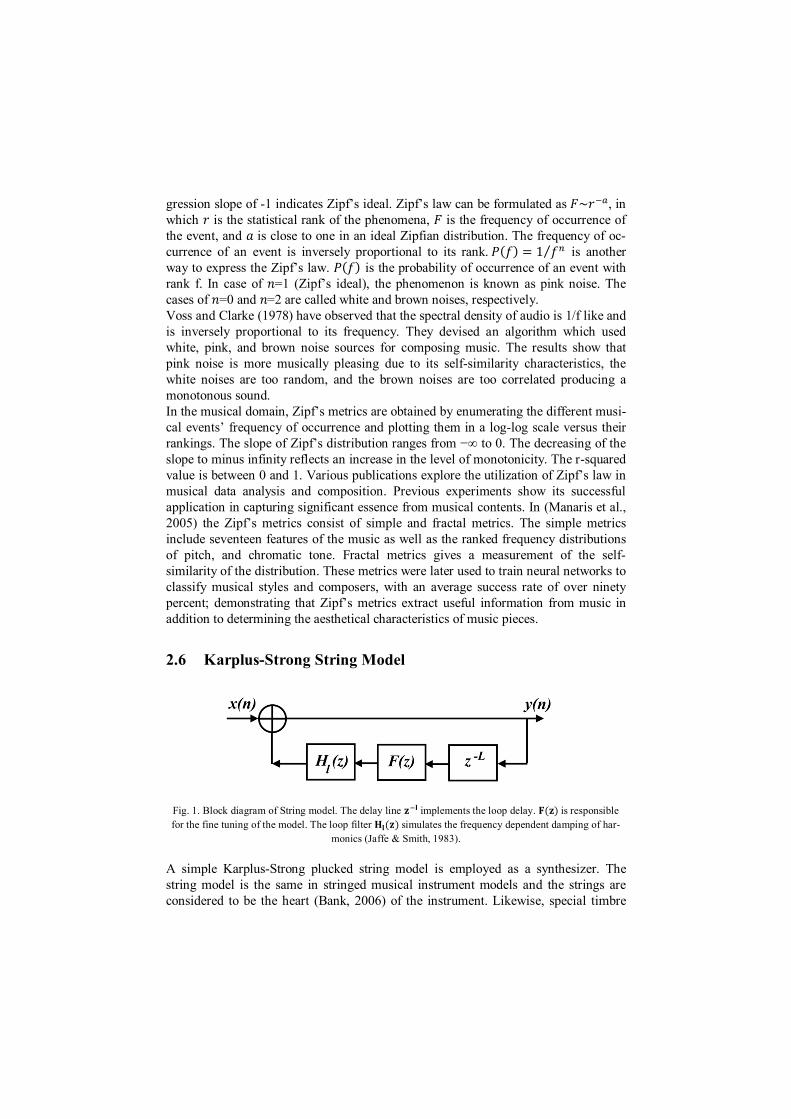
Fig. 1. Block diagram of String model. The delay line 퐳 퐥 implements the loop delay.퐅(퐳) is responsible for the fine tuning of the model. The loop filter 퐇퐥(퐳) simulates the frequency dependent damping of har-

monics (Jaffe & Smith, 1983).

A simple Karplus-Strong plucked string model is employed as a synthesizer. The string model is the same in stringed musical instrument models and the strings are considered to be the heart (Bank, 2006) of the instrument. Likewise, special timbre

characteristics of a musical instrument is determined by the excitation type (whether plucked, struck, bowed), the way the strings are fastened to the instrument body, the coupling between the strings, body and diverse physical aspects eventuating between strings, body, and air. The instrument body will affect the acoustical properties of the tones due to their geometrical structure, the building material, and the wood pattern. The block diagram of the String model is displayed in figure 1. The general string synthesis model 푆(푧) integrates a feedback loop with a cascade of a delay line, a frac-tional delay filter, and a loop filter. The delay line and the fractional delay filter both contribute to the delay line around the loop and determine the fundamental frequency of the tone (Erkut et al., 2000). The loop filter simulates the damping of harmonics. The delay line length for making tone having fundamental frequency 푓 would be 퐿 = 푓 푓⁄ , where 푓 is the sampling rate. The sampling rate throughout this investiga-tion has been chosen to be 44100Hz. Since 퐿 is substantially non-integer, a fractional delay filter is required to implement the non-integral part of the delay (Erkut et al., 2000). The loop filter is a low pass filter possessing the functionality of attenuating the harmonics due to their propagation around the loop (Jaffe & Smith, 1983).

3 Liquid Persian Music Context

Liquid Persian Music (LPM) (Arshi & Davis, 2015, 2016), and its predecessor Liquid Brain Music (or LBM) (Turner, 2008; Woods, 2009), are auditory software tools de-veloped at the University of Hull. LPM explores the idea of artificial life systems in producing voices which can be considered as new types of electronic music. Music, likewise many other physical phenomena can be described as the behaviour of simple waveforms. This has been the fundamental concept in the first version of LPM software. In LBM the produced voices of the system are a collection of sinusoidal waves with various frequencies, amplitudes, and phases. These waves are then added together through an additive synthesis mechanism (Cavaliere & Piccialli, 1997; Roads, 1988). One of the approaches for minimizing the dissonance of this sinusoidal waves and improving the quality of the voices was to introduce musical notes to the new version of LBM system. Composing sinusoidal waves with special proportions can produce musical notes. The spectrum (Van Loan, 1987) of a note consists of a fundamental frequency and a series of harmonic2 partials (Fletcher & Rossing, 1991). On this account a musical instrument model has been utilized. Musical instruments are generally categorized to woodwind, stringed, and struck instruments and their electronically implementation are based on the types of their excitation (Cook & Scavone, 2008) and their body impulse responses (Bank, 2007; Türckheim, Smit, & Mores, 2010). A basic Karplus-Strong plucked string (Jaffe & Smith, 1983) model

2 Although inharmonicity (Barbieri, 1998; Järveläinen & Karjalainen, 2006; Rocchesso &

Scalcon, 1999) is an important feature of many stringed and percussive musical instruments, it has been neglected for simplicity throughout this implementation. The inharmonicity gives a factor of deviation from the harmonic series and contributes to the naturalness (Rauhala & Välimäki, 2006; Rauhala, 2007) of the sounds.

has been implemented. This model is later parameterized with different configurations of the system. The elementary cellular automata (CA) used in LPM consists of an assembly of cells arranged in a one dimensional array that produces a two dimensional matrix over time. Each cell is in one of k finite states at time t, and all the cells evolve simultane-ously. The state of a cell at time t depends on its state and its neighbours’ states at time t-1. In the one dimensional elementary CA (used in this study), the permutations of each cell with its two adjacent neighbours specifies eight situations. Once allocated to binary states, the selection of one of the 256 local transition rules specify the CA evolution (Wolfram, 2002). In LPM, for every time step of the CA, the pattern matcher extracts the difference between consecutive generations. Twenty different pattern matching rules have been defined in this software as well as metrics using Dice’s coefficient, and Jaccard simi-larity. The obtained values from the pattern matchers are then fed as parameters into the synthesizer for producing the sounds. Some of the synthesizer parameters include ADSR envelope, loop gain, and the musical instrument string length for defining frequency. Further information about the software can be found in (Davis, 2015). An important point is that the aggregation of a CA rule and a pattern matching rule on each of the synthesizer elements does not produce a single note but a collection of notes; these are referred to as voices throughout this paper.

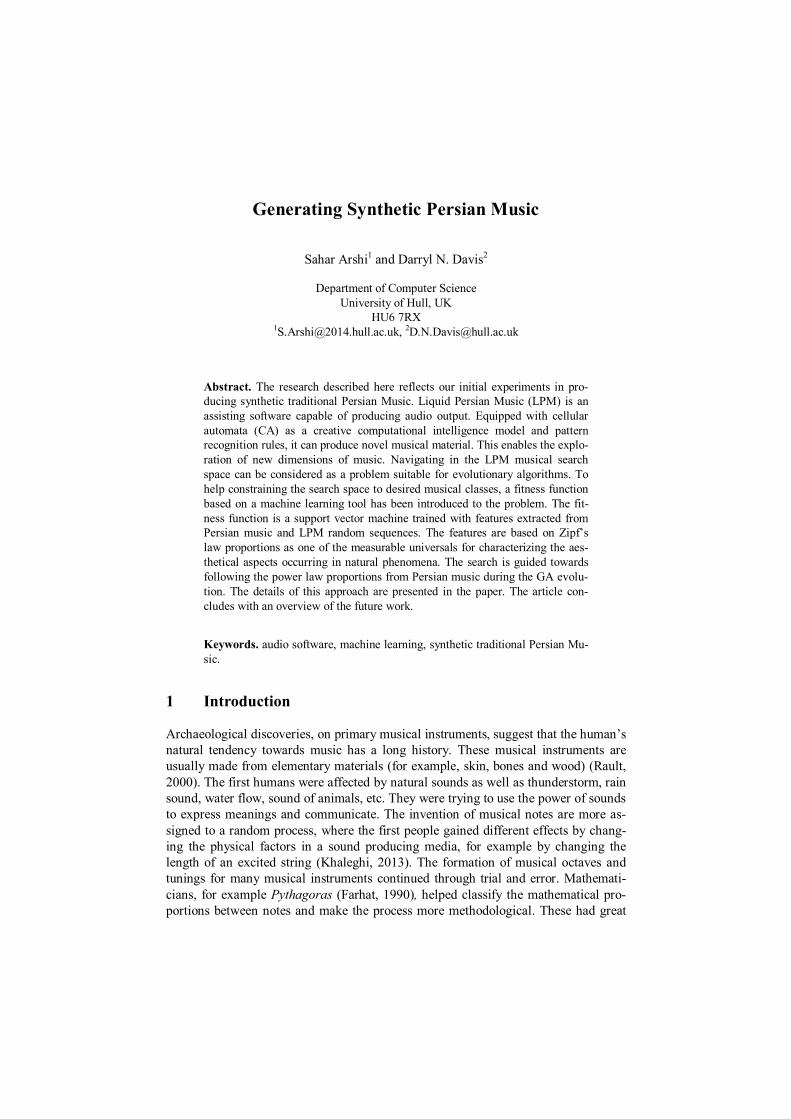
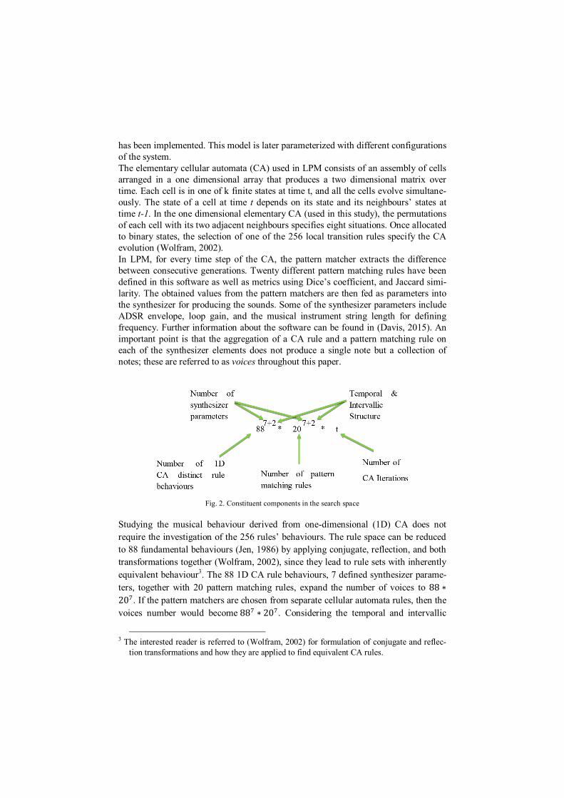
Fig. 2. Constituent components in the search space

Studying the musical behaviour derived from one-dimensional (1D) CA does not require the investigation of the 256 rules’ behaviours. The rule space can be reduced to 88 fundamental behaviours (Jen, 1986) by applying conjugate, reflection, and both transformations together (Wolfram, 2002), since they lead to rule sets with inherently equivalent behaviour3. The 88 1D CA rule behaviours, 7 defined synthesizer parame-ters, together with 20 pattern matching rules, expand the number of voices to 88 ∗20 . If the pattern matchers are chosen from separate cellular automata rules, then the voices number would become88 ∗ 20 . Considering the temporal and intervallic

3 The interested reader is referred to (Wolfram, 2002) for formulation of conjugate and reflec-

tion transformations and how they are applied to find equivalent CA rules.

patterns and the CA number of iterations the number of voices produced would ex-pand to 88 ∗ 20 ∗ t(where t is the number of CA iterations). This defines the base auditory search space for the computational framework being developed. Figure 2 shows the components in the search space. The final target of this part of the research is to evolve the arrangements of the produced voices in the form of a melody.

4 The design of LPM Sequencer

It has been stated in (Arshi & Davis, 2016) that sequencing LPM voices is a task suit-able for evolutionary algorithms. Applying Genetic Algorithms for search and optimi-zation of musical sequences has special requirements. For example, defining the search space; specifying the musical knowledge and rule representation; and the choice of an appropriate fitness function (Burton & Vladimirova, 1999). The search for finding optimal solutions is guided by assigning higher fitness to competent indi-viduals. Since there are, in effect, infinite possibilities for producing music; it is nec-essary to define suitable constraints for limiting the search space. As stated in the previous sections LPM outputs are a set of voices instead of notes. The voices resemble musical motives of varying lengths depending on the number of cellular automata iterations involved in their production. The design of competent genotypes and phenotypes are requirements for an efficient search. The genotypes are codes which manifest a higher level of behaviour known in the phenotype. For exam-ple eye colour is coded in genes. However, what is seen as blue, green, and brown etc., are the phenotypes. It should be noted that in the LPM system, the phenotypes are the voices which are heard as the behaviours of the individuals and the genotypes are the set of genes coded whether as binary or integer representations. A first naïve design for the search space would be to define the individuals as the elements of voices set. Regarding the huge search space and our current facilities, software implementation is nearly impossible unless the search space is reduced by a notable amount. Perhaps selecting a limited number of voices and evolving them would be a more feasible solution. During the evolution of such a design, all the con-tributing parameters change dynamically to a point that fulfils predefined musical expectations or at least tries to do so. This stabilization includes a gradual justification of musical parameters and general improvement in each generation. There are no unique solutions to musical problems, In fact starting from the same initial conditions, the search may result to different sets of solutions in every execution. Further improvement in the design is to divide the search problem into several multi-optimization ones, relating to the constituent elements of the produced melody based on the LPM output. The first search determines the structure of the melody, including the pitch frequency, the intervals and the note durations. The second search problem involves the optimization of the remaining synthesizer elements. This separation pro-vides two categories of different natures for exploration. The search pool sizes of which becomes 88 ∗ 20 ∗ 푡 and 88 ∗ 20 respectively. Evaluators for the individ-uals of each of these search spaces vary. This paper focuses on the first optimization problem though. The related fitness function scores every one of the individuals based on their statistical aesthetical competence, coded in their individual genes.

4.1 The design of LPM Sequencer

According to what has been discussed in the previous section, there are 88 ∗ 20 ∗푡musical motives in the search space, where t is the number of cellular automata iterations. The next phase would be to sketch the genotypes. In the terminology of evolutionary algorithms there are various ways for encoding the genotypes, as well as binary encoding, permutation encoding, tree encoding, and value encoding (Obitko, 1998). The latter is used for this experiment. Direct value encoding can be used in problems, where some complicated values, such as real numbers, are used. The appli-cation of binary encoding for this type of problems would be very difficult. In value encoding, chromosomes consist of values related to the problem, which can have different formats from real number to alphabets (Obitko, 1998) .

Voice 1, Layer 1 (from 1 to 9) Voice 2, Layer 1(from1 to 9)

Cellular Automata

Rule #

PatternMatcher Rule #

Number of

Generations

Cellular Automata

Rule #

PatternMatcher Rule #

Number of

Generations...

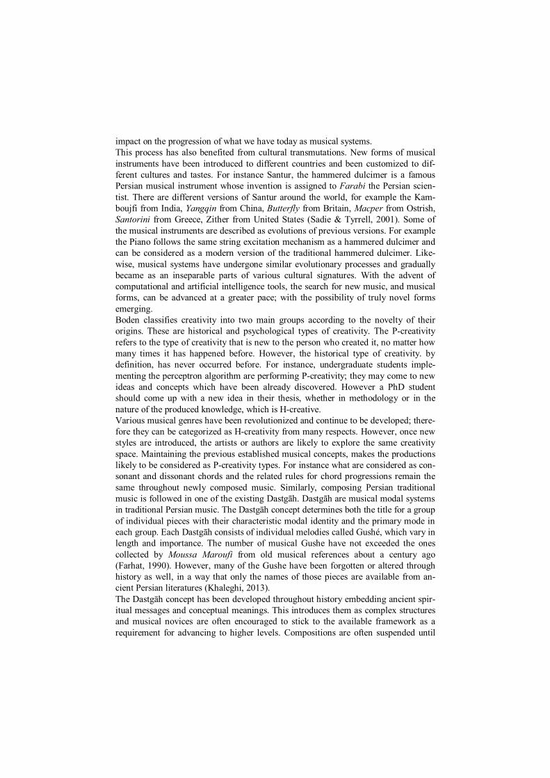
Fig. 3.The genotypes in the first level. For each of the nine constituent layers.

Two types of genotypes have been defined for addressing the problem of evolving LPM voices. One possible architecture for genotypes is to tackle them as sequences of blocks with three values in each. These values are the cellular automata rule number, pattern matching rule number, and the quantity of cellular automata generations in-volved. A schema of genotypes in this level is shown in figure 3.

Voice 1 Voice 2 Voice 3 Voice 4 ... Voice n

Fig. 4.The genotypes in the second level, after untwisting the genotypes in the first level.

Another possibility for the genotypes architecture is presented in figure 4. The geno-types are the outputs of pattern matching rules over t generations of CA for each of the blocks, sequenced one after the other. Extending the genotypes provides the po-tential for defining additive operators to the sequence in a more scrutinized level. The two different genotypes require the design of distinct set of crossover and mutation operators regarding their natures. The number of blocks varies in different genotypes which can imply the length of the producing musical pieces. Although having genotypes with different lengths can add some complexity in the implementation of evolutionary algorithm operators, they signify various possibilities for musical motives lengths. In order to avoid lengthy sequences and heavy processing time for evolving those sequences, the maximum length of the sequenced voices should not exceed a predefined limit.

4.2 Genetic Algorithm Operators Evolutionary algorithm operators, provide tools for exploring the search space (Burton & Vladimirova, 1999). The genotypes in LPM sequencing problem have been coded as blocks, with each block representing the information for producing one mu-sical motive. Therefore the genotypes consist of motives sequenced one after the oth-er. The composition happens by applying operators to sequences in a musical way. Apart from the classical selection, crossover and mutation operators (Goldberg, 1989; K.F. Man et al., 1999), there are sets of operators which are inspired by composition techniques as well as sequencing phrases, retrograding, transposition, swapping the phrases and rearranging them (Lo, 2012). This section has a brief overlook to the defined evolutionary operators grouped according to their functionality. Classical and musical operators are borrowed from (Goldberg, 1989; Lo, 2012; Matlab, 2016) and adopted to be compatible for evolving two types of genotypes.

4.2.1 Genetic Algorithm Operators

Tournament Selection 1: Two individuals are selected from the population and a random number (r) is generated between 0 and 1. If r is smaller than a pre-determined number (T), then the fitter individual is returned, otherwise the weaker one is selected.

Tournament selection 2: A number of elements equalling to the Tournament size are randomly selected from the individuals’ pool, and the fittest ones is returned as a parent.

Roulette wheel selection or fitness proportionate selection: After calculating the total fitness of the population (F), the probability of selection for each of the indi-viduals are computed by dividing their fitness (푓 ) to F (푝 = 푓 퐹⁄ ). The cumula-tive probability is then computed for each chromosome (푞 = ∑푝 ). A random number (r) is generated then, If it is less than the cumulative probability of the first individual (푞 ) in the population, that individual will be returned as parent, other-wise the 푖 chromosome where 푞 < 푟 < 푞 will be selected. One of the draw-backs from roulette wheel selection is that the individuals with higher fitness are more likely to be selected, which may result to sub-optimal solutions and pre-mature convergence.

Rank selection: The genotypes in the pool are ranked according to their fitness, the ranks are employed as fitness values for selecting the individuals. This selection method is more expensive due to slower convergence however, the solutions are more mature.

4.2.2 Crossover Operators

Scattered crossover 1: This operator generates a random binary vector, as a mask. The child inherits the genes from the first parent where the mask is 1, and the rest of the genes are taken from the second parent in the loca-tions where the mask vector have the value of zero.

Scattered crossover 2: This operator employs the same concept as the first scattered crossover operator, except it is designed for genotypes with dif-ferent lengths. In this case an index vector with the sum of the lengths of the two genotypes as parents is generated and the elements are permuted randomly. The lengths for children are arbitrarily selected within the range of the sum of the lengths of both parents. These numbers can be chosen as the same lengths of parents chromosomes.

Single point crossover 1: This operator generates a random integer n be-tween one and the length of the parents. The genes in the locations less than or equal to n are selected from the first parent and the genes located in indices greater than n are inherited from these locations of the second parent. The second offspring seizes the genes from alternate positions on the parents’ genes.

Single point crossover 2: In the case the chromosomes from the two par-ents have different lengths, two random integers are selected within the lengths of each of the two parents. The first child inherits the first section of the first parent and the second one from the second parent. While the other offspring seizes the remaining sections from the parents.

Two point crossover: Two random integers are selected within the length of parents’ genes which indicate the truncating locations. The first off-spring would alternately inherit from the first and last sections of the par-ent 1, and the second section from parent 2.

4.2.3 Mutation Operators

Mutation: a random number is generated between 0 and 1, for all the ele-ments in the genotype. If this number is less than the mutation probability then the corresponding gene will go under mutation operation. Otherwise it will be left unchanged.

The operators in the range of second phase genotypes are inspired by (Lo, 2012) and consist of the following: Multiple elements Modification: N integer numbers are selected within

the length of chromosome. The values of the specified location will then go under modification.

Segment alteration: A segment is selected within the length of the geno-type. All the elements in the segment will be altered within acceptable thresholds.

Segment placement: This operator selects two random segments, finds the fitter one, and replicates it by replacing it in the location of the weaker segment. The fitness of each of the segments within a larger segment can be calculated in the same agenda.

Segment retrograde: Randomly selects a segment, then the elements are sorted in a reverse ordering.

Segment Transposition: A segment is randomly selected and the elements are all added or subtracted by a constant value within the acceptable threshold defined.

Segment ascending/ descending ordering: A segment is selected random-ly, and the elements are reordered in an ascending or descending manner.

Segment copy and paste from musical training set data: a segment is se-lected from training samples with high fitness and placed instead of a ran-dom segment in the chromosome.

4.3 Fitness Function Design We will need to define various types of fitness functions to address the multi-optimization problem at hand. In this paper the process for obtaining a fitness func-tion based on the first determined criteria is described and the design and implementa-tion of the remainder criteria are left as future research tasks of this project. Support Vector Machine Regression Model is used as a trainable fitness function for LPM. The training musical data consists of a set of Persian pop4 music in MIDI format and the LPM sequences. The SVM regression model should be able to differentiate be-tween LPM musical sequences and Persian pop music. Numbers between zero and one are allocated to the newly generated sequences. This number specifies the degree of similarity to Persian pop music, which is the ultimate goal of GA optimization.

4.3.1 Training Dataset This section relates to the data collection of Persian Pop Music in MIDI Format and Data Collection from LPM Sequence Generator in order to train a support vector re-gression model as fitness function. In this study a set of Persian Pop (PP) music in MIDI format are collected from free databases on the net. The MIDI format makes the feature extraction procedure easy. Despite audio signals which need special procedures for obtaining the features as well as pitch, and duration. Matlab (Matlab, 2016) MIDI tool-box (Eerola & Toiviainen, 2004) is employed for its functionalities in reading MIDI data files and extracting some of the musical characteristics. Musical pieces in MIDI format can be evocated in Matlab by readMIDI command and stored in a matrix with seven columns repre-senting Onset (beat), Duration (beat), MIDI channel, MIDI pitch, Velocity, Onset (Second), and Duration (Second) data. The number of rows in a MIDI matrix depends on the number of musical notes presented in the piece. A database of LPM sequences have been produced for training the SVM regression model together with PP music. Every record in the database consists of a random collection of sequences from LPM Outputs. Each sequence is generated by applying a specific pattern matching rule over a CA progression in t number of iterations. The length of a collection of sequences equals the total number of CA iterations applied. The process of producing databases of random sequences continues to nine dimen-sions. Each dimension governs the data required for producing LPM audio music. The number of columns might differ from each other from row to row in a single dimen-sion regarding the length of the sequences. However this number should be equiva-

4 The current fitness function is trained with Persian pop music and LPM sequences. The future

research targets more complicated case of Persian traditional music instead.

lent in identical rows in different dimensions. For example having the pitch of a note without its duration is meaningless.

TABLE 1. THE NORMALIZATION VALUE RANGES FOR THE MUSICAL DIMENSIONS IN LPM SEQUENCES

Musical Dimension Lower Range Upper Range

Pitch Frequency 100 Hz 3000 Hz

Duration 1/16 sec 2 sec

Onset 1/16 sec 2 sec

Attack 0.001 0.5

Decay 0.001 4

Sustain 0 4

Release 0.5 0.9

Loop Filter 0.01 0.05

Interval -20 20

The second phase would be to normalize the data in each dimension. This normaliza-tion has been conducted on the basis of trial and error and by considering stability of the synthesizer filters. Moreover some musical theory consistencies have been taken into account as well. The sequence of PMR outputs for different CA could often pro-duce numbers in an extensive range contributing to inconsistent frequencies and un-acceptable note durations. For example the duration of a note could be one minute, while the next one would be 10 minutes. It has been decided to constrain the occur-rence of these types of compositions by normalizing the related values. The normali-zation ranges shown in table 1 have been considered for various dimensions. Since the focus in this paper is to evolve LPM sequences based on their melodic structures, only three dimensions related to pith, duration, and onset would be ade-quate for addressing the current problem. Evolving the rest of the dimensions are discarded for now and subjects to further investigations.

4.3.2 Feature Extraction Two sets of data have been analysed for extracting the Zipf’s metrics. The first data set consists of 205 Persian pop music samples in MIDI format. The second data set includes 200 samples of LPM sequences. A set of 248 Zipf’s features have been ex-tracted from the two databases. These Zipf’s metrics can be defined, and categorized in three main groups using the definitions given by (Manaris et al., 2005): Regular Metrics: This set calculates entropy from first level events as well

as pitch, duration, onset. Higher order Metrics: Gives the difference between two events in the

regular metrics. The number of differentiations calculated is optional, however 3 to 4 levels are usually sufficient, while the higher orders may attain no new information. The attributes in this category are the deriva-

tives of the regular metrics up to level 4. Some example includes: pitch_d1, pitch_d2, pitch_d3, pitch_d4.

Local variability metrics: This set captures the entropy of the difference of an event from the local average. Attributes in this category have been pro-duced from the first level attributes and their derivatives up to second lev-el. For example pitch_LV, pitch_d1_LV, pitch_d2_LV, are the attributes built upon pitch matrix.

4.3.3 Data Cleaning Attributes with large number of same values have been considered as redundant and been removed from both LPM and PP Zipfian metrics. Although they could have been used as powerful indicators for dichotomizing the two classes, they behaved more like biased attributes which did not contribute to recognizable meaning among LPM or PP datasets. Some of the other attributes came up with minus infinity or Nan values. Although minus Infinite5 (-Inf) and Nan6 are meaningful values in the Zipfian metrics, they made the Weka classifier to act abnormally. On the other hand, these values have been repeated throughout some attributes several times, which made the related attribute biased and meaningless. After removing the attributes with large number of Nan or –Inf values, only one record was left with some –Inf values. The related records have been deleted from the dataset to minimize the chances of misbe-haviour by the classifier algorithm.

The fitness function used in this work is developed using data mining and classifi-cation methodology. The intention is that will transfer to genotype evaluation. In or-der to do so, it is important to use input attributes that are not bi-polar over the class labels used. Hence, attributes with overlapping values for the two classes are more desirable ones. The non-overlapping attributes for the two classes gives the designed machine learning tool a strong discriminating capability of use in the evolutionary algorithm. If this were not the case, and bi-polar attributes were used, the generated fitness function would lead to the discard of most of the generated audio samples as non-Persian music.

4.3.4 Attribute Selection Attribute Selection have been conducted through several levels. Step 1 reduces the number of features from 248 to 154 as described in the section depicting data clean-ing. The biased attributes and those with non-overlapping values have been removed in this phase, leaving us with 154 features. Table 2 and figure 5 depict an example list of attributes who have been removed for having non-overlapping classes or having empty or minus infinite values for some of their records. These are considered as undesirable attributes. Figure 6 shows a set of features (after the data cleaning phase) with more desirable overlapping of distribution graphs for the two classes of LPM and PP Zipf’s metrics.

5 -Inf indicates that the measured musical data is monotonous. 6 Nan shows the unavailability of the related event so that it could not be measured

TABLE 2. A LIST OF EXAMPLE ATTRIBUTES WHO HAVE BEEN REMOVED. SUPPORTING GRAPHS SHOWING THEIR VALUE DISTRIBUTION ARE AVAILABLE IN FIGURE 5.

Attribute Name Feature Category Reason Removed

Duration_Distance2 First Level

Non- overlapping classes

Harmonic_Bigrams_d1 Higher order met-rics

Quantized_duration_d2 Higher order met-rics

Pitch_distance2 First Level

Chromatic_Pitch_Distance2_d2 Higher order met-rics

Melodic_Consonance First Level

Nan or minus infinite values for one or both of the classes

Pitch_Distance2_d2 Higher order met-rics

Quantized_Duration_Distance1_d2 Higher order met-rics

Harmonic_consonance First Level

Chord_Progression First Level

The second level chooses 40 attributes out of 154 features. Attributes were evaluated in Weka (Hall et al., 2009) by ReliefF, Info Gain, Gain Ratio, and Symmetrical Un-cert algorithms using Ranker search method (Kononenko & Kukar, 2007). The attrib-utes are given values between 0 and 1, and are sorted in descending order by Weka. The assigned values are employed for further investigation towards selecting con-sistent attributes. A simple approach have been taken for choosing the best set of fea-tures acknowledged by applying evaluators. The process behind attribute selection in this level is depicted in table 3 as a small sample of the whole attribute set. Attributes with evaluation credits less than 0.1 are marked as undesirable. These features are separately colour coded with blue, and orange in each of the evaluators’ categories in the table. In the next step the attributes in each evaluator groups are sorted by the attributes number, done by the help of Excel’s custom sort. This allows us to compare the different evaluations of identical features easily, since it arranges the same ones in one row. In the final step features not been colour coded in any of the evaluators re-sults, are marked with yellow colour. These remaining 40 attributes have values greater than 0.1 among all the evaluators.

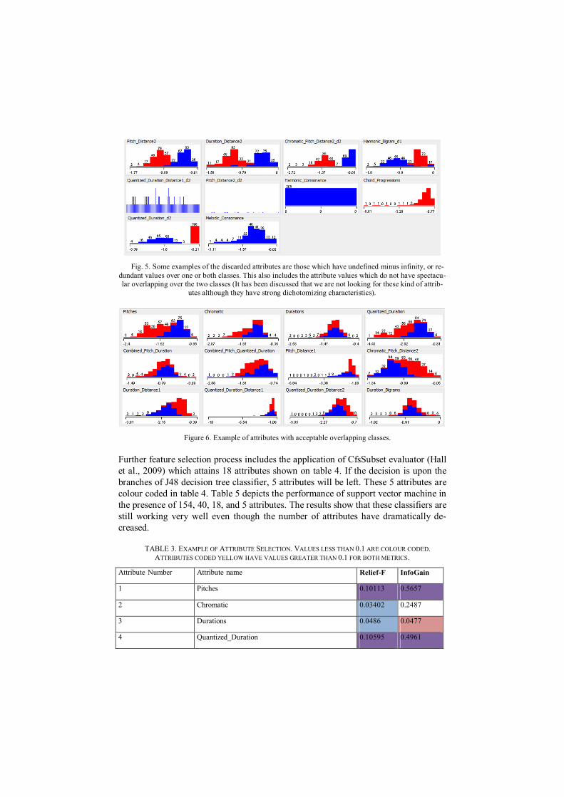
Fig. 5. Some examples of the discarded attributes are those which have undefined minus infinity, or re-dundant values over one or both classes. This also includes the attribute values which do not have spectacu-lar overlapping over the two classes (It has been discussed that we are not looking for these kind of attrib-

utes although they have strong dichotomizing characteristics).

Figure 6. Example of attributes with acceptable overlapping classes.

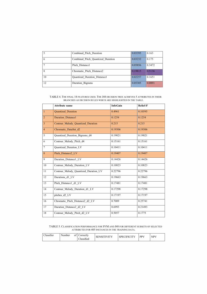
Further feature selection process includes the application of CfsSubset evaluator (Hall et al., 2009) which attains 18 attributes shown on table 4. If the decision is upon the branches of J48 decision tree classifier, 5 attributes will be left. These 5 attributes are colour coded in table 4. Table 5 depicts the performance of support vector machine in the presence of 154, 40, 18, and 5 attributes. The results show that these classifiers are still working very well even though the number of attributes have dramatically de-creased.

TABLE 3. EXAMPLE OF ATTRIBUTE SELECTION. VALUES LESS THAN 0.1 ARE COLOUR CODED. ATTRIBUTES CODED YELLOW HAVE VALUES GREATER THAN 0.1 FOR BOTH METRICS.

Attribute Number Attribute name Relief-F InfoGain

1 Pitches 0.10113 0.5657

2 Chromatic 0.03402 0.2487

3 Durations 0.0486 0.0477

4 Quantized_Duration 0.10595 0.4961

5 Combined_Pitch_Duration 0.03395 0.163

6 Combined_Pitch_Quantized_Duration 0.03232 0.175

7 Pitch_Distance1 0.05856 0.3472

8 Chromatic_Pitch_Distance2 0.19815 0.5136

10 Quantized_Duration_Distance1 0.02257 0.1651

12 Duration_Bigrams 0.05305 0.0891

TABLE 4. THE FINAL 18 FEATURES USED. THE J48 DECISION TREE ACHIEVES 5 ATTRIBUTES IN THEIR

BRANCHES AS DECISION RULES WHICH ARE HIGHLIGHTED IN THE TABLE.

Attribute name InfoGain Relief-F

1 Quantized_Duration 0.4961 0.10595

2 Duration_Distance1 0.1254 0.1254

3 Contour_Melody_Quantized_Duration 0.215 0.215

4 Chromatic_DataSet_d2 0.19306 0.19306

5 Quantized_Duration_Bigrams_d4 0.19021 0.19021

6 Contour_Melody_Pitch_d4 0.15161 0.15161

7 Quantized_Duration_LV 0.10411 0.10411

8 Pitch_Distance2_LV 0.19407 0.19407

9 Duration_Distance1_LV 0.14426 0.14426

10 Contour_Melody_Duration_LV 0.10823 0.10823

11 Contour_Melody_Quantized_Duration_LV 0.22796 0.22796

12 Durations_d1_LV 0.19663 0.19663

13 Pitch_Distance1_d1_LV 0.17481 0.17481

14 Contour_Melody_Duration_d1_LV 0.17298 0.17298

15 pitches_d2_LV 0.17197 0.17197

16 Chromatic_Pitch_Distance2_d2_LV 0.7089 0.25741

17 Duration_Distance2_d2_LV 0.6993 0.21493

18 Contour_Melody_Pitch_d2_LV 0.5057 0.1775

TABLE 5. CLASSIFICATION PERFORMANCE FOR SVM AND J48 FOR DIFFERENT SUBSETS OF SELECTED ATTRIBUTES FOR 405 INSTANCES IN THE TRAINING DATA.

Classifier Number of Correctly Classified

SENSITIVITY SPECIFICITY PPV NPV

Attributes Instances

SVM 154 99.75% 100.00 99.50 99.51 100.00

J48 154 97.03 % 98.54 95.50 95.73 98.45

SVM 40 100 % 100.00 100.00 100.00 100.00

J48 40 98.02 % 99.51 96.50 96.68 99.48

SVM 18 100 % 100.00 100.00 100.00 100.00

J48 18 98.02 % 99.51 96.50 96.68 99.48

SVM 5 99.25 % 98.54 100.00 100.00 98.52

J48 5 99.01 % 99.51 98.50 98.55 99.49

4.4 The GA Implementation The GA process starts with the generation of initial population. According to the ar-chitectures propounded for genotypes (shown in figures 3 and 4) two types of popula-tions can be produced. The concept of GA would stay the same for evolving two types of genotypes, however, the nature of GA operators would be different, giving us the chance to evolve chromosomes in different levels for studying various effects in the result. The evolution of two architectures can be programmed to happen one after another, however, the user can select to apply both levels of evolution to sequences or choose only one as well as entering the second evolution phase directly. The related program has the ability to save the evolved sequences during different generations in various executions. This gives the programmer the opportunity to change the GA parameters or select various sets of GA operators for studying their effects during audio test. The first population is built in a three dimensional database. Each of the dimensions include a random sequence from CA number, PMR number, and the number of CA iterations involved. The dimensions carry pitch, duration, and onset information. Number of rows in database equal the size of population. The number of columns in every row are taken to be equivalent to the length of the sequences. The procedure for producing the second type GA initial population is more or less like the one taken in section for generating the training data set for SVM regression model. The second database consists of the values produced by PMR on CA. It can be somehow considered as the decoded information in the previous stage. The generation of the second database however requires an additional normalization phase consider-ing the governor dimensions as explained in table 1. The normalization takes place in every iteration of GA algorithm to make sure the data are musically meaningful. The GA program can evolve the population sequences in two levels. Once the se-quences in the first level are settled with particular CA rules, PM rules and t itera-tions, the second level of evolution can be started by expanding the genotypes and obtaining the second level of genotypes. The second format is the decoded version of the first one. However, applying the operators provided for the second level leaves the sequences in their latest format. The transformation to the second format is irreversi-

ble; the sequences can no longer be formatted as CA-PMR-T codes after the second phase operations. First level of operation plays around with values of cellular automa-ta and pattern matching rules, and the selection/arrangement of sequences in a proper way in relation to each other. The second level is determined to be compatible with the variation of crossover and mutation operators defined to cover some aspects of music theory. During each iteration, the Zipf’s metrics for the chosen attributes are extracted from population individuals. The fitness of each of those individuals are predicted by ap-plying the trained support vector regression model. The parameters used in GA configuring are: Elites percentage, mutation rate, muta-tion fraction, crossover fraction, and tournament size. Elites are a proportion of the population, we want to transfer to the next generation without any change. Elites are generally selected from the fittest elements in the population. Elites themselves can still be selected in GA operations since we believe they have the valuable set of genes and can increase the mean fitness of the population. Mutation rate characterizes the probability of an individual chromosome being mutated. Crossover/mutation fraction determines the fraction of the population (except elites) which are generated by cross-over/mutation operation. The tournament size value is employed in tournament selec-tion operator.

4.5 Implementation Results TABLE 6. GA CONFIGURATION PARAMETERS FOR GRAPHS SHOWN IN FIGURES 7, 8, AND 9. THE

PARAMETERS FOR FIGURE 8 GIVE A SET OF NUMBERS; THE FIRST ONE IS FOR EVOLVING FIRST GENOTYPES LEVEL; THE SECOND ONE ARE RELATED TO THE SECOND EVOLUTION LEVEL.

Parameter Fig7a Fig7b Fig7c Fig8a Fig8b Fig8c Fig9a Fig9b Fig9c

mutation_rate 0.25 0.5 0.75 0.25:0.25 0.25:0.5 0. 5:0.25 0.25 0.5 0.25

mutation_fraction 0.5 0.7 0.9 0.5:0.5 0.5:0.5 0.7:0.7 0.5 0.5 0.7

crossover_rate 0.7 0.9 0.7 0.7:0.7 0.7:0.7 0.9:0.9 0.7 0.7 0.9

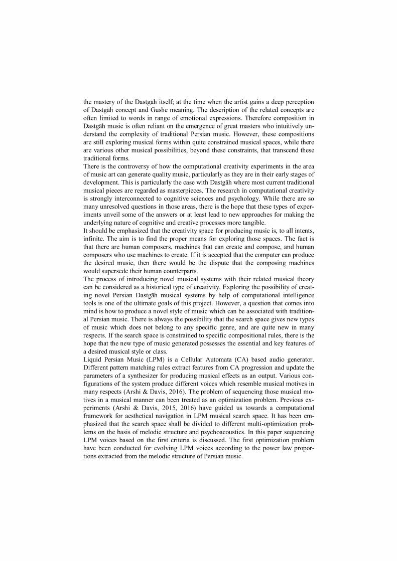
In this section the performance of GA is studied against different parameterizations and choice of operators. Various graphs depict the minimum, mean, and maximum of the fitness function over generation progression. Table 6 presents the parameterisation of the results shown in the figures 7, 8, and 9. Elite percentage and tournament size are fixed at 10%, and 5 respectively. Figure 7, 8, and 9 illustrate various execution results for different GA parameterizations for both genotypes architectures. Figure 7 subfigures illustrate a gradual growth in the fitness function mean value over GA iterations. Experimenting with higher number of iterations proposes the GA evolution is likely to converge to a mean value of approximately 0.6 which is slightly better than middle range value average.

Fig. 7. Minimum, Mean and Maximum fitness function value over 50 generations for various GA genera-

tions with genotypes in first architecture.

Fig. 8. Minimum, Mean and Maximum fitness function values over 50 generations for various GA exe-

cutions after two levels of evolution.

Moving to the next level of evolution by opening the first level genotypes into their decoded forms and applying the second level range of operators, new outcomes ap-pear. Figure 8 subfigures suggest that continuing the voices evolution by second genotype approach does not target significant improvement in the process of evolu-tion or may need some improvements in the design of the operators.

Fig. 9. Minimum, Mean and Maximum fitness function mean value over 50 generations for various GA

executions. This part are the results of evolving genotypes with the second architecture format without first applying the first architecture level.

Figure 9 depicts the results of evolving the second genotype architecture directly. High fluctuations in the maximum of fitness function over GA progression is a com-mon characteristic over various parameterizations. Mean value follows its alterations in a straight line without aiming to elevate.

4.6 Playing The Evolved Sounds The acquired fitness function values cannot adequately characterize the generated musical sequences qualities. There might be hidden voices emerging in the pool which have the desirable characteristics, yet, the fitness function have not recognized them. On this account, the demand for additive evaluation methods are increased. One of the possible ways contributes to conducting listening tests. This section briefly describes the procedure for setting up an easy sound synthesizer which can be em-ployed as a basis for designing an auditory survey. The synthesizer is built according to Karplus-Strong plucked string model. Implemen-tation is conducted by the help of discrete time filter direct form 1 inspired by Matlab help tutorial on generating guitar chords (Matlab, 2016). Synthesizing each individual note requires separate filter parameterization. The delay line length is determined by dividing the sampling frequency and note pitch. The signal to be input to the filter is an array of zeroes which its length is equal to note duration multiplied by the sam-pling frequency. This impulse signal is then filtered regarding the specifications de-termined in filter design for producing the note. The scheduling algorithm determines when a note should be played. It also manages the synchronization of the notes which are to be played simultaneously. There are notes whose duration are long enough to interrupt with other note onsets. On this account the effects of previous note(s) will remain, while the new musical events are

occurring. Alternatively, they might have damped long before other notes are struck, producing the effect of silence. By once determining the evolved onset times and durations, the scheduler simply adds in the upcoming musical notes to proper cells of a zero array.

5 Discussion and Future Work

This paper addresses details of a research approach for synthesizing Persian-like mu-sic by the assistance of LPM software. The attempt is to evolve LPM voice sequences according to Zipf’s metrics extracted from Persian pop music. An evolutionary envi-ronment have been designed including the genotypes, GA operators, and a fitness function. The preparation of the fitness function have been discussed in a scrutinized manner, consisting of the preparation of training data base and the attribute selection procedure. A support vector regression model as a machine learning tool have been trained with the competent features selected from Persian pop music, and LPM ran-dom sequences database. The GA search is then conducted to follow the Persian mu-sic Zipfian metrics distribution. Some previous experiments in genre classification have employed high dimensions of Zipfian metrics (Li, et al., 2012; Manaris et al., 2007). However, the experiments conducted in this research indicate that even low quantities of Zipfian metrics may be adequate for formulating the characteristics of the problem at hand. This result can be applied to the area of genre classification as well to testify its generality. The result section implies satisfactory steps towards the first level of evolution by the initial genome architecture. However the secondary evolution progress needs to be subject to further refinement and alterations. It is possible that if we were to target aspects of the desired audio signal other than power law proportions, the fitness func-tions would be more effective in producing quality audio output. Moreover, other possible designs for GA operators would assist in the progression towards better overall results. The next important step in the progression of this research is providing means for evaluating the results. This would provide an insight to the quality of the performance of the designed system. The assessment can be performed against some of the prede-termined criteria as well as creativity, pleasantness, and Persian-Dastgāh-likeness of the evolved sounds. There are different methodologies for measuring creativity. These areas can be evaluated according to human subjects. The evaluation of systems of this kind have usually been performed by Turing tests in which the human subjects would distinguish the machine composed pieces from the human composed ones. More crea-tivity are assigned to undistinguishable pieces in these kinds of practices. Yet, these measurements rely more on human standards of creativity. Once this assumption have been established that the musical pieces are machine gen-erations, they can be judged against the predetermined criteria regardless of Turing tests. This restraints possible objectivity and bias that can occur in the process of de-signing the Turing test. Nonetheless, we cannot escape the reality that people would critic the generated sequences based on their own tastes of music and perception of creativity. Apart from this types of difficulties this evaluation strategy could have, it

would possibly reveal some hidden aspects about human aesthetical perceptions be-yond current knowledge for measuring such. The evaluation result can not only be used for refining the system design and parame-terization based on some unforeseen factors, they can also be embedded as part of the fitness function. For example the existence of some dynamics as well as musical ex-pressions make them seem to rely more on human intelligence, which gives a human composed musical piece to be rated as one in a Turing test. This makes the music more humanlike, or Persian like composition at least according to the level of expec-tations in the current project. Designing the process of evaluation requires determining the evidence for each cho-sen criteria, the employed samples, ways to collect the evidence, scales for character-izing the quality, evaluating parameters, and standard qualities. The evaluation can take place as qualitative or quantitative judgements. The qualitative methodology involves gathering musical values and performing statistical computations on the test outcome. The qualitative assessments are usually performed by means of surveys. The qualitative survey can also accompany our evaluation methodology, providing us with some feedback on the evolved sounds.

References [1] Arshi, S., & Davis, D. N. (2015). Towards a Fitness Function for Musicality

using LPM. The 6th York Doctoral Symposium. [2] Arshi, S., & Davis, D. N. (2016). A Computational Framework for Aesthetical

Navigation in Musical Search Space. In AISB symposium on computational creativity. Sheffield, UK.

[3] Bank, B. (2007). Direct design of parallel second-order filters for instrument body modeling. Proc. International Computer Music Conference (ICMC), Vol. I, pp458–465. Retrieved from http://www.mit.bme.hu/~bank/publist/icmc07.pdf

[4] Barbieri, P. (1998). The inharmonicity of musical string instrument. [5] Buckles, B. P., & Petry, F. (1992). Genetic Algorithms. [6] Burges, C. J. (1998). A Tutorial on Support Vector Machines for Pattern

Recognition. Data Mining and Knowledge Discovery, 2(2), 121–167. http://doi.org/10.1023/A:1009715923555

[7] Burks, A. W. (1970). Von Neumann’s Self-Reproducing Automata. Essays on Cellular Automata.

[8] Burraston, D., & Edmonds, E. (2005). Cellular automata in generative electronic music and sonic art: a historical and technical review. Digital Creativity, 16(3), 165–185. http://doi.org/10.1080/14626260500370882

[9] Burraston, D., Edmonds, E., Livingstone, D., & Miranda, E. R. (2004). Cellular Automata in MIDI based Computer Music. Proceedings of the International Computer Music Conference, 4, 71–78. Retrieved from http://citeseerx.ist.psu.edu/viewdoc/download?doi=10.1.1.6.3882&amp;rep=rep1&amp;type=pdf

[10] Burton, a R., & Vladimirova, T. (1999). Generation of musical sequences with

genetic techniques. Computer Music Journal, 23(4), 59–73. http://doi.org/10.1162/014892699560001

[11] Cavaliere, S., & Piccialli, A. (1997). Granular synthesis of musical signals, Musical Signal Processing. (C. Roads, S. Pope, A. Piccialli, & G. DePoli, Eds.).

[12] Cook, P. R., & Scavone, G. P. (2008). The Synthesis ToolKit in C++ (STK). Retrieved from http://ccrma.stanford.edu/software/stk/

[13] Cristianini, N., & Shawe-Taylor, J. (2000). An introduction to support vector machines : and other kernel-based learning methods. Cambridge University Press.

[14] Darwin, C. (1906). The Origins of Species. In Chapter 4, Natural selection. London, England: OUP Oxford; Revised edition edition (13 Nov. 2008).

[15] Davis, D. N. (2015). Computer and Artificial Music: Liquid Persian Music. Retrieved September 1, 2015, from http://www2.dcs.hull.ac.uk/NEAT/dnd/music/lpm.html

[16] Doornbusch, P. (2005). The Music of CSIRAC: Australia’s First Computer Music. Common Ground.

[17] Eerola, T., & Toiviainen, P. (2004). MIDI Toolbox: MATLAB Tools for Music Research. MATLAB tools for music research. Jyväskylä, Finland: …. University of Jyväskylä: Kopijyvä, Jyväskylä, Finland. Retrieved from http://scholar.google.com/scholar?hl=en&btnG=Search&q=intitle:MIDI+Toolbox#6

[18] Erkut, C.; Välimäki, V.; Karjalainen, M.; Laurson, M., (2000) Extraction of Physical and Expressive Parameters for Model-Based Sound Synthesis of the Classical Guitar, AES108th Convention, Paris, February 2000

[19] Farhat, H. (1990). The Dastgah Concept in Persian Music. Cambridge University Press.

[20] Fernández, J. D., & Vico, F. (2013). Ai methods in algorithmic composition: A comprehensive survey. Journal of Artificial Intelligence Research, 48, 513–582. http://doi.org/10.1613/jair.3908

[21] Fletcher, N., & Rossing, T. (1991). The Physics of Musical Instruments. New York, USA: Springer-Verlag.

[22] Goldberg, D. E. (1989). Genetic Algorithm in search, optimization, and machine learning.

[23] Hall, M., Frank, E., Holmes, G., Pfahringer, B., Reutemann, P., & Witten, I. H. (2009). The WEKA Data Mining Software: An Update; SIGKDD Explorations, 11(1).

[24] Hiller, L. A., & Isaacson, L. M. (1979). Experimental Music: Composition With an Electronic Computer. Greenwood Press; New edition edition.

[25] Horner, A., & Goldberg, D. E. (1991). Genetic algorithms and computer-assisted music composition. In In Proceedings of the International Conference on Genetic Algorithms.

[26] Jaffe, D. a., & Smith, J. O. (1983). Extensions of the Karplus-Strong Plucked-String Algorithm. Computer Music Journal. http://doi.org/10.2307/3680063

[27] Järveläinen, H., & Karjalainen, M. (2006). Perceptibility of inharmonicity in the acoustic guitar. Acta Acustica United with Acustica, 92(5), 842–847.

[28] Jen, E. (1986). Global properties of cellular automata. Journal of Statistical Physics, 43(October), 219–242. http://doi.org/10.1007/BF01010579

[29] K.F. Man, Tang, K. S., & Kwong, S. (1999). Genetic algorithms : concepts and designs. London: Springer.

[30] Khaleghi, R. (2013). A Vision to Music (Persian) (Eight). Jourchin. [31] Kononenko, I., & Kukar, M. (2007). Machine Learning and Data Mining:

introduction to Principles and Algorithms. [32] Li, T., Ogihara, M., & Tzanetakis, G. (Eds.). (2012). Music Data mining. CRC

Press, Taylor & Francis Group. [33] Lo, M. Y. (2012). Evolving Cellular Automata for Music Composition with

Trainable Fitness Functions. Electronic Engineering, (March). [34] Loan, C. Van. (1987). Computational Frameworks for the Fast Fourier

Transform. Society for Industrial and Applied Mathematics. [35] Manaris, B., Romero, J., Machado, P., Krehbiel, D., Hirzel, T., Pharr, W., &

Davis, R. B. (2005). Zipf’s Law, Music Classification, and Aesthetics. Computer Music Journal, 29(1), 55–69.

[36] Manaris, B., Roos, P., Machado, P., Krehbiel, D., Pellicoro, L., & Romero, J. (2007). A corpus-based hybrid approach to music analysis and composition. Proceedings of the National Conference on Artificial Intelligence, 22, 7.

[37] Matlab. (2016). Matlab. The MathWorks, Inc., Natick, Massachusetts, United States.

[38] McCormack, J. (2007). Facing the Future: Evolutionary Possibilities for Human-Machine Creativity. The Art of Artificial Evolution: A Handbook on Evolutionary Art and Music, 417–451. http://doi.org/10.1007/978-3-540-72877-1_19

[39] Miranda, E. R. (2001). Evolving cellular automata music: From sound synthesis to composition. Proceedings of the Workshop on Artificial Life Models for Musical Applications-ECAL, 12. Retrieved from http://citeseerx.ist.psu.edu/viewdoc/download?doi=10.1.1.4.1231&amp;rep=rep1&amp;type=pdf

[40] Miranda, E. R. (2002). Sounds of artificial life. In Proceedings of the 4th Conference on Creativity & and Cognition, ACM (pp. 173–177).

[41] Obitko, M. (1998). Introduction to Genetic Algorithms. Retrieved from http://www.obitko.com/tutorials/genetic-algorithms/encoding.php

[42] Rauhala, J. (2007). Physics-Based Parametric Synthesis of Inharmonic Piano Tones. Retrieved from http://lib.tkk.fi/Diss/2007/isbn9789512290666/

[43] Rauhala, J., & Välimäki, V. (2006). Tunable dispersion filter design for piano synthesis. IEEE Signal Processing Letters, 13(5), 253–256. http://doi.org/10.1109/LSP.2006.870376

[44] Rault, L. (2000). Musical Instruments: A worldwide survey of traditional music making.

[45] Roads, C. (1988). Introduction to Granular synthesis. Computer Music Journal, 12(2), 11–13. http://doi.org/150.237.96.59

[45] Rocchesso, D., & Scalcon, F. (1999). Bandwidth of perceived inharmonicity for physical modeling of dispersive strings. IEEE Transactions on Speech and Audio Processing, 7(5), 597–601. http://doi.org/10.1109/89.784113

[46] Sadie, S., & Tyrrell, J. (2001). The New Grove Dictionary of Music and Musicians.

[47] Smola, a J., & Schölkopf, B. (2004). A tutorial on support vector regression.

Statistics and Computing, 14, 199–222. http://doi.org/10.1023/B:STCO.0000035301.49549.88

[48] Steinwart, I., & Christmann, A. (2008). Support Vector Machines. New York: Springer-Verlag.

[49] Theodoridis, S. (2009). Pattern Recognition (4th edition). [50] Türckheim, F., Smit, T., & Mores, R. (2010). String Instrument Body Modeling

Using Fir Filter Design and Autoregressive Parameter Estimation. Proc. of the 13th Int. Conference on …, 1–6. Retrieved from http://dafx10.iem.at/papers/TuerckheimSmitMores_DAFx10_P10.pdf

[51] Turner, C. (2008). Liquid Brain Music. University of Hull. [52] Vapnik, V. N. (1995). The Nature of Statistical Learning Theory. Springer-

Verlag. [53] Vapnik, V. N. (1998). Statistical Learning Theory. New York: John Wiley &

Sons. [54] Voss, R. F., & Clarke, J. (1978). “1/f noise” in music: Music from 1/f noise.

Journal of the Acoustical Society of America. http://doi.org/10.1121/1.381721 [55] Wang, C., & Gao, Z. (2012). Image denoising method based on v-support vector

regression and noise detection. In Proceedings of the 2012 2nd International Conference on Computer and Information Application.

[56] Wolfram, S. (2002). A New Kind of Science. [57] Woods, N. V. (2009). Liquid Brain Music: Phase II, University of Hull. [58] Yin, S., Wu, F., Luo, H., & Gao, H. (2015). Support vector regression based

approach for key index forecasting with applications. Proceeding - 2015 IEEE International Conference on Industrial Informatics, INDIN 2015, 591–596. http://doi.org/10.1109/INDIN.2015.7281800