Embed Size (px)
Citation preview
ARTICLE IN PRESS
Journal of Econometrics 128 (2005) 253–282
0304-4076/$ -
doi:10.1016/j
$Presente
in particular�CorrespoE-mail ad
(P. Sibbertse1Research2Research
acknowledge
www.elsevier.com/locate/econbase
Generating schemes for long memory processes:regimes, aggregation and linearity$
James Davidsona,�,1, Philipp Sibbertsenb,2
aSchool of Business and Economics, University of Exeter, Exeter EX4 4PU, UKbFachbereich Statistik, Universitat Dortmund, Vogelpothsweg 87D-44221 Dortmund, Germany
Received 2 March 2004
Abstract
This paper analyses a class of nonlinear time series models exhibiting long memory. These
processes exhibit short memory fluctuations around a local mean (regime) which switches
randomly such that the durations of the regimes follow a power law. We show that if a large
number of independent copies of such a process are aggregated, the resulting processes are
Gaussian, have a linear representation, and converge after normalisation to fractional
Brownian motion. Alternatively, an aggregation scheme with Gaussian common components
can yield the same result. However, a non-aggregated regime process is shown to converge to a
Levy motion with infinite variance, suitably normalised, emphasising the fact that time
aggregation alone fails to yield a FCLT. Two cases arise, a stationary case in which the partial
sums of the process converge, and a nonstationary case in which the process itself converges,
the Hurst coefficient falling in the ranges (12; 1) and (0; 1
2), respectively. We comment on the
relevance of our results to the interpretation of the long memory phenomenon, and also report
see front matter r 2004 Elsevier B.V. All rights reserved.
.jeconom.2004.08.014
d at the NSF/NBER Time Series Conference, Philadelphia, September 2002. We are grateful
to Mark Jensen, Richard Davis and Rob Engle for useful comments.
nding author. Tel.: +44 2920 874558; fax: +44 2920 874419.
dresses: [email protected] (J. Davidson), [email protected]
n).
supported by the ESRC under award L138251025.
undertaken while visiting Cardiff University. The support of Volkswagenstiftung is gratefully
d.
ARTICLE IN PRESS
J. Davidson, P. Sibbertsen / Journal of Econometrics 128 (2005) 253–282254
some simulations aimed to throw light on the problem of discriminating between the models in
practice.
r 2004 Elsevier B.V. All rights reserved.
JEL classification: C22
Keywords: Long memory; Regime-switching; Aggregation; Levy motion
1. Introduction
Autoregressive unit roots are a popular feature of econometric models, not leastthanks to the attractive feature that stationarity can be induced by either differencingor forming cointegrating linear combinations of economic time series. However, anoften remarked drawback with this approach is that many important series do notseem to fall, logically or empirically, into either of the Ið0Þ (stationary) or Ið1Þ(difference stationary) categories. Their movements may appear mean reverting, forexample, yet too persistent to be explained by a stationary, short-memory process.The fractionally integrated class of long memory models provide a seeminglyattractive alternative, in which the Ið1Þ=Ið0Þ dichotomy is replaced by a continuumof persistence properties. In this class, a time series xt has the representationð1� LÞdxt ¼ ut for �
12odo 1
2where ut is a stationary, weakly dependent, zero mean
process. See Granger and Joyeux (1980), Hosking (1981) and Beran (1994) amongother well-known references on these models. As detailed in Davidson (2002b),cointegration theory can be adapted straightforwardly to this set-up. Davidson andde Jong (2000) show that the normalised partial sums of such series converge tofractional Brownian motion (fBM) under quite general conditions.However, this approach has its own drawback, that fractional integration cannot
be modelled by difference equations of finite order. Thinking of a time series modelas describing a representative agent’s actions, incorporating hypothesised beha-vioural features such as adjustment lags and rational expectations, it is natural to seethis behaviour as conditioned on the ‘recent past’, represented by at most a finitenumber of autoregressive lags. Unless a unit root is involved, all such models exhibitexponentially short memory. It is impossible to generate hyperbolic memory decayfrom finite order difference equations. Long memory models necessarily involve theinfinite history of the observed process, and devising economic models with thisstructure is, for obvious reasons, a lot harder than constructing finite order models.A series can, of course, be modelled to have long memory characteristics through anerror correction model driven by exogenous long memory; but finding a plausibleroute to endogenous long memory is difficult.The attempts to devise such mechanisms in the literature have abandoned the
representative-agent dynamic framework in favour of some form of cross-sectionalaggregation. Since macroeconomic time series are not in fact generated bythe behaviour of a fictional representative agent, but represent the net effect ofmany heterogeneous agents interacting, cross-sectional aggregation is a plausible
ARTICLE IN PRESS
J. Davidson, P. Sibbertsen / Journal of Econometrics 128 (2005) 253–282 255
modelling framework, although it poses some severe conceptual difficulties. The bestknown example is due to Granger (1980) who, exploiting concepts developedindependently by Robinson (1978), pointed out that summing a collection of low-order ARMA processes yields an ARMA process of higher order and, eventually, ofinfinite order. By arranging for the largest autoregressive roots of the micro-processes to be drawn from a Beta distribution with a concentration of mass close to1, Granger showed that the resulting moving average coefficients declinehyperbolically, and hence can be closely approximated by a fractional-integrationprocess. This approach has been used by, among others, Ding and Granger (1996) tomodel conditional heteroscedasticity in financial time series, and Byers et al. (1997,2000, 2002) to model the dynamics of opinion polling.More recent contributions have focused on the aggregation of nonlinear processes.
Taqqu et al. (1997), Parke (1999) and Mikosch et al. (2002) propose similar models,involving the aggregation of persistent shocks whose durations follow a power lawdistribution. For example, in the context of modelling ethernet traffic, Taqqu et al.aggregate binary processes switching between 0 and 1 where the switch-times aredistributed according to a power law. They invoke the central limit theorem‘sideways’ to establish Gaussianity of the finite dimensional distributions, and thenshow that the power law entails the inter-temporal covariance structure of fBM,so that (in a continuous-time framework) this distribution must describe theaggregate process.Parke’s (1999) error duration (ED) model considers the cumulation of a sequence
of random variables that switch to 0 after a random delay that again follows a powerlaw. Thus, were the delays of infinite extent the process would be a random walk,and if of zero extent, an i.i.d. process. Controlling the probability of decay allows themodel to capture persistence anywhere between these extremes. Parke shows that theED process has the same covariance structure as the fractionally integrated linearprocess, and does not consider the question of convergence to fBM. This is an issuewe consider in the sequel.Diebold and Inoue (2001) are concerned with the issue of confusing fractionally
integrated processes with processes that are stationary and short memory, butexhibit periodic ‘regime shifts’, i.e., random changes in the series mean. They showthat if such switches occur with a low probability related to sample size (T), then thevariance of the partial sums will be related to sample size in just the same way as afractionally integrated process. Thus, the variance of the partial sums of an Ið0Þprocess increase by definition at the rate T, whereas that of a fractional long memoryðIðdÞÞ process increase at the rate T1þ2d : Diebold and Inoue show that exactly thesame behaviour is observed if an independent process is added to a random variablethat changes value with a particular low probability. If this probability isp ¼ OðT2d�2Þ for 0odo1; then the variance of the partial sums grows like T1þ2d :Hence, it is argued, such a process might be mistaken for a fractionally integratedprocess in a given sample. We also comment on this conclusion in the sequel.The paper is structured as follows. Section 2 describes a class of nonlinear models
based on random switches of regime (local mean) with durations following a powerlaw. We establish the basic property of the processes, that the autocorrelations also
ARTICLE IN PRESS
J. Davidson, P. Sibbertsen / Journal of Econometrics 128 (2005) 253–282256
follow a power law, and describe a simple mechanism for contingent regime shiftswhich preserves this property. Section 3 then considers processes formed by thecross-sectional aggregation of regime-switching models. Two aggregation schemesare described, one with independent micro-units (Section 3.1) and one where themicro-processes are driven in part by common components (Section 3.2). Section 4then develops the properties of the aggregate processes, showing that under eithermodel they have a linear representation in the limit, and deriving an invarianceprinciple. It is also shown that different limit processes arise without aggregation.Section 5 extends the analysis to the case of nonstationary processes, in which themean length of a regime is infinite, although it is shown that the difference processescan be analysed after a rescaling modification. Section 6 relates our findings to thecited literature on these models, and Section 7 reports some simulations of testsof linearity in an ARFIMA framework. Section 8 contains some concludingremarks, commenting on the possible extension to include deterministic components.Section 9 collects the proofs of the main results.
2. A stochastic regimes model
The building blocks of the models we consider in this paper are processes havingthe form
X t ¼ mt þ et; (2.1)
where et is a stationary, short-memory ‘Ið0Þ’ process with zero mean,3 and
mt ¼ kj ; Sj�1otpSj ;
where fSj ;�1ojo1g is a strictly increasing, integer-valued random sequence, andfkj ;�1ojo1g is a real zero-mean random sequence, representing the conditionalmean of the process during regime j. The duration of the jth regime is the integer-valued random variable
tj ¼ Sj � Sj�1:
The basic assumption is that the tail probabilities of the tj follow a power law. Asimilar model, although omitting our ‘noise’ component et; has been investigated byLiu (2000). An interesting feature of the model is that the power law can allowrelatively long-lasting regimes to arise. Although these are relatively rare eventsmeasured in ‘‘regime time’’, they account, by construction, for a significantproportion of calendar time. In other words, the typical observed characteristic ofsuch a series is a ‘bunching’ of regime changes in calendar time, periods of frequentswitching interspersed with periods of quiescence.The full set of assumptions to be maintained in the sequel are as follows. These are
intended to cover as many alternatives as possible, while keeping the proofs of theimportant properties reasonably compact. They can certainly be extended in various
3We define an Ið0Þ process as one whose normalised partial sums converge weakly to regular Brownian
motion. See Davidson (2002a) for further details.
ARTICLE IN PRESS
J. Davidson, P. Sibbertsen / Journal of Econometrics 128 (2005) 253–282 257
directions to encompass special cases without altering the basic characteristics we areinterested in. We will make use of the symbol ’ as follows: an ’ bn for bn40 ifjanj=bn ! C for some unspecified 0oCo1: This is equivalent to an � Cbn; wherean � bn is used to mean janj=bn ! 1:
Assumption 1.
(a)
4I
the i
The bivariate process fkj ; tjg1�1 is strictly stationary.
(b)
Pðt0 ¼ cÞ ’ c�1�aLðcÞ as c ! 1; 1oao2; where Lð:Þ is slowly varying at 1 and9 b40 such that LðcÞ=logbc ! 0:4 P(c)
Eðk0Þ ¼ 0; Eðk20Þ ¼ s2ko1; Eðk0ksÞX0 for sX0; and 1s¼0Eðk0ksÞo1:
(d) Let T denote the s-field generated by ftj ;�1ojo1g: There exists a constant0oBo1 such that for sX0;
BEðk0ksÞpEðk0ksjTÞpB�1Eðk0ksÞ a:s: (2.2)
(e)
fetg1�1 is strictly stationary with Eðe0Þ ¼ 0 and Eðe20Þ ¼ s2e ;P1
s¼0Eðe0ehÞo1; andEðm0ehÞ ¼ Eðe0mhÞ ¼ 0 for all hX0:
Assumption 1(b) implies the key power law property
Pðt04cÞ ’ c�aLðcÞ:
Note that the expected duration of a regime is given under Assumption 1(b) as
Eðt0Þ ¼X1c¼1
cPðt0 ¼ cÞo1: (2.3)
In the sequel, we shall need to calculate the probability that a randomly chosenobservation falls in a regime of duration c. Defining JðtÞ ¼ minfj; tpSjg; in otherwords the index of the regime prevailing at calendar date t, observe that for cX1;
PðSJðtÞ � SJðtÞ�1 ¼ cÞ ¼cPðt0 ¼ cÞ
Eðt0Þ: (2.4)
Assumption 1(c) controls the dependence of successive regimes in a fairly naturalmanner. All the restrictions hold if the regimes are serially independent, for example,and also if they are connected by a first-order autoregressive process with positivecoefficient. They can certainly be relaxed in particular cases, where more specificrestrictions can be invoked, but to cover all these cases would complicate thearguments excessively.Assumption 1(d) controls the dependence between the fkjg and ftjg processes by
extending the restrictions of part (c) to the conditional distributions. These areessentially mild constraints to ensure that the parameter a is relevant to the memoryof the process in the manner to be shown subsequently.
n the sequel, the symbol L is used for a generic slowly varying component. For example, if L satisfies
ndicated restrictions then so does L2; which might be represented by writing L2 ¼ L:
ARTICLE IN PRESS
J. Davidson, P. Sibbertsen / Journal of Econometrics 128 (2005) 253–282258
Assumption 1(e) describes the noise process and is likewise mainly simplifying, torule out awkward cases, and might be relaxed at the cost of more specific restrictionson the behaviour of the noise process. The main problem here is that etmtþh ¼ etmt
so long as t þ h falls in the current regime, so that summability restrictions on thesecovariances are tricky to handle.Under these assumptions, with 1oao2; the process is covariance stationary
(and hence strictly stationary) and long memory. The following theorem is similar toone obtained independently by Liu (2000). However, we extend Liu’s result byallowing dependence both over time and between the various stochastic components.
Theorem 2.1. Under Assumption 1, if gh ¼ EðX 0X hÞ then gh40 for all h and
gh ’ h1�aLðhÞ:
A fairly wide class of data generation processes are covered by Assumption 1. Inthe simplest case, the pair kj ; tj are drawn at time Sj�1; and are then conditionallyfixed for the duration of the jth regime. However, it is more realistic to suppose thatswitching times can depend on the current state of the process, and the followingexample shows how this might happen.Let a random drawing at time Sj�1 give, not tj ; but a conditional Bernoulli
distribution governing the switch date, under which the mean time-to-switch followsthe power law. At each date t, an independent binary random variable with values‘switch’ and ‘don’t switch’ is drawn. Let pj denote the switch probability in regime j,so that the probability of a switch after exactly m periods is ð1� pjÞ
m�1pj : Therefore
PðmXxÞ ¼ pj
X1m¼x
ð1� pjÞm�1
¼ ð1� pjÞx�1 (2.5)
and the mean of the distribution is
mj ¼ pj
X1m¼0
mð1� pjÞm�1
¼1
pj
� 1;
so pj ¼ 1=ðmj þ 1Þ: Regimes must run for at least one period, so mjX1: In the simplestcase, this parameter might be drawn from the power law distribution with density
f ðmÞ ¼ am�1�a: (2.6)
Note that this integrates to 1 over ½1;1Þ; and Pðm4xÞ ¼ x�a for xX1; as required.
Theorem 2.2. Let tj be the number of periods until switching of a regime driven by mj ; a
drawing from the distribution in (2.6). Then, Pðtj4cÞ ’ c�a:
With this set-up, it is more accurate to write the duration as tjt; a random variableevolving according to the rule: tj;tþ1 ¼ tjt þ 1 with probability 1� pj ; and tj;tþ1 ¼
tjþ1;tþ1 ¼ 0; otherwise. Note that Assumption 1 allows the independent Bernoullirandom variable at date t to be dependent on the innovations of the noise process et;and hence a shock hitting the system can precipitate a change of regime. Only theprobability of this occurrence (which can be related to the size of shock needed toprecipitate the switch) is fixed at time Sj�1:
ARTICLE IN PRESS
J. Davidson, P. Sibbertsen / Journal of Econometrics 128 (2005) 253–282 259
3. Two models of cross-sectional aggregation
Our interest in these stochastic regimes processes is their relationship with thephenomena of long memory and fractional integration. We assume that suchprocesses govern the behaviour of agents in the economy at the micro level, but thatwhat is observed is the aggregate of their activities. This cross-sectional aggregationis a crucial feature of the analysis. We consider two contrasting models ofaggregation, which yield essentially the same distributional result, although fromvery different premises.
3.1. Independent aggregation
Our first approach follows essentially that of Taqqu et al. (1997). Consider thenormalised aggregate process
FMt ¼ M�1=2
XMi¼1
XðiÞt ;
where Xð1Þt ; . . . ;X ðMÞ
t are independent copies of X t: Note that
EðFMt FM
tþhÞ ¼ gh
follows directly from the independence, where gh is defined in Theorem 2.1. LetfFtg
1�1 denote the limiting random process as M ! 1; defined by the relation
ðF Mt1; . . . ;FM
tKÞ!
dðF t1 ; . . . ;FtK
Þ; (3.1)
where t1; . . . ; tK is any finite collection of time coordinates and ‘!d’ denotes weak
convergence. Under the assumptions, note that the limit in (3.1) is multivariateGaussian, with covariance matrix having elements gjtj�tk j
for 1pj; kpK : Theextension to the infinite-dimensional process fFtg
1�1; stationary and Gaussian with
autocovariance sequence fgh; hX0g; is assured by the Kolmogorov consistencytheorem (e.g. Davidson (1994) Theorem 12.4). Note that allowing the micro-processes to have heterogeneous distributions, subject to the Lindeberg condition, isan easy extension that we avoid only for the sake of simplicity of exposition.
3.2. Common components
In this model, we dispense with the assumption that the micro-processes areindependent, but impose Gaussianity instead of deriving it. The model of the ithmicro-process is
XðiÞt ¼ m
ðiÞt þ Et þ eðiÞt ;
mðiÞt ¼ K
SðiÞ
Jðt;iÞ�1þ k
ðiÞJðt;iÞ;
where SðiÞj is the date of switch j by individual i, and Jðt; iÞ ¼ minfj : tpS
ðiÞj g:Here, Kt
and Et are stationary processes representing ‘macro’ influences that are common to
ARTICLE IN PRESS
J. Davidson, P. Sibbertsen / Journal of Econometrics 128 (2005) 253–282260
all the ‘micro’ processes. In other words, at switch date SðiÞj ; the ith regime mean is
equated with the current value of the common regime process at that date, plus theidiosyncratic component k
ðiÞj : The regime durations tðiÞj are strictly idiosyncratic,
however. Formally, we assume the following:
Assumption 2.
(a)
The bivariate process fKt;Etg1�1 is stationary and Gaussian.P(b)
EðK0Þ ¼ 0; EðK20Þo1; EðK0KhÞX0 for hX0; and 1h¼0EðK0KhÞo1:P
(c) EðE0Þ ¼ 0; EðE20Þo1; 1
s¼0EðE0EhÞo1; and EðK0EhÞ ¼ EðE0KhÞ ¼ 0 for allhX0:
Regarded in isolation, note that any one of the individual processes XðiÞt ; subject to
the common components satisfying Assumption 2 and the idiosyncratic onesAssumption 1, itself satisfies Assumption 1. It could not be distinguished from thepurely independent case. However, the mechanism of aggregation is quite different.Note that K
SðiÞ
Jðt;iÞ�1is discretely drawn from the set fKt�1;Kt�2;Kt�3; . . .g with
probabilities governed by the power law distribution with parameter a: Define arandom variable
1ðiÞt ðrÞ ¼
1; SðiÞJðt;iÞ�1 ¼ t � r;
0; otherwise;
(
the indicator of the event that the ith process underwent its most recent switch ofregime at time t � r: Noting that
XðiÞt ¼
X1r¼1
1ðiÞt ðrÞKt�r þ k
ðiÞJðt;iÞ þ Et þ eðiÞt ; (3.2)
define FMt ¼ M�1
PMi¼1X
ðiÞt : Since the switch times are distributed independently in
the population, a straightforward application of the law of large numbers (e.g.Khinchine’s Theorem) yields
FMt !
prF t ¼
X1r¼1
PðrÞKt�r þ Et; (3.3)
where ‘!pr’ denotes convergence in probability, and
PðrÞ ¼ Eð1ðiÞt ðrÞÞ
¼X1c¼r
Pð1ðiÞt ðrÞ ¼ 1jPðSJðt;iÞ � SJðt;iÞ�1 ¼ cÞPðSJðt;iÞ � SJðt;iÞ�1 ¼ cÞ
¼1
Eðt0Þ
X1c¼r
Pðt0 ¼ cÞ ¼ Oðr�aLðrÞÞ: ð3:4Þ
Here the third equality makes use of (2.4) together with the fact that date t has anequal chance 1=c of falling anywhere in a regime of length c. It can be verified thatP1
r¼1PðrÞ ¼ 1 as required. As in the independent case, we may extend from the finite-dimensional limit distributions implied by (3.3) to a limit stochastic process fF tg:
ARTICLE IN PRESS
J. Davidson, P. Sibbertsen / Journal of Econometrics 128 (2005) 253–282 261
Note the two important differences from the purely independent case, however. Thelimit is normalised by M�1; not M�1=2; and it does not depend on the idiosyncraticcomponents at all, since these average out to zero. Because of these differingconvergence rates, it appears difficult to build a model in which the limit depends onboth ‘macro’ and ‘micro’ components. Also, be careful to note that the conclusion
plimM�1XMi¼1
1ðiÞt ðrÞ ¼ PðrÞ;
for any t, on which (3.3) depends, rules out a common component in the regimesprocesses tðiÞj : These must be purely idiosyncratic. It is not hard to see that any tendencyfor regime switches to be co-ordinated in the population will lead to ‘jumps’ of theaggregate at the preferred dates, which would rule out time-invariance of thecoefficients in (3.3).We show directly that the aggregate model inherits the covariance structure of the
micro processes, as follows:
Theorem 3.1. Let Assumption 2 hold for the common components and Assumption 1 for
the idiosyncratic components, which are also distributed independently of each other and
of the common components. If gh ¼ EðF0FhÞ then gh40 for all h and gh ’ h1�aLðhÞ:
4. Representation and invariance principle
Let H ¼ ð3� aÞ=2 for 1oao2; corresponding to Hurst’s coefficient, so that thebounding cases a ¼ 2 and a ¼ 1 correspond to H ¼ 1
2and H ¼ 1 respectively. We
next show that the aggregate process has the variance characteristics associated withlong memory increments. Let
s2T ¼XT
g¼1
XT
h¼1
gjg�hj ¼ EXT
t¼1
F2t
!
and note from Theorem 2.1 that the sequence fghg is positive and monotone, andgh ’ h2H�2LðhÞ: It follows directly that, for any fixed g,
PTh¼1gjg�hj ¼ OðT2H�1LðTÞÞ:
Hence
s2T ¼ OðT2HLðTÞÞ:
In view of the stationarity, we can assume the existence of a finite positive constant
s2 ¼ limT!1
ðT2HLðTÞÞ�1s2T :
The sequence fFtg is strictly stationary with finite variance g0; and purelynondeterministic, by construction. The Wold (1938) decomposition theorem (see e.g.Davidson (2000) Theorem 5.2.1) therefore implies the form
Ft ¼X1j¼0
yjZt�j ; (4.1)
ARTICLE IN PRESS
J. Davidson, P. Sibbertsen / Journal of Econometrics 128 (2005) 253–282262
where the sequence fZtg is stationary and uncorrelated with variance s2Z ¼ g0=
P1
j¼0y2j :
However, fF tg is Gaussian, either by the CLT in the independent aggregationcase or, in the common components model, because under Assumption 2, Ft in (3.3)is a linear function of Gaussian processes Et;Kt;Kt�1;Kt�2 . . . with fixedsummable coefficients. According to the Wold construction, the residuals Zt
are arbitrarily well approximated by finite linear combinations of the observedprocess. They are therefore themselves Gaussian, and, being uncorrelated, areindependently and identically distributed. The conclusion may be stated formallyas follows.
Theorem 4.1. Under either Assumption 1 in the independent aggregation case, or
Assumption 2 in the common components case, the limiting aggregate process
fFt;�1oto1g has representation (4.1) whereP1
j¼0y2j o1 and Zt �
NIð0; g0=P1
j¼0y2j Þ:
This shows that linearity need not be an intrinsic feature of the data generationprocess, in order for linear models to be useful for modelling purposes. As we showin Section 7, the ARFIMA(p; d; q) model could provide a good approximation inmany cases, with d ¼ H � 1
2:
The next step is to establish the invariance principle. Write
ZMT ðxÞ ¼ s�1T
X½Tx�
t¼1
FMt ; 0pxp1; (4.2)
where ½x� denotes the largest integer not exceeding x.
Theorem 4.2. ZMT !
dsBH as M;T ! 1 (sequentially), where BH denotes fractional
Brownian motion of type 15 with parameter H.
The expression ‘M ;T ! 1 (sequentially)’ means that M must be taken to thelimit for each t ¼ 1; . . . ;T ; with T fixed, and the limit of this procedure is taken withrespect to T. It is clear that this is the case relevant to the present context, but notethat the limit with respect to T ;M ! 1 (sequentially) may be different, as may anyscheme of joint convergence by setting (say) M ¼ MðTÞ for some monotoneincreasing function. The next theorem in this section illustrates the importance of thedistinction. See Phillips and Moon (1999) for a discussion of the relationshipsbetween sequential and joint convergence (weakly, or in probability) for double-indexed samples.It may be the case (and this assertion is explored in the simulations reported in
Section 7) that quite a low value of M is sufficient to yield an adequate linearapproximation. However, the next result demonstrates that the invariance propertiesobtained in Theorem 4.2 are not obtained without cross-sectional aggregation. Inother words, the usual argument from time aggregation fails. We introduce thefollowing extra assumptions.
5See Marinucci and Robinson (1999), and also Davidson and de Jong (2000) for details.
ARTICLE IN PRESS
J. Davidson, P. Sibbertsen / Journal of Econometrics 128 (2005) 253–282 263
Assumption 3.
(a)
6T
here
The sequence fðkj ; tjÞ; �1ojo1g is i.i.d.R
(b)ftjpcgPðs�1k jkjj4c=tjjtjÞdF ðtjÞ ¼ oðc�aÞ:
Then, we have the following result.
Theorem 4.3. Let X T ðxÞ ¼ ðT1=aLðTÞÞ�1P½Tx�
t¼1 X t; 0pxp1; where X t is defined in
(2.1). If Assumptions 1 and 3 hold then X T !dLa; where La is stable Levy motion with
stability parameter a:
Since 1=aoH in the range 1oao2; note the implication of this result, that withM ¼ 1 the process defined in (4.2) converges to zero, albeit slowly because ð3� aÞ=2and 1=a are quite close over most of the range ð1; 2Þ: Of course, this fact points to theinappropriateness of normalising by the variance of the process, which is diverging asT ! 1: Also, since the increments of the limit process have no variance, note howreversing the order of M and T in Theorem 4.2 cannot yield a Gaussian limit in this case.A related analysis has been given independently by Mikosch et al. (2002). These
authors consider an independent aggregation model similar to Taqqu et al. (1997), inthe context of modelling network traffic. They show that whether the limit in theirmodel is Gaussian or Levy can be related to what, in our context, would be therelative rates of simultaneous increase of M and T. However, as just noted, suchpotentially interesting considerations are not really germane to the present analysis.Our two counting processes are strictly sequential, relating in the first case to theunderlying data generation process, and in the second to the mode of its observation.Assumption 3(a) is imposed just for simplicity. Results for dependent regimes are
certainly available, but the additional complications with the proof go beyond thescope of the present paper, where the aim is simply to exhibit a counter-example tothe Gaussian case. Assumption 3(b) is a natural extension of Assumption 1(d), andensures that kj does not itself contribute to the tail behaviour of the randomvariables kjtj that feature in the proof, in such a way that a does not define therelevant power law. Again, this is just for simplicity. It will certainly be satisfied if theconditional probability declines exponentially with c, for example.
5. The nonstationary case
In this section, we consider how the regimes model can be extended to thenonstationary case 0oao1:6 As noted, the expected regime duration is infinitein this case according to (2.3), and the calculations in Theorem 2.1 demonstratethat the process is not covariance stationary. However, consider the differencesDX t ¼ Dmt þ Det; where
Dmt ¼DkJðtÞ; t ¼ SJðtÞ�1 þ 1;
0; otherwise;
�
he boundary case a ¼ 1 is also nonstationary, but requires special treatment and is not considered
. Note that is corresponds to the case d ¼ 0:5 in the fractionally integrated model.
ARTICLE IN PRESS
J. Davidson, P. Sibbertsen / Journal of Econometrics 128 (2005) 253–282264
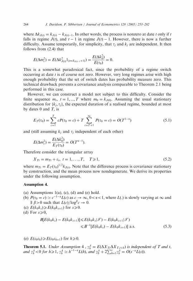
where DkJðtÞ ¼ kJðtÞ � kJðtÞ�1: In other words, the process is nonzero at date t only if t
falls in regime JðtÞ; and t � 1 in regime JðtÞ � 1: However, there is now a furtherdifficulty. Assume temporarily, for simplicity, that tj and kj are independent. It thenfollows from (2.4) that
EðDm2t Þ ¼ EðDk2
JðtÞ1ft¼SJðtÞ�1þ1gÞ ¼EðDk2
0Þ
Eðt0Þ¼ 0:
This is a somewhat paradoxical fact, since the probability of a regime switchoccurring at date t is of course not zero. However, very long regimes arise with highenough probability that the set of switch dates has probability measure zero. Thistechnical drawback prevents a covariance analysis comparable to Theorem 2.1 beingperformed in this case.However, we can construct a model not subject to this difficulty. Consider the
finite sequence mt; t ¼ 1; :::;T where m0 ¼ kJð0Þ: Assuming the usual stationarydistribution for fkj ; tjg; the expected duration of a realised regime, bounded at mostby dates 0 and T, is
ET ðt0Þ ¼XT
c¼1
cPðt0 ¼ cÞ þ TX1
c¼Tþ1
Pðt0 ¼ cÞ ¼ OðT1�aÞ (5.1)
and (still assuming kj and tj independent of each other)
EðDm2t Þ ¼
EðDk20Þ
ET ðt0Þ¼ OðTa�1Þ:
Therefore consider the triangular array
X Tt ¼ mTt þ et; t ¼ 1; . . . ;T ; TX1; (5.2)
where mTt ¼ ET ðt0Þ1=2kJðtÞ: Note that the difference process is covariance stationary
by construction, and the mean process now nondegenerate. We derive its propertiesunder the following assumption.
Assumption 4.
(a)
Assumptions 1(a), (c), (d) and (e) hold. (b) Pðt0 ¼ cÞ ’ c�1�aLðcÞ as c ! 1; 0oao1; where Lð:Þ is slowly varying at 1 and9 b40 such that LðcÞ=logbc ! 0:
(c) Eðk0ksÞXEðk0ksþ1Þ for sX0: (d) For sX0;B½Eðk0ksÞ � Eðk0ksþ1Þ�pEðk0ksjTÞ � Eðk0ksþ1jTÞ
pB�1½Eðk0ksÞ � Eðk0ksþ1Þ� a:s: ð5:3Þ
(e)
Eðe0ehÞXEðe0ehþ1Þ for hX0:Theorem 5.1. Under Assumption 4 , gDh ¼ EðDX TtDX T ;tþhÞ is independent of T and t,and gDho0 for hX1; gDh ’ h�1�aLðhÞ; and gD0 þ 2
Psh¼1g
Dh ¼ Oðs�aLðsÞÞ:
ARTICLE IN PRESS
J. Davidson, P. Sibbertsen / Journal of Econometrics 128 (2005) 253–282 265
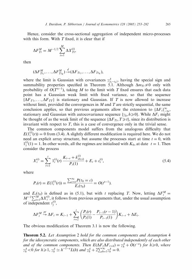
Hence, consider the cross-sectional aggregation of independent micro-processeswith this form. With T fixed, it is clear that if
DF MTt ¼ M�1=2
XMi¼1
DXðiÞTt;
then
ðDFMTt1
; . . . ;DFMTtK
Þ!dðDFTt1 ; . . . ;DFTtK
Þ;
where the limit is Gaussian with covariances gDjtj�tkj; having the special sign and
summability properties specified in Theorem 5.1. Although DmTta0 only withprobability of OðTa�1Þ; taking M to the limit with T fixed ensures that each datapoint has a Gaussian weak limit with fixed variance, so that the sequencefDF T1; . . . ;DFTT g is stationary and Gaussian. If T is now allowed to increasewithout limit, provided the convergences in M and T are strictly sequential, the sameconclusion applies, so that previous arguments allow the extension to fDFtg
1�1;
stationary and Gaussian with autocovariance sequence fgh; hX0g: While DF t mightbe thought of as the weak limit of the sequence fDFTt;TXtg; since its distribution isinvariant with respect to T, this is a case of convergence only in the trivial sense.The common components model suffers from the analogous difficulty that
Eð1ðiÞt ðrÞÞ ¼ 0 from (3.4). A slightly different modification is required here. We do not
need an explicit array structure, but assume the processes start at time t ¼ 0; with1ðiÞ1 ð1Þ ¼ 1: In other words, all the regimes are initialised with K0; at date t ¼ 1: Thenconsider the process
XðiÞt ¼
Xt
r¼1
1ðiÞt ðrÞ
Kt�r þ kðiÞJðt;iÞ
Ptð1Þþ Et þ eðiÞt ; (5.4)
where
PtðrÞ ¼ Eð1ðiÞt ðrÞÞ ¼
P1
c¼rPðt0 ¼ cÞ
Etðt0Þ¼ Oðta�1Þ:
and Etðt0Þ is defined as in (5.1), but with t replacing T. Now, letting DFMt ¼
M�1PM
i¼1DXðiÞt ; it follows from previous arguments that, under the usual assumption
of independent tðiÞj ;
DF Mt !
prDFt ¼ Kt�1 þ
Xt
r¼2
PtðrÞ
Ptð1Þ�
Pt�1ðr � 1Þ
Pt�1ð1Þ
� Kt�r þ DEt:
The obvious modification of Theorem 3.1 is now the following.
Theorem 5.2. Let Assumption 2 hold for the common components and Assumption 4for the idiosyncratic components, which are also distributed independently of each other
and of the common components. Then EðDFtDF tþhÞ ¼ gDh þ Oðt�aÞ for hX0; where
gDho0 for hX1; gDh ’ h�1�aLðhÞ and gD0 þ 2P1
h¼1gDh ¼ 0:
ARTICLE IN PRESS
J. Davidson, P. Sibbertsen / Journal of Econometrics 128 (2005) 253–282266
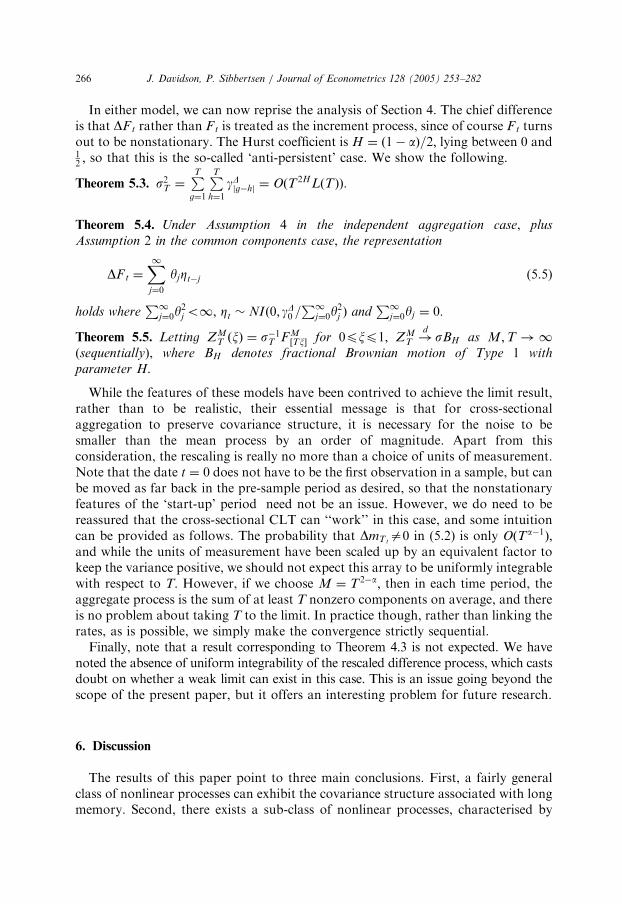
In either model, we can now reprise the analysis of Section 4. The chief differenceis that DF t rather than Ft is treated as the increment process, since of course F t turnsout to be nonstationary. The Hurst coefficient is H ¼ ð1� aÞ=2; lying between 0 and12 ; so that this is the so-called ‘anti-persistent’ case. We show the following.
Theorem 5.3. s2T ¼PTg¼1
PTh¼1
gDjg�hj ¼ OðT2HLðTÞÞ:
Theorem 5.4. Under Assumption 4 in the independent aggregation case, plus
Assumption 2 in the common components case, the representation
DF t ¼X1j¼0
yjZt�j (5.5)
holds whereP1
j¼0y2j o1; Zt � NIð0; gD0 =
P1
j¼0y2j Þ and
P1
j¼0yj ¼ 0:
Theorem 5.5. Letting ZMT ðxÞ ¼ s�1T FM
½Tx� for 0pxp1; ZMT !
dsBH as M ;T ! 1
(sequentially), where BH denotes fractional Brownian motion of Type 1 with
parameter H.
While the features of these models have been contrived to achieve the limit result,rather than to be realistic, their essential message is that for cross-sectionalaggregation to preserve covariance structure, it is necessary for the noise to besmaller than the mean process by an order of magnitude. Apart from thisconsideration, the rescaling is really no more than a choice of units of measurement.Note that the date t ¼ 0 does not have to be the first observation in a sample, but canbe moved as far back in the pre-sample period as desired, so that the nonstationaryfeatures of the ‘start-up’ period need not be an issue. However, we do need to bereassured that the cross-sectional CLT can ‘‘work’’ in this case, and some intuitioncan be provided as follows. The probability that DmTt
a0 in (5.2) is only OðTa�1Þ;and while the units of measurement have been scaled up by an equivalent factor tokeep the variance positive, we should not expect this array to be uniformly integrablewith respect to T. However, if we choose M ¼ T2�a; then in each time period, theaggregate process is the sum of at least T nonzero components on average, and thereis no problem about taking T to the limit. In practice though, rather than linking therates, as is possible, we simply make the convergence strictly sequential.Finally, note that a result corresponding to Theorem 4.3 is not expected. We have
noted the absence of uniform integrability of the rescaled difference process, which castsdoubt on whether a weak limit can exist in this case. This is an issue going beyond thescope of the present paper, but it offers an interesting problem for future research.
6. Discussion
The results of this paper point to three main conclusions. First, a fairly generalclass of nonlinear processes can exhibit the covariance structure associated with longmemory. Second, there exists a sub-class of nonlinear processes, characterised by
ARTICLE IN PRESS
J. Davidson, P. Sibbertsen / Journal of Econometrics 128 (2005) 253–282 267
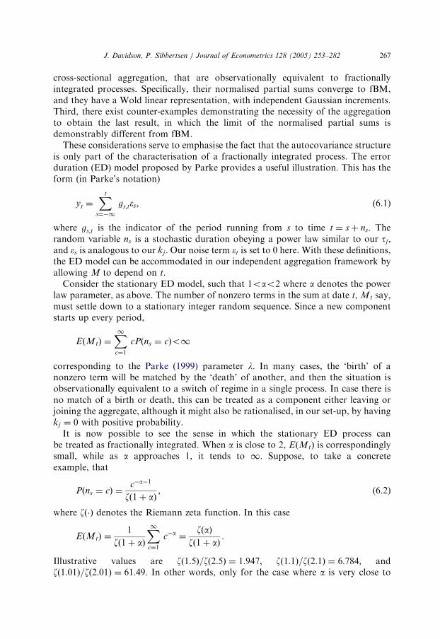
cross-sectional aggregation, that are observationally equivalent to fractionallyintegrated processes. Specifically, their normalised partial sums converge to fBM,and they have a Wold linear representation, with independent Gaussian increments.Third, there exist counter-examples demonstrating the necessity of the aggregationto obtain the last result, in which the limit of the normalised partial sums isdemonstrably different from fBM.These considerations serve to emphasise the fact that the autocovariance structure
is only part of the characterisation of a fractionally integrated process. The errorduration (ED) model proposed by Parke provides a useful illustration. This has theform (in Parke’s notation)
yt ¼Xt
s¼�1
gs;tes; (6.1)
where gs;t is the indicator of the period running from s to time t ¼ s þ ns: Therandom variable ns is a stochastic duration obeying a power law similar to our tj ;and es is analogous to our kj : Our noise term et is set to 0 here. With these definitions,the ED model can be accommodated in our independent aggregation framework byallowing M to depend on t.Consider the stationary ED model, such that 1oao2 where a denotes the power
law parameter, as above. The number of nonzero terms in the sum at date t, Mt say,must settle down to a stationary integer random sequence. Since a new componentstarts up every period,
EðMtÞ ¼X1c¼1
cPðns ¼ cÞo1
corresponding to the Parke (1999) parameter l: In many cases, the ‘birth’ of anonzero term will be matched by the ‘death’ of another, and then the situation isobservationally equivalent to a switch of regime in a single process. In case there isno match of a birth or death, this can be treated as a component either leaving orjoining the aggregate, although it might also be rationalised, in our set-up, by havingkj ¼ 0 with positive probability.It is now possible to see the sense in which the stationary ED process can
be treated as fractionally integrated. When a is close to 2, EðMtÞ is correspondinglysmall, while as a approaches 1, it tends to 1: Suppose, to take a concreteexample, that
Pðns ¼ cÞ ¼c�a�1
zð1þ aÞ; (6.2)
where zð�Þ denotes the Riemann zeta function. In this case
EðMtÞ ¼1
zð1þ aÞ
X1c¼1
c�a ¼zðaÞ
zð1þ aÞ:
Illustrative values are zð1:5Þ=zð2:5Þ ¼ 1:947; zð1:1Þ=zð2:1Þ ¼ 6:784; andzð1:01Þ=zð2:01Þ ¼ 61:49: In other words, only for the case where a is very close to
ARTICLE IN PRESS
J. Davidson, P. Sibbertsen / Journal of Econometrics 128 (2005) 253–282268
the nonstationary case of unity (corresponding to the IðdÞ process with d close to 0.5)is the number of terms in the aggregate large. Clearly, the central limit theoremcannot be invoked to justify Gaussianity in this process. While it may be that theshocks et themselves are Gaussian, yt is the sum of a randomly varying number ofindependent terms, and therefore its marginal distribution would be mixed Gaussianin that case. From this point of view, we must be careful to distinguish between thestationary ED process and the fractionally integrated process. In particular, thepartial sums of the former process do not converge to fBM, in general.In the nonstationary case of (6.1) the number of terms in the sum increases with
time, and the conventional argument from time aggregation appears to imply aGaussian limit. In view of the covariance structure demonstrated in Parke (1999),this suggests possible convergence to fBM with 1
2odo1: However, the proof of thisconjecture would require a different approach to that adopted for Theorem 4.2. Notethat even with Gaussian shocks, a linear representation of the form (5.5) does nothold for the difference process; this is
Dyt ¼ et �Xt�1
s¼�1
Dgs;tes;
where the number of nonzero terms for sot is a random variable with mean fallingbetween zero and 1.Unlike the ED model, the models constructed by Diebold and Inoue (2001) are
explicitly ‘false’, in the sense that they define stochastic arrays in which the incidenceof regime shifting is linked to sample size. In all of their cases, allowing the samplesize to increase sufficiently would reveal that the processes are nonlinear randomwalks, having the covariance characteristics of an Ið1Þ process. The message of theseauthors is that modellers face a hazard of mis-identification, because the incidence ofstructural change is adventitiously linked to the length of available series.However, like Parke (1999), they focus wholly on the issue of the autocovariance
structure. This, as we have shown, is only one defining characteristic of a fractionallyintegrated process, and we have highlighted the existence of a linear representationas another. The nature of the connection between these features can be clarifiedinformally by ‘discretizing’ the fBM. Let X ðxÞ; 0pxp1; be fBM with Hurstparameter H and, for convenience, normalised such that EX ð1Þ2 ¼ 1: Fix a finiteinteger nX1 and consider the sequence
xnt ¼ ð2nÞ2HðX ððt þ 1Þ=2n þ 1
2Þ � X ðt=2n þ 1
2ÞÞ; t ¼ �n; . . . ; ðn � 1Þ: (6.3)
Then note that xnt � Nð0; 1Þ by construction, and also, as would be expected,
Theorem 6.1. Eðxntxn;tþhÞ ’ h2H�2:
Taking n large, let an approximate Wold decomposition, truncated at n lags, beapplied to the sequence xn1; . . . ;xnn: In view of the Gaussianity, the shock processin this decomposition is independently distributed, and in view of the autocovariancestructure, it can also be seen that the linear representation approximates tothe fractional integration model. What this shows is that if a partial sum process
ARTICLE IN PRESS
J. Davidson, P. Sibbertsen / Journal of Econometrics 128 (2005) 253–282 269
converges to fBM, then under some degree of time aggregation (averagingsuccessive blocks of observations of length ½Tb� for 0obo1; say) the time-aggregated sequence (with ½T1�b� þ 1 terms) should possess an increasingly exactlinear representation, as T increases. We suggest the value of this remark is to showthat, even if we do not postulate that the process in question is exactly linear in thesense of Theorem 4.1, there always exists a natural approach to distinguishingprocesses having fBM as their weak limit from alternatives. This is by tests oflinearity.
7. Testing linearity
In this section we attempt to quantify the practical role of our result, as anapproximation theorem, by means of a small simulation experiment. A test oflinearity is applied to generated models in the ‘aggregate-of-independent-regimes’class. If the approximation is good with even a small M then arguably the result ismore tolerant of failure of the assumptions, but this behaviour will clearly depend onthe value of a; among other factors. We do not consider the common componentsmodel here, but since it is the independence of switch dates that delivers the crucialaggregation property in each case, the experiment should have quite generalimplicationsFor practical purposes we have to limit consideration to a class of linear
parametric models with the right covariance structure, and the ARFIMA(p; d; q)class is the natural choice for this purpose. It is true that the class of models in ournull hypothesis is larger than the ARFIMA class, but there are reasonable groundsto think that the ARFIMA class can approximate any linear process with therequisite properties pretty well. This is not a Monte Carlo study, since there is nospecial interest in determining the distribution of the estimators. The approximatingARFIMA models are simply fitted to large samples, of 20,000 data points each, sothat the parameter estimates can be regarded as close to their probability limits. Tosimplify the model selection process, the class of models considered is restricted tothe ARFIMA(p; d; 0), and p was chosen to optimise the value of the consistentSchwarz (1978) criterion. For the selected equation, test statistics for modeladequacy were recorded.Our chosen diagnostic test for nonlinearity is the McLeod and Li (1983)
portmanteau test, corresponding to the Box–Pierce statistic computed for thesquared residuals. Although there are several possible tests for linearity, this one isappropriate since correlation in the squares is a natural dummy alternativehypothesis. Forcing a linear representation onto a process exhibiting periodic jumpsin the local mean is likely to induce conditional heteroscedasticity, in the form ofruns of larger than average residuals in the neighbourhood of the jumps. There istherefore hope that this test should be relatively powerful against the alternatives ofinterest. The Brock-Dechert-Scheinkman test of residual independence (Brock et al.,1996) was also considered, but in preliminary experiments this proved to have ratherlow power by comparison.
ARTICLE IN PRESS
Table 1
a ¼ 1:5; s2� ¼ 0:2
M 100 20 10 5 1
d 0.31 0.31 0.31 0.30 0.28
p 2 2 2 2 2
lmax 0.37 0.38 0.39 0.42 0.42
B-P(25) 28 15 18 16 11
M-L(25) 29 45 115 222 1027
J. Davidson, P. Sibbertsen / Journal of Econometrics 128 (2005) 253–282270
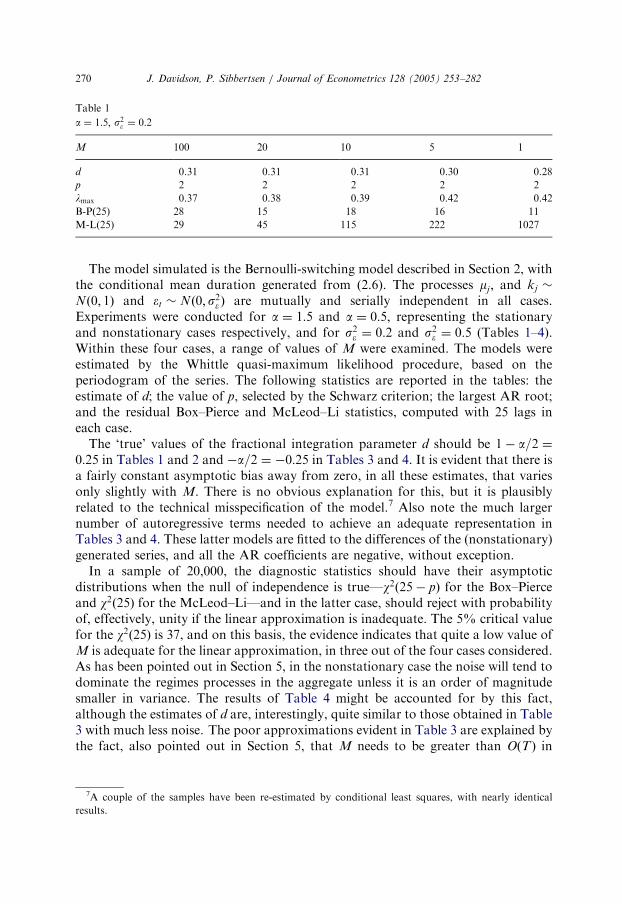
The model simulated is the Bernoulli-switching model described in Section 2, withthe conditional mean duration generated from (2.6). The processes mj ; and kj �
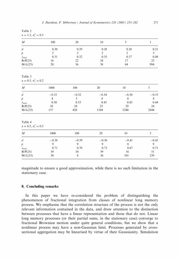
Nð0; 1Þ and et � Nð0; s2e Þ are mutually and serially independent in all cases.Experiments were conducted for a ¼ 1:5 and a ¼ 0:5; representing the stationaryand nonstationary cases respectively, and for s2e ¼ 0:2 and s2e ¼ 0:5 (Tables 1–4).Within these four cases, a range of values of M were examined. The models wereestimated by the Whittle quasi-maximum likelihood procedure, based on theperiodogram of the series. The following statistics are reported in the tables: theestimate of d; the value of p, selected by the Schwarz criterion; the largest AR root;and the residual Box–Pierce and McLeod–Li statistics, computed with 25 lags ineach case.The ‘true’ values of the fractional integration parameter d should be 1� a=2 ¼
0:25 in Tables 1 and 2 and �a=2 ¼ �0:25 in Tables 3 and 4. It is evident that there isa fairly constant asymptotic bias away from zero, in all these estimates, that variesonly slightly with M. There is no obvious explanation for this, but it is plausiblyrelated to the technical misspecification of the model.7 Also note the much largernumber of autoregressive terms needed to achieve an adequate representation inTables 3 and 4. These latter models are fitted to the differences of the (nonstationary)generated series, and all the AR coefficients are negative, without exception.In a sample of 20,000, the diagnostic statistics should have their asymptotic
distributions when the null of independence is true—w2ð25� pÞ for the Box–Pierceand w2ð25Þ for the McLeod–Li—and in the latter case, should reject with probabilityof, effectively, unity if the linear approximation is inadequate. The 5% critical valuefor the w2ð25Þ is 37, and on this basis, the evidence indicates that quite a low value ofM is adequate for the linear approximation, in three out of the four cases considered.As has been pointed out in Section 5, in the nonstationary case the noise will tend todominate the regimes processes in the aggregate unless it is an order of magnitudesmaller in variance. The results of Table 4 might be accounted for by this fact,although the estimates of d are, interestingly, quite similar to those obtained in Table3 with much less noise. The poor approximations evident in Table 3 are explained bythe fact, also pointed out in Section 5, that M needs to be greater than OðTÞ in
7A couple of the samples have been re-estimated by conditional least squares, with nearly identical
results.
ARTICLE IN PRESS
Table 2
a ¼ 1:5; s2� ¼ 0:5
M 100 20 10 5 1
d 0.30 0.29 0.28 0.28 0.21
p 2 2 2 2 3
lmax 0.31 0.32 0.35 0.37 0.49
B-P(25) 16 22 24 17 25
M-L(25) 20 36 38 64 994
Table 3
a ¼ 0:5; s2� ¼ 0:2
M 1000 100 20 10 5
d �0.33 �0.32 �0.34 �0.30 �0.33
p 4 5 4 4 4
lmax 0.50 0.53 0.45 0.43 0.44
B-P(25) 10 10 25 29 24
M-L(25) 137 428 1104 2240 2844
Table 4
a ¼ 0:5; s2� ¼ 0:5
M 1000 100 20 10 5
d �0.38 �0.39 �0.36 �0.41 �0.42
p 9 9 9 8 9
lmax 0.71 0.70 0.72 0.67 0.71
B-P(25) 39 10 59 16 51
M-L(25) 30 8 36 101 239
J. Davidson, P. Sibbertsen / Journal of Econometrics 128 (2005) 253–282 271
magnitude to ensure a good approximation, while there is no such limitation in thestationary case.
8. Concluding remarks
In this paper we have re-considered the problem of distinguishing thephenomenon of fractional integration from classes of nonlinear long memoryprocess. We emphasise that the correlation structure of the process is not the onlyrelevant information contained in the data, and draw attention to the distinctionbetween processes that have a linear representation and those that do not. Linearlong memory processes (or their partial sums, in the stationary case) converge tofractional Brownian motion under quite general conditions, but we show that anonlinear process may have a non-Gaussian limit. Processes generated by cross-sectional aggregation may be linearised by virtue of their Gaussianity. Simulation
ARTICLE IN PRESS
J. Davidson, P. Sibbertsen / Journal of Econometrics 128 (2005) 253–282272
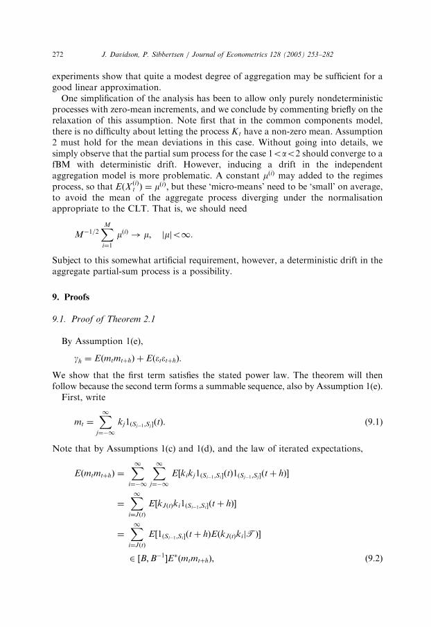
experiments show that quite a modest degree of aggregation may be sufficient for agood linear approximation.One simplification of the analysis has been to allow only purely nondeterministic
processes with zero-mean increments, and we conclude by commenting briefly on therelaxation of this assumption. Note first that in the common components model,there is no difficulty about letting the process Kt have a non-zero mean. Assumption2 must hold for the mean deviations in this case. Without going into details, wesimply observe that the partial sum process for the case 1oao2 should converge to afBM with deterministic drift. However, inducing a drift in the independentaggregation model is more problematic. A constant mðiÞ may added to the regimesprocess, so that EðX
ðiÞt Þ ¼ mðiÞ; but these ‘micro-means’ need to be ‘small’ on average,
to avoid the mean of the aggregate process diverging under the normalisationappropriate to the CLT. That is, we should need
M�1=2XMi¼1
mðiÞ ! m; jmjo1:
Subject to this somewhat artificial requirement, however, a deterministic drift in theaggregate partial-sum process is a possibility.
9. Proofs
9.1. Proof of Theorem 2.1
By Assumption 1(e),
gh ¼ EðmtmtþhÞ þ EðetetþhÞ:
We show that the first term satisfies the stated power law. The theorem will thenfollow because the second term forms a summable sequence, also by Assumption 1(e).First, write
mt ¼X1
j¼�1
kj1ðSj�1;Sj �ðtÞ: (9.1)
Note that by Assumptions 1(c) and 1(d), and the law of iterated expectations,
EðmtmtþhÞ ¼X1
i¼�1
X1j¼�1
E½kikj1ðSi�1;Si �ðtÞ1ðSj�1;Sj �ðt þ hÞ�
¼X1
i¼JðtÞ
E½kJðtÞki1ðSi�1;Si �ðt þ hÞ�
¼X1
i¼JðtÞ
E½1ðSi�1;Si �ðt þ hÞEðkJðtÞkijTÞ�
2 ½B;B�1�E�ðmtmtþhÞ; ð9:2Þ
ARTICLE IN PRESS
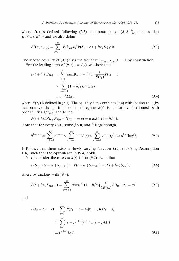
J. Davidson, P. Sibbertsen / Journal of Econometrics 128 (2005) 253–282 273
where JðtÞ is defined following (2.3), the notation x 2 ½B;B�1�y denotes thatBypxpB�1y and we also define
E�ðmtmtþhÞ ¼X1
i¼JðtÞ
EðkJðtÞkiÞPðSi�1ot þ hpSiÞX0: (9.3)
The second equality of (9.2) uses the fact that 1ðSJðtÞ�1;SJðtÞ�ðtÞ ¼ 1 by construction.For the leading term of (9.2) i ¼ JðtÞ; we show that
Pðt þ hpSJðtÞÞ ¼X1c¼1
maxf0; ð1� h=cÞgc
Eðt0ÞPðt0 ¼ cÞ
’X1
c¼hþ1
ð1� h=cÞc�aLðcÞ
’ h1�aLðhÞ; ð9:4Þ
where Eðt0Þ is defined in (2.3). The equality here combines (2.4) with the fact that (bystationarity) the position of t in regime JðtÞ is uniformly distributed withprobabilities 1=tJðtÞ; and hence
Pðt þ hpSJðtÞjSJðtÞ � SJðtÞ�1 ¼ cÞ ¼ maxf0; ð1� h=cÞg:
Note that for every e40; some b40; and h large enough,
h1�a�e’X1
c¼hþ1
c�a�eoX1
c¼hþ1
c�aLðcÞoX1
c¼hþ1
c�alogbc ’ h1�alogbh: (9.5)
It follows that there exists a slowly varying function LðhÞ; satisfying Assumption1(b), such that the equivalence in (9.4) holds.Next, consider the case i ¼ JðtÞ þ 1 in (9.2). Note that
PðSJðtÞot þ hpSJðtÞþ1Þ ¼ Pðt þ hpSJðtÞþ1Þ � Pðt þ hpSJðtÞÞ; (9.6)
where by analogy with (9.4),
Pðt þ hpSJðtÞþ1Þ ¼X1
c¼hþ1
maxf0; ð1� h=cÞgc
2Eðt0ÞPðt0 þ t1 ¼ cÞ (9.7)
and
Pðt0 þ t1 ¼ cÞ ¼Xc�1j¼1
Pðt1 ¼ c � t0jt0 ¼ jÞPðt0 ¼ jÞ
’Xc�1j¼1
ðc � jÞ�1�aj�1�aLðc � jÞLðjÞ
’ c�1�aLðcÞ ð9:8Þ
ARTICLE IN PRESS
J. Davidson, P. Sibbertsen / Journal of Econometrics 128 (2005) 253–282274
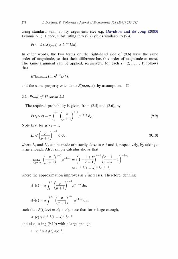
using standard summability arguments (see e.g. Davidson and de Jong (2000)Lemma A.1). Hence, substituting into (9.7) yields similarly to (9.4)
Pðt þ hpSJðtÞþ1Þ ’ h1�aLðhÞ:
In other words, the two terms on the right-hand side of (9.6) have the sameorder of magnitude, so that their difference has this order of magnitude at most.The same argument can be applied, recursively, for each i ¼ 2; 3; . . . : It followsthat
E�ðmtmtþhÞ ’ h1�aLðhÞ:
and the same property extends to EðmtmtþhÞ; by assumption. &
9.2. Proof of Theorem 2.2
The required probability is given, from (2.5) and (2.6), by
Pðtj4cÞ ¼ aZ 1
1
mmþ 1
� c�1
m�1�a dm: (9.9)
Note that for m4c � 1;
Lcpm
mþ 1
� c�1
pUc; (9.10)
where Lc and Uc can be made arbitrarily close to e�1 and 1, respectively, by taking c
large enough. Also, simple calculus shows that
max1pmo1
mmþ 1
� c�1
m�1�a ¼ 1�1þ ac � 1
� c�1c � 1
1þ a� 1
� �1�a
� e�1�að1þ aÞ1þac�1�a;
where the approximation improves as c increases. Therefore, defining
A1ðcÞ ¼ aZ c
1
mmþ 1
� c�1
m�1�a dm;
A2ðcÞ ¼ aZ 1
c
mmþ 1
� c�1
m�1�a dm;
such that PðtjXcÞ ¼ A1 þ A2; note that for c large enough,
A1ðcÞpe�1�að1þ aÞ1þac�a
and also, using (9.10) with c large enough,
e�1c�apA2ðcÞpc�a:
ARTICLE IN PRESS
J. Davidson, P. Sibbertsen / Journal of Econometrics 128 (2005) 253–282 275
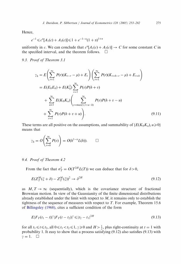
Hence,
e�1pca½A1ðcÞ þ A2ðcÞ�p1þ e�1�að1þ aÞ1þa
uniformly in c. We can conclude that ca½A1ðcÞ þ A2ðcÞ� ! C for some constant C inthe specified interval, and the theorem follows. &
9.3. Proof of Theorem 3.1
gh ¼ EX1r¼1
PðrÞðKt�r � mÞ þ Et
! X1r¼1
PðrÞðKtþh�r � mÞ þ Etþh
!
¼ EðE0EhÞ þ EðK20ÞX1v¼1
PðvÞPðh þ vÞ
þX1u¼1
EðK0KuÞX1
v¼maxð1;1þu�hÞ
PðvÞPðh þ v � uÞ
þX1v¼1
PðvÞPðh þ v þ uÞ
!: ð9:11Þ
These terms are all positive on the assumptions, and summability of fEðK0KuÞ; uX0gmeans that
gh ¼ OX1v¼h
PðvÞ
!¼ Oðh1�aLðhÞÞ: &
9.4. Proof of Theorem 4.2
From the fact that s2T ¼ OðT2HLðTÞÞ we can deduce that for d40;
EðZMT ðxþ dÞ � ZM
T ðxÞÞ2 ! d2H (9.12)
as M;T ! 1 (sequentially), which is the covariance structure of fractionalBrownian motion. In view of the Gaussianity of the finite dimensional distributionsalready established under the limit with respect to M, it remains only to establish thetightness of the sequence of measures with respect to T : For example, Theorem 15.6of Billingsley (1968), cites a sufficient condition of the form
EjFT ðt1 � tÞjgjFT ðt � t2Þjgpjt2 � t1j
2H (9.13)
for all t1ptpt2; all 0pt1ot2p1; gX0 and H4 12; plus right-continuity at t ¼ 1 with
probability 1. It easy to show that a process satisfying (9.12) also satisfies (9.13) withg ¼ 1: &
ARTICLE IN PRESS
J. Davidson, P. Sibbertsen / Journal of Econometrics 128 (2005) 253–282276
9.5. Proof of Theorem 4.3
Assume without loss of generality that S0 ¼ 0: Since tj is the duration of regime j,
½T1=aLðTÞ��1X½Tx�
t¼1
X t ¼ ½T1=aLðTÞ��1XJð½Tx�Þ�1
j¼1
kjtj
þ kJð½Tx�Þð½Tx� � SJð½Tx�Þ�1Þ þX½Tx�
t¼1
et
!
¼ sk½JðTÞ1=aLðJðTÞÞ��1
XJð½Tx�Þ�1
j¼1
Uj þ opð1Þ;
where JðTÞ is defined following (2.3) and
Uj ¼ EðtjÞ�1=a kjtj
sk
noting that, since T ¼PJðTÞ
j¼1 tj where tj is an i.i.d. and integrable random variable,
JðTÞ1=aLðTÞ
T1=aLðJðTÞÞ!pr
EðtjÞ�1=a:
Further note that Uj is an i.i.d., zero-mean random variable. By Assumption 3(b)
Pðjkjjtj4cÞ ¼
Zftj4cg
Pðs�1k jkjj4c=tjjtjÞdF ðtjÞ þ oðc�aÞ:
Also note that
C1Pðtj4cÞpZftj4cg
Pðs�1k jkjj4c=tjjtjÞdF ðtjÞpPðtj4cÞ;
where C1 is an almost sure lower bound of Pðs�1k jkjj41jtjÞ; and C140 since arandom variable with unit variance must have positive probability mass above 1.Hence
PðjUjj4cÞ ’ Pðtj4cÞ ’ c�aLðcÞ:
Let FU denote the c.d.f. of Uj : Since EðkjÞ ¼ 0 and tj40; both tails of thedistribution obey the power law such that
1� F U ðcÞ ’ c�aLðaÞ; F U ð�cÞ ’ c�aLðaÞ:
Thus, we have
1� F U ðxcÞ
1� F U ðcÞ! x�a;
FU ð�xcÞ
FU ð�cÞ! x�a:
According to (e.g.) Theorem 9.34 of Breiman (1968), this condition is necessary andsufficient for F U to lie in the domain of attraction of a stable law with parameter a:
ARTICLE IN PRESS
J. Davidson, P. Sibbertsen / Journal of Econometrics 128 (2005) 253–282 277
In other words,
a�1JðTÞ
XJð½Tx�Þ�1
j¼1
Uj � bJðTÞ
!!dLaðxÞ;
where
nPðUj4ancÞ ! c�a as n ! 1 (9.14)
and bT ! 0: Note that setting an ¼ n1=aLðnÞ for a suitably chosen slowlyvarying function L solves (9.14) (see Davis (1983), or e.g. Feller (1966) Sections9.6 and 17.5). Finally, the theorem follows by application of (e.g.) Embrechts et al.(1997) Theorem 2.4.10. &
9.6. Proof of Theorem 5.1
In the following let T be finite, but large enough to allow consideration of hoT aslarge as desired. Defining the T-measurable random variable Qðt; uÞ ¼
Pu�1s¼0 tJðtÞþs;
note that
PðQðt; uÞ ¼ hÞ ’ h�1�aLðhÞ;
for any t and u40; following from arguments in the proof of Theorem 2.1. Next notethat
DmTtDmT ;tþh ¼
ET ðt0ÞDk2JðtÞ t ¼ SJðtÞ�1 þ 1; h ¼ 0
ET ðt0ÞDkJðtÞDkJðtÞþu; t ¼ SJðtÞ�1 þ 1; h ¼ Qðt; uÞ
0; otherwise:
8><>:
Applying arguments similar to those in the proof of Theorem 2.1, it follows usingAssumption 1(d) that
EðDm2TtÞ 2 ½B;B�1�EðDk2
0Þ (9.15)
and
EðDmTtDmT ;tþhÞ 2 ½B;B�1�X1u¼1
EðDk0DkuÞPðQð0; uÞ ¼ hÞ
’ h�1�aLðhÞ ð9:16Þ
from Assumption 4(b). It follows from the fact that ftjg has a stationary distributionthat the sequence defined by (9.15) and (9.16) is independent of t and T.Therefore, consider
gDh ¼ EðDmTtDmTtþhÞ þ EðDetDetþhÞ; (9.17)
where the cross-products vanish by Assumption 4(e). The assumption furtherensures the second right-hand side term is of smaller order in h than the first one.
ARTICLE IN PRESS
J. Davidson, P. Sibbertsen / Journal of Econometrics 128 (2005) 253–282278
Under stationarity and Assumption 4,
EðDk0DkuÞ ¼ 2½Eðk0kuÞ � Eðk0ku�1Þ�
EðDe0DeuÞ ¼ 2½Eðe0euÞ � Eðe0eu�1Þ�
�o0; u ¼ 1;
p0; uX2:
�(9.18)
These results therefore show that gDho0 for h40; and also that gDh ’ h�1�aLðhÞ:Next,note that for any covariance stationary random sequence xt;
EðDx2t Þ þ 2EðDxtDxt�1Þ þ � � � þ 2EðDxtDxt�hÞ
¼ Eðxt � xt�1Þðxt þ xt�1 � 2xt�h�1Þ
¼ 2½EðxtxtþhÞ � Eðxtxtþhþ1Þ�: ð9:19Þ
Therefore, in view of (9.15), (9.16) and the assumptions, and since (9.19) also appliesto et; we conclude from (9.17) and (9.18) that
gD0 þ 2Xs
h¼1
gDh ¼ Oðs�aLðsÞÞ: &
9.7. Proof of Theorem 5.2
Note first that we can write
DF t ¼ Kt�1 þXt�1r¼1
xtrKt�r�1 þ DEt;
where
�xtr ¼Pt�1ðrÞ
Pt�1ð1Þ�
Ptðr þ 1Þ
Ptð1Þ
¼Pðt0 ¼ rÞPt
c¼1 Pðt0 ¼ cÞ�
Pðt0 ¼ tÞPr�1
c¼1Pðt0 ¼ cÞPt�1c¼1Pðt0 ¼ cÞ
Ptc¼1 Pðt0 ¼ cÞ
¼ Pðt0¼ rÞ þ Oðt�aLðrÞÞ:
Letting DF�t ¼ Kt�1 þ
P1
r¼1Pðt0 ¼ rÞKt�r�1 þ DEt; note that DFnt is stationary and
EðDF t � DFnt Þ2¼ Oðt�aÞ; so we do the calculations for DFn
t : To fix ideas, considerinitially the case of Kt serially uncorrelated. In this case, substituting into theformula in (9.11), replacing Pð1Þ by 1 and Pðv þ 1Þ by �Pðt0 ¼ vÞ for 1pvot; and 0otherwise, yields
gD0 ¼ EðDE20Þ þ EðK2
0Þ 1þX1v¼1
Pðt0 ¼ vÞ2
!
gDh ¼ EðDE0DEhÞ þ EðK20Þ �Pðt0 ¼ hÞ þ
X1v¼1
Pðt0 ¼ vÞPðt0 ¼ h þ vÞ
!; hX1:
Verify first that these terms are Oðh�1�aÞ; and second that they are negative for hX1;
which in respect of EðDE0DEhÞ follows from (9.18) and Assumption 2(c). Third,
ARTICLE IN PRESS
J. Davidson, P. Sibbertsen / Journal of Econometrics 128 (2005) 253–282 279
observe that
1þX1v¼1
Pðt0 ¼ vÞ2 þ 2X1h¼1
�Pðt0 ¼ hÞ þX1v¼1
Pðt0 ¼ vÞPðt0 ¼ h þ vÞ
!
¼ 1�X1v¼1
Pðt0 ¼ vÞ
!2
¼ 0:
These results, together with (9.19) in respect of the terms in EðDE0DEhÞ; imply, asrequired,
gD0 þ 2X1h¼1
gD0 ¼ 0:
To extend these results to the case of serially correlated Kt; consider (9.11) again, andnote that for any sequence PðvÞ; and all u40;
X1v¼maxð1;1þuÞ
PðvÞPðv � uÞ þX1v¼1
PðvÞPðv þ uÞ
þ 2X1h¼1
X1v¼maxð1;1þu�hÞ
PðvÞPðh þ v � uÞ þX1v¼1
PðvÞPðh þ v þ uÞ
!
¼ 2X1v¼1
PðvÞ
!2
: &
9.8. Proof of Theorem 5.3
Theorem 5.1 establishes that, for any fixed g,P1
h¼�1gDjg�hj ¼ 0: Hence, 0XgDh ’
h2H�2LðhÞ implies that
XT
h¼�T
gDjg�hj ¼ �X�T�1
h¼�1
þX1
h¼Tþ1
!gDjg�hj ’
X1h¼Tþ1
h2H�2LðhÞ ’ T2H�1LðTÞ;
where the final rate of convergence follows, under Assumption 4(b), by an argumentanalogous to (9.5). &
9.9. Proof of Theorem 5.4
The linear structure with independent increments follows from Wold’s Theoremand the Gaussianity, exactly as for the case 1oao2; and it remains to establish thesummation properties of the coefficients. Note that FT ¼
PTs¼1DF s ¼
PTt¼�1aTtZt;
ARTICLE IN PRESS
J. Davidson, P. Sibbertsen / Journal of Econometrics 128 (2005) 253–282280
where
aTt ¼
PT�t
j¼0
yj ; t40;
PT�t
j¼1�t
yj ; tp0:
8>>><>>>:
(9.20)
Hence
EðF2T Þ ¼ s2Z
XT
t¼�1
a2Tt ¼ s2ZX0
t¼�1
XT�t
j¼1�t
yj
!2
þ s2ZXT
t¼1
XT�t
j¼0
yj
!2
: (9.21)
However, we also know from Theorem 5.3 that
EðF2T Þ ¼ OðT1�aLðTÞÞ:
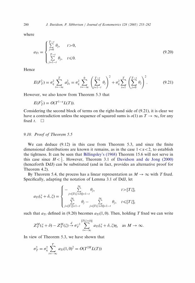
Considering the second block of terms on the right-hand side of (9.21), it is clear wehave a contradiction unless the sequence of squared sums is oð1Þ as T ! 1; for anyfixed t. &
9.10. Proof of Theorem 5.5
We can deduce (9.12) in this case from Theorem 5.3, and since the finitedimensional distributions are known it remains, as in the case 1oao2; to establishthe tightness. It can be seen that Billingsley’s (1968) Theorem 15.6 will not serve inthis case since Ho 1
2: However, Theorem 3.1 of Davidson and de Jong (2000)
(henceforth DdJ) can be substituted (and in fact, provides an alternative proof forTheorem 4.2).By Theorem 5.4, the process has a linear representation as M ! 1 with T fixed.
Specifically, adapting the notation of Lemma 3.1 of DdJ, let
aTtðxþ d; xÞ ¼
�P1
j¼½TðxþdÞ�þ1�t
yj ; t4½Tx�;
P1j¼½Tx�þ1�t
yj �P1
j¼½TðxþdÞ�þ1�t
yj ; tp½Tx�;
8>>><>>>:
such that aTt defined in (9.20) becomes aTtð1; 0Þ: Then, holding T fixed we can write
ZMT ðxþ dÞ � ZM
T ðxÞ!ds�1T
X½TðxþdÞ�
t¼�1
aTtðxþ d; xÞZt as M ! 1:
In view of Theorem 5.3, we have shown that
s2T ¼ s2ZXT
t¼�1
aTtð1; 0Þ2¼ OðT2HLðTÞÞ
ARTICLE IN PRESS
J. Davidson, P. Sibbertsen / Journal of Econometrics 128 (2005) 253–282 281
and hence,
s�2T s2ZX½TðxþdÞ�
t¼�1
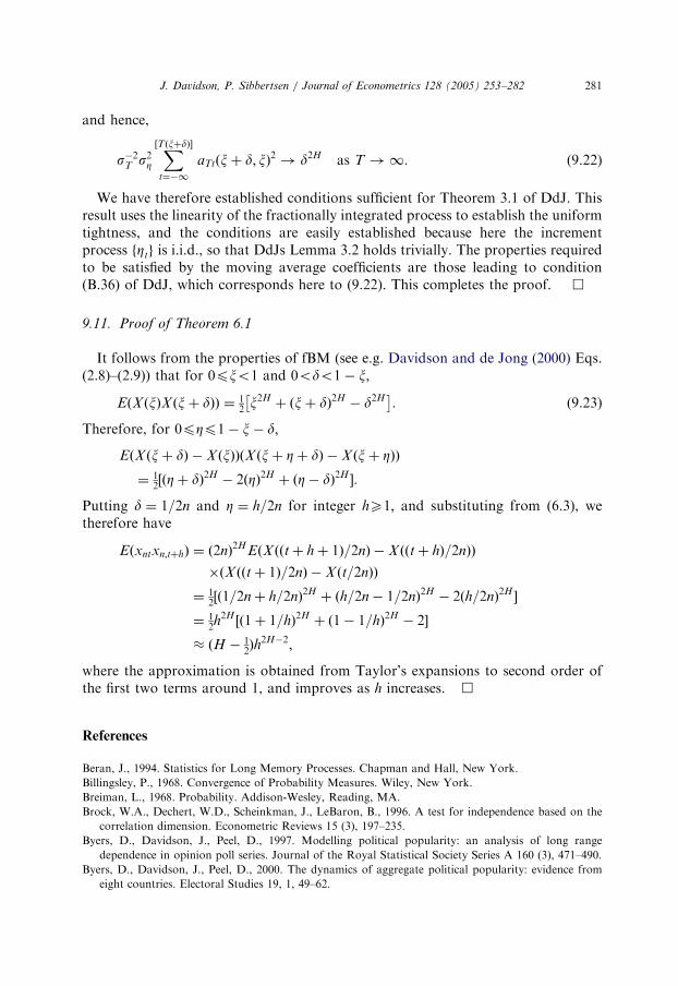
aTtðxþ d; xÞ2 ! d2H as T ! 1: (9.22)
We have therefore established conditions sufficient for Theorem 3.1 of DdJ. Thisresult uses the linearity of the fractionally integrated process to establish the uniformtightness, and the conditions are easily established because here the incrementprocess fZtg is i.i.d., so that DdJs Lemma 3.2 holds trivially. The properties requiredto be satisfied by the moving average coefficients are those leading to condition(B.36) of DdJ, which corresponds here to (9.22). This completes the proof. &
9.11. Proof of Theorem 6.1
It follows from the properties of fBM (see e.g. Davidson and de Jong (2000) Eqs.(2.8)–(2.9)) that for 0pxo1 and 0odo1� x;
EðX ðxÞX ðxþ dÞÞ ¼ 12x2H
þ ðxþ dÞ2H� d2H
� �: (9.23)
Therefore, for 0pZp1� x� d;
EðX ðxþ dÞ � X ðxÞÞðX ðxþ Zþ dÞ � X ðxþ ZÞÞ
¼ 12½ðZþ dÞ2H
� 2ðZÞ2Hþ ðZ� dÞ2H
�:
Putting d ¼ 1=2n and Z ¼ h=2n for integer hX1; and substituting from (6.3), wetherefore have
Eðxntxn;tþhÞ ¼ ð2nÞ2HEðX ððt þ h þ 1Þ=2nÞ � X ððt þ hÞ=2nÞÞ
�ðX ððt þ 1Þ=2nÞ � X ðt=2nÞÞ
¼ 12½ð1=2n þ h=2nÞ2H
þ ðh=2n � 1=2nÞ2H� 2ðh=2nÞ2H
�
¼ 12h2H
½ð1þ 1=hÞ2Hþ ð1� 1=hÞ2H
� 2�
� ðH � 12Þh2H�2;
where the approximation is obtained from Taylor’s expansions to second order ofthe first two terms around 1, and improves as h increases. &
References
Beran, J., 1994. Statistics for Long Memory Processes. Chapman and Hall, New York.
Billingsley, P., 1968. Convergence of Probability Measures. Wiley, New York.
Breiman, L., 1968. Probability. Addison-Wesley, Reading, MA.
Brock, W.A., Dechert, W.D., Scheinkman, J., LeBaron, B., 1996. A test for independence based on the
correlation dimension. Econometric Reviews 15 (3), 197–235.
Byers, D., Davidson, J., Peel, D., 1997. Modelling political popularity: an analysis of long range
dependence in opinion poll series. Journal of the Royal Statistical Society Series A 160 (3), 471–490.
Byers, D., Davidson, J., Peel, D., 2000. The dynamics of aggregate political popularity: evidence from
eight countries. Electoral Studies 19, 1, 49–62.
ARTICLE IN PRESS
J. Davidson, P. Sibbertsen / Journal of Econometrics 128 (2005) 253–282282
Byers, D., Davidson, J., Peel, D., 2002. Modelling political popularity: a correction. Journal of the Royal
Statistical Society A 165, 1, 187–189.
Davidson, J., 1994. Stochastic Limit Theory: An Introduction for Econometricians. Oxford University
Press, Oxford.
Davidson, J., 2000. Econometric Theory. Blackwell Publishers, Oxford.
Davidson, J., 2002a. Establishing conditions for the functional central limit theorem in nonlinear and
semiparametric time series processes. Journal of Econometrics 106, 243–269.
Davidson, J., 2002b. A model of fractional cointegration, and tests for cointegration using the bootstrap.
Journal of Econometrics 110, 187–212.
Davidson, J., de Jong, R.M., 2000. The functional central limit theorem and weak convergence to
stochastic integrals II: fractionally integrated processes. Econometric Theory 16, 5, 621–642.
Davis, R.A., 1983. Stable limits for partial sums of dependent random variables. Annals of Probability 11
(2), 262–269.
Diebold, F.X., Inoue, A., 2001. Long memory and regime switching. Journal of Econometrics 105,
131–159.
Ding, Z., Granger, C.W.J., 1996. Modelling volatility persistence of speculative returns: a new approach.
Journal of Econometrics 73, 185–215.
Embrechts, P., Kluppelberg, C., Mikosch, T., 1997. Modelling Extremal Events. Springer, Berlin.
Feller, W., 1966. An Introduction to Probability Theory and its Applications, vol. 2. Wiley, New York.
Granger, C.W.J., 1980. Long memory relationships and the aggregation of dynamic models. Journal of
Econometrics 14, 227–238.
Granger, C.W.J., Joyeux, R., 1980. An introduction to long memory time series models and fractional
differencing. Journal of Time Series Analysis 1, 1, 15–29.
Hosking, J.R.M., 1981. Fractional differencing. Biometrika 68, 1, 165–176.
Liu, M., 2000. Modeling long memory in stock market volatility. Journal of Econometrics 99, 139–171.
Marinucci, D., Robinson, P.M., 1999. Alternative forms of fractional Brownian motion. Journal of
Statistical Inference and Planning 80, 111–122.
McLeod, A.I., Li, W.K., 1983. Diagnostic checking ARMA time series models using squared-residual
autocorrelations. Journal of Time Series Analysis 4, 269–273.
Mikosch, T., Resnick, S., Rootzen, H., Stegeman, A., 2002. Is network traffic approximated by stable
Levy motion or fractional Brownian motion? Annals of Applied Probability 12, 23–68.
Parke, W.R., 1999. What is fractional integration? Review of Economics and Statistics 81, 632–638.
Phillips, P.C.B., Moon, H.R., 1999. Linear regression limit theory for nonstationary panel data.
Econometrica 67, 1057–1112.
Robinson, P.M., 1978. Statistical inference for a random coefficient autoregressive model. Scandinavian
Journal of Statistics 5, 163–168.
Schwarz, G., 1978. Estimating the dimension of a model. Annals of Statistics 6, 461–464.
Taqqu, M.S., Willinger, W., Sherman, R., 1997. Proof of a fundamental result in self-similar traffic
modeling. Computer Communication Review 27, 5–23.
Wold, H., 1938. A Study in the Analysis of Stationary Time Series. Almqvist and Wicksell, Uppsala.