Generating Query Templates for a Personalized ServiceLevel Agreement in the Cloud

Alekzander Malcom, Jennifer Ortiz

ABSTRACTPublic Clouds today provide a variety of services for data analysissuch as Google BigQuery and Azure. Each service comes with apricing model and service level agreement (SLA). Today’s pricingmodels and SLAs are described at the level of compute resources(instance-hours or gigabytes processed). They are also differentfrom one service to the next. Both conditions make it difficult forusers to select a service, pick a configuration, and predict the ac-tual analysis cost. To address this challenge, we propose a newabstraction, called a Personalized Service Level Agreement, whereusers are presented with what they can do with their data in terms ofquery capabilities, guaranteed query performance and fixed hourlyprices. In this paper, we primarily focus on exploring the searchspace of potential query capabilities and time thresholds based ona Cloud service.

1. INTRODUCTIONMany data management systems today are available as Cloud ser-vices. For example, Amazon Web Services (AWS) [1] includethe Relational Database Service (RDS) and Elastic MapReduce(EMR); Google offers BigQuery [4]; and SQL Server is availableon Windows Azure [2]. Each service comes with a pricing modelthat indicates the price to pay based on the level of service.

An important challenge with today’s pricing models is that theyforce users to translate their data management needs into resourceneeds (How many instances should I use? How many gigabyteswill my queries process?). There is thus a disconnect between theresource-centric approach expressed by Cloud providers and whatthe users actually wish to acquire [7]. The knowledge required tounderstand the resources needed for data management workloads isa challenge – particularly when a user does not always have a clearunderstanding of their data or even know what they are lookingfor [8]. Furthermore, pricing models can be wildly different acrossproviders [9]. For example, Azure charges for the size of computeinstances acquired, while BigQuery charges per GB processed by aquery. This heterogeneity complicates the decision behind select-ing a service.

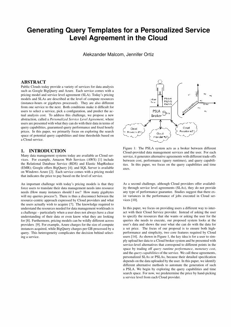
Figure 1: The PSLA system acts as a broker between differentCloud-provided data management services and the user. For eachservice, it generates alternative agreements with different trade-offsbetween cost, performance (query runtimes), and query capabili-ties. In this paper, we focus on the query capabilities and timeaxes.

As a second challenge, although Cloud providers offer availabil-ity through service level agreements (SLAs), they do not provideany type of performance guarantee. Studies suggest that there ex-ist variances in the performance of jobs executed in Cloud ser-vices [10].

In this paper, we focus on providing users a different way to inter-act with their Cloud Service provider. Instead of asking the userto specify the resources that she wants or asking the user for thequeries she needs to execute, our proposed system looks at theuser’s data and shows the user what she can do with the data fora set price. The focus of our proposal is to ensure both high-performance and simplicity, two core features required by Cloudusers [14]. As shown in Figure 1, the key idea is for a user to sim-ply upload her data to a Cloud broker system and be presented withservice-level alternatives that correspond to different points in thespace by trading off query runtime performance, monetary cost,and the query capabilities of the service. We call these agreements,personalized SLAs or PSLAs, because their detailed specificationdepends on the data uploaded by the user. In this paper, we identifydifferent alternative methods to automate the generation of sucha PSLA. We begin by exploring the query capabilities and timesearch space. For now, we predetermine the price by hand-pickinga service level from each Cloud provider.

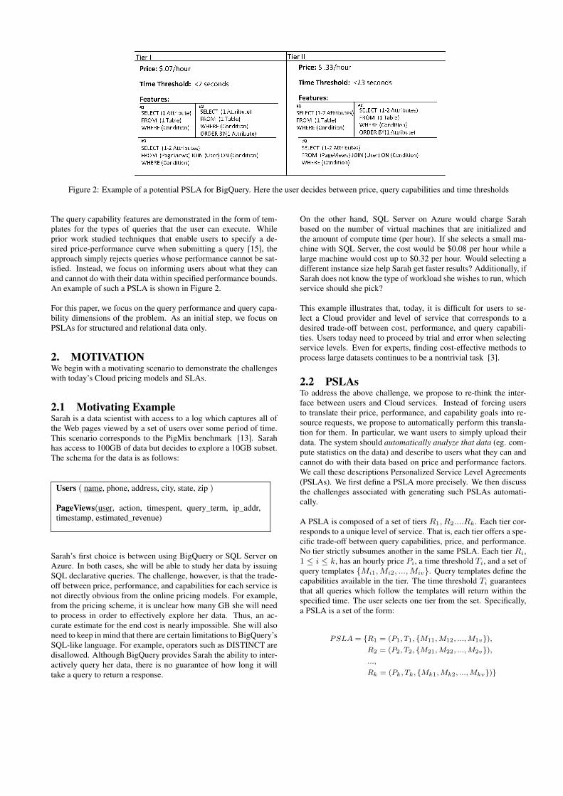
Figure 2: Example of a potential PSLA for BigQuery. Here the user decides between price, query capabilities and time thresholds

The query capability features are demonstrated in the form of tem-plates for the types of queries that the user can execute. Whileprior work studied techniques that enable users to specify a de-sired price-performance curve when submitting a query [15], theapproach simply rejects queries whose performance cannot be sat-isfied. Instead, we focus on informing users about what they canand cannot do with their data within specified performance bounds.An example of such a PSLA is shown in Figure 2.

For this paper, we focus on the query performance and query capa-bility dimensions of the problem. As an initial step, we focus onPSLAs for structured and relational data only.

2. MOTIVATIONWe begin with a motivating scenario to demonstrate the challengeswith today’s Cloud pricing models and SLAs.

2.1 Motivating ExampleSarah is a data scientist with access to a log which captures all ofthe Web pages viewed by a set of users over some period of time.This scenario corresponds to the PigMix benchmark [13]. Sarahhas access to 100GB of data but decides to explore a 10GB subset.The schema for the data is as follows:

Users ( name, phone, address, city, state, zip )

PageViews(user, action, timespent, query_term, ip_addr,timestamp, estimated_revenue)

Sarah’s first choice is between using BigQuery or SQL Server onAzure. In both cases, she will be able to study her data by issuingSQL declarative queries. The challenge, however, is that the trade-off between price, performance, and capabilities for each service isnot directly obvious from the online pricing models. For example,from the pricing scheme, it is unclear how many GB she will needto process in order to effectively explore her data. Thus, an ac-curate estimate for the end cost is nearly impossible. She will alsoneed to keep in mind that there are certain limitations to BigQuery’sSQL-like language. For example, operators such as DISTINCT aredisallowed. Although BigQuery provides Sarah the ability to inter-actively query her data, there is no guarantee of how long it willtake a query to return a response.

On the other hand, SQL Server on Azure would charge Sarahbased on the number of virtual machines that are initialized andthe amount of compute time (per hour). If she selects a small ma-chine with SQL Server, the cost would be $0.08 per hour while alarge machine would cost up to $0.32 per hour. Would selecting adifferent instance size help Sarah get faster results? Additionally, ifSarah does not know the type of workload she wishes to run, whichservice should she pick?

This example illustrates that, today, it is difficult for users to se-lect a Cloud provider and level of service that corresponds to adesired trade-off between cost, performance, and query capabili-ties. Users today need to proceed by trial and error when selectingservice levels. Even for experts, finding cost-effective methods toprocess large datasets continues to be a nontrivial task [3].

2.2 PSLAsTo address the above challenge, we propose to re-think the inter-face between users and Cloud services. Instead of forcing usersto translate their price, performance, and capability goals into re-source requests, we propose to automatically perform this transla-tion for them. In particular, we want users to simply upload theirdata. The system should automatically analyze that data (eg. com-pute statistics on the data) and describe to users what they can andcannot do with their data based on price and performance factors.We call these descriptions Personalized Service Level Agreements(PSLAs). We first define a PSLA more precisely. We then discussthe challenges associated with generating such PSLAs automati-cally.

A PSLA is composed of a set of tiers R1, R2....Rk. Each tier cor-responds to a unique level of service. That is, each tier offers a spe-cific trade-off between query capabilities, price, and performance.No tier strictly subsumes another in the same PSLA. Each tier Ri,1 ≤ i ≤ k, has an hourly price Pi, a time threshold Ti, and a set ofquery templates {Mi1,Mi2, ...,Miv}. Query templates define thecapabilities available in the tier. The time threshold Ti guaranteesthat all queries which follow the templates will return within thespecified time. The user selects one tier from the set. Specifically,a PSLA is a set of the form:

PSLA = {R1 = (P1, T1, {M11,M12, ...,M1v}),R2 = (P2, T2, {M21,M22, ...,M2v}),...,

Rk = (Pk, Tk, {Mk1,Mk2, ...,Mkv})}

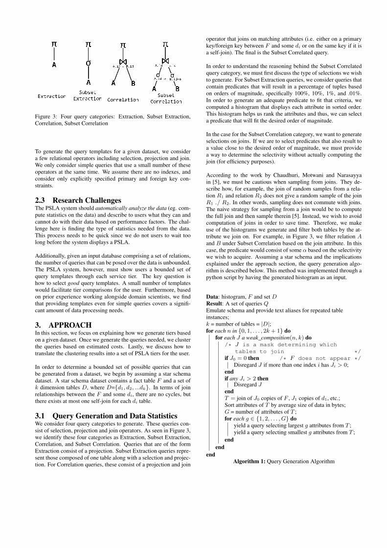
Figure 3: Four query categories: Extraction, Subset Extraction,Correlation, Subset Correlation

To generate the query templates for a given dataset, we considera few relational operators including selection, projection and join.We only consider simple queries that use a small number of theseoperators at the same time. We assume there are no indexes, andconsider only explicitly specified primary and foreign key con-straints.

2.3 Research ChallengesThe PSLA system should automatically analyze the data (eg. com-pute statistics on the data) and describe to users what they can andcannot do with their data based on performance factors. The chal-lenge here is finding the type of statistics needed from the data.This process needs to be quick since we do not users to wait toolong before the system displays a PSLA.

Additionally, given an input database comprising a set of relations,the number of queries that can be posed over the data is unbounded.The PSLA system, however, must show users a bounded set ofquery templates through each service tier. The key question ishow to select good query templates. A small number of templateswould facilitate tier comparisons for the user. Furthermore, basedon prior experience working alongside domain scientists, we findthat providing templates even for simple queries covers a signifi-cant amount of data processing needs.

3. APPROACHIn this section, we focus on explaining how we generate tiers basedon a given dataset. Once we generate the queries needed, we clusterthe queries based on estimated costs. Lastly, we discuss how totranslate the clustering results into a set of PSLA tiers for the user.

In order to determine a bounded set of possible queries that canbe generated from a dataset, we begin by assuming a star schemadataset. A star schema dataset contains a fact table F and a set ofk dimension tables D, where D={d1, d2, ...dk}. In terms of joinrelationships between the F and some di, there are no cycles, butthere exists at most one self-join for each di table.

3.1 Query Generation and Data StatisticsWe consider four query categories to generate. These queries con-sist of selection, projection and join operators. As seen in Figure 3,we identify these four categories as Extraction, Subset Extraction,Correlation, and Subset Correlation. Queries that are of the formExtraction consist of a projection. Subset Extraction queries repre-sent those composed of one table along with a selection and projec-tion. For Correlation queries, these consist of a projection and join

operator that joins on matching attributes (i.e. either on a primarykey/foreign key between F and some di or on the same key if it isa self-join). The final is the Subset Correlated query.

In order to understand the reasoning behind the Subset Correlatedquery category, we must first discuss the type of selections we wishto generate. For Subset Extraction queries, we consider queries thatcontain predicates that will result in a percentage of tuples basedon orders of magnitude, specifically 100%, 10%, 1%, and .01%.In order to generate an adequate predicate to fit that criteria, wecomputed a histogram that displays each attribute in sorted order.This histogram helps us rank the attributes and thus, we can selecta predicate that will fit the desired order of magnitude.

In the case for the Subset Correlation category, we want to generateselections on joins. If we are to select predicates that also result toa value close to the desired order of magnitude, we must providea way to determine the selectivity without actually computing thejoin (for efficiency purposes).

According to the work by Chaudhuri, Motwani and Narasayyain [5], we must be cautious when sampling from joins. They de-scribe how, for example, the join of random samples from a rela-tion R1 and relation R2 does not give a random sample of the joinR1 ./ R2. In other words, sampling does not commute with joins.The naive strategy for sampling from a join would be to computethe full join and then sample therein [5]. Instead, we wish to avoidcomputation of joins in order to save time. Therefore, we makeuse of the histograms we generate and filter both tables by the at-tribute we join on. For example, in Figure 3, we filter relation Aand B under Subset Correlation based on the join attribute. In thiscase, the predicate would consist of some α based on the selectivitywe wish to acquire. Assuming a star schema and the implicationsexplained under the approach section, the query generation algo-rithm is described below. This method was implemented through apython script by having the generated histogram as an input.

Data: histogram, F and set DResult: A set of queries QEmulate schema and provide text aliases for repeated tableinstances;k = number of tables = |D|;for each n in {0, 1, . . . , 2k + 1} do

for each J a weak_composition(n, k) do/* J is a mask determining which

tables to join */if J0 = 0 then /* F does not appear */

Disregard J if more than one index i has Ji > 0;endif any Ji > 2 then

Disregard JendT = join of J0 copies of F , J1 copies of d1, etc.;Sort attributes of T by average size of data in bytes;G = number of attributes of T ;for each g ∈ {1, 2, . . . , G} do

yield a query selecting largest g attributes from T ;yield a query selecting smallest g attributes from T ;

endend

endAlgorithm 1: Query Generation Algorithm

We should note that the form of the weak composition problemneeded here, i.e. to find integers xi ≥ 0 such that

∑ki=1 xi = n

has a very simple recursive solution.

Data: integer n to be partitioned, integer k partsResult: list of lists of non-negative integers, each of which sums

to n and has length kif k = 1 then

yield List(n)else

for each i in {0, 1, . . . , n} dofor each X a weak_composition of n− i into k − 1 partsdo

yield X+List(i)end

endend

Algorithm 2: Weak Composition

3.2 Clustering Estimated Query CostsBefore generating tiers for the PSLA, we must gain a sense of theperformance for each query. Once the queries are generated, werun all the queries on different levels of service through Azure. Weacquired one small virtual instance (1 virtual core, 1.75 GB Ram)and a large virtual instance (4 virtual cores, 14 GB Ram) whereboth instances include SQL Server 2008.

Assuming we wish to utilize the estimated costs of the queries todetermine the PSLA tiers, we need to first determine whether theestimated costs from the SQL Server optimizer really reflect thequery runtimes. For each machine, we cluster for the query run-times and for the estimated query costs. We use WEKA [6] tocluster results based on k-means algorithm.

In order to determine whether there exists a similarity betweenthe real query times and the estimated costs, we utilize a criterioncalled Variation of Information (VI) from Meila’s work in [11].This criterion measures the amount of information lost or gained inchanging from clustering C to clustering C′. The paper refers to aclustering as a partition of a set of points into sets C1, C2, . . . , Ck.In our case, we refer the query runtimes as C and the estimatedquery times as C′. The VI equation takes into account the entropyassociated with each clustering referred to as H(C) and H(C′) aswell as the reduction in uncertainty based on given knowledge asexpressed through I(C, C′). We display the equation below. Formore details about this criterion, see [11].

V I(C, C′) = H(C) +H(C′)− 2I(C, C′)

VI will always result in a non-negative value (further, VI is a met-ric on the space of all clusterings). One property of the VI equa-tion states that if both clusterings are the same, then the result willbe 0. The upper bound (or maximum) between two clusterings isV I(C, C′) ≤ 2 log K, where K represents the maximum numberof clusters between C and C′, and provided that K2 is less than thenumber of data points.

3.3 Cluster to Tier TranslationIn this section, we describe a method to translate the clusters fromestimated query compute costs into tiers. Each tier will be com-posed of a set of query templates. First, we define a query templatemore precisely. We use this definition to distinguish between querytemplates.

Definition Let a set of query templates M1,M2, ...Mk representthe queries that are shown to the user. Each query template, Mi,takes the form of one of the query categories described from Fig-ure 3. Specifically a query template consists of a category, a set oftables, and a selectivity level (either 100%, 10%, 1%, or .01%).

3.3.1 Tier Generation AlgorithmIn this algorithm, we focus on generating a set of tiers T from agiven clustering C. Each cluster Ci in the clustering consists of aset of points P1, P2, . . . , Pk. For each cluster we iterate through,we will generate a new tier and add the query template to the cur-rent tier. However, if the query template exists in the current tier ora previous tier, it is not added to the current tier. Below, we describethe algorithm. We run this algorithm on each estimated query com-pute cost of each service level (small and large) and provide all theresulting tiers to the user. In this algorithm, the abstraction of apoint Pi is defined as a function that returns the query template thatthe point represents. We iterate through all the points in each clus-ter and add the abstraction of Pi to a tier. As we iterate, if Pi iscontained in a query in the current tier, we disregard the point anddo not add it to the tier. Currently, this process is done manually.

Data: A Clustering CResult: A set of Tierssort clusters descending by average estimated cost ;initialize T = ∅;for each cluster Ci in clustering C do

initialize tier Ri;for each Pi in Ci do

Q = abstractform(Pi) ;if Q /∈ Ri ∧Q /∈ T then

if ∃Q′ ∈ Ri where Q v Q’ thenDiscard Q;

elseRi = Ri ∪ {Q};

endend

endif Ri 6= ∅ then

yield Ri;T = Ri ∪ T ;

endend

Algorithm 3: Tier Generation Algorithm

4. RESULTSIn this section we describe the results for Azure small instance andAzure large instance based on the approach described in the previ-ous section.

By using 10GB Pigmix dataset, the query generation algorithmgenerates a total of 460 queries. We cannot expect to both runall the queries in an adequate amount of time and provide the userwith a PSLA thereafter. In fact, running all the queries generated onthe small Azure instance took 2312180ms while it took 2504045mson the large instance. Instead, we look at the estimated query costfrom the optimizer. The SQL Server optimizer provides a type ofmetric that can measure a cost based on CPU and I/O cost that aquery may utilize. Estimating the compute cost of all the querieson the small instance took 7168ms while on the large instance ittook 5668ms.

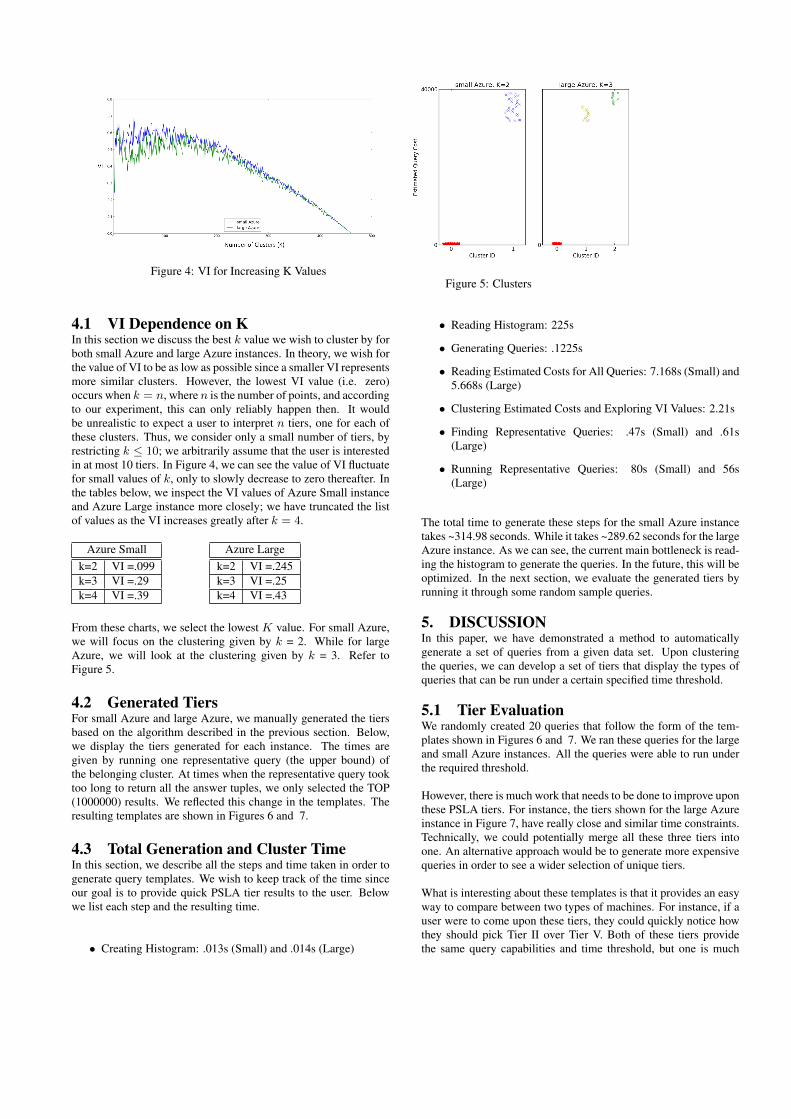
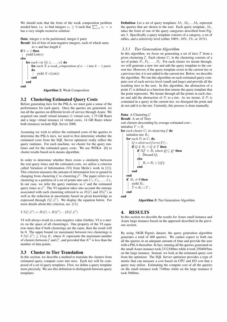
Figure 4: VI for Increasing K ValuesFigure 5: Clusters

4.1 VI Dependence on KIn this section we discuss the best k value we wish to cluster by forboth small Azure and large Azure instances. In theory, we wish forthe value of VI to be as low as possible since a smaller VI representsmore similar clusters. However, the lowest VI value (i.e. zero)occurs when k = n, where n is the number of points, and accordingto our experiment, this can only reliably happen then. It wouldbe unrealistic to expect a user to interpret n tiers, one for each ofthese clusters. Thus, we consider only a small number of tiers, byrestricting k ≤ 10; we arbitrarily assume that the user is interestedin at most 10 tiers. In Figure 4, we can see the value of VI fluctuatefor small values of k, only to slowly decrease to zero thereafter. Inthe tables below, we inspect the VI values of Azure Small instanceand Azure Large instance more closely; we have truncated the listof values as the VI increases greatly after k = 4.

Azure Smallk=2 VI =.099k=3 VI =.29k=4 VI =.39

Azure Largek=2 VI =.245k=3 VI =.25k=4 VI =.43

From these charts, we select the lowest K value. For small Azure,we will focus on the clustering given by k = 2. While for largeAzure, we will look at the clustering given by k = 3. Refer toFigure 5.

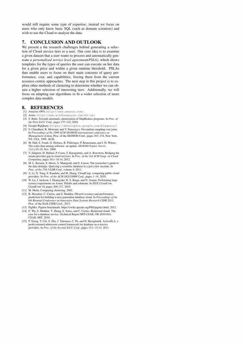
4.2 Generated TiersFor small Azure and large Azure, we manually generated the tiersbased on the algorithm described in the previous section. Below,we display the tiers generated for each instance. The times aregiven by running one representative query (the upper bound) ofthe belonging cluster. At times when the representative query tooktoo long to return all the answer tuples, we only selected the TOP(1000000) results. We reflected this change in the templates. Theresulting templates are shown in Figures 6 and 7.

4.3 Total Generation and Cluster TimeIn this section, we describe all the steps and time taken in order togenerate query templates. We wish to keep track of the time sinceour goal is to provide quick PSLA tier results to the user. Belowwe list each step and the resulting time.

• Creating Histogram: .013s (Small) and .014s (Large)

• Reading Histogram: 225s

• Generating Queries: .1225s

• Reading Estimated Costs for All Queries: 7.168s (Small) and5.668s (Large)

• Clustering Estimated Costs and Exploring VI Values: 2.21s

• Finding Representative Queries: .47s (Small) and .61s(Large)

• Running Representative Queries: 80s (Small) and 56s(Large)

The total time to generate these steps for the small Azure instancetakes ~314.98 seconds. While it takes ~289.62 seconds for the largeAzure instance. As we can see, the current main bottleneck is read-ing the histogram to generate the queries. In the future, this will beoptimized. In the next section, we evaluate the generated tiers byrunning it through some random sample queries.

5. DISCUSSIONIn this paper, we have demonstrated a method to automaticallygenerate a set of queries from a given data set. Upon clusteringthe queries, we can develop a set of tiers that display the types ofqueries that can be run under a certain specified time threshold.

5.1 Tier EvaluationWe randomly created 20 queries that follow the form of the tem-plates shown in Figures 6 and 7. We ran these queries for the largeand small Azure instances. All the queries were able to run underthe required threshold.

However, there is much work that needs to be done to improve uponthese PSLA tiers. For instance, the tiers shown for the large Azureinstance in Figure 7, have really close and similar time constraints.Technically, we could potentially merge all these three tiers intoone. An alternative approach would be to generate more expensivequeries in order to see a wider selection of unique tiers.

What is interesting about these templates is that it provides an easyway to compare between two types of machines. For instance, if auser were to come upon these tiers, they could quickly notice howthey should pick Tier II over Tier V. Both of these tiers providethe same query capabilities and time threshold, but one is much

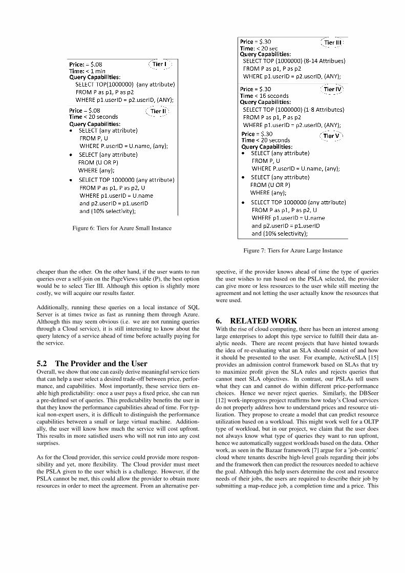
Figure 6: Tiers for Azure Small Instance

Figure 7: Tiers for Azure Large Instance

cheaper than the other. On the other hand, if the user wants to runqueries over a self-join on the PageViews table (P), the best optionwould be to select Tier III. Although this option is slightly morecostly, we will acquire our results faster.

Additionally, running these queries on a local instance of SQLServer is at times twice as fast as running them through Azure.Although this may seem obvious (i.e. we are not running queriesthrough a Cloud service), it is still interesting to know about thequery latency of a service ahead of time before actually paying forthe service.

5.2 The Provider and the UserOverall, we show that one can easily derive meaningful service tiersthat can help a user select a desired trade-off between price, perfor-mance, and capabilities. Most importantly, these service tiers en-able high predictability: once a user pays a fixed price, she can runa pre-defined set of queries. This predictability benefits the user inthat they know the performance capabilities ahead of time. For typ-ical non-expert users, it is difficult to distinguish the performancecapabilities between a small or large virtual machine. Addition-ally, the user will know how much the service will cost upfront.This results in more satisfied users who will not run into any costsurprises.

As for the Cloud provider, this service could provide more respon-sibility and yet, more flexibility. The Cloud provider must meetthe PSLA given to the user which is a challenge. However, if thePSLA cannot be met, this could allow the provider to obtain moreresources in order to meet the agreement. From an alternative per-

spective, if the provider knows ahead of time the type of queriesthe user wishes to run based on the PSLA selected, the providercan give more or less resources to the user while still meeting theagreement and not letting the user actually know the resources thatwere used.

6. RELATED WORKWith the rise of cloud computing, there has been an interest amonglarge enterprises to adopt this type service to fulfill their data an-alytic needs. There are recent projects that have hinted towardsthe idea of re-evaluating what an SLA should consist of and howit should be presented to the user. For example, ActiveSLA [15]provides an admission control framework based on SLAs that tryto maximize profit given the SLA rules and rejects queries thatcannot meet SLA objectives. In contrast, our PSLAs tell userswhat they can and cannot do within different price-performancechoices. Hence we never reject queries. Similarly, the DBSeer[12] work-inprogress project reaffirms how today’s Cloud servicesdo not properly address how to understand prices and resource uti-lization. They propose to create a model that can predict resourceutilization based on a workload. This might work well for a OLTPtype of workload, but in our project, we claim that the user doesnot always know what type of queries they want to run upfront,hence we automatically suggest workloads based on the data. Otherwork, as seen in the Bazaar framework [7] argue for a ’job-centric’cloud where tenants describe high-level goals regarding their jobsand the framework then can predict the resources needed to achievethe goal. Although this help users determine the cost and resourceneeds of their jobs, the users are required to describe their job bysubmitting a map-reduce job, a completion time and a price. This

would still require some type of expertise; instead we focus onusers who only know basic SQL (such as domain scientists) andwish to use the Cloud to analyze the data.

7. CONCLUSION AND OUTLOOKWe present a the research challenges behind generating a selec-tion of Cloud service tiers to a user. Our core idea is to examinea given dataset that a user wants to process and automatically gen-erate a personalized service level agreement(PSLA), which showstemplates for the types of queries the user can execute on her datafor a given price and within a given runtime threshold. PSLAsthus enable users to focus on their main concerns of query per-formance, cost, and capabilities, freeing them from the currentresource-centric approaches. The next step in this project is to ex-plore other methods of clustering to determine whether we can ob-tain a higher selection of interesting tiers. Additionally, we willfocus on adapting our algorithms to fit a wider selection of morecomplex data models.

8. REFERENCES[1] Amazon AWS. http://aws.amazon.com/.[2] Azure. http://www.windowsazure.com/en-us/.[3] S. Babu. Towards automatic optimization of MapReduce programs. In Proc. of

the First SoCC Conf., pages 137–142, 2010.[4] Google BigQuery. https://developers.google.com/bigquery/.[5] S. Chaudhuri, R. Motwani, and V. Narasayya. On random sampling over joins.

In Proceedings of the 1999 ACM SIGMOD international conference onManagement of data, Proc. of the SIGMOD Conf., pages 263–274, New York,NY, USA, 1999. ACM.

[6] M. Hall, E. Frank, G. Holmes, B. Pfahringer, P. Reutemann, and I. H. Witten.The weka data mining software: an update. SIGKDD Explor. Newsl.,11(1):10–18, Nov. 2009.

[7] V. Jalaparti, H. Ballani, P. Costa, T. Karagiannis, and A. Rowstron. Bridging thetenant-provider gap in cloud services. In Proc. of the 3rd ACM Symp. on CloudComputing, pages 10:1–10:14, 2012.

[8] M. L. Kersten, S. Idreos, S. Manegold, and E. Liarou. The researcher’s guide tothe data deludge: Querying a scientific database in a just a few seconds. InProc. of the 37th VLDB Conf., volume 4, 2011.

[9] A. Li, X. Yang, S. Kandula, and M. Zhang. CloudCmp: comparing public cloudproviders. In Proc. of the ACM SIGCOMM Conf., pages 1–14, 2010.

[10] W. Lu, J. Jackson, J. Ekanayake, R. S. Barga, and N. Araujo. Performing largescience experiments on Azure: Pitfalls and solutions. In IEEE CloudCom,CloudCom’10, pages 209–217, 2010.

[11] M. Meila. Comparing clustering. 2002.[12] B. Mozafari, C. Curino, and S. Madden. Dbseerl resource and performance

prediction for building a next generation database cloud. In Proceedings of the6th Biennial Conference on Innovative Data Systems Research CIDR 2013,Proc. of the Sixth CIDR Conf., 2013.

[13] PigMix. Pigmix benchmark. https://cwiki.apache.org/PIG/pigmix.html, 2012.[14] E. Wu, S. Madden, Y. Zhang, E. Jones, and C. Curino. Relational cloud: The

case for a database service. Technical Report MIT-CSAIL-TR-2010-014,CSAIL MIT, 2010.

[15] P. Xiong, Y. Chi, S. Zhu, J. Tatemura, C. Pu, and H. HacigümüS. ActiveSLA: aprofit-oriented admission control framework for database-as-a-serviceproviders. In Proc. of the Second SoCC Conf., pages 15:1–15:14, 2011.