arX

iv:1

403.

5006

v2 [

cs.D

B]

4 M

ay 2

016

Generating Preview Tables for Entity Graphs

1Ning Yan∗

2Sona Hasani 2Abolfazl Asudeh 2Chengkai Li1Huawei U.S. R&D Center 2The University of Texas at Arlington

ning.yan.uta@gmail.com {sona.hasani,ab.asudeh}@mavs.uta.edu cli@uta.edu

ABSTRACTUsers are tapping into massive, heterogeneous entity graphs formany applications. It is challenging to select entity graphs for aparticular need, given abundant datasets from many sourcesandthe oftentimes scarce information for them. We propose methodsto produce preview tables for compact presentation of importantentity types and relationships in entity graphs. The preview tablesassist users in attaining a quick and rough preview of the data. Theycan be shown in a limited display space for a user to browse andexplore, before she decides to spend time and resources to fetchand investigate the complete dataset. We formulate severalopti-mization problems that look for previews with the highest scoresaccording to intuitive goodness measures, under various constraintson preview size and distance between preview tables. The opti-mization problem under distance constraint isNP-hard. We designa dynamic-programming algorithm and an Apriori-style algorithmfor finding optimal previews. Results from experiments, compar-ison with related work and user studies demonstrated the scoringmeasures’ accuracy and the discovery algorithms’ efficiency.

1. INTRODUCTIONWe witness an unprecedented proliferation of massive, heteroge-

neousentity graphs that represent entities and their relationships inmany domains. For instance, in Fig. 1—a tiny excerpt of an entitygraph, the edge labeledActor between nodesWill Smith and Men in

Black captures the fact that the person is an actor in the film. Real-world entity graphs include knowledge bases (e.g., DBpedia[2],YAGO [16], Probase [18], Freebase [4] and Google’s KnowledgeVault [8]), social graphs, biomedical databases, and program anal-ysis graphs, to name just a few. Numerous applications are tappinginto entity graphs in domains such as search, recommendation sys-tems, business intelligence and health informatics.

Entity graphs are often represented as RDF triples, due to het-erogeneity of entities and the often lacking schema. The LinkingOpen Data community has interlinked billions of RDF triplesspan-ning over several hundred datasets (http://linkeddata.org). Manyother entity graph datasets are also available from data repositoriessuch as the NCBI databases (http://www.ncbi.nlm.nih.gov), Ama-

∗Work done while at the University of Texas at Arlington.Permission to make digital or hard copies of all or part of this work for personal orclassroom use is granted without fee provided that copies are not made or distributedfor profit or commercial advantage and that copies bear this notice and the full citationon the first page. Copyrights for components of this work owned by others thanACM must be honored. Abstracting with credit is permitted. To copy otherwise, orrepublish, to post on servers or to redistribute to lists, requires prior specific permissionand/or a fee. Request permissions from permissions@acm.org.

SIGMOD’16, June 26-July 01, 2016, San Francisco, CA, USAc© 2016 ACM. ISBN 978-1-4503-3531-7/16/06. . . $15.00

DOI: http://dx.doi.org/10.1145/2882903.2915221

Figure 1: An excerpt of an entity graph.

zon’s Public Data Sets (http://aws.amazon.com/publicdatasets) andData.gov (http://www.data.gov).

It is challenging to select entity graphs for a particular need,given abundant datasets from many sources and oftentimes scarceinformation available about them. While sources such as theafore-mentioned data repositories often provide dataset descriptions, onecannot get a direct look at an entity graph before fetching it. Down-loading a dataset and loading it into a database can be a dauntingtask. A data worker may need to tackle many challenges beforethey can start any real work on an entity graph.

In this paper, we propose methods to automatically producepre-view tables for entity graphs. Given an entity graph with a largenumber of entities and relationships, our methods select from themany entity types a few important ones and produce a table foreach chosen entity type. Such a table comprises a set of attributes,selected among many candidates, each of which corresponds to arelationship associated with the corresponding entity type. A tuplein the table consists of an entity belonging to the entity type and itsrelated entities for the table attributes.

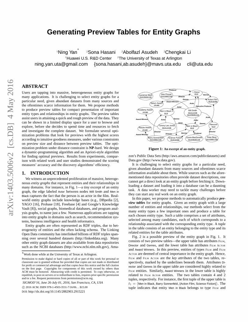
Fig. 2 is a possible preview of the entity graph in Fig. 1. Itconsists of two preview tables—the upper table has attributesFILM ,Director and Genres, and the lower table has attributesFILM ACTOR

andAward Winners. In this preview, entities of typesFILM andFILM

ACTOR are deemed of central importance in the entity graph. Hence,FILM and FILM ACTOR are thekey attributes of the two tables, re-spectively, marked by the underlines beneath them. AttributesDi-

rector andGenres in the upper table are considered highly related toFILM entities. Similarly,Award Winners in the lower table is highlyrelated toFILM ACTOR entities. The two tables contain 4 and 2tuples, respectively. For instance, the first tuple of the upper table ist1 = 〈Men in Black, Barry Sonnenfeld, {Action Film, Science Fiction}〉. Thetuple indicates that entityMen in Black belongs to typeFILM and

FILM Director Genrest1 Men in Black Barry Sonnenfeld { Action Film, Science Fiction}t2 Men in Black II Barry Sonnenfeld { Action Film, Science Fiction}t3 Hancock Peter Berg -t4 I, Robot Alex Proyas { Action Film}

FILM ACTOR Award Winnerst5 Will Smith Saturn Awardt6 Tommy Lee Jones Academy Award

Figure 2: A 2-table preview of the entity graph in Fig. 1. (Upper andlower tables for subgraphs #1 and #2 in Fig. 3, respectively.)

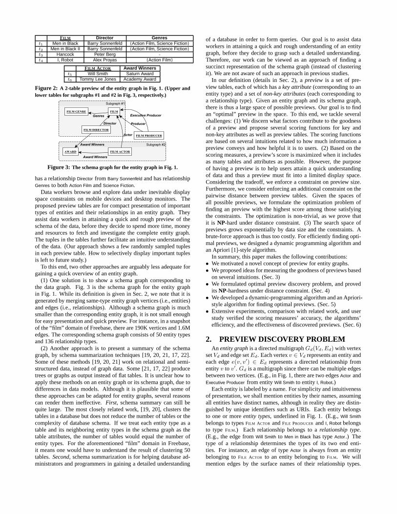
Figure 3: The schema graph for the entity graph in Fig. 1.

has a relationshipDirector from Barry Sonnenfeld and has relationshipGenres to bothAction Film andScience Fiction.

Data workers browse and explore data under inevitable displayspace constraints on mobile devices and desktop monitors. Theproposed preview tables are for compact presentation of importanttypes of entities and their relationships in an entity graph. Theyassist data workers in attaining a quick and rough preview oftheschema of the data, before they decide to spend more time, moneyand resources to fetch and investigate the complete entity graph.The tuples in the tables further facilitate an intuitive understandingof the data. (Our approach shows a few randomly sampled tuplesin each preview table. How to selectively display importanttuplesis left to future study.)

To this end, two other approaches are arguably less adequateforgaining a quick overview of an entity graph.

(1) One solution is to show a schema graph corresponding tothe data graph. Fig. 3 is the schema graph for the entity graphin Fig. 1. While its definition is given in Sec. 2, we note that it isgenerated by merging same-type entity graph vertices (i.e., entities)and edges (i.e., relationships). Although a schema graph ismuchsmaller than the corresponding entity graph, it is not smallenoughfor easy presentation and quick preview. For instance, in a snapshotof the “film” domain of Freebase, there are 190K vertices and 1.6Medges. The corresponding schema graph consists of 50 entitytypesand 136 relationship types.

(2) Another approach is to present a summary of the schemagraph, by schema summarization techniques [19, 20, 21, 17, 22].Some of these methods [19, 20, 21] work on relational and semi-structured data, instead of graph data. Some [21, 17, 22] producetrees or graphs as output instead of flat tables. It is unclearhow toapply these methods on an entity graph or its schema graph, due todifferences in data models. Although it is plausible that some ofthese approaches can be adapted for entity graphs, several reasonscan render them ineffective.First, schema summary can still bequite large. The most closely related work, [19, 20], clusters thetables in a database but does not reduce the number of tables or thecomplexity of database schema. If we treat each entity type as atable and its neighboring entity types in the schema graph asthetable attributes, the number of tables would equal the number ofentity types. For the aforementioned “film” domain in Freebase,it means one would have to understand the result of clustering 50tables.Second, schema summarization is for helping database ad-ministrators and programmers in gaining a detailed understanding

of a database in order to form queries. Our goal is to assist dataworkers in attaining a quick and rough understanding of an entitygraph, before they decide to grasp such a detailed understanding.Therefore, our work can be viewed as an approach of finding asuccinct representation of the schema graph (instead of clusteringit). We are not aware of such an approach in previous studies.

In our definition (details in Sec. 2), apreview is a set of pre-view tables, each of which has akey attribute (corresponding to anentity type) and a set ofnon-key attributes (each corresponding toa relationship type). Given an entity graph and its schema graph,there is thus a large space of possible previews. Our goal is to findan “optimal” preview in the space. To this end, we tackle severalchallenges: (1) We discern what factors contribute to the goodnessof a preview and propose several scoring functions for key andnon-key attributes as well as preview tables. The scoring functionsare based on several intuitions related to how much information apreview conveys and how helpful it is to users. (2) Based on thescoring measures, a preview’s score is maximized when it includesas many tables and attributes as possible. However, the purposeof having a preview is to help users attain a quick understandingof data and thus a preview must fit into a limited display space.Considering the tradeoff, we enforce a constraint on preview size.Furthermore, we consider enforcing an additional constraint on thepairwise distance between preview tables. Given the spacesofall possible previews, we formulate the optimization problem offinding an preview with the highest score among those satisfyingthe constraints. The optimization is non-trivial, as we prove thatit is NP-hard under distance constraint. (3) The search space ofpreviews grows exponentially by data size and the constraints. Abrute-force approach is thus too costly. For efficiently finding opti-mal previews, we designed a dynamic programming algorithm andan Apriori [1]-style algorithm.

In summary, this paper makes the following contributions:• We motivated a novel concept of preview for entity graphs.• We proposed ideas for measuring the goodness of previews based

on several intuitions. (Sec. 3)• We formulated optimal preview discovery problem, and proved

its NP-hardness under distance constraint. (Sec. 4)• We developed a dynamic-programming algorithm and an Apriori-

style algorithm for finding optimal previews. (Sec. 5)• Extensive experiments, comparison with related work, and user

study verified the scoring measures’ accuracy, the algorithms’efficiency, and the effectiveness of discovered previews. (Sec. 6)

2. PREVIEW DISCOVERY PROBLEMAn entity graph is a directed multigraphGd(Vd, Ed) with vertex

setVd and edge setEd. Each vertexv ∈ Vd represents an entity andeach edgee(v, v′) ∈ Ed represents a directed relationship fromentityv to v′. Gd is a multigraph since there can be multiple edgesbetween two vertices. (E.g., in Fig. 1, there are two edgesActor andExecutive Producer from entityWill Smith to entity I, Robot.)

Each entity is labeled by a name. For simplicity and intuitivenessof presentation, we shall mention entities by their names, assumingall entities have distinct names, although in reality they are distin-guished by unique identifiers such as URIs. Each entity belongsto one or moreentity types, underlined in Fig. 1. (E.g.,Will Smith

belongs to typesFILM ACTOR andFILE PRODUCER andI, Robot belongsto type FILM .) Each relationship belongs to arelationship type.(E.g., the edge fromWill Smith to Men in Black has typeActor .) Thetype of a relationship determines the types of its two end enti-ties. For instance, an edge of typeActor is always from an entitybelonging toFILE ACTOR to an entity belonging toFILM . We willmention edges by the surface names of their relationship types.

Gd(Vd, Ed) an entity graphv ∈ Vd an entity

e(v, v′) ∈ Ed a directed relationship from entityv to entityv′

Gs(Vs, Es) a schema graphτ ∈ Vs an entity type

γ(τ, τ ′) ∈ Es a relationship type from entity typeτ to entity typeτ ′

T a preview tableT.key the key attribute ofT

T.nonkey the non-key attributes ofTT.τ the set of entities of typeτ—the key attribute ofTt ∈ T a tuplet in preview tableTt.τ t’s value onτ which is the key attribute ofTt.γ t’s value on non-key attributeγ

P = {P[1], ...,P[k]} a preview, which consists ofk preview tablesPopt an optimal previewS(P) the score of previewPS(T ) the score of preview tableT

Scov(τ), Swalk(τ) score of key attributeτ based on coverage/random-walkSτcov(γ), S

τent(γ) score of non-key attributeγ based on coverage/entropy

T the space of all possible preview tablesP the space of all possible previews

dist(τ, τ ′) distance betweenτ andτ ′ in schema graphGs

Table 1: Notations.

Two different relationship types may have the same surface namefor intuitively expressing their meanings, although underlyinglythey have different identifiers. For instance, theAward Winners edgefrom Will Smith to Saturn Award and theAward Winners edge fromBarry

Sonnenfeld to Razzie Award belong to two different relationship types.The former is for relationships fromFILM ACTOR to AWARD, while thelatter is for relationships fromFILM DIRECTOR to AWARD.

Given an entity graphGd(Vd, Ed), its schema graph is a directedgraphGs(Vs, Es), where each vertexτ ∈ Vs represents an entitytype and each directed edgeγ(τ, τ ′) ∈ Es represents a relationshiptype from entity typeτ to τ ′. An edgeγ(τ, τ ′) ∈ Es if and only ifthere exists an edgee(v, v′) ∈ Ed wheree has typeγ, v has typeτandv′ has typeτ ′. Fig. 3 shows the schema graph corresponding tothe entity graph in Fig. 1. A schema graph is a multigraph as therecan be multiple relationship types between two entity types. (E.g.,two relationship types—Producer andExecutive Producer—are fromentity typeFILM PRODUCER to FILM .) It is clear from the above defi-nitions that, given a data graph, the corresponding schema graph isuniquely determined.

Definition 1 (Preview Table and Preview). Given an entity graphGd(Vd, Ed) and its schema graphGs(Vs, Es), a preview table Thas a mandatorykey attribute (denotedT.key) and at least onenon-key attributes (denotedT.nonkey). T corresponds to a star-shape subgraph of the schema graphGs(Vs, Es). The key attributecorresponds to an entity typeτ ∈ Vs, and each non-key attributecorresponds to a relationship typeγ(τ, τ ′) ∈ Es or γ(τ ′, τ ) ∈ Es.Note that the edges from and to an entity are both important. Hence,a non-key attribute corresponds to eitherγ(τ, τ ′) or γ(τ ′, τ ).

The preview tableT consists of a set of tuples. The number oftuples equals the number of entities of typeτ (the key attribute ofT ), i.e.,|T | = |T.τ | andT.τ = {v|v ∈ Vd ∧ v has typeτ}. Givenan arbitrary tuplet ∈ T , we denotet’s key attribute value byt.τ .Each tuplet attains a distinct value oft.τ . Its value on a non-keyattributeγ(τ, τ ′), denotedt.γ(τ, τ ′) or simplyt.γ, is a set—the setof entities in entity graphGd incident fromt.τ through an edge oftypeγ(τ, τ ′). More formally,t.γ(τ, τ ′) = {u|u ∈ Vd∧e(t.τ, u) ∈Ed ∧ u belongs to typeτ ′}. Symmetrically, its value on a non-keyattributeγ(τ ′, τ ) is the set of entities inGd incident tot.τ throughan edge of typeγ(τ ′, τ ), i.e.,t.γ(τ ′, τ ) = {u|u ∈ Vd∧e(u, t.τ ) ∈Ed ∧ u belongs to typeτ ′}.

A preview P is a set of preview tables, i.e.,P = {P [1], ...,P [k]},where∀i 6= j,P [i].key 6= P [j].key, k 6 |Vs| is the total numberof preview tables. Note that|Vs| is the number of vertices inGs,i.e., the number of entity types inGd.

According to Definition 1, the upper and lower tables in Fig. 2correspond to the star-shape subgraphs #1 and #2 in Fig. 3, respec-tively. The key attribute in the upper table isFILM and the non-keyattributes areDirector and Genres. The key attribute in the lowertable isFILM ACTOR and its non-key attribute isAward Winners. It isworth noting that, although each tuple’s value on the key attributeis non-empty, unique and single-valued, its value on a non-keyattribute can be empty (e.g.,t3.Genres in Fig. 2), duplicate (e.g.,t1.Director andt2.Director in Fig. 2) and multi-valued (e.g.,t1.Genres

andt2.Genres in Fig. 2). It also follows that a preview table is not arelational table.

By Definition 1, every vertexτ in a schema graph can serve asthe key attribute of a candidate preview table, which also includesat least one non-key attribute—an edge incident onτ . We useTto denote the space of all possible preview tables. A previewis aset of preview tables. We useP to denote the space of all possiblepreviews. Note thatP ⊂ 2T, i.e., not every member of the powerset2T is a valid preview, because by Definition 1 preview tables ina preview cannot have the same key attribute.

Problem Statement: Given an entity graphGd(Vd, Ed) and itscorresponding schema graphGs(Vs, Es), the preview discoveryproblem is to findPopt—the optimal preview among all possiblepreviews. We shall develop the notions of goodness and optimalityfor a preview and define goodness measures in Sec. 3.

Note that the preview discovery problem focuses on selectingkey and non-key attributes for preview tables. It does not selecttuples. As our goal is to help users attain a good initial under-standing of the schema of an entity graph, we argue that it is onlynecessary to show a small number of tuples instead of all. Ourcurrent approach is to randomly select a few. How to choose themost representative tuples is left for future work.

3. SCORING MEASURES FOR PREVIEWSIn this section, we discuss the scoring functions for measuring

the goodness of previews for entity graphs. The measures arebasedon the intuition that a good preview should 1) relate to as manyentities and relationships as possible and 2) help users understandan entity graph and its schema graph. The first intuition is obvious,as a preview relating to only a small number of entities or rela-tionships will inevitably lose lots of information and thuslead topoor comprehensibility of the original graph. The second intuitionmodels the goodness of previews according to users’ behavior inbrowsing entity and schema graphs.

3.1 Preview ScoringThe score of a previewP = {P [1], ...,P [k]} is simply aggre-

gated from individual preview tables’ scores, by summation:

S(P) =

k∑

i=1

S(P [i]), (1)

whereS(P [i]) is the score of a preview tableP [i], defined as:S(P [i]) = S(τ )×

∑

γ∈P[i].nonkey

Sτ (γ), (2)

whereS(τ ) is the score of the key attribute ofP [i] (i.e.,P [i].key=τ )andSτ (γ) is the score of a non-key attributeγ in P [i]. S(τ ) andSτ (γ) are defined and elaborated in Sec. 3.2 and Sec. 3.3.

In the above definition, the score of a preview table equals theproduct of its key attribute’s score and the summation of itsnon-key attributes’ scores. The definition gives the key attributeτ muchhigher importance than any individual non-key attribute, becausethe preview table centers around the entities of typeτ and describestheir non-key attributes, i.e., their relationships with other entities.

It is possible to propose many viable scoring functions for pre-views, key attributes and non-key attributes. Furthermore, tech-

niques such as learning-to-rank [12] may be applied in rankingpreviews by features related to key and non-key attributes,althoughthe feasibility of collecting many labelled data is less clear in thiscase. We leave it to future work to explore this direction. Nev-ertheless, we note that the results on the optimization problems inSection 4 and the algorithms in Section 5 will stand, as long as thescoring function replacing Eq. 1 and Eq. 2 is monotonic with regardto S(τ ) andSτ (γ), and the measures definingS(τ ) andSτ (γ) donot affect the results.

3.2 Key Attribute ScoringCoverage-based scoring measure: Given an entity graphGd(Vd,Ed) and its corresponding schema graphGs(Vs, Es), the key at-tribute τ of a candidate preview tableT corresponds to an entitytype, i.e.,τ ∈ Vs. If the entity graph consists of many entities oftype τ , includingT in the preview makes the preview relevant toall those entities. The coverage-based scoring measure thus definesthe score ofτ as the number of entities bearing that type:

Scov(τ ) = |{v|v ∈ Vd ∧ v has typeτ}|For example, given the entity graph in Fig. 1 and the correspond-

ing schema graph in Fig. 3, the coverage-based score of the keyattributeFILM is Scov(FILM ) = 4.Random-walk based scoring measure: We consider arandom-walk process over a graphG converted from the schema graphGs(Vs, Es), inspired by the PageRank algorithm [5] for Web pageranking and many related ideas. Similar toGs, vertices inG areentity types and edges are relationship types. Different from Gs,the edges are undirected. As explained in Def. 1, the edges fromand to an entity are both important to the entity. The edge betweenτi andτj in G is weighted by the number of relationships (i.e., thenumber of edges) in the entity graph between entities of types τiandτj . We denote the weight bywij , defined as follows.

wij = wji =∑

γ(τi,τj)∈Es

|{e|e ∈ Ed ∧ e has typeγ(τi, τj)}|

+∑

γ(τj ,τi)∈Es

|{e|e ∈ Ed ∧ e has typeγ(τj , τi)}|

In the |Vs| × |Vs| transition matrix M , an elementMij corre-sponds to thetransition probability from τi to τj in G. Mij equalsthe ratio ofwij to the total weight of all edges incident onτi in G:

Mij = wij/∑

k

wik

For example, based on Fig. 3, the transition probability from FILM

to FILM GENRE is MFILM ,FILM GENRE = wFILM ,FILM GENRE/(wFILM ,FILM GENRE +wFILM ,FILM ACTOR +wFILM ,FILM DIRECTOR +wFILM ,FILM PRODUCER) = 5/(5+6+4+3) = 0.28. The transition probability fromFILM to FILM PRODUCER isMFILM ,FILM PRODUCER = wFILM ,FILM PRODUCER/(wFILM ,FILM GENRE + wFILM ,FILM ACTOR

+ wFILM ,FILM DIRECTOR + wFILM ,FILM PRODUCER) = 3/(5 + 6 + 4 + 3) = 0.17.Suppose a random walker traverses inG, either by going from

an entity typeτi to another entity typeτj through the edge betweenthem with probabilityMij or by jumping to a random entity type.Entity types that are more likely to be visited by the user areofhigher importance. The random walk process will converge toastationary distribution which represents the chances of entity typesbeing visited. The stationary distributionπ of the random walkprocess is given as follows. Note that a similar idea was appliedin [19] for ranking relational tables by importance.

π = πMThe random-walk based score of a candidate key attributeτi is:Swalk(τi) = πi,whereπi is the stationary probability ofτi.

3.3 Non-Key Attribute ScoringCoverage-based scoring measure: The coverage-based scoringmeasure for non-key attribute is similar to that for key attribute.

Given an entity graphGd(Vd, Ed) and its schema graphGs(Vs, Es),consider a candidate preview tableT with key attributeτ . A non-key attributeγ of T corresponds to a relationship type, i.e.,γ ∈ Es.If the entity graph contains many edges (i.e., relationships) belong-ing to typeγ, incorporating such a relationship type into tableTmakes it relevant to all those relationships and their correspondingentities. The coverage-based scoring measure thus defines the scoreof γ as the number of relationships bearing that type:

Sτcov(γ) = |{e|e ∈ Ed ∧ e has typeγ}|

For example, given the entity graph in Fig. 1 and the schemagraph in Fig. 3, the coverage-based scores of non-key attributesDirector andGenres areSFILM

cov (Director) = 4 andSFILMcov (Genres) = 5.

The coverage-based scoring measure for non-key attribute is sym-metric, i.e., givenγ(τ, τ ′) (or γ(τ ′, τ )) ∈ T.nonkey, Sτ

cov(γ) ≡

Sτ ′

cov(γ). Both τ and τ ′ can be the key attribute of a differentpreview table, in whichγ is a non-key attribute. The scores ofγ in the two tables are equal.

Entropy-based scoring measure: For a preview tableT withkey attributeτ , we measure the goodness of a non-key attributeγ(τ, τ ′) (or γ(τ ′, τ )) by how much information it provides toT ,for which theentropy of γ (H(γ)) is a natural choice of measure:

Sτent(γ) = H(γ) =

∑

j=1

nj

|t.γ|log(

|t.γ|

nj

),

wherenj is the number of tuples inT that attain the samejthattribute valueu on non-key attributeγ(τ, τ ′) (or γ(τ ′, τ )), i.e.,u ∈ Vd ∧ u has typeτ ′ and nj = |{v|v ∈ T.τ ∧ e(v, u) ∈Ed (or e(u, v) ∈ Ed)∧e has typeγ}|. |t.γ| is the number of tuplesin T with non-empty values onγ(τ, τ ′) (or γ(τ ′, τ )). Continuethe running example. The entropy-based scores of non-key at-tributesDirector andGenres areSFILM

ent (Director) = (2/4) log(4/2)+

(1/4) log(4/1) + (1/4) log(4/1) = 0.45, andSFILMent (Genres) =

(2/3) log(3/2)+(1/3) log(3/1) = 0.28. Note that for two valueson a multi-valued attribute (e.g., {Action Film, Science Fiction} and{ Action Film} for FILM .Genres in Fig. 2), we consider them equivalentif and only if they have the same set of component values. By def-inition, the entropy-based scoring measure for non-key attribute isasymmetric, i.e., givenγ(τ, τ ′) (orγ(τ ′, τ ))∈ T.nonkey, Sτ

ent(γ) 6≡

Sτ ′

ent(γ).

4. OPTIMAL PREVIEWS UNDER SIZE ANDDISTANCE CONSTRAINTS

In this section, based on the scoring measures defined in Sec.3,we formulate several optimization problems that look for the opti-mal previews with best scores under various constraints on previewsize and distance between preview tables. We prove that someofthese optimization problems areNP-hard.

By Eq. 1 (or any other monotonic aggregate function), the scoreof a preview monotonically increases by its member preview tables—the more preview tables in a preview, the higher its score. Similarlyby Eq. 2, the score of a preview table monotonically increases byits non-key attributes. The properties are formally statedin thefollowing two propositions. Recall thatP andT denote the spaceof all possible previews and all possible preview tables.Proposition 1. Given previewsP1,P2 ∈ P, if P1 ⊇ P2, thenS(P1) ≥ S(P2).Proposition 2. Given preview tablesT1, T2 ∈ T, if T1.key =T2.key andT1.nonkey ⊇ T2.nonkey, thenS(T1) ≥ S(T2).

By the above propositions, a preview’s score is maximized whenit includes as many tables and attributes as possible. However, apreview must fit into a limited display space, due to constraintsposed by mobile devices and desktop monitors. Therefore thesize

and the goodness score of a preview present a tradeoff. Consideringthe tradeoff, we enforce a constraint on preview size, givenby a pairof integers(k, n), wherek is the number of allowed preview tablesandn is the number of allowed non-key attributes in the tables.Their values may be either manually chosen by interactive users orautomatically suggested based on the size of a display space. Thepreviews satisfying the size constraint are calledconcise previews.

An alternative size constraint is a maximally allowed number ofattributes per preview table. However, we do not consider such aconstraint in this paper. We argue that forcing each previewtableto have the same width can cause two problems—on the one hand,the allocated space for some preview tables may be wasted becausethey do not have as many important non-key attributes; on theotherhand, the fixed space is insufficient for other preview tableswithmore important non-key attributes.

Further, for obtaining either a coherent or a diverse preview, weenforce an additional constraint on the pairwise distance betweenpreview tables. The distance between two preview tablesT1 andT2 (denoteddist(T1, T2)) is the length of the shortest undirectedpath1 between their key attributesT1.key andT2.key in schemagraphGs. (Recall that the key attributes are vertices (i.e., entitytypes) inGs.) For example, the distance between the two tables inFig. 2 is1, which is the shortest path length betweenFILM andFILM

ACTOR in the schema graph in Fig. 3. Similarly, for the two tableswhose key attributes areFILM andAWARD, their distance would be2.

Based on the above notion of distance, the constraint on tabledistance is given by an integerd, which is the maximum (resp.minimum) distance between preview tables. The previews satisfy-ing the distance constraint are calledtight (resp. diverse) previews.Intuitively speaking, the preview tables in a tight previeware highlyrelated to each other due to their short pairwise distance, while thepreview tables in a diverse preview are not tightly related to eachother and cover different types of concepts. Arguably, bothtypesof previews are useful for understanding an entity graph. Weshallcompare them empirically in Sec. 6.

Below we formally define the three types of previews and thecorresponding optimization problems. Note that we assume theconstraintsk, n, d are given. While it is intuitive for a user tospecify desired values for these constraints, it is helpfulif a systemcan automatically suggest values. We leave it to future work.

Definition 2 (Concise, Tight and Diverse Previews). Given the sizeconstraint(k, n), a concise preview hask preview tables (i.e., keyattributes) and no more thann non-key attributes in the tables.2

The space of all concise previews is

Pk,n = {P∣

∣ P ∈ P, |P| = k,k

∑

i=1

|P [i].nonkey| ≤ n}.

Given the size constraint(k, n) and the distance constraintd,a tight preview (diverse preview) is a concise preview in which thedistance between any pair of preview tables is smaller (greater) thanor equal tod. The space of all tight previews is

Pk,n,≤d = {P∣

∣ P ∈ Pk,n,∀T1, T2 ∈ P , dist(T1, T2) ≤ d}.The space of all diverse previews isPk,n,≥d = {P

∣

∣ P ∈ Pk,n, ∀T1, T2 ∈ P , dist(T1, T2) ≥ d}.

1 An undirected path in a directed graph is a path in which the edges arenot all oriented in the same direction. 2 A preview with less thannnon-key attributes may outscore another preview with exactly n non-keyattributes. Further, a set ofk entity types may have only less thann edgesin the schema graph. Hence, the condition|P[i].nonkey| ≤ n instead of|P[i].nonkey| = n. On the other hand, it is safe to assume that an entitygraph with practical significance always has more thank entity types underany reasonably smallk. Therefore an optimal preview always should haveexactlyk preview tables, given the monotonic scoring function (cf. Eq. 1).

Given the spaces of concise, tight and diverse previews, we for-mulate three optimization problems—finding anoptimal previewwith the highest score in the corresponding space of previews.

Definition 3 (Optimal Preview Discovery Problem). The optimiza-tion problem of finding anoptimal preview is defined as follows,whereP can be any of the aforementioned three spaces—Pk,n,Pk,n,≤d andPk,n,≥d.

Popt ∈ arg maxP∈P

S(P) (3)

Note that thearg max function may return a set of optimal pre-views due to ties in scores.

For example, given the entity graph in Fig. 1, using coverage-based scoring measures for both key and non-key attributes,anoptimal concise preview consisting of 2 tables and 6 non-keyat-tributes (i.e.,k=2, n=6) is P = {T1 : FILM , Actor ,Genres, Director ,Producer ; T2 : FILM ACTOR, Actor , Award Winners}. The edgeActor is anon-key attribute in bothT1 andT2, in different directions. An opti-mal diverse preview under the same size constraint (k=2, n=6) anddistance constraintd=2 is P = {T1 : FILM , Actor ,Genres, Director ,Producer , Executive Producer ;T2 : AWARD, Award Winners}.

4.1 NP-hardness of the Optimal Tight and Di-verse Preview Discovery Problems

The optimal preview discovery problem is non-trivial. Particu-larly, the problem in the spaces of both tight previews (Pk,n,≤d)and diverse previews (Pk,n,≥d) is NP-hard.

Theorem 1. Optimal tight preview discovery isNP-hard.

Proof. The decision version of the optimal tight preview discoveryproblem isTightPreview (Gs, k, n, d, s)—Given a schema graphGs, decide whether there exists such a previewP that (1)P hask tables and no more thann non-key attributes; (2) the distancebetween every pair of preview tables is not greater thand; and (3)the preview’s score is at leasts, i.e.,S(P) ≥ s.

We construct a reduction, in polynomial-time, from theNP-hardClique problem toTightPreview (Gs, k, n, d, s). Recall that thedecision version ofClique(G, k) is to, given a graphG(V,E),decide whether there exists a clique inG with k vertices. Thereduction is by constructing a schema graphGs from G. For sim-plicity of exposition, in both this proof and the proof of Theorem 2,we assume the schema graphGs is undirected and every edgeγin Gs corresponds to the same relationship type. This assumptionis made without loss of generality. Note that our following proofcasts no requirement on the score of a preview (i.e.,s = 0) andthus no requirement on the scores of key and non-key attributesin Gs. Hence, edge orientation and its corresponding relationshiptype bears no significance in the proof.

Formally, we construct a schema graphGs(Vs, Es) from Gthrough a vertex bijectionf : V → Vs:

• ∀e(v, v′) ∈ E, there exists an edge (i.e., relationship type)γ(τ, τ ′)∈ Es, whereτ = f(v) andτ ′ = f(v′).

• ∀γ(τ, τ ′) ∈ Es, there exists an edgee(v, v′) ∈ E, wherev =f−1(τ ) andv′ = f−1(τ ′).

Clique(G, k) is thus reduced toTightPreview (Gs, k, k, 1, 0) bythe above bijections.

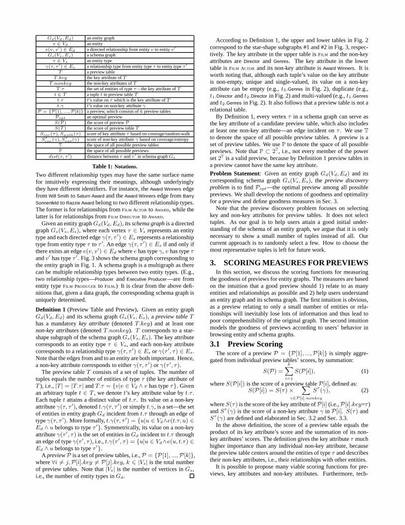
TheNP-hardness of the optimal diverse preview discovery prob-lem is also based on a reduction from the Clique problem, althoughthe proof is more complex.Theorem 2. Optimal diverse preview discovery isNP-hard.

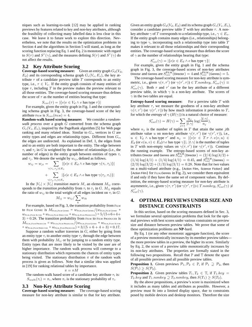
Proof. The decision version of the optimal diverse preview discov-ery problem isDiversePreview (Gs, k, n, d, s)—Given a schemagraphGs, decide whether there exists such a previewP that (1)P

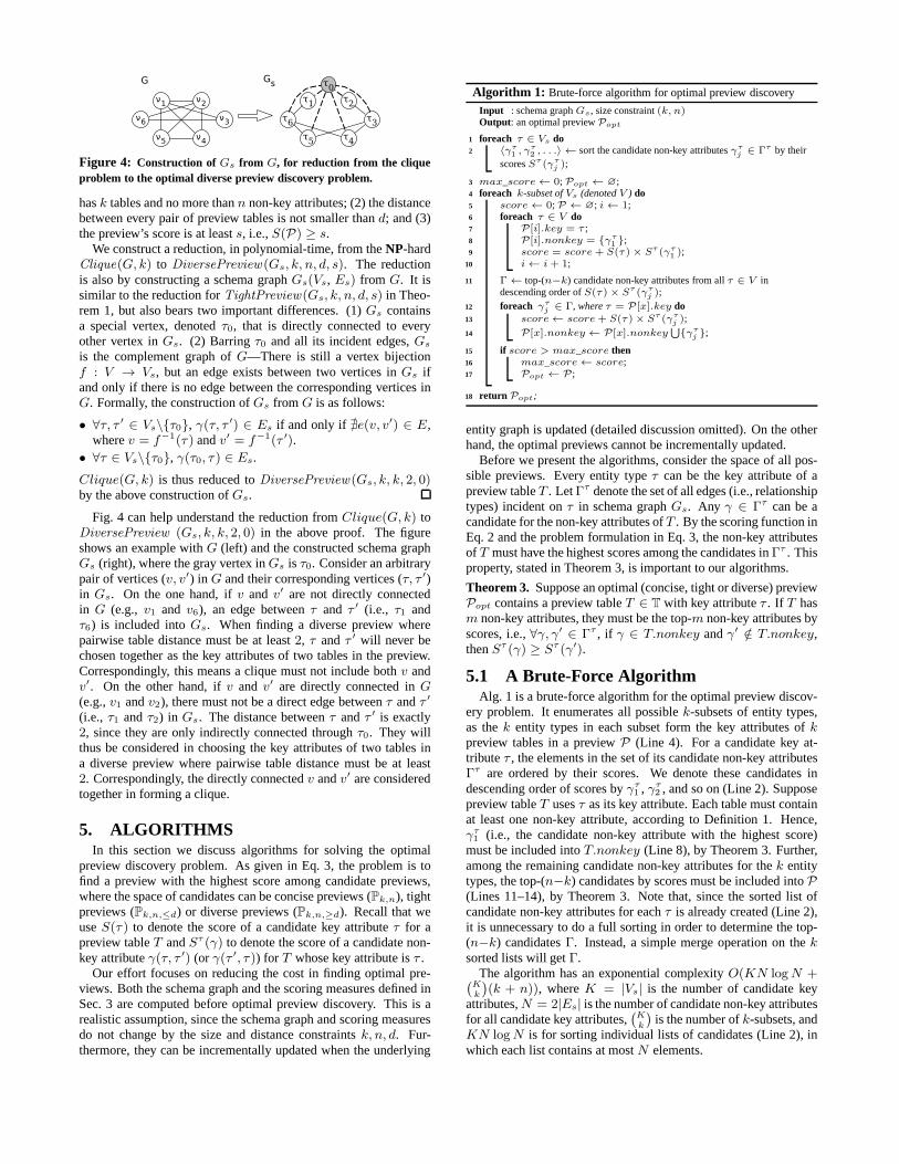
Figure 4: Construction of Gs from G, for reduction from the cliqueproblem to the optimal diverse preview discovery problem.

hask tables and no more thann non-key attributes; (2) the distancebetween every pair of preview tables is not smaller thand; and (3)the preview’s score is at leasts, i.e.,S(P) ≥ s.

We construct a reduction, in polynomial-time, from theNP-hardClique(G, k) to DiversePreview (Gs, k, n, d, s). The reductionis also by constructing a schema graphGs(Vs, Es) from G. It issimilar to the reduction forTightPreview (Gs, k, n, d, s) in Theo-rem 1, but also bears two important differences. (1)Gs containsa special vertex, denotedτ0, that is directly connected to everyother vertex inGs. (2) Barringτ0 and all its incident edges,Gs

is the complement graph ofG—There is still a vertex bijectionf : V → Vs, but an edge exists between two vertices inGs ifand only if there is no edge between the corresponding vertices inG. Formally, the construction ofGs from G is as follows:

• ∀τ, τ ′ ∈ Vs\{τ0}, γ(τ, τ ′) ∈ Es if and only if ∄e(v, v′) ∈ E,wherev = f−1(τ ) andv′ = f−1(τ ′).

• ∀τ ∈ Vs\{τ0}, γ(τ0, τ ) ∈ Es.

Clique(G, k) is thus reduced toDiversePreview (Gs, k, k, 2, 0)by the above construction ofGs.

Fig. 4 can help understand the reduction fromClique(G, k) toDiversePreview (Gs, k, k, 2, 0) in the above proof. The figureshows an example withG (left) and the constructed schema graphGs (right), where the gray vertex inGs is τ0. Consider an arbitrarypair of vertices (v, v′) in G and their corresponding vertices (τ, τ ′)in Gs. On the one hand, ifv and v′ are not directly connectedin G (e.g., v1 and v6), an edge betweenτ and τ ′ (i.e., τ1 andτ6) is included intoGs. When finding a diverse preview wherepairwise table distance must be at least2, τ andτ ′ will never bechosen together as the key attributes of two tables in the preview.Correspondingly, this means a clique must not include bothv andv′. On the other hand, ifv and v′ are directly connected inG(e.g.,v1 andv2), there must not be a direct edge betweenτ andτ ′

(i.e., τ1 andτ2) in Gs. The distance betweenτ andτ ′ is exactly2, since they are only indirectly connected throughτ0. They willthus be considered in choosing the key attributes of two tables ina diverse preview where pairwise table distance must be at least2. Correspondingly, the directly connectedv andv′ are consideredtogether in forming a clique.

5. ALGORITHMSIn this section we discuss algorithms for solving the optimal

preview discovery problem. As given in Eq. 3, the problem is tofind a preview with the highest score among candidate previews,where the space of candidates can be concise previews (Pk,n), tightpreviews (Pk,n,≤d) or diverse previews (Pk,n,≥d). Recall that weuseS(τ ) to denote the score of a candidate key attributeτ for apreview tableT andSτ (γ) to denote the score of a candidate non-key attributeγ(τ, τ ′) (or γ(τ ′, τ )) for T whose key attribute isτ .

Our effort focuses on reducing the cost in finding optimal pre-views. Both the schema graph and the scoring measures definedinSec. 3 are computed before optimal preview discovery. This is arealistic assumption, since the schema graph and scoring measuresdo not change by the size and distance constraintsk, n, d. Fur-thermore, they can be incrementally updated when the underlying

Algorithm 1: Brute-force algorithm for optimal preview discovery

Input : schema graphGs, size constraint(k, n)Output : an optimal previewPopt

1 foreach τ ∈ Vs do2 〈γτ

1 , γτ2 , . . .〉 ← sort the candidate non-key attributesγτ

j ∈ Γτ by theirscoresSτ (γτ

j );

3 max_score← 0; Popt ← ∅;4 foreach k-subset of Vs (denoted V ) do5 score← 0; P ← ∅; i← 1;6 foreach τ ∈ V do7 P[i].key = τ ;8 P[i].nonkey = {γτ

1 };9 score = score+ S(τ)× Sτ (γτ

1 );10 i← i + 1;

11 Γ← top-(n−k) candidate non-key attributes from allτ ∈ V indescending order ofS(τ)× Sτ (γτ

j );12 foreach γτ

j ∈ Γ, where τ = P[x].key do13 score← score+ S(τ)× Sτ (γτ

j );14 P[x].nonkey ← P[x].nonkey

⋃{γτ

j };

15 if score > max_score then16 max_score← score;17 Popt ← P ;

18 return Popt;

entity graph is updated (detailed discussion omitted). On the otherhand, the optimal previews cannot be incrementally updated.

Before we present the algorithms, consider the space of all pos-sible previews. Every entity typeτ can be the key attribute of apreview tableT . LetΓτ denote the set of all edges (i.e., relationshiptypes) incident onτ in schema graphGs. Any γ ∈ Γτ can be acandidate for the non-key attributes ofT . By the scoring function inEq. 2 and the problem formulation in Eq. 3, the non-key attributesof T must have the highest scores among the candidates inΓτ . Thisproperty, stated in Theorem 3, is important to our algorithms.

Theorem 3. Suppose an optimal (concise, tight or diverse) previewPopt contains a preview tableT ∈ T with key attributeτ . If T hasm non-key attributes, they must be the top-m non-key attributes byscores, i.e.,∀γ, γ′ ∈ Γτ , if γ ∈ T.nonkey andγ′ /∈ T.nonkey,thenSτ (γ) ≥ Sτ (γ′).

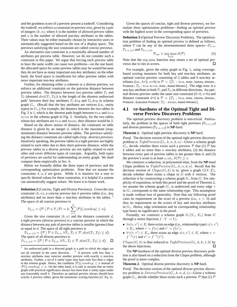
5.1 A Brute-Force AlgorithmAlg. 1 is a brute-force algorithm for the optimal preview discov-

ery problem. It enumerates all possiblek-subsets of entity types,as thek entity types in each subset form the key attributes ofkpreview tables in a previewP (Line 4). For a candidate key at-tributeτ , the elements in the set of its candidate non-key attributesΓτ are ordered by their scores. We denote these candidates indescending order of scores byγτ

1 , γτ2 , and so on (Line 2). Suppose

preview tableT usesτ as its key attribute. Each table must containat least one non-key attribute, according to Definition 1. Hence,γτ1 (i.e., the candidate non-key attribute with the highest score)

must be included intoT.nonkey (Line 8), by Theorem 3. Further,among the remaining candidate non-key attributes for thek entitytypes, the top-(n−k) candidates by scores must be included intoP(Lines 11–14), by Theorem 3. Note that, since the sorted listofcandidate non-key attributes for eachτ is already created (Line 2),it is unnecessary to do a full sorting in order to determine the top-(n−k) candidatesΓ. Instead, a simple merge operation on theksorted lists will getΓ.

The algorithm has an exponential complexityO(KN logN +(

K

k

)

(k + n)), whereK = |Vs| is the number of candidate keyattributes,N = 2|Es| is the number of candidate non-key attributesfor all candidate key attributes,

(

K

k

)

is the number ofk-subsets, andKN logN is for sorting individual lists of candidates (Line 2), inwhich each list contains at mostN elements.

Algorithm 2: Dynamic-programming algorithm for optimal concisepreview discovery

Input : schema graphGs, size constraint(k, n)Output : an optimal concise previewPopt

1 foreachx← 1 to K do2 〈γτx

1 , γτx2 , . . .〉 ← sort the candidate non-key attributesγ

τxj ∈ Γτx by

their scoresSτx (γτxj );

3 for x← 1 to K do4 for i← 1 to min(k, x) do5 for j ← i to n do6 Popt(i, j, x)← Popt(i, j, x− 1);7 for m← 1 to min(j − i + 1, |Γτx |) do8 Tm

x .key ← τx;9 Tm

x .nonkey ← top-m candidate non-key attributes inΓτx ;

10 P ← Popt(i− 1, j −m,x− 1)⋃{Tm

x };11 if S(P) > S(Popt(i, j, x)) then12 Popt(i, j, x)← P ;

13 Popt ← Popt(k, n,K);14 return Popt;

Alg. 1 is for finding one of the optimal previews. To find alloptimal previews, it needs simple extension to deal with ties inscores, which we will not further discuss.

The same brute-force algorithm is applicable for optimal previewdiscovery in all three types of spaces—concise, tight and diversepreviews. The pseudo code in Alg. 1 is for concise previews anddoes not enforce distance constraint, for simplicity of presentation.Enforcing distance constraint for tight/diverse previewsis straight-forward, by performing distance check on every pair of previewtables in eachk-subset of entity types.5.2 A Dynamic-Programming Algorithm for

Concise Preview Discovery ProblemAs the combinatorial number ofk-subsets grows exponentially,

the performance of the above brute-force algorithm becomesun-acceptable for finding an optimal preview under modest size con-straints. We thus developed a dynamic-programming algorithm todiscover optimal concise previews more efficiently.

Consider an arbitrary order on allK entity types—τ1, . . . , τK .We usePopt(k, n, x) to denote an optimal concise preview amongthe firstx entity typesτ1, . . . , τx. The optimal concise previewdiscovery problem is to findPopt(k, n,K). Popt(k, n, x) can beconstructed from the solutions to smaller problems, in two ways:(1) It can be equal toPopt(k, n, x−1), i.e., itsk tables andn non-key attributes are from the firstx−1 entity types and thex-th entitytypeτx does not contribute anything; (2) It can also be the union ofPopt(k−1, n−m,x−1) and a tableTm

x , wherePopt(k−1, n−m,x−1)is an optimal preview withk−1 tables andn−m non-key attributesamong the firstx−1 entity types, andTm

x is the table whose keyattribute isτx and whose non-key attributes are the top-m elementsin Γτx—the sorted list of candidate non-key attributes forτx. Thenumberm is between1 andn−(k−1) (or less if there are lessthan n−(k−1) elements inΓτx ), since each of thek−1 tablesin Popt(k−1, n−m,x−1) must contribute at least one non-keyattribute. The optimal substructure of the problem is as follows.(We omit boundary cases (k = 1 or x = 1 or n = k) for brevity.)

Popt(k, n, x) = argmaxP∈P(k,n,x)

S(P)

P(k, n, x) =

Popt(k, n, x−1),Popt(k−1, n−1, x−1)

⋃

{T 1x},

Popt(k−1, n−2, x−1)⋃

{T 2x},

...

Popt(k−1, k−1, x−1)⋃

{Tn−(k−1)x }

,

Algorithm 3: Apriori-style Algorithm for optimal tight/diversepreview discovery

Input : schema graphGs, size constraint(k, n), distance constraintdOutput : an optimal tight/diverse previewPopt

1 L2 ← ∅;2 foreachi← 1 to K do3 foreachj ← i + 1 to K do4 if dist(τi, τj) ≤ d then /* ≥ d for diverse preview*/5 L2 ← L2 ∪ {〈i j〉};

6 i← 3;7 while i ≤ k andLi−1 6= ∅ do8 Li ← ∅;9 foreachA,B ∈ Li−1 s.t. (∀j < i− 1 : A[j] = B[j]) and

(A[i− 1] < B[i− 1]) do/* ≥ d for diverse preview */

10 if dist(τA[i−1], τB[i−1]) ≤ d then11 Li ← Li ∪ {〈A[1] . . . A[i− 1]B[i− 1]〉};

12 i← i+ 1;

13 if Lk = ∅ then14 return ∅;

15 max_score← 0;16 foreachA ∈ Lk do17 P ← ComputePreview(A);18 if score(P) > max_score then19 max_score← score(P);20 Popt ← P ;

21 return Popt;

whereTmx .key = τx andTm

x .nonkey = top-m candidate non-keyattributes inΓτx . Note that the optimal substructure is inapplicablewhen previews must satisfy distance constraint in additionto sizeconstraint (details omitted). Therefore the dynamic-programmingalgorithm is for concise previews but not tight/diverse previews.

The pseudo code of the dynamic-programming algorithm is shownin Alg. 2. Its complexity isO(KN logN + Kkn2). Similar toAlg. 1, Alg. 2 is for finding one optimal preview. Finding all opti-mal previews requires simple extension to deal with ties in scores,which we will not further discuss.

Both Alg. 1 and 2 assume that, given anyk entity types (keyattributes), they always together have at leastn non-key attributes.That may not be true in reality. In fact, for two previews withthesame number of tables, the preview with less non-key attributesmay have the higher score than the other preview. Note that, inEq. 3, the optimal preview is not required to have exactlyn non-key attributes. It is simple to extend Alg. 1 and 2 to fully complywith the definition. Given any entity typeτ , if it has less thanncandidate non-key attributes, we can simply pad the sorted list Γτ

by pseudo non-key attributes with zero scores.

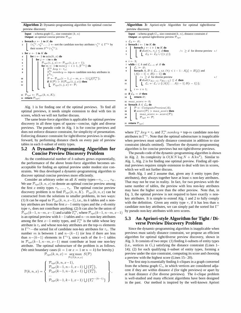
5.3 An Apriori-style Algorithm for Tight / Di-verse Preview Discovery Problem

Since the dynamic-programming algorithm is inapplicable whenpreviews must satisfy distance constraint, we propose an efficientalgorithm for optimal tight/diverse preview discovery, shown inAlg. 3. It consists of two steps: (1) findingk-subsets of entity types(i.e., vertices inGs) satisfying the distance constraint (Lines 1–14); (2) for each qualifyingk-subset of entity types, forming apreview under the size constraint, computing its score and choosinga preview with the highest score (Lines 15– 20).

The first step is essentially findingk-cliques in a graph convertedfrom the schema graphGs, in which vertices are considered adja-cent if they are within distanced (for tight previews) or apart byat least distanced (for diverse previews). Thek-clique problemis well-studied and many efficient algorithms have been designedin the past. Our method is inspired by the well-known Apriori

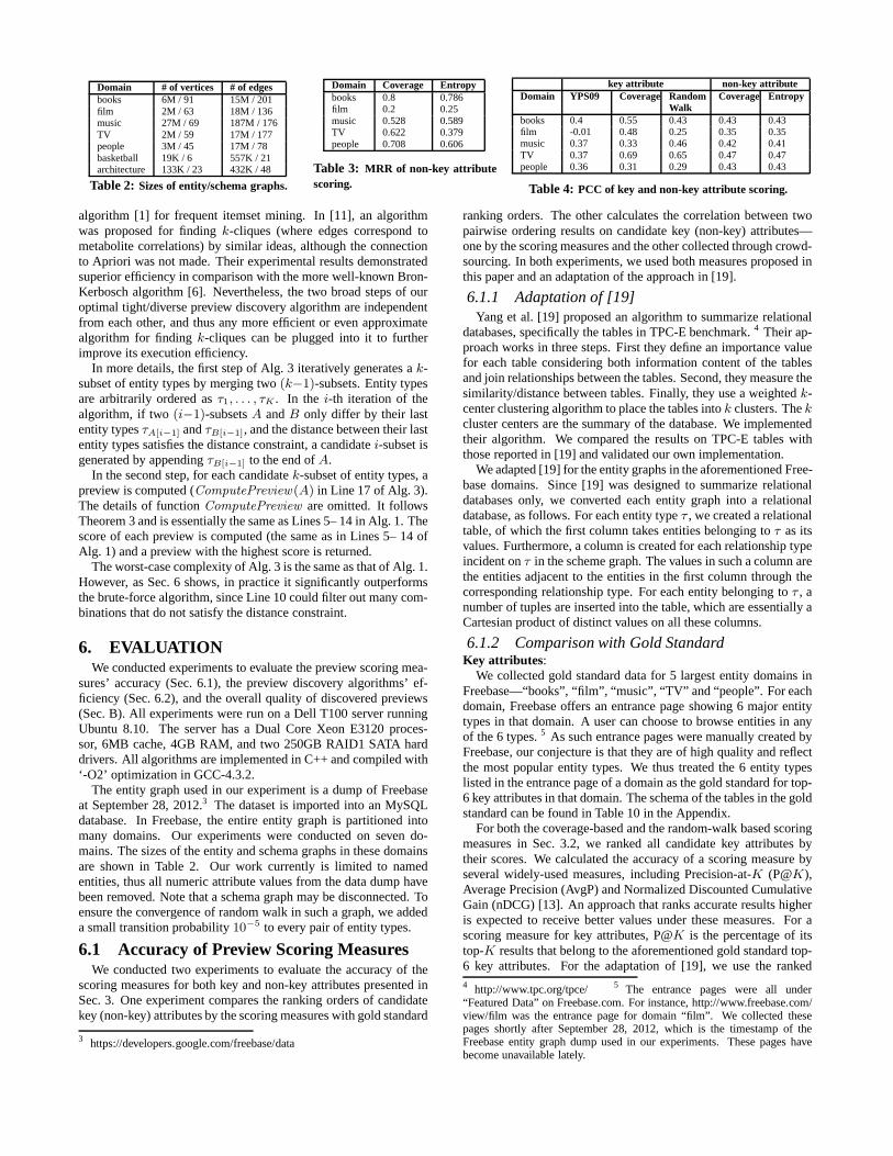
Domain # of vertices # of edgesbooks 6M / 91 15M / 201film 2M / 63 18M / 136music 27M / 69 187M / 176TV 2M / 59 17M / 177people 3M / 45 17M / 78basketball 19K / 6 557K / 21architecture 133K / 23 432K / 48

Table 2: Sizes of entity/schema graphs.

Domain Coverage Entropybooks 0.8 0.786film 0.2 0.25music 0.528 0.589TV 0.622 0.379people 0.708 0.606

Table 3: MRR of non-key attributescoring.

key attribute non-key attributeDomain YPS09 Coverage Random

WalkCoverage Entropy

books 0.4 0.55 0.43 0.43 0.43film -0.01 0.48 0.25 0.35 0.35music 0.37 0.33 0.46 0.42 0.41TV 0.37 0.69 0.65 0.47 0.47people 0.36 0.31 0.29 0.43 0.43

Table 4: PCC of key and non-key attribute scoring.

algorithm [1] for frequent itemset mining. In [11], an algorithmwas proposed for findingk-cliques (where edges correspond tometabolite correlations) by similar ideas, although the connectionto Apriori was not made. Their experimental results demonstratedsuperior efficiency in comparison with the more well-known Bron-Kerbosch algorithm [6]. Nevertheless, the two broad steps of ouroptimal tight/diverse preview discovery algorithm are independentfrom each other, and thus any more efficient or even approximatealgorithm for findingk-cliques can be plugged into it to furtherimprove its execution efficiency.

In more details, the first step of Alg. 3 iteratively generates ak-subset of entity types by merging two(k−1)-subsets. Entity typesare arbitrarily ordered asτ1, . . . , τK . In the i-th iteration of thealgorithm, if two(i−1)-subsetsA andB only differ by their lastentity typesτA[i−1] andτB[i−1], and the distance between their lastentity types satisfies the distance constraint, a candidatei-subset isgenerated by appendingτB[i−1] to the end ofA.

In the second step, for each candidatek-subset of entity types, apreview is computed (ComputePreview (A) in Line 17 of Alg. 3).The details of functionComputePreview are omitted. It followsTheorem 3 and is essentially the same as Lines 5– 14 in Alg. 1. Thescore of each preview is computed (the same as in Lines 5– 14 ofAlg. 1) and a preview with the highest score is returned.

The worst-case complexity of Alg. 3 is the same as that of Alg.1.However, as Sec. 6 shows, in practice it significantly outperformsthe brute-force algorithm, since Line 10 could filter out many com-binations that do not satisfy the distance constraint.

6. EVALUATIONWe conducted experiments to evaluate the preview scoring mea-

sures’ accuracy (Sec. 6.1), the preview discovery algorithms’ ef-ficiency (Sec. 6.2), and the overall quality of discovered previews(Sec. B). All experiments were run on a Dell T100 server runningUbuntu 8.10. The server has a Dual Core Xeon E3120 proces-sor, 6MB cache, 4GB RAM, and two 250GB RAID1 SATA harddrivers. All algorithms are implemented in C++ and compiledwith‘-O2’ optimization in GCC-4.3.2.

The entity graph used in our experiment is a dump of Freebaseat September 28, 2012.3 The dataset is imported into an MySQLdatabase. In Freebase, the entire entity graph is partitioned intomany domains. Our experiments were conducted on seven do-mains. The sizes of the entity and schema graphs in these domainsare shown in Table 2. Our work currently is limited to namedentities, thus all numeric attribute values from the data dump havebeen removed. Note that a schema graph may be disconnected. Toensure the convergence of random walk in such a graph, we addeda small transition probability10−5 to every pair of entity types.

6.1 Accuracy of Preview Scoring MeasuresWe conducted two experiments to evaluate the accuracy of the

scoring measures for both key and non-key attributes presented inSec. 3. One experiment compares the ranking orders of candidatekey (non-key) attributes by the scoring measures with gold standard

3 https://developers.google.com/freebase/data

ranking orders. The other calculates the correlation between twopairwise ordering results on candidate key (non-key) attributes—one by the scoring measures and the other collected through crowd-sourcing. In both experiments, we used both measures proposed inthis paper and an adaptation of the approach in [19].

6.1.1 Adaptation of [19]Yang et al. [19] proposed an algorithm to summarize relational

databases, specifically the tables in TPC-E benchmark.4 Their ap-proach works in three steps. First they define an importance valuefor each table considering both information content of the tablesand join relationships between the tables. Second, they measure thesimilarity/distance between tables. Finally, they use a weightedk-center clustering algorithm to place the tables intok clusters. Thekcluster centers are the summary of the database. We implementedtheir algorithm. We compared the results on TPC-E tables withthose reported in [19] and validated our own implementation.

We adapted [19] for the entity graphs in the aforementioned Free-base domains. Since [19] was designed to summarize relationaldatabases only, we converted each entity graph into a relationaldatabase, as follows. For each entity typeτ , we created a relationaltable, of which the first column takes entities belonging toτ as itsvalues. Furthermore, a column is created for each relationship typeincident onτ in the scheme graph. The values in such a column arethe entities adjacent to the entities in the first column through thecorresponding relationship type. For each entity belonging to τ , anumber of tuples are inserted into the table, which are essentially aCartesian product of distinct values on all these columns.

6.1.2 Comparison with Gold StandardKey attributes:

We collected gold standard data for 5 largest entity domainsinFreebase—“books”, “film”, “music”, “TV” and “people”. For eachdomain, Freebase offers an entrance page showing 6 major entitytypes in that domain. A user can choose to browse entities in anyof the 6 types.5 As such entrance pages were manually created byFreebase, our conjecture is that they are of high quality andreflectthe most popular entity types. We thus treated the 6 entity typeslisted in the entrance page of a domain as the gold standard for top-6 key attributes in that domain. The schema of the tables in the goldstandard can be found in Table 10 in the Appendix.

For both the coverage-based and the random-walk based scoringmeasures in Sec. 3.2, we ranked all candidate key attributesbytheir scores. We calculated the accuracy of a scoring measure byseveral widely-used measures, including Precision-at-K (P@K),Average Precision (AvgP) and Normalized Discounted CumulativeGain (nDCG) [13]. An approach that ranks accurate results higheris expected to receive better values under these measures. For ascoring measure for key attributes, P@K is the percentage of itstop-K results that belong to the aforementioned gold standard top-6 key attributes. For the adaptation of [19], we use the ranked4 http://www.tpc.org/tpce/ 5 The entrance pages were all under“Featured Data” on Freebase.com. For instance, http://www.freebase.com/view/film was the entrance page for domain “film”. We collected thesepages shortly after September 28, 2012, which is the timestamp of theFreebase entity graph dump used in our experiments. These pages havebecome unavailable lately.

0 5 10 15 20

K(books)

0.0

0.2

0.4

0.6

0.8

1.0

Pre

cis

ion

-at-

K

0 5 10 15 20

K(film)

0 5 10 15 20

K(music)

0 5 10 15 20

K(tv)

0 5 10 15 20

K(people)

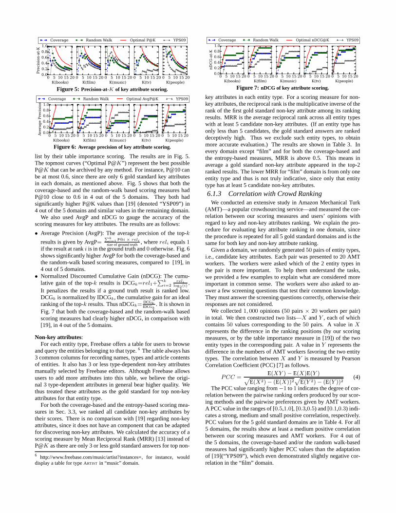
Coverage Random Walk Optimal P@K YPS09

Figure 5: Precision-at-K of key attribute scoring.

0 5 10 15 20

K(books)

0.0

0.2

0.4

0.6

0.8

1.0

Avera

ge P

recis

ion

0 5 10 15 20

K(film)

0 5 10 15 20

K(music)

0 5 10 15 20

K(tv)

0 5 10 15 20

K(people)

Coverage Random Walk Optimal AvgP@K YPS09

Figure 6: Average precision of key attribute scoring.

list by their table importance scoring. The results are in Fig. 5.The topmost curves (“Optimal P@K”) represent the best possibleP@K that can be archived by any method. For instance, P@10 canbe at most 0.6, since there are only 6 gold standard key attributesin each domain, as mentioned above. Fig. 5 shows that both thecoverage-based and the random-walk based scoring measureshadP@10 close to 0.6 in 4 out of the 5 domains. They both hadsignificantly higher P@K values than [19] (denoted “YSP09”)in4 out of the 5 domains and similar values in the remaining domain.

We also used AvgP and nDCG to gauge the accuracy of thescoring measures for key attributes. The results are as follows:

• Average Precision (AvgP): The average precision of the top-k

results is given by AvgP=∑k

i=1 P@i × relisize of ground truth , wherereli equals1

if the result at ranki is in the ground truth and0 otherwise. Fig. 6shows significantly higher AvgP for both the coverage-basedandthe random-walk based scoring measures, compared to [19], in4 out of 5 domains.

• Normalized Discounted Cumulative Gain (nDCG): The cumu-lative gain of the top-k results is DCGk=rel1+

∑k

i=2reli

log2(i).

It penalizes the results if a ground truth result is ranked low.DCGk is normalized by IDCGk, the cumulative gain for an idealranking of the top-k results. Thus nDCGk=

DCGk

IDCGk. It is shown in

Fig. 7 that both the coverage-based and the random-walk basedscoring measures had clearly higher nDCG, in comparison with[19], in 4 out of the 5 domains.

Non-key attributes:For each entity type, Freebase offers a table for users to browse

and query the entities belonging to that type.6 The table always has3 common columns for recording names, types and article contentsof entities. It also has 3 or less type-dependent non-key attributesmanually selected by Freebase editors. Although Freebase allowsusers to add more attributes into this table, we believe the origi-nal 3 type-dependent attributes in general bear higher quality.Wethus treated these attributes as the gold standard for top non-keyattributes for that entity type.

For both the coverage-based and the entropy-based scoring mea-sures in Sec. 3.3, we ranked all candidate non-key attributes bytheir scores. There is no comparison with [19] regarding non-keyattributes, since it does not have an component that can be adaptedfor discovering non-key attributes. We calculated the accuracy of ascoring measure by Mean Reciprocal Rank (MRR) [13] instead ofP@K as there are only 3 or less gold standard answers for top non-

6 http://www.freebase.com/music/artist?instances=, forinstance, woulddisplay a table for typeARTIST in “music” domain.

0 5 10 15 20

K(books)

0.0

0.2

0.4

0.6

0.8

1.0

nD

CG

-at-

K

0 5 10 15 20

K(film)

0 5 10 15 20

K(music)

0 5 10 15 20

K(tv)

0 5 10 15 20

K(people)

Coverage Random Walk Optimal nDCG@K YPS09

Figure 7: nDCG of key attribute scoring.

key attributes in each entity type. For a scoring measure fornon-key attributes, the reciprocal rank is the multiplicative inverse of therank of the first gold standard non-key attribute among its rankingresults. MRR is the average reciprocal rank across all entity typeswith at least 5 candidate non-key attributes. (If an entity type hasonly less than 5 candidates, the gold standard answers are rankeddeceptively high. Thus we exclude such entity types, to obtainmore accurate evaluation.) The results are shown in Table 3.Inevery domain except “film” and for both the coverage-based andthe entropy-based measures, MRR is above 0.5. This means inaverage a gold standard non-key attribute appeared in the top-2ranked results. The lower MRR for “film” domain is from only oneentity type and thus is not truly indicative, since only thatentitytype has at least 5 candidate non-key attributes.

6.1.3 Correlation with Crowd RankingWe conducted an extensive study in Amazon Mechanical Turk

(AMT)—a popular crowdsourcing service—and measured the cor-relation between our scoring measures and users’ opinions withregard to key and non-key attributes ranking. We explain thepro-cedure for evaluating key attribute ranking in one domain, sincethe procedure is repeated for all 5 gold standard domains andis thesame for both key and non-key attribute ranking.

Given a domain, we randomly generated50 pairs of entity types,i.e., candidate key attributes. Each pair was presented to20 AMTworkers. The workers were asked which of the 2 entity types inthe pair is more important. To help them understand the tasks,we provided a few examples to explain what are considered moreimportant in common sense. The workers were also asked to an-swer a few screening questions that test their common knowledge.They must answer the screening questions correctly, otherwise theirresponses are not considered.

We collected1, 000 opinions (50 pairs× 20 workers per pair)in total. We then constructed two lists—X andY , each of whichcontains50 values corresponding to the50 pairs. A value inXrepresents the difference in the ranking positions (by our scoringmeasures, or by the table importance measure in [19]) of the twoentity types in the corresponding pair. A value inY represents thedifference in the numbers of AMT workers favoring the two entitytypes. The correlation betweenX andY is measured by PearsonCorrelation Coefficient (PCC) [7] as follows.

PCC =E(XY )− E(X)E(Y )

√

E(X2)− (E(X))2√

E(Y 2)− (E(Y ))2(4)

The PCC value ranging from−1 to1 indicates the degree of cor-relation between the pairwise ranking orders produced by our scor-ing methods and the pairwise preferences given by AMT workers.A PCC value in the ranges of [0.5,1.0], [0.3,0.5) and [0.1,0.3) indi-cates a strong, medium and small positive correlation, respectively.PCC values for the 5 gold standard domains are in Table 4. For all5 domains, the results show at least a medium positive correlationbetween our scoring measures and AMT workers. For 4 out ofthe 5 domains, the coverage-based and/or the random walk-basedmeasures had significantly higher PCC values than the adaptationof [19](“YPS09”), which even demonstrated slightly negative cor-relation in the “film” domain.

Brute-Force Algorithm Dynamic-Programming Algorithm

B A M

101

104

107

domain

Exe

cutio

nT

ime

(ms)

k=5,n=10

3 6 9k

music,n=20

8 12 16 20n

music,k=6

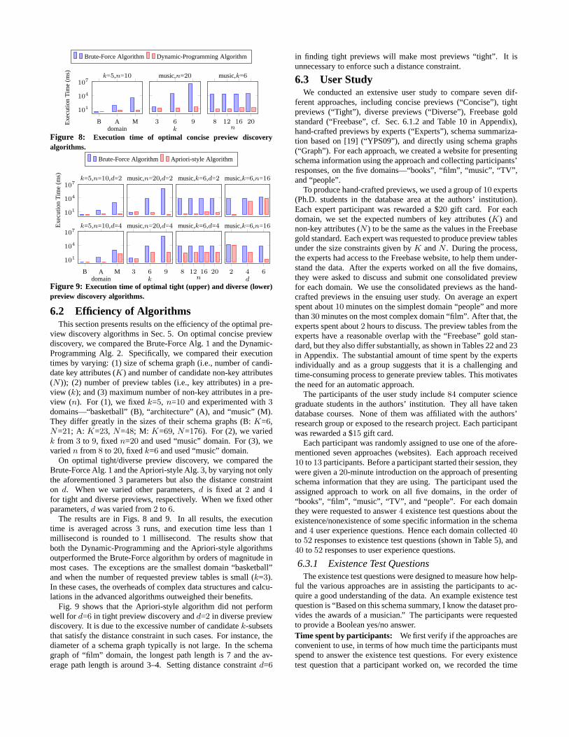
Figure 8: Execution time of optimal concise preview discoveryalgorithms.

Brute-Force Algorithm Apriori-style Algorithm

101

104

107

Exe

cutio

nT

ime

(ms)

k=5,n=10,d=2 music,n=20,d=2 music,k=6,d=2 music,k=6,n=16

B A M

101

104

107

domain

k=5,n=10,d=4

3 6 9k

music,n=20,d=4

8 12 16 20n

music,k=6,d=4

2 4 6d

music,k=6,n=16

Figure 9: Execution time of optimal tight (upper) and diverse (lower)preview discovery algorithms.

6.2 Efficiency of AlgorithmsThis section presents results on the efficiency of the optimal pre-

view discovery algorithms in Sec. 5. On optimal concise previewdiscovery, we compared the Brute-Force Alg. 1 and the Dynamic-Programming Alg. 2. Specifically, we compared their executiontimes by varying: (1) size of schema graph (i.e., number of candi-date key attributes (K) and number of candidate non-key attributes(N )); (2) number of preview tables (i.e., key attributes) in a pre-view (k); and (3) maximum number of non-key attributes in a pre-view (n). For (1), we fixedk=5, n=10 and experimented with3domains—“basketball” (B), “architecture” (A), and “music” (M).They differ greatly in the sizes of their schema graphs (B:K=6,N=21; A: K=23, N=48; M: K=69, N=176). For (2), we variedk from 3 to 9, fixedn=20 and used “music” domain. For (3), wevariedn from 8 to 20, fixedk=6 and used “music” domain.

On optimal tight/diverse preview discovery, we compared theBrute-Force Alg. 1 and the Apriori-style Alg. 3, by varying not onlythe aforementioned 3 parameters but also the distance constrainton d. When we varied other parameters,d is fixed at2 and 4for tight and diverse previews, respectively. When we fixed otherparameters,d was varied from2 to 6.

The results are in Figs. 8 and 9. In all results, the executiontime is averaged across 3 runs, and execution time less than 1millisecond is rounded to 1 millisecond. The results show thatboth the Dynamic-Programming and the Apriori-style algorithmsoutperformed the Brute-Force algorithm by orders of magnitude inmost cases. The exceptions are the smallest domain “basketball”and when the number of requested preview tables is small (k=3).In these cases, the overheads of complex data structures andcalcu-lations in the advanced algorithms outweighed their benefits.

Fig. 9 shows that the Apriori-style algorithm did not performwell for d=6 in tight preview discovery andd=2 in diverse previewdiscovery. It is due to the excessive number of candidatek-subsetsthat satisfy the distance constraint in such cases. For instance, thediameter of a schema graph typically is not large. In the schemagraph of “film” domain, the longest path length is 7 and the av-erage path length is around 3–4. Setting distance constraint d=6

in finding tight previews will make most previews “tight”. Itisunnecessary to enforce such a distance constraint.

6.3 User StudyWe conducted an extensive user study to compare seven dif-

ferent approaches, including concise previews (“Concise”), tightpreviews (“Tight”), diverse previews (“Diverse”), Freebase goldstandard (“Freebase”, cf. Sec. 6.1.2 and Table 10 in Appendix),hand-crafted previews by experts (“Experts”), schema summariza-tion based on [19] (“YPS09”), and directly using schema graphs(“Graph”). For each approach, we created a website for presentingschema information using the approach and collecting participants’responses, on the five domains—“books”, “film”, “music”, “TV”,and “people”.

To produce hand-crafted previews, we used a group of10 experts(Ph.D. students in the database area at the authors’ institution).Each expert participant was rewarded a $20 gift card. For eachdomain, we set the expected numbers of key attributes (K) andnon-key attributes (N ) to be the same as the values in the Freebasegold standard. Each expert was requested to produce previewtablesunder the size constraints given byK andN . During the process,the experts had access to the Freebase website, to help them under-stand the data. After the experts worked on all the five domains,they were asked to discuss and submit one consolidated previewfor each domain. We use the consolidated previews as the hand-crafted previews in the ensuing user study. On average an expertspent about10 minutes on the simplest domain “people” and morethan30 minutes on the most complex domain “film”. After that, theexperts spent about2 hours to discuss. The preview tables from theexperts have a reasonable overlap with the “Freebase” gold stan-dard, but they also differ substantially, as shown in Tables22 and 23in Appendix. The substantial amount of time spent by the expertsindividually and as a group suggests that it is a challengingandtime-consuming process to generate preview tables. This motivatesthe need for an automatic approach.

The participants of the user study include84 computer sciencegraduate students in the authors’ institution. They all have takendatabase courses. None of them was affiliated with the authors’research group or exposed to the research project. Each participantwas rewarded a $15 gift card.

Each participant was randomly assigned to use one of the afore-mentioned seven approaches (websites). Each approach received10 to13 participants. Before a participant started their session,theywere given a20-minute introduction on the approach of presentingschema information that they are using. The participant used theassigned approach to work on all five domains, in the order of“books”, “film”, “music”, “TV”, and “people”. For each domainthey were requested to answer4 existence test questions about theexistence/nonexistence of some specific information in theschemaand4 user experience questions. Hence each domain collected40to 52 responses to existence test questions (shown in Table 5), and40 to 52 responses to user experience questions.

6.3.1 Existence Test QuestionsThe existence test questions were designed to measure how help-

ful the various approaches are in assisting the participants to ac-quire a good understanding of the data. An example existencetestquestion is “Based on this schema summary, I know the datasetpro-vides the awards of a musician.” The participants were requestedto provide a Boolean yes/no answer.Time spent by participants: We first verify if the approaches areconvenient to use, in terms of how much time the participantsmustspend to answer the existence test questions. For every existencetest question that a participant worked on, we recorded the time

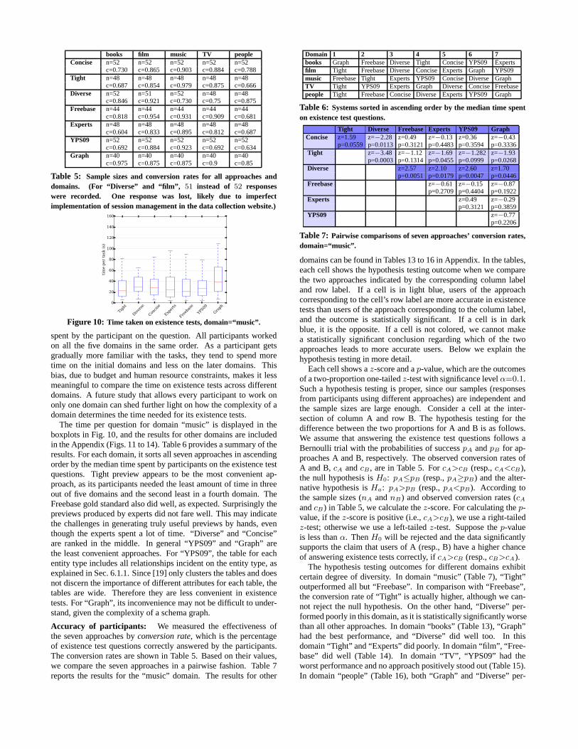
books film music TV peopleConcise n=52 n=52 n=52 n=52 n=52

c=0.730 c=0.865 c=0.903 c=0.884 c=0.788Tight n=48 n=48 n=48 n=48 n=48

c=0.687 c=0.854 c=0.979 c=0.875 c=0.666Diverse n=52 n=51 n=52 n=48 n=48

c=0.846 c=0.921 c=0.730 c=0.75 c=0.875Freebase n=44 n=44 n=44 n=44 n=44

c=0.818 c=0.954 c=0.931 c=0.909 c=0.681Experts n=48 n=48 n=48 n=48 n=48

c=0.604 c=0.833 c=0.895 c=0.812 c=0.687YPS09 n=52 n=52 n=52 n=52 n=52

c=0.692 c=0.884 c=0.923 c=0.692 c=0.634Graph n=40 n=40 n=40 n=40 n=40

c=0.975 c=0.875 c=0.875 c=0.9 c=0.85

Table 5: Sample sizes and conversion rates for all approaches anddomains. (For “Diverse” and “film”, 51 instead of 52 responseswere recorded. One response was lost, likely due to imperfectimplementation of session management in the data collection website.)

Tigh

t

Diver

se

Con

cise

Exp

erts

Fre

ebas

e

YPS09

Gra

ph0

20

40

60

80

100

120

140

160

tim

e p

er

task (

s)

Figure 10: Time taken on existence tests, domain=“music”.

spent by the participant on the question. All participants workedon all the five domains in the same order. As a participant getsgradually more familiar with the tasks, they tend to spend moretime on the initial domains and less on the later domains. Thisbias, due to budget and human resource constraints, makes itlessmeaningful to compare the time on existence tests across differentdomains. A future study that allows every participant to work ononly one domain can shed further light on how the complexity of adomain determines the time needed for its existence tests.

The time per question for domain “music” is displayed in theboxplots in Fig. 10, and the results for other domains are includedin the Appendix (Figs. 11 to 14). Table 6 provides a summary oftheresults. For each domain, it sorts all seven approaches in ascendingorder by the median time spent by participants on the existence testquestions. Tight preview appears to be the most convenient ap-proach, as its participants needed the least amount of time in threeout of five domains and the second least in a fourth domain. TheFreebase gold standard also did well, as expected. Surprisingly thepreviews produced by experts did not fare well. This may indicatethe challenges in generating truly useful previews by hands, eventhough the experts spent a lot of time. “Diverse” and “Concise”are ranked in the middle. In general “YPS09” and “Graph” arethe least convenient approaches. For “YPS09”, the table foreachentity type includes all relationships incident on the entity type, asexplained in Sec. 6.1.1. Since [19] only clusters the tablesand doesnot discern the importance of different attributes for eachtable, thetables are wide. Therefore they are less convenient in existencetests. For “Graph”, its inconvenience may not be difficult tounder-stand, given the complexity of a schema graph.

Accuracy of participants: We measured the effectiveness ofthe seven approaches byconversion rate, which is the percentageof existence test questions correctly answered by the participants.The conversion rates are shown in Table 5. Based on their values,we compare the seven approaches in a pairwise fashion. Table7reports the results for the “music” domain. The results for other

Domain 1 2 3 4 5 6 7books Graph FreebaseDiverse Tight Concise YPS09 Expertsfilm Tight FreebaseDiverse Concise Experts Graph YPS09music FreebaseTight Experts YPS09 Concise Diverse GraphTV Tight YPS09 Experts Graph Diverse Concise Freebasepeople Tight FreebaseConcise Diverse Experts YPS09 Graph

Table 6: Systems sorted in ascending order by the median time spenton existence test questions.

Tight Diverse Freebase Experts YPS09 GraphConcise z=1.59 z=−2.28 z=0.49 z=−0.13 z=0.36 z=−0.43

p=0.0559 p=0.0113 p=0.3121 p=0.4483 p=0.3594 p=0.3336Tight z=−3.48 z=−1.12 z=−1.69 z=−1.282 z=−1.93

p=0.0003 p=0.1314 p=0.0455 p=0.0999 p=0.0268Diverse z=2.57 z=2.10 z=2.60 z=1.70

p=0.0051 p=0.0179 p=0.0047 p=0.0446Freebase z=−0.61 z=−0.15 z=−0.87

p=0.2709 p=0.4404 p=0.1922Experts z=0.49 z=−0.29

p=0.3121 p=0.3859YPS09 z=−0.77

p=0.2206

Table 7: Pairwise comparisons of seven approaches’ conversion rates,domain=“music”.

domains can be found in Tables 13 to 16 in Appendix. In the tables,each cell shows the hypothesis testing outcome when we comparethe two approaches indicated by the corresponding column labeland row label. If a cell is in light blue, users of the approachcorresponding to the cell’s row label are more accurate in existencetests than users of the approach corresponding to the columnlabel,and the outcome is statistically significant. If a cell is in darkblue, it is the opposite. If a cell is not colored, we cannot makea statistically significant conclusion regarding which of the twoapproaches leads to more accurate users. Below we explain thehypothesis testing in more detail.

Each cell shows az-score and ap-value, which are the outcomesof a two-proportion one-tailedz-test with significance levelα=0.1.Such a hypothesis testing is proper, since our samples (responsesfrom participants using different approaches) are independent andthe sample sizes are large enough. Consider a cell at the inter-section of column A and row B. The hypothesis testing for thedifference between the two proportions for A and B is as follows.We assume that answering the existence test questions follows aBernoulli trial with the probabilities of successpA andpB for ap-proaches A and B, respectively. The observed conversion rates ofA and B,cA andcB , are in Table 5. ForcA>cB (resp.,cA<cB),the null hypothesis isH0: pA≤pB (resp.,pA≥pB) and the alter-native hypothesis isHa: pA>pB (resp.,pA<pB). According tothe sample sizes (nA andnB) and observed conversion rates (cAandcB) in Table 5, we calculate thez-score. For calculating thep-value, if thez-score is positive (i.e.,cA>cB), we use a right-tailedz-test; otherwise we use a left-tailedz-test. Suppose thep-valueis less thanα. ThenH0 will be rejected and the data significantlysupports the claim that users of A (resp., B) have a higher chanceof answering existence tests correctly, ifcA>cB (resp.,cB>cA).

The hypothesis testing outcomes for different domains exhibitcertain degree of diversity. In domain “music” (Table 7), “Tight”outperformed all but “Freebase”. In comparison with “Freebase”,the conversion rate of “Tight” is actually higher, althoughwe can-not reject the null hypothesis. On the other hand, “Diverse”per-formed poorly in this domain, as it is statistically significantly worsethan all other approaches. In domain “books” (Table 13), “Graph”had the best performance, and “Diverse” did well too. In thisdomain “Tight” and “Experts” did poorly. In domain “film”, “Free-base” did well (Table 14). In domain “TV”, “YPS09” had theworst performance and no approach positively stood out (Table 15).In domain “people” (Table 16), both “Graph” and “Diverse” per-

Likert ScaleScore

Q1: How easy wasit to read the schemasummary of this domain?

Q2: How much understanding ofthe data in this domain can yougain from the schema summary?

Q3: How helpful was the schemasummary in assisting you to under-stand the data of this domain?

Q4: Is the schema summary missingimportant information about data in thisdomain?

1 Very hard Very little Not helpful at all It provides very little important information.2 Hard A Little Did not help much It provides some important information.3 Neutral Neutral Neutral Neutral4 Easy Some Somewhat helpful It provides most of the important information.5 Very easy Very much Very helpful It provides all important information.

Table 8: User experience questionnaire.

Question 1 2 3 4 5 6 7Q1 FreebaseDiverse Graph Experts YPS09 Concise TightQ2 Graph FreebaseYPS09 Diverse Concise Tight ExpertsQ3 Graph FreebaseYPS09 Diverse Experts Concise TightQ4 YPS09 Concise Experts Graph Tight FreebaseDiverse

Table 9: Systems sorted in descending order by average userexperience scores across five domains.

formed very well. Across all domains, it is quite surprisingthat“Experts” was never statistically significantly better than any otherapproach, except for “Diverse” in domain “music”.

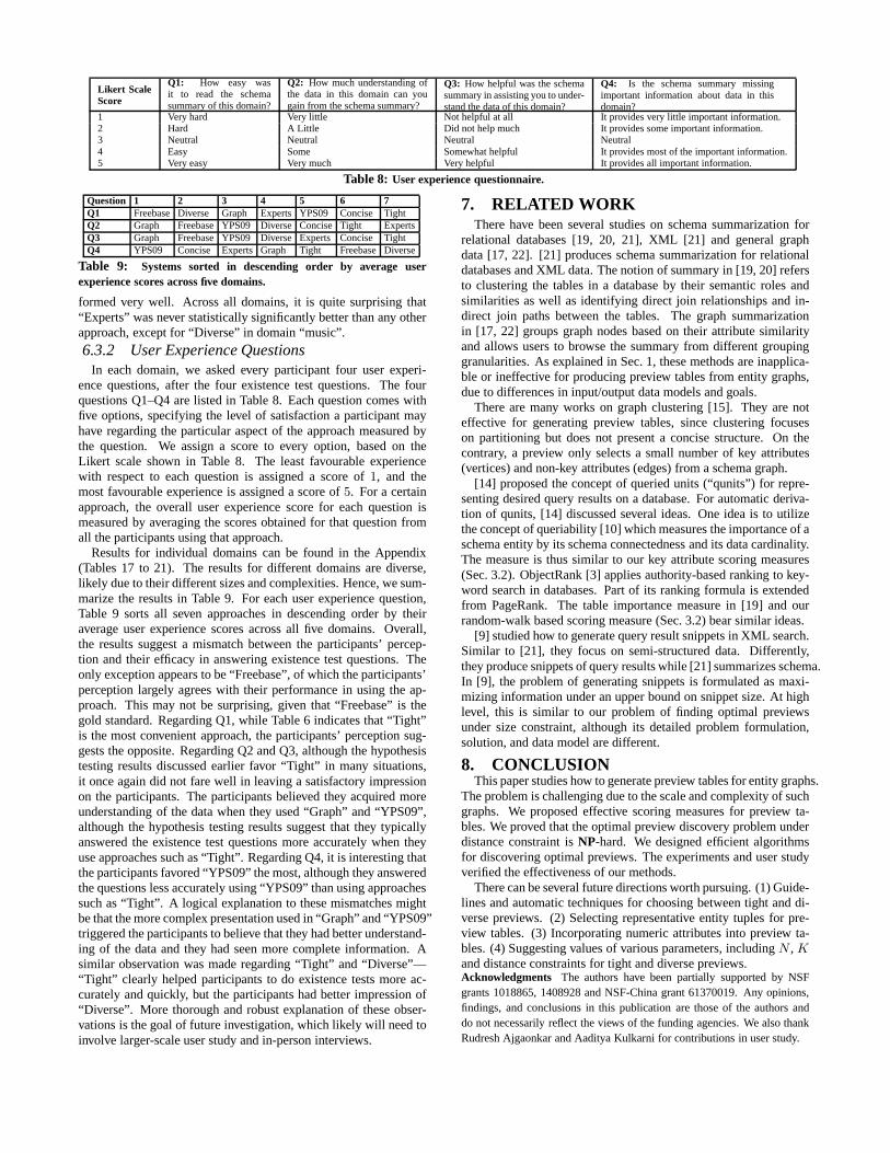
6.3.2 User Experience QuestionsIn each domain, we asked every participant four user experi-

ence questions, after the four existence test questions. The fourquestions Q1–Q4 are listed in Table 8. Each question comes withfive options, specifying the level of satisfaction a participant mayhave regarding the particular aspect of the approach measured bythe question. We assign a score to every option, based on theLikert scale shown in Table 8. The least favourable experiencewith respect to each question is assigned a score of1, and themost favourable experience is assigned a score of5. For a certainapproach, the overall user experience score for each question ismeasured by averaging the scores obtained for that questionfromall the participants using that approach.

Results for individual domains can be found in the Appendix(Tables 17 to 21). The results for different domains are diverse,likely due to their different sizes and complexities. Hence, we sum-marize the results in Table 9. For each user experience question,Table 9 sorts all seven approaches in descending order by theiraverage user experience scores across all five domains. Overall,the results suggest a mismatch between the participants’ percep-tion and their efficacy in answering existence test questions. Theonly exception appears to be “Freebase”, of which the participants’perception largely agrees with their performance in using the ap-proach. This may not be surprising, given that “Freebase” isthegold standard. Regarding Q1, while Table 6 indicates that “Tight”is the most convenient approach, the participants’ perception sug-gests the opposite. Regarding Q2 and Q3, although the hypothesistesting results discussed earlier favor “Tight” in many situations,it once again did not fare well in leaving a satisfactory impressionon the participants. The participants believed they acquired moreunderstanding of the data when they used “Graph” and “YPS09”,although the hypothesis testing results suggest that they typicallyanswered the existence test questions more accurately whentheyuse approaches such as “Tight”. Regarding Q4, it is interesting thatthe participants favored “YPS09” the most, although they answeredthe questions less accurately using “YPS09” than using approachessuch as “Tight”. A logical explanation to these mismatches mightbe that the more complex presentation used in “Graph” and “YPS09”triggered the participants to believe that they had better understand-ing of the data and they had seen more complete information. Asimilar observation was made regarding “Tight” and “Diverse”—“Tight” clearly helped participants to do existence tests more ac-curately and quickly, but the participants had better impression of“Diverse”. More thorough and robust explanation of these obser-vations is the goal of future investigation, which likely will need toinvolve larger-scale user study and in-person interviews.

7. RELATED WORKThere have been several studies on schema summarization for

relational databases [19, 20, 21], XML [21] and general graphdata [17, 22]. [21] produces schema summarization for relationaldatabases and XML data. The notion of summary in [19, 20] refersto clustering the tables in a database by their semantic roles andsimilarities as well as identifying direct join relationships and in-direct join paths between the tables. The graph summarizationin [17, 22] groups graph nodes based on their attribute similarityand allows users to browse the summary from different groupinggranularities. As explained in Sec. 1, these methods are inapplica-ble or ineffective for producing preview tables from entitygraphs,due to differences in input/output data models and goals.

There are many works on graph clustering [15]. They are noteffective for generating preview tables, since clusteringfocuseson partitioning but does not present a concise structure. Onthecontrary, a preview only selects a small number of key attributes(vertices) and non-key attributes (edges) from a schema graph.

[14] proposed the concept of queried units (“qunits”) for repre-senting desired query results on a database. For automatic deriva-tion of qunits, [14] discussed several ideas. One idea is to utilizethe concept of queriability [10] which measures the importance of aschema entity by its schema connectedness and its data cardinality.The measure is thus similar to our key attribute scoring measures(Sec. 3.2). ObjectRank [3] applies authority-based ranking to key-word search in databases. Part of its ranking formula is extendedfrom PageRank. The table importance measure in [19] and ourrandom-walk based scoring measure (Sec. 3.2) bear similar ideas.

[9] studied how to generate query result snippets in XML search.Similar to [21], they focus on semi-structured data. Differently,they produce snippets of query results while [21] summarizes schema.In [9], the problem of generating snippets is formulated as maxi-mizing information under an upper bound on snippet size. At highlevel, this is similar to our problem of finding optimal previewsunder size constraint, although its detailed problem formulation,solution, and data model are different.

8. CONCLUSIONThis paper studies how to generate preview tables for entitygraphs.

The problem is challenging due to the scale and complexity ofsuchgraphs. We proposed effective scoring measures for previewta-bles. We proved that the optimal preview discovery problem underdistance constraint isNP-hard. We designed efficient algorithmsfor discovering optimal previews. The experiments and userstudyverified the effectiveness of our methods.

There can be several future directions worth pursuing. (1) Guide-lines and automatic techniques for choosing between tight and di-verse previews. (2) Selecting representative entity tuples for pre-view tables. (3) Incorporating numeric attributes into preview ta-bles. (4) Suggesting values of various parameters, includingN , Kand distance constraints for tight and diverse previews.Acknowledgments The authors have been partially supported by NSFgrants 1018865, 1408928 and NSF-China grant 61370019. Any opinions,findings, and conclusions in this publication are those of the authors anddo not necessarily reflect the views of the funding agencies.We also thankRudresh Ajgaonkar and Aaditya Kulkarni for contributions in user study.

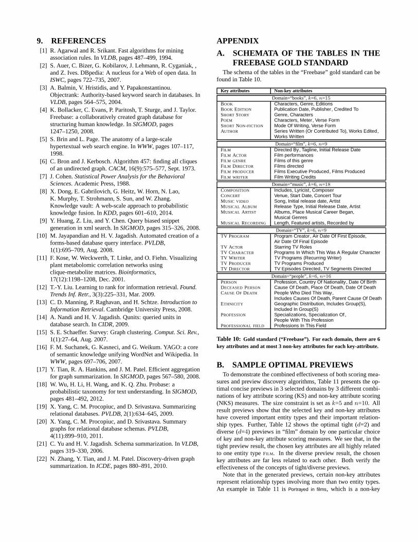
9. REFERENCES[1] R. Agarwal and R. Srikant. Fast algorithms for mining

association rules. InVLDB, pages 487–499, 1994.[2] S. Auer, C. Bizer, G. Kobilarov, J. Lehmann, R. Cyganiak,,

and Z. Ives. DBpedia: A nucleus for a Web of open data. InISWC, pages 722–735, 2007.

[3] A. Balmin, V. Hristidis, and Y. Papakonstantinou.Objectrank: Authority-based keyword search in databases.InVLDB, pages 564–575, 2004.

[4] K. Bollacker, C. Evans, P. Paritosh, T. Sturge, and J. Taylor.Freebase: a collaboratively created graph database forstructuring human knowledge. InSIGMOD, pages1247–1250, 2008.

[5] S. Brin and L. Page. The anatomy of a large-scalehypertextual web search engine. InWWW, pages 107–117,1998.

[6] C. Bron and J. Kerbosch. Algorithm 457: finding all cliquesof an undirected graph.CACM, 16(9):575–577, Sept. 1973.

[7] J. Cohen.Statistical Power Analysis for the BehavioralSciences. Academic Press, 1988.

[8] X. Dong, E. Gabrilovich, G. Heitz, W. Horn, N. Lao,K. Murphy, T. Strohmann, S. Sun, and W. Zhang.Knowledge vault: A web-scale approach to probabilisticknowledge fusion. InKDD, pages 601–610, 2014.

[9] Y. Huang, Z. Liu, and Y. Chen. Query biased snippetgeneration in xml search. InSIGMOD, pages 315–326, 2008.

[10] M. Jayapandian and H. V. Jagadish. Automated creation of aforms-based database query interface.PVLDB,1(1):695–709, Aug. 2008.

[11] F. Kose, W. Weckwerth, T. Linke, and O. Fiehn. Visualizingplant metabolomic correlation networks usingclique-metabolite matrices.Bioinformatics,17(12):1198–1208, Dec. 2001.

[12] T.-Y. Liu. Learning to rank for information retrieval.Found.Trends Inf. Retr., 3(3):225–331, Mar. 2009.

[13] C. D. Manning, P. Raghavan, and H. Schtze.Introduction toInformation Retrieval. Cambridge University Press, 2008.

[14] A. Nandi and H. V. Jagadish. Qunits: queried units indatabase search. InCIDR, 2009.

[15] S. E. Schaeffer. Survey: Graph clustering.Comput. Sci. Rev.,1(1):27–64, Aug. 2007.

[16] F. M. Suchanek, G. Kasneci, and G. Weikum. YAGO: a coreof semantic knowledge unifying WordNet and Wikipedia. InWWW, pages 697–706, 2007.

[17] Y. Tian, R. A. Hankins, and J. M. Patel. Efficient aggregationfor graph summarization. InSIGMOD, pages 567–580, 2008.

[18] W. Wu, H. Li, H. Wang, and K. Q. Zhu. Probase: aprobabilistic taxonomy for text understanding. InSIGMOD,pages 481–492, 2012.

[19] X. Yang, C. M. Procopiuc, and D. Srivastava. Summarizingrelational databases.PVLDB, 2(1):634–645, 2009.

[20] X. Yang, C. M. Procopiuc, and D. Srivastava. Summarygraphs for relational database schemas.PVLDB,4(11):899–910, 2011.

[21] C. Yu and H. V. Jagadish. Schema summarization. InVLDB,pages 319–330, 2006.

[22] N. Zhang, Y. Tian, and J. M. Patel. Discovery-driven graphsummarization. InICDE, pages 880–891, 2010.

APPENDIX

A. SCHEMATA OF THE TABLES IN THEFREEBASE GOLD STANDARD

The schema of the tables in the “Freebase” gold standard can befound in Table 10.

Key attributes Non-key attributes

Domain=“books”,k=6, n=15BOOK Characters, Genre, EditionsBOOK EDITION Publication Date, Publisher , Credited ToSHORT STORY Genre, CharactersPOEM Characters, Meter , Verse FormSHORT NON-FICTION Mode Of Writing, Verse FormAUTHOR Series Written (Or Contributed To), Works Edited ,

Works Written

Domain=“film”, k=6, n=9FILM Directed By , Tagline, Initial Release DateFILM ACTOR Film performancesFILM GENRE Films of this genreFILM DIRECTOR Films directedFILM PRODUCER Films Executive Produced , Films ProducedFILM WRITER Film Writing Credits

Domain=“music”,k=6, n=18COMPOSITION Includes, Lyricist, ComposerCONCERT Venue, Start Date, Concert TourMUSIC VIDEO Song, Initial release date, ArtistMUSICAL ALBUM Release Type, Initial Release Date, ArtistMUSICAL ARTIST Albums, Place Musical Career Began,

Musical GenresMUSICAL RECORDING Length, Featured artists, Recorded by

Domain=“TV”, k=6, n=9TV PROGRAM Program Creator , Air Date Of First Episode,

Air Date Of Final EpisodeTV ACTOR Starring TV RolesTV CHARACTER Programs In Which This Was A Regular CharacterTV WRITER TV Programs (Recurring Writer)TV PRODUCER TV Programs ProducedTV D IRECTOR TV Episodes Directed , TV Segments Directed

Domain=“people”,k=6, n=16PERSON Profession, Country Of Nationality , Date Of BirthDECEASED PERSON Cause Of Death, Place Of Death, Date Of DeathCAUSE OF DEATH People Who Died This Way ,

Includes Causes Of Death, Parent Cause Of DeathETHNICITY Geographic Distribution, Includes Group(S),

Included In Group(S)PROFESSION Specializations, Specialization Of ,

People With This ProfessionPROFESSIONAL FIELD Professions In This Field

Table 10: Gold standard (“Freebase”). For each domain, there are 6key attributes and at most 3 non-key attributes for each key-attribute.

B. SAMPLE OPTIMAL PREVIEWSTo demonstrate the combined effectiveness of both scoring mea-

sures and preview discovery algorithms, Table 11 presents the op-timal concise previews in 3 selected domains by 3 different combi-nations of key attribute scoring (KS) and non-key attributescoring(NKS) measures. The size constraint is set ask=5 andn=10. Allresult previews show that the selected key and non-key attributeshave covered important entity types and their important relation-ship types. Further, Table 12 shows the optimal tight (d=2) anddiverse (d=4) previews in “film” domain by one particular choiceof key and non-key attribute scoring measures. We see that, in thetight preview result, the chosen key attributes are all highly relatedto one entity typeFILM . In the diverse preview result, the chosenkey attributes are far less related to each other. Both verify theeffectiveness of the concepts of tight/diverse previews.

Note that in the generated previews, certain non-key attributesrepresent relationship types involving more than two entity types.An example in Table 11 isPortrayed in films, which is a non-key

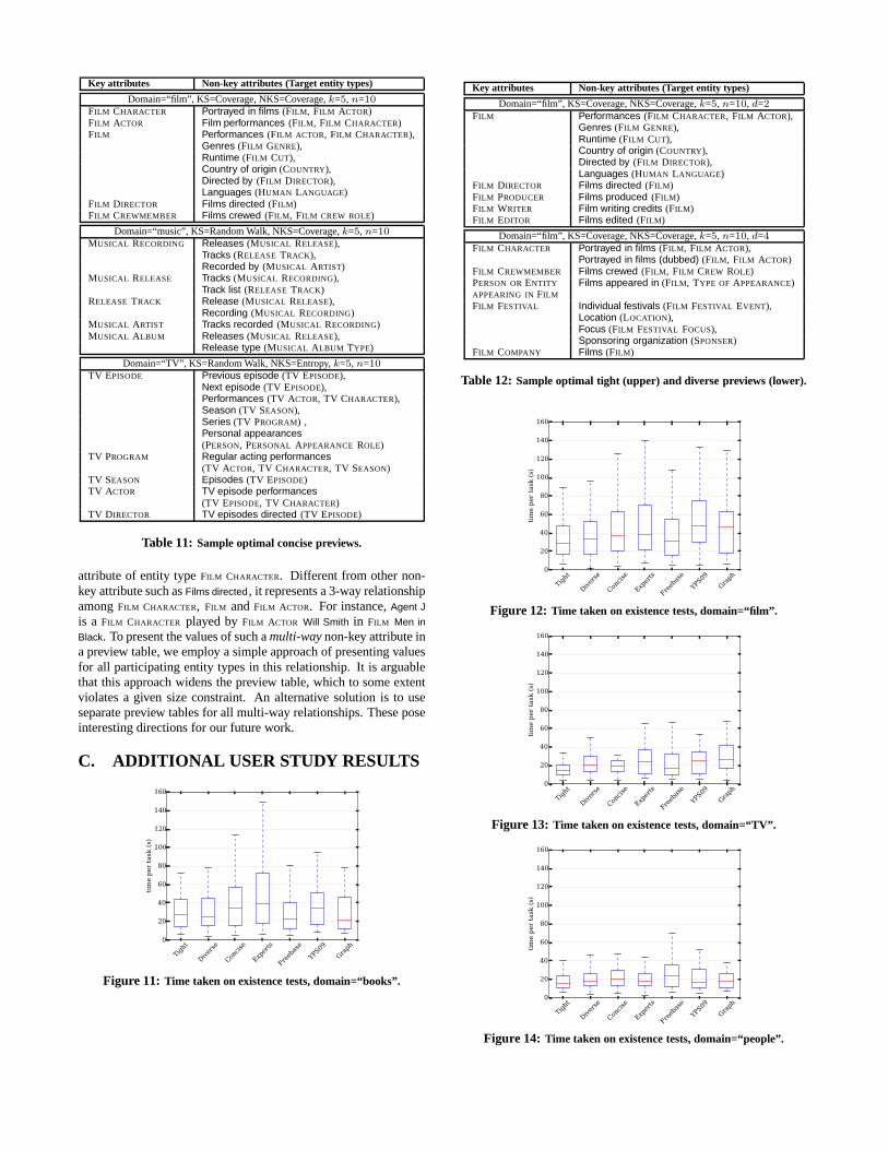
Key attributes Non-key attributes (Target entity types)

Domain=“film”, KS=Coverage, NKS=Coverage,k=5, n=10FILM CHARACTER Portrayed in films (FILM , FILM ACTOR)FILM ACTOR Film performances (FILM , FILM CHARACTER)FILM Performances (FILM ACTOR, FILM CHARACTER),

Genres (FILM GENRE),Runtime (FILM CUT),Country of origin (COUNTRY),Directed by (FILM DIRECTOR),Languages (HUMAN LANGUAGE)

FILM DIRECTOR Films directed (FILM )FILM CREWMEMBER Films crewed (FILM , FILM CREW ROLE)

Domain=“music”, KS=Random Walk, NKS=Coverage,k=5, n=10MUSICAL RECORDING Releases (MUSICAL RELEASE),

Tracks (RELEASE TRACK),Recorded by (MUSICAL ARTIST)

MUSICAL RELEASE Tracks (MUSICAL RECORDING),Track list (RELEASE TRACK)

RELEASE TRACK Release (MUSICAL RELEASE),Recording (MUSICAL RECORDING)

MUSICAL ARTIST Tracks recorded (MUSICAL RECORDING)MUSICAL ALBUM Releases (MUSICAL RELEASE),

Release type (MUSICAL ALBUM TYPE)

Domain=“TV”, KS=Random Walk, NKS=Entropy,k=5, n=10TV EPISODE Previous episode (TV EPISODE),

Next episode (TV EPISODE),Performances (TV ACTOR, TV CHARACTER),Season (TV SEASON),Series (TV PROGRAM) ,Personal appearances(PERSON, PERSONAL APPEARANCEROLE)

TV PROGRAM Regular acting performances(TV ACTOR, TV CHARACTER, TV SEASON)

TV SEASON Episodes (TV EPISODE)TV ACTOR TV episode performances

(TV EPISODE, TV CHARACTER)TV D IRECTOR TV episodes directed (TV EPISODE)

Table 11: Sample optimal concise previews.

attribute of entity typeFILM CHARACTER. Different from other non-key attribute such asFilms directed, it represents a 3-way relationshipamongFILM CHARACTER, FILM andFILM ACTOR. For instance,Agent J

is a FILM CHARACTER played byFILM ACTOR Will Smith in FILM Men in

Black. To present the values of such amulti-way non-key attribute ina preview table, we employ a simple approach of presenting valuesfor all participating entity types in this relationship. Itis arguablethat this approach widens the preview table, which to some extentviolates a given size constraint. An alternative solution is to useseparate preview tables for all multi-way relationships. These poseinteresting directions for our future work.

C. ADDITIONAL USER STUDY RESULTS

Tigh

t

Diver

se

Con

cise

Exp

erts

Fre

ebas

e

YPS09

Gra

ph0

20

40

60

80

100

120

140

160

tim

e p

er

task (

s)

Figure 11: Time taken on existence tests, domain=“books”.

Key attributes Non-key attributes (Target entity types)

Domain=“film”, KS=Coverage, NKS=Coverage,k=5, n=10, d=2FILM Performances (FILM CHARACTER, FILM ACTOR),

Genres (FILM GENRE),Runtime (FILM CUT),Country of origin (COUNTRY),Directed by (FILM DIRECTOR),Languages (HUMAN LANGUAGE)

FILM DIRECTOR Films directed (FILM )FILM PRODUCER Films produced (FILM )FILM WRITER Film writing credits (FILM )FILM EDITOR Films edited (FILM )

Domain=“film”, KS=Coverage, NKS=Coverage,k=5, n=10, d=4FILM CHARACTER Portrayed in films (FILM , FILM ACTOR),

Portrayed in films (dubbed) (FILM , FILM ACTOR)FILM CREWMEMBER Films crewed (FILM , FILM CREW ROLE)PERSON ORENTITY Films appeared in (FILM , TYPE OF APPEARANCE)APPEARING IN FILM

FILM FESTIVAL Individual festivals (FILM FESTIVAL EVENT),Location (LOCATION),Focus (FILM FESTIVAL FOCUS),Sponsoring organization (SPONSER)

FILM COMPANY Films (FILM )

Table 12: Sample optimal tight (upper) and diverse previews (lower).

Tigh

t

Diver

se

Con

cise

Exp

erts

Fre

ebas

e

YPS09

Gra

ph0

20

40

60

80

100

120

140

160

tim

e p

er

task (

s)

Figure 12: Time taken on existence tests, domain=“film”.

Tigh

t

Diver

se

Con

cise

Exp

erts

Fre

ebas

e

YPS09

Gra

ph0

20

40

60

80

100

120

140

160

tim

e p

er

task (

s)

Figure 13: Time taken on existence tests, domain=“TV”.

Tigh

t

Diver

se

Con

cise

Exp

erts

Fre

ebas

e

YPS09

Gra

ph0

20

40

60

80

100

120

140

160

tim

e p

er

task (

s)

Figure 14: Time taken on existence tests, domain=“people”.

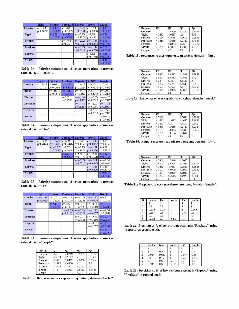
Tight Diverse Freebase Experts YPS09 GraphConcise z=−0.47 z=1.45 z=1.02 z=−1.34 z=−0.43 z=3.15

p=0.3192 p=0.0735 p=0.1539 p=0.0901 p=0.3336 p=0.0008Tight z=1.89 z=1.45 z=−0.85 z=0.05 z=3.49

p=0.0294 p=0.0735 p=0.1977 p=0.4801 p=0.0002Diverse z=−0.37 z=−2.72 z=−1.86 z=2.06

p=0.3557 p=0.0033 p=0.0314 p=0.0197Freebase z=−2.25 z=−1.42 z=2.32

p=0.0122 p=0.0778 p=0.0102Experts z=0.92 z=4.13

p=0.1788 p=0.0000YPS09 z=3.47

p=0.0003

Table 13: Pairwise comparisons of seven approaches’ conversionrates, domain=“books”.

Tight Diverse Freebase Experts YPS09 GraphConcise z=−0.16 z=0.92 z=1.49 z=−0.45 z=0.29 z=0.14

p=0.4364 p=0.1788 p=0.0681 p=0.3264 p=0.3859 p=0.4443Tight z=1.06 z=1.61 z=−0.28 z=0.45 z=0.29

p=0.1446 p=0.0537 p=0.3897 p=0.3264 p=0.3859Diverse z=0.66 z=−1.34 z=−0.63 z=−0.73

p=0.2546 p=0.0901 p=0.2643 p=0.2327Freebase z=−1.86 z=−1.23 z=−1.31

p=0.0314 p=0.1093 p=0.0951Experts z=0.73 z=0.55

p=0.2327 p=0.2912YPS09 z=−0.13

p=0.4483

Table 14: Pairwise comparisons of seven approaches’ conversionrates, domain=“film”.

Tight Diverse Freebase Experts YPS09 GraphConcise z=−0.14 z=−1.74 z=0.40 z=−1.01 z=−2.40 z=0.24

p=0.4443 p=0.0409 p=0.3446 p=0.1562 p=0.0082 p=0.4052Tight z=−1.57 z=0.52 z=−0.85 z=−2.21 z=0.37

p=0.0582 p=0.3015 p=0.1977 p=0.0136 p=0.3557Diverse z=2.01 z=0.73 z=−0.65 z=1.82

p=0.0222 p=0.2327 p=0.2578 p=0.0344Freebase z=−1.33 z=−2.61 z=−0.14

p=0.0918 p=0.0045 p=0.4443Experts z=−1.38 z=1.16

p=0.0838 p=0.1230YPS09 z=2.40

p=0.0082

Table 15: Pairwise comparisons of seven approaches’ conversionrates, domain=“TV”.

Tight Diverse Freebase Experts YPS09 GraphConcise z=−1.37 z=1.16 z=−1.19 z=−1.15 z=−1.73 z=0.76

p=0.0853 p=0.1230 p=0.1170 p=0.1251 p=0.0418 p=0.2236Tight z=2.43 z=0.15 z=0.22 z=−0.34 z=1.98

p=0.0075 p=0.4404 p=0.4129 p=0.3669 p=0.0239Diverse z=−2.25 z=−2.23 z=−2.78 z=−0.34

p=0.0122 p=0.0129 p=0.0027 p=0.3669Freebase z=0.06 z=−0.48 z=1.82

p=0.4761 p=0.3156 p=0.0344Experts z=−0.56 z=1.79

p=0.2877 p=0.0367YPS09 z=2.31

p=0.0104

Table 16: Pairwise comparisons of seven approaches’ conversionrates, domain=“people”.

System Q1 Q2 Q3 Q4Concise 3.5 4.0769 3.9231 3.6154Tight 3.5833 3.9167 4 3.3333Diverse 3.9231 3.8462 4.0769 3.6364Freebase 3.8182 4.0909 4 3.6Experts 3.3333 3.75 4.2727 3.5YPS09 3.75 3.8333 3.8462 3.5385Graph 4.4 4.1 4.1 3.3333

Table 17: Responses to user experience questions, domain=“books”.

System Q1 Q2 Q3 Q4Concise 4 4.0909 4.4167 3.7692Tight 4.0833 4.6667 4.5 3.75Diverse 4.1538 4.4615 4.4615 3.3846Freebase 4.1818 4.3636 4.2727 3.4545Experts 4 4.0833 4.25 3.2727YPS09 3.5385 4.3077 4.2308 4Graph 3.8 4.7 4.6 4

Table 18: Responses to user experience questions, domain=“film”.

System Q1 Q2 Q3 Q4Concise 3.8462 3.8462 4.1538 3.5833Tight 3.6667 3.8333 4.0833 3.75Diverse 3.75 3.75 3.9167 3Freebase 3.8182 4.2727 4.4545 3.5455Experts 4.1667 4.1667 4.5 4.3333YPS09 4.3077 4.5385 4.4615 3.8333Graph 3.6 4.6 4.5 3.9

Table 19: Responses to user experience questions, domain=“music”.

System Q1 Q2 Q3 Q4Concise 3.7692 4 3.7692 3.7692Tight 4.1667 4.1667 4.1667 3.6667Diverse 4.0833 4.25 4.4167 3.6667Freebase 4.5455 4.3636 4.2727 3.2727Experts 4.1667 3.8333 3.8333 3.6667YPS09 3.5385 3.6154 3.7692 3Graph 3.5 4.6 4.4 3.9

Table 20: Responses to user experience questions, domain=“TV”.

System Q1 Q2 Q3 Q4Concise 4.2308 4.3846 4.3077 4Tight 2.9167 3.6364 3.4545 2.9167Diverse 4.0833 4.1667 4.0833 3.5833Freebase 3.9091 4.0909 4.0909 3.4545Experts 3.9167 4.0833 4.0833 3.75YPS09 4.3333 4.4615 4.6923 4.3846Graph 4.5 4.1 4 3.1

Table 21: Responses to user experience questions, domain=“people”.

K books film music TV people1 1 1 1 1 12 0.5 0.5 1 1 13 0.334 0.334 1 1 0.6644 0.25 0.5 1 0.75 0.55 0.2 0.6 1 0.6 0.66 0.333 0.5 0.833 0.5 0.5

Table 22: Precision-at-K of key attribute scoring in “Freebase”, using“Experts” as ground truth.

K books film music TV people1 1 1 1 1 12 1 0.5 1 1 0.53 0.667 0.667 1 0.667 0.6674 0.5 0.75 1 0.75 0.755 0.4 0.6 0.8 0.6 0.66 0.333 0.5 0.833 0.5 0.5

Table 23: Precision-at-K of key attribute scoring in “Experts”, using“Freebase” as ground truth.