Signal Processing 6 (1984) 61-66 61 North-Holland

S H O R T C O M M U N I C A T I O N

G E N E R A T I N G M U L T I P L I E R S F O R A R A D I X - 4 P A R A L L E L FFT A L G O R I T H M

J.A. J O H N S T O N

Cambridge University Engineering Department, Trumpington Street, Cambridge CB21PZ, UK

Received 11 November 1982 Revised 20 January 1983 and 31 August 1983

Abstract. One method of computing a radix-2 N-point DFT uses N/2 butterflies in parallel, interconnected by a perfect shuffle mapping. For the radix-2 case the multipliers required by each butterfly at each stage can be computed from those in the previous stage. This note extends the method to the radix-4 DFT.

Zusammen|assung. Eine Methode zur Berechnung von radix-2 N-Punkte DFT's verwendet N/2 'butterflies' die parallel geschaltet werden und durch einin perfekten 'shuffle' zusammengeschaltet werden. Im radix-2 Fall k6nnen die ben6tigten Multiplikatoren jeweils aus den laufenden Werten berechnet werden. Diese Kommunikation verallgemeinert die Methode ffir radix-4 DFT's.

R6sum~. Une m6thode de calcul de DFT ~ N points ~ base 2 utilise N/2 papillons au parallele, interconnect6s par un ordonnancement parfait. Pour le cash base 2, les multiplicurs necessaires pour chaque papillon fi chaque 6tape pr6cedent. Cette correspondance 6tend ces r6sultats h la DFT h base 4.

Keywords. Fast Fourier transform, parallel processing.

1. Introduction

A radix-2 parallel FFT algori thm for a t ransform of N = 2 " points due to Pease [1], consists of m

iterations using a set of N / 2 butterflies opera t ing in parallel. The inputs and outputs of the butterflies

are connec ted via a perfect shuffle mapping [2] to provide the required data permuta t ion be tween stages.

At each stage a different multiplier (twiddle factor) may be required for each butterfly. There are several

different methods of providing these multipliers. They could be s tored in a central read-only m e m o r y and

sent to each unit as required, or each butterfly could store the values it requires. Bo th these methods have dis-advantages. In the first me thod a control unit would be required together with complex

interconnect ions to ensure that each butterfly received the correc t multiplier at the correct time. The

principal d is-advantage of the second me thod is that the butterflies are no longer identical, making it

difficult to apply LSI techniques to the hardware . A third me thod [3] of providing the multipliers involves

generat ing the multipliers in each stage f rom a permuta t ion of the multipliers used in the previous stage. This involves extra computa t ion but obviates the need for many interconnect ions and a large central store.

This no te extends the me thod of generat ing multipliers to a radix-4 version of the parallel FFT algorithm.

A dec imat ion- in- f requency algori thm is used, a l though a decimat ion- in- t ime decomposi t ion is equally valid.

0165-1684/84/$3.00 © 1984, Elsevier Science Publishers B.V. (North-Holland)

6 2 J.A. Johnston / Multipliers for Radix-4 FFT

2. Derivation of the algorithm

The radix-4 FFT algorithm is derived from the DFT defined as:

N--1

A ( r ) = ( 1 / N ) ~ X ( k ) W rk, r = 0 , 1 . . . . . N - l , (1) k = 0

where A ( r ) and X ( k ) are the transform pair and W is defined as:

W = exp(- j2~r /N) .

The transform length, N, is constrained to be a power of four, i.e.: N = 4 " . The indices r and k (and an additional index v to be used later) are defined as radix-4 numbers as follows:

r = 4 " - ~ r , _ ~ + , . . . , +4r1+ ro

A--~t. + +4k~+k0 k ~.. .r ' ~n -1 , " • •

/3 = 4 n - l D n _ l + , . . . , + 4 t ~ l + V o

(rn-1 . . . . . r~, ro) (2a)

( k n _ l , . . . , k l , k o ) (2b)

( v , - 1 , • • • , v l , Vo) (2c)

Substituting (2a) and (2b) in (1), grouping the W terms according to r and defining a set of n partial result arrays the DFT can be computed by iteration of (3).

Xp+l ( ro , r 1 . . . . . rp, k n - p - 2 . . . . . ko)

= (1/4)[Xp(ro . . . . . rp-1, 0, kn-p-2 . . . . . k o ) + ( - j ) r p X p ( r o , . . . , rp-1, 1, k , -p -2 . . . . . go)

+( -1 ) rpXp(ro . . . . . rp-1, 2, k . -p-2 . . . . . ko)+(j)rpXp(ro . . . . . rp-1, 3, k . -p -2 . . . . . k0)]

X waPrp(4n-p-2kn-p 2 + ' " + k ° ) , (3)

where:

X o ( k ) = X ( k ) , p = 0 , 1 . . . . . n - l , k_ 1 = 0

A ( r , _ l . . . . . rl, to) = X,(ro, rl . . . . . r , - 0 .

To obtain the parallel FFT algorithm the partial result arrays are permutated according to the following

two mappings:

Yp(S, k , -p -2 , . . . , ko, ro . . . . . rp_,) = Xp(ro . . . . . rp_,, S, k , -p-2 . . . . . ko), (4)

where S is the variable over which each summation is made, and:

Yp+l(kn-p-2 . . . . . ko, ro . . . . . rp-1, rp) = Xp+l(ro . . . . . rp-1, rp, k , -p-2 . . . . . ko). (5)

Substituting (4) and (5) into (3) and making the following change of variables:

-Un_l = kn_p_ 2-

l ) p+ l = ko

v , = ro

t)o = r p

Signal Processing

X(kl

J.A. Johnston / Multipliers for Radix-4 FFT

p=0 p=l p=2 A(r)

63

Fig. 1. Data flow for radix-4 parallel FFT, N = 64.

Vol. 6, No. 1, January 1984

64 J.A. Johnston / Multipliers for Radix-4 FFT '

gives the parallel algorithm (6). The data flow of this algorithm is given in Fig. 1.

Y.+ , (v . -1 . . . . . v,, Vo)= (1 /4 ) [ Yp(O, v . - t . . . . . v,) + ( - j ) vo rp (1 , v._, . . . . . v,)

+ ( - 1 ) voYp (2 , v._, . . . . . v , )+ ( j ) voYp(3 , v._, . . . . . v , ) ]

X W/30 (4"-Ivn-I+'''+4p-lvp+I)4-1 .

The multipliers required at each stage are defined by:

Mp(Vn-1 . . . . . /31) = W(4"-lo" I+"+4pvp)4-1.

To generate the multipliers in the following stage the following theorem is used:

Mp+,( v._, . . . . . /32,/31) = (j)v, . [ Mp( v,, v._, . . . . . / 32 ) ] 4

Proof: Mp+I(/3,-I . . . . . /31) : W(4n- lvn- I+ ' "+4p+lvp+I)4 l = W(4n-lvn_l+...+4p+lVp+l)4-1 [ W(4 . - l v1 ) ]4

= W(3"4n-I)Vl . W(4n-lVl+4n-2Vn_l+'"+4pvp+l )

= [ W(3N/4)] vl . [ W (4n l Vl+4n-2v" l+---+4pVp+l)4-114

.'. Mp+,(v, , - , . . . . . /31) = ( j ) ~ ' " [Mo(v , , /3.-, . . . . . /32)] 4-

NB: [ W(4"-'v')]4 = (WN)~ ' = 1.

Incorporating (7) into (6) gives the final algorithm:

Y.+t( v . - t . . . . . v,, Vo)= (1/4)[ Yp(O, v . - t . . . . . v,) + ( - j ) vo Yp(1, v . - t . . . . . v,)

+ ( - 1 ) v o Y p ( 2 , v,,-1 . . . . . v,)

+ ( j ) v o Y p ( 3 , v . - , . . . . . vt)]" [Mp+,(v._, . . . . . v,)] v°

Mp+i(v._, . . . . . v2, Vl) = (j)v, . [Mp(v,,/3,,_, . . . . . /32) ] 4

M o ( Vn-1 . . . . . /32, V l ) = w(4n-lvn- l +"'+42v2+4Vl +Vn-1)4 I,

p=0,1 . . . . . n - l ; A ( v n _ 1 . . . . . Vo)= Yn(Vo . . . . . vn-1)

(6)

(7)

Signal Pr~essing

Yp(O,Vn_l,...,v I)

Yp(1,vn_ ~ ..... v~)

Mp(vj,Vn_l,...,v 2) . . . .

Yp(2,Vn~ ..... v I)

Yp(3Xn-i,...,vl)

(Vn_,,...,vz,v I)

v 0 v t

Hp+l(vn_w..,vl)

--Yp+1(Vn _' ..... vi,O)

--Yp+1(Vn_,,...,vi,1)

---Hp÷1(Vn_v...,v2,v I)

--Yp+l(vn_v...,v,,2)

--Yp+l(vn_t,...,vl,3)

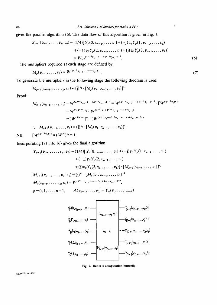
Fig. 2. Radix-4 computation butterfly.

NB: 1 • W q = W q

j • W q = w ( q - N / 4 )

J.A. Johnston / Multipliers for Radix-4 FFT

- 1 • W q = W (N/E+q)

- j . W q _~_ w(q-3N/4)

65

Mo(v2,v 1)

Mo(O, h_

M

M

M

M

M

M

M

M

Mo13,3)=6w~

Ml(V2,V 1) M2(v2,v 1) M3(v2,v 1) p=O p=l p=2

Fig. 3. F l o w o f m u l t i p l i e r s , N = 64.

Vol. 6, No. 1, January 1984

66

3. Example and discussion

J.A. Johnston / Multipliers ]:or Radix-4 FFT

The butterfly unit is shown in Fig. 2. Each unit receives four data points and one multiplier, computes the 4-point DFT, calculates the new multiplier value and performs multiplication by the twiddle factors before passing on the new data and multiplier value. The new multiplier values are computing using the multiplying circuits while the add/subtract logic is computing the 4-point DFT. The paths and values of the multipliers at each stage of the algorithm for N = 64 are given in Fig. 3. Note that the multiplier paths are in parallel with one of the data paths for each butterfly thus simplifying the interconnections.

While the algorithm simplifies the problems of interconnection and data storage, it has the dis-advantage that recursive computation of the twiddle factors may lead to rounding errors, and hence errors in the transform output. This would become more serious as the length of th~ transform increases.

4. Conclusions

The method of generating multipliers for a parallel FFT algorithm has been extended to include the radix-4 case. The algorithm and the computation of the multipliers are illustrated for the case of N = 64.

Acknowledgment

The financial support of the Science and Engineering Research Council is acknowledged.

References

[1] M.C. Pease, "An adaptation of the fast Fourier transform for parallel processing" Ass. Comput. Mach. J., Vol. 15, April 1968, pp. 252-264.

[2] H.S. Stone, "Parallel processing with the perfect shuffle", IEEE Trans. Computers, Vol. 20, No. 2., February 1971, pp. 153-161. [3] W.R. Cyre and G.J. Lipovski, "On generating multipliers for a cellular fast Fourier transform processor" IEEE Trans. Computers

Vol. 21, No. 1, January 1972, pp. 83-87.

Signal Processing