Embed Size (px)
Citation preview
OutlineIntroduction
Constructing Levy Random FieldsInference
Discussion & Future Work
Generating Levy Random Fields
Robert L Wolperthttp://www.stat.duke.edu/∼rlw/
Department of Statistical Scienceand
Nicholas School of the EnvironmentDuke University
Durham, NC USA
Arhus University2009 May 21–22
R L Wolpert Generating Levy Random Fields

OutlineIntroduction
Constructing Levy Random FieldsInference
Discussion & Future Work
Outline
IntroductionMotivation: Moving AveragesContinuous TimeLevy-Khinchine
Constructing Levy Random FieldsBare-Hands ConstructionElegant ConstructionMusielak-Orlicz spaces for Poisson IntegralsMultivariate Random FieldsInverse Levy Measure ConstructionExplicit Examples: St(α, β, γ, δ)
Inference
Discussion & Future Work
R L Wolpert Generating Levy Random Fields
OutlineIntroduction
Constructing Levy Random FieldsInference
Discussion & Future Work
Motivation: Moving AveragesContinuous TimeLevy-Khinchine
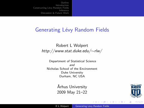
Moving Averages
A common, flexible way to construct stationary time series(discrete-time stochastic processes):Begin w/ i.i.d. sequence ζi : i ∈ N (or maybe i ∈ Z), set
Xi :=∑
j
bjζi−j
Mean and covariance of Xi easy to compute;
OLS forecasting also easy (at least if b(z) :=∑q
j=0 bj zq−j is apolynomial with all its roots in the unit disk)
R L Wolpert Generating Levy Random Fields
OutlineIntroduction
Constructing Levy Random FieldsInference
Discussion & Future Work
Motivation: Moving AveragesContinuous TimeLevy-Khinchine
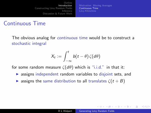
Continuous Time
The obvious analog for continuous time would be to construct astochastic integral
Xt :=
∫ t
−∞b(t − θ) ζ(dθ)
for some random measure ζ(dθ) which is “i.i.d.” in that it:
assigns independent random variables to disjoint sets, and
assigns the same distribution to all translates ζ(t + B)
R L Wolpert Generating Levy Random Fields
OutlineIntroduction
Constructing Levy Random FieldsInference
Discussion & Future Work
Motivation: Moving AveragesContinuous TimeLevy-Khinchine
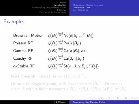
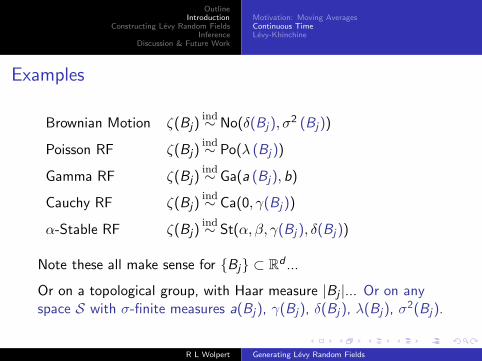
Examples
Brownian Motion ζ(Bj)ind∼ No(δ|Bj |, σ
2 |Bj |)
Poisson RF ζ(Bj)ind∼ Po(λ |Bj |)
Gamma RF ζ(Bj)ind∼ Ga(a |Bj |, b)
Cauchy RF ζ(Bj)ind∼ Ca(0, γ|Bj |)
α-Stable RF ζ(Bj)ind∼ St(α, β, γ|Bj |, δ|Bj |)
Note these all make sense for Bj ⊂ Rd ...
Or on a topological group, with Haar measure |Bj |... Or on anyspace S with σ-finite measures a(Bj), γ(Bj), δ(Bj ), λ(Bj), σ2(Bj).
R L Wolpert Generating Levy Random Fields
OutlineIntroduction
Constructing Levy Random FieldsInference
Discussion & Future Work
Motivation: Moving AveragesContinuous TimeLevy-Khinchine
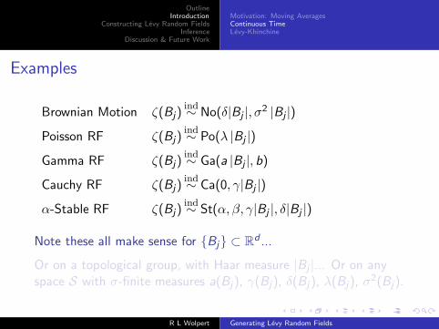
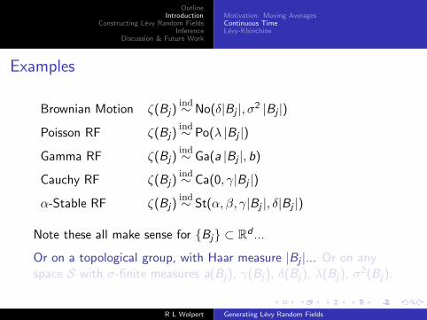
Examples
Brownian Motion ζ(Bj)ind∼ No(δ(Bj ), σ
2 (Bj))
Poisson RF ζ(Bj)ind∼ Po(λ (Bj ))
Gamma RF ζ(Bj)ind∼ Ga(a (Bj), b)
Cauchy RF ζ(Bj)ind∼ Ca(0, γ(Bj ))
α-Stable RF ζ(Bj)ind∼ St(α, β, γ(Bj ), δ(Bj ))
Note these all make sense for Bj ⊂ Rd ...
Or on a topological group, with Haar measure |Bj |... Or on anyspace S with σ-finite measures a(Bj), γ(Bj), δ(Bj ), λ(Bj), σ2(Bj).
R L Wolpert Generating Levy Random Fields
OutlineIntroduction
Constructing Levy Random FieldsInference
Discussion & Future Work
Motivation: Moving AveragesContinuous TimeLevy-Khinchine
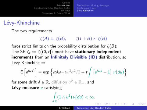
Levy-Khinchine
The two requirements
ζ(A) ⊥⊥ ζ(B), ζ(t + B) ∼ ζ(B)
force strict limits on the probability distribution for ζ(B):The SP ζt := ζ
(
(0, t])
must have stationary independentincrements from an Infinitely Divisible (ID) distribution, soLevy-Khinchine ⇒
E[
e iω ζt
]
= exp
itδω−tω2σ2/2 + t
∫
[
e iωu − 1]
ν(du)
for some drift δ ∈ R, diffusion σ2 ∈ R+, andLevy measure ν satisfying
∫
R
(1 ∧ u2) ν(du) < ∞.
R L Wolpert Generating Levy Random Fields
OutlineIntroduction
Constructing Levy Random FieldsInference
Discussion & Future Work
Motivation: Moving AveragesContinuous TimeLevy-Khinchine
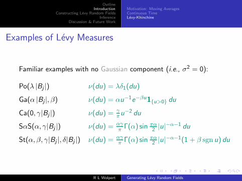
Examples of Levy Measures
Familiar examples with no Gaussian component (i.e., σ2 = 0):
Po(λ |Bj |) ν(du) = λδ1(du)
Ga(α |Bj |, β) ν(du) = αu−1e−βu1u>0 du
Ca(0, γ|Bj |) ν(du) = γπu−2 du
SαS(α, γ|Bj |) ν(du) = αγπ
Γ(α) sin πα2 |u|−α−1 du
St(α, β, γ|Bj |, δ|Bj |) ν(du) = αγπ
Γ(α) sin πα2 |u|−α−1(1 + β sgn u) du
R L Wolpert Generating Levy Random Fields
OutlineIntroduction
Constructing Levy Random FieldsInference
Discussion & Future Work
Motivation: Moving AveragesContinuous TimeLevy-Khinchine
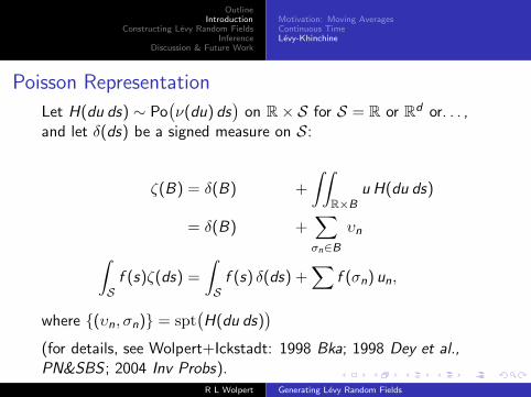
Poisson Representation
Let H(du ds) ∼ Po(
ν(du) ds)
on R × S for S = R or Rd or. . . ,
and let δ(ds) be a signed measure on S:
ζ(B) = δ(B) +
∫∫
R×B
u H(du ds)
= δ(B) +∑
σn∈B
υn
∫
Sf (s)ζ(ds) =
∫
Sf (s) δ(ds) +
∑
f (σn) un,
where (υn, σn) = spt(
H(du ds))
(for details, see Wolpert+Ickstadt: 1998 Bka; 1998 Dey et al.,PN&SBS ; 2004 Inv Probs).
R L Wolpert Generating Levy Random Fields
OutlineIntroduction
Constructing Levy Random FieldsInference
Discussion & Future Work
Motivation: Moving AveragesContinuous TimeLevy-Khinchine
Confession
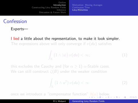
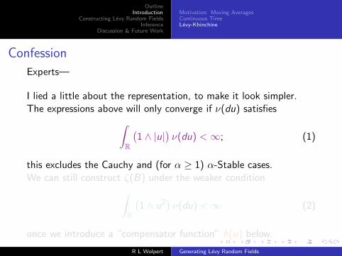
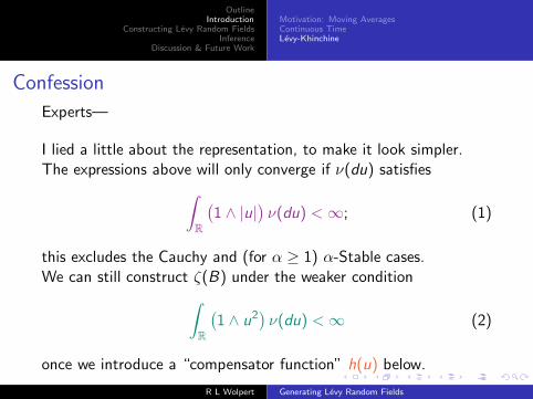
Experts—
I lied a little about the representation, to make it look simpler.The expressions above will only converge if ν(du) satisfies
∫
R
(
1 ∧ |u|)
ν(du) < ∞; (1)
this excludes the Cauchy and (for α ≥ 1) α-Stable cases.We can still construct ζ(B) under the weaker condition
∫
R
(
1 ∧ u2)
ν(du) < ∞ (2)
once we introduce a “compensator function” h(u) below.
R L Wolpert Generating Levy Random Fields
OutlineIntroduction
Constructing Levy Random FieldsInference
Discussion & Future Work
Motivation: Moving AveragesContinuous TimeLevy-Khinchine
Confession
Experts—
I lied a little about the representation, to make it look simpler.The expressions above will only converge if ν(du) satisfies
∫
R
(
1 ∧ |u|)
ν(du) < ∞; (1)
this excludes the Cauchy and (for α ≥ 1) α-Stable cases.We can still construct ζ(B) under the weaker condition
∫
R
(
1 ∧ u2)
ν(du) < ∞ (2)
once we introduce a “compensator function” h(u) below.
R L Wolpert Generating Levy Random Fields
OutlineIntroduction
Constructing Levy Random FieldsInference
Discussion & Future Work
Motivation: Moving AveragesContinuous TimeLevy-Khinchine
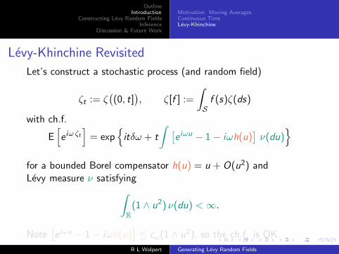
Levy-Khinchine Revisited
Let’s construct a stochastic process (and random field)
ζt := ζ(
(0, t])
, ζ[f ] :=
∫
Sf (s)ζ(ds)
with ch.f.
E[
e iω ζt
]
= exp
itδω + t
∫
[
e iωu − 1 − iωh(u)]
ν(du)
for a bounded Borel compensator h(u) = u + O(u2) andLevy measure ν satisfying
∫
R
(1 ∧ u2) ν(du) < ∞.
Note[
e iωu − 1 − iωh(u)]
≤ cω(1 ∧ u2), so the ch.f. is OK.
R L Wolpert Generating Levy Random Fields
OutlineIntroduction
Constructing Levy Random FieldsInference
Discussion & Future Work
Motivation: Moving AveragesContinuous TimeLevy-Khinchine
Levy-Khinchine Revisited
Let’s construct a stochastic process (and random field)
ζt := ζ(
(0, t])
, ζ[f ] :=
∫
Sf (s)ζ(ds)
with ch.f.
E[
e iω ζt
]
= exp
itδω + t
∫
[
e iωu − 1 − iωh(u)]
ν(du)
for a bounded Borel compensator h(u) = u + O(u2) andLevy measure ν satisfying
∫
R
(1 ∧ u2) ν(du) < ∞.
Note[
e iωu − 1 − iωh(u)]
≤ cω(1 ∧ u2), so the ch.f. is OK.
R L Wolpert Generating Levy Random Fields
OutlineIntroduction
Constructing Levy Random FieldsInference
Discussion & Future Work
Bare HandsLess InelegantMusielak-Orlicz spaces for Poisson IntegralsMultivariate Random FieldsInverse Levy Measure (ILM) ConstructionExplicit Examples: St(α, β, γ, δ)
Bare-Hands ConstructionFor “small” ǫ > 0,
ζǫt := δt +
∫∫
(−ǫ,ǫ)c×(0,t]u H(du ds) −
∫∫
(−ǫ,ǫ)c×(0,t]h(u) ν(du)ds
:= δǫt +
∫∫
(−ǫ,ǫ)c×(0,t]u H(du ds), δǫ := δ −
∫
(−ǫ,ǫ)ch(u) ν(du)
ζt := limǫ→0
ζǫt = lim
ǫ→0
[
δǫt +∑
uj : |uj | > ǫ, sj ≤ t]
(3)
ujiid∼ νǫ(du)/νǫ
+ ⊥⊥ sjiid∼ Un(T), νǫ(du) := 1|u|>ǫν(du)
Note:
If∫ (
1 ∧ |u|)
ν(du) = ∞ then∑
uj doesn’t converge absolutely &typically δǫ → ±∞ as ǫ → 0... but limit (3) still OK
R L Wolpert Generating Levy Random Fields
OutlineIntroduction
Constructing Levy Random FieldsInference
Discussion & Future Work
Bare HandsLess InelegantMusielak-Orlicz spaces for Poisson IntegralsMultivariate Random FieldsInverse Levy Measure (ILM) ConstructionExplicit Examples: St(α, β, γ, δ)
More Elegant Construction
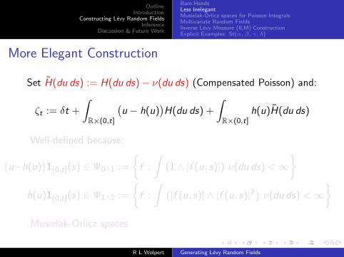
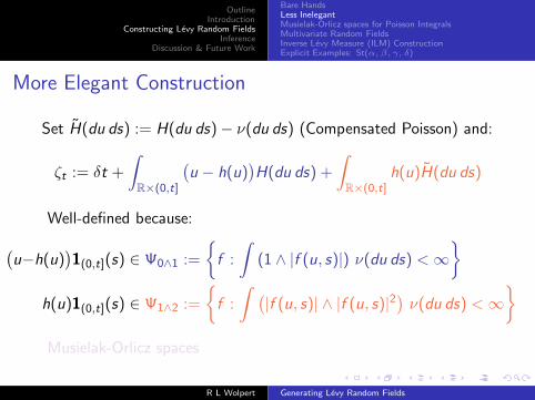
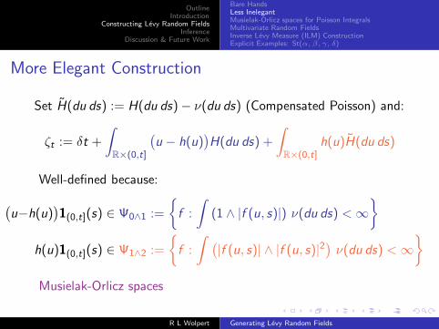
Set H(du ds) := H(du ds) − ν(du ds) (Compensated Poisson) and:
ζt := δt +
∫
R×(0,t]
(
u − h(u))
H(du ds) +
∫
R×(0,t]h(u)H(du ds)
Well-defined because:
(
u−h(u))
1(0,t](s) ∈ Ψ0∧1 :=
f :
∫
(1 ∧ |f (u, s)|) ν(du ds) < ∞
h(u)1(0,t](s) ∈ Ψ1∧2 :=
f :
∫
(
|f (u, s)| ∧ |f (u, s)|2)
ν(du ds) < ∞
Musielak-Orlicz spaces
R L Wolpert Generating Levy Random Fields
OutlineIntroduction
Constructing Levy Random FieldsInference
Discussion & Future Work
Bare HandsLess InelegantMusielak-Orlicz spaces for Poisson IntegralsMultivariate Random FieldsInverse Levy Measure (ILM) ConstructionExplicit Examples: St(α, β, γ, δ)
More Elegant Construction
Set H(du ds) := H(du ds) − ν(du ds) (Compensated Poisson) and:
ζt := δt +
∫
R×(0,t]
(
u − h(u))
H(du ds) +
∫
R×(0,t]h(u)H(du ds)
Well-defined because:
(
u−h(u))
1(0,t](s) ∈ Ψ0∧1 :=
f :
∫
(1 ∧ |f (u, s)|) ν(du ds) < ∞
h(u)1(0,t](s) ∈ Ψ1∧2 :=
f :
∫
(
|f (u, s)| ∧ |f (u, s)|2)
ν(du ds) < ∞
Musielak-Orlicz spaces
R L Wolpert Generating Levy Random Fields
OutlineIntroduction
Constructing Levy Random FieldsInference
Discussion & Future Work
Bare HandsLess InelegantMusielak-Orlicz spaces for Poisson IntegralsMultivariate Random FieldsInverse Levy Measure (ILM) ConstructionExplicit Examples: St(α, β, γ, δ)
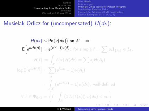
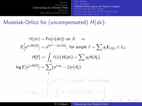
Musielak-Orlicz for (uncompensated) H(dx):
H(dx) ∼ Po(
ν(dx))
on X ⇒
E[
e iωH(A)]
= e(e iω−1)ν(A); for simple f =∑
aj1Aj ∈ L1,
H[f ] :=
∫
Xf (x)H(dx) =
∑
ajH(Aj )
log E[
e iωH[f ]]
=∑
j
(e iωaj − 1)ν(Aj )
=
∫
X
(
e iωf (x) − 1)
ν(dx), well-defined
∀ f ∈ Ψ0∧1:=
f :
∫
X(1 ∧ |f (x)|) ν(dx) < ∞
R L Wolpert Generating Levy Random Fields
OutlineIntroduction
Constructing Levy Random FieldsInference
Discussion & Future Work
Bare HandsLess InelegantMusielak-Orlicz spaces for Poisson IntegralsMultivariate Random FieldsInverse Levy Measure (ILM) ConstructionExplicit Examples: St(α, β, γ, δ)
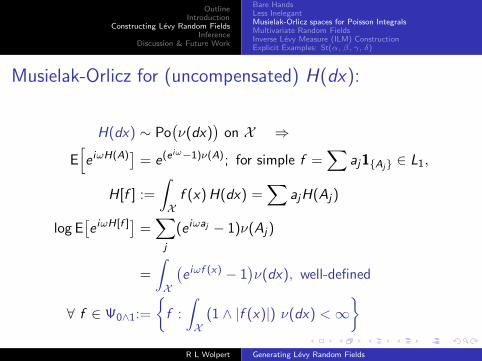
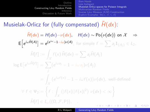
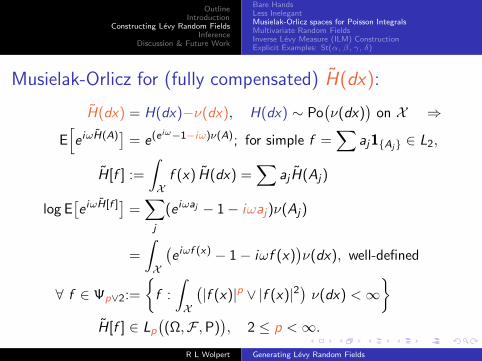
Musielak-Orlicz for (fully compensated) H(dx):
H(dx) = H(dx)−ν(dx), H(dx) ∼ Po(
ν(dx))
on X ⇒
E[
e iωH(A)]
= e(e iω−1−iω)ν(A); for simple f =∑
aj1Aj ∈ L2,
H[f ] :=
∫
Xf (x) H(dx) =
∑
ajH(Aj)
log E[
e iωH[f ]]
=∑
j
(e iωaj − 1 − iωaj)ν(Aj)
=
∫
X
(
e iωf (x) − 1 − iωf (x))
ν(dx), well-defined
∀ f ∈ Ψ2:=
f :
∫
X
(
|f (x)||f (x)|2)
ν(dx) < ∞
H[f ] ∈ Lp
(
(Ω,F ,P))
, .
R L Wolpert Generating Levy Random Fields
OutlineIntroduction
Constructing Levy Random FieldsInference
Discussion & Future Work
Bare HandsLess InelegantMusielak-Orlicz spaces for Poisson IntegralsMultivariate Random FieldsInverse Levy Measure (ILM) ConstructionExplicit Examples: St(α, β, γ, δ)
Musielak-Orlicz for (fully compensated) H(dx):
H(dx) = H(dx)−ν(dx), H(dx) ∼ Po(
ν(dx))
on X ⇒
E[
e iωH(A)]
= e(e iω−1−iω)ν(A); for simple f =∑
aj1Aj ∈ L2,
H[f ] :=
∫
Xf (x) H(dx) =
∑
ajH(Aj)
log E[
e iωH[f ]]
=∑
j
(e iωaj − 1 − iωaj)ν(Aj)
=
∫
X
(
e iωf (x) − 1 − iωf (x))
ν(dx), well-defined
∀ f ∈ Ψ2:=
f :
∫
X
(
|f (x)||f (x)|2)
ν(dx) < ∞
H[f ] ∈ Lp
(
(Ω,F ,P))
, .
R L Wolpert Generating Levy Random Fields

OutlineIntroduction
Constructing Levy Random FieldsInference
Discussion & Future Work
Bare HandsLess InelegantMusielak-Orlicz spaces for Poisson IntegralsMultivariate Random FieldsInverse Levy Measure (ILM) ConstructionExplicit Examples: St(α, β, γ, δ)
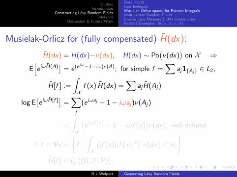
Musielak-Orlicz for (fully compensated) H(dx):
H(dx) = H(dx)−ν(dx), H(dx) ∼ Po(
ν(dx))
on X ⇒
E[
e iωH(A)]
= e(e iω−1−iω)ν(A); for simple f =∑
aj1Aj ∈ L2,
H[f ] :=
∫
Xf (x) H(dx) =
∑
ajH(Aj)
log E[
e iωH[f ]]
=∑
j
(e iωaj − 1 − iωaj)ν(Aj)
=
∫
X
(
e iωf (x) − 1 − iωf (x))
ν(dx), well-defined
∀ f ∈ Ψ1∧2:=
f :
∫
X
(
|f (x)|1 ∧ |f (x)|2)
ν(dx) < ∞
H[f ] ∈ Lp
(
(Ω,F ,P))
, .
R L Wolpert Generating Levy Random Fields

OutlineIntroduction
Constructing Levy Random FieldsInference
Discussion & Future Work
Bare HandsLess InelegantMusielak-Orlicz spaces for Poisson IntegralsMultivariate Random FieldsInverse Levy Measure (ILM) ConstructionExplicit Examples: St(α, β, γ, δ)
Musielak-Orlicz for (fully compensated) H(dx):
H(dx) = H(dx)−ν(dx), H(dx) ∼ Po(
ν(dx))
on X ⇒
E[
e iωH(A)]
= e(e iω−1−iω)ν(A); for simple f =∑
aj1Aj ∈ L2,
H[f ] :=
∫
Xf (x) H(dx) =
∑
ajH(Aj)
log E[
e iωH[f ]]
=∑
j
(e iωaj − 1 − iωaj)ν(Aj)
=
∫
X
(
e iωf (x) − 1 − iωf (x))
ν(dx), well-defined
∀ f ∈ Ψp∧2:=
f :
∫
X
(
|f (x)|p ∧ |f (x)|2)
ν(dx) < ∞
H[f ] ∈ Lp
(
(Ω,F ,P))
, 1 ≤ p ≤ 2.
R L Wolpert Generating Levy Random Fields
OutlineIntroduction
Constructing Levy Random FieldsInference
Discussion & Future Work
Bare HandsLess InelegantMusielak-Orlicz spaces for Poisson IntegralsMultivariate Random FieldsInverse Levy Measure (ILM) ConstructionExplicit Examples: St(α, β, γ, δ)
Musielak-Orlicz for (fully compensated) H(dx):
H(dx) = H(dx)−ν(dx), H(dx) ∼ Po(
ν(dx))
on X ⇒
E[
e iωH(A)]
= e(e iω−1−iω)ν(A); for simple f =∑
aj1Aj ∈ L2,
H[f ] :=
∫
Xf (x) H(dx) =
∑
ajH(Aj)
log E[
e iωH[f ]]
=∑
j
(e iωaj − 1 − iωaj)ν(Aj)
=
∫
X
(
e iωf (x) − 1 − iωf (x))
ν(dx), well-defined
∀ f ∈ Ψp∨2:=
f :
∫
X
(
|f (x)|p ∨ |f (x)|2)
ν(dx) < ∞
H[f ] ∈ Lp
(
(Ω,F ,P))
, 2 ≤ p < ∞.
R L Wolpert Generating Levy Random Fields
OutlineIntroduction
Constructing Levy Random FieldsInference
Discussion & Future Work
Bare HandsLess InelegantMusielak-Orlicz spaces for Poisson IntegralsMultivariate Random FieldsInverse Levy Measure (ILM) ConstructionExplicit Examples: St(α, β, γ, δ)
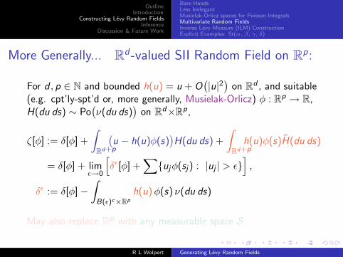
More Generally... Rd -valued SII Random Field on R
p:
For d , p ∈ N and bounded h(u) = u + O(
|u|2)
on Rd , and suitable
(e.g. cpt’ly-spt’d or, more generally, Musielak-Orlicz) φ : Rp → R,
H(du ds) ∼ Po(
ν(du ds))
on Rd×R
p,
ζ[φ] := δ[φ] +
∫
Rd+p
(
u − h(u)φ(s))
H(du ds) +
∫
Rd+ph(u)φ(s)H(du ds)
= δ[φ] + limǫ→0
[
δǫ[φ] +∑
ujφ(sj) : |uj | > ǫ]
,
δǫ := δ[φ] −
∫
B(ǫ)c×Rp
h(u)φ(s) ν(du ds)
May also replace Rp with any measurable space S
R L Wolpert Generating Levy Random Fields
OutlineIntroduction
Constructing Levy Random FieldsInference
Discussion & Future Work
Bare HandsLess InelegantMusielak-Orlicz spaces for Poisson IntegralsMultivariate Random FieldsInverse Levy Measure (ILM) ConstructionExplicit Examples: St(α, β, γ, δ)
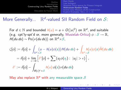
More Generally... Rd -valued SII Random Field on S:
For d ∈ N and bounded h(u) = u + O(
|u|2)
on Rd , and suitable
(e.g. cpt’ly-spt’d or, more generally, Musielak-Orlicz) φ : S → R,H(du ds) ∼ Po
(
ν(du ds))
on Rd×S,
ζ[φ] := δ[φ] +
∫
Rd×S
(
u − h(u)φ(s))
H(du ds) +
∫
Rd×Sh(u)φ(s)H(du ds)
= δ[φ] + limǫ→0
[
δǫ[φ] +∑
ujφ(sj) : |uj | > ǫ]
,
δǫ := δ[φ] −
∫
B(ǫ)c×Sh(u)φ(s) ν(du ds)
May also replace Rp with any measurable space S
R L Wolpert Generating Levy Random Fields
OutlineIntroduction
Constructing Levy Random FieldsInference
Discussion & Future Work
Bare HandsLess InelegantMusielak-Orlicz spaces for Poisson IntegralsMultivariate Random FieldsInverse Levy Measure (ILM) ConstructionExplicit Examples: St(α, β, γ, δ)
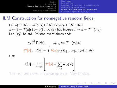
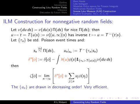
ILM Construction for nonnegative random fields:
Let ν(du ds) = ν(du|s)Π(ds) for nice Π(ds); thenu 7→ t = T (u|s) := ν((u,∞)|s) has inverse t 7→ u = T ←(t|s).Let τn be std. Poisson event times and:
sniid∼ Π(ds), un|sn := T ←(τn|sn)
δn[φ] := δ[φ] −
∫
h(u)φ(s)1τn>T (u|s)ν(du ds)
then
ζ[φ] = limn→∞
δn[φ] +∑
j≤n
ujφ(sj )
The un are drawn in decreasing order! Very efficient.
R L Wolpert Generating Levy Random Fields
OutlineIntroduction
Constructing Levy Random FieldsInference
Discussion & Future Work
Bare HandsLess InelegantMusielak-Orlicz spaces for Poisson IntegralsMultivariate Random FieldsInverse Levy Measure (ILM) ConstructionExplicit Examples: St(α, β, γ, δ)
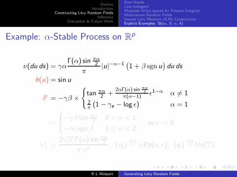
Example: α-Stable Process on Rp
ν(du ds) = γαΓ(α) sin πα
2
π|u|−α−1
(
1 + β sgn u)
du ds
h(u) = sin u
δǫ = −γβ ×
tan πα2 +
2αΓ(α) sin πα2
π(α−1) ǫ1−α α 6= 12π
(1 − γe − log ǫ) α = 1
→
−γβ tan πα2 0 < α < 1
−∞ sgnβ 1 ≤ α < 2as ǫ → 0
νǫ+ =
2γ|T|Γ(α) sin πα2
π ǫα, uj
iid∼ ±Pa(α, ǫ), sj
iid∼ Un(T)
R L Wolpert Generating Levy Random Fields
OutlineIntroduction
Constructing Levy Random FieldsInference
Discussion & Future Work
Bare HandsLess InelegantMusielak-Orlicz spaces for Poisson IntegralsMultivariate Random FieldsInverse Levy Measure (ILM) ConstructionExplicit Examples: St(α, β, γ, δ)
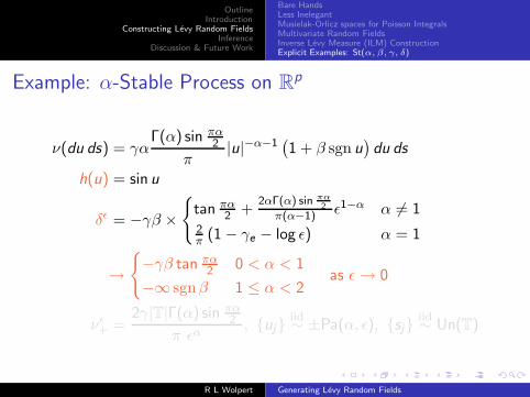
Example: α-Stable Process on Rp
ν(du ds) = γαΓ(α) sin πα
2
π|u|−α−1
(
1 + β sgn u)
du ds
h(u) = sin u
δǫ = −γβ ×
tan πα2 +
2αΓ(α) sin πα2
π(α−1) ǫ1−α α 6= 12π
(1 − γe − log ǫ) α = 1
→
−γβ tan πα2 0 < α < 1
−∞ sgnβ 1 ≤ α < 2as ǫ → 0
νǫ+ =
2γ|T|Γ(α) sin πα2
π ǫα, uj
iid∼ ±Pa(α, ǫ), sj
iid∼ Un(T)
R L Wolpert Generating Levy Random Fields
OutlineIntroduction
Constructing Levy Random FieldsInference
Discussion & Future Work
Bare HandsLess InelegantMusielak-Orlicz spaces for Poisson IntegralsMultivariate Random FieldsInverse Levy Measure (ILM) ConstructionExplicit Examples: St(α, β, γ, δ)
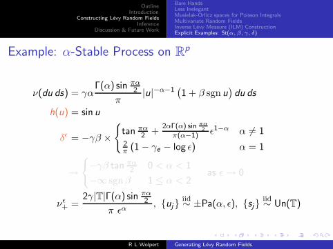
Example: α-Stable Process on Rp
ν(du ds) = γαΓ(α) sin πα
2
π|u|−α−1
(
1 + β sgn u)
du ds
h(u) = sin u
δǫ = −γβ ×
tan πα2 +
2αΓ(α) sin πα2
π(α−1) ǫ1−α α 6= 12π
(1 − γe − log ǫ) α = 1
→
−γβ tan πα2 0 < α < 1
−∞ sgnβ 1 ≤ α < 2as ǫ → 0
νǫ+ =
2γ|T|Γ(α) sin πα2
π ǫα, uj
iid∼ ±Pa(α, ǫ), sj
iid∼ Un(T)
R L Wolpert Generating Levy Random Fields
OutlineIntroduction
Constructing Levy Random FieldsInference
Discussion & Future Work
Bare HandsLess InelegantMusielak-Orlicz spaces for Poisson IntegralsMultivariate Random FieldsInverse Levy Measure (ILM) ConstructionExplicit Examples: St(α, β, γ, δ)
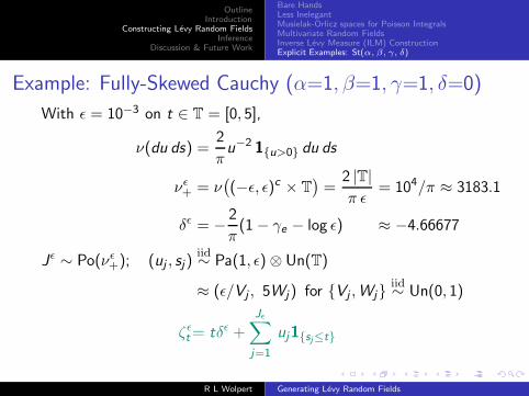
Example: Fully-Skewed Cauchy (α=1, β=1, γ=1, δ=0)
With ǫ = 10−3 on t ∈ T = [0, 5],
ν(du ds) =2
πu−2 1u>0 du ds
νǫ+ = ν
(
(−ǫ, ǫ)c × T)
=2 |T|
π ǫ= 104/π ≈ 3183.1
δǫ = −2
π(1 − γe − log ǫ) ≈ −4.66677
Jǫ ∼ Po(νǫ+); (uj , sj)
iid∼ Pa(1, ǫ) ⊗ Un(T)
≈ (ǫ/Vj , 5Wj) for Vj ,Wjiid∼ Un(0, 1)
ζǫt = tδǫ +
Jǫ∑
j=1
uj1sj≤t
R L Wolpert Generating Levy Random Fields
OutlineIntroduction
Constructing Levy Random FieldsInference
Discussion & Future Work
Bare HandsLess InelegantMusielak-Orlicz spaces for Poisson IntegralsMultivariate Random FieldsInverse Levy Measure (ILM) ConstructionExplicit Examples: St(α, β, γ, δ)
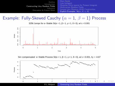
Example: Fully-Skewed Cauchy (α = 1, β = 1) Process
0 1 2 3 4 5
0.0
0.5
1.0
1.5
2.0
Time
Jum
ps
3256 Jumps for α−Stable St(α = 1, β = 1, γ = 1, δ = 0), w/ ε = 0.001
0 1 2 3 4 5
01
23
4
Time
Pro
cess
Sin−compensated α−Stable Process St(α = 1, β = 1, γ = 1, δ = 0), w/ ε = 0.001, δε = −4.67
R L Wolpert Generating Levy Random Fields
OutlineIntroduction
Constructing Levy Random FieldsInference
Discussion & Future Work
Bare HandsLess InelegantMusielak-Orlicz spaces for Poisson IntegralsMultivariate Random FieldsInverse Levy Measure (ILM) ConstructionExplicit Examples: St(α, β, γ, δ)
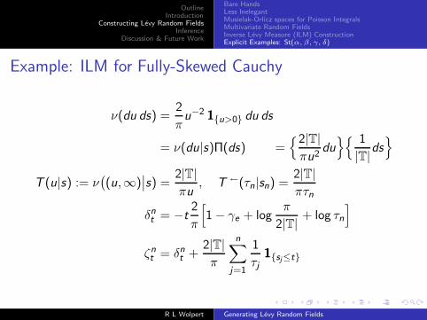
Example: ILM for Fully-Skewed Cauchy
ν(du ds) =2
πu−2 1u>0 du ds
= ν(du|s)Π(ds) =2|T|
πu2du
1
|T|ds
T (u|s) := ν(
(u,∞)∣
∣s) =2|T|
πu, T ←(τn|sn) =
2|T|
πτn
δnt = −t
2
π
[
1 − γe + logπ
2|T|+ log τn
]
ζnt = δn
t +2|T|
π
n∑
j=1
1
τj
1sj≤t
R L Wolpert Generating Levy Random Fields
OutlineIntroduction
Constructing Levy Random FieldsInference
Discussion & Future Work
Bare HandsLess InelegantMusielak-Orlicz spaces for Poisson IntegralsMultivariate Random FieldsInverse Levy Measure (ILM) ConstructionExplicit Examples: St(α, β, γ, δ)
Amusing side-light...
Let τj be event times of standard Poisson process andlet σj = ±1 with equal probabilities; then the limits
X := (2/π) limn→∞
n∑
j=1
1
τj
− log n
∼ St(1, 1, 1, δ), δ =2
πlog
πe
2+ γe
Y := (2/π) limn→∞
n∑
j=1
σj
τj∼ St(1, 0, 1, 0) = Ca(0, 1)
exist even though neither sum converges absolutely!
R L Wolpert Generating Levy Random Fields
OutlineIntroduction
Constructing Levy Random FieldsInference
Discussion & Future Work
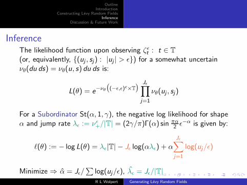
InferenceThe likelihood function upon observing ζǫ
t : t ∈ T
(or, equivalently, (uj , sj) : |uj | > ǫ) for a somewhat uncertainνθ(du ds) = νθ(u, s) du ds is:
L(θ) = e−νθ
(
(−ǫ,ǫ)c×T
) Jǫ∏
j=1
νθ(uj , sj)
For a Subordinator St(α, 1, γ), the negative log likelihood for shapeα and jump rate λǫ := νǫ
+/|T| = (2γ/π)Γ(α) sin πα2 ǫ−α is given by:
ℓ(θ) := − log L(θ) = λǫ|T| − Jǫ log(αλǫ) + α
Jǫ∑
j=1
log(uj/ǫ)
Minimize ⇒ α = Jǫ/∑
log(uj/ǫ), λǫ = Jǫ/|T|
R L Wolpert Generating Levy Random Fields
OutlineIntroduction
Constructing Levy Random FieldsInference
Discussion & Future Work
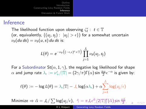
InferenceThe likelihood function upon observing ζǫ
t : t ∈ T
(or, equivalently, (uj , sj) : |uj | > ǫ) for a somewhat uncertainνθ(du ds) = νθ(u, s) du ds is:
L(θ) = e−νθ
(
(−ǫ,ǫ)c×T
) Jǫ∏
j=1
νθ(uj , sj)
For a Subordinator St(α, 1, γ), the negative log likelihood for shapeα and jump rate λǫ := νǫ
+/|T| = (2γ/π)Γ(α) sin πα2 ǫ−α is given by:
ℓ(θ) := − log L(θ) = λǫ|T| − Jǫ log(αλǫ) + α
Jǫ∑
j=1
log(uj/ǫ)
Minimize ⇒ α = Jǫ/∑
log(uj/ǫ), γ = πJǫǫα/2|T|Γ(α) sin πα
2
R L Wolpert Generating Levy Random Fields
OutlineIntroduction
Constructing Levy Random FieldsInference
Discussion & Future Work
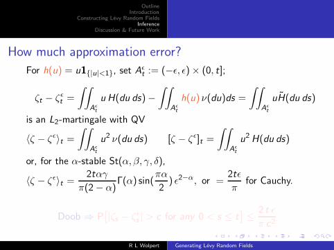
How much approximation error?
For h(u) = u1|u|<1, set Aǫt := (−ǫ, ǫ) × (0, t];
ζt − ζǫt =
∫∫
Aǫt
u H(du ds) −
∫∫
Aǫt
h(u) ν(du)ds =
∫∫
Aǫt
uH(du ds)
is an L2-martingale with QV
〈ζ − ζǫ〉t =
∫∫
Aǫt
u2 ν(du ds) [ζ − ζǫ]t =
∫∫
Aǫt
u2 H(du ds)
or, for the α-stable St(α, β, γ, δ),
〈ζ − ζǫ〉t =2tαγ
π(2 − α)Γ(α) sin(
πα
2) ǫ2−α, or =
2tǫ
πfor Cauchy.
Doob ⇒ P[
|ζs − ζǫs | > c for any 0 < s ≤ t
]
≤2 t ǫ
π c2
R L Wolpert Generating Levy Random Fields
OutlineIntroduction
Constructing Levy Random FieldsInference
Discussion & Future Work
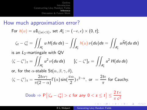
How much approximation error?
For h(u) = u1|u|<1, set Aǫt := (−ǫ, ǫ) × (0, t];
ζt − ζǫt =
∫∫
Aǫt
u H(du ds) −
∫∫
Aǫt
h(u) ν(du)ds =
∫∫
Aǫt
uH(du ds)
is an L2-martingale with QV
〈ζ − ζǫ〉t =
∫∫
Aǫt
u2 ν(du ds) [ζ − ζǫ]t =
∫∫
Aǫt
u2 H(du ds)
or, for the α-stable St(α, β, γ, δ),
〈ζ − ζǫ〉t =2tαγ
π(2 − α)Γ(α) sin(
πα
2) ǫ2−α, or =
2tǫ
πfor Cauchy.
Doob ⇒ P[
|ζs − ζǫs | > c for any 0 < s ≤ t
]
≤2 t ǫ
π c2
R L Wolpert Generating Levy Random Fields
OutlineIntroduction
Constructing Levy Random FieldsInference
Discussion & Future Work
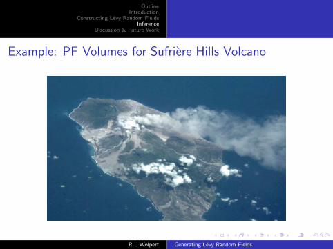
Example: PF Volumes for Sufriere Hills Volcano
R L Wolpert Generating Levy Random Fields
OutlineIntroduction
Constructing Levy Random FieldsInference
Discussion & Future Work
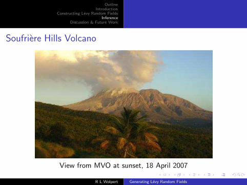
Soufriere Hills Volcano
View from MVO at sunset, 18 April 2007
R L Wolpert Generating Levy Random Fields

OutlineIntroduction
Constructing Levy Random FieldsInference
Discussion & Future Work
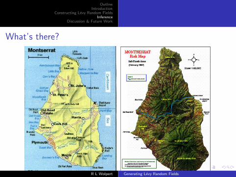
Where is Montserrat?
R L Wolpert Generating Levy Random Fields
OutlineIntroduction
Constructing Levy Random FieldsInference
Discussion & Future Work
What’s there?
R L Wolpert Generating Levy Random Fields
OutlineIntroduction
Constructing Levy Random FieldsInference
Discussion & Future Work
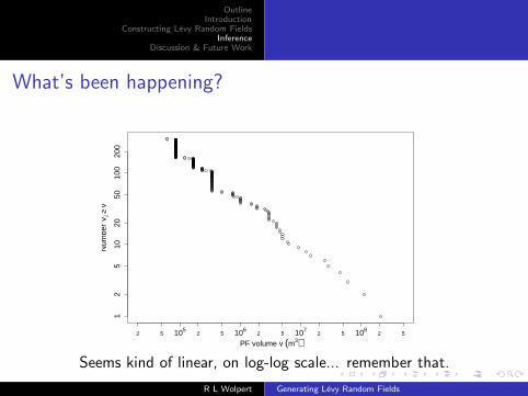
What’s been happening?
12
510
2050
100
200
PF volume v (m3)
Num
ber
Vj≥
v
2 5 1052 5 106
2 5 1072 5 108
2 5
Seems kind of linear, on log-log scale... remember that.
R L Wolpert Generating Levy Random Fields
OutlineIntroduction
Constructing Levy Random FieldsInference
Discussion & Future Work
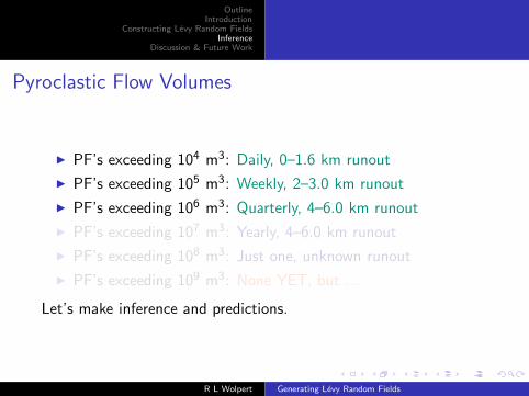
Pyroclastic Flow Volumes
PF’s exceeding 104 m3: Daily, 0–1.6 km runout
PF’s exceeding 105 m3: Weekly, 2–3.0 km runout
PF’s exceeding 106 m3: Quarterly, 4–6.0 km runout
PF’s exceeding 107 m3: Yearly, 4–6.0 km runout
PF’s exceeding 108 m3: Just one, unknown runout
PF’s exceeding 109 m3: None YET, but ...
Let’s make inference and predictions.
R L Wolpert Generating Levy Random Fields
OutlineIntroduction
Constructing Levy Random FieldsInference
Discussion & Future Work
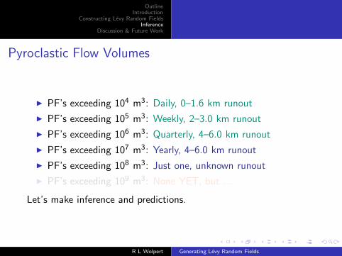
Pyroclastic Flow Volumes
PF’s exceeding 104 m3: Daily, 0–1.6 km runout
PF’s exceeding 105 m3: Weekly, 2–3.0 km runout
PF’s exceeding 106 m3: Quarterly, 4–6.0 km runout
PF’s exceeding 107 m3: Yearly, 4–6.0 km runout
PF’s exceeding 108 m3: Just one, unknown runout
PF’s exceeding 109 m3: None YET, but ...
Let’s make inference and predictions.
R L Wolpert Generating Levy Random Fields
OutlineIntroduction
Constructing Levy Random FieldsInference
Discussion & Future Work
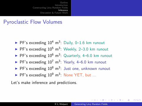
Pyroclastic Flow Volumes
PF’s exceeding 104 m3: Daily, 0–1.6 km runout
PF’s exceeding 105 m3: Weekly, 2–3.0 km runout
PF’s exceeding 106 m3: Quarterly, 4–6.0 km runout
PF’s exceeding 107 m3: Yearly, 4–6.0 km runout
PF’s exceeding 108 m3: Just one, unknown runout
PF’s exceeding 109 m3: None YET, but ...
Let’s make inference and predictions.
R L Wolpert Generating Levy Random Fields
OutlineIntroduction
Constructing Levy Random FieldsInference
Discussion & Future Work
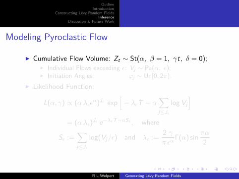
Modeling Pyroclastic Flow
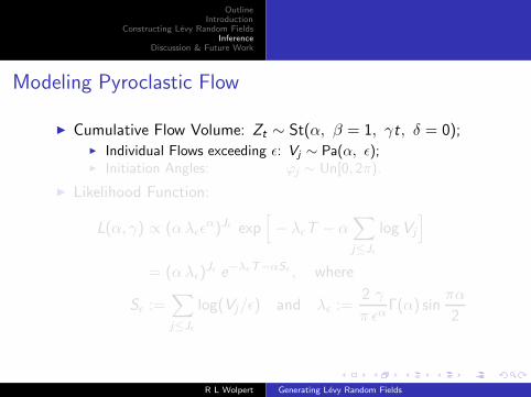
Cumulative Flow Volume: Zt ∼ St(α, β = 1, γt, δ = 0); Individual Flows exceeding ǫ: Vj ∼ Pa(α, ǫ); Initiation Angles: ϕj ∼ Un[0, 2π).
Likelihood Function:
L(α, γ) ∝ (α λǫǫα)Jǫ exp
[
− λǫT − α∑
j≤Jǫ
log Vj
]
= (α λǫ)Jǫ e−λǫT−αSǫ , where
Sǫ :=∑
j≤Jǫ
log(Vj/ǫ) and λǫ :=2 γ
π ǫαΓ(α) sin
πα
2
R L Wolpert Generating Levy Random Fields
OutlineIntroduction
Constructing Levy Random FieldsInference
Discussion & Future Work
Modeling Pyroclastic Flow
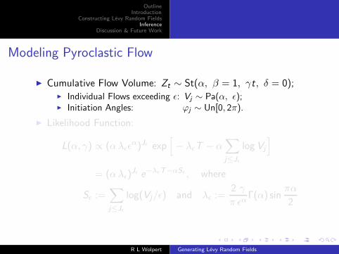
Cumulative Flow Volume: Zt ∼ St(α, β = 1, γt, δ = 0); Individual Flows exceeding ǫ: Vj ∼ Pa(α, ǫ); Initiation Angles: ϕj ∼ Un[0, 2π).
Likelihood Function:
L(α, γ) ∝ (α λǫǫα)Jǫ exp
[
− λǫT − α∑
j≤Jǫ
log Vj
]
= (α λǫ)Jǫ e−λǫT−αSǫ , where
Sǫ :=∑
j≤Jǫ
log(Vj/ǫ) and λǫ :=2 γ
π ǫαΓ(α) sin
πα
2
R L Wolpert Generating Levy Random Fields
OutlineIntroduction
Constructing Levy Random FieldsInference
Discussion & Future Work
Modeling Pyroclastic Flow
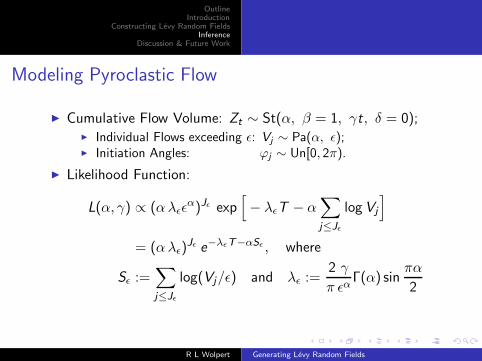
Cumulative Flow Volume: Zt ∼ St(α, β = 1, γt, δ = 0); Individual Flows exceeding ǫ: Vj ∼ Pa(α, ǫ); Initiation Angles: ϕj ∼ Un[0, 2π).
Likelihood Function:
L(α, γ) ∝ (α λǫǫα)Jǫ exp
[
− λǫT − α∑
j≤Jǫ
log Vj
]
= (α λǫ)Jǫ e−λǫT−αSǫ , where
Sǫ :=∑
j≤Jǫ
log(Vj/ǫ) and λǫ :=2 γ
π ǫαΓ(α) sin
πα
2
R L Wolpert Generating Levy Random Fields
OutlineIntroduction
Constructing Levy Random FieldsInference
Discussion & Future Work
Modeling Pyroclastic Flow
Cumulative Flow Volume: Zt ∼ St(α, β = 1, γt, δ = 0); Individual Flows exceeding ǫ: Vj ∼ Pa(α, ǫ); Initiation Angles: ϕj ∼ Un[0, 2π).
Likelihood Function:
L(α, γ) ∝ (α λǫǫα)Jǫ exp
[
− λǫT − α∑
j≤Jǫ
log Vj
]
= (α λǫ)Jǫ e−λǫT−αSǫ , where
Sǫ :=∑
j≤Jǫ
log(Vj/ǫ) and λǫ :=2 γ
π ǫαΓ(α) sin
πα
2
R L Wolpert Generating Levy Random Fields
OutlineIntroduction
Constructing Levy Random FieldsInference
Discussion & Future Work
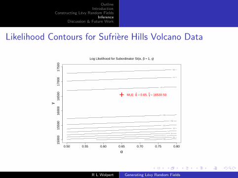
Likelihood Contours for Sufriere Hills Volcano Data
α
γ
0.50 0.55 0.60 0.65 0.70 0.75 0.80
1500
015
500
1600
016
500
1700
017
500
+
Log Likelihood for Subordinator St(α, β = 1, γ)
MLE: α = 0.65, γ = 16530.50
R L Wolpert Generating Levy Random Fields
OutlineIntroduction
Constructing Levy Random FieldsInference
Discussion & Future Work
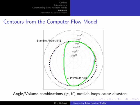
Contours from the Computer Flow Model
8.6V=10
8.7V=10
8.8V=10
8.9V=10
9V=10
9.1V=10
Bramble Airport Ψ(⋅)↓
← Plymouth Ψ(⋅)
Angle/Volume combinations (ϕ,V ) outside loops cause disasters
R L Wolpert Generating Levy Random Fields
OutlineIntroduction
Constructing Levy Random FieldsInference
Discussion & Future Work
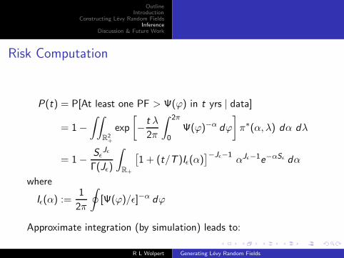
Risk Computation
P(t) = P[At least one PF > Ψ(ϕ) in t yrs | data]
= 1 −
∫∫
R2+
exp
[
−t λ
2π
∫ 2π
0Ψ(ϕ)−α dϕ
]
π∗(α, λ) dα dλ
= 1 −Sǫ
Jǫ
Γ(Jǫ)
∫
R+
[
1 + (t/T )Iǫ(α)]−Jǫ−1
αJǫ−1e−αSǫ dα
where
Iǫ(α) :=1
2π
∮
[Ψ(ϕ)/ǫ]−α dϕ
Approximate integration (by simulation) leads to:
R L Wolpert Generating Levy Random Fields

OutlineIntroduction
Constructing Levy Random FieldsInference
Discussion & Future Work
Estimated Risk of Catastrophic Flows
0 10 20 30 40 500.0
0.2
0.4
0.6
0.8
1.0
← P(t) at Bramble Airport
P(t) at Plymouth →
Time t (years)
P(t)
= P[
Cat
astro
phe
in t
yrs
| Dat
a ]
Probability of disaster in next t yearsR L Wolpert Generating Levy Random Fields

OutlineIntroduction
Constructing Levy Random FieldsInference
Discussion & Future Work
Ongoing Work & Extensions
Related papers on spatial & spat/temp Levy-based BNPReg’n models (w/ N Best, M Clyde, E ter Horst, L House,K Ickstadt, S Mukherjee, N Pillai, C Tu) and upcomingpapers (w/M Huber, M OConnell, Z Ouyang, D Woodard)
Posterior distributions in Bayesian models (RJ-MCMC)
Elicitation issues (w/ K Mengersen)
Consistency properties (w/ N Pillai)
Spatial Maximal fields (w/ D Nychka)
Perfect simulation of Levy (w/G Roberts)
Spatial Risk Models (Volcanoes! w/ J Berger, S Bayarri, etal.)
Need better/more output measures (movies, etc.— help!)
R L Wolpert Generating Levy Random Fields
OutlineIntroduction
Constructing Levy Random FieldsInference
Discussion & Future Work
Thanks!
to the Department of Mathematical Sciences at Alborg University,esp. Jesper Møller.
More details (references, this talk in .pdf, related work) areavailable from website
http://www.stat.duke.edu/∼rlw/or on request from
Thanks too to NSF, SAMSI, DSCR, MSO.
R L Wolpert Generating Levy Random Fields


![Generating random variables Iyambar/MAE5704/Aula1... · Aula 1. Generating random variables I. 18 Accept-reject method. [RC, Ch.2.3] When the inverse method will fail, we must turn](https://img.pdfslide.us/doc/110x75/5f2dfcaa518b376726048106/generating-random-variables-i-yambarmae5704aula1-aula-1-generating-random.jpg)