GENERALtESTIMA TAGRtCUL

Charles R.RaL~.Chhw

,

Lih-Yuan O·William C.Scot Rumb

S-T-STRATIFIEDS0, ,E ... _0.

ABOR SURVEY···

GENERALIZED POST-STRATIFIED ESTIMATORS IN THE AGRICUL-TURAL LABOR SURVEY, By Charles R. Perry, Raj S. Chhikara*, Lih-Yuan Deng**,William C. Iwig and Scot Rumburg, Sampling and Estimation Research Section, SurveyResearch Branch, Research Division, National Agricultural Statistics Service, UnitedStates Department of Agriculture, Washington DC 20250-2000, July 1993, Report No.SRB-93-04.

ABSTRACT

The design-based characteristics of a general post-stratified estimator are investi-gated. Each of the four post-stratified estimators of current interest to NASS is a specialcase of the general post-stratified estimator. An approximation to the design-variance ofthe general estimator is derived using Taylor series methodology.

A simulation study is performed to evaluate the relative efficiency of certain list-onlytype post-stratified estimators. The approximate variance formula for the generalizedpost-stratified estimator is evaluated. The numerical evaluations show that the per-formance of a post-stratified estimator is largely a function of the sample size used toestimate the post-stratum weights, the sample size used to estimate the post-stratummeans of the variable of interest, and the ratio of these two sample sizes. The relativeefficiency increases as this ratio of two sample sizes increases. The approximate varianceformula is found to be reasonably accurate for moderate size samples and highly accuratefor large size samples.

KEYWORDS

Taylor series expansion; Design-variance; Post-stratified estimator; Simulation; Bias;Relative efficiency.

This paper was prepared for distribution to the research communityoutside the U.S. Department of Agriculture. The views expressedherein are not necessarily those of NASS or USDA.

ACKNOWLEDGEMENTS

We thank Fred Vogel for putting forward the "strawman" concept and thus stimulat-ing our thinking about new approaches to estimation. We also thank Ron Bosecker, JimDavies and George Hanuschak for their helpful suggestions, Phil Kott for his technicalreview of this report and Jiannong Wang for his assistance in conducting the simulationstudy.

*Raj S. Chhikara is Professor, Division of Computing and Mathematics, University of Houston-Clear Lake.**Lih- Yuan Deng is Associate Professor, Department of Mathematical Sciences, Memphis State University.

TABLE OF CONTENTS

SUMMARY 111

INTRODUCTION - 1

A GENERALIZED POST-STRATIFIED ESTIMATOR 2

TAYLOR SERIES VARIANCE APPROXIMATION 4

EMPIRICAL SIMULATION EVALUATIONS 13

DESCRIPTION OF SAMPLING PROCEDURE FOR SIMULATION 13

ESTIMATORS UNDER CONSIDERATION FOR SIMULATION 14

MODEL FOR DATA GENEHATION 16

SIMULATION PARAMETERS 18

SIMULATION PROCED{THE 19

NUMERICAL RESULTS _ - 21

RECOM~'IENDATIONS _ 23

TABLES 1-4. RELATIVE PERCENT BIAS, RELATIVE EFFICIENCY AND

APPROXIt-.IATE VARIANCE RATIO 25

APPENDIX A: ESTIMATING THE DESIGN-BIAS AND ITS VARIANCE 29

APPENDIX B: VARIAI\CE OF THE RATIO OF POST-STRATIFIED

ESTIMATORS FROM TWO OCCASIOKS 30

REFERENCES 32

11

SUMMARY

A post-stratification approach to estimation in follow-on surveys is formulated in

the context of the Agricultural Labor Survey. A generalized post-stratified estimator is

defined that makes use of the area and list frame samples from both the June Agricultural

Survey and the follow-on Agricultural Labor Surveys. The approach includes as special

cases two sets of post-stratified estimators of interest to NASS: (1) multiple-frame post-

stratified estimators that use both area and list respondents from the follow-on survey

and (2) list-only post-stratified estimators that use the list respondents from the follow-

on survey exclusively. For each special case two possibilities for estimating the post-

stratum means are included under the generalized approach: (1) the unweighted average

response and (2) the weighted average response where the weights are the expansion

factors associated with the sample units. Consideration of the special cases is motivated

by the desire to use only list samples in follow-on survey.

The complexity of the multiple-frame sample design makes the variance of the gen-

eralized post-stratified estimator somewhat intractable. A computational formula for

estimating the variance in the most general multiple-frame setting is derived using the

Taylor series methodology. The approximate variance formula is extended by analogy to

obtain estimators for the variance of the design-bias and the variance of the ratio of two

general post-stratified estimators from two occasions.

An extensive simulation study is performed to evaluate numerically the performance

of certain list-only post-stratified estimators. Both the bias and the relative efficiency of

each estimator are evaluated. From the numerical results given in the paper, it follows

that the post-stratification improves upon the precision of an estimator, provided that

the sample size in a follow-on labor survey is moderate to large and that the variable used

in post-stratifying the agricultural operations is reasonably correlated with the variable of

interest. Also the performance of a post-stratified estimator is heavily dependent upon the

sample size used in estimating post-stratum sizes. The relative efficiency of an estimator

relative to the direct expansion estimator (computed using their mean square errors)

increases as the size of the larger sample from a base period survey increases relative to

III

the size of the smaller sample from a follow-on survey. The numerical evaluations of the

approximate variance formula show it to be fairly accurate for moderate sample sizes and

highly accurate for large samples as one would expect.

IV

INTRODUCTION

A multiple-frame sampling methodology is the basis of agricultural surveys conducted

by the National Agricultural Statistics Service (NASS) of the U.S. Department of Agri-

cultural (USDA). This methodology consists of sampling both a list frame and an area

frame with the two samples drawn independently. List sampling is much more convenient

and efficient compared to the area frame sampling. The former however does not provide

a full coverage of all the agricultural operations. Thus, the area frame samples are used

to compensate for the list undercoverage. The estimation method requires determination

of the overlap or nonoverlap (OL/NOL) areas between the list and area samples. Since

this OL/NOL delineation process is labor intensive and the NOL involves many fewer

samples, its component of an estimate is often quite unreliable and is produced at an

undesirable high cost.

In his "strawman" proposal, Vogel (1990) advocated a new approach to sampling and

estimation for NASS surveys. One of the key ideas underlying this proposal is the use

of post-stratified estimators in follow-on surveys. The use of post-stratified estimators

is motivated by a desire to produce list-only estimates and a desire to eliminate the

OL/NOL delineation. The desire to produce list-only estimates results primarily from

the need to reduce respondent burden on NOL operations. The desire to eliminate the

OL/NOL delineation results from the assumption that the overall quality of the survey

would be improved by eliminating the numerous non-sampling errors associated with

the complexity of the OL/NOL delineation. The word "strawman" in the proposal title

implies that the post-stratification should be viewed as a baseline approach for developing

improved estimation.

This idea has stimulated us to evaluate certain post-stratified estimators that might

be useful in achieving the above objectives. The next section of this paper formulates a

general post-stratified estimator in the context of the NASS Agricultural Labor Survey

and explains how each of the post-stratified estimators of current interest to NASS is

obtained as a special case. A design-based computational formula for estimating the

variance of the general post.-stratified estimator is derived using Taylor series methodol-

ogy. More importantly, this paper develops a set of rather general design-based variance

and bias formulas for evaluating post-stratified estimators with respect to the sampling

designs used by NASS.

A simulation study is performed to evaluate the relative efficiency of certain post-

stratified estimators. The approximate variance formula derived from a Taylor series

expansion is evaluated for its accuracy and hence, its appropriateness for estimating the

variance of the general post -stratified estimator.

In Appendix A, we show how to write the obvious estimator of the design-bias of the

general post-stratified estimator in a form analogous to the estimator itself. We then show

how to use the general vClrianceformula to estimate the variance of such an estimated

design- bias.

A companion report (Rumburg, Perry, Chhikara and Iwig, 1993) provides detailed

design-based empirical evaluations of the multiple fraIlle and list-only post-stratified

estimators of the numlwr of hired workers for the NASS A!!;l'icultural Labor Survey using

the 1991-92 Labor Survey and June Agricultural Survey data for the states of Florida

and California. III this appli('ation, the post-stratum sizes 'were estimated using only all

the area samples from the .1une Agricultural Survey.

A GENERALIZED POST-STRATIFIED ESTIMATOR

In the context of a follow-on agricultural survey, a gf'neraJized post-stratified estimator

of a characteristic of interest, say population total in a statl' or region, is of the form:

(1)

where, for the post-stratuIll k:,

2

Zk represents an estimate of the "size" of post-stratum k obtained from the base survey,

e.g. June Agricultural Survey (JAS), Xk represents an estimate of the "size" of post-

stratum k obtained from the follow-on survey, e.g. an Agricultural Labor Survey (ALS),

and 1\ represents an estimate of the total, Yk , for the item of interest for post-stratum

k, derived from the follow-on survey.

For application to the ALS (i.e., follow-on labor surveys) there are four post-stratified

estimators of primary interest as studied by Rumburg, et ai. (1993). If we let Mk

represent an estimate of the population size for post-stratum k derived from the JAS

(the base survey), then by a simple transformation of the data the four estimators can

be written as:

YC(List+NOL)wt = L MkYk(List+NOL)wt, (1.1)

where Yk(List+NOL)wt denotes the weighted mean of all List and NOL sample

responses that are in post-stratum k,

(1.2)

where fh(List+NOL) denotes the simple mean of all List and NOL sample

responses that are in post-stratum k,

YC(List)wt = L AhYk(List)Wb (1.3)

where Yk(List)wt denotes the weighted mean of all List sample responses that

are in post-stratum k, and

(1.4)

where Yk(List) denotes the simple mean of all List samples that are in post-

stratum k.

3

Each of these estimators (1.1)-(1.4) is easily written in the notation of the general

post-stratified estimator. For example, the estimator (1.1) is put in the notation of the

general form, by equating Mk with Zk and then equating Yh List+NOL)wt with Yk divided

by Xk, since in the latter case, it equals the sum of the f'xpanded y's in post-stratum

k divided by the sum of associated weights. Similarly follows the description of other

estimators in the notation of the general estimator.

Cochran (1977, pages 142-144) considered the problem of estimating totals and means

for domains. If this estimation is extended to the whole population, one has the estimator

as in (1.3). Sar-ndal, Swensson and Wretman (1991, pa.l!;f'268) considered a estimator

similar to (1.3) with the post-stratum size Mk assumf'd known. Hence, their estimator is

a special case of the genf'ralized post-stratified estimator ddined in Equation (1).

TAYLOR SERIES VARIANCE APPROXIMATION

Following the standard Taylor linearization method (V.:o]tf'r1985, page 226), the first-

order approximation of the design-variance of the gen('ralized post-stratified estimator Ggiven in Equation (1) can be written as:

v (G) = l' (t acZ k Z I;; -+ acYk }rl;; -+ DC x k·Y 1;;) ,k=l

where

ac }kaCZk = aZ

k1(2,y,l)= X

k'

ac Zk8GYk = 8Yk 1(2,y,x)= XI;;'

ac Z I;;YkDC Xk = aXk 1(2,Y,l)= - Xi .

4

(2)

and

Z = (Zl,'" ,ZK) = (E(ZJ), ... ,E(ZK)),

Y = (YI,'" ,YK) = (E(YJ),··· ,E(YK)),

X = (Xl,'" ,XK) = (E(XI),· .. ,E(XK))'

In the general form of the post-stratified estimator, each Zb Yk and Xk will have a

list and an area frame component. Hence these estimators can be written as:

~ ~ ~Xk = Xu + XAk, (3)

where the list and area frame components are denoted by subscripts L and A, respectively.

Since samples are drawn independently from the list and area frames, the list esti-

mates Zu, Yu and ~tuare independent of the area estimates ZAb YAk and ~tAk' Thus

the Taylor series variance approximation can be rewritten as:

V(G) = V (~iJGZ'ZU + iJGy,Yu + iJGx,xu)

+ V (~iJGZ,ZAk + iJGy,YAk + iJGX,XAk) . (4)

Since the list frame sample for the Agricultural Labor Survey (i.e., for the follow-

on current period survey) is drawn independently of the list frame sample for the June

Agricultural Survey (i.e., for the base survey), the list estimate ZU is independent of the

other list estimates Yu and Xu. Thus the first term of Equation (4) can be rewritten

as:

v (t DCzkZU + DCyk}TLk + DCXkXU)k=l

= V (t DCZkZLJk) + V (t DCYkYLck + DCXk~tLCk)' (5)k=l k=l

5

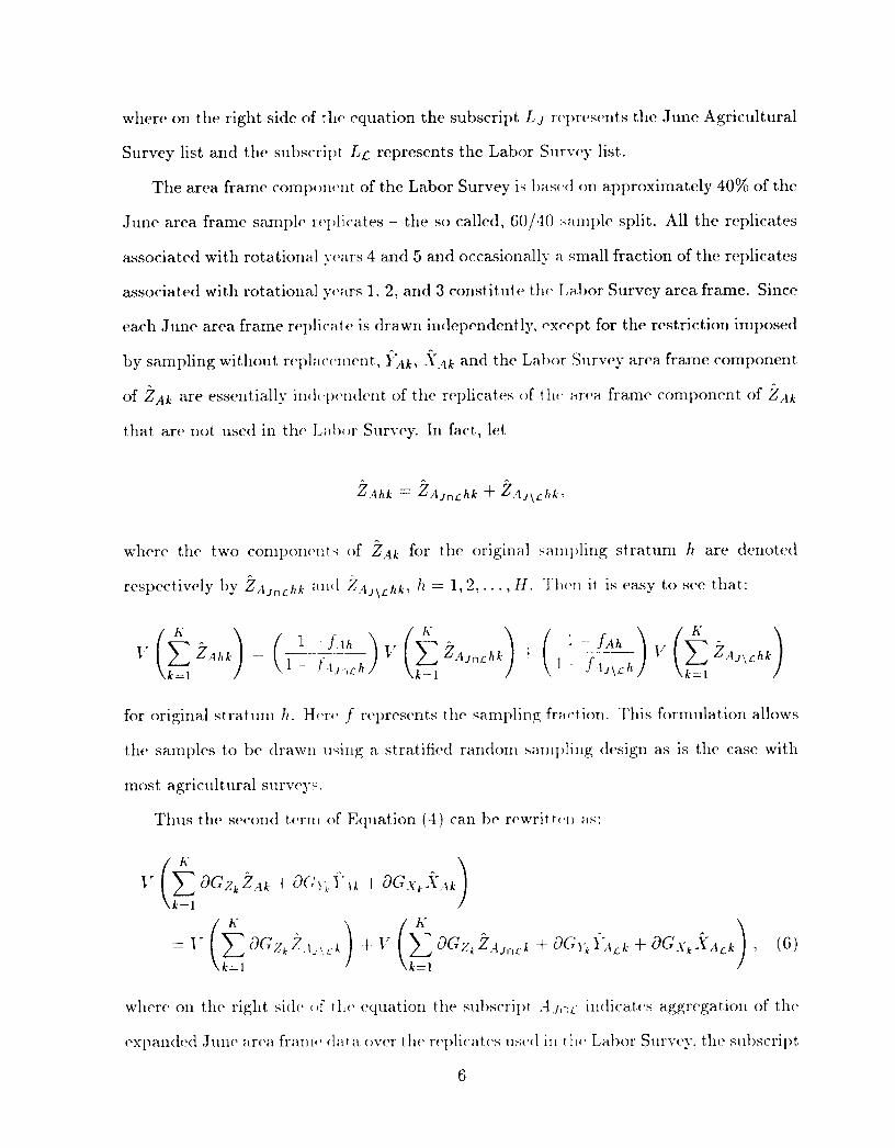
where on the right side of tlw C'quation the subscript LJ represent.s the June Agricultural

Survey list and the subscript L{. represent.s the Labor Smvey list.

The area frame componcnt of the Labor Survey is hased on approximately 40% of the

June area frame sample replicates - the so called, GO/40 sample split. All the replicates

associated with rotational years 4 and 5 and occasionally a small fraction of the replicates

associated with rotational ycars 1, 2, and 3 constitute tIll' LClhor Survey area frame. Since

each J 1lIH' area frame replicate is drawn independently. ex.ept for the restriction imposed

by sampling without replaC('lllCnt, f~tb ~tAk and the Labor Survey area frame component

of ZAk are essentially indqwndell t of the replicates of tIll' h n'a frame component of ZAk

that are not used in the La h, lr Survey. In fact, let

, , ,

ZAhk = ZAJnLhk + ZAJ\Lhk,

where the two component--: of ZAk for the original ;;ampling stratum h are denoted

respectively hy ZAJnchk illld ZAJ\Lhb h = 1,2, ... , H. Tlwll it is pasy to see that:

for original stratum h. Hcrc f reprf'sent;; tlw sampling {riJi'lion. This formulation allows

the samples to be drawn \l"ing a stratified random :-.ampling design as is the case with

most agricultural surveys.

Thus the second krIll of Equation (4) can 1)(' rewrith'll as:

(G)

where on the right side of 1Le equation the subscript A ]rlL' indicates aggregation of the

expanded June area framc data over the replicate's used ill rill' Labor Survey. the suhscript

6

AJ\C indicates aggregation of the expanded June area frame data over the replicates

not used in the Labor Survey and the subscript Ac indicates Labor Survey area frame

expansion and aggregation. This equality assumes that appropriate adjustments are

made to all variance calculations as discussed above to account for differences in finite

population correction factors. Operationally these differences can be ignored since almost

all area frame sampling fractions are less than one percent.

Replacing the right hand side of Equation (4) with the expression given in Equations

(5) and (6), the Taylor series expansion variance of G becomes:

V(G) = V (f. 8CZ/cZLJk) + V (f. 8CY/cYLt:.k + 8Cx/cXLt:.k)k=l k=l

+ V (~aGZ'ZAJ\'» + V (~aGz,ZAJn'> + aGy,YA,> + aGX,XA'» ,(7)

where the subscript

(1) LJ represents data expansion and aggregation for the June Agricultural Sur-

vey list,

(2) Lc represents data expansion and aggregation for the Labor Survey list,

(3) AJnc represents data expansion for the June Agricultural Survey area frame

and aggregated over the replicates used in the Labor Surveys (replicates

associated with rotational years 4 and 5 and a small fraction of the replicates

associated with rotational years 1, 2, and 3 ),

(4) AJ\c represents data expansion for the June Agricultural Survey area frame

and aggregated over the replicates not used in Labor Surveys, and

(5) Ac represents Labor Survey area frame data expansion and aggregation.

To complete the derivation of the computational form of the Taylor series variance

estimation formula, some additional notation is needed. For the list component of the

7

June Agricultural Survey, let

ZLJk = L ZLJhb

hEHLJ

Z LJhk = tVLJh L ZLJhl b( k, I,}, i),iEnLJh

(8)

if unit i of JAS list stratum hi,; in post-stratum k

(ltherwise.

Note that the notation LhEH denotes the' summation over all strata corresponding tos

survey type S. For example. S = L) is the June surv!'y m~iI]g the list frame.

In Equation (8), the ('xpausion factor HiLJh = N['Jh/77/'Jh, where NLJh and nLJh arc

respectively the populatio[] si:l,e and sample size for J AS Ii,! frame stratum h.

For the list component of the Labor Survey, let

}\ck = L }"J,c hb

hEHLc

}-J'Lhk = lVLch L YLchi b( k, I(hi),

iEnLch

and

t/,[k = L .'cJ,chb

hElILc

XLLhk = 1VLch L J:Lchi/l(A',I(hi),

IEnLch

where

(9)

(10)

{

1,b(k, Lchi) =

0,

if unit i of Lahor list stratllIll h is in post-stratum k

(Ithcrwise.

In Equations (9) and ( 10), the expansion factor HTLCh =-VLc h In Lch, where NJ'Lh and

nLch are resp('ctively th(' pop,dation size and sample siz(' fOI Lahor list frame stratum h.

8

For the area frame component of the June Agricultural Survey, let

ZAJni:k = L ZAJn£hk,hEHAJn£

ZAJn£hk = WAJh L ZAJn£hik,

iEnAJn£h

ZAJn£hik = 2: ZAJn£hij 8(k, A]nchij),jEMAJn£hi

where

(11)

(1) L:iEn indicates the sum is over all nAJn£h June area frame sampleAJn£h

segments of stratum h that are used in the Labor Survey area frame,

(2) L:' M indicates the sum is over all MAJn£hi tracts of sample segment}E AJn£hi

AJnchi,

(3)

and

{

I,8(k, AJnchij) =

0,

if tract j of segment AJnchi is in post-stratum k

otherwise

where

ZAJ\£k = 2: ZAJ\£hk,

hEHAJ\£

ZAJ\£hk = WAJh 2: ZAJ\£hik,

iEnAJ\£h

ZAJ\£hik = 2: ZAJ\£hij 8(k, AJ\chij),jEMAJ\£hi

(12)

(1) L:iEn indicates the sum is over all nAJ\£h June area frame sample seg-AJ\£h

ments of stratum h that are not used in the Labor Survey area frame,

(2) L:}'EM ' indicates the sum is over all MAJ\£hi tracts of segment AJ\chi,AJ\£h.

9

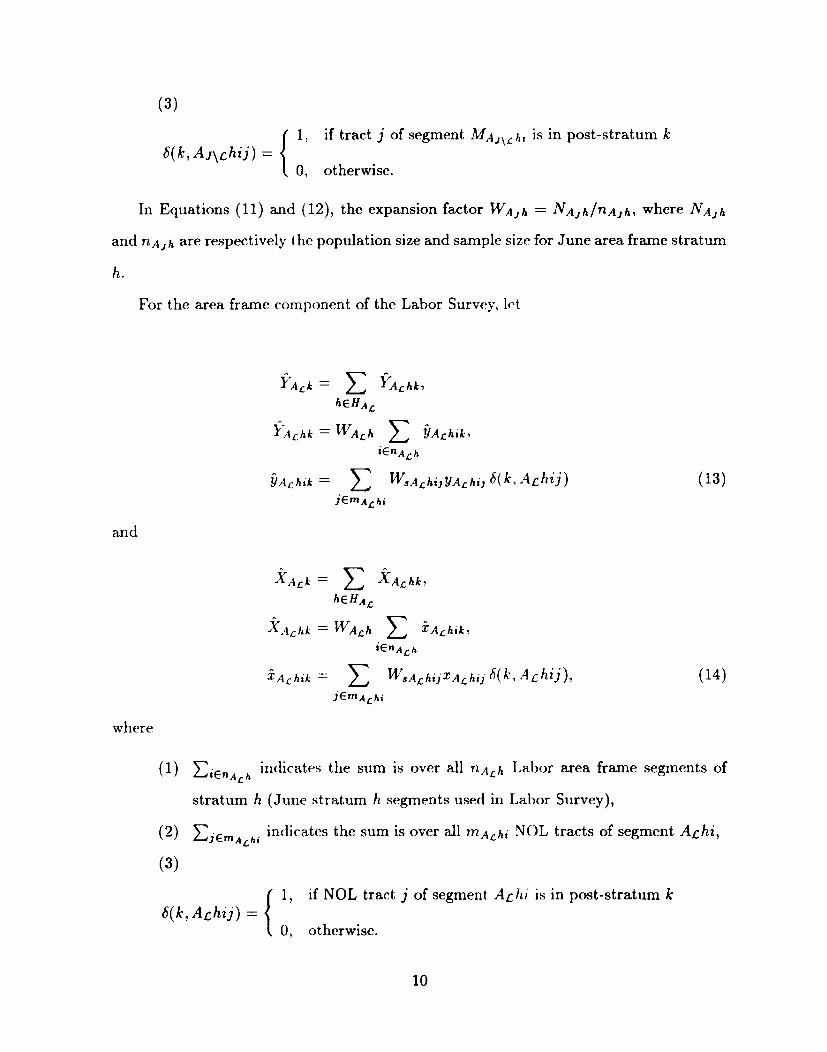
(3)

{

I,6(k, AJ\chij) =

0,

if tract j of segment M AJ \L.h I is in post-stratum k

otherwise.

In Equations (11) and (12), the expansion factor WAJh = NAJh/nAJh, where NAJh

and nAJh are respectively the population size and sample size for June area frame stratum

h.

For the area frame component of the Labor Survey, let

}rA.ck = L YA.chbhEHA.c

fA.chk = WA.ch L YA.chik,iEnA.ch

YA.chik = L WsA.chijYA.chiJ 8(k, Achij)jEmA.chi

and

XA.ck = L XA.chk'hEHA.c

"YA.chk = WA.ch L XA.chibiEnA.ch

XA.chik = L WsA.chijXA.chij 8(k, Achij),jEmA.chi

where

(13)

(14)

(1) L:iEn indicates the sum is over all nA.ch Labor area frame segments ofA.ch

stratum h (June stratum h segments used in Labor Survey),

(2) L:1"Em "indicates the sum is over all mA.chi N"OL tracts of segment A£hi,A.chl

(3)

{

I,8(k, A£hij) =

0,

if NOL tract j of segment A£hi is in post-stratum k

otherwise.

10

In Equations (13) and (14), the first phase expansion factor WA.ch = N A.ch/nA£h =NAJh/nA.ch , where NA£h = NAJh and nA.ch are respectively the population size and

sample size for Labor area frame stratum h. The second phase expansion factor for tract

j from segment i and stratum h which is selected in second phase sample from post-

select stratum s is W .•A£hii = N .•A£h/n .•A£h , where N .•A£h and n .•A.ch are respectively the

population size and sample size for post-select stratum s.

By substituting Equations (8) through (14) in Equation (7) and rearranging the order

of summation the first-order Taylor series variance can be rewritten as:

V(G)= VLJ (L WLJh.L (t8GZkZLJhib(k,LJhi))) +hEHLJ IEnLJh k=l

VL£ (LWL£h . L (tl8GYtYL£hi + 8GXtXL£hi] b(k, LChi)))) +EHL£ IEnL£h k=l

VAJ\£ ( L WAJh. L . L (t8GZkZAJ\£hijb(k,AJ\Chij))) +hEHAJ\£ IEnAJ\£h lEMAJ\.chi k=l

VA.c ( L WAJh [. L . L (t 8GZtzAJn£hij b(k,AJnChij))] +EHAJn£ IEnAJn£hlEMAJn£hi k=l

LWAJh. L [. D¥ ..A£hij (tl8GYkYA£hii+8GXtXA£hii]b(k,AChij))1)·hEHA.c IEnA.ch lEmA£hi k=l 5)

The sequence of computations necessary to produce the first- order Taylor series

variance estimate are indicated more clearly by rewriting Equation (15) as:

V(G) = L VLJhEHLJ

11

where

K

tLJhi = WLJh.I: DC Zk ZLJhi 8(k, LJhi),k=]

K

t LLhi = WLLh .I:[DCYk YLLhi + DCXkX LLhi] 8( k, L£hi),k=l

K

tAJ\Lhi = WAJh I: .I:8CzkZAJ\Lhij8(k,AJ\1:hlj),jEJfAJ\Lhi k=]

K

tAJnLhi = WAJh L L 8CZkZAJnLhij 8(k, AJn£hij),jEMAJnl:hi k=]

K

tALhi = n"Ach L n"sALhij.I: [8CYkYALhij + c1GXkxALhiJ] 8(k,A£hij).jEm Ac'" k=]

The general form of the formula for computing the stratum level variance estimates

in Equation (16) is given by:

where the stratum popuiatioll and sample sizes are determiI]('d by the subscripts as these

appear in Equations (16) and as previously defined in Equations (7)-(14).

The use of Equation (17) to compute the stratum 1('w1\'ariances is discussed in Kott

(1990b). Equation (17) provides unbiased stratum 1('v('1n.riance estimates for the first

and s('cond terms of Eqllation (16) and for the third t(TtlJ wllf'n the finite population

correction factor is adjusted as indicated in the discussion preceding Equation (6). Since

the fourth term of Eqllation (16) involves a second pha.se of sampling, the stratum level

estimates derived from Eqllation (17) will be slightly ("ow;crvative, [see Kott (1990b)

pages 19-22, particularly Equation (26) on page 22, tlH'rf·illJ. Operationally, the finite

population correction factors in Equation (17) are ,Q/'Iwrally ignored. The effect of

ignoring the finite population mrrection factors on the varianr'c estimates is not important

since the sampling rate in most strata is very small.

12

EMPIRICAL SIMULATION EVALUATIONS

In this section, we evaluate the performance of the generalized post-stratified estima-

tor and its variance formula discussed in the previous section by conducting a simulation

study. The NASS sampling design involves separate stratifications for the list and area

frames. So it is desirable to simulate data for the two frames separately for the evaluation.

In the post-stratification approach described above, the JAS serves as a base survey and

the ALS as a follow-on survey. As such we have used this base and follow-on survey

format to simulate the data. Although we consider simulations based only on a single

type of sampling frame and hence, do not exactly simulate the two separate stratifications

analogous to NASS, it however emulates the basic approach adopted in the construction

of the generalized post-stratified estimator which makes use of J AS sample responses

to estimate post-stratum sizes and ALS sample responses to estimate the post-stratum

means. The sampling procedure and estimators considered for simulation evaluations are

descri bed next.

Description of sampling procedure for simulation.

The sampling procedure for simulation is based on the concept that the original

stratification is common to both the base survey and the follow-on survey. This ap-

proach is general enough to be applicable to many situations involving follow-on sur-

veys. Presently we consider the stratification for the list frame and evaluate the post-

stratification methodology for the list-only estimators. Therefore, the subscript L (for

list frame) will be dropped from the notations in previous sections.

(1) Suppose there is a sample of size nJh' representing the JAS sample values,

from the list frame which consists of H original strata with NJh as the size

of h-th stratum, h = 1,2, ... ,H.

(2) After a JAS sample is taken, observations are post-stratified into K post-

strata according to some stratification variables with some observed charac-

13

teristics. Population counts for the post-strata are produced once annually

from the JAS and then these counts are fixed for the ALS.

(3) mJh k is the number of units in the h-th ori.e;inal stratum classified into the,k-th post-stratum in the J AS sample.

(4) An independent sample of size n£h' representin!~ the ALS sample values, is

drawn from the list frame.

(5) After an independent ALS sample is taken, we post-stratify observations,

according to the stratification variable, into K PoOst-strata same as those for

the JAS sample.

(6) m£h k is the number of units in the h-th original stratum classified into the,k-th post-stratum in the ALS sample.

Estimators under consideration for simulation.

We denote by Yc the generalized post-stratified estimator given in Equation (1), that

IS

(18)

where

G~ - ZkYkk - ~ ,

Xk

for post-stratum k. In terms of the above notations, Zb .\'k and Yk can be expressed as:

H~ ~ NJhZk=L-mJh k

h=l nJ h '

an estimate of the" size" of post-stratum k derived from J AS,

represents an estimate of the "size" of post-stratum k df'riwd from ALS, and

14

(19)

(20)

(21)

represents an estimate of the total, Yk , for the item of interest for post-stratum k, derived

from the ALS.

Note that the generalized post-stratified estimator can also be re-written as

K

YCwt = L:AhYk,k=l

where

and

(22)

Since Y k is a weighted mean of the sample observations in post-stratum k, Yc wt corre-

sponds to the weighted post-stratified estimator given in Equation (1.3).

The other post-stratified estimator considered is one that uses the simple mean of

the sample observations in a post-stratum:

K

YCunwt = L:MkYk,k=l

where

(23)

A ~ NJhMk = ~ --m Jh k'

h=l nJh '

This corresponds to the unweighted post-stratified estimator given in Equation (1.4).

In this simulation study, another post-stratified estimator considered is based on the

use of the combined expansion factor, i.e. the unweighted post-stratum count estimates,

in addition to the unweighted post-stratum mean estimates. This unweighted "combined"

estimator is:

K

YCunwt(C) = L:MkYk,k=l

15

(24)

where

Yk = 11k·

This estimator is motivated by the observation that there can be large variation 1Il

estimating the post-stratum count separately in each original stratum and so a com-

bined population count f'stilllate across all post-strata will ~tabilize this variation. TlH'

term "combined" is uSf'd Ilf're in the manner similar to the "combined ratio estimator"

discussed in survey samplin.t; lit.erature. [See, for examplt', Cochran (1977, pages 164-

169).]

For the sake of comparison, also considered is the direct f'xpansion estimator of Y

given by

Model for data generation.

H

Yst = L NJhYh·h=1

(25)

The following steps cUt' followed to generate a response variable y and a correlated

auxiliary variable :r to fmm a population of H original strata with stratum size NJh

for h = 1,2, ... , H, and anotber auxiliary variable tv for post-stratification of population

units. In the context of the ALS, the variable y represents tlw number of hired workers,

x is the size of farm operatioll and w is the peak numlwr of workers expected durin,!!;the

year for the farm labor.

(1) For each h = 1,2 .... ,H,

follows:

1,2, ... , NJh, stra"um data are generated as

(a) First we ~('nerate a population of base v<llnesZhi uniformly distributed

over all illterval, say

where [' stands for the uniform distrihution and interval (Z1,Z2) IS

chosen to he (5,8).

16

(b) The values for the auxiliary variable x representing the farm operation

size are generated using the model,

where £2 t'V N(O,ai), vh t'V U(VI, V2) and CKh t'V U(~I,~2)' The

parameter values chosen are: ai = 1, (VI, V2) = (3,5) and (~}, ~2) =(0.5,4).

Steps (a )-(b) would generate values that may vary due to size, stratum or

other characteristics of population units. More specifically, Zhi represents the

unit size, Vh represents the stratum mean, and CKh represents the dependence

of the stratification variable on the unit size.

Next, we consider another auxiliary variable w to be used for post-stratification.

This variable may be similar to x, but invariably it is expected to reflect

additional information.

(c) Generate

x' hi = Zhi + £1, where £1 t'V N(O, an,where ai is chosen to be 1.

(d) From values generated in steps (b) and (c), generate

(27)

where Ph is generated randomly from the uniform distribution over

an interval. Presently the interval is taken to be (0.0,0.1). This

makes Whi not to be too different from Xhi. This consideration is

quite appropriate in the context of the ALS since the use of the peak

number of workers as a ~tratification variable is reflected in the list

frame stratification.

17

(e) For the response variable y, generat e

Yhi = jlh + (3hll'hi + fl. (28)

where f3 '"'" l'l(O, 0"5) and J1h are selected randomly from U(M1, Mz)

and (3h are selected randomly from U(B1, B2). This model takes

into a,count the differences in response due to stratum and other

charact,'risti,s of population units.

(2) The variate 1/'/11' representing an auxiliary varia hie for post-stratification, is, in

theory, a better stratification variable than the ori~inal stratification variable

in order for the post-stratification to be efficient.

(3) Once ll'hl arc ~I'lj('rated, we sort the values of /I'll! and find the cut-off points

for the post-stratincation. (Say, AI < Az < ... <~ .-1/\-1 are the cut-off points

so that if Whi E=(Ak-1, Ak), tl1('n t11('unit is classified as belonging to post-

strat urn Ie.)

Simulation parameters.

Several parameters (which, we think, will not affect thI' 'l1ltcome much) are fixed in

this simulation study:

(1) Population sizes are randomly generated from (T ( 500, 5000).

(2) The number of original strata H = 6 and thc n1lIHlwrof post strata, K = 8.

The total sample sizc f<)rALS is H( = 50,100,200, 40ll. whC're

H

1l( = L1l£h'h=]

(29)

The relative size of the expallsion factor NJh/1l£h is randomly generated; where we first

generate randomly Eh from C( 50,200), and then rescale Eh snch that L~=] 1l£h = n(.

It is straightforward to 'OIllpntc the appropriate scalin~ constant c for the expansion

18

factors, Nlh/n.ch = c * Eh for h = 1,2, ... , H, so that

,£f=l Nlh/Ehc = ------.n

We then selected the following cases of the various parameters in Equation (28).

(1) The standard deviation of error term E3 is chosen to be 0"3 = 1 and 0"3 = 2.

(2) The intercept of /lh is selected from the range (Ml,M2) = (5.0,8.0).

(3) The slope of (3h is selected from the interval (Bl, B2) = (1.0,2.0) and the

interval (Bl, B2) = (3.0,4.0).

In general, the post-stratification will be more effective than the original stratification,

if (1) E3 is smaller, (2) the range of (Ml' Af2) is narrower and (3) t,he values of (Bl, B2) are

larger. However, when the range (Ml, M2) was considered to be (5.0,6.0), the evaluation

results were similar as in the case of range (5.0,8.0).

The J AS sample is used to estimate the population size of each post-stratum. We

consider the sample size ratio, nJ/n.c = 1.0,1.5,2.0,2.5,3.0,4.0,5.0, where n J is the total

sam pIe size in June and n.c is the total sam pIe size for ALS.

Simulation procedure.

Recall that we have assumed both J AS and ALS have the same sampling frame for

the purpose of this simulation study. The simulation procedure and the computations

made are as follows:

(1) For a given stratum h, a sample (corresponding to J AS) of size nJ h = n.ch * r,

(r = 1.0,1.5,2.0,2.5,3.0,4.0,5.0) is selected from the population. The sample

data are used to compute the estimate of the k-th post-stratum population

count, Mk, for k = 1,2, ... , K.

(2) For a given stratum h, an independent sample (corresponding to ALS) of size

n.ch' is selected from the ALS. The sample data arc used to compute Y k or

ih, the sample average of k-th post-stratum, k = 1,2, ... , K.

19

(3) For each sample selected according to the parameters chosen, we compute

YCunwt, YCunwt(C)' YCwt and the direct expansion estimator Yst.

(4) Repeat the above step 2,000 times and compute its mean deviation from the

true population value as an estimate for the hias .. The percent biases of the

four estimators, }'C:unwt, YCunwt(G), YCwt and }~t are computed as follows:

Bst =

Bu(G) =

[(?_1 2: Yst) IY - 1] * 100%,~OOO .2000 tImes

[( __1 "'"' Ycunwt) II' - 1] * 100%,2000 ~2000 times

[(20100 ~ }TcunwtrCl) Ir- 1] * 100%,

2000 tImes

[(?_1 2: }Tcwt) IY -~1] * 100%,_000 .2000 times

where Y = L~=1 NJ h Yh is the population total.

(5) Similarly, compute its mean squared deviations from the true population value

as an estimate for the MSE:

l' = _1_ ( "'"' (}~' _ Y)2)2000 ~ st ,2000 tImes

1 ("'"' ~ . '))Sit = 2000 ~ (YCunwt -})~ ,2000 tImes ,

1 ("'"' A, 2)Su(C) = 2000 ~ (YCunll't(C) ~ }) ,2000 tImes

1 ("'"' A, , '»)Sur = 2000 ~ (rC wt - })~ ,

2000 times .

(6) The sample variance, SA, computed accordiIl~ to the approximate variance

formula given in the previolls section (with tlI(' neCf'ssary simplification) is

also obtained for rach iteration a.nd tlH'n is RYf'rllg;rd over all 2000 iterations.

20

(7) The relative percentage biases, Bu, Bu(c), and Bw, and the relative efficiencies,

V / Su, V / Su(C), and V / Sw, of the post-stratified estimators are computed.

In order to distinguish between various parameter inputs and stratifications, we also

compute the design efficiency for the original stratification and for the post-stratification

as follows:1-f S2

Deff-H = n_L. _

",H !=..1lLW2 S2'L..,h=1 n.ch h h

where n£, the total sample size, is defined in Equation (29),

and

Similarly, the design efficiency of the post-stratification, Deff-K, is computed. The

design efficiency, Deff-H (or Deff-K) is the relative efficiency that can be expected for

the stratified (or post-stratified) estimator over the direct expansion estimator when the

population counts are known. Of course, the population counts for post-stratification are

unknown in our case and these have to be estimated from JAS.

Numerical Results.

The simulation evaluation results are listed in Tables 1-4. In two cases (Tables 1-2),

Deff-H and Deff-K are not too much different and hence the post-stratification is not

much more efficient than the original stratification. However, Deff-K is substantially

higher than Deff-H in the other two cases (Tables 3-4), making the post-stratification

much more efficient than the original stratification. Based on the numerical results, the

following conclusions are drawn:

(1) The relative efficiencies for the three post-stratified estimators, the weighted

(}'I"awi), the unweighted (Ya unwt), and the unweighted "combined" (Ya unwt(C)),

21

as shown in Tahles 1~4 are increasing functions (If TtJ /n£, the ratio of sample

sizes between .J AS and ALS. This can be attributed to the fact that the larger

the sample siz(' is in JAS, more efficiently the po:-t-stratum population counts

are estimated. One also finds that when the two sample sizes nJ and n£ are

about equal, there is no gain in the post-stri1tified estimators over the direct

expansion estimator.

(2) When the total sample size in ALS is small, say 1'1£ = 50, and when the post-

stratification i" not effective as reflected in the Deff-K value of being close

to 1, all three post-stratified estimators have 11lrger variances than the direct

expansion estimator Yst [Tables 1 and 2 with 11 [ = 50].

(3) For a moderate to large ALS sample siz(', say 1/ L :=: 100,200 or 400, the com-

bined unweighted C'stimators (}Cunwt(C)) and tlw wC'ighted estimator (Yewt)

have smaller variances than tlw direct expansioll estimator (}Tsd, especially

when the post stratification is more effective. [Tables 14]. On the other

hand, when tlw efficiencies of the original aIld post stratifications are about

the same [Tahles ] and 2], fTe unu'/(C) may Ilot ))1' jH'tter than f~/.(4) The observed vari;mce approximation SA is \Try close to the observed mean

square error (:'vISE) of the post-stratified estimator YCwt when n£ ~ 100.

However, whell the ALS sample size is small. say 1/£ = 50, the approximate

variance formula underestimates the observed ),ISE by 30%-50%.

(5) Among three post -stratified estimators considered, the weighted estimator

pre wd tends to have the smallest bia.<;,and the un weighted estimator (Ye unwt),

the largest bias. For example, when n£ ~ lOO, tIe hias of Yewt is always less

than 0.16% of the true population total: wll('[,(<lS the largest biases of the

unweighted estimators (}Te unw/(C') and f"(; unu,d are about 0.6% and 1.0% of

the true population total. Of course, the direct expansion estimator }~t is an

unbiasC'd estimator of the population total.

22

(6) The unweighted "separate" estimator CYc unwt) is the worst post-stratified

estimator both in terms of the bias and the MSE. The unweighted "combine"

estimator (Yc unwt( C)) is slightly better than the weighted estimator (Yc wt) in

some cases [Tables 3 and 4], and Ycwt is slightly better YCunwt(C) in one case

[Table 1]; while in other case [Table 2], YCunwt(C) is better when nc ::;200

and Yc wt is better when nc = 400. The main reason is that as the sample

size becomes larger, the bias (which is of the constant order) becomes more

dominant than the variance (which is of order line) in the MSE and thus

the weighted estimator (}Tcwt) becomes more efficient because it has smaller

bias.

RECOMMENDATIONS

(1) When the sample size nc is small, the post-stratification estimators are not

recommended even when there is a good post-stratification variable.

(2) The general weighted post-stratified estimators (f"c wt) is recommended pro-

vided nc is moderate to large and there is an effective post-stratification

variable. The unweighted "combined" estimator }TCunwt(C) sometimes tends

to have a slightly smaller variance, however, }TC wt tends to have a smaller

bias. There is one major advantage of }TCwt over Yc unwt( C): the variance

formula and its variance estimate are readily available for }TO wt. Therefore,

YCwt is recommended over }TCunwt(C)'

(3) The performance of the post-stratified estimators is a function of the ratio of

two sample sizes, nJ Inc. The relative efficiency of fa wi or fc U7lwt(C) over Yst

increascs as nJ Inc increases. For a post-stratified cstimator to be efficient,

nJ Inc > 1. Based on the results in Tablcs 1-4, it is recommended to have

the sample size ratio nJ Inc ~ 2.

23

(4) The Taylor series approximate variance formula is recommended for estimat-

ing the design variance of the post-stratified wt'ight.ed estimator, }TC wil since

it is found to he reasonably accurate for moderate size samples and highly

accurate for large size samples.

In the above recommendations, the sample size n£ is termed small, moderate or large

on the basis of the following criteria for average number of sample units per stratum,

say n£h: n£ is small if 17£h <: 10, n£ is moderate if 10 S II£h :::;30, and n£ is large if

n£h > 30.

24

Table 1: Relative Percent Bias, Relative Efficiencyand Approximate Variance Ratio.

deff-H= 1.6764, deff-K= 1.8743ai = 1.00, /3 '" U(1.0, 2.0)

ReI. Percent Bias ReI. Efficiency RationJ/n£. Bu Bu(c) Bw V/Su V/ Su(c) V/Sw SA/Sw

1.000 0.974 0.604 0.153 0.478 0.545 0.503 0.8131.500 0.846 0.634 -0.001 0.494 0.550 0.511 0.6722.000 0.963 0.587 0.142 0.549 0.613 0.588 0.6072.500 0.920 0.637 0.088 0.676 0.738 0.725 0.6513.000 0.985 0.632 0.147 0.659 0.743 0.727 0.6424.000 1.090 0.732 0.257 0.750 0.857 0.857 0.6355.000 0.952 0.582 0.102 0.720 0.799 0.790 0.547

nJ/n£. Bu Bu(c) Bw V/Su V/Su(c) V/Sw SA/Sw1.000 0.942 0.4 73 0.080 0.570 0.742 0.711 1.0411.500 0.978 0.549 0.128 0.662 0.875 0.872 1.0102.000 0.918 0.458 0.066 0.832 1.140 1.109 1.0262.500 1.022 0.571 0.157 0.839 1.160 1.213 1.0053.000 0.989 0.527 0.128 0.863 1.236 1.265 1.0194.000 1.000 0.538 0.136 0.916 1.315 1.376 0.9755.000 0.969 0.503 0.103 0.991 1.457 1.504 1.010

nJ /n£. Bu Bu(c) Bw V/Su V/Su(c) V/Sw SA/Sw1.000 0.909 0.411 0.028 0.507 0.774 0.772 1.0131.500 0.904 0.401 0.027 0.629 1.020 1.061 1.0402.000 0.999 0.482 0.119 0.594 1.020 1.133 0.9732.500 0.946 0.446 0.068 0.674 1.179 1.304 1.0093.000 0.915 0.405 0.027 0.653 1.167 1.258 0.9754.000 0.957 0.443 0.070 0.699 1.316 1.500 1.0175.000 0.946 0.448 0.062 0.719 1.340 1.580 1.001

nJ/n£. Bu Bu(c) Bw V/Su V / Su(c) V/Sw SA/Sw1.000 0.921 0.417 0.011 0.388 0.729 0.858 0.9931.500 0.921 0.416 0.018 0.405 0.837 1.045 1.0132.000 0.931 0.433 0.023 0.421 0.910 1.165 0.9742.500 0.951 0.451 0.049 0.416 0.928 1.279 0.9843.000 0.945 0.449 0.034 0.454 1.052 1.508 1.0234.000 0.955 0.460 0.045 0.451 1.064 1.600 1.0035.000 0.958 0.460 0.052 0.463 1.115 1.724 0.994

25

Table 2: Relative Percent Bias, Relative Efficiencyand Approximate Variance Ratio.

deff-H= 1.2790, deff-K= 1.4369a~ = 2.00, /3 rv U(1.0, 2.0)

nC = 50ReI. Percellt Bias ReI. Efficiency Ratio

nJ/nc Bu Bu(Cl---

Bw V/Su V / Su(G) V/Sw SA/Sw1.000 0.929 0.555 0.166 0.614 0.670 0.610 0.8431.500 0.777 0.564 -0.033 0.611 0.656 0.597 0.7022.000 0.915 0.537 0.152 0.663 0.708 0.669 0.6722.500 0.854 0.570 0.069 0.768 0.807 0.759 0.6963.000 0.916 0.563 0.123 0.779 0.833 0.787 0.718

-- -0.295 0.814 0.875 0.833 0.6894.000 1.078 0.720

5.000 0.884 0.518--

0.080 0.809 0.850 0.816 0.625-

nJ/nc Bu-~

Bu((')

1.000 0.891 0.4231.500 0.932 0.5022.000 0.841 0.3802.500 0.961 0.512

---

0.938 0.4 74--

3.0000.961 0.500

--4.000

--5.000 0.895 0.430

__ n ___

Bw V/Su V/ Su(G) ~r/ Sw SA/Sw1.076 0.726 0.842 0.777 0.983U42 0.783 0.914 0.859 0.9681.043 0.942 1.099 1.013 0.987).135 0.948 1.107 1.062 0.944).120 0.933 1.113 1.056 0.999).138 0.966 1.141 1.095 0.9281.072 1.039 1.232 1.161 0.959

nJ/nc Bu Bu(Cl __ Bw V/Su V / Su(G) V/Sw SA/Sw1.000 0.849 0.351 0.018 0.701 0.898 0.835 0.9811.500 0.819 0.316 -0.004 0.819 1.055 0.997 0.9922.000 0.971 0.454 0.139 0.776 1.050 1.032 0.9472.500 0.902 0.402 0.074 0.860 1.155 1.109 0.9623.000 0.866 0.306

---0.022 0.833 1.113 1.055 0.928

4.000 0.914 0.401 0.070 0.869 1.197 1.158 0.9675.000 0.889 0.390 0.052 0.890 1.209 1.189 0.976

nJ /nc Bu Bu(c} Bw V/Su V / Su(G) YISw SA/Sw1.000 0.851 0.347 -0.012 0.598 0.897 0.911 0.9901.500 0.866 0.362 0.018 0.615 0.968 1.010 1.0052.000 0.872 0.374 0.010 0.638 1.017 1.037 0.9562.500 0.917 0.419 0.069 0.619 1.009 1.089 0.9733.000 0.898 0.402 0.031 0.672 1.122 1.212 1.0304.000 0.912 0.418 0.051 0.669 1.115 1.214 0.9845.000 0.918 0.419 0.061 0.677 1.131 1.256 0.974

- -

26

Table 3: Relative Percent Bias, Relative Efficiencyand Approximate Variance Ratio.

deff-H= 1.2635, deff-K= 4.6269/71 = 1.00, (3 "-' U(3.0,4.0)

n£. = 50ReI. Percent Bias ReI. Efficiency Ratio

nJ /nl:. Bu Bu(C) Bw V/Su V/Su(C) V/Sw SAISw1.000 0.474 -0.008 -0.008 0.650 0.730 0.657 0.8221.500 0.340 0.072 -0.163 0.725 0.809 0.723 0.6882.000 0.489 -0.004 0.003 0.874 0.957 0.891 0.6232.500 0.424 0.056 -0.070 1.131 1.225 1.144 0.6583.000 0.492 0.028 -0.008 1.116 1.234 1.140 0.6314.000 0.622 0.153 0.130 1.407 1.598 1.491 0.6305.000 0.502 0.019 -0.008 1.321 1.430 1.361 0.522

n I:. = 100nJ/nl:. Bu Bu(c) Bw VjSu V / Su(C) V/Sw SA/Sw

1.000 0.524 -0.094 0.014 0.771 0.914 0.828 1.0161.500 0.584 0.017 0.083 1.018 1.245 1.116 0.9822.000 0.499 -0.105 -0.003 1.380 1.692 1.504 0.9872.500 0.627 0.033 0.116 1.533 1.994 1.807 1.0193.000 0.589 -0.020 0.081 1.684 2.218 1.968 0.9744.000 0.594 -0.015 0.086 1.954 2.626 2.358 0.9715.000 0.574 -0.040 0.064 2.236 3.060 2.739 1.005

nl:. = 200nJ/nl:. Bu Bu(C) Bw VjSu VI Su(C) V/Sw SA/Sw

1.000 0.521 -0.139 0.003 0.761 0.957 0.864 1.0091.500 0.533 -0.132 0.017 1.097 1.440 1.325 1.0492.000 0.610 -0.072 0.094 1.130 1.646 1.472 0.9442.500 0.556 -0.105 0.042 1.392 2.002 1.828 0.9943.000 0.525 -0.152 0.001 1.402 2.009 1.847 0.9744.000 0.566 -0.113 0.044 1.677 2.662 2.445 1.0065.000 0.568 -0.096 0.048 1.821 2.977 2.772 0.989

n I:. = 400nJ/nl:. Bu Bu(c) Bw VjSu VI Su(C) V/Sw SA/Sw

1.000 0.540 -0.126 0.004 0.709 0.997 0.937 0.9851.500 0.531 -0.137 -0.001 0.853 1.292 1.232 1.00 12.000 0.552 -0.108 0.017 0.997 1.706 1.567 0.9862.500 0.562 -0.100 0.032 1.048 1.924 1.782 0.9873.000 0.566 -0.092 0.029 1.192 2.352 2.171 0.9824.000 0.570 -0.085 0.032 1.286 2.768 2.568 0.9835.000 0.574 -0.085 0.040 1.383 3.241 3.030 1.011

27

:Sw SA Sw837 1.008036 0.964349 0.977.538 0.982597 0.976774 0.944983 0.973

Table 4: Relative Percent Bias, Relative Efficiencyand Approximate VariancC' Ratio.

deff-H= 1.1857, deff-K= 2.97'/60'5 = 2.00, j3 rv U(3.0, 4.0)

-ReI. Efficiency

-RatioReI. Percent Bias

nJ/n£. Bu Bu(G) Bw V/Su V/Su(G) '_'(Sw SA/Sw1.000 0.447 -0.038 0.000 0.690 0.760 0.682 0.8381.500 0.298 0.029 -0.182 0.726 0.794 0.709 0.6892.000 0.459 -0.034 0.009 0.864 0.925 0.864 0.6512.500 0.384 0.015 -0.082 1.079 1.145 1.059 0.6833.000 0.450 -0.013 -0.022 1.082 1.163 1.072 0.6774.000 0.614 0.146 0.153 1.277 1.396 1.292 0.6705.000 0.461 -0.021 -0.021 1.226 1.285 1.224 0.583

--

nJ In£. Bu Bu(e) Bw V / Sv. V/Su(G) \71.000 0.493 -0.125 0.012 0.807 0.922 O.1.500 0.555 -0.012 0.091 0.997 1.161 1.2.000 0.452 -0.152 -0.017 1.317 1.502 1.2.500 0.590 -0.004

-0.103 1.428 1.684 1.

3.000 0.557 -0.052 0.077 1.492 1.785 1.4.000 0.571 -0.039

-0.087 1.638 1.956 1.

5.000 0.530 -0.084 0.045 1.845 2.193 1._no

nJln£. Bu Bu(G) Bw V/Su V/Sv.(C) , '{Sw SA/Sw1.000 0.485 -0.175 -0.004 0.811 0.961 0.868 0.9951.500 0.481 -0.184 -0.002 1.113 1.321 1.222 1.0192.000 0.593 -0.089 0.106 1.125 1.468 1.319 0.9362.500 0.529 -0.132 0.045 1.343 1.707 1.547 0.9743.000 0.495 -0.181 -0.002 1.307 1.625 1A91 0.9434.000 0.540 -0.139 0.044 1.513 2.003 1.830 0.9815.000 0.532 -0.131 0.042 1.621 2.133 1.a87 0.974

- .

nJ In£.1.0001.5002.0002.5003.0004.0005.000

Bv.0.4980.4980.5160.5410.5370.5430.550

Bv. CI-0.169-0.170-0.144-0.120-0.121-0.111-0.109

Bw V/Su V/ SuCCI lTSw SA/Sw-0.010 0.782 0.997 0.946 0.988-0.001 0.911 1.217 1.1G8 0.9960.009 1.032 1.471 1.357 0.9650.044 1.064 1.608 1.490 0.9710.027 1.221 1.918 1.785 1.0090.036 1.278 2.073 1.923 0.9770.046 1.349 2.248 2.114 0.979

--------- --- -

28

APPENDIX A:

ESTIMATING THE DESIGN-BIAS AND ITS VARIANCE

Since any direct expansion estimator is design unbiased, the design-bias of the gen-

eralized post-stratified estimator,G , can be estimated by:

(AI)

where'V/cdrepresents the direct expansion estimator of the total,Yk, for the item of interest

for post-stratum k derived from the Agricultural Labor Survey, and where ZIc, Xk and

'V/care defined as in Equation (1).

In terms of the above notation, the first-order approximation of the design-variance

of the estimated bias, ~, of the generalized post-stratified estimator estimator, G, can be

written as:

(A2)

where the partial derivatives and other notation are interpreted as in Equation (2).

Equation (A2) is easily justified by considering separately two cases, one where )\ = 'Vt,and the other where 'Vk =I- ii, and then observing that 8Y:d = 1, for k = 1,··· , K.

k

(Actually for completeness, the proof requires one to consider, as a special case, the

special situation where Yk =I-Y/ and yet YknD = Y:nD for some subdomain D. An

example of this situation occurs when Y/ is the direct expansion estimate over both the

list and NOL, and Yk is the direct expansion estimate over the list only.)

Since Equation (A2) can be derived from Equation (2) by replacing 8GYk Yk with

8GYJ: Y/c - Y/, it follows that the computations necessary to produce the first-order

Taylor series variance estimate of design-bias of the generalized post-stratified estimator

estimator, G, are given by the equation that result from making similar changes to

Equation (16):

29

V(,B) = I: VLJhEHLJ

where

K

tLJhi = WLJh I:BG Zk Zj,Jhi 8( k, LJhi),k=lK

tLcJai = WL.ch L[BG}'k YI[hi + 8GXkXL[hd 8U-, Lchi),k=l

K

tAJ\.chi = WAJh L 2::8GzkzAJ\.chij8(k,AJ\£hiJ),jEMAJ\fhi k=l

K

tAJn.chi = WAJh L I:8GZkZAJn.chij8(k,AJn£hij),jEMAJnChi k=l

K

tA.chi = WA.ch L IVsAchij L [DGYkYA.chij - Y~ChiJ + DGXkXAChi)] 8(k, A£hij).jEmA.chi k=l

The stratum level variance estimates in Equation (A3) arf' romputed with the formula

given in Equation (17).

APPENDIX B:

VARIANCE OF THE RATIO OF POST-STRATIFIED

ESTIMATORS FROM TWO OCCASIONS

Suppose a population has been sampled and the charRet ('fisties of interest estimated

with the same generalized post-stratified estimators on two occasions. (For example, a

characteristic on the Agricultural Labor Survey ha.-;lweI! f'stimatf'd from the common

30

replicates on two monthly surveys.) Let

(Bl)

where

and

The superscripts tl and tz represent respectively estimatf's from the first and second

occasIOn. The Taylor series estimator of the variance of the f'stimatf'd ratio is:

Since

(B2)

and

the varIance of the ratio is easily evaluated by applying the computational varIance

formula given in Equation (16) to each of the components etl, et2 and etl + et2, and

then substituting the results in Equation (B2).

The derivation given above for the variance of the ratio of two generalized post-

stratified estimators simply combines two Taylor series variance formulas. Thus, the

derived formula is not the same as one would have obtained by applying the Taylor series

methodology directly to the ratio of the two generalized post-stratified estimators, which

can be easily verified. However, the two variance formulas are asymptotically equivalent.

31

REFERENCES

Cochran, W. G. (1977), Sampling Techniques, 3rd edition, John Wiley & Sons, New

York.

Holt, D. and Smith, T.M.F. (1979), "Post-Stratification," J01Lrnal of Royal Statistical

Society Series A, 142, p. 33-46.

Kott, P.S. (1990a), "Some .\lathematical comments on J\hdified "Strawman" Estima-

tors, " NASS Internal Disnlssion Paper.

Kott, P. S. (1990b), ":,'fatlwmatical Formulae for the HlS9 Survey Processing System

(SPS) Summary, " SRI3 Research Rpport No. SRB·90-0S, Washington, D. C., May

1990.

Rumburg, S., Perry, C. R .. Chhikara, R. S., and Iwi~, \\1. C. (1993), "Analysis of

Generalized Post-stratification Approach for the Agrinlltural Labor Survey, " SRB

Research Report No. SRB-93-05, Washington, D. C., .July 1993.

Sarndal, C.E., Swensson, D. and Wretman, J. (1992), Model A.~.~i,~tedSurvey Sampling,

Springer- Verlag, New York.

Vogel, F. A. (1990), ""Strawman" Proposal for I\lult.iple Frame Sampling, " NASS

Internal Memos; Octoher- November 1990.

Wolter, K. M. (1985), Introduction to Variance E.~tirnation, Springer-Verlag, New

York.

32