DRAFT

1

Generalizing Sudoku Strategies

Kevin Gromley (March 2014)

Sudoku puzzles are quite popular, and numerous strategies exist for solving them. In the

general literature these strategies are considered individually and given evocative names

such as “X-wing” and “Swordfish”.

In this paper I will generalize some of these strategies, using ideas from set theory and

combinatorics. These generalizations show the relationship of various individual strategies,

and should help in coding algorithms for both solving and generating Sudoku puzzles.

About Sudoku

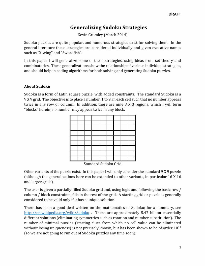
Sudoku is a form of Latin square puzzle, with added constraints. The standard Sudoku is a

9 X 9 grid. The objective is to place a number, 1 to 9, in each cell such that no number appears

twice in any row or column. In addition, there are nine 3 X 3 regions, which I will term

“blocks” herein; no number may appear twice in any block.

Standard Sudoku Grid

Other variants of the puzzle exist. In this paper I will only consider the standard 9 X 9 puzzle

(although the generalizations here can be extended to other variants, in particular 16 X 16

and larger grids).

The user is given a partially-filled Sudoku grid and, using logic and following the basic row /

column / block constraints, fills in the rest of the grid. A starting grid or puzzle is generally

considered to be valid only if it has a unique solution.

There has been a good deal written on the mathematics of Sudoku; for a summary, see

http://en.wikipedia.org/wiki/Sudoku . There are approximately 5.47 billion essentially

different solutions (eliminating symmetries such as rotation and number substitution). The

number of minimal puzzles (starting clues from which no cell value can be eliminated

without losing uniqueness) is not precisely known, but has been shown to be of order 1025

(so we are not going to run out of Sudoku puzzles any time soon).

2

Approach and Nomenclature

A Sudoku puzzle can be considered to be a collection of constraint sets, i.e., a collection of

rows, columns, and blocks. I use the term ‘constraint set’ to reflect the basic rule of the

puzzle, i.e., that each number appears exactly once in each constraint set. Further, the layout

of the Sudoku grid determines the relationship of these constraint sets, i.e, which sets

intersect and where.

In this paper I will use the following nomenclature:

P Sudoku puzzle

Si Particular constraint set (row, column, or block); this is a set of cells within P

S Set of all constraint sets

SR, SC, SB Sets of all row, column, and block constraint sets, respectively

Cn Cell set; this is a particular collection of cells within P (e.g., the intersection of

two constraint sets Si and Sj)

c A particular cell

V Value set; this is a particular collection of valid options (i.e., this is ‘open’

values; a cell that is filled in has no open values)

V(C) Value set associated with cell set C (all the valid open values in set C)

v A particular value

I will also use the normal set operators. These are summarized in Appendix 1.

With this in hand we can consider generalizations of various solution strategies. These

strategies take the form of rules to eliminate possible values (v’s) from unfilled cells in the

puzzle.

Single-S Strategies

We consider two complementary strategies for individual row / column / block constraints.

One addresses combinations of cells, the other combinations of values.

In words, the cell combination strategy is as follows:

For each constraint set Ss, consider each proper subset of cells in Ss (i.e., each

combination of 1 to 8 cells in Ss). Let n be the number of cells in a particular subset

or combination. If there are exactly n valid values in all these cells combined, then

none of these values is available for other cells in Ss.

3

In terms of our nomenclature:

(1) 𝐹𝑜𝑟 𝑒𝑎𝑐ℎ 𝑆𝑠 𝑖𝑛 𝑃 (𝑠 = 1 𝑡𝑜 27)

𝐹𝑜𝑟 𝑒𝑎𝑐ℎ 𝑆 𝑐 ⊂ 𝑆𝑠

𝐿𝑒𝑡 𝑛𝑐 = |𝑆𝑐| 𝑎𝑛𝑑 𝑉𝑐 = ⋃ 𝑉(𝑐𝑖 𝑖∈𝑆𝑐).

𝐼𝑓 |𝑉𝑐| = 𝑛𝑐 , 𝑡ℎ𝑒𝑛

𝑓𝑜𝑟 𝑎𝑙𝑙 𝑣 ∈ 𝑉𝑐 , 𝑣 ∉ 𝑉(𝑆𝑐𝑐).

(Here, the expression “For each Sc” means taking all the combinations of cells within

Ss; more on this below.)

In words, the value combination strategy is as follows:

Consider each possible combination of n valid values, Vn. Consider each constraint

set Ss. If there are exactly n cells in S in which all the values of Vn lie, then no other

values are available to these n cells.

In terms of our nomenclature:

(2) 𝐹𝑜𝑟 𝑒𝑎𝑐ℎ 𝑆𝑠 𝑖𝑛 𝑃

𝐶𝑜𝑛𝑠𝑖𝑑𝑒𝑟 𝑒𝑎𝑐ℎ 𝑐𝑜𝑚𝑏𝑖𝑛𝑎𝑡𝑖𝑜𝑛 𝑉 𝑛 𝑜𝑓 𝑛 𝑣𝑎𝑙𝑖𝑑 𝑣𝑎𝑙𝑢𝑒𝑠.

𝐿𝑒𝑡 𝐶𝑉𝑛= ⋃ (𝑎𝑙𝑙 𝑐𝑖 𝑆𝑠

𝑖𝑛 𝑆𝑠 𝑓𝑜𝑟 𝑤ℎ𝑖𝑐ℎ {𝑉(𝑐𝑖) ∩ 𝑉𝑛} ≠ ∅).

𝐼𝑓 |𝐶𝑉𝑛| = 𝑛 , 𝑡ℎ𝑒𝑛

𝑓𝑜𝑟 𝑎𝑙𝑙 𝑐𝑖 ∈ 𝐶𝑉𝑛, 𝑖𝑓 𝑣 ∉ 𝑉𝑛, 𝑡ℎ𝑒𝑛 𝑣 ∉ 𝑉(𝑐𝑖) .

Combinations of cells and values appear in the above strategies. Since there are 9 cells in

any S and 9 permissible values, the number of combinations in both strategies is theoretically

the same:

(𝑛𝑘

) 𝑤ℎ𝑒𝑟𝑒 𝑛 = 9 𝑓𝑜𝑟 𝑆𝑢𝑑𝑜𝑘𝑢

Elements (k)

Combinations

1 9

2 36

3 84

4 126

5 126

6 84

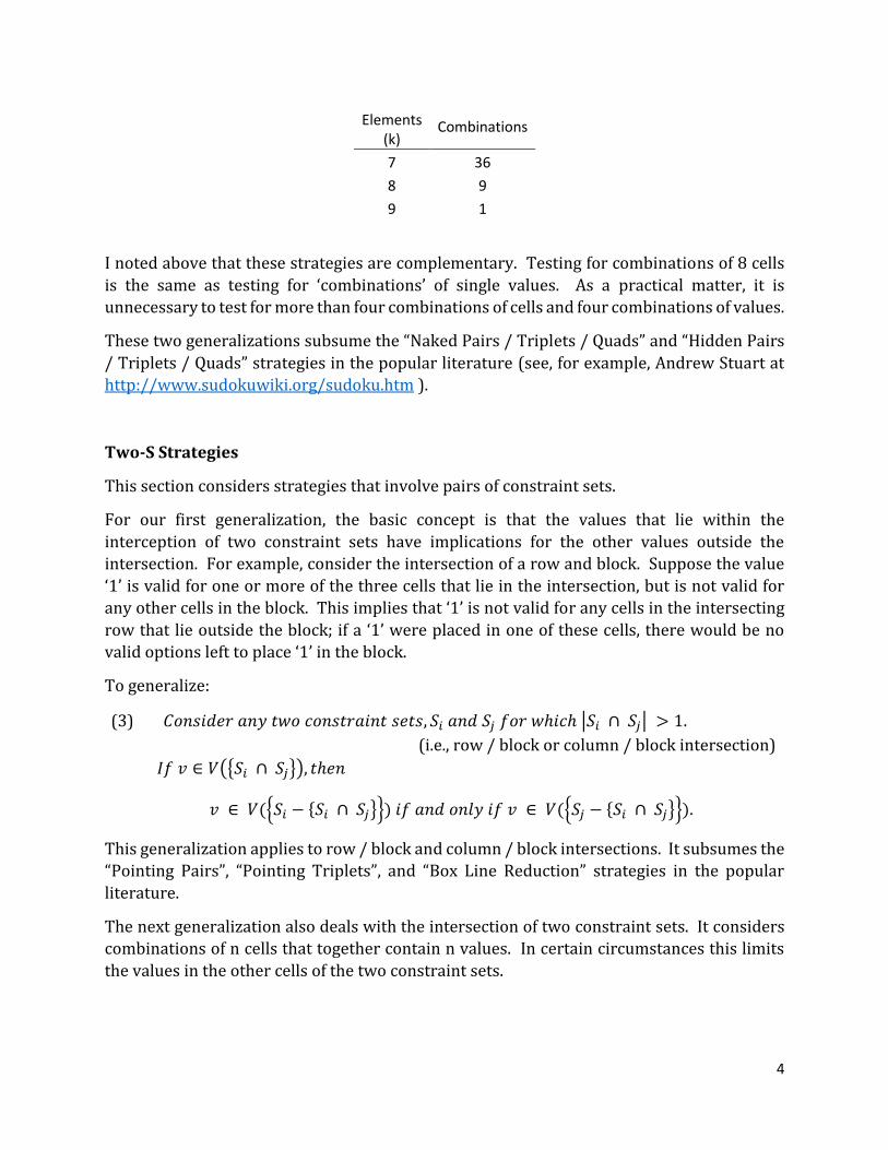
4

Elements (k)

Combinations

7 36

8 9

9 1

I noted above that these strategies are complementary. Testing for combinations of 8 cells

is the same as testing for ‘combinations’ of single values. As a practical matter, it is

unnecessary to test for more than four combinations of cells and four combinations of values.

These two generalizations subsume the “Naked Pairs / Triplets / Quads” and “Hidden Pairs

/ Triplets / Quads” strategies in the popular literature (see, for example, Andrew Stuart at

http://www.sudokuwiki.org/sudoku.htm ).

Two-S Strategies

This section considers strategies that involve pairs of constraint sets.

For our first generalization, the basic concept is that the values that lie within the

interception of two constraint sets have implications for the other values outside the

intersection. For example, consider the intersection of a row and block. Suppose the value

‘1’ is valid for one or more of the three cells that lie in the intersection, but is not valid for

any other cells in the block. This implies that ‘1’ is not valid for any cells in the intersecting

row that lie outside the block; if a ‘1’ were placed in one of these cells, there would be no

valid options left to place ‘1’ in the block.

To generalize:

(3) 𝐶𝑜𝑛𝑠𝑖𝑑𝑒𝑟 𝑎𝑛𝑦 𝑡𝑤𝑜 𝑐𝑜𝑛𝑠𝑡𝑟𝑎𝑖𝑛𝑡 𝑠𝑒𝑡𝑠, 𝑆𝑖 𝑎𝑛𝑑 𝑆𝑗 𝑓𝑜𝑟 𝑤ℎ𝑖𝑐ℎ |𝑆𝑖 ∩ 𝑆𝑗| > 1.

(i.e., row / block or column / block intersection)

𝐼𝑓 𝑣 ∈ 𝑉({𝑆𝑖 ∩ 𝑆𝑗}), 𝑡ℎ𝑒𝑛

𝑣 ∈ 𝑉({𝑆𝑖 − {𝑆𝑖 ∩ 𝑆𝑗}}) 𝑖𝑓 𝑎𝑛𝑑 𝑜𝑛𝑙𝑦 𝑖𝑓 𝑣 ∈ 𝑉({𝑆𝑗 − {𝑆𝑖 ∩ 𝑆𝑗}}).

This generalization applies to row / block and column / block intersections. It subsumes the

“Pointing Pairs”, “Pointing Triplets”, and “Box Line Reduction” strategies in the popular

literature.

The next generalization also deals with the intersection of two constraint sets. It considers

combinations of n cells that together contain n values. In certain circumstances this limits

the values in the other cells of the two constraint sets.

5

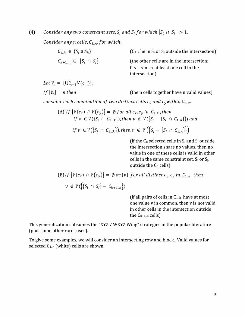
(4) 𝐶𝑜𝑛𝑠𝑖𝑑𝑒𝑟 𝑎𝑛𝑦 𝑡𝑤𝑜 𝑐𝑜𝑛𝑠𝑡𝑟𝑎𝑖𝑛𝑡 𝑠𝑒𝑡𝑠, 𝑆𝑖 𝑎𝑛𝑑 𝑆𝑗 𝑓𝑜𝑟 𝑤ℎ𝑖𝑐ℎ |𝑆𝑖 ∩ 𝑆𝑗| > 1.

𝐶𝑜𝑛𝑠𝑖𝑑𝑒𝑟 𝑎𝑛𝑦 𝑛 𝑐𝑒𝑙𝑙𝑠, 𝐶1..𝑛, 𝑓𝑜𝑟 𝑤ℎ𝑖𝑐ℎ:

𝐶1..𝑘 ∈ {𝑆𝑖 ∆ 𝑆𝑘} (C1..k lie in Si or Sj outside the intersection)

𝐶𝑘+1..𝑛 ∈ {𝑆𝑖 ∩ 𝑆𝑗} (the other cells are in the intersection;

0 < k < n → at least one cell in the

intersection)

𝐿𝑒𝑡 𝑉𝑛 = {⋃ 𝑉(𝑐𝑚𝑛𝑚=1 )}.

𝐼𝑓 |𝑉𝑛| = 𝑛 𝑡ℎ𝑒𝑛 (the n cells together have n valid values)

𝑐𝑜𝑛𝑠𝑖𝑑𝑒𝑟 𝑒𝑎𝑐ℎ 𝑐𝑜𝑚𝑏𝑖𝑛𝑎𝑡𝑖𝑜𝑛 𝑜𝑓 𝑡𝑤𝑜 𝑑𝑖𝑠𝑡𝑖𝑛𝑐𝑡 𝑐𝑒𝑙𝑙𝑠 𝑐𝑥 𝑎𝑛𝑑 𝑐𝑦𝑤𝑖𝑡ℎ𝑖𝑛 𝐶1..𝑘.

(A) 𝐼𝑓 {𝑉(𝑐𝑥) ∩ 𝑉(𝑐𝑦)} = ∅ 𝑓𝑜𝑟 𝑎𝑙𝑙 𝑐𝑥, 𝑐𝑦 𝑖𝑛 𝐶1..𝑘 , 𝑡ℎ𝑒𝑛

𝑖𝑓 𝑣 ∈ 𝑉({𝑆𝑖 ∩ 𝐶1…𝑘}), 𝑡ℎ𝑒𝑛 𝑣 ∉ 𝑉({𝑆𝑖 − {𝑆𝑖 ∩ 𝐶1..𝑛}}) 𝑎𝑛𝑑

𝑖𝑓 𝑣 ∈ 𝑉({𝑆𝑗 ∩ 𝐶1…𝑘}), 𝑡ℎ𝑒𝑛 𝑣 ∉ 𝑉 ({𝑆𝑗 − {𝑆𝑗 ∩ 𝐶1..𝑛}})

(if the Cn selected cells in Si and Sj outside

the intersection share no values, then no

value in one of these cells is valid in other

cells in the same constraint set, Si or Sj,

outside the Cn cells)

(B) 𝐼𝑓 {𝑉(𝑐𝑥) ∩ 𝑉(𝑐𝑦)} = ∅ 𝑜𝑟 {𝑣} 𝑓𝑜𝑟 𝑎𝑙𝑙 𝑑𝑖𝑠𝑡𝑖𝑛𝑐𝑡 𝑐𝑥, 𝑐𝑦 𝑖𝑛 𝐶1..𝑘 , 𝑡ℎ𝑒𝑛

𝑣 ∉ 𝑉({{𝑆𝑖 ∩ 𝑆𝑗} − 𝐶𝑘+1..𝑛})

(if all pairs of cells in C1..k have at most

one value v in common, then v is not valid

in other cells in the intersection outside

the Ck+1..n cells)

This generalization subsumes the “XYZ / WXYZ Wing” strategies in the popular literature

(plus some other rare cases).

To give some examples, we will consider an intersecting row and block. Valid values for

selected C1..n (white) cells are shown.

6

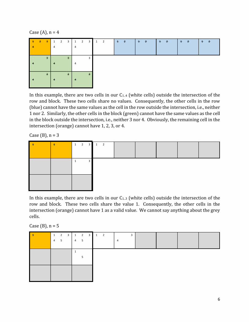
Case (A), n = 4

In this example, there are two cells in our C1..4 (white cells) outside the intersection of the

row and block. These two cells share no values. Consequently, the other cells in the row

(blue) cannot have the same values as the cell in the row outside the intersection, i.e., neither

1 nor 2. Similarly, the other cells in the block (green) cannot have the same values as the cell

in the block outside the intersection, i.e., neither 3 nor 4. Obviously, the remaining cell in the

intersection (orange) cannot have 1, 2, 3, or 4.

Case (B), n = 3

In this example, there are two cells in our C1..3 (white cells) outside the intersection of the

row and block. These two cells share the value 1. Consequently, the other cells in the

intersection (orange) cannot have 1 as a valid value. We cannot say anything about the grey

cells.

Case (B), n = 5

1 2 3 1 2 3 1 2 3 1 2 1 2 1 2 1 2 1 2 1 2

4 4 4

3 3 3

4 4 4

3 3 3

4 4 4

1 1 1 2 3 1 2

1 3

1 1 2 3 1 2 3 1 2 3

4 5 4 5 4

1

5

7

In this example, there are three cells in our C1..5 (white cells) outside the intersection of the

row and block. One pair of these cells shares the value 1. Consequently, the other cell in the

intersection (orange) cannot have 1 as a valid value. We cannot say anything about the grey

cells.

Multi-S Strategies

This family of strategies considers the interactions of multiple constraint sets.

First we consider an even number of intersecting constraint sets.

(5) 𝐶𝑜𝑛𝑠𝑖𝑑𝑒𝑟 𝑎𝑛𝑦 2𝑁 𝑐𝑜𝑛𝑠𝑡𝑟𝑎𝑖𝑛𝑡 𝑠𝑒𝑡𝑠, 𝑆2𝑁, 𝑁 > 1, 𝑠𝑢𝑐ℎ 𝑡ℎ𝑎𝑡,

𝐹𝑜𝑟 𝑎𝑙𝑙 𝑆𝑖, 𝑆𝑖′ ∈ 𝑆1..𝑁 𝑎𝑛𝑑 𝑎𝑙𝑙 𝑆𝑗, 𝑆𝑗′ ∈ 𝑆𝑁+1..2𝑁,

{𝑆𝑖 ∩ 𝑆𝑗} ≠ ∅ 𝑎𝑛𝑑 {𝑆𝑖 ∩ 𝑆𝑖′≠𝑖} = ∅ 𝑎𝑛𝑑 {𝑆𝑗 ∩ 𝑆𝑗′≠𝑗} = ∅

(e.g, S1..N are in SR and SN+1..2N are in

SC, or vice versa; for the case

where N = 2 we may also have

either S1..N or SN+1..2N in SB)

𝐿𝑒𝑡 𝑆𝑖 ∈ 𝑆1..𝑁 𝑎𝑛𝑑 𝑆𝑗 ∈ 𝑆𝑁+1..2𝑁 .

𝐿𝑒𝑡 𝑆𝑖′ = {⋃ {𝑆𝑖 ∩ 𝑆𝑗}2𝑁

𝑗=𝑁+1 } (𝑆𝑖′ is all cells in Si that

intersect with SN+1..2N ; i = 1..N)

𝑎𝑛𝑑 𝑆𝑗′ = {⋃ {𝑆𝑖 ∩ 𝑆𝑗}𝑁

𝑖=1 }. (analogous definition for Sj;

j = N+1..2N)

𝐼𝑓, 𝑓𝑜𝑟 𝑎𝑙𝑙 𝑖 = 1 𝑡𝑜 𝑁, 𝑣 ∈ 𝑉(𝑐𝑘) 𝑓𝑜𝑟 𝑎𝑙𝑙 𝑐𝑘 ∈ 𝑆𝑖′ 𝑎𝑛𝑑

𝑣 ∉ 𝑉({𝑆𝑖 − 𝑆𝑖′}) , 𝑡ℎ𝑒𝑛 (v is an option for every

intersection cell, but for no other

cells in Si, i = 1..N)

𝑓𝑜𝑟 𝑎𝑙𝑙 𝑗 = 𝑁 + 1 𝑡𝑜 2𝑁, 𝑣 ∉ 𝑉({𝑆𝑗 − 𝑆𝑗′}).

(v is not an option for cells in Sj

outside the intersection cells)

𝐴𝑛𝑑 𝑐𝑜𝑛𝑣𝑒𝑟𝑠𝑒𝑙𝑦 𝑓𝑜𝑟 𝑎𝑙𝑙 𝑗 = 𝑁 + 1 𝑡𝑜 2𝑁.

(Note: for N = 2, we may have blocks involved, e.g., the intersection of two rows and two

blocks. In this case, we must add the stipulation that our v above appears in only one cell of

each intersection. This is obviously not necessary to add in the case of row / column sets,

since each intersection is one cell.)

8

This generalization covers the “X-Wing”, “Swordfish”, and “Jellyfish” strategies in the popular

literature, as well as some other rare cases.

The last generalization addresses combinations of n cells that contain n values, but span

multiple constraint sets. The general idea is as follows: Consider sets of n cells, Cn, that

combined have n values, but which reside in different constraint sets. Consider a cell cm

outside Cn in one or more of the constraint sets in which at least one cell, but not all cells, of

Cn reside. Then the cm cell partitions Cn into two subsets, those cells that share a constraint

set with cm (Coc) and those that do not (Co). If the open values in Co are in some sense bounded

by the open values in Coc, in some circumstances we may draw a conclusion about

permissible values for cm.

(6) 𝐶𝑜𝑛𝑠𝑖𝑑𝑒𝑟 𝑎𝑙𝑙 𝑠𝑒𝑡𝑠 𝑜𝑓 𝑛 𝑐𝑒𝑙𝑙𝑠, 𝐶𝑛, 𝑓𝑜𝑟 𝑤ℎ𝑖𝑐ℎ |𝑉(𝐶𝑛)| = 𝑛.

𝐶𝑜𝑛𝑠𝑖𝑑𝑒𝑟 𝑎𝑙𝑙 𝑠𝑒𝑡𝑠 𝑜𝑓 𝑁 𝑐𝑜𝑛𝑠𝑡𝑟𝑎𝑖𝑛𝑡 𝑠𝑒𝑡𝑠, 𝑆𝑁, 𝑁 ≤ 𝑛 + 1,

𝑓𝑜𝑟 𝑤ℎ𝑖𝑐ℎ, 𝑓𝑜𝑟 𝑒𝑎𝑐ℎ 𝑆𝑖 ∈ 𝑆𝑁 , {𝑆𝑖 ∩ 𝐶𝑛} ≠ ∅, 𝑎𝑛𝑑 {𝑆𝑖 ∩ {𝑆𝑁 − 𝑆𝑖}} ≠ ∅.

(pick up to n+1 constraint sets that

contain the cells in Cn, taking care

that each constraint set has at least

one intersection with another in

SN)

𝐶𝑜𝑛𝑠𝑖𝑑𝑒𝑟 𝑎𝑙𝑙 𝑐𝑚 ∈ {𝑆𝑁 − 𝐶𝑛}. (pick a cell in SN outside Cn)

𝐿𝑒𝑡 𝑆𝑚 = ⋃ {𝑆𝑖 ∈ 𝑆𝑁 𝑓𝑜𝑟 𝑤ℎ𝑖𝑐ℎ 𝑆𝑖 ∩ {𝑐𝑚} ≠ ∅}𝑖

(this is all constraint sets in SN that

contain cm)

𝐿𝑒𝑡 𝐶𝑜 = {𝐶𝑛 − {𝐶𝑛 ∩ 𝑆𝑚}} . (this is all cells in Cn outside Sm)

𝐼𝑓 |𝐶𝑜| > 0 𝑡ℎ𝑒𝑛

𝐹𝑜𝑟 𝑒𝑎𝑐ℎ 𝑐𝑖 𝑖𝑛 𝐶𝑜 , 𝑙𝑒𝑡 𝑆𝑖 = ⋃ {𝑆𝑗 ∈ 𝑆𝑁 𝑓𝑜𝑟 𝑤ℎ𝑖𝑐ℎ 𝑆𝑗 ∩ {𝑐𝑖} ≠ ∅}𝑗

(this is all the constraint sets in SN

that contain ci)

𝐿𝑒𝑡 𝐶𝑖′ = {𝐶𝑜

𝑐 ∩ 𝑆𝑖} (this is all the cells of Cn, outside of

Co, (i.e., in Sm) that lie in constraint

sets containing ci)

𝐼𝑓, 𝑓𝑜𝑟 𝑎𝑙𝑙 𝑐𝑗 ∈ {𝑆𝑚 ∩ 𝐶𝑛} , 𝑐𝑗 ∈ 𝑜𝑓 {⋃ 𝐶𝑖′

𝑖∈𝐶𝑜} 𝑎𝑛𝑑 (every cell of Cn in Sm shares at least

one constraint set with a cell in Co)

𝑓𝑜𝑟 𝑎𝑙𝑙 𝑐𝑖𝑖𝑛 𝐶𝑜 , 𝑉(𝑐𝑖) ⊆ 𝑉(𝐶𝑖′), 𝑎𝑛𝑑 (the set of values for each ci is a

subset of the values of the Cn cells in

9

Sm that share constraint set(s) with

ci)

𝑓𝑜𝑟 𝑠𝑜𝑚𝑒 𝑆𝑖, |𝑉({𝐶𝑛 ∩ 𝑆𝑖})| ≤ |{𝐶𝑛 ∩ 𝑆𝑖} |, 𝑡ℎ𝑒𝑛 (for at least one of the Si constraint

sets associated with the ci in Co, the

number of values in the Cn cells in Si

is no greater than the number of Cn

cells in Si)

𝐼𝑓 𝑡ℎ𝑒𝑟𝑒 𝑒𝑥𝑖𝑠𝑡𝑠 𝑣 𝑠𝑢𝑐ℎ 𝑡ℎ𝑎𝑡 𝑣 ∉ 𝑉(𝐶𝑜), 𝑣 ∈ 𝑉(𝐶𝑖′), 𝑎𝑛𝑑

𝑓𝑜𝑟 𝑒𝑎𝑐ℎ 𝑑𝑖𝑠𝑡𝑖𝑛𝑐𝑡 𝑐𝑥, 𝑐𝑦 𝑖𝑛 𝐶𝑖′ , {𝑉(𝑐𝑥) ∩ 𝑉(𝑐𝑦)} = {𝑣} 𝑜𝑟 ∅, 𝑡ℎ𝑒𝑛

𝑣 ∉ 𝑉(𝑐𝑚) (if v is not a value in Co and v is the

only common value among the cells

in Ci’, v cannot be a value for the

chosen cell cm)

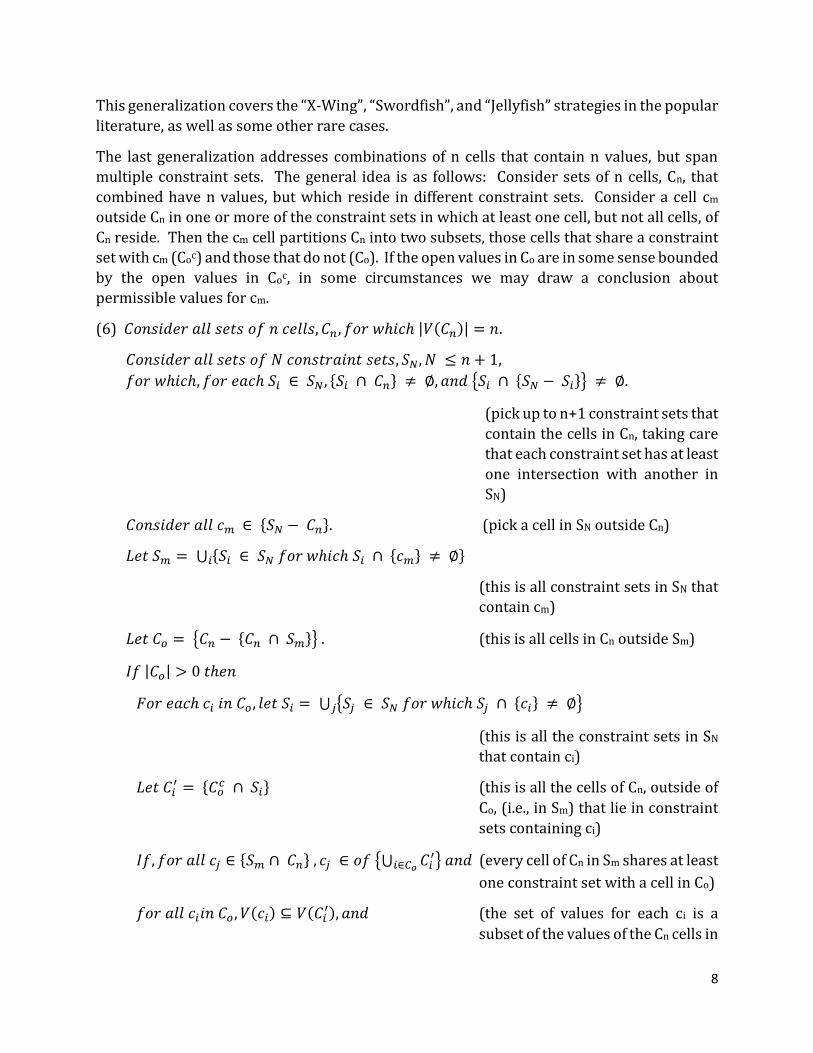
This is a complex strategy, dealing with multiple constraint sets and cells. To illustrate an

example for n = 3:

Our three cells with three values are (R1,C5), (R3,C3), and (R3,C5). We are considering four

constraint sets, R1, R3, B1, and C5 1. If we look at cm = any of the first three cells in R1, we

see that:

Sm = R1 and B1, and hence includes (R1,C5) and (R3,C3) .

Co is one cell in this case, so ci = (R3,C5), Si = {R3 and C5}, and Ci’ = {(R1,C5), (R3,C3)}.

The values in ci -- {2,3} -- are a subset of the values in Ci’ -- {1,2,3}.

1 Here, R indicates row, C column, and B block.

C3 C5

1 1 1 1 2

R1

1 3 2 3

R3

B1

10

The number of Cn cells in Si is three, equal to the number of possible values, so this

test is also met.

The cells in Ci’, (R1,C5) and (R3,C3) only share the value 1, and 1 is not present in ci = (R3,C5).

Consequently, none of the first three cells in R1 may have the value 1.

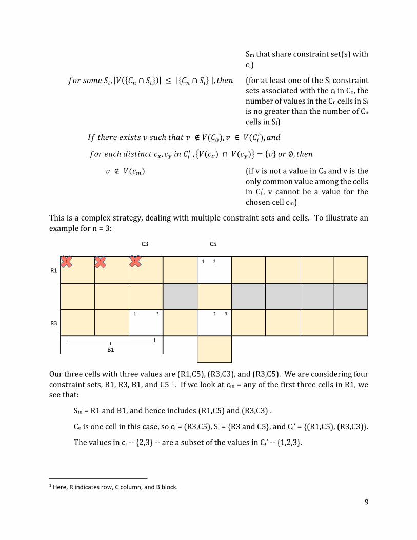
Another example, n = 5:

As before, the white cells show our Cn=5, with their permitted values due to values set

elsewhere. Our SN are again R1, R3, B1, and C5. Stepping through:

1. Consider cm as cell (R3,C1). For this cell, Sm = {R3 and B1}, C0 = {(R1,C4), (R1,C5)}.

2. The values in (R1,C4) are a subset of the values in {(R1,C2),(R1,C3)}, and the values

in (R1,C5) are a subset of the values in {(R1,C2),(R1,C3),(R3,C5)}, so this test is met.

3. Consider cell (R1,C5), an element of C0. Let this be ci. For this cell, Si = {R1 and C5}

and Ci’ = {(R1,C2),(R1,C3),(R3,C5)}.

4. The number of Cn cells in Si is five, as is the number of possible values, so this test is

met.

5. The value “1” is not an element of the Co cells but is the only common element among

the Ci’ cells. Consequently, 1 cannot be a value for cm (R3,C1). The same logic applies

to (R3,C2) and (R3,C3).

(Note: in step 3, we might have considered cell (R1,C4). However, this does not pass the test

that the number of values in Ci’ cannot be greater than the number of cells – four cells, five

combined values. But the strategy also tests the other cell(s) in C0, in this case (R1,C5).)

C1 C2 C3 C4 C5

1 2 3 2 3 2 3

R1 4 4 4 5

1 1 1 1

R3 5

B1

11

This generalization covers different variants of ‘Y-Wing’ and ‘XY-Chains’ in the popular

literature.

Generalized Solution Algorithm

We have covered several general strategies for Sudoku. Many others exist. Solving a puzzle

does not necessarily require all strategies. This leads to some interesting open questions.

But first a bit more background.

Let us add the follow nomenclature:

R0 the basic rule set for Sudoku; i.e., each value v appears exactly once in each Si.

Rx additional solution strategies that we choose to apply; this may include some

or all of the generalizations noted here, plus others.

For these purposes we will restrict Rx to strategies that are state-deterministic. That is, they

can be applied based on the current state of the puzzle (filled in cells) and do not require

making guesses of values or backtracking (although iterative applications of the rules are

allowed). They are of the form “if the puzzle has this state (filled in cells), then we may

eliminate these values as potential options from these cells”. The generalizations in this

paper are all of this sort.

(As an aside, a state-deterministic rule set has this property: if a puzzle can be solved using

only state-deterministic rules, than that solution is unique. The converse is not necessarily

true, which gets to the issue of completeness, discussed in the next section.)

A general algorithm for solving a given Sudoku puzzle P (assuming it has a solution) is as

follows.

1. Apply R0 iteratively to remove options from non-filled-in cells. Iterate so long as

values are removed.

2. Check for any cells that only have one valid option.

A. If there are any such cells, fill them in.

i. If all cells are filled in, stop, the puzzle is complete.

ii. If some cells remain open, loop back to 1.

B. If no open cell has a single option remaining, go to 3.

3. Apply Rx iteratively to remove options from non-filled-in cells. Iterate so long as

values are removed.

A. If any values are removed, loop back to 1.

B. Otherwise, go to 4.

4. Select a cell in which to make a guess.

5. Select an open value for the guess cell.

6. Apply 1 – 3 iteratively until one of these three possible outcomes:

A. The puzzle is solved – stop.

12

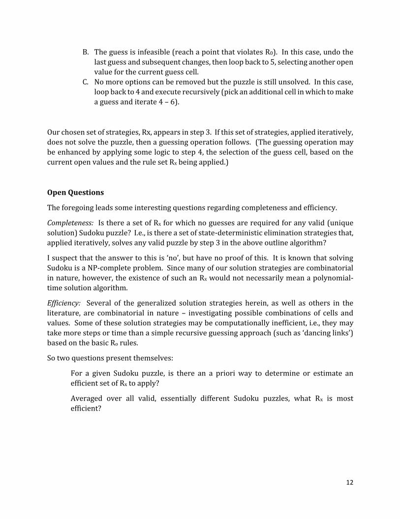
B. The guess is infeasible (reach a point that violates R0). In this case, undo the

last guess and subsequent changes, then loop back to 5, selecting another open

value for the current guess cell.

C. No more options can be removed but the puzzle is still unsolved. In this case,

loop back to 4 and execute recursively (pick an additional cell in which to make

a guess and iterate 4 – 6).

Our chosen set of strategies, Rx, appears in step 3. If this set of strategies, applied iteratively,

does not solve the puzzle, then a guessing operation follows. (The guessing operation may

be enhanced by applying some logic to step 4, the selection of the guess cell, based on the

current open values and the rule set Rx being applied.)

Open Questions

The foregoing leads some interesting questions regarding completeness and efficiency.

Completeness: Is there a set of Rx for which no guesses are required for any valid (unique

solution) Sudoku puzzle? I.e., is there a set of state-deterministic elimination strategies that,

applied iteratively, solves any valid puzzle by step 3 in the above outline algorithm?

I suspect that the answer to this is ‘no’, but have no proof of this. It is known that solving

Sudoku is a NP-complete problem. Since many of our solution strategies are combinatorial

in nature, however, the existence of such an Rx would not necessarily mean a polynomial-

time solution algorithm.

Efficiency: Several of the generalized solution strategies herein, as well as others in the

literature, are combinatorial in nature – investigating possible combinations of cells and

values. Some of these solution strategies may be computationally inefficient, i.e., they may

take more steps or time than a simple recursive guessing approach (such as ‘dancing links’)

based on the basic Ro rules.

So two questions present themselves:

For a given Sudoku puzzle, is there an a priori way to determine or estimate an

efficient set of Rx to apply?

Averaged over all valid, essentially different Sudoku puzzles, what Rx is most

efficient?

13

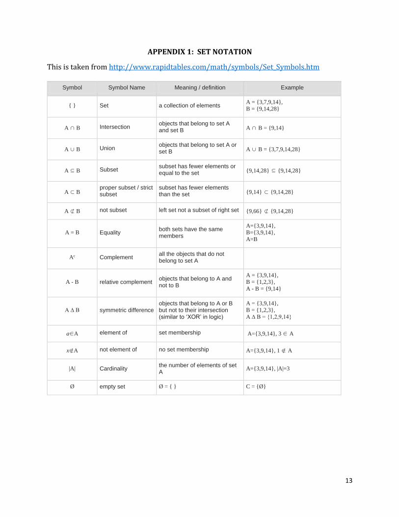
APPENDIX 1: SET NOTATION

This is taken from http://www.rapidtables.com/math/symbols/Set_Symbols.htm

Symbol Symbol Name Meaning / definition Example

{ } Set a collection of elements A = {3,7,9,14},

B = {9,14,28}

A ∩ B Intersection objects that belong to set A and set B A ∩ B = {9,14}

A ∪ B Union objects that belong to set A or set B A ∪ B = {3,7,9,14,28}

A ⊆ B Subset subset has fewer elements or equal to the set {9,14,28} ⊆ {9,14,28}

A ⊂ B proper subset / strict subset

subset has fewer elements than the set {9,14} ⊂ {9,14,28}

A ⊄ B not subset left set not a subset of right set {9,66} ⊄ {9,14,28}

A = B Equality both sets have the same members

A={3,9,14},

B={3,9,14},

A=B

Ac Complement all the objects that do not belong to set A

A - B relative complement objects that belong to A and not to B

A = {3,9,14},

B = {1,2,3},

A - B = {9,14}

A ∆ B symmetric difference objects that belong to A or B but not to their intersection (similar to ‘XOR’ in logic)

A = {3,9,14},

B = {1,2,3},

A ∆ B = {1,2,9,14}

a∈A element of set membership A={3,9,14}, 3 ∈ A

x∉A not element of no set membership A={3,9,14}, 1 ∉ A

|A| Cardinality the number of elements of set A

A={3,9,14}, |A|=3

Ø empty set Ø = { } C = {Ø}